12

3-D Analysis of Conduction Velocity in Relation to Ventricular Anatomy

Jeroen van den Akker BMTE04.36 2003-2004

Supervisors: Robert W.Mills (UCSD, La Jolla, California)

P.M.Bovendeerd (Technical University Eindhoven)

mhj

CHAPTER 1 PHYSIOLOGY ...................................................................................................... 3 1.1 MYOFIBER ARCHITECTURE ................................................................................................... 3 1.2 ELECTROPHYSIOLOGIC EFFECTS OF VENTRICULAR MECHANICAL LOADING....................... 3

CHAPTER 2 METHOD ............................................................................................................... 4 2.1 EXPERIMENTAL PREPARATION.............................................................................................. 4 2.2 3-D MESH RECONSTRUCTION ............................................................................................... 4 2.3 MARKER SEGMENTATION...................................................................................................... 7 2.4 FIBER ANGLE FITTING ......................................................................................................... 11 2.5 STRAIN ANALYSIS ............................................................................................................... 11 2.6 ACTIVATION TIME, CONDUCTION VELOCITY & CONDUCTION PATH................................. 13

CHAPTER 3 RESULTS ............................................................................................................. 16 CHAPTER 4 DISCUSSION ....................................................................................................... 21

4.1 METHOD DISADVANTAGES & LIMITATIONS ........................................................................ 21 4.2 EXPLICATION OF RESULTS................................................................................................... 22 4.3 FUTURE RECOMMENDATIONS ............................................................................................. 23

CONCLUSION............................................................................................................................ 24 REFERENCES ............................................................................................................................ 25

1

Introduction High blood pressure, a problem increasing rapidly in clinical practice, can cause dilatation of the heart. This stretch will increase the conduction time over the enlarged epicardial surface and possibly deteriorate the conducting velocity of the stretched fibers. Moreover the fiber orientation alternates, possibly resulting in an orientation which requires an increase in the amount of fibers needed to spread the action potential from apex to base. Such alterations in myocardial action potential spread have been implicated in contributing to reentrant arrhythmias [13]. The aim of this study was to investigate if conduction time in the dilated heart is increased simply as a function of distance or if fiber orientation and regional strains are a determinant as well. Therefore, the following experiment is conducted. A mesh of an isolated rabbit heart is constructed in a finite element program using two orthogonal contour images. Conduction velocity on the left ventricular free wall is measured by optical mapping using video imaging and a voltage sensitive dye. Arrays of markers are painted on the heart before inflation, simulating natural dilatation. Their relative displacements after dilatation are a measure for the epicardial strain. Standard fiber angle values are included for calculating epicardial strains in fiber and cross fiber direction. This technique provides a tool to quantify conduction velocity relative to strain and fiber orientation.

2

Chapter 1 Physiology The timing of depolarization of cardiac tissue depends upon path length, conduction velocity and fiber orientation. Highest velocity occurs in the direction parallel to the muscle fibers. Furthermore conduction velocity is influenced by the applied mechanical stimulation, which is believed to increase activation time [10,12].

1.1 Myofiber Architecture The cardiac ventricles have a complex three-dimensional muscle fiber architecture with a clear predominant fiber axis throughout most of the wall. In the human left ventricle, muscle fiber angle typically varies continuously from about -60° (measured clockwise from the circumferential axis) at the epicardium to about +70° at the endocardium. There are also small increases in fiber orientation from end-diastole to systole (7-19°), with greatest changes at the epicardium and apex (see Figure 2.10) [14]. The conduction velocity in regular ventricular muscle fibers is about 0,3 to 0,5 m/s. However, for Purkinje fibers, which form a specialized conductive system, this varies from 0,02 to 4 m/s [5]. With respect to the myofibers, propagation is generally 2-4 times faster in the longitudinal than transverse direction. Sung et al. found a typical epicardial conduction velocity of 0,4 m/s in the fiber direction, and 0,18 m/s in the cross fiber direction [10]. The maximum component of epicardial stretch and the derived wall thinning increase substantially from base to apex. The direction of greatest stretch at moderate and high filling pressures coincides closely with the local epicardial fiber direction, suggesting that the left-handed epicardial fiber helices stretch preferentially during passive filling to maximize end-diastolic fiber lengths [8].

1.2 Electrophysiologic Effects of Ventricular Mechanical Loading Mechanical stimulation of cardiac cells can induce electrophysiologic changes. This is called mechano-electrical feedback. As the intraventricular pressure increases, so does myocardial elastance: the myocardium becomes stiffer. The time-varying ventricular elastance reaches its maximum in close parallel to intraventricular pressure. This serves as a protective mechanism against stretch during the period of mechanical systole [3,12]. Mechanical stretch shortens Action Potential Duration (APD), especially at early repolarization, and decreases refractory periods. This causes transient depolarizations, thereby increasing the susceptibility for arrhythmias. For more details, see [3]. Stretch-activated channels have been identified as a potential mechanism for mechano-electrical feedback. One function of these channels in cardiac muscles is the intrinsic regulation of contractility. However, experiments conducted by Sung et al. didn’t show any effect of these channels on conduction velocity (CV) and APD [12]. Previous experiments mostly have shown increased activation times and decreased CV during ventricular loading, although remarkably sometimes a velocity increase was found. After a left ventricular end-diastolic pressure increase from 0 to 30 mmHg, Sung et al. found an epicardial activation time increase of about 25 %. This resulted in a 16 % decreased surface conduction velocity. Epicardial strain averages 0,040 in heart muscle fiber direction and 0,032 in cross fiber direction [12].

3

Chapter 2 Method This chapter starts with the experimental setup and data recording procedures. Then the reconstruction of a three dimensional mesh is explained. Epicardial strains resulting from an applied load are calculated, making use of painted markers. Incorporating standard fiber angle values enables conversion to strains in fiber and cross fiber direction. The activation time acquisition is mentioned briefly, since this topic was investigated in a previously conducted project. After fitting the activation time field to the mesh, the velocity vector field was calculated. Then activation times and conduction velocity along the conduction path were obtained.

2.1 Experimental Preparation All experiments were conducted in isolated, perfused rabbit hearts. The heart was paced and a latex balloon was inserted into the left ventricle (LV). After preconditioning the myocardium, the balloon volume resulting in a peak End Diastolic Pressure of 30 mmHg was recorded. This volume is then used for loading experiments. A voltage-sensitive dye was injected into the perfusate, and an electromechanical uncoupling agent (BDM) was added during data acquisition to prevent contraction and thereby eliminate motion artifact. As a consequence, the time-varying mechano-electrical feedback effect is eliminated. However, the myocardium is expected to be stiffer after applying the load (see § 1.2). Optical images of the LV free wall were captured at a speed of 399 frames per second to record action potential propagation. An array of titanium dioxide markers was painted onto the LV. Titanium dioxide is chosen because of its high optical contrast and low tissue damage. A high resolution camera captured two orthogonal views of the heart, both undeformed and deformed. These images were used for LV geometric reconstruction and strain computation. For experimental and recording details, see [10,12].

2.2 3-D Mesh Reconstruction The gross geometry of the heart was reconstructed from the orthogonal biplane images of the lateral and posterior views. First any part of the heart touching the left or right vertical image side had to be deleted (see Figure 2.1, left side). Then the image was thresholded and converted to a binary image, in which the white heart pixels have value one. The heart contour was extracted by searching for all nonzero pixels connected to at least one zero-valued pixel, with a connectivity of 4. This means that at least one of the four pixels directly next to a white pixel, has to be black. Then this contour is superimposed on the original image (see Figure 2.1, right side).

4

Figure 2.1 Left side: original heart, lateral view (vertical red line = deleted part); Right side: automatically extracted lateral heart contour

The contour bottom was adapted because the experimental setup introduces too many artifacts in this area. Thus to obtain a complete contour (Figure 2.2, right side), a user has to select a few bottom contour points (Figure 2.2, left side)

Figure 2.2 Left side: user adjusted lateral contour; Right side: complete lateral heart contour

In the 3-D mesh creation, the region above the top row of markers wasn’t modeled since this area isn’t activated by the epicardial wavefront, but transmurally, making activation times highly irregular. The location of all contour points was translated into a coordinate system having x directed along the long axis of the heart with the z-x plane forming the lateral view and the y-x plane forming the posterior view. The origin was located along the x-axis at a point two thirds of the distance from apex to contour top. The location of the apex was identified in each of the images as the bottom point of the heart (see Figure 2.3, left side). The vertical difference between

5

the apex positions in the two orthogonal images was used to assemble the two boundary contours into a common three-dimensional coordinate frame (see Figure 2.3, right side). The segmentation and coordinate manipulations were performed semi-automatically in Matlab, a computational environment containing many image processing routines. To facilitate fitting a surface model to epicardial ventricular geometry, the three-dimensional rectangular Cartesian coordinates (x,y,z) of the orthogonal boundary contours were transformed to prolate spheroidal coordinates (λ,µ,θ):

x = d cosh λ cos µ, (1) y = d sinh λ sin µ cos θ, (2)

z = d sinh λ sin µ sin θ. (3)

The focal length of the ellipsoid, d, was defined from the major and minor radii using the equation: d2 = b2 – a2 (4) The minor radius a was taken to be one half the diameter of the origin as measured from the images. The major radius b was the distance along the x-axis from the origin to the apex (see Figure 2.3, left side). The transformation into prolate spheroidal coordinates facilitates the fit by reducing the problem to one coordinate, λ (see Figure 2.3, right side).

Figure 2.3 Left side: lateral heart view (a = width/2; b = 2/3 height); Right side [9] : orthogonal contours fit to prolate spheroidal finite-element model

Using linear least-squares methods, the λ nodal coordinate parameters of a bicubic Hermite finite-element mesh were fitted to the epicardial surface points (see Figure 2.3, right side) [4,7]. The initial finite-element surface model used for the fit was a truncated ellipsoid, with focus d, consisting of 12 elements (four circumferential elements by three longitudinal elements). Basal

6

nodes were located at θ = 0˚, 90˚, 180˚, and 270˚. Projections of each geometric data point along the radial direction to the surface were calculated, and a least-squares fit of the data in the radial direction λ of the prolate spheroidal coordinate system was used to deform the mesh (see Figure 2.4). Bicubic Hermite basis functions assure the continuity of first derivatives of the interpolated geometric coordinates across element boundaries [4]. Constraints imposed on the fit ensured derivative symmetry at the apex [10]. The fit of the truncated ellipsoid to the three-dimensional contours of the whole heart was performed for both an undeformed and deformed geometry. The posterior half of both meshes, containing those points with their y-coordinate greater than zero, has been removed since markers have only been attached to the left ventricle, the anterior half. Furthermore removing the posterior mesh half simplifies the fitting and reduces calculation time significantly. The surface model was constructed in Continuity, a computational environment for finite element analysis.

Figure 2.4: Truncated ellipsoid fitted to undeformed heart contour (front, respectively top view)

2.3 Marker Segmentation The starting point for the strain analysis was the identification of the titanium dioxide markers and their corresponding positions after applying the load. All markers on the left ventricular free wall were captured by the lateral image. Thus for strain calculation, only these images were used. Marker segmentation was performed identically for the undeformed and deformed heart. After removing unused image portions the image intensity was adjusted to improve the contrast. This was done by mapping the original intensity values to new values such that 1% of the data is saturated at low and high intensities of the original image. Then morphological opening was performed. In this process, an erosion is followed by a dilation, while the same structuring element is used for both operations. Performing an erosion means that each image pixel value changes to the minimum value of all the pixels in the input pixel's neighborhood. The size of a pixel’s neighborhood depends on the structuring element being used, in this case a disk-shaped element with radius 6. In a dilation, the value of the output pixel is the maximum value of all the

7

pixels in the input pixel's neighborhood. Thus morphological opening removes small objects from an image while preserving the shape and size of larger objects in the image, thereby resulting in an estimated image background (see Figure 2.5, right side).

Figure 2.5 Left side: original heart; Right side: heart after cropping, intensity adjusting & morphological opening (estimated background image)

Now the background image was subtracted from the original image. Then the intensity image was converted to a binary image. The level for image thresholding is determined by Otsu's method, which chooses the threshold to minimize the intraclass variance of the black and white pixels (see Figure 2.6) [9]. Figure 2.6 Left side: background subtracted from heart; Right side: subtracted heart thresholded to convert to black & white

Next, all objects containing fewer than 10 pixels were removed, and little black holes within the white markers were filled (see Figure 2.7, left side). Then for each white object the boundary pixels were determined. These values were used to calculate the centroid and area of each object.

8

Now it was determined which objects are actually titanium dioxide markers. Therefore it was assumed that all applied markers are circularly shaped. The following roundness metric was calculated for each object:

2

4perimeter

areametric ∗=

π (5)

By filling in the standard equations for perimeter (2π*r) and area (π*r2) it can be easily seen that a perfect circular object will have a metric value which equals one. By discarding all objects with a metric value lower than 0,65 a fairly good marker selection was obtained. Before calculating the roundness metric, the perimeter of each object was estimated (see Figure 2.7, right side). This was done by summing all distances between two adjacent boundary points. Thus for the distance L1 between boundary points 1 and 2 holds:

( ) ( )22 12121 yyxxL −+−= (6)

Figure 2.7 Left side: objects on heart; Right side: estimation of object perimeter

Now all selected objects were displayed in the original, cropped image by placing a red star on the object’s centroid. Furthermore the roundness metrics and object numbers are shown (see Figure 2.8).

9

Figure 2.8 Markers on original, cropped image, with roundness metric and object number (e.g. 0.96@16)

In the next step, selected objects which aren’t markers were deleted simply by entering their object number. Finally missing markers were added by clicking at their center. Now the x- and z-coordinates of the titanium dioxide markers are known for both the undeformed and deformed heart. These coordinates were translated to the system used for the mesh generation. Then these data points were projected along the y-direction (see Figure 2.3) to their corresponding fitted mesh. Thereby two data sets of marker points in x-, y-, and z-coordinates are available (see Figure 2.9), enabling strain analysis (see § 2.5). So 3-D marker locations were obtained by combination of 2-D image and a 3-D geometry model.

10

Figure 2.9: Left side: markers on undeformed heart; Right side: markers on deformed heart (marker numbers = purple; contour = blue; apex = yellow)

2.4 Fiber Angle Fitting Epicardial fiber angle measurements from a previously developed model were projected onto the fitted, undeformed mesh and then fit with bicubic Hermite interpolation [14]. These fiber data were used to calculate the strain in fiber and cross fiber direction (see § 2.5).

Figure 2.10: Fitted, undeformed mesh containing fiber angle measurements [10]

2.5 Strain Analysis The two marker data sets, in cartesian coordinates (see § 2.3), were used to deform the unloaded, fitted 3-D mesh. Therefore it was necessary to connect each marker of the undeformed heart to its corresponding deformed marker (see Figure 2.11) .

11

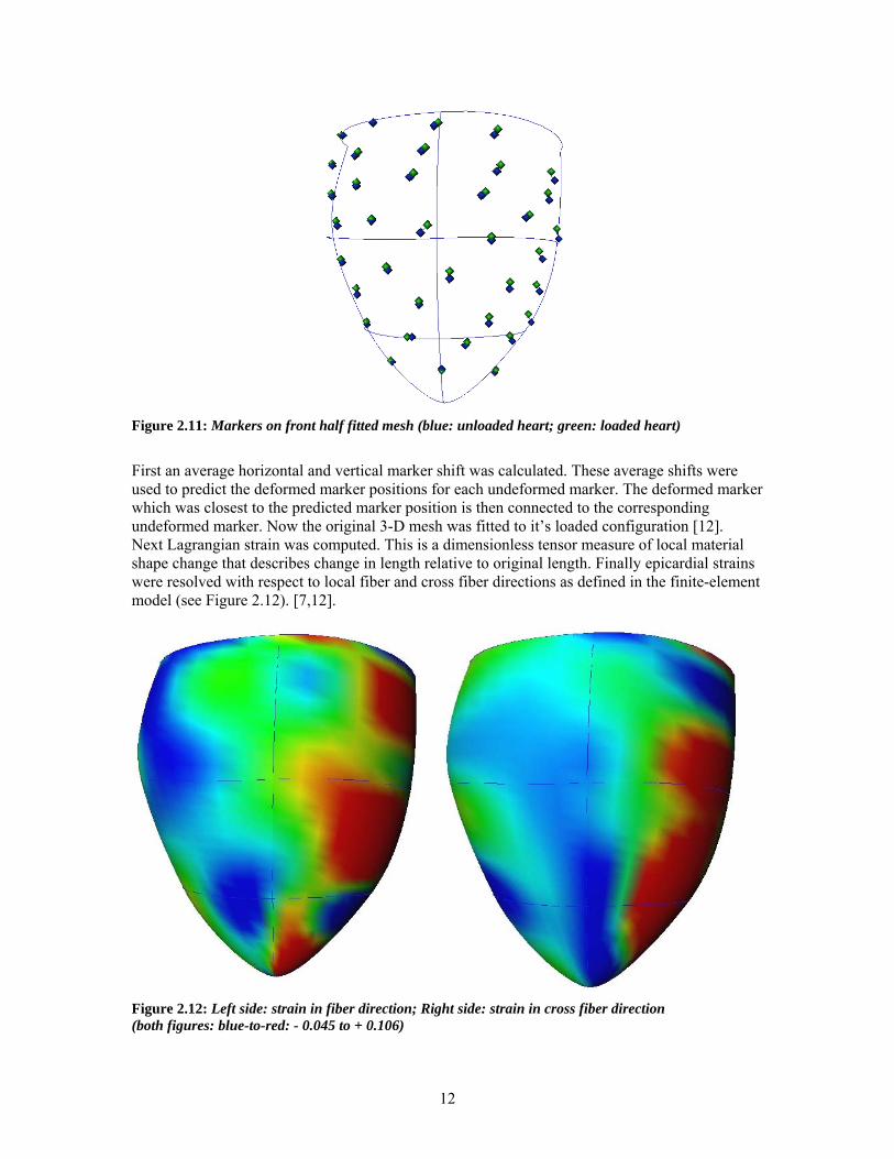
Figure 2.11: Markers on front half fitted mesh (blue: unloaded heart; green: loaded heart)

First an average horizontal and vertical marker shift was calculated. These average shifts were used to predict the deformed marker positions for each undeformed marker. The deformed marker which was closest to the predicted marker position is then connected to the corresponding undeformed marker. Now the original 3-D mesh was fitted to it’s loaded configuration [12]. Next Lagrangian strain was computed. This is a dimensionless tensor measure of local material shape change that describes change in length relative to original length. Finally epicardial strains were resolved with respect to local fiber and cross fiber directions as defined in the finite-element model (see Figure 2.12). [7,12].

Figure 2.12: Left side: strain in fiber direction; Right side: strain in cross fiber direction (both figures: blue-to-red: - 0.045 to + 0.106)

12

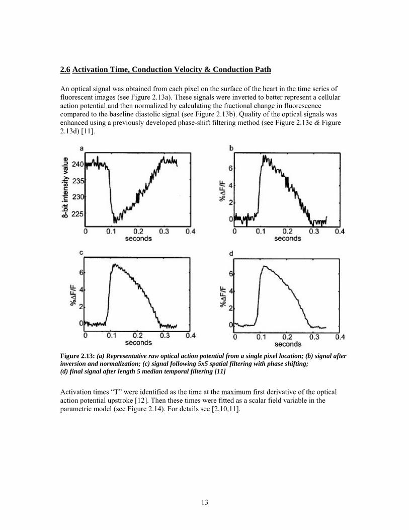
2.6 Activation Time, Conduction Velocity & Conduction Path An optical signal was obtained from each pixel on the surface of the heart in the time series of fluorescent images (see Figure 2.13a). These signals were inverted to better represent a cellular action potential and then normalized by calculating the fractional change in fluorescence compared to the baseline diastolic signal (see Figure 2.13b). Quality of the optical signals was enhanced using a previously developed phase-shift filtering method (see Figure 2.13c & Figure 2.13d) [11].

Figure 2.13: (a) Representative raw optical action potential from a single pixel location; (b) signal after inversion and normalization; (c) signal following 5x5 spatial filtering with phase shifting; (d) final signal after length 5 median temporal filtering [11]

Activation times “T” were identified as the time at the maximum first derivative of the optical action potential upstroke [12]. Then these times were fitted as a scalar field variable in the parametric model (see Figure 2.14). For details see [2,10,11].

13

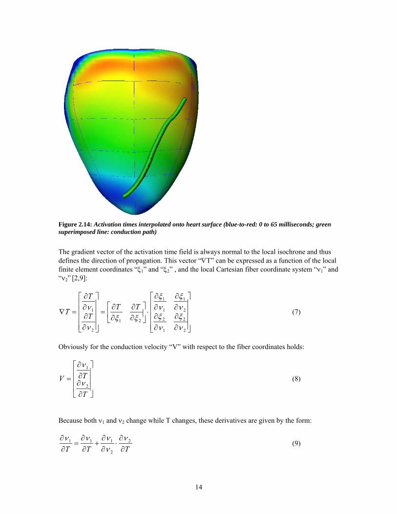
Figure 2.14: Activation times interpolated onto heart surface (blue-to-red: 0 to 65 milliseconds; green superimposed line: conduction path)

The gradient vector of the activation time field is always normal to the local isochrone and thus defines the direction of propagation. This vector “∇T” can be expressed as a function of the local finite element coordinates “ξ1” and “ξ2” , and the local Cartesian fiber coordinate system “ν1” and “ν2” [2,9]:

⎥⎥⎥⎥

⎦

⎤

⎢⎢⎢⎢

⎣

⎡

∂∂

∂∂

∂∂

∂∂

⋅⎥⎦

⎤⎢⎣

⎡∂∂

∂∂

=

⎥⎥⎥⎥

⎦

⎤

⎢⎢⎢⎢

⎣

⎡

∂∂∂∂

=∇

2

2

1

2

2

1

1

1

21

2

1

νξ

νξ

νξ

νξ

ξξν

ν TTT

T

T (7)

Obviously for the conduction velocity “V” with respect to the fiber coordinates holds:

⎥⎥⎥

⎦

⎤

⎢⎢⎢

⎣

⎡

∂∂∂∂

=

T

TV2

1

ν

ν

(8)

Because both ν1 and ν2 change while T changes, these derivatives are given by the form:

TTT ∂∂⋅

∂∂

+∂∂

=∂∂ 2

2

111 ννννν

(9)

14

This results in the following expression for the conduction velocity [10]:

⎥⎥⎥⎥⎥⎥⎥⎥⎥⎥⎥

⎦

⎤

⎢⎢⎢⎢⎢⎢⎢⎢⎢⎢⎢

⎣

⎡

⎟⎟⎠

⎞⎜⎜⎝

⎛∂∂

+⎟⎟⎠

⎞⎜⎜⎝

⎛∂∂

∂∂

⎟⎟⎠

⎞⎜⎜⎝

⎛∂∂

+⎟⎟⎠

⎞⎜⎜⎝

⎛∂∂

∂∂

=

2

2

2

1

2

2

2

2

1

1

νν

ν

νν

ν

TT

T

TT

T

V (10)

The magnitude of the velocity vector thus described the speed of propagation, and the direction of propagation was expressed by the angle that the vector subtended with respect to the local fiber direction. The conduction path, as shown in Figure 2.14, starts at a point close to the pacing site. The starting point is identical for the unloaded and loaded heart. However the conduction path can be slightly different for both cases, dependant on the exact velocity vector field. Changes in velocity field are a direct result of differences in fiber stretching [2,10]. The area regarded for analysis was limited to regions where the activation times were less than 45 milliseconds. It appears that within this time window, the imaged propagation primarily reflects epicardial conduction [10].

15

Chapter 3 Results For the coordinate values along the activation path (see Figure 2.14), activation times, conduction velocity and strain values in two directions are selected. Also, average conduction velocities for the undeformed and deformed heart are compared. Figure 3.1 shows activation times as a function of distance from pacing site. In this case, the action potential propagates slightly faster in the unloaded heart. However, the other three rabbits tested all show faster action potential spread for the loaded heart.

Figure 3.1: Activation times as function of distance from pacing site along conduction path (· = unloaded; * = loaded) (rabbit number 148)

The activation time at a distance of 20 millimeters from the pacing site is used to calculate an average conduction velocity.

Rabbit number

T10 mm

(unloaded) (ms) T20 mm

(unloaded) (ms)V20 mm (unloaded)

(m/s) T10 mm

(loaded) (ms) T20 mm

(loaded) (ms) V20 mm

(loaded) (m/s)148 28,3 48,3 0,41 30,8 49,2 0,41 153 29,9 48,6 0,41 26,5 44,9 0,45 155 27,5 48,5 0,41 25,5 46,6 0,43 156 37,5 67,7 0,30 35,0 61,2 0,33

Table 3.1: Activation times at 10 and 20 mm from the pacing site, and average conduction velocity over 20 mm (all for both the unloaded and loaded heart)

16

Except for the last rabbit, activation time at 10 mm is about 27-30 ms. However, the point 10 mm farther along the conduction path is typically activated within another 18-21 ms. In the majority of the conducted experiments, conduction velocity is slightly higher for the loaded heart (+0,03 m/s). For rabbit 156, activation times are rather high. At a distance of 10 mm, it takes another 10 milliseconds to activate the muscle fiber.

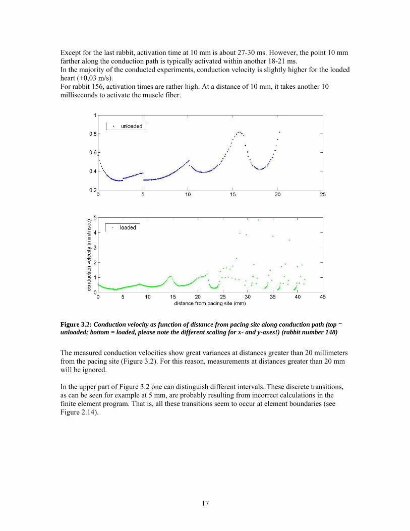
Figure 3.2: Conduction velocity as function of distance from pacing site along conduction path (top = unloaded; bottom = loaded, please note the different scaling for x- and y-axes!) (rabbit number 148)

The measured conduction velocities show great variances at distances greater than 20 millimeters from the pacing site (Figure 3.2). For this reason, measurements at distances greater than 20 mm will be ignored. In the upper part of Figure 3.2 one can distinguish different intervals. These discrete transitions, as can be seen for example at 5 mm, are probably resulting from incorrect calculations in the finite element program. That is, all these transitions seem to occur at element boundaries (see Figure 2.14).

17

The upper part of Figure 3.3 shows an alternative representation of conduction velocity. Now, for regularly spaced points an average conduction velocity is obtained by averaging velocities measured along the 2 mm conduction path before such a point. There’s clearly a gradual increase in conduction velocity along the conduction path. This is in good agreement with the observation made earlier, that the second 10 mm requires a reduced activation time in comparison with the first 10 mm.

Figure 3.3: Top: Conduction velocity as function of distance from pacing site along conduction path (· = unloaded; * = loaded) Bottom: Fiber (· = EFF) & cross fiber strain (* = ECF) as function of distance from pacing site along conduction path (rabbit number 148)

Strains in fiber (EFF) and cross fiber direction (ECF) are plotted using the same method as used for velocities (see Figure 3.3, bottom). In this case, the strain in fiber direction gradually increases. Strain in cross fiber direction starts to increase from a distance of 6 mm along the conduction path, but this strain still has a negative value along the first 11 mm.

18

Figure 3.4 & Figure 3.5 show strain values for different rabbits in fiber and cross fiber direction respectively.

Figure 3.4: Strain in fiber direction as function of distance from pacing site along conduction path · = rabbit number 148 * = rabbit number 153 + = rabbit number 155 ο = rabbit number 156

Strains in fiber direction appear to be fairly irregular. For rabbit 156, strain values are almost always negative. For the other three hearts there doesn’t seem to be one common fiber strain pattern.

19

Figure 3.5: Strain in cross fiber direction as function of distance from pacing site along conduction path · = rabbit number 148 * = rabbit number 153 + = rabbit number 155 ο = rabbit number 156

In three out of four hearts, strains in cross fiber direction remain relatively constant. Along almost the complete conduction path, cross fiber strain has a value between +0,02 and +0,06. In heart 148, decreased strain values along the beginning of the activation path are compensated by higher values near the end of this path.

20

Chapter 4 Discussion In this study we’ve combined regular video images, optical mapping and finite element analysis to investigate various factors affecting epicardial action potential spread. Thereby it’s possible to correlate electrical activation patterns with structural myocardial features such as 3-D anatomy and fiber architecture. However it should always be kept in mind that we’re only looking at the heart surface, and that endocardial and Purkinje layers may exhibit different properties.

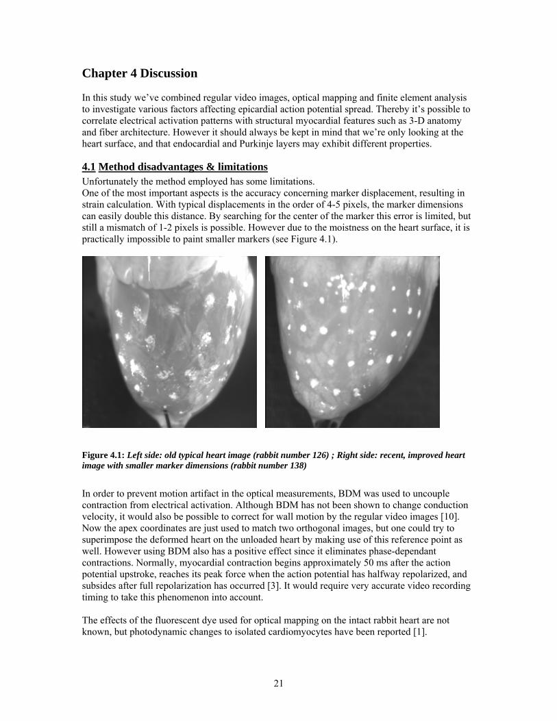
4.1 Method disadvantages & limitations Unfortunately the method employed has some limitations. One of the most important aspects is the accuracy concerning marker displacement, resulting in strain calculation. With typical displacements in the order of 4-5 pixels, the marker dimensions can easily double this distance. By searching for the center of the marker this error is limited, but still a mismatch of 1-2 pixels is possible. However due to the moistness on the heart surface, it is practically impossible to paint smaller markers (see Figure 4.1).

Figure 4.1: Left side: old typical heart image (rabbit number 126) ; Right side: recent, improved heart image with smaller marker dimensions (rabbit number 138)

In order to prevent motion artifact in the optical measurements, BDM was used to uncouple contraction from electrical activation. Although BDM has not been shown to change conduction velocity, it would also be possible to correct for wall motion by the regular video images [10]. Now the apex coordinates are just used to match two orthogonal images, but one could try to superimpose the deformed heart on the unloaded heart by making use of this reference point as well. However using BDM also has a positive effect since it eliminates phase-dependant contractions. Normally, myocardial contraction begins approximately 50 ms after the action potential upstroke, reaches its peak force when the action potential has halfway repolarized, and subsides after full repolarization has occurred [3]. It would require very accurate video recording timing to take this phenomenon into account. The effects of the fluorescent dye used for optical mapping on the intact rabbit heart are not known, but photodynamic changes to isolated cardiomyocytes have been reported [1].

21

Furthermore one should realize that the wave front is propagating epicardially as well as transmurally. Therefore it’s possible that basal regions are being activated long before the epicardial conduction wave arrives at this region [10]. We tried to minimize this problem by discarding areas with activation times greater than 45 milliseconds.

4.2 Explication of Results In the majority of the conducted experiments, activation times are slightly higher for the unloaded heart (see Table 4.1). This results in an increased conduction velocity of about +0,03 m/s for the loaded heart (see Table 3.1). These observations contribute to the ambiguous results previously reported (see § 1.2). Rabbit number

∆T10 mm

(unloaded-loaded) (ms) ∆ T20 mm

(unloaded-loaded) (ms) 148 -2,5 -0,9 153 +3,4 +3,7 155 +2,0 +1,9 156 +2,5 +6,5

Table 4.1: Activation time differences between unloaded & loaded heart at distances of 10 & 20 millimeters along conduction path

According to Table 3.1, activation times are higher for the second 10 mm along the conduction path. This indicates that conduction velocity is higher near the base than near the apex (see Top Figure 3.3). By looking at Figure 2.10, one could pose that this is a consequence of the local fiber orientation. Closer to the base, fibers are more closely aligned to the activation path. This means that here, fewer muscle fibers are necessary to conduct the action potential, resulting in a higher conduction velocity (see § 1.1). In the last experiment, activation times are rather high. This could be due to deteriorated conduction properties of the muscle fibers. Figure 3.4 shows negative strains for this heart along almost the complete conduction path. Therefore the decreased velocity could result from changes in conduction properties of the compressed muscle fibers. At distances greater than 20 mm from the pacing site, activation times and conduction velocity don’t exhibit a regular pattern anymore (see Figure 3.2). This is probably because the action potential activates parts of this area transmurally long before the epicardial wave front arrives. This breakthrough is the consequence of a higher conduction velocity in the so-called Purkinje fibers (see § 1.1). Although the conduction path for the various hearts is almost identical, strains in fiber direction show great variances (see Figure 3.4). In some areas, negative strain values are found. This would indicate a decreased volume in this part of the ventricle. In case of a pressure load applied from within the ventricle, it is very unlikely to find negative values over large areas. In contrast, strains in cross fiber directions do seem to follow a regular pattern (see Figure 3.5). This strain has a relatively constant value in most cases. In the case of heart 148, average strain is of the order of the strain values for the other hearts: decreased values along the beginning of the activation path are compensated by higher strains near the end.

22

4.3 Future Recommendations The experimental setup and data processing techniques as discussed in this paper promise to become an useful and valuable tool in understanding the role of individual heart muscle fibers and their local strains regarding action potential propagation. Besides acquiring fundamental knowledge, a few of the promising applications are the following. The role of stretch-activated channels can be further investigated if stretch-dependant currents mediated by these channels are measured. Then it would be possible to correlate these currents with regional strains and conduction velocity. Another promising area is the effect of pacing site on strain distributions and ultimately contracting characteristics. This can potentially improve pacemaker placement [14]. Currently, activation times were fitted to the 3-D mesh as a continuous scalar field variable with first-derivative continuity. However, there can be cases where the activation time doesn’t have to be smooth or continuous. For example, wave front collision or reentrant arrhythmia could result in a velocity discontinuity. In such cases it might be better to increase the number of elements and ignore the first derivative demand [10].

23

Conclusion The goal of this experiment was to investigate the role of geometry, fiber orientation and regional strains on conduction velocity. Of course, stretching the fibers results in an increased path length. Due to programming difficulties, the effect of fiber orientation could not yet be fully explored. Alterations in fiber orientation after myocardium stretching can change the number of fibers involved in action potential spread. The fiber angle along the conduction path, a quantity which became available during the end phase of this project, can be a measure for this number. Hypothetically, one would expect an inverse relation between the number of involved fibers and the conduction velocity. This could be a point of focus for a future project. Unfortunately, the role of regional strains remains unclear. Therefore it might be sensible to conduct a few reference experiments for testing the accuracy of the method employed for measuring local strains. A first step could be inflating a spherically shaped object and then checking the margin of error of Lagrangian strains obtained with the aid of painted surface markers. In another experiment the actual fiber angels along the epicardial conduction path should be compared with the standard fiber angels used currently (see § 2.4). At this moment, strain results appear to be too untrustworthy. When the method turns out to be reliable, possibly after some minor method adjustments, more experiments can deepen the insight in muscle fiber properties.. Then it will become possible to fully investigate the relation between conduction velocity and regional fiber strain.

24

References [1] Banville, I., Gray, R.A., 2002. Effect of Action Potential Duration and Conduction Velocity

Restitution and Their Spatial Dispersion on Alternans and the Stability of Arrhytmias. Journal of Cardiovascular Electrophysiology 13, 1141-1149. [2] Bayly, P.V., KenKnight, B.H., Rogers, J.M., Hillsley, R.E., Ideker, R.E., Smith, W.M. Estimation of Conduction Velocity Vector Fields from Epicardial Mapping Data. IEEE Transactions on Biomedical Engineering 45, 563-571. [3] Franz, M.R., 1996. Mechano-electric Feedback in Ventricular Myocardium. Cardiovascular Research 32, 15-24. [4] Grabow, N., 2000. Nonhomogeneous Strain Analysis in the Right Ventricular Epicardial

Surface of the Ejecting Mouse Heart (La Jolla, San Diego, Projektarbeit). [5] Guyton, A.C., Hall, J.E., 1996. Textbook of Medical Physiology (W.B. Saunders Company, Philadelphia) [6] Hunter, P., Pullan, A., 2000. FEM/BEM notes (Auckland, New Zealand). [7] Mazhari, R., 1999. Regional flow-function Relations during Acute Myocardial Ischemia and

Reperfusion (UCSD, San Diego, Dissertation). [8] McCulloch, A., Smaill, B.H., Hunter, P.J., 1989. Regional Left Ventricular Epicardial Deformation in the Passive Dog Heart. Circulation Research 64, 721-733. [9] Otsu, N., 1979. A Threshold Selection Method from Gray-Level Histograms. IEEE Transactions on Systems, Man, and Cybernetics 9, 62-66. [10] Sung, D., Omens, J.H., McCulloch, A.D., 2001. Model-Based Analysis of Optically Mapped

Epicardial Activation Patterns and Conduction Velocity. Annals of Biomedical Engineering 28, 1085-1092. [11] Sung, D., Somayajula-Jagai, J., Cosman, P., Mills, R., McCulloch, A.D., 2001. Phase Shifting Prior to Spatial Filtering Enhances Optical Recordings of Cardiac Action Potential Propagation. Annals of Biomedical Engineering 29, 854-861. [12] Sung, D., Mills, R.W., Schettler, J., Narayan, S.M., Omens, J.H., McCulloch, A.D., 2003.

Ventricular Filling Slows Epicardial Conduction and Increases Action Potential Duration in an Optical Mapping Study of the Isolated Rabbit Heart. Journal of Cardiovascular

Electrophysiology 14, 739-749. [13] Vetter, F.J., 2001. Fitting the LV Geometry in Continuity (UCSD, San Diego, Notes) [14] Vetter, F.J., McCulloch, A.D., 1998. Three-dimensional analysis of regional cardiac function: a model of rabbit ventricular anatomy. Progress in Biophysics & Molecular Biology 69, 157-183. [15] http://cmrg.ucsd.edu/modelling/cont5/guide

25