2d transformation of graphics unit 2. what is geometric transformation? operations that are applied...
TRANSCRIPT

2D Transformation of Graphics
Unit 2

• What is geometric transformation?
• Operations that are applied to the geometric description of an object to change its position, orientation, or size are called geometric transformations.

• So the geometric-transformation functions that are available in some system are following:
1. Translation
2. Rotation
3. Scaling
4. Other useful transforms includes: reflection and shear.

• Translation
• Rotation

• Scaling
• Uniform Scaling
• Un-uniform Scaling

• Reflection
• Shear

• Why do we need geometric transformations in CG( motivation )?
• As a viewing aid
• As a modeling tool
• As an image manipulation tool

• Two-Dimensional(2D) Translation
We perform a translation on a single coordinate point by adding offsets to its coordinates so as to generate a new coordinate position.
Similarly, a translation is applied to an object that is defined with multiple coordinate positions by relocating all the coordinate positions by the same displacement along parallel paths.
Suppose tx and ty is the translation distances, (x, y) is the original coordinates, is the new coordinate position.
txxx y y ty
'( , ')x y

• Express the translation use matrix equation as following:
• Translation is a rigid-body transformation that moves objects without deformation.
• Ex: Translate a polygon with coordinates
A(2, 5), B(7, 10), C(10, 2) by 3 units x direction and 4 units in y direction
(Hint : Add 3 to all x values and 4 to all values).
x x tx
y y ty
• Write a C++ program to translate :
• A point
• A line
• A Rectangle
• A Polygon (Triangle)

/* C++ program */
#include<iostream.h>
#include<graphics.h>
#include<math.h>
void main()
{
clrscr();
int x,y,tx,tx;
/* initialise graphics
------------------------ */
detectgraph(&gd,&gm);
initgraph(&gd,&gm,“c:\\tc\\bgi");

cout<<“Enter x, y:”cin>>x>>y;cout<<“Enter tx,ty”cin>>tx>>ty;putpixel(x,y,15);delay(100);putpixel(x+tx,y+ty,15);getch();closegraph();}
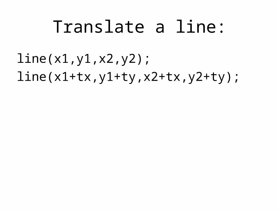
Translate a line:
line(x1,y1,x2,y2);
line(x1+tx,y1+ty,x2+tx,y2+ty);

Translate a rectangle:
rectangle(x1,y1,x2,y2);
rectangle(x1+tx,y1+ty,x2+tx,y2+ty);

Two-Dimensional Rotation• We generate a rotation transformation of an object by
specifying a rotation axis and a rotation angle. All points of the object are then transformed to new positions by rotating the points through the specified angle about the rotation axis.
• A 2D rotation of an object is obtained by repositioning the object along a circular path in the xy plane, the rotation axis is perpendicular to the xy plane.
• Parameters for 2D rotation is rotation angle and a rotation point( pivot point) .
• Rotation angle define a positive values for counterclockwise rotation about the pivot point.
),( rr yx

• r is the constant distance of the point form the origin, angle is the original angular position of the point from the horizontal, and is the rotation angle.
• Substitute expression (1) into (2)
cos
sin
x r
y r
cossinsincos)sin('
sinsin-coscos)cos('
rrry
rrrx
( 1)
( 2)


Matrix form
P’=P.R
cossin'
sincos'
yxy
yxx( 3)
cos sin
sin cosx y x y

Example 1
• A point (4, 3) is rotated by an angle of 45 degrees. Find the rotation matrix and resultant point.
• Rotate a line from A(0,0) to B(200,100) by 45 degrees.
• Rotate a polygon with coordinates A(2, 5),
B(7, 10), C(10, 2) by an angle of 45 degrees.
• Write a C program to Rotate :
• A point
• A line
• A Rectangle
• A Polygon (Triangle)


Two-Dimensional(2D) Scaling• To alter the size of an object, we apply a scaling
transformation. A simple two-dimensional scaling operation is performed by multiplying object positions (x, y) by scaling factors sx and sy to produce the transformed coordinate .
• Scaling factors sx scales an object in the x coordinate.
),( rr yx'
'x
y
x x S
y y S
0
0x
y
Sx y x y
S

Properties of the scaling transformation.
• Any positive values can be assigned to the scaling factors sx and sy. Values less then 1 reduce the size of object, the object will close up the original at the same time. In contrast , enlarge the size of object.
• When sx and sy are assigned to the same values, a uniform scaling is produced which maintains relative object proportions.

• Unequal values for sx and sy result in a differential scaling that is often used in design applications.
• Negative values can also be specified for the scaling parameters, this not only resizes an object, it reflects the object one or more of the coordinate axes.


• Write a C++ program to scale :
• A point
• A line
• A Rectangle
• A Polygon (Triangle)

Point:cout<<“Enter x, y:”cin>>x>>y;cout<<“Enter sx,sy”cin>>sx>>sy;Initgraph(&gd,&gm,”..\\bgi”);putpixel(x,y,15);delay(100);putpixel(x*sx,y*sy,15);getch();closegraph();}

Scale a line:
line(x1,y1,x2,y2);
line(x1*sx,y1*sy,x2*sx,y2*sy);
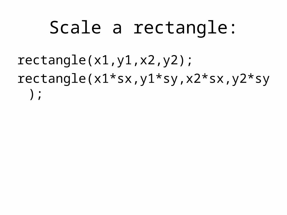
Scale a rectangle:
rectangle(x1,y1,x2,y2);
rectangle(x1*sx,y1*sy,x2*sx,y2*sy);

•

Q. Scale the polygon with coordinates A(2,5) B(7,10) and C(10,2) by two units in x-direction and two units in y-direction and plot the graph.
Q. Scale the polygon with coordinates A(2,5) B(7,10) and C(10,2) by -2 units in x-direction and 3 units in y-direction and plot the graph.

Matrix Representations and Homogeneous Coordinates• It is well known that many application involves
sequences of geometric transformations. For example, an animation might require an object to be translated, rotated and scaled at each increment of the motion. If you want to first rotates an object, then scales it, you can combine those two transformation to a composite transformation like the following equation:
•
0 cos sincos sin*
0 sin cossin cosx x x
y y y
S S SA S R
S S S

• However, it will be difficult to deal with the above composite transformation and translation together. Because, translation is not 2 by 2 matrix representation.
• So ,here we consider how the matrix representations discussed in the previous sections can be reformulated so that such transformation sequences can be efficiently processed.

• In fact, we can expressed three basic two-dimensional transformation( translation, rotation, and scaling) in the general matrix form:
• Now this equation can be reformulated to eliminate the matrix addition operation using Homogeneous Coordinates.
21' MPMP

• What is Homogeneous Coordinates?• A standard technique for expanding each two-
dimensional coordinate position representation (x, y) to three-element representation , called Homogeneous Coordinates, where homogeneous h is a nonzero value such that
• • For geometric transformation, we can chose the
homogeneous parameter h to be any nonzero value. Thus there are an infinite number of equivalent homogeneous representations for each coordinate point (x, y) .
•
( , , )h hx y h
,h hx yx y
h h

• A convenient choice is simply to set h=1, so each two-dimensional position is then represented with homogeneous coordinate (x,y,1).
• Expressing positions in homogenous coordinates allows us to represent all geometric transformation equations as matrix multiplications, which is the standard method used in graphics systems. Two dimensional coordinate positions are represented with three-elements column vectors, and two-dimensional transformation operations are expressed as 3X3 matrices.

• Homogeneous coordinate representation of 2D Translation
• This translation operation can be written in the abbreviated form
1100
10
01
1
y
x
ty
tx
y
x
' ( , )x yP T t t P

• Homogeneous coordinate representation of 2D Rotation
' ( )P R P
This translation operation can be written in the abbreviated form
1100
0cossin
0sincos
1
y
x
y
x

• Homogeneous coordinate representation of 2D Scaling
1100
00
00
1
y
x
sy
sx
y
x
' ( , )P S sx sy P
This scaling operation can be written in the abbreviatedform

Two-Dimensional Composite Transformation• Using matrix representations, we can set up a
sequence of transformation as a composite transformation matrix, by calculating the product of the individual transformations.
• And, since many positions in a scene are typically transformed by the same sequence, its is more efficient to first multiply the transformation matrices to form a single composite matrix.
• So the coordinate position is transformed using the composite matrix M, rather than applying the individual transformations M1 and then M2
'2 1P M M P
M P

General Two-Dimensional Pivot-Point Rotation
(Rotation about an arbitrary point)
• So we can generate a 2D rotation about any other pivot point (x, y) by performing the following sequence of translate-rotate-translate operations.
(xr,yr)
(xr,yr)
(xr,yr)
(xr,yr)

• (1) Translate the object so that the pivot-point position is moved to the coordinate origin.
• (2) Rotate the object about the coordinate origin.• (3) Translate the object so that the pivot point is
returned to its original position.• The composite transformation matrix for this
sequence is obtained with the concatenation:
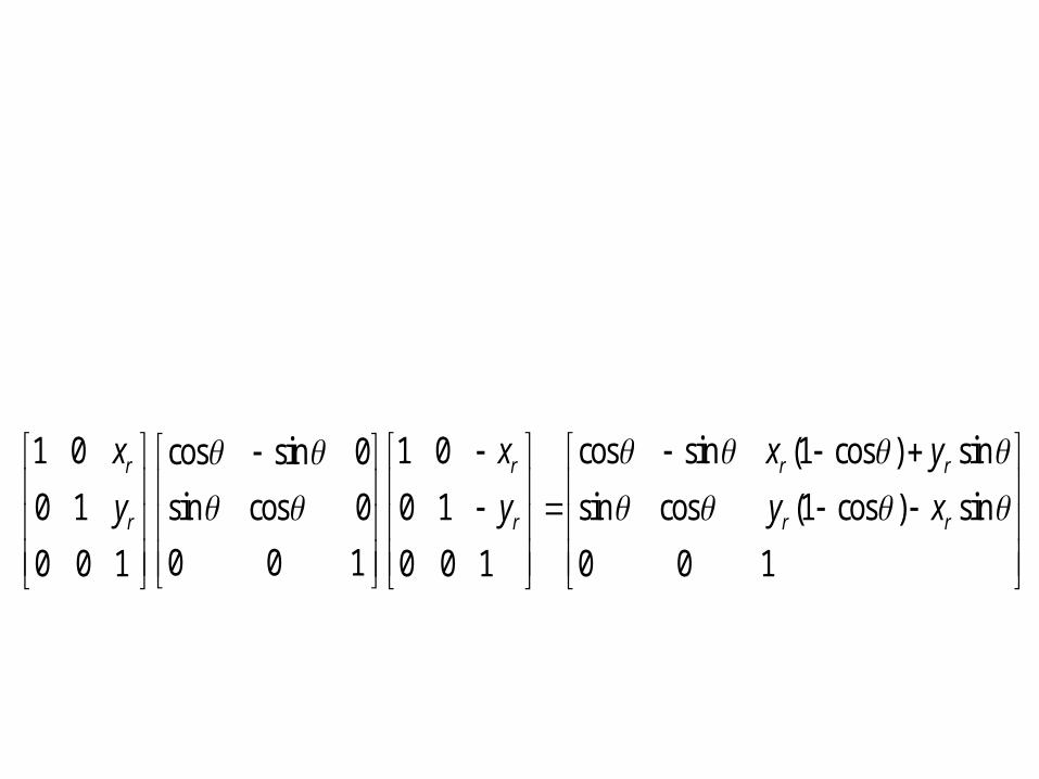
1 0 1 0 cos sin (1 cos ) sincos sin 0
0 1 sin cos 0 0 1 sin cos (1 cos ) sin
0 0 10 0 1 0 0 1 0 0 1
r r r r
r r r r
x x x y
y y y x

Problems:
• Perform the rotation of a point A(2,3) about point (1,1) by angle of 45 degrees.
• Perform the rotation of a point A(2,3), B(5,5), C(4,3) about point (1,1) by angle of 45 degrees.

• Other 2D transformations:
• Reflection with respect to the axis
• • X axis • y axis
100
010
001
100
010
001
x
y 1
32
1’
3’2’x
y1
32
1’
3’ 2’

• Reflection with respect to a line y=x
100
001
010
x
y

• Shear• Two common shearing transformations are those
that shift coordinate x values and those that shift y values.
• An x-direction shear relative to the x axis is produced with the transformation matrix
100
010
01 xsh
x’ = x + shx · y, y’ = y
x
y
x
y
(0,0) (1,0)
(1,1)(0,1)
(0,0) (1,0)
(3,1)(2,1)

• Y-Shear
100
01
001
Shy
x’ = x , y’ = y + shy*x

Thank You!!

General 3D Rotations
(1) Rotating about an axis that is parallel to one of the coordinates axes.
• Step1, Translate the object so that the rotation axis coincides with the parallel coordinate axis.
• Step2, Perform the specified rotation about that axis.
• Step3, Translate the object so that rotation axis is moved back to its original.

• A coordinate position P is transformed with the sequence
' 1 ( )xP T R T P

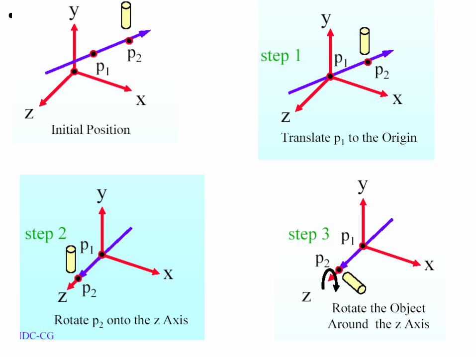
• (2) Rotated about an axis that is not parallel to one of the coordinate axes.
• In this case, we also need rotation to align the rotation axis with a selected coordinate axis and then to bring the rotation axis back to its original orientation.
• A rotation axis can be defined with two coordinate position, or one position and direction angles (direction cosines ).
• Now we assume that the rotation axis is defined by two points, and that the direction of rotation is to be counter clockwise when looking along the axis from p2 to p1.

• The components of the rotation axis vector are then computed as:
• And the unit rotation-axis vector u is
• Where
•
2 1
2 1 2 1 2 1( , , )
V P P
x x y y z z
( , , )V
u a b cV
2 1 2 1 2 1, ,x x y y z z
a b cV V V

• Step1. Translate the object so that the rotation axis passes through the coordinate origin
• Step2, Rotate the object so that the axis of rotation coincides with one of the coordinate axes.
• Step3, Perform the specified rotation about the selected coordinate axis
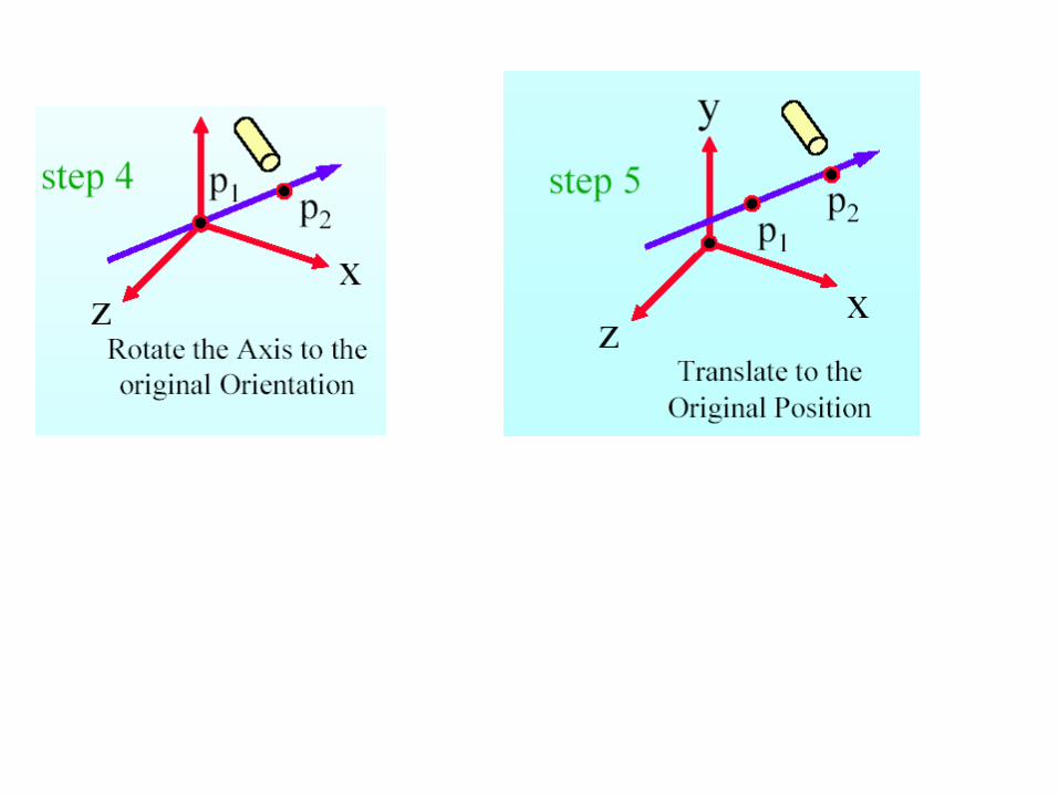
• Step4, Apply inverse rotations to bring the rotation axis back to its original orientation.
• Step5 ,Apply the inverse translation to bring the rotation axis to its original spatial position.
• we can transform the rotation axis onto any one of the three coordinate axes. But the z axis is often a convenient choice.

•


• The first step in the rotation sequence is to set up the translation matrix that repositions the rotation axis so that it passes through the coordinate origin. We move p1 to the origin.

• The next step we will put the rotation axis onto the z axis. We can use the coordinate-axis rotations to accomplish this alignment in two steps. For this example, we first rotate about the x axis, then rotate about y axis. The x axis rotation gets vector u into the x-z plane, and the y-axis rotation swings u around to the z axis.
x
z
yu

• Since rotation calculations involve sine and cosine functions, so we can use standard vector operation to obtain elements of the two rotation matrices. A vector dot product can be used to determine the cosine term, and a vector cross product can be used to calculate the sine term.
• Firstly, we establish the transformation matrix for rotation around the x axis by determining the values for the sine and cosine of the rotation angle necessary to get u into the x-z plane.

Inverse Transformation
• To undo the applied transformation Inverse Transformation is applied.
• Inverse of T is T-1.
• T T-1=I (Identity Matrix)

Thank you !!!

• Not required

• Question 1: • If the rotation point is an arbitrary pivot position ,
can you give the correct rotation expression?
• How to rotate a line segment or a polygon?
),( rr yx
' ( ) cos ( )sin
' ( )sin ( )cosr r r
r r r
x x x x y y
y y x x y y
( 3)

• Similarly, we can obtain the matrix representation of General 2D Fixed-Point Scaling.( question ).
• (1) Translate the object to so that the fixed point coincides with the coordinate origin.
• (2) Scale the object with respect to the coordinate origin.
• (3) Use the inverse of the translation in step (1) to return the object to its original position.

•
100
)1(0
)1(0
100
10
01
100
00
00
100
10
01
yfy
xfx
f
fx
f
f
sys
sxs
y
x
s
s
y
x
y
Translate Scale Translate
(xr,y
r)(xr,yr)
(xr,yr)
(xr,yr)
yxffffyxff ssyxSyxTssSyxT ,,,, ,,

• We also obtain General 2D Scaling Directions.• Suppose we want to apply scaling factors with
values specified by parameters s1 and s2 in the directions shown in the following fig.

• To accomplish the scaling without changing the orientation of the object.(1) we perform a rotation so that the directions for s1 and s2 coincide with the x and y axes, respectively.
(2) Then the scaling transformation S(s1,s2) is applied.
(3) An opposite rotation to return points to their original orientations.

100
0cossinsincos)(
0sincos)(sincos
)(),()( 22
2112
122
22
1
211
ssss
ssss
RssSR
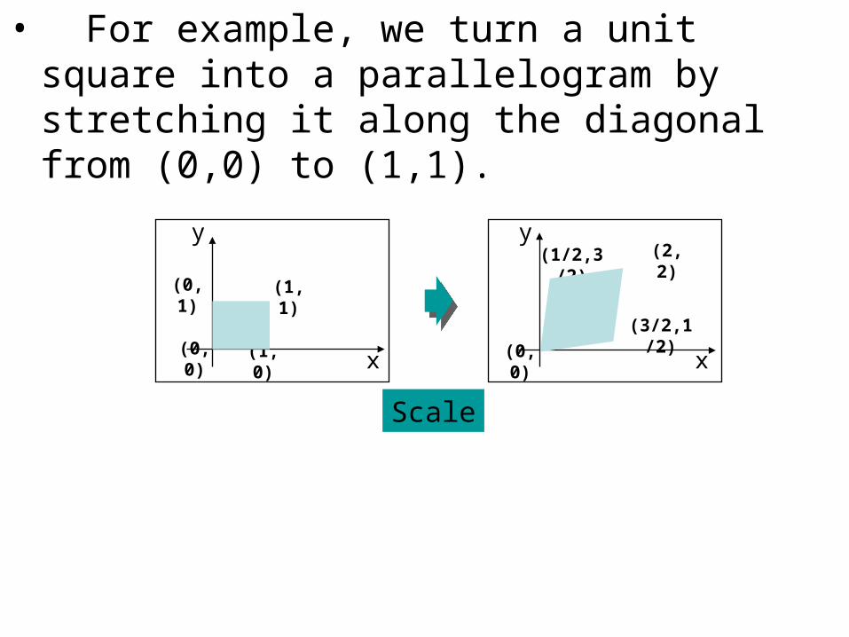
• For example, we turn a unit square into a parallelogram by stretching it along the diagonal from (0,0) to (1,1).
x
y
(0,0)
(3/2,1/2)
(1/2,3/2)
(2,2)
x
y
(0,0) (1,0)
(0,1) (1,1)
Scale

• We first rotate the diagonal onto the y axis using angle 45 degree. Then we double its length with the scaling values s1=1 and s2=2, and then we rotate again to return the diagonal to its original orientation.

• Matrix Concatenation Properties
• (1) Multiplication of matrices is associative.
• (2) Transformation products, on the other hand, may not be commutative.

• Other 2D transformations:
• Reflection with respect to the axis
• • X axis • y axis • original point
100
010
001
100
010
001
100
010
001
x
y 1
32
1’
3’2’x
y1
32
1’
3’ 2
x
y
3
1’
3’ 2
1
2

• Reflection with respect to a line
100
001
010
x
y

• Shear• Two common shearing transformations are those
that shift coordinate x values and those that shift y values.
• An x-direction shear relative to the x axis is produced with the transformation matrix
100
010
01 xsh
x’ = x + shx · y, y’ = y
x
y
x
y
(0,0) (1,0)
(1,1)(0,1)
(0,0) (1,0)
(3,1)(2,1)

• Any real number can be assigned to the shear parameter shx. A coordinate position (x, y) is then shifted horizontally by an amount proportional to its perpendicular distance ( y value ) from the x axis.
• We can generate x-direction shears relative to other reference lines with yref=-1.
• Now, coordinate positions are transformed as
x’ = x + shx · (y-yref), y’ = y
•
(3,1)

• The following Fig. illustrates the conversion of a square into a parallelogram with shy=0.5 and yref=-1.
100
010
1 refxx yshsh
x
y
x
y
(0,0) (1,0)
(1,1)(0,1)(1/2,0)
(3/2,0)
(2,1)(1,1)
(0,-1)

• Shearing operations can be expressed as a sequences of basic transformations. Such as a series of rotation and scaling matrices

General 3D Rotations
(1) Rotating about an axis that is parallel to one of the coordinates axes.
• Step1, Translate the object so that the rotation axis coincides with the parallel coordinate axis.
• Step2, Perform the specified rotation about that axis.
• Step3, Translate the object so that rotation axis is moved back to its original.

• A coordinate position P is transformed with the sequence
' 1 ( )xP T R T P

• (2) Rotated about an axis that is not parallel to one of the coordinate axes.
• In this case, we also need rotation to align the rotation axis with a selected coordinate axis and then to bring the rotation axis back to its original orientation.
• A rotation axis can be defined with two coordinate position, or one position and direction angles (direction cosines ).
• Now we assume that the rotation axis is defined by two points, and that the direction of rotation is to be counter clockwise when looking along the axis from p2 to p1.

• The components of the rotation axis vector are then computed as:
• And the unit rotation-axis vector u is
• Where
•
2 1
2 1 2 1 2 1( , , )
V P P
x x y y z z
( , , )V
u a b cV
2 1 2 1 2 1, ,x x y y z z
a b cV V V

• Step1. Translate the object so that the rotation axis passes through the coordinate origin
• Step2, Rotate the object so that the axis of rotation coincides with one of the coordinate axes.
• Step3, Perform the specified rotation about the selected coordinate axis
• Step4, Apply inverse rotations to bring the rotation axis back to its original orientation.
• Step5 ,Apply the inverse translation to bring the rotation axis to its original spatial position.
• we can transform the rotation axis onto any one of the three coordinate axes. But the z axis is often a convenient choice.
•

• The first step in the rotation sequence is to set up the translation matrix that repositions the rotation axis so that it passes through the coordinate origin. We move p1 to the origin.

• The next step we will put the rotation axis onto the z axis. We can use the coordinate-axis rotations to accomplish this alignment in two steps. For this example, we first rotate about the x axis, then rotate about y axis. The x axis rotation gets vector u into the x-z plane, and the y-axis rotation swings u around to the z axis.
x
z
yu

• Since rotation calculations involve sine and cosine functions, so we can use standard vector operation to obtain elements of the two rotation matrices. A vector dot product can be used to determine the cosine term, and a vector cross product can be used to calculate the sine term.
• Firstly, we establish the transformation matrix for rotation around the x axis by determining the values for the sine and cosine of the rotation angle necessary to get u into the x-z plane.
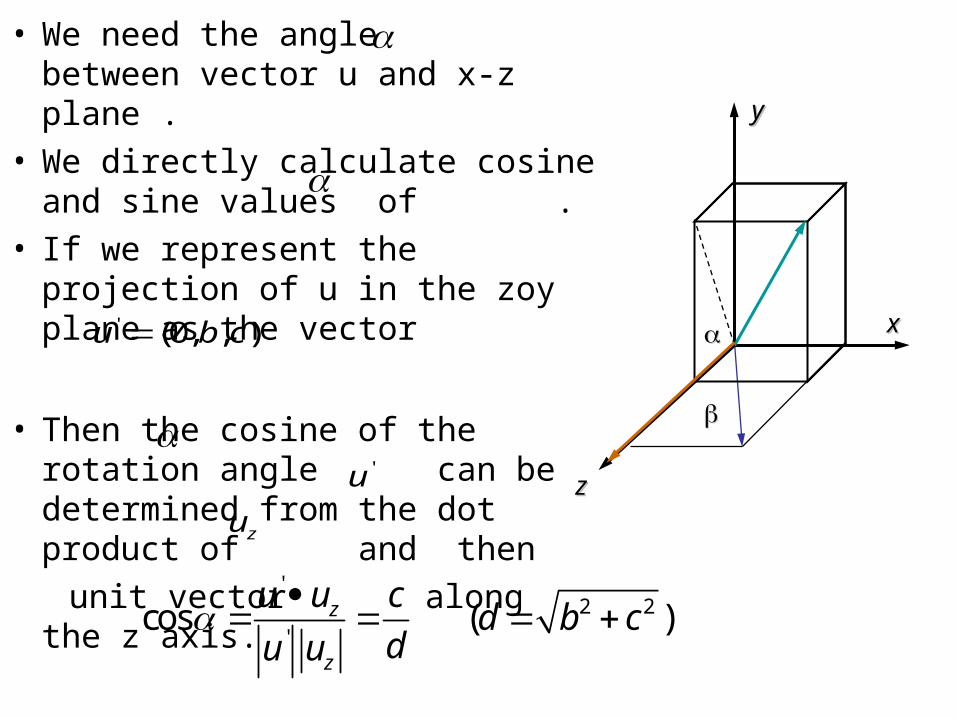
• We need the angle between vector u and x-z plane .
• We directly calculate cosine and sine values of .
• If we represent the projection of u in the zoy plane as the vector
• Then the cosine of the rotation angle can be determined from the dot product of and then
unit vector along the z axis.
zz
xx
yy
' (0, , )u b c
'u
zu
'2 2
'cos ( )z
z
u u cd b c
du u

Similarly, we can determine the sine of from the cross product of
So
' ' sinz x zu u u u u
'z xu u u b
' sinx z xu u u u b
sinb
d

• So the matrix elements for rotation of this vector about the x axis and into the xz plane:
1 0 0 01 0 0 0
0 00 cos sin 0
0 sin cos 00 0
0 0 0 10 0 0 1
x
c b
d dRb c
d d

• The rotation matrix about y axis is
cos 0 sin 0 0 0
0 1 0 0 0 1 0 0
sin 0 cos 0 0 0
0 0 0 1 0 0 0 1
y
d a
Ra d

• The third step we have aligned the rotation axis with the positive z axis. The specified rotation angle we can now be applied as a rotation about the z axis
cos sin 0 0
sin cos 0 0
0 0 1 0
0 0 0 1
zR
zz
xx
yy

• So the transformation matrix for rotation about an arbitrary axis can then be expressed as the composition of these seven individual transformations:
•
TRRRRRTR xyzyx )()()()()()( 111