2d spline curves - comp575comp575.web.unc.edu/files/2010/12/splines.pdf · 3 classical approach...
TRANSCRIPT

1
Spline Curves
COMP 575/COMP 770
2
Motivation: smoothness
• In many applications we need smooth shapes
– that is, without discontinuities
• So far we can make
– things with corners (lines, squares, rectangles, …)
– circles and ellipses (only get you so far!)
[Bo
ein
g]

3
Classical approach
• Pencil-and-paper draftsmen also needed smooth
curves
• Origin of “spline:” strip of flexible metal
– held in place by pegs or weights to constrain shape
– traced to produce smooth contour
4
Translating into usable math
• Smoothness
– in drafting spline, comes from physical curvature
minimization
– in CG spline, comes from choosing smooth functions
• usually low-order polynomials
• Control
– in drafting spline, comes from fixed pegs
– in CG spline, comes from user-specified control points
5
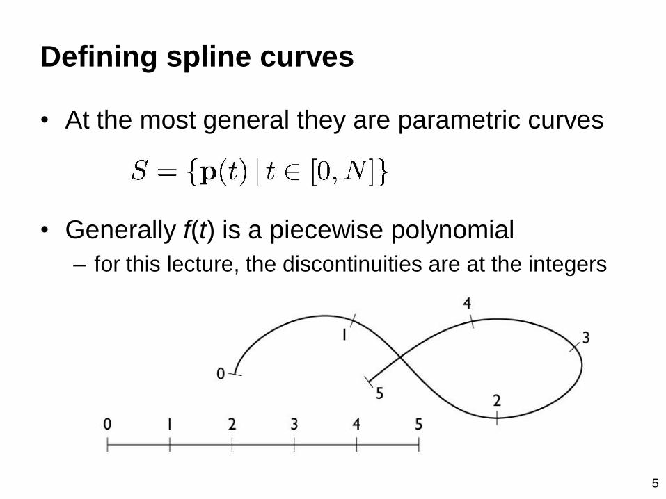
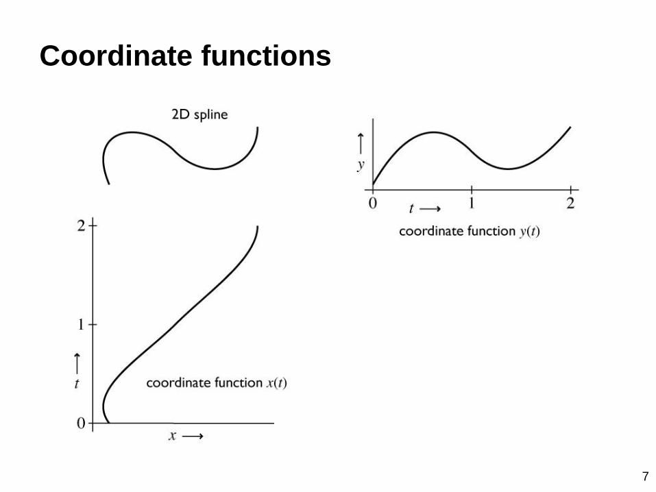
Defining spline curves
• At the most general they are parametric curves
• Generally f(t) is a piecewise polynomial
– for this lecture, the discontinuities are at the integers
6
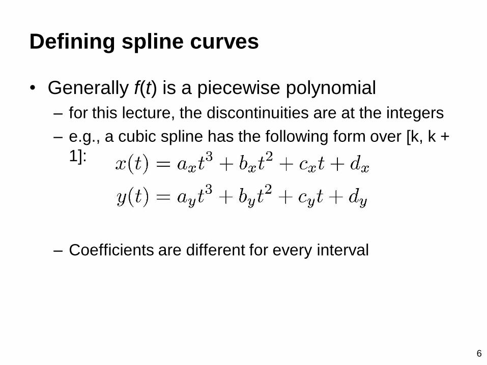
Defining spline curves
• Generally f(t) is a piecewise polynomial
– for this lecture, the discontinuities are at the integers
– e.g., a cubic spline has the following form over [k, k +
1]:
– Coefficients are different for every interval
7
Coordinate functions

8
Coordinate functions

9
Control of spline curves
• Specified by a sequence of control points
• Shape is guided by control points (aka control
polygon)
– interpolating: passes through points
– approximating: merely guided by points

10
How splines depend on their controls
• Each coordinate is separate
– the function x(t) is determined solely by the x
coordinates of the control points
– this means 1D, 2D, 3D, … curves are all really the
same
• Spline curves are linear functions of their controls
– moving a control point two inches to the right moves x(t)
twice as far as moving it by one inch
– x(t), for fixed t, is a linear combination (weighted sum)
of the control points’ x coordinates
– p(t), for fixed t, is a linear combination (weighted sum)
of the control points
11
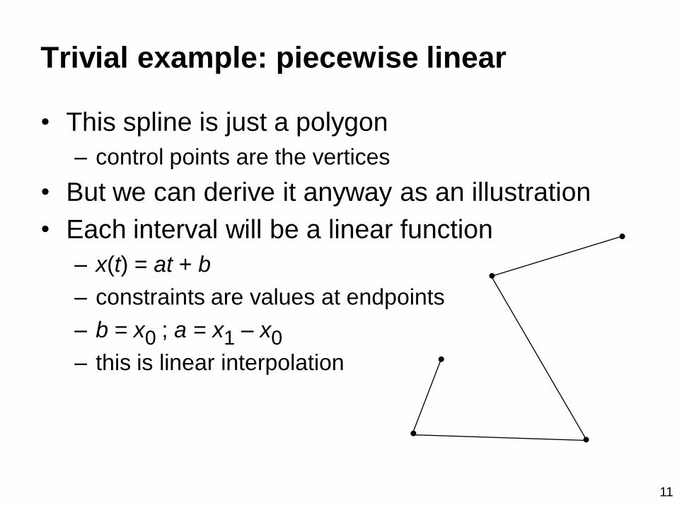
Trivial example: piecewise linear
• This spline is just a polygon
– control points are the vertices
• But we can derive it anyway as an illustration
• Each interval will be a linear function
– x(t) = at + b
– constraints are values at endpoints
– b = x0 ; a = x1 – x0
– this is linear interpolation
12
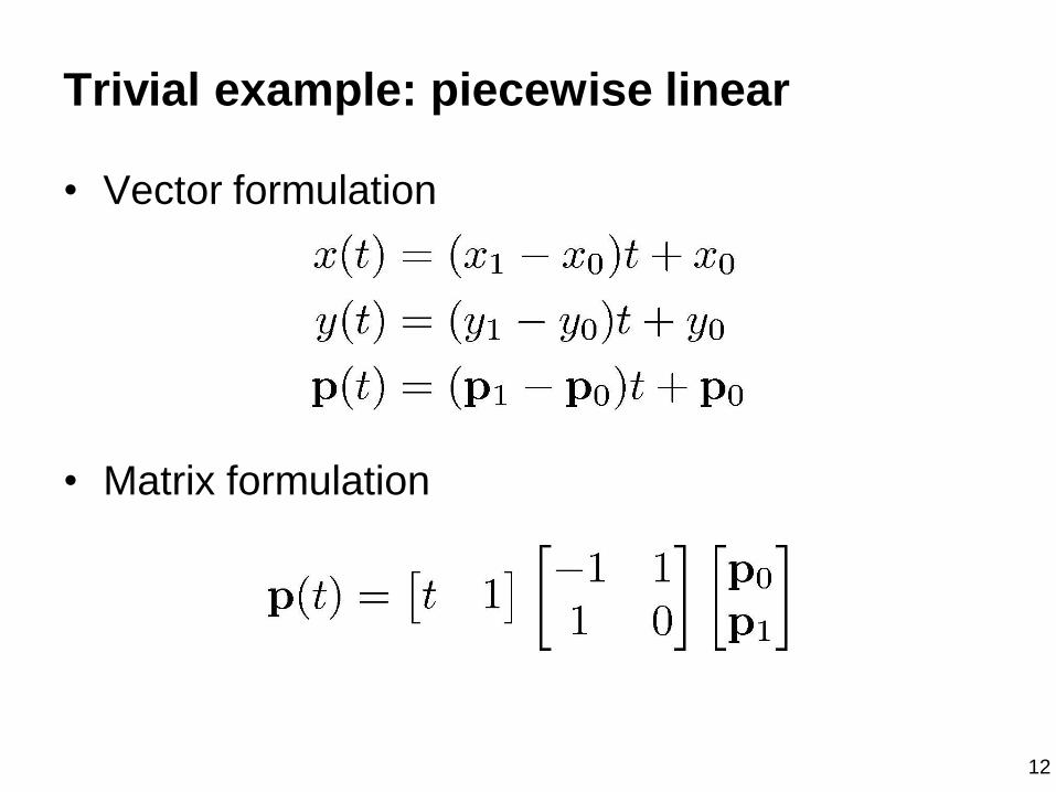
Trivial example: piecewise linear
• Vector formulation
• Matrix formulation

13
Trivial example: piecewise linear
• Basis function formulation
– regroup expression by p rather than t
– interpretation in matrix viewpoint

14
Trivial example: piecewise linear
• Vector blending formulation: “average of points”
– blending functions: contribution of each point as t
changes
15
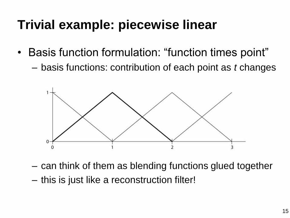
Trivial example: piecewise linear
• Basis function formulation: “function times point”
– basis functions: contribution of each point as t changes
– can think of them as blending functions glued together
– this is just like a reconstruction filter!
16
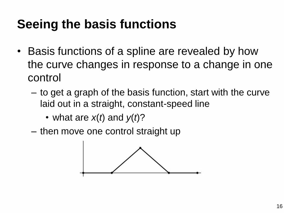
Seeing the basis functions
• Basis functions of a spline are revealed by how
the curve changes in response to a change in one
control
– to get a graph of the basis function, start with the curve
laid out in a straight, constant-speed line
• what are x(t) and y(t)?
– then move one control straight up
17
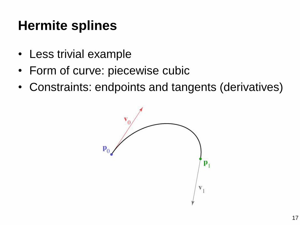
Hermite splines
• Less trivial example
• Form of curve: piecewise cubic
• Constraints: endpoints and tangents (derivatives)
18
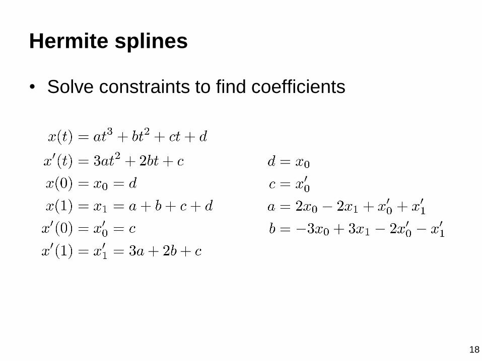
Hermite splines
• Solve constraints to find coefficients
19
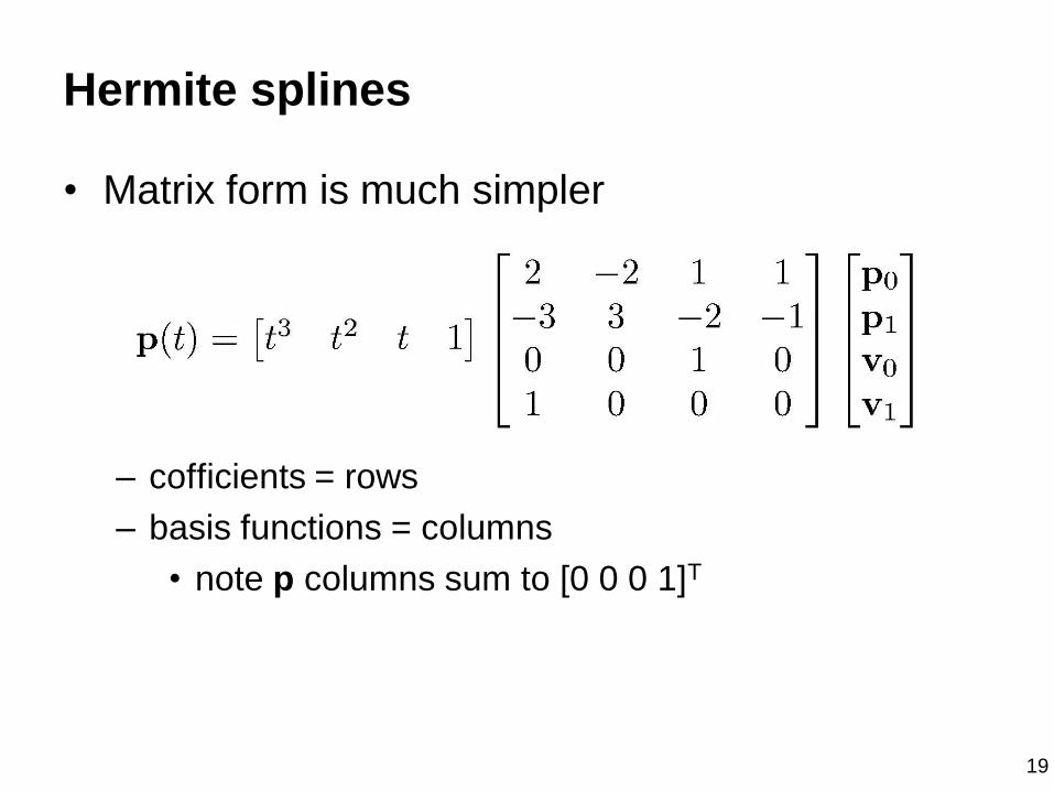
Hermite splines
• Matrix form is much simpler
– cofficients = rows
– basis functions = columns
• note p columns sum to [0 0 0 1]T
20
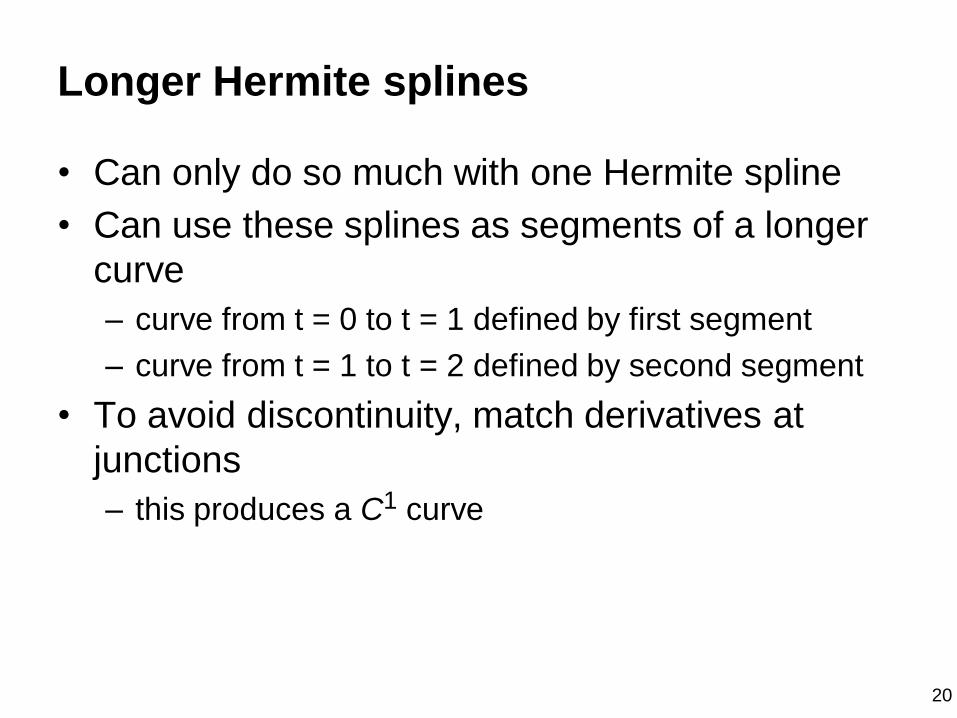
Longer Hermite splines
• Can only do so much with one Hermite spline
• Can use these splines as segments of a longer
curve
– curve from t = 0 to t = 1 defined by first segment
– curve from t = 1 to t = 2 defined by second segment
• To avoid discontinuity, match derivatives at
junctions
– this produces a C1 curve
21
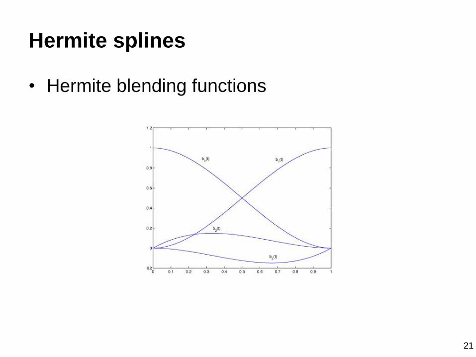
Hermite splines
• Hermite blending functions
22
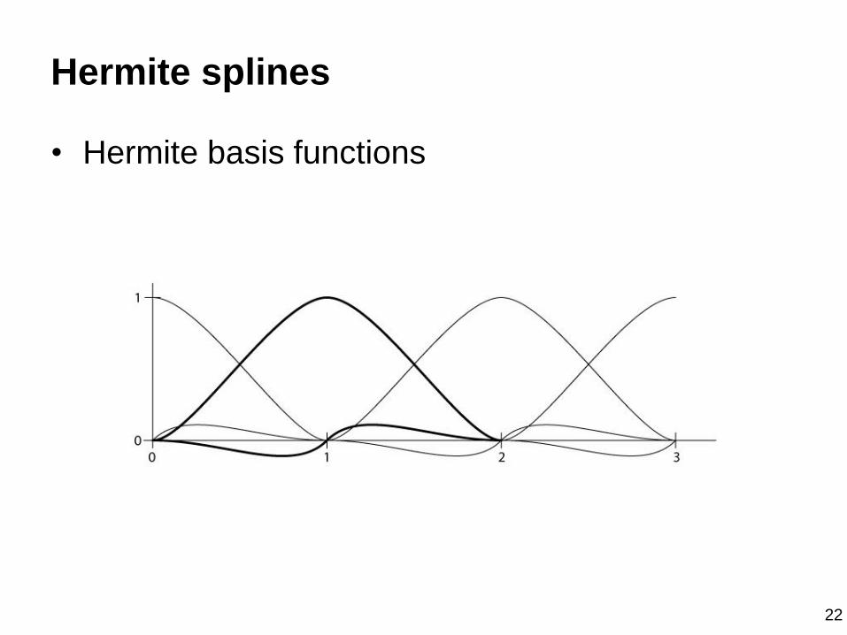
Hermite splines
• Hermite basis functions
23
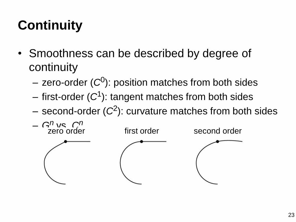
Continuity
• Smoothness can be described by degree of
continuity
– zero-order (C0): position matches from both sides
– first-order (C1): tangent matches from both sides
– second-order (C2): curvature matches from both sides
– Gn vs. Cnzero order first order second order
24
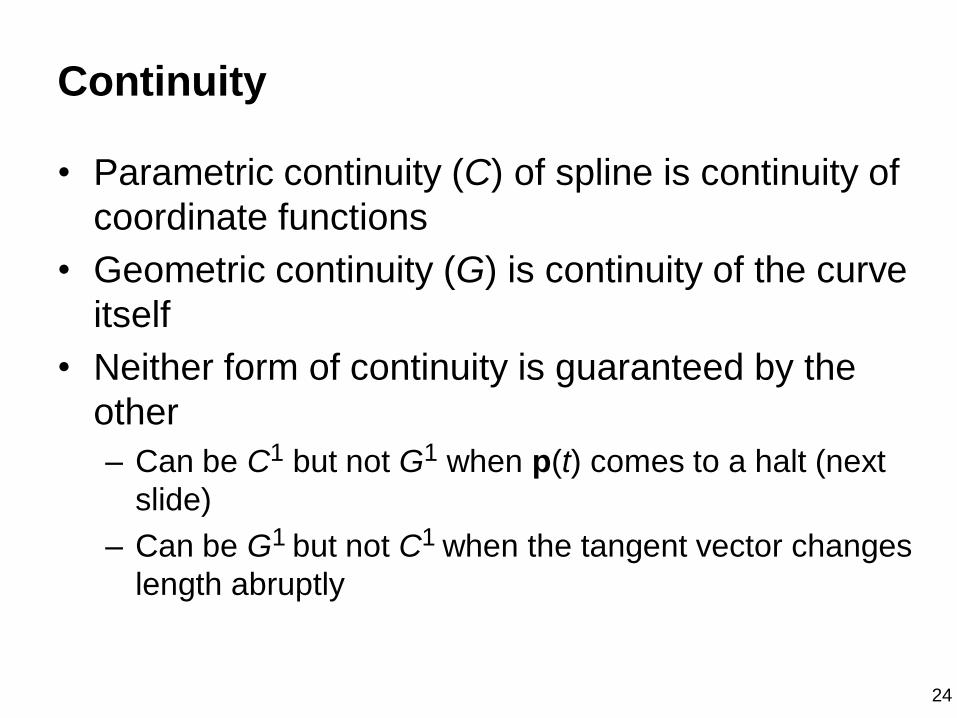
Continuity
• Parametric continuity (C) of spline is continuity of
coordinate functions
• Geometric continuity (G) is continuity of the curve
itself
• Neither form of continuity is guaranteed by the
other
– Can be C1 but not G1 when p(t) comes to a halt (next
slide)
– Can be G1 but not C1 when the tangent vector changes
length abruptly
25
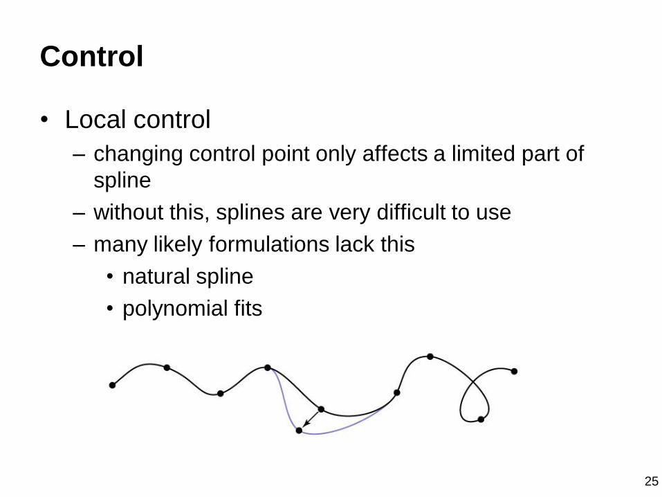
Control
• Local control
– changing control point only affects a limited part of
spline
– without this, splines are very difficult to use
– many likely formulations lack this
• natural spline
• polynomial fits

26
Control
• Convex hull property
– convex hull = smallest convex region containing points
• think of a rubber band around some pins
– some splines stay inside convex hull of control points
• make clipping, culling, picking, etc. simpler
YES YES YES NO
27
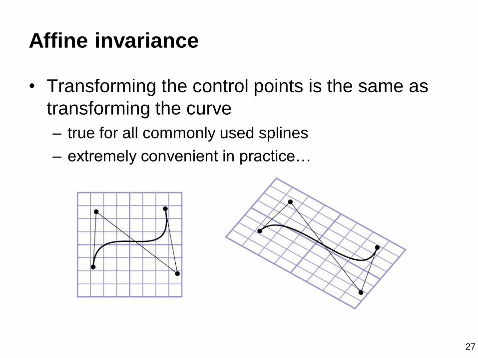
Affine invariance
• Transforming the control points is the same as
transforming the curve
– true for all commonly used splines
– extremely convenient in practice…
28
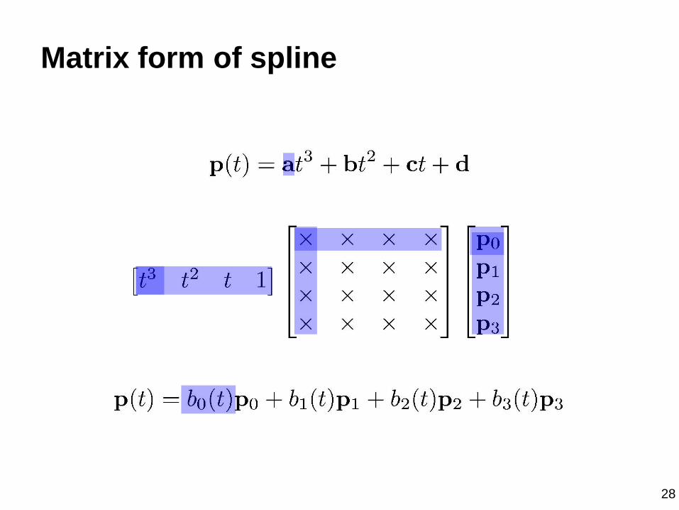
Matrix form of spline
29
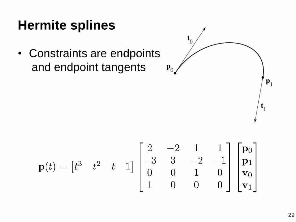
Hermite splines
• Constraints are endpoints
and endpoint tangents
30
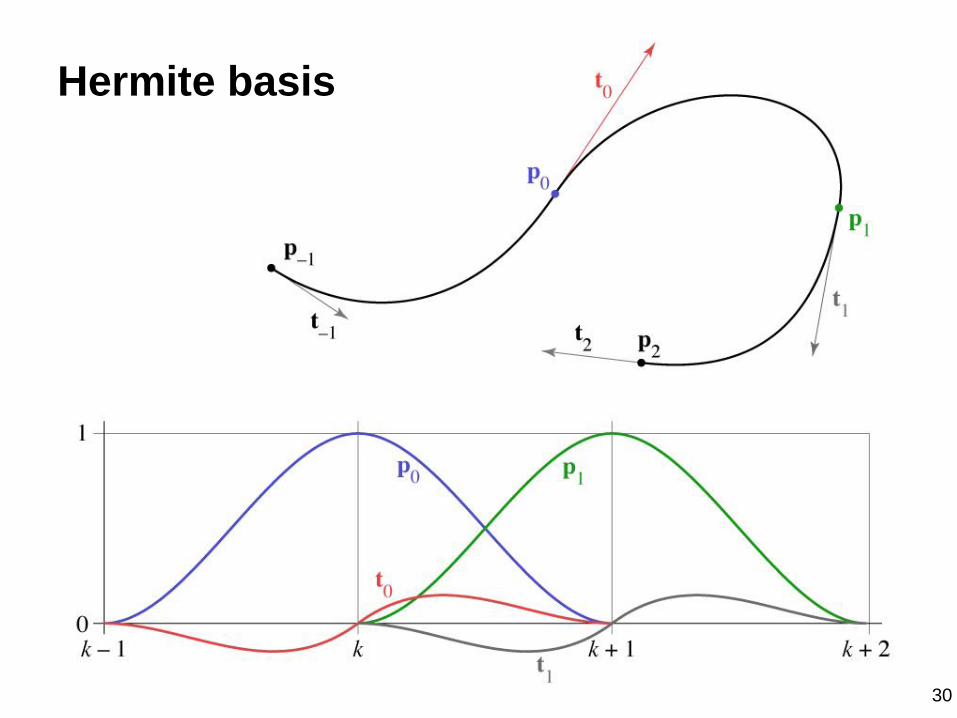
Hermite basis
31
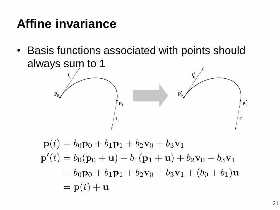
Affine invariance
• Basis functions associated with points should
always sum to 1
32
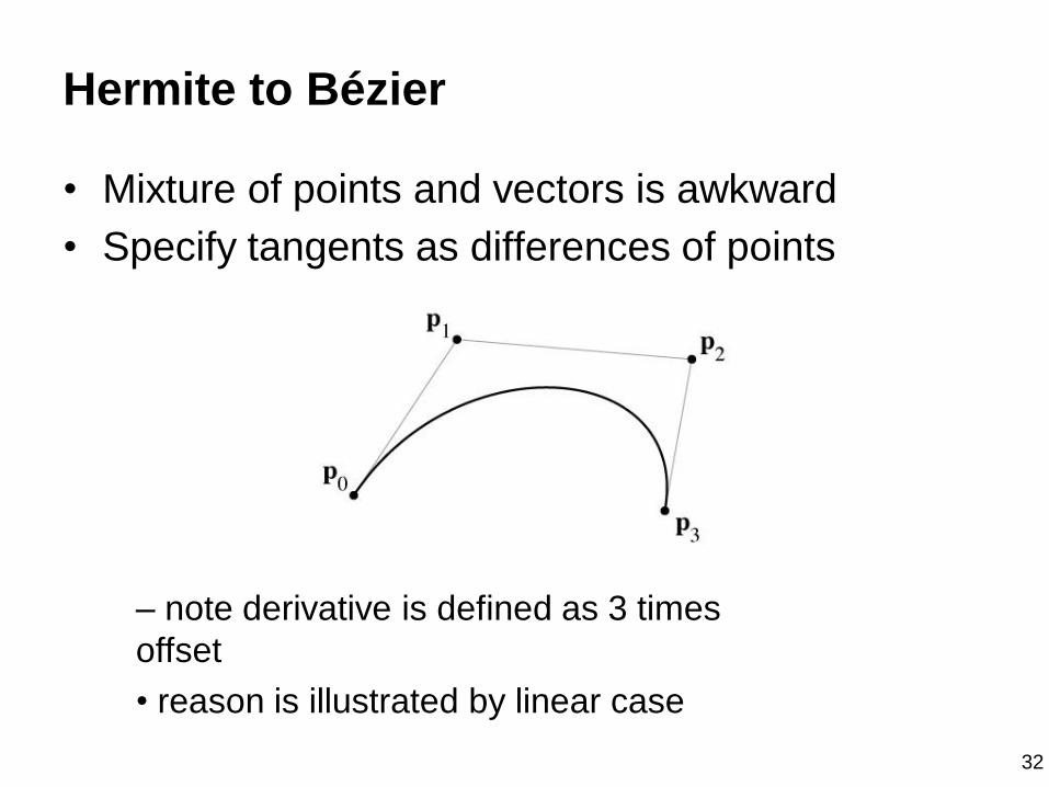
Hermite to Bézier
• Mixture of points and vectors is awkward
• Specify tangents as differences of points
– note derivative is defined as 3 times
offset
• reason is illustrated by linear case
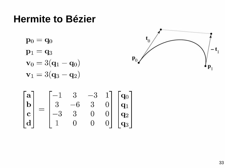
33
Hermite to Bézier
34
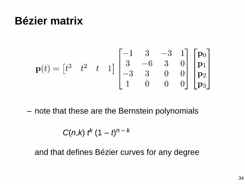
Bézier matrix
– note that these are the Bernstein polynomials
C(n,k) tk (1 – t)n – k
and that defines Bézier curves for any degree

35
Bézier basis
36
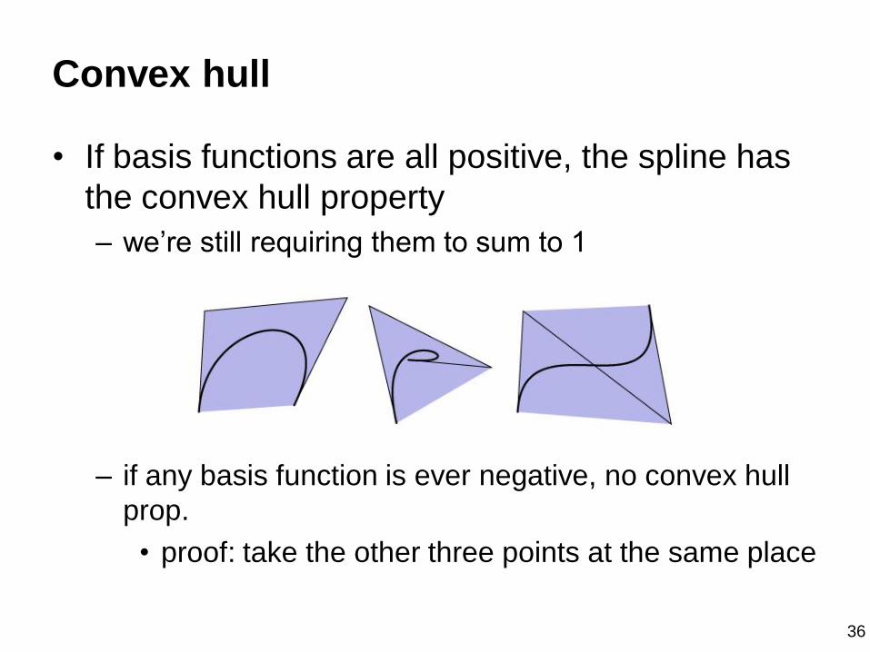
Convex hull
• If basis functions are all positive, the spline has
the convex hull property
– we’re still requiring them to sum to 1
– if any basis function is ever negative, no convex hull
prop.
• proof: take the other three points at the same place
37
Chaining spline segments
• Hermite curves are convenient because they can
be made long easily
• Bézier curves are convenient because their
controls are all points and they have nice
properties
– and they interpolate every 4th point, which is a little odd
• We derived Bézier from Hermite by defining
tangents from control points
– a similar construction leads to the interpolating Catmull-
Rom spline
38
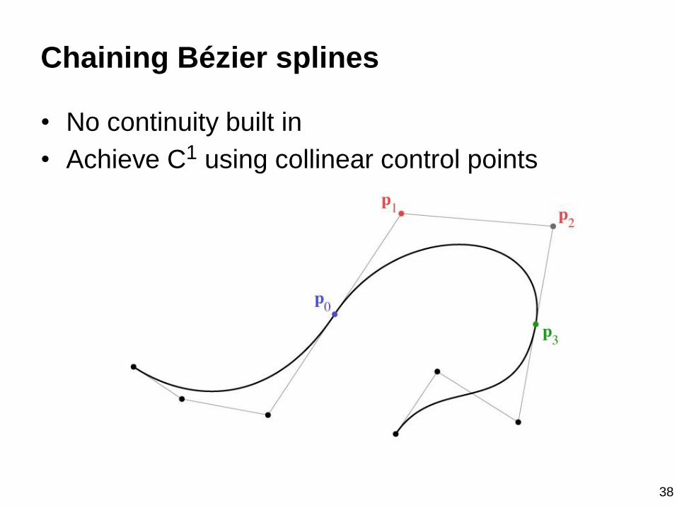
Chaining Bézier splines
• No continuity built in
• Achieve C1 using collinear control points
39
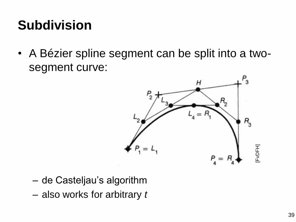
Subdivision
• A Bézier spline segment can be split into a two-
segment curve:
– de Casteljau’s algorithm
– also works for arbitrary t
[FvD
FH
]

40
Cubic Bézier splines
• Very widely used type, especially in 2D
– e.g. it is a primitive in PostScript/PDF
• Can represent C1 and/or G1 curves with corners
• Can easily add points at any position
41
B-splines
• We may want more continuity than C1
– http://en.wikipedia.org/wiki/Smooth_function
• We may not need an interpolating spline
• B-splines are a clean, flexible way of making long
splines with arbitrary order of continuity
• Various ways to think of construction
– a simple one is convolution
– relationship to sampling and reconstruction
42
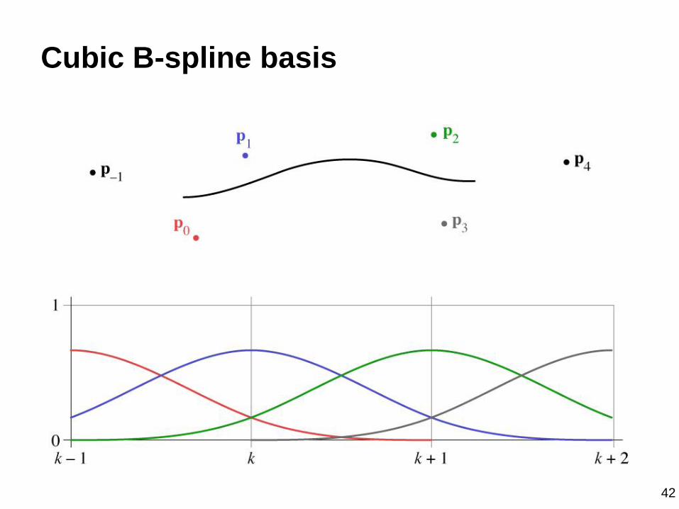
Cubic B-spline basis
43
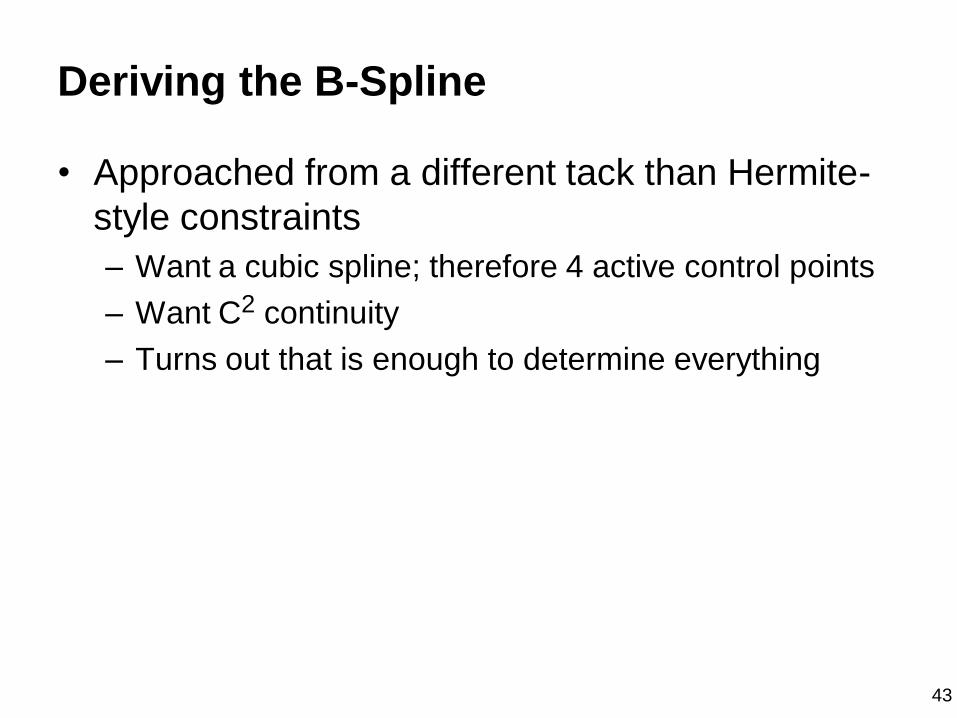
Deriving the B-Spline
• Approached from a different tack than Hermite-
style constraints
– Want a cubic spline; therefore 4 active control points
– Want C2 continuity
– Turns out that is enough to determine everything
44
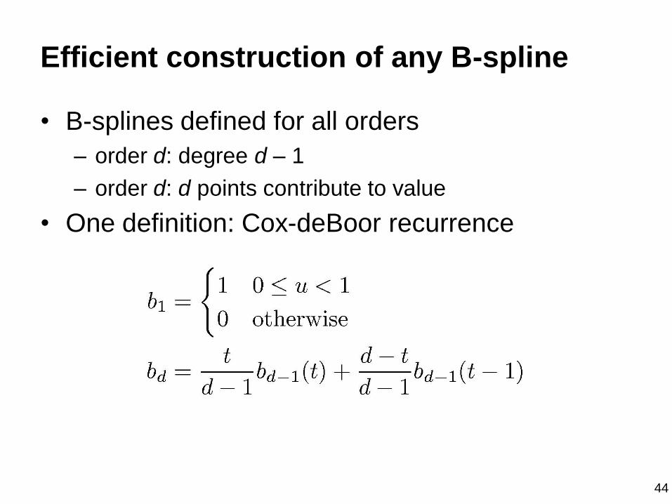
Efficient construction of any B-spline
• B-splines defined for all orders
– order d: degree d – 1
– order d: d points contribute to value
• One definition: Cox-deBoor recurrence
45
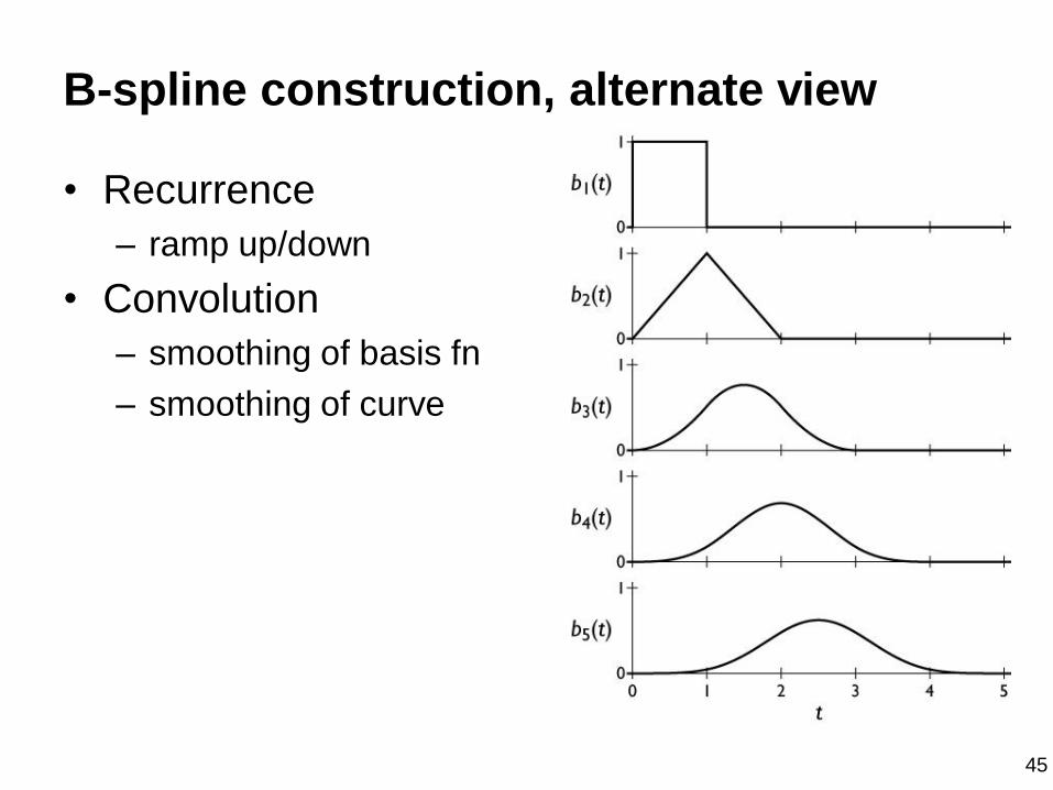
B-spline construction, alternate view
• Recurrence
– ramp up/down
• Convolution
– smoothing of basis fn
– smoothing of curve
46
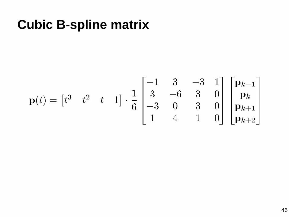
Cubic B-spline matrix
47
Other types of B-splines
• Nonuniform B-splines
– discontinuities not evenly spaced
– allows control over continuity or interpolation at certain
points
– e.g. interpolate endpoints (commonly used case)
• Nonuniform Rational B-splines (NURBS)
– ratios of nonuniform B-splines: x(t) / w(t); y(t) / w(t)
– key properties:
• invariance under perspective as well as affine
• ability to represent conic sections exactly
48
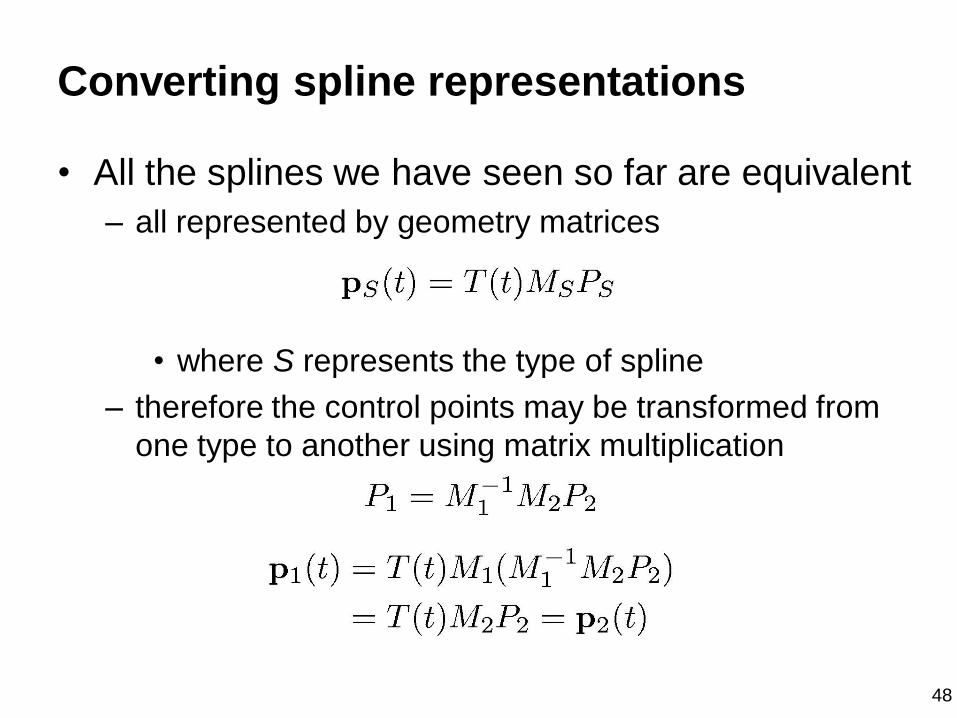
Converting spline representations
• All the splines we have seen so far are equivalent
– all represented by geometry matrices
• where S represents the type of spline
– therefore the control points may be transformed from
one type to another using matrix multiplication
49
Evaluating splines for display
• Need to generate a list of line segments to draw
– generate efficiently
– use as few as possible
– guarantee approximation accuracy
• Approaches
– reccursive subdivision (easy to do adaptively)
– uniform sampling (easy to do efficiently)
50
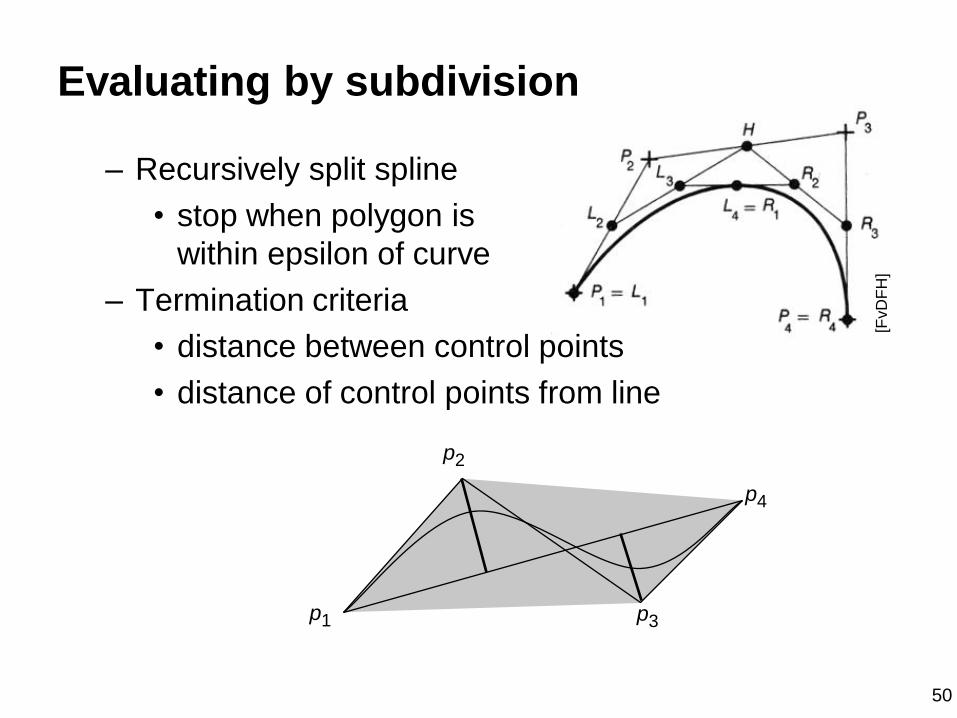
Evaluating by subdivision
– Recursively split spline
• stop when polygon is
within epsilon of curve
– Termination criteria
• distance between control points
• distance of control points from line
p1
p2
p3
p4
[FvD
FH
]

51
Evaluating with uniform spacing
• Forward differencing
– efficiently generate points for uniformly spaced t values
– evaluate polynomials using repeated differences