2d nearly orthogonal mesh generation

INTERNATIONAL JOURNAL FOR NUMERICAL METHODS IN FLUIDSInt. J. Numer. Meth. Fluids 2004; 46:685–707Published online 6 September 2004 in Wiley InterScience (www.interscience.wiley.com). DOI: 10.1002/�d.770

2D nearly orthogonal mesh generation

Yaoxin Zhang∗;†;‡, Yafei Jia§ and Sam S. Y. Wang¶

National Center for Computational Hydroscience and Engineering; The University of Mississippi;P.O. Box 1500; Oxford; MS 38677; U.S.A.

SUMMARY

The Ryskin and Leal (RL) system is the most widely used mesh generation system for the orthogonalmapping. However, when this system is used in domains with complex geometry, particularly in thosewith sharp corners and strong curvatures, serious distortion or overlapping of mesh lines may occurand an acceptable solution may not be possible. In the present study, two methods are proposed togenerate nearly orthogonal meshes with the smoothness control. In the �rst method, the original RLsystem is modi�ed by introducing smoothness control functions, which are formulated through theblending of the conformal mapping and the orthogonal mapping; while in the second method, the RLsystem is modi�ed by introducing the contribution factors. A hybrid system of both methods is alsodeveloped. The proposed methods are illustrated by several test examples. Applications of these methodsin a natural river channel are demonstrated. It is shown that the modi�ed RL systems are capable ofproducing meshes with an adequate balance between the orthogonality and the smoothness for complexcomputational domains without mesh distortions and overlapping. Copyright ? 2004 John Wiley &Sons, Ltd.

KEY WORDS: nearly orthogonal mesh generation; e�ect-control factor; contribution factor; smoothnesscontrol function

1. INTRODUCTION

Computational �uid dynamics (CFD) solves a set of highly non-linear partial di�erential equa-tions (PDE) in a physical domain, which is usually discretized and represented by a compu-tational mesh. Despite the numerical method used, the success of solving these PDEs depends

∗Correspondence to: Y. Zhang, National Center for Computational Hydroscience and Engineering, The Universityof Mississippi, P.O. Box 1500, Oxford, MS 38677, U.S.A.

†E-mail: [email protected]‡Research Assistant.§Research Associate Professor and Senior Investigator.¶F.A.P Barnard Distinguished Professor and Director.

Contract=grant sponsor: USDA Agriculture Research Service; contract=grant number: 58-6408-2-0062Contract=grant sponsor: The University of Mississippi

Received 14 July 2003Copyright ? 2004 John Wiley & Sons, Ltd. Revised 17 June 2004

686 Y. ZHANG, Y. JIA AND S. S. Y. WANG

largely on the mesh quality. As the general academic criteria, the orthogonality and smooth-ness are often used to evaluate the mesh quality quantitatively.Extensive research in the past has made it possible for high quality mesh generation [1–17].

A detailed review of mesh generation research in the 1990s can be found in Reference [18].One of the most widely used methods for mesh generation was developed by Thompsonet al. [16] (often referred to as TTM method). In this method, a sophisticated system ofPoisson equations with inhomogeneous source terms, called control functions, is solved. Theoriginal version of this method cannot generate an orthogonal mapping, unless an appropriateset of control functions is used.Since the late 1970s, orthogonal mesh generation has been the objective of many researchers

[1–12]. The early method for generating 2D orthogonal mesh was through the conformalmapping, but it requires the scale factors be equal in all directions, which somehow punishesthe quality of the resulting mesh. Hung and Brown [1] tried to alleviate this problem byusing the non-constant, and adjustable distortion function throughout the domain. Mobleyand Stewart [3] constructed the orthogonal mapping by using the non-uniform stretching ofthe conformal co-ordinates. Ryskin and Leal [5] introduced a covariant Laplace equationsystem for the orthogonal mapping and their success led to the wide use of this system[6–12], often referred to as RL. They identi�ed two kinds of methods corresponding totwo kinds of boundaries, namely, ‘strong constraint’ method and ‘weak constraint’ method.The former is for domains whose shape is not known in advance, but is to be determinedas a part of the solution and the latter is for domains with known prescribed boundarycorrespondence.In the RL system, the distortion function f, which is de�ned as a ratio of the scale factors

in two di�erent directions, is no longer constant and needs to be determined. In general, fcannot be prescribed arbitrarily. As classi�ed by E�ca [11], there are three di�erent treatmentsof the distortion function: (1) Calculate f from its de�nition at the boundaries and then obtainthe values in the domain by interpolation or by solving a Laplace equation; (2) specify a classof admissible functions for f to guarantee a unique solution; (3) calculate f from its de�nitionfor the whole domain. In order to provide a smooth variation of f throughout the domain,Tamamidis and Assanis [6] used a Laplace equation with a source term to calculate f. Allieviand Calisal [7] calculated f according to its de�nition in the whole domain and obtainedgood results, but they claimed their success was due to the Bubnov–Galerkin formulation.Kang and Leal [8] calculated f during the preliminary step in their non-iterative scheme ofmesh generation. Duraiswami and Prosperetti [10], based on quasi-conformal mapping theory,speci�ed a class of admissible functions for f. E�ca [11] and Akcelik et al. [12] also calculatedf from its de�nition in the entire domain during an iteration process.When using the RL system to generate an orthogonal mapping, in some cases with com-

plex geometries, the local orthogonality constraint may become so restrictive that the localsmoothness is sacri�ced. This usually results in serious distortion or overlapping of meshlines in certain region of the domain. In order to prevent mesh lines from overlapping ontoeach other, Akcelik et al. [12] introduced the inhomogeneous source terms into the RL sys-tem, which controls favourably the scale factors and hence the aspect ratio of the result-ing grid. In Reference [12], a parameter called the force constant is used to optimize meshempirically.In this study, two methods are proposed to resolve the mesh distortion and overlapping

problems. The �rst one is an extension of the work of E�ca [11] and Akcelik et al. [12]

Copyright ? 2004 John Wiley & Sons, Ltd. Int. J. Numer. Meth. Fluids 2004; 46:685–707

2D NEARLY ORTHOGONAL MESH GENERATION 687

based on the RL system. Compared to Akcelik’s work, a set of new control functions forsmoothness is introduced into RL system. The control functions are achieved through blendingthe conformal mapping and the orthogonal mapping. The second method is a novel schemeof the RL system. Contribution factors are introduced to control the grid spaces. A hybridRL system combining both methods is also proposed. Several examples are discussed in thispaper and the comparisons of mesh quality to other methods are demonstrated.

2. MESH GENERATION SYSTEMS

The elliptic system is the most widely used in 2D mesh generation, which is derived fromthe Laplace equation for the stream function and the velocity potential function. Among thesemethods, the TTM system developed by Thompson et al. [16] and the RL system proposedby Ryskin and Leal [5] are brie�y introduced here.

2.1. RL system

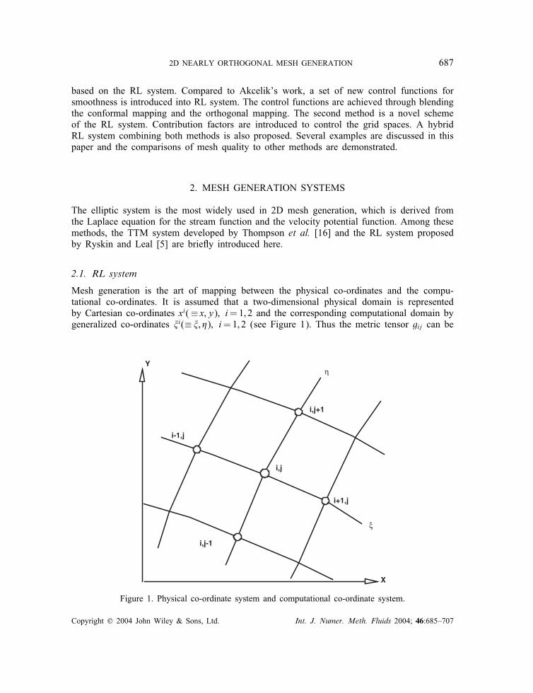
Mesh generation is the art of mapping between the physical co-ordinates and the compu-tational co-ordinates. It is assumed that a two-dimensional physical domain is representedby Cartesian co-ordinates xi(≡ x; y); i=1; 2 and the corresponding computational domain bygeneralized co-ordinates �i(≡ �; �); i=1; 2 (see Figure 1). Thus the metric tensor gij can be

X

Y

i,j

i+1,j

i-1,j

i,j+1

i,j-1

ξ

η

Figure 1. Physical co-ordinate system and computational co-ordinate system.



written as:

g=

∣∣∣∣∣(x2� + y

2�) (x�x� + y�y�)

(x�x� + y�y�) (x2� + y2�)

∣∣∣∣∣ (1)

where x�= @x=@�, and so forth.The simple observation, that the physical co-ordinates satisfy the Laplace equation, can be

made. That is,

∇2xi=0 (2)

A 2D orthogonal mesh must satisfy the condition g12 = g21 = 0, which implies

x� = −f · y� (3a)

y� = f · x� (3b)where the distortion factor f is de�ned as the ratio of the scale factors in � and � direction,i.e.

f=h�h�=

(x2� + y

2�

x2� + y2�

)1=2(4)

and

h�= g1=211 ; h�= g

1=222 (5)

If f=1, Equation (3) reduces to the Cauchy–Riemann conditions and the mesh is con-formal. According to Equations (2) and (3), the generalized co-ordinates � and � satisfy thefollowing partial di�erential equations:

@@�

(f@x@�

)+@@�

(1f@x@�

)=0 (6a)

@@�

(f@y@�

)+@@�

(1f@y@�

)=0 (6b)

Equation (6) is the Laplace mesh generation system used by Ryskin and Leal [5].

2.2. TTM system

The elliptic system used by Thompson et al. [16] for numerical mesh generation is the Poissonequation with the following form:

@2�@x2

+@2�@y2

= P(�; �) (7a)

@2�@x2

+@2�@y2

=Q(�; �) (7b)



where (�; �) is computational co-ordinate system and (x; y) is physical co-ordinate system;P; Q are control functions.Transforming the above equations, one can obtain,

�@2x@�2

− 2� @2x

@�@�+ �

@2x@�2

+ �(P@x@�+Q

@x@�

)=0 (8a)

�@2y@�2

− 2� @2y

@�@�+ �

@2y@�2

+ �(P@y@�+Q

@y@�

)=0 (8b)

where �= g22; �= g12; �= g11 and �= g.In Reference [16], the control functions were originally constructed to control the grid spac-

ing and clustering e�ectively, but cannot generate an orthogonal mapping. If the orthogonalcondition is applied (�=0) and the following control functions are selected, Equation (8) canalso generate orthogonal mapping:

P=1h�h�

f�; Q=1h�h�

(1f

)�

(9)

Substitution of Equation (9) into (8) and rearrangement leads to the RL system.

3. PRESENT STUDY

When the RL system is applied in cases with complex geometries, the local orthogonality con-straint may become too restrictive to resolve a good local balance between the orthogonalityand the smoothness. Instead, it results in the mesh distortions and overlapping.Using the central di�erence scheme to discretize Equation (6) at one typical grid point

(i; j), one can obtain:

Fi; jxi; j =fi+1=2; jxi+1; j + fi−1=2; jxi−1; j +1

fi; j+1=2xi; j+1 +

1fi; j−1=2

xi; j−1 (10a)

Fi; jyi; j =fi+1=2; jyi+1; j + fi−1=2; jyi−1; j +1

fi; j+1=2yi; j+1 +

1fi; j−1=2

yi; j−1 (10b)

where

Fi; j = fi+1=2; j + fi−1=2; j +1

fi; j+1=2+

1fi; j−1=2

The generic discretization form can be written as:

(x; y)i; j=∑nbAnb(x; y)nb (11)

where ‘nb’ denotes the neighbouring nodes and Anb is the coe�cient.



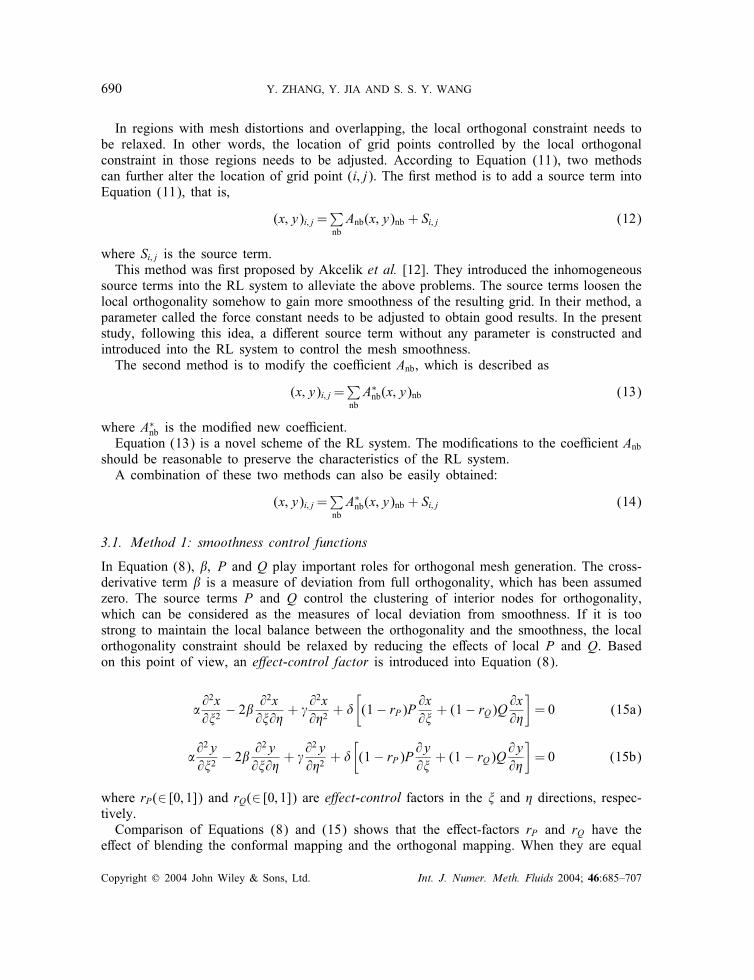
In regions with mesh distortions and overlapping, the local orthogonal constraint needs tobe relaxed. In other words, the location of grid points controlled by the local orthogonalconstraint in those regions needs to be adjusted. According to Equation (11), two methodscan further alter the location of grid point (i; j). The �rst method is to add a source term intoEquation (11), that is,

(x; y)i; j=∑nbAnb(x; y)nb + Si; j (12)

where Si; j is the source term.This method was �rst proposed by Akcelik et al. [12]. They introduced the inhomogeneous

source terms into the RL system to alleviate the above problems. The source terms loosen thelocal orthogonality somehow to gain more smoothness of the resulting grid. In their method, aparameter called the force constant needs to be adjusted to obtain good results. In the presentstudy, following this idea, a di�erent source term without any parameter is constructed andintroduced into the RL system to control the mesh smoothness.The second method is to modify the coe�cient Anb, which is described as

(x; y)i; j=∑nbA∗nb(x; y)nb (13)

where A∗nb is the modi�ed new coe�cient.

Equation (13) is a novel scheme of the RL system. The modi�cations to the coe�cient Anbshould be reasonable to preserve the characteristics of the RL system.A combination of these two methods can also be easily obtained:

(x; y)i; j=∑nbA∗nb(x; y)nb + Si; j (14)

3.1. Method 1: smoothness control functions

In Equation (8), �; P and Q play important roles for orthogonal mesh generation. The cross-derivative term � is a measure of deviation from full orthogonality, which has been assumedzero. The source terms P and Q control the clustering of interior nodes for orthogonality,which can be considered as the measures of local deviation from smoothness. If it is toostrong to maintain the local balance between the orthogonality and the smoothness, the localorthogonality constraint should be relaxed by reducing the e�ects of local P and Q. Basedon this point of view, an e�ect-control factor is introduced into Equation (8).

�@2x@�2

− 2� @2x

@�@�+ �

@2x@�2

+ �[(1− rP)P @x@� + (1− rQ)Q@x@�

]=0 (15a)

�@2y@�2

− 2� @2y

@�@�+ �

@2y@�2

+ �[(1− rP)P@y@� + (1− rQ)Q@y@�

]=0 (15b)

where rP(∈ [0; 1]) and rQ(∈ [0; 1]) are e�ect-control factors in the � and � directions, respec-tively.Comparison of Equations (8) and (15) shows that the e�ect-factors rP and rQ have the

e�ect of blending the conformal mapping and the orthogonal mapping. When they are equal



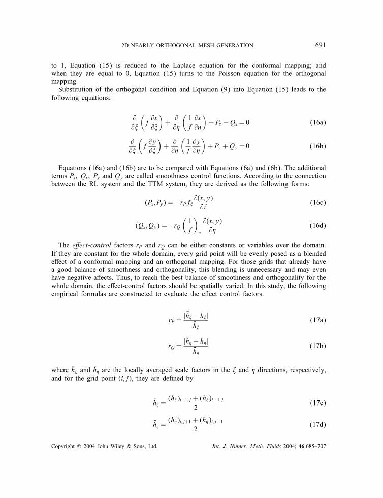
to 1, Equation (15) is reduced to the Laplace equation for the conformal mapping; andwhen they are equal to 0, Equation (15) turns to the Poisson equation for the orthogonalmapping.Substitution of the orthogonal condition and Equation (9) into Equation (15) leads to the

following equations:

@@�

(f@x@�

)+@@�

(1f@x@�

)+ Px +Qx =0 (16a)

@@�

(f@y@�

)+@@�

(1f@y@�

)+ Py +Qy =0 (16b)

Equations (16a) and (16b) are to be compared with Equations (6a) and (6b). The additionalterms Px; Qx; Py and Qy are called smoothness control functions. According to the connectionbetween the RL system and the TTM system, they are derived as the following forms:

(Px; Py) = −rPf� @(x; y)@�(16c)

(Qx;Qy) = −rQ(1f

)�

@(x; y)@�

(16d)

The e�ect-control factors rP and rQ can be either constants or variables over the domain.If they are constant for the whole domain, every grid point will be evenly posed as a blendede�ect of a conformal mapping and an orthogonal mapping. For those grids that already havea good balance of smoothness and orthogonality, this blending is unnecessary and may evenhave negative a�ects. Thus, to reach the best balance of smoothness and orthogonality for thewhole domain, the e�ect-control factors should be spatially varied. In this study, the followingempirical formulas are constructed to evaluate the e�ect control factors.

rP =| �h� − h�|�h�

(17a)

rQ =| �h� − h�|�h�

(17b)

where �h� and �h� are the locally averaged scale factors in the � and � directions, respectively,and for the grid point (i; j), they are de�ned by

�h� =(h�)i+1; j + (h�)i−1; j

2(17c)

�h� =(h�)i; j+1 + (h�)i; j−1

2(17d)



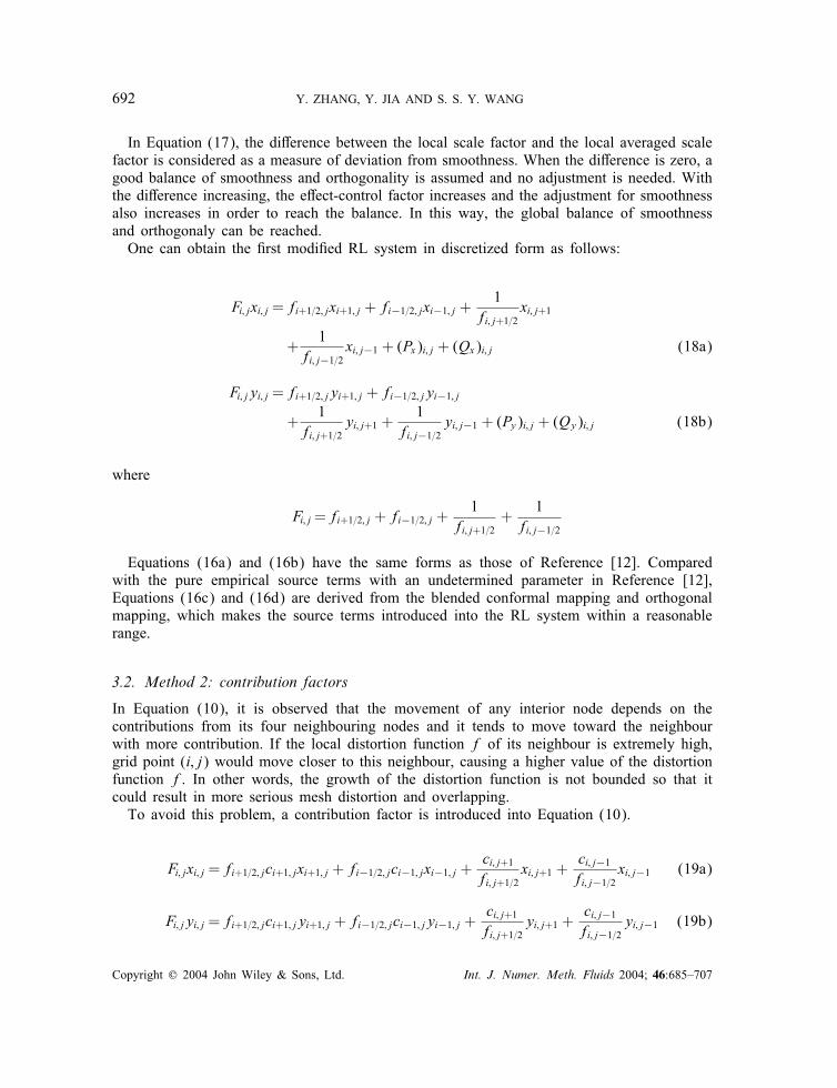
In Equation (17), the di�erence between the local scale factor and the local averaged scalefactor is considered as a measure of deviation from smoothness. When the di�erence is zero, agood balance of smoothness and orthogonality is assumed and no adjustment is needed. Withthe di�erence increasing, the e�ect-control factor increases and the adjustment for smoothnessalso increases in order to reach the balance. In this way, the global balance of smoothnessand orthogonaly can be reached.One can obtain the �rst modi�ed RL system in discretized form as follows:

Fi; jxi; j =fi+1=2; jxi+1; j + fi−1=2; jxi−1; j +1

fi; j+1=2xi; j+1

+1

fi; j−1=2xi; j−1 + (Px)i; j + (Qx)i; j (18a)

Fi; jyi; j =fi+1=2; jyi+1; j + fi−1=2; jyi−1; j

+1

fi; j+1=2yi; j+1 +

1fi; j−1=2

yi; j−1 + (Py)i; j + (Qy)i; j (18b)

where

Fi; j=fi+1=2; j + fi−1=2; j +1

fi; j+1=2+

1fi; j−1=2

Equations (16a) and (16b) have the same forms as those of Reference [12]. Comparedwith the pure empirical source terms with an undetermined parameter in Reference [12],Equations (16c) and (16d) are derived from the blended conformal mapping and orthogonalmapping, which makes the source terms introduced into the RL system within a reasonablerange.

3.2. Method 2: contribution factors

In Equation (10), it is observed that the movement of any interior node depends on thecontributions from its four neighbouring nodes and it tends to move toward the neighbourwith more contribution. If the local distortion function f of its neighbour is extremely high,grid point (i; j) would move closer to this neighbour, causing a higher value of the distortionfunction f. In other words, the growth of the distortion function is not bounded so that itcould result in more serious mesh distortion and overlapping.To avoid this problem, a contribution factor is introduced into Equation (10).

Fi; jxi; j =fi+1=2; jci+1; jxi+1; j + fi−1=2; jci−1; jxi−1; j +ci; j+1fi; j+1=2

xi; j+1 +ci; j−1fi; j−1=2

xi; j−1 (19a)

Fi; jyi; j =fi+1=2; jci+1; jyi+1; j + fi−1=2; jci−1; jyi−1; j +ci; j+1fi; j+1=2

yi; j+1 +ci; j−1fi; j−1=2

yi; j−1 (19b)



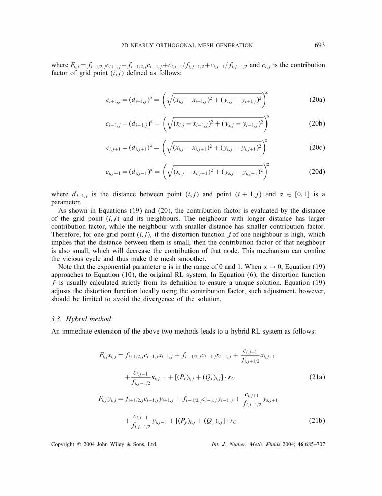
where Fi; j=fi+1=2; jci+1; j+fi−1=2; jci−1; j+ci; j+1=fi; j+1=2+ci; j−1=fi; j−1=2 and ci; j is the contributionfactor of grid point (i; j) de�ned as follows:

ci+1; j = (di+1; j)�=(√

(xi; j − xi+1; j)2 + (yi; j − yi+1; j)2)�

(20a)

ci−1; j = (di−1; j)�=(√

(xi; j − xi−1; j)2 + (yi; j − yi−1; j)2)�

(20b)

ci; j+1 = (di; j+1)�=(√

(xi; j − xi; j+1)2 + (yi; j − yi; j+1)2)�

(20c)

ci; j−1 = (di; j−1)�=(√

(xi; j − xi; j−1)2 + (yi; j − yi; j−1)2)�

(20d)

where di+1; j is the distance between point (i; j) and point (i + 1; j) and � ∈ [0; 1] is aparameter.As shown in Equations (19) and (20), the contribution factor is evaluated by the distance

of the grid point (i; j) and its neighbours. The neighbour with longer distance has largercontribution factor, while the neighbour with smaller distance has smaller contribution factor.Therefore, for one grid point (i; j), if the distortion function fof one neighbour is high, whichimplies that the distance between them is small, then the contribution factor of that neighbouris also small, which will decrease the contribution of that node. This mechanism can con�nethe vicious cycle and thus make the mesh smoother.Note that the exponential parameter � is in the range of 0 and 1. When � → 0, Equation (19)

approaches to Equation (10), the original RL system. In Equation (6), the distortion functionf is usually calculated strictly from its de�nition to ensure a unique solution. Equation (19)adjusts the distortion function locally using the contribution factor, such adjustment, however,should be limited to avoid the divergence of the solution.

3.3. Hybrid method

An immediate extension of the above two methods leads to a hybrid RL system as follows:

Fi; jxi; j =fi+1=2; jci+1; jxi+1; j + fi−1=2; jci−1; jxi−1; j +ci; j+1fi; j+1=2

xi; j+1

+ci; j−1fi; j−1=2

xi; j−1 + [(Px)i; j + (Qx)i; j] · rC (21a)

Fi; jyi; j =fi+1=2; jci+1; jyi+1; j + fi−1=2; jci−1; jyi−1; j +ci; j+1fi; j+1=2

yi; j+1

+ci; j−1fi; j−1=2

yi; j−1 + [(Py)i; j + (Qy)i; j] · rC (21b)



where c; Px; Qx; Py and Qy are de�ned in Equations (20) and (16); rC ∈ [0; 1] controls thee�ects of the smoothness control functions.With the exponential parameter �=0 and rC =0, Equation (21) will be reduced to Equa-

tion (10) (original RL); with �=0 and rC =1, Equation (18) (RL with smoothness controlfunctions) will be obtained; and with �¿0 and rC =0, Equation (21) will turn to Equation(19) (RL with contribution factors).

4. SOLUTION PROCESS

The numerical procedure of Equation (21) is an iterative process similar to that of Reference[10]. The maximum di�erence between the grid co-ordinates in consecutive steps is used asthe convergence condition.

max(√

(xni; j − xn−1i; j )2 + (yni; j − yn−1i; j )2

)¡10−6 (22)

where n is the iteration number.The linear Equation (21) is solved iteratively and the iterative algorithm is as follows:

a. Identify the boundaries of the domain and use an algebraic method to obtain an initialmesh.

b. Calculate the distortion function f from its de�nition Equation (4).c. Calculate the smoothness control functions from Equation (16).d. Calculate the contribution factors from Equation (20).e. Solve Equation (21) with �xed f obtained from step b, the smoothness control functionsfrom step c and the contribution factors from step d.

f. Update the mesh and check if the convergence condition is satis�ed. If not, repeat stepsfrom b to f.

5. BOUNDARY CONDITIONS

The mesh generation based on the elliptic system is a boundary value problem, and theboundary conditions have signi�cant in�uences on the resulting mesh.Either the Dirichlet or the Neumann boundary conditions can be applied to solve the elliptic

system. As stated in Reference [14], Equations (6) and (8) are second-order PDEs, which cansupport only one set of boundary conditions. That is, the Dirichlet and the Neumann boundaryconditions cannot be enforced simultaneously.The Dirichlet boundary conditions are generally used to solve the elliptic mesh generation

system. If the Neumann conditions are applied, the Dirichlet conditions must be dropped,which may make the resulting mesh not boundary-�tted. To resolve this problem, a kind ofDirichlet–Neumann conditions is usually used to simulate the Neumann boundary conditions



(A1) (A3)

(A2) (A4)

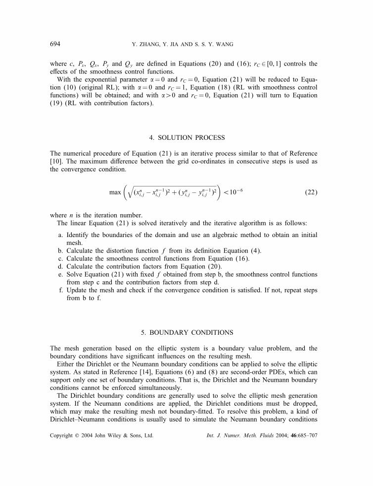
Figure 2. Meshes in domain A with the Dirichlet conditions in all boundaries: (A1) the RL system;(A2) the RL with smoothness control functions; (A3) the RL with contribution factors, �=0:01; and

(A4) the hybrid RL system, �=0:005 and rC =0:5.

[11]. That is, the grid points slide along the boundary (Dirichlet) to satisfy the Neumannconditions.In the present study, the Dirichlet conditions are used for all the boundaries and the

Dirichlet–Neumann conditions (sliding boundary conditions) will also be explored to testthe e�ects of the boundary conditions on the mesh quality.



(B1)

(B2)

(B3)

(B4)

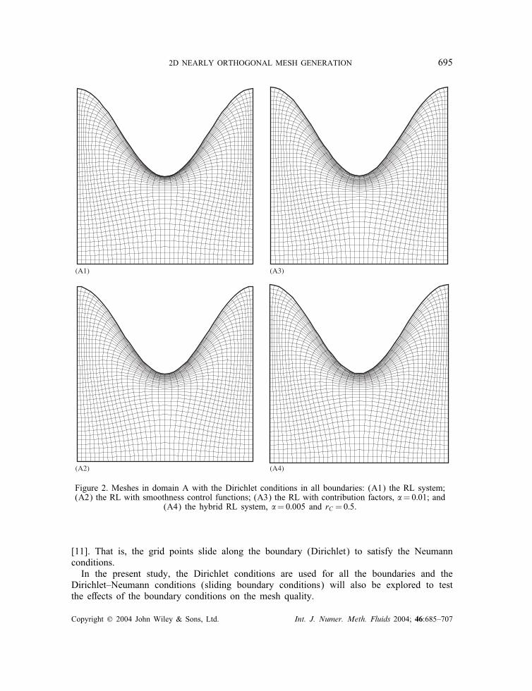
Figure 3. Meshes in domain B with the Dirichlet conditions in all boundaries: (B1) the RL system;(B2) the RL with smoothness control functions; (B3) the RL with contribution factors, �=0:01; and

(B4) the hybrid RL system, �=0:002 and rC =0:5.

6. EXAMPLES AND DISCUSSIONS

Several cases commonly used in the literatures [7–12] are selected as examples here forillustration and discussion. Although the adaptivity, referring to the control of the mesh densitydistribution according to the physics of a particular problem, is often used to evaluate the meshquality, in this paper the quality of mesh is evaluated quantitatively by several indicators, such



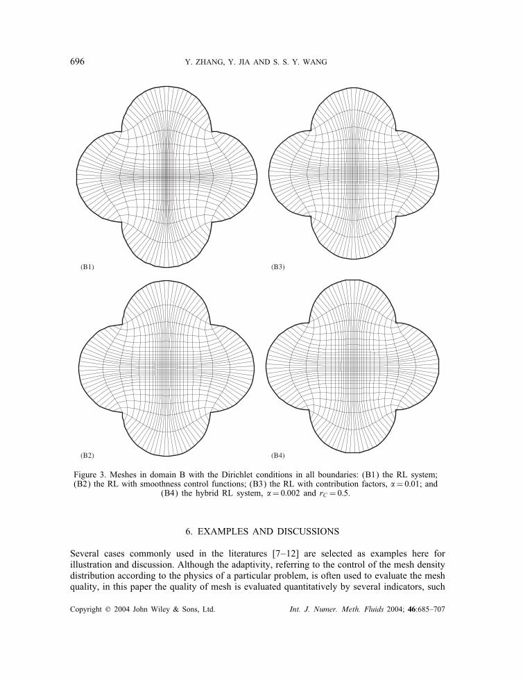
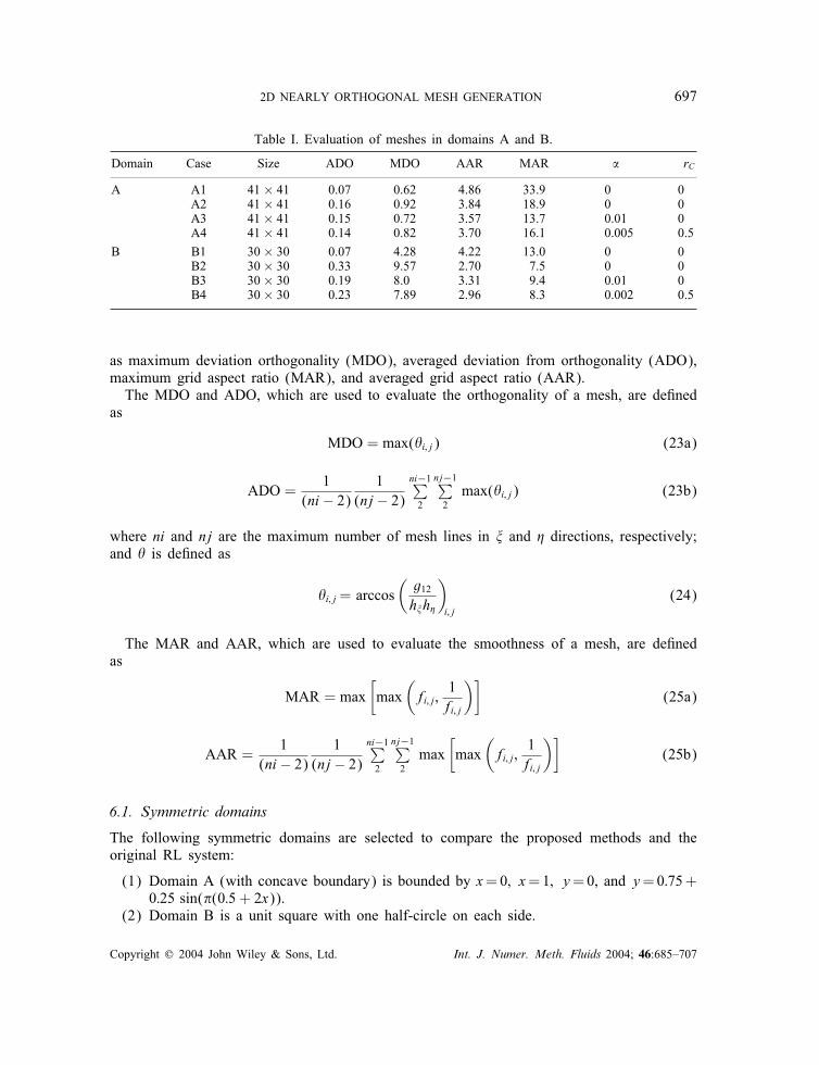
Table I. Evaluation of meshes in domains A and B.

Domain Case Size ADO MDO AAR MAR � rC

A A1 41× 41 0.07 0.62 4.86 33.9 0 0A2 41× 41 0.16 0.92 3.84 18.9 0 0A3 41× 41 0.15 0.72 3.57 13.7 0.01 0A4 41× 41 0.14 0.82 3.70 16.1 0.005 0.5

B B1 30× 30 0.07 4.28 4.22 13.0 0 0B2 30× 30 0.33 9.57 2.70 7.5 0 0B3 30× 30 0.19 8.0 3.31 9.4 0.01 0B4 30× 30 0.23 7.89 2.96 8.3 0.002 0.5

as maximum deviation orthogonality (MDO), averaged deviation from orthogonality (ADO),maximum grid aspect ratio (MAR), and averaged grid aspect ratio (AAR).The MDO and ADO, which are used to evaluate the orthogonality of a mesh, are de�ned

as

MDO = max(�i; j) (23a)

ADO =1

(ni − 2)1

(nj − 2)ni−1∑2

nj−1∑2max(�i; j) (23b)

where ni and nj are the maximum number of mesh lines in � and � directions, respectively;and � is de�ned as

�i; j= arccos(g12h�h�

)i; j

(24)

The MAR and AAR, which are used to evaluate the smoothness of a mesh, are de�nedas

MAR = max[max

(fi; j;

1fi; j

)](25a)

AAR =1

(ni − 2)1

(nj − 2)ni−1∑2

nj−1∑2max

[max

(fi; j;

1fi; j

)](25b)

6.1. Symmetric domains

The following symmetric domains are selected to compare the proposed methods and theoriginal RL system:

(1) Domain A (with concave boundary) is bounded by x=0; x=1; y=0, and y=0:75+0:25 sin(�(0:5 + 2x)).

(2) Domain B is a unit square with one half-circle on each side.



(C1) (C2)

(C3) (C4) (C5)

Figure 4. Meshes in domain C: (C1) the RL system, the Dirichlet conditions in all boundaries; (C2)the RL with smoothness control functions, the Dirichlet conditions in all boundaries; (C3) the RL withcontribution factors, �=0:2, the Dirichlet conditions in all boundaries; (C4) the hybrid RL system,�=0:2 and rC =1:0, with the Dirichlet conditions in all boundaries; and (C5) the RL system, thesliding conditions for the right curved boundary and the Drichlet conditions in other boundaries.

Initial meshes with uniform nodal distribution along the four boundaries, namely, top bound-ary, bottom boundary, left boundary, and right boundary, were generated by the algebraicmethod. Figures 2 and 3 show the comparisons of meshes with di�erent methods for domainsA and B, respectively. Table I summarizes the quality of meshes.The mesh lines are contracted to the concaved top boundary in domain A, and to the centre

lines of domain B in x and y directions. The original RL system generated the best orthogonalmeshes with the worst smoothness. Using the modi�ed RL systems, the smoothness of the



(D1) (D2)

(D3) (D4)

(D5)

Figure 5. Meshes in domain D: (D1) the RL system, the Dirichlet conditions in all boundaries; (D2)the RL with smoothness control functions, the Dirichlet conditions in all boundaries; (D3) the RL withcontribution factors, �=0:6, the Dirichlet conditions in all boundaries; (D4) the hybrid RL system,�=0:5 and rC =1:0, with the Dirichlet conditions in all boundaries; and (D5) the RL system, the

sliding conditions for the two circles and the Drichlet conditions in other boundaries.

resulting mesh has been improved signi�cantly with the orthogonality suppressed a little. Thesmoothest mesh was obtained from the RL system with contribution factors, and the hybridRL system produced better mesh in smoothness than the RL system with smoothness controlfunctions.

6.2. Asymmetric domains

Two asymmetric domains are used to further test the proposed methods.

(1) Domain C is bounded by x=0; y=0; y=1, and x= 12 +

16 cos(�y).

(2) Domain D is bounded by two-half circles and x-axis. The radius of the small circle isone-third of that of the big one.



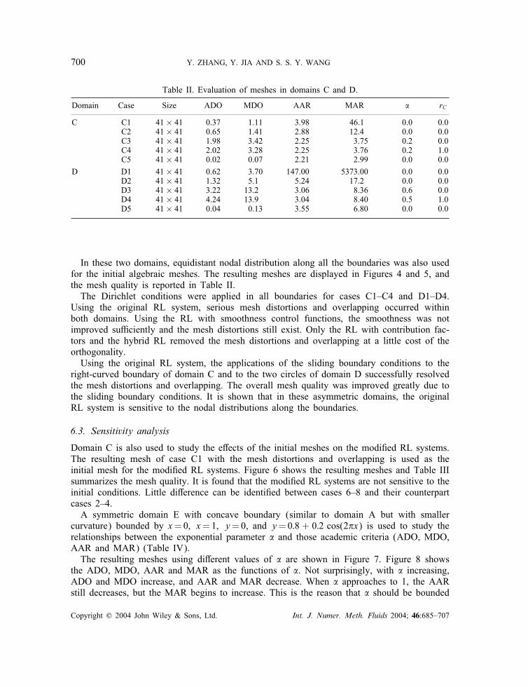
Table II. Evaluation of meshes in domains C and D.


C C1 41× 41 0.37 1.11 3.98 46.1 0.0 0.0C2 41× 41 0.65 1.41 2.88 12.4 0.0 0.0C3 41× 41 1.98 3.42 2.25 3.75 0.2 0.0C4 41× 41 2.02 3.28 2.25 3.76 0.2 1.0C5 41× 41 0.02 0.07 2.21 2.99 0.0 0.0

D D1 41× 41 0.62 3.70 147.00 5373.00 0.0 0.0D2 41× 41 1.32 5.1 5.24 17.2 0.0 0.0D3 41× 41 3.22 13.2 3.06 8.36 0.6 0.0D4 41× 41 4.24 13.9 3.04 8.40 0.5 1.0D5 41× 41 0.04 0.13 3.55 6.80 0.0 0.0

In these two domains, equidistant nodal distribution along all the boundaries was also usedfor the initial algebraic meshes. The resulting meshes are displayed in Figures 4 and 5, andthe mesh quality is reported in Table II.The Dirichlet conditions were applied in all boundaries for cases C1–C4 and D1–D4.

Using the original RL system, serious mesh distortions and overlapping occurred withinboth domains. Using the RL with smoothness control functions, the smoothness was notimproved su�ciently and the mesh distortions still exist. Only the RL with contribution fac-tors and the hybrid RL removed the mesh distortions and overlapping at a little cost of theorthogonality.Using the original RL system, the applications of the sliding boundary conditions to the

right-curved boundary of domain C and to the two circles of domain D successfully resolvedthe mesh distortions and overlapping. The overall mesh quality was improved greatly due tothe sliding boundary conditions. It is shown that in these asymmetric domains, the originalRL system is sensitive to the nodal distributions along the boundaries.

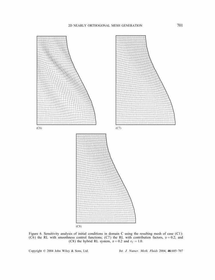
6.3. Sensitivity analysis

Domain C is also used to study the e�ects of the initial meshes on the modi�ed RL systems.The resulting mesh of case C1 with the mesh distortions and overlapping is used as theinitial mesh for the modi�ed RL systems. Figure 6 shows the resulting meshes and Table IIIsummarizes the mesh quality. It is found that the modi�ed RL systems are not sensitive to theinitial conditions. Little di�erence can be identi�ed between cases 6–8 and their counterpartcases 2–4.A symmetric domain E with concave boundary (similar to domain A but with smaller

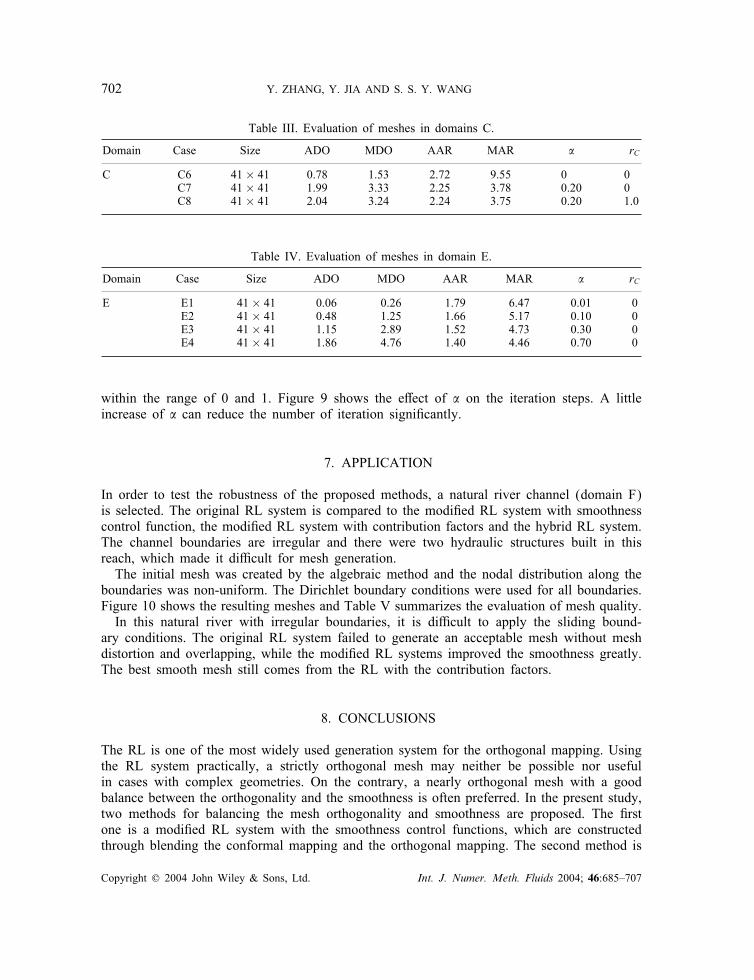
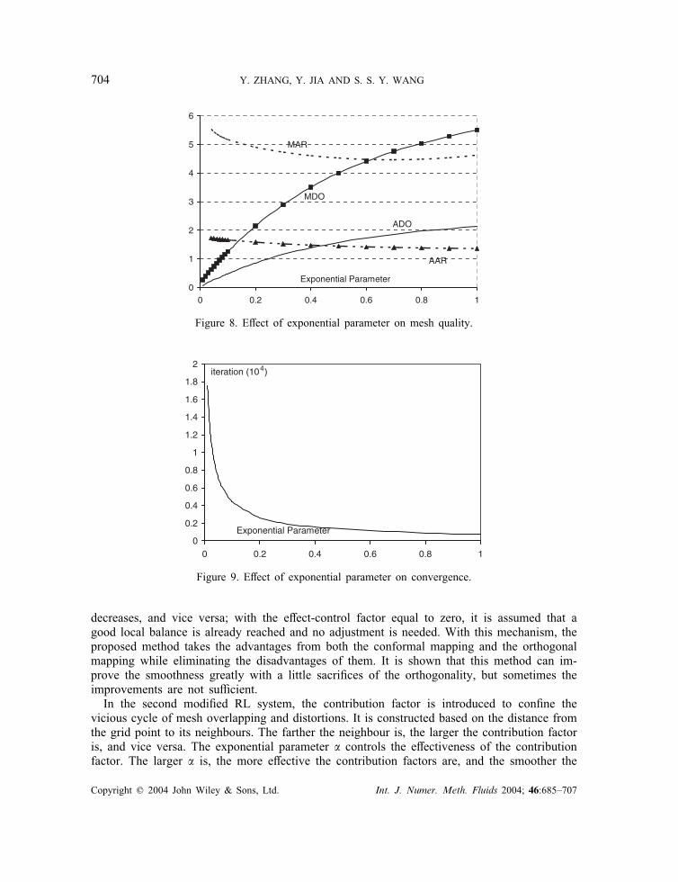
curvature) bounded by x=0; x=1; y=0, and y=0:8 + 0:2 cos(2�x) is used to study therelationships between the exponential parameter � and those academic criteria (ADO, MDO,AAR and MAR) (Table IV).The resulting meshes using di�erent values of � are shown in Figure 7. Figure 8 shows

the ADO, MDO, AAR and MAR as the functions of �. Not surprisingly, with � increasing,ADO and MDO increase, and AAR and MAR decrease. When � approaches to 1, the AARstill decreases, but the MAR begins to increase. This is the reason that � should be bounded



(C6) (C7)

(C8)

Figure 6. Sensitivity analysis of initial conditions in domain C using the resulting mesh of case (C1):(C6) the RL with smoothness control functions; (C7) the RL with contribution factors, �=0:2; and

(C8) the hybrid RL system, �=0:2 and rC =1:0.



Table III. Evaluation of meshes in domains C.


C C6 41× 41 0.78 1.53 2.72 9.55 0 0C7 41× 41 1.99 3.33 2.25 3.78 0.20 0C8 41× 41 2.04 3.24 2.24 3.75 0.20 1.0

Table IV. Evaluation of meshes in domain E.


E E1 41× 41 0.06 0.26 1.79 6.47 0.01 0E2 41× 41 0.48 1.25 1.66 5.17 0.10 0E3 41× 41 1.15 2.89 1.52 4.73 0.30 0E4 41× 41 1.86 4.76 1.40 4.46 0.70 0

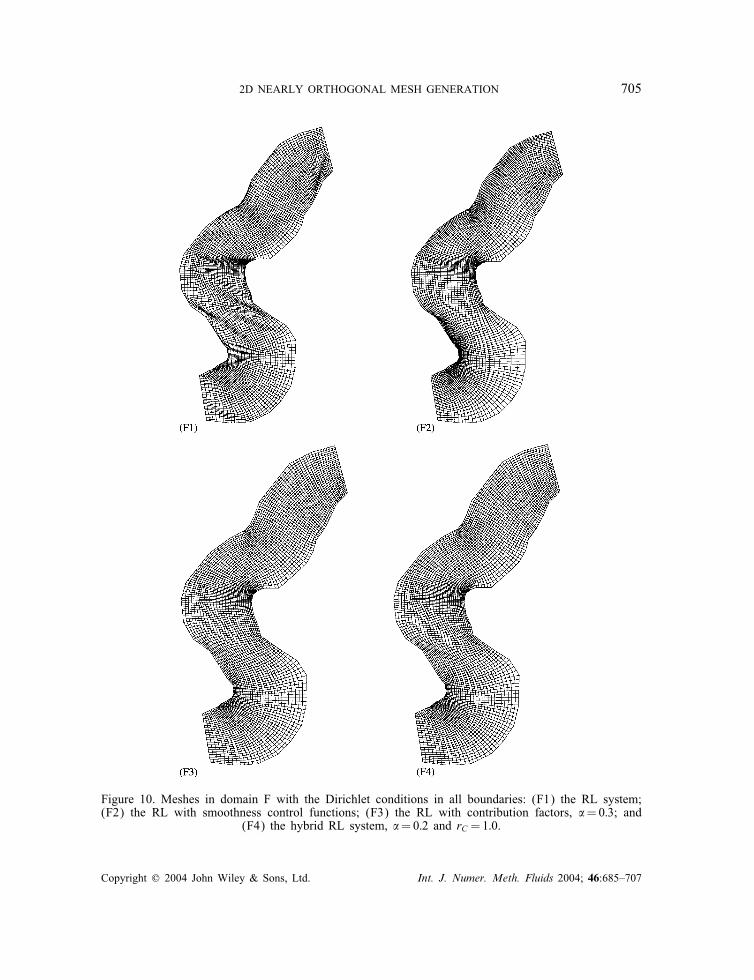
within the range of 0 and 1. Figure 9 shows the e�ect of � on the iteration steps. A littleincrease of � can reduce the number of iteration signi�cantly.

7. APPLICATION

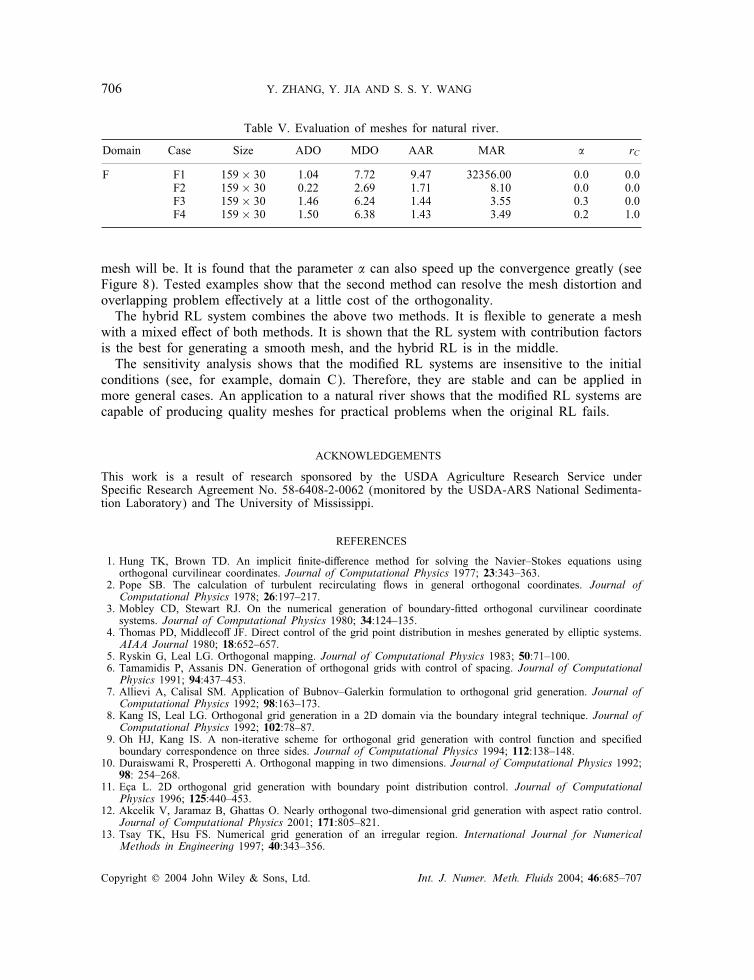
In order to test the robustness of the proposed methods, a natural river channel (domain F)is selected. The original RL system is compared to the modi�ed RL system with smoothnesscontrol function, the modi�ed RL system with contribution factors and the hybrid RL system.The channel boundaries are irregular and there were two hydraulic structures built in thisreach, which made it di�cult for mesh generation.The initial mesh was created by the algebraic method and the nodal distribution along the

boundaries was non-uniform. The Dirichlet boundary conditions were used for all boundaries.Figure 10 shows the resulting meshes and Table V summarizes the evaluation of mesh quality.In this natural river with irregular boundaries, it is di�cult to apply the sliding bound-

ary conditions. The original RL system failed to generate an acceptable mesh without meshdistortion and overlapping, while the modi�ed RL systems improved the smoothness greatly.The best smooth mesh still comes from the RL with the contribution factors.

8. CONCLUSIONS

The RL is one of the most widely used generation system for the orthogonal mapping. Usingthe RL system practically, a strictly orthogonal mesh may neither be possible nor usefulin cases with complex geometries. On the contrary, a nearly orthogonal mesh with a goodbalance between the orthogonality and the smoothness is often preferred. In the present study,two methods for balancing the mesh orthogonality and smoothness are proposed. The �rstone is a modi�ed RL system with the smoothness control functions, which are constructedthrough blending the conformal mapping and the orthogonal mapping. The second method is



(E1)

(E2)

(E3)

(E4)

Figure 7. Meshes in domain E with the Dirichlet conditions in all boundaries: (E1) RL with contributionfactors, �=0:01; (E2) RL with contribution factors, �=0:1; (E3) RL with contribution factors, �=0:3;

and (E4) RL with contribution factors, �=0:7.

a modi�ed RL system with the contribution factors. A hybrid RL system combining thesetwo methods is also developed. Comparisons between the RL system and the modi�ed RLsystems have been illustrated by several examples and application.In the �rst modi�ed RL system, the e�ect-control factor is constructed to automatically

adjust the balance between the orthogonality and the smoothness for the whole domain. Withthe e�ect-control factor increasing, the local smoothness increases and the local orthogonality



0

1

2

3

4

5

6

0 0.2 0.4 0.6 0.8 1

ADO

MDO

MAR

AAR

Exponential Parameter

Figure 8. E�ect of exponential parameter on mesh quality.

0

0.2

0.4

0.6

0.8

1

1.2

1.4

1.6

1.8

2

0 0.2 0.4 0.6 0.8 1

iteration (10 )

Exponential Parameter

4

Figure 9. E�ect of exponential parameter on convergence.

decreases, and vice versa; with the e�ect-control factor equal to zero, it is assumed that agood local balance is already reached and no adjustment is needed. With this mechanism, theproposed method takes the advantages from both the conformal mapping and the orthogonalmapping while eliminating the disadvantages of them. It is shown that this method can im-prove the smoothness greatly with a little sacri�ces of the orthogonality, but sometimes theimprovements are not su�cient.In the second modi�ed RL system, the contribution factor is introduced to con�ne the

vicious cycle of mesh overlapping and distortions. It is constructed based on the distance fromthe grid point to its neighbours. The farther the neighbour is, the larger the contribution factoris, and vice versa. The exponential parameter � controls the e�ectiveness of the contributionfactor. The larger � is, the more e�ective the contribution factors are, and the smoother the



Figure 10. Meshes in domain F with the Dirichlet conditions in all boundaries: (F1) the RL system;(F2) the RL with smoothness control functions; (F3) the RL with contribution factors, �=0:3; and

(F4) the hybrid RL system, �=0:2 and rC =1:0.



Table V. Evaluation of meshes for natural river.


F F1 159× 30 1.04 7.72 9.47 32356.00 0.0 0.0F2 159× 30 0.22 2.69 1.71 8.10 0.0 0.0F3 159× 30 1.46 6.24 1.44 3.55 0.3 0.0F4 159× 30 1.50 6.38 1.43 3.49 0.2 1.0

mesh will be. It is found that the parameter � can also speed up the convergence greatly (seeFigure 8). Tested examples show that the second method can resolve the mesh distortion andoverlapping problem e�ectively at a little cost of the orthogonality.The hybrid RL system combines the above two methods. It is �exible to generate a mesh

with a mixed e�ect of both methods. It is shown that the RL system with contribution factorsis the best for generating a smooth mesh, and the hybrid RL is in the middle.The sensitivity analysis shows that the modi�ed RL systems are insensitive to the initial

conditions (see, for example, domain C). Therefore, they are stable and can be applied inmore general cases. An application to a natural river shows that the modi�ed RL systems arecapable of producing quality meshes for practical problems when the original RL fails.

ACKNOWLEDGEMENTS

This work is a result of research sponsored by the USDA Agriculture Research Service underSpeci�c Research Agreement No. 58-6408-2-0062 (monitored by the USDA-ARS National Sedimenta-tion Laboratory) and The University of Mississippi.

REFERENCES

1. Hung TK, Brown TD. An implicit �nite-di�erence method for solving the Navier–Stokes equations usingorthogonal curvilinear coordinates. Journal of Computational Physics 1977; 23:343–363.

2. Pope SB. The calculation of turbulent recirculating �ows in general orthogonal coordinates. Journal ofComputational Physics 1978; 26:197–217.

3. Mobley CD, Stewart RJ. On the numerical generation of boundary-�tted orthogonal curvilinear coordinatesystems. Journal of Computational Physics 1980; 34:124–135.

4. Thomas PD, Middleco� JF. Direct control of the grid point distribution in meshes generated by elliptic systems.AIAA Journal 1980; 18:652–657.

5. Ryskin G, Leal LG. Orthogonal mapping. Journal of Computational Physics 1983; 50:71–100.6. Tamamidis P, Assanis DN. Generation of orthogonal grids with control of spacing. Journal of ComputationalPhysics 1991; 94:437–453.

7. Allievi A, Calisal SM. Application of Bubnov–Galerkin formulation to orthogonal grid generation. Journal ofComputational Physics 1992; 98:163–173.

8. Kang IS, Leal LG. Orthogonal grid generation in a 2D domain via the boundary integral technique. Journal ofComputational Physics 1992; 102:78–87.

9. Oh HJ, Kang IS. A non-iterative scheme for orthogonal grid generation with control function and speci�edboundary correspondence on three sides. Journal of Computational Physics 1994; 112:138–148.

10. Duraiswami R, Prosperetti A. Orthogonal mapping in two dimensions. Journal of Computational Physics 1992;98: 254–268.

11. E�ca L. 2D orthogonal grid generation with boundary point distribution control. Journal of ComputationalPhysics 1996; 125:440–453.

12. Akcelik V, Jaramaz B, Ghattas O. Nearly orthogonal two-dimensional grid generation with aspect ratio control.Journal of Computational Physics 2001; 171:805–821.

13. Tsay TK, Hsu FS. Numerical grid generation of an irregular region. International Journal for NumericalMethods in Engineering 1997; 40:343–356.



14. Knupp P, Steinberg S. Fundamentals of Grid Generation. CRC Press: Boca Raton, 1994.15. Beale SB. A �nite volume method for numerical grid generation. International Journal for Numerical Methods

in Fluids 1999; 30:523–540.16. Thompson JF, Thames FC, Mastin CW. TOMCAT—a code for numerical generation of boundary-�tted

curvilinear coordinate system on �elds containing any number of arbitrary two-dimensional bodies. Journalof Computational Physics 1977; 24:274–302.

17. Thompson JF, Warsi ZUA, Mastin CW. Numerical Grid Generation: Foundation and Application. North-Holland: New York, 1985.

18. Thompson JF. A re�ection on grid generation in the 90s: trends, needs, and in�uences. 5th InternationalConference on Grid Generation in CFS, Mississippi State University, 1996.


2d nearly orthogonal mesh generation

Documents