2d heteronuclear nmr measurements of spin-lattice relaxation times in the rotating frame of x

JOURNAL OF MAGNETIC RESONANCE 94,82- 100 ( 199 1)

2D Heteronuclear NMR Measurements of Spin-Lattice Relaxation Times in the Rotating Frame of X Nuclei in Heteronuclear

HX Spin Systems

JEFFREY W. PENG,* +t V. THANABAL, * AND GERHARD WAGNER*,+

*Department of Biological Chemistry and Molecular Pharmacology, Harvard Medical School, 240 Longwood Avenue, Boston, Massachusetts 021 IS; and TBiophysics Research Division,

University of Michigan, 2200 Bonisteel Boulevard, Ann Arbor, Michigan 48109

Received November 30, 1990

Theoretical and experimental aspects of T,, are discussed for a heteronuclear HX two- spin system (T$) where only the X nucleus is spin-locked. An expression for TE in terms of spectral density functions and the effective magnetic field parameters is developed. It shows that T:, offers potentially dierent information about the spectral densities than either r:, TF, or the steady-state NOEX. We present a 2D heteronuclear NMR pulse sequence for measuring site-specific T$‘s in biomolecules. The sequence is based on a double-INEPT transfer and applies a spin lock to the heteronuclei for variable delays. If a weak on-resonance spin lock is used, and if the spectral density functions are assumed to be Lorentzians, then rc is theoretically indistinguishable from r:. We conclude with an application of the pulse sequence to the uniformly ‘5N-enriched protein eglin c. The rc, data reflect the differential mobility in the molecule. o 199 t Academic PESS, h.

NMR relaxation studies of X nuclei in heteronuclear HX spin systems can provide information about the global and internal motions of biomolecules (1-3). Hence, they are powerful tools for the experimentalist interested in biomolecular dynamics. Recently developed techniques for measuring such relaxation times use various heteronuclear multidimensional NMR pulse sequences to provide the necessary frequency resolution, as well as to lend sensitivity enhancement (I, 3). Additionally, the increasing availability of isotopic enrichment alleviates the problem of poor sensitivity due to low natural abundance of such biological heteronuclei as “N and r3C. Making use of these assets, dynamical information for a large number of different sites in the molecule can simultaneously be obtained.

Thus far the most commonly measured relaxation parameters of heteronuclei HX spin systems include TF, TF, and the steady-state NOEX that develops due to satu- ration of the H spin (I-3). In this paper, we discuss the measurement of the spin- lattice relaxation time in the rotating frame, Tj$. Tfp is the decay constant of magnetization locked along the effective field, Beff. Previous studies of T,, include work by Abragam ( 4) ) Jones (5), James (6-9), and Blicharski ( I&z, lob). The derivation of the homonuclear T,, has been given by Jones (5) and Blicharski (1&z, lob). James et al. (6, 9) have used 1 D 13C off-resonance TTp measurements to get information about protein rotational correlation times and internal dynamics.

$ To whom correspondence should be addressed.

0022-2364/91 $3.00 Copyright 0 1991 by Academic Pa-es, Inc. All right.5 of reproduction in any form rserved.

82

HETERONUCLEAR RELAXATION-TIME MEASUREMENTS 83

In this paper, we use the semiclassical relaxation formalism to arrive at an expression for TFp for an HX spin system. Our approach follows that of Jones ( 5). T$ is expressed in terms of the spectral density functions, J(w), and the radiofrequency Ilip angle, /?. An expression is also obtained for the heteronuclear cross-relaxation rate in the rotating frame, u,““. Blicharski (IOU) has gi ven a Typ expression in terms of the Wigner 3-j symbols, assuming isotropic rigid tumbling of the molecule. If we assume rigid body tumbling of the molecule as well, then our results are equivalent to that contained in the more general expression of Blicharski ( ZOa). We also present a 2D NMR pulse sequence to measure Typ for each heteronucleus in the molecule of interest. We then present TTp relaxation data from the proteinase inhibitor eglin c 100% isotopically enriched in “N.

Relaxation parameters are related to overall and internal molecular motions through their dependence on the spectral density functions, J( 0). Specifically, the relaxation parameters sample the spectral density at particular frequencies with varying weights. It is seen that TFp samples different frequencies of J(o) than either Tr, TF, or the steady-state NOEX. In principle, this means that Typ can give new information concerning the spectral properties of J( w ) . The T$ data on eglin c support the information from other relaxation parameter measurements ( TT , NOE *) in revealing the more mobile regions of the molecule. Thus, TTp is sensitive to dynamical heterogeneity in biomolecules.

THEORY

TTp is the relaxation time for magnetization along the effective magnetic field in the rotating frame. The physical situation is illustrated for an arbitrary spin- 1 nucleus with Larmor frequency 00 in Fig. 1. The rotating frame is defined by the xyz axes, with the static, superconducting field & pointing along +z. B,, defines the laboratory Z axis, which is coincident with the rotating-frame z axis. The effective field is indicated by the vector B,@, which is tipped away from the z axis by an angle 0. The z component

2. B,

FIG. 1. Magnetic field vectors in the rotating frame for a nucleus of Larmor frequency q,.

84 PENG, THANABAL, AND WAGNER

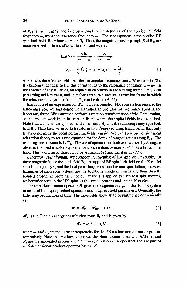
of Berr is (w - wO)/y and is proportional to the detuning of the applied RF field frequency w, from the resonance frequency wo. The x component is the applied RF spin-lock field, B1, where w, = - yBr . Thus, the magnitude and tip angle B of B,g are parameterized in terms of w, wI in the usual way as

-YBl WP) = (w - wo) = (wo” w)

Befl = !- VW; + (w - wo)2 = - 5 , ill Y

where o, is the effective field described in angular frequency units. When ,!I = (x/2), B,,r becomes identical to Br ; this corresponds to the resonance condition w = wo. In the absence of any RF fields, all applied fields vanish in the rotating frame. Only local perturbing fields remain, and therefore this constitutes an interaction frame in which the relaxation analysis for T, and T2 can be done (4, II ).

Extraction of an expression for T% in a heteronuclear HX spin system requires the following steps. We first define the Hamiltonian operator for two unlike spins in the laboratory frame. We must then perform a rotation transformation of the Hamiltonian, so that we can work in an interaction frame where the applied fields have vanished. Note that we have two applied fields: the static B. and the radiofrequency spin-lock field Bi . Therefore, we need to transform to a doubly rotating frame. After this, only terms concerning the local perturbing fields remain. We can then use semiclassical relaxation theory to get a rate equation for the decay of magnetization along B,s. The resulting rate constant is 1 / Typ. The use of operator methods as discussed by Abragam obviates the need to solve explicitly for the spin density matrix, u(t), as a function of time. This is discussed thoroughly by Abragam (4) and Ernst et al. ( ZZ ) .

Laboratory Hamiltonian. We consider an ensemble of HX spin systems subject to three magnetic fields: the static field Bo, the applied RF spin-lock field on the X nuclei at radial frequency w, and the local perturbing fields from the non-spin-lattice processes. Examples of such spin systems are the backbone amide nitrogens and their directly bonded protons in proteins. Since our analysis is applied to such real spin systems, we hereafter refer to the HX spins as the amide protons and their 15N nuclei.

The spin-Hamiltonian operator # gives the magnetic energy of the ‘H- 15N system in terms of both spin product operators and magnetic field parameters. Generally, the latter may be functions of time. The three fields allow x to be partitioned conveniently as

se = x; + J&F + V(t).

tiz is the Zeeman energy contribution from B. and is given by

121

sfz = wpzz + wnivz, [31

where W, and wP are the Larrnor frequencies for the “N nucleus and the amide proton, respectively. Note that we have expressed the Hamiltonian in units of h/2?r. Z, and N, are the associated proton and 15N z-magnetization spin operators and are part of a 16dimensional product-operator basis (12).


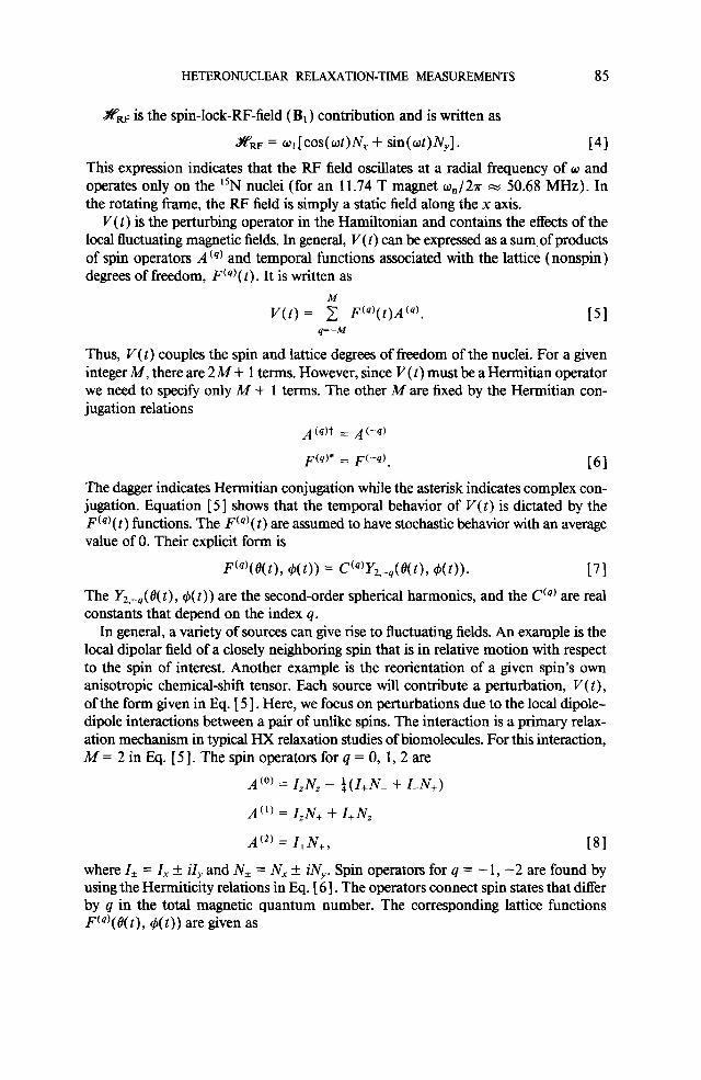
&& is the spin-lock-RF-field ( B1 ) contribution and is written as

SRF = 0, [ cos( ot)Nx + sin(wt)l\r,] . t41 This expression indicates that the RF field oscillates at a radial frequency of w and operates only on the 15N nuclei (for an 11.74 T magnet oJ27r = 50.68 MHz). In the rotating frame, the RF field is simply a static field along the x axis.

V(t) is the perturbing operator in the Hamiltonian and contains the effects of the local fluctuating magnetic fields. In general, V(t) can be expressed as a sum. of products of spin operators Acq) and temporal functions associated with the lattice (nonspin) degrees of freedom, F(@( t) . It is written as

V(t) = ; F(q’(t)A(q). t51 q=-M

Thus, V(t) couples the spin and lattice degrees of freedom of the nuclei. For a given integer M, there are 2M + 1 terms. However, since V(t) must be a Hermitian operator we need to specify only A4 + 1 terms. The other A4 are fixed by the Hermitian conjugation relations

At&t = A(h)

J’(4)* = F(-d. [61 The dagger indicates Hermitian conjugation while the asterisk indicates complex conjugation. Equation [ 51 shows that the temporal behavior of V(t) is dictated by the Fcq)( t) functions. The Fcq)( t) are assumed to have stochastic behavior with an average value of 0. Their explicit form is

F’q’(W, 4(t)) = Ccq’Y,,-,W), 4(t)). t71

The Yz,-,( 19( t), I$( t)) are the second-order spherical harmonics, and the Ccq) are real constants that depend on the index q.

In general, a variety of sources can give rise to fluctuating fields. An example is the local dipolar field of a closely neighboring spin that is in relative motion with respect to the spin of interest. Another example is the reorientation of a given spin’s own anisotropic chemical-shift tensor. Each source will contribute a perturbation, V(t), of the form given in Eq. [ 5 1. Here, we focus on perturbations due to the local dipole- dipole interactions between a pair of unlike spins. The interaction is a primary relaxation mechanism in typical HX relaxation studies of biomolecules. For this interaction, M=2inEq.[5].Thespinopcratorsforq=O, 1,2are

A(‘) = Z,N, - ~(Z+N- + Z-N+)

A(‘) = Z,N+ + Z+N,

A’*’ = Z+N+, t81 where Z-C = Z, + iZ, and N, = N, + iN,,. Spin operators for q = - 1, -2 are found by using the Hermiticity relations in Eq. [ 61. The operators connect spin states that differ by q in the total magnetic quantum number. The corresponding lattice functions Fcq)(8(t), 4(t)) are given as


F(O) = (y :,i’ F Y2,0(@(0, 4(t))

[91

where (Y = -y,,yJ Y&. The variables 8(t) and r$( t) describe the orientation of the “N-H bond vector r& t),

with respect to the static field Bo. The vector undergoes rotational diffusion due to the overall tumbling of the molecule and any internal dynamics, while the spin degrees of freedom stay parallel or antiparallel with B. . In this way, the F(q) become stochastic functions of time. In summary the net perturbation operator of the laboratory Ham- iltonian due to dipole-dipole interactions is

V(t) = -a(3 cos28 - 1) IzNz - $ (I+N- + I-N,) ( 1

cos 19(e-‘@)](ZzN+ + Z+N,) + HC

- $ [sin20(e-“6)](Z,N,.) + HC, [lo]

where HC indicates the Hermitian conjugate of the preceding term. Transformation to the doubly rotating coordinate frame. We are now in a position

to change to an interaction frame wherein the applied field terms in the Hamihonian vanish. Note that the traditional rotating frame will not suffice since it retains the effective field, B,e. A convenient approach is given by Abragam (4). In this approach we transform the Hamiltonian to a doubly rotating I?ame. This frame is the result of three successive rotation transformations on the laboratory coordinate frame. There- fore, these rotations are best described by the Euler angles cy, ,L3, and y. The first rotation is through an angle a(t) = wt about the laboratory Z axis. We show this in Fig. 2a. Uppercase labels X, Y, and Z mark the laboratory axes and lowercase labels x, y, and z mark the rotated axes. The result is the usual rotating frame, as in Fig. 1. We continue with a second rotation through the angle @ about the new y axis (line of nodes), as shown in Fig. 2b. This results in the axes x*, y*, and z*. The angle /? is the same tip angle for the effective field Bes as that shown in Fig. 1. Therefore, the z* axis is parallel to B,g. From the perspective of a spectroscopist in the x*y *z* frame, Betr serves the same purpose as B,, did in the laboratory frame. Thus, it can be “transformed away” in the same manner that & was. Namely, we do a third rotation through an angle y(t) = wet about the tipped z* axis (figure axis). This brings us to the final coordinate frame x’y’z’, where z’ and z* are the same. This last rotation is shown in Fig. 2c. All applied magnetic fields have vanished; thus, we have transformed to the interaction frame appropriate for the study of relaxation phenomena of the simpler rotating frame.


zz 2

&

z*, z ’

coot X

Y x

a) b.1 x’ C.)

X Y >-

Y’ Rotation Tmsfommiom U

e------e-*

Doubly Rotating Frame

FIG. 2. The three successive rotations of the doubly rotating frame. (a) Rotation about laboratory Z axis through 01 = wt. (b) Rotation about y (line of nodes) through tip angle @ Effective field Bdf. is parallel to z*. (c) Final rotation about z* (figure axis) through y = OJ. Below, the laboratory axes are denoted by the X YZ axes, and the doubly rotating frame axes are denoted by the x’y’z’ axes.

Since the proton spin operators commute with the nitrogen spin operators the proton rotation transformations can be considered independently. In particular, whereas three rotations were necessary for the 15N nuclei (X nuclei), only one is necessary for the protons (‘H nuclei) since the latter suffer no spin lock. Thus the required proton rotation transformation is about the laboratory 2 axis through an angle a = o,t . The total rotation transformation is then given by the unitary operator U, which consists of the three 15N rotations and the single proton rotation. It is written as

where

u = UJJ,,

Up = exp( iw,tZ,)

illal

[llbl and

U, = exp(io,tN,)exp(@lN,)exp(iwtN,). [1 ICI Of course, since the nitrogen and proton spin operators commute, the order of transformation in Eq. [ 1 la] is irrelevant.

To summarize, the effective Hamiltonian in the doubly rotating frame is obtained by applying the net rotation operator U to the laboratory expression given in Eq. [ 21.


The end result is simply the rotated version of V(t). We designate this transformed operator as V’(t). In terms of the spin operators and lattice functions, we have

V’(t) = UV(t)U+

= -(y d

F Y&O(t), 4(t)) cIz,N: - (s/2)e’“JZ,N: + HC I

- $ ((c - 1)/2)e”“p-“n+“e”I+N: + HC

1 - - Sel(Wp-Wn)‘I+N: + HC

4

- ; ((c + 1)/2)e i(wp-wn-4t~+q + HC I

3a -- 2 d

E Y,,-,(d(t), $(t)){(c + 1)/2)ei(Yn+We)flzN;

+ se’“n’I,N: + ((c - 1)/2)e’(“+e)‘I,NL - (s/2)e’(“p+“e)‘I+N;

+ Ce'"p'l+N; - (s/2)ei(“'p-"~)fI+~- > + HC

3ff -- 4 1/’

$ Y&(f?(t), f$(t)){ei(wP+wn+ue)‘((c + 1)/2)Z+N;

+ se ‘(w@“n)fI+N: + ((c - 1)/2)e i(“~+wn--oe)t~+~P > + HC. [ 121

Again, HC indicates the Hermitian conjugate of the previous term. For the Y,,-, and Y,,-, terms, the Hermitian conjugation is to be taken for the entire previous bracketed term, As expected, the laboratory spin operators are rotated into linear combinations of operators native to the doubly rotating frame. The latter operators are indicated by primes. To reduce the complexity of the above Eq. [ 121, we have used s and c in place of sin /.3 and cos ,f3, respectively.

Macroscopic rate equations and T z. The form of the Hamiltonian in the doubly rotating frame given by Eq. [ 121 along with the spin density operator u(t) allows us to write a rate equation for the decay of magnetization along Beg. All information concerning the ensemble of ‘H- “N spins can be obtained from a( t ) . The macroscopic value for any observable, M, is given by the ensemble-averaged expectation value of its associated quantum operator. This average is given by the well-known trace relation

(M)(t) = Tr(a(t)M}. 1131

We use (M) to indicate the macroscopic variable and M to indicate the quantum mechanical operator.

The equation of motion for u(t) in the doubly rotating frame (interaction frame) is governed by V’(t) and is written as

do s

a,

z=-0 ((VW), [v’(t - 71, a(t) - ~“lll)W. 1141


The angled brackets (( )) indicate that an ensemble average is to be taken over the time-dependent parts of V( t’)‘; iW is the density operator at thermodynamic equilibrium. If we insert the expression for V’(t) into the equation of motion given in Eq. [ 141, we then obtain

da 1 (Mm) -= -- dt 2 c (P(Wp))[Aj-q), [A?), a(t) - a”]]) [I51

(q=-M,p=-m)

The JCq)( wg)) terms are spectral density functions sampled at the transition frequencies w$); they arise from the aforementioned ensemble average over V’(t) (vide infra) . It is understood that in arriving at Eq. [ 151, we consider only those times t that are significantly longer than the correlation times characterizing the stochastic processes associated with V’(t) . This is a fundamental restriction of the semiclassical relaxation theory (4, II ). If we take the overall molecular tumbling as the stochastic process, then Eq. [ 15 ] is valid for times t % T,, where 7, is the molecular tumbling correlation time.

Eq. [ 131 gives the time behavior for (M), where (M) is the observed value for operator M. It seems to require prior integration of density operator Eq. [ 15 1. For- tunately, this is not necessary since the operator methods of Abragam (4) allow us to derive the rate equation for M directly. One multiplies the density operator Eq. [ 15 ] by the desired observable M and then takes the trace. Using the fact that the trace of any product of operators is unchanged by a cyclic shuffle of the operators, one im- mediately obtains the macroscopic rate equation

do = -k ‘y’ (J(q)(ti(q))Tr([A$-q) [API, M]](a(t) - P)>). dt P 3 [16]

(P,4)

Here, we need to define only the spectral densities JCq)(wf)) and the double com- mutator, [AiWq), [A& M] 1, which involves the observable of interest and the spin operators of V’(t) . The summation is over all terms in the transformed Hamiltonian V’(t) given in Eq. [12]. Index q runs from -Mto Mas in Eq. [4]. Recall that in going from the laboratory frame to the doubly rotating frame, the operators A (q) are mapped into linear combinations of operators A, (q). The index p runs over the operators in these linear combinations.

The spectral densities JCq’(op)) are the Fourier transforms of the autocorrelation function for the various angular functions FCq)( 8( t), d(t) ) , evaluated at the frequencies wg). Thus, for arbitrary frequency w, we have

s

+W .P(w) = ( kiw”( F@)( &,)F* (q)( a( t)))dt), -a, 1171

where Q stands for the angles (19, 4). ( Ftq’( Qo)F * (q)( Q( t))) is the autocorrelation function for a given liCq)( 19( t), 9(t)) and is the direct result of the ensemble average in Eq. [ 141. JCq)(w) is a real, even function of w. An analytical form for JCq’( w) requires a motional model for the “N- ‘H bond vector rnp. Only then can the autocorrelation for the FCq) be described and the Fourier transform given by Eq. [ 171 evaluated. For example, the traditional model of the molecule as an isotropically tumbling rigid body yields


pqw) = I T, 27r (1 + (W&)2) ’ WI

where T, is the molecular rotational correlation time. Note that the only q dependence is via the real constant C(q). The functional dependence on w is independent of q. We hereafter refer to this functional dependence simply as J( 0). Equation [ 18a] can then be rewritten as

J’qw) = !c$ qw)* [18bl

Physically, J( w ) represents the frequency distribution of the reorientational motions of the bond vector rnp. The goal of the molecular dynamicist, then, is to character- ize J(w).

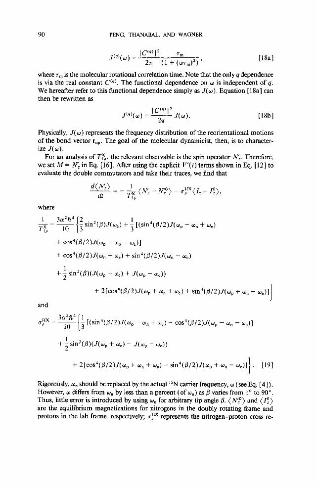
For an analysis of 7’Tp, the relevant observable is the spin operator N’. Therefore, we set M = N: in Eq. [ 161. After using the explicit V’(t) terms shown in Eq. [ 121 to evaluate the double commutators and take their traces, we find that

d(N) dt

- - & (N: - N’,O) - CI;‘(Z~ - Z:),

where

-=- sin2(p).Z(w,) + f [(sin4(/3/2)J(w, - % + we)

+ cos4(p/2).@, - u, - w,)]

+ cos4(/3/2)J(o, + 0,) + sin4(P/2)J(w, - w,)

+ i sin2(/3)(.Z(w, + w,) + J(w, - 0,))

+ 2[cos4(~/2)J(w, + 0, + w,) + sin4(@/2).Z(w, + w, - w,)] I

and

OP HX = F [$ [(sin4(@/2)J(+, - w, + 0,) - cos4(/3/2).Z(w, - 0, - w,)]

+ + sin2(P)(.Z(o, + w,) - J(w, - %I)

+ 2[cos4(p/2)J(w, + 0, + w,) - sin4(@/2)J(w, + w, - o,)] . 1

[19]

Rigorously, w, should be replaced by the actual “N carrier frequency, w ( see Eq. [ 4 ] ) . However, w differs from w, by less than a percent (of w,) as Z3 varies from 1 o to 90”. Thus, little error is introduced by using w, for arbitrary tip angle 8. (N’,‘) and (It) are the equilibrium magnetizations for nitrogens in the doubly rotating frame and protons in the lab frame, respectively; g:” represents the nitrogen-proton cross re-


laxation and is not to be confused with the spin density matrix u(t) discussed previously. Since Rq. [ 19 ] involves both (N: - N$‘) and (1, - 1:)) (N:) can generally change due to energy transfer to the lattice via T$, or due to cross relaxation to the protons via uHX . We note some distinctive features of the time constants TTp and u,“” . First, their dependence on the spectral density functions, J( w ), is weighted by various trigonometric functions of the tip angle ,!?. Additionally, the frequencies sampled by the spectral densities are w,, wP * w,, w, f w,, and or f w, f. w,. These are sidebands of the usual sampling frequencies 0, wP , w, , and wp -t w, seen in the well-known expressions for T? and Tf . The fact that TE samples different frequencies means that we can monitor different spectral regions of J(w). This is shown schematically in Fig. 3. In principle, spin-lock sequences can be engineered to monitor J( w ) at a desired set of frequencies.

If the molecule suffers no motion other than rigid isotropic tumbling, the autocorrelation function for the reorientation of the internuclear vector r,p can be described by a single exponential with a decay constant 7,. This results in a Lorentzian form for J(w) shown in Eq. [ lSa]. Then for certain values of the flip angle B, Tj$ reduces to the familiar heteronuclear TT and T;. Consider the limit where p approaches 0. This corresponds to a totally off-resonance RF field. Then all sine terms in Eq. [ 191 vanish. Typically, (w,/~P) is in the kilohertz range, as opposed to the megahertz values of Larmor frequencies ( w, / 2a) and ( w,,/ 27r). In such cases, we can neglect the RF contribution to the Larmor frequencies and make the approximations J( wP f w, + w,) = J( w,, + wn), J( wP + w,) = J( wP), and J( w, f w,) = J( w,). We then arrive at the familiar TT expression

1 ;~r:,=$g,,,wp- W”) + 3J(w,) + ww, + %>>, VW

lim g,“” = q {Ww, + wn) - J(q, - ~“11. [20bl PO Note that u,“” reduces to the familiar cross-relaxation rate first derived by Solomon ( 13), and the rate equation [ 191 simply becomes one of the Solomon equations.

Now consider the limit where p approaches ( 7r/ 2) and therefore cos( ,8/ 2) = sin( P/ 2) = 1/2/2. This corresponds to the on-resonance limit. If we keep the approximations of J(w, f W, f w,) = J(w, + w,), J(w, + w,) = J(w,), and J(w, +- w,) = J(w,) we get

1

/3-w/2 TI, lim x = 2. azh4 {4J(w,) + J(w, - W”)

+ 3J(w,) + 6J(w,) + 6J(w, + w,)}, [21a]

lim u,“” = 0. [21bl P--/2

This is identical to the expression for TF except for the lowest-frequency term, which is J( w,) instead of J( 0). In principle, it should be possible to map the spectral density function near the zero frequency by measuring on-resonance TE values for varying w, values. Note also that the cross-relaxation term vanishes. Therefore, the use of polarization-transfer methods from protons to nitrogens (X nuclei), which equalizes


J(a)

I

\ C

% JL 2%

I- I I I

l- I I I I

I

I

log(N

FIG. 3. Sampling of a hypothetical spectral density function J(w) by T$. The arrowed spikes are the sampling frequencies. They are sidebands symmetrically offset by fo, to the usual sampling frequencies indicated by the dashed lines. The samplings are weighted by trigonometric functions of the Bti tip angle, P.

the proton populations, is justified in the relaxation experiment discussed (see Fig. 5 ) . For w,/ 2a in the kilohertz range, J( we) will be sensitive to processes with correlation times much longer than those germane to the spectral density functions evaluated at the various Larmor frequencies wP f w, , wP, and w,. For protein molecules with 7, in the range of nanoseconds, WJ, 4 1. As a result, J( w,) is well approximated by J( 0). Therefore, in the limit of a weak on-resonance spin lock and the assumption of a Lorentzian spectral density function, T$ contains the same spectral information as Tf.

It is also informative to compare the behavior of these relaxation times as a function of T, with the assumption that J(w) is Lorentzian. Figure 4 plots log,,( Ti) against logiO(~,), where Ti is either Typ at various tip angles P, T?, or Tf. We note that Typ for /3 = 90” shows the same kind of behavior as T?. Specifically, both relaxation times ultimately increase with correlation time aRer reaching a minimum. This increase occurs for 7, > ( 1 /urnin), where W,in represents the lowest-frequency spin transition for a particular relaxation time. Essentially, slower molecular tumbling results in longer T, values, which weight the spectral density function toward lower frequencies. This is easily visualized if J(w) is a simple Lorentzian distribution; a longer 7, produces a sharper, narrower “peak” about zero frequency. As a result, the overlap between the high-intensity portion of J(o) and the nonzero spin transition frequencies progressively decreases. The associated relaxation process is therefore retarded and the relaxation time lengthens. Since the lowest transition frequency sampled by Typ is typically several orders of magnitude lower than that in T?, the increasing edge of TE occurs at much longer correlation times. Clearly, 7, can never exceed 1 /W,in for TF. Therefore, TF continues to decrease monotonically with 7, until plateauing at a particular rigid lattice value (not shown). Note again that for T, on the order of nanoseconds, Tf and T$ for ,f3 = 90” are equal. However, it must be stressed that


'-12.0-11.5-11.0-10.5-10.0 -9.5 -9.0 -8.5 -8.0 -7.5 -7.0 -6.5 -6.0 -5.5 -5.0 -4.5 -4.0 -3.5 -3.0 log10 (Tm /se4

FIG. 4. Log,,,-log,, plot of r:, T:, and T:, versus molecular correlation time T,. Tj$ is shown for flip angles /3 = 90”, 30”, lo”, and lo. The Ty, plots are indicated by the solid curves with flip angle labels. The r: and T: plots are shown by the broken curves above and below, respectively.

this equality holds only if the spectral density function J(o) is given by a Lorentzian (and only then is r, defined). Figure 4 also shows the behavior of TTo as a function of T, at flip angle values of /3 = I”, lo”, and 30”. As 6 progresses from 0” to 90”, we see the transition from TF to Tf behavior. Note that since Fig. 4 is plotted on a logarithmic scale, the T? and TE values for T, in the range of 3-4 ns may appear deceptively close. In fact, for T, = 3.5 ns, T?/ TTp is approximately 2.

EXPERIMENTS AND RESULTS

The 2D NMR pulse sequence for measuring TE values is shown in Fig. 5. The sequence allows the measurement of TT(, times for each X nucleus in a molecule. In our experiments, the X nuclei are protein backbone amide “N nuclei. The sequence begins with equilibrium proton magnetization which is transferred via an INEPT sequence to the nitrogens. After the INEPT transfer, we have antiphase 21,N, magnetization. We follow with a tuned refocusing period to get N, magnetization. A “N spin lock keeps the N, magnetization locked along x for a relaxation delay T. The remnant magnetization is then frequency labeled during the t, evolution period. A reversed, refocused INEPT converts the magnetization back to the protons for sen-


X A C

AJ2 Al2Al2 Al2 H

X

FIG. 5. Two-dimensional pulse sequence for measuring r$ times in heteronuclear HX systems. Proton ( ‘H) pulses are shown on the upper trace and X nuclei pulses are given on the lower trace. Solvent suppression is achieved by initial presaturation of the solvent protons; 90” and 180” pulses are indicated by the thin and thick vertical bars, respectively. Delays include the X-nucleus spin lock, which is indicated by the shaded region of length ‘T, the tuned delay A/2 = 1 /( 4Jnx), the X nucleus evolution period t, , and the proton detection period t2. The pulse phases are as follows: (A) y, -y . . . , (B) x, x, -x, -x, . . . , + TPPI, (C) x,x,x,x,-x,-x,-x,-x ,.... The receiver phases are --x, x, x, -x, x, -x, -x, x, . . . . Broadband decoupling is used during the proton detection period as indicated by the MLEV-64 period on the X nuclei.

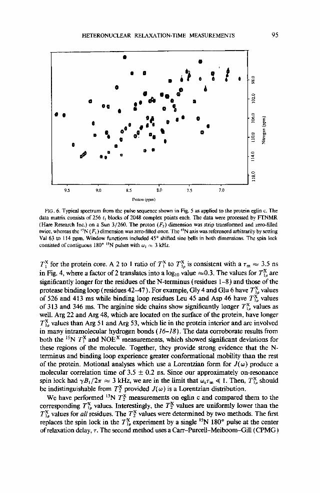
sitivity-enhanced, broadband-decoupled acquisition. Sign discrimination in F, is achieved by the TPPI method of Marion and Wiithrich ( 14). The minimum phase cycle involves eight scans, typically with 256 t, blocks acquired. The final result is a heteronuclear COSY spectrum with the cross-peak intensities attenuated by the extent of relaxation allowed. A typical spectrum is shown in Fig. 6. Each cross peak corresponds to the backbone amide I5 N of a specific residue. In our experiments, the “N spin lock was composed of contiguous 15N 180,” pulses. Use of other pulse trains such as WALTZ- 16 was avoided since the magnetization is not necessarily fixed along B,K during these sequences. The 180” pulse lengths were 168 ps, corresponding to 0,/27r = 2976 Hz. The tip angles (6) for the amides ranged between 75” and 90”. Thus we can approximate the spin lock as being on resonance for all backbone amide cross peaks.

We have implemented this experiment on a General Electric Q500 spectrometer and applied it to the 100% 15N-enriched protein eglin c. Eglin c functions as an inhibitor for proteinases such as elastase, subtilisin, and chymotrypsin. It consists of 70 residues resulting in a molecular weight of 8 111 Da. The proton assignments have been given by Hyberts et al. (15). The sample concentration was ~4.5 mM and the pH was set to 3.0. For a series of nine 2D spectra, the total acquisition time was approximately two days. Relative peak intensities were obtained by integrating slices along the F2 dimension through the cross-peak maxima for each 2D spectrum. For each cross peak, the intensities were fitted .to a monoexponential decay by a nonlinear least-squares fit routine using the software package PLOT (New Unit Inc., Ithaca, New York). The fitted decay constant gives Trp. An example is shown in Fig. 7.

The distribution of TE versus residue number is shown in Fig. 8. Blank columns indicate either prolines or residues that could not be quantitated due to-resonance overlap. Data at the positions 7 l-74 indicate the 4 arginine side-chain E-nitrogens for the residues Arg 22,48,5 1, and 53, which also constitute HX spin systems. The values are uniform for the backbone nitrogens of the protein core. The average TFD value is 2 15 ms with an uncertainty of t 11 ms. This is approximately half of the average


9.5 9.0 8.5 8:O 1.5 7.0

Proton (ppm)

FIG. 6. Typical spectrum from the pulse sequence shown in Fig. 5 as applied to the protein eglin c. The data matrix consists of 256 t, blocks of 2048 complex points each. The data were processed by FTNMR (Hare Research Inc.) on a Sun 3/260. The proton (Fr) dimension was strip transformed and zero-filled twice, whereas the lsN (F, ) dimension was zero-hlled once. The “N axis was referenced arbitrarily by setting Val 63 to 114 ppm. Window functions included 45” shifted sine bells in both dimensions. The spin lock consisted of contiguous 180” “N pulses with or = 3 kHz.

Ty for the protein core. A 2 to 1 ratio of TT to Typ is consistent with a T, = 3.5 ns in Fig. 4, where a factor of 2 translates into a log,, value ~0.3. The values for TTp are significantly longer for the residues of the N-terminus (residues l-8 ) and those of the protease binding loop (residues 42-47 ) . For example, Gly 4 and Glu 6 have TE values of 526 and 413 ms while binding loop residues Leu 45 and Asp 46 have T$ values of 3 13 and 346 ms. The arginine side chains show significantly longer T$ values as well. Arg 22 and Arg 48, which are located on the surface of the protein, have longer TFp values than Arg 5 1 and Arg 53, which lie in the protein interior and are involved in many intramolecular hydrogen bonds (16-18). The data corroborate results from both the “N TF and NOEX measurements, which showed significant deviations for these regions of the molecule. Together, they provide strong evidence that the N- terminus and binding loop experience greater conformational mobility than the rest of the protein. Motional analyses which use a Lorentzian form for J(w) produce a molecular correlation time of 3.5 f 0.2 ns. Since our approximately on-resonance spin lock had -yB,/2?r m 3 kHz, we are in the limit that W,T, Q 1. Then, TTo should be indistinguishable from Tf provided J(w) is a Lorentzian distribution.

We have performed 15N TF measurements on eglin c and compared them to the corresponding Typ values. Interestingly, the Tr values are uniformly lower than the TE values for all residues. The TF values were determined by two methods. The ftrst replaces the spin lock in the Tyn experiment by a single 15N 180” pulse at the center of relaxation delay, 7. The second method uses a Can--Purcell-Meiboom-Gill (CPMG)


0 20 40 60

Rela~aatio? IkY& iEisefY 160 200 220

FIG. 7. Example of 15N TE fit for the His 65 residue in eglin c. The TE value is 237 ms with an rmsd of 2.2%.

train of refocusing “N 180” pulses. CPMG duty cycles of 1 and 2% were used, with the “N 180” pulse width being 110 ps. These approaches are shown in Fig. 9. The resultant T? values are a50 and 25% reduced from the T% values for the single refocusing pulse and CPMG train ( 1% duty cycle), respectively. A comparison of relaxation curves for the three methods for residue His 65 of eglin c is shown in Fig. 10. The discrepancies from the Tz values are well outside the range of uncertainty for both the Tc and the TF experiments. It should be stressed that the relaxation times for all residues in eglin c increase without exception. In addition, the relative profile of relaxation times seen in Fig. 8 is essentially preserved; those l5 N spins that have relatively longer TF times also have longer T$ times.

A rigorous explanation of why the TE values are significantly longer than the corresponding Tf values remains elusive.’ Chemical exchange due to conformational isomerizations of the protein can cause apparently shorter T? values, especially in the single 180” experiment. However, such exchange processes should be localized in the protein and therefore cannot explain the global increase of T?, over T?.

‘Note added in proof: We have subsequently found that the short Tf values are caused by the evolution of in-phase NX,,y magnetization into antiphase 21&,J magnetization. Antiphase magnetization relaxes much faster than in-phase magnetization due to dipole-dipole interactions between the amide proton and other spatially close protons. Therefore, the short rf values are caused by proton-proton dip&u relaxation and not scalar relaxation of the second kind.


” 4 6 12 16 20 24 26 32 36 40 44 46 52 56 60 64 66 72 76 60

Residue Number

FIG. 8. Distribution of Tc for the 15N nuclei in eglin c. Blank columns are due to either prolines or overlapped cross peaks. The average uncertainty in the TF, values is + 11 ms. Significantly larger ryp values are observed for the more mobile parts of the protein. ry, values for the first residues (e.g., 2-4,6) exceed 500 ms and are off scale. Positions 7 1 to 74 are the N’ of the a&nines in positions 22,48,5 1, and 53. The N’ at positions 22 and 48 are solvent exposed and have off-scale 7’7, values of 542 and 781 ms, respectively. In contrast, the N’ at positions 5 1 and 53 are involved in intramolecular hydrogen bonding and have much shorter rt values of 234 and 300 ms, respectively.

Scalar relaxation of the second kind (4) has been suggested by Kay et al. (3) as the culprit mechanism causing the short TF values. This mechanism would involve fluc- tuations of the scalar interaction between the “N and ‘H caused by zero-quantum transitions between the amide protons and neighboring protons. The TTp experiment would be immune to the effects of scalar relaxation, since it decouples the “N nuclei from their amide protons during the spin lock. In contrast, the JNH coupling remains intact in the single 180” experiment (and to a lesser extent in the CPMG experiment ) and thus the scalar relaxation would result in apparently shorter TF times. However, this explanation seems unlikely for reasons discussed by Abragam (4). In particular, scalar relaxation of the second kind demands that the amide protons have relaxation times much shorter than ( 27rJNH)-l. (JNH is approximately 90 Hz, and therefore l/ 27r JNH is approximately 1.77 ms/rad). If this were the case, heteronuclear decoupling for the “N evolution would be unnecessary since the 15N doublet corresponding to populations with the amide proton spin up and spin down would automatically col- lapse. Furthermore, the theory of the proposed scalar relaxation treats the amide protons as lattice variables instead of spin operators. This means that the amide proton relaxation must occur faster than any time interval relevant to the “N relaxation experi-


FIG. 9. Alternative methods of measuring transverse relaxation times, TF. (a) Single 180” refocusing pulse; (b) CPMG 180” pulse train. (c) Spin lock. These sequences can all be inserted just prior to the t, evolution period in Fig. 5. The transverse relaxation times are the shortest for the single 180” pulse. They are progressively longer for CPMG trains of a larger duty cycle. In the limit that the duty cycle reaches lOO?& we get an on-resonance spin lock in case (c) .

ments. In effect, the amide proton spin fhps act as another stochastic perturbation from the lattice on the 15N spins, and the amide proton T1 and T2 become additional correlation times describing the “random field” seen by the 15N spins. However, the proton relaxation times are at least in the 100 ms time scale. Clearly then, the amide protons cannot be considered part of the lattice and an explanation using the theory for scalar relaxation of the second kind (4) is inappropriate.

An alternative explanation does not involve scalar relaxation at all, but rather the spectral density function, J( 0). Recall that the equivalence between TT and T% is

9 I 0

0 20 40 60 60 100 120 140 160 160 200 220 Relaxation Delay T /msec

FIG. 10. Comparison of T: via single 1 SO”, rg via CPMG, and TE for the same 15N nucleus (His 65 ) . The triangular plot is from the single 180” experiment, the open circle plot is from the CPMG experiment, and the solid circle plot is from the Ty, experiment of Fig, 5. The relaxation times are 136 f 4, 177 + 9, and 237 + 4 ms, respectively.

HETERONIJCLEAR RELAXATION-TIME MEASUREMENTS 99

based on the approximation that J( w,) = J( 0). This approximation assumes that J(w) is a Lorentzian described by a single correlation time, r,,,, which is on the order of nanoseconds. In this case, J(w) does not vary significantly over the low (kilohertz) frequencies characteristic of typical (w,/2~) values, and therefore the approximation is justified. However, there is no a priori reason to expect such flat behavior of J(w) at low frequencies. There may be internal protein motions at such frequencies that lead to much more complex spectral densities. It is therefore possible that J(w,) is significantly different from J( 0)) and that this alone accounts for the different results from the Tyo experiment and the other transverse relaxation experiments.

CONCLUDING REMARKS

We have shown theoretically that heteronuclear Tg measurements can offer spectral information not available in either Tr, TF, or NOEX. Specifically, TFp samples side- band frequencies offset by fw, from the zero-, single-, and double-quantum frequencies usually sampled in an HX spin system. When a Lorentzian form for J(w) is assumed, Typ reduces to Ty and Tf for the following cases. In the limit of a vanishing spin- lock field, T?( becomes Tr , and the rate equations for relaxation become Solomon’s equations ( 13). In the limit of an on-resonance spin lock, Typ resembles T$ except that the lowest frequency sampled is the effective field frequency, w,. If w, is much smaller than 1 /T,, then TE contains the same spectral information as Tf .

We have also presented a 2D heteronuclear pulse sequence to measure site-specific Typ values in biomolecules. We have applied the Typ experiment to the 70-residue protein, eglin c. The TE values are significantly longer than the corresponding Tc values obtained by using a single 180” pulse in the center of the relaxation delay, or by using a CPMG pulse train. Furthermore, we have observed that the TE values are longer for all “N nuclei in the protein. Therefore, the lengthening cannot be attributed to chemical exchange due to conformational isomerizations. Additionally, the lengthening cannot be attributed to scalar relaxation of the second kind (4)) which demands proton relaxation times well below the millisecond time scale. Those interested in a quantitative analysis of their data should consider carefully how the transverse relaxation times are to be measured. The variation of Tz values along the backbone of eglin c shows that it is sensitive to dynamical heterogeneity. TE is therefore another useful parameter in the experimental characterization of biomolecular motions.

ACKNOWLEDGMENTS

We thank Dr. Dirk Heinz and Dr. Marcus Griitter, Ciba-Geigy, Base], Switzerland, for the gift of 15N eglin c. We also thank Dr. Marc Adler for useful discussions and assistance with the use of PLOT. This work was supported by NSF Grants DMB-86 16059, DMB-9007878, and BBS 86 15223 and NIH Training Grant T32-GM08270-03 to J.P.

REFERENCES

1. (a) N. R. NIRMALA AND G. WAGNER, J. ilm. C/rem. Sot. 110,7557 (1988); (b), J. Mugn. Reson. 82, 659 (1989).

2. M. J. DELLWO AND A. J. WAND, J. Am. Chem. Sot. 111,457l (1989). 3. L. E. KAY, D. A. TORCHIA, AND A. BAX, Biochemistry 28,8972 ( 1989). 4. A. ABRAGAM, “The Principles of Nuclear Magnetism,” Chap. 8, Clarendon Press, Oxford, 196 1.


5. G. P. JONES, Phys. Rev. 148,332 (1966). 6. T. L. JAMES, G. B. MATSON, AND I. D. KUNTZ, J. Am. Chem. Sot. 100,359O ( 1978). 7. T. L. JAMES AND G. B. MATSON, J. Magn. Reson. 33,345 (1979). 8. T. L. JAMES, G. B. MATSON, I. D. KUNTZ, AND R. W. FISHER, J. Magn. Reson. 28,417 (1977). 9. T. L. JAMES AND S. P. SAWAN, J. Am. Chem. Sot. 101,705O ( 1979).

10. (a) J. S. Blicharski, Acta Phys. Pal. A 41,223 (1972); (b) Z. Naturjbrsch. A 27, 1355 (1972). 11. R. R. ERNST, G. BODENHAUSEN, AND A. WOKAUN, “Principles of Nuclear Magnetic Resonance in

One and Two Dimensions,” pp. 50-57, Clarendon Press, Oxford, 1987. 12. 0. W. SORENSEN, G. W. EICH, M. H. LEVITT, G. BQDENHAUSEN, AND R. R. ERNST, Prog. NMR

Spectrosc. 16, 163 (1983). 13. I. SOLOMON, Phys. Rev. 99,559 (1955). 14. D. MARION AND K. WUTHRICH, Biochem. Biophys. Res. Commun. 113,967 ( 1983). 15. S. G. HYBERTS AND G. WAGNER, Biochemistry 29, 1465 ( 1990). 16. (a) W. BODE, E. PAPAMOKOS, D. MUSIL, U. SEEM~LLER, AND H. FRITZ, EMBO J. 5,813 ( 1986); (6)

W. BODE, E. PAPAMOKOS, AND D. MUSIL, Eur. J. B&hem. 166,673 (1987). 17. C. A. MCPHALEN, A. SCHNEBLI, AND M. N. G. JAMES, FEBS Letf. 188,SS (1985). 18. C. A. MCPHALEN AND M. N. G. JAMES, Biochemistry 26,261 (1987).

2d heteronuclear nmr measurements of spin-lattice relaxation times in the rotating frame of x

Documents