2appendices dd
TRANSCRIPT
Copy No.
Guide for Mechanistic-Empirical Design OF NEW AND REHABILITATED PAVEMENT
STRUCTURES
FINAL DOCUMENT
APPENDIX DD-1: RESILIENT MODULUS AS FUNCTION OF SOIL
MOISTURE-SUMMARY OF PREDICTIVE MODELS
NCHRP
Prepared for National Cooperative Highway Research Program
Transportation Research Board National Research Council
Submitted by ARA, Inc., ERES Division
505 West University Avenue Champaign, Illinois 61820
June 2000
ii
Acknowledgment of Sponsorship This work was sponsored by the American Association of State Highway and Transportation Officials (AASHTO) in cooperation with the Federal Highway Administration and was conducted in the National Cooperative Highway Research Program which is administered by the Transportation Research Board of the National Research Council. Disclaimer This is the final draft as submitted by the research agency. The opinions and conclusions expressed or implied in this report are those of the research agency. They are not necessarily those of the Transportation Research Board, the National Research Council, the Federal Highway Administration, AASHTO, or the individual States participating in the National Cooperative Highway Research program. Acknowledgements The research team for NCHRP Project 1-37A: Development of the 2002 Guide for the Design of New and Rehabilitated Pavement Structures consisted of Applied Research Associates, Inc., ERES Consultants Division (ARA-ERES) as the prime contractor with Arizona State University (ASU) as the primary subcontractor. Fugro-BRE, Inc., the University of Maryland, and Advanced Asphalt Technologies, LLC served as subcontractors to either ARA-ERES or ASU along with several independent consultants. Research into the subject area covered in this Appendix was conducted at ASU. The authors of this Appendix are Dr. M.W. Witczak, Mr. Dragos Andrei, and Dr. W.N. Houston. Specifically, Dr. Witczak coordinated the overall research effort, outlined the problems, monitored progress, set schedules and deadlines and provided periodic technical review of research results as they became available. Mr. Andrei performed the literature review, summarized the models from the literature and developed the new normalized model. Dr. Houston provided periodic supervision, review of the results as they became available, and offered numerous suggestions. Foreword This report first summarizes existing models from the literature that incorporate the variation of resilient modulus with moisture. Subsequently, it discusses the selection of specific models to predict changes in modulus due to changes in moisture that were eventually considered for implementation in the 2002 Guide for the Design of New and Rehabilitated Pavement Structures. The information contained in this section serves as a supporting reference to the resilient modulus discussions presented and PART 2, Chapter 3, and PART 3, Chapters 3, 4, 6, and 7 of the Design Guide.
iii
Table of Contents
Page
Introduction..........................................................................................................................1
Objective ..............................................................................................................................6
Analysis and Assumptions...................................................................................................6
Summary of Models...........................................................................................................10
Li and Selig Model for Fine-grained Subgrade Soils ........................................................10
Drumm et al. Model for Fine-grained Subgrade Soils.......................................................11
Jin et al. Model for Coarse-grained Subgrade Soils ..........................................................17
Jones and Witczak Model for Fine-grained Subgrade Soils..............................................19
Rada and Witczak Model for Base Materials ....................................................................21
Santha’s Models for Coarse-grained and Fine-grained Subgrade Soils ............................21
CRREL Model for Frozen Coarse-grained and Fine-grained Materials............................27
Muhanna et al. Model for Fine-grained Subgrade Soils ....................................................31
Summary ............................................................................................................................33
Proposed Model .................................................................................................................35
Revised Model ...................................................................................................................56
Implementation ..................................................................................................................63
Recommendations for Further Study .................................................................................65
Bibliography ......................................................................................................................67
iv
List of Tables
Page Table1. Gradient of MR with Respect to Saturation Degree..............................................15
Table 2. Regression Coefficients (Rada and Witczak) ......................................................24
Table 3. Regression Coefficients and Symbols (CRREL/Frozen).....................................30
Table 4. Coefficients for the Revised Model .....................................................................62
Table 5. Complexity of the Model.....................................................................................64
v
List of Figures
Page
Figure 1. Influence of Resilient Modulus on Dry Density...................................................2
Figure 2. Post-compaction Variation in Moisture Content..................................................8
Figure 3. Data Points at Constant Compactive Effort..........................................................9
Figure 4. Data Points at Constant Dry Density....................................................................9
Figure 5. Variation of Modulus with Moisture/Saturation (Li and Selig) .........................12
Figure 6. Effects of Post-Compaction Saturation on MR...................................................13
Figure 7. Variation of Modulus with Moisture/Saturation (Drumm et al.) .......................16
Figure 8. Normalized Modulus Vs. Measured Variation in Moisture Content .................18
Figure 9. Variation of Modulus with Moisture/Saturation (Jin et al.) ...............................20
Figure 10. Relationship between Modulus, Moisture Content and Degree of Saturation
(Jones and Witczak)...........................................................................................................22
Figure 11. Variation of Modulus with Moisture/Saturation (Jones and Witczak).............23
Figure 12. Variation of Modulus with Moisture/Saturation (Rada and Witczak) .............25
Figure 13. Variation of Modulus with Moisture/Saturation (Santha/Fine-grained) ..........28
Figure 14. Variation of Modulus with Moisture/Saturation (Santha/Coarse-grained) ......29
Figure 15. Variation of Modulus with Temperature (CRREL/Frozen) .............................32
Figure 16. Variation of Modulus with Moisture/Saturation (Muhanna et al.)...................34
Figure 17. Variation of Modulus with Moisture/Saturation for All Fine-grained
Materials ......................................................................................................................36, 37
Figure 18. Variation of Modulus with Moisture/Saturation for All Coarse-grained
Materials ......................................................................................................................38, 39
vi
Figure 19. Semilog Plot (Li and Selig) ..............................................................................40
Figure 20. Semilog Plot (Drumm et al.) ............................................................................41
Figure 21. Semilog Plot (Jin et al.) ....................................................................................42
Figure 22. Semilog Plot (Jones and Witczak)....................................................................43
Figure 23. Semilog Plot (Rada and Witczak) ....................................................................44
Figure 24. Semilog Plot (Santha/Fine-grained) .................................................................45
Figure 25. Semilog Plot (Santha/Coarse-grained) .............................................................46
Figure 26. Semilog Plot (Muhann et al.)............................................................................47
Figure 27. Variation of Modulus with Moisture by AASHTO Class ................................49
Figure 28. Linear Regression in the Semi-log Space for Fine-grained Materials .......50, 51
Figure 29. Linear Regression in the Semi-log Space for Coarse-grained Materials ...52, 53
Figure 30. Values of kS by Model, for Fine-grained Materials..........................................54
Figure 31. Values of kS by Model for Coarse-grained Materials.......................................55
Figure 32. Revised Model for Fine Grained Materials ................................................58, 59
Figure 33. Revised Model for Coarse Grained Materials ............................................60, 61
DD-1.1
Introduction
It is well known that in a pavement structure, with time, the moisture content of the
unbound layers may change, due to variation in environmental conditions, producing a
change in modulus as well. For purposes of design of a new pavement or evaluation of an
existing one; it is necessary to predict the change in modulus corresponding to an
expected or measured change in moisture content. Moisture, along with other factors,
affects the resilient modulus (MR) of unbound materials. These factors are discussed in
the following paragraphs.
Factors Related to Soil Physical State:
• moisture content: all other conditions being equal, the higher the moisture content the
lower the modulus; however, moisture has two separate effects:
- First, it can affect the state of stress: through suction or pore water pressure;
Because suction and water content are correlated through the “soil-water
characteristic curve”, it is important to investigate if both variables are needed in a
predictive model;
- Second, it can affect the structure of the soil, through destruction of the
cementation between soil particles.
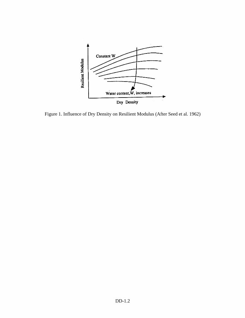
• dry density: at low moisture contents, a lower density will give a lower MR. The
relationship is reversed for high moisture contents, as shown in Figure 1 (Seed et al.
1962). Any change in volume is reflected in a change in dry density; therefore, void
ratio (e) may be used instead of dry density.
• degree of saturation: a third parameter, uniquely defined by moisture content, dry
density (or void ratio) and specific gravity of solids (Gs) is the degree of saturation
DD-1.2
Figure 1. Influence of Dry Density on Resilient Modulus (After Seed et al. 1962)
DD-1.3
(S). The relationship between the three physical state parameters is presented in
Equations 1 and 2, depending on which parameter is used as a measure of volume
changes (i.e dry density or void ratio):
⎟⎟⎠
⎞⎜⎜⎝
⎛−
⋅=
1dry
wsGwS
γγ
(1)
ewGS s ⋅=
(2)
Where:
S = degree of saturation (variable)
Gs = specific gravity (constant)
w = moisture content (variable)
γw = unit weight of water (constant)
γdry = dry unit weight (variable)
e = void ratio (variable)
Equations 1 and 2 show that knowing any two of the three parameters: w, S and γdry,
the third may be found, provided Gs is known or can be estimated well. The use of all
three parameters as predictors in a model is therefore incorrect, due to redundancy.
On the other hand, the use of only one of these parameters is sufficient only if no
volume change during wetting or drying (i.e. a constant dry density or void ratio) is
assumed. For all cases where variations in moisture content are accompanied by
volume changes, any two of the three parameters need to be used to properly predict
the change in modulus, together with known Gs.
DD-1.4
• temperature: becomes the most important factor in predicting the resilient modulus of
frozen materials while for thawed materials it has little to no significant influence.
Factors Related to the State of Stress:
• bulk stress: total volumetric component – for lab test conditions such as triaxial, this
stress is determined from:
θ σ σ σ= + +1 2 3
• octahedral shear stress: total deviatoric component – for triaxial test conditions this
stress is determined from:
( ) ( ) ( )τ σ σ σ σ σ σoct = ⋅ − + − + −13 1 2
2
1 3
2
2 3
2
• pore pressures/suction: unbound materials used in pavement design are generally in a
partly saturated state, especially if they fall above the phreatic surface (GWT). The
state of stress in unsaturated materials can be characterized by the following
parameters (Fredlund et al. (12)):
- (σ3 – ua) = net confining pressure (also called net normal stress)
- (σ1 – σ3) = deviator stress
- (ua – uw) = matric suction
Where:
σ3 = total confining pressure;
σ1 = total major principal stress;
ua = pore air pressure;
uw = pore water pressure.
DD-1.5
Matric suction greatly affects the state of stress and consequently the modulus
(Gehling et al. (10), Fredlund et al. (12), Lekarp et al. 2000 (13), Drumm et al. (14),
Edil and Motan (15)). For saturated elements of soil it is therefore desirable to use
effective stresses (total stress minus pore water pressure) in predicting the modulus.
For nearly saturated soils (S>95%) where ua – uw = 0, using total stress minus uw as
an effective stress is normally satisfactory and this effective stress can be related to
modulus. However, if the value of S is well below 95% and ua – uw is greater than
zero, it is typically necessary to use two stress state variables, σ – ua and ua – uw, to
define the stress state which is then related to modulus. An acceptable definition of
the stress state can sometimes be achieved by using total stresses, provided a
parameter related to suction (e.g. water content or degree of saturation) is used in
addition to the total stress. Also, both components of loading (i.e. volumetric and
deviatoric) should be used (Santha (6), Andrei (16)).
Factors Related to the Structure/Type of Material:
• compaction method;
• particle sizes (grain size distribution);
• particle shape (related to friction);
• nature of the bonds between particles and their sensitivity to water (moisture).
In the field, unbound materials used in pavements are typically first compacted to
moisture and density near the optimum, and then, with time, the moisture content will
reach an equilibrium condition which varies depending on drainage properties and
environmental conditions. In order to simulate this variation in the lab, it is recommended
to first compact the specimens at optimum moisture content and maximum dry density
DD-1.6
and then vary the moisture content (by soaking or drying) until the desired moisture
content is achieved. Then, the resilient modulus test should be performed. Especially in
the case of fine-grained (cohesive) soils, compacting directly at the desired moisture
content and density can result in specimens with a different structure, that do not model
the structure of the material in actual field conditions, because of path dependency for
wetting or drying.
Objective
The objective of this study was to select and then summarize existing models from the
literature that incorporate the variation of resilient modulus with moisture. Using these
published literature models, it was then desirable to select a model or models that would
analytically predict changes in modulus due to changes in moisture. This model (models)
will then be considered for implementation in the 2002 Guide for the Design of New and
Rehabilitated Pavement Structures.
Analysis and Assumptions
When plotting resilient modulus versus moisture for a given material, distinct curves are
obtained depending on the variation of density. Therefore, constant dry density,
decreasing density (swell), increasing dry density (collapse) or variable dry density (e.g.
along the compaction curve) will plot, for the same material, as four different curves.
Ideally, to avoid confusion and to obtain comparable plots, the best curve to use is the
one that simulates the volume changes expected to occur in field for that material.
However, data describing variation in dry density which is realistic for the field was
DD-1.7
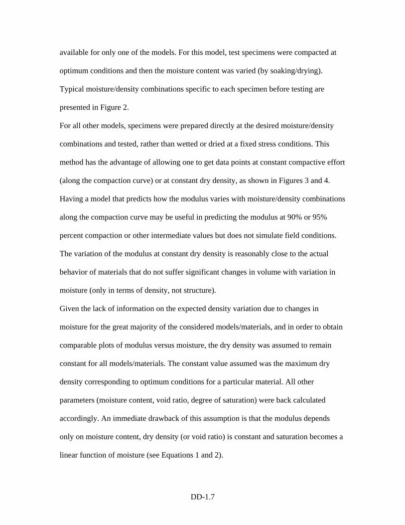
available for only one of the models. For this model, test specimens were compacted at
optimum conditions and then the moisture content was varied (by soaking/drying).
Typical moisture/density combinations specific to each specimen before testing are
presented in Figure 2.
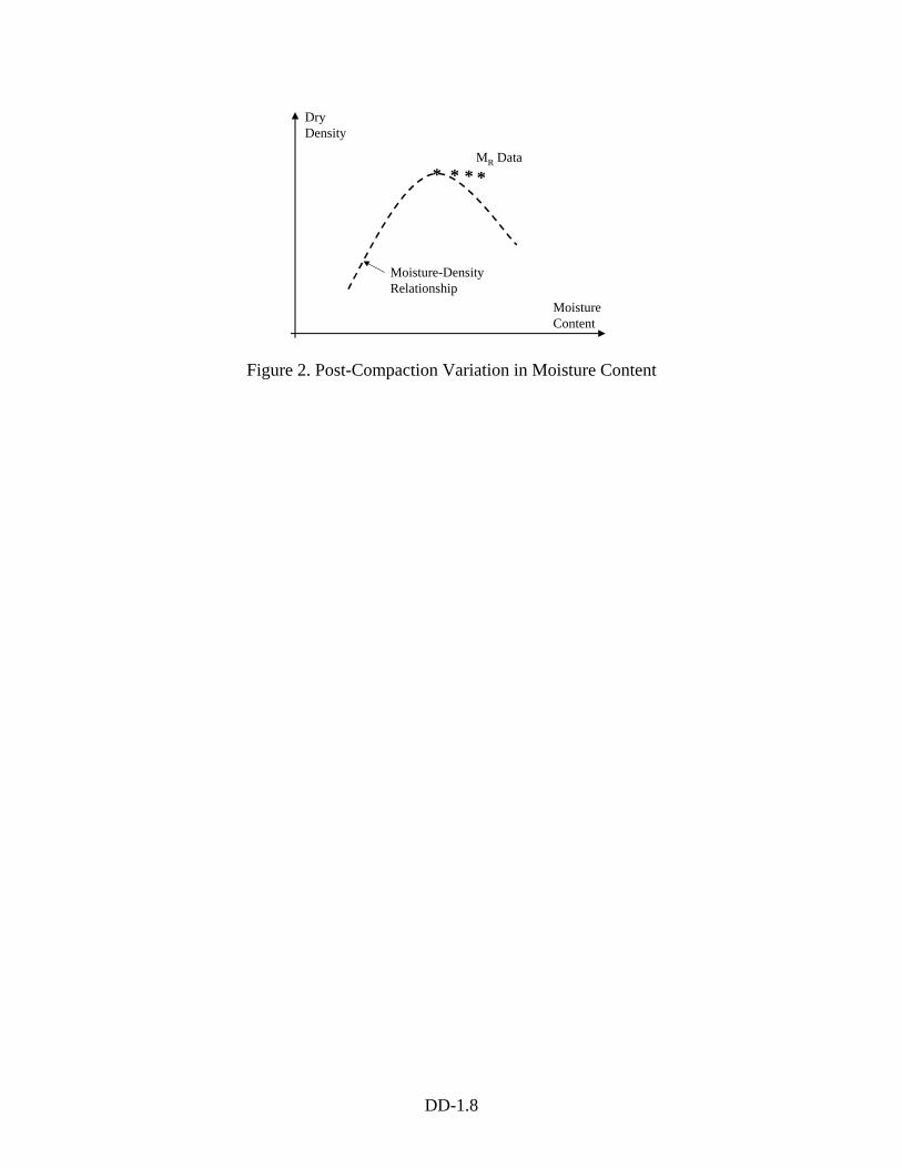
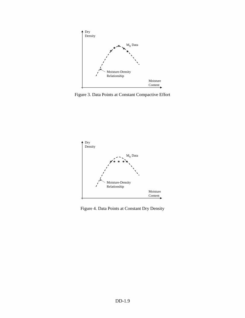
For all other models, specimens were prepared directly at the desired moisture/density
combinations and tested, rather than wetted or dried at a fixed stress conditions. This
method has the advantage of allowing one to get data points at constant compactive effort
(along the compaction curve) or at constant dry density, as shown in Figures 3 and 4.
Having a model that predicts how the modulus varies with moisture/density combinations
along the compaction curve may be useful in predicting the modulus at 90% or 95%
percent compaction or other intermediate values but does not simulate field conditions.
The variation of the modulus at constant dry density is reasonably close to the actual
behavior of materials that do not suffer significant changes in volume with variation in
moisture (only in terms of density, not structure).
Given the lack of information on the expected density variation due to changes in
moisture for the great majority of the considered models/materials, and in order to obtain
comparable plots of modulus versus moisture, the dry density was assumed to remain
constant for all models/materials. The constant value assumed was the maximum dry
density corresponding to optimum conditions for a particular material. All other
parameters (moisture content, void ratio, degree of saturation) were back calculated
accordingly. An immediate drawback of this assumption is that the modulus depends
only on moisture content, dry density (or void ratio) is constant and saturation becomes a
linear function of moisture (see Equations 1 and 2).
DD-1.8
DryDensity
MoistureContent
* * * *
Moisture-DensityRelationship
MR Data
Figure 2. Post-Compaction Variation in Moisture Content
DD-1.9
DryDensity
MoistureContent
* * **
Moisture-DensityRelationship
MR Data
*
Figure 3. Data Points at Constant Compactive Effort
DryDensity
MoistureContent
* * **
Moisture-DensityRelationship
MR Data
*
Figure 4. Data Points at Constant Dry Density
DD-1.10
Summary of Models
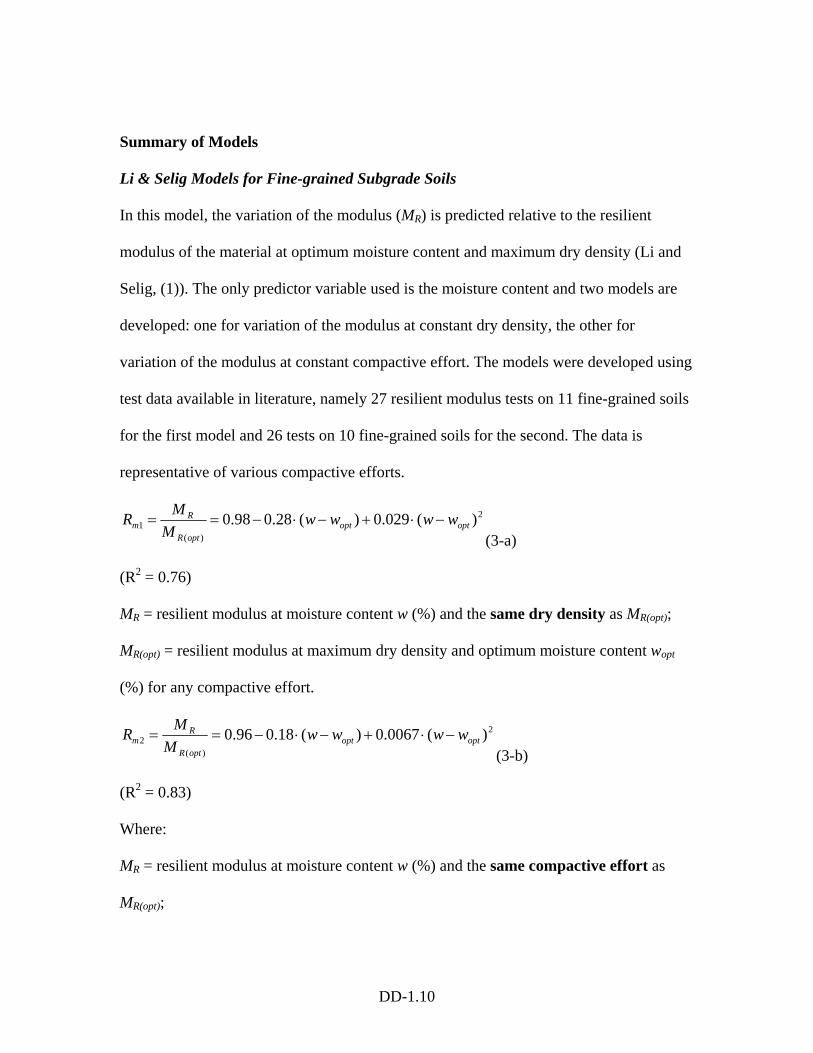
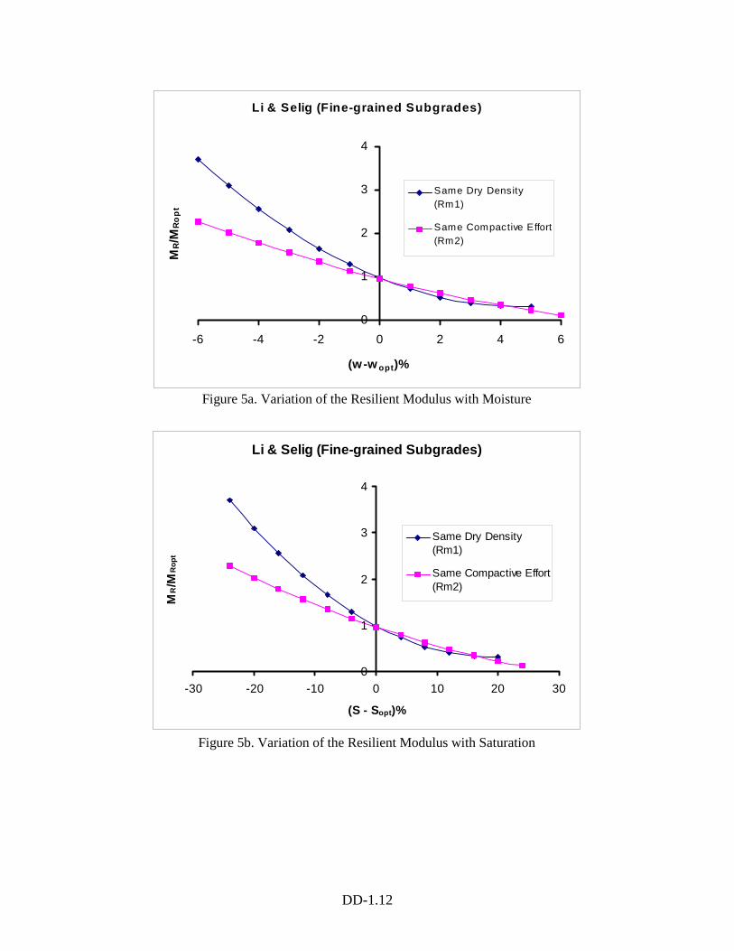
Li & Selig Models for Fine-grained Subgrade Soils
In this model, the variation of the modulus (MR) is predicted relative to the resilient
modulus of the material at optimum moisture content and maximum dry density (Li and
Selig, (1)). The only predictor variable used is the moisture content and two models are
developed: one for variation of the modulus at constant dry density, the other for
variation of the modulus at constant compactive effort. The models were developed using
test data available in literature, namely 27 resilient modulus tests on 11 fine-grained soils
for the first model and 26 tests on 10 fine-grained soils for the second. The data is
representative of various compactive efforts.
2
)(1 )(029.0)(28.098.0 optopt
optR
Rm wwww
MMR −⋅+−⋅−==
(3-a)
(R2 = 0.76)
MR = resilient modulus at moisture content w (%) and the same dry density as MR(opt);
MR(opt) = resilient modulus at maximum dry density and optimum moisture content wopt
(%) for any compactive effort.
2
)(2 )(0067.0)(18.096.0 optopt
optR
Rm wwww
MMR −⋅+−⋅−==
(3-b)
(R2 = 0.83)
Where:
MR = resilient modulus at moisture content w (%) and the same compactive effort as
MR(opt);

DD-1.11
MR(opt) = resilient modulus at maximum dry density and optimum moisture content wopt
(%) for any compactive effort.
The variation in modulus with respect to moisture content and degree of saturation as
predicted by the mentioned models is presented in Figure 5.
An attempt was made by the authors to use normalized water content (w/wopt) as a
predictor variable but the correlation was poorer.
Note that the models (3-a, 3-b) are irrational for (w-wopt) = 0, where the value of the ratio
is 0.98 and respecively 0.96 instead of 1.00. Given the nature of the data used in
calibration, it was assumed that the variation of the modulus with moisture is independent
of variation in compactive effort or state of stress.
The general trends noted by the authors are:
- the lower the water content , the higher the modulus (at constant dry density, or at
constant compactive effort);
- at lower moisture contents, the modulus tends to increase with increasing dry density,
whereas at higher moisture contents the modulus tends to decrease with increasing
dry density.
The idea of plotting normalized modulus (MR/MR(opt)) versus normalized moisture
content (w-wopt) or normalized saturation degree (S-Sopt) was adopted and used for all the
models presented in this summary.
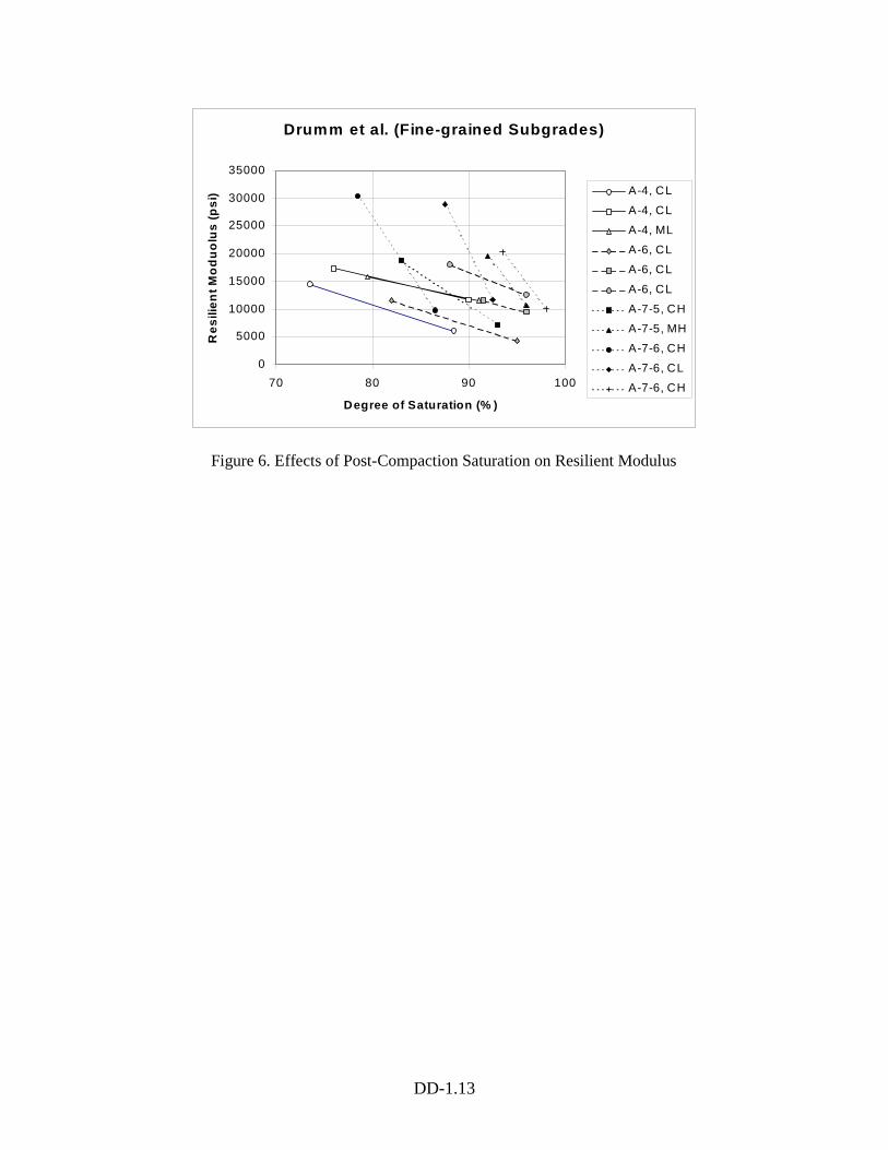
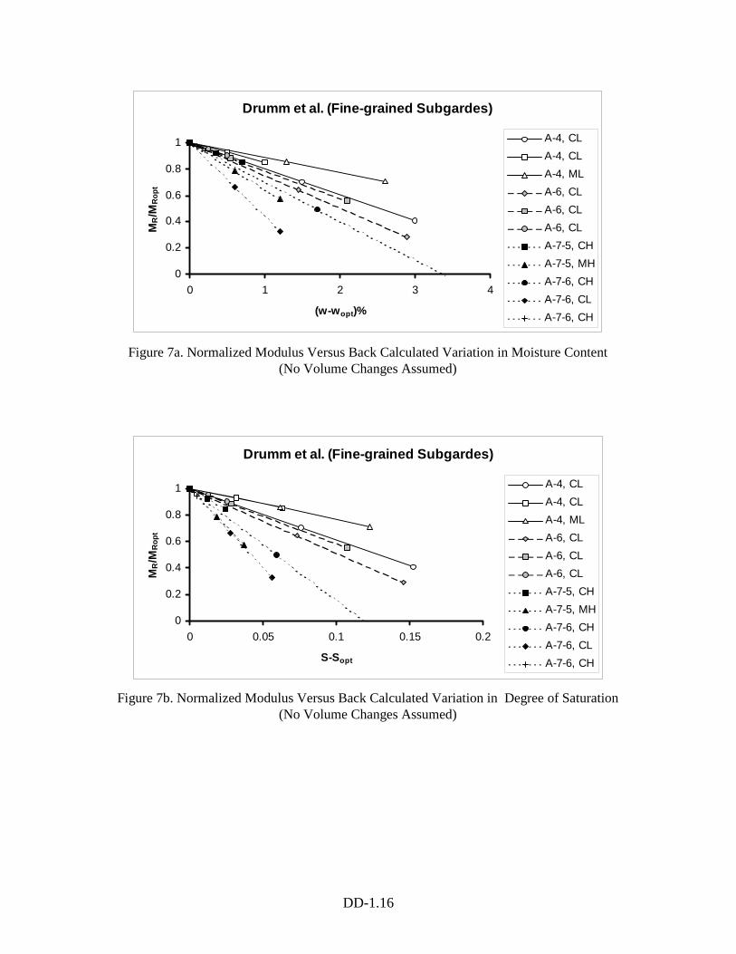
Drumm et al. Model for Fine-grained Subgrade Soils
Another model that uses MR(opt) as a reference value (Drumm et al (2)) is based on the
linear relationship observed between resilient modulus and degree of saturation, as shown
in Figure 6.
DD-1.12
Li & Selig (Fine-grained Subgrades)
0
1
2
3
4
-6 -4 -2 0 2 4 6
(w-w opt)%
MR/M
Ro
pt
Same Dry Density(Rm1)
Same Compactive Effort(Rm2)
Figure 5a. Variation of the Resilient Modulus with Moisture
Li & Selig (Fine-grained Subgrades)
0
1
2
3
4
-30 -20 -10 0 10 20 30
(S - Sopt)%
MR/M
Rop
t
Same Dry Density(Rm1)
Same Compactive Effort(Rm2)
Figure 5b. Variation of the Resilient Modulus with Saturation
DD-1.13
Drumm et al. (Fine-grained Subgrades)
0
5000
10000
15000
20000
25000
30000
35000
70 80 90 100
Degree of Saturation (% )
Res
ilien
t Mo
du
olu
s (p
si) A-4, CL
A-4, CL
A-4, ML
A-6, CL
A-6, CL
A-6, CL
A-7-5, CH
A-7-5, MH
A-7-6, CH
A-7-6, CL
A-7-6, CH
Figure 6. Effects of Post-Compaction Saturation on Resilient Modulus
DD-1.14
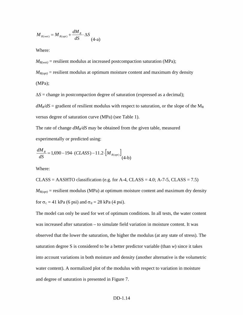
SdS
dMMM RoptRwetR ∆⋅+= )()(
(4-a)
Where:
MR(wet) = resilient modulus at increased postcompaction saturation (MPa);
MR(opt) = resilient modulus at optimum moisture content and maximum dry density
(MPa);
∆S = change in postcompaction degree of saturation (expressed as a decimal);
dMR/dS = gradient of resilient modulus with respect to saturation, or the slope of the MR
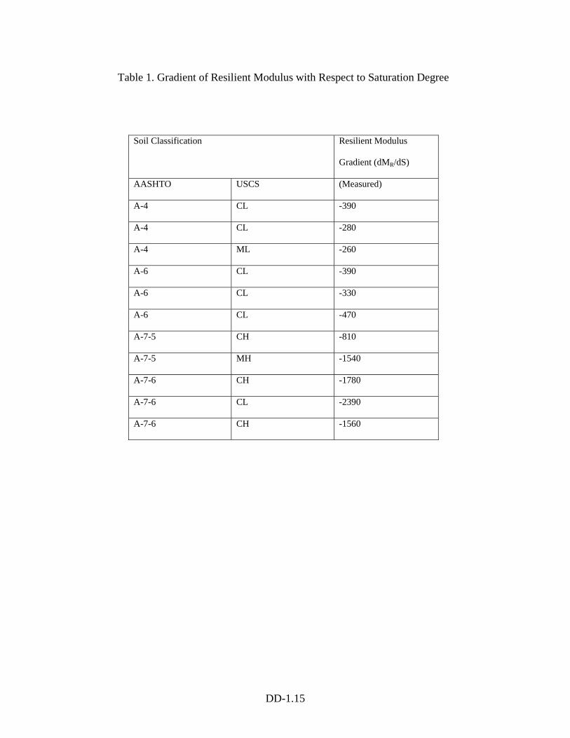
versus degree of saturation curve (MPa) (see Table 1).
The rate of change dMR/dS may be obtained from the given table, measured
experimentally or predicted using:
[ ])(2.11)(194690,1 optRR MCLASS
dSdM
⋅−⋅−=(4-b)
Where:
CLASS = AASHTO classification (e.g. for A-4, CLASS = 4.0; A-7-5, CLASS = 7.5)
MR(opt) = resilient modulus (MPa) at optimum moisture content and maximum dry density
for σc = 41 kPa (6 psi) and σd = 28 kPa (4 psi).
The model can only be used for wet of optimum conditions. In all tests, the water content
was increased after saturation – to simulate field variation in moisture content. It was
observed that the lower the saturation, the higher the modulus (at any state of stress). The
saturation degree S is considered to be a better predictor variable (than w) since it takes
into account variations in both moisture and density (another alternative is the volumetric
water content). A normalized plot of the modulus with respect to variation in moisture
and degree of saturation is presented in Figure 7.
DD-1.15
Soil Classification Resilient Modulus
Gradient (dMR/dS)
AASHTO USCS (Measured)
A-4 CL -390
A-4 CL -280
A-4 ML -260
A-6 CL -390
A-6 CL -330
A-6 CL -470
A-7-5 CH -810
A-7-5 MH -1540
A-7-6 CH -1780
A-7-6 CL -2390
A-7-6 CH -1560
Table 1. Gradient of Resilient Modulus with Respect to Saturation Degree
DD-1.16
Figure 7a. Normalized Modulus Versus Back Calculated Variation in Moisture Content (No Volume Changes Assumed)
Drumm et al. (Fine-grained Subgardes)
0
0.2
0.4
0.6
0.8
1
0 1 2 3 4
(w-wopt)%
MR/M
Rop
t
A-4, CLA-4, CLA-4, MLA-6, CLA-6, CLA-6, CLA-7-5, CHA-7-5, MHA-7-6, CHA-7-6, CLA-7-6, CH
Figure 7b. Normalized Modulus Versus Back Calculated Variation in Degree of Saturation (No Volume Changes Assumed)
Drumm et al. (Fine-grained Subgardes)
0
0.2
0.4
0.6
0.8
1
0 0.05 0.1 0.15 0.2
S-Sopt
MR/M
Rop
t
A-4, CLA-4, CLA-4, MLA-6, CLA-6, CLA-6, CLA-7-5, CHA-7-5, MHA-7-6, CHA-7-6, CLA-7-6, CH
DD-1.17
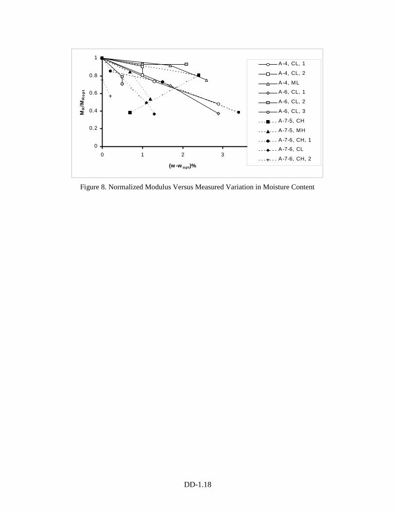
Figure 7a shows moisture content values back calculated assuming a constant dry
density; in Figure 8, the actual measured moisture contents are used, in order to show the
influence of volume changes upon moisture content. The need for an assumption
regarding the variation of density is illustrated by soils A-4, CL, 2; A-6, CL, 3 and A-7-5,
CH. For these materials, a reduction in volume makes the saturation degree increase even
if the moisture content stays constant or decreases. This supports the idea that moisture
content alone is not sufficient as a predictor variable. However, assuming a constant dry
density, moisture content will always increase with increased saturation (see Equations 1,
2).
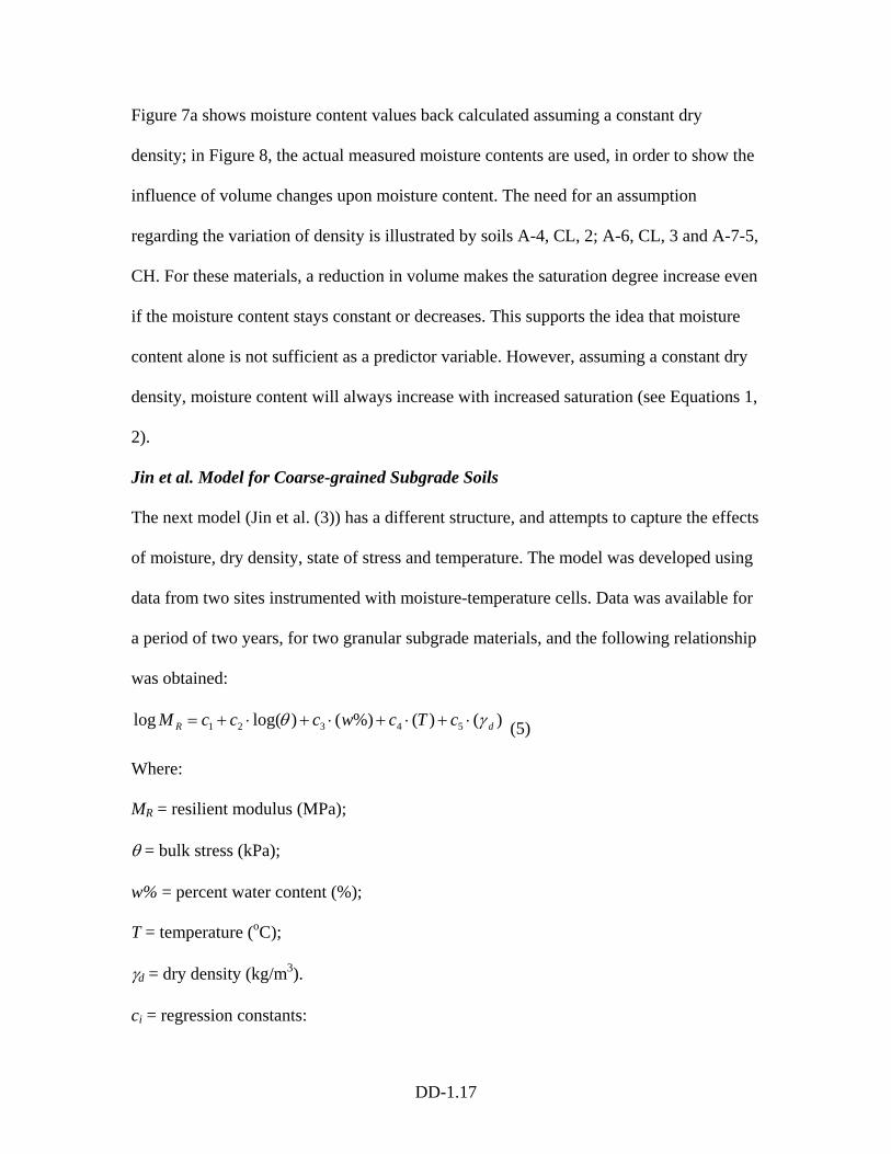
Jin et al. Model for Coarse-grained Subgrade Soils
The next model (Jin et al. (3)) has a different structure, and attempts to capture the effects
of moisture, dry density, state of stress and temperature. The model was developed using
data from two sites instrumented with moisture-temperature cells. Data was available for
a period of two years, for two granular subgrade materials, and the following relationship
was obtained:
)()(%)()log(log 54321 dR cTcwcccM γθ ⋅+⋅+⋅+⋅+= (5)
Where:
MR = resilient modulus (MPa);
θ = bulk stress (kPa);
w% = percent water content (%);
T = temperature (oC);
γd = dry density (kg/m3).
ci = regression constants:
DD-1.18
0
0.2
0.4
0.6
0.8
1
0 1 2 3 4
(w -w opt)%
MR
/MR
op
t
A-4, CL, 1
A-4, CL, 2
A-4, ML
A-6, CL, 1
A-6, CL, 2
A-6, CL, 3
A-7-5, CH
A-7-5, MH
A-7-6, CH, 1
A-7-6, CL
A-7-6, CH, 2
Figure 8. Normalized Modulus Versus Measured Variation in Moisture Content
DD-1.19
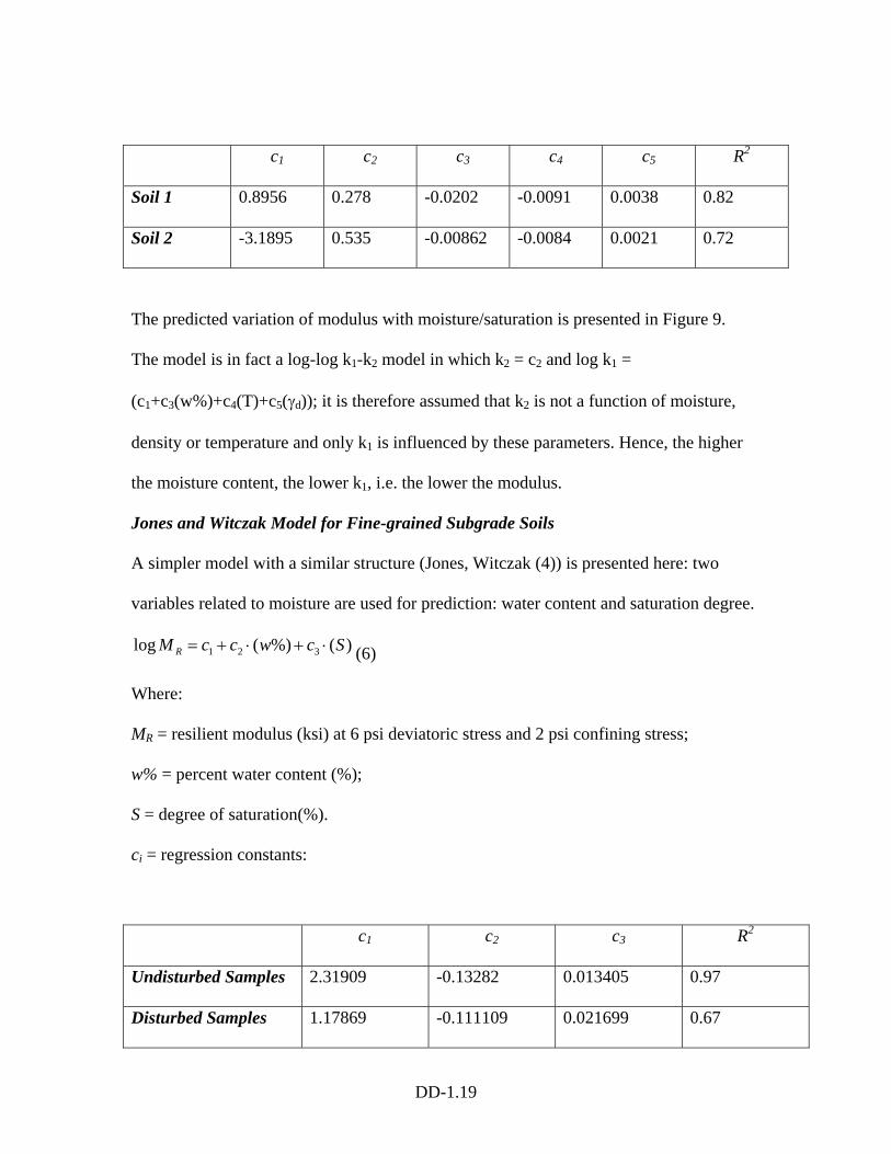
c1 c2 c3 c4 c5 R2
Soil 1 0.8956 0.278 -0.0202 -0.0091 0.0038 0.82
Soil 2 -3.1895 0.535 -0.00862 -0.0084 0.0021 0.72
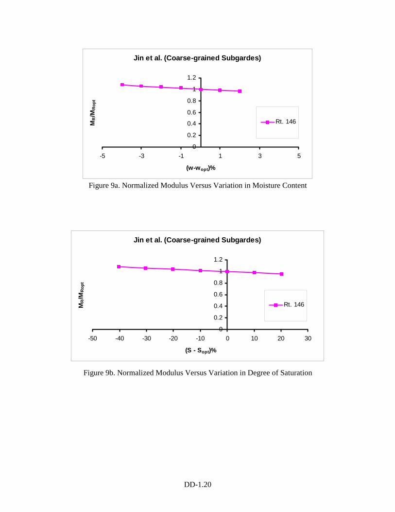
The predicted variation of modulus with moisture/saturation is presented in Figure 9.
The model is in fact a log-log k1-k2 model in which k2 = c2 and log k1 =
(c1+c3(w%)+c4(T)+c5(γd)); it is therefore assumed that k2 is not a function of moisture,
density or temperature and only k1 is influenced by these parameters. Hence, the higher
the moisture content, the lower k1, i.e. the lower the modulus.
Jones and Witczak Model for Fine-grained Subgrade Soils
A simpler model with a similar structure (Jones, Witczak (4)) is presented here: two
variables related to moisture are used for prediction: water content and saturation degree.
)(%)(log 321 ScwccM R ⋅+⋅+= (6)
Where:
MR = resilient modulus (ksi) at 6 psi deviatoric stress and 2 psi confining stress;
w% = percent water content (%);
S = degree of saturation(%).
ci = regression constants:
c1 c2 c3 R2
Undisturbed Samples 2.31909 -0.13282 0.013405 0.97
Disturbed Samples 1.17869 -0.111109 0.021699 0.67
DD-1.20
Figure 9a. Normalized Modulus Versus Variation in Moisture Content
Jin et al. (Coarse-grained Subgardes)
0
0.2
0.4
0.6
0.8
1
1.2
-5 -3 -1 1 3 5
(w-wopt)%
MR/M
Rop
t
Rt. 146
Figure 9b. Normalized Modulus Versus Variation in Degree of Saturation
Jin et al. (Coarse-grained Subgardes)
0
0.2
0.4
0.6
0.8
1
1.2
-50 -40 -30 -20 -10 0 10 20 30
(S - Sopt)%
MR/M
Rop
t
Rt. 146
DD-1.21
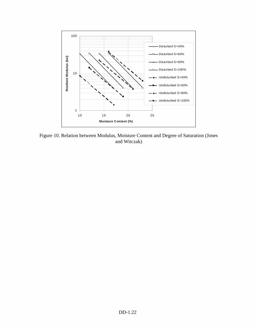
The model was developed for both undisturbed (in-situ) and lab-compacted subgrade
soils at the San Diego Test Road. They only predict for a given state of stress. Predicted
resilient modulus values along curves of constant saturation are presented for both sets of
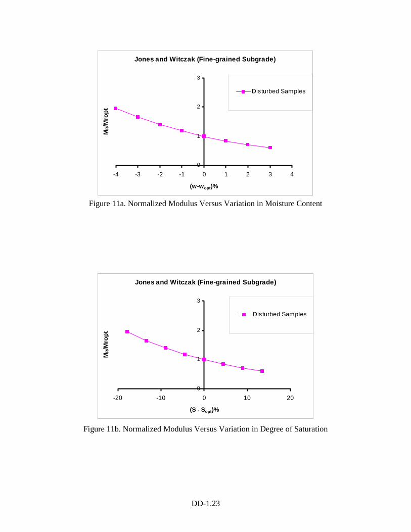
coefficients in Figure 10. Normalized plots are presented for disturbed (lab-compacted)
samples in Figure 11.
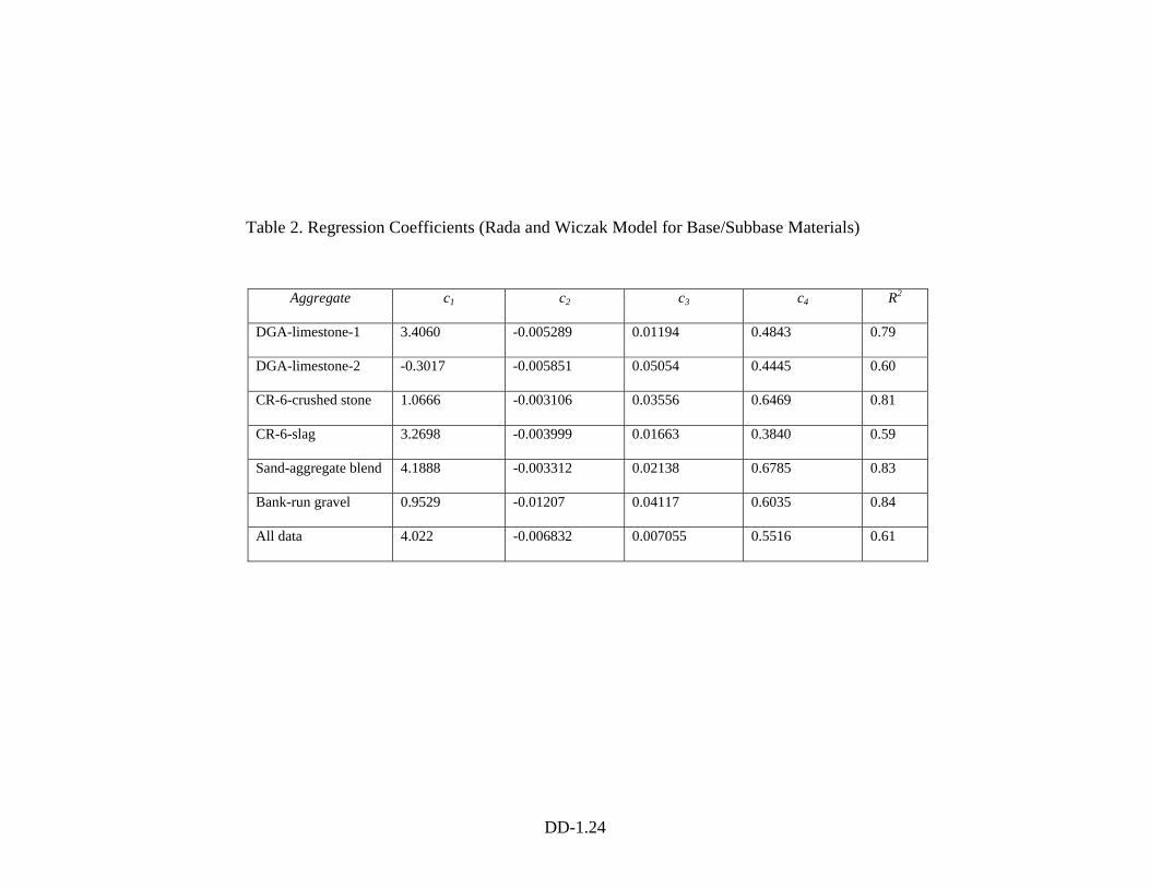
Rada and Witczak Model for Base/Subbase Materials
The next model (Rada, Witczak (5)) has a similar form but takes into account the effect
of the state of stress and percent compaction of a variety of granular material used as
subbase and base courses in the state of Maryland. The model form is:
)log()(log 4321 θ⋅+⋅+⋅+= cPCcSccM R (7)
Where:
MR = resilient modulus (psi);
θ = bulk stress (psi);
S = degree of saturation (%);
PC = percentage compaction relative to modified density (%).
ci = regression constants are given in Table 2.
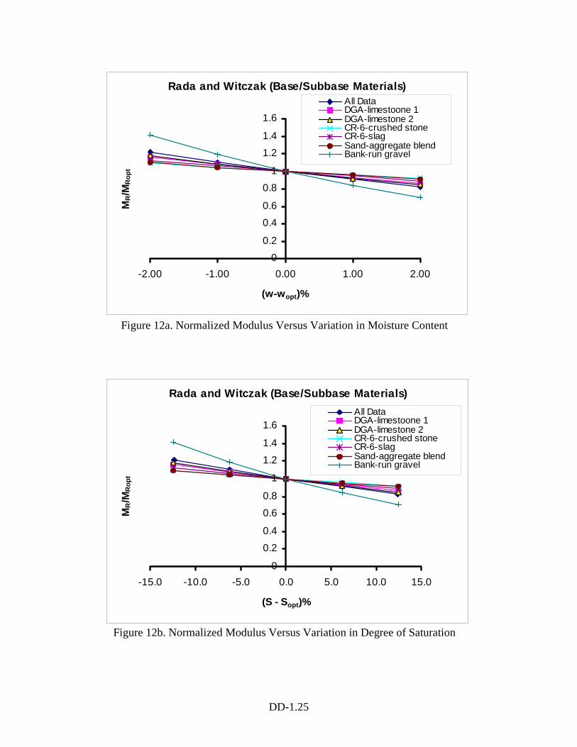
This model is also a log-log k1-k2 model in which k2 = c4 and log k1 = (c1+c2(S)+c3(PC)).
It is therefore assumed that k2 is not a function of moisture, density or temperature and
only k1 is influenced by these parameters. The variation of the modulus with
moisture/saturation is presented for all materials in Figure 12.
Santha’s Models for Coarse-grained and Fine-grained Subgrade Soils
Santha used a different approach to predict how the regression constants of a predictive
MR model would vary depending on moisture, density and other parameters (Santha (6)).
DD-1.22
1
10
100
10 15 20 25
Moisture C ontent (%)
Res
ilien
t Mod
ulus
(ksi
)
Dis turbed S=40%
Dis turbed S=60%
Dis turbed S=80%
Dis turbed S=100%
Undisturbed S=40%
Undisturbed S=60%
Undisturbed S=80%
Undisturbed S=100%
Figure 10. Relation between Modulus, Moisture Content and Degree of Saturation (Jonesand Witczak)
DD-1.23
Figure 11a. Normalized Modulus Versus Variation in Moisture Content
Jones and Witczak (Fine-grained Subgrade)
0
1
2
3
-4 -3 -2 -1 0 1 2 3 4
(w-wopt)%
MR/M
ropt
Disturbed Samples
Figure 11b. Normalized Modulus Versus Variation in Degree of Saturation
Jones and Witczak (Fine-grained Subgrade)
0
1
2
3
-20 -10 0 10 20
(S - Sopt)%
MR/M
ropt
Disturbed Samples
DD-1.24
Aggregate c1 c2 c3 c4 R2
DGA-limestone-1 3.4060 -0.005289 0.01194 0.4843 0.79
DGA-limestone-2 -0.3017 -0.005851 0.05054 0.4445 0.60
CR-6-crushed stone 1.0666 -0.003106 0.03556 0.6469 0.81
CR-6-slag 3.2698 -0.003999 0.01663 0.3840 0.59
Sand-aggregate blend 4.1888 -0.003312 0.02138 0.6785 0.83
Bank-run gravel 0.9529 -0.01207 0.04117 0.6035 0.84
All data 4.022 -0.006832 0.007055 0.5516 0.61
Table 2. Regression Coefficients (Rada and Wiczak Model for Base/Subbase Materials)
DD-1.25
Figure 12a. Normalized Modulus Versus Variation in Moisture Content
Figure 12b. Normalized Modulus Versus Variation in Degree of Saturation
Rada and Witczak (Base/Subbase Materials)
0
0.2
0.4
0.6
0.8
1
1.2
1.4
1.6
-2.00 -1.00 0.00 1.00 2.00
(w-wopt)%
MR/M
Rop
t
All DataDGA-limestoone 1DGA-limestone 2CR-6-crushed stoneCR-6-slagSand-aggregate blendBank-run gravel
Rada and Witczak (Base/Subbase Materials)
0
0.2
0.4
0.6
0.8
1
1.2
1.4
1.6
-15.0 -10.0 -5.0 0.0 5.0 10.0 15.0
(S - Sopt)%
MR/M
Rop
t
All DataDGA-limestoone 1DGA-limestone 2CR-6-crushed stoneCR-6-slagSand-aggregate blendBank-run gravel
DD-1.26
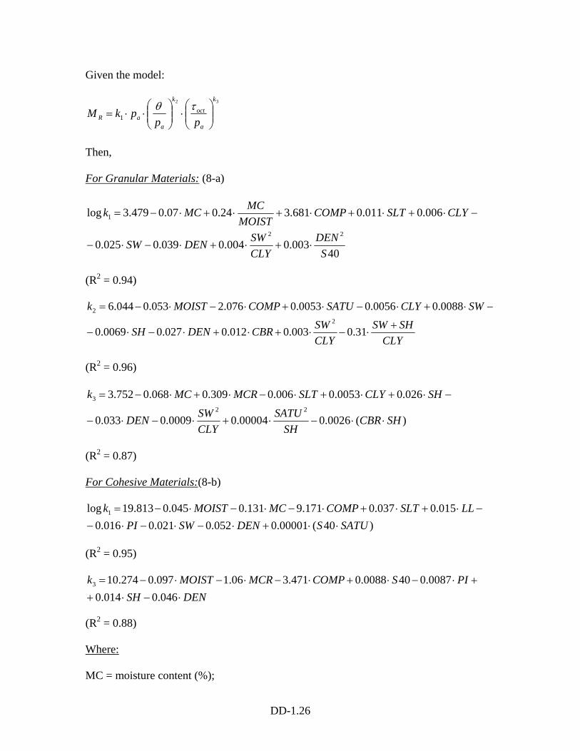
Given the model:
32
1
k
a
oct
k
aaR pp
pkM ⎟⎟⎠
⎞⎜⎜⎝
⎛⋅⎟⎟
⎠
⎞⎜⎜⎝
⎛⋅⋅=
τθ
Then,
For Granular Materials: (8-a)
40003.0004.0039.0025.0
006.0011.0681.324.007.0479.3log
22
1
SDEN
CLYSWDENSW
CLYSLTCOMPMOIST
MCMCk
⋅+⋅+⋅−⋅−
−⋅+⋅+⋅+⋅+⋅−=
(R2 = 0.94)
CLYSHSW
CLYSWCBRDENSH
SWCLYSATUCOMPMOISTk
+⋅−⋅+⋅+⋅−⋅−
−⋅+⋅−⋅+⋅−⋅−=
31.0003.0012.0027.00069.0
0088.00056.00053.0076.2053.0044.62
2
(R2 = 0.96)
)(0026.000004.00009.0033.0
026.00053.0006.0309.0068.0752.322
3
SHCBRSH
SATUCLYSWDEN
SHCLYSLTMCRMCk
⋅⋅−⋅+⋅−⋅−
−⋅+⋅+⋅−⋅+⋅−=
(R2 = 0.87)
For Cohesive Materials:(8-b)
)40(00001.0052.0021.0016.0015.0037.0171.9131.0045.0813.19log 1
SATUSDENSWPILLSLTCOMPMCMOISTk
⋅⋅+⋅−⋅−⋅−−⋅+⋅+⋅−⋅−⋅−=
(R2 = 0.95)
DENSHPISCOMPMCRMOISTk
⋅−⋅++⋅−⋅+⋅−⋅−⋅−=
046.0014.00087.0400088.0471.306.1097.0274.103
(R2 = 0.88)
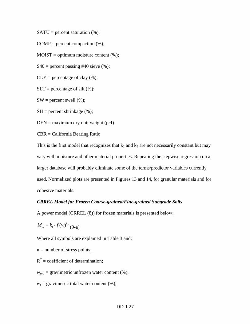
Where:
MC = moisture content (%);
DD-1.27
SATU = percent saturation (%);
COMP = percent compaction (%);
MOIST = optimum moisture content (%);
S40 = percent passing #40 sieve (%);
CLY = percentage of clay (%);
SLT = percentage of silt (%);
SW = percent swell (%);
SH = percent shrinkage (%);
DEN = maximum dry unit weight (pcf)
CBR = California Bearing Ratio
This is the first model that recognizes that k2 and k3 are not necessarily constant but may
vary with moisture and other material properties. Repeating the stepwise regression on a
larger database will probably eliminate some of the terms/predictor variables currently
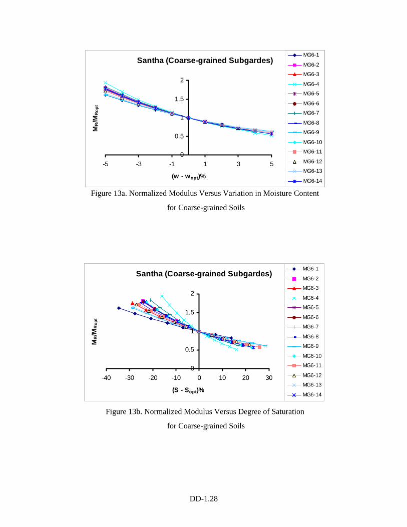
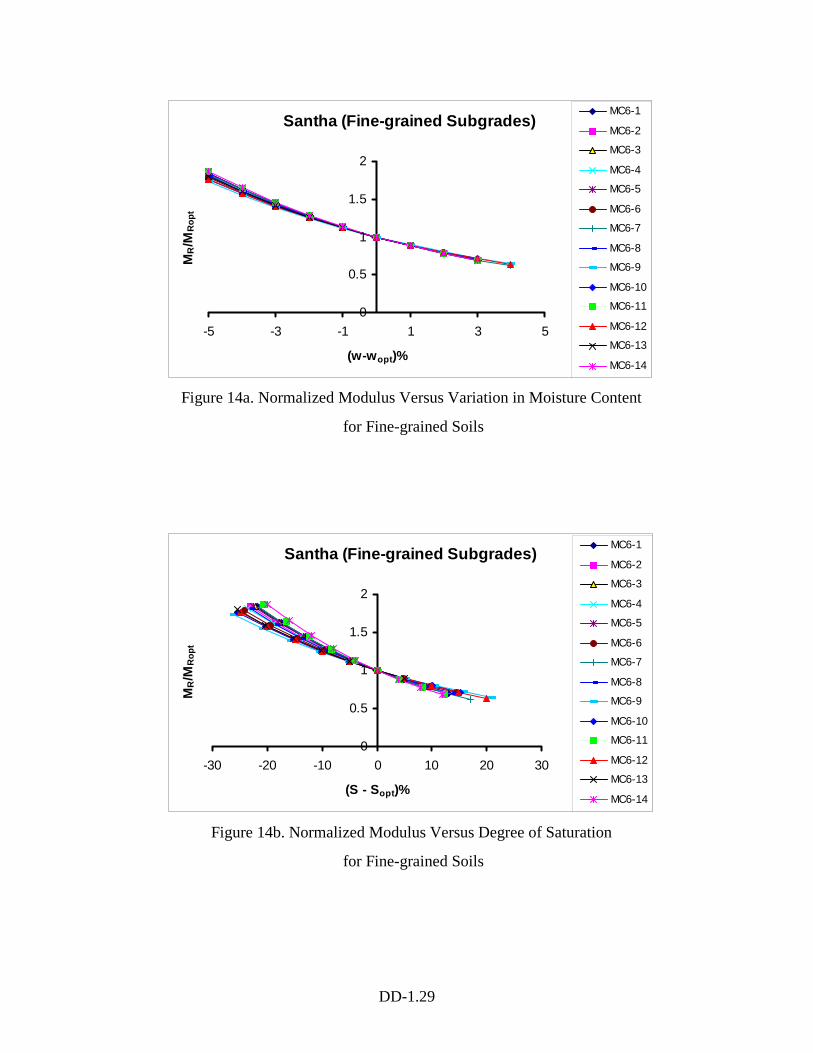
used. Normalized plots are presented in Figures 13 and 14, for granular materials and for
cohesive materials.
CRREL Model for Frozen Coarse-grained/Fine-grained Subgrade Soils
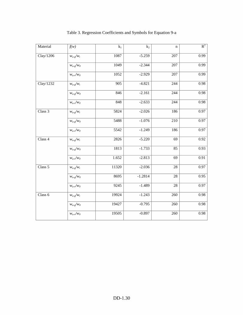
A power model (CRREL (8)) for frozen materials is presented below:
2)(1k
R wfkM ⋅= (9-a)
Where all symbols are explained in Table 3 and:
n = number of stress points;
R2 = coefficient of determination;
wu-g = gravimetric unfrozen water content (%);
wt = gravimetric total water content (%);
DD-1.28
Figure 13a. Normalized Modulus Versus Variation in Moisture Content
for Coarse-grained Soils
Figure 13b. Normalized Modulus Versus Degree of Saturation
for Coarse-grained Soils
Santha (Coarse-grained Subgardes)
0
0.5
1
1.5
2
-5 -3 -1 1 3 5
(w - wopt)%
MR/M
Rop
t
MG6-1
MG6-2
MG6-3
MG6-4
MG6-5
MG6-6
MG6-7
MG6-8
MG6-9
MG6-10
MG6-11
MG6-12
MG6-13
MG6-14
Santha (Coarse-grained Subgardes)
0
0.5
1
1.5
2
-40 -30 -20 -10 0 10 20 30
(S - Sopt)%
MR/M
Rop
t
MG6-1
MG6-2
MG6-3
MG6-4
MG6-5
MG6-6
MG6-7
MG6-8
MG6-9
MG6-10
MG6-11
MG6-12
MG6-13
MG6-14
DD-1.29
Figure 14a. Normalized Modulus Versus Variation in Moisture Content
for Fine-grained Soils
Figure 14b. Normalized Modulus Versus Degree of Saturation
for Fine-grained Soils
Santha (Fine-grained Subgrades)
0
0.5
1
1.5
2
-5 -3 -1 1 3 5
(w-wopt)%
MR/M
Rop
t
MC6-1
MC6-2
MC6-3
MC6-4
MC6-5
MC6-6
MC6-7
MC6-8
MC6-9
MC6-10
MC6-11
MC6-12
MC6-13
MC6-14
Santha (Fine-grained Subgrades)
0
0.5
1
1.5
2
-30 -20 -10 0 10 20 30
(S - Sopt)%
MR/M
Rop
t
MC6-1
MC6-2
MC6-3
MC6-4
MC6-5
MC6-6
MC6-7
MC6-8
MC6-9
MC6-10
MC6-11
MC6-12
MC6-13
MC6-14
DD-1.30
Material f(w) k1 k2 n R2
wu-g/wt 1087 -5.259 207 0.99
wu-g/w0 1049 -2.344 207 0.99
Clay/1206
wu-v/w0 1052 -2.929 207 0.99
wu-g/wt 905 -4.821 244 0.98
wu-g/w0 846 -2.161 244 0.98
Clay/1232
wu-v/w0 848 -2.633 244 0.98
wu-g/wt 5824 -2.026 186 0.97
wu-g/w0 5488 -1.076 210 0.97
Class 3
wu-v/w0 5542 -1.249 186 0.97
wu-g/wt 2826 -5.220 69 0.92
wu-g/w0 1813 -1.733 85 0.93
Class 4
wu-v/w0 1.652 -2.813 69 0.91
wu-g/wt 11320 -2.036 28 0.97
wu-g/w0 8695 -1.2814 28 0.95
Class 5
wu-v/w0 9245 -1.489 28 0.97
wu-g/wt 19924 -1.243 260 0.98
wu-g/w0 19427 -0.795 260 0.98
Class 6
wu-v/w0 19505 -0.897 260 0.98
Table 3. Regression Coefficients and Symbols for Equation 9-a
DD-1.31
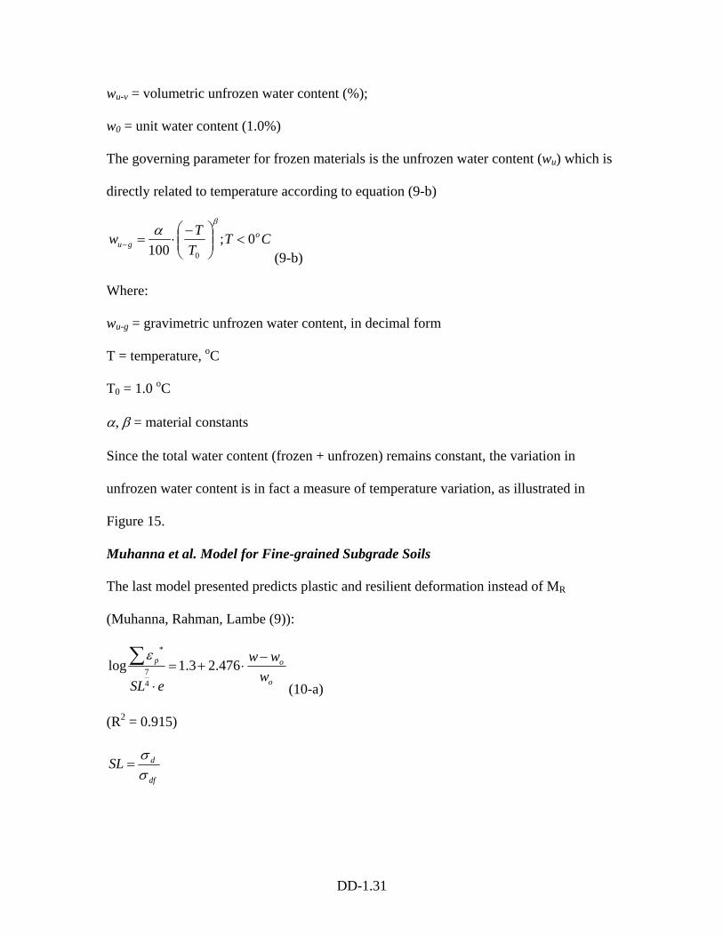
wu-v = volumetric unfrozen water content (%);
w0 = unit water content (1.0%)
The governing parameter for frozen materials is the unfrozen water content (wu) which is
directly related to temperature according to equation (9-b)
CTTTw o
gu 0;100 0
<⎟⎟⎠
⎞⎜⎜⎝
⎛ −⋅=−
βα
(9-b)
Where:
wu-g = gravimetric unfrozen water content, in decimal form
T = temperature, oC
T0 = 1.0 oC
α, β = material constants
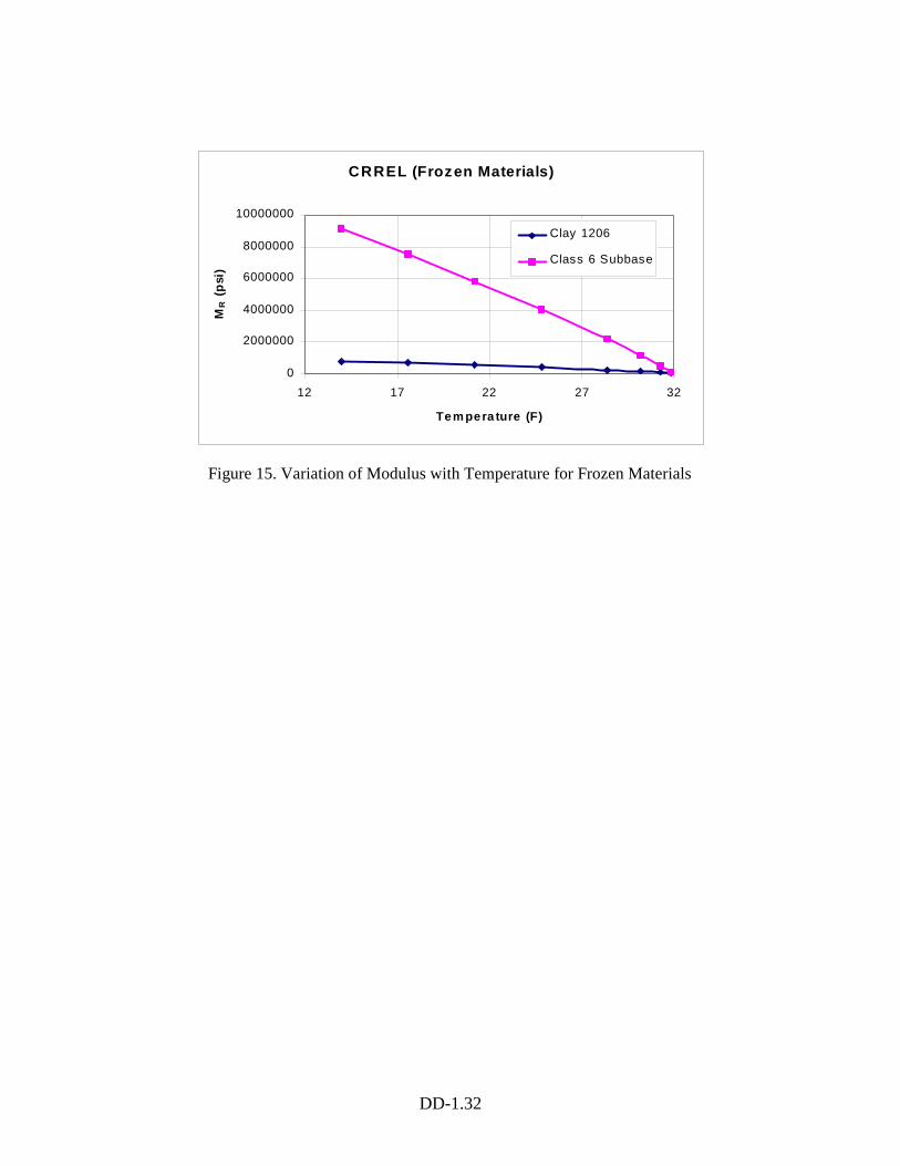
Since the total water content (frozen + unfrozen) remains constant, the variation in
unfrozen water content is in fact a measure of temperature variation, as illustrated in
Figure 15.
Muhanna et al. Model for Fine-grained Subgrade Soils
The last model presented predicts plastic and resilient deformation instead of MR
(Muhanna, Rahman, Lambe (9)):
o
op
www
eSL
−⋅+=
⋅
∑ 476.23.1log47
*ε
(10-a)
(R2 = 0.915)
df
dSLσσ
=
DD-1.32
CRREL (Frozen Materials)
0
2000000
4000000
6000000
8000000
10000000
12 17 22 27 32
Tem pera ture (F)
MR
(psi
)Clay 1206
Class 6 Subbase
Figure 15. Variation of Modulus with Temperature for Frozen Materials
DD-1.33
∑⋅+=
⎟⎟⎠
⎞⎜⎜⎝
⎛ −−
*4
*
27.00132.0
1p
o
o
r
www
εε
(10-b)
(R2 = 0.94)
Where:
Σεp* = total plastic deformation at “apparent shakedown” (%);
Apparent Shakedown State = when, after a large number of repetitions, the plastic strain
is not significant (as opposed to Ratcheting State where the sample fails due to too large
accumulated plastic strain).
SL = stress level;
σd = deviatoric stress (kPa);
σdf = deviatoric stress at failure or at 5.0 % axial strain (kPa);
e = void ratio (decimal);
w = molding water content (%);
wo = optimum moisture content (%);
εr* = resilient strain at “apparent shakedown” (%).
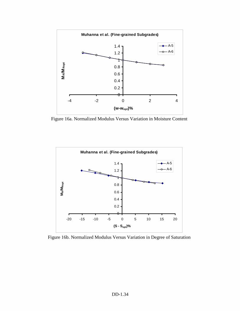
Instead of predicting the resilient modulus, the model predicts the resilient and the total
accumulated plastic deformation. Only moisture content and stress level are used as
predictor variables. The variation of the modulus with moisture/saturation is presented in
Figure 16.
Summary
The variation of the modulus with moisture and density is captured by most of the
models. Degree of saturation (S), gravimetric or volumetric moisture content (w) and
DD-1.34
Figure 16a. Normalized Modulus Versus Variation in Moisture Content
Muhanna et al. (Fine-grained Subgrades)
00.2
0.40.6
0.81
1.21.4
-4 -2 0 2 4
(w-wopt)%
MR/M
Rop
t
A-5
A-6
Figure 16b. Normalized Modulus Versus Variation in Degree of Saturation
Muhanna et al. (Fine-grained Subgrades)
0
0.2
0.4
0.6
0.8
1
1.2
1.4
-20 -15 -10 -5 0 5 10 15 20
(S - Sopt)%
MR/M
Rop
t
A-5
A-6
DD-1.35
suction (u) are used to describe the effects of moisture on resilient modulus. The state of
stress is described by using stress invariants (θ, τoct) or stress levels (σd/σdfailure). The
influence of the other parameters specific to each material is reflected by the values of the
regression constants ci or ki. For Santha’s Models, the values of the regression constants
are predicted using gradation, Atterberg limits, specific gravity and other soil properties.
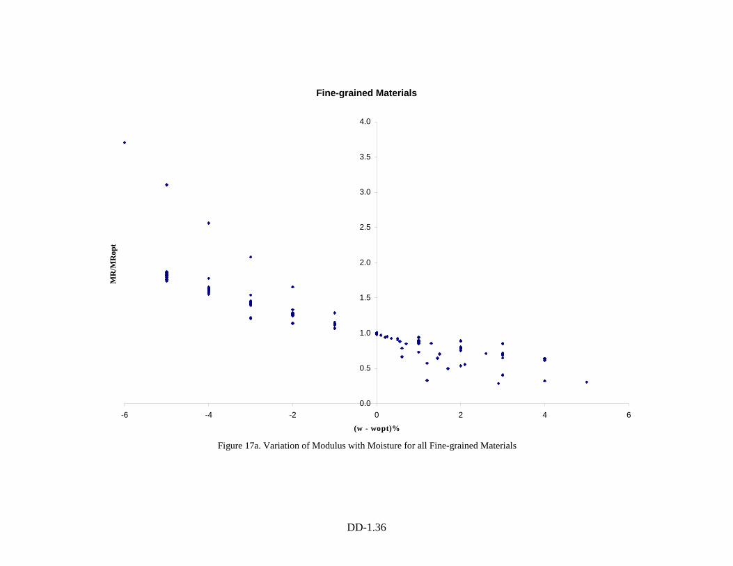
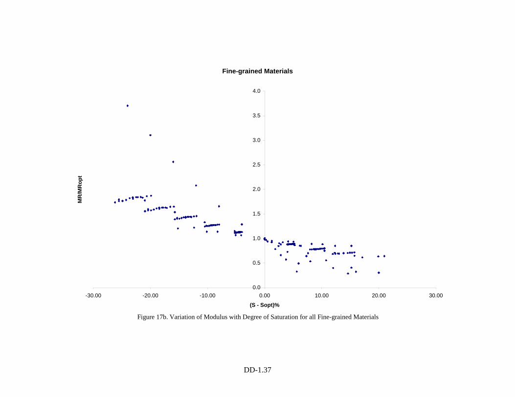
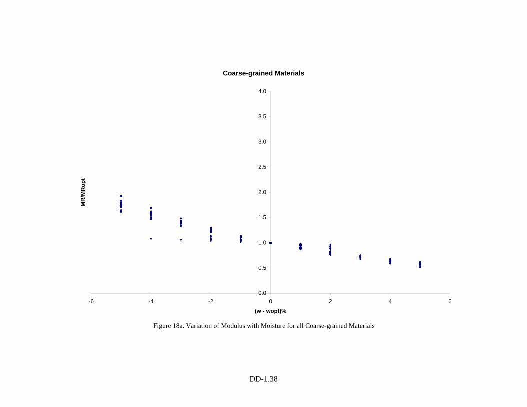
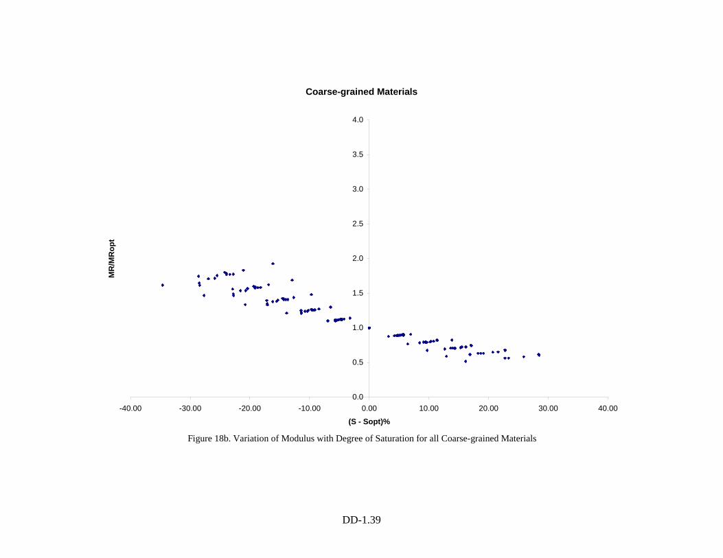
A general trend for fine-grained materials is observed in Figure 17. A similar plot is
developed for all course-grained materials (Figure 18).
Proposed Model
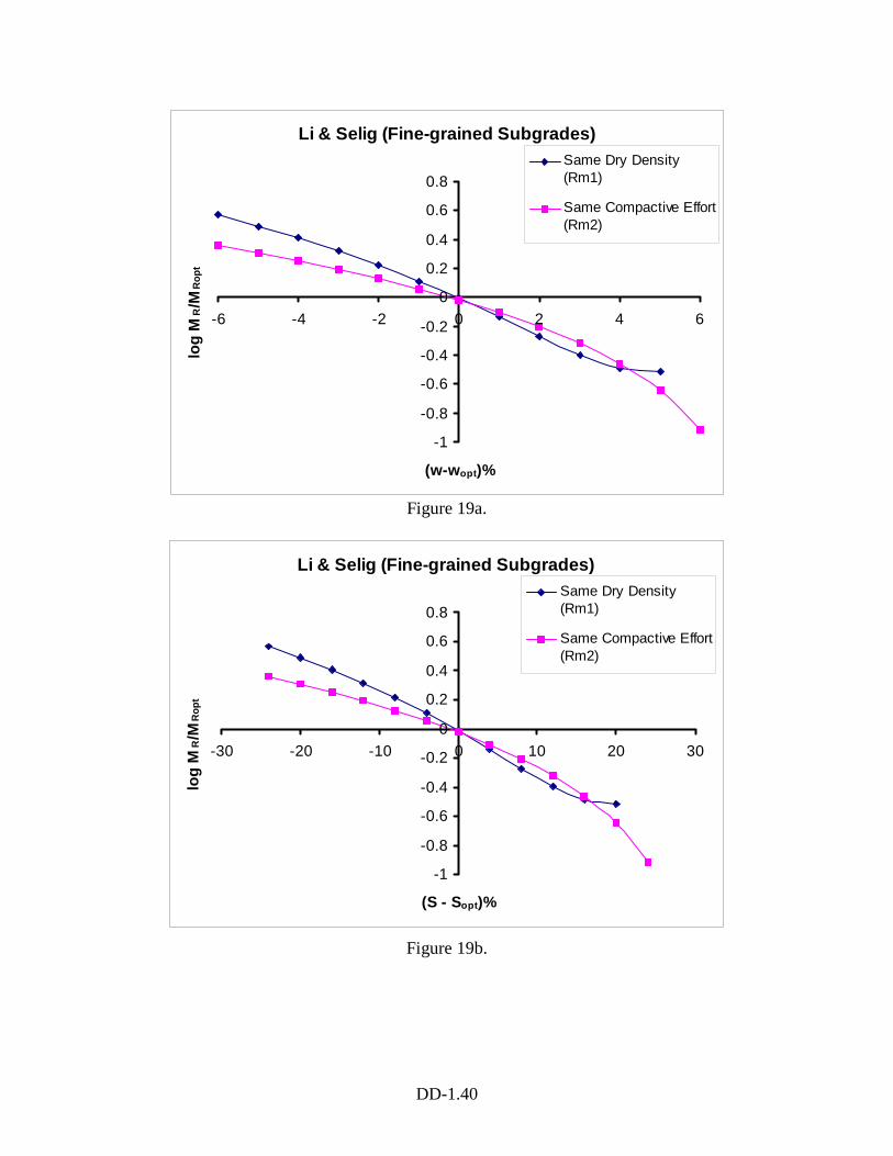
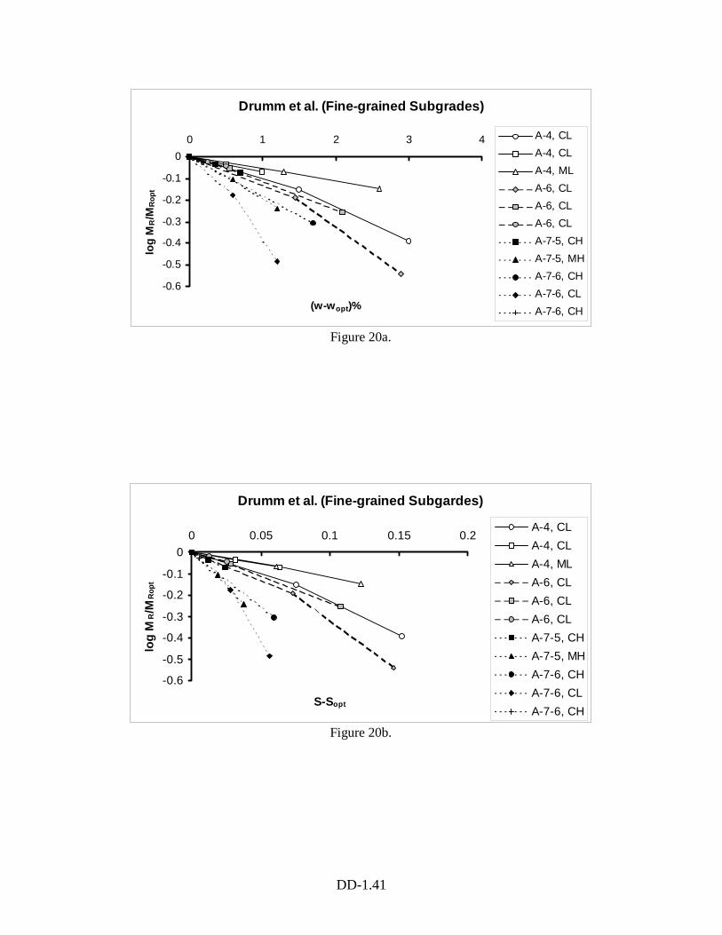
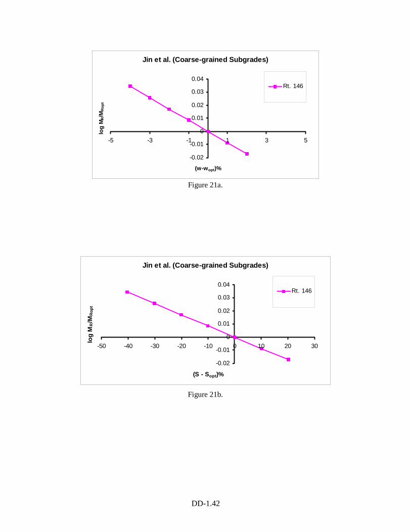
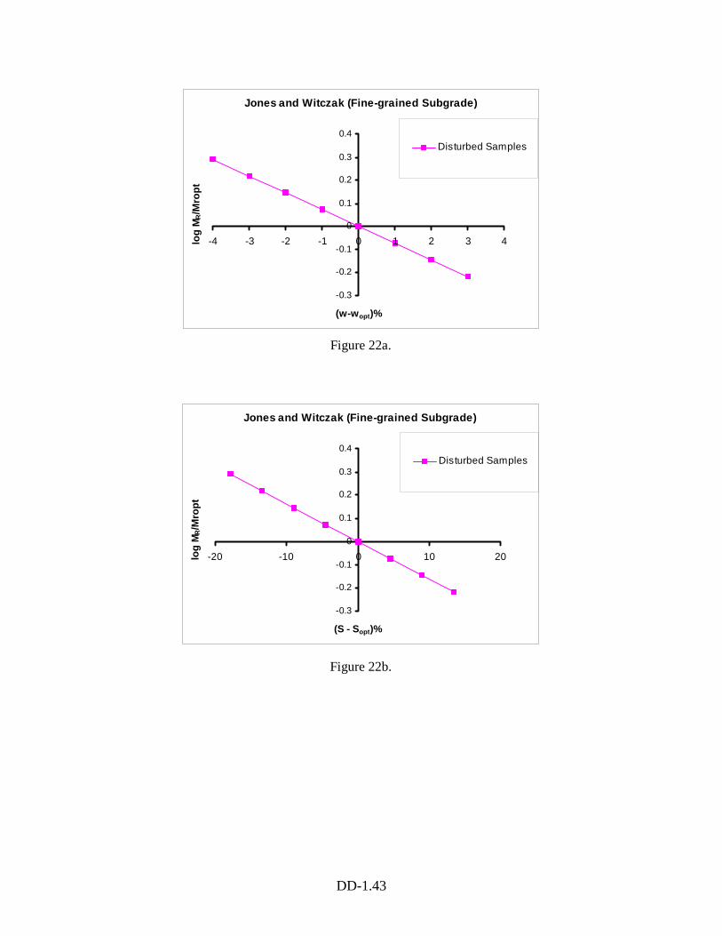
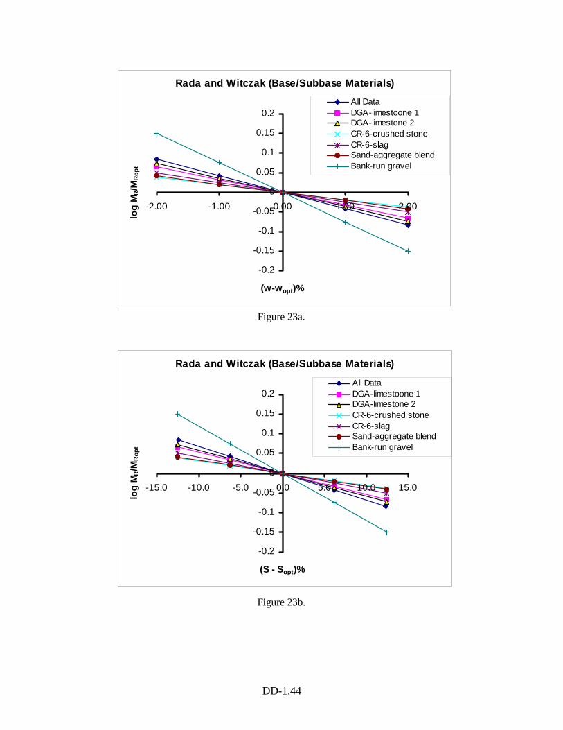
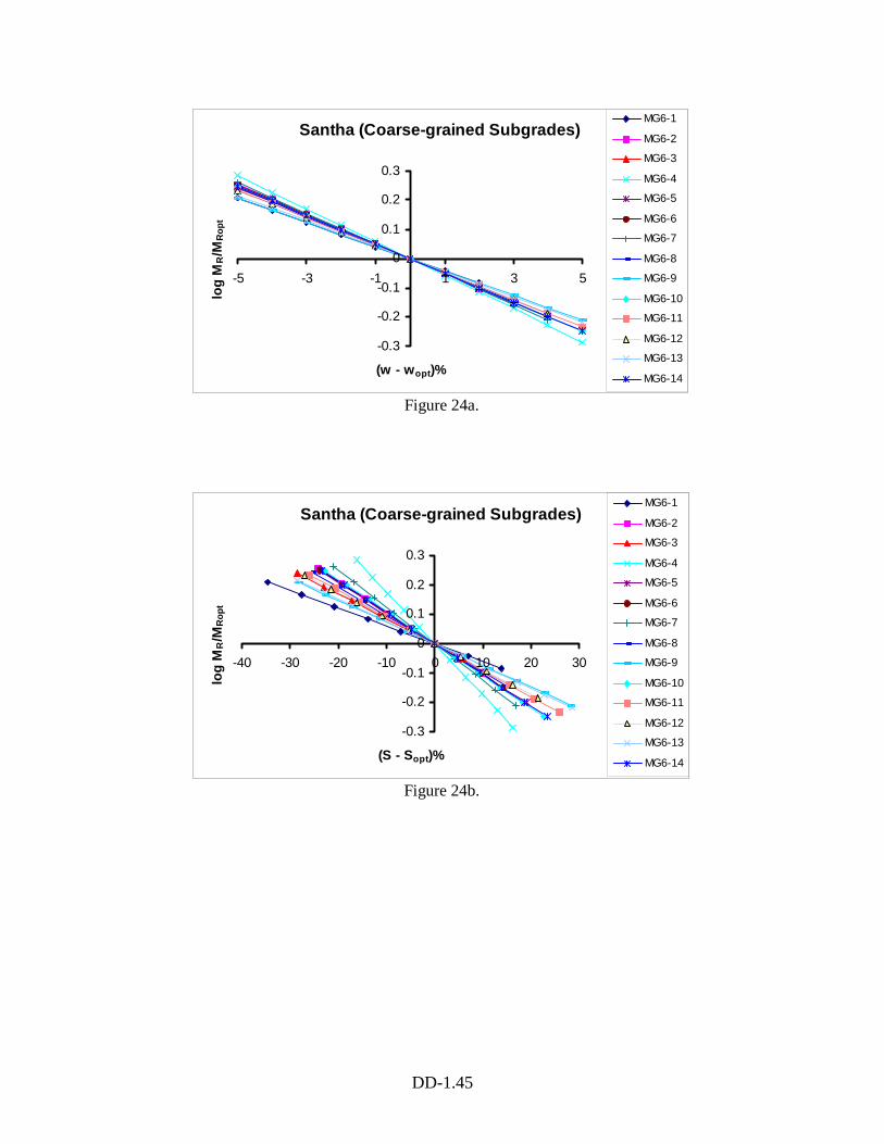
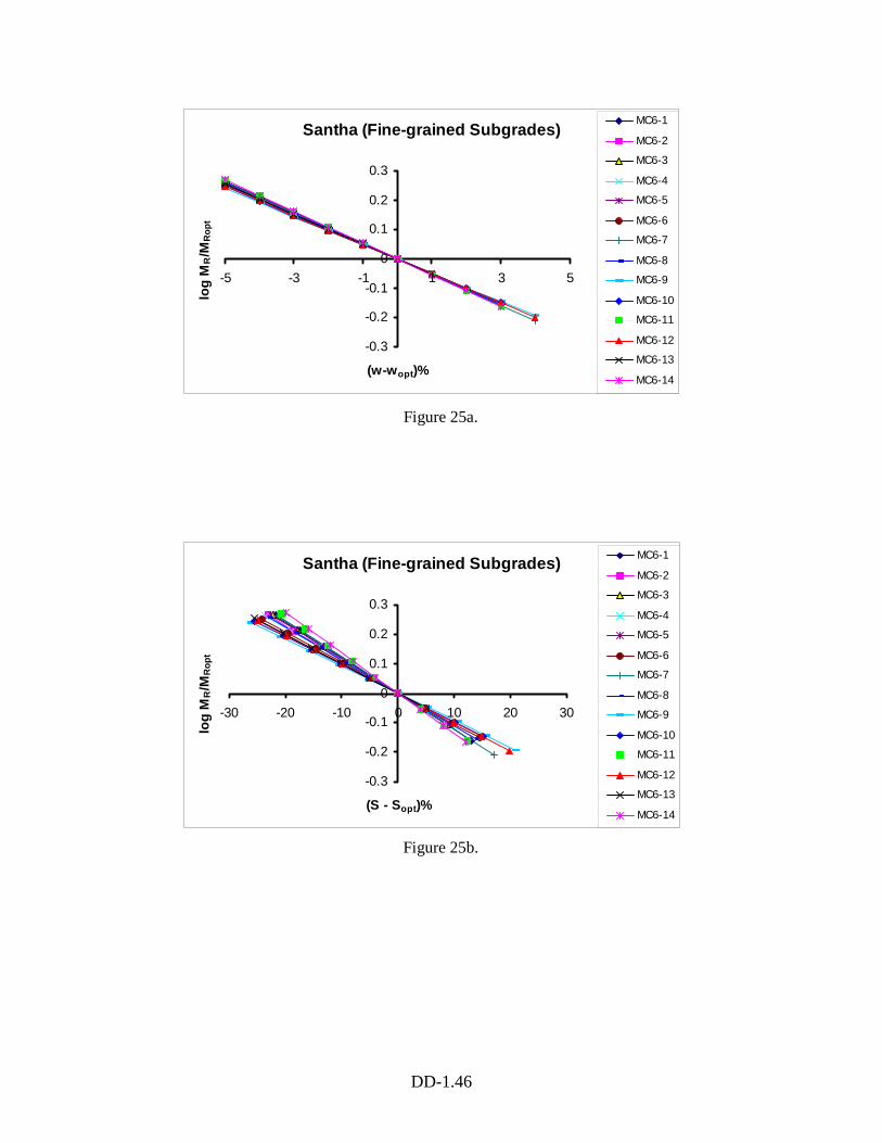
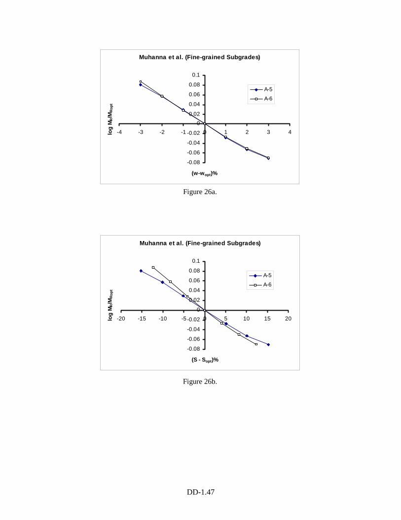
An alternative way to look at the data is to plot the modulus ratio on a log scale. This
would make, for example, a ratio of 3 to plot as far from 1 (MR = MRopt) as a ratio of 1/3,
which is more rational since, in both cases, the initial modulus is three times larger than
the final modulus (assume increasing moisture content). Individual plots of
log(MR/MRopt) versus moisture/saturation are presented in Figures 19 through 26 for all
considered models. The plots show that using the log scale for the modulus ratio, all
models approach a linear relationship, of the form:
( )optwRopt
R wwkMM
−⋅=log(11-1)
Where:
MR = resilient modulus at moisture content w (%);
MR(opt) = resilient modulus at maximum dry density and optimum moisture content wopt
(%);
DD-1.36
Figure 17a. Variation of Modulus with Moisture for all Fine-grained Materials
Fine-grained Materials
0.0
0.5
1.0
1.5
2.0
2.5
3.0
3.5
4.0
-6 -4 -2 0 2 4 6
(w - wopt)%
MR
/MR
opt
DD-1.37
Figure 17b. Variation of Modulus with Degree of Saturation for all Fine-grained Materials
Fine-grained Materials
0.0
0.5
1.0
1.5
2.0
2.5
3.0
3.5
4.0
-30.00 -20.00 -10.00 0.00 10.00 20.00 30.00
(S - Sopt)%
MR
/MR
opt
DD-1.38
Figure 18a. Variation of Modulus with Moisture for all Coarse-grained Materials
Coarse-grained Materials
0.0
0.5
1.0
1.5
2.0
2.5
3.0
3.5
4.0
-6 -4 -2 0 2 4 6
(w - wopt)%
MR
/MR
opt
DD-1.39
Figure 18b. Variation of Modulus with Degree of Saturation for all Coarse-grained Materials
Coarse-grained Materials
0.0
0.5
1.0
1.5
2.0
2.5
3.0
3.5
4.0
-40.00 -30.00 -20.00 -10.00 0.00 10.00 20.00 30.00 40.00
(S - Sopt)%
MR
/MR
opt
DD-1.40
Figure 19a.
Li & Selig (Fine-grained Subgrades)
-1
-0.8
-0.6
-0.4
-0.2
0
0.2
0.4
0.6
0.8
-6 -4 -2 0 2 4 6
(w-wopt)%
log
MR/M
Rop
t
Same Dry Density(Rm1)
Same Compactive Effort(Rm2)
Figure 19b.
Li & Selig (Fine-grained Subgrades)
-1
-0.8
-0.6
-0.4
-0.2
0
0.2
0.4
0.6
0.8
-30 -20 -10 0 10 20 30
(S - Sopt)%
log
MR/M
Rop
t
Same Dry Density(Rm1)
Same Compactive Effort(Rm2)
DD-1.41
Figure 20a.
Figure 20b.
Drumm et al. (Fine-grained Subgrades)
-0.6
-0.5
-0.4
-0.3
-0.2
-0.1
00 1 2 3 4
(w-wopt)%
log
MR/M
Rop
t
A-4, CLA-4, CLA-4, MLA-6, CLA-6, CLA-6, CLA-7-5, CHA-7-5, MHA-7-6, CHA-7-6, CLA-7-6, CH
Drumm et al. (Fine-grained Subgardes)
-0.6
-0.5
-0.4
-0.3
-0.2
-0.1
00 0.05 0.1 0.15 0.2
S-Sopt
log
MR/M
Rop
t
A-4, CLA-4, CLA-4, MLA-6, CLA-6, CLA-6, CLA-7-5, CHA-7-5, MHA-7-6, CHA-7-6, CLA-7-6, CH
DD-1.42
Figure 21a.
Figure 21b.
Jin et al. (Coarse-grained Subgrades)
-0.02
-0.01
0
0.01
0.02
0.03
0.04
-5 -3 -1 1 3 5
(w-wopt)%
log
MR/M
Rop
t
Rt. 146
Jin et al. (Coarse-grained Subgrades)
-0.02
-0.01
0
0.01
0.02
0.03
0.04
-50 -40 -30 -20 -10 0 10 20 30
(S - Sopt)%
log
MR/M
Rop
t
Rt. 146
DD-1.43
Figure 22b.
Figure 22a.
Jones and Witczak (Fine-grained Subgrade)
-0.3
-0.2
-0.1
0
0.1
0.2
0.3
0.4
-4 -3 -2 -1 0 1 2 3 4
(w-wopt)%
log
MR/M
ropt
Disturbed Samples
Jones and Witczak (Fine-grained Subgrade)
-0.3
-0.2
-0.1
0
0.1
0.2
0.3
0.4
-20 -10 0 10 20
(S - Sopt)%
log
MR/M
ropt
Disturbed Samples
DD-1.44
Figure 23a.
Figure 23b.
Rada and Witczak (Base/Subbase Materials)
-0.2
-0.15
-0.1
-0.05
0
0.05
0.1
0.15
0.2
-2.00 -1.00 0.00 1.00 2.00
(w-wopt)%
log
MR/M
Rop
t
All DataDGA-limestoone 1DGA-limestone 2CR-6-crushed stoneCR-6-slagSand-aggregate blendBank-run gravel
Rada and Witczak (Base/Subbase Materials)
-0.2
-0.15
-0.1
-0.05
0
0.05
0.1
0.15
0.2
-15.0 -10.0 -5.0 0.0 5.0 10.0 15.0
(S - Sopt)%
log
MR/M
Rop
t
All DataDGA-limestoone 1DGA-limestone 2CR-6-crushed stoneCR-6-slagSand-aggregate blendBank-run gravel
DD-1.45
Figure 24b.
Figure 24a.
Santha (Coarse-grained Subgrades)
-0.3
-0.2
-0.1
0
0.1
0.2
0.3
-5 -3 -1 1 3 5
(w - wopt)%
log
MR/M
Rop
t
MG6-1
MG6-2
MG6-3
MG6-4
MG6-5
MG6-6
MG6-7
MG6-8
MG6-9
MG6-10
MG6-11
MG6-12
MG6-13
MG6-14
Santha (Coarse-grained Subgrades)
-0.3
-0.2
-0.1
0
0.1
0.2
0.3
-40 -30 -20 -10 0 10 20 30
(S - Sopt)%
log
MR/M
Rop
t
MG6-1
MG6-2
MG6-3
MG6-4
MG6-5
MG6-6
MG6-7
MG6-8
MG6-9
MG6-10
MG6-11
MG6-12
MG6-13
MG6-14
DD-1.46
Figure 25a.
Figure 25b.
Santha (Fine-grained Subgrades)
-0.3
-0.2
-0.1
0
0.1
0.2
0.3
-5 -3 -1 1 3 5
(w-wopt)%
log
MR/M
Rop
t
MC6-1
MC6-2
MC6-3
MC6-4
MC6-5
MC6-6
MC6-7
MC6-8
MC6-9
MC6-10
MC6-11
MC6-12
MC6-13
MC6-14
Santha (Fine-grained Subgrades)
-0.3
-0.2
-0.1
0
0.1
0.2
0.3
-30 -20 -10 0 10 20 30
(S - Sopt)%
log
MR/M
Rop
t
MC6-1
MC6-2
MC6-3
MC6-4
MC6-5
MC6-6
MC6-7
MC6-8
MC6-9
MC6-10
MC6-11
MC6-12
MC6-13
MC6-14
DD-1.47
Figure 26a.
Figure 26b.
Muhanna et al. (Fine-grained Subgrades)
-0.08
-0.06
-0.04
-0.02
0
0.02
0.04
0.06
0.08
0.1
-4 -3 -2 -1 0 1 2 3 4
(w-wopt)%
log
MR/M
Rop
t
A-5
A-6
Muhanna et al. (Fine-grained Subgrades)
-0.08
-0.06
-0.04
-0.02
0
0.02
0.04
0.06
0.08
0.1
-20 -15 -10 -5 0 5 10 15 20
(S - Sopt)%
log
MR/M
Rop
t
A-5
A-6
DD-1.48
kw = gradient of log resilient modulus ratio (log (MR/MRopt)) with respect to variation in
percent moisture content (w – wopt); kw is a material constant and can be obtained by
linear regression in the semi-log space.
In terms of degree of saturation:
( )optSRopt
R SSkMM
−⋅=log(11-2)
Where:
MR = resilient modulus at degree of saturation S (%);
MR(opt) = resilient modulus at maximum dry density and optimum moisture content;
Sopt = degree of saturation at maximum dry density and optimum moisture content, (%);
kS = gradient of log resilient modulus ratio (log (MR/MRopt)) with respect to variation in
degree of saturation (S – Sopt) expressed in (%); kS is a material constant and can be
obtained by regression in the semi-log space.
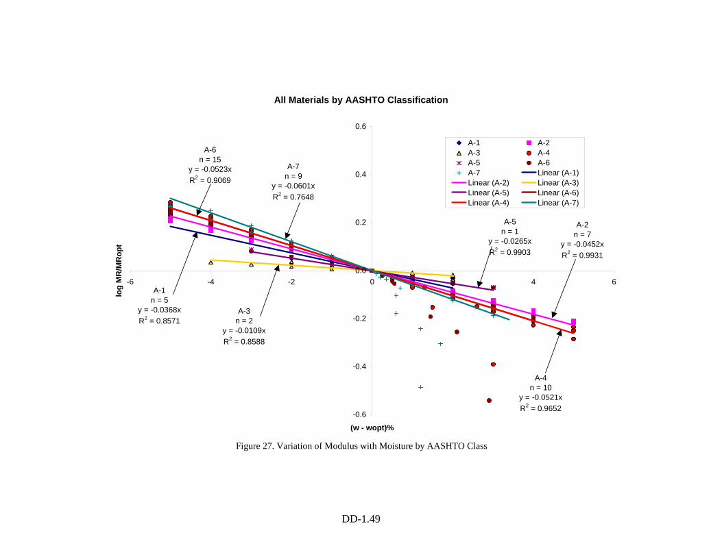
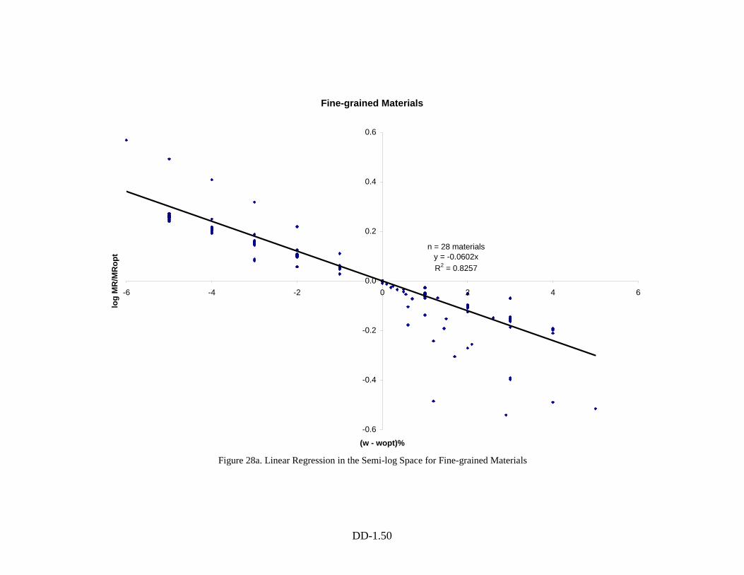
In Figure 27, materials are divided by AASHTO classification in an attempt to assign kw
values to each soil class. In Figures 28a and 29a, through regression in the semi-log
space, typical kw values are obtained for fine-grained materials (kw = -0.0602) and coarse-
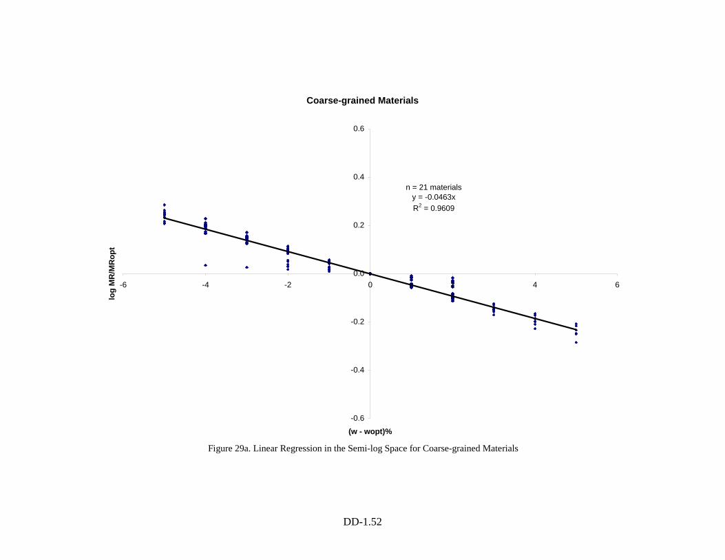
grained materials (kw = -0.0463). In other words, a 1% increase in moisture content will
cause, on the average, a 13% reduction in modulus for fine-grained soils, 10%
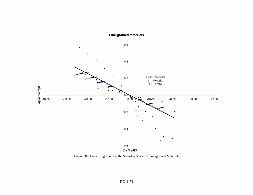
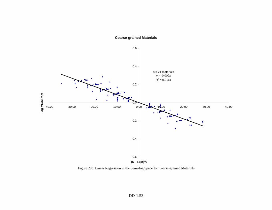
respectively for coarse-grained soils. In terms of saturation (see Figures 28b and 29b),
typical kS values are: kS = -0.0128 for fine-grained materials and kS = -0.009 for coarse-
grained materials. A 1% increase in degree of saturation will cause, on the average, a 3%
reduction in modulus for fine-grained soils and a 2% reduction for coarse-grained soils.
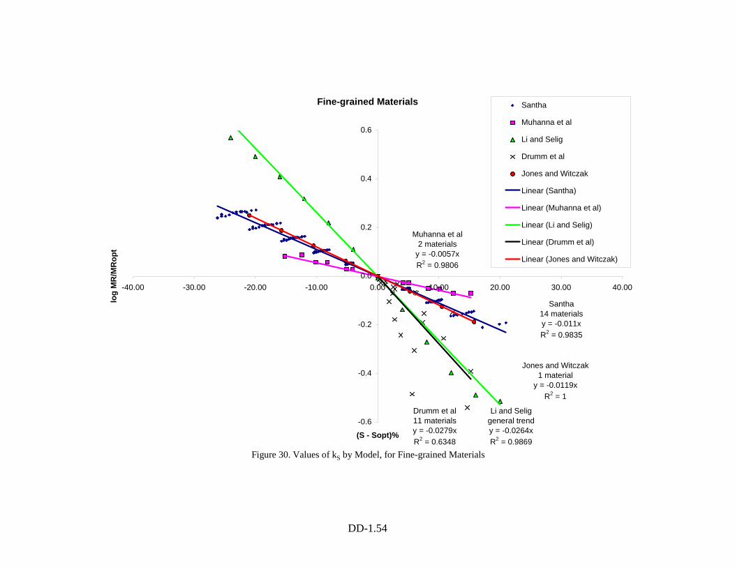
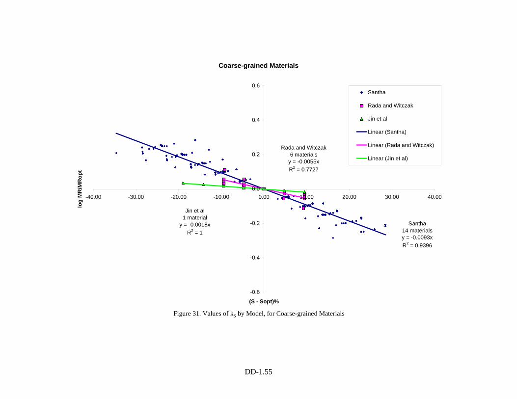
In Figures 30 and 31, kS values corresponding to each model are obtained. The database
available to date includes results from 7 different investigators for 49 different soils.
DD-1.49
Figure 27. Variation of Modulus with Moisture by AASHTO Class
All Materials by AASHTO Classification
A-1n = 5
y = -0.0368xR2 = 0.8571
A-2n = 7
y = -0.0452xR2 = 0.9931
A-3n = 2
y = -0.0109xR2 = 0.8588
A-5n = 1
y = -0.0265xR2 = 0.9903
A-6n = 15
y = -0.0523xR2 = 0.9069
A-4n = 10
y = -0.0521xR2 = 0.9652
A-7n = 9
y = -0.0601xR2 = 0.7648
-0.6
-0.4
-0.2
0.0
0.2
0.4
0.6
-6 -4 -2 0 2 4 6
(w - wopt)%
log
MR
/MR
opt
A-1 A-2A-3 A-4A-5 A-6A-7 Linear (A-1)Linear (A-2) Linear (A-3)Linear (A-5) Linear (A-6)Linear (A-4) Linear (A-7)
DD-1.50
Figure 28a. Linear Regression in the Semi-log Space for Fine-grained Materials
Fine-grained Materials
n = 28 materialsy = -0.0602xR2 = 0.8257
-0.6
-0.4
-0.2
0.0
0.2
0.4
0.6
-6 -4 -2 0 2 4 6
(w - wopt)%
log
MR
/MR
opt
DD-1.51
Figure 28b. Linear Regression in the Semi-log Space for Fine-grained Materials
Fine-grained Materials
n = 28 materialsy = -0.0128xR2 = 0.796
-0.6
-0.4
-0.2
0.0
0.2
0.4
0.6
-40.00 -30.00 -20.00 -10.00 0.00 10.00 20.00 30.00 40.00
(S - Sopt)%
log
MR
/MR
opt
DD-1.52
Figure 29a. Linear Regression in the Semi-log Space for Coarse-grained Materials
Coarse-grained Materials
n = 21 materialsy = -0.0463xR2 = 0.9609
-0.6
-0.4
-0.2
0.0
0.2
0.4
0.6
-6 -4 -2 0 2 4 6
(w - wopt)%
log
MR
/MR
opt
DD-1.53
Figure 29b. Linear Regression in the Semi-log Space for Coarse-grained Materials
Coarse-grained Materials
n = 21 materialsy = -0.009xR2 = 0.9161
-0.6
-0.4
-0.2
0.0
0.2
0.4
0.6
-40.00 -30.00 -20.00 -10.00 0.00 10.00 20.00 30.00 40.00
(S - Sopt)%
log
MR
/MR
opt
DD-1.54
Figure 30. Values of kS by Model, for Fine-grained Materials
Fine-grained Materials
Santha14 materialsy = -0.011xR2 = 0.9835
Muhanna et al2 materials
y = -0.0057xR2 = 0.9806
Li and Seliggeneral trendy = -0.0264xR2 = 0.9869
Drumm et al11 materialsy = -0.0279xR2 = 0.6348
Jones and Witczak1 material
y = -0.0119xR2 = 1
-0.6
-0.4
-0.2
0.0
0.2
0.4
0.6
-40.00 -30.00 -20.00 -10.00 0.00 10.00 20.00 30.00 40.00
(S - Sopt)%
log
MR
/MR
opt
Santha
Muhanna et al
Li and Selig
Drumm et al
Jones and Witczak
Linear (Santha)
Linear (Muhanna et al)
Linear (Li and Selig)
Linear (Drumm et al)
Linear (Jones and Witczak)
DD-1.55
Figure 31. Values of kS by Model, for Coarse-grained Materials
Coarse-grained Materials
Santha14 materialsy = -0.0093xR2 = 0.9396
Rada and Witczak6 materials
y = -0.0055xR2 = 0.7727
Jin et al1 material
y = -0.0018xR2 = 1
-0.6
-0.4
-0.2
0.0
0.2
0.4
0.6
-40.00 -30.00 -20.00 -10.00 0.00 10.00 20.00 30.00 40.00
(S - Sopt)%
log
MR
/MR
opt
Santha
Rada and Witczak
Jin et al
Linear (Santha)
Linear (Rada and Witczak)
Linear (Jin et al)
DD-1.56
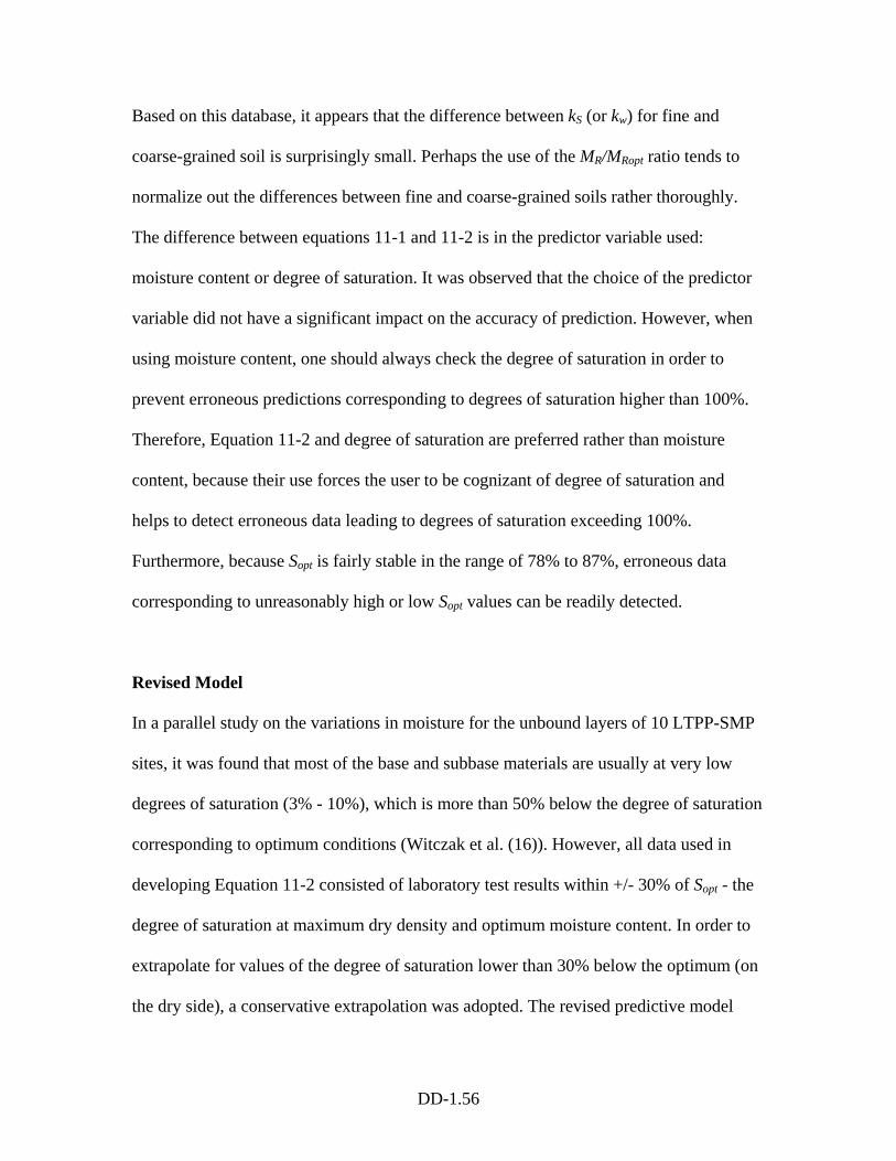
Based on this database, it appears that the difference between kS (or kw) for fine and
coarse-grained soil is surprisingly small. Perhaps the use of the MR/MRopt ratio tends to
normalize out the differences between fine and coarse-grained soils rather thoroughly.
The difference between equations 11-1 and 11-2 is in the predictor variable used:
moisture content or degree of saturation. It was observed that the choice of the predictor
variable did not have a significant impact on the accuracy of prediction. However, when
using moisture content, one should always check the degree of saturation in order to
prevent erroneous predictions corresponding to degrees of saturation higher than 100%.
Therefore, Equation 11-2 and degree of saturation are preferred rather than moisture
content, because their use forces the user to be cognizant of degree of saturation and
helps to detect erroneous data leading to degrees of saturation exceeding 100%.
Furthermore, because Sopt is fairly stable in the range of 78% to 87%, erroneous data
corresponding to unreasonably high or low Sopt values can be readily detected.
Revised Model
In a parallel study on the variations in moisture for the unbound layers of 10 LTPP-SMP
sites, it was found that most of the base and subbase materials are usually at very low
degrees of saturation (3% - 10%), which is more than 50% below the degree of saturation
corresponding to optimum conditions (Witczak et al. (16)). However, all data used in
developing Equation 11-2 consisted of laboratory test results within +/- 30% of Sopt - the
degree of saturation at maximum dry density and optimum moisture content. In order to
extrapolate for values of the degree of saturation lower than 30% below the optimum (on
the dry side), a conservative extrapolation was adopted. The revised predictive model
DD-1.57
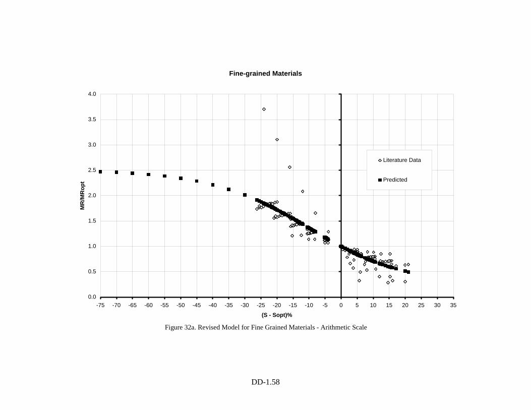
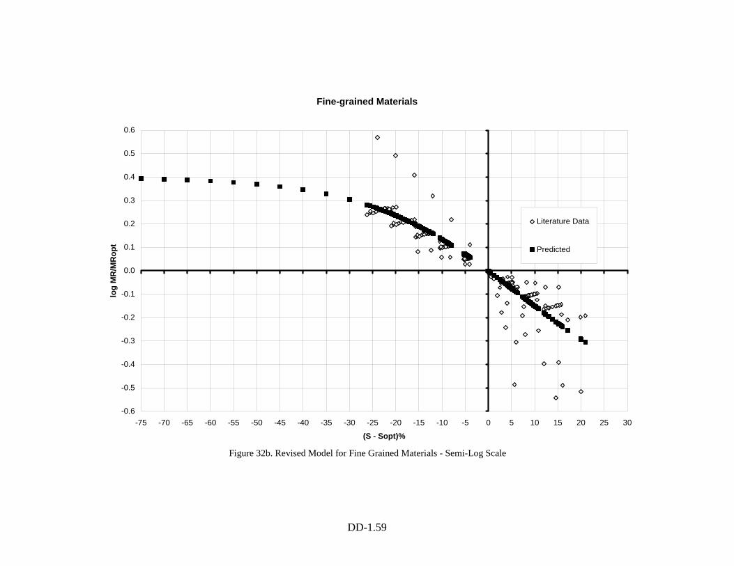
(Equation 12) uses a sigmoid that approaches the linear relationship observed within +/-
30% of Sopt but flattens out for the degrees of saturation lower than 30% below the
optimum. This extrapolation is in general agreement with known behavior of unsaturated
materials in that, when a material becomes sufficiently dry, further drying increments
produce less increase in stiffness and strength (Fredlund and Rahardjo (17)). The
predictions of the revised model are given in Figures 32 and 33, for coarse-grained and
fine-grained materials.
( )( )optSRopt
R
SSkEXPaba
MM
−⋅++−
+=β1
log (12)
Where:
a = minimum of log(MR/MRopt);
b = maximum of log(MR/MRopt);
β = location parameter – obtained as a function of a and b by imposing the condition of a
zero intercept:
⎟⎠⎞
⎜⎝⎛−=
ablnβ
(12-1)
kS = regression parameter;
(S – Sopt) = variation in degree of saturation expressed in decimal; (Note that the use of S
in equation form was changed from percent to decimal when the revised (nonlinear)
model was adopted).
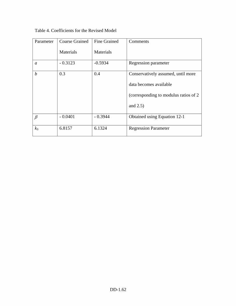
Using the available literature data and assuming a maximum modulus ratio of 2.5 for
fine-grained materials and 2 for coarse-grained materials, the values of a, b, β and kS for
coarse-grained and fine-grained materials are given in Table 4.
DD-1.58
Fine-grained Materials
0.0
0.5
1.0
1.5
2.0
2.5
3.0
3.5
4.0
-75 -70 -65 -60 -55 -50 -45 -40 -35 -30 -25 -20 -15 -10 -5 0 5 10 15 20 25 30 35
(S - Sopt)%
MR
/MR
opt
Literature Data
Predicted
Figure 32a. Revised Model for Fine Grained Materials - Arithmetic Scale
DD-1.59
Fine-grained Materials
-0.6
-0.5
-0.4
-0.3
-0.2
-0.1
0.0
0.1
0.2
0.3
0.4
0.5
0.6
-75 -70 -65 -60 -55 -50 -45 -40 -35 -30 -25 -20 -15 -10 -5 0 5 10 15 20 25 30
(S - Sopt)%
log
MR
/MR
opt
Literature Data
Predicted
Figure 32b. Revised Model for Fine Grained Materials - Semi-Log Scale
DD-1.60
Coarse-grained Materials
0.0
0.5
1.0
1.5
2.0
2.5
3.0
3.5
4.0
-75 -70 -65 -60 -55 -50 -45 -40 -35 -30 -25 -20 -15 -10 -5 0 5 10 15 20 25 30 35
(S - Sopt)%
MR
/MR
opt
Literature Data
Predicted
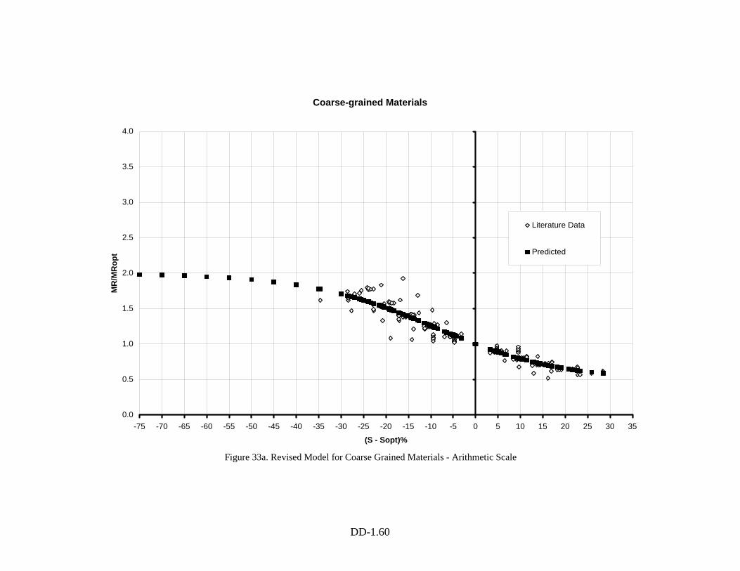
Figure 33a. Revised Model for Coarse Grained Materials - Arithmetic Scale
DD-1.61
Coarse-grained Materials
-0.6
-0.5
-0.4
-0.3
-0.2
-0.1
0.0
0.1
0.2
0.3
0.4
0.5
0.6
-75 -70 -65 -60 -55 -50 -45 -40 -35 -30 -25 -20 -15 -10 -5 0 5 10 15 20 25 30
(S - Sopt)%
log
MR
/MR
opt
Literature Data
Predicted
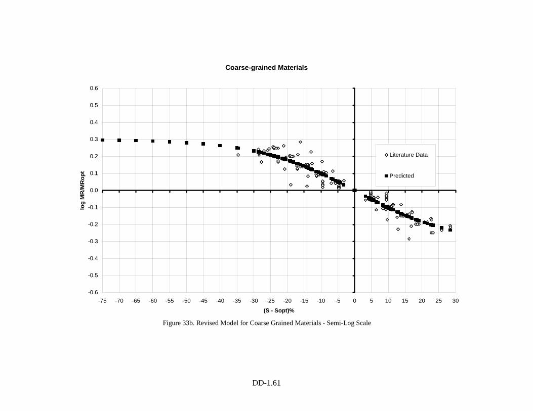
Figure 33b. Revised Model for Coarse Grained Materials - Semi-Log Scale
DD-1.62
Table 4. Coefficients for the Revised Model
Parameter Coarse Grained
Materials
Fine Grained
Materials
Comments
a - 0.3123 -0.5934 Regression parameter
b 0.3 0.4 Conservatively assumed, until more
data becomes available
(corresponding to modulus ratios of 2
and 2.5)
β - 0.0401 - 0.3944 Obtained using Equation 12-1
kS 6.8157 6.1324 Regression Parameter
DD-1.63
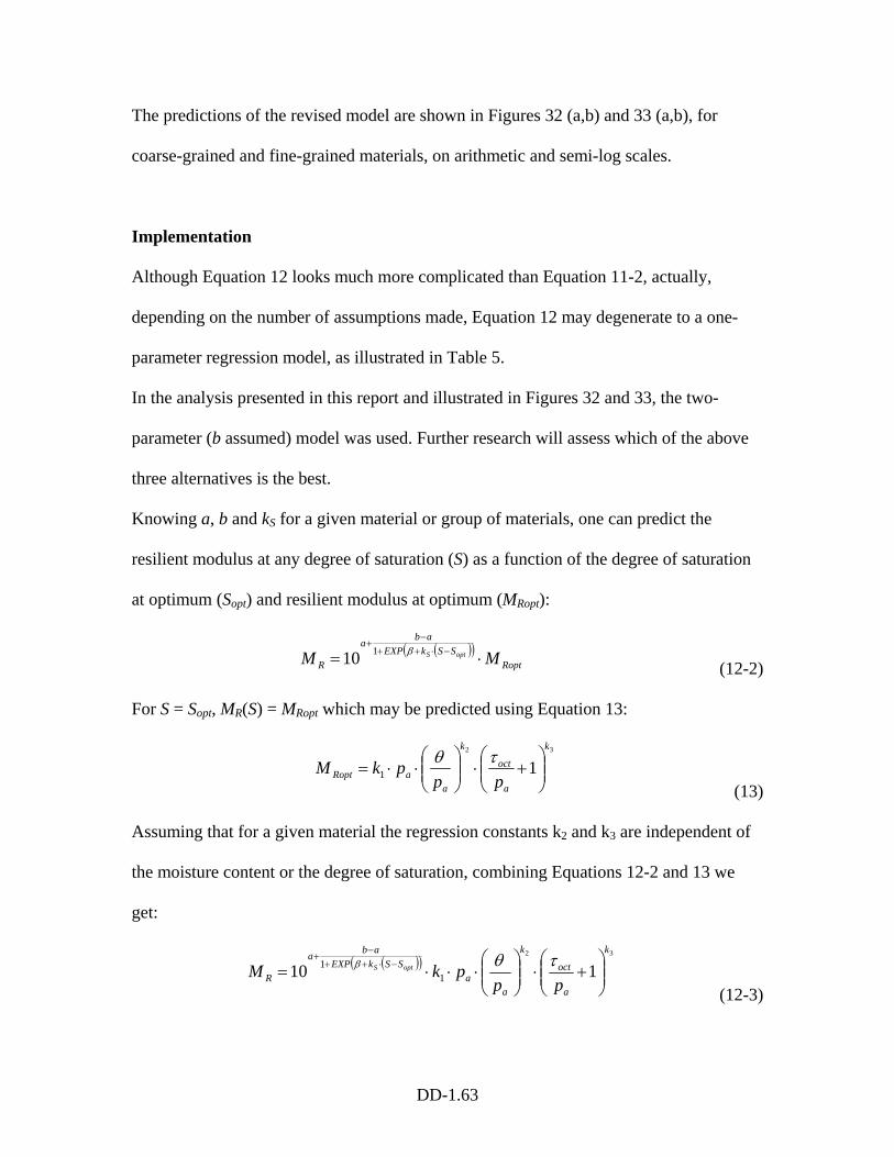
The predictions of the revised model are shown in Figures 32 (a,b) and 33 (a,b), for
coarse-grained and fine-grained materials, on arithmetic and semi-log scales.
Implementation
Although Equation 12 looks much more complicated than Equation 11-2, actually,
depending on the number of assumptions made, Equation 12 may degenerate to a one-
parameter regression model, as illustrated in Table 5.
In the analysis presented in this report and illustrated in Figures 32 and 33, the two-
parameter (b assumed) model was used. Further research will assess which of the above
three alternatives is the best.
Knowing a, b and kS for a given material or group of materials, one can predict the
resilient modulus at any degree of saturation (S) as a function of the degree of saturation
at optimum (Sopt) and resilient modulus at optimum (MRopt):
( )( )Ropt
SSkEXPaba
R MM optS ⋅= −⋅++−
+β110 (12-2)
For S = Sopt, MR(S) = MRopt which may be predicted using Equation 13:
32
11
k
a
oct
k
aaRopt pp
pkM ⎟⎟⎠
⎞⎜⎜⎝
⎛+⋅⎟⎟
⎠
⎞⎜⎜⎝
⎛⋅⋅=
τθ
(13)
Assuming that for a given material the regression constants k2 and k3 are independent of
the moisture content or the degree of saturation, combining Equations 12-2 and 13 we
get:
( )( )32
110 11
k
a
oct
k
aa
SSkEXPaba
R pppkM optS
⎟⎟⎠
⎞⎜⎜⎝
⎛+⋅⎟⎟
⎠
⎞⎜⎜⎝
⎛⋅⋅⋅= −⋅++
−+ τθβ
(12-3)

DD-1.64
Table 5. Complexity of the Model
Assumptions Regression Constants
to be Found
Comments
No
Assumptions
a, b, kS An equivalent power or polynomial model would
require the same number of regression constants
(i.e. 3)
b a, kS Two-parameter regression model
a, b kS One-parameter regression model; the value of a
actually controls the shape of the predicted curve
in the semi-log space, on the wet side:
a relatively high value will let the curve flatten
again, as in Figure 33; a relatively low value will
straighten the curve on the wet side. An
extremely low value will even bend it
downward.

DD-1.65
Although better goodness of fit statistics (Se/Sy, R2) could be obtained performing the
regression in the arithmetic space, by regressing in the semi-log space, errors
corresponding to lower MR values are given more weight which is beneficial because we
strive for higher accuracy on the “wet side” of the optimum (i.e. Si – Sopt > 0), where
modulus values are lower and therefore more critical.
It should be noted that if changes in moisture content are accompanied by
significant changes in soil density, the variation in MR will not be smooth, as was shown
by Figure 8. Therefore, corrections for expansion or collapse should be introduced. The
effect of density changes on MR is indicated by the coefficients appearing in models (5),
(8-a,b) and (9-b). As more MR test results become available it should be possible to better
quantify the effects of density changes.
Recommendations for Further Study
Very few of the studies reported in the literature on resilient modulus and
moisture are based on test results obtained on specimens wetted post-compaction.
Because post-compaction represents the process followed in the prototype, this
shortcoming could be serious for some soils. Further, very few of these past studies have
quantified the effect of density and most studies have employed only one stress level.
Therefore, for a given soil it is rather difficult to assess the effect of density, stress level
and moisture content. What is needed is a comprehensive test program covering a range
of:
• soil types
• density

DD-1.66
• moisture contents (wet and dry of optimum, with post-compaction moisture
variation)
• stress states
If the post-compaction moisture variation were imposed under constant and realistic
stress state, then any corresponding change in density would likewise be realistic.
Variations in MR derived from a test program of this type would provide the highest
possible quality of data for future estimations of MR.
DD-1.67
References:
1. Li D. and Selig E.T. Resilient Modulus for Fine Grained Subgrade Soils. ASCE Journal of Geotechnical Engineering, Vol. 120, No. 6, June, 1994, pp. 939-957.
2. Drumm E.C., Reeves J.S., Madgett M.R. and Trolinger W.D. Subgrade Resilient
Modulus Correction for Saturation Effects. ASCE Journal of Geotechnical and Geoenvironmental Engineering, Vol. 123, No. 7, July, 1997, pp. 663-670.
3. Jin M.S., Lee K.W. and Kovacs W.D. Seasonal Variation of Resilient Modulus of
Subgrade Soils. ASCE Journal of Transportation Engineering, Vol. 120, No.4, July/August, 1994, pp. 603-616.
4. Jones M.P. and Witczak M.W. Subgrade Modulus on the San Diego Test Road.
Transportation Research Record 641, TRB, National Research Council, 1977, Washington, D.C., pp. 1-6.
5. Rada G. and Witczak M.W. Comprehensive Evaluation of Laboratory Resilient
Moduli Results for Granular Material. Transportation Research Record 810, TRB, National Research Council, 1981, Washington, D.C., pp. 23-33.
6. Santha B.L. Resilient Modulus of Subgrade Soils: Comparison of Two Constitutive
Equations. Transportation Research Record 1462, TRB, National Research Council, Washington, D.C., pp. 79-90.
7. Berg R.L., Bigl S.R., Stark J.A. and Durell G.D. Resilient Modulus Testing of
Materials from Mn/ROAD, Phase 1. U.S. Army Corps of Engineers Cold Regions Research & Engineering Laboratory, Special Report No. 96-19, September 1996.
8. Muhanna A.S., Rahman M.S. and Lambe P.C. A Model for Resilient Modulus and
Permanent Strain of Subgrade Soils. Preprint, Paper No. 981084, Transportation Research Board, 77th Annual Meeting, January 11-15, 1998, Washington, D.C.
9. Gehling W.Y.Y., Ceratti J.A., Nunez W.P. and Rodrigues M.R. A Study on the
Influence of Suction on the Resilient Behavior of Soils from Southern Brazil. Proceedings of the Second Int. Conf. On Unsaturated Soils, 27-30 August, 1998, Beijing, China, Vol. 2.
10. Seed H.B., Chan C.K., and Lee C.E. Resilience characteristics of subgrade soils and
their relation to fatigue failures in asphalt pavement. Proc. First Int. Conf. On Struct. Design of Asphalt Pavements, University of Michigan, Ann Arbor, 1962.
11. Fredlund D.G., Bergan A.T and Wong P.K. Relation Between Resilient Modulus and
Stress Conditions for Cohesive Subgrade Soils. Transportation Research Record 642, TRB, National Research Council, 1977, Washington, D.C., pp. 73-81.
DD-1.68
12. Lekarp F., Isacsson U., and Dawson A. State of the Art. I: Resilient Response of Unbound Aggregates. ASCE Journal of Transportation Engineering, Vol. 126, No. 1, Jan./Feb., 2000, pp. 76-83.
13. Drumm E.C., Rainwater R.N., Andrew J., Jackson N.M., Yoder R.E. and Wilson
G.V. Pavement Response due to Seasonal Changes in Subgrade Moisture Conditions. Proceedings of the Second Int. Conf. On Unsaturated Soils, 27-30 August, 1998, Beijing, China, Vol. 2.
14. Edil T.B. and Motan S.E. Soil-Water Potential and Resilient Behavior of Subgrade
Soils. Transportation Research Record 705, TRB, National Research Council, 1979, Washington, D.C., pp. 54-63.
15. Andrei D. Development of a Harmonized Test Protocol for the Resilient Modulus of
Unbound Materials Used in Pavement Design, Master Thesis, University of Maryland at College Park, 1999.
16. Witczak M.W., Houston W.N. and Andrei D. Resilient Modulus as Function of Soil
Moisture – A Study of the Expected Changes in Resilient Modulus of the Unbound Layers with Changes in Moisture for 10 LTPP Sites. Development of the 2002 Guide for the Development of New and Rehabilitated Pavement Structures, NCHRP 1-37 A, Inter Team Technical Report (Seasonal 2), June 2000.
17. Fredlund D.G. and Rahardjo H. Soil Mechanics for Unsaturated Soils. John Wiley &
Sons, Inc. 1993
Copy No.
Guide for Mechanistic-Empirical Design OF NEW AND REHABILITATED PAVEMENT
STRUCTURES
FINAL DOCUMENT
APPENDIX DD-2: RESILIENT MODULUS AS FUNCTION OF SOIL
MOISTURE – A STUDY OF THE EXPECTED CHANGES IN RESILIENT MODULUS OF THE UNBOUND LAYERS
WITH CHANGES IN MOISTURE FOR 10 LTPP SITES
NCHRP
Prepared for National Cooperative Highway Research Program
Transportation Research Board National Research Council
Submitted by ARA, Inc., ERES Division
505 West University Avenue Champaign, Illinois 61820
June 2000
ii
Acknowledgment of Sponsorship This work was sponsored by the American Association of State Highway and Transportation Officials (AASHTO) in cooperation with the Federal Highway Administration and was conducted in the National Cooperative Highway Research Program which is administered by the Transportation Research Board of the National Research Council. Disclaimer This is the final draft as submitted by the research agency. The opinions and conclusions expressed or implied in this report are those of the research agency. They are not necessarily those of the Transportation Research Board, the National Research Council, the Federal Highway Administration, AASHTO, or the individual States participating in the National Cooperative Highway Research program. Acknowledgements The research team for NCHRP Project 1-37A: Development of the 2002 Guide for the Design of New and Rehabilitated Pavement Structures consisted of Applied Research Associates, Inc., ERES Consultants Division (ARA-ERES) as the prime contractor with Arizona State University (ASU) as the primary subcontractor. Fugro-BRE, Inc., the University of Maryland, and Advanced Asphalt Technologies, LLC served as subcontractors to either ARA-ERES or ASU along with several independent consultants. Research into the subject area covered in this Appendix was conducted at ASU. The authors of this Appendix are Dr. M.W. Witczak, Dr. W.N. Houston, and Mr. Dragos Andrei. Dr. M.W. Witczak coordinated the overall research effort of the 2002 Design Guide Team, outlined problems to be addressed, and made specific assignments of tasks for this study. He was also responsible for the final review of the report. Dr. W.N. Houston provided the day-to-day supervision of the study and assisted with the analysis of the results and report preparation. Mr. Dragos Andrei conducted the literature search, gathered the data, and performed the analyses contained in this report. Moisture predictions for the 10 LTPP sites were obtained from other studies being conducted at ASU by Witczak, Houston, Zapata and Richter of the FHWA. Foreword This appendix presents the results of applying the Design Guide model that relates changes in modular ratio to changes in degrees of saturation of unbound materials to 10 LTPP sites where moisture content variation data predicted by the EICM are available. The information contained in this appendix serves as a supporting reference to the resilient modulus discussions presented and PART 2, Chapter 3, and PART 3, Chapters 3, 4, 6, and 7 of the Design Guide.
iii
Abstract
As part of the overall effort to develop a working, practical subsystem to predict resilient
moduli (MR) for unbound material throughout the life of a pavement system, the effect of
moisture changes on MR has been studied and evaluated. A simple model relating
changes in modular ratio to changes in degree of saturation has been adopted to assess
changes in the MR values. This report presents the results of the application of this simple
model to 10 LTPP sites where moisture content variation data predicted by the EICM are
available.
The results show that the seasonal variations in MR (for non frost affected zones) are
typically fairly small, of the order of +/- 10 to 15%. Oscillations as high as +/- 25 to 50%
occasionally occur, but are not frequent. Overall, these seasonal oscillations appear to be
much smaller than the oscillations expected from freezing and thawing. Also, in most
cases, particularly for the bases and subbases, the effect of change in moisture from the
initial (optimum compaction) conditions to the final equilibrium condition is much larger
than the seasonal oscillations.
iv
Table of Contents
Page
Introduction..........................................................................................................................1
Objective ..............................................................................................................................1
Analysis................................................................................................................................2
Discussion of Results.........................................................................................................11
Use of Hand Calculations as a Check on EICM output.....................................................32
Conclusions........................................................................................................................37
Recommendations – General .............................................................................................38
Recommendations – Relative to the Implementation of the MR Model into the 2002
Guide..................................................................................................................................39
References..........................................................................................................................42
v
List of Tables
Page
Table 1. CBR values as a Function of Material Type..........................................................3
Table 2. Model Parameters ..................................................................................................5
Table 3. Input Data Summary............................................................................................10
Table 4. Check on EICM Outputs with Manual Calculations – Comparisons of MR
Adjustment Factors .............................................................................................35

vi
List of Figures
Page
Figure 1. Values of ks for Coarse Grained Materials...........................................................6
Figure 2. Values of ks for Fine Grained Materials...............................................................6
Figure 3. Arizona ...............................................................................................................12
Figure 4. Colorado .............................................................................................................14
Figure 5. Connecticut.........................................................................................................16
Figure 6. Georgia ...............................................................................................................18
Figure 7. Maine..................................................................................................................20
Figure 8. Manitoba.............................................................................................................22
Figure 9. Minnesota ...........................................................................................................24
Figure 10. New Hampshire ................................................................................................26
Figure 11. Texas.................................................................................................................28
Figure 12. Vermont............................................................................................................30
Figure 13. Predicted SWCC based on D60 and PI .............................................................34
DD-2.1
A Study of the Expected Changes in Resilient Modulus of Unbound Layers with
Changes in Moisture for 10 LTPP Sites
Introduction
The task of quantifying the expected cumulative damage due to load associated distress
of a pavement system begins with estimation of the initial resilient modulus for each
layer. Next, changes in MR with temperature are estimated for any asphalt layers and
changes in moisture content are estimated for all unbound layers. Finally, in order to
predict seasonal changes, these changes in moisture content must be eventually translated
to changes in MR.
A literature study was recently completed at ASU, which helped quantify the sensitivity
of MR to changes in degree of saturation (1). In general, it was found that a 1% increase
in degree of saturation will cause, on the average, a 3% reduction in modulus for fine-
grained soils and a 2% reduction for coarse-grained soils.
Objective
The objective of this study was to investigate the magnitude of change in resilient
modulus due to variation in moisture for 10 LTPP sites, as predicted by the newly
developed Resilient Modulus – Moisture model developed at ASU (1). These 10 LTPP
sites were the same sites that were used to examine the suitability of predictions of real
time moisture content change by a revised EICM (Enhanced Integrated Climatic Model)
model (2).
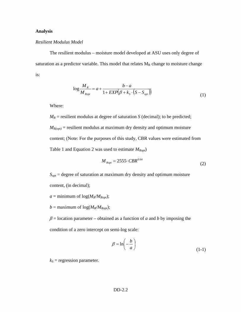
DD-2.2
Analysis
Resilient Modulus Model
The resilient modulus – moisture model developed at ASU uses only degree of
saturation as a predictor variable. This model that relates MR change to moisture change
is:
( )( )optSRopt
R
SSkEXPaba
MM
−⋅++−
+=β1
log (1)
Where:
MR = resilient modulus at degree of saturation S (decimal); to be predicted;
MR(opt) = resilient modulus at maximum dry density and optimum moisture
content; (Note: For the purposes of this study, CBR values were estimated from
Table 1 and Equation 2 was used to estimate MRopt)
64.02555 CBRM Ropt ⋅= (2)
Sopt = degree of saturation at maximum dry density and optimum moisture
content, (in decimal);
a = minimum of log(MR/MRopt);
b = maximum of log(MR/MRopt);
β = location parameter – obtained as a function of a and b by imposing the
condition of a zero intercept on semi-log scale:
⎟⎠⎞
⎜⎝⎛−=
ablnβ
(1-1)
kS = regression parameter.
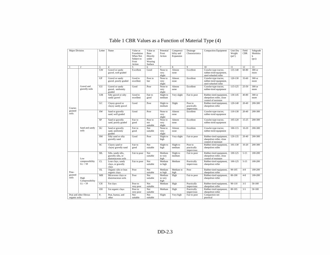
DD-2.3
Table 1 CBR Values as a Function of Material Type (4)
Major Division Letter Name Value asFoundationWhen NotSubject toFrostAction
Value asBaseDirectlyunderWearingSurface
PotentialFrostAction
Compressi-bility andExpansion
DrainageCharacteristics
Compaction Equipment Unit DryWeight(pcf )
FieldCBR
SubgradeModulusk(pci)
1 2 3 4 5 6 7 8 9 10 11 12 13GW Gravel or sandy
gravel, well gradedExcellent Good None to
veryslight
Almostnone
Excellent Crawler-type tractor,rubber-tired equipment,steel-wheeled roller
125-140 60-80 300 ormore
GP Gravel or sandygravel, poorly graded
Good toexcellent
Poor tofair
None toveryslight
Almostnone
Excellent Crawler-type tractor,rubber-tired equipment,steel-wheeled roller
120-130 35-60 300 ormore
GU Gravel or sandygravel, uniformlygraded
Good Poor None toveryslight
Almostnone
Excellent Crawler-type tractor,rubber-tired equipment
115-125 25-50 300 ormore
GM Silty gravel or siltysandy gravel
Good toexcellent
Fair togood
Slight tomedium
Very slight Fair to poor Rubber-tired equipment,sheepsfoot roller, closecontrol of moisture
130-145 40-80 300 ormore
Gravel andgravelly soils
GC Clayey gravel orclayey sandy gravel
Good Poor Slight tomedium
Slight Poor topracticallyimpervious
Rubber-tired equipment,sheepsfoot roller
120-140 20-40 200-300
SW Sand or gravellysand, well graded
Good Poor None toveryslight
Almostnone
Excellent Crawler-type tractor,rubber-tired equipment
110-130 20-40 200-300
SP Sand or gravellysand, poorly graded
Fair togood
Poor tonotsuitable
None toveryslight
Almostnone
Excellent Crawler-type tractor,rubber-tired equipment
105-120 15-25 200-300
SU Sand or gravellysand, uniformlygraded
Fair togood
Notsuitable
None toveryslight
Almostnone
Excellent Crawler-type tractor,rubber-tired equipment
100-115 10-20 200-300
SM Silty sand or siltygravelly sand
Good Poor Slight tohigh
Very slight Fair to poor Rubber-tired equipment,sheepsfoot roller, closecontrol of moisture
120-135 20-40 200-300
Coarse-grainedsoils
Sand and sandysoils
SC Clayey sand orclayey gravelly sand
Fair togood
Notsuitable
Slight tohigh
Slight tomedium
Poor topracticallyimpervious
Rubber-tired equipment,sheepsfoot roller
105-130 10-20 200-300
ML Silts, sandy silts,gravelly silts, ordiatomaceous soils
Fair to poor Notsuitable
Mediumto veryhigh
Slight tomedium
Fair to poor Rubber-tired equipment,sheepsfoot roller, closecontrol of moisture
100-125 5-15 100-200
CL Lean clays, sandyclays, or gravellyclays
Fair to poor Notsuitable
Mediumto high
Medium Practicallyimpervious
Rubber-tired equipment,sheepsfoot roller
100-125 5-15 100-200LowcompressibilityLL < 50
OL Organic silts or leanorganic clays
Poor Notsuitable
Mediumto high
Medium tohigh
Poor Rubber-tired equipment,sheepsfoot roller
90-105 4-8 100-200
MH Micaceous clays ordiatomaceous soils
Poor Notsuitable
Mediumto veryhigh
High Fair to poor Rubber-tired equipment,sheepsfoot roller
80-100 4-8 100-200
CH Fat clays Poor tovery poor
Notsuitable
Medium High Practicallyimpervious
Rubber-tired equipment,sheepsfoot roller
90-110 3-5 50-100
Fine-grainedsoils High
CompressibilityLL > 50
OH Fat organic clays Poor tovery poor
Notsuitable
Medium High Practicallyimpervious
Rubber-tired equipment,sheepsfoot roller
80-105 3-5 50-100
Peat and other fibrousorganic soils
Pt Peat, humus, andother
Notsuitable
Notsuitable
Slight Very high Fair to poor Compaction notpractical
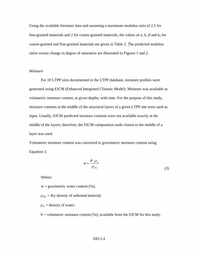
DD-2.4
Using the available literature data and assuming a maximum modulus ratio of 2.5 for
fine-grained materials and 2 for coarse-grained materials, the values of a, b, β and kS for
coarse-grained and fine-grained materials are given in Table 2. The predicted modulus
ratios versus change in degree of saturation are illustrated in Figures 1 and 2.
Moisture
For 10 LTPP sites documented in the LTPP database, moisture profiles were
generated using EICM (Enhanced Integrated Climatic Model). Moisture was available as
volumetric moisture content, at given depths, with time. For the purpose of this study,
moisture contents at the middle of the structural layers of a given LTPP site were used as
input. Usually, EICM predicted moisture contents were not available exactly at the
middle of the layers; therefore, the EICM computation node closest to the middle of a
layer was used.
Volumetric moisture content was converted to gravimetric moisture content using
Equation 3.
dry
wwρ
ρθ ⋅=
(3)
Where:
w = gravimetric water content (%);
ρdry = dry density of unbound material;
ρw = density of water;
θ = volumetric moisture content (%); available from the EICM for this study.
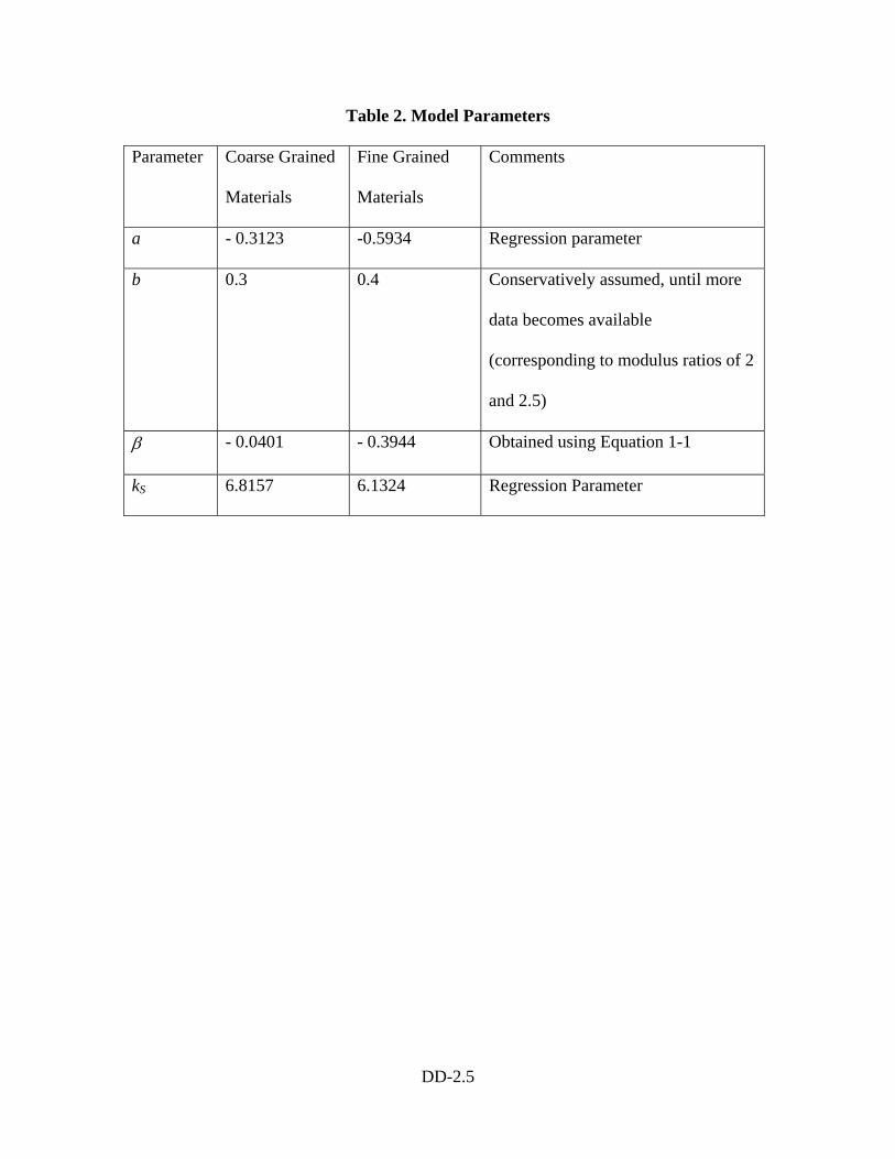
DD-2.5
Table 2. Model Parameters
Parameter Coarse Grained
Materials
Fine Grained
Materials
Comments
a - 0.3123 -0.5934 Regression parameter
b 0.3 0.4 Conservatively assumed, until more
data becomes available
(corresponding to modulus ratios of 2
and 2.5)
β - 0.0401 - 0.3944 Obtained using Equation 1-1
kS 6.8157 6.1324 Regression Parameter
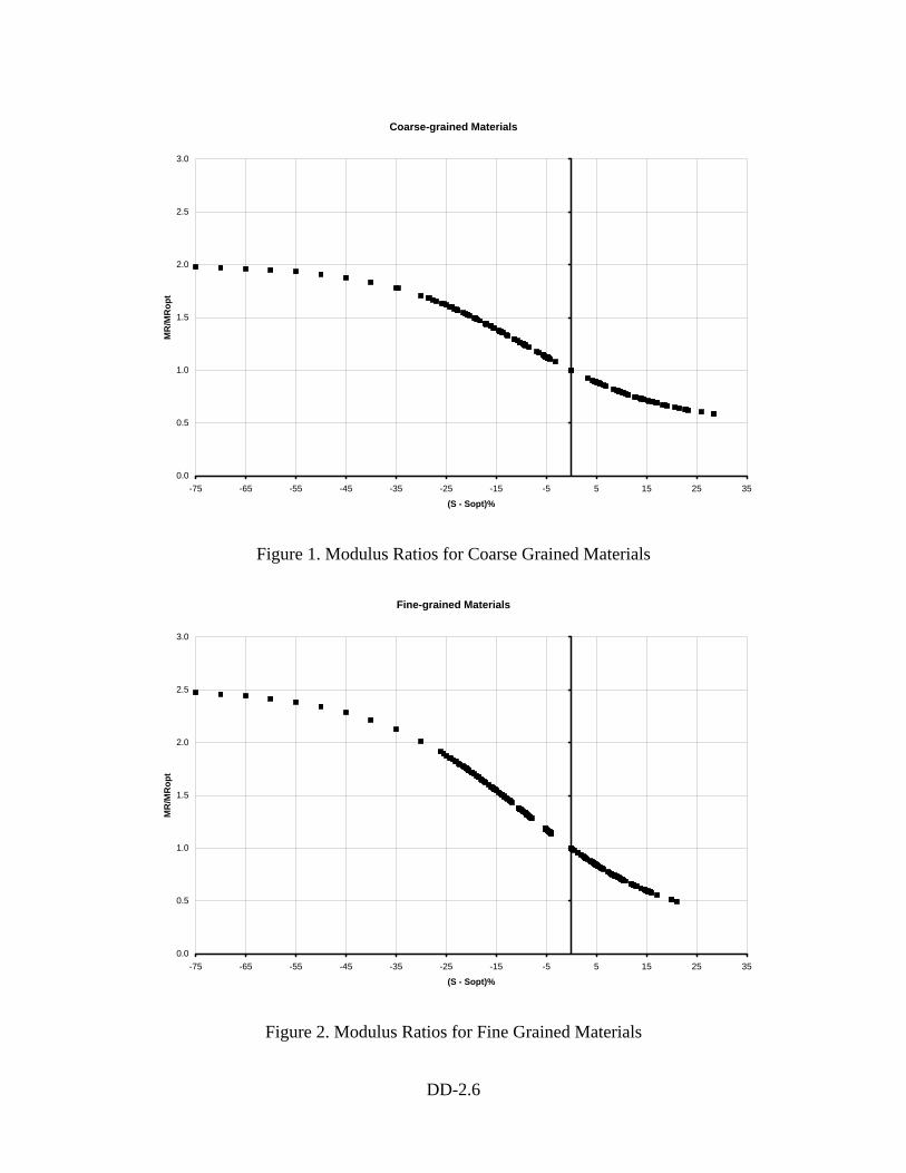
DD-2.6
Coarse-grained Materials
0.0
0.5
1.0
1.5
2.0
2.5
3.0
-75 -65 -55 -45 -35 -25 -15 -5 5 15 25 35
(S - Sopt)%
MR
/MR
opt
Figure 1. Modulus Ratios for Coarse Grained Materials
Fine-grained Materials
0.0
0.5
1.0
1.5
2.0
2.5
3.0
-75 -65 -55 -45 -35 -25 -15 -5 5 15 25 35
(S - Sopt)%
MR
/MR
opt
Figure 2. Modulus Ratios for Fine Grained Materials
DD-2.7
For purposes of this study, the optimum moisture content for standard compaction was
estimated using Equation 4:
1038.060
73.0
6425.80
113.10−⋅=⇒=
+⋅=⇒>
DwwPI
wPIwwPI
opt
opt
(4)
Where:
wopt = optimum moisture content at maximum dry density obtained by standard
compaction (AASHTO T99);
wPI = plasticity index (PI) times the percent passing the No. 200 sieve (in
decimal);
D60 = particle size for which 60% of the material is finer in mm.
In order to obtain the optimum moisture content in the case of modified compactive effort
(T 180), Equations 5a and 5b were used:
9.0853.016.0 2 +⋅+⋅=∆ optoptopt www (5a)
optoptopt www ∆−= )T99()T180( (5b)
Where ∆wopt represents the difference in the wopt for T99 and T180.
The above correlations were developed as part of studies aimed at improvement of the
EICM predictive capability and are described by Witczak et al. (2).
Degree of Saturation
The degree of saturation was computed using Equation 6:
⎟⎟⎠
⎞⎜⎜⎝
⎛−
⋅=
1dry
wsGwS
γγ
(6)
Where:
DD-2.8
S = degree of saturation (%);
Gs = specific gravity of soil solids;
w = gravimetric moisture content (%);
γw = unit weight of water;
γdry = dry unit weight of unbound material.
The degree of saturation is used in Equation 1.
The degree of saturation at optimum moisture content and maximum dry density, Sopt, is
obtained from Equation 7:
78752.6 147.0 +⋅= wPISopt (7)
Where:
wPI = plasticity index (PI) times the percent passing the No. 200 sieve (as a
decimal).
The correlation was developed from a modest database for both standard (AASHTO T99)
and modified (AASHTO T180) compactive efforts. A degree of saturation at optimum of
78% (the intercept) was adopted for all non-plastic materials, as described in Witczak et
al. (2).
Equations 4, 5 and 7 were developed in order to minimize errors induced by
erroneous or missing values of dry density, wopt, and/or specific gravity of solids.
Experience has shown that it is the rule rather than the exception that the reported value
for one or more of the three variables wopt, Gs and γd max for a given soil will be erroneous,
unreasonable or missing. Therefore, in order to establish an internally consistent basis for
assessing the initial compaction conditions for unbound materials, the optimum state (γd =
γd max and w = wopt) has been adopted as the reference condition, and Sopt, wopt and Gs have
DD-2.9
been obtained from correlations with wPI or D60. Equation 8 represents the correlation
developed for Gs. Equation 9 is used to compute γd max, and γd max is used in Equations 3
and 6 as needed.
65.2041.0 29.0 +⋅= wPIGs (8)
sopt
opt
wsd_max
GSw
G
⋅+
⋅=
1
γγ
(9)
Where:
Sopt = degree of saturation at optimum moisture content and maximum dry
density;
Gs = specific gravity;
wopt = optimum moisture content;
γw = unit weight of water;
γd max = dry unit weight at optimum condition.
For the 2002 Design Guide implementation, it will be recommended that directly-
measured values of γd max, wopt, and Gs be used for Level 1. However, for Levels 2 and
3 it will be recommended that the correlations given by Equations 4, 5, 7, and 8 be
used to get Sopt, wopt and Gs and then Equation 9 be used to get γd max.
Using the correlations, equations, and procedures outlined in the preceding section, input
data was generated for the 10 LTPP sites, as shown in Table 3.
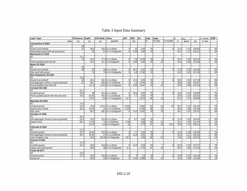
DD-2.10
Table 3 Input Data Summary
Layer Type Thickness Depth ICM Node Class wPI D60 Gs Sopt wopt e ρdry 1 = coarse CBRUnits cm cm cm AASHTO mm % % (std) % (modif) % g/cm3 pcf 2 = fine
Connecticut 9-1803AC 18Gravel (uncrushed) 37 36.5 36.5 A-1-a Base 0 10 2.65 78 7 6 21.0 2.19 136.65 1 55Well-graded sand with silt and gravel 65 67 A-2-4 Subgrade 0 0.48 2.86 78 9 34.2 2.13 133.12 1 30Minnesota 27-1018AC 11.2? 10 16.2 17.9 A-1-b Base 0 2.6 2.675 78 8 7 24.4 2.15 134.16 1 25Poorly-graded sand wilt silt 31.2 31.1 A-3 Subgrade 0 0.38 2.65 78 10 32.5 2.00 124.83 1 20Maine 23-1026AC 16Gravel (uncrushed) 48 40 40 A-1-a Base 0 45.2 2.65 78 6 5 17.8 2.25 140.35 1 55Silty sand with gravel 74 74 A-2-4 Subgrade 0 4.8 2.782 78 7 26.2 2.20 137.56 1 30New Hampshire 33-1001AC 21.6Gravel (uncrushed) 49 46.1 46.1 A-1-a Base 0 12.3 2.65 78 7 6 20.5 2.20 137.18 1 55Soil-aggregate mixture (coarse-grained) 37 89.1 88.6 A-1-b Subbase 0 1.3 2.678 78 8 28.9 2.08 129.67 1 50Poorly-graded sand with silt 117.6 115.9 A-2-4 Subgrade 0 0.25 2.647 78 10 33.9 1.98 123.38 1 20Vermont 50-1002AC 21.1Crushed gravel 53.8 48 50.4 A-1-a Base 0 25.6 2.65 78 6 6 19.0 2.23 138.99 1 70Poorly graded gravel with silt and sand 34.3 92.05 94.5 A-1-a Subbase 0 7.7 2.65 78 7 23.8 2.14 133.62 1 50? 119.2 119 A-7-5 Subgrade 12.3 2.815 88 19 61.3 1.74 108.88 2 10Manitoba 83-1801AC 11.5Crushed gravel 14.2 18.6 20.67 A-1-a Base 0.545 2.684 84 12 10 33.4 2.01 125.50 1 70Gravel (uncrushed) 33.5 42.45 42 A-2-6 Subbase 1.155 2.693 85 12 39.5 1.93 120.48 1 55Silty sand 69.2 68.3 A-2-4 Subgrade 0 0.22 2.831 78 10 36.7 2.07 129.22 2 30Georgia 13-1005AC 19.1Soil-aggregate mixture (coarse-grained) 22.4 30.3 32.5 A-1-a Base 0 8.7 2.65 78 7 6 21.3 2.18 136.30 1 50Clayey sand 60.1 71.55 71 A-4 Subbase 0.36 2.68 84 12 37.1 1.95 121.94 2 15? 111.6 113 A-6 Subgrade 10 2.73 87 18 56.1 35.9 1.75 109.12 2 10Colorado 8-1053AC 11.4Crushed gravel 13.7 18.25 20.5 A-1-a Base 0 7.7 2.65 78 7 6 21.6 2.18 135.99 1 70Soil-aggregate mixture (coarse-grained) 59.7 54.95 57 A-1-a Subbase 0 13.9 2.65 78 7 22.3 2.17 135.16 1 50Lean inorganic clay 94.8 96.95 A-6 Subgrade 20.2 2.89 89 23 74.0 1.66 103.64 2 10Arizona 4-1024AC 27.4Crushed gravel 22.4 38.6 40.8 A-1-a Base 0 14.4 2.65 78 7 6 20.2 2.20 137.57 1 70Clayey sand with gravel 59.8 58 A-2-6 Subgrade 6.1 2.719 87 16 49.7 1.82 113.34 2 15Texas 48-1077AC 13.2Crushed stone 27.4 26.9 26.9 A-1-a Base 0 9 2.6 78 7 6 20.8 2.15 134.26 1 70Sandy silt 50.6 53 A-4 Subgrade 0 0.04 2.685 78 12 41.6 1.90 118.36 1 10
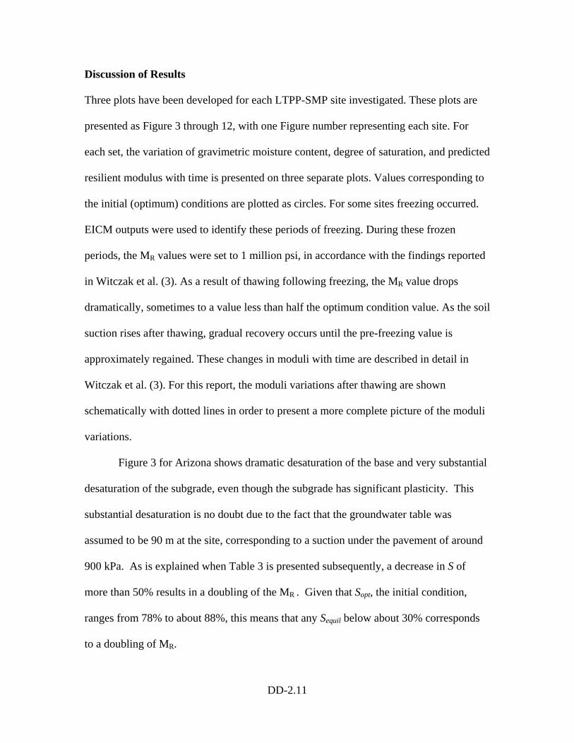
DD-2.11
Discussion of Results
Three plots have been developed for each LTPP-SMP site investigated. These plots are
presented as Figure 3 through 12, with one Figure number representing each site. For
each set, the variation of gravimetric moisture content, degree of saturation, and predicted
resilient modulus with time is presented on three separate plots. Values corresponding to
the initial (optimum) conditions are plotted as circles. For some sites freezing occurred.
EICM outputs were used to identify these periods of freezing. During these frozen
periods, the MR values were set to 1 million psi, in accordance with the findings reported
in Witczak et al. (3). As a result of thawing following freezing, the MR value drops
dramatically, sometimes to a value less than half the optimum condition value. As the soil
suction rises after thawing, gradual recovery occurs until the pre-freezing value is
approximately regained. These changes in moduli with time are described in detail in
Witczak et al. (3). For this report, the moduli variations after thawing are shown
schematically with dotted lines in order to present a more complete picture of the moduli
variations.
Figure 3 for Arizona shows dramatic desaturation of the base and very substantial
desaturation of the subgrade, even though the subgrade has significant plasticity. This
substantial desaturation is no doubt due to the fact that the groundwater table was
assumed to be 90 m at the site, corresponding to a suction under the pavement of around
900 kPa. As is explained when Table 3 is presented subsequently, a decrease in S of
more than 50% results in a doubling of the MR . Given that Sopt, the initial condition,
ranges from 78% to about 88%, this means that any Sequil below about 30% corresponds
to a doubling of MR.
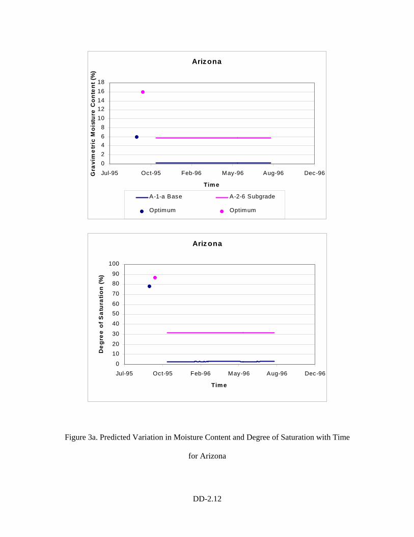
DD-2.12
Arizona
02468
1012141618
Jul-95 Oct-95 Feb-96 May-96 Aug-96 Dec-96
Tim e
Gra
vim
etri
c M
oist
ure
Con
tent
(%)
A-1-a Base A-2-6 Subgrade
Optimum Optimum
Arizona
0
1020
30
40
5060
70
8090
100
Jul-95 Oct-95 Feb-96 May-96 Aug-96 Dec-96
Tim e
Deg
ree
of S
atur
atio
n (%
)
Figure 3a. Predicted Variation in Moisture Content and Degree of Saturation with Time
for Arizona
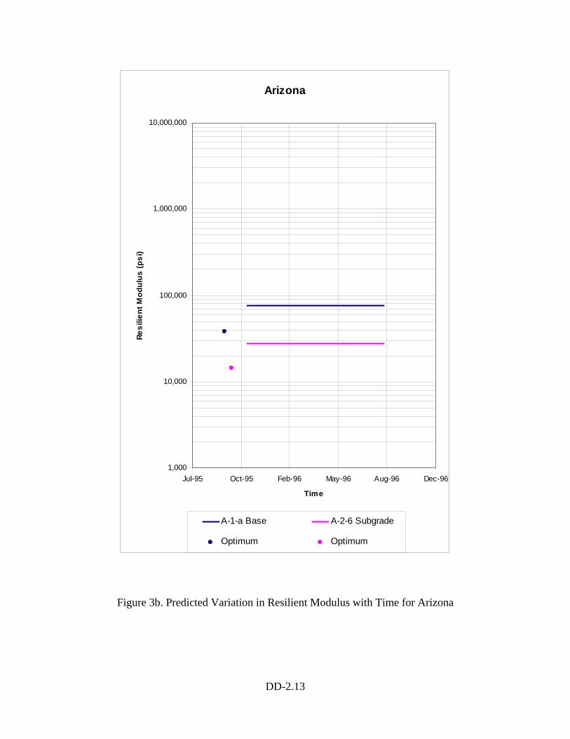
DD-2.13
Arizona
1,000
10,000
100,000
1,000,000
10,000,000
Jul-95 Oct-95 Feb-96 May-96 Aug-96 Dec-96
Time
Resi
lient
Mod
ulus
(psi
)
A-1-a Base A-2-6 Subgrade
Optimum Optimum
Figure 3b. Predicted Variation in Resilient Modulus with Time for Arizona
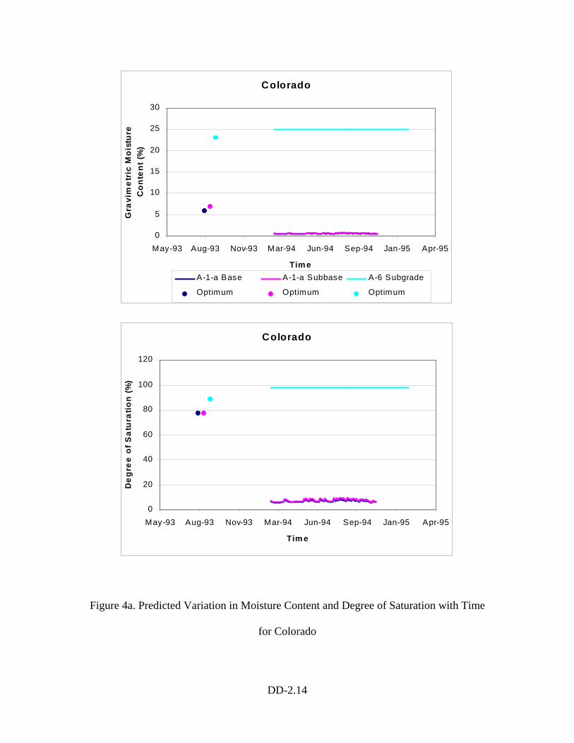
DD-2.14
Colorado
0
5
10
15
20
25
30
May-93 Aug-93 Nov-93 Mar-94 Jun-94 Sep-94 Jan-95 Apr-95
Tim e
Gra
vim
etri
c M
oist
ure
Con
tent
(%)
A-1-a Base A-1-a Subbase A-6 Subgrade
Optimum Optimum Optimum
Colorado
0
20
40
60
80
100
120
May-93 Aug-93 Nov-93 Mar-94 Jun-94 Sep-94 Jan-95 Apr-95
Tim e
Deg
ree
of S
atur
atio
n (%
)
Figure 4a. Predicted Variation in Moisture Content and Degree of Saturation with Time
for Colorado
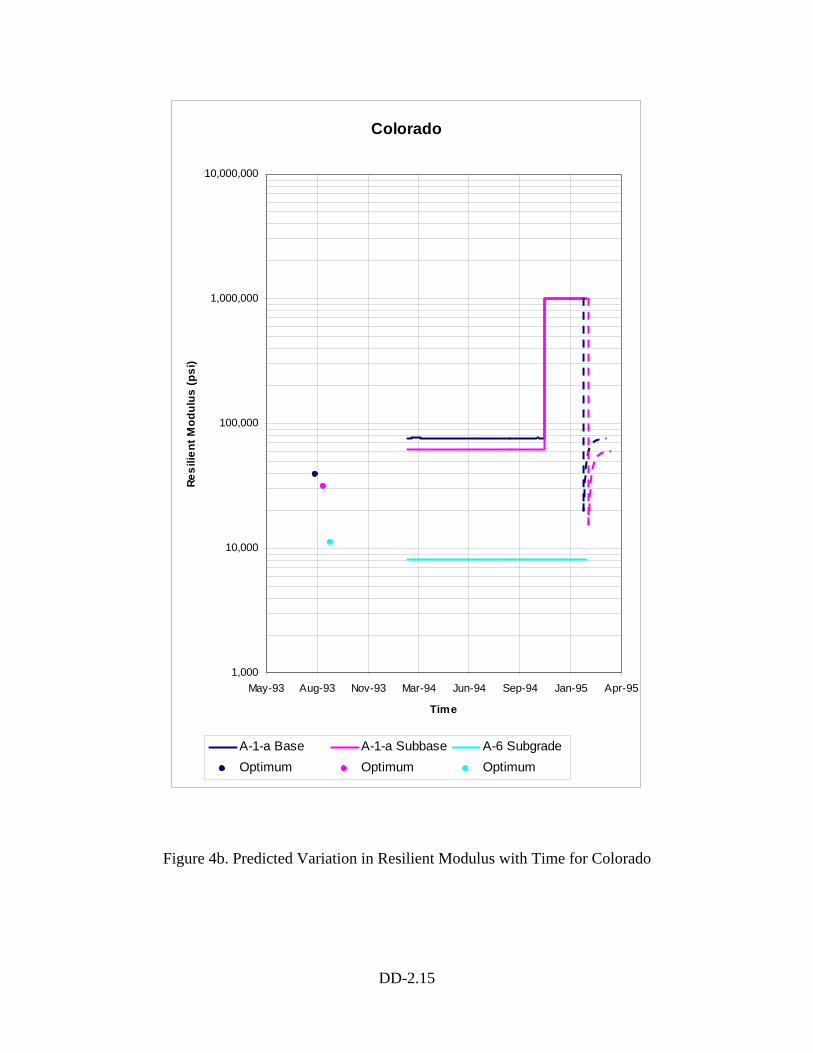
DD-2.15
Colorado
1,000
10,000
100,000
1,000,000
10,000,000
May-93 Aug-93 Nov-93 Mar-94 Jun-94 Sep-94 Jan-95 Apr-95
Time
Resi
lient
Mod
ulus
(psi
)
A-1-a Base A-1-a Subbase A-6 SubgradeOptimum Optimum Optimum
Figure 4b. Predicted Variation in Resilient Modulus with Time for Colorado
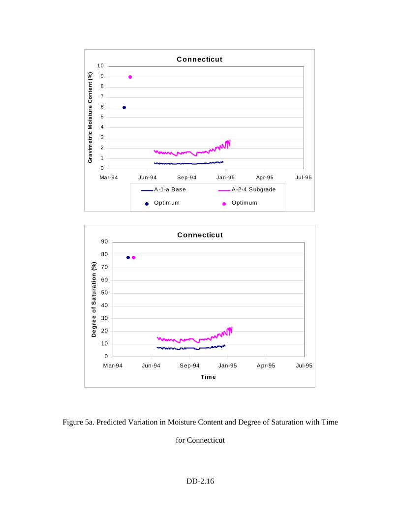
DD-2.16
Connecticut
0
1
2
3
4
5
6
7
8
9
10
Mar-94 Jun-94 Sep-94 Jan-95 Apr-95 Jul-95
Time
Gra
vim
etri
c M
oist
ure
Con
tent
(%)
A-1-a Base A-2-4 Subgrade
Optimum Optimum
Connecticut
0
10
20
30
40
50
60
70
80
90
Mar-94 Jun-94 Sep-94 Jan-95 Apr-95 Jul-95
Tim e
Deg
ree
of S
atur
atio
n (%
)
Figure 5a. Predicted Variation in Moisture Content and Degree of Saturation with Time
for Connecticut
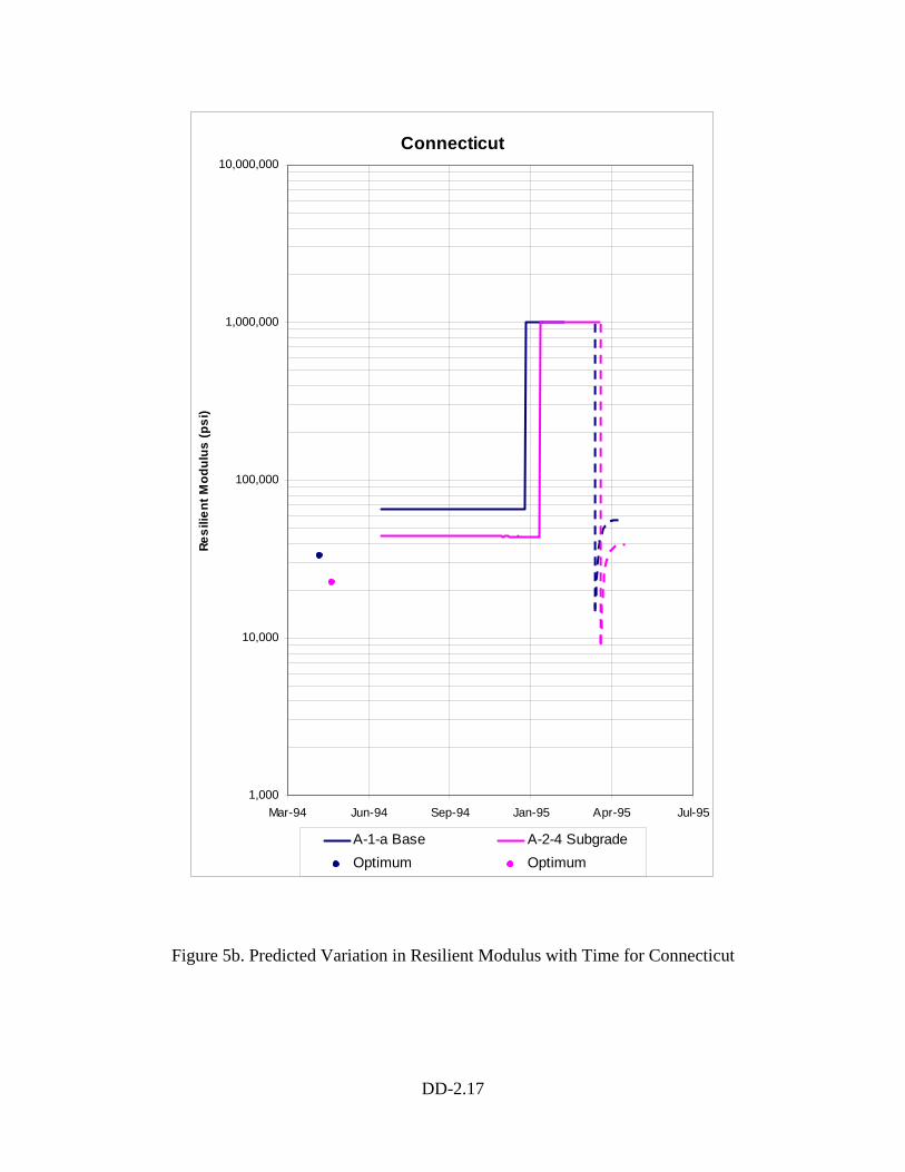
DD-2.17
Connecticut
1,000
10,000
100,000
1,000,000
10,000,000
Mar-94 Jun-94 Sep-94 Jan-95 Apr-95 Jul-95
Time
Resi
lient
Mod
ulus
(psi
)
A-1-a Base A-2-4 SubgradeOptimum Optimum
Figure 5b. Predicted Variation in Resilient Modulus with Time for Connecticut
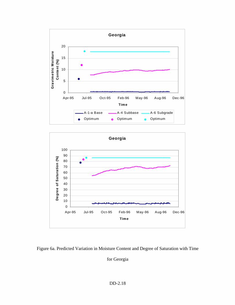
DD-2.18
Georgia
0
5
10
15
20
Apr-95 Jul-95 Oct-95 Feb-96 May-96 Aug-96 Dec-96
Tim e
Gra
vim
etri
c M
oist
ure
Con
tent
(%)
A-1-a Base A-4 Subbase A-6 Subgrade
Optimum Optimum Optimum
Georgia
0
1020
30
40
5060
70
8090
100
Apr-95 Jul-95 Oct-95 Feb-96 May-96 Aug-96 Dec-96
Tim e
Deg
ree
of S
atur
atio
n (%
)
Figure 6a. Predicted Variation in Moisture Content and Degree of Saturation with Time
for Georgia
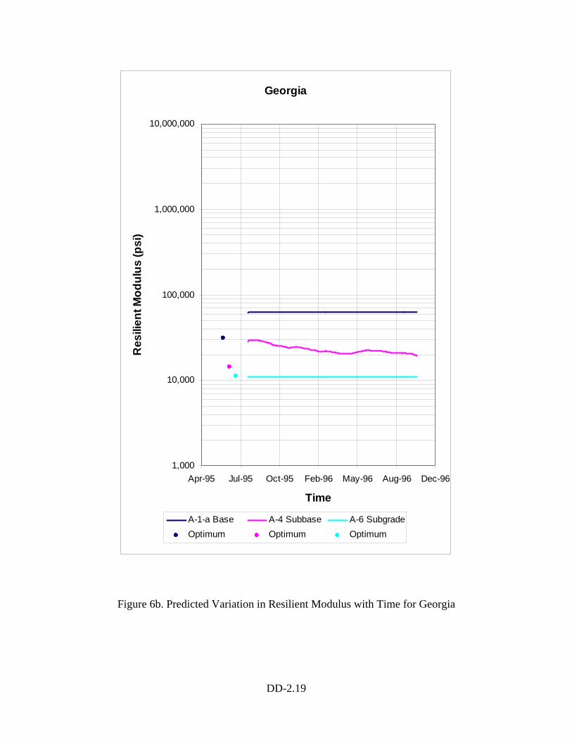
DD-2.19
Georgia
1,000
10,000
100,000
1,000,000
10,000,000
Apr-95 Jul-95 Oct-95 Feb-96 May-96 Aug-96 Dec-96
Time
Res
ilien
t Mod
ulus
(psi
)
A-1-a Base A-4 Subbase A-6 SubgradeOptimum Optimum Optimum
Figure 6b. Predicted Variation in Resilient Modulus with Time for Georgia
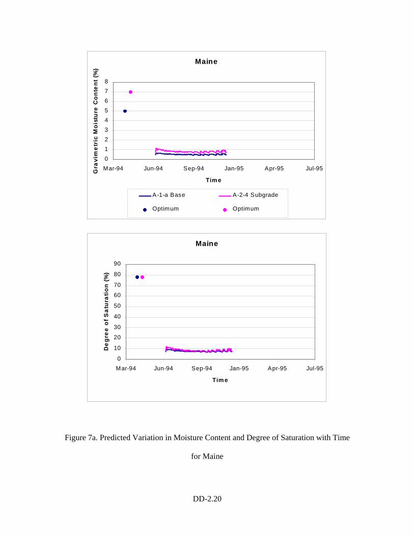
DD-2.20
Maine
012345678
Mar-94 Jun-94 Sep-94 Jan-95 Apr-95 Jul-95
Tim e
Gra
vim
etri
c M
oist
ure
Con
tent
(%)
A-1-a Base A-2-4 Subgrade
Optimum Optimum
Maine
0
10
20
30
40
50
60
70
80
90
Mar-94 Jun-94 Sep-94 Jan-95 Apr-95 Jul-95
Tim e
Deg
ree
of S
atur
atio
n (%
)
Figure 7a. Predicted Variation in Moisture Content and Degree of Saturation with Time
for Maine
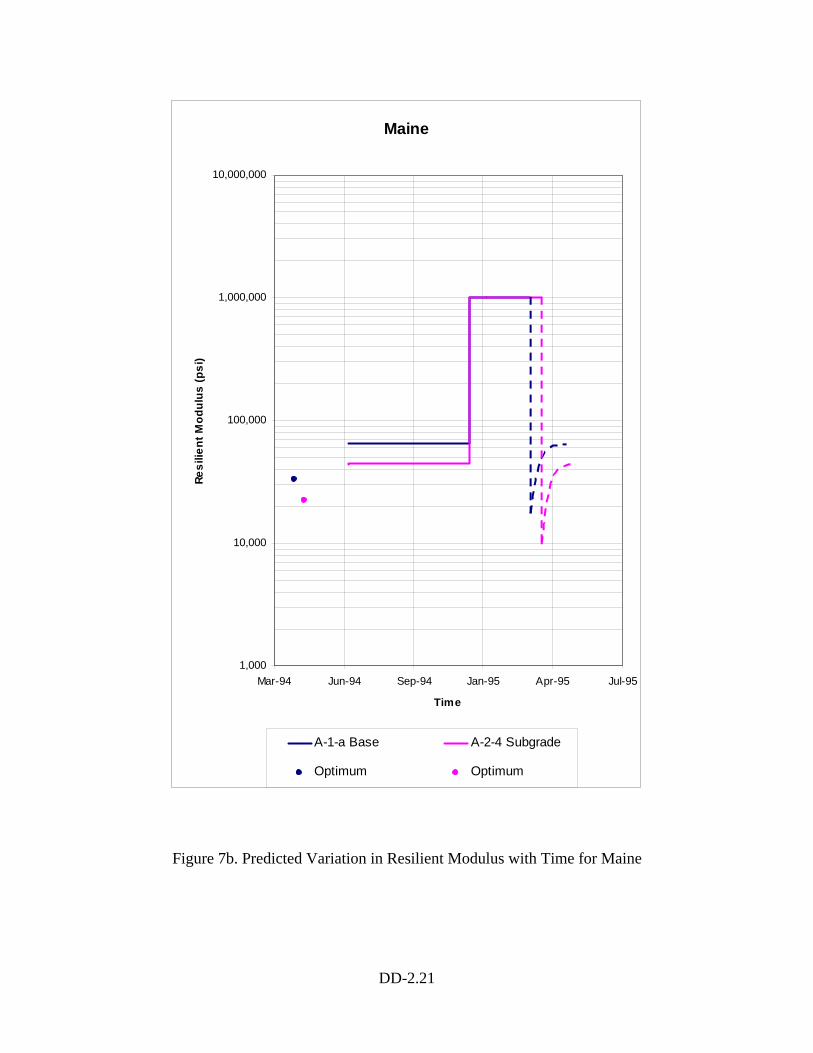
DD-2.21
Maine
1,000
10,000
100,000
1,000,000
10,000,000
Mar-94 Jun-94 Sep-94 Jan-95 Apr-95 Jul-95
Time
Resi
lient
Mod
ulus
(psi
)
A-1-a Base A-2-4 Subgrade
Optimum Optimum
Figure 7b. Predicted Variation in Resilient Modulus with Time for Maine
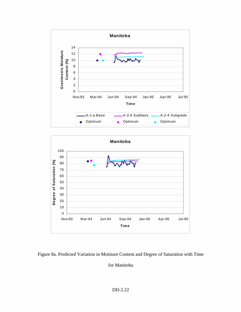
DD-2.22
Manitoba
0
2
4
6
8
10
12
14
Nov-93 Mar-94 Jun-94 Sep-94 Jan-95 Apr-95 Jul-95
Tim e
Gra
vim
etri
c M
oist
ure
Con
tent
(%)
A-1-a Base A-2-6 Subbase A-2-4 Subgrade
Optimum Optimum Optimum
Manitoba
0
10
20
30
40
50
60
70
80
90
100
Nov-93 Mar-94 Jun-94 Sep-94 Jan-95 Apr-95 Jul-95
Tim e
Deg
ree
of S
atur
atio
n (%
)
Figure 8a. Predicted Variation in Moisture Content and Degree of Saturation with Time
for Manitoba
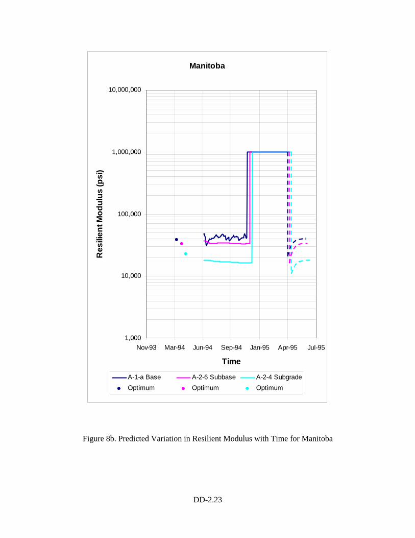
DD-2.23
Manitoba
1,000
10,000
100,000
1,000,000
10,000,000
Nov-93 Mar-94 Jun-94 Sep-94 Jan-95 Apr-95 Jul-95
Time
Res
ilien
t Mod
ulus
(psi
)
A-1-a Base A-2-6 Subbase A-2-4 SubgradeOptimum Optimum Optimum
Figure 8b. Predicted Variation in Resilient Modulus with Time for Manitoba
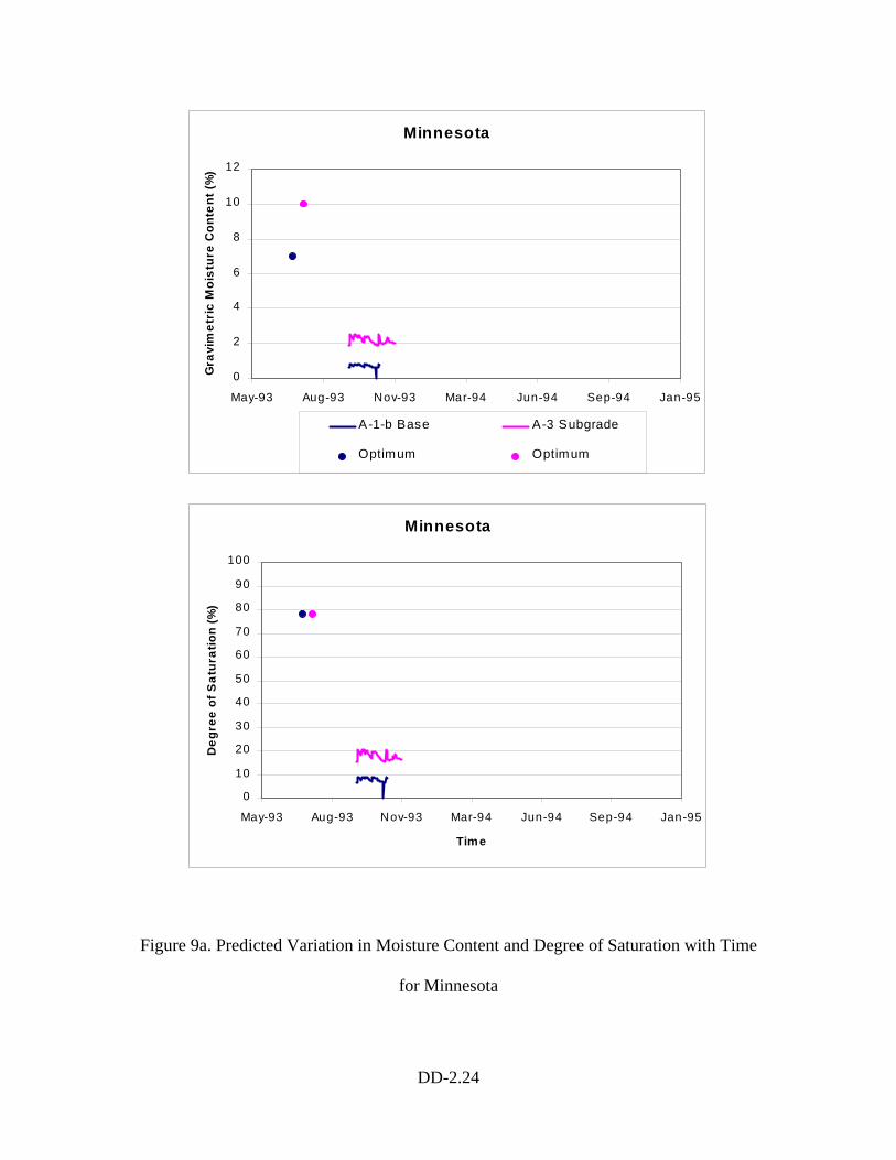
DD-2.24
Minnesota
0
2
4
6
8
10
12
May-93 Aug-93 Nov-93 Mar-94 Jun-94 Sep-94 Jan-95
Time
Gra
vim
etri
c M
oist
ure
Con
tent
(%)
A-1-b Base A-3 Subgrade
Optimum Optimum
Minnesota
0
10
20
30
40
50
60
70
80
90
100
May-93 Aug-93 Nov-93 Mar-94 Jun-94 Sep-94 Jan-95
Time
Deg
ree
of S
atur
atio
n (%
)
Figure 9a. Predicted Variation in Moisture Content and Degree of Saturation with Time
for Minnesota
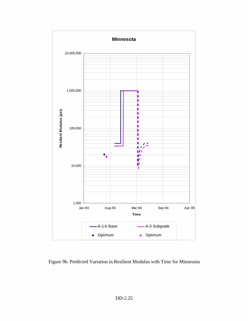
DD-2.25
Minnesota
1,000
10,000
100,000
1,000,000
10,000,000
Jan-93 Aug-93 Mar-94 Sep-94 Apr-95
Time
Resi
lient
Mod
ulus
(psi
)
A-1-b Base A-3 Subgrade
Optimum Optimum
Figure 9b. Predicted Variation in Resilient Modulus with Time for Minnesota
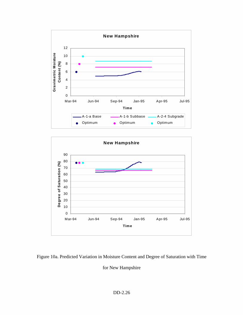
DD-2.26
New Hampshire
0
2
4
6
8
10
12
Mar-94 Jun-94 Sep-94 Jan-95 Apr-95 Jul-95
Tim e
Gra
vim
etri
c M
oist
ure
Con
tent
(%)
A-1-a Base A-1-b Subbase A-2-4 Subgrade
Optimum Optimum Optimum
New Hampshire
0
10
20
30
40
50
60
70
80
90
Mar-94 Jun-94 Sep-94 Jan-95 Apr-95 Jul-95
Tim e
Deg
ree
of S
atur
atio
n (%
)
Figure 10a. Predicted Variation in Moisture Content and Degree of Saturation with Time
for New Hampshire
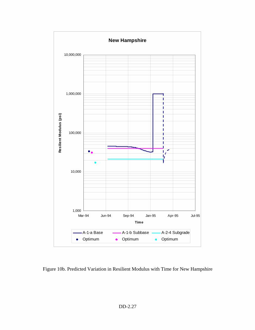
DD-2.27
New Hampshire
1,000
10,000
100,000
1,000,000
10,000,000
Mar-94 Jun-94 Sep-94 Jan-95 Apr-95 Jul-95
Time
Resi
lient
Mod
ulus
(psi
)
A-1-a Base A-1-b Subbase A-2-4 SubgradeOptimum Optimum Optimum
Figure 10b. Predicted Variation in Resilient Modulus with Time for New Hampshire
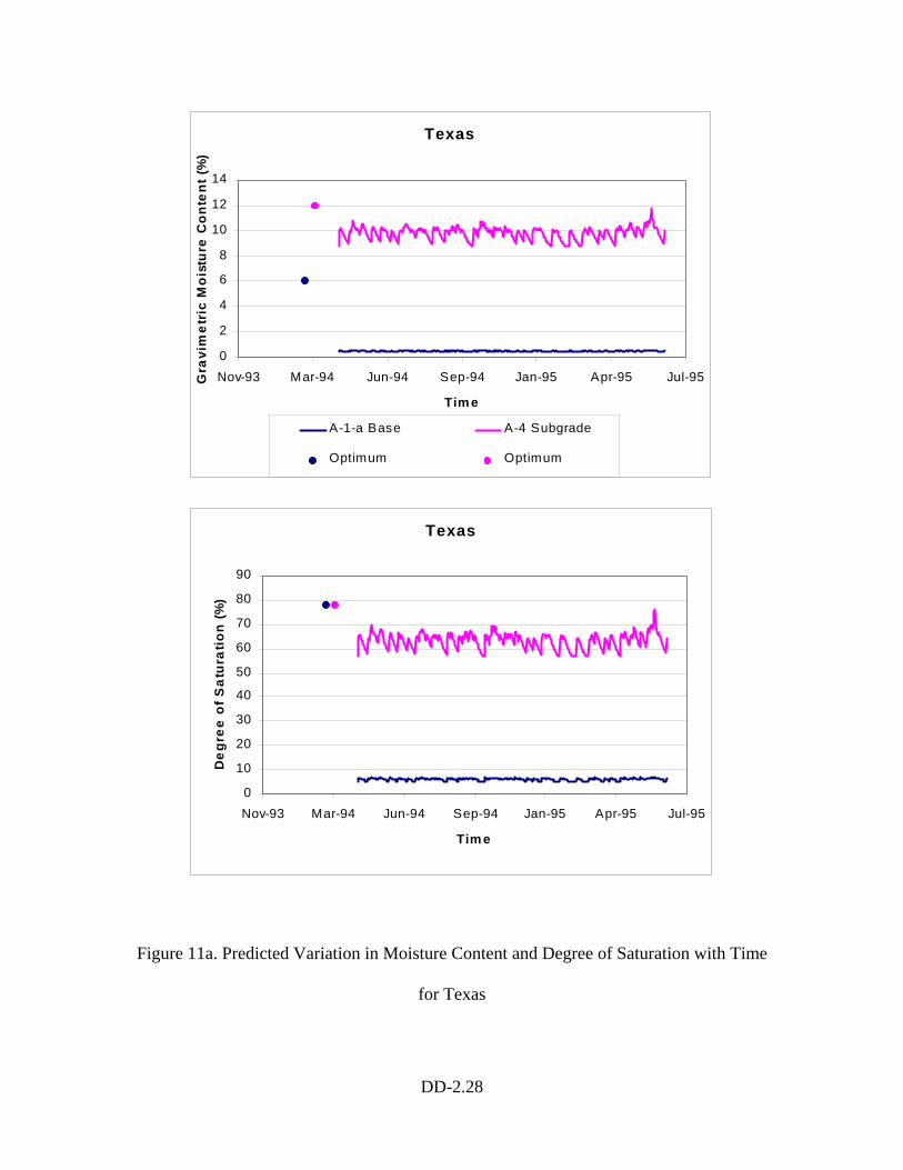
DD-2.28
Texas
0
2
4
6
8
10
12
14
Nov-93 Mar-94 Jun-94 Sep-94 Jan-95 Apr-95 Jul-95
Tim e
Gra
vim
etri
c M
oist
ure
Con
tent
(%)
A-1-a Base A-4 Subgrade
Optimum Optimum
Texas
0
10
20
30
40
50
60
70
80
90
Nov-93 Mar-94 Jun-94 Sep-94 Jan-95 Apr-95 Jul-95
Tim e
Deg
ree
of S
atur
atio
n (%
)
Figure 11a. Predicted Variation in Moisture Content and Degree of Saturation with Time
for Texas
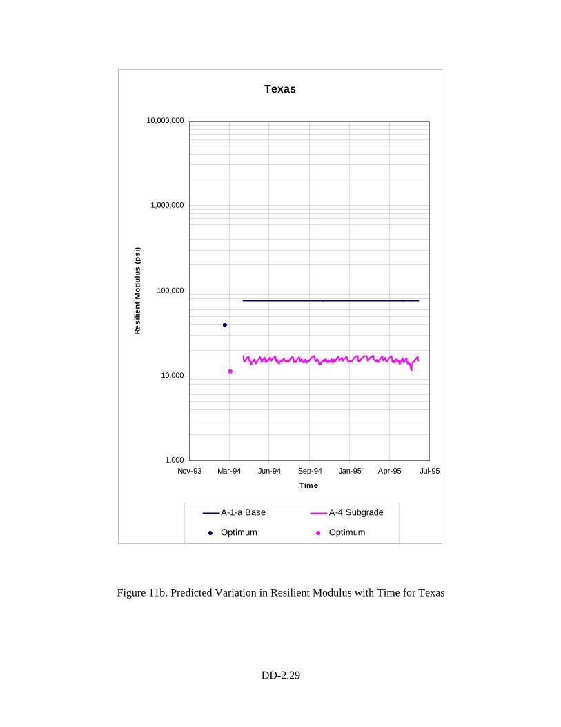
DD-2.29
Texas
1,000
10,000
100,000
1,000,000
10,000,000
Nov-93 Mar-94 Jun-94 Sep-94 Jan-95 Apr-95 Jul-95
Time
Resi
lient
Mod
ulus
(psi
)
A-1-a Base A-4 Subgrade
Optimum Optimum
Figure 11b. Predicted Variation in Resilient Modulus with Time for Texas
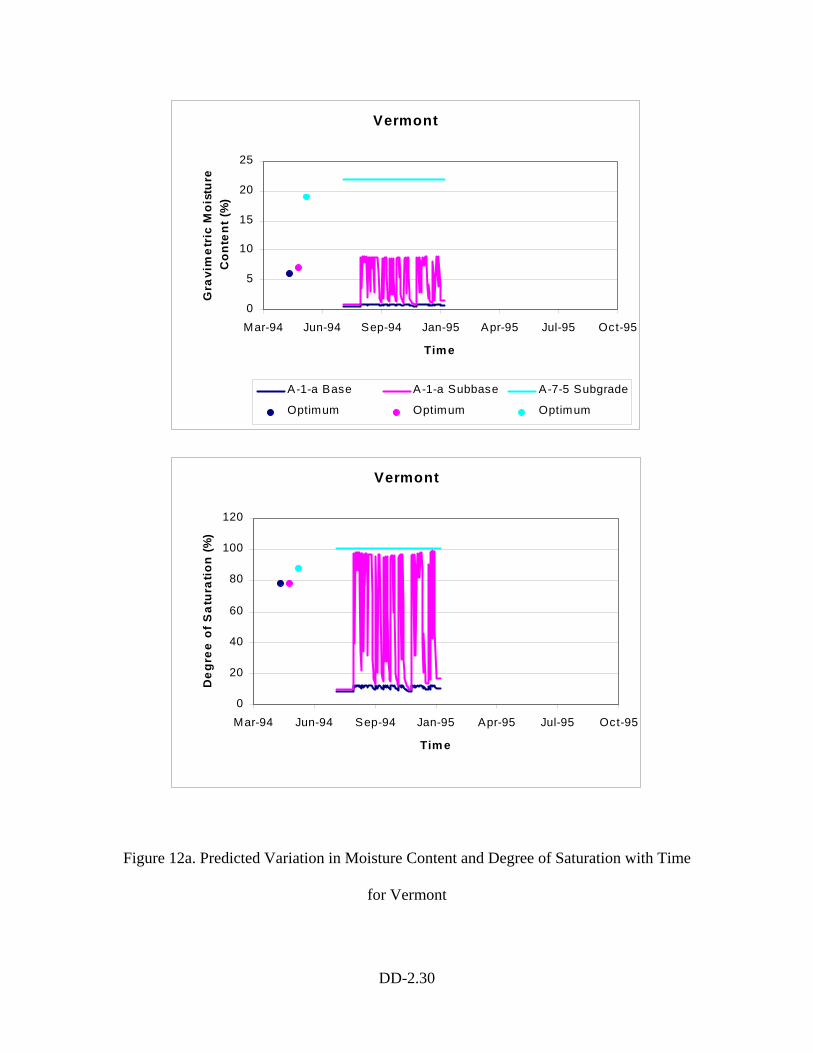
DD-2.30
Vermont
0
5
10
15
20
25
Mar-94 Jun-94 Sep-94 Jan-95 Apr-95 Jul-95 Oct-95
Tim e
Gra
vim
etri
c M
oist
ure
Con
tent
(%)
A-1-a Base A-1-a Subbase A-7-5 Subgrade
Optimum Optimum Optimum
Vermont
0
20
40
60
80
100
120
Mar-94 Jun-94 Sep-94 Jan-95 Apr-95 Jul-95 Oct-95
Tim e
Deg
ree
of S
atur
atio
n (%
)
Figure 12a. Predicted Variation in Moisture Content and Degree of Saturation with Time
for Vermont
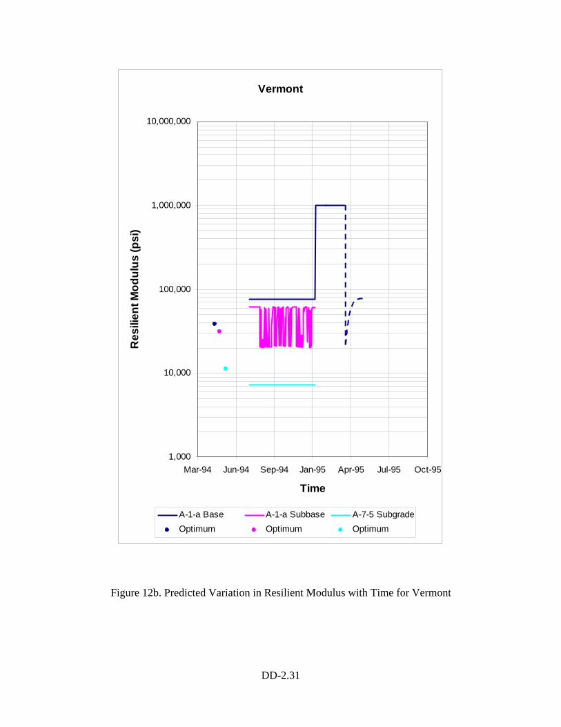
DD-2.31
Vermont
1,000
10,000
100,000
1,000,000
10,000,000
Mar-94 Jun-94 Sep-94 Jan-95 Apr-95 Jul-95 Oct-95
Time
Res
ilien
t Mod
ulus
(psi
)
A-1-a Base A-1-a Subbase A-7-5 SubgradeOptimum Optimum Optimum
Figure 12b. Predicted Variation in Resilient Modulus with Time for Vermont
DD-2.32
All sites except Manitoba and New Hampshire likewise exhibited marked
desaturation of the base. The base for these two had a small amount of plasticity and
were able to retain water under the modest suctions imposed. Sometimes the subbases, if
present, and subgrades desatutated substantially and sometimes they did not, depending
on plasticity. The Vermont subgrade (Figure 12) went to Sequil=100%, but the point of
computation chosen was only 6 cm above the GWT (in fact it was sometimes submerged
due to GWT oscillations). The subgrade at the Vermont site was also fairly high
plasticity and very low permeability. Therefore it was unable to accept quickly the
rainfall water (through cracks in the A/C) from above. The unusually high oscillations in
the subbase degree of saturation were caused by the temporary accumulation of this
water. If the EICM were 2-D and able to account for lateral drainage then perhaps these
oscillations would be damped to some degree.
In almost all cases the MR values followed the expected pattern of being highest
for base, lowest for subgrade and intermediate for subbase. A minor exception is New
Hampshire (Figure 10), but the descriptions of the base and subbase were sufficiently
similar that the initial MRopt values were almost identical.
Use of Hand Calculations as a Check on EICM Output
Given the wPI product, the value of Sopt can readily be manually (electronically)
computed from Equation 7. Once the moisture content at a particular point in the profile
has stabilized to an equilibrium level; then oscillations occur about this value. In general,
these oscillations are due to oscillations in the depth to groundwater (GWT) and due to
rainfall, if the A/C layer has any cracks. In a great majority of cases, these oscillations

DD-2.33
can be seen to have very minor effects on MR, as shown by the plots of MR versus time
for the 10 LTPP sites (Figures 3 through 12). If the effects due to rainfall are more or
less neglected, then the equilibrium degree of saturation, Sequil, can be hand-calculated by
the following procedure.
1. Estimate the average depth, Dequil, from the point in question to the GWT in
meters, for the period of interest.
2. Calculate the equilibrium soil suction, (ua – uw)equil by (ua – uw)equil = γwDequil
3. Use wPI or D60 to select a soil-water characteristic curve, SWCC, from Figure
13.
4. Enter the SWCC with (ua – uw)equil and pick off Sequil in %.
This procedure was followed for 7 layers in 5 sites as shown in Table 3. Consider the
base for the GA site as the first example.
Step 1. Dequil = 4.9 m
Step 2. (ua – uw)equil = (9.81) × (4.9) = 48 kPa
Step 3. D60 = 8.7 mm, but the SWCCs are "capped" at 1 mm. Therefore, use the 1
mm SWCC curve.
Step 4. Enter with (ua – uw) = 48 kPa to get Sequil = 5.5 %
The computations have been carried a couple of steps further in Table 3. The value of
Sopt has been calculated from Equation 7 to be 78%. Thus, (Sequil – Sopt) is -72.5%.
Equation 1 yields the modulus adjustment factor = 2.00, meaning that MR, after drying
from optimum (S = 78%) to Sequil = 5.5%, is 2.00 times the MRopt.
For comparison, consider the EICM output in Figure 6 for GA. The value of Sequil
for the base is about 6.3%, which makes (Sequil – Sopt) = -71.7%. The modulus adjustment
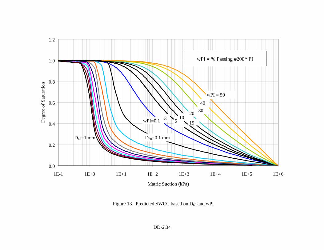
DD-2.34
Figure 13. Predicted SWCC based on D60 and wPI
0.0
0.2
0.4
0.6
0.8
1.0
1.2
1E-1 1E+0 1E+1 1E+2 1E+3 1E+4 1E+5 1E+6
Matric Suction (kPa)
D60=1 mm
wPI=0.1
wPI = 50
3 510
15
20 3040
D60=0.1 mm
wPI = % Passing #200* PI
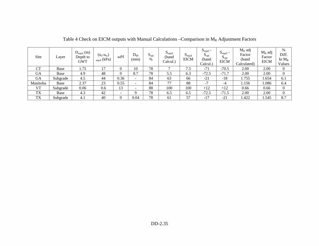
DD-2.35
Table 4 Check on EICM outputs with Manual Calculations –Comparison in MR Adjustment Factors
Site Layer Dequil (m) Depth to
GWT
(uo-uw) equil (kPa) wPI D60
(mm) Sopt %
Sequil (hand
Calcul.)
Sequil EICM
Sequil - Sopt
(hand Calcul.)
Sequil - Sopt
EICM
MR adj Factor (hand
Calculated)
MR adj Factor EICM
% Diff. In MR Values
CT Base 1.75 17 0 10 78 7 7.5 -71 -70.5 2.00 2.00 0 GA Base 4.9 48 0 8.7 78 5.5 6.3 -72.5 -71.7 2.00 2.00 0 GA Subgrade 4.5 44 0.36 - 84 63 66 -21 -18 1.755 1.654 6.1
Manitoba Base 2.37 23 0.55 - 84 77 88 -7 -4 1.156 1.086 6.4 VT Subgrade 0.06 0.6 13 - 88 100 100 +12 +12 0.66 0.66 0 TX Base 4.3 42 - 9 78 6.5 6.5 -72.5 -71.5 2.00 2.00 0 TX Subgrade 4.1 40 0 0.04 78 61 57 -17 -21 1.422 1.545 8.7
DD-2.36
factor is again 2.00, because the curve adopted in Figure 1 flattens out for (S – Sopt)
values lower than -50%.
As a second example, consider the subgrade for GA.
Step 1. Dequil = 4.5 m
Step 2. (ua – uw)equil = (9.81) × (4.5) = 44 kPa
Step 3. wPI = 0.36, which requires some interpolation in Figure 13 .
Step 4. Enter with (ua – uw) = 44 kPa to get Sequil = 63 %
Continuing with the computations indicated in Table 3, Sopt = 84% from Equation 7 and
(Sequil – Sopt) for the hand calculations is -21% and the modulus adjustment factor is 1.755.
Figure 6 for GA shows that Sequil (EICM) for the same period is about 66% ± 3%. Using
Sequil (EICM) = 66%, (Sequil – Sopt) = -18% and the modulus adjustment factor is 1.654.
Given no error in the EICM input data, one would assume that the EICM values would be
superior, because the EICM model accounts for climatic factors and time dependency. If
one assumes the EICM answer is the right answer, then Table 3 shows that, for these
examples, the error suffered by using the simplified hand calculation is typically less than
8 or 10% and sometimes as little as zero, particularly for the non-plastic bases and
subbases which typically dry to S less than 30% (Sequil – Sopt < -50%). The last three
columns of Table 3 also show that there is no reason to suspect substantial error in the
EICM input (or output) for these examples.
DD-2.37
Conclusions
1. For compaction at optimum conditions the degree of saturation, Sopt, and the
optimum water content, wopt, have been correlated with wPI and D60, as has been
Gs. These correlations appear adequate for satisfactorily predicting e, n, and γdmax
and will be recommended for Levels 2 and 3.
2. Optimum conditions; i.e. γd = γd max and w = wopt and S = Sopt are a logical choice
for:
a) The reference condition for evaluation of MR
and
b) The initial conditions at compaction for unbound layers of the pavement
section in the field.
3. The use of Sopt as the initial condition and the use of wPI and D60 correlations to
obtain Sopt, wopt, and Gs, together with the employment of these values to generate
initial input data for the EICM, guarantees that the initial So = Sopt and output
values of S from the EICM will be reasonable or at least less than 100%. Thus the
use of this approach avoids the dramatically spurious spikes in calculated mass –
volume relationships which have been found to be very common when using
reported data from the LTPP database files.
4. The model relating changes in modular ratios to changes in degree of saturation
presented herein appears quite satisfactory for quantifying the effects of moisture
content changes.
5. In a fairly large majority of the cases, the changes in MR which occur due to the
change from So = Sopt to Sequil are considerably larger that the seasonal oscillations
DD-2.38
which occur after the equilibrium state is reached. In fact, it appears that it is a
satisfactorily good engineering approximation to simply assume the MR values are
constant and equal to an average equilibrium value, except during periods of
freezing, thawing, and recovery from thawing.
6. The use of the manual calculation procedure presented for estimation of the Sequil
value has two potentially useful applications:
a) It can be used to check the reasonableness of the EICM output – to check for
an EICM input data error, for example.
b) It can be used as an independent method for estimating Sequil when the EICM
is not used.
Recommendations – General
1. The optimum condition; i.e., γd = γd max, w = wopt , and S = Sopt should be adopted
as:
a) The reference condition for evaluation of MR
b) The initial condition for compacted unbound pavement layers in the field.
2. If actual lab test measurement data are not available, the correlations for Sopt, wopt,
and Gs with wPI and D60 should be used to estimate Sopt, wopt and Gs which are
then used to compute e, n, and γd max as needed for input to the EICM and other
applications relating to MR determinations.
3. The model represented by Equation 1 and illustrated in Figures 1 and 2 should be
used to estimate MR / MRopt.
DD-2.39
4. The hand calculation procedure presented herein should be used (a) to check the
reasonableness of the EICM results for Sequil and (b) to evaluate Sequil when the
EICM is not used.
Recommendations – Relative to the Implementation of the MR Model into the 2002
Guide
The primary objective of the MR studies was to develop a basis and procedure for
determination of MR values for use in the 2002 Guide. Based on the studies completed
and results obtained to date, the following recommendations for implementation are
made.
Unbound Compacted Layers
Level 1
1. Assume initial compacted conditions are γd = γdmax, w = wopt. Use γdmax and wopt for
T180 for bases and use T99 for subbases and subgrades.
2. For each layer measure γdmax, wopt and GS.
3. For each layer measure MRopt for a range of confining pressures and stress levels to
obtain k1, k2 and k3.
4. Use the output from the EICM to estimate the moisture change from the optimum
condition to the equilibrium condition, Sequil – Sopt.
5. Use Equation 1 to estimate MR/MRopt and MR for each layer, to account for moisture
change.
6. Account for change in moduli due to freezing, thawing, and recovery using the
recommendations outlined in Witczak et al. (3).
Level 2
1. Assume initial compacted conditions are γd = γdmax, w = wopt. Use γdmax and wopt for
T180 for bases and use T99 for subbases and subgrades.
DD-2.40
2. Use correlations with index properties and material descriptions to estimate k1, k2 and
k3 parameters corresponding to optimum conditions.
3. Use these ki values to estimate MRopt.
4. Use the output from the EICM to estimate the moisture change from the optimum
condition to the equilibrium condition, Sequil – Sopt.
5. Use Equation 1 to estimate MR/MRopt and MR for each layer, to account for moisture
change.
6. Account for change in moduli due to freezing, thawing, and recovery using the
recommendations outlined in Witczak et al. (3).
Level 3
1. Use soil descriptions and index properties to estimate CBR for each layer.
2. Use MRopt = 2555 CBR0.64 to estimate MRopt for each layer.
3. Use the output from the EICM to estimate the moisture change from the optimum
condition to the equilibrium condition, Sequil – Sopt.
4. Use Equation 1 to estimate MR/MRopt and MR for each layer, to account for moisture
change.
5. Account for change in moduli due to freezing, thawing, and recovery using the
recommendations outlined in Witczak et al. (3).
In-Situ Natural Material Below Compacted Layers
Level 1
1. Use seismic profiling with 10’-15’ geophone spacing to characterize the upper 15’ to
20’ via seismic velocity (vp for deep GWT, and vs for shallow GWT).
2. Use vp and/or vs to compute low-strain MR values and correct these values for strain
level and frequency. Adopt these values as equilibrium values for MR, which are at
equilibrium with the average moisture regime.
3. Account for change in moduli due to freezing, thawing, and recovery using the
recommendations outlined in Witczak et al. (3).

DD-2.41
As a less preferred, less accurate alternative:
1. Use index properties and soil descriptions to estimate k1, k2 and k3 for the in-situ
layers and use the ki to estimate MRequil = MRunfrz.
2. Account for change in moduli due to freezing, thawing, and recovery using the
recommendations outlined in Witczak et al. (3).
Level 2
1. Use seismic profiling with 10’-15’ geophone spacing to characterize the upper 15’ to
20’ via seismic velocity (vp for deep GWT, and vs for shallow GWT).
2. Use vp and/or vs to compute low-strain MR values and correct these values for strain
level and frequency. Adopt these values as equilibrium values for MR, which are at
equilibrium with the average moisture regime.
3. Account for change in moduli due to freezing, thawing, and recovery using the
recommendations outlined in Witczak et al. (3).
As a less preferred, less accurate alternative:
1. Use index properties and soil descriptions to estimate k1, k2 and k3 for the in-situ
layers and use the ki to estimate MRequil.
2. Account for change in moduli due to freezing, thawing, and recovery using the
recommendations outlined in Witczak et al. (3).
Level 3
1. Use soil descriptions and index properties to estimate CBR for each layer.
2. Use MR = 2555 CBR0.64 to estimate MR for each layer.
3. Neglect moisture oscillation effects.
4. Account for change in moduli due to freezing, thawing, and recovery using the
recommendations outlined in Witczak et al. (3).
DD-2.42
References
1. Witczak M.W., Andrei D. and Houston W.N. Resilient Modulus as Function of Soil Moisture – Summary of Predictive Models. Development of the 2002 Guide for the Development of New and Rehabilitated Pavement Structures, NCHRP 1-37 A, Inter Team Technical Report (Seasonal 1), June 2000.
2. Witczak M.W., Houston W.N., Zapata C.E., Richter C., Larson G. and Walsh K.
Improvement of the Integrated Climatic Model for Moisture Content Predictions. Development of the 2002 Guide for the Development of New and Rehabilitated Pavement Structures, NCHRP 1-37 A, Inter Team Technical Report (Seasonal 4), June 2000.
3. Witczak M.W., Houston W.N. and Andrei D. Selection of Resilient Moduli for
Frozen/Thawed Unbound Materials. Development of the 2002 Guide for the Development of New and Rehabilitated Pavement Structures, NCHRP 1-37 A, Inter Team Technical Report (Seasonal 3), June 2000.
4. Yoder E.J. and Witczak M.W. Principles of Pavement Design. 2nd edition, New York,
John Wiley and Sons Inc., 1975.
Copy No.
Guide for Mechanistic-Empirical Design OF NEW AND REHABILITATED PAVEMENT
STRUCTURES
FINAL DOCUMENT
APPENDIX DD-3: SELECTION OF RESILIENT MODULI FOR
FROZEN/THAWED UNBOUND MATERIALS
NCHRP
Prepared for National Cooperative Highway Research Program
Transportation Research Board National Research Council
Submitted by ARA, Inc., ERES Division
505 West University Avenue Champaign, Illinois 61820
June 2000
ii
Acknowledgment of Sponsorship This work was sponsored by the American Association of State Highway and Transportation Officials (AASHTO) in cooperation with the Federal Highway Administration and was conducted in the National Cooperative Highway Research Program which is administered by the Transportation Research Board of the National Research Council. Disclaimer This is the final draft as submitted by the research agency. The opinions and conclusions expressed or implied in this report are those of the research agency. They are not necessarily those of the Transportation Research Board, the National Research Council, the Federal Highway Administration, AASHTO, or the individual States participating in the National Cooperative Highway Research program. Acknowledgements The research team for NCHRP Project 1-37A: Development of the 2002 Guide for the Design of New and Rehabilitated Pavement Structures consisted of Applied Research Associates, Inc., ERES Consultants Division (ARA-ERES) as the prime contractor with Arizona State University (ASU) as the primary subcontractor. Fugro-BRE, Inc., the University of Maryland, and Advanced Asphalt Technologies, LLC served as subcontractors to either ARA-ERES or ASU along with several independent consultants. Research into the subject area covered in this Appendix was conducted at ASU. The authors of this Appendix are Dr. M.W. Witczak, Dr. W.N. Houston, and Mr. Dragos Andrei. Dr. M.W. Witczak provided overall guidance and coordination of the efforts of the 2002 Design Guide Team, including work plan development, scheduling, assignment of personnel and tasks and technical review of results as they became available. In connection with the current report he also identified key sources of data and performed the final review of the report. Dr. W.N. Houston provided supervision and guidance to the study Graduate Research Assistant, Mr. Dragos Andrei. Dr. W.N. Houston also reviewed publications, extracted and synthesized data, and drafted the initial report. Mr. Dragos Andrei located and secured all data sources, reviewed pertinent publications, extracted and synthesized data where available and assisted with the report (drafts and final) preparation. Foreword This appendix presents the derivation of reasonable values of MR for both frozen and thawed unbound materials through evaluation of published results.. The information contained in this appendix serves as a supporting reference to the resilient modulus discussions presented and PART 2, Chapter 3, and PART 3, Chapters 3, 4, 6, and 7 of the Design Guide.

iii
This appendix is the third in a series of four volumes on environmental effects on pavements. The other volumes are: Appendix DD-1: Resilient Modulus As Function Of Soil Moisture-Summary Of
Predictive Models Appendix DD-2: Resilient Modulus As Function Of Soil Moisture – A Study Of
The Expected Changes In Resilient Modulus Of The Unbound Layers With Changes In Moisture For 10 LTPP Sites
Appendix DD-4: Improvement Of The Integrated Climatic Model for Moisture
iv
Abstract
The purpose of this study was to derive reasonable values of MR for both frozen
and thawed unbound materials through evaluation of published results. The values of MR
for frozen materials were extracted as absolute values of MRfrz. For thawed materials the
focus was on a reduction factor, RF, which could be multiplied times the unfrozen
(normal) modulus, MRunfrz, to get the modulus after thawing, MRmin. The following values
were found to be reasonable for the material types indicated: coarse-grained materials –
MRfrz ~ 3*106 psi; Fine-grained silts and silty sands – MRfrz ~ 2*106 psi; clays – MRfrz ~
1*106 psi. Average values of RF and ranges in RF were found for gravel, sand, silt and
clay. In consideration of all data collected it was possible to develop recommendations
for RF as function of % passing no. 200 sieve, P200, and plasticity index, PI. An algorithm
is proposed for using these MRfrz and RF values in conjunction with EICM to produce
time-varying values of MR at a point, throughout the year.
v
Table of Contents
Page
Introduction..........................................................................................................................1
Objective ..............................................................................................................................3
Background..........................................................................................................................3
Results of Literature Search.................................................................................................9
Summary and Conclusions ................................................................................................26
Recommendations..............................................................................................................27
References..........................................................................................................................33
vi
List of Tables
Page
Table 1. Values of Unfrozen, Frozen, and Thawed MR from the Literature .....................10
Table 2. Team Synthesis of MR Values for Frozen Materials ..........................................14
Table 3. Corps of Engineers (COE) Frost-Susceptibility Classification ..........................18
Table 4. Criteria Developed by Others for Predicting Frost-Susceptibility of Soils .........23
Table 5. Change in CBR During Thaw Weakening Period ...............................................24
Table 6. Recommended Values of RF for Coarse-Grained Materials (P200 < 50%)..........28
Table 7. Recommended Values of RF for Fine-Grained Materials (P200 > 50%) .............28
vii
List of Figures
Page
Figure 1. Schematic of Ice Lens Formation.........................................................................4
Figure 2. Relationship Between P200 and P0.02 ...................................................................20
Figure 3. Relationship Between Frost-Heave and P200. .....................................................21
Figure 4. Relationship Between Frost-Heave and PI.........................................................22
Figure 5. Example of Time-Varying MR ...........................................................................32

DD-3.1
SELECTION OF RESILIENT MODULI FOR FROZEN/THAWED UNBOUND
MATERIALS
Introduction
The overall task of evaluating the expected cumulative damage due to load
associated distress of a pavement system involves numerous subtasks as follows:
Subtask 1: Evaluation of resilient modulus, MR, at some reference condition, such as
optimum water content and maximum dry density, as a function of soil type or
gradation or classification.
Subtask 2: Evaluation of expected changes in moisture content, both from the initial or
reference condition and seasonally.
Subtask 3: Evaluation of the effect on MR of changes in soil moisture content with
respect to the reference condition as well as seasonally.
Subtask 4: Evaluation of the effect on MR of changes in material density with respect to
the reference condition.
Subtask 5: Evaluation of the effect of freezing on MR.
Subtask 6: Evaluation of the effect of thawing on MR.
Subtask 7: Utilization of time-varying MR values in the computation of critical pavement
response parameters at various points within the pavement system.
Various studies relevant to the above subtasks are currently in progress at ASU
and some of these studies have already been completed or are near completion as of the
DD-3.2
date of this report. The findings and recommendations from these studies are presented in
a series of Inter Team Technical Reports, and are described as:
I. Improvement of the Integrated Climatic Model for Moisture Content
Predictions by Dr. M.W. Witczak, Dr. W.N. Houston, Dr. C.E. Zapata, Ms.
Cheryl Richter, Mr. G. Larson and Dr. K. Walsh. Development of the 2002 Guide
for the Development of New and Rehabilitated Pavement Structures, NCHRP 1-
37 A, Inter Team Technical Report (Seasonal 4), June 2000 (Relates to Subtask
2).
II. Resilient Modulus as Function of Soil Moisture – Summary of Predictive
Models by Dr. M.W. Witczak, Mr. D. Andrei and Dr. W.N. Houston.
Development of the 2002 Guide for the Development of New and Rehabilitated
Pavement Structures, NCHRP 1-37 A, Inter Team Technical Report (Seasonal 1),
June 2000 (Relates to Subtasks 1, 3 and 4).
III. Resilient Modulus as Function of Soil Moisture – A Study of the Expected
Changes in Resilient Modulus of the Unbound Layers with Changes in
Moisture for 10 LTPP Sites by Dr. M.W. Witczak, Dr. W.N. Houston and Mr.
D. Andrei. Development of the 2002 Guide for the Development of New and
Rehabilitated Pavement Structures, NCHRP 1-37 A, Inter Team Technical Report
(Seasonal 2), June 2000 (Relates to Subtasks 3 and 4).
IV. Selection of Resilient Modului for Frozen/Thawed Materials – by Dr. M.W.
Witczak, Dr. W.N. Houston and Mr. D. Andrei. Development of the 2002 Guide
for the Development of New and Rehabilitated Pavement Structures, NCHRP 1-
DD-3.3
37 A, Inter Team Technical Report (Seasonal 3), (the current report) June 2000
(Relates to Subtasks 5 and 6).
Objective
The objective of the current report was to use existing data from the literature to
evaluate the effects of freezing and thawing on MR of unbound base, subbase and
subgrade soils. The relevance of these studies to the overall task of evaluating expected
load associated damage of pavement systems is indicated by the preceding list of
subtasks.
Background
Before presenting the results of the literature search for the MR values for frozen
and thawed materials, background information describing the conditions leading to frost
action in soil is provided.
Ice Lenses Formation
When water in soil freezes, the water itself undergoes about a 9 % volume
increase (2). Thus a saturated or nearly saturated soil with 35 % porosity would
experience about a 3 % volume increase with a corresponding heave of the ground
surface. Unsaturated soils would exhibit smaller volume changes in accordance with the
degree of saturation. These volume changes are what is expected when no water is added
to the water initially present in the material. However, under special circumstances
freezing may be accompanied by the formation of ice lenses that can range from
millimeters to several centimeters in thickness. These lenses are usually more or less pure
DD-3.4
ice and can cause the ground surface to heave as much as several tens of centimeters (see
Figure 1). When they occur under pavements the resulting damage can arise from two
sources. First, the heave is likely to be differential. Secondly and more importantly, the
melted lens may become a temporary water-filled void with little or no bearing strength.
In any case, the excess water, unless quickly drained, may create a zone of greatly
reduced strength and produce pavement distress if the pavement is loaded before
recovery.
In order to anticipate the formation of ice lenses it is necessary to understand their
mechanism of formation. In the field a freezing front almost always advances from the
surface downward. Thus ice lenses tend to be oriented horizontally. When the water in
soil freezes, adjacent water from below is pulled toward the newly formed ice. Because
freezing below the ground water table (GWT) does not usually occur, the zone of interest
is the capillary zone above the GWT, where the soil water is in tension. When water is
pulled upward toward an ice lens, it moves in response to a fairly substantial gradient in
soil moisture suction because the force of gravity must be overcome. Thus the freezing of
water results in a local depression of the water pressure (or a rise in soil moisture
suction). If water can be supplied to the ice lens fast enough, it will continue to grow in
thickness. However, if the rate of water supply is insufficient, the freezing front will
advance downward and the upward progressing water will be “frozen in its tracks”. A
new ice lens may or may not be formed at greater depth.
Two factors are important to the rate of water supply to the growing ice lenses.
First, the hydraulic conductivity of the soil must be high enough to sustain a substantial
flow of water. Secondly, the GWT must be reasonably shallow, so that the head loss
DD-3.5
between the GWT and the ice lenses is not too great. The saturated hydraulic
conductivity of a soil is controlled by its gradation, or the size of its largest connected
pores. Therefore a medium or coarser sand would appear to be capable of supplying
water to the ice lenses quite adequately. However, a medium or coarser sand in the
capillary zone is not likely to be initially fully saturated, and furthermore it tends to
desaturate dramatically with increase in soil moisture suction (19). Its unsaturated
hydraulic conductivity is typically too low to sustain ice lens growth. A clay of medium
or higher plasticity has strong water retention capacity and remains at rather high degree
of saturation under substantial soil moisture suction. Therefore it might initially be
assumed that it could supply water at a rate sufficient to sustain ice lens growth.
However, these clays have an inherent hydraulic conductivity (i.e. the saturated hydraulic
conductivity) which is too low to sustain ice lens growth. The elimination of clean,
medium and coarser sands and clays of medium and higher plasticity leaves us with silts,
very fine silty sands and sandy silts, and silty clays of low plasticity as “frost-heave
susceptible soils”. These soils have sufficient water retention capacity that they do not
desaturate more or less completely when subjected to significant soil moisture tension. In
addition, these soils exhibit an inherent hydraulic conductivity which is adequate to
sustain ice lens growth, provided the ground water table is nearby and unobstructed. The
boundaries between frost-heave susceptible and non-frost-heave susceptible soils can be
shifted by altering the normal rate of freezing, by retardation of heat removal for
example. However, for the environmental and boundary conditions which normally ensue
in the field, the frost-heave susceptible soils are those listed above. Thus, the necessary
conditions for ice lens formation can be listed:
DD-3.6
1. A frost-heave susceptible soil, as defined above;
2. Prolonged freezing temperature;
3. A supply of water, such as a nearby, unobstructed GWT.
An example of an obstruction between the GWT and an ice lens could be a clean granular
layer, which desaturates under significant soil moisture suction, or a layer of plastic clay,
whose hydraulic conductivity is too low to sustain ice lens growth. However, even if the
frost-heave-susceptible soil extends all the way to the GWT, ice lenses will not form
unless the GWT is nearby, typically a very few meters.
Traditional Remedy for Frost-Susceptible Soils
Because the necessary conditions for ice lens formation have long been
recognized, it is possible to formulate a rather simple, straightforward engineering policy
for dealing with these frost-heave-susceptible soils:
When the conditions favorable to ice lens formation exist, determine the typical,
local depth of freezing empirically and remove and replace frost heave
susceptible soils to this depth.
This procedure probably has been followed fairly consistently by pavement engineers for
the last few decades, but there are certainly notable exceptions to the successful execution
of the general policy. In addition, it has been widely recognized that thawing after
freezing, even in the absence of significant ice lens formation, results in a degradation of
the resilient modulus which can be quite substantial. These effects are described
generally in the next section.
DD-3.7
Degradation of Resilient Modulus due to Thawing
When any soil freezes and then thaws, regardless of whether it is non-frost
susceptible or frost susceptible, there is some degradation of the resilient modulus, even
in the absence of significant ice lens formation. The most plausible explanation for this
degradation is as follows. Even though ice lens formation may not be significant, or
visible, it appears that some water is added to the frozen zone during freezing. This
addition, together with the expansion associated with ice formation, tends to break some
of the particle contacts and interlocking of soil grains. When thawing occurs, the soil-
water mixture behaves as if there were excess water in the thawed zone and soil moisture
suction typically falls to near zero. The reduced soil suction and broken particle
contacts/bonds are in themselves sufficient to explain the observed loss in MR, which can
be as high as 50 or 60%.
The excess water and reduced soil moisture suction readjust with time, as adjacent
layers absorb the excess water and cause the soil suction in the thawed zone to rise.
Eventually this excess water is transmitted by unsaturated flow to the GWT, as the soil
suction and moisture content return to their normal values. The return of the soil suction
to its normal value is accompanied by a return of the MR to its normal value. The duration
of this recovery period is dependent on geometry and the hydraulic conductivity of the
soils involved. Therefore, not surprisingly, granular soils recover much faster than clays.
The characterization of silts, silty sands, and silty clays as frost-heave-susceptible
in the preceding section can be thought of as the classical characterization of frost-
susceptible soils. This classical characterization speaks to the potential for a soil to form
ice lenses when conditions are appropriate. In the last few decades, non-destructive field
DD-3.8
testing, such as FWD, and laboratory resilient testing have been commonplace and it has
been found that essentially all soils are frost-susceptible to some degree, when MR
degradation is used as the measuring stick. Clean granular soils are the least susceptible,
clays are substantially susceptible, and silty soils are the most susceptible. Thus, a more
modern definition of frost susceptibility rates soils with respect to their reduction in MR
upon thawing. Of course it is still true that if a soil actually experiences ice lens
formation and then thaws, the reduction in modulus will be dramatic, typically much
more than if ice lenses do not form. However, it is generally assumed that when highly
frost-heave-susceptible soils combine with conditions strongly favoring ice lens
formation, these soils have been removed and replaced. This assumption seems to prevail
in the research studies presented in the next section, wherein researchers have measured
and estimated loss in MR due to thawing up to a maximum of about 60% loss.
Results of literature search
Literature sources were consulted and salient values of moduli, MR, and ratios of
moduli were extracted. The objective of the search was to obtain absolute values of
moduli for frozen material, termed MRfrz, and the ratio of MR just after thawing, termed
MRmin, to the MR of natural, unfrozen material, termed MRunfrz. The ratio is used as a
reduction factor, termed RF. These definitions are repeated in equation form below.
MRfrz = MRmax = MR for frozen material
MRunfrz = the normal MR for unfrozen material
MRmin = MR just after thawing
RF = modulus reduction factor = MRmin/MRunfrz (1)
DD-3.9
All of the raw data collected is presented in Table 1 and the values for frozen
materials are summarized in Table 2. Most of the data will be discussed in the paragraphs
which follow.
Results from studies at the USACE-CRREL (Cold Regions Research and
Engineering Laboratories) were reported by Berg et al (2). Of most relevance to the
present study are the MRfrz values which range from 0.6 *106 psi for a CL to 7*106 psi for
a dense graded stone. Numerous values of MRfrz were extracted from the Vinson and the
Czajkowski and Vinson papers (17, 8). Their values of MRfrz ranged from about 0.4*106
psi for a silt to about 7*106 psi for a gravel. These values were collected in Table 2 and
averaged for coarse-grained materials (MRfrz_ave ~ 3*106 psi), fine-grained silt and silty
sands (MRfrz_ave ~ 2*106 psi) and clays (MRfrz_ave ~ 1*106 psi).
Of particular interest to the present report is a study reported by Janoo and Berg
(11). They constructed four test sections in the CRREL Research Facility, with the
following characteristics:
• 5cm < thickness of A/C <15 cm
• 0 < thickness of base (GP) + subbase (SW) < 38cm
• all subgrades were plastic clay (CH)
• for both base and subbase, 6% < P200 < 10%, where P200 = % passing the no.
200 sieve
They used several tools and devices to conduct the research, with heavy emphasis on
FWD results. Their key findings are as follows:

DD-3.10
a) The FWD deflections were not much affected until the thaw depths reached
well into the CH subgrade. Therefore, the sand and gravel subbase and base
with 6% - 10% fines showed almost no weakening due to thawing.
b) After substantial thawing of the CH subgrade, the ratio of the 4th sensor
deflection for unfrozen material to the 4th sensor deflection for thawed
material ranged from 50% to 60%. Assuming MR of the subgrade is inversely
proportional to 4th sensor deflection, 50% < RF for CH subgrade < 60%.
c) The authors state, without presenting data, that commonly used RF values
ranged from 50% to 85%.
d) The measured thaw depth correlated well with total area of the FWD
deflection basin.
Esch et al. also presented a very interesting study of 120 sections of highway in
Alaska (9). Their study sections exhibited the following characteristics:
• sections were 0.5 to 1.0 miles long
• some sections exhibited “good” performance
• some sections exhibited “poor” performance; fatigue (alligator cracking) was
the primary measure of distress
• there were very few soils in the profile with significant PI
• there were very few uniform sands or clays; most materials were gravels and
silts, with a substantial range in % fines (P200).
Their most important findings are as follows:
a) They performed a regression analysis of 175 material, dimensional, and
environmental factors with performance. This analysis yielded no useful
DD-3.11
predictions. Only after grouping sections into good performance and poor
performance and looking at factors individually were they able to get some
fairly good correlations.
b) The best indicator of performance was found to be the percent passing the No.
200 sieve (P200):
If P200 < 6%, good performance
If P200 > 11%, poor performance
c) The next best indicator was found to be the percent passing the 0.02 mm sieve
(P0.02mm):
If P0.02mm < 3%, good performance
If P0.02mm > 7%, poor performance
Janoo et al. performed a rather extensive literature review and presented a number
of useful findings and recommendations, some of which are reproduced in the current
report (11). The first is the Corps of Engineers (COE) frost-susceptibility classification,
shown as Table 3. Their original table provided gradation data relative to P0.02mm only.
Because P200 is somewhat easier to obtain and more frequently available, the team has
chosen to focus on P200. The last column showing P200 in Table 3 was estimated by using
the Janoo et al. correlation, which is shown as Figure 2 (11). Figures 3 and 4, from Janoo
et al., show the sensitivity of frost heave to P200 and PI respectively (11). Frost heave of
greater than 18 mm is considered to be very frost-heave susceptible and 13 to 18 mm is
marginal. Table 4 shows that the values of P200 used to separate frost-susceptible from
non-frost-susceptible materials vary significantly around the country and around the
world.
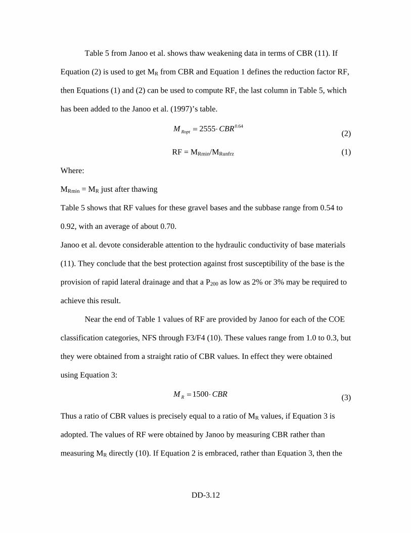
DD-3.12
Table 5 from Janoo et al. shows thaw weakening data in terms of CBR (11). If
Equation (2) is used to get MR from CBR and Equation 1 defines the reduction factor RF,
then Equations (1) and (2) can be used to compute RF, the last column in Table 5, which
has been added to the Janoo et al. (1997)’s table.
64.02555 CBRM Ropt ⋅= (2)
RF = MRmin/MRunfrz (1)
Where:
MRmin = MR just after thawing
Table 5 shows that RF values for these gravel bases and the subbase range from 0.54 to
0.92, with an average of about 0.70.
Janoo et al. devote considerable attention to the hydraulic conductivity of base materials
(11). They conclude that the best protection against frost susceptibility of the base is the
provision of rapid lateral drainage and that a P200 as low as 2% or 3% may be required to
achieve this result.
Near the end of Table 1 values of RF are provided by Janoo for each of the COE
classification categories, NFS through F3/F4 (10). These values range from 1.0 to 0.3, but
they were obtained from a straight ratio of CBR values. In effect they were obtained
using Equation 3:
CBRM R ⋅= 1500 (3)
Thus a ratio of CBR values is precisely equal to a ratio of MR values, if Equation 3 is
adopted. The values of RF were obtained by Janoo by measuring CBR rather than
measuring MR directly (10). If Equation 2 is embraced, rather than Equation 3, then the
DD-3.13
RF values shown in parentheses in Table 1 are obtained. In fact, algebraic manipulation
of Equations 2 and 3 shows that:
64.0CBRRFRF = (4)
Where:
RFCBR = reduction factor obtained from a ratio of CBR values.
Thus the values in Table 1 under Janoo not in parentheses are values of RFCBR and
Equation 4 shows why the values in parentheses are a little higher (10). All other values
of RF in Table 1 and the values in parentheses are as defined by Equation 1. Because
Equation 2 for MR is embraced by the authors of this report, it follows that RF is
embraced by the authors rather than RFCBR.
Summary and Conclusions
Considerations of the mechanisms of frost action and the data obtained from the
literature search, particularly the thorough study by Janoo et al., make it possible to reach
some useful conclusions which can be summarized as follows (11):
1. The conditions necessary for ice lens formation are:
• A frost-heave-susceptible soil such as silt, silty sand or silty
clay with low PI;
• Prolonged freezing temperatures;
• A source of water, such as a nearby, unobstructed GWT.
2. The classical or traditional definition of frost-susceptibility focuses on the
likelihood of significant ice lens formation, under the favorable conditions
cited above.
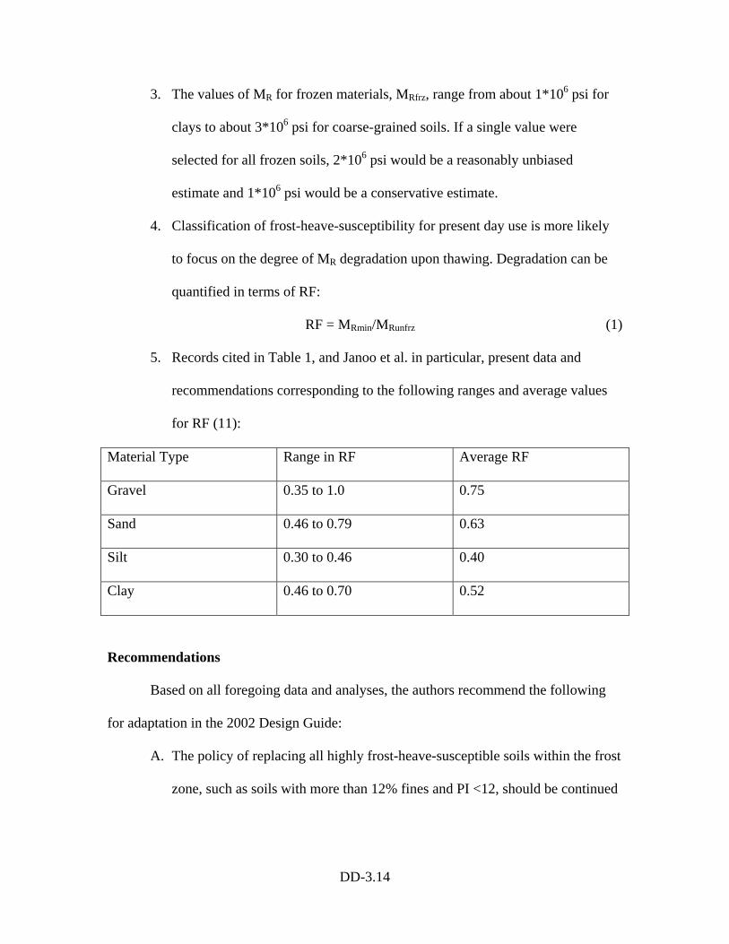
DD-3.14
3. The values of MR for frozen materials, MRfrz, range from about 1*106 psi for
clays to about 3*106 psi for coarse-grained soils. If a single value were
selected for all frozen soils, 2*106 psi would be a reasonably unbiased
estimate and 1*106 psi would be a conservative estimate.
4. Classification of frost-heave-susceptibility for present day use is more likely
to focus on the degree of MR degradation upon thawing. Degradation can be
quantified in terms of RF:
RF = MRmin/MRunfrz (1)
5. Records cited in Table 1, and Janoo et al. in particular, present data and
recommendations corresponding to the following ranges and average values
for RF (11):
Material Type Range in RF Average RF
Gravel 0.35 to 1.0 0.75
Sand 0.46 to 0.79 0.63
Silt 0.30 to 0.46 0.40
Clay 0.46 to 0.70 0.52
Recommendations
Based on all foregoing data and analyses, the authors recommend the following
for adaptation in the 2002 Design Guide:
A. The policy of replacing all highly frost-heave-susceptible soils within the frost
zone, such as soils with more than 12% fines and PI <12, should be continued
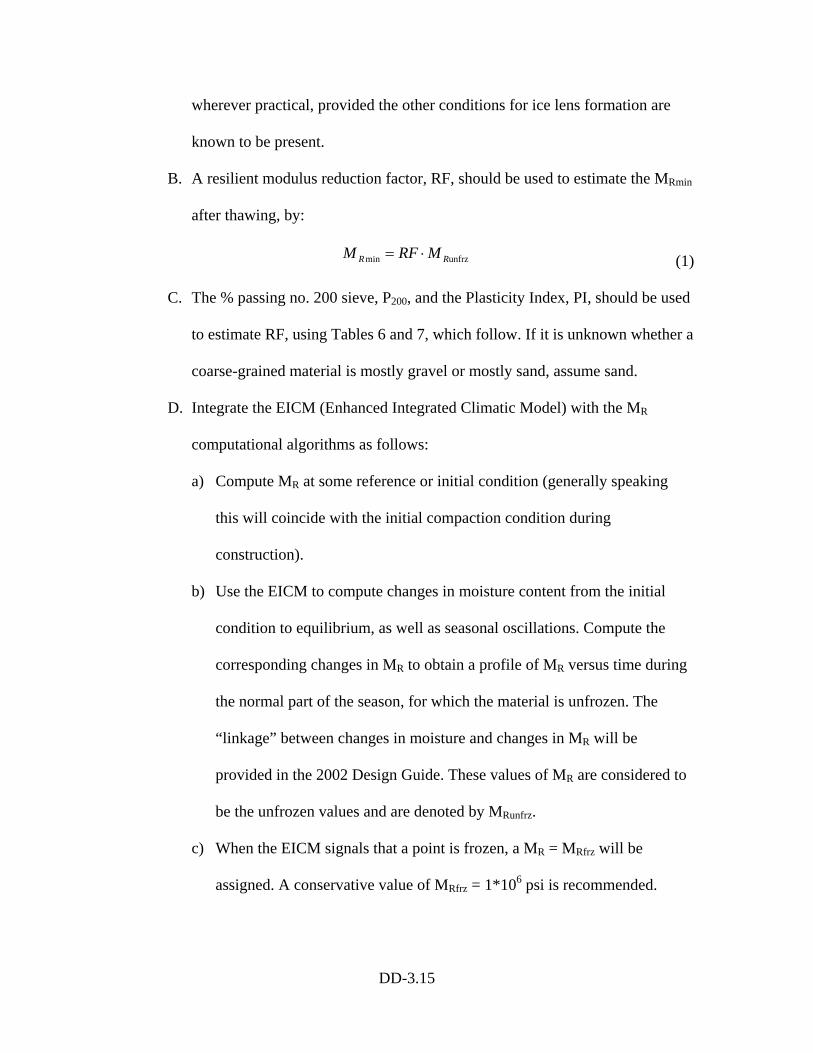
DD-3.15
wherever practical, provided the other conditions for ice lens formation are
known to be present.
B. A resilient modulus reduction factor, RF, should be used to estimate the MRmin
after thawing, by:
unfrzmin RR MRFM ⋅= (1)
C. The % passing no. 200 sieve, P200, and the Plasticity Index, PI, should be used
to estimate RF, using Tables 6 and 7, which follow. If it is unknown whether a
coarse-grained material is mostly gravel or mostly sand, assume sand.
D. Integrate the EICM (Enhanced Integrated Climatic Model) with the MR
computational algorithms as follows:
a) Compute MR at some reference or initial condition (generally speaking
this will coincide with the initial compaction condition during
construction).
b) Use the EICM to compute changes in moisture content from the initial
condition to equilibrium, as well as seasonal oscillations. Compute the
corresponding changes in MR to obtain a profile of MR versus time during
the normal part of the season, for which the material is unfrozen. The
“linkage” between changes in moisture and changes in MR will be
provided in the 2002 Design Guide. These values of MR are considered to
be the unfrozen values and are denoted by MRunfrz.
c) When the EICM signals that a point is frozen, a MR = MRfrz will be
assigned. A conservative value of MRfrz = 1*106 psi is recommended.
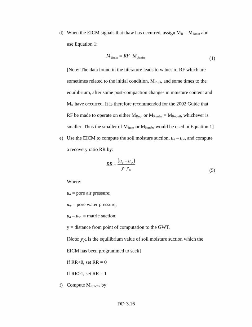
DD-3.16
d) When the EICM signals that thaw has occurred, assign MR = MRmin and
use Equation 1:
unfrzmin RR MRFM ⋅= (1)
[Note: The data found in the literature leads to values of RF which are
sometimes related to the initial condition, MRopt, and some times to the
equilibrium, after some post-compaction changes in moisture content and
MR have occurred. It is therefore recommended for the 2002 Guide that
RF be made to operate on either MRopt or MRunfrz = MRequil, whichever is
smaller. Thus the smaller of MRopt or MRunfrz would be used in Equation 1]
e) Use the EICM to compute the soil moisture suction, ua – uw, and compute
a recovery ratio RR by:
( )w
wa
yuuRR
γ⋅−
= (5)
Where:
ua = pore air pressure;
uw = pore water pressure;
ua – uw = matric suction;
y = distance from point of computation to the GWT.
[Note: yγw is the equilibrium value of soil moisture suction which the
EICM has been programmed to seek]
If RR<0, set RR = 0
If RR>1, set RR = 1
f) Compute MRrecov by:
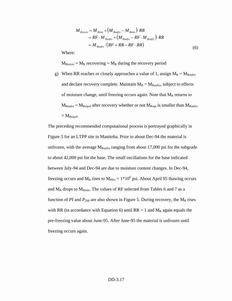
DD-3.17
( ) RRMMMM RminRunfrzRminRrecov ⋅−+=
( )( )RRRFRRRFM
RRMRFMMRF
Runfrz
RunfrzRunfrzRunfrz
⋅−+⋅=
⋅⋅−+⋅=
(6) Where:
MRrecov = MR recovering = MR during the recovery period
g) When RR reaches or closely approaches a value of 1, assign MR = MRunfrz
and declare recovery complete. Maintain MR = MRunfrz, subject to effects
of moisture change, until freezing occurs again. Note that MR returns to
MRunfrz = MRequil after recovery whether or not MRopt is smaller than MRunfrz
= MRequil.
The preceding recommended computational process is portrayed graphically in
Figure 5 for an LTPP site in Manitoba. Prior to about Dec-94 the material is
unfrozen, with the average MRunfrz ranging from about 17,000 psi for the subgrade
to about 42,000 psi for the base. The small oscillations for the base indicated
between July-94 and Dec-94 are due to moisture content changes. In Dec-94,
freezing occurs and MR rises to MRfrz = 1*106 psi. About April 95 thawing occurs
and MR drops to MRmin. The values of RF selected from Tables 6 and 7 as a
function of PI and P200 are also shown in Figure 5. During recovery, the MR rises
with RR (in accordance with Equation 6) until RR = 1 and MR again equals the
pre-freezing value about June-95. After June-95 the material is unfrozen until
freezing occurs again.
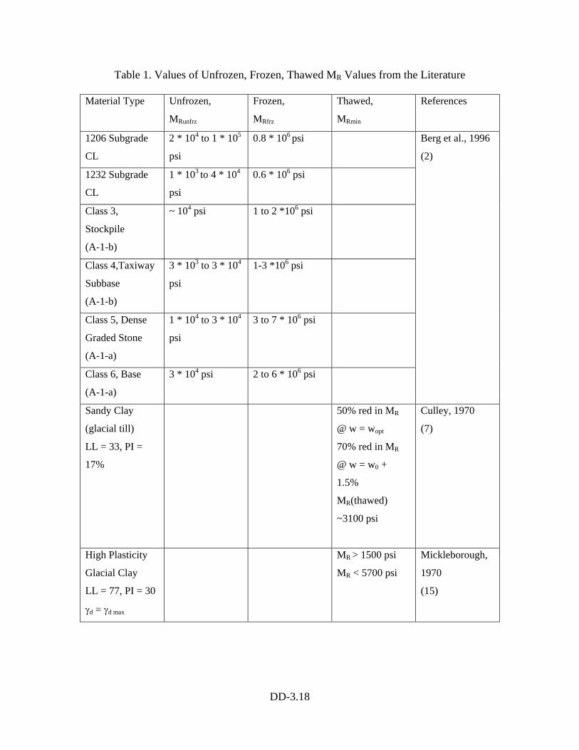
DD-3.18
Table 1. Values of Unfrozen, Frozen, Thawed MR Values from the Literature
Material Type Unfrozen,
MRunfrz
Frozen,
MRfrz
Thawed,
MRmin
References
1206 Subgrade
CL
2 * 104 to 1 * 105
psi
0.8 * 106 psi
1232 Subgrade
CL
1 * 103 to 4 * 104
psi
0.6 * 106 psi
Class 3,
Stockpile
(A-1-b)
~ 104 psi 1 to 2 *106 psi
Class 4,Taxiway
Subbase
(A-1-b)
3 * 103 to 3 * 104
psi
1-3 *106 psi
Class 5, Dense
Graded Stone
(A-1-a)
1 * 104 to 3 * 104
psi
3 to 7 * 106 psi
Class 6, Base
(A-1-a)
3 * 104 psi 2 to 6 * 106 psi
Berg et al., 1996
(2)
Sandy Clay
(glacial till)
LL = 33, PI =
17%
50% red in MR
@ w = wopt
70% red in MR
@ w = w0 +
1.5%
MR(thawed)
~3100 psi
Culley, 1970
(7)
High Plasticity
Glacial Clay
LL = 77, PI = 30
γd = γd max
MR > 1500 psi
MR < 5700 psi
Mickleborough,
1970
(15)
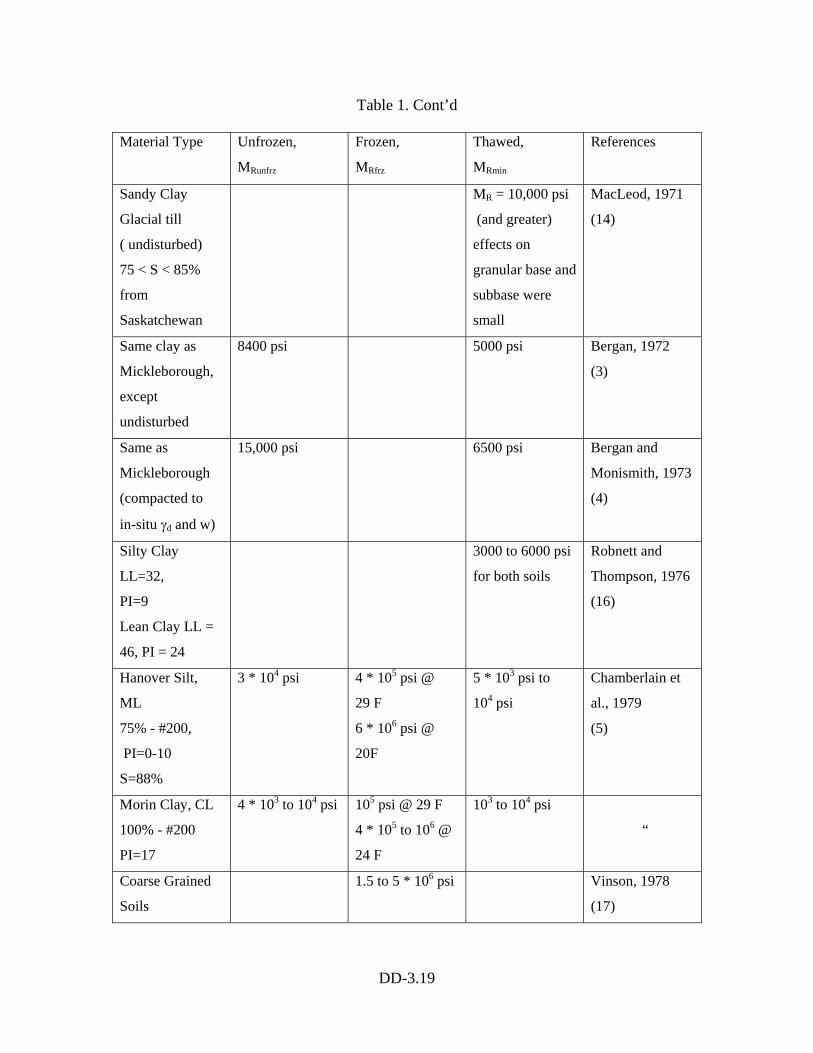
DD-3.19
Table 1. Cont’d
Material Type Unfrozen,
MRunfrz
Frozen,
MRfrz
Thawed,
MRmin
References
Sandy Clay
Glacial till
( undisturbed)
75 < S < 85%
from
Saskatchewan
MR = 10,000 psi
(and greater)
effects on
granular base and
subbase were
small
MacLeod, 1971
(14)
Same clay as
Mickleborough,
except
undisturbed
8400 psi 5000 psi Bergan, 1972
(3)
Same as
Mickleborough
(compacted to
in-situ γd and w)
15,000 psi 6500 psi Bergan and
Monismith, 1973
(4)
Silty Clay
LL=32,
PI=9
Lean Clay LL =
46, PI = 24
3000 to 6000 psi
for both soils
Robnett and
Thompson, 1976
(16)
Hanover Silt,
ML
75% - #200,
PI=0-10
S=88%
3 * 104 psi 4 * 105 psi @
29 F
6 * 106 psi @
20F
5 * 103 psi to
104 psi
Chamberlain et
al., 1979
(5)
Morin Clay, CL
100% - #200
PI=17
4 * 103 to 104 psi 105 psi @ 29 F
4 * 105 to 106 @
24 F
103 to 104 psi
“
Coarse Grained
Soils
1.5 to 5 * 106 psi Vinson, 1978
(17)
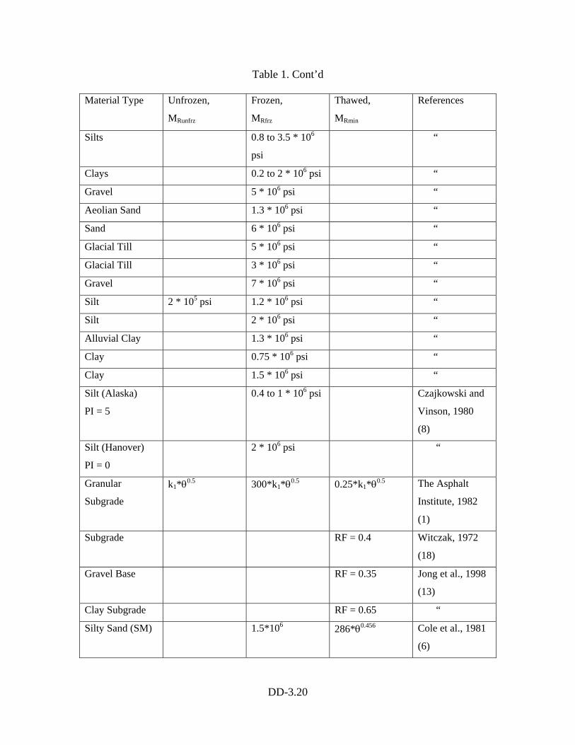
DD-3.20
Table 1. Cont’d
Material Type Unfrozen,
MRunfrz
Frozen,
MRfrz
Thawed,
MRmin
References
Silts 0.8 to 3.5 * 106
psi
“
Clays 0.2 to 2 * 106 psi “
Gravel 5 * 106 psi “
Aeolian Sand 1.3 * 106 psi “
Sand 6 * 106 psi “
Glacial Till 5 * 106 psi “
Glacial Till 3 * 106 psi “
Gravel 7 * 106 psi “
Silt 2 * 105 psi 1.2 * 106 psi “
Silt 2 * 106 psi “
Alluvial Clay 1.3 * 106 psi “
Clay 0.75 * 106 psi “
Clay 1.5 * 106 psi “
Silt (Alaska)
PI = 5
0.4 to 1 * 106 psi Czajkowski and
Vinson, 1980
(8)
Silt (Hanover)
PI = 0
2 * 106 psi “
Granular
Subgrade
k1*θ0.5 300*k1*θ0.5 0.25*k1*θ0.5 The Asphalt
Institute, 1982
(1)
Subgrade RF = 0.4 Witczak, 1972
(18)
Gravel Base RF = 0.35 Jong et al., 1998
(13)
Clay Subgrade RF = 0.65 “
Silty Sand (SM) 1.5*106 286*θ0.456 Cole et al., 1981
(6)
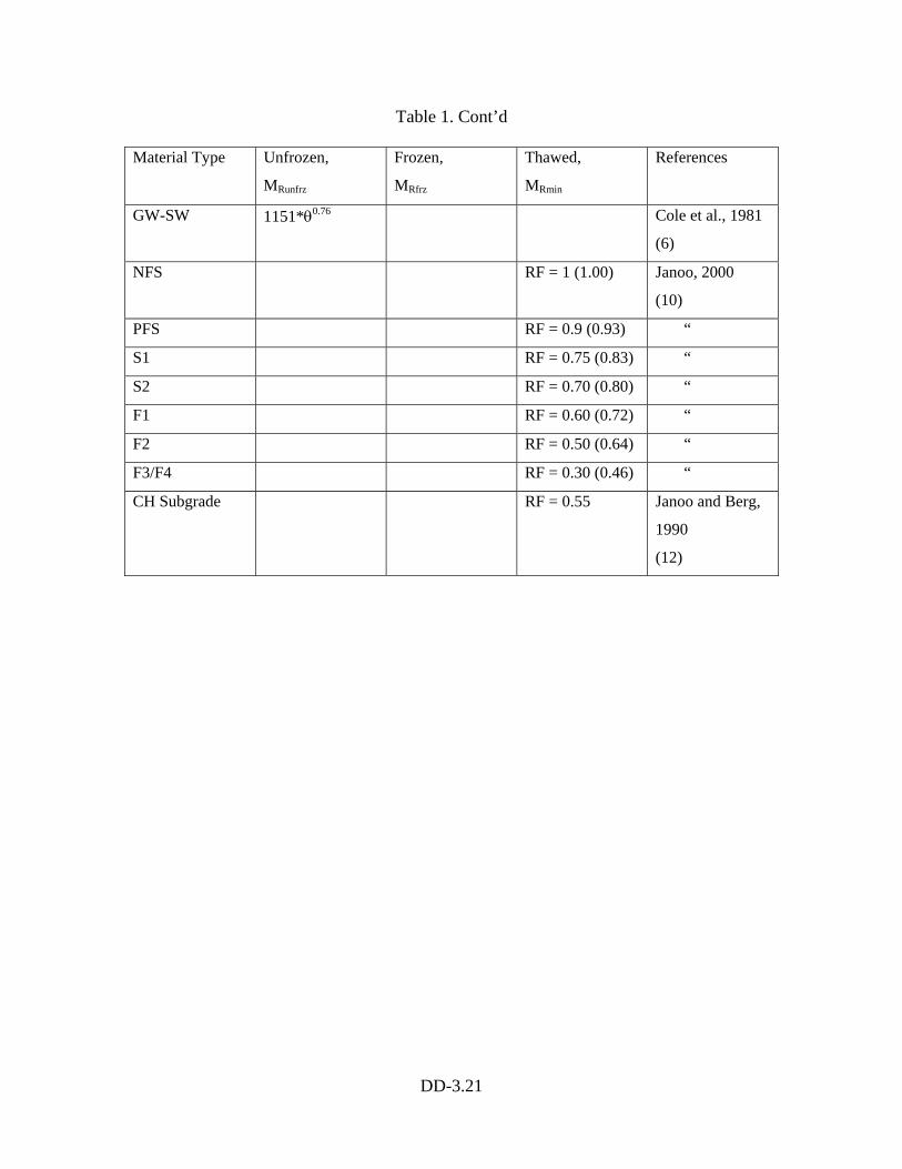
DD-3.21
Table 1. Cont’d
Material Type Unfrozen,
MRunfrz
Frozen,
MRfrz
Thawed,
MRmin
References
GW-SW 1151*θ0.76 Cole et al., 1981
(6)
NFS RF = 1 (1.00) Janoo, 2000
(10)
PFS RF = 0.9 (0.93) “
S1 RF = 0.75 (0.83) “
S2 RF = 0.70 (0.80) “
F1 RF = 0.60 (0.72) “
F2 RF = 0.50 (0.64) “
F3/F4 RF = 0.30 (0.46) “
CH Subgrade RF = 0.55 Janoo and Berg,
1990
(12)

DD-3.22
Table 2. Team Synthesis of MR Values for Frozen Materials
Material Type MRfrz
Coarse-Grained 1.5, 2, 5, 4, 3, 5, 4*106
MRave ~ 3 +/- 1 *106 psi
Fine-Grained-Silts and Silty
Sands
> 10% fines
PI near zero
3.2, 2.2, 1.2, 2, 0.7, 2
MRave = 2 +/- 1 * 106 psi
Clay 0.8, 0.6, 1.1, 1.3, 0.75, 1.5,
MRave ~ 1.0 +/- 0.5 * 106 psi
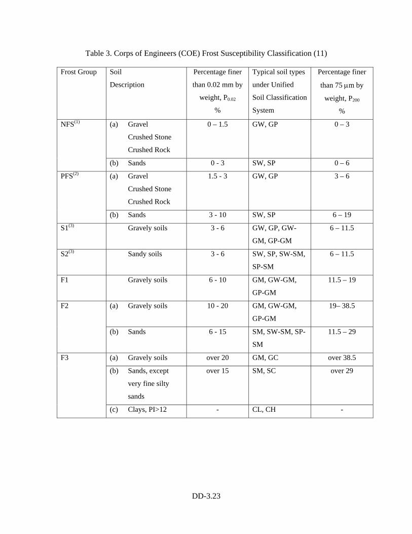
DD-3.23
Table 3. Corps of Engineers (COE) Frost Susceptibility Classification (11)
Frost Group Soil
Description
Percentage finer
than 0.02 mm by
weight, P0.02
%
Typical soil types
under Unified
Soil Classification
System
Percentage finer
than 75 µm by
weight, P200
%
(a) Gravel
Crushed Stone
Crushed Rock
0 – 1.5 GW, GP 0 – 3 NFS(1)
(b) Sands 0 - 3 SW, SP 0 – 6
(a) Gravel
Crushed Stone
Crushed Rock
1.5 - 3 GW, GP 3 – 6 PFS(2)
(b) Sands 3 - 10 SW, SP 6 – 19
S1(3) Gravely soils 3 - 6 GW, GP, GW-
GM, GP-GM
6 – 11.5
S2(3) Sandy soils 3 - 6 SW, SP, SW-SM,
SP-SM
6 – 11.5
F1 Gravely soils 6 - 10 GM, GW-GM,
GP-GM
11.5 – 19
(a) Gravely soils 10 - 20 GM, GW-GM,
GP-GM
19– 38.5 F2
(b) Sands 6 - 15 SM, SW-SM, SP-
SM
11.5 – 29
(a) Gravely soils over 20 GM, GC over 38.5
(b) Sands, except
very fine silty
sands
over 15 SM, SC over 29
F3
(c) Clays, PI>12 - CL, CH -
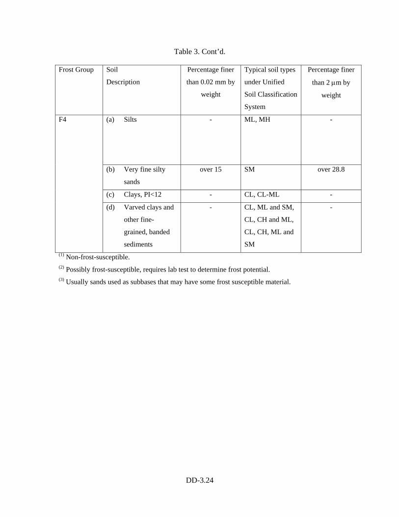
DD-3.24
Table 3. Cont’d.
Frost Group Soil
Description
Percentage finer
than 0.02 mm by
weight
Typical soil types
under Unified
Soil Classification
System
Percentage finer
than 2 µm by
weight
(a) Silts
- ML, MH -
(b) Very fine silty
sands
over 15 SM over 28.8
(c) Clays, PI<12 - CL, CL-ML -
F4
(d) Varved clays and
other fine-
grained, banded
sediments
- CL, ML and SM,
CL, CH and ML,
CL, CH, ML and
SM
-
(1) Non-frost-susceptible. (2) Possibly frost-susceptible, requires lab test to determine frost potential. (3) Usually sands used as subbases that may have some frost susceptible material.
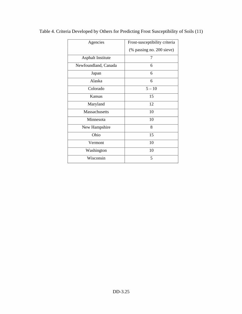
DD-3.25
Table 4. Criteria Developed by Others for Predicting Frost Susceptibility of Soils (11)
Agencies Frost-susceptibility criteria
(% passing no. 200 sieve)
Asphalt Institute 7
Newfoundland, Canada 6
Japan 6
Alaska 6
Colorado 5 – 10
Kansas 15
Maryland 12
Massachusetts 10
Minnesota 10
New Hampshire 8
Ohio 15
Vermont 10
Washington 10
Wisconsin 5
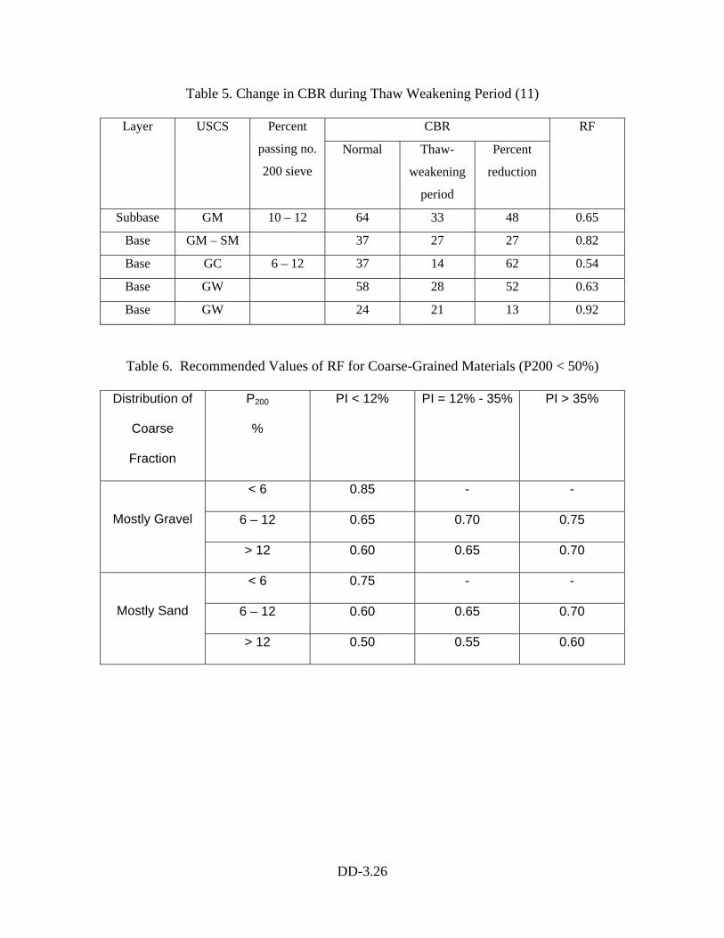
DD-3.26
Table 5. Change in CBR during Thaw Weakening Period (11)
CBR Layer USCS Percent
passing no.
200 sieve
Normal Thaw-
weakening
period
Percent
reduction
RF
Subbase GM 10 – 12 64 33 48 0.65
Base GM – SM 37 27 27 0.82
Base GC 6 – 12 37 14 62 0.54
Base GW 58 28 52 0.63
Base GW 24 21 13 0.92
Table 6. Recommended Values of RF for Coarse-Grained Materials (P200 < 50%)
Distribution of
Coarse
Fraction
P200
%
PI < 12% PI = 12% - 35% PI > 35%
< 6 0.85 - -
6 – 12 0.65 0.70 0.75
Mostly Gravel
> 12 0.60 0.65 0.70
< 6 0.75 - -
6 – 12 0.60 0.65 0.70
Mostly Sand
> 12 0.50 0.55 0.60
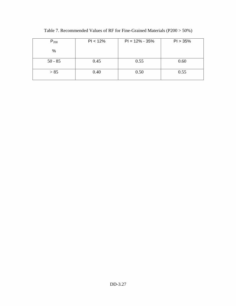
DD-3.27
Table 7. Recommended Values of RF for Fine-Grained Materials (P200 > 50%)
P200
%
PI < 12% PI = 12% - 35% PI > 35%
50 - 85 0.45 0.55 0.60
> 85 0.40 0.50 0.55
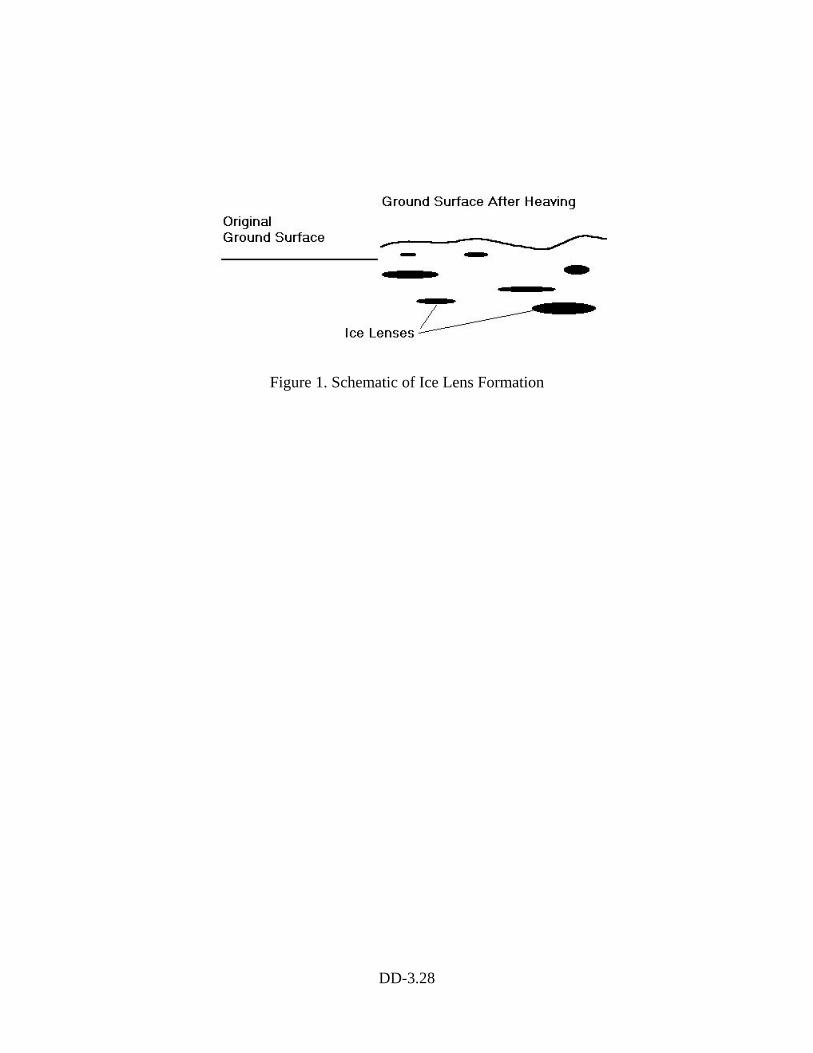
DD-3.28
Figure 1. Schematic of Ice Lens Formation
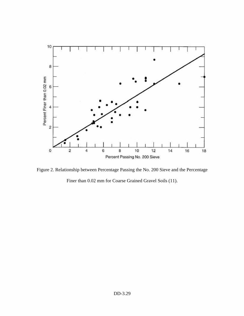
DD-3.29
Figure 2. Relationship between Percentage Passing the No. 200 Sieve and the Percentage
Finer than 0.02 mm for Coarse Grained Gravel Soils (11).
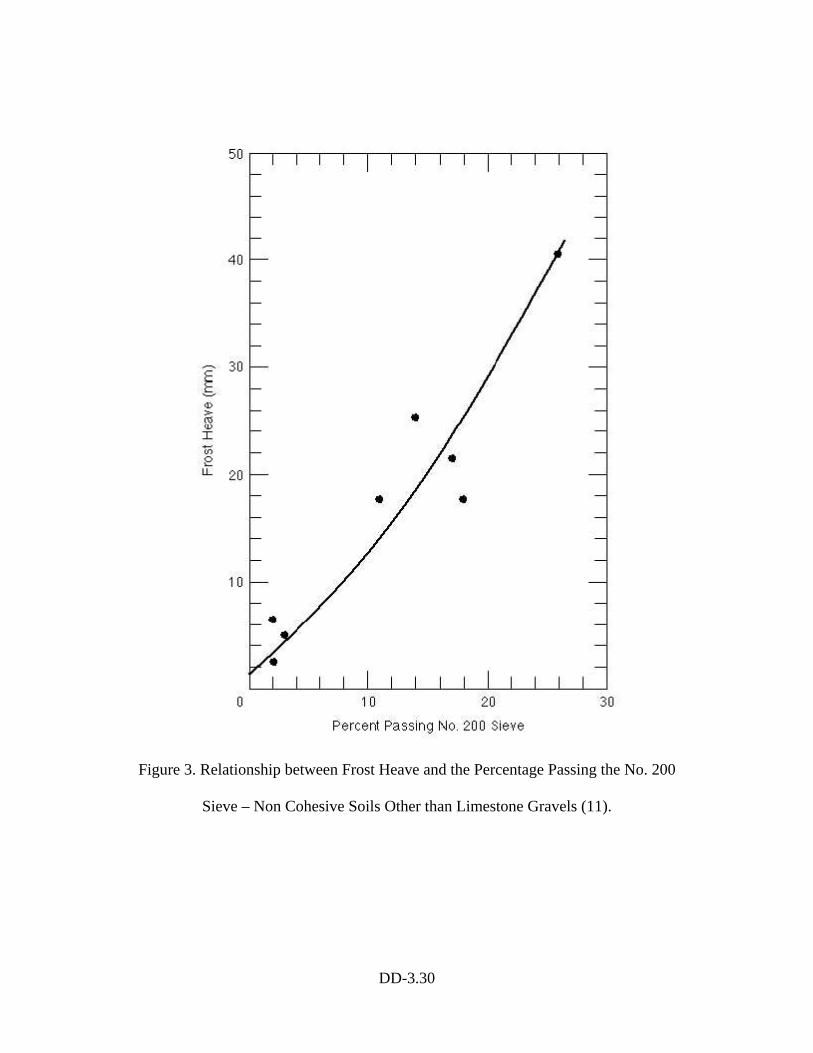
DD-3.30
Figure 3. Relationship between Frost Heave and the Percentage Passing the No. 200
Sieve – Non Cohesive Soils Other than Limestone Gravels (11).
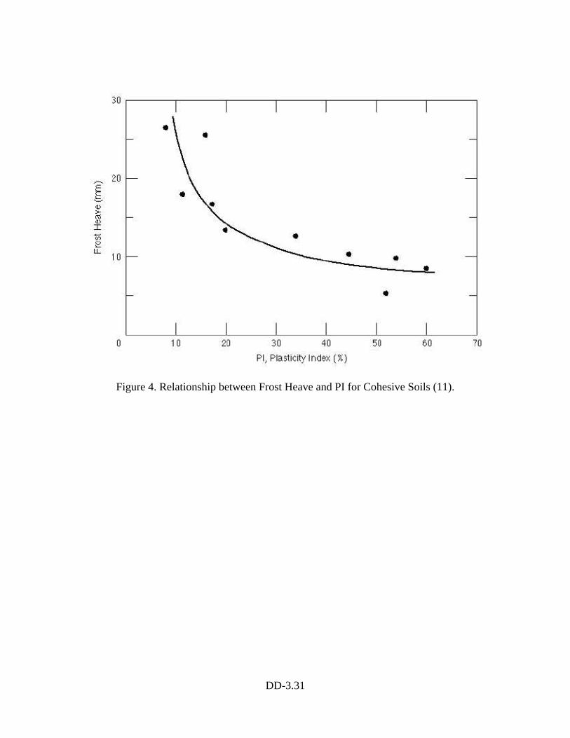
DD-3.31
Figure 4. Relationship between Frost Heave and PI for Cohesive Soils (11).
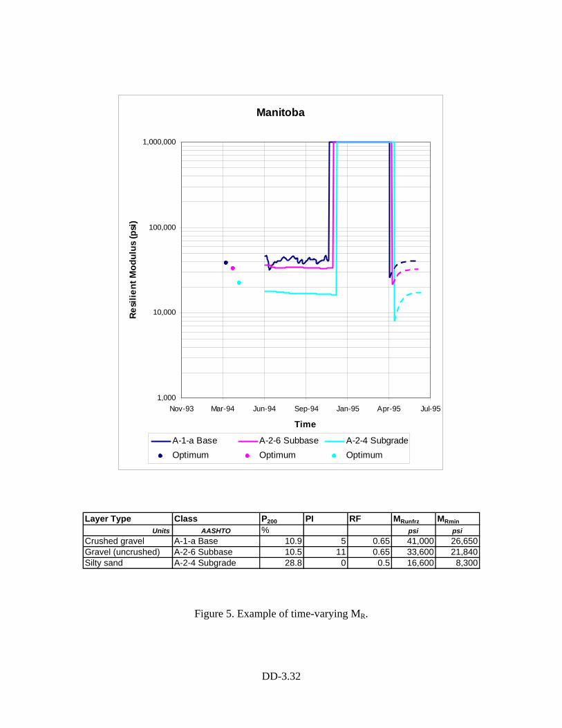
DD-3.32
Manitoba
1,000
10,000
100,000
1,000,000
Nov-93 Mar-94 Jun-94 Sep-94 Jan-95 Apr-95 Jul-95
Time
Resi
lient
Mod
ulus
(psi
)
A-1-a Base A-2-6 Subbase A-2-4 SubgradeOptimum Optimum Optimum
Layer Type Class P200 PI RF MRunfrz MRminUnits AASHTO % psi psi
Crushed gravel A-1-a Base 10.9 5 0.65 41,000 26,650Gravel (uncrushed) A-2-6 Subbase 10.5 11 0.65 33,600 21,840Silty sand A-2-4 Subgrade 28.8 0 0.5 16,600 8,300
Figure 5. Example of time-varying MR.
DD-3.33
References:
1. The Asphalt Institute. Research and Development of the Asphalt Institute’s Thickness Design Manual (MS-1) Ninth Edition. Research Report No. 82-2, August 1982.
2. Berg R.L., Bigl S.R., Stark J.A. and Durell G.D. Resilient Modulus Testing of
Materials from Mn/ROAD, Phase 1. The U.S. Army Cold Regions Research and Engineering Laboratory, Special Report 96-19, September 1996.
3. Bergan A.T. Some Considerations in the Design of Asphalt Concrete Pavements for
Cold Regions. Thesis presented to the University of California, at Berkeley, California, 1972, in partial fulfillment of the requirements for the degree of Doctor of Philosophy.
4. Bergan A.T. and Monismith C.L. Characterization of Subgrade Soils in Cold Regions
for Pavement Design Purposes. Highway Research Record 431, Highway Research Board, Washington, D.C., 1973.
5. Chamberlain E.J., Cole D.M. and Johnson T.C. Resilient Response of Two Frozen
and Thawed Soils. Journal of the Geotechnical Division, Proceedings of the American Society of Civil Engineers, Vol. 105, No. GT2, February, 1979.
6. Cole D.M., Irwin L.H. and Johnson T.C. Effect of Freezing and Thawing on Resilient
Modulus of a Granular Soil Exhibiting Nonlinear Behavior. Transportation Research Record 801, TRB, National Research Council, 1981, Washington, D.C., pp. 19-26.
7. Culley R.W. Effect of Freeze-Thaw Cycling on Stress-Strain Characteristics and
Volume Change of a Till Subjected to Repetitive Loading. Technical Report 13, Saskatchewan Department of Highways, Saskatchewan, Canada, 1970.
8. Czajkowsky R.L. and Vinson T.S. Dynamic Properties of Frozen Silt Under Cyclic
Loading. Journal of the Geotechnical Division, Proceedings of the American Society of Civil Engineers, Vol. 106, No. GT9, September, 1980.
9. Esch D.C., McHattie R.L. and Connor B. Frost-Susceptibility Ratings and Pavement
Structure Performance. Transportation Research Record 809, TRB, National Research Council, 1981, Washington, D.C., pp. 27-34.
10. Janoo V.C. Evaluating Pavement Performance in Cold Regions. ISCORD 2000
proceedings, Hobart, Tasmania, Australia, February 2000. 11. Janoo V.C., Eaton R. and Barna L. Evaluation of Airport Subsurface Materials. The
U.S. Army Cold Regions Research and Engineering Laboratory, Special Report 97-13, May 1997.
DD-3.34
12. Janoo V.C. and Berg R.L. Thaw Weakening of Pavement Structures in Seasonal Frost
Areas. Transportation Research Record 1286, TRB, National Research Council, 1990, Washington, D.C., pp. 217-233.
13. Jong D., Bosscher P.J. and Benson C.H. Field Assessment of Changes in Pavement
Moduli Caused by Freezing and Thawing. Transportation Research Record 1615, TRB, National Research Council, 1998, Washington, D.C., pp. 41-48.
14. MacLeod D.R. Some Fatigue Considerations in the Design of Thin Pavements. Thesis
presented to the University of Saskatchewan, at Saskatchewan, Canada, 1970, in partial fullfilment of the requirements for the degree of Master of Science.
15. Mickleborough B.W. An Experimental Study of the Effects of Freezing on Clay
Subgrades. Thesis presented to the University of Saskatchewan, at Saskatchewan, Canada, 1970, in partial fullfilment of the requirements for the degree of Master of Science.
16. Robnett Q.L. and Thompson M.R. Effect of Lime Treatment on the Resilient Behavior
of Fine Grained Soils. Transportation Research Record 560, TRB, National Research Council, 1976, Washington, D.C., pp. 11-20.
17. Vinson T.S. Parameter Effects on Dynamic Properties of Frozen Soils. Journal of the
Geotechnical Division, Proceedings of the American Society of Civil Engineers, Vol. 104, No. GT10, October, 1978.
18. Witczak M.W. Design of Full-Depth Asphalt Airfield Pavements. The University of
Michigan Third International Conference on the Structural Design of Asphalt Pavements, Vol. I, Proceedings, September 11 – 15, 1972, Grosvenor House, Park Lane, London, England.
19. Witczak M.W., Houston W.N., Zapata C.E., Richter C., Larson G. and Walsh K.
Improvement of the Integrated Climatic Model for Moisture Content Predictions. Development of the 2002 Guide for the Development of New and Rehabilitated Pavement Structures, NCHRP 1-37 A, Inter Team Technical Report (Seasonal 4), June 2000.
20. Witczak M.W., Andrei D. and Houston W.N. Resilient Modulus as Function of Soil
Moisture – Summary of Predictive Models. Development of the 2002 Guide for the Development of New and Rehabilitated Pavement Structures, NCHRP 1-37 A, Inter Team Technical Report (Seasonal 1), June 2000.
21. Witczak M.W., Houston W.N. and Andrei D. Resilient Modulus as Function of Soil
Moisture – A Study of the Expected Changes in Resilient Modulus of the Unbound Layers with Changes in Moisture for 10 LTPP Sites. Development of the 2002 Guide

DD-3.35
for the Development of New and Rehabilitated Pavement Structures, NCHRP 1-37 A, Inter Team Technical Report (Seasonal 2), June 2000.
Copy No.
Guide for Mechanistic-Empirical Design OF NEW AND REHABILITATED PAVEMENT STRUCTURES
FINAL DOCUMENT
APPENDIX DD-4: IMPROVEMENT OF THE INTEGRATED CLIMATIC MODEL FOR MOISTURE CONTENT PREDICTIONS
NCHRP
Prepared for National Cooperative Highway Research Program
Transportation Research Board National Research Council
Submitted by ARA, Inc., ERES Division
505 West University Avenue Champaign, Illinois 61820
June 2000
DD-4.II
Acknowledgment of Sponsorship This work was sponsored by the American Association of State Highway and Transportation Officials (AASHTO) in cooperation with the Federal Highway Administration and was conducted in the National Cooperative Highway Research Program which is administered by the Transportation Research Board of the National Research Council. Disclaimer This is the final draft as submitted by the research agency. The opinions and conclusions expressed or implied in this report are those of the research agency. They are not necessarily those of the Transportation Research Board, the National Research Council, the Federal Highway Administration, AASHTO, or the individual States participating in the National Cooperative Highway Research program. Acknowledgements The research team for NCHRP Project 1-37A: Development of the 2002 Guide for the Design of New and Rehabilitated Pavement Structures consisted of Applied Research Associates, Inc., ERES Consultants Division (ARA-ERES) as the prime contractor with Arizona State University (ASU) as the primary subcontractor. Fugro-BRE, Inc., the University of Maryland, and Advanced Asphalt Technologies, LLC served as subcontractors to either ARA-ERES or ASU along with several independent consultants. Research into the subject area covered in this Appendix was conducted at ASU. The authors of this Appendix are Dr. M. W. Witczak, Dr. W. N. Houston, Dr. C. E. Zapata, Mrs. Cheryl Richter, Mr. Gregg Larson, Dr. Ken Walsh. Dr. Witczak coordinated the overall research effort of the 2002 Design Guide Team, outlined the problems, monitored progress, set schedules and deadlines, and provided periodic technical review of research results as they became available. Ms. Cheryl Richter acquired the input data needed for running the EICM moisture predictions, made EICM runs in parallel with Dr. Zapata, and helped to identify relevant issues to be addressed during team meetings. Drs. Houston, Zapata and Walsh collected the data needed to develop the prediction of the SWCC based on soil properties and developed the SWCC model itself. The EICM modifications were coordinated by Dr. Houston and Zapata with important input from Mr. Gregg Larson. The model code changes were performed by Mr. Gregg Larson. Foreword This appendix presents the derivation of reasonable values of MR for both frozen and thawed unbound materials through evaluation of published results.. The information contained in this appendix serves as a supporting reference to the resilient modulus discussions presented and PART 2, Chapter 3, and PART 3, Chapters 3, 4, 6, and 7 of the Design Guide.

DD-4.III
This appendix is the fourth in a series of four volumes on environmental effects on pavements. The other volumes are: Appendix DD-1: Resilient Modulus As Function Of Soil Moisture-Summary Of Predictive Models Appendix DD-2: Resilient Modulus As Function Of Soil Moisture – A Study Of The Expected
Changes In Resilient Modulus Of The Unbound Layers With Changes In Moisture For 10 LTPP Sites
Appendix DD-3: Selection Of Resilient Moduli For Frozen/Thawed Unbound Materials
DD-4.IV
Abstract
The Enhanced Integrated Climatic Model (EICM), developed under contract with the
Federal Highway Administration (FHWA), was designed to simulate the behavior of
pavement materials and subgrade materials over several years of operation. An
evaluation of the model's moisture prediction capabilities showed that its performance with
regard to moisture predictions for the unbound materials was initially poor and exceeded
the error typically found in field moisture measurements. Those findings pointed to the
need for significant modifications and additions to the EICM moisture content prediction
algorithms. The required modifications were subsequently made, creating version 2.6 of
the EICM.
Modifications to the EICM include the addition of a better functional fit for the soil-water
characteristic curve (SWCC); the incorporation of an algorithm capable of predicting the
SWCC based on soil index properties; the addition of an algorithm for the prediction of the
unsaturated hydraulic conductivity based on the SWCC; and, the development of sets of
default soil parameters based on the ASSHTO Soil Classification System. Verification of
the Version 2.6 showed great improvement on the prediction of the moisture content for
the unbound materials.
DD-4.II
Table of Contents List of Tables.................................................................................................................................. vii List of Figures............................................................................................................................... viii Chapter 1 Introduction The Enhanced Integrated Climatic Model ................................................................................... 1 General Features of the Model....................................................................................................... 1 Objectives of the Research........................................................................................................... 2 Organization of the Report............................................................................................................ 3 Chapter 2 Assessment of the Performance of the EICM Version 2.1........................................................................................................................................ 5 Introduction .................................................................................................................................... 5 Input Requirements for the EICM version 2.1 ............................................................................. 5 Collected Data ............................................................................................................................... 8 Climatic Boundary Conditions ................................................................................................. 9 Infiltration and Drainage......................................................................................................... 19 Asphalt Material Properties ................................................................................................... 19 Material Properties................................................................................................................. 19 Initial Moisture Content Profile............................................................................................... 20 Initial Temperature Profile...................................................................................................... 20 Basis for Comparison ............................................................................................................ 20 Results ......................................................................................................................................... 21 Factors that Contributed to the Poor Predictions of the Water Contents by the EICM............ 30 Short-term Actions Recommended for the Improvement of the EICM..................................... 31 Chapter 3 Modifications to the EICM version 2.1 Moisture Content Prediction ....................................................................................................... 33 Proposed Modifications to the EICM – version 2.1 ................................................................... 33 The Soil-Water Characteristic Curve.......................................................................................... 33 Correlation Between the Fredlund and Xing Fitting Parameters and Soil Index Properties ... 37 Correlations for Soils with PI > 0................................................................................................. 37 Correlations for Soils with PI = 0................................................................................................. 38 Correlation Results ...................................................................................................................... 39 Best-Estimate SWCCs Based on AASHTO Classification....................................................... 45 Best-Estimate SWCCs for Base Course Materials ................................................................... 45 Default Values for Saturated Hydraulic Conductivity, Specific Gravity, and Saturated
Volumetric Water Content........................................................................................................... 45 Unsaturated Hydraulic Conductivity Function............................................................................ 47 Summary ..................................................................................................................................... 48 Chapter 4 Assessment of the EICM Moisture Content Prediction after Modifications EICM Version 2.6 ........................................................................................................................... 49 Introduction .................................................................................................................................. 49 Data Collected ............................................................................................................................. 49 Results ......................................................................................................................................... 50
DD-4.III
Chapter 5 User's Guide and Recommendations EICM version 2.6 - Moisture Content Prediction...................................................................... 77 Introduction .................................................................................................................................. 77 Input Parameters......................................................................................................................... 77 Soil Classification ................................................................................................................... 78 Thickness of the Layer........................................................................................................... 78 Number of Elements for this Layer ....................................................................................... 79 Porosity of the Layer Material................................................................................................ 79 Specific Gravity ...................................................................................................................... 81 Saturated Permeability .......................................................................................................... 81 Dry Density............................................................................................................................. 81 Plasticity Index ....................................................................................................................... 82 Percent Passing #200............................................................................................................ 82 Diameter D60........................................................................................................................... 83 Initial Volumetric Water Content............................................................................................ 83 Equilibrium Volumetric Water Content.................................................................................. 83 Chapter 6 Development of Procedures for Estimating Moisture Content from the Initial State to
Equilibrium Conditions for Newly Constructed Pavements.............................................. 86 Introduction .................................................................................................................................. 86 Correlation for Sopt.................................................................................................................. 87 Correlation for wopt.................................................................................................................. 89 Intended Use of Correlations................................................................................................. 91 Check on Internal Consistency for Sopt, wopt, and Gs............................................................ 94 Chapter 7 Conclusions ................................................................................................................................... 97 Part I. Conclusions Relative to the Maximization of the Agreement between EICM Predicted
Moisture Contents and TDR Measured Moisture Contents for Existing Pavements .............. 97 Part II. Conclusions Relative to the Optimization of Procedures for Predicting the Moisture Content
Change from the Initial to the Equilibrium Condition ................................................................. 99 Chapter 8 Recommendations for Implementation of EICM Input for Use in the 2002 Design
Guide.........................................................................................................................................101 Introduction ................................................................................................................................101 Unbound Compacted Layers....................................................................................................102 Data Required Including Sources and Tests to be Performed..........................................102 Unbound Natural (In-Situ) Layers.............................................................................................105 Data Required Including Sources and Tests to be Performed..........................................105 APPENDICES ...............................................................................................................................107 APPENDIX A VOLUMETRIC WATER CONTENT PROFILES CONNECTICUT (91803) EICM – Version 2.1 .......................................................................................................................108 APPENDIX B VOLUMETRIC WATER CONTENT PROFILES MINNESOTA (91803) EICM – Version 2.1 .......................................................................................................................116
DD-4.IV
APPENDIX C VOLUMETRIC WATER CONTENT PROFILES MAINE (231026) EICM – Version 2.1 .......................................................................................................................123 APPENDIX D VOLUMETRIC WATER CONTENT PROFILES NEW HAMPSHIRE (331001) EICM – Version 2.1 .......................................................................................................................131 APPENDIX E VOLUMETRIC WATER CONTENT PROFILES VERMONT (501002) EICM – Version 2.1 .......................................................................................................................139 APPENDIX F VOLUMETRIC WATER CONTENT PROFILES MANITOBA (831801) EICM – Version 2.1 .......................................................................................................................147 APPENDIX G BEST-ESTIMATE SOIL-WATER CHARACTERISITC CURVES BASED ON AASHTO CLASSIFICATION ...................................................................................156 APPENDIX H BEST-ESTIMATE SOIL-WATER CHARACTERISITC CURVES FOR BASE COURSE MATERIALS.............................................................................................163 APPENDIX I VOLUMETRIC WATER CONTENT PROFILES CONNECTICUT (91803) EICM – Version 2.6 .......................................................................................................................167 APPENDIX J VOLUMETRIC WATER CONTENT PROFILES MINNESOTA (271018) EICM – Version 2.6 .......................................................................................................................174 APPENDIX K VOLUMETRIC WATER CONTENT PROFILES MAINE (231026) EICM – Version 2.6 .......................................................................................................................182 APPENDIX L VOLUMETRIC WATER CONTENT PROFILES NEW HAMPSHIRE (331001) EICM – Version 2.6 .......................................................................................................................190 APPENDIX M VOLUMETRIC WATER CONTENT PROFILES VERMONT (501002) EICM – Version 2.6 .......................................................................................................................198 APPENDIX N VOLUMETRIC WATER CONTENT PROFILES
DD-4.V
MANITOBA (831801) EICM – Version 2.6 .......................................................................................................................206 APPENDIX O VOLUMETRIC WATER CONTENT PROFILES GEORGIA (131005) EICM – Version 2.6 .......................................................................................................................213 APPENDIX P VOLUMETRIC WATER CONTENT PROFILES COLORADO (81053) EICM – Version 2.6 .......................................................................................................................221 APPENDIX Q VOLUMETRIC WATER CONTENT PROFILES ARIZONA (41024) EICM – Version 2.6 .......................................................................................................................233 APPENDIX R VOLUMETRIC WATER CONTENT PROFILES TEXAS (481077) EICM – Version 2.6 .......................................................................................................................238 REFERENCES..............................................................................................................................247
DD-4.VI
List of Tables
Table 1. Input Variables Needed by the EICM - Version 2.1...........................................7
Table 2. Input Data and Sources for the EICM - Version 2.1 for the Connecticut (91803) and Minnesota (271018) Sites........................................................... 10
Table 3. Input Data and Sources for the EICM - Version 2.1 for the Maine (231026), New Hampshire (331001), Vermont (501002), and Manitoba (831801) Sites.................................................................................. 14
Table 4 Equations Used to Represent the Soil-Water Characteristic Curve.............. 34
Table 5. Soil Properties Default Values vs. AASHTO Soil Classification System....... 44
Table 6. Best Estimated D60 for Base Course Materials............................................... 46
Table 7. Summary of Input Parameters for the EICM – Version 2.6 for the Connecticut, Minnesota, Maine, New Hampshire, Vermont, and Manitoba LTPP Sections.................................................................................................. 51
Table 8. Summary of Input Parameters for the EICM – Version 2.6 for the Georgia, Colorado, Arizona, and Texas LTPP Sections ............................................... 56
Table 9. Input Variables Needed by the EICM (version 2.6) for the Material Properties and Initial Temperature and Water Content Profiles Sections..... 78
Table 10. Options for Determining the Porosity of the Layer, Depending on the Known Soil Properties...................................................................................... 80
Table 11. Options for Determining the Specific Gravity of the Layer, Depending on the Known Soil Properties................................................................................ 81
Table 12. Determination of the SWCC based on Percentage Passing #200, Plasticity Index and Diameter D60.................................................................... 82
Table 13. Available Options for the Initial and Equilibrium Water Contents................... 84
Table 14. Listing of Input Parameters Required by the EICM, Including Climatic Data, Infiltration and Drainage Data, Asphalt/PCC Properties and Material Properties for Compacted and Natural In-Situ Layers.................................. 104
DD-4.VII
List of Figures
Figure 1. Measured versus Predicted Moisture Content – EICM version 2.1 Connecticut (91803) ......................................................................................... 22
Figure 2. Measured versus Predicted Moisture Content – EICM version 2.1 Minnesota (271018) ......................................................................................... 23
Figure 3. Measured versus Predicted Moisture Content – EICM version 2.1 Maine (231026)................................................................................................. 24
Figure 4. Measured versus Predicted Moisture Content – EICM version 2.1 New Hampshire (331001)................................................................................ 25
Figure 5. Measured versus Predicted Moisture Content – EICM version 2.1 Vermont (501002)............................................................................................. 26
Figure 6. Measured versus Predicted Moisture Content – EICM version 2.1 Manitoba (831801) ........................................................................................... 27
Figure 7. Summary of Measured versus Predicted Moisture Content for the Base Course Materials – EICM version 2.1.............................................................. 28
Figure 8. Summary of Measured versus Predicted Moisture Content for the Subgrade Materials – EICM version 2.1 ......................................................... 29
Figure 9. Range of SWCCs for Soils with wPI between 0.1 and 3................................ 40
Figure 10. Range of SWCCs for Soils with wPI between 3 and 10................................. 40
Figure 11. Range of SWCCs for Soils with wPI between 10 and 30............................... 41
Figure 12. Range of SWCCs for Soils with wPI between 30 and 50............................... 41
Figure 13. Range of SWCCs for Soils with D60 between 1 and 0.4 mm. ........................ 42
Figure 14. Range of SWCCs for Soils with D60 between 0.4 and 0.1 mm...................... 42
Figure 15. Predicted SWCC based on D60 and wPI......................................................... 43
Figure 16. Measured versus Predicted Moisture Content – EICM version 2.6 Connecticut (91803) ......................................................................................... 64
Figure 17. Measured versus Predicted Moisture Content – EICM version 2.6 Minnesota (271018) ......................................................................................... 65
Figure 18. Measured versus Predicted Moisture Content – EICM version 2.6 Maine (231026)................................................................................................. 66
DD-4.VIII
Figure 19. Measured versus Predicted Moisture Content – EICM version 2.6 New Hampshire (331001)................................................................................ 67
Figure 20. Measured versus Predicted Moisture Content – EICM version 2.6 Vermont (501002)............................................................................................. 68
Figure 21. Measured versus Predicted Moisture Content – EICM version 2.6 Manitoba (831801) ........................................................................................... 69
Figure 22. Measured versus Predicted Moisture Content – EICM version 2.6 Georgia (131005) ............................................................................................. 70
Figure 23. Measured versus Predicted Moisture Content – EICM version 2.6 Colorado (81053).............................................................................................. 71
Figure 24. Measured versus Predicted Moisture Content – EICM version 2.6 Arizona (41024) ................................................................................................ 72
Figure 25. Measured versus Predicted Moisture Content – EICM version 2.6 Texas (481077)................................................................................................. 73
Figure 26. Summary of Measured versus Predicted Moisture Content for the Base Course Materials – EICM version 2.6.............................................................. 74
Figure 27. Summary of Measured versus Predicted Moisture Content for the Subgrade Materials – EICM version 2.6 ......................................................... 75
Figure 28. Summary of Measured versus Predicted Moisture Content for ALL sites – EICM version 2.6 .................................................................................. 76
Figure 29. Correlation between Degree of Saturation at Optimum and wPI .................. 88
Figure 30. Correlation between Gravimetric Water Content at Optimum and wPI......... 88
Figure 31. Correlation between Gravimetric Water Content at Optimum and D60.......... 90
Figure 32. Correlation between Gravimetric Water Content at Optimum (T99) and Difference between wopt (T99) and wopt (T180) ............................................... 90
Figure 33. Correlation between Dry Unit Weight and wPI ............................................... 95
Figure 34. Correlation between Dry Unit Weight and D60 ................................................ 96
Figure 35. Comparison of γdry max from Optimum Conditions with γdry max from wPI/D60 Correlations....................................................................................................... 96

DD-4.1
Introduction The Enhanced Integrated Climatic Model
General Features of the Model
The Enhanced Integrated Climatic Model (EICM) is a one-dimensional coupled heat and
moisture flow program developed for the Federal Highway Administration (FHWA). The
model is intended to predict or simulate the changes in the behavior and characteristics of
pavement and subgrade materials in conjunction with climatic conditions over several
years of operation. The EICM is comprised of three major components:
1) The Infiltration and Drainage Model (ID Model) developed at the Texas A&M
University;
2) The Climatic-Materials-Structural Model (CMS Model) developed at the University
of Illinois; and,
3) The CRREL Frost Heave and Thaw Settlement Model (CRREL Model)
developed at the United States Army Cold Regions Research and Engineering
Laboratory (CRREL).
The EICM computes and predicts the following information throughout the entire
pavement profile: temperature, resilient modulus, pore water pressure, water content, frost
and thaw depths, frost heave and drainage performance. The data is generated for a
period that ranges from one day to several years. The model may be applied to either
asphaltic concrete pavements or Portland cement concrete pavements.
The original version of the EICM was developed at Texas A&M University, Texas
Transportation Institute in 1989 (Lytton et al. 1990). The original version was modified and
released in 1997 under version 2.0 (Larson and Dempsey, 1997). Additional modifications
were performed in 1999, under version 2.1. Improvements in version 2.1 included the
implementation of a standard Microsoft® Windows style interface as well as user input,
computational engine, and output file manipulation improvements. This report provides a
list of the input parameters for the EICM and present results of the model performance on
moisture content predictions. It is not intended to show the user how to operate the
Chapter
1
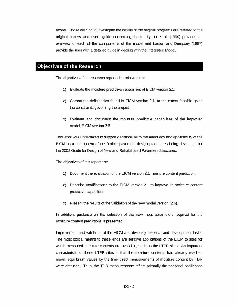
DD-4.2
model. Those wishing to investigate the details of the original programs are referred to the
original papers and users guide concerning them. Lytton et al. (1990) provides an
overview of each of the components of the model and Larson and Dempsey (1997)
provide the user with a detailed guide in dealing with the Integrated Model.
Objectives of the Research
The objectives of the research reported herein were to:
1) Evaluate the moisture predictive capabilities of EICM version 2.1;
2) Correct the deficiencies found in EICM version 2.1, to the extent feasible given
the constraints governing the project;
3) Evaluate and document the moisture predictive capabilities of the improved
model, EICM version 2.6.
This work was undertaken to support decisions as to the adequacy and applicability of the
EICM as a component of the flexible pavement design procedures being developed for
the 2002 Guide for Design of New and Rehabilitated Pavement Structures.
The objectives of this report are:
1) Document the evaluation of the EICM version 2.1 moisture content prediction.
2) Describe modifications to the EICM version 2.1 to improve its moisture content
predictive capabilities.
3) Present the results of the validation of the new model version (2.6).
In addition, guidance on the selection of the new input parameters required for the
moisture content predictions is presented.
Improvement and validation of the EICM are obviously research and development tasks.
The most logical means to these ends are iterative applications of the EICM to sites for
which measured moisture contents are available, such as the LTPP sites. An important
characteristic of these LTPP sites is that the moisture contents had already reached
mean, equilibrium values by the time direct measurements of moisture content by TDR
were obtained. Thus, the TDR measurements reflect primarily the seasonal oscillations
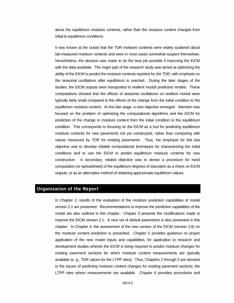
DD-4.3
about the equilibrium moisture contents, rather than the moisture content changes from
initial to equilibrium conditions.
It was known at the outset that the TDR moisture contents were widely scattered about
lab-measured moisture contents and were in most cases somewhat suspect themselves.
Nevertheless, the decision was made to do the best job possible if improving the EICM
with the data available. The major part of the research study was aimed at optimizing the
ability of the EICM to predict the moisture contents reported for the TDR, with emphasis on
the seasonal oscillations after equilibrium is reached. During the later stages of the
studies, the EICM outputs were transported to resilient moduli predictive models. These
computations showed that the effects of seasonal oscillations on resilient moduli were
typically fairly small compared to the effects of the change from the initial condition to the
equilibrium moisture content. At this late stage, a new objective emerged. Attention was
focused on the problem of optimizing the computational algorithms and the EICM for
prediction of the change in moisture content from the initial condition to the equilibrium
condition. This corresponds to focusing on the EICM as a tool for predicting equilibrium
moisture contents for new pavements not yet constructed, rather than comparing with
values measured by TDR for existing pavements. Thus, the emphasis for this last
objective was to develop reliable computational techniques for characterizing the initial
conditions and to use the EICM to predict equilibrium moisture contents for new
construction. A secondary, related objective was to devise a procedure for hand
computation (or spreadsheet) of the equilibrium degrees of saturation as a check on EICM
outputs, or as an alternative method of obtaining approximate equilibrium values.
Organization of the Report
In Chapter 2, results of the evaluation of the moisture prediction capabilities of model
version 2.1 are presented. Recommendations to improve the predictive capabilities of the
model are also outlined in this chapter. Chapter 3 presents the modifications made to
improve the EICM version 2.1. A new set of default parameters is also presented in this
chapter. In Chapter 4, the assessment of the new version of the EICM (version 2.6) on
the moisture content prediction is presented. Chapter 5 provides guidance on proper
application of the new model inputs and capabilities, for application to research and
development studies wherein the EICM is being required to predict moisture changes for
existing pavement sections for which moisture content measurements are typically
available (e. g., TDR values for the LTPP sites). Thus, Chapters 2 through 5 are devoted
to the issues of predicting moisture content changes for existing pavement sections, the
LTPP sites where measurements are available. Chapter 6 provides procedures and

DD-4.4
recommendations for optimizing EICM and related computations to predict changes from
the initial state to the equilibrium condition for new construction. Chapter 7 presents the
conclusions.

DD-4.5
Assessment of the Performance of the EICM Version 2.1
Introduction
The moisture prediction capabilities of the EICM Version 2.1 were evaluated by applying
the model to predict subsurface moisture contents for selected Long Term Pavement
Performance (LTPP) Seasonal Monitoring test sections, and then comparing the results
obtained to the data collected at those test sections. 1
Comparisons of predicted moisture profiles by the EICM version 2.1 with those measured
in the field are presented in this Chapter.
Input Requirements for the EICM version 2.1
The EICM version 2.1 input requirements are subdivided into seven dialog boxes:
1) Integrated model initialization
2) Climatic/boundary conditions
3) Thermal properties
4) Infiltration and drainage variables
5) Asphalt material properties
6) Unbound material properties, and
7) Initial temperature and water content profiles.
1 The Long Term Pavement Performance Program (LTPP) is a 20-year investigation of pavement performance. It was initiated in 1987 as a part of the Strategic Highway Research Program, and has been managed by the Federal Highway administration since 1992. Data characterizing the pavement structure, materials, and performance are being collected for test sections on in-service highways throughout the United States and Canada. Within LTPP, the Seasonal Monitoring program involves a more intensive level of data collection targeted at advancing our understanding of temporal variations in the pavement structure.
Chapter
2
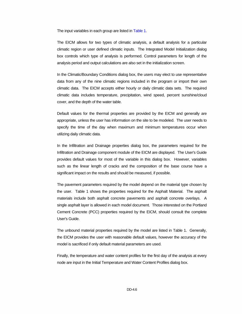
DD-4.6
The input variables in each group are listed in Table 1.
The EICM allows for two types of climatic analysis, a default analysis for a particular
climatic region or user defined climatic inputs. The Integrated Model Initialization dialog
box controls which type of analysis is performed. Control parameters for length of the
analysis period and output calculations are also set in the initialization screen.
In the Climatic/Boundary Conditions dialog box, the users may elect to use representative
data from any of the nine climatic regions included in the program or import their own
climatic data. The EICM accepts either hourly or daily climatic data sets. The required
climatic data includes temperature, precipitation, wind speed, percent sunshine/cloud
cover, and the depth of the water table.
Default values for the thermal properties are provided by the EICM and generally are
appropriate, unless the user has information on the site to be modeled. The user needs to
specify the time of the day when maximum and minimum temperatures occur when
utilizing daily climatic data.
In the Infiltration and Drainage properties dialog box, the parameters required for the
Infiltration and Drainage component module of the EICM are displayed. The User's Guide
provides default values for most of the variable in this dialog box. However, variables
such as the linear length of cracks and the composition of the base course have a
significant impact on the results and should be measured, if possible.
The pavement parameters required by the model depend on the material type chosen by
the user. Table 1 shows the properties required for the Asphalt Material. The asphalt
materials include both asphalt concrete pavements and asphalt concrete overlays. A
single asphalt layer is allowed in each model document. Those interested on the Portland
Cement Concrete (PCC) properties required by the EICM, should consult the complete
User's Guide.
The unbound material properties required by the model are listed in Table 1. Generally,
the EICM provides the user with reasonable default values, however the accuracy of the
model is sacrificed if only default material parameters are used.
Finally, the temperature and water content profiles for the first day of the analysis at every
node are input in the Initial Temperature and Water Content Profiles dialog box.
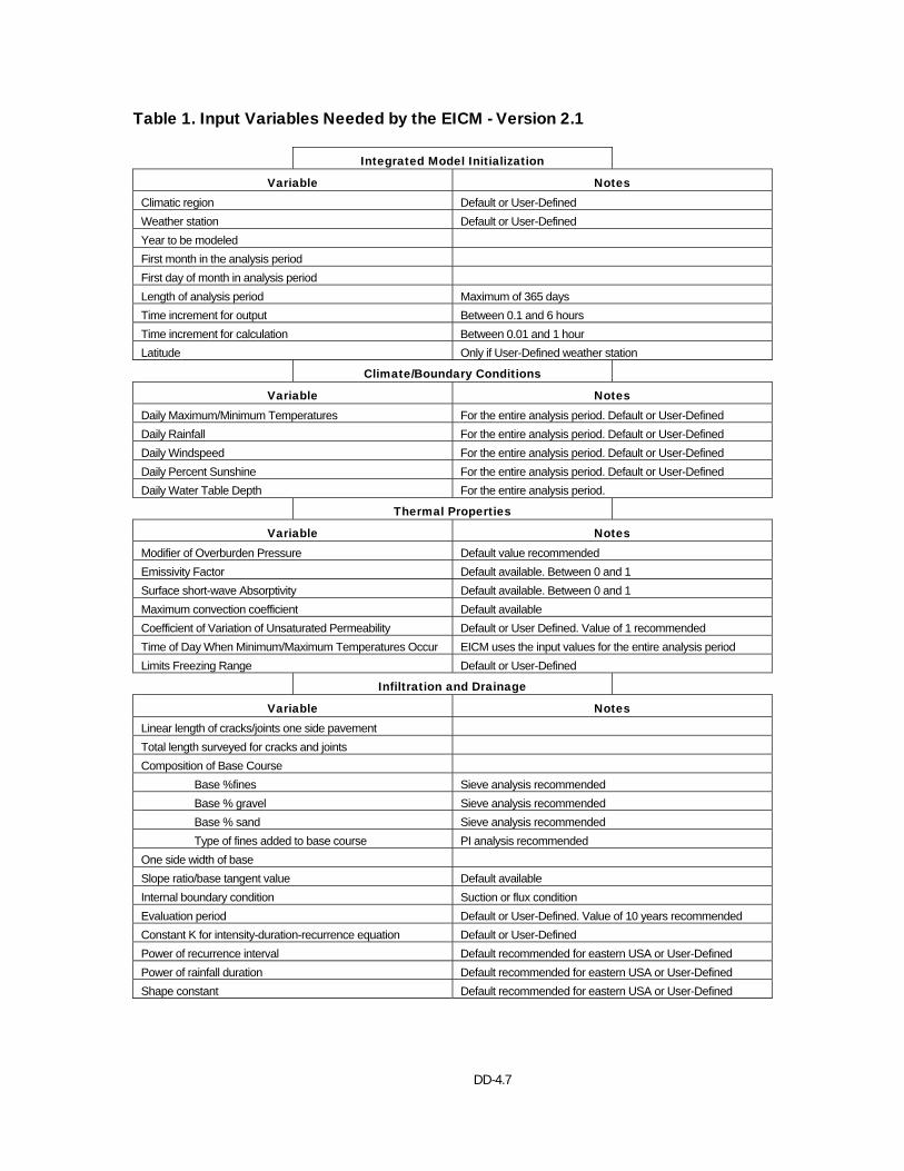
DD-4.7
Table 1. Input Variables Needed by the EICM - Version 2.1
Integrated Model Initialization
Variable Notes Climatic region Default or User-Defined Weather station Default or User-Defined Year to be modeled First month in the analysis period First day of month in analysis period Length of analysis period Maximum of 365 days Time increment for output Between 0.1 and 6 hours Time increment for calculation Between 0.01 and 1 hour Latitude Only if User-Defined weather station
Climate/Boundary Conditions
Variable Notes Daily Maximum/Minimum Temperatures For the entire analysis period. Default or User-Defined Daily Rainfall For the entire analysis period. Default or User-Defined Daily Windspeed For the entire analysis period. Default or User-Defined Daily Percent Sunshine For the entire analysis period. Default or User-Defined Daily Water Table Depth For the entire analysis period.
Thermal Properties
Variable Notes Modifier of Overburden Pressure Default value recommended Emissivity Factor Default available. Between 0 and 1 Surface short-wave Absorptivity Default available. Between 0 and 1 Maximum convection coefficient Default available Coefficient of Variation of Unsaturated Permeability Default or User Defined. Value of 1 recommended Time of Day When Minimum/Maximum Temperatures Occur EICM uses the input values for the entire analysis period Limits Freezing Range Default or User-Defined
Infiltration and Drainage
Variable Notes Linear length of cracks/joints one side pavement Total length surveyed for cracks and joints Composition of Base Course Base %fines Sieve analysis recommended Base % gravel Sieve analysis recommended Base % sand Sieve analysis recommended Type of fines added to base course PI analysis recommended One side width of base Slope ratio/base tangent value Default available Internal boundary condition Suction or flux condition Evaluation period Default or User-Defined. Value of 10 years recommended Constant K for intensity-duration-recurrence equation Default or User-Defined Power of recurrence interval Default recommended for eastern USA or User-Defined Power of rainfall duration Default recommended for eastern USA or User-Defined Shape constant Default recommended for eastern USA or User-Defined
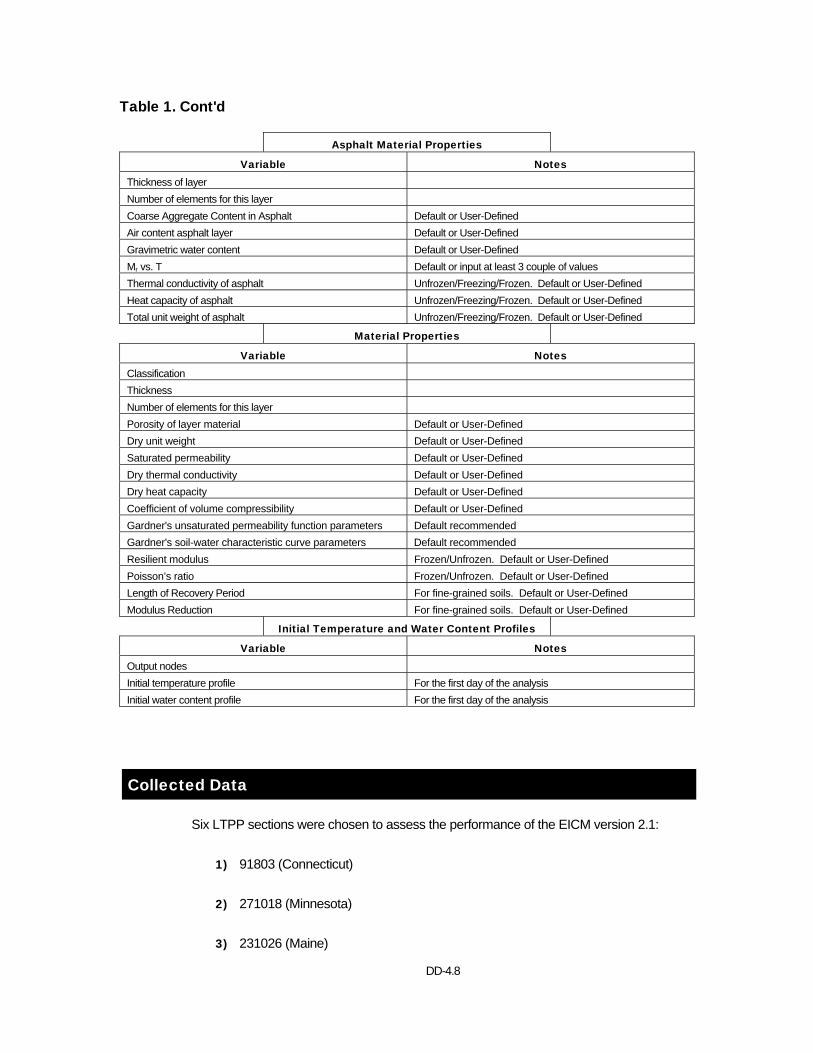
DD-4.8
Table 1. Cont'd
Asphalt Material Properties
Variable Notes Thickness of layer Number of elements for this layer Coarse Aggregate Content in Asphalt Default or User-Defined Air content asphalt layer Default or User-Defined Gravimetric water content Default or User-Defined Mr vs. T Default or input at least 3 couple of values Thermal conductivity of asphalt Unfrozen/Freezing/Frozen. Default or User-Defined Heat capacity of asphalt Unfrozen/Freezing/Frozen. Default or User-Defined Total unit weight of asphalt Unfrozen/Freezing/Frozen. Default or User-Defined
Material Properties
Variable Notes Classification Thickness Number of elements for this layer Porosity of layer material Default or User-Defined Dry unit weight Default or User-Defined Saturated permeability Default or User-Defined Dry thermal conductivity Default or User-Defined Dry heat capacity Default or User-Defined Coefficient of volume compressibility Default or User-Defined Gardner's unsaturated permeability function parameters Default recommended Gardner's soil-water characteristic curve parameters Default recommended Resilient modulus Frozen/Unfrozen. Default or User-Defined Poisson’s ratio Frozen/Unfrozen. Default or User-Defined Length of Recovery Period For fine-grained soils. Default or User-Defined Modulus Reduction For fine-grained soils. Default or User-Defined
Initial Temperature and Water Content Profiles
Variable Notes Output nodes Initial temperature profile For the first day of the analysis Initial water content profile For the first day of the analysis
Collected Data
Six LTPP sections were chosen to assess the performance of the EICM version 2.1:
1) 91803 (Connecticut)
2) 271018 (Minnesota)
3) 231026 (Maine)
DD-4.9
4) 331001 (New Hampshire)
5) 501002 (Vermont)
6) 831801 (Manitoba)
In general, the data used in the evaluation of the EICM version 2.1 were drawn from
DataPave 2.0 (1999). In a few instances, data were obtained from the Seasonal
Monitoring site installation reports for the test sites (Jiang and Tayabji, 1999). Data from
these sources are annotated as such in the tables presenting the input data
The input data used to model these sites are summarized in Tables 2 and 3. To the
extent possible, the values used as input to the model site and material specific data or
test results were obtained for the specific sites being modeled. However, several of the
required data elements involve testing or data collection not conducted for the LTPP test
sites and/or materials. Also, there are a few instances where data ordinarily collected for
the LTPP test sites was missing for a particular section. In these cases, reasonable
values were assumed, based on the available data, and the guidance provided in the
documentation for the EICM (Lytton et al., 1990). Finally, where the variables in question
were unrelated to the prediction of in situ moisture, program default values were used in
the interest of expediency. Assumed values are denoted by shading in the tables.
Specific comments regarding the origins or basis for selection of the values used are
discussed below.
Climatic Boundary Conditions
Daily temperature and rainfall data (including the times at which the daily maximum and
minimum temperature occurred), and (nominally) monthly depth to ground water data
collected at each site for the time period of the simulation were used in the models. Wind
speed and percent sunshine data used were those provided with the EICM for the
weather stations identified in Tables 2 and 3, as these data are not collected at the
seasonal monitoring sites. The recommended default values were used for the remaining
variables.
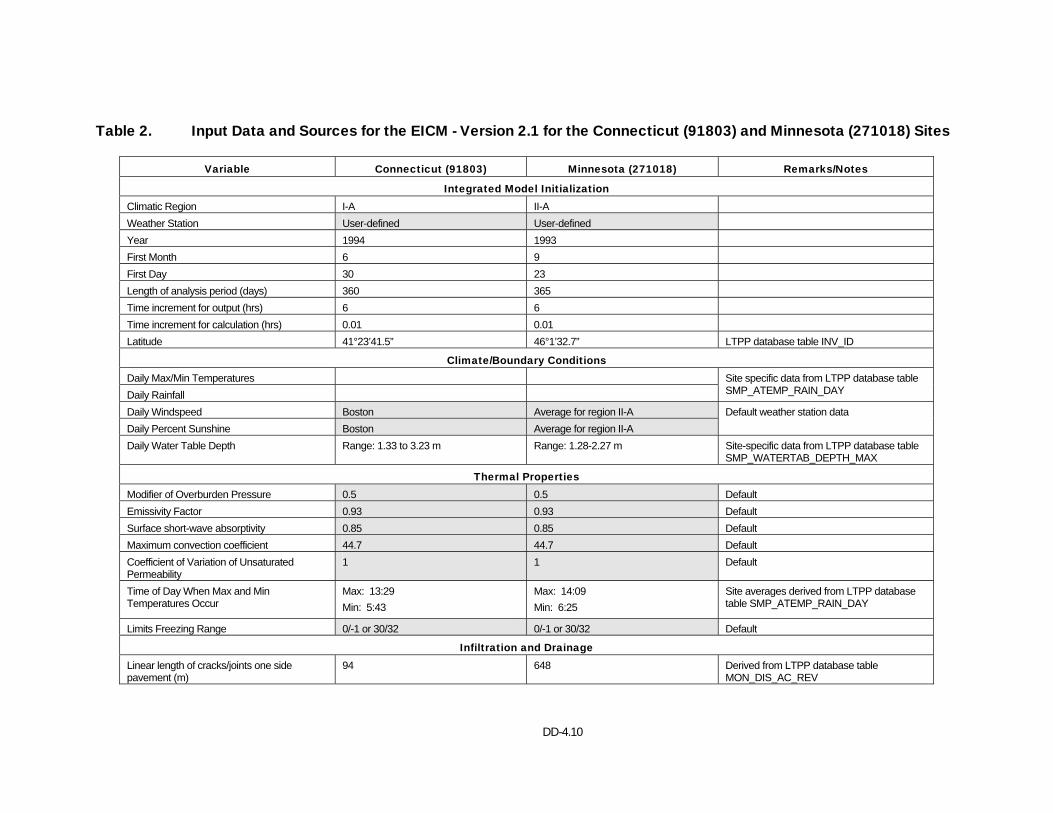
DD-4.10
Table 2. Input Data and Sources for the EICM - Version 2.1 for the Connecticut (91803) and Minnesota (271018) Sites
Variable Connecticut (91803) Minnesota (271018) Remarks/Notes
Integrated Model Initialization Climatic Region I-A II-A Weather Station User-defined User-defined Year 1994 1993 First Month 6 9 First Day 30 23 Length of analysis period (days) 360 365 Time increment for output (hrs) 6 6 Time increment for calculation (hrs) 0.01 0.01 Latitude 41°23’41.5” 46°1’32.7” LTPP database table INV_ID
Climate/Boundary Conditions Daily Max/Min Temperatures Daily Rainfall
Site specific data from LTPP database table SMP_ATEMP_RAIN_DAY
Daily Windspeed Boston Average for region II-A Daily Percent Sunshine Boston Average for region II-A
Default weather station data
Daily Water Table Depth Range: 1.33 to 3.23 m Range: 1.28-2.27 m Site-specific data from LTPP database table SMP_WATERTAB_DEPTH_MAX
Thermal Properties Modifier of Overburden Pressure 0.5 0.5 Default Emissivity Factor 0.93 0.93 Default Surface short-wave absorptivity 0.85 0.85 Default Maximum convection coefficient 44.7 44.7 Default Coefficient of Variation of Unsaturated Permeability
1 1 Default
Time of Day When Max and Min Temperatures Occur
Max: 13:29 Min: 5:43
Max: 14:09 Min: 6:25
Site averages derived from LTPP database table SMP_ATEMP_RAIN_DAY
Limits Freezing Range 0/-1 or 30/32 0/-1 or 30/32 Default
Infiltration and Drainage Linear length of cracks/joints one side pavement (m)
94 648 Derived from LTPP database table MON_DIS_AC_REV
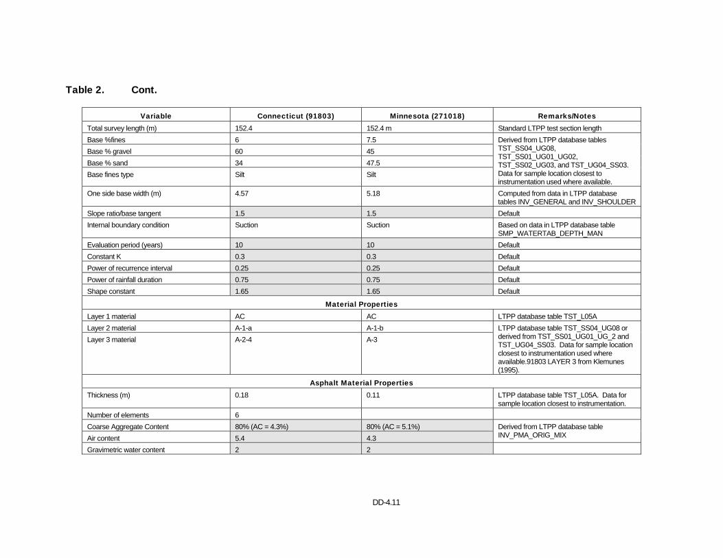
DD-4.11
Table 2. Cont.
Variable Connecticut (91803) Minnesota (271018) Remarks/Notes Total survey length (m) 152.4 152.4 m Standard LTPP test section length Base %fines 6 7.5 Base % gravel 60 45 Base % sand 34 47.5 Base fines type Silt Silt
Derived from LTPP database tables TST_SS04_UG08, TST_SS01_UG01_UG02, TST_SS02_UG03, and TST_UG04_SS03. Data for sample location closest to instrumentation used where available.
One side base width (m) 4.57 5.18 Computed from data in LTPP database tables INV_GENERAL and INV_SHOULDER
Slope ratio/base tangent 1.5 1.5 Default Internal boundary condition Suction Suction Based on data in LTPP database table
SMP_WATERTAB_DEPTH_MAN Evaluation period (years) 10 10 Default Constant K 0.3 0.3 Default Power of recurrence interval 0.25 0.25 Default Power of rainfall duration 0.75 0.75 Default Shape constant 1.65 1.65 Default
Material Properties Layer 1 material AC AC LTPP database table TST_L05A Layer 2 material A-1-a A-1-b Layer 3 material A-2-4 A-3
LTPP database table TST_SS04_UG08 or derived from TST_SS01_UG01_UG_2 and TST_UG04_SS03. Data for sample location closest to instrumentation used where available.91803 LAYER 3 from Klemunes (1995).
Asphalt Material Properties Thickness (m) 0.18 0.11 LTPP database table TST_L05A. Data for
sample location closest to instrumentation. Number of elements 6 Coarse Aggregate Content 80% (AC = 4.3%) 80% (AC = 5.1%) Air content 5.4 4.3
Derived from LTPP database table INV_PMA_ORIG_MIX
Gravimetric water content 2 2
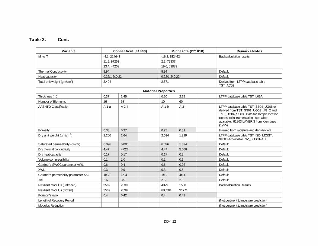
DD-4.12
Table 2. Cont.
Variable Connecticut (91803) Minnesota (271018) Remarks/Notes Mr vs T -4.1, 214643
11.8, 97252 23.4, 44203
-16.3, 153462 2.2, 78337 19.6, 63883
Backcalculation results
Thermal Conductivity 8.94 8.94 Default Heat capacity 0.22/1.2/.0.22 0.22/1.2/.0.22 Default Total unit weight (gm/cm3) 2.494 2.371 Derived from LTPP database table
TST_AC02
Material Properties Thickness (m) 0.37 1.45 0.10 2.25 LTPP database table TST_L05A Number of Elements 16 58 10 60 AASHTO Classification A-1-a A-2-4 A-1-b A-3 LTPP database table TST_SS04_UG08 or
derived from TST_SS01_UG01_UG_2 and TST_UG04_SS03. Data for sample location closest to instrumentation used where available. 91803 LAYER 3 from Klemunes (1995).
Porosity 0.33 0.37 0.23 0.31 Inferred from moisture and density data Dry unit weight (gm/cm3) 2.260 1.64 2.034 1.829 LTPP database table TST_ISD_MOIST,
91803 A-2-4 table INV_SUBGRADE Saturated permeability (cm/hr) 6.096 6.096 6.096 1.524 Default Dry thermal conductivity 4.47 4.023 4.47 5.066 Default Dry heat capacity 0.17 0.17 0.17 0.2 Default Volume compressibility 0.1 1.0 0.1 0.5 Default Gardner's SWCC parameter AWL 0.6 0.4 0.6 0.02 Default XWL 0.3 0.9 0.3 0.8 Default Gardner's permeability parameter AKL 1e-2 1e-4 1e-2 4e-4 Default XKL 2.6 3.5 2.6 2.9 Default Resilient modulus (unfrozen) 3569 2039 4079 1530 Resilient modulus (frozen) 3569 2039 688284 91771
Backcalculation Results
Poisson’s ratio 0.4 0.42 0.4 0.42 Length of Recovery Period (Not pertinent to moisture prediction) Modulus Reduction (Not pertinent to moisture prediction)
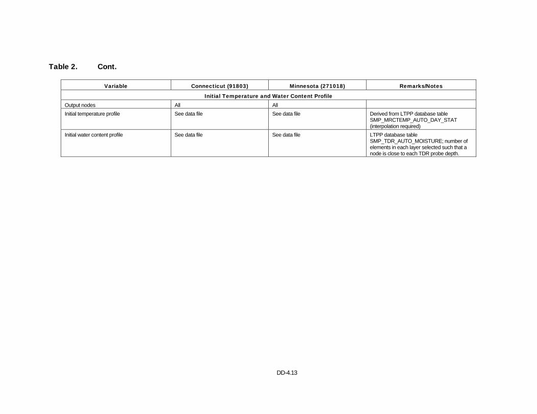
DD-4.13
Table 2. Cont.
Variable Connecticut (91803) Minnesota (271018) Remarks/Notes
Initial Temperature and Water Content Profile Output nodes All All Initial temperature profile See data file See data file Derived from LTPP database table
SMP_MRCTEMP_AUTO_DAY_STAT (interpolation required)
Initial water content profile See data file See data file LTPP database table SMP_TDR_AUTO_MOISTURE; number of elements in each layer selected such that a node is close to each TDR probe depth.
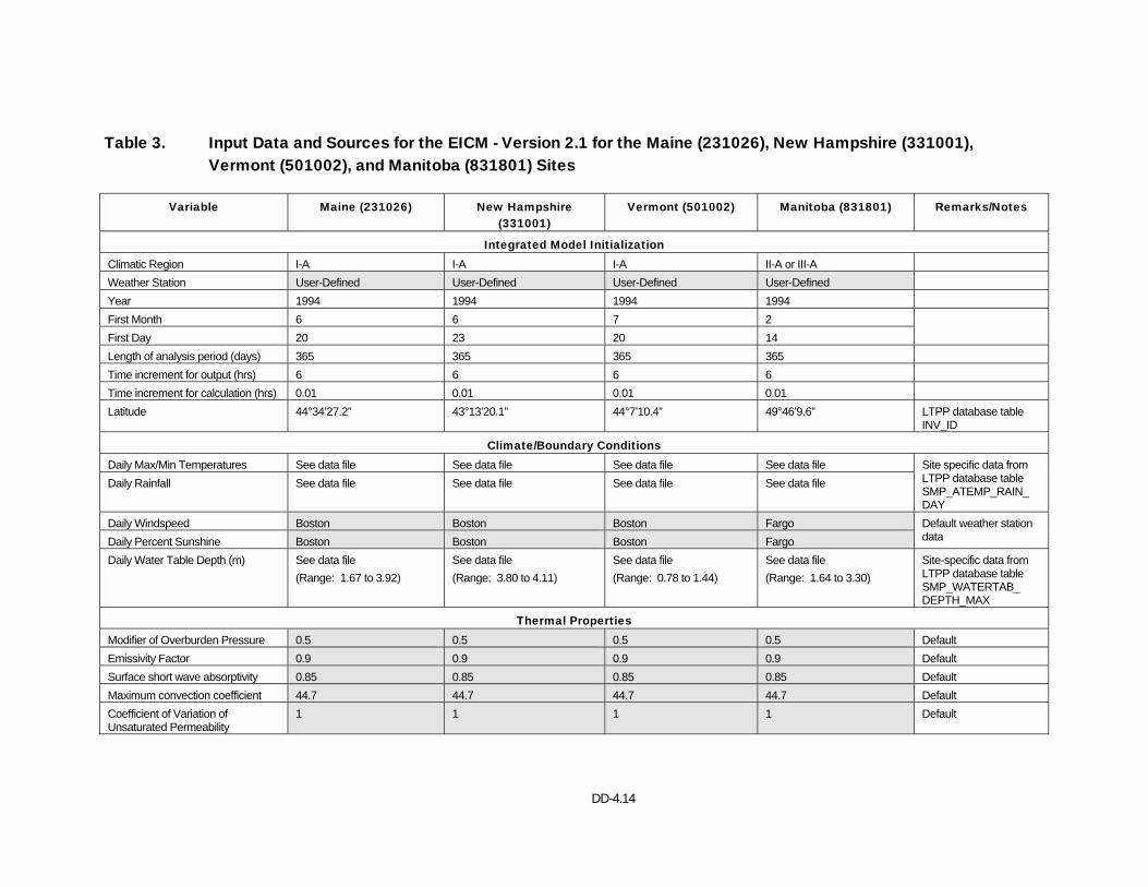
DD-4.14
Table 3. Input Data and Sources for the EICM - Version 2.1 for the Maine (231026), New Hampshire (331001), Vermont (501002), and Manitoba (831801) Sites
Variable Maine (231026) New Hampshire (331001)
Vermont (501002) Manitoba (831801) Remarks/Notes
Integrated Model Initialization Climatic Region I-A I-A I-A II-A or III-A Weather Station User-Defined User-Defined User-Defined User-Defined Year 1994 1994 1994 1994 First Month 6 6 7 2 First Day 20 23 20 14
Length of analysis period (days) 365 365 365 365 Time increment for output (hrs) 6 6 6 6 Time increment for calculation (hrs) 0.01 0.01 0.01 0.01 Latitude 44°34’27.2” 43°13’20.1” 44°7’10.4” 49°46’9.6” LTPP database table
INV_ID
Climate/Boundary Conditions Daily Max/Min Temperatures See data file See data file See data file See data file Daily Rainfall See data file See data file See data file See data file
Site specific data from LTPP database table SMP_ATEMP_RAIN_ DAY
Daily Windspeed Boston Boston Boston Fargo Daily Percent Sunshine Boston Boston Boston Fargo
Default weather station data
Daily Water Table Depth (m) See data file (Range: 1.67 to 3.92)
See data file (Range: 3.80 to 4.11)
See data file (Range: 0.78 to 1.44)
See data file (Range: 1.64 to 3.30)
Site-specific data from LTPP database table SMP_WATERTAB_ DEPTH_MAX
Thermal Properties Modifier of Overburden Pressure 0.5 0.5 0.5 0.5 Default Emissivity Factor 0.9 0.9 0.9 0.9 Default Surface short wave absorptivity 0.85 0.85 0.85 0.85 Default Maximum convection coefficient 44.7 44.7 44.7 44.7 Default Coefficient of Variation of Unsaturated Permeability
1 1 1 1 Default
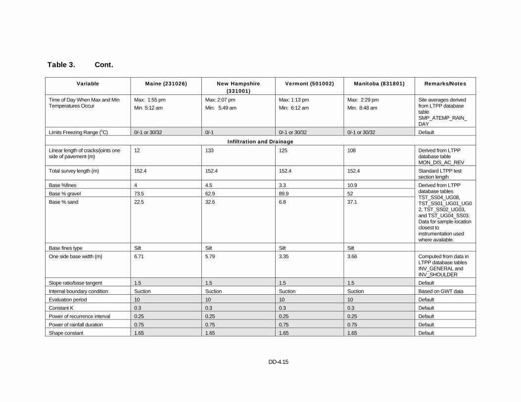
DD-4.15
Table 3. Cont.
Variable Maine (231026) New Hampshire (331001)
Vermont (501002) Manitoba (831801) Remarks/Notes
Time of Day When Max and Min Temperatures Occur
Max: 1:55 pm Min 5:12 am
Max: 2:07 pm Min: 5:49 am
Max: 1:13 pm Min: 6:12 am
Max: 2:29 pm Min: 8:48 am
Site averages derived from LTPP database table SMP_ATEMP_RAIN_ DAY
Limits Freezing Range (oC) 0/-1 or 30/32 0/-1 0/-1 or 30/32 0/-1 or 30/32 Default
Infiltration and Drainage Linear length of cracks/joints one side of pavement (m)
12 133 125 108 Derived from LTPP database table MON_DIS_AC_REV
Total survey length (m) 152.4 152.4 152.4 152.4 Standard LTPP test section length
Base %fines 4 4.5 3.3 10.9 Base % gravel 73.5 62.9 89.9 52 Base % sand 22.5 32.6 6.8 37.1
Derived from LTPP database tables TST_SS04_UG08, TST_SS01_UG01_UG02, TST_SS02_UG03, and TST_UG04_SS03. Data for sample location closest to instrumentation used where available.
Base fines type Silt Silt Silt Silt One side base width (m) 6.71 5.79 3.35 3.66 Computed from data in
LTPP database tables INV_GENERAL and INV_SHOULDER
Slope ratio/base tangent 1.5 1.5 1.5 1.5 Default Internal boundary condition Suction Suction Suction Suction Based on GWT data Evaluation period 10 10 10 10 Default Constant K 0.3 0.3 0.3 0.3 Default Power of recurrence interval 0.25 0.25 0.25 0.25 Default Power of rainfall duration 0.75 0.75 0.75 0.75 Default Shape constant 1.65 1.65 1.65 1.65 Default
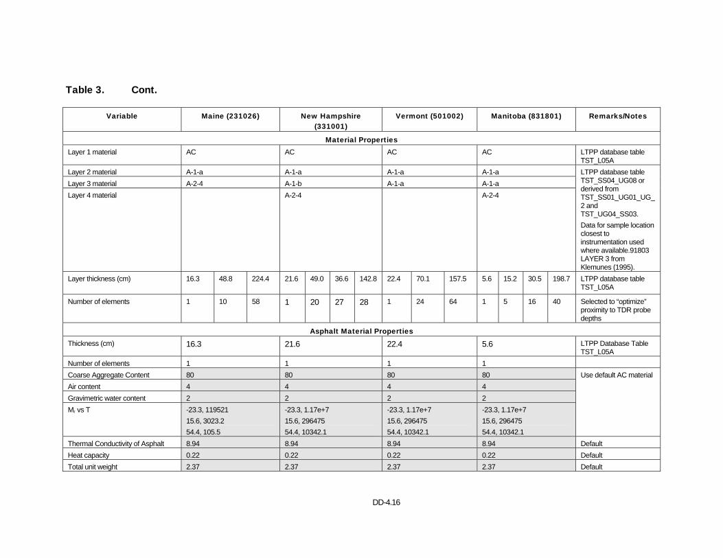
DD-4.16
Table 3. Cont.
Variable Maine (231026) New Hampshire (331001)
Vermont (501002) Manitoba (831801) Remarks/Notes
Material Properties Layer 1 material AC AC AC AC LTPP database table
TST_L05A Layer 2 material A-1-a A-1-a A-1-a A-1-a Layer 3 material A-2-4 A-1-b A-1-a A-1-a Layer 4 material A-2-4 A-2-4
LTPP database table TST_SS04_UG08 or derived from TST_SS01_UG01_UG_2 and TST_UG04_SS03. Data for sample location closest to instrumentation used where available.91803 LAYER 3 from Klemunes (1995).
Layer thickness (cm) 16.3 48.8 224.4 21.6 49.0 36.6 142.8 22.4 70.1 157.5 5.6 15.2 30.5 198.7 LTPP database table TST_L05A
Number of elements 1 10 58 1 20 27 28 1 24 64 1 5 16 40 Selected to “optimize” proximity to TDR probe depths
Asphalt Material Properties Thickness (cm) 16.3 21.6 22.4 5.6 LTPP Database Table
TST_L05A Number of elements 1 1 1 1 Coarse Aggregate Content 80 80 80 80 Air content 4 4 4 4 Gravimetric water content 2 2 2 2 Mr vs T -23.3, 119521
15.6, 3023.2 54.4, 105.5
-23.3, 1.17e+7 15.6, 296475 54.4, 10342.1
-23.3, 1.17e+7 15.6, 296475 54.4, 10342.1
-23.3, 1.17e+7 15.6, 296475 54.4, 10342.1
Use default AC material
Thermal Conductivity of Asphalt 8.94 8.94 8.94 8.94 Default Heat capacity 0.22 0.22 0.22 0.22 Default Total unit weight 2.37 2.37 2.37 2.37 Default
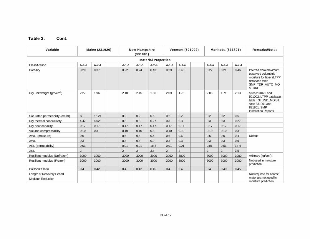
DD-4.17
Table 3. Cont.
Variable Maine (231026) New Hampshire (331001)
Vermont (501002) Manitoba (831801) Remarks/Notes
Material Properties Classification A-1-a A-2-4 A-1-a A-1-b A-2-4 A-1-a A-1-a A-1-a A-1-a A-2-4 Porosity 0.29 0.37 0.22 0.24 0.43 0.29 0.46 0.22 0.21 0.46 Inferred from maximum
observed volumetric moisture for layer (LTPP database table SMP_TDR_AUTO_MOISTURE
Dry unit weight (gm/cm3) 2.27 1.96 2.10 2.15 1.86 2.09 1.76 2.08 1.71 2.13 Sites 231026 and 501002: LTPP database table TST_ISD_MOIST; sites 331001 and 831801: SMP Installation Reports
Saturated permeability (cm/hr) 60 15.24 0.2 0.2 0.5 0.2 0.2 0.2 0.2 0.5 Dry thermal conductivity 4.47 4.023 0.3 0.3 0.27 0.3 0.3 0.3 0.3 0.27 Dry heat capacity 0.17 0.17 0.17 0.17 0.17 0.17 0.17 0.17 0.17 0.17 Volume compressibility 0.10 0.3 0.10 0.10 0.3 0.10 0.10 0.10 0.10 0.3 AWL (moisture) 0.6 0.6 0.6 0.4 0.6 0.6 0.6 0.6 0.4 XWL 0.3 0.3 0.3 0.9 0.3 0.3 0.3 0.3 0.9 AKL (permeability) 0.01 0.01 0.01 1e-4 0.01 0.01 0.01 0.01 1e-4 XKL 2 2 2 3.5 2 2 2 2 3.5
Default
Resilient modulus (Unfrozen) 3000 3000 3000 3000 3000 3000 3000 3000 3000 3000 Resilient modulus (Frozen) 3000 3000 3000 3000 3000 3000 3000 3000 3000 3000
Arbitrary (kg/cm2). Not used in moisture prediction.
Poisson’s ratio 0.4 0.42 0.4 0.42 0.45 0.4 0.4 0.4 0.40 0.45 Length of Recovery Period Modulus Reduction
Not required for coarse materials; not used in moisture prediction

DD-4.18
Table 3. Cont.
Variable Maine (231026) New Hampshire (331001)
Vermont (501002) Manitoba (831801) Remarks/Notes
Initial Temperature and Pore Pressure Profile Output nodes All All All All Initial temperature profile See data file See data file See data file See data file Derived from LTPP
database table SMP_MRCTEMP_ AUTO_DAY_STAT (interpolation required)
Initial water content profile See data file See data file See data file See data file LTPP database table SMP_TDR_AUTO_ MOISTURE; number of elements in each layer selected such that a node is close to each TDR probe depth.
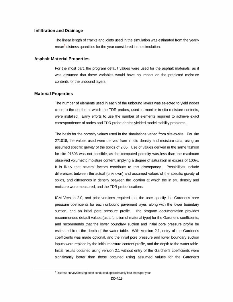
DD-4.19
Infiltration and Drainage
The linear length of cracks and joints used in the simulation was estimated from the yearly
mean1 distress quantities for the year considered in the simulation.
Asphalt Material Properties
For the most part, the program default values were used for the asphalt materials, as it
was assumed that these variables would have no impact on the predicted moisture
contents for the unbound layers.
Material Properties
The number of elements used in each of the unbound layers was selected to yield nodes
close to the depths at which the TDR probes, used to monitor in situ moisture contents,
were installed. Early efforts to use the number of elements required to achieve exact
correspondence of nodes and TDR probe depths yielded model stability problems.
The basis for the porosity values used in the simulations varied from site-to-site. For site
271018, the values used were derived from in situ density and moisture data, using an
assumed specific gravity of the solids of 2.65. Use of values derived in the same fashion
for site 91803 was not possible, as the computed porosity was less than the maximum
observed volumetric moisture content, implying a degree of saturation in excess of 100%.
It is likely that several factors contribute to this discrepancy. Possibilities include
differences between the actual (unknown) and assumed values of the specific gravity of
solids, and differences in density between the location at which the in situ density and
moisture were measured, and the TDR probe locations.
ICM Version 2.0, and prior versions required that the user specify the Gardner’s pore
pressure coefficients for each unbound pavement layer, along with the lower boundary
suction, and an initial pore pressure profile. The program documentation provides
recommended default values (as a function of material type) for the Gardner’s coefficients,
and recommends that the lower boundary suction and initial pore pressure profile be
estimated from the depth of the water table. With Version 2.1, entry of the Gardner’s
coefficients was made optional, and the initial pore pressure and lower boundary suction
inputs were replace by the initial moisture content profile, and the depth to the water table.
Initial results obtained using version 2.1 without entry of the Gardner’s coefficients were
significantly better than those obtained using assumed values for the Gardner’s
1 Distress surveys having been conducted approximately four times per year.
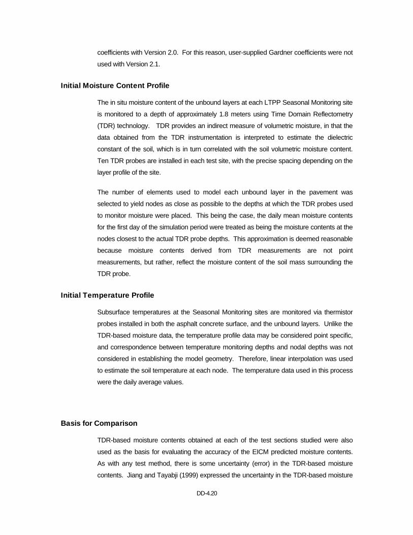
DD-4.20
coefficients with Version 2.0. For this reason, user-supplied Gardner coefficients were not
used with Version 2.1.
Initial Moisture Content Profile
The in situ moisture content of the unbound layers at each LTPP Seasonal Monitoring site
is monitored to a depth of approximately 1.8 meters using Time Domain Reflectometry
(TDR) technology. TDR provides an indirect measure of volumetric moisture, in that the
data obtained from the TDR instrumentation is interpreted to estimate the dielectric
constant of the soil, which is in turn correlated with the soil volumetric moisture content.
Ten TDR probes are installed in each test site, with the precise spacing depending on the
layer profile of the site.
The number of elements used to model each unbound layer in the pavement was
selected to yield nodes as close as possible to the depths at which the TDR probes used
to monitor moisture were placed. This being the case, the daily mean moisture contents
for the first day of the simulation period were treated as being the moisture contents at the
nodes closest to the actual TDR probe depths. This approximation is deemed reasonable
because moisture contents derived from TDR measurements are not point
measurements, but rather, reflect the moisture content of the soil mass surrounding the
TDR probe.
Initial Temperature Profile
Subsurface temperatures at the Seasonal Monitoring sites are monitored via thermistor
probes installed in both the asphalt concrete surface, and the unbound layers. Unlike the
TDR-based moisture data, the temperature profile data may be considered point specific,
and correspondence between temperature monitoring depths and nodal depths was not
considered in establishing the model geometry. Therefore, linear interpolation was used
to estimate the soil temperature at each node. The temperature data used in this process
were the daily average values.
Basis for Comparison
TDR-based moisture contents obtained at each of the test sections studied were also
used as the basis for evaluating the accuracy of the EICM predicted moisture contents.
As with any test method, there is some uncertainty (error) in the TDR-based moisture
contents. Jiang and Tayabji (1999) expressed the uncertainty in the TDR-based moisture

DD-4.21
content data derived for the LTPP test sections in terms of a series of estimated 95%
confidence intervals. The confidence interval applicable to any particular moisture
observation is a function of the standard error of estimate of the regression model used in
the derivation of the moisture content, and the errors in the model parameters. The
applicable confidence limits are shown in the figures comparing the monitored and
predicted moisture contents.
Results
Field (TDR-based) measurements of volumetric water content along with the
corresponding 95% confidence estimated error were compared with the predicted
volumetric water content profile obtained by the EICM version 2.1. In making these
comparisons, the EICM predicted moisture contents for the two nodes adjacent to each
TDR monitoring depth were interpolated to obtain the predicted moisture content
corresponding to the monitored valued. Review of the predicted moisture profiles shows
that this is a reasonable approach to resolving small differences in the depths used for
moisture monitoring and moisture prediction.
The results of the comparison are shown in Figures 1 through 6. The comparisons
between the measured volumetric water content and the predicted volumetric water
content correspond to the dates on the analysis period when TDR measurements were
available. The moisture content profiles are shown in Appendices A through F.
The summary of the results is presented in Figures 7 and 8. Figure 7 shows the water
content prediction for the base course material from the 6 sites previously discussed, and
the results of a linear regression through the data points. Poor agreement between the
monitored and predicted values is reflected in the low coefficient of determination (R2) of
0.05 for the regression. Figure 8 depicts the measured versus predicted volumetric water
content for the subgrade materials along with a linear regression to the data. The
regression of the subgrade materials shows a coefficient of determination of 0.34, better
than that for the base, but still poor. Note also that a substantial number of data points in
both figures fall outside the estimated confidence limits for the field data, even though
these limits are very broad.
The results obtained were presented in a meeting held in Champaign, IL on September
23, 1999. The following persons participated in the meeting: Dr. Matt Witczak (ASU – led
the meeting), Dr. Barry Dempsey (U of I), Dr. Waseem Mirza (ASU), Dr. Bill Houston
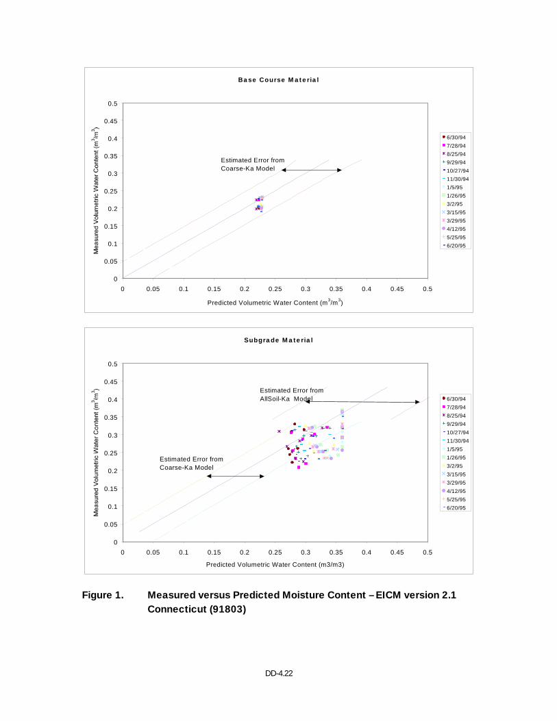
DD-4.22
Base Course Material
0
0.05
0.1
0.15
0.2
0.25
0.3
0.35
0.4
0.45
0.5
0 0.05 0.1 0.15 0.2 0.25 0.3 0.35 0.4 0.45 0.5
Predicted Volumetric Water Content (m3/m3)
6/30/947/28/948/25/949/29/9410/27/9411/30/941/5/951/26/953/2/953/15/953/29/954/12/955/25/956/20/95
Estimated Error from Coarse-Ka Model
Subgrade Material
0
0.05
0.1
0.15
0.2
0.25
0.3
0.35
0.4
0.45
0.5
0 0.05 0.1 0.15 0.2 0.25 0.3 0.35 0.4 0.45 0.5
Predicted Volumetric Water Content (m3/m3)
6/30/947/28/948/25/949/29/9410/27/9411/30/941/5/951/26/953/2/953/15/953/29/954/12/955/25/956/20/95
Estimated Error from AllSoil-Ka Model
Estimated Error from Coarse-Ka Model
Figure 1. Measured versus Predicted Moisture Content – EICM version 2.1 Connecticut (91803)
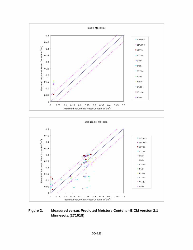
DD-4.23
Base Material
0
0.05
0.1
0.15
0.2
0.25
0.3
0.35
0.4
0.45
0.5
0 0.05 0.1 0.15 0.2 0.25 0.3 0.35 0.4 0.45 0.5Predicted Volumetric Water Content (m3/m3)
10/20/93
11/19/93
12/7/93
1/11/94
2/8/94
3/8/94
3/22/94
4/4/94
4/25/94
6/13/94
7/11/94
8/8/94
Subgrade Material
0
0.05
0.1
0.15
0.2
0.25
0.3
0.35
0.4
0.45
0.5
0 0.05 0.1 0.15 0.2 0.25 0.3 0.35 0.4 0.45 0.5Predicted Volumetric Water Content (m3/m3)
10/20/93
11/19/93
12/7/93
1/11/94
2/8/94
3/8/94
3/22/94
4/4/94
4/25/94
6/13/94
7/11/94
8/8/94
Figure 2. Measured versus Predicted Moisture Content – EICM version 2.1 Minnesota (271018)
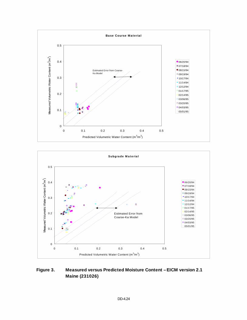
DD-4.24
Base Course Material
0
0.1
0.2
0.3
0.4
0.5
0 0.1 0.2 0.3 0.4 0.5
Predicted Volumetric Water Content (m3/m3)
06/20/94
07/18/94
08/15/94
09/19/94
10/17/94
11/14/94
12/12/94
01/17/95
02/14/95
03/06/95
03/20/95
04/03/95
05/01/95
Estimated Error from Coarse-Ka Model
Subgrade Material
0
0.1
0.2
0.3
0.4
0.5
0 0.1 0.2 0.3 0.4 0.5
Predicted Volumetric Water Content (m3/m3)
06/20/9407/18/9408/15/9409/19/9410/17/9411/14/9412/12/9401/17/9502/14/9503/06/9503/20/9504/03/9505/01/95
Estimated Error from Coarse-Ka Model
Figure 3. Measured versus Predicted Moisture Content – EICM version 2.1 Maine (231026)
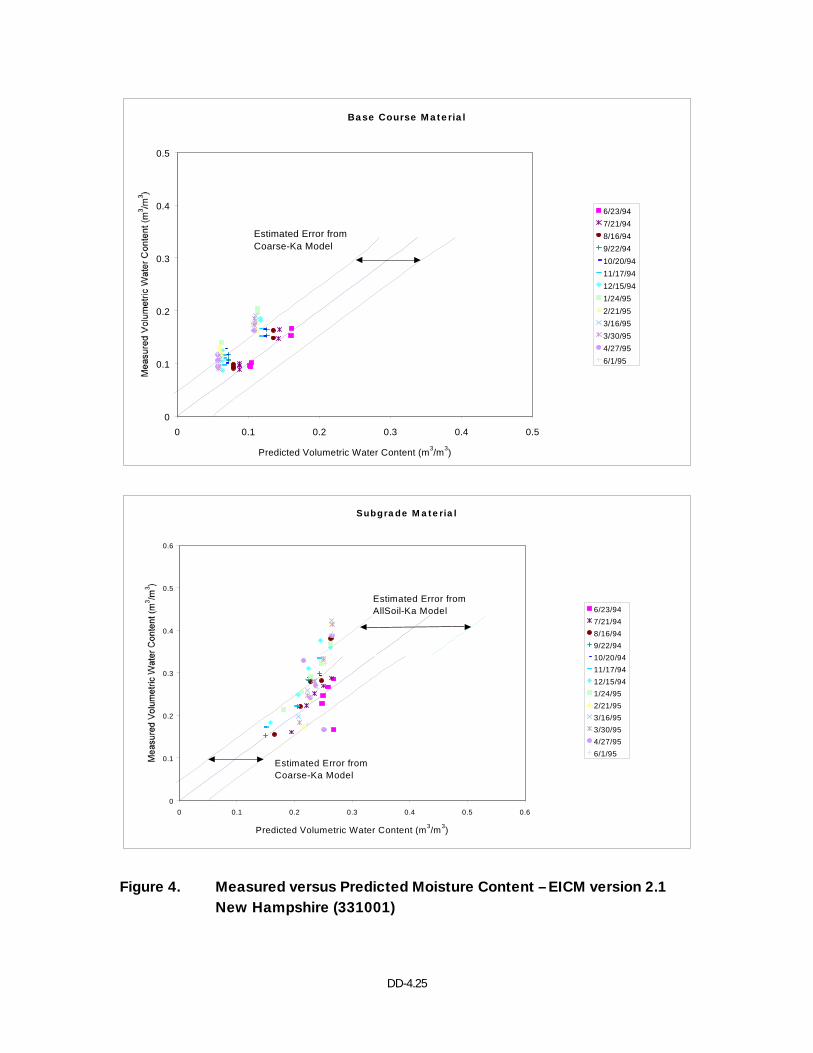
DD-4.25
Base Course Material
0
0.1
0.2
0.3
0.4
0.5
0 0.1 0.2 0.3 0.4 0.5
Predicted Volumetric Water Content (m3/m3)
6/23/947/21/948/16/949/22/9410/20/9411/17/9412/15/941/24/952/21/953/16/953/30/954/27/956/1/95
Estimated Error from Coarse-Ka Model
Subgrade Material
0
0.1
0.2
0.3
0.4
0.5
0.6
0 0.1 0.2 0.3 0.4 0.5 0.6
Predicted Volumetric Water Content (m3/m3)
6/23/947/21/948/16/949/22/9410/20/9411/17/9412/15/941/24/952/21/953/16/953/30/954/27/956/1/95
Estimated Error from Coarse-Ka Model
Estimated Error from AllSoil-Ka Model
Figure 4. Measured versus Predicted Moisture Content – EICM version 2.1 New Hampshire (331001)
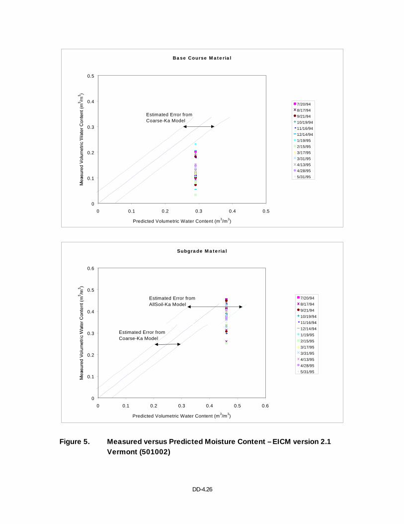
DD-4.26
Base Course Material
0
0.1
0.2
0.3
0.4
0.5
0 0.1 0.2 0.3 0.4 0.5
Predicted Volumetric Water Content (m3/m3)
7/20/948/17/949/21/9410/19/9411/16/9412/14/941/19/952/15/953/17/953/31/954/13/954/28/955/31/95
Estimated Error from Coarse-Ka Model
Subgrade Material
0
0.1
0.2
0.3
0.4
0.5
0.6
0 0.1 0.2 0.3 0.4 0.5 0.6
Predicted Volumetric Water Content (m3/m3)
7/20/948/17/949/21/9410/19/9411/16/9412/14/941/19/952/15/953/17/953/31/954/13/954/28/955/31/95
Estimated Error from Coarse-Ka Model
Estimated Error from AllSoil-Ka Model
Figure 5. Measured versus Predicted Moisture Content – EICM version 2.1 Vermont (501002)
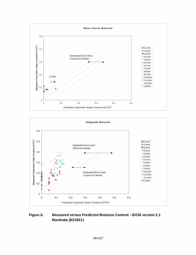
DD-4.27
Base Course Material
0
0.1
0.2
0.3
0.4
0.5
0 0.1 0.2 0.3 0.4 0.5
Predicted Volumetric Water Content (m3/m3)
2/14/943/14/943/28/944/11/944/29/945/13/946/17/947/25/948/18/949/21/9410/19/9411/16/9412/14/941/25/95
Estimated Error from Coarse-Ka Model
Subgrade Material
0
0.1
0.2
0.3
0.4
0.5
0.6
0 0.1 0.2 0.3 0.4 0.5 0.6
Predicted Volumetric Water Content (m3/m3)
2/14/943/14/943/28/944/11/944/29/945/13/946/17/947/25/948/18/949/21/9410/19/9411/16/9412/14/941/25/95
Estimated Error from Coarse-Ka Model
Estimated Error from AllSoil-Ka Model
Figure 6. Measured versus Predicted Moisture Content – EICM version 2.1 Manitoba (831801)
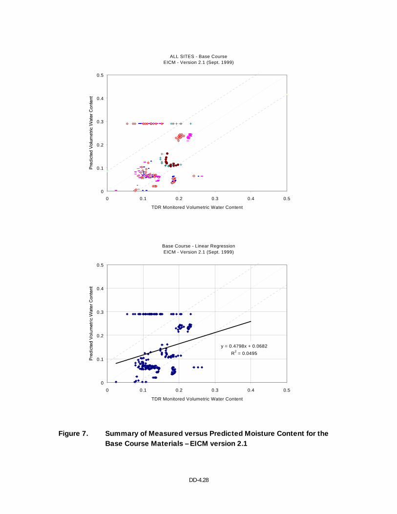
DD-4.28
ALL SITES - Base Course EICM - Version 2.1 (Sept. 1999)
0
0.1
0.2
0.3
0.4
0.5
0 0.1 0.2 0.3 0.4 0.5
TDR Monitored Volumetric Water Content
Base Course - Linear RegressionEICM - Version 2.1 (Sept. 1999)
y = 0.4798x + 0.0682R2 = 0.0495
0
0.1
0.2
0.3
0.4
0.5
0 0.1 0.2 0.3 0.4 0.5
TDR Monitored Volumetric Water Content
Figure 7. Summary of Measured versus Predicted Moisture Content for the Base Course Materials – EICM version 2.1
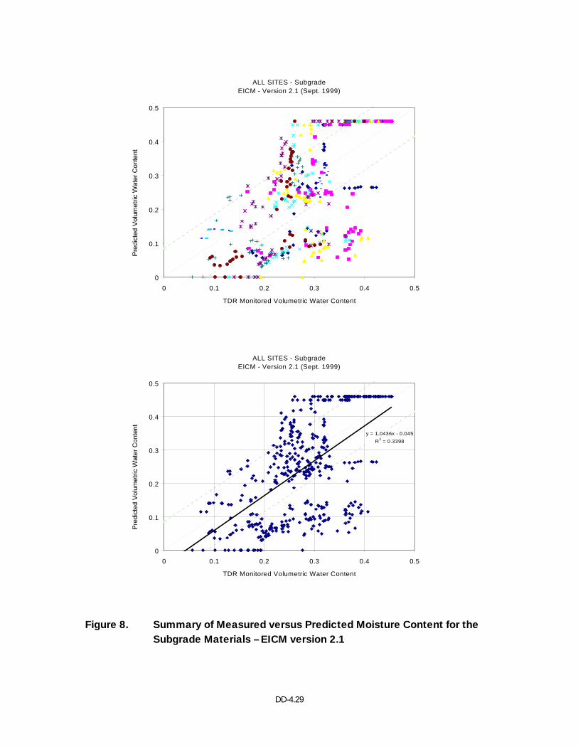
DD-4.29
ALL SITES - SubgradeEICM - Version 2.1 (Sept. 1999)
0
0.1
0.2
0.3
0.4
0.5
0 0.1 0.2 0.3 0.4 0.5
TDR Monitored Volumetric Water Content
ALL SITES - SubgradeEICM - Version 2.1 (Sept. 1999)
y = 1.0436x - 0.045R2 = 0.3398
0
0.1
0.2
0.3
0.4
0.5
0 0.1 0.2 0.3 0.4 0.5
TDR Monitored Volumetric Water Content
Figure 8. Summary of Measured versus Predicted Moisture Content for the Subgrade Materials – EICM version 2.1
DD-4.30
(ASU), Cheryl Richter (FHWA), Gregg Larson (U of I), and Dr. Claudia E. Zapata (ASU).
The assessment of the EICM prediction was primarily based on:
1) Field measurements of volumetric water content for the LTTP sites estimated by
Time Domain Reflectometry (TDR)
2) Pattern of moisture content change with time
3) Magnitude of fluctuations
As shown in Figures 7 and 8, the initial comparisons were not good, with problems
appearing on all three bases of comparison. Several factors that may have contributed to
the poor estimation of the water contents given by the EICM were discussed. The
following section presents a summary of the factors that were considered important to the
prediction of the moisture content by the EICM.
Factors that Contributed to the Poor Predictions of the Water Contents by the EICM
The field measurements of volumetric water content were obtained by using
regression type equations that correlated with the bulk dielectric constant (Ka) given
by the TDR. The correlation was done by subdividing the entire database used in the
regression analysis into two major soil groups: coarse and fine-grained soils. It was
recommended that the use of predictive models developed by Klemunes (1997) for
individual soil classes be explored, as a means of improving the accuracy of the TDR-
based moisture data.
The soil properties needed to input the EICM is rather extensive and usually is not
included in routine soil surveys. Saturated/unsaturated hydraulic conductivity, soil-
water characteristic curve parameters, and porosity are unique for a particular soil and
the use of default values may lead to a poor modeling of the transient moisture
conditions. It was recommended at this meeting to advocate the good practice of
measuring those parameters in order to obtain better predictions.
The main changes in the EICM version 2.1 were focussed on the Flux boundary
condition and no substantial improvements were implemented for the Suction
boundary condition. It was recommended to run the EICM in the Flux boundary
condition mode, as a possible means of improving the predictions.

DD-4.31
More care should be exercised when dividing the soil profile into the different sub-
layers. It is recommended to add sub-layers around the TDR experimental points in
the subbase and subgrade layers to improve the prediction for the first day of the
analysis period.
The EICM makes use of seven sets of Gardner's parameters to represent the soil-
water characteristic curve (SWCC) and the unsaturated hydraulic conductivity. Each
set represents one of the major AASHTO classification groups. The
recommendations were based on use of a hierarchical approach:
1) Generate additional SWCC / unsaturated hydraulic conductivity parameters for
the different soil sub-groups recognized in the AASHTO soil classification system.
2) Replace the SWCC Gardner equation with an equation providing a better
functional fit.
3) Predict the SWCC based on grain-size distribution (GSD) and soil properties, and
4) Incorporate experimentally measured SWCCs and unsaturated hydraulic
conductivity functions into the EICM, when available.
It was recommended that all frozen volumetric water content values be removed from
the comparisons with the EICM results, given the fact that the meaning of TDR-based
moisture contents in frozen or freezing soils is uncertain.
Short-term Actions Recommended for the Improvement of the EICM
The short-term actions recommended for the improvement of the EICM included:
Generate additional soil-water characteristic curves (SWCCs) as a function of soil
properties and the AASHTO soil classification system.
In place of the Gardner equation, substitute a better functional fit for the SWCC and
the unsaturated hydraulic conductivity function.
Improve estimates of saturated permeability and saturated volumetric water content
(porosity) as a function of the AASHTO classification system.
Impose sub-layers around TDR measuring points.

DD-4.32
Remove all frozen volumetric water content data points from the comparisons with the
EICM results.
Explore use of Klemunes class-specific moisture models for computation of TDR-
based moisture contents.
Repeat comparisons using flux boundary conditions.
Add three or four new sites, including one or more in the southwestern climatic region.
All of the above recommendations have been implemented. However, the exploration of
the use of Klemunes class-specific moisture models for computation of TDR-based
moisture contents did not result in the application of those models in the analysis, for the
following reasons:
1) All of Klemunes models use the soil specific gravity as one of the predictor
variables. This parameter is available for only some of the soils considered in this
investigation.
2) The goodness of fit statistics (coefficient of determination, and standard error of
estimate) for the models currently used in the LTPP moisture computation are
better than those for Klemunes A-2-4, A-6, A-7-5, and A-7-6 models. Thus, it
does not appear that application of Klemunes models will improve the accuracy of
the computed moisture contents for those soils. This is particularly true for the A-
6 and A-7 models, which were based on data for only two soils.
3) Based on review of the goodness of fit statistics and number of soils used in their
development, it was deemed worthwhile to pursue application of Klemunes
models for: (1) A-3 soils where the required specific gravity data are available;
and (2) A-1-b soils from the two sites used in the model development. However,
when the models were applied on a trial basis, it was found that there was no
benefit in doing so. Thus, further consideration of these models was abandoned.
Details of the improvements arising from the remaining recommendations are described in
Chapter 3.
DD-4.33
Modifications to the EICM version 2.1 Moisture Content Prediction
Proposed Modifications to the EICM – version 2.1
The proposed changes to the EICM's moisture prediction algorithm included:
1) Select the best functional fit for the soil-water characteristic curve (SWCC)
2) Given Grain Size Distribution (GSD) and Plasticity Index (PI), develop improved
estimates of SWCCs, saturated permeability (ksat), and porosity (θsat).
3) Given AASHTO Classifications, develop improved estimates of SWCCs, ksat, and
θsat
4) Use the initial water content values, together with distance from the Groundwater
Table (GWT) as guidance in choosing the SWCC.
The Soil-Water Characteristic Curve
The SWCC has been defined as the variation of water storage capacity within the macro
and micro pores of a soil, with respect to suction (Fredlund et al., 1995). This relationship
is generally plotted as the variation of the water content (gravimetric, volumetric or degree
of saturation) with soil suction. Several mathematical equations have been proposed to
represent the SWCC. Most of the equations are empirical in nature and are based on the
shape of measured SWCCs. A summary of the most commonly used equations is
presented in Table 4.
The EICM Version 2.1 makes use of the equation proposed by Gardner (1958). Even
though Gardner's equation is widely used, it does not represent a sigmoid, which is
currently believed to be the most accurate shape representing the SWCC. Notice that this
equation has three fitting parameters: θr, a, and b (See Table 4 for definition). Also, in the
EICM version 2.1 and prior versions only two of the three Gardner equation parameters
were treated as variables, with the third, the residual volumetric water content (θr) taken to
Chapter
3
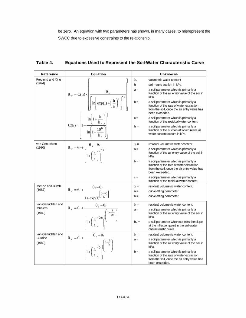
DD-4.34
be zero. An equation with two parameters has shown, in many cases, to misrepresent the
SWCC due to excessive constraints to the relationship.
Table 4. Equations Used to Represent the Soil-Water Characteristic Curve
Reference Equation Unknowns Fredlund and Xing (1994)
⎥⎥⎥⎥⎥⎥⎥
⎦
⎤
⎢⎢⎢⎢⎢⎢⎢
⎣
⎡
⎥⎥⎦
⎤
⎢⎢⎣
⎡
⎥⎥⎦
⎤
⎢⎢⎣
⎡⎟⎠⎞
⎜⎝⎛+
θ×=θ
cb
sw
ah)1exp(ln
)h(C
⎥⎥⎥⎥⎥
⎦
⎤
⎢⎢⎢⎢⎢
⎣
⎡
⎟⎟⎠
⎞⎜⎜⎝
⎛+
⎟⎟⎠
⎞⎜⎜⎝
⎛+
−=
r
6r
h101ln
hh1ln
1)h(C
θw volumetric water content h soil matric suction in kPa a = a soil parameter which is primarily a
function of the air entry value of the soil in kPa.
b = a soil parameter which is primarily a function of the rate of water extraction from the soil, once the air entry value has been exceeded.
c = a soil parameter which is primarily a function of the residual water content.
hr = a soil parameter which is primarily a function of the suction at which residual water content occurs in kPa.
van Genuchten (1980)
cb
rsrw
ah1
⎥⎥⎦
⎤
⎢⎢⎣
⎡⎟⎠⎞
⎜⎝⎛+
θ−θ+θ=θ
θr = residual volumetric water content. a = a soil parameter which is primarily a
function of the air entry value of the soil in kPa.
b = a soil parameter which is primarily a function of the rate of water extraction from the soil, once the air entry value has been exceeded.
c = a soil parameter which is primarily a function of the residual water content.
McKee and Bumb (1987)
[ ]b
a)(h
rsrw
)1exp(1−
+
θ−θ+θ=θ
θr = residual volumetric water content. a = curve-fitting parameter b = curve-fitting parameter
van Genuchten and Mualem (1980)
⎟⎟
⎠
⎞
⎜⎜
⎝
⎛
⎥⎥
⎦
⎤
⎢⎢
⎣
⎡⎟⎠⎞
⎜⎝⎛+
θ−θ+θ=θ
−bm1
1
m
rsrw
b
ah1
θr = residual volumetric water content. a = a soil parameter which is primarily a
function of the air entry value of the soil in kPa.
bm = a soil parameter which controls the slope at the inflection point in the soil-water characteristic curve.
van Genuchten and Burdine (1980)
⎟⎟
⎠
⎞
⎜⎜
⎝
⎛
⎥⎥
⎦
⎤
⎢⎢
⎣
⎡⎟⎠⎞
⎜⎝⎛+
θ−θ+θ=θ
−b2
1
rsrw
b
ah1
θr = residual volumetric water content. a = a soil parameter which is primarily a
function of the air entry value of the soil in kPa.
b = a soil parameter which is primarily a function of the rate of water extraction from the soil, once the air entry value has been exceeded.
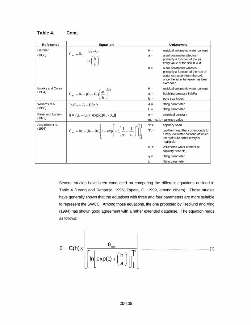
DD-4.35
Table 4. Cont.
Reference Equation Unknowns Gardner (1958) b
rsrw
ah1 ⎟
⎠⎞
⎜⎝⎛+
θ−θ+θ=θ
θr = residual volumetric water content. a = a soil parameter which is
primarily a function of the air entry value of the soil in kPa.
b = a soil parameter which is primarily a function of the rate of water extraction from the soil, once the air entry value has been exceeded.
Brooks and Corey (1964)
bb
rsrw
b
ha)( ⎟
⎠⎞
⎜⎝⎛θ−θ+θ=θ
θr = residual volumetric water content. ab = bubbling pressure in kPa. bb = pore size index.
Williams et al. (1983)
hln BA ln e +=Θ A = fitting parameter B = fitting parameter
Farrel and Larson (1972)
h = (ua – uw)b exp[α(θs - θw)] α = empirical constant (ua – uw)b = air-entry value
Assouline et al. (1998)
⎥⎥
⎦
⎤
⎢⎢
⎣
⎡
⎥⎥⎦
⎤
⎢⎢⎣
⎡⎟⎟⎠
⎞⎜⎜⎝
⎛−
ψξ−−θ−θ+θ=θ
η
ψLLsLw
11exp1)( Ψ = capillary head
ΨL = capillary head that corresponds to a very low water content, at which the hydraulic conductivity is negligible.
θL = volumetric water content at capillary head ΨL.
η = fitting parameter ξ = fitting parameter
Several studies have been conducted on comparing the different equations outlined in
Table 4 (Leong and Rahardjo, 1996; Zapata, C., 1999, among others). Those studies
have generally shown that the equations with three and four parameters are more suitable
to represent the SWCC. Among those equations, the one proposed by Fredlund and Xing
(1994) has shown good agreement with a rather extended database. The equation reads
as follows:
⎥⎥⎥⎥⎥⎥
⎦
⎤
⎢⎢⎢⎢⎢⎢
⎣
⎡
⎥⎥⎦
⎤
⎢⎢⎣
⎡
⎥⎥⎦
⎤
⎢⎢⎣
⎡⎟⎠⎞
⎜⎝⎛+
θ×=θ cb
sat
ah)1exp(ln
)h(C .................................................................. (1)

DD-4.36
⎥⎥⎥⎥
⎦
⎤
⎢⎢⎢⎢
⎣
⎡
⎟⎟⎠
⎞⎜⎜⎝
⎛+
⎟⎟⎠
⎞⎜⎜⎝
⎛+
−=
r
6
r
h101ln
hh1ln
1)h(C ........................................................................................ (2)
Where:
θ = Volumetric water content
θsat = Saturated volumetric water content
a = A soil parameter which is primarily a function of the air entry value of the soil
in kPa.
b = A soil parameter which is primarily a function of the rate of water extraction
from the soil, once the air entry value has been exceeded.
c = A soil parameter which controls the shape and position of the drier portion of
the SWCC.
hr = A soil parameter which is primarily a function of the suction at which the drier
portion of the SWCC tends to level out (kPa).
C(h) = An adjustment factor which forces all curves through a suction of 1,000,000
kPa at zero water content.
In terms of degree of saturation, the Fredlund and Xing equation reads as follows:
⎥⎥⎥⎥⎥⎥
⎦
⎤
⎢⎢⎢⎢⎢⎢
⎣
⎡
⎥⎥⎦
⎤
⎢⎢⎣
⎡
⎥⎥⎦
⎤
⎢⎢⎣
⎡⎟⎠⎞
⎜⎝⎛+
×= cb
ah)1exp(ln
1)h(CS ................................................................. (3)
Where:
S = Degree of saturation, θ/θsat
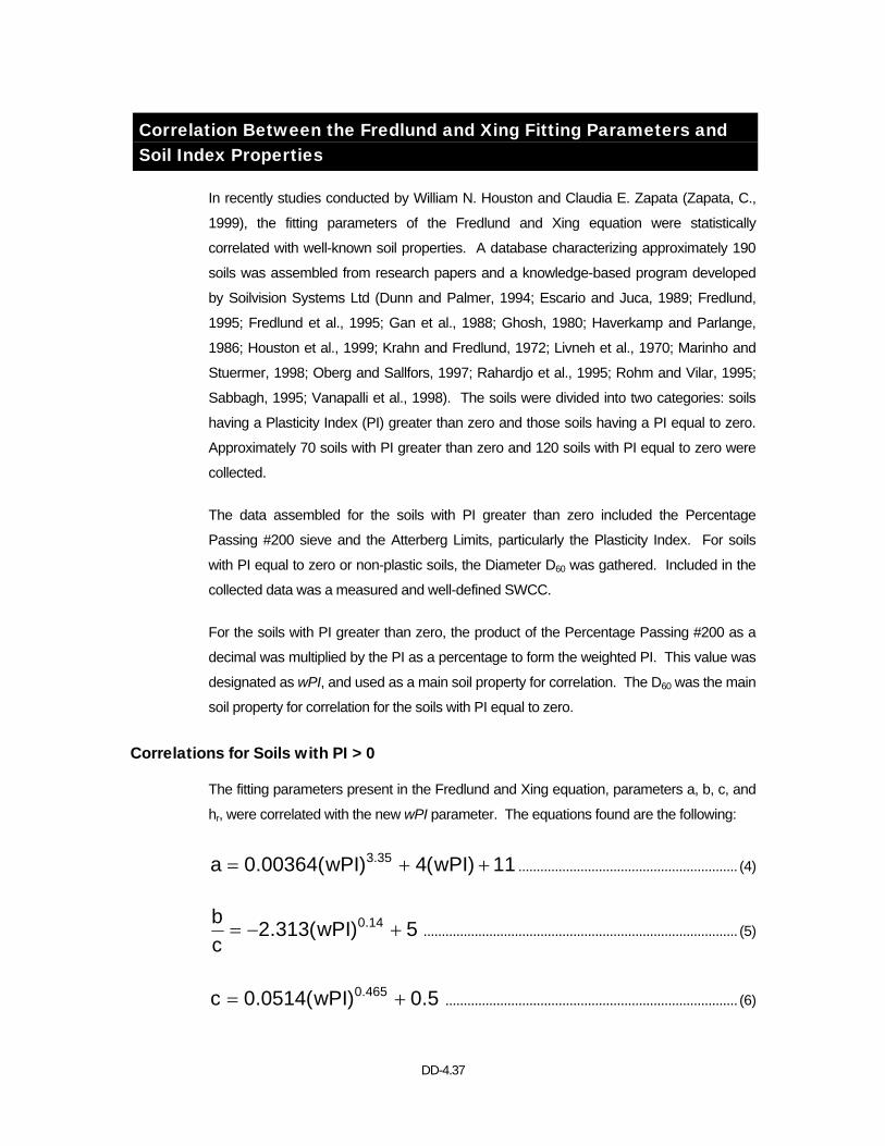
DD-4.37
Correlation Between the Fredlund and Xing Fitting Parameters and Soil Index Properties
In recently studies conducted by William N. Houston and Claudia E. Zapata (Zapata, C.,
1999), the fitting parameters of the Fredlund and Xing equation were statistically
correlated with well-known soil properties. A database characterizing approximately 190
soils was assembled from research papers and a knowledge-based program developed
by Soilvision Systems Ltd (Dunn and Palmer, 1994; Escario and Juca, 1989; Fredlund,
1995; Fredlund et al., 1995; Gan et al., 1988; Ghosh, 1980; Haverkamp and Parlange,
1986; Houston et al., 1999; Krahn and Fredlund, 1972; Livneh et al., 1970; Marinho and
Stuermer, 1998; Oberg and Sallfors, 1997; Rahardjo et al., 1995; Rohm and Vilar, 1995;
Sabbagh, 1995; Vanapalli et al., 1998). The soils were divided into two categories: soils
having a Plasticity Index (PI) greater than zero and those soils having a PI equal to zero.
Approximately 70 soils with PI greater than zero and 120 soils with PI equal to zero were
collected.
The data assembled for the soils with PI greater than zero included the Percentage
Passing #200 sieve and the Atterberg Limits, particularly the Plasticity Index. For soils
with PI equal to zero or non-plastic soils, the Diameter D60 was gathered. Included in the
collected data was a measured and well-defined SWCC.
For the soils with PI greater than zero, the product of the Percentage Passing #200 as a
decimal was multiplied by the PI as a percentage to form the weighted PI. This value was
designated as wPI, and used as a main soil property for correlation. The D60 was the main
soil property for correlation for the soils with PI equal to zero.
Correlations for Soils with PI > 0
The fitting parameters present in the Fredlund and Xing equation, parameters a, b, c, and
hr, were correlated with the new wPI parameter. The equations found are the following:
11)wPI(4)wPI(00364.0a 35.3 ++= ............................................................ (4)
5)wPI(313.2cb 14.0 +−= ...................................................................................... (5)
5.0)wPI(0514.0c 465.0 += ................................................................................ (6)
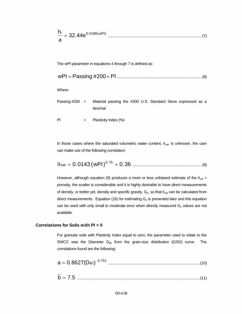
DD-4.38
)wPI(0186.0e44.32ahr
= .............................................................................................. (7)
The wPI parameter in equations 4 through 7 is defined as:
PI 200# Passing wPI ×= ..................................................................................... (8)
Where:
Passing #200 = Material passing the #200 U.S. Standard Sieve expressed as a
decimal
PI = Plasticity Index (%)
In those cases where the saturated volumetric water content, θsat, is unknown, the user
can make use of the following correlation:
36.0)wPI(0143.0 75.0sat +=θ ..................................................................... (9)
However, although equation (9) produces a more or less unbiased estimate of the θsat =
porosity, the scatter is considerable and it is highly desirable to have direct measurements
of density, or better yet, density and specific gravity, Gs, so that θsat can be calculated from
direct measurements. Equation (16) for estimating Gs is presented later and this equation
can be used with only small to moderate error when directly measured Gs values are not
available.
Correlations for Soils with PI = 0
For granular soils with Plasticity Index equal to zero, the parameter used to relate to the
SWCC was the Diameter D60 from the grain-size distribution (GSD) curve. The
correlations found are the following:
751.060)D(8627.0a −= ............................................................................................(10)
5.7b = ...........................................................................................................................(11)
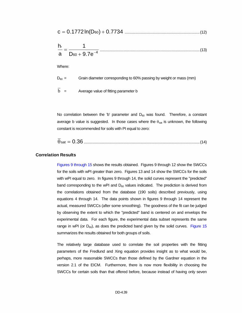
DD-4.39
7734.0)Dln(1772.0c 60 += ...........................................................................(12)
460 e7.9D
1ahr
−+= ....................................................................................................(13)
Where:
D60 = Grain diameter corresponding to 60% passing by weight or mass (mm)
b = Average value of fitting parameter b
No correlation between the 'b' parameter and D60 was found. Therefore, a constant
average b value is suggested. In those cases where the θsat is unknown, the following
constant is recommended for soils with PI equal to zero:
36.0sat =θ ....................................................................................................................(14)
Correlation Results
Figures 9 through 15 shows the results obtained. Figures 9 through 12 show the SWCCs
for the soils with wPI greater than zero. Figures 13 and 14 show the SWCCs for the soils
with wPI equal to zero. In figures 9 through 14, the solid curves represent the "predicted"
band corresponding to the wPI and D60 values indicated. The prediction is derived from
the correlations obtained from the database (190 soils) described previously, using
equations 4 through 14. The data points shown in figures 9 through 14 represent the
actual, measured SWCCs (after some smoothing). The goodness of the fit can be judged
by observing the extent to which the "predicted" band is centered on and envelops the
experimental data. For each figure, the experimental data subset represents the same
range in wPI (or D60), as does the predicted band given by the solid curves. Figure 15
summarizes the results obtained for both groups of soils.
The relatively large database used to correlate the soil properties with the fitting
parameters of the Fredlund and Xing equation provides insight as to what would be,
perhaps, more reasonable SWCCs than those defined by the Gardner equation in the
version 2.1 of the EICM. Furthermore, there is now more flexibility in choosing the
SWCCs for certain soils than that offered before, because instead of having only seven
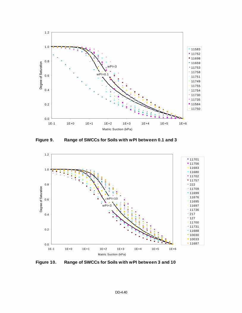
DD-4.40
0.0
0.2
0.4
0.6
0.8
1.0
1.2
1E-1 1E+0 1E+1 1E+2 1E+3 1E+4 1E+5 1E+6
Matric Suction (kPa)
1158311752116981165911753117581175111749117551175411730117351158411750
wPI=0.1
wPI=3
Figure 9. Range of SWCCs for Soils with wPI between 0.1 and 3
0.0
0.2
0.4
0.6
0.8
1.0
1.2
1E-1 1E+0 1E+1 1E+2 1E+3 1E+4 1E+5 1E+6
Matric Suction (kPa)
117011175611683116801170211757222117091169911676116951169711736217127117001173111688100301003311687
wPI=3
wPI=10
Figure 10. Range of SWCCs for Soils with wPI between 3 and 10
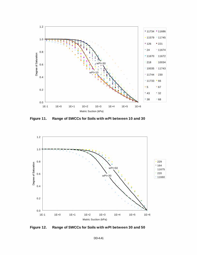
DD-4.41
0.0
0.2
0.4
0.6
0.8
1.0
1.2
1E-1 1E+0 1E+1 1E+2 1E+3 1E+4 1E+5 1E+6
Matric Suction (kPa)
11734 11686
11579 11745
126 221
24 11674
11670 11672
218 10034
10035 11743
11744 230
11733 66
5 67
43 32
38 68
wPI=10
wPI=30
Figure 11. Range of SWCCs for Soils with wPI between 10 and 30
0.0
0.2
0.4
0.6
0.8
1.0
1.2
1E-1 1E+0 1E+1 1E+2 1E+3 1E+4 1E+5 1E+6
Matric Suction (kPa)
2291641167522011660wPI=30
wPI=50
Figure 12. Range of SWCCs for Soils with wPI between 30 and 50
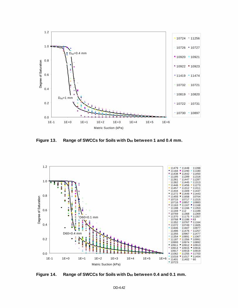
DD-4.42
0.0
0.2
0.4
0.6
0.8
1.0
1.2
1E-1 1E+0 1E+1 1E+2 1E+3 1E+4 1E+5 1E+6
Matric Suction (kPa)
10724 11256
10726 10727
10920 10921
10922 10923
11419 11474
10732 10721
10819 10820
10722 10731
10730 10897
D60=0.4 mm
D60=1 mm
Figure 13. Range of SWCCs for Soils with D60 between 1 and 0.4 mm.
0.0
0.2
0.4
0.6
0.8
1.0
1.2
1E-1 1E+0 1E+1 1E+2 1E+3 1E+4 1E+5 1E+6
Matric Suction (kPa)
11479 11448 1128811184 11290 1118011438 11442 1145011185 11289 1131611361 11447 1128711362 11445 1131311446 11456 1127311457 11312 1131111444 11309 1143711272 11449 1144311455 11658 1070410715 10717 1131510716 10857 1088311163 11167 1116811188 11166 1135311169 112 1118910769 11368 1136911370 11175 1135710768 11186 6311352 10767 1116411072 10749 1160511606 11607 1097711486 11476 1125711355 10967 1147711354 10891 1106711187 11356 1099110993 10974 1089210911 10912 1091310914 10915 1091610917 10918 1091911062 11255 1170311016 11017 1140411401 11402 6010723
D60=0.1 mm
D60=0.4 mm
Figure 14. Range of SWCCs for Soils with D60 between 0.4 and 0.1 mm.
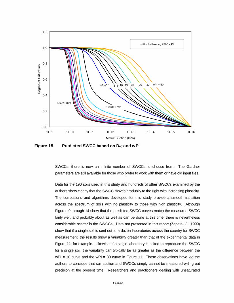
DD-4.43
0.0
0.2
0.4
0.6
0.8
1.0
1.2
1E-1 1E+0 1E+1 1E+2 1E+3 1E+4 1E+5 1E+6
Matric Suction (kPa)
D60=1 mm
wPI=0.1 wPI = 503 5 10 15 20 30 40
D60=0.1 mm
wPI = % Passing #200 x PI
Figure 15. Predicted SWCC based on D60 and wPI
SWCCs, there is now an infinite number of SWCCs to choose from. The Gardner
parameters are still available for those who prefer to work with them or have old input files.
Data for the 190 soils used in this study and hundreds of other SWCCs examined by the
authors show clearly that the SWCC moves gradually to the right with increasing plasticity.
The correlations and algorithms developed for this study provide a smooth transition
across the spectrum of soils with no plasticity to those with high plasticity. Although
Figures 9 through 14 show that the predicted SWCC curves match the measured SWCC
fairly well, and probably about as well as can be done at this time, there is nevertheless
considerable scatter in the SWCCs. Data not presented in this report (Zapata, C., 1999)
show that if a single soil is sent out to a dozen laboratories across the country for SWCC
measurement, the results show a variability greater than that of the experimental data in
Figure 11, for example. Likewise, if a single laboratory is asked to reproduce the SWCC
for a single soil, the variability can typically be as greater as the difference between the
wPI = 10 curve and the wPI = 30 curve in Figure 11. These observations have led the
authors to conclude that soil suction and SWCCs simply cannot be measured with great
precision at the present time. Researchers and practitioners dealing with unsaturated
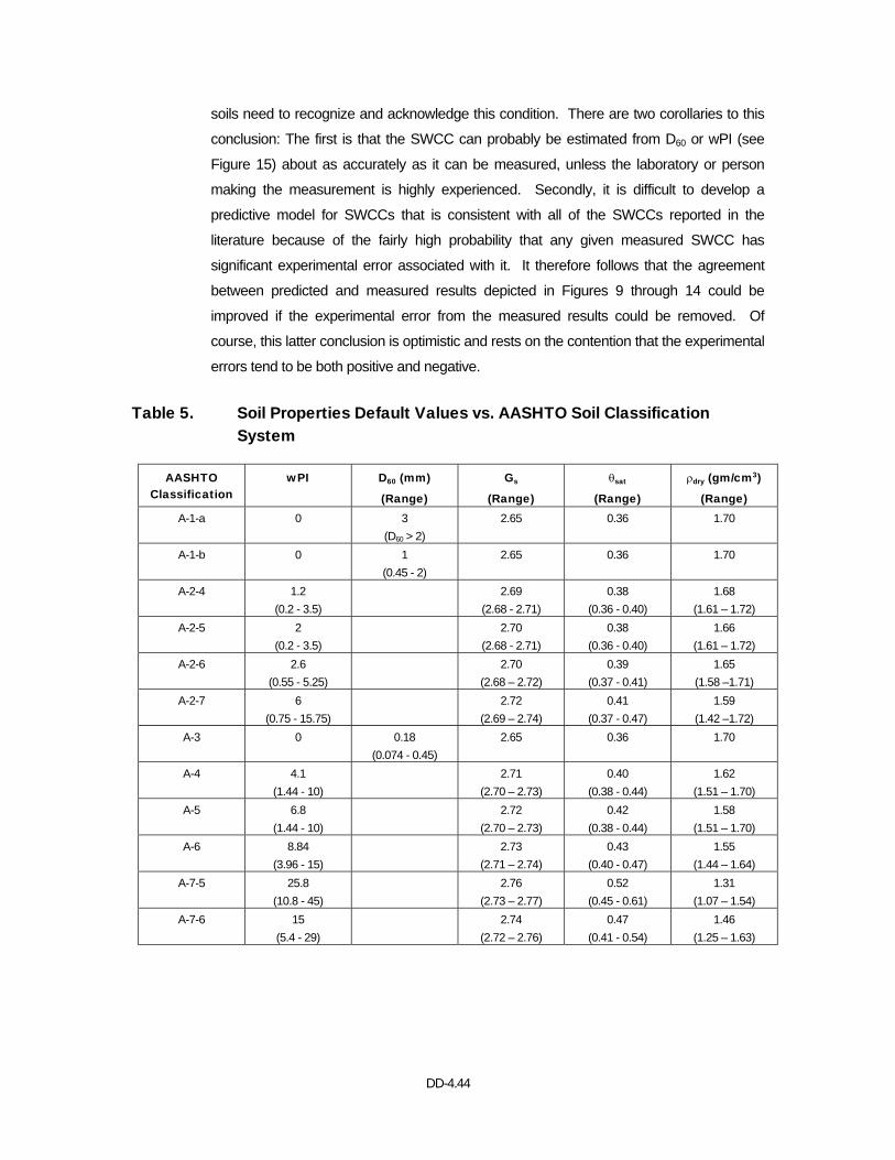
DD-4.44
soils need to recognize and acknowledge this condition. There are two corollaries to this
conclusion: The first is that the SWCC can probably be estimated from D60 or wPI (see
Figure 15) about as accurately as it can be measured, unless the laboratory or person
making the measurement is highly experienced. Secondly, it is difficult to develop a
predictive model for SWCCs that is consistent with all of the SWCCs reported in the
literature because of the fairly high probability that any given measured SWCC has
significant experimental error associated with it. It therefore follows that the agreement
between predicted and measured results depicted in Figures 9 through 14 could be
improved if the experimental error from the measured results could be removed. Of
course, this latter conclusion is optimistic and rests on the contention that the experimental
errors tend to be both positive and negative.
Table 5. Soil Properties Default Values vs. AASHTO Soil Classification System
AASHTO Classification
wPI D60 (mm)
(Range)
Gs
(Range)
θsat
(Range)
ρdry (gm/cm3)
(Range) A-1-a 0
3
(D60 > 2) 2.65 0.36
1.70
A-1-b 0
1
(0.45 - 2) 2.65 0.36
1.70
A-2-4 1.2 (0.2 - 3.5)
2.69 (2.68 - 2.71)
0.38 (0.36 - 0.40)
1.68 (1.61 – 1.72)
A-2-5 2 (0.2 - 3.5)
2.70 (2.68 - 2.71)
0.38 (0.36 - 0.40)
1.66 (1.61 – 1.72)
A-2-6 2.6 (0.55 - 5.25)
2.70 (2.68 – 2.72)
0.39 (0.37 - 0.41)
1.65 (1.58 –1.71)
A-2-7 6 (0.75 - 15.75)
2.72 (2.69 – 2.74)
0.41 (0.37 - 0.47)
1.59 (1.42 –1.72)
A-3 0 0.18 (0.074 - 0.45)
2.65 0.36
1.70
A-4 4.1 (1.44 - 10)
2.71 (2.70 – 2.73)
0.40 (0.38 - 0.44)
1.62 (1.51 – 1.70)
A-5 6.8 (1.44 - 10)
2.72 (2.70 – 2.73)
0.42 (0.38 - 0.44)
1.58 (1.51 – 1.70)
A-6 8.84 (3.96 - 15)
2.73 (2.71 – 2.74)
0.43 (0.40 - 0.47)
1.55 (1.44 – 1.64)
A-7-5 25.8 (10.8 - 45)
2.76 (2.73 – 2.77)
0.52 (0.45 - 0.61)
1.31 (1.07 – 1.54)
A-7-6 15 (5.4 - 29)
2.74 (2.72 – 2.76)
0.47 (0.41 - 0.54)
1.46 (1.25 – 1.63)

DD-4.45
Best-Estimate SWCCs Based on AASHTO Classification
In those cases where neither wPI nor D60 is known, but the AASHTO classification is, a
best-estimate SWCC for each classification is proposed. The SWCC is based on either
wPI or D60. That is, for each AASHTO classification category, either the wPI or the D60
has been estimated. Then this estimate of either wPI or D60 is used together with the
correlations developed to yield a best-estimate SWCC. Table 5 shows the results along
with the probable range of values. This table can also be incorporated in the EICM user's
manual to be used by those that prefer the prediction of the SWCC based on Fredlund
and Xing parameters to the prediction using the Gardner parameters. Appendix G shows
the proposed SWCCs for each AASHTO soil classification.
Best-Estimate SWCCs for Base Course Materials
In cases where the D60 or the wPI for the material are not precisely known, but instead the
material is identifiable as a base course material, an estimated SWCC for each grading is
proposed. The estimated soil parameters to define the SWCC are presented in Table 6.
The base course material classification is based on the AASHTO Designation M 147-65
(1990): Materials for Aggregate and Soil-Aggregate Subbase, Base and Surface Courses.
If the base course material is suspected to have significant plastic fines, it is
recommended that the wPI be used (bottom of Table 6) instead of the D60 criteria.
Appendix H depicts the proposed SWCCs for base course materials.
The modified version of the EICM has not yet fully implemented this feature, but it is
expected to be included in the future in the release version.
Default Values for Saturated Hydraulic Conductivity, Specific Gravity, and Saturated Volumetric Water Content
In cases where the saturated hydraulic conductivity is not known from field or lab testing
and needs to be estimated, the following equation is proposed:
( ) 129.12 1076639k kPa33satsat−+θ−θ= .............................................................(15)
Where:
ksat = saturated hydraulic conductivity (m/s)
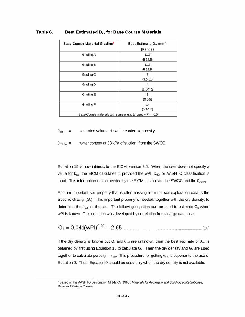
DD-4.46
Table 6. Best Estimated D60 for Base Course Materials
Base Course Material Grading1 Best Estimate D60 (mm)
(Range) Grading A 11.5
(5-17.5) Grading B 11.5
(5-17.5) Grading C 7
(3.5-11) Grading D 4
(1.1-7.5) Grading E 3
(0.5-5) Grading F 1.4
(0.3-2.5) Base Course materials with some plasticity, used wPI = 0.5
θsat = saturated volumetric water content = porosity
θ33kPa = water content at 33 kPa of suction, from the SWCC
Equation 15 is now intrinsic to the EICM, version 2.6. When the user does not specify a
value for ksat, the EICM calculates it, provided the wPI, D60, or AASHTO classification is
input. This information is also needed by the EICM to calculate the SWCC and the θ33kPa.
Another important soil property that is often missing from the soil exploration data is the
Specific Gravity (Gs). This important property is needed, together with the dry density, to
determine the θsat for the soil. The following equation can be used to estimate Gs when
wPI is known. This equation was developed by correlation from a large database.
65.2)wPI(041.0G 29.0s += ..............................................................................(16)
If the dry density is known but Gs and θsat are unknown, then the best estimate of θsat is
obtained by first using Equation 16 to calculate Gs. Then the dry density and Gs are used
together to calculate porosity = θsat. This procedure for getting θsat is superior to the use of
Equation 9. Thus, Equation 9 should be used only when the dry density is not available.
1 Based on the AASHTO Designation M 147-65 (1990): Materials for Aggregate and Soil-Aggregate Subbase, Base and Surface Courses
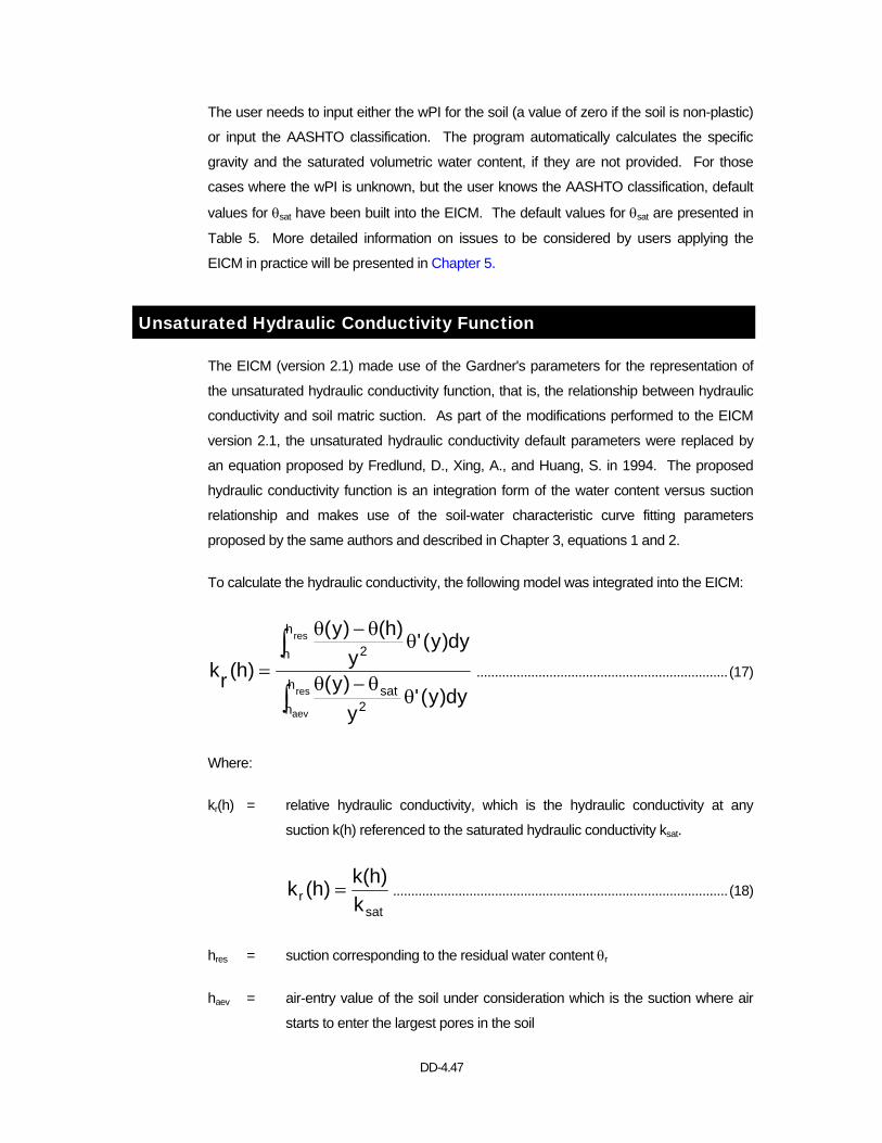
DD-4.47
The user needs to input either the wPI for the soil (a value of zero if the soil is non-plastic)
or input the AASHTO classification. The program automatically calculates the specific
gravity and the saturated volumetric water content, if they are not provided. For those
cases where the wPI is unknown, but the user knows the AASHTO classification, default
values for θsat have been built into the EICM. The default values for θsat are presented in
Table 5. More detailed information on issues to be considered by users applying the
EICM in practice will be presented in Chapter 5.
Unsaturated Hydraulic Conductivity Function
The EICM (version 2.1) made use of the Gardner's parameters for the representation of
the unsaturated hydraulic conductivity function, that is, the relationship between hydraulic
conductivity and soil matric suction. As part of the modifications performed to the EICM
version 2.1, the unsaturated hydraulic conductivity default parameters were replaced by
an equation proposed by Fredlund, D., Xing, A., and Huang, S. in 1994. The proposed
hydraulic conductivity function is an integration form of the water content versus suction
relationship and makes use of the soil-water characteristic curve fitting parameters
proposed by the same authors and described in Chapter 3, equations 1 and 2.
To calculate the hydraulic conductivity, the following model was integrated into the EICM:
∫
∫
θθ−θ
θθ−θ
=res
aev
res
h
h 2sat
h
h 2
dy)y('y)y(
dy)y('y
)h()y(
)h(rk .....................................................................(17)
Where:
kr(h) = relative hydraulic conductivity, which is the hydraulic conductivity at any
suction k(h) referenced to the saturated hydraulic conductivity ksat.
sat
r k)h(k)h(k = ............................................................................................(18)
hres = suction corresponding to the residual water content θr
haev = air-entry value of the soil under consideration which is the suction where air
starts to enter the largest pores in the soil
DD-4.48
y = dummy variable of integration representing suction
θ' = derivative of equation 1
Since Equation 1 is valid over the entire suction range, the integrations in Equation 17 can
be performed from haev to 106 for all type of soils (Fredlund et al., 1994). Furthermore,
Equation 17 assumes that the volume change of the soil structure is negligible.
Summary
The modifications to the EICM water content prediction included:
Representation of the Soil-Water Characteristic Curve (SWCC) by the Fredlund and
Xing equation. The Gardner equation remains available to the EICM user.
The parameters of the Fredlund and Xing equation (Fredlund and Xing, 1994) were
correlated with basic soil index properties: D60 and wPI = Percentage Passing #200
times Plasticity Index (PI).
Default values for the basic soil index properties needed to determine the SWCC
were estimated as a function of the AASHTO Soil Classification System.
Default values for the basic soil index properties needed to determine the SWCC
were estimated for the base course materials designed under AASHTO Designation
M 147-65 (1990): Materials for Aggregate and Soil-Aggregate Subbase, Base and
Surface Courses.
Algorithms to estimate porosity (saturated volumetric water content), specific gravity
and saturated hydraulic conductivity based on wPI were developed.
Incorporation into the EICM of unsaturated hydraulic conductivity prediction based on
the SWCC proposed by Fredlund, et al. (1994). The Gardner parameters for the
unsaturated hydraulic conductivity remain available for use in the EICM.
EICM Version 2.6 reflects these modifications.
DD-4.49
Assessment of the EICM Moisture Content Prediction after Modifications EICM Version 2.6
Introduction
An evaluation of the EICM Version 2.6 was undertaken to verify that the changes made
improved the moisture content predictions. Data from the six Long-Term Test
Performance (LTPP) sections used to assess the EICM version 2.1, and from four
additional LTPP Seasonal Monitoring Sites were used. The new sections are:
1) 131005 (Georgia)
2) 81053 (Colorado)
3) 41024 (Arizona)
4) 481077 (Texas)
Data Collected
The data used in the evaluation of the EICM version 2.6 were drawn from DataPave 2.0
(1999), except as follows.
Data tables SMP_TDR_AUTO_MOISTURE and SMP_FROST_PENETRATION,
SMP_FREEZE_STATE are from release 10.0 of the LTPP Information Management
System.
Tables TST_... are from release 10.2 of the LTPP Information Management System.
In a few instances, data were obtained from the Seasonal Monitoring Site installation
reports for the test sites. Data from this source are annotated as such in the tables
presenting the input data.
Chapter
4
DD-4.50
Specific gravity data are not included in the LTPP database. However, specific gravity
data for some materials are reported on laboratory data sheets associated with LTPP
resilient modulus testing, and Klemunes (1995) reports values for several additional
materials. Where available, these values were used.
In cases where required input data were not available, either because they were not
routinely collected on the LTPP test sections, or because they were otherwise missing
from the LTPP database when this work was undertaken, default values were used, as
noted in the tables presenting the input data.
The data for the ten LTPP sites are presented in Table 7 and Table 8. In a few instances,
the data used as input to Version 2.6 of the EICM differed from that used for Version 2.1.
These differences arise from additional data that became available in the LTPP database,
and additional information that came to the authors’ attention in the intervening time
period.
In the application of EICM Version 2.6, subbase and subgrade layers were subdivided,
such that a mid-depth node would correspond to the depth of each TDR probe used in
LTPP monitoring. The base layer was not subdivided, based on the advice of the EICM
model developers. For clarity, the Material Properties information is shown for each layer
and for each sub-layer, as input into the EICM, given that the water content information
was often available at more than one location within a given layer. For further information
on recommendations for subdividing the pavement profile, refer to the User's Guide and
Recommendations Chapter.
The shading in some boxes in Tables 7 and 8 indicates that a default value was used for
that particular property, instead of a measured value. Also notice, that some of the
information is presented as a file name (i.e., *.txt, *.xls). The information contained on
those files is rather extensive and is not included in this report.
Results
Figures 16 through 25 show the measured versus predicted volumetric water contents by
the EICM version 2.6 for the ten sites. The data for the base course material and the
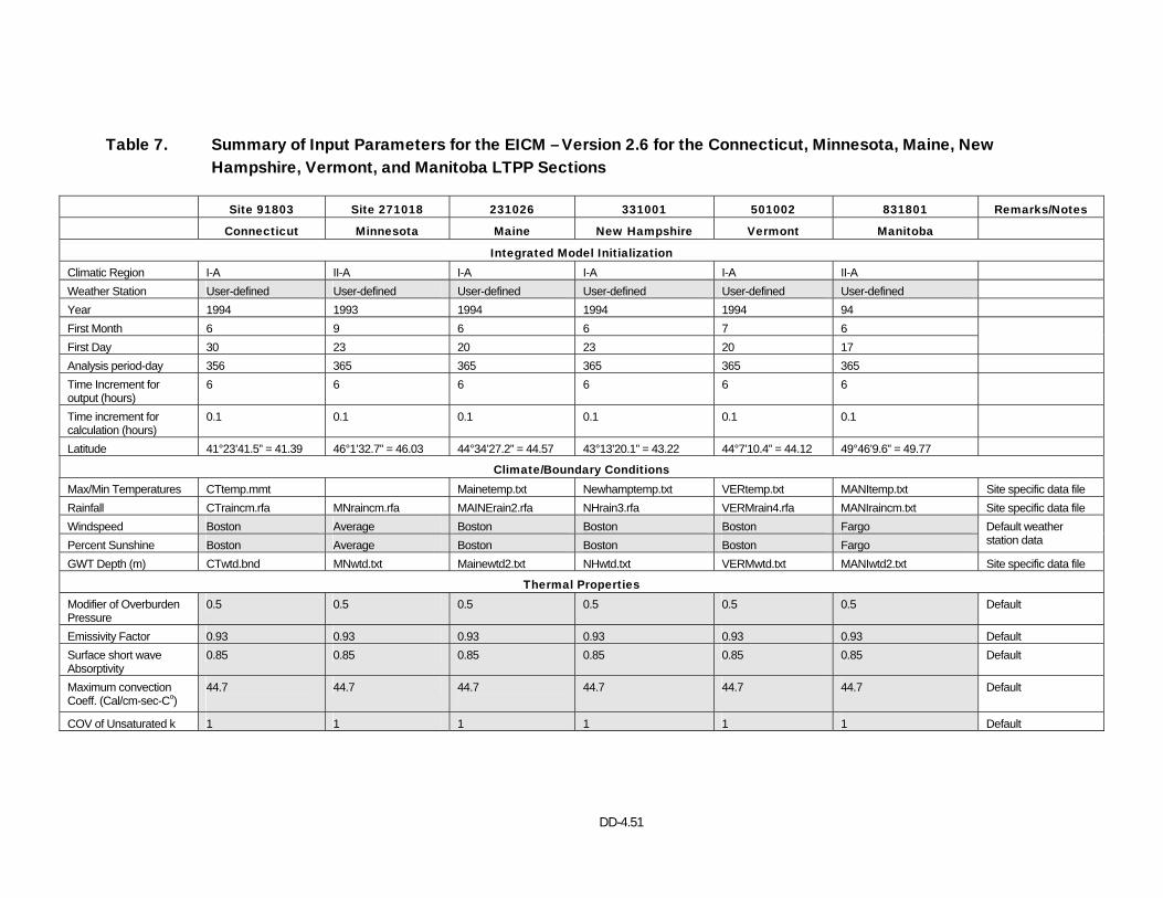
DD-4.51
Table 7. Summary of Input Parameters for the EICM – Version 2.6 for the Connecticut, Minnesota, Maine, New Hampshire, Vermont, and Manitoba LTPP Sections
Site 91803 Site 271018 231026 331001 501002 831801 Remarks/Notes
Connecticut Minnesota Maine New Hampshire Vermont Manitoba
Integrated Model Initialization Climatic Region I-A II-A I-A I-A I-A II-A Weather Station User-defined User-defined User-defined User-defined User-defined User-defined Year 1994 1993 1994 1994 1994 94 First Month 6 9 6 6 7 6 First Day 30 23 20 23 20 17
Analysis period-day 356 365 365 365 365 365 Time Increment for output (hours)
6 6 6 6 6 6
Time increment for calculation (hours)
0.1 0.1 0.1 0.1 0.1 0.1
Latitude 41°23’41.5” = 41.39 46°1’32.7” = 46.03 44°34’27.2” = 44.57 43°13’20.1” = 43.22 44°7’10.4” = 44.12 49°46’9.6” = 49.77
Climate/Boundary Conditions Max/Min Temperatures CTtemp.mmt Mainetemp.txt Newhamptemp.txt VERtemp.txt MANItemp.txt Site specific data file Rainfall CTraincm.rfa MNraincm.rfa MAINErain2.rfa NHrain3.rfa VERMrain4.rfa MANIraincm.txt Site specific data file Windspeed Boston Average Boston Boston Boston Fargo Percent Sunshine Boston Average Boston Boston Boston Fargo
Default weather station data
GWT Depth (m) CTwtd.bnd MNwtd.txt Mainewtd2.txt NHwtd.txt VERMwtd.txt MANIwtd2.txt Site specific data file
Thermal Properties Modifier of Overburden Pressure
0.5 0.5 0.5 0.5 0.5 0.5 Default
Emissivity Factor 0.93 0.93 0.93 0.93 0.93 0.93 Default Surface short wave Absorptivity
0.85 0.85 0.85 0.85 0.85 0.85 Default
Maximum convection Coeff. (Cal/cm-sec-Co)
44.7
44.7 44.7
44.7 44.7 44.7 Default
COV of Unsaturated k 1 1 1 1 1 1 Default
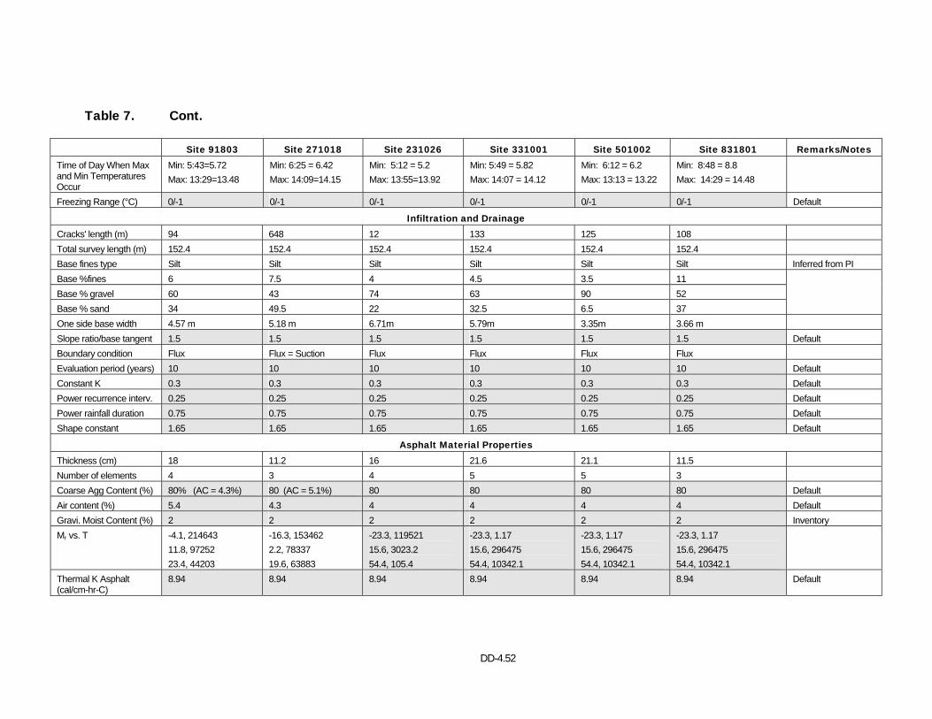
DD-4.52
Table 7. Cont.
Site 91803 Site 271018 Site 231026 Site 331001 Site 501002 Site 831801 Remarks/Notes Time of Day When Max and Min Temperatures Occur
Min: 5:43=5.72 Max: 13:29=13.48
Min: 6:25 = 6.42 Max: 14:09=14.15
Min: 5:12 = 5.2 Max: 13:55=13.92
Min: 5:49 = 5.82 Max: 14:07 = 14.12
Min: 6:12 = 6.2 Max: 13:13 = 13.22
Min: 8:48 = 8.8 Max: 14:29 = 14.48
Freezing Range (°C) 0/-1 0/-1 0/-1 0/-1 0/-1 0/-1 Default
Infiltration and Drainage Cracks' length (m) 94 648 12 133 125 108 Total survey length (m) 152.4 152.4 152.4 152.4 152.4 152.4 Base fines type Silt Silt Silt Silt Silt Silt Inferred from PI Base %fines 6 7.5 4 4.5 3.5 11 Base % gravel 60 43 74 63 90 52 Base % sand 34 49.5 22 32.5 6.5 37
One side base width 4.57 m 5.18 m 6.71m 5.79m 3.35m 3.66 m Slope ratio/base tangent 1.5 1.5 1.5 1.5 1.5 1.5 Default Boundary condition Flux Flux = Suction Flux Flux Flux Flux Evaluation period (years) 10 10 10 10 10 10 Default Constant K 0.3 0.3 0.3 0.3 0.3 0.3 Default Power recurrence interv. 0.25 0.25 0.25 0.25 0.25 0.25 Default Power rainfall duration 0.75 0.75 0.75 0.75 0.75 0.75 Default Shape constant 1.65 1.65 1.65 1.65 1.65 1.65 Default
Asphalt Material Properties Thickness (cm) 18 11.2 16 21.6 21.1 11.5 Number of elements 4 3 4 5 5 3 Coarse Agg Content (%) 80% (AC = 4.3%) 80 (AC = 5.1%) 80 80 80 80 Default Air content (%) 5.4 4.3 4 4 4 4 Default Gravi. Moist Content (%) 2 2 2 2 2 2 Inventory Mr vs. T -4.1, 214643
11.8, 97252 23.4, 44203
-16.3, 153462 2.2, 78337 19.6, 63883
-23.3, 119521 15.6, 3023.2 54.4, 105.4
-23.3, 1.17 15.6, 296475 54.4, 10342.1
-23.3, 1.17 15.6, 296475 54.4, 10342.1
-23.3, 1.17 15.6, 296475 54.4, 10342.1
Thermal K Asphalt (cal/cm-hr-C)
8.94 8.94 8.94 8.94 8.94 8.94 Default
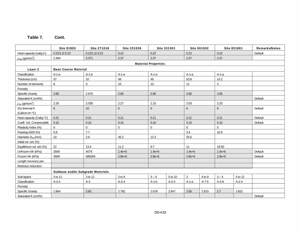
DD-4.53
Table 7. Cont.
Site 91803 Site 271018 Site 231026 Site 331001 Site 501002 Site 831801 Remarks/Notes Heat capacity (cal/g-C) 0.22/1.2/.0.22 0.22/1.2/.0.22 0.22 0.22 0.22 0.22 Default ρtotal (gm/cm3) 2.494 2.371 2.37 2.37 2.37 2.37
Material Properties
Layer 2 Base Course Material Classification A-1-a A-1-b A-1-a A-1-a A-1-a A-1-a Thickness (cm) 37 10 48 49 53.8 14.2 Number of elements 8 3 10 10 11 3 Porosity Specific Gravity 2.65 2.675 2.65 2.65 2.65 2.65 Saturated K (cm/hr) Default ρdry (gm/cm3) 2.26 2.035 2.27 2.15 2.03 2.20 Dry thermal K (Cal/cm-hr-°C)
6 10 6 6 6 6 Default
Heat capacity (Cal/g-°C) 0.21 0.21 0.21 0.21 0.21 0.21 Default Coeff. Vol. Compressibili. 0.10 0.10 0.10 0.10 0.10 0.10 Default Plasticity Index (%) 0 0 0 0 0 5 Passing #200 (%) 5.8 7.7 3.4 10.9 Diameter D60 (mm) 10 2.6 45.2 12.3 25.6 Initial vol. w/c (%) Equilibrium vol. w/c (%) 22 13.4 11.2 9.7 11 18.55 Unfrozen Mr (kPa) 3569 4079 1.4e+6 1.4e+6 1.4e+6 1.4e+6 Default Frozen Mr (kPa) 3569 688284 2.8e+6 2.8e+6 2.8e+6 2.8e+6 Default Length recovery per. Modulus reduction
Subbase and/or Subgrade Materials Sub-layers 3 to 11 3 to 12 3 to 9 3 – 4 5 to 10 3 4 to 9 3 – 4 5 to 12 Classification A-2-4 A-3 A-2-4 A-1-b A-2-4 A-1-a A-7-5 A-2-6 A-2-4 Porosity Specific Gravity 2.864 2.65 2.782 2.678 2.647 2.65 2.815 2.7 2.831 Saturated K (cm/hr) Default
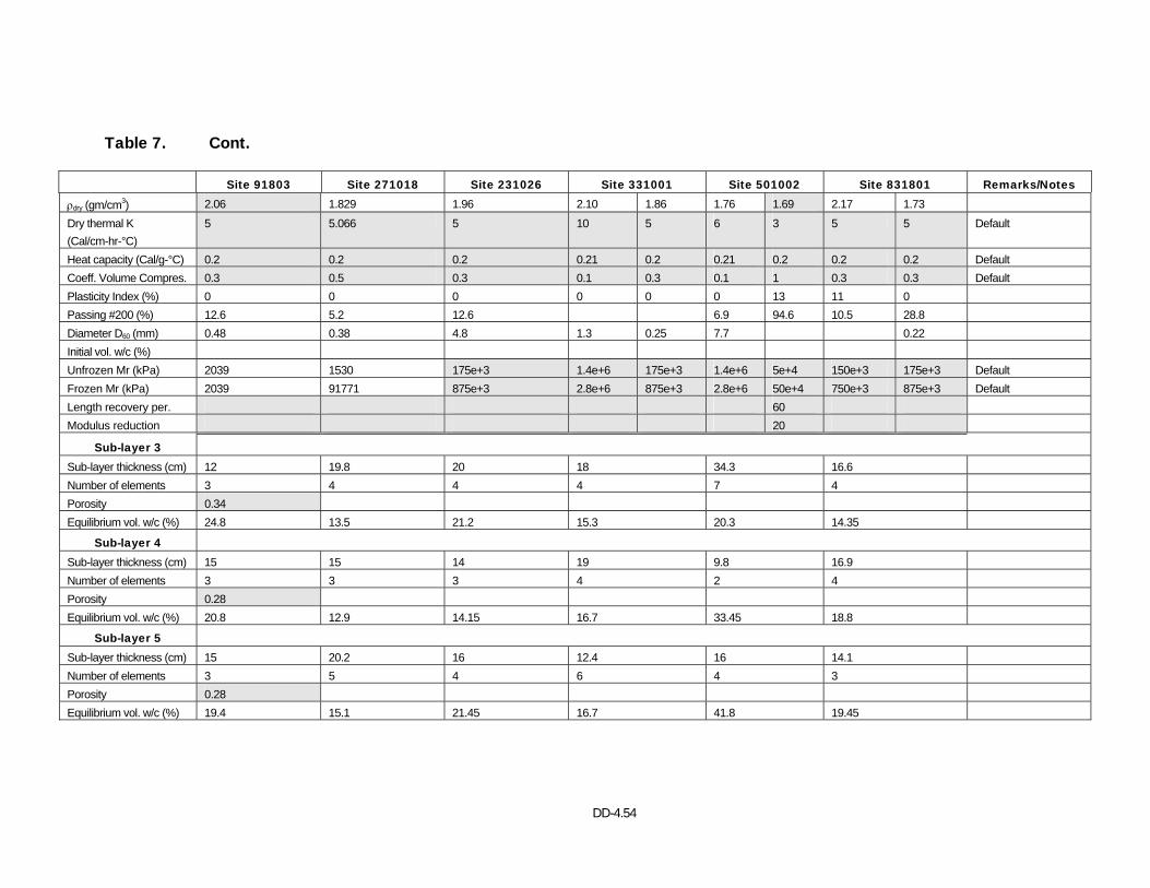
DD-4.54
Table 7. Cont.
Site 91803 Site 271018 Site 231026 Site 331001 Site 501002 Site 831801 Remarks/Notes
ρdry (gm/cm3) 2.06 1.829 1.96 2.10 1.86 1.76 1.69 2.17 1.73 Dry thermal K (Cal/cm-hr-°C)
5 5.066 5 10 5 6 3 5 5 Default
Heat capacity (Cal/g-°C) 0.2 0.2 0.2 0.21 0.2 0.21 0.2 0.2 0.2 Default Coeff. Volume Compres. 0.3 0.5 0.3 0.1 0.3 0.1 1 0.3 0.3 Default Plasticity Index (%) 0 0 0 0 0 0 13 11 0 Passing #200 (%) 12.6 5.2 12.6 6.9 94.6 10.5 28.8 Diameter D60 (mm) 0.48 0.38 4.8 1.3 0.25 7.7 0.22 Initial vol. w/c (%) Unfrozen Mr (kPa) 2039 1530 175e+3 1.4e+6 175e+3 1.4e+6 5e+4 150e+3 175e+3 Default Frozen Mr (kPa) 2039 91771 875e+3 2.8e+6 875e+3 2.8e+6 50e+4 750e+3 875e+3 Default Length recovery per. 60 Modulus reduction 20
Sub-layer 3 Sub-layer thickness (cm) 12 19.8 20 18 34.3 16.6 Number of elements 3 4 4 4 7 4 Porosity 0.34 Equilibrium vol. w/c (%) 24.8 13.5 21.2 15.3 20.3 14.35
Sub-layer 4 Sub-layer thickness (cm) 15 15 14 19 9.8 16.9 Number of elements 3 3 3 4 2 4 Porosity 0.28 Equilibrium vol. w/c (%) 20.8 12.9 14.15 16.7 33.45 18.8
Sub-layer 5 Sub-layer thickness (cm) 15 20.2 16 12.4 16 14.1 Number of elements 3 5 4 6 4 3 Porosity 0.28 Equilibrium vol. w/c (%) 19.4 15.1 21.45 16.7 41.8 19.45
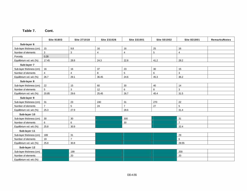
DD-4.55
Table 7. Cont.
Site 91803 Site 271018 Site 231026 Site 331001 Site 501002 Site 831801 Remarks/Notes
Sub-layer 6 Sub-layer thickness (cm) 15 9.8 16 16 25 16 Number of elements 3 3 4 4 5 4 Porosity 0.28 Equilibrium vol. w/c (%) 17.45 28.8 24.3 22.8 41.2 28.2
Sub-layer 7 Sub-layer thickness (cm) 16 16 37 23 30 15 Number of elements 4 4 8 5 6 3 Equilibrium vol. w/c (%) 26.7 29.1 36.45 24.6 45.3 36.2
Sub-layer 8 Sub-layer thickness (cm) 22 15 60 30 40 14 Number of elements 5 3 12 6 8 3 Equilibrium vol. w/c (%) 20.85 29.6 25.45 26.7 45.4 31.5
Sub-layer 9 Sub-layer thickness (cm) 31 23 240 31 270 22 Number of elements 7 5 24 7 27 5 Equilibrium vol. w/c (%) 25.3 27.9 28.6 31.4
Sub-layer 10 Sub-layer thickness (cm) 30 30 300 31 Number of elements 6 6 30 7 Equilibrium vol. w/c (%) 25.8 30.9 32.4
Sub-layer 11 Sub-layer thickness (cm) 189 31 29 Number of elements 19 7 6 Equilibrium vol. w/c (%) 25.8 30.8 28.55
Sub-layer 12 Sub-layer thickness (cm) 199 200 Number of elements 20 20 Equilibrium vol. w/c (%)
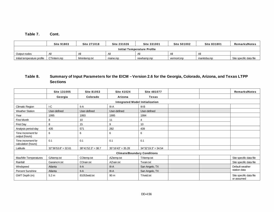
DD-4.56
Table 7. Cont.
Site 91803 Site 271018 Site 231026 Site 331001 Site 501002 Site 831801 Remarks/Notes
Initial Temperature Profile Output nodes All All All All All All Initial temperature profile CTinitem.inp Mninitemp.txt maine.inp newhamp.inp vermont.inp manitoba.inp Site specific data file
Table 8. Summary of Input Parameters for the EICM – Version 2.6 for the Georgia, Colorado, Arizona, and Texas LTPP Sections
Site 131005 Site 81053 Site 41024 Site 481077 Remarks/Notes
Georgia Colorado Arizona Texas
Integrated Model Initialization Climatic Region I-C II-A III-A III-B Weather Station User-defined User-defined User-defined User-defined Year 1995 1993 1995 1994 First Month 8 10 11 4 First Day 8 15 9 10
Analysis period-day 435 571 282 439 Time Increment for output (hours)
6 6 6 6
Time increment for calculation (hours)
0.1 0.1 0.1 0.1
Latitude 32°36’53.8” = 32.61 38°41’52.3” = 38.7 35°16’43” = 35.28 34°32’19.3” = 34.54
Climate/Boundary Conditions Max/Min Temperatures GAtemp.txt COtemp.txt AZtemp.txt TXtemp.txt Site specific data file Rainfall Garaincm.txt COrain.txt AZrain.txt Txrain.txt Site specific data file Windspeed Atlanta II-A III-A San Angelo, TX Percent Sunshine Atlanta II-A III-A San Angelo, TX
Default weather station data
GWT Depth (m) 5.2 m 81053wtd.txt 90 m TXwtd.txt Site specific data file or assumed
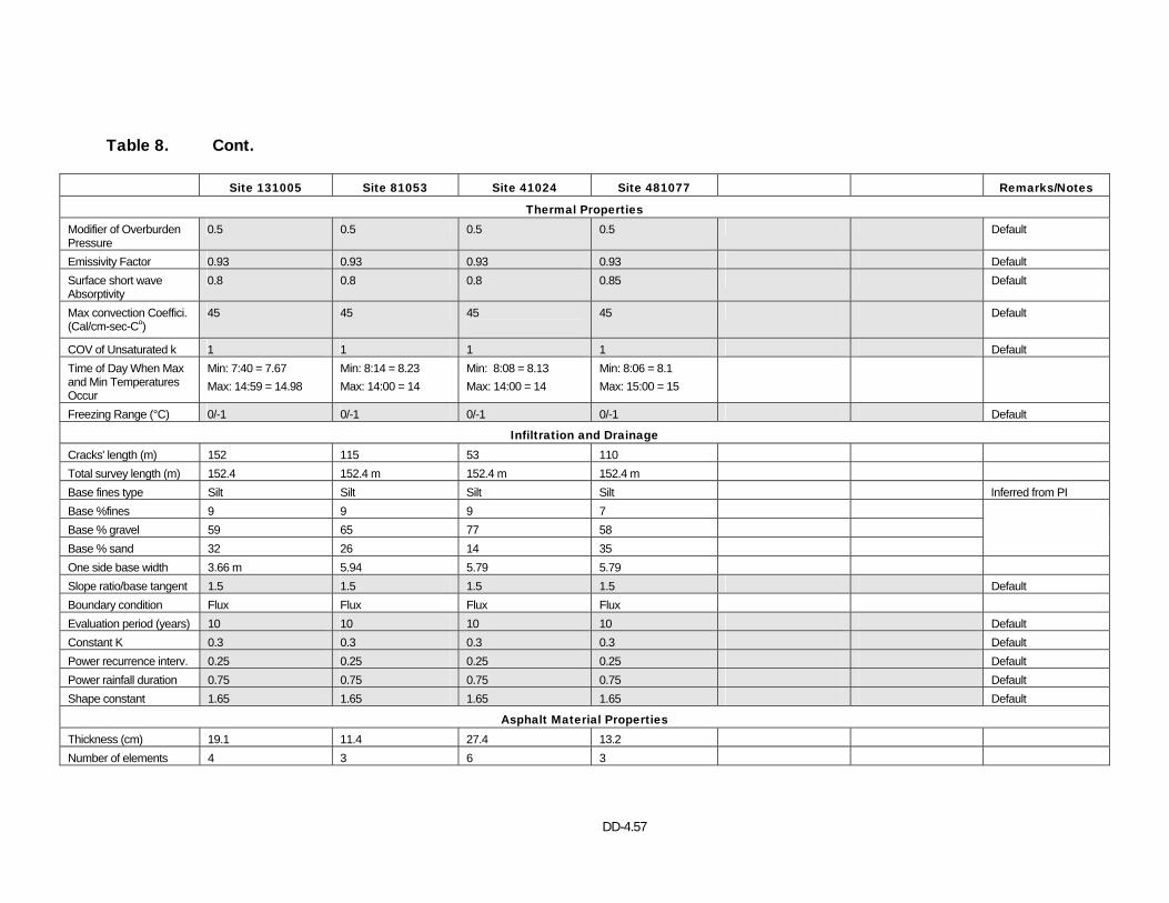
DD-4.57
Table 8. Cont.
Site 131005 Site 81053 Site 41024 Site 481077 Remarks/Notes
Thermal Properties Modifier of Overburden Pressure
0.5 0.5 0.5 0.5 Default
Emissivity Factor 0.93 0.93 0.93 0.93 Default Surface short wave Absorptivity
0.8 0.8 0.8 0.85 Default
Max convection Coeffici. (Cal/cm-sec-Co)
45 45 45
45 Default
COV of Unsaturated k 1 1 1 1 Default Time of Day When Max and Min Temperatures Occur
Min: 7:40 = 7.67 Max: 14:59 = 14.98
Min: 8:14 = 8.23 Max: 14:00 = 14
Min: 8:08 = 8.13 Max: 14:00 = 14
Min: 8:06 = 8.1 Max: 15:00 = 15
Freezing Range (°C) 0/-1 0/-1 0/-1 0/-1 Default
Infiltration and Drainage Cracks' length (m) 152 115 53 110 Total survey length (m) 152.4 152.4 m 152.4 m 152.4 m Base fines type Silt Silt Silt Silt Inferred from PI Base %fines 9 9 9 7 Base % gravel 59 65 77 58 Base % sand 32 26 14 35
One side base width 3.66 m 5.94 5.79 5.79 Slope ratio/base tangent 1.5 1.5 1.5 1.5 Default Boundary condition Flux Flux Flux Flux Evaluation period (years) 10 10 10 10 Default Constant K 0.3 0.3 0.3 0.3 Default Power recurrence interv. 0.25 0.25 0.25 0.25 Default Power rainfall duration 0.75 0.75 0.75 0.75 Default Shape constant 1.65 1.65 1.65 1.65 Default
Asphalt Material Properties Thickness (cm) 19.1 11.4 27.4 13.2 Number of elements 4 3 6 3
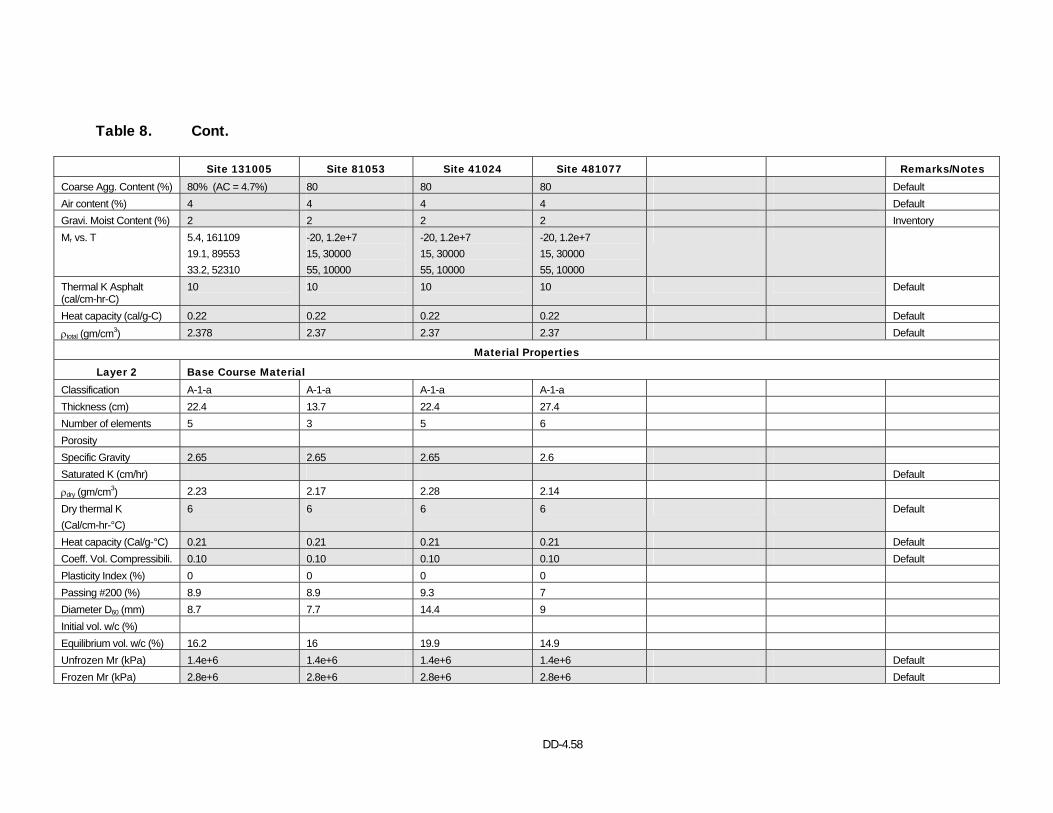
DD-4.58
Table 8. Cont.
Site 131005 Site 81053 Site 41024 Site 481077 Remarks/Notes Coarse Agg. Content (%) 80% (AC = 4.7%) 80 80 80 Default Air content (%) 4 4 4 4 Default Gravi. Moist Content (%) 2 2 2 2 Inventory Mr vs. T 5.4, 161109
19.1, 89553 33.2, 52310
-20, 1.2e+7 15, 30000 55, 10000
-20, 1.2e+7 15, 30000 55, 10000
-20, 1.2e+7 15, 30000 55, 10000
Thermal K Asphalt (cal/cm-hr-C)
10 10 10 10 Default
Heat capacity (cal/g-C) 0.22 0.22 0.22 0.22 Default ρtotal (gm/cm3) 2.378 2.37 2.37 2.37 Default
Material Properties
Layer 2 Base Course Material Classification A-1-a A-1-a A-1-a A-1-a Thickness (cm) 22.4 13.7 22.4 27.4 Number of elements 5 3 5 6 Porosity Specific Gravity 2.65 2.65 2.65 2.6 Saturated K (cm/hr) Default ρdry (gm/cm3) 2.23 2.17 2.28 2.14 Dry thermal K (Cal/cm-hr-°C)
6 6 6 6 Default
Heat capacity (Cal/g-°C) 0.21 0.21 0.21 0.21 Default Coeff. Vol. Compressibili. 0.10 0.10 0.10 0.10 Default Plasticity Index (%) 0 0 0 0 Passing #200 (%) 8.9 8.9 9.3 7 Diameter D60 (mm) 8.7 7.7 14.4 9 Initial vol. w/c (%) Equilibrium vol. w/c (%) 16.2 16 19.9 14.9 Unfrozen Mr (kPa) 1.4e+6 1.4e+6 1.4e+6 1.4e+6 Default Frozen Mr (kPa) 2.8e+6 2.8e+6 2.8e+6 2.8e+6 Default
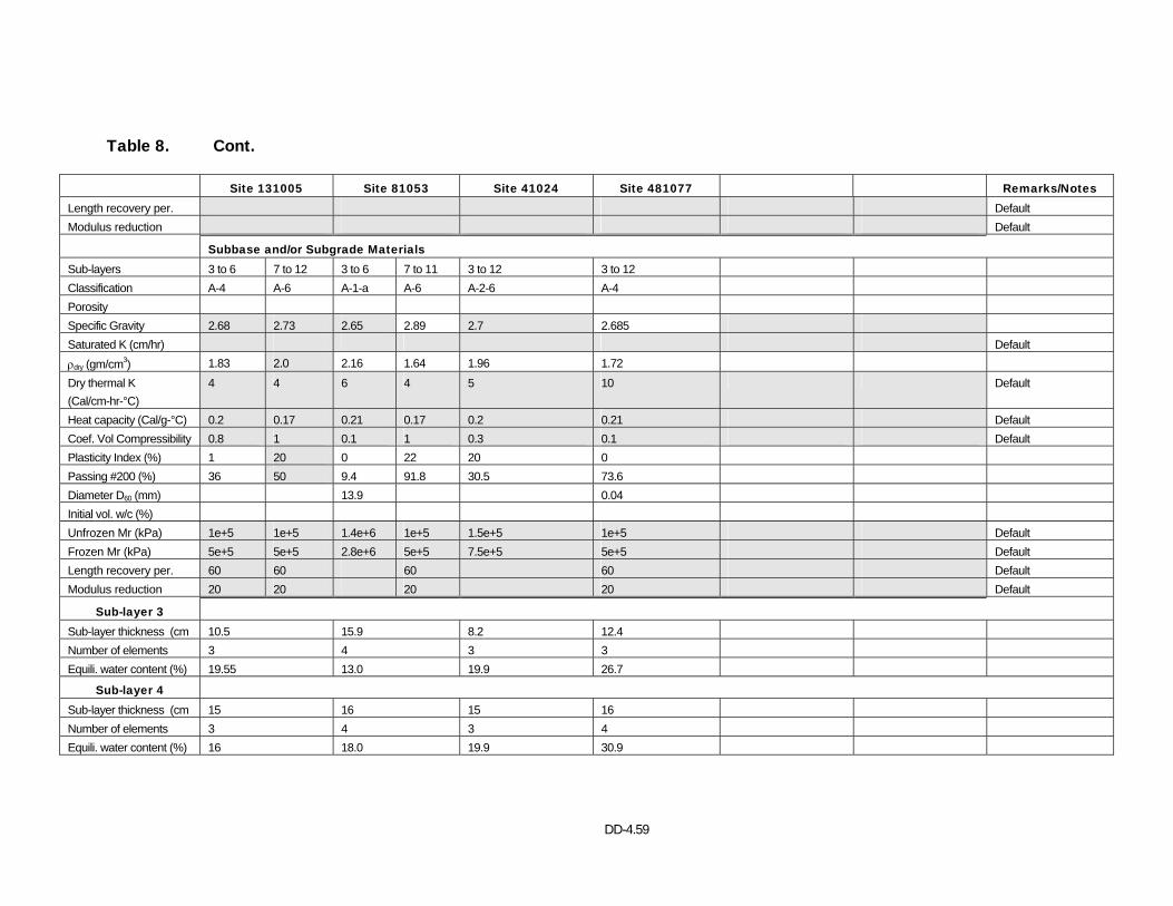
DD-4.59
Table 8. Cont.
Site 131005 Site 81053 Site 41024 Site 481077 Remarks/Notes Length recovery per. Default Modulus reduction Default
Subbase and/or Subgrade Materials Sub-layers 3 to 6 7 to 12 3 to 6 7 to 11 3 to 12 3 to 12 Classification A-4 A-6 A-1-a A-6 A-2-6 A-4 Porosity Specific Gravity 2.68 2.73 2.65 2.89 2.7 2.685 Saturated K (cm/hr) Default ρdry (gm/cm3) 1.83 2.0 2.16 1.64 1.96 1.72 Dry thermal K (Cal/cm-hr-°C)
4 4 6 4 5 10 Default
Heat capacity (Cal/g-°C) 0.2 0.17 0.21 0.17 0.2 0.21 Default Coef. Vol Compressibility 0.8 1 0.1 1 0.3 0.1 Default Plasticity Index (%) 1 20 0 22 20 0 Passing #200 (%) 36 50 9.4 91.8 30.5 73.6 Diameter D60 (mm) 13.9 0.04 Initial vol. w/c (%) Unfrozen Mr (kPa) 1e+5 1e+5 1.4e+6 1e+5 1.5e+5 1e+5 Default Frozen Mr (kPa) 5e+5 5e+5 2.8e+6 5e+5 7.5e+5 5e+5 Default Length recovery per. 60 60 60 60 Default Modulus reduction 20 20 20 20 Default
Sub-layer 3 Sub-layer thickness (cm 10.5 15.9 8.2 12.4 Number of elements 3 4 3 3 Equili. water content (%) 19.55 13.0 19.9 26.7
Sub-layer 4 Sub-layer thickness (cm 15 16 15 16 Number of elements 3 4 3 4 Equili. water content (%) 16 18.0 19.9 30.9
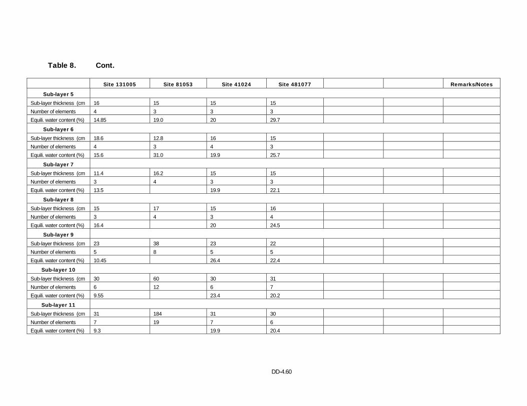
DD-4.60
Table 8. Cont.
Site 131005 Site 81053 Site 41024 Site 481077 Remarks/Notes
Sub-layer 5 Sub-layer thickness (cm 16 15 15 15 Number of elements 4 3 3 3 Equili. water content (%) 14.85 19.0 20 29.7
Sub-layer 6 Sub-layer thickness (cm 18.6 12.8 16 15 Number of elements 4 3 4 3 Equili. water content (%) 15.6 31.0 19.9 25.7
Sub-layer 7 Sub-layer thickness (cm 11.4 16.2 15 15 Number of elements 3 4 3 3 Equili. water content (%) 13.5 19.9 22.1
Sub-layer 8 Sub-layer thickness (cm 15 17 15 16 Number of elements 3 4 3 4 Equili. water content (%) 16.4 20 24.5
Sub-layer 9 Sub-layer thickness (cm 23 38 23 22 Number of elements 5 8 5 5 Equili. water content (%) 10.45 26.4 22.4
Sub-layer 10 Sub-layer thickness (cm 30 60 30 31 Number of elements 6 12 6 7 Equili. water content (%) 9.55 23.4 20.2
Sub-layer 11 Sub-layer thickness (cm 31 184 31 30 Number of elements 7 19 7 6 Equili. water content (%) 9.3 19.9 20.4
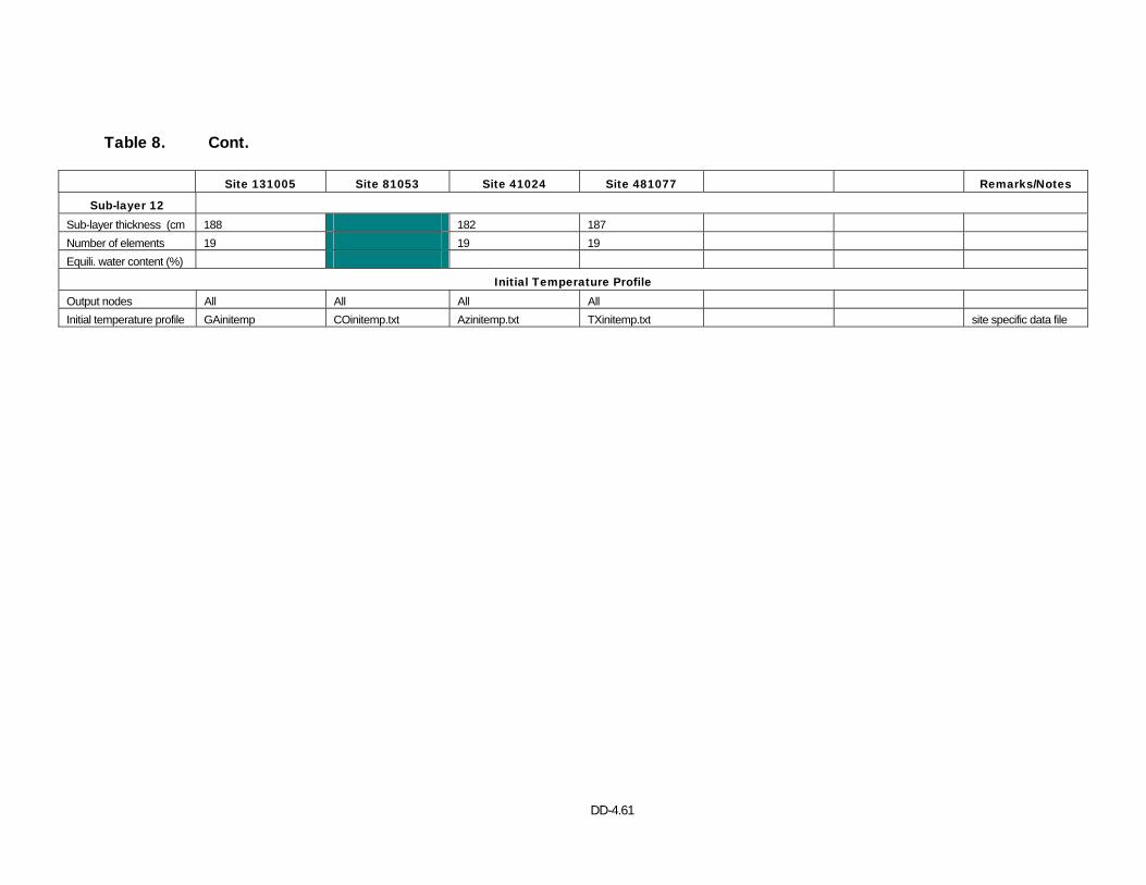
DD-4.61
Table 8. Cont.
Site 131005 Site 81053 Site 41024 Site 481077 Remarks/Notes
Sub-layer 12 Sub-layer thickness (cm 188 182 187 Number of elements 19 19 19 Equili. water content (%)
Initial Temperature Profile Output nodes All All All All Initial temperature profile GAinitemp COinitemp.txt Azinitemp.txt TXinitemp.txt site specific data file

subgrade material was sub-divided on each figure. The volumetric water content profiles
comparing the results for both versions, Version 2.1 and Version 2.6, are included in
Appendices I through R.
The summary of the results is presented in Figures 26 through 28. Figure 26 shows the
water content prediction versus the measured water contents for the base course
materials from the ten sites previously discussed. Note that the Coefficient of
Determination (R2) of 0.65 is a substantial improvement over that for Version 2.1 (R2 =
0.05, see Figure 7). Figure 27 depicts the measured versus predicted volumetric water
content for the subbase and subgrade materials. Again, the R2 of 0.68 is significantly
better than the R2 value obtained with the EICM version 2.1 of 0.34 (see Figure 8). The
overall comparison is shown in Figure 28. The R2 value obtained for the overall data was
0.73. Collectively, these results show that the moisture contents predicted with Version
2.6 of the EICM are in substantially better agreement with the field data than those from
Version 2.1 of the model.
The improvements can be described and summarized as follows:
1) Modifications to the Computation Algorithm (ICM), which improved the match
between predicted and TDR measured values:
a) Improvements to the SWCC (SWCC = f(wPI, D60).
b) Introduction of software providing an adjustment to the SWCC based on
equilibrium water contents.
c) Introduction of correlation between Gs and wPI and the use of this
relationship to obtain the best estimate of the porosity (rather than using the
default values).
Based on these results, it is concluded that equilibrium and initial water contents
are important, and that one or the other is needed to match TDR measured
values. It is further concluded that values of porosity are fairly important and
should be estimated as accurately as possible. Thus, values of density, water
content, PI, and gradation for each layer are needed. Measured values of Gs
would be helpful, but not essential if the other measurements are made or
estimated very well.
2) Needed Input Parameters

DD-4.63
As part of the site investigation and material characterization, the following should
be measured to ensure the greatest possible accuracy in moisture content
predictions obtained with the EICM:
a) Dry density
b) Water content
c) Plasticity Index
d) Gradation
e) Groundwater table depth
3) Overall Comparisons of the Performance of EICM Version 2.6 (New) with that of
Version 2.1 (Old) showed:
a) The new version showed improved predictions in all cases and often,
substantial improvement.
b) The available data do not permit meaningful assessment of the accuracy of
EICM predicted moisture contents in and near frozen layers, because the
measured (TDR) values are suspect for these layers. Thus, no judgment of
the accuracy of the EICM moisture predictions for frozen and freezing
materials can be made on the basis of the work reported herein.
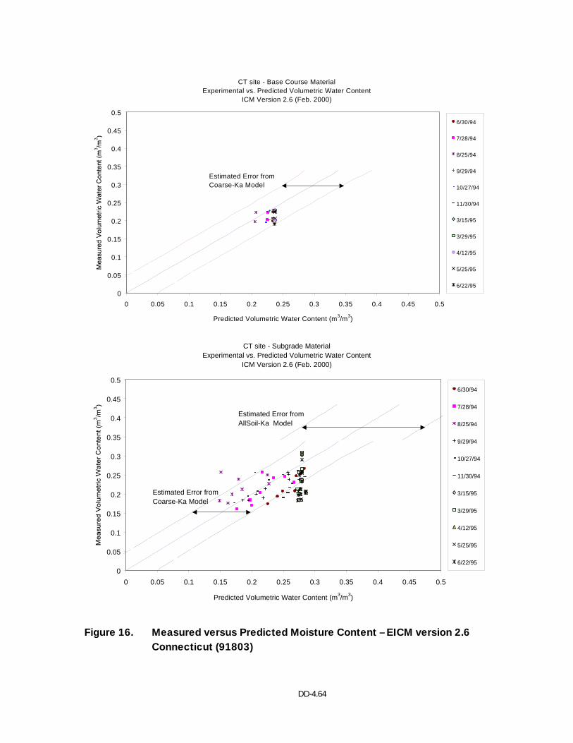
DD-4.64
CT site - Base Course MaterialExperimental vs. Predicted Volumetric Water Content
ICM Version 2.6 (Feb. 2000)
0
0.05
0.1
0.15
0.2
0.25
0.3
0.35
0.4
0.45
0.5
0 0.05 0.1 0.15 0.2 0.25 0.3 0.35 0.4 0.45 0.5
Predicted Volumetric Water Content (m3/m3)
6/30/94
7/28/94
8/25/94
9/29/94
10/27/94
11/30/94
3/15/95
3/29/95
4/12/95
5/25/95
6/22/95
Estimated Error from Coarse-Ka Model
CT site - Subgrade MaterialExperimental vs. Predicted Volumetric Water Content
ICM Version 2.6 (Feb. 2000)
0
0.05
0.1
0.15
0.2
0.25
0.3
0.35
0.4
0.45
0.5
0 0.05 0.1 0.15 0.2 0.25 0.3 0.35 0.4 0.45 0.5
Predicted Volumetric Water Content (m3/m3)
6/30/94
7/28/94
8/25/94
9/29/94
10/27/94
11/30/94
3/15/95
3/29/95
4/12/95
5/25/95
6/22/95
Estimated Error from AllSoil-Ka Model
Estimated Error from Coarse-Ka Model
Figure 16. Measured versus Predicted Moisture Content – EICM version 2.6 Connecticut (91803)
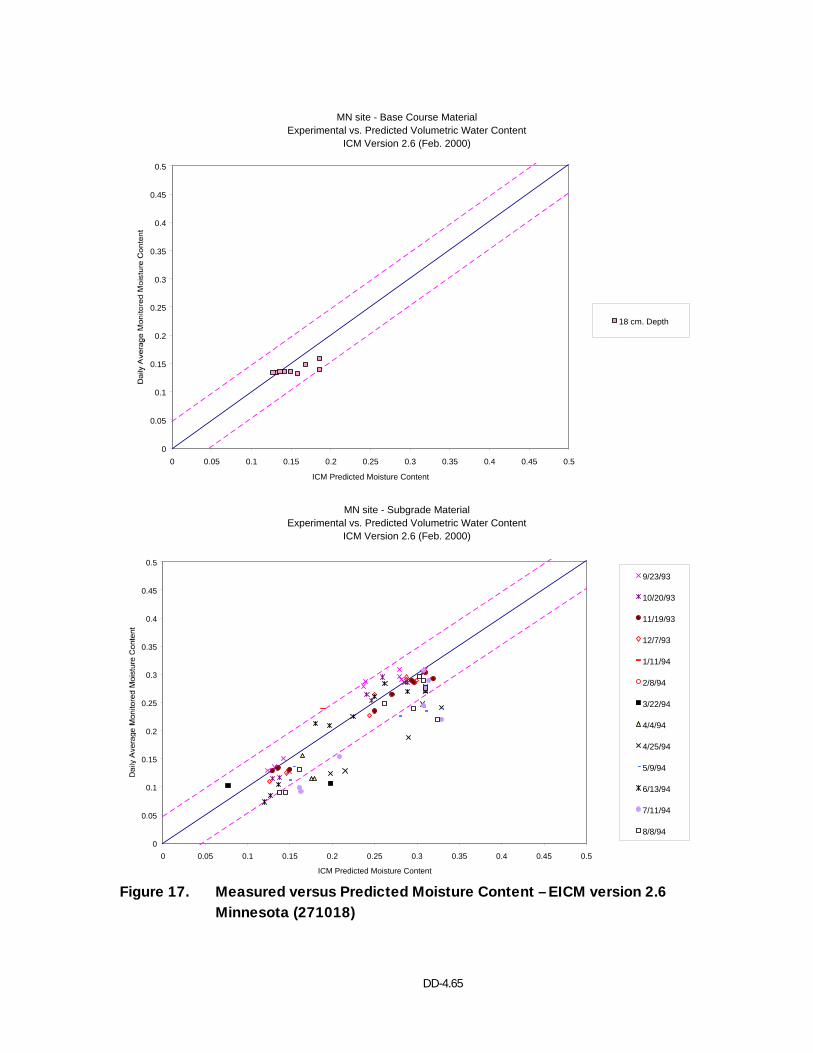
DD-4.65
MN site - Base Course MaterialExperimental vs. Predicted Volumetric Water Content
ICM Version 2.6 (Feb. 2000)
0
0.05
0.1
0.15
0.2
0.25
0.3
0.35
0.4
0.45
0.5
0 0.05 0.1 0.15 0.2 0.25 0.3 0.35 0.4 0.45 0.5
ICM Predicted Moisture Content
18 cm. Depth
MN site - Subgrade MaterialExperimental vs. Predicted Volumetric Water Content
ICM Version 2.6 (Feb. 2000)
0
0.05
0.1
0.15
0.2
0.25
0.3
0.35
0.4
0.45
0.5
0 0.05 0.1 0.15 0.2 0.25 0.3 0.35 0.4 0.45 0.5
ICM Predicted Moisture Content
9/23/93
10/20/93
11/19/93
12/7/93
1/11/94
2/8/94
3/22/94
4/4/94
4/25/94
5/9/94
6/13/94
7/11/94
8/8/94
Figure 17. Measured versus Predicted Moisture Content – EICM version 2.6
Minnesota (271018)
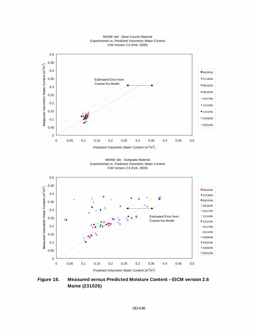
DD-4.66
MAINE site - Base Course Material Experimental vs. Predicted Volumetric Water Content
ICM Version 2.6 (Feb. 2000)
0
0.05
0.1
0.15
0.2
0.25
0.3
0.35
0.4
0.45
0.5
0 0.05 0.1 0.15 0.2 0.25 0.3 0.35 0.4 0.45 0.5
Predicted Volumetric Water Content (m3/m3)
06/20/94
07/18/94
08/15/94
09/19/94
10/17/94
11/14/94
12/12/94
04/03/95
05/01/95
Estimated Error from Coarse-Ka Model
MAINE site - Subgrade Material Experimental vs. Predicted Volumetric Water Content
ICM Version 2.6 (Feb. 2000)
0
0.05
0.1
0.15
0.2
0.25
0.3
0.35
0.4
0.45
0.5
0 0.05 0.1 0.15 0.2 0.25 0.3 0.35 0.4 0.45 0.5
Predicted Volumetric Water Content (m3/m3)
06/20/94
07/18/94
08/15/94
09/19/94
10/17/94
11/14/94
12/12/94
01/17/95
02/14/95
03/06/95
03/20/95
04/03/95
05/01/95
Estimated Error from Coarse-Ka Model
Figure 18. Measured versus Predicted Moisture Content – EICM version 2.6
Maine (231026)
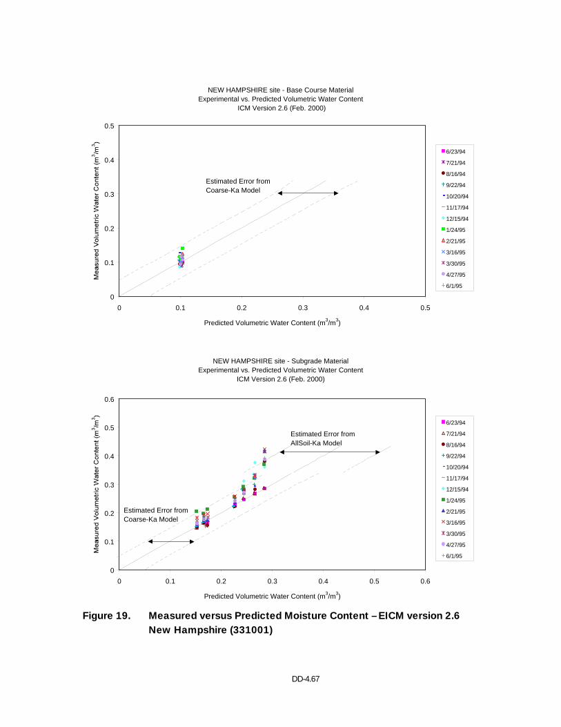
DD-4.67
NEW HAMPSHIRE site - Base Course MaterialExperimental vs. Predicted Volumetric Water Content
ICM Version 2.6 (Feb. 2000)
0
0.1
0.2
0.3
0.4
0.5
0 0.1 0.2 0.3 0.4 0.5
Predicted Volumetric Water Content (m3/m3)
6/23/94
7/21/94
8/16/94
9/22/94
10/20/94
11/17/94
12/15/94
1/24/95
2/21/95
3/16/95
3/30/95
4/27/95
6/1/95
Estimated Error from Coarse-Ka Model
NEW HAMPSHIRE site - Subgrade MaterialExperimental vs. Predicted Volumetric Water Content
ICM Version 2.6 (Feb. 2000)
0
0.1
0.2
0.3
0.4
0.5
0.6
0 0.1 0.2 0.3 0.4 0.5 0.6
Predicted Volumetric Water Content (m3/m3)
6/23/94
7/21/94
8/16/94
9/22/94
10/20/94
11/17/94
12/15/94
1/24/95
2/21/95
3/16/95
3/30/95
4/27/95
6/1/95
Estimated Error from Coarse-Ka Model
Estimated Error from AllSoil-Ka Model
Figure 19. Measured versus Predicted Moisture Content – EICM version 2.6
New Hampshire (331001)
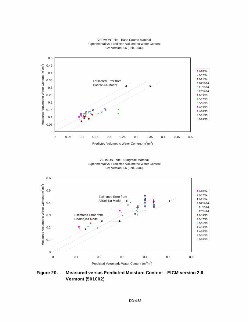
DD-4.68
VERMONT site - Base Course MaterialExperimental vs. Predicted Volumetric Water Content
ICM Version 2.6 (Feb. 2000)
0
0.05
0.1
0.15
0.2
0.25
0.3
0.35
0.4
0.45
0.5
0 0.05 0.1 0.15 0.2 0.25 0.3 0.35 0.4 0.45 0.5
Predicted Volumetric Water Content (m3/m3)
7/20/948/17/949/21/9410/19/9411/16/9412/14/941/19/953/17/953/31/954/13/954/28/955/31/956/28/95
Estimated Error from Coarse-Ka Model
VERMONT site - Subgrade MaterialExperimental vs. Predicted Volumetric Water Content
ICM Version 2.6 (Feb. 2000)
0
0.1
0.2
0.3
0.4
0.5
0.6
0 0.1 0.2 0.3 0.4 0.5 0.6
Predicted Volumetric Water Content (m3/m3)
7/20/948/17/949/21/9410/19/9411/16/9412/14/941/19/953/17/953/31/954/13/954/28/955/31/956/28/95
Estimated Error from Coarse-Ka Model
Estimated Error from AllSoil-Ka Model
Figure 20. Measured versus Predicted Moisture Content – EICM version 2.6
Vermont (501002)
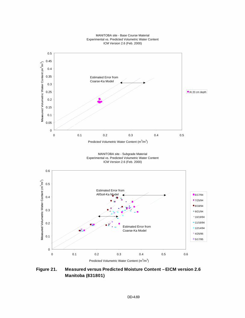
DD-4.69
MANITOBA site - Base Course MaterialExperimental vs. Predicted Volumetric Water Content
ICM Version 2.6 (Feb. 2000)
0
0.05
0.1
0.15
0.2
0.25
0.3
0.35
0.4
0.45
0.5
0 0.1 0.2 0.3 0.4 0.5
Predicted Volumetric Water Content (m3/m3)
At 20 cm depth
Estimated Error from Coarse-Ka Model
MANITOBA site - Subgrade MaterialExperimental vs. Predicted Volumetric Water Content
ICM Version 2.6 (Feb. 2000)
0
0.1
0.2
0.3
0.4
0.5
0.6
0 0.1 0.2 0.3 0.4 0.5 0.6
Predicted Volumetric Water Content (m3/m3)
6/17/94
7/25/94
8/18/94
9/21/94
10/19/94
11/16/94
12/14/94
4/25/95
5/17/95
Estimated Error from Coarse-Ka Model
Estimated Error from AllSoil-Ka Model
Figure 21. Measured versus Predicted Moisture Content – EICM version 2.6
Manitoba (831801)
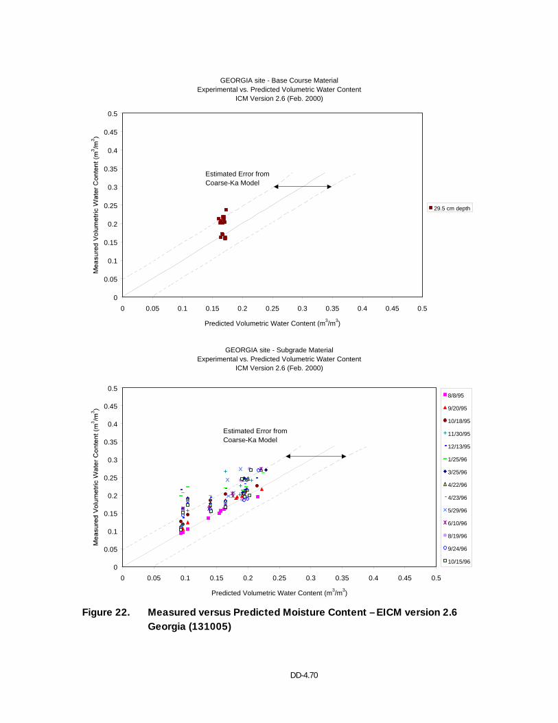
DD-4.70
GEORGIA site - Base Course Material Experimental vs. Predicted Volumetric Water Content
ICM Version 2.6 (Feb. 2000)
0
0.05
0.1
0.15
0.2
0.25
0.3
0.35
0.4
0.45
0.5
0 0.05 0.1 0.15 0.2 0.25 0.3 0.35 0.4 0.45 0.5
Predicted Volumetric Water Content (m3/m3)
29.5 cm depth
Estimated Error from Coarse-Ka Model
GEORGIA site - Subgrade Material Experimental vs. Predicted Volumetric Water Content
ICM Version 2.6 (Feb. 2000)
0
0.05
0.1
0.15
0.2
0.25
0.3
0.35
0.4
0.45
0.5
0 0.05 0.1 0.15 0.2 0.25 0.3 0.35 0.4 0.45 0.5
Predicted Volumetric Water Content (m3/m3)
8/8/95
9/20/95
10/18/95
11/30/95
12/13/95
1/25/96
3/25/96
4/22/96
4/23/96
5/29/96
6/10/96
8/19/96
9/24/96
10/15/96
Estimated Error from Coarse-Ka Model
Figure 22. Measured versus Predicted Moisture Content – EICM version 2.6
Georgia (131005)
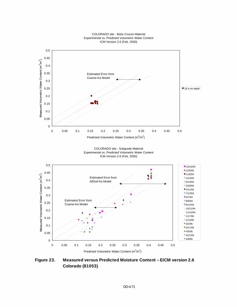
DD-4.71
COLORADO site - Base Course Material Experimental vs. Predicted Volumetric Water Content
ICM Version 2.6 (Feb. 2000)
0
0.05
0.1
0.15
0.2
0.25
0.3
0.35
0.4
0.45
0.5
0 0.05 0.1 0.15 0.2 0.25 0.3 0.35 0.4 0.45 0.5
Predicted Volumetric Water Content (m3/m3)
18.4 cm depth
Estimated Error from Coarse-Ka Model
COLORADO site - Subgrade Material Experimental vs. Predicted Volumetric Water Content
ICM Version 2.6 (Feb. 2000)
0
0.05
0.1
0.15
0.2
0.25
0.3
0.35
0.4
0.45
0.5
0 0.05 0.1 0.15 0.2 0.25 0.3 0.35 0.4 0.45 0.5
Predicted Volumetric Water Content (m3/m3)
10/15/9312/6/931/18/942/14/943/14/943/28/944/11/947/13/948/7/948/8/949/12/9410/21/9411/10/941/17/952/13/953/2/953/17/954/5/954/21/955/8/95
Estimated Error from Coarse-Ka Model
Estimated Error from AllSoil-Ka Model
Figure 23. Measured versus Predicted Moisture Content – EICM version 2.6
Colorado (81053)
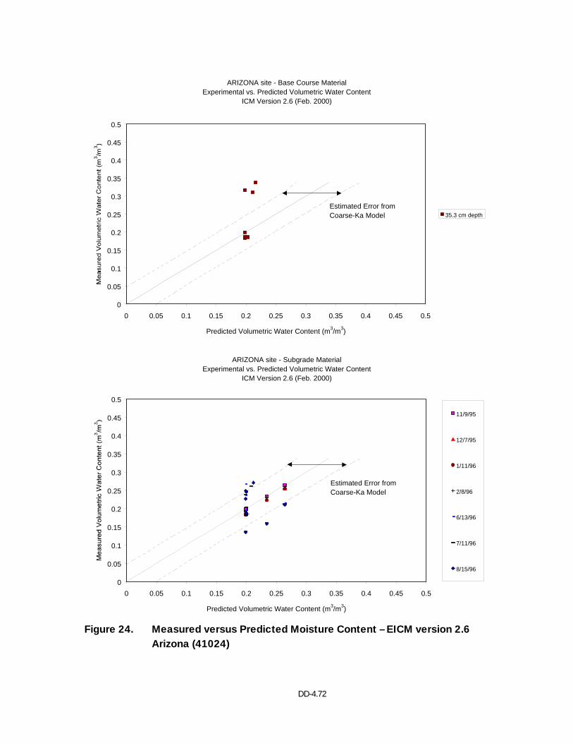
DD-4.72
ARIZONA site - Base Course Material Experimental vs. Predicted Volumetric Water Content
ICM Version 2.6 (Feb. 2000)
0
0.05
0.1
0.15
0.2
0.25
0.3
0.35
0.4
0.45
0.5
0 0.05 0.1 0.15 0.2 0.25 0.3 0.35 0.4 0.45 0.5
Predicted Volumetric Water Content (m3/m3)
35.3 cm depthEstimated Error from Coarse-Ka Model
ARIZONA site - Subgrade Material Experimental vs. Predicted Volumetric Water Content
ICM Version 2.6 (Feb. 2000)
0
0.05
0.1
0.15
0.2
0.25
0.3
0.35
0.4
0.45
0.5
0 0.05 0.1 0.15 0.2 0.25 0.3 0.35 0.4 0.45 0.5
Predicted Volumetric Water Content (m3/m3)
11/9/95
12/7/95
1/11/96
2/8/96
6/13/96
7/11/96
8/15/96
Estimated Error from Coarse-Ka Model
Figure 24. Measured versus Predicted Moisture Content – EICM version 2.6
Arizona (41024)
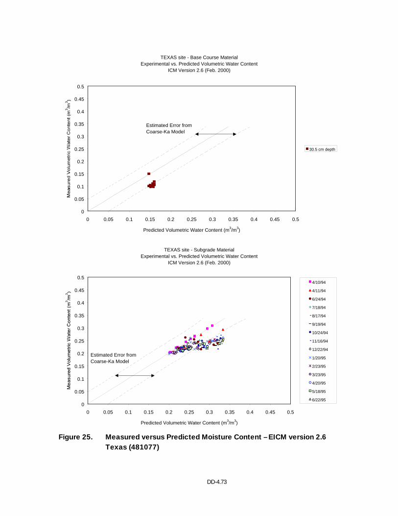
DD-4.73
TEXAS site - Base Course Material Experimental vs. Predicted Volumetric Water Content
ICM Version 2.6 (Feb. 2000)
0
0.05
0.1
0.15
0.2
0.25
0.3
0.35
0.4
0.45
0.5
0 0.05 0.1 0.15 0.2 0.25 0.3 0.35 0.4 0.45 0.5
Predicted Volumetric Water Content (m3/m3)
30.5 cm depth
Estimated Error from Coarse-Ka Model
TEXAS site - Subgrade Material Experimental vs. Predicted Volumetric Water Content
ICM Version 2.6 (Feb. 2000)
0
0.05
0.1
0.15
0.2
0.25
0.3
0.35
0.4
0.45
0.5
0 0.05 0.1 0.15 0.2 0.25 0.3 0.35 0.4 0.45 0.5
Predicted Volumetric Water Content (m3/m3)
4/10/94
4/11/94
6/24/94
7/18/94
8/17/94
9/19/94
10/24/94
11/16/94
12/22/94
1/20/95
2/23/95
3/23/95
4/20/95
5/18/95
6/22/95
Estimated Error from Coarse-Ka Model
Figure 25. Measured versus Predicted Moisture Content – EICM version 2.6
Texas (481077)
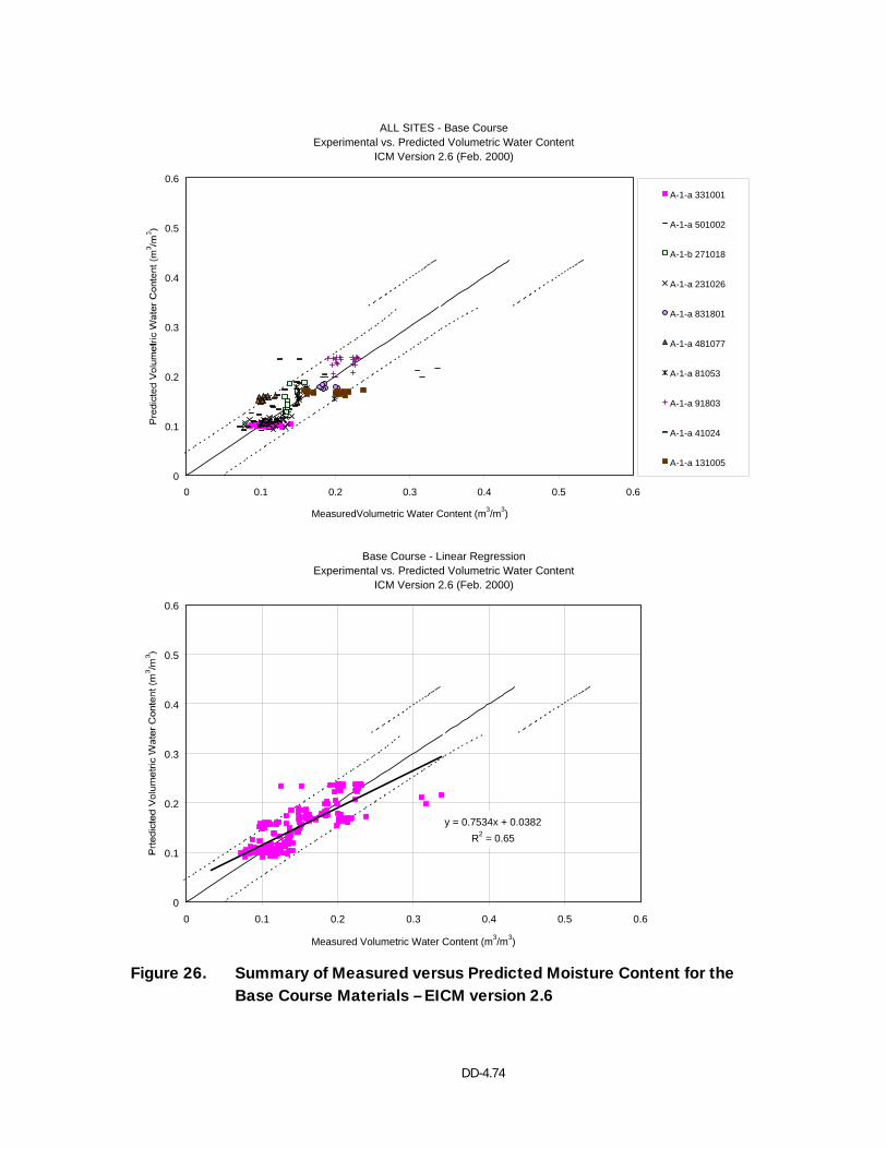
DD-4.74
ALL SITES - Base CourseExperimental vs. Predicted Volumetric Water Content
ICM Version 2.6 (Feb. 2000)
0
0.1
0.2
0.3
0.4
0.5
0.6
0 0.1 0.2 0.3 0.4 0.5 0.6
MeasuredVolumetric Water Content (m3/m3)
A-1-a 331001
A-1-a 501002
A-1-b 271018
A-1-a 231026
A-1-a 831801
A-1-a 481077
A-1-a 81053
A-1-a 91803
A-1-a 41024
A-1-a 131005
Base Course - Linear RegressionExperimental vs. Predicted Volumetric Water Content
ICM Version 2.6 (Feb. 2000)
y = 0.7534x + 0.0382R2 = 0.65
0
0.1
0.2
0.3
0.4
0.5
0.6
0 0.1 0.2 0.3 0.4 0.5 0.6
Measured Volumetric Water Content (m3/m3)
Figure 26. Summary of Measured versus Predicted Moisture Content for the Base Course Materials – EICM version 2.6
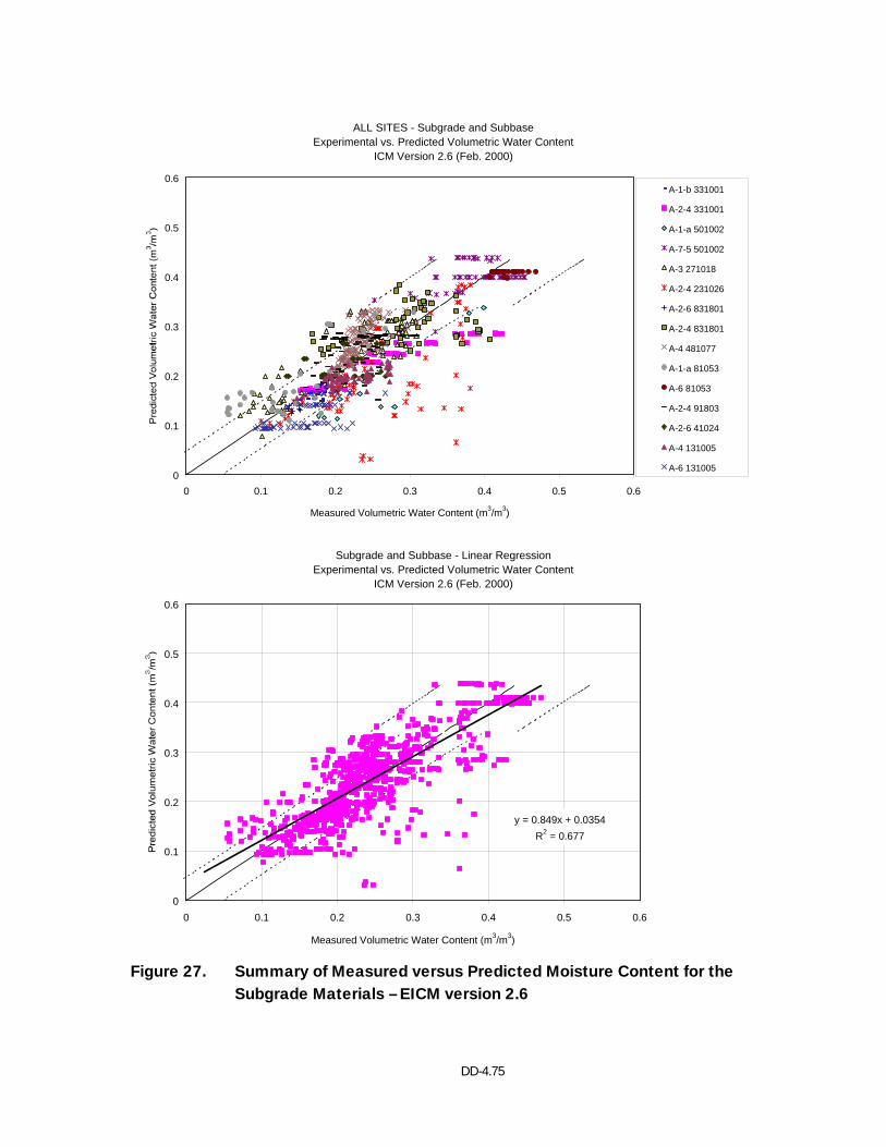
DD-4.75
ALL SITES - Subgrade and SubbaseExperimental vs. Predicted Volumetric Water Content
ICM Version 2.6 (Feb. 2000)
0
0.1
0.2
0.3
0.4
0.5
0.6
0 0.1 0.2 0.3 0.4 0.5 0.6
Measured Volumetric Water Content (m3/m3)
A-1-b 331001
A-2-4 331001
A-1-a 501002
A-7-5 501002
A-3 271018
A-2-4 231026
A-2-6 831801
A-2-4 831801
A-4 481077
A-1-a 81053
A-6 81053
A-2-4 91803
A-2-6 41024
A-4 131005
A-6 131005
Subgrade and Subbase - Linear RegressionExperimental vs. Predicted Volumetric Water Content
ICM Version 2.6 (Feb. 2000)
y = 0.849x + 0.0354R2 = 0.677
0
0.1
0.2
0.3
0.4
0.5
0.6
0 0.1 0.2 0.3 0.4 0.5 0.6
Measured Volumetric Water Content (m3/m3)
Figure 27. Summary of Measured versus Predicted Moisture Content for the Subgrade Materials – EICM version 2.6
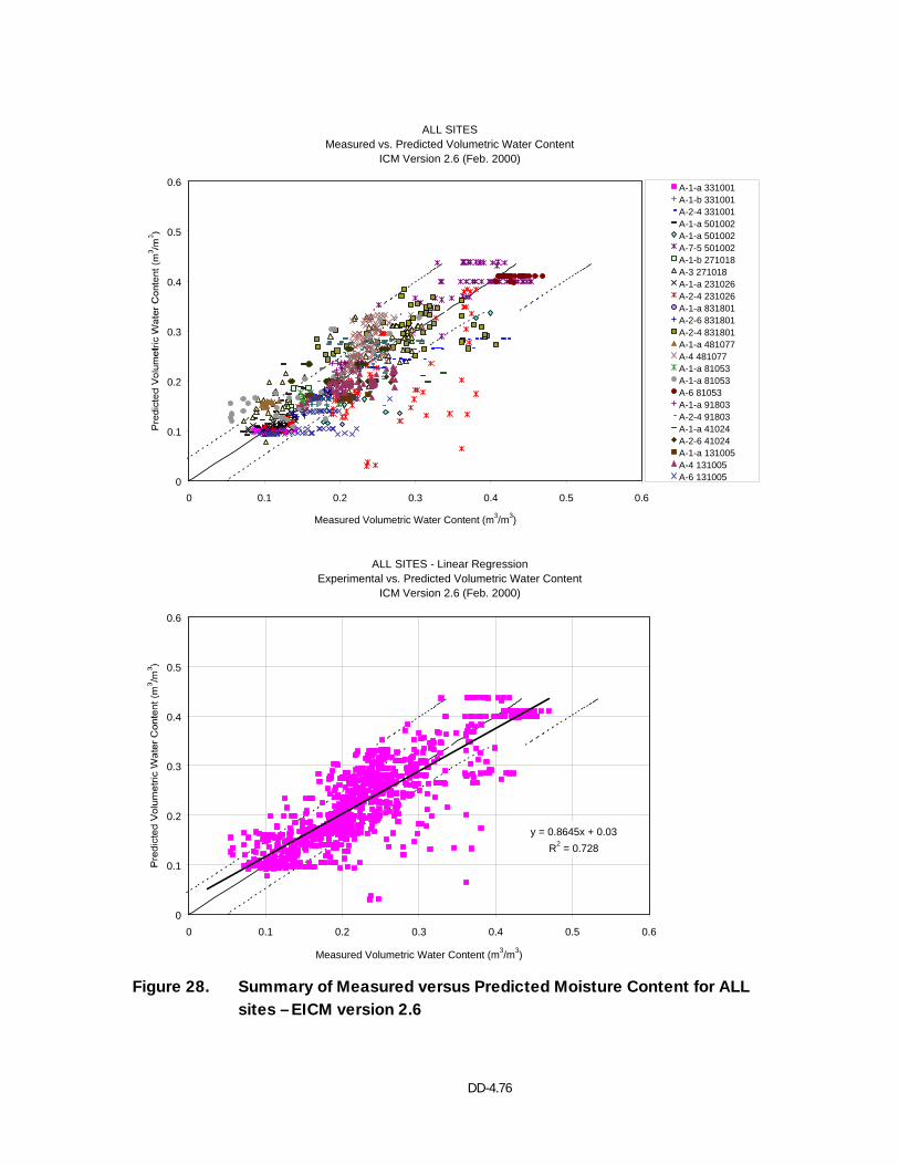
DD-4.76
ALL SITESMeasured vs. Predicted Volumetric Water Content
ICM Version 2.6 (Feb. 2000)
0
0.1
0.2
0.3
0.4
0.5
0.6
0 0.1 0.2 0.3 0.4 0.5 0.6
Measured Volumetric Water Content (m3/m3)
A-1-a 331001A-1-b 331001A-2-4 331001A-1-a 501002A-1-a 501002A-7-5 501002A-1-b 271018A-3 271018A-1-a 231026A-2-4 231026A-1-a 831801A-2-6 831801A-2-4 831801A-1-a 481077A-4 481077A-1-a 81053A-1-a 81053A-6 81053A-1-a 91803A-2-4 91803A-1-a 41024A-2-6 41024A-1-a 131005A-4 131005A-6 131005
ALL SITES - Linear RegressionExperimental vs. Predicted Volumetric Water Content
ICM Version 2.6 (Feb. 2000)
y = 0.8645x + 0.03R2 = 0.728
0
0.1
0.2
0.3
0.4
0.5
0.6
0 0.1 0.2 0.3 0.4 0.5 0.6
Measured Volumetric Water Content (m3/m3)
Figure 28. Summary of Measured versus Predicted Moisture Content for ALL sites – EICM version 2.6
User's Guide and Recommendations EICM version 2.6 - Moisture Content Prediction
Introduction
Recommendations on how best to deal with the new features implemented to improve the
model capability for moisture content predictions are presented in this Chapter. It is not
the intention of the authors to provide the reader with a complete description of the EICM
user's guide. For those interested in features other than the moisture content prediction,
refer to the EICM User's Manual built into the program for complete information (Larson
and Dempsey, 1997).
Input Parameters
The input parameters needed to run the EICM are essentially the same as those outlined
in Chapter 2, Table 1. The main changes reside on the "Material Properties" and "Initial
Temperature and Water Content Profiles" sections. Table 9 shows the variables for the
aforementioned sections and highlights the parameters added to the model. The input
parameters for the remaining sections are unchanged from those presented in Table 1.
The new parameters needed for the EICM version 2.6 will be briefly discussed in the
following sections. For the rest of the parameters, please refer to the EICM's User
Manual.
Several of the input variables for the soil layers have check boxes. If the box is checked,
the associated input box is enabled and ready to accept input variables. If the box is
unchecked, the EICM will either calculate or use a default value for the input variable in
question. The accuracy of the EICM predictions are increased if material specific data is
input, as opposed to the use of default values.
Chapter
5
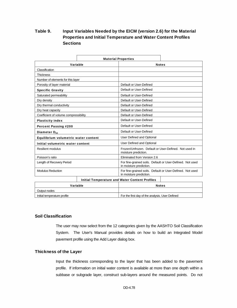
DD-4.78
Table 9. Input Variables Needed by the EICM (version 2.6) for the Material Properties and Initial Temperature and Water Content Profiles Sections
Material Properties
Variable Notes Classification Thickness Number of elements for this layer Porosity of layer material Default or User-Defined
Specific Gravity Default or User-Defined
Saturated permeability Default or User-Defined Dry density Default or User-Defined Dry thermal conductivity Default or User-Defined Dry heat capacity Default or User-Defined Coefficient of volume compressibility Default or User-Defined
Plasticity index Default or User-Defined
Percent Passing #200 Default or User-Defined
Diameter D60 Default or User-Defined
Equilibrium volumetric water content User Defined and Optional
Initial volumetric water content User Defined and Optional
Resilient modulus Frozen/Unfrozen. Default or User-Defined. Not used in moisture prediction.
Poisson’s ratio Eliminated from Version 2.6 Length of Recovery Period For fine-grained soils. Default or User-Defined. Not used
in moisture prediction. Modulus Reduction For fine-grained soils. Default or User-Defined. Not used
in moisture prediction.
Initial Temperature and Water Content Profiles
Variable Notes Output nodes Initial temperature profile For the first day of the analysis. User Defined
Soil Classification
The user may now select from the 12 categories given by the AASHTO Soil Classification
System. The User's Manual provides details on how to build an Integrated Model
pavement profile using the Add Layer dialog box.
Thickness of the Layer
Input the thickness corresponding to the layer that has been added to the pavement
profile. If information on initial water content is available at more than one depth within a
subbase or subgrade layer, construct sub-layers around the measured points. Do not
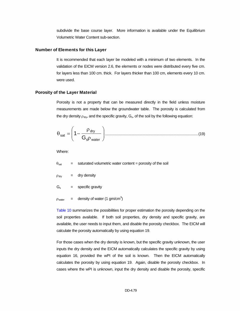
DD-4.79
subdivide the base course layer. More information is available under the Equilibrium
Volumetric Water Content sub-section.
Number of Elements for this Layer
It is recommended that each layer be modeled with a minimum of two elements. In the
validation of the EICM version 2.6, the elements or nodes were distributed every five cm.
for layers less than 100 cm. thick. For layers thicker than 100 cm, elements every 10 cm.
were used.
Porosity of the Layer Material
Porosity is not a property that can be measured directly in the field unless moisture
measurements are made below the groundwater table. The porosity is calculated from
the dry density ρdry, and the specific gravity, Gs, of the soil by the following equation:
⎟⎟⎠
⎞⎜⎜⎝
⎛ρ
ρ−=θ
waters
drysat G
1 ..............................................................................................(19)
Where:
θsat = saturated volumetric water content = porosity of the soil
ρdry = dry density
Gs = specific gravity
ρwater = density of water (1 gm/cm3)
Table 10 summarizes the possibilities for proper estimation the porosity depending on the
soil properties available. If both soil properties, dry density and specific gravity, are
available, the user needs to input them, and disable the porosity checkbox. The EICM will
calculate the porosity automatically by using equation 19.
For those cases when the dry density is known, but the specific gravity unknown, the user
inputs the dry density and the EICM automatically calculates the specific gravity by using
equation 16, provided the wPI of the soil is known. Then the EICM automatically
calculates the porosity by using equation 19. Again, disable the porosity checkbox. In
cases where the wPI is unknown, input the dry density and disable the porosity, specific
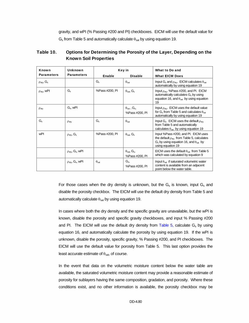
DD-4.80
gravity, and wPI (% Passing #200 and PI) checkboxes. EICM will use the default value for
Gs from Table 5 and automatically calculate θsat by using equation 19.
Table 10. Options for Determining the Porosity of the Layer, Depending on the Known Soil Properties
Known Parameters
Unknown Parameters
Key in
Enable Disable
What to Do and
What EICM Does
ρdry, Gs Gs θsat Input Gs and ρdry. EICM calculates θsat automatically by using equation 19
ρdry, wPI Gs %Pass #200, PI θsat, Gs Input ρdry. %Pass #200, and PI. EICM automatically calculates Gs by using equation 16, and θsat by using equation 19
ρdry Gs, wPI θsat , Gs, %Pass #200, PI
Input ρdry. EICM uses the default value for Gs from Table 5 and calculates θsat automatically by using equation 19
Gs ρdry Gs θsat Input Gs. EICM uses the default ρdry from Table 5 and automatically calculates θsat by using equation 19
wPI ρdry, Gs %Pass #200, PI θsat, Gs Input %Pass #200, and PI. EICM uses the default ρdry from Table 5, calculates Gs by using equation 16, and θsat by using equation 19
ρdry, Gs, wPI θsat, Gs, %Pass #200, PI
EICM uses the default θsat from Table 5 which was calculated by equation 9
ρdry, Gs, wPI θsat Gs, %Pass #200, PI
Input θsat if saturated volumetric water content is available from an adjacent point below the water table.
For those cases when the dry density is unknown, but the Gs is known, input Gs and
disable the porosity checkbox. The EICM will use the default dry density from Table 5 and
automatically calculate θsat by using equation 19.
In cases where both the dry density and the specific gravity are unavailable, but the wPI is
known, disable the porosity and specific gravity checkboxes, and input % Passing #200
and PI. The EICM will use the default dry density from Table 5, calculate Gs by using
equation 16, and automatically calculate the porosity by using equation 19. If the wPI is
unknown, disable the porosity, specific gravity, % Passing #200, and PI checkboxes. The
EICM will use the default value for porosity from Table 5. This last option provides the
least accurate estimate of θsat, of course.
In the event that data on the volumetric moisture content below the water table are
available, the saturated volumetric moisture content may provide a reasonable estimate of
porosity for sublayers having the same composition, gradation, and porosity. Where these
conditions exist, and no other information is available, the porosity checkbox may be
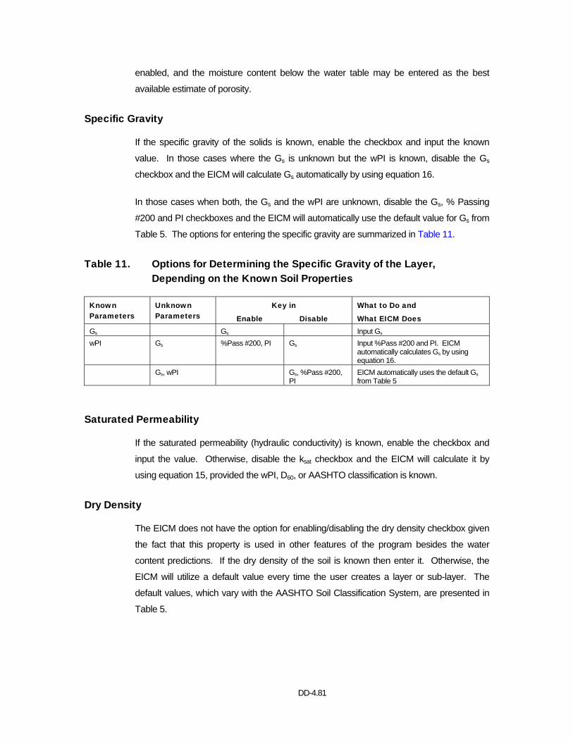
DD-4.81
enabled, and the moisture content below the water table may be entered as the best
available estimate of porosity.
Specific Gravity
If the specific gravity of the solids is known, enable the checkbox and input the known
value. In those cases where the Gs is unknown but the wPI is known, disable the Gs
checkbox and the EICM will calculate Gs automatically by using equation 16.
In those cases when both, the Gs and the wPI are unknown, disable the Gs, % Passing
#200 and PI checkboxes and the EICM will automatically use the default value for Gs from
Table 5. The options for entering the specific gravity are summarized in Table 11.
Table 11. Options for Determining the Specific Gravity of the Layer, Depending on the Known Soil Properties
Known Parameters
Unknown Parameters
Key in
Enable Disable
What to Do and
What EICM Does Gs Gs Input Gs wPI Gs %Pass #200, PI Gs Input %Pass #200 and PI. EICM
automatically calculates Gs by using equation 16.
Gs, wPI Gs, %Pass #200, PI
EICM automatically uses the default Gs from Table 5
Saturated Permeability
If the saturated permeability (hydraulic conductivity) is known, enable the checkbox and
input the value. Otherwise, disable the ksat checkbox and the EICM will calculate it by
using equation 15, provided the wPI, D60, or AASHTO classification is known.
Dry Density
The EICM does not have the option for enabling/disabling the dry density checkbox given
the fact that this property is used in other features of the program besides the water
content predictions. If the dry density of the soil is known then enter it. Otherwise, the
EICM will utilize a default value every time the user creates a layer or sub-layer. The
default values, which vary with the AASHTO Soil Classification System, are presented in
Table 5.

DD-4.82
Plasticity Index
Enable the Plasticity Index (PI) checkbox if the value is known. Otherwise, disable the
checkbox and the EICM will show and use a default value every time the user creates a
layer or sub-layer. The default values can be seen on Table 5 and are a function of the
AASHTO Soil Classification System.
If the soil is nonplastic, enable the PI checkbox and input 0.
The accuracy of the SWCC greatly depends on the Plasticity Index if the initial water
content is not available as will be explained later. Particularly if the initial water content is
unknown, it is recommended to perform the Atterberg Limits test to define the PI rather
than approximate it by Visual Classification. Refer to Table 12 for more information on
how the EICM determines the SWCC based on PI information.
Table 12. Determination of the SWCC based on Percentage Passing #200, Plasticity Index and Diameter D60
Are any of the Following Parameters known?
If
What to Do?
What Does the EICM Do?
Yes Enable the appropriate checkboxes and input the known parameters
%Pass #200
PI D60 No Disable the checkboxes for the unknown
parameters
EICM assigns default values for the checkboxes that have been disabled, or calculates unknown values from known values as outlined in Tables 10 and 11. If wPI=0, EICM uses eqs. 10 to 13 to define the SWCC. Otherwise, it calculates the SWCC by using eqs. 4 to 7
Percent Passing #200
The fines content of the soil is another property that is important to the SWCC of the soil.
Enable the Percent Passing #200 checkbox if the value is known. Otherwise, disable the
checkbox and the EICM will use a default value based on the AASHTO Soil Classification
System. It is recommended to perform a Sieve Analysis or the Standard Test Method for
Materials Finer than #200 Sieve by Washing in order to obtain a more accurate prediction.
Refer to Table 12 for more information on how the EICM determines the SWCC based on
Percent Passing #200 information.

DD-4.83
Diameter D60
D60 is the grain diameter (in mm) corresponding to 60% passing, by weight or mass, on
the Grain Size Distribution Curve. In other words, 60% of the particles by weight are
smaller than the diameter D60. Having the D60, the user enables the checkbox and inputs
the value. Otherwise, the EICM will use a default value based on the AASHTO Soil
Classification System. As is the case with the Percent Passing #200 and PI, the D60 is
important in the determination of the SWCC. Therefore, it is recommended to perform a
Sieve Analysis instead of using the default parameters. Refer to Table 12 for more
information on how the EICM determines the SWCC based on D60 information.
Initial Volumetric Water Content
The initial water content (θo) is the water content at the start of the program or that at the
first day of the analysis. If a value is specified, the entire layer will be set to that water
content. Table 13 presents information on how the EICM deals with the θo data. If the θo
checkbox is enabled, then the water content will march from the given initial value toward
the equilibrium water content (explained in the following sub-section) with time. On the
other hand, if the θo checkbox is disabled, the program sets θo equal to the equilibrium
water content.
Equilibrium Volumetric Water Content
The equilibrium volumetric water content (θeq) is strongly tied to the SWCC of the soil. It is
therefore recommended to perform measurements of water content for each layer in the
pavement profile. Care should be taken to enter the equilibrium volumetric water content,
θeq, rather than the equilibrium gravimetric water content, ωeq. If ωeq is available, manually
calculate the volumetric water content by the following equation, and then enter the
calculated value:
water
dryeqeq ρ
ρω=θ ..............................................................................................................(20)
Where:
θeq = equilibrium volumetric water content
ωeq = equilibrium gravimetric water content
ρdry = dry density
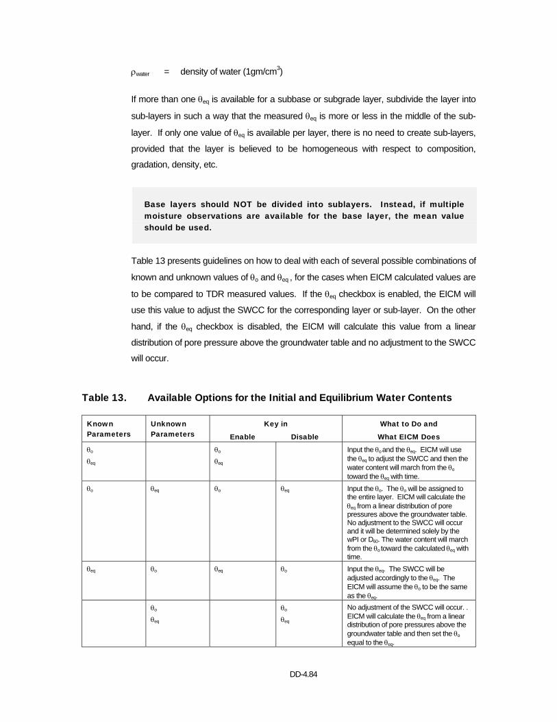
DD-4.84
ρwater = density of water (1gm/cm3)
If more than one θeq is available for a subbase or subgrade layer, subdivide the layer into
sub-layers in such a way that the measured θeq is more or less in the middle of the sub-
layer. If only one value of θeq is available per layer, there is no need to create sub-layers,
provided that the layer is believed to be homogeneous with respect to composition,
gradation, density, etc.
Base layers should NOT be divided into sublayers. Instead, if multiple moisture observations are available for the base layer, the mean value should be used.
Table 13 presents guidelines on how to deal with each of several possible combinations of
known and unknown values of θo and θeq , for the cases when EICM calculated values are
to be compared to TDR measured values. If the θeq checkbox is enabled, the EICM will
use this value to adjust the SWCC for the corresponding layer or sub-layer. On the other
hand, if the θeq checkbox is disabled, the EICM will calculate this value from a linear
distribution of pore pressure above the groundwater table and no adjustment to the SWCC
will occur.
Table 13. Available Options for the Initial and Equilibrium Water Contents
Known Parameters
Unknown Parameters
Key in
Enable Disable
What to Do and
What EICM Does
θo θeq
θo θeq
Input the θo and the θeq. EICM will use the θeq to adjust the SWCC and then the water content will march from the θo
toward the θeq with time. θo θeq θo θeq Input the θo. The θo will be assigned to
the entire layer. EICM will calculate the θeq from a linear distribution of pore pressures above the groundwater table. No adjustment to the SWCC will occur and it will be determined solely by the wPI or D60. The water content will march from the θo toward the calculated θeq with time.
θeq θo θeq θo Input the θeq. The SWCC will be adjusted accordingly to the θeq. The EICM will assume the θo to be the same as the θeq.
θo θeq
θo θeq
No adjustment of the SWCC will occur. . EICM will calculate the θeq from a linear distribution of pore pressures above the groundwater table and then set the θo equal to the θeq.
DD-4.85
The preceding guidelines and suggestions were aimed at maximizing the accuracy with
which the EICM will predict seasonal oscillations in moisture content in pavement layers.
All recommendations were predicated on the following:
1) Predictions were to be compared with TDR measured values for existing
pavements.
2) Seasonal oscillations were of primary interest, rather than the equilibrium value –
which justifies treatment of the first-available TDR reading as θeq, rather than
using EICM to predict θeq.
Chapter 6, which follows, is aimed at prediction of the most likely initial condition, θo, but
through use of the initial degree of saturation, So. The second objective pursued in
Chapter 6 is that of predicting θeq, but in terms of degree of saturation, Sequil. The tracking
of seasonal oscillations in moisture content is de-emphasized. The reason for this
change in emphasis in Chapter 6 is as follows:
Preliminary analyses, made after the work of Chapters 2 through 5 was
completed, showed that the effects of seasonal moisture content variations
on MR were typically minor. The change from the initial condition, So, to the
equilibrium condition, Sequil, typically produces the greatest change in MR.

Development of Procedures for Estimating Moisture Content Changes from the Initial State to Equilibrium Conditions for Newly Constructed Pavements Introduction
The initial conditions at which bases, subbases, and subgrades are compacted are
defined by the dry unit weight, moisture content, and specific gravity of solids. These
interrelationships are given by equations (21) and (22).
swGSe = ......................................................................................................................(21)
e1G ws
dry +γ
=γ .................................................................................................................(22)
Where:
S = degree of saturation
e = void ratio
w = gravimetric moisture content
Gs = specific gravity of solids
γdry = dry unit weight
γw = unit weight of water
Chapter
6
DD-4.87
In equation (21) any three parameters determine the fourth. Thus, for example, e can be
computed from equation (21) and e and Gs can be used to get γdry in equation (22).
The density and water content at which unbound materials are actually compacted in
pavement sections are controlled by compaction specifications. It is very common
practice to require that subbases and subgrades be compacted to at least 95% of and
sometimes 100% of γdry max by T99 (Standard Proctor effort). Bases are commonly
required to be more than 95% of the γdry max by T180 (Modified Proctor effort). Because
contractors typically compact a little above the required minimum it is reasonable to
assume that average initial conditions with respect to density are γdry max (T99) for
subbases and subgrades and γdry max (T180) for bases. The water content is not usually
controlled strictly, but contractors are encouraged to wet materials to a point near the line
of optimums to facilitate compaction. Therefore, it is likewise reasonable to assume that
initial compaction conditions for water content are wopt by T99 for subbases and subgrades
and wopt by T180 for bases.
The preceding discussion relates to density and moisture content as initial conditions for
compacted pavement layers in the field. On a different but related note, data from the
literature on resilient modulus (MR) obtained from laboratory compaction has been
thoroughly studied. This study shows that most lab specimens for MR testing were
compacted at γdry max and wopt. Therefore, the database for MR values has more data
points at optimum conditions (γdry max and wopt) that at any other condition and is a logical
choice as a reference condition for MR. For the reasons stated above, optimum conditions
have been chosen as a best estimate of initial compaction conditions in the field and as a
reference state for estimating changes in MR due to moisture content changes.
Correlation for Sopt
Because of the importance of optimum conditions, it is desirable to be able to estimate the
degree of saturation at optimum, Sopt, from index properties. Because wPI and D60 were
used for the SWCC parameters, they were used again for the correlations that follow.
Figure 29 shows a plot of Sopt versus wPI for a modest-sized database available to the
authors (Witczak and Yau, 1997). Most engineers with experience in compaction testing
would assert that Sopt normally falls between 80 and 88%. These data are generally
consistent with that assertion, and an average value of about 85% could easily be
adopted. However, it is logical that Sopt should increase slightly with wPI. At low values of
S the soil water suction is high and tends to prevent particles from sliding past each other,
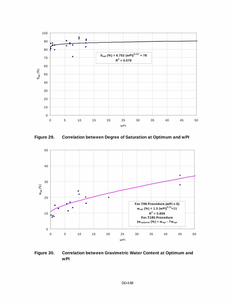
DD-4.88
0
10
20
30
40
50
60
70
80
90
100
0 5 10 15 20 25 30 35 40 45 50
wPI
Sopt (%) = 6.752 (wPI)0.147 + 78R2 = 0.079
Figure 29. Correlation between Degree of Saturation at Optimum and wPI
0
10
20
30
40
50
0 5 10 15 20 25 30 35 40 45 50
wPI
For T99 Procedure (wPI > 0)wopt (%) = 1.3 (wPI)0.73+11
R2 = 0.808For T180 Procedure
(wopt)mod (%) = wopt - ∆wopt
Figure 30. Correlation between Gravimetric Water Content at Optimum and wPI
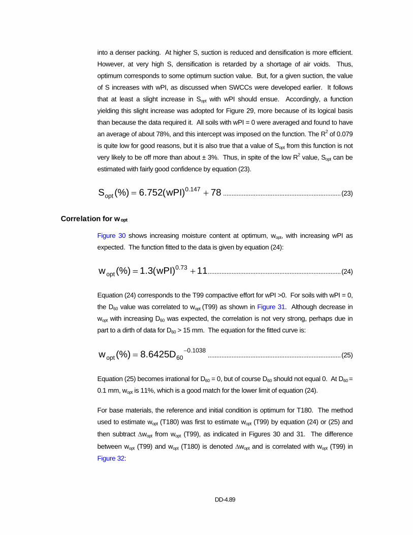
DD-4.89
into a denser packing. At higher S, suction is reduced and densification is more efficient.
However, at very high S, densification is retarded by a shortage of air voids. Thus,
optimum corresponds to some optimum suction value. But, for a given suction, the value
of S increases with wPI, as discussed when SWCCs were developed earlier. It follows
that at least a slight increase in Sopt with wPI should ensue. Accordingly, a function
yielding this slight increase was adopted for Figure 29, more because of its logical basis
than because the data required it. All soils with wPI = 0 were averaged and found to have
an average of about 78%, and this intercept was imposed on the function. The R2 of 0.079
is quite low for good reasons, but it is also true that a value of Sopt from this function is not
very likely to be off more than about ± 3%. Thus, in spite of the low R2 value, Sopt can be
estimated with fairly good confidence by equation (23).
78)wPI(752.6(%)S 147.0opt += .....................................................................(23)
Correlation for wopt
Figure 30 shows increasing moisture content at optimum, wopt, with increasing wPI as
expected. The function fitted to the data is given by equation (24):
11)wPI(3.1(%)w 73.0opt += ..............................................................................(24)
Equation (24) corresponds to the T99 compactive effort for wPI >0. For soils with wPI = 0,
the D60 value was correlated to wopt (T99) as shown in Figure 31. Although decrease in
wopt with increasing D60 was expected, the correlation is not very strong, perhaps due in
part to a dirth of data for D60 > 15 mm. The equation for the fitted curve is:
1038.060opt D6425.8(%)w −= ..............................................................................(25)
Equation (25) becomes irrational for D60 = 0, but of course D60 should not equal 0. At D60 =
0.1 mm, wopt is 11%, which is a good match for the lower limit of equation (24).
For base materials, the reference and initial condition is optimum for T180. The method
used to estimate wopt (T180) was first to estimate wopt (T99) by equation (24) or (25) and
then subtract ∆wopt from wopt (T99), as indicated in Figures 30 and 31. The difference
between wopt (T99) and wopt (T180) is denoted ∆wopt and is correlated with wopt (T99) in
Figure 32:
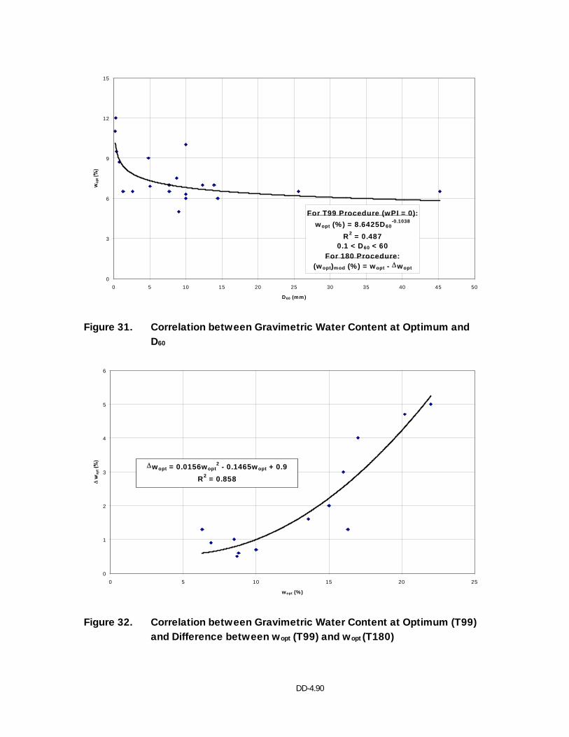
DD-4.90
For T99 Procedure (wPI = 0):wopt (%) = 8.6425D60
-0.1038
R2 = 0.4870.1 < D60 < 60
For 180 Procedure:(wopt)mod (%) = wopt - ∆wopt
0
3
6
9
12
15
0 5 10 15 20 25 30 35 40 45 50
D60 (mm)
Figure 31. Correlation between Gravimetric Water Content at Optimum and D60
0
1
2
3
4
5
6
0 5 10 15 20 25
wopt (%)
∆
∆wopt = 0.0156wopt2 - 0.1465wopt + 0.9
R2 = 0.858
Figure 32. Correlation between Gravimetric Water Content at Optimum (T99) and Difference between wopt (T99) and wopt (T180)
DD-4.91
9.0w1465.0w0156.0w opt2
optopt +−=∆ ..............................................(26)
Thus, wopt (T99) is determined first, then ∆wopt is estimated from equation (26), and wopt
(T180) is calculated by equation (27):
optoptopt w)99T(w)180T(w ∆−= ..................................................................(27)
Intended Use of Correlations
The intended use of these correlations is to support computations, both inside and outside
the EICM, aimed at evaluating pavement material resilient moduli as a function of time and
in consideration of moisture changes. The basic model adopted for evaluating change in
MR due to change in moisture content is given by equation (28). The development of this
model is presented in Witczak et al.(2000), Volumes I and II.
))SS(kexp(1aba
MMlog
optsopt R
R
−+β+−
+=⎟⎟⎠
⎞⎜⎜⎝
⎛............................................(28)
Where:
MR = resilient modulus at any S
MR opt = resilient modulus at γdry max and w = wopt and S = Sopt
a,b, β, ks = model parameters
Sopt = S at optimum, in decimal
S = any degree of saturation at any time, for a layer in the pavement profile, in
decimal
Note that the change in degree of saturation, S – Sopt = ∆S, is an essential quantity in
equation (28). The value of Sopt can be computed inside or outside of the EICM. In either
case it is a simple application of equation (23), and requires only wPI. If wPI = 0, then Sopt
is fixed constant at 78%. The value of S is most conveniently computed inside the EICM.

DD-4.92
Use of EICM
The computational algorithm, which is currently being incorporated in the EICM under
Level 3 as described in Chapter 8, is as follows:
1) For a given pavement profile layer or point within a layer (node), wPI or D60 is
input.
2) Sopt is computed from equation (23).
3) wopt is computed from equation (24) or (25). For base materials, equations (26)
and (27) are also employed.
4) Gs is computed by equation (16): 65.2)wPI(041.0G 29.0s +=
5) e is computed from equation (21).
6) γdry max is computed from equation (22).
7) The initial degree of saturation, So, is set = Sopt, the initial moisture content, wo, is
set = wopt.
8) The initial volumetric water content, θo, is set equal to θopt and computed by
w
max dryopt
w
max dryoopto ww
γ
γ=
γ
γ=θ=θ .........................................(29)
9) The porosity, n, is computed by
sate1en θ=+
= .............................................................................................(30)
Where:
θsat = saturated volumetric water content
Note: At this point, all of the initial condition material properties are established.
However, the total required input data file for the EICM is voluminous and
complex and includes climatic data and position of groundwater table as a
function of time.
DD-4.93
10) When all input data is complete and ready, the EICM can march forward through
time computing values of volumetric water content, θ. These θ values can be
converted to w and/or S values using the equations presented above.
11) If S is computed and plotted as a function of time its stability can be judged.
Experience with the EICM has shown that S typically becomes stable, with
seasonal variations due to climatic conditions and water table variations being
small. Under these circumstances, the average S over a period of relative
stability can be evaluated as Sequilibrium. This equilibrium value of S is of
considerable interest because it represents a condition for which MR is also fairly
stable. Thus, Sequil – Sopt would be used in equation (28) to get MR equil.
Estimation of Sequil outside the EICM
The algorithm outlined above represents the major steps followed by the EICM in
generating initial condition data and then the computation of S in general and Sequil in
particular. The value of Sequil can also be estimated outside the EICM with only modest
loss in accuracy. The following steps may be used to obtain this estimate:
1) For the point in question, determine wPI or D60. Select the corresponding SWCC
from Figure 15.
2) Obtain the average depth to groundwater table (from the point) for a period of
time for which the GWT has been fairly stable, Dequil.
3) Calculate the equilibrium soil water suction (ua – uw) at the point as
( ) equilwequilwa Duu γ=− ..........................................................................(31)
4) Enter the appropriate SWCC from Figure 15 at (ua – uw)equil and pick off Sequil.
The preceding procedure for estimating Sequil is based on the simplifying assumption that
the effects on S of variations in GWT and rainfall are fairly minor, which has been found to
be a good assumption in a great many cases. With Sequil in hand then Sopt, which can also
be estimated outside the EICM, can be used to get Sequil – Sopt and evaluate the effect of
the change in S from Sopt to Sequil on MR.
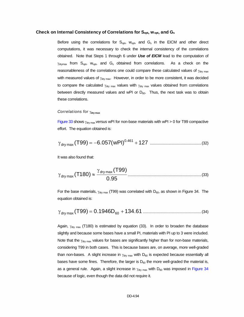
DD-4.94
Check on Internal Consistency of Correlations for Sopt, wopt, and Gs
Before using the correlations for Sopt, wopt, and Gs in the EICM and other direct
computations, it was necessary to check the internal consistency of the correlations
obtained. Note that Steps 1 through 6 under Use of EICM lead to the computation of
γdrymax from Sopt, wopt, and Gs obtained from correlations. As a check on the
reasonableness of the correlations one could compare these calculated values of γdry max
with measured values of γdry max. However, in order to be more consistent, it was decided
to compare the calculated γdry max values with γdry max values obtained from correlations
between directly measured values and wPI or D60. Thus, the next task was to obtain
these correlations.
Correlations for γdry max
Figure 33 shows γdry max versus wPI for non-base materials with wPI > 0 for T99 compactive
effort. The equation obtained is:
127)wPI(057.6)99T( 461.0max dry +−=γ ...................................................(32)
It was also found that:
95.0)99T(
)180T( max drymax dry
γ≈γ .........................................................................(33)
For the base materials, γdry max (T99) was correlated with D60, as shown in Figure 34. The
equation obtained is:
61.134D1946.0)99T( 60max dry +=γ ..........................................................(34)
Again, γdry max (T180) is estimated by equation (33). In order to broaden the database
slightly and because some bases have a small PI, materials with PI up to 3 were included.
Note that the γdry max values for bases are significantly higher than for non-base materials,
considering T99 in both cases. This is because bases are, on average, more well-graded
than non-bases. A slight increase in γdry max with D60 is expected because essentially all
bases have some fines. Therefore, the larger is D60 the more well-graded the material is,
as a general rule. Again, a slight increase in γdry max with D60 was imposed in Figure 34
because of logic, even though the data did not require it.
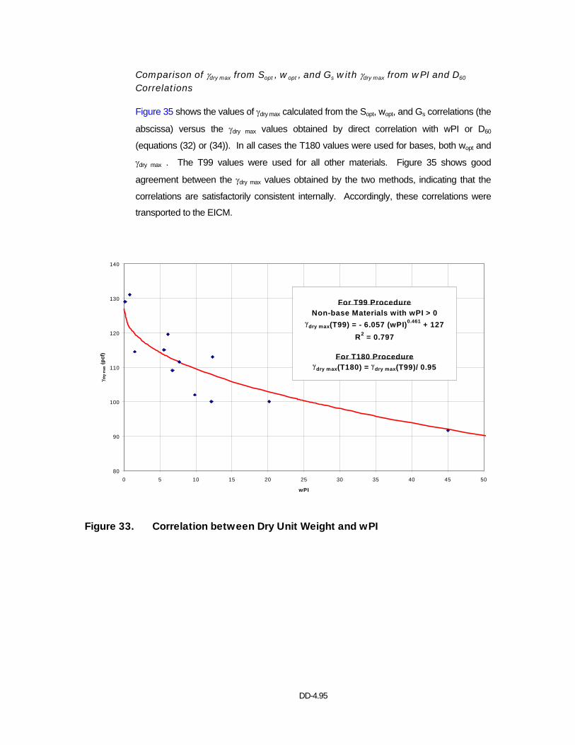
DD-4.95
Comparison of γdry max from Sopt , wopt , and Gs with γdry max from wPI and D60 Correlations
Figure 35 shows the values of γdry max calculated from the Sopt, wopt, and Gs correlations (the
abscissa) versus the γdry max values obtained by direct correlation with wPI or D60
(equations (32) or (34)). In all cases the T180 values were used for bases, both wopt and
γdry max . The T99 values were used for all other materials. Figure 35 shows good
agreement between the γdry max values obtained by the two methods, indicating that the
correlations are satisfactorily consistent internally. Accordingly, these correlations were
transported to the EICM.
80
90
100
110
120
130
140
0 5 10 15 20 25 30 35 40 45 50
wPI
γ
For T99 ProcedureNon-base Materials with wPI > 0
γdry max(T99) = - 6.057 (wPI)0.461 + 127R2 = 0.797
For T180 Procedureγdry max(T180) = γdry max(T99)/ 0.95
Figure 33. Correlation between Dry Unit Weight and wPI
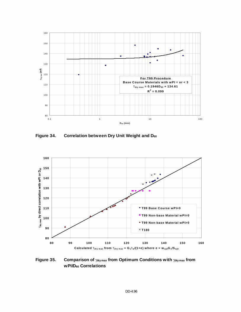
DD-4.96
80
90
100
110
120
130
140
150
160
0.1 1 10 100
D 60 (m m )
γ For T99 ProcedureBase Course Materials w ith wPI = or < 3
γdry m ax = 0.1946D 60 + 134.61R 2 = 0.099
Figure 34. Correlation between Dry Unit Weight and D60
80
90
100
110
120
130
140
150
160
80 90 100 110 120 130 140 150 160Calculated γdry m ax from γdry m ax = G sγw/(1+e) where e = w optG s/S opt
γ
T99 Base Course wPI=0
T99 Non-base M aterial wPI=0
T99 Non-base M aterial wPI>0
T180
Figure 35. Comparison of γdry max from Optimum Conditions with γdry max from wPI/D60 Correlations
Conclusions
The conclusions from this study are divided into two parts, because the emphases and
objectives were somewhat different for Part I and Part II.
Part I. Conclusions Relative to the Maximization of the Agreement between EICM Predicted Moisture Contents and TDR Measured Moisture Contents for Existing Pavements
1) There are several possible explanations for disagreement between EICM predicted
and TDR measured values of moisture content as follows:
i) Errors in the SWCC. A substantial error in the position of the SWCC will produce
a corresponding error in the predicted moisture content or degree of saturation, S,
because the EICM simply computes the equilibrium suction as Dγw – where D is
the distance to the GWT – and enters the SWCC with suction to get θ or S.
ii) Error in the (ua – uw) = Dγw assumption. This assumption is probably fairly
accurate in most cases, when the GWT is shallow. However, some research
indicates that the assumption is not good, particularly when the water table is
deep. If field measurements of equilibrium suctions under pavements are
available, they can be used in the EICM by simply dividing the known ua – uw by
γw and using the resultant D as the input depth to GWT.
iii) Errors in the TDR values. The known weak correlations between TDR measured
moisture contents and lab measured moisture contents illustrate that the value
from any particular TDR probe could be substantially in error.
2) Conclusions relative to these possible explanations are as follows:
i) As a part of this study, considerable effort was devoted to improvement of
SWCCs. The Fredlund and Xing function fit that was adopted provides a better
Chapter
7
DD-4.98
and more complete SWCC characterization than did the Gardner equation. The
SWCCs adopted (Figure 15, Chapter 3) represent a substantial database of 190
soils and agree fairly well with directly measured SWCCs. The improved match
between predicted and TDR measured values cited in Chapter 3 are due in part
to these new SWCCs. After much research into sources and magnitudes of
errors in SWCCs, it has been concluded that the curves of Figure 15, Chapter 3,
are as good as directly measured curves, unless the person / laboratory making
the measurements is highly experienced and well-equipped.
ii) It has been concluded that it is best, at least for the short term, to continue with
the assumption that (ua – uw)equil = Dequilγw. If (ua – uw)equil is known with reliability
from independent sources, it should be input into the EICM, as
Dequil = (ua – uw)equil / γw.
iii) As a part of this study, attempts were made to improve correlations between TDR
and lab measured moisture contents with little success. Unless or until a new set
of calibrations, with less scatter and uncertainty, is obtained, the poor TDR
calibration remains as a source of discrepancy between TDR measured and
EICM predicted moisture contents. A partial cancellation of error due to poor
TDR calibration was accomplished by dividing the prediction task into two parts:
a) prediction of the θeq and b) prediction of the seasonal oscillations over a period
of a year or many years. At the outset of this study, it was assumed that the
seasonal oscillations were to be the more interesting. Consequently, it was
decided to use the first-measured TDR value – in a particular period of interest –
as θeq. This was accomplished by shifting the SWCC until ua – uw, calculated by
ua – uw = Dγw, corresponded to θo. Use of this procedure produced substantial
reduction in the discrepancy between TDR measured and EICM predicted
values. However, it did not cast any light on the question "How well does the
EICM predict θeq values?".
3) Because of the inherent nature of the SWCC, it is necessary to invoke and use mass-
volume relationships in the process of making moisture content predictions.
Experience shows that it is necessary to have internally consistent and reasonably
accurate values of water content, density, and Gs. A significant error in as few as one
of these three can produce serious problems in the predictive process.
4) When the discrepancies between the TDR measured moisture contents and the
EICM predicted values were compared for the (old) Version 2.1 and the (new) Version

DD-4.99
2.6, it was found that the new version showed an improved match in all cases, and
very substantial improvement in most cases.
Part II. Conclusions Relative to the Optimization of Procedures for Predicting the Moisture Content Change from the Initial to the Equilibrium Condition
1) Experience has shown that, more often than not, one or more of the values needed
for material mass – volume relationships is erroneous, unreasonable, or missing when
these values are extracted from databases or engineering reports. When this occurs
it is problematic, because the missing data is usually difficult to recover and the
erroneous data is not always detectable at an early stage. Stated differently, even
when a problem with the data is found, it is not usually easy to fix.
2) It is reasonable to assume that unbound layers are compacted at optimum moisture
content, wopt, and at maximum dry density, γdry max. This assumption is supported by
typical compaction specifications and guidelines and by past experience. Further
impetus to this assumption is added by the fact that resilient modulus, MR, studies
have led to the conclusion that optimum conditions represent the best reference state
for estimation of MR changes due to moisture changes.
3) It has been possible to develop internally consistent correlations between the degree
of saturation at optimum, Sopt, wopt, and Gs with index properties wPI and D60. These
correlations, together with conclusions 1 and 2 above, make it possible to estimate
Sopt, wopt, and Gs and then to calculate void ratio, e, porosity, n, and γdry max without
needed reliance on typically erroneous reported values of γdry, w, and Gs. By
assuming the initial compaction conditions, Sopt, correspond to So, the starting point for
moisture content changes is established quickly and easily, without ambiguity. The
values of Sopt are reproducible, meaning that any user anywhere would get the same
Sopt, given the same wPI and D60.
4) The EICM can be required to output S, thus Sequil can be easily derived from the EICM
output. For cases in which the effects of seasonal variations in moisture content have
relatively minor effect on MR, the ∆S = Sequil – Sopt is available for use in the modular
ratio model for MR.

DD-4.100
5) A fairly good approximation of Sequil can be calculated manually, using a simple
procedure. This computation can be used to check the reasonableness of the EICM
value, or as an independent estimate of Sequil when the EICM is not used.

Recommendations for Implementation of EICM Input for Use in the 2002 Design Guide Introduction
The ICM plays a major role in the 2002 Guide computational framework aimed at
quantification of pavement system response to traffic loading, as a primary step in the
design process. In particular, the EICM is responsible for the provision of temperatures
and temperature gradients for the surface layers as a function of time. For the unbound
layers, the EICM outputs of main interest are the moisture contents and degrees of
saturation as a function of time for each layer as well as the depth of freezing, including
timing and duration, and parameters relating to thawing and recovery therefrom.
What follows in this chapter are recommendations relative to testing required and
computational procedures to be used to obtain needed input data for the EICM for Levels
1, 2, and 3. Unbound compacted layers are treated separately from unbound natural in-
situ layers lying beneath the compacted layers, because the required input typically differs.
Each section contains two lists. The first list addresses the material properties most
relevant to moisture content prediction (parameters defining mass-volume relationships
primarily), indicates how the input data may be generated, and in some cases gives an
indication as to what the EICM may do with the data internally. The second list is in the
form of a table (Table 14) and is simply a listing of input data that the user is required to
supply. In the second list, an attempt has been made to list all data needed to run the
EICM.
Chapter
8
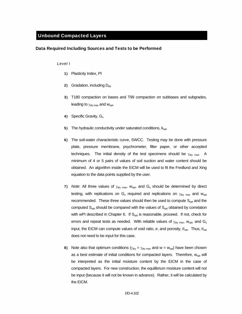
DD-4.102
Unbound Compacted Layers
Data Required Including Sources and Tests to be Performed
Level I
1) Plasticity Index, PI
2) Gradation, including D60
3) T180 compaction on bases and T99 compaction on subbases and subgrades,
leading to γdry max and wopt.
4) Specific Gravity, Gs
5) The hydraulic conductivity under saturated conditions, ksat.
6) The soil-water characteristic curve, SWCC. Testing may be done with pressure
plate, pressure membrane, psychrometer, filter paper, or other accepted
techniques. The initial density of the test specimens should be γdry max. A
minimum of 4 or 5 pairs of values of soil suction and water content should be
obtained. An algorithm inside the EICM will be used to fit the Fredlund and Xing
equation to the data points supplied by the user.
7) Note: All three values of γdry max, wopt, and Gs should be determined by direct
testing, with replications on Gs required and replications on γdry max and wopt
recommended. These three values should then be used to compute Sopt and the
computed Sopt should be compared with the values of Sopt obtained by correlation
with wPI described in Chapter 6. If Sopt is reasonable, proceed. If not, check for
errors and repeat tests as needed. With reliable values of γdry max, wopt, and Gs
input, the EICM can compute values of void ratio, e, and porosity, θsat. Thus, θsat
does not need to be input for this case.
8) Note also that optimum conditions (γdry = γdry max and w = wopt) have been chosen
as a best estimate of initial conditions for compacted layers. Therefore, wopt will
be interpreted as the initial moisture content by the EICM in the case of
compacted layers. For new construction, the equilibrium moisture content will not
be input (because it will not be known in advance). Rather, it will be calculated by
the EICM.
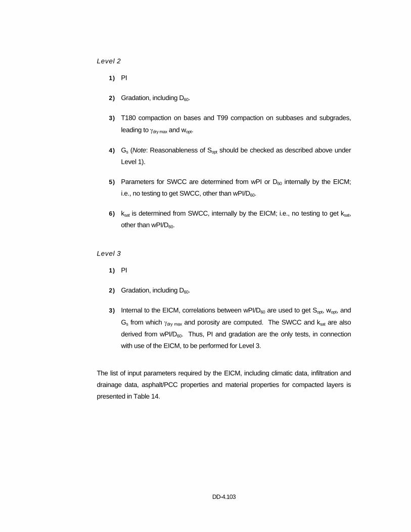
DD-4.103
Level 2
1) PI
2) Gradation, including D60.
3) T180 compaction on bases and T99 compaction on subbases and subgrades,
leading to γdry max and wopt.
4) Gs (Note: Reasonableness of Sopt should be checked as described above under
Level 1).
5) Parameters for SWCC are determined from wPI or D60 internally by the EICM;
i.e., no testing to get SWCC, other than wPI/D60.
6) ksat is determined from SWCC, internally by the EICM; i.e., no testing to get ksat,
other than wPI/D60.
Level 3
1) PI
2) Gradation, including D60.
3) Internal to the EICM, correlations between wPI/D60 are used to get Sopt, wopt, and
Gs from which γdry max and porosity are computed. The SWCC and ksat are also
derived from wPI/D60. Thus, PI and gradation are the only tests, in connection
with use of the EICM, to be performed for Level 3.
The list of input parameters required by the EICM, including climatic data, infiltration and
drainage data, asphalt/PCC properties and material properties for compacted layers is
presented in Table 14.
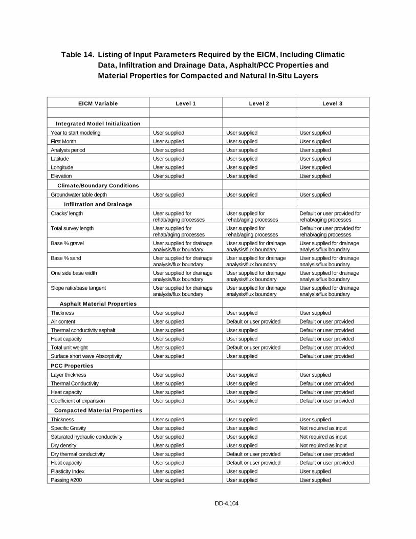
DD-4.104
Table 14. Listing of Input Parameters Required by the EICM, Including Climatic Data, Infiltration and Drainage Data, Asphalt/PCC Properties and Material Properties for Compacted and Natural In-Situ Layers
EICM Variable Level 1 Level 2 Level 3
Integrated Model Initialization Year to start modeling User supplied User supplied User supplied First Month User supplied User supplied User supplied Analysis period User supplied User supplied User supplied Latitude User supplied User supplied User supplied Longitude User supplied User supplied User supplied Elevation User supplied User supplied User supplied
Climate/Boundary Conditions Groundwater table depth User supplied User supplied User supplied
Infiltration and Drainage Cracks' length User supplied for
rehab/aging processes User supplied for rehab/aging processes
Default or user provided for rehab/aging processes
Total survey length User supplied for rehab/aging processes
User supplied for rehab/aging processes
Default or user provided for rehab/aging processes
Base % gravel User supplied for drainage analysis/flux boundary
User supplied for drainage analysis/flux boundary
User supplied for drainage analysis/flux boundary
Base % sand User supplied for drainage analysis/flux boundary
User supplied for drainage analysis/flux boundary
User supplied for drainage analysis/flux boundary
One side base width User supplied for drainage analysis/flux boundary
User supplied for drainage analysis/flux boundary
User supplied for drainage analysis/flux boundary
Slope ratio/base tangent User supplied for drainage analysis/flux boundary
User supplied for drainage analysis/flux boundary
User supplied for drainage analysis/flux boundary
Asphalt Material Properties Thickness User supplied User supplied User supplied Air content User supplied Default or user provided Default or user provided Thermal conductivity asphalt User supplied User supplied Default or user provided Heat capacity User supplied User supplied Default or user provided Total unit weight User supplied Default or user provided Default or user provided Surface short wave Absorptivity User supplied User supplied Default or user provided
PCC Properties
Layer thickness User supplied User supplied User supplied Thermal Conductivity User supplied User supplied Default or user provided Heat capacity User supplied User supplied Default or user provided Coefficient of expansion User supplied User supplied Default or user provided
Compacted Material Properties Thickness User supplied User supplied User supplied Specific Gravity User supplied User supplied Not required as input Saturated hydraulic conductivity User supplied User supplied Not required as input Dry density User supplied User supplied Not required as input Dry thermal conductivity User supplied Default or user provided Default or user provided Heat capacity User supplied Default or user provided Default or user provided Plasticity Index User supplied User supplied User supplied Passing #200 User supplied User supplied User supplied
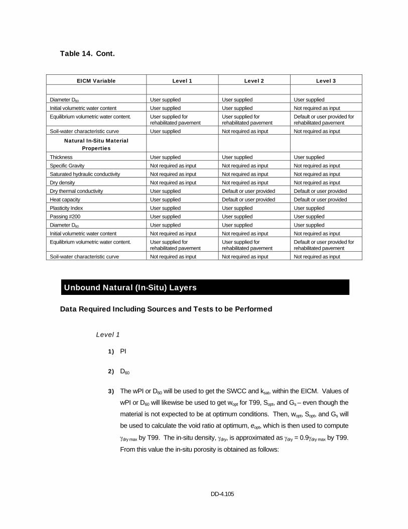
DD-4.105
Table 14. Cont.
EICM Variable Level 1 Level 2 Level 3
Diameter D60 User supplied User supplied User supplied Initial volumetric water content User supplied User supplied Not required as input Equilibrium volumetric water content. User supplied for
rehabilitated pavement User supplied for rehabilitated pavement
Default or user provided for rehabilitated pavement
Soil-water characteristic curve User supplied Not required as input Not required as input
Natural In-Situ Material Properties
Thickness User supplied User supplied User supplied Specific Gravity Not required as input Not required as input Not required as input Saturated hydraulic conductivity Not required as input Not required as input Not required as input Dry density Not required as input Not required as input Not required as input Dry thermal conductivity User supplied Default or user provided Default or user provided Heat capacity User supplied Default or user provided Default or user provided Plasticity Index User supplied User supplied User supplied Passing #200 User supplied User supplied User supplied Diameter D60 User supplied User supplied User supplied Initial volumetric water content Not required as input Not required as input Not required as input Equilibrium volumetric water content. User supplied for
rehabilitated pavement User supplied for rehabilitated pavement
Default or user provided for rehabilitated pavement
Soil-water characteristic curve Not required as input Not required as input Not required as input
Unbound Natural (In-Situ) Layers
Data Required Including Sources and Tests to be Performed
Level 1
1) PI
2) D60
3) The wPI or D60 will be used to get the SWCC and ksat, within the EICM. Values of
wPI or D60 will likewise be used to get wopt for T99, Sopt, and Gs – even though the
material is not expected to be at optimum conditions. Then, wopt, Sopt, and Gs will
be used to calculate the void ratio at optimum, eopt, which is then used to compute
γdry max by T99. The in-situ density, γdry, is approximated as γdry = 0.9γdry max by T99.
From this value the in-situ porosity is obtained as follows:
DD-4.106
i) 1Gesitu-in dry
wssituin −
γγ
=−
ii) situin
situinsatsituin e1
en−
−− +
=θ=
4) All of the above computations are performed inside the EICM. Therefore, only
the PI and D60 need to be measured for natural (in-situ) layers.
Level 2
Same as Level 1 Level 3
Same as Level 1
The list of input parameters required by the EICM, including climatic data, infiltration and
drainage data, asphalt/PCC properties and material properties for compacted layers is
presented in Table 14.

DD-4.107
APPENDIX A VOLUMETRIC WATER CONTENT PROFILES
CONNECTICUT (91803)
EICM – Version 2.1
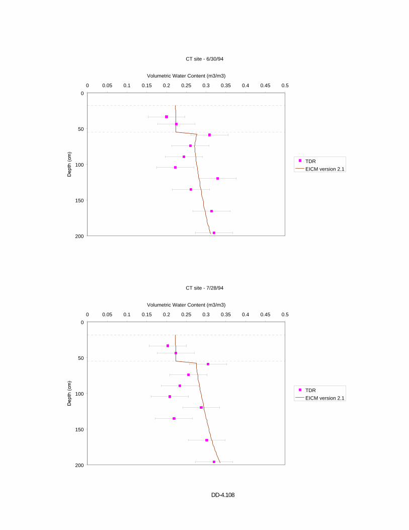
DD-4.108
CT site - 6/30/94
0
50
100
150
200
0 0.05 0.1 0.15 0.2 0.25 0.3 0.35 0.4 0.45 0.5
Volumetric Water Content (m3/m3)
TDREICM version 2.1
CT site - 7/28/94
0
50
100
150
200
0 0.05 0.1 0.15 0.2 0.25 0.3 0.35 0.4 0.45 0.5
Volumetric Water Content (m3/m3)
TDREICM version 2.1
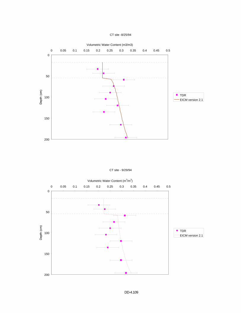
DD-4.109
CT site -8/25/94
0
50
100
150
200
0 0.05 0.1 0.15 0.2 0.25 0.3 0.35 0.4 0.45 0.5
Volumetric Water Content (m3/m3)
TDREICM version 2.1
CT site - 9/29/94
0
50
100
150
200
0 0.05 0.1 0.15 0.2 0.25 0.3 0.35 0.4 0.45 0.5
Volumetric Water Content (m3/m3)
TDREICM version 2.1
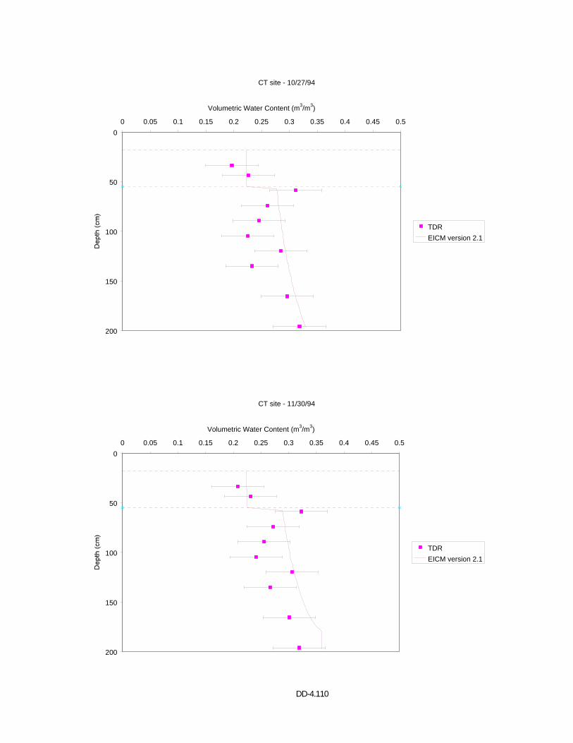
DD-4.110
CT site - 10/27/94
0
50
100
150
200
0 0.05 0.1 0.15 0.2 0.25 0.3 0.35 0.4 0.45 0.5
Volumetric Water Content (m3/m3)
TDREICM version 2.1
CT site - 11/30/94
0
50
100
150
200
0 0.05 0.1 0.15 0.2 0.25 0.3 0.35 0.4 0.45 0.5
Volumetric Water Content (m3/m3)
TDREICM version 2.1
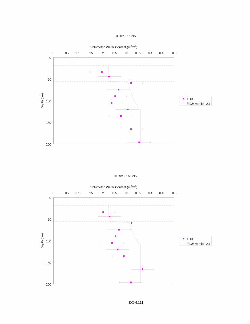
DD-4.111
CT site - 1/5/95
0
50
100
150
200
0 0.05 0.1 0.15 0.2 0.25 0.3 0.35 0.4 0.45 0.5
Volumetric Water Content (m3/m3)
TDREICM version 2.1
CT site - 1/26/95
0
50
100
150
200
0 0.05 0.1 0.15 0.2 0.25 0.3 0.35 0.4 0.45 0.5
Volumetric Water Content (m3/m3)
TDREICM version 2.1
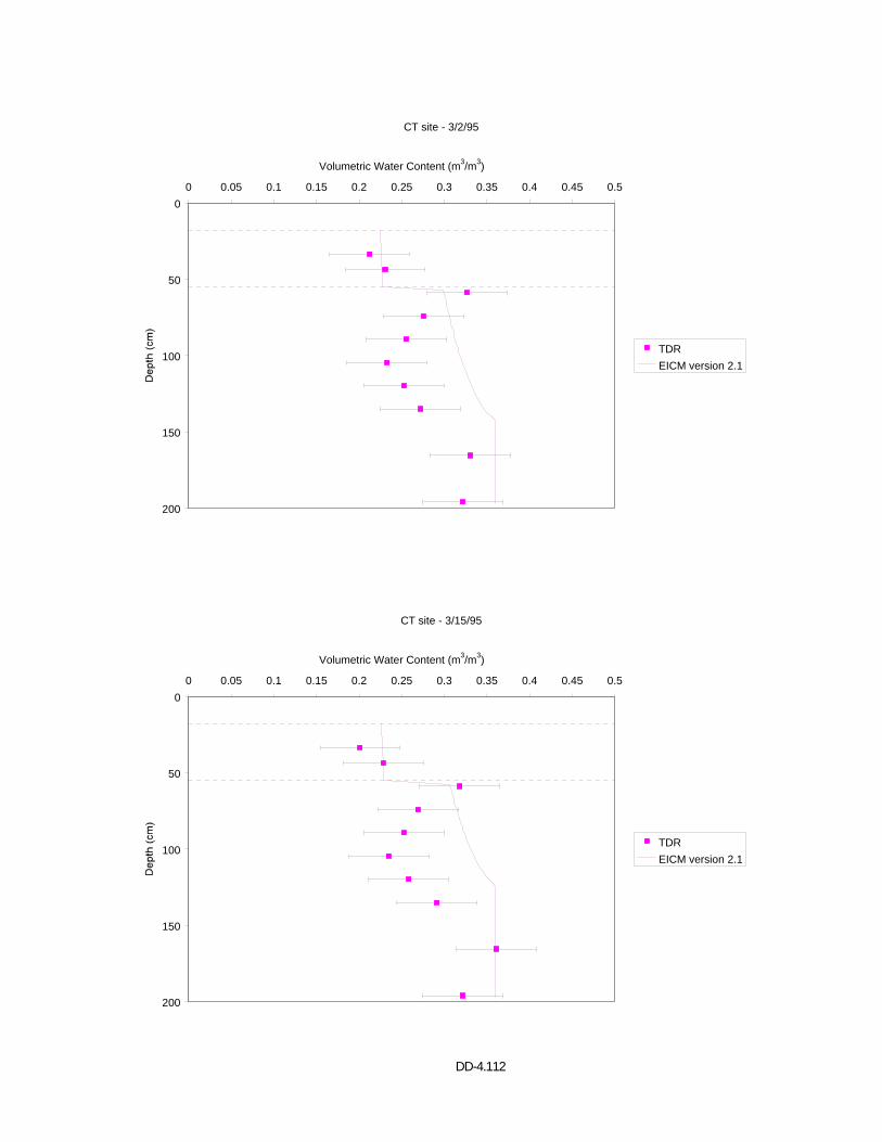
DD-4.112
CT site - 3/2/95
0
50
100
150
200
0 0.05 0.1 0.15 0.2 0.25 0.3 0.35 0.4 0.45 0.5
Volumetric Water Content (m3/m3)
TDREICM version 2.1
CT site - 3/15/95
0
50
100
150
200
0 0.05 0.1 0.15 0.2 0.25 0.3 0.35 0.4 0.45 0.5
Volumetric Water Content (m3/m3)
TDREICM version 2.1
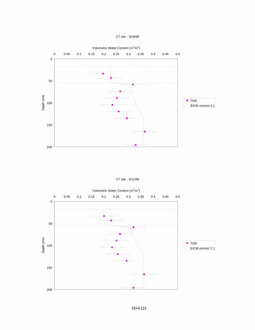
DD-4.113
CT site - 3/29/95
0
50
100
150
200
0 0.05 0.1 0.15 0.2 0.25 0.3 0.35 0.4 0.45 0.5
Volumetric Water Content (m3/m3)
TDREICM version 2.1
CT site - 4/12/95
0
50
100
150
200
0 0.05 0.1 0.15 0.2 0.25 0.3 0.35 0.4 0.45 0.5
Volumetric Water Content (m3/m3)
TDREICM version 2.1
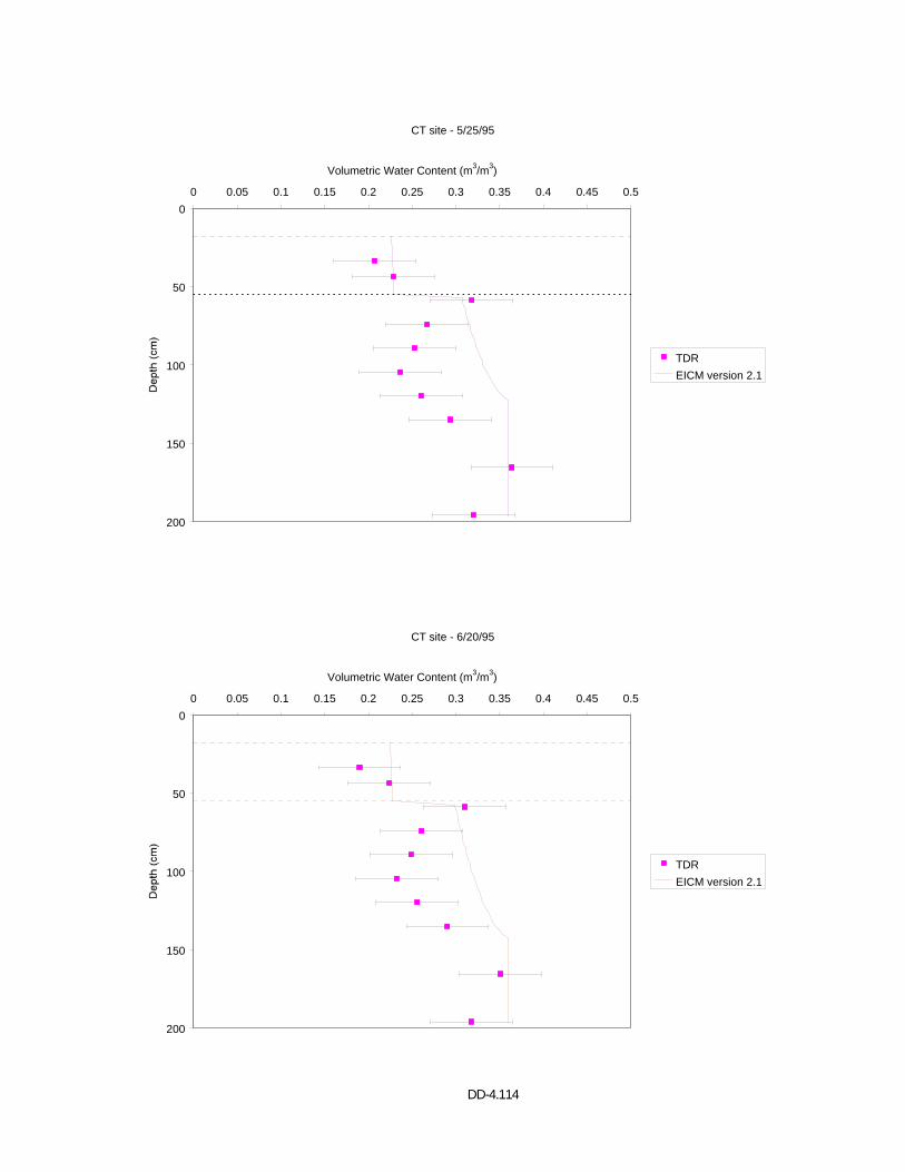
DD-4.114
CT site - 5/25/95
0
50
100
150
200
0 0.05 0.1 0.15 0.2 0.25 0.3 0.35 0.4 0.45 0.5
Volumetric Water Content (m3/m3)
TDREICM version 2.1
CT site - 6/20/95
0
50
100
150
200
0 0.05 0.1 0.15 0.2 0.25 0.3 0.35 0.4 0.45 0.5
Volumetric Water Content (m3/m3)
TDREICM version 2.1

DD-4.115
APPENDIX B VOLUMETRIC WATER CONTENT PROFILES
MINNESOTA (91803)
EICM – Version 2.1
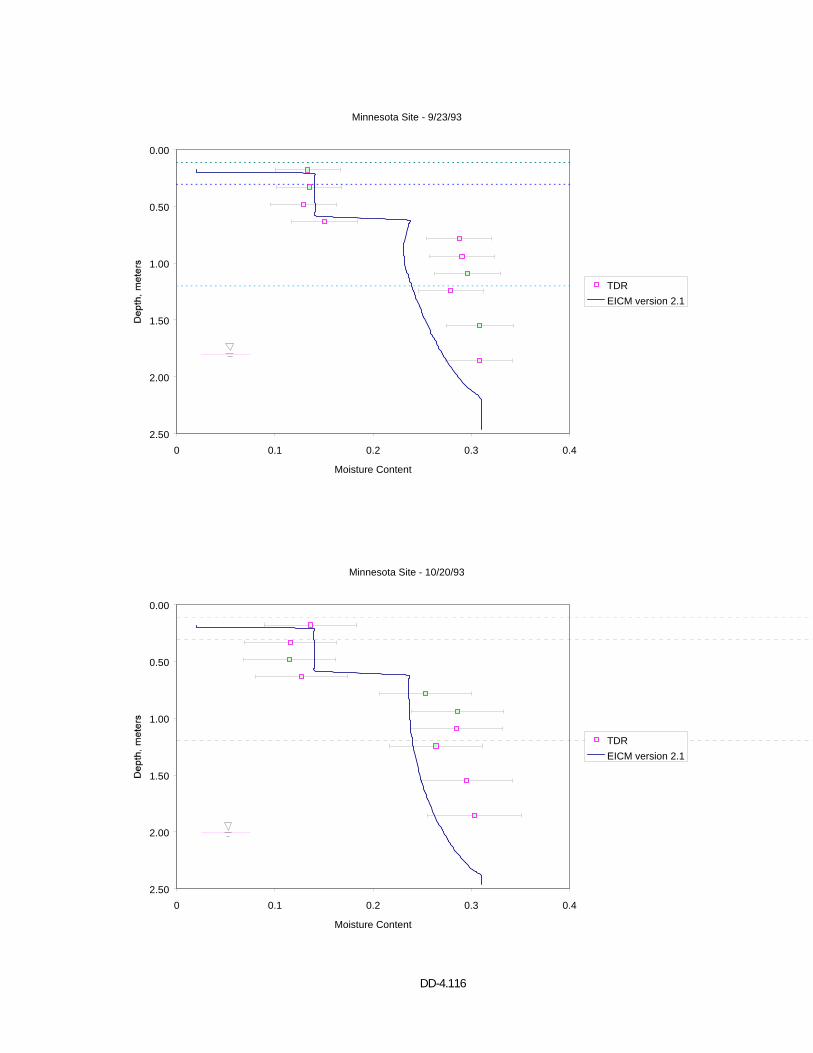
DD-4.116
Minnesota Site - 9/23/93
0.00
0.50
1.00
1.50
2.00
2.500 0.1 0.2 0.3 0.4
Moisture Content
TDREICM version 2.1
Minnesota Site - 10/20/93
0.00
0.50
1.00
1.50
2.00
2.500 0.1 0.2 0.3 0.4
Moisture Content
TDREICM version 2.1
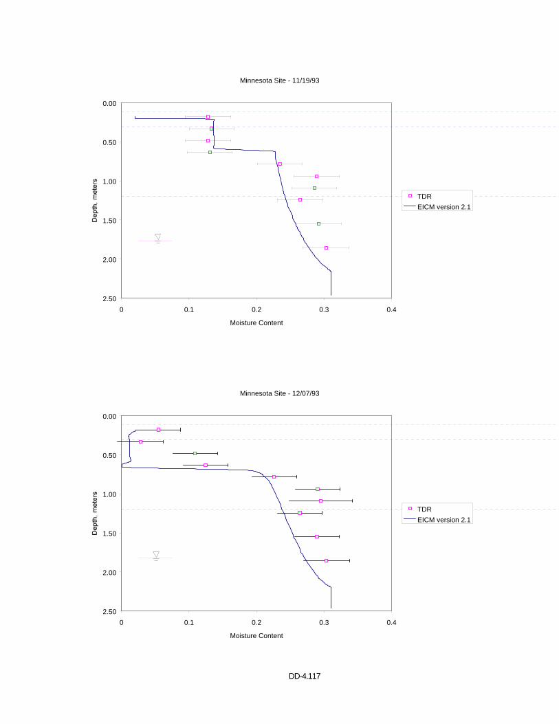
DD-4.117
Minnesota Site - 11/19/93
0.00
0.50
1.00
1.50
2.00
2.500 0.1 0.2 0.3 0.4
Moisture Content
TDREICM version 2.1
Minnesota Site - 12/07/93
0.00
0.50
1.00
1.50
2.00
2.500 0.1 0.2 0.3 0.4
Moisture Content
TDREICM version 2.1
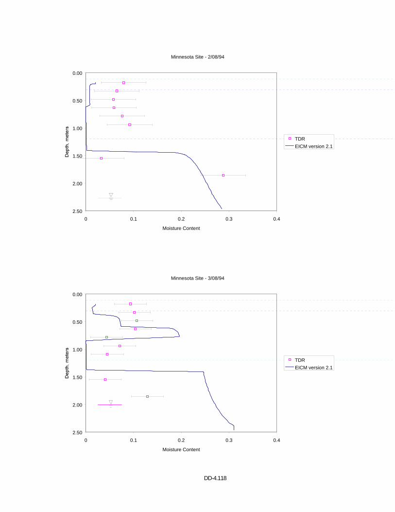
DD-4.118
Minnesota Site - 2/08/94
0.00
0.50
1.00
1.50
2.00
2.500 0.1 0.2 0.3 0.4
Moisture Content
TDREICM version 2.1
Minnesota Site - 3/08/94
0.00
0.50
1.00
1.50
2.00
2.500 0.1 0.2 0.3 0.4
Moisture Content
TDREICM version 2.1
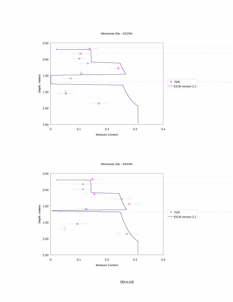
DD-4.119
Minnesota Site - 3/22/94
0.00
0.50
1.00
1.50
2.00
2.500 0.1 0.2 0.3 0.4
Moisture Content
TDREICM version 2.1
Minnesota Site - 4/04/94
0.00
0.50
1.00
1.50
2.00
2.500 0.1 0.2 0.3 0.4
Moisture Content
TDREICM version 2.1
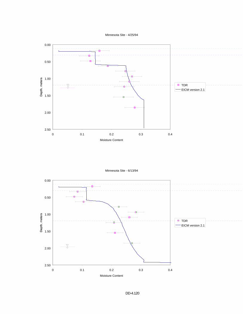
DD-4.120
Minnesota Site - 4/25/94
0.00
0.50
1.00
1.50
2.00
2.500 0.1 0.2 0.3 0.4
Moisture Content
TDREICM version 2.1
Minnesota Site - 6/13/94
0.00
0.50
1.00
1.50
2.00
2.500 0.1 0.2 0.3 0.4
Moisture Content
TDREICM version 2.1
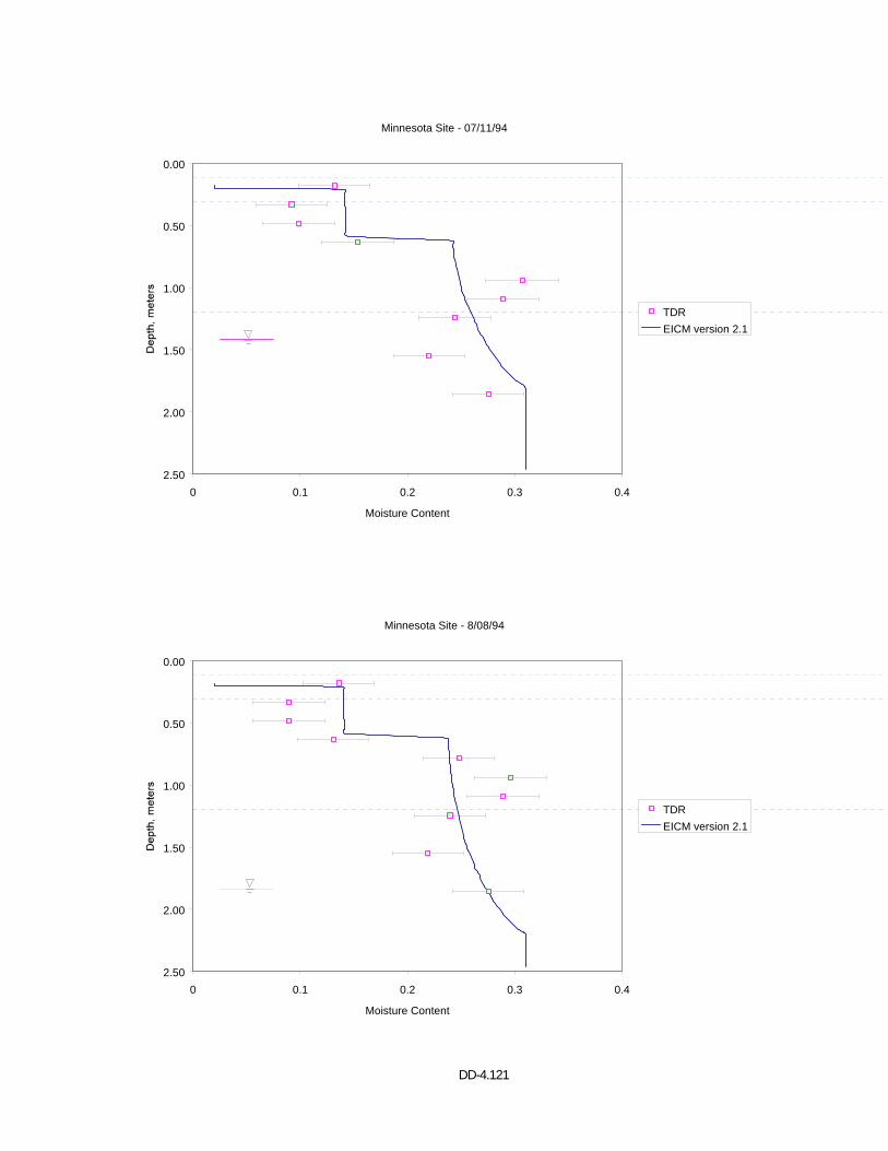
DD-4.121
Minnesota Site - 07/11/94
0.00
0.50
1.00
1.50
2.00
2.500 0.1 0.2 0.3 0.4
Moisture Content
TDREICM version 2.1
Minnesota Site - 8/08/94
0.00
0.50
1.00
1.50
2.00
2.500 0.1 0.2 0.3 0.4
Moisture Content
TDREICM version 2.1

DD-4.122
APPENDIX C VOLUMETRIC WATER CONTENT PROFILES
MAINE (231026)
EICM – Version 2.1
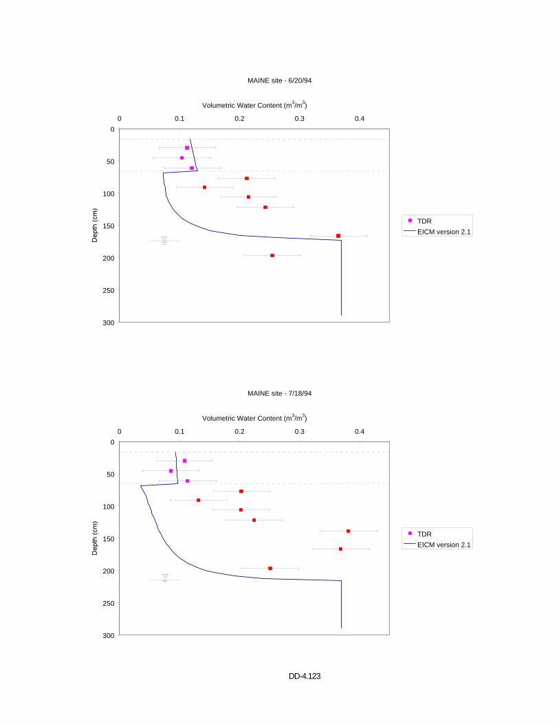
DD-4.123
MAINE site - 6/20/94
0
50
100
150
200
250
300
0 0.1 0.2 0.3 0.4
Volumetric Water Content (m3/m3)
TDREICM version 2.1
MAINE site - 7/18/94
0
50
100
150
200
250
300
0 0.1 0.2 0.3 0.4
Volumetric Water Content (m3/m3)
TDREICM version 2.1
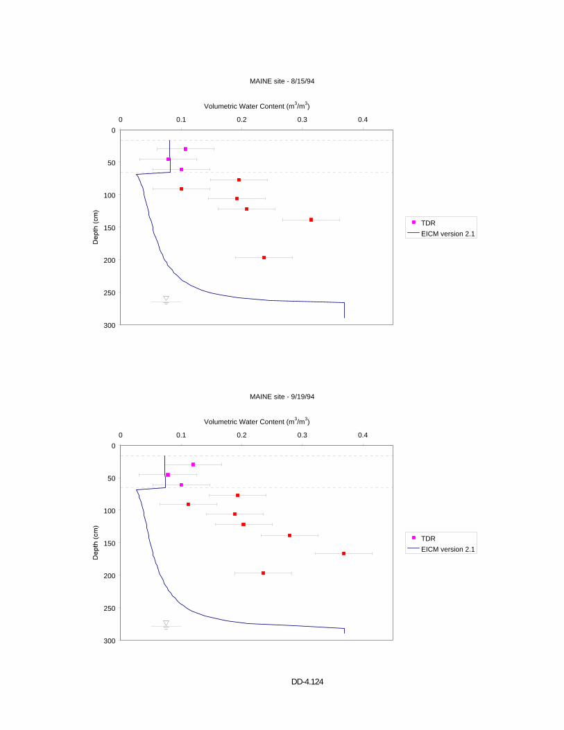
DD-4.124
MAINE site - 8/15/94
0
50
100
150
200
250
300
0 0.1 0.2 0.3 0.4
Volumetric Water Content (m3/m3)
TDREICM version 2.1
MAINE site - 9/19/94
0
50
100
150
200
250
300
0 0.1 0.2 0.3 0.4
Volumetric Water Content (m3/m3)
TDREICM version 2.1
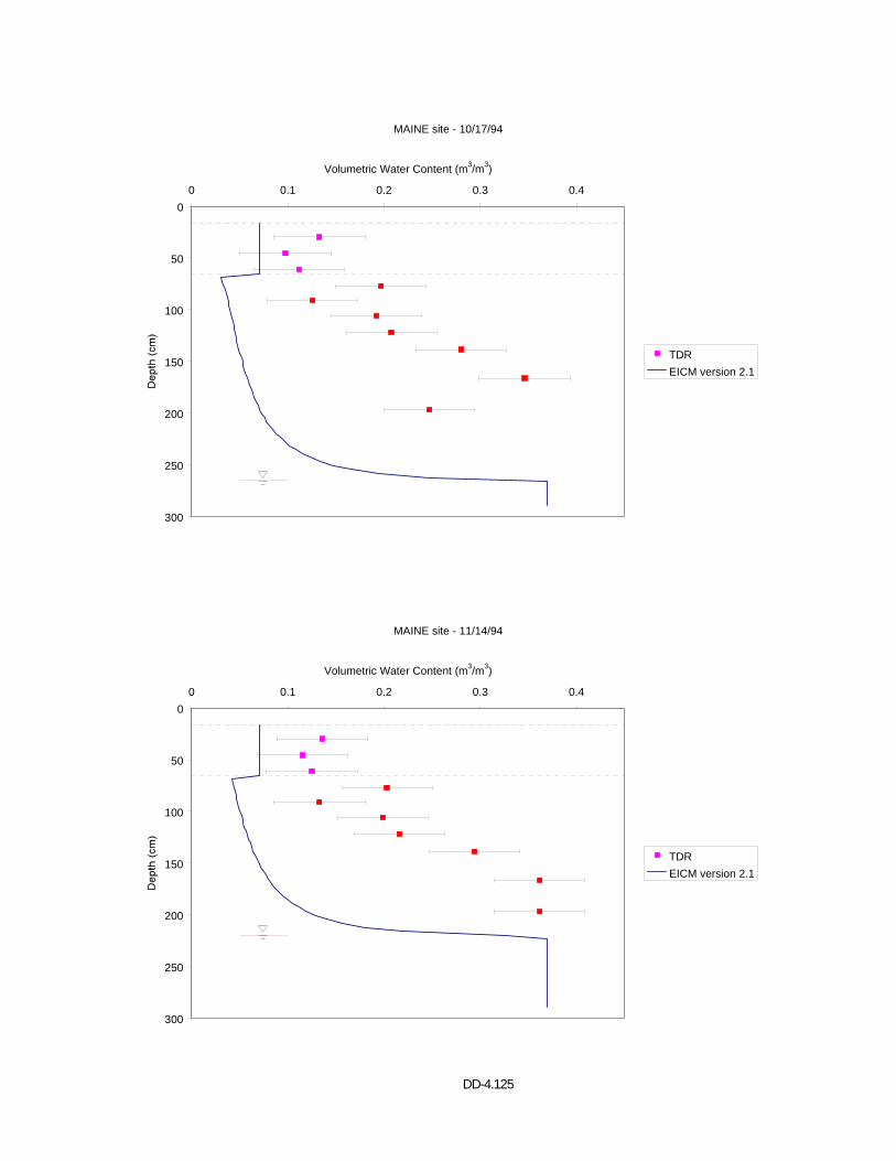
DD-4.125
MAINE site - 10/17/94
0
50
100
150
200
250
300
0 0.1 0.2 0.3 0.4
Volumetric Water Content (m3/m3)
TDREICM version 2.1
MAINE site - 11/14/94
0
50
100
150
200
250
300
0 0.1 0.2 0.3 0.4
Volumetric Water Content (m3/m3)
TDREICM version 2.1
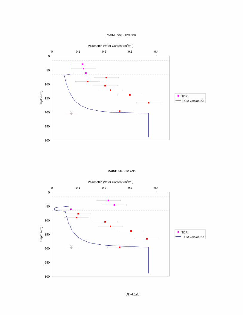
DD-4.126
MAINE site - 12/12/94
0
50
100
150
200
250
300
0 0.1 0.2 0.3 0.4
Volumetric Water Content (m3/m3)
TDREICM version 2.1
MAINE site - 1/17/95
0
50
100
150
200
250
300
0 0.1 0.2 0.3 0.4
Volumetric Water Content (m3/m3)
TDREICM version 2.1
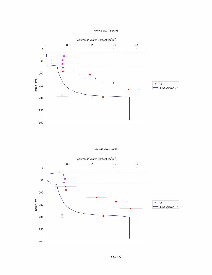
DD-4.127
MAINE site - 2/14/95
0
50
100
150
200
250
300
0 0.1 0.2 0.3 0.4
Volumetric Water Content (m3/m3)
TDREICM version 2.1
MAINE site - 3/6/95
0
50
100
150
200
250
300
0 0.1 0.2 0.3 0.4
Volumetric Water Content (m3/m3)
TDREICM version 2.1
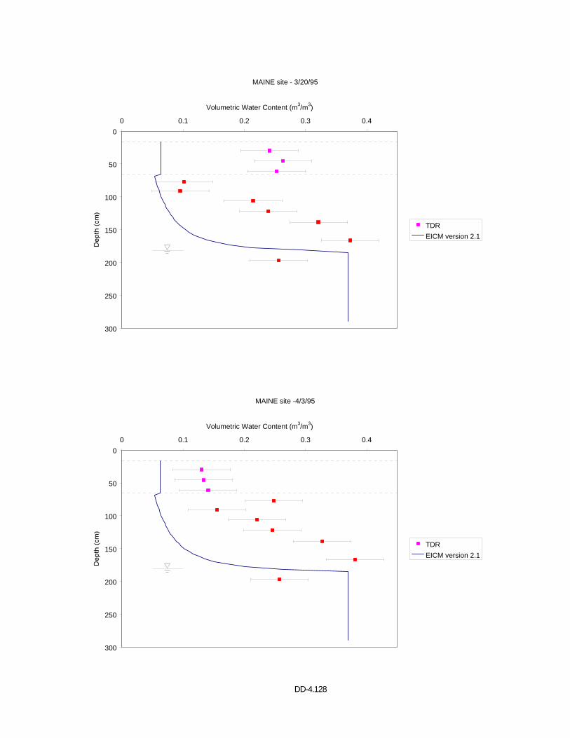
DD-4.128
MAINE site - 3/20/95
0
50
100
150
200
250
300
0 0.1 0.2 0.3 0.4
Volumetric Water Content (m3/m3)
TDREICM version 2.1
MAINE site -4/3/95
0
50
100
150
200
250
300
0 0.1 0.2 0.3 0.4
Volumetric Water Content (m3/m3)
TDREICM version 2.1
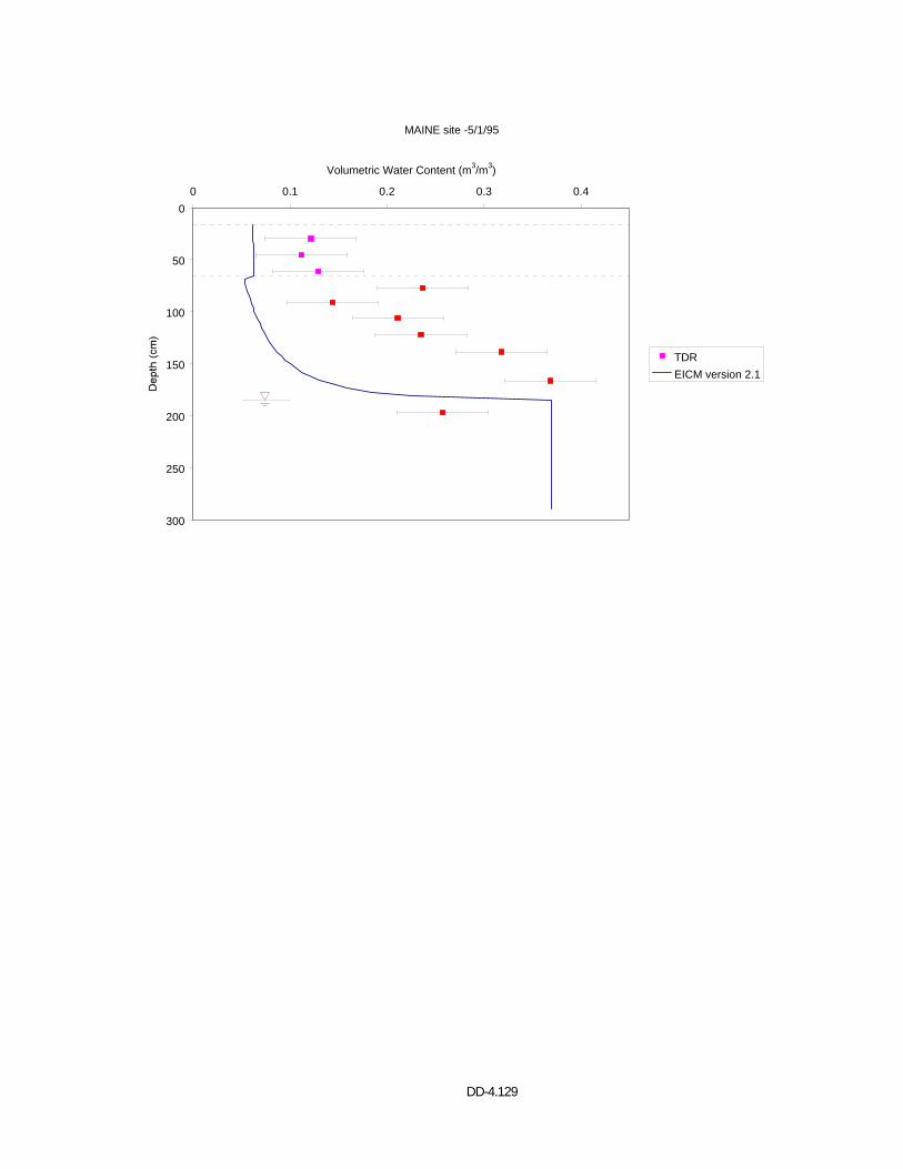
DD-4.129
MAINE site -5/1/95
0
50
100
150
200
250
300
0 0.1 0.2 0.3 0.4
Volumetric Water Content (m3/m3)
TDREICM version 2.1

DD-4.130
APPENDIX D VOLUMETRIC WATER CONTENT PROFILES
NEW HAMPSHIRE (331001)
EICM – Version 2.1
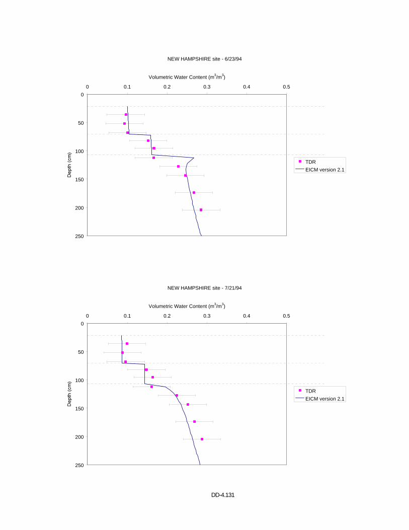
DD-4.131
NEW HAMPSHIRE site - 6/23/94
0
50
100
150
200
250
0 0.1 0.2 0.3 0.4 0.5
Volumetric Water Content (m3/m3)
TDREICM version 2.1
NEW HAMPSHIRE site - 7/21/94
0
50
100
150
200
250
0 0.1 0.2 0.3 0.4 0.5
Volumetric Water Content (m3/m3)
TDREICM version 2.1
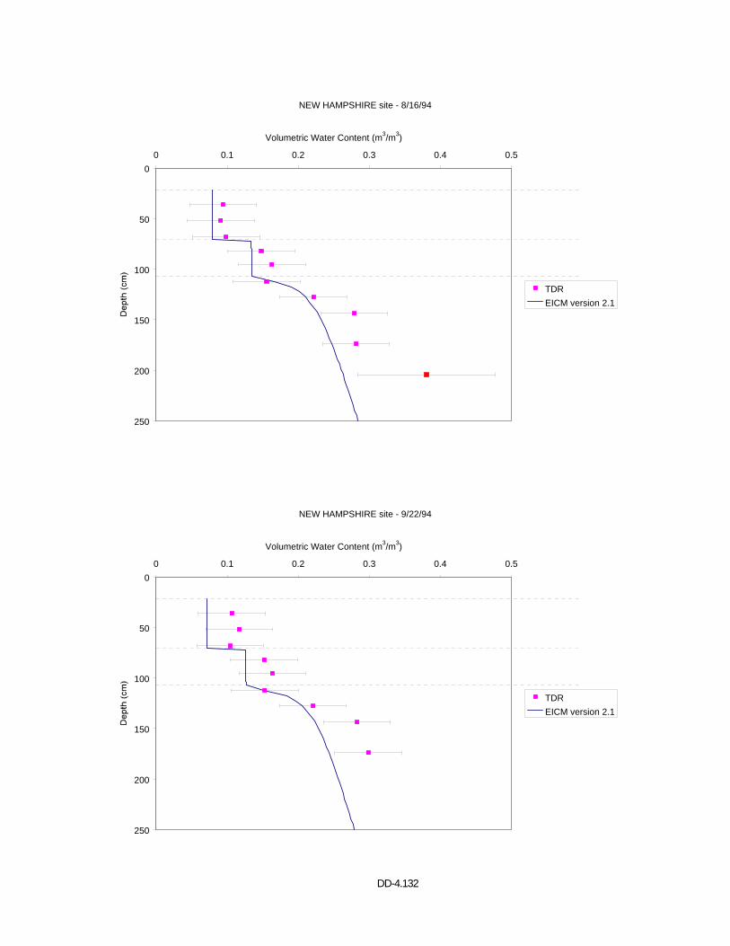
DD-4.132
NEW HAMPSHIRE site - 8/16/94
0
50
100
150
200
250
0 0.1 0.2 0.3 0.4 0.5
Volumetric Water Content (m3/m3)
TDREICM version 2.1
NEW HAMPSHIRE site - 9/22/94
0
50
100
150
200
250
0 0.1 0.2 0.3 0.4 0.5
Volumetric Water Content (m3/m3)
TDREICM version 2.1
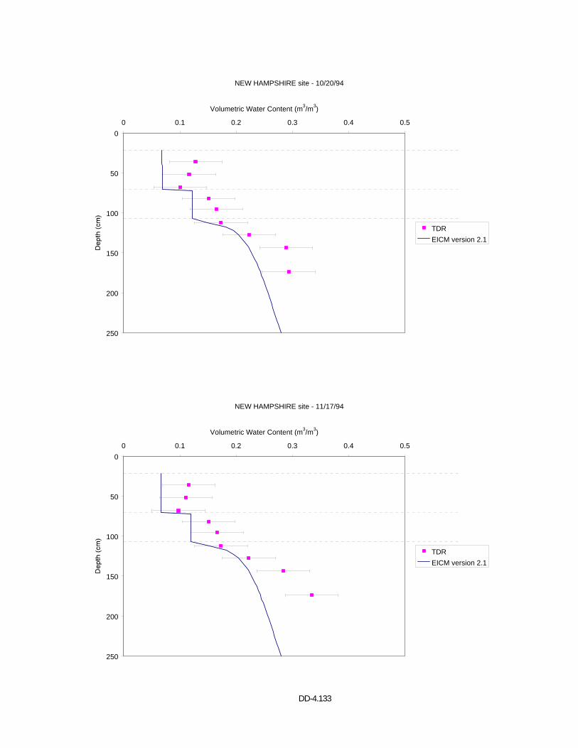
DD-4.133
NEW HAMPSHIRE site - 10/20/94
0
50
100
150
200
250
0 0.1 0.2 0.3 0.4 0.5
Volumetric Water Content (m3/m3)
TDREICM version 2.1
NEW HAMPSHIRE site - 11/17/94
0
50
100
150
200
250
0 0.1 0.2 0.3 0.4 0.5
Volumetric Water Content (m3/m3)
TDREICM version 2.1
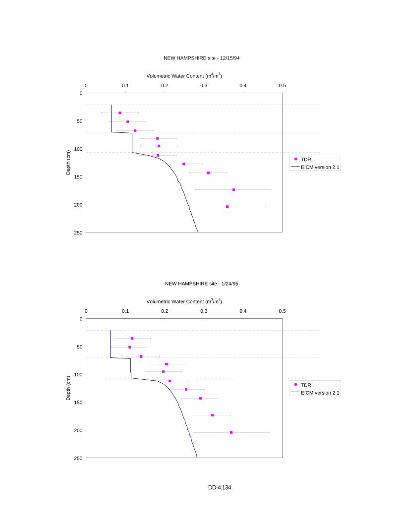
DD-4.134
NEW HAMPSHIRE site - 12/15/94
0
50
100
150
200
250
0 0.1 0.2 0.3 0.4 0.5
Volumetric Water Content (m3/m3)
TDREICM version 2.1
NEW HAMPSHIRE site - 1/24/95
0
50
100
150
200
250
0 0.1 0.2 0.3 0.4 0.5
Volumetric Water Content (m3/m3)
TDREICM version 2.1
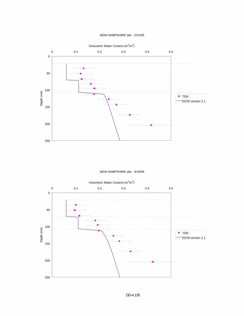
DD-4.135
NEW HAMPSHIRE site - 2/21/95
0
50
100
150
200
250
0 0.1 0.2 0.3 0.4 0.5
Volumetric Water Content (m3/m3)
TDREICM version 2.1
NEW HAMPSHIRE site - 3/16/95
0
50
100
150
200
250
0 0.1 0.2 0.3 0.4 0.5
Volumetric Water Content (m3/m3)
TDREICM version 2.1
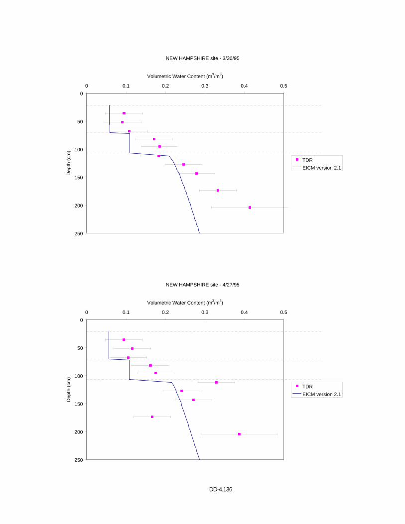
DD-4.136
NEW HAMPSHIRE site - 3/30/95
0
50
100
150
200
250
0 0.1 0.2 0.3 0.4 0.5
Volumetric Water Content (m3/m3)
TDREICM version 2.1
NEW HAMPSHIRE site - 4/27/95
0
50
100
150
200
250
0 0.1 0.2 0.3 0.4 0.5
Volumetric Water Content (m3/m3)
TDREICM version 2.1
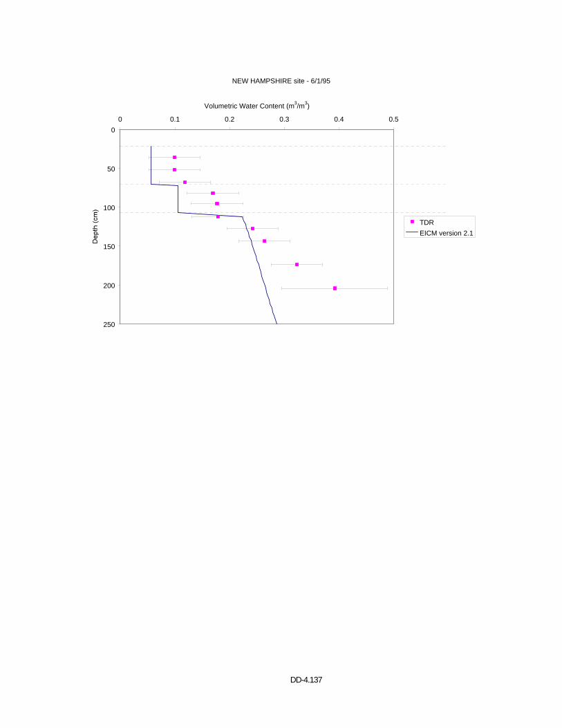
DD-4.137
NEW HAMPSHIRE site - 6/1/95
0
50
100
150
200
250
0 0.1 0.2 0.3 0.4 0.5
Volumetric Water Content (m3/m3)
TDREICM version 2.1

DD-4.138
APPENDIX E VOLUMETRIC WATER CONTENT PROFILES
VERMONT (501002)
EICM – Version 2.1
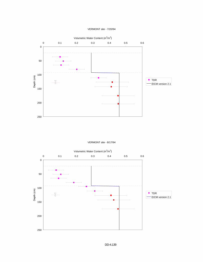
DD-4.139
VERMONT site - 7/20/94
0
50
100
150
200
250
0 0.1 0.2 0.3 0.4 0.5 0.6
Volumetric Water Content (m3/m3)
TDREICM version 2.1
VERMONT site - 8/17/94
0
50
100
150
200
250
0 0.1 0.2 0.3 0.4 0.5 0.6
Volumetric Water Content (m3/m3)
TDREICM version 2.1
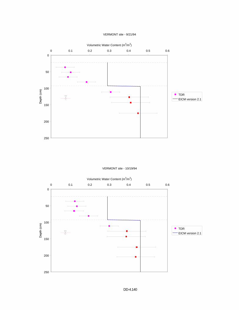
DD-4.140
VERMONT site - 9/21/94
0
50
100
150
200
250
0 0.1 0.2 0.3 0.4 0.5 0.6
Volumetric Water Content (m3/m3)
TDREICM version 2.1
VERMONT site - 10/19/94
0
50
100
150
200
250
0 0.1 0.2 0.3 0.4 0.5 0.6
Volumetric Water Content (m3/m3)
TDREICM version 2.1
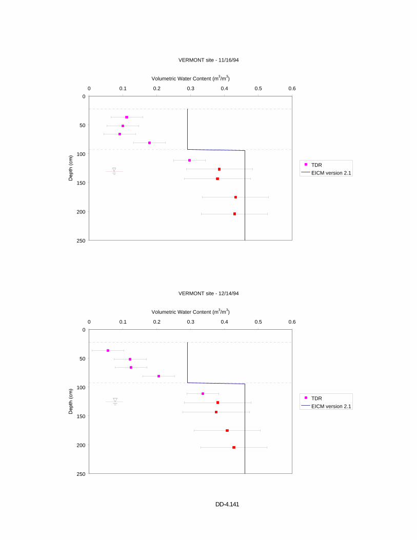
DD-4.141
VERMONT site - 11/16/94
0
50
100
150
200
250
0 0.1 0.2 0.3 0.4 0.5 0.6
Volumetric Water Content (m3/m3)
TDREICM version 2.1
VERMONT site - 12/14/94
0
50
100
150
200
250
0 0.1 0.2 0.3 0.4 0.5 0.6
Volumetric Water Content (m3/m3)
TDREICM version 2.1
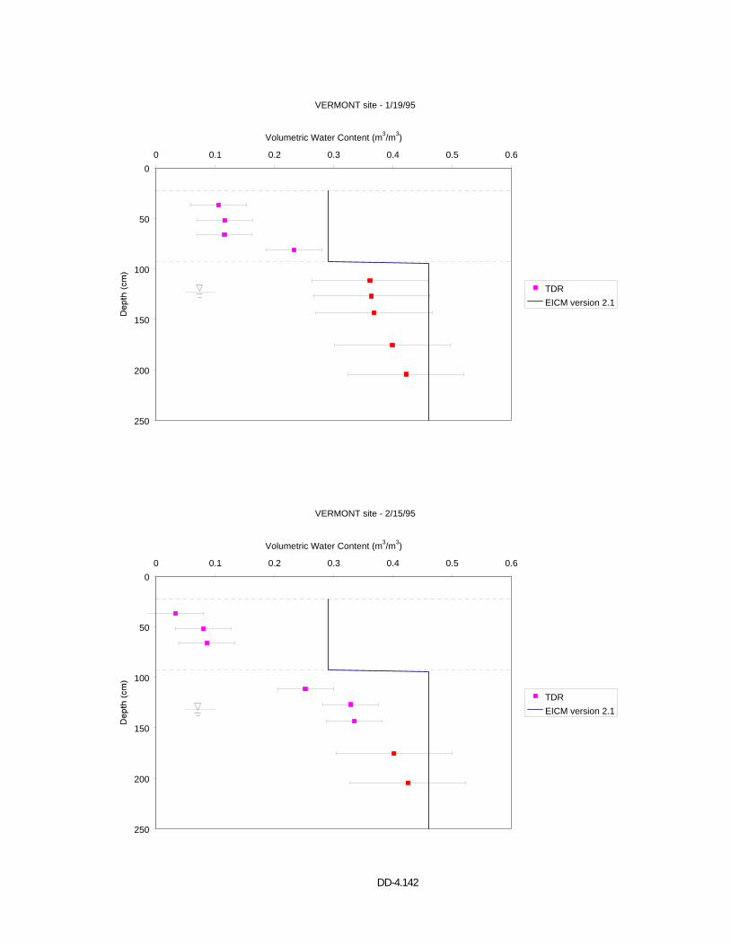
DD-4.142
VERMONT site - 1/19/95
0
50
100
150
200
250
0 0.1 0.2 0.3 0.4 0.5 0.6
Volumetric Water Content (m3/m3)
TDREICM version 2.1
VERMONT site - 2/15/95
0
50
100
150
200
250
0 0.1 0.2 0.3 0.4 0.5 0.6
Volumetric Water Content (m3/m3)
TDREICM version 2.1
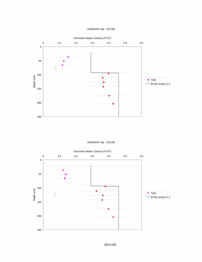
DD-4.143
VERMONT site - 3/17/95
0
50
100
150
200
250
0 0.1 0.2 0.3 0.4 0.5 0.6
Volumetric Water Content (m3/m3)
TDREICM version 2.1
VERMONT site - 3/31/95
0
50
100
150
200
250
0 0.1 0.2 0.3 0.4 0.5 0.6
Volumetric Water Content (m3/m3)
TDREICM version 2.1
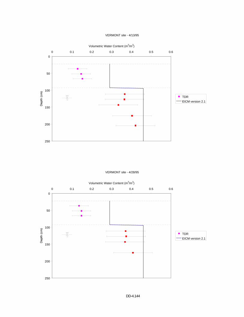
DD-4.144
VERMONT site - 4/13/95
0
50
100
150
200
250
0 0.1 0.2 0.3 0.4 0.5 0.6
Volumetric Water Content (m3/m3)
TDREICM version 2.1
VERMONT site - 4/28/95
0
50
100
150
200
250
0 0.1 0.2 0.3 0.4 0.5 0.6
Volumetric Water Content (m3/m3)
TDREICM version 2.1
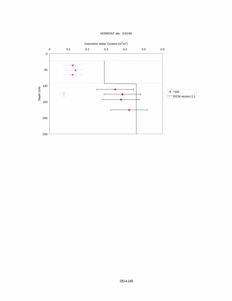
DD-4.145
VERMONT site - 5/31/95
0
50
100
150
200
250
0 0.1 0.2 0.3 0.4 0.5 0.6
Volumetric Water Content (m3/m3)
TDREICM version 2.1

DD-4.146
APPENDIX F VOLUMETRIC WATER CONTENT PROFILES
MANITOBA (831801)
EICM – Version 2.1
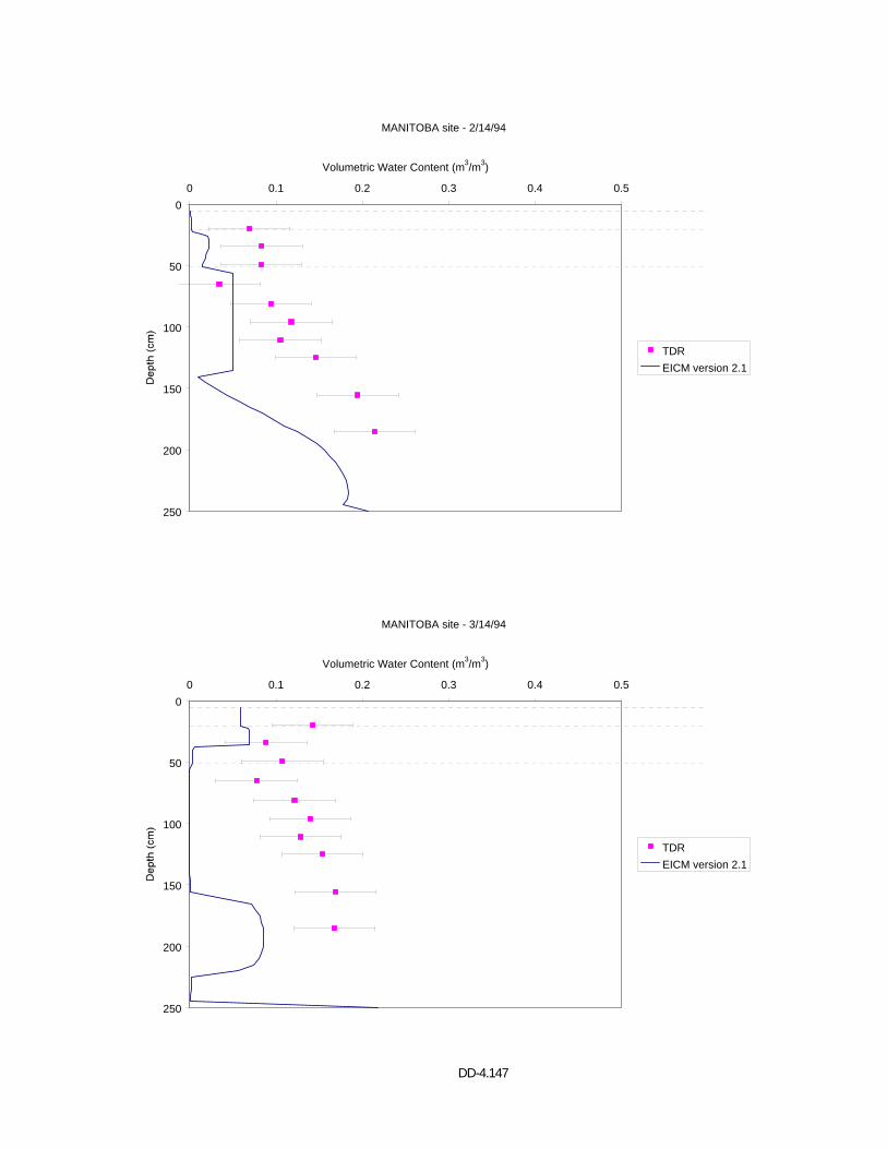
DD-4.147
MANITOBA site - 2/14/94
0
50
100
150
200
250
0 0.1 0.2 0.3 0.4 0.5
Volumetric Water Content (m3/m3)
TDREICM version 2.1
MANITOBA site - 3/14/94
0
50
100
150
200
250
0 0.1 0.2 0.3 0.4 0.5
Volumetric Water Content (m3/m3)
TDREICM version 2.1
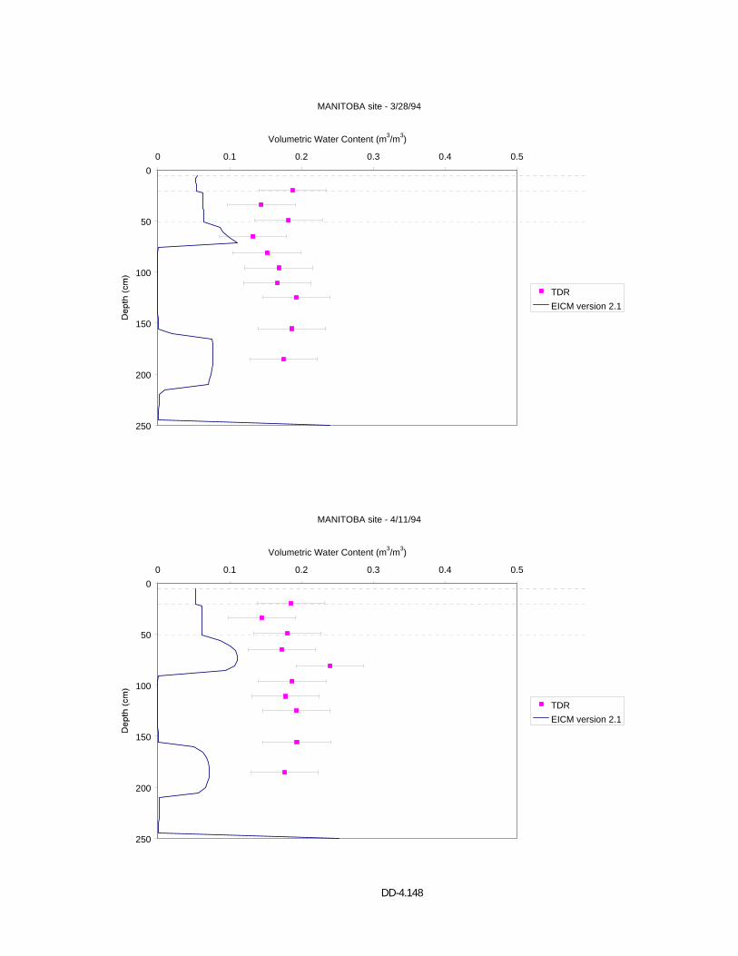
DD-4.148
MANITOBA site - 3/28/94
0
50
100
150
200
250
0 0.1 0.2 0.3 0.4 0.5
Volumetric Water Content (m3/m3)
TDREICM version 2.1
MANITOBA site - 4/11/94
0
50
100
150
200
250
0 0.1 0.2 0.3 0.4 0.5
Volumetric Water Content (m3/m3)
TDREICM version 2.1
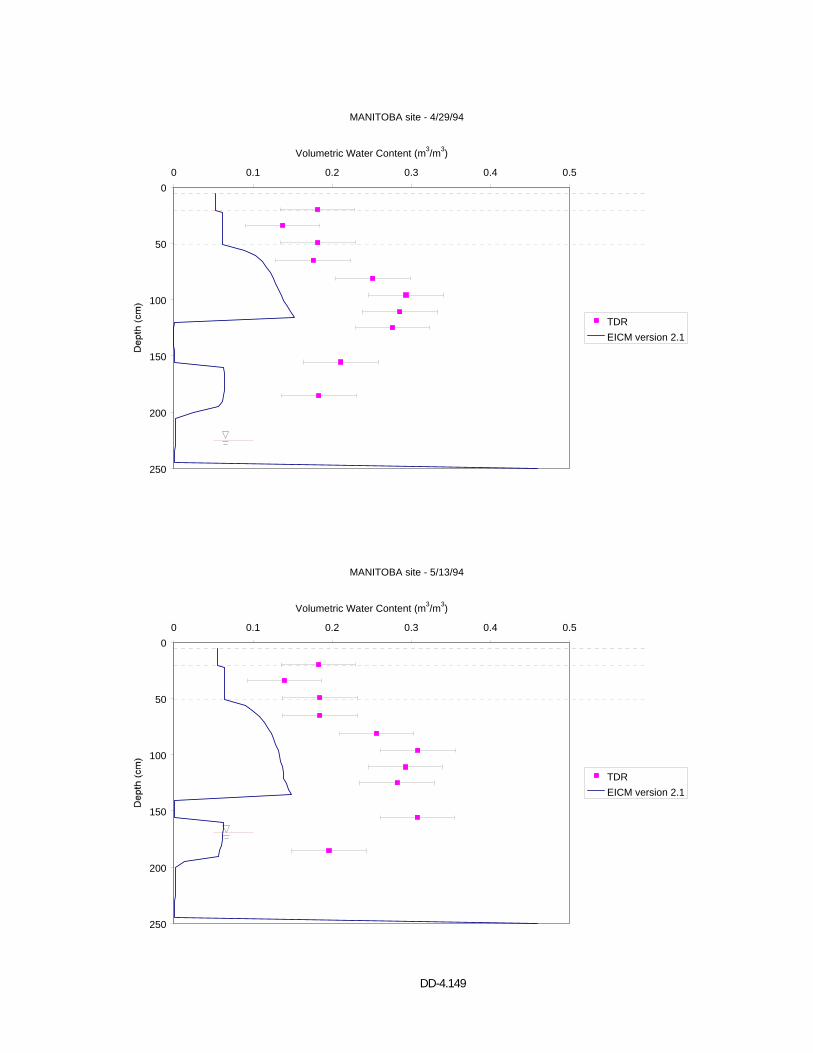
DD-4.149
MANITOBA site - 4/29/94
0
50
100
150
200
250
0 0.1 0.2 0.3 0.4 0.5
Volumetric Water Content (m3/m3)
TDREICM version 2.1
MANITOBA site - 5/13/94
0
50
100
150
200
250
0 0.1 0.2 0.3 0.4 0.5
Volumetric Water Content (m3/m3)
TDREICM version 2.1
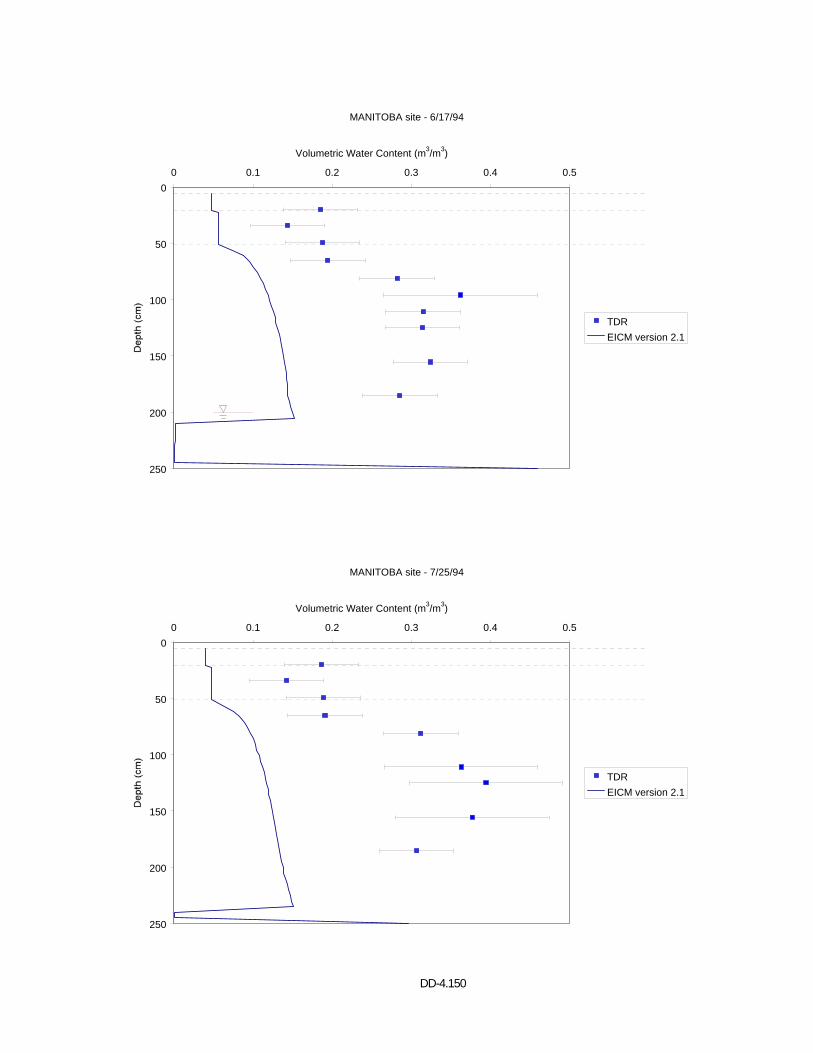
DD-4.150
MANITOBA site - 6/17/94
0
50
100
150
200
250
0 0.1 0.2 0.3 0.4 0.5
Volumetric Water Content (m3/m3)
TDREICM version 2.1
MANITOBA site - 7/25/94
0
50
100
150
200
250
0 0.1 0.2 0.3 0.4 0.5
Volumetric Water Content (m3/m3)
TDREICM version 2.1
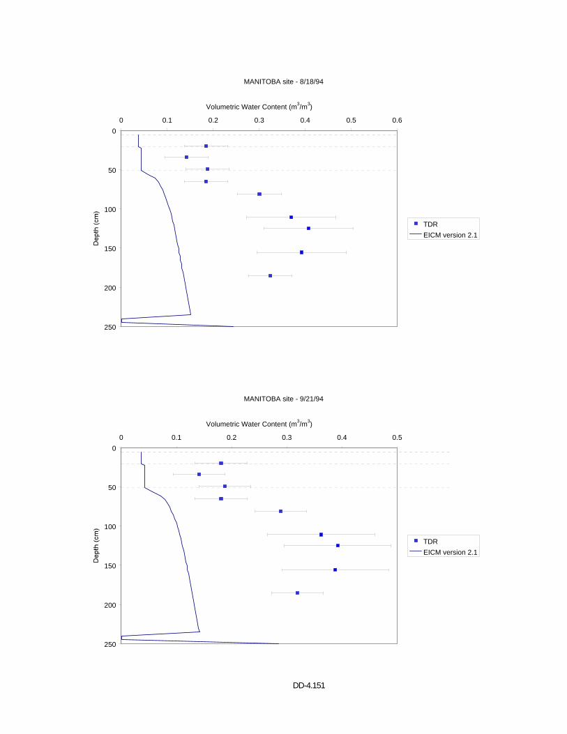
DD-4.151
MANITOBA site - 8/18/94
0
50
100
150
200
250
0 0.1 0.2 0.3 0.4 0.5 0.6
Volumetric Water Content (m3/m3)
TDREICM version 2.1
MANITOBA site - 9/21/94
0
50
100
150
200
250
0 0.1 0.2 0.3 0.4 0.5
Volumetric Water Content (m3/m3)
TDREICM version 2.1
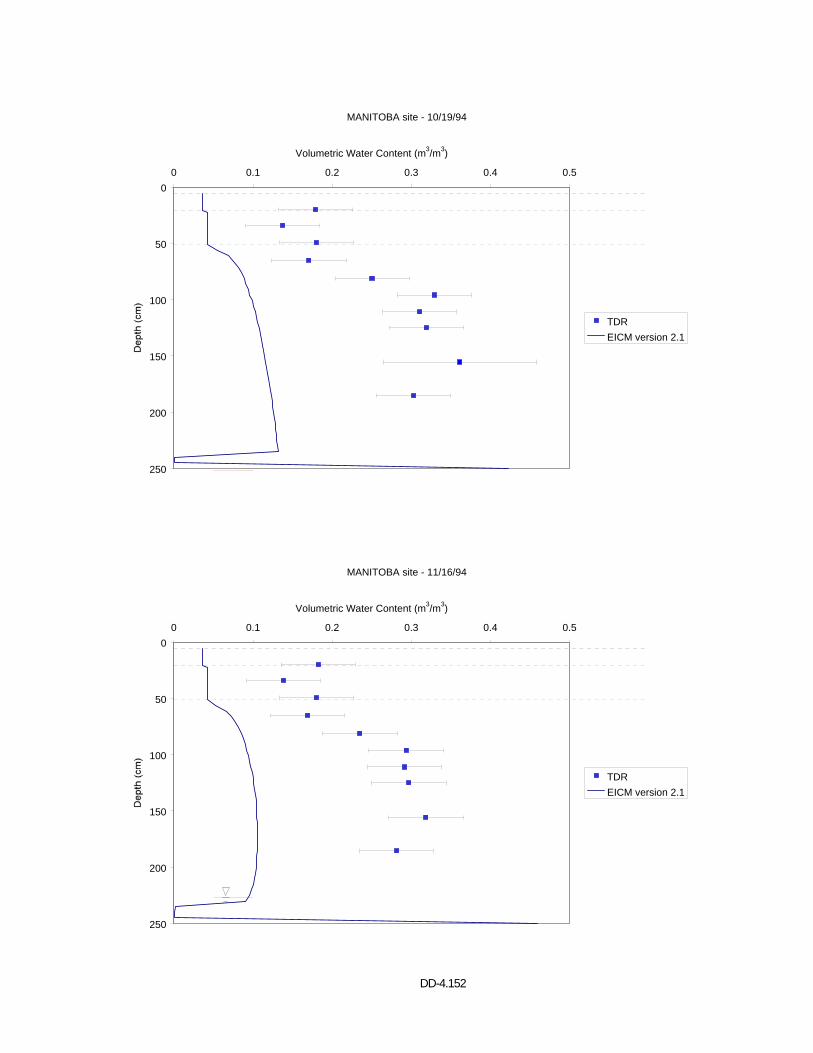
DD-4.152
MANITOBA site - 10/19/94
0
50
100
150
200
250
0 0.1 0.2 0.3 0.4 0.5
Volumetric Water Content (m3/m3)
TDREICM version 2.1
MANITOBA site - 11/16/94
0
50
100
150
200
250
0 0.1 0.2 0.3 0.4 0.5
Volumetric Water Content (m3/m3)
TDREICM version 2.1
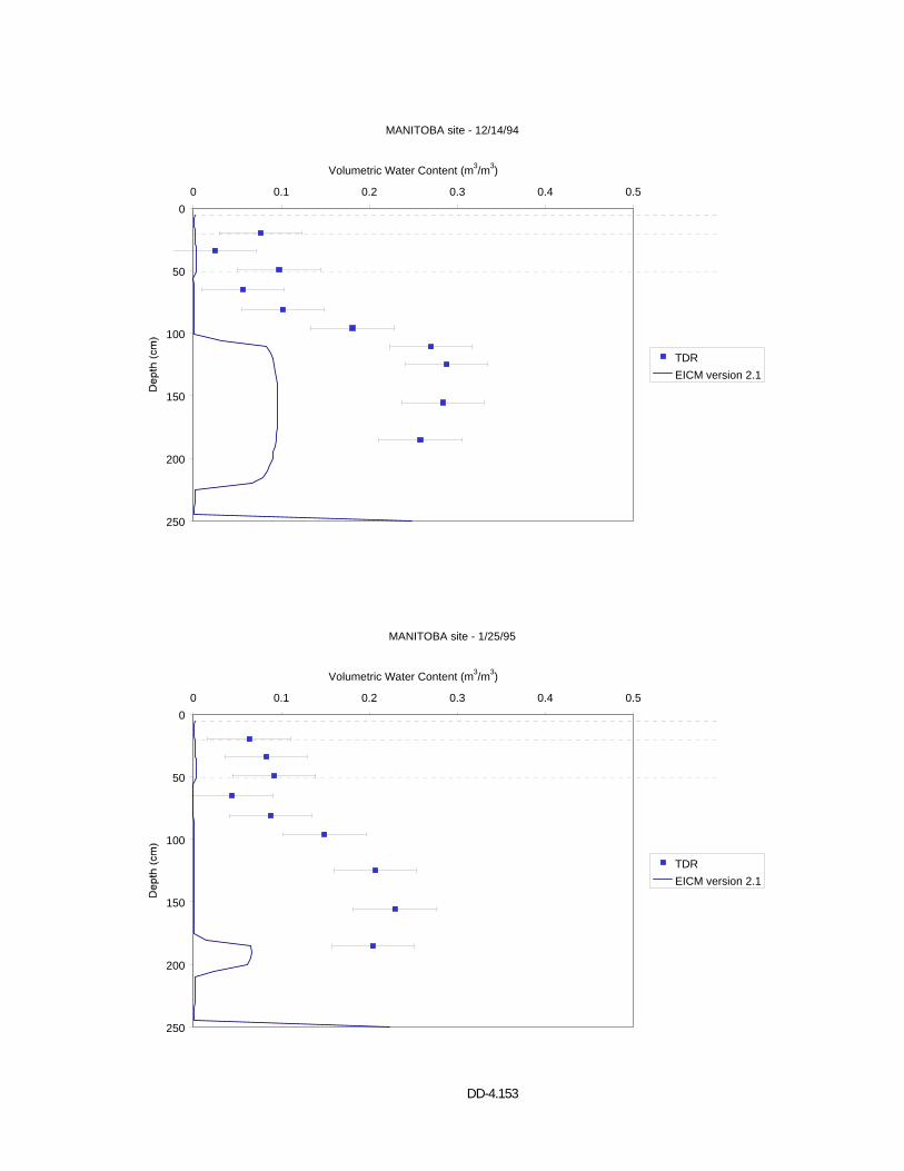
DD-4.153
MANITOBA site - 12/14/94
0
50
100
150
200
250
0 0.1 0.2 0.3 0.4 0.5
Volumetric Water Content (m3/m3)
TDREICM version 2.1
MANITOBA site - 1/25/95
0
50
100
150
200
250
0 0.1 0.2 0.3 0.4 0.5
Volumetric Water Content (m3/m3)
TDREICM version 2.1
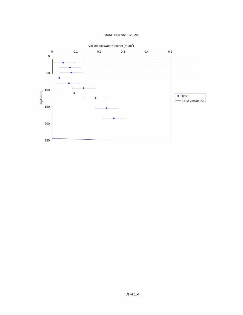
DD-4.154
MANITOBA site - 2/15/95
0
50
100
150
200
250
0 0.1 0.2 0.3 0.4 0.5
Volumetric Water Content (m3/m3)
TDREICM version 2.1

DD-4.155
APPENDIX G BEST-ESTIMATE SOIL-WATER CHARACTERISITC CURVES
BASED ON AASHTO CLASSIFICATION
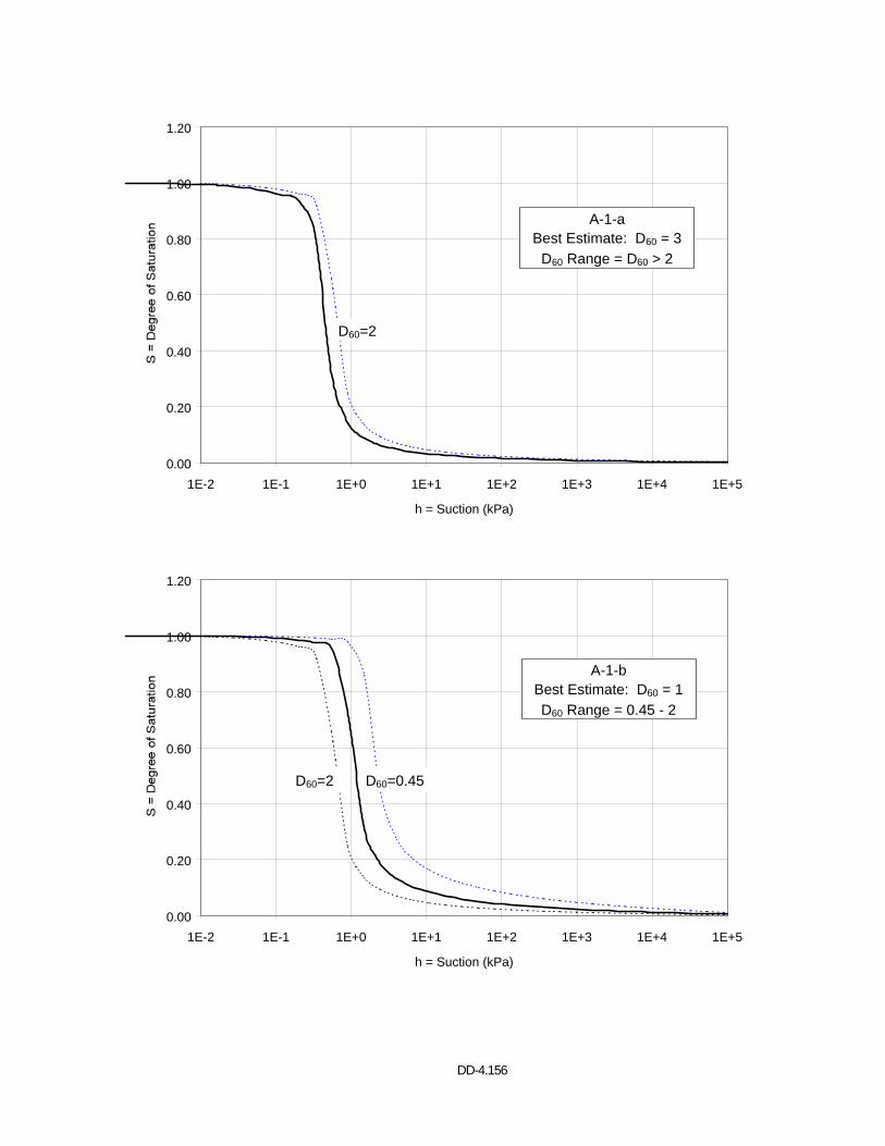
DD-4.156
0.00
0.20
0.40
0.60
0.80
1.00
1.20
1E-2 1E-1 1E+0 1E+1 1E+2 1E+3 1E+4 1E+5
h = Suction (kPa)
D60=2
A-1-aBest Estimate: D60 = 3
D60 Range = D60 > 2
0.00
0.20
0.40
0.60
0.80
1.00
1.20
1E-2 1E-1 1E+0 1E+1 1E+2 1E+3 1E+4 1E+5
h = Suction (kPa)
D60=2 D60=0.45
A-1-bBest Estimate: D60 = 1D60 Range = 0.45 - 2
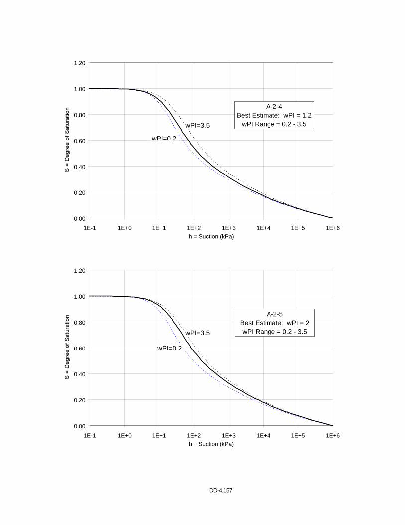
DD-4.157
0.00
0.20
0.40
0.60
0.80
1.00
1.20
1E-1 1E+0 1E+1 1E+2 1E+3 1E+4 1E+5 1E+6h = Suction (kPa)
wPI=3.5
wPI=0 2
A-2-4Best Estimate: wPI = 1.2
wPI Range = 0.2 - 3.5
0.00
0.20
0.40
0.60
0.80
1.00
1.20
1E-1 1E+0 1E+1 1E+2 1E+3 1E+4 1E+5 1E+6h = Suction (kPa)
wPI=3.5
wPI=0.2
A-2-5Best Estimate: wPI = 2wPI Range = 0.2 - 3.5
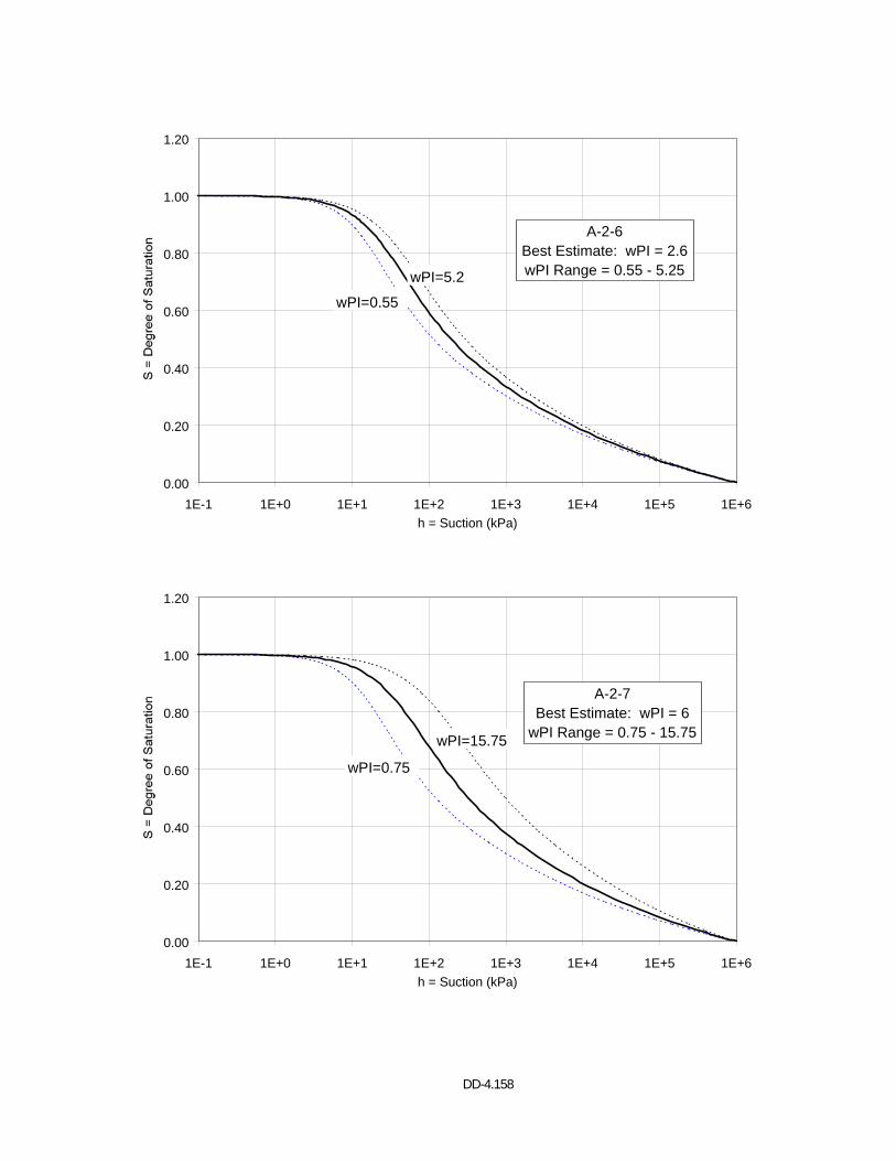
DD-4.158
0.00
0.20
0.40
0.60
0.80
1.00
1.20
1E-1 1E+0 1E+1 1E+2 1E+3 1E+4 1E+5 1E+6h = Suction (kPa)
wPI=5.2
wPI=0.55
A-2-6Best Estimate: wPI = 2.6wPI Range = 0.55 - 5.25
0.00
0.20
0.40
0.60
0.80
1.00
1.20
1E-1 1E+0 1E+1 1E+2 1E+3 1E+4 1E+5 1E+6h = Suction (kPa)
wPI=15.75
wPI=0.75
A-2-7Best Estimate: wPI = 6
wPI Range = 0.75 - 15.75
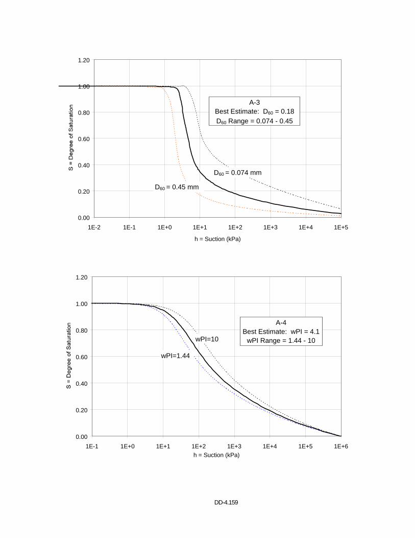
DD-4.159
0.00
0.20
0.40
0.60
0.80
1.00
1.20
1E-2 1E-1 1E+0 1E+1 1E+2 1E+3 1E+4 1E+5
h = Suction (kPa)
A-3Best Estimate: D60 = 0.18D60 Range = 0.074 - 0.45
D60 = 0.45 mm
D60 = 0.074 mm
0.00
0.20
0.40
0.60
0.80
1.00
1.20
1E-1 1E+0 1E+1 1E+2 1E+3 1E+4 1E+5 1E+6h = Suction (kPa)
wPI=10
wPI=1.44
A-4Best Estimate: wPI = 4.1
wPI Range = 1.44 - 10
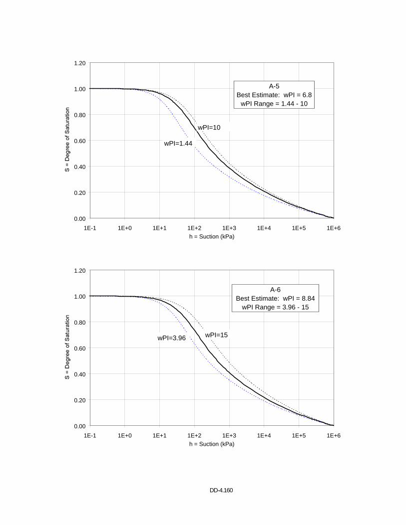
DD-4.160
0.00
0.20
0.40
0.60
0.80
1.00
1.20
1E-1 1E+0 1E+1 1E+2 1E+3 1E+4 1E+5 1E+6h = Suction (kPa)
wPI=10
wPI=1.44
A-5Best Estimate: wPI = 6.8
wPI Range = 1.44 - 10
0.00
0.20
0.40
0.60
0.80
1.00
1.20
1E-1 1E+0 1E+1 1E+2 1E+3 1E+4 1E+5 1E+6h = Suction (kPa)
wPI=15wPI=3.96
A-6Best Estimate: wPI = 8.84
wPI Range = 3.96 - 15
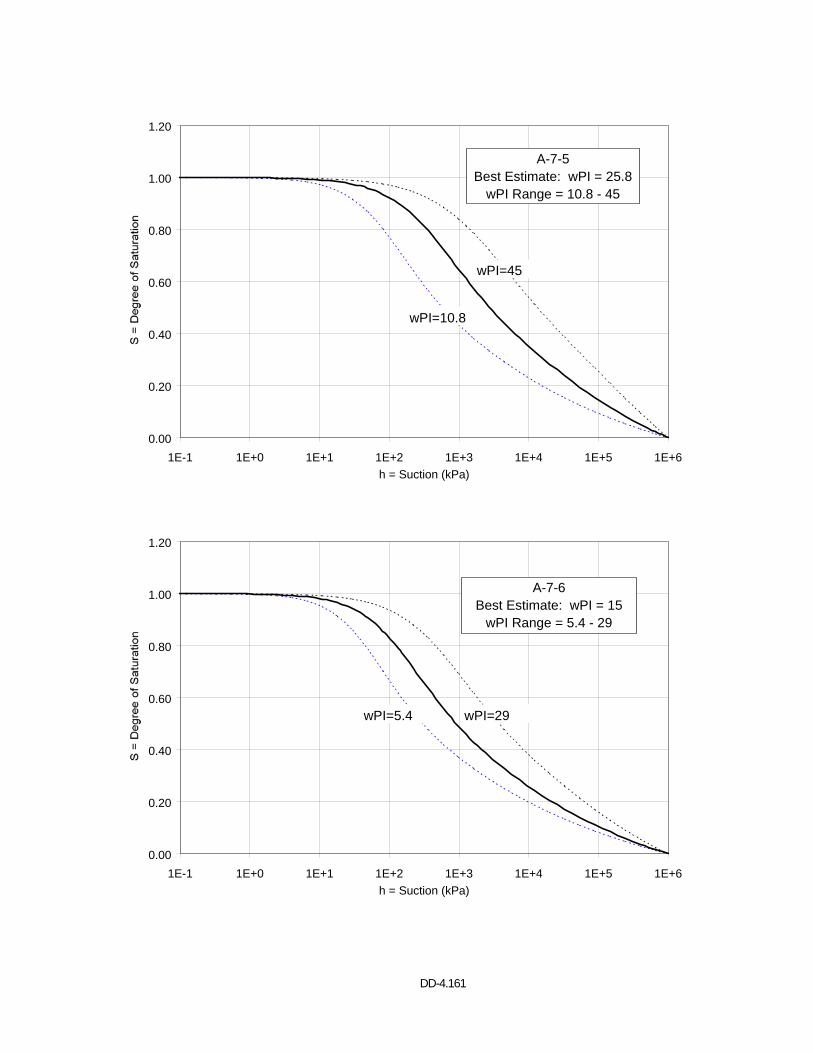
DD-4.161
0.00
0.20
0.40
0.60
0.80
1.00
1.20
1E-1 1E+0 1E+1 1E+2 1E+3 1E+4 1E+5 1E+6h = Suction (kPa)
wPI=45
wPI=10.8
A-7-5Best Estimate: wPI = 25.8
wPI Range = 10.8 - 45
0.00
0.20
0.40
0.60
0.80
1.00
1.20
1E-1 1E+0 1E+1 1E+2 1E+3 1E+4 1E+5 1E+6h = Suction (kPa)
wPI=29wPI=5.4
A-7-6Best Estimate: wPI = 15
wPI Range = 5.4 - 29

DD-4.162
APPENDIX H BEST-ESTIMATE SOIL-WATER CHARACTERISITC CURVES
FOR BASE COURSE MATERIALS
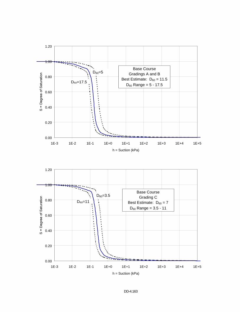
DD-4.163
0.00
0.20
0.40
0.60
0.80
1.00
1.20
1E-3 1E-2 1E-1 1E+0 1E+1 1E+2 1E+3 1E+4 1E+5
h = Suction (kPa)
D60=5
D60=17.5
Base CourseGradings A and B
Best Estimate: D60 = 11.5D60 Range = 5 - 17.5
0.00
0.20
0.40
0.60
0.80
1.00
1.20
1E-3 1E-2 1E-1 1E+0 1E+1 1E+2 1E+3 1E+4 1E+5
h = Suction (kPa)
D60=3.5D60=11
Base CourseGrading C
Best Estimate: D60 = 7D60 Range = 3.5 - 11
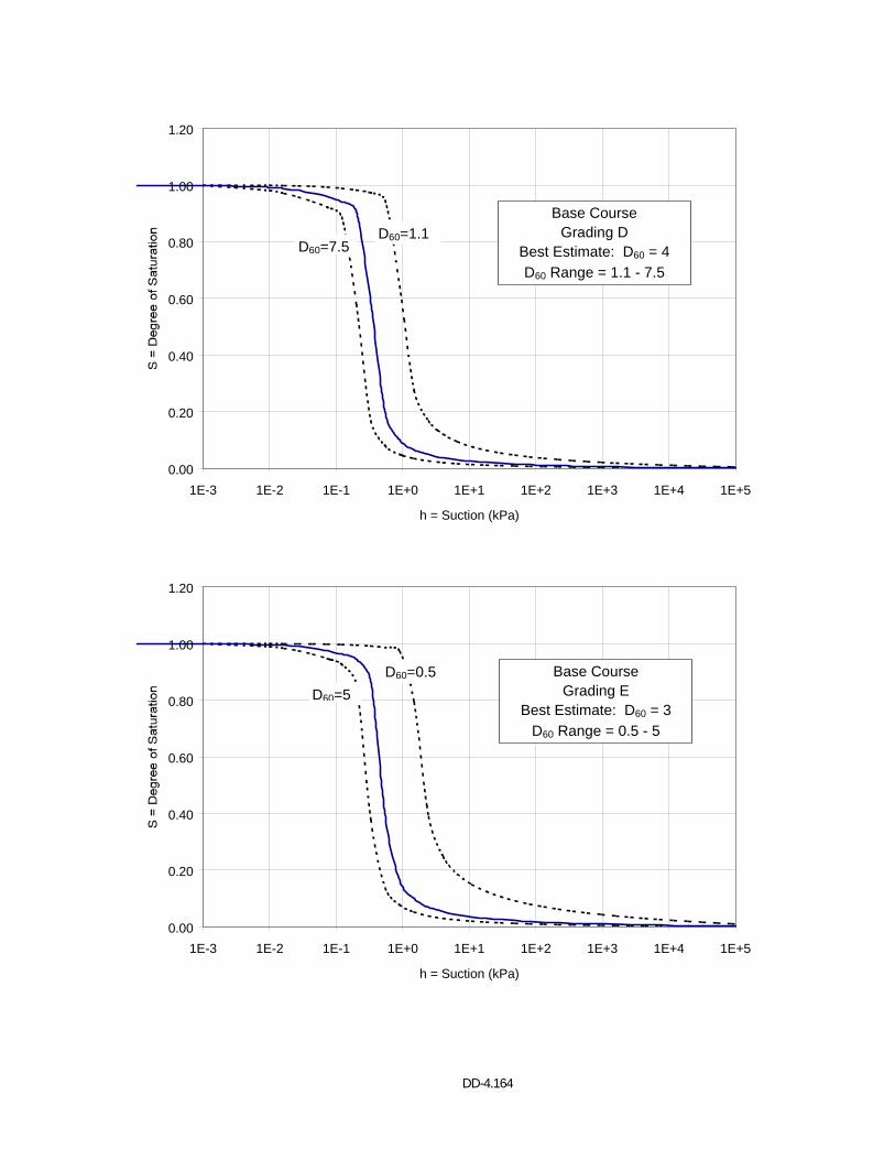
DD-4.164
0.00
0.20
0.40
0.60
0.80
1.00
1.20
1E-3 1E-2 1E-1 1E+0 1E+1 1E+2 1E+3 1E+4 1E+5
h = Suction (kPa)
D60=1.1D60=7.5
Base CourseGrading D
Best Estimate: D60 = 4D60 Range = 1.1 - 7.5
0.00
0.20
0.40
0.60
0.80
1.00
1.20
1E-3 1E-2 1E-1 1E+0 1E+1 1E+2 1E+3 1E+4 1E+5
h = Suction (kPa)
D60=0.5D60=5
Base CourseGrading E
Best Estimate: D60 = 3D60 Range = 0.5 - 5
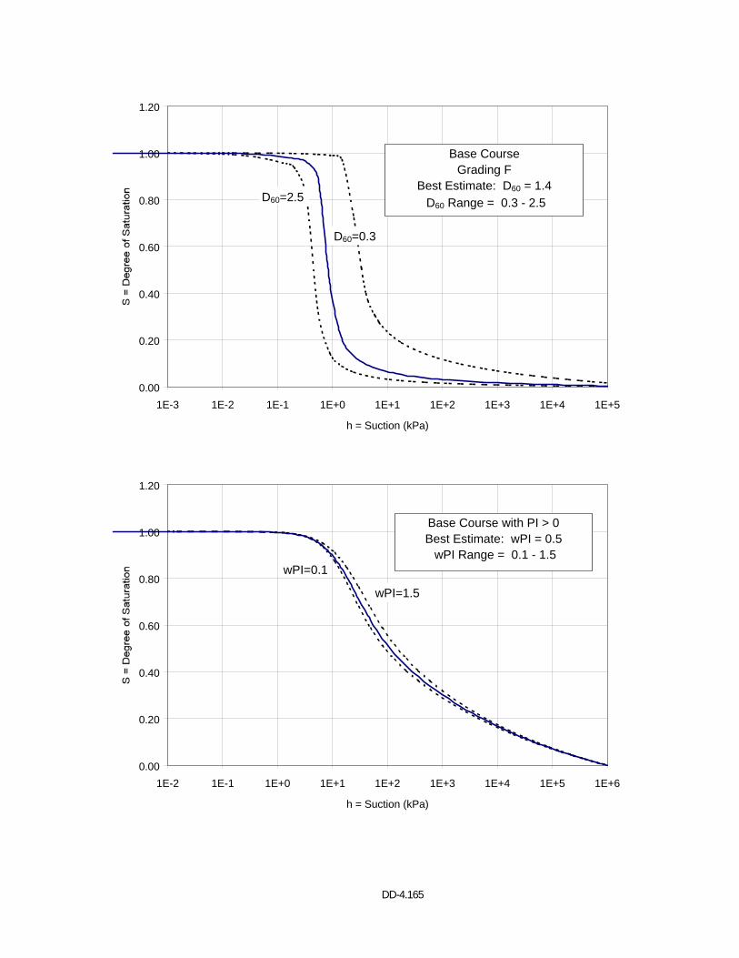
DD-4.165
0.00
0.20
0.40
0.60
0.80
1.00
1.20
1E-3 1E-2 1E-1 1E+0 1E+1 1E+2 1E+3 1E+4 1E+5
h = Suction (kPa)
D60=0.3
D60=2.5
Base CourseGrading F
Best Estimate: D60 = 1.4 D60 Range = 0.3 - 2.5
0.00
0.20
0.40
0.60
0.80
1.00
1.20
1E-2 1E-1 1E+0 1E+1 1E+2 1E+3 1E+4 1E+5 1E+6
h = Suction (kPa)
wPI=1.5
wPI=0.1
Base Course with PI > 0Best Estimate: wPI = 0.5 wPI Range = 0.1 - 1.5

DD-4.166
APPENDIX I VOLUMETRIC WATER CONTENT PROFILES
CONNECTICUT (91803)
EICM – Version 2.6
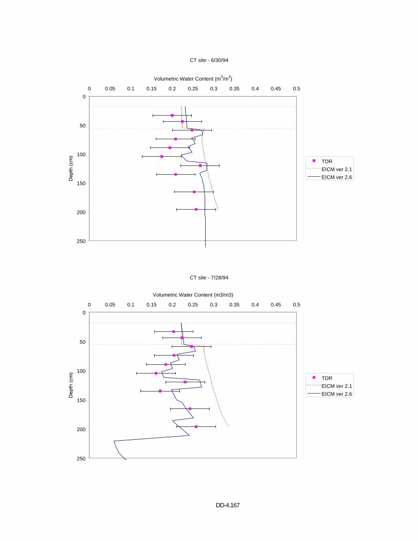
DD-4.167
CT site - 6/30/94
0
50
100
150
200
250
0 0.05 0.1 0.15 0.2 0.25 0.3 0.35 0.4 0.45 0.5
Volumetric Water Content (m3/m3)
TDREICM ver 2.1EICM ver 2.6
CT site - 7/28/94
0
50
100
150
200
250
0 0.05 0.1 0.15 0.2 0.25 0.3 0.35 0.4 0.45 0.5
Volumetric Water Content (m3/m3)
TDREICM ver 2.1EICM ver 2.6
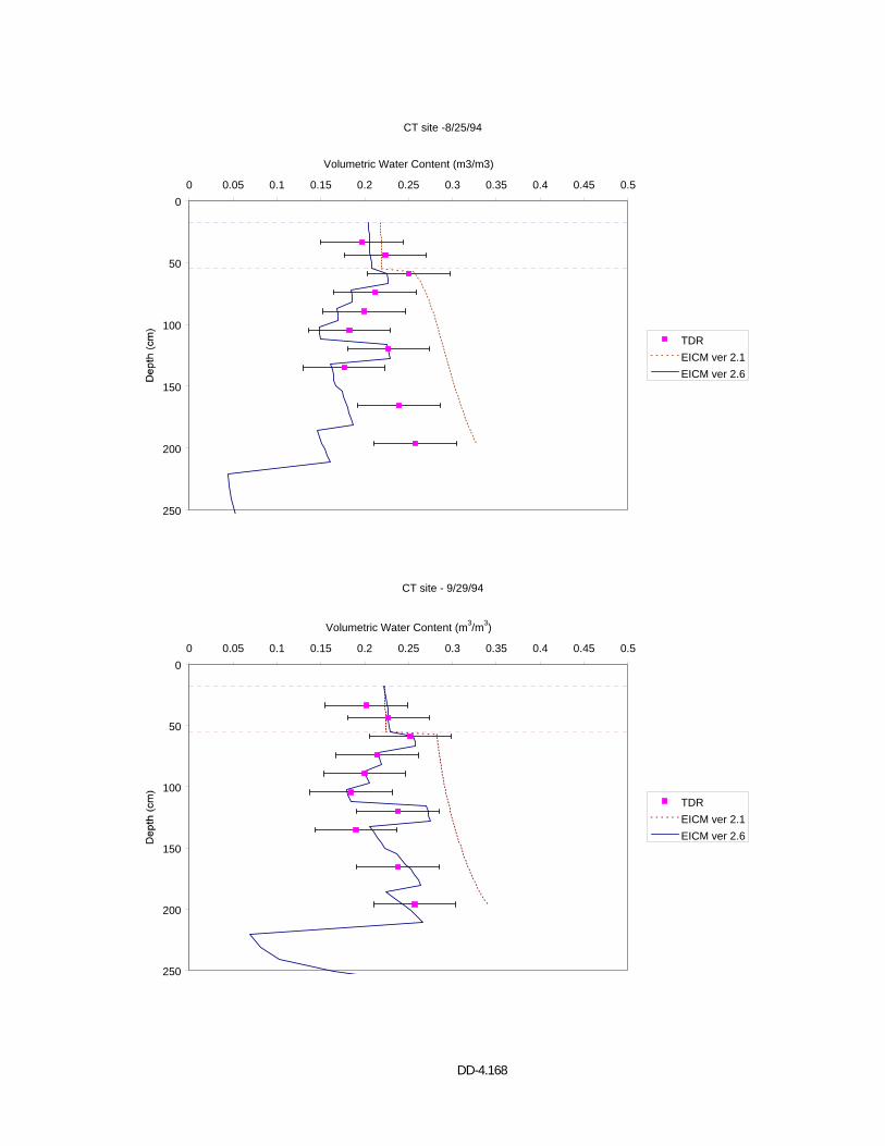
DD-4.168
CT site -8/25/94
0
50
100
150
200
250
0 0.05 0.1 0.15 0.2 0.25 0.3 0.35 0.4 0.45 0.5
Volumetric Water Content (m3/m3)
TDREICM ver 2.1EICM ver 2.6
CT site - 9/29/94
0
50
100
150
200
250
0 0.05 0.1 0.15 0.2 0.25 0.3 0.35 0.4 0.45 0.5
Volumetric Water Content (m3/m3)
TDREICM ver 2.1EICM ver 2.6
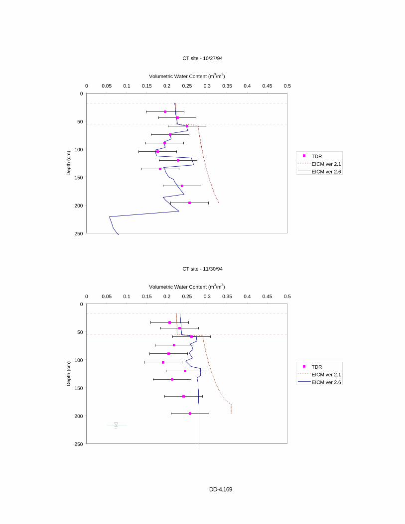
DD-4.169
CT site - 10/27/94
0
50
100
150
200
250
0 0.05 0.1 0.15 0.2 0.25 0.3 0.35 0.4 0.45 0.5
Volumetric Water Content (m3/m3)
TDREICM ver 2.1EICM ver 2.6
CT site - 11/30/94
0
50
100
150
200
250
0 0.05 0.1 0.15 0.2 0.25 0.3 0.35 0.4 0.45 0.5
Volumetric Water Content (m3/m3)
TDREICM ver 2.1EICM ver 2.6
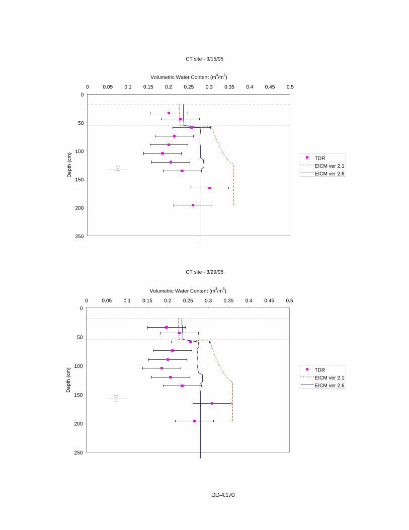
DD-4.170
CT site - 3/15/95
0
50
100
150
200
250
0 0.05 0.1 0.15 0.2 0.25 0.3 0.35 0.4 0.45 0.5
Volumetric Water Content (m3/m3)
TDREICM ver 2.1EICM ver 2.6
CT site - 3/29/95
0
50
100
150
200
250
0 0.05 0.1 0.15 0.2 0.25 0.3 0.35 0.4 0.45 0.5
Volumetric Water Content (m3/m3)
TDREICM ver 2.1EICM ver 2.6
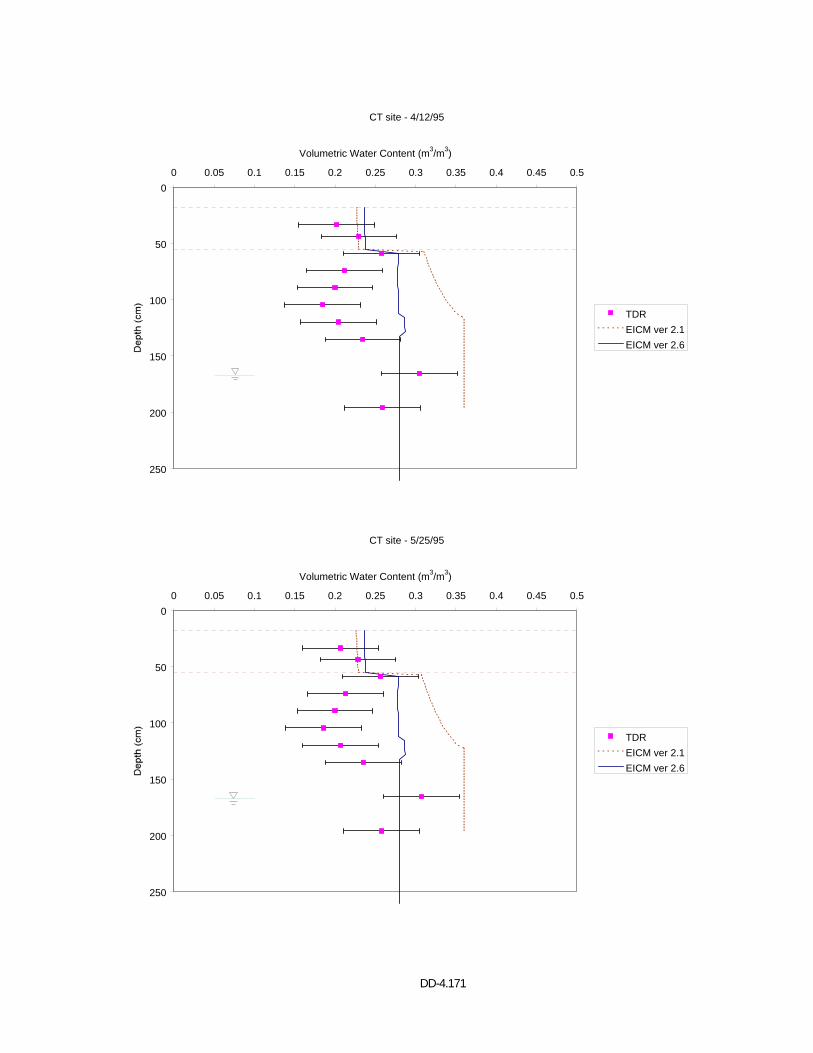
DD-4.171
CT site - 4/12/95
0
50
100
150
200
250
0 0.05 0.1 0.15 0.2 0.25 0.3 0.35 0.4 0.45 0.5
Volumetric Water Content (m3/m3)
TDREICM ver 2.1EICM ver 2.6
CT site - 5/25/95
0
50
100
150
200
250
0 0.05 0.1 0.15 0.2 0.25 0.3 0.35 0.4 0.45 0.5
Volumetric Water Content (m3/m3)
TDREICM ver 2.1EICM ver 2.6
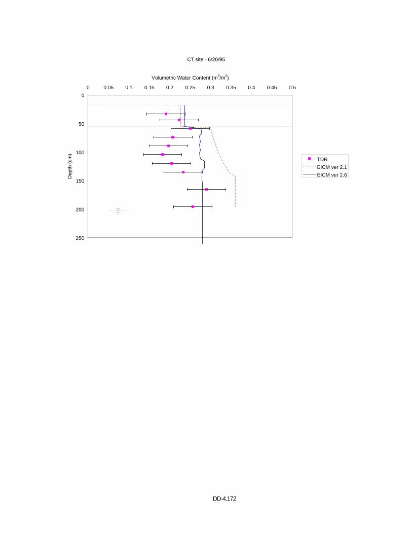
DD-4.172
CT site - 6/20/95
0
50
100
150
200
250
0 0.05 0.1 0.15 0.2 0.25 0.3 0.35 0.4 0.45 0.5
Volumetric Water Content (m3/m3)
TDREICM ver 2.1EICM ver 2.6

DD-4.173
APPENDIX J VOLUMETRIC WATER CONTENT PROFILES
MINNESOTA (271018)
EICM – Version 2.6
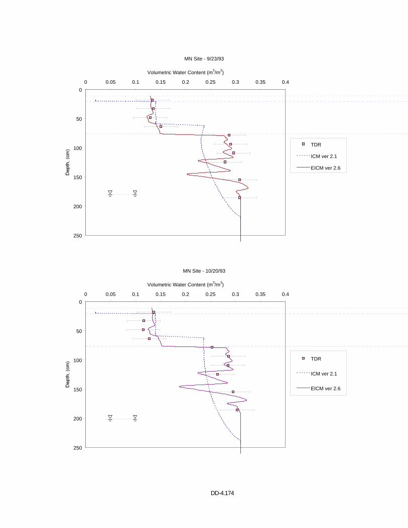
DD-4.174
MN Site - 9/23/93
0
50
100
150
200
250
0 0.05 0.1 0.15 0.2 0.25 0.3 0.35 0.4
Volumetric Water Content (m3/m3)
TDR
ICM ver 2.1
EICM ver 2.6
MN Site - 10/20/93
0
50
100
150
200
250
0 0.05 0.1 0.15 0.2 0.25 0.3 0.35 0.4
Volumetric Water Content (m3/m3)
TDR
ICM ver 2.1
EICM ver 2.6
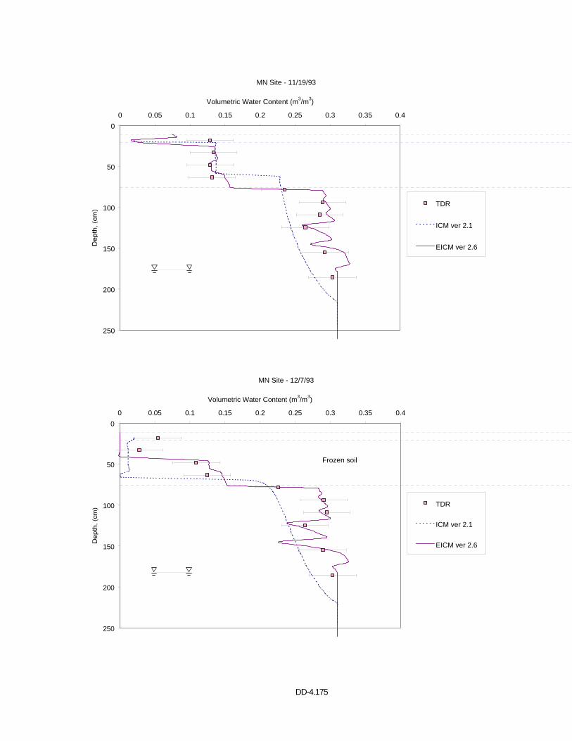
DD-4.175
MN Site - 11/19/93
0
50
100
150
200
250
0 0.05 0.1 0.15 0.2 0.25 0.3 0.35 0.4
Volumetric Water Content (m3/m3)
TDR
ICM ver 2.1
EICM ver 2.6
MN Site - 12/7/93
0
50
100
150
200
250
0 0.05 0.1 0.15 0.2 0.25 0.3 0.35 0.4
Volumetric Water Content (m3/m3)
TDR
ICM ver 2.1
EICM ver 2.6
Frozen soil
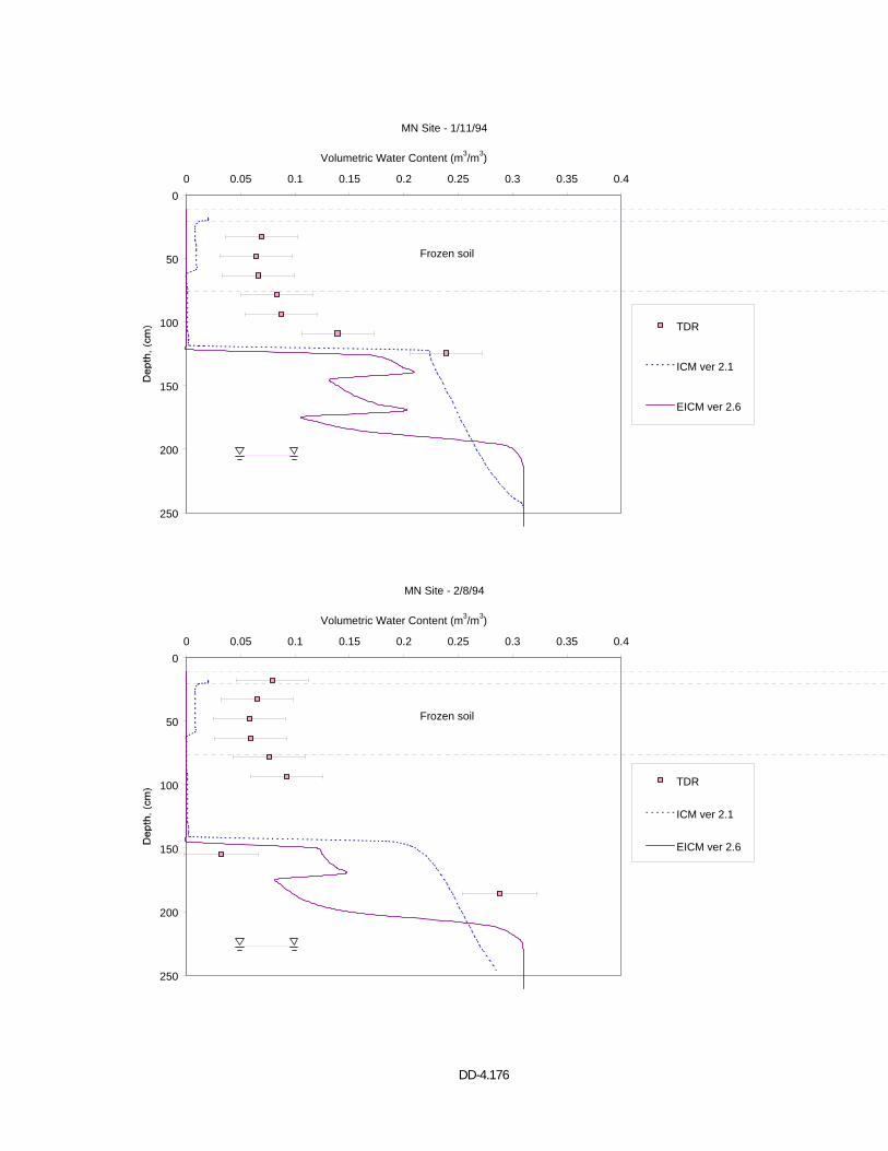
DD-4.176
MN Site - 1/11/94
0
50
100
150
200
250
0 0.05 0.1 0.15 0.2 0.25 0.3 0.35 0.4
Volumetric Water Content (m3/m3)
TDR
ICM ver 2.1
EICM ver 2.6
Frozen soil
MN Site - 2/8/94
0
50
100
150
200
250
0 0.05 0.1 0.15 0.2 0.25 0.3 0.35 0.4
Volumetric Water Content (m3/m3)
TDR
ICM ver 2.1
EICM ver 2.6
Frozen soil
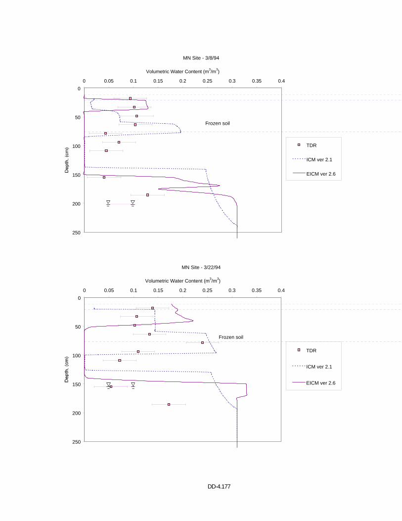
DD-4.177
MN Site - 3/8/94
0
50
100
150
200
250
0 0.05 0.1 0.15 0.2 0.25 0.3 0.35 0.4
Volumetric Water Content (m3/m3)
TDR
ICM ver 2.1
EICM ver 2.6
Frozen soil
MN Site - 3/22/94
0
50
100
150
200
250
0 0.05 0.1 0.15 0.2 0.25 0.3 0.35 0.4
Volumetric Water Content (m3/m3)
TDR
ICM ver 2.1
EICM ver 2.6
Frozen soil
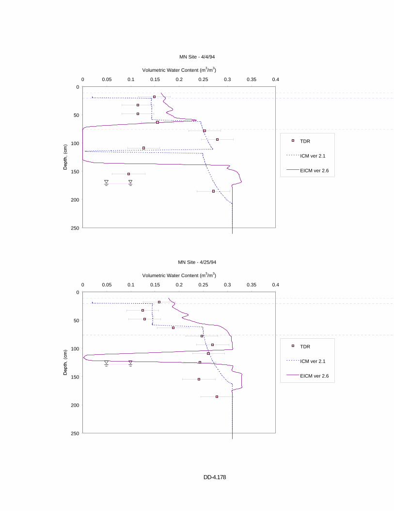
DD-4.178
MN Site - 4/4/94
0
50
100
150
200
250
0 0.05 0.1 0.15 0.2 0.25 0.3 0.35 0.4
Volumetric Water Content (m3/m3)
TDR
ICM ver 2.1
EICM ver 2.6
MN Site - 4/25/94
0
50
100
150
200
250
0 0.05 0.1 0.15 0.2 0.25 0.3 0.35 0.4
Volumetric Water Content (m3/m3)
TDR
ICM ver 2.1
EICM ver 2.6
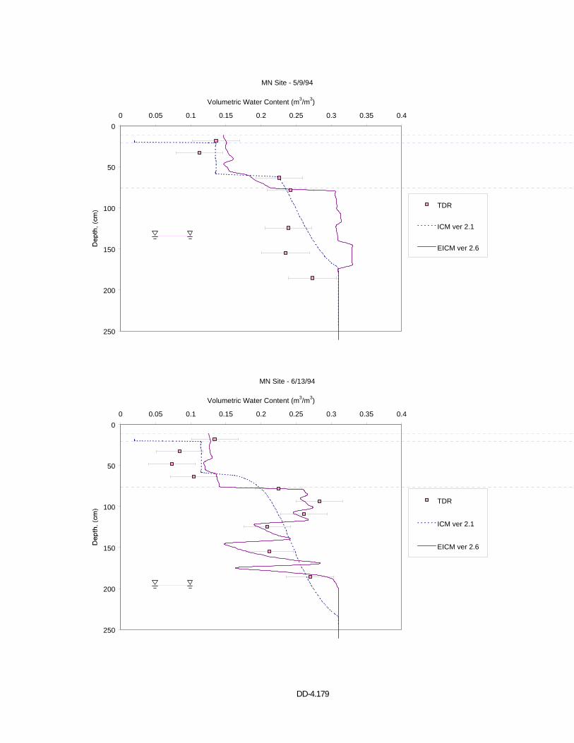
DD-4.179
MN Site - 5/9/94
0
50
100
150
200
250
0 0.05 0.1 0.15 0.2 0.25 0.3 0.35 0.4
Volumetric Water Content (m3/m3)
TDR
ICM ver 2.1
EICM ver 2.6
MN Site - 6/13/94
0
50
100
150
200
250
0 0.05 0.1 0.15 0.2 0.25 0.3 0.35 0.4
Volumetric Water Content (m3/m3)
TDR
ICM ver 2.1
EICM ver 2.6
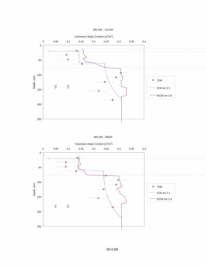
DD-4.180
MN Site - 7/11/94
0
50
100
150
200
250
0 0.05 0.1 0.15 0.2 0.25 0.3 0.35 0.4
Volumetric Water Content (m3/m3)
TDR
ICM ver 2.1
EICM ver 2.6
MN Site - 8/8/94
0
50
100
150
200
250
0 0.05 0.1 0.15 0.2 0.25 0.3 0.35 0.4
Volumetric Water Content (m3/m3)
TDR
ICM ver 2.1
EICM ver 2.6

DD-4.181
APPENDIX K VOLUMETRIC WATER CONTENT PROFILES
MAINE (231026)
EICM – Version 2.6
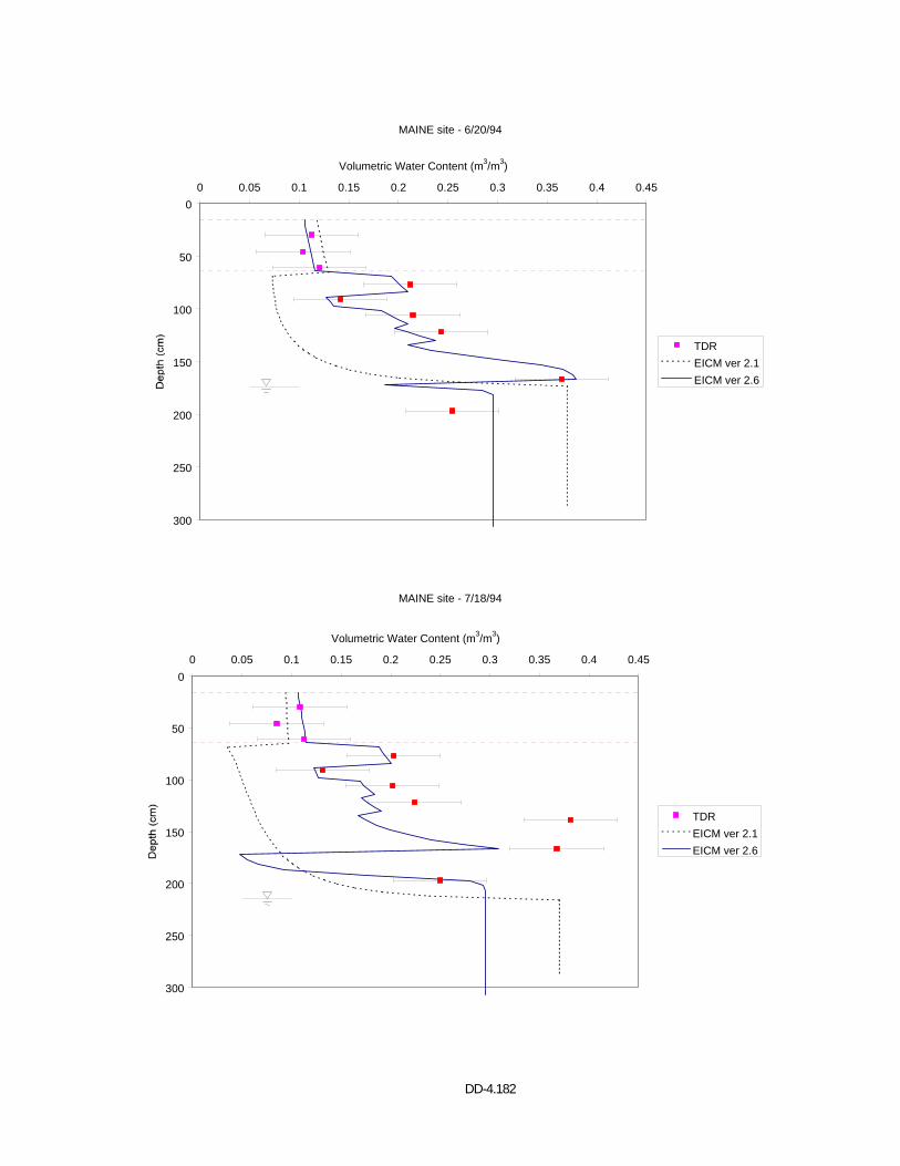
DD-4.182
MAINE site - 6/20/94
0
50
100
150
200
250
300
0 0.05 0.1 0.15 0.2 0.25 0.3 0.35 0.4 0.45
Volumetric Water Content (m3/m3)
TDREICM ver 2.1EICM ver 2.6
MAINE site - 7/18/94
0
50
100
150
200
250
300
0 0.05 0.1 0.15 0.2 0.25 0.3 0.35 0.4 0.45
Volumetric Water Content (m3/m3)
TDREICM ver 2.1EICM ver 2.6
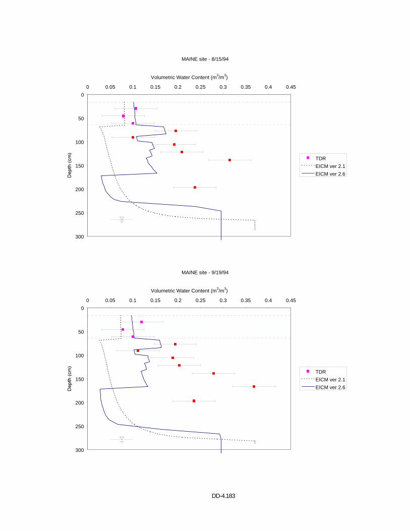
DD-4.183
MAINE site - 8/15/94
0
50
100
150
200
250
300
0 0.05 0.1 0.15 0.2 0.25 0.3 0.35 0.4 0.45
Volumetric Water Content (m3/m3)
TDREICM ver 2.1EICM ver 2.6
MAINE site - 9/19/94
0
50
100
150
200
250
300
0 0.05 0.1 0.15 0.2 0.25 0.3 0.35 0.4 0.45
Volumetric Water Content (m3/m3)
TDREICM ver 2.1EICM ver 2.6
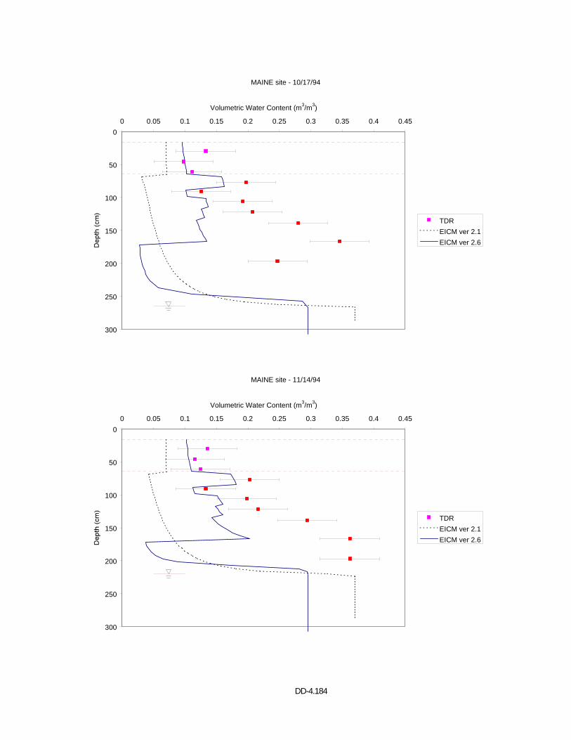
DD-4.184
MAINE site - 10/17/94
0
50
100
150
200
250
300
0 0.05 0.1 0.15 0.2 0.25 0.3 0.35 0.4 0.45
Volumetric Water Content (m3/m3)
TDREICM ver 2.1EICM ver 2.6
MAINE site - 11/14/94
0
50
100
150
200
250
300
0 0.05 0.1 0.15 0.2 0.25 0.3 0.35 0.4 0.45
Volumetric Water Content (m3/m3)
TDREICM ver 2.1EICM ver 2.6
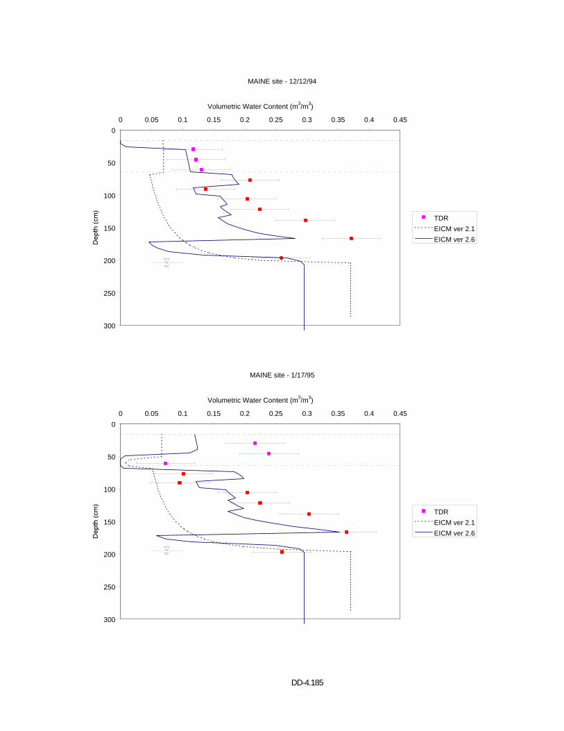
DD-4.185
MAINE site - 12/12/94
0
50
100
150
200
250
300
0 0.05 0.1 0.15 0.2 0.25 0.3 0.35 0.4 0.45
Volumetric Water Content (m3/m3)
TDREICM ver 2.1EICM ver 2.6
MAINE site - 1/17/95
0
50
100
150
200
250
300
0 0.05 0.1 0.15 0.2 0.25 0.3 0.35 0.4 0.45
Volumetric Water Content (m3/m3)
TDREICM ver 2.1EICM ver 2.6
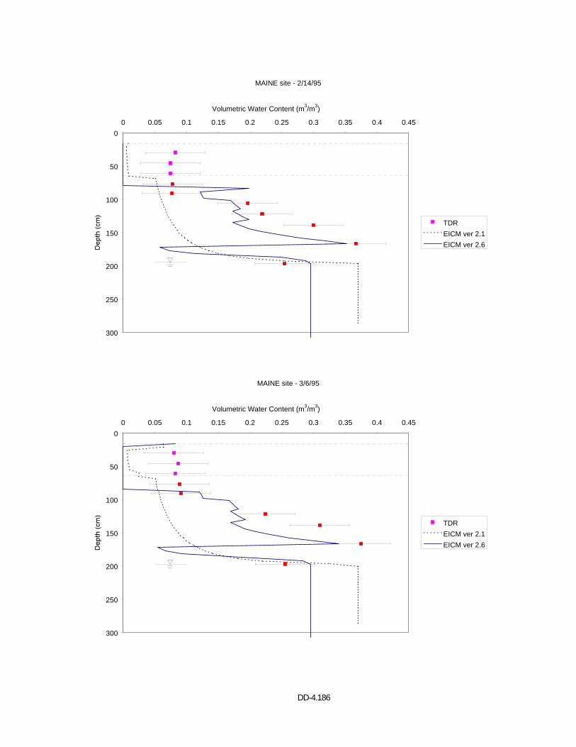
DD-4.186
MAINE site - 2/14/95
0
50
100
150
200
250
300
0 0.05 0.1 0.15 0.2 0.25 0.3 0.35 0.4 0.45
Volumetric Water Content (m3/m3)
TDREICM ver 2.1EICM ver 2.6
MAINE site - 3/6/95
0
50
100
150
200
250
300
0 0.05 0.1 0.15 0.2 0.25 0.3 0.35 0.4 0.45
Volumetric Water Content (m3/m3)
TDREICM ver 2.1EICM ver 2.6
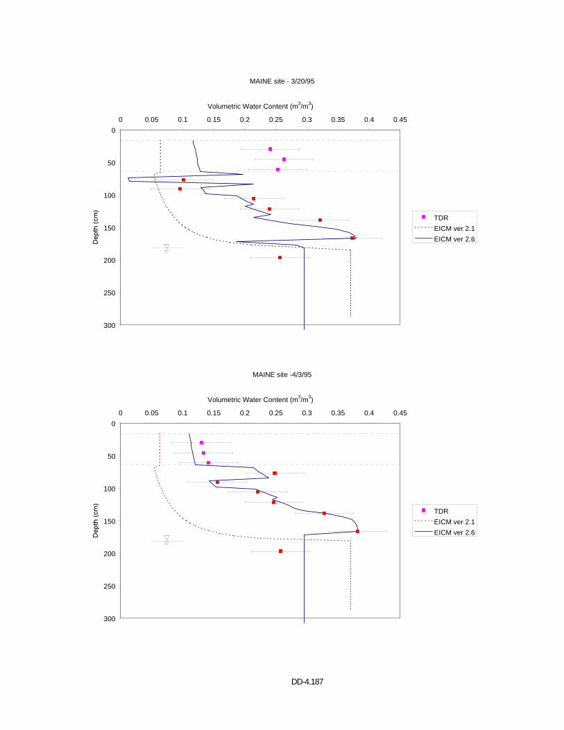
DD-4.187
MAINE site - 3/20/95
0
50
100
150
200
250
300
0 0.05 0.1 0.15 0.2 0.25 0.3 0.35 0.4 0.45
Volumetric Water Content (m3/m3)
TDREICM ver 2.1EICM ver 2.6
MAINE site -4/3/95
0
50
100
150
200
250
300
0 0.05 0.1 0.15 0.2 0.25 0.3 0.35 0.4 0.45
Volumetric Water Content (m3/m3)
TDREICM ver 2.1EICM ver 2.6
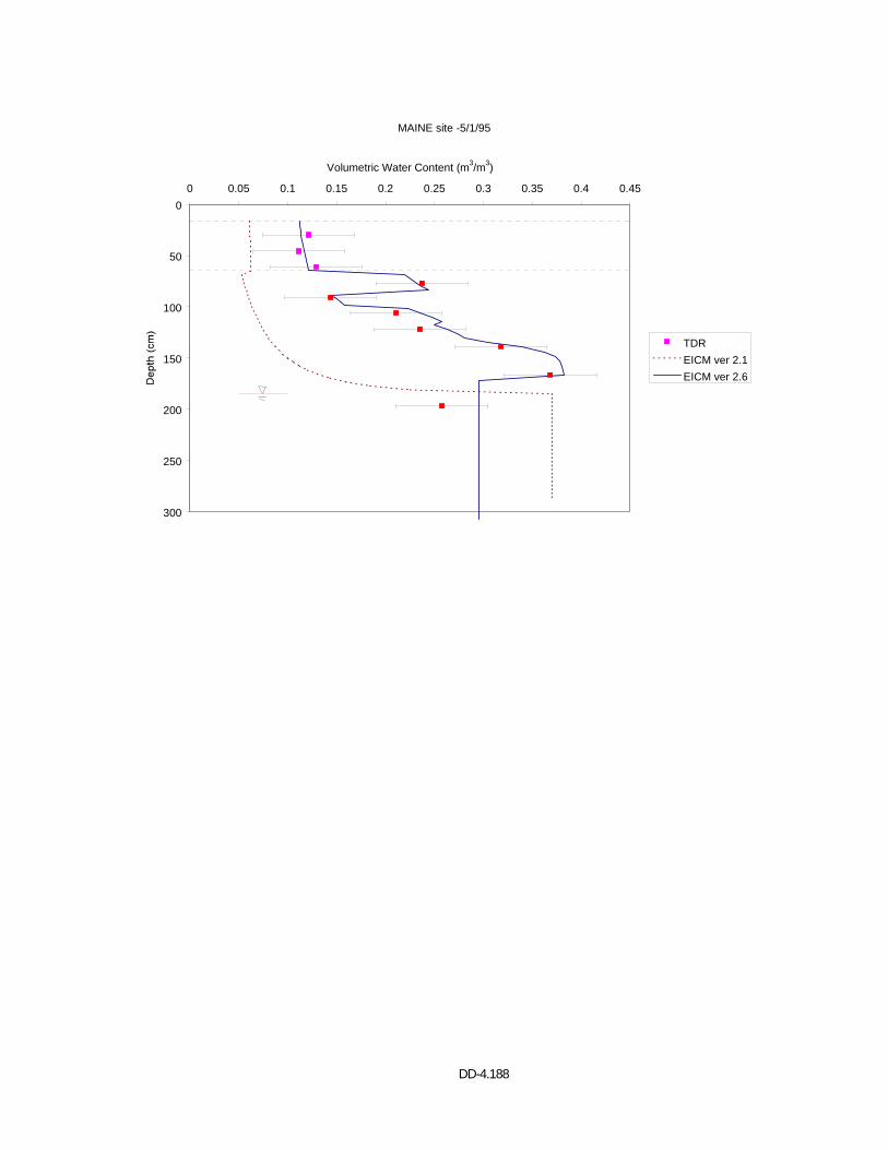
DD-4.188
MAINE site -5/1/95
0
50
100
150
200
250
300
0 0.05 0.1 0.15 0.2 0.25 0.3 0.35 0.4 0.45
Volumetric Water Content (m3/m3)
TDREICM ver 2.1EICM ver 2.6

DD-4.189
APPENDIX L VOLUMETRIC WATER CONTENT PROFILES
NEW HAMPSHIRE (331001)
EICM – Version 2.6
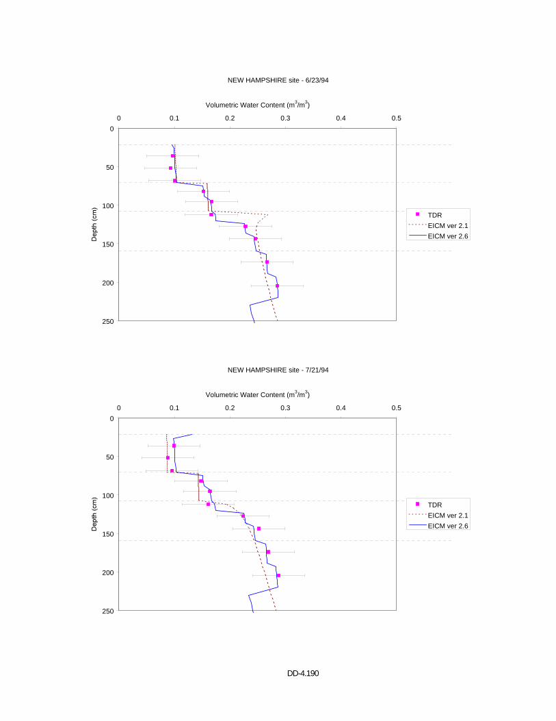
DD-4.190
NEW HAMPSHIRE site - 6/23/94
0
50
100
150
200
250
0 0.1 0.2 0.3 0.4 0.5
Volumetric Water Content (m3/m3)
TDREICM ver 2.1EICM ver 2.6
NEW HAMPSHIRE site - 7/21/94
0
50
100
150
200
250
0 0.1 0.2 0.3 0.4 0.5
Volumetric Water Content (m3/m3)
TDREICM ver 2.1EICM ver 2.6
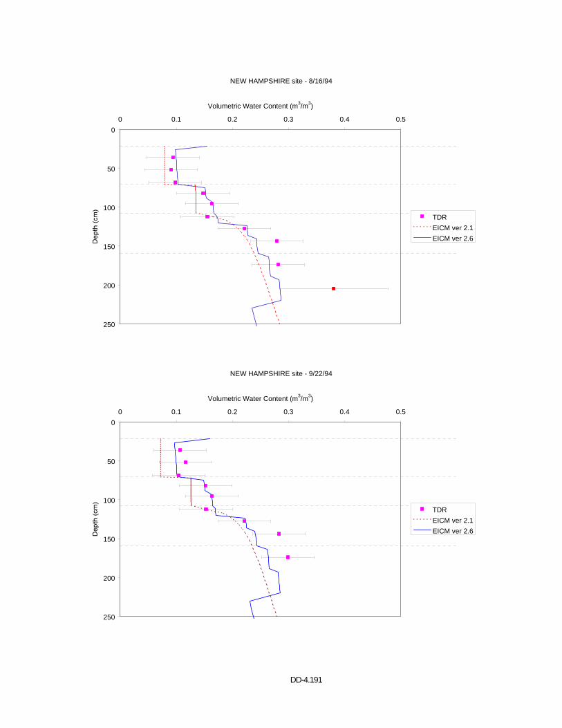
DD-4.191
NEW HAMPSHIRE site - 8/16/94
0
50
100
150
200
250
0 0.1 0.2 0.3 0.4 0.5
Volumetric Water Content (m3/m3)
TDREICM ver 2.1EICM ver 2.6
NEW HAMPSHIRE site - 9/22/94
0
50
100
150
200
250
0 0.1 0.2 0.3 0.4 0.5
Volumetric Water Content (m3/m3)
TDREICM ver 2.1EICM ver 2.6
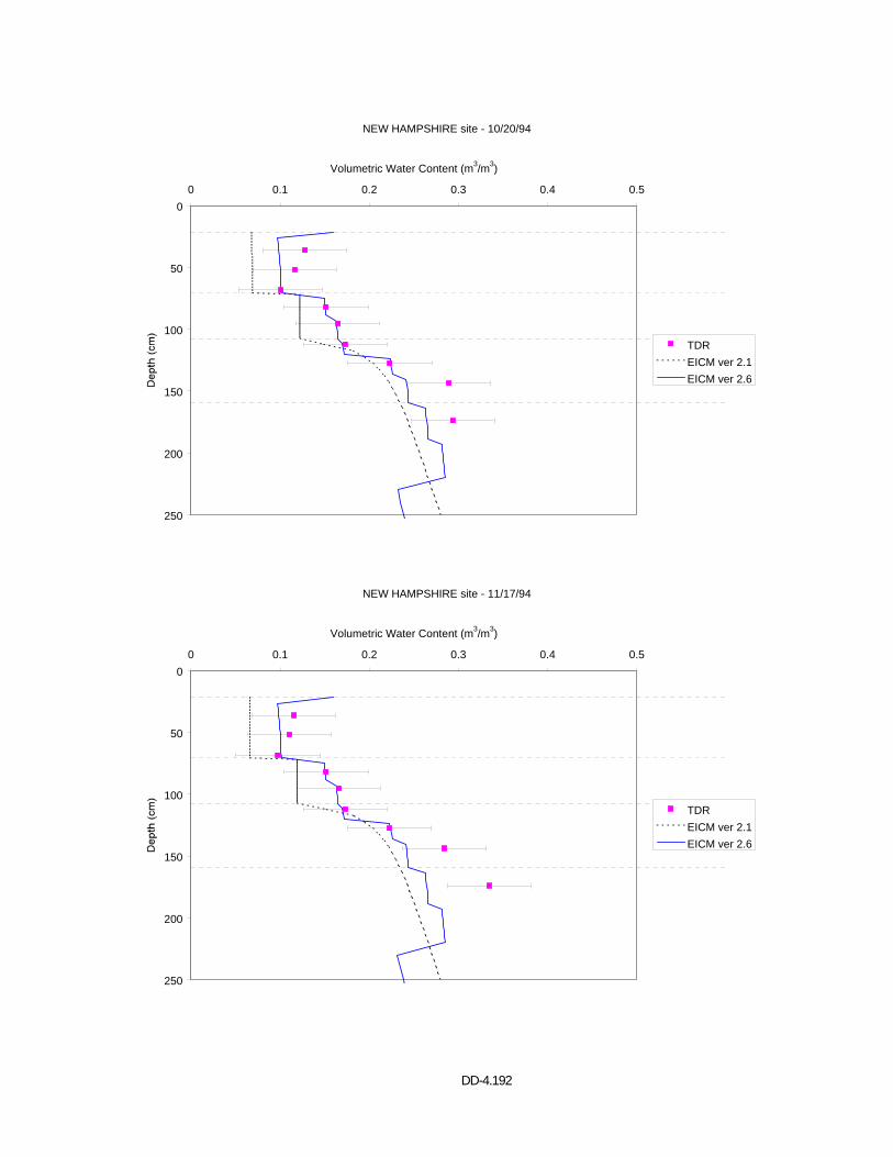
DD-4.192
NEW HAMPSHIRE site - 10/20/94
0
50
100
150
200
250
0 0.1 0.2 0.3 0.4 0.5
Volumetric Water Content (m3/m3)
TDREICM ver 2.1EICM ver 2.6
NEW HAMPSHIRE site - 11/17/94
0
50
100
150
200
250
0 0.1 0.2 0.3 0.4 0.5
Volumetric Water Content (m3/m3)
TDREICM ver 2.1EICM ver 2.6
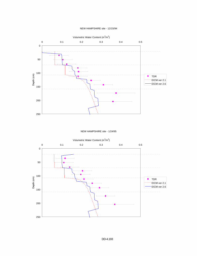
DD-4.193
NEW HAMPSHIRE site - 12/15/94
0
50
100
150
200
250
0 0.1 0.2 0.3 0.4 0.5
Volumetric Water Content (m3/m3)
TDREICM ver 2.1EICM ver 2.6
NEW HAMPSHIRE site - 1/24/95
0
50
100
150
200
250
0 0.1 0.2 0.3 0.4 0.5
Volumetric Water Content (m3/m3)
TDREICM ver 2.1EICM ver 2.6
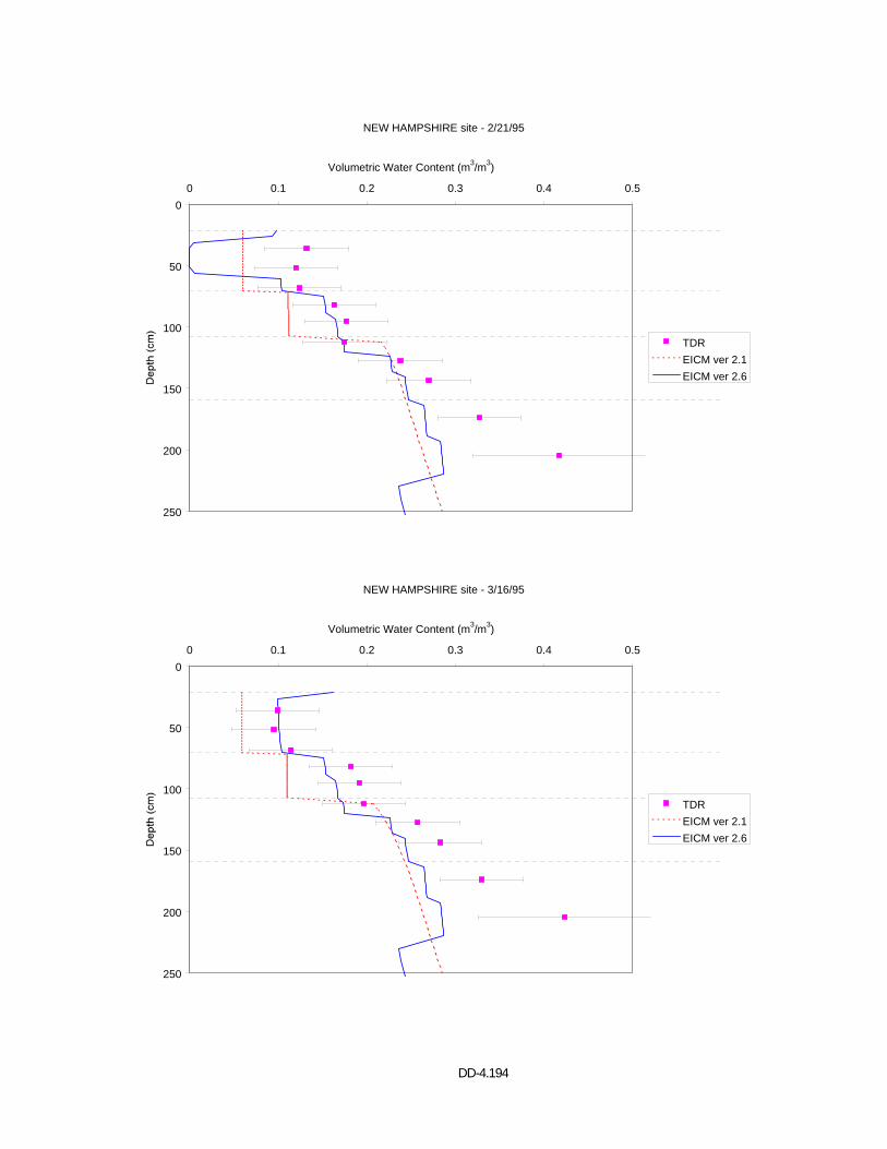
DD-4.194
NEW HAMPSHIRE site - 2/21/95
0
50
100
150
200
250
0 0.1 0.2 0.3 0.4 0.5
Volumetric Water Content (m3/m3)
TDREICM ver 2.1EICM ver 2.6
NEW HAMPSHIRE site - 3/16/95
0
50
100
150
200
250
0 0.1 0.2 0.3 0.4 0.5
Volumetric Water Content (m3/m3)
TDREICM ver 2.1EICM ver 2.6
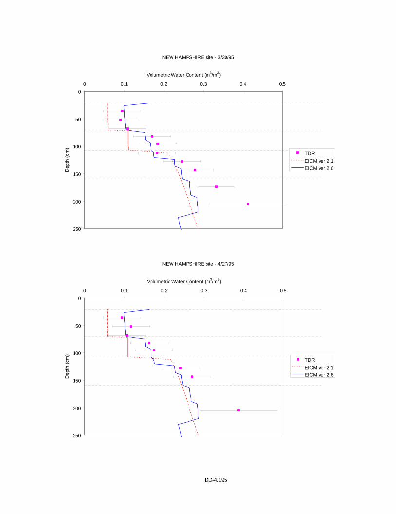
DD-4.195
NEW HAMPSHIRE site - 3/30/95
0
50
100
150
200
250
0 0.1 0.2 0.3 0.4 0.5
Volumetric Water Content (m3/m3)
TDREICM ver 2.1EICM ver 2.6
NEW HAMPSHIRE site - 4/27/95
0
50
100
150
200
250
0 0.1 0.2 0.3 0.4 0.5
Volumetric Water Content (m3/m3)
TDREICM ver 2.1EICM ver 2.6
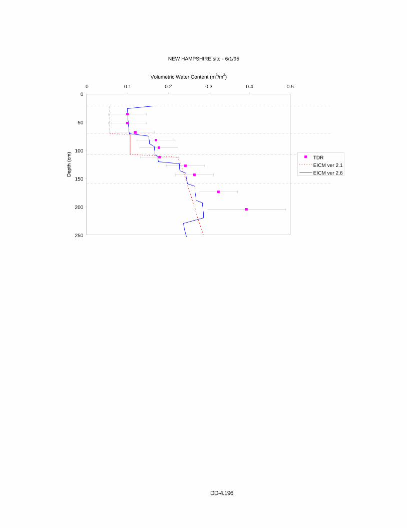
DD-4.196
NEW HAMPSHIRE site - 6/1/95
0
50
100
150
200
250
0 0.1 0.2 0.3 0.4 0.5
Volumetric Water Content (m3/m3)
TDREICM ver 2.1EICM ver 2.6

DD-4.197
APPENDIX M VOLUMETRIC WATER CONTENT PROFILES
VERMONT (501002)
EICM – Version 2.6
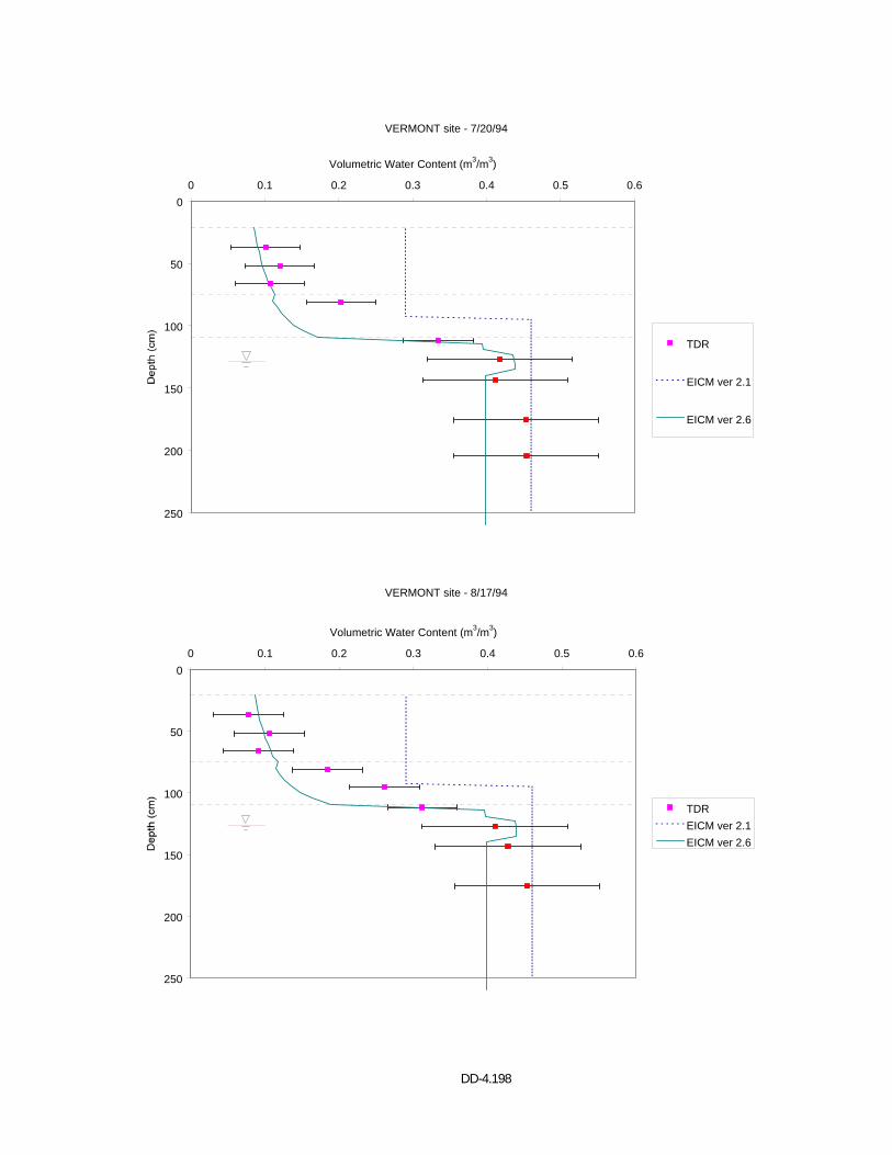
DD-4.198
VERMONT site - 7/20/94
0
50
100
150
200
250
0 0.1 0.2 0.3 0.4 0.5 0.6
Volumetric Water Content (m3/m3)
TDR
EICM ver 2.1
EICM ver 2.6
VERMONT site - 8/17/94
0
50
100
150
200
250
0 0.1 0.2 0.3 0.4 0.5 0.6
Volumetric Water Content (m3/m3)
TDREICM ver 2.1EICM ver 2.6
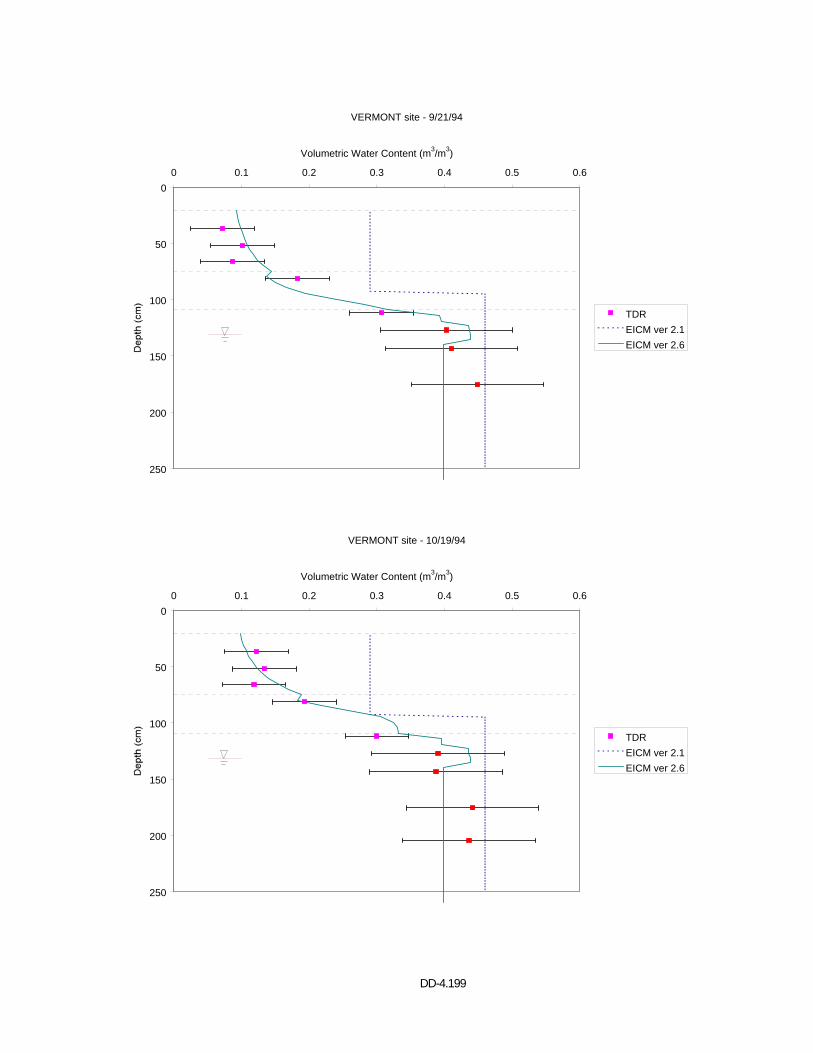
DD-4.199
VERMONT site - 9/21/94
0
50
100
150
200
250
0 0.1 0.2 0.3 0.4 0.5 0.6
Volumetric Water Content (m3/m3)
TDREICM ver 2.1EICM ver 2.6
VERMONT site - 10/19/94
0
50
100
150
200
250
0 0.1 0.2 0.3 0.4 0.5 0.6
Volumetric Water Content (m3/m3)
TDREICM ver 2.1EICM ver 2.6
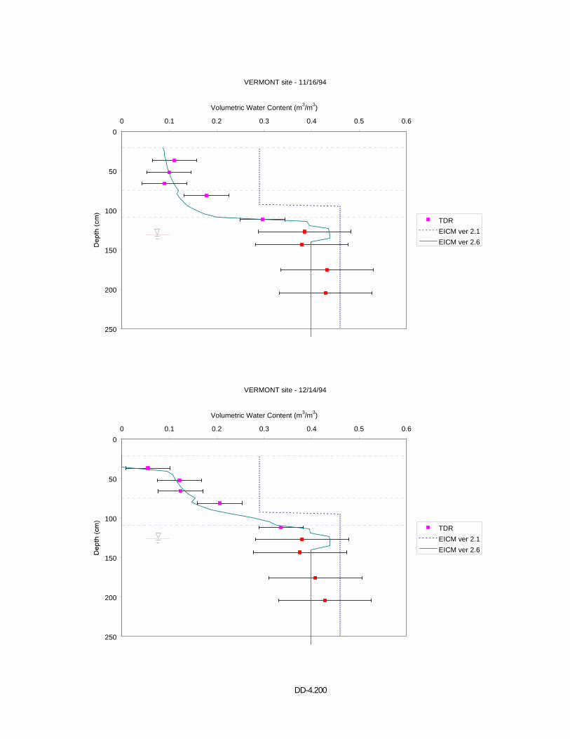
DD-4.200
VERMONT site - 12/14/94
0
50
100
150
200
250
0 0.1 0.2 0.3 0.4 0.5 0.6
Volumetric Water Content (m3/m3)
TDREICM ver 2.1EICM ver 2.6
VERMONT site - 11/16/94
0
50
100
150
200
250
0 0.1 0.2 0.3 0.4 0.5 0.6
Volumetric Water Content (m3/m3)
TDREICM ver 2.1EICM ver 2.6
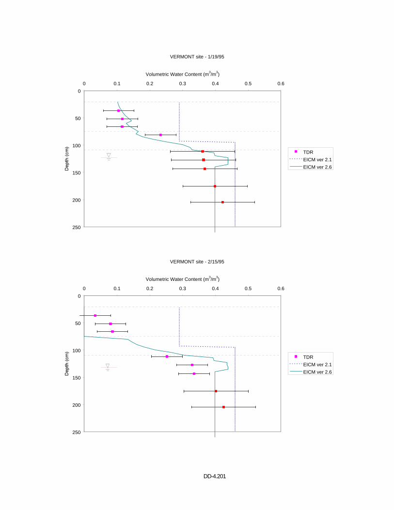
DD-4.201
VERMONT site - 1/19/95
0
50
100
150
200
250
0 0.1 0.2 0.3 0.4 0.5 0.6
Volumetric Water Content (m3/m3)
TDREICM ver 2.1EICM ver 2.6
VERMONT site - 2/15/95
0
50
100
150
200
250
0 0.1 0.2 0.3 0.4 0.5 0.6
Volumetric Water Content (m3/m3)
TDREICM ver 2.1EICM ver 2.6
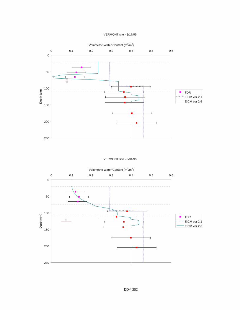
DD-4.202
VERMONT site - 3/17/95
0
50
100
150
200
250
0 0.1 0.2 0.3 0.4 0.5 0.6
Volumetric Water Content (m3/m3)
TDREICM ver 2.1EICM ver 2.6
VERMONT site - 3/31/95
0
50
100
150
200
250
0 0.1 0.2 0.3 0.4 0.5 0.6
Volumetric Water Content (m3/m3)
TDREICM ver 2.1EICM ver 2.6
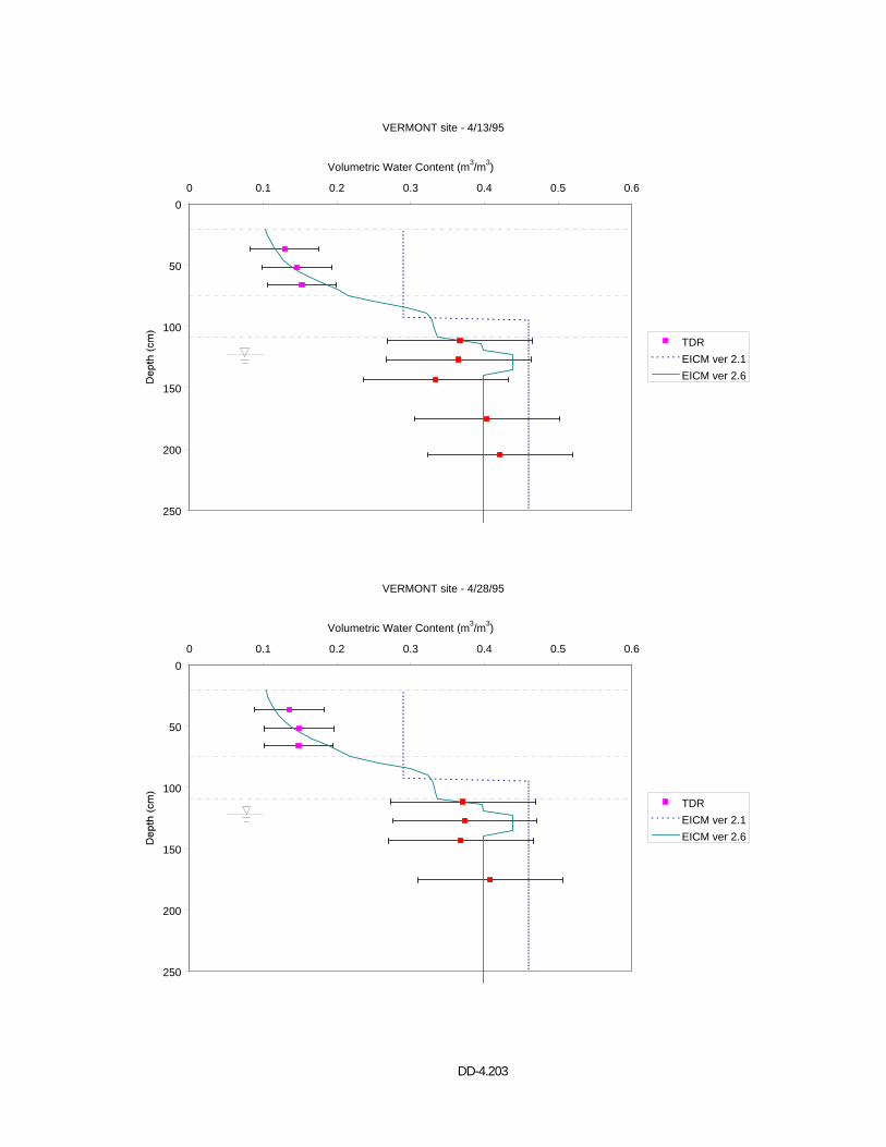
DD-4.203
VERMONT site - 4/13/95
0
50
100
150
200
250
0 0.1 0.2 0.3 0.4 0.5 0.6
Volumetric Water Content (m3/m3)
TDREICM ver 2.1EICM ver 2.6
VERMONT site - 4/28/95
0
50
100
150
200
250
0 0.1 0.2 0.3 0.4 0.5 0.6
Volumetric Water Content (m3/m3)
TDREICM ver 2.1EICM ver 2.6
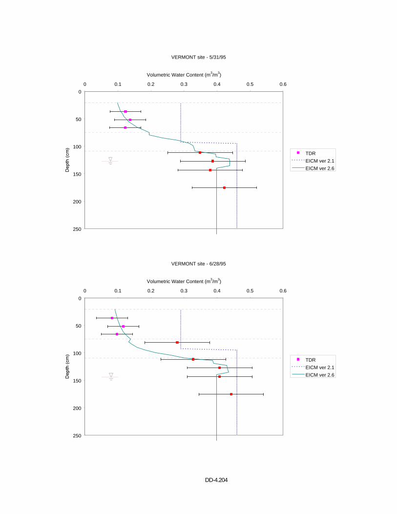
DD-4.204
VERMONT site - 5/31/95
0
50
100
150
200
250
0 0.1 0.2 0.3 0.4 0.5 0.6
Volumetric Water Content (m3/m3)
TDREICM ver 2.1EICM ver 2.6
VERMONT site - 6/28/95
0
50
100
150
200
250
0 0.1 0.2 0.3 0.4 0.5 0.6
Volumetric Water Content (m3/m3)
TDREICM ver 2.1EICM ver 2.6

DD-4.205
APPENDIX N VOLUMETRIC WATER CONTENT PROFILES
MANITOBA (831801)
EICM – Version 2.6
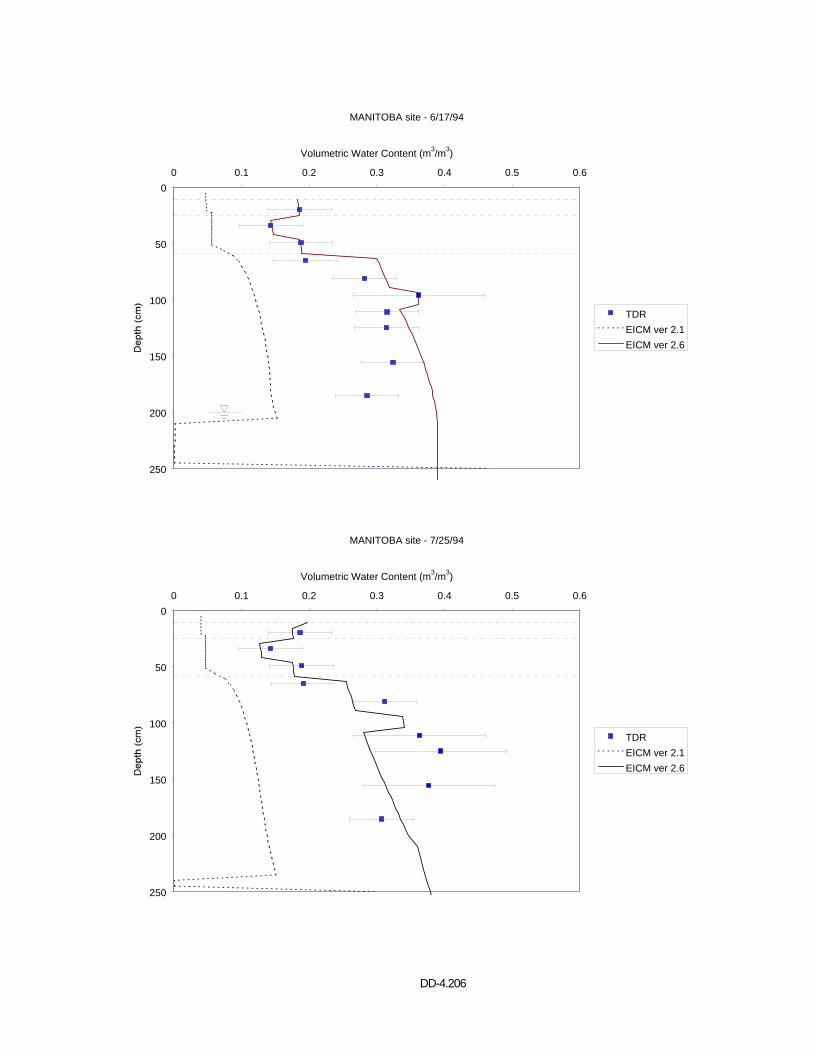
DD-4.206
MANITOBA site - 6/17/94
0
50
100
150
200
250
0 0.1 0.2 0.3 0.4 0.5 0.6
Volumetric Water Content (m3/m3)
TDREICM ver 2.1EICM ver 2.6
MANITOBA site - 7/25/94
0
50
100
150
200
250
0 0.1 0.2 0.3 0.4 0.5 0.6
Volumetric Water Content (m3/m3)
TDREICM ver 2.1EICM ver 2.6
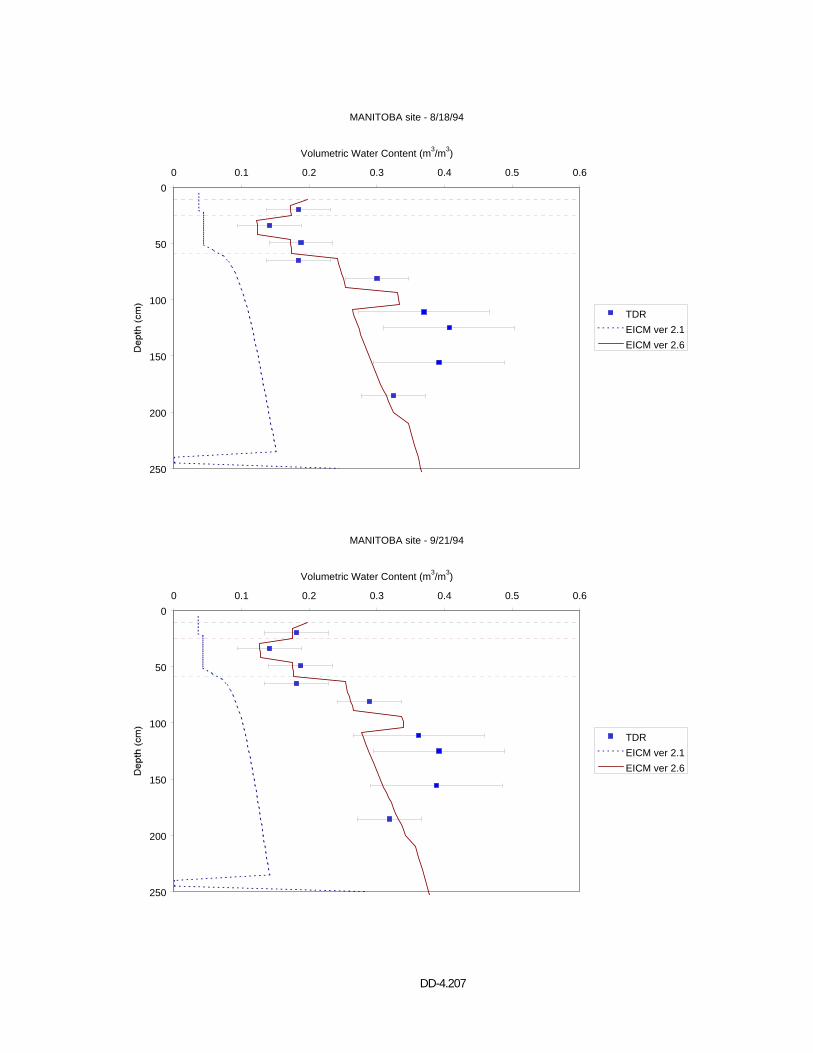
DD-4.207
MANITOBA site - 8/18/94
0
50
100
150
200
250
0 0.1 0.2 0.3 0.4 0.5 0.6
Volumetric Water Content (m3/m3)
TDREICM ver 2.1EICM ver 2.6
MANITOBA site - 9/21/94
0
50
100
150
200
250
0 0.1 0.2 0.3 0.4 0.5 0.6
Volumetric Water Content (m3/m3)
TDREICM ver 2.1EICM ver 2.6
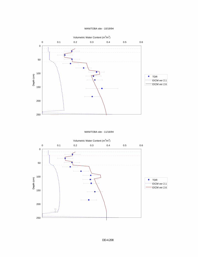
DD-4.208
MANITOBA site - 10/19/94
0
50
100
150
200
250
0 0.1 0.2 0.3 0.4 0.5 0.6
Volumetric Water Content (m3/m3)
TDREICM ver 2.1EICM ver 2.6
MANITOBA site - 11/16/94
0
50
100
150
200
250
0 0.1 0.2 0.3 0.4 0.5 0.6
Volumetric Water Content (m3/m3)
TDREICM ver 2.1EICM ver 2.6
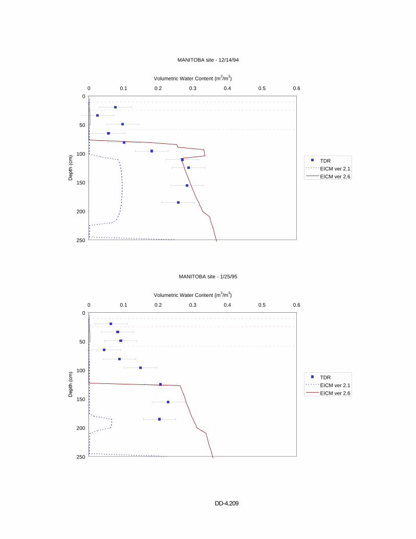
DD-4.209
MANITOBA site - 12/14/94
0
50
100
150
200
250
0 0.1 0.2 0.3 0.4 0.5 0.6
Volumetric Water Content (m3/m3)
TDREICM ver 2.1EICM ver 2.6
MANITOBA site - 1/25/95
0
50
100
150
200
250
0 0.1 0.2 0.3 0.4 0.5 0.6
Volumetric Water Content (m3/m3)
TDREICM ver 2.1EICM ver 2.6
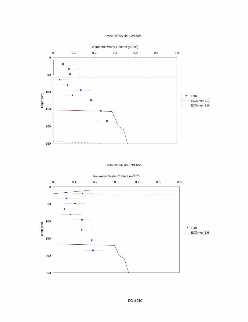
DD-4.210
MANITOBA site - 2/15/95
0
50
100
150
200
250
0 0.1 0.2 0.3 0.4 0.5 0.6
Volumetric Water Content (m3/m3)
TDREICM ver 2.1EICM ver 2.6
MANITOBA site - 3/14/95
0
50
100
150
200
250
0 0.1 0.2 0.3 0.4 0.5 0.6
Volumetric Water Content (m3/m3)
TDREICM ver 2.6
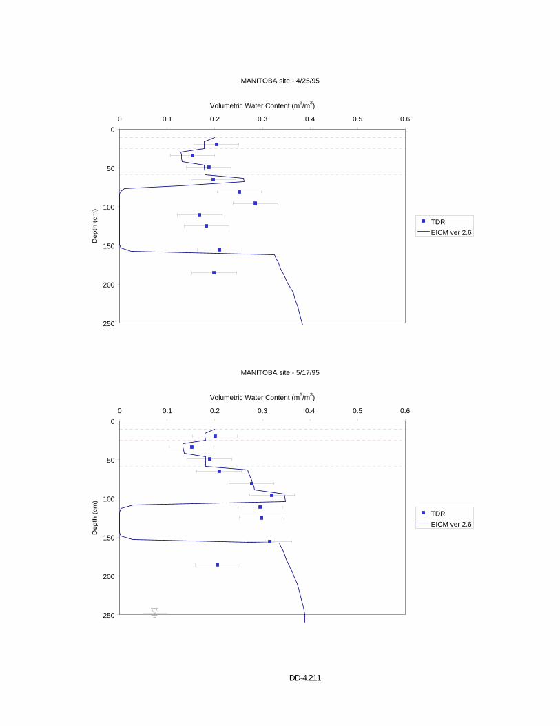
DD-4.211
MANITOBA site - 4/25/95
0
50
100
150
200
250
0 0.1 0.2 0.3 0.4 0.5 0.6
Volumetric Water Content (m3/m3)
TDREICM ver 2.6
MANITOBA site - 5/17/95
0
50
100
150
200
250
0 0.1 0.2 0.3 0.4 0.5 0.6
Volumetric Water Content (m3/m3)
TDREICM ver 2.6

DD-4.212
APPENDIX O VOLUMETRIC WATER CONTENT PROFILES
GEORGIA (131005)
EICM – Version 2.6
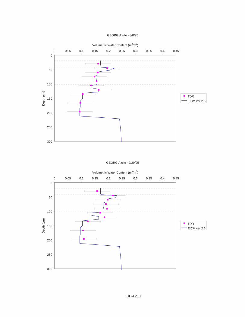
DD-4.213
GEORGIA site - 8/8/95
0
50
100
150
200
250
300
0 0.05 0.1 0.15 0.2 0.25 0.3 0.35 0.4 0.45
Volumetric Water Content (m3/m3)
TDREICM ver 2.6
GEORGIA site - 9/20/95
0
50
100
150
200
250
300
0 0.05 0.1 0.15 0.2 0.25 0.3 0.35 0.4 0.45
Volumetric Water Content (m3/m3)
TDREICM ver 2.6
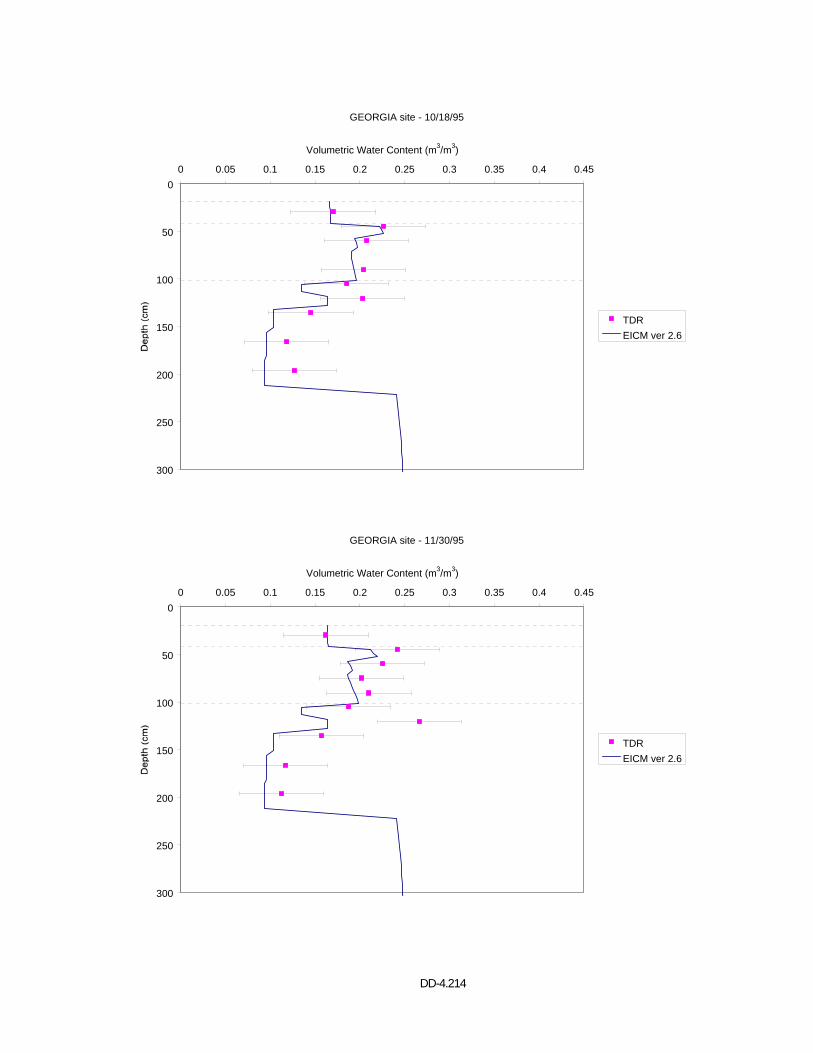
DD-4.214
GEORGIA site - 10/18/95
0
50
100
150
200
250
300
0 0.05 0.1 0.15 0.2 0.25 0.3 0.35 0.4 0.45
Volumetric Water Content (m3/m3)
TDREICM ver 2.6
GEORGIA site - 11/30/95
0
50
100
150
200
250
300
0 0.05 0.1 0.15 0.2 0.25 0.3 0.35 0.4 0.45
Volumetric Water Content (m3/m3)
TDREICM ver 2.6
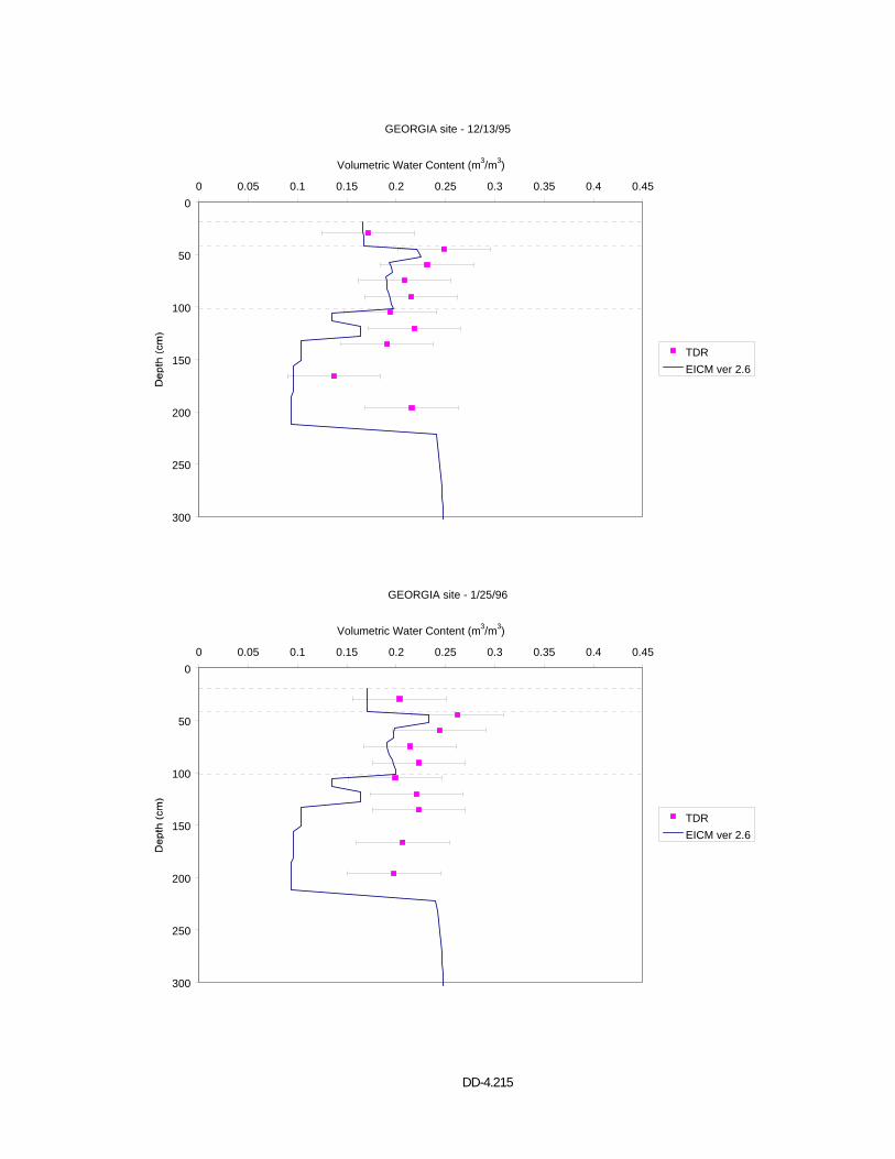
DD-4.215
GEORGIA site - 12/13/95
0
50
100
150
200
250
300
0 0.05 0.1 0.15 0.2 0.25 0.3 0.35 0.4 0.45
Volumetric Water Content (m3/m3)
TDREICM ver 2.6
GEORGIA site - 1/25/96
0
50
100
150
200
250
300
0 0.05 0.1 0.15 0.2 0.25 0.3 0.35 0.4 0.45
Volumetric Water Content (m3/m3)
TDREICM ver 2.6

DD-4.216
GEORGIA site - 3/25/96
0
50
100
150
200
250
300
0 0.05 0.1 0.15 0.2 0.25 0.3 0.35 0.4 0.45
Volumetric Water Content (m3/m3)
TDREICM ver 2.6
GEORGIA site - 4/22/96
0
50
100
150
200
250
300
0 0.05 0.1 0.15 0.2 0.25 0.3 0.35 0.4 0.45
Volumetric Water Content (m3/m3)
TDREICM ver 2.6
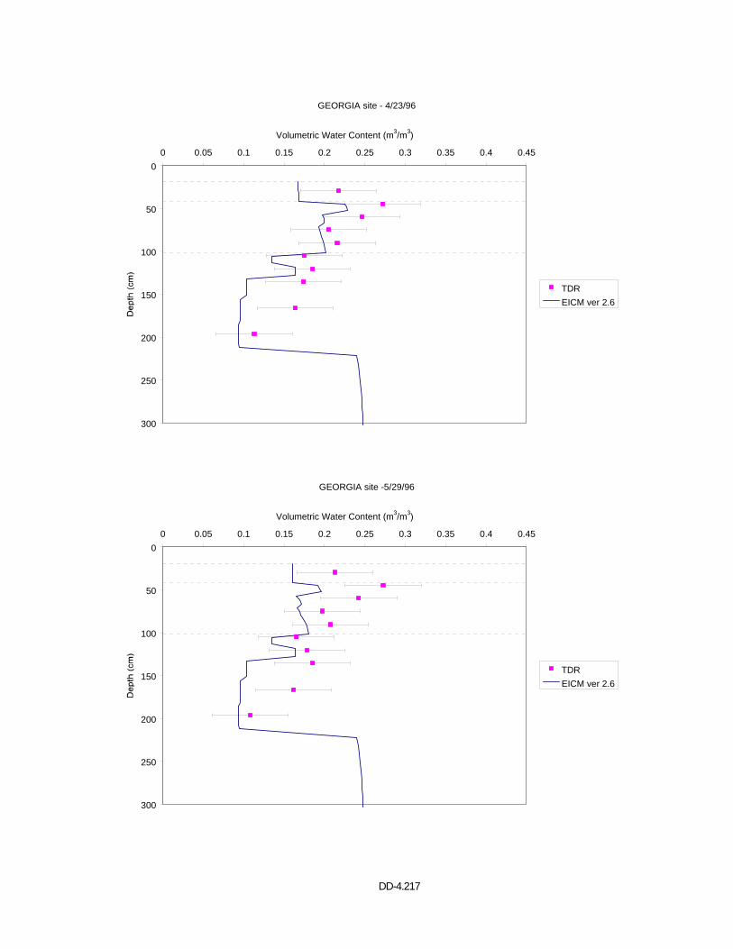
DD-4.217
GEORGIA site - 4/23/96
0
50
100
150
200
250
300
0 0.05 0.1 0.15 0.2 0.25 0.3 0.35 0.4 0.45
Volumetric Water Content (m3/m3)
TDREICM ver 2.6
GEORGIA site -5/29/96
0
50
100
150
200
250
300
0 0.05 0.1 0.15 0.2 0.25 0.3 0.35 0.4 0.45
Volumetric Water Content (m3/m3)
TDREICM ver 2.6
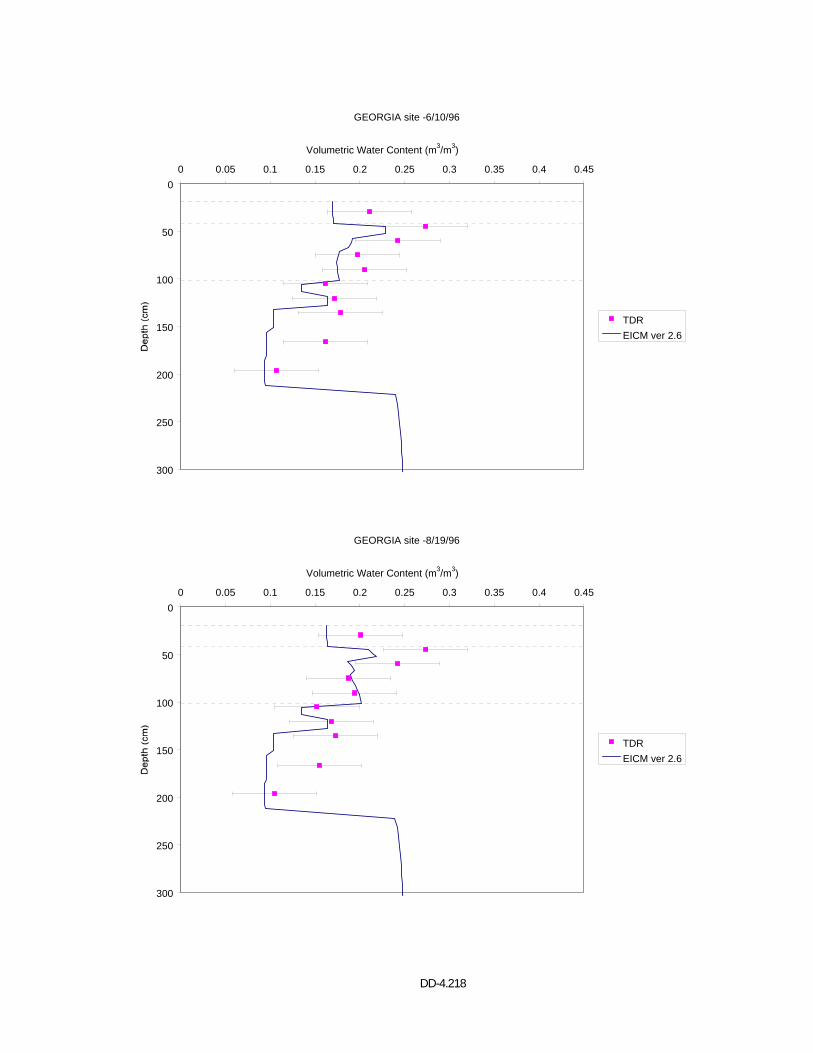
DD-4.218
GEORGIA site -6/10/96
0
50
100
150
200
250
300
0 0.05 0.1 0.15 0.2 0.25 0.3 0.35 0.4 0.45
Volumetric Water Content (m3/m3)
TDREICM ver 2.6
GEORGIA site -8/19/96
0
50
100
150
200
250
300
0 0.05 0.1 0.15 0.2 0.25 0.3 0.35 0.4 0.45
Volumetric Water Content (m3/m3)
TDREICM ver 2.6
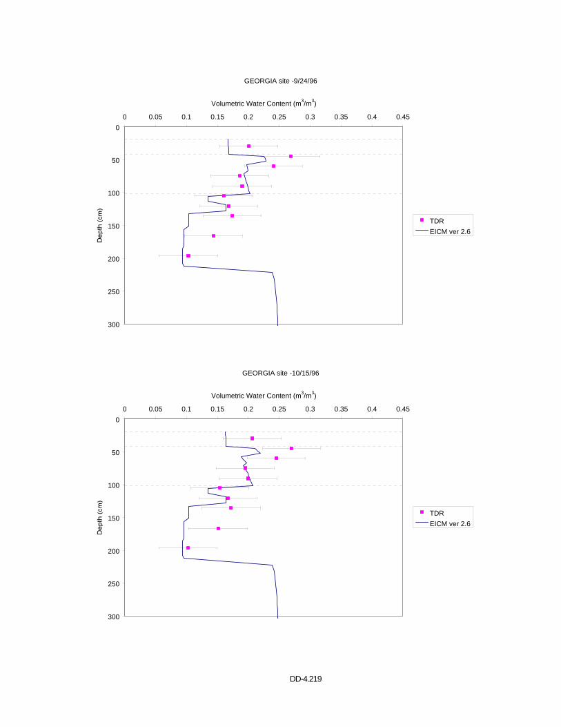
DD-4.219
GEORGIA site -9/24/96
0
50
100
150
200
250
300
0 0.05 0.1 0.15 0.2 0.25 0.3 0.35 0.4 0.45
Volumetric Water Content (m3/m3)
TDREICM ver 2.6
GEORGIA site -10/15/96
0
50
100
150
200
250
300
0 0.05 0.1 0.15 0.2 0.25 0.3 0.35 0.4 0.45
Volumetric Water Content (m3/m3)
TDREICM ver 2.6

DD-4.220
APPENDIX P VOLUMETRIC WATER CONTENT PROFILES
COLORADO (81053)
EICM – Version 2.6
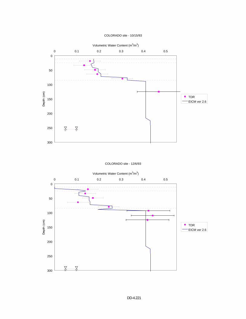
DD-4.221
COLORADO site - 10/15/93
0
50
100
150
200
250
300
0 0.1 0.2 0.3 0.4 0.5
Volumetric Water Content (m3/m3)
TDREICM ver 2.6
COLORADO site - 12/6/93
0
50
100
150
200
250
300
0 0.1 0.2 0.3 0.4 0.5
Volumetric Water Content (m3/m3)
TDREICM ver 2.6
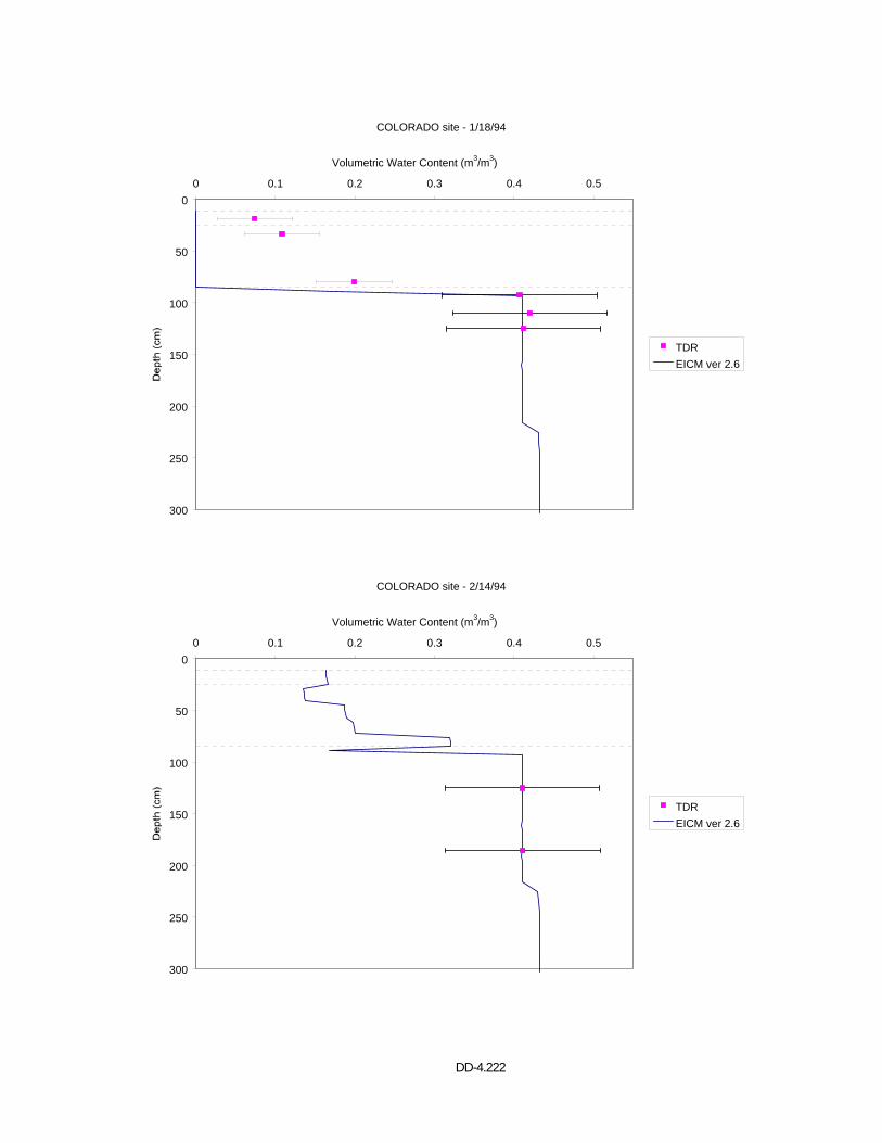
DD-4.222
COLORADO site - 1/18/94
0
50
100
150
200
250
300
0 0.1 0.2 0.3 0.4 0.5
Volumetric Water Content (m3/m3)
TDREICM ver 2.6
COLORADO site - 2/14/94
0
50
100
150
200
250
300
0 0.1 0.2 0.3 0.4 0.5
Volumetric Water Content (m3/m3)
TDREICM ver 2.6
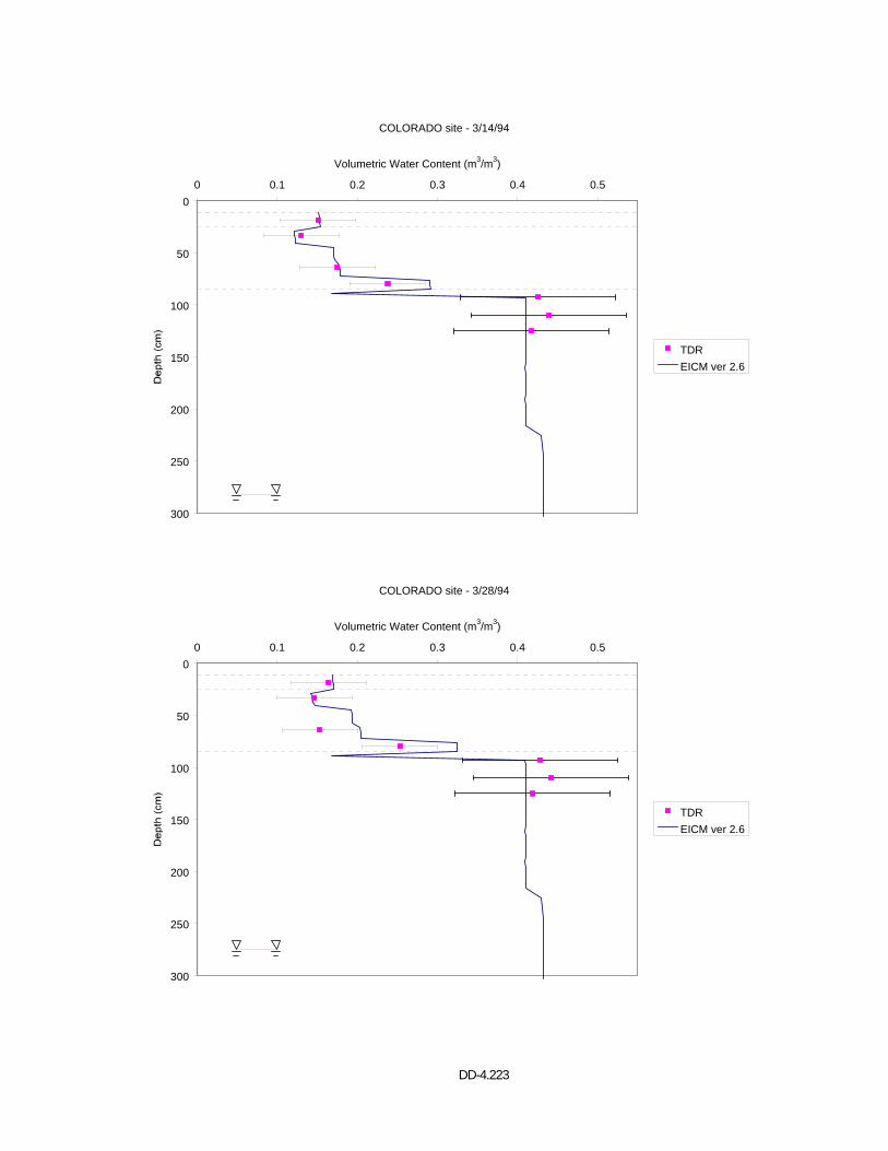
DD-4.223
COLORADO site - 3/14/94
0
50
100
150
200
250
300
0 0.1 0.2 0.3 0.4 0.5
Volumetric Water Content (m3/m3)
TDREICM ver 2.6
COLORADO site - 3/28/94
0
50
100
150
200
250
300
0 0.1 0.2 0.3 0.4 0.5
Volumetric Water Content (m3/m3)
TDREICM ver 2.6
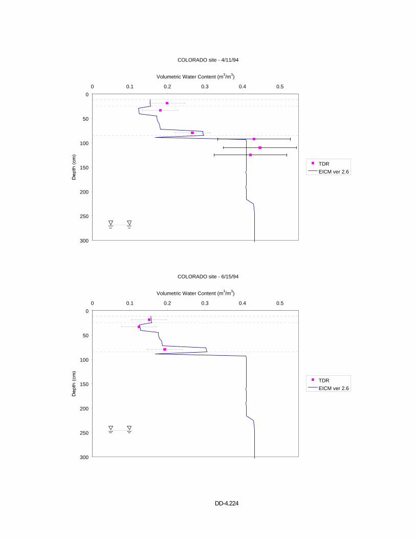
DD-4.224
COLORADO site - 4/11/94
0
50
100
150
200
250
300
0 0.1 0.2 0.3 0.4 0.5
Volumetric Water Content (m3/m3)
TDREICM ver 2.6
COLORADO site - 6/15/94
0
50
100
150
200
250
300
0 0.1 0.2 0.3 0.4 0.5
Volumetric Water Content (m3/m3)
TDREICM ver 2.6
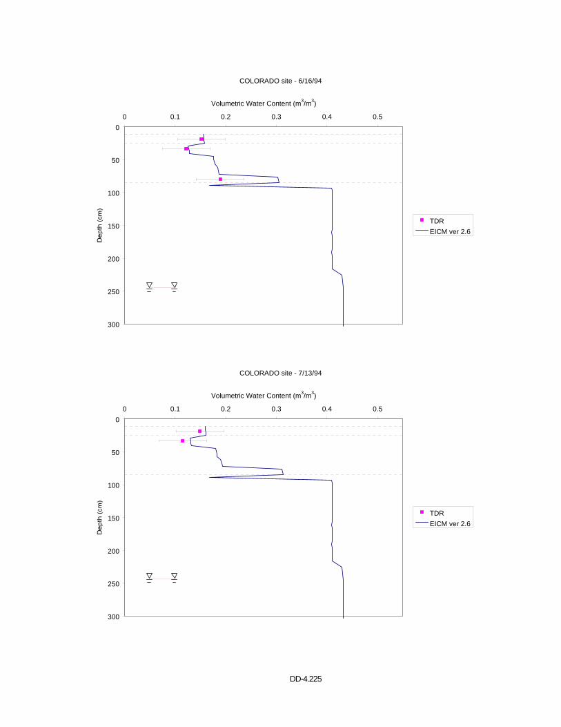
DD-4.225
COLORADO site - 6/16/94
0
50
100
150
200
250
300
0 0.1 0.2 0.3 0.4 0.5
Volumetric Water Content (m3/m3)
TDREICM ver 2.6
COLORADO site - 7/13/94
0
50
100
150
200
250
300
0 0.1 0.2 0.3 0.4 0.5
Volumetric Water Content (m3/m3)
TDREICM ver 2.6
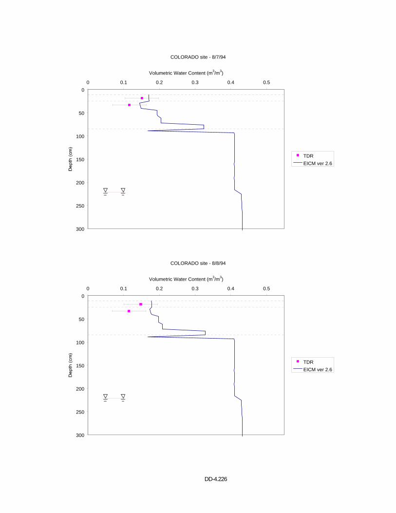
DD-4.226
COLORADO site - 8/7/94
0
50
100
150
200
250
300
0 0.1 0.2 0.3 0.4 0.5
Volumetric Water Content (m3/m3)
TDREICM ver 2.6
COLORADO site - 8/8/94
0
50
100
150
200
250
300
0 0.1 0.2 0.3 0.4 0.5
Volumetric Water Content (m3/m3)
TDREICM ver 2.6
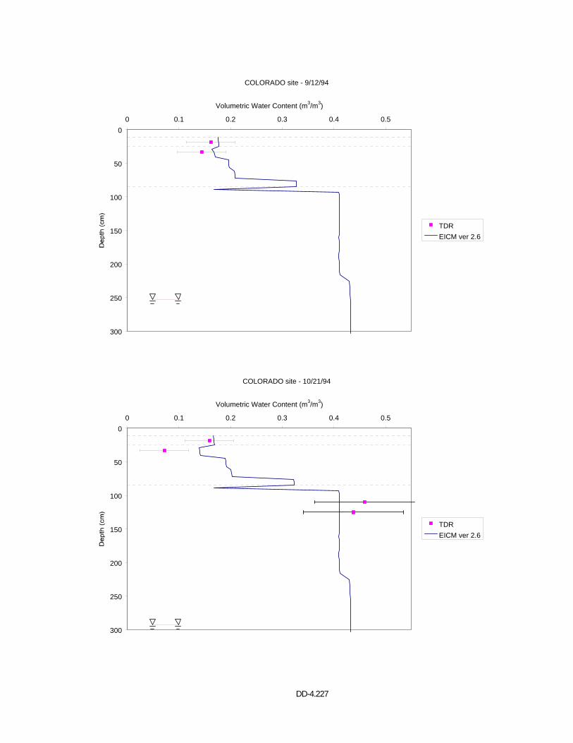
DD-4.227
COLORADO site - 9/12/94
0
50
100
150
200
250
300
0 0.1 0.2 0.3 0.4 0.5
Volumetric Water Content (m3/m3)
TDREICM ver 2.6
COLORADO site - 10/21/94
0
50
100
150
200
250
300
0 0.1 0.2 0.3 0.4 0.5
Volumetric Water Content (m3/m3)
TDREICM ver 2.6
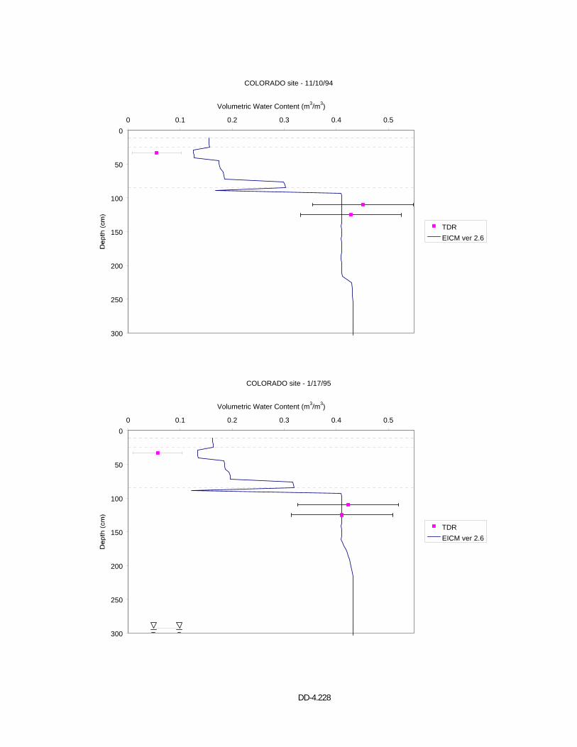
DD-4.228
COLORADO site - 11/10/94
0
50
100
150
200
250
300
0 0.1 0.2 0.3 0.4 0.5
Volumetric Water Content (m3/m3)
TDREICM ver 2.6
COLORADO site - 1/17/95
0
50
100
150
200
250
300
0 0.1 0.2 0.3 0.4 0.5
Volumetric Water Content (m3/m3)
TDREICM ver 2.6
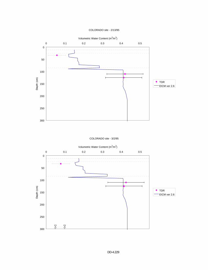
DD-4.229
COLORADO site - 2/13/95
0
50
100
150
200
250
300
0 0.1 0.2 0.3 0.4 0.5
Volumetric Water Content (m3/m3)
TDREICM ver 2.6
COLORADO site - 3/2/95
0
50
100
150
200
250
300
0 0.1 0.2 0.3 0.4 0.5
Volumetric Water Content (m3/m3)
TDREICM ver 2.6
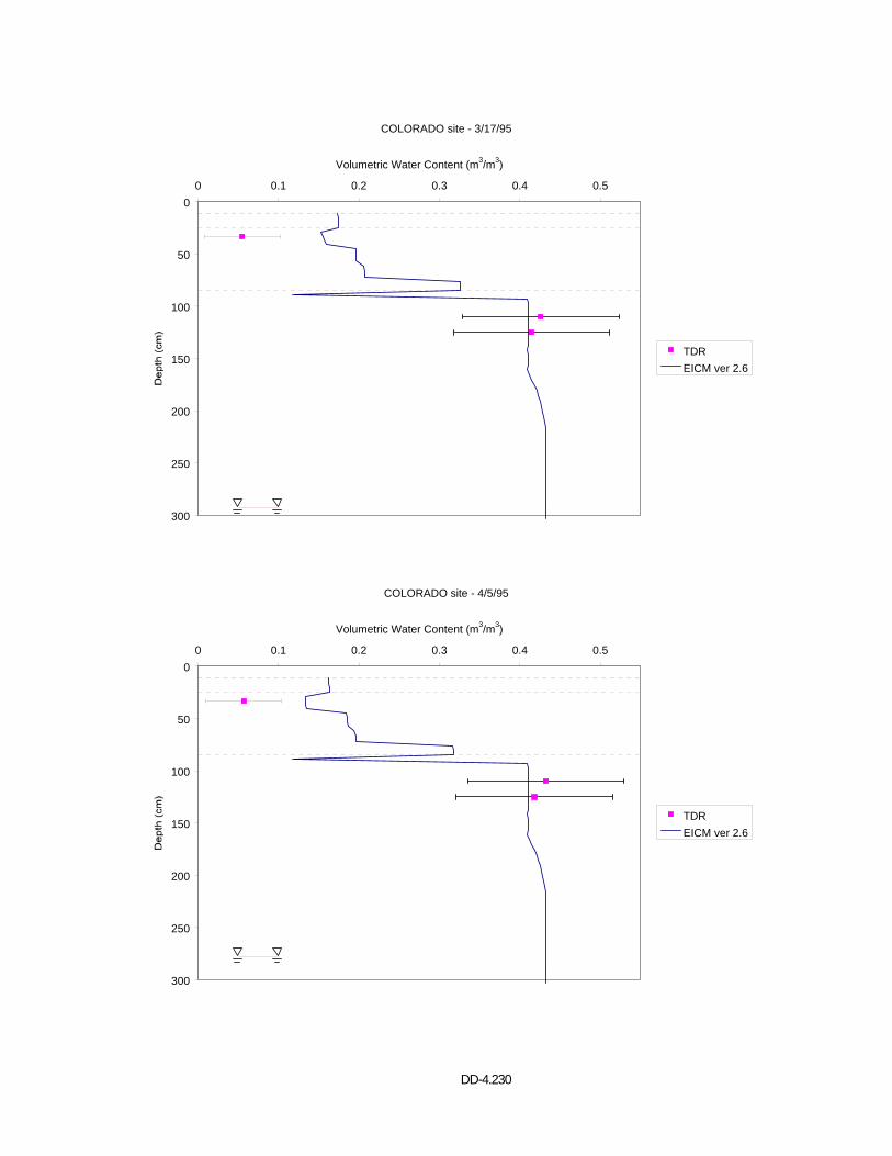
DD-4.230
COLORADO site - 3/17/95
0
50
100
150
200
250
300
0 0.1 0.2 0.3 0.4 0.5
Volumetric Water Content (m3/m3)
TDREICM ver 2.6
COLORADO site - 4/5/95
0
50
100
150
200
250
300
0 0.1 0.2 0.3 0.4 0.5
Volumetric Water Content (m3/m3)
TDREICM ver 2.6
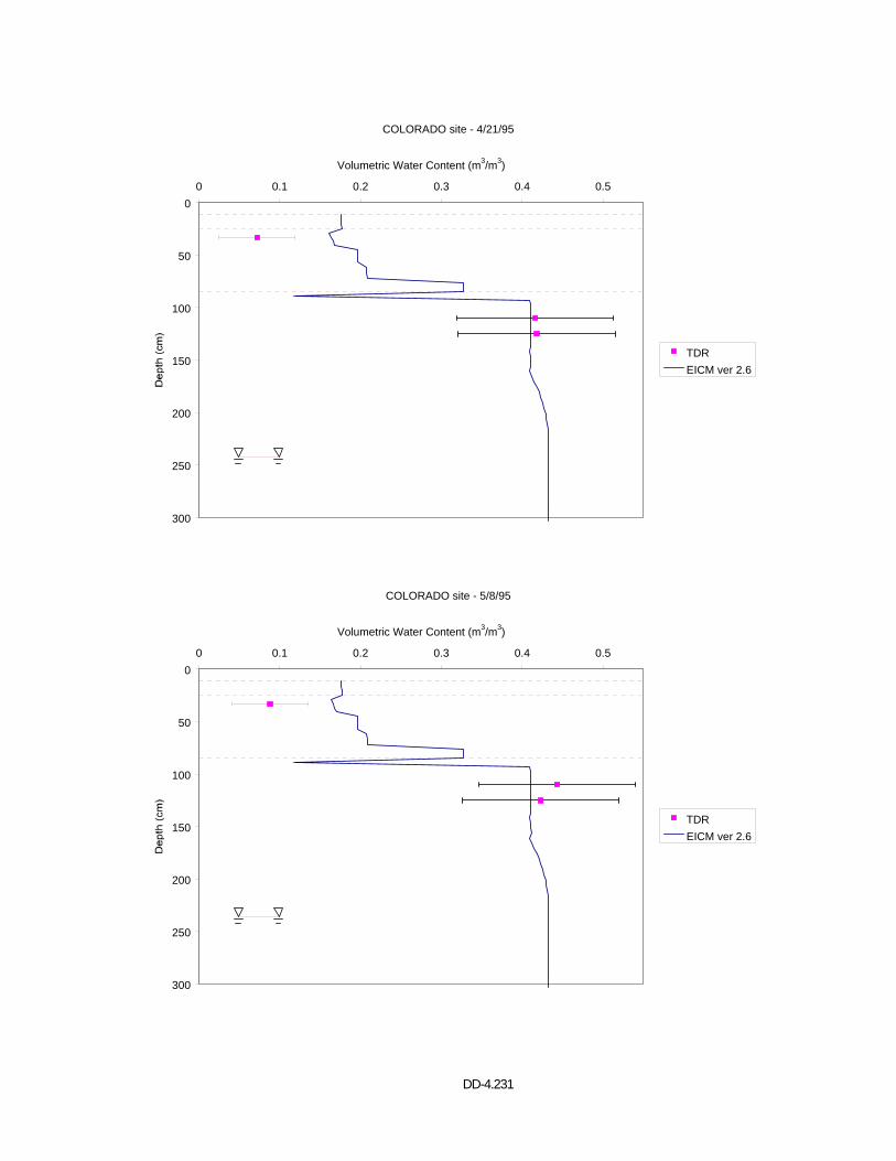
DD-4.231
COLORADO site - 4/21/95
0
50
100
150
200
250
300
0 0.1 0.2 0.3 0.4 0.5
Volumetric Water Content (m3/m3)
TDREICM ver 2.6
COLORADO site - 5/8/95
0
50
100
150
200
250
300
0 0.1 0.2 0.3 0.4 0.5
Volumetric Water Content (m3/m3)
TDREICM ver 2.6

DD-4.232
APPENDIX Q VOLUMETRIC WATER CONTENT PROFILES
ARIZONA (41024)
EICM – Version 2.6
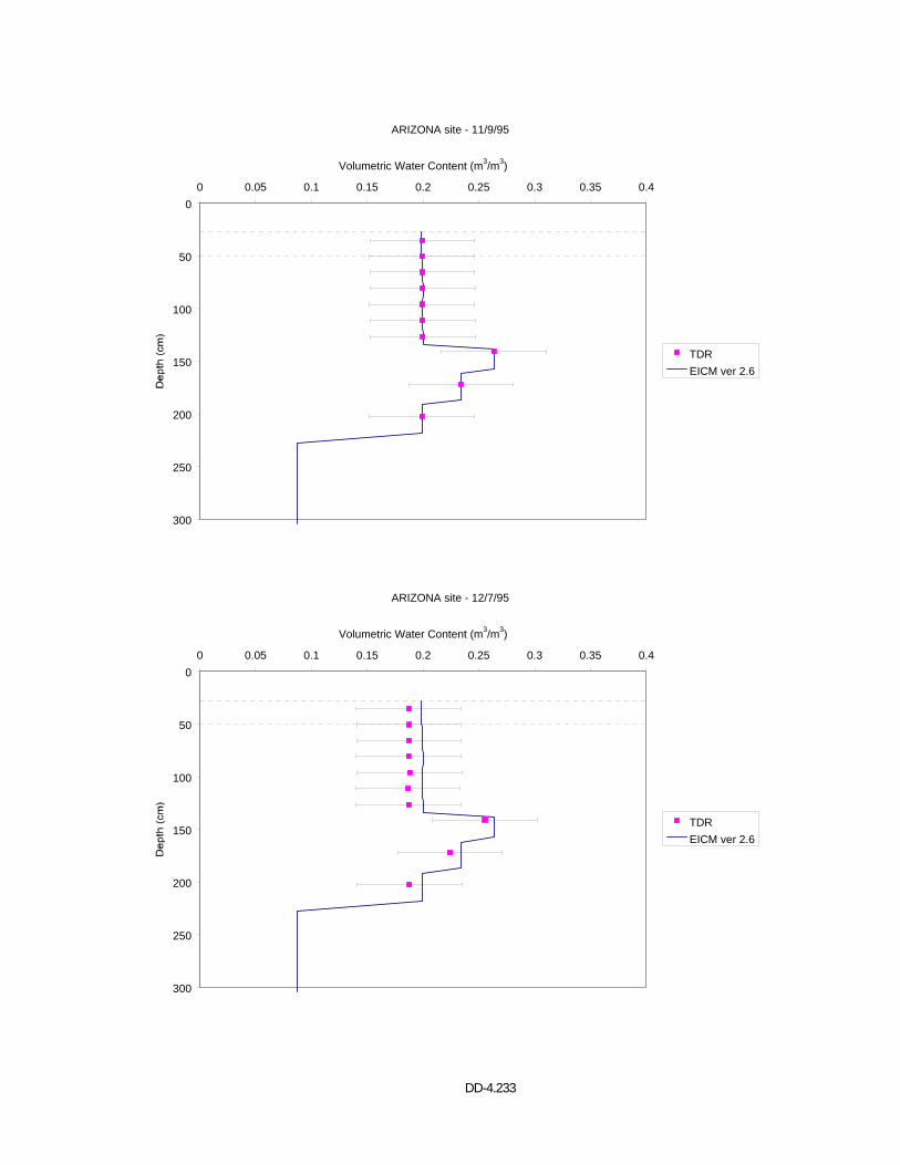
DD-4.233
ARIZONA site - 11/9/95
0
50
100
150
200
250
300
0 0.05 0.1 0.15 0.2 0.25 0.3 0.35 0.4
Volumetric Water Content (m3/m3)
TDREICM ver 2.6
ARIZONA site - 12/7/95
0
50
100
150
200
250
300
0 0.05 0.1 0.15 0.2 0.25 0.3 0.35 0.4
Volumetric Water Content (m3/m3)
TDREICM ver 2.6
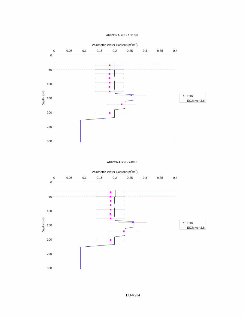
DD-4.234
ARIZONA site - 1/11/96
0
50
100
150
200
250
300
0 0.05 0.1 0.15 0.2 0.25 0.3 0.35 0.4
Volumetric Water Content (m3/m3)
TDREICM ver 2.6
ARIZONA site - 2/8/96
0
50
100
150
200
250
300
0 0.05 0.1 0.15 0.2 0.25 0.3 0.35 0.4
Volumetric Water Content (m3/m3)
TDREICM ver 2.6
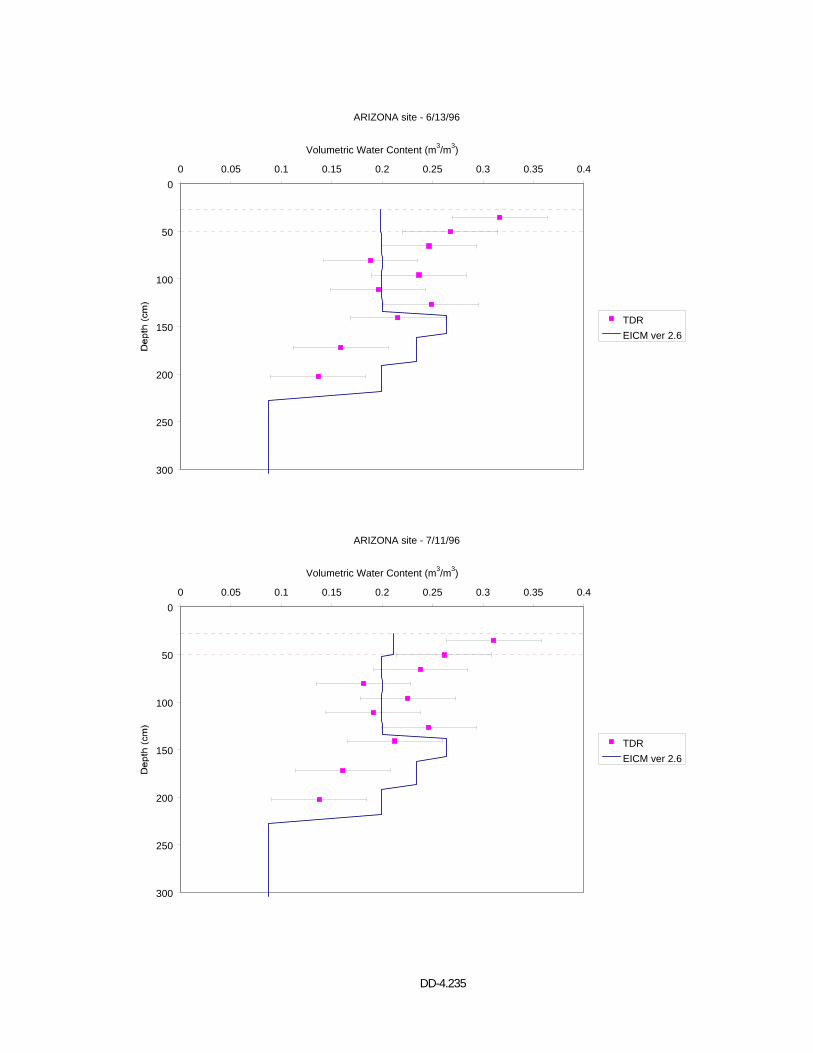
DD-4.235
ARIZONA site - 6/13/96
0
50
100
150
200
250
300
0 0.05 0.1 0.15 0.2 0.25 0.3 0.35 0.4
Volumetric Water Content (m3/m3)
TDREICM ver 2.6
ARIZONA site - 7/11/96
0
50
100
150
200
250
300
0 0.05 0.1 0.15 0.2 0.25 0.3 0.35 0.4
Volumetric Water Content (m3/m3)
TDREICM ver 2.6
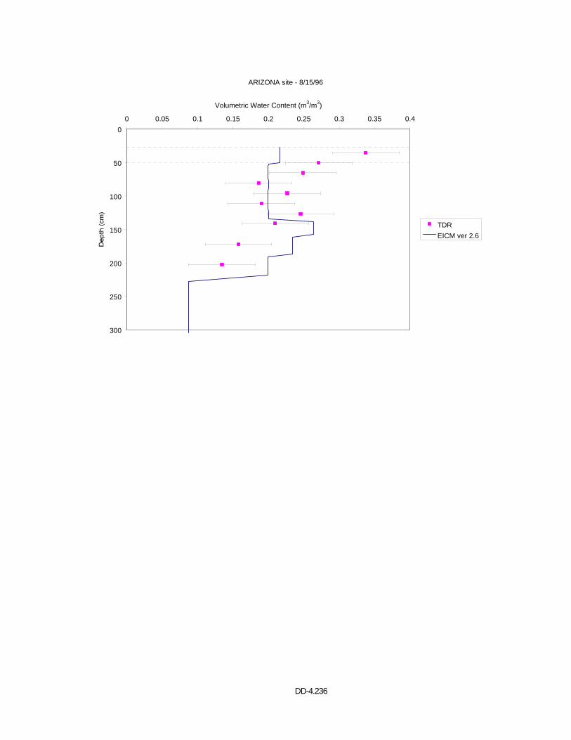
DD-4.236
ARIZONA site - 8/15/96
0
50
100
150
200
250
300
0 0.05 0.1 0.15 0.2 0.25 0.3 0.35 0.4
Volumetric Water Content (m3/m3)
TDREICM ver 2.6

DD-4.237
APPENDIX R VOLUMETRIC WATER CONTENT PROFILES
TEXAS (481077)
EICM – Version 2.6
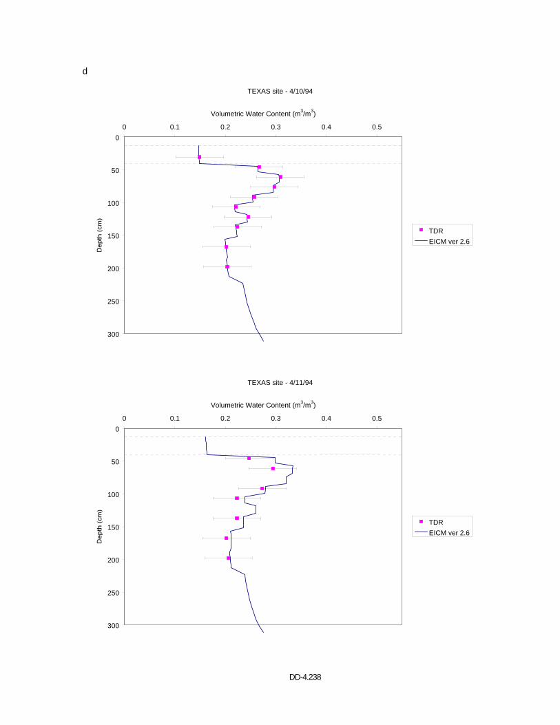
DD-4.238
d
TEXAS site - 4/10/94
0
50
100
150
200
250
300
0 0.1 0.2 0.3 0.4 0.5
Volumetric Water Content (m3/m3)
TDREICM ver 2.6
TEXAS site - 4/11/94
0
50
100
150
200
250
300
0 0.1 0.2 0.3 0.4 0.5
Volumetric Water Content (m3/m3)
TDREICM ver 2.6
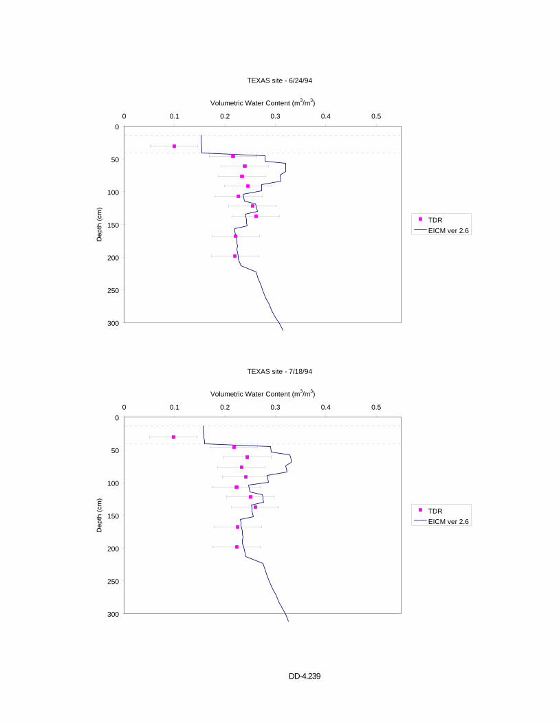
DD-4.239
TEXAS site - 6/24/94
0
50
100
150
200
250
300
0 0.1 0.2 0.3 0.4 0.5
Volumetric Water Content (m3/m3)
TDREICM ver 2.6
TEXAS site - 7/18/94
0
50
100
150
200
250
300
0 0.1 0.2 0.3 0.4 0.5
Volumetric Water Content (m3/m3)
TDREICM ver 2.6
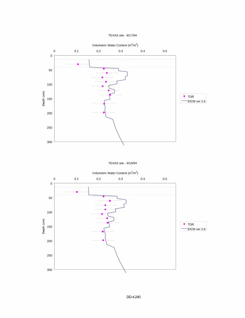
DD-4.240
TEXAS site - 8/17/94
0
50
100
150
200
250
300
0 0.1 0.2 0.3 0.4 0.5
Volumetric Water Content (m3/m3)
TDREICM ver 2.6
TEXAS site - 9/19/94
0
50
100
150
200
250
300
0 0.1 0.2 0.3 0.4 0.5
Volumetric Water Content (m3/m3)
TDREICM ver 2.6

DD-4.241
TEXAS site - 10/24/94
0
50
100
150
200
250
300
0 0.1 0.2 0.3 0.4 0.5
Volumetric Water Content (m3/m3)
TDREICM ver 2.6
TEXAS site - 11/16/94
0
50
100
150
200
250
300
0 0.1 0.2 0.3 0.4 0.5
Volumetric Water Content (m3/m3)
TDREICM ver 2.6
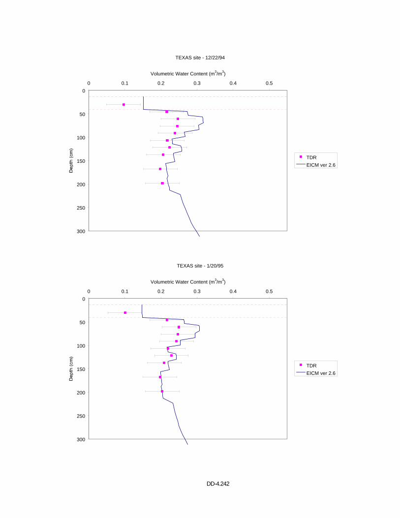
DD-4.242
TEXAS site - 12/22/94
0
50
100
150
200
250
300
0 0.1 0.2 0.3 0.4 0.5
Volumetric Water Content (m3/m3)
TDREICM ver 2.6
TEXAS site - 1/20/95
0
50
100
150
200
250
300
0 0.1 0.2 0.3 0.4 0.5
Volumetric Water Content (m3/m3)
TDREICM ver 2.6
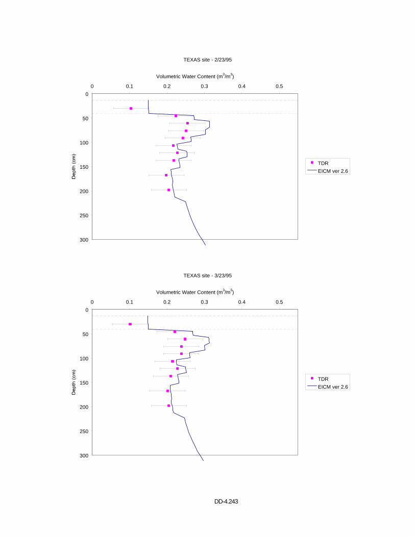
DD-4.243
TEXAS site - 2/23/95
0
50
100
150
200
250
300
0 0.1 0.2 0.3 0.4 0.5
Volumetric Water Content (m3/m3)
TDREICM ver 2.6
TEXAS site - 3/23/95
0
50
100
150
200
250
300
0 0.1 0.2 0.3 0.4 0.5
Volumetric Water Content (m3/m3)
TDREICM ver 2.6
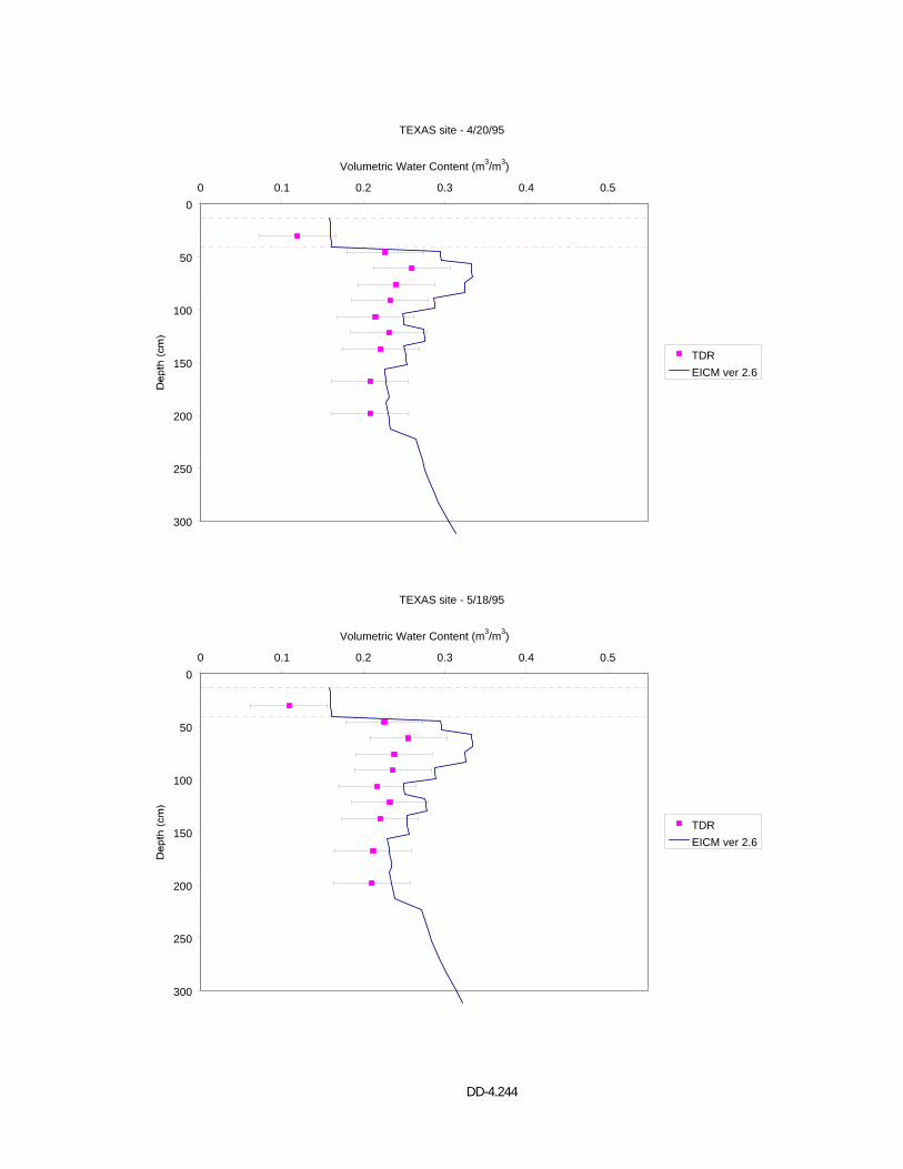
DD-4.244
TEXAS site - 4/20/95
0
50
100
150
200
250
300
0 0.1 0.2 0.3 0.4 0.5
Volumetric Water Content (m3/m3)
TDREICM ver 2.6
TEXAS site - 5/18/95
0
50
100
150
200
250
300
0 0.1 0.2 0.3 0.4 0.5
Volumetric Water Content (m3/m3)
TDREICM ver 2.6
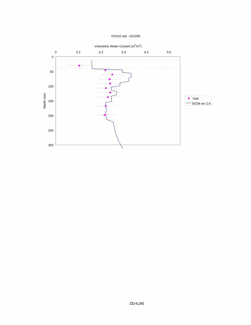
DD-4.245
TEXAS site - 6/22/95
0
50
100
150
200
250
300
0 0.1 0.2 0.3 0.4 0.5
Volumetric Water Content (m3/m3)
TDREICM ver 2.6
DD-4.246
REFERENCES
AASHTO Designation M 147-65. (1990). "Standard Specification for Materials for
Aggregate and Soil-Aggregate Subbase, Base and Surface Courses". AASHTO. pp. 157-
158.
DataPave 2.0. (1999). U.S. Department of Transportation, Federal Highway
Administration, September 1999.
Dunn, R. J. and Palmer, B. S. (1994). "Lessons Learned from the Application of Standard
Test Methods for Field and Laboratory Hydraulic Conductivity Measurement". Hydraulic
Conductivity and Waste Contaminant Transport in Soil, ASTM STP 1142. D. E. Daniel and
S. J. Trautwein, editors. American Society for Testing and Materials, Philadelphia.
Escario, V. and Juca, J. (1989). “Strength and Deformation of Partly Saturated Soils”.
Proceedings of the Twelfth International Conference on Soil Mechanics and Foundation
Engineering, Rio de Janeiro, Vol. 3, pp. 43-46.
Fredlund, D. G. (1995). “Prediction of Unsaturated Soil Functions Using the Soil-Water
Characteristic Curve”. Proceedings of the Bength B. Broms Symposium on Geotechnical
Engineering, Singapore, 13-15 December, pp. 113-133.
Fredlund, D. G., and Xing, A. (1994). “Equations for the Soil-Water Characteristic Curve”.
Canadian Geotechnical Journal, Vol. 31, No. 4, pp. 521 - 532.
Fredlund, D. G., Vanapalli, S. K., Xing, A., and Pufalel, D. E. (1995). “Predicting the Shear
Strength Function for Unsaturated Soils Using the Soil-Water Characteristic Curve”. In:
Unsaturated Soils, Alonso and Delage, editors.
Fredlund, D. G., Xing, A., and Huang, S. (1994). “Predicting the Permeability Function for
Unsaturated Soils Using the Soil-Water Characteristic Curve”. Canadian Geotechnical
Journal, Vol 3. No. 4, pp. 533 - 546.
Fredlund, D. G., Xing, A., Fredlund, M and Barbour, S. L. (1995). “The Relationship of the
Unsaturated Shear Strength to the Soil-Water Characteristic Curve”. Canadian
Geotechnical Journal, Vol. 32, pp. 440-448.
DD-4.247
Gan, J. K. M, Fredlund, D. G., and Rahardjo, H. (1988). "Determination of the Shear
Strength Parameters of an Unsaturated Soil Using the Direct Shear Test". Canadian
Geotechnical Journal. Vol. 25, pp. 500-510.
Ghosh, R. K. (1980). “Estimation of Soil-Moisture Characteristics from Mechanical
Properties of Soils”. Soil Science, Vol. 130, No. 2, pp. 60-63.
Haverkamp, R. and Parlange, J. Y. (1986). “Predicting the Water-Retention Curve from
Particle-Size Distribution: 1. Sandy Soils without Organic Matter”. Soil Science, Vol. 142,
No. 6, pp. 325-339.
Holtz, R. D. and Kovacs, W. D. (1981). An Introduction to Geotechnical Engineering.
Prentice-Hall, Inc.
Houston, W. N., Houston, S. L., Zapata, C., Manepally, C., and Lawrence, C. (1999).
"Influence of Compressibility on Use and Interpretation of Soil Water Characteristic
Curves". Proceedings of the XI Panamerican Conference on Soil Mechanics and
Geotechnical Engineering. Foz do Iguassu, Brazil. pp. 947-954.
Jiang, Y. Jane and Tayabji , Shiraz D. (1999). Analysis of Time Domain Reflectometry
Data From LTPP Seasonal Monitoring Program Test Sections. Final Report, FHWA-RD-
99-115, July 1999.
Klemunes, J. A. (1995). Determining Soil Volumetric Moisture Using Time Domain
Reflectometry. Master's Thesis. Faculty of the Graduate School, University of Maryland.
Krahn, J., and Fredlund, D. G. (1972). “On Total, Matric and Osmotic Suction”. Soil
Science, Vol. 114, No. 5, pp. 339 - 347.
Larson, G. and Dempsey, B. J. (1997). Enhanced Integrated Climatic Model. Version 2.0.
University of Illinois at Urbana-Champaign and Newmark Civil Engineering Laboratory.
Report No. DTFA MN/DOT 72114.
Leong, E. C., and Rahardjo, H., (1996). “A Review on Soil-Water Characteristic Curve
Equations”. Geotechnical Research Report, NTU/GT/96-5, Nanyang Technological
University, NTU-PWD Geotechnical Research Centre, Singapore.
Livneh, M., Kinsky, J. and Zaslavsky, D. (1970). “Correlation of Suction Curves with the
Plasticity Index of Soils”. Journal of Materials, JMLSA, Vol. 5, No. 1, March 1970, pp. 209-
220.
DD-4.248
Lytton, R. L., Pufahl, D. E., Michalak, C. H., Liang, H. S., and Dempsey, B. J. (1990). An
Integrated Model of the Climatic Effects on Pavements. Texas Transportation Institute,
Texas A&M University. Report No. FHWA-RD-90-033, Federal Highway Administration,
McLean, VA.
Marinho, F. A. M. and Stuermer, M. M. M. (1998). "Aspects of the Storage Capacity of a
Compacted Residual Soil". Proceedings of the Second International Conference on
Unsaturated Soils. Vol. 1. Beijing, China. August, 27-30.
Oberg AL. and Sallfors G. (1997). "Determination of Shear Strength Parameters of
Unsaturated Silts and Sands Based on the Water Retention Curve". Geotechnical Testing
Journal. Vol. 20, No. 1. pp. 40−48.
Rahardjo, H., Chang, H. M. F. and Lim, T. T. (1995). “Shear Strength and in Situ Matric
Suction of a Residual Soil”. In: Unsaturated Soils. Alonso & Delage, editors. pp. 637-643.
Rohm, S. A. and Vilar, O. M. (1995). “Shear Strength of an Unsaturated Sandy Soil”. In:
Unsaturated Soils. Alonso & Delage, editors. pp. 189-193.
Sabbagh, A. (1995). “Prediction of Volume Change in Unsaturated Clays”. In: Unsaturated
Soils. Alonso & Delage, editors. pp. 791-796.
SoilVision User’s Guide. (1997). Version 1.2 [Computer software]. SoilVision Systems,
Ltd. Saskatoon, Saskatchewan, Canada.
Vanapalli, S K., Sillers, W. S. and Fredlund, M. D. (1998). "The Meaning and Relevance of
Residual State to Unsaturated Soils". 51st Canadian Geotechnical Conference. Edmonton,
Albert, October 4-7, pp. 1-8.
Witczak, M. W., Yau, A. (1997). Development of the Resilient and Plastic Response
Parameters of Selected Unbound Base/Subbase/Subgrade Materials, Vol. 1.
Witczak, M. W., Andrei, D., and Houston, W. N. (2000). "Resilient Modulus as Function of
Soil Moisture - Summary of Predictive Models". Development of the 2002 Guide for the
Development of New and Rehabilitated Pavement Structures, NCHRP 1-37 A, an Inter
Team Technical Report. Vol. 1.
Witczak, M. W., Houston, W. N., and Andrei, D., (2000). "A Study of the Expected
Changes in Resilient Modulus of the Unbound Layers with Changes in Moisture for 10
LTPP Sites". Development of the 2002 Guide for the Development of New and

DD-4.249
Rehabilitated Pavement Structures, NCHRP 1-37 A, an Inter Team Technical Report.
Vol. 2.
Zapata, C. E. (1999). Uncertainty in Soil-Water Characteristic Curve and Impacts on
Unsaturated Shear Strength Predictions. Ph.D. Dissertation, Arizona State University,
Tempe, United States.