2900

User Manual

(5.xx Code)

Larson•Davis Laboratories 1681 W 820 N Provo, UT 84601 November 26, 1997

LARSON•DAVISLABORATORIES

2900 Manual

Larson•Davis Laboratories

Larson•Davis Incorporated1681 West 820 NorthProvo, Utah 84601801-375-0177

Copyright

Copyright

1993 by Larson•Davis Incorporated. This man-ual and the hardware described in it are copyrighted, with allrights reserved. The manual may not be copied in whole or inpart for any use without prior written consent of Lar-son•Davis Inc.

Trademarks

MS-DOS is a registered trademark of Microsoft Corp.

Warranty

Larson•Davis warrants this product to be free from defects inmaterial and workmanship for two years from the date of orig-inal purchase.

During the first year of the warranty period, Larson•Davis willrepair, or at its option, replace any defective component(s)without charge for parts or labor. During the second year of thewarranty period, there will be no charge for replacement parts.

For customers within the continental United States, service isprovided for instruments returned, freight prepaid, to an autho-rized service center. The product will be returned freight pre-paid.

For international customers, please contact your exclusive Lar-son•Davis representative for details on local service and ship-ping arrangements.

The Larson•Davis warranty applies only to products manufac-tured by Larson•Davis Inc., and does not include batteries.Accessories and items not manufactured by Larson•Davis Inc.are covered by the warranty of the original equipment manufac-turer.

Product defects caused by misuse, accidents, or user modifica-tion are not covered by this warranty.

No other warranties are expressed or implied, Larson•Davis isnot responsible for consequential damages.

1

TABLE OF CONTENTS

Chapter 1 Introduction.......................................................................................................1-1

Front Panel Controls .................................................................................................................... 1-2

Dedicated Hardkeys ................................................................................................................ 1-2

ASCII Hardkeys ....................................................................................................................... 1-3

Softkeys ................................................................................................................................... 1-4

The Arrow Keys and associated Hardkeys .................................................................................. 1-5

Cursor Control ......................................................................................................................... 1-5

Range Control.......................................................................................................................... 1-5

Instrument Boot-up Procedure ..................................................................................................... 1-6

Resetting RAM............................................................................................................................. 1-7

Upgrading Software ..................................................................................................................... 1-7

Display Control............................................................................................................................. 1-7

Setting Backlight and Viewing Angle ....................................................................................... 1-7

Beeper Control ............................................................................................................................. 1-9

Color Monitor................................................................................................................................ 1-9

Power Supply ............................................................................................................................... 1-9

Battery Power .......................................................................................................................... 1-9

DC Power .............................................................................................................................. 1-10

Charging Batteries ................................................................................................................. 1-10

Microphone Connection ............................................................................................................. 1-10

Alternative Inputs ....................................................................................................................... 1-11

Accelerometers with Internal Electronics............................................................................... 1-11

Charge-coupled Accelerometers ........................................................................................... 1-11

Direct Voltage Inputs ............................................................................................................. 1-11

AC Outputs................................................................................................................................. 1-11

Single Channel Standard Analysis Mode .............................................................................. 1-11

Dual Channel Standard, Cross or Intensity Analysis Mode ................................................... 1-12

SLM Mode ............................................................................................................................. 1-12

Front Panel Display Format ....................................................................................................... 1-12

Messages Displayed on the Left of the Screen ..................................................................... 1-12Location A, Displayed Data Type ...................................................................................... 1-13Location B, vsREF Display Status and Statistics .............................................................. 1-13Location C, Autostore Status............................................................................................. 1-13Location D, Frequency Trigger Status............................................................................... 1-13Location E, Control Status................................................................................................. 1-14Location F, Active File ....................................................................................................... 1-14

Messages Displayed on the Right of the Screen................................................................... 1-14Note Display Line .............................................................................................................. 1-14Location A, Units Name..................................................................................................... 1-14Location B, Digital Differentiation or Integration and Bandwidth Compensation Status.... 1-14Location C, Digital Display Weighting and Status of Time Trigger .................................... 1-15Location D, Run Time........................................................................................................ 1-15Location E, Averaging Type .............................................................................................. 1-15Location F, Averaging Time............................................................................................... 1-15Location G, Input Type ...................................................................................................... 1-16

2900 MANUAL

2

Location H, Analog Input Weighting .................................................................................. 1-16Location I, Frequency Range between Highpass/Lowpass Filters with Linear Weighting Selected1-16Location J, Operational Status .......................................................................................... 1-16Location K, Date and Time................................................................................................ 1-16Location L, Filter Status and Frequency at the Cursor Position ........................................ 1-16Location M, Channel and Parameter Information.............................................................. 1-17Location N, Amplitude Data corresponding to Cursor Position ......................................... 1-18Location O, Loudness Level .............................................................................................. 1-19Location P, Data from Tacho or Order Tracking Boards ................................................... 1-19Location Q, Status of the Horizontal Arrow Keys .............................................................. 1-19

Noise Floor ............................................................................................................................ 1-20

Model 2800 and 2900 Specifications ......................................................................................... 1-21

Input....................................................................................................................................... 1-21Analog Input Filters............................................................................................................ 1-21

Digital Characteristics ................................................................................................................ 1-21

Digitization ............................................................................................................................. 1-21

Anti-aliasing ........................................................................................................................... 1-21

Detector ................................................................................................................................. 1-21

Dynamic Range ..................................................................................................................... 1-22

Amplitude Stability ................................................................................................................. 1-22

Amplitude Linearity ................................................................................................................ 1-22

Filters ......................................................................................................................................... 1-22

Octave and Fractional Octave ............................................................................................... 1-22

FFT............................................................................................................................................. 1-22

Zoom Capability..................................................................................................................... 1-22

Time Domain Windows (FFT analysis).................................................................................. 1-23

Measured And Displayed Parameters ....................................................................................... 1-23

Sound Level Meter Mode (2800/2900) .................................................................................. 1-23

Standard Analysis Mode (2800/2900), Octave and FFT ....................................................... 1-23

Intensity Analysis Mode (2900 only), Octave and FFT .......................................................... 1-23

Cross Channel Analysis Mode (2900 only), FFT ................................................................... 1-23

Cross Channel Analysis Mode (2900 only, Octave Bandwidths............................................ 1-24

Digital Averaging ........................................................................................................................ 1-24

Octave Bandwidths................................................................................................................ 1-24

FFT Bandwidths..................................................................................................................... 1-24

Digital Display Weighting ........................................................................................................... 1-24

For Standard (2800/2900) and Intensity Analysis (2900 only) Modes;.................................. 1-24

Units ........................................................................................................................................... 1-25

Memory ...................................................................................................................................... 1-25

CMOS Non-volatile: ............................................................................................................... 1-25

Floppy Disk ............................................................................................................................ 1-25

Noise Generator......................................................................................................................... 1-25

Digital Output and Control.......................................................................................................... 1-25

Analog Outputs ...................................................................................................................... 1-26

Display Characteristics............................................................................................................... 1-26

Internal LCD........................................................................................................................... 1-26

External Color Display (Color Video Adapter required) ......................................................... 1-26

2900 MANUAL

3

Environmental ............................................................................................................................ 1-26

Physical...................................................................................................................................... 1-26

Power ......................................................................................................................................... 1-27

Battery Power ........................................................................................................................ 1-27

DC Power .............................................................................................................................. 1-27

2900 Block Diagram................................................................................................................... 1-28

Chapter 2 Menu Structure For Instrument Operation .....................................................2-1

Softkey Menu Concept................................................................................................................. 2-1

Analyzer Mode......................................................................................................................... 2-1

Submenus................................................................................................................................ 2-2

Sound Level Meter Modes ........................................................................................................... 2-3

Shift Menu.................................................................................................................................... 2-4

Chapter 3 Sound Level Meter Operating Modes .............................................................3-1

Sound Pressure Level Measurements: Single Channel Sound Level Meter with Frequency Analysis (SLM+A) Mode............................................................................................................................. 3-2

Setup ....................................................................................................................................... 3-2

Changing the Microphone Bias Voltage .................................................................................. 3-3

Changing the Microphone Input............................................................................................... 3-3

Changing the SLM Analog Filters ............................................................................................ 3-4

Selecting SLM and Frequency Analysis Weighting ................................................................. 3-4

Warm-up Time ......................................................................................................................... 3-5

Alignment of the Microphone Boom and Microphone/Preamplifier .............................................. 3-5

Microphone Boom Alignment................................................................................................... 3-5

SLM Standards ........................................................................................................................ 3-6

IEC 651-1979........................................................................................................................... 3-6

ANSI S1.4-1983....................................................................................................................... 3-6

Microphone/Preamplifier Alignment......................................................................................... 3-6

Free-Field Measurements........................................................................................................ 3-7

Random Incidence Measurements .......................................................................................... 3-9

Effect of Windscreen.............................................................................................................. 3-10

Position of Operator............................................................................................................... 3-11

Making a Sound Level Measurement .................................................................................... 3-11

Adjusting the Input Gain ........................................................................................................ 3-11

Overload Indication................................................................................................................ 3-12

Autoranging ........................................................................................................................... 3-12

Measurement Range ............................................................................................................. 3-12

Primary Indicator Range ........................................................................................................ 3-14

Non-linear Distortion .............................................................................................................. 3-14

Selecting the Displayed Parameter............................................................................................ 3-14

Frequency Analysis Display ....................................................................................................... 3-16

Calibration .................................................................................................................................. 3-17

Sound Level Calibrator .......................................................................................................... 3-17

Calibration Procedure ............................................................................................................ 3-17

Effect of Microphone Extension Cable................................................................................... 3-19

Noise Floor Measurement and Proximity Message ................................................................... 3-19

2900 MANUAL

4

Environmental Effects on SLM Measurements .......................................................................... 3-20

Magnetic Field ....................................................................................................................... 3-20

Temperature .......................................................................................................................... 3-20

Humidity................................................................................................................................. 3-20

Temperature and Humidity; Permanent Damage .................................................................. 3-21

Effect of Vibration .................................................................................................................. 3-21

Sound Pressure Level Measurements; Dual Channel Sound Level Meter with Frequency Analysis (SLM+A) Mode, Two Microphones ............................................................................................ 3-22

Setup ..................................................................................................................................... 3-22

Sound Pressure Level Measurement; Dual Channel Sound Level Meter with Frequency Analysis (SLM+A), Single Microphone ..................................................................................................... 3-23

Sound Pressure Level Measurements using the Wide Dynamic Range Sound Level Meter (WDR SLM) function ............................................................................................................................. 3-23

Accessing the WRD SLM Menu ............................................................................................ 3-23

Selecting the Microphone Input and the Bias Voltage ........................................................... 3-24

Selecting the Frequency Weighting ....................................................................................... 3-25

Chapter 4 2900 Instrument Setup Via The System Menu ...............................................4-1

System Menu ............................................................................................................................... 4-1

Accessing the System Menu ................................................................................................... 4-2

Selection of Analysis Type....................................................................................................... 4-2Standard Mode.................................................................................................................... 4-2Cross Mode ......................................................................................................................... 4-3Intensity Mode ..................................................................................................................... 4-3

Frequency Range Considerations ........................................................................................... 4-3Octave Frequency Analysis................................................................................................. 4-3FFT Frequency Analysis...................................................................................................... 4-3

Selection of Filter Type ............................................................................................................ 4-4Accessing the Filter Menu ................................................................................................... 4-4Selection of Octave and Fractional Octave Filters .............................................................. 4-5Selection of FFT Filtering .................................................................................................... 4-6Selection of Number of Lines .............................................................................................. 4-7Selection of Time Weighting Window.................................................................................. 4-7Selection of Baseband Full Scale Frequency (Base-Bd)..................................................... 4-9FFT Zoom Analysis to Increase Frequency Resolution....................................................... 4-9Limitation on Zoom Multiplier............................................................................................. 4-11Printing FFT Data in Tabular Format................................................................................. 4-12

Accessing Input Menu ........................................................................................................... 4-12Setting the Microphone Bias Voltage ................................................................................ 4-12

Branching a Signal from One Input Connector to both Analysis Channels (Dual Channel Analysis Only, Standard or Sound Level Meter)....................................................................................... 4-13

Setting the Analog Filters for the Frequency Analysis Function........................................ 4-13

Internal Calibration Signal...................................................................................................... 4-13Offsetting Gain Between Channels ................................................................................... 4-14Setting the Autorange Aperture......................................................................................... 4-14

Operation of the Noise Generator (OPT 10 Required) .......................................................... 4-14Connection ........................................................................................................................ 4-15Selecting Spectral Content ................................................................................................ 4-15Selecting Operational Mode .............................................................................................. 4-15

Operation of the Signal Generator (OPT 11 Required) ......................................................... 4-16Operational Mode.............................................................................................................. 4-16

2900 MANUAL

5

Sine Generator, Single Tone............................................................................................. 4-16Sine Generator, Dual Tone................................................................................................ 4-18Autolevel Control; Sine Generator..................................................................................... 4-19Pink Noise Generator; Wideband or Bandlimited.............................................................. 4-20Autolevel Control; Bandlimited Pink Noise ........................................................................ 4-21White Noise Generator; Wideband or Pseudo .................................................................. 4-22Pulse Generator ................................................................................................................ 4-22

Interface Operations .............................................................................................................. 4-23

Selection of Intensity Probe or Remote Control..................................................................... 4-23

Remote Control using Model 3200RC Remote Control Module ............................................ 4-24Setup ................................................................................................................................. 4-24Operation........................................................................................................................... 4-25Communication with User-defined Setups ........................................................................ 4-25

DC Output.............................................................................................................................. 4-26

I/O Port Control...................................................................................................................... 4-27A/D Inputs #1, #2 and #3................................................................................................... 4-27

I/O Channels #1, #2 and #3................................................................................................... 4-27

Frequency Domain Interface Trigger of I/O Channel 3.......................................................... 4-28

Key A and Key B Control ....................................................................................................... 4-29

Beeper Control....................................................................................................................... 4-30

Selecting the RS-232 Interface.............................................................................................. 4-30

Setting the Clock.................................................................................................................... 4-30

The Resets Menu .................................................................................................................. 4-31

Remaining System Softkeys.................................................................................................. 4-32

Chapter 5 Selection of Averaging Parameters ................................................................5-1

Selecting Averaging Type ............................................................................................................ 5-1

Accessing Averaging Menu ..................................................................................................... 5-1

Averaging Type: Octave Filters ............................................................................................... 5-1

Averaging Type: FFT Filters .................................................................................................... 5-2

Averaging Time............................................................................................................................ 5-3

Averaging Time with Linear Types .......................................................................................... 5-3

Averaging Time with Exponential Types.................................................................................. 5-3

Averaging Time with Constant Confidence Type (Octave Bandwidths Only).......................... 5-4

Averaging Time with Spectral Type Averaging (FFT Bandwidths Only).................................. 5-4

Signal Averaging Considerations ................................................................................................. 5-5

Stationary Signals.................................................................................................................... 5-5Time Averaging ................................................................................................................... 5-5Linear Time Averaging ........................................................................................................ 5-6Constant Confidence Time Averaging................................................................................. 5-6Spectrum Averaging............................................................................................................ 5-6Periodic Signals................................................................................................................... 5-7

Transient Signals ..................................................................................................................... 5-7Linear Repeat Time Averaging............................................................................................ 5-7Exponential Time Averaging................................................................................................ 5-7

Chapter 6 Analysis Menus; Selection Of Measurement And Display Parameters.......6-1

Standard Analysis ........................................................................................................................ 6-1

Selection of Display Format for Dual Channel Mode............................................................... 6-2

Average Spectrum Display ...................................................................................................... 6-2

2900 MANUAL

6

Selection of Display Parameter ............................................................................................... 6-3

Max Spectrum Display............................................................................................................. 6-3

Dual Channel Display Mode .................................................................................................... 6-4

Loudness Measurement .......................................................................................................... 6-5

Cross Analysis ............................................................................................................................. 6-6

Cross Analysis of FFT Filters................................................................................................... 6-6Selection and Indication of Displayed Channel ................................................................... 6-8Display of Complex Data Records:...................................................................................... 6-8Display of Time Records ..................................................................................................... 6-9

Cross Analysis with Octave Filters .......................................................................................... 6-9

Intensity Analysis ....................................................................................................................... 6-10

Display of Broadband Data ........................................................................................................ 6-10

Chapter 7 Performing a Measurement .............................................................................7-1

Manual Control of Run/Stop......................................................................................................... 7-1

Continuously Running Time Averaging ................................................................................... 7-1

Finite Length Time Averaging.................................................................................................. 7-2

Input Gain Control ........................................................................................................................ 7-2

Manual Control of Input Gain................................................................................................... 7-2

Offsetting Gain Between Channels.......................................................................................... 7-3

Autorange of Input Gain........................................................................................................... 7-3

Response Time of Digital Filters .................................................................................................. 7-4

Possible Overload Indication upon Resuming Analysis........................................................... 7-4

Chapter 8 Cursor Control ..................................................................................................8-1

Solid and Dotted Cursors Moving Independently......................................................................... 8-1

Solid and Dotted Cursors Moving Together ................................................................................. 8-2

Harmonic Cursors ........................................................................................................................ 8-2

Fixing Cursor Positions ................................................................................................................ 8-3

Chapter 9 Selection of Units and Calibration ..................................................................9-1

Units ............................................................................................................................................. 9-1

Accessing Units Menu ............................................................................................................. 9-1

Creation of Unit Names ........................................................................................................... 9-1

Assignment of Unit Names ...................................................................................................... 9-2

Assignment of Integration or Differentiation............................................................................. 9-2

1/1 and 1/3 Octave Integration and Differentiation Operations................................................ 9-3

FFT Integration and Differentiation Operations ....................................................................... 9-3

Calibration .................................................................................................................................... 9-4

Calibration Based on a Transducer Sensitivity Value.............................................................. 9-4Logarithmic Units Calibration (dB⁄Volt) ................................................................................ 9-4Logarithmic Units Calibration Microphone K-factor ............................................................. 9-5Linear Units Calibration ....................................................................................................... 9-5

Calibration Based on a Reference Signal................................................................................ 9-6

Calibration Using the Test Signal ............................................................................................ 9-7

Storage and Recall of Units Information ...................................................................................... 9-7

Storage of Units Data .............................................................................................................. 9-8

Recall of Units Data ................................................................................................................. 9-8

2900 MANUAL

7

Chapter 1 0 Digital Display including Broadband Acoustic Frequency Weighting, Us-er-defined Frequency Weighting and Integration of FFT Spectra..............10-1

Accessing the Display Menu...................................................................................................... 10-1

Selecting Bandwidth for Display of 1/3 Octaves .................................................................... 10-2

Display of the Average Spectrum .......................................................................................... 10-2

Selecting Integration .............................................................................................................. 10-2

Digital Display Weighting ........................................................................................................... 10-3

Accessing the Digital Weighting Menu .................................................................................. 10-3

Exiting From Display Weighting............................................................................................. 10-4

User Weighting........................................................................................................................... 10-4

Creating a User Weighting Curve .......................................................................................... 10-5

Interpolation Function ............................................................................................................ 10-5

Creating a User Weighting Curve from a Measured Spectrum ............................................. 10-5

The Active Register ............................................................................................................... 10-6

Storing the Active Register into Storage Registers................................................................ 10-6

Recalling from Storage Registers .......................................................................................... 10-7

Adding Registers ................................................................................................................... 10-7

Subtracting Registers ............................................................................................................ 10-7

Storage of User Curve Records............................................................................................. 10-7

Recall of User Curves............................................................................................................ 10-8

Exiting from the Setuser Menu .............................................................................................. 10-8

Chapter 1 1 Trigger Function s ...........................................................................................11-1

Time-domain Triggering ............................................................................................................. 11-1

Trigger Level.......................................................................................................................... 11-1

Trigger Slope ......................................................................................................................... 11-2

Trigger Delay ......................................................................................................................... 11-2

Channel 2 Delay .................................................................................................................... 11-4

Arming and Disabling............................................................................................................. 11-4

Frequency Domain Triggering.................................................................................................... 11-4

Selecting Trigger Frequency.................................................................................................. 11-5

Selecting the Trigger Criterion ............................................................................................... 11-5

Selecting the Trigger Level .................................................................................................... 11-6

Frequency Domain Trigger Setup for the SLM Mode ............................................................ 11-6

Arming and Disabling............................................................................................................. 11-6

Automatic Re-Arming............................................................................................................. 11-7

Chapter 1 2 Storage and Recall of Instrument Setup s ....................................................12-1

Labeling and Assigning Softkeys ............................................................................................... 12-2

Changing 2900 Setup from Softkeys ..................................................................................... 12-2

Reset of User-defined Setups................................................................................................ 12-2

Storage of User-defined Setups ............................................................................................ 12-2

Recall of User-defined Setups ............................................................................................... 12-3

Exiting from the Setup Menu ................................................................................................. 12-3

Chapter 1 3 Storing and Recalling Non-Autostore Dat a..................................................13-1

Files Operations ......................................................................................................................... 13-1

2900 MANUAL

8

Accessing the Files Menu...................................................................................................... 13-1

Files Information .................................................................................................................... 13-1

Creation of Files..................................................................................................................... 13-2

Renaming Files...................................................................................................................... 13-2

Deleting Files ......................................................................................................................... 13-3

Formatting a Floppy Disk....................................................................................................... 13-3

File Transfers to/from Disk..................................................................................................... 13-3

Selection of the Active File .................................................................................................... 13-4

Record Operations from the Files Menu .................................................................................... 13-4

Classification of Record Types .............................................................................................. 13-4

Records Listing ...................................................................................................................... 13-5

Note Editing ........................................................................................................................... 13-5

Deleting Records ................................................................................................................... 13-5

Recalling a Record from the Files Menu................................................................................ 13-5

Storage of Normal (Non-autostored) Data to Internal Memory .................................................. 13-6

Storage of Data Blocks .......................................................................................................... 13-6

Record Classification ............................................................................................................. 13-6

Storage Verification ............................................................................................................... 13-9

Setup Information .................................................................................................................. 13-9

Notes ..................................................................................................................................... 13-9

Recall and Display of Data Records (Non-autostored) from Memory ........................................ 13-9

Analyzer Setup for Recall .................................................................................................... 13-10

Recall Operation .................................................................................................................. 13-10

Record Type and Number Indication ................................................................................... 13-11

Note Presentation ................................................................................................................ 13-11

Changing Displayed Record Number .................................................................................. 13-11

Cursor Utilization ................................................................................................................. 13-11

Deleting Stored Records .......................................................................................................... 13-12

Block Averaging of Stored Records ......................................................................................... 13-12

Block Maximum of Stored Records.......................................................................................... 13-12

Block Summation of Stored Records ....................................................................................... 13-13

Waterfall Display of Stored Records ........................................................................................ 13-14

Exiting from the Recall Mode............................................................................................... 13-15

Memory Requirements (Non-autostore Records) .................................................................... 13-16

Chapter 14 Annotation of Data Blocks.............................................................................14-1

Annotation of Data Blocks.......................................................................................................... 14-1

Chapter 15 Autostore by Time ..........................................................................................15-1

Setup for an Autostore Sequence.............................................................................................. 15-1

Accessing the Autostore Menu .............................................................................................. 15-1

Defining Delta Time and End Time........................................................................................ 15-2

Delta Time Limitations ........................................................................................................... 15-2

Selection of Spectral Type to be Autostored ......................................................................... 15-3

Count Averaging Special Considerations .............................................................................. 15-3

Initiation of an Autostore byTime Sequence .............................................................................. 15-3

2900 MANUAL

9

Manual Start .......................................................................................................................... 15-3

Frequency Trigger Start ......................................................................................................... 15-4

Conclusion of an Autostore byTime Sequence .......................................................................... 15-5

Disabling Autostore byTime................................................................................................... 15-5

Data Storage Format.................................................................................................................. 15-6

Averaging Time Considerations ................................................................................................. 15-6

FFT Analysis.......................................................................................................................... 15-6

Octave Filters......................................................................................................................... 15-7

Recall and Display of Autostored Data ...................................................................................... 15-7

Displaying Individual Spectra................................................................................................. 15-8

Cursor Control ....................................................................................................................... 15-9

Display of Amplitude vs. Time.................................................................................................... 15-9

Leq Measurements in the vsTime Display Mode................................................................. 15-10

Changing the Displayed Frequency Band ........................................................................... 15-11

Broadband Level versus Time ............................................................................................. 15-11

SLM Data versus Time ........................................................................................................ 15-11

Displaying the Same Frequency of Another Record............................................................ 15-12

Displaying and Storing Leq, MIN, MAX, SEL, and Mx.Spec Spectra....................................... 15-12

Deleting Autostore Records ..................................................................................................... 15-13

Averaging of Autostore byTime Records ................................................................................. 15-13

Block Maximum of Autostored byTime Records ...................................................................... 15-14

Block Summation of Autostored byTime Records.................................................................... 15-15

Waterfall Display of Autostored Records ................................................................................. 15-16

Chapter 16 Autostore by Tach ..........................................................................................16-1

Tachometer Input (TACH).......................................................................................................... 16-1

Second Tachometer Input (SPEED) .......................................................................................... 16-1

TACH/SPEED Display in Intensity Mode ................................................................................... 16-1

byTach Autostore ....................................................................................................................... 16-2

Setting the Tacho Parameters ................................................................................................... 16-2

Tach/Speed Scaling............................................................................................................... 16-3

Interval and Span Settings..................................................................................................... 16-4

Influence of Slope on Test Procedure ................................................................................... 16-6

Tach/Speed Calibration ......................................................................................................... 16-7

Trigger Smoothing ................................................................................................................. 16-8

Enabling Autostore byTach ........................................................................................................ 16-9

Recall of Data Autostored byTach ........................................................................................... 16-10

Displaying Individual Spectra............................................................................................... 16-11

Channel Selection................................................................................................................ 16-11

Cursor Control ..................................................................................................................... 16-11

Averaging of Autostore byTach Records ................................................................................. 16-11

Block Maximum of Autostored byTach Records ...................................................................... 16-13

Waterfall Display of Autostored Records ................................................................................. 16-14

vsRPM Graphics ...................................................................................................................... 16-15

2900 MANUAL

10

Chapter 17 vsRPM Graphics .............................................................................................17-1

Real-time vsRPM Graphics........................................................................................................ 17-2

Color Monitor Pen Format ..................................................................................................... 17-2

LCD Display Pen Format ....................................................................................................... 17-3

Accessing a Trace ................................................................................................................. 17-4

Pen Selection......................................................................................................................... 17-4

Channel Selection.................................................................................................................. 17-4

Frequency Band Selection..................................................................................................... 17-4

Order Selection...................................................................................................................... 17-5

RPM/Speed Selection............................................................................................................ 17-5

Horizontal Scale Selection..................................................................................................... 17-5

Slope Selection...................................................................................................................... 17-5

Incremental Control of the Trace ........................................................................................... 17-6

Control of Trace Status.......................................................................................................... 17-7

Suspending Color Monitor Updates....................................................................................... 17-7

Performing a Test .................................................................................................................. 17-7

Examination of the Traces ..................................................................................................... 17-8

Hiding Traces......................................................................................................................... 17-8

Storage of Trace Displays ..................................................................................................... 17-8

Recall of Trace Displays ........................................................................................................ 17-8

vsRPM Graphics from byTach Autostored Records .................................................................. 17-9

Standard Mode Data.............................................................................................................. 17-9

Modification of the Graphic Parameters ................................................................................ 17-9

Storage and Recall of Trace Records.................................................................................. 17-10

Intensity Mode Data............................................................................................................. 17-10

Post-process Order Tracking ................................................................................................... 17-11

Peak Hunt Procedure .......................................................................................................... 17-12

Bandwidth Averaging Procedure ......................................................................................... 17-13

Chapter 18 Statistics and Ln Calculations.......................................................................18-1

Setup for Statistical Analysis...................................................................................................... 18-1

Setting the Update Interval .................................................................................................... 18-2

Setting Measurement Range ................................................................................................. 18-2

Use of Autoranging ................................................................................................................ 18-2

Turning the Statistics Analysis On and Off ............................................................................ 18-3

Selecting the Ln Values for Calculation and Display ............................................................. 18-3

Running the Statistics Mode .................................................................................................. 18-4

Calculation and Display of Data............................................................................................. 18-4

Selecting the Display Channel Number ................................................................................. 18-5

Modifying the Parameter Table Values.................................................................................. 18-5

Hiding a Trace ....................................................................................................................... 18-5

Clearing the Statistics Table .................................................................................................. 18-6

Storing the Ln Trace .............................................................................................................. 18-6

Storing the Statistics Table .................................................................................................... 18-6

Recalling Ln Traces ............................................................................................................... 18-6

Recalling a Statistics Table.................................................................................................... 18-7

2900 MANUAL

11

Merging Statistics Tables....................................................................................................... 18-7

Chapter 19 Control of Display Formats, Cross-Channel Normalization and Use of Key Macros19-1

Accessing the Display Menu...................................................................................................... 19-1

Dual Channel Side-by-Side Display Mode................................................................................. 19-1

Displaying 1/3 Octave Spectra in 1/1 Octave Format ................................................................ 19-2

Digital Reading of A-Weight and Summation Bands.................................................................. 19-2

Digital Display Weighting ........................................................................................................... 19-2

Display of Spectra Relative to a Reference Spectrum............................................................... 19-3

Dual Channel Measurements ................................................................................................ 19-4

Returning to Normal Display Format ..................................................................................... 19-4

Control of Vertical Display.......................................................................................................... 19-4

Control of Display Range....................................................................................................... 19-5

Bandwidth Compensation (Power Spectral Density) ................................................................. 19-7

Control of Horizontal Display...................................................................................................... 19-8

Selection of Logarithmic/Linear Format ................................................................................. 19-8

Control of Display Range....................................................................................................... 19-8

Normalization of Amplitude and Phase Between Channel 1 and Other Channels .................... 19-9

Connection of the Noise Generator............................................................................................ 19-9

Normalization in Cross Mode, Using FFT Filtering .................................................................. 19-10

Selection of 100 Line Resolution ......................................................................................... 19-10

Selection of Baseband Full Scale Frequency ...................................................................... 19-10

Noise Generator Setup ........................................................................................................ 19-10

Measurement....................................................................................................................... 19-10

Normalization....................................................................................................................... 19-11

Toggling Normalization ON and OFF .................................................................................. 19-11

Normalization in the Cross Mode, using Octave Bandwidths .................................................. 19-12

Key Macros .............................................................................................................................. 19-12

Creating Macros .................................................................................................................. 19-12

McSTOP and McWAIT and McREPT Softkeys ................................................................... 19-13

Resetting Macros................................................................................................................. 19-13

Executing Macros ................................................................................................................ 19-13

Delayed Macro Execution.................................................................................................... 19-14

Storing Macros..................................................................................................................... 19-14

Recalling Macros ................................................................................................................. 19-14

Chapter 20 Sound Intensity Measurements.....................................................................20-1

Sound Intensity Standards ......................................................................................................... 20-2

Instrument Standards ............................................................................................................ 20-2

Application Standards............................................................................................................ 20-3

Setup and Calibration of the Measurement System................................................................... 20-3

Sound Pressure Level Calibration ......................................................................................... 20-3

Setup for 1/3 octave Intensity Measurement ......................................................................... 20-3

Pressure, Temperature and Spacer Length Input ................................................................. 20-4

Amplitude and Phase Normalization; 1/1, 1/3 Octave Measurements .................................. 20-4

2900 MANUAL

12

Sound Intensity using Narrow Band (FFT) Analysis .................................................................. 20-7

Definition of Surface Area (m2) for the Power Calculation......................................................... 20-7

Job, Part, Area Labels................................................................................................................ 20-8

Entering Label Names ......................................................................................................... 20-10

Selection of Display Parameters .............................................................................................. 20-11

Selecting Displayed Parameters.......................................................................................... 20-11

Readout of Broadband Levels ............................................................................................. 20-11

Reducing the Frequency Display Range ............................................................................. 20-11

Reducing the Amplitude Display Range .............................................................................. 20-12

Performing the Intensity Measurement .................................................................................... 20-12

Storage and Recall of Intensity Spectra................................................................................... 20-13

Editing the JOB, PART and AREA Names, the surface Area value and the Note Field of a Stored Intensity Spectrum ............................................................................................................... 20-14

Power Summation.................................................................................................................... 20-15

Accessing Power Summation Menu .................................................................................... 20-15

Search Field Concept .......................................................................................................... 20-15

Manually Entering Labels into the Search Field .................................................................. 20-16

Entering Labels by Recalling Spectra.................................................................................. 20-16

Performing a Power Summation.......................................................................................... 20-16

Storage of Power Spectra.................................................................................................... 20-17

Recall of Power Spectra ...................................................................................................... 20-17

Power Summation Example ................................................................................................ 20-17Three Level Search: ........................................................................................................ 20-18Two Level Search:........................................................................................................... 20-18Single Level Search:........................................................................................................ 20-18

Field Indicators Specified in the Standard ISO 9614-1: 1993 (E) ............................................ 20-19

Temporal Variability Indicator (F1)....................................................................................... 20-19

Surface Pressure-intensity Indicator (F2), Negative Partial Power Indicator (F3), and Field Non-uniformity Indicator (F4) ............................................................................................... 20-20

Surface Pressure—Intensity Indicator ............................................................................. 20-20Negative Partial Power Indicator ..................................................................................... 20-21Field Non-Uniformity Indicator ......................................................................................... 20-21

Alternate Presentation Format for F2, F3 and F4 ................................................................ 20-23

Chapter 21 Room Acoustics Measurements ...................................................................21-1

Sound Decay Measurements..................................................................................................... 21-1

Use of the Noise Generator ................................................................................................... 21-2Procedure.......................................................................................................................... 21-2

Use with Impulsive Excitation ................................................................................................ 21-3

Evaluation of Reverberation Time.............................................................................................. 21-4

RT60 Register........................................................................................................................ 21-4

Reading Current RT60........................................................................................................... 21-5

Manual Entry of RT60 Values................................................................................................ 21-5

Manual Determination of RT60 Using the Cursors ................................................................ 21-6

Automatic Determination of RT60 Using Max–based Thresholds ......................................... 21-7

Automatic Determination of RT60 Using Fixed Thresholds................................................. 21-10

Averaging of Autostored Time Decay Records.................................................................... 21-11

Storage and Recall of RT60 Data ............................................................................................ 21-12

2900 MANUAL

13

Recall of RT60 ..................................................................................................................... 21-12

Room Acoustics Measurements .............................................................................................. 21-12

Airborne Sound Transmission Loss Measurements ............................................................ 21-13

ASTM Airborne Sound Transmission Parameters............................................................... 21-15

ISO Airborne Sound Transmission Parameter .................................................................... 21-16

Impact Sound Insulation Measurements ............................................................................. 21-18

ASTM Impact Sound Transmission ..................................................................................... 21-19

ISO Impact Isolation ............................................................................................................ 21-20

Noise Criteria Curves........................................................................................................... 21-21

Noise Rating Curves............................................................................................................ 21-22

The RC Noise Rating Procedure ......................................................................................... 21-22

Chapter 22 Classification (Class) Lines (Optional Feature) ...........................................22-1

General Explanation of the Concept .......................................................................................... 22-1

Accessing the Class Lines..................................................................................................... 22-3

Labeling the Class Lines........................................................................................................ 22-4

Creating a Single Class Line ................................................................................................. 22-4

Assigning Max or Min Mode .................................................................................................. 22-7

Creating Multiple Class Lines ................................................................................................ 22-8

Turning On a Class Line Family ............................................................................................ 22-8

Assigning Class Lines to an Input Channel ........................................................................... 22-8

Automatic Judgement of Spectra (all channels) Using a Softkey .......................................... 22-9

Manual Judgement of a Displayed Spectrum using a Softkey ............................................ 22-10

Automatic Judgement Based on Stop State of Analyzer ..................................................... 22-11

Classifications Requiring Line Crossings at Multiple Frequencies ...................................... 22-11

Storage of Class Lines to Setup Menu Softkeys ................................................................. 22-12

Recalling a Set of Class Lines from Setup Menu Softkeys.................................................. 22-12

Storing Class Lines Stored under Setup Menu Softkeys to Non–volatile Memory .............. 22-13

Recalling Class Lines from Non–Volatile Memory to the Class Lines Setup Softkeys ........ 22-13

Turning Off the Class Lines Function .................................................................................. 22-13

Chapter 23 2900 Printing Data Screen Displays and Tables..........................................23-1

Accessing the Print Menu .......................................................................................................... 23-1

Initializing the Printer.................................................................................................................. 23-1

Creating the Logo....................................................................................................................... 23-1

Selecting Printer Type................................................................................................................ 23-2

Printing the LCD Screen Display................................................................................................ 23-2

Printing a Data Table ................................................................................................................. 23-2

Printing LCD Screen Display and Data Table ............................................................................ 23-2

Print to Screen (List) Function.................................................................................................... 23-2

Aborting a Printout ..................................................................................................................... 23-3

Ejecting a Sheet of Paper, or Making a Form Feed ................................................................... 23-3

Printing the Color Monitor Display.............................................................................................. 23-3

Block Printing of Stored Data Records....................................................................................... 23-3

Custom Printouts........................................................................................................................ 23-4

Accessing the Custom Printout Module................................................................................. 23-4

2900 MANUAL

14

Scaling of the Custom Printout .............................................................................................. 23-4

General Description ............................................................................................................... 23-8

Custom Graphic Configuration .............................................................................................. 23-9

LCD Graphic Printout........................................................................................................... 23-10

Measurement Parameter Text Strings................................................................................. 23-10

User Text Strings ................................................................................................................. 23-11

Storing a Custom Printout Setup to a Softkey ..................................................................... 23-11

Recalling a Custom Print Setup from a Softkey................................................................... 23-12

Storing Print Setups to Memory........................................................................................... 23-12

Recalling Print Setups from Memory ................................................................................... 23-13

Default Custom Printout Setups .......................................................................................... 23-13

Initiating Printing of a Custom Printout ................................................................................ 23-15

Chapter 24 Use of External Color Monitor for Display and Instrument Control...........24-1

Hardware Considerations........................................................................................................... 24-1

Activating the External Monitor .................................................................................................. 24-3

System Operation Using Pop-Up Control Window..................................................................... 24-4

Selecting the Number of Display Windows............................................................................ 24-5

System Operation Without the Control Window......................................................................... 24-5

Global Configuration Windows .............................................................................................. 24-5

Base Frequency..................................................................................................................... 24-5

Selection of Analysis Type..................................................................................................... 24-6

Selection of Filter Type .......................................................................................................... 24-6

Selection of Detector Type .................................................................................................... 24-6

Selection of Averaging Time.................................................................................................. 24-6

Selection of Master Display Type .......................................................................................... 24-7

Selecting the Number of Analysis Channels.......................................................................... 24-8

Selecting the Number of Data Display Windows ................................................................... 24-8

Setting the Range (Input Gain) .............................................................................................. 24-8

Selecting vsTime or vsTach Autostore .................................................................................. 24-9

Running and Stopping the Analysis....................................................................................... 24-9

Individual Data Display Windows........................................................................................... 24-9

Display Type .......................................................................................................................... 24-9

Channel Number.................................................................................................................. 24-10

Selection of Broadband and Highpass/lowpass Filters........................................................ 24-10

Selection of Units................................................................................................................. 24-10

Cursor Control and Selection of Graphic Display Parameters ................................................. 24-11

Cursor Control ..................................................................................................................... 24-11

Vertical Display Range Control............................................................................................ 24-11

Horizontal Display Range Control........................................................................................ 24-11

Line Type ............................................................................................................................. 24-12

Linear and A-Weighted Data ............................................................................................... 24-12

Recall and Display of Data....................................................................................................... 24-13

Running Macros................................................................................................................... 24-13

Recalling Setups.................................................................................................................. 24-13

Displaying in the vsRPM/Speed Format .................................................................................. 24-14

2900 MANUAL

15

Selecting the vsRPM/Speed Format.................................................................................... 24-14

Selecting vsRPM or vsSpeed .............................................................................................. 24-15

Assigning Pens to Frequencies or Orders ........................................................................... 24-15

Assigning Traces to Pens .................................................................................................... 24-16

Hiding or Unhiding Traces ................................................................................................... 24-16

Cursor Control ..................................................................................................................... 24-16

Modifying the Left and Right RPM/Speed Axis Limit ........................................................... 24-16

Selecting Band Tracking...................................................................................................... 24-17

Chapter 25 Softkey Menus ................................................................................................25-1

Appendix A Index ................................................................................................................ . A-1

2900 MANUAL

16

Introduction 1-1

1 Introduction

The Model 2900 Real-time SLM performs two measurementfunctions simultaneously; that of a Precision Sound LevelMeter and that of a real-time frequency analyzer.

As a digital sound level meter, it simultaneously calculatesthe sound pressure level corresponding to the followingdetectors: RMS Slow, RMS Fast, Impulse and Peak. The Minand Max values of the Slow, Fast and Impulse detectors overthe measurement period are maintained. At the same time, itcalculates both LEQ and SEL integrated values. In certainversions of the Model 2900, such as delivered to Germanusers, the Min and Max values of the Impulse weightedsound level are replaced by the Taktmaximal (Fast weighted)3 and 5 values.

As a real-time analyzer, it can perform single or dual channelfrequency analysis using digital 1/1 and 1/3 octave band-widths and FFT analysis using 100, 200, 400 or 800 line res-olution. When equipped with the optional OPT 80 AcousticIntensity Module, and using a Larson•Davis intensity probe,it can perform acoustic intensity measurements in both digi-tal (1/1 and 1/3 octave) and FFT filter formats. Using digitalfilters, it can generate statistics and Ln data using one or twochannels.

In its autostore mode, it can store spectra as fast as 400spectra/second to non-volatile memory, and subsequentlydisplay data in selected bandwidths as a function of time.Additional on-board software permits the calculation and dis-play of reverberation time, sound transmission loss, NC, andSTC. Along with these analysis capabilities, the 2900 pro-vides a high degree of versatility in data presentation on thescreen. The user may control the vertical and horizontalscreen formats (log/linear) as well as the display ranges. Inconjunction with horizontal and vertical display expansioncapabilities to provide the highest visual resolution of data,vertical window and horizontal pan functions may be used tomove the expanded data blocks for easy examination.

2900 MANUAL

1-2 Introduction

Front Panel Controls

Figure 1-1

Front Panel

Some of these hardkeys have a label imprinted on the upperand lower levels of the key face. When simply pressing thekey, the action associated with the lower level label isinvoked. The action associated with the upper label isinvoked by pressing the

SHIFT

key prior to pressing the keyitself.

Dedicated Hardkeys

Figure 1-2

Dedicated Hardkeys

R/S

RESET

ONOFF

DT

SHIFT-

+SPACE

,

0

CLEARRECALL3

/2

;

1

:

4

<

7

( )

8

5

=

HX

GW

FV

EU

CS

BR

AQ

YI P

]O[

N%

M#

L@

K!

JZ

SYSTEM

SCREEN

PRINT

?

LOCAL

"

9

*

6

>

9

*

6

>

CH2

$

CH1

\

CURSOR

RANGE

AUTO

EXIT

STORE

&

SLM

.

MODEL

2900

LARSON•DAVIS

SHIFT

R/S

RESET

ONOFF

DT

SHIFT-

+SPACE

,

0

CLEARRECALL3

/2

;

1

:

4

<

7

( )

8

5

=

HX

GW

FV

EU

CS

BR

AQ

YI P

]O[

N%

M#

L@

K!

JZ

SYSTEM

SCREEN

PRINT

?

LOCAL

"

9

*

6

>

9

*

6

>

CH2

$

CH1

\

CURSOR

RANGE

AUTO

EXIT

STORE

&

SLM

.

MODEL

2900

LARSON•DAVIS

SHIFT

2900 MANUAL

Introduction 1-3

The above illustration highlights a number of hardkeys onthe front panel of the Model 2900 whose functions are as fol-lows:

ASCII Hardkeys

With the exception of the hardkeys listed above, the remain-ing hardkeys on the front panel of the Model 2900 areimprinted with two different ASCII characters (number, letter,character or space). One role of these keys is to input alpha-numeric data when naming data files and when writing mes-sages into the data block note fields previous to storage.Whenever such a data field is open at the upper right of the

HardKeys Hardkey Functions

OFF

Turn OFF analyzer

ON

Turn ON analyzer. When pressed simultaneously with the

SHIFT

key, produces a hard reset and re-boot

SCREEN

Adjust SCREEN angle and control backlight

SYSTEM

Display SYSTEM Menu

LOCAL

Put analyzer into LOCAL control mode

RESET

RESET data buffers.

R/S

Run/Stop of analyzer

PRINT

PRINT a hardcopy of data

SHIFT

SHIFT key to activate upper letter/symbol/word on hardkeys. Press

SHIFT

, release, then press hardkey

EXIT

EXIT from a softkey menu to a higher level menu. Also used to enter alphanumeric data after it has been input into the open data field on the upper right of the screen (e.g. when writing a note or entering a value of linear averaging time)

STORE

STORE displayed data block

RECALL

RECALL and display a stored data record

CLEAR

CLEAR the alphanumeric string in the open data field on the upper right of the screen (e.g. when editing a note)

AUTO

Activate input AUTOranging

CH 1

Select input connector 1 (nearest the right side of the top panel of the 2900) for the input signal to the sound level meter and frequency analyzer functions indicated by the message “Input 1” on the right side of the screen, third line down.

CH 2

Select input connector 2 (nearer the center of top panel of the 2900) for the input signal to the sound level meter and frequency analyzer func-tions indicated by the message “Input 2” on the right side of the screen, third line down.

SLM

Brings the Wide Dynamic Range Sound Level Meter [WDRSLM] Menu to the display of the 2900 for setup and data display.

2900 MANUAL

1-4 Introduction

display, indicating that alphanumeric characters are to beentered, these keys will perform that function. When theupper character on the key is desired, the

SHIFT

hardkeymust be pressed prior to pressing the key itself.

Softkeys

Figure 1-3

Softkeys

The hardkeys aligned horizontally above and below the dis-play, as illustrated above, play a major role in the operationof the 2900. When the instrument is in operation, one of avariety of different softkey Menus will be displayed on thescreen which will place a series of alphanumeric labelsdirectly below (upper row) and above (lower row) these keys.There will not necessarily be a label for every key; some maybe blank. We refer to these as programmable keys, or soft-keys, because the role of each hardkey is to enable an actionor activity associated with the particular label which is dis-played above or below it. Thus, the role of each key willchange as the Menu being displayed changes.

In some cases pressing a softkey will result in a specificaction, such as opening a data entry field on the display sothat a numerical or an alphanumeric value may be entered.We have adapted the convention that the softkey label bewritten in lower case letters when the action of the softkey isto call for an alphanumeric entry. In other cases, pressing asoftkey will cause the Menu displayed on the screen to bechanged to another Menu with a different set of softkeylabels.

In this manual, when we refer to a particular softkey we shalluse the format

XXXX [Y]

where

XXXX

is the softkey labeland

Y

is the lower alphanumeric character imprinted on the

R/S

RESET

ONOFF

DT

SHIFT-

+SPACE

,

0

CLEARRECALL3

/2

;

1

:

4

<

7

( )

8

5

=

HX

GW

FV

EU

CS

BR

AQ

YI P

]O[

N%

M#

L@

K!

JZ

SYSTEM

SCREEN

PRINT

?

LOCAL

"

9

*

6

>

9

*

6

>

CH2

$

CH1

\

CURSOR

RANGE

AUTO

EXIT

STORE

&

SLM

.

MODEL

2900

LARSON•DAVIS

SHIFT

2900 MANUAL

Introduction 1-5

associated hardkey. For example,

AUTOSTR [P]

would referto the key on the far right of the row below the display, whichhas the character “P” imprinted on it, and the label“AUTOSTR” displayed on the screen directly above it.

The Arrow Keys and associated Hardkeys

The four keys on the lower right of the 2900 front panel witharrow symbols indicating upward vertical, downward vertical,left horizontal and right horizontal, play a very important rolein the operation of the Model 2900. The lower pair of keys,denoted by the left and right horizontal arrow symbols, canperform a variety of functions which are user-assigned bypressing particular hardkeys or softkeys. At any time, theassigned role of these horizontal arrow keys is indicated onthe lower right of the display by a message preceded by anasterisk *.

When the analyzer boots up, the message will read “*dottedcrsr”. Use the horizontal arrow keys to move the cursoracross the screen. Single presses advance the cursor a singlestep in the direction indicated by the symbol on the key.Holding the key down will produce a series of cursor move-ments as if the key were being pressed repeatedly. Pressingthe

SHIFT

key along with an arrow key invokes the actionassociated with the double headed arrow symbol on theupper portion of the key label. In this case, the first cursormovement will be larger than for the single headed arrow,and each subsequent movement will be even larger. With 1/1and 1/3 octave filters it may not be necessary to use the dou-ble headed arrow keys, but with the large number of filtersassociated with FFT analysis it is best to use the doubleheaded arrow keys to move the cursor near to the desiredposition, then use the single headed arrows for exact place-ment of the cursor. The horizontal arrow keys are also usedfor paging through stored data records as part of a datarecall.

Cursor Control

If the horizontal arrow keys are assigned to some functionother than controlling the cursor, pressing the hardkey

CURSOR

will assign these keys to control whichever cursorwas last under the control of these keys. Pressing the

CURSOR

key while these keys are already assigned to controlthe cursor will bring to the screen the Cursor Menu for theselection of cursor type.

Range Control

Pressing the hardkey

RANGE

will assign the horizontal arrowkeys to control the input range by changing the input attenu-ators, indicated by the message “*range XXX” on the lower

2900 MANUAL

1-6 Introduction

right of the screen where XXX is the full scale amplitude.Each press of the left arrow key will decrease the full scalelevel by 10 dB while presses of the right arrow key willincrease the full scale level by 10 dB increments.

Although there is no message indication on the screen toindicate it, the vertical arrow keys can also control the rangesetting; each press producing a 10 dB change. It is necessaryto observe the displayed amplitude indicators on the left ofthe display to determine the modification of the full scalelevel in response to presses of these two keys.

Instrument Boot-up Procedure

Upon pressing the hardkey

ON

, the Model 2900 will gothrough a boot-up procedure during which the following mes-sage will appear briefly on the screen;

Press: [-] boot, [*] reset RAM, [>] disk, [/] RS232 BOOT ROM VERSION X.XX (C) 1993 Larson-Davis, Inc.

The message is to inform the user which keys to press duringthe pause to reboot the RAM or to reload the internal soft-ware via the floppy disk or the RS-232 interface. If no actionis taken, the message will disappear after about seven sec-onds and the bootup will continue. To terminate the pauseand continue immediately with the bootup press the hardkey[-] as indicated in the message.

When the 2900 is first booted up from the ROM, the softwareis transferred into the RAM. From then on, unless the ROM isreset, the 2900 will boot-up using the software stored in theRAM.

Just before the bootup procedure is complete, on the upperright of the display will briefly appear a message of the form“Version 5.XX © 1991, 96”, followed by another message ofthe form “Vers SLM+A 4.43 SLM 1.0”. For the purpose of cer-tification, the code versions associated with the sound levelmeter functions have been separated from the general operat-ing and analyzer code. Once a sound level meter code versionhas been released, no modifications are made without chang-ing the code version. Most certifications are made for a spe-cific code number. Thus, while the general operational andanalyzer code may be modified frequently to make improve-ments and add new features, the sound level meter versionsare rarely changed once they have been shown by a certifyingagency to be acceptable. The first message (Version 5.XX..)shown refers to the general operating and analyzer code. Inthe second message (SLM+A) refers to the code version for the(SLM with parallel frequency analysis) function and SLMrefers to the wide dynamic range sound level meter(WDRSLM) function.

2900 MANUAL

Introduction 1-7

Resetting RAM

Should the software in the RAM somehow become corrupted,operational difficulties could be experienced. In that case,during the interval the above message is displayed, the usercould press the * key (which requires a press of the SHIFTkey first to invoke the upper character on the key) to reset theRAM as indicated by the message. This will generate a resetof the RAM, followed by a re-boot of the 2900 from the ROM.Since all data stored in the 2900 will be lost when the RAM isreset, it is recommended that the user contact theLarson•Davis customer service department before initiatingthis procedure.

Upgrading Software

It is possible to upgrade the internal software of the 2900 viathe floppy disk drive or the RS232 interface. To upgrade viathe floppy disk drive, place the disk containing the updatedsoftware file into the drive and, while the above message isbeing displayed, press the > key (which requires a press ofthe SHIFT key first to invoke the upper character of the key).This will load the ROM memory with the new software code,and initiate a re-boot using this software. A software upgradeis delivered on a single 3 1/2 inch disk. Following theupgrade, access the Reset Menu and manually reset all of thefunctions represented by softkeys in this menu before usingthe instrument.

Display Control

Setting Backlight and Viewing Angle

To adjust the screen display parameters, press SCREEN andnote the message “ADJUST CONTRAST AND EXIT” on theupper right of the screen. Also the message “*contrast” on thelower right of the screen will indicate that the horizontalarrow keys are now controlling the view angle of the LCDscreen. Press these keys until the optimum viewing angle forthe present user position is obtained.

Figure 1-4 Screen Menu

2900 MANUAL

1-8 Introduction

Pressing the softkey BKLT ON [C] will turn the display back-lighting ON and pressing BKLT OFF [E] will turn it OFF. Thebacklight does increase the current draw on the battery, so itis recommended that the backlight be used only when neces-sary when operating the 2900 from internal batteries. Inorder to conserve power for battery powered units, the back-light automatically turns off when no keys have been pressedfor a period of four minutes. It turns on again as soon as akey is pressed. Press EXIT to exit from the Screen Menu.

2900 MANUAL

Introduction 1-9

Beeper Control

The Model 2900 can produce an audio output, or beep, corre-sponding to the following conditions:

1. The press of a hardkey or softkey

2. An overload condition at one of the inputs

3. An error condition

4. Any combination of the above three

The beeper function can be programmed by the user from theI/O Menu, as explained in Chapter 4. The default condition isthat all of the above activities result in a beeper output.

Color Monitor

Display of analyzer setup and data blocks on the color moni-tor is described in Chapter 24, along with an explanation ofthe mouse/trackball control of the analyzer.

Power Supply

Battery Power

The Model 2900 can operate for up to four hours in the Runmode using the removable NiCd battery pack supplied withthe instrument. When it is On, but not Running, the powerconsumption is reduced by 40%. The current drain of theinstrument is too high for it to work effectively with alkalinebatteries. The supply voltage is displayed on the upper rightof the screen for approximately eight seconds whenever thehardkey SYSTEM is pressed. When operating on batteries,this will be the battery voltage. When connected to an exter-nal DC power supply, this will be the power supply voltage.The voltage will then be displayed on the upper right of thescreen. In order to accurately read the battery voltage leveljust after unplugging the AC/DC converter (see below), let theinstrument run for an instant and stop it prior to performingthat measurement.

While operating, should the battery voltage drop to below 6.9volts, the flashing message “Recharge BATTERY soon!” will bedisplayed on the upper right of the screen. Should the batteryvoltage level be further reduced to below 6.5 volts, the instru-ment will be shutdown automatically since the processormight not function properly at that reduced voltage level.Just prior to the shutdown, the message “DEAD BATTERY-Shut Down” will appear on the upper right of the screen,accompanied by an audible beep.

2900 MANUAL

1-10 Introduction

DC Power

The Model 2900 can be powered from an external 11-16 Vdcpower supply plugged into the miniature phono plug locatedon the extreme left of the top panel. An AC/DC converter isdelivered with the 2900 to permit operation from mainspower. When a DC voltage source is supplied, the supply volt-age can be read in the same manner as described above forreading the battery voltage.

Charging Batteries

When an external DC voltage is supplied, typically using themains powered AC/DC converter supplied with the instru-ment, a charging voltage is applied to the rechargeable bat-tery pack within the instrument. A totally discharged packwill require approximately 15 hours for a full recharge.

Caution: Because of the charging voltage applied to the bat-tery pack within the instrument under DC operation, onlyrechargeable batteries should be used.

For rapid recharging of 2800/2900 battery packs external tothe instrument, Larson•Davis offers the optional Model 2829-EC. This “smart” charger unit provides a regulated chargerate to optimize battery life and avoid overcharging. A dis-charged battery pack can be fully recharged by the Model2829-EC in 3.5 hours.

Microphone Connection

Screw the microphone firmly onto the microphone preampli-fier (900B or 910B) and use the short length of microphonecable supplied with the 2900 (EC1.5) to connect the micro-phone preamplifier to one of the microphone input connec-tors on the top panel of the 2900. Then, while holding thepreamplifier such that it is aligned with the microphoneholder, with the connector end toward the cylindricalmicrophone holder, back it slowly into the holder until it isfirmly in place with the cable passing through slot.

If the microphone boom is not used, the user should beaware of the potential for error associated with impropermicrophone placement and take appropriate measures whendesigning an alternative microphone placement system suchas using an external tripod mount.

2900 MANUAL

Introduction 1-11

Alternative Inputs

Accelerometers with Internal Electronics

The Larson Davis Model 950B, which plugs into a micro-phone input, has a six foot miniature cable terminating in amicrodot connector. This device provides a 2 mA current todrive accelerometers containing internal preamplifiers suchas the ICPTM designs from PCB Piezotronics and theIsotronTM designs from Endevco.

Charge-coupled Accelerometers

Charge-coupled accelerometers should be connected to theanalyzer inputs through the high impedance Model 900Bmicrophone preamplifier by replacing the microphone car-tridge with either the adaptor AD010 (BNC male cable con-nection) or the adaptor AD015 (microdot male cableconnection).

Direct Voltage Inputs

The adaptor AD 045 is used to modify the 5-pin microphoneinput connector to a BNC input connector for use with directvoltage inputs.

AC Outputs

There are two connectors on the top panel producing AC out-put signals; AC 1 and AC 2 as indicated on the rear panellabel. The load impedance should be at least 2 kΩ.

Single Channel Standard Analysis Mode

When the 2900 is configured to the single channel StandardAnalysis Mode, the input signal may be applied to eitherChannel 1 or Channel 2. This is indicated by the message“Input 1” or “Input 2” on the right side of the screen, thirdline down from the top. The same AC output will be obtainedfrom both AC 1 and AC 2, and this AC signal will be fre-quency weighted by the user-selectable analog input filter, asindicated by the message on the right side of the screen, thirdline down from the top, far right side. This could be A-weight-ing, C-weighting, or linear weighting with one of the variousavailable combinations of highpass and lowpass filters.

2900 MANUAL

1-12 Introduction

Dual Channel Standard, Cross or Intensity Analysis Mode

When the 2900 is configured to the dual channel Standard,Cross or Intensity Analysis Mode, the signal produced fromAC 1 will correspond to the Channel 1 input signal and thesignal produced from AC 2 will correspond to the Channel 2input signal. Both signals will be frequency weighted by thesame choice of user-selectable analog input filter, as indi-cated by the message on the right side of the screen, thirdline down from the top, far right side. This could be A-weight-ing, C-weighting, or linear weighting with one of the variousavailable combinations of highpass and lowpass filters.

SLM Mode

When the 2900 is configured to one of the SLM Modes ofoperation, different weightings can be selected for the SLMand the Frequency Analysis functions. In this case, the out-put from AC 1 is weighted the same as the Frequency Analy-sis Function and the output from AC 2 is weighted the sameas the SLM.

Front Panel Display Format

The setup of the 2900 is completely described by the parame-ters shown on the screen. In addition, descriptive informationconcerning the data block is being displayed.

One way to assist you, the operator, to appreciate the controlwhich you have over the manner in which the 2900 measuresand displays data is to list the many different messageswhich may appear on the screen, and to provide a brief expla-nation of each.

Use this section as a quick reference as well when the mean-ing of a particular message is not clear. We have used boldtype to indicate messages which would appear literally asshown here, and regular type when the message will be analphanumeric string which is not predefined by the system.

Messages Displayed on the Left of the Screen

The messages which may appear on the left of the screen willappear in six distinct positions, or locations, as shown in theLocations at the Left of the Screen on page 13. Listed beloware the different messages which may appear within each ofthese locations.

2900 MANUAL

Introduction 1-13

Figure 1-5 Locations at the Left of the Screen

Location A, Displayed Data Type The following messages may appear when Standard Analysishas been selected:

Leq Equivalent Level Spectrum, an acousticparameter

MAX Maximum Spectrum

MIN Minimum Spectrum

SEL Single Event Level, an acoustic parameter

Max.S Spectrum measured for highest broadbandlevel

(blank) Normal Spectrum

The following messages may appear when Cross Analysis hasbeen selected:

MAG Magnitude of a complex spectrum

PHASE Phase of a complex spectrum

REAL Real part of a complex spectrum

IMAG Imaginary part of a complex spectrum

dBPP Magnitude of the Cepstrum

Location B, vsREF Display Status and Statistics

vsREF Indicates display is relative to a user-designat-ed reference spectrum

STAT Indicates the Statistics Mode (Ln) is active

(blank) Indicates the display is not relative to a refer-ence spectrum

Location C, Autostore Status bTIME Indicates autostore byTime is active

bTACH Indicates autostore byTach is active

(blank) Indicates autostore is not active

Location D, Frequency Trigger Status TRIG Indicates frequency trigger is enabled

A

B

C

D

E

F

2900 MANUAL

1-14 Introduction

(blank) Indicates frequency trigger is inactive

Location E, Control Status REM Instrument is under remote control

LOC Instrument is under local control

Location F, Active File This location displays the name of the active memory file intowhich data will be stored and from which data will berecalled. Defined by the user from the Files Menu.

Messages Displayed on the Right of the Screen

There are 17 different locations on the right side of thescreen, as shown in Locations at the Right of the screen onpage 14, within which messages may be displayed.

Figure 1-6 Locations at the Right of the screen

Note Display Line There may be another line displayed above these locations,which begins with the expression “Note:”. This is a user-defined note which can be stored with specific data blocks.However, because this line may not always appear unlesssome note operations have been performed, we have notincluded it as one of these locations. For the same reason,when in the following chapters we describe a particularparameter as being displayed on the right side of the screen,“Nth line down” we do not include the Note line in the count.

Location A, Units Name The units name presently defined for the channel being dis-played will appear in this location. This will be dBµV, SPL or auser-defined name created from the Units Menu.

Location B, Digital Differentiation or Integration and Bandwidth Compensation Status

d2 Double Differentiation (multiply by -ω2)

d1 Single Differentiation (multiply by jω)

Single Integration (division by jω)

Double Integration (division by -ω2)

A B C D

E F

G H I

J K

L1-3

M

N

O

QP

1∫2∫

2900 MANUAL

Introduction 1-15

Indicates that bandwidth compensation is ac-tive, producing amplitude as power spectraldensity. This symbol appears alongside thosedescribed above.

(blank) Indicates that neither digital differentiation nordigital integration are active, and that the spec-tra are in RMS units (bandwidth compensationis inactive)

Location C, Digital Display Weighting and Status of Time Trigger

A A-Weighting Active

C C-Weighting Active

USER User Weighting Active

−A Negative A-Weighting Active

−C Negative C-Weighting Active

−USER Negative User Weighting Active

(blank) No Digital Weighting Active

ARM Indicates that the Time Trigger is Active andArmed

Location D, Run Time Elapsed runtime of analyzer, in seconds, since the last databuffer reset

Location E, Averaging Type

Location F, Averaging Time For Linear Single, Linear Repeat, and Exponential Averaging,a value in seconds will be displayed.

For BT Exponential and BT Linear Averaging, a value in unitsof Bandwidth-Time Product will be displayed

~

LINEAR SINGLE Linear Single (seconds)

LINEAR REPEAT Linear Repeat (seconds)

EXPONENTIAL Exponential (seconds)

BT EXPONENTIAL Constant Confidence with Exponen-tial Averaging; Octave Bandwidths only

BT LINEAR Constant Confidence with Linear Averaging; Octave Bandwidths only

EXPONENTIAL by N Exponential Averaging based on number of spectra; FFT only

COUNT SINGLE Linear Spectrum Averaging based on Number of Spectra; FFT only

COUNT REPEAT Linear Repeat Spectrum Averaging based on Number of Spectra; FFT only

COUNT MANUAL ACCEPT

Linear Spectrum Averaging based on Number of Spectra, manual Accept; FFT only

2900 MANUAL

1-16 Introduction

For Exponential by N, Count Single, Count Repeat and CountManual Accept Averaging, a values representing Number ofSpectra will be displayed.

Location G, Input Type

Location H, Analog Input Weighting A-WEIGHT Analog A-Weighting Active

C-WEIGHT Analog C-Weighting Active

LINEAR No Analog Weighting Active

Location I, Frequency Range between Highpass/Lowpass Filters with Linear Weighting Selected

1 Hz- 20 kHz

20 Hz-20 kHz

1 Hz-10 kHz

20 Hz-10 kHz

In Dual channel mode (STAND 2) these may be different foreach channel. The frequency range indicated on the screen isfor the channel being displayed, as indicated in Location M.

Location J, Operational Status STOP No Sampling in Progress

RESET No Sampling, Data Buffer has been Reset

RUN Sampling in Progress

Location K, Date and Time These correspond to the beginning of a measurement. Add tothis the run time to obtain the date and time of the comple-tion of the measurement. The date format ddmmmyy. Thetime is in the 24 hour format hh:mm:ss.

Location L, Filter Status and Frequency at the Cursor Position

The message format for this location is a function of theactive filter type.

Octave Filters

L1 FILTER # ANSI Filter Number

L2 Frequency Value

L3 L/1 Long Filter, 1/1 Octave

L/3 Long Filter, 1/3 Octave

Input 1 Indicates the 2900 is in the SLM mode, or the sin-gle channel Standard Analysis mode, and that channel 1 is the active input.

Input 2 Indicates the 2900 is in the SLM mode, or the sin-gle channel Standard Analysis mode, and that channel 2 is the active input.

Dual Indicates that the 2900 is in one of the dual chan-nel modes, such as dual channel Standard, Cross or Intensity, and that both channels 1 and 2 are active.

L1 L2 L3

2900 MANUAL

Introduction 1-17

S/1 Short Filter, 1/1 Octave

S/3 Short Filter, 1/3 Octave

FFT Filtering

L1 FREQ.

L2 Frequency Value

L3 Weighting of Time Buffer, AA indicates that anti-aliasingfilters are active

R Rectangular Weighting

H Hanning Weighting

F Flat Top Weighting

Z Zero Pad Weighting

I Impact Weighting on Channel 1; Rectangu-lar on others

E Impact Weighting on Channel 1; ExponentialWeighting on others

Location M, Channel and Parameter Information

The format of the message in this location is a function of theActive Analysis Type.

Channel X of Y, Displayed Data Type where X is the Dis-played Channel Number and Y is the Number of Active Chan-nels

Possible displayed data types are as follows:

NORMAL, LEQ, MIN, MAX, SEL, Mx.Spec

Cross Analysis

Displayed Data Type, D- Channel Indication

When the data type is a single channel parameter such asautospectrum, the number displayed after the D- is the num-ber of the displayed channel.

Possible single channel parameters are as follows:

Autospectrum, Auto Correlation, Impulse Response; Mag-nitude Cepstrum, Time, Weighted Time

When the data type is a cross channel parameter, the num-ber displayed after the D- is the number of the channel whichhas been crossed with channel 1, the reference channel.

Possible cross channel parameters are as follows:

Cross Spectrum, Cross Correlation, Coherence, TransferFunction; H1, H2 or H3, Inverse Transfer; H1, H2 or H3

2900 MANUAL

1-18 Introduction

Intensity Analysis

Displayed Data Type

Possible displayed data types are as follows:

INTENSITY , QUALITY , SPL, PARTICLE.V , POWER

Location N, Amplitude Data corresponding to Cursor Position

N1, Dotted Cursor Active

With the dotted cursor active, denoted by the message “*dot-ted cursor” on the lower right of the screen, the value dis-played in location N1 will be the amplitude corresponding tothe dotted cursor position, in the format “d = XX.X “to indi-cate that the level is for the dotted cursor.

N1, Solid Cursor Active

With the solid cursor active, denoted by the message “*solidcursor” on the lower right of the screen, the value displayedin location N1 will be the amplitude corresponding to thesolid cursor position, in the format “s = XX.X” to indicate thatthe level is for the solid cursor.

N1, Both Cursors Active

With both cursors active, denoted by the message “*bothcrsrs” on the lower right of the screen, the value displayed inlocation N1 will be the level associated with the dotted cursorminus the level associated with the solid cursor. The formatused is “∆ = XX.X” to indicated that the number represents adifference in levels.

N2, Dotted or Solid Cursors Active

With either the dotted or solid cursor active, the value in N2corresponds to the total energy between the analog highpassand lowpass filters selected for the inputs modules, the fre-quency range of which is displayed in location I.

The value of the linear, or non-weighted, total energy is indi-cated in the format “S = XX.X”

The value of the A-Weighted total energy is indicated in theformat “A = XX.X”

N2, Both Cursors Active

With both cursors active, the values displayed along with theΣ and A represent the total energy between the two cursors,rather than between the analog filters as is the case witheither the dotted or solid cursor active.

N1 N2

2900 MANUAL

Introduction 1-19

Location O, Loudness Level When the Model 2900 is in the Standard Analysis Mode using1/3 octave filters, this location will display the loudness levelin units of phons and the Loudness in sones, as specified byISO Recommendation R523, Method B.

The message “PHONES= ?WGT?” indicates that an analogbroadband weighting filter (A or C-weight) has been selectedin the input path, making the measurement of Phones impos-sible. With any other configuration of the 2900, this locationwill be blank.

Location P, Data from Tacho or Order Tracking Boards

There are two inputs on these boards to accept pulse trainsignals from external transducers.The software-scaled valuesof the frequencies of these pulse trains are displayed in theformat

TACH =XXX.X SPEED =XXX.X

Location Q, Status of the Horizontal Arrow Keys

This location indicates the assigned role of the horizontalarrow keys. Possible messages are as follows:

*dotted crsr Dotted Cursor Control

*solid crsr Solid Cursor Control

*both crsr Control Both Cursors Together

*OFF Cursor Control Off

*range Input Attenuator Control

*V.Offset Vertical Display Window Control

*H.Offset Horizontal Pan Control When Using an Expanded X-Axis.

*recall Data Block Recall Control

*contrast Screen Contrast Control

*new data Control of independent parameter during a paging process, such as selecting the fre-quency value for the display of vsTime records

*lifter Control of time domain editing while display-ing liftered spectrum

*noise Control of Noise Generator Output Level

*MEMORY Files Menu, controlling Memory File Listing Highlight Position

*DISK Files Menu, controlling Disk File Listing Highlight Position

*RECORDS Files Menu, controlling Records Listing High-light Position

2900 MANUAL

1-20 Introduction

Noise Floor

The noise floor of the Model 2900 was measured by placing aLarson•Davis Model AD005 dummy microphone on themicrophone preamplifier which provides a shunt capacitanceequal to that of an actual 1⁄2 inch microphone (18 pF), andshorting the input.

Figure 1-7 Noise Floor in dB re. 1 microvolt 1/3 octave bandwidths

Figure 1-8 Noise Floor in dB re. 1 microvolt 200 line FFT

Figure 1-9 Noise Floor in dB re. 1 microvolt 200 line FFT; Energy Spectral Density

2900 MANUAL

Introduction 1-21

Model 2800 and 2900 Specifications

Input

Measuring Range: - 10 to 200 dB SPL with appropriatetransducer

Impedance: 10 GΩ || 2.0 pF with preamplifier

Polarization Voltage: 0, 28, 200 VDC

Gain: - 30 to 90 dB in 10 dB steps

Connector: Multi-pin for use with Larson•Davis Models900B (1/2”) and 910B (1/4”) microphone preamplifiers andECXXX microphone extension cables.

Adapters: Available for use with ICP accelerometers anddirect voltage inputs.

Analog Input Filters Highpass/Lowpass Filters

3-pole Chebyshev

Highpass: 1 Hz, 20 Hz

Lowpass: 10 kHz, 20 kHz

A-weight and C-weight Filters in accordance with the follow-ing:

ANSI S1.4-1983 Type 0

IEC 651 Type 0 and IEC 804 Type 0

Digital Characteristics

Digitization

16-bit A:D per channel

Anti-aliasing

Oversampling delta-sigma converter providing anti-aliasingstop band rejection >96 dB

Detector

Digital true RMS with 0.1 dB resolution

2900 MANUAL

1-22 Introduction

Dynamic Range

> 80 dB

Amplitude Stability

± 0.1 dB

Amplitude Linearity

The greater of ± 0.05 dB or ± 0.005% of the maximum inputsignal. Linearity is measured using a sine wave test signal inthe upper 40 dB of the dynamic range. For signals more than40 dB below maximum input the linearity is measured usinga two-tone test procedure.

Filters

Octave and Fractional Octave

1/1 and 1/3 octave real-time digital filters

Satisfying or exceeding requirements for ANSI S1.11-1986 Type 0-AA and Type 1-D (user selectable) and IEC 225.

Lower Frequency Limit: 1 Hz

Upper Frequency Limit: 20 kHz (1-channel)10 kHz (2-channels)

FFT

100, 200, 400, 800 line FFT analysis

Upper frequency limit: 20 kHz in 4 ranges (1 or 2 channels)

Maximum real-time frequency: 20 kHz (1-channel)10 kHz (2-channel)

Zoom Capability

Real-time zoom: X512

Buffered* (non-real-time) Zoom: X32

* applies to dual channel FFT with full scale frequency of20 kHz

2900 MANUAL

Introduction 1-23

Time Domain Windows (FFT analysis)

Rectangular, Hanning, Flat-Top, ZeroPad* (w or w/o Bowtiecorrection), Impact*, Exponential*

*2900 Only

Triggering

Continuous (free-run)

Digital remote (via interface)

Frequency domain: level in selected frequency band

Time Domain: Level in channel 1 (- 99% to +99% full scale)

adjustable ch 1 delay (±)

adjustable ch 2 delay w/r to ch l (+ only)

Measured And Displayed Parameters

Sound Level Meter Mode (2800/2900)

Simultaneous measurement of sound pressure level (A, C orLinear weighted) corresponding to the following detectors:RMS Slow, RMS Fast, Min and Max (RMS Slow and RMSFast), Impulse, Leq, Peak, Taktmaximal 3 andTaktmaximal 5.

A time history trace of RMS Slow, RMS Fast, Leq, or Impulseis displayed in real-time, simultaneously with a frequencyspectrum display.

Standard Analysis Mode (2800/2900), Octave and FFT

Normal, Leq, Max, Min and SEL Spectra; plus MaxSpec

Intensity Analysis Mode (2900 only), Octave and FFT

Intensity, SPL, Particle Velocity, Quality (Int/SPL)

Cross Channel Analysis Mode (2900 only), FFT

Autospectra, Cross Spectra, Transfer Functions (H1,H2),Inverse Transfer Functions, Coherence, Coherent OutputPower, Waveforms, Weighted Waveforms, Auto-correlation,Cross-correlation, Impulse Response, Cepstra, Liftered Spec-tra

2900 MANUAL

1-24 Introduction

Cross Channel Analysis Mode (2900 only, Octave Bandwidths

Autospectra, Cross Spectra, Transfer Functions (H1,H2),Inverse Transfer Functions, Coherence, Coherent OutputPower

Digital Averaging

Octave Bandwidths

Linear Single: 0.0025 sec’s to 278 hours

Linear Repeat: 0.0025 sec’s to 278 hours

Exponential: 1/64 sec to 512 sec’s, binary sequence

BT/Exponential: 1 to 32,768 BT products,

binary sequency, Exponential averaging

BT/Lin: 1 to 32,768 BT products,

binary sequency, Linear averaging

FFT Bandwidths

Linear single, linear repeat, exponential,

Exponential by N (number of spectra),

Count single (number of spectra),

Count repeat (number of spectra),

Count manual (number of spectra, manual accept)

Digital Display Weighting

For Standard (2800/2900) and Intensity Analysis (2900 only) Modes;

Octave and FFT Bandwidths:

No weight, A-weight, C-weight, user weight,

-(A-weight), -(C-weight), -(user weight)

2900 MANUAL

Introduction 1-25

Units

dB re 1 µV, dB SPL, dB re 1 pW/m2 (intensity),

dB re 1 pW (sound power), user definable (and named) units,log or linear scale, including:

single or double integration

single or double differentiation

scaling factor

User selectable bandwidth compensation

(e.g. power spectral density)

Memory

CMOS Non-volatile:

256 KB standard (typical capacity of 992 1/3 octave or 142800-line FFT spectra)

Additional 1 MB available

Floppy Disk

External 3 1/2” MS-DOS compatible floppy disk drive, pow-ered from the 2800/2900, is available as an option. Supportshigh density (1.44 MB) and low density (720 KB) formatdisks.

Noise Generator

The optional noise generator provides pink and white broad-band random noise, with the On/Off synchronized withbyTime autostore for automatic measurement of sound decayin rooms. It can also provide a sequence of digitally repeat-able one millisecond duration noise bursts with the repeti-tions rate user adjustable.

Digital Output and Control

Printer Output: Centronics Parallel Port for use with aHewlett-Packard compatible laser printer or an Epsoncompatible printer with graphics capability. Also used forcommunication with Model 2500 Color Video Adapter

Computer Interface: RS-232

2900 MANUAL

1-26 Introduction

Analog Outputs

AC output: 5 volt full scale

DC Output: 0-5 Volts

Display Characteristics

Internal LCD

Type: Flat panel, supertwist with anti-reflective treatment

Backlighting: Electroluminescent

Contrast: Adjustable: dark to full sunlight

Size: Height 2.6 inch (6.60 cm)

Width 9.3 inch (23.62 cm)

Resolution: 128 X 489, with full graphics and alphanumer-ics

External Color Display (Color Video Adapter required)

1, 2 or 4 display windows using EGA, VGA or SuperVGAMonitor

Environmental

Operating Temperature: 13 to 122° F (-10 to 50° C)

Storage Temperature: -13 to 158° F (-25 to 70° C)

Relative Humidity (non-condensing): 90% max at 104° F(40° C)

Physical

Size: 11” wide x 7.75” high x 2.4” thick(28 cm x 19.7 cm x 6.1 cm)

Weight: 7.5 lb. (3.4 kg)

2900 MANUAL

Introduction 1-27

Power

Battery Power

Typical operating time in Run mode is 4 hours using remov-able NiCd pack supplied with the instrument, reduced byoperation of the noise generator and the floppy disk drive.When On, but not Running, power consumption is reducedby approximately 40%. When using the AC/DC convertersupplied with the instrument, the NiCd battery pack ischarged while within the instrument. Typical charge timeafter total discharge is 15 hours.

DC Power

11-16 VDC. Typical current requirements:

1.5 Amp @ 11Volt; 0.5 Amp @ 16 Volt

AC/DC converter is supplied with the 2800/2900

2900 MANUAL

1-28 Introduction

2900 Block Diagram

PowerSupply

NicadBatt.

External Power11 to 16 VDC

Preamp Bias

0, 28, 200 V

Preamp Input

Ch#2

1V @ 1KHz

TestOscillator

AC

AC

16bit A/D

16bit A/D

Printer I/O 25 Pin

A/D &Control I/O 15 Pin

RS232Interface 9 Pin

Keyboard&

LCD Display

Clock Timer

History DataStorage 256KB

Lithium Cell

26 PinInterface

External Disk Drive

Switching Matrix

1HZ 10kHz20Hz 20kHz

AwtCwt

Filters

HP LP

NOISE

Pink White

1v. @ 1KHz or NOISE(if option is installed)

Source OutputO

ptional

Optional1M or 4M Expansion Memory

Tach Input 5v logicpos. edge trigger

DC Out4.5V Max20dB/ V.

Ch#1 Out #1

Out #2

AC Outputs2900

RTA Mode

In Ch#1= Out #1

In Ch#2= Out #2

SLM Mode

Out #1= RTAOut #2= SLM

In Ch#1 Out #1= RTAOut #2= SLM

In Ch#2

2900Block Diagram

Microprocessor & Digital Signal Processor (X 2)

Menu Structure For Instrument Operation 2-1

2 Menu Structure For Instrument Operation

Softkey Menu Concept

The main user interface of the Model 2900 consists of aninterlinked network of displayed softkey Menus, each ofwhich has associated with it a set of softkey labels. Asexplained in the Introduction, when the user presses a par-ticular softkey, the result may be a direct action or it mayresult in the display of a different softkey Menu. We refer to aparticular softkey using the format XXXX [Y] where XXXX isthe softkey label and Y is the lower alphanumeric characterimprinted on the associated hardkey. For example,AUTOSTR [P] would refer to the key on the far right of therow below the display, which has the character “P” imprintedon it, and the label “AUTOSTR” displayed on the screendirectly above it.

References to front panel hardkeys are made using bold capi-tal letters without any brackets, such as SYSTEM. To invokethe upper character of a hardkey, press SHIFT before press-ing the key.

Analyzer Mode

When the Model 2900 has completed its bootup sequence, itis configured as a single channel frequency analyzer. We saythat it is “in the analyzer mode” and the set of softkeys whichare displayed represent the Analyzer Menu. Because of theanalysis flexibility inherent in the 2900, offering the choice ofoctave and FFT bandwidths and such features as byTimeautostorage, frequency domain triggering, noise generatorcontrol, room acoustics, etc., we draw a distinction betweenthe setup and the operation of the analysis function by creat-ing a hierarchy of Menus which differentiate between setupoperations and general measurement and analysis opera-tions. The following diagram indicates the structural interac-tion between the Analyzer Menu, the System Menu and theSystem submenus.

2900 MANUAL

2-2 Menu Structure For Instrument Operation

The functions which are performed within each of theseMenus are as follows:

Submenus

The Main Menu has a number of submenus as shown in thefollowing diagram.

Units Filter I/O Noise Input Color Setup Files Resets System

Submenus

System Menu

Analyzer Menu

(accessed by hardkey SYSTEM )

Class

Sig.Gen or

Menu Name Menu Function

Analyzer Operational menu for Analysis

System Selection of number of input channels and path between the System submenus and the Main Menu.

Units Select units, define and store user-defined units, perform calibration

Filter Selection of Filter type and parameters

Class Setup of Class Lines

I/O Setup of I/O operations

Sig.Gen Setup of digital signal generator

Noise Setup of Noise generator

Input Setup of Input modules

Color Setup Menu for external Color monitor

Setup Storage and recall of user-created instrument Set-ups

Files Creation, selection and directory of stored data Files

Resets Menu for Resets

2900 MANUAL

Menu Structure For Instrument Operation 2-3

The general functions performed within each of these Menusand Submenus are as follows:

Sound Level Meter Modes

There are two sound level meter modes of operation available.The Wide Dynamic Range Sound Level Meter (WDRSLM)Mode serves solely as a precision sound level meter. Thisfunction is fully described in Chapter 3, Sound Level MeterOperating Modes.

Also available are the (SLM +A) Modes, single and dual chan-nel, for which frequency analysis is performed in parallel withthe sound level meter function. This function is alsodescribed in Chapter 3.

Because the Single and Dual Channel Sound Level Meterwith Analyzer Modes provide frequency analysis in parallelwith the sound level meter function, a brief description of afew of the most fundamental aspects of the frequency analy-sis function also appear. However, if the user is to fully appre-ciate all of the features of the frequency analysis function, heshould become familiar with the remaining chapters of the

Display Note Rooms Stat F.Trig Setup Files Autostore

Analyzer Menu

only

bandwidth

octaveDetector

only

bandwidth

octavevsRPM

Menu Name Menu Function

Display Selection of digital or user weighting for data Dis-play

Notes Annotate (add Notes to) data blocks before storage

Stat Menu for measuring and displaying Statistics and Ln data

F.Trig Setup of Frequency Trigger

Setup Storage and recall of instrument Setups

Files Creation, selection and directory of stored data Files

Autostore Setup and selection of parameters for Autostore of data byTime

Rooms Room acoustics post-processing routines

vsRPM Access vsTach Autostore Display Menu

2900 MANUAL

2-4 Menu Structure For Instrument Operation

manual. In some cases, the setup of the analysis function isbest performed within the analyzer mode, after which the2900 can be returned to the SLM mode for measurement.When the 2900 has been placed in the SLM mode, it can bereturned to the single channel Standard Analysis mode towhich it originally boots up by pressing the key combinationSYSTEM, STAND .

Shift Menu

There is one more softkey Menu which is not accessed fromone of the other Softkey Menus. We shall refer to this as theSHIFT Menu, and it is accessed by pressing the SHIFT hard-key. When this is done, the SHIFT Menu will appear onscreen for about 4 seconds, during which time the user maypress one of the softkeys. When exiting from this Menu, or ifno softkeys have been pressed within 4 seconds, the instru-ment will return to the Menu which had been previously dis-played.

A complete set of softkey Menus for the Model 2900 is pre-sented in Chapter 25.

Sound Level Meter Operating Modes 3-1

3 Sound Level Meter Operating Modes

A sound level meter is an instrument designed to measureand display the broadband sound pressure level of an acous-tic signal. Very stringent performance specifications forsound level meters have been established internationally. TheModel 2900 is designed to satisfy or exceed the requirementsof the following standards:

ANSI S1.4 1983 TYPE 1

IEC 651 TYPE 1

IEC 804 TYPE 1

Although sound level meters can be equipped with filters topermit the user to measure the energy content of a signal asa function of frequency, this capability is outside the defini-tion of a sound level meter and no reference to a frequencyanalysis measurement capability is contained in the interna-tional sound level meter standards.

In this chapter we discuss the setup and operation of thesound level meter functions available on the Model 2900 inthe following order:

• Single Channel Sound Level Meter with Frequency Analy-sis Mode 1/1 and 1/3 octave digital filters or FFT analysisto 20 kHz.

• Dual Channel Sound Level Meter with Frequency AnalysisMode 1/1 or 1/3 octave digital filters to 10 kHz.

• Wide Dynamic Range Sound Level Meter Mode; no fre-quency analysis provided.

Although the sections describing the Dual Channel SoundLevel Meter with Frequency Analysis Mode and the WideDynamic Range Sound Level Meter Mode appear later in thischapter, it is strongly recommended that you read the pre-ceding sections as well, since they contain many operationaldetails, specifications and information such as microphonealignment, calibration, and noise floor measurement whichare not repeated in the sections which follow.

2900 MANUAL

3-2 Sound Level Meter Operating Modes

Sound Pressure Level Measurements: Single Channel Sound Level Meter with Frequency Analysis (SLM+A) Mode

Setup

From the Main Menu, access the System Menu by pressingSYSTEM. Select the SLM+A mode by pressing SLM+A [B].Since this section is concerned with the single channel ver-sion of the SLM+A Mode, press the key #Chanls [A] until themessage “Channel 1 of 1 NORMAL” appears on the right ofthe screen, 6th line down. The dual channel mode corre-sponding to the message “Channel 1 of 2 NORMAL” isdescribed later in this chapter.

Press EXIT to return to the SLM Menu shown in Figure 3-1 :SLM Menu.

Figure 3-1 SLM Menu

When the 2900 is in the SLM+A mode, there are three lines ofdisplay on the lower right of the screen which indicate thesetup of the sound level meter function as well as displayingthe measured sound pressure level.

In the default setup as delivered from the factory, the Chan-nel 1 microphone input will be active with a 200 volt DC biasvoltage applied. This is the recommended bias voltage for usewith Larson•Davis air condenser microphones and the Model900B 1/2" or 910B 1/4" microphone preamplifiers. It is pos-sible to change the bias voltage to 28 volts, or to turn off thepolarization voltage for use with electret or prepolarizedmicrophones as described below.

In the default setup an analog A-weighting filter is insertedinto the input signal path and the 2900 is thus set to displaythe A-weighted RMS Slow sound pressure level along with theMin and Max values of the RMS Slow level during the mea-surement interval. The A-weighted sound pressure level mea-sured with the RMS Slow detector is the measurement mostcommonly called for in application standards.

2900 MANUAL

Sound Level Meter Operating Modes 3-3

Changing the Microphone Bias Voltage

Normally the Model 2900 will be used with one of the LarsonDavis air condenser microphones and either the Model 900B1/2" or Model 910B 1/4" microphone preamplifier, whichrequires a highly stable DC polarization voltage. In thedefault setup, the 2900 is set to use the Channel 1 micro-phone input with a 200 volt bias voltage. If an electret or pre-polarized microphone is to be used, the polarization voltageshould be switched off. Some users may wish to select a 28volt bias voltage, either to reduce the microphone sensitivity,or to improve the microphone operation in extremely highhumidity situations. To change the bias voltage, access theSystem Menu by pressing the hardkey SYSTEM and accessthe Input Menu, shown in Figure 3-2 : Input Menu by press-ing INPUT [K].

Figure 3-2 Input Menu

Note that the value of the microphone bias voltage presentlyactive will be displayed on the upper right of the screen forapproximately 4 seconds. To change the polarization voltage,press one of the following:

To return to the SLM Menu, press EXIT twice.

Changing the Microphone Input

To take the signal from either the Channel 1 or the Channel 2microphone input connector, press either CH1 or CH2. Theactive input will be indicated by the message on the right sideof the screen, third line down from the top.

Softke ys Softke y Functions

0 V [A] Bias voltage OFF, for use with electret or prepolar-ized microphones

28 V [B] 28 volt bias voltage active

200 V [C] 200 volt bias voltage active

2900 MANUAL

3-4 Sound Level Meter Operating Modes

Changing the SLM Analog Filters

In the default setup the A-weighting filter is active. The SLMInput Menu shown in Figure 3-2, used to change the micro-phone bias voltage, is also used to select the analog filters foruse in the signal path of the sound level meter. Press the keysequence SYSTEM, INPUT [K] to access this menu. Tochange the analog weighting, press one of the following:

Note that the choice of analog filter selected for the soundlevel meter function is displayed on the lower right of thescreen. To return to the SLM Menu, press EXIT twice.

Selecting SLM and Frequency Analysis Weighting

The weighting can also be modified from the Weight Menu,shown in Figure 3-3 : SLM Weight Menu, which is accesseddirectly from the SLM Menu by pressing Weight [M].

Figure 3-3 SLM Weight Menu

This Menu permits the user to select the weightings for boththe sound level meter function and the frequency analysisfunction from the same menu. These weightings are indepen-dent from one another. Unless one is changing the micro-phone bias voltage at the same time, most users will utilizethe Weight Menu for changing the weighting function when inthe sound level meter mode because it is more convenient toaccess (one keystroke from the SLM Menu) and because it

Softke ys Softke y Functions

A-WGT [I] Inserts an A-Weighting filter in the sound level meter signal path

C-WGT [J] Inserts a C-Weighting filter in the sound level meter signal path

1 -20k [K] Inserts a 1 Hz highpass filter and a 20 kHz low-pass filter in the sound level meter signal path

20 -20k [L] Inserts a 20 Hz highpass filter and a 20 kHz lowpass filter in the sound level meter signal path

1 -10k [M] Inserts a 1 Hz highpass filter and a 10 kHz low-pass filter in the sound level meter signal path

20 -10k [N] Inserts a 20 Hz highpass filter and a 10 kHz lowpass filter in the sound level meter signal path

2900 MANUAL

Sound Level Meter Operating Modes 3-5

permits modification of the frequency analysis weighting atthe same time.

The weightings represented by the softkeys below the screenare for the sound level meter function, as seen by the factthat a change of this selection is reflected by a correspondingchange in the SLM weighting displayed at the lower right ofthe screen.

The weightings represented by the softkeys above the screenare for the frequency analysis function, as seen by the factthat a change of this selection is reflected by a correspondingchange in the frequency analysis weighting displayed on theright side of the screen, third line down.

For the linear weightings, the upper frequency of the spec-trum display will always be the same as the upper frequencyselected for the analysis. For A and C-weighting, the upperfrequency will be 20 kHz. However, the value of the lower fre-quency used for the spectrum display can be selectedbetween two different values, as follows:

Upon selecting the frequency range, the higher of the twooptional values of lower frequency will be used in the display.Repeated presses of the softkey WIDE [H] will toggle thelower frequency value between the two optional values.

Warm-up Time

A two minute warm-up time should be allowed before validreadings of Sound Level can be made.

Alignment of the Microphone Boom and Microphone/Preamplifier

Microphone Boom Alignment

The microphone boom fixation is designed such that themain boom element extends outward from the upper rightcorner in a direction corresponding to a continuation of thediagonal between the lower left and the upper right corners ofthe front panel. When making a measurement of a specificnoise source, whether the instrument is handheld ormounted on a tripod, the front panel should be approxi-mately horizontal and the instrument aligned such that themain boom element is “aimed” at the noise source to be mea-

Weighting Lower Frequency Options, HzA-Weight 0.8, 25C-Weight 0.8, 25

Linear; 1 - 10 kHz 0.8, 6.3Linear; 1 - 20 kHz 0.8, 6.3Linear; 20 - 10 kHz 0.8, 25Linear; 20 - 20 kHz 0.8, 25

2900 MANUAL

3-6 Sound Level Meter Operating Modes

sured. Thus sound waves emanating from that source willimpinge the instrument case along the front panel diagonalfrom the upper right corner to the lower left corner.

SLM Standards

The two major standards establishing performance specifica-tions for sound level meters are ANSI S1.4-1983 and IEC651-1979. In the United States, the ANSI standard is mostgenerally utilized while the IEC standard is usually followedin other countries, particularly in Europe. While the Model2900 meets the specifications for Type 1 according to bothstandards, the selection of microphone type and orientationduring a measurement may be different depending upon thestandard being followed.

IEC 651-1979

The approach of the IEC standard is that the sound level tobe measured is the result of a well-defined noise sourcewhose position in space is known, and that the effects ofreflections and other noise sources on the measured soundpressure level are secondary compared to the effect of thedirectly radiated sound energy. This is referred to as afree-field incidence measurement situation. In terms of thisstandard, the choice and orientation of the microphoneshould be such that the measurement will be most accuratein cases where the sound field is indeed radiated from thatsource. For this reason, most European users will select afree-field microphone for use with their Model 2900.

ANSI S1.4-1983

The approach of the ANSI standard is that in many acousticmeasurement situations the exact location of the noisesource is not clear, such as observed in room acoustics situa-tions where the sound field is often diffuse due to reflectionsof the sound waves from various solid surface and the exist-ence of multiple sound sources. This is referred to as a ran-dom incidence measurement situation. Another instance iswhere the sound source is moving, such as in passby mea-surements of vehicle noise or aircraft operations. In terms ofmeasuring a single noise source, the ANSI standard seeks toobtain the greatest accuracy for any possible position of thesource with respect to the microphone. For this reason, mostAmerican users will select a random incidence microphonefor use with their Model 2900.

Microphone/Preamplifier Alignment

When using the Model 2900 for a sound level measurement,it is important to establish whether or not the measurementto be made is free-field or random incidence.

2900 MANUAL

Sound Level Meter Operating Modes 3-7

Free-Field Measurements

When the measurement is of the free-field type, the bestresults will be obtained using a free-field microphone (Lar-son•Davis Models 2520, 2540, 2541 or 2570). In this case,the microphone should be aligned such that the sound wavesradiated from the source impinge the microphone in a direc-tion normal to the diaphragm. Thus, the axis of the micro-phone is “aimed” at the source. With the microphone boomaligned with the source as described in the section Micro-phone Boom Alignment, turn the microphone preamplifierholder such that the axis of the microphone and preamplifierare also “aimed” toward the source.

The best free-field response of a random incidence micro-phone is obtained when the sound waves radiated from thesource pass over the microphone in a direction nearly parallelto the diaphragm, which is referred to as “grazing” incidence.Thus, in cases where it is necessary to make a free-field mea-surement with a random incidence microphone, the micro-phone should be aligned such that the angle between themicrophone axis and the line between the microphone andthe sound source is approximately 85°. As above, the micro-phone boom should be aligned with the source, but themicrophone preamplifier holder turned to produce thedesired angle. The angular response of the random incidencemicrophone is not so sensitive that the angle of incidence beexactly 85°, but this does produce the flattest frequencyresponse. When the source is moving with respect to themicrophone, such as during a vehicle passby measurement,this angle cannot be maintained for all positions, so a verticalmicrophone alignment is preferable.

Figure 3-4 2900 free-field response using Model 2541 free-field microphone

Angles of Incidence

400

1200

2000

2800

3600

4400

5200

6000

6800

7600

8400

9200

1000

0

1080

0

1160

0

1240

0

1320

0

1400

0

1480

0

1560

0

1640

0

1720

0

1800

0

1880

0

1960

0

-16

-14

-12

-10

-8

-6

-4

-2

0

2

4

dB

Frequency, Hz

0°

30°

60°

90°

150°120°

180°

Ø

2900 MANUAL

3-8 Sound Level Meter Operating Modes

Figure 3-5 2900 free-field correction at calibration angle of incidence using Model 2560 random incidence microphone

Figure 3-6 2900 free-field response using Model 2560 random incidence microphone

400

800

1200

1600

2000

2400

2800

3200

3600

4000

4400

4800

5200

5600

6000

6400

6800

7200

7600

8000

8400

8800

9200

-1

-0.8

-0.6

-0.4

-0.2

0

0.2

0.4

0.6

0.8

1

Rel

ativ

e S

PL

(dB

)

Frequency (Hz)

Angles of IncidenceØ

400

1200

2000

2800

3600

4400

5200

6000

6800

7600

8400

9200

1000

0

1080

0

1160

0

1240

0

1320

0

1400

0

1480

0

1560

0

1640

0

1720

0

1800

0

1880

0

1960

0-16

-14

-12

-10

-8

-6

-4

-2

0

2

4

dB

Frequency, Hz

0°

30°

60°

90°

120°150°

180°

2900 MANUAL

Sound Level Meter Operating Modes 3-9

Random Incidence Measurements

When the measurement is of the random incidence type, thebest results will be obtained using a random-incidencemicrophone (Larson•Davis Models 2530, 2559 or 2560). Insuch a case alignment is of no concern, since the position ofthe radiating source cannot be clearly identified. In mostcases, one would align the microphone preamplifier holdersuch that the axis is vertical, since this would minimize theeffect of the body of the operator on the resulting sound field.Due to the relatively strong directionality characteristics of afree-field microphone, it is not recommended that they beused for precision measurements in a random-incidencemeasurement situation.

Figure 3-7 2900 random incidence response using Model 2560 random incidence microphone

400

800

1200

1600

2000

2400

2800

3200

3600

4000

4400

4800

5200

5600

6000

6400

6800

7200

7600

8000

8400

8800

9200

-1

-0.8

-0.6

-0.4

-0.2

0

0.2

0.4

0.6

0.8

1

Rel

ativ

e S

PL

(dB

)

Frequency (Hz)

2900 MANUAL

3-10 Sound Level Meter Operating Modes

Effect of Windscreen

The corrections which should be added to the measured datawhen using the Larson•Davis Model WS001 3 1/2" diameterwindscreen with a 1/2" Larson•Davis microphone are asindicated in the following graphs.

Co

rre

ctio

n, d

BC

orr

ect

ion

, d

B

2900 MANUAL

Sound Level Meter Operating Modes 3-11

Position of Operator

When making a measurement, it is recommended that theobserver be positioned as far behind and to the right of theinstrument front panel as possible to minimize interference ofthe sound field at the microphone resulting from body reflec-tions. Note that the viewing angle of the LCD screen may beadjusted to optimize viewing by an operator in this position. Ifpossible, the instrument should be mounted on a tripod dur-ing a measurement. If the instrument is to be handheld dur-ing the measurement, the user should hold the instrumentas far away from his body as possible, and as far as possibleto the left of his body centerline.

Making a Sound Level Measurement

Pressing the R/S key (Run/Stop) will start and stop a mea-surement. The sound pressure level corresponding to theSLM setup is displayed digitally on the lower right of thescreen in large numbers. The height of the vertical bar near-est to the center of the screen is an analog indication of thesame sound pressure level, and it will move up and down inresponse to variations in the sound level. As the measure-ment proceeds, the sound pressure level will be traced acrossthe screen as a function of time in a manner analogous to astrip chart recorder.

The elapsed time of the measurement is indicated in secondson the right side of the screen, first line down from the top.Repeatedly pressing the R/S key after beginning a measure-ment will pause, then restart the measurement without reset-ting the data buffer. Thus, the elapsed time will continue toincrease and the integrated levels will represent data mea-sured since the last reset of the instrument.

To reset the data buffers and set the elapsed time to zero,press RESET.

Adjusting the Input Gain

The hardkeys with the upward and downward vertical arrowsymbols are used to control the input attenuators, and thusthe vertical scaling of the display. Pressing the upward verti-cal arrow key will increase the full scale amplitude and press-ing the downward vertical arrow key will decrease it. One canalso use the horizontal arrow keys to adjust the input gain byfirst pressing RANGE. The gain can be changed with the2900 in either the RUN or the STOP mode. Whenever the gainis changed, the data buffer is reset and the elapsed time ini-tialized to zero for another measurement. One would typicallydecrease the full scale value until the sound level trace isclearly visible, preferable in the upper half of the screen ifpossible, without overloading the input.

2900 MANUAL

3-12 Sound Level Meter Operating Modes

Overload Indication

An overload is indicated by an audible beep accompanied bythe large inverse video message “OVER” on the screen. Theinverse video overload message will disappear when the over-load condition no longer exists. Since some of the measuredparameters involve integration over time, the existence of anoverload at any time during the measurement would be asource of error. To indicate that an overload had occurredduring a measurement, the letters “OV” will appear to theupper right of the digital display of the sound level. This indi-cation will not disappear until a reset of the data buffer isperformed

Autoranging

When measuring a stable sound level, the user may wish toutilize the Autoranging function. This is described in the sec-tion Autorange of Input Gain in Chapter 7. In the worst case,using flat weighting with the 1 Hz highpass filter selected, atime interval of 45 seconds should be allowed for filter set-tling after a range change. In practice, examination of thetime history trace should indicate when the measured anddisplayed sound level has become stable.

Measurement Range

The range of sound pressure levels over which measurementsin the SLM mode can be made to Type 1 accuracy are listedbelow for a range of Larson•Davis microphones. The lowerlimit is established as being 10 dB above the measured noisefloor in order to maintain the error to less than 0.4 dB. Theupper limit is established as the level at which overloadoccurs when excited by a sinusoidal signal. For signals hav-ing a crest factor of 10, the overload will occur at a level20 dB below the stated limit.

1. Using Larson•Davis Model 2570 or 2575 1" microphones having a nominal sensitivity of 45 mV/Pa with a Model 900B preamplifier:

Weighting Measurement Range

A-weighting 13–135 dB

C–weighting 15–135 dB

20 Hz – 20 kHz 17–135 dB

1 Hz – 20 kHz 25–135 dB

2900 MANUAL

Sound Level Meter Operating Modes 3-13

2. Using Larson•Davis Model 2541 or 2560 1/2" micro-phones having a nominal sensitivity of 44 mV/Pa with a Model 900B preamplifier:

3. Using Larson•Davis Model 2540 or 2559 1/2" micro-phones having a nominal sensitivity of 12.5 mV/Pa with a Model 900B preamplifier:

4. Using Larson•Davis Model 2520 1/4" microphone having a nominal sensitivity of 4 mV/Pa with a Model 910B pream-plifier:

5. Using Larson•Davis Model 2530 1/4" microphone having a nominal sensitivity of 1.5 mV/Pa with a Model 910B preamplifier:

Weighting Measurement Range

A-weighting 18–135 dB

C–weighting 23–135 dB

20 Hz – 20 kHz 25–135 dB

1 Hz – 20 kHz 35–135 dB

Weighting Measurement Range

A-weighting 36–148 dB

C–weighting 36–148 dB

20 Hz – 20 kHz 37–148 dB

1 Hz – 20 kHz 48–148 dB

Weighting Measurement Range

A-weighting 47–157 dB

C–weighting 54–157 dB

20 Hz – 20 kHz 55–157 dB

1 Hz – 20 kHz 65–157 dB

Weighting Measurement Range

A-weighting 54–166 dB

C–weighting 60–166 dB

20 Hz – 20 kHz 61–166 dB

1 Hz – 20 kHz 69–166 dB

2900 MANUAL

3-14 Sound Level Meter Operating Modes

Primary Indicator Range

The primary indicator range is defined by IEC 651 and ANSIS1.4-1983 as a specified range of the indicator for which thesound level meter readings are within particularly close toler-ances on level linearity. Linearity is measured using sinusoi-dal test signals.

The primary indicator range of the Model 2800/2900 SLM+Amode is 65 dB. This means that, although the dynamic rangeof the instrument as an analyzer is greater than 80 dB, mea-surements of sound level made using the instrument in theSLM mode will be within the Type 1 primary indicator rangelinearity specifications when the level is within 65 dB of thefull scale value. During a measurement, whenever the mea-sured sound pressure level drops to more than 65 dB belowthe full scale value, two question marks “??” will be displayedto the right of the sound level digital readout on the lowerright side of the screen.

Non-linear Distortion

Measurements were made to determine non-linear distortionbetween the sound input and the signal output according toIEC 651 (subclause 6.9) and ANSI S1.4-1983 (sub-clause 5-9). Using A, C, and Flat (20 Hz-10 kHz, 20 Hz-20 kHz, 1 Hz-10 kHz, and 1 Hz-20 kHz) weightings, the error was less than±1 dB for frequencies above 10 Hz.

Selecting the Displayed Parameter

With the exception of the analog weighting and highpass/lowpass filters, the Model 2900 is totally digital. As such,simultaneous measurements are made using the followingdetectors: RMS Slow, RMS Fast, Impulse and Peak. The Minand Max values of the RMS Slow, Fast and Impulse detectorsover the measurement period are maintained. At the sametime, it calculates both LEQ and SEL integrated values. Incertain versions of the Model 2900, such as delivered to Ger-man users, the Min and Max values of the Impulse weightedsound level are replaced by the Taktmaximal (Fast weighted)3 and 5 values.

Leq is a parameter used for the analysis of time-varyingacoustic signals. It represents the steady level which, inte-grated over the measurement period, would produce thesame energy as the actual signal. The time used for the cal-culation is the elapsed time since the last data reset.

SEL (Single Event Level) is similar to Leq, except that it repre-sents the steady signal which, integrated over a one secondtime period, would produce the same energy as the actualsignal integrated over the elapsed time since the last datareset.

2900 MANUAL

Sound Level Meter Operating Modes 3-15

To select the desired display, press one of the following:

SLOW [I] Produces a display of the RMS Slow level, alongwith the Min and Max values of the RMS Slowlevel since the last data reset, as shown in Fig-ure 3-8 : Slow Display. The averaging time ofthe Slow detector is 1 second.

Figure 3-8 Slow Display

FAST [J] Produces a display of the RMS Fast level, alongwith the Min and Max values of the RMS Fastlevel since the last data reset as shown in Fig-ure 3-10 : Impulse Display. The averaging timeof the Fast detector is 1/8 second.

Figure 3-9 Fast Display

IMPULSE [K] Produces a display of the Impulse weighted lev-el, along with the Min and Max values of theImpulse weighted level since the last data reset,as shown in Figure 3-10 : Impulse Display. Theaveraging time of the Impulse detector is 35milliseconds, but it is also characterized by avery slow (3 dB/second) decay rate. For the ver-sions producing the Taktmaximal 3 and 5 val-ues, the weighting is Fast, even though thedisplay of these is accessed by pressing theIMPULSE [K] softkey.

Figure 3-10 Impulse Display

2900 MANUAL

3-16 Sound Level Meter Operating Modes

LEQ [L] Produces a display of the Leq integrated level,along with the SEL integrated level and themaximum Peak level which has occurred sincethe last data reset as shown in Figure 3-11 :Leq Display. The Peak detector has a rise timeof 50 microseconds.

Figure 3-11 Leq Display

Frequency Analysis Display

Since the Model 2900 performs a single channel frequencyanalysis function simultaneous with sound level meter mea-surements, a frequency spectrum of the acoustic signal ispresented on the left side of the screen at the same time thesound level is being displayed. Although different values ofanalog highpass and lowpass filters may be inserted in thesignal path of the frequency analysis function, the frequencyspectrum display presented in the SLM Mode will always rep-resent the frequency range 6.3 Hz - 20 kHz.

As explained earlier in this chapter, the weighting functionsfor the sound level meter and the frequency analysis func-tions can be independently selected from the Weight Menu. Inmost cases, the user will select the frequency analysisweighting from among the four linear weightings with differ-ent combinations of highpass and lowpass filters; 1 Hz - 20 kHz, 1 Hz - 10 kHz, 20 Hz - 20 kHz and 20 Hz - 10 kHz.

There is tremendous power and flexibility built into the fre-quency analysis capability of the Model 2900. The remainingchapters of this manual are largely devoted to describing itsuse as a frequency analyzer. It is recommended that the userread these chapters carefully to fully appreciate the featuresprovided.

In the remainder of this chapter, we seek only to provide suf-ficient explanation of the frequency analysis function to per-mit the user to properly calibrate the instrument for soundlevel measurements.

2900 MANUAL

Sound Level Meter Operating Modes 3-17

In the default setup of the Model 2900 as delivered from thefactory, at the completion of the bootup sequence, the fre-quency analysis function is configured as follows:

Calibration

The subject of calibration of the Model 2900 for sound andvibration measurements is dealt with in detail in Chapter 9 ofthis manual. However, for the purpose of quickly calibratingthe Model 2900 for a sound level measurement, the followingdescription is provided.

Sound Level Calibrator

It is the usual practice in the acoustics field to utilize a soundlevel calibrator to perform the calibration of a sound levelmeter. This device fits over the grid cap of the microphoneand exposes the microphone to a known sound pressure levelat a fixed frequency. Although the calibration may be per-formed using calibrators providing various combinations ofsignal level and frequency, the sound level meter standardsrequire that the manufacturer recommend a specific refer-ence level and reference frequency for calibration. Lar-son•Davis recommends calibration be done using a referencelevel of 94.0 dB at a frequency of 1 kHz, which can be pro-vided by the Larson•Davis Model CAL200 Sound Level Cali-brator.

The CA200 begins producing the calibrated sound level uponpressing the button on the side. When equipped with fullycharged batteries the sound will remain on for a period of atleast one minute. As the batteries become weaker, the cali-brator will shut off sooner than one minute, but the level andfrequency will remain correct during the time it is operating.

Calibration Procedure

We will assume that the Model 2900 has just been turned onand it has booted up to the default setup as delivered fromthe factory. The frequency analysis function will be config-ured for 1/3 octave analysis, with flat weighting over the fre-quency range 20 Hz - 20 kHz. This is indicated on the thirdline down on the right of the screen, at the right end of theline. If the weighting is different due to a boot-up modifica-

Microphone input: Channel 1

Analog Filtering: 20 Hz highpass and 20 kHz lowpass filters

Digital Filtering: 1/3 Octave Bandwidths

Averaging Type: Exponential

Averaging Time: 1/8 second (corresponds to SLM Fast)

Units: SPL (sound pressure level)

2900 MANUAL

3-18 Sound Level Meter Operating Modes

tion, access the Weighting Menu and press 20 -20k [D] toselect flat weighting with those values of analog lowpass andhighpass filters at the input of the frequency analysis func-tion. If the microphone bias voltage is to be different than thedefault 200 volts, change that as described at the beginningof this chapter.

Access the sound level meter function by pressing SLM,place the calibrator over the microphone, switch it ON, andpress the R/S key to begin a measurement. Use the upwardand downward vertical arrow keys to adjust the range untilthe sound level trace on the screen falls within 20 dB of thefull scale. The spectrum displayed on the left of the screenshould indicate a dominant peak at the frequency of thesound produced by the calibrator. Press R/S a second time tostop the measurement.

Using the left and right horizontal arrow keys, move the dot-ted cursor until it is located over the frequency band corre-sponding to the predominant frequency peak in thespectrum. On the right side of the screen, fifth line down fromthe top, is displayed the frequency of this cursor position.This value should agree with the frequency specification ofthe calibrator.

On the seventh line down from the top is displayed the levelcorresponding to the cursor position of the spectrum display,in the format “d=XXX.X”. The letter “d” indicates that thisvalue is for the dotted cursor position. If the displayed levelvalue is equal to the sound pressure level specification of thecalibrator at that frequency, then the 2900 is properly cali-brated and no further adjustments are required.

In the default setup of the SLM function, the displayed soundpressure level is A-weighted while the 1/3 octave spectrum isunweighted. Thus, the measured sound pressure level dis-played on the lower right of the screen will not equal the levelcorresponding to the calibrator frequency of spectrum display(unless the frequency of the calibrator is 1 kHz, in which casethey may be equal). This is why the calibration is performedusing the spectrum level measured at the fundamental fre-quency of the calibrator.

If the displayed level is different than that specified for thecalibrator, press the following key sequence:

SYSTEM, UNITS [F], and level [H]

which will produce the message “Enter Level + XXX.X” onthe upper right of the screen. The XXX.X represents the levelpresently being displayed for the frequency band covered bythe dotted cursor. The flashing cursor beneath the first digitprompts the user to enter the numerical value of the soundpressure level produced by the calibrator using the numerickeypad on the front of the 2900 and press EXIT. Press EXITtwice more to return to the SLM Menu.

2900 MANUAL

Sound Level Meter Operating Modes 3-19

Check the calibration by switching the calibrator ON oncemore, setting the instrument to the recommended referencerange setting of 120 dB full scale, making another measure-ment, and verifying that the sound pressure level read for thecursor position is the same as the level produced by the cali-brator. When the original calibration was far from the propersetting, a second calibration may be required to get completeagreement within 0.1 dB.

Effect of Microphone Extension Cable

Following calibration, insertion of a Larson•Davis ModelECXXX microphone extension cable having a length of lessthan 500 feet (150 m) between the instrument and the micro-phone preamplifier will not require a correction to the cali-bration.

Noise Floor Measurement and Proximity Message

When measuring low level sound pressure levels, we wish tobe certain that the indicated value is not affected by the noisefloor of the instrument. More specifically, we would like toknow when the measured sound pressure level is within 5 dBof the noise floor of the instrument.

To do this, we first measure the noise floor of the instrument.This should be done by replacing the microphone to be usedby a dummy microphone having the following electricalimpedance:.

Dummy microphones are available from Larson•Davis Labor-atories. If a dummy microphone is not at hand, it is possibleto simulate the same condition by turning off the microphonebias voltage. A short circuit is made at the input before mak-ing the measurement. Set the 2900 to the weighting which isto be used for the measurement; A, C or one of the linearweightings, select the Slow detector and make a measure-ment. Adjust the gain until the measured value is within 20dB of the full scale. When the indicated value of SPL is stable,press R/S to stop the measurement. To modify the noise floor,press the following sequence of keys: SYSTEM, UNITS [F],Noise.F [E]. This will produce the message “New NOISE-FLOOR? was X.XX” where X.XX is the previously measuredand stored value of noise floor for the selected weighting.Press YES [A] to replace the old value with the one just mea-sured. Otherwise, press NO [C] to keep the previous value ofnoise floor.

SignalInput

1.5 kΩ 18 pFPreamplifier

1,000 pF

2900 MANUAL

3-20 Sound Level Meter Operating Modes

Now, when performing a sound level measurement, wheneverthe measured sound pressure level falls to within 5 dB of thenoise floor, the message “+N” will appear to the lower right ofthe digital display of the sound pressure level on the lowerright of the screen.

Since there are six different weightings possible; A, C andfour different combinations of highpass/lowpass filters, it isrecommended that the user measure and store a noisefloorfor each of these such that the proper noisefloor proximityindication will occur no matter which has been selected atthe time of the measurement.

When the units are reset from the Resets Menu by pressingR.UNITS [B] as described in Chapter 4, the noise floor val-ues for all the weightings will be reset to zero.

Environmental Effects on SLM Measurements

Magnetic Field

The maximum noise floor of the Model 2900 equipped with aModel 2541 high sensitivity microphone when exposed to a60 Hz magnetic field of strength 10 A/m2 (1 Oersted) is asfollows:

Temperature

The maximum variation of sound pressure level due to tem-perature variation over the range -10 to 50° C, referred to theindication at 20° C, is less than ±0.5 dB. At low tempera-tures, approaching 0° C or below, the response of the LCDdisplay may become very slow. However, the accuracy of thedata measured and stored will remain within specifications.

Humidity

The range of humidity over which the complete instrument,including the microphone, is intended to operate continu-ously is 0 to 99% relative humidity, non-condensing.

The maximum variation of sound pressure level due tohumidity variation over the range 30% to 95% relativehumidity, non- condensing, referenced to the indication at65%, is less than ± 0.5 dB.

A-weighting 15 dB

C-weighting 24 dB

Flat weighting(20 Hz - 20 kHz)

25 dB

2900 MANUAL

Sound Level Meter Operating Modes 3-21

Temperature and Humidity; Permanent Damage

The range of temperature and humidity conditions beyondwhich permanent damage to the instrument may result:

Effect of Vibration

Figure 3-12 below presents the broadband sound pressurelevel measured over the frequency range 20 Hz–20 kHz whenthe instrument is excited by a sinusoidal vibration of ampli-tude 1 m/s2, compared to that measured by a non-vibratingmicrophone placed near the vibrating microphone. Theinstrument is mounted on the exciter with the front panelhorizontal and the vibration excitation applied in the verticaldirection. Two cases are studied; with the microphonealigned horizontally such as would typically be used with afree-field microphone (left) and with the microphone alignedvertically such as would be used with a random incidencemicrophone (right).

Figure 3-12 Complete instrument being excited

Figure 3-13 presents similar data measured when the micro-phone and preamplifier only are excited in the vertical direc-tion, as indicated, with the instrument stationary.

Temperature: - 20 to 60° CHumidity: 0 to 99% relative humidity, non-condensing

Acoustic Response to Vibration with completeinstrument being excited

01020304050607080

Excitation Frequency, Hz

dB

Reference Level

20

40

63

10

0

16

0

25

0

40

0

63

0

10

00

31

.5 50

80

12

5

20

0

31

5

50

0

80

0

ReferenceMicrophone

90

Acoustic Response to Vibration with completeinstrument being excited

0

1020

3040

5060

7080

90

Excitation Frequency, Hz

dB

Reference Level

20

40

63

10

0

16

0

25

0

40

0

63

0

10

00

31

.5 50

80

12

5

20

0

31

5

50

0

80

0

ReferenceMicrophone

2900 MANUAL

3-22 Sound Level Meter Operating Modes

Figure 3-13 Microphone only being excited

Sound Pressure Level Measurements; Dual Channel Sound Level Meter with Frequency Analysis (SLM+A) Mode, Two Microphones

The Dual Channel Sound Level Meter with Frequency Analy-sis Mode provides much of the functionality of the SingleChannel Sound Level Meter with Frequency Analysis Modefor both Channels 1 and 2 simultaneously. Due to the addi-tional signal processing demands of the dual channel mode,only 1/1 and 1/3 octave spectra are measured and the high-est frequency filter is limited to 10 kHz. This does not affectthe ability of the SLM function to meet the Type 1 sound levelmeter standards.

Setup

From the Main Menu, access the System Menu by pressingSYSTEM. Select the SLM+A mode by pressing SLM+A [B].Press the key #Chanls [A] until the message “Channel 1 of 2NORMAL” appears on the right side of the screen, 6th linedown. If the notation of the right side of the screen, third linedown, is not “Dual” (it could be “Input 1” or “Input 2”), pressINPUT [K], and #Inputs [G] to change it to “Dual”.

The operation in this mode is essentially the same as for theSingle Channel Sound Level Meter with Analyzer Mode. How-ever, the frequency weighting is selected individually for eachchannel; these need not be the same. Press the appropriatechannel key, CH1 or CH2, prior to selecting the frequencyweighting for that channel, as indicated by the message“Channel 1 of 2 NORMAL” or “Channel 2 of 2 NORMAL on theright side of the screen.

Although the frequency weighting can be selected indepen-dently for each channel, the same weighting will apply toboth the SLM and the frequency analysis function. The fre-quency weighting is selected using the lower set of softkeys in

Acoustic Response to Vibration with microphone beingexcited

0

10

20

30

40

50

60

70

Excitation Frequency, Hz

dB ReferenceMicrophone

dB

Reference Level

20

40

63

10

0

16

0

25

0

40

0

63

0

10

00

31

.5 50

80

12

5

20

0

31

5

50

0

80

0

2900 MANUAL

Sound Level Meter Operating Modes 3-23

the Weighting Menu. The lower limit of the frequency displaywill be set to 6.3 Hz when the selection has a 1 Hz lower lim-iting frequency and 25 Hz when it has a 20 Hz lower limitingfrequencyor when the A or C weighting have been selected.The lower limit of the frequency display can be changed to 0.8Hz by pressing WIDE [H]. Pressing this softkey again willreturn the lower limit of the frequency display to the previoussetting.

Each channel should be individually calibrated, pressingCH1 or CH2 to access that channel prior to calibrating. Also,the noise floor measurement and proximity message shouldbe set up individually for each channel.

Sound Pressure Level Measurement; Dual Channel Sound Level Meter with Frequency Analysis (SLM+A), Single Microphone

In this model, the signal from a single microphone isbranched to both SLM+A measurement channels, permittingmeasurements of the same signal to be performed using dif-ferent frequency weightings. The two channels are setup asdescribed in the section above. Then, before initiating theanalysis, from the Input Menu press # Inputs [G] which willchange the parameter displayed on the right of the screen,3rd line down, to either “Input 1” or “Input 2”. Select theinput channel to which the measurement microphone is con-nected by pressing either CH1 and CH2 and EXIT. Performthe measurement as usual, using the hardkeys CH1 andCH2 to select which of the two (SLM+A) analysis is being dis-played. If different requency weightings have been used, thecorresponding weighting displayed on the lower right of thescreen near the digital SPL readout will change as well.

Sound Pressure Level Measurements using the Wide Dynamic Range Sound Level Meter (WDR SLM) function

In this mode, the two A/D convertors usually used for each ofthe two microphone inputs are used together, offset, to mea-sure a single channel, providing a primary indicator range inexcess of 80 dB. This means that the Type 1 specificationscorresponding to ANSI S1.4 1983 and IEC 651 and IEC 804are met over the entire 80 dB dynamic range of the instru-ment. Frequency analysis is not provided in this mode ofoperation.

Accessing the WRD SLM Menu

To access the WDR SLM menu, as shown in Figure 3-14,press the hardkey SLM.

2900 MANUAL

3-24 Sound Level Meter Operating Modes

Figure 3-14 WDR SLM Menu

In this mode, the following parameters are measured simul-taneously:

• Sound Pressure Level (Lp) using Slow Weighting

• Maximum and Minimum values of Slow Lp since last reset

• Sound Pressure Level (Lp) using Fast Weighting

• Maximum and Minimum values of Fast Lp since last reset

• Sound Pressure Level (Lp) using Impulse Weighting

• Maximum and Minimum values of Impulse Lp since lastreset

• Equivalent-continuous Sound Pressure Level (Leq)

• Single Event Level (SEL)

• Peak Sound Pressure Level (Lpeak)

Slow, Fast, and Impulse sound pressure levels are indicatedby the bar graphs on the left of the display. Digital values ofthe measured parameters are displayed on the lower right ofthe display. Select the parameters to be displayed using thefollowing keys:

Note that the cursor is inactive in the WDR SLM function, asindicated by the message “*OFF” on the lower right side of thescreen.

Selecting the Microphone Input and the Bias Voltage

The active microphone input is shown on the right of the dis-play as “Input 1” or “Input 2”. The default setting of theinstrument when delivered from the factory is “Input 1” cor-responding to the connector on the top panel nearest theedge. To select the microphone input press CH1 or CH2.

Softke ys Softke y Functions

SLOW [I] Lp Slow, with Max and Min values

FAST [J] Lp FAST, with Max and Min values

IMPULSE [K] Impulse, with Max and Min values

LEQ [L] Leq, SEL, Lpeak

2900 MANUAL

Sound Level Meter Operating Modes 3-25

To set the microphone bias voltage, press the key sequenceSYSTEM, INPUT [K], and one of the following: 0V [A],28V [B], or 200V [C]. The factory default bias voltages 200volts. Press EXIT twice to return to the WDR SLM menu.

Selecting the Frequency Weighting

The frequency weighting is selected as follows:

The active frequency weighting is indicated on the lower rightof the screen.

Softke ys Softke y Functions

A-WGT [A] A-Weighting

C-WGT [B] C-Weighting

20 - 20k [C] 20 Hz highpass/20 kHz lowpass

2900 MANUAL

3-26 Sound Level Meter Operating Modes

2900 Instrument Setup Via The System Menu 4-1

4 2900 Instrument Setup Via The System Menu

At any time, the setup and operational status of the analyzerare indicated on the display as described in Chapter 1, LCDDisplay Parameter Presentation Format. It is possible thatthe 2900 will bootup to exactly the setup desired, but that ishighly unlikely unless the bootup configuration has beenmodified by the user to match his requirements exactly. Usu-ally the user will move immediately to the System Menu, fromwhich he may recall and possibly modify a setup previouslycreated and stored, or he may proceed to create a completenew setup. He will then exit to one of the Analysis Menus forinstrument operation. If one or more particular instrumentsetups are used frequently, the user may save each of thesesetups or even replace the bootup setup with one of them.

System Menu

These Menus are accessed directly from the System Menu.

Menu Name Menu Function

System Selection of number of input channels and path between the System submenus and the Analysis Menus.

Units Select units, define and store user-defined units, perform calibration

Filter Selection of Filter type and parameters

I/O Setup of computer I/O interface

Noise Setup of Noise generator

Input Setup of Input modules

Color Setup Menu for external Color monitor

Setup Storage and recall of user-created instru-ment Setups

Files Creation, selection and directory of stored data Files

Resets Menu for Resets

Units Filter I/O Noise Input Set u

SYSTEM

2900 MANUAL

4-2 2900 Instrument Setup Via The System Menu

Accessing the System Menu

The System Menu, Figure 4-1 : System Menu, is accessedfrom any Softkey Menu by pressing SYSTEM.

Figure 4-1 System Menu

The user might choose to examine the instrument setup indetail, as indicated on the right of the display, and changeitem-by-item those parameters which are not as desired forhis measurement, but with some practice it is more efficientto simply create a totally new setup.

We will first concern ourselves with setting up those parame-ters related to the measurement itself, and address the I/O,Noise, Clock, Color, Setup, Files and Resets Menus later inthis Chapter.

Selection of Analysis Type

The Analysis mode is selected by pressing one of the followingsoftkeys:

The softkey SLM+A [B] will place the 2900 in the SoundLevel Meter with Analysis Mode permitting it to performsound pressure level and frequency spectral measurementssimultaneously as described in Chapter 3.

Standard Mode In the Standard Analysis Modes, six different forms of spec-tra (Normal, Leq, Min, Max, SEL and MaxSpec) are calculatedfor each channel, regardless of filter type. The distinctionbetween these is explained in Chapter 6. The softkey#Chanls [A] toggles the Standard Mode between single anddual channel analysis, as indicated by the message “Channel1 of 1” or “Channel 1 or 2” on the right of the display, 6th linedown.

For single channel Standard Analysis, the user may select touse either of the two input connectors by using the hardkeysCH1 and CH2. The connector closest to the right side of theinstrument represents channel 1.

Softke ys Softke y Functions

STAND [C] for Standard Analysis

CROSS [D] for Cross Analysis

INTENSY [E] for Intensity Analysis

2900 MANUAL

2900 Instrument Setup Via The System Menu 4-3

For dual channel Standard Analysis, the two input connec-tors are used simultaneously to represent channels 1 and 2,with the one closest to the right side of the instrument beingchannel 1. The results of this measurement are comparableto having a single channel analyzer connected to each of theinputs, since no cross channel parameters are measured.

Cross Mode In the Cross Mode of operation with FFT filtering, the follow-ing data are measured and displayed: Autospectra, CrossSpectra, Auto Correlation, Cross Correlation, Transfer Func-tions (3 forms), Impulse Response, Coherence, Coherent Out-put Power, Time Waveforms and Weighted Time Waveforms.

In the Cross Mode of operation with Octave filtering, the fol-lowing data are measured and displayed: Autospectra, CrossSpectra, Transfer Functions (three forms), Coherence andCoherent Output Power.

Intensity Mode Used in the Intensity Analysis mode with a Larson•DavisAcoustic Intensity Probe, the Model 2900 will measure anddisplay Acoustic Intensity, Particle Velocity, Sound PressureLevel, and Quality (Intensity/ Pressure). The format of thedata presentation in the frequency domain will be the sameas the filter type selected (Octave or FFT).

When the Analysis Mode is selected by pressing one of thesethree softkeys, System Menu will remain active on the dis-play. However, when exiting from the System Menu, the sys-tem will proceed to the analysis Menu corresponding to theselected analysis mode.

Frequency Range Considerations

Octave Frequency Analysis The octave filters (1/1 and 1/3) operate only in real-time.Therefore, increasing the number of active channels has theeffect of reducing the maximum frequency of the analysis.

Table 4-1 Effect of Number of Channels on Octave Bandwidth Frequency Ranges, Hz

FFT Frequency Analysis A baseband FFT analysis can always be configured to use anyof the available full scale frequency values (2.5 kHz, 5 kHz,10 kHz, or 20 kHz) for each channel, regardless of the num-ber of input channels selected. However, the larger the num-ber of channels selected, the lower will be the frequencyrange for which the analysis is performed in real time. Themaximum baseband full scale frequency for real time analy-sis is 20 kHz/N, where N = number of active channels.

Number of Channels

Bandwidth

1/1 Octave 1/3 Octave

1 1.0 - 16k 0.8 - 20k

2 1.0 - 8k 0.8 - 10k

2900 MANUAL

4-4 2900 Instrument Setup Via The System Menu

Table 4-2 Baseband Full Scale Frequencies for which real-time analysis is obtained, as a function of the number of channels

Selection of Filter Type

The following diagram shows the Menus accessed directlyfrom the Filter Menu.

The functions performed within each of these Menus are asfollows:

Note that all the submenus refer to FFT analysis. All actionsrequired to select and configure octave-type filters are donefrom the Filter Menu itself.

Accessing the Filter Menu The Filter Menu, shown in Figure 4-2 : Filter Menu, isaccessed from the System Menu by pressing FILTER [G].

Figure 4-2 Filter Menu

The softkeys along the top of the display apply to octave andfractional octave filters and those along the bottom apply toFFT.

Number of Channels, N 20k/N Real-time Full Scale Frequencies

1 20k 20k, 10k, 5k, 2.5k

2 10k 10k, 5k, 2.5k

Menu Name Menu Function

Filter 1. Select and configure octave-type Filters

2. Select FFT Filtering and number of lines

FFTzoom Select FFT zoom factor

Window Select FFT time weighting Window

Base-Hz Select FFT Baseband full scale frequency

SYSTEM

Filter

FFT zoom Window Base-Hz

2900 MANUAL

2900 Instrument Setup Via The System Menu 4-5

Only one of these two filter types can be active at one time.

Selection of Octave and Fractional Octave Filters

Select the filter bandwidth by pressing one of the following:

The effective bandwidth for the 1/1 octave filters is 0.7071*fc,where fc is the filter center frequency. The effective band-width for the 1/3 octave filters is 0.2316*fc. The maximumpermissible input voltage is 10 Vrms, corresponding to themaximum permissible input voltage to the instrument; withthe range selected appropriately to avoid overload. Externalambient sound fields have no effect on the performance ofthe digital filters.

In North America, the applicable standard for this type of fil-ter is ANSI S1.11-1986 Specification for Octave-Band andFractional-Octave-Band Analog and Digital Filters. In thisstandard, filters are specified by both a Type number and aSub-Type letter as shown in the following tables:

Table 4-3 ANSI S1.11-1986 Tables

Criteria for selecting Type Number

Criteria for selecting Sub-Type letter

In terms of the IEC (International Electrotechnical Commis-sion), the most recent standard governing octave filters is IECPublication 225-1966. The Technical Committee No. 29 ispresently working on a revision to the document.

Softke ys Softke y Functions

1/1 oct [A] for full octave bandwidth

1/3 oct [B] for one-third octave bandwidth

White Noise BandwidthError, millibel

Type Number

≤ 10 0

≤ 25 1

≤ 41* depends on passband ripple

2 or 3*

Composite BandwidthError, millibel

Sub-Type letter

≤ 13 AA

≤ 25 A

≤ 50 B

≤ 100 C

> 100 D

2900 MANUAL

4-6 2900 Instrument Setup Via The System Menu

There are three different octave-type digital filter algorithmsavailable in the Model 2900, represented by the softkeys

LONG [F], SHORT [G] and REVERSE [H] on the right of theupper row.

With regard to the ANSI standard, the Long filter satisfies theANSI S1.11-1986 requirements for Type 0-AA, the highestclassification possible under that standard. The Short filtersatisfies the requirements for Type 1-D. For measurementswhich require a particularly fast filter time response such asmeasuring gunshots, the Short filter may be preferable,although the slope of the filter skirts is less than that of theLong filter, so the filter resolution is not as fine. In the previ-ous standard ANSI-S1.11-1986 (R-1976), which was super-ceded by the 1986 version, the highest classification of 1/3octave filters was Class III. For those whose measurementrequire mentsmight still be governed by the old standard,note that all these 1/3 octave filters of the Model 2900 exceedthe requirements of Type III.

Before the advent of digital filters, many of the commerciallyavailable 1/3 octave analog filters were based on a 6-poledesign. In instances where it is desired that the result of themeasurement match as closely as possible the results whichwould have been obtained using one of these older analog fil-ters, the Short filter is recommended.

The Long and Short digital filter algorithms are designed toprovide a fast rise time and slow decay time. For the mea-surement of rapid time decays, a reversed filter algorithm hasbeen implemented which provides a slower rise time but afaster decay time. The Reverse filter, selected by pressingreverse [H], provides a decay time approximately ten timesfaster than that of the Short filter.

With regard to IEC Publication 225-1966, all these filters sat-isfy the requirements.

The filter algorithm is selected by pressing either LONG [F],SHORT [G] or REVERSE [H]. When octave and fractionaloctave filters are active this is indicated on the right side ofthe display, right end of the fifth line down, in the format of aletter (L for Long, S for Short or R for Reverse) followed by thesymbol / and a number (1 or 3) which represents the fractionof an octave used for the bandwidth). While in the FilterMenu, the bandwidth and the filter type may be changedindependently by simply pressing the appropriate softkey.

Return to the System Menu by pressing EXIT.

Selection of FFT Filtering There are three parameters which must be defined to performa baseband FFT analysis; the number of lines, the timeweighting window and the full scale frequency.

2900 MANUAL

2900 Instrument Setup Via The System Menu 4-7

Selection of Number of Lines Select the FFT analysis mode and the number of lines bypressing one of the following softkeys:

The last four characters in the fifth row down on the rightside of the display will indicate the state of the FFT filtersetup (H8AA, for example). The first character indicates thetype of time weighting window which is active (R,H,F,Z,I or E)as explained in the following section. The second characterindicates the multiple of 100 lines which has been selected(1,2,4 or 8). The characters “AA” appearing at the end of thefield indicate that analog anti-aliasing filters are presentbefore the A/D converter in the analog portion of the instru-ment.

*Because of the large number of parameters calculated in theStandard Analysis configurations (Normal, Max, Min, Leq,etc.), the 800 line resolution cannot be used in the dualchannel Standard Analysis (STAND 2) mode. There is norestriction for the single Standard, Cross or Intensity modes.

Selection of Time Weighting Window If the analyzer had been set to FFT analysis earlier in thesame measurement session, the time weighting window willbe the same as set at that time. Otherwise, it will be as set bythe internal software when the unit is booted up. The defaultsetup for the 2900 as delivered from the factory selects theHanning window. Because many users utilize the same timeweighting window for most of their FFT analysis, particularlythe Hanning window, it may not be necessary to modify thewindow selection when creating an FFT setup. The TimeWeighting Window Menu, shown in Figure 4-3 : FFT WindowMenu, is accessed from the Filter Menu by pressingWINDOW [N].

Figure 4-3 FFT Window Menu

Lines Softkeys

100 line [I]

200 line [J]

400 line [K]

800 line [L]

2900 MANUAL

4-8 2900 Instrument Setup Via The System Menu

Select the desired time weighting window by pressing one ofthe following:

The active time weighting window is indicated on the right ofthe display (fifth line down, fourth character from the right);R,H,F,Z, or I corresponding to the first letter of one of theabove choices.

For the analysis of steady signals, most users will selecteither the Hanning or the Flat Top window. The Hanninggives better frequency resolution while the Flat Top gives bet-ter amplitude accuracy in the passband. Rectangular weight-ing provides the finest frequency resolution, but it is oftenaccompanied by excessive leakage of energy to the neighbor-ing sidebands.

The Impact and Exponential Weighting windows are generallyused for modal analysis applications. The Impact Weightingis used on the channel where an impact excitation is appliedto a structure, typically using an instrumented hammer pro-viding an analog signal of force versus time. The ImpactWeighting window consists of a 1/2 cosine curve rising fromzero to unity over eight samples, followed by a horizontal sec-tion of length thirty-two samples at unity height, followed byanother 1/2 cosine dropping from unity to zero over eightsamples. The user selects the trigger delay of the FFT analy-sis such that the actual force waveform occurs totally withinthe window, and signals outside the window are reduced tozero digital values.

Exponential Weighting is used on the channel where theresponse of the structure to the impact excitation is beingmeasured. The term Exp-N refers to an exponential weightingwindow where the attenuation at the end of the time windowis N*10 dB with respect to the unity attenuation at the begin-ning of the time window. By forcing the response amplitudeto near zero at the end of the response time window, theeffect of leakage on the measurement of the frequencyresponse function is minimized. However, this also has theeffect of adding artificial damping to the measured results

Softke ys Softke y Functions

RECT. [A] for Rectangular Weighting on all channels

HANNING [B] for Hanning Weighting on all channels

FLAT [C] for Flat Top Weighting on all channels

ZEROPAD [D] for Zero Pad with/without Bow Tie Correction on all channels

IMPACT [E] for Impact Weighting on channel 1 Rectangular Weighting on channel 2

EXP-2 [F] Impact Weighting on channel 1Exp-2 Weighting on channel 2

EXP-4 [G] Impact Weighting on channel 1 Exp-4 Weighting on channel 2

EXP-6 [H] Impact Weighting on channel 1Exp-6 Weighting on channel 2

2900 MANUAL

2900 Instrument Setup Via The System Menu 4-9

which must be taken into account when the analyticalresults of the modal analysis are used to estimate structuraldamping.

After selecting a time weighting window, the instrument willreturn to the Filter Menu.

Selection of Baseband Full Scale Frequency (Base-Bd)

The FFT analysis is begun with a baseband analysis, whichmeans that the frequency range of the analysis will extendfrom DC (0 Hz) to a selected full scale frequency value. TheFull Scale Frequency Menu, shown in Figure 4-4 : Base BandMenu, is accessed from the Filter Menu by pressing BASE-Bd [O].

Figure 4-4 Base Band Menu

The message “Select UPPER BAND EDGE” will appear on theupper right of the display. Make a selection by pressing oneof the following softkeys:

NOTE: When performing a baseband analysis, if the selected full-scale frequency is >10 kHz using two channels the analysiswill not be performed in real-time.

FFT Zoom Analysis to Increase Frequency Resolution

When the FFT analysis is first selected, the instrument issetup to perform a baseband analysis (zoom =1) which meansthat the analysis range will extend from DC (0 Hz) to theselected full-scale frequency. The frequency resolution ofeach filter will be the upper frequency divided by the numberof lines used for the FFT analysis. For example, using 800lines and a full scale of 20 kHz, the frequency resolution willbe 25 Hz (20,000/800 lines). As the cursor is moved acrossthe spectrum display, from line-to-line the frequency willchange in steps of 25 Hz. If the full-scale frequency isreduced to 5 kHz, the frequency resolution will be increased;that is, the frequency increments from band-to-band will bedecreased to 6.25 Hz (5000/800). Thus, reducing the fullscale frequency will increase the resolution. However, unlessthe spectral components of interest are at low frequencies,the range of choices for the full scale frequency will be limitedas a means to improve resolution.

20kHz [A

10kHz [B]

5kHz [C]

2.5kHz [D]

2900 MANUAL

4-10 2900 Instrument Setup Via The System Menu

The frequency resolution of the FFT analysis can beincreased substantially by utilizing the zoom analysis mode.Essentially, this means that the number of lines selected forthe analysis are used over a narrower frequency range thanoriginally chosen for the baseband analysis.

Access the Zoom Menu, Figure 4-5 : Zoom Menu, from theFilter Menu by pressing FFTZOOM [M].

Figure 4-5 Zoom Menu

The zoom multiplier is selected from 2 to 512 (binarysequence) by pressing the key above or below the desirednumber. Selecting 1 produces a baseband analysis. The totalfrequency range covered by the zoom analysis will be equal tothe full-scale frequency of the baseband analysis divided bythe zoom multiplier. For example, when a zoom multiplier of16 is used after a 0 - 20 kHz baseband analysis, the totalwidth of the zoom analysis will be 1250 Hz (20 kHz/16).Using 800 lines, the frequency resolution would then be1.56 Hz per band (1250/800).

The cursor position at the time the zoom analysis is initiateddefines the center of the zoom frequency range (the use of thecursor is explained in Chapter 7). Continuing the aboveexample, if the cursor had been placed at 1 kHz before thezoom, 1 kHz will be the center of the new 1250 Hz wide fre-quency range. Therefore, the frequency scale seen on the dis-play will be from 375 Hz to 1,625 Hz (1250 Hz/2 = 625 Hz;1 kHz-625 Hz = 375 Hz; 1 kHz + 625 Hz = 1,625 Hz). Had thecursor been located at 5 kHz, the zoom analysis would coverthe range from 4,375 Hz to 5,625 Hz. During the zoom analy-sis, the cursor will move to the center of the screen, still rep-resenting the same frequency value, and the display willshow the total frequency range of the zoom analysis.

If the cursor position before the zoom analysis is less than1/2 of the zoom total frequency range (say 500 Hz, in ourexample), the above calculation indicates that a negativevalue for the low frequency limit would result

. In such a case, the zoom center fre-quency is made equal to 1/2 of the zoom total frequencyrange (in the example to 625 Hz), producing a zoom fre-quency range beginning at 0 Hz. Similarly, should the cursorbe located very near the upper frequency limit of the base-band range, the zoom center frequency would be adjusted toa lower frequency value if necessary so that the zoom fre-

500 625– 125Hz–=( )

2900 MANUAL

2900 Instrument Setup Via The System Menu 4-11

quency upper limit would never be greater than the basebandupper frequency limit.

The best procedure is to begin with a baseband full-scale fre-quency no higher than is sufficient to analyze the frequenciesof interest. Then, to examine in more detail specific frequencycomponents or sub-sections of the original frequency range,use the zoom analysis capability.

The analysis performed by the zoom FFT depends uniquelyupon the upper frequency, time weighting and number oflines used for the baseband analysis and the selected zoomfactor. If one performed a baseband analysis, followed by azoom analysis using a multiplier of 4, then another zoomanalysis using a zoom factor of 32, the result would be thesame as if the zoom factor of 32 had been used initially afterthe baseband analysis (assuming the same center frequencywere used for both analyses). The zoom analyses do not“build” upon one another.

The time required for the zoom analysis to be performed willalways be longer than that required for the original basebandanalysis. In fact, there is an inverse relationship between thetime required and the bandwidth (zoom multiplier). A zoomanalysis using a zoom multiplier of 64 will require a timeinterval 64 times longer than the baseband analysis uponwhich it is based. The user must bear this in mind whenusing very large zoom factors, since the time required untilthe first spectrum appears on the screen could be a numberof minutes, even with the very high speed processor used bythe Model 2900!

Once in the Zoom Menu, move the cursor to the frequencyabout which the zoom analysis is to be performed, then pressthe softkey corresponding to the desired zoom factor. Themessage “ZOOM = XX” displayed below the frequency axisindicates that the active zoom factor is “XX”.

Once in the zoom mode, one can dynamically “pan” the fre-quency range of the analysis to lower or higher frequencies.This is done by pressing BASE Hz [O] and using the horizon-tal arrow keys to shift the location of the center frequencyabout which the analysis is being performed.

To exit from the Zoom Menu, press EXIT.

When the FFT parameters are set as desired, return to theSystem Menu by pressing EXIT. Once selected, FFT analysiscan be operated from any of the Analysis Menus (Standard,Cross or Intensity), but to invoke or modify zoom analysis, itis necessary to return to the Zoom Menu.

Limitation on Zoom Multiplier When the Model 2900 is operating in a dual channel mode(Stand 2, Cross or Intensity) using FFT analysis and the fullscale frequency has been selected to be 20 kHz, the analysiswill not be performed in real-time. In this case, the zoom

2900 MANUAL

4-12 2900 Instrument Setup Via The System Menu

function is buffered rather than real-time, which will limit themaximum permissible value of zoom multiplier to 32.

Printing FFT Data in Tabular Format The use of the printing capabilities of the Model 2900 isdescribed in Chapter 23. When dealing with FFT spectrameasured using many lines of resolution, it may happen thatonly data within small frequency regions of the total analysisfrequency range are of interest, making it desirable that theAmplitude/Frequency data presented in the tabular printoutcover only that range. The data presented in the tabularprintout represent only those frequency bands shown in thedisplay. Thus, by modifying the horizontal display range asdescribed in Chapter 19, the frequency range of both the tab-ular printout and the screen display will be reduced accord-ingly.

Accessing Input Menu

To select the microphone bias voltage and define the inputsignal path to the analyzer, from the System Menu pressINPUT [K] which will bring to the screen the Input Menu,shown in FFigure 4-6 : Input Menu.

Figure 4-6 Input Menu

Setting the Microphone Bias Voltage Upon accessing the Input Menu the value of the microphonebias voltage presently active will be displayed on the upperright of the screen for approximately 4 seconds. To changethe polarization voltage, press one of the following:

Softke ys Softke y Functions

O V [A] Bias voltage OFF, for use with electret or prepolar-ized microphones

28 V [B] 28 volt bias voltage active

200 V [C] 200 volt bias voltage active

2900 MANUAL

2900 Instrument Setup Via The System Menu 4-13

Branching a Signal from One Input Connector to both Analysis Channels (Dual Channel Analysis Only, Standard or Sound Level Meter)

When performing a dual channel analysis, there may beapplications where the user wishes to direct the signal from asingle microphone, accelerometer or other input to both anal-ysis channels, since these can be setup with different fre-quency weightings. Once the measurement parameters havebeen established for the two anayses, press # Inputs [G] andthen either CH1 or CH2 to select the input connector towhich the transducer whose signal is to be measured is con-nected. The selection will be confirmed by the message “Input1” or “Inputs 2” on the right of the screen, 3rd line down.

Setting the Analog Filters for the Frequency Analysis Function

From the Input Menu the user can select to utilize either abroadband weighting filter (A-weight or C-weight) in the sig-nal path, or a pair of highpass/lowpass filters, by pressingone of the following:

When the Model 2900 is in a dual channel mode (STAND 2),the analog filters can be selected independently for eachinput channel. The filters for channel 1 are set by pressingCH1 prior to making the selection (resulting in the message“Channel 1 of 2...” on the right of the screen) and the filtersfor channel 2 are set by pressing CH2 prior to making theselection (resulting in the message “Channel 2 of 2...” on theright of the screen. To have the same choice of filters for bothchannels, press SAME [0], which will set the filters for thechannel not being displayed to be the same as those of thechannel being displayed.

Internal Calibration Signal

From the Input Menu, the user can select to insert a 1 kHzsquare wave signal whose fundamental frequency amplitudeis 1 volt through the input for purposes of verification andinstrument calibration. Press TEST [O] to turn on this sig-nal, which will also produce the message “Internal Calibra-tion On” on the upper right of the screen. Press TEST [O] asecond time to turn off the calibration signal.

Softke ys Softke y Functions

A-WGT [I] Inserts an A-Weighting filter in the signal path

C-WGT [J] Inserts a C-Weighting filter in the signal path

1 -20k [K] Inserts a 1 Hz highpass filter and a 20 kHz lowpass filter in the signal path

20 -20k [L] Inserts a 20 Hz highpass filter and a 20 kHz lowpass filter in the signal path

1 -10k [M] Inserts a 1 Hz highpass filter and a 10 kHz lowpass filter in the signal path

20 -10k [N] Inserts a 20 Hz highpass filter and a 10 kHz lowpass filter in the signal path

2900 MANUAL

4-14 2900 Instrument Setup Via The System Menu

Offsetting Gain Between Channels The gain of channel 2 with respect to channel 1 is adjustedfrom the Input Menu by pressing ∆RANGE [P] which willassign the horizontal arrow keys the role of adjusting the gainoffset as indicated by the message “*∆range XX” on the lowerright of the screen. The XX denotes the offset between chan-nel 2 and channel 1, and this will change as the horizontalarrow keys are pressed. Both positive and negative values ofoffset are permitted. After the offset has been set, assign thehorizontal keys to another function, such as controlling thecursor.

The normal range control will continue to adjust the gain ofboth channels together in 10 dB steps, but the offset willremain between them as seen by comparing the full scale val-ues of the two channels.

To remove the offset, repeat the same procedure used to setthe offset but adjust for a zero value of offset.

Setting the Autorange Aperture The 2900 input range settings may be set automatically bythe Autorange Function, which is described in detail in Chap-ter 6. Under autorange control the system seeks to set theinput attenuators such that the maximum displayed signalamplitude falls within an amplitude window extending fromfull scale down to a level equal to the Autorange Aperture,without an overload. The default value of the Autorange Aper-ture is 20 dB. This may be changed by the user from theInput Menu by pressing AUTO.RA [E], and in response tothe prompt on the upper right of the display, typing in a valueusing the keypad and pressing EXIT.

This concludes the portion of this chapter which deals withsetup parameters directly related to the measurement pro-cess. Pressing EXIT will return the system to the AnalysisMenu corresponding to the Analysis Mode last selected whilein the System Menu.

Operation of the Noise Generator (OPT 10 Required)

The Noise Menu, shown in Figure 4-7 : Noise Menu, isaccessed from the System Menu by pressing NOISE [J].

Figure 4-7 Noise Menu

The status of the noise generator is indicated by the messageon the upper right of the screen, indicating the spectral con-tent of the noise (pink or white) and the operational status

2900 MANUAL

2900 Instrument Setup Via The System Menu 4-15

(ON, OFF, ON/RUN or OFF/RUN). Pink noise has equalenergy content per percentage bandwidth and is usually usedwith octave bandwidth measurements. White noise has equalenergy content per constant bandwidth and is most oftenused in conjunction with FFT analysis.

Connection The connector for the noise source output is located on thetop panel of the instrument as indicated by the rear panellabel. The load impedance should be at least 6 kΩ.

Selecting Spectral Content The spectral content of the noise is selected by pressingeither PINK [M] or WHITE [N].

Selecting Operational Mode Pressing ON [A] or OFF [B] will cause the generator to becontinually ON or OFF. Pressing ON/RUN [C] will engage thenoise generator when the analyzer is in the run mode. Con-versely, pressing OFF/RUN [D] will disengage the noise gen-erator when the analyzer is in the run mode. Changes in theoperational status or the spectral content will bring theappropriate message to the upper right of the screen.

A typical application of the OFF/RUN mode is the measure-ment of reverberation time. A room is filled with acousticenergy and then the energy decay is measured after thesound source is turned off. With the 2900 configured to per-form 1/3 octave analysis using the autostore measurementmode, pressing the R/S key initiates RUN which turns off thenoise generator and begins the autostorage of spectra duringthe decay process. During the initial interval of analysis,there will be a finite time before data is available from each ofthe filters. The lower the frequency of the filter, the longer theinterval before the appearance of data from the filter. There-fore, it is convenient to delay the shutoff of the noise genera-tor until data is being produced from all the filters of interest.The user sets this delay time by pressing DELAY [O]. Notethe message “*delay X.X s” on the lower right of the screenindicating that by pressing the horizontal arrow keys, theuser can set the delay time, in seconds, as desired. To releasethe horizontal arrow keys from controlling the delay time,press CURSOR. The use of the 2900 for the measurement ofreverberation time is described in detail in Chapter 21.

The 2900 also provides a noise burst mode which generatesrepetitive noise bursts having a 1 millisecond duration. Theinitial burst is resequenced for the subsequent bursts, sothat the spectral content of each burst is identical. The soft-keys PINK [M] and WHITE [N] are used to select the generalspectral shape of the noise burst. The bursts are initiated bypressing BURST [E], which produces the message “PINKNOISE IS BURST” or “WHITE NOISE IS BURST” on the upperright of the screen. The repetition rate of the burst is set bypressing DELAY [O] and using the horizontal arrow keys toadjust the rate, in seconds, as indicated by the message “*delay XX.Xs” on the lower right of the screen.

2900 MANUAL

4-16 2900 Instrument Setup Via The System Menu

Operation of the Signal Generator (OPT 11 Required)

The OPT 11 Signal Generator provides swept sine (with track-ing filter and feedback level control), dual frequency sweptsine and a pulse generator in addition to the pink and whitenoise provided by the OPT 10 Noise Generator. Also, there isan autolevel feature for use with the pink noise to assist inequalizing the noise level in a test room.

The Signal Generator Menu, shown in Figure 4-8 : SignalGenerator, is accessed from the System Menu by pressingSIG.GEN [J].

Figure 4-8 Signal Generator

Operational Mode The operational mode of the signal generator (On, Off,On⁄Run and Off⁄Run) is set from this Menu in exactly thesame manner as described for the Noise Generator in the pre-ceding section.

Sine Generator, Single Tone The Sine Generator Menu, shown in Figure 4-9 : Sine Gener-ator, is accessed from the Signal Generator Menu, by press-ing SINE [I].

Figure 4-9 Sine Generator

Upon accessing this menu, the first word in the messageappearing briefly on the upper right of the screen should be“Sine”. If instead it is “2tone” indicating that the dual tonemode is active, press 2-tone [N] to put it back into the singletone mode. The sine generator can be used with either 1/1,1/3 octave digital filters or FFT analysis. When learning touse the sine generator function, it is particularly useful touse the sine generator as an input to the analyzer with theFFT analysis mode selected.

The user can define two frequency limits, Fstart and Fend, bypressing the softkeys Fstart [A] and Fend [B] respectively,using the numeric keypad to enter a value of frequency in Hz,and pressing EXIT. Upon pressing either key, the frequency

2900 MANUAL

2900 Instrument Setup Via The System Menu 4-17

value presently assigned is indicated on the upper right of thescreen. The displayed value will change in response to modifi-cations made using the numeric keys.

The output frequency from the signal generator can be manu-ally set to the value of Fstart by pressing @START [I], and toFend by pressing @END [J]. A frequency sweep is begun bypressing SWEEP [K]. The frequency of the output signal willthen sweep from Fstart to Fend, producing a constant user-defined voltage output (Lse) and then from Fend back to Fstartproducing another constant user-defined voltage output (Les).The frequency will continue to sweep back and forth betweenFstart and Fend producing the programmed levels until eitherthe sweep is paused by pressing SWEEP [K], or the fre-quency is set manually to either Fstart or Fend by pressing@START [I] or @END [J]. When the sweep has beenpaused, pressing SWEEP [K] again will result in the contin-uation of the sweep from the state it was in when the pauseoccurred.

The rate of the sweep can be either logarithmic or linear inthe frequency domain. Whenever one of the parameters of thesine generator is changed, the frequency state of the outputsignal is indicated on the upper right of the screen forapproximately ten seconds. This message will indicatewhether the frequency is fixed at the “Start” frequency, fixedat the “End” frequency or in a “Sweep” mode. It will also indi-cate whether the generator output is “ON” or “OFF”, andwhether the selected sweep rate is “LOG” or linear, in whichcase the sweep rate may be defined either by the “time” of thesweep or by the “count” of the number of cycles per sweep.

The sweep mode is toggled between logarithmic and linearmodes by repeated presses of the softkey [L]. The label of thatsoftkey at anytime will be either LOG or LIN, indicating thatpressing the softkey will change it to the mode correspondingto the label. The active mode is briefly indicated on the upperright of the screen when most of the softkeys are pressed.

The Fstart-to-Fend sweep rate is set using the softkey [C] andthe Fend-to-Fstart sweep rate is set using the softkey [D]. Thelabels on these keys will depend upon the selected sweepmode as described in the following four paragraphs.

When the sweep mode is “LOG”, these keys will be labeledR.se [C] and R.es [D] (R for “rate”). Pressing either of thesekeys will produce a message on the upper right of the screenindicating the present value and prompting the user to makea modification via the numeric keypad, if desired, and pressENTER. The units in the logarithmic sweep mode aredecade/second.

When the sweep mode is linear and based on time, these keyswill be labeled T.se [C] and T.es [D], and the units are sec-onds per sweep. Press either key to display the present valueand to modify the value, as described in the preceding para-graph.

2900 MANUAL

4-18 2900 Instrument Setup Via The System Menu

When the sweep mode is linear and based on cycle count,these keys will be labeled N.se [C] and N.es [D], and theunits will be the number of cycles per sweep. Press either keyto display the present value and to modify the value, asdescribed previously.

When in the linear sweep mode, repeatedly pressing the soft-key [M] will toggle between time and count, as can be seen bythe changing of the label between TIME and COUNT.

The output level corresponding to the Fstart-to-Fend portion ofthe sweep is set using the softkey Lse [E], and that for theFend-to-Fstart portion of the sweep using the softkey Les [F].Upon first pressing either key, the presently assigned value isdisplayed. Either press ENTER to keep the same value ormodify the value using the numeric keypad and then pressENTER. The value can range from a maximum of .9999 to aminimum of .0000. The maximum value will produce a volt-age output of approximately 3 Vrms, and other values willproduce a proportionally lower output voltage. The softkey<-ATT [G] will attenuate the output level by 20 dB each timeit is pressed, up to a maximum attenuation of -60 dB. Withattenuation in effect, the softkey ->ATT [H] will reduce theattenuation by 20 dB each time it is pressed, until there is noattenuation in effect. A message on the upper right of thescreen will indicate the status of the attenuation whenevereither of these keys is pressed.

To obtain the optimum performance from the digital-to-ana-log converter (DAC), try to keep the level value as large aspossible by using the 20 dB attenuator steps rather thancontinue reducing the level. For example, once the level isbelow .0999, the same output voltage can be obtained byincreasing the attenuation by 20 dB and setting the levelback to .9999.

Sine Generator, Dual Tone With the sine generator set for a single tone, activate the dualtone mode by pressing 2-tone [N]. The first word in the mes-sage appearing briefly on the upper right of the screen will be“2tone”. Repeated presses of this key toggles the statusbetween single and dual tone. The Dual Tone GeneratorMenu is shown in Figure 4-10 : Dual tone Generator.

Figure 4-10 Dual tone Generator

The frequency of the second tone will be greater than the firsttone by a fixed number of cycles. This is set by pressing∆F [H]. The message on the upper right will indicate thepresently assigned value of the frequency difference. Either

2900 MANUAL

2900 Instrument Setup Via The System Menu 4-19

press ENTER to keep the same value or modify the valueusing the numeric keypad and press ENTER.

The user selects the relative amplitude of the first tone (L1) bypressing L1 [G], entering a value between 0 and 1 using thenumeric keypad, and pressing ENTER. The sum of the rela-tive amplitudes of the two tones are set equal to one, so therelative amplitude of the second tone will be given by the rela-tionship L2 = (1 - L1). Setting L1 to 0.5 will result in bothtones having equal amplitudes. Once setup, both tones canbe swept in the same manner as a single tone.

Autolevel Control; Sine Generator This feature is used with the dual channel Model 2900 to per-form calibration of accelerometers and microphones. Foraccelerometer testing, the output of the sine generator isused to drive a shaker, upon which are mounted both a refer-ence accelerometer and a test accelerometer. The signal fromthe reference accelerometer is connected to the Channel 1input and the signal from the accelerometer under test isconnected to the Channel 2 input. The instrument is set tothe STAND 2 Mode with FFT filtering active and the Max levelselected for display.

Before beginning the test, the output frequency is set to Fstartby pressing @START [I], at which time the level will corre-spond to that set for Lse. The autolevel mode is actuated bypressing Auto-L [O] which will produce a message on theupper right of the screen whose first word is either “Auto” if inthe single tone mode, or “Auto2” if in the dual tone mode. Thetest is begun by pressing SWEEP [K]. With the autolevelmode active, Channel 1 is used as a feedback channel, withthe output of the sine generator being modified as necessaryto maintain the level measured in Channel 1 constant. Thus,should the frequency of the signal approach a resonant fre-quency of the amplifier/shaker system, the detection of anincrease in the measured level would result in a decrease ofthe output level in order to maintain a constant accelerationlevel of the shaker. A digital tracking filter in the feedbackloop assures that only the feedback level at the signal genera-tor frequency is being compared to the programmed outputlevel for shaker control. Unless the system under test isextremely non-linear, the accelerometer signals measured inboth channels will have the same frequency as the generator.By selecting the Max display mode, as the sweep progressesthe displayed curves will represent the measured level as afunction of frequency. If properly implemented, at the conclu-sion of the test the trace displayed for Channel 1 should beflat as a result of the autolevel control and the trace forChannel 2 will represent the frequency response of the testaccelerometer.

Like any circuit, the feedback loop has a finite response time,which means that if the level of the reference channelchanges too rapidly, the modification of the output level maynot be fast enough to maintain the reference level within

2900 MANUAL

4-20 2900 Instrument Setup Via The System Menu

desired limits. This is largely controlled by the sweep rate.For instance, when the frequency is sweeping through asharp resonance, if the trace of the reference channel showsan increase during the test, the sweep rate should bereduced. Another source of instability in the feedback loopcould be the existence of a time delay between the excitationand the response. For example, when generating a sine signalin a room there could be a significant delay between the gen-eration of the signal and its detection by a measuring micro-phone due to the time required for the signal to propagatebetween the source and the microphone. In the signal gener-ator there is a low pass filter after the detector whoseresponse can be adjusted by the user using the softkeyFILTER [P]. The selected value can be between 0 and 16,with 16 representing the slowest loop response. In general,the user would begin using a zero value and, should instabil-ity be observed which could be due to a time delay, this valuecould be increased to improve the stability.

For microphone testing in a relatively anechoic (acousticallynon-reflective) environment, the reference and test acceler-ometer are replaced by reference and test microphonesplaced near one another (yet not so close as to interfere withthe respective responses) in the radiated field of a loud-speaker. The output of the sine generator is used to drive theamplifier/speaker system and the reference microphone isused as the feedback signal for the generator.

Pink Noise Generator; Wideband or Bandlimited

The Wideband Pink Noise Menu, shown in Figure 4-11 :Wideband Pink Noise, is accessed from the Signal GeneratorMenu by pressing PINK [J].

Figure 4-11 Wideband Pink Noise

Pink noise has equal energy per percentage bandwidth (e.g.,octave or 1/3 octave). As with the sine generator, the level isset using the softkey LEVEL [E] and entering a valuebetween 0 and .9999 using the numeric keypad. The keys<-ATTEN [G] and ->ATTEN [H] will produce attenuation orreduction in attenuation in 20 dB increments, also asdescribed for the sine generator.

When 1/3 octave digital filters have been selected, the gener-ator can also produce 1/3 octave bandlimited pink noise.From the Broadband Pink Noise Menu, the Bandlimited PinkNoise Menu, shown in Figure 4-12 : Bandlimited Pink Noise,is accessed by pressing 1/3 [A].

2900 MANUAL

2900 Instrument Setup Via The System Menu 4-21

Figure 4-12 Bandlimited Pink Noise

As with the wideband pink noise, the key LEVEL [E] is usedto set the relative output level of the signal, and the keys<-ATTEN [G] and ->ATTEN [H] are used to add andremove attenuation at all frequencies in increments of 20 dB.The keys ALL [I] and NONE [J] are used to turn On or Offthe noise in all 1/3 octave bands simultaneously. The On/Offstatus of the noise in individual bands can also be set on aband-by-band basis, using the keys ON [C] and OFF [D] toset the status of the band indicated by the active cursor. Inthis manner, noise can be generated for any combination of1/3 octave bands, contiguous or not. When using the ana-lyzer to measure the spectrum of the noise generated, theuser should bear in mind the effect of filter selectivity (due tofilter skirts not being perfectly vertical) on the measuredspectrum. For example, with noise generated in a singleband, the measurement will produce a spectrum indicatingnoise in the two adjacent sidebands at levels approximately17 dB lower. This phenomenon is associated with the mea-surement process only, and does not represent the muchmore accurate bandlimited noise actually being produced.Toreturn to the Wideband Pink Noise Menu, press WIDE [A].

Autolevel Control; Bandlimited Pink Noise

In the Bandlimited Pink Noise mode, the autolevel feature isused to improve the noise spectrum in a test room for thepurpose of making sound decay measurements. Because thesound absorption of room surfaces tends to increase with fre-quency, it usually happens that the spectrum of a roomexcited with pink noise will fall off greatly with increasing fre-quency. This makes it difficult to measure the decay of allbands in real-time because the levels in the higher frequencybands are not sufficiently greater than the background noiseto make a good measurement. In well-equipped test laborato-ries, a 1/3 octave spectrum shaper is often used to shape thefrequency spectrum of the electrical excitation to the ampli-fier driving the speaker such that a flatter sound spectrum isobtained in the room. As with the sine wave autolevelingfunction, the signal measured in channel 1 is used as the ref-erence. Upon pressing Auto-L [L], the level differencebetween each frequency band of the measured signal andthat of the frequency band having the lowest level is noted.Then, the output level for each of these higher level frequen-cies is decreased by that amount in order to produce a spec-trum which will more nearly approximate a flat 1/3 octavespectrum inside the room. Unlike the autolevel in the sinemode, this is not a feedback operation but simply a single

2900 MANUAL

4-22 2900 Instrument Setup Via The System Menu

correction to the output spectrum which takes place whenthe key is pressed.

White Noise Generator; Wideband or Pseudo

The Wideband White Noise Menu, shown in Figure 4-13 :Wideband White Noise, is accessed from the Signal GeneratorMenu by pressing WHITE [K]. White noise has equal energyper constant bandwidth (e.g., narrowband FFT analysis).Wideband white noise can be used with either digital filters orFFT analysis. The LEVEL [E], <-ATTEN [G] and->ATTEN [H] keys are used in the same manner asdescribed above for the pink noise generator.

Figure 4-13 Wideband White Noise

When FFT analysis has been selected, a pseudo-white noiseoutput is possible. The Pseudo-White Noise Menu, shown inFigure 4-14 : Pseudo-White Noise, is accessed from the WhiteNoise Menu by pressing the key PSEUDO [A].

Figure 4-14 Pseudo-White Noise

When FFT analysis is taking place, the analysis represents afinite number of frequency bands based on the number oflines selected for the measurement (100, 200, 400 or 800). Itis not really necessary, therefore, for the generator to producea truly wideband signal. In the pseudo-white noise mode, thesignals are generated at the center frequency of each of thebands represented by the lines of the frequency analysis.This permits the generator output power to be concentratedon the same frequencies which are being measured by theFFT analysis, even when zoom analysis is being performed.

Pulse Generator The Pulse Generator Menu, shown in Figure 4-15 : PulseGenerator, is accessed from the Signal Generator by pressingPULSE [L].

2900 MANUAL

2900 Instrument Setup Via The System Menu 4-23

Figure 4-15 Pulse Generator

A series of either positive or negative pulses can be generatedfrom this menu. The status of the generator is indicatedbriefly by a message on the upper right of the screen when-ever one of the keys is pressed. The key POS/NEG [B] willtoggle the polarity between positive and negative goingpulses, as indicated on the upper right of the screen. Thetime increment for which the pulse is Positive or Negative, inmilliseconds, is set by pressing T.on [C], entering a valueusing the numeric keypad and pressing ENTER. The timeincrement for which the pulse is to have a zero value, in milli-seconds, is set by pressing T.off [C], entering a value usingthe numeric keypad and pressing ENTER. The LEVEL [E]key is used to set the output in the same manner asexplained in the preceding sections.

When using the analyzer to measure and display the wave-form generated using the pulse generator (Cross Mode, FFTAnalysis, Count Averaging, Time display), the effect of eventhe lowest frequency highpass filter at the input (1 Hz) will bea DC offset as well as some distortion of the rectangularshape of the pulses. This is purely a measurement phenome-non, not a true representation of the actual signal being gen-erated.

Interface Operations

The I/O Menu, shown in Figure 4-16 : I/O Menu, is accessedfrom the System Menu by pressing I/O [I].

Figure 4-16 I/O Menu

Selection of Intensity Probe or Remote Control

The opto-isolated inputs (see page 4-26) can be used, amongother things, to communicate with a sound intensity probe ora remote control. To make a selection press RS1/INT [H]

2900 MANUAL

4-24 2900 Instrument Setup Via The System Menu

from the I/O Menu, which will bring up the RS1⁄INT Menu,shown in Figure 4-17 : RS1/INT Menu.

Figure 4-17 RS1/INT Menu

To select the use of a remote control, described in the follow-ing section, press RS1 [A]

To select the use of a sound intensity probe, press one of thefollowing based on the Model number of the probe beingused.

Remote Control using Model 3200RC Remote Control Module

The Model 3200RC Remote Control Module, shown in Figure4-18 : 3200RC Remote Control, communicates with theModel 2900 through a cable to the RS-232 interface. Thismodule permits the user to perform the following activities:

1. Run the analyzer

2. Stop the analyzer

3. Stop the analyzer and store the data block

4. Examine the names (labels) of the seven user-defined ana-lyzer setups

5. Reboot the analyzer to one of the seven user-defined set-ups. The module is powered by an internal 9 volt battery. However, the RS-232 circuit board can be modified to power the remote control unit through the RS-232 cable. If the remote control unit is ordered at the same time as the analyzer, this modification will already have been made upon delivery.

Setup Connect the 3200RC to the 2900 serial port (RS-232 inter-face). From the I/O Menu, press 3200RC [A] to activate thecommunication link. Press the 3200RC START key to turnon the module. The 3200RC will display the message “L-D RCTerminal System Ready”. If the cable is connected and work-ing properly, the 2900 will display the message “3200RC ison” on the upper right of the screen, and then the 3200RCwill display the message “Communications with 2900 OK”. Ifinstead the message “L-D RC Terminal System Ready”

INT2250 [B], INT2251 [C] or INT2260 [D]

LARSON•DAVIS

MODEL 3200RC

*

4

1

5

2

6

3

7

START CANCEL

STOP PAUSE

Figure 4-18 3200RC Remote Control

2900 MANUAL

2900 Instrument Setup Via The System Menu 4-25

remains on the module, there is either a problem with thecable or the user has not set the 2900 for the 3200RC func-tion.

Operation The following keys on the 3200RC module are used forremote operation of the 2900:

Communication with User-defined Setups

The ability of the 2900 to name (label), store and recall up toseven user-defined instrument setups is described in Chap-ter 12. The user should read this chapter before proceedingwith this section. The following keys on the 3200RC are usedto communicate with the remote setups of the Model 2900.

3200RC Key Function

START Places the 2900 in the RUN mode and dis-plays the message “START” on the 3200RC. If the last command from the 3200RC had been STOP or CANCEL, the data buffer will be reset before the analysis begins. If the last command from the 3200RC had been PAUSE the data buffer is not reset before the analysis begins.

STOP Places the 2900 in the STOP mode and stores the data block. The 3200RC will display the message “STOP, STORED n” where n is the record number into which the data block has been stored.The next press of START will reset the data buffer before starting the analy-sis.

CANCEL Places the 2900 in the STOP mode without storing a data block. The 3200RC will display the message “CANCEL”. The next press of START will reset the data buffer before start-ing the analysis.

PAUSE Places the 2900 in the STOP mode without storing a data block. The 3200RC will display the message “PAUSE”. The next press of START will continue the analysis without resetting the data buffers

3200RC Key Function

Numeric keys, 1-7

The numbers 1-7 refer to the seven softkeys aligned below the 2900 display which can be labeled by the user and to which user-defined setups can be stored. The numbers 1-7 are assigned from left to right across the row of softkeys.Upon pressing one of these numeric keys, the user-defined label for that softkey will be displayed on the 3200RC in the format “Setup #n is: sssssss”.

2900 MANUAL

4-26 2900 Instrument Setup Via The System Menu

The 3200RC will turn itself off after a period of 15 minuteswithout a keypress in order to preserve the battery power.

DC Output

There is a connector on the rear panel of the 2900, as indi-cated on the label, which produces a DC voltage proportionalto a user-selected frequency or sound level meter parameter.The load impedance should be at least 2 kΩ. Full scale is rep-resented by 4.5 volts, decreasing 1 volt/20 dB. This isselected from the I/O Menu by pressing DC out [B], whichwill produce the message “DC output @ XXXXXX”, whereXXXXXX indicates which frequency band or sound levelmeter parameter is to be represented by the DC output volt-age. If the 2900 is set for 1/1 or 1/3 octave bandwidths, themessage will indicate both the ANSI filter number and thecenter frequency. If it is set for FFT analysis, only the centerfrequency will appear. The horizontal arrow keys are nowused to select a frequency or sound level meter parameter.The sound level meter parameters are higher in sequencethan the frequency bands, meaning that when a frequencyband is indicated, continual presses of the right arrow keywill access higher and higher frequencies, and following thatthe sound level meter parameters SLOW, SLOW MIN, SLOWMAX, FAST, FAST MIN, FAST MAX, IMPULSE, IMPL.MIN,IMPL.MAX, LEQ, SEL, PEAK, and finally Spectrum ∑. Spec-trum ∑ is not a sound level meter parameter, but the summa-tion of the energy contained in all the bands of the frequencyspectrum. Presses of the left arrow will move downward insequence through these sound level meter parameters andthen the frequency bands.

* This key represents a shift function. Press-ing it will produce an “s” on the lower right of the 3200RC display. The subsequent keypress will be treated as a different func-tion than the keypress without the preced-ing shift operator. After the keypress following the shift has been made, the shift state is reset to normal. After the shift has been initiated by the * key, and before another key has been pressed, a second press of the * key will reset the shift state to normal.

• followed by a digit 1-7 (e.g. shifted digit)

The 2900 will reboot the setup represented by the digit. The 3200RCwill display the message “Boot setup #n ssssss” where n is the setup number and sssssss is the setup name (label).

* START (e.g. shift, START)

The 3200RC will turn off. The 2900 will dis-play the message “3200RC is off”.

3200RC Key Function

2900 MANUAL

2900 Instrument Setup Via The System Menu 4-27

I/O Port Control

As indicated by the label on the rear panel of the 2900, thereis a separate I/O Port connector for communication withexternal devices. Operations with this port are performedfrom the I/O Port Menu, shown in Figure 4-19 : I/O PortMenu, which is accessed from the I/O Menu by pressing IOPort [C].

Figure 4-19 I/O Port Menu

A/D Inputs #1, #2 and #3 The connector pins 2, 3 and 4 are connected to three sepa-rate 8-bit A/D converters for the purpose of reading the DCvoltage applied by external devices. These could, for example,be used to read the output of pressure and temperaturetransducers. The input voltage can cover the range 0 to 5volts. To read the voltage applied to these inputs, from theI ⁄O Menu press one of the following: ADC 1 [I], ADC 2 [J], orADC 3 [K]. This will produce the message“ADC Volts = X.XX” on the upper right of the screen, whereX.XX is the voltage level corresponding to the ADC which wasselected by the keystroke.

I/O Channels #1, #2 and #3

These are associated with the connector pins 5, 6 and 7.Each one has two TTL states; either set and held Low or setHigh with the possibility of being set Low by an externaldevice. The CPU monitors the states of all three of these pins.The state of each is set Low by pressing the following:

The state of each is set High, with the potential of having thestate changed by an input signal, by pressing the following:

To display the status of all three of these pins, pressBITS [L]. The I/O Channel 1 has an alternative function as a

Softke ys Softke y Functions

Low 1 [A] Sets I/O Channel 1 Low

Low 2 [C] Sets I/O Channel 2 Low

Low 3 [E] Sets I/O Channel 3 Low

Softke ys Softke y Functions

Hi/In 1 [B] Sets I/O Channel 1 High

Hi/In 2 [D] Sets I/O Channel 2 High

Hi/In 3 [F] Sets I/O Channel 3 High

2900 MANUAL

4-28 2900 Instrument Setup Via The System Menu

counter such that is can measure the frequency of an inputpulse train. A typical application is with a wind speed moni-tor which produces pulses as it rotates.

Frequency Domain Interface Trigger of I/O Channel 3

It is possible to trigger the analyzer into the Run state basedon the level of the input signal in a specified frequency band(or the sum band, or one of the sound level meter parame-ters), as described in Chapter 11. This is referred to as theFrequency Domain Trigger Function.

This same criteria can be used to change the state of the I/OChannel 3 from High to Low, independent of whether the Fre-quency Domain Trigger Function controlling the Run state isactive or not. We shall refer to this as the Frequency DomainInterface Trigger. By monitoring the state of I/O Channel 3,the user can detect the satisfaction of the trigger criteria bythe change of state from High to Low. It is the responsibilityof the user, however, to provide the hardware necessary toinvoke the desired action based upon the detection of thischange of state.

The desired frequency domain trigger criteria is establishedfrom the Frequency Trigger Menu exactly as described inChapter 11. After the trigger criteria has been set, if this isnot to be used to trigger the Run state (i.e., the frequencydomain trigger function is to be inactive), be sure to pressOFF [O] before exiting from the Frequency Trigger Menu. Inpreparation for the use of the frequency domain interfacetrigger, access the I/O Port Menu and press Hi/ln 3 [F] toset the Channel 3 state to High. To assign the frequency trig-ger criteria already established to change the state to Lowupon satisfaction of the trigger criteria, press TRIG [G].Subsequent presses of this key will toggle the FrequencyDomain Interface Trigger between On and Off. When this isOn, or active, a “T” will appear as part of the status of I/OChannel 3.

For example, suppose the model 2900 is monitoring thesound pressure level produced by an external electronicnoise source and that the noise source is to be shut down ifthe peak sound pressure level exceeds a user-specified level.The user could develop a hardware module capable of switch-ing off the signal to the speaker upon detection of the High-to-Low state change of I/O Channel 3. Since the Peak SPL isthe parameter of interest, the SLM Mode should be selected.From the SLM Mode, it is necessary to access the AutostoreMenu in order to access the Frequency Trigger Menu. Fromthere, select to monitor the Peak Level, and select the “≥” cri-teria and use the level [P] to set the maximum permittedPeak level. Since the Frequency Domain Trigger function isnot to be used, press OFF [O] before exiting the menu bypressing EXIT. Following this, return to the I/O Port Menuand press the key sequence Hi/ln 3 [F], TRIG [G] and exitto the Main Menu to run.

2900 MANUAL

2900 Instrument Setup Via The System Menu 4-29

Key A and Key B Control

The pins 9, 10, 11, 13, 14 and 15 are used to implement apair of opto-isolated inputs and a pair of opto-isolated out-puts, as shown in Figure 4-20 : Opto-isolated Connections.

Figure 4-20 Opto-isolated Connections

The most common use of this is in conjunction with theLarson•Davis Model 2250 Acoustic Intensity Probe, whichhas two buttons (thumb and forefinger actuated) on the han-dle and a plug on the analyzer end of the cable for connectionto the above mentioned receptacle. A separate control box foruse with this receptacle is also available from Larson•DavisLaboratories. These two keys are then programmed such thata press of each of these keys simulates a press of one of thesoftkeys or hardkeys of the 2900.

Programming of the acoustic intensity probe keys is donefrom the I/O Menu. To program the forefinger actuated key,press KEY A [D], which will produce the message “PRESSEXIT, THEN THE KEY” on the upper right of the screen. Pro-ceed by pressing EXIT, followed by whatever softkey or hard-key is to be simulated by a press of Key A. Program thethumb actuated key by similarly pressing KEY B [E], EXIT,then the softkey or hardkey which KEY B is to simulate.

In many cases, these keys are programmed for rapid acquisi-tion and storage of data when using the acoustic intensityprobe by programming KEY A to simulate the R/S key andKEY B to simulate the hardkey STORE. When exponentialaveraging has been selected, the user will press KEY A onceto initiate averaging, another time to stop averaging, thenKEY B to store the measured data.

In many instances, however, linear averaging will be selectedand the user will scan the probe across a particular surfaceduring the linear averaging process. In this case, one press ofKey A will initiate averaging, and the averaging will automati-cally stop at the end of the averaging time, which will be indi-cated on the LED on the upper end of the probe handle.Then, simply press KEY B to store the data.

Opto-isolatorIn

In A

In B

CommonAnode

Opto-isolatorOut

Out A

Out B

CommonEmitter

2900 MANUAL

4-30 2900 Instrument Setup Via The System Menu

Beeper Control

The function of the audio beeper signal is controlled from theBeeper Menu, accessed from the I/O Menu by pressingBeeper [F]. The beeper can be programmed to output anaudio signal corresponding to the following:

1. The press of a hardkey or softkey

2. An overload condition at one of the inputs

3. An error condition

4. Any combination of the above three

The following softkeys program the beeper function as fol-lows:

Selecting the RS-232 Interface

The RS-232 interface is made active by pressing RS-232 [I].The Baud rate for the data transfer across the interface (kilo-byte/second) is selected by pressing one of the following soft-keys:

Setting the Clock

The internal clock of the 2900 is set from the System Menuby pressing clock [M]. A message on the upper right of thescreen will prompt the user to enter the data and time, in theformat “DD/MM/YY HH:MM:SS” using the keypad, and pressEXIT.

Softke ys Softke y Functions

NONE [A[ No beeper signal at all

ALL [B] Beeper signal for 1, 2 and 3

KEYS [C] Toggles On/Off the beeper signal for a key press

OVER [D] Toggles On/Off the beeper signal on overload condition

ERROR [E] Toggles On/Off the beeper signal on error condi-tion

Baud Softke ys

300 [J]

600 [K]

1200 [L]

2400 [M]

4800 [N]

9600 [O]

19200 [P]

2900 MANUAL

2900 Instrument Setup Via The System Menu 4-31

The Resets Menu

Although there is often a reset softkey in individual softkeymenus to reset certain user-defined items, or even the entireRAM memory, the Model 2900 has combined these into a sin-gle Reset Menu as well for efficient access. The Reset Menu,shown in Figure 4-21 : Resets Menu, is accessed from theSystem Menu by pressing RESETS [P].

Figure 4-21 Resets Menu

Pressing each of the following keys will initiate the particularreset indicated.

In each case, upon pressing the softkey a message on theupper right of the screen will request user verification of thereset operation. To continue the reset operation pressYES [A]. To abort the reset operation, press NO [C]. To exitfrom the Reset Menu, press EXIT.

Softke ys Softke y Functions

R.MEMRY [A] Reset of RAM Memory, loss of stored data

R.UNITS [B] Reset of User-Defined Units

R.SETUP [C] Reset of User-Created Setups

R.RT60 [D] Reset of RT60 Register

R.USER [E] Reset of User-Weighting

R.MACRO [F] Reset of Macros

R.STATS [G] Reset of Ln Statistics Table

2900 MANUAL

4-32 2900 Instrument Setup Via The System Menu

Remaining System Softkeys

The softkeys appearing in the System Menu which have notbeen described in this Chapter are explained in detail in laterchapters as follow:

Softke ys Softke y Functions

COLOR [M] This softkey is used to access the Color Menu for multi-window color data display and total instrument control via mouse or trackball using an external EGA, VGA, or Super VGA color monitor. See Chapter 24.

SETUP [N] This softkey is used to access the Setup Menu for creation, storage and recall of user-created setups of the Model 2900. See Chapter 12.

FILES [O] This softkey is used to access the Files Menu for creation and manipulation of data files and records associated with the internal memory and the floppy disk of the Model 2900. See Chapter 13.

Selection of Averaging Parameters 5-1

5 Selection of Averaging Parameters

After the analyzer has been setup from the System Menu, theuser will exit to one of the three Analysis Menus to perform ameasurement. Before actually beginning the measurement,the averaging parameters should be defined. Since the sametheoretical considerations apply to the averaging setup foreach these analysis types, this chapter is devoted to that sub-ject and placed in sequence before the chapters describingthe detailed operation of the analyzer.

Selecting Averaging Type

Accessing Averaging Menu

From any of the three Analysis Menus, access the AveragingMenu by pressing DETECTR [H] . The range of choices ofaveraging type will be represented by the softkeys along thetop of the display. The choices will be different dependingupon whether Octave or FFT filtering has previously beenselected. Further information about these averaging methodsis presented later in this chapter under Signal AveragingConsiderations.

Averaging Type: Octave Filters

When Octave filtering has been selected, pressingDETECTR [H] will cause the Menu illustrated in Figure 5-1 :Octave Averaging Type Menu to be displayed.

Figure 5-1 Octave Averaging Type Menu

2900 MANUAL

5-2 Selection of Averaging Parameters

Select the desired averaging method by pressing one of thefollowing:

Averaging Type: FFT Filters

When FFT filtering has been selected, pressing DETECTR [H]will cause the Menu illustrated in Figure 5-2 : FFT AveragingType Menu to be displayed.

Figure 5-2 FFT Averaging Type Menu

Select the desired averaging method by pressing one of thefollowing:

With Linear Single, averaging continues until the specifiedaveraging time is reached, then averaging is stopped.

With Linear Repeat, after the averaging time is reached thedetector is reset and the averaging process is begun again;this repeats until manually stopped.

Exponential produces a running time-averaging process sim-ilar to an RLC analog circuit. This averaging must be stoppedmanually.

Constant Confidence averaging produces a running time-averaging with a different effective averaging time for each fil-

Softke ys Softke y Functions

LIN.S [A] Linear Single (seconds)

LIN.R [B] Linear Repeat (seconds)

EXP [C] Exponential (seconds)

BT/EXP [D] Constant Confidence with Exponential Averag-ing

BT/LIN [E] Constant Confidence with Linear Averaging

Softke ys Softke y Functions

LIN.S [A] Linear Single (seconds)

LIN.R [B] Linear Repeat (seconds)

EXP [C] Exponential (seconds)

EXPO.N [D] Exponential Averaging based on number of spectra (# spectra)

COUNT.S [E] Spectral Single (# spectra)

COUNT.R [F] Spectral Repeat (# spectra)

COUNT.M [G] Spectral, Manual Accept

2900 MANUAL

Selection of Averaging Parameters 5-3

ter such that the same statistical accuracy for a noise signalis obtained for each frequency band. The Exp or Lin refer tothe algorithm used to calculate the averaged value. This aver-aging method must also be stopped manually.

In Spectral Single averaging, the individual spectra are aver-aged together until a specified number of spectra is reached,then averaging is stopped. A check for overloads is performedas each spectrum is produced; overloaded spectra arerejected from the averaging process.

With Spectral Repeat, the detector is reset and the spectrumaveraging begun again, until a manual stop.

Spectrum averaging with Manual Accept is mainly used whenmeasuring structural frequency response functions with aninstrumented hammer. The data generated from each individ-ual hammer blow is examined, and if satisfactory, acceptedmanually for inclusion in the spectrum averaging process.This continues until the desired number of spectra have beenaveraged together, or until manually stopped.

Note that the averaging type message displayed on the rightof the 2900 will change as the selected type is changed.

Averaging Time

After an averaging type has been selected, press AV.TIME [I]to select an averaging time.

Averaging Time with Linear Types

When the selected averaging type is Linear Single or LinearRepeat, a message on the upper right of the display willprompt the user to enter a value, in seconds, using the key-pad, then press EXIT .

Averaging Time with Exponential Types

When the selected averaging type is Exponential, the Menushown in Figure 5-3 : Exponential Averaging Time Menu willpresent the user with 16 different values of averaging time,from 1/64s to 512s, in a binary sequence. Press the keyabove or below the desired value, then press EXIT .

2900 MANUAL

5-4 Selection of Averaging Parameters

Figure 5-3 Exponential Averaging Time Menu

Averaging Time with Constant Confidence Type (Octave Bandwidths Only)

When the selected averaging type is Constant Confidence, theMenu shown in Figure 5-4 : Constant Confidence AveragingTime Menu will present the user with 16 different values ofBT product, from 1 to 32,786, in a binary sequence. Press thekey above or below the desired value, then press EXIT .

Figure 5-4 Constant Confidence Averaging Time Menu

Averaging Time with Spectral Type Averaging (FFT Bandwidths Only)

When the selected averaging type is EXP.N or Count Single,Count Repeat or Count Manual, the Menu shown in Figure5-5 : Count Averaging Menu will present the user with 16 dif-ferent values, from 1 spectrum to 32,786 spectra, in a binarysequence. Press the key above or below the desired value,then press EXIT .

Figure 5-5 Count Averaging Menu

The averaging times for Linear, Exponential, Constant Confi-dence and Spectral averaging are stored independently. Oncea value has been selected for each of these, that value of aver-aging time will reappear with the selection of that averagingtype.

2900 MANUAL

Selection of Averaging Parameters 5-5

A common procedure is to begin an analysis using a fastexponential averaging while the range setting is adjusted,then change to a long linear average to obtain a very accurateresult. Prepare by selecting exponential averaging, select anaveraging time of 1/64s, then select linear single, and anaveraging time of 16s. Now, whenever exponential is selectedthe 1/64s time will appear, but when the averaging method ischanged to linear single, the 16s time will be recalled.

Signal Averaging Considerations

The spectra measured with most acoustic and vibrationtransducers contain a certain amount of random variability,partly because the exciting force and mechanical responsecharacteristics are frequently random in nature (such asaerodynamically-generated sound and structural vibration)and partly because there is often random noise associatedwith the measurement system itself.

Stationary Signals

A signal which is steady, except for the effect of random vari-ations which have well-defined statistical characteristics, isreferred to as stationary.

Time Averaging The statistical accuracy of measuring stationary signals canbe increased by Time Averaging. In principle, the accuracy ofthe measurement increases as the averaging time isincreased: the trade-off is between accuracy and measure-ment time.

For Gaussian white noise passing through an ideal bandpassfilter, the standard deviation can be approximated as follows:

ε:Standard deviation of the rms level (dB)

B:Bandwidth of Bandpass (Hz)

T:Averaging Time (sec)

From this, the statistical accuracy of the measurement canbe estimated as follows:

There is a 68.3% probability that the measured value iswithin ±ε of the statistically correct value, a 95.5% probabilitythat it is within ±2ε of the correct value, and a 99.7% proba-bility that it is within ±3ε of the correct value.

ε 4.34

BT------------=

2900 MANUAL

5-6 Selection of Averaging Parameters

Example: We are performing an 800 line FFT measurementon a random signal using a frequency range of 0 to 10 kHz,and wish to have 68.3% confidence that the result is within0.5 dB of the statistically correct value. What value of averag-ing time should we select?

B = 10,000 Hz/800 = 12.5 Hz

If the frequency range were 0-500 Hz, an equally accuratemeasurement would require an averaging time of 120s.

Linear Time Averaging When using the FFT measurement mode of the instrument,the bandwidths are all equal, and therefore the averagingtime required for equal accuracy in each bandwidth will bethe same. Therefore, a linear average is generally selectedwhen measuring stationary signals with constant bandwidthfilters. The linear average for each filter is calculated by divid-ing the sum of the individually sampled values (in linearunits) by the number of samples.

Constant Confidence Time Averaging When using constant percentage bandwidth filters such as1/1 and 1/3, octave bands, the bandwidths become narroweras the center frequencies become lower. The statistical accu-racy will be progressively less at lower frequencies whenusing a linear average with these filters. In order to haveequal statistical accuracy for all bandwidths, each filter musthave a different averaging time. For this reason, the constantconfidence averaging (BT = constant) is generally used.

The following table shows the standard deviation associatedwith some of the BT product values provided with the digitalfilter version of the 2900.

When using the Model 2900 in the constant confidence mode,either linear or exponential averaging may be selected. Expo-nential averaging is discussed below under Transient Sig-nals.

Spectrum Averaging When the amplitude of the signal is too high during TimeAveraging, the instrument will indicate with the messageOVER that an overload has occurred. The only way to correct

T1B--- 4.34

ε----------

2 112.5---------- 4.34

0.5----------

2

6s= = =

BT ε (dB)

1 4.3

4 2.2

16 1.0

32 0.8

64 0.5

256 0.3

512 0.2

2048 0.1

8192 0.05

2900 MANUAL

Selection of Averaging Parameters 5-7

this situation is to keep increasing the range and taking mea-surements until no overloads occur.

In the FFT mode, spectrum averaging is permitted: The spec-trum of each measurement is included in a single averagedspectrum. The number of spectra to be averaged is specified,but before a spectrum is included in the average, it is exam-ined for overloads. Overloaded spectra are rejected. Measure-ment and rejection continue until the number of specifiedspectra to be averaged is reached.

Periodic Signals When the signal is periodic (such as a sinusoid, square, ortriangular wave), the amplitude as a function of frequency iswell-defined. The detector will provide an accurate measure-ment using an averaging time on the order of one period(1/frequency), so lengthy averaging times are not required.Near periodic signals are observed in rotating machinery atthe first 3 to 5 harmonics of the shaft rotation speed and ingearboxes at the tooth mesh frequencies and their harmon-ics.

Transient Signals

When the spectral characteristics of a signal are changingwith time, we face a more complex situation. Typically, onewould wish to measure and observe a series of spectra takenat regular time intervals chosen sufficiently small that thetime-varying behavior of the spectra is clear. This implies thatthe averaging time must be no larger than the time intervalwhich represents a significant change in the spectral charac-teristics. Conflicting with this is the requirement that theaveraging time be sufficiently long that a statistically accu-rate result is obtained. Because it is not always possible tosatisfy both requirements, a certain amount of experimenta-tion with averaging times may be required to define the signalproperly.

Linear Repeat Time Averaging To utilize linear averaging for the analysis of a transient sig-nal, select Linear Repeat. Beginning with the trigger or thepressing of the R/S key, the analyzer will measure and dis-play a series of linearly averaged spectra. Since the detectoris reset at the end of each averaging period, each spectrumwill represent the frequency analysis of time data occurringonly during the time period when that average was being cal-culated. To store these spectra, put the unit in the Autostoremode, and use a data storage interval equal to the value ofthe linear averaging time.

Exponential Time Averaging Exponential averaging is based on the averaging characteris-tics of analog RC detector circuits. If a step input is applied tosuch a detector, the output value rises in an exponentialmanner until the output level finally reaches that of the inputlevel. The time constant of such a detector is defined as thetime required for the output level to reach 99% of the inputlevel.

2900 MANUAL

5-8 Selection of Averaging Parameters

With a digital analyzer, a time constant is selected, and a lin-early averaged value is calculated for each time interval equalto the time constant. The exponentially averaged value pro-duced at any instant is calculated as a weighted sum of thepreviously measured linear values, with the most recent val-ues contributing the most weight to the sum. As the analysisproceeds, the result is a running average which is dominatedby the most recent value but which is also smoothed out bythe contributions of the preceding values.

An example is the analog meter. The position of the needlefollows the output of the RC-averaging circuit. When theaveraging time is small, the needle may oscillate very rapidlyin response to a varying signal. The observer can see theshort-term variation of the signal, but the averaging time maybe too short to provide a readable value. With a longer aver-aging time, a smaller, less rapid needle variation occurs, pro-viding a more readable number.

Exponential averaging is frequently used when one wishes tovisually observe on the display screen the time-dependentbehavior of the spectrum of a signal. The averaging time isadjusted until the short-term variations are minimized, yet2900 the response is still sufficiently rapid to follow the long-term time variation of the spectrum. Even with steady sig-nals, the user will frequently use exponential averaging to ini-tially observe the signal and set the input attenuators for anear full-scale signal level without overloads. Then he willswitch to linear averaging to perform the analysis more accu-rately.

Analysis Menus; Selection Of Measurement And Display Parameters 6-1

6 Analysis Menus; Selection Of Measurement And Display Parameters

The parameters which can be measured and displayed by theModel 2900 depend upon which Analysis mode has beenselected by the user from the system menu.

Standard Analysis : Spectral data are measured for each ofthe input channels, but no cross channel parameters aremeasured.

Cross Analysis : Frequency and Time Domain (FFT only) dataare measured for each input channel and also cross channelparameters are measured between channels 1 and 2.

Intensity Analysis : Spectral data corresponding to acousticintensity are measured. This implies a cross channel mea-surement between channel 1 and 2.

Since these are very different, we will discuss each within aseparate section of this chapter. Control of the display for-mats, such as linear amplitude scales, logarithmic frequencyscales for FFT, combining percentage bandwidths to obtainlarger bandwidths, and the readout of the broadband (A-Weight and Linear) levels will be discussed later.

Standard Analysis

After having setup the analyzer for Standard Analysis, Singleor Dual Channel, in the System Menu, upon exiting from thatMenu the Standard Analysis Menu will be displayed asshown in Figure 6-1 : Standard Analysis Menu. This Menuwill be the same for either type of frequency analysis, Octaveor FFT.

Figure 6-1 Standard Analysis Menu

2900 MANUAL

6-2 Analysis Menus; Selection Of Measurement And Display Parameters

When single channel Standard Analysis has been selected,the active input channel is indicated on the right side of thescreen by the message “Input 1” or “Input 2”. Use the hard-keys CH1 and CH2 to select which is to be used.

When dual channel Standard Analysis has been selected, thismessage will read “Dual” to indicate that both channels arebeing measured simultaneously.

Selection of Display Format for Dual Channel Mode

When dual channel Standard Analysis has been selected theuser can choose to view the spectrum for channel 1, the spec-trum for channel 2, or the spectra for both channels in aside-by-side format. For a single channel spectral displaypress CH1 or CH2 depending upon which channel is to bedisplayed. This selection is also indicated on the right of thedisplay, 6th line down, by the message “Channel 1 of 2” or“Channel 2 of 2”.

The dual channel display mode is activated from the DisplayMenu, accessed from the Main Menu by pressingDISPLAY [F] . From the Display Menu, repeated presses of thesoftkey Multi [H] will toggle the dual display mode betweenON and OFF. When the dual channel display mode is activethe message “Multichannel Display” will appear below thehorizontal axis toward the left side. When the dual channeldisplay mode is active the CH1 and CH2 keys are used toposition the cursor to readout the levels corresponding toeither the channel 1 spectrum on the left half of the display,or the channel 2 spectrum on the right half of the display.This will also be indicated by the message “Channel 1 of 2” or“Channel 2 of 2” on the right of the display, 6th line down.

Average Spectrum Display

In the dual channel mode the user can also select to view theaverage of the spectra of the two channels. The average isactivated from the Display Menu, accessed from the MainMenu by pressing DISPLAY [F] . From the Display Menurepeated presses of the softkey AVERAGE [D] will toggle theaverage mode between ON and OFF. When the averge mode isON, the message on the right of the screen, 6th line down,will be “Channel Α of 2”. If the dual display mode is active atthe time, the average spectrum will appear only on the lefthalf of the display. Thus, repeated presses of theAVERAGE [D] key will shift the left half of the displaybetween a representation of the vector sum and the spectrumfor channel 1. The right half will continue to display the spec-trum for channel 2.

2900 MANUAL

Analysis Menus; Selection Of Measurement And Display Parameters 6-3

Selection of Display Parameter

Select the particular spectrum type to be displayed by press-ing one of the following:

While making a measurement, one generally selects Normalin order to view the spectrum of one, or both, of the inputchannels live on the display. However, for any measurementmade in the Standard Analysis Mode, the four other spectra(Leq, Min, Max and SEL) are also calculated for channel 1(STAND 1) or both channels (STAND 2). These can be viewedduring or after the measurement by simply selecting thedesired spectrum type as explained above. To change the dis-played channel for dual channel analysis, simply press CH1or CH2.

The displayed spectrum type is indicated on the right of thescreen (sixth line down). If the measurement is stopped andstarted repeatedly without a reset, the calculation of the Leq,Min, Max and SEL spectra continue without reset and willinclude the contributions of all signals since the last reset.

Max Spectrum Display

There are some applications such as vehicle passby measure-ments where the user wishes to display the frequency spec-trum associated with the highest broadband level which hasoccurred during a testing interval. In addition to calculatingthe Leq, Minimum, Maximum and SEL spectra during a mea-surement sequence (since last data reset) as described above,the 2900 also saves a spectrum (Max Spectrum) correspond-

Softke ys Softke y Functions

NORMAL [A] Normal displays the averaged spectrum as selected from the Averaging Menu.

Leq [B] Leq is a parameter generally used for the anal-ysis of time-varying acoustic signals. It repre-sents the steady level which, integrated over a time period, would produce the same energy as the actual signal.The time period used for the calculation is the elapsed time since the last data reset.

MIN [C] A Minimum spectrum displays the minimum signal level measured in each filter band since the last data reset.

MAX [D] A Maximum spectrum displays the maximum signal level measured in each filter band since the last data reset.

SEL [E] SEL (Single Event Level) is similar to Leq, except that it represents the steady signal which, integrated over a one second time period, would produce the same energy as the actual signal over the time since the last data reset.

2900 MANUAL

6-4 Analysis Menus; Selection Of Measurement And Display Parameters

ing to the highest broadband level which has occurred. Thespecific broadband level which is used to determine the MaxSpectrum depends upon the operational mode of the 2900.When the 2900 is in the SLM mode, it is the sound pressurelevel measured by the sound level meter function which isused. This permits different weightings to be applied to theSLM and analysis functions. For example, if the user wishesto see the unweighted spectrum associated with the maxi-mum weighted sound pressure level, he should measure theMax Spectrum with the 2900 in the SLM mode, with SLMfunction weighted appropriately (A or C) and the analysisfunction set to one of the four linear weightings. When thesound level meter response is set to Slow, Fast or Impulse,the sound pressure level measured for that response is usedin determining the Max Spectrum. If the response is set toLeq, the Slow response will be used for this.

When the 2900 is in the Standard Analysis mode, it is thebroadband sum level calculated by summing the energy in allthe frequency bands indicated by the height of the verticalbar on the right of the frequency spectrum display which hasthe summation symbol beneath it. In this case, both thebroadband level and all measured spectra will have the sameanalog weighting as selected by the user. However, if the mea-surement had been made using A or C-weighting, the usercould still use the (-A) or (-C) digital display weighting func-tions to examine the measured spectra in an unweightedform.

To display the Max Spectrum when in the frequency analysismode, from the Analysis Menu press Mx.Spec [L] . When inthe SLM mode, this is done by pressing the key sequenceDISPLAY [F], Mx.Spec [C] .The message “Mx.Spec” on theright of the screen alongside the displayed channel numberindicates that the spectrum being displayed represents thespectrum associated with the highest broadband level sincethe last data reset. Note that this spectrum is not automati-cally stored to memory. The user must press STORE to storethe Mx.Spectrum or Spectra. The storage and recall of datarecords is discussed in Chapter 13.

For each vehicle passby measurement, the user would resetthe data buffer by pressing SHIFT, RESET , begin the mea-surement by pressing R/S as the vehicle approaches, end themeasurement by pressing R/S again after the vehicle haspassed by, press Mx.Spec [L] to recall the Max Spectrum andthen press STORE to store the spectrum. The user can per-form a data reset operation while the measurement is inprogress, which will initialize the Leq, Minimum, Maximum,SEL and Max Spectrum values to zero and begin the calcula-tions again.

Dual Channel Display Mode

When the Model 2900 is configured for dual channel mea-surements in the Standard Analysis Mode, it is possible to

2900 MANUAL

Analysis Menus; Selection Of Measurement And Display Parameters 6-5

display the spectra for both channels simultaneously in aside-by-side configuration. From the Main Menu, presses ofthe softkey sequence DISPLAY [F] , Multi [H] will togglebetween the single and the dual channel display formats.This function is described in more detail in Chapter 19, Con-trol of Display Formats.

Loudness Measurement

When in the Standard Analysis Mode with 1/3 octave filter-ing, the Loudness in sones and the Loudness Level in phonscorresponding to ISO Recommendation R523 Method B(sometimes referred to as Zwicker loudness after theresearcher who developed the method) are calculated anddisplayed on the lower right of the screen. There are twoforms which correspond to measurements made in diffuseacoustic fields where energy is from all directions such asinside a reflective space, and measurements made in the free-field where the sound is radiated without reflection from asingle acoustic source. The display form “DIFF. Ph=XXSn=YY” indicates that the diffuse field method is active whilethe format “FREE Ph=XX Sn=YY” indicates that the free-fieldmethod is active. The units of loudness level is phones.

The selection of which form of the Loudness function is to becalculated is done from the Digital Display Menu, accessedby pressing the softkey sequence DISPLAY [F], Dig.WGT [I] .To select the desired form of loudness press one of the follow-ing:

After one of these keys have been pressed, the loudness insones, from which the loudness level is being calculated, isdisplayed as a function of critical bands as shown inFigure 6-2.

Figure 6-2 Loudness versus Critical Bands

Although the cursor will move through each critical band anddisplay the amplitude, the frequency values are only given tothe nearest 1/3 octave band center frequency. When the ana-lyzer is running a real-time display of loudness is provided.When stopped, the display is for the last spectrum in the databuffer.

Softke ys Softke y Functions

Zw.FREE [A] Free-field Loudness.

Zw.DIFF [B] Diffuse-field Loudness

2900 MANUAL

6-6 Analysis Menus; Selection Of Measurement And Display Parameters

Cross Analysis

The Cross Menu which appears after setting up the analyzerand exiting from the System Menu will depend on the filtertype (octave or FFT) which was selected, because FFT filtersmeasure both time domain and frequency domain functionswhile octave filters measure only frequency domain func-tions.

Cross Analysis of FFT Filters

The Menu which is first displayed when Cross Analysis andFFT filtering have been selected is shown in Figure 6-3 : FFTCross Analysis Menu 1.

Figure 6-3 FFT Cross Analysis Menu 1

There are more parameters which can be measured and dis-played when doing Cross Analysis with FFT filters than canbe presented in one screen Menu, so two forms of this Menuare available. Pressing the softkey DISPLAY [F] will toggle theCross Menu from the form shown above to the one shownbelow, which offers a different set of parameter choices.

Figure 6-4 FFT Cross Analysis Menu 2

Select the parameter to be displayed by pressing one of thesoftkeys listed below. The complex data types are indicatedby an asterisk *. It is explained below how to change the dis-play format of complex variables.

From first Menu form:

Softke ys Softke y Functions

A.SPECT [A] Autospectrum (each channel)

C.SPECT [B] Cross Spectrum* (ch.2 vs. ch.1)

X-FER [C] Transfer Function* (ch.2 vs. ch.1). Repeated presses display H1, H2 or H3 as defined below

2900 MANUAL

Analysis Menus; Selection Of Measurement And Display Parameters 6-7

From second Menu form:

In the Model 2900, cross channel measurements are betweenchannels 1 and 2. The basic measurements performed by theModel 2900 in the FFT analysis mode are an autospectrumfor each input channel (G11 and G22) and a cross spectrumbetween Channel 1 and channel 2 (G12). The remainingparameters are calculated from these as indicated below.

• Coherence

• Transfer Function Estimates

In the following, F-1 is inverse Fourier Transform.

• Autocorrelation

COHER [D] Coherence (ch.2 vs. ch.1). When the Coher-ence is being displayed, pressing ALTERN [I] will produce a display of Coherent Output Power. Repeated presses will toggle the dis-play between Coherent Output Power and Coherence.

TIME [E](count ave.

only)

Weighted and Unweighted Time Waveforms (each channel). Sequence of Displayed Data: repeated presses of TIME [E ]

1. Weighted Time Record

2. Time Record

Softke ys Softke y Functions

A.CORRE [A] Auto Correlation (each channel)

C.CORRE [B] Cross Correlation* (ch.2 vs. ch.1)

IMPULSE [C] Impulse Response* (ch.2 vs. ch.1)

INVERSE [D] Inverse Transfer Function* (H1) (ch2 vs. ch.1)

CEPSTRM [E] Cepstrum (each channel)

LIFTER [L] Liftered Spectrum (each channel)

Softke ys Softke y Functions

γ122 G12

2

G11G22-----------------=

H1

G12

G11--------=

H2

G22

G21--------=

H3G22

G11--------= (Displayed phase is from H1

Rii τ( ) F 1– Gii[ ] i; 1 2,= =

2900 MANUAL

6-8 Analysis Menus; Selection Of Measurement And Display Parameters

• Cross Correlation

• Impulse Response

• Cepstrum

• Liftered Spectrum

Where L (τL) is the lifter defined below:

Ls (τL) Short-pass lifter equals 0 for quefrency greaterthan τL, unity otherwise.

LL (τL) Long-pass lifter equals 0 for quefrency lessthan τL, unity otherwise.

The value of τL is selected with the horizontal cursor keys asindicated by the “*lifter” message on the lower right of the dis-play.

Selection and Indication of Displayed Channel

For all of the above frequency and time-domain parameters,the displayed channel is changed by pressing CH1 or CH2.

In the case of autospectrum and autocorrelation, the dis-played channel number refers to the input channel. Thecross channel functions are always calculated between chan-nel 1 (the reference channel) and channel 2.

Display of Complex Data Records: A complex variable requires two functions to express it. Onecan represent such a function by a pair consisting of a mag-nitude function and a phase function (polar coordinates), orby a pair consisting of a real function and an imaginary func-tion (rectangular coordinates). When the user presses the keyto display one of these functions, he will obtain either a realor a magnitude function, as indicated at the upper left of thescreen. To observe the other function within the coordinatesystem (real/imaginary or magnitude/phase) simply pressALTERN [I] .

To change from one coordinate system to the other(polar-rectangular), press P<>R [K] .

NOTE: The cursor does not change position when these keys areused. This permits the user to move the cursor to a frequencyof interest, and read the values of magnitude, phase, real andimaginary for that frequency by simply changing the displayformat, even though he cannot display more that a singlefunction at one time.

R12 τ( ) F 1– G12[ ]=

h τ( ) F 1– H1[ ]=

Cii τ( ) F 1– Giilog[ ] i; 1 2,= =

Lii f( ) F L τL( ) Cii• τ( )[ ] i; 1 2,= =

2900 MANUAL

Analysis Menus; Selection Of Measurement And Display Parameters 6-9

Display of Time Records It is necessary to select Count Averaging (L, R or M) in orderto be able to view one of the time records for each channel.This is so that an integral number of time records are dealtwith in the averaging process. Sequential presses of TIME [E]will produce displays of the Weighted Time Record and theTime Record (unweighted).

The Time Record is the time waveform for each input channelas sampled and stored into the time buffer. The WeightedTime Record is the same data after having been multiplied bythe time weighting function (Hanning, Flat Top, etc.) previousto the FFT calculation.

Cross Analysis with Octave Filters

Compared to the many parameters produced by Cross Analy-sis using FFT filtering, with Octave filtering only the fre-quency domain parameters are calculated and displayed.After setting up the analyzer and exiting from the SystemMenu, the Cross Menu with Octave Filters, shown in Figure6-5 : Octave Cross Analysis Menu, is displayed.

Figure 6-5 Octave Cross Analysis Menu

Select the parameter to be displayed by pressing one of thesoftkeys listed below.

An asterisk “*” indicates a complex parameter. In the CrossAnalysis Mode using Octave filters, these are only available inthe magnitude/phase format. Thus, the softkey P<>R will notappear in the Menu. Otherwise, the selection of channelnumber, form of transfer function and magnitude or phasedisplay is as explained in the proceeding section.

Softke ys Softke y Functions

A.SPECT [A] Auto Spectrum (each channel)

C. SPECT [B] Cross Spectrum* (ch.2 vs. ch.1)

X-FER [C] Transfer Function* (ch.2 vs. ch.1). Repeated presses display H1, H2 or H3.

COHER. [D] Coherence (ch.2 vs. ch.1). A second press will display Coherent Output Power

INVERSE [E] Inverse Transfer Function* (ch.2 vs. ch.1)

2900 MANUAL

6-10 Analysis Menus; Selection Of Measurement And Display Parameters

Intensity Analysis

The Intensity Analysis Menu which appears after setting upthe analyzer and exiting from the system Menu is shown inFigure 6-6 : Intensity Analysis Menu.

Figure 6-6 Intensity Analysis Menu

To select the desired display parameter, press one of the fol-lowing:

2900 Intensity parameters are measured between channel 1and channel 2. See Chapter 20 for a more detailed discussionof intensity measurements and analysis.

Display of Broadband Data

Regardless of the Analysis Type, there are two vertical barson the right of the spectrum display whose height representsbroadband data calculated from the spectra data. The onewith the summation symbol beneath it is the total energy cal-culated from the spectral data being displayed. This could bereferred to as the linear or overall level. The one with the “A”beneath it represents the same spectral data with the A-weighting correction included, so it can be referred to as theA-weighted level.

If it is desired to accurately measure the energy between twofrequencies other than the available combinations of lowerand upper frequencies, use the Both Cursor readout formatand place the two cursors at the desired frequency limits asdescribed in Chapter 8.

When analog A or C-weighting has been selected at the inputof the frequency analysis function, the “A” bar will show nodata. However, since an analog weighting function is beingused and the broadband data is calculated from the spec-trum itself, the summation band now includes the effect ofthe analog weighting, and thus represents the A or C-weighted level.

Softke ys Softke y Functions

INTNSTY [B] Intensity Spectrum

QUALITY [C] Quality Spectrum (Intensity/SPL of Ch. 1)

SPL [D] SPL Spectrum of Channel 1

P.VELOC [E] Particle Velocity

2900 MANUAL

Analysis Menus; Selection Of Measurement And Display Parameters 6-11

A digital readout of the broadband level is presented on theright of the screen, seventh line down. Either the summationsymbol or the letter “A” will appear to indicate which of thetwo broadband levels is being displayed. To switch betweenthese two presentations, access the Display Menu and pressSUM [E], which toggles this digital display between them.

2900 MANUAL

6-12 Analysis Menus; Selection Of Measurement And Display Parameters

Performing a Measurement 7-1

7 Performing a Measurement

In this section we discuss the use of the R/S key to manuallyinitiate and stop a measurement, how to reset the databuffer, manual control of input gain and use of the autorang-ing function for automatic input gain adjustment. A mea-surement can also be initiated by the input signal amplitudeitself and from an external pulse, as explained in Chapter 11Trigger Functions.

Manual Control of Run/Stop

Manual control of the 2900 to initiate and stop a measure-ment is via the R/S hardkey at the lower left of the frontpanel. The initial press will begin the averaging process. Onthe right of the display (fourth line down), the operational sta-tus will be indicated as “RUN”. The run time display on theright end of the first line will indicate the number of secondswhich have elapsed since the averaging was initiated.

Continuously Running Time Averaging

If the averaging type has been selected to be Linear Repeat,Exponential, BT/Exp, BT/Lin or Count Repeat, the averagingwill continue until the R/S is pressed again. This will pausethe averaging, the run time will cease to increase, and theoperational status will change to “STOP”. Should R/S bepressed again, averaging will recommence, the operationalstatus will return to “RUN” and the run time will pick up thecount from the time displayed when the averaging had beenpreviously paused. If in Standard Mode, the Max, Min, Leq,and SEL data will include contributions from all signalsapplied to the inputs during all time intervals when the oper-ational status was RUN, beginning from the original initiationof the averaging process.

To reset the data buffer in order to begin a new averagingperiod containing no prior signal data, press RESET (SHIFT ,then RESET). This will clear the data buffers, set the runtime to zero, and change the operational status to “RESET”.

Caution : Do not press SHIFT and OFF simultaneously, asthis will produce a hard reset and reboot of the instrument.

2900 MANUAL

7-2 Performing a Measurement

Finite Length Time Averaging

If the averaging type has been selected to be Linear Single,Count Single or Count Manual, and if the R/S key is notpressed again, the averaging will continue until such time asthe selected averaging time (number of spectra) has beenreached. The operational status will then change to “STOP”and the run time will display the same value as the averagingtime shown on the line directly below. After completing anaveraging cycle, a subsequent press of the R/S key will auto-matically reset the data buffer and begin another average. Itis not necessary to manually reset the data buffer beforebeginning another averaging cycle. If the R/S key is pressedbefore the averaging cycle is completed, the averaging processwill be paused. Pressing R/S again will recommence thesame averaging cycle without loss of data measured duringthe previous time interval, and the run time will continuefrom the value displayed at the time of the pause.

Input Gain Control

When making a measurement, the input gain should be setsuch that none of the input channels are overloaded, yet thesignals produce significant amplitude levels on the frequencydisplay. When there is an overload in any of the input chan-nels while the analyzer is running, the message “OVER” willappear in an inverse video form near the center of the screen.When making a measurement with fairly steady signals, it iscommon practice to set the Averaging Type to one of the con-tinuously running forms of averaging such as Exponential,BT/Exp or BT/Lin, using a small value of averaging timesuch that time variations of the signal amplitude will beclearly visible on the screen. The input gain control is thenadjusted to obtain an optimum setting for the given input sig-nals. Once a satisfactory setting has been made, the averag-ing time is then increased for superior accuracy.

Manual Control of Input Gain

Press the hardkey RANGE to put the input range under thecontrol of the horizontal arrow keys, which will be indicatedby the message “*range” on the lower right of the display.This message also indicates the full scale value of the screen.

Pressing the right horizontal arrow key increases the fullscale value in 10 dB steps (decrease gain) and pressing theleft horizontal arrow key decreases the full scale value(increase gain) in 10 dB steps.

The upward and downward vertical arrow keys can also beused to change the gain, although there is no indication onthe lower right of the screen to indicate this function. Press-ing the upward vertical arrow key increases the full scale

2900 MANUAL

Performing a Measurement 7-3

value and pressing the downward vertical arrow keydecreases the full scale value.

Offsetting Gain Between Channels

If there is a great difference between the signal levels at thedifferent inputs, it may happen that one channel will be nearoverload while another will have such a low signal level as torepresent only a fraction of the available dynamic range of theinput. In such a case, it may be necessary to set an offsetbetween the channels such that there is a difference betweenthe full scale values.

In the Model 2900, the channel 2 gain can be offset withrespect to the channel 1 gain from the Input Menu by press-ing ∆RANGE [P] which will produce the message “* ∆rangeXX” on the lower right side of the screen indicating that thehorizontal arrow keys are now programmed to adjust the off-set of channel 2 with respect to channel 1. The numericalfield XX in the message indicates the amount of offset, inunits of dB, presently active. Each press of the left arrow keywill decrease the offset in 10 dB steps while pressing the rightarrow key will increase the offset in 10 dB steps, as indicatedby the changing value of XX in the message on the lower rightof the screen. The offset is limited to ±30 dB. When thedesired amount of offset has been selected, press CURSOR toremove the horizontal arrow keys from continuing to adjustthe offset.

Autorange of Input Gain

A more convenient way to set the input gain is to use theautorange feature. With the analyzer running, press AUTO,which will produce the message “Auto Ranging is ENABLED”on the upper right of the display. This will automaticallyadjust the input gain until the amplitude of the peak detectorfor any input channel falls within the aperture of full scalewithout an overload. While the autoranging process is inprogress, the screen message will switch between “AutoRanging is ENABLED” and “Ranging”. This switching willcease when the proper range has been achieved. PressingRANGE will return the range control to the horizontal arrowkeys. The 20 dB window below full scale into which theautoranging seeks to place the highest peak component is thedefault value of the Ranging Aperture. This value may bechanged from the Input Menu by pressing AUTO.RA [E] andentering a new value. When the Ranging Aperture is smallwith respect to the variability of the input signals, the autor-anging may be unable to find a stable setting. If this occurs,increase the Aperture.

The speed with which the autorange responds is related tothe response of the input modules, which in turn dependsupon the values of highpass filters which are active. For the

2900 MANUAL

7-4 Performing a Measurement

fastest autoranging operation, select a frequency range hav-ing a 20 Hz lower limit.

After the autoranging process has stabilized to the propergain setting, press RANGE to turn off the autoranging func-tion and put the range under manual control

Response Time of Digital Filters

In the case of frequency analysis using digital filters, whenthe analysis is initiated following a STOP, RESET sequence,there is a time delay associated with the output of each filter.The lower frequency filters, which have the narrowest band-widths, have the longest response time. Because the filter lev-els are not displayed until valid data are available, the upperfrequency filter levels will appear before those of the lower fre-quency filters. Once the filters are running, however, and themeasurement is stopped by pressing R/S without a reset, thefrequency analysis function continues to run in the back-ground. When the R/S key is pressed again, there will be noadditional response time and the data display and calcula-tion of parameters such as Leq will be resumed immediately.

Possible Overload Indication upon Resuming Analysis

Suppose that during the period when the measurement ispaused between presses of the R/S key, as explained above,an input signal capable of overloading the analyzer occurs.Since the display is not running, the overload indication can-not appear at that instant. But because the overload indica-tion is a latching one, the overload indication will appearwhen the R/S key is pressed to resume the analysis. In suchan instance, it could be puzzling to the user to see an over-load indication upon resuming the measurement when it isknown that the input signal at that instant was not sufficientto produce an overload. it is, rather, an indication that anoverload did occur sometime during the time interval whenthe measurement was paused, but the analysis function wasstill running.

Cursor Control 8-1

8 Cursor Control

The cursors are controlled by the horizontal arrow softkeys atthe lower right of the front panel. The hardkey CURSOR isused to place the cursors under control of these keys. Themanner of which this is done depends on the state of the hor-izontal arrow keys at the time. If these keys have beenassigned to perform some function other than cursor move-ment, such as controlling the gain, then pressing CURSORwill assign the horizontal arrow keys to control the movementof which ever cursor (dotted or solid) was last active. A secondpress of CURSOR will produce the display of the CursorMenu, shown in Figure 8-1 : Cursor Menu.

If the cursor had already been under control of the horizontalarrow keys, then a single press of CURSOR will produce theCursor Menu.

Figure 8-1 Cursor Menu

Solid and Dotted Cursors Moving Independently

There are two cursors available, a solid cursor and a dottedcursor. To have the horizontal arrow keys control the positionof either of these, press one of the following keys:

When one of these is selected, the message “*solid crsr” or“*dotted crsr” will appear on the lower right of the display toindicate which is active. The frequency corresponding to theactive cursor position will be displayed on the right of thescreen (fifth line down), just above the line of triangles. Theamplitude value corresponding to the frequency (time) posi-tion of the active cursor will be displayed on the lower right ofthe display (seventh line down) just below the channel num-

Softke ys Softke y Functions

SOLID [O] Solid Cursor Control by horizontal arrow keys

DOTTED [P] Dotted Cursor Control by horizontal arrow keys

2900 MANUAL

8-2 Cursor Control

ber indication. The letter “s” indicates that the solid cursor isbeing read and the letter “d” indicates that the dotted cursoris being read.

The two vertical bars at the right of the display represent theSummation and A-Weighted broadband levels, designated bythe symbol for summation “S” and the letter “A” below,respectively. With either of these cursors active, these broad-band levels representing the Summation and A-Weighted Lev-els correspond to the energy between 1 Hz and 20 kHz.

Solid and Dotted Cursors Moving Together

If the key BOTH [N] is pressed, the two cursors will movetogether under control of the horizontal arrow keys, main-taining a constant spacing between them as they move acrossthe display. The message will be “both crsrs”. The frequencyreadout (fifth line down) will be indicated by the symbol “∆”and the values of the frequencies corresponding to both solidand dotted cursors will be indicated, in that order, in theform “solid freq. - dotted freq”.

The amplitude readout, indicated by the symbol “∆” on theseventh line down, will display the difference between theamplitude corresponding to the solid cursor and the ampli-tude corresponding to the dotted cursor.

The displayed broadband levels representing the Summationand A-Weighted Levels will now represent the energy betweenthe two cursor frequencies rather than between the analoginput filters. With a displayed spectrum which is not uni-form, note that moving the two cursors together across thescreen will result in amplitude variations of these two broad-band levels as more or less energy falls between them.

Harmonic Cursors

When FFT filtering is being used and the horizontal frequencyaxis is linear, it is possible to use the display to investigatepossible harmonic relationships between peaks in frequencydomain functions. Place the active cursor (solid or dotted) ata frequency which might be the fundamental frequency of aseries of harmonically related spectral peaks, and from theCursor Menu press HARMNIC [L] . Superimposed upon thespectral data will be a series of very finely dotted verticallines, each located at one of the frequencies representing aharmonic (integer multiple of the fundamental frequency).Note that the horizontal arrow keys continue to control theactive cursor. With the Harmonic Cursors active, shift theposition of the active cursor and note that the harmonic cur-sors follow in order to maintain their relative positions at har-monic frequencies. To turn off the harmonic cursors, simplypress HARMNIC [L] a second time. Repeated pressingHARMNIC [L] toggles the harmonic cursors on and off.

2900 MANUAL

Cursor Control 8-3

When examining a spectrum which does indeed contain anumber of peaks which are harmonically related, moving thecursor until there is good alignment between the harmoniccursors and these spectral peaks is a good way to accuratelydetermine the fundamental frequency of the harmonic series.The higher harmonics are very sensitive to slight changes inthe value of the fundamental frequency, so small cursormovements which seem to have a negligible effect upon theposition of the cursor with respect to the fundamental fre-quency will produce large displacements of these higher har-monic cursors.

Fixing Cursor Positions

Pressing OFF [K] will fix the cursor positions on the screen,essentially disengaging the horizontal arrow keys from con-trolling the cursors without assigning it to another role. Thiswill be accompanied by the message “*OFF” on the lower rightof the screen. Pressing BOTH [N], SOLID [O] or DOTTED [ [P]will reassign the cursor to horizontal arrow key control.

Pressing EXIT exits from the Cursor Menu to whichevermenu had been previously displayed.

2900 MANUAL

8-4 Cursor Control

Selection of Units and Calibration 9-1

9 Selection of Units and Calibration

The input to each channel of the 2900 will in all cases be avoltage signal from a transducer. The role of calibration is torelate this signal to the sensitivity of the transducer, and ifrequired, to perform integration or differentiation of the sig-nal and modify the units of the data output to those desiredby the user.

Units

Accessing Units Menu

From the System Menu, access the Units Menu by pressingUNITS [F] , which will produce the display shown in Figure9-1 : Units Menu.

Figure 9-1 Units Menu

Creation of Unit Names

The first step in calibration is to define the name of the mea-surement unit which is to be used for each channel. The rowof softkey labels at the bottom of the display, keys [I] - [P] ,presents the choice of unit names. When delivered, the onlykeys representing actual unit names are dB µV [I] andSPL [J] ; the remaining keys names are labeled “undef” forUNDEFINED. The user can create names to associate withthe remainder of these keys, such as g, m/sec, ft/sec2, psi,mil, etc. as required. Once created, unless the user changesthem or clears them, these names will remain among thechoices available.

To name (attach a label to) a softkey, press name [B] andrespond to the prompt “Push units to name” by pressing oneof the softkeys [K] - [P] . The message “Enter setup name” fol-

2900 MANUAL

9-2 Selection of Units and Calibration

lowed by a flashing cursor prompts the user to type a setupname of up to 7 characters and press EXIT. The newly cre-ated label will now appear above the designated softkey.Unless this label is changed or the set of user-defined labelsis reset, it will remain active in the Units Menu. The softkeysdB µV [I] and SPL [J] cannot be changed. If the keyR.UNITS [D] is pressed, the labels for all the user definablesoftkeys will be reset to UNDEFINED.

Assignment of Unit Names

The unit names to be assigned to the individual channels areselected from among the choices of unit names representedby the softkeys along the bottom of the screen. Select a par-ticular channel by pressing the corresponding numerical keyon the right of the front panel. The displayed channel numberwill be indicated on the right side of the display (sixth linedown). With only one channel active, Channel 1 is automati-cally selected. Press the softkey having the desired unitsname as its label to assign that name to the selected channel.Note that the name now assigned to that channel is displayedon the first line of the upper right of the display.

For dual channel applications, if the channels are to have dif-ferent units, select the channels one at a time, assigning aname to each as described above. When finished, use thenumerical keys to page through the channels and verify thatthe proper name appears on the display for each channel.

If both channels are to have the same unit names, afterassigning a name to one of the channels press SAME [C] andthat same name will be assigned to the other channels.

Assignment of Integration or Differentiation

Use the numerical keypad to select the channel which is tohave digital integration (single or double) or differentiation(single or double) applied to its signal. Press SLOPE [A] toaccess the Slope Menu shown in Figure 9-2 : Slope Menu.

Figure 9-2 Slope Menu

2900 MANUAL

Selection of Units and Calibration 9-3

Press one of the following keys to define the integration ordifferentiation which is desired.

When the selection is made, the choice is indicated by a sym-bol in the first line on the right of the display.

Each digital integration is performed by dividing the level ateach frequency band by , where f is the center fre-quency of the filter; and each digital differentiation is per-formed by multiplying the level at each frequency by thissame factor.

1/1 and 1/3 Octave Integration and Differentiation Operations

When using the 1/1 and 1/3 octave filters, the integrationand differentiation operations are purely display functions.This means that when single or double integration has beenselected, the displayed spectrum will include the effect of thisoperation but the spectrum which is stored is neither inte-grated nor differentiated. Should that stored spectrum berecalled without integration or differentiation selected, therewill be no integration or differentiation of the displayed spec-trum. However, if the user selects an integration or differenti-ation operation previous to the recall operation, that functionwill be represented in the displayed spectrum. Note that theeffect of an integration, division by , is to decrease thelevels at all frequencies above 1 radian/sec. For example, thelevel at 1 kHz will be reduced by 76 dB, which could causethe resulting spectrum to drop below the bottom of thescreen. It is often necessary to utilize the vertical offset func-tion, described in the Section “Control of the Vertical Display”in Chapter 19 to bring the integrated spectrum back up ontothe screen.

FFT Integration and Differentiation Operations

Due to the large number of spectral lines used with FFT anal-ysis, the integration and differentiation operations are per-formed in the DSP processor, and are therefore not a displayfunction. This means that the integration and differentiationoperations are performed as part of the measurement and arerepresented in the spectrum previous to display.

The integration operations described here can be applied toFFT spectra measured using either the Standard or the CrossAnalysis Modes, since the effect of the integration on phasebetween channels has been taken into consideration. How-

Softke ys Softke y Functions

d2/dt2 [A] Double Differentiation

d/dt [B] Single Differentiation

signal [C] No Differentiation or Integration

integrl [D] Single Integration

dbl-int [E] Double Integration

2 π f⋅ ⋅

2 π f⋅ ⋅

2900 MANUAL

9-4 Selection of Units and Calibration

ever, due to limitations associated with the number of avail-able bits of resolution, the integrated levels of FFT spectra areonly valid for frequencies above 1% of the full scale fre-quency. For frequency bands at frequencies below 1% of fullscale, the integration operation is not performed and the lev-els will not be altered. For applications where phase is not ofconcern and the spectra are measured using the StandardAnalysis Mode, single and double integration can be per-formed as a display weighting function from the Digital Dis-play Weighting Menu discussed in Chapter 10. Theseintegrations are valid over the complete frequency range.

Upon storage, the integrated or differentiated spectrum isstored; and upon recall, without selecting integration or dif-ferentiation, the displayed spectrum will already include theintegration or differentiation operation which was performedat the time of measurement and storage. Furthermore, ifintegration or differentiation had been selected previous tothe recall, the displayed spectrum would be the same onewhich was stored, regardless of the fact that single or doubleintegration or differentiation symbols are shown on thescreen. Simply stated, when working with FFT spectra, theintegration and differentiation operations are performed onthe measurement, but not upon data recalled from memory.

Because of this, it is important that the user store the unitsused for the measurement along with the data. This way, byrecalling the stored units at the time of recalling the datablock, any integration or differentiation operations which hadbeen performed at the time of the measurement will be indi-cated on the right of the screen.

Calibration

Calibration is done one input at a time. Select the input to becalibrated using the numeric keypad, then follow the appro-priate calibration procedure described in the following sec-tions.

Calibration Based on a Transducer Sensitivity Value

When a calibrator is not available, the analyzer can be cali-brated by using a known value of the sensitivity of the trans-ducer and signal conditioning system. There are twoalternative procedures which may be used with the Model2900, depending upon whether the user wishes to expressthe data in logarithmic units (dB) or linear units.

Logarithmic Units Calibration (dB⁄Volt) After a unit name has been assigned to the channel to be cal-ibrated, the desired integration or differentiation defined, andthat channel has been selected using the numerical keypad,press V cal [G] . The message “Enter dB/Volt XXX” on theright of the display will prompt the user for a numerical

2900 MANUAL

Selection of Units and Calibration 9-5

entry. Use the keypad to type the sensitivity in dB/Volt andpress EXIT .

Example: The microphone being used has a sensitivity of 50 mV/Pa. Nodifferentiation or integration is required for a sound pressurelevel measurement. To have an output of 1 V from this micro-phone, it would have to be exposed to a sound pressure of 20Pa (e.g. 50 mv/Pa X 20 Pa = 1V). The sound pressure level,Lp, corresponding to this is calculated as follows:

Lp = 20 log10 [P/Pref] = 20 log10[20/20×10-6]

Lp = 120 dB

Enter this value as the calibration level.

Logarithmic Units Calibration Microphone K-factor

A microphone which has a sensitivity of exactly 50 mV/Pawill have a logarithmic sensitivity of 120 dB/Volt. The open-circuit K-factor, K0, is an indication of the degree to which thesensitivity of a microphone varies from this 50 mV/PA refer-ence value. Thus when performing a calibration using decibelunits, the sensitivity can be calculated from the K-factor pro-vided on the microphone calibration chart as follows:

dB/Volt = 120 + K0

When using Larson•Davis analyzers with Larson•Davismicrophone preamplifiers, the system sensitivity is relativelyindependent of the length of the microphone extension cableup to lengths exceeding 50 feet. However, when using exten-sion cables longer than that, it is best to correct the open cir-cuit sensitivity of the microphone for the effect of the cablelengths when performing the calibration. Contact Lar-son•Davis for further information.

Linear Units Calibration When using a transducer such as an accelerometer, mostusers prefer to measure in units such as “g”, m/s2, m/s, etc.rather than decibels. Since the default unit is decibels,change the scale by pressing SHIFT , Y-AXIS [B] followed byLIN/LIN [A] or LIN/LOG [C] depending upon whether thescaling of the vertical axis is to be linear or logarithmic. Theuses of different units is described in more detail in Chapter19, Control of Display Formats. After a unit name has beenassigned to the channel to be calibrated, the desired integra-tion or differentiation defined, and that channel has beenselected using the keypad, press mV cal [F] .

The message “Enter mV/unit XXX” will prompt the user for anumerical entry. Use the keypad to type the sensitivity inmV/unit and press EXIT .

Example: With an accelerometer having a sensitivity of χmV/g andwishing to have the instrument read in units of g, select thename G for the units name. No differentiation or integrationis required and the value of sensitivity to be entered will be χ.

2900 MANUAL

9-6 Selection of Units and Calibration

The sensitivity value to be entered must correspond to theunits name assigned to that channel. When the units name isthe same as the units utilized in expressing the sensitivity ofthe transducer, as in the example above, this is straight-forward. However, when the named units are to be differentfrom those used to express the transducer sensitivity, theentered sensitivity must be properly scaled to represent thenamed units.

Continuing with the above example, suppose one wishes toread the data in units of ft./sec 2. First create the units nameFT/SEC2 and assign it to the channel to be calibrated. Since1.0 g = 32.2 ft/s2, we can always multiply the given sensiti-vity by because it has a value of unity. Thus, we cal-culate the sensitivity/unit as follows:

If we wished to express the data as a velocity, in units of ft/s,we would assign the units name of FT/SEC to that channel.We would select to single integrate the signal to obtain veloc-ity and would still use 1.553 as the value of mV/unit becausethe single integration would transform the ft/s2 to ft/s. If wewanted the velocity expressed in in/s, the proper sensitivityin mV/unit would be calculated as follows:

Calibration Based on a Reference Signal

The preferred method of calibration is to apply a known exci-tation level to the transducer and calibrate the analyzer tothat value. The advantage in using this method is that it veri-fies the integrity of the transducer and the cable connecting itto the input module. This is common practice when usingprecision condenser microphones and is becoming increas-ingly common with accelerometers as well. Many acousticsprofessionals will first calibrate the system using the K-factorof the microphone. They will then use a sound level calibratoras described below to verify the K-factor calibration. An errorgreater than a few tenths of a decibel could be an indicationof a faulty microphone, preamplifier, or cable.

When using a sound level calibrator, the known excitationlevel will be in decibels so the vertical scale should be loga-rithmic. While applying the known excitation to the trans-ducer, perform a measurement and stop the analysis with themeasured spectrum displayed on the screen (when using anacoustic calibrator, select the Long 1/3 Octave filters). Move

1 32.2g⁄f t s2⁄--------------------

50mV g⁄ 1 32.2g⁄f t s2⁄--------------------× 1.553 mV

f t s2⁄--------------=

sensitivity value

1.553mVf t s⁄

---------------------- 1 12ft⁄in

------------------× 0.129 mvin s⁄-----------=

sensitivity value

2900 MANUAL

Selection of Units and Calibration 9-7

the cursor to the frequency of the excitation, then presslevel [G] . The message “Enter Level XXX” on the right of thedisplay will prompt the user for a numerical entry. Type theknown amplitude of the excitation via the keypad and pressEXIT . If using a LARSON•DAVIS Model CA 250 Sound LevelCalibrator, the excitation frequency will be 250 Hz, the Cali-bration Level will be 114 dB, and no differentiation or inte-gration is necessary.

When using an accelerometer calibrator, the known excita-tion will typically be in units of “g” or m/s2, so before per-forming the calibration set the vertical axis to an appropriatescale as described in the previous section.

Calibration Using the Test Signal

When the sensitivity of the transducer is known, the 1 kHzsquare wave test signal can be used to calibrate the 2900.This procedure is simpler than that described above. Simplycalculate the excitation amplitude to the transducer whichwould be required to produce an output of 1 Volt. Perform ameasurement with the test signal ON, stop the measurementand move the cursor to the 1 kHz frequency band represent-ing the fundamental frequency. Press level [H] , enter the cal-culated amplitude value using the keypad, and press EXIT .

Storage and Recall of Units Information

It is important to realize that the units names, integration ordifferentiation and calibration are display functions. As men-tioned previously, the actual input to each channel is a volt-age signal which is then integrated or differentiated andscaled to produce the measurement units as defined by theuser in the Units Menu. Because these are purely displayfunctions, when the data are stored they are stored in thesame pure voltage form as measured, without the integra-tion/differentiation and scaling operations which were per-formed as part of the display function.

For example, suppose the transducer were an accelerometerand the user wished to see the data in units of inch/sec. Theactual measurement would produce a voltage proportional tothe acceleration. The user would use the Units Menu to namethe units IN/S, invoke a single integration to obtain velocityfrom acceleration, and then use the calibration to obtain theproper scaling. The result would be a display of a velocityspectrum, in inch/second units, as a function of frequency.

Let us further suppose that this measurement is stored andin the meantime the units are changed such that there is nointegration or differentiation, and the scaling is changed.Upon recall, the spectrum which will be seen will be in theform of acceleration versus frequency, and the magnitude willbe whatever corresponds to the presently active units calibra-

2900 MANUAL

9-8 Selection of Units and Calibration

tion. To obtain the results which had previously been dis-played at the time of the measurement, the same Units setupmust be employed. Thus, it is recommended that the Units bestored in addition to the measured data so they can berecalled and used when the data are recalled and displayed.

Storage of Units Data

To store the complete set of Units softkeys which have beencreated, press STORE. The message “STORE - Units DataN” on the upper right of the screen indicates that this set ofUnits softkeys have been stored to the active memory files asthe Nth record of Type “Units Data”.

Recall of Units Data

To recall a set of Units Data from the active memory file,press RECALL . The message “Over Write ALL UNIT data?” onthe upper right of the screen indicates that the present set ofUnits will be lost if the recall is continued. Press YES [A] tocontinue the recall, and press NO [C] to abort the recall oper-ation.

If the recall is continued, the message “RECALL - Units DataN” on the upper right of the screen indicates that the Nthrecord of the Type Units Data has been recalled, and the soft-key labels will change to reflect those in the stored record.

The message “*recall data” on the lower right of the screenindicates that the horizontal arrow keys are assigned to con-trol the recall of Units Data records from the active memoryfile. Pressing these keys permit the user to select the particu-lar record number which contains the desired set of UnitsData. Reassign the horizontal arrow keys to control the cur-sor in order to prevent the recall of other records.

Digital Display including Broadband Acoustic Frequency Weighting, User-defined Frequency Weighting and Integration of FFT Spectra 10-1

10 Digital Display including Broadband Acoustic Frequency Weighting, User-defined Frequency Weighting and Integration of FFT Spectra

Accessing the Display Menu

The Display Menu is accessed from either the Standard Anal-ysis Menu or the Intensity Analysis Menu by pressingDISPLAY [F]. The display functions are not available for usewith the Cross Analysis Mode. The resulting Menu willresemble either Figure 10-1 or Figure 10-2, depending uponwhether the octave filters or the FFT analysis is active.

Figure 10-1 Display Menu (octave bandwidths)

Figure 10-2 Display Menu (Standard Mode with FFT)

2900 MANUAL

10-2 Digital Display including Broadband Acoustic Frequency Weighting, User-defined Frequency Weighting and Integration of FFT Spectra

Selecting Bandwidth for Display of 1/3 Octaves

When the measurement has been made using 1/3 octave fil-ters, the display may be presented in either 1/1 or 1/3 octaveformat. The user makes this selection by pressing one of thefollowing softkeys, [1/1] A or [1/3] B, as shown in Figure10-1. The 1/1 octave levels are obtained by summing thethree 1/3 octave levels contained within each 1/1 octaveband.

Display of the Average Spectrum

When the analyzer is in the dual channel Standard AnalysisMode with 1/1 or 1/3 octave filters, it is possible to displaythe average spectrum calculated from the spectra measuredfor channel 1 and 2. The default state is to display either thechannel 1 spectrum or the channel 2 spectrum, as indicatedby the message “Channel X of 2” on the right of the screen,6th line down. “X” denotes the channel number whose spec-trum is being displayed, which is selected using the CH1 orCH2 hardkeys. To calculate and display the average of thesetwo spectra, press AVERAGE [D] which will produce the mes-sage “Channel A of 2” on the right side of the screen, 6th linedown. Repeated presses of AVERAGE [D] will toggle betweenthe default and the average display modes.

Selecting Integration

When the instrument is in the Standard Analysis Mode per-forming FFT frequency analysis, the softkeys [A] and [B]invoke single and double integration, respectively, as shownin Figure 10-2. When either the single or double integrationhave been selected, this will be indicated on the right side ofthe screen, first line down. Each integration is performed bydividing the level in each frequency band by 2πƒ. This meansthat the levels for all bands at frequencies greater than 1 Hzwill be reduced in value. As a result, many of the spectrumlevels previously visible when the non-integrated spectrumwas being displayed may disappear below the minimum axisof the display following integration. Use the Vertical Offsetfunction in the Shift Menu to bring the displayed levels backup to within the range of levels being displayed.

Single and Double Integration of FFT spectra can also beinvoked from the Units Menu as described in Chapter 9.However, due to limitations related to the number of bits ofresolution, that method of integration is invalid for frequen-cies below 1% of the full scale frequency. The method utilizedhere, while restricted to FFT spectra measured using theStandard Analysis Modes, is valid over the complete fre-quency range.

The integration of octave bandwidth spectra is invoked fromthe Units Menu as described in Chapter 9.

2900 MANUAL

Digital Display including Broadband Acoustic Frequency Weighting, User-defined Frequency Weighting and Integration of FFT Spectra 10-3

Digital Display Weighting

The display weighting is digital and independent from theinput signal analog weighting selected from the input menu.Its effect is to weight the spectral data before presentation onthe display. Display weighting is not available when the CrossAnalysis Mode is active. The Model 2900 offers two types ofdigital display weighting:

1. Broadband Acoustic Weighting corresponding to the A and C filters

2. User-defined Weighting

Accessing the Digital Weighting Menu

From the Display Menu, access the Digital Weighting Menu,shown in Figure 10-3, by pressing Dig. Wgt [I] .

Figure 10-3 Digital Display Weighting

Note that the softkeys associated with Zwicker Loudness onthe upper left only appear when 1/3 octave filters are active.The use of Zwicker Loudness function is discussed in Chap-ter 6, Analysis Menus; Selection of Measurement and DisplayParameters.

The A and C weighting curves are defined by the sound levelmeter standards IEC 651-1979 and ANSI S1.4 1983. Theuser can select to weight the displayed spectrum by positiveor negative versions of either the A or the C curve. Whenrecording environmental noise using a sound level meter withthe AC output connected to a recorder, some users like to Aor C-weight the AC output. This tends to increase the mea-surement range of the recording because environmentalnoise tends to have large levels at frequencies below thehuman hearing range which are not of interest. When playingback such a recording for analysis, the use of the negativeweightings will produce an unweighted spectrum display.

In other applications, such as the analysis of hand/arm orwhole body vibration, users wish to weight the spectrum by auser-defined weighting spectrum. The procedure for settingup and storing user-defined weightings is described in thefollowing section. The default state is No Weighting.

2900 MANUAL

10-4 Digital Display including Broadband Acoustic Frequency Weighting, User-defined Frequency Weighting and Integration of FFT Spectra

The desired digital display weighting is selected as follows:

Exiting From Display Weighting

Press EXIT to exit from the Display Weighting Menu back tothe active Analysis Menu.

User Weighting

Creation, storing, recalling and manipulation of user weight-ing curves are performed in the Setuser Menu, Figure 10-4 :Setuser Menu, accessed from the Display Weighting Menu bypressing SETUSER [F]

Figure 10-4 Setuser Menu

Softke ys Softke y Functions

NO WGT [I] No Weighting

A [J] A-Weighting

C [K] C-Weighting

USER [L] User Defined Weighting

-A [M] -A-Weighting (negative)

-C [N] -C-Weighting (negative)

-USER [O] -User Defined Weighting (negative)

2900 MANUAL

Digital Display including Broadband Acoustic Frequency Weighting, User-defined Frequency Weighting and Integration of FFT Spectra 10-5

Creating a User Weighting Curve

To create a user weighting curve, first press CLEAR [C] toensure that the working buffer is zeroed.

For each bandwidth which is to have a non-zero value, movethe cursor to that band, press edit [P] and in response to theprompt on the upper right of the display, use the keypad totype in the desired value, then press EXIT . The entered valuewill be displayed upon the screen and the cursor will move tothe next filter band. It is necessary to press edit [P] each timebefore entering a value for a frequency band. However, thenumerical value in the entry window when it opens is thesame as the value previously entered, so a horizontal weight-ing line can be entered by repeatedly pressing the keysequence edit [P] , EXIT .

Interpolation Function

Rather than enter the amplitude of each band one-by-one,one may choose to define a section of the user weightingcurve where the amplitude values of successive bands are tofall along a straight line (values are interpolated from astraight line). To do this, move the cursor to the frequencyband which represents the low frequency limit of the sectionand press INTERP [N] . The message “AUTO INTERPOLATIONIS ON” will appear on the upper right of the display. Pressedit [P] and use the keypad to type in the amplitude for thisfrequency band, and press EXIT . Now move the cursor to thefrequency band which represents the high frequency limit ofthe section to be defined, press edit [P] , type the amplitudevalue for that band and press EXIT . The amplitudes of allbands between these two bands will fall along a straight linedrawn between them. If the cursor is now moved to a higherfrequency and an amplitude entered, another straight lineinterpolated section will be defined because the interpolationfunction is still ON. To turn the interpolation function OFF,simply press INTERP [N] a second time.

Creating a User Weighting Curve from a Measured Spectrum

After a spectrum has been measured and it is being dis-played, it can be made into a user weighting curve by press-ing MAKE [M] . At the right of the display there will be aprompt “MAKE USER, ZERO AT +000.0”, which permits theuser to add a dc offset in creating the user weighting curvefrom the spectrum. Use the keypad to enter the desired off-set, then press EXIT . For no offset, simply press EXITdirectly without typing a value.

2900 MANUAL

10-6 Digital Display including Broadband Acoustic Frequency Weighting, User-defined Frequency Weighting and Integration of FFT Spectra

The Active Register

There is an active register associated with user weighting.This register holds one user weighting curve for each of thefollowing bandwidths; 1/1 octave, 1/3 octave, and FFT,which together make up a set of user curves. Whenever theSetuser Menu is accessed, the user weighting curve in theactive register corresponding to the present analyzer band-width will be displayed. When the user clears, creates andedits a user curve as described in the preceding section, he ismodifying the user weighting in the active register associatedwith that bandwidth.

When originally accessing the Setuser Menu, the user weight-ing curve displayed is whatever happened to be in the activefile for that bandwidth at that time. This is why the clearoperation is recommended before creating a new user curve.The clear operation only clears the user curve in the activeregister which corresponds to the active bandwidth, not theentire set of user curves.

Suppose that the 2900 is configured to a 1/1 octave band-width, the Setuser Menu is used to create a user curve, andwithout any specific storage operation the user exits from theSetuser Menu, reconfigures the 2900 to a 1/3 octave band-width, accesses the Setuser Menu and creates a user curve.Then, he exits from the Setuser Menu, reconfigures for anFFT bandwidth, accesses the Setuser Menu and creates auser curve. Although no storage operation has been per-formed, all three of these user curves, or a set, are containedin the active register. Should the user exit from the SetuserMenu and reconfigure to another bandwidth, upon returningto the Setuser Menu the user weighting curve which is in theactive register for that bandwidth will be displayed.

Storing the Active Register into Storage Registers

There are 4 nonvolatile storage registers available into whichthe set of user weighting curves in the active register can bestored. This is done by pressing STR.USR [I] . The message onthe upper right of the screen,

“USER # (1-4) TO STORE X”

with a flashing cursor on the X prompts the user to input aregister number between 1-4 using the numeric keypad andpress EXIT . The data in these registers will remain intactunless the nonvolatile memory is reset or the data in the reg-isters are overwritten by recall of a User Curve record, asdescribed later in this chapter. Since the active register con-tains a complete set of user weighting curves, one each for 1/1, 1/3, and FFT bandwidths, the storage register will there-fore contain these same four user curves.

2900 MANUAL

Digital Display including Broadband Acoustic Frequency Weighting, User-defined Frequency Weighting and Integration of FFT Spectra 10-7

Recalling from Storage Registers

To recall a set of user weighting curves from a storage registerback into the active register, press RCL.USR [J] . The mes-sage on the upper right of the screen,

“USER # (1-4) TO RECALL X”

with a flashing cursor on the X prompts the user to input thenumber of the storage register whose curves are recalled,using the numeric keypad, and press EXIT . Since these arerecalled into the active register, the user weighting curvebased on the presently active bandwidth which was in thestorage register will be displayed.

Adding Registers

The user can add the set of user curves in any of the fourstorage registers to the set in the active register by pressingADD [K]. The message

“USER # (1-4) TO ADD? N”

prompts the user to input a storage register number usingthe numeric keypad and press EXIT . The user weightingcurve resulting from the addition is displayed. User curvesfrom the same bandwidths are added together, so each of thefour bandwidth user curves in the active register reflect theresult of the addition process.

Subtracting Registers

The user can subtract the set of user curves in any of the fourstorage registers from the set in the active register by press-ing SUBTRCT [L] . The message

“USER # (1-4) TO SUBTRCT? N”

prompts the user to input a storage register number usingthe numeric keypad and press EXIT . The user weightingcurve resulting from the subtraction is displayed. Usercurves from the same bandwidths are subtracted, so each ofthe four bandwidth user curves in the active register reflectthe result of the subtraction operation.

Storage of User Curve Records

Pressing the hardkey STORE will result in all the userweighting curves (15) contained in the active register and thefour storage registers being stored into a single record in theactive memory file whose name is displayed on the lower leftof the screen. The message “STORE - User Curves N” on theright of the screen indicates that these curves have been

2900 MANUAL

10-8 Digital Display including Broadband Acoustic Frequency Weighting, User-defined Frequency Weighting and Integration of FFT Spectra

stored as the Nth record of the type “User Curves” into theactive file. Like any other record, a note field may be added tothe record previous to storage, and the note field can beedited from the Files Menu as described in Chapter 13,Record Operations from the Files Menu. And like any otherrecord, User Curves can be transferred from memory to thefloppy disk and recalled back into memory from the floppydisk.

Recall of User Curves

To recall a User Curve record from the active memory file,press RECALL . The message “RECALL - User Curves N” onthe upper right of the screen indicates that the Nth record ofthe type “User Curves” has been recalled. The contents of theactive user weighting register and the four storage registerswill now contain the user weighting curves which had beenrecalled from Nth User Curve record. The curve from theactive register corresponding to the analyzer bandwidth willbe displayed.

The message “*recall data” on the lower right of the screenindicates that the horizontal arrow keys are assigned to con-trol the recall of records from within the file. Presses of thesekeys permits the user to page backwards and forwardsthrough the sequential User Weighting records to find the onewhich is desired. As this paging takes place, the displayeduser curve will change to reflect the user curve of that band-width stored in the newly recalled User Record.

The user may now recall a set of user weighting curves fromany one of the four storage registers into the active register asdescribed earlier in this section.

Exiting from the Setuser Menu

Pressing the EXIT key will exit from the Setuser Menu backto the Display Weighting Menu. The display weighting statuswill be whatever it had been when the Setmenu wasaccessed. Thus, if it had been something other than USER, itwill be necessary to change to USER or -USER before thenewly created user weighting curves will have an influence onthe displayed data. If USER or -USER had been active at thetime of accessing the Setuser Menu, the effect of the newlycreated user weighting curve will be immediately apparent.

A second press of EXIT will exit from the Display WeightingMenu to the active Analysis Menu.

Trigger Functions 11-1

11 Trigger Functions

The 2900 can be put into a mode whereby signal averaging isinitiated by the satisfaction of certain trigger criteria. Thereare two types of trigger functions available: time-domain trig-gering (for use with FFT filtering only), and frequency-domaintriggering.

Time-domain Triggering

Time-domain triggering requires that FFT filtering be selectedfor use with Cross Analysis and that Count Averaging beactive. As the name implies, the Time Trigger is based uponthe input signal as sampled in the time domain (e.g. the valueof the digitized sample measured by the analog/digital con-verter). Only the signal applied to Channel 1 can be used forthe Time Trigger. The Time Trigger Menu, shown in Figure11-1 : Time Trigger Menu is accessed from the Cross Menuby pressing T.TRIG [M] .

Figure 11-1 Time Trigger Menu

The first two trigger criteria are the level and slope of the sig-nal, as indicated by the expression “xx%” displayed on theright of the screen. The trigger level is in percent of full scale,and the slope is indicated by the positive or negative directionof the arrow.

Trigger Level

To increase or decrease the level, press LEVEL [M] . The mes-sage “*trig.level” will appear at the lower right indicating thatthe horizontal arrow keys are to be used in setting the level.As these keys are rotated, the change in level can be seen onthe display.

2900 MANUAL

11-2 Trigger Functions

Trigger Slope

The slope is toggled between positive and negative by press-ing SLOPE [L] .

Trigger Delay

When the trigger function is Armed by pressing R/S, thesampling and storage of waveform data into the time buffersof both input channel begins. The size of the time buffer, innumber of samples, depends upon the number of linesselected for the FFT analysis as follows:

However, once the buffers are full, instead of transferring thecontents to the FFT processor, as is usually done in FFT anal-ysis, the data is shifted through the buffer sample by sample,the oldest data being lost as new data points enter. Once full,each buffer will at any instant hold a full set of samples rep-resenting the time waveform over the preceding time intervalrequired to fill the buffer (e.g. using 400 line and a full scaleof 10 kHz; 1024 samples spaced 39 microseconds apart rep-resenting a time interval of 40 milliseconds). At the instantthe trigger criteria are satisfied by the data being sampled atthe input of channel 1, there are a number of different waysthe analysis can proceed.

1. One could elect to save all or a selected number of the most recent samples in the time buffers, then fill the remainder of the buffers with data points sampled after the trigger. When the buffers are full, they are transferred to the FFT processor and the system then continues as in a normal FFT analysis. With this option, by saving data points already in the buffers, the system has pre-trigger information describing the analog waveforms sampled before the trigger event occurred.

2. One could elect to save none of the data points within the buffers at the instant of triggering, and begin filling the buffers anew from that instant.

3. One could elect to save none of the data points in the buff-ers at the instant of triggering, and also to wait a selected number of samples before beginning to fill the buffers again.

The manner in which the system deals with these possibili-ties is determined by the Trigger Delay.

# Lines # Samples

100 256

200 512

400 1,024

800 2, 048

2900 MANUAL

Trigger Functions 11-3

Zero Trigger Delay represents saving none of the previouslymeasured data points, as in item (2) above.

A Trigger Delay of N samples implies item (3) above, where Nis the number of samples which are allowed to pass beforestorage into the buffers begins.

A Trigger Delay of -N samples corresponds to item (1) above,where N is the number of most recent values in the bufferswhich are saved at the instant of triggering.

The Trigger Delay is set by pressing DELAY [N] , using thehorizontal arrow keys; the right arrow to increase the value ofthe delay, and the left arrow to decrease it.

The message “*trig. delay” on the lower right of the displayindicates the role of the horizontal arrow keys. As they arepressed, the value of the Trigger Delay is displayed on theright of the screen by the message “td= xx”, where xx is thedelay in number of samples.

With FFT filtering, the time between samples is calculatedfrom the relationship BT = 1, which is the fastest rate atwhich statistically independent samples can be taken. There-fore, the time between samples is a function of the basebandfull-scale frequency, the number of lines used for the analy-sis, and the zoom factor.

The following formula can be used to determine the timebetween samples:

T = Time between samples in seconds

Ffs = Baseband full scale frequency (before zooming)

Z = Zoom multiplier (1 for baseband analysis)

Example: Using a full scale of 10 kHz, and no zoom:

To determine the total delay time, multiply T by the numberof delay samples.

TZ

2.56 F fs --------------------=

T1

2.56 10kHz×--------------------------------- 39µs= =

2900 MANUAL

11-4 Trigger Functions

Channel 2 Delay

The Trigger Delay as set above applies to all channels. Insome measurement situations, it is desirable to delay thebeginning of sample storage in the buffer for channel 2 anadditional number of samples. This is the Channel 2 Delay,which is defined as a delay with respect to Channel 1. TheChannel 2 Delay is set by pressing

2-DELAY [O]

, and usingthe horizontal arrow keys as was done to set the Time Delay.The value of the Channel 2 Delay is indicated on the screenby the message “Ch2= xx”, where xx is the delay in number ofsamples. This value will always be positive.

Arming and Disabling

When the parameters have been entered, and the user exitsback to the Analysis Menu, the trigger parameters willremain on the lower right of the display, to indicate that theTime Trigger is active.

Pressing

R/S

will arm the trigger, indicated by the message“ARM” at the upper right of the display. The sampling ofinput data and transfer to the time buffer will begin at thispoint. As soon as the input signal in Channel 1 satisfies thetrigger criteria, data analysis will begin. At the same time, themessage on the upper right of the display will change from“ARM” to “GET”, to indicate the occurrence of triggering.

The time trigger function is turned off from the Time TriggerMenu by pressing

OFF [P]

. The time trigger parameters willthen disappear from the display.

Frequency Domain Triggering

When Frequency Domain Triggering is active, the criteriaused to determine when the analyzer is to be triggered intooperation are the amplitude of the signal in a specified fre-quency band, and the slope, if desired. This method of trig-gering can be used with either Octave or FFT filtering (exceptwith Count Averaging). The Frequency Trigger Menu shownin Figure 11-2 : Frequency Trigger Menu is accessed fromeither the Standard Analysis Menu or the Autostore Menu bypressing

F.TRIG [M]

. When doing Standard Analysis it is eas-iest to access this from the Standard Menu; for the otherforms of analysis the Autostore Menu must be used. Since inthe majority of cases the Frequency Trigger is used withAutostore, however, this is not a major inconvenience.

2900 MANUAL

Trigger Functions 11-5

Figure 11-2

Frequency Trigger Menu

When the Frequency Trigger Menu is first displayed, the mes-sage on the upper right of the screen will be of the followingform:

[Trigger Criterion] [Trigger Frequency] [Trigger Level]

The trigger Criterion will be >=, ,<=,

↑

, or

↓

. When the fre-quency bandwidth is 1/1 or 1/3 octave, the band number aswell as the center frequency will appear. For FFT, only the fre-quency will appear.

Selecting Trigger Frequency

The horizontal arrow keys are used to select the trigger fre-quency, as indicated by the message “*Trigger” on the lowerright of the screen. The right and left horizontal arrow keyspage forward and backward, respectively, through the rangeof available frequency values as indicated by the changingvalue of the trigger frequency displayed on the upper right ofthe screen. When paging through the frequencies, one stepbeyond the highest frequency is “Spectrum

∑

”, meaning that

the autostore will trigger based on the level of the overalllevel.

Selecting the Trigger Criterion

The trigger criterion and amplitude level are selected asfollows:

Signal Level >= Specified Level

Press >=

[I]

, and note the message “>=” on the upper right ofthe display. Triggering will occur whenever the level in thatband equals or exceeds the programmed value.

Signal Level <= Specified Level

Press <=

[L]

, and note the message “<=” on the upper right ofthe display. Triggering will occur whenever the level in thatband is less than or equal to the trigger level.

Signal Level = Specified Level (positive slope)

Press

+SLOPE [J]

, and note the message “

↑

” on the upperside of the display. Triggering will occur whenever the signal

2900 MANUAL

11-6 Trigger Functions

in the specified band has both the trigger level and a positiveslope.

Signal Level = Specified Level (negative slope)

Press

-SLOPE [K]

and note the message “

↓

” on the right sideof the display. Triggering will occur whenever the signal inthe specified band has both the trigger level and a negativeslope.

From the Frequency Trigger Menu, the trigger level set by theuser will always be displayed in decibel format at the topright of the screen, as shown in the figure depicting the Fre-quency Trigger Menu. However, when the vertical scale hasbeen set to linear, upon pressing

level [P]

to input the triggerlevel, it will be seen from the format of the entry field that thetrigger level should be input in linear units such as m/sec, g,etc. After entering this linear value, it will then be displayedin the Frequency Trigger Menu as a decibel level consistentwith the calibration of the instrument.

Selecting the Trigger Level

To input the trigger level, press

level [P]

which will producethe message “TRIGGER LEVEL = XX.X” on the upper right ofthe screen. Type in the desired value using the numeric key-pad and press

EXIT

.

Frequency Domain Trigger Setup for the SLM Mode

The previous description for establishing the trigger criteriaapplies when the instrument is in the Single or Dual channelFrequency Analyzer Mode. When the instrument is in theSLM Mode of operation, there is no softkey

F.TRIG [M]

avail-able in the Main Menu. Instead, access the Autostore Menuby pressing

AUTOSTR [P]

, from which the

F.TRIG [M]

soft-key is available.

When the Model 2900 is in the SLM Mode of operation, whenpaging upwards through the frequency bands in order to setthe Trigger Frequency, the steps beyond the highest fre-quency will sequentially produce the different SLM parame-ters prior to reaching Spectrum

∑

.

Arming and Disabling

The Frequency Domain Trigger is enabled as soon as the Fre-quency Trigger Menu is accessed and displayed, indicated bythe message “TRIG” on the left axis of the screen. To disablethis function, press

OFF [O]

before exiting from this Menu.

With the instrument in the Standard storage mode, pressingthe

R/S

key will initiate frequency analysis, as indicated bythe spectra appearing on the screen. However, spectrum

2900 MANUAL

Trigger Functions 11-7

averaging will not begin until the trigger criterion is satisfied.This can be verified by watching the elapsed time indicationon the first line down on the right side of the screen, and not-ing that nothing appears until after the trigger criterion issatisfied.

With the instrument in the byTime autostore mode, pressingthe

R/S

key will initiate spectrum analysis as indicated bythe display of spectra along with the message “AUTO STOREIN PROGRESS” on the upper right of the screen. However,spectrum averaging and autostorage will not begin until thetrigger criterion is satisfied. The use of the Frequency DomainTrigger with the byTime autostore operation is useful for thecapture of data automatically based upon an even which mayoccur when the instrument is left unattended. Multipleevents can be stored using the Automatic Re-Arming functiondescribed below.

When the 2900 has been set in the autostore mode with a fre-quency trigger established and armed by pressing the

R/S

key and no trigger has occurred, a subsequent press

R/S

willdisarm the frequency trigger and the message “No DataStored” will appear on the upper right of the display. Contin-ued presses of the

R/S

key will simply toggle the 2900between the armed and disarmed states.

Automatic Re-Arming

If one wishes the 2900 to reset itself following a triggeredautostore sequence, and rearm the Frequency Trigger to beready to autostore following a subsequent event, from theFrequency Trigger Menu, before selecting the trigger criteria,press

RE-ARM [N]

. This key toggles the Rearm function onand off, as indicated by the message “Autostore rearm modeset” or “Autostore rearm mode off” on the upper right of thedisplay.

2900 MANUAL

11-8 Trigger Functions

Storage and Recall of Instrument Setups 12-1

12 Storage and Recall of Instrument Setups

When the 2900 is first delivered, there will be one defaultinstrument setup to which the unit will configure whenever itis turned on and the software is booted up. The InstrumentSetup Menu, shown in Figure 12-1 : Setup Menu is accessedfrom the System Menu by pressing SETUP [N], permitting theuser to define a number of different Setups. The Menu can beused to change the existing instrument Setup to one of thestored Setups, and also to define to which of the stored Set-ups the unit will be configured when it is next booted up.

Figure 12-1 Setup Menu

The softkeys along the bottom of the display represent theeight possible instrument setups which can be defined at onetime. The one represented by the key DEFAULT [I] is adefault setup delivered from the factory and it cannot bechanged by the user. The remaining ones will originally belabeled undef for undefined. The user can create a particularinstrument setup and store it under a particular softkeylabeled with an appropriate name.

2900 MANUAL

12-2 Storage and Recall of Instrument Setups

Labeling and Assigning Softkeys

When the 2900 has been configured as desired, first assign aname or label to the softkey to be used for the setup by press-ing name [B] , then the choice of softkeys [J] to [P]. Inresponse to the prompt on the upper right of the display, typein the desired name using the keypad, and press EXIT . Ifthere is already a setup name displayed which is to bechanged, press SHIFT , followed by CLEAR before typing inthe new name. The name will now appear as the softkey label.To assign the present instrument setup to the softkey, pressSTORE [E] . The message “PUSH SETUP TO STORE” on theupper right of the screen will prompt the user to press theSetup softkey with the appropriate label for this setup.

Changing 2900 Setup from Softkeys

Normally the 2900 will boot up to its default setup as definedat the factory during production. To reconfigure the 2900 toone of the user-defined setups created as described above,access the Setup Menu by pressing SETUP [N], and press theuser-defined (and labeled) softkey ([J] - [P]) which representsthe desired analyzer setup. The 2900 will immediately bereconfigured as specified by the user-defined setup whichthat softkey represents.

If it is desired that the 2900 boot up directly to one of theuser-defined setups instead of to the default setup, press>BOOT [F] and in response to the message “PUSH SETUPFOR ATTN BOOT” press the softkey which represents theanalyzer setup which is to be active after the analyzer bootsup when turned on.

Reset of User-defined Setups

Pressing the softkey R.SETUP [D] will produce the message“*ARE YOU SURE?* on the upper right of the screen. To con-tinue with the reset press YES [A] . To abort the reset, pressNO [C]. After a reset, the labels on all the user-defined soft-keys will return to undef .

Storage of User-defined Setups

The entire set of user-defined setups, including the softkeylabels, will be stored as a record to the active memory filewhose name is displayed on the lower left of the screen bypressing STORE. The message “STORE Setups N” on theupper right of the screen indicates that they have been storedinto the Nth record of type “Setups” in the active memory file.

2900 MANUAL

Storage and Recall of Instrument Setups 12-3

Recall of User-defined Setups

Pressing RECALL from the Setup Menu will result in therecall of a set of User-defined setups and softkey labels fromthe active memory file. The message “Overwrite ALL SET-UPS?” on the upper right of the screen warns the user thatthe recall will result in the loss of the user-defined setupspresently active in the Setup Menu. Press YES [A] to continuewith the recall. Press NO [C] to abort the recall operation. Themessage “RECALL - Setups N” on the upper right indicatesthat the Nth Setup record from the active memory file hasbeen recalled. The message “*recall data” on the lower right ofthe screen indicates that the horizontal arrow keys can beused to page through the Setup records available within thefile. As each record is recalled, the set of softkey labels willchange to correspond with the data in that record.

Exiting from the Setup Menu

When the desired setup record has been recalled, either pressthe appropriate softkey to change the analyzer setup or exitfrom the Setup Menu by pressing EXIT .

2900 MANUAL

12-4 Storage and Recall of Instrument Setups

Storing and Recalling Non-Autostore Data 13-1

13 Storing and Recalling Non-Autostore Data

This chapter discusses the file and record structure used forthe storage of data in the analyzer, the transfer of filesbetween the internal memory and the optional floppy disk,and the storage and recall of normal (non-autostored) datablocks. The storage and recall of autostored data blocks isdiscussed in Chapters 15 and 16.

Files Operations

Data measured or generated from the 2900 are stored to non-volatile RAM memory (or optionally to volatile DRAM memory)as data records within user created and named data files.When the optional floppy disk drive, Model 2510, is con-nected, these files can be subsequently transferred frominternal memory to a floppy disk, and also from a floppy diskback into the internal memory.

Accessing the Files Menu

The Files Menu, shown in Figure 13-1 : Files Menu, isaccessed from any of the Analysis Menus by pressingFILES [O] .

Figure 13-1 Files Menu

Files Information

The left half of the screen displays information concerningthe files stored in the memory of the 2900. This consists ofthe name, date and time of file creation and the size of the filein bytes. The right half of the screen displays similar infor-mation concerning the files stored on the floppy disk.

2900 MANUAL

13-2 Storing and Recalling Non-Autostore Data

Near the top of the display, the amount of memory alreadyused for stored data records and the amount of free memoryavailable for further data storage are indicated for both theinternal memory and the disk memory on the left and righthalves, respectively, of the screen. The capacity and volumename (user-assigned) of the disk in the disk drive is also indi-cated.

One of the files names displayed on each side of the screenwill be highlighted by a horizontal black background strip.The user can shift the list of internal memory files up anddown past the highlight using the softkeys ↑ [C] and ↓ [K].

Similarly, the list of floppy disk files can be shifted up ordown using the softkeys ↑ [E] and ↓ [M].

When the Files Menu is first displayed, presses of the hori-zontal arrow keys will result in an up or down paging of theinternal memory files on the left of the screen. However,whenever any of the up or down arrow softkeys have beenused for vertical shifting of the files on either side of thescreen, presses of the horizontal arrow keys will result inpaging of the files on that same side of the screen.

In most of the file manipulations, operations are performedon the file which is highlighted. Thus, the use of these verti-cal arrow softkeys and the horizontal arrow keys are funda-mental in selecting a particular file. The paging of the files upand down is also necessary when there are more files thancan be displayed on the screen at one time.

Creation of Files

A new internal memory file is created by pressing create [A].The message “Enter new name:” on the right of the screen,accompanied by a blinking cursor, will prompt the user totype in a file name of up to eight characters using the keypadand then press EXIT . The new file information will then belisted at the bottom of the internal memory file listing, and itwill also be highlighted. Note that when typing the file name,the hardkey CLEAR may be used to clear the entry field andthe horizontal arrow keys can be used for editing.

Renaming Files

The highlighted internal memory file name can be renamedby pressing rename [J] . In response to the prompt on theright of the screen, type a new name and press EXIT . Thenew name will then appear in place of the former name in thelisting. If after selecting to rename the file it is desired toabort that operation, simply use the CLEAR hardkey to clearthe entry field and press EXIT . The message “Invalid name”will appear on the right of the screen and the file name will beunchanged.

2900 MANUAL

Storing and Recalling Non-Autostore Data 13-3

The highlighted disk file name can be similarly changed usingthe softkey rename [O].

Deleting Files

The highlighted internal memory file can be deleted by press-ing delete [I] . The message “Delete highlighted file?” on theright of the screen prompts verification of the delete operationby the user, who will press YES [A] to proceed with the dele-tion, or NO [C] to abort the deletion operation.

The files management of the Model 2900 requires that therealways be at least one defined file, so when there is only asingle file defined, it cannot be deleted. In such a case, simplycreate another file prior to making the deletion. There can bea problem in the case where the entire memory of the instru-ment is used for a single file. That file cannot be deleted sinceit is the only one, yet the user cannot create a new filebecause there is no memory available to store it. The solutionis to delete one or more records within that file until there issufficient memory available, 256 bytes, to create a new fileand thus delete the other one as desired.

The highlighted disk file can be similarly deleted by pressingthe softkey delete [N] .

Formatting a Floppy Disk

Place the disk to be formatted into the floppy disk drive. Notethat any data already stored on this disk will be lost as aresult of this operation. Press format [F] , which will producethe message “Enter volume: 2900 Data” with a flashing cur-sor over the 2. This prompts the user to input a volume namefor this disk. Use the keypad to type in the desired name andpress EXIT . It is not obligatory that a volume name beentered; the user may choose to clear the entry field using theCLEAR key and enter the blank field as the name.

Upon entering the volume name, the message “OK to formatthis disk?” will appear on the right of the screen requestingverification of the formatting operation. To continue pressYES [A] . To abort the formatting operation, press NO [C].

File Transfers to/from Disk

Only complete files can be transferred between the internalmemory and a formatted floppy disk. All data transfers to thedisk are from internal memory; data cannot be stored directlyto disk from the analyzer data buffers.

To transfer the highlighted memory file to the disk, pressdisk → [D]. Following the transfer, the file will appear high-lighted with the same name at the bottom of the floppy filelisting. If there is already a file on the floppy disk having the

2900 MANUAL

13-4 Storing and Recalling Non-Autostore Data

same name, the message “Overwrite this file?” will appear onthe right of the screen. To approve this overwriting operation,which will cause the original file of this name on the floppydisk to be lost, press YES [A] . To abort the file transfer andsave the original file on the disk, press NO [C].

The highlighted disk file can be transferred to the internalmemory in a similar manner by pressing ← mem [L] .

Selection of the Active File

When measuring with the 2900, only one of the internalmemory files can be active. All storage of data from the ana-lyzer to internal memory will be to the active file, and all datawhich is recalled from internal memory will be from the activefile. The active file is determined by the internal memory filewhich is highlighted when the EXIT key is pressed, whichreturns the 2900 to the Analysis Menu which had been activewhen the Files Menu was originally accessed.

Whenever the 2900 is being used for measurements andanalysis, the name of the active file appears on the lower leftof the display. Changing the active memory file involvesaccessing the Files Menu, highlighting the desired memoryfile name (creating and naming a new one if necessary) andexiting back to the Analysis Menu.

Record Operations from the Files Menu

Classification of Record Types

When data is stored from the analyzer data buffers to theactive file record, the data blocks are classified into 45 differ-ent record types based on the type of data being stored. Theseare the record types which are permitted:

Normal, Leq, Minimum, Maximum, SEL, RT60, vsRPM Trace, Ln Trace, Ln Table, Intensity, Power, Autospec-trum, AutoCorrel, Normalizatn, CrossSpectr, CrossCorrel, Transfer Fn, Impulse, Coherence, Time Wavefm, Cep-strum, Lifter, By Tach, By Time, User Curves, Setups, Units Data, SLM, (Normal + SLM), (Leq + SLM), (Minimum + SLM), (Maximum + SLM), (SEL + SLM), (MaxSpec + SLM), (ByTime + SLM) (ByTach + SLM), MaxSpectrum, Macros Data, By Tach Int, By Time Int, By Tach Crs, By Time Crs, Print Setup, Class Setup and FieldInd

See the section Record Classification later in this chapter fora more detailed explanation.

2900 MANUAL

Storing and Recalling Non-Autostore Data 13-5

Records Listing

From the Files Menu, a listing of the data records stored inthe highlighted memory file is displayed on the right half ofthe screen as shown in Figure 13-2 : Records Menu by press-ing RECORDS [B].

Figure 13-2 Records Menu

The softkeys ↑ [E] and ↓ [M] can be used to shift the recordlisting vertically upwards and downwards while the highlighton the left of the screen remains on the name of the filewhose records are being displayed. The listing of the recordsincludes the Record Type and Record Number of each, alongwith a Note. The note field displays the first 17 characters ofthe note which was attached to the record at the time of stor-age. In order to see a note which is more than 17 charactersin length, press note [G].

Note Editing

When the records are listed as described above, the user maycreate or edit the note field of the highlighted record by press-ing note [G] . The creation and editing of notes is described indetail in Chapter 14.

Deleting Records

The highlighted record on the right side of the screen can bedeleted from the memory file highlighted on the left side ofthe screen by pressing delete [N] . The message “Deleterecord?” on the right of the screen prompts the user to verifythe deletion operation. Press YES [A] to proceed with thedeletion, or NO [C] to abort the deletion operation.

Recalling a Record from the Files Menu

From the record listing, depending on the record type, thehighlighted record can be recalled and displayed by pressingKEEP [H] . This will produce the message “KEEP record andexit?” on the right of the screen. To abort the procedure pressNO [C].

To continue the recall procedure, press YES [A] . The analyzersetup will be configured to that which was active at the time

2900 MANUAL

13-6 Storing and Recalling Non-Autostore Data

that data record was stored and the corresponding AnalysisMenu will be displayed along with the data stored in the datarecord. The word KEEP is used to indicate that the analyzersetup configuration will be kept to that recalled from the datarecord.

Only records having the form of spectra or time waveformblocks can be recalled and displayed from the Files Menu asdescribed here. The following types of records cannot berecalled in this manner:

vsRPM Trace, Ln Trace, Ln Table, User Curves, Setups, UnitsData, Macros Data, Print Setup, Class Setup and Field Indi-cators

When the 2900 is not in the Files Menu, stored records canbe recalled from the active memory file using the RECALLhardkey as described later in this chapter.

Storage of Normal (Non-autostored) Data to Internal Memory

Storage of Data Blocks

We refer to the storage mode of the 2900 as normal unlessthe autostore mode of storage is active. In the normal mode ofstorage, the displayed data block is stored each time theSTORE hardkey is pressed. This data block is stored as asingle record into the active memory file, whose name is dis-played on the lower left of the screen. If the indicated filename is not the one into which it is desired to store the datablock, it is necessary to return to the Files Menu and high-light the desired file before exiting so that it becomes theactive file.

Record Classification

The classification of the records into types is based on thesetup of the analyzer and the specific parameter which isbeing displayed. These are as follows:

Sound level data measured using the Wide DynamicSound Level Meter Mode and stored using the normalstorage mode:

SLM

Sound level and spectral data measured using the SoundLevel Mode and stored using the normal storage mode:

(Normal + SLM), (Leq + SLM), (Minimum + SLM), (Maximum +SLM), (SEL + SLM), (MaxSpec + SLM)

2900 MANUAL

Storing and Recalling Non-Autostore Data 13-7

Sound Level and Spectral data measured using the SoundLevel Mode and stored using the Autostore byTime orbyTach mode:

(byTime + SLM), (byTach + SLM)

Spectral data measured using the Normal Analysis modeand the normal storage mode:

Normal, Leq, Minimum, Maximum, SEL or MaxSpectrum,depending on which of these parameters is being displayed.

Spectral data measured using the Cross Analysis modeand the normal storage mode; FFT and Octave band-widths:

AutoSpectrm, CrossSpectrm, Transfer Fn or Coherencedepending on which of these parameters is being displayed.

Spectral and time domain data measured using the CrossAnalysis mode and the normal storage mode; FFT band-widths only:

AutoCorrel, CrossCorrel, Impulse, Time Wavefm, Cepstrumor Lifter depending on which of these parameters is being dis-played.

Spectral data measured using the Intensity mode and thenormal storage mode:

Intensity or Power depending on which of these parameters isbeing displayed.

Spectral data measured using the Autostore By Timestorage mode:

By Time(Standard Analysis mode)

By Time Crs(Cross Analysis mode)

By Time Int(Intensity mode)

Spectral data measured using the Autostore By Tach stor-age mode:

By Tach(Standard Analysis mode)

By Tach Crs(Cross Analysis mode)

By Tach Int(Intensity Analysis mode)

Curves generated using Ln and Statistics using the Stan-dard Analysis, WDR SLM, or SLM+A mode and the normalstorage mode:

Ln Trace, Ln Table

2900 MANUAL

13-8 Storing and Recalling Non-Autostore Data

Level versus RPM curves generated and displayed fromthe vsRPM Graphics Menu

vsRPM Trace

Decay Time curves displayed from the RT60 Menu

RT60

Cross channel normalization curves generated by thenormalization procedure to minimize cross channelamplitude/phase mismatch

Normalizatn

User Weighting Curves generated and displayed from theSet User Menu

User Curves

2900 Setups stored from the Setup Menu

Setups

Units

Units Data

Stored macros

Macros Data

Custom Print Setups stored from Print Menu

Print Setup

Classification Lines stored from Class Lines Setup Menu

Class Setup

Field Indicators stored fromIntensity Power SummationMenu

Field Ind

The user must bear in mind that ONLY the displayed datablock is stored. For example, in the Standard Analysis Mode,spectra for Normal, Leq, Max, Min and SEL are calculated foreach input channel. If the 2900 is set for dual channels stan-dard analysis and the display mode is set for Normal, thenpressing STORE will result in the storage of one record oftype Normal which contains a Normal spectrum for bothchannels. If the user wishes to store the Leq spectra as well,the display must be changed to LEQ mode and the STOREkey pressed again, resulting in the storage of one data recordof type Leq which contains an Leq spectrum for each of thetwo channels. Similarly, storage of the Max, Min and SEL

2900 MANUAL

Storing and Recalling Non-Autostore Data 13-9

spectra require selection of each of these display modes and apress of STORE.

In the case of complex data blocks, the data block is stored inthe format of the display (real/imaginary or magnitude/phase). If the user wishes to be able to recall and display thedata block in both the rectangular and polar coordinate rep-resentations, he must display and store the block twice,using each of the coordinate systems.

Storage Verification

Following the storage operation, the message “STORE - XXXXN” will appear on the upper right of the display. XXXXdenotes the type classification of the stored record and N isan integer indicating that this particular record is the Nthrecord of that particular type which has been stored into theactive file. Records of each type are numbered sequentiallywithin a file in the order of their storage.

Setup Information

When the data block represents measured data such as aspectrum or a time waveform block, complete setup informa-tion of the analyzer (Analysis mode, averaging type and time,autostore or not, etc.) at the time of the acquisition of thedata block is stored in the data record.

Notes

Information contained in the note field at the time of storageof the data block is also stored in the data record. The NoteMenu is accessed by pressing the softkey note [G] . The usershould thus create the desired note before storing the datablock, as described in more detail in Chapter 14. The usercan also add a note to a record after it has been stored asdescribed earlier in the section Record Operations from theFiles Menu of this chapter.

Recall and Display of Data Records (Non-autostored) from Memory

This section refers to the recall of non-autostore records fromone of the operational menus of the 2900. Recall of recordsfrom the Files Menu was discussed earlier in this chapter.

Records are recalled from the active memory file, whose nameis indicated on the lower left of the screen. If this is not thefile from which it is desired to recall records, it is necessary toreturn to the Files Menu, highlight the desired file and thenexit to make that the active file. If the desired file is on afloppy disk, that file must be transferred to the analyzer

2900 MANUAL

13-10 Storing and Recalling Non-Autostore Data

memory and made the active file before recall can be per-formed.

Analyzer Setup for Recall

An explanation of the classification of records at the time ofstorage was presented above. In order to recall a particulartype of record, the 2900 must be placed in a setup configura-tion which corresponds to the type of record to be recalled.

Examples:

1. With the 2900 in the Standard Analysis mode and the nor-mal storage mode, and the selected display parameter Leq, then the recall operation will recall only records of the type Leq.

Change the display parameter to Maximum, and only Maximum type records will be recalled. Both FFT and octave bandwidths can be recalled.

2. With the 2900 in the Cross Analysis mode, normal storage mode, and the selected display parameter Coherence, only records classified Coherence will be recalled. Both FFT and octave bandwidths can be recalled. If the display parameter is changed to Impulse, only impulse response records measured with FFT filtering will be recalled.

3. With the 2900 in the autostore By Time storage mode, regardless of the Analysis mode, only By Time records will be recalled. These may be FFT or octave bandwidths.

4. With the 2900 in the RT60 Menu, only RT60 records will be recalled.

5. With the 2900 in the SLM Mode, set for normal storage, and the selected display parameter Leq, then the recall operation will recall only data records of the type (Leq + SLM). Change the display parameter to Normal and only records of the type (Normal + SLM) will be recalled. In either case, both SLM and spectral data will be recalled. However, the time history line analogous to a strip chart recording which was drawn during the original measure-ment is not stored with the measurement, so it will not appear after a recall. In order to store a time history of the sound pressure level and the spectrum, the vsTime autostorage function must be used. This is described in Chapter 15.

Recall Operation

Data Records are recalled from the active memory file bypressing RECALL . This will result in the display of the RecallMenu, shown in Figure 13-3 : Recall Menu.

2900 MANUAL

Storing and Recalling Non-Autostore Data 13-11

Figure 13-3 Recall Menu

At the same time, one of the stored data records correspond-ing to the 2900 display setup will be recalled.

Record Type and Number Indication

The message “RECALL XXXX N” on the upper right of thescreen indicates that the Nth record of the type XXX has beenrecalled from the active memory file and is being displayed. Inmany cases the first record of that type will be recalled, but ifsome recent operations have been made on one of the records(for example if a record had recently been stored or recalled)then that record number will be recalled. The instrumentsetup corresponding to that recalled record will also be dis-played.

Note Presentation

The note stored along with the record will also be displayedon the upper right of the display in the format“Note:XXXXXXXXX”. Only 19 characters can be displayed inthis display format. If the note field is larger than 19 charac-ters, press note [G] to display the entire note. Press EXIT toreturn to the data display.

Changing Displayed Record Number

After a recall operation, the message “recall data” on thelower right of the display indicates that the horizontal arrowkeys now control the recall of records. Pressing them willpage sequentially through the records of the same type, asindicated by the changing value of N in the message on theupper right of the screen. The right horizontal arrow recallsrecords placed later in the sequence (higher record numbers)and the left horizontal arrow recalls records placed earlier(lower record numbers) in the sequence. To jump fasterthrough the record numbers, use the SHIFT key in conjunc-tion with the horizontal arrow keys.

Cursor Utilization

In order to utilize the cursor to readout the data being dis-played, press CURSOR. This will activate one of the cursorsand place it under the control of the horizontal arrow keys.

2900 MANUAL

13-12 Storing and Recalling Non-Autostore Data

The use of cursors is explained in more detail in Chapter 8.Press * recall [P] to reassign the horizontal arrow keys to therole of paging through the stored records of that type.

Deleting Stored Records

There are two ways in which stored records can be deleted.From the Recall Menu, the record which was last recalled,indicated by the value of N in the message “Recall - Type N”on the upper right of the screen, will be deleted upon press-ing DELETE [I] . The message “Delete the current record?” onthe upper right of the screen will appear for verification of thedeletion. Press YES [A] to continue with the deletion, orNO [C] to abort the deletion.

Following the deletion, the remaining records will berepacked. Those records following the one deleted will bemoved down one in sequence within the file, reducing each oftheir record numbers by one. As a result, the message on theupper right of the screen will still indicate the same value of Nas before the deletion, but this record will now represent therecord which had been stored just after the deleted recordsince its index has been reduced from N+1 to N. Thoserecords located before the deleted record in sequence withinthe file will maintain their positions and record numbers.

Individual stored records can also be deleted from the FilesMenu as explained in this chapter under the section RecordOperations From the Files Menu.

Block Averaging of Stored Records

Sequentially stored records of the same type can be averagedtogether using the Block Averaging Function. From the RecallMenu, press B.AVE [B], which will bring to the upper right ofthe screen the message “AVERAGE: 0001 - 0002". Use thenumeric fields until they represent the range of record num-bers which are to be averaged together. Upon pressing EXITa single averaged spectrum will be created and displayed.Note that it will have the word “AVERAGE” on the right side ofthe screen, first line down, instead of the elapsed time whichis usually displayed with measured spectra. In order to storethis averaged spectrum, press STORE. The message on theupper right of the screen will indicate into which record it hasbeen stored.

Block Maximum of Stored Records

The Block Maximum operation can be applied to sequentiallystored records of the same type and bandwidth to determinethe maximum amplitude which occurred in each frequencyband over the entire set of sequential records. From the

2900 MANUAL

Storing and Recalling Non-Autostore Data 13-13

Recall Menu, press B.MAX [C] which will bring to the upperright of the screen the following message

Use the numeric keypad and the horizontal arrow keys toenter values representing the first and the last of thesequence of record numbers over which the block maximumoperation is to be performed. Upon pressing EXIT , the opera-tion is performed and the resulting spectrum is displayed.Note that the word MAXIMUM appears on the right of thescreen, 2nd line down, in place of the elapsed time usuallydisplayed with a measured spectrum, to indicate that thisspectrum is the result of the Block Maximum operation. Fol-lowing the Block Maximum operation the spectrum is notautomatically stored. To store this spectrum, press STORE.The record number into which the spectrum has been storedwill be indicated on the upper right of the screen.

If the records contained within the specified range are not allof the same type and bandwidth, the Block Maximum opera-tion will not be completed, and the message “NOT SIMILARDATA” will appear on the upper right of the screen.

Block Summation of Stored Records

Sequentially stored records of the same type and bandwidthcan be averaged together using the Block Summation func-tion. This is a Root-Mean-Square summation which is appro-priate for the addition of decibel levels. From the RecallMenu, press B.SUM [D], which will bring to the screen thefollowing message:

Use the numeric keypad and the horizontal arrow keys toenter values representing the record numbers of the first andthe last records to be summed. Upon pressing EXIT, thesummation will be performed and the resulting spectrum dis-played. Note that the word SUMMATION appears on the rightside of the screen, 2nd line down, in place of the elapsed timedisplayed for measured spectrum, to indicate that this spec-trum is the result of a block summation rather than a mea-surement. This spectrum is not automatically stored. PressSTORE to store the spectrum, following which the record intowhich the spectrum has been stored will appear on the upperright of the screen.

If the records contained within the specified range are not allof the same type and bandwidth, the Block Summation oper-ation will not be completed and the message “NOT SIMILARDATA” will appear on the upper right of the screen.

Last N

MAXIMUM: 0001 - 0002

Last N

RMS SUM: 0001 - 0002

2900 MANUAL

13-14 Storing and Recalling Non-Autostore Data

Waterfall Display of Stored Records

The waterfall display function permits the sequential displayof a series of individual spectra of the same type which havebeen stored in sequence, each one remaining on the screenafter it has been displayed. Thus, we will see drawn upon thescreen one spectrum, then overlaid upon that another spec-trum, then another, etc.

Once in the Recall Menu, press W.Fall [A] which will bring upthe Waterfall Menu, shown in Figure 13-4 : Waterfall Menu;2D Format.

Figure 13-4 Waterfall Menu; 2D Format

On the right of the screen we see a table indicating thepresent values of START, END and DELTA. These representthe first and last records in sequence which are to be dis-played, and the incremental record number between dis-played spectra, respectively. For example, using the followingcombination

START = 0010

END = 0020

DELTA = 0002

the records displayed will be numbers 10, 12, 14, 18 and 20in sequence.

To edit any of these numbers, press START [E], END [F] orDELTA [G]. This will produce the message “W.FALL sXXXX,eXXXX, dXXXX” with a flashing cursor to denote whereinputs from the keypad will begin. The only differencebetween initiating this input with the START [E], END [F] orDELTA [G] softkeys is that the flashing cursor will be posi-tioned for immediate editing of the START, END or DELTAvalues, respectively. Use the numeric keypad and the hori-zontal arrow keys to edit the values as required and pressEXIT. The display sequence will begin immediately uponpressing that key.

There are two formats available for the presentation of thewaterfall plots. In the two dimensional format, produced bypressing DRAW-1 [C], the spectra are simply overlaid, one ata time, without any offsets in the vertical and horizontal

2900 MANUAL

Storing and Recalling Non-Autostore Data 13-15

directions. This produces a graphic as shown in Figure 13-4 :Waterfall Menu; 2D Format.

In the three dimensional format, produced by pressingDRAW-2 [D], an offset in both the vertical and horizontaldirections is added to each successive spectrum curve, pro-viding perspective to the view.

Figure 13-5 Waterfall Menu; 3D Format

Exiting from the Recall Mode

Although the record type which was recalled from memorywas determined by some aspects of the analyzer setup at thetime of recall, there are other setup parameters which may bedifferent between the recalled records. For example, withinthe records classified as Normal, some may use FFT filteringand others 1/3 octave. In addition, a variety of different aver-aging methods and times may have been used for the differ-ent measurements. Suppose the user had the analyzerconfigured for FFT analysis at the time the recall was initi-ated, and that during the recall operation a record measuredusing 1/3 octave was recalled and displayed. It will benoticed that when the 1/3 octave record was recalled, thesetup parameters on the screen changed from those associ-ated with FFT analysis to those associated with 1/3 octaveanalysis. The user has two options as to which setup the ana-lyzer will be configured after exiting from the recall operation.

To have the 2900 return to the setup which was active at thetime the recall operation was initiated, press EXIT. The dis-play of the recalled data block will be lost when this is donesince the setup which had been active prior to the recall oper-ation may not be the same as that corresponding to the pres-ently displayed data block.

To have the 2900 remain in the setup configuration shown onthe screen (based on the record last recalled), pressKEEP [H] . It is necessary to follow this procedure if therecalled data block is to remain on the screen.

In either case, the 2900 will then return to the SLM or Ana-lyzer Menu.

2900 MANUAL

13-16 Storing and Recalling Non-Autostore Data

Memory Requirements (Non-autostore Records)

Each point of a data block (spectrum, time record, RT60data, etc.) requires 2 bytes for storage. Complex spectrarequire two points per filter band. The note field requires 64bytes.

Annotation of Data Blocks 14-1

14 Annotation of Data Blocks

Annotation of Data Blocks

It is possible to annotate a data block, such as adding a testnumber, comments concerning the measurement process,the test procedure, etc. and store them along with the datablock. The softkey note [G] which is used for the annotationfeature, is found in nearly all the Menus of the 2900. Toaccess the Note Menu, shown in Figure 14-1 : Note Menu,press note [G] . If there was already a note attached to thedata block displayed when the key was pressed, it will now bedisplayed on the screen along with the number of charactersof the note (on the upper right of the display). Otherwise, thenote field will be blank.

Figure 14-1 Note Menu

If creating a note from a blank field, simply type in the notevia the keypad and press EXIT when finished. There are anumber of editing features associated with the creation of thenote field to provide flexibility and format control.

When typing into the note field with the alphanumeric keys,after 40 characters appear on a line a “+” symbol will appearat the end of the line and the blinking cursor will move to thenext line down at the left margin for the beginning of a newline.

While entering characters, pressing the RANGE hardkey onthe lower right of the front panel will terminate the presentline and move the text cursor to the left margin of the nextline down. Multiple presses of this key will move the text cur-sor down by a number of lines equal to the number of key-strokes.

2900 MANUAL

14-2 Annotation of Data Blocks

When a sequence of characters have been typed onto thescreen, the horizontal arrow keys may be used to move theblinking text cursor forward and backward through the text.Pressing the CURSOR hardkey on the lower right of the frontpanel will delete the character highlighted by the text cursor.All following characters will be scrolled backwards to fill inthe space created by the deletion of the character. When thetext cursor is within a text string, typing additional charac-ters will cause them to be inserted to the left of the cursorposition.

Note that there is a space key on the right of the front panel.When the text cursor is within a text string and the RANGEkey is pressed, the portion of the string to the right of andincluding the character highlighted by the cursor will beshifted vertically downward and to the left margin to begin anew line. Repeated presses will move the cursor furtherdownward.

Pressing CLEAR will clear the entire text string. In mostcases when the note [G] key is pressed, the previouslyentered or recalled text string will appear. Use the CLEAR keyto erase the previous note before beginning a new one, unlessthe new note will be sufficiently similar that editing would bemore efficient.

After creating the note field for the data block, store the blockand the note by pressing STORE [I] . Now, recall the datablock by pressing RECALL [J] and observe that the first 19characters of the note field are displayed on the upper right ofthe display. If the stored note field is larger than 19 charac-ters, simply press note [G] to display the complete note in thecenter of the display.

To edit the note field of a particular data block after it hasbeen stored, it is necessary to work from the Files Menu. Thisis explained in detail in Chapter 13, under the section RecordOperations from the Files Menu.

Autostore by Time 15-1

15 Autostore by Time

This chapter describes the byTime autostore capability of the2900. Before beginning this chapter, read Chapter 13, “Stor-ing and Recalling Data” to understand the general file struc-ture used for data storage and how to perform file operations.

Setup for an Autostore Sequence

Before beginning an autostore operation, the data file intowhich the autostore data records are to be stored must beopened, as explained in the preceding chapter. Following this,return to one of the Analysis Menus.

Accessing the Autostore Menu

Access the Autostore Menu, shown in Figure 15-1 : AutostoreMenu, by pressing AUTOSTR [P] .

Figure 15-1 Autostore Menu

In the Autostore byTime storage mode, the 2900 will measureand store spectra at equally spaced time intervals (in sec-onds) over a specified period of time (also in seconds). Anyfrequency or time domain data blocks may be autostored.

In the Analyzer mode of operation, one or two data blocks arestored each time interval, depending on whether single ordual channel analysis has been selected. With the 2900 setfor dual channel Cross analysis, both time and frequencydomain data may be stored.

When the SLM mode of operation has been selected, in addi-tion to a single channel frequency spectrum, the followingSLM data are stored at each time interval: SLOW, SLOW MIN,SLOW MAX, FAST, FAST MIN, FAST MAX, IMPL MIN, IMPLMAX, Leq, SEL, Peak and Spectrum ∑.

2900 MANUAL

15-2 Autostore by Time

Defining Delta Time and End Time

To prepare the 2900 for a byTime autostore operation, firstset the time interval desired between successive storages bypressing delta [C] which will produce the message “DELTATIME = XXXXXX.XXXX” along with the flashing window cur-sor indicated that a numerical input is required. Type in thenumber and press EXIT . Note that the value last entered forDelta Time is already displayed, so if the same value isdesired simply press EXIT immediately.

Next set the total time period over which the automatic stor-age is to continue by pressing endstor [D] which will producethe message “END TIME = XXXXXX.XXXX”. Type a valueusing the numerical keypad and press EXIT . As for the DeltaTime, the data field for the entry of the END TIME value willalready contain the value last entered, so if that same valueis desired, simply press EXIT .

Delta Time Limitations

The time required to transfer the data to memory during theautostore sequence places some limitations on the minimumvalue which can be set for the DELTA TIME. This is a func-tion of the bandwidth and the number of channels as indi-cated below. If the user selects a value less than theminimum permitted value, the DELTA TIME will default tothe minimum value. This is easily demonstrated by inputtinga zero value for this parameter, then pressing the delta [C]softkey and noting the value which is displayed in the para-meter input field on the upper right of the display.

Table 15-1 Minimum DELTA Time, milliseconds, using Octave and Fractional Octave Bandwidths

Table 15-2 Minimum DELTA TIME, milliseconds using FFT bandwidths

Filter Bandwidth, octaves

# Channels 1/1 1/3

1 2.5 2.5

2 5.0 5.0

FFT AnalysisNumber of lines

# Channels 100 200 400 800

1 5 10 20 40

2 10 20 40 80

2900 MANUAL

Autostore by Time 15-3

Although we have entered the autostorage parameters, theautostore function is not yet enabled. The 2900 can still berun in a standard manner by pressing R/S. The autostorebyTime mode is enabled by pressing byTIME [B] . The mes-sage “bTIME” will appear to the left of the display to indicatethat the Autostore byTime mode is active.

Selection of Spectral Type to be Autostored

It is the displayed spectrum type which are sequentiallystored into the autostore record. Thus, it is possible toautostore Normal, Leq, MIN, MAX, SEL, or Mx.Spec spectra.In most applications, it will be the Normal spectra which willbe desired for the autostore operation. If the active displaytype is not that which is desired for the autostore, exit fromthe Autostore Menu to the Main Menu and change to thedesired display type before initiating the autostore sequence.

Count Averaging Special Considerations

When FFT filtering is used in conjunction with Count Averag-ing, the DELTA and ENDSTORE numbers refer to number ofspectra rather than time. In that case, the prompts for dataentry on the right of the screen will refer to DELTA COUNTand END COUNT, respectively. The actual rate at which spec-tra are stored depends upon the rate at which they are pro-duced by the processor, which in turn depends upon thenumber of lines and number of channels used. Therefore, theautostorage is not strictly speaking a byTime operation, andone loses the reference to absolute time because only thespectrum number is identified with each spectrum. Neverthe-less, the mechanics of the process are similar enough in pro-cedure that the same general description should suffice.

Initiation of an Autostore byTime Sequence

An autostore sequence may be initiated manually or auto-matically using a Frequency Trigger.

Manual Start

Once the Autostore parameters (Delta Time and End Time)have been set, and the 2900 has been put into the AutostoreMode by pressing byTIME [B] , an autostore sequence willbegin as soon as the R/S key is pressed. Both the measure-ment of the spectra and their automatic storage will be initi-ated in this manner.

In some instances the user would like to be able to observespectra being measured and displayed before manuallybeginning the autostorage sequence. This is done from theFrequency Trigger Menu, accessed from the Autostore Menu

2900 MANUAL

15-4 Autostore by Time

by pressing F.TRIG [M] , and then pressing MANUAL [M] .This will produce the message “Manual use [R/S]” on theupper right of the display. Following this, pressing the R/Shardkey will begin the measurement and display of spectraalong with the indication that the 2900 is in the ARMED stateon the right of the display. A subsequent press of R/S willinitiate the autostorage sequence beginning with the nextspectrum to arrive from the processor. Pressing OFF [P] fromthe Frequency Trigger Menu will take the 2900 out of thisparticular mode of manual triggering.

Frequency Trigger Start

The Frequency Trigger is used when the user wishes to ini-tiate the autostorage sequence based on the amplitude of oneof the frequency bands measured on Channel One. The Fre-quency Trigger Menu, shown in Figure 15-2 : Frequency Trig-ger Menu is accessed from the Autostore Menu by pressingF.TRIG [M] .

Figure 15-2 Frequency Trigger Menu

Note that the message “TRIG” appears on the left of the dis-play to indicate that the Frequency Trigger Mode is active.

The setup of the Frequency Trigger function is described inChapter 11.

After the setup of the Frequency Trigger, pressing the R/Skey will put the 2900 in the ARMED state as indicated by themessage on the right of the display. At the same time, themeasurement and display of spectra will begin. Actual aver-aging and autostorage of spectra will not begin until thesequence is initiated by the satisfaction of the FrequencyTrigger criteria. When this occurs, the state of the 2900 willchange to RUN as indicated on the right of the display.

If no event occurs to produce a frequency trigger, a subse-quent press of the R/S key will disarm the frequency triggerand the message “NO TIME HISTORY STORED” will appearon the upper right of the display. Continued presses of the R/S key will simply toggle the 2900 between the armed anddisarmed states. To disable the Frequency Trigger altogether,access the Frequency Trigger Menu from the Autostore Menuby pressing F.TRIG [M] and then press OFF [O].

For cases where the analyzer is to be used unattended, it isconvenient to have the 2900 rearm itself automatically after

2900 MANUAL

Autostore by Time 15-5

an autostore initiated by the frequency trigger so that dataassociated with a series of events can be captured. This isdone from the Frequency Trigger Menu by pressingRE ARM [N] after selecting the frequency trigger criteria. Thiswill produce the message “Autostore rearm mode set” on theright of the display. As usual, pressing R/S will arm the fre-quency trigger function. However, after the completion of anautostore sequence initiated by the frequency trigger, the2900 will return to the ARMED state so that a subsequenttrigger will initiate another autostore sequence. In this mode,there is no message on the display indicating the storage of arecord. Pressing the R/S key will disarm the frequency trig-ger and return the system to the manual trigger mode. Themessage “NO TIME HISTORY STORED” simply means thatthis last press of the R/S key did not produce an autostore,and does not indicate that the preceding frequency triggeredrecords were not stored.

Conclusion of an Autostore byTime Sequence

Whether the autostore sequence is initiated by a manual trig-ger or by a frequency trigger, the 2900 will then begin pro-ducing spectra which will be stored automatically at the timeintervals selected by Delta Time until the time period corre-sponding to End Time is reached. A value of elapsed time isstored with each spectrum (or set of spectra if multichannelswere used). In the special case of FFT filtering with CountAveraging, the spectrum number rather than the elapsedtime is stored, and the sequence ends when the total numberof stored spectra specified under End Time is reached.

At the conclusion an autostore sequence (except when theRE-ARM Mode is active), the data will be automatically storedand then recalled for display to the screen to indicate intowhich record number the data have been stored. The mes-sage will be “STORE - By Time N” where N is the record num-ber into which the data have been stored. Detaileddescriptions of the data storage format and the display proce-dure are presented later in this Chapter.

When the manual start method is being used to initiateautostore sequences using the R/S key, at the conclusion ofeach sequence another sequence can be initiated immedi-ately by another press of the R/S key. The user may continueto perform autostore operations in this manner until thememory is full, indicated by the message “OUT OF MEMORY”on the upper right of the display.

Disabling Autostore byTime

When the 2900 is in the Autostore byTime mode of operation,as indicated by the message “bTime” on the left of the display,pressing the softkey OFF [A] will return the operating mode

2900 MANUAL

15-6 Autostore by Time

to the standard (non-autostore) storage mode. The message“bTime” will then no longer be displayed.

Data Storage Format

Autostorage can be used with 1 or 2 channels in all threeAnalysis Modes with either Octave or FFT filtering. There area variety of data display formats available with each Analysismode (Normal, Leq, Max, Min, and SEL for Standard;Autospectra, Cross Spectra, Transfer Function, etc. forCross; and Intensity, Quality, Average SPL and Particle Veloc-ity for Intensity). The display format of the sequentiallyacquired and stored spectra will be the same as the displayformat active at the time of storage.

Averaging Time Considerations

FFT Analysis

When using the Linear Repeat averaging type, the time inter-val between storage of spectra should be set equal to orgreater than the averaging time to avoid trying to store databefore it is available: A spectrum (or pair of spectra for dualchannel) is read from the averaging buffer for storage at thetime interval set by Delta Time. At this time the averagingbuffer is reset to zero. If the time interval is less than theaveraging time, zero data is stored prior to good data beingavailable.

Example: Suppose the analyzer is configured for single channel and800 line FFT. At this configuration, the smallest autostoretime interval which can be input is 0.04 s because that is therate at which new FFT spectra are produced. If the autostoretime interval is smaller than that, say 0.01 s, an empty aver-aging buffer will be read three times before a full one is avail-able.

Example: If the time interval had been selected to be 0.12 s, the averagevalue would change every 0.04 s as a new spectrum is addedto the linear average. After 0.12 s the average of three spectrawould be stored, and the averaging buffer would reset andbegin calculating a new average.

Example: If the time interval was not used but rather the averaging hadbeen selected to be Count = 4, storing of data would be afterfour spectra are averaged: The value in the averager would beupdated every 0.04 s as a new spectrum is added to the spec-trum average. But after four spectra had been averaged(0.16 s), the data would be stored, and the averager would bereset and begin calculating another average.

2900 MANUAL

Autostore by Time 15-7

Octave Filters

For true by-time operation of Autostore function, the user willgenerally select Linear Repeat, Exponential, BT/Exp or BT/Lin averaging. The storage operations are governed by theinternal clock, and whenever an integer multiple of theselected value of Delta Time is reached, whatever data is inthe averaging buffer(s) is stored.

Using Linear Repeat, it is logical to set the Delta Time valueto equal the averaging time. Since the averager is reset at theend of each interval, each spectrum stored would representan average calculated over the preceding Delta Time interval.Should the Delta Time be set to three times the averagingtime, the detector would be reset twice before storage of aspectrum, meaning that the spectrum stored would representonly data measured over the last third of the interval time.

Similarly, with Exponential Averaging, it is logical to set theDelta Time to be close in value to the averaging time. If theDelta Time were much less than the averaging time, therewould be very little difference between the stored spectra dueto the time constant of the averaging process. If it were muchlarger, there could be great changes in the spectra betweenintervals which would not be seen. One could use Linear Sin-gle, with a Delta Time less than the averaging time, but thiswould only display the build-up of the averaging process overa single averaging cycle.

When BT/Exp or BT/Lin are selected, the averaging times ofthe lower frequency filters are longer than those of the higherfrequency filters because they have narrower bandwidths.This means that the averaged values of the lower frequencyfilter bands will be updated less frequently than the higherfrequency band averaged values. At the end of any givenDelta Time interval, it is only necessary to store the valuescorresponding to frequency bands whose averages have beenupdated since the last data storage operation. This is a muchmore efficient storage procedure than storing a full spectrumfor each time interval which optimizes the use of the datamemory. It is therefore recommended that one of these beused when it is necessary to store as many spectra as possi-ble over a long time interval.

Recall and Display of Autostored Data

Pressing the hardkey RECALL while the 2900 is in theautostore byTime mode will recall one of the By Time typerecords from the Active Memory File whose name is listed onthe lower left of the screen. The message “RECALL - By TimeN” on the upper right of the screen will indicate that the Nthrecord of the type By Time has been recalled. (If the 2900 isin the SLM Mode, the message will be “RECALL-ByTime +SLM N”). In most cases this will be the record number whichwas last stored or recalled. To determine how many By Time

2900 MANUAL

15-8 Autostore by Time

records have been stored in a particular record, and to exam-ine their note fields, use the Files Menu.

If the desired record is in another file, it will be necessary toaccess the Files Menu, change the Active Memory File andexit before performing the recall operation.

At the same time, the Recall Menu shown in Figure 15-3 :Autostore Recall Menu will be displayed

Figure 15-3 Autostore Recall Menu

and the message “*recall data” on the lower right of thescreen will indicate that the horizontal arrow keys areassigned to recall the individual spectra from the recalledrecord.

To recall an autostored record stored earlier (previous to) theone which has been recalled, press A.Prev [N] and note thatthe index N in the message on the upper right has beendecreased by one, indicating that the previous record hasnow been recalled. Repeated presses of A.Prev [N] will pagethe recall procedure continually towards the first recordstored in that file.

Similarly, pressing A.Next [O] will result in the recall of theautostored record which was stored later (after) the onewhich had originally been recalled, as indicated by a unityincrease in the value of N in the message on the upper right.Repeated presses of A.Next [O] will page the recall procedurecontinually towards the last record stored in that file.

Displaying Individual Spectra

Once the desired record has been recalled, presses of the hor-izontal arrow keys will page through the individual spectracontained in the autostore record, bringing them sequentiallyto the screen. Each spectrum is tagged with the time it wasstored, relative to the initiation of the autostore sequence.This is displayed on the right of the screen, first line down.An exception is when count averaging was used, in whichcase this field will show the spectrum number rather than atime value.

Presses of the left horizontal arrow key will produce a pagingbackwards in sequence toward the first spectrum stored.When there are many spectra in the record, pressing the

2900 MANUAL

Autostore by Time 15-9

SHIFT key along with the horizontal arrow key will produce ajump of more than a single spectrum, which is useful whenseeking a spectrum far in sequence from the one being dis-played. Use the keys CH1 and CH2 to select the displayedchannels.

If during the data acquisition an overload condition occurs atone or more of the inputs, the inverse video message “OVER-LOAD” will appear on the screen. However, the overload con-dition may not have affected all the inputs and may not havebeen in effect during the complete time period of the acquisi-tion, meaning that some of the individual spectra in theautostored record may be accurate while others may be inac-curate due to the overload. While examining the individualspectra during the recall operation, the same message“OVERLOAD” will appear along with each spectrum whichcorresponded to an overload condition during the data acqui-sition.

Cursor Control

To utilize the cursor for readout of the amplitude and fre-quency values of the displayed spectrum, press the hardkeyCURSOR which will assign the horizontal arrow keys to con-trol the cursor which was last active (dotted or solid). A sec-ond press of that key will bring up the Cursor Menu forselection of cursor type.

Press *recall [P] to reassign the horizontal arrow keys to therole of paging through the spectra within the autostorerecord.

Display of Amplitude vs. Time

When a series of spectra have been autostored as a functionof time, it is possible to select any single frequency band anddisplay the level in that band as a function of time, exactly asif the original signal had been passed through a band-passfilter and then displayed upon a level recorder. To do this,recall the desired autostore record, move the active cursor tothe desired frequency band, and press vsTIME [D]. Theamplitude vs. time curve will appear on the display as shownin Figure 15-4 : By Time Display.

Figure 15-4 By Time Display

2900 MANUAL

15-10 Autostore by Time

The cursors can now be used to read the amplitude and timevalues of the displayed data. To display the broadband levelversus time, see the section Broadband Level versus Time.

The amplitude versus time display mode is available for usewith the following:

(1) Normal, Leq, Max, Min and SEL data records autostoredBy Time using the Standard Analysis mode

(2) Intensity and SPL data records autostored By Time usingthe Intensity Analysis mode. In this case, the softkeysINTENSITY [B] and SPL [D] are used to select whichparameter is to be displayed.

Although data records can be autostored By Time using theCross Analysis mode, the amplitude versus time displaymode cannot be used with these records.

If any of the individual spectra within the autostored recordcorrespond to overloads, upon pressing the vsTIME [C] soft-key to obtain a vsTime display the inverse video message“OVERLOAD” will also appear. Also, both cursors will con-verge together at the position along the horizontal axis corre-sponding to the time when the overload condition firstoccurred during the autostore acquisition sequence. Once inthe vsTime display mode, the overload message will no longerappear when the FREQ [M] softkey is used to change the fre-quency band of the display. The initial indication of an over-load should be sufficient to warn that the effects of theoverload will influence the data in any of the frequency bandsfor time values greater than that for which the overload firstoccurred.

Leq Measurements in the vsTime Display Mode

When data is being displayed in this mode, there are threevalues of Leq indicated digitally on the lower right of thescreen, as shown in Figure 15-5.

Figure 15-5 Leq Data in vsTime Display

From left to right, these represent the following:

Leq for the entire record(Denoted by the symbols *|*|* above)

Leq for the portion of the record outside the two cursors(Denoted by the symbols *| |* above)

2900 MANUAL

Autostore by Time 15-11

Leq for the portion of the record between the two cursors(Denoted by the symbols |*| above)

Changing the Displayed Frequency Band

The frequency band which the displayed amplitude/timecurve represents is indicated on the right of the display justabove the indication of the displayed channel. To examine theamplitude/time curve corresponding to another frequencyband without returning to the spectrum display and selectinganother frequency band, press DATA [M] . The horizontalarrow keys assignment message on the lower right willbecome “*new data”. As these keys are pressed, the indicatedfrequency band on the right of the display will change, andthe amplitude/time curve corresponding to that indicatedfrequency will be displayed. This permits the user to displaythe amplitude/time curve for any frequency band using thehorizontal arrow keys to scroll through the frequency bandsone-by-one.

Broadband Level versus Time

While changing the displayed frequency band in the versustime display mode, if the right horizontal arrow key is used tomove one increment beyond the highest frequency band, thenthe displayed curve will be that of the broadband level versustime, as indicated by the phrase “spectrum ∑” instead of abandwidth center frequency on the fifth line down on theright of the screen.

Although the digital display weighting can be used in orderthat the autostored spectra be weighted before display, thebroadband level is calculated before the effect of the displayweighting is included. Thus, the user cannot take a series ofautostored spectra and use digital weighting in order toobtain a curve of weighted broadband level (e.g. dBA) versustime. If the user wishes to examine the weighted broadbandlevel versus time in addition to unweighted spectral data, theSLM Mode should be used with the autostore function. Inthat case, the SLM function can be A or C-weighted while theanalyzer function is left unweighted.

SLM Data versus Time

When the 2900 is in the Wide Dynamic Range Sound LevelMeter Mode, after pressing DATA [M] the measured parame-ters can be displayed as a function of time in the followingorder, using the right hand arrow to page upwards throughthe list:

SLOW, SLOW MIN, SLOW MAX, FAST, FAST MIN, FAST MAX, IMPULSE, IMPL MIN, IMPL MAX, Leq, SEL, PEAK

2900 MANUAL

15-12 Autostore by Time

When the 2900 is in the SLM+A Mode, after pressingDATA [M] the measured parameters can be displayed as afunction of time in addition to the data for each frequencyband. While using the right arrow key to page upwardsthrough the frequency bands, after the highest band isreached, continue presses will display additional data in thefollowing order:

SLOW, SLOW MIN, SLOW MAX, FAST, FAST MIN, FAST MAX, IMPULSE, IMPL MIN, IMPL MAX, Leq, SEL, PEAK. and Spectrum ∑.

If these data were taken in the Dual Channel SLM+A Mode,use the hardkeys CH1 and CH2 to select the channel forwhich the data are to be stored.

Displaying the Same Frequency of Another Record

Suppose a number of autostore records have been stored,possibly representing reverberation decays measured at anumber of different points within a room, and the userwishes to examine how the amplitude vs. time curves for aparticular frequency vary from record to record. He begins asdescribed above, recalling a record, selecting a frequencyband with the cursor, and displaying the amplitude/timecurve by pressing vsTIME [C] . If he now presses A.Prev [K]the amplitude/time curve for the same frequency, but calcu-lated from the record stored previously will be displayed.Similarly, pressing A.Next [L] will produce the amplitude/time curve for the record stored after the one which was pre-viously displayed. The key DATA [M] and the horizontalarrow keys can still be used to change the desired frequencyband while examining amplitude/time curves from the vari-ous stored records.

Displaying and Storing Leq, MIN, MAX, SEL, and Mx.Spec Spectra

During a byTime autostore measurement sequence, the Leq,MIN, MAX, SEL, and Mx.Spec spectra are also calculated forthe total time of the autostore sequence. Although theautostored spectra are automatically stored at the conclusionof sequence, the Leq, MIN, MAX, SEL, and Mx.Spec are notautomatically stored. If the user wishes to examine these it isimportant that this be done immediately following the dataacquisition before the data buffer is reset. For example, if arecall operation is performed immediately following theacquisition in order to examine the autostored data records,the data buffer will be reset and these other spectra will nolonger be available. Although these other types of spectra canbe displayed, they cannot be stored while the instrument is inthe Autostore mode. So, following the conclusion of theautostore sequence, turn off the autostore mode from theAutostore Menu, access the Main Menu, and use the Leq [B] ,MIN [C], MAX [D] , SEL [E], and Mx.Spec [L] hardkeys to dis-

2900 MANUAL

Autostore by Time 15-13

play each of these other types of spectra, and use the STOREhardkey to store the displayed spectrum type.

Because the autostored spectra themselves can be of the typeNormal, Leq, MIN, MAX, SEL, or Mx.Spec depending uponwhich display type is active at the initiation of the autostoresequence, be careful when switching between these displaytypes while doing multiple autostore measurements. Mostapplications call for the autostorage of Normal spectra, but ifthe display type is switched to Leq, for example, to displayand store the Leq spectra following the autostore sequence,and the display type is not changed back to Normal beforethe next autostore sequence, the next sequence will store Leqspectra instead of Normal spectra.

It is possible to create a key macro function which will in oneoperation perform the autostore sequence, and then sequen-tially display and store each of the other spectra and reset thedisplay type to Normal in preparation for the next autostoresequence. Key macros are described in Chapter 17 of thismanual.

Deleting Autostore Records

There are two way in which autostore records can be deleted.From the Recall Menu, the record which was last recalled,indicated by the value of N in the message “Recall - ByTime N” on the upper right of the screen, will be deleted uponpressing DELETE [I]. The message “Delete the currentrecord?” on the upper right of the screen will appear for veri-fication of the deletion. Press YES [A] to continue with thedeletion, or NO [C] to abort the deletion.

Following the deletion, the remaining records will berepacked. Those records following the one deleted will bemoved down one in sequence within the file, reducing each oftheir record numbers by one. As a result, the message on theupper right of the screen will still indicate the same value of Nas before the deletion, but this record will now represent therecord which had been stored just after the deleted recordsince its index has been reduced from N+1 to N. Thoserecords located before the deleted record in sequence withinthe file will maintain their positions and record numbers.

Individual autostore records can also be deleted from theFiles Menu as explained in Chapter 13 under the sectionRecord Operation From the Files Menu.

Averaging of Autostore byTime Records

Sequentially stored autostore records can be averagedtogether using the Block Averaging Function. From the RecallMenu, press B.AVE [B], which will bring to the upper right ofthe screen the message “AVERAGE: 0001 - 0002". Use the

2900 MANUAL

15-14 Autostore by Time

numeric keys and the horizontal arrow keys to edit the twonumeric fields until they represent the range of record num-bers of the autostore records which are to be averagedtogether. The number of blocks which can be averaged in asingle operation is limited to twenty. Upon pressing EXIT asingle averaged autostore record will be created and storedinto the next available autostore record number.

As with non-autostored spectra, it is necessary that the filtertype and bandwidth, and highpass and lowpass filters usedfor the autostored measurements be the same. In addition, itis necessary that the number of spectra in each record be thesame. The average is a spectrum-by-spectrum average,meaning that if there are M autostore records being averaged,the Nth frequency spectrum in the averaged record repre-sents the energy average of the M different Nth spectra, oneper record.

Each spectrum in an autostore byTime record has associatedwith it a time index. When averaging is performed, the M val-ues of time associated with the Nth spectrum in each recordare averaged together to produce an averaged value to assignto the Nth spectrum in the averaged record. The user is cau-tioned to think carefully when performing averaging ofautostored blocks in order to understand just what the resultmay mean physically. In the case of sound decay measure-ments where the same values of time interval Delta Time andtime period End Time are used, and if the time delay betweenthe beginning of the analysis and the shutoff of the time gen-erator is consistent between tests, then the time indices forall M of the Nth spectra will be nearly the same, and the aver-aged value of the time index assigned to the Nth spectrum inthe average record will be meaningful.

One could imagine, however, an instance where the intervalDelta Time used for spectral storage of the different autostorerecords were vastly different due to the measurement setupsbeing different, yet the number of spectra per record happento be the same. The averaging process would calculate valuesof the Time Index for each spectrum in the average record, asdescribed above, but the result would be meaningless.

Block Maximum of Autostored byTime Records

The Block Maximum operation can be applied to AutostoredbyTime records of the same type and bandwidth which havebeen stored sequentially (record numbers in a sequence). Asexplained above, the result of the Block Averaging operationis a similar autostore record where the Nth spectrum is theaverage of all the Nth spectra contained in the separateautostore records being averaged. The Block Maximum oper-ation is similar, except that for each frequency band in theNth spectrum, the amplitude is that of the highest leveloccurring at the same frequency across all the Nth spectra inthe separate autostore records rather than their average. To

2900 MANUAL

Autostore by Time 15-15

perform the Block Maximum operation, from the Recall Menupress B.MAX [C] , which will bring to the upper right of thescreen the following message:

Use the numeric keypad and the horizontal arrow keys toenter values representing the first and the last of thesequence of record numbers over which the block maximumoperation is to be performed. The Autostore Block Maximumoperation is limited to a maximum number of sequentialrecords of twenty. Upon pressing EXIT , the operation will beperformed and the resulting spectrum stored.

NOTE: The word MAXIMUM appears on the right of the screen, 2ndline down, in place of the elapsed time usually displayed witha measured spectrum, to indicate that this spectrum is theresult of the Block Maximum operation. If the records con-tained within the specified range are not all of the same typeand bandwidth, the Block Maximum operation will not becompleted, and the message “NOT SIMILAR DATA” willappear on the upper right of the screen.

Block Summation of Autostored byTime Records

Like the Block Average and the Block Maximum operations,the Block Summation operation can be applied to AutostoredbyTime records of the same type and bandwidth which havebeen stored sequentially (record numbers in sequency). Theresult is a similar autostore record where the Nth spectrum isthe Root Mean Square (RMS) sum of all the Nth spectra con-tained in the separate autostore records being summed. Thisis the proper sum to utilize when adding decibels. To performthe Block Summation operation, from the Recall Menu pressB.SUM [D], which brings to the upper right of the screen thefollowing message:

Use the numeric keypad and the horizontal arrow keys toenter values representing the first and last sequence ofrecord numbers over which the summation is to be per-formed. The autostore block summation operation is limitedto a maximum number of sequential records of twenty. Uponpressing EXIT , the operation will be performed and theresulting spectrum stored.

NOTE: The word SUMMED appears on the right of the screen, 2ndline down, in place of the elapsed time usually displayed witha spectrum, to indicate that this spectrum is the result of ablock summation operation. If the records contained withinthe specified range are not all of the same type and band-width, the block summation operation will not be completed

Last N

MAXIMUM: 0001 - 0002

Last N

RMS SUM: 0001 - 0002

2900 MANUAL

15-16 Autostore by Time

and the message “NOT SIMILAR DATA” will appear on theupper right of the screen.

Waterfall Display of Autostored Records

The waterfall display function permits the sequential displayof a series of individual spectra within a By Time typeautostored record, each one remaining on the screen after ithas been displayed. Thus, we will see drawn upon the screenone spectrum, then overlaid upon that another spectrum,then another, etc.

Access the Recall Menu by pressing RECALL and use theA.Prev [N] and A.Next [O] keys to recall the record numberfrom which the spectra are to be displayed. Then pressW.Fall [A] which will bring up the Waterfall Menu, shown inFigure 15-6 : Waterfall Menu.

Figure 15-6 Waterfall Menu

On the right of the screen we see a table indicating thepresent values of START, END and DELTA. These representthe first and last spectra in sequence which are to be dis-played, and the incremental record number between dis-played spectra, respectively. For example, using the followingcombination:

The spectra displayed will be numbers 10, 12, 14, 18 and 20in sequence.

To edit any of these numbers, press START [E] , END [F] orDELTA [G] . This will produce the message

“W.FALL sXXXX,eXXXX,dXXXX”

with a flashing cursor to denote where inputs from the key-pad will begin. The only difference between initiating thisinput with the START [E] , END [F] or DELTA [G] softkeys isthat the flashing cursor will be positioned for immediate edit-ing of the START, END or DELTA values, respectively. Usethe numeric keypad and the horizontal arrow keys to edit thevalues as required and press EXIT . The display sequence willbegin immediately upon pressing that key.

START = 0010

END = 0020

DELTA = 0002

2900 MANUAL

Autostore by Time 15-17

There are two formats available for the presentation of thewaterfall plots. In the two dimensional format, produced bypressing DRAW-1 [C], the spectra are simply overlaid, one ata time, without any offsets in the vertical and horizontaldirections. This produces a graphic as shown in Figure 15-6 :Waterfall Menu.

In the three dimensional format, produced by pressingDRAW-2 [D], an offset in both the vertical and horizontaldirections is added to each successive spectrum curve, pro-viding perspective to the view.

Figure 15-7 Waterfall Menu: 3D Format

Usually, one begins by displaying all the spectra within therecord using a large enough spectral increment number thatthe drawing does not take too long. Then, based on the obser-vations of the display sequence, the range of spectra isreduced to a sequence of particular interest, with a smallerincrement to produce more details of the spectral changesover that range of spectra.

2900 MANUAL

15-18 Autostore by Time

Autostore by Tach 16-1

16 Autostore by Tach

Tachometer Input (TACH)

On the top panel of the Model 2900 is a connector labeledTACH INPUT. This is designed to be used with a tachometerwhich outputs an analog pulse train whose frequency is pro-portional to the rotation rate of a rotating machine. The 2900detects the frequency of this pulse train and displays thevalue digitally on the lower right of the screen in the format“TACH = XXX.X”. The frequency can be scaled using internalsoftware, permitting the display of frequency in units otherthan Hz, such as RPM. This is also useful for cases wherethere are more than one pulse per revolution of the machine.We recommend the Larson•Davis Model T100 Tachometer,which is battery operated and works with inductive, opticaland piezoelectric pickups.

Second Tachometer Input (SPEED)

There is a second tachometer input available on the I/O Portpin 5 which works totally independent from the signal on theTACH INPUT connector. The software-scaled value of the fre-quency of this pulse train is also displayed on the lower rightof the 2900 in the format “SPEED = XXX.X”. The namederives from the most common application, a vehicle test inwhich the TACH INPUT is a tachometer signal from theengine and the other input is from a tachometer using anoptical pickup aimed at a reflective line on a tire, thereby pro-ducing a frequency proportional to vehicle speed. However,this is really just another tachometer channel, so it need notbe measuring speed in spite of the label used in the display.

TACH/SPEED Display in Intensity Mode

When in the Intensity mode, there is normally insufficientspace on the right side of the screen for the display of theTACH and SPEED values due to the space taken up by theJOB:PART:AREA names. However, since there is not a powersummation for intensity data taken in the vsTach autostoremode, there is really no practical use for these names. Inorder to display the TACH and SPEED data in the Intensity

2900 MANUAL

16-2 Autostore by Tach

Mode, from the Main Menu press SHIFT and TACH/JB [G] .This will replace the display of PART: and AREA: with thefield “TACH: X.X SPEED: Y.Y”. Repeating this key sequencewill return the right side of the screen to the usual IntensityMode format.

byTach Autostore

Using the scaled values of RPM and Speed, the 2900 canautostore spectra at regularly spaced increments of RPM andSpeed, beginning and ending at user specified values of bothparameters. The autostore may be done using either octavebandwidths or FFT frequency analysis. A particular advan-tage of using the octave bandwidths is that digital filter spec-tra are produced much more rapidly from the processor thanare FFT data blocks. One can store 1/3 octave spectra as fastas 400 spectra/second while successive FFT spectra will beat least 40 milliseconds apart.

The Autostore byTach function is controlled from the sameAutostore Menu used for Autostore byTime. This Menu,shown in Figure 16-1 : Autostore Menu, is accessed from anyof the Analysis Menus by pressing AUTOSTR [P] .

Figure 16-1 Autostore Menu

Setting the Tacho Parameters

The Tacho parameters are set from the Tacho Menu, shownin Figure 16-2 : Tachset Menu, which is accessed from theAutostore Menu by pressing TACHSET [K] .

Figure 16-2 Tachset Menu

2900 MANUAL

Autostore by Tach 16-3

Tach/Speed Scaling

The pulse train signal (pulses/sec) applied to each of thehardware inputs, TACH and SPEED, is detected by the 2900as a frequency (Hz). For example, if the signal input to theTACH input represented a single pulse per revolution of ashaft, the units of TACH as read by the 2900 would be shaftspeed in Hz (rev/sec). Often one would prefer other units,such as RPM, and also there may be more than a single pulseper revolution. In the Model 2900, the pulse rate is multipliedby a user-defined scale factor (default value of unity) to per-mit the use of a variety of units.

Example: To detect the shaft rotational rate, a probe is used near a gearon the shaft. The gear has 32 teeth, thereby producing apulse train at the rate of 32 times the shaft speed. The desireis to calibrate the 2900 so that the TACH value is measuredin units of Hz (rev/sec).

Set the Scale factor = 1/N = 1/32 = 0.03125 rev/pulse

Signal into the TACH module = X Pulse/sec

Scaled value = X pulse/sec × 0.03125 rev/pulse = 0.03125 × X rev/sec

Example: The axle rotation is monitored. Every rotation the axle moves2 × π × r ft., which equals 6.28r ft. The desire is to calibratethe 2900 so that the Speed value is measured in units of ft/sec.

Set the Scale factor = 6.28r, which has units of ft/rev

Signal into the module = X pulse/sec

Scaled value = X pulse/sec ×1 rev/pulse × 6.28r ft/rev= 6.28r × X ft/sec

Example: The gear in Example 1 is on the axle in Example 2. The desireis to calibrate the 2900 so that the Speed value is measuredin units of ft/sec.

Set the Scale factor = 0.03125 rev/pulse × 6.28r ft/rev= 0.196 ft/pulse

Signal into the module = X pulse/sec

Scaled value = 0.196 ft/pulse × X pulse/sec= 0.19625 × X ft/sec

2900 MANUAL

16-4 Autostore by Tach

The following keys are used to set the Tacho and Speed Scaling:

Whenever the analyzer is running, the scaled values of TACHand SPEED are displayed in real-time on the lower right ofthe screen.

Interval and Span Settings

The purpose of the Autostore byTach function is so that aseries of spectra can be stored automatically at user-definedintervals of RPM and/or Speed as a vehicle or machine isaccelerating or decelerating. The intervals for RPM and Speedare set independently by the user, who can also select a slope(+,- or +/-) for the interval sequence.

The autostorage function is independent of the data acquisi-tion. As an analyzer, the 2900 will be operating in a normalmanner during an autostore sequence, producing new spec-tra at regular intervals of time based on the selection of theanalysis type and the averaging method and time. See thepreceding chapter for more information on averaging timeconsiderations. As each spectrum is produced from the pro-cessor, the values of TACH and SPEED are looked at to deter-mine if a spectrum storage is called for by either of theseparameters. If so, the data block in the buffer is stored alongwith the current values of TACH and SPEED; if not, the sys-tem waits for the next spectrum to be produced.

Spectra are produced from the math processor at discretetime intervals. When fractional octave filtering is used, theTach and Speed values are read at 2.5 ms intervals. UsingFFT filtering, these values are read at the same rate as theFFT spectral blocks are produced (100 line, 10 ms; 200 line,20 ms; etc.). For this reason, it is not possible to ensure thatdata storage will take place at precisely defined intervals ofTach or Speed because no spectra might appear which hap-pen to have exactly these Tach or Speed values. For this rea-son, we define both minimum and maximum values of theincrements of Tach and Speed for which data storage is tooccur. t.∆min and s.∆min represent the increments of Tachand Speed for which we would like data storage to occur.t.∆max and s.∆max represent maximum acceptable values of

Softkeys Softke y Functions

t.scale [A] This is the user-defined scale factor which con-verts the pulse rate to the desired Tach fre-quency units, as described in the preceding examples. The format is exponential: X.XXX E+XX

s.scale [I] This is the user-defined scale factor which con-verts the pulse rate to the desired Speed fre-quency units, as described in the preceding examples. The format is exponential: X.XXX E+XX

2900 MANUAL

Autostore by Tach 16-5

these intervals for which the autostorage is to continue in anormal manner.

Consider a case where we have set t.∆min to 50 RPM andt.∆max to an extremely high value such that it is unlikelyever to occur, such as 50,000 RPM. We have set the Slope to+, and the last data storage was at 1,000 RPM. The next spec-trum stored will be the first one for which the RPM value is1,050 OR GREATER (unless it exceeds 50,000). It may bethat the first spectrum satisfying that condition will corre-spond to an RPM of 1,058, in which case that spectrum willbe stored and the system will now seek another spectrumwhose interval of RPM is 50 or more greater than 1,058.

The values of t.∆max and s.∆max are used for situationswhere the Tach or Speed values change so rapidly that theinterval values of Tach/Speed for which data storage actuallyoccur could become unacceptably greater than those speci-fied by t.∆min and s.∆min. Or, there could be spikes on theTach/Speed inputs which would result in data storage corre-sponding to the values produced by these spikes. t.∆max ands.∆max are defined to limit on the high side the acceptablerange of increments for Tach and Speed. Data storagerequires that the measured spectrum have incremental val-ues of Tach and/or Speed with respect to those of the spec-trum last stored falling within these minimum and maximumvalues.

Consider the case of a vehicle acceleration where the Tachinterval values have been set to t.∆min = 5 and t.∆max = 10.After each autostorage operation, a spectrum with a value ofTach falling between these limits must occur if the autostor-age is to continue in a regular manner. Suppose that a spec-trum was stored having a Tach value of 4,000 and that due toa particularly rapid acceleration the next spectrum producedcorresponded to a Tach value of 4,015. No spectrum storagewould occur until the driver slowed the vehicle sufficientlythat a spectrum was measured having a Tach value between4,005 and 4,010. He could then resume the acceleration andcontinue the autostorage sequence.

In most tests where the byTach autostore is to be used, thereis a particular range of RPM or Speed over which the data isof interest. In the Model 2900 this is defined as the span ofinterest, and since there are two possible independentparameters, RPM and Speed, the user can define both anRPM Span and a Speed Span. Each Span will be defined by aLOW and a HIGH value of RPM or Speed.

2900 MANUAL

16-6 Autostore by Tach

Influence of Slope on Test Procedure

The positive slope condition (SLOPE = +) is appropriate for avehicle acceleration or a machine runup. In this case, it isnecessary that at the moment of initiation of the testsequence either the RPM or the Speed value, or both, bebelow the LOW value of the corresponding Span range. As thetest proceeds and the RPM and Speed values increase,autostorage will be initiated when either of these variablesincreases sufficiently to exceed the LOW value, thus fallingwithin the Span. Autostorage will then continue at positiveincremental values RPM and Speed corresponding to t,∆minand s,∆min. There will be no storage for negative incrementalvalues of RPM or Speed. When either RPM or Speed haveincreased enough to exceed the HIGH limit of the correspond-ing Span, the autostore sequence is stopped automatically.

The negative slope condition (SLOPE = -) is appropriate for avehicle deceleration or a machine coast down. In that case,the situation is the reverse of that for the positive slope.Either RPM, Speed or both must be above the HIGH value ofthe corresponding Span at the initiation of the sequence, andautostorage will begin when one of these falls within theappropriate Span range. Autostorage will then occur at nega-tive incremental values of RPM and Speed until one of themfalls below the LOW value of the corresponding Span, atwhich time the autostorage sequence will be stopped.

The positive/negative slope condition (SLOPE = +/-) is appro-priate for a vehicle acceleration followed by a deceleration, ora machine runup followed by a coastdown. In the first phase,the procedure is the same as that for a positive slope condi-tion, in that either or both RPM and Speed must be belowtheir LOW Span values at the time of initiation of the test andonce one of these values moves into its Span range, autostor-age will occur at positive incremental values until one of themexceeds its HIGH value, thus moving out of the Span range.This completes the acceleration/runup phase. In the secondphase, the procedure corresponds to a negative slope condi-tion and the deceleration/coastdown is begun. As the RPMand Speed decrease such that one or both values fall withintheir Span range, data will be autostored at negative incre-mental values of RPM and Speed until either of them fallsbelow the corresponding LOW value, at which time theautostorage sequence is stopped. If neither the RPM nor theSpeed values exceeds the HIGH limit of their Spans before thesecond phase (deceleration/coastdown) is begun, thesequence will not be stopped automatically and it will be nec-essary to press the R/S key to stop the autostore sequence.

2900 MANUAL

Autostore by Tach 16-7

The following keys are used to set the Span and Interval val-ues and the Slope setting:

Tach/Speed Calibration

There is another manner in which the scaling of the Tach andSpeed signals can be performed dynamically based on thestate of an operating vehicle or machine. From the TachsetMenu access the Tach/Speed Calibration Menu, shown inFigure 16-3 : Tach/Speed Calibration Menu, by pressing X-cal [F] .

Figure 16-3 Tach/Speed Calibration Menu

As described in the preceding section, the fundamental read-out of the Tach and Speed is in units of frequency represent-ing on the number of pulses per second seen at the twoinputs. The scaling is done to convert these frequencies toalternative units such as RPM (Tach) or Miles/Hour (Speed).In the calibration method, the user specifies a value of Tachor Speed (or both) which he wishes the 2900 to display at theinstant he manually initiates the calibration procedure. Thescaling is then automatically performed such that the fre-quency measured at the input(s) will produce the specifiedvalue(s) on the screen.

For example, suppose the user wishes to drive a vehicle at aspeed of 50 miles/hour as indicated by the speedometer and

Softke ys Softke y Functions

t.span [B] RPM Span for which data storage based on Tach value will occur; format is “LOW/HIGH”

t.∆min [C] Minimum Tach interval for which data storage will occur

t.∆max [D] Maximum Tach interval for which data storage will occur

s.span [J] Speed Span for which data storage based on Speed value will occur; format is “LOW/HIGH”

s.∆min [K] Minimum Speed interval for which data stor-age will occur

s.∆max [L] Maximum Speed interval for which data stor-age will occur

SLOPE [G] Repeatedly pressing this key will change the sign associated with increments for the storage of data between +, -, and +-, as indicated on the upper right of the screen.

2900 MANUAL

16-8 Autostore by Tach

perform the Speed calibration at that moment. He wouldpress C.speed [B] and in response to the message “ENTERSPEED” on the upper right of the screen, type 50.0 using thekeypad and press EXIT . Now whenever the 2900 sees asequence of two presses of the R/S key the Speed scaling willbe set such that the display readout of Speed is 50. He willnow press R/S once to begin the analysis and drive the vehi-cle until a speedometer reading of 50 miles/hour is obtained.At this point the readout of Speed will be in units of fre-quency. He then presses R/S a second time to perform thecalibration and to stop the analysis. The 2900 will now becalibrated to display Speed in units of miles/hour for thatparticular vehicle.

Suppose upon accessing the Tach/Speed Calibration Menuonly the key C.tach [A] is used to preset a value of the Tachreadout to be calibrated for a particular machine condition.Then following two successive presses of the R/S key theTach scaling will be set such that the readout will indicatethat preset calibration value for whatever frequency wasbeing read at the Tach input at that instant.

If both the C.tach [A] and C.speed [B] keys are used to inputcalibration values after accessing the Tach/Speed CalibrationMenu, then both will be scaled to these calibration values fol-lowing two successive presses of the R/S key.

Trigger Smoothing

In some instances, the signal from the tachometer pickupmay develop some FM “jitter” due to vibration of the rotatingstructural element of the machine under test which is beingused for detection of the tacho signal. An example of thiswould be a tire upon which a white target line has beendrawn to trigger a signal from a photo-electric sensing probe.At high speeds, tire vibrations would produce such an effecton the signal.

To improve the performance under these circumstances, thedigital treatment of the Tach/Speed signals includes averag-ing algorithms. Access the Tacho/Speed Averaging Menus,shown in Figure 16-4 : Tach/Speed Linear Averaging Menuand Figure 16-5 : Tach/Speed Exponential Averaging Menu,from the Tachset Menu by pressing X-AVE [H] .

Figure 16-4 Tach/Speed Linear Averaging Menu

2900 MANUAL

Autostore by Tach 16-9

Figure 16-5 Tach/Speed Exponential Averaging Menu

Figure 16-4 represents the Linear Averaging Mode and Figure16-5 represents the Exponential Averaging Mode. The mes-sage at the upper right of the screen will indicate which ofthis is being displayed. Pressing the key [A] (which may belabeled Linear or EXPO.) will switch the display between thetwo. The message on the upper right of the screen will indi-cate the presently active averaging time for that averagingtype. Select the Menu corresponding to the desired averagingtype using the softkey [A]. Then, press one of the softkeysalong the bottom row to select the desired averaging time andpress EXIT to return to the Tachset Menu.

The linear averaging times are expressed in units of seconds.The exponential averaging times specify the averaging timeconstant by its corresponding (equivalent) base 2 exponentvalue (1 to 64).

In general, the user should select as small an averaging timeas possible as long as stable trigger operation is obtained.The main detrimental effect of averaging is that the averagedvalue will lag behind the instantaneous value by a degreerelated to the amount of averaging and the slew rate of thetacho pulse rate. As a result, the tacho and speed valuesstored along with the spectra will be slightly different thanthe true values occurring at the instant of storage.

When the averaging of the Tach/Speed signals has beendefined, press EXIT to return to the Tachset Menu.

Enabling Autostore byTach

From the Autostore Menu, enable Autostore byTach by press-ing byTACH [J] .

The message “bTACH” will appear on the left of the screen toindicate that the Autostore byTach mode is active. Press R/Sto initiate operation.

If the complete test sequence (variation of RPM/Speed) corre-sponding to the choice of the Slope parameter proceeds asdescribed earlier, the autostorage sequence will be automati-cally stopped. Once the autostorage has begun, however, theuser can stop the sequence at any time by pressing R/S. Andin cases where the sequence has begun but the parameters

2900 MANUAL

16-10 Autostore by Tach

do not satisfy the requirements for automatic termination ofthe autostorage sequence, the manual stop will be required.

Recall of Data Autostored byTach

Pressing the hardkey RECALL while the 2900 is in theautostore byTach mode will recall one of the By Tach typerecords from the active memory file whose name is listed onthe lower left of the screen. The message “RECALL - By TachN” on the upper right of the screen will indicate that the Nthrecord of the type By Tach has been recalled. In most casesthis will be the record number which was last stored orrecalled. To determine how many By Tach records have beenstored in a particular record, and to examine their note fields,use the Files Menu.

If the desired record is in another memory file, it will be nec-essary to access the Files Menu, change the active memoryfile and exit before performing the recall operation.

Upon pressing the RECALL key, the Recall Menu shown inFigure 16-6 : Autostore Recall Menu will be displayed

Figure 16-6 Autostore Recall Menu

and the message “*recall data” on the lower right of thescreen will indicate that the horizontal arrow keys areassigned to recall the individual spectra from the recalledrecord.

To recall an autostored record stored earlier (previous to) theone which has been recalled, press A.Prev [N] and note thatthe index N in the message on the upper right has beendecreased by one, indicating that the previous record hasnow been recalled. Repeated presses of A.Prev [N] will pagethe recall procedure continually towards the first recordstored in that file.

Similarly, pressing A.Next [O] will result in the recall of theautostored record which was stored later (after) the onewhich had originally been recalled, as indicated by a unityincrease in the value of N in the message on the upper right.Repeated presses of A.Next [O] will page the recall procedurecontinually towards the last record stored in that file.

2900 MANUAL

Autostore by Tach 16-11

Displaying Individual Spectra

Once the desired record has been recalled, presses of theright arrow key will page through the individual spectra con-tained in the autostore record, bringing them sequentially tothe screen. Each spectrum is tagged with the time relative tothe initiation of the autostore sequence. This is displayed onthe right screen, first line down. The values of Tach andSpeed corresponding to the instant of spectrum storage arealso displayed at the lower right of the screen.

Presses of the left arrow key will produce a paging backwardsin sequence toward the first spectrum stored.

Channel Selection

When the autostore operation was performed with two chan-nels active, there will be a complete set of spectral data foreach channel. To select the input channel whose data are tobe displayed, use the hardkeys CH1 and CH2 and note onthe right of the display, sixth line down, the change in theindicated channel number.

Cursor Control

To utilize the cursor for readout of the amplitude and fre-quency values of the displayed spectrum, press CURSORwhich will assign the horizontal arrow keys to control thecursor which was last active (dotted or solid). A second pressof that key will bring up the Cursor Menu for selection of cur-sor type.

Press *recall [P] to reassign the horizontal arrow keys therole of paging through a spectra within the autostore record.

Averaging of Autostore byTach Records

It is possible to average together a series of byTach autostorerecords when they have been stored in sequential records. Toinitiate this operation, recall one of these records and fromthe Recall Menu press B.AVE [B], producing the byTachBlock Averaging Menu as shown in Figure 16-7 : byTachBlock Averaging Menu.

Figure 16-7 byTach Block Averaging Menu

2900 MANUAL

16-12 Autostore by Tach

The “RPM” in the message on the upper right of the screenindicates that the records will be averaged in terms of theparameters associated with the vsRPM storage format. Inorder to average the records in terms of the parameters asso-ciated with the vsSpeed format, press the softkey SPEED [H],which will change this “RPM” to “SPEED”. To change back to“RPM”, press the softkey TACH [H] .

The direction of the vertical arrow at the beginning of themessage on the upper right of the screen must match thedirection of the autostored data being averaged (upwards ifthe RPM/Speed values are increasing during the test, down-wards if they are decreasing), otherwise the averaging will notbe performed. The softkeys ↑ [F] and ↓ [G] are used to changethe direction of the arrow in the message. If the test valuesincrease up to the upper limit, then decrease back down tothe lower limit, the averaging is performed using data foreither the upwards portion or the downwards portion, corre-sponding to the direction of the arrow at the beginning of themessage. In this manner a test which involved both direc-tions can be divided into two data blocks, one for each direc-tion.

In this operation the averaging is performed over a user-selected range of RPM or Speed, utilizing a user-specifiedincrement (or step size) of RPM or Speed. The message dis-played on the screen indicates the start value of RPM orSpeed over which the averaging is to be done (indicated bythe “s”), the end value (indicated by the “e”) and the incre-mental value. The default values of s, e and delta, whichappear on the screen, will correspond to the RPM or Speedrange and incremental value utilized at the time of dataacquisition. The user is not constrained to use these defaultvalues for the averaging. the values in the three display fieldscan be edited by using the numeric keypad and the horizon-tal arrow keys and pressing EXIT .

In each autostored record there is a range of RPM or Speedvalues, over which there is one spectrum per channel storedat approximately equal intervals. In general, neither the loweror upper limits of the range, nor the interval sizes themselves,will be exactly the same for different records, even thoughthey may have been captured using the same instrumentsetup. When specifying the range for the averaging, it is rec-ommended that the start and end values of RPM or Speed bechosen such that they will fall within the range of values cov-ered by each of the autostored records. If not, the actualrange of RPM or Speed values for which data will be producedin the averaged record will be reduced such that all of theindividual records have data points within that range.

When the averaging is performed, extrapolation between theactual RPM or speed values in the individual autostoredrecords is performed which permits the user to select a valueof increment ∆ different than that which may have been pro-grammed during the data acquisition process. The result isthat the spectra in the averaged block will appear at precisely

2900 MANUAL

Autostore by Tach 16-13

the requested RPM or speed increments. For example, if thedata storage had been programmed to nominally store dataevery 100 RPM, the user can select the perform the averageusing an increment of 10 RPM, providing better resolutionover the range of the test data. This also means that the aver-aging process can be utilized on a single record to “normalize”the RPM or Speed increments in the data block. As wasexplained earlier, in practice the data will not be stored atexactly the specified increments of RPM or Speed. By per-forming an average of this record using the same value ofRPM or Speed increment originally specified for theautostore, the resulting spectra will appear at precisely thedesired increments.

Once the values of s, e and delta have been set as desired andentered by pressing EXIT , the following message will appearon the screen to prompt the user to specify the sequence ofrecord numbers over which the average is to be performed:

Use the numeric keypad and horizontal arrow keys to editthis field as desired and press EXIT to perform the average.In the case where one wishes to simply “normalize” the RPMor Speed increment of a single record as described above, setboth fields to the same record number. The resulting recordwill be stored in the next available record of the type By Tachand then recalled, as indicated by the message

on the upper right of the screen, where N is the record num-ber into which it was stored. Note that when displaying thefirst spectrum in sequence within the block, the note “AVER-AGED” is displayed on the first line on the right of the screento indicate that this data block was the result of an averagingprocess and not the result of an actual measurement.

Block Maximum of Autostored byTach Records

The Block Maximum operation can be applied to AutostoredbyTach records of the same type and bandwidth which havebeen stored sequentially (record numbers in a sequence). Asexplained above, the result of the Block Averaging operationis a similar autostore record where the Nth spectrum is theaverage of all the Nth spectra contained in the separateautostore records being averaged. The Block Maximum oper-ation is similar, except that for each frequency band in theNth spectrum, the amplitude is that of the highest leveloccurring at the same frequency across all the Nth spectra inthe separate autostore records rather than their average. Toperform the Block Maximum operation, from the Recall Menu

Last N

AVERAGE: 0001 - 0002

“RECALL byTach - N”

2900 MANUAL

16-14 Autostore by Tach

press B.MAX [C] . The same sequence of messages, prompt-ing for user input, will appear as they do for the Averagingoperations described in the preceeding section. The AutostoreBlock Maximum operation is limited to a maximum numberof sequential records of twenty. Upon pressing EXIT , theoperation will be performed and the resulting spectrumstored.

NOTE: The word MAXIMA appears on the right of the screen, 2ndline down, in place of the elapsed time usually displayed witha measured spectrum, to indicate that this spectrum is theresult of the Block Maximum operation. If the records con-tained within the specified range are not all of the same typeand bandwidth, the Block Maximum operation will not becompleted, and the message “NOT SIMILAR DATA” willappear on the upper right of the screen.

Waterfall Display of Autostored Records

The waterfall display function permits the sequential displayof a series of individual spectra within a By Tach typeautostored record, each one remaining on the screen after ithas been displayed. Thus, we will see drawn upon the screenone spectrum, then overlaid upon that another spectrum,then another, etc.

Access the Recall Menu by pressing RECALL and use theA.Prev [N] and A.Next [O] keys to recall the record numberfrom which the spectra are to be displayed. Then pressW.Fall [A] which will bring up the Waterfall Menu, shown inFigure 16-8 : Waterfall Menu.

Figure 16-8 Waterfall Menu

On the right of the screen we see a table indicating thepresent values of START, END and DELTA. These representthe first and last spectra in sequence which are to be dis-played, and the incremental record number between dis-played spectra, respectively. For example, using the followingcombination:

START = 0010

END = 0020

DELTA = 0002

2900 MANUAL

Autostore by Tach 16-15

The spectra displayed will be numbers 10, 12, 14, 18 and 20in sequence.

To edit any of these numbers, press START [E] , END [F] orDELTA [G] . This will produce the message

“W.FALL sXXXX,eXXXX,dXXXX”

with a flashing cursor to denote where inputs from the key-pad will begin. The only difference between initiating thisinput with the START [E] , END [F] or DELTA [G] softkeys isthat the flashing cursor will be positioned for immediate edit-ing of the START, END or DELTA values, respectively. Usethe numeric keypad and the horizontal arrow keys to edit thevalues as required and press EXIT . The display sequence willbegin immediately upon pressing that key.

There are two formats available for the presentation of thewaterfall plots. In the two dimensional format, produced bypressing DRAW-1 [C], the spectra are simply overlaid, one ata time, without any offsets in the vertical and horizontaldirections. This produces a graphic as shown in Figure 16-8 :Waterfall Menu.

In the three dimensional format, produced by pressingDRAW-2 [D], an offset in both the vertical and horizontaldirections is added to each successive spectrum curve, pro-viding perspective to the view.

Figure 16-9 Waterfall Menu: 3D Format

Usually, one begins by displaying all the spectra within therecord using a large enough spectral increment number thatthe drawing does not take too long. Then, based on the obser-vations of the display sequence, the range of spectra isreduced to a sequence of particular interest, with a smallerincrement to produce more details of the spectral changesover that range of spectra.

vsRPM Graphics

The 2900 provides a unique vsRPM Graphic capability whichcan be used with byTach autostored data. This permits thegeneration and display of a number of curves in the formatamplitude versus RPM or Speed where each curve corre-sponds to a specific channel and frequency (or order).

2900 MANUAL

16-16 Autostore by Tach

When octave bandwidths or standard FFT spectra have beenautostored, the graphic may be in the form of frequency ver-sus RPM/Speed or order versus RPM/Speed. The latter isobtained using a Post-process order tracking.

A detailed description of the vsRPM Graphic capability is pre-sented in Chapter 17.

vsRPM Graphics 17-1

17 vsRPM Graphics

As explained in Chapter 16, Autostore by Tach, it is possibleto read the RPM and Speed values of a vehicle or machineduring a test and to autostore spectra at regular intervals ofRPM or vehicle speed using the byTACH storage mode. ThevsRPM Graphics capability permits the 2900 to simulta-neously display several different curves in an amplitude ver-sus RPM/Speed format. Each curve would represent aparticular channel and frequency band (or order value), user-definable.

When octave bandwidth or standard FFT analysis is utilized,the spectral data can be used directly to produce curves offrequency band versus RPM/Speed. However, by using a pro-cedure which we refer to as post-process order tracking,these curves can also be generated in the form of order ver-sus RPM/Speed. This procedure is explained in detail later inthe chapter under the section Post-process Order Tracking.

There are two different modes of operation of the vsRPMGraphics:

1. Real-time vsRPM Graphics

Without utilizing the autostore capability directly, the sys-tem can be set up to measure and plot the curves repre-senting selected data as a function of RPM or Speed live on the display as the test takes place. For example, if a machine is run-up from a low to a high value of RPM, the curves would be drawn on the display from left to right as the test proceeds. Only spectra measured in the Standard Analysis Mode can be handled in this manner. The data corresponding to these curves can be stored to memory for subsequent recall, viewing and printing. The spectra may be autostored in the byTach mode at the same time, but this is not required.

2. vsRPM Graphics from byTach Autostored Records

When the byTACH autostore capability have previously been utilized to measure and store Standard and Intensity spectra as a function of RPM/Speed, the vsRPM Graphics can be used in conjunction with the stored data to gener-ate sets of curves as a function of RPM or Speed. Each set of curves generated by this procedure can be stored to memory for subsequent recall, viewing and printing. Note that the Real-time vsRPM display mode can be active dur-ing a test in which the byTACH autostorage procedure is

2900 MANUAL

17-2 vsRPM Graphics

used to store data as a function of RPM/Speed. During the test the data can be observed in real time on the screen as the test proceeds, permitting the test engineer to verify that the test has proceeded as desired.

Real-time vsRPM Graphics

The first step in performing Real-time vsRPM Graphics is tosetup the 2900 to the desired measurement configuration,including number of channels, analysis type, filter type, aver-aging type and time, etc. The 2900 must be in the StandardAnalysis mode. It is not necessary to activate the byTachautostore mode to perform real-time vsRPM Graphics. How-ever, the user may select to perform a vsRPM autostore at thesame time as generating a real-time vsRPM display. The twoprocedures are totally independent.

Color Monitor Pen Format

Although we have not yet discussed the use of the color mon-itor in this manual, it is necessary to first explain the mannerin which this display is constructed on the color monitor inorder to describe the similar display operation on the LCDscreen.

The color display permits the user to have as many as fourdifferent display windows active at one time. Since each win-dow may contain a different combination of curves arrangedin such a fashion that some curves appear in more than onewindow, we permit the user to define as many as 32 differentpens. Each pen is user-defined to represent a particularchannel and either a particular frequency or a particularorder number, depending on the nature of the data. The userthen decides which pens he wishes to see in each window. Upto six curves, or traces, can be presented in each window, sothe user assigns a pen number to each trace as part of thevsRPM display setup.

Consider an example where the user is dealing with twochannels of 1/3 octave spectra as a function of RPM/Speed.For the purpose of the vsRPM Graphics display, he maydefine the pens as follows:

Pen Number Channel Number Frequency, Hz

1 1 500

2 2 500

3 1 1k

4 2 1k

5 1 2k

2900 MANUAL

vsRPM Graphics 17-3

He may then select to display four curves, or traces, in eachof the four windows by assigning these pens as follows:

The use of the color display is described in more detail inChapter 24. In the remainder of this chapter it is assumedthat the user is working with the LCD display of the analyzer.

LCD Display Pen Format

LCD Display Pen Format When working with the LCD dis-play of the 2900 the user can generate only a single set of upto six different traces at a time. Because there is only one setof traces, there is no reason to assign a particular pen tomore than one trace. As a result, there really is no justifica-tion for selecting pen numbers for each trace which are differ-ent than the trace numbers themselves. For this reason, inthe following we shall make it a standard procedure to keepthe pen numbers the same as the trace numbers. The preced-ing section was presented simply because it is possible todefine them differently, and if the user chooses to do so hemay.

Parameter Selection From the Standard Analysis Menu,access the vsRPM Graphics Menu, shown in ,by pressingvsRPM [J] .

6 2 2k

7 1 4k

8 2 4k

Pen Number Channel Number Frequency, Hz

Window 1: Trace Number Pen Number producing Channel Number Frequency, Hz 1 1 1 500

2 2 2 500Window 2: Trace Number Pen Number producing Channel Number Frequency, Hz

1 3 1 1k2 4 2 1k

Window 3: Trace Number Pen Number producing Channel Number Frequency, Hz1 1 1 5002 3 1 1k3 5 1 2k4 7 1 4k

Window 4: Trace Number Pen Number producing Channel Number Frequency, Hz1 2 2 5002 4 2 1k3 6 2 2k4 8 2 4k

2900 MANUAL

17-4 vsRPM Graphics

Figure 17-1 vsRPM Graphics Menu

The parameters which define the individual traces are con-tained in the table on the lower right of the screen. Each rowrepresents a specific trace (numbered 1-6) along with thepresently assigned values of PEN, channel (C), and frequency(FREQUENCY) or order (ORDER) arranged in rows.

Accessing a Trace

To modify the parameters associated with a particular trace,use the numeric keypad and press the key corresponding tothe number of the trace to be modified. The symbol “>” willappear to the left of that trace number to indicate that it isnow the trace to which modifications will be assigned.

Pen Selection

As mentioned above, we will adopt the convention that thepen numbers shall be made the same as the trace numbers.If upon accessing the table the pen numbers do not corre-spond to the trace numbers, modify them to do so as follows.Access each trace and press PEN [N]. Use the horizontalarrow keys to modify the pen number until it corresponds tothe trace number.

Channel Selection

After accessing the desired trace number, pressCHANNEL [O] repeatedly and note that this will togglebetween channels 1 and 2. Use this method to obtain thedesired input channel number for each trace.

Frequency Band Selection

After accessing the desired trace number, press FREQ [P]and use the horizontal arrow keys to sequence through thefilter center frequencies corresponding to the analysis typepresently active for the 2900. Beyond the highest center fre-quency will appear SUM, which represents the summation ofthe energy contained in all the frequency bands. Set the fre-quency in the table to the desired value.

2900 MANUAL

vsRPM Graphics 17-5

If instead of FREQ [P] the softkey ORDER [P] is displayed,press B-FREQ [L] to change it to FREQ [P] before selectingthe frequency band.

Order Selection

Whether the 2900 has been configured for octave bandwidthsor standard FFT filtering, it is possible to present the vsRPMcurves in the form of orders rather than frequency. To dothis, press B-ORDER [L] to change the parameter repre-sented by the last row of the table from FREQUENCY toORDER. Set the order number for each trace as described inthe preceding paragraph. When creating order plots fromstandard frequency analysis measurements, it may also bedesirable to set the peak search parameters. It is suggestedthat the user read the section Post-process Order Trackingbefore selecting orders when working with octave bandwidthor standard FFT filters.

RPM/Speed Selection

A message on the upper right of the screen will state either“SOURCE IS TACH INPUT”, meaning that the format of theplot will be amplitude versus RPM, or “SOURCE IS SPEEDINPUT”, meaning that the format will be amplitude versusSpeed. Pressing RPM/SPD [F] will toggle between these two,as indicated by the change in the message.

Horizontal Scale Selection

Select the lower and upper horizontal scale limits by pressingX-SPAN [D] which will produce the message “LOW/HIGHXXXXX/YYYYY” on the upper right of the screen whereXXXXX represents the left end of the screen and YYYYY theright end of the screen in either RPM or Speed scaled units,whichever is active at the time. Use the numeric keypad toenter the desired values and press EXIT . These lower andupper values will be displayed on the screen just below theaxis.

Note that data for both RPM and Speed are saved during eachtest, which means that both a vsRPM and a vsSpeed plot maybe displayed following a test, although only one of them maybe active during the test.

Slope Selection

Repeated presses of SLOPE [A] will toggle the slope parame-ter between +, - and +/- as indicated by the message on theupper right of the screen “DISPLAY SLOPE IS SET TO XX”where XX is either +, - or +/-.

2900 MANUAL

17-6 vsRPM Graphics

When the slope parameter is +, the curves will be drawn fromleft to right across the screen in a continuous manner onlyfor positive increments of RPM/Speed. Should the RPM/Speed decrease temporarily during a test and then beginincreasing, the curve generation will be seen to pause duringthe period the RPM/Speed is less than the maximum valuepreviously achieved, and then will be renewed when theRPM/Speed values exceed that previous maximum value.

When the slope parameter is -, the inverse applies, and thecurves will be generated from right to left corresponding todecreasing values of RPM/Speed.

When the slope parameter is +/-, the generated curves maymove to the left or right across the screen, and in instancewhere the RPM/Speed value changes both positively and neg-atively during a test a loop pattern may be generated.

In some tests, it is desired to observe data produced only byincreases or decreases in the RPM or Speed values. Forexample, during a machine run-up there may be a temporaryreduction in RPM which would cause the drawn curves toloop back to the left on the screen before continuing to bedrawn toward the right. One may wish not to show that por-tion of the curves. Or, one may wish to generate curves dur-ing an automobile acceleration and be certain that the curveswill not reverse back toward the left when the automobiledecelerates after the test is completed. Setting the slopeparameter to + would provide the desired results.

Incremental Control of the Trace

New data points which could be used by the graphics routineare generated every time a new spectrum is produced by theprocessor. To limit the density of these points on the screen,new points for each curve are only generated whenever thedata satisfies user selected criteria for display.

Graphically, in order to avoid having a large number of pointsfor each curve plotted very close together when either thelevel values or the RPM/Speed values (or both) are not chang-ing rapidly, the user establishes a minimum variation ofeach, one of which must be exceeded if a new point is to bedrawn. For example, if the minimum level variation is 2.0 dBand the minimum RPM variation is 10 RPM, then a new pointwill not be plotted until the new data point has either a level2.0 dB or more above or below the point plotted previously forthat curve, or an RPM value 10 or more above or below thepreviously plotted point.

The incremental RPM/Speed value required for the genera-tion of a new point is determined by the value of t.∆min ands.∆min as set from the Tachset Menu. In addition, to mini-mize the possibility that a sudden spike in the value of RPM/Speed might create discontinuities in the curves, the valuesof t.∆max and s.∆max are also used to define the maximum

2900 MANUAL

vsRPM Graphics 17-7

increment of RPM/Speed for which a new point is to be gen-erated.

The incremental amplitude value required for the generationof a new point is set by pressing ∆level [B] , which results inthe message “ENTER dB THRESHOLD XXX.X” on the upperright of the screen. Use the numeric keypad to enter thedesired value and press EXIT .

Control of Trace Status

The 2900 allows 4 kilobytes of memory to the generation ofthe traces in the Real-time vsRPM Graphics mode. These aredivided among the number of traces which are active. Eachpoint requires 6 bytes; 2 each for the trace amplitude, theRPM value and the Speed value.

To make a trace inactive previous to a test in order toincrease the amount of memory available for the remainingpens, access it via the numerical keypad and pressSTATUS [I] . The letter “U”, denoting Unassigned, will appearto the left of an inactive trace in the parameter table.Repeated presses of STATUS [I] will toggle the status betweenactive and unassigned. Any combination of traces may bemade inactive.

Suspending Color Monitor Updates

Because the color monitor can be dealing with up to 32 differ-ent pens and up to four different display windows, the gener-ation of the Real-time vsRPM Graphics may be slower whenthe color monitor is active. Pressing VIDEO [E] will toggle thesystem between the states “Video updates suspended” and“Video updates restored” as indicated by the message on theupper right of the screen.

Performing a Test

When the parameters have been input as required, simplypress the R/S hardkey to begin a test. The scaled values ofRPM and Speed can be read on the lower right of the displayas the test proceeds. Whenever the RPM/Speed values fallbetween the lower and upper limits of the screen, the pointsfor each of the curves will be drawn across the screen corre-sponding to the incremental RPM/Speed and amplitude lev-els and the slope parameter. In a typical machine runup orautomobile acceleration test, the RPM will begin at a valueless than the lower limit of the screen. As soon as the RPMreaches the lower limit value, the curves will begin to appearand will be drawn from left to right across the screen.

If the limit of the memory is exceeded during a test, the oldestdata points will be replaced with newer ones, although the

2900 MANUAL

17-8 vsRPM Graphics

portions of the curves corresponding to the older pointsalready drawn of the screen will remain.

At the conclusion of the test, press R/S to stop the dataacquisition and graphics generation.

Examination of the Traces

At the conclusion of the test, the cursor can be used to exam-ine the data point by point. Level values for each trace corre-sponding to the cursor position are presented in theparameter table. The value of RPM/Speed and the pointnumber for the cursor position are displayed on the lowerright of the screen. Numbers travel with the cursor on thescreen to identify the individual traces. Pressing RPM/SPD [F] will switch the format between vsRPM and vsSpeed.

Hiding Traces

In many cases it may be desirable to improve the readabilityof the Trace Display by removing, or hiding, one or moretraces from the screen. A trace is hidden by accessing it withthe numeric keypad and pressing HIDE [J] . The fact that apen is hidden is indicated by a letter “H” to the right of thetrace number in the parameter table. A second press ofHIDE [J] will “unhide” the trace, or cause it to reappear onthe screen.

Storage of Trace Displays

At the conclusion of a test, pressing STORE will result in thestorage of the Trace Display presently on the screen. To storeboth vsRPM and vsSpeed Trace Displays, they must each bedisplayed and stored. The message “STORE - vsRPM TraceN” on the upper right of the screen will indicate the TraceDisplay has been stored to the active memory file as the Nthrecord of the type vsRPM Trace.

The data representing all traces, hidden or not, are storedalong with the parameter table.

Recall of Trace Displays

To recall a Trace Display, the autostore function must be offand the 2900 in the vsRPM Menu. If either byTime or byTachautostore is active at this time these will override the fact thatthe vsRPM Menu is being displayed, the data records for thattype will be recalled instead.

Press RECALL to recall a Trace Record, which will producethe message “RECALL - vsRPM Trace N” on the upper right ofthe screen to indicate that the Nth record of type vsRPMTrace has been recalled from the active memory file. Use the

2900 MANUAL

vsRPM Graphics 17-9

horizontal arrow keys to recall other vsRPM Trace recordsfrom the active memory file.

vsRPM Graphics from byTach Autostored Records

Standard Mode Data

The procedure for generating vsRPM Graphics from byTachautostored records is not greatly different from that used forthe Real-time vsRPM Graphics. The first step is to activatethe byTach autostore mode, press RCL and use theA.Prev [N] and A.Next [O] keys to recall the desired autostorerecords. Then press vsRPM [C] to access the vsRPM GraphicsMenu as shown in Figure 17-1.

Upon accessing the vsRPM Graphics Menu, the RPM axis willbe scaled to the X-Span used for the autostored data and agraphic will be generated corresponding to the frequency/order values and channel numbers already programmed intothe table. Use the keys to modify the parameters in the tableas desired, and press REDRAW [M] to obtain a new graphicdisplay. The user can press the key and use the cursor toread out the levels of the different traces and to hide them asdesired.

The user can now use the cursor to readout the values of theindividual traces and hide traces exactly as was done withthe graphic produced in the Real-time vsRPM Graphic mode.

Modification of the Graphic Parameters

In the Real-time vsRPM Graphics mode, the only data whichare stored in the graphics memory buffer are those associ-ated with the specific channel numbers and frequenciesassigned to the traces previous to performing the test. Oncethe graphic has been created it cannot be modified, with theexception that traces can be hidden.

With the vsRPM Graphics based on autostored records, theentire set of complete spectra for each channel are availablefor use in the graphics routine. Thus, the user can now mod-ify most of the graphics parameters, such as the channelsand frequencies (or orders) defined for each trace, the hori-zontal axis endpoints, the slope parameter, and switchbetween Frequency and Orders in those cases where this isconsistent with the data type. Simply press REDRAW [M]after modifying the parameter table as desired.

2900 MANUAL

17-10 vsRPM Graphics

Storage and Recall of Trace Records

The storage and recall of the displayed vsRPM graphic is per-formed exactly as explained for the Real-time vsRPM Graph-ics.

Because of the versatility of this routine for displaying datausing different combinations of channel and frequency (ororder) for each trace, the user may choose to generate andstore a variety of graphic displays as vsRPM Trace records.

Intensity Mode Data

To recall intensity spectra autostored vsRPM, set the 2900 tothe Intensity Mode with vsRPM autostore active and pressRECALL . Use the A.Prev [M] and A.Next [N] softkeys torecall the desired record number of that type. In this case,the vsRPM Graphics Menu will look somewhat different, asshown in Figure 17-2 : vsRPM Graphics Menu (IntensityData).

Figure 17-2 vsRPM Graphics Menu (Intensity Data)

In this mode, the user can select to graph either intensity orsound pressure level spectra. In the graphic parameter table,the column beneath the C will no longer represent the chan-nel number. Instead there will appear either an “S” or an “I”to represent Sound Pressure Level or Intensity, respectively.The softkey spl/int [O] will toggle the value for the selectedtrace between these two. When the selected value is “I”, anupward or downward vertical arrow will appear to the right ofthe amplitude value in the first column, to represent positive(upward) or negative (downward) intensity corresponding tothe alignment of the intensity probe.

The softkey SPL/INT [L] will toggle the graphic between a dis-play of sound pressure level versus RPM/Speed and a displayof intensity versus RPM/Speed. When the display representssound pressure level, the units indicated on the right side ofthe screen, second line down, will be “dB SPL”. When the dis-play represents intensity, the units will be “dBpW/m2”. Ifsome of the traces have been defined to represent intensityand others pressure, then graphic data will appear for eitherthe Intensity or the Sound Pressure display choice. Note thatthe table will present both intensity and sound pressure levelamplitudes corresponding to the cursor position regardless ofwhich graphics mode has been selected.

2900 MANUAL

vsRPM Graphics 17-11

Post-process Order Tracking

Post-process Order Tracking permits the user to generatecurves of order versus RPM/Speed when octave bandwidthsor standard FFT filtering are utilized.

The key to this is the availability of the Tach and Speed datafor each spectrum. In the real-time mode, values of Tach andSpeed are being read with each spectrum. When byTachautostored data are being used, values of Tach and Speedhave already been stored along with each spectrum. Whenperforming Post-process Order Tracking, either Tach orSpeed will be selected by the user to serve as the referencefrequency.

The methodology for Post-process order tracking is to notethe value of the reference frequency associated with the spec-trum, determine into which filter band that frequency wouldfall, and take the amplitude of that bandwidth as the ampli-tude of the first harmonic. A similar procedure is followed foreach multiple of the reference frequency to determine theamplitude of the higher orders.

As far as setting up the 2900 to perform Post-process ordertracking, the user proceeds as explained above in the sec-tions describing Real-time vsRPM Graphics and vsRPMGraphics from byTach autostored data. The main differenceis that the parameter to be setup in the last column for eachtrace will be ORDER instead of FREQUENCY. If the vsRPMGraphics Menu is indicating a softkey FREQ [P] , press B–FREQ [L] to change FREQ to ORDER. When setting thisparameter, pressing the horizontal arrow keys will pagethrough a sequence of order numbers instead of frequency.

2900 MANUAL

17-12 vsRPM Graphics

Peak Hunt Procedure

In cases where the rate of change of the reference signal ishigh, the time delay inherent in the digital filters may causethe peaks associated with the different orders to fall into oneof the frequency bands adjacent to the one where the calcula-tion predicts it ought to be found. Fortunately, in many caseswhere order analysis is used, most of the dominant compo-nents are order related. In such instances, the use of a peakhunting routine can correct this problem. From the vsRPMGraphics Menu, press WIDTH [H] which will produce thePeak Hunt Menu, shown in Figure 17-3 : Peak Hunt andBandwidth Averaging Menu.

Figure 17-3 Peak Hunt and Bandwidth Averaging Menu

The choices of the Peak Hunt parameter are represented bythe row of softkeys above the screen:

pick 1 [A] pick 3 [B] pick 5 [C] pick 7 [D]

With pick 3 selected, the program examines the amplitude ofnot only the frequency band which is calculated to representa particular order, but also those of each adjacent sideband.Of these three bands, the one whose amplitude is the largestis taken to represent that order.

With pick 5 the search includes the two adjacent bands oneach side, and with pick 7 the three adjacent sidebands oneach side. With pick 1, no sidebands are examined.

Note that when this analysis is being performed fromautostored spectral data, the user can generate a variety ofvsRPM/Speed graphics using different choices of the peakhunt parameter.

When using octave bandwidths for Post-process order track-ing, selecting the SHORT filter algorithm rather than theLONG one will reduce the filter delay. Since in most cases thesignal components of concern will be harmonically related,the loss in bandwidth selectivity will not affect the accuracysignificantly.

2900 MANUAL

vsRPM Graphics 17-13

Bandwidth Averaging Procedure

When working with fractional octave filters, the amplitude atthe crossover point between adjacent filters is -3 dB relativeto the passband. Therefore, when tracking a constant ampli-tude signal which is changing in frequency, the order vsRPM/Speed curve will dip by 3 dB each time the signal fallsbetween two filter bands. This effect can be reduced by aver-aging the levels in more than one bandwidth.

The number of bandwidths over which the averaging is to beperformed is selected from the Peak Hunt and BandwidthAveraging Menu shown in Figure 17-3. The choices are repre-sented by the softkeys below the screen.

Another reason for utilizing the Bandwidth Averaging is toincrease the effective bandwidth of the analysis for the pur-pose of comparing the data with that measured using a dif-ferent bandwidth, such as that measured using a differentanalysis system.

2900 MANUAL

17-14 vsRPM Graphics

Statistics and Ln Calculations 18-1

18 Statistics and Ln Calculations

Statistics and Ln values (n = 1-99 in integer steps) can be cal-culated using either 1/1 or 1/3 octave bandwidth. Statisticalvalues are calculated for each frequency band and, in theSLM mode, all the sound level meter parameters. An Ln valuefrom a set of measurements represents the amplitude levelwhich was exceeded “n” percent of the time over the measure-ment period. For example, suppose that the level in the 250Hz frequency band has been sampled 1,000 times, and thatthe value calculated for L90 is 85 dB. This means that 90% ofthe samples (900 samples) had level values above 85 dB. Inthe Model 2900, Ln values are determined in integer stepsfrom L01 to L99 over a user-positioned measurement range of120 dB. Autoranging must be utilized to obtain this largemeasurement range, since the dynamic range of the 2900 isapproximately 80 dB. Other statistical values which are cal-culated for each frequency band are the maximum value, theminimum value, the median value, the mean value and thestandard deviation. In the SLM and single channel Standardmode, the resolution of the statistics is 0.5 dB. In the dualchannel Standard mode, the resolution of 1.0 dB.

Setup for Statistical Analysis

Statistical analysis can be performed with the 2900 in eitherthe SLM or the Analyzer Mode. In the Analyzer Mode statis-tics are calculated in 1/1 or 1/3 octave frequency band-widths. In the SLM Mode, statistics are calculated for thesound pressure level (both Slow and Fast response) in addi-tion to those for the 1/1 or 1/3 octave bandwidths. Becausethe weighting of the SLM function is selected independentlyfrom the weighting of the Analyzer function, the user canselect A or C-weighting for the SLM statistics and linearweighting for the frequency band statistics.

If using the 2900 in the Analyzer Mode, access the StatisticsMenu, shown in Figure 18-1 : Statistics Menu, from the Ana-lyzer Menu by pressing STAT [K] .

If using the 2900 in the SLM Mode, access the StatisticsMenu from the SLM Menu by pressing the sequenceDISPLAY [F], STAT [B].

3200 MANUAL–OPT 42

18-2 Statistics and Ln Calculations

Figure 18-1 Statistics Menu

Setting the Update Interval

Data are taken from the measurement buffer to the StatisticsTable at regular time intervals specified by the user. Beforeturning on the statistics mode, set this interval by pressingS.Time [B] , which will bring to the upper right of the screenthe message “UPDATE DELTA = XXXXXX.XXXX”. Use thenumeric keypad to type in the desired value, in seconds, andpress EXIT . The statistics mode must be off when modifyingthe update interval. If it is on, the message “Turn statistics offfirst” will appear briefly on the upper right of the screen.

Setting Measurement Range

The measurement can be made over a measurement range of120 dB. The statistics mode must be off to modify the mea-surement range. To observe the selected range, or to modifyit, press dB-SPAN [C] and note that the presently selectedrange is indicated on the lower right side of the screen in theform “*tbl XX/YYY”, meaning that the statistics table is con-figured to handle sampled level values ranging from XX up toYYY. Note that XX may have negative values. While this mes-sage is displayed, use the horizontal arrow keys to move this120 dB range to encompass the desired range of input valuesfor the measurement to be made.

Use of Autoranging

The autoranging function is meant to deal with situationswhere the general sound level increases or decreases signifi-cantly, yet slowly, over time such as may occur during 24hour measurements where the night time levels are substan-tially lower than the day time levels. During the short timeperiod (typically several seconds) when the autoranging pro-cess is taking place, data will not be available for updating ofthe statistical table, so there will be a loss of information. Asa result, the autoranging function may not be able to dealeffectively with short term events which initiate an autorang-ing operation. For example, should the instrument gain beset such that a vehicle passby produces an overload, there-fore initiating an autorange operation, data corresponding tothe passby would be lost during the overload and the autor-anging operation.

3200 MANUAL–OPT 42

Statistics and Ln Calculations 18-3

The duration of the autoranging operation will depend uponboth the averaging time and the highpass filter selection. Thefastest response results from the use of the lowest averagingtime and the highest value of highpass filter.

When the application is such that significant noise events ofshort duration are of major interest, and the general back-ground levels are very low, it is best that autoranging not beutilized. The instrument range should be set to handle theevents without overload. In such a case, much of the back-ground noise may fall below the lower limit of the measure-ment, as indicated by significant values of the displayedparameter “%UNDER”.

Turning the Statistics Analysis On and Off

Repeated presses of the softkey ON/OFF [A] will toggle thestate of the statistics mode between on and off. If the statis-tics mode is off, pressing this key will result in the message“Statistics mode is ON” on the upper right of the screen. If thestatistics mode is on at the time this key is pressed, the mes-sage on the upper right of the screen will be “*ARE YOUSURE?*” to remind the user that the data presently in theStatistics Table will be lost if the statistics mode is turned off.To proceed, press YES [A]. To abort the turn-off procedureand leave the statistics mode on, press NO [C].

Selecting the Ln Values for Calculation and Display

The Statistics Table which is generated during a measure-ment when the statistics mode is on is capable of producingLn values between 1 and 99, in integer steps, for each fre-quency and for the broadband level. Up to six statisticscurves, each corresponding to a particular value of n, can becalculated and displayed at one time. The statistics parame-ter table on the right of the screen is used to assign a value ofn to each of the six curves which may be drawn.

Select the trace number (1-6) whose parameter value is to bechanged by pressing that numerical value on the keypad. Thesymbol “>>” will appear to the left of the trace number indi-cating that it has been addressed and may be modified. Tochange the value of n corresponding to the desired Ln, pressN [N], and press the horizontal arrow keys until the desiredvalue appears. Note that one increment below the value n=1the word Max will appear, indicating that the parameter is setfor the maximum value. Similarly, one increment above then=99 the word Min will appear, indicating that the parameteris set for the minimum value.

If it is desired that less than six traces are to be used,addressing any trace and pressing CLEAR [G] will disablethat trace, indicated by a space where the parameter valuewould normally appear. No data is calculated or displayed fora trace which has been cleared. Note that when a previously

3200 MANUAL–OPT 42

18-4 Statistics and Ln Calculations

cleared trace is addressed, the parameter value which hadbeen displayed at the time the trace was cleared will reap-pear.

Running the Statistics Mode

When the statistics mode has been turned on and the statis-tics parameter table set as desired, press R/S to begin theanalysis. The state of the analyzer, as indicated on the fourthline down on the right side of the screen will change to RUNto indicate that the analysis has begun and that the StatisticsTable is receiving input and being updated at the regulartime intervals set by the user. However, no curves will bedrawn until either the analysis is stopped by pressing R/S oruntil the softkey REDRAW [H] is pressed. When either ofthese keys is pressed, the Ln data and curves representingthem are generated from the data in the Statistics Table atthat instant. There is no mode whereby the Ln values andcurves are generated and displayed in real-time.

It is not necessary to keep the Statistics Menu on the screenduring the analysis. Most users would probably prefer toreturn to the Standard Analysis Menu in order to observe thespectral display during the analysis period.

Calculation and Display of Data

After the analysis has been running, from the Statistics Menupress either R/S or REDRAW [H] to generate and display thecurves corresponding to the parameters in the statisticsparameter table.

When the statistics are being calculated from the analyzermode of operation, the complete horizontal scale is used torepresent the frequency range of the analysis. The horizontalarrow keys are used to move the cursor across the frequencyrange. The cursor position is indicated on the right of thescreen, fifth line down. The Ln values for each pen corre-sponding to the cursor position are presented in the table.

When the statistics are being calculated from the SLM modeof operation, the left three-quarters of the horizontal scalerepresent the frequency range and the remaining portion rep-resents the sound pressure level statistics. As the cursor ismoved upwards through the frequency range, after passingthrough the highest frequency band, continued movement tothe right will produce in sequence the statistics associatedwith the Slow detector of the SLM, those for the Fast detectorand the spectral sum. The last parameter is not producedfrom the sound level meter function, but calculated from thefrequency analysis as the sum of the energy of all the fre-quency bands.

3200 MANUAL–OPT 42

Statistics and Ln Calculations 18-5

The median and standard deviation are calculated as follows:

The instrument cannot, of course, measure levels which arebelow the lower limit of the selected measurement range. Inorder to provide an indication that levels are frequently fallingbelow this lower limit, the parameter “%UNDER” is displayed.In cases where the “%UNDER” is high, and the Lmax levelsare much lower than the upper limit of the measurementrange, the input gain should be increased, thus shifting themeasurement range downward to include more lower levelvalues.

Selecting the Display Channel Number

With the Model 2900 set to dual channels mode (STAND 2),independent Statistics Tables are generated for each channel.Ln statistics and curves can be displayed for only one chan-nel at a time. The number of the channel whose statistics arebeing displayed (1 or 2) is displayed on the right of thescreen, 5th line down, to the right of the frequency corre-sponding to the cursor position. The default selection ischannel 1. Pressing the softkey CHANNNEL [0] will togglethis between the two channels as indicated by changes in the5th line on the right of the screen.

Modifying the Parameter Table Values

The parameter value, n, for any trace may be changed in thestatistics parameter table by simply addressing the desiredtrace using the numeric keypad, pressing N [N] and using thehorizontal arrow keys in the same manner as originally usedto set the statistics parameter table values. The entire set ofcurves will be regenerated and drawn immediately uponchanging any parameter value. Even though a redraw is inprogress, the user can continue to use the horizontal arrowkeys to modify a parameter. Eventually, after a series ofredraws, the display will correspond to the final value enteredinto the table.

Hiding a Trace

For reasons of clarity, the user may wish to display only oneor several of the six traces at a time. Any trace may be hiddenby addressing it and pressing HIDE [F] . When this is done,the curve corresponding to that trace will not appear on thescreen. The status of a hidden trace is indicated by an aster-

mean:x1n--- xi

i 1=

n

∑=

STDDEV 1n 1–------------ xi x–( )2

i 1=

n

∑=

3200 MANUAL–OPT 42

18-6 Statistics and Ln Calculations

isk * to the left of the trace number. Any number of tracesmay be hidden at one time. To unhide, or to again include atrace in the set of curves being displayed, simply address thattrace and once again press HIDE [F] . The asterisk will thendisappear to denote that the trace is no longer hidden.

Clearing the Statistics Table

Repeated presses of the R/S key will simply start and stopthe analysis; there will be no reset of the Statistics Table.Whenever the analyzer is running, the Statistics Table willcontinue to be updated and will represent the statisticalcharacteristics associated with all measurements since theStatistics mode was turned on, or was last cleared. In orderto clear the Statistics Table to begin a new independent mea-surement sequence, press R.STAT [D] which will produce themessage “*ARE YOU SURE?*” on the upper right of thescreen. To continue and clear the Statistics Table, pressYES [A] . To abort the clearing operation and preserve theactive Statistics Table, press NO [C].

Storing the Ln Trace

To store the data associated with the statistics parametertable presently displayed, including hidden traces, can bestored to the active memory file by pressing STORE. This willbe sufficient data to regenerate the curves presently dis-played on the screen. The message displayed on the upperright of the screen, “STORE - Ln Trace N” indicates that thisdata have been stored as the Nth record of type Ln Trace inthe active memory file. It is recommended that a descriptivenote be created before storage of the Ln Trace. Although theLn Trace notes are not displayed during the recall procedure,the record listing in the Files Menu will permit the user toobserve the notes attached to each stored Ln trace record.

Storing the Statistics Table

The complete Statistics Table can be stored to memory bypressing STO-TBL [I] . Note that storage of the StatisticsTable requires a large amount of memory, in excess of 22 KB.It is recommended that a descriptive note be created prior tostoring the Statistics Table. Although the Statistics Tablenotes are not displayed during the recall procedure, therecord listing in the Files Menu will permit the user toobserve the notes attached to each stored Statistics Tablerecord.

Recalling Ln Traces

To recall an Ln Trace, from the Statistics Menu pressRECALL . The message on the upper right of the screen,

3200 MANUAL–OPT 42

Statistics and Ln Calculations 18-7

“RECALL - Ln Trace N” indicates the Nth record of type LnTrace has been recalled from the active memory file. If a dif-ferent Ln Trace record number is desire, use the horizontalarrow keys to access it. Press another key such as CURSORto remove the KNOB from the recall mode and keep the dataon the screen.

The cursor can be used to readout the data values corre-sponding the statistics parameter table and the displayedcurves. Hidden traces can also be unhidden. However,attempts to modify the values in the statistics parametertable by pressing N [N] will produce the message “Illegal withrecall data!”. This is because the complete Statistics Tablemust be available to calculate statistics for values of n differ-ent than those already present in the statistics parametertable.

Recalling a Statistics Table

To recall a Statistics Table, press RCL-TBL [J] . The messageon the upper right of the screen will prompt the user to enterthe record number of the Statistics Table to be recalled usingthe numeric keypad and press EXIT . This will produce themessage “* ARE YOU SURE?*” on the upper right of thescreen, warning the user that the recalled Statistics Tablewill overwrite the Statistics Table presently active in the2900. To proceed press YES [A] . To abort the recall andmaintain the present Statistics Table intact, press NO [C].

Once the Statistics Table has been recalled, data and curveswill be produced as described above. The user may then mod-ify the statistics parameter table and the displayed curves asdesired.

Merging Statistics Tables

A stored Statistics Table can be merged with the active statis-tics table by pressing MRG-TBL [K] . This will produce themessage “Enter RECORD number XX”, prompting the user toenter the record number of the stored Statistics Table whichis to be merged with the active Statistics Table using thenumeric keypad and press EXIT . This will be followed by themessage “*ARE YOUR SURE?” warning that the newlymerged Statistics Table will overwrite the presently activeStatistics Table. To continue press YES [A] . To abort themerge and preserve the present Statistics Table, pressNO [C].

An example of the use of the merge function would be whereone wishes to know the noise statistics for the morning rushhour each day during the workweek, and also the statisticsfor the entire weeks morning rush hour periods. The Statis-tics Table measured each morning will give the daily informa-tion. If the Statistics Table is stored daily, then at theconclusion of the week all five of these tables could be merged

3200 MANUAL–OPT 42

18-8 Statistics and Ln Calculations

together to produce a single table representing the week longmorning statistical data for use in producing statistics forthat entire sample period.

Control of Display Formats, Cross-Channel Normalization and Use of Key Macros 19-1

19 Control of Display Formats, Cross-Channel Normalization and Use of Key Macros

Accessing the Display Menu

Many of the functions discussed in this Chapter are initiatedfrom the Display Menu, shown in Figure 19-1, which isaccessed from the Main Menu by pressing DISPLAY [F].

Figure 19-1 Display Menu

Dual Channel Side-by-Side Display Mode

When the Model 2900 is configured for dual channel mea-surements in the Standard Analysis Mode, it is possible todisplay the spectra for both channels simultaneously in aside-by-side configuration as shown in Figure 19-2 : MultiDisplay Format. The spectrum for channel 1 is displayed onthe left side of the screen and the spectrum for channel 2 isdisplayed on the right side of the screen.

Figure 19-2 Multi Display Format

This function is enable from the Display Menu by pressingMulti [H]. Repeated presses of this softkey will togglebetween the single and the dual channel display formats. Thecursor and the data readouts on the right side of the screenwill correspond to one of the two displays (channels) as indi-cated by the message “Channel 1 of 2 NORMAL” or “Channel

2900 MANUAL

19-2 Control of Display Formats, Cross-Channel Normalization and Use of Key Macros

2 of 2 NORMAL” on the right side of the screen, sixth linedown. Use the hardkeys CH1 and CH2 to select which of thetwo channels are to be accessed by the cursor and readout onthe right side of the screen.

Displaying 1/3 Octave Spectra in 1/1 Octave Format

When a spectrum has been measured using 1/3 octave band-widths, it is possible to sum these in groups of three in orderto produce a spectrum having 1/1 octave bandwidths. This isdisplayed from the Display Menu, Figure 19-1, by pressing 1/1 [A]. To return to the 1/3 octave bandwidths representa-tion, press 1/3 [B].

When 1/1 octave bandwidths have been used for the mea-surement, only the 1/1 octave format is possible, so neitherof the softkeys 1/1 [A] or 1/3 [B] will appear in the DisplayMenu.

Digital Reading of A-Weight and Summation Bands

Also located in the Display Menu is the key SUM [E] whichcontrols the digital readout of the broadband levels repre-sented by the two vertical bars on the right of the spectrumdisplay. When solid or dotted cursors are active, these repre-sent the A-Weighted and Linear broadband levels calculatedfrom the sum of the energy measured 1 Hz and 20 kHz.These are identified below the bars by the letter “A” and thesummation symbol “S”, respectively. Repeatedly pressingSUM [E] will cause the digital value displayed on the lowerright of the screen to toggle between these two, as indicatedby the “A” or summation symbol on the line below the Chan-nel Indication.

When the "*both" cursor mode is active, these bands repre-sent the A-Weighted and Linear broadband levels calculatedfrom the sum of the energy between the two cursors, ratherthan between the highpass and lowpass filters.

Digital Display Weighting

Digital Display Weighting is controlled from the DisplayMenu, shown in Figure 19-3 : Display Menu, which isaccessed from either the Standard or Intensity Analysis Menuby pressing DISPLAY [F].

2900 MANUAL

Control of Display Formats, Cross-Channel Normalization and Use of Key Macros 19-3

Figure 19-3 Display Menu

This Menu permits the user to select an A, C, User, −A, −C or−User Weighting Function to be applied to measured spectraldata before it is displayed. This will be in addition to analogweighting which may have been applied at the input. Digitaldisplay weighting is described in detail in Chapter 10. Thekey SETUSER [F] is used to create the User Weightings. Dis-play weighting is not possible when using Cross Analysis.

Display of Spectra Relative to a Reference Spectrum

In some application it is desirable to compare two spectra, orto display spectra relative to some user-defined spectrum.Although the 2900 can only display a single spectrum on theLCD screen at one time, it is possible to display relative to areference spectrum. This is quite useful when using logarith-mic amplitude scales (dB) because this format produces aspectrum which represents the difference between theselected and the reference spectrum.

The spectrum which is to be defined as the reference spec-trum must first be displayed. In most cases it will be a spec-trum already measured and stored, so simply recall it. If ithas not already been stored, it is best to store it at this timesince one will probably need to recall it at a later time to showjust what the reference spectrum looked like. Access the ShiftMenu, shown in Figure 19-4 : Shift Menu, by pressingSHIFT and then press SetREF [O]. The message “vsREF” onthe left of the screen along the vertical axis indicates that theamplitudes correspond to a spectrum being displayed relativeto the reference spectrum. Because we are now displaying thesame spectrum which was selected as the reference spec-trum, (a spectrum relative to itself) all points will have zeroamplitude, resulting in a horizontal line.

Figure 19-4 Shift Menu

2900 MANUAL

19-4 Control of Display Formats, Cross-Channel Normalization and Use of Key Macros

Any spectra now displayed, whether just measured orrecalled from memory (remember to press KEEP [H] whenexiting from the Recall Menu) will be displayed relative to thereference spectrum. If the message “Reference may notmatch” appears on the upper right of the screen, this indi-cates that the displayed and reference spectra have differentbandwidths and a display of this spectrum versus thepresent reference spectrum is not appropriate.

Dual Channel Measurements

When the Model 2900 is configured for dual channel analy-sis, the data block to be used as a reference will represent adual channel measurement and the spectra for channels 1and 2 will in most cases be different. However, the spectrumfor only one of these two channels can be displayed at thetime the reference spectrum is defined.

By pressing sameREF [N], the displayed spectrum will bedefined as the reference spectrum for both channels. Thismakes it very easy to display the difference between two spec-tra measured simultaneously in the dual channel mode.

By pressing SetREF [O], the spectrum corresponding tochannel 1 will be defined as the reference spectrum for chan-nel 1 and the spectrum corresponding to channel 2 will bedefined as the reference spectrum for channel 2.

Returning to Normal Display Format

All spectra are measured and stored in their absolute format;the versus reference display mode is purely a display func-tion. Return to the normal spectral display format from theShift Menu by pressing vsREF [P] a second time. Repeatedpresses of vsREF [P] will toggle the vsREF display mode onand off.

Control of Vertical Display

There are four different vertical display formats possible withthe Model 2900. The default format active upon turning onthe instrument (unless the boot setup has been modified) islog/log, meaning that the numbers along the vertical scale(gradations) and the cursor readout are in logarithmic (dB)units, and the scaling format of the screen is logarithmic aswell. This is the format used most often for acoustic measure-ments. To modify the vertical scaling, access the Y-AxisMenu, shown in Figure 19-4, by pressing the key sequenceSHIFT, Y-AXIS [X].

2900 MANUAL

Control of Display Formats, Cross-Channel Normalization and Use of Key Macros 19-5

Figure 19-5 Y-Axis Menu

To select a new scaling format, press one of the following:

Control of Display Range

Normally the screen will display an amplitude range of 80 dBusing the logarithmic format. In linear format, this will beseen as 100% to 0% from top to bottom, expressed in units ofpercent of full scale. This display range can be reduced fromthe Shift Menu (accessed from the Analysis Menu by pressingSHIFT) by pressing V.SCALE [C], which will bring to thescreen the Vertical Scale Menu shown in Figure 19-6 : Verti-cal Scaling Menu.

Figure 19-6 Vertical Scaling Menu

Softke ys Softke y Functions

LIN/LIN [A] Linear gradations and cursor readouts on a linear scale

LOG/LOG [B] Log gradations and cursor readouts on a log scale

LIN/LIN [C] Linear gradations and cursor readouts on a log scale

SQU/LOG [D] Squared linear gradations and cursor readouts on a log scale; useful for display of power spec-tral density

2900 MANUAL

19-6 Control of Display Formats, Cross-Channel Normalization and Use of Key Macros

Press one of the following keys to obtain the full screen rangeas indicated below:

Table 19-1 Vertical Scales

* Display of frequency domain functions will be either log orlinear.

† The Normalized display range is used for display of time-domain functions such as autocorrelation, cross correla-tion, coherence, coherent output power, time, weightedtime and averaged time.

After this is done, note that the value of the full scale on thedisplay remains the same, but that the numbers below arereduced as a result of the decrease in the display range.

When the displayed amplitude range is made less than thedynamic range of the measurement, the resolution seen onthe screen is increased but the entire valid range of the mea-sured data can no longer be seen at one time. For example,when the displayed amplitude range is decreased from 80 dBto 20 dB, only the upper 20 dB of the data will be visible onthe screen.

This conflict is resolved by offsetting the position of the dis-play window relative to the full scale of the measurement. Theoffset is dynamically adjustable by the user, providing amoveable display window of high resolution which can beshifted up or down through the range of the measured data.This is done from the Shift Menu by pressing V.OFSET [D],which will produce the message “*V.Offset xx” indicating thatthe horizontal arrow keys have been assigned to control theposition of the vertical display window. Use the horizontalarrow keys to shift the window in step of 10 dB. As the win-dow is shifted, the value of xx in the message will change toindicate the position of the window, in multiples of 10 dB, rel-ative to the full scale of the original display. For example, themessage “*V.Offset-03” indicates that the displayed full scalevalue is 30 dB below the full scale of the actual measureddata. To reset the window to the zero position, simply pressV.OFSET [D] a second time (or move it back with the hori-zontal arrow keys, and then assign the horizontal arrow keysto another role, such as controlling the cursor.

Key *Log FullDisplay Range

*Linear FullDisplay Range

† NormalizedDisplay Range

8* [A] 10 100% to 87.5% 0.12 to -0.12

4* [B] 20 100% to 75.0% 0.25 to -0.25

2* [C] 40 100% to 50% 0.50 to -0.50

1* [D] 80 100% to 0% 1.00 to -1.00

2900 MANUAL

Control of Display Formats, Cross-Channel Normalization and Use of Key Macros 19-7

Note that the vertical display range and offset are setuniquely for each display function. This means, for example,that in the Cross Analysis Mode different ranges and offsetscan be set for the display of Autospectum, Transfer Function,and Coherence data.

The use of very small display ranges, such as 10 dB, can leadto confusion if the user forgets that it has been selected assuch. For example, if a new measurement is initiated it mayappear that there is a malfunction in the measurement sys-tem when no data appears on the screen. It may simply bethat the highest component in the spectrum is more than 10dB below the full scale and therefore not visible without mov-ing the viewing window.

Bandwidth Compensation (Power Spectral Density)

When displaying spectra, whether in octave or FFT band-widths, the amplitude of each filter band represents the RMSvalues of the energy measured contained within that band.This is not typically a problem when using octave bandwidthsbecause their bandwidths and center frequencies are estab-lished by international standards.

However, when performing FFT analysis the bandwidth ofeach filter depends upon the following factors: number oflines, baseband full scale frequency and zoom factor. Since avariety of each of these are available with most analyzers, itcould be very difficult to compare measurements made withdifferent combinations of these parameters. One way of deal-ing with this is to compensate for the bandwidth by dividingthe energy within each band by the bandwidth of the filterand use this as the amplitude value for the display. The unitswould then be in the form of energy/Hz. This form of datapresentation is often referred to as power spectral density. Avery common application is in the measurement of randomvibration, where the desired amplitude units are g2/Hz.

To display spectra in the bandwidth compensated format,access the Display Menu (from the Analysis Menu pressDISPLAY [F]) and press BWNORM [P]. The fact that band-width compensation is active is indicated on the right of thescreen, first line, after the units name, by the symbol .Repeated presses of BWNORM [P] will turn bandwidth com-pensation on and off.

When using the LIN/LIN or LIN/LOG vertical display formatwith the bandwidth compensation active, the units will be( ). When using the SQU/LOG vertical displayformat with the bandwidth compensation active, the unitswill be [(linear unit)2/Hz]. Thus, with the system calibrated tounits of “g”, the LIN/LIN and LIN/LOG vertical displays will

while the SQU/LOG vertical display will provideg2⁄Hz..

~

linear unit Hz⁄

g Hz⁄

2900 MANUAL

19-8 Control of Display Formats, Cross-Channel Normalization and Use of Key Macros

Control of Horizontal Display

Selection of Logarithmic/Linear Format

When displaying spectra measured using fractional octave fil-ters, the horizontal axis representing frequency will be loga-rithmic. When displaying time-domain functions, thehorizontal axis representing time will be linear. Neither ofthese can be changed.

When displaying spectra measured using FFT filtering, thedefault setting of the horizontal axis representing frequencywill be linear. However, from the Shift Menu shown in Figure19-2, repeated presses of X-AXIS [B] will toggle the format ofthis scale between logarithmic and linear.

Control of Display Range

In the default condition, the measured data block will be dis-played such that the frequency (or time) range used for themeasurement extends completely across the screen from leftto right. This represents a horizontal scale factor of unity.The user can change this value. When a scale factor of eightis selected, for example, the total horizontal width of the datablock is multiplied by eight, so that only one-eighth of thewidth of the block can be seen at one time, but the screenresolution will be eight times greater than with unity scalefactor. This is done from the Shift Menu (Accessed from theAnalysis Menu by pressing SHIFT) by pressing H.SCALE [E]which will bring to the screen the Horizontal Scale Menushown in Figure 19-7 : Horizontal Scaling Menu.

Figure 19-7 Horizontal Scaling Menu

Select the Horizontal Scale Factor by pressing the corre-sponding softkey.

Only a portion of the total data block will be visible at onetime when the horizontal scale factor is greater than 1. Inorder to be able to pan the displayed portion horizontally,from the Shift Menu, press H.OFSET [F] which will producethe message “*H. Offset xx” on the lower right of the screenindicating that the horizontal offset of the displayed portionof the horizontal axis is now under control of the horizontalarrow keys. A second press of H.OFSET [F] will reset thehorizontal offset to zero.

2900 MANUAL

Control of Display Formats, Cross-Channel Normalization and Use of Key Macros 19-9

Normalization of Amplitude and Phase Between Channel 1 and Other Channels

When using the Cross Analysis Mode, channel 1 is the refer-ence channel. Each cross channel measurement such ascross spectrum, transfer function, and coherence are madebetween channels 1 and 2. In order to minimize the effect ofamplitude and phase mismatch between the channels, a nor-malization procedure can be utilized to correct for such mis-matches.

When the Model 2900 is used in the Intensity Analysis Mode,cross spectrum measurements are used for the determina-tion of intensity, so normalization to correct for mismatchbetween channels may also be desirable to obtain the bestpossible accuracy for intensity measurements.

The procedure is to input the same broadband noise intoboth input channels and measure the transfer functionbetween them. Any variation from a unity value of magnitudeand a zero value of phase represents the effect of mismatch.Once measured, this transfer function can then be used tobuild a correction function which will normalize the crosschannel data taken in subsequent measurements to correctfor these errors.

If only the amplitude and phase of the analyzer itself are to benormalized, the broadband noise source is applied directly tothe input connectors. When using Larson•Davis side-vented1/2" or 1/4" microphones such as supplied with the Model2260 Sound Intensity Probe, the user can utilize the ModelCAL291 Residual Intensity Calibrator in conjunction with thenoise source to amplitude and phase match the completemeasurement system including the microphones and pream-plifiers. The CAL291 applies the same amplitude acoustic sig-nal, with zero phase difference between them, to bothmicrophones.

Connection of the Noise Generator

The internal noise generator of the Model 2900 will be usedfor the normalization procedure. If normalizing just theinstrument, use a BNC “T” connector and several cables todirect the output of the generator to both inputs using aADP012 BNC-to-5-pin Switchcraft adaptor.

If normalizing through measurement microphones, connectthe output of the generator to the input of the CAL291 andpress the microphones firmly into the microphone openings.

2900 MANUAL

19-10 Control of Display Formats, Cross-Channel Normalization and Use of Key Macros

Normalization in Cross Mode, Using FFT Filtering

Normalization using FFT filtering must be done using thesame values of highpass and lowpass filters and choice oftime weighting window as will be used for subsequent mea-surements. If any of these are changed after the normaliza-tion has been done, the normalization must be redone.Therefore, setup the analyzer accordingly.

Selection of 100 Line Resolution

FFT normalization curves are always measured using 100line resolution. If during a subsequent analysis a larger num-ber of lines is selected, the correction function will be extrap-olated from the one created using 100 lines.

Selection of Baseband Full Scale Frequency

The system memory permits the measurement and storage ofa unique normalization function for each permissible value ofbaseband full scale frequency. Following the normalizationprocedure, with normalization active, during subsequentmeasurements the 2900 will utilize the stored normalizationfunction which corresponds to the value of baseband fullscale frequency selected for the analysis. Thus, it is best tomeasure and store a normalization curve for each permittedbaseband full scale frequency to be certain that the resultswill be correct for any value of full scale frequency which maybe selected. Otherwise, there may be normalization curves inmemory which do not correspond to the measurement beingmade.

Noise Generator Setup

Set the noise generator to white noise, and turn it on. Whitenoise is used because its equal energy per constant band-width spectrum produces a nominally flat spectrum shapewith FFT filtering.

Measurement

Set the analyzer to Count Single Averaging and a sufficientlylarge number of spectra that a very stable, accurate measure-ment of transfer function is made. Observe the display of thetransfer function during the measurement to verify that ishas converged to a stable value. If there is any doubt, averageover a larger number of spectra.

2900 MANUAL

Control of Display Formats, Cross-Channel Normalization and Use of Key Macros 19-11

Normalization

Access the Shift Menu, shown in Figure 19-8 : NormalizationMenu, by pressing SHIFT, and quickly pressNORMSET [M].

Figure 19-8 Normalization Menu

The real part of the inverse transfer function will be displayedon the screen at this time. To display the imaginary part,press ALTERN [I]. The message “are you sure?” on the upperright of the screen will prompt the user to verify that hewishes to replace whatever correction function may have pre-viously been stored for that baseband frequency value withthe newly calculated correction function.

To store the correction function press YES [A]. The displaywill return to the Menu which had been active prior toaccessing the Shift Menu, and the Normalization Mode of the2900 will be active, as shown by the message NORM on theleft of the screen.

To abort the storage procedure, press NO [B]. The screen willrevert to the Menu active prior to accessing the Shift Menu,but the Normalization Mode of the 2900 will not be active.

If it happens that the 2900 already had the NormalizationMode active at the time of attempting to set the normalizationcorrection function, the message “Normalization must beOFF” will appear on the upper right of the screen. It will benecessary to turn off the normalization mode and repeat thetransfer function measurement before completing the nor-malization procedure.

Toggling Normalization ON and OFF

From the Shift Menu shown above, the normalization mode isturned on and off by repeated presses of the softkeyNORMALZ [N]. The corresponding messages on the screenwill be “Normalization is ON” or “Normalization is OFF”.

Thus, whenever the Normalization is OFF the measurementis a simple cross channel measurement, and when it is ON,the stored correction function corresponding to the selectedbaseband full scale frequency will be used to correct the mea-sured results.

2900 MANUAL

19-12 Control of Display Formats, Cross-Channel Normalization and Use of Key Macros

Normalization in the Cross Mode, using Octave Bandwidths

The normalization procedure used with Octave Bandwidths isnearly identical to that used with FFT bandwidth. The maindifferences are as follows:

1. Pink noise is recommended rather than white noise.

2. Use Linear Averaging for the measurement, with an aver-aging time sufficiently long that a stable value of transfer function is obtained.

Correction functions for 1/1 and 1/3 octave bandwidths arestored separately. This means that once the proper correctionfunction has been stored for each bandwidth, the user canswitch between bandwidths without re-calculating the cor-rection function. However, the user must be certain that thecorrection function being used has been generated using thesame highpass and lowpass filters as the analyzer setup.

The octave bandwidth normalization functions created andstored while in the Cross Analysis Mode are used only whennormalization is activated from the Cross Mode.

Key Macros

The operation of the Model 2900 can be simplified by the useof user-defined key macros. A key macro permits the user todefine up to fifty sequential keypresses and, upon executingthe macro, have the operation of the analyzer proceed as ifeach of these keypresses were being performed manually inthe order programmed. A simple example would be where theuser is doing dual channel structural dynamics measure-ments, and wishes to store the excitation and responseautospectra, the transfer functions H1 and H2 in both rect-angular and polar coordinates, and the coherence. Undermanual operation, each variable must be recalled in thedesired format, then stored. By stringing together the key-presses representing the selection of display parameter, thecoordinate system (where applicable), and the store com-mand within a macro, simple execution of the macro wouldperform the complete sequence, and it would be available foruser execution whenever required. Up to eight different mac-ros can be available at one time. Macros can also be stored tomemory and recalled for keyboard use.

Creating Macros

To create a macro, press the key sequence MACRO,CREATE [A] which will display the Macro Menu. As directedby the message on the upper right of the screen, press one ofthe keys [I] – [P to select which key is to be used later to exe-cute the macro, type in a label to identify it and press EXIT.

2900 MANUAL

Control of Display Formats, Cross-Channel Normalization and Use of Key Macros 19-13

Following this sequence, it will record sequential keypressesperformed by the user until either the hardkey - is pressedagain or fifty keypresses have been performed.

While making key presses during the creation of a macro, ifthe SPACE key is pressed previous to pressing a key, thatkey press will be included in the macro but it will not be exe-cuted during the programming of the macro. This is very use-ful when utilizing the keys STORE and R/S during thedefinition of a macro.

McSTOP and McWAIT and McREPT Softkeys

The are three softkeys in the Shift Menu which can be usedin the creation of macros. McSTOP [I] will cause the macroprocessor to pause during its execution until the analyzer isin the STOP state, at which time the execution will continue.This is useful for defining macros which will initiate a mea-surement and also perform operations after the measure-ment has been completed. This implies the use of anaveraging method where the measurement sequence stopswithout the requirement of manual intervention (e.g. linearsingle or count single) or an autostore measurement.

The softkey McWAIT [J] is used to provide a wait state dur-ing the execution of a macro. Upon pressing this key, a menuwill offer the user a choice of wait periods in a binarysequence beginning with 0.25 second.

The softkey McREPT [K] is used to generate a repeat of themacro. When this is used, the macro will continue to berepeated until the analyzer is stopped manually by pressingthe hardkey SPACE.

Resetting Macros

From the Reset Menu, pressing R.MACRO [F] will clear allthe macros presently active.

Executing Macros

To execute a macro, simple press MACRO to display theMacro Menu, followed by the softkey corresponding to thedesired macro. The message “MACRO: Executing N”, where Nis the letter (I-P) of the softkey corresponding to the macrobeing executed, will appear on the upper right of the screen.When executing a macro the menu displayed on the screenmust be the same one which was displayed when the macrowas created. The message “MACRO MENU MISMATCH” willappear on the upper right of the screen when the wrongmenu is being displayed when attempting to execute a macro.

A macro can also be executed via the opto-isolated ports,such as from one of the keys on the intensity probe. When

2900 MANUAL

19-14 Control of Display Formats, Cross-Channel Normalization and Use of Key Macros

programming the role of Key A or Key B from the I/O Menu,use the key sequence -, SPACE, [digit 0-9].

For example, to program the Key A to execute the macro 3,use the sequence KEY A [D], -, SPACE, 3.

Delayed Macro Execution

In order to schedule the execution of a macro at a futuretime, press SHIFT, McSTART [L], which will bring to theupper right of the screen the message “Macro M on DD atHH:MM:SS”. “M” is the number of the macro to be executed,“DD” is the day for the execution and “HH:MM:SS” is the timefor the execution. The letter “M” will be flashing to indicatethat the cursor is centered on that letter waiting for an entry.

Storing Macros

To store a set of up to eight macros which are active in theanalyzer, press the key sequence MACRO, STORE.

The message “Macros Data N” on the upper right of thescreen will indicate that these macros are stored in the Nthrecord of type Macros Data. In order to differentiate betweenthe stored Macros Data records, it is recommended that thenote field be used to tag each with a descriptive word orphrase.

Recalling Macros

Records of type Macros Data are recalled from the FilesMenu. List the records on the right side of the screen, movethe highlight to the desired Macros Data record, and pressKEEP [H] to perform the recall.

Sound Intensity Measurements 20-1

20 Sound Intensity Measurements

Selection of the sound intensity operating mode permits theModel 2900 (equipped with OPT 80) and used with the Lar-son•Davis Model 2260 Sound Intensity probe, to determinethe flow of acoustic energy between the two microphones in adirection parallel to the axis between them. During the mea-surement, sound pressure data are being sampled at eachmicrophone in a synchronized manner. The sound intensityis then calculated in software based upon a knowledge of thespacing between the microphones and the temperature andstatic pressure of the medium.

The intensity display depends upon the filters selected for theanalysis; 1/1 and 1/3 octave, or 100, 200, 400, or 800 lineFFT. When exponential weighting using a short time-constanthas been selected, the probe can be moved and rotated toprobe around a sound source, permitting the user to observein real time the changes in the intensity spectrum. This canbe useful for rapidly identifying the physical location of domi-nant sound radiators.

Most often the parameter of interest is the acoustic powerflowing across a selected surface element, determined bymultiplying the surface area by the average intensity mea-sured in the direction normal to the surface. In a typicalproject, one measures the acoustic power associated withmany separate area elements which together form an enve-lope in space totally enclosing the device under test. Once theintensity at each point has been measured and stored, alongwith the area value, then power values can be calculated notonly for each area element, but for groups of elements whichtogether make up larger sections of the overall surface. Tooffer maximum flexibility in these calculations, the individualelements are denoted by AREA names. Groupings of theseAREAs, which together make up larger surface areas, aredenoted by PART names. Finally, the totality of PARTs aredenoted by a JOB name.

When ByTime or ByTach autostore are used with the 2900 inthe Intensity Analysis Mode, both Intensity and SPL spectrawill be stored simultaneously. Upon recall, either of thesedata types may be displayed in the vsTime or vsRPM formatas explained in Chapters 15 and 16.

2900 MANUAL

20-2 Sound Intensity Measurements

Sound Intensity Standards

There are two types of applicable standards for sound inten-sity; instrument standards which present minimum perfor-mance requirements for the instruments to be used toperform the measurement and application standards whichprovides a methodology to be followed in order to obtainaccurate results. In North America most users will followstandards approved by the American National StandardsInstitute (ANSI) while in other countries most users will fol-low standards approved by the International ElectrotechnicalCommission (IEC) and the International Standards Organiza-tion (ISO).

All of these standards are intended to provide sound intensitymeasurements in one-third octave bands or octave bands.There are no standards which define the measurement ofsound intensity in narrow band (FFT) frequency format.

Instrument Standards

ANSI S1.9-1996 Instruments for the Measurement of SoundIntensity

IEC 1043:1993 Instruments for the measurement of soundintensity -Instruments which measure intensity with pairs ofpressure sensing microphones.

Both of these standards address the accuracy requirementsof the sound intensity measurement system in terms of thepressure-residual intensity index. They also define therequirements for the following devices;

1. Residual intensity testing device

2. Sound intensity calibrator

When calibrated as recommended in this manual, the combi-nation of the Model 2900 analyzer and the Model 2260 SoundIntensity probe meets or exceeds the specifications of boththese standards for a sound intensity measurement system.

The Larson•Davis Model CAL291 Residual Intensity Calibra-tor meets or exceeds the specifications as a residual intensitytesting device as defined in both these standards. To drivethe Model CAL291 the Model 2900 must be equipped witheither the 2800-OPT 10 Noise Generator of the 2800-OPT 11Signal Generator.

The Larson•Davis Model CAL290 Sound Intensity Calibratormeets or exceeds the specifications of both these standardsas a sound intensity calibrator. It also meets the specifica-tions of IEC 1043:1993 as a residual intensity testing device.It does not, however, meet the more stringent residual inten-sity testing device requirements of ANSI S1.9-1996.

2900 MANUAL

Sound Intensity Measurements 20-3

Application Standards

ANSI S12.12-1992 Engineering Method for the Determinationof Sound Power Levels of Noise Sources using Sound Inten-sity. This standard addresses both discrete point and scan-ning measurement techniques.

ISO 9614-1 Acoustics-Determination of sound power levels ofnoise sources using sound intensity. Part 1: Measurement atdiscrete points

ISO 9614-2 Acoustics-Determination of sound power levels ofnoise sources using sound intensity. Part 2: Measurement byscanning

Setup and Calibration of the Measurement System

In the following we describe the calibration of a measurementsystem consisting of a Model 2900 analyzer and a Model2260 Sound Intensity Probe.

Sound Pressure Level Calibration

Set the Model 2900 to the dual channel Standard Mode ofanalysis. Set both channels to the frequency range1 Hz-10 kHz. Select SPL units for both channels. Use a Type0, 1 or 1L calibrator to calibrate each of the input channelsas described in Chapter 9, Selection of Units and Calibration.The Model CAL290 can also be used to perform the soundpressure level calibration using the Sound Pressure LevelMode.

Setup for 1/3 octave Intensity Measurement

From the Main Menu, set the Model 2900 to the IntensityMode by pressing SYSTEM, INTENSY [E] and press EXITto display the Intensity Analysis Menu, shown in Figure 20-1.

Figure 20-1 Intensity Analysis Menu

Select the 1 Hz - 10 kHz frequency range by pressing SYS-TEM, INPUT [K], 1-10K [M], EXIT. Select the long 1/3octave filters by pressing SYSTEM, FILTER [G], 1/3oct [B],long [F], EXIT. The 1/1 octave filters could be selected, but

2900 MANUAL

20-4 Sound Intensity Measurements

data measured using 1/3 octave filters can also be displayedin 1⁄1 octave format.

Pressure, Temperature and Spacer Length Input

Determine the atmospheric pressure in millibars and thetemperature in °C at the location where the measurement isto be made. This data is provided by the Model CAL290.Select the microphone spacer to be used based on data pro-vided with the intensity probe and note the length. Pressingpr⁄t⁄sp [l] will open the appropriate data entry field on theupper right of the screen. Enter these parameters using thenumeric keypad and press EXIT.

Amplitude and Phase Normalization; 1/1, 1/3 Octave Measurements

For sound intensity measurements, it is essential to have thebest possible amplitude and phase match between channelsin order to meet the pressure-residual-intensity specifica-tions of the standard. It is recommended that the Lar-son•Davis Model CAL291 Residual Intensity Calibrator beused for this procedure. In order to use the CAL291, theModel 2900 must be equipped with either the 2800-OPT 10Noise Generator or the 2800-OPT 11 Signal Generator. TheLarson•Davis Model CAL290 can be used in the ResidualIntensity Mode if following the ISO standards, but betterphase accuracy will be obtained using the CAL291.

Loosen the connection of the adjustable arm of the intensityprobe, remove the spacer, lay the probe on the surface sup-porting the calibrator with the handle positioned above thecalibrator and press the microphones firmly into the twomicrophone openings. Set the detector of the 2900 to expo-nential averaging with a 1 second averaging time.

If using the CAL291, set the Noise Generator or the SignalGenerator to provide a pink noise signal. If using the CAL290,select the Residual Intensity Mode and 1/3 octave band sig-nal. Press R/S to begin an intensity measurement. Use thevertical arrow keys to select as low a value of full scale ampli-tude as possible without overloading the input. Press R/S tostop the measurement.

Change the detector to a one minute linear single average bypressing DETECTR [H], LIN.S [A], AV.TIME [H], 2 [H],EXIT, EXIT. Perform a one minute measurement by press-ing R/S and waiting until the instrument state changes fromRUN to STOP.

The data on the screen will be the residual intensity of themeasurement system without normalization. Internally, theModel 2900 is measuring the transfer function between thesignals at the two microphone inputs. Because a residualintensity testing device is being used as the acoustic sourcefor both microphones, we know that they are exposed to

2900 MANUAL

Sound Intensity Measurements 20-5

equal amplitude signals with zero phase difference betweenthem (within the limits of the standard for the residual inten-sity calibrator). Thus, any variation of the magnitude of thetransfer function from unity (0 dB) and of the phase from zerois the result of errors in the measurement system, whichincludes the microphones, intensity probe electronics andthe analyzer. Having measured the transfer function, a cor-rection function can be generated which can be used toimprove the precision of measured cross channel data suchas sound intensity. We refer to this procedure as normaliza-tion.

To perform the amplitude and phase normalization, pressSHIFT, NORMSET [M], YES [A]. This creates the correctionfunction and activates its use in subsequent measurementsas indicated by the message “NORM” on the left of the screen.The use of this correction function may be toggled on and offby subsequent presses of the key sequence SHIFT, NOR-MALZ [N]. The correction function will remain as last mea-sured until changed by a new normalization procedure.

To verify that the system has been properly normalized, per-form a second one minute measurement using the residualintensity testing device with pink noise as the source. Touniquely define this measurement as one associated with theverification of the normalization procedure, assign it the JOBname “NORM” by pressing job [I], using the keypad to enterthe name “NORM” into the field on the upper right of the dis-play and pressing EXIT. Store the measurement asJOB:NORM by pressing STORE. Of course some other namemay be used for this purpose, as long as the user is carefulnot to use a similar JOB name during subsequent measure-ments. Having completed this naming/storing sequence, thepressure-residual-intensity index associated with this mea-surement can be displayed by pressing the key sequencePOWER [A], S>JOB [I], F2 P-I [B]. The results shouldresemble those in Figure 20-2, measured with the instrumen-tation system set for a 25 mm spacer distance.

Figure 20-2 Pressure-residual-intensity display

2900 MANUAL

20-6 Sound Intensity Measurements

The Class 1 minimum pressure-residual intensity require-ments for a sound intensity measurement system specifiedby ANSI S1.9-1996 and IEC 1043:1993 are as follows:

If the system is working properly and calibrated as specified,the pressure-residual-intensity index should be significantlybetter than the minimum values specified by the standards.

Press EXIT to return to the Intensity Menu.

Frequency, Hz ANSI S1.9-1996 IEC 1043:1993

50 13.0 12.0

63 13.0 13.0

80 13.0 14.0

100 13.0 15.0

125 13.0 16.0

160 13.7 17.0

200 14.7 18.0

250 15.7 19.0

315 15.7 19.0

400 15.7 19.0

500 15.7 19.0

630 15.7 19.0

800 15.7 19.0

1,000 15.7 19.0

1,250 15.7 19.0

1,600 15.7 19.0

2,000 15.7 19.0

2,500 15.7 19.0

3,150 15.7 19.0

4,000 15.7 19.0

5,000 15.7 19.0

6,300 14.9 19.0

8,000 13.7 -

10,000 12.9 -

2900 MANUAL

Sound Intensity Measurements 20-7

Sound Intensity using Narrow Band (FFT) Analysis

Although there are no standards governing the measurementof sound intensity using narrow band (FFT) analysis, thereare applications where such a measurement may be of greatvalues, particularly when it is important to know the fre-quency content of the sound intensity or sound power withgreater frequency resolution than provided by 1/3octavebands. With the Model 2900, sound intensity measurementscan be performed using FFT analysis. Setup the 2900 asdescribed above for 1/3 octaves, but instead of 1/3 octave fil-ters select the number of lines desired for the FFT analysis(100, 200, 400 or 800), Hanning weighting and the basebandfull scale frequency desired for the analysis.

When using FFT analysis for sound intensity, the normaliza-tion procedure must be performed from the Cross Mode asdescribed in Chapter 19-8. When the normalization has beencompleted, return to the Intensity Mode to perform soundintensity measurements. Note that the normalization proce-dure must be performed for the same set of analysis parame-ters (frequency range, time weighting window and basebandfull scale frequency) to be used for the subsequent measure-ments. To avoid problems, it is best to repeat the normaliza-tion prior to utilizing the FFT analysis mode for soundintensity analysis.

Definition of Surface Area (m 2) for the Power Calculation

The intensity measurement produces a spectrum represent-ing values of acoustic power flowing through a unit surfacearea perpendicular to the direction of alignment of the inten-sity probe. The linear units of intensity are Watt/squaremeter. The intensity level, in logarithmic units, is expressedas dB relative to 1 pW/m2 (1.0 × 10-12 W/m2).

In many measurement projects, we typically take a singlemeasured intensity spectrum as being the average value oversome representative surface area, and then calculate theactual power flowing across that surface by multiplying themeasured intensity by the surface area. The units of acousticpower are thus Watts. The units of the acoustic power levelare dB relative to 1 pW (1.0 × 10-12 W).

When an intensity spectrum is displayed, both the intensityand the acoustic power levels corresponding to the position ofthe active cursor are displayed on the right side of the dis-play. The intensity level is shown as normal for the cursorreadout, with an “s” or a “d” to denote the solid or dotted cur-sor. The acoustic power level is displayed below the intensitylevel in the format POW = XX @ xxxx m2; XX is the acousticpower level based upon the value used for the Surface Area,xxxx. The value of surface area is entered from the SetupMenu by pressing meter2 [M], which will bring to the upper

2900 MANUAL

20-8 Sound Intensity Measurements

right of the screen a field indicating the present value of Sur-face Area. If acceptable, press EXIT; otherwise type in thedesired value using the keypad before pressing EXIT.

In the following section it will be shown how each individualmeasurement can have associated with it an AREA name aswell as a value of surface area. Upon entering the AREA namethere will be a prompt to enter a value of surface area as well,in which case it is not necessary to use the meter2 [M] key toinput a value of surface area.

Job, Part, Area Labels

As explained in the preceding paragraph, one generally asso-ciates a value of surface area with the measurement of anacoustic intensity spectrum in order that the acoustic powerflowing through that surface may be calculated and dis-played.

Furthermore, as described in the introduction to this chap-ter, it is especially convenient to build upon these measure-ments and areas a structure which permits the summation ofthe acoustic power over logical groups of areas which aremeaningful in terms of the test object itself. In the 2900, wedo this by permitting the user to define an area label for eachmeasurement in addition to a numerical value of surfacearea. We call this the AREA label. We may then decide that adesignated number of AREAs are to make up a larger group-ing which we label as a PART. Finally, we may decide that adesignated number of these PARTs are to make up an evenlarger grouping which we label as a JOB.

It is quite common in acoustic power measurements to imag-ine a rectangular envelope in space enclosing a test objectwhich is placed on the ground. We might choose to call theentire surface by the JOB label SOURCE. The well-definedsurfaces making up the totality of this envelope could beassigned PART labels TOP, FRONT, REAR, LEFT and RIGHT.If we choose to subdivide each of these PARTS into four sepa-rate areas, we could label them as UP LEFT, UP RIGHT, LOWLEFT and LOW RIGHT.

The complete test would involve the measurement of fourspectra for each of the five surfaces making up the total enve-lope, a total of 20 measurements. As each measurement ismade, the proper value of Surface Area is entered. Then, theposition of that measurement in the hierarchy of labels isdefined by assigning AREA, PART and JOB labels to each.Following our example, the JOB:PART:AREA labels for themeasurements would be as follows:

SOURCE:TOP:UP LEFT

SOURCE:TOP:UP RIGHT

2900 MANUAL

Sound Intensity Measurements 20-9

SOURCE:TOP:LOW LEFT

SOURCE:TOP:LOW RIGHT

SOURCE:FRONT:UP LEFT

SOURCE:FRONT:UP RIGHT

SOURCE:FRONT:LOW LEFT

SOURCE:FRONT:LOW RIGHT

SOURCE:REAR:UP LEFT

SOURCE:REAR:UP RIGHT

SOURCE:REAR:LOW LEFT

SOURCE:REAR:LOW RIGHT

SOURCE:LEFT:UP LEFT

SOURCE:LEFT:UP RIGHT

SOURCE:LEFT:LOW LEFT

SOURCE:LEFT:LOW RIGHT

SOURCE:RIGHT:UP LEFT

SOURCE:RIGHT:UP RIGHT

SOURCE:RIGHT:LOW LEFT

SOURCE:RIGHT:LOW RIGHT

There is no obligation that the numerical values of surfaceareas used for the individual measurements be equal. Oncethe measurement has been made, the Surface Area defined,and the JOB:PART:AREA labels assigned, the measurementis stored.

In the Power Summation section of this chapter, we will seehow we can use the internal programming of the 2900 to sumthe power from groups of AREAs to obtain power for eachPART, and for the entire JOB.

1/1 Octave Bandwidths: 0.707 ∗ Fc

1/3 Octave Bandwidths: 0.23 ∗ Fc

2900 MANUAL

20-10 Sound Intensity Measurements

Entering Label Names

To assign the labels to each measurement, press each of thefollowing keys and respond to the prompt on the upper rightof the display by typing the desired name using the keypadand pressing EXIT.

AREA has both a label and a numerical value of surface area.After the label has been typed and entered, an entry field willopen at the upper right of the screen for input of a numericalvalue of surface area as indicated by the message “SQUAREMETERS = XXXXX”. The value XXXXX in the field will betaken from the AREA field on the lower right. If the value is tobe the same, simply press EXIT; otherwise input a new valuefrom the keypad before pressing EXIT.

As each label is entered, it will appear on the lower right ofthe display alongside the appropriate designation JOB, PARTor AREA. The numerical value of surface area for the AREAlabel can be edited without changing the AREA label bypressing meter2 [M], inputting a new value and pressingEXIT. Be sure to store each measurement after defining thelabels and making the measurement.

The user is not obliged to assign labels to measurements, butwithout them the power summation capability of the 2900cannot be utilized. It is possible to assign labels or to modifythem after they have been stored, but it may be more conve-nient to do this at the time of data acquisition and storage.

Softke ys Softke y Functions

job [I] The total envelope surface being measured. It is composed of PART surfaces.

part [J] A subset of the total envelope surface. It is com-posed of AREA surfaces.

area [K] A subset of the JOB surface.

2900 MANUAL

Sound Intensity Measurements 20-11

Selection of Display Parameters

In the Intensity Analysis Mode, the user can choose to dis-play the intensity level spectrum, the SPL level of Channel 1,the particle velocity spectrum or the quality spectrum. Qual-ity is calculated as the ratio of the intensity to the averagesound pressure level or in logarithmic format the differencebetween the intensity level and the average sound pressurelevel. Quality is used as an indication of the degree to whichthe intensity data can be taken as an accurate representationof the true intensity.

Selecting Displayed Parameters

To select the spectrum to be displayed, press one of the fol-lowing:

These parameters will be associated with a single microphonepair connected to channels 1 and 2.

Readout of Broadband Levels

The two vertical bars displayed to the right of the spectrum(INTNSTY, SPL and P.VELOC displays only) represent thetotal energy between the high-pass and low-pass filters(denoted by the summation symbol Σ beneath) and the totalA-weighted energy between the high-pass and low-pass filters(denoted by the symbol “A” beneath).

Either of these values may be displayed digitally. At any par-ticular time, the digital indication on the right of the screenalongside the indication of the cursor amplitude will beassigned to represent one of these two, as indicated by thesymbol “A” or “Σ” alongside the corresponding digital value.Pressing the softkey SUM [E] in the Display Menu will togglethis display between these two.

Reducing the Frequency Display Range

In the intensity mode, the default frequency display range is25 Hz-10 kHz. Depending upon the nature of the soundsource being measured, there may be very little sound poweremitted above 5 kHz. And, unless the 50 mm spacer is beingused, the sound intensity data measured at the lower fre-quencies will be invalid. In these instances, the horizontal

Softke ys Softke y Functions

INTNSTY [B] Displays the Acoustic Intensity Spectrum

QUALITY [C] Displays the Quality Spectrum

SPL [D] Sound Pressure Level Spectrum of Channel 1

P.VELOC [E] Displays the Particle Velocity Spectrum in units of dB re.1 nm/s

2900 MANUAL

20-12 Sound Intensity Measurements

display scaling can be changed to decrease the display rangeand increase the resolution as described in Chapter 19, sec-tion “Control of Horizontal Display”. For example, if the cur-sor is placed at 1.25 kHz and the horizontal scaling changedto 2, the frequency display range will be 315 Hz-5 kHz.

Reducing the Amplitude Display Range

Due to the relatively small valid dynamic range of intensitymeasurements, it may be desirable to select a smaller displayrange (<80 dB) when viewing intensity. The amplitude displayrange is changed from the Shift Menu by pressingV.SCALE [C] and making a selection as described in detail inChapter 19.

Performing the Intensity Measurement

The most common standards which define the procedure tobe followed in performing a measurement of the sound powerradiated by a noise source based on sound intensity mea-surements are the following:

• ISO 9614-1 Acoustics-Determination of sound power lev-els of noise sources using sound intensity - Measurementat discrete points.

• ISO 9614-2 Acoustics-Determination of sound power lev-els of noise sources using sound intensity. Part 2: Mea-surement by scanning.

• ANSI S12.12-1992 Engineering method for the determina-tion of sound power levels of noise sources using soundintensity.

The ANSI (American National Standard Institute) standard istypically followed in the United States, while the ISO stan-dard is more commonly followed in countries other than theUnited States. Each of these standards are very detailed andcomplex. It is strongly recommended that the user becomefamiliar with the complete standard appropriate to their mea-surement situation, as it is outside the scope of this manualto cover all the aspects of these standards.

Since both of these standards call for the use of 1/1 or 1/3octave bandwidths, from the Filter Menu press 1/1 oct [A] or1/3 [B] to select the desired bandwidth.

Each of these standards employ a single measurement ofsound intensity as the average intensity across a representa-tive surface. The ISO standard establishes a number of FieldIndicators, one which is a function of time and the others ofspacial position, and a detailed procedure which must be fol-lowed to achieve a desired grade of accuracy. Later in thischapter is a section describing how these indicators can beevaluated by the Model 2900 and displayed in a particularly

2900 MANUAL

Sound Intensity Measurements 20-13

useful format for field applications. The ANSI standard pre-sents an Appendix B (which is not considered to be a part ofthe standard) in which a number of indicators are describedwhich may be used for evaluating data quality. However,these are included with the standard for guidance and infor-mational purposed only.

The averaging time of the intensity measurement should beset according to the requirements of the particular standardbeing followed. When using exponential averaging, both theISO and ANSI standards are satisfied by selecting ConstantBandwidth averaging using a BT product of at least 400. Tosetup the Model 2900 for this, from the Main Menu press thesoftkey sequence DETECTR [H], BT/EXP [D],AVE.TIME [H], 512 [J], EXIT to set the instrument for BT= 512 (the 2900 does not include the value of 400 among thechoices of averaging times in this mode). This is a continu-ously running average. It is up to the user to determine whento stop the measurement. If the user is watching the instru-ment display, it would be sufficient to run until the displayedspectrum is seen to be stable over the frequency range ofinterest. Alternatively, the averaging should continue untilthe run time is equal to or greater than the value of T corre-sponding to the lowest frequency of interest, T = 512/B,where B is the bandwidth of the lowest frequency filter. Thebandwidth is calculated from the center frequency of the filterband as follows:

The ANSI standard also permits the use of fixed time periodaveraging. In such a case one could set the instrument to uti-lize linear averaging with an averaging time equal to orgreater than the value of T calculated in the preceding para-graph. This is done from the Intensity Main Menu by pressingthe softkey sequence DETECTR [H], LIN.S [A],AVE.TIME [H], using the numeric keypad to enter the valueof T, then pressing EXIT. When using this linear averagingmethod, the averaging will stop automatically when the pro-grammed averaging time has passed. When using a Lar-son•Davis intensity probe, a change in the status of the LEDswill inform the user when the measurement has been com-pleted.

The ANSI standard also permits the use of scanning duringthe measurement, meaning that the intensity probe is moveduniformly over each area segment during the measurement.The result is a single intensity spectrum which has beenaveraged both in time and spatially over the defined measure-ment area. Scanning can be combined with either of the aver-aging methods described in the above paragraphs.

Storage and Recall of Intensity Spectra

To store the displayed Intensity spectrum, press STOREwhich will produce the message “STORE-INTENSITY n” onthe upper right of the screen to indicate that the spectrum

2900 MANUAL

20-14 Sound Intensity Measurements

has been stored into the active file as the nth record of typeIntensity. Both the Intensity and the SPL spectra are stored,along with the JOB, PART, and AREA names, the surfacearea associated with the AREA, and the setup as displayed onthe right of the screen. The Quality and Particle Velocity spec-tra are calculated from the Intensity and SPL spectra, so it isnot necessary to store them.

Intensity spectra are recalled from the Intensity Menu bypressing RECALL which will produce the message “RECALL-Intensity N” on the upper right of the screen to indicate thatthe Nth record of type Intensity has been recalled and isbeing displayed. The message “*recall data” on the lower rightof the screen indicates that the horizontal arrow keys are incontrol of the recall process. Pressing the left arrow key willsequentially recall records lower in number than the onepresently recalled, while the right arrow key will sequentiallyrecall records higher in number than the one being displayed.

When performing a recall from the Intensity Menu, the Inten-sity spectrum will always be displayed, even though the dis-play parameter may have been different (SPL, Quality orParticle Velocity) at the time the recall was initiated. However,following the use of the KEEP [H] key to maintain theselected record on the screen, any of those alternative param-eters can be displayed by pressing QUALITY [C], SPL [D] orP.VELOC [E].

Note that Intensity, SPL, Quality and Particle Velocity spectracan also be stored automatically as a function of time orRPM/Speed using the byTime and byTach autostore func-tions as described in Chapters 15 and 16. Upon recall thesedata can be displayed in the formats level versus time or levelversus RPM/Speed.

Editing the JOB, PART and AREA Names, the surface Area value and the Note Field of a Stored Intensity Spectrum

First recall the spectrum whose parameters are to be editedby pressing RECALL and using the horizontal arrow keys tobring to the screen the desired record. Then press edit [K]and respond to the message “*ARE YOU SURE?” on the upperright of the screen by pressing YES [A]. To abort the editoperation instead, press NO [C].

Each of these parameters can now be edited by pressing theassociated softkey, Note [G], job [I], part [J], area [K] ormeter2 [M], typing in the new entry using the alphanumeric

2900 MANUAL

Sound Intensity Measurements 20-15

keypad and pressing EXIT. To return to the Recall Menupress EXIT another time. At this time the modified parame-ters will replace the original parameters. To return to theIntensity Menu, press EXIT one more time.

Power Summation

Stored along with each measurement are the following:

1. The labels for JOB:PART:AREA (blank if not assigned)

2. A numerical value of surface area corresponding to the measurement for purposes of power calculation

3. The measured intensity spectrum

4. The SPL spectrum for Channel 1

The Quality and Particle Velocity are not stored because theycan be calculated from the intensity and average SPL spectra.

Accessing Power Summation Menu

To perform summations of the stored power spectra, from theMain Menu press POWER [A] which will access the PowerSummation Menu shown in Figure 20-3 : Power SummationMenu.

Figure 20-3 Power Summation Menu

Search Field Concept

At the upper right of the screen will be the power summationsearch field “???????:???????:???????”, which defines howthe stored intensity spectra are to be summed. The format ofthe search field is as follows:

JOB_name:PART_name:AREA_name.

If names are inserted into the JOB, PART, and AREA fields inthe search field, then all stored spectra which have thesesame three labels can be summed together to produce a sin-gle power spectrum. Since each measurement is unique,there should not be more than one stored spectrum with thesame JOB, PART and AREA labels. In that case, the dis-played power spectrum will be for a single measurement.

2900 MANUAL

20-16 Sound Intensity Measurements

However, if the user specifies names for JOB and PART only,leaving ???????? in the AREA field, for exampleFAN:FRONT:???????, all spectra having those specified JOBand PART labels (in this example FAN and FRONT), regard-less of the AREA labels, will be summed and the resultingpower spectrum displayed.

If only a name for JOB is specified, for exampleFAN:???????:???????, then the summation spectrum will bebased upon all the spectra having that specified JOB label (inthis example, FAN), regardless of their PART and AREAlabels.

Manually Entering Labels into the Search Field

Names can be typed directly into the search field by pressingthe key S>EDIT [L]. This will result in a flashing cursorbelow the first character of the JOB field. Use the alphanu-meric keypad and the horizontal arrow keys to type thedesired characters into the field and press EXIT. Note thatthe names must be literally identical to those used as JOB,PART and AREA names, including blank spaces. For exam-ple, if the JOB field before entry of a name is ??????? and thename to be entered is CAR, then the three letters must be fol-lowed by four spaces.

Entering Labels by Recalling Spectra

There is a much easier way to enter names into the searchfield without the necessity of typing them. Before accessingthe Power Summation Menu, recall one of the stored spectrawhich already has the desired labels stored with it. Don’t for-get to press KEEP [H]. These labels will appear in the fieldsat the lower right of the display as each spectrum is recalled.When the Power Summation Menu is accessed, they willremain there, requiring only the use of the S>JOB [I],S>PART [J] and S>AREA [K] softkeys to transfer them intothe upper right search field.

Performing a Power Summation

When the desired names have been entered into the powersummation search field, press Power [A] to perform the sum-mation.The spectrum representing the power sum will thenbe displayed. When the summation has been completed, thesearch field will no longer be displayed on the upper right ofthe screen, but the JOB, PART and AREA names associatedwith the search, and whose spectra have been summed toproduce the displayed power spectrum, are indicated on thelower right side of the screen.

NOTE: When in the Power Summation Menu the units indicated onthe right of the screen will be POWER in units of dB re. 1 pW(dBpW on the screen) rather than the units INTENSITY in

2900 MANUAL

Sound Intensity Measurements 20-17

dB re. 1 pW per square meter (dBpW/m2 on the screen)which appear when in the Intensity Main Menu.

As with other spectrum displays, the frequency and ampli-tude corresponding to the cursor position are displayed digi-tally on the right of the screen when the SOLID or DOTTEDcursor is active. When the BOTH cursor mode is active, thedigital display will indicate the total power between the cur-sor frequencies in both unweighted (to the right of the sum-mation sign) and A-Weighted (to the right of the letter “A”)formats, and the cursors will move together in response topresses of the horizontal arrow keys. The level displayed tothe right of the delta symbol on the right of the screen is thedifference between the amplitude corresponding to the dottedcursor position and that corresponding to the solid cursorposition. The ability to readout the power associated with afrequency range larger than a single frequency bandwidth isimportant when studying the characteristics of broadbandnoise sources.

Storage of Power Spectra

Power spectra are stored from the Power Summation Menuby pressing STORE which will produce the message“STORE-Power N” on the upper right of the screen to indicatethat the displayed spectrum has been stored into the activefile as the Nth record of type Power.

Recall of Power Spectra

Power spectra are recalled from the Power Summation Menuby pressing RECALL, which will produce the message“RECALL-Power N” on the upper right of the screen to indi-cate that the Nth record of type Power has been recalled fromthe active files and is being displayed. The message “*recalldata” on the lower right of the screen indicates that the hori-zontal arrow keys are programmed to control which record isbeing recalled and displayed. Presses of the left arrow key willsequentially recall records lower in number than the onepresently recalled, while the right arrow key will sequentiallyrecall records higher in number than the one presentlyrecalled. Once the desired record has been recalled, pressKEEP [H] to stop the recall operation and return the systemto the Power Summation Menu with the recalled spectrum onthe display. Pressing EXIT instead of KEEP [H] will abortthe recall process, clear the display and return control to thePower Summation Menu without a recalled spectrum beingdisplayed.

Power Summation Example

Consider a sound intensity measurement project consistingof a JOB named MACHINE that radiates noise from PARTsnamed FRONT and REAR. To accurately define the noise

2900 MANUAL

20-18 Sound Intensity Measurements

radiation characteristics of the MACHINE, FRONT and REARare each divided into four AREAs named UP-LFT, UP-RGT,LOW-LFT, AND LOW-RGT. The intensity of each AREA ismeasured, and the data is stored in eight Intensity records asdepicted in Table 20-1: JOB Named MACHINES.

Table 20-1 JOB Named MACHINES

Three Level Search: To display the power spectrum of the measurement associ-ated with the labels MACHINE:REAR:UP-LEFT, from theIntensity Analysis Menu recall the intensity spectrum fromrecord number 5 because it has those particular label names.Then access the Power Summation Menu and copy the labelsinto the Power Search Field by pressing S>JOB [I],S>PART [J] and S>AREA [K]. The Power Search Field willnow read MACHINE:REAR:UP-FRONT. Press Power [A] toperform and display the summation spectrum, which in thiscase is not really a summation because only record 5 satisfiesthe search field criteria.

Two Level Search: To calculate and display the power spectrum representingthe sum of all the measurements made on the PART namedFRONT, from the Intensity Analysis Menu recall record 1, 2, 3or 4 because any of these have stored with them the desiredJOB and PART labels MACHINE and FRONT. To perform thesummation, access the Power Summation Menu and pressS>JOB [I] and S>PART [J] so that the Power Search Fieldnow reads MACHINE:FRONT:???????. Pressing Power [A]will calculate the summation of the intensity spectra storedin records 1,2,3 and 4 because they all satisfy the search fieldcriteria.

Single Level Search: To calculate and display the power spectrum correspondingto the entire JOB labeled MACHINE, from the Intensity Anal-ysis Menu recall any one of the records 1-8, since all of themhave the desired JOB label. Access the Power SummationMenu and press S>JOB [I] which will make the PowerSearch Field read MACHINE:???????:???????. Pressing

RECORD NUMBER

PART NAME

AREA NAME

1 FRONT UP-LFT

2 FRONT UP-RGT

3 FRONT LOW-LFT

4 FRONT LOW-RGT

5 REAR UP-LFT

6 REAR UP-RGT

7 REAR LOW-LFT

8 REAR LOW-RGT

2900 MANUAL

Sound Intensity Measurements 20-19

Power [A] will calculate the summation of the intensityspectra stored in records 1 through 8 because all of them sat-isfy the search filed criteria.

Field Indicators Specified in the Standard ISO 9614-1: 1993 (E)

Temporal Variability Indicator (F 1)

The temporal variability indicator is calculated from a seriesof short-time-average measurements of intensity, at a singleposition, as follows:

where:

is the mean value of for M short time average samples calculated by the formula

With the Model 2900 we utilize the vsTime autostore capabil-ity to evaluate F1. With the analyzer setup to measure inten-sity using the desired selection of filter type and bandwidth,pressure/temperature/spacer length and a representativevalue of surface area, select Linear Repeat Averaging bypressing the following key sequence: DETECTR [H],LIN R [B]. Select the desired short-time-average value (thestandard recommends 8 - 12 seconds or an integral numberof cycles for periodic signals) by pressing AV.TIME [H], enter-ing the desired number using the numeric keypad, andpressing EXIT.

Return to the Intensity Main Menu and access the AutostoreMenu by pressing AUTOSTR [P]. Set the time intervalbetween autostored spectra to equal the value of the short-time-average value by pressing delta [C], entering the valueusing the numeric keypad and pressing EXIT. The number ofshort-time-averaged values to be stored during a measure-ment sequence, M, is established by setting the total timeperiod for the autostore equal to the short-time-average mul-tiplied by M. The standard recommends a value of M = 10.For example, if the short-time-average value is 10, set thevalue of endstore to M*10 = 100. This is done by pressingendstor [D], entering the value using the numeric keypad,and pressing EXIT. Activate the byTime autostore mode bypressing bytime [B], which will produce the message“bTIME” along the vertical axis on the left of the screen.

Place the intensity probe in position relative to the test speci-men where the temporal variation is to be determined and

F11

In-----

1M 1–-------------- Ink In–[ ]

2

K 1–

M

∑=

In In Ink

In1M-----

Ink

K 1=

M1

∑=

2900 MANUAL

20-20 Sound Intensity Measurements

press R/S to begin the measurement. A sequence of M spec-tra, each measured over the short-time-average period, willbe stored automatically in a single block at the conclusion ofthe sequence. Note the record number under which this mea-surement is stored. This is displayed on the upper right of thescreen in the format “STORE By Time Int N” where N is therecord number.

If F1 is to be evaluated at a number of different positions, it isrecommended that the Note Field or the JOB:PART:AREAfields be defined prior to each measurement to facilitate dif-ferentiation between records upon recall.

To display F1, make sure the instrument is set to the Inten-sity Mode and that the autostore mode is active (which it willbe if the display is performed immediately following the mea-surement). Press RECALL to initiate a recall operation anduse the A.Prev [N] and A.Next [O] softkeys to access thedesired record number. When the desired autostore recordhas been recalled, press F1 FTV [G] to display F1 as a func-tion of frequency, as shown in Figure 20-4 : F1 Display. Thestandard recommends that the values of F1 not exceed 0.8over the frequency range of the intensity measurement.

Figure 20-4 F1 Display

Surface Pressure-intensity Indicator (F 2), Negative Partial Power Indicator (F 3), and Field Non-uniformity Indicator (F 4)

These parameters, calculated from a sequence of measure-ments made at different spacial positions over a defined sur-face enclosing the test specimen, are used as indicators of theaccuracy of the measurement procedure. The formulas are asfollows:

Surface Pressure—Intensity Indicator eq. (1)

where:

is the surface sound pressure level calculated from theequation:

eq. (2)

is the surface normal unsigned intensity level calculatedfrom the equation:

F2 Lp L In–=

Lp

Lp 10log1N----

100.1Lpi

i 10=

N

∑ dB=

L In

2900 MANUAL

Sound Intensity Measurements 20-21

eq. (3)

where is the unsigned normal sound intensity at mea-surement position .

Negative Partial Power Indicator eq. (4)

where is the surface sound pressure level calculated fromequation (2);

is the surface normal signed intensity level calculatedfrom the equation

eq. (5)

is the signed magnitude of the normal sound intensitycomponent measured at position on the measurement sur-face:

is the reference sound intensity, 10-12 Wm-2

NOTE: Where the normal sound intensity component level at position is

expressed as XX dB, the value of shall be calculated from the equation

; where the normal sound intensity component level

at position is expressed as (-) XX dB, the value of shall be cal-

culated from the equation .

If is negative, the measurement array does not sat-

isfy the requirements of the standard.

Field Non-Uniformity Indicator eq. (6)

where is the mean value of M short time average samples of calculated from the equation:

eq. (7)

In the previous section, Power Summation, it is shown howthe sound power can be determined over a surface areanamed Part by performing a two level search using the fieldJOB:PART:???????. The search identifies all the intensitymeasurements stored in the database which correspond tothe Area elements which together makeup the larger surfacearea named Part. From the Power Summation Menu, theindicators defined above can also be determined and dis-

L In 10log1N----

I ni I 0⁄[ ]i 1=

N

∑ dB=

I nii

F3 Lp LIn–=

Lp

LIn

LIn 10log1N----

I ni I 0⁄i 1=

N

∑ dB=

I nii

I 0

LIni i

I ni

Ini I 0 10XX( ) 10⁄( )×=

LIni i L Ini

Ini I 0– 10XX( ) 10⁄( )×=

I ni I 0⁄∑

F41

I n----

1N 1–------------- I ni I n–[ ]

2

i 1–

N

∑=

I nI nk I n

I n1M-----

I nk

k 1=

M

∑=

2900 MANUAL

20-22 Sound Intensity Measurements

played as a function of frequency over the same surface areaby pressing the following keys:

The resulting display will resemble Figure 20-5 : F2 Display,Figure 20-6 : F3 Display and Figure 20-7 : F4 Display below.

Figure 20-5 F2 Display

Figure 20-6 F3 Display

Figure 20-7 F4 Display

In order to calculate these parameters over the complete setof intensity measurements, which represent all the separatearea elements contained within all the Parts, use the singlelevel search "JOB:???????:???????". This global evaluation ofthese parameters should only be used when equal surfacearea values have been utilized for every intensity measure-ment.

Softkeys Softkey Functions

F2 P-I [B] F2, Surface Pressure-intensity Indicator

F3 NPP [C] F3, Negative Partial Power Indicator

F4 FNU [D] F4, Field Non-uniformity Indicator

2900 MANUAL

Sound Intensity Measurements 20-23

Alternate Presentation Format for F 2, F3 and F4

The manner in which these Field Indicators are applied to asound intensity project requires that further calculations beperformed. In the following section, we present several otherparameters which can more directly provide the user with theinformation needed to assess what actions may be requiredin order to satisfy the requirements of the standard.

The parameter F4 is used to determine the adequacy of mea-surement positions (referred to in the standard as criterion 2)as follows: “The number N of probe positions uniformly dis-tributed over a chosen measurement surface is regarded assufficient if N > CF4

2 “

The value of N is a function of frequency as well as the degreeof precision desired (Precision/Grade 1 or Engineering/Grade2). To evaluate the adequacy of measurement positions usedover a particular Part, perform a two level search“JOB:PART:??????” using that Part name.

To determine and display N as a function of frequency corre-sponding to the Precision/Grade 1 requirement, pressC1*F4^2 [N]. The result will resemble Figure 20-8 : C1*F42Display.

Figure 20-8 C1*F42 Display

To obtain the same information corresponding to the Engi-neering/Grade 2 requirement, press C2*F4^2 [O]. In eithercase, if the largest value of N obtained across the frequencyrange used for the measurement is less than the number ofseparate measurements (Areas) used within that Part, thenthis aspect of the standard is satisfied. If that is not the case,repeat the test using a number of measurements (Areas)equal to or greater than N and examine this criterion again.

Another parameter of importance is (F3 - F2), which is used inconjunction with criterion 2 to suggest actions to be taken toimprove the accuracy of the measurement. Using the samesearch field (JOB:PART:???????) utilized above to determinethe value of N, press (F3-F2) [P] to obtain the display shownin Figure 20-8.

2900 MANUAL

20-24 Sound Intensity Measurements

Figure 20-9 (F3-F2) Display

The manner in which the standard is written places empha-sis on which of the following is obtained:

(F3 - F2) < 1 dB 1 dB < (F3 - F2) < 3 dB

(F3 - F2) > 3 dB

It is a simple matter, using the display format of Figure 20-9 :(F3-F2) Display, to determine which of these situations corre-sponds to the measured data over the frequency range ofinterest.

Room Acoustics Measurements 21-1

21 Room Acoustics Measurements

Sound Decay Measurements

One of the most common acoustics tests performed for theevaluation of room acoustics is the measurement of reverber-ation time, or early decay time. This is done by injectingacoustic energy into the room, usually with loudspeakers, anexploding balloon or a starter pistol, and then examining thedecay of the sound pressure level as a function of time. Onegenerally wishes to evaluate the reverberation time in 1/3octave frequency bands, since the result of the measurementcan be used to determine the sound absorption in the room,which is a function of frequency.

To make such a measurement with the 2900 it should beconfigured for Standard Analysis, using 1/3 octave filtering,and with the Autostorage Mode active so that a series of spec-tra are measured and stored during the sound decay at regu-lar time intervals which are short with respect to thereverberation time to be measured. Typical values of rever-beration times are 0.1 to 3 s.

The time decay process is a statistical one, such that therewill be a variation of results between tests measured at thesame position in the room using apparently identical soundexcitation, and between tests made at different measurementpoints in the room. To achieve good statistical accuracy,numerous tests are generally performed with the microphoneat different positions in the room, often performing a numberof tests at each position.

In any case, the data for each individual decay measurementwill be stored in a unique autostore record. Several autostoredecays may be averaged together with the block averagingfunction. (See Chapter 15, Averaging of Autostore Records.)This will give a smoother decay plot to use for RT60 measure-ments.

2900 MANUAL

21-2 Room Acoustics Measurements

Use of the Noise Generator

When using electronic amplifiers and speakers to excite theroom for a reverberation test, the noise generator built intothe Model 2900 is ideal.

Typically one would select Pink Noise in order to provideapproximately equal acoustic power per 1/3 octave band-width. One would like to achieve a fairly flat sound spectrumover the frequency range of interest in the room previous tobeginning the decay measurement, because that provides agood dynamic range at each frequency for the decay mea-surement. In some cases it is desirable to use a spectrumshaper between the noise generator and the amplificationsystem to optimize the initial sound spectrum. In thisdescription we refer to the Noise Generator. Instrumentsequipped with the Signal Generator could use either Wide-band Pink Noise or 1/3 Octave Bandlimited Noise, whichwould permit the utilization of the autolevel function.

Procedure 1. Using a microphone input, configure the 2900 as follows: Standard analysis, 1/3 octave filtering, no autostorage, exponential averaging of 1/8 s.

2. Access the Noise Menu from the System Menu by pressing NOISE [J].

3. Select pink noise by pressing PINK [M], and turn the gen-erator on by pressing ON [A]. The noise generator will now deliver a pink noise signal to the amplification system.

4. The horizontal arrow keys will control the output level of the noise generator, indicated by the message “*noise −X.X” where X.X is the output level with respect to the max-imum output.

5. Begin measuring by pressing the R/S key.

6. Set the gain appropriately, and then adjust the noise gen-erator and the sound reproduction system until the room is well excited by a spectrum which is fairly flat in the fre-quency range of interest. If the level is not high enough, there may not be sufficient range between the exited levels and the background noise to make a meaningful measure-ment.

7. Change the averaging to Linear Repeat.

8. With respect to the anticipated decay time, set a very short averaging time (say 0.05 s).

9. Put the analyzer into the autostore mode, using an inter-val equal to the averaging time and an Endstore longer than the anticipated decay time (possibly 2 s).

2900 MANUAL

Room Acoustics Measurements 21-3

10.Access the Noise Menu again, and press OFF/RUN [D] to put the noise generator into the Off-with-Run mode. Set a delay time long enough for the lowest frequency filter to respond before the noise shuts off.

11.Return to the Standard Analysis Menu and press the R/S key to begin analysis and the autostorage of data.

12.At the completion of the autostore sequence, the autostored record will be recalled and displayed.

Move the cursor to a frequency band of interest and pressvsTIME [C] to examine the decay curve. Press DATA [M] anduse the horizontal arrow keys to examine the decay curves forthe other frequency bands (See Chapter 15 for a moredetailed description of the use of the autostore mode and thecontrol of the display).

Based upon the results of this test, the user may decide tomodify the values of averaging time, Endstore and initial exci-tation sound level to improve the measurement. Autostorerecords whose data are not satisfactory for later analysis maybe deleted.

Use with Impulsive Excitation

When an external source of impulsive noise is to be used forthe tests, the Frequency Domain Trigger capability can beutilized.

Move the active cursor to a frequency band which will bestrongly excited by the source. Set the trigger criteria to be+SLOPE. It may be necessary to experiment with the value ofthe trigger amplitude until a value is found which triggersreliably, but not too long before the decay begins.

The 2900 will be configured for Standard Analysis, 1/3Octave, and autostore mode as described in the precedingsection. In some situations, such as music hall acousticsstudies, there is much more information to be obtained fromthe time history of the level in each band than just the rever-beration time, such as the timing of arrivals of reflections, theexistence of flutter echoes, etc. The 2900 is ideally suited forthese tests as well.

2900 MANUAL

21-4 Room Acoustics Measurements

Evaluation of Reverberation Time

A typical decay curve will resemble Typical Decay Curve onpage 4.

Figure 21-1 Typical Decay Curve

In this log amplitude versus time format, the major portion ofthe curve will be linear (with some variations), especially overthe first 10 to 20 dB of the decay. Eventually the level willapproach the background noise level of the room, which willlimit the actual dB range over which the level will decay. Thevalue which is referred to as the reverberation time, RT60, isby convention the time which would be required for the levelto decay by 60 dB. In most cases, there is not a sufficient dif-ference between the initial level and the background level fora 60 dB decay to be measured. In practice, one measures theslope of the upper portion of the decay curve over a timeinterval where the curve is linear (the early decay portion),then extrapolates this to calculate the time which would berequired for a 60 dB decay. For example, if the slope of theearly decay portion of the curve is 33 dB/s. the RT60is = 1.8 s.

RT60 Register

There is an RT60 register in the 2900 which can store a valueof reverberation time for each frequency band. There are anumber of ways by which reverberation time values can becalculated and stored into this register. It is possible to per-form averaging in this file, such that a newly calculated valueis averaged together with the previously stored value. TheRT60 file may be stored to non-volatile memory.

2900 MANUAL

Room Acoustics Measurements 21-5

Reading Current RT60

The RT60 Menu, shown in Figure 21-2, is accessed from thevsTime display of a byTime autostore record by pressingRT60 [B].

Figure 21-2 RT60 Menu

The display indicates the values last stored in the RT60 regis-ter.

The cursor can be used to read the value of RT60, and thenumber of averages which have been used to determine thatRT60 value (#AVG).

When evaluating a new set of RT60 values, begin by settingall RT60 values to zero by pressing R.RT60 [D].

Manual Entry of RT60 Values

Suppose the value of RT60 is known from previous measure-ments for one or more frequency bands, and the user wishesto simply enter these values into the register. Move the cursorto the desired band, press edit [P] and respond to theprompt on the upper right of the display by typing in thevalue using the keypad and pressing EXIT. Note that theentered level will appear as a vertical bar on the screen, andthat the number of averages will be unity.

One reason the user may wish to enter values manually is tomake use of the Transmission Loss calculation software,which requires RT60 values which the user may have previ-ously determined.

2900 MANUAL

21-6 Room Acoustics Measurements

Manual Determination of RT60 Using the Cursors

The evaluation of RT60 values from autostored decay timerecords is done from the Autostore Menu. From the AutostoreMenu with the vsTime autostore mode active, recall anautostored decay measurement by pressing RECALL. Movethe cursor to a frequency band of interest, and pressvsTIME [C] to obtain a decay curve for that frequency band.Use the softkeys SOLID [N], DOTTED [O] and BOTH [P],the and the horizontal arrow keys to move the solid and dot-ted cursors such that they define the portion of the curvewhich is to be used for the determination of the slope of thedecay and from that the value of RT60 for that frequency, asshown in Figure 21-1 : Typical Decay Curve.

When either the solid or the dotted cursor is active, the leveland the relative time (with respect to the beginning of theautostore record) of the cursor intersection with the displayedcurve are displayed on the right of the screen. When bothcursors are active, the level and time differences between theintersections of the two cursors are displayed.

Although the overall form of the early decay curve is linear,there will always be statistical variations of the measuredcurve with respect to a straight line. In the 2900, a linearregression is made using the points on the decay curvebetween the cursors to determine a curve, and the slope ofthat straight line is used for the determination of the RT60.

The result is displayed on the right of the screen in the for-mat: “RT60 XX.XX ctr Y.YY” where XX.XX is the decay timeand Y.YY is the time corresponding to the center of the por-tion of the curve used for the extraction of the decay time.Both are in units of seconds.

If the RT60 register has not been cleared before beginningthis sequence of curvefitting and evaluation of RT60, accessthe RT60 Menu by pressing RT60 [B] and press RESET [D].Respond to the message “Erase RT60 database?” by pressingYES [A] unless you have made an error, in which case abortthe clear operation by pressing NO [C]. Exit back to thevsTime display by pressing EXIT.

To enter the value of RT60 for that frequency into the RT60register, press REPLACE [C]. The name implies that thisvalue will replace whatever value was previously in the regis-ter at that frequency. One could then access the RT60 Menu(press RT60 [B]) to verify that the value has been acceptedinto the register. Place the active cursor on the band of inter-est and note the expression “RT60= X.XX #AVE= 01" indi-cating that the value of RT60 at the cursor position is X.XXand that only a single curvefit has been used to determinethis value.

To continue with the manual method of determining RT60values, press DATA [M] and use the horizontal arrow keys to

2900 MANUAL

Room Acoustics Measurements 21-7

change the frequency of the displayed decay curve and repeatthe procedure for curvefitting and storing the result for thisfrequency into the corresponding RT60 register. With oneautostore set of data, the user could thus calculate and storean RT60 value for each frequency of interest without leavingthe vsTime Display Menu.

If the user has made several decay measurements, after cal-culating and storing the RT60 value from one of the autostorerecords, he could press A.Prev [K] or A.Next [L] while still inthe vsTime Display to bring to the screen the decay curve forthe preceding or subsequent measurement, without changingthe frequency. Again he could use the cursors to determinethe RT60 value, but in this case he would pressAVERAGE [D] which would average the new RT60 value withthe previously stored value, and store the average value inthe register. In the RT60 Menu, the value of #AVE whichwould now be displayed for that band will be two. Continuingin this manner, the user could manually average RT60 valuesfor each frequency band over the entire set of decay measure-ments. The number of averages used for each frequency bandneed not be the same.

Although this manual method is slower than the automaticmethod described below, there is an advantage in that eachdecay curve can be examined by the user, and the best timesegment of each used for evaluating the RT60 value. With theautomatic method, there can be particular problems obtain-ing satisfactory decay curves at the low and high frequencylimits. The manual method permits the careful selection ofdata to be used.

Automatic Determination of RT60 Using Max–based Thresholds

A common practice in the determination of RT60 values fromsound decay curves is to apply the curvefit to the portion ofthe decay curve beginning when the sound level has decayedto 5 dB below the initial noise level and ending when the levelhas decayed even further below the initial noise level, 25 dBfor example. This is achieved automatically in the Model 2900using Max–based threshold levels

From the vsTime Menu, if the text on the 10th line down onthe right side of the screen reads “AutoTH Max–: XX YY”,then the Max–based Threshold mode is already active. If themessage reads “THRESHOLDS: XX YY”, then the FixedThresholds (described in the following section) are active. Tomodify the mode of the thresholds, access the RT60 Menu bypressing RT60 [B] and note that repeated presses ofAutoTH [K] toggles the threshold mode between Max–basedand Fixed as indicated by the text on the right of the screen.Select the Max–based mode and press EXIT to return to thevsTime Menu.

The beginning of the portion of the decay curve used for thecurvefit is defined by the upper threshold. Select the upper

2900 MANUAL

21-8 Room Acoustics Measurements

threshold by pressing hthresh [J], which will produce themessage “ENTER THRESHOLD Max–nnn.n” on the upperright of the screen. Use the numeric keypad to enter a valuewhich will define the beginning of the curvefit time interval asthe instant when the sound level has decayed to nnn.n dBbelow the highest value which had occurred during the mea-surement. In the example above, this would be 005.0 dB.Press EXIT to accept the value, which will then appear asYY.Y in the text field “AutoTH Max–: XX.X YY.Y” on the rightof the screen.

The end of the portion of the decay curve used for the curvefitis defined by the lower threshold. Select the lower thresholdby pressing lthresh [I], which will produce the message“ENTER THRESHOLD Max–nnn.n” on the upper right of thescreen. Use the numeric keypad to enter a value which willdefine the end of the curvefit time interval as the instantwhen the sound has decayed to nnn.n dB below the highestvalue which had occurred during the measurement. In theexample above, this would be 020.0 dB. Press EXIT to acceptthe value, which will then appear as XX.X in the text field“AutoTH Max–:XX.X YY.Y” on the right of the screen.

To perform automatic curvefitting, access the RT60 Menufrom the vsTime Menu by pressing RT60 [B]. If this is to bethe first curvefit made with this set of decay records, pressthe softkey sequence RESET [D], YES [A] to reset the RT60register.

The automatic curvefitting process may be applied to a lim-ited number of frequency bands if desired. This is done bypositioning the solid and dotted cursors along the frequencyaxis such that they enclose just those frequency bands forwhich the curvefit is to be performed. Use the softkeysSOLID [N], DOTTED [O] and BOTH [P] along with the hori-zontal arrow keys to define this region; the CURSOR hardkeywill not function from the RT60 Menu. The frequency rangebetween the cursors is indicated digitally on the right of thescreen, 5th line down, by the message “∆ƒ = XX – YY” whereXX is the lower frequency limit and YY is the upper frequencylimit. If it is desired to apply the curvefit to the entire set offrequency bands, place the cursors at the two extreme limitsof the frequency axis.

After positioning the cursors, pressing Auto.RE [E] will ini-tiate the following sequence for each filter band betweenthem:

1. In the time domain, the upper and lower threshold values, relative to the maximum level during the measurement time, are used to define the time interval over which the curvefit is to be performed. In some cases where the back-ground noise level is higher than the level corresponding to the initial noise level minus the decay of the lower threshold, the decay curve will not cross the lower thresh-old. In such a case, the curvefit for that frequency is aborted and a value of zero is assigned as the RT60 time.

2900 MANUAL

Room Acoustics Measurements 21-9

2. A least–squares best–fit is performed on the portion of the decay curve within the time interval defined by the two thresholds to determine the slope of the decay.

3. From the slope of the decay curve, the data is extrapolated to produce the RT60 value, in seconds, to represent the time which would have been required for a decay of 60 seconds at the same rate of decay.

4. The RT60 value for that frequency band is stored in the RT60 register, replacing whatever value had been there previously. The .RE in the Auto.RE [E] implies that the new value REPLACES the previous value.

At the conclusion of the automatic curvefit procedure, theRT60 values for all the frequency bands between the cursorswill be displayed. The message “THRESHOLD NOT MET–NORT60” means that for at least one frequency band, the condi-tion described in (1) above has occurred and, therefore, in atleast one band an RT60 value of zero will occur in the dis-play. Even when this message appears and the zero valueoccurs for one or more frequency bands, for all the frequencybands where the curvefit has been successfully applied RT60values will be stored in the RT60 register and they will appearin the RT60 display. As the cursor is moved across the RT60display, the RT60 value for the indicated frequency will bedisplayed digitally on the right of the screen, 8th line down,along with the number of averages used to calculate theRT60 value. At this instant, since the RT60 was reset beforebeginning, the message will read “#AVE = 01” for all bandshaving a non–zero value of RT60.

In those cases where the automatic curvefit has failed to pro-vide a non–zero value of RT60, it is recommended that theuser examine the decay curve to determine why this has hap-pened. In extreme conditions it may be necessary to utilize amanual curvefit between cursors for each troublesome fre-quency band to determine a meaningful RT60 value and tostore it in the RT60 register.

For statistical accuracy, it is common to make multiple decaymeasurements at each microphone position and to averagethe RT60 values determined for each decay together in theRt60 register. When the RT60 register already contains val-ues, pressing the key Auto.AV [F] instead of Auto.RE [E]will cause the RT60 values automatically measured at eachfrequency to be averaged with the value (or values) alreadycontained in the RT60 register rather than to replace them.Using the vsTime autostore synchronized with the noise gen-erator, it is easy to rapidly measure multiple decays, each ofwhich will be stored in a separate vsTime record. Note thatthe softkeys Auto.RE [E] and Auto.A [F] are available in thevsTime Menu as well as the RT60 Menu. When the data arewell behaved, it is more convenient and rapid to do the curve-fitting from the RT60 Menu because the A.Prev [K] andA.Next [L] keys used for moving between different vsTimeautostored blocks are in that Menu. Using the automatic

2900 MANUAL

21-10 Room Acoustics Measurements

curve fit technique, the user would recall the first vsTimerecord and determine a set of RT60 values using the keyAuto.RE [E]. Then, upon pressing A.Next [L], the nextvsTime record will be recalled. Pressing Auto.Av [F] will thenproduce a second set of RT60 values based on the secondvsTime decay record and these would be averaged with thefirst set of RT60 values already in the RT60 register. Continu-ing in this manner each of the vsTime records would besequentially recalled and automatic curve fit performed toproduce RT60 values based on the average of a number ofseparate decay measurements.

At any time during the recall and curvefitting process theuser can access the RT60 Menu to display the RT60 values.Using the cursor, both the average value of RT60 and thenumber of averages upon which the value is based are dis-played for the frequency corresponding to the cursor position.

Automatic Determination of RT60 Using Fixed Thresholds

This procedure is exactly the same as that described above,with the exception that the upper and lower threshold valuesused to define the portion of the time decay curve over whichthe curvefit is to be performed are actual levels of the decaycurve rather than the difference between the decay curvelevel and maximum noise level previous to the decay process.For example, one could select to perform the curve fit overthe time interval during which the level decays from 90 to 70dB. To select the Fixed Threshold mode, from the RT60 Menupress Auto.TH [K] until the message on the right of the dis-play, 10th line down, reads “THRESHOLDS: XX.X YY.Y” andpress Exit.

Select the upper threshold by pressing hthresh [J], whichwill produce the message “ENTER THRESHOLD Max–nnn.n”.Use the numeric keypad to enter a value which will define thebeginning of the curvefit time interval as the instant when thesound level equals nnn.n dB. In the example above thiswould be 090.0 dB. Press EXIT to accept the value, whichwill then appear as YY.Y in the text field “THRESHOLDS:XX.X YY.Y” on the right of the screen.

Select the lower threshold in the same manner by pressinglthresh [I], which will produce the message “ENTERTHRESHOLD Max–nnn.n”. Use the numeric keypad to entera value which will define the end of the curvefit time intervalas the instant the sound level has decayed to nnn.n dB. Inthe example above this would be 070.0 dB. Press EXIT toaccept the value, which will then appear as XX.X in the textfield “THRESHOLDS: XX.X YY.Y” on the right of the screen.

The curve fit are performed as described for the Max–basedthresholds. The key Auto.RE [E] will initiate an automaticcurvefit based on the fixed thresholds and the RT60 valueswill replace the values previously stored in the RT60 register.The key Auto.AV [F] will initiate an automatic curvefit based

2900 MANUAL

Room Acoustics Measurements 21-11

on the fixed thresholds and the RT60 values will be averagedwith those already stored in the RT60 register. There is oneaspect of using the fixed thresholds to bear in mind, however.When using fixed thresholds, it is a required condition thatthe decay curve at each frequency begin above the upperthreshold and decay to a level below the lower threshold. Forany frequency band for which both conditions are not satis-fied, the curvefit procedure is aborted and the value RT60 isassigned to be zero. This produces the message “THRESH-OLD NOT MET–NO RT60” to warn that for at least one fre-quency band a zero value of RT60 will appear in the RT60register. When using Max–based thresholds, the upperthreshold will always be below the initial noise level, so theonly instance where the calculation of the RT60 at a particu-lar frequency would be aborted will be when the decay curvereaches the background noise level before the lower thresh-old condition is met.

Averaging of Autostored Time Decay Records

Rather than calculating RT60 values for each time decaycurve and averaging these together, one might prefer to aver-age together the original time decay curves measured for anumber of tests in order to obtain a single averaged decaycurve and then use this curve to calculate RT60 values.

A general description of the averaging of autostore records ispresented at the end of Chapter 15. It must be rememberedthat the data in the different autostore records are averagedtogether bin-by-bin. This means first of all that the spectralstorage rate (DELTA) used during the acquisition must be thesame for all records. Also, the beginning of the decay for eachrecord should occur at approximately the same number oftime intervals from the beginning of the record. This can bedone by using the noise generator in the “OFF/RUN” modeand using the same value of Delay Time, since this deter-mines the instant of the shut-off of the noise generator rela-tive to the beginning of each autostore sequence.

If a large number of decays are to be measured over a singletesting period, typically a number of decays at each of a num-ber of microphone positions, there may not be sufficientmemory in the 2900 to store an autostore record for each. Itmay be desirable from a memory utilization standpoint tomeasure multiple decays at each microphone position, aver-age these together, then delete the original decay records andsave only the averaged decay curve for later calculation ofRT60 values for each microphone position. This block averag-ing of decay curves, followed by record deletion, can be donemuch more rapidly in the field than evaluating and storingRT60 values for each decay before deleting the autostorerecords, which is another alternative for the efficient use ofmemory.

2900 MANUAL

21-12 Room Acoustics Measurements

Storage and Recall of RT60 Data

When a set of RT60 values have been determined and savedin the RT60 register using one of the methods described pre-viously, store the register to memory from the RT60 Menu bypressing STORE. This will produce the message “STORE -RT60 N” on the upper right of the screen indicating that ithas been stored into the active file as the Nth record of typeRT60.

Do not forget that a note field may be created and stored witheach RT60 record, which may be very useful later for differ-entiating between different stored records.

Recall of RT60

To recall an RT60 data block from the active memory file, the2900 must be in the RT60 Menu. Pressing RECALL will pro-duce the message “Overwrite ALL RT60 data?” indicating thatif the RT60 recall operation is continued, this newly recalleddata will take the place of the data previously in the RT60register. To continue, press YES [A]. To abort the recall andsave the data which is presently in the RT60 register, pressNO [C].

Upon continuing the recall, the message “RECALL - RT60N” on the upper right of the screen will indicate that the NthRT60 record has been recalled from the active memory andplaced in the RT60 register, which is now being displayed.The message “*recall data” on the lower right of the screenindicates that the horizontal arrow keys are assigned to recallRT60 records. Press the horizontal arrow keys to recall anddisplay the particular RT60 record which is desired. PressCURSOR to reassign the horizontal arrow keys so they willno longer control the record recall function.

Room Acoustics Measurements

Airborne sound transmission loss is a measure of the acous-tical isolation provided between adjacent rooms or spaces bywalls or partition elements such as floor-ceiling assemblies,doors, windows or roofs. It is used to estimate the level ofnoise which will exist in a room containing no sources ofnoise due to the presence of a noise source within an adja-cent room.

Impact isolation is a measure of the impact sound insulationof a floor-ceiling assembly and associated supporting struc-tures. It is used to estimate the level of noise which will existin a room containing no sources of noise due to the presenceof impact excitation on the upper side of the floor-ceilingassembly, such as footsteps on the floor of the space abovethe room.

2900 MANUAL

Room Acoustics Measurements 21-13

There exist clearly established standards for the measure-ment and calculation of the parameters associated with bothairborne sound transmission loss and impact sound insula-tion. It is essential that the user be familiar with these stan-dards before undertaking such tests, since there are manyfine details which must be addressed precisely during themeasurement phase of the project. These details are beyondthe scope of this manual.

The firmware within the Model 2900 is designed to performthe calculations as specified in these standards, but theaccuracy of the final results is highly dependent upon theproper attention to measurement details.

There are two different standards organizations whose stan-dards are followed by the majority of the acoustic profession-als. In the United States, the standards from the AmericanSociety of Testing Materials (ASTM) are usually appropriate,while in the remainder of the world the standards from theInternational Standards Organization (ISO) are most com-monly followed. Many countries have also instituted theirown national standards, but in most cases these are identicalin procedure to the ISO standards. As you will see in the fol-lowing sections, the calculations of the acoustic parametersdone within the Model 2900 can be performed according toeither ASTM or ISO standards.

Airborne Sound Transmission Loss Measurements

The determination of the airborne sound transmission loss,either in a laboratory or the field, requires a noise source,typically a loudspeaker, within one room which is designatedthe Source Room. The adjacent room, designated the Receiv-ing Room, will be excited acoustically by energy transmittedthrough the wall or partition element between the two rooms.In many cases the loudspeaker will be excited to producebroadband noise, typically pink noise. With the speaker oper-ating, the space-averaged 1/3 octave sound pressure levelspectra are measured within both the Source and the Receiv-ing Room. The space-averaged spectrum may be determinedby making a number of separate measurements at differentlocations within the room and performing a block averageoperation. Another technique is to mount the microphoneand preamplifier on a rotating microphone boom and performa linear single average over a time interval which representsseveral complete rotations of the boom. If using a Model2900, it is possible to make measurements in the Source andReceiving Rooms simultaneously by utilizing two micro-phones.

In addition to the Source Room and Receiving Room spectra,a measurement of the background noise in the ReceivingRoom is performed without excitation of the Source Room. Incases where the spectrum levels measured in the ReceivingRoom during excitation from the Source Room are close inmagnitude to those of the background spectrum levels, the

2900 MANUAL

21-14 Room Acoustics Measurements

standards call for a correction factor to be applied to the mea-sured Receiving Room levels to account for the effect of thebackground noise on the measurement.

The fourth parameter which must be measured is the sounddecay time, RT60, within the Receiving Room. This is typi-cally done by moving the speaker from the Source Room tothe Receiving Room and following the procedures describedearlier in this Chapter of the manual.

At the conclusion of the measurement phase of the project,the following data will have been measured and stored in theanalyzer.

1. Source Room spectrum (space-averaged)

2. Receiving Room spectrum (space-averaged)

3. Receiving Room background spectrum

4. Sound decay time (RT60)

To calculate and display the airborne sound transmissionparameters, access the Rooms Menu, as shown in Figure21-4, from the Main Menu by pressing ROOMS [I].

Figure 21-3 Rooms Menu

Input values of the Test Partition Surface Area (m2) and theReceiving Room Volume (m3) by pressing surface [D] andvolume [E], respectively, typing in the value via the numerickeypad, and pressing EXIT.

Recall the space-averaged Source Room spectrum and pressthe key sequence SET-> [I], SOURCE [M] to define it as suchfor the calculation. Similarly, recall the space-averagedReceiving Room spectrum, press SET-> [I], RECEIVE [N],and recall the Receiving Room background spectrum andpress SET-> [I], BACK.GD [O] to define them for the calcula-tion. Once they have been defined, these data blocks can bedisplayed by pressing SOURCE [M], RECEIVE [N], orBACK.GD [O] to examine the Source Room, Receiving Roomor Receiving Room background spectra, respectively. Onlythe data in the frequency range 100 Hz-4 kHz are saved inthese files since the analysis is limited to that frequencyrange.

In some cases a user may be confident that the ReceivingRoom spectrum is sufficiently above the background spec-trum that no correction will be necessary and not wish to

2900 MANUAL

Room Acoustics Measurements 21-15

measure the background spectrum. In this case, simplypress CLR.BG to reset the levels of the background spectrumto be used for the calculation to zero dB in all frequencybands.

To define the RT60 record to be used for the calculation,press RT60 [F] to access the RT60 Menu. If the desiredrecord is already in that buffer, simply press EXIT to returnto the Rooms Menu. Otherwise, press RECALL, YES [A], usethe horizontal arrow keys to recall the desired record, thenpress EXIT.

Select the standards organization whose standards you wishto follow for the determination of the airborne sound trans-mission parameters by pressing either ASTM [I] or ISO [J].

ASTM Airborne Sound Transmission Parameters

Pressing ASTM [I] will produce the ASTM Rooms Menu asshown in Figure 21-5.

Figure 21-4 ASTM Rooms Menu

The following lists a set of parameters which are defined bythe ASTM standards.

To perform the calculation and display the result as a func-tion of frequency on the analyzer screen, simply press thesoftkey whose label corresponds to that parameter. (Theparameter Ln is discussed in a later section on Impact NoiseIsolation.)

If a message “WARNING: High Background” appears on theupper right of the screen, this means that the differencebetween the Receiving Room spectrum and the ReceivingRoom background spectrum levels at one frequency or moreis less than 5 dB. In such a case, the corrected spectrumcan only be used as an estimate of the upper limit of theimpact noise level and this should be noted in the report.

Parameter Standar d

Noise Reduction (NR) ASTM E90-90 and E336-90

Normalized Noise Reduction (NNR) ASTM 336-90

Transmission Loss (TL) ASTM E90-90

Field Transmission Loss (FTL) ASTM E336-90

2900 MANUAL

21-16 Room Acoustics Measurements

As an example, Figure 21-6 shows a display of Field Trans-mission Loss.

Figure 21-5 Field Transmission Loss Display

ASTM Standard E413-87 defines single number rating indi-ces corresponding to each of the above parameters which aredetermined by a curvefitting procedure described in thestandard. When each of the above parameters are displayedas a function of frequency, the results of the curvefitting pro-cedure are overlaid on the screen as well. The calculated sin-gle number rating index (or indices) are displayed on thelower right of the screen. The message “def = XX” whichappears to the right of the index value represents the sum ofthe deficiencies above the curvefit line as described in thestandard.

ISO Airborne Sound Transmission Parameter

Pressing ISO [J] will produce the ISO Rooms Menu as shownin Figure 21-7

Figure 21-6 ISO Rooms Menu

The following lists a set of parameters which are defined bythe standard ISO 140/4 1978 Field measurements of air-borne sound insulation between rooms. Another standard,ISO 140/3 1978 Laboratory measurements of airbornesound insulation of building elements defines sound reduc-tion index (R), but in most cases this will be the same as the

Parameter Index

Noise Reduction (NR) Noise Isolation Class (NIC)

Normalized Noise Reduction (NNR)

Normalized Noise Isolation Class (NNIC)

Transmission Loss (TL) Sound Transmission Class (STC)

Field Transmission Loss (FTL)

Field Sound Transmission Class (FSTC)

2900 MANUAL

Room Acoustics Measurements 21-17

apparent sound reduction index (R’) defined in 140/4. Thus,we use the symbol R’ to represent both for these calculations.

The standard ISO 717/1 1982 defines single number ratingindices corresponding to each of these parameters which aredetermined by a curvefitting procedure described in thestandard. When each of the above parameters are displayedas a function of frequency, the results of the curvefitting pro-cedure are overlaid as well. The calculated single numberrating index (or indices) are displayed on the lower right ofthe screen. The message “def = XX” which appears to theright of the index value represents the sum of the deficienciesabove the curvefit line as described in the standard.

To perform the calculation and display the result as a func-tion of frequency on the analyzer screen, simply press thesoftkey whose label corresponds to that parameter.

The parameters Ln and LnT are discussed in a later section onImpact Sound Insulation.

As an example, Figure 21-8 shows a display of Sound Reduc-tion Index.

If a message “WARNING: High Background” appears on theupper right of the screen, this means that the differencebetween the Receiving Room spectrum and the ReceivingRoom background spectrum levels at one frequency or moreis less than 3 dB. In such a case, precise values for theReceiving Room spectrum levels cannot be determined andthe results should not be considered valid.

If a message “Deviation > 8 dB” appears on the upper right ofthe screen, it means that a maximum unfavorable deviationgreater than 8 dB has occurred in at least one frequencyband when determining the values of the Indices.

Figure 21-7 Sound Reduction Index

Parameter Standar d

Apparent Sound Reduction Index (R’)

ISO 140/3-1978 (E) and ISO 140/4-1978 (E)

Level Difference (L) ISO 140/4-1978 (E)

Standardized Level Difference (DnT) ISO 140/4-1978 (E)

2900 MANUAL

21-18 Room Acoustics Measurements

Impact Sound Insulation Measurements

The determination of Impact Sound Insulation, whether in alaboratory or in the field, requires the use of a standardizedtapping machine to deliver impacts on the floor of the upperspace, which acts as a source of sound generation in theroom below. A space-averaged 1/3 octave sound pressurespectrum of the sound in the test room below is measuredwhile the tapping machine is in operation. It is very impor-tant to follow the standard carefully, as it may be necessaryto measure not only at different points within the test room,but also with the tapping machine placed at several differentposition on the floor of the upper room. The use of the blockaveraging function will serve to combine the spectra fromthese different measurements into a single space-averagedspectrum as required.

A background spectrum is also measured in the test roomwhile the tapping machine is not being operated.

As is done for the measurement of airborne sound transmis-sion, it is necessary to measure the sound decay time (RT60)in the test room as described earlier in this Chapter. Actually,the procedure for the determination of Impact Sound Insula-tion is similar to that for airborne sound transmission loss,with the exception being that the tapping machine producesthe acoustic excitation in the test room so there is no SourceRoom as such, just a Receiving Room.

At the conclusion of the measurement phase of the project,the following data will have been measured and stored in theanalyzer.

1. Test Room (Receiving Room) spectrum (space-averaged, possibly source position averaged as well)

2. Test Room background spectrum

3. Sound decay time (RT60)

To determine the impact sound insulation parameters,access the Rooms Menu, as shown in Figure 21-4, from theMain Menu by pressing ROOMS [I].

Parameter Index

Level Difference (D) Weighted Level Difference (DW)

Apparent Sound Reduction Index ( R’)

Apparent Weighted Sound Reduction Index (R’W) and Air-borne Sound Insulation Mar-gin (M’a)

Standardized Level Differ-ence (DnT)

Weighted Apparent Standard-ized Sound Reduction Index (DnT,W)

2900 MANUAL

Room Acoustics Measurements 21-19

Input the value of the Test Room volume (m3) by pressingvolume [L], typing the value via the numeric keypad, andpress EXIT.

Recall the space-averaged Test Room spectrum and pressRECEIVE [N] to define it as such for the calculation. Then,recall the Test Room background spectrum and pressBACK.GD [O] to define that for the calculation. In somecases a user may be confident that the Test Room spectrumis sufficiently above the background spectrum that no correc-tion will be necessary and they do not wish to measure thebackground spectrum. In this case, simply press CLR.BG toreset the levels of the background spectrum to be used for thecalculation to zero dB in all frequency bands.

To define the RT60 record to be used for the calculation,press RT60 [F] to access the RT60 Menu. If the desiredrecord is already in that buffer, simply press EXIT to returnto the Rooms Menu. Otherwise, press RECALL, YES [A], usethe horizontal arrow keys to recall the desired record, thenpress EXIT.

Select the standards organization whose standards you wishto follow for the determination of the impact sound insulationparameters by pressing either ASTM [I] or ISO [J].

ASTM Impact Sound Transmission

Pressing ASTM [I] will produce the ASTM Rooms Menu asshown in Figure 21-5.

The standard ASTM E1007-90 Field Measurement of TappingMachine Impact Sound Transmission Through Floor-CeilingAssemblies and Associated Support Structures describes theprocedure for determining the Normalized Impact SoundPressure Level (Ln) from the measured data. Another stan-dard, ASTM E492-90 Impact Noise Isolation, Laboratory isappropriate for laboratory measurements, but the actual cal-culation of the Normalized Impact Sound Pressure Level isthe same as used in the field.

The standard ASTM 989-89 Impact Isolation Class describesthe determination of Field Impact Insulation Class (FIIC)from the Normalized Impact Sound Pressure Level using acurvefitting technique. The same calculation is applied to thelaboratory measurements to obtain the Impact InsulationClass (IIC).

To determine these ASTM parameters, simply press Ln [I] toobtain a display similar to Figure 21-9.

If a message “WARNING: High Background” appears on theupper right of the screen, this means that the differencebetween the Test Room spectrum and the Test Room back-ground spectrum levels at one frequency or more is less than5 dB. In such a case, the corrected spectrum can only be

2900 MANUAL

21-20 Room Acoustics Measurements

used as an estimate of the upper limit of the impact noiselevel and this should be noted in the report.

Figure 21-8 Normalized Impact Sound Pressure Level Display

ISO Impact Isolation

Pressing ISO [J] will produce the ISO Rooms Menu as shownin Figure 21-7

The following parameters are defined by the standard ISO140/7 1978 Field measurements of impact sound insulationof floors. Another standard, ISO 140/6 1978 Laboratorymeasurement of insulation of floors is appropriate for labora-tory testing, but the calculation procedure is the same asused for the field measurements. Thus, we use the parame-ter symbols with a prime, denoting field measurements, inthe analyzer firmware.

The standard ISO 717/2 1982 defines single number ratingindices corresponding to each of these parameters which aredetermined by a curvefitting procedure described in the stan-dard.

To determine and display these ISO parameters, simply pressthe softkey whose label corresponds to the desired parameter.

If a message “WARNING: High Background” appears on theupper right of the screen, this means that the differencebetween the Test Room spectrum and the Test Room back-ground spectrum levels at one frequency or more is less than3 dB. In such a case, precise values for the Receiving Room

Parameter Standar d

Normalized Impact Sound Pressure Level (L’n)

ISO 140/7-1978 (E) and ISO 140/8-1978 (E)

Standardized Impact Sound Pressure Level (L’nT)

ISO 140/8-1978 (E)

Parameter Index

Normalized Impact Sound Pres-sure Level (L’n)

Weighted Normalized Impact Sound Pressure Level (L’n,W) and Impact Sound Protection Margin (M’i)

Standardized Impact Sound Pressure Level (L’nT)

Weighted Standardized Impact Sound Pressure Level (L’nT,W)

2900 MANUAL

Room Acoustics Measurements 21-21

spectrum levels cannot be determined and the results shouldnot be considered valid.

If a message “Deviation > 8 dB” appears on the upper right ofthe screen, it means that a maximum unfavorable deviationgreater than 8 dB has occurred in at least one frequencyband when determining the values of the Indices.

As an example, Figure 21-10 shows an example of a Stan-dardized Impact Sound Pressure Level display.

Figure 21-9 Standardized Impact Sound Pressure Level

Noise Criteria Curves

A single number technique for representing the character ofsteady indoor background noise is based on the 1957 NoiseCriteria Curves. These are a set of similar octave band refer-ence curves which are overlaid graphically upon an octavefrequency spectrum measured in the room to represent thebackground noise. Each curve is designated by a number,which represents the value of sound pressure level corre-sponding to the 1 kHz band. The user seeks that referencecurve which is not exceeded by any of the background noiseoctave bandwidth levels but which is as close to touching oneof them as possible.

In the 2900 this function can be performed automaticallyusing a displayed 1/1 octave spectrum which has either justbeen measured, or has been recalled from memory. If thespectrum has been measured using 1/3 or octaves, it mustfirst be converted to the 1/1 octave bandwidth format fromthe Display Menu by pressing 1/1 [A]. Access the RoomsMenu from the Analysis Menu by pressing ROOMS [I], andthen press NC [A] to obtain the display shown in Figure21-10 : NC Menu. The best-fit NC curve is displayed as anoverlay with the spectrum, and the NC value correspondingto that curve is displayed digitally on the right side of thescreen in the format “NOISE CRITERION = XX.X”. The NCdisplay cannot be stored to internal memory, but it can beprinted out in the usual manner.

2900 MANUAL

21-22 Room Acoustics Measurements

Figure 21-10 NC Menu

Noise Rating Curves

The Noise Rating (NR) Curves are used in the same manneras the Noise Criteria (NC) Curves to produce a single numberrating of steady background noise according to the ISO Rec-ommendation ISO/R–1996–1971, Acoustics–Assessment ofNoise with Respect to Community Response. With the spec-trum of the background noise displayed in a 1/1 octavebandwidth format, from the Rooms Menu press NR [B].

The RC Noise Rating Procedure

The RC Noise Rating Procedure is presented in the ANSIStandard ANSI S12.2-1995 Criteria for Evaluating RoomNoise. In addition to producing a single number rating of thebackground steady background noise, the quality of the spec-tra is described in terms of one or more of the following:

The spectrum measurement must use either the 1 Hz-10 kHzor the 1 Hz-20 kHz frequency range to have the required lowfrequency bands. As with the NC and NR rating procedures,the steady background noise spectrum is displayed in the 1⁄1octave bandwidths format. Then, from the Rooms Menupress RC [C].

Neutral Spectrum (N)

Rumbly Spectrum (R)

Hissy Spectrum (H)

Acoustically Induced Perceptible Vibration (Va and/or Vb)

Classification (Class) Lines (Optional Feature) 22-1

22 Classification (Class) Lines (Optional Feature)

General Explanation of the Concept

The class lines function of the analyzer is a graphical tech-nique for classifying a spectrum (or spectra) in terms of itsinteraction with a family (or families) of user–defined curves.

In this section we describe the use of class lines as applied tospectral data displayed on the analyzer in the amplitude ver-sus frequency format. The class lines function can also beemployed with spectra/order data displayed in the multi-linevsRPM/Speed format. This is described in a later section ofthis chapter.

A simple example of the use of class lines applied to fre-quency spectra is a quality control application where a soundor vibration spectrum measured for a machine under test iscompared to a curve in the frequency domain to determinewhether or not the machine is acceptable or not (e.g. Pass/Fail decision).

In Figure 22-1 : Pass Example below, the spectrum is belowthe curve at all frequencies, indicating an acceptable unit(Pass), while in Figure 22-2 : Fail Example the spectrum levelat 1.6 kHz exceeds the curve, indicating an unacceptable unit(Fail) based on that criterion, even though the spectrum lev-els are below those of the spectrum shown in Figure 22-1 atmost frequencies.

Figure 22-1 Pass Example

2900 MANUAL

22-2 Classification (Class) Lines (Optional Feature)

Figure 22-2 Fail Example

A more advanced approach is indicated in Figure 22-3 : Clas-sification Example, where a family of parallel curves are usedfor the comparison with the test spectrum.

Figure 22-3 Classification Example

The classification of the spectrum in this case could be basedon the frequency for which the level has exceeded the maxi-mum number of curves of this family. In this case there aresix curves, labeled 0—5. Although the level has exceeded onecurve at 10 Hz and at 80 Hz, and two curves at 125, 160 and400 Hz, the maximum incursion of the spectrum into thefamily of curves is at 1.6 kHz where the spectrum levelcrosses four curves. The classification table on the right ofthe screen indicates that for the spectrum measured in chan-nel 1 of the analyzer, the classification is based on a family ofclassification curves named “CURV–1”. The classificationvalue of “4” reported in the table indicates that this spectrumhas, at one frequency, crossed four of the lines of that familyof classification curves, and that at no other frequency didthe spectrum cross a larger number of curves (five or more).Looking back at Figure 22-1 and Figure 22-2, we see that theclassification table also indicates Pass or Fail as 0 (Pass, nocrossing of curve) or 1 (Fail, curve has been crossed).

Further examination of the classification table indicates thepossibility of comparing the test spectrum with four differentfamilies of curves, denoted in this example as CURV–1,CURV–2, CURV–3 AND CURV–4, since there are four col-umns available. In addition, the existence of two rows corre-sponding to Ch1 and Ch 2 implies that the spectra measuredfor channels 1 and 2 can be compared independently againstthese four families of curves. Of course one can only displayone of the two spectra at one time, along with the appropriatefamily of classification curves.

When working with data in the vsRPM/Speed format the usercan define as many as 32 pens, each representing a specific

2900 MANUAL

Classification (Class) Lines (Optional Feature) 22-3

channel number and frequency band or order number, asdescribed in Chapter 17. When performing the class linesfunction the additional rows appearing in the first columnbelow the Ch 1 and Ch 2 rows, denoted “Pn N” (N = 1,2,3,...),permit the class lines to be applied to each of the curves cor-responding to each pen number as well as to the two chan-nels of data displayed on the analyzer itself. Although thesepens were originally defined for use with the multi-windowdisplay capability when operating the analyzer with an exter-nal color monitor, via the Model 2500 Color Display Adaptor,it is not necessary to actually use the external display whenperforming the class lines function in this manner.

The ability to classify a test item according to different classi-fication criteria in a single operation is of great practicalimportance. Suppose, for example, the test object is a motorwhich is used in a variety of different machines and the majorconcern of the machine manufacturer is that the radiatednoise be within acceptable limits. In many cases the noiseradiation by the machine associated with the motor willdepend predominantly upon the vibration spectrum of themotor, the transfer function of the vibration between themotor mount and the sound radiating surfaces of themachine, and the radiation efficiency of the machine surfacein converting surface vibration into acoustically radiatedenergy. Thus the actual noise radiated by a particularmachine will depend on both the parameters of the motorand those of the machine itself.

The design of one machine may make it particularly suscepti-ble to motor vibrations at a particular frequency, yet ratherinsensitive to those at other frequencies. Stated another way,when the goal of the test program is to minimize the noiseradiated by a machine utilizing that motor, then the classifi-cation of a motor in terms of its vibration spectrum must insome way reflect the vibration transmission/noise radiationcharacteristics of the machine itself. Simply said, with thisclassification technique using four different classificationcurve families, one for each of four different machine designs,the motors could be sorted or classified in terms of accept-ability for use in any of these four different machine designsby a single test. The fact that two channels can be measuredand classified at once permit the user to classify the sound orvibration of one motor at two positions, or to test two motorson different test lines at the same time.

Accessing the Class Lines

Class lines are only applicable to spectra measured in theStandard Analysis Mode (STAND 1 or STAND 2), so the ana-lyzer must first be configured to one of these. Both digital fil-ters and FFT analysis may be used. Access the Class LinesMenu from the System Menu by pressing CLASS [H] . If theClass Lines function is already ON, the Class Lines Menushown in Figure 22-4 : Class Lines Menu will be displayed. Ifthe Class Lines function is switched OFF, press C.ON [F] to

2900 MANUAL

22-4 Classification (Class) Lines (Optional Feature)

turn it ON. The default bootup has the Class Lines functionswitched OFF.

Figure 22-4 Class Lines Menu

Labeling the Class Lines

To identify a set or family of class lines, the user can assign alabel having up to seven characters to each of the softkeys[A], [B], [C] and [D]. When delivered, each of these softkeyswill be labeled “default”. Create a label by pressing NAME [K]which will produce the message “Push Class to Name” on theupper right of the screen. Press the softkey for which label isto be defined. The message “Enter class name:” with a flash-ing cursor beneath the first character of the field prompts theuser to type in a label name using the alphanumeric keypadand press EXIT .

Creating a Single Class Line

Press EDIT [I] and reply to the message “Select Class to edit”on the upper right of the screen by pressing one of the soft-keys [A], [B], [C] or [D]. The screen will look like Figure 22-5 :Default Editing Menu, unless a line or family of lines havebeen created previously.

Figure 22-5 Default Editing Menu

Since we are describing the creation of a single class line, ifthere are a family of curves displayed upon accessing the EditMenu, press #REPEAT [B] , use the numeric keypad to type“00” into the field on the upper right of the screen and pressEXIT , which will collapse the family of lines to a single baseline.

The generation of a single class line is essentially the creationof a connect–the–dots sequence on the screen using up to amaximum of twenty points. There are always at least two

2900 MANUAL

Classification (Class) Lines (Optional Feature) 22-5

points active. If a class line has not already been created, thedisplay will be of the default setup, as shown in Figure 22-5.

The coordinates of a selected point are indicated graphicallyon the screen by the intersection of a horizontal and a verticalline and numerically on the upper right of the screen by themessage

when using digital filters, or the message

when using FFT filtering. X represents the number of theselected point, Y represents the total number of points pres-ently defined for the line, nn.n is the amplitude coordinate ofpoint X and the center frequency is the frequency coordinateof point X.

The two default points will be located horizontally at the twolowest frequency band center frequencies, with amplitudes of80.0 and 90.0 dB for points 1 and 2, respectively.

The key <point [I] and >point [J] are used to move along theline from point to point. Press these two keys and notice howthe horizontal and vertical lines move to “cross–hair” theselected point coordinates on the screen and how the ampli-tude and frequency coordinates are displayed digitally on theupper right of the screen. In this exercise we want to showhow to create a class line from the default state. To return thestatus of the class lines to the default state, press the follow-ing key sequence from the Class Lines Menu: SETUP [J] ,DEFAULT [H] , YES [A] , EXIT which will reset all the labelsfor [A], [B], [C] and [D] to “default” and replace all the pre–existing curves to two point curves having the coordinatesdescribed above.

For the purpose of this exercise, we will create a class linenamed “TEST”. Begin by naming this class line by pressingthe key sequence NAME [K] , [A], SHIFT , CLEAR, T, E, S, T,EXIT .

To create the class line, press the key sequence EDIT [I] ,TEST [A] . Use the keys <point [I] and >point [J] to move thehorizontal and vertical cross–hair lines between points oneand two, noting their coordinates as displayed on the upperright of the screen. We will begin the creation by accessingpoint 1. Press the up and down vertical arrow hardkeys onthe lower right of the front panel and notice that point 1 willbe moved up or down in steps of 0.1 dB. If the SHIFT hard-

“point X of Y: nn.n

(ANSI filter number) (center frequency)

“point X of Y: nn.n

(center frequency)

2900 MANUAL

22-6 Classification (Class) Lines (Optional Feature)

key is pressed at the same time, point 1 will move up or downin steps of 1.0 dB. Pressing the left or right horizontal arrowkeys will shift the location of point 1 left or right along the fre-quency axis in steps of one filter bandwidth. Pressing theSHIFT hardkey at the same time will result in a much largerstep size.

In this exercise, we are going to create the line shown in Fig-ure 22-6 : Single Class LIne Example.

Figure 22-6 Single Class LIne Example

Begin by accessing point 1 and using the vertical and hori-zontal arrow keys to move it to the coordinates (70 dB,10 Hz). Note that as this point is moved horizontally to theright, its designation is changed to point 2 because it is nowto the right of the other point, now designated as point 1.Next, access the other point, now point 1, and move it to thecoordinates (70 dB, 63 Hz). Fix the location of this point bypressing add pnt [K] , and notice that the coordinates listedon the upper right are for point 3. Use the cursors to movepoint 3 to the coordinates (80 dB, 63 Hz) and pressadd pnt [K] . Continue the sequence as follows:

The class line is now completed. Use the <point [I] and>point [J] keys to move back and forth through the sequenceof points. If you press EXIT , the class line will disappearbecause we are out of the editing mode and have not turnedthem ON. If you do exit, you can return to editing this line bypressing EDIT [I] , TEST [A] .

As points are added, deleted and moved, they are alwaysnumbered sequentially across the screen from left to right. Inthe editing mode, when an existing point is accessed, it canstill be moved vertically and horizontally. For small move-

move point 4 to (80 dB, 630 Hz), add pnt [K]

move point 5 to (60 dB, 630 Hz), add pnt [K]

move point 6 to (60 dB, 2 kHz), add pnt [K]

move point 7 to (50 dB, 2 kHz), add pnt [K]

move point 8 to (50 dB, 4 kHz), add pnt [K]

move point 9 to (40 dB, 4 kHz), add pnt [K]

move point 10 to (40 dB, 10 kHz), add pnt [K]

2900 MANUAL

Classification (Class) Lines (Optional Feature) 22-7

ments, you will see that is simply deforms the shape of theline, as would be expected. However, if it is moved horizon-tally sufficiently far that it passes one of the other existingpoints, either to the left or the right, its point number isshifted accordingly and the point which had been passed nowassumes the point number previously associated with thepoint being moved and the point which was moved will have apoint number one lower or higher depending upon whether ithas moved to the left or right of the existing point. When anexisting point is deleted, all the numbers of the points insequence to the right of that point are decreased by one, andwhen a point is added within a sequence of existing points allthe numbers of the points in sequence to the right will beincreased by one.

The best way to become familiar with the creation of a singleclass line is to experiment. Until one becomes quite familiarwith the method, the recommended technique is to sketchthe desired pattern on paper, with coordinates, and generatethe line using a simple series of points created sequentiallyfrom left to right.

Assigning Max or Min Mode

In most noise and vibration applications of this technique,the desirable result of a test is that noise or vibration spec-trum levels be as low as possible. In terms of the class lines,this might correspond to the desire that the spectrum levelsremain below a single classification line, or that they cross asfew lines in the upward direction as possible. We refer to thisas the Max mode of operation, and when a family of classlines is created, they are numbered sequentially in the verti-cally upward direction beginning with 0 (see section below).The higher the number associated with the classification of aspectrum using the Max mode, the more “severe” the ratingbecause it is associated with increasingly higher spectrumlevels (or at least at one frequency).

The class lines also support a Min mode. In terms of a singleclass line, a classification of 0 indicates that the spectral lev-els are all above the line and a classification of 1 denotes thatin at least one frequency band the level is below the classline. A family of lines created from the Min mode are num-bered sequentially in the downward vertical direction, start-ing with 0. The classification of a spectrum indicates thedegree to which the spectrum levels have penetrated down-wards across the family of lines, and how many lines havebeen crossed in that direction.

In the editing mode, repeated presses of the softkey [A] willtoggle the mode between Max and Min, as indicated by thelabel displayed above that key.

2900 MANUAL

22-8 Classification (Class) Lines (Optional Feature)

Creating Multiple Class Lines

A family of parallel class lines can be generated from a singleclass line by pressing #REPEAT [B] , and in response to themessage “Number of repeats nn” on the upper right of thescreen use the numeric keypad to type in a value and pressEXIT . To set the spacing between the lines, press∆WIDTH [C] and in response to the message “Repeat Deltann dB”, use the numeric keypad to type in the number of dBspacing to used between lines and press EXIT .

When in the Max mode, the class lines will be numberedsequentially in the upward vertical direction as shown in Fig-ure 22-7 : Multiple Class Lines Example.

Figure 22-7 Multiple Class Lines Example

In the Min mode, they will be numbered sequentially in thedownward vertical direction.

Turning On a Class Line Family

Repeatedly pressing one of the class line softkeys [A], [B], [C]or [D] will toggle the status of that line between ON and OFF.ON status is indicated by an arrowhead symbol to the left ofthe softkey label. Each may be set to ON or OFF indepen-dently. In the ON state, class lines previously defined for eachfamily will be displayed when not in the editing mode. Whenmore than one family is in the ON state, the class lines for allthe ON families will be displayed simultaneously. A family ofclass lines cannot be assigned (see below) or used for com-parison to a spectrum unless it is in the ON state.

Assigning Class Lines to an Input Channel

At any given time there could be as many as four families ofclass lines defined and in the ON state. The assignment oper-ation establishes which family, or families, of class lines areto be used for comparison with a spectrum measured for aparticular channel. Access the Assignment Menu by pressingASSIGN [L] , producing a display such as shown in Figure22-8 : Assignment Menu.

2900 MANUAL

Classification (Class) Lines (Optional Feature) 22-9

Figure 22-8 Assignment Menu

Utilize the softkeys ↑ [E] and ↓ [M] to align the highlightedline with either Channel 1 or Channel 2, this being the inputchannel to which the class line families are to be assigned.Repeatedly pressing any one of the softkeys named for a par-ticular family of class lines (in Figure 22-8 these are namedCURVS–1 [A] , CURVS–2[B], CURVS–3 [C] and CURVS–4 [D])will cause the name to alternately appear and disappearalong the row associated with that channel number. All thenames appearing along the row at the time of exiting from theAssignment Menu are assigned to that channel. Once theseare assigned, whenever a judgement (or comparison) is madebetween a spectrum measured for that channel and the classlines, the comparison will be made simultaneously using allthe class line families whose names appear in the row associ-ated with that channel. In this manner different combina-tions of the four possible class line families may be assignedto the two input channels.

Automatic Judgement of Spectra (all channels) Using a Softkey

In order to perform a judgement of spectra based on classlines using a softkey, it is first necessary to press the softkeycorresponding to the hardkey [O] until its label isUSE KEY [O] .

Since measurements cannot be made while in the Class LinesMenu, exit to either the System Menu or the Main Menuusing the EXIT hardkey. From there, either perform a newmeasurement or recall and keep a previously stored mea-surement, and access the Class Lines Menu by pressingCLASS [H] (if in the System Menu) or the sequence SYSTEM,CLASS [H] (if in the Main Menu). Perform the judgement bypressing a. JUDGE [N], which will produce a display similarto that shown in Figure 22-9 : Automatic Judgement Exam-ple.‘

Figure 22-9 Automatic Judgement Example

2900 MANUAL

22-10 Classification (Class) Lines (Optional Feature)

In the table displayed on the right of the screen, for eachchannel there will be a number corresponding to each of theassigned class line families indicating the classification ofthat spectrum with respect to that particular family of classlines. In this example note that the family CURVS-1 is in theMax mode while the family CURVS-2 is in the Min mode. Anexample of this combination of modes might be where themost desireable result is that the spectrum lie completelybetween the two families, and the larger the variation, ineither the upward or downward direction, the less acceptablethe result.

Even though only one spectrum can be displayed at a time,channel 1 or channel 2, the judgement is made for bothchannels at the same time. If, just previous to the judgement,the highlighted line in the Assignment Menu had beenaligned with channel 2, it is possible that the line for channel1 will not be seen on the table. In that case use the ↑ [G] soft-key to bring that line back down into the table.

Manual Judgement of a Displayed Spectrum using a Softkey

As above, press the softkey corresponding to the hardkey [O]until its label is USE KEY [O] . Return to the System Menu orthe Main Menu and either make a new measurement or recalland keep a previously stored measurement. Display the spec-trum which is to be judged (channel 1 or channel 2), thenaccess the Class Lines Menu and press m. JUDGE [P] whichwill produce the message “Select class to judge” on the upperright of the screen.

Upon pressing a softkey representing one of the named classline families, a selection of softkeys will be presented at thetop of the screen, each one representing one line of the familyselected. There will only be as many lines represented as weredefined for that family originally. Press any one of these, not-ing that only that particular line of that family is displayed,permitting visual comparison of the spectrum with that line.However, at this point, the set of softkeys representing differ-ent lines of that family remains along the top of the screen,enabling the user to continue to select any particular line ofthat family for visual comparison against the displayed spec-trum.

NOTE: At this particular point in the sequence we are describing, theentire set of lines of the families not yet selected do appear,along with the single line of the selected family.

Upon exiting from this Menu the message “Select class tojudge” will again appear on the upper right of the screen.However, if, previous to exiting, a single line of one family hadbeen displayed as a result of a previous selection, then onlythis single line of that family will continue to be displayed. Atthis point the user can select another family and proceed, asdescribed above, to display only one line of that family. Theresult will be that one line only, for each of these two different

2900 MANUAL

Classification (Class) Lines (Optional Feature) 22-11

families, are displayed along with the spectrum, in additionto the entire set of lines for the families not yet selected. Con-tinuing until one line from each of the families has beenselected, the user can visually compare the spectrum withany single line from any or all of the four possible families.

Automatic Judgement Based on Stop State of Analyzer

For this particular mode of operation, press the softkey corre-sponding to the hardkey [O] until its label is AT STOP [O] . Inthis mode it is not necessary to access the Class Line Menuto perform a judgement, which makes it ideal for on–lineapplications. Exit to either the System Menu or the MainMenu and press R/S to begin a measurement. As soon as themeasurement is stopped, either by pressing the R/S key asecond time or waiting until a linear single average or a countsingle average is completed, the judgement is performed andthe judgement table automatically displayed on the right ofthe screen. Press EXIT to return to the System or MainMenu, and R/S to initiate a new measurement preparatory toperforming another judgement as described above.

Classifications Requiring Line Crossings at Multiple Frequencies

In the preceding descriptions, the classification of a spectrumwas based upon the farthest penetration of any one spectrumlevel into a family of class lines, either in the upward direc-tion for Max mode or in the downward direction for Minmode. The numerical classification was simply the number oflines crossed at the frequency representing the furthest pene-tration. Another classification scheme could involve therequirement that the line of maximum penetration be crossedat multiple frequencies. This is done from the Editing Menuby pressing qualify [D] and in response to the message“Points to qualify nn” on the upper right of the screen, typ-ing in a number using the numeric keypad and pressingEXIT . In the example shown in Figure 22-10 : JudgementExample using qualification = 3, a value of 03 has beenentered as the qualification value for the family CURV–1.

Figure 22-10 Judgement Example using qualification = 3

Upon performing a judgement of a spectrum, the numericalclassification of the spectrum will represent the maximumnumber of lines in that family which have been crossed atleast three times. As can be seen in the table, the classifica-tion in this example is 4 because four lines have been crossed

2900 MANUAL

22-12 Classification (Class) Lines (Optional Feature)

at a minimum of three frequencies and the fifth line has onlybeen crossed at two frequencies. Had the qualification valuebeen zero this spectrum would have been classified as 6because all six lines have been crossed at one frequency.

Storage of Class Lines to Setup Menu Softkeys

Each set of four user–defined and named class lines can bestored to non–volatile memory from the Class Lines SetupMenu, shown in Figure 22-11 : Class Lines Setup Menu,which is accessed from the Class Lines Menu by pressingSETUPS [J] .

Figure 22-11 Class Lines Setup Menu

A different set of class lines can be stored under each of theeight softkeys at the bottom of the screen. When first deliv-ered, each of these softkeys will have the label “undef” to indi-cate that no user–defined label has yet been defined for them.Prior to storing a set of class lines to a particular softkey it isbest to assign a meaningful name to its label in order to beable to remember in the future which set of class lines hasbeen stored there. This is done by pressing NAME [A] ,responding to the message “Push Setup to Name” on theupper right of the screen by pressing the softkey whose labelis to be defined, responding to the subsequent message“Enter setup name” by typing in a name using the alphanu-meric keypad, and pressing EXIT . This name will now appearas the softkey label above the hardkey it represents. This pro-cedure simply labels a softkey so the user may label as manyof these eight softkeys as desired, either all at once or as con-venient.

To store the presently active set of class lines to any of theeight softkeys along the bottom of the screen pressSTORE [C] , and in response to the message “Store in thissetup” on the upper right of the screen simply press the soft-key to which that set of class lines is to be stored.

Recalling a Set of Class Lines from Setup Menu Softkeys

To recall a set of class lines stored under a softkey in theClass Lines Setup Menu simply press that key. The message“Overwrite current setup?”, on the upper right of the screen,warns that this procedure will cause the four class lines pres-ently active to be replaced by the set which is being recalledand, unless the presently active set has already been stored,

2900 MANUAL

Classification (Class) Lines (Optional Feature) 22-13

it will be lost. Press YES [A] to continue with the recall orNO [C] to abort the recall operation. After completing therecall operation, and exiting from the Class Line Setup Menuto the Class Lines Menu, the names of the four class line fam-ilies which have been recalled will appear as softkey labels atthe top of the screen.

Storing Class Lines Stored under Setup Menu Softkeys to Non–volatile Memory

As explained above, a set of four class line families can bestored to each of the eight softkeys in the Class Lines SetupMenu, which represents a total of thirty–two class line fami-lies. All of these can, in turn, be stored to the non–volatilememory as a Class setup record and, if desired, stored tofloppy disk as well. Thus the user can develop a library of dif-ferent class lines, each stored in either non–volatile memoryor on disk. Upon recalling a single Class setup record, allthirty–two families are recalled in groups of four, one per soft-key. From the Class Lines Setup Menu press STORE andnote the message on the upper right of the screen “STORE –Class setup n” indicating that all class lines stored under alleight of the softkeys have been stored to the nth record oftype Class setup”.

Recalling Class Lines from Non–Volatile Memory to the Class Lines Setup Softkeys

To perform this operation press RECALL . The message“Overwrite all setup?” on the upper right of the screen warnsthat the setups being recalled will replace those presentlyactive under all softkeys and that, unless they have alreadybeen stored as a Class setup, they will be lost. Press YES [A]to continue with the recall or NO [C] to abort the recall. WhenYES [A] has been pressed the message “RECALL – Classsetup n” will appear on the upper right of the screen to indi-cate that the nth record of type Class setup has beenrecalled. At the same time the labels of the eight softkeysalong the bottom of the screen will indicate the names usedto store each set of four class line families. At this point,before exiting, the left and right horizontal arrow keys can beused to page backwards and forwards through all the storedrecords of type Class setups. As this is done the value of therecord number in the message on the upper right and thesoftkey labels will change accordingly. When the desiredClass setup record has been recalled press EXIT to cease therecall process and return to the Class Lines Setup Menu.

Turning Off the Class Lines Function

To turn off the Class Line function, from the Class LinesMenu, press C.OFF [F] .

2900 MANUAL

22-14 Classification (Class) Lines (Optional Feature)

2900 Printing Data Screen Displays and Tables 23-1

23 2900 Printing Data Screen Displays and Tables

The Model 2900 can print any displayed data directly to aHewlett Packard compatible laser printer or an Epson Com-patible printer equipped with Graphics capability via theCentronics parallel interface. A tabular output of the datadisplayed on the screen can also be obtained.

Accessing the Print Menu

The Print Menu, shown in Figure 23-1 : Print Menu, isaccessed by pressing the hardkey PRINT .

Figure 23-1 Print Menu

Initializing the Printer

If the printer is connected and turned on when the 2900 isbooted up, the printer initialization is performed as part ofthe boot up procedure. In cases where the initialization wasnot performed at that time, such as when the printer hasbeen connected after boot up, press init [O] .

Creating the Logo

A user-defined logo or heading is printed at the top of eachprintout from the Model 2900. To create the logo, pressLOGO [F] and in response to the message “Logo:” on theupper right of the screen type in the desired logo using thealphanumeric keypad in the same manner as used to createnotes for annotating data records, and press EXIT .

2900 MANUAL

23-2 2900 Printing Data Screen Displays and Tables

Selecting Printer Type

Press TYPE [G] to select the printer type which is to be usedfor the printout. Use the keys ↑ [B] and ↓ [J] to scroll theprinter listing vertically until the desired printer is high-lighted. Many printers use an interrupt communication withthe printer which permits the analyzer to continue drawingwhile the printer is printing, which we refer to as FAST mode.Pressing the key [L] will toggle the softkey label betweenFAST and COMPAT. Set this to FAST when using a printerwhich supports the interrupt communication and to COM-PAT. for those which do not. When in doubt, try FAST and ifthis does not work select COMPAT. When the printer hasbeen selected as described above, press EXIT to return to thePrint Menu.

Printing the LCD Screen Display

To obtain a printout of the display presently on the LCDscreen, press screen [A] . Because three screen display print-outs will fit onto a single sheet, the actual printout will notoccur until the third of a sequence of display printouts is ini-tiated. To obtain a screen display printout on a single sheetpress eject [N] following screen [D] .

Printing a Data Table

To obtain a printout in tabular form of the data which isbeing displayed on the LCD screen, press table [B] . In thetabular printout, the measured data values will be printedunder the column labeled “RMS-dB”. When Digital DisplayWeighting has been selected to be other than No Weighting(NO WGT), the displayed values will be different from themeasured values by the amount of the selected weightingfunction. The display weighted values are printed under thecolumn labeled “DISP-dB”.

Printing LCD Screen Display and Data Table

To obtain a printout of both the display presently on the LCDscreen and a data table representing the data being dis-played, press all [C].

Print to Screen (List) Function

To print a Data Table to the screen instead of a printer, pressList [D] , which will provide the user with softkeys to selectthe desired format of the listing: Left, Right, and Wrapped.

2900 MANUAL

2900 Printing Data Screen Displays and Tables 23-3

Aborting a Printout

To abort a printout in progress of LCD screen data, pressabort [P] .

Ejecting a Sheet of Paper, or Making a Form Feed

To eject a single sheet of paper from the printer or to create aform feed, press eject [N] .

Printing the Color Monitor Display

To obtain a black and white printout of the display shown onthe optional Model 2500 Color Video Adaptor, pressvideo [E] .

Block Printing of Stored Data Records

The block print function permits the Model 2900 to recall andprint a sequence of stored data records of the same data type.To do this, first recall a record of the type which is to beprinted. The softkey BLOCK [D] will not appear until after astored record has been recalled. Then, while still in the RecallMenu, press PRINT , which will display the complete PrintMenu as shown in Figure 23-1 : Print Menu, including thesoftkey BLOCK [D]. Pressing BLOCK [D] will then display theBlock Print Menu shown in Figure 23-2 : Block Print Menu,and the message “Pick data to block print” on the upper rightof the screen.

Figure 23-2 Block Print Menu

Select among the options by pressing one of the following:

screen [A], table [B] or all [C].

The message “RECORD # XXXX - # YYYY” on the upper rightof the screen will indicate the range of record numbers of thattype which are presently stored in the active file. Use the key-pad to edit these numbers such that they represent the rangeof sequential records which are to be printed, and pressEXIT . To abort a printout in progress, press abort [P] .

2900 MANUAL

23-4 2900 Printing Data Screen Displays and Tables

Custom Printouts

When using either laser or Epson compatible printers, youcan generate and store up to eight custom printout formatscapable of presenting the displayed data block using a scal-able graph size, in either portrait or landscape orientation.Along with the measured data, the custom printout caninclude most of the measurement setup parameters as textstrings and eight user-defined text strings whose characters,location, size and location (vertical/horizontal) are underyour control.

Accessing the Custom Printout Module

From the Print Menu, press EDIT [K] to access the EditMenu, shown in Figure 23-3 : Edit Menu (custom printouts).

Figure 23-3 Edit Menu (custom printouts)

Scaling of the Custom Printout

The workspace available for the custom printout dependsupon the orientation selected for the graphic. In the portraitorientation the available height is 260 mm and the availablewidth is 200 mm. In the landscape orientation, the availableheight is 200 mm and the available width is 260 mm. Figure23-4 : Portrait Worksheet and Figure 23-5 : Landscape Work-sheet present worksheets to assist you in the layout of thecustom printouts for portrait and landscape orientations,respectively. As part of the definition of a custom printout,the user establishes the portion of the available height andwidth of the printout which is to be used for the graphic pre-sentation of the data by defining the coordinates of the origin(lower left corner) and the height and width of the graphic.Similarly, the user defines the origin of each printed textstring, the character size and the orientation (vertical or hori-zontal). It is recommended to begin by using a copy of one ofthese worksheet to sketch an approximation of the desiredcustom printout.

2900 MANUAL

2900 Printing Data Screen Displays and Tables 23-5

2900 MANUAL

23-6 2900 Printing Data Screen Displays and Tables

Figure 23-4 Portrait Worksheet

2900 MANUAL

2900 Printing Data Screen Displays and Tables 23-7

Figure 23-5 Landscape Worksheet

2900 MANUAL

23-8 2900 Printing Data Screen Displays and Tables

General Description

As an example, consider the custom printout illustrated inFigure 23-6 : Example of Custom Printout.

Figure 23-6 Example of Custom Printout

This particular example includes two separate graphic areas:a direct reproduction of the LCD display from the analyzeritself and a scaled custom graphic at the bottom of the page.The text strings printed on the upper portion of the printoutdescribe parameters associated with the measurement of thedata, all of which are stored as part of the data block in theanalyzer and available for printout under user control. Thevarious other text lines such as “USER-DEFINED PRINT-OUT”, “SPL IN DECIBELS”, “1/3 OCTAVE BANDWIDTHS”,“HIGH SPEED TEST”, “TRAIL 8” and “MAJOR TONE” areuser-defined text strings.

The location, size and orientation of each of the measurementsetup text strings and the user-defined text strings are underuser control, so the general form of a custom printout couldbe very different from this example. However, certain of theseitems fall into groups and are either set ON or OFF when con-figuring a custom printout. Referring to Figure 23-3, the soft-key GRAPH [A] is pressed to initiate the configuration of thecustom graphic portion of the printout. If this has beenselected to be an active part of the present configuration(turned ON), there will be a small symbol displayed to theleft of the softkey label. If this symbol is not displayed, it indi-cates that the custom graphic portion of the printout isturned OFF and it will not be printed.

2900 MANUAL

2900 Printing Data Screen Displays and Tables 23-9

Press the softkey SCREEN [B] to configure the position, sizeand orientation of the printout reproducing the LCD displayon the analyzer screen. You may set this to ON or OFF.

Press the softkey TEXT [C] to configure the location, size andorientation of the measurement setup text strings stored withthe data block in the instrument. There are fourteen of these,and each may be turned ON or OFF independent of the oth-ers.

The softkey FRAME [D] turns ON or OFF the printing of aframe outlining the page of the printout.

The softkey ORIENT [H] selects either portrait or landscapeorientation of the printout.

Custom Graphic Configuration

The eight softkeys explained below are used to define the sep-arate user-defined text lines, including location, size, and ori-entation. Each may be set ON or OFF individually.

To configure the custom graphic portion of the printout,press GRAPHIC [A] . In response to the message “Print SCAL-ABLE GRAPHIC ?” on the upper right of the screen, pressYES [A] if a graphic is desired in the printout or NO [C] if it isnot. If NO, the display will return to the Edit Menu. If YES,the configuration procedure will continue with the display ofthe message

“Enter Position:”“X = nn.n Y = nn.n mm”

Enter numerical values defining the origin (lower left corner)of the graphic.

Following this, the message

“Enter Size:”“W = nn.n H = nn.n”

will prompt you to enter values for the width and height ofthe portion to be used for the custom graphic in the samemanner as the coordinates of the origin were input above.

Next, the message “Print FRAME, AXES & GRID?” promptsyou to select either YES [A] or N [C] to turn ON or OFF theprinting of these parameters of the custom graphic printout.

The following message “Print DOTTED CURSOR?” permitsyou to select whether or not the dotted cursor, with a digitalprintout of the frequency and amplitude corresponding to thecursor position, is to appear in the custom graphic printout.Select YES [A] or NO [C]. If YES, the message will prompt youfor input of the origin of the Trace Legend block on the cus-tom printout. The Trace Legend is applicable only with thevsRPM/Speed display format of the analyzer where multiple

2900 MANUAL

23-10 2900 Printing Data Screen Displays and Tables

curves are displayed simultaneously. The trace legend is atable indicating the line type used for each of the differentcurves as well as the level at the cursor position for eachcurve. If turned ON for other display formats, nothing differ-ent will be seen on the Custom Printout.

The next message “Print CLASS LINES?” prompts you todecide whether or not the class lines are to be included onthe custom graphic printout. Select YES [A] or NO [C].

LCD Graphic Printout

A reproduction of the LCD display on the analyzer as part ofthe custom printout can be configured by pressingSCREEN [B]. If YES, messages on the upper right of thescreen will prompt for input of the origin, width and height ofthe portion of the printout to be used for the reproduction ofthe LCD display, in the same manner as the parameters forthe custom graphic were input. If NO, this function will beturned OFF for the custom printout.

Measurement Parameter Text Strings

Press TEXT [C] to access the Text Menu shown in Figure23-7 : Text Menu.

Figure 23-7 Text Menu

Each of the fourteen labeled softkeys refers to a particularparameter associated with the measurement and stored aspart of the data block whose status or value may be pre-sented as a text string on the custom printout. The specificparameters are as follows:

Softke ys Softke y Functions

TIME [A] Current Time

NOTE [B] Note (stored with data block)

VERS [C] Version Number of Analyzer Firmware

RECALL [D] If data has been recalled from memory, identi-fies the filename, data type and record num-ber

UNITS [E] Units of displayed parameter

R.TIME [F] Run Time of the measurement

DETCTR [G] Detector and Averaging Time

INPUT [H] Input setting (analog filters)

S.TIME [I] Spectrum Time (of measurement)

2900 MANUAL

2900 Printing Data Screen Displays and Tables 23-11

Upon pressing any of these keys, and responding to theprompt by pressing YES [A] , subsequent messages willprompt you to input the origin, character height and orienta-tion of the printout of that text string. The text string can beoriented to print horizontally from left to right by selectingLEFT [A] or vertically from lower to upper by selecting UP [C].

To turn OFF the printing of that particular text string in thecustom printout, select NO [C] in response to the originalprompt message “Print <string parameter> ?”. You can con-figure all of these text strings as desired, yet select individu-ally whether each is to appear on the final printout.

User Text Strings

The eight softkeys below the screen on the Edit Menu areused to define user-defined text strings, which may be up totwenty-five characters in length. These are configured muchthe same as the measurement setup text strings describedabove. Upon pressing any one of these, the message “PrintUSER TEXT # n?” indicates that you are addressing the nthuser-defined text string. Press YES [A] to print that text. Sub-sequent messages will prompt you to input the origin, sizeand orientation of the printed string. The final message“Enter text” prompts you to input the actual text string usingthe alphanumeric keypad, the press EXIT . The symbol willappear to the left of the label for each user-defined text stringwhich has been set ON and which will be printed.

Selecting NO [C] in response to the original message “PrintUSER TEXT # n?” will turn OFF the printing of that particu-lar string. When the text string has been set to OFF, the sym-bol will not appear to the left of its softkey label.

Storing a Custom Printout Setup to a Softkey

From the Print Menu, press SETUPS [J] to access the Cus-tom Print Setup Menu shown in Figure 23-8 : Setups Menu.

FILTER [J] Filter Type

CHANNL [K] Channel Number

TYPE [L] Data Type

TACH [M] Tach and Speed values

INTEN [N] Job, Part and Area Names

Softke ys Softke y Functions

2900 MANUAL

23-12 2900 Printing Data Screen Displays and Tables

Figure 23-8 Setups Menu

When delivered, all eight of the softkey labels the screen willread “undef” to indicate they are as yet undefined. Beforestoring a custom print setup, assign a label identifying thecustom printout setup to one of the softkeys as follows: PressNAME [A] . The message “Push Setup To Name” will promptyou to press the softkey to which the label is to be assigned.The message “Enter setup name:” will then prompt you toinput the label name using the alphanumeric keypad andpress EXIT . The newly entered name will now appear as thelabel of that softkey.

To store the custom print setup presently active, pressSTORE [C] and respond to the message “Store in this setup:”by pressing the softkey to which the setup name has beenassigned. Up to eight different custom print setups can bestored by name, one for each softkey. To delete all the setupspreviously stored, and to return all the softkey labels to“undef”, press RESET [B] . The message ““ARE YOU SURE?”prompt for confirmation of the reset operation. Press YES [A]or NO [C] as appropriate.

Recalling a Custom Print Setup from a Softkey

To recall, or make active, a custom print setup which hasbeen stored to a softkey, simply press the labeled softkey towhich the desired setup has been previously stored. The mes-sage “Overwrite current setup?” warns that the presentlyactive setup will be lost when the one being recalled is madeactive. Press YES [A] to proceed with the recall or pressNO [C] to abort the recall operation.

Storing Print Setups to Memory

The storage operation described above is to store a singlecustom print setup to one of the eight softkeys in the CustomPrint Setup Menu. These setups will remain active in non-vol-atile memory when the instrument is shut off. However, it ispossible to store the entire set of eight setups, with their soft-key labels, to non-volatile memory as well. Thus, while youcan have access of up to eight different setups from the Cus-tom Print Setup Menu, any number of these sets of eight set-ups can be recalled from memory as well, replacing the eightwhich were previously available. Press STORE to store thepresent set of Custom Print Setups to memory. The Message“STORE-Print Setup N” on the upper right of the screen indi-

2900 MANUAL

2900 Printing Data Screen Displays and Tables 23-13

cates that this set of Custom Print Setups have been storedas the Nth record of the type Print Setup in memory.

Recalling Print Setups from Memory

To recall a Print Setup from memory, press RECALL . Themessage “Overwrite ALL SETUPS?” on the upper right of thescreen warns that upon recall all the custom print setupspresently stored in the eight labeled softkeys will be lost. Ifthese are of importance, they should be stored as describedin the proceeding paragraph prior to recalling another setfrom memory. Press YES [A] to continue with the recall oper-ation or press NO [C] to abort the recall operation.

Upon pressing YES [A] , the message “RECALL-Print Setup N”on the upper right of the screen will indicate that the NthPrint Setup (consisting of eight setup softkeys) has beenrecalled. If this is not the record number corresponding to thePrint Setup desired, use the left and right arrow keys to pagethrough the sequence of record numbers until the desiredrecord number is displayed, then press EXIT .

NOTE: While paging through the sequence of Print Setup records thesoftkey labels stored with that record number will appear onthe screen, making it easy to determine when the desiredPrint Setup record has been accessed.

Default Custom Printout Setups

Two pre-defined user setups, one in portrait format and onein landscape format, are included to assist you in the cre-ation of custom printouts. These are selected by pressingPORTDEF [G] or LANDEF [H] , respectively, and respondingto the message “overwrite current setup?” on the upper rightof the screen by pressing YES [A] . Examples of these defaultcustom printouts are shown in Figure 23-9 : Portrait Defaultand Figure 23-10 : Landscape Default.

2900 MANUAL

23-14 2900 Printing Data Screen Displays and Tables

Figure 23-9 Portrait Default

Figure 23-10 Landscape Default

2900 MANUAL

2900 Printing Data Screen Displays and Tables 23-15

Initiating Printing of a Custom Printout

With the desired custom printout active and the desired datablock displayed, simply press user [I] to initiate the printout.The message “Print Error” on the upper right of the screenindicates a problem with the communication between theanalyzer and the printer. To abort a printout, simply pressabort [P] . In cases where the printer has a buffer memory,the printing cannot be stopped until the buffer has beenprinted and the analyzer is again in communication with theprinter.

2900 MANUAL

23-16 2900 Printing Data Screen Displays and Tables

Use of External Color Monitor for Display and Instrument Control 24-1

24 Use of External Color Monitor for Display and Instrument Control

(Model 2500 Color Video Adaptor required)

The Model 2500 Color Video Adaptor permits the Model 2900to communicate with an external color monitor (EGA, VGA orSuper VGA) via the Centronics interface. The user can selectto have one, two or four data display windows open simulta-neously on the external monitor screen. The system alsoincludes a three-button mouse which connects to the hard-ware module for control of the analyzer and selection of dis-play parameters on the monitor screen.

Utilization of an external color monitor will reduce slightlythe display update rate of the 2900 LCD display, resulting ina somewhat more jerky action to the movement of the dis-played lines or bars. However, this does not affect the inter-nal signal processing, so no additional errors in the datavalues are produced.

Hardware Considerations

The front panel of the Model 2500 Color Video Adaptor isshown in Figure 24-1 : Hardware Module Front Panel below.

Figure 24-1 Hardware Module Front Panel

LARSON•DAVISModel 2500

Color Video Adaptor

ANALOG OUT DIGITAL OUT

MOUSE

LINE ACTIVITY

PRINTER OUT

DC IN9-15V, 1.5A

Analog Out Connector Use this to connect a VGA or Super VGA monitor to the hard-ware module.

Digital Out Connector Use this to connect an EGA monitor to the hardware module.

Mouse Connector Use this connect a bus mouse, trackball or other similar type control device to the hardware module.

2900 MANUAL

24-2 Use of External Color Monitor for Display and Instrument Control

Figure 24-2 Hardware Module Rear Panel.

Printer Out Because the Centronics interface on the Model 2900 will be connected to the hardware module, use this connector for the printer.

Digital Out Connector This LED indicator is illuminated when the hardware module is connected to line voltage and turned on.

Line This LED indicator flashes whenever data transfer between the Model 2900 and the hardware module is taking place.

ANALYZER IN MONITOR

LARSON•DAVISPROVO, UT MADE IN USA

LINE

3A 1A

VOLTAGESEL

Analyzer In Use this to connect the 2900 Centronics interface to the hardware module using a standard Centronics interface cable.

Voltage Set Set this to correspond to the local AC line voltage.

Power Line Connectors The connector on the far right of the hardware module rear panel is for the line, or mains, connection of the hardware module. The connector to the left of that one is designed to power the external monitor, although it is not necessary to use it. The monitor may be connected directly to mains. The advantage of using this connector is that the power to the monitor will be switched on when the 2900 is booted up.

2900 MANUAL

Use of External Color Monitor for Display and Instrument Control 24-3

Activating the External Monitor

The hardware module and the external monitor should beswitched on when the 2900 is turned on and booted up. If themonitor is connected later, a reboot will be necessary. Afterthe bootup procedure is completed, press SYSTEM, and thenCOLOR [M] to access the Color Monitor Menu, shown in Fig-ure 24-3 : Color Monitor Menu.

Figure 24-3 Color Monitor Menu

Select the proper screen resolution by pressing one the fol-lowing:

• 640 X 350 [B] For EGA Monitors

• 640 X 480 [C] For VGA and Super VGA Monitors

• 800 X 600 [D] For Super VGA Monitors

When using a Super VGA monitor, the 800 X 600 mode willgive the finest reproduction of the alphanumeric characterson the screen. However, the time response of the display willbe slightly slower, which may be noticeable when using FFTanalysis with a high number of lines. The vertical scan ratefor the 800 X 600 resolution is 56 Hz, which may produceflicker on some monitors. Some newer monitors may not sup-port this scan rate, in which case the 800 X 600 resolutioncannot be utilized.

To turn off the color monitor mode of operation, pressOFF [A] .

2900 MANUAL

24-4 Use of External Color Monitor for Display and Instrument Control

System Operation Using Pop-Up Control Window

The middle mouse button is used to open and close a pop-upControl Window in the center of the monitor screen, asshown in Figure 24-4 : External Monitor Main Menu below.

Figure 24-4 External Monitor Main Menu

Under mouse control, there is a network of interlockedmenus identical to the softkey menus which appear on theLCD screen of the Model 2900. It is assumed that the userhas become familiar with the operation of the Model 2900using the front panel hardkeys and softkeys before beginningto work with the color monitor mode of instrument operation.

Each simulated key appearing on the monitor may haveupper and lower labels or alphanumeric characters. Note thatwhen the Control Window is open, the mouse pointer cannotbe moved outside the boundaries of the window. To “press” akey, move the mouse until its pointer is located within therectangle of the desired key. Click the left button to initiatethe activity associated with the lower level label, or click theright button to initiate the activity associated with the upper

2900 MANUAL

Use of External Color Monitor for Display and Instrument Control 24-5

level label. Clicking the middle key will close the Control Win-dow.

Selecting the Number of Display Windows

To select the number of data display windows to be open onthe external monitor, access the System Menu from the MainMenu by clicking on SYSTEM, then access the Color Menu byclicking on COLOR. Select the number of display windows byclicking on one of the following: SINGLE, DUAL, or QUAD. Incertain operations it may be desirable to display on the exter-nal monitor the same display which is shown on the 2900LCD screen. This is selected by clicking on LC.

System Operation Without the Control Window

Much of the instrument control and selection of displayparameters can also be performed with the mouse using pop-up windows overlaid on the data display windows without theneed to open the Control Window. Whenever one of thesewindows is opened, the user will be presented with number ofoptions based on the particular window which was opened.The user must point the mouse at one of these and clickeither the left or right button to make a selection. Once thewindow is open, a selection must be made.

Global Configuration Windows

Regardless of the number of data windows open (1, 2 or 4),the upper portion of the video display will always look asshown in Figure 24-4.

Most of the instrument setup, and some of the video displayfunctions, are controlled by the following windows, each ofwhich is labeled in green:

STATE , MODE, FILTER , MASTER , #CH, WIND, KNOB,AVERAGING, AVG TIME, BASE FREQ, RANGE andAUTOSTR

The selected parameter of each is indicated in white in thelower portion of each window. The selections made withineach of these windows applies to all data display windows,whether one, two or four have been opened.

Base Frequency

When using FFT filters and operating the instrument fromthe front panel keypad, the analysis zoom function generatesthe zoom analysis about the frequency of the active cursor. Itis not possible to have the instrument zoom about one of thecursors on the color display. So, this window is used, via the

2900 MANUAL

24-6 Use of External Color Monitor for Display and Instrument Control

mouse, to adjust the center frequency of the zoom analysis.Unless the instrument is set to FFT analysis with the zoomfactor greater than unity, the mouse will not be able tochange the base frequency number.

Selection of Analysis Type

The selection of the analysis type is performed by clicking onMODE and clicking on either SLM (to select the Sound LevelMeter Mode), Standard 1, Standard 2 , Cross, or Intensity .

When utilizing the SLM Mode with the color monitor, the 1/3octave filter bandwidth should also be selected. The resultingdisplay will consist of the spectrum on the left 2/3 of thescreen and the sound level values, in bargraph format, on theright 1/3 of the screen. As a cursor is moved over these bars,the readout field level value, from left to right in the followingsequence:

Slow, Slow Min, Slow Max, Fast, Fast Min, Fast Max, Impulse, Impulse Min, Impulse Max, Leq, SEL and Peak

To exit without changing the mode selection, click on Exit .

Selection of Filter Type

The filter type is selected by clicking on FILTER and clickingon the parameters displayed in the window which opens.Since only one click may be made on an open window, it mayrequire several operations with this window to set the filtersas desired. For example, selection of FFT could require oneclick for selection of the number of lines, one for selection ofthe time domain window, one for selection of baseband fullscale frequency, and finally another to select a zoom value.However, since these parameters are independently selected,in many cases the parameters such as weighting function,baseband full scale frequency and zoom value may already beas desired.

Selection of Detector Type

The detector type is selected by clicking on DETECTOR andclicking on the desired type from among those presented inthe window.

Selection of Averaging Time

The averaging time is selected by clicking on AVG TIME .When the detector type has been set to Exponential, BTExponential or BT Linear, the window which opens willpresent a list of averaging types available for the active detec-tor type. Simply click on the desired choice.

2900 MANUAL

Use of External Color Monitor for Display and Instrument Control 24-7

When the averaging type has been set to Linear Single or Lin-ear Repeat, the message “Click for AVG Time” will appearwithin the window.

When the selected averaging type is Linear Single or LinearRepeat, it is necessary to enter the averaging time character-by-character rather than select from a list of available values.In such a case, upon clicking the AVE TIME window, it isnecessary to click upon the message “Click for AVG TIME”which will bring the message and data field “DETECTORTIME 0000000.0000” to the upper right of the screen. Toenter a number into the field, click on the center mouse but-ton to open the Global Configuration Window and use themouse to click, character-by-character, the number. Theindividual characters will appear on the upper right of thedisplay as they are clicked. The items PREV and NEXT canalso be used. When the desired number has been entered,click on EXIT and then close the window by clicking the cen-ter mouse button.

Selection of Master Display Type

The master display type is selected by clicking on MASTER .The choices available depend upon the selected Analysis Typeand filtering as follows:

Standard Analysis with Octave or FFT Filters

• Normal, Leq, Lmin, Lmax, SEL, and vsTach

Cross Analysis with FFT Filters

• Auto Spectra,

• Auto Correlation (Real/Imag)

• Auto Correlation (Mag/Phase)

• Inverse Transfer Function (Real/Imag)

• Cross Spectrum (Mag/Phase)

• Cross Correlation (Real/Imag)

• Cross Correlation (Mag/Phase)

• Transfer Function H1 (Real/Imag)

• Transfer Function H1 (Mag/Phase)

• Transfer Function H2 (Real/Imag)

• Transfer Function H2 (Mag/Phase)

• Transfer Function H3 (Mag/Phase)

• Impulse Response (Real/Imag)

2900 MANUAL

24-8 Use of External Color Monitor for Display and Instrument Control

• Impulse Response (Mag/Phase)

• Coherence (Mag/Power)

• Weighted Time

• Time

• Magnitude Cepstrum

• Liftered Spectrum

Cross Analysis with Octave Filters

• Auto Spectra

• Inverse Transfer Function (Real/Imag)

• Cross Spectrum (Mag/Phase)

• Transfer Function H1 (Mag/Phase)

• Transfer Function H2 (Mag/Phase)

• Transfer Function H3 (Mag/Phase)

• Coherence (Mag/Power)

Intensity

• All intensity display functions

Selecting the Number of Analysis Channels

The window entitled #CH is used to select the number ofchannels for the Frequency Analyzer Mode.

Selecting the Number of Data Display Windows

Click on WIND to select the number of display windows, Sin-gle , Dual, or Quad. Another choice is LCD which reproducesthe LCD display of the 2900 on the color monitor. In thepresent version of the 2900 software, not all the display func-tions available on the instrument display are available on thecolor monitor; such as the vsTime display of autostored data.In order to see this on the video display screen, the LCD dis-play mode can be used.

Setting the Range (Input Gain)

To modify the amplitude range in 10 dB steps via a change ofthe input gain, place the mouse pointer over the windowGAIN and click on the left (right) mouse key to decrease(increase) the range key.

2900 MANUAL

Use of External Color Monitor for Display and Instrument Control 24-9

Selecting vsTime or vsTach Autostore

To select, or turn off, the autostore function, click the mouseover the window labeled AUTOSTR and click to select fromamong the following: Off, by Time, by Tach and Exit. Thename of the selection will remain displayed within th ewin-dow to indicate to the user the state of the autostore func-tion.

Running and Stopping the Analysis

The control of the Run/Stop function is performed by clickingon STATE, which opens a window providing the options RUN,STOP and RESET. Clicking on the desired choice will per-form that function and the window will then close. Note thatwhen the state is STOP, upon clicking on STATE the mousepointer will be aligned with RUN, which means that a doubleclick will change the analyzer from STOP to RUN. Similarly,when the state is RUN, upon clicking on STATE the mousepointer will be aligned with STOP, meaning that a doubleclick will stop the analyzer.

Individual Data Display Windows

These four windows appear without headings above eachdata display, whether one, two or four are being used. Thismeans that the parameters selected via these windows maybe different for each data display.

Display Type

The upper left parameter window for each display windowpresents a choice of display types which depend upon theAnalysis mode which is presently active, and in the case ofCross, the filter type which is active as well. For example, ifthe Analysis Mode is Intensity, then the choice of displaytypes available for each display window will be Intensity,Quality, Sound Pressure Level, and Particle Velocity. If theAnalysis Mode is Cross and if FFT filtering has been selected,there will be 24 choices available in the MASTER window atthe top of the screen and 31 possible display types for eachdisplay window from which to choose.

In many cases, there will be among the choices for the dis-play type those which are the same as the choices for MAS-TER. Others will be different. For example, in the StandardAnalysis Mode, the choices for MASTER will be Normal , Leq ,Lmin , Lmax , SEL and vsTach . The choices for display typewill be Normal , Leq , Lmin , Lmax , SEL, vsTach , and MaxSpectra . The processor of the Model 2900 cannot update allthe available display types and transfer them to the colormonitor fast enough to present a satisfactory display. There-fore, only in a display window whose display type matches

2900 MANUAL

24-10 Use of External Color Monitor for Display and Instrument Control

that selected in MASTER will the display be updated rapidlyduring a measurement;. Those windows whose display typesdo not match will show a static grey outline during the mea-surement. However, after the analyzer is stopped, the data inall these windows will be updated and displayed.

Consider an example where the user selects a four windowdata display. Most often the user would like to observe thedynamically changing spectra during the measurement, sohe would select both the MASTER Global Configuration Win-dow and one of the four display windows to be Normal . Thedisplay types for the remaining three windows might be Leq ,Lmax , and Max Spectrum . During the measurement theNormal window will display data but there will be no validdata shown in the other windows. Upon stopping the mea-surement, data will be displayed in these windows as well.

Channel Number

The upper right parameter window for each display windowpermits the user to select the channel whose data is to bedisplayed. Click on this window and select either 1 or 2. Toexit without making a selection, click on EXIT .

Selection of Broadband and Highpass/lowpass Filters

The parameter window farthest to the left on the lower level isfor the selection of Broadband weighting and selection ofHighpass/lowpass filters. Click on this window to select abroadband weighting filter (A or C) or to select a frequencyrange defined by highpass and lowpass filters inserted intothe input path. While this selection changes the analog filtersused in the measurement, the frequency range of the displaywill remain the same; 1 Hz–20 kHz as in the 2900 itself.

Selection of Units

The parameter window farthest to the right on the lower levelis for the selection of units. For the creation of user definedunits, the pop-up Control Window must be opened. Click onSYSTEM and then UNITS. Once defined, these will appearamong the choices available within the Units parameter win-dow.

2900 MANUAL

Use of External Color Monitor for Display and Instrument Control 24-11

Cursor Control and Selection of Graphic Display Parameters

There are two cursors for each data display window and anumber of graphic display parameters which are selectedindependently for each.

Cursor Control

The frequency and amplitude corresponding to the location ofthe yellow (blue) cursor is indicated by the yellow (blue) num-bers below each data display window. For octave filters, theANSI filter number is also presented. To move the yellow orblue cursor, point the mouse so it is within the parameterwindow containing the cursor data of the desired color. Eachpress of the left mouse button will move the cursor one fre-quency band to the left, and each press of the right mousebutton will move it one frequency band to the right. Holdingeither the left or the right mouse button down and moving themouse to the left or right will move the cursor continuously inthe same direction.

The numbers in the parameter window to the right of the bluecursor data window, denoted by the delta symbol, representthe difference between the level for the yellow cursor and thelevel for the blue cursor. When the mouse is pointed withinthis window, the cursors can be moved together using themouse buttons as described in the preceding paragraph.

Vertical Display Range Control

To shift the vertical display range for a particular data displaywindow, point the mouse within the grey area surroundingthe vertical scale values. Each press of the left mouse buttonwill shift the scale down and each press of the right mousebutton will shift it up.

Directly beneath each data display window is a message“VZOOM= N”, where N = 1, 2, 4 or 8. This indicates that thepresent vertical display range is equal to (80/N) dB. Unlessthis has already been modified by the user, the value of N willbe unity. To increase the vertical display resolution, pointand click the mouse within this parameter window. Thewindow which opens will present the user with a choice ofvalues. Use the mouse to select the one desired.

Horizontal Display Range Control

Directly beneath each data display window is a message“HZOOM= N”, where N= 1,2,4 or 8.

This indicates that the horizontal axis presently used for thedisplay represents 1/N of the total range of the data block.Unless this has already been modified by the user, the value

2900 MANUAL

24-12 Use of External Color Monitor for Display and Instrument Control

of N will be unity. To increase the graphic resolution of a datadisplay window in the horizontal axis, move the yellow cursorto the center of the portion of the display which is to be thecenter of the expanded display. Point and click the mouse inthe parameter window containing the message, and select thedesired value.

The values of the horizontal axis parameters corresponding tothe left and right limits of each data display window are indi-cated in the parameter windows just below each end of thehorizontal axis.

These will change as the horizontal display range is changed.

Line Type

Pointing and clicking the mouse within the general data dis-play area will open a window offering a choice of line types.Select the one desired for that data window.

Line, Bar, Line for Bar, and Outlined Bar are simply differentgraphic presentations of single channel data. When the Stan-dard Analysis Mode has been selected along with two inputchannels, the selection of Multiline for Line Type will permitthe display of both channels in the same display window.When Multiline is selected, a window will open listing Chan-nel 1 (in blue letters) and Channel 2 (in green letters). Point-ing the mouse at either of these channel numbers andclicking will toggle the state of that line between On and Off.When either is Off, the color (blue or green) will be replacedby black. To exit without making a change, click on Exit.

When the Cross Analysis Mode has been selected, all param-eters with the exception of Autospectra and Time are crossspectra, and therefore cannot have a different display foreach channel. In those cases, the selection of Multiline willindicate Channel 2vs1 (in blue) to show that this is a crosschannel data type and no dual channel display is possible. Inthe Intensity Mode, no parameters can be displayed whichhave different values for each channel, so no multiline dis-play can appear.

Linear and A-Weighted Data

The overall values of the data within each data display win-dow are indicated by two vertical bars on the right of the win-dow and digital values are displayed just above the upperright corner of the window.

The data presented in green represents the linearly weightedoverall value calculated over the range 1 Hz-20 kHz.

The data presented in orange represents the A-Weighted over-all value over the range 1 Hz-20 kHz.

2900 MANUAL

Use of External Color Monitor for Display and Instrument Control 24-13

Recall and Display of Data

Clicking on either of the two windows entitled STORE andRECALL on the upper right of the color display replicates theaction of pressing the similarly named hardkeys on the frontpanel of the instrument.

When performing a recall operation, the data type recalledwill correspond to the selection in the MASTER window, justas when using the instrument in a stand-along configuration,the setup of the analyzer will determine what type of data arerecalled. For example, if the MASTER window shows Leq,then only data of type Leq will be recalled. Also, if it is desiredto recall data of the type byTime, the analyzer must be config-ured to the byTime autostore mode before performing therecall. It is necessary to utilize the Control window in order tochange the 2900 between byTime autostore and Standardstorage.

After clicking on RECALL , the data type, record number andnote, if any, will be displayed in the blue field on the upperright of the display. In order to recall other record numbers ofthe same data type, click on the center mouse button to openthe Global Configuration Window and click on the left or rightarrow keys to page backwards or forwards through the storeddata records just as is done when operating the instrumentfrom the front panel. The message on the upper right of thedisplay will reflect the change in record number and notefield, if any, as different record numbers are recalled.

When a recall has been performed, the labels of two of thesewindows will change to EXIT and KEEP. Clicking on EXITwill return the analyzer to the state which was active previ-ous to the recall operation, causing the recalled data to dis-appear from the display. Clicking on KEEP will change thesetup of the 2900 to that used to make the displayed mea-surement, and the recalled data will remain on the display.

Running Macros

Key macros can be run from the color display by clickingupon the window MACROS on the upper right of the screen.A window will open permitting the user to select from one often previously defined and stored macros. The definition andstorage of the macros from the color monitor requires the useof the Control Window.

Recalling Setups

To recall a previously defined and stored instrument setup,click the mouse on the window SETUPS on the upper right ofthe display. A window will open permitting the user to selectone of eight previously defined, named and stored setups.

2900 MANUAL

24-14 Use of External Color Monitor for Display and Instrument Control

The definition, naming and storing of the setups from thecolor display requires the use of the Control Window.

Displaying in the vsRPM/Speed Format

In Chapter 17, vsRPM Graphics, it is explained how the 2900can be used to measure and present spectral data in a vsRPMor vsSpeed format using either the Real-time Graphics modeor the Graphics from byTach Autostored records. The proce-dure used to relate pens to trace numbers when using thecolor monitor is also described.

Selecting the vsRPM/Speed Format

In order to set up a color display using the vsRPM/Speed for-mat, set the MODE Parameter to Standard. Then using theMASTER window, select “vs Tach”. This will produce a dis-play as shown in Figure 24-5 : External Monitor vsRPM/Speed Display. Note that when multiple windows are beingused, some may be set for the vsRPM/Speed display modewhile others are in the normal vs. frequency or order displaymode.

Figure 24-5 External Monitor vsRPM/Speed Display

2900 MANUAL

Use of External Color Monitor for Display and Instrument Control 24-15

Selecting vsRPM or vsSpeed

When the “vs Tach” display mode is active, the layout of theavailable parameter windows above and below that data dis-play window will change. To the right above each display win-dow will be two windows referring to RPM and SPEED,respectively. When operating in the vsRPM mode, these twowill display the value of the RPM and Speed signals in thesame manner as they are displayed on the lower right of the3200 screen. The label RPM or SPEED of one of these will bebrighter than the other to indicate that the display formatselected corresponds to that mode. Clicking the mouse oneither of these two parameter windows will offer the user thechoice of RPM or SPEED.

Assigning Pens to Frequencies or Orders

As explained in Chapter 17, the user can define up to 32 dif-ferent pens, each of which will be assigned to represent a par-ticular frequency or order value and a particular channelwhen multiple channels are being used. To make such anassignment, click the mouse on the window entitled PEN. Usethe mouse to select one of the 32. The selected pen numberwill appear in the PEN window.

If the number is displayed brightly, that pen is alreadyenabled and the window to the right will display the brightmessage “On”. If that pen has not been enabled, it is dis-abled. In that case the number will not be displayed brightlyand the window to the right will display the message “Off” ina non-brightly displayed state. To enable or disable that pen,click the mouse on the STAT window and click either On orOff.

Next for that pen number, click on the CH window to selectthe channel which it is to represent.

To select the frequency or order number which the pen is torepresent, place the mouse pointer in the ORDER window,depress the left mouse button, and slide the mouse left orright to scan through the range of permitted values of thisvariable. Single presses of the left (right) mouse button willincrement the selection downward (upward). When one isselecting the frequency or order value, it is best that the 2900be in the vsRPM Menu which is accessed from the MainMenu. If the 2900 happens to be in the vsRPM mode associ-ated with the recall of stored data, the data will be redrawneach time the frequency/order variable is changed, whichtakes too much time to be practical.

2900 MANUAL

24-16 Use of External Color Monitor for Display and Instrument Control

Assigning Traces to Pens

There are six traces numbered 1 - 6 that may be displayed foreach data display window which has been set to the vsTachdisplay format. The trace parameters are presented beloweach data display window. To the right of each trace numberare two windows indicating the pen number assigned to thattrace and the amplitude value of that trace corresponding tothe position of the cursor across the RPM/Speed axis. Toassign a pen to a trace number, click the mouse on the firstwindow to the right of the trace number and select fromamong the 32 available pen numbers.

Hiding or Unhiding Traces

If the simultaneous display of all six traces is confusing, anynumber of traces may be hidden to prevent their display onthe screen, although the data remains accessible. To hide orunhide a trace, click the mouse on the window presenting thetrace number and select either HIDE or UNHIDE. When atrace is hidden, the letter “H” will appear in place of the tracenumber.

Cursor Control

There is not a cursor as such in terms of a moveable verticalline, but a set of numbers (1-6 for each trace) which movetogether across the RPM/Speed axis. This is done by placingthe mouse pointer within the second window to the right ofany of the active traces, depressing the left cursor button andsliding the mouse left or right. Single presses of the left andright mouse buttons will result in single interval movementsto the left or right, respectively. The value of RPM or Speedcorresponding to the cursor position will be displayed in theRPM or SPEED window directly above the data display win-dow.

Modifying the Left and Right RPM/Speed Axis Limit

The value of RPM/Speed corresponding to the left and rightlimits of the horizontal axis are indicated in windows justbelow the axis at both ends. To shift either of these values,simply place the mouse pointer within the window, depressthe left mouse button and slide the mouse left or right. Or,use single presses of the left and right mouse buttons for sin-gle step changes in the value.

2900 MANUAL

Use of External Color Monitor for Display and Instrument Control 24-17

Selecting Band Tracking

As explained in Chapter 17, when the data have been mea-sured in the vsRPM/Speed mode using normal frequencyanalysis, postprocess order tracking can be used to calculateand display the data as orders rather than frequency basedon the RPM or Speed value attached to the spectrum. Inorder to select band tracking, click the mouse pointer in theTRACK MODE window and select BAND TRK. When in theBAND TRK mode, the ORDER window will now assign ordernumbers to the pens instead of frequency values.

To switch back to a display of frequency bands, use theTRACK MODE window to select NORMAL.

2900 MANUAL

24-18 Use of External Color Monitor for Display and Instrument Control

Softkey Menus 25-1

25 Softkey Menus

Sof

tkey

Men

us -

25-

2

FIG

UR

E 2

5-1

Sys

tem

Men

u

Sel

ect N

umbe

rof

cha

nnel

sS

elec

t Uni

tsS

elec

t Fil

teri

ng

#Cha

nls

[A]

UN

ITS

[F

]Fi

gure

25-

9F

ILT

ER

[G

]Fi

gure

25-

10

Sel

ect I

nter

face

,P

rogr

am O

pto-

Port

sC

ontr

ol N

oise

or

Sig

nal G

ener

ator

Set

up I

nput

s, S

igna

l Con

diti

onin

g,A

nalo

g H

ighp

ass/

Low

pass

Fil

ters

Set

Dat

ean

d T

ime

I/O

[I]

Figu

re 2

5-11

NO

ISE

[J]

Figu

re 2

5-12

INP

UT

[K

]Fi

gure

25-

13

Set

up E

xter

nal

Col

or M

onit

orS

tore

and

Rec

all

Ana

lyze

r S

etup

sA

cces

s Fi

les

Men

uA

cces

s R

eset

Men

u

CO

LO

R [

M]

Figu

re 2

5-14

SE

TU

P [

N]

Figu

re 2

5-15

FIL

ES

[O

]Fi

gure

sR

ES

ET

S [

P]

Figu

re 2

5-18

cloc

k [L

]

25-1

6, 2

5-17

Sel

ect A

naly

sis

Fun

ctio

n

SL

M+

A [

B]

STA

ND

AR

D [

C]

INT

EN

SIT

Y [

E]

CR

OS

S [

D]

(pre

ss S

YST

EM

)

Sel

ect C

lass

Lin

es (

opti

onal

)

Cla

ss [

H]

orS

IG. G

EN

[J]

Figu

re 2

5-36

Figu

re 2

5-44

(1 o

r 2)

Figu

re 2

5-2

Figu

re 2

5-5

Figu

re 2

5-6

orFi

gure

25-

8Fi

gure

25-

7

Sof

tkey

Men

us -

25-

3

FIG

UR

E 2

5-2

SL

M+

A M

enu

Sel

ect D

ispl

ay P

aram

eter

Sel

ect D

igit

al W

eigh

ting

NO

RM

AL

[A

]L

eq [

B ]

MA

X [

D]

SE

L [

E]

DIS

PL

AY

[F

]Fi

gure

25-

4no

te [

G]

Sel

ect

Type

and

S

elec

t Sou

nd L

evel

Par

amet

erS

tore

/Rec

all

Ana

lyze

r

DE

TE

CT

R [

H]

Figu

re 2

5-20

SL

OW

[I]

Acc

ess

File

s M

enu

FIL

ES

[O

]Fi

gure

25-

16, 2

5-17

AU

TO

ST

R [

P]

Figu

re 2

5-25

and

acce

ss S

tati

stic

s M

enu

Cre

ate/

Edi

tN

ote

Fiel

d

MIN

[C

]

FAS

T [

J]S

ET

UP

[N

]Fi

gure

25-

11

Set

up A

utos

tore

byT

ime/

byTa

ch

Ave

ragi

ng

Para

met

er S

etup

s

IMP

UL

SE

[K

]L

EQ

[L

]

and

Mx.

Spe

c D

ispl

ay

to D

ispl

ay

Sel

ect A

nalo

g Fi

lter

s fo

rS

ound

Lev

el M

eter

and

Freq

uenc

y A

naly

zer

Fun

ctio

ns

Wei

ght [

M]

Figu

re 2

5-3

(Fro

m S

YS

TE

M M

enu,

Fig

ure

25-1

)

Sof

tkey

Men

us -

25-

4

FIG

UR

E 2

5-3

SL

M W

eigh

t Men

u

Sel

ect W

eigh

ting

for

Ana

lysi

s F

unct

ion

A-W

GT

[A

]C

-WG

T [

B]

1-20

k [C

]1-

10k

[E]

20-1

0k [

F]

Sel

ect W

eigh

ting

for

SL

M F

unct

ion

A-W

GT

[I]

C-W

GT

[J]

1-20

k [K

]20

-20k

[L

]1-

10k

[M]

20-1

0k [

N]

20-2

0k [

D]

(fro

m S

LM

Men

u, F

igur

e 25

-2)

Sof

tkey

Men

us -

25-

5

FIG

UR

E 2

5-4

SL

M D

ispl

ay M

enu

Cre

ate/

Edi

t

note

[G

]

Acc

ess

Dig

ital

Dis

play

Wei

ghti

ng M

enu

Togg

le B

andw

idth

Dig

.WG

T [

I]B

WN

OR

M [

P]

Not

e Fi

eld

Com

pens

atio

n O

N/O

FF

Acc

ess

Sta

tist

ics

Men

uD

ispl

ayM

ax S

pect

rum

STA

T [

B]

Mx.

Spe

c [C

]Fi

gure

25-

23

(fro

m S

LM

Men

u, F

igur

e 25

-2)

Acc

ess

vsR

PM

Gra

phic

s M

enu

vsR

PM

[A

]Fi

gure

25-

22

Figu

re 2

5-19

B

Sof

tkey

Men

us -

25-

6

FIG

UR

E 2

5-5

Sta

ndar

d A

naly

sis

Men

u (1

and

2 C

hann

els)

Sel

ect D

ispl

ay P

aram

eter

Sel

ect D

igit

al W

eigh

ting

NO

RM

AL

[A

]L

eq [

B ]

MA

X [

D]

SE

L [

E]

DIS

PL

AY

[F

]Fi

gure

25-

19no

te [

G]

Sel

ect

Type

and

Acc

ess

Aco

usti

cs

Acc

ess

Gra

phic

s S

tore

/Rec

all

Ana

lyze

r

DE

TE

CT

R [

H]

Figu

re 2

5-20

(oct

ave

filt

ers

only

)F.

TR

IG [

M]

Figu

re 2

5-24

Acc

ess

File

s M

enu

FIL

ES

[O

]Fi

gure

25-

16, 2

5-17

AU

TO

ST

R [

P]

Figu

re 2

5-25

and

Bro

adba

nd R

eado

utC

reat

e/E

dit

Not

e Fi

eld

MIN

[C

]

Tri

gger

vsR

PM

[J]

Figu

re 2

5-22

SE

TU

P [

N]

Figu

re 2

5-15

Set

up A

utos

tore

byT

ime/

byTa

ch

Ave

ragi

ng

Para

met

er

Roo

m

Men

u

Figu

re 2

5-21

vsR

PM

Men

uFr

eque

ncy

Set

ups

Acc

ess

Sta

tist

ics

Men

u

STA

T [

K]

Figu

re 2

5-23

Dis

play

Spe

ctru

mco

rres

pond

ing

to

the

max

imum

broa

dban

d le

vel

Mx.

Spe

c [L

]

(Exi

t fro

m S

yste

m M

enu,

Fig

ure

25

- 1, a

fter

sel

ecti

ng S

TAN

D 1

or

STA

ND

2)

RO

OM

S [

I]

Sof

tkey

Men

us -

25-

7

FIG

UR

E 2

5-6

Cro

ss A

naly

sis

Men

u w

ith

Oct

ave

Filt

erin

g

Sel

ect D

ispl

ay P

aram

eter

A.S

PE

C [

A]

C.S

PE

C [

B]

X-F

ER

[C

]C

OH

ER

[D

]IN

VE

RS

E [

E]

Sel

ect A

vera

ging

Type

and

Par

amet

er

Togg

le B

andw

idth

Com

pens

atio

n

DE

TE

CT

R [

H]

Figu

re 2

5-20

ALT

ER

N [

I]B

WN

OR

M [

J]

Sto

re/R

ecal

lA

naly

zer

Set

ups

Acc

ess

File

s M

enu

Set

up A

utos

tore

byT

ime/

byTa

ch

SE

TU

P [

N]

Figu

re 2

5-15

FIL

ES

[O

]Fi

gure

25-

16, 2

5-17

note

[G

]

Cre

ate/

Edi

tN

ote

Fiel

d

Sel

ect C

ompl

ex

Mag

nitu

de/P

hase

On/

Off

AU

TO

ST

R [

P]

Figu

re 2

5-25

Para

met

er

(Exi

t fro

m S

yste

m M

enu,

Fig

ure

25-1

, aft

er s

elec

ting

CR

OS

S a

nd O

ctav

e Fi

lter

s)

Sof

tkey

Men

us -

25-

8

FIG

UR

E 2

5-7

Cro

ss A

naly

sis

Men

u w

ith

FF

T F

ilte

ring

Sel

ect D

ispl

ay P

aram

eter

(To

ggle

Bet

wee

n U

pper

and

Low

er R

ows

wit

h D

ispl

ay [

F])

A.S

PE

CT

[A

]A

.CO

RR

E [

A]

C.S

PE

CT

[B

]C

.CO

RR

E [

B]

X-F

ER

[C

]IM

PU

LS

E [

C]

CO

HE

R [

D]

INV

ER

SE

[D

]T

IME

[E

]C

EP

ST

RM

[E]

DIS

PL

AY

[F

]

note

[G

]

Cre

ate/

Edi

tN

ote

Fiel

d

Togg

le B

andw

idth

Com

pens

atio

nO

n/O

ff

Sel

ect C

ompl

ex P

aram

eter

Rea

l/Im

ag o

rM

agni

tude

/Pha

se

Sel

ect A

vera

ging

Type

and

S

elec

t Coo

rdin

ate

Pola

r/R

ecta

ngul

arS

yste

mPa

ram

eter

BW

NO

RM

[J]

ALT

ER

N [

I]D

ET

EC

TR

[H

]Fi

gure

25-

20P

< >

R [

K]

Sto

re/R

ecal

lA

naly

zer

Set

ups

Acc

ess

File

s M

enu

Set

up A

utos

tore

byT

ime/

byTa

ch

SE

TU

P [

N]

Figu

re 2

5-15

F

ILE

S [

O]

Figu

re 2

5-16

, 25-

17A

UT

OS

TR

[P

]Fi

gure

25-

25

Togg

le A

nti-

alia

sing

Filt

ers

on/o

ffS

etup

Tim

e T

rigg

er

AL

IAS

[L

]T.

TR

IG [

M]

Figu

re 2

5-26

(Exi

t fro

m S

yste

m M

enu,

Fig

ure

25-1

, aft

er s

elec

ting

CR

OS

S a

nd F

FT

filt

erin

g)

LIF

TE

R

[L

]

Dis

play

Lif

tere

d S

pect

rum

Sof

tkey

Men

us -

25-

9

FIG

UR

E 2

5-8

Inte

nsit

y A

naly

sis

Men

u

Acc

ess

File

sM

enu

SE

TU

P [

N]

Figu

re 2

5-15

FIL

ES

[O

]Fi

gure

25-

16, 2

5-17

AU

TO

ST

R [

P]

Figu

re 2

5-25

Acc

ess

Pow

er S

umm

atio

nM

enu

Sel

ect D

ispl

ay P

aram

eter

PO

WE

R [

A]

INT

NS

TY

[B

]Q

UA

LIT

Y [

C]

SP

L [

D]

P.V

EL

OC

[E

]

Sel

ect D

igit

al W

eigh

ting

and

Bro

adba

nd R

eado

utC

reat

e/E

dit

Not

e Fi

eld

Sel

ect A

vera

ging

Type

and

Par

amet

erIn

put L

abel

Nam

esfo

r Jo

b, P

art a

nd A

rea

DIS

PL

AY

[F

]Fi

gure

25-

19no

te [

G]

DE

TE

CT

R [

H]

Figu

re 2

5-20

job

[I]

part

[J]

area

[K

]

Sto

re/R

ecal

lA

naly

zer

Set

upIn

put V

alue

for

Sur

face

Are

aIn

put V

alue

s fo

r P

ress

ure,

Te

mpe

ratu

re a

nd S

pace

rS

etup

Aut

osto

reby

Tim

e/by

Tac

h

met

er2

[M]

pr/t

/sp

[L]

(Exi

t fro

m S

yste

m M

enu,

Fig

ure

25-1

, aft

er s

elec

ting

Int

ensi

ty)

Sof

tkey

Men

us -

25-

10

FIG

UR

E 2

5-9

Uni

ts M

enu

Sel

ect D

iffe

rent

iati

onor

Int

egra

tion

Ass

ign

Nam

eto

Uni

ts K

eyM

ake

all C

hann

els

have

sam

e U

nits

Res

et U

ser-

defi

ned

Uni

ts

SL

OP

E [

A]

nam

e[B

]S

AM

E [

C]

R.U

NIT

S [

D]

Inpu

t a m

V/U

nit

Cal

ibra

tion

Val

ueIn

put a

dB

/Vol

tC

alib

rati

on V

alue

Sel

ect d

B

µ

VU

nits

Sel

ect S

PL

Uni

tsS

elec

t Use

r-de

fine

d U

nits

mV

cal

[P

]V

cal

[G

]dB

µ

V [

I][K

] -

[P]

Inpu

t a n

umer

ical

valu

e to

cal

ibra

tele

vel o

f in

dica

ted

freq

uenc

y ba

nd

leve

l [H

]S

PL

[J]

(fro

m S

yste

m M

enu,

Fig

ure

25-1

)

Inpu

t Noi

se F

loor

Lev

els

for

SL

M M

ode

Noi

se.F

[E

]

Sof

tkey

Men

us -

25-

11

FIG

UR

E 2

5-10

Filt

er M

enu

Sel

ect O

ctav

e Fi

lter

ing

and

Ban

dwid

ths

Sel

ect S

hape

of

Oct

ave

Filt

er

1/1

oct [

A]

1/3

oct [

B]

long

[F

]sh

ort [

G]

Sel

ect F

FT

Fil

teri

ngan

d N

umbe

r of

Lin

esS

elec

t Zoo

mM

ulti

plie

r

Sel

ect T

ime

Win

dow

for

FF

T

100

line

[I]

200

line

[J]

400

line

[K

]80

0 li

ne [

L]

FF

T Z

OO

M [

M]

Figu

re

WIN

DO

W [

N]

Figu

re

25-2

125

-22

Wei

ghti

ngS

elec

t Bas

eban

dF

ull S

cale

Freq

uenc

y

Bas

e-B

d [O

]

Filt

er M

enu

Sel

ect O

ctav

e Fi

lter

ing

and

Ban

dwid

ths

Sel

ect S

hape

of

Oct

ave

Filt

er

1/1

oct [

A]

1/3

oct [

B]

long

[F

]sh

ort [

G]

Sel

ect F

FT

Fil

teri

ngan

d N

umbe

r of

Lin

esS

elec

t Zoo

mM

ulti

plie

rS

elec

t Tim

e W

eigh

ting

Win

dow

for

FF

T

100

line

[I]

200

line

[J]

400

line

[K

]80

0 li

ne [

L]

FF

T Z

OO

M [

M]

Figu

re 2

5-27

WIN

DO

W [

N]

Figu

re 2

5-28

Sel

ect F

FT

Bas

eban

dF

ull S

cale

Fre

quen

cy

BA

SE

- B

d [O

]Fi

gure

25-

29

(fro

m S

yste

m M

enu,

Fig

ure

25-1

)

Sof

tkey

Men

us -

25-

12

FIG

UR

E 2

5-11

I/O

Men

u

Sel

ect P

aram

eter

by D

C v

olta

ge o

utpu

tC

onfi

gure

I/O

Por

tP

rogr

am O

pto-

Port

s(r

ear

pane

l)

Sw

itch

opt

o-is

olat

ed in

puts

DC

out

[B

]IO

por

t [C

]K

EY

A [

D]

KE

Y B

[E

]R

S1/

INT

[G

]

Sel

ect R

S-2

32

Sel

ect R

S-2

32 B

aud

Rat

e

RS

-232

[I]

Inte

rfac

e

300

[J]

600

[K]

1200

[L

]24

00 [

M]

4800

[N

]96

00 [

O]

1920

0 [P

]

Bee

per

[F]

betw

een

rem

ote

swit

ch m

ode

and

inte

nsit

y pr

obe

mod

eto

be

repr

esen

ted

Set

Bee

per

Ope

rati

on

Figu

re 2

5-33

Figu

re 2

5-32

(fro

m S

yste

m M

enu,

Fig

ure

25-1

)

rem

ote

cont

rol

3200

RC

[A

]

Ena

ble

or d

isab

le

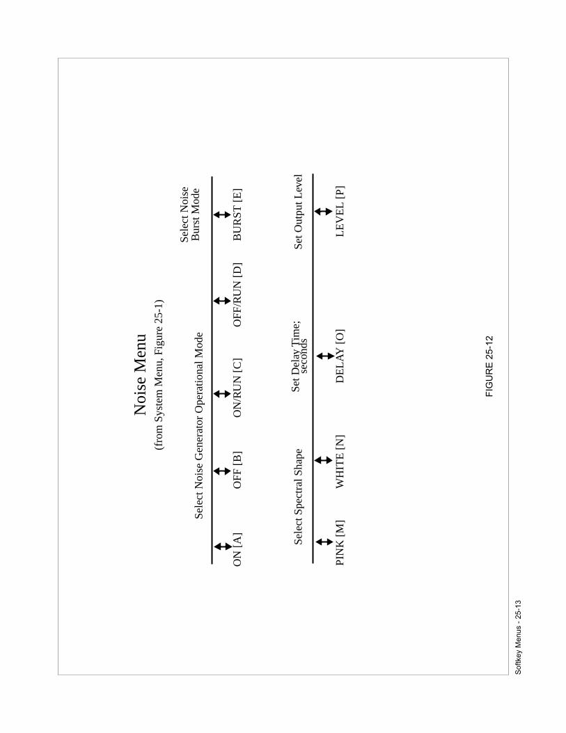
Sof

tkey

Men

us -

25-

13

FIG

UR

E 2

5-12

Noi

se M

enu

Sel

ect N

oise

Gen

erat

or O

pera

tion

al M

ode

ON

[A

]O

FF

[B

]O

N/R

UN

[C

]

Sel

ect S

pect

ral S

hape

Set

Del

ay T

ime;

Set

Out

put L

evel

PIN

K [

M]

WH

ITE

[N

]D

EL

AY

[O

]L

EV

EL

[P

]

OF

F/R

UN

[D

]

seco

nds

Sel

ect N

oise

Bur

st M

ode

BU

RS

T [

E]

(fro

m S

yste

m M

enu,

Fig

ure

25-1

)

Sof

tkey

Men

us -

25-

14

FIG

UR

E 2

5-13

Inpu

t Men

u(f

rom

Sys

tem

Men

u, F

igur

e 25

-1)

SA

ME

[O

]

App

ly s

elec

ted

wei

ghti

ngto

bot

h ch

anne

ls

Off

set C

hann

el 2

∆RA

NG

E [

P]

wit

h re

spec

t to

Cha

nnel

1

Sel

ect M

icro

phon

e B

ias

Vol

tage

Sel

ect B

road

band

Wei

ghti

ng F

unct

ion

28V

[B

]20

0 V

[C

]

Sel

ect L

inea

r W

eigh

ting

,

1-20

k [K

]20

-20k

[L

]

TE

ST

[H

]A

-WG

T [

I]

Togg

le O

N/O

FF

C-W

GT

[J]

0V [

A]

choi

ce o

f H

ighp

ass/

Low

pass

filt

ers

1 kH

z sq

uare

wav

e fo

r te

st

20-1

0k [

N]

1-10

k [M

]AU

TO

.RA

[E

]

Set

Aut

oran

geap

ertu

re

Sof

tkey

Men

us -

25-

15

FIG

UR

E 2

5-14

Col

or D

ispl

ay M

enu

Turn

Off

Sel

ect N

umbe

r of

Win

dow

s

OF

F[A

]64

0 X

350

[B

]64

0 X

480

[C

]S

ING

LE

[I]

DU

AL

[J]

Dup

lica

te L

CD

Dis

play

on C

olor

Mon

itor

Col

or M

onit

orTu

rn O

n E

xter

nal C

olor

Mon

itor

and

Sel

ect R

esol

utio

nfo

r C

olor

Dis

play

800

X 6

00 [

D]

QU

AD

[K

]

LC

D [

L]

(fro

m S

yste

m M

enu,

Fig

ure

25-1

)

Sof

tkey

Men

us -

25-

16

FIG

UR

E 2

5-15

Set

up M

enu

Ass

ign

Nam

eto

Set

up K

eyR

eset

Use

r-de

fine

d S

etup

sS

tore

pre

sent

Set

upto

Use

r-de

fine

d S

etup

Ass

ign

Ana

lyze

r to

B

oot-

up to

a U

ser-

nam

e [B

]R

. SE

TU

P [

D]

ST

OR

E [

E]

→ B

OO

T [

F]

Sel

ect D

efau

ltS

elec

t Use

r-de

fine

d

note

[G

]

Cre

ate/

Edi

t

DE

FAU

LT [

I][J

] -

[P]

defi

ned

Set

up

Set

upS

etup

Not

e Fi

eld

(fro

m S

yste

m M

enu,

Fig

ure

25-1

or

one

of th

e A

naly

sis

Men

us, F

igur

es 2

5-5,

6,7

, and

8)

Sof

tkey

Men

us -

25-

17

FIG

UR

E 2

5-16

File

s M

enu

(Mem

ory)

Cre

ate

and

Nam

eM

ove

Lef

t Sid

eS

tore

Hig

hlig

hted

Mov

e R

ight

Sid

e

crea

te [

A]

RE

CO

RD

S [

B]

[C]

[D]

Rec

all H

ighl

ight

edM

ove

Rig

ht S

ide

Del

ete

Hig

hlig

hted

Ren

ame

Hig

hlig

hted

Dis

k Fi

le

mem

[M

][M

]re

nam

e [O

]

Del

ete

Hig

hlig

hted

Mem

ory

File

Ren

ame

Hig

hlig

hted

File

Mov

e L

eft S

ide

form

at [

F]

dele

te [

I]re

nam

e [J

][K

]

Form

at D

isk

Hig

hlig

ht D

own

Dis

k Fi

le to

Mem

ory

Hig

hlig

ht D

own

Dis

k Fi

le

dele

te [

N]

a M

emor

y Fi

le

disk

[E]

Hig

hlig

ht U

pM

emor

y Fi

le to

Dis

kH

ighl

ight

Up

Lis

t Rec

ords

in H

ighl

ight

edM

emor

y Fi

le

Figu

re 2

5-17

(fro

m S

yste

m M

enu,

Fig

ure

25-1

or

one

of th

e A

naly

sis

Men

us, F

igur

es 2

5-5,

6, 7

, and

8)

Sof

tkey

Men

us -

25-

18

FIG

UR

E 2

5-17

File

s M

enu

(Rec

ords

)

Cre

ate

and

Nam

ea

Mem

ory

File

Mov

e L

eft S

ide

Mov

e R

ight

Sid

eE

dit N

ote

Fiel

d of

crea

te [

A]

[C ]

[E]

note

[G

]

Exi

t Fil

e M

enu

and

setu

pan

alyz

er to

be

sam

e as

Del

ete

Hig

hlig

hted

Mem

ory

File

Ren

ame

Hig

hlig

hted

Mem

ory

File

Mov

e L

eft S

ide

KE

EP

[H

]de

lete

[J]

rena

me

[J]

[K]

Mov

e R

ight

Sid

eH

ighl

ight

Dow

nD

elet

e H

ighl

ight

ed R

ecor

d (R

ight

Sid

e)fr

om H

ighl

ight

ed M

emor

yFi

le (

Lef

t Sid

e)

[M]

dele

te [

N]

Hig

hlig

hted

Up

Hig

hlig

hted

Up

Hig

htli

ghte

d R

ecor

d

Hig

hlig

hted

Rec

ord

Hig

hlig

ht D

own

(fro

m F

iles

Men

u (M

emor

y), F

igur

e 25

-16)

Sof

tkey

Men

us -

25-

19

FIG

UR

E 2

5-18

Res

ets

Men

u

Res

et a

naly

zer

Res

et th

e

R.M

EM

RY [

A]

R.S

ET

UP

[C

]R

.RT

60 [

D]

Res

et th

e

R.U

SE

R [

E]

R.M

AC

RO

[F

]

mem

ory

Res

et a

ll R.S

TAT

S [

G]

Res

et u

nits

user

-def

ined

setu

psac

tive

RT

60

R.U

NIT

S [

B]

stat

isti

csta

ble

buff

er

Res

et a

llus

er-d

efin

eddi

gita

l wei

ghti

ng

Res

et a

llus

er-d

efin

edke

y m

acro

s

(fro

m S

yste

m M

enu,

Fig

ure

25-1

)

Sof

tkey

Men

us -

25-

20

FIG

UR

E 2

5-19

Dis

play

Men

u

Cre

ate/

Edi

t

SE

TU

SE

R [

F]

note

[G

]

Togg

le B

andw

idth

Togg

le B

road

band

Acc

ess

Use

r BW

NO

RM

[P

]

Dig

ital

Rea

dout

Bet

wee

n ∑

and

A-w

gtW

eigh

ting

Set

up M

enu

Not

e Fi

eld

SU

M [

E]

Com

pens

atio

n O

N/O

FF

Figu

re 2

5-30

(fro

m o

ne o

f th

e A

naly

sis

Men

us, F

igur

e 25

-5, 6

, 7, a

nd 8

)

Togg

le

Dis

play

Mod

eO

n an

d O

ff

AV

ER

AG

E [

D]

Togg

le D

ispl

ay M

ode

betw

een

Sin

gle

and

Dua

l(S

TAN

D 2

onl

y)

MU

LTI

[H]

Sel

ect

Dis

play

1/1

[A]

Oct

ave

Ban

dwid

th

1/3

[B]

Sel

ect S

ingl

e

Inte

grat

ion

∫ [A

]or D

oubl

e ∫∫ [B

]

For

FF

TA

naly

sis:

For

octa

veB

andw

idth

s:

Acc

ess

Dig

ital

Dis

play

Wei

ghti

ng M

enu

Dig

.WG

T [

I]Fi

gure

25-

19B

Ave

rage

Spe

ctru

m

Sof

tkey

Men

us -

25-

21

FIG

UR

E 2

5-19

B

Dig

ital

Dis

play

Men

u

Zw

.FR

EE

[A

]Z

w.D

IFF

[B

]

Sel

ect f

orm

of

Zw

icke

r L

oudn

ess

(fro

m D

ispl

ay M

enu,

Fig

ure

25-9

)

Sel

ect D

igit

al D

ispl

ay W

eigh

ting

NO

WG

T [

I]A

[J]

C [

K]

US

ER

[L

]-A

[M

]-C

[N

]-U

SE

R [

O]

Sof

tkey

Men

us -

25-

22

FIG

UR

E 2

5-20

Det

ecto

r M

enu,

Oct

ave

Ban

dwid

ths

Sel

ect A

vera

ging

Typ

e

LIN

.S [

A]

EX

P [

C]

BT

/EX

P [

D]

Sel

ect A

vera

ging

Typ

e

LIN

.R [

B]

BT

/LIN

[E

]A

V.T

YP

E [

H]

CO

UN

T.S

[E

]E

XP

O.N

[D

]

Sel

ect A

vera

ging

Tim

e

Det

ecto

r M

enu,

FF

T A

naly

sis

LIN

.S [

A]

LIN

.R [

B]

EX

P [

C]

AV.

TY

PE

[H

]C

OU

NT.

R [

F]

CO

UN

T.M

[G

]

Sel

ect

Tim

eA

vera

ging

(fro

m o

ne o

f th

e A

naly

sis

Men

us, F

igur

e 25

-5, 6

, 7, a

nd 8

)

Sof

tkey

Men

us -

25-

23

FIG

UR

E 2

5-21

A

Roo

ms

Men

u

Dis

play

Rec

eivi

ng R

oom

NC

[A

]

BA

CK

.GD

[F

]

AS

TM

[I]

ISO

[J]

Eva

luat

e N

C R

atin

g

Sel

ect S

tand

ard

Gro

up to

of 1

/1 O

ctav

e S

pect

rum

back

grou

nd s

pect

rum

foll

ow f

or C

alcu

lati

ons

(fro

m th

e S

tand

ard

Ana

lysi

s M

enu,

Fig

ure

25-5

)

Ent

er S

urfa

ce A

rea

surf

ace

[D]

of P

arti

tion

, m2

NR

[B

]

Eva

luat

e N

R R

atin

gof

1/1

Oct

ave

Spe

ctru

m

RC

[C

]

Eva

luat

e R

C R

atin

gof

1/1

Oct

ave

Spe

ctru

m

and

Acc

ess

Men

u

Ent

er V

olum

e of

volu

mne

[E

]

Rec

eivi

ng R

oom

, m3

Rec

eive

, and

Bac

kgro

und

keys

SE

T->

[L

]

to d

efin

e da

ta b

lock

to b

e us

ed

Use

wit

h S

ourc

e,

SO

UR

CE

[M

]

Dis

play

Sou

rce

Roo

mS

pect

rum

RE

CE

IVE

[N

]

Dis

play

Rec

eivi

ng R

oom

S

pect

rumAcc

ess

RT

60 [

F]

RT

60 M

enu

Figu

re 2

5-21

BFi

gure

25-

21C

Res

et R

ecei

ving

Roo

m

CL

R.G

D [

P]

back

grou

nd s

pect

rum

toa

very

sm

all v

alue

Sof

tkey

Men

us -

25-

24

FIG

UR

E 2

5-21

B

AS

TM

Men

u

NR

[A

]

Eva

luat

e N

oise

Red

ucti

onan

d N

oise

Iso

lati

on

(fro

m th

e R

oom

s M

enu,

Fig

ure

25-2

1A)

FT

L [

D]

Eva

luat

e Fi

eld

Tra

nsm

issi

on a

nd

Fiel

d S

ound

Tra

nsm

issi

on C

lass

Ln

[I]

Eva

luat

e N

orm

aliz

ed I

mpa

ct S

ound

Pre

ssur

e L

evel

and

Fi

eld

Impa

ct I

sola

tion

Cro

ssTL

[C

]

Eva

luat

e T

rans

mis

sion

Los

san

d S

ound

Tra

nsm

issi

on C

lass

NN

R [

B]

Eva

luat

e N

orm

aliz

ed

Nor

mal

ized

Noi

se I

sola

tion

Cla

ssN

oise

Red

ucti

on a

nd

Sof

tkey

Men

us -

25-

25

FIG

UR

E 2

5-21

C

ISO

Men

u

D [

A]

DnT

[C

]

Eva

luat

e L

evel

Dif

fern

ceE

valu

ate

Sta

ndar

dize

d L

evel

and

Wei

ghte

d L

evel

Dif

fere

nce

Dif

fere

nce

and

Wei

ghte

d

(fro

m th

e R

oom

s M

enu,

Fig

ure

25-2

1A)

R’ [

B]

App

aren

t Wei

ghte

d S

ound

Red

ucti

on I

ndex

,an

d A

irbo

rne

Sou

nd I

nsul

atio

n M

argi

nA

ppar

ent S

tand

ariz

ed S

ound

Red

ucti

on I

ndex

Eva

luat

e S

tand

ardi

zed

Impa

ct S

ound

Pre

ssur

e L

evel

L’nT

[J]

and

Wei

ghte

d S

tand

ardi

zed

Impa

ctS

ound

Pre

ssur

e L

evel

Eva

luat

e N

orm

aliz

ed I

mpa

ct S

ound

Pre

ssur

e L

evel

,

L’n

[I]

Wei

ghte

d N

orm

aliz

ed I

mpa

ct S

ound

Pre

ssur

e L

evel

,an

d Im

pact

Sou

nd P

rote

ctio

n M

argi

n

Eva

luat

e S

ouin

d R

educ

tion

Ind

ex,

Sof

tkey

Men

us -

25-

26

FIG

UR

E 2

5-22

vsR

PM

Men

u

Set

slo

pe

SL

OP

E [

A]

∆ le

vel [

B]

TAG

BA

RS

[C

]X

-Spa

n [D

]V

IDE

O [

E]

X-A

XIS

[F

]no

te [

G]

WID

TH

[H

]S

TAT

US

[I]

HID

E [

J]

Sel

ect C

hann

elfo

r in

dica

ted

trac

e

CH

AN

NE

L [

O]

+, -

, ±

Am

plit

ude

sens

itiv

ity

of r

eal-

tim

etr

acki

ng d

ispl

ayTo

ggle

Tag

bars

ON

/OF

F

Set

lim

its

for

hori

zont

al a

xis,

R

PM

/Spe

ed

Togg

le c

olor

di

spla

yO

N/O

FF

Togg

le h

oriz

onta

lax

is b

etw

een

RP

M/S

peed

Cre

ate/

Edi

tN

ote

Fiel

d

Sel

ect P

eak

Hun

tPa

ram

eter

for

Post

-pro

cess

Ord

er T

rack

ing

Set

Sta

tus

of s

elec

ted

trac

eH

ide

or U

nhid

ese

lect

ed tr

ace

Acc

ess

Tach

/Spe

edS

cali

ng M

enu

Sel

ect p

aram

eter

for

vsR

PM

gra

phS

elec

t tra

ce to

set p

aram

eter

s

PE

N [

N]

CA

L [

M]

B-O

RD

ER

S [

L]

B-F

RE

Q [

L]

TAC

HS

ET

[K

]

Sel

ect p

aram

eter

for

indi

cate

d tr

ace

FR

EQ

[P

]O

RD

ER

[P

]

Figu

re 2

5-31

(fro

m th

eSta

ndar

d A

naly

sis

Men

u, F

igur

e 25

-5)

Sof

tkey

Men

us -

25-

27

FIG

UR

E 2

5-23

Sta

tist

ics

Men

u

ST

O-T

BL

[I]

RC

L-T

BL

[J]

MR

G-T

BL

[K

]

Sel

ect N

for

Sto

re s

tati

stic

sta

ble

Rec

all s

tati

stic

s

Mer

ge r

ecal

led

N [

N]

tabl

e

stat

isti

cs ta

ble

wit

h ac

tive

stat

isti

cs ta

ble

Ln

valu

e of

indi

cate

d tr

ace

(fro

m S

LM

Dis

play

Men

u, F

igur

e 25

-4 o

r S

tand

ard

Ana

lysi

s M

enu,

Fig

ure

25-5

)

ON

/OF

F [

A]

S.T

IME

[B

]dB

-SPA

N [

C]

R.S

TAT

[D

]

Set

tim

e in

terv

alfo

r up

date

of

stat

isti

cs m

atri

xS

et A

mpl

itud

e R

ange

of s

tati

stic

s m

atri

xR

eset

sta

tist

ics

mat

rix

Togg

le S

tati

stic

sO

N/O

FF

HID

E [

F]

Hid

e or

Unh

ide

sele

cted

trac

e

CL

EA

R [

G]

Cle

artr

aces

RE

DR

AW

[H

]

late

st d

ata

from

stat

isti

cs ta

ble

Red

raw

usi

ng

CH

AN

NE

L [

O]

Sw

itch

bet

wee

nch

anne

ls 1

and

2

Sof

tkey

Men

us -

25-

28

FIG

UR

E 2

5-24

Freq

uenc

y T

rigg

er M

enu

Sel

ect T

rigg

er C

rite

ria

for

curs

or f

requ

ency

Sel

ect M

anua

l Tri

gger

>=

[I]

+S

LO

PE

[J]

-SL

OP

E [

K]

<=

[L

]M

AN

UA

L [

M]

Sel

ect A

utom

atic

Rea

rmfo

llow

ing

an A

utos

tore

Turn

off

Freq

uenc

y T

rigg

erIn

put l

evel

cor

resp

ondi

ngto

trig

ger

crit

eria

RE

-AR

M [

N]

OF

F [

O]

leve

l [P

]

(fro

m S

tand

ard

Ana

lysi

s M

enu,

Fig

ure

25-5

)

Sof

tkey

Men

us -

25-

29

FIG

UR

E 2

5-25

Aut

osto

re M

enu

byT

IME

[B

]en

dsto

r [D

]de

lta

[C]

OF

F [

A]

note

[G

]

F.T

RIG

[M

]F

ILE

S [

O]

Turn

Off

Set

byT

ime

Cre

ate/

Edi

tA

utos

tore

Fun

ctio

n

Sel

ect

byT

ime

Aut

osto

reA

utos

tore

Para

met

ers

Not

eFi

eld

Acc

ess

Acc

ess

Freq

uenc

y T

rigg

er M

enu

File

sM

enu

byTA

CH

[J]

Sel

ect

byTa

chA

utos

tore

(fro

m S

LM

Dis

play

Men

u, F

igur

e 25

-2 o

r S

tand

ard

Ana

lysi

s M

enu,

Fig

ure

25-5

)

TAC

HS

ET

[K

]

Acc

ess

Tach

set

Men

u

Figu

re 2

5-31

Figu

re 2

5-24

Figu

re 2

5-16

Sof

tkey

Men

us -

25-

30

FIG

UR

E 2

5-26

Tim

e T

rigg

er M

enu

Adj

ust C

h 2

dela

yw

/r to

Ch

1

DE

LA

Y [

N]

2-D

EL

AY

[O

]O

FF

[P

]

Sel

ect S

pect

rum

Dis

play

Cre

ate/

Edi

t

A.S

PE

CT

[A

]T

IME

[E

]no

te [

G]

Sel

ect C

ompl

ex P

aram

eter

Rea

l/Im

ag o

r M

ag/P

hase

Togg

le B

andw

idth

Com

pens

atio

n O

N/O

FF

Sel

ect P

olar

or

Rec

tang

ular

Coo

rdin

ates

ALT

ER

N [

I]B

WN

OR

M [

J]P

<>

R [

K]

Adj

ust T

rigg

erD

elay

+ o

r -

Adj

ust T

rigg

erL

evel

Togg

le S

lope

C

rite

ria

↑ or

↓Tu

rn o

ffT

ime

Tri

gger

LE

VE

L [

M]S

elec

t Tim

e D

omai

nD

ispl

ayN

ote

Fiel

d

SL

OP

E [

L]

(fro

m C

ross

Ana

lysi

s w

ith

FF

T F

ilte

ring

Men

u, F

igur

e 25

-7)

Sof

tkey

Men

us -

25-

31

FIG

UR

E 2

5-27

FF

T Z

oom

Men

u

Sel

ect Z

oom

Mul

tipl

ier

1 [A

]B

AS

E-H

z [O

]2

[B]

4[C

]8[

D]

16 [

E]

32 [

F]

64 [

G]

128

[I]

256

[J]

512

[K]

(fro

m F

ilte

r M

enu,

Fig

ure

25-1

0)

Use

hor

izon

tal a

rrow

key

sto

sel

ect C

ente

r Fr

eque

ncy

of Z

oom

Ana

lysi

s

Sof

tkey

Men

us -

25-

32

FIG

UR

E 2

5-28

FF

T T

ime

Wei

ghti

ng M

enu

Sel

ect T

ime

Wei

ghti

ng F

unct

ion

RE

CT.

[A

]F

LA

T [

C]

IMPA

CT

[E

]Z

ER

OPA

D [

D]

HA

NN

ING

[B

]E

XP

-2 [

F]

EX

P-4

[G

]E

XP

-6 [

H]

Figu

re 2

5-25

(fro

m F

ilte

r M

enu,

Fig

ure

25-1

0)

Sof

tkey

Men

us -

25-

33

FIG

UR

E 2

5-29

20 k

Hz[

A]

5 kH

z [C

]

FF

T B

aseb

and

Men

u

10 k

Hz

[B]

2.5

kHz

[C]

(fro

m F

ilte

r M

enu,

Fig

ure

25-1

0)

Sof

tkey

Men

us -

25-

34

FIG

UR

E 2

5-30

Set

Use

r M

enu

Sto

re D

ispl

ayed

Use

r W

eigh

ting

CL

EA

R [

C]

ST

O.U

SR

[I]

Sub

trac

t Rec

alle

d U

ser

Wei

ghti

ng

RC

L.U

SR

[J]

AD

D [

K]

SU

BT

RC

T [

L]

MA

KE

[M

]

Cle

ar W

orki

ng D

ata

Buf

fer

Rec

all S

tore

d U

ser

Wei

ghti

ng

Add

Rec

alle

d U

ser

Wei

ghti

ngC

reat

e a

Use

r W

eigh

ting

Cur

veto

Dis

play

ed C

urve

from

Dis

play

ed C

urve

from

Dis

play

ed S

pect

rum

Togg

le I

nter

pola

tion

Fun

ctio

n O

N/O

FF

Inpu

t Lev

el V

alue

for

Cur

sor

Posi

tion

edit

[P

]IN

TE

RP

[N

](fro

m D

ispl

ay M

enu,

Fig

ure

25-1

9)

Sof

tkey

Men

us -

25-

35

FIG

UR

E 2

5-31

Tach

set M

enu

t.sca

le [

A]

t.∆m

in [

C]

t.∆m

ax [

D]

X-c

al [

F]

X-A

VE

[H

]s.

scal

e [I

]

Sca

ling

for

Aut

osto

reA

uto-

scal

ing

of

Togg

le s

lope

Sca

le S

peed

Sca

le R

PM

t.spa

n [B

]

Sca

ling

for

aut

osto

rage

s.sp

an [

J]

Tach

o In

put

base

d on

RP

M

SL

OP

E [

G]

s.∆m

in [

K]

s.∆m

ax [

L]

+, -

, ±Ta

cho

Inpu

tba

sed

on s

peed

Tach

Par

amet

ers

Tach

omet

erA

vera

ging

(fro

m v

sRP

M M

enu,

Fig

ure

25-2

2)

t.inp

ut [

E]

Bet

wee

n C

h1, C

h2 a

nd

Ext

erna

l Jac

k

Togg

le T

ach/

Spe

ed I

nput

Sof

tkey

Men

us -

25-

36

FIG

UR

E 2

5-32

IO P

ort M

enu

Low

1 [

A]

Hi/

In 2

[D

]L

ow 3

[E

]H

i/In

3 [

F]

AD

C 2

[J]

AD

C 3

[K

]

Rea

d V

olta

ge L

evel

On

AD

Cs

1, 2

and

3

Set

Sta

tus

of I

O p

orts

1, 2

and

3

Low

2 [

C]

AD

C 1

[I]

Hi/

In 1

[B

]

(fro

m I

/O M

enu,

Fig

ure

25-1

1)

Dis

play

bit

s st

ate

BIT

S [

L]

for A

DC

1,2

and

3

Sof

tkey

Men

us -

25-

37

FIG

UR

E 2

5-33

Bee

per

Men

u

NO

NE

[A

]K

EY

S [

C]

Bee

per A

ctiv

eN

o B

eepe

rB

eepe

r fo

rB

eepe

r fo

rB

eepe

r fo

r

AL

L [

B]

OV

ER

[D

]E

RR

OR

[E

]

for

all c

ondi

tion

ske

y pr

esse

sov

erlo

ader

ror

cond

itio

ns

(fro

m I

/O M

enu,

Fig

ure

25-1

1)

Sof

tkey

Men

us -

25-

38

FIG

UR

E 2

5-34

Sta

ndar

d R

ecal

l Men

u

Perf

orm

W.F

all [

A]

B.A

VE

[B

]K

EE

P [

H]

DE

LE

TE

[I]

*rec

all [

P]

Sel

ect

Exi

t fro

m R

ecal

l Men

u;

Blo

ck

Ave

ragi

ngD

ispl

ayW

ater

fall

Kee

p 29

00 S

etup

the

sam

e as

the

last

reca

lled

dat

ablo

ck

Del

ete

Rec

ord

Rea

ssig

n ho

rizo

ntal

arr

ow k

eys

pres

ently

dis

play

edto

rec

all r

ole

(aft

er c

ontr

olli

ng c

urso

r)

(pre

ss R

EC

AL

L)

Perf

orm

B.M

AX

[C

]

Blo

ck

Max

imum

Perf

orm

B.S

UM

[D]

Blo

ck

Ave

rage

Sof

tkey

Men

us -

25-

39

FIG

UR

E 2

5-35

Aut

osto

re R

ecal

l Men

u

Perf

orm

W.F

all [

A]

vsT

IME

[E

]

Rec

all R

ecor

d

B.A

VE

[B

]K

EE

P [

H]

DE

LE

TE

[I]

A.P

rev

[N]

A.N

ext [

M]

*rec

all [

P]

Pre

sent

Dat

a in

Sel

ect

Exi

t fro

m R

ecal

l Men

u;

Blo

ck

Ave

ragi

ngD

ispl

ayW

ater

fall

vers

us T

ime

Form

at,

sele

cted

fre

quen

cy

Kee

p 29

00 S

etup

the

sam

e as

the

last

reca

lled

dat

ablo

ck

Del

ete

Rec

ord

Rec

all R

ecor

dR

eass

ign

hori

zont

al a

rrow

pres

ently

dis

play

edP

revi

ous

inne

xt in

Sto

rage

Seq

uenc

eS

tora

ge S

eque

nce

keys

to r

ecal

l rol

e(a

fter

con

trol

ling

cur

sor)

(pre

ss R

EC

AL

L, w

ith

auto

stor

e ac

tivat

ed)

Perf

orm

B.M

AX

[C

]

Blo

ck

Max

imum

Perf

orm

B.S

UM

[D

]

Blo

ck

Sum

mat

ion

Sof

tkey

Men

us -

25-

40

FIG

UR

E 2

5-36

Sig

nal G

ener

ator

Men

u

Sel

ect S

igna

l Gen

erat

or O

pera

tion

al M

ode

ON

[A

]O

FF

[B

]O

FF

/RU

N [

D]

<-A

TT

[G

]->

AT

T [

H]

Acc

ess

Men

u fo

r S

elec

ted

Sig

nal T

ype

SIN

E [

I]Fi

gure

25-

37P

INK

[J]O

N/R

UN

[C

]

WH

ITE

[K

]P

UL

SE

[L

]D

EL

AY

[O

]

Set

Del

ay T

ime,

sec

onds

(fro

m S

yste

m M

enu,

Fig

ure

25-1

)

Con

trol

Att

enua

tion

Figu

re 2

5-43

Figu

re 2

5-41

Figu

re 2

5-39

Sof

tkey

Men

us -

25-

41

FIG

UR

E 2

5-37

Sin

e G

ener

ator

Men

u

Set

Fre

quen

cy S

wee

p L

imit

s

Fst

art [

A]

Fend

[B

]T.

es [

D]

Lse

[E

]L

es [

F]

Con

trol

Att

enua

tion

Sw

eep

Con

trol

<-A

TT

[G

]->

AT

T [

H]

Set

Aut

o L

evel

Aut

o-L

[O

]F

ILT

ER

[P

]Set

Sw

eep

Lev

els

T.se

[C

]

@S

TAR

T [

I]

2-to

ne [

N]

Figu

re 2

5-38

Adj

ust R

espo

nse

@E

ND

[J]

SW

EE

P [

K]

Set

Sw

eep

Tim

es

Acc

ess

2-to

ne M

enu

LIN

[L

]

(fro

m S

igna

l Gen

erat

or M

enu,

Fig

ure

25-3

7)

TIM

E [

M]

or

LO

G [

L]

or

CO

UN

T [

M]

orN

se [

C]

orR

.se

[C]

orN

es [

D]

orR

.es

[D]

Sof

tkey

Men

us -

25-

42

FIG

UR

E 2

5-38

Dua

l Ton

e M

enu

Set

Fre

quen

cy S

wee

p L

imit

s

Fst

art [

A]

Fend

[B

]T.

es [

D]

Lse

[E

]L

es [

F]

Set

Rel

ativ

e S

wee

p C

ontr

ol

L1

[G]

∆F [

H]

Set

Aut

o L

evel

Aut

o-L

[O

]F

ILT

ER

[P

]Set

Sw

eep

Lev

els

T,se

[C

]

@S

TAR

T [

I]

1ton

e [N

]

Adj

ust R

espo

nse

@E

ND

[J]

SW

EE

P [

K]

Set

Sw

eep

Tim

es

Acc

ess

1ton

e M

enu

LIN

[L

]

(fro

m S

ine

Gen

erat

or M

enu,

Fig

ure

25-3

7)

TIM

E [

M]

or

LO

G [

L]

or

CO

UN

T [

M]

.or

Nse

[C

]or

R.s

e [C

]

orN

es [

D]

orR

.es

[D]

Set

Dif

fere

nce

Am

plit

udes

Freq

uenc

y

Sof

tkey

Men

us -

25-

43

FIG

UR

E 2

5-39

Wid

eban

d P

ink

Noi

se M

enu

Acc

ess

Ban

dlim

ited

1/3

[A ]

LE

VE

L [

E]

(fro

m S

igna

l Gen

erat

or M

enu,

Fig

ure

25-3

6)

Pin

k N

oise

Men

u

Figu

re 2

5-40

Set

Am

plit

ude

Con

trol

Att

enua

tion

<-A

TT

[G

]->

AT

T [

H]

Sof

tkey

Men

us -

25-

44

FIG

UR

E 2

5-40

Ban

dlim

ited

Pin

k N

oise

Men

u

WID

E [

A]

Figu

re 2

5-39

ON

[C

]

Set

Aut

olev

el

Aut

o-L

[L

]D

OT

TE

D [

P]

OF

F [

D]

->A

TT

[H

]

Cur

sor

Con

trol

LE

VE

L [

E]

<-A

TT

[E

]

(fro

m W

ideb

and

Pin

k N

oise

Men

u, F

igur

e 25

-39)

Pin

k N

oise

Men

uA

cces

s W

ideb

and

Indi

cate

d Fr

eque

ncy

Ban

dS

et S

tate

of

Set

Am

plit

ude

Con

trol

Att

enua

tor

SO

LID

[O

]B

OT

H [

N]

all b

ands

NO

NE

[J]

all b

ands

AL

L [

I]

Turn

on

Turn

off

Sof

tkey

Men

us -

25-

45

FIG

UR

E 2

5-41

Wid

eban

d W

hite

Noi

se M

enu

PS

UE

DO

[A

]Fi

gure

25-

42->

AT

T [

H]

LE

VE

L [

E]

<-A

TT

[G

]

(fro

m S

igna

l Gen

erat

or M

enu,

Fig

ure

25-3

6)

Noi

se M

enu

Acc

ess

Psu

edo-

Whi

teS

et A

mpl

itud

eC

ontr

ol A

tten

uati

on

Sof

tkey

Men

us -

25-

46

FIG

UR

E 2

5-42

Psu

edo-

Whi

te N

oise

Men

u(f

rom

Wid

eban

d W

hite

Noi

se M

enu,

Fig

ure

25-4

1)

WID

E [

A]

Figu

re 2

5-41

->A

TT

[H

]L

EV

EL

[E

]<

-AT

T [

G]

Whi

te N

oise

Men

uA

cces

s W

ideb

and

Set

Am

plit

ude

Con

trol

Att

enua

tion

Sof

tkey

Men

us -

25-

47

FIG

UR

E 2

5-43

Pul

se N

oise

Men

u

Sel

ect D

irec

tion

of

Pul

ses

Sel

ect T

ime

On

Set

Am

plit

ude

PO

S/N

EG

[B

]L

EV

EL

[E

]T.

on [

C]

Sel

ect T

ime

Off

T.of

f [D

]

(fro

m S

igna

l Gen

erat

or M

enu,

Fig

ure

25-3

6)

Sof

tkey

Men

us -

25-

48

FIG

UR

E 2

5-44

Cla

ss L

ines

Men

u

Use

r-de

fine

able

nam

es f

or C

lass

Lin

e

Und

ef [

A]

Und

ef [

B ]

Und

ef [

D]

C.O

N [

F]

ED

IT [

I]Fi

gure

25-

45

a.JU

DG

E [

N]

m.J

UD

GE

[P

]

Set

Cla

ss L

ines

ON

/OF

F

Und

ef [

C]

AS

SIG

N [

L]

SE

TU

PS

[J]

NA

ME

[K

]

(fro

m S

yste

m M

enu,

Fig

ure

25-1

)

orC

.OF

F [

F]

Acc

ess

Cla

ss L

ines

Edi

t Men

uS

etup

Men

uA

cces

s C

lass

Lin

esN

ame

Cla

ss L

ines

Ass

ign

Cla

ss L

ines

Figu

re 2

5-47

Sel

ect J

udge

men

t Typ

e

US

E K

EY

[O

]

Sof

tkey

Men

us -

25-

49

FIG

UR

E 2

5-45

Cla

ss L

ines

Edi

t Men

u(f

rom

Cla

ss L

ines

Men

u, F

igur

e 25

-44)

Sel

ect m

ax/m

in

max

[A

]or

min

[A

]

of li

ne r

epea

tsS

elec

t num

ber

betw

een

line

sS

elec

t Wid

thpa

ram

eter

Set

qua

lifi

er

# R

EP

EA

T [

B]

∆ W

IDT

H [

C]

qual

ify

[D]

Shi

ft to

poi

ntS

hift

to p

oint

Add

new

poi

ntD

elet

e po

int

at le

ftat

rig

htH

oriz

onta

l arr

ows

Con

trol

Cur

sor

Hor

izon

tal A

rrow

sM

ove

Freq

uenc

yL

ocat

ion

of P

oint

<-p

oint

[J]

->po

int [

Jad

d pn

t [K

]de

l pnt

[L

]*d

otte

d [N

]*f

req

[O]

Sof

tkey

Men

us -

25-

50

FIG

UR

E 2

5-46

Cla

ss L

ines

Set

up M

enu

(fro

m C

lass

Lin

es M

enu,

Fig

ure

25-4

5)

Ass

ign

Nam

eR

eset

Set

ups

Sto

re S

etup

sS

elec

t def

ault

Set

up F

orm

at

Sel

ect S

etup

(la

bele

d by

def

ined

Nam

es)

to S

etup

Key

[I]

- [P

]

NA

ME

[A

]R

ES

ET

[B

]S

TO

RE

[C

]D

EFA

ULT

[H

]

Sof

tkey

Men

us -

25-

51

FIG

UR

E 2

5-47

SH

IFT

Men

u(P

ress

har

dkey

SH

IFT

)

For

FF

T,

X-A

XIS

[A

]

disp

lay

form

atS

elec

t y-a

xis

scal

e fa

ctor

Sel

ect v

erti

cal

cont

rol v

erti

cal o

ffse

tL

et h

oriz

onta

l arr

ow k

eys

Y-A

XIS

[B

]V.

SC

AL

E [

C]

V.O

FS

ET

[D

]

Dis

play

Ins

trum

ent

Mac

ro P

rogr

amm

ing

Key

sS

yste

m I

nfor

mat

ion

SY

SIN

FO

[H

]M

cST

OP

[I

McW

AIT

[J]

McR

EP

T [

K]

McS

TAR

T [

L]

Togg

le b

ewee

nli

n an

d lo

g sc

ales

cont

rol h

oriz

onta

l off

set

Let

hor

izon

tal a

rrow

key

s

H.O

FS

ET

[F

]

scal

e fa

ctor

Sel

ect h

oriz

onta

l

H.S

CA

LE

[E

]

Use

dis

play

ed s

pect

rum

as r

efer

ence

for

both

cha

nnel

s

Sam

eRE

F [

N]

Use

cor

resp

ondi

ng c

hann

elsp

ectr

a as

ref

eren

ces

for

each

cha

nnel

s

Sam

eRE

F [

N]

Sel

ect d

ispl

aye

vers

us a

ref

eren

ce

spec

trum

mod

e

vsR

EF

[P

]

Figu

re 2

5-48

Sof

tkey

Men

us -

25-

52

FIG

UR

E 2

5-48

Y-A

XIS

Men

u(f

rom

SH

IFT

Men

u, F

igur

e 25

-47)

Lin

ear

Uni

ts

LIN

/LIN

[A

]

Log

Sca

leL

og U

nits

Log

Sca

leL

inea

r U

nits

Log

Sca

leS

quar

ed L

inea

r U

nits

LO

G/L

OG

[B

]L

IN/L

OG

[C

]S

QU

/LO

G [

D]

Lin

ear

Sca

ling

A-1

A Index

AA.CORRE 6-7A.SPECT 6-6, 6-9A/D Inputs 4-27AC output 1-11Accelerometer Connection 1-11Acoustic Intensity Probe 4-3Acoustic Intensity, see IntensityAmplitude/phase display 6-8Analysis Mode 4-1

Cross 4-3, 6-6Intensity 4-3, 6-10Standard 4-2, 6-1

Annotation 14-1Arrow Keys 1-5Auto Correlation 6-7Auto Spectrum 6-9Autorange 7-3Autospectrum 6-6Autostore byTach 16-1

Enabling autostore byTach 16-9Influence of slope 16-6Interval/Span settings 16-4Recall and display of data 16-10Setting Tach parameters 16-2Speed Input 16-1Tach/Speed calibration 16-7Tach/Speed scaling 16-4Tacho Input 16-1

Autostore byTime 15-1amplitude vs. time display 15-9averaging 15-7block maximum 13-12broadband vs. time 15-11concluding sequence 15-5displaying spectra 15-8initiating a sequence 15-3recall and display 15-7SLM data vs. time 15-11waterfall display 15-16, 16-14

Average 6-2

Average spectrum display 6-2Averaging 5-1

autostore byTime 15-6, 15-13constant confidence time 5-6continuously running time 7-1count 15-3exponential time 5-7FFT filters 5-2finite length time 7-2linear repeat time 5-7linear time 5-6methods 5-2octave filters 5-1periodic signals 5-7signal 5-5spectrum 5-6, 5-7time 5-5time decay records 21-11

Averaging Consideration 5-5Averaging time 5-3Averaging Type

FFT filter 5-2Octave Filters 5-1

Averaging, SpectraConstant Confidence 5-4Exponential 5-4FFT 5-2Octaves 5-1

A-Weight 3-4, 19-2

BBandwidth Compensation 19-7Battery 1-9Beeper control 1-9, 4-30Block Averaging 16-13

byTach Autostore 16-11byTime Autostore 15-13Standard 13-12

Block MaximumbyTach Autostore 16-13byTime Autostore 15-14

A-2

2900 MANUAL

Standard 13-12boot-up 1-6, 4-1

CC. SPECT 6-9C.CORRE 6-7C.SPECT 6-6Calibration 3-17

analyzer 9-6SLM 3-17using internal test signal 9-7using transducer sensitivity 9-4

CEPSTRM 6-7Cepstrum 6-7Channel

Dual 6-1Single 6-1

Channel Selection 6-2Class (Classification) Lines 22-1, 25-48

Accessing 22-3Assigning 22-7, 22-8Creating 22-4, 22-8Judgement 22-9, 22-10, 22-11Labeling 22-4Recall 22-12, 22-13Storage 22-12, 22-13Turning On 22-8

Clock 4-30COHER 6-7, 6-9Coherence 6-7, 6-9Color Monitor 24-1Complex 6-8CROSS 6-6Cross Analysis Mode 4-3, 6-6Cross Correlation 6-7Cross Spectrum 6-6, 6-9Cursor

control 1-5dotted 1-18, 8-1fixing positions 8-3harmonic 8-2moving 8-1solid 1-18, 8-1

C-Weight 3-4

DDC Output 4-26Deleting

autostore records 15-13

non-autostored records 13-12delta time 15-2Differentiation 9-3Disk operations 13-3Display 1-7

backlight 1-8channel selection 6-8color monitor 24-1complex functions 6-8control horizontal range 19-8control of 1-9control vertical range 19-4polar coordinates 6-8printing 23-2rectangular coordinates 6-8Sine Generator 4-16spectra relative to a reference spectrum 19-3viewing angle 1-7

displayed 10-8Displays

byTime 15-9Display 19-3FFT 10-1Field indicators 20-20, 20-22Intensity 6-10, 20-1Leq byTime 15-10Loudness 6-5Multi spectra 19-1NC 21-22Octave, Cross 6-9octaves 10-1Pressure-residual-intensity 20-2Rooms, ASTM 21-15Rooms, Impact 21-20, 21-21Rooms, ISO 21-17RT60 21-5SLM 3-2SLM, Fast 3-15SLM, Impulse 3-15SLM, Leq 3-16SLM, Slow 3-15SLM, WDR 3-24Sound Reduction 21-17Standard Analysis 6-1Statistics 18-2Vertical scaling 19-5vsRPM Graphics 17-4vsRPM, Intensity 17-10Waterfall 13-14, 15-16, 16-14

2900 MANUAL

A-3

Y-axis 19-5

Eelapsed time 3-11end time 15-2external monitor 24-1

FFFT 4-9FFT analysis 4-3, 4-6Files

accessing 13-1creating 13-2deleting 13-3description 13-1renaming 13-2selecting active 13-4transfering to/from disk 13-3

Filters 4-3analog 4-13fractional octave 4-4

floppy disk 13-3

GGain Control 3-11, 7-2

Offsetting between channels 7-3

Hhorizontal scale 19-8

II/O Channels 4-27I/O Port Control 4-27IMPULSE 6-7Impulse Response 6-7Input 3-2Input gain control 3-11, 7-2Integration 9-2Intensity 20-1

Definition of Areas 20-7Entering Labels 20-10Job/Part/Area 20-8Power Summation 20-15Selection of Display 20-11

Intensity Analysis Mode 4-3Interface

operations 4-24RS-232 4-30

INTNSTY 6-10, 20-11INVERSE 6-7, 6-9

Inverse Transfer Function 6-7, 6-9

Kkey macros 19-12Keys

arrow hardkeys 3-11Arrow Keys

cursor 1-5Range 1-5

cursor hardkey 1-5dedicated hardkeys 1-2, 1-5horizontal arrow 3-11macros 19-12R/S hardkey 7-1Range hardkey 1-5softkeys 1-4vertical arrow 3-11

LLeq 6-3LIFTER 6-7Liftered Spectrum 6-7Ln Calculations 18-1Loudness 6-5

MMacros 19-12

creating 19-12executing 19-13recalling 19-14resetting 19-13

Macros storing 19-14Manual control 7-1MAX 6-3Max Spectrum 6-3Menus

Analyzer 2-1ASTM Rooms 21-15, 25-24Autostore 15-1, 16-2, 25-29Autostore Recall 16-10Autostore recall 15-8, 25-39Beeper 25-37Block print 23-3byTach Block Averaging 16-11byTime display 15-9Class Lines 22-4, 25-48

Assigning 22-8Editing 22-4, 25-49Setups 22-12, 25-50

A-4

2900 MANUAL

Color monitor 24-3, 25-15Cross analysis with FFT Filtering 25-8Cursor 8-1Decay curve 21-4Detector 25-22Digital Display 10-3Display 19-3, 25-20, 25-21Dual Tone 25-42External monitor 24-4FFT 4-4FFT averaging 5-2FFT baseband 4-9, 25-33FFT Window 4-7, 25-32FFT zoom 4-10, 25-31Files 13-1, 25-17Files (Records) 25-18Filter 4-4, 25-11Frequency trigger 11-5, 15-4, 25-28Horizontal scaling 19-8I/O 4-23, 25-12Input 3-2, 4-12, 25-14Intensity analysis 6-10, 20-3, 25-9IO port 4-27, 25-36ISO Rooms 21-16, 25-25Leq in vsTime display 15-10Loudness 6-5Multi Display 19-1Noise 4-14, 25-13Noise Criteria 21-22Normalization 19-11Note 14-1Octave averaging type 5-1Peak Hunt 17-12Pink Noise, Bandlimited 4-20, 25-44Pink Noise, Wideband 4-20, 25-43Power summation 20-15Pressure-residual-intensity display 20-5Print 23-1Pulse Generator 4-22Pulse Noise 25-47Recall 13-11, 15-8Records 13-5Resets 4-31, 25-19Rooms 25-23RS1/INT 4-24RT60 21-5Setup 12-1, 25-16Setuser 10-4, 25-34Shift 2-4, 19-3, 25-51

Signal Generator 4-16, 25-40Bandlimited Pink 4-20, 25-44Dual Tone 4-18, 25-42Psuedo-White 4-22, 25-46Pulse 25-22, 25-47Sine 4-16, 25-41Wideband Pink 4-21, 25-43Wideband White 4-22, 25-45

Sine Generator 25-41Sine Generator, Dual Tone 4-18Sine Generator, Single Tone 4-16SLM 3-2, 25-3SLM display 25-5SLM weight 3-4, 25-4Slope 9-2Standard Analysis 6-1Standard Analysis (1 and 2 channels) 25-6Standard recall 25-38Statistics 18-2, 25-27System 2-1, 4-1, 4-2, 25-2Tach/Speed Averaging 16-8, 16-9Tach/Speed Calibration 16-7Tachset 25-35Time trigger 11-1, 25-30time weighting 4-4Units 9-1, 25-10Vertical scaling 19-5vsRPM 25-26vsRPM graphics 17-4, 17-10Waterfall 13-14, 15-16, 16-14White Noise, Psuedo 4-22, 25-46White Noise, Wideband 4-22, 25-45Y-Axis 19-5, 25-52

MicrophoneConnection 1-10electret 3-3polarization voltage 3-3preamplifier 3-7prepolarized 3-2

MIN 6-3Multi 6-2, 6-5, 19-1

NNC 21-21Noise Criteria Curves 21-21noise floor 1-20, 3-19Noise Generator 4-14Noise Generator (see Signal Generator also) 4-14,

21-2

2900 MANUAL

A-5

Noise Rating Curves 21-22NORMAL 6-3Normalization

Amplitude/Phase 19-9Cross Mode, FFT 19-10Cross Mode, Octaves 19-12

note 14-1NR 21-22

OOutputs

AC 1-11DC 4-26

overload indication 3-11

PP.VELOC 6-10, 20-11Particle Velocity 6-10, 20-11Pink Noise (see Noise Generator and Signal Gener-

ator)Post-processing Order Tracking 17-11Power

Battery 1-9DC 1-10

Primary Indicator Range 3-14printing 23-1Pulse (see Signal Generator)

QQUALITY 6-10, 20-11Quality 6-10, 20-11

RRange control 1-5, 3-11, 7-2

offset between channels 7-3RC Noise Rating Curves 21-22Real/imaginary display 6-8Recall

byTach autostored records 16-10, 25-39byTime autostored records 15-7, 25-39Ln Traces 18-6Macros 19-14non-autostore records 13-10, 25-38RT60 21-12setups 12-3Statistics table 18-7Units 9-7user-weighting curves 10-7, 10-8

Records 13-5classifying 13-4, 13-6

editing or deleting 13-5listing 13-5recalling 13-5

reference spectrum 19-3Remote Control Module 4-24Reset 12-2Reverberation Time 21-4room acoustics 21-1

SSEL 6-3Setup 12-1, 13-10

default 3-2, 3-17, 4-7for autostore 15-1, 16-2for recall 13-11labeling and assigning 12-2recall of setup 12-3reset 12-2statistical analysis 18-1storing a setup 12-2via system menu 4-1

Signal Generator 4-16, 25-40Pink Noise 4-20, 25-43Pulse 4-22, 25-47Sine, Dual Tone 4-18, 25-42Sine, Single Tone 4-16, 25-41White Noise 4-22, 25-45

Signal Typeperiodic 5-7stationary 5-5transient 5-7

Sine Wave (see Signal Generator)SLM

SLM+A, dual channel 3-22SLM+A, single channel 3-2SLM, wide dynamic range 3-24

Softkeys 1-4changing setup 12-2labeling and assigning 12-2menu concept 2-1

software upgrade 1-7Sound Intensity, see IntensitySound Level Meter See SLMspectral density 19-7SPL 6-10, 20-11STAND 2 4-2Standard Analysis Mode 4-2, 6-1Statistics 18-1, 18-3

calculation and display 18-4

A-6

2900 MANUAL

merging tables 18-7recalling Ln traces 18-6storing and recalling tables 18-7storing Ln Traces 18-6

StoragebyTime autostore records 15-5classification by record type 13-6Ln Trace 18-6Macros 19-14non-autostore records 13-6setups 12-2Statistics Table 18-7Units 9-7user-weighting curves 10-6, 10-7

Stored Records 13-14block averaging 13-12, 15-13deleting 13-12, 15-13waterfall display 13-14, 15-16, 16-14

Summation Bands 19-2

TTaktmaximal 3-15Test Signal 4-13, 9-7TIME 6-7Time Display 6-7Time Domain Trigger 11-1Trace 18-6

recall Ln 18-6storing Ln 18-6

Transfer Function 6-6, 6-9Trigger 11-1

arming and disabling 11-6automatic re-arming 11-7Frequency Domain 11-4, 15-4selecting criterion 11-5selecting frequency 11-5selecting level 11-6Time domain 11-1, 15-5

UUnits 9-1

names 9-1storage and recall 9-7

user weighting 10-7

Vvertical scale 19-5vsRPM

Post-process Order Tracking 17-11

Real-time Graphics 17-2vsRPM Graphics 17-1

from vsRPM autostored data 17-9

WWeighting (analog)

Analyzer 4-13SLM 3-4

Weighting (digital) 19-2active register 10-6display 10-3interpolation 10-5user 10-5

White Noise (see Noise Generator and Signal Gen-erator)

XX-FER 6-6, 6-9

ZZw.DIFF 6-5Zw.FREE 6-5