264-994-1-pb

8/10/2019 264-994-1-PB

http://slidepdf.com/reader/full/264-994-1-pb 1/5

Int. J Sci. Emerging Tech. Vol-2 No. 1 October, 2011

21

Modelling and Simulation of Non-Linear

Analysis of the Cardiovascular SystemDr. Yogendra B.Gandole

Department of Electronics

Adarsha Science J.B.Arts and Birla Commerce Mahavidyalaya, Dhamangaon Rly-444709 (India)

Email: [email protected]

Abstract — The physiological oscillators produce

oscillations, in the form of stable, closed trajectory

called a limit cycle. These oscillations exhibit the

phenomenon of frequency entrainment or phase

locking. These are analyzed by presenting Vanderpol

oscillator. Vanderpol oscillator is a non-linear oscillator.

In the non-limit cycle oscillator, external disturbance

move the phase trajectory to different orbit around the

centre and will not come to original point, where as in

limit cycle oscillator, the phase trajectory returns to its

original location. When Vander Pol oscillator is driven

by the external frequency, which is different with

natural frequency of the oscillator, then the resultant

output is mixture of components that result from the

interaction of the driving periodicity on natural

oscillations. If the external frequency is equal to natural

frequency of vendorpol oscillator, then nonlinear system

will adopt the external frequency. The time courses of

oscillatory activity of heart and phase trajectories are

generated by Vanderpol model and simulated using the

Simulink. The response of VanderPol oscillator forvarious external frequencies is also obtained.

Keywords — Vanderpol oscillator, cardiovascular system,

conduction system.

1. Introduction

The parameters of heart rate variability and

blood pressure variability have proved to be useful

analytical tools in cardiovascular physics and

medicine. Model-based analysis of these variability’s

additionally leads to new prognostic information

about mechanisms behind regulations in thecardiovascular system. Riedl et al [1] analyze the

complex interaction between heart rate, systolic

blood pressure, and respiration by nonparametric

fitted nonlinear additive autoregressive models with

external inputs. Controlling irregular and chaotic

heartbeats is a key issue in cardiology, underlying the

experimental and clinical use of artificial pacemakers.

There are different strategies of control, based on

either in the use of external sources of periodic or

quasi-periodic signals, as well as the use of small

perturbations to stabilize periodic orbits embedded in

the chaotic dynamics [2-6], Synchronization of two

system can be seen as a particular problem of control,

where the reference signal is generated by the drivesystem, and the controlled process corresponds to the

response system. Control engineering techniques, as

well as specific methods based on special properties

of chaotic systems, have been applied to thesynchronization problem [7-9]. In this paper, the

oscillatory activity of heart is analyzed, by presenting

vanderpol oscillator .

The physiological oscillators exhibit a behaviorthat is quite different from the ordinary non-limit

cycle oscillators. On the phase plane, these oscillators

produce oscillations in the form of a stable, closed

trajectory called a limit cycle. In limit cycle

oscillators, when external perturbations move the

state point away from the limit cycle, it always

rejoins the original trajectory. If the state point is

moved to a location outside the limit cycle or alocation inside the limit cycle, the original oscillatory

behavior is reestablished after some time, where as in

the non-limit cycle oscillators, external disturbancesmove the phase trajectory to a different orbit. A

nonlinear oscillator (Vanderpol oscillator) differs

from a linear oscillator, as the former can exhibit the

phenomenon of entrainment or Phase locking.

However, when a nonlinear oscillator is driven by an

external periodic stimulus whose frequency is quitedifferent from the former, the output of the

oscillatory system will contain a mixture of

components that result from the interaction of the

driving periodicity and the natural oscillation.Frequency entrainment is an important phenomenon,

from a practical standpoint, since it forms the basison which heart pacemaker’s work. Frequency

entrainment also explains the synchronization of

many biological rhythms to the light-dark cycle, the

coupling between respiration and blood pressure, as

well as the synchronization of central pattern

generators during walking and running.

2. Vanderpol Equation

The heartbeat is considered as a Relaxation

oscillator and the first dynamic model of oscillatoryactivity in the heart is explained by taking the

__________________________________________________________________________

International Journal of Science & Emerging Technologies

IJSET, E-ISSN: 2048 - 8688

Copyright © ExcelingTech, Pub, UK (http://excelingtech.co.uk/)

http://excelingtech.co.uk/




8/10/2019 264-994-1-PB



22

following second order non-linear differential

equation, named as a Vander pol equation,

2

2

d x

dt - c (1-x

2)dx

dt + x= 0 (1)

Where the constant c>0

The phase plane properties of the vanderpol equation

are most conveniently explored by applying

‘Lienard’s transformation,

y =1

c

dx

dt +

3

3

x - x (2)

Differentiating equation (2) with respect to time, and

substituting the result in the equation (1) then,

dy

dt =

x

c

(3)

Rearranging equation (2), we have

dx

dt = c(y-

3

3

x + x) (4)

Equations (3) and (2) form a set of coupled first order

differential equations, which do not have a closedform analytic solution.

To deduce the phase plane locations of the null

clines, consider the x – Null cline (dx

dt =0) that

corresponds to the locus defined by the cubic

function.

y =

3

3

x - x (5)

and, y – null cline (dy

dt =0) is given by the vertical

axis, or

x=0 (6)

The x and y null clines intersect at one point that is atthe origin (0, 0). The characteristic equation

describing the dynamics in the vicinity of (0, 0) takes

the form,

2 – c + 1 = 0 (7)

(a) When c 2, the roots of equation (7) will be real

and positive, then the singular point will be

unstable node.

(b) When c 2, the roots become complex with positive real parts. In this case singular point is

an unstable focus; therefore for all feasiblevalues of c, the equilibrium point at the origin

will be an unstable one.

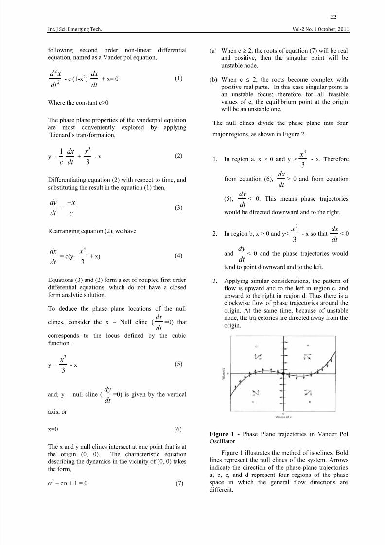
The null clines divide the phase plane into four

major regions, as shown in Figure 2.

1. In region a, x > 0 and y >

3

3

x - x. Therefore

from equation (6),dx

dt > 0 and from equation

(5),dy

dt < 0. This means phase trajectories

would be directed downward and to the right.

2. In region b, x > 0 and y<

3

3

x - x so that

dx

dt < 0

anddy

dt < 0 and the phase trajectories would

tend to point downward and to the left.

3. Applying similar considerations, the pattern of

flow is upward and to the left in region c, andupward to the right in region d. Thus there is a

clockwise flow of phase trajectories around the

origin. At the same time, because of unstable

node, the trajectories are directed away from the

origin.

Figure 1 - Phase Plane trajectories in Vander Pol

Oscillator

Figure 1 illustrates the method of isoclines. Bold

lines represent the null clines of the system. Arrows

indicate the direction of the phase-plane trajectories

a, b, c, and d represent four regions of the phasespace in which the general flow directions are

different.

8/10/2019 264-994-1-PB



23

3. Modeling of the Vander pol oscillatorThe model of the oscillatory dynamics is shown in

Figure 2.

Figure 2 - Simulation model of the vanderpol

oscillator.

When a nonlinear oscillator, which is a Vander

pol oscillator, is driven by an external periodic

stimulus whose frequency is different from the

former, the output of the oscillatory system will

contain a mixture of components that result from theinteraction of the driving periodicity and the natural

oscillation. Here equation (3) and equation (4) are

modified as

dydt

=

c

x

c B Sin 2 ft. (8)

dx

dt = c (y -

3

3

x + x) (9)

Figure 3 - Model of vanderpol oscillator with

external forcing frequency

Figure 3 shows the model of vanderpol

oscillator, with external forcing frequency, which is

used to analyze the frequency entrainment

phenomenon. When external frequency is close to the

system natural frequency, the system follows the

external frequency and the system becomes

frequency entrained.

4. Results and Analysis

The value of c is taken as 3 in the equations (3)and (4) to have phase trajectories as shown in

Figure 2.

The value of x is chosen from – 2 to 2 and value

for y is chosen from – 1 to 1.

The value of B is taken as 1 in equation (8) and c

is chosen as 3.The natural frequency of oscillator

is taken as 0.113 Hz. The forcing frequency is

taken as 0.01Hz, 0.08Hz, 0.14Hz and 0.2 Hz.Then these forcing frequencies are combined

with natural frequency of oscillator and resultant

output waveforms are shown in

Non-linear Analysis

Response of oscill atory activity of cardio vascular

system generated by vanderpol model

1. Time-course of oscillatory activity generated by

vanderpol model

Figure 4 - time courses of oscillatory activity

generated by vanderpol oscillator

Figure 4 shows the time courses of oscillatory

activity generated by vanderpol oscillator. The

vanderpol oscillator is a non-linear oscillator. It

represents the oscillatory activity of heart.

2. Phase portrait showing limit cycle formed byseveral trajectories

Figure 5 - Phase portrait showing limit cycle formed

by several trajectories

8/10/2019 264-994-1-PB



24

The physiological oscillators exhibit behaviour,

which is quite different from the ordinary non-limit

cycle oscillators. On the phase plane, these oscillators

produce oscillations in the form of a stable, closed

trajectory called a limit cycle. In limit cycle

oscillators, when external perturbations move the

state point away from the limit cycle, it always rejoins the original trajectory. In the stable limit cycle,

the state point always returns to its original trajectoryeven after an external disturbance moves it to a

different location (Fig.5).

Responses of vanderpol oscillator to external

sinusoidal frequency

1. When External sinusoidal frequency forcing is

less than 0.113Hz, forcing frequency = 0.01Hz

Figure 6 - Resultant waveform When External

sinusoidal frequency forcing is less than 0.113Hz

Figure 6 shows the resultant waveform, which is a

mixture of the forcing and natural frequencies

2.

when external sinusoidal frequency is 0.01Hz

Figure 7 - Resultant waveform when external

sinusoidal frequency is 0.01 Hz

In this stable limit cycle, the state pointalways returns to its original trajectory even after

an external disturbance moves it to a differentlocation (Figure 7)

3. External sinusoidal forcing frequency = 0.08HZ

Figure 8 - Waveform when External sinusoidal

forcing frequency = 0.08HZ

It is same as natural frequency of vanderpol

oscillator, this phenomenon is called frequency

entrainment (Fig.8).

4. Phase portrait showing limit cycle formed by

several trajectories, when Sinusoidal forcing

frequency=0.08Hz

Figure 9 - Phase portrait when Sinusoidalforcing frequency=0.08Hz

However, when a nonlinear oscillator is

driven by an external periodic forcing frequency,whose frequency approaches, the natural

frequency of the nonlinear oscillator, then

vanderpol system adopts the external forcingfrequency.If we observe the above response, it is

same as natural frequency of vanderpol

oscillator, this phenomenon is called frequency

entrainment (Figure 9).

5. Response of the vander pol oscillator to external

sinusoidal forcing frequency = 0.14HZ

Figure10 - Response of the vander pol oscillator

to external sinusoidal forcing frequency =

0.14HZ

The resultant waveform is a mixture of the

forcing and natural frequencies (Fig.10).


several trajectories when Sinusoidal forcingfrequency = 0.14HZ

Figure 11 - Phase portrait when Sinusoidalforcing frequency = 0.14HZ

8/10/2019 264-994-1-PB



25

The Phase portrait, showing limit cycle formed

by several trajectories, when external sinusoidal

frequency is 0.14Hz (Fig.11). In this stable limit

cycle, the state point always returns to its original

trajectory even after an external disturbance moves it

to a different location.

7. Response of the vander pol oscillator to external

sinusoidal forcing frequency = 0.20HZ

Figure 12 - Response of the vander pol oscillator to

external sinusoidal forcing frequency = 0.20HZ.

When the forcing frequency, is greater than

natural frequency the response of vanderpol

oscillator,is as shown in figure, because the resultantwaveform is a mixture of the forcing and natural

frequencies (Fig.12).


several trajectories when Sinusoidal forcing

frequency = 0.20HZ

Figure 13 - Phase portrait when Sinusoidal

forcing frequency = 0.20HZ

The Phase portrait, showing limit cycle formed by

several trajectories, when external sinusoidalfrequency is 0.20Hz (Fig. 13) .In this stable limit

cycle, the state point always returns to its original

trajectory even after an external disturbance moves itto a different location.

5. Conclusions

A mathematical model based on six differential

equations with dead-times is used for heart rhythm

dynamics simulation, and different non-desirable behaviors (cardio-pathologies) are used for testing

our control algorithm. The time courses of oscillatory

activity and phase plane trajectory are obtained by

Vander pol oscillator using simulation. The oscillator

has its natural frequency of 0.113Hz. When externaldriving frequency is lower (0.01Hz) or greater

(0.2Hz) than the natural frequency, then response is a

mixture of both natural and external frequencies.

These oscillations are different compared to natural

frequency oscillations. When external frequency

(0.08Hz) is close to the system natural frequency

(0.113Hz), then system follows the external

frequency and the system becomes frequencyentrained.

References

1. M. Riedl, A. Suhrbier, H. Malberg,

T. Penzel,

G.

Bretthauer, J. Kurths,and N. Wessel , “ Modeling the

cardiovascular system using a nonlinear additive

autoregressive model with exogenous input”, Phys.

Rev. E, 78 (1), pp 9.

2. Pecora L. M., T. L. Carrol (1990). Synchronizationin chaotic systems. Physical Review Letter, 64, pp

821=824.

3. Sprott J. C. (2006). Chaos and Time-Series Analysis.

Oxford University Press.

4. Gonzalez-Miranda J. M. (2004). Synchronizationand control of chaos. Imperial College Press.

5. Pikovsky A., M. Rosenblum, J. Kurths (2001).

Synchronization. A universal concept in nonlinear

sciences. Cambridge University Press.

6. Guckenheimer J., P. Holmes (1983). Nonlinear

oscillations, dynamical systems, and bifurcations ofvector fields. Springer.

7.

Skogestad S., I. Postlethwaite (2001). Multivariable

Feedback Control .

8. Grimble M. J. (2001). Industrial control system

design. Wiley.

9. Zhou K., J. C. Doyle, K. Glover (1996). Robust andoptimal control . Prentice Hall.

http://publish.aps.org/search/field/author/Penzel_T


http://publish.aps.org/search/field/author/Bretthauer_G


http://publish.aps.org/search/field/author/Wessel_N


http://pre.aps.org/browse


http://pre.aps.org/vtoc/PRE/v78

http://pre.aps.org/vtoc/PRE/v78







264-994-1-pb

Documents