2.6 the fast fourier transform - ntuacorelab.ntua.gr/~nkotsani/slides/fft.pdf · 2.6.0 introduction...

2.6.0 Introduction 2.6.1 An alternative representation of polynomials 2.6.2 Evaluation by divide-and-conquer 2.6.3 Interpolation

2.6 The Fast Fourier TransformAlgorithms (S.Dasgupta, C.H.Papadimitriou, U.V.Vazirani)

Natalia KotsaniAlgorithms and Complexity I, MPLA

January 16, 2014

2.6 The Fast Fourier Transform


Table of contents2.6.0 Introduction

History of the FFTWhy multiplying polynomials?Brute-force

2.6.1 An alternative representation of polynomialsAn important propertyExtended representationsSketch of the FFT

2.6.2 Evaluation by divide-and-conquerPoint value representationThe recursionThe complex nth roots of unity

2.6.3 InterpolationInversion FormulaThe FFT algorithmTransform circuit



History of the FFT

History of the FFT

I 1965, publication (J.W. Culey, J.W. Tukey)

I 1963, presentation at IBM (J.W. Tukey)

I late 1930s, usage for hand calculations

I early 1800s, paper on interpolation, in Latin (C.F.Gauss)

J.W Tukey was reluctant to publish FFT because he felt that thiswas a simple observation that was probably already known.Typical of the period: algorithms were considered second classmathematical objects



Why multiplying polynomials?


Multiplying polynomials is crucial for signal processing.A signal is any quantity that is a function of time (capture a human voice bymeasuring fluctuations in air pressure, the pattern of stars in the night sky, by

measuring brightness as a function of angle etc.).

In order to extract information from a signal, we need to first digitize it bysampling and, then, to put it through a system that will transform it. The

output is called the response of the system:



Brute-force

Multiplying polynomials: Brute-forceDivide-and-conquer: fast algorithms for multiplying integers andmatrices; next target is polynomials.

(a0 +a1x +...+adxd)·(b0 +b1x +...+bdxd) = c0 +c1x +...+c2dx2d

A(x) · B(x) = C (x)

(1 + 2x + 3x2) · (2 + x + 4x) = 2 + 5x + 12x2 + 11x3 + 12x4

c0 = a0b0 = 2c1 = a0b1 + a1b0 = 5

c2 = a0b2 + a1b1 + a2b0 = 12

ck = a0bk + a1bk−1 + ... + akb0 =k∑

i=0

aibk−1

(convolution of the input vectors a and b, denoted c = a⊗ b)

Complexity: Θ(d2)2.6 The Fast Fourier Transform


An important property

An important property

FactA degree-d polynomial is uniquely characterized by its values atany d + 1 distinct points.

We can specify a degree-d polynomial A(x) = a0 + a1x + ... + adxdby either one of the following:

I Its coefficients a0, a1, ..., adI The values A(x0),A(x1), ...,A(xd)

The second is the more attractive for polynomial multiplication!

C (x) = A(x) · B(x)⇒ C (xk) = A(xk) · B(xk), for any point xk



Extended representations

Extended representations

We must face the problem, however, thatdegree(C ) = degree(A) + degree(B)

I if A and B are of degree-bound d, then C is of degree-bound2d

We must therefore begin with extended point-value representationsfor A and for B consisting of 2d point-value pairs each.

Complexity: Θ(d)



Sketch of the FFT

Sketch of the FFT

We expect the input polynomials, and also their product, to bespecified by coefficients. So we need:

I evaluation: translate from coefficients to values, which is justa matter of evaluating the polynomial at the chosen points,

I multiplication: in the value representation,

I interpolation: translate back to coefficients.



Sketch of the FFT

Sketch of the FFT



Point value representation

EvaluationTheorem (Uniqueness of an interpolating polynomial)For any set {(x0, y0), (x1, y1)..., (xn, yn)} of n point-value pairs such thatall the xk values are distinct, there is a unique polynomial A(x) ofdegree-bound n such that yk = A(xk) for k = 0, ..., n − 1.




Alexandre-Theophile Vandermonde (1735-1796)A.T.Vandermonde was a French musician, mathematician and chemist who workedwith Bezout and Lavoisier; his name is now principally associated with determinanttheory in mathematics. He was born in Paris, and died there.

Vandermonde was a violinist, and became engaged with mathematics only around1770. In Memoire sur la resolution des equations (1771) he reported on symmetricfunctions and solution of cyclotomic polynomials. In Remarques sur des problemes desituation (1771) he studied knight’s tours: ”Whatever the twists and turns of a systemof threads in space, one can always obtain an expression for the calculation of itsdimensions, but this expression will be of little use in practice. The craftsman whofashions a braid, a net, or some knots will be concerned, not with questions ofmeasurement, but with those of position: what he sees there is the manner in whichthe theads are interlaced”.

The same year he was elected to the French Academy of Sciences. Memoire sur desirrationnelles de differents ordres avec une application au cercle (1772) was oncombinatorics, and Memoire sur l’elimination (1772) on the foundations ofdeterminant theory. These papers were presented to the Academie des Sciences, andconstitute all his published mathematical work.





Computing a point-value representation for a polynomial given incoefficient form is in principle straightforward:

I select n distinct points x0, x1, ..., xnI evaluate A(xk) for k = 0, 1, ..., n

Horners methodA(x0) = a0 + x0(a1 + x0(a2 + ... + x0(an−2 + x0(an−1))...))

Complexity: O(n2).




Picking the n pointsComputing a point-value representation for a polynomial given incoefficient form is in principle straightforward:

I select n distinct points x0, x1, ..., xnI evaluate A(xk) for k = 0, 1, ..., n

Horners methodA(x0) = a0 + x0(a1 + x0(a2 + ... + x0(an−2 + x0(an−1))...))

Horners method Complexity: Θ(n)Evaluation Complexity: Θ(n2)

IF we choose the points xk cleverly, we can accelerate thiscomputation to run in time Θ(nlgn)!




Picking the n pointsHeres an idea for how to pick the n points at which to evaluate apolynomial A(x) of degree n − 1: positive-negative pairs

±x1,±x2, ...,±xn/2−1

the even powers of xi coincide with those of xi (overlapping).I 3 + 4x + 6x2 + 2x3 + x4 + 10x5 = (3 + 6x2 + x4) + x(4 + 2x2 + 10x4)

A(x) = Ae(x2) + xAo(x2)

I Ae(·) polynomial with the even-numbered coefficients (degree ≤ n/2 − 1)

I Ao(·) with the odd-numbered coefficients (degree ≤ n/2 − 1)

I the terms polynomial in parentheses are polynomials in x2

evaluating A(x) at n paired points ±x1,±x2, ...,±xn/2−1 reduces to evaluatingAe(x) and Ao(x) (which each have half the degree of A(x)) at n/2 points, x2

0 , ..., x2n/2−1



The recursion

The recursion

The original problem of size n is in this way recast as twosubproblems of size n/2, followed by some linear-time arithmetic.

T (n) = 2T (n2 ) + O(n)

Complexity: O(nlogn)



The recursion

The recursion: a problem

The plus-minus trick only works at the top level of the recursion!How can a square be negative?

The reverse engineering of the process



The complex nth roots of unity


I the n complex solutions to the equation zn = 1

I the complex numbers 1, ω, ω2, ..., ωn−1 where ω = e2pi/n

I the nth roots are plus-minus paired: ωn/2+j = −ωj

I squaring them produces the (n/2)nd roots of unity.



Inversion Formula

Inversion FormulaI evaluation is multiplication by M = Mn(ω)I interpolation is multiplication by M−1 = 1

nMn(ω−1).

The FFT multiplies an arbitrary n-dimensional vector (which we have

been calling the coefficient representation) by the n × n matrix:

where ω is a complex nth root of unity, and n is a power of 2.Its (j , k)th entry (starting row-count and column-count at zero) is ωjk .



Inversion Formula

Inversion FormulaI multiplication by M = Mn(ω) maps the kth coordinate axis (the vector

with all zeros except for a 1 at position k) onto the kth column of M

I the columns of M are orthogonal (at right angles) to each other

I the axes of an alternative coordinate system, (Fourier basis, FFT is a rigid rotation)



The FFT algorithm

Interpolation - The FFT

coefficients ⇔ values

Complexity: O(nlogn), when {xi} are complex nth roots of unity (1, ω, ..., ωn−1)

〈values〉 = FFT (〈coefficients〉, ω)

Interpolation is the inverse operation:

〈coefficients〉 = 1nFFT (〈values〉, ω−1)



The FFT algorithm

The FFT algorithm

I M’s columns are segregated into evens and odds

I simplified entries in the bottom half of the matrix using ωn/2 = −1 andωn = 1



The FFT algorithm

The FFT algorithm

the product of Mn(ω) with vector (a0, ..., an−1), a size-n problem, can be

expressed in terms of two size-n/2 problems: the product of Mn/2(ω2) with

(a0, a2, ..., an−2) and with (a1, a3, ..., an−1).

Running time is T (n) = 2T (n/2) + O(n) = O(nlogn).



Transform circuit

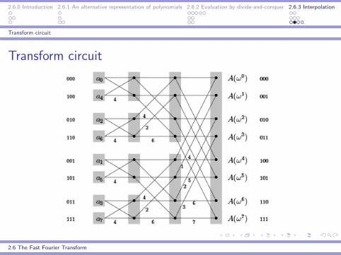
Transform circuitThe divide-and-conquer step of the FFT can be drawn as a very simple circuit.

I the edges are wires carrying complex numbers from left to right

I a weight of j means multiply the number on this wire by ωj

I when two wires come into a junction from the left, the numbers they arecarrying get added up

So the two outputs depicted are executing the commands:



Transform circuit

Transform circuit



Transform circuit

Transform circuit

I For n inputs there are log2n levels, each with n nodes, for a total ofn log n operations

I The inputs are arranged in the order specified by the recursion

I The resulting order in binary (000, 100, 010, 110, 001, 101, 011, 111)

is the same as the natural one (000, 001, 010, 011, 100, 101, 110, 111)

except the bits are mirrored

I There is a unique path between each input aj and each outputA(ωk)

I On the path between aj and A(ωk), the labels add up to jkmod8

I the FFT circuit is a natural for parallel computation and directimplementation in hardware.



Transform circuit

Bibliography

T. Cormen and C. Leiserson and R. Rivest, Introduction toAlgorithms. MIT Press, 1990.

Sanjoy Dasgupta and Christos H. Papadimitriou and Umesh V.Vazirani, Algorithms. McGraw-Hill, 2008.

Jon Kleinberg and Eva Tardos, Algorithm design. PearsonEducation, 2006.


2.6 the fast fourier transform - ntuacorelab.ntua.gr/~nkotsani/slides/fft.pdf · 2.6.0 introduction...

Documents