25 years of quantum hall eﬀect (qhe) a personal...

The Quantum Hall Effect, 1 – 21c© Birkhauser Verlag, Basel, 2005 Poincare Seminar 2004

25 Years of Quantum Hall Effect (QHE)A Personal View on the Discovery,Physics and Applications of this Quantum Effect

Klaus von Klitzing

1 Historical Aspects

The birthday of the quantum Hall effect (QHE) can be fixed very accurately. Itwas the night of the 4th to the 5th of February 1980 at around 2 a.m. duringan experiment at the High Magnetic Field Laboratory in Grenoble. The researchtopic included the characterization of the electronic transport of silicon field effecttransistors. How can one improve the mobility of these devices? Which scatteringprocesses (surface roughness, interface charges, impurities etc.) dominate the mo-tion of the electrons in the very thin layer of only a few nanometers at the interfacebetween silicon and silicon dioxide? For this research, Dr. Dorda (Siemens AG) andDr. Pepper (Plessey Company) provided specially designed devices (Hall devices)as shown in Fig.1, which allow direct measurements of the resistivity tensor.

For the experiments, low temperatures (typically 4.2 K) were used in orderto suppress disturbing scattering processes originating from electron-phonon in-teractions. The application of a strong magnetic field was an established methodto get more information about microscopic details of the semiconductor. A reviewarticle published in 1982 by T. Ando, A. Fowler, and F. Stern about the electronicproperties of two-dimensional systems summarizes nicely the knowledge in thisfield at the time of the discovery of the QHE [1].

Since 1966 it was known, that electrons, accumulated at the surface of asilicon single crystal by a positive voltage at the gate (= metal plate parallel tothe surface), form a two-dimensional electron gas [2]. The energy of the electronsfor a motion perpendicular to the surface is quantized (“particle in a box”) andeven the free motion of the electrons in the plane of the two-dimensional systembecomes quantized (Landau quantization), if a strong magnetic field is appliedperpendicular to the plane. In the ideal case, the energy spectrum of a 2DEG instrong magnetic fields consists of discrete energy levels (normally broadened dueto impurities) with energy gaps between these levels. The quantum Hall effect isobserved, if the Fermi energy is located in the gap of the electronic spectrum andif the temperature is so low, that excitations across the gap are not possible.

The experimental curve, which led to the discovery of the QHE, is shown inFig. 2. The blue curve is the electrical resistance of the silicon field effect tran-

2 K. von Klitzing

Figure 1: Typical silicon MOSFET device used for measurements of the xx- andxy-components of the resistivity tensor. For a fixed source-drain current betweenthe contacts S and D, the potential drops between the probes P − P and H − Hare directly proportional to the resistivities ρxx and ρxy. A positive gate voltageincreases the carrier density below the gate.

sistor as a function of the gate voltage. Since the electron concentration increaseslinearly with increasing gate voltage, the electrical resistance becomes monotoni-cally smaller. Also the Hall voltage (if a constant magnetic field of e.g. 19.8 Teslais applied) decreases with increasing gate voltage, since the Hall voltage is basi-cally inversely proportional to the electron concentration. The black curve showsthe Hall resistance, which is the ratio of the Hall voltage divided by the currentthrough the sample. Nice plateaus in the Hall resistance (identical with the trans-verse resistivity ρxy) are observed at gate voltages, where the electrical resistance(which is proportional to the longitudinal resistivity ρxx) becomes zero. These ze-ros are expected for a vanishing density of state of (mobile) electrons at the Fermienergy. The finite gate voltage regions where the resistivities ρxx and ρxy remainunchanged indicate, that the gate voltage induced electrons in these regions do notcontribute to the electronic transport- they are localized. The role of localized elec-trons in Hall effect measurements was not clear. The majority of experimentalistsbelieved, that the Hall effect measures only delocalized electrons. This assump-tion was partly supported by theory [3] and formed the basis of the analysis ofQHE data published already in 1977 [4]. These experimental data, available to

25 Years of Quantum Hall Effect (QHE) 3

Figure 2: Hall resistance and longitudinal resistance (at zero magnetic field and atB = 19.8 Tesla) of a silicon MOSFET at liquid helium temperature as a functionof the gate voltage. The quantized Hall plateau for filling factor 4 is enlarged.

the public 3 years before the discovery of the quantum Hall effect, contain alreadyall information of this new quantum effect so that everyone had the chance tomake a discovery that led to the Nobel Prize in Physics 1985. The unexpectedfinding in the night of 4./5.2.1980 was the fact, that the plateau values in the Hallresistance ρxy are not influenced by the amount of localized electrons and can beexpressed with high precision by the equation ρxy = h/ie2 (h=Planck constant,e=elementary charge and i the number of fully occupied Landau levels). Also itbecame clear, that the component ρxy of the resistivity tensor can be measured di-rectly with a volt- and amperemeter (a fact overlooked by many theoreticians) andthat for the plateau values no information about the carrier density, the magneticfield, and the geometry of the device is necessary.

4 K. von Klitzing

Figure 3: Copy of the original notes, which led to the discovery of the quantumHall effect. The calculations for the Hall voltage UH for one fully occupied Landaulevel show, that the Hall resistance UH/I depends exclusively on the fundamentalconstant h/e2.


Figure 4: Experimental uncertainties for the realization of the resistance 1 Ohmin SI units and the determination of the fine structure constant α as a function oftime.

The most important equation in connection with the quantized Hall resis-tance, the equation UH = h/e2 ·I, is written down for the first time in my notebookwith the date 4.2.1980. A copy of this page is reproduced in Fig. 3. The validityand the experimental confirmation of this fundamental equation was so high thatfor the experimental determination of the voltage (measured with a x−y recorder)the finite input resistance of 1 MΩ for the x − y recorder had to be included as acorrection. The calculations in the lower part of Fig. 3 show, that instead of thetheoretical value of 25813 Ohm for the fundamental constant h/e2 a value of about25163 Ohm should be measured with the x−y recorder, which was confirmed withhigh precision. These first measurements of the quantized Hall resistance showedalready, that localized electrons are unimportant and the simple derivation on thebasis of an ideal electron system leads to the correct result. It was immediatelyclear, that an electrical resistance which is independent of the geometry of thesample and insensitive to microscopic details of the material will be important formetrology institutes like NBS in the US (today NIST) or PTB in Germany. Soit is not surprising, that discussions with Prof. Kose at the PTB about this new

6 K. von Klitzing

quantum phenomenon started already one day after the discovery of the quantizedHall resistance (see notes in Fig. 3).

Figure 5: The number of publications related to the quantum Hall effect increasedcontinuously up to a value of about one publication per day since 1995.

The experimental results were submitted to Phys. Rev. Letters with the ti-tle: “Realization of a Resistance Standard based on Fundamental Constants” butthe referee pointed out, that (at this time) not a more accurate electrical resis-tor was needed but a better value for the fundamental constant h/e2. Interest-ingly, the constant h/e2 is identical with the inverse fine-structure constant α−1 =(h/e2)(2/µ0c) = 137.036 · · · where the magnetic constant µ0 = 4π10−7N/A2 andthe velocity of light c = 299 792 458 m/s are fixed numbers with no uncertain-ties. The data in Fig. 4 show indeed, that the uncertainty in the realization ofthe electrical unit of 1Ω within the International System of Units (SI units) wassmaller (until 1985) than the uncertainty for h/e2 or the inverse fine-structureconstant. As a consequence, the title of the first publication about the quantumHall effect was changed to: “New Method for High-Accuracy Determination of theFine-Structure Constant Based on Quantized Hall Resistance”[5]. The number ofpublications with this new topic “quantum Hall effect” in the title or abstractincreased drastically in the following years with about one publication per dayfor the last 10 years as shown in Fig. 5. The publicity of the quantized Hall ef-fect originates from the fact, that not only solid state physics but nearly all otherfields in physics have connections to the QHE as exemplarily demonstrated by thefollowing title of publications:

BTZ black hole and quantum Hall effects in the bulk/boundary dynamics [6].Quantum Hall quarks or short distance physics of quantized Hall fluids [7].A four-dimensional generalization of the quantum Hall effect [8].


Quantum computation in quantum-Hall systems [9].Higher-dimensional quantum Hall effect in string theory [10].Is the quantum Hall effect influenced by the gravitational field? [11].

Up to now, more than 10 books were published about the quantum Hall effect[12–19] and the most interesting aspects are summarized in the Proceedings of theInternational Symposium “Quantum Hall Effect: Past, Present and Future” [20].

Figure 6: Summary of high precision data for the quantized Hall resistance up to1988 which led to the fixed value of 25 812.807 Ohm recommended as a referencestandard for all resistance calibrations after 1.1.1990 .

2 Quantum Hall Effect and Metrology

The most important aspect of the quantum Hall effect for applications is thefact that the quantized Hall resistance has always a fundamental value of h/e2 =25812.807 · · · Ohm. This value is independent of the material, geometry and mi-croscopic details of the semiconductor. After the discovery of this macroscopicquantum effect many metrological institutes repeated the experiment with muchhigher accuracy than available in a research laboratory and they confirmed, thatthis effect is extremely stable and reproducible. Fig. 6 summarizes the data (pub-lished until 1988) for the fundamental value of the quantized Hall resistance andit is evident that the uncertainty in the measurements is dominated by the un-certainty in the realization of the SI Ohm. From the internationally accepted def-initions for the basic SI units “second”, “meter”, “kilogram”, and “Ampere” it isclear, that all mechanical and electrical quantities are well defined. However theoverview in Fig. 7 shows also, that the base unit Ampere has a relatively large un-certainty of about 10−6 if deduced from the force between current carrying wires.

8 K. von Klitzing

Figure 7: Basic and derived SI units for mechanical and electrical quantities.

Apparently, the derived unit 1Ω = 1s−3m2kgA−2 (which depends in principle onall basic units) should have an even larger uncertainty than 10−6. However, asshown in Fig. 4, the SI Ohm is known with a smaller uncertainty than the basicunit Ampere which originates from the fact, that a resistance can be realized viathe a.c. resistance R = 1/ωC of a capacitor C. Since the capacitance C of a ca-pacitor depends exclusively on the geometry (with vacuum as a dielectric media),one can realize a SI Ohm just by using the basic units time (for the frequencyω/2π) and length (for a calculable Thomson-Lampert capacitor [21]), which areknown with very small uncertainties. Therefore an uncertainty of about 10−7 forthe realization of the SI Ohm is possible so that the fine-structure constant canbe measured via the QHE directly with the corresponding accuracy. However, thequantized Hall resistance is more stable and more reproducible than any resistorcalibrated in SI units so that the Comite Consultatif d’Electricite recommended,“that exactly 25 812.807 Ohm should be adopted as a conventional value, denotedby RK−90, for the von Klitzing constant RK” and that this value should be usedstarting on 1.1.1990 to form laboratory reference standards of resistances all overthe world [22]. Direct comparisons between these reference standards at differentnational laboratories (see Fig. 8) have shown, that deviations smaller than 2 ·10−9

for the reference standards in different countries are found [23] if the publishedguidelines for reliable measurements of the quantized Hall resistance are obeyed[24]. Unfortunately, this high reproducibility and stability of the quantized Hall re-sistance cannot be used to determine the fine-structure constant directly with highaccuracy since the value of the quantized Hall resistance in SI units is not known.Only the combination with other experiments like high precision measurements(and calculations) of the anomalous magnetic moment of the electron, gyromag-netic ratio of protons or mass of neutrons lead to a least square adjustment of thevalue of the fine-structure constant with an uncertainty of only 3.3 ·10−9 resulting


Figure 8: Reproducibility and stability of the quantized Hall resistance deducedfrom comparisons between different metrological institutes. The observed uncer-tainties of about 2.10−9 is two orders of magnitude smaller than the uncertaintyin the realization of a resistance calibrated in SI Ohms.

in a value for the von Klitzing constant of RK = 25812.807449 ± 0.000086 Ohm(CODATA 2002 [25]). Accurate values for fundamental constants (especially forthe fine-structure constant) are important in connection with the speculation thatsome fundamental constants may vary with time. Publications about the evidenceof cosmological evolution of the fine-structure constant are questioned and couldnot be confirmed. The variation ∂α/∂t per year is smaller than 10−16.

Figure 9: Realization of a two-dimensional electrons gas close to the interfacebetween AlGaAs and GaAs.

The combination of the quantum Hall effect with the Josephson effect (whichallows an representation of the electrical voltage in units of h/e) leads to thepossibility, to compare electrical power (which depends on the Planck constanth) with mechanical power (which depends on the mass m). The best value forthe Planck constant is obtained using such a Watt balance [26]. Alternatively, onemay fix the Planck constant (like the fixed value for the velocity of light for thedefinition of the unit of length) in order to have a new realization of the unit ofmass.

10 K. von Klitzing

Figure 10: Hall resistance and longitudinal resistivity data as a function of themagnetic field for a GaAs/AlGaAs heterostructures at 1.5 K .

3 Physics of Quantum Hall Effect

The textbook explanation of the QHE is based on the classical Hall effect dis-covered 125 years ago [27]. A magnetic field perpendicular to the current I in ametallic sample generates a Hall voltage UH perpendicular to both, the magneticfield and the current direction:

UH = (B · I)/(n · e · d)

with the three-dimensional carrier density n and the thickness d of the sample.For a two-dimensional electron gas the product of n · d can be combined as atwo-dimensional carrier density ns. This leads to a Hall resistance

RH = UH/I = B/(ns · e)

Such a two-dimensional electron gas can be formed at the semiconductor/insulatorinterface, for example at the Si−SiO2 interface of a MOSFET (Metal Oxid Semi-conductor Field Effect Transistor) or at the interface of a GaAs−AlGaAs HEMT(High Electron Mobility Transistor) as shown in Fig. 9. In these systems the elec-trons are confined within a very thin layer of few nanometers so that similar tothe problem of “particle in a box” only quantized energies Ei(i = 1, 2, 3 · · ·) forthe electron motion perpendicular to the interface exist (electric subbands).

A strong magnetic field perpendicular to the two-dimensional layer leads toLandau quantization and therefore to a discrete energy spectrum:

E0,N = E0 + (N + 1/2)hωc (N = 0, 1, 2, ...)

The cyclotron energy hωc = heB/mc is proportional to the magnetic field B andinversely proportional to the cyclotron mass mc and equal to 1.16 meV at 10 Teslafor a free electron mass m0.


Due to the electron spin an additional Zeeman splitting of each Landau levelappears which is not explicitly included in the following discussion. More importantis the general result, that a discrete energy spectrum with energy gaps existsfor an ideal 2DEG in a strong magnetic field and that the degeneracy of eachdiscrete level corresponds to the number of flux quanta (F · B)/(h/e) within thearea F of the sample. This corresponds to a carrier density ns = e · B/h foreach fully occupied spin-split energy level E0, N and therefore to a Hall resistanceRH = h/i · e2 for i fully occupied Landau levels as observed in the experiment. Atypical magnetoresistance measurement on a GaAs/AlGaAs heterostructure underQHE conditions is shown in Fig. 10.

Figure 11: Discrete energy spectrum of a 2DEG in a magnetic field for an idealsystem (no spin, no disorder, infinite system, zero temperature). The Fermi energy(full red line) jumps between Landau levels at integer filling factors if the electronconcentration is constant.

This simple “explanation” of the quantized Hall resistance leads to the cor-rect result but contains unrealistic assumptions. A real Hall device has alwaysa finite width and length with metallic contacts and even high mobility devicescontain impurities and potential fluctuations, which lift the degeneracy of the Lan-dau levels. These two important aspects, the finite size and the disorder, will bediscussed in the following chapters.

3.1 Quantum Hall Systems with Disorder

The experimental fact, that the Hall resistance stays constant even if the fillingfactor is changed (e.g. by varying the magnetic field at fixed density), cannot beexplained within the simple single particle picture for an ideal system. A sketch of

12 K. von Klitzing

Figure 12: Measured variation of the electrostatic potential of a 2DEG as a functionof the magnetic field. The black line marks a maximum in the coulomb oscillationsof a metallic single electron on top of the heterostructure, which corresponds to aconstant electrostatic potential of the 2DEG relative to the SET.

the energy spectrum and the Fermi energy as a function of the magnetic field isshown in Fig. 11 for such an ideal system at zero temperature. The Fermi energy(full blue line) is located only at very special magnetic field values in energy gapsbetween Landau levels so that only at these very special magnetic field values andnot in a finite magnetic field range the condition for the observation of the QHE isfulfilled. On the other hand, if one assumes, that the Fermi energy remains constantas a function of the magnetic field (dotted line in Fig. 11), wide plateaus for thequantized Hall resistance are expected, since the Fermi energy remains in energygaps (which correspond to integer filling factors and therefore to quantized Hallresistances) in a wide magnetic field range. However, this picture is unrealistic since


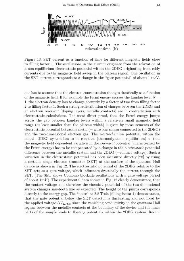
Figure 13: SET current as a function of time for different magnetic fields closeto filling factor 1. The oscillations in the current originate from the relaxation ofa non-equilibrium electrostatic potential within the 2DEG originating from eddycurrents due to the magnetic field sweep in the plateau region. One oscillation inthe SET current corresponds to a change in the “gate potential” of about 1 meV.

one has to assume that the electron concentration changes drastically as a functionof the magnetic field. If for example the Fermi energy crosses the Landau level N =1, the electron density has to change abruptly by a factor of two from filling factor2 to filling factor 1. Such a strong redistribution of charges between the 2DEG andan electron reservoir (doping layers, metallic contacts) are in contradiction withelectrostatic calculations. The most direct proof, that the Fermi energy jumpsacross the gap between Landau levels within a relatively small magnetic fieldrange (at least smaller than the plateau width) is given by measurements of theelectrostatic potential between a metal (= wire plus sensor connected to the 2DEG)and the two-dimensional electron gas. The electrochemical potential within themetal - 2DEG system has to be constant (thermodynamic equilibrium) so thatthe magnetic field dependent variation in the chemical potential (characterized bythe Fermi energy) has to be compensated by a change in the electrostatic potentialdifference between the metallic system and the 2DEG (=contact voltage). Such avariation in the electrostatic potential has been measured directly [28] by usinga metallic single electron transistor (SET) at the surface of the quantum Halldevice as shown in Fig 12. The electrostatic potential of the 2DEG relative to theSET acts as a gate voltage, which influences drastically the current through theSET. (The SET shows Coulomb blockade oscillations with a gate voltage periodof about 1mV ). The experimental data shown in Fig. 12 clearly demonstrate, thatthe contact voltage and therefore the chemical potential of the two-dimensionalsystem changes saw-tooth like as expected. The height of the jumps correspondsdirectly to the energy gap. The “noise” at 2.8 Tesla (filling factor 4) demonstrates,that the gate potential below the SET detector is fluctuating and not fixed bythe applied voltage ∆V2DES since the vanishing conductivity in the quantum Hallregime between the metallic contacts at the boundary of the device and the innerparts of the sample leads to floating potentials within the 2DEG system. Recent

14 K. von Klitzing

Figure 14: Sketch of a device with a filling factor slightly below 1. Long-rangepotential fluctuations lead to a finite area within the sample (localized carriers)with vanishing electrons (= filling factor 0) surrounded by an equipotential line.The derivation of the measured Hall voltage UH show, that closed areas withanother filling factor than the main part of the device leads to a Hall effect whichis not influenced by localized electrons.

measurements have demonstrated [29], that time constants of many hours areobserved for the equilibration of potential differences between the boundary of aQHE device and the inner part of the sample as shown in Fig. 13. The oscillationsin the SET current can be directly translated into a variation of the electrostaticpotential below the position of the SET since one period corresponds to a “gatevoltage change” for the SET of about 1 meV. The non-equilibrium originates froma magnetic field sweep in regions of vanishing energy dissipation, which generateseddy currents around the detector and corresponding Hall potential differences ofmore than 100 meV perpendicular to these currents. These “Hall voltages” are notmeasurable at the outer Hall potential probes (at the edge of the sample), sinceall eddy currents cancel each other. The current distribution is unimportant forthe accuracy of the quantized Hall resistance!

In order to explain the width of the Hall plateaus, localized electrons in thetails of broadened Landau levels have to be included. A simple thought experimentillustrates, that localized states added or removed from fully occupied Landaulevels do not change the Hall resistance (see Fig. 14). For long range potentialfluctuations (e.g. due to impurities located close to the 2DEG) the Landau levelsfollow this potential landscape so that the energies of the Landau levels changewith position within the plane of the device. If the energy separation betweenLandau levels is larger than the peak value of the potential fluctuation, an energygap still exists and a fully occupied Landau level (e.g. filling factor 1) with theexpected quantized Hall resistance RK can be realized. In this picture, a fillingfactor 0.9 means, that 10% of the area of the device (= top of the hills in the


Figure 15: Skipping cyclotron orbits (= diamagnetic current) at the boundaries ofa device are equivalent to the edge channels in a 2DEG with finite size.

potential landscape) becomes unoccupied with electrons as sketched in Fig. 14.The boundary of the unoccupied area is an equipotential line (with an unknownpotential) but the externally measured Hall voltage UH , which is the sum of theHall voltages of the upper part of the sample (current I2) and the lower part(current I1), adds up to the ideal value expected for the filling factor 1 (greyregions). Eddy currents around the hole with i = 0 will vary the currents I1 andI2 but the sum is always identical with the external current I.

The quantized Hall resistance breaks down, if electronic states at the Fermienergy are extended across the whole device. This is the case for a half-filledLandau level if the simple percolation picture is applied. Such a singularity athalf-filled Landau levels has been observed experimentally [30].

This simple picture of extended and localized electron states indicates, thatextended states always exist at the boundary of the devices. This edge phenomenonis extremely important for a discussion of the quantum Hall effect in real devicesand will be discussed in more detail in the next chapter. In a classical picture,skipping orbits as a result of reflected cyclotron orbits at the edge lead to diamag-netic currents as sketched in Fig 15. Therefore, even if the QHE is characterizedby a vanishing conductivity σxx (no current in the direction of the electric field), afinite current between source and drain of a Hall device can be established via thisdiamagnetic current. If the device is connected to source and drain reservoirs withdifferent electrochemical potentials (see Fig. 15), the skipping electrons establishdifferent electrochemical potentials at the upper and lower edge respectively. En-ergy dissipation appears only at the points (black dots in Fig. 15) where the edgepotentials differ from the source/drain potentials.

16 K. von Klitzing

Figure 16: Ideal Landau levels for a device with boundaries. The fully occupiedLandau levels in the inner part of the device rise in energy close to the edge formingcompressible (“metallic”) stripes close to the crossing points of the Landau levelswith the Fermi energy EF .

3.2 Edge Phenomena in QHE Devices

The simple explanation of the quantized Hall resistance as a result of fully occupiedLandau levels (with a gap at the Fermi energy) breaks down for real devices withfinite size. For such a system no energy gap at the Fermi energy exists underquantum Hall condition even if no disorder due to impurities is included. This isillustrated in Fig. 16 where the energy of the Landau levels is plotted across thewidth of the device. The Fermi energy in the inner part of the sample is assumed tobe in the gap for filling factor 2. Close to the edge (within a characteristic depletionlength of about 1µm) the carrier density becomes finally zero. This correspondsto an increase in the Landau level energies at the edge so that these levels becomeunoccupied outside the sample. All occupied Landau levels inside the sample haveto cross the Fermi energy close to the boundary of the device. At these crossingpoints “half-filled Landau levels” with metallic properties are present.

Selfconsistent calculations for the occupation of the Landau levels show thatnot lines but metallic stripes with a finite width are formed parallel to the edge [31].The number of stripes is identical with the number of fully occupied Landau levelsin the inner part of the device. These stripes are characterized by a compressibleelectron gas where the electron concentration can easily be changed since the Lan-dau levels in these regions are only partly filled with electrons and pinned at the


Figure 17: Experimental determination of the position of incompressible (= insu-lating) stripes close to the edge of the device for the magnetic field range 1.5 - 10Tesla.

Figure 18: Hall potential distribution of a QHE device measured with an AFM.The innermost incompressible stripe (= black lines) acts as an insulating barrier.The Hall potential is color coded with about half of the total Hall voltage for thedark grey-light grey potential difference.

18 K. von Klitzing

Fermi energy. In contrast, the incompressible stripes between the compressible re-gions represent fully occupied Landau levels with the typical isolating behavior ofa quantum Hall state. If the single electron transistor shown in Fig. 12 is locatedabove an incompressible region, increased noise is observed in the SET currentsimilar to the noise at 2.8 Tesla in Fig. 12. In order to visualize the position ofthe stripes close to the edge, not the SET is moved but an artificial edge (= zerocarrier density) is formed with a negative voltage at a gate metal located close tothe SET. The edge (= position with vanishing carrier density) moves with increas-ing negative gate voltage closer to the detector and alternatively incompressible(increased SET noise) and compressible strips (no SET noise) are located belowthe SET detector. The experimental results in Fig. 17 confirm qualitatively thepicture of incompressible stripes close to the edge which move away from the edgewith increasing magnetic field until the whole inner part of the device becomesan incompressible region at integer filling factor. At slightly higher magnetic fieldsthis “bulk” incompressible region disappears and only incompressible stripes withlower filling factor remain close to the boundary of the device.

The influence of the incompressible stripes on the Hall potential distributionhas been measured with an atomic force microscope. The results in Fig. 18 show,that the innermost incompressible stripe has such strong “insulating” propertiesthat about 50% of the Hall potential drops across this stripe. The other 50%of the Hall potential drops close to the opposite boundary of the device acrossthe equivalent incompressible stripe. In principle the incompressible stripes shouldbe able to suppress the backscattering across the width of a Hall device so thateven for an ideal device without impurities (= localized states due to potentialfluctuations) a finite magnetic field range with vanishing resistivity and quantizedHall plateaus should exist [32]. However, the fact, that the plateau width increasessystematically with increasing impurity concentration (and shows the expecteddifferent behavior for attractive and repulsive impurities) shows, that localizedstates due to impurities are the main origin for the stabilization of the quantizedHall resistance within a finite range of filling factors. A vanishing longitudinalresistivity always indicates, that a backscattering is not measurable. Under thiscondition the quantized Hall resistance is a direct consequence of the transmissionof one-dimensional channels [33].

4 Correlated Electron Phenomena in Quantum Hall Systems

Many physical properties of the quantum Hall effect can be discussed in a sin-gle electron picture but it is obvious that the majority of modern research andpublications in this field include electron correlation phenomena. Even if the frac-tional quantum Hall effect [34] (which is a manifestation of the strong electron-electron interaction in a two-dimensional system) can be nicely discussed as theinteger quantum Hall effect of weakly interacting quasi particles called compos-ite fermions [35], the many-body wave function of the quantum Hall system is the


basis for the discussion of different exciting new phenomena observed in correlatedtwo-dimensional systems in strong magnetic fields. Many of these new phenomenacan only be observed in devices with extremely high mobility where the electron-electron interaction is not destroyed by disorder. Experiments on such devicesindicate, that phenomena like superfluidity and Bose-Einstein condensation [36],skyrmionic excitations [37], fractional charges [38], a new zero resistance stateunder microwave radiation [39] or new phases based on a decomposition of a half-integer filling factor into stripes and bubbles with integer filling factors [40] areobservable. The two-dimensional electron system in strong magnetic field seemsto be the ideal system to study electron correlation phenomena in solids with thepossibility to control and vary many parameters so that the quantum Hall effectwill remain a modern research field also in the future.

References

[1] T. Ando, A. Fowler, and F. Stern, Rev. Mod. Phys. 54, 437 (1982).

[2] A.B. Fowler, F.F. Fang, W.E. Howard, and P.J. Stiles, Phys Rev. Lett. 16,901 (1966).

[3] H. Aoki and H. Kamimura, Solid State Comm. 21, 45 (1977).

[4] Th. Englert and K. v. Klitzing, Surf. Sci. 73, 70 (1978).

[5] K. v. Klitzing, G. Dorda and M. Pepper, Phys. Rev. Lett. 45, 494 (1980).

[6] Y.S. Myung, Phys. Rev. D 59, 044028 (1999).

[7] M. Greiter, Int. Journal of Modern Physics A 13 (8), 1293 (1998).

[8] S.C. Zhang and J. Hu, Science 294, 823 (2001).

[9] V. Privman, I.D. Vagner and G. Kventsel, Phys. Lett. A239, 141 (1998).

[10] M. Fabinger, J. High Energy Physics 5, 37 (2002).

[11] F.W. Hehl, Y.N. Obukhov, and B. Rosenow, Phys. Rev. Lett. 93, 096804(2004).

[12] R.E. Prange and S. Girvin (ed.), The Quantum Hall Effect, Springer, NewYork (1987).

[13] M. Stone (ed.), Quantum Hall Effect, World Scientific, Singapore (1992).

[14] M. Janen, O. Viehweger, U. Fastenrath, and J. Hajdu, Introduction to theTheory of the Integer Quantum Hall Effect, VCH Weinheim (1994).

[15] T. Chakraborty, P. Pietilinen, The Quatnum Hall Effects, 2nd Ed., Springer,Berlin (1995).

20 K. von Klitzing

[16] S. Das Sarma and A. Pinczuk, Perspectives in Quantum Hall Effects, JohnWiley, New York (1997).

[17] O. Heinonen (ed.), Composite Fermions: A Unified View of the Quantum HallRegime, World Scientific, Singapore (1998).

[18] Z.F. Ezawa, Quantum Hall Effects - Field Theoretical Approach and RelatedTopics, World Scientific, Singapore (2002).

[19] D. Yoshioka,Quantum Hall Effect, Springer, Berlin (2002).

[20] Proc. Int. Symp. Quantum Hall Effect: Past, Present and Future, Editor R.Haug and D. Weiss, Physica E20 (2003).

[21] A.M. Thompson and D.G. Lampard, Nature 177, 888 (1956).

[22] T.J. Quinn, Metrologia 26, 69 (1989).

[23] F. Delahaye, T.J. Witt, R.E. Elmquist and R.F. Dziuba, Metrologia 37, 173(2000).

[24] F. Delahaye and B. Jeckelmann, Metrologia 40, 217 (2003).

[25] The most recent values of fundamental constants recommended by CODATAare available at: http://physics.nist.gov/cuu/constants/index.html.

[26] E.R. Williams, R.L. Steiner, D.B. Nevell, and P.T. Olsen, Phys. Rev. Lett.81, 2404 (1998).

[27] E.H. Hall, American Journal of Mathematics, vol ii, 287 (1879).

[28] Y.Y. Wei, J. Weis, K. v. Klitzing and K. Eberl, Appl. Phys. Lett. 71 (17),2514 (1997).

[29] J. Huls, J. Weis, J. Smet, and K. v. Klitzing, Phys. Rev. B69 (8), 05319 (2004).

[30] S. Koch, R.J. Haug, K. v. Klitzing, and K. Ploog, Phys. Rev B43 (8), 6828(1991).

[31] D.B.Chklovskii, B.I. Shklovskii, and L.I. Glazmann, Phys. Rev. B46, 4026(1999).

[32] A. Siddiki and R.R. Gerhardts, Phys. Rev. B70, (2004).

[33] M. Bttiker, Phys. Rev. B38, 9375 (1988).

[34] D.C. Tsui, H.L. Stormer, and A.C. Crossard, Phys. Rev. Lett. 48, 1559 (1982).

[35] J.K. Jain, Phys. Rev. Lett. 63, 199 (1989).


[36] M.Kellogg, J.P. Eisenstein, L.N. Pfeiffer, and K.W. West, Phys. Rev. Lett. 93,036801 (2004).

[37] A.H. MacDonald, H.A. Fertig, and Luis Brey, Phys. Rev. Lett. 76, 2153 (1996).

[38] R. de-Picciotto, M. Reznikov, M. Heiblum, Nature 389, 162 (1997).

[39] R.G. Mani, J.H. Smet, K. V. Klitzing, V. Narayanamurti, W.B. Johnson, andV. Urmanski, Nature 420, 646 (2002).

[40] M.P. Lilly, K.B. Cooper, J.P. Eisenstein, L.N. Pfeiffer, and K.W. West, Phys.Rev. Lett. 82, 394 (1999).

Klaus von KlitzingMax-Planck-Institut fur FestkorperforschungHeisenbergstr. 1D-70569 StuttgartGermanyemail: [email protected]

25 years of quantum hall eﬀect (qhe) a personal...

Documents