23790284 1 voltage source pwm inverter
DESCRIPTION
pwmTRANSCRIPT

1. Voltage-Source PWM Inverter
1.1 Introduction
In contrast to grid connected ac motor drives, hardly variable in speed, power electronic devices (e.g. inverter), providing voltage supply variable in both frequency and magnitude, are used to operate ac motors at frequencies other than the supply frequency. Developments in this direction have taken place long ago, but a techno-economical solution could not be found until the late 1980s because of stringent space requirements, non-availability of high power devices and prohibitive cost of electronic devices and components. Rapid developments in the field of power electronics (inverter grade thyristor, GTO thyristor, IGBT etc.) and miniaturization/mass production of control electronics (development of VLSI technology and microprocessor based digital control systems) have reached such a stage that variable ac inverter drives are becoming increasingly popular in today’s motor drives. Presently, inverter drives meet not only weight and space constraints, but also are economically viable. In general, two basic types of inverters exist: Voltage-source inverter (VSI), employing a dc link capacitor and providing a switched voltage waveform, and current-source inverter (CSI), employing a dc link inductance and providing a switched current waveform at the motor terminals. CS-inverters are robust in operation and reliable due to the insensitivity to short circuits and noisy environment. VS-inverters are more common compared to CS-inverter since the use of Pulse Width Modulation (PWM) allows efficient and smooth operation, free from torque pulsations and cogging [Bose 97]. Furthermore, the frequency range of VSI is higher and they are usually more inexpensive when compared to CSI drives of the same rating [Dub 89]. In this chapter, only voltage-source inverters are considered. Although the power flow through the device is reversible, it is called an inverter because the predominant power flow is from the dc bus to the three-phase ac motor load. Bi-directional power flow is an important feature for motor drives as it allows regenerative breaking, i.e. the kinetic energy of the motor and its load is recovered and returned to the grid when the motor slows down. In electric vehicle application, the dc bus energy is supplied directly from primary energy sources, e.g. batteries.
2 Chapter 1
In ac grid connected motor drives, a rectifier, usually a common diode bridge providing a pulsed dc voltage from the mains, is required. Alternatively, a second ac-to-dc converter, acting as a rectifier during the motoring mode and an inverter during the breaking mode, is used between drive and utility grid. An additional benefit of the active front end is enabling unity power factor, (sinusoidal) current flows to or from the grid. Although the basic circuit for an inverter may seem simple, accurately switching these devices provides a number of challenges for the power electronic engineer. The most common switching technique is called Pulse Width Modulation (PWM). PWM is a powerful technique for controlling analog circuits with a processor’s digital outputs. PWM is employed in a wide variety of applications, ranging from measurement and communications to power control and conversion. In ac motor drives, PWM inverters make it possible to control both frequency and magnitude of the voltage and current applied to a motor. As a result, PWM inverter-powered motor drives are more variable and offer in a wide range better efficiency and higher performance when compared to fixed frequency motor drives. The energy, which is delivered by the PWM inverter to the ac motor, is controlled by PWM signals applied to the gates of the power switches at different times for varying durations to produce the desired output waveform. There are several PWM modulation techniques. It is beyond the scope of this book to describe them all in detail. The following illustration describes the basic three-phase inverter topology and typical pulse width modulation methods. Furthermore, issues of phase voltage distortion/identification due to the inverter non-linearity are discussed in detail.
1.2 Voltage-Source PWM Inverter
A typical voltage-source PWM converter performs the ac to ac conversion in two stages: ac to dc and dc to variable frequency ac. The basic converter design is shown in figure 1.1. The grid voltage is rectified by the line rectifier usually consisting of a diode bridge. Presently, attention paid to power quality and improved power factor has shifted the interest to more supply friendly ac-to-dc converters, e.g. PWM rectifier. This allows simultaneously active filtering of the line current as well as regenerative motor braking schemes transferring power back to the mains. The dc voltage is filtered and smoothed by the capacitor C in the dc bus (figure 1.1). The capacitor is of appreciable size (2-20 mF) and therefore a major cost item [Bose 97]. Alternatively, the inverter can be supplied from a fixed dc voltage. The filtered dc voltage is usually measured for control purpose. Because of the nearly constant dc bus voltage, a number of PWM inverters with their associated motor drives can be supplied from one common diode bridge. The inductive reactance L between rectifier and ac supply is used to reduce commutation dips produced by the rectifier, to limit fault current and to soften voltages spikes of the mains.

Voltage-Source PWM Inverter 3
T1
T4
D4
D1 C
T3
T6
D6
D3
T5
T2
D2
D5
power supply
AC motor Udc
Rectifier DC bus Inverter
Switching logic
L
Figure 1.1: Basic three-phase voltage-source converter circuit.
Neglecting the voltage drop of the inductances (current depending) and diodes (Ud ≈ 1V if i > 0), the positive potential of the dc bus voltage equals the highest potential of the three phases and the negative potential equals the lowest potential of the three phases. Since each phase owns one negative and one positive maximum potential during one period of the net frequency, the rectifier input voltage equals the maximum of the positive and negative line voltages, respectively. Thus, the rectifier input voltage traces six pulses as shown in figure 1.2 by the thick line.
0 5 10 15 20400
500
600
t [ms]
Udc
[V]
0 5 10 15 200
0.5
1
t [ms]
i B6 [A
]
0 5 10 15 20-1
0
1
t [ms]
i a [A]
0 5400
500
600
Udc
[V]
0 50
20
40
i B6 [A
]
0 5-40
-20
0
20
40
i a [A]
Udc
uab -uca ubc -uab uca -ubc uab -uc
Figure 1.2: Line voltages (uab, ubc, uca), dc bus voltagof the first phase ia and output current iB6 of a B6
Left: No inverter output power (inverter losseRight: Inverter output power Pout ≈ 5,5
Figure 1.2 presents typical voltage and current wavefsupplied by a stiff grid. As indicated by the dashed liincreases, if the absolute value of a line voltage is hConsequently, the dc voltage increases slightly. A dc vovoltage supply causes a reduction of the rectifier inp
U
10 15 20t [ms]
10 15 20t [ms]
10 15 20t [ms]
dc
-ubc a ubc -uabuca
e Udc, line current -diode bridge. s ≈ 10 W). kW.
orms of a B6-diode bridge nes, the rectifier current iB6 igher than the dc voltage.
ltage higher than the current ut current until the current

4 Chapter 1
equals zero and the diode bridge blocks the supply voltage. The rectifier current iB6 is identically reflected by the line currents. The sign of each line current depends on the two non-blocking diodes each conducting the positive and negative rectifier current, respectively. During the conducting period, the difference of line and dc voltage is active as voltage drop over the line inductances and resistances. The higher the line inductances, the smaller the line current peaks. However, the value of the line inductances is limited due to economic and efficiency reasons. Furthermore, the average dc voltage depends on the line inductances and the inverter output power. The maximum dc voltage (no load) is equal to the maximum amplitude of the line voltages. Due to voltage drops of line inductances, resistances and rectifier diodes, the dc voltage slightly decreases with increasing load. For more details concerning the rectifier, see [Bose 97], [Dub 89] et al. According to figure 1.1, the dc voltage is switched in a three-phase PWM inverter by six semiconductor switches in order to obtain pulses, forming three-phase ac voltage with the required frequency and amplitude for motor supply. The switching devices must be capable of being turned “on” as well as turned “off”. During the last years, major progress has been made in the development of new power semiconductor devices. The simpler requirement driving the power switches and the higher maximum switching-frequency, enabling higher operating frequencies (higher motor speed), provide continually rising output power. The new generation of switching devices is capable of conducting more current and blocking higher voltages. The alternatives at present are gate turn-off thyristor (GTO), MOS controlled thyristor (MCT), bipolar junction transistor (BJT), MOS field effect transistor (MOSFET) and insulated gate bipolar transistor (IGBT). The IGBT is a combination of power MOSFET and bipolar transistor technology and combines the advantages of both. In the same way as a MOSFET, the gate of the IGBT is isolated and its driving power is very low. However, the conducting voltage is similar to that of a bipolar transistor. Presently, IGBTs dominate the medium-power range of variable speed drives. Since the maximal current rating of IGBT modules is around 1 kA and the voltage rating is approximately 3 kV, they will gradually replace GTOs at higher power levels [Vas 99]. Parallel to the power switches, reverse recovery diodes are placed conducting the current depending on the switching states and current sign. These diodes are required, since switching off an inductive load current generates high voltage peaks probably destroying the power switch. Exemplary for one inverter leg, figure 1.3 presents the basic configuration and the inverter output voltage depending on the switching state and current sign. The basic configuration of one inverter output phase consists of upper and lower power devices T1 and T4, and reverse recovery diodes D1 and D4. When transistor T1 is on, a voltage ½ Udc is applied to the load. Considering an inductive load, the current increases subsequently. If the load draws positive current,

Voltage-Source PWM Inverter 5
it will flow through T1 and supply energy to the load. To the contrary, if the load current ia is negative, the current flows back through D1 and returns energy to the dc source.
ua0
T1
T4 D4
D1
ia < 0
C/2
C/2
ωt
ia
ua0
ωt
-½ Udc
½ Udc
T1 on
T4 on
τdead
D1
drop
D4
drop
T1
drop
T4
drop
0
0
ua0
T1
T4
C/2 ½ Udc
D4
D1
ia > 0
C/2 ½ Udc
½ Udc
½ Udc
T4 off
T1 off
T4 on
T1 on
ua0
Similarly if T4 is on, which is equal to T1 off, a voltage -½ Udc is applied to the load and the current decreases. If ia is positive, the current flows through D4 returning energy to the dc source. A negative current yields T4 conducting and supplying energy to the load.
Figure 1.3: Basic configuration of a half-bridge inverter and center-tapped inverter output voltage.
Left: Switching states and current direction. Right: Output voltage and line current.
According to figure 1.3, with T1 on and drawing positive load current ia, the output voltage ua0 will be less than ½ Udc by the on-state voltage drop of T1. When the load current reverses, the output voltage will be higher than ½ Udc by the voltage drop across D1. Similarly, the output voltage is slightly changed by the voltage drop of the lower devices T4 and D4. Normally, the on-state voltage and diode drops (≈1 V) are ignored and the center-tapped inverter is represented as generating the voltage ½ Udc and -½ Udc, respectively. Neglecting additionally the dead-time interval τdead, the behavior of the power devices together with the reverse recovery diode is equally described by ideal two-position switches.

6 Chapter 1
1.3 Pulse Width Modulation
Usually, the on- and off-states of the power switches in one inverter leg are always opposite. Therefore, the inverter circuit can be simplified into three 2-position switches. Either the positive or the negative dc bus voltage is applied to one of the motor phases for a short time. Pulse width modulation (PWM) is a method whereby the switched voltage pulses are produced for different output frequencies and voltages. A typical modulator produces an average voltage value, equal to the reference voltage within each PWM period. Considering a very short PWM period, the reference voltage is reflected by the fundamental of the switched pulse pattern. Apart from the fundamental wave, the voltage spectrum at the motor terminals consists of many higher harmonics. The interaction between the fundamental motor flux wave and the 5th and 7th harmonic currents produces a pulsating torque at six times of the fundamental supply frequency. Similarly, 11th and 13th harmonics produce a pulsating torque at twelve times the fundamental supply frequency [Dub 89]. Furthermore, harmonic currents and skin effect increase copper losses leading to motor derating. However, the motor reactance acts as a low-pass filter and substantially reduces high-frequency current harmonics. Therefore, the motor flux (IM & PMSM) is in good approximation sinusoidal and the contribution of harmonics to the developed torque is negligible. To minimize the effect of harmonics on the motor performance, the PWM frequency should be as high as possible. However, the PWM frequency is restricted by the control unit (resolution) and the switching device capabilities, e.g. due to switching losses and dead time distorting the output voltage. There are various PWM schemes. Well-known among these are sinusoidal PWM, hysteresis PWM, space vector modulation (SVM) and “optimal” PWM techniques based on the optimization of certain performance criteria, e.g. selective harmonic elimination, increasing efficiency, and minimization of torque pulsation [Jen 95]. While the sinusoidal pulse-width modulation and the hysteresis PWM can be implemented using analog techniques, the remaining PWM techniques require the use of a microprocessor. A modulation scheme especially developed for drives is the direct flux and torque control (DTC). A two-level hysteresis controller is used to define the error of the stator flux. The torque is compared to its reference value and is fed into a three-level hysteresis comparator. The phase angle of the instantaneous stator flux linkage space phasor together with the torque and flux error state is used in a switching table for the selection of an appropriate voltage state applied to the motor [Dam 97], [Vas 97]. Usually, there is no fixed pattern modulation in process or fixed voltage to frequency relation in the DTC. The DTC approach is similar to the FOC with hysteresis PWM. However, it takes the interaction between the three phases into account. In the following subsections, hysteresis PWM, sinusoidal PWM and SVM are discussed in more detail.

Voltage-Source PWM Inverter 7
1.3.1 Hysteresis PWM Current Control
Hysteresis current control is a PWM technique, very simple to implement and taking care directly for the current control. The switching logic is realized by three hysteresis controllers, one for each phase (figure 1.4). The hysteresis PWM current control, also known as bang-bang control, is done in the three phases separately. Each controller determines the switching-state of one inverter half-bridge in such a way that the corresponding current is maintained within a hysteresis band ∆i.
1/2 Udc
0ωt
ωt Output voltage
0
Hysteresis band ∆iCurrent reference
Real current
-1/2 Udc
ia
ua0
Switching logic
ib*
∆i ib
ic*
∆i ic
ia*
∆i ia
Figure 1.4: Hysteresis PWM, current control and switching logic. To increase a phase current, the affiliated phase to neutral voltage is equal to the half dc bus voltage until the upper band-range is reached. Then, the negative dc bus voltage -½ Udc applied as long as the lower limit is reached &c. More complicated hysteresis PWM current control techniques also exist in practice, e.g. adaptive hysteresis current vector control is based on controlling the current phasor in a α/β-reference frame. These modified techniques take care especially for the interaction of the three phases [Jen 95]. Obviously, the dynamic performance of such an approach is excellent since the maximum voltage is applied until the current error is within predetermined boundaries (bang-bang control). Due to the elimination of an additional current controller, the motor parameter dependence is vastly reduced. However, there are some inherent drawbacks [Brod 85]:
• No fixed PWM frequency: The hysteresis controller generates involuntary lower subharmonics.
• The current error is not strictly limited. The signal may leave the hysteresis band caused by the voltage of the other two phases.
• Usually, there is no interaction between the three phases: No strategy to generate zero-voltage phasors.
• Increased switching frequency (losses) especially at lower modulation or motor speed.
• Phase lag of the fundamental current (increasing with the frequency).

8 Chapter 1
Hysteresis current control is used for operation at higher switching frequency, as this compensates for their inferior quality of modulation. The switching losses restrict its application to lower power levels. Due to the independence of motor parameters, hysteresis current control is often preferred for stepper motors and other variable-reluctance motors. A carrier-based modulation technique, as described in the next subsection, eliminates the basic shortcomings of the hysteresis PWM controller [Bose 97]. However, when being compared to the hysteresis PWM, an additional current control loop, calculating the reference voltages, is required when subsequent modulation schemes are applied to high-performance motion control systems.
1.3.2 Sinusoidal Pulse Width Modulation
Three-phase reference voltages of variable amplitude and frequency are compared in three separate comparators with a common triangular carrier wave of fixed amplitude and frequency (figure 1.5-1.6). Each comparator output forms the switching-state of the corresponding inverter leg [Dub 89], [Leo 85]. In torque controlled ac motor drives using sinusoidal PWM, the reference voltages (u*
a, u*b, u*
c) are usually calculated by an additional current control loop (FOC).
Switching logic
ub*
uc*
ua*
comparator
Current controller
id*
id
d,q
a,b,c
ud*
Current controller
iq*
iq
uq*
Carrier wave
comparator
comparator
Figure 1.5: Sinusoidal PWM, current control and switching logic. As shown in figure 1.6, a saw-tooth- or triangular-shaped carrier wave, determining the fixed PWM frequency, is simultaneously used for all three phases. This modulation technique, also known as PWM with natural sampling, is called sinusoidal PWM because the pulse width is a sinusoidal function of the angular position in the reference signal.

Voltage-Source PWM Inverter 9
uab
ua0
ub0
uc0
Phase b Phase a Phase c
ωt
ωt
ωt
ωt
ωt
Carrier wave
Uref
Udc/2
-Udc/2
Upper switch “on”
Lower switch “on”
Figure 1.6: Principle of sinusoidal PWM generation. Since the PWM frequency, equal to the frequency of the carrier wave, is usually much higher than the frequency of the reference voltage, the reference voltage is nearly constant during one PWM period TPWM. This approximation is especially true considering the sampled data structure within a digital control system. Depending on the switching states, the positive or negative half dc bus voltage is applied to each phase. At the modulation stage, the reference voltage is multiplied by the inverse half dc bus voltage compensating the final inverter amplification of the switching logic into real power supply. According to figure 1.7, the mean value of the output voltage, resulting from a reference voltage being constant within one PWM-period, depends on the on- and off-states of the affiliated switch:
( )2
11210
dc
PWMTa
PWMao
UttT
dtuT
uPWM
∆−∆== ∫ (1.1)

10 Chapter 1
1
ua0
∆t1 ∆t2
TPWM
-1
0
t
t
Udc /2
-Udc /2
ua0
*00 aa uu =
1
ua0
∆t1/2 ∆t2
TPWM
-1
0
∆t1/2
t
t
Udc /2
-Udc /2
ua0
*00 aa uu =
2
*0
dc
a
Uu
2
*0
dc
a
Uu
Saw-tooth carrier wave
Triangular carrier wave
Figure 1.7: Sinusoidal modulation at constant or sampled reference voltage for one phase.
Left: Saw-tooth shaped carrier wave. Right: Triangular-shaped carrier wave. The switch on- and off-times (∆t1 and ∆t2) are calculated according to figure 1.7 by setting the carrier wave equal to the reference voltage related to the dc bus voltage:
221
*0
!
1dc
a
PWM Uut
T=∆+− (1.2)
⇒
+=∆
21
2
*0
1dc
aPWM
UuTt (1.3)
−=∆−=∆
21
2
*0
12dc
aPWMPWM U
uTtTt (1.4)
Applying (1.3)-(1.4) on (1.1) shows the mean value of the output voltage ua0 being equal to the reference voltage u*
a0:
−−
+=
21
221
221 *
0*
0
dc
aPWM
dc
aPWMdc
PWMao U
uTU
uTUT
u (1.5)
⇒ *0aao u=u (1.6)
Apart over-modulation, this modulation technique produces an average voltage value, equal to the reference voltage within each PWM period. Therefore, the
Voltage-Source PWM Inverter 11
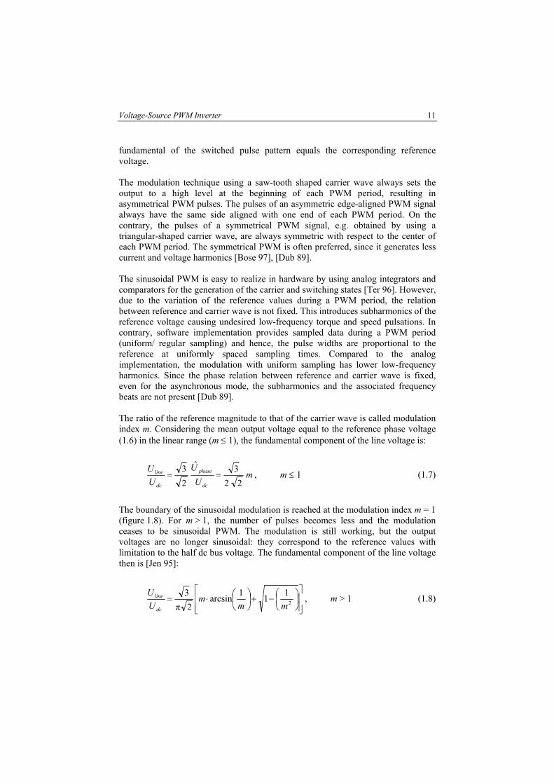
fundamental of the switched pulse pattern equals the corresponding reference voltage. The modulation technique using a saw-tooth shaped carrier wave always sets the output to a high level at the beginning of each PWM period, resulting in asymmetrical PWM pulses. The pulses of an asymmetric edge-aligned PWM signal always have the same side aligned with one end of each PWM period. On the contrary, the pulses of a symmetrical PWM signal, e.g. obtained by using a triangular-shaped carrier wave, are always symmetric with respect to the center of each PWM period. The symmetrical PWM is often preferred, since it generates less current and voltage harmonics [Bose 97], [Dub 89]. The sinusoidal PWM is easy to realize in hardware by using analog integrators and comparators for the generation of the carrier and switching states [Ter 96]. However, due to the variation of the reference values during a PWM period, the relation between reference and carrier wave is not fixed. This introduces subharmonics of the reference voltage causing undesired low-frequency torque and speed pulsations. In contrary, software implementation provides sampled data during a PWM period (uniform/ regular sampling) and hence, the pulse widths are proportional to the reference at uniformly spaced sampling times. Compared to the analog implementation, the modulation with uniform sampling has lower low-frequency harmonics. Since the phase relation between reference and carrier wave is fixed, even for the asynchronous mode, the subharmonics and the associated frequency beats are not present [Dub 89]. The ratio of the reference magnitude to that of the carrier wave is called modulation index m. Considering the mean output voltage equal to the reference phase voltage (1.6) in the linear range (m ≤ 1), the fundamental component of the line voltage is:
mU
UUU
dc
phase
dc
line
223ˆ
23
== , m ≤ 1 (1.7)
The boundary of the sinusoidal modulation is reached at the modulation index m = 1 (figure 1.8). For m > 1, the number of pulses becomes less and the modulation ceases to be sinusoidal PWM. The modulation is still working, but the output voltages are no longer sinusoidal: they correspond to the reference values with limitation to the half dc bus voltage. The fundamental component of the line voltage then is [Jen 95]:
−+
⋅= 2
111arcsin2π
3mm
mUU
dc
line , m > 1 (1.8)

12 Chapter 1
0
1 2 3 4
0
0.1
0.2
0.3
0.4
0.5
0.6
0.7
0.8
m [ ]
Ulin
e/Udc
[ ]
223
π6
Figure 1.8: Line voltage (rms) in function of the modulation index.
When m is made sufficiently large, the phase voltage becomes a square wave and the line voltage becomes a 6-step waveform.
ua0
ωt
u*
2dcU
−
24 dcUπ
ua0
2dcU
− ub0
2
*0
dc
a
Uu
2
*0
dc
b
Uu
u
dcU−
dcU
2dcU
ωt
ωt
1-1
carrier wave
uab
fundamental
Figure 1.9: Strong overmodulation and square-wave shaped output voltage with affiliated fundamental.
Top: Reference voltages (u*a0, u*
b0) and carrier wave. Middle: Phase-to-neutral output voltage ua0 and affiliated fundamental. Bottom: Phase-to-neutral output voltage ub0 and line voltage uab.
The square wave of the phase voltage expressed in Fourier-coefficients is:
[∑∞
−−
=n
dca tn
nUu ω
π)12(sin
121
24
0 ] (1.9)
Using sinusoidal PWM generation, the maximum fundamental phase voltage is limited by the dc bus voltage:

Voltage-Source PWM Inverter 13
dcphase UUπ2ˆ
max, = (1.10)
However, this maximum voltage should not be exploited since overmodulation results in a strong increased spectrum of lower voltage and current harmonics especially for the 5th, 7th and 11th harmonics. In figure 1.10, the current of an induction motor (scalar control) in the linear range (m = 1) and at overmodulation (m = 1,33) is presented to illustrate the involuntary current distortion.
0 0.01 0.02 0.03 0.04 0.05-4
-2
0
2
4
t [s]
i a [A]
m = 1
m = 1,33
Figure 1.10: Measured current at different modulation indexes.
(induction motor in open loop: uref = 200 V sin(ωt); Udc = 400 V and Udc = 300 V resp.) Basic drawbacks of the sinusoidal PWM are the not ideal use of the dc bus voltage and the non-existent interaction between the three phases resulting in superfluous changes of switching states, increasing semiconductor losses and introducing a higher harmonic content at the motor terminals.
1.3.2.1 Injection of a Third Harmonic
According to (1.9), also multiple of third harmonics are present in the voltage spectrum. However, the third harmonics are eliminated and not existent in the current spectrum since the sum of the phase current of a three-phase ac machine equals zero. As shown in figure 1.11, the range of the sinusoidal PWM can be increased by adding third harmonics to the reference voltages. The same third harmonic is added to each of the three reference voltages. Adding third harmonics agrees with a simultaneous variation of the potential in all phases, thus not recognized at the terminals of an ac motor with isolated neutral point:
)()( 00
!
00 thirdbthirdabaab uuuuuuu +−+=−= (1.11)
Therefore, the introduction of a third harmonic does not distort the line voltages since third harmonic components in the phase voltages are cancelled.

14 Chapter 1
A geometrical calculation yields the maximum possible increase of the linear area with the harmonic amplitude being 1/6 of the reference voltage amplitude. Such an injection of a third harmonic results in a 15,5% higher maximum output voltage without overmodulation. According to [Jen 95], the harmonic content of the resulting current spectrum of ac motor drives is minimal at injection of a third harmonic with the amplitude being 1/4 of the reference voltage amplitude, still increasing the maximum output voltage without overmodulation by 12%.
ua0
t
2
*0
dc
a
Uu
u*a0 third harmonic
2dcU
−
2dcU
t
t
reference plus third harmonic
-1
1
carrier wave
Figure 1.11: Injection of a third harmonic and modulation.
Obviously, also multiple of third harmonics do not disturb the current spectrum and are suitable injection signals. As can be shown [Jen 95], the subsequently described space vector modulation is equal to the sinusoidal PWM with injection of a suitable triangular-shaped signal containing all existing multiple of third harmonics.
1.3.3 Space Vector Modulation (SVM)
Space-vector pulse width modulation has become a popular PWM technique for three-phase voltage-source inverters in applications such as control of induction and permanent magnet synchronous motors. The mentioned drawbacks of the sinusoidal PWM are vastly reduced by this technique. Instead of using a separate modulator for each of the three phases, the complex reference voltage phasor is processed as a whole. Therefore, the interaction between the three motor phases is exploited. It has been shown, that SVM generates less harmonic distortion in both output voltage and current applied to the phases of an ac motor and provides a more efficient use of the supply voltage in comparison with direct sinusoidal modulation techniques [Jen 95].

Voltage-Source PWM Inverter 15
As shown in table 1.1, there are eight possible combinations of on and off patterns for the three upper electronic switches feeding the three-phase power inverter (figure 1.1). Notice that the on and off states of the lower power switches are opposite to the upper ones and so completely determined once the states of the upper power electronic switches are known. The phase voltages corresponding to the eight combinations of switching patterns can be mapped into the α/β frame through α/β-transformations [Hen 92]. This transformation results in six non-zero voltage vectors and two zero vectors. The non-zero vectors form the axes of a hexagonal containing six sectors (S1 − S6) as shown in figure 1.12. The angle between any adjacent two non-zero vectors is 60 electrical degrees. The zero vectors are at the origin and apply a zero voltage vector to the motor. The derived α/β voltages in terms of the dc bus voltage Udc are summarized in table 1.1.
Table 1.1: Switching table and α/β transformation of affiliated state voltage vectors.
3dcU 32 dcU
3dcU 3dcU 32 dcU
3dcU 3dcU 32 dcU
32 dcU− 32 dcU
3dcU− 3dcU− 32 dcU
3dcU 3dcU− 32 dcU
Switch no. α/β-transformation of the states
State S1 S3 S5 Ux,α Ux,β |Ux|
000 OFF OFF OFF 0 0 0
100 ON OFF OFF 2 0
110 ON ON OFF
010 OFF ON OFF −
011 OFF ON ON 0
001 OFF OFF ON
101 ON OFF ON
111 ON ON ON 0 0 0
100
110
101 001
011
010 Uβ
000 111
Uα
S6
S2
S1
S5 S4
S3
Figure 1.12: Hexagon, formed by the basic space vectors and sector definition (S1 − S6). Using the transformation of the three phase voltages to the α/β reference frame, the voltage phasor Uref represents the spatial phasor sum of the three phase voltages. When the desired output voltages are three-phase sinusoidal voltages with 120°

16 Chapter 1
phase shift, Uref becomes a revolving phasor with the same frequency and a magnitude equal to the corresponding line-to-line rms voltage. The objective of the space vector PWM technique is to approximate the reference voltage phasor Uref by a combination of the eight switching patterns. Practically, only the two adjacent states (Ux and Ux+60) of the reference voltage phasor and the zero states should be used [Jen 95] as demonstrated by the example in figure 1.13. The reference voltage Uref can be approximated by having the inverter in switching states Ux and Ux+60 for t1 and t2 duration of time respectively.
( 60211
++= xxPWM
ref UtUtT
U ) (1.12)
Of course, the affiliated sector must be known first. The sector identification and the calculation of t1 and t2 are presented in the next subsection. Since the sum of t1 and t2 should be less than or equal to TPWM, the inverter has to stay in zero state for the rest of the period. The remaining time t0 is assigned to one or both zero-voltage phasors.
210 ttTt PWM −−= (1.13)
Applying only one of the two zero-voltage states during a PWM period, results in an asymmetric edge-aligned PWM signal. This is often undesired (higher harmonics) but reduces the required switching number by 33% since one inverter leg does not switch during that particular PWM period. Here, the remaining time t0 is equally assigned to both states. As illustrated in figure 1.13, all state changes are obtained in each case by switching only one inverter leg.
40% ‘100’
50% ‘110’
Uref = U ejωt
100 110 110 100 111 000 000
TPWM
ua0
ub0
uc0
5% ‘000’
5% ‘111’
Figure 1.13: Example of duty-cycle generation. As mentioned above, the reference voltage is actually equal to the desired three-phase output voltages mapped to the α/β frame. The envelope of the hexagonal formed by the basic space vectors, as shown in figure 1.12, is the locus of the maximum output voltage. In order to avoid overmodulation, the magnitude of Uref must be limited to the shortest radius of this envelope. This gives a maximum rms value of the line-to-line and phase output voltages of
Voltage-Source PWM Inverter 17
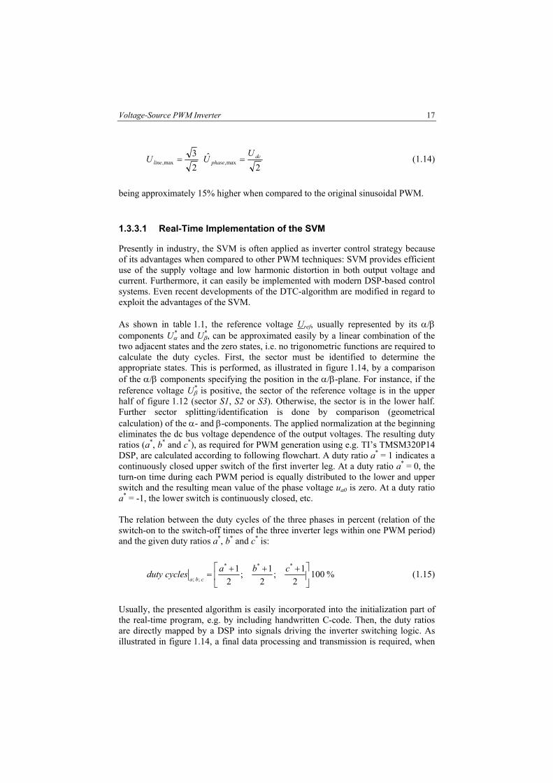
2ˆ
23
max,max,dc
phaselineU
UU == (1.14)
being approximately 15% higher when compared to the original sinusoidal PWM.
1.3.3.1 Real-Time Implementation of the SVM
Presently in industry, the SVM is often applied as inverter control strategy because of its advantages when compared to other PWM techniques: SVM provides efficient use of the supply voltage and low harmonic distortion in both output voltage and current. Furthermore, it can easily be implemented with modern DSP-based control systems. Even recent developments of the DTC-algorithm are modified in regard to exploit the advantages of the SVM. As shown in table 1.1, the reference voltage Uref, usually represented by its α/β components Uα
* and Uβ*, can be approximated easily by a linear combination of the
two adjacent states and the zero states, i.e. no trigonometric functions are required to calculate the duty cycles. First, the sector must be identified to determine the appropriate states. This is performed, as illustrated in figure 1.14, by a comparison of the α/β components specifying the position in the α/β-plane. For instance, if the reference voltage Uβ
* is positive, the sector of the reference voltage is in the upper half of figure 1.12 (sector S1, S2 or S3). Otherwise, the sector is in the lower half. Further sector splitting/identification is done by comparison (geometrical calculation) of the α- and β-components. The applied normalization at the beginning eliminates the dc bus voltage dependence of the output voltages. The resulting duty ratios (a*, b* and c*), as required for PWM generation using e.g. TI’s TMSM320P14 DSP, are calculated according to following flowchart. A duty ratio a* = 1 indicates a continuously closed upper switch of the first inverter leg. At a duty ratio a* = 0, the turn-on time during each PWM period is equally distributed to the lower and upper switch and the resulting mean value of the phase voltage ua0 is zero. At a duty ratio a* = -1, the lower switch is continuously closed, etc. The relation between the duty cycles of the three phases in percent (relation of the switch-on to the switch-off times of the three inverter legs within one PWM period) and the given duty ratios a*, b* and c* is:
%1002
1;2
1;2
1 ***
;;
+++=
cbacyclesdutycba
(1.15)
Usually, the presented algorithm is easily incorporated into the initialization part of the real-time program, e.g. by including handwritten C-code. Then, the duty ratios are directly mapped by a DSP into signals driving the inverter switching logic. As illustrated in figure 1.14, a final data processing and transmission is required, when

18 Chapter 1
additionally a slave DSP generating the PWM pulses, e.g. TI’s TMSM320P14, is used. To avoid overflow of the fixed-point slave DSP, all duty ratios must be limited to ± 1. Since the P14 DSP uses 16-bit compare registers for the PWM generation, the calculated values are adjusted by the given multiplication before they are finally transmitted to the slave DSP generating the PWM signals. As illustrated in a subsequent chapter (e.g. figure 3.2), each two PWM channels are employed to generate the correct pulses for the inverter.
Sector 2 & 5:Sector 1 & 4: Sector 3 & 6:
Sector 1 Sector 2 Sector 3 Sector 4 Sector 5 Sector 6
Yes
No
No
No
No
No
P14 DSP
|u| ≤ 1 Overflow protection
16 bit compare register
normalization
PWM 1−6
Uα*, Uβ
*
215-1
dcU1
23
0* ≥βu
**
31
βα uu ≥
**
31
βα uu −≥ **
31
βα uu ≥
*
31
βα uu −≥
***
31
βα uua +=
***
33
βα uub +−=
** ac −=
** 2 αua =
**
32
βub =
** bc −=
***
31
βα uua −=
** ab −=
***
33
βα uuc −−=
duty ratios: (a*; b*; c*)
Voltage reference
Figure 1.14: Flowchart of SVM and data transmission to a TMSM320P14 DSP. The turn-on times t0, t1 and t2 of the applied switching states during each PWM period, as introduced in (1.12)-(1.13) for illustration purpose, are not required for implementation of the SVM. However, they are easily calculated by the duty cycles of the three phases. For instance, the zero states ‘000’ and ‘111’ are each equal to the minimum of the duty cycles given in (1.15) multiplied by the PWM period TPWM.

Voltage-Source PWM Inverter 19
1.4 Dead-Time Effect & Voltage Distortion
For voltage-source PWM inverters, a dead-time interval is required to prevent the “shoot-through” effect of a half-bridge during a change of the switching states. All semiconductor-switching devices react delayed to the turn-off signals owing to the storage time. During this storage time, depending on the operating point, the switch is not able to block the dc link voltage. Therefore, to avoid a short circuit of the half-bridge, a dead-time interval must be introduced between the turn-off signal of a switch and the turn-on signal controlling the opposite switch. The dead time τdead is usually constant and determined as the maximum value of storage time τst plus an additional safety margin. The dead times of common IGBT-inverters used in industry vary between τdead ≈ 1-5 µs. Although the dead time is short, it causes deviations from the desired fundamental inverter output voltage. The effects of the dead time on the output voltage will be described from one half-bridge of the PWM inverter according to figure 1.15. The basic configuration consists of upper and lower power devices T1 and T4, and reverse recovery diodes D1 and D4.
½ Udc
-½ Udc
UT1
UD4
u a0
Ideal gating pulse pattern
T1
T4
pulse pattern with dead time
T1
T4
τdead
½ Udc
-½ Udc
UD1
UT4
u a0
T1
T4
T1
T4
τdead
Ideal gating pulse pattern
pulse pattern with dead time
τdead fPWM Udc τdead fPWM Udc
ua0
T1
T4
C/2 ½ Udc
D4
D1
ia > 0
C/2 ½ Udc
T1 off
T1 on
ua0
T1
T4 D4
D1
ia < 0
C/2
C/2
½ Udc
½ Udc
T4 off
T4 on
Figure 1.15: Error voltage due to the dead-time effect. Left: Positive load current. Right: Negative load current.
Considering the no-load case, the storage time of the semiconductors is very small when compared to the dead time: Switching off a power device, the current

20 Chapter 1
commutates directly to the diodes. This condition results in the desired voltage, which is applied to the motor terminals. In contrast to this, switching on a power device is delayed by the dead time. During the dead-time interval, the diode continues conducting until the dead time elapses and the opposite power device is switched on. This condition results in a loss of voltage at the motor terminals indicated by the gray marked area in figure 1.15. With a positive current, the duty cycles are shorter and with negative currents longer than required. Hence, the actual duty cycle of a bridge is always different from the one of the reference voltage. It is either increased or decreased, depending on the load current polarity. Furthermore, the voltage drops of the power switches UT, respectively the voltage drop of the reverse recovery diode UD, are considered. Summarizing, the voltage distortion can be described by an error voltage ∆U
dcPWMdeadDT UfUUU ⋅⋅+
+≈∆ τ
2 (1.16)
depending on the dead time τdead, the dc bus voltage Udc, the PWM frequency fPWM and the voltage drops UD and UT of IGBT and diode [Bose 97]. This error voltage and the resistances RT and RD of the switch changes the inverter output voltage ua0 from its intended value uref to:
)sign(20 iURRiuu DT
refa ⋅∆−+
⋅−≈ , (1.17)
The dead time reduces the effective turn-on time and produces the undesired fifth- and seventh-order harmonics in the inverter output voltage [Dod 90]. Furthermore, it generates sub-harmonics, resulting in torque pulsation and possible instability at low-speed and light-load operation [Leg 97], [Mur 92]. The resulting speed oscillation and the voltage distortion are illustrated in figure 1.16 showing the dead-time effect on a 1,5 kW induction motor drive in open loop (scalar) control at low speed and light-load operation. Considering the given drive setup (τdead = 2,5 µs; fPWM = 10 kHz) and according to (1.16), the error voltage amounts to ∆U = 12,5 V (equal to 15,3 V in the alpha/beta reference frame). A reduction of the average voltages occurs according to (1.17) when one of the phase currents changes its sign. The motor currents have the tendency to maintain their values after a zero crossing. In generator mode, the behavior of the motor current is contrary resulting in a steeper rise of the current after zero crossing. In any case, the motor torque is influenced as it can be observed by speed oscillations at six times of the fundamental frequency. The dead-time problem is more serious in high-power gate-turn-off thyristor (GTO) inverter systems than in the case of IGBT or MOSFET inverters, since the GTO requires a longer dead time. However, the use of fast switching devices using high carrier frequencies (5-20 kHz) with lower dead-time values (1-5 µs), will not free the system of the described distortion. Higher PWM frequencies improve the

Voltage-Source PWM Inverter 21
waveform quality by raising the order of theoretical harmonics, but low frequency sub-harmonics persist due to the dead time. Furthermore, to avoid unnecessary switching losses and short-term overheating of a switching device, minimum time duration in the switching states must be forced. If the commanded voltage value is less than the required minimum, the affiliated switching state must be either extended in time or skipped. This causes additional distortion of the inverter output voltages. Therefore, a compromise must be made by choosing a suitable PWM frequency: a high PWM frequency improves the theoretical quality of the waveform, but may increase simultaneously the voltage distortion due to the dead-time effect.
0 0.25 0.5 0.75 1-40
-20
0
20
40
t [s]
Uα
[V]
0 0.25 0.5 0.75 1-4
-2
0
2
4
t [s]
I α [A
]
0 0.25 0.5 0.75 135
40
45
50
55
60
t [s]
n [r
pm
]
-40 -20 0 20 40-40
-20
0
20
40
Uα
[V]
Uβ [V
]
uref
uβ (uα) uα
uref
Figure 1.16: Open-loop control of an induction motor & dead-time effect (Udc =500 V, no load).
Left: Measured current Iα, measured voltage Uα and reference voltage Uref. Right: Measured/reference speed and voltage trajectories.
1.4.1 Dead-Time Compensation
Remarkable efforts have been made to compensate the voltage distortion due to the dead-time effect [Choi 96], [Leg 97], [Sep 94]. Most dead-time compensation methods are based on an average value theory: the lost voltage is averaged over an operating cycle and added vectorially to the command voltage [Mur 87], [Jeo 91]. Dead-time compensation can be implemented in hardware or software. The hardware compensator operates by closed loop control [Mur 87]. Previous commutation times are measured and used to control the next duty cycles. However, a potential-free measurement of the inverter output voltages is required. Software compensators are mostly designed in feed-forward mode. Depending on the sign of the respective phase current, a fixed time delay is either added to or subtracted from the command voltage.
22 Chapter 1
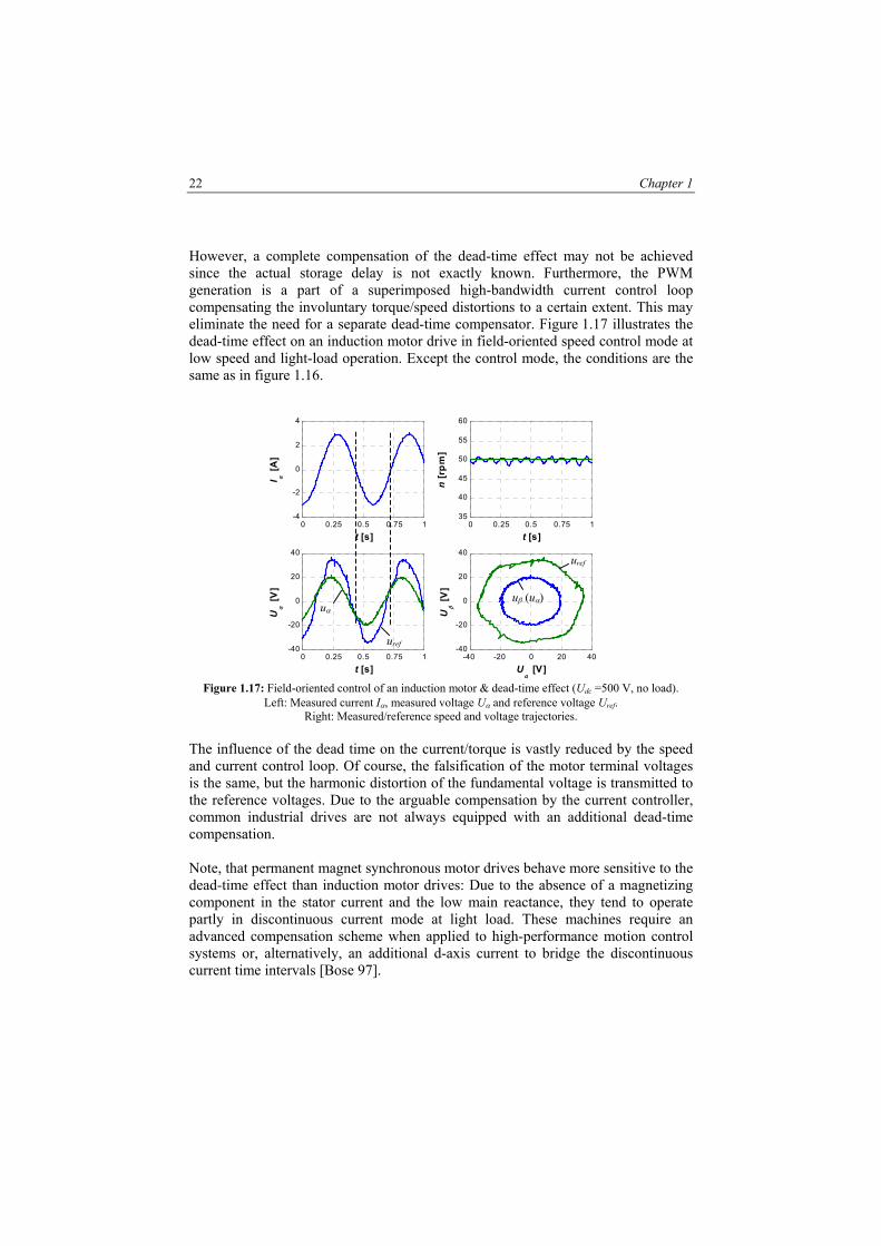
However, a complete compensation of the dead-time effect may not be achieved since the actual storage delay is not exactly known. Furthermore, the PWM generation is a part of a superimposed high-bandwidth current control loop compensating the involuntary torque/speed distortions to a certain extent. This may eliminate the need for a separate dead-time compensator. Figure 1.17 illustrates the dead-time effect on an induction motor drive in field-oriented speed control mode at low speed and light-load operation. Except the control mode, the conditions are the same as in figure 1.16.
0 0.25 0.5 0.75 1-40
-20
0
20
40
t [s]
Uα
[V]
0 0.25 0.5 0.75 1-4
-2
0
2
4
t [s]
I α [A
]
0 0.25 0.5 0.75 135
40
45
50
55
60
t [s]
n [r
pm
]
-40 -20 0 20 40-40
-20
0
20
40
Uα
[V]
Uβ [V
]
uref
uβ (uα) uα
uref
Figure 1.17: Field-oriented control of an induction motor & dead-time effect (Udc =500 V, no load). Left: Measured current Iα, measured voltage Uα and reference voltage Uref.
Right: Measured/reference speed and voltage trajectories. The influence of the dead time on the current/torque is vastly reduced by the speed and current control loop. Of course, the falsification of the motor terminal voltages is the same, but the harmonic distortion of the fundamental voltage is transmitted to the reference voltages. Due to the arguable compensation by the current controller, common industrial drives are not always equipped with an additional dead-time compensation. Note, that permanent magnet synchronous motor drives behave more sensitive to the dead-time effect than induction motor drives: Due to the absence of a magnetizing component in the stator current and the low main reactance, they tend to operate partly in discontinuous current mode at light load. These machines require an advanced compensation scheme when applied to high-performance motion control systems or, alternatively, an additional d-axis current to bridge the discontinuous current time intervals [Bose 97].

Voltage-Source PWM Inverter 23
1.4.2 Dead-Time Generation
The switching transitions of real switches, especially the transition from current conducting to voltage blocking, are not infinitely fast. After conducting, a finite time is required, mainly to remove the space charge, before a semiconductor switch is able to block the supply voltage. Switching off a power device, the current commutates to the opposite recovery diode (constant current direction) and the power switch starts to block the dc voltage. If a switch of one inverter leg is turned on before the opposite switch blocks the dc bus voltage, the whole dc bus voltage is shorten across this leg (figure 1.1) resulting in a very high short-circuit current only limited by the resistances of the power switches. Obviously, such a high short-circuit current may destroy the power switches as well as the drive system and the dc link capacitor. To avoid such short-circuit conditions, a dead-time interval is added between the turn-off signal of a switch and the turn-on signal controlling the opposite switch. Dead time control prevents any cross-conduction or shoot-through current from flowing through the main power switches during switching transitions by controlling the turn-on times of the semiconductor drivers. The high-side driver is not allowed to turn on until the voltage at the junction of the opposite power switch is low and vice versa. During the dead-time interval, recovery diodes continue conducting until the dead time elapses and the opposite power device is switched on. In modern DSP systems, the dead time generation is usually programmable, e.g. added as extra time in a compare register/timer. Considering analog circuits, the fixed dead-time generation of one half-bridge is easily generated by a RC-circuit coupled to two optocouplers, each controlling the opposite switches of one inverter half-bridge as described in figure 1.18. Additionally, such a hardware realization takes care for galvanic isolation of the digital control system and the power electronics. The resistance R is calculated by the resistance voltage drop divided by the operating current of the optocoupler IP:
P
ds
IUUR −
= (1.18)
According to figure 1.18, changing the switching signal Us from a positive to a negative voltage (e.g.: Us = ±12V) results in a discharging of the capacitor depending on the photodiode operating voltage (Ud ≈ 1V if i > 0). While the photodiode P1 directly blocks, the dead-time τdead passes before the capacitor voltage equals the voltage -Ud, equal to the on state of photodiode P2 driving the opposite switch of the inverter leg:
ddCR
dsdeadc UUeUUtUdead
−=+
−+==
− !1)()(
τ
τ (1.19)

24 Chapter 1
Thus, a minimum capacitor value is required to guarantee the dead-time interval τdead:
⇒
+
−≥
ds
d
dead
UUUR 21ln
C τ (1.20)
Optocoupler 1
PWM logic:US = ±12V R
C
IP2
IP1
UC
US
IP IP2IP1 IP1
τdead
t
Switching logic
-Ud
UC
-Ud
-Us
UC
t
t τdead
Optocoupler 2
Figure 1.18: Analog dead-time generation. Left: Exemplary hardware circuit for one inverter leg. Right: Switching logic, voltage and affiliated current of an optocoupler driving the power switch.
1.5 PWM Inverter Drives and Motor Insulation
Variable speed ac drives are used in ever-increasing numbers because of their well-known benefits for energy efficiency and for flexible control of processes and machinery using low-cost readily available maintenance-free ac motors. While the connection of a motor to an inverter supply is straightforward, some basic considerations are necessary to ensure trouble free long-term operation. Insulation performance is one of the considerations required in engineering variable speed drive solutions. Following summary provides basic information to enable the correct matching of low voltage ac motors and PWM inverters with respect to motor insulation:
Motor winding insulation experiences higher voltage stresses when used with an inverter than when connected directly to the ac mains supply.
The higher stresses are dependent on the motor cable length and are caused by the fast rising voltage pulses of the drive and transmission line effects in the cable.
For supply voltages less than 500V ac, most standard motors are immune to these higher stresses.
Voltage-Source PWM Inverter 25
For supply voltages over 500V ac, a motor with an enhanced winding insulation system is required. Alternatively, additional components can be added to limit the voltage stresses to acceptable levels.
Where the drive spends a large part of its operating time in braking mode, the effect is similar to increasing the supply voltage by up to 20%.
For drives with PWM active front ends (regenerative and/or unity power factor), the effective supply voltage is increased by around 15%.
1.6 Conclusions
Controlled power supply for electric drives is obtained usually by converting the mains ac supply. A typical converter consists of power electronic circuits, employing switching devices such as thyristors, transistors, GTOs, MOSFETSs, IGBTs and diodes as well as a host of associated control and interfacing circuits. The conversion process allows fast control of voltage, current or power to the motor via the gate circuits of the converter switches. In this way, the required dynamic response requirements of high-performance ac motor drives can be met. This chapter provides a detailed survey of voltage-source PWM inverter drives with emphasis on the modulators and control methods. The most common three-phase inverter topology is that of a switch mode voltage source inverter. VS-inverters consist of two main sections, a controller to set the operating frequency and a three-phase inverter to generate the required sinusoidal three-phase voltage from a dc bus voltage. The basic concepts of pulse width modulation are illustrated. PWM is the process of modifying the width of the pulses in a pulse train in direct proportion to a small control signal. The greater the control voltage, the wider the resulting pulses become. By using a sinusoid of the desired frequency as control voltage for a PWM circuit, it is possible to produce a high-power waveform whose average voltage varies sinusoidally in a manner suitable for driving ac motors. Due to the significant flexibility in controlling the inverter switches, a large number of switching algorithms were introduced and some of these have gained wide acceptance and are fully developed. Usually, the behavior of the power devices together with the reverse recovery diode is described by ideal two-position switches. In practice, a dead-time interval is required to prevent the “shoot-through” effect of a half-bridge during a change of the switching states. Although the dead time is short, it causes deviations from the desired fundamental inverter output voltage. Issues of the resulting phase voltage distortion due to the inverter non-linearity as well as compensation methods are discussed in detail.


2. Regenerative Braking and Ride-Through at Power Interruptions
2.1 Introduction
Voltage dips and sags of short duration constitute a serious problem for many applications and especially for variable speed drives (frequency converters) in industry. Early types of frequency converter for motor drives were notoriously sensitive to supply disturbances and often had to perform a full stop and restart to resume operation. The economic impact, of what actually is a mere incident, therefore could turn out to be quite substantial. Usually, voltage source PWM inverter drives are equipped with an under-voltage protection mechanism, causing the system to shut down within a few milliseconds after a power interruption in the regular grid. This shut down mechanism can be associated with a total loss of system control since the control electronics are usually powered by the (in this case discharged) dc-link capacitor. Particularly in multi-motor drives, a loss of mutual synchronization may be critical. This may entail damage or loss of material in sensitive applications as the production of textile fibers, paper mills, or extrusion drives. Generally, it is required to wait until the machine has come to a complete standstill to enable restarting [Baa 89]. Braking to zero speed and restarting obviously is not an adequate solution. Many continuous production processes in industry are sensitive to a larger variation in speed or losing control at worst. In addition, time and additional workload required to get a plant ready for restart may be considerable. This chapter discusses a design concept avoiding the standstill/restarting interval at power interruptions. The proposed solution to the problem is to recover some of the mechanical energy stored in the rotating masses by kinetic buffering. When the power supply is interrupted, a dc link voltage control is applied to force an immediate transition into the regenerative mode. During the interruption interval, the drive system continues to operate at almost zero electromagnetic torque, just regenerating a minor amount of power to cover the electrical losses in the inverter. This maintains the dc link capacitor well charged, keeping the electronic control circuits active, since they are supplied from the dc link through a switched mode converter. In this way, the drive remains controllable even at power interruptions of several seconds. Of course, the (still controlled) braking of the drive depends on the

28 Chapter 2
actual load torque. Since drive control is never lost, the voltage control scheme can be applied to multi motor drives as well. The implemented regenerative braking scheme allows the inverter to keep its dc bus voltage at a predetermined minimum level as long as possible, expanding the time in which supply voltage can be reapplied without the time-consuming dc-link capacitor recharging cycle. The temporary speed dip is generally tolerable, since the most frequent power interruptions last only for a few milliseconds. The implemented voltage control scheme is derived from a torque controlled dc bus voltage. Considering realistic conditions, the ride-through capability at short-time power interruptions is discussed. Measured results are presented and evaluated to demonstrate the performance and the stability of the system.
2.2 Voltage Dips
A voltage dip is a short-duration reduction in the supply voltage, in many cases due to network faults somewhere in the energy distribution system. During a voltage dip, the voltages in the three phases are no longer the same, causing a number of problems. A major fault more than 100 km away from a customer may still yield a significant voltage dip. Mains voltage dips and short interruptions are caused by a wide variety of phenomena. They can be caused by nearby events, such as a faulty load on an adjacent branch circuit causing a circuit breaker to operate, or perhaps by a large motor or other large load on the same circuit being switched on. They can also be caused by far away events such as lightning strokes or downed power lines. In case of a fault in the power distribution grid, an automatic circuit recloser may cycle open and close several times within a short period attempting to clear the fault, thus resulting in a sequence of short interruptions noticed by downstream loads. In any case, the voltage changes produced can affect the operation of or even damage nearby electrical equipment as e.g. drives. Therefore, immunity for these types of events should be available to ensure safe and reliable product operation. Voltage dips are probably the power quality disturbance with the highest impact on customers. The voltage drop yields tripping of process control equipment such as adjustable-speed drives, process computers and switchgears. This in turn leads to production halts, lasting much longer than the dip itself. Voltage dips of 100 ms duration can lead to production halts of 24 hours or more. The economic impact per event may be less than for regular interruptions, but the annual impact is in many cases higher. An ac motor directly connected to the regular grid may slow down during such a power failure. An air-gap flux wave may be still in existence, but its magnitude, phase angle and speed changes. Then, a return of the voltage with inadequate values necessarily produces large current/torque transients. As has been reported by industrial users, these transients generated by the motor may even cause a break of the drive shaft. However, this problem can be overcome using a simple relay as a

Regenerative Braking and Ride-Through at Power Interruptions 29
watchdog or over-current protection. Nevertheless, a time-consuming restart or other special mechanisms may be required. Concerning motor drives supplied by voltage source inverters, a dip on all three phases leads to an instantaneous decrease of the dc link voltage, whereas a single-phase dip may allow continued operating of the drive, albeit at higher rectifier stress. Rectifier bridges must be properly designed to withstand these high peak currents. Due to advances in semiconductor technology, modern variable speed drives can tolerate the high peak currents occurring when the power supply is restored after a short disturbance. Furthermore, powerful digital signal processors enable drive manufacturers to implement regenerative braking schemes allowing the inverter to keep its dc-link voltage at a required minimum level. The availability of electrical power from the public supply as a function of the down time at interruptions (in Germany) is given in [Sch 85] indicating that a power interruption of more than 10 ms is likely to occur every 200 h, on average. Against this, the mean times between failures due to long time power interruptions are of the order of several 10 000 h. Short time interruptions of the power supply are therefore the most frequent cause for inverter failure. A ride-through scheme at these short-time power interruptions is presented in the next subsection.
2.3 Ride-Through Scheme
A relatively large electrolytic capacitor (100-1000 µF / kW) is usually inserted in the dc link to stiffen the dc bus voltage and provide a path for the rapidly changing currents drawn by the inverter. However, the amount of energy stored in the dc link capacitor is normally insufficient to maintain the inverter active during a short power failure interval. When a power interruption occurs, the dc-link energy is absorbed by the motor within a few milliseconds. Since the electronic control system loses power as well, the inverter shuts down commanded by an under-voltage protection in order to avoid possible damage to the electronic or drive equipment [Baa 89]. It is then required to wait until the machine has come to a complete standstill to enable restarting. However, time-intensive restarting is obviously not an adequate solution. One approach to avoid the standstill interval following a power interruption is described in [Sei 92]. The control scheme is applicable to general-purpose inverters with scalar motor control. Although this scheme can catch a running machine, the time required for synchronization (up to 6 s) is too long for many critical applications. It becomes even more severe with multi motor drives. Here, a solution is presented using the high dynamic performance of a field-oriented motor control. The dc link capacitor is a major cost item in the drive system and an increase of the capacitor is therefore economically not feasible [Bose 97]. In contrast, the kinetic
30 Chapter 2
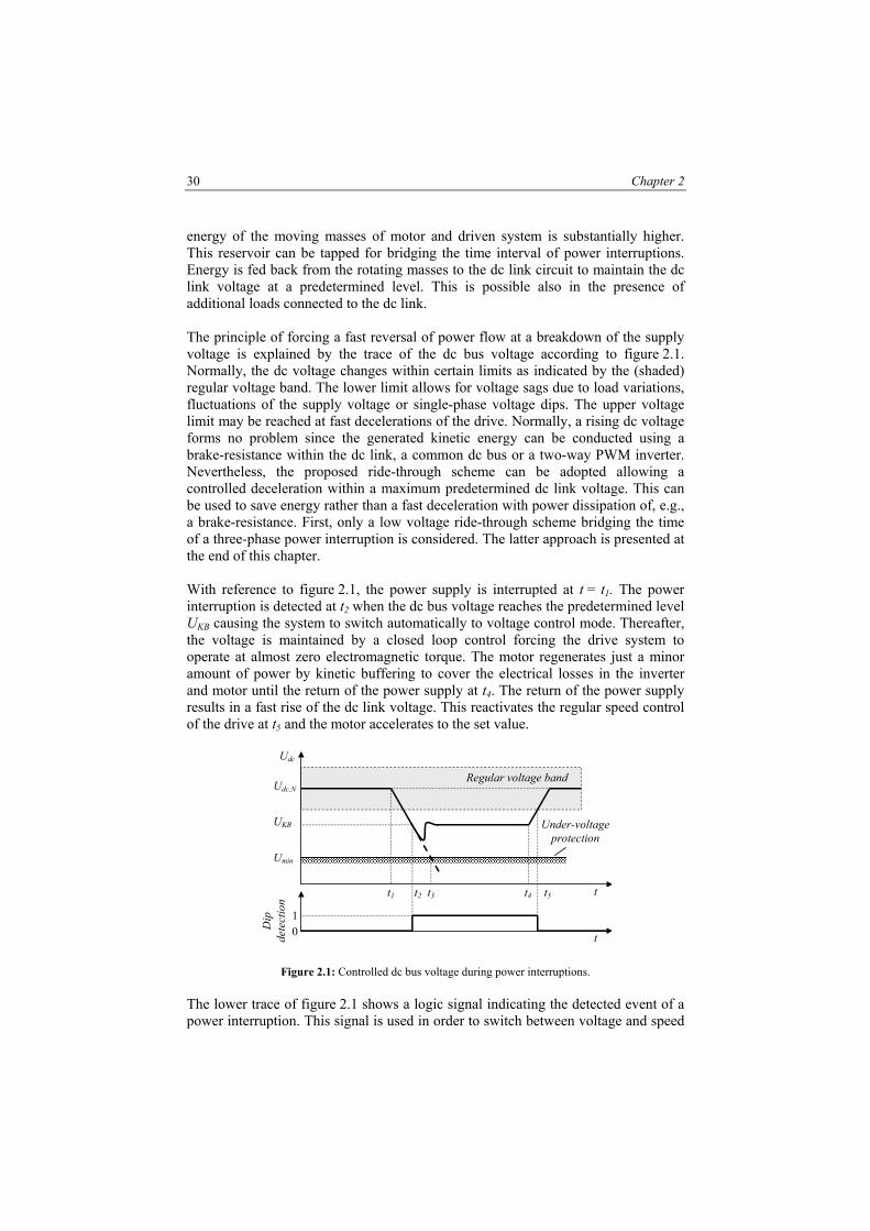
energy of the moving masses of motor and driven system is substantially higher. This reservoir can be tapped for bridging the time interval of power interruptions. Energy is fed back from the rotating masses to the dc link circuit to maintain the dc link voltage at a predetermined level. This is possible also in the presence of additional loads connected to the dc link. The principle of forcing a fast reversal of power flow at a breakdown of the supply voltage is explained by the trace of the dc bus voltage according to figure 2.1. Normally, the dc voltage changes within certain limits as indicated by the (shaded) regular voltage band. The lower limit allows for voltage sags due to load variations, fluctuations of the supply voltage or single-phase voltage dips. The upper voltage limit may be reached at fast decelerations of the drive. Normally, a rising dc voltage forms no problem since the generated kinetic energy can be conducted using a brake-resistance within the dc link, a common dc bus or a two-way PWM inverter. Nevertheless, the proposed ride-through scheme can be adopted allowing a controlled deceleration within a maximum predetermined dc link voltage. This can be used to save energy rather than a fast deceleration with power dissipation of, e.g., a brake-resistance. First, only a low voltage ride-through scheme bridging the time of a three-phase power interruption is considered. The latter approach is presented at the end of this chapter. With reference to figure 2.1, the power supply is interrupted at t = t1. The power interruption is detected at t2 when the dc bus voltage reaches the predetermined level UKB causing the system to switch automatically to voltage control mode. Thereafter, the voltage is maintained by a closed loop control forcing the drive system to operate at almost zero electromagnetic torque. The motor regenerates just a minor amount of power by kinetic buffering to cover the electrical losses in the inverter and motor until the return of the power supply at t4. The return of the power supply results in a fast rise of the dc link voltage. This reactivates the regular speed control of the drive at t5 and the motor accelerates to the set value.
Udc,N
UKB
Umin
t t1 t2 t4
Under-voltageprotection
t5
t
Regular voltage band
0 1
Dip
de
tect
ion t3
Udc
Figure 2.1: Controlled dc bus voltage during power interruptions.
The lower trace of figure 2.1 shows a logic signal indicating the detected event of a power interruption. This signal is used in order to switch between voltage and speed
Regenerative Braking and Ride-Through at Power Interruptions 31
control mode. If the inverter control did not react on this signal, the dc bus voltage continues falling as indicated by the dashed line. The inverter would shut down at t3 by the under-voltage protection at the voltage level Umin. Without kinetic buffering, the maximum acceptable duration of a power interruption can be determined by
( ) (∫ +=−3
1
2min
2,2
1 t
tloadlossNdc dtTPUUC ω ) (2.1)
where Ploss is the power dissipation of motor and inverter. In speed control mode, the motor speed and consequently the losses as well as the load torque are usually constant. Typical values of this time interval, mainly depending on the prevailing mechanical power at the motor shaft, are of the order of 1-50 ms. Of course, the voltage control must become active before this time has been elapsed. The maximum time interval ∆tmax of bridging power interruptions by kinetic buffering can be appraised by solving:
( ) (∫∆
+=+−max
22min
2, 2
121
tloadlossrefNdc dtTPJUUC ωω ) (2.2)
In contrast to (2.1), losses and load torque are now speed dependent. The stored kinetic energy is obtained by the inertia of the moving masses and the actual speed at power interruption, normally equal to the reference speed ωref. Using kinetic buffering, a maintained and controlled operation of several seconds is possible.
2.4 DC Bus Voltage Control
Primarily, the proposed voltage control scheme at power interruptions has been developed for a PV-powered water pump system [Ter 02]. There, the voltage control is designed to withstand abrupt power interruptions, occurring at an instantaneous decrease of the irradiance intensity (e.g. passing clouds). The total power failure considered here can be regarded as a worst-case situation. The most important control loop for the stability of the entire system is the dc bus voltage control. The system has been set up to work independently in island operation. All control and measurement units are supplied by the dc bus. A dc voltage beyond given limits leads inevitably to a crash of the entire system. The voltage reference is calculated by an overlaid MPP-Tracking and controlled directly or indirectly by the speed of the motor. Due to the lack of a major storage element in the dc bus, the power of the PV array must be used immediately to accelerate the PMSM. As irradiance increases, resulting in a higher output power of the PV array, the input power of the dc bus is

32 Chapter 2
higher than the output. The voltage control must immediately accelerate the PMSM to stay in the MPP of the PV array. With decreasing irradiance, the power of the PV array is smaller than the output in the dc bus. The difference comes from the capacitor, being discharged. This is the most critical condition. The dc bus collapses, if this condition remains resulting in a voltage drop beyond given limits. Hence, the inverter must slow down the PMSM to a new stable operating point. Therefore, the voltage controller has to accelerate/decelerate the motor very quickly guaranteeing a balanced input/output power ratio in the dc bus. Figure 2.2 shows the energy flow within the system without loss considerations.
IPV IInv
Solar generator
Udc
Idc
motor-pumpsystem
Pkinetic
Ppump
PPV
Figure 2.2: Energy flow of the PV-powered water pump systems. The energy generated by the PV array is used to drive the motor/pump system. Depending on the difference between energy generation and consumption, the dc bus capacitor is charged or discharged:
dtIC
U dcdc ∫=1 (2.3)
The dynamic behavior of the voltage control is determined by energy equations. The electromagnetic power developed by the motor can be divided in kinetic power Pkinetic accelerating the motor-pump system and pumping power Ppump. Only the kinetic power can be used to feed back energy to the dc bus and to control the voltage.
loadel TdtdJT +=ω (2.4)
loadpumpkineticelel TdtdJPPTP ωωωω +=+== (2.5)
Subsequently, the drive efficiency is not taken into account, because of the opposite influence at acceleration and braking. The losses are small compared to the mechanical energy consumption. Furthermore, the loss fluctuation is almost as slowly as the variation of the pumping power. Therefore, they are as being a part of
Regenerative Braking and Ride-Through at Power Interruptions 33
the load. Without considering the drive efficiency, the input power of the inverter matches the electromagnetic output power generated by the motor.
( dcPVdcInvdcel IIUIUP )−=≈ (2.6)
In steady state, the voltage Udc and motor speed ω are constant. The energy generated by the PV array is completely used to pump water:
• ⇒ const=dcU 0=dcI (2.7)
• const=ω ⇒ (2.8)
≈=
PVdcpump
kinetic
IUPP 0
2.4.1 Speed controlled dc bus voltage
Normally, the motor speed of a conventional drive supplied by a regular grid via a diode rectifier is completely independent of the dc bus voltage. Here, a PV array is the source and a water pump acts as load. A relation between motor speed and dc bus voltage can be obtained by linearization of the dynamic behavior. The electromagnetic torque of the motor can be controlled very fast given the bandwidth of the current control loop (960 Hz), whereas the load torque varies slowly with speed. The speed can be controlled beyond current/torque limitation with a bandwidth of approximately 26 Hz. Therefore, also the kinetic power Pkinetic can be varied faster than the pumping power Ppump. Due to similar considerations, the dc current Idc can be controlled faster than the dc bus voltage Udc. Therefore, the following equation is valid during transients:
dtd
ddT
dtdJ load ω
ωω
>>2
2
(2.9)
Using (2.5)-(2.6) and assuming constant pumping power and constant current IPV of the PV array for a short time, the linearized relation between dc voltage and motor speed ω is described by:
loaddcdcPVdc TdtdJIUIU ωωω +=− (2.10)
constIUTP PVdcloadpump ≈≈= ω (2.11)
dcdckinetic IUdtdJP −≈=ωω (2.12)

34 Chapter 2
dtdJ
dtdUCU dc
dcωω−=⇒ (2.13)
With the transfer function of the closed loop speed control beyond current/torque limitations
11
)()(
* +=
speedsss
τωω (2.14)
and using (2.13), the resulting linearized transfer function with the reference speed ω* as input and the dc bus voltage Udc as output can be written as
11
11
)()(
* +⋅
+⋅−=
Vfspeed
dc
ssCJ
ssU
ττω, (2.15)
where τspeed is the equivalent time constant of the speed control loop and τVf the time constant of the voltage measurement including all other smaller time constants. In fact, the loop to be controlled covers a dominant time constant and a smaller time constant. Using a PI controller, the dominant time constant can be equalized. The cut-off frequency of the control loop is calculated by setting the time constant of the PI controller equal to the largest open loop time constant and choosing a phase margin guaranteeing a stable system:
speedu ττ = (2.16)
( )2
)(arctan πωτπωϕ −−= cVfcR (2.17)
VfRc τϕπω /)2
tan( −=⇒ (2.18)
The gain of the PI controller Kpu is determined by setting the broken-loop amplification at the cut-off frequency A(ωc) to zero:
( ) 01log20log20)(!
2 =
+−
−−== cVfc
pu
u
KJCA
cωτωτω ωω (2.19)
( ) 12 +−=⇒ Vfccupu JCK τωωτ (2.20)
Regenerative Braking and Ride-Through at Power Interruptions 35
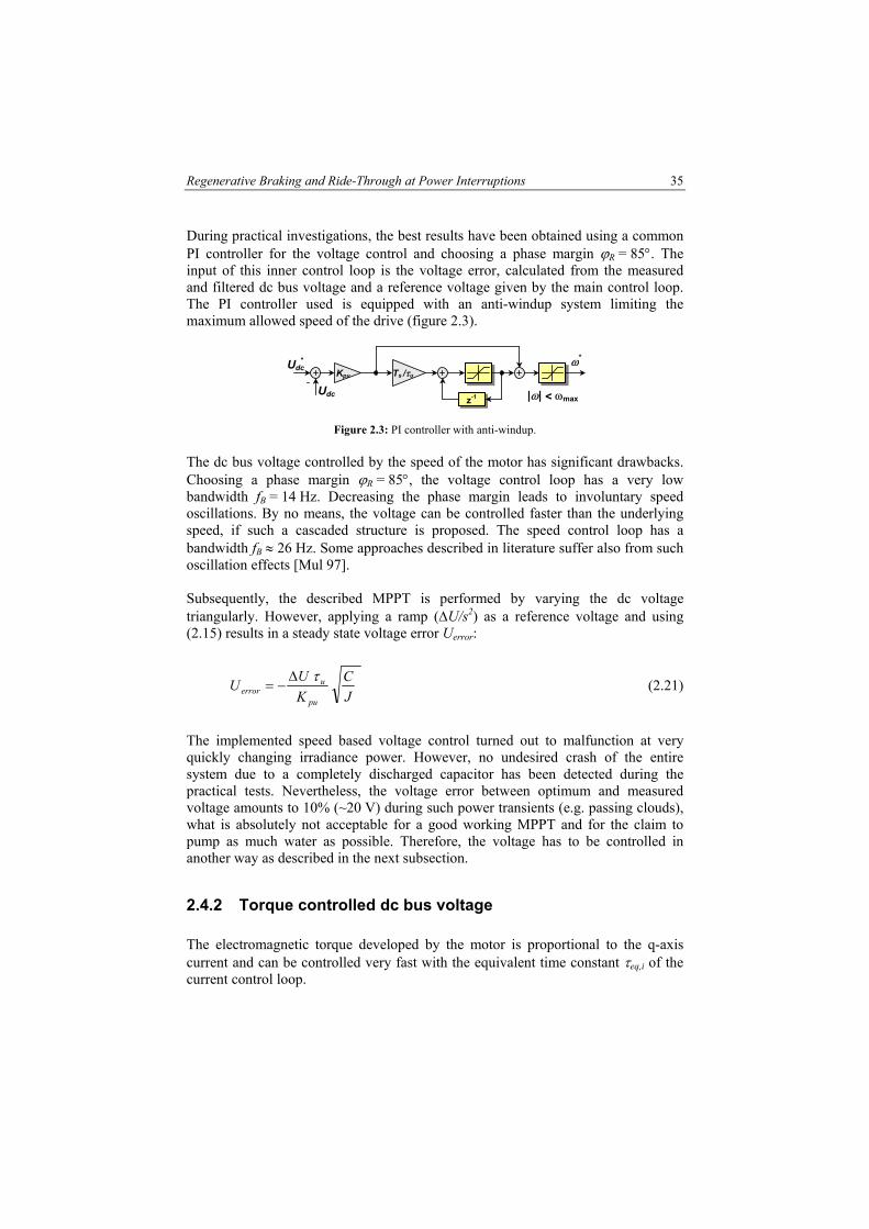
During practical investigations, the best results have been obtained using a common PI controller for the voltage control and choosing a phase margin ϕR = 85°. The input of this inner control loop is the voltage error, calculated from the measured and filtered dc bus voltage and a reference voltage given by the main control loop. The PI controller used is equipped with an anti-windup system limiting the maximum allowed speed of the drive (figure 2.3).
Kpu
ω*Udc
*
Udc
Ts /τu
z-1 |ω| < ωmax
Figure 2.3: PI controller with anti-windup.
The dc bus voltage controlled by the speed of the motor has significant drawbacks. Choosing a phase margin ϕR = 85°, the voltage control loop has a very low bandwidth fB = 14 Hz. Decreasing the phase margin leads to involuntary speed oscillations. By no means, the voltage can be controlled faster than the underlying speed, if such a cascaded structure is proposed. The speed control loop has a bandwidth fB ≈ 26 Hz. Some approaches described in literature suffer also from such oscillation effects [Mul 97]. Subsequently, the described MPPT is performed by varying the dc voltage triangularly. However, applying a ramp (∆U/s2) as a reference voltage and using (2.15) results in a steady state voltage error Uerror:
JC
KUU
pu
uerror
τ∆−= (2.21)
The implemented speed based voltage control turned out to malfunction at very quickly changing irradiance power. However, no undesired crash of the entire system due to a completely discharged capacitor has been detected during the practical tests. Nevertheless, the voltage error between optimum and measured voltage amounts to 10% (~20 V) during such power transients (e.g. passing clouds), what is absolutely not acceptable for a good working MPPT and for the claim to pump as much water as possible. Therefore, the voltage has to be controlled in another way as described in the next subsection.
2.4.2 Torque controlled dc bus voltage
The electromagnetic torque developed by the motor is proportional to the q-axis current and can be controlled very fast with the equivalent time constant τeq,i of the current control loop.

36 Chapter 2
11
)()(
,* +
=ieqel
el
ssTsT
τ (2.22)
Neglecting the load torque, the following relation between motor speed and electromagnetic torque is valid:
sJsTs
el
1)()(
=ω , Tload = 0 (2.23)
In fact, the load torque is presently handled as a system disturbance, being true considering pumping and PV power to be equal in steady state. Replacing the speed ω in (2.14)-(2.15) by the electromagnetic torque Tel defined in (2.22)-(2.23), results in a linearized transfer function with the reference torque Tel
* as input and the dc bus voltage Udc as output:
11
1111
)()(
,* +
⋅+
⋅⋅−=Vfieqel
dc
sssCJsTsU
ττ, (2.24)
The voltage can be controlled directly by the electromagnetic torque of the motor. A PI controller equipped with an anti-windup system limiting the maximum allowed torque/current is used to calculate the reference torque. The parameters of the PI controller are determined by choosing the time constant τu larger than the sum of the two open loop time constants and setting the gain Kpu in order to get a maximum possible phase margin ϕR, guaranteeing a stable system:
( ) στττ kkT Vfiequ =+= , , with: k > 1 (2.25)
upu
CJkK
τ−= (2.26)
( ) )1(arctan)(arctank
kcR −=⇒ ωϕ (2.27)
Best results are obtained by choosing 10 < k <40, corresponding to a phase margin of 55° < ϕR < 72°. The practically implemented torque controlled voltage loop has a bandwidth fB ≈ 235 Hz, being 16 times larger than the other approach. The calculation of the bandwidth takes no current/torque limitation into account.

Regenerative Braking and Ride-Through at Power Interruptions 37
Applying a ramp (∆U/s2) as reference voltage, results in a zero steady-state voltage error, being obviously due to the integrating term in (2.24). This property is very advantageously for the implementation of a MPPT. Compared to the other approach, the dc bus voltage directly controlled by the torque has many advantages regarding speed of response, steady-state error and robustness. Thus, all following experiments are made based on this approach. The voltage controller (figure 6.5) switches only in speed control mode, if the maximum speed is reached and the PV array generates sufficient power or if the motor/pump system pumps too much water for the storage capacity. In spite of controlling the dc bus voltage by the electromagnetic torque, the speed/position estimation within this PV powered water pump system is not superfluous. Both, PMSM and induction motor, being part of a high performance drive, require information of the field position. The structure of the dc bus voltage control integrated into the speed control system is presented in figure 2.4. The proposed control algorithm requires a fast torque control scheme. The well-known principle of field orientation [Leo 85] is employed here. The high performance speed/torque control of the given ac motor drives are described in chapter 7 as well as the calculation of the controller parameter. The mechanical position sensor is replaced by an observer requiring no additional measurements. Only measurements of motor current and dc bus voltage are necessary. Whenever the logic signal (‘dip logic’, figure 2.4) indicates a power interruption, the torque reference is temporarily switched from the regular speed controller to the voltage controller. The ‘dip logic’ is obtained using a simple (digital) relay with, considering the given installation, a switch on point UKB = 340 V and a switch off point at 360 V. The predetermined reference voltage Udc
* should be within these boundaries to prevent involuntary torque transients or oscillations of the logic signal: Ideal is the switch on point. The integrator is used for both speed and voltage control. Of course, the integrator time constant is automatically tuned. This prevents involuntary torque transients and saves computation time. Note the negative sign of the voltage controller gain as well as the multiplication by the sign of the motor speed. During power interruptions, the dc bus voltage can be maintained only when negative electromagnetic power is generated by the motor. A positive power decreases the dc voltage. Considering a four-quadrant drive, negative electromagnetic power is generated by inverse signs of torque and speed:
elel TP ω= (2.28)
The multiplication with the sign of the motor speed is dropped in the PV-powered control system since the pump is driven only in one (positive) direction.

38 Chapter 2
Enable voltage control
TorqueControl
& EKF
SVM Inverter
ia
ub*
uc*
AC motor
ib
load
ua*
ω
ω*
Tel*
Udc
Udc*
Udc
PI voltage control
Power supply
z-1
|T| < Tmax
Ts /τu
Ts /τn
-Kpu
Kpn Speed
reference PI speed control
sign(ω) ω
Dip logic
Figure 2.4: Block diagram of the dc bus voltage control integrated into the speed control system. The entire system is controlled by a digital signal processor (DSP) realizing dc bus voltage control, speed/torque control of the drive and start-up and shut down automatism's. All control and measurement units are supplied by the dc bus. A dc voltage beyond given limits leads inevitably to an undesired crash of the entire system. In particular, the supply of power to the electronic control circuits of the inverter must continue without interruption to maintain the system in operation.
2.5 Experimental Examples at Power Interruptions
A 3 kW permanent magnet synchronous machine (PMSM) supplied by a voltage source PWM inverter has been used to verify the proposed approach. Instead of using a PMSM, the implemented regenerative voltage control is also suitable for an induction motor driving the load. The dynamic performance of induction motor and PMSM are similar, only the efficiency of the former is lower especially at partial load. The used load machine is a dc motor drive with constant electrical excitation coupled with a variable resistor bench. The performance of the ride-through at power interruptions has been tested using a regular grid as power supply and applying an abrupt power interruption on all three phases for a short time (approximately 2 s). Figure 2.5 presents a measurement of dc bus voltage and motor speed without applying the proposed voltage control. The speed reference amounts to ω* = 1000 rpm and no load is applied. The dc link capacitor is discharged to a critical level within ∆t ≈ 0,1 s. The under-voltage protection switches on and the drive is out of control. This time is much shorter with applied load torque.

Regenerative Braking and Ride-Through at Power Interruptions 39
0 2 4 6 8 10 12 140
100
200
300
400
500
t [s]
Udc
[V]
0 2 4 6 8 10 12 140
200
400
600
800
1000
t [s]
n [r
pm
]
Under-voltage protection
Out of control
Figure 2.5: Power interruption without voltage control (no load).
Top: Voltage of the dc link. Bottom: Motor speed.
Figure 2.6 shows the experimental result of the voltage control enabled when a short time three-phase power interruption is applied. After detecting the voltage dip, the voltage controller has to decelerate the motor very quickly guaranteeing a balanced input/output power ratio in the dc bus. Otherwise, the dc bus would be discharged and the system collapses. However, the implemented regenerative braking scheme allows the inverter to keep its dc bus voltage at the pre-determined minimum level, expanding the time in which supply voltage can be reapplied without the time-consuming dc-link capacitor recharging cycle. Initially, the drive system is in speed control mode with a reference speed n* = 1000 rpm. If the capacitor is discharged to a level lower than UKB =340 V, a voltage dip is detected and the system switches automatically to the voltage control mode with a predetermined voltage reference of Udc
* = 340V. Choosing the reference voltage Udc
* lower than the ‘dip logic’ switch on point UKB results in a current/torque peak at the beginning of the voltage control mode: As can be seen in [Ter 00b], the controller starts then with an involuntary acceleration of the drive. The system returns to the speed control mode at a voltage level higher than Udc = 360 V or if the motor speed is higher than the speed reference. The deceleration of the motor during the power interruption is small, because no load is applied. Figure 2.7 shows the experimental results of a comparable power interruption but with a load torque applied to the motor. The applied load amounts to 75% of the rated torque. Due to the load, the deceleration is much faster. However, the power needed to keep the voltage at a minimum level is the same, as can be seen at the small negative q-axis current during the interruption interval. In fact, this power (~20 W) generated by the kinetic energy of the drive system is nearly constant and almost completely used to compensate the inverter losses.

40 Chapter 2
-1 -0.5 0 0.5 1 1.5 2 2.5 3 3.5 4320
340
360
380
400
420
t [s]
Udc
[V]
-1 0 1 2 3 4
200
400
600
800
1000
1200
t [s]
n [r
pm
]
-1 0 1 2 3 4
-5
0
5
10
15
20
t [s]
i q [A
]
voltage dip
Figure 2.6: Ride-through at power interruption without load torque. Top: Voltage of the dc link. Bottom: Motor speed and q-axis current.
-1 -0.5 0 0.5 1 1.5 2 2.5 3 3.5 4320
340
360
380
400
420
t [s]
Udc
[V]
-1 0 1 2 3 4
200
400
600
800
1000
1200
t [s]
n [r
pm
]
-1 0 1 2 3 4
-5
0
5
10
15
20
t [s]
i q [A
]
voltage dip
Figure 2.7: Ride-through at power interruption with load torque (75% rated torque).
Top: Voltage of the dc link. Bottom: Motor speed and q-axis current. Without the voltage dip control, the capacitor is completely discharged, considering the given experiment and according to
ω
ω
load
load
TUCt
tTUC
2
2
21
21
=∆⇒
∆≈ (2.29)

Regenerative Braking and Ride-Through at Power Interruptions 41
in ∆t = 29 ms. A critical voltage level according to (2.1) is reached after ∆t = 10 ms requiring a time-intensive restart of the converter. With the implemented voltage control, a kinetic buffering during a total energy drop is possible for several seconds. The span of time depends on the drive moment of inertia and the actual speed at the moment of the voltage dip. Figure 2.8 presents a measurement at sustained power failure. Before the drive gets uncontrolled by the under-voltage protection, the motor has come to a complete standstill. However, the motor stays controllable during braking, being important especially for critical applications as multi-motor drives.
-1 0 1 2 3 4 5 6 7 8 90
100
200
300
400
t [s]
Udc
[V]
-1 0 1 2 3 4 5 6 7 8 90
200
400
600
800
1000
1200
t [s]
n [r
pm
]
Under-voltage protection
Figure 2.8: Ride-through at everlasting power failure (no load).
Top: Voltage of the dc link. Bottom: Motor speed.
2.6 Special Drive Deceleration Tool
The proposed ride-through scheme at power interruptions can be easily transformed into a special drive-braking tool. The upper voltage limit of the inverter may be reached at fast braking of the drive. Regularly, the surplus generated kinetic energy is handled using a braking-resistance within the dc link, a common dc bus or a two-way PWM inverter (figure 2.9). Nevertheless, the voltage control can be adopted allowing a controlled braking with a maximum predetermined dc link voltage and without redirecting the kinetic energy. The kinetic energy is usefully conducted to the load mainly responsible for the braking during the voltage control mode. Thus, this deceleration tool can be used, when saving energy is preferable to a fast braking with power dissipation in, e.g., a brake-resistance. If the dynamic performance is not crucial, the installation of a brake-resistance, power switch and cooler may be eliminated. Especially in small motor drives, the economic gain is considerable.

42 Chapter 2
Power supply
Common dc bus PWM converter Motor 1
Inverter 1 Load 1
Motor 2 Inverter 2
Load 2 Braking- resistance
S1
Figure 2.9: Active front end, braking-resistance and common dc bus. With reference to the given drive, the system switches automatically to voltage control mode at a preset level higher than Udc > 600 V. The block diagram of the dc bus voltage control integrated into the speed control system is equal to the earlier described structure (figure 2.4). Once in voltage control mode, the system continues to operate with the predetermined voltage reference Udc
* = 600V. Finally, the system turns back to speed control mode when the motor speed reaches the reference speed or at a voltage level lower than Udc = 590 V. The ‘switching logic’ is obtained using a simple (digital) relay linked to the required speed information (figure 2.10).
| ω* | ≤ | ω |
Udc Switching
logic Udc > 600V ⇒ 1Udc < 590V ⇒ 0 ω*
ω
Figure 2.10: Switching logic of the braking tool.
The design constraint of the absolute value of reference speed being lower than the absolute value of real speed is very important. Otherwise, the motor would, once in voltage control mode, brake to zero and wait until the capacitor is discharged by the inverter losses to the level of Udc = 590 V. Thereafter, the motor accelerates to the reference speed. Figure 2.11 shows the experimental result of the implemented drive deceleration tool using the 3 kW PMSM. Initially, the drive system is in speed control mode with a reference speed of n* = 1500 rpm. At t = 0 s, the speed reference changes to n* = 500 rpm and the switch on point (Udc = 600V) of the voltage control is reached 60 ms later. The implemented control scheme enables the inverter to keep its dc bus voltage at the predetermined level. The braking of the drive is mainly caused by the load torque. Reaching the reference speed, the system returns to the speed control mode. Using a brake-resistance within the dc link, the kinetic energy ∆Wkin
( 22
212
1 ωω −=∆ JWkin ) (2.30)
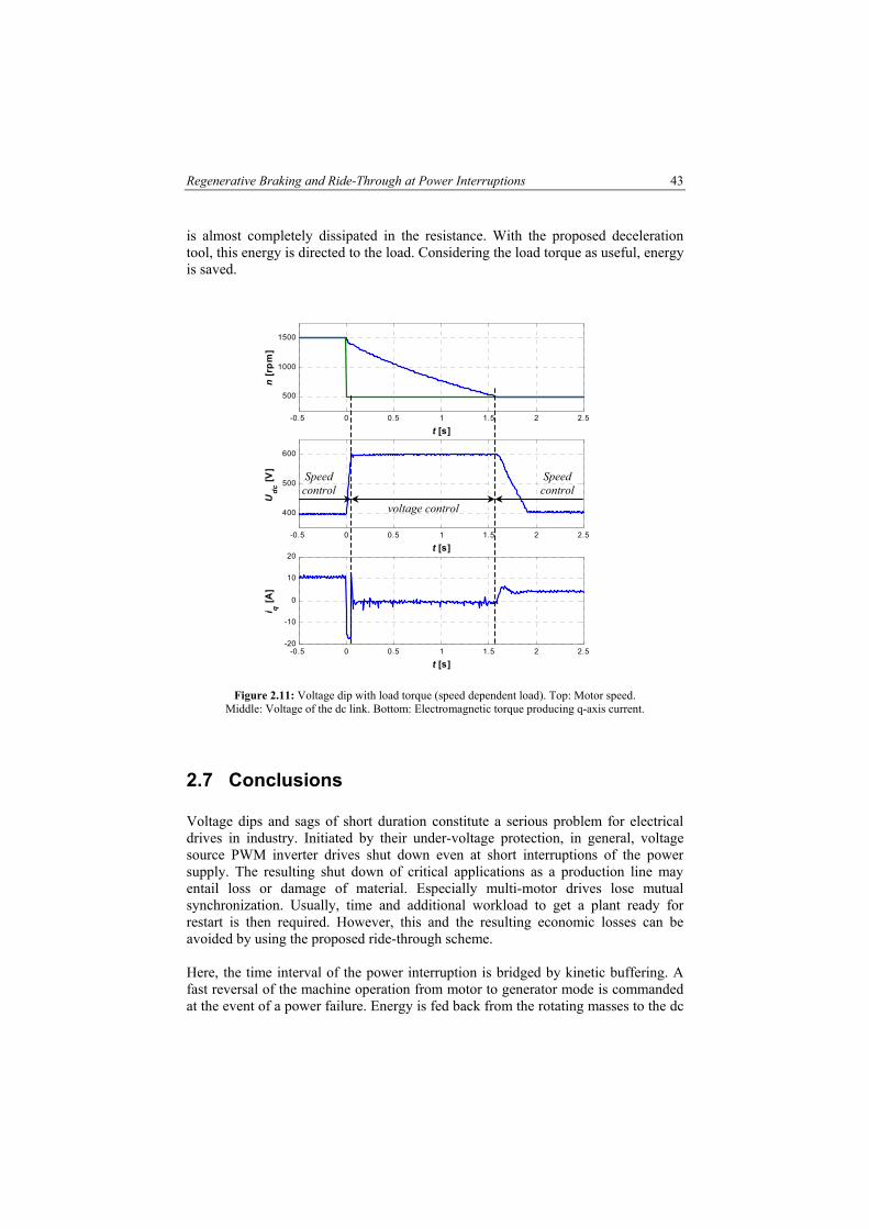
Regenerative Braking and Ride-Through at Power Interruptions 43
is almost completely dissipated in the resistance. With the proposed deceleration tool, this energy is directed to the load. Considering the load torque as useful, energy is saved.
-0.5 0 0.5 1 1.5 2 2.5
400
500
600
t [s]
Udc
[V]
-0.5 0 0.5 1 1.5 2 2.5
500
1000
1500
t [s]
n [r
pm
]
-0.5 0 0.5 1 1.5 2 2.5-20
-10
0
10
20
t [s]
i q [A
]
Speed control
Speed control
voltage control
Figure 2.11: Voltage dip with load torque (speed dependent load). Top: Motor speed. Middle: Voltage of the dc link. Bottom: Electromagnetic torque producing q-axis current.
2.7 Conclusions
Voltage dips and sags of short duration constitute a serious problem for electrical drives in industry. Initiated by their under-voltage protection, in general, voltage source PWM inverter drives shut down even at short interruptions of the power supply. The resulting shut down of critical applications as a production line may entail loss or damage of material. Especially multi-motor drives lose mutual synchronization. Usually, time and additional workload to get a plant ready for restart is then required. However, this and the resulting economic losses can be avoided by using the proposed ride-through scheme. Here, the time interval of the power interruption is bridged by kinetic buffering. A fast reversal of the machine operation from motor to generator mode is commanded at the event of a power failure. Energy is fed back from the rotating masses to the dc

44 Chapter 2
link circuit to maintain the dc link voltage at a predetermined level. This is possible also in the presence of additional loads connected to the dc link. Due to advances in semiconductor technology, modern electric drives can withstand the high peak currents occurring when the power supply is restored after a short disturbance. Keeping the capacitor well charged has the additional advantage of the control electronics being powered over a longer time span, avoiding a time-consuming restart of the drive. In voltage control mode, the dc bus voltage is directly controlled by the electromagnetic torque of the motor. The proposed voltage control scheme was primarily developed for the PV-powered water pump system. The drive continues operating even after a quite long power interruption of several seconds. The temporary speed dip is generally tolerable, since the most frequent power interruptions last only for a few milliseconds. Since drive control is never lost, the voltage control scheme can be applied to multi-motor drives as well. Finally, the proposed ride-through scheme at power interruptions is transformed into a special drive deceleration tool for saving energy and simplifying the inverter setup. Measured results are presented and evaluated to demonstrate the performance and the system stability. Powerful digital signal processing is used to implement the proposed regenerative braking schemes, expanding the time in which supply voltage can be reapplied without the time-consuming dc-link capacitor recharging cycle.
3. DSP-based Drive Control and Measurements
3.1 Introduction
Classically, motor control was designed with analog components as they are easy to design and can be implemented with relatively inexpensive components. Nevertheless, there are several drawbacks with analog systems including aging, temperature drift and reliability due to EMC problems. Regular adjustment is required in those cases. Furthermore, any upgrade is difficult, as the design is hardwired. Digital systems, on the other hand, offer improvement over analog circuits. The mentioned drawbacks as drift and external influences are eliminated since most functions are performed digitally. DSP technology allows both, a high level of performance and cost reduction. Upgrades can easily be made in software. DSP’s have the capabilities to concurrently control a system and simultaneously monitor it. A dynamic control algorithm adapts itself in real time to variations in system behavior. Furthermore, implementation of complex control approaches is possible and the drive system reliability can be improved. For development purpose, a commercially available DSP based environment is used. The heart of the controller board is a TMS320C31 digital signal processor. A slave processor is employed to perform the digital input and output and generate the PWM signals. The controller board can be directly programmed using MATLAB/SIMULINK. A standard VS-PWM inverter with IGBTs is adapted to be commanded by the DSP controller board. This chapter presents the mutual interactions between control design and real-time implementation. The DSP controller board, code generation, experiment management and hardware interface including required measurements are explained. Issues of phase voltage distortion/identification due to the inverter non-linearity are discussed in detail. Finally, the used inverter and different PWM generation schemes are evaluated. Optimizing (slimming down) a working control algorithm regarding required computational effort, code optimization and implementation on a more inexpensive hardware for the final product is something, to be considered in the final stage of the development process.

46 Chapter 1
3.2 Controller board, Programming and Experiment Management
The motor control is implemented using a DSP based controller board with additional I/O features and an encoder interface. The DS1102 single-board system from dSpace™ (Germany) employs a TMS320C31 digital signal processor operating at 60 MHz for the main program and a slave subsystem with a TMSM320P14 fixed-point DSP for the I/O subsystems and PWM generation. In addition, the used development platform contains a comprehensive selection of I/O interfaces that meet typical requirements for rapid motor control prototyping:
• 4 analog-to-digital converters • 4 digital-to-analog converters • 16 bit-selectable digital I/O lines • PWM generation on up to 6 channels • 2 incremental encoder interfaces
A connector panel provides easy access to all input and output signals: Analog signals via BNC connectors, all digital signals via Sub-D connectors. The single-board hardware (appendix A) is integrated on a standard 16-bit PC/AT card slotted straight into a PC using the ISA bus as a backplane. The main DSP of the controller board can be directly programmed using MATLAB/SIMULINK by The MathWorks™. This application software is de-facto standard in the control community, so no further explanation is given. SIMULINK is a graphical user interface integrated in MATLAB® for modeling and constructing block diagrams via drag & drop operations. Its large block library is enhanced by specific dSpace-blocks and own user-defined libraries simplifying automatic code generation and experiment setup including initialization of the I/O subsystems and PWM generation. Real-Time Workshop is the code generation extension provided by The MathWorks™. It generates C-code automatically from block diagrams and state-flow systems. For flexibility, the user can introduce own C-code into the block diagram by computation-time extensive S-functions or alternatively by special user-codes implying a change of the support software. The own C-code should be preferred, whenever a part of the control algorithm contains many if-loops (e.g. space vector modulation) or in very extensive programs, e.g. sensorless speed control with Kalman filtering. Addressing the TI compiler and automatic download to the DSP is done via the Real-Time Interface (RTI). For more information on programming and implementation software, it is referred to the appropriate manuals. The Total Development Environment (dSpace’ TDE) bundles a set of tools supporting seamless transition from theory to simulation of new control algorithms to real-time implementations. Software tools, such as CONTROLDESK, allow parameter tuning/changing and data recording during the experiment in real-time mode. CONTROLDESK is the comprehensive experimental environment software providing management, control and automation of experiments. This user interface

Voltage-Source PWM Inverter 47
enables access to every variable of the original block diagram. Figure 3.1 gives an idea on how the experiment management looks like. Controller parameters can be changed on-line (e.g.: speed reference) while the response is observed/recorded simultaneously.
Figure 3.1: Screen plot during ac motor control experiment with the DS1102. Usually, no code for the TMSM320P14 fixed-point DSP is generated, but the appropriate I/O functions are automatically included by the slave-DSP’s EPROM. However, the support software has been changed in order to implement different PWM strategies as well as variable PWM frequencies. This is extremely valuable during the development of high-performance motor control using PWM outputs in order to drive power switches. The modification of the support software has been made in assembler code, since no C-compiler for the slave-DSP exists. Compared to the original three-phase PWM generation performed in 73 µs, the computation time has been significantly reduced to 17 µs. This new code is automatically included at every compilation of the main program. The implemented modifications are summarized in a separate manual.
3.3 Controller Interface
The laboratory test drive consists of a host PC for the controller board, an IGBT inverter, and ac motor drive with variable load, current/voltage sensors and an incremental encoder. Figure 3.2 shows the control setup with the DS1102 controller board. Photos of the experimental set-up are presented in appendix A.

48 Chapter 1
High performance motor control requires accurate information on motor currents and dc bus voltage. Here, the motor currents are measured in two phases using LEM sensors. The dc bus voltage is measured via a galvanically isolated potentiometer. These signals are fed to the interface connected to the inputs of the A/D converters. Due to involuntary parasitic disturbances (EMC-problems), the measured signals should be filtered in either an analog or digital way. In general, digital filtering is preferred. Phase shifts introduced by filtering can be corrected (if necessary) by the transformation angle from the stator to the rotor reference frame. Only low-weighted analog first order filters with a cut-off frequency 5 kHz are added between voltage/current measurements and the A/D converters of the controller board. The rotor position is measured using an incremental encoder and directly fed to the encoder interface of the controller board.
Interface
PWMInverter
ia
ub*
uc*
ACmotor
ib
ua*
Udc
Power supply MPP-
Tracking
Curr
ent [
A]
Voltage [V]
control prototyping
Load
EXOR
EXOR
EXOR
PWM 2PWM 1
PWM 3PWM 4PWM 5PWM 6enable
P14
DS1102-Processor Board
C31
Incremental encoder signal Θ
Figure 3.2: Control setup with DS1102. The PWM generation scheme implemented in the slave processor is based on phase voltage reference values. PWM generation on up to 6 channels is possible. Both subharmonic PWM generation and space vector modulation have been implemented. The inverter used is a modified standard VS-PWM inverter with IGBTs. An interface provides a galvanic isolation between controller board and inverter. The PWM switching signals are fed directly from the slave processor to the inverter using a high performance optical link, allowing to keep both inverter and drive several meters from the PC with the controller board. Therefore, the signal transmission is unaffected by EMC-problems. An enable signal, using one of the digital I/O lines together with the same high performance optical link, supervises both entire control system and inverter. The TMSM320P14 slave DSP generates duty cycles with 40 ns edge resolution and 160 ns PWM period resolution. In this high precision mode, the P14 always sets the output to a high level at the beginning of each PWM period, resulting in

Voltage-Source PWM Inverter 49
asymmetrical PWM pulses. The pulses of an asymmetric edge-aligned PWM signal always have the same side aligned with one end of each PWM period. On the contrary, the pulses of a symmetrical PWM signal are always symmetric with respect to the center of each PWM period. The symmetrical PWM is often preferred, since it generates less current and voltage harmonics [Bose 97], [Dub 89]. In order to overcome the problem of asymmetrical PWM generated by the P14, each of the two PWM channels are employed to generate the pulses for one phase as shown in figure 3.2 and 3.3. By means of an EXOR gate, pulses symmetrical to the center of the PWM period can be achieved if the switching times of each two channels, depending on the required duty cycle, are calculated according to the example reflecting the calculation for the first motor phase:
2
1aphase
cycleduty1PWM
−= (3.1)
2
1aphase
cycleduty2PWM
+= (3.2)
TPWM
PWM 1
PWM 2
ua*
TPWM
EX
OR
Figure 3.3: Principle of symmetrical PWM generation with DS1102. The presented algorithm is incorporated into the ‘user-code’ of the real-time program. The ‘user-code’ offers the inclusion of handwritten C-code into the initialization part and the timer-driven task running with the base sample time and is preferable compared to the use of Simulink C-coded S-function since it saves computation time. Every S-function block used in a Simulink model introduces an execution time overhead of about 9 µs in the real-time program due to the associated function calls. Considering the given development platform (DS1102 60MHz), the computation requirement of the implemented SVM and the data transmission to the slave DSP amounts to 22 µs.
50 Chapter 1
3.4 Measurements
Phase current and dc bus voltage measurements, as described in the following subsections, are required for most high-performance motion control systems. The measurement of the motor speed/position may be eliminated by estimation techniques. The rotor position is measured here for control purpose or for comparison with sensorless drive schemes. An incremental encoder with 1024 lines is used. This signal is directly fed to the encoder interface of the controller board. More details on position measurement and the transformation to a speed signal are given in chapter 4.
3.4.1 Phase Current Measurement
Accurate measurement of the phase current is a key element in obtaining optimum high-performance motor control. Measurement accuracy and bandwidth influence directly the current control loop as well as all overlaid loops. Filtering a feedback signal additionally decreases the dynamic response time of the loop [Leo 85]. Current is typically measured by one of two methods: voltage drop across a resistor or magnetic transducer. Resistive shunt sensing has the advantage of a relatively low-cost sensor. A drawback is the trade-off between sensitivity and power dissipated in the resistor. Since the actual motor current is the desired value, the sensing resistor is usually placed in series with the motor phase. This complicates the measurement, because the signal of interest is a millivolt differential value across the resistor, but the common-mode voltage of the motor phase is typically hundreds of volts switching at high frequency with rapid du/dt. Magnet sensors, on the other hand, are isolated by their very nature. This means that the motor current can directly be measured without the common-mode voltage problems mentioned before. They use a ring-type magnetic core with a Hall-effect semiconductor element placed in an air gap to measure the magnetic flux resulting from the primary current ip through the center of the core (figure 3.4). In “closed-loop” Hall effect current sensors, a canceling coil of e.g. 1000 turns is wound around the magnetic core. A built-in feedback amplifier drives current through the canceling coil in such a way that the flux, measured by the Hall-effect sensor, is always forced to be zero. Therefore, dc current can be measured. The output of the current transducer is the canceling current, equal to the measured current scaled-down by the ratio of coil turns. The overall bandwidth, accuracy and temperature independence of these transducers has proven to be sufficient for motor drive applications.

Voltage-Source PWM Inverter 51
Figure 3.4: Principle of current measurement via “closed-loop” Hall effect current sensor.
In this work, the motor currents are measured by LEM-modules. The bandwidth of the used magnet sensor devices is 150 kHz and the response time is smaller than 1 µs. The secondary (canceling) current is is transformed into a voltage signal ui by measuring the voltage drop across the sensing resistor RM (figure 3.4). This signal is fed to an anti-aliasing filter connected to the inputs of the A/D converters. Subsequently, the measured signals may be filtered by a digital low-pass filter. However, rather than additionally filtering the current signals, observer-based techniques can be used in order to reduce phase lags.
3.4.2 Measurement of DC Bus Voltage
In most high-performance motor control applications, the measurement of the dc bus voltage is required for the exact transformation of the reference voltages into the duty cycles for the inverter PWM. Even when the inverter is supplied by a constant voltage (regular grid), the dc voltage varies due to load variations. In some applications described later (e.g. power interruptions, braking schemes, PV-systems), the dc bus voltage is the main control variable. Furthermore, knowledge of the dc bus voltage makes a more complicated measurement of the phase voltages superfluous. The measurement of the dc bus voltage is not as crucial as the current measurement since the dc voltage is filtered and smoothed by a capacitor of appreciable size present in the dc bus. Usually, one side of the dc bus is grounded eliminating the common-mode problem already described at the current measurement. In the applications mentioned, the dc voltage is measured via a resistive potentiometer, a high-performance galvanic isolation and a first-order analog filter (cut-off frequency 5 kHz) connected to one A/D-converter of the controller board.
3.5 Phase Voltages
The field-oriented control of ac motor drives, e.g. induction motor and PMSM, demands the measurement of the motor current in two phases and the knowledge of the dc link voltage. This makes a more complicated measurement of the phase voltages superfluous. However, in some applications, such as sensorless field-

52 Chapter 1
oriented control and exact flux estimation, the inverter output voltages are required to calculate desired state values. The output voltage can be measured or, by using the information of the dc link voltage, estimated by means of the reference voltages. However, the inverter output voltages are much distorted when compared to the reference voltages and the use of the estimation is therefore not obvious.
3.5.1 Phase Voltage Measurement
A phase voltage measurement is difficult since the inverter output voltages are composed of discrete high-voltage/high-frequency pulses. Therefore, a potential-free measurement is required. A possible measurement setup and affiliated problems are described in [Maes 01]. Beyond over-modulation, the frequency spectrum of the output voltages generated by SVM consists of a fundamental frequency and many higher harmonics around the PWM frequency. Only the fundamental voltage wave contains useful information for the digital motion control. Thus, all high-frequency components should be eliminated by a low-pass filter. Due to the low-pass filter, the measured voltages suffer from phase delay and are not adequate for use in control purposes [Choi 96]. Particularly at low-speed and light-load operation, where the undesired phase delay is negligible, problems due to the accuracy of measurement may arise: The fundamental phase voltage is very small in these operating points and only a fraction of the measured pulses with a magnitude equal to the dc link voltage. Nowadays, a measurement of the phase voltages is seldom used. This is mainly caused by the complexity and extra costs of the additional measuring devices. The development platform used here enables a simultaneous measurement of only four signals, limited by the number of available analog-to-digital converters. However, three A/D converters are already reserved for the measurement of dc bus voltage and motor current in two phases. Thus, considering the given control setup, the motor voltages must be calculated considering the inverter’s non-linearity. In a voltage-source PWM inverter several causes distorting the output voltages can be found. The reasons for this originate from the inherent characteristics of the power switches such as voltage drop, voltage transition slope, turn on/off time and delay of the control signals. However, this delay distortion is small when compared to the dead-time effect [Bose 97] and is therefore usually disregarded.
3.5.2 Phase Voltage Estimation
For some subsequent described applications, such as sensorless speed control and flux estimation, the exact inverter output voltages are required to calculate desired state values. However, they are not measured due to the lack of sufficient analog-to-digital converters, but calculated by means of the reference voltages with

Voltage-Source PWM Inverter 53
consideration of the inverter non-linearity and the homopolar component generated by the SVM. A compensation of the dead-time effect is not implemented since the actual storage delay, varying depending on the operating point, is not exactly known. Practical investigations have shown even a deterioration of the observer performance by using an inadequate compensation approach: If the compensation is not perfect, a duplication of the dead-time effect at zero crossings of the current may occur. Due to the delayed reaction of almost all semiconductor switches at turn-on and turn-off, the phase voltages strongly deviate from the reference voltages. The voltage distortion does not depend on the magnitude of the reference voltages and hence its relative influence is very strong in the lower speed range where the reference voltage is small. Actually, the dead-time error is one of the major reasons limiting the performance of sensorless control in low speed operation [Choi 94], [Lee 96]. Disregarding this distortion yields in the subsequently described speed/flux observer to large position and speed errors, especially at low motor speed, where the error voltage becomes a multiple of the reference voltage. Therefore, the dead-time effect is considered at the estimation of the phase voltages. Figure 3.5 presents a comparison of the error voltage calculated by (1.17) and the measured falsification of the fundamental voltages.
-10 -8 -6 -4 -2 0 2 4 6 8 10-15
-10
-5
0
5
10
15
I1 [A]
Ure
f - U
10 [V
]
Measurement
Equation (3.11)
Figure 3.5: Dead-time effect: Measured and estimated error voltage
(Udc =400 V, fPWM = 10 kHz, τd = ± 2,5 µs). The speed-controlled ac motor is supplied by a voltage-source PWM inverter. The PWM generation is performed by space vector modulation. SVM provides a more efficient use of the supply voltage in comparison with sinusoidal modulation methods by imposing a homopolar system u0 in all three phases (multiple of third harmonics).
( cba uuuu ++=31
0 ) (3.3)

54 Chapter 1
However, this homopolar system reflected in the line-to neutral voltages, must be considered in the Park transformation:
−
−−=
c
b
a
uuu
uu
23
230
21
211
32
β
α (3.4)
In the case of an ideal inverter, the fundamental voltages at the motor terminals assume the shape of the reference voltage. The reference voltages Uref are equal to the duty ratios xref = (a*; b*; c*) calculated by the SVM (figure 1.14) multiplied by the half dc bus voltage:
refdcref xUU21
= , |a*| ≤ 1; |b*| ≤ 1; |c*| ≤ 1 (3.5)
All together, using these reference voltages, the required alpha/beta voltages uα, uβ are calculated according to the block diagram in figure 3.6 considering both the non-linearity of the inverter and the homopolar system of the SVM.
SVM
uα
Eq.(3.10)
i1 i2
signi3
Udc 1/2
Equation(3.13) uβ
xref = (a*; b*; c*)
Figure 3.6: Block diagram of voltage estimation. Note that the calculation of the alpha/beta voltages described above is only valid without strong over-modulation. The voltage spectrum in normal operation consists approximately of one fundamental and many higher harmonics around the PWM frequency. Over-modulation yields a voltage spectrum consisting of all uneven harmonics. In fact, a current controller with a special anti-windup system (see subsection 2.6.3) has been implemented, avoiding these operating points as well as the low harmonics.
3.6 Safety Issues & Enable Subsystem
A computer-aided control system is used as a development platform monitoring and recording the experimental data. Furthermore, the safety-related monitoring and the start-up and shut down automatisms are implemented in software on the main DSP

Voltage-Source PWM Inverter 55
board. The implemented safety-related monitoring (figure 3.7) consists of detecting over-current and over-speed, both depending on the drive system, and a pre-determined voltage window. The minimum and maximum admissible dc bus voltage mainly depends on the inverter used. An inadmissible failure disables the entire system, requiring a manual reset. The reset signal is activated only by the rising edge of a manual reset protecting the drive/inverter from an everlasting reset while an error may be still active. In addition, fuses are integrated in the motor current circuit as well as in the dc bus voltage measurement.
error logic
Udc Iα,β
enable signal
n
enable
z-1
reset u > 0
z-1
1
error ≡ 0 no error ≡ 1
0 ⇔ 1
0 ⇔ 1
Figure 3.7: Safety-related monitoring & enable logic of the drive system. The enable signal controls both the entire control system and the inverter (figure 3.2). All gating pulses of the power switches are set to zero in case of an error. However, special care has to be paid when a PMSM with high motor speed is operated in flux weakening mode. A disabled inverter causes the return of the unrestrained permanent magnet flux linkage and the dc bus voltage may reach unacceptable (dangerous) high values, if no additional power dissipation is connected in the dc link. The offset of the current measurement is seldom exact equal to zero, which causes a summation by the integrators of the controller even when the drive is disabled. Therefore, all integrator values within the control scheme are multiplied by the enable signal. This feature resets all registers at a restart and prevents an unwanted overflow of integrator registers.
3.7 Conclusions
All subsequently described motor control algorithms are implemented using the DSP-based development platform DS1102 from dSpace™. In this chapter, an overview of the given controller board and the hardware interface between DSP and drive system has been presented. The main DSP of the controller board can be directly programmed using MATLAB/SIMULINK. For flexibility, the user can introduce own C-code into the block diagrams. Software tools allow parameter tuning/changing and data recording during the experiment in real-time mode. The laboratory test set-up consists of a host PC for the controller board, an IGBT inverter, and ac motor drives with variable load, current/voltage sensors and an

56 Chapter 1
incremental encoder. A hardware interface providing symmetric PWM signals and transforming required measurements has been added to the experimental set-up. Support software has been changed in order to implement different PWM strategies as well as variable PWM frequencies on the TMSM320P14 slave-DSP. Different PWM generation schemes are evaluated. A standard VS-PWM inverter with IGBTs is adapted to be commanded by the DSP controller board. The PWM switching signals are fed directly from the slave processor to the inverter using a high-performance optical link. Furthermore, the inverter is supervised by an enable subsystem. Issues of phase voltage distortion/identification due to the inverter non-linearity are discussed in detail. The required inverter output voltages are not measured but calculated by means of the reference voltages with consideration of the inverter non-linearity and the homopolar component generated by the SVM.
4. Sensorless Speed Control of Induction Motor Drives
4.1 Introduction
Induction motors are relatively cheap and rugged machines. Much attention has been given to induction motor control for starting, braking, speed reversal, speed change, etc. When the drive requirements include fast dynamic response and accurate speed or torque control, it is necessary to operate the motor in a closed loop mode with feedback of the motor speed. Only a closed loop control of the motor meets the requirements including fast dynamic response, accurate speed and torque control or even a higher efficiency by means of flux optimization. However, the speed sensor has several disadvantages from the viewpoint of drive cost, reliability and signal noise immunity. Therefore, it is necessary to achieve precise motor control without using position or speed sensors. This chapter deals with the speed control of induction motor drives without a shaft sensor. The field oriented control (FOC) technique is used, together with an estimation of the motor speed. Both rotor field magnitude and position are estimated by summation of rotor speed and slip frequency. The structure of the implemented sensorless control is based on the Extended Kalman Filter theory (EKF). There are many models of sensorless speed controllers described in literature dealing with the Extended Kalman Filter theory. They are mostly based on the models of [Bru 90] or [Vas 94]. Brunsbach estimates four states in a rotor-fixed reference frame. The model of Vas, using the motor equations in a stator-fixed reference frame, has shown a more stable behavior, but its disadvantage is its higher order (5 states are observed). This is a drawback when the EKF algorithm has to be implemented in real-time. However, the model is much simpler than the first one, since it does not contain conversions between the stator and field coordinate system, resulting in comparable execution times for both. This approach has become commonplace. However, this model also causes some problems, especially at low motor speed and speed reversals. The estimated states are time-dependent resulting in an error driven nature of the observer even at steady state. Furthermore, the estimated speed is lagging the real speed during transients, because the speed is assumed to be constant during the sampling period.

58 Chapter 5
Here, a new model for speed estimation is proposed. This approach is shown to offer a significant improvement of the drive performance. Along with the speed, also rotor flux, flux position and acceleration of the drive are estimated. The speed estimation does not lag the actual motor speed, both in steady state and during periods of acceleration or braking. The discussion starts by selecting a suitable motor model. Two marginal different models are given; their advantages and drawbacks are briefly discussed. Then, the design and implementation of the observer are explained in detail. A 1,5 kW induction motor experimental system has been built to verify this approach. Results are presented to demonstrate the performance of the system. The discussion ends by evaluating the influence of motor parameter variations and designing a parameter adaptation scheme in real-time to track these variations.
4.2 Model of the Induction Motor in Discrete Time
As mentioned above, a motor model is required for the implementation of speed estimation via the Kalman filter approach. Choosing a stator flux reference frame causes time-dependent states resulting in an error driven nature of the observer even at steady state. Signal lags are inevitably increased. Significant problems arise especially due to the zero crossing of the states at low motor speed and speed reversal. Here, the system model of the induction motor used is based on the motor equations in a rotor flux reference frame [Bla 72], [Hen 92]. The angle of the transformation from the stator to the rotor reference frame coincides with the rotor flux angle γ rotating at synchronous speed ωµ. Thus, the rotor flux lies entirely in the d-axis. At steady state, all values, apart from the flux angle, are constant. The electrical properties of the induction motor in continuous time are completely described by two voltage equations of the stator, two rotor equations and a torque equation:
dtdi
iRui
dtdi
qs
dd
d µµ τσωστστ 111 )1( −−+=+ (4.1)
µµµ ωτσωστστ iiRu
idtdi
ds
q111 )1( −−−=+ (4.2)
diidtdi
=+ µµτ 2 (4.3)
µµ τ
ωωi
iqr
2
+= (4.4)
qr
hqrd
r
hel ii
LLpi
LLpT µψ
211 == (4.5)

Sensorless Speed Control of Induction Motor Drives 59
The torque equation (4.5) clearly shows the required torque control property of providing a torque proportional to the torque command current iq. The mechanical equation of the drive is:
dtd
pJ
dtdJTT r
loadelωω
==− (4.6)
The choice of input and output vector of the model has been determined by the structure of the electrical equivalent circuit. The induction motor is supplied by a voltage source PWM inverter. The voltages are not necessary measured, but can be calculated by means of the reference voltages. The current has to be measured for the implementation of the field-oriented control. According to (4.4), the flux speed ωµ can be written as a function of the electrical rotor speed, q-axis and magnetizing current. This property is neglected in many speed observers assuming the speed of the rotor flux to be constant during the small sample time interval Ts [Bru 91]. [Lut 93] uses this approximation even for the discrete state space control of the induction motor. However, such an approximation can be the origin of a poor estimation during transients. In fact, the speed of the rotor flux, illustrated in figure 4.1, changes directly with and as fast as the q-axis current, i.e. the electromagnetic torque.
0.1 0.2 0.3 0.4 0.5 0.6 0.7 0.8 0.9 10
50
100
150
200
250
t [s]
ω [r
ad/s
]
ωr
ωµ
ωslip Load step
Figure 4.1: Flux, slip and rotor speed during transients.
(simulation of a 0,8 kW induction motor drive) Furthermore, the derivative of the magnetizing current is often disregarded [Bru 91]. Neglecting a change of the magnetizing current in (4.1) may be an acceptable approximation of the d/q-axis current equations, but yields no significant advantage with regard to the computing effort. Thus, the substitutions in the model matrices should be made by using (4.3)-(4.4). This eliminates both flux speed and flux derivative in the stator voltage equations (4.1)-(4.2):

60 Chapter 5
( )
s
dq
qrd
s
ddq
qr
dd
Ruii
ii
i
Ruiii
iii
dtdi
12221
1221
)1()1(1
)1(
στστσ
τω
στσ
στ
στστσ
τω
στ
µµ
µµ
+−
+
++
−−
−=
+−−
−
++
−=
(4.7)
s
qrd
qrq
s
qqrd
qr
Ru
iii
ii
Rui
iii
iidtdi
1221
1221
)1()1(1
)1(
στω
σσ
τω
στσ
στ
σττω
σσ
τω
στ
µµ
µµ
+−
−
+−
−−
−=
+
+
−−
+−
−=
(4.8)
Assuming a very small sample time Ts, the transformation from continuous to the discrete time state space causes a negligible error. This discretization error is usually disregarded, but might be considered later as a part of the noise covariance matrix. Consequently, the error is compensated by the filter feedback matrix.
s
dssq
qrsdskd R
uTiTii
iTiTi
122211,
)1()1(11στστ
στ
ωστ
σστ µ
µ
+−
+
++
−+−≈+ (4.9)
s
qsrsd
qrsqskq R
uTiTi
ii
TiTi1221
1,)1()1(11
στω
σσ
τω
στσ
στ µµ
+−
−
+−
−+−≈+ (4.10)
Equations (4.3)-(4.4) lead directly to an expression of the magnetizing current respectively the flux position in the discrete time domain:
µµ ττiTiTi s
ds
k
−+≈+
221, 1 (4.11)
µµ τ
ωγωγγi
iTTT q
srssk2
1 ++=+≈+ (4.12)
The flux angle is limited to |γ | < π avoiding an overflow of a register at rotation of the rotor in one direction over a long time span. This non-linearity reflects no negative influence on the EKF. The electrical behavior of the induction motor is completely described by these equations in discrete time and with the rotor speed as a variable. The speed must be estimated by the filter. Thus, a suitable state equation is required. Because usually neither the load torque nor its time variation is known, a simplification of the mechanical equation is necessary.
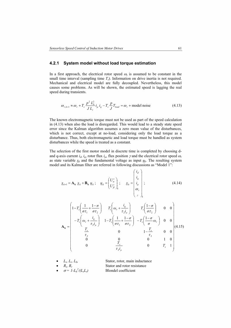
Sensorless Speed Control of Induction Motor Drives 61
4.2.1 System model without load torque estimation
In a first approach, the electrical rotor speed ωr is assumed to be constant in the small time interval (sampling time Ts). Information on drive inertia is not required. Mechanical and electrical model are fully decoupled. Nevertheless, this model causes some problems. As will be shown, the estimated speed is lagging the real speed during transients.
noisemodel22
1, +=−+≈+ rloadsqr
hsrkr T
JpTii
LJLp
T ωωω µ (4.13)
The known electromagnetic torque must not be used as part of the speed calculation in (4.13) when also the load is disregarded. This would lead to a steady state speed error since the Kalman algorithm assumes a zero mean value of the disturbances, which is not correct, except at no-load, considering only the load torque as a disturbance. Thus, both electromagnetic and load torque must be handled as system disturbances while the speed is treated as a constant. The selection of the first motor model in discrete time is completed by choosing d- and q-axis current id, iq, rotor flux iµ, flux position γ and the electrical rotor speed ωr as state variable xk and the fundamental voltage as input uk. The resulting system model and its Kalman filter are referred in following discussions as “Model 1”:
kkk uxx kk BA +=+1 ; k
s
s
k UU
u
=
β
α ;
k
r
q
d
k iii
x
=
γ
µ
ω; (4.14)
−
−
−
−+−
+−
−
+
−+−
=
10001000
0010
001111
001111
2
22
212
2221
sµ
s
ss
rssµ
qrs
sµ
qrss
Ti
T
TT
ωσσT
σσ
σT
ii
ωT
σσT
ii
ωTσσ
σT
τ
ττ
τττ
ττττ
kA (4.15)
• Ls, Lr, Lh, Stator, rotor, main inductance • Rs, Rr Stator and rotor resistance • σ = 1-Lh
2/(LsLr) Blondel coefficient

62 Chapter 5
• τ1 = Ls/Rs Stator time constant • τ2 = Lr/Rr, Rotor time constant
The input matrix Bk describes the weighted transformation from a stator-fixed to the rotor flux reference frame.
( ) ( )( ) ( )
−
=
000000
cossinsincos
γγγγ
σ s
s
LT
kB , (4.16)
The resulting output vector yk consists of the estimated motor current in a stator-fixed reference frame (α/β-system, indices: ‘s’). To avoid double calculations, the sin/cos-terms of the flux angle should be calculated only once and used in both input and output matrix.
( ) ( )( ) ( ) kks
s
kxx
IIy
−==
=
000cossin000sincos
ˆˆ
γγγγ
β
αkC (4.17)
A block diagram of the discrete motor model together with the feedback matrix of the observer is shown in figure 4.2. The motor speed as well as all other states are considered as both, state and parameter. The model matrices Bk and Ck depend on the position of the rotor flux γ, the matrix Ak on q-axis current iq, rotor flux iµ and rotor speed ωr.
Bk
xk+1 ⇒ xk
Ak
+ +
EKF
Ck
+
UαS
UβS
xk+1 γk+1
γk
Measurement: Iα
s Iβ
s
yk + +-
∆yk
∆x
z-1
Figure 4.2: Block diagram of the discrete motor model and EKF.
4.2.2 System model with load torque estimation
The second motor model, in future referred to as “Model 2”, uses additional information on the electromagnetic torque generated by the motor. Additionally to

Sensorless Speed Control of Induction Motor Drives 63
the given states, also the acceleration due to the load torque is estimated. The model presented in this subsection does not assume the velocity ωr but the load torque Tload to be constant in a small time interval (sampling time Ts). This results in an improved performance during transients of the motor speed. Iron and friction losses of the induction motor are also part of the estimated load torque. Using the torque, rather than the speed gives a better handle on the mechanical behavior, as in this way acceleration is controlled, being the input to the speed variations. The acceleration of the drive equals the difference between electromagnetic Tel and load torque Tload related to the drive inertia J. The load torque is generally unknown, but constant at steady state. It creates a disturbance of the speed control loop, which is compensated by the controller. In steady state, the acceleration of the drive is zero by definition. Thus, the differential equation of the acceleration due to the load torque is:
0≈
= load
l TJp
dtd
dtdα (4.18)
loadlkl TJp
=≈⇒ + αα 1, (4.19)
Now, the known electromagnetic torque is used as part of the speed calculation, improving the accuracy of the speed:
lsqr
hsrkr Tii
LJLp
T αωω µ −+≈+
22
1, (4.20)
In contrast to the remarks concerning the load torque in (4.13), the inaccuracy of (4.18)-(4.20) has a zero mean value, being a precondition of the Kalman algorithm. Only a variation of the load is handled as model inaccuracy. This inaccuracy is neglected here, but will be taken into account afterwards at the evaluation of the noise covariance matrix. In addition, erroneous electromagnetic torque calculation and inertia identification are handled as model noise. However, the influence of both an incorrect estimation of the electromagnetic torque due to electrical parameter variations and an incorrect identification of the drive inertia are small compared to a potential load variations. The discrete form of the second model is:
kkk uxx kk BA +=+1 ; k
s
s
k UU
u
=
β
α ;
kl
r
q
d
k
iii
x
=
αγ
ωµ (4.21)

64 Chapter 5
−
−
−
−
−+−
+−
−
+
−+−
=
100000
0100
0100
00010
0001111
0001111
2
2222
212
2221
ss
sr
hs
ss
rssq
rs
sq
rss
Ti
T
TiLJLpT
TT
TTi
iT
Ti
iTT
µ
µ
µ
µ
τ
ττ
ωσ
σστ
σσττ
ω
στσ
τω
στσ
στ
kA (4.22)
( ) ( )( ) ( )
−
=
00000000
cossinsincos
γγγγ
σ s
s
LT
kB (4.23)
( ) ( )( ) ( ) kks
s
kxx
IIy
−==
=
0000cossin0000sincos
ˆˆ
γγγγ
β
αkC (4.24)
This model has a disadvantage: its order is higher. This is a drawback when the EKF algorithm has to be implemented in real-time. However, one major advantage of this model is that it does not assume the speed to be constant during the sample time. The involuntary lag of the speed signal is avoided by the additional estimation of the load acceleration. In fact, the estimation of the acceleration is insignificantly lagging at a continuous load torque variation. Nevertheless, the acceleration is, apart from an initial change, nearly constant during both changing the speed reference and applying load torque. This special drive property is caused by the current/torque limitation within the speed control loop. Thus, the acceleration is almost constant and can be estimated accurately. The other advantage originates from the higher accuracy of the speed specification. This accuracy is considered at the calculation of the noise covariance matrix. A lower value indicates a more accurate estimation and accordingly results in a smother speed signal. Obviously, the performance of the system increases as the information of the known electromagnetic torque is used. Only the load torque is handled as if it were an unknown system disturbance, being true for many motor drives. If the load-speed relation is known, this information can be used for further improvement of the

Sensorless Speed Control of Induction Motor Drives 65
estimation performance. In that case, the equation of the load acceleration αl is determined employing equations (4.5), (4.6) and (4.19):
JTTp
ddT
dtd
ddT
dtdT loadel
r
loadr
r
loadload −⋅==
ωω
ω (4.25)
⇒r
loadklq
r
hsklkl d
dTiiLJLp
JpT
ωααα µ
−+≈+ ,
22
,1, (4.26)
If the known load-speed relation is applied to the algorithm, also the system model inaccuracy is lower. The noise covariance Q can be reduced, resulting in a very smooth steady state speed signal and almost no lag during acceleration or braking periods. Both with and without applying the load-speed relation, the performance of the estimator is only slightly affected by a precise knowledge of the inertia. If the inertia J is set to infinite, the behavior of the algorithm is like the one neglecting the torque command inputs and assuming the speed to be constant in a small time interval. Naturally, the inertia must not be set to zero to guarantee a stable functioning. In all other cases, a mismatch of the inertia is handled by the EKF as system noise. The steady state estimation of the load torque becomes erroneous but the speed estimation remains correct.
4.3 Extended Kalman Filter Algorithm
The induction motor torque depends on both air-gap flux and speed, but neither torque versus flux nor torque versus speed relations are linear. This complicates the design of control systems and speed estimation for induction machines. Due to the lack of a system with linear equations, also the state model of the induction motor used is non-linear. The mechanical speed and position of the flux are considered as both, state and parameter. The model matrices Bk and Ck depend on the position of the rotor flux, the matrix Ak on q-axis current iq, rotor flux iµ and rotor speed ωr. Therefore, the extended Kalman filter (EKF) has to be used to estimate the parameters of the model matrices, as well. The EKF performs a re-linearization of the non-linear state model for each new estimation step, as it becomes available. Furthermore, the EKF provides a solution that directly cares for the effects of measurement or system noise. The errors concerning the parameters of the system model are also handled as system noise. A more complete introduction to the general idea of the Kalman filter can be found in literature [Bram 94], [May 79], Bro 92]. Here, only the basic equations of the EKF are repeated. The EKF algorithm used is based on [Bram 94]. The Kalman filter estimates a process by using a form of feedback control. The signal flow of the EKF in a recursive manner is shown in figure 4.3.

66 Chapter 5
1/z
q
d
uu
kkx 1+
x∂Φ∂
kkx∆1−kkx xh
∂∂
1/z
Predictor
Filter
Pk|k-1
Pk+1|k
Pk|k Kk Kk ∆Yk
kmeasuredk yyY −=∆
Figure 4.3: Block diagram of the extended Kalman filter.
The Kalman algorithm distinguishes between filter and predictor equations. The predictor equations are responsible for projecting the state to obtain the “a priori” estimation of the next time step. The filter equations, also called measurement update, are responsible for the feedback to obtain an improved “a posterior” estimate. The predicted value of the state vector xk+1|k is corrected by adding the product of filter gain and the difference between estimated and measured output vector yk to the state vector xk|k. In addition still the equation for the corrected covariance matrix Pk|k is required.
( )( )kxhyxx kkkkkkk ,1|1|| −− −+= kK (4.27)
1k|kk1k|kk|k PKPP −=− −∂∂
−=1|
|kkxxx
h (4.28)
The matrix Kk is the feedback matrix of the extended Kalman filter. This matrix determines how the state vector xk|k is modified after the output of the model yk is compared to the measured output of the system. The filter gain matrix is defined by:
1
1|1|1||||
−
=−==−
+
∂∂
∂∂
∂∂
=−−−
RPPK 1k|k1k|kk kkkkkk xx
T
xxxx
T
xh
xh
xh (4.29)
in which R is based on the covariance matrix of the measurement signal noise. Based on the calculated state vector xk|k, a new value of the state vector can be predicted. The same applies to the error covariance matrix. The prediction is:
( )kkkkk uxkkx ,,,1 1||1 −+ +Φ= (4.30)
Tkkxx
T
xx kkkk xxΓΓ+
∂Φ∂
∂Φ∂
= ==+ QPP k|kk|1k |||| (4.31)

Sensorless Speed Control of Induction Motor Drives 67
with the covariance matrix Q reflecting the system noise. All equations of the EKF algorithm can be written as a function of a system vector Φ and an output vector h describing the re-linearized model of the induction motor. The system and output vector respectively can be derived from the model equations of the induction motor.
( ) ( ) ( ) kkkkkkkkkkk uxxxuxkk ||||1| ,,,1 kk BA +=+Φ − (4.32)
( ) ( ) 1|1|1| , −−− = kkkkkk xxkxh kC (4.33)
In addition, the derivatives of system and output vector are required for the EKF algorithm. The derivative of the system vector of Model 2 results in:

68 Chapter 5
+
+
−+−
+−
+
−+−
=∂Φ∂
000000
00000
00000
00000
0000111
00002111
2
222
2212
221
µ
µ
µµ
µ
τ
τ
τστσ
σττω
τω
στσ
στ
iT
iLJLpT
Ti
iTi
iT
ii
TT
x
s
r
hs
s
ds
qrs
qrss
(4.34)
−
−
−
−
−
+−
−−
−
−
+
100000
0100
0100
000100
01100
0100
22
222
22
22
2
2
sq
s
sqr
hs
s
ds
sdsr
dqs
qs
sqs
qs
Tii
T
TiLJLpT
T
uL
TiiTiii
T
uL
TiTi
iT
µ
µµ
µ
τ
τ
σσσω
σσ
τ
στστσ
where uq and ud are voltages in a rotor-flux reference frame, already calculated by the product of α/β-voltages and input matrix Bk. Thus, the result can be used to save computing time. Note that the q-axis voltage influences the linearized specification of d-axis current and vice-versa. The corresponding derivative of the system vector of Model 1 is obtained by dropping the last column as well as the last row in (4.34) and setting the elements
2,4x∂Φ∂ and 3,4x∂
Φ∂ to zero. In this way, the influence of electromagnetic and
load torque on the speed is canceled. The derivative of the output vector of Model 2 is:

Sensorless Speed Control of Induction Motor Drives 69
( ) ( ) ( ) ( )( ) ( ) ( ) ( )( ) ( )( ) ( )
−−=
−−−−
=∂∂
0ˆ00cossin0ˆ00sincos
0sincos00cossin0cossin00sincos
α
β
γγγγ
γγγγγγγγ
ii
iiii
xh
qd
qd
(4.35)
The calculation of the estimated α/β-current is already executed by the output matrix C of the system model and should be used in (4.35) to avoid double calculations. The corresponding derivative for Model 1 is obtained by dropping the last column in (4.35). The remaining variables of the algorithm are the noise covariance matrices Q and R and an initial matrix P0|0 representing the covariance of the known initial conditions. They consist only of diagonal elements.
4.4 Real-Time Implementation of the EKF
4.4.1 Measurement & system noise
One critical step towards the implementation of the extended Kalman filter algorithm is the search for the best covariance matrices. They have to be set-up based on the stochastic properties of the corresponding noise. The noise covariance R accounts for the measurement noise introduced by the current sensors and the quantization errors of the A/D converters. Increasing R reflects a stronger disturbance of the current. The noise is weighted less by the filter, causing a more filtered current but also a slower transient performance of the system. The noise covariance Q describes the system model inaccuracy, the errors of the parameters and the noise introduced by the voltage estimation. Q has to be increased at stronger noise levels driving the system, entailing a more heavily weighting of the measured current and a faster transient performance. Thus, changing the covariance matrices R and Q affects both the transient duration and the steady state operation of the filter. An initial matrix P0|0 represents the matrix of the covariance in knowledge of the initial conditions. Varying P0|0 affects neither the transient performance nor the steady state conditions of the system and can be chosen at random. The covariance matrices R, Q and P0|0 are assumed to be diagonal due to the lack of sufficient statistical information to evaluate their off-diagonal terms. Furthermore, the diagonal characteristic holds the possibility of saving a lot of computing time as shown in the next subsection. In general, the entries of the covariance matrices are unknown and cannot be calculated. They are often set to the unity matrix. In order to achieve the optimal

70 Chapter 5
filter performance, the filter parameters R and Q can be obtained by tuning based on experimental investigations. This describes an iterative process of searching the best values. It is almost impossible to find a plausible evaluation of these parameters in literature with regard to the sensorless control of motor drives. However, it is preferable to have a rational basis for choosing the required parameters. In either case, whether or not a superior filter performance can be obtained by an additional tuning process, an initial guess of the values is welcome. As shown, the value of the different parameters differs a lot. Furthermore, the filter performance may change dramatically by varying only one value. Without any previous knowledge and considering the high dimension of the matrices, tuning is very arduously or can even lead to an unstable behavior of the observer. For instance, changing the sample time requires a new tuning process. A design equation has the additional advantage of being independent of the given installation, and it can easily be assigned to other drive installations without an expert tuning the parameters. The measurement covariance R can be measured easily in advanced. Measuring is generally possible because the current measurement is needed anyway while operating the filter. Some off-line sample measurements are taken in order to determine the variance of the measurement error. This is done by applying a constant line-to-line voltage across two phases containing a current sensor and measuring the resulting dc current. It must be noted, that the measured current should not be supplementary filtered, apart from an anti-aliasing filter of course. The noise on the raw measurements will possibly be non-linearly transformed resulting in second order terms, which may be significant. The Kalman approach handles white and uncorrelated measurement noise and produces the minimum variance estimate. Therefore, this is already an optimal filter. A current measurement respecting the given installation yields a measurement noise covariance matrix, being almost proportional to the dc bus voltage within a voltage range 300V < Udc < 600V:
24
42
6
6
A105,100105,1
VA
108,100108,1
⋅⋅
−
⋅⋅
=−
−
−
−
dcUR (4.36)
In case of the system covariance, the calculation is less deterministic. Nevertheless, an estimation of the matrix elements is possible using some simplifications. Furthermore, the given assumptions have been examined experimentally. All given values are calculated using the parameters of the 1,5 kW induction motor drive and a sample time Ts = 200 µs. The calculated values are valid for both system models; Considering (4.9)-(4.10), the inaccuracy of the current calculation is mainly affected by the accuracy of the voltage identification being the input of the system.

Sensorless Speed Control of Induction Motor Drives 71
inaccuracyvoltageinaccuracymodelcurrent ⋅≈s
s
LT
σ (4.37)
The voltage can be either measured or calculated by means of the reference voltages being the output of the entire control loop. Here, the phase voltages are calculated. Therefore, the accuracy is only affected by the non-linearity of the converter. This non-linearity has its origin in the delayed reaction of the switches at turn-on and -off, also called dead-time effect [Bose 97]. Therefore, the accuracy of the voltage calculation, described by an error voltage ∆U, is simplified dependent on the dead-time τdead, the dc bus voltage Udc and the PWM-frequency fPWM of the inverter:
dcPWMdead UfU τ≈∆ (4.38)
The influence of parameter variation is marginal compared to this dead-time effect. So, the covariance of the current model inaccuracy can be estimated by:
2
31)1,1(
∆≈
s
s
LUTQ
σ (4.39)
)1,1()2,2( QQ = (4.40)
For the given drive, using a sample time Ts = 200 µs, a dead-time τdead = 2 µs and a PWM-frequency fPWM = 10 kHz, the covariance amounts to:
2A0018,0)2,2()1,1( == QQ (4.41)
The model estimation inaccuracy of magnetizing current iµ and flux position γ is only caused by the discretization of the continuous equations. In contrast to Model 1, the speed specification within Model 2 is very accurate. The inaccuracy is much lower and mainly caused by the discretization error. Considering a very small sample time, these errors are negligible. Nevertheless, the worst of all approximations is to set the model inaccuracy to zero. White noise is a much better approximation than zero. Thus, this discretization error is considered by a very small value in the noise covariance matrix Q. The maximum discretization error of the magnetizing current is dependent on the maximum motor current and the rotor time constant.
−−
−= ∑ ∫
∞
=
+
0
)1(
2
,,
2
,,var)3,3(k
Tk
kT
kkdkkds
s
s
dtiiii
TQττ
µµ (4.42)

72 Chapter 5
2522
22max
2
max A106,23
var)3,3( −⋅≈=
<⇒
ττss TiTiQ (4.43)
Assuming a maximum acceleration of αmax = 1000 s-2 and a sample time Ts = 200 µs, the variance of the flux position is estimated by:
−<
−= ∫∑ ∫
+∞
=
+ s
s
s
s
Tk
kTss
k
Tk
kTks dttTkTdttTQ
)1(
maxmax0
)1(
var)(var)5,5( ααωω (4.44)
1142
max2
max 103,3482
var)5,5( −⋅≈=
<⇒ ss TTQ αα (4.45)
For Model 2, the inaccuracy of the motor speed calculation is also caused by the discretization error dependent on the maximum acceleration and its time variation. Based on common bandwidth of torque control loops, a maximum variation time constant τtorque = 1 ms is chosen.
−= ∑ ∫
∞
=
+
0
)1(
2Model )(var)4,4(k
Tk
kTks
s
s
dttTQ αα (4.46)
22
42max
2max
2Model10033,0
482var)4,4(
sTTQ
torque
s
torque
s ≈=
<⇒
τα
τα (4.47)
These values are very small resulting in smooth signal shapes. They could be set to the maximum in order to achieve maximum dynamic performance of the drive. For Model 1, the inaccuracy of the motor speed calculation is higher due to the simplified specification and can be found from the maximum inertia related torque variation:
( max1Model 2var)4,4( )αsTQ =< (4.48)
2
2max
2
1Model s1013,0
3)4,4( ≈<⇒
αsTQ (4.49)
In contrast to Model 1, the speed inaccuracy for Model 2 is transferred to the acceleration equation. The variance of the acceleration in system Model 2 equals the variance of the inertia related load. The load torque is generally unknown. However, an estimation of the variance top-limit can be obtained by assuming a maximum torque-inertia relation of the drive. The calculation is based on the considerations made in chapter 4: A constant relation of Tmax/J = 1000 s-2 is assumed. Considering

Sensorless Speed Control of Induction Motor Drives 73
the number of pole pairs p and a maximum torque variation time constant τload = 2 ms, the top-limit of the acceleration inaccuracy and of the process variance is:
torque
skloadkload
JTTp
JTT
pτmax
max
1,,inaccuracymodel ≈
−< − (4.50)
4
2
max 11482121)6,6(
sJTTp
Qtorque
s ≈
<⇒
τ (4.51)
The dynamic and smoothness of both speed and acceleration estimation is tuned by Q(6,6). This parameter should be smaller, if the load torque is known very well or a smooth speed signal is more important than the loop dynamic. A high value increases the dynamic performance, but also the noise of the estimated signals. With respect to the given drive setup, Q(6,6) is set to 5% of the value given in (4.51) in order to obtain a good compromise between dynamic performance and smooth torque command response. All other coefficients of the system covariance matrix are set to the given values. It should be noted, that the calculation of all process covariance matrices is proportional to the square of the sample time. Thus, the given constants should be adapted accordingly, if a different sample time is chosen. However, it is a major advantage of the proposed model, that estimation accuracy and stability of the entire control system are much less sensitive to tuning the covariance matrices compared to other models.
4.4.2 Computing requirements
The speed estimation and the entire control of the induction motor are implemented on a TMS320C31 DSP with 128 K × 32-bit RAM. The implemented algorithm estimates five states for Model 1 and six for Model 2. The computing demand grows almost with the third power of the state dimension. Furthermore, they contain conversions between stator and field coordinate system and a computation time intensive matrix inversion. The algorithm can be implemented with relatively few instructions using matrix calculation. However, without any modification, the resulting algorithm leads to a program that is not suitable for real-time implementation, since it is very complex especially due to the matrix inversion. The execution time would be higher than 400 µs, respectively 700 µs, using the given DSP. In consequence, also the bandwidth of the current/torque controller would be very small. Furthermore, the performance of the EKF decreases as the sample time increases.

74 Chapter 5
The turnaround time of the final control system, using Model 2, amounts to 187 µs. Only a few extra calculations are necessary compared to the speed observer based on Model 1 requiring a turnaround time of 167 µs. The used sample time is set to Ts =220 µs. However, the execution time is not that meaningful. The DSP power is simultaneously used for monitoring and recording the experimental data. Due to developing reasons of the installation, the remaining field-oriented control is not optimized regarding the computation requirement: e.g., the implemented FOC contains three different speed controllers for performance comparison. An overview of the computing requirement considering the different approaches is summarized in table 4.1.
Table 4.1: Computation requirement of different EKF approaches.
Number of Summations [ ]
Number of Multiplications [ ]
Turnaround time of the entire control [µs]
Model 1 Matrix calc.
546 662 >400
Model 2 Matrix calc.
881 1026 >700
Model 1 optimized
207 254 167
Model 2 optimized
255 320 187
Keeping the size of the program limited is achieved by optimizing the model with hand calculations and exploiting matrix symmetry. The covariance matrices Q, R and initial matrix P0|0 are set to be symmetrically. In consequence, also the matrix Pk|k-1 becomes symmetrical which can be exploited avoiding double calculations and higher memory demand. The implemented EKF covers no superfluous multiplications by zero. Several matrix calculations of the EKF algorithms are the same and can be used in different equations, e.g. in (4.28)-(4.29). Furthermore, the sine and cosine of the flux angle is calculated only once and used in the EKF as well as in the Clarke-transformations [Bose 97] of currents and voltages.
4.4.3 Model comparison
Two models are closely examined. The first one is based on an approach, that has become commonplace in almost every speed observer. They do not recognize the actual torque command inputs to the system and assume the velocity ω to be constant in a small time interval. In effect, such techniques treat the known torque command input as if it were an unknown disturbance torque. Thus, they generally lag the actual motor speed during periods of acceleration or braking. The second motor model uses the additional information on the electromagnetic motor torque. Additionally, the acceleration due to the load torque is estimated. This model does not assume the velocity but the load torque to be constant in a small time interval (sampling time Ts). The inaccuracy of the speed calculation is transferred to the load, which is usually unknown anyway. This results in an improved

Sensorless Speed Control of Induction Motor Drives 75
performance during transients (figure 4.4) presenting the response to a step of the speed reference and to a load step. Figure 4.5 shows some important details of figure 4.4.
-0.1 -0.05 0 0.05 0.1 0.15 0.2 0.25 0.3 0.35 0.40
500 1000 1500
t [s]
n [r
pm]
-0.1 -0.05 0 0.05 0.1 0.15 0.2 0.25 0.3 0.35 0.4-5 0 5
10 15
t [s]
T [N
m]
Figure 4.4: Step of the speed reference and response to a load step. Top: Real and estimated speed with and without load torque estimation. Bottom: Estimation of electromagnetic and load torque.
0 0.005 0.01 0.015 0.02 0.025 0.03 0.035 0.04 0.045 0.050
200 400 600
t [s]
n [r
pm]
0.05 0.1 0.15 0.2 0.25 0.3900
950
1000 1050
t [s]
n [r
pm]
1
With αl estimation
Without αl estimation
Tel
Tload
2
Figure 4.5: Details of figure 4.4. Top: Details indicated by Box 1.
Bottom: Details indicated by Box 2. Simulations are performed to compare both algorithms using the improved algorithm as feedback to control the motor. With the other algorithm in the control loop, the obtained results are almost the same but with a higher overshoot due to the delayed response of speed and current controller. A simultaneous real-time implementation of both algorithms requires a faster DSP. Nevertheless, the simulation has the advantage of calculating the real motor speed without any delay in contrast to a real-time implementation using a filter for the measured speed signal (see also figure 5.7). The estimated speed signal requires no additional filter. The smoothness and the transient performance of the signals are adjustable by the noise covariance matrix Q of the EKF algorithm [Ter 01].
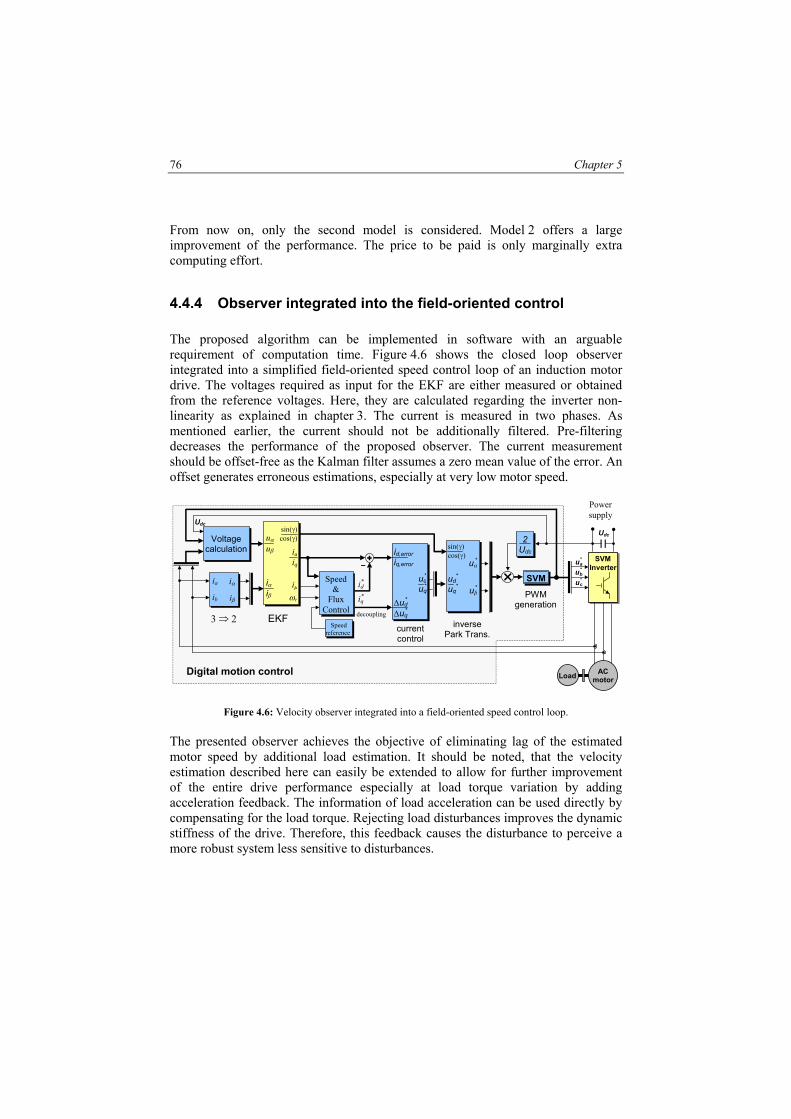
76 Chapter 5
From now on, only the second model is considered. Model 2 offers a large improvement of the performance. The price to be paid is only marginally extra computing effort.
4.4.4 Observer integrated into the field-oriented control
The proposed algorithm can be implemented in software with an arguable requirement of computation time. Figure 4.6 shows the closed loop observer integrated into a simplified field-oriented speed control loop of an induction motor drive. The voltages required as input for the EKF are either measured or obtained from the reference voltages. Here, they are calculated regarding the inverter non-linearity as explained in chapter 3. The current is measured in two phases. As mentioned earlier, the current should not be additionally filtered. Pre-filtering decreases the performance of the proposed observer. The current measurement should be offset-free as the Kalman filter assumes a zero mean value of the error. An offset generates erroneous estimations, especially at very low motor speed.
ia
ib
iα
iβ
Voltage calculation
3 ⇒ 2
iα iβ
sin(γ)cos(γ)
ωr
idiq
EKF
ud*
uq*
id,erroriq,error
sin(γ) cos(γ)
uα*
uβ*
SVM
current control
inverse Park Trans.
PWM generation
Speed reference
id*
iq*
Speed &
Flux Control
iµud
*
uq*
∆ud*
∆uq* decoupling
SVM Inverter ub
*
uc*
AC motor
ua*
Udc
Load
uα uβ
Udc
Power supply
Digital motion control
2 Udc
Figure 4.6: Velocity observer integrated into a field-oriented speed control loop. The presented observer achieves the objective of eliminating lag of the estimated motor speed by additional load estimation. It should be noted, that the velocity estimation described here can easily be extended to allow for further improvement of the entire drive performance especially at load torque variation by adding acceleration feedback. The information of load acceleration can be used directly by compensating for the load torque. Rejecting load disturbances improves the dynamic stiffness of the drive. Therefore, this feedback causes the disturbance to perceive a more robust system less sensitive to disturbances.
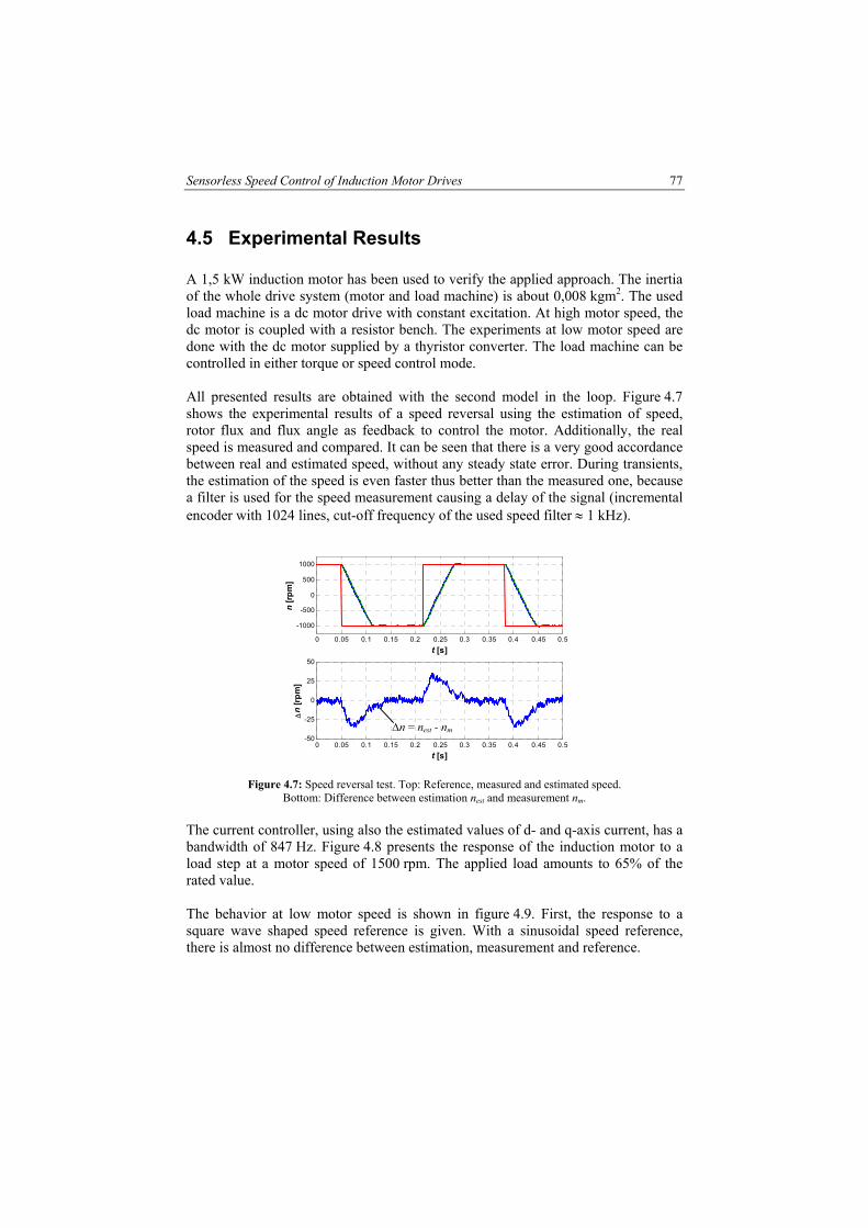
Sensorless Speed Control of Induction Motor Drives 77
4.5 Experimental Results
A 1,5 kW induction motor has been used to verify the applied approach. The inertia of the whole drive system (motor and load machine) is about 0,008 kgm2. The used load machine is a dc motor drive with constant excitation. At high motor speed, the dc motor is coupled with a resistor bench. The experiments at low motor speed are done with the dc motor supplied by a thyristor converter. The load machine can be controlled in either torque or speed control mode. All presented results are obtained with the second model in the loop. Figure 4.7 shows the experimental results of a speed reversal using the estimation of speed, rotor flux and flux angle as feedback to control the motor. Additionally, the real speed is measured and compared. It can be seen that there is a very good accordance between real and estimated speed, without any steady state error. During transients, the estimation of the speed is even faster thus better than the measured one, because a filter is used for the speed measurement causing a delay of the signal (incremental encoder with 1024 lines, cut-off frequency of the used speed filter ≈ 1 kHz).
0 0.05 0.1 0.15 0.2 0.25 0.3 0.35 0.4 0.45 0.5
-1000
-500
0
500
1000
t [s]
n [rp
m]
0 0.05 0.1 0.15 0.2 0.25 0.3 0.35 0.4 0.45 0.5-50
-25
0
25
50
t [s]
∆n
[rpm
]
∆n = nest - nm
Figure 4.7: Speed reversal test. Top: Reference, measured and estimated speed.
Bottom: Difference between estimation nest and measurement nm. The current controller, using also the estimated values of d- and q-axis current, has a bandwidth of 847 Hz. Figure 4.8 presents the response of the induction motor to a load step at a motor speed of 1500 rpm. The applied load amounts to 65% of the rated value. The behavior at low motor speed is shown in figure 4.9. First, the response to a square wave shaped speed reference is given. With a sinusoidal speed reference, there is almost no difference between estimation, measurement and reference.

78 Chapter 5
0 0.1 0.2 0.3 0.4 0.5 0.6 0.7 0.8 0.9 11400
1450
1500
1550
1600
t [s]
n [rp
m]
0 0.25 0.5 0.75 10
2
4
6
t [s]
i q [A]
0 0.25 0.5 0.75 10
5
10
15
t [s]T lo
ad [N
m]
nm
nest
Figure 4.8: Response to a load step. Top: Measured speed nm and
estimated speed nest. Bottom: q-axis current and load torque estimation.
0 0.01 0.02 0.03 0.04 0.05 0.06 0.07 0.08 0.09 0.1-50
-25
0
25
50
t [s]
n [rp
m]
0 0.01 0.02 0.03 0.04 0.05 0.06 0.07 0.08 0.09 0.1
-25
0
25
t [s]
n [rp
m]
0 0.002 0.004 0.006 0.008 0.01 0.012 0.014 0.016 0.018 0.02-50
-25
0
25
50
t [s]
n [rp
m]
nest
nm
nest
nm nref
Figure 4.9: Behavior at low motor speed. Top: Square wave speed reference (20 Hz).
Middle: Sinusoidal speed reference (20 Hz). Bottom: Sinusoidal speed reference (100 Hz). Even at low motor speed and standstill the proposed control scheme is able to manage the load torque (figure 4.10-4.11). Load is applied using a dc motor operating in torque control mode. The arising torque ripple components are typical of a thyristor converter and are returned to the signals of speed and load torque estimation respectively.

Sensorless Speed Control of Induction Motor Drives 79
0 0.5 1 1.5 2 2.5 3-2
0
2
4
6
8
t [s]
I dc [A
]
0
0.5 1 1.5 2 2.5 3
-60
-40
-20
0
20
40
60
t [s]
n [rp
m] nest
nm
Figure 4.10: Response to a load step at standstill. Top: Armature current of the load machine.
Bottom: Measured speed nm and estimated speed nest.
0 0.5 1 1.5 2 2.5 3 3.5 4-2
0
2
4
6
8
t [s]
I dc [A
]
0 0.5 1 1.5 2 2.5 3 3.5 40
60
120
t [s]
n [rp
m]
0 0.5 1 1.5 2 2.5 3 3.5 40
5
10
15
t [s]
T load
[Nm
]
Figure 4.11: Response to a load step at low motor speed (nref = 60 rpm). Top: Armature current of the load machine. Middle: Measured and estimated speed. Bottom: Estimation of the load torque.
Also at high motor speed and flux weakening, a good performance of the EKF can be obtained. Figure 4.12 demonstrates the behavior of the speed and flux estimation in this speed range. The flux is inversely proportional to the motor speed. In consequence, the applied fundamental motor voltage remains nearly constant. Only a small transient is needed to adapt the required d- and q-axis current. This feature of the EKF makes the proposed system also suitable for applications with flux optimization increasing the drive efficiency. However, a minimum flux is required to guarantee a stable operation of the EKF. The minimum flux for the given induction motor drive amounts to approximately 10% of the rated value.

80 Chapter 5
0 0.05 1 0.15 0.2 0.250
500
1000
1500
2000
2500
3000
t [s]
n [rp
m]
0.
0 0.05 0.1 0.15 0.2 0.251
1.5
2
2.5
3
3.5
t [s]
i µ [A
]
0 0.05 0.1 0.15 0.2 0.250
50
100
150
200
250
300
t [s]
+
| [V
]
nm
nest nref
Flux weakening |U
αU
β-300 -200 -100 0 100 200 300
-300
-200
-100
0
100
200
300
uα [V]
u β [V]
Flux weakening
Figure 4.12: Behavior at high motor speed and flux weakening. Top: Speed response
and applied voltage amplitude. Bottom: Magnetizing current and applied voltage.
4.6 Motor Parameter Sensitivity and Adaptation
The used motor model, as well as the implemented EKF, contains four electrical motor parameters: stator inductance Ls, stator resistance Rs, rotor time constant τ2 and leakage (Blondel) coefficient σ. All other parameters, as e.g. the stator time constant τ1, are linked to these parameters. Obviously, the quality of the speed estimation in the observer depends on the accuracy with which the motor parameters are known. Inaccurate model parameters lead to misalignment of the field-oriented coordinate system, impairing the dynamic performance of the drive. Possibly more important is the steady-state accuracy of the speed control, being poor with detuned model parameters. If the machine operates under no-load conditions, the relevant parameters are stator resistance and stator self-inductance. Particularly at low motor speed, the speed estimation is sensitive to an inaccurate stator resistance value in the observer model. Also the leakage inductance value, being the decisive parameter at high motor speed, should be properly tuned to the actual leakage inductance of the machine. The implemented real-time adaptation of these parameters is based on monitoring of magnetizing and d-axis current in steady state. Assuming a constant rotor flux, equation (4.3) can be simplified:
02 ==−=dtdi
iidµ
µ τε (4.52)
Equation (4.52) is valid in every steady-state operating condition, guaranteed by the flux controller of the field-oriented control system. However, the error ε becomes non-zero at a mismatch of stator resistance and inductance respectively. As can be
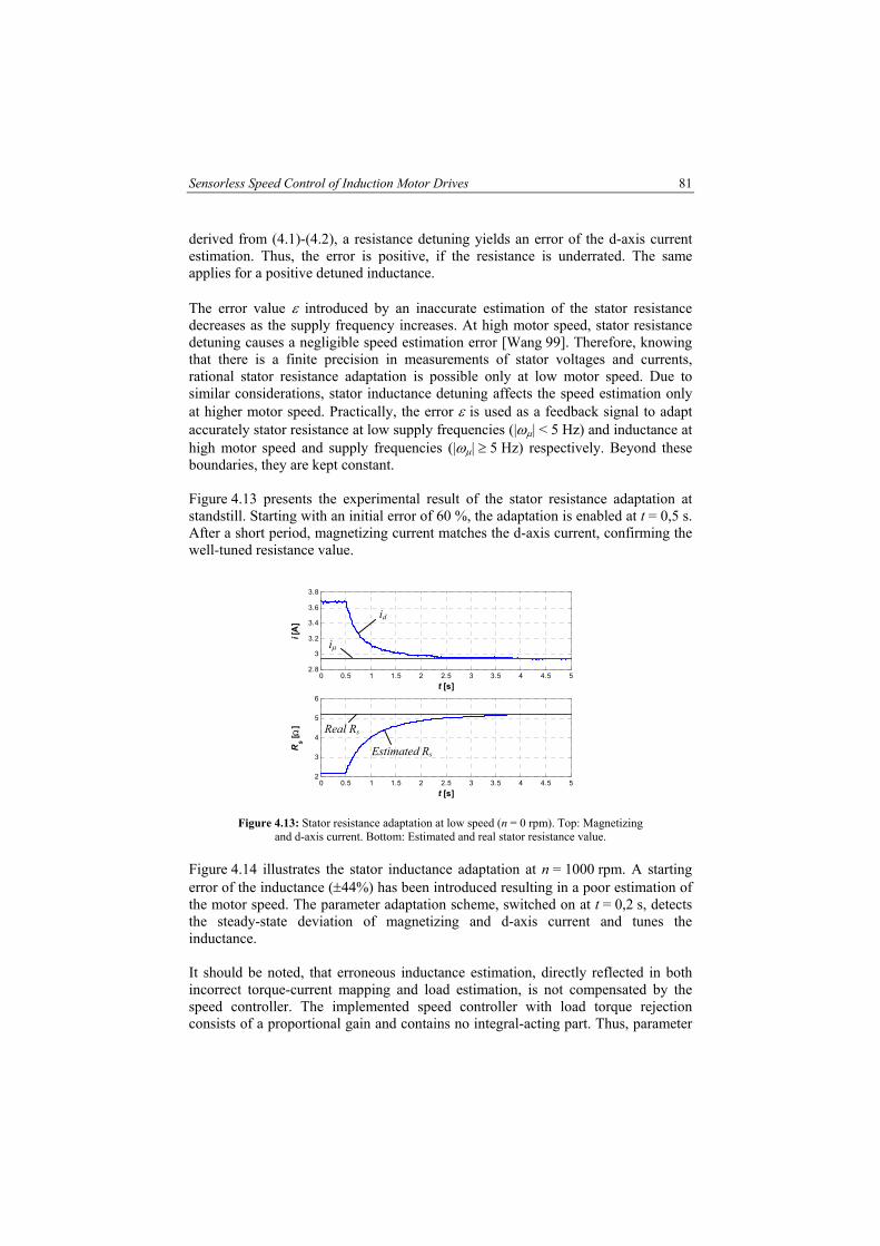
Sensorless Speed Control of Induction Motor Drives 81
derived from (4.1)-(4.2), a resistance detuning yields an error of the d-axis current estimation. Thus, the error is positive, if the resistance is underrated. The same applies for a positive detuned inductance. The error value ε introduced by an inaccurate estimation of the stator resistance decreases as the supply frequency increases. At high motor speed, stator resistance detuning causes a negligible speed estimation error [Wang 99]. Therefore, knowing that there is a finite precision in measurements of stator voltages and currents, rational stator resistance adaptation is possible only at low motor speed. Due to similar considerations, stator inductance detuning affects the speed estimation only at higher motor speed. Practically, the error ε is used as a feedback signal to adapt accurately stator resistance at low supply frequencies (|ωµ| < 5 Hz) and inductance at high motor speed and supply frequencies (|ωµ| ≥ 5 Hz) respectively. Beyond these boundaries, they are kept constant. Figure 4.13 presents the experimental result of the stator resistance adaptation at standstill. Starting with an initial error of 60 %, the adaptation is enabled at t = 0,5 s. After a short period, magnetizing current matches the d-axis current, confirming the well-tuned resistance value.
0 0.5 1 1.5 2 2.5 3 3.5 4 4.5 52.8
3
3.2
3.4
3.6
3.8
t [s]
i [A
]
0 0.5 1 1.5 2 2.5 3 3.5 4 4.5 52
3
4
5
6
t [s]
Rs [ Ω
]
id
iµ
Real Rs
Estimated Rs
Figure 4.13: Stator resistance adaptation at low speed (n = 0 rpm). Top: Magnetizing
and d-axis current. Bottom: Estimated and real stator resistance value. Figure 4.14 illustrates the stator inductance adaptation at n = 1000 rpm. A starting error of the inductance (±44%) has been introduced resulting in a poor estimation of the motor speed. The parameter adaptation scheme, switched on at t = 0,2 s, detects the steady-state deviation of magnetizing and d-axis current and tunes the inductance. It should be noted, that erroneous inductance estimation, directly reflected in both incorrect torque-current mapping and load estimation, is not compensated by the speed controller. The implemented speed controller with load torque rejection consists of a proportional gain and contains no integral-acting part. Thus, parameter

82 Chapter 5
mismatch yields a steady-state error of the speed control loop. However, this steady-state error can be used as an adaptation watchdog or, alternatively to the proposed algorithm, as a parameter-correcting feedback signal.
0 0.25 0.5 0.75 1 1.25 1.5
3
4
5
t [s]
i [A
]
0 0.25 0.5 0.75 1 1.25 1.5350
400
450
500
550
t [s]
L s [mH
]
0 0.25 0.5 0.75 1 1.25 1.5975
1000
1025
1050
t [s]
n [rp
m]
0 0.25 0.5 0.75 1 1.25 1.52
2.5
3
3.5
t [s]
i [A
]
0 0.25 0.5 0.75 1 1.25 1.5
200
250
300
350
t [s]
L s [mH
]
0 0.25 0.5 0.75 1 1.25 1.5994
996
998
1000
1002
t [s]
n [rp
m]
iµ id
iµ id
Parameter adaptation switched ON
Parameter adaptation switched ON
nm nest
nref nm
Figure 4.14: Adaptation of the stator inductance. Top: Magnetizing and d-axis current. Middle: Stator inductance. Bottom: Estimated, real and reference speed. Left: Initial inductance value 44 % overrated.
Right: Initial inductance value 44 % underrated. Figure 4.15 shows the experimental result of the real-time inductance adaptation at variable rotor flux. As can be seen, the inductance is clearly dependent on the saturation level of the machine. Actual and estimated speed are in excellent agreement, confirming the well-tuned inductance value. Applying load torque, the obtained results are equivalent. Usually, a flux controller keeps the rotor flux constant. Rotor flux variations due to both load and electromagnetic torque changes are small and do not significantly affect the observer performance. However, according to (4.52), the adaptation must be disabled during fast rotor flux transients at e.g. initial start, flux weakening and flux optimization. With respect to the given drive setup, the influence of the leakage coefficient σ on the observer performance is very low and hardly measurably. Furthermore, a mismatch is partially compensated by the inductance adaptation. Therefore, an adaptation of σ is not implemented. No major problem exists in determining the stator frequency ωµ. To the contrary, the estimation error of the rotor frequency ωslip, directly reflected in the accuracy of the rotor speed estimation ωr, depends on the rotor time constant. This error increases proportionally to the q-axis current and load respectively. The rotor time constant varies in a fairly wide range during operation. Variations of the rotor inductance are caused by changes of magnetization. Furthermore, the rotor time constant changes with the machine temperature. Assuming an equivalent influence of the saturation level on both the stator and rotor inductance, the stator inductance adaptation

Sensorless Speed Control of Induction Motor Drives 83
scheme is used to compensate these variations. However, a real-time adaptation scheme of the rotor time constant compensating the temperature variations has not yet been realized. A simulation scheme based on the feedback of the observer state error ∆x (figure 4.2) turned out to malfunction in practice, since the obtained signals are too low and noisy to carry suitable information. A promising solution of tuning the rotor time constant in real-time is based on the evaluation of rotor slot harmonics [Jia 97]. This method permits high speed-accuracy in steady state and allows even position control. However, detection of rotor slot harmonics should not be used as a stand-alone solution for speed estimation, since the dynamic performance of such systems is very poor [Ish 82], [Kre 92]. To the contrary, the dynamic performance of the proposed observer is excellent. Together with the detection of rotor slot harmonics, compensating slow temperature variations, a system with both high dynamic performance and high steady-state accuracy is obtained.
0 10 20 30 40 501
2
3
4
5
t [s]
i [A
]
0 10 20 30 40 50250
300
350
400
450
t [s]
L s [mH
]
0 10 20 30 40 50990
995
1000
1005
1010
t [s]
n [rp
m]
1 2 3 4 5250
300
350
400
450
iµ [A]
L s [mH
]
nm
nest
Figure 4.15: Adaptation of the stator inductance. Top: Magnetizing current, d-axis current and stator inductance. Bottom: Estimated, real, reference speed and flux dependence of the stator inductance.
4.7 Conclusions
This chapter presents the design and the implementation of a field-oriented high-performance motor drive with speed, flux and torque estimation. The speed controlled induction motor drive requires no shaft sensor measuring speed or position. The price to be paid is a more extensive and complicated control algorithm. However, no additional measurements are required. The structure of the implemented sensorless control is based on the extended Kalman filter theory. Results of the dynamic and steady-state behavior of a sensorless speed control of an induction motor are given. After the correct system model is chosen for the Extended Kalman Filter, the results are satisfactory. Both at very low and at high

84 Chapter 5
motor speed with flux weakening, the proposed control scheme is working very well. The described control system is a solution without mechanical sensors for a wide range of applications where good steady state and dynamic properties are required. Keeping the size of the program reasonable and still reaching a very good performance is achieved by optimizing the model by hand calculations and exploiting matrix symmetry. The performance of the system increases as the information of the known electromagnetic torque is used. Only the load torque is handled as if it were an unknown system disturbance. If the load-speed relation is known, this information can be used for a further improvement of the performance. The speed estimation does not lag the actual motor speed, both in steady state and during periods of acceleration or braking. Steady-state errors are used for parameter adaptation.

5. Sensorless Speed Control of PMSM
5.1 Introduction
With the introduction of permanent magnets with a high flux density as well as a high coercivity in the late eighties, synchronous motors with permanent magnets became an attractive alternative for applications in high performance variable speed drives. Significant advantages arise from the simplification in construction, the reduction in losses and the improvement in efficiency. One of the most active areas of control development during recent years involving these motor types has been the evolution of new techniques for eliminating the position and speed sensor. Elimination of the shaft-mounted sensor is required in many applications since this device is often one of the most expensive and fragile components in the entire drive system. The approaches to sensorless drives vary depending on the rotor flux distribution. A motor with a trapezoidal rotor flux distribution (BLDM, brushless dc motor) provides an attractive candidate: Two out of three stator windings are excited at the same time and the unexcited winding can be used as a sensor. The control scheme as well as the position detection is relatively simple. The rotor speed and position can be determined by the electromagnetic field induced in the unexcited winding [Erd 84], [Mat 90]. This is usually done either by a zero crossing approach of the back-EMF or by a phase-locked loop technique to lock on to the back-EMF waveform in the unexcited winding. It is enough to detect the rotor position every 60° to obtain a proper switching sequence. On the contrary, the permanent magnet synchronous motor (PMSM), having a sinusoidal flux distribution, excites all three windings at the same time. Both the control algorithm and the speed/position estimation become more complicated. The information on the rotor position is required continuously. However, the PMSM is applicable for fine torque control where a very low level of torque pulsations is required. Several schemes for position sensorless operation of PMSM have been reported in literature and are reviewed e.g. in [Raj 94]. The position detection methods are mainly based on Kalman filtering or Model Reference Adaptive Systems using the motor parameters and measurements of motor currents and voltages.

86 Chapter 6
The drive system studied in this chapter is a sensorless control of a PMSM based on the extended Kalman filter theory using only the measurements of motor current and dc bus voltage for the estimation of speed and rotor position. On top of the speed, also the acceleration of the drive is estimated offering a significant improvement of the drive performance. The applied approach is mainly a transfer of the earlier described sensorless control of the induction motor to the motor equations of the PMSM. Therefore, this chapter explains only differences in detail while many still valid statements of previous chapters are not repeated. Theoretical analyses based on the physical viewpoint are presented and the associated experimental results are shown. This chapter also describes the influence on the control design reflected by the feedback of the estimated values. A torque that at average differs from zero, is only produced if the excitation is precisely synchronized with the rotor speed and instantaneous position. The controller has to ensure that the motor never experiences loss of synchronization. Due to rotor asymmetry, the PMSM is also suitable for position control. A 3 kW, 4 kW and 45 kW PMSM have been used to verify this approach. The discussion ends by evaluating a parameter adaptation scheme in real-time to track motor parameter variations.
5.2 Model of the PMSM in Discrete Time
The system model considered is a PMSM having permanent magnets mounted on the rotor. The resulting back-EMF voltage induced in each stator phase winding during rotation can be modeled quite accurately as a sinusoidal waveform. A mathematical model describing the PMSM motor dynamics in a rotor flux reference frame is well known [Jah 86], [Hen 92]. The electrical properties of the PMSM in continuous time are completely described by two stator voltage equations:
qqrd
ddsd iLdtdiLiRu ω−+= (5.1)
Mdrddrq
qqsq iLdtdi
LiRu Ψ+++= ωω (5.2)
In a PMSM with surface-mounted magnets, torque control can be achieved very simply, since the instantaneous electromagnetic torque can be expressed similarly to that of the dc machine as the product of q-axis current iq and magnet flux ΨMd. In case of interior permanent magnets, the additional reluctance torque can be exploited:
( )( )ddqMdqel iLLipT −−Ψ= (5.3)
In contrary to the induction machine, the flux angle γ rotates synchronously with the rotor speed. With the same simplifications as introduced in the induction motor study, the mechanical equation is:

Sensorless Speed Control of PMSM 87
dtd
pJ
dtdJTT r
loadelωω
==− (5.4)
rdtd ωγ
= (5.5)
Tolerating a small discretization error, the transformation from continuous time to the discrete time state space is equivalent to:
d
dsq
d
qrsd
d
sskd L
uTi
LL
TiLR
Ti ++
−≈+ ω11, (5.6)
q
qs
q
Mdsd
q
drsq
q
sskq L
uT
LTi
LLTi
LRTi +
Ψ−−
−≈+ ω11, (5.7)
( )( ) loadsddqMdqsrkr TJpTiLLi
JpT −−−Ψ+≈+
2
1, ωω (5.8)
rsk T ωγγ +≈+1 (5.9)
From the control viewpoint, the PMSM has four electrical parameters: stator resistance Rs, d- and q-axis inductance Ld and Lq, and permanent magnet flux linkage ΨMd. The inductances are considered to be constant, which is verified by measurements [Van 98] and numerical calculations of the given PMSM [Pah 98]. The influence of parameter variations is compensated by real-time adaptation of the flux linkage ΨMd. The known electromagnetic torque is used as part of the speed calculation, vastly increasing the accuracy of the speed specification and the dynamics of the drive. However, this approach requires information on the load, since the Kalman algorithm assumes a zero mean value of the disturbances. As mentioned in the previous chapter, an additional estimation of the load torque increases the observer performance as well as the performance of the speed control loop. The price to be paid is a minor extra computing time. Therefore, the acceleration due to the load torque is estimated additionally:
0≈
= load
l TJp
dtd
dtdα (5.10)
loadlkl TJp
=≈⇒ + αα 1, (5.11)
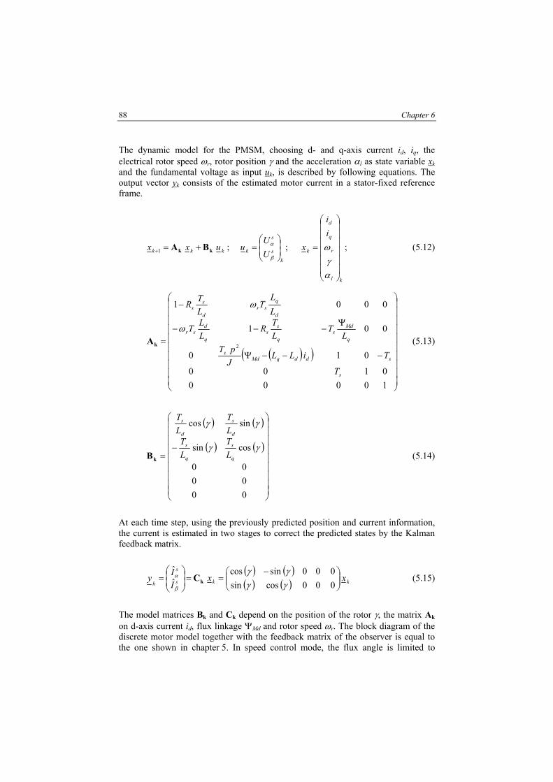
88 Chapter 6
The dynamic model for the PMSM, choosing d- and q-axis current id, iq, the electrical rotor speed ωr, rotor position γ and the acceleration αl as state variable xk and the fundamental voltage as input uk, is described by following equations. The output vector yk consists of the estimated motor current in a stator-fixed reference frame.
kkk uxx kk BA +=+1 ; k
s
s
k UU
u
=
β
α ;
kl
r
q
d
k
ii
x
=
αγ
ω ; (5.12)
( )( )
−−−Ψ
Ψ−−−
−
=
100000100
010
001
0001
2
s
sddqMds
q
Mds
q
ss
q
dsr
d
qsr
d
ss
T
TiLLJpT
LT
LTR
LLT
LL
TLTR
ω
ω
kA (5.13)
( ) ( )
( ) ( )
−=
000000
cossin
sincos
γγ
γγ
q
s
q
s
d
s
d
s
LT
LT
LT
LT
kB (5.14)
At each time step, using the previously predicted position and current information, the current is estimated in two stages to correct the predicted states by the Kalman feedback matrix.
( ) ( )( ) ( ) kks
s
kxx
IIy
−==
=
000cossin000sincos
ˆˆ
γγγγ
β
αkC (5.15)
The model matrices Bk and Ck depend on the position of the rotor γ, the matrix Ak on d-axis current id, flux linkage ΨMd and rotor speed ωr. The block diagram of the discrete motor model together with the feedback matrix of the observer is equal to the one shown in chapter 5. In speed control mode, the flux angle is limited to

Sensorless Speed Control of PMSM 89
|γ | < π. In contrary to the induction motor drive, the studied PMSM is also suitable for position control since the rotor asymmetry can be exploited. Therefore, the overflow protection has to be disregarded in position control mode. However, a loss of exact position information is not admissible in any case.
5.3 Real-Time Implementation
According to the EKF algorithm described in chapter 5, all equations can be written as a function of a system vector Φ and an output vector h describing the re-linearized model of the PMSM. The derivatives of the output and the transposed system vector are:
( ) ( ) ( ) ( ) ( )( ) ( ) ( ) ( )
( ) ( )( ) ( )
−−=
−−−−
=∂
∂=
∂∂
0ˆ0cossin0ˆ0sincos
0sincos0cossin0cossin0sincos
α
β
γγγγ
γγγγγγγγ
ii
iiii
xx
xh
qd
qd
k
k
k
kC
(5.16)
( )
( )
( )( )
( )
−
−
Ψ+−
−−Ψ−
−−
−−
=
∂
+∂=
∂Φ∂
1000
010
01
001
001
2
2
s
dq
sq
d
s
sMdddq
sq
d
qs
ddqMds
q
ss
d
qsr
qdqs
q
dsr
d
ss
T
k
kk
T
k
k
T
uLTu
LT
TiLLTi
LL
T
iLLJpT
LTR
LL
T
iLLJ
pTLLT
LTR
xux
x
ω
ω
kk BA
(5.17)
The noise covariance matrices Q and R and an initial matrix P0|0 are evaluated corresponding to the remarks on the induction motor drive. The matrices R, Q and P0|0 are diagonal due to the lack of sufficient statistical information to evaluate their off-diagonal terms. Furthermore, their diagonal nature saves a lot of computing time. P0|0 affects neither the transient performance nor the steady state conditions of the system and can be chosen at random. An off-line current measurement, referring to the 3 kW PMSM drive installation, yields a measurement noise covariance matrix, which is almost proportional to the dc bus voltage within a voltage range 300V < Udc < 600V:

90 Chapter 6
232
5 A107,10
07,1VA10
15,10015,1 −−
−
= dcUR (5.18)
The measurement of the noise largely exhibits independence of the motor current. The values a larger compared to the measurement noise of the induction machine supplied by the same inverter. This is mainly due to the smaller inductances of the PMSM smoothing the PWM pulses. For an external field (armature reaction) the magnets behave as air, introducing a large reluctance and thus a low main inductance. The coefficients of the system covariance matrix are calculated according to subsection 4.4.1 taking a sample time Ts = 200 µs and the parameter of the 3 kW PMSM into account:
22
A0,02131)1,1( =
∆=
d
s
LuTQ (5.19)
2
2
A0,005931)2,2( =
∆=
q
s
LuT
Q (5.20)
256104
s1102,3s102)3,3( −− ⋅=⋅= sTQ (5.21)
11444 102,3s102)4,4( −− ⋅=⋅= sTQ (5.22)
46822
s12,43
s1102,1)5,5( ⋅=⋅= kTpkQ s , with: k ≤ 1 (5.23)
The transient performance of the observer is tuned by the factor k in (5.23). All other coefficients of the system covariance matrix are set to the given values. A high tuning factor k increases the dynamic performance, but also the noise of the estimated signals. Within the implemented speed control, the information on load acceleration is used as input of the speed controller directly compensating the load torque (figure 5.1). Rejecting load disturbances inproves the dynamic stiffness of the drive and is superior compared to common PI controller [Lor 99]. However, a rough torque command results in increased torque ripples and motor heating by current harmonics. In order to obtain a good compromise between dynamic performance and a smooth torque command response and with respect to the given installation, the tuning factor k is set to 10%. Figure 5.1 shows the structure of the implemented position and speed controller with load torque rejection. The calculated reference torque Tel
* is mapped into reference commands for d- and q-axis current. The current commands id
* and iq* are extracted according the constraint of maximum torque-per-
ampere operation, being nearly equivalent to maximum drive efficiency [Bose 97].
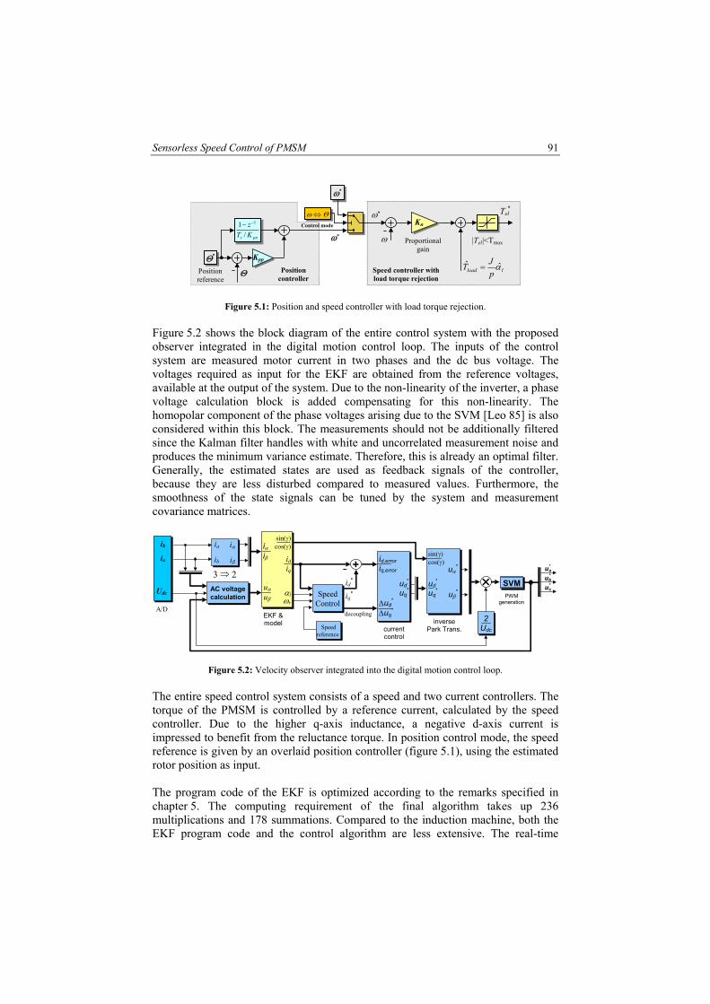
Sensorless Speed Control of PMSM 91
ω*
Tel*
Θ Position controller
Θ*
ω ⇔ Θ
Position reference
Kpp
pns KTz
/1 1−−
ω*
ω*
ω |Tel|<Tmax
lload pJT αˆ =
Proportional gain
Kn
Speed controller with load torque rejection
Control mode
Figure 5.1: Position and speed controller with load torque rejection. Figure 5.2 shows the block diagram of the entire control system with the proposed observer integrated in the digital motion control loop. The inputs of the control system are measured motor current in two phases and the dc bus voltage. The voltages required as input for the EKF are obtained from the reference voltages, available at the output of the system. Due to the non-linearity of the inverter, a phase voltage calculation block is added compensating for this non-linearity. The homopolar component of the phase voltages arising due to the SVM [Leo 85] is also considered within this block. The measurements should not be additionally filtered since the Kalman filter handles with white and uncorrelated measurement noise and produces the minimum variance estimate. Therefore, this is already an optimal filter. Generally, the estimated states are used as feedback signals of the controller, because they are less disturbed compared to measured values. Furthermore, the smoothness of the state signals can be tuned by the system and measurement covariance matrices.
ia
ib
iα
iβ
AC voltage calculation
3 ⇒ 2
iα iβ
sin(γ)cos(γ)
ωr
idiq
EKF & model
ud*
uq*
id,erroriq,error
sin(γ) cos(γ)
uα*
uβ*
current control
inverse Park Trans.
PWM generation
Speed reference
id*
iq* Speed
Control
ud*
uq*
∆ud*
∆uq* decoupling
ub*
uc*
ua*
uα uβ
Udc
ia
ib
A/D
αl
SVM
2 Udc
Figure 5.2: Velocity observer integrated into the digital motion control loop. The entire speed control system consists of a speed and two current controllers. The torque of the PMSM is controlled by a reference current, calculated by the speed controller. Due to the higher q-axis inductance, a negative d-axis current is impressed to benefit from the reluctance torque. In position control mode, the speed reference is given by an overlaid position controller (figure 5.1), using the estimated rotor position as input. The program code of the EKF is optimized according to the remarks specified in chapter 5. The computing requirement of the final algorithm takes up 236 multiplications and 178 summations. Compared to the induction machine, both the EKF program code and the control algorithm are less extensive. The real-time

92 Chapter 6
implementation of the Kalman filter integrated into the motion controller is carried out using a TMS320C31 DSP in which the turnaround time of the entire control system amounts to 153 µs. Therefore, the filter can operate in a system having a maximum sampling frequency of 6,5 kHz, or a theoretical system bandwidth of 3,25 kHz. This high bandwidth allows the EKF to be used in high-performance real-time motion systems.
5.4 Experimental Results
The proposed speed sensorless control scheme has been tested using a 3 kW, 4 kW and 45 kW PMSM (data are given in appendix B). However, to keep the presented results clear, all experimental results presented in this chapter are measurements using the 3 kW prototype motor. Some additional experiments regarding the 4 kW motor, specially designed for PV-powered water pump systems, are presented in chapter 7. Since the DSP power is simultaneously used for monitoring purposes and recording experimental data, the sample time used is fixed to Ts =200 µs. A dc generator with constant excitation coupled to a variable resistor bench is used to load the PMSM. Via a power switch a load step can be applied. Additionally, the load torque is measured by a torque transducer. All experimental results and measurements are carried out using the estimated states as feedback to a speed controller with load torque rejection (figures 5.1 and 5.2). The bandwidth of both current controllers using also the estimated values of d- and q-axis current is about 950 Hz. The bandwidth of the current loop is not decreased by using the EKF instead of the field-oriented control with position measurement. Figure 5.3 shows the experimental results of a speed reversal using the estimated speed and position as feedback. Additionally, the real speed and position are measured for comparison. There is a very good agreement between real and estimated speed and position respectively. Using the information on generated electromagnetic torque and drive acceleration, the noise as well as the lag in the estimated speed signal is even lower than the measured and filtered speed signals during transients. Furthermore, figure 5.3 exhibits the influence of signal lag due to data transmission. Without any delay, the required phase voltages, calculated by means of the voltage references controlling the inverter, are directly available in the control loop. To the contrary, the affiliated current response is measured not before the next sample period of the digital control system. Neglecting the current signal lag causes a poor estimation of the position angle. Therefore, an extra sample delay is added in the loop of the estimated phase voltages used in the observer algorithm. The observer presented achieves the objective of eliminating the lag of the estimated motor speed by additional estimation of the load. Figure 5.4 presents the response of

Sensorless Speed Control of PMSM 93
the PMSM to a load step (75% rated torque) at a motor speed of 1000 RPM. The information on load acceleration is directly used to compensate for the load torque. Rejecting load disturbances increases the dynamic stiffness of the drive. Therefore, this feedback causes the disturbance to perceive a more robust system responding less to disturbances. Compared to a common PI speed controller, the overshoot at steps of both speed reference and load torque is vastly decreased or even vanishes since the speed controller used (figure 5.1) contains of no integral-acting part.
0 0.1 0.2 0.3 0.4 0.5 0.6 0.7 0.8 0.9 1 1.1 1.2
-500
-250
0
250
500
t [s]
n [rp
m]
0 0.1 0.2 0.3 0.4 0.5 0.6 0.7 0.8 0.9 1 1.1 1.2-5
0
5
10
15
20
t [s]
i q [A]
0 0.1 0.2 0.3 0.4 0.5 0.6 0.7 0.8 0.9 1 1.1 1.2-20
-10
0
10
20
t [s]
∆n
[rpm
]
0 0.1 0.2 0.3 0.4 0.5 0.6 0.7 0.8 0.9 1 1.1 1.2-0.2
-0.1
0
0.1
0.2
t [s]
∆γ [
rad]
nref
(a)
iq* iq
(b)
∆n = nest - nm
(c)
Without extra delay With extra delay (d)
Figure 5.3: Speed reversal test. Top: Speed reference nref, estimated speed nest and measured speed nm. Middle: Estimated q-axis current (b) and difference between estimated and measured speed (c).
Bottom: Error of the angle estimation and influence of current/voltage signal lag.

94 Chapter 6
0 0.2 0.4 0.6 0.8 1 1.2 1.4 1.6 1.8 2
980
1000
1020
t [s]
n [rp
m]
0 0.2 0.4 0.6 0.8 1 1.2 1.4 1.6 1.8 2-5
0
5
10
15
20
t [s]
i q [A]
0 0.2
0.4 0.6 0.8 1 1.2 1.4 1.6 1.8 2-5
0
5
10
15
t [s]
T [N
m]
Tload
nm
nest
Tel
Tm
Tel
Figure 5.4: Response to a load step (75% rated torque). Top: Measured and estimated speed. Middle: Estimated q-axis current. Bottom: Estimated load Test, measured load Tm and electromagnetic torque Tel.
In steady state, the estimated load in figure 5.4 equals to the measured load. This is not obvious since iron and friction losses of the PMSM are part of the estimated but not of the measured torque. Furthermore, erroneous electromagnetic torque calculations and inertia identification are directly reflected at the load calculation. However, this influence is small compared to a potential load variation. In fact, the torque calculation might be incorrect, but the real load is compensated by the real torque and the steady state speed error sticks to zero. Only the dynamics of the load estimation are important for exact speed calculation without any delay. As can be seen, the delay between estimated and measured load is insignificant. Therefore, the proposed speed control offers a vast improvement of the drive performance also if the load is not absolutely known. At low motor speed (n ⇒ 0), the equations of the PMSM are simplified, as the voltage induced by the magnets is very small. Therefore, no prediction can be made on the position of the magnets and the EKF fails. Since at standstill only dc-values are given, the necessary flux variation must be forced by impressing a test signal into the system. A signal, easy to implement, is an additional sinusoidal reference current in the d-axis of the motor, using the d/q axis-symmetry of the rotor to estimate the real position. In all experimental results presented the following d-axis reference current is used:
−⋅+=
+=
rpm3001)
s11002sin(A3*
*,
nti
iii
d
testdrefd
π, with: |n| ≤ 300 rpm (5.24)
whereby the reference d-axis current id
* results from the speed controller calculating the required torque motor. The amplitude and frequency of the test signal is
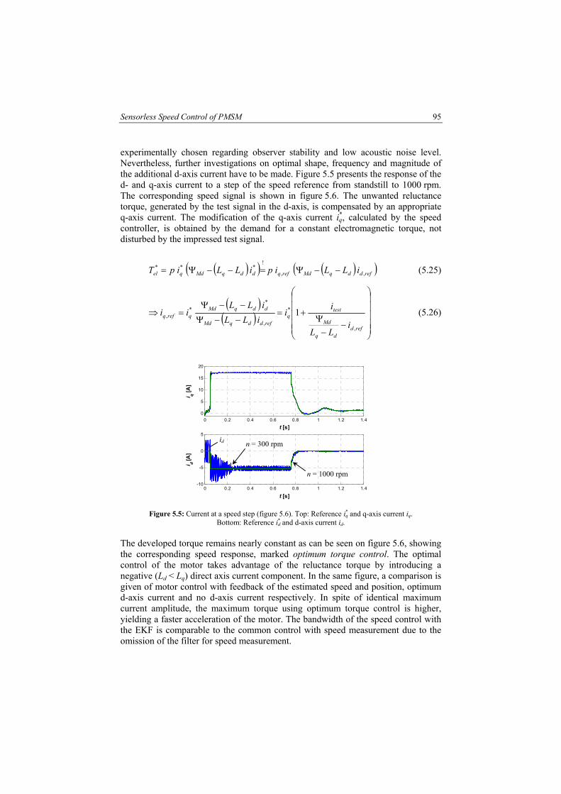
Sensorless Speed Control of PMSM 95
experimentally chosen regarding observer stability and low acoustic noise level. Nevertheless, further investigations on optimal shape, frequency and magnitude of the additional d-axis current have to be made. Figure 5.5 presents the response of the d- and q-axis current to a step of the speed reference from standstill to 1000 rpm. The corresponding speed signal is shown in figure 5.6. The unwanted reluctance torque, generated by the test signal in the d-axis, is compensated by an appropriate q-axis current. The modification of the q-axis current iq
*, calculated by the speed controller, is obtained by the demand for a constant electromagnetic torque, not disturbed by the impressed test signal.
( )( ) ( )( )refddqMdrefqddqMdqel iLLipiLLipT ,,
!*** −−Ψ=−−Ψ= (5.25)
( )( )
−−
Ψ+=
−−Ψ
−−Ψ=⇒
refddq
Md
testq
refddqMd
ddqMdqrefq
iLL
ii
iLLiLL
ii,
*
,
**
, 1 (5.26)
0 0.2 0.4 0.6 0.8 1 1.2 1.40
5
10
15
20
t [s]
i q [A]
0 0.2 0.4 0.6 0.8 1 1.2 1.4-10
-5
0
5
t [s]
i d [A]
id n = 300 rpm
n = 1000 rpm
Figure 5.5: Current at a speed step (figure 5.6). Top: Reference iq
* and q-axis current iq. Bottom: Reference id
* and d-axis current id. The developed torque remains nearly constant as can be seen on figure 5.6, showing the corresponding speed response, marked optimum torque control. The optimal control of the motor takes advantage of the reluctance torque by introducing a negative (Ld < Lq) direct axis current component. In the same figure, a comparison is given of motor control with feedback of the estimated speed and position, optimum d-axis current and no d-axis current respectively. In spite of identical maximum current amplitude, the maximum torque using optimum torque control is higher, yielding a faster acceleration of the motor. The bandwidth of the speed control with the EKF is comparable to the common control with speed measurement due to the omission of the filter for speed measurement.

96 Chapter 6
0 0.2 0.4 0.6 0.8 1 1.2 1.40
200
400
600
800
1000
1200
t [s]
n [rp
m]
nref
Optimum torque control
id = 0
Figure 5.6: Speed step with feedback of the estimated speed and position (EKF). Comparison of torque
control with optimum d-axis current and no d-axis current respectively.
5.5 Position Estimation and Start-up
Using a position sensor as feedback device, a special start-up strategy is required to find the absolute rotor position as indicated by an encoder index pulse. This start-up procedure is necessary in both position control and speed or torque control mode. A torque is only produced if the excitation is precisely synchronized with the rotor speed and instantaneous position. A start-up strategy is executed by impressing a (assumed) q-axis current and slowly increasing the initial assumption of the rotor angle until the motor rotates and the index pulse is found. However, the motor has to rotate up to one mechanical revolution. Once the index is found, all registers are reset and the drive is ready for normal operation. In drive systems without a position sensor, it is generally difficult to estimate the initial rotor position. If the rotor position can not be exactly estimated, the starting torque of the motor decreases and the motor may temporarily rotate in the wrong direction after start. A starting strategy often proposed is based on energizing two windings by a large armature current (about rated current) and expecting the rotor to align with a certain definite position. This method yields the direction of the magnet axis but cannot distinguish between North and South Pole. To the contrary, the presented sensorless control scheme is self-starting. Here, the variation of the inductance as a function of the rotor position is used to obtain the position. Due to the low permeability of the magnet material, the inductance along the q-axis of the PMSM with interior permanent magnets is larger than the inductance along the d-axis. Impressing the test signal (5.24), the difference is detected by the Kalman algorithm and the estimated position converges automatically to the real position. Figure 5.7 presents the initial start-up of the digital control system. Aligning the initial value of the estimated position to the

Sensorless Speed Control of PMSM 97
magnet position, the resulting convergence is very smooth. If the initial value of the estimated position is opposite to the rotor position, the motor temporarily rotates in the wrong direction. This effect can be avoided by operating the drive in open-loop control and impressing a test signal in one motor phase. Once the position is detected, the drive returns to the closed-loop control. The controller has to ensure that the motor never experiences loss of synchronization. However, the rotor asymmetry makes the PMSM also suitable for position control (figure 5.8). For the drive setup with the 3 kW PMSM, the steady-state error of the electrical position angle is smaller than 2,3°. This error, as well as the performance of the algorithm, mainly depends on the quality and accuracy of voltage and current measurement. It should be remarked, that the proposed algorithm only identifies the electrical position. The absolute mechanical rotor position is not detectable.
0 0.5 1 1.5-4
-2
0
2
4
t [s]
γ [ra
d]
0 0.5 1 1.5-100
-50
0
50
100
t [s]
n [rp
m]
0 0.5 1 1.5
-0.4
-0.2
0
0.2
t [s]
γ [ra
d]
0 0.5 1 1.5-10
-5
0
5
10
t [s]
n [rp
m]
γm γm
γest γest
nm
nest
nm nest
Figure 5.7: Start-up of the sensorless speed control. Top: Estimated position γest and measured positionγm.
Bottom: Estimated and measured speed. Left: Initial value of the position estimation almost opposite to the rotor position. Right: Initial value of the position estimation almost aligned to the rotor position.

98 Chapter 6
0 0.05 0.1 0.15 0.2 0.25 0.3 0.35 0.4 0.45 0.5-50
0
50
100
150
200
t [s]
n [rp
m]
0 0.05 0.1
0.15 0.2 0.25 0.3 0.35 0.4 0.45 0.5
0
1
2
3
t [s]
γ [ra
d]
0 0.05 0.1 0.15 0.2 0.25 0.3 0.35 0.4 0.45 0.5-0.1
-0.05
0
0.05
0.1
t [s]
∆γ [
rad]
∆γ = γest - γm
γref
nest nm
nref
Figure 5.8: Position control of the 3 kW PMSM. Top: Position reference γref, estimated position γest and
measured position γm. Middle: Difference between estimated and measured position. Bottom: Speed reference nref, estimated speed nest and measured speed nm.

Sensorless Speed Control of PMSM 99
5.6 Motor Parameter Adaptation
The motor model of the PMSM as well as the implemented EKF contains four electrical motor parameters: d/q-axis inductances Ld and Lq, stator resistance Rs and permanent magnet flux linkage ΨMd. For the given PMSM, the ohmic voltage drop is very small. Thus, the influence of a stator resistance variation is very low and hardly measurably. The key mechanical drive parameter is the moment of inertia J. A mismatch of the inertia affects the observer performance only during transients and causes no steady-state error. Therefore, an adaptation of Rs and J is not considered. The most influential motor parameter, affecting the steady-state error and the observer performance, is the permanent magnet flux linkage ΨMd. Applying flux adaptation, the torque-current mapping via a look-up table according to figure 2.12 is no longer suitable. Assuming exact knowledge of the motor parameters and using the d-axis current, the torque reference Tel
*, determined by the speed controller, is transformed to a q-axis current reference iq
*:
))((
**
ddqMd
elq iLLp
Ti−−Ψ
= (5.27)
According to (2.50), the optimum torque control of the PMSM yields two solutions for the d-axis current reference id
*:
2*
2
*
)(2)(2 qdq
Md
dq
Mdd i
LLLLi +
−Ψ
±−
Ψ= (5.28)
The positive sign is valid for PMSM with Ld > Lq. Here, only the case Ld ≤ Lq (PMSM with inset magnets) is considered. Thus, the negative sign in (5.28) must be used. Erroneous flux estimation yields incorrect speed estimation. Furthermore, it is directly reflected in the torque-current mapping. An incorrect torque-current mapping is not compensated by the speed controller since the implemented speed controller with load torque rejection consists of a proportional gain and contains no integral-acting part. Thus, erroneous flux estimation results in a steady-state error of the speed control loop. However, this error is used for flux adaptation. The structure of the implemented flux adaptation, the speed controller with load torque rejection and the modified torque-current mapping is shown in figure (5.9). The electromagnetic torque is almost proportional to the flux linkage. According to (5.3) and (5.8), increasing the estimated flux linkage results in a higher absolute value of

100 Chapter 6
the estimated electromagnetic torque and speed respectively. The presented adaptation must be disabled at steps of the speed reference to avoid erroneous flux calculation during transients.
sign(ω*)
Tload
id*
pΨMd
Lq-Ld 2
iq*
x1
x2 2
221 xx +
Kn Tel
*
|Tel| < Tmax
ω*
ω
αJ/p
∆ΨMd
id
∆ΨMdKΨ
∆ΨMd = ∫ KΨ ∆ω dt
∆ω
Current mapping
Speed control and flux adaptation
Initial value
Initial value
Flux error
Figure 5.9: Real-time adaptation of the flux linkage, speed control with load torque rejection and modified current mapping (Ld ≤ Lq).
Figure 5.10 presents experimental results of the proposed flux adaptation. An initial error of the flux linkage (±20 %) has been introduced resulting in poor motor speed estimation. The speed estimation as well as the steady-state error is affected by a parameter mismatch. The flux adaptation detects the steady-state error and corrects the initial flux linkage. After a short period, the estimated speed matches the measured speed, indicating the correct estimation of the flux linkage.
0 0.5 1 1.5 2 2.5 30.25
0.26
0.27
0.28
0.29
0.3
0.31
t [s]
ΨM
d [Vs]
0 0.5 1 1.5 2 2.5 3-10
-5
0
5
10
t [s]
∆n
[rpm
]
0 0.5 1 1.5 2 2.5 30.2
0.21
0.22
0.23
0.24
0.25
0.26
t [s]
ΨM
d [Vs]
0 0.5 1 1.5 2 2.5 3-10
-5
0
5
10
t [s]
∆n
[rpm
]
estimated flux linkage real flux
linkage
Parameter adaptation switched ON
Parameter adaptation switched ON
∆n = nest - nref ∆n = nest - nm
Figure 5.10: Adaptation of the flux linkage. Top: Estimated and real flux linkage. Bottom: Difference
between reference speed (nref = 1000 rpm), estimated speed nest and measured speed nm. Left: Initial flux linkage 20 % overrated. Right: Initial flux linkage 20 % underrated.
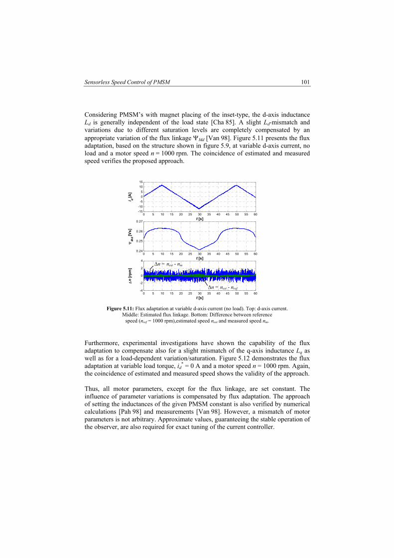
Sensorless Speed Control of PMSM 101
Considering PMSM’s with magnet placing of the inset-type, the d-axis inductance Ld is generally independent of the load state [Cha 85]. A slight Ld-mismatch and variations due to different saturation levels are completely compensated by an appropriate variation of the flux linkage ΨMd [Van 98]. Figure 5.11 presents the flux adaptation, based on the structure shown in figure 5.9, at variable d-axis current, no load and a motor speed n = 1000 rpm. The coincidence of estimated and measured speed verifies the proposed approach.
0 5 10 15 20 25 30 35 40 45 50 55 60-15-10
-505
1015
t [s]
i d [A]
0 5 10 15 20 25 30 35 40 45 50 55 600.24
0.25
0.26
0.27
t [s]
ΨM
d [Vs]
0 5 10 15 20 25 30 35 40 45 50 55 60-4
-2
0
2
4
t [s]
∆n
[rpm
]
∆n = nest - nm
∆n = nest - nref
Figure 5.11: Flux adaptation at variable d-axis current (no load). Top: d-axis current. Middle: Estimated flux linkage. Bottom: Difference between reference
speed (nref = 1000 rpm),estimated speed nest and measured speed nm.
Furthermore, experimental investigations have shown the capability of the flux adaptation to compensate also for a slight mismatch of the q-axis inductance Lq as well as for a load-dependent variation/saturation. Figure 5.12 demonstrates the flux adaptation at variable load torque, id
* = 0 A and a motor speed n = 1000 rpm. Again, the coincidence of estimated and measured speed shows the validity of the approach. Thus, all motor parameters, except for the flux linkage, are set constant. The influence of parameter variations is compensated by flux adaptation. The approach of setting the inductances of the given PMSM constant is also verified by numerical calculations [Pah 98] and measurements [Van 98]. However, a mismatch of motor parameters is not arbitrary. Approximate values, guaranteeing the stable operation of the observer, are also required for exact tuning of the current controller.
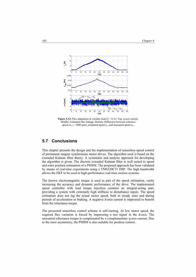
102 Chapter 6
0 5 10 15 20 25 30 35 40 45 50 55 600
5
10
15
t [s]
i q [A]
0 5 10 15 20 25 30 35 40 45 50 55 600.25
0.255
0.26
0.265
t [s]
ΨM
d [Vs]
0 5 10 15 20 25 30 35 40 45 50 55 60-4
-2
0
2
4
t [s]
∆n
[rpm
]
∆n = nest - nm
∆n = nest - nref
Figure 5.12: Flux adaptation at variable load (id* = 0 A). Top: q-axis current.
Middle: Estimated flux linkage. Bottom: Difference between reference speed (nref = 1000 rpm), estimated speed nest and measured speed nm.
5.7 Conclusions
This chapter presents the design and the implementation of sensorless speed control of permanent magnet synchronous motor drives. The algorithm used is based on the extended Kalman filter theory. A systematic and analytic approach for developing the algorithm is given. The discrete extended Kalman filter is well suited to speed and rotor position estimation of a PMSM. The proposed approach has been validated by means of real-time experiments using a TMS320C31 DSP. The high bandwidth allows the EKF to be used in high-performance real-time motion systems. The known electromagnetic torque is used as part of the speed estimation, vastly increasing the accuracy and dynamic performance of the drive. The implemented speed controller with load torque rejection contains no integral-acting part, providing a system with extremely high stiffness to disturbance inputs. The speed estimation does not lag the actual motor speed, both in steady state and during periods of acceleration or braking. A negative d-axis current is impressed to benefit from the reluctance torque. The presented sensorless control scheme is self-starting. At low motor speed, the required flux variation is forced by impressing a test signal in the d-axis. The unwanted reluctance torque is compensated by a complementary q-axis current. Due to the rotor asymmetry, the PMSM is also suitable for position control.

Sensorless Speed Control of PMSM 103
Mismatch of motor parameters yields incorrect speed estimation and erroneous torque-current mapping. Therefore, a real-time flux adaptation scheme, tracking motor parameter variations, has been implemented. All proposed control approaches are verified by experimental results.


6. PV-Powered Water Pump Systems
6.1 Introduction
The use of photovoltaic (PV) energy sources for water pumping and irrigation applications, especially in remote or rural areas in developing countries, is receiving considerable attention. Large urban populations in developing countries do not have access to safe drinking water sources (standpipes or boreholes) or to sanitary services (sewers, septic tanks or wet latrines). According to statistics of the World Health Organization, the number of people without access to safe water in 1990 was 1,1 billion [WHO 96]. Human health depends on an adequate supply of potable water. Therefore, PV-powered water pump systems can improve peoples living conditions, where power from a utility is not available or too expensive to install. Furthermore, it is not economically viable to connect such remote areas to the national electric grid. While many of the references for residential applications are available in technical details, it is difficult to locate technical references for the interaction between PV arrays and an electric machine, especially in water pumping without battery storage [Mul 97]. This chapter briefly reviews present technology and applications of PV powered water pump systems and exhibits an extensive description of a new control approach. The two basic design approaches of PV arrays for water pumping system applications are the use of battery, for a backup of the pumping system, and the other is to pump directly from the PV power without battery. There are advantages and drawbacks associated with each design. With a battery module, the system energy generated by the sun can be stored in the battery. With the second approach, the motor/pump subsystem can be powered either by directly connecting to the PV array, or by using a maximum power point tracker (MPPT), a dc-dc converter and an inverter interfacing motor and PV array. In this work, a system is designed, not requiring a battery. The fact that no battery is required is a key element in the design. Batteries tend to be very unreliable in the overall framework and furthermore, they are of “interest” to people living there for other purposes, too (read: they are often stolen). The system analyzed here is a PV powered water pumping system avoiding the use of the additional dc-dc converter, a battery and its losses. Several new approaches
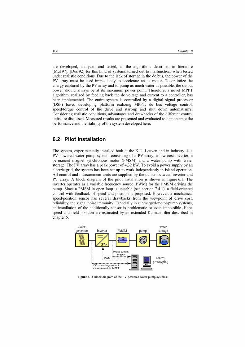
106 Chapter 8
are developed, analyzed and tested, as the algorithms described in literature [Mul 97], [Dus 92] for this kind of systems turned out to malfunction, when tested under realistic conditions. Due to the lack of storage in the dc bus, the power of the PV array must be used immediately to accelerate an ac motor. To optimize the energy captured by the PV array and to pump as much water as possible, the output power should always be at its maximum power point. Therefore, a novel MPPT algorithm, realized by feeding back the dc voltage and current to a controller, has been implemented. The entire system is controlled by a digital signal processor (DSP) based developing platform realizing MPPT, dc bus voltage control, speed/torque control of the drive and start-up and shut down automatism's. Considering realistic conditions, advantages and drawbacks of the different control units are discussed. Measured results are presented and evaluated to demonstrate the performance and the stability of the system developed here.
6.2 Pilot Installation
The system, experimentally installed both at the K.U. Leuven and in industry, is a PV powered water pump system, consisting of a PV array, a low cost inverter, a permanent magnet synchronous motor (PMSM) and a water pump with water storage. The PV array has a peak power of 4,32 kW. To avoid a power supply by an electric grid, the system has been set up to work independently in island operation. All control and measurement units are supplied by the dc bus between inverter and PV array. A block diagram of the pilot installation is shown in figure 6.1. The inverter operates as a variable frequency source (PWM) for the PMSM driving the pump. Since a PMSM in open loop is unstable (see section 7.4.1), a field-oriented control with feedback of speed and position is proposed. However, a mechanical speed/position sensor has several drawbacks from the viewpoint of drive cost, reliability and signal noise immunity. Especially in submerged-motor/pump systems, an installation of the additionally sensor is problematic or even impossible. Here, speed and field position are estimated by an extended Kalman filter described in chapter 6.
water storage
pump
inverter
Solar generator
PMSM
MPP- Tracking
Curr
ent [
A]
Voltage [V]
Phase current for EKF
DC bus voltage/currentmeasurement for MPPT
control prototyping
PWM
Figure 6.1: Block diagram of the PV-powered water pump systems.

Ride-Through at Power Interruptions 107
Furthermore, the control system is equipped with a MPPT and a voltage control guaranteeing a balanced input/output power ratio in the dc bus. The MPPT and voltage control are realized by feeding back the dc bus voltage and current to the controller. Additionally, measurements of motor currents in two phases are required for speed estimation and torque control of the PMSM. The motor voltages required for the EKF are not measured, but calculated from the reference voltages determining the PWM output of the controller. A computer-aided control system is used as a developing platform monitoring and recording the experimental data. Provisionally, the entire control algorithm, safety-related monitoring and the start-up and shut down automatism’s are implemented on a TMS320C31 DSP. The I/O subsystems and the PWM generation are based on TMS320P14 working as a slave-DSP. However, the final algorithms are intended to be implemented in a simple microcontroller ensuring an overall low cost system.
6.3 PV Array
The voltage-current characteristic of one PV element at constant cell temperature and with the irradiance of the sunlight as a parameter is shown in figure 6.2. In the same figure, also the output power of the PV element is drawn as a function of the module voltage. The power PPV is calculated by the product of dc bus voltage Udc and current IPV. The Maximum Power Point (MPP) is characterized by the voltage, where the PV array generates maximum output power.
0 5 10 15 20 250
1
2
3
4
5
6
7
8
9
Udc [V]
I PV [A
]
15
30
45
60
75
90
105
120
135
P PV [W
]
current
MPP
power
Figure 6.2: Characteristic of one PV element at constant cell temperature.
The PV element characteristics are a function of the irradiance of the sunlight and the cell temperature. In figure6.2, six different levels of insolation are illustrated. High current curves correspond to high insolation levels while low current curves correspond to lower insolation levels. With increasing irradiance, the MPP moves

108 Chapter 8
along the marked line. In order to stay at the point of maximum power at rising irradiance, the current in the dc bus must be increased, while the dc voltage remains nearly constant. The voltage at the MPP changes with the array temperature while the current is almost unaffected. At lower cell temperature, the MPP characteristic is situated in a higher voltage range. The voltage temperature coefficient of the PV elements used amounts to –82 mV/°C. Therefore, connecting 12 modules in series and a temperature variation of 10 K results in an optimum voltage shift of 9,84 V on a rated voltage of 180 V, i.e. ±5 %. Thus, the optimum output voltage of the PV array is not constant and moves as condition varies. The practically studied PV array consists of 36 modules with a total peak power of 4,32 kW. All wires of the single PV elements are assembled in a modular way using a switchboard panel, connected in series or parallel. The different experimental connections are presented in Table 6.1. The experimental results obtained are similar demonstrating the high flexibility of both the previously and later described control algorithms. However, to match the requirements of the final inverter and to keep the presented results clear, all experimental results presented in this chapter are measurements using 12 modules in series and 3 modules in parallel.
Table 6.1: Various connections of the PV array with a peak power of 4,32 kW.
Number of modules in
series
Number of modules in
parallel
Imax [A]
Umax [V]
6 6 44,7 129 9 4 29,8 193,5 12 3 22,35 258 18 2 14,9 387
6.4 Motor/Pump Subsystem
Surface applications for irrigation systems are mostly driven by dc machines while for installations in the drilling holes submersible induction motor/pump systems are used. Commutator motors have very desirable control characteristics, but they are not applicable for submersible installations. Furthermore, their use is limited by a number of factors [Bose 97]:
• Need for regular maintenance of the commutator; • Relatively heavy rotor with a high inertia; • Difficulty in producing a totally enclosed motor as required for some
hazardous (e.g. submersible motor/pump system) applications; • Relatively high cost;
A pumping system based on an ac motor drive is an attractive alternative where reliability and maintenance-free operation is important [Bhat 87]. However, small
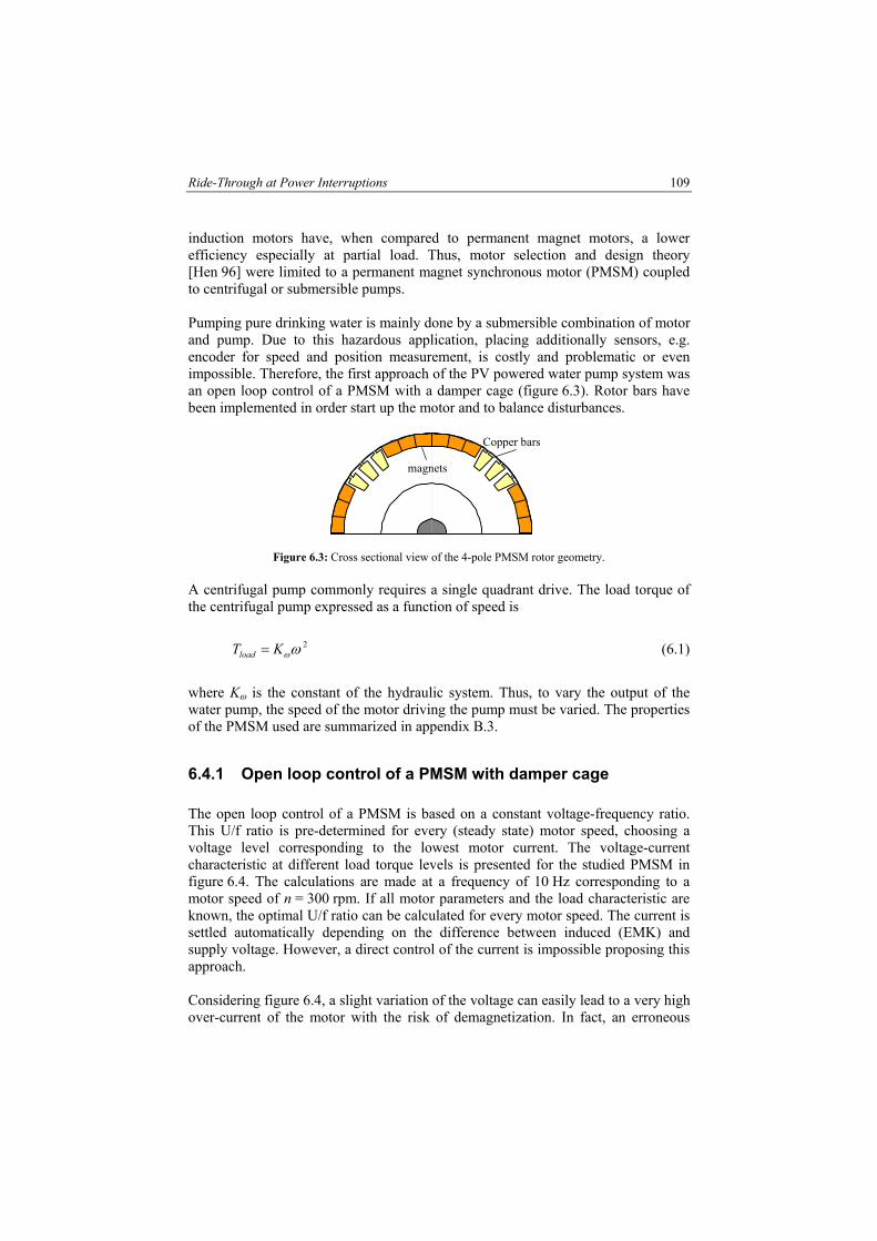
Ride-Through at Power Interruptions 109
induction motors have, when compared to permanent magnet motors, a lower efficiency especially at partial load. Thus, motor selection and design theory [Hen 96] were limited to a permanent magnet synchronous motor (PMSM) coupled to centrifugal or submersible pumps. Pumping pure drinking water is mainly done by a submersible combination of motor and pump. Due to this hazardous application, placing additionally sensors, e.g. encoder for speed and position measurement, is costly and problematic or even impossible. Therefore, the first approach of the PV powered water pump system was an open loop control of a PMSM with a damper cage (figure 6.3). Rotor bars have been implemented in order start up the motor and to balance disturbances.
Copper bars
magnets
Figure 6.3: Cross sectional view of the 4-pole PMSM rotor geometry. A centrifugal pump commonly requires a single quadrant drive. The load torque of the centrifugal pump expressed as a function of speed is
2ωωKTload = (6.1)
where Kω is the constant of the hydraulic system. Thus, to vary the output of the water pump, the speed of the motor driving the pump must be varied. The properties of the PMSM used are summarized in appendix B.3.
6.4.1 Open loop control of a PMSM with damper cage
The open loop control of a PMSM is based on a constant voltage-frequency ratio. This U/f ratio is pre-determined for every (steady state) motor speed, choosing a voltage level corresponding to the lowest motor current. The voltage-current characteristic at different load torque levels is presented for the studied PMSM in figure 6.4. The calculations are made at a frequency of 10 Hz corresponding to a motor speed of n = 300 rpm. If all motor parameters and the load characteristic are known, the optimal U/f ratio can be calculated for every motor speed. The current is settled automatically depending on the difference between induced (EMK) and supply voltage. However, a direct control of the current is impossible proposing this approach. Considering figure 6.4, a slight variation of the voltage can easily lead to a very high over-current of the motor with the risk of demagnetization. In fact, an erroneous

110 Chapter 8
calculation of the optimum voltage cannot be avoided due to parameter and load torque variations as well as measurement errors and the non-linearity of the inverter.
10 11 12 13 14 15 16 17 0
5
10
15
20
25
U [V]
I [A
] Torque[0->10Nm]
Figure 6.4: Voltage-current characteristic at variable torque (f = 10 Hz). Due to dead-time effects, the error between reference and output voltage of the inverter used amounts to ∆U ≈ 15 V resulting unaccompaniedly in a current variation of 22 A for the studied PMSM at a speed of 300 rpm. According to (1.16)-(1.17), the voltage error ∆U depends on PWM frequency, dc bus voltage, dead time and current direction. This non-linear effect creates a distortion of motor current and torque. Without a damper cage, the PMSM in open loop is an undamped, oscillating system [Mel 91], [Hen 91]. Slight variations of the electrical angle
ϑϑϑ ∆+= 0 (6.2)
result in a self-exited oscillation with an undamped natural frequency fe:
0cos 0max2
2
=∆+∆ ϑϑϑ T
dtd
pJ (6.3)
)2sin( tfeπϑ =∆ (6.4)
pJTfe
0max cos21 ϑπ
=⇒ (6.5)
The frequency fe of the PMSM used varies between 0 Hz < fe <10 Hz for maximum load (ϑ0 = 90°) and no load (ϑ0 = 0°) respectively. This oscillation creates a

Ride-Through at Power Interruptions 111
distortion of current and torque generated by the motor, leading to an electromagnetic instability of the drive. In order to soften the system, the PMSM should be equipped with a damper cage [Hen 91]. The resulting damper time constant Tdamp can be calculated using:
21
'22
1
21
2 )1(32 σω
+= RUp
JTdamp (6.6)
The modified PMSM used has a damper time constant of Tdamp ≈ 60 ms. Considering the natural frequency, this value is far too large. For a sufficiently damped system, the time constant and thus the rotor resistance must be smaller. Therefore, a stable and dynamic open-loop control of the given PMSM is impossible. A modification of the PMSM geometry, including a completely closed damper cage [Con 86] and inset magnets, could improve the performance. Nevertheless, it is much better to consider another control approach. As explained in the next sections, a high dynamic drive is indispensably for a correct operation of the water pump system. In fact, this has been the starting motivation for the development of the earlier described high-performance motor drive with speed, flux and torque estimation.
6.5 Control of a PV-Powered Water Pump System
Most PV powered water pump systems consist of two different control units. The first is a dc unit with or without a battery as energy storage. In this unit, the MPPT is controlled by varying the duty ratio of a dc-dc converter. Using this converter leads to a less complicated control algorithm for the MPPT. Varying the dc bus voltage can be done more quickly and without changing the power or frequency of the motor. The influence of a changing irradiance level during a searching procedure is reduced. On the other hand, this converter introduces many losses, amongst others:
• Switching losses • Valve losses • Copper and iron losses in the filter coil
In control systems without a battery, the dc bus may collapse when an unbalanced input/output power ratio occurs at the dc bus. Therefore, systems without battery require a more complex and complicated control algorithm. The second unit controls the speed of motor and pump. Here, a novel control approach is proposed avoiding the use of the additional dc-dc converter, a battery and its losses. The overall control of the PV-powered water pump system consists of a current/torque controller, a speed controller without a shaft sensor and a main control consisting of a dc bus voltage controller and the

112 Chapter 8
MPPT. The voltage control varies the speed/torque of the PMSM in order to stay within the calculated optimum voltage given by the MPPT. The structure of the overall control system is shown in figure 6.5.
START-UP &
MPPT -1
TorqueControl
& EKF
SVM Inverter
ia
ub*
uc*
AC motor
ib
pump
ua*
ω
ω*Tel
*
Tel*
|ω|<ωmax
Tel*
Udc
Udc*
IPV Udc
IPV
PI with anti windup
PID with anti windup
PI with anti windup
PV power supply
Voltage control
Figure 6.5: Block diagram of the entire control system.
In contrast to the very quickly and frequently changing irradiance intensity, the cell temperature of the PV array and thus the dc voltage in the MPP varies very slowly. Therefore, the control of the PV-powered water pump system is performed by varying the dc voltage in a small range, searching the MPP and controlling the speed/torque characteristic of the motor in order to stay within the calculated optimal voltage corresponding to the highest efficiency of the system. The adaptive MPPT algorithm is described in detail in sections 7.7. The dc bus voltage can be controlled either by the speed of the motor requiring an additional speed control loop or directly by the electromagnetic torque affecting the motor speed derivation. The different control approaches are indicated by the switch in figure 6.5. Advantages and drawbacks of both control approaches are explained in the next section. The first approach turned out to malfunction, when tested under extreme but realistic conditions. However, many algorithms described in literature are based on the variation of the speed reference; e.g.: [Mul 97] varies the power by changing the frequency output of the inverter stepwise, being even slower than using an extra speed control loop. The high-performance speed/torque control of the PMSM is described in previous chapters. The mechanical position sensor is replaced by an observer requiring no additional measurements. Only measurements of motor current and dc bus voltage are necessary. Figure 6.6 shows the experimental results of a speed step with a centrifugal pump as load and using a regular grid as power supply (Udc = 220V). With sufficient power generated by a PV array, the results obtained would be the same. Otherwise, the dc bus would be discharged and the system collapses. The applied load at n = 2000 rpm amounts 85% of the rated motor torque. The current/torque controller has a bandwidth of 960 Hz. According to subsection 2.5.1,

Ride-Through at Power Interruptions 113
the optimal torque control of the motor takes advantage of the reluctance torque by introducing a negative (Ld < Lq) direct-axis current component increasing the efficiency of the drive.
0 0.25 0.5 0.75 1 1.25 1.50
500 1000 1500 2000 2500
t [s]
n [r
pm]
Measurement
Reference
0 0.25 0.5 0.75 1 1.25 1.5-10
0 10 20 30
t [s]
i [A
] iq
id
Figure 6.6: Speed step with a pump load using a regular grid as power supply. Top: Measured and reference speed. Bottom: d- and q-axis current.
The start-up and shut down logic is based on the motor speed and the open-circuit voltage. Below a speed of n ≈ 180 rpm, the centrifugal pump used is not able to pump water. A non-productive idle run is not conducive for the durability of the pump and all other wear. Therefore, the system goes in standby modus and all PWM pulses are disabled if the PV power supply is definitively too low. The energy consumption of all control and measurement units and the inverter in standby modus amounts to 20 W. A start-up procedure requires a pre-determined minimum open-circuit voltage guaranteeing a productive motor speed, being higher than the minimum speed of the shut down automatism. The implemented safety-related monitoring consists of detecting over-current and over-speed, both depending on the motor/pump system, and a pre-determined voltage window mainly defined by the PV array coupled to the inverter. An inadmissible failure disables the entire system, requiring a manual reset by an expert. However, no such failure has been detected during weeks of testing.
6.6 DC Bus Voltage Control

114 Chapter 8
6.6.1 Experimental results of the voltage control
In figure 6.7 the response of the voltage, q-axis current and speed for a step of the voltage reference from 225 to 125 V and back to 225 V is shown. It can be seen, that the voltage and the torque producing q-axis current are controlled very fast. They are already in steady state, while the speed still varies. The speed of the motor changes indirectly, controlled by the electromagnetic torque until the reference voltage is reached.
0 0.2 0.4 0.6 0.8 1100
150
200
250
t [s]
Udc
[V]
0 0.2 0.4 0.6 0.8 1-30
-15
0
15
30
t [s]
i q [A]
0 0.2 0.4 0.6 0.8 1600
700
800
900
t [s]
n [rp
m]
Reference
Measurement
Figure 6.7: Step of the voltage reference from 225V to 125V and back to225V. Top: dc bus voltage. Middle: q-axis current. Bottom: Motor speed.
The MPP of the PV array used is situated between 185 and 195 V. Without voltage control the voltage area below the MPP (Udc < 185 V) is unstable. Slightly increasing the motor speed in this unstable area, results in a very quick discharge of the capacitor leading inevitably to a crash of the entire system. The averaged voltage error of this inner control loop is smaller than 0.1%. Even at the starting procedure and under very quickly changing irradiance, the error reaches a maximum of 0.5%. The averaged voltage error delivers the minimum search range for the later described main control (MPPT) providing the reference voltage. An important feature of the system is the independence of the pipe characteristic. The pumping head or water pressure can be varied by a throttle lever increasing/decreasing both water pressure and reversely water flow. Thus, also the pipe characteristic changes. Figure 6.8 demonstrates this independence by varying the pumping head from a ½ m (=½ bar) to 10 m (=10 bar) and back to ½ m. The

Ride-Through at Power Interruptions 115
response of the voltage control is plotted above, below the speed. The reaction time of the voltage control is quite slow due to the time intensive valve closure. The experiments are made with a reference voltage of Udc = 191V approximately agreeing with the MPP of the PV array.
0 1 2 3 4 5180
185
190
195
200
t [s]
Udc
[V]
0 1 2 3 4 51100
1200
1300
1400
1500
t [s]
n [rp
m]
0 1 2 3 4 5180
185
190
195
200
t [s]
Udc
[V]
0 1 2 3 4 51100
1200
1300
1400
1500
t [s]
n [rp
m]
Reference
Figure 6.8: Variation of the pumping head.
Left: ½ m ⇒ 10 m. Right: 10 m ⇒ ½ m. One of the most important features of the voltage control is its robustness during power interruptions, occurring at instantaneous decrease of irradiance (e.g. passing clouds). This property has been tested using a regular grid as power supply and applying a complete power interruption on all three phases for a short time agreeing with the worst-case condition of the system. These tests were done with a smaller, 3 kW prototype PMSM. The implemented regenerative braking scheme allows the inverter to keep its dc bus voltage at the pre-determined minimum level, expanding the time in which supply voltage can be reapplied without the time-consuming dc-link capacitor recharging cycle. The experimental results of such short time three-phase power interruptions are shown in section 8.5.
6.7 Maximum Power Point Tracking (MPPT)
The voltage reference of the dc bus voltage control is calculated by an overlaid maximum power point tracking (MPPT). Compared to a common voltage tracking, the efficiency of the output power of a PV array can be increased about 2 % by MPP-Tracking. The MPP is characterized by the voltage, where the PV array generates maximum output power. The main problems of matching the MPP with a PV array as power supply are related to the non-linear, solar irradiance and cell temperature-dependent voltage and current characteristics of the PV array. The characteristics are affected by the contamination, the sunlight irradiance and the cell temperature. To reach the MPP at rising irradiance level, the current in the dc bus must be increased while the dc bus

116 Chapter 8
voltage remains nearly constant. The voltage at the MPP changes with array temperature and current is almost unaffected. At lower cell temperature, the MPP characteristic is situated in a higher voltage range. Thus, the optimum output voltage of the PV array is not constant and moves as conditions vary. The MPPT is the main control loop, calculating the MPP and the search range of the dc bus voltage, and delivers a reference quantity to the voltage control loop. First, a default voltage and search range is given. After the default voltage is reached, it is varied slightly around this point. The quantity of this variation is given by the search range. During this variation, the power generated by the PV array is measured and the voltage linked to the maximum power is stored during the respective searching procedure. The new optimum voltage and the new search range are calculated from these actual measurements and in its stored values by an adaptive control algorithm. With these new quantities, the controller starts again a searching procedure to find the MPP. Figure 6.9 shows the flow chart of the MPP-Tracking.
Uref < Uopt - ∆U
Decrease Uref
Calculate Uopt • Optimum voltage: Uopt • Search range: ∆U • Search speed: dU/dt
Measurement
Reference voltage Uref
Startup with initial values
NO
NO
YES
YES
Uref
Increase Uref
Uref > Uopt + ∆U
Calculate ∆U
Uref
Uref
t
Figure 6.9: Flow chart of the MPP-Tracking. The previous values are very important for the calculation of the new optimum voltage and search range. If, e.g., the new calculated optimum voltage during a searching procedure with rising voltage is situated higher than the last optimum voltage, the MPP-voltage seems to change. However, this can also indicate an increasing irradiance. If the second condition occurs, the controller should not change the new optimum voltage. Otherwise, the calculated voltage drifts from the MPP. The same considerations are also valid for decreasing irradiance. Thus, the adaptive control must be able to distinguish between a changing MPP and changing conditions. A new optimum voltage is only calculated, when a tendency is indicated by a searching procedure with both rising and falling voltage reference.
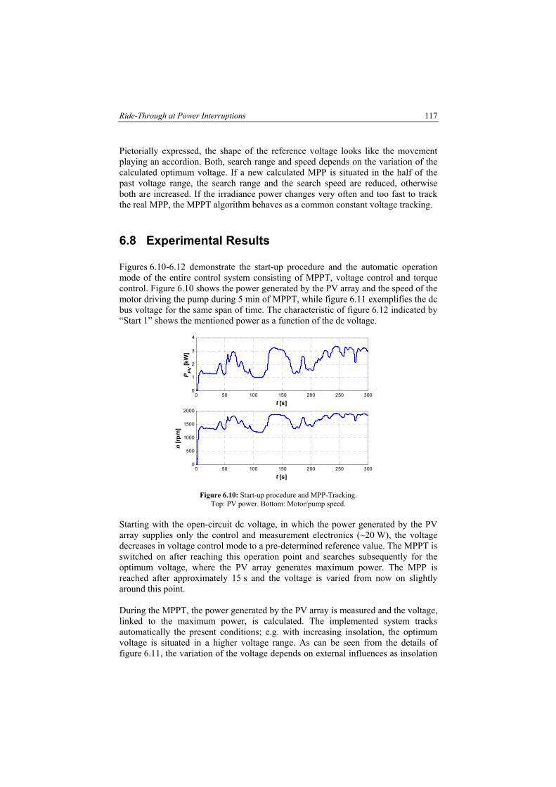
Ride-Through at Power Interruptions 117
Pictorially expressed, the shape of the reference voltage looks like the movement playing an accordion. Both, search range and speed depends on the variation of the calculated optimum voltage. If a new calculated MPP is situated in the half of the past voltage range, the search range and the search speed are reduced, otherwise both are increased. If the irradiance power changes very often and too fast to track the real MPP, the MPPT algorithm behaves as a common constant voltage tracking.
6.8 Experimental Results
Figures 6.10-6.12 demonstrate the start-up procedure and the automatic operation mode of the entire control system consisting of MPPT, voltage control and torque control. Figure 6.10 shows the power generated by the PV array and the speed of the motor driving the pump during 5 min of MPPT, while figure 6.11 exemplifies the dc bus voltage for the same span of time. The characteristic of figure 6.12 indicated by “Start 1” shows the mentioned power as a function of the dc voltage.
0 50 100 150 200 250 3000
1
2
3
4
t [s]
P PV [k
W]
0 50 100 150 200 250 3000
500
1000
1500
2000
t [s]
n [rp
m]
Figure 6.10: Start-up procedure and MPP-Tracking. Top: PV power. Bottom: Motor/pump speed.
Starting with the open-circuit dc voltage, in which the power generated by the PV array supplies only the control and measurement electronics (~20 W), the voltage decreases in voltage control mode to a pre-determined reference value. The MPPT is switched on after reaching this operation point and searches subsequently for the optimum voltage, where the PV array generates maximum power. The MPP is reached after approximately 15 s and the voltage is varied from now on slightly around this point. During the MPPT, the power generated by the PV array is measured and the voltage, linked to the maximum power, is calculated. The implemented system tracks automatically the present conditions; e.g. with increasing insolation, the optimum voltage is situated in a higher voltage range. As can be seen from the details of figure 6.11, the variation of the voltage depends on external influences as insolation

118 Chapter 8
or temperature variations and is adjusted automatically. In steady state, the variation of reference voltage is very small and almost constant.
0 50 100 150 200 250 300180
200
220
240
t [s]
Udc
[V]
265 270 275 280 285 290 295190
191
192
193
194
195
t [s]
Udc
[V]
Box 1
Udc
Udc,ref
Figure 6.11: Start-up procedure and MPP-Tracking.
Top: dc bus voltage. Bottom: Details indicated by Box 1. Due to the lack of storage element in the dc bus, the power of the PV array must be used immediately to accelerate the PMSM. Measurements during a sunny day of the implemented MPPT are plotted in figure 6.12 showing the power of the PV array as a function of the dc voltage Udc. Three different starting conditions are shown to demonstrate the ability of reproduction of the MPPT. The direction of the searching procedure is indicated by the arrows. The characteristic indicated by ‘Start 1’ refers to the time exposure of figures 6.10-6.11. The artificial starting point exhibits the MPPT starting in an unstable area, where slightly increasing the motor speed results in a very quick discharge of the capacitor. This starting point is reached by first using the voltage control mode with a reference Udc
* = 120V and then switching over to the MPPT control mode. However, this artificial starting point is never reached during regular operation. The measured results demonstrate the ability of reproduction as well as the stability of the entire system.

Ride-Through at Power Interruptions 119
100 120 140 160 180 200 220 2400
0.5
1
1.5
2
2.5
3
3.5
P PV [k
W]
Udc [V]
MPP
Start 2Artificial starting point
Start 1
Figure 6.12: Measured results of the MPP-Tracking using a PV array with a peak
power of 4,32 kW and a PMSM driving a centrifugal pump (sunny day). Instead of a permanent magnet synchronous motor, the implemented MPPT and voltage control are also suitable for an induction motor driving the pump. The performance of induction motor and PMSM are similar, only the induction motor efficiency is lower especially at partial load. Here, in contrast to all other earlier presented results, a PV array with a peak power of 1,2 kW and a 1,5 kW induction motor driving the centrifugal pump was used. The MPPT during a cloudy day, with this second installation, is presented in figure 6.13. Four different starting conditions (a-d) are shown. Characteristic ‘c’ and ‘d’ starts in an artificial operation point. The characteristic ‘a’ is situated in a higher voltage range, because it shows the first searching procedure at a lower cell temperature.
120 130 140 150 160 170 180 190 200 2100
50
100
150
200
250
P PV [W
]
Udc [V]
MPP
d
c
b
a
Figure 6.13: Measured results of the MPP-Tracking using a PV array with a peak
power of 1,2 kW and an induction motor driving the pump (6 hours of a cloudy day).
120 Chapter 8
6.9 Conclusions
This chapter presents the design and the implementation for PV-powered water pump systems using a PMSM without a shaft sensor. In a first approach, the performance of a PMSM with damper cage in open loop control is evaluated. Due to the insufficient damper cage, a stable and dynamic open-loop control of the given PMSM is impossible. Furthermore, a simple U/f control is absolutely inferior compared to a field-oriented high performance motor drive with speed, flux and torque estimation. The price to be paid is a more extensive and more complicated control algorithm. However, no additionally measurements are required. Additionally, an increased efficiency of the entire system is achieved. Due to the lack of storage in the dc bus, the power of the PV array is used immediately to accelerate the motor. Practical investigations are done to demonstrate the stability of the dc bus voltage control, the independence of the pump characteristic and its robustness during power interruptions. To optimize the energy captured by the PV array and to pump as much water as possible, the output power should always be at its maximum power point. Increasing the efficiency of the system is very advantageously considering the cost-intensive PV array installation amounting to 70% of the total system costs. Therefore, a novel MPPT algorithm, realized by feeding back the dc voltage and current to a controller, has been developed and implemented. The measured results of the MPPT exhibit the ability of reproduction and the stability of the entire control system. The development of a second prototype PMSM for submersible applications has been stopped for practical and economic reasons. The design constraints due to the mechanical construction of the motor housing and stator iron, together with the filling of the motor interior with water yield a very unusual mechanical rotor construction. The classical rotor design of a permanent magnet synchronous machine with surface mounted magnets would inherit the fixing of the magnets with glue and a polymer bandaging. The long-term stability for use directly in water of both permanent magnets and bandage cannot be guaranteed by the manufacturer. This applies even for coated magnets. The production costs of such a machine are enormous. Due to the design constraints, only a marginal efficiency increase can be expected by replacing the induction motor with the PMSM. However, the implemented MPPT and voltage control are suitable for both a PMSM and an induction motor driving the pump. In the meantime, a request for the installation of the presented PV powered water pump system has been received from four different countries: Mali, Mauritania, Senegal and Chad.

7. Conclusions
7.1 Summary & Conclusions
This thesis concerned high-performance motion control systems with a voltage source inverter supplying both squirrel-cage induction motors and permanent magnet synchronous motors. Basic control techniques, that allow dynamic torque and flux control in a decoupled way, are direct torque control (DTC) and field-oriented control (FOC). Summarizing, the DTC provides a better dynamic torque response whereas the FOC provides a better steady-state behavior. With respect to the planned applications where the motor speed is the main control variable, the FOC has been chosen as final control scheme. Considering field-oriented control, it is possible to control separately the flux and torque producing components of the supply currents. In particular, the concept of field orientation and the resulting ability to directly control the electromagnetic torque were discussed in chapter 2. Torque control, which constitutes the most basic motor control function, maps very directly into current control because of the close association between current and torque generation in any PMSM and induction motor drive. There are many excellent books on the topics of electrical machines and drives. However, it is believed that the present thesis is novel in many respects. The basic FOC-scheme is refined systematically adding additional features step by step. Flux weakening is widely known in literature. Less appreciated is the ability to operate the induction motor above the nominal flux at low speed to enhance the torque per ampere relation and thus better utilize the available power supply current. The approach has been further refined by flux optimization. Contrary to the assertions in literature, this feature makes the induction motor superior compared to the PMSM in a wide operation range when efficiency is considered especially in the range where iron losses are dominant. The choice of a suitable flux control strategy depends on the respective application. In the realized implementations, it can be switched over easily and in real-time to different strategies. Considering flux weakening of the PMSM, the algorithms presented in literature are based on pre-calculations postulating a constant dc bus voltage. In this work, the dc bus voltage is variable over a wide range requiring an alternative approach. Therefore, an automatic flux adaptation scheme has been implemented.

122 Chapter 9
Whereas anti-windup systems are well known in literature, an anti-windup system within the current controller is neglected since the maximum voltage is limited by the power inverter itself. However, the presented current control with anti-windup is essential considering the dc bus voltage variable over a wide range. A commercially available DSP based environment is used for development purpose. However, the support software has been changed in order to implement different PWM strategies as well as variable PWM frequencies. This is extremely valuable during the development of high-performance motor control using PWM outputs in order to drive power switches. Chapter 3 presents the collaboration between control design and real-time implementation. The DSP controller board, code generation, experiment management and hardware interface including required measurements are explained. Issues of measurement distortion/identification due to the inverter non-linearity are discussed in detail. Chapter 4 exhibits a new approach of speed estimation employing an incremental encoder as measurement device. Among the speed, also rotor position and the acceleration of the drive are estimated. The implemented algorithm is based on a linear Kalman Filter. The discussion extends to the implementation of an advanced speed control loop. It has been shown that this approach offers a significant improvement of the entire drive performance. This chapter can be also regarded as a smart introduction into observer theory. Advanced observer theory has been applied to approaches eliminating the need of position/speed measurement. The sensorless speed control of both permanent magnet synchronous motor and squirrel-cage induction motor drives, which is nowadays the most attractive research area of electrical motor drives, is presented in chapter 5 and 6. New models for speed estimation are proposed. The structures of the implemented sensorless control schemes are based on the extended Kalman filter theory. The approach requires no additional measurements. The terminal voltages are not measured; they are reconstructed by using the monitored dc bus voltage and the switching functions of the inverter considering non-linearities due to the dead time of the power switches. Among the speed, also rotor flux, flux position and the acceleration of the drive are estimated. The speed estimation does not lag the actual motor speed, both in steady state and during acceleration/braking. Compared to sensorless control schemes described in literature, the experimental results have shown to offer a significant improvement of the drive performance. Within this thesis, different control approaches considering respective applications were developed and implemented. Special care has been taken for the viability of the real-time implementation: A comprehensive and clear description of controller design and affiliated parameter calculation is given for all treated applications. Furthermore, all proposed control schemes were verified by experimental results. The implementation of a PV-powered water pump system using a PMSM without a shaft sensor is described in chapter 7. This system reflects one application employing many of the drive features, designed and implemented in this work. New

Conclusions 123
approaches were developed because the algorithms described in literature for this kind of systems turned out to malfunction. A novel maximum power point tracking optimizing the energy captured by the PV array has been designed and implemented. The PV-powered water pump system consists, among other control loops, of a high-performance dc bus voltage control, which constitutes the most important control function guaranteeing the stability of the drive. As discussed in chapter 8, the realized dc bus voltage control is also applicable for ride-through schemes at power interruptions considering inverter-controlled drives supplied by a regular grid. The proposed solution to the problem is to recover some of the mechanical energy stored in the rotating masses by kinetic buffering. This maintains the dc link capacitor well charged keeping the electronic control circuits active. The temporary speed dip is generally tolerable, since the most frequent power interruptions last only for a few milliseconds. Furthermore, the proposed ride-through scheme at power interruptions has been transformed into a special drive braking tool saving energy and simplifying the inverter setup: the installation of brake-resistance, power switch and cooler may be eliminated.
7.2 Further Research
Using the TMS320C31 DSP providing 60 MFlops, the proposed algorithms have been realized only by means of costly code optimizations. The limit of the possible code and memory size has been reached. The calculation of the closed loop current transfer function has shown the large influence of delays within the loop as e.g.: measurement filter, sample time, PWM frequency and signal lag of data transmission. Further increasing the program size will lead to execution times, which are no longer suitable for high-performance motion control. In particular, it is interesting to implement the proposed algorithms on faster DSPs. It is expected that the dynamic performance, especially of the torque control loop, can be vastly increased. Presently, a new DSP development platform based on TI’s most recent processor-generation, the TMS320C6711 DSP providing 1000 MFlops, is under construction within the ELECTA group. This new development platform provides a system, which will be capable of implementing even more extended and computation time intensive algorithms. Considering a more powerful control system, there are many applications possible, e.g.: The noise covariance matrices within the mentioned sensorless speed control system can be adapted in real-time dependent on the given operating point. This can be done by e.g. another extended Kalman filter or artificial intelligence. Various reluctance motors will have an increased role in the future. An expansion of the proposed sensorless control schemes to these motor types forms surely an interesting task.

124 Chapter 9
The proposed observer together with advanced control techniques can be applied to the active filter (active front-end) design, which forms nowadays an interesting field in the area of power quality. Especially a disturbance (current harmonics) rejection approach, similar to the proposed load torque rejection approach within the speed/current control loop of drives, promises a vastly increased performance. Classical control theory suffers from some limitations due to non-linearity, time-invariance etc. of the controlled system. These problems can be overcome by using artificial-intelligence-based control techniques. In literature, e.g. [Vas 99], it is expected that intelligent sensorless instantaneous torque-controlled drives incorporating some form of intelligence will become the standard in the future. These drives will not require machine or controller parameters, and all the control and estimation tasks are performed by a single artificial-intelligence-based system.
