2.29 numerical fluid mechanics fall 2011 lecture 21 fluid mechanics . pfjl lecture 21, ... numerical...
TRANSCRIPT
PFJL Lecture 21, 1 Numerical Fluid Mechanics 2.29
2.29 Numerical Fluid Mechanics
Fall 2011 – Lecture 21
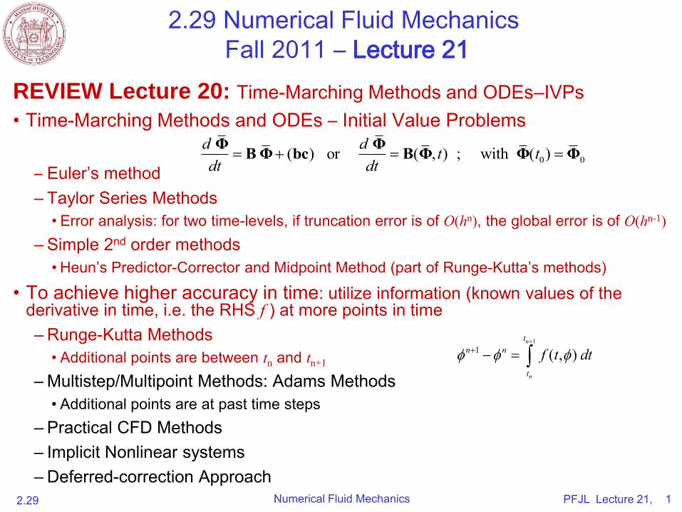
REVIEW Lecture 20: Time-Marching Methods and ODEs–IVPs
• Time-Marching Methods and ODEs – Initial Value Problems
– Euler’s method – Taylor Series Methods
• Error analysis: for two time-levels, if truncation error is of O(hn), the global error is of O(hn-1) – Simple 2nd order methods
• Heun’s Predictor-Corrector and Midpoint Method (part of Runge-Kutta’s methods)
• To achieve higher accuracy in time: utilize information (known values of the derivative in time, i.e. the RHS f ) at more points in time – Runge-Kutta Methods
• Additional points are between tn and tn+1 – Multistep/Multipoint Methods: Adams Methods
• Additional points are at past time steps – Practical CFD Methods – Implicit Nonlinear systems – Deferred-correction Approach
0 0( ) or ( , ) ; with ( )d d t tdt dt
Φ ΦBΦ bc B Φ Φ Φ
11 ( , )
n
n
tn n
t
f t dt

PFJL Lecture 21, 2 Numerical Fluid Mechanics 2.29
TODAY (Lecture 21): End of Time-Marching
Methods, Grid Generation and Complex Geometries
• Time-Marching Methods and ODEs – IVPs: End – Multistep/Multipoint Methods – Implicit Nonlinear systems – Deferred-correction Approach
• Complex Geometries – Different types of grids – Choice of variable arrangements
• Grid Generation – Basic concepts and structured grids
• Stretched grids • Algebraic methods • General coordinate transformation • Differential equation methods • Conformal mapping methods
– Unstructured grid generation • Delaunay Triangulation • Advancing Front method
PFJL Lecture 21, 3 Numerical Fluid Mechanics 2.29
References and Reading Assignments
• Chapters 25 and 26 of “Chapra and Canale, Numerical Methods for Engineers, 2010/2006.”
• Chapter 6 (end) and Chapter 8 on “Complex Geometries” of “J. H. Ferziger and M. Peric, Computational Methods for Fluid Dynamics. Springer, NY, 3rd edition, 2002”
• Chapter 6 (end) on “Time-Marching Methods for ODE’s” of “H. Lomax, T. H. Pulliam, D.W. Zingg, Fundamentals of Computational Fluid Dynamics (Scientific Computation). Springer, 2003”
• Chapter 9 on “Grid Generation” of T. Cebeci, J. P. Shao, F. Kafyeke and E. Laurendeau, Computational Fluid Dynamics for Engineers. Springer, 2005.
• Ref on Grid Generation only:
– Thompson, J.F., Warsi Z.U.A. and C.W. Mastin, “Numerical Grid Generation, Foundations and Applications”, North Holland, 1985

PFJL Lecture 21, 4 Numerical Fluid Mechanics 2.29
Multistep/Multipoint Methods
• Additional points are at time steps at which data has already
been computed
• Adams Methods: fitting a (Lagrange) polynomial to the
derivatives at a number of points in time
– Explicit in time (up to tn): Adams-Bashforth methods
– Implicit in time (up to tn+1): Adams-Moulton methods
– Coefficients βk’s can be estimated by Taylor Tables:
• Fit Taylor series so as to cancel higher-order terms
1 ( , )n
n n kk k
k n K
f t t
11 ( , )
nn n k
k kk n K
f t t

PFJL Lecture 21, 5 Numerical Fluid Mechanics 2.29
Example: Taylor Table for the
Adams-Moulton 3-steps (4 time-nodes) Method
11 1 1 2
1 1 0 1 1 2 2
dDenoting , , ' ( , ) and ' ( , ) , one obtains for 2 :
( , ) ( , ) ( , ) ( , ) ( , )
nn n
n n n k n n n nk n k n n n n
k K
uh t u u f t u u f t u Kdt
u u f t u t h f t u f t u f t u f t u
Taylor Table: • The first row (Taylor
series) + the last 5 rows (Taylor series for each term) must sum to zero
• This can be satisfied up to the 5th column (4th order term)
• Hence, the AM method with 4-time levels is 4th order accurate
1 0 1 2solving for the ' 9 / 24, 19 / 24, 5/ 24 and 1/ 24k s

PFJL Lecture 21, 6 Numerical Fluid Mechanics 2.29
Example of Adams Methods for
Time-Integration
(Adams-Bashforth, with ABn meaning nth order AB)
(Adams-Moulton, with AMn meaning nth order AM)
PFJL Lecture 21, 7 Numerical Fluid Mechanics
2.29
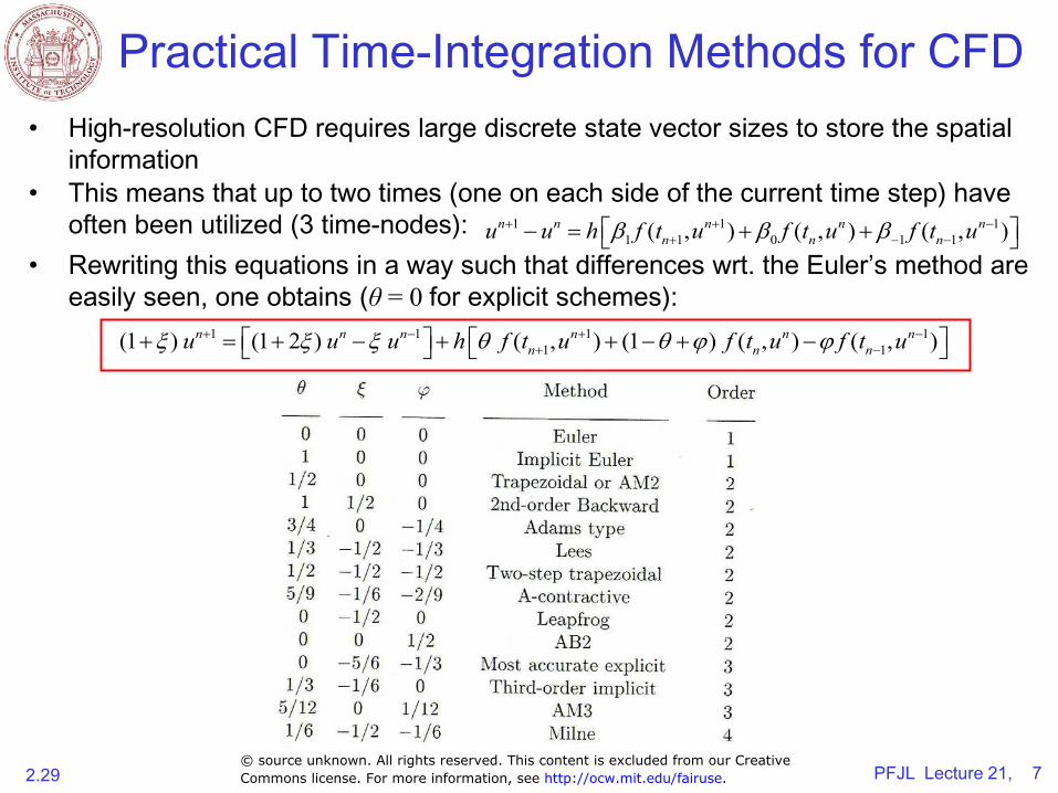
Practical Time-Integration Methods for CFD
• High-resolution CFD requires large discrete state vector sizes to store the spatial
information
• This means that up to two times (one on each side of the current time step) have
often been utilized (3 time-nodes):
• Rewriting this equations in a way such that differences wrt. the Euler’s method are
easily seen, one obtains (θ = 0 for explicit schemes):
1 1 11 1 0 1 1( , ) ( , ) ( , )n n n n n
n n nu u h f t u f t u f t u
1 1 1 11 1(1 ) (1 2 ) ( , ) (1 ) ( , ) ( , )n n n n n n
n n nu u u h f t u f t u f t u
© source unknown. All rights reserved. This content is excluded from our CreativeCommons license. For more information, see http://ocw.mit.edu/fairuse.

Implementation of Implicit Time-Marching Methods:
Nonlinear Systems and Larger dimensions
• Consider the nonlinear system (discrete in space):
• For an explicit method in time, solution is straightforward
– For explicit Euler:
– More general, e.g. AB:
• For an implicit method
– For Implicit Euler:
– More general:
=> a nontrivial scheme is needed to obtain
2.29 Numerical Fluid Mechanics PFJL Lecture 21, 8
0 0( , ) ; with ( )d t tdt
Φ B Φ Φ Φ
1 ( , ) tn n n nt Φ Φ B Φ
1 1( , ,..., , ) tn n n n K nt Φ F Φ Φ Φ
1nΦ
1 1 1 1
1 1 1 1
( , , ,..., , ) t or( , , ,..., , ) 0 ; with t
n n n n n K n
n n n n K n n
tt
Φ F Φ Φ Φ ΦF Φ Φ Φ Φ F F Φ1 1 1 1( , , ,..., , ) 0 ; with tn n n n K n n1 1 1 1n n n n K n n1 1 1 1( , , ,..., , ) 0 ; with tn n n n K n n( , , ,..., , ) 0 ; with t1 1 1 1 1 1 1 1n n n n K n n n n n n K n n1 1 1 1n n n n K n n1 1 1 1 1 1 1 1n n n n K n n1 1 1 1( , , ,..., , ) 0 ; with tn n n n K n n( , , ,..., , ) 0 ; with t ( , , ,..., , ) 0 ; with tn n n n K n n( , , ,..., , ) 0 ; with t1 1 1 1( , , ,..., , ) 0 ; with t1 1 1 1n n n n K n n1 1 1 1( , , ,..., , ) 0 ; with t1 1 1 1 1 1 1 1( , , ,..., , ) 0 ; with t1 1 1 1n n n n K n n1 1 1 1( , , ,..., , ) 0 ; with t1 1 1 11 1 1 1n n n n K n n1 1 1 1 1 1 1 1n n n n K n n1 1 1 1 1 1 1 1n n n n K n n1 1 1 1 1 1 1 1n n n n K n n1 1 1 11 1 1 1( , , ,..., , ) 0 ; with t1 1 1 1n n n n K n n1 1 1 1( , , ,..., , ) 0 ; with t1 1 1 1 1 1 1 1( , , ,..., , ) 0 ; with t1 1 1 1n n n n K n n1 1 1 1( , , ,..., , ) 0 ; with t1 1 1 1 1 1 1 1( , , ,..., , ) 0 ; with t1 1 1 1n n n n K n n1 1 1 1( , , ,..., , ) 0 ; with t1 1 1 1 1 1 1 1( , , ,..., , ) 0 ; with t1 1 1 1n n n n K n n1 1 1 1( , , ,..., , ) 0 ; with t1 1 1 1F Φ Φ Φ Φ F F Φ
n n n n K n nΦ Φ Φ Φ F F Φ
n n n n K n n1 1 1 1n n n n K n n1 1 1 1 1 1 1 1n n n n K n n1 1 1 1Φ Φ Φ Φ F F Φ
1 1 1 1n n n n K n n1 1 1 1 1 1 1 1n n n n K n n1 1 1 1( , , ,..., , ) 0 ; with tΦ Φ Φ Φ F F Φ( , , ,..., , ) 0 ; with t( , , ,..., , ) 0 ; with tn n n n K n n( , , ,..., , ) 0 ; with tΦ Φ Φ Φ F F Φ( , , ,..., , ) 0 ; with tn n n n K n n( , , ,..., , ) 0 ; with t( , , ,..., , ) 0 ; with tΦ Φ Φ Φ F F Φ( , , ,..., , ) 0 ; with t( , , ,..., , ) 0 ; with tn n n n K n n( , , ,..., , ) 0 ; with tΦ Φ Φ Φ F F Φ( , , ,..., , ) 0 ; with tn n n n K n n( , , ,..., , ) 0 ; with t( , , ,..., , ) 0 ; with tt( , , ,..., , ) 0 ; with tΦ Φ Φ Φ F F Φ( , , ,..., , ) 0 ; with tt( , , ,..., , ) 0 ; with t( , , ,..., , ) 0 ; with tn n n n K n n( , , ,..., , ) 0 ; with tt( , , ,..., , ) 0 ; with tn n n n K n n( , , ,..., , ) 0 ; with tΦ Φ Φ Φ F F Φ( , , ,..., , ) 0 ; with tn n n n K n n( , , ,..., , ) 0 ; with tt( , , ,..., , ) 0 ; with tn n n n K n n( , , ,..., , ) 0 ; with t( , , ,..., , ) 0 ; with tn n n n K n n( , , ,..., , ) 0 ; with t ( , , ,..., , ) 0 ; with tn n n n K n n( , , ,..., , ) 0 ; with tΦ Φ Φ Φ F F Φ( , , ,..., , ) 0 ; with tn n n n K n n( , , ,..., , ) 0 ; with t ( , , ,..., , ) 0 ; with tn n n n K n n( , , ,..., , ) 0 ; with t1 1 1 1( , , ,..., , ) 0 ; with t1 1 1 1n n n n K n n1 1 1 1( , , ,..., , ) 0 ; with t1 1 1 1 1 1 1 1( , , ,..., , ) 0 ; with t1 1 1 1n n n n K n n1 1 1 1( , , ,..., , ) 0 ; with t1 1 1 1Φ Φ Φ Φ F F Φ
1 1 1 1( , , ,..., , ) 0 ; with t1 1 1 1n n n n K n n1 1 1 1( , , ,..., , ) 0 ; with t1 1 1 1 1 1 1 1( , , ,..., , ) 0 ; with t1 1 1 1n n n n K n n1 1 1 1( , , ,..., , ) 0 ; with t1 1 1 11 1 1 1( , , ,..., , ) 0 ; with t1 1 1 1n n n n K n n1 1 1 1( , , ,..., , ) 0 ; with t1 1 1 1t1 1 1 1( , , ,..., , ) 0 ; with t1 1 1 1n n n n K n n1 1 1 1( , , ,..., , ) 0 ; with t1 1 1 1 1 1 1 1( , , ,..., , ) 0 ; with t1 1 1 1n n n n K n n1 1 1 1( , , ,..., , ) 0 ; with t1 1 1 1t1 1 1 1( , , ,..., , ) 0 ; with t1 1 1 1n n n n K n n1 1 1 1( , , ,..., , ) 0 ; with t1 1 1 1Φ Φ Φ Φ F F Φ
1 1 1 1( , , ,..., , ) 0 ; with t1 1 1 1n n n n K n n1 1 1 1( , , ,..., , ) 0 ; with t1 1 1 1t1 1 1 1( , , ,..., , ) 0 ; with t1 1 1 1n n n n K n n1 1 1 1( , , ,..., , ) 0 ; with t1 1 1 1 1 1 1 1( , , ,..., , ) 0 ; with t1 1 1 1n n n n K n n1 1 1 1( , , ,..., , ) 0 ; with t1 1 1 1t1 1 1 1( , , ,..., , ) 0 ; with t1 1 1 1n n n n K n n1 1 1 1( , , ,..., , ) 0 ; with t1 1 1 1 Φ Φ Φ Φ F F Φ ( , , ,..., , ) 0 ; with t ( , , ,..., , ) 0 ; with tΦ Φ Φ Φ F F Φ( , , ,..., , ) 0 ; with t ( , , ,..., , ) 0 ; with tn n n n K n n n n n n K n nΦ Φ Φ Φ F F Φ
n n n n K n n n n n n K n n( , , ,..., , ) 0 ; with tn n n n K n n( , , ,..., , ) 0 ; with t ( , , ,..., , ) 0 ; with tn n n n K n n( , , ,..., , ) 0 ; with tΦ Φ Φ Φ F F Φ( , , ,..., , ) 0 ; with tn n n n K n n( , , ,..., , ) 0 ; with t ( , , ,..., , ) 0 ; with tn n n n K n n( , , ,..., , ) 0 ; with t1 1 1 1n n n n K n n1 1 1 1 1 1 1 1n n n n K n n1 1 1 1 1 1 1 1n n n n K n n1 1 1 1 1 1 1 1n n n n K n n1 1 1 1Φ Φ Φ Φ F F Φ
1 1 1 1n n n n K n n1 1 1 1 1 1 1 1n n n n K n n1 1 1 1 1 1 1 1n n n n K n n1 1 1 1 1 1 1 1n n n n K n n1 1 1 11 1 1 1( , , ,..., , ) 0 ; with t1 1 1 1n n n n K n n1 1 1 1( , , ,..., , ) 0 ; with t1 1 1 1 1 1 1 1( , , ,..., , ) 0 ; with t1 1 1 1n n n n K n n1 1 1 1( , , ,..., , ) 0 ; with t1 1 1 1 1 1 1 1( , , ,..., , ) 0 ; with t1 1 1 1n n n n K n n1 1 1 1( , , ,..., , ) 0 ; with t1 1 1 1 1 1 1 1( , , ,..., , ) 0 ; with t1 1 1 1n n n n K n n1 1 1 1( , , ,..., , ) 0 ; with t1 1 1 1Φ Φ Φ Φ F F Φ
1 1 1 1( , , ,..., , ) 0 ; with t1 1 1 1n n n n K n n1 1 1 1( , , ,..., , ) 0 ; with t1 1 1 1 1 1 1 1( , , ,..., , ) 0 ; with t1 1 1 1n n n n K n n1 1 1 1( , , ,..., , ) 0 ; with t1 1 1 1 1 1 1 1( , , ,..., , ) 0 ; with t1 1 1 1n n n n K n n1 1 1 1( , , ,..., , ) 0 ; with t1 1 1 1 1 1 1 1( , , ,..., , ) 0 ; with t1 1 1 1n n n n K n n1 1 1 1( , , ,..., , ) 0 ; with t1 1 1 1
1 1 1( , ) tn n n nt Φ Φ B Φ
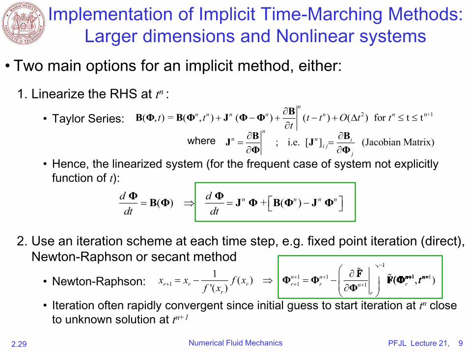
Implementation of Implicit Time-Marching Methods:
Larger dimensions and Nonlinear systems
• Two main options for an implicit method, either:
1. Linearize the RHS at tn :
• Taylor Series:
where
• Hence, the linearized system (for the frequent case of system not explicitly
function of t):
2. Use an iteration scheme at each time step, e.g. fixed point iteration (direct),
Newton-Raphson or secant method
• Newton-Raphson:
n• Iteration often rapidly convergent since initial guess to start iteration at t close n+1to unknown solution at t
2.29 Numerical Fluid Mechanics PFJL Lecture 21, 9
2 n+1( , ) = ( , ) ( ) ( ) ( ) for t tn
n n n n n nt t t t O t tt
BB Φ B Φ J Φ Φ
; i.e. [ ] (Jacobian Matrix)n
n n ii j
j
B BJ JΦ Φ
( ) + ( )n n n nd ddt dt
Φ ΦB Φ J Φ B Φ J Φ
1
1 1 1 11 1 1
1 ( ) ( , )'( )
n n n nr r r r r rn
r r
x x f x tf x
FΦ Φ F ΦΦ
1
1 1 1 11 1 1 1 1 1 1 11 1 1 1n n n n1 1 1 1 1 1 1 1n n n n1 1 1 11 1 1 1( ) ( , )1 1 1 1n n n n1 1 1 1( ) ( , )1 1 1 1x x f x t1 1 1 1( ) ( , )1 1 1 1n n n n1 1 1 1( ) ( , )1 1 1 1 1 1 1 1( ) ( , )1 1 1 1n n n n1 1 1 1( ) ( , )1 1 1 1x x f x t1 1 1 1( ) ( , )1 1 1 1n n n n1 1 1 1( ) ( , )1 1 1 1 1 1 1 1 1 1 1 11 1 1 1 1 1 1 11 1 1 1 1 1 1 1 1 1 1 1 1 1 1 11 1 1 1 1 1 1 1 1 1 1 1 1 1 1 11 1 1 1n n n n1 1 1 1 1 1 1 1n n n n1 1 1 1 1 1 1 1n n n n1 1 1 1 1 1 1 1n n n n1 1 1 11 1 1 1n n n n1 1 1 1 1 1 1 1n n n n1 1 1 1 1 1 1 1n n n n1 1 1 1 1 1 1 1n n n n1 1 1 11 1 1 1( ) ( , )1 1 1 1n n n n1 1 1 1( ) ( , )1 1 1 1x x f x t1 1 1 1( ) ( , )1 1 1 1n n n n1 1 1 1( ) ( , )1 1 1 1 1 1 1 1( ) ( , )1 1 1 1n n n n1 1 1 1( ) ( , )1 1 1 1x x f x t1 1 1 1( ) ( , )1 1 1 1n n n n1 1 1 1( ) ( , )1 1 1 1 1 1 1 1( ) ( , )1 1 1 1n n n n1 1 1 1( ) ( , )1 1 1 1x x f x t1 1 1 1( ) ( , )1 1 1 1n n n n1 1 1 1( ) ( , )1 1 1 1 1 1 1 1( ) ( , )1 1 1 1n n n n1 1 1 1( ) ( , )1 1 1 1x x f x t1 1 1 1( ) ( , )1 1 1 1n n n n1 1 1 1( ) ( , )1 1 1 11 1 1 1( ) ( , )1 1 1 1n n n n1 1 1 1( ) ( , )1 1 1 1x x f x t1 1 1 1( ) ( , )1 1 1 1n n n n1 1 1 1( ) ( , )1 1 1 1 1 1 1 1( ) ( , )1 1 1 1n n n n1 1 1 1( ) ( , )1 1 1 1x x f x t1 1 1 1( ) ( , )1 1 1 1n n n n1 1 1 1( ) ( , )1 1 1 1 1 1 1 1( ) ( , )1 1 1 1n n n n1 1 1 1( ) ( , )1 1 1 1x x f x t1 1 1 1( ) ( , )1 1 1 1n n n n1 1 1 1( ) ( , )1 1 1 1 1 1 1 1( ) ( , )1 1 1 1n n n n1 1 1 1( ) ( , )1 1 1 1x x f x t1 1 1 1( ) ( , )1 1 1 1n n n n1 1 1 1( ) ( , )1 1 1 1 F
F 1 1 1 1 1 1 1 1F1 1 1 1 1 1 1 11 1 1 1 1 1 1 1 1 1 1 1 1 1 1 1F1 1 1 1 1 1 1 1 1 1 1 1 1 1 1 11 1 1 1n n n n1 1 1 1 1 1 1 1n n n n1 1 1 1 1 1 1 1n n n n1 1 1 1 1 1 1 1n n n n1 1 1 1F1 1 1 1n n n n1 1 1 1 1 1 1 1n n n n1 1 1 1 1 1 1 1n n n n1 1 1 1 1 1 1 1n n n n1 1 1 11 1 1 1( ) ( , )1 1 1 1n n n n1 1 1 1( ) ( , )1 1 1 1x x f x t1 1 1 1( ) ( , )1 1 1 1n n n n1 1 1 1( ) ( , )1 1 1 1 1 1 1 1( ) ( , )1 1 1 1n n n n1 1 1 1( ) ( , )1 1 1 1x x f x t1 1 1 1( ) ( , )1 1 1 1n n n n1 1 1 1( ) ( , )1 1 1 1 1 1 1 1( ) ( , )1 1 1 1n n n n1 1 1 1( ) ( , )1 1 1 1x x f x t1 1 1 1( ) ( , )1 1 1 1n n n n1 1 1 1( ) ( , )1 1 1 1 1 1 1 1( ) ( , )1 1 1 1n n n n1 1 1 1( ) ( , )1 1 1 1x x f x t1 1 1 1( ) ( , )1 1 1 1n n n n1 1 1 1( ) ( , )1 1 1 1F1 1 1 1( ) ( , )1 1 1 1n n n n1 1 1 1( ) ( , )1 1 1 1x x f x t1 1 1 1( ) ( , )1 1 1 1n n n n1 1 1 1( ) ( , )1 1 1 1 1 1 1 1( ) ( , )1 1 1 1n n n n1 1 1 1( ) ( , )1 1 1 1x x f x t1 1 1 1( ) ( , )1 1 1 1n n n n1 1 1 1( ) ( , )1 1 1 1 1 1 1 1( ) ( , )1 1 1 1n n n n1 1 1 1( ) ( , )1 1 1 1x x f x t1 1 1 1( ) ( , )1 1 1 1n n n n1 1 1 1( ) ( , )1 1 1 1 1 1 1 1( ) ( , )1 1 1 1n n n n1 1 1 1( ) ( , )1 1 1 1x x f x t1 1 1 1( ) ( , )1 1 1 1n n n n1 1 1 1( ) ( , )1 1 1 1 F
1 1 1 1( ) ( , )1 1 1 1( ) ( , )1 1 1 1( ) ( , )n n n n( ) ( , )( ) ( , )x x f x t( ) ( , )( ) ( , )n n n n( ) ( , )x x f x t( ) ( , )n n n n( ) ( , )1 1 1 1 1 1 1 11 1 1 1( ) ( , )1 1 1 1 1 1 1 1( ) ( , )1 1 1 11 1 1 1n n n n1 1 1 1 1 1 1 1n n n n1 1 1 11 1 1 1( ) ( , )1 1 1 1n n n n1 1 1 1( ) ( , )1 1 1 1 1 1 1 1( ) ( , )1 1 1 1n n n n1 1 1 1( ) ( , )1 1 1 11 1 1 1( ) ( , )1 1 1 1n n n n1 1 1 1( ) ( , )1 1 1 1x x f x t1 1 1 1( ) ( , )1 1 1 1n n n n1 1 1 1( ) ( , )1 1 1 1 1 1 1 1( ) ( , )1 1 1 1n n n n1 1 1 1( ) ( , )1 1 1 1x x f x t1 1 1 1( ) ( , )1 1 1 1n n n n1 1 1 1( ) ( , )1 1 1 1( ) ( , )x x f x t( ) ( , )Φ Φ F Φ( ) ( , )x x f x t( ) ( , )( ) ( , )n n n n( ) ( , )x x f x t( ) ( , )n n n n( ) ( , )Φ Φ F Φ( ) ( , )n n n n( ) ( , )x x f x t( ) ( , )n n n n( ) ( , )1 1 1 1( ) ( , )1 1 1 1n n n n1 1 1 1( ) ( , )1 1 1 1x x f x t1 1 1 1( ) ( , )1 1 1 1n n n n1 1 1 1( ) ( , )1 1 1 1 1 1 1 1( ) ( , )1 1 1 1n n n n1 1 1 1( ) ( , )1 1 1 1x x f x t1 1 1 1( ) ( , )1 1 1 1n n n n1 1 1 1( ) ( , )1 1 1 1Φ Φ F Φ
1 1 1 1( ) ( , )1 1 1 1n n n n1 1 1 1( ) ( , )1 1 1 1x x f x t1 1 1 1( ) ( , )1 1 1 1n n n n1 1 1 1( ) ( , )1 1 1 1 1 1 1 1( ) ( , )1 1 1 1n n n n1 1 1 1( ) ( , )1 1 1 1x x f x t1 1 1 1( ) ( , )1 1 1 1n n n n1 1 1 1( ) ( , )1 1 1 11 1 1 11 1 1 1 1 1 1 11 1 1 1n n n n1 1 1 1 1 1 1 1n n n n1 1 1 11 1 1 1( ) ( , )1 1 1 1n n n n1 1 1 1( ) ( , )1 1 1 1x x f x t1 1 1 1( ) ( , )1 1 1 1n n n n1 1 1 1( ) ( , )1 1 1 1 1 1 1 1( ) ( , )1 1 1 1n n n n1 1 1 1( ) ( , )1 1 1 1x x f x t1 1 1 1( ) ( , )1 1 1 1n n n n1 1 1 1( ) ( , )1 1 1 1
PFJL Lecture 21, 10 Numerical Fluid Mechanics 2.29
Deferred-Correction Approaches
• Size of computational molecule affects both storage
requirements and effort needed to solve the algebraic system
at each time-step
– Usually, we wish to keep only the nearest neighbors of the center
node P in the LHS of equations (leads to tri-diagonal matrix or
something close to it) ⇒ easier to solve linear/nonlinear system
– But, approximations that produce such molecules are often not
accurate enough
• Way around this issue?
– Leave only the terms containing the nearest neighbors in the LHS and
bring all other more-remote terms to the RHS
• This requires that these terms be evaluated with previous or old values,
which may lead to divergence of the iterative scheme
• Better approach?

PFJL Lecture 21, 11 Numerical Fluid Mechanics 2.29
Deferred-Correction Approaches, Cont’d
• Better Approach
– Compute the terms that are approximated with a high-order approximation
explicitly and put them in the RHS
– Take a simpler approximation to these terms (that give a small
computational molecule). Insert it twice in the equation, with a + and - sign
– One of these two simpler approximation, keep it in the LHS of the
equations (with unknown variables values, e.g. implicit/new). Move the
other to the RHS (e.g. computing it explicitly using existing/old values)
– The RHS now contains the difference between two explicit approximations
of the same term, and is likely to be small
• Likely no convergence problems to an iteration scheme (Jacobi, GS, SOR, etc)
or gradient descent (CG, etc)
– Once the iteration converges, the low order approximation terms (one
explicit, the other implicit) drop out and the solution corresponds to the
higher-order approximation
• Using H & L for high & low orders: oldH L H L A x b A x b A x A x
PFJL Lecture 21, 12 Numerical Fluid Mechanics 2.29
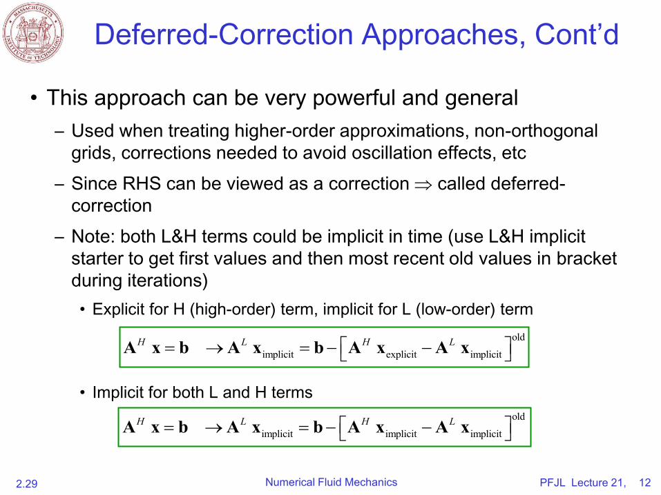
Deferred-Correction Approaches, Cont’d
• This approach can be very powerful and general
– Used when treating higher-order approximations, non-orthogonal
grids, corrections needed to avoid oscillation effects, etc
– Since RHS can be viewed as a correction called deferred-
correction
– Note: both L&H terms could be implicit in time (use L&H implicit
starter to get first values and then most recent old values in bracket
during iterations)
• Explicit for H (high-order) term, implicit for L (low-order) term
• Implicit for both L and H terms
old
implicit explicit implicitH L H L A x b A x b A x A x
old
implicit implicit implicitH L H L A x b A x b A x A x

PFJL Lecture 21, 13 Numerical Fluid Mechanics 2.29
Deferred-Correction Approaches, Cont’d
• Example 1: FD methods with High-order Pade’ schemes
– One can use the PDE itself to express implicit Pade’ time derivative
as a function of n+1 (see homework 6)
– Or, use deferred-correction (within an iteration scheme of index r): • In time:
• In space:
• The complete 2nd order CDS would be used on the LHS. The RHS would be
the bracket term: the difference between the Pade’ scheme and the “old” CDS.
When the CDS becomes as accurate as Pade’, this term in the bracket is zero
• Note: Forward/Backward DS could have been used instead of CDS, e.g. in
time,
1nt
1 1 Pade'1 1 1 1
2 2
rr rn n n n
n nt t t t
1 1 Pade'1 1 1 1
2 2
rr ri i i i
i ix x x x
1 1 Pade'1 1
1 1
rr rn n n n
n nt t t t

PFJL Lecture 21, 14 Numerical Fluid Mechanics 2.29
Deferred-Correction Approaches, Cont’d
• Example 2 with FV methods: Higher-order Flux approximations
– Higher-order flux approximations are computed with “old values” and a
lower order approximation is used with “new values” (implicitly) in the
linear system solver:
where Fe is the flux. The Low order approximation can be UDS or CDS.
• Convergence and stability properties are close to those of the Low order implicit
term since the bracket is often small compared to this implicit term
• In addition, since bracket term is small, the iteration in the algebraic equation
solver can converge to the accuracy of higher-order scheme
• Additional numerical effort is explicit with “old values” and thus much smaller
than the full implicit treatment of the higher-order terms
– A factor can be used to produce a mixture of pure low and pure high order.
This can be used to remove undesired properties, e.g. oscillations of high-
order schemes
oldL H Le e e eF F F F
old(1 )L H L
e e e eF F F F
PFJL Lecture 21, 15 Numerical Fluid Mechanics 2.29
Grid Generation and Complex Geometries:
Introduction • Many flows in engineering and science involve complex geometries
• This requires some modifications of the algorithms:
– Ultimately, properties of the numerical solver depend on the:
• Choice of the grid
• Vector/tensor components (e.g. Cartesian or not)
• Arrangement of the variables on the grid
• Different types of grids:
– Structured grids: families of grid lines such that members of the same family do
not cross each other and cross each member of other families only once
– Advantages: simpler to program, neighbor connectivity, resultant algebraic
system has a regular structure => efficient solvers
– Disadvantages: can be used only for simple geometries, difficult to control the
distribution of grid points on the domain (e.g. concentrate in specific areas)
– Three types (names derived from the shape of the grid):
• H-grid: a grid which can map into a rectangle
• O-grid: one of the coordinate lines wraps around or is “endless”. One introduces an artificial cut at which the grid numbering jumps
• C-grid: points on portions of one grid line coincide (used for body with sharp edges)
PFJL Lecture 21, 16 Numerical Fluid Mechanics 2.29
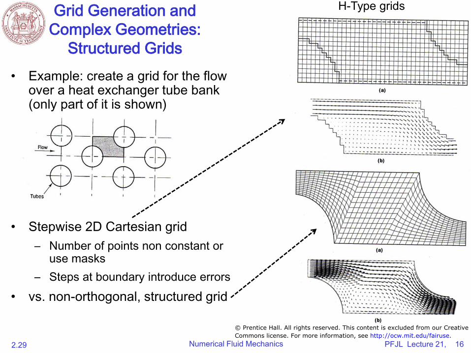
Grid Generation and
Complex Geometries:
Structured Grids
• Example: create a grid for the flow over a heat exchanger tube bank (only part of it is shown)
• Stepwise 2D Cartesian grid
– Number of points non constant or use masks
– Steps at boundary introduce errors
• vs. non-orthogonal, structured grid
H-Type grids
© Prentice Hall. All rights reserved. This content is excluded from our CreativeCommons license. For more information, see http://ocw.mit.edu/fairuse.

PFJL Lecture 21, 17 Numerical Fluid Mechanics 2.29
Grid Generation and
Complex Geometries:
Block-Structured Grids
• Grids for which there is one or more level subdivisions of the solution domain
– Can match at interfaces or not
– Can overlap or not
• Block structured grids with overlapping blocks are sometimes called “composite” or “Chimera” grids
– Interpolation used from one grid to the other
– Useful for moving bodies (one block attached to it and the other is a stagnant grid)
• Special case: Embedded or Nested grids, which can use different dynamics at different scales
Grid with 3 Blocks, with an O-Type grid (for coordinates around the cylinder)
Grid with 5 blocks, including H-Type and C-Type, and non-matching interface:
“composite” or Chimera” Grid
Grids © Springer. All rights reserved. This content is excluded from our Creative
Commons license. For more information, see http://ocw.mit.edu/fairuse.
PFJL Lecture 21, 18 Numerical Fluid Mechanics 2.29
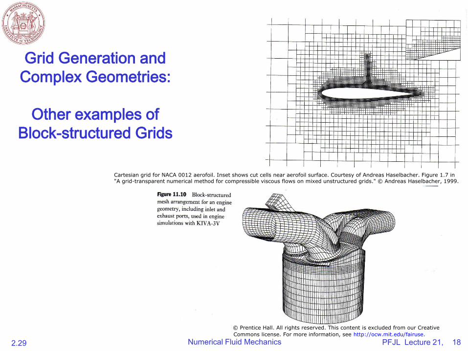
Grid Generation and
Complex Geometries:
Other examples of
Block-structured Grids
Cartesian grid for NACA 0012 aerofoil. Inset shows cut cells near aerofoil surface. Courtesy of Andreas Haselbacher. Figure 1.7 in "A grid-transparent numerical method for compressible viscous flows on mixed unstructured grids." © Andreas Haselbacher, 1999.
© Prentice Hall. All rights reserved. This content is excluded from our Creative
Commons license. For more information, see http://ocw.mit.edu/fairuse.

PFJL Lecture 21, 19 Numerical Fluid Mechanics 2.29
Grid Generation and Complex Geometries:
Unstructured Grids
• For very complex geometries, most flexible grid is one for
which one can fit any physical domain: i.e. unstructured
• Can be used with any discretization scheme, but best
adapted to FV and FE methods
• Grid most often made of:
– Triangles or quadrilaterals in 2D
– Tetrahedra or hexahedra in 3D
• Advantages
– Unstructured grid can be made orthogonal if needed
– Aspect ratio easily controlled
– Grid may be easily refined
• Disadvantages:
– Irregularity of the data structure: nodes locations and
neighbor connections need to be specified explicitly
– The matrix to be solved is not regular anymore and the size
of the band needs to be controlled by node ordering
Triangular grid for three-element aerofoil. Courtesy of Andreas Haselbacher. Used with permission. Figure 1.5 in "A grid-transparent numerical method for compressible viscous flows on mixed unstructured grids." © Andreas Haselbacher, 1999.
PFJL Lecture 21, 20 Numerical Fluid Mechanics 2.29
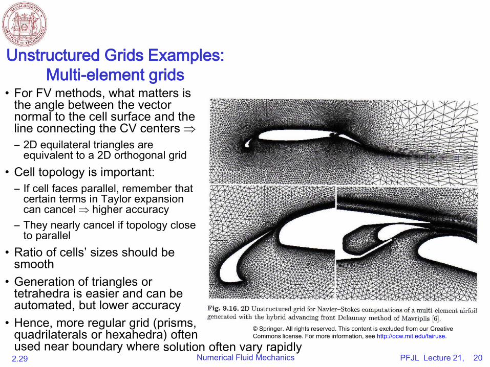
Unstructured Grids Examples:
Multi-element grids • For FV methods, what matters is
the angle between the vector normal to the cell surface and the line connecting the CV centers
– 2D equilateral triangles are equivalent to a 2D orthogonal grid
• Cell topology is important:
– If cell faces parallel, remember that certain terms in Taylor expansion can cancel higher accuracy
– They nearly cancel if topology close to parallel
• Ratio of cells’ sizes should be smooth
• Generation of triangles or tetrahedra is easier and can be automated, but lower accuracy
• Hence, more regular grid (prisms, quadrilaterals or hexahedra) often used near boundary where solution often vary rapidly
© Springer. All rights reserved. This content is excluded from our CreativeCommons license. For more information, see http://ocw.mit.edu/fairuse.
PFJL Lecture 21, 21 Numerical Fluid Mechanics 2.29
Complex Geometries:
The choice of velocity (vector) components
• Cartesian (used in this course)
– With FD, one only needs to employ modified equations to take into
account of non-orthogonal coordinates (change of derivatives due to
change of spatial coordinates from Cartesian to non-orthogonal)
– In FV methods, normally, no need for coordinate transformations in the
PDEs: a local coordinate transformation can be used for the gradients
normal to the cell faces
• Grid-oriented:
– Non-conservative source terms appear in the equations (they account
for the re-distribution of momentum between the components)
– For example, in polar-cylindrical coordinates, in the momentum
equations:
• Apparent centrifugal force and apparent Coriolis force

PFJL Lecture 21, 22 Numerical Fluid Mechanics 2.29
Complex Geometries:
The choice of variable arrangement
• Staggered arrangements
– Improves coupling u ↔ p
– For Cartesian components
when grid lines change by
90 degrees, the velocity
component stored at the
cell face makes no
contribution to the mass
flux through that face
– Difficult to use Cartesian
components in these cases
– Hence, for non-orthogonal grids, grid-oriented velocity components often used
• Collocated arrangements (mostly used here) – The simplest one: all variables share the same CV – Requires more interpolation
Variable arrangements on a non-orthogonal grid. Illustrated are a staggered arrangement with (i) contravarient velocity components and (ii) Cartesian velocity components, and (iii) a colocated arrangement with Cartesian velocity components.
Velocities Pressure
(I) (II) (III)
Image by MIT OpenCourseWare.

PFJL Lecture 21, 23 Numerical Fluid Mechanics 2.29
Classes of Grid Generation
• An arrangement of discrete set of grid points or cells needs to be generated
for the numerical solution of PDEs (fluid conservation equations)
– Finite volume methods:
• Can be applied to uniform and non-uniform grids
– Finite difference methods:
• Require a coordinate transformation to map the irregular grid in the spatial domain to a
regular one in the computational domain
• Difficult to do this in complex 3D spatial geometries
• So far, only used with structured grid (could be used with unstructured grids with
polynomials defining the shape of around a grid point)
• Three major classes of grid generation: i) algebraic methods, ii) differential
equation methods and iii) conformal mapping methods
• Grid generation and solving PDE can be independent
– A numerical (flow) solver can in principle be developed independently of the grid
– A grid generator then gives the metrics (weights) and the one-to-one
correspondence between the spatial-grid and computational-grid

MIT OpenCourseWarehttp://ocw.mit.edu
2.29 Numerical Fluid MechanicsFall 2011
For information about citing these materials or our Terms of Use, visit: http://ocw.mit.edu/terms.