2.1 low level analysis of microarrays - ביה"ס למדעי...

Analysis of DNA Chips and Gene Networks Spring Semester, 2007

Lecture 2: March 8, 2007Lecturer: Rani Elkon Scribe: Yuri Solodkin and Andrey Stolyarenko1

2.1 Low Level Analysis of Microarrays

2.1.1 Introduction

This course deals with high level analysis of data gathered by microarrays. Different typesof high level analysis include:

• Clustering

• Biclustering

• Reconstruction of transcriptional networks

• Induction of classification rules (diagnostic signatures)

High level analysis methods are based on an expressions matrix. Each cell in this matrixrepresents the expression level of a gene under some biological condition. Low level analysisof microarrays is the set of methods used to obtain the expressions matrix from the physicaldata gathered from the microarray (i.e., luminance measurements for each probe on thearray, see Figure 2.1).

Low level analysis of microarrays extracts, normalizes and removes errors from the numer-ical data extracted from the luminance levels.

2.1.2 Microarray Technologies

There are two type of microarray technologies:

• Single channel microarrays are presented with a single type of target (e.g., treatmentcells). They provide absolute gene expression values and can only be used if the numberof probes for each target is explicitly known.

1Based in part on a scribe by Amos Mosseri and Eitan Hirsh, March 2005

2 Analysis of DNA Chips and Gene Networks c©Tel Aviv Univ.

Figure 2.1: Scanned microarray result

• Dual channel microarrays are presented with two different targets (e.g., test andcontrol cells). The RNA in each target is marked with a different florescent color,green (Cy3) and red (Cy5). At the end of the process the results are filtered by color(using a photomultiplier tube) and the resulting images are merged to a single image(see Figure 2.2). This technology is used when the number of probes for each target isunknown, and thus can only provide relative gene expression values.

2.1.3 Types of Microarrays

Currently, three types of microarrays are in widespread use.

Spotted cDNA Microarrays

In a spotted cDNA microarray, which uses dual channel technology, each probe is a mRNAsequence or an EST2 created by the method of PCR3. The probes’ length is 300-1000 bases.The probes are placed on the chip using a spotter, which is a mechanic head that touchestest tubes containing the probes and then touches the microarray, placing the probes on it,(see Figure 2.3). The chips are created in batches, (see Figure 2.4)

2ESTs are mRNA sequences that form a fraction of a gene’s sequence [20]3PCR is a biochemical procedure done to amplify a sequence of DNA [15]

Low Level Analysis of Microarrays 3

Figure 2.2: Dual channel technology. Notice the use of two different colors on the same chip,during the preparation process and analysis process.

Figure 2.3: Mechanic head touches test tubes


Figure 2.4: A batch of Spotted cDNA chips

Since the spotted cDNA microarray provide only relative values between the targets,universal common references [5] are used to compare between results of experiments thatwere carried out in different labs.

The spotted cDNA microarray has 2 main disadvantages. The first is that the probesare double stranded (there is no way to know how many of the probes were separated) thushindering hybridization. Heat is used to separate the probes before they are placed on thearray. The second is the length of the probe that might cause cross-hybridization in which atarget will bind the probe, even though it is only a partial match. On the other hand, thisis a relatively cheap method to create microarrays (∼$10 per array). Most of the researchfacilities have the needed equipment to create the spotted cDNA microarrays for their use4.About 50% of the microarrays used nowadays are spotted cDNA microarrays.

Spotted Oligonucleotide Arrays

Spotted oligonucleotide arrays, manufactured by Agilent, previously a part of HP, utilizingknowledge in inkjet, use synthetic oligonucleotides as probes. This is single channel technol-ogy. Each probe is 60-70 bases long and placed on the chip using inkjet technology printing(SurePrint, see Figure 2.5). When using synthetic oligonucleotides the probes are singlestranded, with known sequence, allowing better hybridization and less cross-hybridization.On the other hand, this method is relatively expensive (∼$200-$500 per array).

4Starting Stanford at 95’


Figure 2.5: SurePrint printing technology

The probe‘s sequence on the chip is chosen to be selective for the transcripts it’s supposedto detect. There are a number of available types of chips, for example:

• Human

– Whole human genome microarray: 44K probes (41K known and predicted genes)

– 19K well characterized genes (1A)

– 19K ESTs and predicted genes (1B)

• Mice - 41K probes representing over 20K genes

• Other organisms - rat, Arabidopsis, rice, yeast

The method is quite new and thus not as wide-spread as the other two.

Affymetrix GeneChip Arrays

Affymetrix microarrays are currently the most common commercial microarrays. For eachgene two types of probes sets are used, positive match probes (PM) and a mismatch probes(MM). The PM probes are about 25 bases long, matching different positions along the gene.An MM probe is added for every PM probe (see Figure 2.2). This probe differs from thePM probe only by the base in the middle. The mismatch probe is used to detect cross-hybridization, in which case the positive match probe and its mismatch probe will bothbind to the target. Only if hybridization occurs for the positive match probe, and not itsmismatch probe, we know that this is a true hybridization. (see Figure 2.6)


For example, let’s assume that the sequence of the gene to be detected is:ATGCTGATCGATGCAGAATCGATC. A possible PM probe will be TGATC and theMM probe will be TGTTC. The possible hybridization results will be analyzed as follows:

• Both probes are detected - cross-hybridization or non specific binding has occurred.this probe won’t provide any useful information.

• Only the correct probe is detected - a specific binding occurred. Of course, in a realexperiment one would require all of the correct probes (or at least most of them) to bedetected in order to decide that the gene is present.

• Neither probe was detected - the target gene probably isn’t present.

Figure 2.6: Affymetrix GeneChip arrays. An example of the PM-MM probe pair method.

As in Agilent chips, there are tailor made chips for a number of organisms:

• Human

– Human Genome U133 plus 2 - 47,000 probe sets for known genes andEST transcripts

– Human Genome Focus Array: 8,500 well annotated genes

– Human Cancer G110 Array: 1,700 genes implicated in cancer

• Near whole genome chips - Rat, Drosophilae, C.Elegans, Arabidopsis, Yeast, ZebraFish, E.Coli.

• Human tiling chips - coverage of the whole genome. Used to discover transcribedmicroRNAs (non-conding genes), TF binding sites and sites of chromatin modifications.


• Exon chips. Used to identify splice variants (alternative splicing). In different tissuetypes (e.g. brain and eye tissues) occur different splice variants for the same mRNAsequence. These chips might help understanding the different splice variants and theproteins produced in different body cells.

2.1.4 Analysis Process

The low level analysis is divided into three major steps:

• Image Analysis

• Signal summary (Affymetrix)

• Normalization

Image analysis

The first step in low level analysis of a microarray is image analysis, a process in which theraw visual data of observed illumination intensities is transformed into an estimate for geneexpression levels (for each probe). This step is mostly composed of image processing tasksand transformation of the image into numbers.

Grid alignment

The first step of image analysis is grid alignment (superimposing a grid on the scannedintensities). The grid is found by locating the borders of each probe. Many error factorsmay occur (e.g., movement of the scanner during the scan) which make it hard to align a gridwith the entire picture. This is solved by segmenting the picture and aligning each segmentto its own grid (see Figure 2.7 [16]). Affymetrix microarrays are created with E. coli probesalong their border. By adding E.coli nucleic acid to the tested sample it is possible to assurethat these probes will be detected and will help determine the borders of the chip and itsgrid alignment (see Figure 2.8).

Target detection

The second step in a low level analysis is target detection, the process of deciding whichpixels in the scanned picture will be used to calculate the intensity of a probe. This task isespecially important in spotted cDNA microarrays in which the spotter creates an unevenspread of each probe’s copies causing an uneven intensity measurement for each probe type[16] (see Figures 2.9 and 2.10).


Figure 2.7: General Grid Alignment

Figure 2.8: Affymetrix chip grid alignment - An example of illuminating the corner andborders of the array.


Figure 2.9: Target detection. Notice the highlighted pixels the target detection methodlocked on.

Figure 2.10: Intensity picture for cDNA micro as a function of the grid cell’s pixel location.Notice the crater like distribution of probes

Target intensity extraction

The third steps extracts the intensity for every probe and provides the user with numericalvalues. Few possible options are to use the mean intensity value or the median. For example,Affymetrix use a 64 pixel per cell resolution and takes the 75th percentile as the cell’s value,dismissing border pixels (see Figure 2.11).

Local background correction

The intensities measured may be severely biased due to dust, glare and non specific binding.Local background correction is used to crudely correct these biases.


Figure 2.11: Affymetrix target intensity extraction. PM and MM cells have different expres-sion level

Summation of probe set signals for Affymetrix chips

Since Affymetrix uses PM and MM probes, a combination of both expression values shouldbe calculated. There are a number of methods to do this calculation ([10],[6],[7]).

In general we will mark the expression level of probe j for transcript i by index ij. Theexpression level for positive probe j will be marked as PMij, the expression level for mismatchprobe j will be marked as MMij, the true expression level for gene i will be marked θi andthe calculated expression level for gene i will be marked Ei.

Average Difference (MAS 4)

This method is based on the idea that the gene expression level is estimated by the differencebetween the PM and the MM value, with the exception of completely random error :

θi + εij = PMij −MMij

To cancel the noise we should take the mean value for all of the probes :

Ei =

∑(PMij −MMij)

T

(where T is the number of MM-PM probe pairs).

A possible improvement is to ignore outliers, probes with intensities very different fromthe rest and treat them as measurement errors.

The problem with the MAS4 model is that it assumes all εij have an equal distribution soit could be cancelled by a simple mean. It appears that the distribution of errors depends onthe general intensity of the probe, as the error increases with the targets’ expression levels.(see Figure 2.12)


Figure 2.12: Error level growing with the intensity.

MAS 5

One way to reduce intensity dependence is to use a multiplicative error factor

PMij −MMij = εij · θi

which can be transformed using log to give

log(PMij −MMij) = log(εij · θi)

and

log(Ei) =

∑(log(PMij −MMij))

TIn order to handle obvious measurement errors a smaller weight is given to values far fromthe mean (in comparison to the values’ variance)

log(Ei) =∑

(wj · log(PMij −MMij))

When wj is bigger when PMij, MMij are closer to their mean.

dCHIP

The dCHIP method, devised by Li and Wong [19] is based on a model in which in addition torandom errors each probe has a different affinity to hybridization and some of the probes forthe same gene have stronger affinities and will have higher expression [7] (see Figure 2.13).


Figure 2.13: Affinity effect for Affymetrix probes. The X-axis represents the probe pairserial number. The Y-axis represents the genes expression levels. Two different conditionsare displayed here, C1 and C2


αj · θi + εij = PMij −MMij

Where αj is the affinity of probe j to hybridization. Multiple arrays (10-20) are requiredin order to fit a model and obtain good estimates for αj and θi. This can be done once forevery kind of chip5.

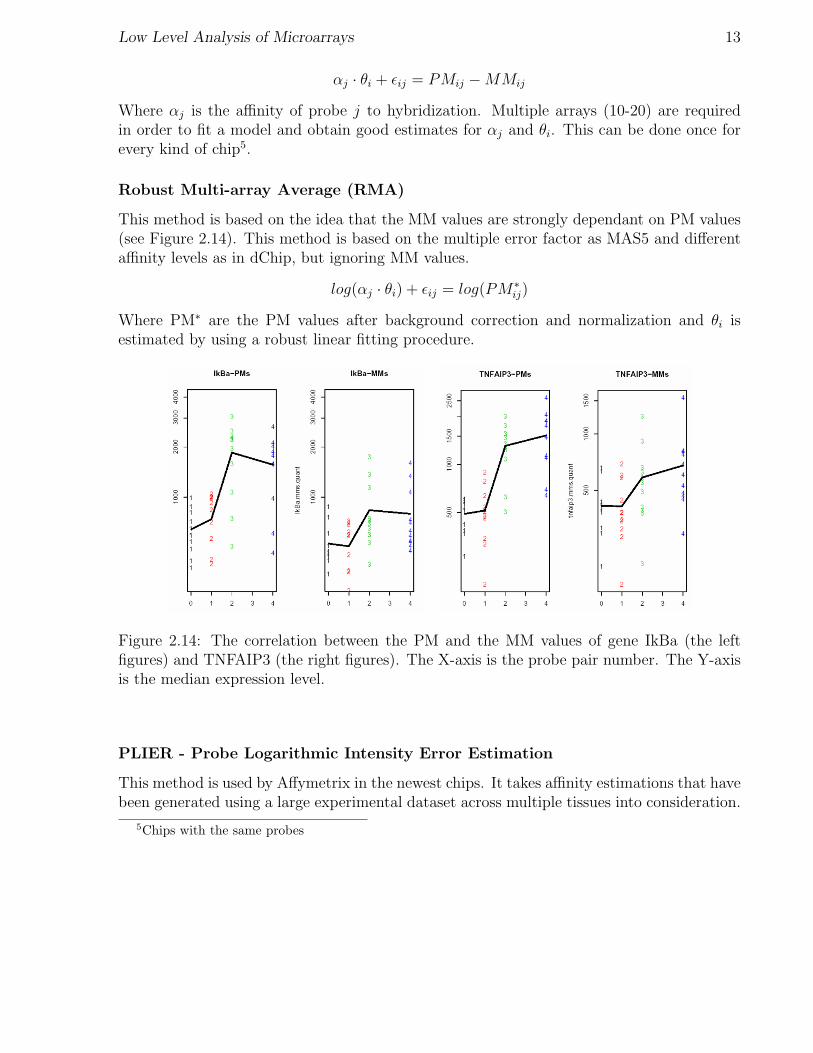
Robust Multi-array Average (RMA)

This method is based on the idea that the MM values are strongly dependant on PM values(see Figure 2.14). This method is based on the multiple error factor as MAS5 and differentaffinity levels as in dChip, but ignoring MM values.

log(αj · θi) + εij = log(PM∗ij)

Where PM∗ are the PM values after background correction and normalization and θi isestimated by using a robust linear fitting procedure.

Figure 2.14: The correlation between the PM and the MM values of gene IkBa (the leftfigures) and TNFAIP3 (the right figures). The X-axis is the probe pair number. The Y-axisis the median expression level.

PLIER - Probe Logarithmic Intensity Error Estimation

This method is used by Affymetrix in the newest chips. It takes affinity estimations that havebeen generated using a large experimental dataset across multiple tissues into consideration.

5Chips with the same probes


The error model smoothly passes from additive (at low intensities) to multiplicative (at highintensities). The model fitting can be chosen by the user from: (PM - MM), (PM - B6), PMand (PM + MM).

Comparing the methods

To compare the effect of different methods, a controlled test was performed. 11 knownRNAs were added to a test sample in known concentrations (which were much higher thanthe concentrations of native sequences in the sample). The expression levels of these RNAsamples were calculated using each of the methods and the results were compared to thecorrect values. Based on these tests, it appears that RMA is the best among the presentedmethods (see Figure 2.15).

Normalization

The normalization step deals with the fact that the results from identical experiments ontwo identical microarrays will never be exactly the same. In addition to unavoidable randomerrors (see Figure 2.16A) there are also systematic differences (see Figure 2.16B) caused by:

• Different incorporation efficiencies of dyes. For example, green colored markers arestronger then red ones (measured as stronger illumination) creating a bias betweenexperiments done with green and red markers.

• Different amounts of mRNA in the tested sample, causing different expression levels.

• Difference in experimenter or protocol. This problem is especially important whencomparing data gathered in different labs.

• Different scanning parameters

• Differences between chips created in different production batches.

Those differences can be corrected by the use of normalization methods that remove sys-tematic errors (biases) from the data. Without correcting these differences, it is impossibleto compare the results of two experiments.

In the following graphs, the gene expression levels will be presented as a histogram oflog(intensity) values. The results from two chips (or two tests of the same sample withdiffering markers) will be colored in red and green (e.g., see Figure 2.17A). Notice that eventhough a comparison of identical samples is used in Figure 2.17A, normalization is importantwhen comparing different samples in order to detect differential genes. In such cases it isharder to normalize the results because one cannot know whether the different expression

6Background intensity


Figure 2.15: Comparison results: RMA, dChip and MAS5. The left figure depicts theexperiment results when the spiked-in RNAs were selected randomly. The right figure depictsthe results of spiked-in RNAs with concentrations 2 times higher than those of the testsample. Notice that these are ROC diagrams. The closer the curve to the upper left corner,the better is the performance [7].


Figure 2.16: A comparison of two (green and red) identical samples over differentchips/channels. The X-axis and the Y-axis are the intensity levels at each experiment.(A) shows expected results with noise, and (B) shows results with systematic bias. Ideally,all the data points will be on the main diagonal.

levels are caused due to actual differences or a normalization problem. A normalizationscheme should answer two questions:

• Which genes (probes) are used for the normalization process

• How is the normalization performed, i.e., what is the mathematical algorithm used tonormalize the values.

Finding the normalization genes

There are a number of methods for choosing the normalization genes, i.e., the genes onwhich the normalization scheme will be based.

1. All gene normalization

Using all of the genes on the chips for normalization is based on the assumption that most ofthe genes have the same expression levels in the two (different) samples which are compared.Also, the proportion of the differential genes is assumed to be low (less than 20%). Thismethod is inappropriate when the previous assumption is wrong. For example, when thesamples are highly heterogeneous (e.g., samples from completely different tissues), or whenusing dedicated chips (e.g., human cancer arrays).


2. Housekeeping genes only

The idea is to use a small set of genes that, based on prior knowledge, are known to haveequal expression levels in the compared samples. Two currently used normalization schemesare based on housekeeping genes:

• Affymetrix chips have a set of 100 housekeeping genes used for normalization

• NHGRI’s cDNA microarrays have a set of 70 housekeeping genes

One problem with using housekeeping genes is that they are usually expressed at high levels,so they are not informative for the normalization of the low intensities range. Anotherproblem is that the validity of the assumption about the equal expression level of thesegenes is questionable.

3. Spiked in controls

In the spiked in controls method, a number of control mRNAs are added to each sample.These mRNAs are taken from another organism (to make sure that they do not exist in thesample itself). The microarrays are designed to have probes that detect these mRNAs. Thecontrols are added in a range of concentrations, providing normalization data for differentexpression levels. This method’s main limitation is that due to the fact that the controlsare added only to the final sample, they cannot compensate for differences caused during itspreparation. Only differences in the scanning and image analysis steps can be compensated.For example, two samples that were produced with different amounts of mRNA due to someexperimental error. The controls are added in equal amounts, so they can provide no clueon the initial difference. Since preparation is probably the most common cause for biases,this method’s effectiveness is limited. Furthermore, spike-in normalization is based on small(70-100) number of probes so it isn’t as robust as the other methods.

4. Invariant set

Contrary to the other methods, in the invariant set method, one decides on the normalizationgenes only after the results are analyzed. The idea is to detect genes with similar expressionlevels in all of the chips, assuming they should have an identical expression level and base thenormalization scheme on them. One way to detect these genes is by ranking the expressionlevels for all of the genes and choose genes with the same rank (global biases should haveless effect on the comparative rank of each gene).

Normalization methods


Once the normalization genes were chosen, there are a number of methods for the nor-malization itself. All of these methods are computed based on the expression levels of thenormalization genes, and later the transformation is applied to the entire data set.

1. Global normalization (Scaling)

This normalization scheme is intended to equalize the mean value of the expression levels.All of the values are multiplied by the ratio (k) between the mean expression level of thenormalization genes in the two samples. The normalization factor k is

k =

∑(E1

i )∑(E2

i )

when the summation is over the normalization genes. (where Eji is the expression level

for gene i in sample j). Normalization of E2i values is done by multiplication by k. (see

Figure 2.17 and Figure 2.18). Note this this normalization will work only when we areconsidering a constant difference between the samples.

Figure 2.17: Histogram before (A) and after (B) global normalization. A distribution dia-gram of two identical samples when tested on two chips. The X-axis is the intensity leveland the Y-axis is the density. After normalization, the mean value of the two distributionsis identical, although the distribution is not identical.

2. Intensity-dependent Normalization (Lowess normalization)

Lowess normalization [12][9] is using different normalization factors for high and low expres-sion genes to compensate for intensity dependent biases. Different expression level genesshould be normalized with different factors. Before tackling the lowess normalization, it is


Figure 2.18: boxplots (see appendix 1) before and after global normalization.

important to be familiar with the M vs. A plots which help detect intensity dependentbiases. The X axis is the average intensity of a gene in both samples(chips):

A =log(E1

i · E2i )

2

The Y axis is the log ratio of these intensities:

M = log(E1

i

E2i

)

For example, Figure 2.19 shows a situation in which there is no intensity dependent bias(the ratio between expression values (Y axis) does not change according to the expressionlevels themselves (X axis)) On the other hand, Figure 2.20 shows a situation in which theratio between expression levels changes completely for different expression levels. For lowerexpression levels one of the chips’ values are measured to be higher than the other’s, and thissituation is reversed for higher expression values. It is obvious that this situation cannot becorrected by global normalization. Lowess normalization fits a local regression curve to theM vs. A graph and uses it to calculate a normalization factor that depends on the meanintensity. The normalization is performed by multiplying the expression level for each geneby the factor fitting its expression level (see Figure 2.20). The effect on the distributions canbee seen in Figure 2.21.

3. Quantile normalization

Quantile normalization normalizes the data to have identical intensity distributions (seeFigure 2.22). It makes sure that both samples will have the same intensity distribution


Figure 2.19: log intensity (M) vs. Average intensity (A) with no bias.

Figure 2.20: M vs. A with bias.In the left figure a global factor will not work, thus theLowess method (right figure) is needed.


histogram. It doesn’t promise that the same genes will have the same intensities. Quantile

Figure 2.21: After lowess normalization. Notice that the mean of all intensities distributionsare the same, although the distributions themselves can be very different.

normalization is done by sorting the gene expression levels. Let Eji be the expression level of

gene i in chip j. After sorting, let Ejk be the k-th largest expression level for chip j. This is

the expression level of gene i for some i : Ejk = Ej

i . The normalization computes the medianintensity for each rank:

< Ik >=

∑Ej

k

T

Finally, the expression level Ejk of each gene i is replaced with this median. In this way, for

each rank k, there is a pair of genes, one on each chip, with the same value. Thus, the chipswill have the same expression level distribution (see Figure 2.23)

Summary

A comparison based on a specific dataset presented in [4, 17] showed that quantile normal-ization gave the best results, with lowess giving comparable results.

A number of normalization tools are available:

• BioConductor [18]. Can be used on both Affymetrix and cDNA microarrays


Figure 2.22: After quantile normalization. All distributions are identical.

Figure 2.23: Quantile normalization. Each color is a specific gene, Ii denotes the rankedintensity of a gene. The Ii values are the average for each rank.

Identification of Differential Genes 23

• dCHIP [19]. Can be used only for Affymetrix and is based on quantile normalization,using the Invariant set method to choose normalization genes

• Expander [8]. Can be used on both Affymetrix and cDNA microarrays and can useboth quantile normalization and lowess normalization.

2.2 Identification of Differential Genes

The most common microarray experiment is a comparison between 2 samples - a treatmentsample and a control sample. The goal is to identify genes that are differently expressed inthe two samples. The number of microarrays is usually very low (2-4). There are a numberof methods to identify the differently expressed genes. An important perquisite of thesemethods is the ability to asses the chance of false positives, the chance that a gene will bedetected as differential even though it’s not. Without it, it is impossible to know whetherthe results of the experiment are reliable.

2.2.1 Fold change

This method considers genes whose mean expression level (between treatment and controlsamples) has changed by at least 1.75-2 fold as differential genes. This naive method has anumber of major limitations:

• No estimation is given for the chance of false positives

• It is biased to genes with low expression level. A small change, due to an error, couldbe enough to mark genes as differential (see Figure 2.24). An improvement can bedone by using a cutoff to filter genes with a low expression level.

• There is no consideration of the variability of gene expression levels over a number ofmicroarrays. It is enough for one treatment microarray to show a very high expressionlevel for a gene, for this gene to be marked as differential. Yet, in other treatmentmicroarrays, this gene might have low expression level, possibly showing that someother biological phenomena took place in the specific sample analyzed by the firstmicroarray. (see Figure 2.25 for example).

Note that empirical results show a false positive rate of 60-70 percent when using this method.


Figure 2.24: Fold Change limit. Here we see the fold change (Y-axis) as a function of theintensity (X-axis) biased to low expression levels. Notice that for small values, a large foldchange occurs even for a small change of the expression level. In such situation one shouldconsider choosing some cut-off intensity level, to avoid ”noise” from the low intensity areas.

Figure 2.25: Fold Change limit. Note that both g1 and g2 have the same mean value of2 (200/100), however their variances are different. Eventually, they end up with the samet-score.


2.2.2 T-test

The T-test is based on normalization of the expression level change, with the variance of themean expression levels (of the treatment and control samples). In case the expression levelchange is high, in comparison with the variance of the mean expression values, an assumptioncan be made that there is a real difference in gene concentration, i.e. the gene is differential.On the other hand, even if the difference is large, but the gene has high variance, we willnot treat it as differential. The t-score value is computed the following way:

t =Mc −Mt√

S2c

nc+

S2t

nt

where S2c , S

2t are the variance estimates in control and treatment samples respectively; Mc, Mt

are the mean levels in control and treatment samples respectively; nc, nt are the number ofcontrol and treatment samples respectively. A p-value7 is calculated for each t-score in orderto asses the chance for a false positive. Genes with a predefined high value will be ignored(see Figure 2.26). There are other methods of estimating the p-value of difference between

Figure 2.26: Example of computation of t-score and p-value when comparing control andtreatment. Though, the fold change of both genes is 2, we can see that they have verydifferent p-values. If we would consider only genes with p-value less than 0.01, only g1 wouldbe declared differential

samples. One such method is Cyber-T, it improves the variance estimation in case of a smallnumber of tests [1].

2.2.3 Multiple Testing

t-score based methods are problematic when used for microarray analysis due to statisticalproblem of multiple testing. When testing a very large number of cases (genes), the numberof false positives should be taken into account. When considering a totally random samples,where no genes are differentially expressed, but 10,000 genes are tested, a gene with a p-value as low as 0.0001 is still absolutely expected. In order to avoid receiving too many false

7the chance to have a given t-score, or higher, in case of a random sample


positives the decision about the cut-off p-value should take into consideration the number ofcases examined.

Bonferroni Correction

The Bonferroni correction [3] states that in order to have a given chance of false positives q,while doing N experiments, p-value should be chosen as q

N. For example, given the numbers

described above, choose cutoff of 0.000001 for p-value in order to have a chance of 0.01 forone false positive.

The problem with the Bonferroni correction is that the t-value, required for such a lowp-value, will most probably limit the number of true positives found. Using the Bonferronicorrection promises a low chance for false positives but also may cause a large number of falsenegatives (differential genes that would be filtered out because of the high t-value threshold).

False Discovery Rate

The idea behind false discovery rate (FDR)[2][11] is to choose an acceptable proportionof false positives among the genes declared as differential, for example 10 percent (thispercentage will be marked q). The FDR method ranks the tested genes according to their p-values and chooses, as differential genes, only the first k genes, those with the lowest p-value,so that:

pi ≤ i ∗ q

N

The procedure guarantees that the false positives fraction will not exceed q.

The problem with FDR is, like the rest of the presented methods, the assumption that thegene expression, of different genes on the chip is independent. This is biologically incorrectsince many genes’ expressions are correlated.

Significance Analysis of Microarray

Significance Analysis of Microarray (SAM)[13] is intended to deal with the fact that geneexpressions are correlated in an unknown manner. It uses permutations to get an ’empirical’estimate for the FDR of the reported differential genes. Instead of using the above FDRcalculation, it tries to rename the different genes as if the two sample groups have beenmixed up (e.g. we take 3 “green” control samples and 3 “red” treatment samples and changetheir colors). By taking many different permutations and summing up the resulting numberof differential genes the significance of the original result can be seen. The lower the numberof differential genes under a random permutation the higher the chance that the result istrue. The SAM algorithm is :


• Compute for each gene a statistic that measures its relative expression difference incontrol vs treatment (t-score or a variant).

• Rank the genes according to their difference score

• Set a cutoff d0 and consider all genes above it as differential. The number of differentialgenes is Nd.

• Permute the condition labels, and count how many genes got score above d0. Thenumber of genes is Np

• Repeat on many (all possible) permutations and count Npj

• Estimate FDR as the proportion: <Npj>

Nd


2.3 Appendix

2.3.1 Boxplots [14]

Figure 2.27: Explanation of boxplots diagrams

Boxplots are method for graphical representation of a distribution, based on representingthe different quartiles. The range is divided by five values (as shown in Figure 2.27):

• The upper line indicates the maximal value.

• The upper line in the colored box indicates the upper quartile of the values.

• The middle line in the colored box indicates the median.

• The lower line in the colored box indicates the lower quartile of the values.

• The lower line indicates the minimal value.

The five number summary leads to a graphical representation of a distribution called theboxplot.

Bibliography

[1] P. Baldi and A. D. Long. A Bayesian framework for the analysis of microarray expressiondata: regularized t-test and statistical inferences of gene changes. Bioinformatics, 17:509-519, 2001.

[2] Y. Benjamini and Y. Hochberg. Controlling the false discovery rate: A practical andpowerfull approach to multiple testing. J.R Statist. soc, Ser B. 57: 289-300, 1995.

[3] C. E. Bonferroni. Il calcolo delle assicurazioni su gruppi di teste. Studi Onore delProfessore Salvatore Ortu Carboni, 13-60, 1935.

[4] B.M. Bolstad et al. A comparison of normalization method for high density oligonu-cleotide array data based on variane and bias. Bioinformatics, 19(2):185-93, 2003.

[5] N. Novoradovskaya et al. Universal reference RNA as a standard for microarray exper-iments. Genomics, 5:20, 2004.

[6] R. A. Irizarry et al. Exploration, normalization, and summaries of high density oligonu-cleotide array probe level data. Biostatistics, 4(2):249-64, 2003.

[7] R. A. Irizarry et al. Summaries of Affymetrix GeneChip probe level data. Nucleic AcidsRes, 31(4):e15, 2003.

[8] R.Shamir et al. EXPANDER an integrative program suite for microarray data analysis.Bioinformatics, 6:232, 2005.

[9] Y. H. Yang et al. Normalization for cDNA microarray data: a robust composite methodaddressing single and multiple slide systematic variation. Nucleic Acids Res, 30(4):e15,2002.

[10] C. Li and W. H. Wong. Model-based analysis of oligonucleotide arrays: Expressionindex computation and outlier detection. PNAS, 98:31-36, 2001.

[11] V. Melfi. False discovery rates and their application to microarray data analysis.http://www.stt.msu.edu/ huebner/melfifdr.pdf, 2003.

29

30 BIBLIOGRAPHY

[12] G. K. Smyth and T. Speed. Normalization of cDNA microarray data. METHODS:Selecting Candidate Genes from DNA Array Screens: Application to Neuroscience, 29-37, 2003.

[13] V. Tusher., R. Tibshirani., and G. Chu. Significance analysis of microarrays applied tothe ionizing radiation response. PNAS, 98: 5116-5121, 2001.

[14] http://en.wikipedia.org/wiki/Box_plot.

[15] http://en.wikipedia.org/wiki/Polymerase_chain_reaction.

[16] http://research.nhgri.nih.gov/microarray/image_analysis.html.

[17] http://stat-www.berkeley.edu/users/bolstad/normalize/.

[18] http://www.bioconductor.org.

[19] http://www.dchip.org/.

[20] http://www.ncbi.nlm.nih.gov/About/primer/est.html.

2.1 low level analysis of microarrays - ביה"ס למדעי...

Documents