5

CHAPTER 2

THE PROBLEM OF MULTICOLLINEARITY

2.1 Introduction

Regression analysis examines the relationship between a dependent variable Y

and one or more independent variables p21 XXX ,...,, . Such an analysis assumes the use of

a model with a specified set of independent variables. But in many cases we do not know

exactly what variables should be included in a model. Hence, one may propose an initial

model, often containing a large number of independent variables, and proceed with a

statistical analysis aiming at revealing the correct model.

The inclusion of a large number of variables in a regression model often results in

multicollinearity. The term multicollinearity refers to high correlation among the

independent variables. This occurs when too many variables have been put into the model

and a number of different variables measure similar phenomena. The existence of

multicollinearity affects the estimation of the model as well as the interpretation of the

results.

In this chapter we will give some preliminary material on:

1. The general regression situation.

2. Multicollinearity and how to detect it.

3. Strategies for coping with collinear data.

2.2 The General Regression Situation

The following definitions and proofs concerning multiple regression are based on

Draper and Smith (1981) as well as on Rao and Toutenburg (1999).

Suppose we have a model under consideration, which can be written in the form

6

UXβΥ += (2.2.1)

where Y is an ( )1×T vector of observations on a random variable, X is an ( )pT × matrix

of observations of the p independent variables, β is a ( )1×p vector of unobserved

parameters, and U is an ( )1×T vector of errors. We often use the following assumptions:

a) X is a fixed matrix of regressors (nonrandom),

b) The rank of X is p

c) Normality of the errors, i.e. the errors follow a normal distribution with zero mean

vector and variance- covariance matrix Ι2σ , i.e.: ( )I0U 2,N~ σ . This assumption is

required for tests of significance and also for the construction of confidence and

prediction intervals. It implies that the errors are homoscedastic, i.e. ( ) 2σ=tUV for

all T,...,1t = , and that they are independent, i.e. ( ) 0cov =′tt ,UU for all T,...,1tt =′≠ .

A direct consequence from the distributional assumption for U is that

( )IXβY 2,N~ σ .

Let us now consider the least squares method which is the most common method

of estimating the parameters of the model. Since the error U is equal to XβY − we shall

estimate it with the residual which is defined as 0XβYU −=ˆ , where 0β is an arbitrary

choice for β . The least squares coefficient vector minimizes the sum of squared

residuals:

( ) ( )00 XβYXβYUU −′−=′ ˆˆ

0000 XβXβXβYYXβYY ′′+′−′′−′=

000 XβXβYXβ2YY ′′+′′−′= (2.2.2)

It can be determined by differentiating (2.2.2), with respect to 0β , and setting the

resulting matrix equation equal to zero. Let β be the solution, then β satisfies the least

squares normat equations

( ) YXβXX ′=′ ˆ . (2.2.3)

7

If X is not of full rank, XX′ is singular, (2.2.3) has a set of solutions

( ) ( )( )ωXXXXIYXXXβ ′′−+′′= −−ˆ ,

where ( )−′XX is a generalized inverse (see Appendix A) of XX′ and ω is an arbitrary

vector. Then either the model should be expressed in terms of fewer parameters or

additional restrictions on the parameters must be given or assumed.

If the normal equations are independent, XX′ is nonsingular, and its inverse exists. In

this case the solution of the normal equations is unique and is given by the following

expression:

( ) YXXXβ 1 ′′= −ˆ . (2.2.4)

Once β has been estimated by β , we can write the residual as

( ) ( )YHIYXXXXYβXYU 1 −=′′−=−= −ˆˆ ,

where ( ) XXXXH 1 ′′= − and I is the identity matrix. Further, the sum of squares of

residuals divided by T-p,

pT

s−′

=UU ˆˆ

2 , (2.2.5)

can be shown to be a consistent and unbiased estimator of 2σ . The estimated regression

is UβXY ˆˆ += and since 0ˆ =′UX the total sum of squares is

UUβXXβYY ˆˆˆˆ ′+′′=′ (2.2.6)

where βXXβ ˆˆ ′′ is the sum of squares due to regression, and UU ˆˆ ′ is the sum of squares

due to errors. The multiple correlation coefficient, which measures the goodness of fit, is

then defined as

YYUU

YYβXXβ

′′

−=′′′

=ˆˆ

1ˆˆ

2R . (2.2.7)

8

2R tends to overestimate the true value of the coefficient. The following formula, which

gives the multiple correlation coefficient adjusted by the degrees of freedom and is

therefore unbiased, can be used instead:

11)1(1 2

adj2

−−−

−−=pT

TRR .

The least squares estimate of β , β , has some well-known properties (see e.g. in Seber,

1977):

1. It is an estimate of β , which minimizes the residual sum of squares, irrespective of

any distribution properties of the errors.

2. Under the assumption of normality of the errors, β is the maximum likelihood

estimate of β .

3. The elements of β are linear functions of the observations n21 Y,...,Y,Y , and provide

unbiased estimates of the elements of β which have the minimum variances,

irrespective of any distributional properties of the errors (BLUE).

It can be deduced that since ( ) 0=UE then

( ) ( ) ( )YXXXβ 1 EE ′′= −ˆ

= ( ) XβXXX 1 ′′ −

=β (2.2.8)

and β is an unbiased estimate of β . If we further assume that the tU are uncorrelated and

have the same variance then ( ) nV IU 2σ= and ( ) ( )UY VV = . Hence the variance

covariance matrix of β is given by

( ) ( )( )YXXXβ 1 ′′= −VV ˆ

= ( ) ( ) ( ) 1−− ′′′ XXXYXXX 1 V

= ( ) ( )( ) 12 −− ′′′ XXXXXX 1σ

= ( ) 12 −′XXσ . (2.2.9)

9

2.3 Multicollinearity In order to study the relationships among variables we collect data either from

designed experiments or observational studies. It is not always possible, however, to

carefully design controlled experiments in order to ensure that sufficient sample

information is available. Observational studies are used instead and as the name implies,

observe the variables and simply record them. Therefore some or most of the explanatory

variables will be random hence the existence of high correlations among them is possible.

In terms of multiple linear regression higly interrelated explanatory variables mean that

we measure the same phenomenon using more than one variable. Though

multicollinearity does not affect the goodness of fit or the goodness of prediction, it can

be a problem if our purpose is to estimate the individual effects of each explanatory

variable. Once multicollinearity is detected, the best and obvious solution to the problem

is to obtain and incorporate more information. Unfortunately, the researcher is usually not

able to do so. Other procedures have been developed instead, for instance, model

respecification, biased estimation, and various variable selection procedures.

Recall that one of the assumptions for the model (2.2.1) was that X is of full rank,

i.e. 0≠′XX . This requirement says that no column of X can be written as exact linear

combination of the other columns. If X is not of full rank, then 0=′XX , so that a) the

ordinary least squares (OLS) estimate ( ) YXXXβ 1 ′′= −ˆ is not uniquely defined and b) the

sampling variance of the estimate is infinite. However, if the columns of X are nearly

collinear (although not exactly) then XX′ is close to zero and the least squares

coefficients become unstable since ( ) ( ) 12ˆ −′= XXβ σV can be too large. Multicollinearity

among the columns can exist in varying degrees. One extreme situation is where the

columns of X are pairwise orthogonal (that is, 0=ji XX for all i and j, ji ≠ ), so that

there is a complete lack of multicollinearity; at the other extreme is the case of perfect

linear relationship among the X’s, that is, there exist nonzero constants ic (i = 1,…, p),

such that 0...2211 =+++ jkkjj XcXcXc (see e.g. Huang, 1970).

10

In practice neither of the above extreme cases is often met. In most cases there is

some degree of intercorrelation among the explanatory variables. It should be noted that

multicollinearity in addition to regression analysis, is also connected to time series

analysis. It is also quite frequent in cross-section data (Koutsoyiannis, 1977).

We now turn to an example to illustrate our discussion of multicollinearity.

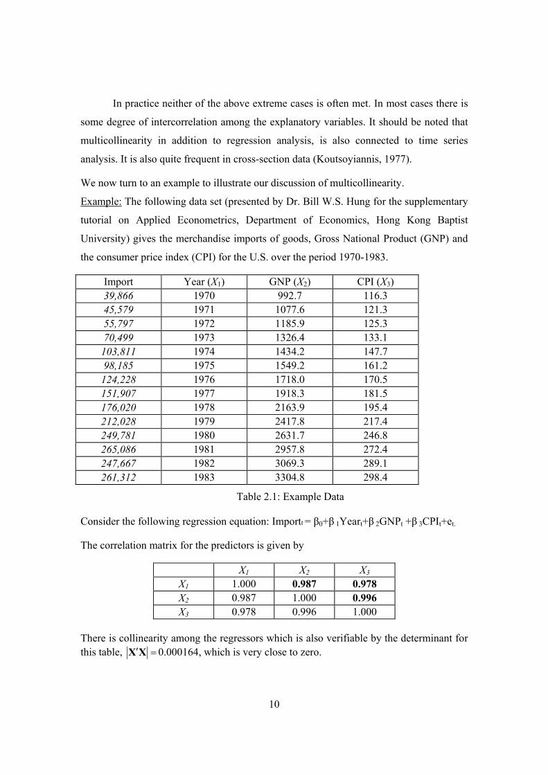
Example: The following data set (presented by Dr. Bill W.S. Hung for the supplementary

tutorial on Applied Econometrics, Department of Economics, Hong Kong Baptist

University) gives the merchandise imports of goods, Gross National Product (GNP) and

the consumer price index (CPI) for the U.S. over the period 1970-1983.

Import Year (X1) GNP (X2) CPI (X3) 39,866 1970 992.7 116.3 45,579 1971 1077.6 121.3 55,797 1972 1185.9 125.3 70,499 1973 1326.4 133.1

103,811 1974 1434.2 147.7 98,185 1975 1549.2 161.2

124,228 1976 1718.0 170.5 151,907 1977 1918.3 181.5 176,020 1978 2163.9 195.4 212,028 1979 2417.8 217.4 249,781 1980 2631.7 246.8 265,086 1981 2957.8 272.4 247,667 1982 3069.3 289.1 261,312 1983 3304.8 298.4

Table 2.1: Example Data Consider the following regression equation: Importt = β0+β 1Yeart+β 2GNPt +β 3CPIt+et.

The correlation matrix for the predictors is given by

X1 X2 X3

X1 1.000 0.987 0.978 X2 0.987 1.000 0.996 X3 0.978 0.996 1.000

There is collinearity among the regressors which is also verifiable by the determinant for this table, =′XX 0.000164, which is very close to zero.

11

As a next step, we calculate 1)( −′XX ,

47.929 -79.686 32.476 -79.686 259.848 -180.854 32.476 -180.854 149.366

These large numbers will give large coefficient estimates and large estimated values for

the variance of these estimates.

2.3.1 Effects of Collinearity The principles of least squares are not invalidated by the existence of

multicollinearity since we still obtain the best linear unbiased estimates. The fact is that

the data will simply not allow any method to distinguish between the effects of collinear

variables on the dependent variable.

The consequences of collinearity in the case of several variables are:

• High estimated variance of β

The existence of multicollinearity tends to inflate the estimated variances of the

parameter estimates, which means that the confidence intervals for the parameters will be

wide, and thus increasing the likelihood of not rejecting a false hypothesis. Since the

regression coefficient measures the effect of the corresponding independent variable,

holding constant all other variables, the existence of high correlation with other

independent variables makes the estimation of such a coefficient difficult. Inflated

variances are quite harmful to the use of regression analysis for estimation and hypothesis

testing.

• High estimated variance of Y

The existence of multicollinearity tends to inflate the estimated variances of predicted

values, that is, predictions of the response variable for sets of x values, especially when

these values are not in the sample. The estimated variance of the predicted values is given

by: ( ) ( ) ( ) ( ) XXXXXβXβXY 1 ′′=′== −2ˆˆˆ σVVV . Therefore, correlated X’s correspond to

large values of ( ) 1−′XX and inflated estimated variances for Y .

12

• Unstable regression coefficients

The parameter estimates and their standard errors become extremely sensitive to slight

changes in the data points.

• Wrong signs for regression coefficients

Coefficients will have wrong signs or an implausible magnitude (e.g. in econometric

models there are coefficients that must have positive sign. Multicollinearity may lead to a

coefficient with negative sign).

• Effect on specification

Given the above, variables may be dropped from the analysis, not because they have no

effect but simply because the sample is inadequate to isolate the effect precisely.

2.4 Detecting Collinearity Many diagnostics have been proposed in the literature in order to determine whether there

is multicollinearity among the columns of X. Some of them will be discussed and better

illustrated through an example.

2.4.1 Correlation Coefficients A simple method for detecting multicollinearity is to calculate the correlation

coefficients between any two of the explanatory variables. If these coefficients are greater

than 0.80 or 0.90 then this is an indication of multicollinearity. A more elaborate rule is

the following: if ijr is the sample correlation coefficient between iX and jX ,

( )( )

( ) ( )1

22

1 1

T

ki i kj jk

ij T T

ki i kj jk k

X X X Xr

X X X X

=

= =

− −=

− −

∑

∑ ∑

and 2R is the multiple correlation as defined in (2.2.7) between dependent and

independent variables, multicollinearity is said to be “harmful” if 2Rrij ≥ (Huang, 1970).

Such simple correlation coefficients are sufficient but not necessary condition for

13

multicollinearity. In many cases there are linear dependencies, which involve more than

two explanatory variables, that this method cannot detect (Judge et al., 1985).

We can extend the concept of simple correlation between independent variables to

multiple correlation within an independent variables set. A variable iX then, would be

harmfully multicollinear only if its multiple correlation with other members of the

independent variable set, 2iR , were greater than the dependent variable’s multiple

correlation with the entire set, 2R (Greene, 1993).

2.4.2 Calculation of XX′ A test which is most commonly used relies on the property that the determinant of

a singular matrix is zero. Defining a small, positive test value, 0>ε , a solution is

attempted only if the determinant based on a normalized correlation matrix is larger than

this value, i.e. ε>′XX ; Recall that the position of such a determinant on the scale is

10 ≤′≤ XX . The closer XX′ is to 0, the greater the severity of multicollinearity and the

closer XX′ is to 1, the less the degree of multicollinearity. Note that, in practice XX′ is

rarely greater than 0.1.

Near singularity may result from strong, sample pairwise correlation between

independent variables, or from a more complex relationship between several members of

a set. The determinant gives no information about this interaction.

2.4.3 Leamer’s Method Leamer (in Greene, 1993) have suggested the following measure of the effect of

multicollinearity for the jth variable:

( )( )( )

211

1

2

′

−=

−

−

∑jj

i jijj

XXc

XX,

14

where ( ) 1−′ jjXX is the jj-th element of the matrix ( ) 1−′XX . This measure is the square root

of the ratio of the variances of jβ when estimated without and with the other variables. If

jX was uncorrelated with the other variables, jc would be 1. Otherwise, jc is equivalent

to ( ) 2121 jR− , where 2jR is the multiple correlation of the variable jX as dependent with

the other members of the independent variable set as predictors.

2.4.4 The Condition Index

Another way to test the degree of multicollinearity is the magnitude of the

eigenvalues of the correlation matrix of the regressors. Large variability among the

eigenvalues indicates a greater degree of multicollinearity. Two features of these

eigenvalues are of interest:

• Eigenvalues of zero indicate exact collinearities. Therefore, very small eigenvalues

indicate near linear dependencies or high degrees of multicollinearity.

• The square root of the ratio of the largest to the smallest eigenvalue21

min

max

=

λλ

K ,

called the condition number, is a commonly employed index of the “instability” of the

least-squares regression coefficients. A large condition number (say, 10 or more)

indicates that relatively small changes in the data tend to produce large changes in the

least-squares estimate. In this event, the correlation matrix of the regressors is said to

be ill conditioned (Greene, 1993). Observe the following simple situation where we

have a two regressors model: the condition number is 21

212

212

21

min

max

1

1

−

+=

=

r

rK

λλ

.

Setting K equal to 10 corresponds to =212r 0.9608 (Fox, 1997).

15

2.4.5 Variance Inflation Factors A consequence of multicollinearity is the inflation of variation. For the jth

independent variable, the variance inflation factor is defined as

VIF = ( )21

1

jR−,

2jR is already defined in section 2.4.3. These factors are useful in determining which

variables may be involved in the multicollinearities.

The sampling variance of the jth coefficient jβ is

( ) ( ) ( ) 2

2

2 111ˆ

jjj STR

V−−

=σβ

where ( )

11

2

2

−

−=∑=

T

XXS

T

ijij

j is the variance of jX and 2σ the error variance (Fox, 1997).

The term 211

jR−, indicates the impact of collinearity on the precision of the estimate jβ .

It can be interpreted as the ratio of the variance of jβ to what that variance would be if

jX were uncorrelated with the remaining iX . The inverse of VIF (i.e 1- 2jR ) is called

tolerance.

It is better to examine the square root of the VIF than the VIF itself because the

precision of estimation of jβ is proportional to the standard error of jβ (not its

variance). Because of its simplicity and direct interpretation, the VIF (or its square root)

is the principal diagnostic for desribing the sources of imprecision. There are no formal

criteria for determining the magnitude of variance inflation factors that cause poorly

estimated coefficients. According to some authors, multicollinearity is problematic if

largest VIF exceeds value of 10, or if the mean VIF is much greater than 1. However, the

latter values are rather arbitrary (Fox, 1997). A VIF equal to 10 implies that the 2jR is 0.9.

16

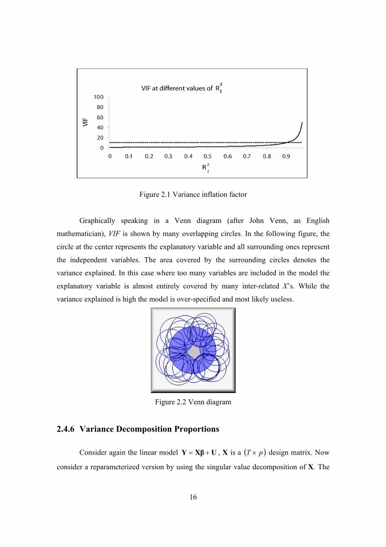
Figure 2.1 Variance inflation factor

Graphically speaking in a Venn diagram (after John Venn, an English

mathematician), VIF is shown by many overlapping circles. In the following figure, the

circle at the center represents the explanatory variable and all surrounding ones represent

the independent variables. The area covered by the surrounding circles denotes the

variance explained. In this case where too many variables are included in the model the

explanatory variable is almost entirely covered by many inter-related X’s. While the

variance explained is high the model is over-specified and most likely useless.

Figure 2.2 Venn diagram

2.4.6 Variance Decomposition Proportions Consider again the linear model UXβY += , X is a ( )pT × design matrix. Now

consider a reparameterized version by using the singular value decomposition of X. The

17

matrix can be written as PQΛX 21 ′= , where Q is a ( )pT × matrix such that IQQ =′

and P′ is a ( )pp× matrix such that IPP =′ . Thus, the variance of the OLS estimator is

( ) ( ) PPΛXXβ 1 ′=′= −− 212ˆ σσV ,

where Λ is a diagonal matrix whose elements are pλλλ ,...,, 21 , the eigenvalues of XX′ .

Using this decomposition makes it possible to decompose the estimated variance of each

regression coefficient into a sum of the data matrix X. We can express the variance of a

single coefficient as

( ) ∑=

=p

j j

kjk

pV

1

22ˆ

λσβ ,

where pkj denotes the (k, j)th element of the matrix P. Consequently, the proportion of

( )kV β associated with any single eigenvalue is

∑=

= p

jjkj

jkjkj

p

p

1

2

2

λ

λφ .

It is useful to view these values as in table 2.2:

Eigenvalue ( )1βV ( )2βV …… ( )kV β …… ( )pV β

1λ 11φ 21φ . 1kφ . 1pφ

2λ 12φ 22φ . 2kφ . 2pφ

. . . . .

pλ p1φ p2φ …… kpφ …… ppφ

Table 2.2 Variance-Decomposition Proportions

The columns in the table sum to one. The presence of two or more large values of kjφ in

a row indicates that linear dependence associated with the corresponding eigenvalue is

18

adversely affecting the precision of the associated coefficients. Values of kjφ greater than

0.50 are considered large (Judge et al., 1985).

2.4.7 The Farrar and Glauber Tests Farrar and Glauber (1967) also proposed a procedure for detecting

multicollinearity comprised of three tests. The first one examines whether collinearity is

present, the second one determines which regressors are collinear and the third one

determines the form of multicollinearity. Based on the assumption that X is multivariate

normal the authors propose the following:

• The chi-square test for the presence of multicollinearity

The null hypothesis is that the X’s are orthogonal. A statistic based on the determinant

XX′ could provide a useful first measure of the presence of multicollinearity within the

independent variables. Bartlett (1937) obtained a transformation of XX′ ,

( ) XX′

+−−−= ln52

6112

* pTχ ,

that is distributed approximately as chi square with ( )121 −= ppν degrees of freedom; p

is the number of independent variables. This is the well known Bartlett’s sphericity test.

From the sample data we obtain the empirical value 2*χ . If this value is greater than the

tabulated value of 2νχ , we reject the assumption of orthogonality.

• The F-test for the determination of collinear regressors

The null hypothesis is that 2iR is equal to zero. Consider the variable iZ , which is equal

to 21 iR− and the new variate,

=

−−

−=

111

ppT

Ziiω

−−

− 11 2

2

ppT

RR

i

i .

19

The distribution of iω is the F-distribution with T-p and p-1 degrees of freedom since

1

2

−pRi (and

pTRi

−− 21

) is distributed as a chi-square with p-1 (and T-p respectively) degrees

of freedom under the null hypothesis. Since 2iR is the multiple correlation coefficient

between iX and the other members of X, iω is the ratio of explained to unexplained

variance. If the observed value Fi >ω , we accept that the variable iX is multicollinear.

• The t-test for the pattern

To understand the form of collinearity in X, the authors use the partial correlation

coefficients between iX and jX , which describe the relationship of iX and jX when all

other members of X are held fixed, namely pijr ..12. . The basic hypothesis here is that

pijr ..12. = 0. To test this hypothesis we are based in the following statistic

pij

pij

r

pTrt

..12.2

..12.*

1−

−=ν

which is distributed as Student’s with pT −=ν degrees of freedom. If tt >*ν , where t

is the theoretical value of the Student’s distribution with ν degrees of freedom, then we

accept that the variables iX and jX are responsible for the multicollinearity. Therefore if

the ith variable is detected collinear by the F-test presented above and the null hypothesis

based on the partial correlation coefficient between iX and jX is rejected then we can

conclude that the jth variable is responsible for the multicollinearity of the ith variable.

These tests have been greatly criticized. Robert Wichers (1975) claims that the

third test, where the authors use the partial-correlation coefficients pijr ..12. , is ineffective

while O’Hagan and McCabe (1974) quote, “Farrar and Glauber have made a fundamental

mistake in interpreting their diagnostics.”

20

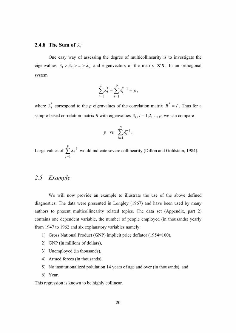
2.4.8 The Sum of 1−iλ

One easy way of assessing the degree of multicollinearity is to investigate the

eigenvalues pλλλ >>> ...21 and eigenvectors of the matrix XX′ . In an orthogonal

system

pp

ii

p

ii == ∑∑

=

−

= 1

1*

1

* λλ ,

where *iλ correspond to the p eigenvalues of the correlation matrix IR =* . Thus for a

sample-based correlation matrix R with eigenvalues iλ , i = 1,2,…, p, we can compare

p vs ∑=

−p

ii

1

1λ .

Large values of ∑=

−p

ii

1

1λ would indicate severe collinearity (Dillon and Goldstein, 1984).

2.5 Example

We will now provide an example to illustrate the use of the above defined

diagnostics. The data were presented in Longley (1967) and have been used by many

authors to present multicollinearity related topics. The data set (Appendix, part 2)

contains one dependent variable, the number of people employed (in thousands) yearly

from 1947 to 1962 and six explanatory variables namely:

1) Gross National Product (GNP) implicit price deflator (1954=100),

2) GNP (in millions of dollars),

3) Unemployed (in thousands),

4) Armed forces (in thousands),

5) No institutionalized polulation 14 years of age and over (in thousands), and

6) Year.

This regression is known to be highly collinear.

21

Parameter estimates

Parameter Estimate

Std. Error StandardizedEstimate

t value p-value

Intercept -3,482,259 890420 0 -3.91 0.0036

GNP deflator

15.06187 84.91493 0.04628 0.18 0.8631

GNP -0.03582 0.03349 -1.01375 -1.07 0.3127

Unemployed -2.02023 0.48840 -0.53754 -4.14 0.0025

Armed forces

-1.03323 0.21427 -0.20474 -4.82 0.0009

Population -0.05110 0.22607 -0.10122 -0.23 0.8262

Year 1829.15146 455.4785 2.47966 4.02 0.0030 Multiple R-squared: 0.9955

Table 2.3: The values of the regression coefficients and the p-values

We note that some predictors (e.g. population) have large p-values though we would

expect them to be significant. If we check the correlation matrix below we will find

several large pairwise correlations.

GNP deflator

GNP Unemployed Armed forces

Population Year

GNP deflator Sig. (2-tailed)

1.000 .

GNP Sig. (2-tailed)

0.992 .000

1.000.

Unemployed Sig. (2-tailed)

0.621 .010

0.604 .013

1.000 .

Armed forces Sig. (2-tailed)

0.465

.070

0.446 .083

-0.177 .511

1.000 .

Population Sig. (2-tailed)

0.979 .000

0.991 .000

0.687 .003

0.364 .165

1.000 .

Year Sig. (2-tailed)

0.991 .000

0.995 .000

0.668 .005

0.417 .108

0.994 .000

1.000 .

Table 2.4: The correlation matrix of the predictors

22

In what follows, let us calculate some of the multicollinearity diagnostics presented in

section 2.4. Specifically, the variance inflation factors, the coefficients of

determination 2iR , and Leamer’s measure.

The predictors VIF 2iR Leamer’s ic

GNP deflator 135.532 0.993 0.086

GNP 1788.513 0.999 0.024

Unemployed 33.619 0.970 0.173

Armed forces 3.589 0.721 0.528

Population 399.151 0.997 0.050

Year 758.981 0.998 0.036

Table 2.5: The multicollinearity diagnostics

The variance inflation factors are large, namely 399.151 for “population”, 758.981 for

“year” and up to 1788.513 for the “GNP” regressor. Considering that the VIF for the

orthogonal predictors is 1 we see that there is considerable variance inflation. Consider

next 2iR , the multiple correlation of the variable Xi as dependent with the other members

of the independent variable set as predictors. These values vary from 0.721 to 0.999

suggesting that GNP for instance is well explained by the remaining independent

variables. Next we present the eigenvalues and the variance decomposition proportions

Variance Proportions Dimension Eigenvalue (Constant) GNP

deflator GNP Unemployed Armed

Forces Population Year

1 6.861 .00 .00 .00 .00 .00 .00 .00

2 .008 .00 .00 .00 .01 .09 .00 .00

3 .046 .00 .00 .00 .00 .06 .00 .00

4 .000 .00 .00 .00 .06 .43 .00 .00

5 .002 .00 .46 .02 .01 .12 .01 .00

6 .000 .00 .50 .33 .23 .00 .83 .00

7 .000 1.00 .04 .65 .69 .30 .16 1.00

Table 2.6: Eigenvalues and variance proportions

23

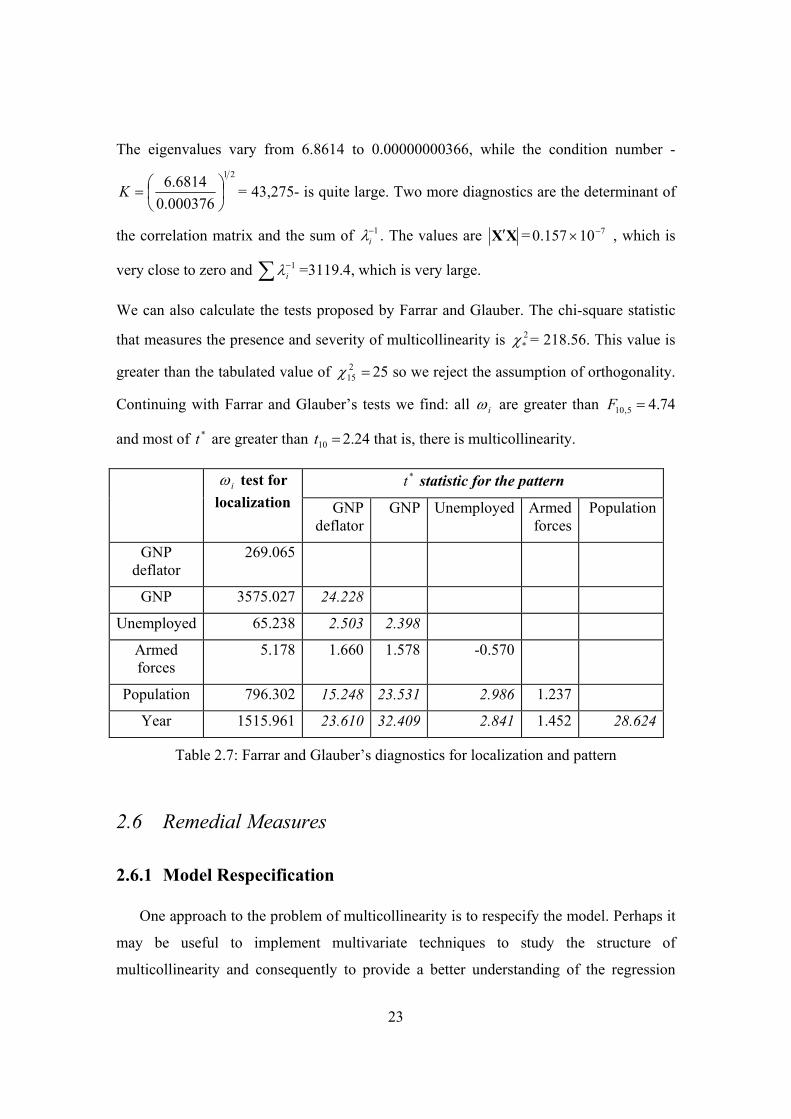
The eigenvalues vary from 6.8614 to 0.00000000366, while the condition number -21

000376.06814.6

=K = 43,275- is quite large. Two more diagnostics are the determinant of

the correlation matrix and the sum of 1−iλ . The values are XX′ = 710157.0 −× , which is

very close to zero and ∑ −1iλ =3119.4, which is very large.

We can also calculate the tests proposed by Farrar and Glauber. The chi-square statistic

that measures the presence and severity of multicollinearity is 2*χ = 218.56. This value is

greater than the tabulated value of =215χ 25 so we reject the assumption of orthogonality.

Continuing with Farrar and Glauber’s tests we find: all iω are greater than =5,10F 4.74

and most of *t are greater than =10t 2.24 that is, there is multicollinearity.

*t statistic for the pattern iω test for localization GNP

deflatorGNP Unemployed Armed

forces Population

GNP deflator

269.065

GNP 3575.027 24.228

Unemployed 65.238 2.503 2.398

Armed forces

5.178 1.660 1.578 -0.570

Population 796.302 15.248 23.531 2.986 1.237

Year 1515.961 23.610 32.409 2.841 1.452 28.624

Table 2.7: Farrar and Glauber’s diagnostics for localization and pattern

2.6 Remedial Measures

2.6.1 Model Respecification

One approach to the problem of multicollinearity is to respecify the model. Perhaps it

may be useful to implement multivariate techniques to study the structure of

multicollinearity and consequently to provide a better understanding of the regression

24

relationships. One such multivariate method is principal components, developed in the

early part of the 20th century.

Principal component analysis is a multivariate technique that attempts to describe

interrelationships among a set of variables. Starting with a set of observed values on a set

of p variables, the method uses linear transformations to create a new set of variables,

called the principal components, which have the following properties:

• The principal component variables, or simply the components, are jointly

uncorrelated.

• The first principal component has the largest variance of any linear function of

the original variables. The second component has the second largest variance, and so

on.

We shall describe the method briefly following Jackson (1991):

The principal components of the p standardized regressors are a new set of p variables

derived from X by a linear transformation: XAW = , where A is the ( )pp ×

transformation matrix. The transformation A is selected so that the columns of W are

orthogonal-that is, the principal components are uncorrelated. In addition, A is

constructed so that the first component accounts for maximum variance in the X’s; the

second for maximum variance under the constraint that it is orthogonal to the first; and so

on. The principal components therefore partition the variance of the X’s.

The transformation matrix A contains (by columns) normalized eigenvectors of the

correlation matrix of the regressors XRXX =′ . The columns of A are ordered by their

corresponding eigenvalues: the first column corresponds to the eigenvector of the largest

eigenvalue, and the last column to the smallest. The eigenvalue jλ associated with the jth

component represents the variance attributable to that component. If there are perfect

collinearities in X, then some eigenvalues of XR will be 0, and there will be fewer than

p principal commponents, the number of components corresponding to

rank( X )=rank( XR ).

25

As we showed earlier the jVIF is equal to ( )211 jR− . It can also be shown that the jVIF

is the diagonal entry of 1XR− and since

1XR− = AAΛ 1 ′− ,

where =Λ ( )pdiag λλ ,...,1 is the matrix of eigenvalues of XR , the jVIF can be expressed

as function of the eigenvalues of XR and the principal components, i.e.:

=jVIF ∑=

p

i i

jiA

1

2

λ. (2.6.1)

Thus, it is only the small eigenvalues that contribute to large sampling variance, but only

for those regressors that have large coefficients associated with the corresponding “short”

principal components.

Principal components analysis is considered a remedy for multicollinearity since

we can calculate one or several principal components on the set of collinear variables and

use the components in the regression instead of the original variables. A possible

problem, though, is a possible lack of interpretability of the transformed set of variables.

2.6.2 Variable Selection When a number of variables in a regression analysis do not appear to contribute

significantly to the predictive power of the model, or when the regressors are highly

correlated, it is natural to try to find a suitable subset of important or useful variables. An

optimum subset model is one that, for a given number of variables, produces the

minimum error sum of squares, or, equivalently, the maximum 2R . The only way to

ensure finding optimum subsets is to examine all possible subsets. Fortunately, high-

speed computing capabilities make such a procedure feasible for models with a moderate

number of variables.

When the examination of the R-square values does not reveal any obvious choices for

selecting the most useful model, we can use instead a number of other statistics. Among

these, the most frequently used is the pC statistic, proposed by Mallows (see Fox, 1997).

This statistic is a measure of total squared error for a subset model containing p

26

independent variables. The total squared error is a measure of the error variance plus the

bias introduced by not including important variables in a model. It may, therefore,

indicate whether variable selection is deleting too many variables. The pC statistic has

the following form:

pC = ( ) ( ) 12 +−− pTMSE

pSSE

where MSE is the error mean square for the full model, ( )pSSE is the error sum of

squares for the subset model containing p independent variables (not including the

intercept), and T is the total sample size. It is recommended that pC be plotted against

p , and further select that subset size where the minimum pC first approaches ( p +1),

starting from the full model in order to derive the best model.

A number of other statistics are available to assist in choosing subset models.

Some are relatively obvious, such as the residual mean square or standard deviations,

while others are related to 2R , with some providing adjustments for degrees of freedom.

Subset techniques have the advantage of revealing alternative, nearly equivalent models,

and thus avoid the misleading appearance of producing a uniquely “correct” result.

Popular alternatives to the guaranteed optimum subset selection are the stepwise

procedures that add or delete variables one at a time until, by some criterion based on 2R ,

a reasonable stopping point is reached. These selection methods do not guarantee finding

optimum subsets, but they work quite well in many cases and are especially useful for

models with many variables. Such selection methods are:

Backward selection; Starts with a full regression equation that includes all the

independent variables. The 2R induced from deleting each independent variable, or the

partial F test value for each independent variable treated as though it were the last

variable to enter the regression equation, is calculated. The lowest partial F test value

(which corresponds to the variable that contributes least to the fit of the model) is

compared with a predetermined critical tabulated F-value. If this partial F value is

smaller than the tabulated F -value we delete it and examine the regression with the

remaining independent variables. The procedure stops when all coefficients remaining in

27

the model are statistically significant. Note, that the decision rule is irreversible; once a

variable has been deleted, it is deleted permanently.

Forward selection: The process begins with the inclusion of the variable with the

largest correlation with the dependent variable. Next, variables are entered according to

their squared partial correlation controlling for those variables already in the model. The

process continues until no variable considered for addition to the model provides a

reduction in sum of squares considered statistically significant at the predetermined level.

An important feature of this method is that once a variable has been selected, it stays in

the model.

Stepwise selection: It begins similarly to forward selection but differs in that the

decision to include a predictor is not irreversible.

For more information see Dillon and Goldstein (1984). A technical objection to stepwise

methods is that they can fail to return the optimal subset of regressors of a given size.

In applying variable selection, it is essential to keep in mind the following: Variable

selection is a good strategy when the variables are orthogonal or nearly so. On the

contrary when the variables are highly correlated or include curvilinear effects of other

variables this is not a promising method. In these cases biased estimation has proven to

be a good solution as it is better to use a part of all the variables than all of some variables

and none of the remaining ones.

2.6.3 Biased Estimation Another approach to deal with collinear data is biased estimation. Least-squares

estimators provide unbiased estimates of parameters. The essential idea here is to trade a

small amount of bias in the coefficient estimates for a substantial reduction in coefficient

sampling variance. The precision of a biased estimate, called the mean squared error, is

the square of the bias plus the variance. The hoped-for result is a smaller mean-squared

error of estimation of the β ’s than is provided by the least-squares estimates.

28

Ridge regression

The most common biased estimation method is ridge regression. Hoerl and Kennard

(1970) proved that it is always possible to choose a positive value of a constant, namely

the ridge constant, so that the mean-squared error of the ridge estimator is less than the

mean-squared error of the least-squares estimator. Their equation of the ridge estimate is

( ) ( ) ,ˆ 1 YXIXXβ ′+′= −kk (2.6.2)

where 0≥k is the nonstochastic quantity called the ridge constant, ( ( ) ββ =0ˆ is the

ordinary LS estimator) and I is the identity matrix.

The arbitrary selection of a “ridge constant” in ridge regression controls the extent to

which ridge estimates differ from the least-squares estimates: the larger the ridge

constant, the greater the bias and the smaller the variance of the ridge estimator. The vital

issue therefore is to find a value of k for which the trade-off of bias against variance is

favorable. In other words, ridging can be viewed as a compromise between fitting the

data as well as possible, while not allowing any one coefficient to get very large.

Unfortunately, to pick the optimal ridge constant generally requires knowledge about the

unknown β ’s that we are trying to estimate (Fox, 1997).

A number of methods have been proposed for selecting the constant k . One very

popular method is to compute ridge regression estimates for a set of values of k starting

with k = 0 (the unbiased estimate) and to plot these coefficients against k (Ridge Trace).

As the value of k increases from zero, the coefficients involved in multicollinearities

change rapidly. However, as k increases further, these coefficients change more slowly.

The selection of k is done by examining such a plot and choosing that value of k where

the coefficients settle down. We will present analytically ridge regression in the next

chapter.

Shrinkage estimators

Shrinkage estimators are of the form

ββ ˆˆ sSH = (2.6.3)

29

where 10 ≤≤ s is a deterministically or stochastically chosen constant. The only known

shrinkage estimator (SH) with a stochastically chosen value of s possessing any optimal

properties is the estimator due to James and Stein (see Gunst and Mason, 1977). Provided

3≥p and IXX =′ , the SH estimator is given by (2.6.3) with

′′

−=ββUUˆˆˆˆ

1,0max cs (2.6.4)

where ( ) ( )2220 +−<< νpc , UU ˆˆ ′ is the residual sum of squares using β to predict the

response and ν is the number of degrees of freedom on which UU ˆˆ ′ is based. The

estimator SHβ with s given by (2.6.4) has smaller MSE than LS. Moreover, the

MSE( SHβ ) is minimized for s given by (2.6.4) if ( ) )2(2 +−= νpc .

The drawbacks of SH are the requirements that 3≥p and IXX =′ ; and as Gunst and

Mason comment this eliminates most of the cases met in practice.

Generalized inverse estimators (Marquardt, 1970)

Since the matrix XX′ is singular, an option is to invert it by means of a generalized

inverse. Let the diagonalized matrix be denoted D, with ordered diagonal elements

pλλλ ≥≥≥ ...21 and the eigenvector matrix that transforms XX′ into D be denoted S.

Thus,

DXSXS =′′

where ISS =′ . Then

( ) .SSDXX 11 ′=′ −−

Suppose XX′ is of rank r, so that the last ( )rp − ordered elements of D are zero (or

nearly so; if XX′ is only “nearly singular”). Partition S as follows:

( )rpr −= SSS :

where rS is ( )rp× ; rp−S is ( )( )rpp −× and then partition D as

=

−rp

r

D

DD

M

LLL

M

0

0

30

where rD is ( )rr × ; rp−D is ( ) ( )( )rprp −×− .

Now, by assumption, rp−D is zero, so that 1−−rpD = 0 by definition. Thus, the inverse

becomes

′=′ −+rrrr SDSXX 1)( . (2.6.5)

A class of generalized inverse regression estimators is defined by

YXXX(β ′′= ++r)ˆ . (2.6.6)

In general, there is an “optimum” value for r for any problem, but it is desirable to

examine the generalized inverse solution for a range of admissible values for r (see Rao,

C.R. and Toutenburg, H. 1999)

2.6.4 Prior Information about the Regression Coefficients Another approach to estimation with collinear data is to introduce additional prior

information that reduces the ambiguity produced by collinearity. In a Bayesian

framework the incorporation of prior information is achieved as usual by the use of a

prior density function upon the parameter vector β . For the Bayesian, a singular or near-

singular XX′ matrix causes no special problems. The difficulty that Bayesians have

when the data are collinear is that the posterior distribution becomes very sensitive to

changes in the prior distribution (Judge et al., 1985).

2.6.5 Partial Least Squares Partial Least Squares (PLS) is a method for constructing predictive models when

the variables are too many and highly collinear (Tobias, 1999). Like principal component

analysis, the basic idea of PLS is to extract several latent factors and responses from a

large number of observed variables. More specifically, the aim is to predict the response

by a model that is based on linear transformations of the explanatory variables. The

regression models are of the following type

,...ˆ22110 ppZZZY ββββ ++++= (2.6.7)

31

where the iZ are linear combinations of the explanatory variables kXXX ,...,, 21 such that

the sample correlation coefficient for any pair ji ZZ , ji ≠ is 0. The simple consequence

of this feature is that parameters kβ in equation (2.6.7) may be estimated by simple

univariate regressions of Y against kZ (Rao and Toutenburg, 1999). It is important to

note that in PLS the emphasis is on prediction rather than explaining the underlying

relationships between the variables. Note also that unlike an ordinary least squares

regression, PLS can accept multiple dependent variables.

2.7 Multicollinearity with Stochastic Regressors Consider the linear regression model with stochastic regressors

UXβY += ,

where Y is a ( )1×T vector of observations, X is now a ( )pT × stochastic matrix, β is a

( )1×p vector of unknown parameters, and U is a ( )1×T vector of errors that is

distributed independently of X so that ( ) 0=XUE and ( ) IXUU 2σ=′E .

First, we could analyze the sample design as if X were nonstochastic with all

results conditional on the values of the sample actually drawn. Multicollinearity can then

be properly analyzed as a feature of the sample, not the population. This is usually the

approach followed.

On the other hand, if we are willing to assume that the iX are normally and

independently distributed, the tests of Farrar and Glauber are available and confidence

statements can be made. Wichers (see Farrar and Glauber, 1976) proposes a modification

of the Farrar and Glauber tests designed to identify the nature of the linear dependencies.

Alternatively, we may test hypotheses about the characteristic roots, which are now

themselves stochastic. Note that we are not testing for the singularity or nonsingularity of

X, for if exact linear constraints were obeyed in the population, the sample would obey

those constraints with probability one and XX′ would be singular. Thus, we are testing

32

only whether or not there is little independent variation within a set of explanatory

variables.

Given the assumption of the stochastic regressor model, the search for improved

estimators becomes difficult. Although little has been done in this area some sampling

experiments indicate that the Stein-like estimators may do well when the covariance

matrix is estimated rather than known. Consider the situation where Y and X are jointly

normal. Under this model and if the loss function is the mean square error of prediction,

an estimator was found that dominates the usual maximum likelihood estimator (Judge et

al., 1985).

2.8 Multicollinearity and Prediction

In general, regression models are used for the related purposes of description and

estimation, i.e. the description of the relationship between Y and X and the accurate

estimation of the value of individual coefficients, or the purpose of prediction, i.e. the

prediction of the value of the dependent variable in a future period.

Multicollinearity is a problem if we are using regression for description or

estimation. When multicollinearity is present one cannot examine the individual effects

of each explanatory variable. If the purpose is the estimation of individual coefficients,

either the inclusion or the exclusion of intercorrelated variables will not help, because the

estimates in both cases will most probably be imprecise. In this case the only real

improvement in the estimate is to use additional information, for example extraneous

estimates, larger samples, and so on.

If the purpose of the estimation is to predict the values of the dependent variable,

then we may include the intercorrelated variables and ignore the problems of

multicollinearity, provided that we are certain that the same pattern of intercorrelation of

the explanatory variables will continue in the period of prediction (Koutsoyiannis, 1977).

This is because multicollinearity will not affect the forecasts of a model but only the

weights of the explanatory variables in the model.