15

2. INSTRUMENTATION AND TECHNIQUES

2.1. Introduction

This chapter covers the detailed instrumentation including the in-house developed instruments

used in this work. The chapter elaborately describes about a new type of sensor called pulsating

sensors, their classification, working principle and their unique features. Generally sophisticated

and costly instruments are used for the trace assay of analytical species at sub mgL-1 and µgL-1

levels. These instruments are not only expensive but also require a trained operator to run the

instrument smoothly. Seldom such instruments are within the reach of a large number of

laboratories and therefore evolving analytical techniques with simple and cost effective

instruments becomes attractive. In view of this analytical techniques were developed using in-

house built sensors for trace assay of various species of interest to nuclear industry. The

analytical techniques developed and validated in this work are based on either conductivity or

potentiometry principle. The conductometric and potentiometric units used in this work have

been designed and developed in-house and their instrumentation is entirely different from that of

commercially available conductivity and potentiometric units. This chapter brings out the

detailed working principles and instrumentation of both conductometric and potentiometric units

based on pulsating instrumentation.

Besides conductivity and EMF measurements, PC based rapid conductometric and

potentiometric titration facilities for carrying out trace analysis has been developed in our

laboratory. The details of both the titration setups are presented in sections 2.7 and 2.8 of this

chapter. A graphical user interface (GUI) in C language was developed to follow titrations

16

through a PC. A brief description of the GUI, the flowchart, salient features, and some typical

titration plots obtained using the GUI are given in section 2.5. Apart from in-house built

instruments many commercial instruments were also used to validate the various analytical

techniques developed using pulsating sensors. Section 2.9 brings out the list of commercial

instruments used in this work along with their working principle.

2.2. Pulsating Sensors

Pulsating sensors are designed to generate the first electronic response directly in digital domain

and thus avoiding the intermediate signal processing step which is normally used in conventional

devices. Pulsating sensors are constructed to respond very sensitively to shifts in one of the four

properties namely, (i) resistivity (or conductivity), (ii) dielectric permeability, (iii) inductance

and (iv) EMF of the physical or physico-chemical system being probed. These four different

classes of sensors individually or in combination offer an extensive scope for monitoring diverse

parameters. Any parameter that causes either of the above property to change, directly or

indirectly, becomes measureable. The basic sensing element in the first three class of sensors are

a pair of electrodes or set of electrodes or a coil as the probe in a desired medium and is placed

directly in the timing circuit of a R-C or R-C-L type appropriately designed miniature logic gate

oscillator circuit (LGO) whose output is a train of rectangular pulses of 5V amplitude at a

frequency determined by the prevailing time constant. The output from such a sensor thus

alternates between logic states 0 and 1. Any parameter, which has direct or indirect effect on the

conductive (R), capacitive (C) or inductive property (L) of the static or dynamic physical or

physico-chemical system, is measureable as it manifests through its influence on the time

constant by either R or C or L, and hence, on the digital pulse frequency. In the case of EMF

based measurements the EMF of the medium as sensed by the electrode is directly converted to

17

frequency using a lab made Voltage to frequency (V to f) converter. Since the signal output from

all the four classes of sensors is in the form of digital pulse frequency these sensors are named as

pulsating sensors. Schematic diagrams as shown in Figures II.1a, II.1b, II.1c and II.1d

demonstrates the working principle of each class of sensors.

Measurements with pulsating sensors involve counting of pulses for fixed duration for the

determination of frequency by an appropriate device (standalone embedded system or through a

PC). Pulse frequency carries information with respect to the parameter being made to sense and

the relationship between frequency and the parameter of interest is determined by appropriate

calibration. The calibration co-efficients are then loaded in a PC or in an embedded system to

convert the frequency to the parameter of interest. These sensors consume very low power and

require only 5 V DC in most of the cases and 12 V DC in a few cases. Even they can be

operated by battery. Hence they are handy and are suitable for field measurements.

In comparison conventional instrumentation with commonly available sensors involve handling

of analog signals in the crucial stages right from extraction of primary electronic responses as

small voltage or current signals, their pre amplification, signal conditioning to further

amplification. Usually digital systems take over only after these stages with addition of analog-

to-digital conversion devices.

18

Fig.II.1a. LGO circuit for conductance based measurements.

Fig.II.1b. LGO circuit for dielectric based measurements.

Fig.II.1c. LGO circuit for inductance based measurements.

19

Fig.II.1d. LGO circuit for EMF monitoring.

2.3. Pulsating type conductivity meters

Conventional conductivity monitoring instruments available in the market work on the principle

of alternating current bridge circuit. The use of alternating current avoids problems associated

with polarization and electrolysis. Recently four electrode systems [50] have been introduced to

measure highly conducting solutions. The use of four electrode system avoids polarization and

fouling of electrodes. A low cost high performance conductivity meter composed of a triangular

wave generator, a current-to voltage converter, and a precision half-wave rectifier implemented

with only one integrated circuit (TL084) has been reported [51]. This instrument was designed

for measuring solution conductivities ranging from <0.1 µScm−1 to 20 mS cm−1. In another

approach an electronic conditioning circuit which converts electrical conductivity of solution to

voltage has been reported in order to get reliable readings without the effect of polarization [52].

However in our laboratory an entirely novel sensing and measurement system has been

developed for rapid monitoring of shifts in conductance with high precision and sensitivity [13].

These devices operate entirely in digital domain with time dependent monitoring facilities in

single channel or in multichannel modes. The advantage of such unconventional systems is that

20

it not only simplifies the instrumentation but also makes the system less expensive and readily

compatible for PC based measurements.

2.3.1. Sensing methodology

Figure II.1a shows the schematic representation of a typical RC LGO circuit used for the

measurement of solution conductance. A conductivity probe with a pair of platinum electrodes

forms the variable R component while a fixed capacitor forms the C component. When powered

by a 5V DC the LGO circuit oscillates between the logic gates 0 and 1. Thus the signal generated

by the LGO circuit is a train of rectangular pulses of 5V amplitude. Pulse frequency is

determined by counting the pulses for fixed duration either using a standalone embedded system

or using a PC loaded with a customized GUI. However during the course of this work all the

conductivity measurements (refer chapters 4, 5 and 6) were carried out using a PC. The

relationship between frequency and conductance is given by the following equation

f α 1/ RC (1)

where f= frequency, R= resistance and C=capacitance.

As 1/R is conductance (K) and also as conductance is related to conductivity (k) by the following

equation

K = k/x (2)

where x is the cell constant of the conductivity probe

Equation 1 becomes

f α k (3)

21

It has been observed that a linear relationship exists between the two variables in a narrow range

of calibration while a higher degree polynomial fit becomes more appropriate when covering a

wider range. Hence in order to avoid error in measurement a multipoint calibration technique has

been adopted.

2.3.2. Calibration

The technique adopted to calibrate a pulsating type conductivity probe is entirely different from

the technique adopted to calibrate a commercially available probe. Commercially available

conductivity probes make use of a single point calibration approach for the determination of cell

constant. Depending upon the range the resistance of a suitable KCl standard is measured. The

corresponding conductivity value of the KCl solution is obtained from the literature. Using the

resistance (R) and conductivity (k) data the cell constant (l/a) is determined using the following

formula [53] given below

k = (1/R) * (l/a) (4)

With the knowledge of cell constant the unknown conductivity of a solution is determined by

measuring the solution resistance and multiplying its value with the predetermined cell constant.

However in the case of pulsating type conductivity meters a multipoint calibration technique is

adopted. Here a series of standard KCl solutions are generated in situ such that the resulting

solution conductivities cover the entire application range. After generating each KCl standard the

corresponding stable frequency value is noted. In order to evaluate the conductivity of KCl

standards the following technique is adopted. Using the equivalent conductance and

concentration data available in the literature [54] a polynomial relationship between equivalent

conductance and square root of concentration is established. With the help of this relationship the

22

equivalent conductance of KCl standards are determined. Finally by knowing the equivalent

conductance and concentration the solution conductivity of each KCl standard is found out by

the formula as given below.

ΛKCl = k / C (5)

where Λ is the equivalent conductance and C is the concentration

From the frequency and conductivity data as generated by the above described procedure a

suitable polynomial relationship is established. The resulting polynomial coefficients are then

loaded to a GUI in order to convert the measured frequency to conductivity. Figure II.2 shows a

typical calibration plot between frequency and conductivity along with the second degree

polynomial relationship.

0 200 400 600 800 1000

0

10

20

30

40 Y =-2.79969+0.03915 X+7.04413E-6 X2

Co

nd

ucti

vit

y /

Scm

-1

Frequency / Hz

Fig.II.2 A typical second degree calibration plot between frequency and conductivity for a lab made conductivity sensor.

23

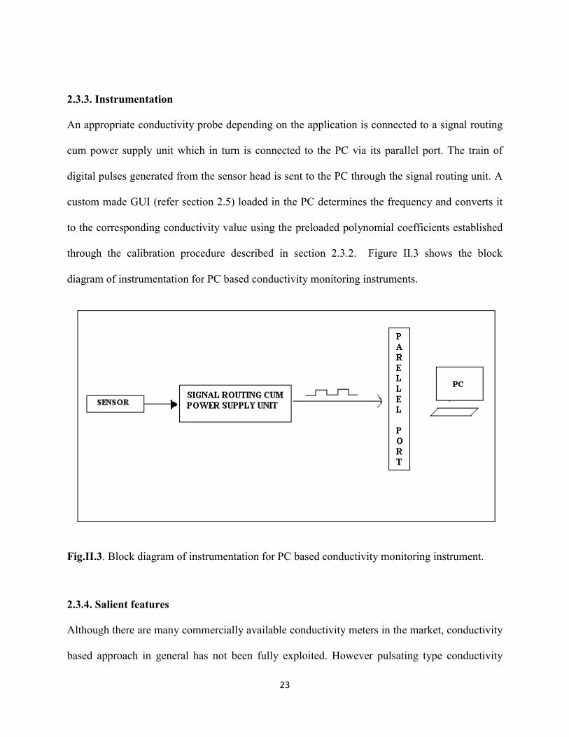
2.3.3. Instrumentation

An appropriate conductivity probe depending on the application is connected to a signal routing

cum power supply unit which in turn is connected to the PC via its parallel port. The train of

digital pulses generated from the sensor head is sent to the PC through the signal routing unit. A

custom made GUI (refer section 2.5) loaded in the PC determines the frequency and converts it

to the corresponding conductivity value using the preloaded polynomial coefficients established

through the calibration procedure described in section 2.3.2. Figure II.3 shows the block

diagram of instrumentation for PC based conductivity monitoring instruments.

Fig.II.3. Block diagram of instrumentation for PC based conductivity monitoring instrument.

2.3.4. Salient features

Although there are many commercially available conductivity meters in the market, conductivity

based approach in general has not been fully exploited. However pulsating type conductivity

24

meters have many salient features which allow these sensors to be deployed in diverse

applications. Some of the salient features are listed below

(i) Simplified instrumentation: Since the output from the probe is transitor-transitor logic

pulses no other pulse conditioning circuits are required. This greatly simplifies the

instrumentation. In comparison the conventional instruments require pre-

amplification, signal conditioning, post amplification and analog to digital converters.

(ii) High resolution and sensitivity: The conductivity probes offer high precision, high

resolution and high sensitivity in measurement.

(iii) Response time: Response time is defined as the time taken by a probe to reach 63% of

the final stable value. The response time of pulsating type conductivity probes are less

than 100 milli seconds and hence they are suitable for carrying out rapid

conductometric titrations.

(iv) Communication to long distances: The instrumentation is capable of transmitting

noise free signal from LGO to long distances (up to 100 meters) without distortion or

loss in the signal quality.

(v) Flexibility in probe design: There is a lot of flexibility in probe design depending

upon the specific application. The oscillator circuit can be either fixed into the probe

head using epoxy resin or it can be placed near the probe.

(vi) PC based titrations: Pulsating conductivity probes are readily compatible with PC as

the signal produced from the probe is directly in the digital domain. Hence they are

highly suitable for carrying out PC based titrations with reduced instrumentation.

(vii) Compatible for field use: Since pulsating conductivity probes work on 5V DC they

are portable and therefore compatible for field use.

25

2.4. EMF based measurements

In the course of this work (refer chapter 3) all EMF measurements were carried out through a PC

although the measurements can also be carried out using a standalone embedded unit. For

carrying out PC based EMF measurements an appropriate probe (combination type pH electrode,

platinum calomel electrodes etc) is connected to a V to f converter which in turn is connected to

the signal routing unit. The V to f device converts the potential of the electrochemical system

under investigation to digital pulses of 5V magnitude. The pulses are communicated to the PC

using an interfacing cable. The GUI described in section 2.5 determines the frequency and

converts it to EMF by applying a conversion factor.

2.5. Graphical user interface for recording titrations

In order to carryout conductometric and potentiometric titrations using pulsating sensors a GUI

was developed in C language [55]. Apart from carrying out titrations the GUI can also be used to

measure conductivity and EMF. The flowchart of the GUI is shown in Figure II.4. The GUI is

designed to handle three pulsating type sensors as the signal routing unit can support a maximum

of three sensors only. The signal routing unit communicates the pulses generated from all the

three sensor heads along with a reference frequency to the PC through an interfacing cable. The

GUI simultaneously counts the pulses received from all the probes for a fixed duration to

determine the frequencies. The frequency values are then plotted in three different channels as a

function of real time. Scaling of axis, choosing appropriate sampling time, conversion of

frequency to the parameter of interest, recording titration plots and other host of features are

further accessed using the online menu keys.

26

Fig.II.4. Flowchart of the graphical user interface.

27

Figure II.5 shows a typical screen capture view of a conductometric titration plot obtained using

the GUI. The first channel shows the real time shift in conductivity while the second channel

shows the number of peaks registered during the course of titration with each peak representing a

fixed aliquot of titrant. The third channel which is earmarked for potentiometric titrations is left

unused. A fourth channel that gets automatically generated after the completion of titration

represents the shift in conductivity in the volume domain. The volume domain plot is generated

using the data registered in the first and second channels. The plot shows four distinct regions

with three endpoints. The end points are obtained by the intersection of least square fitted lines

of adjacent regions while the fitted lines are generated by selecting a pair of points in each

region.

Fig. II.5. Screen capture view of a PC based conductometric titration plot.

28

In the case of potentiometric titrations the first channel is left unused where as channels 2 and 3

are engaged. Channel-3 records the real time shift in EMF while channel-2 records the number of

peaks registered during the course of titration. A fourth channel in volume domain unfolds

immediately after the completion of titration. Figure II.6 shows the screen capture view of a

typical potentiometric titration plot along with the derivative plot. In this particular case the shift

in pH during an acid base titration was monitored using a combination type pH electrode.

Fig.II.6. Screen capture view of a PC based potentiometric titration plot.

29

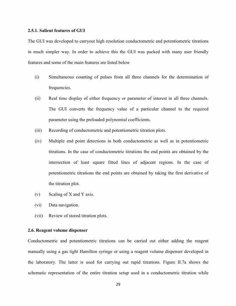
2.5.1. Salient features of GUI

The GUI was developed to carryout high resolution conductometric and potentiometric titrations

in much simpler way. In order to achieve this the GUI was packed with many user friendly

features and some of the main features are listed below

(i) Simultaneous counting of pulses from all three channels for the determination of

frequencies.

(ii) Real time display of either frequency or parameter of interest in all three channels.

The GUI converts the frequency value of a particular channel to the required

parameter using the preloaded polynomial coefficients.

(iii) Recording of conductometric and potentiometric titration plots.

(iv) Multiple end point detections in both conductometric as well as in potentiometric

titrations. In the case of conductometric titrations the end points are obtained by the

intersection of least square fitted lines of adjacent regions. In the case of

potentiometric titrations the end points are obtained by taking the first derivative of

the titration plot.

(v) Scaling of X and Y axis.

(vi) Data navigation.

(vii) Review of stored titration plots.

2.6. Reagent volume dispenser

Conductometric and potentiometric titrations can be carried out either adding the reagent

manually using a gas tight Hamilton syringe or using a reagent volume dispenser developed in

the laboratory. The latter is used for carrying out rapid titrations. Figure II.7a shows the

schematic representation of the entire titration setup used in a conductometric titration while

30

Figure II.7b shows the zoomed in schematic of the volume dispenser. The dispenser is connected

to the second channel of the signal routing unit for carrying out an automated titration. The

dispenser consists of an ordinary medical syringe that is locally available in the market. The

piston that comes along with the syringe is not used in the set up as the reagent is made to fall

under the influence of gravity as distinct drops through the syringe needle. In order to detect the

number of drops falling inside the titration vessel a SS wire is placed adjacent to the needle with

the wire and the needle forming an electrode pair. The wire is placed such that each drop resides

momentarily between the electrodes before getting dislodged. Shorting occurs every time the

drop touches the electrodes and this in turn gives rise to a maximum frequency. The frequency

drops back to a minimum value once the shorting gets discontinued due to the displacement of

the drop from the electrodes. Thus during the course of titration a train of peaks gets registered in

the second channel of the PC screen as drops get formed and dislodged from the electrodes.

Figure II.8 shows a typical titration plot obtained using the automated dispenser with the second

channel showing the distinct peaks. From the figure it is seen that it takes less than a minute to

complete the titration. Unlike in the case of manual addition of reagent, where there is no

constraint in choosing the sampling time, in titrations involving the volume dispenser the data is

sampled for either 0.25 seconds or 0.3 seconds only. This is because the sampling time in an

automated titration is limited by the time taken for a drop to form and arrive inside the titration

vessel and therefore the data has to be sampled before the arrival of the next drop inside the

titration vessel.

31

Fig.II.7a. Schematic representation of a complete conductometric titration facility using the reagent volume dispenser.

Fig.II.7b. Schematic representation of the reagent volume dispenser.

32

Fig. II.8. A typical potentiometric titration plot obtained using the reagent volume dispenser.

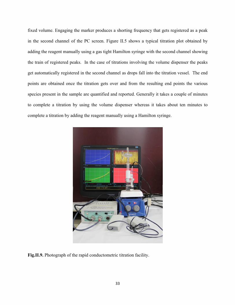
2.7. Conductometric titration facility

The PC based rapid conductometric titration facility consists of a pulsating type conductivity

probe, a signal routing cum power supply unit, a PC loaded with GUI described in section 2.5

and an reagent volume dispenser described in section 2.6. For carrying out a conductometric

titration the conductivity probe is connected to the first channel while the volume dispenser is

connected to the second channel of the signal routing unit. The photograph of the entire rapid

titration facility is shown in Figure II.9. There is also a provision to carryout titrations manually

using a gas tight Hamilton syringe. Manual addition of reagent is followed when high resolution

titration plots are required even in dilute solutions. In such cases the volume dispenser is

disconnected and instead a marker available on the signal routing unit is engaged. In a manual

titration the marker is pressed momentarily just before the addition of each aliquot of reagent of

33

fixed volume. Engaging the marker produces a shorting frequency that gets registered as a peak

in the second channel of the PC screen. Figure II.5 shows a typical titration plot obtained by

adding the reagent manually using a gas tight Hamilton syringe with the second channel showing

the train of registered peaks. In the case of titrations involving the volume dispenser the peaks

get automatically registered in the second channel as drops fall into the titration vessel. The end

points are obtained once the titration gets over and from the resulting end points the various

species present in the sample are quantified and reported. Generally it takes a couple of minutes

to complete a titration by using the volume dispenser whereas it takes about ten minutes to

complete a titration by adding the reagent manually using a Hamilton syringe.

Fig.II.9. Photograph of the rapid conductometric titration facility.

34

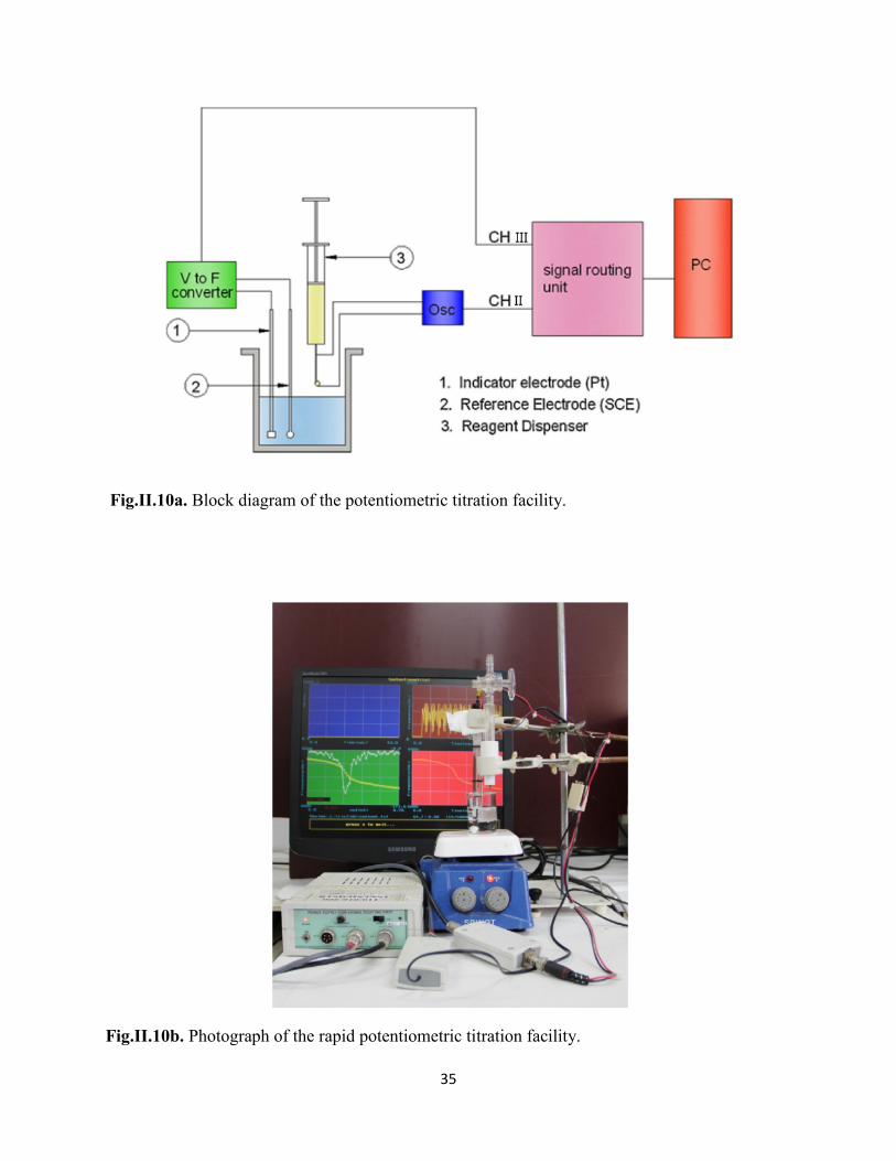
2.8. Potentiometric titration facility

The PC based rapid potentiometric titration facility consists of a suitable reference-indicator

electrode pair, a V to f converter, a power supply cum signal routing unit, a reagent volume

dispenser and a PC loaded with the GUI. Figure II.10a shows the block diagram of the entire

titration setup while Figure II.10b shows its actual photograph. The V to f device converts the

potential of the electrochemical system to digital pulses of 5V magnitude. This approach of

converting the analog output to digital domain simplifies the instrumentation and also makes the

signal compatible to PC. Further there is a provision for EMF measurements at three different

sensitivity ranges namely; X (gain 1), 10X (gain 10) and 100 X (gain 100). The required

sensitivity can be selected through the knob on the signal routing unit.

As in the case of conductometric titrations potentiometric titrations too can be carried out either

manually or using the volume dispenser. Automated titrations are carried out by connecting the

volume dispenser to the second channel of the signal routing unit whereas the marker is engaged

for carrying out manual titrations. Figure II.8 shows a typical potentiometric titration plot

obtained by using the automated dispenser where the end point is obtained by taking the first

derivative of the plot.

35

Fig.II.10a. Block diagram of the potentiometric titration facility.

Fig.II.10b. Photograph of the rapid potentiometric titration facility.

36

2.9. Commercial instruments used in the thesis

During the course of this work many commercial instruments were used in order to validate the

analytical techniques developed using pulsating sensors. The following commercial instruments

were used in this work and a brief description of each device along with its working principle is

presented below.

2.9.1. UV-Visible spectrophotometer

A UV-visible spectrophotometer is used to study the interaction of UV- visible light on the

compound under investigation. The main components of a UV-visible spectrophotometer are a

spectroscopic source (H2, D2, W lamp), a monochromator, a sample cell, a detector and a signal

processor and read out unit [56]. Tungsten filament is used as a source to cover the visible region

whereas a deuterium lamp or hydrogen lamp is used to cover the UV region. UV-Visible

spectrophotometers are of two types, single beam spectrophotometers and double beam

spectrophotometers. Single beam instruments have single light path whereas double beam

instruments have two separate light paths, one for the test solution and another for the blank.

Thus single beam instruments require the interchange of sample and blank solutions for each

wavelength and therefore are better suited to manual than automatic operation [57]. In contrast,

double beam instruments automatically vary the wavelength and record the absorbance as a

function of wavelength and therefore offer more convenience in recording a spectrum. A UV-

Visible instrument can be used for both quantitative as well as qualitative analysis. Quantitative

analyses are performed based on the well known Beer Lambert’s law [58]. The law states that

the absorbance of a solution is linearly related to the concentration (c) of the absorbing species

and the path length (b) of the radiation in the absorbing medium. The relationship is shown

below

37

log (Io / I) = A = ε b c (6)

Where A is the absorbance of the solution, Io is the intensity of radiation before entering the

solution, I is the intensity of radiation emerging from the solution, ε is the molar absorptivity in

mol-1 L cm-1, b is the path length in cm and c is the concentration of solution in mol L-1.

The instrument measures the ratio of intensity of light emerging from the sample (I) to the

intensity of light entering the sample (I0). The ratio is called transmittance and is related to

absorbance by the following formula

A = -log (I / Io) (7)

In the work involving analysis of boron in light water and heavy water by conductometric

titration approach (refer chapter 4), a Thermo make double beam spectrophotometer model

number UV 2600 was used for validation. Standard curcumin spectrophotometric method was

followed to analyze boron [39]. The method involves acidification of sample with hydrochloric

acid and evaporating it to dryness in the presence of curcumin reagent. Heating is carried out at

55oC in a constant temperature bath. This results in the formation of a red rosocyanin complex

which is taken up in iso-propyl alcohol and read spectrophotometrically at 540 nm. In the current

spectrophotometric work all the analysis were carried out in a 10mm path length cell.

2.9.2. Infrared spectrophotometer

An infrared (IR) spectrophotometer Wilks Miran 1A was used to measure the isotopic purity of

heavy water when the concentration of heavy water in the samples exceeded 98% (ref Chapter

5). Mixed rare earth oxide was used as IR source whereas a thermocouple was used as detector.

Generally IR spectroscopy is used when the sample is highly enriched in heavy water (> 88%) or

when the concentration of heavy water in the sample is very low (<9%). In the intermediate

38

ranges (between 9% to 88%) a refractometer is used. An IR spectrophotometer is used to study

the vibrational excitation of bonds by the absorption of infra red radiation. In modern

laboratories three types of spectrophotometers are used, (i) dispersive spectrophotometers, (ii)

Fourier transform spectrophotometers and (iii) filter photometers. The first two are used for

obtaining complete spectra for qualitative identification whereas filter photometers are designed

for quantitative work [59]. Like UV-visible spectrophotometer most of the IR

spectrophotometers have the following components, (i) a source, (ii) a wavelength selector, (iii) a

sample cell, (iv) a detector and (v) a signal processing and read out unit. However the

components of an IR spectrophotometer deviate in many aspects as compared to a UV-Visible

spectrophotometer. Infrared sources are heated solids in place of tungsten or deuterium lamps,

infrared gratings are much coarser, the IR detector responds to heat rather than photons and the

optical components in an IR instrument are constructed out of sodium chloride or potassium

bromide [59]. None the less as in the case of quantitative measurements involving UV-visible

spectroscopy, here too Beer Lambert’s law is used for quantification.

Vibrational absorption occurs in the infrared region where the energy of radiation is insufficient

to excite electronic transitions. Vibrational frequency (ν) of a bond is inversely proportional to

the reduced mass (µ) of the atoms constituting the bond [60]

ν = (1/2π)(k/µ)1/2 (8)

where k is the force constant.

Since O-H and O-D have different reduced masses their vibrational frequencies differ which in

turn causes their characteristic excitation frequencies to be different. O-H shows a characteristic

absorption at 3400 cm-1 while O-D shows a characteristic absorption at 2500 cm-1. In the case of

39

quantitative measurements involving enriched heavy water (>88%) the absorption is measured at

3400 cm-1 whereas in the case of low grade heavy water (<9%) the absorption is measured at

2500 cm-1.

2.9.3. Ion chromatograph

Ion chromatography (IC) is an analytical technique in which anions and cations are separated by

the difference in the rate of migration through a column containing either anion or cation

exchange particles [61]. The ion having the greatest affinity for the column is eluted last while

the ion having the least affinity is eluted first. The instrument is highly useful as a number of

cations or anions can be analyzed simultaneously in a single run within a very short period

(usually less than 30 minutes). IC has been successfully applied to the analysis of ions in many

extremely diverse types of samples. Ions have been determined in difficult matrices such as

toothpaste, brines and caustics apart from much simpler matrices such as potable water and rain

water. The instrument is capable of detecting ions down to a few µgL-1 levels using minimum

sample volume. An IC can be used in a variety of instrument configurations with different

column sets and eluent. Typically an IC consists of an eluent pump, sample injection valve,

separation column, a suppressor coupled to a conductivity detector and, a regenerating pump

with electronic timer and control [62]. In this technique a known volume of sample is introduced

into a mobile eluent stream which carries the sample to the separator column. The analytes get

separated on the column based on their affinity towards the ion exchange particle loaded inside

the column. The affinity is defined in terms of distribution coefficient K, which is simply the

ratio of concentrations of a given component in the stationary phase to that in the mobile phase

[63]. The eluent containing the separated ions pass through a suppressor column before entering

the conductivity detector. The purpose of suppressor column is twofold, (i) it suppresses the

40

background conductivity of the eluent and (ii) it enhances the analyte conductivity. The resulting

chromatogram as recorded by a PC consists of a train of conductivity peaks due to the various

analytes as a function of time. In this technique there are number of parameters which can be

altered to increase the efficiency of separation and to decrease the analysis time, they are (i)

separator column length, (ii) separator column capacity, (iii) eluent strength, (iv) use of organic

modifiers in the eluent, (v) flow rate of eluent and (vi) gradient elution [62].

In the work involving analysis of boron in light water and heavy water by direct conductivity

approach (refer chapter 4), a Dionex make IC model number ICS-1100 was used for validation.

An ion pac IC borate column (9 x 250 mm) was used as the separator column, 2.5 mM methan

sulphonoic acid + 60 mM mannitol acted as eluent, loop volume was 100 micro liters, flow rate

was 1 ml min-1, while no concentrator or suppressor was used [64].

2.9.4. Refractometer

Refraction is a phenomenon in which the direction of light changes as it passes from one medium

to the other. Refraction occurs due to the difference in velocity of light in the two mediums. The

extent of bending of light is determined by the refractive index of the medium and refractive

index in turn is determined using a refractometer. A Karl Zeiss make Abbe refractometer was

used to validate the work involving the isotopic determination of heavy water by conductivity

approach (refer chapter 5). The instrument was used when samples contained heavy water in the

range of 9% to 88%. The instrument consists of a source of monochromatic light, an assembly of

two prisms, and a telescope [65]. A drop of sample is placed between the two prisms forming a

thin film. One prism acts as an illuminating prism while the other acts as a refracting prism. A

light source is projected through the illuminating prism whose bottom surface is roughened in

order to generate light rays travelling in all directions from each point on the surface.

41

Consequently light enters the refracting prism in a variety of angles which is sharply limited by

the critical angle [66].The critical ray forms the boundary between the bright light and dark

portions of the field when viewed through the telescope. This demarking boundary is adjusted to

the cross hairs to read the scale. In order to get quantitative information on the isotopic purity of

heavy water by this technique a calibration plot is generated using known standards of heavy

water and measuring the signal output of each standard. Heavy water concentration and the

signal output obey a linear relationship and this relationship is used to determine the unknown

concentration of heavy water in a sample.