© 2018 Lydia E. Kwon

BIOSENSOR AND ASSAY DEVELOPMENTFOR THE DETECTION OF DISEASE BIOMARKERS

AT THE POINT OF CARE

BY

LYDIA E. KWON

THESIS

Submitted in partial fulfillment of the requirementsfor the degree of Master of Science in Bioengineering

in the Graduate College of theUniversity of Illinois at Urbana-Champaign, 2018

Urbana, Illinois

Adviser:

Professor Brian T. Cunningham

ABSTRACT

Starting with the advent of biosensors in the late 1950s and early 1960s,

biosensors have come to play a major role in various aspects of human life,

including our environment, food and drink, safety, and health. In particular,

the detection of clinically relevant biomarkers for the screening, diagnosing,

and monitoring of diseases such as cancer is an important goal in improving

the treatment outcome and the quality of life of patients. In this thesis,

an overview of biosensors and their applications is followed by a detailed

description of how a photonic crystal biosensor platform with the capacity

for fluorescence enhancement was combined with an automated multiplexed

microfluidic flow system and an automated spot-finding and data genera-

tion algorithm for the detection of a cancer biomarker in human serum and

plasma.

ii

To my family, for their love and support.

iii

ACKNOWLEDGMENTS

First and foremost, I would like to express my gratitude toward my advisor,

Prof. Brian T. Cunningham, for all the support and words of wisdom he

provided me throughout my graduate studies.

I also want to thank the past and present members of the NanoSensors

Group for their helpful discussions and fun times. In particular, I thank

Tiantian Tang, for relaying to me the fundamental knowledge I needed to

start the PCEF project. I also thank Dr. Caitlin Race and Myles Foreman

for their contributions to the project. I especially want to thank Dr. Jui-

Nung Liu, Dr. Yue Zhuo, Dr. Weili Chen, and Qinglan Huang for helping

me to understand how photonic crystals work and for constantly giving me

courage and support.

I would also like to acknowledge my family members and relatives who

have provided me with unending moral, emotional, and spiritual support

during times of difficulty.

I would like to acknowledge financial support from the IGERT fellowship

(National Science Foundation Grant 0965918). In addition, the project was

funded by the National Institutes of Health under Grant 5R33CA177446-02

and Grant 5R01GM086382-03.

iv

TABLE OF CONTENTS

LIST OF TABLES . . . . . . . . . . . . . . . . . . . . . . . . . . . . . vii

LIST OF FIGURES . . . . . . . . . . . . . . . . . . . . . . . . . . . . viii

CHAPTER 1 BIOSENSORS FOR THE DETECTION OFCLINICALLY RELEVANT BIOMARKERS . . . . . . . . . . . . . 11.1 Overview of Biosensors . . . . . . . . . . . . . . . . . . . . . . 1

1.1.1 What is a Biosensor? . . . . . . . . . . . . . . . . . . . 21.1.2 Methods of Transduction . . . . . . . . . . . . . . . . . 41.1.3 Factors to Consider in Biosensor Development . . . . . 81.1.4 Biosensor Applications . . . . . . . . . . . . . . . . . . 12

1.2 Optical Biosensors . . . . . . . . . . . . . . . . . . . . . . . . 131.2.1 Fluorescence as an Optical Signal . . . . . . . . . . . . 141.2.2 Photonic Crystals . . . . . . . . . . . . . . . . . . . . . 171.2.3 Photonic Crystal Enhanced Fluorescence (PCEF) . . . 20

1.3 Biosensors for Medical Applications . . . . . . . . . . . . . . . 221.3.1 Biochemical Assays . . . . . . . . . . . . . . . . . . . . 221.3.2 Clinical Relevance of Biomarkers . . . . . . . . . . . . 251.3.3 Receiver Operating Characteristic (ROC) Curve:

Evaluation of Screening and Diagnostic Tests . . . . . 26

CHAPTER 2 PCEF WITH MICROFLUIDIC INTEGRATIONFOR ANTIVIRAL ANTIBODY DETECTION . . . . . . . . . . . 302.1 Introduction . . . . . . . . . . . . . . . . . . . . . . . . . . . . 30

2.1.1 Human Papillomavirus (HPV) . . . . . . . . . . . . . . 302.1.2 PCEF for the Detection of HPV Oncoproteins . . . . . 34

2.2 Process and Methodology . . . . . . . . . . . . . . . . . . . . 342.2.1 Fabrication of photonic crystals . . . . . . . . . . . . . 342.2.2 Surface modification of the PC . . . . . . . . . . . . . 352.2.3 Bioreceptor Immobilization via Microarray Printing . . 362.2.4 Microfluidic Cartridges . . . . . . . . . . . . . . . . . . 382.2.5 Fluorescence-Linked Immunosorbent Assay (FLISA) . . 402.2.6 Laser Line-Scanning Instrument . . . . . . . . . . . . . 41

2.3 Results and Discussion . . . . . . . . . . . . . . . . . . . . . . 422.3.1 Dose-Response Curves . . . . . . . . . . . . . . . . . . 43

v

2.3.2 Clinical Samples . . . . . . . . . . . . . . . . . . . . . 46

CHAPTER 3 CONCLUSIONS . . . . . . . . . . . . . . . . . . . . . 563.1 Important Considerations . . . . . . . . . . . . . . . . . . . . 56

3.1.1 Improving SNR . . . . . . . . . . . . . . . . . . . . . . 563.1.2 Appropriate Sample Size . . . . . . . . . . . . . . . . . 593.1.3 Improving Specificity . . . . . . . . . . . . . . . . . . . 59

3.2 Concluding Remarks . . . . . . . . . . . . . . . . . . . . . . . 603.2.1 Overview of Results . . . . . . . . . . . . . . . . . . . . 603.2.2 Future Work . . . . . . . . . . . . . . . . . . . . . . . . 60

REFERENCES . . . . . . . . . . . . . . . . . . . . . . . . . . . . . . . 62

vi

LIST OF TABLES

1.1 Contingency table . . . . . . . . . . . . . . . . . . . . . . . . . 27

2.1 Contingency table for PCEF results . . . . . . . . . . . . . . . 502.2 Combination of off- and on-resonance PCEF results . . . . . . 52

vii

LIST OF FIGURES

1.1 General schematic of a biosensor . . . . . . . . . . . . . . . . . 31.2 Calibration curve . . . . . . . . . . . . . . . . . . . . . . . . . 101.3 Diagram of fluorescence . . . . . . . . . . . . . . . . . . . . . 151.4 Schematic of photonic crystals . . . . . . . . . . . . . . . . . . 171.5 Diagram of a 1D photonic crystal . . . . . . . . . . . . . . . . 191.6 Diagram of enhanced excitation and extraction . . . . . . . . . 221.7 Schematic of assays . . . . . . . . . . . . . . . . . . . . . . . . 23

2.1 Photonic crystal . . . . . . . . . . . . . . . . . . . . . . . . . . 352.2 Protein microarray . . . . . . . . . . . . . . . . . . . . . . . . 372.3 Microfluidic cartridges . . . . . . . . . . . . . . . . . . . . . . 382.4 Fluorescence-linked immunosorbent assay (FLISA) . . . . . . 402.5 Laser line-scanning detection instrument . . . . . . . . . . . . 422.6 Dose-response curves . . . . . . . . . . . . . . . . . . . . . . . 442.7 Distribution of enhancement factors . . . . . . . . . . . . . . . 462.8 Plots of clinical results . . . . . . . . . . . . . . . . . . . . . . 482.9 Tables of clinical results . . . . . . . . . . . . . . . . . . . . . 502.10 ROC Curves of Repeats . . . . . . . . . . . . . . . . . . . . . 54

viii

CHAPTER 1

BIOSENSORS FOR THE DETECTION OFCLINICALLY RELEVANT BIOMARKERS

This chapter provides a general overview of biosensors and focuses on their

application in the detection of clinically significant biomarkers. Particular

emphasis will be placed on the general aspects of biosensors and the factors

to consider in their design and development. Furthermore, the fundamentals

of photonic crystal optical biosensors for enhancing fluorescence signals—

the biosensor platform used in the work presented here—will be described.

Finally, the medical applications of biosensors and a method for determining

the diagnostic capacity of such biosensors will also be provided.

1.1 Overview of Biosensors

From the moment we are born, we are bombarded with environmental sig-

nals, generally in the forms of touch, smell, sound, sight, and taste. The

human body is composed of countless receptors which detect and convert

these physical cues into information that can be processed by the brain into

something we can understand. Through this process of sensing, we are able

to feel the softness of silk, smell the delicious aroma of coffee, appreciate

the fluid melody of Chopin, observe the blazing red and deep yellow of the

autumn leaves, and enjoy the tartness of a honeycrisp apple.

Perhaps not as complex as the natural sensors of the human body, but

just as intricate and complicated in their own right, are the manufactured

sensors that we use everyday in our technologically advanced era. Since

around the 1860s when Wilhelm von Siemens built a copper wire resistor to

make temperature measurements—one of the first human-made sensors to be

developed [1, 2]—sensors have played an important role in helping humans

gather information about the environment.

In particular, the advent of biosensors in the early 1960s has led to growing

1

research on the chemical and biological applications of sensors in such fields

as environmental monitoring, the food industry, defense and security, and—

of particular interest here—human health.

1.1.1 What is a Biosensor?

As in the past, no all-encompassing definition seems to exist for the term

“sensor”—an issue stemming from the fact that definitions vary among disci-

plines based on the history of sensor development in the respective fields [1].

In some fields, “sensor” has often been used interchangeably with “trans-

ducer.” Based on the definition established by the Instrument Society of

America in 1975, for example, “transducer” is preferred to “sensor” and

“detector,” and is defined as “a device which provides a usable output in

response to a specific measurand” [3]. Here, the output is limited to an

“electrical quantity” and a measurand to “a physical quantity, property, or

condition which is measured.” However, sensors have since been developed

to measure quantities, properties, and conditions that are chemical (e.g., pH

and concentration) and biological or biomedical (e.g., blood pressure, heart

rate, and oxygen saturation), as well as physical (e.g., mass, pressure, and

luminosity).

For the purposes of this work, we will differentiate between “sensor” and

“transducer.” We will define a sensor very generally, as an instrument or

device which performs two main functions: (1) recognition of an input that

may be physical, chemical, or biological in nature, and (2) transduction—that

is, the conversion of one form of energy to another. In a sensor, the physical,

chemical, or biological input is recognized by a recognition element and

converted by the transducer to another form of energy that is readable or

accessible for further use.

Biosensors are a class of sensors in which the recognition element is

biological in origin [4, 5]. Termed a bioreceptor, the biological recogni-

tion element is selective for the species of interest, called the analyte [6, 7].

The bioreceptor senses a biochemical interaction or change that occurs at

the molecular level, and the transducer(s) converts this biorecognition event

into a measurable signal or readable output.

Examples of bioreceptors include enzymes, antibodies, and nucleic acids,

2

Figure 1.1: General schematic of a biosensor. The bioreceptor recognizes the analyte

in the input sample. This biorecognition event is ultimately converted into a usable or

readable output signal by one or more transducers.

which are inherently selective for specific substrates, antigens, and comple-

mentary strands, respectively. Several biochemical tests, or assays, have been

developed which utilize the biochemical interactions between these biorecep-

tors and their respective analytes. Variations of these assays are often in-

tegrated into biosensors for the detection of small molecules, proteins, and

nucleic acids. This will be described more in Section 1.3.1.

Biosensors are generally developed as alternatives to traditional analytical

methods, which require bulky and expensive instrumentation and which can

also be very time- and resource-consuming. An important goal in biosensor

development is to minimize the overall footprint of the sensor while keeping

it affordable and amenable for use in areas where environmental conditions

and lack of personnel, funds, or other resources make traditional methods

impractical or even impossible. Biosensors exhibit several characteristics

which make them great candidates as alternatives to traditional methods.

First, the bioreceptor lends a natural selectivity for the analyte, precluding

the need to develop complicated and oft-expensive methods of detection. The

biorecognition element and transducer are often integrated onto the surface of

the sensing element, further reducing the footprint. In addition, the sensing

element interfaces with the instrumentation, namely the electronics and the

display. With the proper selection of materials, a biosensor can be designed to

be self-contained, with reliable and inexpensive single-use sensing elements.

This is often preferred over a more expensive and reusable sensor, particularly

in clinical applications, where cross-contamination of samples can be an issue

with reusable sensors.

3

1.1.2 Methods of Transduction

As defined previously, the transducer of the biosensor functions to convert

the biorecognition event occurring at the molecular level on the surface of the

sensing element, to a measurable signal which corresponds to a qualitative

or quantitative measurement of the target analyte. The various transduction

methods may be categorized into the following four groups: mechanical,

calorimetric, electrochemical, and optical [4, 8].

Mechanical Transduction

Mechanical transduction is primarily associated with acoustic biosensors,

which generally utilize a piezoelectric material such as quartz. Mechanical

stress applied to a piezoelectric material is coupled to potential generation,

and vice versa. In a bulk acoustic wave (BAW) biosensor, such as the well-

known quartz crystal microbalance (QCM), a potential is applied across the

surface of a piezoelectric transducer to cause it to vibrate at its resonant fre-

quency, which depends on the mass of the material. When the target analyte

binds to a receptor immobilized on the surface of the piezoelectric transducer,

the addition of mass causes a shift in the frequency, which is usually the mea-

surable output of a QCM biosensor. This change in frequency can then be

used to determine the change in mass and to indirectly determine the type,

count, or concentration of the corresponding analyte. However, there are sen-

sitivity limitations when measurements are performed in aqueous samples as

opposed to air, because the acoustic signal is directed toward the bulk sub-

strate in a BAW sensor. In contrast, a surface acoustic wave (SAW) sensor

remains sensitive even in liquid, due to the fact that the signal propagates

along the surface of the sensor. Micro- and nano-electromechanical systems,

such as microcantilevers, can similarly be used to determine the mass of

analytes that interact with the bioreceptors immobilized on the cantilever

surface. [4, 8, 9]

While mechanical transducers boast high sensitivity (below attograms),

real-time data response, low cost, and small sensor footprint, one major

disadvantage of these transducers is the suboptimal selectivity. Because the

measurements are based on mass differences, special care must be taken in

order to ensure the frequency change is truly due to the analyte of interest.

4

Proper calibration after bioreceptor immobilization, the nature of the sample

medium (i.e., liquid or air), and the presence of non-target molecules are all

factors to consider [9]. Overall, mechanical transducers may be more suitable

for determining the fundamental properties of molecules and for studying

the binding kinetics of molecular interactions, rather than the detection of

biomarkers in complex media.

Calorimetric Transduction

A calorimetric transducer generates a signal in the form of heat in response

to the biochemical recognition event. The catalysis of the analyte by the

bioreceptor, most often an enzyme, generates heat and leads to a temperature

change (∆T ), which is determined by the moles of product (nP ), change in

molar enthalpy (∆H), and the total heat capacity (CS):

∆T = −nP∆H

CS(1.1)

Calorimetric transducers can be as simple as the bioreceptor integrated

with a simple thermistor. Enzyme thermistors, which are usually enzyme-

immobilized columns placed in a flow cell integrated with a thermistor, have

been used to detect as low as 10 µM of physiologically significant compounds

such as glucose, creatine, and urea [10]. However, the type of recognition that

occurs on calorimetric biosensors are limited to those that generate sufficient

heat to be detected, such as enzyme-catalyzed reactions. Furthermore, the

sensitivity demonstrated by these biosensors is relatively low compared to

the other transduction methods discussed. [4, 8, 10]

Electrochemical Transduction

In an electrochemical transducer, the biorecognition event generates a change

in the electrical signal or electrical property of the surrounding medium.

Typically, an electrochemical sensor is based on the three-electrode system,

composed of a reference electrode, counter electrode, and working (or sensing)

electrode. The bioreceptor is usually immobilized on the working electrode,

while the reference electrode provides a stable and well-established potential

and the counter electrode serves to close the circuit. [4, 11]

5

In an amperometric transducer, the voltage applied to the electrode is held

constant, and the biorecognition event results in a measurable change in

current. Bioreceptors such as enzymes, antibodies, and nucleic acid aptamers

have been demonstrated on amperometric biosensors [11–13]. In fact, the

first biosensor, published in 1962 by Clark and Lyons, was an amperometric

biosensor for measuring glucose using the glucose oxidase enzyme [12].

Meanwhile, a constant current is applied in a potentiometric transducer,

and the biorecognition event results in a measurable change in potential.

Biosensors utilizing this type of transducer have commonly been used in

the detection of ions, including hydrogen cations for pH measurements [4].

In addition, bioreceptors such as enzymes, antibodies, oligonucleotides, ion

channels and receptors, cells, and tissue slices, have been used with potentio-

metric sensors for the detection of small molecules (e.g., urea and creatinine),

proteins (e.g., hepatitis B surface antigen and tumor necrosis factor (TNF)),

and nucleic acids [4, 14].

For biosensors utilizing impedance transduction, an alternating current

(AC) voltage is applied, and the flow of charged species results in a mea-

surable in-phase or out-of-phase current response. Alternatively, the change

in sample composition as the analyte interacts with the bioreceptor results

in a measurable change in resistance of the sample. Impedance biosensors

have been used with antibody, protein, oligonucleotide, aptamer, and pep-

tide bioreceptors for the detection of proteins, small molecules, and nucleic

acids. [4, 15]

A biorecognition event in a capacitance transducer results in a change in

the dielectric properties or the thickness of the dielectric layer at the electrode

surface. Capacitive biosensors have been demonstrated for the detection of

small molecules, heavy metals, proteins, oligonucleotides, saccharides, and

microorganisms [16].

Electrochemical sensors directly convert the biochemical signal to an elec-

trical output, making them very amenable to miniaturization and integration

with microelectronic circuits, as exemplified by the commercialized glucose

sensors widely used by diabetic patients today. Prior to miniaturization,

however, electrochemical sensors can be quite unwieldy; the potentiometer

and electrical connections to the reference, working, and counter electrodes

can occupy a relatively large footprint. Furthermore, electrochemical setups

are susceptible to electromagnetic interference and must be enclosed in a

6

Faraday cage to shield from such effects. While electrochemical biosensors

can be very useful for detecting analytes in aqueous solutions, they are also

limited in the fact that the electrodes must always be immersed in solution.

Optical Transduction

Optical transducers convert a biorecognition event into an electromagnetic

(EM) signal, most commonly in the ultraviolet (UV), visible, and infrared

wavelength range. Types of optical measurements enabled by optical trans-

ducers include absorbance, transmittance, reflectance, and luminescence.

The absorbance and transmittance of an absorbing medium describe the

efficiency with which light is absorbed. Absorbance, A(λ), can be used to

calculate the concentration of analyte in the absorbing medium and is given

by the Beer-Lambert Law,

A(λ) = log(I0

If) = ε(λ)lc (1.2)

where λ is the wavelength of interest, and I0 and If are the intensities of the

light beam entering and exiting the absorbing medium, respectively. Further-

more, ε(λ) is the molar absorption coefficient [L·mol−1·cm−1], l is the path

length [cm], and c is the concentration [mol·L−1]. Transmittance, T (λ),

describes the ratio between the intensities of the entering and exiting beam,

T (λ) =IfI0

(1.3)

and is therefore related to the absorbance as follows:

A(λ) = − log T (λ) (1.4)

Meanwhile, reflectance describes the behavior of a beam of light to change

direction at the interface of two different media. The angle of the reflected

beam may be the same as the incident angle of the wave on the surface of the

interface, as in a mirror. Alternatively, the beam may experience diffuse re-

flectance, or scattering of the beam in multiple directions as a consequence of

undergoing multiple reflections and refractions in a non-homogeneous, non-

metallic medium—a common phenomenon in biological specimens.

7

In contrast to absorbance, transmittance, and reflectance—which may be

considered universal optical properties—luminescence is not a property found

in just any molecule. Luminescence describes the spontaneous emission

of radiation from certain molecules or compounds as a result of electronic

or vibrational excitation, without resulting in an increase in temperature

[17]. Luminescent compounds may be organic, inorganic, or organometallic.

Several types of luminescence phenomena exist and include bioluminescence,

chemiluminescence, and photoluminescence.

Bioluminescence is the emission of EM radiation resulting from an in vivo

biochemical reaction. Some well-known examples include the glow of fireflies,

jellyfish, and the milieu of microorganisms which cause ocean water to glow

at night. In fact, luciferase and green fluorescent protein (GFP), two well-

known fluorescent species (termed fluorophores) used widely in biomedical

applications, were originally isolated from fireflies and jellyfish, respectively.

Chemiluminescence is the phenomenon in which photons are emitted as a

result of a chemical reaction such as oxidation. This form of luminescence

has some presence in biosensing applications, such as with the Luminex assay

(Luminex Corp, Austin, TX).

Lastly, photoluminescence includes the phenomena of fluorescence and

phosphorescence, and arises when photons are emitted as a result of light

absorption which excites electrons to a higher energy level. As alluded to

earlier, not all molecules are inherently luminescent and therefore may not be

detected directly. In this case, luminescent labels (particularly fluorophores)

may be attached directly or indirectly to the analyte of interest in order to

make its presence optically detectable. This is a highly researched topic with

extensive applications in biosensing and will be discussed in greater detail in

Section 1.2.

1.1.3 Factors to Consider in Biosensor Development

It is important to characterize the performance of a biosensor in the pro-

cess of evaluating its suitability for a particular application. Depending on

its intended use, it may be appropriate for the biosensor to return a qual-

itative response, reflecting either the presence or absence of the analyte of

interest. For other applications, it may be important for the biosensor to

8

return a quantitative response, outputting the numerical analyte concentra-

tion. In addition, a quantitative result may be used to output a binary

positive-or-negative response based on a predetermined threshold. The fol-

lowing factors are used to describe the performance characteristics of any

biosensor and should be considered during the design and evaluation pro-

cess: selectivity, limits of detection and quantification, dynamic range, linear

range, sensitivity, response time, repeatability and reproducibility, stability,

and lifetime [6–8,18].

Selectivity and Specificity

One of the most important qualities of a good biosensor is its selectivity,

which is the ability of the biosensor to respond to the target analyte in the

presence of other components in the sample. A distinction between selectiv-

ity and specificity is drawn in analytical chemistry, where specificity is the

ultimate form of selectivity—that is, a response is given only to a particular

individual or group of analytes, regardless of the presence of contaminants

or concomitants in the sample [8, 19]. Direct interaction of the other com-

pound(s) with the bioreceptor results in specific interference, while the inter-

action of the non-target compounds with other parts of the sensing element

results in non-specific interference. The selectivity of a biosensor is primarily

determined by the natural selectivity of the bioreceptor for one (or a few)

specific targets. While designing and evaluating a biosensor, it is important

to choose the proper bioreceptor(s) with a sufficiently high selectivity for the

analyte(s) of interest.

Calibration Curve

It is important to establish a calibration curve in the process of evaluating

and characterizing a biosensor in its suitability for detecting a particular an-

alyte. To do so, the biosensor is interrogated with a range of different known

concentrations of the target of interest, and the response of the biosensor to

the range of doses of analyte is represented in a graph. When the proper

range of concentrations is tested, the resulting dose-response curve generally

follows the shape of a sigmoidal curve. The lower end of such a dose-response

curve consists of concentrations below the limit of detection (LOD), mean-

9

Figure 1.2: Calibration curve.

ing that the signal output is virtually indistinguishable from a blank sample.

The LOD is defined as the lowest concentration of the target analyte that can

be distinguished from the background or blank by the biosensor. The output

value corresponding to the LOD (yLoD) is given as k standard deviations

(σblank) above the mean (µblank) output for the blank sample [8]:

yLOD = µblank + kσblank (1.5)

where k corresponds to the desired confidence level. Generally, LOD is often

determined from the output value which corresponds to three standard de-

viations above the mean output of the blank or background—that is, k = 3

in the above equation—corresponding to a 99.7% confidence interval [8, 18].

The value above which the analyte concentration can be determined reliably

is called the limit of quantification (LOQ), and the output value corre-

sponding to the LOQ (yLOQ) is given as ten standard deviations above the

mean output of the blank sample [8]:

yLOQ = µblank + 10σblank (1.6)

Meanwhile, the upper portion of a sigmoidal dose-response curve represents

the saturation point of the biosensor, and the highest evaluated concentration

for which the output value is quantifiable, is the upper limit of detection. The

dynamic range of the biosensor is given by the ratio of the upper and lower

limits of detection. Generally, a biosensor should have a dynamic range of

at least one order of magnitude [8]. The linear region that lies between the

10

lower limit of detection and the saturation point of the calibration curve is

the linear range of the biosensor, in which the output signal is proportional

to the analyte concentration. In general, the output signal y in this region is

given by a linear equation:

y = mc+ y0 (1.7)

where c is the analyte concentration and the slope m corresponds to the

sensitivity of the biosensor. Explicitly, sensitivity describes the change in

the output signal in response to a unit change in the target analyte. If the

linear region encompasses the concentration near zero, then the y-intercept

y0 is the output signal for the blank or background.

Response Time

The time it takes to reach a “practically constant value” in response to the

exposure of analyte to the sensor [8], or 63% of its final output value in

response to a step change in analyte concentration [7], is the response time

of the biosensor. The response time is an important factor in determining the

overall time for a sensor to perform sequential analysis of a series of samples.

While fundamental limitations may exist due to the physicochemical process

occurring in the biorecognition event, certain factors such as diffusion limits,

can be overcome through, for example, the incorporation of convection or

mixing.

Reliability

The reliability of a biosensor is determined by its precision and accuracy.

Precision describes the ability of the sensor to return a statistically accept-

able response to the same sample over multiple separate tests, while accuracy

describes how close the result indicated by the sensor is to the true value.

Furthermore, the repeatability of a biosensor describes its ability to return

a statistically similar output over multiple measurements under the same

conditions, while a biosensor demonstrates reproducibility if it is able to

give a precise and accurate response to the same sample under different con-

ditions. In addition to precision and accuracy, it is important for a biosensor

to exhibit good stability and lifetime in order for results to be repeatable and

11

reproducible. A biosensor with good stability suffers insignificant change in

the baseline signal (drift) or the sensitivity of the sensor in a given amount

of time. Furthermore, the lifetime describes the period of time for which

the biosensor returns a reliable response without significant loss of its afore-

mentioned performance characteristics.

To summarize, any good biosensor is highly selective for the analyte of

interest, has a relatively wide dynamic range—at least spanning an order

of magnitude [8]—with a linear range covering the relevant analyte concen-

trations and demonstrates high reproducibility between measurements. In

addition, a biosensor designed for early detection and screening of a disease,

when the analyte of interest tends to be present in low concentrations [20],

would benefit from high sensitivity and a low LOD. Furthermore, a biosensor

should be properly designed for a suitable lifetime, and the stability of the

biological component(s) of the biosensor should be accounted for, depend-

ing on the final application of the biosensor. In order to achieve this, it is

important to choose a suitable bioreceptor that is highly selective for the an-

alyte of interest. It is important that the bioreceptor is properly immobilized

and that its conformation and/or functionality, which affect the selectivity

of biological molecules, is minimally compromised.

1.1.4 Biosensor Applications

Since the first reported biosensor in the early 1960’s [12], biosensors have

been developed for numerous applications to serve as more cost-effective and

rapid alternatives to traditional analytical methods such as those involving

liquid and gas chromatography, mass spectrometry, and microbial culture.

Electrochemical, optical, and piezoelectric biosensors incorporating anti-

bodies, enzymes, aptamers, and even microorganisms as bioreceptors have

been used for the detection of toxic gases, pollutants, and toxic small molecules

for environmental applications [21–25].

The food and drink industry has utilized mainly electrochemical and some

optical sensors for determining the nutritional content, freshness, and con-

tamination by pathogens of consumable products using enzymes, antibodies,

and nucleic acids as sensing elements [24–27].

Beside these, one major application of biosensors has been in the field of

12

healthcare for the purpose of detecting and quantifying physiologically and

clinically relevant analytes, termed biomarkers. Even the first published

biosensor referenced earlier, which utilized the glucose oxidase enzyme for

detecting glucose, has been developed and commercialized for monitoring

glucose, particularly in diabetic patients [28,29]. Micro- and nanotechnology

have made the glucose biosensor extremely user-friendly, returning an almost

instantaneous readout of the glucose concentration from a needle-stick of

blood. The glucose sensor is self-contained in a small handheld device and

serves as a prime example of the potential of biosensors for biomedical and

clinical applications.

More recent advances in biosensors for applications in healthcare include

the detection of protein, nucleic acid, and cellular biomarkers from blood,

sputum, and urine for cancer, bacterial and viral pathogens, and biological

toxins [25, 30–35]. Smartphone biosensors which can be used in limited-

resource healthcare settings have also been demonstrated [36, 37]. Further-

more, biosensors have also been developed for the purposes of elucidating the

fundamental properties of cells—such as cell mass and density rate [38, 39],

cell-cell interactions [40], and cell-matrix interactions [41, 42]—which may

prove useful for developing pharmaceutical drugs for the treatment of dis-

eases. The different types of biochemical assays used with biosensors for

the purpose of screening, diagnosing, and monitoring diseases, as well as a

method for evaluating the quality of such biosensors against gold standard

references will be described in greater detail in Section 1.3.

1.2 Optical Biosensors

As discussed previously, optical biosensors employ optical transducers which

convert the biorecognition event into an optical signal such as absorbance,

transmittance, reflectance, or luminescence. An optical sensor may involve

a label which performs the optical transduction, or it may be label-free by

utilizing certain optically active sensing surfaces.

Optical measurements involving the absorption or emission of a photon by

a component of the sensing surface at a specific wavelength often requires

a label which performs the optical transduction. This is often achieved by

directly labeling the analyte with a molecule that generates an optical signal,

13

such as a fluorophore or chromophore. Another method is to associate the

analyte with a biological transducer, such as an enzyme, which acts on a

chromogenic reagent to generate a color change, as is the case with the well-

established enzyme linked immunosorbent assay (ELISA).

Label-free optical biosensors function by monitoring shifts in the optical

signal that occur due to changes in the physical properties of a sensing surface

due to its interactions with the analyte. This generally involves the use

of optical waveguides, as with photonic crystal (PC) biosensors and those

sensors utilizing surface plasmon resonance (SPR) [35,43].

This work utilizes an optical sensor that integrates concepts from both the

labeled and label-free methods. Specifically, bioreceptors were immobilized

upon a photonic crystal surface. While the ability of a photonic crystal in

responding to changes in the refractive index of the surface medium could be

used for label-free detection, its properties were used to enhance the signal

achieved from a fluorophore which was used to indirectly label the analyte.

This method, termed photonic crystal enhanced fluorescence (PCEF), will be

described in detail later in this section. First, let us begin with an overview

of the concept of fluorescence.

1.2.1 Fluorescence as an Optical Signal

Fluorescence is a subcategory of photoluminescence, which involves the ab-

sorption and emission of photons based on the transition of electrons of

photoluminescent species between different electronic energy states, and also

encompasses the phenomena of phosphorescence and delayed fluorescence.

Fluorescence is the phenomenon that occurs when an excitable electron in

a molecule absorbs energy from a photon, causing it to enter a higher energy

electronic state. In the process of returning to the ground state energy level,

the electron emits a photon with an equal or lower energy than what was

absorbed. A molecule that exhibits fluorescence is called a fluorophore.

Mechanism for Fluorescence

Upon absorbing energy in the form of a photon, a fluorophore may experience

changes in its electronic, vibrational, and rotational states. The Jablonski

diagram is commonly used to depict the different energy states of a molecule

14

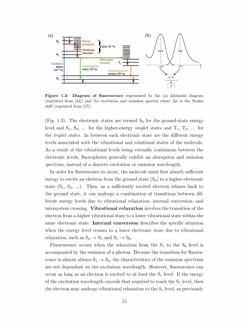
Figure 1.3: Diagram of fluorescence represented by the (a) Jablonski diagram

(reprinted from [44]) and (b) excitation and emission spectra where ∆v is the Stokes

shift (reprinted from [17]).

(Fig. 1.3). The electronic states are termed S0 for the ground-state energy

level and S1, S2, ... for the higher-energy singlet states and T1, T2, ... for

the triplet states. In between each electronic state are the different energy

levels associated with the vibrational and rotational states of the molecule.

As a result of the vibrational levels being virtually continuous between the

electronic levels, fluorophores generally exhibit an absorption and emission

spectrum, instead of a discrete excitation or emission wavelength.

In order for fluorescence to occur, the molecule must first absorb sufficient

energy to excite an electron from the ground state (S0) to a higher electronic

state (S1, S2, ...). Then, as a sufficiently excited electron relaxes back to

the ground state, it can undergo a combination of transitions between dif-

ferent energy levels due to vibrational relaxation, internal conversion, and

intersystem crossing. Vibrational relaxation involves the transition of the

electron from a higher vibrational state to a lower vibrational state within the

same electronic state. Internal conversion describes the specific situation

when the energy level crosses to a lower electronic state due to vibrational

relaxation, such as S2 → S1 and S1 → S0.

Fluorescence occurs when the relaxation from the S1 to the S0 level is

accompanied by the emission of a photon. Because the transition for fluores-

cence is almost always S1 → S0, the characteristics of the emission spectrum

are not dependent on the excitation wavelength. However, fluorescence can

occur as long as an electron is excited to at least the S1 level. If the energy

of the excitation wavelength exceeds that required to reach the S1 level, then

the electron may undergo vibrational relaxation to the S1 level, as previously

15

discussed. A caveat to note here is that, shining just any high-excitation

wave upon a fluorophore will not result in fluorescence. The absorption and

emission spectra of a fluorophore most often appear as a curve with a peak ex-

citation or emission wavelength—the difference of which is called the Stokes

shift, ∆v (Fig. 1.3(b)). More accurately, the Stokes shift is represented in

wavenumbers (v), which is the reciprocal of wavelength (v = 1λ).

The reason for the absorption and emission spectra is because the molecu-

lar bonds of the fluorophore have a resonance condition that can only be met

(to different degrees) by a specific range of wavelengths. These parameters

depend on the chemical structure of the fluorophore, with certain chemical

groups causing red- or blue-shifts in the spectra. Generally, the electrons

of fluorophores with higher efficiency have a higher degree of conjugation—

alternating single (σ) and double (π) bonds—which results in the delocaliza-

tion of electrons. The efficiency of a fluorophore is measured by the quantum

yield, given as the ratio of the number of emitted photons to the number of

absorbed photons, and describes the total amount of light emission over the

entire fluorescence spectral range of the fluorophore. [17,44]

Photobleaching and Other Effects

Unfortunately for fluorescence applications, fluorescence is not the only way

in which a fluorophore may return to the ground state. Intersystem cross-

ing involves the forbidden transition of an electron from the first level of the

singlet state (S1) to the first level of the triplet state (T1). This occurs if

the vibrational energy levels between the two states are the same and the

spin state of the electron is reversed from its original spin state. Once a

molecule has undergone intersystem crossing, it may eventually (1) return

to the ground state without photon emission, (2) return to the ground state

from the triplet state, accompanied by photon emission, termed phosphores-

cence, or (3) undergo another forbidden transition back to the S1 level and

return to the ground state accompanied by photon emission, termed delayed

fluorescence. The molecule may also absorb additional energy while in the

T1 state, exciting it to a higher triplet state and further delaying its return

to ground state. Overall, compared to the fluorescence phenomenon which

takes on the order of nanoseconds to occur, the time for non-fluorescent phe-

nomena to occur is predominantly determined by the lifetime in the T1 state,

16

which can be anywhere from microseconds to tens of seconds [17].

This may pose a possible issue for fluorescence detection instruments which

employ line scanning, which involves scanning a surface with an excitation

illumination line [44]. If a fluorophore is trapped in the triplet state during

the short time in which that region is being excited and the emission intensity

is being collected, no signal will be captured from the trapped fluorophore.

While this may be less of an issue in ensemble studies, it may be an important

consideration for single-molecule fluorescence studies.

Photobleaching is a result of molecular degradation which renders the

fluorophore permanently non-fluorescent, though the causes of photobleach-

ing are yet to be fully elucidated. It is possible that certain chemical reac-

tions, facilitated by the interaction of molecular oxygen (O2) with the fluores-

cent species trapped in the triple state, may cause permanent changes in the

fluorophore structure via covalent bonding, which render it incapable of flu-

orescence [44]. Most reversible photobleaching effects, however, are believed

to be due to molecules trapped in the T1 state, as discussed previously [44].

Some of the effects of photobleaching may be minimized or delayed by the

use of reducing agents which compete with molecules in the T1 state to react

with O2.

1.2.2 Photonic Crystals

Photonic crystals (PCs) are nanostructures composed of alternating high and

low refractive index dielectric materials with the periodicity extending in one,

two, or three dimensions (Fig. 1.4). The detailed theory behind PCs can be

found in [45], while one-dimensional (1D) PCs, of the kind used in this work,

have been expounded in previous graduate theses [46–48]. Based on these

references, the basic principles behind the multilayer 1D PC is provided here.

Figure 1.4: Schematic of photonic crystals with the periodicity of the alternating

high and low refractive indices (indicated by the different colors) extending in (a) one,

(b) two, and (c) three dimensions. Adapted from [46].

17

The Layers of a 1D Photonic Crystal

The multilayer 1D PC used in this and other similar works is composed of

an optional substrate layer and the cavity and slab layers (Fig. 1.5). The

substrate mainly functions as the base upon which the other two layers are

fabricated, and has a refractive index of n3. The substrate has generally

been composed of quartz [49], glass [42, 50], or silicon [30–32]. The cavity

layer is composed of a dielectric material with a low refractive index, n2.

Materials such as quartz, ultraviolet-curable polymer (UVCP), and silicon

dioxide (SiO2) have previously been used. This layer functions as a cavity

in which Fabry-Perot resonance occurs; the refractive index value and cavity

thickness (tc) are important parameters for this phenomenon. In addition,

the cavity layer is comprised of a grating structure with a grating period

Λ. Other important parameters of the grating include depth, fill-factor,

and angle. The slab layer, which functions as the guided-mode layer, is

composed of a dielectric material with a high refractive index, n1, and a

thickness, ts. The material for the slab has generally been titanium dioxide

(TiO2). The slab layer also has a grating structure of the same period Λ as

the cavity layer, though the other parameters may differ due to limitations in

the fabrication process. Lastly, though it is not fabricated per se to be part

of the multilayer 1D PC, certain parameters of the surrounding medium,

such as the refractive index, are carefully considered when designing the PC.

The resonance condition of the 1D PC is designed to match an EM wave of

a specific wavelength that is incident on the surface at a particular angle.

These values depend on the refractive index of the medium (n0), which is

generally lower than that of the slab layer, virtually making this a fourth

layer in the multilayer 1D PC with alternating low and high refractive index

dielectric materials.

Properties of a 1D Photonic Crystal

The multilayer 1D PC utilizes diffraction gratings, total internal reflection,

guided-mode resonance, and Fabry-Perot reflections to achieve a high quality

factor (Q factor) as a resonator. The important parameters in matching

the resonance condition of a particular PC are the wavelength, angle, and

polarization of the incident EM wave in the surrounding medium.

18

Figure 1.5: Diagram of a 1D photonic crystal with the substrate (RI = n3), cavity

(RI = n2) of thickness tc, and slab (RI = n1) of thickness ts, with the coupling wavelength

coming from the surrounding medium (RI = n0). RI = refractive index.

The diffraction grating functions to phase-match, or couple, a specific

EM wave whose properties fulfill the resonance conditions of the PC, into

the PC. The period (Λ) of the diffraction grating required to have only the

zeroth- and first-order diffraction is given by

Λ <λ0

n2

(1.8)

where λ0 is the illumination wavelength in the surrounding medium. This

relation is based on three assumptions. First, it assumes that the angle of

incidence for the resonance condition is normal to the surface. Second, the

angle of the transmitted first-order diffraction is greater than the critical

angle at the top and bottom boundaries of the slab layer, satisfying the

conditions for total internal reflection (TIR). Lastly, the refractive index

of the surrounding medium (n0) is lower than that of the cavity layer (i.e.,

n0 < n2). Based on these assumptions, it is clear from this relationship that

the distance of the grating period must be sub-wavelength.

Once the first-order diffracted EM wave transmits into the slab layer, it

becomes trapped in the slab due to TIR, and the slab layer functions as a

leaky guided-mode resonator (GMR). The transmitted first-order diffrac-

tion wave propagates along the slab waveguide, but does not continue forever

and eventually leaks out of the resonator. As a result of the propagation of

the wave in the GMR, an evanescent field—an EM field whose intensity de-

cays exponentially—is generated outside the slab layer, at both the top and

bottom interfaces. The thickness of the slab layer is designed to contain the

19

zeroth order mode while precluding higher order modes which may occur with

the transverse electric (TE) or transverse magnetic (TM) polarization. The

resonant response resulting from TM polarization has been demonstrated

to have a higher Q factor when compared to TE polarization, based on a

narrower linewidth.

Lastly, the multiple Fabry-Perot reflections of the PC depend on the

thickness of both the slab and cavity layers, as well as the refractive indices of

each layer in the multilayer PC. In the slab and cavity layers, the Fabry-Perot

reflection may cause some of the transmitted EM wave from the previous layer

to be reflected and transmitted back out of the PC in an angle-dependent

direction. In general, PCs intended for use with instrumentation in which the

detection optics are located directly above the PC, are designed to re-direct

the EM wave back out at normal incidence.

In summary, the PC is highly sensitive to the wavelength, angle of inci-

dence, and polarization of the illumination source. The 1D PCs discussed

here are designed with a diffraction grating with a sub-wavelength grating

period that permits a pre-determined wavelength of light to couple into the

waveguide layer of the PC at normal incidence. It is preferable for the inci-

dent EM wave to be TM-polarized in order to maximize the Q factor. The

diffracted TM-polarized wavelength is transmitted into the slab layer which

acts as a waveguide, resulting in high-density evanescent fields at the top

and bottom interfaces of the slab layer. Meanwhile, some of the transmitted

EM waves are reflected back out at normal incidence from the slab and cav-

ity layers due to Fabry-Perot reflection. Peak signal intensities up to 8000

times of that achievable with a non-nanostructured surface such as glass have

been reported using PCs following similar design parameters [30]. The high

Q factor of PCs corresponds to a higher EM field density on the surface

and is desirable in applications such as label-free detection and fluorescence

enhancement [35,42].

1.2.3 Photonic Crystal Enhanced Fluorescence (PCEF)

PCs may be used to enhance the overall fluorescent signal near the surface of

the PC via two independent mechanisms. First, the high-density evanescent

field generated at the surface of the PC as a result of the GMR of a TM-

20

polarized wave can serve to achieve the enhanced excitation of fluorescent

species within the average decay length of the evanescent field (Fig. 1.6(a)).

This requires the PC to be designed such that the diffraction grating allows

the excitation wavelength of the fluorophore to be coupled into the waveg-

uide. The effect of the enhanced excitation mechanism can be harnessed

by illuminating the surface with the specified wavelength and polarization,

at the proper incidence angle. That is, the enhanced excitation is an effect

achievable only when the illumination matches the resonance conditions of

the PC; therefore, it is called the on-resonance condition.

Second, the PC can also be designed to promote the enhanced extrac-

tion of emitted photons by redirecting some of the emitted photons normal

to the surface, in the direction of the collection instrument, via Fabry-Perot

reflection. The enhanced extraction mechanism is a result of the inherent

property of the PC and is, therefore, always active, regardless of the nature

of the illumination. In other words, the enhanced extraction is indepen-

dent of the resonance condition of the PC and is therefore referred to as the

off-resonance condition.

The enhancement factor (EF) is a useful quantity used to compare the

fluorescence intensities achieved under different conditions:

EF =I

Iref

(1.9)

When acting simultaneously, the effects of enhanced excitation and enhanced

extraction are compounded and have demonstrated enhancement factors of

up to 7500× [49]. Here, the total enhancement contributed by the two

enhancement mechanisms is calculated by comparing the intensity of the

fluorescent species in the on-resonance condition to the intensity of the same

fluorescent species on a “normal” surface, such as an unpatterend glass slide

(EFtot = Ion

Iglass). The individual contribution of enhanced excitation can be

calculated by comparing the intensities at on-resonance and off-resonance

(EFon = Ion

Ioff), and the individual contribution from the enhanced extraction

mechanism can be obtained by comparing the off-resonance intensity with

the intensity on the reference material (EFoff = Ioff

Iref)

The enhancing mechanism of the PC makes it a desirable candidate for

optical biosensing applications and have been used for the detection of pro-

teins [31, 32,49], nucleic acids [30], and cellular components [50].

21

Figure 1.6: Diagram of (a) enhanced excitation and (b) enhanced extraction. Reprinted

from [48].

1.3 Biosensors for Medical Applications

Interest in the discovery of new biomarkers has grown over the last decade or

so, along with the development of more sensitive and specific biosensors for

clinical applications. In particular, various biosensors have been developed

in the past for the purposes of screening, diagnosing, and monitoring dis-

eases through the detection of biomarkers. These biosensors utilize various

biochemical assays in order to detect specific analytes. Some of these assays

are described below.

1.3.1 Biochemical Assays

Biochemical assays for medical applications serve to detect the presence of an

analyte through the use of biochemical molecules and their interactions with

one another. In general, these can involve affinity-based recognition between

antigen and antibody or target and aptamer, enzyme-substrate reactions,

and nucleic acid hybridization (Fig. 1.7). The samples tested in these assays

may be the purified analyte in buffer, or the analyte in a complex biological

medium such as blood, urine, or sputum. Some assays may incorporate

live cells and monitor the production of analyte in real-time, as with the

interferon-gamma release assays (IGRA) [40]. Analytes detected using these

methods may be small molecules, proteins, nucleic acids, organelles, and

whole cells [51].

22

Figure 1.7: Schematic of the interactions that occur in the biochemical assays for (a)

antigen and antibody, (b) enzyme and substrate, (c) hybridization of nucleic acid strands,

and (d) target and aptamer. Adapted from [8] and [40].

Immunoassays

Assays based on antigen-antibody recognition are termed immunoassays

based on the fact that antibodies are products of the immune response to

antigens. While there are a spectrum of antibodies, also called immunoglob-

ulins (Ig’s), which play different roles in the various stages of the immune

response to various antigens, the ones most often utilized in immunoassays

are immunoglobulin G (IgG). IgG comprises the majority of the population of

antibodies found in serum, which refers to the non-cellular and non-clotting

components of blood. The general form of IgG is composed of two heavy and

two light chains, with the two arms of the antibody (the Fab region) contain-

ing the variable regions which bind to the antigen; therefore, a single IgG

has the capacity to bind two antigenic sites—either two individual antigens

or two antigenic sites on the same large antigen (such as a bacterium). The

“pole” region (Fc) of IgG is species-conserved, meaning that members of the

same species exhibit the same Fc region while members of different species

will exhibit a different Fc region. Antibodies of one species against another

are generated against the Fc region.

23

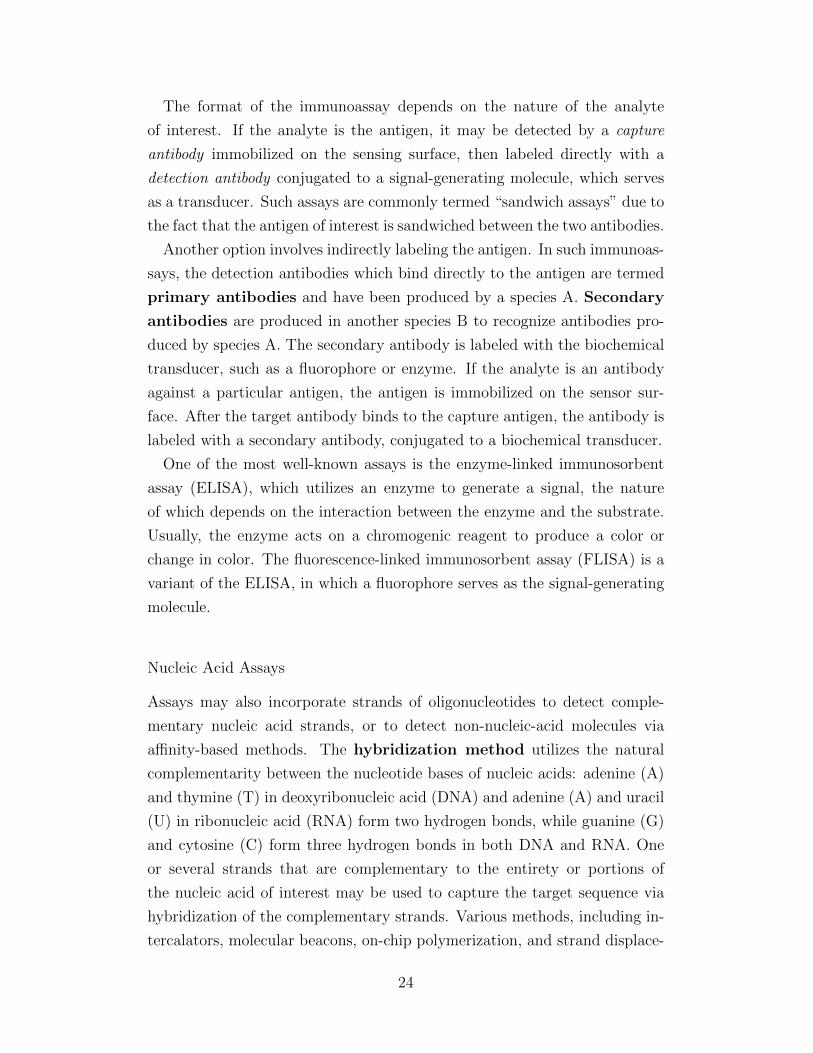
The format of the immunoassay depends on the nature of the analyte

of interest. If the analyte is the antigen, it may be detected by a capture

antibody immobilized on the sensing surface, then labeled directly with a

detection antibody conjugated to a signal-generating molecule, which serves

as a transducer. Such assays are commonly termed “sandwich assays” due to

the fact that the antigen of interest is sandwiched between the two antibodies.

Another option involves indirectly labeling the antigen. In such immunoas-

says, the detection antibodies which bind directly to the antigen are termed

primary antibodies and have been produced by a species A. Secondary

antibodies are produced in another species B to recognize antibodies pro-

duced by species A. The secondary antibody is labeled with the biochemical

transducer, such as a fluorophore or enzyme. If the analyte is an antibody

against a particular antigen, the antigen is immobilized on the sensor sur-

face. After the target antibody binds to the capture antigen, the antibody is

labeled with a secondary antibody, conjugated to a biochemical transducer.

One of the most well-known assays is the enzyme-linked immunosorbent

assay (ELISA), which utilizes an enzyme to generate a signal, the nature

of which depends on the interaction between the enzyme and the substrate.

Usually, the enzyme acts on a chromogenic reagent to produce a color or

change in color. The fluorescence-linked immunosorbent assay (FLISA) is a

variant of the ELISA, in which a fluorophore serves as the signal-generating

molecule.

Nucleic Acid Assays

Assays may also incorporate strands of oligonucleotides to detect comple-

mentary nucleic acid strands, or to detect non-nucleic-acid molecules via

affinity-based methods. The hybridization method utilizes the natural

complementarity between the nucleotide bases of nucleic acids: adenine (A)

and thymine (T) in deoxyribonucleic acid (DNA) and adenine (A) and uracil

(U) in ribonucleic acid (RNA) form two hydrogen bonds, while guanine (G)

and cytosine (C) form three hydrogen bonds in both DNA and RNA. One

or several strands that are complementary to the entirety or portions of

the nucleic acid of interest may be used to capture the target sequence via

hybridization of the complementary strands. Various methods, including in-

tercalators, molecular beacons, on-chip polymerization, and strand displace-

24

ment, have been used to transduce and amplify this molecular event [33]. In

the affinity-based method, nucleic acid aptamers may be synthesized to

exhibit binding affinities to proteins and small molecules. Aptamers, being

made of nucleic acids, are more stable than antibodies or proteins which are

prone to denaturation, and when properly designed, can exhibit very high

affinity for their targets and has been used as bioreceptors for small molecules

and proteins [33,40].

1.3.2 Clinical Relevance of Biomarkers

In the broadest sense of the term, biomarkers are objectively measurable

markers which hold physiological, pathological, or pharmacological signifi-

cance [51]. As such, biomarkers may refer to measurements such as blood

pressure, oxygen saturation, and electrocardiograms. More recently, however,

biomarkers have come to refer to molecular biomarkers such as certain

small molecules, proteins, genes and gene fragments, transcripts, and cells

and cell fragments which have clinical implications. Examples of molecular

biomarkers currently in use include glucose for diabetes monitoring, cardiac

troponin for cardiac arrest, and interferon gamma release for tuberculosis

infection (QuantiFERON IGRA). Valid biomarkers demonstrate their sig-

nificance in providing insight as to the etiology and pathomechanism of the

disease, detecting the presence or absence of disease, predicting prognosis, or

determining the effect of therapy. Ultimately, the goal is to use the informa-

tion provided by the biomarker to improve the clinical outcome, perhaps in

the form of an increased survival rate and/or improved quality of life. Var-

ious new potential biomarkers for infectious and non-infectious diseases are

being discovered and tested for this purpose.

Non-Intrusive Sample Collection

Often, the focus in chronic diseases, such as cancer, is placed on screening

and diagnosing the type of cancer, or monitoring the treatment efficacy.

Though the focus here will primarily be on biomarkers related to cancer

screening, diagnosis, and monitoring, the general concept may be applied to

other diseases as well.

25

The “gold standard” for cancer diagnosis generally involves a biopsy, an

invasive procedure involving the removal of a sample of the suspected tumor.

Though the study of a biopsy specimen may provide useful histological and

genetic information, its repeated use in serial sampling to, for example, mon-

itor treatment efficacy is highly impractical. In the case of screening, when it

is possible that the tumor is benign, an invasive procedure such as a biopsy

might be considered sub-optimal. While it has been shown that a positive

prognosis is highest during the earliest stages of cancer, this also corresponds

to the lowest likelihood of a palpable tumor to be biopsied [20,52,53]. Unlike

the traditional biopsy, a liquid biopsy involves the detection of biomarkers

within bodily fluids—such as blood, saliva, or urine—that can be obtained

in a non-intrusive manner [54]. It is now widely accepted that panels of

biomarkers, rather than single biomarkers, are required for reliable cancer

identification and patient stratification [20]. Microarrays of various biorecep-

tors to a panel of biomarkers may be integrated with a microfluidic platform

that utilizes a liquid biopsy sample for potential use in point-of-care (POC)

testing. POC tests occur at the bedside or home of the patient or a limited-

resource setting instead of a specialized laboratory, can dramatically reduce

time and cost, and are especially suited for the purposes of screening and

monitoring diseases.

1.3.3 Receiver Operating Characteristic (ROC) Curve:Evaluation of Screening and Diagnostic Tests

The receiver operating characteristic (ROC) curve is a method used to as-

sess the validity of a diagnostic tool compared to an existing gold standard,

which may be another diagnostic assay or the disease state as determined by

a traditional method such as biopsy [55, 56]. When comparing a new diag-

nostic method against a more established diagnostic assay based on a binary

(positive or negative) outcome, the sensitivity and specificity values vary

depending on the threshold above which the result is considered positive.

The test results of a newly proposed diagnostic method are compared to

the results obtained using the gold standard method in order to evaluate

its reliability as a diagnostic method. The number of positive test results

that correspond to an “actual” positive, as determined by the gold standard,

26

Reference

R+ R−

Test T+ True Positive

(TP)False Positive

(FP)PPV = TP

TP+FP

T− False Negative(FN)

True Negative(TN)

NPV = TNTN+FN

Se = TPTP+FN Sp = TN

TN+FP

Sensitivity Specificity

Table 1.1: Contingency Table

is called the number of true positives (TP). The number of positive test

results that are actually negative are termed false positives (FP). The total

number of positive results given by the test is the sum of the true and false

positives (T+ = TP + FP). The number of true negatives (TN) is given

by the number of negative test results which correspond to actual negative

results, while the number of false negatives (FN) is given by the number of

negative results that are actually positive. The sum of the positive and false

negatives is the total number of negative test results (T− = TN + FN). The

sum of the true positives and false negatives represents the total number

of actual positives as determined by the reference (R+ = TP + FN), and

the total number of actual negatives are given by the sum of true negatives

and false positives (R− = TN + FP). This can be nicely organized in a

contingency table, as shown in Table 1.1.

Important indicators that help with interpreting the results of a diagnostic

test, such as the positive predictive value (PPV = TPTP+FP ) and the negative

predictive value (NPV = TNTN+FN ), can be calculated using the information

from a contingency table. The PPV gives the probability that someone who

tests positive really has the disease, while the NPV gives the probability that

someone who tests negative really does not have the disease. These values

are particularly meaningful when the actual disease state is known and used

as the reference. In fact, the PPV is one of the important values used by

clinicians to interpret the results of medical diagnostic tests and to help make

clinical decisions about individual patients [57]. However, the PPV and NPV

values are dependent on the prevalence of the disease in the population—that

is, the percentage of a given population that is positive for the disease state.

27

As the prevalence increases in a population, the PPV increases while the

NPV decreases. [56,58]

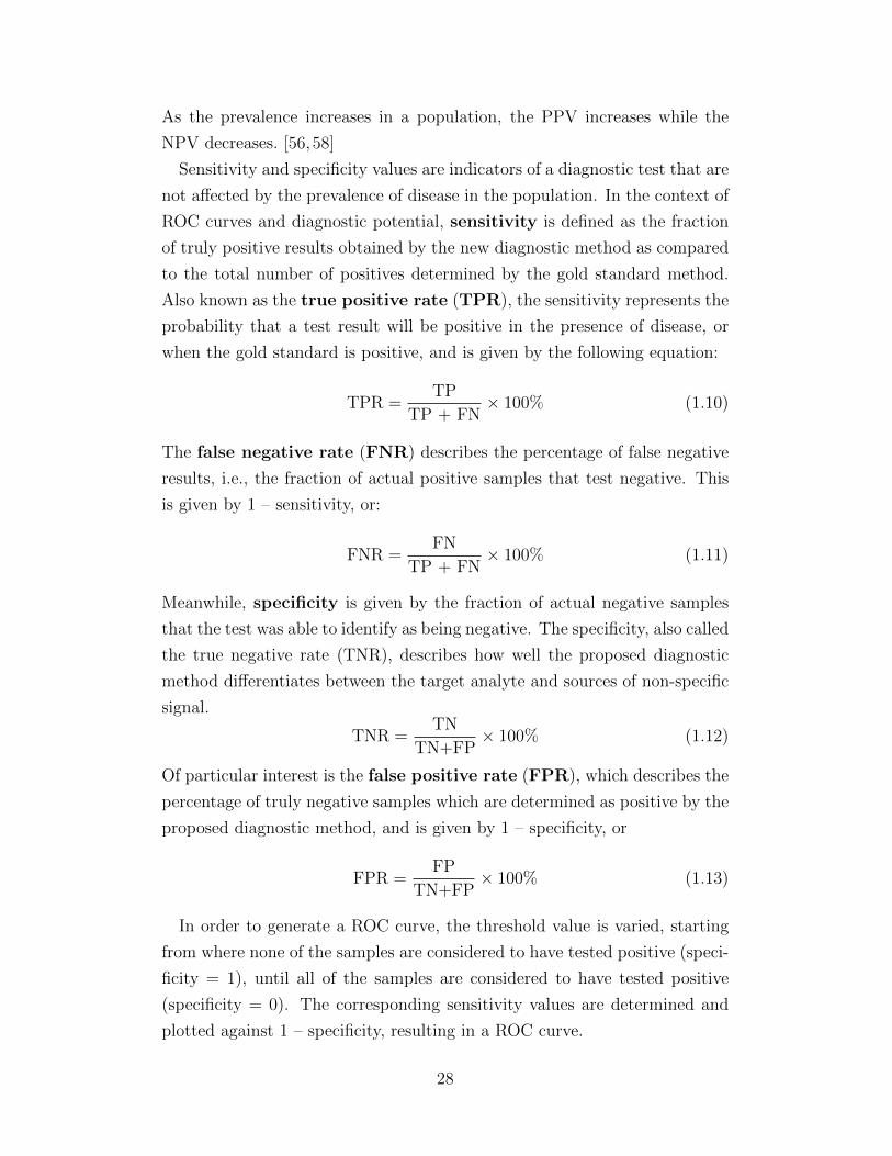
Sensitivity and specificity values are indicators of a diagnostic test that are

not affected by the prevalence of disease in the population. In the context of

ROC curves and diagnostic potential, sensitivity is defined as the fraction

of truly positive results obtained by the new diagnostic method as compared

to the total number of positives determined by the gold standard method.

Also known as the true positive rate (TPR), the sensitivity represents the

probability that a test result will be positive in the presence of disease, or

when the gold standard is positive, and is given by the following equation:

TPR =TP

TP + FN× 100% (1.10)

The false negative rate (FNR) describes the percentage of false negative

results, i.e., the fraction of actual positive samples that test negative. This

is given by 1 – sensitivity, or:

FNR =FN

TP + FN× 100% (1.11)

Meanwhile, specificity is given by the fraction of actual negative samples

that the test was able to identify as being negative. The specificity, also called

the true negative rate (TNR), describes how well the proposed diagnostic

method differentiates between the target analyte and sources of non-specific

signal.

TNR =TN

TN+FP× 100% (1.12)

Of particular interest is the false positive rate (FPR), which describes the

percentage of truly negative samples which are determined as positive by the

proposed diagnostic method, and is given by 1 – specificity, or

FPR =FP

TN+FP× 100% (1.13)

In order to generate a ROC curve, the threshold value is varied, starting

from where none of the samples are considered to have tested positive (speci-

ficity = 1), until all of the samples are considered to have tested positive

(specificity = 0). The corresponding sensitivity values are determined and

plotted against 1 – specificity, resulting in a ROC curve.

28

An “optimum” sensitivity and specificity pair that best suits the purpose

of the testing method can be determined through the ROC curve, and the

corresponding threshold value can be determined for a binary (positive or

negative) result. However, it is first important to recognize that the sensi-

tivity and specificity requirements differ for a screening versus a diagnostic

test.

The purpose of a screening test is to provide a more affordable and time-

effective method that is minimally invasive and less risky for individuals in

determining the probability of a particular disease or condition. Depending

on the result of the test, the individual can rest assured that they probably

do not have the disease, or be referred for more rigorous testing. For a

screening test, the goal is to minimize the number of true positive individuals

that are overlooked, since individuals with the disease who receive a negative

screening result will likely be unable to detect the disease in a timely fashion,

possibly leading to devastating results. In other words, the FNR should be

as low as possible—or the sensitivity should be high. On the other hand, the

purpose of a diagnostic method is to determine, with high confidence, that

an individual has a particular disease or condition. Therefore, a diagnostic

test should be very specific for the disease; the FPR should be low. These

factors should be considered when determining the proper cutoff value of a

new screening or diagnostic method.

The area under the curve (AUC) can be considered an unbiased indicator

of the overall performance of the screening/diagnostic test, as it is not de-

termined by arbitrary decision criteria or cut-off values. A ROC curve with

an AUC of 1 perfectly matches with the gold standard results (or the disease

state) and is the ideal result for a testing method. Meanwhile, an AUC of 0.5

indicates that the diagnostic test is no different from making determinations

by random chance. Therefore, an AUC above 0.5 indicates that the screen-

ing/diagnostic method is better than making random chance decisions. In

general, an AUC of 0.7–0.8 has been considered as “acceptable”, 0.8–0.9 as

“excellent”, and more than 0.9 as “outstanding” [59].

29

CHAPTER 2

PCEF WITH MICROFLUIDICINTEGRATION FOR ANTIVIRAL

ANTIBODY DETECTION

Here, I present the work that was published in [32] and [60] and specifically

go into further detail regarding the biomedical and clinical aspects of the

study. More details regarding the scanning method and automation of data

acquisition can be found in [32] and [61].

2.1 Introduction

A photonic crystal (PC) biosensor was used to enhance the optical signal

from fluorophores in a fluorescence-linked immunosorbent assay (FLISA) for

the detection of a potential biomarker for human papillomavirus (HPV)-

associated oropharyngeal cancer (OPC). The motivation for this work is

provided below.

2.1.1 Human Papillomavirus (HPV)

Human papillomaviruses (HPVs) are small, non-enveloped DNA viruses with

a circular genome of double-stranded DNA. The HPV genome, approximately

8 kilobases in length, contains regions of “early genes” and “late genes.”

The proteins coded by the early genes, designated E1–E8, carry out non-

structural functions that allow the virus to hijack the machinery of the host

cell to promote the propagation of the virus while evading cell cycle regu-

lation. The late genes code for the viral capsid proteins, L1 and L2, which

form the protective packaging for the viral genome and are necessary for the

spread and transmission of the virion—the complete and infectious form of

the virus—to other host cells. HPV displays a tropism for keratinocytes of

squamous epithelia and have been found to infect the anogenital and oropha-

ryngeal regions of the human body. Over 100 different types of HPV have

30

been identified to date. Of these, at least thirteen types—including HPV

types 16 and 18—are considered high-risk because of the extent to which the

viral proteins are able to disregulate the cell cycle and make the conditions

conducive to the development of cancer. It is known that more than 99% of

cervical lesions have been associated with viral sequences, with HPV types

16 and 18 contributing to at least 70% of cervical cancers [62]. Furthermore,

HPV has been known to be associated with over 40% of cancers of the head

and neck, or oropharyngeal cancers (OPC) [62].

The Viral Life Cycle of HPV

As of yet, all HPV types appear to exclusively infect squamous epithelial

cells, specifically targeting basal keratinocytes. The viral life cycle of HPV

has been shown to be very closely tied to the differentiation process of ker-

atinocytes. The HPV viral life cycle and oncogenic potential, which is thor-

oughly reviewed in [62] and [63], is briefly summarized below.

HPV first gains access to the host cell through a micro-tear or wound

exposing the basal membrane in the stratified squamous epithelium. The L1

protein, which is the major component of the outer shell (“capsid”) of the

HPV, binds to heparan sulfate proteoglycans (HSPGs) found in the basal

membrane. A change in capsid conformation leads to the L2 protein being

exposed and cleaved. The cleaved L2 protein binds to surface molecules

on the target keratinocyte, leading to another conformation change. This

finally exposes the host receptor binding domain on the L1 protein. The

subsequent interaction of this domain with the host cell receptor allows the

virion to enter the cell.

After successfully infecting the cell, the viral genome remains episomal—

able to replicate independently or in association with the host chromosome.

In the early stage of infection, the viral genome is minimally amplified to

around 50–100 copies per cell, and the early viral genes are expressed in

strictly controlled amounts. The infected primitive basal keratinocyte then

undergoes mitosis, and as part of its natural differentiation process, one of

the daughter cells transitions away from the basal layer. The differentiation

of the cell into a keratinocyte triggers the productive, or lytic, phase of the

viral life cycle.

During the productive phase, the viral genome is amplified to over a thou-

31

sand copies per cell. This requires active DNA synthesis machinery in the

host cell, which should have already exited the S phase of the cell cycle. HPV

prolongs the DNA replication phase in the host cell while evading the usual

cell cycle checks through the action of the early proteins, E6 and E7. After

sufficient amplification of the viral genome, the early proteins E1–E4 are ex-

pressed, followed by the L1 and L2 capsid proteins. While L1 is the major

capsid protein and is able to self-assemble into virus-like particles, L2 is the

protein that actually binds the viral DNA. Proteins L1 and L2 encapsidate

the viral genome, and the complete, packaged forms are released from the

differentiated host cell, now located in the uppermost layer of the epithelium,

as virions capable of infecting new cells.

Once begun, the lytic phase is generally irreversible, and the virus must

compete with the host immune system to replicate successfully and produce

virions before host cell lysis occurs. On the other hand, the virus may choose

to enter the latent phase of the viral life cycle. In the latent phase, the

HPV adapts an “immune-evasion strategy” in which the expression of viral

proteins which might lead to an immune response is absent or minimal. If the

viral genome integrates into the host genome, it loses its ability to replicate

into virions; therefore, the viral genome generally remains episomal with the

potential enter the productive phase later.

Oncogenic Potential of HPV Proteins

The HPV genome codes for several proteins—namely E5, E6, and E7—which

may induce the development of cancerous cells. Due to their propensity for

making the host environment conducive to the formation and development of

cancer, these proteins are considered oncogenic proteins, or “oncoproteins.”

The oncogenic potential of proteins E6 and E7 have been studied quite

extensively. Protein E7 targets the retinoblastoma (Rb) family of tumor sup-

pressors for degradation, leading to a p53-dependent inhibition of cell growth

and activation of apoptosis, known as programmed cell death. However, this

apoptotic pathway is also disabled by protein E6, which ubiquitinates the

p53 tumor suppressor protein, leading to its degradation. Together, the two

proteins E6 and E7 are able to maintain the host cell in S phase, during

which DNA is replicated, in differentiating keratinocytes.

While all HPVs express proteins E6 and E7, the production of these pro-

32

teins alone is insufficient for transforming cells into cancer cells. The E6 and

E7 proteins produced by high-risk viruses such as HPV 16 and 18 demon-

strate a higher affinity for their respective targets than do their low-risk

counterparts. Furthermore, the high-risk HPV E6 and E7 proteins have

been shown to promote genomic instability in the host and to immortalize

keratinocytes. Therefore, proteins E6 and E7 are considered oncoproteins

due to their inhibitory effect on tumor suppressors and tendency to induce

genomic instability and cell immortality.

Though the oncogenic potential of protein E5 has not been as comprehen-

sively studied as that of proteins E6 and E7, it has been shown that protein

E5 may delay the degradation of epidermal growth factor receptor (EGFR),

allowing the basal undifferentiated host cell to continue to proliferate [64].

HPV Proteins as Potential Biomarkers for HPV-associated OPC

The proteins expressed by HPV can potentially serve as biomarkers for de-

termining which OPC cases are associated with HPV. Studies have shown

that patients with HPV-associated OPC (HPV-OPC) are more likely than

those without HPV association to have a favorable outcome to treatment [65].

Such patients can benefit from less intense treatment options which diminish

the risk of treatment side-effects that negatively affect quality of life, without

compromising survival outcomes [65].

As capsid proteins of a non-enveloped virus, proteins L1 and L2 are likely

to be in direct contact with the host immune cells. Therefore, antibodies

against L1 and L2 are likely to be present in individuals. One may recall that

the L2 capsid protein is not readily exposed without proper initial binding by

the L1 protein, and that the L2, not L1, protein directly interacts with the

viral genome. In fact, L1 proteins self-assemble into a capsid without the viral

genome and is thus used in vaccines for HPV. Detection of antibodies against

the L1 protein has been shown to indicate a successful HPV vaccination

status or exposure to a HPV infection regardless of whether the virus is

currently in the lytic or latent stage [66, 67]. It has been shown that 50–

70% of individuals exposed to HPV develop antibodies against L1, which are

detectable in the serum years after the infection has been cleared [67].

Meanwhile, the early proteins are not readily exposed to the host immune

system and are less likely to have an immune response mounted against them.

33

However, if the host cell undergoes necrosis, during which the components of

the infected cell (including the viral proteins) are exposed to the surrounding

environment and resulting in a host immune response, it is possible that an-

tibodies may be formed against them. In particular, host antibodies against

the oncoproteins E5, E6, and E7 may be more appropriate for the early de-

tection of HPV-associated cancers, since the presence of antibodies against

HPV viral proteins might be correlated with the possible presence of a tu-

mor that is not yet detectable using conventional methods. Previous studies

have shown that 40–80% of OPC cases are associated with HPV, and that

up to 90% of these are caused by HPV type 16 (HPV16) [65]. In particu-

lar, antibodies against HPV16 E7 protein have been detected in 63–69% of

OPC cases, while less than 4% of healthy controls had detectable antibodies

against either proteins E6 or E7 [67–69].

2.1.2 PCEF for the Detection of HPV Oncoproteins

It has been recognized for some time that panels of biomarkers, rather than

a single biomarker, can improve the specificity of biosensors [20, 53, 54].

Although several possible biomarkers for HPV-OPC have been discussed,

developing and optimizing an assay for the detection of a panel of biomark-

ers would require studies of cross-reactivity and the characterization and

optimization of the bioreceptor and analyte pairs, which was beyond the

scope of this study. The aim of this work was to evaluate the capability of

an optical biosensor platform, PCEF, in giving reliable and accurate results

for an antigen-antibody affinity-based assay, termed the fluorescence-linked

immunosorbent assay (FLISA). Therefore, the most readily available and

well-tested antigen, protein E7, was selected as the bioreceptor to detect

anti-E7 antibody from a complex medium such as serum and plasma.

2.2 Process and Methodology

2.2.1 Fabrication of photonic crystals

PCs were fabricated as detailed previously in [30]. As depicted in Fig. 2.1(a),

these PCs were composed of a one-dimensional grating structure with 40 nm

34

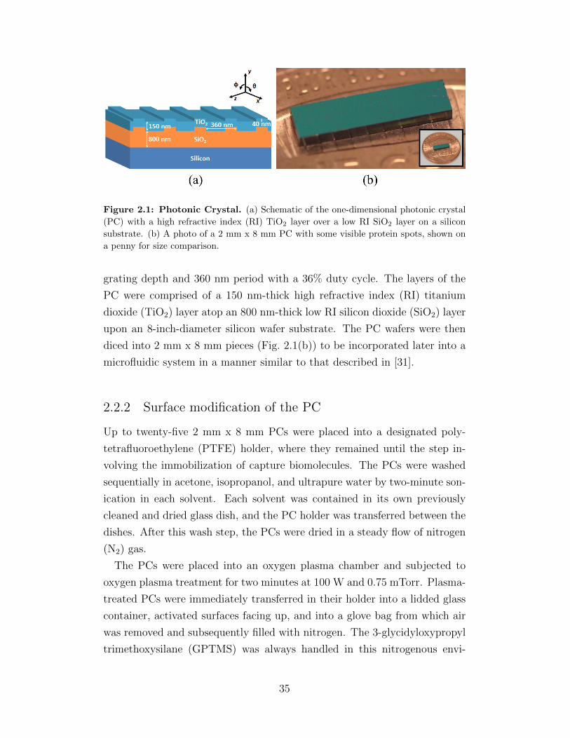
Figure 2.1: Photonic Crystal. (a) Schematic of the one-dimensional photonic crystal

(PC) with a high refractive index (RI) TiO2 layer over a low RI SiO2 layer on a silicon

substrate. (b) A photo of a 2 mm x 8 mm PC with some visible protein spots, shown on

a penny for size comparison.

grating depth and 360 nm period with a 36% duty cycle. The layers of the

PC were comprised of a 150 nm-thick high refractive index (RI) titanium

dioxide (TiO2) layer atop an 800 nm-thick low RI silicon dioxide (SiO2) layer

upon an 8-inch-diameter silicon wafer substrate. The PC wafers were then

diced into 2 mm x 8 mm pieces (Fig. 2.1(b)) to be incorporated later into a

microfluidic system in a manner similar to that described in [31].

2.2.2 Surface modification of the PC

Up to twenty-five 2 mm x 8 mm PCs were placed into a designated poly-

tetrafluoroethylene (PTFE) holder, where they remained until the step in-

volving the immobilization of capture biomolecules. The PCs were washed

sequentially in acetone, isopropanol, and ultrapure water by two-minute son-

ication in each solvent. Each solvent was contained in its own previously

cleaned and dried glass dish, and the PC holder was transferred between the

dishes. After this wash step, the PCs were dried in a steady flow of nitrogen

(N2) gas.

The PCs were placed into an oxygen plasma chamber and subjected to

oxygen plasma treatment for two minutes at 100 W and 0.75 mTorr. Plasma-

treated PCs were immediately transferred in their holder into a lidded glass

container, activated surfaces facing up, and into a glove bag from which air

was removed and subsequently filled with nitrogen. The 3-glycidyloxypropyl

trimethoxysilane (GPTMS) was always handled in this nitrogenous envi-

35

ronment in order to minimize exposure to atmospheric oxygen which may

inactivate the GPTMS over time.

Under nitrogen, GPTMS (4.96 µL per 2 mm x 8 mm PC) was pipetted

into the glass container containing the PCs in the PC holder. The PCs were

incubated overnight (12–16 hours) in a vacuum oven at 80 ℃ and 30 Torr,

permitting the formation of siloxane bonds between the activated oxygen on

the surface of the plasma-treated TiO2 PC layer and the silicon atoms of the

epoxysilane.

After silanization, the PCs were sequentially sonicated for two minutes

each in aqueous toluene, methanol, and ultrapure water; each was held in

previously cleaned and thoroughly dried, designated glass dishes. The PCs

were dried with N2 and stored in their holder for up to one month under vac-

uum prior to immobilizing capture biomolecules on the surface via printing.

2.2.3 Bioreceptor Immobilization via Microarray Printing

Sub-nanoliter drops of various solutions containing proteins were printed in

an array format upon the surface of the silanized PCs using a non-contact

printer (GeSiM Nano-Plotter 2.1) with piezoelectric pipetting tips (Nano-Tip

A-J, designed for dispensing 0.25 nL droplets). As depicted in Fig. 2.2, each

column of the protein array represents a different type or concentration of

protein. Ten rows of each protein were printed. The proteins printed were

the following: 50 µg/mL Alexa Fluor 647-conjugated streptavidin (AF-SA);

160 µg/mL bovine serum albumin (BSA); 12.5, 25, and 50 µg/mL protein

A/G; and 457.6 µg/mL recombinant protein E7. The AF-SA columns, one

on either edge of the microarray, served as a positive reference. The BSA

column served as the negative control. The protein A/G columns, which

bind to the Fc portion of any IgG antibody [70], were designed for internal

calibration and experimental control. and 457.6 µg/mL recombinant protein

E7 of HPV type 16 (provided by the Anderson Lab at Arizona State Univer-

sity, ASU [71]). All proteins were diluted to the final printed concentration

with phosphate buffered saline (PBS).

Both printing and incubation were performed within an enclosed environ-

ment at ambient temperature (24–28 ℃) and 60% relative humidity. The

incubation period of 12–16 hours allowed the formation of covalent bonds

36

Figure 2.2: Protein Microarray. (a) Schematic of the protein microarray layout

on the 2 mm x 8 mm PC surface. (b) Bright-field image of the protein array prior

to washing away unbound proteins. The red region represents the approximate region

scanned by the line scanner, with the vertical laser line moving in the direction of the

red arrow. (c) Fluorescence intensity image obtained using the line scanner. (d) The

regions recognized by the automated spot-finding algorithm are circled in red. The protein

columns for (b, c, d) are as follows: 1 AF-SA, 2 – 4 Protein A/G, 5 cE2 protein, 6

GST, 7 E7 protein, 8 BSA, and 9 representative background. Columns 5 and 6 were

not evaluated here.

37

Figure 2.3: Microfluidic Cartridges. (a) Photo of the single- (left) and four-channel

(right) cartridges with food coloring to indicate the sample flow channels. The sample

is introduced into the sample inlet (red). Reagents are flowed through the reagent inlet

(purple) using the automated flow system. (b) Exploded view, showing the layers of the

four-channel cartridge. (c) Schematic of the assembled four-channel cartridge.

between the primary amines of the proteins and the epoxy functional groups

of the silanized PC. This chemistry results in a secondary amine with an al-

cohol side group. After the incubation period, the protein microarrays were

imaged under a bright-field microscope and dried in a desiccator for at least

10 minutes in order to minimize spot smearing. The PCs were incubated

in 1% casein in 1X PBS (Bio-Rad) for one hour to passivate the bare PC

surface and thus inhibit nonspecific binding. The PCs were then soaked in

1x PBS (Sigma-Aldrich) for ten minutes and then dried with a stream of N2.

Afterward, the PCs were stored in a sealed, desiccated container at 4oC until

use in the subsequent assay.

2.2.4 Microfluidic Cartridges

While the microfluidic cartridges used previously in the Cunningham group

had been fabricated using stereolithography [31], a slightly different fabrica-

tion method was developed here in order to solve some recurrent issues with

leakage and cracked glass that resulted from the bowing of the surface of the

3D-printed cartridges.

Here, the microfluidic cartridges (25 mm x 75 mm x 8 mm) were assembled

from layers of laser-machined acrylic of varying thicknesses and double-sided

adhesive (DSA; 3M Optically Clear Adhesive 8212) of approximately 150 µm

thickness. The laser etching method was used to etch around the inlet and

outlet holes to permit flush fitting with the flanged tubing of the automated

38

flow set up. A custom-built alignment press incorporating controlled appli-

cation of force via a torque wrench was used to assemble these cartridges.

A 1/4-inch acrylic layer served as the base layer upon which a 1/32-inch

acrylic cavity layer was adhered using three DSA layers. Two DSA layers

comprising the fluid channel were adhered upon the cavity layer, resulting

in channels with a rectangular cross-section with approximate dimensions of

2 mm x 300 µm. The PC with immobilized capture proteins was inserted

into the cavity, and the channel was sealed by a 0.170 mm non-fluorescent

glass coverslip (Schott NEXTERION) immediately before the assay was per-

formed.

While single-channel cartridges with previously published dimensions [31]

were fabricated using this new method, four-channel cartridges were also

designed. Based on the flow channel dimensions, the single-channel cartridge

holds 10 µL of sample, while the four-channel cartridge holds 6 µL of sample

per sensor. A photo of the assembled single- and four-channel cartridges, as

well as schematics of the four-channel cartridge, can be found in Fig. 2.3.

The four-channel cartridge was designed to enable multiplexing with the

automated flow setup, which supports one cartridge at a time [31]. A new mi-

crofluidic cartridge holder was designed out of 3D-printed material to specif-

ically hold the four-channel cartridge, to be interchangeable with the single-

channel cartridge holder, and to interface the cartridge with the automated

flow system. In order to facilitate integration with the current automated

flow equipment, the four-channel cartridge was designed such that the sample

can be introduced to each of the four channels individually via micropipette

through the sample inlet holes (red), as shown in Fig. 2.3(a). When the car-

tridge is interfaced with the automated flow setup, the central hole (purple)

serves as a common inlet for the reagents, while the sample inlets now func-

tion as four separate outlet holes leading to four separate waste reservoirs.

By multiplexing four separate samples, approximately 7-10 minutes can be

saved per sample; each four-channel cartridge saved an average of 25 minutes

from the total assay run time for each set of samples. In addition, the acrylic-

based cartridges experienced fewer leaks and cracks in the glass coverslip.

Furthermore, these cartridges are more manufacturable and cost-effective

($0.62/cartridge) than the 3D-printed cartridges ($5/cartridge). This makes

the cartridges more suitable as single-use, disposable biosensors for testing

clinical samples.

39

Figure 2.4: Fluorescence-Linked Immunosorbent Assay (FLISA). 1 The sample

is introduced manually and incubated for 3 hours. 2 Unbound molecules are washed

away with PBST using the automated flow system. 3 Secondary antibody is flowed

automatically and incubated for 1 hour. 4 PBST is followed by drying with N2 gas.

2.2.5 Fluorescence-Linked Immunosorbent Assay (FLISA)

The fluorescence-linked immunosorbent assay (FLISA) was performed in the

cartridges as schematized in Fig. 2.4. As described previously, an array of

proteins were printed upon the PC prior to its integration with the microflu-

idic cartridge. In this assay, the bioreceptor of interest is the HPV viral

antigen, recombinant protein E7 (Anderson Lab, ASU). In a manner similar

to an indirect enzyme-linked immunosorbent assay (ELISA), E7 was immo-

bilized on the PC substrate to recognize anti-E7 antibody in the sample.

In order to obtain a dose-response curve, the FLISA was performed in the

four-channel cartridges. Known concentrations of mouse anti-E7 antibody

(Santa Cruz Biotechnology) were spiked into human male AB serum (Sigma-

Aldrich) which had been diluted twenty-fold in PBS. A secondary antibody

mixture of Alexa Fluor 647-conjugated goat anti-mouse IgG and goat anti-

human IgG (each at 1 µg/mL) was used to label the mouse anti-E7 antibody

40

and the protein A/G internal calibration spots, respectively. Forty clinical

samples provided by the Anderson Lab at ASU and which had been approved

previously for clinical testing as part of the HOTSPOT study (IRB-36563)

[72] were also tested. Each of these clinical samples were diluted twenty-fold

in PBS, and the FLISA was performed with 10 µL of each sample in separate

single-channel cartridges. Only the fluorescence-labeled goat anti-human IgG

was used in the secondary antibody solution. All forty clinical sample tests

were performed together as one batch on three separate occasions.

The sample was introduced manually via micropipette through the sam-

ple inlet of the microfluidic cartridge. The liquid was drawn up through

the flow channel via capillary action, covering the PC surface and reaching

the outlet hole. The sample was incubated in the cartridge for 3 hours at

room temperature, after which the cartridge was connected to an automated

controlled flow system (Fluigent) previously used in [31]. Unbound material

was washed away by flowing phosphate buffered saline with 0.05% Tween 20

(PBST, Sigma-Aldrich) through the channel for 30 s at 30 mBar, followed

by N2 gas for 10 s at 50 mBar. A solution of secondary antibody tagged

with Alexa Fluor 647 (Jackson ImmunoResearch) was flowed for 20 s at 30

mBar. The sample was allowed to incubate for 1 hour at room temperature

in an environment protected from light. The channel was then washed with

a flow of PBST for 30 s at 30 mBar, followed by drying with N2 gas for four

minutes. Finally, the cartridge was removed from the flow system, covered

with foil, and stored in a desiccator at room temperature for at least two

hours, until scanned. Complete drying of the surface proved to be crucial for

obtaining reliable fluorescence readings.

2.2.6 Laser Line-Scanning Instrument

The custom-built laser line-scanning instrument (“line-scanner”) previously

reported in [30] and [31] was used here. In the early stages of this work,

large standard deviations were observed among spots of the same protein

along different points of the Gaussian laser line profile. In an attempt to

reduce these deviations, an apodization filter—made by depositing a 12 nm

layer of gold, 4 mm in diameter, at the center of an optically transparent

glass plate—was added to the optical path such that the gold spot would

41

Figure 2.5: Laser Line-Scanning Detection Instrument. (a) Schematic of the line-

scanner with the apodization filter modification. (b) The graph shows the laser line profile

with (blue) and without (red) the apodization filter.

attenuate the center of the laser profile, where the illumination was most

intense. An updated schematic of this modified line-scanner, along with the

laser line profile before and after the addition of the apodization filter, is

shown in Fig. 2.5.

The detection instrument was used to obtain images of the fluorescent pro-

tein spots by scanning the surface of the PC with a 637 nm illumination line

that is collimated in one direction but focused on the other. The on-resonance

angle was obtained by scanning the incident angle from 0 to 8 degrees for

the protein E7 column near the bottom or top edge of the microarray. As

depicted in Fig. 2.2(b), the length of the laser line is approximately 750 µm,

illuminating three to four spots per column in a single scan. After the on-

resonance angle of the protein E7 column was determined, all the columns

of the protein microarray were line-scanned at this fixed angle of incidence.

The scanning region was shifted to the center of the PC to avoid the region

that had already been exposed to laser illumination in order to minimize the

effects of photobleaching. After the on-resonance scan, the same region was

scanned again at the off-resonance angle, which was generally fixed at 8◦.

2.3 Results and Discussion

Information regarding the mean and median intensities of the fluorescent

spots and their corresponding background intensities were obtained from

the images scanned with the PCEF instrumentation, through an automatic

42

spot-finding algorithm described in [32] and referred to in Fig. 2.2(d). The

following is a presentation of the results, analysis, and interpretation of these

data.

Each protein column in a given line-scanned image consisted of three full

spots. A set of three representative background spots was determined—

one each for the top, middle, and bottom regions of the scanned region, as

shown in Fig. 2.2(d). The median intensity of these background spots was

subtracted from the corresponding top, middle, or bottom protein spot for

each column of the microarray. The set of three final background-subtracted

intensities for each protein column were averaged, then normalized by the av-

eraged background-subtracted median spot intensity for serum spiked with

100 ng/mL anti-E7 antibody in order to enable comparisons across batches of

tests. While the protein microarrays incorporated several columns of on-chip

internal positive controls (AF-SA and protein A/G), these did not function

well as a means of normalization. The protein A/G spots of varying con-

centrations proved useful as an experimental control but not for internal

calibration or to enable inter-test comparisons, as was the original intention.

Therefore, the 100 ng/mL spiked sample was always tested in every batch of

experiments to serve as a positive control to which all other samples in the

batch were normalized.

2.3.1 Dose-Response Curves

A dose-response curve was obtained by performing the FLISA in four-channel

microfluidic cartridges with concentrations of mouse anti-E7 antibody rang-

ing from 1 ng/mL to 1000 ng/mL (6.7 pM – 6.7 nM) spiked into twenty-fold

diluted human male AB serum in PBS. Several calibration curves were ob-

tained, and tests from different days were compared to each other by nor-

malizing by the mean intensity of the 100 ng/mL anti-E7 antibody sample

for the corresponding assay date.

One may recall that Eq. 1.5 is used to determine the signal which cor-

responds to the limit of detection (LOD). The LOD of the assay may be

determined numerically from the mean and standard deviation (σ) of a set

of twenty-fold diluted serum samples without any spiked antibody, which

would serve as the “blank.” The LOD would be calculated by setting k = 3

43

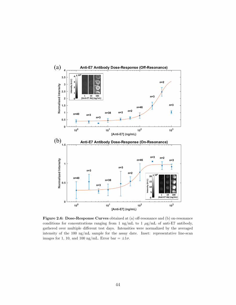
Figure 2.6: Dose-Response Curves obtained at (a) off-resonance and (b) on-resonance

conditions for concentrations ranging from 1 ng/mL to 1 µg/mL of anti-E7 antibody,

gathered over multiple different test days. Intensities were normalized by the averaged

intensity of the 100 ng/mL sample for the assay date. Inset: representative line-scan

images for 1, 10, and 100 ng/mL. Error bar = ±1σ.

44

for a confidence level of 99.7%, or k = 2 for a confidence level of 95%. Here,

the LOD was determined for each sample by calculating the value 3σ above

the mean of the background spot intensities.

The compiled calibration curves for both the off- and on-resonance condi-

tions are shown in Fig. 2.6. The extent of signal enhancement at on-resonance

may not be immediately clear from the calibration curves, as the y-axis rep-

resents the intensity normalized to the 100 ng/mL spiked sample, instead of

the raw intensity. However, the intensity scale bar of the figure inset clearly

shows that there is at least a 5x increase in intensity at the on-resonance con-

dition. While samples at and below 10 ng/ml of analyte (anti-E7 antibody)

are below the LOD at off-resonance, the enhanced excitation phenomenon of

the on-resonance condition brings the spot intensities at 10 ng/mL above the

LOD. Furthermore, spots near 1 ng/mL (6.7 pM) of analyte are even made

visually detectable at on-resonance.

Due to the enhancement of the fluorescence intensity signal, the calibra-

tion curve for the on-resonance condition saturates at a concentration be-

tween 100 and 250 ng/mL of analyte. The linear range, in which the anti-E7

antibody concentration may be quantifiable, spans the lower end of the con-

centration values (25–200 ng/mL). Meanwhile, the calibration curve for the

off-resonance condition does not appear to saturate within the tested con-

centrations. Furthermore, the linear range for the off-resonance condition

is approximately 100–500 ng/mL. The platform may potentially achieve a

broader linear range of 25–500 ng/mL (0.17–3.33 nM) of the analyte by

scanning samples at both on- and off-resonance conditions.

The on-resonance condition not only increases the fluorescence intensity of

the spots; it also amplifies the intrinsic variability in the assay, resulting in

larger error bars (±1σ) at on-resonance compared to those at off-resonance.

The intrinsic variability primarily arises from non-uniform surface coverage

by the protein in the printed spots. Non-uniform evaporation during the

incubation and/or drying process after printing may result in differential

protein densities throughout the spot [73]. Known as the “coffee-ring effect,”

the proteins in solution are concentrated at the edge of the spot, resulting in

spots with a low-density center surrounded by a high-density ring.

This phenomenon can be observed in the spots for 100 ng/mL analyte

at off-resonance (Fig. 2.6(a) inset), in which the spots experienced uniform

enhancement via the enhanced extraction mechanism. When these same

45

Figure 2.7: Distribution of Enhancement Factors between off- and on-resonance of

the protein E7 columns after complete FLISA for the dose-response samples. Those with

SNR < 1 (background brighter than spot) were excluded.

spots were illuminated at on-resonance, as shown in the inset of Fig. 2.6(b),

only the center of the spots were highly fluorescent, while the signal from

the edges was minimal due to the resonant condition matching that of the

spot center. The reverse may also happen, in which the on-resonance angle

matches the resonant condition of the spot edge. Due to the PC sensitivity

to variations in surface density, the on-resonance condition matches either

the center or edge of a non-uniform spot, but not both. As shown in Fig. 2.7,

the enhancement factor between off- and on-resonance was not always fixed

at ∼5x, but displayed a Poisson-like distribution.

2.3.2 Clinical Samples

Forty clinical plasma samples, obtained from twenty OPC patients and twenty

healthy controls, were tested on the PCEF platform. The FLISA was per-

formed for each sample in separate single-channel cartridges, and off- and on-

resonance images were obtained via the line-scanning detection instrument.

The Demirci Lab (Stanford University) concurrently performed conventional

ELISAs on aliquots of the same forty samples [71]. If the goal of the project

had been to evaluate the clinical relevance of the HPV viral protein E7 as

46

a biomarker for HPV-OPC, the results would have been compared to the

OPC status. Instead, the results obtained from the PCEF platform were

compared to those of the ELISA, the “gold standard” diagnostic method for

immunoassays, in order to evaluate the suitability of the PCEF biosensor

platform as a diagnostic tool.

A total of 23 samples (all twenty OPC patient samples and three control

samples) showed detectable concentrations of anti-E7 antibody through the

ELISA, while the remaining 17 were negative for the analyte with ELISA.

Of the forty total samples, nine were removed from analysis as a result of

inconsistencies (i.e., low positive control intensity or enhancement of back-

ground instead of target) in the PCEF results. The remaining 31 samples,

consisting of 14 ELISA-positive and 17 ELISA-negative samples, have been

analyzed and interpreted.

Receiver Operating Characteristic (ROC) Curve Analysis

A ROC curve was generated to compare the PCEF results with the ELISA

results as a reference. The threshold value was varied, and the sensitivity

and specificity (or 1 – specificity) values were calculated using the equations

from Section 1.3.3.

As described previously, the average background-subtracted median inten-

sity of the protein E7 column was obtained for each clinical sample. In order

to enable inter-sample comparison, the average intensity value was normal-

ized by the average background-subtracted median intensity of the protein

E7 column for pooled human AB serum (Sigma-Aldrich) spiked with 100

ng/mL mouse anti-E7 antibody, which served as the external positive con-

trol for each batch of tests. The equations above were coded into a MATLAB

script, which was used to compile the sensitivity and specificity values for

all relevant threshold levels of fluorescence intensity at off- and on-resonance

for the 31 clinical samples which had been deemed acceptable based on the

internal positive and negative control spots. These sensitivity and specificity

pairs were plotted in order to generate the ROC curves shown in Fig. 2.8(a,b).

The AUC was 0.83 for the off-resonance condition and 0.76 at on-resonance

for the 31 clinical samples evaluated. The “best” combination of specificity

and sensitivity corresponded to 71% and 79%, respectively, for both the

off- and on-resonance conditions. At these specificity and sensitivity values,

47

Figure 2.8: Plots of Clinical Results. (a,b) Receiver operating characteristic (ROC)

curves at off- and on-resonance. (c,d) Scatter plot of background-subtracted intensity

values prior to normalization, at off- and on-resonance. Horizontal dotted lines represent

threshold values. Error bar = ±1σ.

48

the associated cutoff intervals for the normalized values were determined

to be [0.20, 0.32) for off-resonance and [0.57, 0.61) for on-resonance. That

is, samples with normalized intensity values less than 0.20 were considered

negative, while those with values greater than 0.32 were considered positive in

the off-resonance condition. Likewise in the on-resonance condition, samples

with normalized intensity values less than 0.57 were considered negative,

while those with values above 0.61 were considered positive. Any unknown

samples whose results fall within the cutoff intervals would be considered to

have an inconclusive result. The cutoff interval is relatively large for the off-

resonance condition due to the small sample size, as well as the tendency for

the intensity values to be clustered at the lower range. The cutoff interval

is narrower for the on-resonance condition, at which the fluorescent signal

tends to be enhanced to be spread out toward the upper range.

The distribution of the results, separated into Negative ELISA (blue) and

Positive ELISA (red) populations, is shown in Fig. 2.8(c,d). The intensity

values are based on the average background-subtracted median intensity prior

to normalization, to demonstrate the noticeably higher intensities at on-

resonance. The dotted lines indicate the cutoff threshold, above which the

result is considered positive. This value was determined by calculating the

intensity value which corresponds to the midpoint of the cutoff interval—

1.79×104 for off-resonance and 8.35×105 for on-resonance.

The enhanced excitation phenomenon occurring at the on-resonance con-

dition increased the fluorescence intensity level of the protein E7 column to

a visible range in almost all cases. One may recall that the enhanced extrac-

tion phenomenon, which enhances the original signal by at least 5-6× [46], is

always active, even in the off-resonance condition. As with the dose-response

curve, the enhancement factor between off- and on-resonance varied among

the samples, ranging between 10–25× for most samples and up to 100–200×in a few cases. Due to the signal enhancement, several samples which were

considered negative at off-resonance were considered positive when measured

at the on-resonance condition.

The results from all accepted samples is tabulated in Fig. 2.9(a). As de-

fined earlier, specificity describes the percentage of actual negative samples

detected by the diagnostic method under evaluation, while sensitivity de-

scribes the percentage of actual positive samples detected by the diagnostic

test. The “actual” states of the samples are determined as the known disease

49

Figure 2.9: Tables of Clinical Results. (a) Table of results of all acceptable samples,

where discrepancies with ELISA results are highlighted in yellow. (b) Representative

results of clinical samples, compared to ELISA results and OPC status.

ELISA

R+ R−

PC

EF T+ TP (11) FP (5) PPV = 11

11+5= 69%

T− FN (3) TN (12) NPV = 1212+3

= 80%

Se = 1111+3

= 79% Sp = 1212+5

= 71%

Table 2.1: Contingency Table for PCEF Results

50

state or the result of an established, gold standard reference. In this case,

the PCEF biosensor is the diagnostic test and the reference is the ELISA.

A specificity of 71% corresponds to five false positive test results, and a

sensitivity of 79% corresponds to three false negative test results; these are

highlighted in yellow. A contingency table that summarizes these results is

shown in Table 2.1.

Of the seven samples for which the PCEF biosensor gave false positive

results at either off- or on-resonance, two samples were positive only at off-

resonance and not at on-resonance; and two different samples were well be-

low the cutoff interval at off-resonance but brought above the cutoff at on-

resonance. The remaining three samples showed false positive results at both

off- and on-resonance. A total of five unique ELISA-positive samples were de-

termined as negative by the PCEF biosensor at either off- or on-resonance.

Only one sample was found to be negative at both off- and on-resonance;

two samples were considered positive only at off-resonance, while another

two samples were considered positive only at on-resonance.

Off- and on-resonance images of the protein E7 column of representative

samples for nine different results, as compared with the ELISA and OPC

status, are presented in Fig. 2.9(b). 1 and 2 represent the majority of

cases, in which both the off- and on-resonance results were in agreement with

both the ELISA and OPC status. 3 – 9 represent cases in which there were

discrepancies between the PCEF results and the ELISA status. Specifically,

3 – 5 indicate cases in which at least one PCEF result (either off- or on-

resonance, or both) tested positive for an ELISA-negative sample. 6 – 9

represent cases in which at least one PCEF result was negative for an ELISA-

positive sample. 9 is the one case in which both PCEF results were negative

for an ELISA-positive sample.

In all cases–including those where the sample was considered positive at

off-resonance but negative at on-resonance–the intensity was enhanced well

above the visible threshold. From an examination of the images presented in

Fig. 2.9(b), it is clear that the fluorescence spots are visible at on-resonance

in all but two cases ( 1 and 8 ), even when they were considered to be

negative based on the background-subtracted result. This is most likely a

consequence of non-specific interaction and binding of plasma components

to the PC surface, resulting in an abnormally high background intensity for

some samples, such as 5 and 9 , where the spots are visible but read as

51

negative.

Overall, the high rate of false positives (FPR = 1 – specificity = 29%) may

be a result of the ability of the PCEF system to enhance the fluorescence

signal. It is not inconceivable that anti-E7 antibody was being detected in

supposed “healthy controls” by the PCEF biosensor when the levels had

been too low for detection by ELISA or other conventional methods. The

sensitivity of 79% corresponds to a false negative rate (FNR = 1 – sensitivity)

of 21%.

ELISA

R+ R−

(-)

Com

bo

PC

EF T+ 9 3 PPV = 75%

T− 5 14 NPV = 74%

Se = 64% Sp = 82%

ELISA

R+ R−

(+)

Com

bo

PC

EF T+ 13 7 PPV = 65%

T− 1 10 NPV = 91%

Se = 93% Sp = 59%

Table 2.2: Combination of Off- and On-Resonance PCEF Results. Only samples

with a positive test for both off- and on-resonance conditions are considered positive (left),

or only samples with a negative test for both conditions are considered negative (right).

The results of the off- and on-resonance conditions may be combined in

order to achieve a higher sensitivity overall. As shown in Table 2.2, there are

two options in combining the results of the off- and on-resonance conditions.

First, only those samples with a positive result for both off- and on-resonance

conditions would be considered to be positive. In other words, any sample

that has a negative result in either off- or on-resonance will be considered

negative. This increases the stringency of the test and increases the specificity

from 71% to 82%, while the sensitivity is decreased to 64%. This may be

more suitable for a diagnostic test, for which a high specificity and PPV are

essential.

The second option is to lower the stringency of the test by considering

samples with a positive result from either condition to be positive. That

is, only those samples with a negative result for both off- and on-resonance

conditions will be considered to be a negative result. This increases the

sensitivity of the test, as is desirable for a screening method, though at the

expense of the specificity. This option results in a sensitivity of 93%, or a

FNR of 7%, and a specificity of 59%.

The results up to this point have been based on using the quantitative

intensity values to determine a cutoff threshold based on the best sensitivity

and specificity combination as determined by the ROC curve. An alterna-

52

tive method would be a qualitative, visual analysis of the images at a fixed

intensity range. For example, fixing the on-resonance images to an inten-

sity range of 0 to 3.2×105 arbitrary units (AU) successfully identifies all the

ELISA-positive samples as positive, resulting in a 100% sensitivity. However,

the specificity is dramatically decreased to 12%, meaning that only two of

the 17 ELISA-negative samples had visually undetectable protein E7 spots.

A similar analysis of the off-resonance images at a fixed intensity range from

0 to 1.0×105 results in 76% specificity and 64% sensitivity. As discussed

previously, the on-resonance image of 9 in Fig. 2.9(b) is a prime example of

a sample with very high and obvious fluorescent spots that was considered to

be negative in the quantitative analysis due to abnormally high background

noise. While an entirely qualitative analysis may be suboptimal, a method

to use the qualitative analysis as a means to ‘cross-check’ the quantitative

result may improve the performance of the PCEF platform as a screening,

or even diagnostic, tool.

Repeatability

Testing of these same clinical samples was independently performed two ad-

ditional times–once with the same twenty-fold dilution of samples, and once

using a hundred-fold dilution. The total number of acceptable samples for

each set of tests was thirty (14 ELISA-negative and 16 ELISA-positive) for

the twenty-fold dilution and twenty-nine (13 ELISA-negative and 16 ELISA-

positive) for the hundred-fold dilution.

The AUC value for the twenty-fold dilution repeat was 0.70 at off-resonance

and 0.64 at on-resonance for the normalized background-subtracted median

intensity values (Fig. 2.10(a,b)). When the raw median intensities without

background-subtraction were considered, the AUCs were slightly higher, at

0.73 and 0.66 for off- and on-resonance, respectively (Fig. 2.10(c,d)).

The test was repeated at a hundred-fold dilution as an attempt to reduce

the number of false positives. Unfortunately, a majority of the sample in-

tensities were very close to the background, resulting in an AUC of 0.46 and

0.58 for off- and on-resonance, respectively (curves not shown). When the

raw intensities were considered, the AUC was 0.68 at off-resonance and 0.63

at on-resonance (Fig. 2.10(e,f)).

The clinical samples were stored at -80 ℃ and aliquoted for future use

53

Figure 2.10: ROC Curves of Repeats. (a,b) ROC curves based on results from a set

of twenty-fold diluted repeat samples, using normalized, background-subtracted intensities

for off- and on-resonance. (c,d) Based on results from twenty-fold diluted repeat samples,

using raw median intensity values. (e,f) ROC curves based on results from a set of hundred-

fold diluted repeat samples, using raw median intensity values for off- and on-resonance.

54

during the first batch of testing, and it is possible that the quality of the

samples was reduced in the subsequent tests due to the extra freeze-thaw

cycles. Regardless of the AUC values, all intensity values at off-resonance

were enhanced at least ten-fold at on-resonance in all three tests, confirming

the ability of the PCEF system to increase fluorescence signals to a detectable

threshold.

55

CHAPTER 3

CONCLUSIONS

A photonic crystal biosensor platform with the capacity for fluorescence en-

hancement and incorporating an automated multiplexed microfluidic flow

system and an automated spot-finding and data generation algorithm was

evaluated as a potential diagnostic tool. The fluorescence enhancement prop-

erty of the system enables the platform to have a high sensitivity, while the

automation capability of the fluidic assay reduces user error and variability

which may be introduced with the manual handling of reagents. Though the

details of the process were not discussed here, the automated spot-finding

and data generation algorithm also eliminates user bias in spot determina-

tion. Furthermore, multiplexing of samples and automated data acquisition

increased the throughput of the platform. Though it was not overtly studied

here, the 10 by 10 microarray of different proteins used in this work demon-

strates the potential for multiplexed analyte detection from the same sample,

which may improve the specificity and predictive value of the biosensor.

3.1 Important Considerations

While the PCEF biosensor platform has demonstrated high sensitivity, re-

duction of user error and variation via automation, and high multiplexing

potential for high assay throughput, additional improvements and considera-

tions can make the PCEF biosensor an even more reliable diagnostic method.

Several suggestions are discussed below.

3.1.1 Improving SNR

There were several cases, particularly among the clinical samples, where the

SNR was suboptimal. By definition, a low SNR results because either the

56

background noise is too high or the spot signal is too low (or perhaps a

combination of both). Possible causes for this are discussed below.

Non-Uniformity of Spots

Spots with non-uniform protein density may make it difficult to find the on-

resonance angle. Even if an on-resonance angle is determined, it only applies

to part of the spot, so that only a fraction of the total signal is collected.

If the resonance condition of the spot is too difficult to find, the angle may

instead match the resonance condition of the background, enhancing the

background noise instead of the spot signal.

As described in [73], non-uniformity in the protein density of a spot is

caused when a droplet of protein solution establishes a non-zero contact

angle with the PC surface and the initial contact line is fixed. As the solvent

evaporates from the edge of the deposited droplet, liquid from the interior

of the droplet must replenish the evaporated liquid. In this way, the solute

(protein) in the solution is carried with the solvent to the edge of the droplet

as it evaporates. In particular, droplets with higher contact angle appeared

to have thicker solute deposits at the edges. This process ultimately leads to

the coffee-ring morphology of spots that were evident in some of the protein

microarrays.

The following are ways in which the protein density might be made more

uniform. Adding a surfactant such as Tween 20 or Triton X to the printing

solution would reduce the contact angle, allowing the droplet to spread more

evenly over the surface. Though glycerol was not used here in order to

reduce the streaking of protein spots, addition of an appropriate percentage

of glycerol into the protein solution may prevent complete evaporation of the

spot and promote the uniform deposition of protein in the spot. [74,75]

Non-Specific Interactions at the Surface

The proper selection of the blocking agent can help reduce unwanted back-

ground noise which reduces the SNR. It is particularly important to consider

the factors that may hinder the protein-protein interactions that generate the

specific signal. One important consideration is the nature of the sample. The

background noise in previously reported fluorescence images, where the ana-

57

lyte was spiked into buffer, has been shown to be very low [30,31]. However,

when serum or plasma samples were used, the background noise increased

dramatically, most likely due to non-specific interactions of serum or plasma

components with the casein-blocked surface. Plasma samples generally had

a higher background than serum samples, possibly due to the presence of

clotting factors in plasma, which are absent in serum.

Suboptimal passivation, or blocking, of the PC surface may result in non-

specific binding which contributes to the overall background noise. While

1% casein in 1× PBS was used in this work, it may be useful to experiment

with other blockers, such as 1% BSA, a non-protein blocker, or even whole

serum. The inclusion of a surfactant such as Tween 20 or Triton X in the

blocking buffer has also been shown to help block non-specific protein-protein

interactions [76]. It has been shown that different blockers may be more

appropriate for some types of protein assays than others [74–76].

Biochemical Interactions

Suboptimal biochemical interactions in the assay procedure may result in a

lower-than-desirable signal [8]. The bioreceptor may exhibit an affinity for

molecules other than the analyte of interest, resulting in lower selectivity.

Even if it is specific to the analyte, it is possible that the bond between

the bioreceptor and analyte is easily disrupted, resulting in lower sensitivity.

The signal strength may not be adversely affected if the non-specific binding

of molecules to the bioreceptor generates a non-specific signal, though the

specificity of the assay would be compromised. However, if no signal is gener-

ated from the non-specific binding, the non-specific molecules are competing

with the signal-generating target analyte, resulting in an overall lower signal

strength. It is possible that the interaction between the recombinant protein

E7 and the anti-E7 antibodies (derived from mouse for the dose-response

curves and human for the clinical samples) was not fully optimized.

A newly proposed diagnostic platform may be underestimated if a not-yet-

established assay is used for the purposes of proving its diagnostic capability,

due to the possibility that the biochemical interactions of the assay have not

been sufficiently studied, characterized, and optimized. This can be avoided

by first validating the diagnostic ability of the platform with an established

assay. Then the validated diagnostic platform may be used to validate or

58

characterize a developing assay. Through this cycle of validating and es-

tablishing new methods, both new diagnostic platforms and new diagnostic

assays may continue to be developed and improved.

3.1.2 Appropriate Sample Size

In order to obtain an estimate of the accuracy of a diagnostic test within a

reasonable confidence interval, it is important to test an appropriate number

of samples. The sample size necessary to achieve an accurate assessment of

the sensitivity, specificity, and AUC of a newly proposed diagnostic method

can be estimated beforehand, so that the appropriate number of samples

can be obtained. Prior knowledge of the sample size necessary to obtain

statistically meaningful results can help to prevent under-sampling, which

may lead to results with poor statistical power, and over-sampling, which can

lead to over-consumption of resources. Factors to consider when estimating

sample size include: the a priori estimate based on literature or previous

experience or performance on a different assay, the disease status or the

prevalence of the disease in question, and the desired confidence interval and

acceptable margin of error. The equations and considerations involved in

estimating the proper sample size, as well as tables enumerating some of

these estimates based on the aforementioned factors, are given in [77].

3.1.3 Improving Specificity

The specificity of a biosensor rests largely on its associated bioreceptor and

may benefit greatly from the detection of a panel of biomarkers, rather than a

single biomarker. The PCEF biosensor has already demonstrated the capac-

ity to incorporate several columns of different bioreceptors detecting different

analytes and can benefit from incorporating multiple different bioreceptors

to test a panel of biomarkers. For example, the specificity of the PCEF

biosensor platform in conjunction with the assay for HPV-OPC, which was

71% for the off- and on-resonance results separately and 59% for the com-

bined results, may be improved by incorporating several HPV16 biomarkers,

instead of just protein E7, in the microarray. The other viral proteins which

were previously discussed in Section 2.1.1, including the capsid protein L1

59

and the other oncoproteins E5 and E6, could be potential biomarkers that

may help improve the specificity of the HPV-OPC assay. Optimizing such

a system would require characterization of cross-reactivity among the pro-

posed biomarkers and selection of the optimal bioreceptors and analytes with

minimal cross-reactivity.

3.2 Concluding Remarks

3.2.1 Overview of Results

The potential for the PCEF biosensor platform to be used in clinical applica-

tions was assessed by performing FLISA with protein E7 as the bioreceptor

and anti-E7 antibody as the analyte. A combined linear range of 25–500

ng/mL (0.17–3.33 nM) of spiked anti-E7 antibody in twenty-fold diluted

serum was obtained. Concentrations as low as 1 ng/mL (6.7 pM) of anti-E7

antibody were visually detectable.

Furthermore, forty clinical samples were assayed, and ROC curves were

generated. The AUC for the off- and on-resonance conditions were 0.83 and

0.76, respectively. The most “balanced” pair of sensitivity and specificity

pairs were 79% and 71%, respectively, for both the off- and on-resonance

conditions separately. The cutoff values as determined by this sensitivity

and specificity pair were applied to make binary decisions about the test

result as positive or negative. Not all the samples had the same result of

“positive” or “negative” for both off- and on-resonance. When the results

of these tests were combined such that only samples with a negative result

for both conditions is considered to be negative, the resulting sensitivity and

specificity were 93% and 59%, respectively. With these values, the current

system may be suitable as an early screening tool, identifying clinical samples

as positive, negative, or indeterminate if the values are within the cutoff

interval.

3.2.2 Future Work

The factors discussed in Section 3.1 may be considered and improved upon

in future projects in order to make the PCEF platform more suitable for

60

clinical applications and use at the point of care. Because different types

of biomarkers (e.g., protein, antibody, transcripts, etc.) signify different

aspects of a disease, a biosensor which incorporates these different types

of biomarkers may be able to provide a more comprehensive and clinically

significant set of information regarding the state of a disease. Incorporating a

high-specificity assay method such as this with a sensitive biosensor platform

such as the PCEF system can provide a highly reliable screening and/or

diagnostic test to reduce the morbidity and improve the quality of life of

patients suffering from cancer and other diseases.

61

REFERENCES

[1] T. Grandke and J. Hesse, “Introduction,” in Sensors: Fundamentals andGeneral Aspects, ser. Sensors: A Comprehensive Survey, T. Grandke andW. H. Ko, Eds. Weinheim, FRG: VCH, 1989, vol. 1, ch. 1, pp. 1–16.

[2] National Research Council, “Introduction to sensors,” in Expanding theVision of Sensor Materials. Washington, DC: The National AcademiesPress, 1995, ch. 1, pp. 9–18.

[3] N. R. council, ISA-37.1-1975 (1982), Electrical Transducer Nomencla-ture and Terminology. Research Triangle Park, NC: Instrument Societyof America, 1975.

[4] J. L. B. Wingard and J. P. Ferrance, “Concepts, biological components,and scope of biosensors,” in Biosensors with Fiberoptics, ser. Contem-porary Instrumentation and Analysis, D. L. Wise and L. B. Wingard,Eds. Totowa, NJ: Humana Press, 1991, ch. 1, pp. 1–27.

[5] N. S. Fracchiolla, S. Artuso, and A. Cortelezzi, “Biosensors in clinicalpractice: Focus on oncohematology,” Sensors, vol. 13, pp. 6423–6447,May 2013.

[6] N. Bhalla, P. Jolly, N. Formisano, and P. Estrela, “Introduction tobiosensors,” Essays in Biochemistry, vol. 60, pp. 1–8, June 2016.

[7] Y. H. Lee and R. Mutharasan, “Biosensors,” in Sensor Technology Hand-book, J. S. Wilson, Ed. Burlington, MA: Newnes, 2005, ch. 6, pp.161–180.

[8] F.-G. Banica, Chemical Sensors and Biosensors: Fundamentals andApplications. Research Triangle Park, NC: Instrument Society of Amer-ica, 1975.

[9] R. Fogel, J. Limson, and A. Seshia, “Acoustic biosensors,” Essays Bio-chemistry, vol. 60, no. 1, pp. 101–110, Jun 2016.

[10] M. Yakovleva, S. Bhand, and B. Danielsson, “The enzyme thermistor—A realistic biosensor concept. A critical review,” Analytica Chimica Acta,vol. 766, pp. 1–12, 2013.

62

[11] J. L. Hammond, N. Formisano, P. Estrela, S. Carrara, and J. Tkac,“Electrochemical biosensors and nanobiosensors,” Essays Biochemistry,vol. 60, no. 1, pp. 69–80, Jun 2016.

[12] J. L.C. Clark and C. Lyons, “Electrode systems for continuous monitor-ing in cardiovascular surgery,” Annals NY Acad Sci, vol. 102, pp. 29–45,1962.

[13] P. Bollella and L. Gorton, “Enzyme based amperometric biosensors (re-view article),” Sensors and Biosensors, vol. 10, pp. 157–173, Jul 2018.

[14] R. Koncki, “Recent developments in potentiometric biosensors forbiomedical analysis,” Analytica Chimica Acta, vol. 599, pp. 7–15, Aug2007.

[15] R. Radhakrishnan, I. I. Suni, C. S. Bever, and B. D. Hammock,“Impedance biosensors: applications to sustainability and remainingtechnical challenges,” ACS Sustainable Chemistry & Engineering, vol. 2,pp. 1649–1655, Jun 2014.

[16] G. Erturk and B. Mattiasson, “Capacitive biosensors and molecularlyimprinted electrodes,” Sensors (Basel), vol. 17, no. 390, pp. 1–21, Feb2017.

[17] B. Valeur and M. N. Berberan-Santos, Molecular Fluorescence: Prin-ciples and Applications, 2nd ed. Weinheim, Germany: Wiley-VCH,2012.

[18] C. Ray, “Fit-for-purpose validation,” in Translating Molecular Biomark-ers into Clinical Assays: Techniques and Applications, ser. AAPS Ad-vances in the Pharmaceutical Sciences Series, R. Weiner and M. Kelley,Eds. AG Switzerland: Springer International Publishing, 2016, vol. 21,ch. 1, pp. 1–16.

[19] J. Vessman, “Selectivity or specificity? validation of analytical meth-ods from the perspective of an analytical chemist in the pharmaceuticalindustry,” J Pharm Biomed Anal, vol. 14, pp. 867–869, 1996.

[20] J. F. Rusling, C. V. Kumar, J. S. Gutkind, and V. Patel, “Measurementof biomarker proteins for point-of-care easly detection and monitoringof cancer,” Analyst, vol. 135, pp. 2496–2511, Oct 2010.

[21] C. I. L. Justino, A. C. Duarte, and T. A. P. Rocha-Santos, “Recentprogress in biosensors for environmental monitoring: a review,” Sensors,vol. 17, no. 2918, pp. 1–25, Dec 2017.

[22] M. Trojanowicz, “Determination of pesticides using electrochemical en-zymatic biosensors,” Electroanalysis, vol. 14, pp. 1311–1328, 2002.

63

[23] I. Palchetti and M. Mascini, “Nucleic acid biosensors for environmentalpollution monitoring,” Analyst, vol. 133, pp. 846–854, 2008.

[24] P. Leonard, S. Hearty, J. Brennan, L. Dunne, J. Quinn, T. Chakraborty,and R. O’Kennedy, “Advances in biosensors for detection of pathogensin food and water,” Enzyme and Microbial Technology, vol. 32, no. 1,pp. 3–13, Jan 2003.

[25] M. Nayak, A. Kotian, S. Marathe, and K. Chakravortty, “Detectionof microorganisms using biosensors—A smarter way towards detectiontechniques,” Biosensors and Bioelectronics, vol. 25, no. 4, pp. 661–667,Dec 2009.

[26] L. D. Mello and L. T. Kubota, “Review of the use of biosensors as ana-lytical tools in the food and drink industries,” Food Chemistry, vol. 77,no. 2, pp. 237–256, May 2002.

[27] L. Barthelmebs, C. Calas-Blanchard, G. Istamboulie, J.-L. Marty, andT. Noguer, Biosensors as analytical tools in food fermentation industry,ser. Advances in Experimental Medicine and Biology. Boston, MA:Springer, 2010, vol. 698, ch. 22, pp. 293–307.

[28] J. Wang, “Glucose biosensors: 40 years of advances and challenges,”Electroanalysis, vol. 13, no. 12, pp. 983–988, 2001.

[29] J. Wang, “Electrochemical glucose biosensors,” Chemical Reviews, vol.108, no. 2, pp. 814–825, 2008.

[30] S. George, V. Chaudhery, M. Lu, M. Takagi, N. Amro, A. Pokhriyal,Y. Tan, P. Ferreira, and B. T. Cunningham, “Sensitive detection of pro-tein and miRNA cancer biomarkers using silicon-based photonic crys-tals and a resonance coupling laser scanning platform,” Lab on a Chip,vol. 13, pp. 4053–4064, Oct 2013.

[31] Y. Tan, T. Tang, H. Xu, C. Zhu, and B. T. Cunningham, “High sen-sitivity automated multiplexed immunoassays using photonic crystalenhanced fluorescence microfluidic system,” Biosensors and Bioelectron-ics, vol. 73, pp. 32–40, Nov 2015.

[32] C. M. Race, L. E. Kwon, M. T. Foreman, Q. Huang, H. Inan, S. Kesiraju,P. Le, S. J. Lim, A. M. Smith, R. C. Zangar, U. Demirci, K. S. Anderson,and B. T. Cunningham, “An automated microfluidic assay for photoniccrystal enhanced detection and analysis of an antiviral antibody cancerbiomarker in serum,” IEEE Sensors, vol. 18, no. 4, pp. 1464–1473, Feb2018.

64

[33] J. Kirsch, C. Siltanen, Q. Zhou, A. Revzin, and A. Simonian, “Biosensortechnology: recent advances in threat agent detection and medicine,”Chem Soc Rev, vol. 42, pp. 8733–8768, Jul 2013.

[34] S. Patel, R. Nanda, S. Sahoo, and E. Mohapatra, “Biosensors in healthcare: the milestones achieved in their development towards lab-on-chip-analysis (review article),” Biochemistry Research International, vol.2016, no. 3130469, pp. 1–12, 2016.

[35] B. T. Cunningham, M. Zhang, Y. Zhuo, L. Kwon, and C. Race, “Recentadvances in biosensing with photonic crystal surfaces: a review,” IEEESensors Journal, vol. 16, no. 10, pp. 3349–3366, May 2016.

[36] L. Kwon, K. D. Long, Y. Wan, H. Yu, and B. T. Cunningham, “Medicaldiagnostics with mobile devices: Comparison of intrinsic and extrinsicsensing,” Biotechnology Advances, vol. 34, pp. 291–304, 2016.

[37] K. D. Long, E. V. Woodburn, H. M. Le, U. K. Shah, S. S. Lumetta, andB. T. Cunningham, “Multimode smartphone biosensing: the transmis-sion, reflection, and intensity spectral (TRI)-analyzer,” Lab on a Chip,vol. 17, no. 19, pp. 3246–3257, 2017.

[38] R. Bashir, “Microcantilevers track single-cell mass,” Nature Biotechnol-ogy, vol. 34, no. 11, pp. 1125–1126, Nov 2016.

[39] Y. Zhuo, J. S. Choi, T. Marin, H. Yu, B. A. Harley, and B. T. Cun-ningham, “Quantitative imaging of cell membrane-associated mass den-sity using photonic crystal enhanced microscopy (PCEM),” Progress inQuantum Electronics, vol. 50, pp. 1–18, 2016.

[40] T. Kwa, Q. Zhou, Y. Gao, A. Rahimian, L. Kwon, Y. Liu, and A. Revzin,“Reconfigurable microfluidics with integrated aptasensors for monitor-ing intercellular communication,” Lab on Chip, vol. 14, no. 10, pp. 1695–1704, Feb 2014.

[41] W. Chen, K. D. Long, J. Kurniawan, M. Hung, H. Yu, B. A. Harley,and B. T. Cunningham, “Planar photonic crystal biosensor for quantita-tive label-free cell attachment microscopy,” Advanced Optical Materials,vol. 3, no. 11, pp. 1623–1632, 2015.

[42] Y. Zhuo, J. S. Choi, T. Marin, H. Yu, B. A. Harley, and B. T. Cunning-ham, “Quantitative analysis of focal adhesion dynamics using photonicresonator outcoupler microscopy (PROM),” Light: Science & Applica-tions, vol. 7, no. 9, pp. 1–15, May 2018.

[43] Y. Zhuo and B. T. Cunningham, “Label-free biosensor imaging on pho-tonic crystal surfaces,” Sensors Journal, Invited Review, vol. 15, no. 9,pp. 21 613–21 635, 2015.

65

[44] J. W. Lichtman and J. Conchello, “Fluorescence microscopy,” NatureMethods, vol. 2, pp. 910–919, Dec 2005.

[45] J. D. Joannopoulos, S. G. Johnson, J. N. Winn, and R. D. Meade,Photonic Crystals: Molding the flow of light, 2nd ed. Princeton, NJ:Princeton University Press, 2008.

[46] A. Pokhriyal, “Evanescent field enhanced fluorescence on a photoniccrystal surface,” Ph.D. dissertation, University of Illinois, Urbana-Champaign, Urbana, IL, 2013.

[47] T. Tang, “Silicon based photonic crystal coupled to an optical cavityfor highly sensitive biodetection,” M.S. thesis, University of Illinois,Urbana-Champaign, Urbana, IL, 2015.

[48] M. Foreman, “Cavity coupled photonic crystal enhanced fluorescence forhigh sensitivity biomarker detection,” M.S. thesis, University of Illinois,Urbana-Champaign, Urbana, IL, 2016.

[49] A. Pokhriyal, M. Lu, V. Chaudhery, C.-S. Huang, S. Schulz, and B. T.Cunningham, “Photonic crystal enhanced fluorescence using a quartzsubstrate to reduce limits of detection,” Optics Express, vol. 18, no. 24,pp. 24 793–24 808, Nov 2010.

[50] W. Chen, K. D. Long, H. Yu, Y. Tan, J. S. Choi, B. A. Harley, and B. T.Cunningham, “Enhanced live cell imaging via photonic crystal enhancedfluorescence microscopy,” Analyst, vol. 139, no. 22, pp. 5954–5963, Nov2014.

[51] K. K. Jain, The Handbook of Biomarkers, 2nd ed. New York, NY:Springer, 2017.

[52] J. D. Brooks, “Translational genomics: the challenge of developing can-cer biomarkers,” Genome Research, vol. 22, pp. 183–187, Feb 2012.

[53] L. Wu and X. Qu, “Cancer biomarker detection: recent achievementsand challenges,” Chem Soc Rev, vol. 44, pp. 2963–2997, May 2015.

[54] G. Brock, E. Castellanos-Rizaldos, L. Hu, C. Coticchia, and J. Skog,“Liquid biopsy for cancer screening, patient stratification and monitor-ing,” Translational Cancer Research, vol. 4, no. 3, pp. 280–290, Jun2015.

[55] S. H. Park, J. M. Goo, and C.-H. Jo, “Receiver operating characteris-tic (ROC) curve: Practical review for radiologists,” Korean Journal ofRadiology, vol. 5, no. 1, pp. 11–18, Mar 2004.

66

[56] K. Hajian-Tilaki, “Receiver operating characteristic (ROC) curve anal-ysis for medical diagnostic test evaluation,” Caspian Journal of InternalMedicine, vol. 4, no. 2, pp. 627–635, 2013.

[57] R. Trevethan, “Sensitivity, specificity, and predictive values: Founda-tions, pliabilities, and pitfalls in research and practice,” Front PUblicHealth, vol. 5, no. 307, Nov 2017.

[58] R. Parikh, A. Mathai, S. Parikh, G. C. Sekhar, and R. Thomas, “Under-standing and using sensitivity, specificity and predictive values,” IndianJ Ophthalmol, vol. 56, no. 1, pp. 45–50, Jan-Feb 2008.

[59] J. N. Mandrekar, “Receiver operating characteristic (ROC) curve indiagnostic test assessment,” J Thorac Oncol, vol. 5, pp. 1315–1316, 2010.

[60] L. Kwon, C. Race, M. Foreman, and B. Cunningham, “An automatedmicrofluidic assay for the detection of cancer biomarkers in serum usingphotonic crystal enhanced fluorescence,” Proc. IEEE SENSORS, pp. 1–3, Oct./Nov. 2016.

[61] C. M. Race, L. Kwon, , and B. T. Cunningham, “Achieving uniformityand reproducibility for photonic crystal fluorescence enhanced disease di-agnostic microarrays,” Proc. IEEE SENSORS, pp. 1–3, Oct./Nov. 2016.

[62] C. A. Moody and L. A. Laimins, “Human papillomavirus oncoproteins:pathways to transformation,” Nature Reviews, vol. 10, pp. 550–560, Aug2010.

[63] P. Pinidis, P. Tsikouras, G. Iatrakis, S. Zervoudis, Z. Koukouli,Z. Bothou, G. Galazios, and S. Vladareanu, “Human papilloma virus’life cycle and carcinogenesis,” MÆdica, vol. 11, no. 1, pp. 48–54, March2016.

[64] A. Venuti, F. Paolini, L. Nasir, A. Corteggio, S. Roperto, M. S. Campo,and G. Borzacchiello, “Papillomavirus E5: the smallest oncoprotein withmany functions,” Molecular Cancer, vol. 10, no. 140, pp. 1–18, Nov 2011.

[65] S. Marur, G. D’Souza, W. H. Westra, and A. A. Forastiere, “HPV-associated head and neck cancer: a virus-related cancer epidemic,”Lancet Oncology, vol. 11, no. 8, pp. 781–789, Aug 2010.

[66] R. Ewaisha, I. Meshay, J. Resnik, B. A. Katchman, and K. S. Ander-son, “Programmable protein arrays for immunoprofiling HPV-associatedcancers,” Proteomics, vol. 16, pp. 1215–1224, Apr 2016.

67

[67] K. S. Anderson, J. Wong, G. D’Souza, A. B. Riemer, J. Lorch, R. Had-dad, S. I. Pai, J. Longtine, M. McClean, J. LaBaer, K. T. Kelsey, andM. Posner, “Serum antibodies to the HPV16 proteome as biomarkers forhead and neck cancer,” British Journal of Cancer, vol. 104, pp. 1896–1905, Apr 2011.

[68] G. D’Souza, N. D. Gross, S. I. Pai, R. Haddad, K. S. Anderson, S. Ra-jan, J. Gerber, M. L. Gillison, and M. R. Posner, “Oral human papillo-mavirus (HPV) infection in HPV-positive patients with oropharyngealcancer and their partners,” Journal of Clinical Oncology, vol. 32, no. 23,pp. 2408–2415, Aug 2014.

[69] G. D’Souza, A. R. Kreimer, R. Viscidi, M. Pawlita, C. Fakhry, W. M.Koch, W. H. Westra, and M. L. Gillison, “Case-control study of humanpapillomavirus and oropharyngeal cancer,” NEJM, vol. 356, no. 19, pp.1944–1956, May 2007.

[70] T. Rispens and G. Vidarsson, Human IgG subclasses. Waltham, MA:Academic Press, 2014, ch. 9, pp. 159–177.

[71] H. Inan, S. Wang, F. Inci, M. Baday, R. Zangar, S. Kesiraju, K. S. An-derson, B. T. Cunningham, and U. Demirci, “Isolation, detection, andquantification of cancer biomarkers in HPV-associated malignancies,”Scientific Reports, vol. 7, Jun 2017.

[72] K. S. Anderson, J. E. Gerber, G. D’Souza, S. I. Pai, J. N. Cheng,R. Alam, S. Kesiraju, D. Chowell, N. D. Gross, R. Haddad, M. L. Gilli-son, and M. Posner, “Biologic predictors of serologic responses to HPVin oropharyngeal cancer: the HOTSPOT study,” Oral Oncology, vol. 51,no. 8, pp. 751–758, Aug 2015.

[73] R. D. Deegan, O. Bakajin, T. F. Dupont, G. Huber, S. R. Nagel, andT. A. Witten, “Capillary flow as the cause of ring stains from driedliquid drops,” Nature, vol. 389, pp. 827–829, Oct 1997.

[74] S. L. Seurynck-Servoss, A. M. White, C. L. Baird, K. D. Rodland, andR. C. Zangar, “Evaluation of surface chemistries for antibody microar-rays,” Anal Biochem, vol. 371, no. 1, pp. 105–115, Dec 2007.

[75] L. Mezzasoma, T. Bacarese-Hamilton, M. D. Cristina, R. Rossi, F. Bis-toni, and A. Crisanti, “Antigen microarrays for serodiagnosis of infec-tious diseases,” Clinical Chemistry, vol. 48, no. 1, pp. 121–130, 2002.

68

[76] M. R. Arkin, M. A. Glicksman, H. Fu, J. J. Havel, and Y. Du, “In-hibition of protein-protein interactions: non-cellular assay formats,” inAssay Guidance Manual [Internet], G. S. Sittampalam, N. P. Coussens,K. Brimacombe, and et al., Eds. Bethesda, MD: Eli Lilly Companyand the National Center for Advancing Translational Sciences, 2012 Mar18 [Updated 2012 Oct 1], pp. 2004–.

[77] K. Hajian-Tilaki, “Sample size estimation in diagnostic test studies ofbiomedical informatics,” J Bio Inform, vol. 48, pp. 193–204, 2014.

69