2018 06 04 manual tw brücke engl.docx)

TW Brücke

Verification of arch bridges according to the thrust line method � LA (Limit Analysis) � EC 6 with NAD � UIC-Code 778-3

Manual 05/2017

TW Brücke

Content

1 Program installation 4

1.1 System requirements 4

1.2 Installation 4

1.3 Activation of the dongle (Hardlock) for additional licensing 5

1.4 Software License Model 5

1.5 Support 5

1.6 Symbols 6

2 Program Description 7

3 Arches 12

3.1 Circular or Parabolic arches 12

3.2 Multiple centered arch, semi-elliptical arch 13

3.3 Generating the Joints 13

3.4 Mesh Density of the Stone 14

3.5 Material Characteristics 15

4 Abutment 18

4.1 Geometry Input 18

4.2 Material Parameters 19

4.3 Mounting of the abutment base 19

4.4 Horizontal Mounting of the Abutment Outer Side 21

4.4.1 Fixed Mounting 21

4.4.2 Bedding of the Abutment Outer Side According to UIC Code 778-3 21

4.4.3 Earth pressure on the Abutment Outer Side 23

4.4.4 Free Support 23

5 Pillars 24

5.1 Geometry input 24

5.2 Material Parameters 25

5.3 Mounting at the pillar’s base 25

6 Infilling 26

6.1 Infilling with Stiffness 26

6.1.1 Material Parameters 26

6.2 Infilling only as a Load 27

7 Loads and Forces 28

7.1 Permanent Actions - Static Loads 28

7.2 Variable Actions - Live Loads 29

7.2.1 Load Model 1 30

7.2.2 Load Model 71 30

7.3 Load Factor STR/GEO 32

8 Verification Methods 33

8.1 Limit Analysis method (LA) - Partial safety concept 34

8.2 Limit Analysis method (LA) Global safety concept 36

8.3 EC6-1-1 / NCI Appendix NA.L 38

8.4 UIC-Code 778-3 40

8.5 Compilation of results 42

TW Brücke

9 Appendix 43

9.1 Application of the Load 43

9.1.1 Load Determination for Road Traffic 43

9.1.2 Load Determination for Railway Traffic 43

9.1.3 Load Diagrams 45

9.1.4 Load application / Transfer 47

9.1.5 Reduction Factor for taking a spatial load into account 48

9.1.6 Load Crossings/Moving Load 50

9.1.7 Oscillation Coefficient 50

9.2 Safety concepts 51

9.2.1 Partial Safety Concept 51

9.2.2 Global Safety Concept 52

9.3 Strength values 54

9.3.1 More Accurate Determination of the Capacity Curve 54

9.3.2 EC 6 for Natural Stone Masonry 58

9.3.3 UIC-Code 778-3 59

10 Bibliography 61

TW Brücke

1 Program installation

1.1 System requirements

TW Brücke has been tested on systems with following minimal requirement: � Operating systems from Windows 7 onwards � Screen resolution of 1280 x 1024 pixels � Computer with a processor starting from year 2013 onwards

1.2 Installation

Insert the CD into the CD drive or select the TW Brücke Download and start the installer TWSolution*.exe with a double click (if auto start does not start by itself) Then follow the installation instructions! Please select installing the dongle driver when installing the full version.

To install the dongle as a network dongle, run Setup on the server and select the option - "Network Dongle" during the installation of the dongle driver.

TW Brücke

1.3 Activation of the dongle (Hardlock) for additional licensing

TW Brücke without a dongle is a complete program version, with a limitation in the system geometry of the bridge which can be calculated. All items (templates) which are included are fully functional without a dongle. For an unrestricted use a dongle is required (complete version). Please send us the dongle number (see red outline in picture below) on the USB Dongle to the Email address: [email protected]

We will send you the dongle activation without delay once you have purchased the software. The activation file must be double-clicked. This will then activate the dongle.

1.4 Software License Model

TW Brücke can be installed using different options, as a: � Single User License (Workstation), � Network License (Office License), and licenses : � Single-User, � Multi-User, � Software as a service. When using the "Software as a service", it will be usable within three days of

installation and administration. The minimum usage period is one month. TW Brücke can be updated at anytime free of charge using the download link: http://www.tragwerk-software.de/index.php/downloads/151-tw-solution. (The link can also be found under the help menu). The new features of the "patches" (version maintenance) are described there. For the delivery by CD, we charge 5 Euros plus shipping costs.

1.5 Support

During business hours, telephone support is available at: Tel. 0049/(0)351/4338050 At any time, support is available through email at: [email protected] You should receive a reply within one business day.

TW Brücke

In addition, TragWerk supports all customers using Teamviewer (http://www.teamviewer.com), it is free to install and required to receive support. The customer can directly see, in real time, the remote maintenance or operation on his/her screen.

1.6 Symbols

Symbols used in this manual:

Information

Tipp

Example

TW Brücke

2 Program Description

TW Brücke allows the calculation and verification of brick arch- and vault bridges, taking into account the structural non-linearity's caused by gaping joints. Furthermore, it is also possible to examine unreinforced arch constructions (without tensile strength). The input of the shape is to be circular, parabolic, semi-elliptical arch thickness, which can also be conical. The geometry of the abutments and pillars is defined by horizontal sections. At the top of the pillars, the bottom of the two impost blocks can be defined individually and have a setoff. The infilling can be modelled as a load or with stiffness. Above the abutments and pillars the infilling can be shaped as a "concrete wedge", with a different stiffness (e.g. with tamped concrete) than the other areas, if these consist of lower-strength material (e.g. packed gravel) this can significantly increase the strength of the construction within the impost area.

Picture 1 Arch Bridge

The bottom of the abutment can be mounted with definable spring stiffness in the horizontal and vertical directions, or with contact elements which only transmit compressive stresses. The outer sides of the abutment can also be mounted with a horizontal spring load. For live loads, any desired load diagram can be defined. The core of the computation is the thrust line method [1, 2] which is calculated using a non-linear model. The resulting thrust line is determined for each load diagram and each step of applying the loading, based on the geometry and material properties, the mounting methods and loading. The FE models, which can be generated with TW Brücke, describe the masonry of the arches not only as a continuous unit, but also as a discontinuum in order to reproduce the effect of "gaping joints" in the masonry (Picture 2). Using non-linear models may result in time-consuming, complex calculations due to the iterative method, however with modern computer technology, the load effects and positioning can be computed with sufficient speed on the 2D calculation model.

TW Brücke

The FE system is modelled with plane elements in the plane distortion state. For the simulation of the contact conditions in the joint areas, contact elements are used internally which have only compressive forces and COULOMBIC friction , but don't transfer any tensile forces.

Picture 2 Discontinuum model (gaping joints)

TW Brücke automatically controls the iteration process to solve the nonlinear calculation. The efficiency of the calculations is directly affected by the number of finite elements. Fine structures lead to more accurate results, but cause a corresponding higher computation effort due to the larger number of equation systems. With an increasing number of load diagrams, it only increases linearly. Picture 3 shows the Load Model 1 (LM1) as an example of the road loading. A load propagation in the transverse direction is not set up here for the time being, as it stays well on the safe side of the structural limits. With a suitable height of the infilling, the entire axle load can alternatively be distributed across the whole track width. For a more detailed provision for the spatial load bearing (cross-distribution) of an intact arch bridges without longitudinal cracks, reduction factors [3] can be used. In this way, in the case of very high degrees of utilization of the arcs, the loading can be reduced due to the existing cross distribution of the load diagram.

TW Brücke

Picture 3 Load model 1

With the calculation of the resultant thrust line, the stress (normal force with eccentricity) is known as a path in each cross section up to the complete load application. In order to determine the utilization rate of the arch construction, plotting the stress resistance (value of the cross sectional load capacity) as a curve of the absorbable normal force with increasing load eccentricity is required. The cross sectional load capacity can be determined using the selected verification method with the geometry and material values. With the limit analysis method (LA) a realistic determination using a separate FE model is possible [4](Picture 4).

TW Brücke

Picture 4 Load Capacities as a Function of fD,St, fZ,St and the eccentricity of m=6e/t

For the selected validation method (LA, EC6, UIC), with a known thrust line the degree of utilization is calculated for each cross section. The relevant cross section is selected from all load diagrams and documented. For each load increasing step and joint or section in the arch, it is possible to graphically output the values of the respective combination of the normal force N and the related eccentricity m=6e/t with the evaluation of the thrust line (Picture 5).The data points (N,m) for all load increasing steps lead to the respective load path of a joint, which is the result of the step-by-step application of the traffic load.

Picture 5 Determination of the resultant thrust line /average of resultant stress //bridge profile upper –

lower limit

For each triangle /joint the height is proportional to the normal force, the width represents the eccentricity

TW Brücke checks whether for any joint and any load increasing step, a set of values (N,m) intersects the calculated limit analysis curve of the bridge profile. If such a case occurs, it indicates that the ultimate limit state is surpassed in that section. The

TW Brücke

accuracy of the intersection determination increases with the number of defined (chosen) sub steps, as the non-linear stress path for the calculation of the intersection point is linearized in sections.

Picture 6 Determining the failure load

The ultimate limit of an arch bridge occurs at the latest, with the development of a fourth hinge joint (that is a joint where the forces are tending the blocks apart from each other), then a kinematic system has been created due to the increased load.

TW Brücke

3 Arches

With TW Brücke up to 12 arches with pillars and abutments can be generated and calculated (Picture 7).

Picture 7 Bridge generating

Three different arch forms are available: � circular arc, � parabolic arc and � two or three centered arc, semi-elliptical arc

The arches can also be modelled in a conical form

3.1 Circular or Parabolic arches

The span (L) and rise (ST_H) refer to the system line of the arch. Furthermore, the arch thickness at the crown (tS) and the impost (tK) are to be specified (Picture 9). The number of stones determines the position of the joints. For unreinforced concrete these are also the points for verification (mathematical gaping joints) . The global coordinate system (GCS: xG, yG) for the whole building construction originates in the first arch (Picture 8).

Picture 8 Geometric parameters of an arch, GCS

Picture 9 Input of circular arc geometry

TW Brücke

3.2 Multiple centered arch, semi-elliptical arch

Three- or five-part centered arches (with 3 or 5 circle segments) can be generated. This requires the input of the radii and the corresponding angle of the circle segments.

Picture 10 Generation of the three-centered arch

Picture 11 Generation of the five-centered arch

3.3 Generating the Joints

The nodes at the joint boundaries between the stones are linked by contact elements. These allow only the transmission of compressive and friction forces using a coefficient of friction (0<µ<1.0). The tensile strength at the contact zone is therefore set to zero, by which cracked tension zones or gaping joints can be discerned accurately for the increasing loads.

TW Brücke

Picture 12 Mutual intrusion of stones due to insufficient contact strength (super elevated representation)

When choosing a very large contact strength (e.g. 1e10), the elastic modulus of the masonry should already take the flexibility of the joint material into account. A contact stiffness chosen too low allows too deep intrusion into the opposite edges of the elements, due to which the numerical system reacts very soft (Picture 12).

Picture 13 Definition of the calculation settings

3.4 Mesh Density of the Stone

The mesh density (Picture 14) is to be defined along the direction of the length and thickness (radial) of the arch (Picture 13).

� Arch length direction quantity: 2...10 � Arch thickness direction quantity: 4...20

Picture 14 Mesh density

TW Brücke

3.5 Material Characteristics

The material characteristics are described by approximation using normal distributions (also logarithmic normal distributions). The following statistical average, standard deviations and variation coefficients are exemplary shown for an example of sandstone [5]: fD,St = 58,05 N/mm² fSZ,St = 4,8 N/mm² (Average) σD,St = 10,32 N/mm² σSZ,St = 0,764 N/mm² (Standard Deviation) vD,St = 17,78 % vSZ,St = 15,92 % (Variation Coefficient <30%) The average tensile strength is calculated from the mean splitting tensile strength of the stone: fZ,St ≅ 0,9 · fSZ,St ≅ 0,9 · 4,80 = 4,32 N/mm²

Picture 15 Histograms of the stone compressive strength fD,St and the stone splitting tensile

strength fSz,St from the quarry Lohmen (Pirna, Saxony) [5]

The 5% quantile values are determined with the "t-distribution by Student" for the 505 samples examined [6]: f5%= f - k · xσ

f5%= f - 1,648 · xσ

f D,St,5%= 58,05 - 1,648 · 10,32 = 41,07 N/mm² f Z,St,5% = 4,32 - 1,648 · 0,76 = 3,07 N/mm² Tab. 1 Statistical strength as a function of sample size

Number of Samples n 6 12 30 505

Fractile factor kn 2,18 1,87 1,73 1,648 f D,St,5% [N/mm²] 35,55 38,75 40,19 41,07 f Z,St,5%[N/mm²] 2,66 2,90 3,01 3,07

Ultimate load N0 [kN/m] 12.537 13.587 14.037 14.378 Difference [%] 12,8 5,5 2,3 0

If a higher strength is required to demonstrate the design, this can also be achieved by increasing the sample size of the test. Using an example of an arc with thickness t = 60cm(Tab. 1) the difference in the load bearing capacity for a centric loading N0 can be seen here. In this example, using 6 samples compared to using 30 samples, gives a 10% lower characteristic strength.

TW Brücke

The elastic modulus of the masonry arch can be estimated as follows from BERNDT [7]:

µ−

µ⋅µ⋅−⋅⋅+⋅

µ−

µ⋅µ⋅+

⋅

+

=

Mö

Mö

Mö

StMö

St

StMö

Mö

St

St

St

MW

121

h

t

E

E

h

t

121

Eh

t1

E

with: µMö Poisson's ratio of the mortar µSt Poisson's ratio of the stone ESt Elastic modulus of stone EMö Elastic modulus of mortar t Joint thickness hSt Stone height

Picture 16 Input Material of the Arch

For the determination of the Ultimate Limit State (ULS), the corresponding strength parameters, depending on the verification method used, lead to the compressive strength of the masonry for centric loading. For the different verification methods, the following minimum input for material and geometry is required: Limit Analysis Method

� Compressive strength of stone fD,St as a 5%-quantile � Tensile strength of stone fZ,St as a 5%-quantile � Compressive strength of mortar fD,Mö as an average � Thickness of mortar joints tMö � Arch thickness, Stone height t, hSt

EC6 (DIN EN 1996 -1 -1 with NAD{National Application Document} for natural stone masonry)

� Grade (block masonry) � Compressive strength of stone fD,St as a 5%-quantile � Compressive strength of mortar fD,Mö as an average

TW Brücke

EC6 (DIN EN 1996-1-1 with NAD for Bonded Masonry) � Masonry compressive strength fk,MW, for bonded brick work the rated fk-values

are to be reduced by 20%. UIC-Code 778-3

� Compressive strength of stone fD,St � Tensile strength of stone fZ,St � Compressive strength of mortar fD,Mö � Thickness of mortar joints tMö � Stone height hSt

Since the design is calculated in the plane distortion state, the bridge width is set as 1.0m. The material values for E und ν are internally converted according

to the following formulas:

ν−ν

=νν−

=1

;1

EE

2

TW Brücke

4 Abutment

The influence of the resistance of the abutment on the bearing and deformation behaviour of the arches is taken into account. TW Brücke does not carry out the dimensioning of the abutments, but instead determins the deformations and stresses for a separate verification. The stiffer the abutments are, the more load the arches can bear.

Picture 17 Input of the abutments‘ geometry through horizontal cuts

4.1 Geometry Input

Each abutment is described by horizontal sections or cuts. For every section, three values are inputted (Picture 18), the local coordinates (x,y) at the left end of the abutment and the width b of the cut. TW Brücke allows 3 to 20 cuts for each abutment.

Picture 18 Input of the abutments‘ geometry

x, y [m] The height of an abutment is |y| ≤ 99 m; y is inputted using negatives b [m] b ≤ 15 m.

TW Brücke

4.2 Material Parameters

Elastic modulus, Poisson's ratio, and density must be entered. The input is separate for the left and right abutment.

Picture 19 Material characteristics of abutments

The factors are the respective multiplier for the computation run and can be assigned separately. When, for example, the dead load of the first arch is not to be multiplied by the asverage, but multiplied by a factor of 1.35, it is still possible to reduce the second arch's loading by a factor of 0.9. If the infilling above the abutment is made from a different material, this construction can be taken into account with the so-called "concrete wedge" (Picture 20).

Picture 20 Material characteristics for wedge above impost

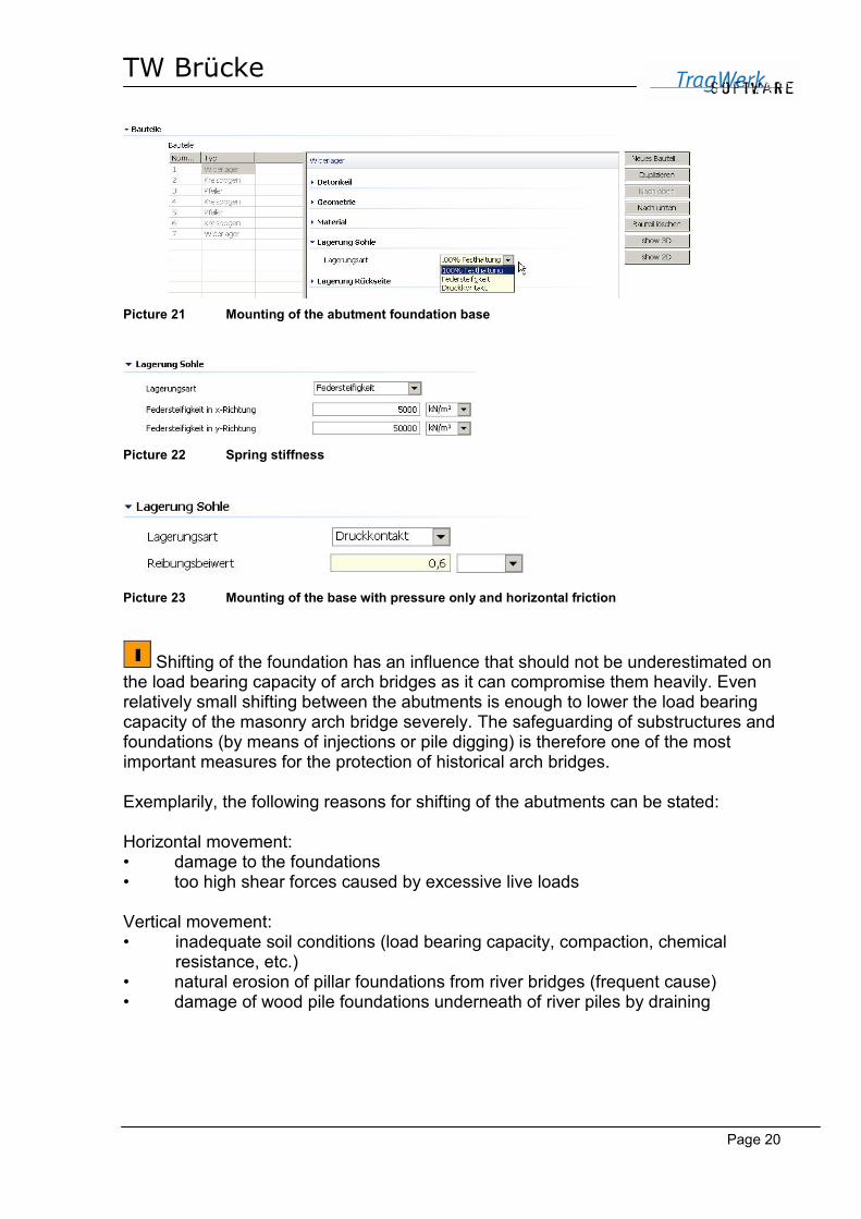
4.3 Mounting of the abutment base

The abutment absorbs the horizontal and vertical bearing forces of the arch and directs them into the adjacent foundation soil. For this, the bearing pressure is applied to the ground beneath it. The pushing forces from the arch activate opposing forces in the ground through friction. For this, the abutments must possess the necessary dimensions and strength. The heavier the abutments are, the larger the horizontal loads are that can be transferred into the ground through the base. The abutment foundation can either be mounted using elastic springs, a rigid support, or with contact elements only transferring pressure.

TW Brücke

Picture 21 Mounting of the abutment foundation base

Picture 22 Spring stiffness

Picture 23 Mounting of the base with pressure only and horizontal friction

Shifting of the foundation has an influence that should not be underestimated on the load bearing capacity of arch bridges as it can compromise them heavily. Even relatively small shifting between the abutments is enough to lower the load bearing capacity of the masonry arch bridge severely. The safeguarding of substructures and foundations (by means of injections or pile digging) is therefore one of the most important measures for the protection of historical arch bridges. Exemplarily, the following reasons for shifting of the abutments can be stated: Horizontal movement: • damage to the foundations • too high shear forces caused by excessive live loads Vertical movement: • inadequate soil conditions (load bearing capacity, compaction, chemical

resistance, etc.) • natural erosion of pillar foundations from river bridges (frequent cause) • damage of wood pile foundations underneath of river piles by draining

TW Brücke

4.4 Horizontal Mounting of the Abutment Outer Side

TW Brücke offers several possibilities for the mounting and support of the abutment outer sides:

� Fixed mounting � Bedding module e.g. according to UIC Code 778-3[11]) � Earth pressure � Free movement

4.4.1 Fixed Mounting

A fixed mounting (100% Fixed) is modelled with a very stiff spring support.

Picture 24 Mounting methods

4.4.2 Bedding of the Abutment Outer Side According to UIC Code 778-3

Picture 25 Horizontal spring stiffness for bedding of the outer side of the abutment

Example for sand; medium density; dry: nh = 6.700 kN/m³ (Tab.2); Distance OKG to OK Abutment 3.00m, Height of Abutment 4.00m Horizontal bedding factor for per meter strips z⋅= hhs nC (= linear spring stiffness

vertical along the abutment outer side per meter of horizontal displacement) Top: � Chs,OK WL = 6.700 kN/m³ · 3,00 m = 20.100 kN/m² Bottom: � Chs,UK WL = 6.700 kN/m³ · (3,00 m + 4,00 m) = 46.900 kN/m²

TW Brücke

Horizontal Modulus of Subgrade Reaction for Sand

For the determination of the horizontal modulus of subgrade reaction Chs the following calculation is valid:

B

znC hhs ⋅=

With: Chs horizontal modulus of subgrade reaction [kN/m³] nh horizontal bedding factor [kN/m³] from Tab.2 z Vertical coordinate from top edge of road [m] B 1 m wide abutment strips Tab. 2 Horizontal embedding factors nh in [kN/m³] for sand as a function of the compactness density ID

Sand Light Average Dense

Compactness Density ID 0 ≤ ID< 0,33 0,33 ≤ ID< 0,67 0,67 ≤ ID< 1,0 Dry or wet under water 2.240

1.280 6.700 4.480

17.900 10.900

Horizontal modulus of subgrade reaction for pre-consolidated clay

For the determination of the horizontal modulus of subgrade reaction Chs is valid:

B

0,203kC h1hs ⋅=

With: Chs horizontal modulus of subgrade reaction [kN/m³] kh1 horizontal bedding factor [kN/m³] from Tab.3 B 1 m wide abutment strips Tab. 3 Horizontal bedding factor kh1 in [kN/m

3] for pre-consolidated clay as a function of the

consistency number IC according to Terzaghi

Consistency Pre-consolidated clay

stiff semi solid solid

Compactness density ID 0,75 < IC≤ 1,00 1,00 < IC≤ ICS IC>ICS Limit Values kh1 16.000 – 32.000 32.000 – 64.000 64.000 Recommended Values kh1 24.000 48.000 96.000 With: ICS consistency number at the contraction limit

TW Brücke

Horizontal Modulus of Subgrade Reaction for soils which lie between sand

and pre-consolidated clay

For soils which lie between sand and pre-consolidated clay, with a plasticity number IP in the limits of 0.1 ≤ IP ≤ 0.3 and with a consistency number in the range of 0.75 < IC to IC > ICS, the approximate determination of the horizontal modulus of subgrade reaction CHS the correlation values from Tab. 4 can be used. Intermediate values for IP are to be interpolated linearly within the limits of 0.1 ≤ IP ≤ 0.3. Tab. 4 Horizontal Bedding Factor kh1 in [kN/m³]

Plasticity number IP Consistency number IC

IP = 0,3 IP = 0,2 IP = 0,1

0,75 < IC≤ 1,00 24.000 30.000 43.000 1,00 < IC≤ ICS 48.000 60.000 86.000

IC>ICS 96.000 120.000 170.000

4.4.3 Earth pressure on the Abutment Outer Side

The earth pressure (qo, qu in kN/m) on the abutment along the height of the infilling at the top (o) and base (u).

Picture 26 Earth Pressure

4.4.4 Free Support

In rare cases, the abutment is not supported horizontally..

Picture 27 Free support

TW Brücke

5 Pillars

The influence of the pillar strength on the bearing and deformation behaviour of the arches is taken into account. TW Brücke does not dimension the pillars, but instead determines the deformations and stresses for a separate verification.

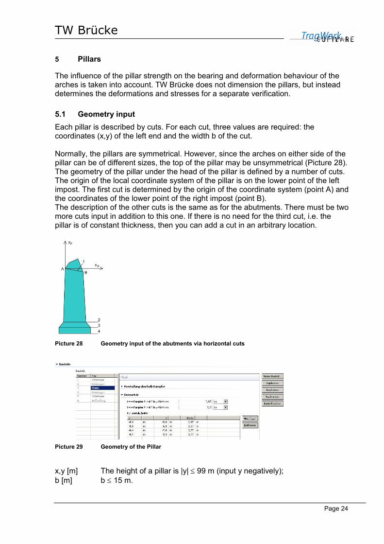
5.1 Geometry input

Each pillar is described by cuts. For each cut, three values are required: the coordinates (x,y) of the left end and the width b of the cut. Normally, the pillars are symmetrical. However, since the arches on either side of the pillar can be of different sizes, the top of the pillar may be unsymmetrical (Picture 28). The geometry of the pillar under the head of the pillar is defined by a number of cuts. The origin of the local coordinate system of the pillar is on the lower point of the left impost. The first cut is determined by the origin of the coordinate system (point A) and the coordinates of the lower point of the right impost (point B). The description of the other cuts is the same as for the abutments. There must be two more cuts input in addition to this one. If there is no need for the third cut, i.e. the pillar is of constant thickness, then you can add a cut in an arbitrary location.

Picture 28 Geometry input of the abutments via horizontal cuts

Picture 29 Geometry of the Pillar

x,y [m] The height of a pillar is |y| ≤ 99 m (input y negatively); b [m] b ≤ 15 m.

TW Brücke

5.2 Material Parameters

See Abutment Section 4.2.

5.3 Mounting at the pillar’s base

See Abutment Section 4.3. Beneath the common area of arches in so-called viaducts, pillars primarily take up the vertical forces introduced by the arches. The horizontal forces applied to the ground are relatively low, in fact, the opposing force from arches on both sides of a pillar almost cancel each other out. Depending on the stress loading and stiffness ratios of the surrounding areas, the shearing forces are transferred to those areas as well.

TW Brücke

6 Infilling

TW Brücke provides several variables for the infilling to be able to determine the bearing capacity. The height (Picture 30, structure height) is measured from the crest of the first arch to the upper surface of the infilling.

6.1 Infilling with Stiffness

The infilling is calculated with a mesh of finite elements. This approach's requires a stiff or rigid infilling in reality, as is the case for lean concrete.

6.1.1 Material Parameters

If a strength is to be assigned to the infilling, then the elastic modulus and Poisson's ratio and density must be specified. If the infilling is used only as a load, then only the density is required.

Picture 30 Infilling with stiffness

The elastic modulus of the infilling should be a maximum of 1/10th of the elastic modulus of the arch. Otherwise the infilling is acts as a "frame" with the

compressive zone above the arch. The infillling will thus be regarded as a "tensile zone" and the computation will show that this has failed. For the case that the infilling is more elastic, the arch can carry the loads arithmetically and it can structurally be verified.

TW Brücke

6.2 Infilling only as a Load

To be on the safe side, the infilling is applied here only as a load to the top of the arch. For non-binding, loose, uncompacted material (sand, gravel, ballast) this approach (Picture 31) is more suitable than the previously mentioned mesh with the stiffer finite elements. The traffic loads are spread according to BOUSSINEQ-FRÖHLICH bell shaped over the height of the infilling and to the top of the arch.

Picture 31 Infilling as a load without stiffness

TW Brücke

7 Loads and Forces

The effects on the bridge are divided into two groups: 1. permanent actions - static loads • The dead load of the bridge • an additional vertical block load extending over the entire length of the bridge

(e.g. road cover or ballast) • the earth pressure on the outer sides of the abutments 2. variable actions - dynamic loads • Traffic loads in different positions (moving load)

Picture 32 Live Load Diagram

If a contact task (discontinuous model with gaping joints), and thus a non-linear calculation, is selected, the loads are applied as follows; 1. dead load of the bridge 2. step-by-step applying of the traffic load. An iteration procedure is started for each applied load, to solve the contact task in the joints. If the system remains stable, the next loading step is applied. When choosing a linear calculation, all loads are applied in one step. If the resultant force line is outside the first core range, then the results are unrealistic.

7.1 Permanent Actions - Static Loads

Static loads on the construction are to be considered according to DIN EN 1991 [8] with the input of the density. In addition, a uniform line load can be defined as a constant load, for calculating loads from the roadway structure.

The permanent loads (dead load) of a vault bridge result from parts of the vaulted brickwork, the brickwork, the infilling, and the roadway structure.

Since, in the case of conventional square brickwork, the joints take up less than 5%

TW Brücke

of the area, therefore, just the density of the stones can be used for the total vault masonry.

7.2 Variable Actions - Live Loads

TW Brücke allows any load diagram to be used for road and rail traffic according to for instance DIN 1072 [9] or DIN EN 1996-2 [10]. For the non-linear calculation, the program internally calculates the traffic load in sub-steps under incremental increase of the load. For each sub-step, the system response and balance is recalculated and the result is stored for the later evaluation. The following load diagrams are shown in Appendix 9.1.3: • Load model 1 (LM1) • HGV 60 • HGV 30 • GV 16/16 • GV 12/12 • GV 9/9 • GV 6/6 • GV 3/3 • load model 71 (LM 71) • load model heavy load 0 (SW 0) • load model heavy load 2 (SW 2) The location and the size of the load coordinate are determined. The load position refers to the global coordinate system originating in the arc center of the first arc (Picture 32).

TW Brücke

7.2.1 Load Model 1

In the region of the wheel loads (L = 0.4m) and in the remaining areas, the following distributed load is applied to the 1 m wide arch strip (Picture 33) according to section 9.1.1 with a cross distribution over the track width of 3.0m.

Picture 33 Load Model LM1 from road traffic on an example bridge

7.2.2 Load Model 71

In contrast to road traffic loads, in the rail traffic load models the dynamic effects are not included but must be verified separately in the calculations. The characteristic values of the axle and line loads, are to be multiplied with a factor, for train lines where traffic is heavier or lighter than regular (standardised) traffic. The loads multiplied by this coefficient are called "graded vertical loads". Possible load class coefficients α according to DIN EN 1991-2: 0,75 – 0,83 – 0,91 – 1,00 – 1,10 – 1,21 – 1,33 – 1,46

The following characteristic loads must be multiplied by the load class factor when taken into account:

� Load model 71 and load model SW/0 � Centrifugal forces � side impact � starting and braking loads � combined response of load-bearing structure and track to variable loads � derailment loads � vertical substitute loads for earth constructions and earth pressures

Tab. 5 Tab. 5 Load class coefficient according to NDP to 6.3.2 (3)P Note

Load situation Load class coefficient α according to DIN EN 1991-2/NA

Maintenance trains with 25 ton wheel load 1,21 S-Bahn - Commuter Train 0,80 Construction stages (all of the above loads) 1,00

TW Brücke

When determining the dynamic coefficient (oscillation coefficient), usually a carefully maintained track can be assumed. For this, Φ2 is to be applied. From the multiplication of the coefficients, the required load factor (γL...Gamma required) can be determined.

Example with an oscillation coefficient: γL = ϕSchw · γLM71 = 1,13 · 1,3 = 1,47. The bridge is safe if the verification with this load factor can be acchieved.

In order to determine the degree of utilization of the design, it is advisable to apply the traffic load with a higher traffic load factor than the required gamma (Picture 34, traffic load factor = 2.0): Traffic load factor ≥ gamma required (γL) The load diagram is multiplied internally by the traffic load factor and is applied in the defined number of sub-steps.

Picture 34 Input load model LM71 from rail traffic

Picture 35 Load model LM71 from rail traffic

TW Brücke

7.3 Load Factor STR/GEO

The safety factors for traffic loads (load factors gamma required) must be specified according to the selected Verification method. Further factors, e.g. the vibration coefficient and the load factor coefficient must be multiplied with this. Tab. 6 Load factor γF

Norm Table or Section Content of the Standard γF

UIC-Code 778-3 [11]) 4.3 Effects Reference to DIN EN 1991 (γ however, in DIN EN 1990)

1,45

DIN EN 1990/NA Tab. A2.4 (B), Remark 2

Load Model LM 71 1,45

DB-RiL 805 [12] Number 805.0101, Section 2, Table 1

Calculating of existing Railway Bridges

1,30

DB-RiL 805 Number 805.0101, Section 2, Table 1

Calculating of existing Railway Bridges for operating loads

1,20

Recalculation guideline for existing road bridges [13]

Section 10.2, Tab. 10.8 LM1 nach DIN EN 1991-2/NA

1,35

Recalculation guideline for existing road bridges

Section 10.2, Tab. 10.8 ≤ BK 60/30(DIN 1072) 1,50

Recalculation guideline for existing road bridges

Section 10.2, Tab. 10.8 LM1 (DIN Fb 101)

1,50

TW Brücke

8 Verification Methods

Choice of the calculation method for the structural verification of the Arches in the ULS (Ultimate Limit State of load bearing capacity)

� LA (Limit Analysis) [2, 14, 4] � EC6: DIN EN 1996 - 1 - 1 [15] with NAD [16] � UIC: UIC Code 778-3 [11

Picture 36 Selecting the verification method

Below the design concepts will be applied to a practical example. The load combination used here consists of the bridge dead load and the load model LM 71.

Characteristic material values

Stone: Compressive strength: f D,St,5%= 26,0 N/mm² Tensile strength: f Z,St,5%= 1,8 N/mm² Mortar: Compressive strength: fD,Mö = 2,5 N/mm² (average)

TW Brücke

8.1 Limit Analysis method (LA) - Partial safety concept

For the material values from the expert report, the following tensile strengths are obtained with the partial safety coefficients: Stone: Compressive strength: fD,St,d = 26,0 N/mm² / 1,3 = 20,0 N/mm² Tensile strength: fZ,St,d = 1,8 N/mm² / 1,8 = 1,0 N/mm² Mortar: Compressive strength: fD,Mö = 2,5 N/mm² / 1,0 = 2,50 N/mm² (average) For the verification, for each arch thickness, the cross-sectional capacity (rated load-bearing curve) is required (see appendix 9.3). In the case of conical arches, the smallest and largest cross-section thickness is generally sufficient (Picture 37). Intermediate values are interpolated by TW Brücke automatically.

Input of the load-bearing capacity of the 1m-wide bridge strip with the unit in kN/m (bridge width).

Picture 37 Inputting the capacity curves for various arch thicknesses

TW Brücke determines the intersection point (Picture 38) between the load path and the capacity curve. To calculate a possible breaking point, the load diagram is increased by 10 steps up to 3.0 times the load.

TW Brücke

Picture 38 Capacity curve and load-bearing path of the relevant cut in the Arch

In the most stressed arch cross-section, when increasing the load by the factor γBruch = 2.09, the capacity curve intersects the load bearing path and the fracture state is determined. If there is no intersection point for the load factor γL = ϕSchw ·γLM71 = 1,13 • 1,3 = 1,47 (Picture 39), then the structural stability would also be verified.

Picture 39 Load position with resultant force line γ= 1,47 -times the load

With the help of the resultant force line load-bearing method, the degree of utilization of the arch construction is: η = γL/ γBruch = 1,47/ 2,09 = 0,7< 1,0 Verified!

Rated Capacity Curve

Load Bearing Path

TW Brücke

8.2 Limit Analysis method (LA) Global safety concept

The verification is carried out with the characteristic value of the action multiplied by the oscillation coefficient. The safety factors are aggregated on the resistance side. For the material values from the expert opinion (technical expertise), the following rated strengths result from the global safety factor of γM = 3,0 on the resistance side: Stone: Compressive strength: fD,St,d = 26,0 N/mm² / 3,0 = 8,67 N/mm² Tensile strength: fZ,St,d = 1,8 N/mm² / 3,0 = 0,60 N/mm² Mortar: Compressive strength: fD,Mö = 2,5 N/mm² / 1,0 = 2,50 N/mm² (average)

Input of the load-bearing capacity of the 1m-wide bridge strip with the unit in kN/m (bridge width).

Picture 40 Input capacity curve for arch thickness t = 73cm

TW Brücke determines the intersection point (Picture 41) between the load path and the capacity curve. For this purpose, the load diagram is also increased in 10 steps up to 3 times the load.

TW Brücke

Picture 41 Rated capacity curve and load-bearing path of the relevant section in the Arch

In the most stressed arch cross-section, the rated capacity curve intersects the load bearing path when increasing the load by the factor γBruch = 1.53 and the fracture state is determined. If there is no intersection point for the load factor γL = ϕSchw ·γLM71 = 1,13 • 1,0 = 1,13(Picture 42), then the structural stability would also be verified. However, the degree of utilization ≤ 1.0 will then not be able to be determined more accurately.

Picture 42 Load position with the resultant force line for γ= 1,13 times the load

With the help of the load-bearing method, the degree of utilization of the arch construction with the global safety concept is as follows: η = γL/ γBruch = 1,13/ 1,53 = 0,73< 1,0 Verified!


Load Bearing Path

TW Brücke

8.3 EC6-1-1 / NCI Appendix NA.L

In the case of verification of the masonry in the ultimate limit state, it must be ensured that the rated value of the load NEd in a cross-section does not exceed the rated value of the load-bearing resistance NRd of this cross-section: NEd ≤ NRd

The characteristic brickwork compressive strength of the sandstone square masonry with the input values (see Appendix 9.3.2) after interpolating is fk = 6.34 N/mm2 = 6.340 kN/m2 [16]. The rated value fd of the compressive strength follows: fd = ζ · fk / γM

The material safety factors are taken from EC 6 and NAD [15, ] with γM = 1.5 and a preselected durability factor of ζ = 0.85

Picture 43 Material safety and durability factor according to EC6

With the rated strength fd = 0.85 • 6.34 / 1.5 = 3.59 N / mm² the rated value of the bearing capacity under centric load for the cross section is as follows: Nrd = A fd with: A...area of the cross-section Nrd = 0.73 m • 1,0 m • 3.590 kN/m² = 2.623 kN The rated value of the loadable standard load under eccentric loading is defined by the standards with a linear reduction: NRd = φ · A · fd with: A ... Area of cross-section φ ...Load factor for load eccentricity φ = 1 – 2e/t with: t ... arch thickness TW Brücke determines the intersection point (Picture 44) between the load path and the capacity curve. For this purpose, the load diagram is also increased in 10 steps up to 3 times the loading to determine a potential fracture point.

TW Brücke

Picture 44 Rated capacity curve and load path of the relevant section

For the load model LM71, it must be shown that this load with a oscillation coefficient and load factor of .γL = ϕSchw ·γLM71 = 1,13 · 1,45= 1,64 does not result in a mathematical failure.

Picture 45 Load position with resultant force line with γ= 1,48 times the load in a calculated fracture

state

With the fracture point γBruch = 1,48, the degree of utilization of the arch construction results in: η = γL/ γBruch = 1,64/ 1,48 = 1,1> 1,0 Not verified! The traffic load with the load factor γL = 1.64 can not be carried successfully. For at least one joint, an intersection between the load path and the rated capacity curve exists during the load increase to γL -required (Picture 44). The load-bearing capacity of this example bridge (Picture 44) cannot be verified in this case, according to EC 6-1-1/NA


Load Bearing Path

ΝΡδ = φ A fd

TW Brücke

8.4 UIC-Code 778-3

According to the UIC Code [17] the load-bearing capacity is considered to be verified if the stress value of the load is less than or equal to the value of the load-bearing resistance (σd≤ fd) . The stresses are to be determined with the following characteristic effects γL = ϕSchw ·γLM71 = 1.13 • 1.3 = 1.47 multiplied by the oscillation coefficient and the load factor. With the material safety γM considered, the rated strength fd gives: fd = fk / γM with: γM = 2.0 (material safety)

Picture 46 Material safety factor

The material safety of 2.0 is approximately 10% greater than the value according to EC 6 with γM/ ζ = 1,5 / 0,85 = 1,76.

The centric load-bearing capacity of the masonry is determined by the UIC code on the basis of the equation according to OHLER [18]. In this more accurate calculation (Appendix 9.3.3) the stone compressive and tensile strengths, the mortar compressive strength as well as the geometry are taken into account. With the coefficients a = 1 and b = 2.2 for the square masonry with a stone height of hs = 64cm and joint thickness of tF = 1.5 cm, the characteristic masonry compressive strength results in:

2

,

,

,,,k /18,11

8,1642

0,265,05,12,21

5,25,00,265,00,15,25,0

2

5,01

5,05,05,0 f mmN

fh

ftbffa

f

StZS

StDF

MöDStDMÖD =

⋅⋅⋅⋅⋅

+

⋅−⋅⋅+⋅=

⋅⋅⋅⋅⋅

+

⋅−⋅⋅+⋅=

fk = 11.180 kN/m² The rated strength fd is given for the material safety factor γM = 2,0 as: fd = 11.180/ 2,0 = 5.590 kN/m² And thus the rated load-bearing capacity of the arch of 73 cm thickness under centric loading: NRd = A · fd = 0,73 m · 1,0 m · 5.590kN/m²=4.081 kN The verification is also carried out with the internal forces. In addition for the effect of eccentric loading, the load factor φ = 1 − 2e/t is used according to EC 6 and set to zero for large load eccentricities from m= 6 ⋅ e/t = 2,0 according to the UIC code.

TW Brücke

The verification of the load eccentricity recommended in the code would lead to higher loads than the allowable limit of rigid plastic material and is therefore not used here (see section 9.3.3). A significant advantage of the evaluation with the internal forces is that no stress peaks at "internal corners" are dimension-relevant for the FE-analysis, which is known to be influenced strongly by the mesh fineness and could otherwise result in unrealistically high values. Due to the integration over the arch cross-section to the resultant, these stress points are not relevant here, but are contained in the integral average. TW Brücke determines the intersection point (Picture 47) between the load path and the capacity curve. For this purpose, the load diagram is increased in 10 sub steps up to 3 times the loading to determine a potential fracture point.

Picture 47 Rated capacity curve and load-bearing path of the relevant cut

For the load model LM71, it must be verified that this load (Picture 48) with an added oscillation coefficient and load factor of γL = ϕSchw ·γLM71 = 1,13 · 1,3= 1,47 does not result in a mathematical failure.

Picture 48 Load position with resultant force line with 1,47 times the load


Load Bearing Path

NRd

= φ A fd

TW Brücke

With the fracture point γBruch = 2,71 the degree of utilization of the arch construction results in: η = γL/ γBruch = 1,47/ 2,71= 0,54< 1,0 Verified!

8.5 Compilation of results

The calculation with four different safety concepts results in different degrees of utilization as was to be expected: Tab. 7 Degrees of utilization according to various verification methods

Verification Method Degree of Utilization

LA + Partial safety concept 70 % LA + Global Safety Concept 73 % EC6 110 % UIC 54 % The Limit Analysis Method (LA) is based on a more accurately determined load-bearing capacity in dependence of the load eccentricity. For the EC6 and UIC verifications, only the values under centric stress are included in the standards, the UIC gives an analytical verification and in EC6, table values are available. Here the relevant load bearing capacities from eccentric loadings are the result of a very simplified linear relationship.

TW Brücke

9 Appendix

9.1 Application of the Load

9.1.1 Load Determination for Road Traffic

In the area of the wheel loads (L=0.4m), the following line load is a resultant on the 1 m wide strip of the vault (see Picture 3): without cross-distribution with q = 240 kN/ 2-Räder = 120 kN q = 120 kN / 0,40 m + (1,00 m – 0,40 m) ⋅ 9 kN/m² = 305,40 kN/m (L=0,4m) with transverse distribution over road width 3.0m with q = 240 kN/ 3 = 80 kN q = 80 kN / 0,40 m + ((3,0 m – 0,80 m) ⋅ 9 kN/m²)/3 = 206,60 kN/m (L=0,4m)

9.1.2 Load Determination for Railway Traffic

It is permitted to distribute the wheel load over three rail support points. For this, the middle rail is assigned the track load Qvi/2 and the two adjacent rails are assigned Qvi/4. Based on a sleeper distance of 60cm, the wheel load is simplified as a uniformly distributed line load over a length of 2 x 60 cm = 120 cm. For simplification purposes the favourable longitudinal load distribution under the sleepers through the ballast bed is neglected. The load diagram for the FE calculations is as follows: At a maximum permissible gauge of 1470mm and a rail head width of 74.3mm (UIC 60), r is obtained as follows: r = 1470mm + 74.3mm = 1544.3mm and the eccentricity e according to DIN-FB 101 to: e = r/18 = 85.79mm For a single load N=100kN, the percentage of the load is determined, which is acting on the 1m strip of the arch.

TW Brücke

eQv1 Qv2

Qv1 + Qv2

2,60 m

4:1

4:1

2,75 m

r

0,30 m

N = Qv1 + Qv2

1m

N

M

-+

(N · e)/W +

N/A

-

-

1m

A1

= 0,4

A = 0,6

σl

σr

σ1

1m

e

1m-Streifen im Grundriss


=

A1 40.7− kN=A1

σ1 σr+

21m( )

2⋅=

σ1 38.22−kN

m2

=σ1 σr

σr σl−

b1⋅ m−=

σr 43.17−kN

m2

=σrN e⋅

W

N

A+=

σl 29.56−kN

m2

=σlN− e⋅

W

N

A+=

A 2.75m2

=A b h⋅=

W 1.26m3

=Wb

2h⋅

6=

h 1m=b 2.75m=N 100− kN=

Für eine Einzellast N = 100 kN wird der

prozentuale Anteil dieser Last ermittelt,

welcher auf den 1m-Streifen des

Brückenbogens wirkt.

e 85.79mm=er

18=

und die Exzentrizität e nach DIN-FB 101 zu:

r 1544.3mm=r 1470mm 74.3mm+=

Bei einer maximal zulässigen Spurweite

von 1470 mm und einer Schienenkopf-Breite

von 74,3 mm (UIC 60) ergibt sich r zu:eQv1 Qv2

Qv1 + Qv2

2,60 m

4:1

4:1

2,75 m

r

0,30 m

N = Qv1 + Qv2

1m

N

M

-+

(N · e)/W +

N/A

-

-

1m

A1

= 0,4

A = 0,6

σl

σr

σ1

1m

e



=

eQv1 Qv2

Qv1 + Qv2

2,60 m

4:1

4:1

2,75 m

r

0,30 m

N = Qv1 + Qv2

1m

N

M

-+

(N · e)/W +

N/A

-

-

1m

A1

= 0,4

A = 0,6

σl

σr

σ1

1m

e



=

A1 40.7− kN=A1

σ1 σr+

21m( )

2⋅=

σ1 38.22−kN

m2

=σ1 σr

σr σl−

b1⋅ m−=

σr 43.17−kN

m2

=σrN e⋅

W

N

A+=

σl 29.56−kN

m2

=σlN− e⋅

W

N

A+=

A 2.75m2

=A b h⋅=

W 1.26m3

=Wb

2h⋅

6=

h 1m=b 2.75m=N 100− kN=

Für eine Einzellast N = 100 kN wird der

prozentuale Anteil dieser Last ermittelt,

welcher auf den 1m-Streifen des

Brückenbogens wirkt.

e 85.79mm=er

18=

und die Exzentrizität e nach DIN-FB 101 zu:

r 1544.3mm=r 1470mm 74.3mm+=

Bei einer maximal zulässigen Spurweite

von 1470 mm und einer Schienenkopf-Breite

von 74,3 mm (UIC 60) ergibt sich r zu:

Picture 49 View of a 1m strip in the layout of the track cross-section

The illustrated simplified stress distribution shows that, without consideration of centrifugal forces, approximately 40% of the vertical load is applied to the 1 m wide bridge arch in the 2D model. The "blurred" load diagram shown in Picture 51 can be derived from this. The actual spatial stress distribution is not considered here, so with this assumption one still stays on the safe side.

Picture 50 Load Model LM 71

TW Brücke

unbegrenzt unbegrenzt0,20 m

1,20 m

0,40 m

1,20 m

0,40 m

1,20 m

0,40 m 0,20 m

1,20 m

4 x Qvk = 83,33 kN/m

qvk = 32 kN/mqvk = 32 kN/m


1,20 m

0,40 m

1,20 m

0,40 m

1,20 m

0,40 m 0,20 m

1,20 m

4 x Qvk = 83,33 kN/m



1,20 m

0,40 m

1,20 m

0,40 m

1,20 m

0,40 m 0,20 m

1,20 m

4 x Qvk = 83,33 kN/m



1,20 m

0,40 m

1,20 m

0,40 m

1,20 m

0,40 m 0,20 m

1,20 m

4 x Qvk = 83,33 kN/m


Picture 51 Blurred Load Diagram of the LM71 with 40% of the load diagram LM1 on the 1m strip

9.1.3 Load Diagrams

Picture 52 Load Model LM1 with road traffic

Picture 53 Load Model SLW (HGV) 60 with road traffic

Picture 54 Load Model SLW (HGV) 30 with road traffic

Picture 55 Load Model Truck 16/16 with road traffic


TW Brücke




Picture 60 Load Model LM 71 with rail traffic

Picture 61 Load Model LM SW/0 with rail traffic

Picture 62 Load Model LM SW/2 with rail traffic

TW Brücke

9.1.4 Load application / Transfer

The loading is carried out according to the method of BOUSSINESQ-FRÖHLICH. By using the stress distribution in the half-space, it is possible to calculate with a variable depth.

Picture 63 Stresses in the element as a result of a load on the half-space surface with a point load [19]

According to BOUSSINEQ, a perpendicular single load P (Picture 64) on an elastic, isotropic, and volume-constant, half-space with the elastic modulus E and Poisson's ratio ν, creates radial stresses σr, tangential stresses σt, from which next to others the vertical normal stresses σz can be calculated. These vertical stresses are here independent of E and ν. As the soil is non-linearly elastic, FRÖHLICH's is therefore based solely on equilibrium considerations and assumes the stress σr is proportional to 1/r2.

Picture 64 Load distribution (qualitative) from the infilling to the upper side of the arch

FRÖHLICH also modified the derivation and introduced the concentration factor νk, which considers the concentration of the stresses around the load axis. Picture 64 shows the course of the σz stresses in a horizon at the depth z = constant for νk = 3, νk = 5 and νk = 8. The more cohesive the infilling material, the more the stresses are distributed. The greater the ability of the infilling material to distribute stresses by friction are, the more concentrated the stresses around the load axis are. With a large concentration factor (Picture 65), one stays on the safe side, as the load application is more concentrated.

TW Brücke

a) b)a) b) Picture 65 a) Qualitative dependence of the concentration factor νk on the soil type

b) Course of the σz stresses at different concentration factors νk

9.1.5 Reduction Factor for taking a spatial load into account

The actual spatial load-bearing capacity, for example in the case of several traffic lanes of different loading, can also be taken into account in the 1m verification strip with reduction factors [3] . This makes it possible to detect existing load reserves which are due to transmittable effects in the transverse direction of the arch masonry. Regarding the spread of the acting wheel loads, the stresses (supporting area) generated in the arch in the transverse direction can thus be regarded indirectly via reduction factors in the 2D system (resultant force line). The reduction factors provided give the engineer an efficient calculation possibility of a vault bridge with a 2D model. For intact vaults, the degree of utilization is thus on the safe side. Picture 66 shows the possible load increase due to a cross-distribution.

Fracture mechanical Failure: the stone is to soft and begins to crumble /fail Mechanical failure of the System: the Stone in itself is strong enough to withstand the pressure, but due to the pressure an open joint is formed and the system fails as a whole.

TW Brücke

Picture 66 Failure state at γ-fold LM1 for fD,St = 10; 30 and 60 N/mm²

TW Brücke

9.1.6 Load Crossings / Moving Load

In order to find the relevant load diagram of the chosen load model, that maximizes the utilization of the arch bridge, TW Brücke can calculate the load passage in up to 99 load steps. A load passage, for example, starts at the left point A and ends at the right point E (Picture 67).

LM 1, DIN FB 101

A E

Schritt 1: Verlängerung der Flächenlast von A bis E Schritt 2: Vorfahren der Doppelachse um ∆L, anschließend Schritt 1

∆L = konstant

LM 1, DIN FB 101

A E

∆L

⇔

LM 1, DIN FB 101

A E

Schritt 1: Verlängerung der Flächenlast von A bis E Schritt 2: Vorfahren der Doppelachse um ∆L, anschließend Schritt 1

∆L = konstant

LM 1, DIN FB 101

A E

∆L

⇔ Picture 67 Passage of the Load Model 1

For each load position of the double axis, all the load diagrams of the surface load between points A and E are examined. The start of the surface load remains fixed at point A. This setting considerably reduces the number of load diagrams per passage, thus saving computing time. Through random chosen tests, it was found that in no case the experiments resulted in a significant increase in cross-section loading due to a variable starting point of the surface load.

The step width is to be selected according to the span (for example, ∆L = 30 cm at L = 10 m). In order to save computation time, a complete passage with a

larger step size can be carried out first in order to discover the range of the relevant load diagram. In a second step, a further load passage in the previously outlined range is to be carried out with a smaller step width in order to precisely determine the relevant load diagram while keeping an appropriate efficiency.

9.1.7 Oscillation Coefficient

In order to take account of the rapid load changes and oscillations from track and wheel unevenness occurring during the crossing of the train, the static load diagram is to be increased by the dynamic coefficient. This oscillation coefficient is calculated for “tracks with careful maintenance” as follows [10]:

ϕ2= min(ϕ2; 1,67)

...2-times the clear span of each individual vault according to DIN EN 1991-2; Tab. 6.2

TW Brücke

9.2 Safety concepts

TW Brücke supports verification for both: � Partial safety concept [2, 14, 4] as well as the � Global Safety concept [2, 14, 4].

9.2.1 Partial Safety Concept

The following safety factors (Tab. 8) meet the required failure probability.

Tab. 8 Safety factors for the partial safety concept (see. Tab. 6)

Effects γf Commentary

Road Traffic (characteristic Value)

1,30 1,20 1,35

Recalculation classes according to DIN 1072; Special vehicles according to special specifications Recalculation for LM1 (Recalculation guideline; DIN EN 1991-2/NA)

Rail Traffic (characteristic value)

1,30 1,20 ---

UIC 71 according to DB-RiL 805; Special vehicles, line class according to special specifications Load diagram fully covers the actual railway operating loads All additional loads and special loads according to RiL 805

Dead Loads (average)

1,10 0,90

In case of unfavourable effect for traction safety In case of favourable effect for traction safety

Abutment settlements (average)

1,00 According to foundation soil report; For undamaged arches which have been in place for an extended time, without an increase in loading, the report is unnecessary

Structure Sizes *) γm Commentary

Structure geometry (average)

1,00

From the building plans or on-site measurement

Elastic Modulus of building materials (average)

0,90 ... 1,10

Calculation for upper and lower limit value; For average apply a value of 1.0

Geometry of stones and joints (average)

1,00

On-site inspection is always necessary; Determine joint width conservatively

Stone compressive stress**)

1,80 1,30

Based on the Average Based on the 5 %-fractile (characteristic value) Validity limit: v = σ / m < 30% (variation coefficient)

Stone tensile strength**)

1,80 Based on the 5% fractile (characteristic value) Validity limit: v = σ / m < 30% (variation coefficient)

Mortar compressive stress (average)

1,00 Uniaxial compressive strength

Compressive strength overlay; concrete topping (average)

1,80 Based on the 5 % fractile (characteristic value); Is only significant if the stone arch is planned to be calculated as „supported“ (Able to support the starting and braking loads from traffic)

Alternatively, individual factors are perceivable, in order for example, to meet better or worse actual conditions of the arch structure.

TW Brücke

9.2.2 Global Safety Concept

A global safety concept has the advantage that the uncertainties of the input information are collected in the integral mean. This principle is useful, for example, if the characteristic strength values of the masonry must be rough estimates when statistical sampling would cause an unacceptably high cost. Here, there is scope for action of the engineer, which also allows subjective information (like empirical values, impression of the state of the structure, etc.) to be included. A global safety concept with characteristic effects and a summary safety factor on the resistance side is recommended mainly for the following applications:

� For numerically non-linear calculation of the system load, for action characteristic values and for the structure “computational mean values” are to be applied. The for this necessary deterministic variant investigations of the calculation model are of same importance as the correct safety factor.

� In the case of war-damaged structures which have been repaired after their

destruction. As a result of the explosions and the collapse of parts, in these buildings one has to reckon with hidden cracks and deformations, e.g. “shifting” of stone layers against one another, which cannot be found and clarified completely by preliminary investigations.

� The same applies to bridges damaged by natural disasters. Strength changes

due to cracking and compression of the system compared to the original state can cause considerable model uncertainties in the recalculation of existing constructions, even if examinations of alternatives are carried out. The safety factor should then be set higher accordingly.

� Viaducts must be regarded in many cases as “conglomerate constructions”.

The information from expert reports for a reasonable cost about the individual building materials is usually not sufficient, to be able to apply the partial safety concept for the entire structure.

� If the masonry strengths are only known by magnitude (non-statistical

sampling) and characteristic strengths are based on empirical values or only on a few samples.

A “global safety factor” of γM =3.0 is recommended for the materials if the building construction condition is at least good. Resistance side:

Stone tensile strength: γZ,St = 3.0 (Based on the 5% quantile value) Stone compressive strength: γD,St = 3.0 (Based on the 5% quantile value) For natural stone bridges with greater uncertainties in the model, it is recommended to increase the safety factor accordingly. This may be required for:

TW Brücke

• Possible damage (e.g. rehabilitated war or disaster damage) with hidden microcracks in the stone;

• Post-compressed masonry with different compressive results; however, a higher mortar strength could be applied instead;

• Masonry with relevant with moisture or frost damage of the stone • Using a material assessment which only shows the strength of the masonry by magnitude. The characteristic material values of the compressive strength and the tensile strength (5% quantile values) are divided by the “global safety factor”, so that the rated strength is the basis for the verification. The traffic load is set to γL = 1.0; other factors e.g. oscillation coefficients must be considered additionally. In analogy to the method with partial safety factors it is to be verified that the stress from the characteristic loading remains below the permissible rated load.

TW Brücke

9.3 Strength values

9.3.1 More Accurate Determination of the Capacity Curve

If there are no values for the realistic load bearing capacity for the given geometry and material parameters of the masonry available, the load curve can be determined for each cross-section slice by commissioning this at [email protected] For the determination of the cross-sectional capacity, a 2D calculation model is used in which stones and mortar joints are modelled separately and are cross-linked with four-knotted disk elements for the 2D distortion state. Thus the deformations perpendicular to the plane are obstructed, but the three-axial stress state in stone and mortar are evaluated. The dimensions of the stone, the thickness of the joints, and parameters of the materials are also chose able. The stones and mortar joints are generated with different mesh densities (Picture 68). Compared to the stone with its linear-elastic material behaviour, the bearing gap in the wall structure must be more closely meshed due to the non-linear material behaviour of the mortar in the wall joint, since plastically deformed regions require a sufficient density of integration points. Material laws are applied for the stones according to MOHR-COULOMB and for the mortar according to DRUCKER-PRAGER. With this, the failure load can be determined for any loading.

Picture 68 FE-Model of the masonry cross-section with a region showing the mesh density [4]

TW Brücke

Load bearing capacity under centric load (analytical)

From a multitude of calculation formulas [4], the following should be mentioned [20, 21]:

Load bearing capacity under eccentric loading (numerical)

For the calculation of the load bearing capacity under eccentric loading, there is no general analytical calculation algorithm known, according to the author’s knowledge. Therefore, the FE method is used here. Picture 69 shows the stress distribution in the cross-section for the different load eccentricities with associated failure loads. The gaping joints from an eccentricity bigger than the first core width (from m=1.0) are visible. For the load bearing capacity under centric loading, the failure loads correspond well with the results of the calculation formula mentioned.

TW Brücke

Picture 69 Stress distribution in the failure state for different loads eccentricity

From the input values from material and geometry a realistic load can be calculated even under extreme eccentric loading (Picture 70).

TW Brücke

Picture 70 A set of load bearing curves for different stone compressive and tensile strengths [22]

TW Brücke

9.3.2 EC 6 for Natural Stone Masonry

The strength values under centric loading are determined by the quality class, the stone and mortar compressive strength, and the geometry conditions according to Tab. 9 Intermediate values may be interpolated linearly. The characteristic stone compressive strength can be determined in a simplified method using 80% of the sampled mean value. Tab. 9 Characteristic values of the compressive strength of natural stone masonry according to EC6-1-

1, NCI Appendix NA. L

TW Brücke

9.3.3 UIC-Code 778-3

The UIC code determines the centric load-bearing capacity of the masonry on the basis of the equation according to OHLER [18]. In this more precise calculation of the characteristic cross-sectional strength, the stone compressive and tensile strength, the mortar compressive strength, as well as the geometry are regarded. Characteristic masonry compressive strength:

StZS

StDF

MöDStDMÖD

fh

ftbffa

f

,

,

,,,k

2

5,01

5,05,05,0 f

⋅⋅⋅⋅⋅

+

⋅−⋅⋅+⋅=

Tab. 10 Coefficients a and b

a b Brickwork Masonry 0,6 0,6 Natural Stone Brickwork (Stone height > 300mm)

1,0 2,2

Natural Stone Layer Brickwork (Stone height 200 - 300mm)

0,8 1,0

Square hewn Stone (Ashlar) (uncut Stone, high Mortar ratio)

0,1 0,4

The load carrying capacity under eccentric loading is described with the load carrying factor φ=1,8-1,2⋅(1-m/3) in the range of m= 1.0 to 2.0. Picture 71 shows the graph, according to which the load bearing capacity is above the “upper limit” (rigid-plastic stress distribution). From there onward the load carrying factor is used for eccentric loading with the “upper limit” φ= 1 – 2 e/t according to EC 6 and also used with the second core width (m=2.0).

Picture 71 Load bearing curves according to UIC code and modified according to EC 6

TW Brücke

TragWerk Software Döking + Purtak GbR Prellerstraße 9 01309 Dresden Tel. 0351/ 433 08 50 Contact: Fax 0351/ 433 08 55 Dr.-Ing. Frank Purtak e-mail [email protected]

TW Brücke

10 Bibliography

[1] PURTAK, F.; GEIßLER, K.: "Bogenbrücken aus Natursteinmauerwerk – Entwicklung eines

realitätsnahen Berechnungsmodells für den statischen Nachweis von Bogenbrücken aus Natursteinmauerwerk". Forschungsvorhaben Nr. KU 0425001KAT2, Schlussbericht 03/2006

[2] PURTAK, F.: "Gewölbebrücken aus Natursteinmauerwerk – Entwicklung eines

Berechnungsverfahrens zum statischen Nachweis von Gewölbebrücken unter Ausnutzung der räumlichen Tragwirkung". Forschungsvorhaben Nr. IW061178, Schlussbericht 05/2010

[3] HIRSCH, U.: „Nachweiskonzept für Bogenbrücken aus Natursteinmauerwerk“, Master-Arbeit,

Hochschule für Technik und Wirtschaft Dresden (FH), Fachbereich Bauingenieurwesen /Architektur, 2007

[4] Purtak, F.: Tragfähigkeit von schlankem Quadermauerwerk aus Naturstein. Dissertation,

TU Dresden, 2001 [5] CURBACH, M.; PROSKE, D.: "Abschätzung des Verteilungstyps der Mauerwerksdruckfestigkeit

bei Sandsteinmauerwerk". Wissenschaftliche Schrift, Technische Universität Dresden, Fakultät Bauingenieurwesen

[6] PAPULA, L.: "Mathematik für Ingenieure und Naturwissenschaftler". Band 3, 4. Auflage, Friedr.

Vieweg & Sohn Verlagsgesellschaft mbH, Braunschweig/Wiesbaden, 2001 [7] BERNDT, E.: "Zur Druck- und Schubfestigkeit von Mauerwerk – experimentell nachgewiesene

Strukturen aus Elbsandstein". In: Bautechnik 73, Heft 4, 1996 [8] ...: DIN EN 1991– Eurocode 1: "Einwirkungen auf Tragwerke". Teil 1: Wichten und

Flächenlasten von Baustoffen Bauteilen und Lagerstoffen, Juni 2002 [9] ...: DIN 1072: "Straßen- und Wegbrücken – Lastannahmen". DIN Deutsches Institut für

Normung e.V., Dezember 1985 [10] ...:DIN EN 1991-2: Eurocode 1: Einwirkungen auf Tragwerke – Teil 2: Verkehrslasten auf

Brücken [11] n: INTERNATIONALER EISENBAHNVERBAND: UIC-Kodex 778-3, "Empfehlungen für die

Bewertung des Tragvermögens bestehender Gewölbebrücken aus Mauerwerk und Beton". 1995

[12] ... : DB Richtlinie 805: "Tragsicherheit bestehender Eisenbahnbrücken". DB Netz AG, 2002 [13] Richtlinie zur Nachrechnung von Straßenbrücken im Bestand(Nachrechnungsrichtlinie) -

Bundesministerium für Verkehr, Bau und Stadtentwicklung Abteilung Straßenbau [14] PURTAK, F.; HIRSCH, U.: „Nachweisverfahren für Brücken aus Natursteinmauerwerk“,

Mauerwerk Kalender 2011, Ernst & Sohn Verlag [15] ...:DIN EN 1996-1-1 – "Eurocode 6: Bemessung und Konstruktion von Mauerwerksbauten –

Teil 1-1: Allgemeine Regeln für bewehrtes und unbewehrtes Mauerwerk“ [16] ...: DIN EN 1996-1-1/NA – "Nationaler Anhang – National festgelegte Parameter – Eurocode 6:

Bemessung und Konstruktion von Mauerwerksbauten – Teil 1-1/NA: Allgemeine Regeln für bewehrtes und unbewehrtes Mauerwerk“

TW Brücke

[17] n: INTERNATIONALER EISENBAHNVERBAND: UIC-Kodex 778-3, "Empfehlungen für die

Bewertung des Tragvermögens bestehender Gewölbebrücken aus Mauerwerk und Beton". 1995

[18] OHLER, A.: Zur Berechnung der Druckfestigkeit von Mauerwerk unter Berücksichtigung der

mehrachsigen Spannungszustände in Stein und Mörtel. In Bautechnik 5 (1986) [19] n: Universität Duisburg-Essen - Institut für Grundbau und Bodenmechanik:

Geotechnik 1; Spannungen im Boden, Spannungen unter begrenzter Auflast, Formänderung und Konsolidierung

[20] PÖSCHEL, G.; SABHA, A.: Ein theoretisches Modell zum Tragverhalten von

Elbsandsteinmauerwerk. In: Jb. 1993 SFB 315, S. 111-117 [21] SABHA, A; WEIGERT, W.: Einfluß der Steinhöhe auf das Tragverhalten einschaligen

Mauerwerks. In: Jb. 1995 SFB 315, S. 249-260 [22] HIRSCH, U.: "Tragfähigkeitsuntersuchungen von Quadermauerwerk zur statischen Beurteilung

von Bogenbrücken". Diplomarbeit, Hochschule für Technik und Wirtschaft Dresden (FH), Fachbereich Bauingenieurwesen/Architektur, 2004

2018 06 04 manual tw brücke engl.docx)

Documents