2017 algae harmonization study: evaluating the potential

Argonne is a U.S. Department of Energy laboratory managed by UChicago Argonne, LLC under contract DE-AC02-06CH11357. NREL is a national laboratory of the U.S. Department of Energy Office of Energy Efficiency & Renewable Energy Operated by the Alliance for Sustainable Energy, LLC, under contract DE-AC36-08GO28308. Pacific Northwest National Laboratory is operated by Battelle for the United States Department of Energy under contract DE-AC05-76RL01830.

Technical Report ANL-18/12; NREL/TP-5100-70715; PNNL-27547 August 2018

2017 Algae Harmonization Study: Evaluating the Potential for Future Algal Biofuel Costs, Sustainability, and Resource Assessment from Harmonized Modeling Contributing Authors Report Coordination: Ryan Davis2

Resource Assessment: Andre Coleman3 and Mark Wigmosta3

Algae Farm TEA: Ryan Davis2 and Jennifer Markham2

CAP Conversion TEA: Jennifer Markham,2 Ryan Davis,2 and Christopher Kinchin2 HTL Conversion TEA: Yunhua Zhu,3 Susanne Jones,3 and Christopher Kinchin2

System LCA: Jeongwoo Han,1 Christina Canter,1 and Qianfeng Li1

1 Argonne National Laboratory 2 National Renewable Energy Laboratory 3 Pacific Northwest National Laboratory

2017 Algae Harmonization Study: Evaluating the Potential for Future Algal Biofuel Costs, Sustainability, and Resource Assessment from Harmonized Modeling Contributing Authors Report Coordination: Ryan Davis2

Resource Assessment: Andre Coleman3 and Mark Wigmosta3

Algae Farm TEA: Ryan Davis2 and Jennifer Markham2

CAP Conversion TEA: Jennifer Markham,2 Ryan Davis,2 and Christopher Kinchin2 HTL Conversion TEA: Yunhua Zhu,3 Susanne Jones,3 and Christopher Kinchin2

System LCA: Jeongwoo Han,1 Christina Canter,1 and Qianfeng Li1

1 Argonne National Laboratory 2 National Renewable Energy Laboratory 3 Pacific Northwest National Laboratory

Suggested Citation ANL, NREL, and PNNL. 2017 Algae Harmonization Study: Evaluating the Potential for Future Algal Biofuel Costs, Sustainability, and Resource Assessment from Harmonized Modeling. Golden, CO: National Renewable Energy Laboratory. NREL/ TP-5100-70715 https://www.nrel.gov/docs/fy18osti/70715.pdf.

Technical Report ANL-18/12; NREL/TP-5100-70715; PNNL-27547 August 2018

https://www.nrel.gov/docs/fy18osti/70715.pdf

NOTICE

This work was authored by the National Renewable Energy Laboratory, operated by Alliance for Sustainable Energy, LLC, for the U.S. Department of Energy (DOE) under Contract No. DE-AC36-08GO28308; Argonne National Laboratory, managed by UChicago Argonne, LLC, under DOE Contract No. DE-AC02-06CH11357; and Pacific Northwest National Laboratory, operated by Battelle under DOE Contract No. DE-AC05-76RL01830. Funding provided by the U.S. Department of Energy Office of Energy Efficiency and Renewable Energy Bioenergy Technologies Office. The views expressed in the article do not necessarily represent the views of the DOE or the U.S. Government.

This report is available at no cost from the National Renewable Energy Laboratory (NREL) at www.nrel.gov/publications.

U.S. Department of Energy (DOE) reports produced after 1991 and a growing number of pre-1991 documents are available free via www.OSTI.gov.

NREL prints on paper that contains recycled content.

http://www.nrel.gov/publications

http://www.osti.gov/

iv This report is available at no cost from the National Renewable Energy Laboratory (NREL) at www.nrel.gov/publications.

Nomenclature AD anaerobic digestion AFDW ash-free dry weight ANL Argonne National Laboratory BAT Biomass Assessment Tool BETO Bioenergy Technologies Office BGY billion gallons per year BGGE/yr billion gallons gasoline

equivalent per year BT16 2016 Billion-Ton Report CAP combined algae processing CC carbon capture CHP combined heat and power CONUS conterminous United States DAP diammonium phosphate DOE U.S. Department of Energy FAME fatty acid methyl ester FFA free fatty acid FY fiscal year GAI Global Algae Innovations GHG greenhouse gas GREET Greenhouse Gases, Regulated

Emissions, and Energy Use in Transportation

HCSD high-carbohydrate Scenedesmus

HT hydrotreated HTL hydrothermal liquefaction HUC Hydrologic Unit Code INL Idaho National Laboratory LCA life-cycle analysis LCI life-cycle inventory MBSP minimum biomass selling price MFSP minimum fuel selling price MM million MYPP Multi-Year Program Plan NETL National Energy Technology

Laboratory NREL National Renewable Energy

Laboratory PNNL Pacific Northwest National

Laboratory PU polyurethane PUFA poly-unsaturated fatty acid RA resource assessment SA succinic acid SFA saturated fatty acid TDI toluene diisocyanate TEA techno-economic analysis USFA unsaturated fatty acid WTW well-to-wheel

v

Executive Summary To present a more unified picture of the long-term future potential for algal biofuels and the goals that must be met to reach that potential, four national laboratory algae modeling groups collaborated to harmonize respective models for resource assessment, techno-economic analysis, and life-cycle analysis of algal biomass production and conversion processes. In contrast to prior harmonization studies that this group has previously conducted, which focused on establishing benchmarks attributed to current performance at the time, the primary intent of the present harmonization study was to project these models to forward-looking targets that must be achieved to improve economic and environmental sustainability metrics towards more viable levels in the future, within limitations for location availabilities identified by resource assessment modeling and thus national-scale fuel output potential (i.e., billion gallons gasoline equivalent per year, BGGE/yr).

Based on constraints imposed by screening criteria (most notably including CO2 sourcing by advanced carbon capture and transport of flue gas point sources, and availability of fresh or saline water resources to support cultivation demands), the resource assessment (RA) modeling identified 2.7 MM acres of total available cultivation area located across southern latitudes of the contiguous United States best suited for algal biomass production on fresh water, and 7.1 MM acres for cultivation in saline water. At an individual farm size of 5,000 acres, this translates to 532 freshwater farms or 1,414 saline farms. At a targeted annual average cultivation productivity of roughly 26 g/m2/day over the selected site consortia, the algal biomass production and harvesting cost was modeled at $472/ton on average over all freshwater sites (ash-free dry weight [AFDW] basis; varying from $443-$522/ton by individual location), which collectively yielded roughly 104 MM tons/year of algal biomass. For the saline case at similar productivity levels, the algal biomass costs were higher at $655/ton on average (varying between $617-$684/ton), attributed to increased costs for salt handling and disposal, but with substantially higher national-scale biomass potential at 235 MM tons/year given increased access to saline water resources beyond freshwater constraints.

The resulting biomass yield/cost outputs were evaluated through two conversion pathway models, namely combined algae processing (CAP) and hydrothermal liquefaction (HTL), which in turn were also configured to a set of future technical/process targets to reduce minimum fuel selling prices (MFSPs) toward future goals. In the CAP pathway, this was done by considering multi-product biorefinery concepts producing fuels alongside high-value coproduct opportunities, including polyurethanes (produced from a fraction of lipids) and succinic acid (and related derivatives, produced via fermentation of algal sugars) as proof-of-concept examples among numerous other bioproduct options. The latter coproduct was only included under the saline case to offset higher saline biomass costs, while sugars were converted to fuels in the freshwater case. Techno-economic modeling generated curves for yield outputs versus modeled MFSPs over various scenarios. In summary, the CAP freshwater case with coproduction of polyurethanes alongside fuels was estimated to enable roughly 1, 4, or 8 BGGE/yr fuels (based on three scenarios for polyurethane market volume capacities) at a modeled MFSP near or below $2/GGE. After reaching saleable product volume limits, the process reverted to making fuels alone without the coproduct, which translated to an overall fuel output ranging between 10 and 11 BGGE/yr at a weighted average MFSP between $4.20/GGE and $5.68/GGE. In the saline

vi

CAP case, the combination of polyurethane and succinic acid classes of coproducts enabled up to 5 BGGE/yr of fuels at a similar $2/GGE MFSP value, when considered within maximum market volume thresholds for both example coproduct types, after which point the process again reverted to fuel production alone, which translated to overall fuel outputs between 25 and 28 BGGE/yr at weighted average MFSPs between $6.04 and $7.45/GGE. While the above coproduct scenarios considered thresholds at 100% of current market volumes, the intent is not to imply algal coproducts completely subsuming entire product market shares, but rather to understand tradeoffs between coproduct and biofuel output volumes and costs based on selected example coproducts as proof-of-concept for such multi-fuel/product algal biorefineries.

In the HTL pathway, costs were reduced by blending algae with lower-cost woody biomass to mitigate seasonal variations and by recovering HTL phase aqueous material for conversion to additional fuel. For the freshwater HTL case, up to 21 BGGE/yr biofuels could be produced nationally (including contributions from both freshwater algae and woody co-feed biomass, with algae contributing about 75 wt% to the yearly average blended feed) for a cumulative weighted average fuel cost of $3.68/GGE, assuming a woody feedstock cost of $84/dry ton. Using the same basis, the saline HTL case produces 56 BGGE/yr (including the wood contribution to the feedstock) at a fuel cost of $4.53/GGE. Doubling the conversion plant scale by bringing in more wood reduces the combined feedstock cost, and would enable meeting a $3/GGE MFSP for the fresh water case, but not the saline case. The latter would require considerably more woody biomass co-feed. Further reduction in the MFSP could be achieved through the use of locally available, lower cost terrestrial biomass or alternative waste biomass sources, as well as producing chemical coproducts rather than fuel from HTL aqueous carbon. These options should be considered in future studies by coupling algae and terrestrial biomass resource assessment.

The well-to-wheel (WTW) greenhouse gas (GHG) emissions, fossil energy demand, and freshwater use were determined for CAP (with and without the coproducts) and HTL conversion, integrated with the front-end algae farm model. For the CAP pathway, the overall average GHG emissions for the freshwater cases varied widely between -29.3 and 54.6 g-CO2e/MJ dependent on coproduct market capacity, which represents 131% and 42% reduction relative to petroleum diesel at 94.3 g-CO2e/MJ. The CAP saline cases varied from -512 to 55.0 g-CO2e/MJ overall average GHG emissions. In both cases, the negative GHG values are attributed to maximum inclusion of coproducts, generating sizeable displacement credits relative to petrochemical products (which are energy- and GHG-intensive to produce in the case of these product examples) as well as for sequestering biogenic carbon in the bioproduct, and the positive GHG values are attributed to modeled scenarios that exhaust the markets for those given coproducts and revert back to producing only fuels. Thus, this highlights that coproducts (including other options beyond the proof-of-concept example products evaluated here) will be necessary in order to meet both cost and GHG goals, and alternatively if GHG goals cannot be met without coproducts, it would not be a realistic scenario anyway as the biorefinery would not otherwise be economically viable. GHG emissions estimates for HTL were less variable because they do not include coproducts, with an average over the full site consortium of 39.7 and 39.5 g-CO2e/MJ for the freshwater and saline cases, respectively, exceeding 50% GHG emission reductions relative to petroleum diesel. In all conversion pathways, CO2 sourcing choice and associated energy demand can have substantial impacts on overall system GHG emissions, thus this is an important metric for continued analysis moving forward. Fossil energy consumption values generally followed similar trends as GHG emissions. Freshwater use varies greatly by location and

vii

scenario, with the CAP scenarios using more water than HTL (per GGE of fuel produced), and arid locations using substantially more water than humid/high-precipitation locations (driven by pond evaporation losses). While the higher water evaporation/consumption rates in arid locations may be solved by focusing on saline water rather than freshwater resources, the TEA showed that this incurs non-negligible penalties in costs, both for lining the ponds as well as for disposing of significant volumes of salt blowdown waste to maintain tolerable salt levels (which again is much more significant in arid locations with high net evaporation rates).

In all, while based on a number of scenarios for technical goals not yet demonstrated but plausible to achieve over coming years, the harmonized outputs indicate promising potential for algal biofuels to make a significant contribution to the U.S. fuels market, based on substantial quantities of biomass (104–235 MM tons/yr) projected to be available at costs below $700/ton (generally below $500/ton for freshwater cultivation). Recent legislation extending CO2 utilization credits to algae help to reduce these costs further, with a brief analysis included at the end of the report around the implications on biomass and fuel costs. While these algal biomass costs are still significantly higher than terrestrial biomass cost targets, the potential for high fuel yields and/or high-value tailored coproducts from algal biomass is shown here to provide plausible paths to achieve future targets for cost and sustainability metrics at meaningful volumes.

viii

Table of Contents Introduction ................................................................................................................................................. 1 Summary of Model Inputs/Framework ...................................................................................................... 2

Overall Modeling Basis: CO2 Sourcing Considerations ......................................................................... 2 Resource Assessment ............................................................................................................................. 5

Land Screening .............................................................................................................................. 7 Meteorology .................................................................................................................................. 7 Open Pond Model .......................................................................................................................... 8 Biomass Growth Model ................................................................................................................ 9 Water Supply and Demand.......................................................................................................... 11 CO2 Supply and Demand ............................................................................................................ 12

TEA: Algae Farm Model ...................................................................................................................... 20 TEA: Combined Algae Processing (CAP) Conversion ........................................................................ 24 TEA: Hydrothermal Liquefaction (HTL) Conversion .......................................................................... 32 Life-Cycle Analysis .............................................................................................................................. 36

Results ....................................................................................................................................................... 39 RA: Outputs to TEA Farm Model ........................................................................................................ 39 TEA: Farm Model ................................................................................................................................ 42 TEA: CAP Conversion Model.............................................................................................................. 45 TEA: HTL Conversion Model.............................................................................................................. 51 Life-Cycle Analysis .............................................................................................................................. 57 Overall Output Summary ..................................................................................................................... 69

Concluding Remarks ................................................................................................................................ 72 References ................................................................................................................................................. 74 Appendix A. Other Modeled Coproduct Market Scenarios for CAP Conversion with Coproducts .. 83 Appendix B. Example of Freshwater Site Group 7 and Saline Site Group 6 MFSP Cost Breakouts:

Fuels-Only Versus Fuels Plus Coproducts Scenarios ................................................................... 86 Appendix C. Detailed Cost Data for Algae/Wood Blend Feedstock HTL and Upgrading Systems in

Different Sites ..................................................................................................................................... 87 Appendix D. Life Cycle Inventory Data for the Pathways Examined ................................................... 88

1

Introduction In 2012, the U.S. Department of Energy’s (DOE’s) Bioenergy Technologies Office (BETO) assembled an informal consortium of algae modeling teams from Pacific Northwest National Laboratory (PNNL), National Renewable Energy Laboratory (NREL), and Argonne National Laboratory (ANL) focused respectively on resource assessment (RA)/growth modeling, process and techno-economic analysis (TEA) modeling, and life-cycle analysis (LCA) modeling for algal biofuel systems, in order to better integrate and harmonize key modeling assumptions around consistent parameters and to ensure the outputs of the respective models “spoke the same language” in reflecting a common basis. This activity was initiated in November 2011 with a harmonization workshop, which solicited inputs from key stakeholders across the algae R&D community, to identify gaps and areas where improved assumptions were required. The 2012 effort culminated in a harmonization report [1], focused on RA, TEA, and LCA implications attributed to benchmark technologies envisioned to support a cumulative 5 billion gallons per year (BGY) algal fuel production output at national-scale, via open pond algae cultivation, dewatering to 20 wt% solids, and conversion to fuels via extraction and upgrading of lipids. Subsequently, a similar exercise was repeated in 2013 but focused on algal conversion to fuels via hydrothermal liquefaction (HTL), with PNNL’s algae TEA team added to the harmonization group for this focus area [2].

While the 2012 and 2013 harmonization efforts did achieve their primary objective to place all independent models on a common footing with respect to key modeling inputs such as spatially and temporally specific cultivation parameters (e.g., seasonal productivities specific to individual algae farm locations), process pathway configurations, unit-level operating conditions, and yields, they were still a largely hypothetical exercise based on assumptions and available literature data which was limited at the time (particularly with respect to outdoor/commercially relevant operations spanning cultivation through conversion to fuels). Additionally, the primary focus of both harmonization efforts was on establishing benchmarks intended to reflect expected current technology performance at the time, without considering longer-term technology development potential and associated cost/sustainability improvements.

Over subsequent years since 2013, significant progress has been made in better understanding “real-world” operations for both producing and converting algal biomass to fuels and other products, with a growing number of credible data points in the literature that better inform modeling inputs for technology choices, operating conditions, and yields [3-7]. Concomitantly the models themselves have improved with respect to the level of detail and modeling rigor in their ability to accommodate such experimental data as well as to project out to future targets [8-13]. In light of these improvements and to enable a better understanding of algal biofuel resource, economic, and sustainability metrics, BETO instructed the harmonization team to reassemble in 2017 and update the harmonization models to reflect recent learnings, as the subject of the present analysis. However, rather than repeating a benchmarking exercise as was the focus of the prior analyses, the scope of the new harmonization update was focused primarily on orienting the models toward future goals with the intent to understand the currently estimated potential for algal biofuel costs (minimum fuel selling prices, or MFSPs), environmental sustainability (as indicated by greenhouse gas emissions, or GHGs), and national-scale fuel output (BGY) when subject to realistic resource constraints in the RA model (including land

2

availability, fresh versus saline water sourcing, and CO2 availability from existing point sources as key considerations for future commercial scale-up). As such, this analysis documents a number of aspirational objectives that must be demonstrated in the future in order to achieve simultaneous cost and GHG reduction goals at reasonable fuel scales.

The remainder of this report documents key updates to the respective model framework inputs relative to the prior 2012–2013 harmonization activities and resultant outputs for algae farm resource siting and cultivation productivity targets (RA), algal biomass yields and costs (algae farm TEA), algal biofuel yields and costs (NREL combined algae processing [CAP] TEA and PNNL HTL TEA), and supply chain sustainability metrics (LCA). The overall structure of the model linkages remains the same as in prior analyses, i.e. (1) the RA model identifies the most optimum farm locations based on overlaid screening criteria and predicts site- and season-specific cultivation productivities at each farm; (2) the individual farm sites are aggregated into “representative averages” across distinguished site groupings and the resulting average seasonal productivities are input to the TEA farm models; (3) the biomass outputs and costs calculated from the TEA farm models for the representative site groups are sent to the conversion models (including both CAP and HTL conversion in this study) to calculate fuel yields and MFSPs; and (4) the farm and conversion process model input/output inventories are furnished to ANL to calculate overall life-cycle metrics. The primary output of this effort is to quantify the future potential MFSP and GHG emissions for both conversion pathways alongside their respective cumulative BGY fuel outputs, and to understand how they might vary at lower or higher cumulative BGY yields, as a means to estimate the total U.S. fuel potential that may be produced from algae at economically viable and environmentally sustainable levels in the future.

Summary of Model Inputs/Framework Overall Modeling Basis: CO2 Sourcing Considerations Relative to the earlier harmonization activities, a number of key additional constraining factors have been added to the present exercise with respect to algae farm siting considerations, notably including waste CO2 availability from existing point sources (further details for resource assessment inputs are summarized in the following section). This spurred a question early on in establishing the basis for the overall approach to CO2 sourcing, which has recently become evident as a major factor in commercializing algal biofuels moving forward [14]. Based on recent key analyses, primarily the NREL 2016 Algae Farm Design Report [9] and the ORNL/BETO 2016 Billion-Ton Report Algae chapter [12], sourcing CO2 via bulk flue gas transport from co-located power plants and other sources carries several technical, logistical, and scalability hurdles that are highly dependent on the CO2 concentration in the bulk flue gas and could significantly hinder the practical deployment of algal farms in supporting commodity-scale fuel outputs (i.e., >5 BGY) – summarized as follows:

a) Technical: Based on discussions with a number of external engineering consultants [15,16], large flue gas compressors of the size envisioned here (i.e., an order of 80 MW maximum instantaneous power demand) may not allow for power cycling on/off between daytime and nighttime, as the amount of required torque for a cold startup could place major burdens on the electrical grid given a four- to six-fold higher current draw versus steady-state operation [17]. There may be options to circumvent this issue, but if not, this

3

would require running the compressor throughout a 24-hour day to maintain pressure; the compressor could likely be turned down to a degree at night, but if based on a centrifugal compressor, the turndown capability is low. In NREL’s 2016 algae farm design report, it was assumed the compressor could be turned down by roughly 15% at night [9], which over a 24-hour day translated to more power to compress the given amount of CO2 than was originally generated at the power plant to deliver that amount of CO2, which would incur major penalties for LCA.

b) Logistical: To deliver the flue gas from the farm gate to individual ponds at low pressures, a large and complex network of 4–5 ft flue gas ducts and blowers would be required to route the flue gas long distances throughout the farm to individual ponds. This is both logistically impractical and significantly more capital cost-intensive than smaller pipelines generally less than 1 ft in diameter to carry pure CO2 at high pressures (i.e., attributed to supercritical carbon capture of power plant flue gas off site). Again, NREL’s algae farm design case estimated a roughly eightfold higher capital cost for on-farm flue gas pipeline distribution relative to high-purity/high-pressure CO2, which would be magnified given that the installed capital costs would only be utilized 50% of the time (daylight hours). More details behind points a–b (summarized here) can be found in Section 6.1 of the design report [9].

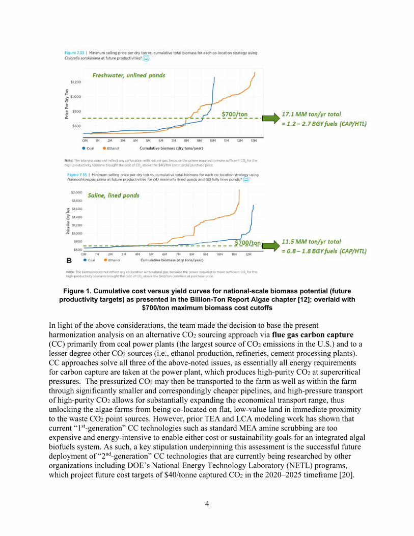
c) Scalability: Based on the findings documented in the 2016 Billion-Ton Report Algae chapter [12], which constrained resource assessment modeling to co-located flue gas availability from coal and natural gas power plants and ethanol production facilities, the resulting cost versus biomass yield curves indicate limited potential for national scalability of algal biomass output under this co-location constraint. Namely, Figure 1 shows yield curves for a “future” technology scenario (centered around a 25 g/m2/day cultivation productivity target – similar to the targets in this exercise) as presented in that report, overlaid by a threshold of $700/ton biomass cost as a rough estimate for the maximum plausible biomass cost that could still potentially enable achieving BETO’s fuel cost goals of $2/GGE (though would still require aggressive strategies for co-processing with other feedstocks or pursuing high-value coproducts). At this upper limit, the combined national biomass potential is roughly 17 MM tons/year for the freshwater case, or roughly 12 MM tons/year for the saline case (coal power plant plus ethanol plant curves, excluding natural gas which was not found in the study to enable economical CO2 supply for the future scenario given lower flue gas CO2 concentrations); which in turn, based on projected CAP and HTL conversion target yields [18], would translate to 1.2–2.7 BGY fuel yield potential for the freshwater case, or 0.8–1.8 BGY for the saline case. With recent BETO focus primarily on saline cultivation moving forward to avoid freshwater competition, this implies that the maximum national-scale fuel potential for algal biofuels is less than 2 BGY when constraining algae farm CO2 sourcing to co-located bulk flue gas transfer from nearby power plant and ethanol point sources. This falls short of BETO’s ultimate vision of 5 BGY as an opportunity for algal biofuels to make a meaningful contribution to the U.S. fuel pool (roughly 210 BGGE/yr [19]).

4

Figure 1. Cumulative cost versus yield curves for national-scale biomass potential (future

productivity targets) as presented in the Billion-Ton Report Algae chapter [12]; overlaid with $700/ton maximum biomass cost cutoffs

In light of the above considerations, the team made the decision to base the present harmonization analysis on an alternative CO2 sourcing approach via flue gas carbon capture (CC) primarily from coal power plants (the largest source of CO2 emissions in the U.S.) and to a lesser degree other CO2 sources (i.e., ethanol production, refineries, cement processing plants). CC approaches solve all three of the above-noted issues, as essentially all energy requirements for carbon capture are taken at the power plant, which produces high-purity CO2 at supercritical pressures. The pressurized CO2 may then be transported to the farm as well as within the farm through significantly smaller and correspondingly cheaper pipelines, and high-pressure transport of high-purity CO2 allows for substantially expanding the economical transport range, thus unlocking the algae farms from being co-located on flat, low-value land in immediate proximity to the waste CO2 point sources. However, prior TEA and LCA modeling work has shown that current “1st-generation” CC technologies such as standard MEA amine scrubbing are too expensive and energy-intensive to enable either cost or sustainability goals for an integrated algal biofuels system. As such, a key stipulation underpinning this assessment is the successful future deployment of “2nd-generation” CC technologies that are currently being researched by other organizations including DOE’s National Energy Technology Laboratory (NETL) programs, which project future cost targets of $40/tonne captured CO2 in the 2020–2025 timeframe [20].

5

The present analysis thus assumes $40/tonne CO2 cost at the coal power plant source (reflective of the original DOE-NETL basis), subsequently scaled to $50/tonne CO2 for cement production and pulp and paper manufacturing, and $20/tonne CO2 for ammonia, ethanol, hydrogen, and petrochemical production. Additional costs are calculated for variable transport distances to each individual algae farm as documented in the next section.

Finally, the associated parasitic energy demands attributed to such 2nd-generation CC technologies were furnished by NETL researchers as 0.63 MJe/kg-CO2 (representing the power plant’s net electricity output loss that would be incurred as a result of implementing the CC system) [21]. This value was evaluated initially through ANL’s LCA model and found to result in overall GHG emissions that did not quite achieve the 50% GHG reduction goals (relative to petroleum diesel), based on previous target models for HTL/CAP configurations that were coupled with upstream cultivation [18]. However, if the pond circulation (paddlewheels, previously shown to contribute substantially to system energy demands [1]) were also shut down at night, the GHG reductions did surpass the 50% target (recognizing that the present analysis subsequently targets alternative HTL and CAP processing schemes relative to the prior Multi-Year Program Plan (MYPP) pathways in order to achieve more aggressive cost targets here). Thus, this represents a second future stipulation that the present analysis calls for, namely that pond circulation/paddlewheels must be shut down at nighttime to conserve power and associated GHG emission penalties. There is some precedent for this strategy already known to have been implemented without noticeable degradation to overall biomass productivity or quality; this has been primarily observed under the ATP3 Consortium’s [22] advanced field study trials at the Cal-Poly testbed site, which evaluated this approach against 24-hour circulation without noticeable performance differences, as well as information furnished by Global Algae Innovations (GAI) who indicated similar results [9].

Beyond this key consideration for CO2 sourcing as the underlying basis for the harmonization approach, other inputs specific to each respective model are documented in the following sections.

Resource Assessment Based on discussions between the PNNL Biomass Assessment Tool (BAT) and NREL TEA teams, updated screening criteria were defined for the RA model as relevant to the NREL farm model and to reflect current-state progress in the modeling since the 2012/2013 model harmonization effort. An overview of the assumptions and approaches is presented in Table 1.

6

Table 1. Resource Assessment Assumptions and Approaches Used in the 2017 Model Harmonization Effort

Model/Analysis Component 2017 Model Harmonization (RA)

Land Screening Defined by screening parameters documented in Wigmosta et al. [23] and within the BT16 report [12]. The major difference from the 2012/2013 Model Harmonization is removal of all forested lands from consideration.

Minimum Production Area 5,000 acres (vs. 1,200 acres in previous harmonization efforts)

Meteorology 33-year 1/8° gridded time-series (NLDAS2) (vs. CLIGEN stochastic weather in previous harmonization efforts)

Pond Model Variable depth based on providing best productivity rates; most often at 15-cm (vs. single strain in 30-cm deep open pond in previous harmonization efforts)

Growth Model -Freshwater strain rotation for maximum productivity including (Chlorella sorokiniana DOE 1412 [warm season]; Kirchneriella cornuta [Monoraphidium sp.] [cold season]); Scenedemus obliquus [freshwater, brackish water, all year]) -Saline water strain rotation for maximum productivity including (Picochlorum sp. LANL [warm season]; Nannochloropsis salina [marine, warm season]) -PNNL Microalgae Growth Model [24-26] -Productivity linearly scaled to an increased mean annual rate of 25 g/m2-day (based on sites located around Gulf Coast and Florida) -Minimum annual productivity threshold of 20 g/m2-day -Harvest to maintain 0.5 g/L biomass pond concentration -Previous harmonization efforts featured a single strain in 30-cm deep open ponds

CO2 Co-Location -CO2 sourced from coal-fired power plants, natural gas power plants, cement plants, fertilizer and ammonia plants, other chemical plants such as hydrogen production, petroleum and natural gas processing, pulp and paper mills, and metal production - Assumes 80% capture of total supply at source -Carbon capture and transport at high pressure -New CO2 location-allocation/supply-demand model to route pipes from CO2 sources to pond targets - New CO2 transport model where pipe size and pump stations dynamically determined and costed based on total supply and transport distance -Economic cutoff of $55/tonne for CO2 capture and transport -No CO2 availability screening was done in prior BETO harmonization efforts

Water Supply -Long-term mean monthly flows based on National Hydrography Dataset (NHDPlus v2.1) using the Enhanced Runoff Method (EROM) -Available water supply constrained to withdrawing 5% or less of the mean annual flow based on HUC-6 level estimates from the National Hydrography Dataset -A future water supply scenario (and now available) constraint is to replace the 5% mean annual flow rule in previous harmonization studies with Tennant (1976) [27] lower bound of optimal flow (60% in-stream flow for high- and low-flow periods) for HUC-8 level sub-basin

Water Allocation -Water allocation based on site-by-site long-term mean annual water accounting with each HUC-6 with water supply provided at 5% of mean annual flow with priority selection given to highest producing sites. Candidate production sites were excluded if water resource was exhausted supplying higher-productivity sites.

7

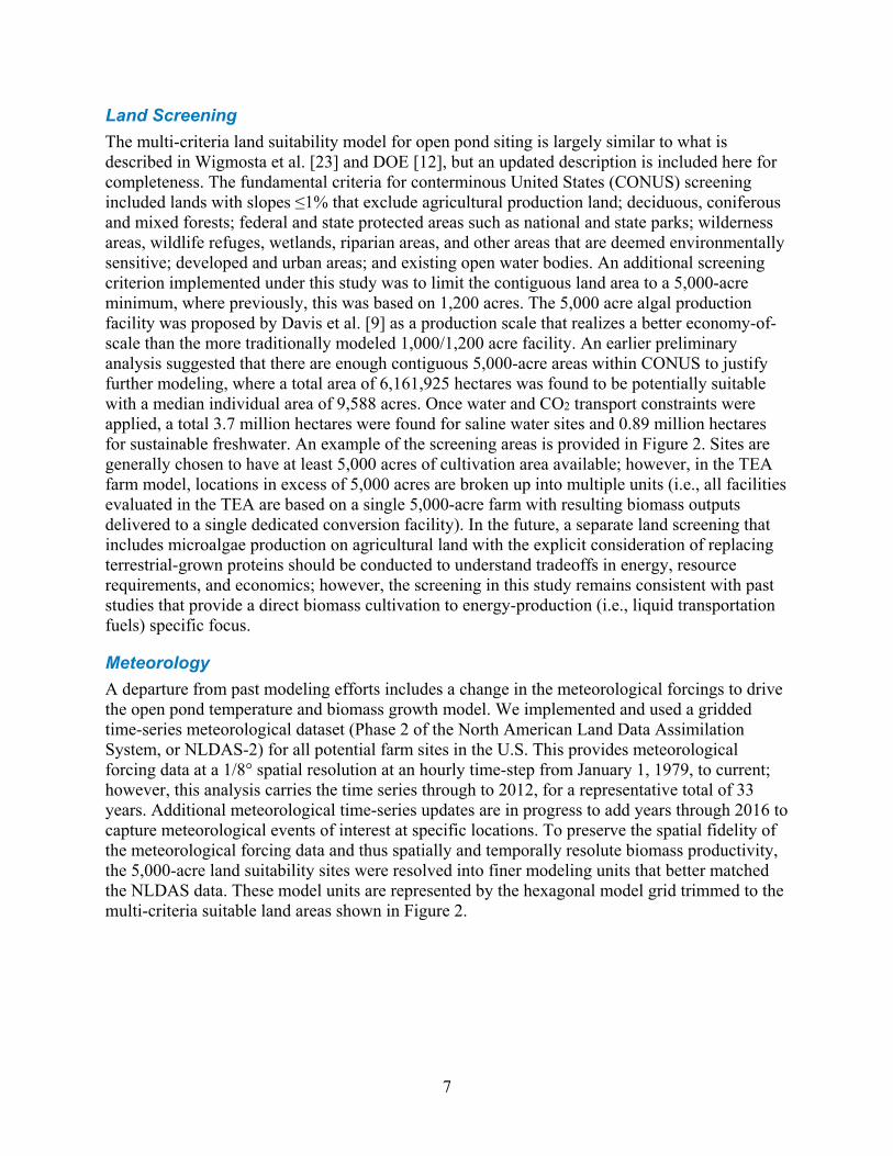
Land Screening The multi-criteria land suitability model for open pond siting is largely similar to what is described in Wigmosta et al. [23] and DOE [12], but an updated description is included here for completeness. The fundamental criteria for conterminous United States (CONUS) screening included lands with slopes ≤1% that exclude agricultural production land; deciduous, coniferous and mixed forests; federal and state protected areas such as national and state parks; wilderness areas, wildlife refuges, wetlands, riparian areas, and other areas that are deemed environmentally sensitive; developed and urban areas; and existing open water bodies. An additional screening criterion implemented under this study was to limit the contiguous land area to a 5,000-acre minimum, where previously, this was based on 1,200 acres. The 5,000 acre algal production facility was proposed by Davis et al. [9] as a production scale that realizes a better economy-of-scale than the more traditionally modeled 1,000/1,200 acre facility. An earlier preliminary analysis suggested that there are enough contiguous 5,000-acre areas within CONUS to justify further modeling, where a total area of 6,161,925 hectares was found to be potentially suitable with a median individual area of 9,588 acres. Once water and CO2 transport constraints were applied, a total 3.7 million hectares were found for saline water sites and 0.89 million hectares for sustainable freshwater. An example of the screening areas is provided in Figure 2. Sites are generally chosen to have at least 5,000 acres of cultivation area available; however, in the TEA farm model, locations in excess of 5,000 acres are broken up into multiple units (i.e., all facilities evaluated in the TEA are based on a single 5,000-acre farm with resulting biomass outputs delivered to a single dedicated conversion facility). In the future, a separate land screening that includes microalgae production on agricultural land with the explicit consideration of replacing terrestrial-grown proteins should be conducted to understand tradeoffs in energy, resource requirements, and economics; however, the screening in this study remains consistent with past studies that provide a direct biomass cultivation to energy-production (i.e., liquid transportation fuels) specific focus.

Meteorology A departure from past modeling efforts includes a change in the meteorological forcings to drive the open pond temperature and biomass growth model. We implemented and used a gridded time-series meteorological dataset (Phase 2 of the North American Land Data Assimilation System, or NLDAS-2) for all potential farm sites in the U.S. This provides meteorological forcing data at a 1/8° spatial resolution at an hourly time-step from January 1, 1979, to current; however, this analysis carries the time series through to 2012, for a representative total of 33 years. Additional meteorological time-series updates are in progress to add years through 2016 to capture meteorological events of interest at specific locations. To preserve the spatial fidelity of the meteorological forcing data and thus spatially and temporally resolute biomass productivity, the 5,000-acre land suitability sites were resolved into finer modeling units that better matched the NLDAS data. These model units are represented by the hexagonal model grid trimmed to the multi-criteria suitable land areas shown in Figure 2.

8

Figure 2. Example land suitability, hexagonal model grid, resulting potential biomass production, and CO2 resources within north-central Florida prior to modeled CO2 allocations.

Open Pond Model The open pond temperature model is identical to what is described in Wigmosta et al. [23] and Perkins and Richmond [28], with the exception that a pond/soil heat-exchange routine was implemented to better represent the open pond water temperature throughout the model time-series. The open pond model was run hourly at each potentially suitable site for 33 years with a 1-year spin-up to allow the pond/soil heat-exchange to stabilize. BAT modeled thermal properties at a range of pond depths have been previously validated against open pond observations. Three pond depths—15-, 20-, and 25-cm—were run with the intent of identifying and selecting the best biomass productivity rates on a monthly time-step as described below and follows depths that have experimentally been shown to improve performance and can scale-up [29,30]. Thus, pond depths can vary from month to month on a site-specific basis in response to meteorological conditions, pond temperature, light attenuation through the water column, biomass concentrations and resulting strain productivity. Each run provides the water temperature and evaporative loss at an hourly time-step, and is post-processed to determine net water use including direct precipitation inputs to the ponds. This information also provides the foundation for the saline-based blowdown calculations.

9

Figure 3. Example differences in BAT-modeled water temperature as a function of depth (left) and biomass productivities under baseline condition (fixed depth and strain; gray) and under rotation

condition (varying depth and strain rotation; green).

Biomass Growth Model For this analysis, we implemented the PNNL Microalgae Growth Model [24-26] to provide model parameterizations based on extensive growth experiments for three freshwater and two saline strains. The PNNL Microalgae Growth Model was developed for predicting biomass productivity in outdoor ponds under nutrient-replete conditions and diurnally fluctuating light intensities and water temperatures. It can be run in batch and continuous culture mode at different culture depths and, in addition to incident sunlight and water temperature data, requires the following experimentally determined strain-specific input parameters: growth rate as a function of light intensity and temperature, biomass loss rate in the dark as a function of temperature and light intensity during the preceding light period, and the scatter-corrected biomass light absorption coefficient.

It is assumed that light and temperature are the key and instantaneous determinants of microalgae growth and productivity, and that no other factors such as nutrients, CO2, and mixing (i.e., mass-transfer) are limiting. Furthermore, it is assumed that the culture pH remains constant via feedback-controlled CO2 addition and that there is no growth inhibition by photosynthetic oxygen or other compounds.

The growth model was developed for open ponds where the majority of light attenuation occurs only in the vertical direction. The vertical water column is divided into a user defined number of layers, typically 50–100. It also assumes water temperature is spatially uniform over the entire water column in a given time-step. The biomass concentration in each layer is assumed to increase exponentially from B(t) to B(t+Δt) during time interval Δt as follows [25]:

teB(t)t)B(t ∆⋅⋅=∆+ µ (Eq. 1)

where µ is the specific growth rate (day-1) in the respective volume layer.

Since the application of Eq. 1 requires knowledge of the specific growth rate at the particular temperature and light intensity within each layer, it is necessary to know how µ varies with temperature and light intensity. In dilute cultures with minimum self-shading, the specific growth

10

rate of microalgae can be experimentally determined as a function of temperature and light as follows:

I)f(T, μ = (Eq. 2)

where, f(T,I) is the two-dimensional array (or surface) of specific growth rates measured for different combinations of temperature and light intensity values. Since each microalgae strain has a unique response to light (i.e., compensation light intensity, saturating light intensity, and photo-inhibition) and temperature (i.e., optimum temperature and temperature tolerance range), the function f(T,I) is strain-specific and must be experimentally determined prior to running the model. It is assumed that individual cells respond instantaneously to the new light conditions as they enter each successive volume layer and that they exhibit the corresponding experimentally determined specific growth rate for that particular light intensity. This response has been verified in the laboratory by measurements of conventional P-I curves that clearly indicate that changes in light intensity produce immediate changes in photosynthetic oxygen evolution.

Since biomass loss overnight due to dark respiration can have a significant, negative effect on biomass productivity, it is necessary to know the rate of biomass loss (µdark) in the absence of light (I=0) as a function of temperature (T) and the average light intensity (Iavg) to which the cells were exposed in the mixed pond culture during the preceding day [31,25]:

)I f(T, μ avgdark = (Eq. 3)

Iavg is calculated by averaging light attenuation profiles in the water column culture for each time-step (Δt) over the entire day preceding the night in which biomass loss due to dark respiration occurred. Biomass loss rates in the dark (µdark) as a function of temperature and average light intensity were independently determined in laboratory experiments.

All strains were run for each potential site using the hourly pond temperature model results and strain-specific parameterizations as input. As a further step, we implemented site-specific algal strain rotation (per source water type) to reduce the seasonality effects in productivity and ultimately increase annual yield. We used three freshwater and two saline water strains:

• Freshwater: o Chlorella sorokiniana (DOE 1412 [warm season]) o Kirchneriella cornuta (Monoraphidium sp. [cold season]) o Scenedemus obliquus (freshwater, brackish water, and all-year).

• Saline water: o Picochlorum sp. (LANL [warm season]) o Nannochloropsis salina (marine and warm season).

All strains were parameterized for the PNNL Microalgae Growth Model. At each location, separate hourly runs were made for each strain and 3 pond depths (15-, 20-, and 25-cm) for a period of 33 years. Then, for each location, the strain/depth combination that produced the greatest biomass for a given month was ultimately selected and used. For freshwater, this included evaluating nine possible combinations of strain and pond depth, for each month. For saline, this resulted in six possible combinations. Typically, rotation between strain and depth

11

only occurred once a year at the transition between warm and cooler months and the most frequently occurring pond depth amongst all sites and strains was 15 cm. Strain rotation logistics are not explicitly considered in the models, but may be timed to coincide with a planned shutdown for pond cleaning (as part of the 35 day/year downtime), or introduced at the appropriate point and allowed to become the dominant strain for the seasonal period. Biomass harvesting was dynamic and assumed this took place once pond concentrations reached 0.5 g/L (fixed constant in all seasons and pond depth scenarios).

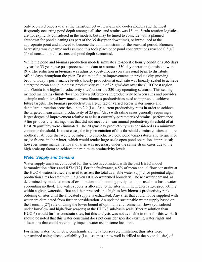
While the pond and biomass production models simulate site-specific hourly conditions 365 days a year for 33 years, we post-processed the data to assume a 330-day operation (consistent with [9]). The reduction in biomass was adjusted (post-process) on a seasonal basis to distribute offline days throughout the year. To estimate future improvements in productivity (moving beyond today’s performance levels), hourly production at each site was linearly scaled to achieve a targeted mean annual biomass productivity value of 25 g/m2/day over the Gulf Coast region and Florida (the highest productivity sites) under the 330-day operating scenario. This scaling method maintains climate/location driven differences in productivity between sites and provides a simple multiplier of how much current biomass productivities need to improve to achieve future targets. The biomass productivity scale-up factor varied across water source and depth/strain rotation scenarios, up to 2.9 (i.e. ~3x current productivity rates in order to achieve the targeted mean annual productivity of 25 g/m2/day) with saline cases generally requiring a larger degree of improvement relative to at least currently-parameterized strains’ performance. After productivity scaling, sites that did not meet the mean-annual productivity threshold of at least 20 g/m2/day were eliminated. The 20 g/m2/day productivity was considered as a minimum economic threshold. In most cases, the implementation of this threshold eliminated sites at more northerly latitudes that would be subject to unproductive cold pond temperatures and frequent or major freezes in the winter, which would render large-scale open pond operations impractical; however, some manual removal of sites was necessary under the saline strain cases due to the high scale-up factor to achieve the minimum productivity levels.

Water Supply and Demand Water supply analysis conducted for this effort is consistent with the past BETO model harmonization efforts and BT16 [12]. For the freshwater, a 5% of mean annual flow constraint at the HUC-6 watershed scale is used to assess the total available water supply for potential algal production sites located within a given HUC-6 watershed boundary. The net water demand, as determined by modeled rates of evaporation and incoming precipitation, is used in a basic water accounting method. The water supply is allocated to the sites with the highest algae productivity within a given watershed first and then proceeds in a high-to-low biomass productivity rank-ordering of sites until the allocated supply is exhausted. Any sites that could not be supplied with water are eliminated from further consideration. An updated sustainable water supply based on the Tennant [27] rule of using the lower bound of optimum environmental flows (considered under low-flow and high-flow seasons) at the HUC-8 sub-basin scale (finer resolution than HUC-6) would further constrain sites, but this analysis was not available in time for this work. It should be noted that this water constraint does not consider specific existing water rights and allocations that could potentially impede water use in some locations.

For saline water, volumetric constraints are not a foreseeable limitation, thus sites were constrained using direct availability (i.e., assumes a new well is drilled at the potential site) of

12

non-competitive saline water [32]. For saline scenario blowdown calculations performed within the TEA, an input saline concentration of 7.7 g/L with a maximum pond concentration strain tolerance of 40 g/L is established (applied universally across all sites). Further study is warranted to consider source water salinities on a more individual location basis, to distinguish brackish versus saline water cultivation evaluated across different strain salinity limits. For the saline runs, the net water demand is adjusted based on saline-influenced evaporative losses.

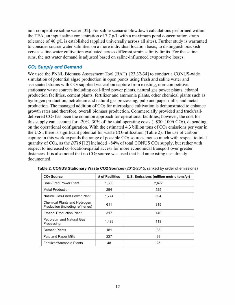
CO2 Supply and Demand We used the PNNL Biomass Assessment Tool (BAT) [23,32-34] to conduct a CONUS-wide simulation of potential algae production in open ponds using fresh and saline water and associated strains with CO2 supplied via carbon capture from existing, non-competitive, stationary waste sources including coal-fired power plants, natural gas power plants, ethanol production facilities, cement plants, fertilizer and ammonia plants, other chemical plants such as hydrogen production, petroleum and natural gas processing, pulp and paper mills, and metal production. The managed addition of CO2 for microalgae cultivation is demonstrated to enhance growth rates and therefore, overall biomass production. Commercially provided and truck/rail-delivered CO2 has been the common approach for operational facilities; however, the cost for this supply can account for ~20%–30% of the total operating costs (~$30–100/t CO2), depending on the operational configuration. With the estimated 4.3 billion tons of CO2 emissions per year in the U.S., there is significant potential for waste CO2 utilization (Table 2). The use of carbon capture in this work expands the range of possible CO2 sources, not so much with respect to total quantity of CO2, as the BT16 [12] included ~84% of total CONUS CO2 supply, but rather with respect to increased co-location/spatial access for more economical transport over greater distances. It is also noted that no CO2 source was used that had an existing use already documented.

Table 2. CONUS Stationary Waste CO2 Sources (2012-2015, ranked by order of emissions)

CO2 Source # of Facilities U.S. Emissions (million metric tons/yr)

Coal-Fired Power Plant 1,339 2,677

Metal Production 294 525

Natural Gas-Fired Power Plant 1,774 394

Chemical Plants and Hydrogen Production (including refineries) 611 315

Ethanol Production Plant 317 140

Petroleum and Natural Gas Processing 1,489 113

Cement Plants 181 83

Pulp and Paper Mills 227 38

Fertilizer/Ammonia Plants 48 25

13

For this analysis, CO2 supply was driven by annual estimates derived from NETL’s NATCARB v.1502 [35] and Middleton et al. [36] (Figure 4). While the scope of the current analysis is based on annually available CO2 supply, a new capability has been developed within the BAT to model hourly CO2 supply (Figure 5) and associated hourly CO2 demand based on algal productivity rates (Figure 6) that reflect diurnal and intra-annual supply variations. This is particularly important to reflect CO2 availability in the electricity-generation sector for which coal-fired power plants are the dominant source of waste CO2 in the U.S. (Table 2) and will be implemented nationally in future analyses.

Figure 4. CO2 point source emissions and associated total annual output for 2012–2013 [35,36]

14

Figure 5. BAT-modeled hourly CO2 emissions data from the Stanton Energy Center, Florida

(Orlando Utilities Commission), including the coal-fired Units 1 and 2, and the combined-cycle natural gas plant, Stanton A

Figure 6. CO2 availability and hourly AFDW biomass production for Chlorella at a 25-cm pond

depth at 1,000-acre unit farm for April 18, 2012

For the 2017 Model Harmonization analysis, we are considering all key sources of waste CO2 at once, thus, the most cost-effective sources of CO2 are supplied first, followed by additional sources as required to fulfill the needs of a production site. Thus, multiple CO2 sources can meet the need of a given site, or a single CO2 source may feed multiple production sites.

The total hourly carbon demand, based on a 330-day operation and scaled-up productivity under the freshwater and saline biomass scenarios described previously, is calculated by:

𝐷𝐷𝐶𝐶𝐶𝐶2= 𝐵𝐵∗𝑊𝑊𝑊𝑊𝐵𝐵𝐵𝐵𝐵𝐵

𝐸𝐸𝐶𝐶𝐶𝐶2∗ 𝑊𝑊𝐶𝐶𝐶𝐶𝐵𝐵2

(Eq. 4)

15

Where,

DCO2 = CO2 demand (kg/hr) B = AFDW biomass (kg/hr) WCBio = Carbon fraction in biomass (0.55) ECO2 = CO2 utilization efficiency (0.75) WCC02 = Carbon fraction in CO2 (0.273)

The total CO2 supply provided through carbon capture is assumed at 80% of reported annual total supply and the calculated site-level biomass productivity-based CO2 demand provide the basis for the CO2 accounting and selection model. The CO2 utilization efficiency value would benefit from a sensitivity analysis using more conservative values (ECO2 < 0.75) to understand effects of sites that are excluded, but was beyond the scope of the current effort. A new BAT CO2 transport and allocation model was developed specifically for the 2017 Model Harmonization effort to account for carbon capture, compression, and transport from CO2 source to the production site. The key equations and parameters used are established from literature values as described below.

The CO2 transport model is first established using a location-allocation spatial network model. This type of modeling has often been used for performing logistics analysis, competitive siting of businesses, or defining optimal locations for critical resources such as emergency response (i.e., paramedic, fire stations, hospitals, etc.), where the basic premise is having a facility of some capacity that can serve required demands. In the case of CO2 transport, the “facility” is defined as a stationary CO2 source with a capacity or supply of CO2 at 80% of the total reported annual release. The demand locations are defined as the centroids within the hexagonal cells representing the algal production sites, where the actual CO2 demand is defined for each hexagonal cell as defined in Eq. 4 and is conceptually represented in Figure 7. Note the straight-line connections between the CO2 source and the algal production sites provide a visual representation of the linkages and not the actual pipeline route calculated.

Figure 7. Representation of CO2 delivery from CO2 source (blue point) to production sites. The

straight allocation lines are only visual and do not represent the actual pipeline route taken.

16

The routing network was established using national right-of-way datasets that provide a potential pipeline pathway between the stationary CO2 source and the algal production sites. Because many of the algal production sites may not have a nearby right-of-way, a “snapping tolerance” was established to extend the routes to areas where no known right-of-way exists. The location-allocation spatial network model was established as a “maximum coverage” type model [37-39]; with a finite cost formulated by:

Maximize �𝑧𝑧 = �𝛼𝛼𝑖𝑖𝑦𝑦𝑖𝑖𝑖𝑖∈𝐼𝐼

� (Eq. 5)

Subject to:

𝑦𝑦𝑖𝑖 ≤ � 𝑥𝑥𝑖𝑖 𝑗𝑗∈𝑁𝑁𝐵𝐵

∀𝑖𝑖 ∈ 𝐼𝐼 (Eq. 6)

�𝑥𝑥𝑗𝑗 = 𝑃𝑃𝑗𝑗∈𝐽𝐽

(Eq. 7)

𝑥𝑥𝑗𝑗 ,𝑦𝑦𝑖𝑖 ∈ 0,1 ∀𝑗𝑗 ∈ 𝑗𝑗, 𝑖𝑖 ∈ 𝐼𝐼, 𝑆𝑆 ≤ 𝑁𝑁𝑖𝑖 , 𝑥𝑥𝑖𝑖 ,𝑦𝑦𝑖𝑖

Where,

𝐼𝐼 = Set of algal production sites with defined CO2 demand 𝐽𝐽 = Set of point source CO2 sites with a defined CO2 supply 𝑃𝑃 = Total number of point source CO2 sites to be used (we considered all available) 𝑥𝑥𝑖𝑖 = 1 if point source CO2 site used at 𝑗𝑗, otherwise is 0 𝑦𝑦𝑖𝑖 = 1 if algal production site 𝑖𝑖 can be supplied with CO2, otherwise is 0 𝑆𝑆 = Impedance cutoff of $55/tonne delivered CO2 (considers CapEx and OpEx costs) 𝑁𝑁𝑖𝑖 = Set of all possible point source CO2 sites that can service algal production sites 𝑖𝑖 𝛼𝛼𝑖𝑖= The total population of CO2 demand from the algal production sites 𝑖𝑖

Thus, the intent of Eq. 5 is to maximize the number of algal production sites (and their specific CO2 demand) that can be supplied by point source CO2; Eq. 6 indicates the potential for CO2 demand to be met, provided that CO2 can be supplied with the $55/tonne impedance cutoff (𝑆𝑆); and Eq. 7 gives the total number of point source CO2 sites that can be used. The notion is to establish CO2 sourcing to as many production sites as possible within the constraints of available CO2 supply and a $55/tonne total delivery cost (impedance cutoff). In cases where there was available CO2 supply, but costs exceeded $55/tonne, these sites were eliminated from further consideration, and CO2 was allocated to other algal production sites, if possible. This approach also ensures a spatial and cost-optimized solution, thus if a site has the option to receive CO2 from two or more suppliers, the least expensive transport option is used. A single CO2 source can supply multiple algal production sites provided the CO2 supply is sufficient. In this case, a

17

prioritization analysis is applied where the total CO2 supply is routed to the least-expensive locations first, and continues until the CO2 supply is exhausted.

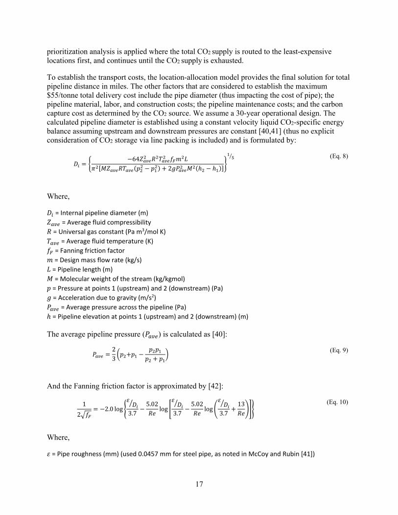
To establish the transport costs, the location-allocation model provides the final solution for total pipeline distance in miles. The other factors that are considered to establish the maximum $55/tonne total delivery cost include the pipe diameter (thus impacting the cost of pipe); the pipeline material, labor, and construction costs; the pipeline maintenance costs; and the carbon capture cost as determined by the CO2 source. We assume a 30-year operational design. The calculated pipeline diameter is established using a constant velocity liquid CO2-specific energy balance assuming upstream and downstream pressures are constant [40,41] (thus no explicit consideration of CO2 storage via line packing is included) and is formulated by:

𝐷𝐷𝑖𝑖 = �−64𝑍𝑍𝑎𝑎𝑎𝑎𝑎𝑎2 𝑅𝑅2𝑇𝑇𝑎𝑎𝑎𝑎𝑎𝑎2 𝑓𝑓𝐹𝐹𝑚𝑚2𝐿𝐿

𝜋𝜋2[𝑀𝑀𝑍𝑍𝑎𝑎𝑎𝑎𝑎𝑎𝑅𝑅𝑇𝑇𝑎𝑎𝑎𝑎𝑎𝑎(𝑝𝑝22 − 𝑝𝑝12) + 2𝑔𝑔𝑃𝑃𝑎𝑎𝑎𝑎𝑎𝑎2 𝑀𝑀2(ℎ2 − ℎ1)]�15�

(Eq. 8)

Where,

𝐷𝐷𝑖𝑖 = Internal pipeline diameter (m) 𝑍𝑍𝑎𝑎𝑎𝑎𝑎𝑎 = Average fluid compressibility 𝑅𝑅 = Universal gas constant (Pa m3/mol K) 𝑇𝑇𝑎𝑎𝑎𝑎𝑎𝑎 = Average fluid temperature (K) 𝑓𝑓𝐹𝐹 = Fanning friction factor 𝑚𝑚 = Design mass flow rate (kg/s) 𝐿𝐿 = Pipeline length (m) 𝑀𝑀 = Molecular weight of the stream (kg/kgmol) 𝑝𝑝 = Pressure at points 1 (upstream) and 2 (downstream) (Pa) 𝑔𝑔 = Acceleration due to gravity (m/s2) 𝑃𝑃𝑎𝑎𝑎𝑎𝑎𝑎 = Average pressure across the pipeline (Pa) ℎ = Pipeline elevation at points 1 (upstream) and 2 (downstream) (m)

The average pipeline pressure (𝑃𝑃𝑎𝑎𝑎𝑎𝑎𝑎) is calculated as [40]:

𝑃𝑃𝑎𝑎𝑎𝑎𝑎𝑎 =23�𝑝𝑝2+𝑝𝑝1 −

𝑝𝑝2𝑝𝑝1𝑝𝑝2 + 𝑝𝑝1

�

(Eq. 9)

And the Fanning friction factor is approximated by [42]:

12�𝑓𝑓𝐹𝐹

= −2.0 log �𝜀𝜀𝐷𝐷𝑖𝑖�

3.7−

5.02𝑅𝑅𝑅𝑅

log �𝜀𝜀𝐷𝐷𝑖𝑖�

3.7−

5.02𝑅𝑅𝑅𝑅

log�𝜀𝜀𝐷𝐷𝑖𝑖�

3.7+

13𝑅𝑅𝑅𝑅��

(Eq. 10)

Where,

𝜀𝜀 = Pipe roughness (mm) (used 0.0457 mm for steel pipe, as noted in McCoy and Rubin [41])

18

The Reynolds number, 𝑅𝑅𝑅𝑅, is defined by:

𝑅𝑅𝑅𝑅 =4𝑚𝑚𝜇𝜇𝜋𝜋𝐷𝐷𝑖𝑖

(Eq. 11)

Where,

𝜇𝜇 = Fluid viscosity (Pa s)

Additional details can be examined in McCoy and Rubin [41].

The pipeline cost model was established based on Parker [43] where a regression cost model is based on published capital costs of natural gas lines across the country from 1991 to 2003. These costs are represented by materials, labor, construction costs, right-of-way, and miscellaneous costs. Their year 2000 dollars were adjusted to 2014 dollars. These are formulated as follows:

Materials 𝐶𝐶𝑚𝑚𝑎𝑎𝑚𝑚 = [330.5 ∗ 𝐷𝐷2 + 687 ∗ 𝐷𝐷𝑖𝑖 + 26960] ∗ 𝐿𝐿 + 35000

(Eq. 12)

where 𝐷𝐷 is the nominal pipeline diameter (inches), and 𝐿𝐿 is total pipeline length (miles). Labor

𝐶𝐶𝑙𝑙𝑎𝑎𝑙𝑙𝑙𝑙𝑙𝑙 = [343 ∗ 𝐷𝐷2 + 2074 ∗ 𝐷𝐷𝑖𝑖 + 170013] ∗ 𝐿𝐿 + 185000

(Eq. 13)

Construction 𝐶𝐶𝑐𝑐𝑙𝑙𝑐𝑐𝑐𝑐𝑚𝑚 = [674 ∗ 𝐷𝐷2 + 11754 ∗ 𝐷𝐷𝑖𝑖 + 234085] ∗ 𝐿𝐿 + 405000

(Eq. 14)

Right-of-Way 𝐶𝐶𝑅𝑅𝐶𝐶𝑅𝑅 = [577 ∗ 𝐷𝐷2 + 29788] ∗ 𝐿𝐿 + 40000

(Eq. 15)

Miscellaneous 𝐶𝐶𝑚𝑚𝑖𝑖𝑐𝑐𝑐𝑐 = [8417 ∗ 𝐷𝐷 + 7324] ∗ 𝐿𝐿 + 95000

(Eq. 16)

Pipeline operating and maintenance (O&M) costs were established from McCoy and Rubin [41] which were ultimately established from Bock et al. [44]. The original 1999 dollars used in Bock et al. [44] were adjusted to 2014 dollars.

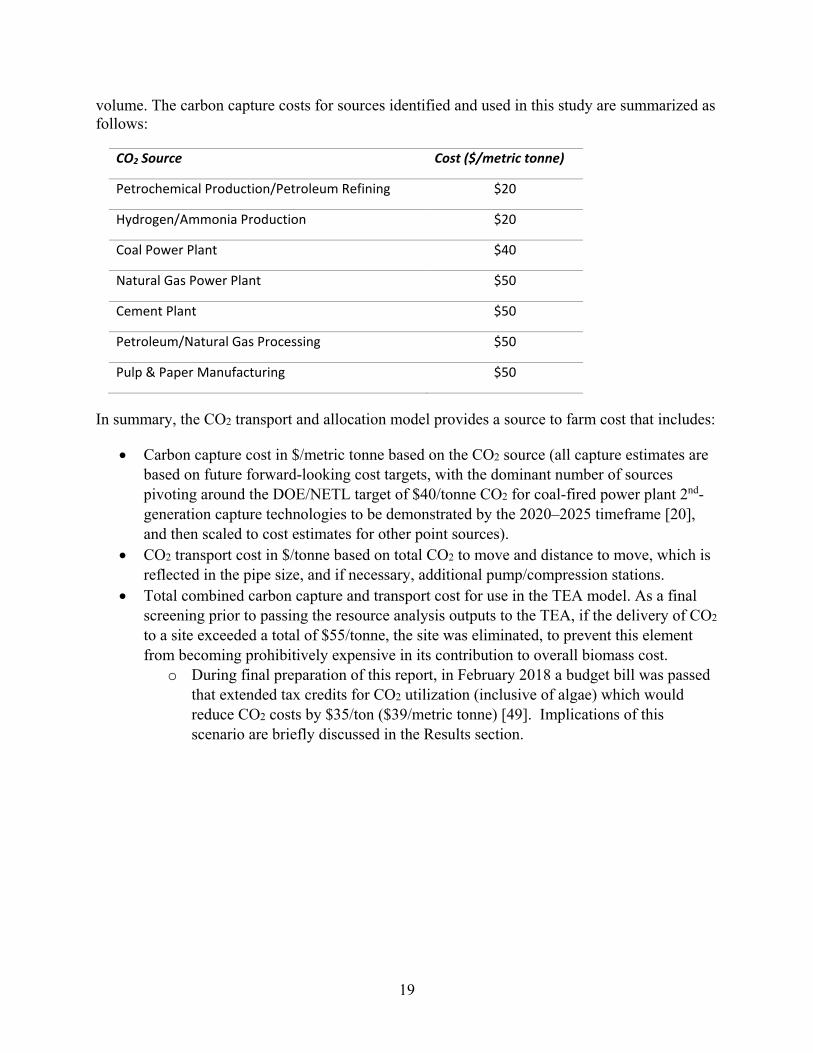
The carbon capture costs used here were simplified per estimated ranges, cost adjustments, and future projections in [45,46], Gerdes et al. [47], Rubin et al. [48], and [20]. It should be noted that most of the carbon capture costs have been established for power plants; however, limited cost data are available for industrial processes such as chemical production, ethanol, hydrogen, etc. While the CO2 stream coming from these sources is at a much higher purity, the costs are predominantly associated with CO2 compression. The literature also notes that for smaller volume CO2 medium-purity sources such as cement plants, the economies of scale aren’t achieved, thus may still be more expensive than a lower-purity CO2 source with overall greater

19

volume. The carbon capture costs for sources identified and used in this study are summarized as follows:

CO2 Source Cost ($/metric tonne)

Petrochemical Production/Petroleum Refining $20

Hydrogen/Ammonia Production $20

Coal Power Plant $40

Natural Gas Power Plant $50

Cement Plant $50

Petroleum/Natural Gas Processing $50

Pulp & Paper Manufacturing $50

In summary, the CO2 transport and allocation model provides a source to farm cost that includes:

• Carbon capture cost in $/metric tonne based on the CO2 source (all capture estimates are based on future forward-looking cost targets, with the dominant number of sources pivoting around the DOE/NETL target of $40/tonne CO2 for coal-fired power plant 2nd-generation capture technologies to be demonstrated by the 2020–2025 timeframe [20], and then scaled to cost estimates for other point sources).

• CO2 transport cost in $/tonne based on total CO2 to move and distance to move, which is reflected in the pipe size, and if necessary, additional pump/compression stations.

• Total combined carbon capture and transport cost for use in the TEA model. As a final screening prior to passing the resource analysis outputs to the TEA, if the delivery of CO2 to a site exceeded a total of $55/tonne, the site was eliminated, to prevent this element from becoming prohibitively expensive in its contribution to overall biomass cost.

o During final preparation of this report, in February 2018 a budget bill was passed that extended tax credits for CO2 utilization (inclusive of algae) which would reduce CO2 costs by $35/ton ($39/metric tonne) [49]. Implications of this scenario are briefly discussed in the Results section.

20

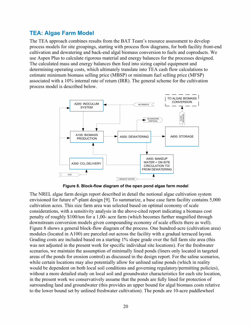
TEA: Algae Farm Model The TEA approach combines results from the BAT Team’s resource assessment to develop process models for site groupings, starting with process flow diagrams, for both facility front-end cultivation and dewatering and back-end algal biomass conversion to fuels and coproducts. We use Aspen Plus to calculate rigorous material and energy balances for the processes designed. The calculated mass and energy balances then feed into sizing capital equipment and determining operating costs, which ultimately translate into TEA cash flow calculations to estimate minimum biomass selling price (MBSP) or minimum fuel selling price (MFSP) associated with a 10% internal rate of return (IRR). The general scheme for the cultivation process model is described below.

A500: DEWATERINGA100: BIOMASS PRODUCTION

A400: MAKEUP WATER + ON-SITE CIRCULATION TO/

FROM DEWATERING

A300: CO2 DELIVERY

A200: INOCULUM SYSTEM

TO ALGAE BIOMASS CONVERSION

NUTRIENTS

CO2

MAKEUP WATER

A600: STORAGE

ALG

AL

BIO

MAS

S

BLOWDOWN DISPOSAL

Figure 8. Block-flow diagram of the open pond algae farm model

The NREL algae farm design report described in detail the notional algae cultivation system envisioned for future nth-plant design [9]. To summarize, a base case farm facility contains 5,000 cultivation acres. This size farm area was selected based on optimal economy of scale considerations, with a sensitivity analysis in the above-cited report indicating a biomass cost penalty of roughly $100/ton for a 1,00- acre farm (which becomes further magnified through downstream conversion models given compounding economy of scale effects there as well). Figure 8 shows a general block-flow diagram of the process. One hundred-acre (cultivation area) modules (located in A100) are parceled out across the facility with a gradual terraced layout. Grading costs are included based on a starting 1% slope grade over the full farm site area (this was not adjusted in the present work for specific individual site locations). For the freshwater scenarios, we maintain the assumption of minimally lined ponds (liners only located in targeted areas of the ponds for erosion control) as discussed in the design report. For the saline scenarios, while certain locations may also potentially allow for unlined saline ponds (which in reality would be dependent on both local soil conditions and governing regulatory/permitting policies), without a more detailed study on local soil and groundwater characteristics for each site location, in the present work we conservatively assume that the ponds are fully lined for protection of surrounding land and groundwater (this provides an upper bound for algal biomass costs relative to the lower bound set by unlined freshwater cultivation). The ponds are 10-acre paddlewheel

21

driven raceways with costs and circulation power demands based on an average of four vendor-provided cases as documented in the algae farm design report. As noted previously, paddlewheels are targeted to run for 12 hours per day with nighttime shutdown to reduce power usage given the strong influence this parameter has on the LCA, resulting in a power demand of 27.8 kWh/ha/day. Fully lined ponds in the saline case would likely affect the hydrodynamics and reduce the circulation power demand, but this was not adjusted in this case. The inoculum system was also maintained consistently with the algae farm design report, utilizing tubular photobioreactors, covered 2-acre raceway ponds, and fully lined 2-acre ponds, sized based on a targeted 20 days between re-inoculation events for any given pond (i.e., re-inoculating 5% of the overall farm pond volume every day, with the maximum design basis set based on summertime productivities; winter productivities would be lower, but so would the frequency of culture crashes and thus a longer period between re-inoculations).

As described above, pure CO2 (produced from carbon capture of flue gas from coal-fired power plants and other point sources) is transported to the farm gate via a high-pressure pipeline. The BAT Team’s analysis provided the cost of off-site CO2 transport and the cost of the carbon capture on a dollar per metric ton basis (discussed above). A pipeline network within the facility brings the CO2 from a storage tank to individual ponds as described in the algae farm design report. Although the design report had originally targeted 90% utilization of the delivered CO2 to the ponds, this study takes a more conservative approach and reduces that parameter to 75% utilization efficiency; this is still a widely-debated metric regarding maximum possible retention efficiency, but upon further discussions with other experts [50] and review of literature [51,52], 75%–90% retention efficiencies in the pond culture do appear theoretically possible given optimal pond design, i.e., channel velocities and sump locations appropriately matched to algal growth rates and CO2 uptake demands, coupled with optimal pH and alkalinity conditions in the pond (these considerations will be the subject of more detailed analysis moving forward), thus 75% is used as a target goal for optimally designed systems at scale-up. Beyond CO2 carbon capture, other means of delivering CO2 to algae ponds are also possible and are the subject of ongoing research, including direct atmospheric CO2 capture [53] or scrubbing into a bicarbonate system which may be directly used as the pond cultivation media [54].

The process assumes a continuous mode of cultivation and harvesting to maximize on-stream utilization of pond capital costs, with a fixed harvest density at 0.5 g/L from the ponds. Once harvested, the biomass is routed through three stages of dewatering to reach a final solids content of 20 wt% (ash free dry weight, or AFDW). First, in-ground settling with a 4-hour residence time concentrates the biomass from 0.5 g/L to 10 g/L. A hollow-fiber membrane further increases the solids content to 130 g/L following the settling ponds. Finally, a centrifuge further raises the final solids content to 200 g/L. Again, all design and cost details attributed to the dewatering system are further documented in the algae farm design report [9]. As discussed in that report, the use of in-ground settlers for primary dewatering is assumed as a goal case, based on extreme cost-minimization that would be required to process such tremendous volumes of water (roughly 450 MM gal/day in peak season) which necessitates a highly cost-effective operation to maintain economic viability. While there is some data/anecdotal evidence of the efficacy of such an operation [55,56,51], this will be a key area for further public validation as may warrant BETO support in the future, e.g. to verify settling times and resultant concentrations for different strains of interest. Likewise, the secondary membrane dewatering step is based on operational knowledge furnished by a membrane developer (Global Algae Innovations [57]) but as yet

22

without published data to validate; thus again this operation would benefit from further public verification opportunities around the projected concentration factors and power usage. The concentrated algae biomass is routed to short-term storage (surge capacity up to 24 hours), with a 1% AFDW loss assumed during storage. The facility also includes design and cost considerations for water recycle and on-site circulation pipelines. A portion of the clarified recycle stream from primary dewatering is removed from the system as blowdown to control buildup of salts to maintain salt levels at the strain tolerance limits in the ponds, primarily an issue for the saline cases. As noted above, the saline models universally set the incoming makeup water at 7.7 g/L salts and the tolerance limit at 40 g/L, from which blowdown requirements were set as a function of seasonal evaporation rates (higher net evaporation translates to higher blowdown removal). The saline blowdown is disposed of via deep-well saltwater injection, a practice also employed in hydraulic fracturing technologies for petroleum extraction, at a cost of $1.50/m3 as an average of literature values for an owner-operated injection well located at or near the farm [58-62]. An alternative approach to employ evaporation ponds and landfilling of residual inorganics was also considered, but found to be more costly and thus was not pursued.

For the present harmonization work, the primary inputs to the farm model that were integrated with outputs from BAT included seasonal cultivation productivity, harvest density (always fixed at 0.5 g/L), net evaporation rate (total evaporation minus precipitation), water source, water salinity, blowdown rates required to maintain pond salinity limits, CO2 gate cost to the facility (based on BAT analysis for CO2 source/capture costs and transport distance/cost to the facility), and number/area of selected sites that met the screening criteria parameters set in the BAT models. The resulting individual farm locations identified by the BAT model were then collapsed down into consortia groups, each of which were then averaged for the key TEA input parameters noted above to constitute an individual “representative site” for each group to be run through the subsequent TEA and LCA models, similar to the approach taken in prior algae model harmonizations [1]. The farm model costs do not presently account for any sort of containment system i.e. in the event of catastrophic weather events or other scenarios where the loss of algal biomass containment would be unacceptable, for example if engineered strains were utilized. The costs for such a system would be speculative at this level of analysis detail, and also would vary by site/region of the country, but this concept warrants investigation in the future.

Also consistent with the NREL algae farm design report, the harvested biomass composition was set to a future target projection consistent with compositional attributes as have been previously measured for mid-harvest, high-carbohydrate Scenedesmus (HCSD) [9]. The elemental and component compositions for this strain are shown below in Table 3. Notably, the lipid content for this biomass is 26% as free fatty acids (27% as FAME, equivalent to TAG), which is a mid-level value and is not expected to place unreasonable burdens in simultaneously increasing future target productivities to the 25 g/m2/day range, given known tradeoffs between productivity and lipid content. It should be emphasized that the metric of interest here is the composition, not necessarily the strain, i.e., we are asserting that the future productivity goals are concomitant with a harvested composition as reflected in Table 3, regardless of the strain(s) employed, or if employing strain rotation strategies, that the overall average composition of harvested biomass still reflects these targets. In the case of saline cultivation, the ash content may be higher than that shown here (which was based on a freshwater trial), but given that all key cultivation parameters, e.g., productivity and dewatering solids content, are set on an AFDW basis, this would not impact overall fuel/product yields.

23

Table 3. Elemental and Component Compositions Targeted in This Study, Originally Based on High-Carbohydrate Scenedesmus (HCSD) Biomass (adjusted to 100% mass balance closure for

models) [9].

Elemental (AFDW) C 54.0% H 8.2% O 35.5% N 1.8% S 0.2% P 0.22% Total 100.0% Component (dry wt) Ash 2.4% Protein 13.2% FAME lipids as free fatty acids1 26.0% Glycerol1 3.0% Non-fuel polar lipid impurities 1.0% Sterols2 1.8% Fermentable carbohydrates 47.8% Non-fermentable carbohydrates 3.2% Cell mass 1.6% Total 100.0%

1 Lipids originally characterized as triglycerides (1:1 FAME equivalent); adjusted here to free fatty acid (FFA) plus glycerol (reflective of actual components in pretreated hydrolysate for Scenedesmus biomass).

2 Sterols originally included in “polar lipid impurity” fraction in prior models. Value currently estimated for HCSD, based on a representative earlier-harvest biomass sample.

Considering the targets enumerated above, a number of key hurdles/uncertainties must be addressed moving forward in achieving the stipulated projections. First and most importantly from a TEA/LCA driver standpoint, cultivation performance must continue to improve, both around productivity (moving from the latest “state of technology” benchmarks at roughly 10 g/m2/day [10] up to the 25 g/m2/day target), as well as compositional quality (moving beyond nutrient-replete, high-protein/low-carbohydrate and lipid biomass typically associated with current benchmarks [4] up to compositions closer to that in Table 3 i.e. ~70% carbohydrates plus lipids). Strain robustness/crash resistance must also continue to improve in order to reflect the minimal costs projected in the design case for inoculum trains (based on re-inoculating a given pond once every 20 days or longer). Additionally, the ability to shut pond circulation down at night without significant impacts to cultivation performance, as well as the ability for harvested biomass to auto-flocculate under short (<4 hour) settling times up to 10 g/L and then concentrate through membranes at concentrations and power demands consistent with GAI inputs will also be important to further validate publicly at a meaningful scale moving forward. Finally, more in-depth quantification of CO2 carbon capture integration logistics and scheduling with algal cultivation systems, including CO2 retention efficiencies and uptake rates in the ponds, will be key to verifying the opportunities for algal carbon capture/utilization and tracking the carbon dynamics once delivered to the ponds.

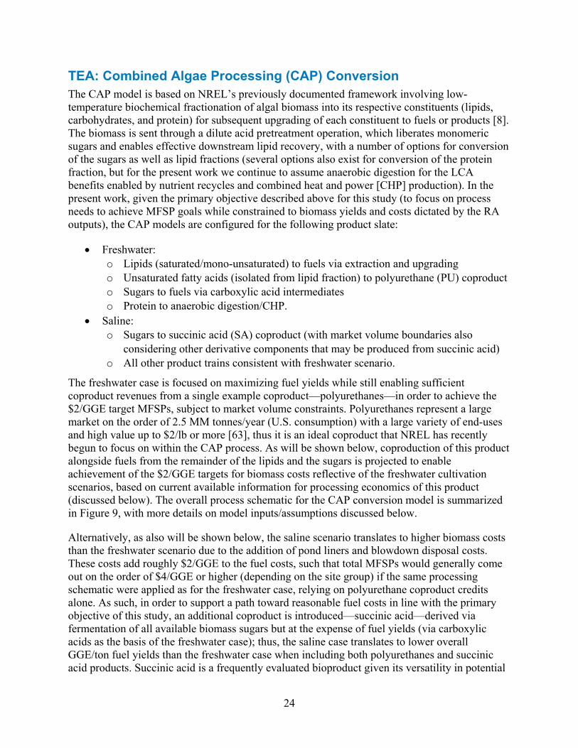
24

TEA: Combined Algae Processing (CAP) Conversion The CAP model is based on NREL’s previously documented framework involving low-temperature biochemical fractionation of algal biomass into its respective constituents (lipids, carbohydrates, and protein) for subsequent upgrading of each constituent to fuels or products [8]. The biomass is sent through a dilute acid pretreatment operation, which liberates monomeric sugars and enables effective downstream lipid recovery, with a number of options for conversion of the sugars as well as lipid fractions (several options also exist for conversion of the protein fraction, but for the present work we continue to assume anaerobic digestion for the LCA benefits enabled by nutrient recycles and combined heat and power [CHP] production). In the present work, given the primary objective described above for this study (to focus on process needs to achieve MFSP goals while constrained to biomass yields and costs dictated by the RA outputs), the CAP models are configured for the following product slate:

• Freshwater: o Lipids (saturated/mono-unsaturated) to fuels via extraction and upgrading o Unsaturated fatty acids (isolated from lipid fraction) to polyurethane (PU) coproduct o Sugars to fuels via carboxylic acid intermediates o Protein to anaerobic digestion/CHP.

• Saline: o Sugars to succinic acid (SA) coproduct (with market volume boundaries also

considering other derivative components that may be produced from succinic acid) o All other product trains consistent with freshwater scenario.

The freshwater case is focused on maximizing fuel yields while still enabling sufficient coproduct revenues from a single example coproduct—polyurethanes—in order to achieve the $2/GGE target MFSPs, subject to market volume constraints. Polyurethanes represent a large market on the order of 2.5 MM tonnes/year (U.S. consumption) with a large variety of end-uses and high value up to $2/lb or more [63], thus it is an ideal coproduct that NREL has recently begun to focus on within the CAP process. As will be shown below, coproduction of this product alongside fuels from the remainder of the lipids and the sugars is projected to enable achievement of the $2/GGE targets for biomass costs reflective of the freshwater cultivation scenarios, based on current available information for processing economics of this product (discussed below). The overall process schematic for the CAP conversion model is summarized in Figure 9, with more details on model inputs/assumptions discussed below.

Alternatively, as also will be shown below, the saline scenario translates to higher biomass costs than the freshwater scenario due to the addition of pond liners and blowdown disposal costs. These costs add roughly $2/GGE to the fuel costs, such that total MFSPs would generally come out on the order of $4/GGE or higher (depending on the site group) if the same processing schematic were applied as for the freshwater case, relying on polyurethane coproduct credits alone. As such, in order to support a path toward reasonable fuel costs in line with the primary objective of this study, an additional coproduct is introduced—succinic acid—derived via fermentation of all available biomass sugars but at the expense of fuel yields (via carboxylic acids as the basis of the freshwater case); thus, the saline case translates to lower overall GGE/ton fuel yields than the freshwater case when including both polyurethanes and succinic acid products. Succinic acid is a frequently evaluated bioproduct given its versatility in potential

25

product derivatives that may be made from it, such as 1,4-butanediol, maleic anhydride, tetrahydrofuran, 1,3-butadiene, and numerous other chemicals [64]. While the market for succinic acid itself is relatively small (36,000 tonnes/year U.S. consumption), the potential growth for this product is large with a market well over 2 MM tonnes/year when including potential derivative products [63]. With market values at $1/lb or more, succinic acid is thus also an attractive coproduct to consider in cases with high biomass carbohydrate composition as is assumed here. Thus for the saline case, this second example coproduct is added, also within market volume constraints. On the latter point, given the relatively modest market for succinic acid itself (which is merely intended to serve as one example coproduct opportunity among numerous others that could be derived from sugars), and to better demonstrate the market application of this type of coproduct, we evaluate the economics of the CAP process reflecting the costs of production and purification of succinic acid (described below) alongside its market value, but taking this example concept out through market volume boundaries inclusive of several additional potential product derivatives. Specifically, we consider the succinic acid coproduct “class” over total collective market volume limits of:

a) Succinic acid b) 1,4-butanediol c) Maleic anhydride d) Tetrahydrofuran e) Adipic acid f) 1,3-butadiene

The cumulative world market volumes for the six products above total 18 MM metric tons per year or 13.3 MM metric tons of carbon in the coproduct [64-69]. It is recognized that each of the above five products beyond succinic acid would translate to different final product yields (given different elemental compositions) and market values, but as a detailed TEA analysis of each individual coproduct opportunity is beyond the scope of this work, succinic acid yields and market values are used as a proxy for the other listed derivatives that may be produced from it for example purposes in demonstrating the value that may be garnered from algal sugars to non-fuel coproducts. More broadly, we emphasize that for both the freshwater and saline scenarios evaluated here, we have selected a limited number of specific coproducts (i.e., polyurethanes and succinic acid “classes” of coproducts) to perform a rigorous TEA analysis in the CAP conversion models, to serve as proof-of-concept examples of opportunities to reduce MFSPs toward BETO goals at “meaningful” national-scale potential. While the market volumes for these examples are relatively large, they are not infinite, and thus we consider the possibility of reducing algal fuel costs with these example coproducts over various market scenarios (presented in the Results section) up until cutting off the analysis at the saturation limits for the national-scale consortium of farm sites identified by the BAT models. In reality, different coproducts would be produced from different biorefineries (with a large number of other coproduct possibilities that are not evaluated here [63]).

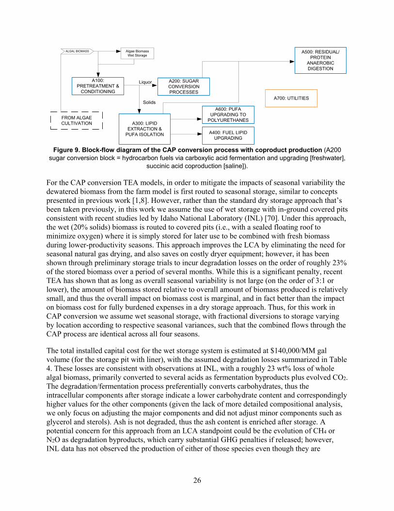
26

A200: SUGAR CONVERSION PROCESSES

LiquorA100: PRETREATMENT &

CONDITIONING

A300: LIPID EXTRACTION &

PUFA ISOLATION

A600: PUFA UPGRADING TO

POLYURETHANES

A400: FUEL LIPID UPGRADING

A700: UTILITIES

A500: RESIDUAL/ PROTEIN

ANAEROBIC DIGESTION

Algae Biomass Wet Storage

Solids

FROM ALGAE CULTIVATION

ALGAL BIOMASS

Figure 9. Block-flow diagram of the CAP conversion process with coproduct production (A200

sugar conversion block = hydrocarbon fuels via carboxylic acid fermentation and upgrading [freshwater], succinic acid coproduction [saline]).

For the CAP conversion TEA models, in order to mitigate the impacts of seasonal variability the dewatered biomass from the farm model is first routed to seasonal storage, similar to concepts presented in previous work [1,8]. However, rather than the standard dry storage approach that’s been taken previously, in this work we assume the use of wet storage with in-ground covered pits consistent with recent studies led by Idaho National Laboratory (INL) [70]. Under this approach, the wet (20% solids) biomass is routed to covered pits (i.e., with a sealed floating roof to minimize oxygen) where it is simply stored for later use to be combined with fresh biomass during lower-productivity seasons. This approach improves the LCA by eliminating the need for seasonal natural gas drying, and also saves on costly dryer equipment; however, it has been shown through preliminary storage trials to incur degradation losses on the order of roughly 23% of the stored biomass over a period of several months. While this is a significant penalty, recent TEA has shown that as long as overall seasonal variability is not large (on the order of 3:1 or lower), the amount of biomass stored relative to overall amount of biomass produced is relatively small, and thus the overall impact on biomass cost is marginal, and in fact better than the impact on biomass cost for fully burdened expenses in a dry storage approach. Thus, for this work in CAP conversion we assume wet seasonal storage, with fractional diversions to storage varying by location according to respective seasonal variances, such that the combined flows through the CAP process are identical across all four seasons.

The total installed capital cost for the wet storage system is estimated at $140,000/MM gal volume (for the storage pit with liner), with the assumed degradation losses summarized in Table 4. These losses are consistent with observations at INL, with a roughly 23 wt% loss of whole algal biomass, primarily converted to several acids as fermentation byproducts plus evolved CO2. The degradation/fermentation process preferentially converts carbohydrates, thus the intracellular components after storage indicate a lower carbohydrate content and correspondingly higher values for the other components (given the lack of more detailed compositional analysis, we only focus on adjusting the major components and did not adjust minor components such as glycerol and sterols). Ash is not degraded, thus the ash content is enriched after storage. A potential concern for this approach from an LCA standpoint could be the evolution of CH4 or N2O as degradation byproducts, which carry substantial GHG penalties if released; however, INL data has not observed the production of either of those species even though they are

27

analyzed for [71]. Thus, this does not appear to be an issue, although could be a concern in a more aerobic storage environment (i.e. if the cover or seal were significantly compromised).

Table 4. Input Compositions to CAP Models Before and After Wet Storage Losses (based on raw HCSD composition as well as adjustments applied to the HCSD baseline to reflect degradation losses as

measured by INL [72])

Raw Algae Wet Storage Algae Solids content (wt%) 20% 20% Algae composition (wt%) Protein 13.2 14.2 FFA 26.0 27.5 Ash 2.4 3.1 Fermentable carbohydrates 47.8 46.2 Non-fermentable carbohydrates 3.2 1.7 Glycerol 3.0 3.0 Sterol 1.8 1.8 Non-fuel polar lipid impurities 1.0 1.0 Cell mass 1.6 1.6 Sum 100.0 100.0 Whole algal biomass intact after storage (kg) 1.0 0.77 Acid produced per kg of whole algae (after storage) Succinic acid, kg 0.090 Lactic acid, kg 0.083

Following seasonal storage as warranted, the biomass is routed to the CAP conversion operations, i.e., dilute acid pretreatment, fermentation, lipid extraction, isolation and upgrading of poly-unsaturated fatty acids (PUFAs) to polyurethanes, and anaerobic digestion (AD). All operations that have been previously evaluated and documented will not be repeated here, namely pretreatment, lipid extraction, lipid hydrotreating, and AD; all design and cost details associated with those operations are consistent with prior studies [8]. For the remaining operations (fermentation to carboxylic acids for fuels or succinic acid for coproducts and PUFA upgrading to polyurethanes), the process inputs/assumptions will be briefly summarized below.

The first “new” CAP operation that has not been previously documented is sugar fermentation to carboxylic acids for subsequent upgrading to fuels (utilized for the freshwater scenario). This pathway leverages recent NREL work done under the Biochemical Conversion platform which has been investigating this route as a promising option for anaerobic fermentation of corn stover sugars to fuel products [73], and all process inputs/targets are set consistently here for algal sugars. In prior CAP models, sugars were converted to ethanol, which although allows for a simple and low-cost route for converting sugars to fuel products, aligns less with BETO priorities focused on fungible hydrocarbon fuels [18]. Alternatively, fermentation to carboxylic acid intermediates represents one of several anaerobic approaches to hydrocarbon biofuels (less costly than aerobic approaches) that recent NREL research is pursuing. In summary, sugars are

28

converted in large 1-MM gallon anaerobic fermentation vessels to short carboxylic acids primarily in the C2–C4 range (acetic and butyric acids), which are continuously removed from the fermentation broth via extraction across a membrane into a solvent given their toxicity to the host organism. The acids are recovered from the solvent via distillation, and are then routed to a number of catalytic upgrading steps consisting of ketonization (yielding primarily C3, C5, and C7 ketones), condensation, and deoxygenation to finished hydrocarbon fuels primarily in the C7–C11 range. The operating conditions, as well as design/cost details, for all biological and catalytic conversion steps are consistent with recent NREL targets for biochemical conversion pathways, including a fermentation acids yield of 0.48 g/g available sugars, 1.5-day fermentation residence time, and complete conversion of intermediate components across each of the ketonization, condensation, and hydrotreating steps for upgrading of the recovered acids.

Next, the other fermentation case that had not been previously evaluated for algal conversion until recently is production of succinic acid for sale as a coproduct (utilized for the saline scenario to offset higher biomass costs, also assumed as a proxy for other related derivative products as noted above). While this pathway was not originally considered in NREL’s CAP conversion design report, it was investigated through TEA in more recent work [10]. The details and assumptions for the succinic acid pathway were set consistently with those utilized in NREL’s biochemical conversion pathway from corn stover hydrolysate [74]; in summary, the fermenters, maintained at a pH of 7 with the addition of caustic, are fed with the sugars, as well as CO2 bubbled at 0.1 VVM (volume per volume per minute) [74]. The succinate organism (Actinobacillus succinogenes) can convert glucose, mannose, and glycerol [75,76]. Within the main reactors, 60% of glucose and mannose and 65% of glycerol is converted per-pass into succinic acid. After fermentation, succinic acid is recovered and purified from other byproducts. Design and cost details for the purification train were based on guidance from an engineering subcontractor, and consistent with published work [74]. In the separation, cells and large particles are removed through ultrafiltration and sent to wastewater treatment. An ion exchange unit then converts sodium succinate to succinic acid, and a nanofiltration unit provides additional purification to remove particle fines and impurities that may cause color in the final product. Finally, a crystallizer produces succinic acid crystals, and approximately 90% of the mother liquor from crystallization (which contains the unconverted sugars) is recycled back to fermentation to increase overall sugar conversion. After the recycle, final recovered succinic acid yield is 0.71 g/g of monomeric sugars and glycerol routed to the succinate fermentation train.

For both the carboxylic acid (fuels) and succinic acid (coproduct) pathways, the presence of insoluble solids is expected to hinder the fermentation and product recovery operations, thus we incorporate a solid-liquid separation (SLS) step to remove algal solids from the soluble sugar stream prior to fermentation. This is accomplished via two-stage centrifugation with a water wash. Given upper limits on solids content of roughly 30% for the centrifuge cake stream, a single-stage centrifugation step would lead to large sugar losses on the order of 25%–30%. Thus, to minimize those losses, a second centrifugation step is added with the inclusion of a water wash to re-dilute the solids stream from primary centrifugation; this leads to an overall sugar recovery of more than 95%.

The final process train requiring further discussion is for polyurethane production, coproduced in both the freshwater and saline scenarios. Although bio-based PUs have historically been produced commercially from soybean oil (specifically the unsaturated fatty acids [USFAs]) [77],

29

they can also be produced from USFAs of other feedstocks, and are of interest as a product from algae. The process for creating PUs from algae oil includes five main steps:

1. USFA separation via urea complexing 2. Epoxidation of USFA 3. Ring opening of epoxides to create polyols 4. Esterification of resulting polyols with glycerol to create higher molecular weight polyols 5. PU production by reacting polyols with toluene diisocyanate (TDI).

In the first step, the USFAs need to be separated from other oil products after hexane extraction. There are several methods for separation including countercurrent chromatography, crystallization, distillation of methyl esters, super critical fluid extraction, and urea complexing (modeled here) [78,79]. In urea complexing, urea reacts with saturated fatty acids (SFAs) to form solid crystals while keeping USFAs in the non-inclusion fraction [80].The process uses ethanol as a solvent to carry urea, and mixes the ethanol/urea stream with the oil stream from hexane extraction in a reactor [80]. At first, the reactor is maintained at 65oC to create a homogenous mixture of the ethanol, urea, and oil, but the reactor cools to 20oC to facilitate the fractionation [80]. This method of separation does not recover 100% of the USFAs. In fact, based on examples from patent literature the separation is dependent on several factors including the carbon chain length of the fatty acids and the number of double bonds [80]. The model uses a representative separation for the process as shown in Table 5. Table 5 also shows the fatty acid profile for the target biomass composition (consistent with HCSD biomass described above) as determined experimentally (internal data). The FFA, urea, and ethanol feed rates are set based on a mass ratio of 1:1:5 [80].

Table 5. Fatty Acid Profile and Separation for Urea Complexing

Fatty Acids Carbon Number

Degree of Unsaturation

Fatty Acid Profile (Percent of Incoming FFAs)

Percent in Urea Complex Stream [80]

Percent in Non-Inclusion Fraction [80]

18 2 7.8% 17% 83%

18 3 6.2% 39% 61%

18 1 49.7% 39% 61%

18 0 4.2% 100% 0%

16 1 11.9% 5% 95%

16 0 19.2% 88% 12%

20 0 1.0% 100% 0%

Following the creation of the urea complex, the ethanol containing non-inclusion fraction undergoes distillation where the ethanol solvent is recovered and recycled back to the reactor [80]. The USFAs bottoms from the column are washed with warm water (65oC) and enter a decanter to phase separate the USFAs from any urea that did not complex with the SFA [80]. The purified USFAs then continue to the next process step. At the same time, the urea complex with the SFAs exiting the reactor is washed with warm water (65oC). The urea separates from the

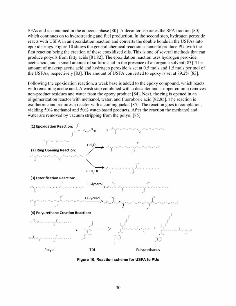
30

SFAs and is contained in the aqueous phase [80]. A decanter separates the SFA fraction [80], which continues on to hydrotreating and fuel production. In the second step, hydrogen peroxide reacts with USFA in an epoxidation reaction and converts the double bonds in the USFAs into epoxide rings. Figure 10 shows the general chemical reaction scheme to produce PU, with the first reaction being the creation of these epoxidized oils. This is one of several methods that can produce polyols from fatty acids [81,82]. The epoxidation reaction uses hydrogen peroxide, acetic acid, and a small amount of sulfuric acid in the presence of an organic solvent [83]. The amount of makeup acetic acid and hydrogen peroxide is set at 0.5 mols and 1.5 mols per mol of the USFAs, respectively [83]. The amount of USFA converted to epoxy is set at 89.2% [83].

Following the epoxidation reaction, a weak base is added to the epoxy compound, which reacts with remaining acetic acid. A wash step combined with a decanter and stripper column removes non-product residues and water from the epoxy product [84]. Next, the ring is opened in an oligomerization reactor with methanol, water, and fluoroboric acid [82,85]. The reaction is exothermic and requires a reactor with a cooling jacket [85]. The reaction goes to completion, yielding 50% methanol and 50% water-based products. After the reaction the methanol and water are removed by vacuum stripping from the polyol [85].

Figure 10. Reaction scheme for USFA to PUs

(1) Epoxidation Reaction: +

(2) Ring Opening Reaction:

+ CH3OH

+ H2O

(3) Esterification Reaction: + Glycerol

+ Glycerol

(4) Polyurethane Creation Reaction:

+

Polyurethanes

+

TDI Polyol

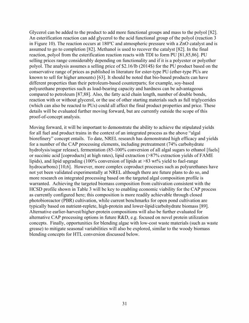
31

Glycerol can be added to the product to add more functional groups and mass to the polyol [82]. An esterification reaction can add glycerol to the acid functional group of the polyol (reaction 3 in Figure 10). The reaction occurs at 180oC and atmospheric pressure with a ZnO catalyst and is assumed to go to completion [82]. Methanol is used to recover the catalyst [82]. In the final reaction, polyol from the esterification reaction reacts with TDI to form PU [81,85,86]. PU selling prices range considerably depending on functionality and if it is a polyester or polyether polyol. The analysis assumes a selling price of $2.16/lb (2014$) for the PU product based on the conservative range of prices as published in literature for ester-type PU (ether-type PUs are known to sell for higher amounts) [63]. It should be noted that bio-based products can have different properties than their petroleum-based counterparts; for example, soy-based polyurethane properties such as load-bearing capacity and hardness can be advantageous compared to petroleum [87,88]. Also, the fatty acid chain length, number of double bonds, reaction with or without glycerol, or the use of other starting materials such as full triglycerides (which can also be reacted to PUs) could all affect the final product properties and price. These details will be evaluated further moving forward, but are currently outside the scope of this proof-of-concept analysis.

Moving forward, it will be important to demonstrate the ability to achieve the stipulated yields for all fuel and product trains in the context of an integrated process as the above “algal biorefinery” concept entails. To date, NREL research has demonstrated high efficacy and yields for a number of the CAP processing elements, including pretreatment (74% carbohydrate hydrolysis/sugar release), fermentation (85-100% conversion of all algal sugars to ethanol [fuels] or succinic acid [coproducts] at high rates), lipid extraction (>87% extraction yields of FAME lipids), and lipid upgrading (100% conversion of lipids at >83 wt% yield to fuel-range hydrocarbons) [10,6]. However, more complex coproduct processes such as polyurethanes have not yet been validated experimentally at NREL although there are future plans to do so, and more research on integrated processing based on the targeted algal composition profile is warranted. Achieving the targeted biomass composition from cultivation consistent with the HCSD profile shown in Table 3 will be key to enabling economic viability for the CAP process as currently configured here; this composition is more readily achievable through closed photobioreactor (PBR) cultivation, while current benchmarks for open pond cultivation are typically based on nutrient-replete, high-protein and lower-lipid/carbohydrate biomass [89]. Alternative earlier-harvest/higher-protein compositions will also be further evaluated for alternative CAP processing options in future R&D, e.g. focused on novel protein utilization concepts. Finally, opportunities for blending algae with low-cost waste materials (such as waste grease) to mitigate seasonal variabilities will also be explored, similar to the woody biomass blending concepts for HTL conversion discussed below.

32

TEA: Hydrothermal Liquefaction (HTL) Conversion In this study, algae/woody biomass blend feedstock-based HTL was simulated and evaluated. The TEA is based on the current blended feedstock HTL testing work. PNNL conducted HTL testing with different algae strains, woody biomass, and algae/woody biomass blend feedstock: 100% saltwater or freshwater algae, 100% wood, 50 wt% saltwater algae/50 wt% wood, 50 wt% freshwater algae/50 wt% wood, and 25 wt% freshwater algae/75 wt% wood. Among these tests, the 50 wt% freshwater algae (Chlorella/50 wt% wood [clean pine]) blend has the highest biocrude yield overall at 46%. Since the biocrude yield is 33% for the 100 wt% clean pine only and 43% for 100 wt% freshwater algae based on PNNL HTL testing results, it appears that there is a synergistic effect on biocrude yield for the blended feedstock at the 50% ratio [90,91]. However, when the wood contribution to the blended feedstock was increased to 75 wt%, the biocrude yield was the same as the 100% wood case.

PNNL also conducted lab-scale semi-continuous cultivation testing by using the recycled HTL aqueous phase from HTL testing. The test results demonstrated that the algae productivity in a medium with the HTL recycled stream was not statistically different than that in a control medium. Therefore, the bio-availability of the recycled nitrogen (N) and phosphorous (P) from algae HTL has been verified and demonstrated. Although the testing only verified the algae only case, it provided a reasonable basis to assume that the effluent from the algae/woody biomass blend feedstock can be biodegraded, and its nutrient elements, such as N, P, and carbon, can become available nutrients for algae growth.

Based on the above testing work and previous HTL case studies for algae only, the algae/wood blend feedstock HTL and upgrading system performance and cost model were developed and evaluated in this study. Figure 11 shows the block-flow diagram for the algae/wood blend feedstock conversion via HTL and upgrading system. In the modeled commercial scale plant, dewatered algae blended with woody biomass are pumped to the HTL reactor. Condensed phase liquefaction then takes place through the effects of time, heat, and pressure. The resulting HTL products (biocrude, solid, aqueous, and gas) are separated and the HTL biocrude is hydrotreated to form diesel and some naphtha-range fuels. The hydrotreating is assumed to be co-located with the algae ponds and HTL conversion. The HTL aqueous phase is assumed to be sent to an upgrading process for additional fuel production, which is combined with the fuels from the biocrude hydrotreating process as the final fuel products. The process off-gas is used to generate hydrogen, heat, and power. Nutrients recovered from the small amount of HTL solids produced are recycled to the algae farm, thus bio-char is not available for other uses. Also recycled to the ponds are the HTL aqueous upgrading effluent, hydrotreating aqueous effluent, and carbon dioxide containing flue gas. The purpose of the aqueous phase upgrading is to produce additional fuels and thus reduce the overall system cost. Recycling aqueous effluent streams, nutrients from solid treatment and flue gas can reduce the consumption and cost of nutrients in the cultivation process.

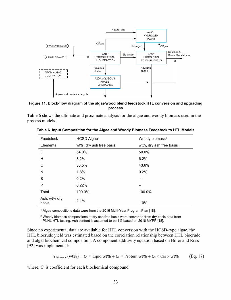
33

Figure 11. Block-flow diagram of the algae/wood blend feedstock HTL conversion and upgrading

process

Table 6 shows the ultimate and proximate analysis for the algae and woody biomass used in the process models.

Table 6. Input Composition for the Algae and Woody Biomass Feedstock to HTL Models

Feedstock HCSD Algae1 Woody biomass2

Elements wt%, dry ash free basis wt%, dry ash free basis

C 54.0% 50.0%

H 8.2% 6.2%

O 35.5% 43.6%

N 1.8% 0.2%

S 0.2% --

P 0.22% --

Total 100.0% 100.0%

Ash, wt% dry basis 2.4% 1.0% 1 Algae compositions data were from the 2016 Multi-Year Program Plan [18]. 2 Woody biomass compositions at dry ash free basis were converted from dry basis data from

PNNL HTL testing. Ash content is assumed to be 1% based on 2016 MYPP [18].

Since no experimental data are available for HTL conversion with the HCSD-type algae, the HTL biocrude yield was estimated based on the correlation relationship between HTL biocrude and algal biochemical composition. A component additivity equation based on Biller and Ross [92] was implemented:

Y biocrude (wt%) = C1 × Lipid wt% + C2 × Protein wt% + C3 × Carb. wt% (Eq. 17)

where, Ci is coefficient for each biochemical compound.

34

The coefficient in the above model represents the conversion efficiency of individual biochemical compound to biocrude. Based on PNNL HTL experimental data of six algae strains [93,11,94], as shown in Table 7, the values of the coefficients C1, C2, and C3 were calibrated and the results are: C1 = 0.95, C2 = 0.18, and C3 = 0.35. Part of the experimental information is listed in Jones et al. [11]. The predicted biocrude yields are calculated based on the average values of biochemical compounds in algae feedstock and the calibrated coefficients values.

Table 7. Predicted and Experimental HTL Biocrude Yields of Algae Feedstock with Different Biochemical Composition

Biochemical comp., wt% AFDW

BPA Hi lipid Scenedesmus

Chlorella (FY2012)

Chlorella (FY2016)

BPA low lipid Tetraselmis

HCSD target

Lipid 57 - 64% 18% 28% 28% 12 - 30% 17% 31%

Protein 3.5 - 4.1% 61% 45% 45% 27 - 59% 41% 14%

Carbohydrate 33 - 39% 21% 27% 27% 29 - 43% 42% 55%

Biocrude yield, wt% AFDW

Predicted 71% 35% 44% 44% 40% 38% 51%

Experimental 71% 36% 43% 43% 37% 40% n/a

The predicted and experimental biocrude yields were compared to each other, as shown in Figure 12. A linear trend line is added and the regression coefficient of the line is about 0.99. The r2 is also close to 1. It indicates that the component additivity equation with the above calibrated coefficients can provide reasonable predictions for biocrude yields from HTL of algae. Therefore, for the harmonization algae feedstock, the HTL biocrude yield is predicted to be 51% based on the above equation. When different experimental results were used for calibration, different values of coefficients can be obtained. Li et al. [95] employed a similar component additivity model to predict the biocrude yields, and their coefficient values are different from those in this study. More experimental results are required to validate the prediction equation of this study.

Figure 12. Experimental and predicted biocrude yields

y = 0.9916xR² = 0.9941

0%

10%

20%

30%

40%

50%

60%

70%

80%

0% 10% 20% 30% 40% 50% 60% 70% 80%

Test

ed B

iocr

ude

Yiel

d

Calculated Biocrude Yield

HCSD

35

For an algae/woody biomass conversion plant, the annual plant scale is assumed to be sized to match the summer season algal productivity. The algae yield differences between summer and other seasons are made up by using woody biomass. For each seasonal case, the blend ratio of algae-to-wood was calculated based on the seasonal algae yield and the added woody biomass amount. For the overall single case, the annual average of algae and wood feed flowrates in four seasons were calculated. For each site, the summer productivities are different and thus lead to different plant scales. The blend feedstock composition is calculated based on the HCSD-type algae and woody biomass composition (Table 6) and their blend ratios. The blended feedstock cost is linearly calculated from the blend ratios of algae and wood, and their individual feedstock costs.

The stoichiometry for the HTL conversion process for 100% algae was developed for the HTL model. The simulation results were used as the base values for the blended feedstock HTL cases. For the 100% algae case, the predicted HTL biocrude yield is 51% AFDW feedstock basis (as shown in Table 7). The biocrude yield for woody biomass only is 33% based on experimental results. The biocrude yields were assumed based on the algae only HTL simulation results and the HTL experimental data for algae/woody biomass blend feedstock with different blend ratios. As demonstrated by the experimental work, there is a synergistic effect on biocrude yield for the blended feedstock at the 50 wt% algae and 50 wt% wood blend ratio, which has the optimal biocrude yields compared to algae only, woody only, and the 75 wt% wood cases [91,90]. Since there is no experimental result for the HCSD-type algae HTL and its blend feedstock HTL, the optimal biocrude yields for HCSD algae/wood blend biomass are assumed to be the same as the predicted yield for the HCSD algae only case. Therefore, for the seasons with algae blend ratio higher than 50 wt% in the blend feedstock, the biocrude yields are assumed to be 51%, the same as the algae only case. It is assumed that the low woody biomass blend ratio does not change the biocrude yields significantly compared to the algae only case. For winter seasons when the algae blend ratio is generally less than 50 wt%, the biocrude yield is estimated by considering the biocrude yields of algae only and woody only cases, and their blend ratios.

The hydrotreated (HT) biocrude yields are estimated based on the HT yield of the algae only case, yield of the wood only case, and their blend ratio in the feedstock. The final fuel product properties, including heating values and densities, are estimated in the same way. The final production cost was estimated based on the annual average of blend feedstock flowrates, biocrude yields, HT organics yields, and other performance results.

The aqueous phase organics recovery and upgrading to fuels is based on advanced membrane research at NREL and ORNL [96] and research at PNNL for conversion of mixed organic oxygenates to fuel [97]. Separations work is also ongoing for a related process in the Bioprocessing Separations Consortium [98]. For this study, a portion of the organic compounds in the aqueous phase are separated from water by using hydrophobic membranes. The carbon contained in the permeate is assumed to be 75% of total carbon in the aqueous phase. The permeate is then sent to a zeolite-type catalytic upgrading process to produce additional fuel. The fuel yield is assumed to be approximately 40% of the permeate, which is consistent with an average aqueous organic molecule containing two carbons and two oxygens. HTL could be implemented today as it is not dependent upon the HCSD algae composition targets projected in the future under this study. However, biocrude yields will typically be lower for the faster-growing (high protein) algae currently available. This effect is somewhat mitigated by the

36

inclusion of additional fuel production from recovery of aqueous organics, for which research is ongoing.

Demonstrating biocrude yields on HCSD and blends of HCSD with wood or other terrestrial biomass is a key research gap. However, HTL could be implemented today as it can be used with any type of algae or blend and is not dependent upon the projected HCSD algae composition in this study. Thus, cost reduction strategies for HTL are underway, whether or not HCSD biomass composition goals materialize in the projected form or timeframe as envisioned. The goal is to improve biocrude yield and quality using existing algae. Sequential HTL (two-temperature stages) research is currently under investigation as a means of recovering carbohydrate intermediates during a low temperature step for further conversion to valuable co-products, followed by higher temperature HTL of the unconverted solids portion to produce higher quality biocrude. Use of inexpensive non-algal sources for blending with algae will be assessed as a means to significantly lower the overall costs. Resource assessment for these combined feeds needs to be understood at various scales of algal and terrestrial biomass availability. Biocrude upgrading research is focusing on producing an easily hydrotreated feedstock for distillate fuels that could be processed in a dedicated unit or co-processed with petroleum in a conventional refinery, the latter allowing leveraging existing capital equipment. Such work includes reducing the nitrogen content in biocrude and removing fine particulate matter that may plug fixed bed upgrading reactors. Valorizing HTL aqueous carbon by direct recovery of constituents for sale (organic acids for example) or by concentration for further conversion is an additional potential source of revenue. The effects of recycling the treated aqueous phase to the ponds needs further study. Lab-scale cultivation tests have successfully cultivated algae on HTL aqueous phase recycle streams. This work needs to be extended to HTL aqueous of mixed feeds (algae and terrestrial biomass) both in the lab and in field trials.

Life-Cycle Analysis The boundary for the LCA includes all energy and chemicals associated with biomass growth and dewatering, nutrient supply, algae conversion, displacement of any coproducts, fuel transportation and distribution, and combustion in vehicles. Emissions for producing system inputs (e.g., energy and chemicals) are also included in the boundary, allowing for the full WTW impacts to be determined. The functional unit is one mega joule (MJ) of total fuel. The Greenhouse Gases, Regulated Emissions, and Energy Use in Transportation (GREET) model [92] was expanded to include biofuels produced from microalgae, considering the two conversion technologies, CAP and HTL. WTW GHG emissions, fossil energy use, and freshwater consumption were calculated using life-cycle inventories (LCIs) provided by NREL and PNNL. Impacts due to infrastructure materials, which were determined for the previous algae model harmonization effort [99], were not included in this analysis because the algae system has undergone numerous changes (e.g., CO2 delivery, piping, and conversion).

The LCI for cultivation and dewatering, in both the freshwater and saline scenarios, were provided by NREL according to each site group. Inputs included electricity use, nutrients (N, P, and CO2), water use (in biomass, evaporation, and blowdown), and CO2 outgassing. The outgassing was considered biogenic and therefore offset by CO2 capture at the CO2 sources. Any recycle of nutrients from conversion was not applied to cultivation, but rather considered a credit in the downstream conversion process. The default CO2 capture/delivery energy from CC was

37

applied in GREET based on a parasitic energy demand of 0.63 MJe/kg-CO2 as noted previously, based on guidance from NETL researchers specific to future targets for “2nd-generation” CC technologies [21]. This value for CC energy demand also corresponds with an average of those in other literature [100-102]. Other studies have shown variations in the estimates of CC parasitic energy demand. Simulations by Strube and Manfrida [103] estimated 1.0 MJe/kg-CO2 for integration at a pulverized coal power plant. Rubin et al. [48] similarly reported values averaging around roughly 1.0 MJe/kg for current “state of the art” technologies, increasing to roughly 1.5 MJe/kg for older technologies such as standard MEA amine scrubbing. This “state of the art” value also corresponds consistently with Fout et al. [104] who reported 1.03 MJe/kg for an advanced amine system. However, one confounding factor is that the majority of published literature including those cited above focus on greenfield applications (i.e. building the power plant and carbon capture system integrated together from scratch), rather than retrofits (adding a CC system to an existing power plant) as is implied here based on RA site selection focused on existing power plant CO2 sources. Retrofit applications are likely to incur higher parasitic energy penalties given the difficulties to integrate into existing heat exchange networks. One study focused specifically on retrofit applications was based on a report by Supekar et al. [105], wherein ANL examined retrofitting coal and NG plants for CC using two design cases: an integrated CC system and an auxiliary turbine supporting a CC system [106]. The integrated CC uses its own heat and power for CC while the latter uses auxiliary NG (which is more efficient than a coal boiler) to supply a portion of required heat and power. The results indicated a parasitic energy demand for retrofitting CC at coal boiler power plants of 1.015 MJe/kg-CO2 with the integrated CC design, and 0.627 MJe/kg-CO2 with the auxiliary NG turbine design. Thus, at present it is unclear what may be the “best case” values possible for future 2nd-generation CC parasitic energy demand, and how those values may differ between greenfield versus retrofit applications. Taking into account the above variations, this study conducted a sensitivity analysis on the parasitic energy demand increasing up to 1.0 MJe/kg-CO2, included in all scenarios examined through LCA.

NREL also provided the LCI for the CAP conversion processes. Inputs included pretreatment, conversion, and coproduct chemicals, supplemental natural gas, exported electricity, process water, nutrient and water recycles, and algae biomass loss during storage. All nutrients recycled back to the algal ponds received a displacement credit, on a 1:1 basis, for nutrients used during cultivation. A displacement credit was also taken for electricity, using the U.S. average grid mix and accounting for a transmission and distribution loss of 6.5% [92].

The CAP conversion processes produce a large amount of chemical coproducts. A key issue in dealing with these coproducts is how to capture their environmental impacts especially under the current fuel-focused GHG regulations. ANL conducted a recent analysis examining this specific issue for integrated biorefineries coproducing significant quantities of bio-derived chemical coproducts, and demonstrated that only the displacement method can fully account for the GHG emission reduction benefits offered by non-fuel products (relative to other allocation-based methods) [107]. Following the same rationale, this study used the displacement method for handling of the polyurethane and succinic acid coproducts in the overall LCA. Polyurethane is produced from numerous chemicals in addition to algal fatty acids, as shown in Table 8, some of which were not available in GREET. Those chemicals not available that comprised less than 1 wt% of the total chemical input were excluded from the analysis, as it was assumed their impact would be negligible. Polyurethane was treated with a displacement credit in the LCA for

38

replacement of polyurethane rigid foam produced from petroleum [92]. The other coproduct, succinic acid, is produced exclusively in the saline case and also received a displacement credit for the replacement of petroleum-derived adipic acid as a proxy for succinic acid [108]. These coproducts also received a sequestration credit because they contain a portion of the biogenic carbon from the algae. The polyurethane contains 67% carbon by mass, of which 55% is biogenic, while succinic acid contains 47% carbon by mass, all of which is biogenic.

Table 8. Chemicals Used for CAP Polyurethane Production (chemicals not available in GREET were excluded if they were less than 1 wt% of the total)

Chemical % of Total Inputs (wt%) Data Source Comment

Urea 0.9% GREET

Ethanol 9.1% GREET

Sulfuric Acid 0.5% GREET

Acetic Acid 4.7% GREET

H2O2 10.9% GREET

Sodium Hydroxide 3.1% GREET

Fluoroboric Acid 0.1% N/A Excluded because low wt%

Methanol 7.4% GREET

Glycerol 10.3% GREET1

Inert Gas N2 16.1% GREET

Catalyst, T-Amine 0.1% GREET2

N-Ethylmorpholine 0.2% N/A Excluded because low wt%

Silicone Surfactant 0.5% N/A Excluded because low wt%

Stannous Octoate 0.2% N/A Excluded because low wt%

Toluene Diisocyanate 36.0% USLCI3 1 From soy oil 2 Assumed ZMP catalyst due to high energy intensity for production being the most conservative estimate 3 From [109]

PNNL provided the LCI information for the HTL process. Inputs included algae, waste wood, chemicals, electricity, natural gas, process water, and recycled streams of nutrients and water. The recycled streams were treated the same as the CAP process, with the conversion technology receiving credit for nutrients recycled to the cultivation process. In the LCI information obtained from PNNL and NREL, recycled nutrients were specified in the amount of N and P recycled. Thus, these quantities of N and P were converted into mass of ammonia (NH3) and diammonium phosphate (DAP) by calculating the DAP from the phosphorus recycle and the ammonia from the sum of both NH3 and DAP. The input of waste wood was assumed to be from construction and demolition waste. The waste is considered burden-free until it is collected, where it is sorted, stored, and eventually transported to the biorefinery. These processes use electricity and diesel, which were previously analyzed in GREET for the production of high-octane gasoline [92].

39

Results RA: Outputs to TEA Farm Model The outputs from the RA identified over 150 individual sites within the United States meeting the screening criteria outlined above. To translate the outputs to the TEA farm model, which is manually run through season-specific Aspen plus process models to determine the mass and energy balances of the process, it is both time intensive and impractical to run over 600 individual cases. Instead, similar to previous harmonization efforts, we grouped sites based on their general locations to pare the 150 sites down into 9 groupings for the freshwater case or 8 groupings for the saline case, with the average of each grouping serving to define a single “representative” farm for the given group. Figure 13 shows the resulting freshwater RA output site locations and their groupings. Table 9 provides more information on the total area within each grouping, the weighted average of the productivity based on the area per group, the weighted average of the evaporation rate, and the weighted average of the CO2 cost to deliver the captured CO2 to the facility gate, all of which are subsequently used as inputs to the TEA farm models. Likewise, Figure 14 and Table 10 provide similar details for the saline scenario. Notably, when removing the constraint for freshwater availability in moving to the saline scenario, the BAT model identified 882 more potential unit farms which translated to roughly 2.5 times higher total cultivation area and biomass production potential on a national scale, relative to the freshwater case.

40

Table 9. Freshwater Cases Developed from BAT Analysis as Input to TEA Farm Models Based on Representative Site Groupings

Group Num.

Total Area (Acres)

Number of 5,000-acre Facilities

Productivity (g/m2/day) Net Pond Evaporation Rate (cm/day) CO2 Cost

$/tonne (2014$)

Annual Average Winter Spring Summer Fall


1 200,642 40.1 25.95 12.72 32.29 34.94 23.84 0.50 0.10 0.48 0.96 0.46 $42.09

2 110,710 22.1 23.65 4.43 30.50 38.80 20.87 0.38 0.07 0.41 0.71 0.32 $41.49

3 669,801 134.0 25.53 10.74 32.73 35.15 23.51 0.45 0.16 0.56 0.70 0.38 $39.90

4 296,815 59.4 27.93 19.20 29.47 37.94 25.09 0.24 0.08 0.26 0.47 0.17 $40.63

5 316,646 63.3 27.14 17.09 29.72 37.35 24.38 0.10 0.01 0.11 0.20 0.09 $32.39

6 156,851 31.4 25.13 12.27 28.92 36.71 22.60 0.13 0.02 0.08 0.29 0.12 $41.42

7 293,307 58.7 26.19 15.12 29.57 36.20 23.87 0.07 0.00 0.05 0.14 0.08 $39.51

8 329,933 66.0 28.68 22.00 30.35 36.72 25.65 0.10 0.05 0.25 0.07 0.04 $40.96

9 283,859 56.8 25.39 13.09 29.82 35.64 23.02 0.06 0.01 0.07 0.11 0.04 $41.67

Total 2,658,565 532 26.37 14.55 30.70 36.32 23.91 0.24 0.07 0.29 0.41 0.20 $39.69

Figure 13. Map of freshwater cases determined by BAT and broken into groupings

Group 1 Group 2

Group 3

Group 4

Group 6

Group 5

Group 7

Group 8

Group 9

41

Table 10. Saline Cases Developed from BAT Analysis as Input to TEA Farm Models Based on Representative Site Groupings

Group Num.

Total Area (Acres)

Number of 5,000-acre Facilities

Productivity (g/m2/day) Net Pond Evaporation Rate (cm/day) CO2 Cost

$/tonne (2014$)



1 597,713 119.5 27.31 14.13 35.28 36.67 23.17 0.57 0.11 0.55 1.10 0.54 $43.45

2 1,309,442 261.9 26.87 12.20 34.93 37.59 22.74 0.55 0.18 0.69 0.86 0.46 $41.87

3 859,205 171.8 25.50 15.53 28.16 37.18 21.11 0.26 0.06 0.26 0.51 0.20 $40.96

4 1,322,984 264.6 25.34 15.54 28.33 35.93 21.54 0.10 0.00 0.12 0.18 0.09 $39.76

5 971,459 194.3 23.90 11.45 28.53 36.06 19.57 0.17 0.02 0.12 0.39 0.16 $40.70

6 484,228 96.8 24.50 13.24 28.84 35.36 20.58 0.09 0.00 0.08 0.19 0.10 $41.76

7 995,894 199.2 26.27 16.57 29.36 35.78 23.36 0.11 0.07 0.26 0.07 0.06 $41.14

8 530,148 106.0 25.04 14.34 29.83 35.94 20.06 0.08 0.01 0.13 0.12 0.06 $41.52

Total 7,071,073 1,414 25.66 14.14 30.44 36.41 21.66 0.25 0.06 0.30 0.43 0.22 $41.20

Figure 14. Map of saline cases determined by BAT and broken into groupings

Group 1

Group 2

Group 3

Group 4

Group 5

Group 6

Group 7

Group 8

42

TEA: Farm Model Since there are two different conversion methods evaluated in this study (CAP and HTL), we split the TEA into (1) cultivation and dewatering costs provided as MBSP in dollars per U.S. ton of algae produced (AFDW) and (2) conversion costs provided as MFSP in dollars per GGE. All costs are provided on a 2014$ basis. Figure 15 presents the MBSP of the site groupings using the productivity, pond evaporation rate, and CO2 prices from Table 9 (freshwater) and Table 10 (saline). The figure also displays each grouping’s corresponding minimum, maximum, and average productivity, as well as the weighted average MBSP for all groups based on the number of individual 5,000-acre farms attributed to each respective group (hereafter referred to as Freshwater/Saline Group Average). In agreement with previous analyses [1], higher average productivities result in lower MBSPs, as do tighter seasonal variabilities given more efficient year-round utilization of installed equipment (shown for example in comparing freshwater site group 7 against 1 and 3, where all exhibit similar average productivities, but less variability for group 7 and correspondingly lower MBSP). Individually, freshwater site groups 8, 4, and 5 (generally Florida and Texas) indicate the lowest MBSPs due to the highest average productivities and low seasonal variability, while group 2 (northern Midwest states, i.e., Nevada, Utah, and Colorado) stands out with a more distinctly higher MBSP and significantly higher seasonal variability with very low winter productivities.

The MBSP of the overall Freshwater Group Average is $472/ton AFDW (weighted average reflective of different overall cultivation areas for each group), which is $22/ton lower than the MBSP target from the algae farm design report (when put on the same 2014 cost year basis) [9], reflective of a marginally higher weighted-average targeted productivity of 26.4 g/m2/day compared to the 25 g/m2/day basis in the algae farm design report. Additionally, the freshwater cases are assumed to be universally located in areas with sufficient soil characteristics to allow for minimally lined ponds (although high-permeability soils are not explicitly excluded as soil characteristics are not part of the RA screening criteria), and also do not incur water disposal costs. We have shown previously that full pond liners add more than $100/ton to the MBSPs (as also reflected below in the saline results), highlighting that this would be another important parameter for RA to consider in the future for both freshwater and saline cultivation scenarios, i.e., including site screening criteria tied to soil conditions or other factors that would dictate the need for liners. In any case where liners were required, the resulting cost premiums also may be mitigated through the use of lower-cost liner materials or installation methods, as others are currently investigating.

The right side of Figure 15 presents the same results for the saline scenario, with rolled-up MBSPs shown for each site group average case but now also explicitly breaking out the contribution associated with full pond liners as well as blowdown salt disposal costs (neither of which are large factors in the freshwater scenarios). The MBSP of the overall Saline Group Average is $655/ton AFDW (weighted average across all site groups), $183/ton higher than the Freshwater Group Average driven by the extra costs incurred for salt management associated with full pond liners and blowdown disposal. In this case, the individual site group trends are the same as for the freshwater scenario for the portion of the MBSPs excluding salt disposal, i.e., with respect to average and seasonal productivities. However, the inclusion of salt disposal alters the trends in overall MBSP for some cases with high evaporation rates attributed to more arid locations such as California and the Southwest. As described above, blowdown removal was set

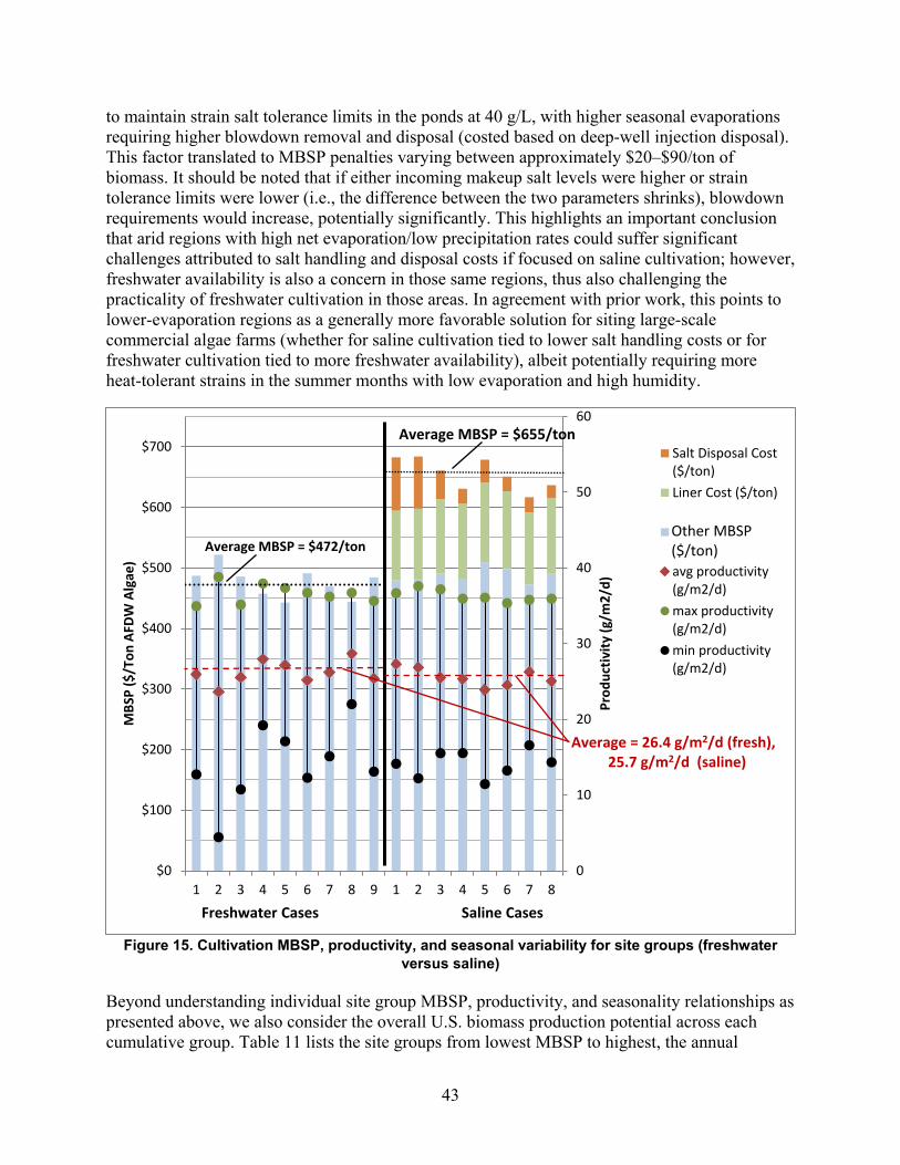
43

to maintain strain salt tolerance limits in the ponds at 40 g/L, with higher seasonal evaporations requiring higher blowdown removal and disposal (costed based on deep-well injection disposal). This factor translated to MBSP penalties varying between approximately $20–$90/ton of biomass. It should be noted that if either incoming makeup salt levels were higher or strain tolerance limits were lower (i.e., the difference between the two parameters shrinks), blowdown requirements would increase, potentially significantly. This highlights an important conclusion that arid regions with high net evaporation/low precipitation rates could suffer significant challenges attributed to salt handling and disposal costs if focused on saline cultivation; however, freshwater availability is also a concern in those same regions, thus also challenging the practicality of freshwater cultivation in those areas. In agreement with prior work, this points to lower-evaporation regions as a generally more favorable solution for siting large-scale commercial algae farms (whether for saline cultivation tied to lower salt handling costs or for freshwater cultivation tied to more freshwater availability), albeit potentially requiring more heat-tolerant strains in the summer months with low evaporation and high humidity.

Figure 15. Cultivation MBSP, productivity, and seasonal variability for site groups (freshwater

versus saline)

Beyond understanding individual site group MBSP, productivity, and seasonality relationships as presented above, we also consider the overall U.S. biomass production potential across each cumulative group. Table 11 lists the site groups from lowest MBSP to highest, the annual

0

10

20

30

40

50

60

$0

$100

$200

$300

$400

$500

$600

$700

1 2 3 4 5 6 7 8 9 1 2 3 4 5 6 7 8

Prod

uctiv

ity (g

/m2/

d)

MBS

P ($

/Ton

AFD

W A

lgae

)

Freshwater Cases Saline Cases

Salt Disposal Cost($/ton)Liner Cost ($/ton)

MBSP ($/ton)

avg productivity(g/m2/d)max productivity(g/m2/d)min productivity(g/m2/d)

Average MBSP = $472/ton

Average MBSP = $655/ton

Average = 26.4 g/m2/d (fresh), 25.7 g/m2/d (saline)

Other MBSP ($/ton)

44

biomass production per facility within each site group (tied to each group’s average cultivation productivity), the cumulative algae production output from group to group, and the cumulative weighted average of the MBSP as each subsequent group is added on. In all, the total freshwater algae biomass potential in the U.S. is modeled at 104 MM tons/year when constrained to an average productivity near 25 g/m2/day for future targets, coupled with the other screening factors discussed previously for the BAT model including CO2 and freshwater availability. In contrast, the saline algae biomass potential is estimated from the BAT model to be significantly higher, 235 MM tons/year at a similar average cultivation productivity target but focused on saline water resource availability rather than freshwater. However, due to the additional costs for salt management discussed above, this biomass comes at a cost premium of approximately $183/ton (weighted average of all site groups), which must be overcome through additional downstream conversion cost reductions or increased coproduct revenues to maintain MFSP cost targets relative to the freshwater case. Alternatively, if the ponds only required minimal liners consistent with the freshwater case (but still maintaining blowdown salt disposal costs), the saline weighted average MBSP would reduce to $533/ton, only $60/ton higher than the freshwater average.

Table 11. Matrix of Key Harmonized Model Outputs for Algae Cultivation (organized by site group in order of increasing MBSPs; tracking cumulative [summative] algae biomass yield versus rolling weighted-

average MBSP across each sequential group)

Site group

Weighting (# of 5,000-acre

farms in group)

Algal biomass production per 5,000-

acre farm (tons/yr [AFDW])

Cumulative MM tons/yr biomass

AFDW

Site group MBSP ($/ton)

Cumulative weighted

average MBSP ($/ton)

Freshwater scenario

5 63.3 201,676 12.8 $443 $443

8 66.0 213,222 26.8 $444 $444

4 59.4 207,443 39.2 $457 $448

7 58.7 194,779 50.6 $469 $453

9 56.8 188,906 61.3 $484 $459

1 40.1 193,036 69.1 $487 $462

3 134.0 189,890 94.5 $486 $469

6 31.4 186,789 100.4 $491 $470

2 22.1 175,544 104.2 $522 $472

Saline scenario

7 199.2 195,287 38.9 $617 $617

4 264.6 188,345 88.7 $631 $625

8 106.0 186,188 108.5 $637 $627

6 96.8 182,241 126.1 $651 $630

3 171.8 189,262 158.6 $661 $637

5 194.3 177,605 269.5 $678 $644

1 119.5 202,543 182.9 $683 $648

2 261.9 199,137 235.0 $684 $655

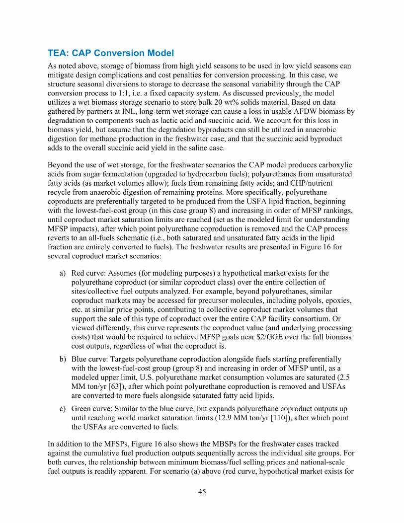
45

TEA: CAP Conversion Model As noted above, storage of biomass from high yield seasons to be used in low yield seasons can mitigate design complications and cost penalties for conversion processing. In this case, we structure seasonal diversions to storage to decrease the seasonal variability through the CAP conversion process to 1:1, i.e. a fixed capacity system. As discussed previously, the model utilizes a wet biomass storage scenario to store bulk 20 wt% solids material. Based on data gathered by partners at INL, long-term wet storage can cause a loss in usable AFDW biomass by degradation to components such as lactic acid and succinic acid. We account for this loss in biomass yield, but assume that the degradation byproducts can still be utilized in anaerobic digestion for methane production in the freshwater case, and that the succinic acid byproduct adds to the overall succinic acid yield in the saline case.

Beyond the use of wet storage, for the freshwater scenarios the CAP model produces carboxylic acids from sugar fermentation (upgraded to hydrocarbon fuels); polyurethanes from unsaturated fatty acids (as market volumes allow); fuels from remaining fatty acids; and CHP/nutrient recycle from anaerobic digestion of remaining proteins. More specifically, polyurethane coproducts are preferentially targeted to be produced from the USFA lipid fraction, beginning with the lowest-fuel-cost group (in this case group 8) and increasing in order of MFSP rankings, until coproduct market saturation limits are reached (set as the modeled limit for understanding MFSP impacts), after which point polyurethane coproduction is removed and the CAP process reverts to an all-fuels schematic (i.e., both saturated and unsaturated fatty acids in the lipid fraction are entirely converted to fuels). The freshwater results are presented in Figure 16 for several coproduct market scenarios:

a) Red curve: Assumes (for modeling purposes) a hypothetical market exists for the polyurethane coproduct (or similar coproduct class) over the entire collection of sites/collective fuel outputs analyzed. For example, beyond polyurethanes, similar coproduct markets may be accessed for precursor molecules, including polyols, epoxies, etc. at similar price points, contributing to collective coproduct market volumes that support the sale of this type of coproduct over the entire CAP facility consortium. Or viewed differently, this curve represents the coproduct value (and underlying processing costs) that would be required to achieve MFSP goals near $2/GGE over the full biomass cost outputs, regardless of what the coproduct is.

b) Blue curve: Targets polyurethane coproduction alongside fuels starting preferentially with the lowest-fuel-cost group (group 8) and increasing in order of MFSP until, as a modeled upper limit, U.S. polyurethane market consumption volumes are saturated (2.5 MM ton/yr [63]), after which point polyurethane coproduction is removed and USFAs are converted to more fuels alongside saturated fatty acid lipids.

c) Green curve: Similar to the blue curve, but expands polyurethane coproduct outputs up until reaching world market saturation limits (12.9 MM ton/yr [110]), after which point the USFAs are converted to fuels.

In addition to the MFSPs, Figure 16 also shows the MBSPs for the freshwater cases tracked against the cumulative fuel production outputs sequentially across the individual site groups. For both curves, the relationship between minimum biomass/fuel selling prices and national-scale fuel outputs is readily apparent. For scenario (a) above (red curve, hypothetical market exists for

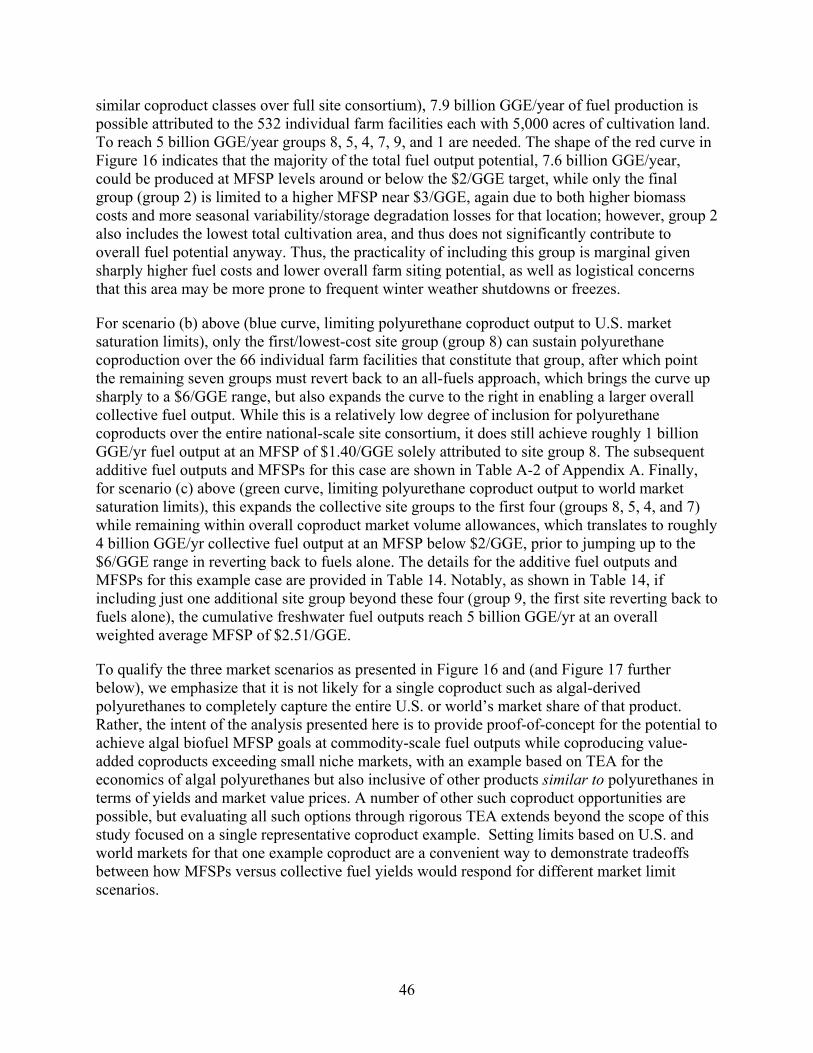
46

similar coproduct classes over full site consortium), 7.9 billion GGE/year of fuel production is possible attributed to the 532 individual farm facilities each with 5,000 acres of cultivation land. To reach 5 billion GGE/year groups 8, 5, 4, 7, 9, and 1 are needed. The shape of the red curve in Figure 16 indicates that the majority of the total fuel output potential, 7.6 billion GGE/year, could be produced at MFSP levels around or below the $2/GGE target, while only the final group (group 2) is limited to a higher MFSP near $3/GGE, again due to both higher biomass costs and more seasonal variability/storage degradation losses for that location; however, group 2 also includes the lowest total cultivation area, and thus does not significantly contribute to overall fuel potential anyway. Thus, the practicality of including this group is marginal given sharply higher fuel costs and lower overall farm siting potential, as well as logistical concerns that this area may be more prone to frequent winter weather shutdowns or freezes.

For scenario (b) above (blue curve, limiting polyurethane coproduct output to U.S. market saturation limits), only the first/lowest-cost site group (group 8) can sustain polyurethane coproduction over the 66 individual farm facilities that constitute that group, after which point the remaining seven groups must revert back to an all-fuels approach, which brings the curve up sharply to a $6/GGE range, but also expands the curve to the right in enabling a larger overall collective fuel output. While this is a relatively low degree of inclusion for polyurethane coproducts over the entire national-scale site consortium, it does still achieve roughly 1 billion GGE/yr fuel output at an MFSP of $1.40/GGE solely attributed to site group 8. The subsequent additive fuel outputs and MFSPs for this case are shown in Table A-2 of Appendix A. Finally, for scenario (c) above (green curve, limiting polyurethane coproduct output to world market saturation limits), this expands the collective site groups to the first four (groups 8, 5, 4, and 7) while remaining within overall coproduct market volume allowances, which translates to roughly 4 billion GGE/yr collective fuel output at an MFSP below $2/GGE, prior to jumping up to the $6/GGE range in reverting back to fuels alone. The details for the additive fuel outputs and MFSPs for this example case are provided in Table 14. Notably, as shown in Table 14, if including just one additional site group beyond these four (group 9, the first site reverting back to fuels alone), the cumulative freshwater fuel outputs reach 5 billion GGE/yr at an overall weighted average MFSP of $2.51/GGE.

To qualify the three market scenarios as presented in Figure 16 and (and Figure 17 further below), we emphasize that it is not likely for a single coproduct such as algal-derived polyurethanes to completely capture the entire U.S. or world’s market share of that product. Rather, the intent of the analysis presented here is to provide proof-of-concept for the potential to achieve algal biofuel MFSP goals at commodity-scale fuel outputs while coproducing value-added coproducts exceeding small niche markets, with an example based on TEA for the economics of algal polyurethanes but also inclusive of other products similar to polyurethanes in terms of yields and market value prices. A number of other such coproduct opportunities are possible, but evaluating all such options through rigorous TEA extends beyond the scope of this study focused on a single representative coproduct example. Setting limits based on U.S. and world markets for that one example coproduct are a convenient way to demonstrate tradeoffs between how MFSPs versus collective fuel yields would respond for different market limit scenarios.

47

Figure 16. CAP conversion modeled cases showing cumulative fuel production and

corresponding MFSP/MBSP (freshwater scenario). Three MFSP curves are shown representing different coproduct market volume scenarios: (a) red curve—no market saturation limits for PU or related

coproducts (i.e., expanding into additional markets such as polyols, epoxies, etc. such that market capacity exists over full site collection); (b) blue curve—PU is coproduced until hitting U.S. market

consumption limit, after which point PU coproduction is eliminated and reverts to fuels-only for remainder of curve; (c) green curve—PU is coproduced until hitting world market consumption limit, after which point

PU coproduction is eliminated and reverts to fuels-only for remainder of curve. PU = polyurethanes.

As described above, for the saline scenarios the CAP model replaces the sugar-to-fuel train (via carboxylic acid intermediates) with sugars-to-succinic acid (SA) and SA derivatives as a second example coproduct to offset the higher biomass costs. The PU coproduct is again, for model studies, evaluated within market volume limitations for polyurethanes; however, because the algal biomass production scale is so much larger for each site group in the saline case, the U.S. market for PUs would become saturated before fully satisfying the first site group. As such, for the saline MFSP curves only world markets are reflected for the PU coproduct. Likewise, for model studies, the SA coproduct “class” also only considers total world market volumes for SA and the five other derivative components identified above (1-4 butanediol, maleic anhydride, tetrahydrofuran, adipic acid, and 1,3-butadiene), again with the caveats in mind as noted previously about the different market values and yield-equivalents for those given derivative components relative to succinic acid. The saline results are presented in Figure 17 for several coproduct market scenarios:

a) Red curve: Assumes (for modeling purposes) a market exists for the polyurethane and SA coproducts (or similar coproduct classes) over the entire collection of sites/collective fuel outputs analyzed. Again, additional coproducts with similar functionalities and prices

$0

$100

$200

$300

$400

$500

$600

$0.00

$2.00

$4.00

$6.00

$8.00

$10.00

$12.00

0 2 4 6 8 10 12

MBS

P ($

/US

Ton)

MFS

P ($

/GG

E)

Cumulative Fuel Production (Billion GGE/year)

MFSP ($/GGE) - NoCoproduct MarketLimitsMFSP Average - NoCoproduct MarketLimitsMFSP ($/GGE) - USPU Market Capacity

MFSP Average - USPU Market Capacity

MFSP ($/GGE) -World PU MarketCapacityMFSP Average -World PU MarketCapacityMBSP ($/tonAFDW)-Freshwater

MBSP Average($/ton AFDW)

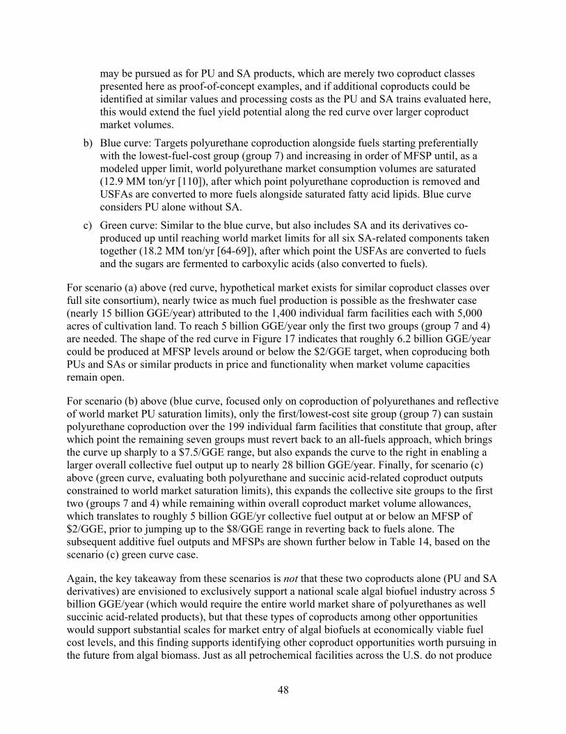
48

may be pursued as for PU and SA products, which are merely two coproduct classes presented here as proof-of-concept examples, and if additional coproducts could be identified at similar values and processing costs as the PU and SA trains evaluated here, this would extend the fuel yield potential along the red curve over larger coproduct market volumes.

b) Blue curve: Targets polyurethane coproduction alongside fuels starting preferentially with the lowest-fuel-cost group (group 7) and increasing in order of MFSP until, as a modeled upper limit, world polyurethane market consumption volumes are saturated (12.9 MM ton/yr [110]), after which point polyurethane coproduction is removed and USFAs are converted to more fuels alongside saturated fatty acid lipids. Blue curve considers PU alone without SA.

c) Green curve: Similar to the blue curve, but also includes SA and its derivatives co-produced up until reaching world market limits for all six SA-related components taken together (18.2 MM ton/yr [64-69]), after which point the USFAs are converted to fuels and the sugars are fermented to carboxylic acids (also converted to fuels).

For scenario (a) above (red curve, hypothetical market exists for similar coproduct classes over full site consortium), nearly twice as much fuel production is possible as the freshwater case (nearly 15 billion GGE/year) attributed to the 1,400 individual farm facilities each with 5,000 acres of cultivation land. To reach 5 billion GGE/year only the first two groups (group 7 and 4) are needed. The shape of the red curve in Figure 17 indicates that roughly 6.2 billion GGE/year could be produced at MFSP levels around or below the $2/GGE target, when coproducing both PUs and SAs or similar products in price and functionality when market volume capacities remain open.

For scenario (b) above (blue curve, focused only on coproduction of polyurethanes and reflective of world market PU saturation limits), only the first/lowest-cost site group (group 7) can sustain polyurethane coproduction over the 199 individual farm facilities that constitute that group, after which point the remaining seven groups must revert back to an all-fuels approach, which brings the curve up sharply to a $7.5/GGE range, but also expands the curve to the right in enabling a larger overall collective fuel output up to nearly 28 billion GGE/year. Finally, for scenario (c) above (green curve, evaluating both polyurethane and succinic acid-related coproduct outputs constrained to world market saturation limits), this expands the collective site groups to the first two (groups 7 and 4) while remaining within overall coproduct market volume allowances, which translates to roughly 5 billion GGE/yr collective fuel output at or below an MFSP of $2/GGE, prior to jumping up to the $8/GGE range in reverting back to fuels alone. The subsequent additive fuel outputs and MFSPs are shown further below in Table 14, based on the scenario (c) green curve case.

Again, the key takeaway from these scenarios is not that these two coproducts alone (PU and SA derivatives) are envisioned to exclusively support a national scale algal biofuel industry across 5 billion GGE/year (which would require the entire world market share of polyurethanes as well succinic acid-related products), but that these types of coproducts among other opportunities would support substantial scales for market entry of algal biofuels at economically viable fuel cost levels, and this finding supports identifying other coproduct opportunities worth pursuing in the future from algal biomass. Just as all petrochemical facilities across the U.S. do not produce

49

only two (of the same) products, a national-scale consortium of algal biorefineries would also be expected to produce a large number of diverse bioproducts alongside fuels, as market drivers would dictate to ensure economic profitability.

Figure 17. CAP conversion modeled cases showing cumulative fuel production and corresponding MFSP/MBSP (saline scenario). Three MFSP curves are shown representing different coproduct market volume scenarios: (a) red curve—no market saturation limits for PU and SA or related coproducts; (b) blue curve—PU is coproduced until hitting world market consumption limit, after which

point PU coproduction is eliminated and reverts to fuels-only for remainder of curve; (c) green curve—PU and SA are both coproduced until hitting world market consumption limits, after which point all

coproduction is eliminated and reverts to fuels-only for remainder of curve. PU = polyurethanes; SA = succinic acid (used as a proxy for other SA derivative components as well for market volume

considerations).

Table 12 provides a summary of the key mass balances and carbon yields from the CAP conversion models, attributed to each site group across the scenarios presented in Figure 16 and Figure 17.

$0

$100

$200

$300

$400

$500

$600

$700

$0.00

$2.00

$4.00

$6.00

$8.00

$10.00

$12.00

0 5 10 15 20 25 30

MBS

P($/

US

Ton)

MFS

P ($

/GG

E)

Cumulative Fuel Production (Billion GGE/year)

MFSP ($/GGE) - NoCoproduct MarketLimitsMFSP ($/GGE) - NoCoproduct MarketLimitsMFSP ($/GGE) - WorldPU Market Capacity

MFSP Average - WorldPU Market Capacity

MFSP ($/GGE) - WorldMarkets (SA and PUCoproducts)MFSP Average - WorldMarkets (SA and PUCoproducts)MBSP ($/ton AFDW) -Saline

MBSP Average ($/tonAFDW)

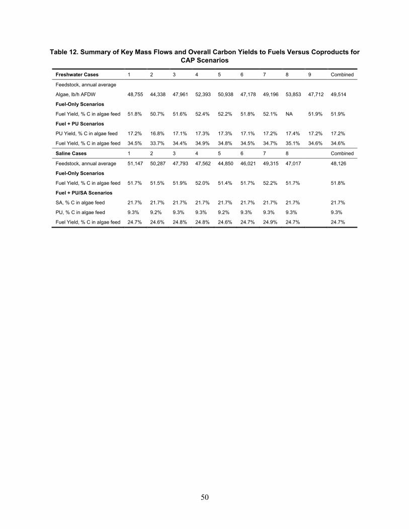
50

Table 12. Summary of Key Mass Flows and Overall Carbon Yields to Fuels Versus Coproducts for CAP Scenarios

Freshwater Cases 1 2 3 4 5 6 7 8 9 Combined

Feedstock, annual average

Algae, lb/h AFDW 48,755 44,338 47,961 52,393 50,938 47,178 49,196 53,853 47,712 49,514

Fuel-Only Scenarios

Fuel Yield, % C in algae feed 51.8% 50.7% 51.6% 52.4% 52.2% 51.8% 52.1% NA 51.9% 51.9%

Fuel + PU Scenarios

PU Yield, % C in algae feed 17.2% 16.8% 17.1% 17.3% 17.3% 17.1% 17.2% 17.4% 17.2% 17.2%

Fuel Yield, % C in algae feed 34.5% 33.7% 34.4% 34.9% 34.8% 34.5% 34.7% 35.1% 34.6% 34.6%

Saline Cases 1 2 3 4 5 6 7 8 Combined

Feedstock, annual average 51,147 50,287 47,793 47,562 44,850 46,021 49,315 47,017 48,126

Fuel-Only Scenarios

Fuel Yield, % C in algae feed 51.7% 51.5% 51.9% 52.0% 51.4% 51.7% 52.2% 51.7% 51.8%

Fuel + PU/SA Scenarios

SA, % C in algae feed 21.7% 21.7% 21.7% 21.7% 21.7% 21.7% 21.7% 21.7% 21.7%

PU, % C in algae feed 9.3% 9.2% 9.3% 9.3% 9.2% 9.3% 9.3% 9.3% 9.3%

Fuel Yield, % C in algae feed 24.7% 24.6% 24.8% 24.8% 24.6% 24.7% 24.9% 24.7% 24.7%

51

TEA: HTL Conversion Model The major mass flows and key yields to fuels for the modeled blend algae/woody biomass HTL systems are listed in Table 13. For each site case, the annual average of the algae and wood feed flowrates were compiled.

Table 13. Major Mass Flows and Yields to Fuels for Algae/Woody Biomass Blend Feedstock HTL and Upgrading Scenarios



Algae, lb/h AFDW 48,746 44,329 47,952 52,385 50,928 47,169 49,187 53,844 47,704 49,505

Woody Biomass, lb/h AFDW 16,865 28,394 18,056 18,783 19,170 21,747 18,802 15,103 19,255 18,672

Total Feedstock, lb/h AFDW 65,612 72,724 66,009 71,167 70,098 68,917 67,988 68,947 66,959 68,177

Blend Ratio

Algae, wt% 74.0% 61.0% 72.8% 73.8% 72.8% 68.5% 72.5% 78.3% 71.5% 72.8%

Woody Biomass, wt% 26.0% 39.0% 27.3% 26.3% 27.3% 31.5% 27.5% 21.8% 28.5% 27.3%

HTL

Biocrude Yield, % of AFDW feedstock 48.1% 47.0% 47.9% 51.0% 51.0% 48.0% 48.4% 51.0% 48.2% 48.3%

Aqueous Phase Upgrading

% C of total C in Aqueous Phase for Fuel Production 75% 75% 75% 75% 75% 75% 75% 75% 75% 75%

Hydrotreating

Organics Yield, % dry biocrude 85% 85% 85% 85% 85% 85% 85% 85% 85% 85%

H2 Consumption, g/g dry biocrude 0.034 0.034 0.034 0.034 0.034 0.034 0.034 0.034 0.034 0.034

Saline Cases 1 2 3 4 5 6 7 8 Combined


Algae, lb/h AFDW 51,138 50,279 47,785 47,555 44,842 46,012 49,307 47,010 48,118

Woody Biomass, lb/h AFDW 17,452 20,062 21,881 19,889 22,789 20,381 17,885 20,467 20,150

Total Feedstock, lb/h AFDW 68,590 70,341 69,666 67,444 67,631 66,392 67,192 67,477 68,268

Blend Ratio

Algae, wt% 74.5% 71.3% 68.8% 70.5% 66.3% 69.3% 73.3% 69.8% 70.5%

Woody Biomass, wt% 25.5% 28.8% 31.3% 29.5% 33.8% 30.8% 26.8% 30.3% 29.5%

HTL

Biocrude Yield, % of AFDW feedstock 48.3% 47.9% 48.4% 48.4% 47.9% 48.2% 51% 48.3% 48.3%

Aqueous Phase Upgrading

% C of total C in Aqueous Phase for Fuel Production 75% 75% 75% 75% 75% 75% 75% 75% 75%

Hydrotreating

Organics Yield, % dry biocrude 85% 85% 85% 85% 85% 85% 85% 85% 85%

H2 Consumption, g/g dry biocrude 0.034 0.034 0.034 0.034 0.034 0.034 0.034 0.034 0.034

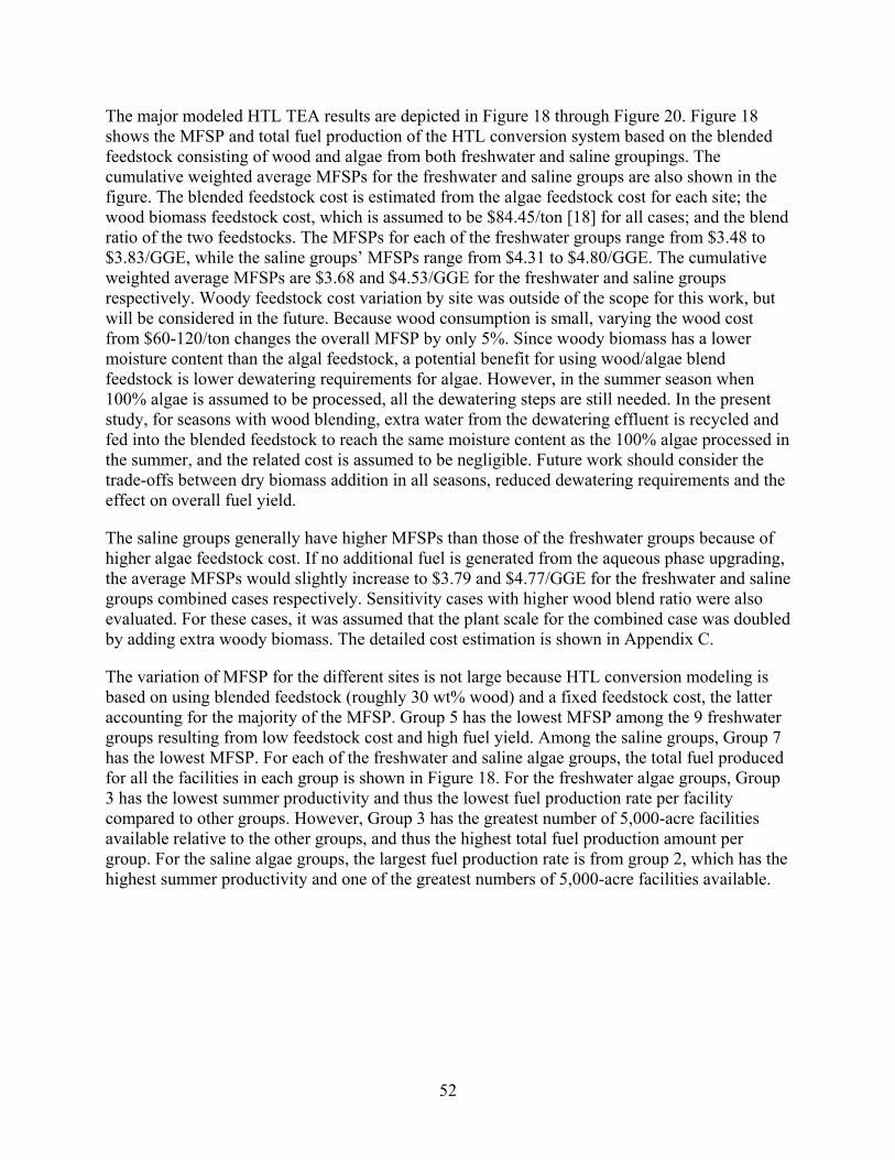
52

The major modeled HTL TEA results are depicted in Figure 18 through Figure 20. Figure 18 shows the MFSP and total fuel production of the HTL conversion system based on the blended feedstock consisting of wood and algae from both freshwater and saline groupings. The cumulative weighted average MFSPs for the freshwater and saline groups are also shown in the figure. The blended feedstock cost is estimated from the algae feedstock cost for each site; the wood biomass feedstock cost, which is assumed to be $84.45/ton [18] for all cases; and the blend ratio of the two feedstocks. The MFSPs for each of the freshwater groups range from $3.48 to $3.83/GGE, while the saline groups’ MFSPs range from $4.31 to $4.80/GGE. The cumulative weighted average MFSPs are $3.68 and $4.53/GGE for the freshwater and saline groups respectively. Woody feedstock cost variation by site was outside of the scope for this work, but will be considered in the future. Because wood consumption is small, varying the wood cost from $60-120/ton changes the overall MFSP by only 5%. Since woody biomass has a lower moisture content than the algal feedstock, a potential benefit for using wood/algae blend feedstock is lower dewatering requirements for algae. However, in the summer season when 100% algae is assumed to be processed, all the dewatering steps are still needed. In the present study, for seasons with wood blending, extra water from the dewatering effluent is recycled and fed into the blended feedstock to reach the same moisture content as the 100% algae processed in the summer, and the related cost is assumed to be negligible. Future work should consider the trade-offs between dry biomass addition in all seasons, reduced dewatering requirements and the effect on overall fuel yield.

The saline groups generally have higher MFSPs than those of the freshwater groups because of higher algae feedstock cost. If no additional fuel is generated from the aqueous phase upgrading, the average MFSPs would slightly increase to $3.79 and $4.77/GGE for the freshwater and saline groups combined cases respectively. Sensitivity cases with higher wood blend ratio were also evaluated. For these cases, it was assumed that the plant scale for the combined case was doubled by adding extra woody biomass. The detailed cost estimation is shown in Appendix C.

The variation of MFSP for the different sites is not large because HTL conversion modeling is based on using blended feedstock (roughly 30 wt% wood) and a fixed feedstock cost, the latter accounting for the majority of the MFSP. Group 5 has the lowest MFSP among the 9 freshwater groups resulting from low feedstock cost and high fuel yield. Among the saline groups, Group 7 has the lowest MFSP. For each of the freshwater and saline algae groups, the total fuel produced for all the facilities in each group is shown in Figure 18. For the freshwater algae groups, Group 3 has the lowest summer productivity and thus the lowest fuel production rate per facility compared to other groups. However, Group 3 has the greatest number of 5,000-acre facilities available relative to the other groups, and thus the highest total fuel production amount per group. For the saline algae groups, the largest fuel production rate is from group 2, which has the highest summer productivity and one of the greatest numbers of 5,000-acre facilities available.

53

Figure 18. HTL conversion MFSP and fuel production by group (freshwater and saline scenario)

To investigate the relationship between different cost impact factors, the correlation coefficients between key cost variables were calculated for the HTL models. The correlation coefficient is 0.93 between the MFSP and the blended feedstock cost for the freshwater cases and it is 0.99 for the saline cases. Therefore, the blended feedstock cost has significant impacts on the MFSP. The correlation coefficient between the MFSP and the product yield is -0.93 for the freshwater algae cases and -0.91 for the saline cases. It also showed a strong correlation between the MFSP and plant scales. Among these factors, the most significant one is still the blend feedstock cost, which is most impacted by the annual average blend ratio of the algae in the blend stock and moderately affected by the algae only feedstock cost. Therefore, lower blended feedstock cost (lower algae blend ratio and lower algae feedstock price), larger plant scale, and higher final fuel yields lead to lower MFSP.

The MBSPs for 100% algae, algae/wood blended feedstock, and MFSPs are paired with the corresponding cumulative fuel production from related groups and depicted in Figure 19 and Figure 20. These figures demonstrate the strong correlation between the blended feedstock cost and the MFSPs. The woody biomass has much lower feedstock cost than the algae feedstock and thus the blend feedstock has lower MBSP and leads to lower MFSP than algae only cases. Another cost benefit for using woody biomass is eliminating the need to dry and store algae during times of high productivity (summer) for use during periods of low algal productivity (winter) as a means of addressing seasonal variations.

0.0

2.0

4.0

6.0

8.0

10.0

12.0

$0.00

$0.50

$1.00

$1.50

$2.00

$2.50

$3.00

$3.50

$4.00

$4.50

$5.00

1 2 3 4 5 6 7 8 9 1 2 3 4 5 6 7 8

Fuel

Pro

duct

ion

(Bill

ion

GG

E/ye

ar)

MFS

P ($

/GG

E)

Freshwater Groups Saline Groups

MFSP ($/GGE)

Fuel Production(Billion GGE/year)

Avg MFSP for Freshwater Sites = $3.68/GGE

Avg MFSP forSaline Sites= $4.53/GGE

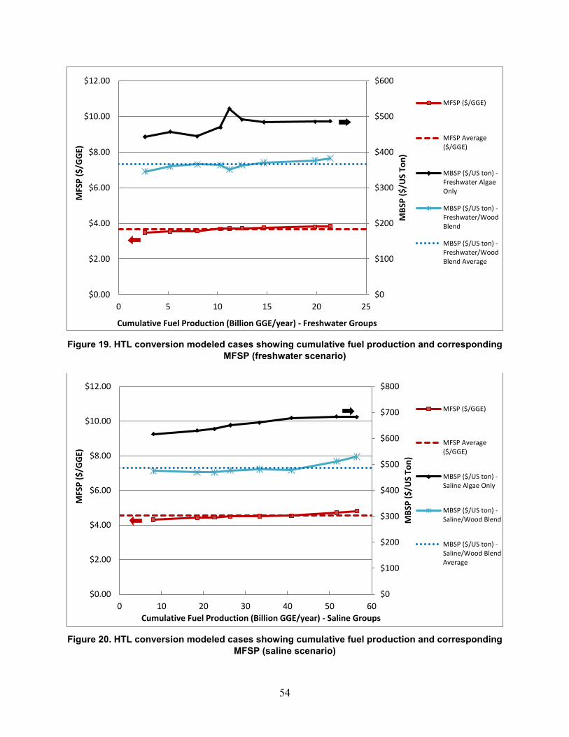
54

Figure 19. HTL conversion modeled cases showing cumulative fuel production and corresponding

MFSP (freshwater scenario)

Figure 20. HTL conversion modeled cases showing cumulative fuel production and corresponding

MFSP (saline scenario)

$0

$100

$200

$300

$400

$500

$600

$0.00

$2.00

$4.00

$6.00

$8.00

$10.00

$12.00

0 5 10 15 20 25

MBS

P ($

/US

Ton)

MFS

P ($

/GG

E)

Cumulative Fuel Production (Billion GGE/year) - Freshwater Groups

MFSP ($/GGE)

MFSP Average($/GGE)

MBSP ($/US ton) -Freshwater AlgaeOnly

MBSP ($/US ton) -Freshwater/WoodBlend

MBSP ($/US ton) -Freshwater/WoodBlend Average

$0

$100

$200

$300

$400

$500

$600

$700

$800

$0.00

$2.00

$4.00

$6.00

$8.00

$10.00

$12.00

0 10 20 30 40 50 60

MBS

P ($

/US

Ton)

MFS

P ($

/GG

E)

Cumulative Fuel Production (Billion GGE/year) - Saline Groups

MFSP ($/GGE)

MFSP Average($/GGE)

MBSP ($/US ton) -Saline Algae Only

MBSP ($/US ton) -Saline/Wood Blend

MBSP ($/US ton) -Saline/Wood BlendAverage

55

To evaluate the impacts of the HTL aqueous phase upgrading and the wood blend ratio on the fuel production cost, two sensitivity cases were investigated, including a case with no aqueous phase upgrading and another one with high wood blend ratio. The baseline cases are the combined cases for freshwater and saline groups. The MFSP and total fuel production for both the baseline and two sensitivity cases are shown in Figure 21. For high wood blend ratio cases, it was assumed that the plant scale for the baseline cases was doubled by adding extra woody biomass. For no aqueous upgrading cases, the MFSP impact is limited compared to the baseline cases. Although no aqueous phase upgrading leads to about 15% reduction in total fuel production, it reduces the capital and operating cost by removing the aqueous phase upgrading related equipment and raw material consumptions. In addition, no aqueous phase upgrading also leads to more nutrients available for recycle to the algae farms and thus greater nutrient recycle credits compared to the baseline cases. The combined impacts of lower fuel production, lower system cost, and higher nutrient recycle credits lead to slight increases in the MFSPs, on the order of 2% for the freshwater combined case and 5% for the saline combined case.

Figure 21. HTL conversion modeled scenarios showing fuel production and corresponding MFSP for combined and high wood cases

The wood percentage in the blended feedstock increases from about 30 wt% for the baseline cases to about 65 wt% in the high wood blend ratio cases. The total annual fuel production increases, but it is less than double the baseline amount because HTL of 100% woody biomass has lower biocrude yields than HTL of 100% algae and thus leads to lower biocrude yields as the percentage of wood in the blended feed increases. This effect is somewhat offset by increased recovery of HTL aqueous organics material followed by conversion to additional fuel. This leads to higher fuel yields from the aqueous phase and thus the fuel output from the aqueous phase for the high wood case is slightly more than double the baseline case. However, this is not enough to double the overall fuel yield. As discussed in the previous section, there is a synergistic effect on

$0.00

$1.00

$2.00

$3.00

$4.00

$5.00

$6.00

$7.00

$8.00

0.0

10.0

20.0

30.0

40.0

50.0

60.0

70.0

80.0

90.0

100.0

Freshwatercombined -

baseline

Freshwatercombined -

no aqupgrading

Freshwatercombined -high woodblend ratio

Salinecombined -

baseline

Salinecombined -

no aqupgrading

Salinecombined -high woodblend ratio

MFS

P ($

/GG

E)

Tota

l Fue

l Pro

duct

ion

(bill

ion

GG

E/yr

) Fuel fromalgae

Fuel fromwood

Fuel fromHTL aqueousupgrading

MFSP

56

the biocrude yield of the blended feedstock when the blend is about 50/50 algae/wood by weight. In the simulation, the biocrude yield is not estimated by separately adding algae yields to wood yields, but by specifying a single yield for the blended feedstock directly based on the algae-to-wood ratio. Furthermore, because of the high carbohydrate content, HCSD-type algae likely produces more CO2 than wood does during HTL. Given these effects, an absolute allocation of fuel yield to either algae or wood is not possible. However, Figure 21 is presented to show the fuel production allocation if it was a function of the percentage of algae and wood in the feed mix, but again, this should not be further reported without the caveats given above.

Higher wood feedstock blend ratio leads to lower blended feedstock cost because of the lower cost of wood feedstock compared to algae. As the percentage of wood in the blended feed increases, the modeled blend feedstock cost decreases approximately 39% and 41% compared to the baseline combined cases of the freshwater and saline groups respectively. With the larger plant scale and lower feedstock cost, both freshwater and saline algae cases have much lower MFSPs. The lower MFSP of the high wood cases mainly results from the lower blend feedstock cost and larger plant scale. For the freshwater groups, the MFSP is about 19% lower than the baseline case. For the saline groups, the MFSP for the high wood case decreases about 23% compared to the baseline. Because the saline algae feedstock cost is about 39% higher than the freshwater case, higher wood blend ratio leads to a greater decrease in the blended feedstock cost.

Wood (or any low cost dry biomass) was used in small quantities to equalize feed flowrates to HTL caused by algal seasonal variation; the majority feed annually was still algae. Therefore, adding wood eliminated the natural gas cost for algae drying in summer and spring compared to a 100% algae system (although alternative wet storage methods are also possible as discussed above in the CAP case). Wood is less expensive than algae, but processed on its own without algae results in a much lower biocrude yield and requires the addition of a base to maintain neutral pH. Base addition is not necessary with mixed wood/algae feed even in the winter when the algae fraction is low. Furthermore, wood addition improves the biofuel cold flow properties over 100% algae. Algae provide good cetane compounds missing from wood based HTL fuels and produces primarily distillate fuel. A manuscript is currently being prepared to detail the cost implications of mixed feeds.

57

Life-Cycle Analysis The LCA results for the freshwater scenario, which include the WTW GHG emissions and fossil energy and freshwater use, are presented in Figure 22 for the CAP cases with and without PU coproducts as well as the HTL case. The site groups evaluated for the CAP process are reflective of the three example coproduct market scenarios described above, which in all cases at least maintain PU coproduction for group 8 (i.e. in no scenario does group 8 not include PU coproduction), thus LCA results for CAP “group 8 without coproducts” are omitted. The WTW GHG emissions depend largely on the conversion technologies, the coproduct, and the CC energy demand for sourcing cultivation CO2, more than by the regional groupings. The CAP cases with PU coproduct exhibit the lowest GHG emissions ranging from -32.1 to -24.5 g-CO2e/MJ at 0.63 MJe/kg-CO2 of CC energy demand. If the higher CC energy demand basis (1.0 MJe/kg-CO2) is used, the GHG emissions increase by 21.8 – 24.1 g-CO2e/MJ. As additional site groups are able to include PU coproduction before reaching market saturation constraints (e.g. moving from the U.S. to World PU market curve examples in Figure 16), a larger share of the total collective sites could claim the much lower GHG emissions credit based on PU coproduct displacement of petroleum-derived products, thus reducing the “aggregate” GHG emissions for the entire site collection (discussed below). On the other hand, the CAP cases without inclusion of PU coproducts show the highest GHG emissions ranging from 62.6 to 67.4 g-CO2e/MJ at 0.63 MJe/kg-CO2 of CC energy demand. With 1.0 MJe/kg-CO2 of CC energy demand, the GHG emissions increase by 16.0 – 17.3 g-CO2e/MJ. The impacts of CC energy demand are lower in the CAP cases without PU coproducts than with PU coproducts because of the higher fuel yields in the former without coproducts (i.e. higher fuel yields dilute the impact of such a difference, which is also the case in HTL). For HTL, the GHG emissions range from 37.8 to 41.6 g-CO2e/MJ at 0.63 MJe/kg-CO2 of CC energy demand, increasing by 3.2 to 6.4 g-CO2e/MJ at 1.0 MJe/kg-CO2 of CC energy demand. When viewing each site group individually, the CAP cases that include coproducts and all HTL cases can meet the targets of at least 50% GHG emissions reduction relative to low sulfur diesel (94.3 g-CO2e/MJ).

The fossil energy use, Figure 22B, shows the same trends as the GHG emissions: in the CAP case with PU coproduct, the fossil energy use ranges from -0.71 to -0.63 MJ/MJ fuel produced at 0.63 MJe/kg-CO2 of CC energy demand. The alternative case at 1.0 MJe/kg-CO2 of CC energy demand increases the fossil energy use by 0.22 to 0.24 MJ/MJ. Without PU coproduct, the CAP cases use 0.73 to 0.78 MJ of fossil energy per MJ of fuel produced at 0.63 MJe/kg-CO2 CC energy demand, increasing by 0.16 to 0.17 MJ/MJ for the alternative 1.0 MJe/kg-CO2 CC energy demand scenario. HTL indicates a smaller range from 0.48 to 0.52 MJ/MJ at 0.63 MJe/kg-CO2 of CC energy demand and 0.52 to 0.58 MJ/MJ at 1.0 MJe/kg-CO2 of CC energy demand. All of these scenarios are lower than low sulfur diesel at 1.21 MJ/MJ.

Unlike the GHG emissions and fossil energy use results, freshwater use varies less by technologies or CC energy demand but more strongly across the regional groupings (driven in turn by dramatic differences in cultivation evaporation rates across the site groups), as shown in Figure 22C. The largest freshwater demand is seen in Groups 1 and 3 (California and the U.S. Southwest) with the CAP case including coproducts exhibiting the highest individual consumption at 21.7 L/MJ. In each group, water consumption per MJ of fuel produced is driven by total MJ fuel yields, with the highest water consumption associated with the lowest fuel yield case (CAP with PU coproduct), followed by CAP without PU coproduct and then HTL (highest

58

MJ fuel yields and thus lowest per-MJ water consumption). For reference, low sulfur diesel freshwater consumption is 0.082 L/MJ.

Figure 22. LCA results by individual site group for all conversion cases (freshwater scenario). A) WTW GHG emissions, B) fossil energy use, and C) freshwater use by group for CAP with and without

polyurethane (PU) coproduct, and HTL.

The WTW GHG emissions, fossil energy, and freshwater use are dependent on the conversion technology applied as shown in Figure 22. The differences in these technologies are highlighted for the freshwater scenario in Figure 23, which provides a breakdown for Group 7 as a representative example. The GHG emissions, Figure 23A, are provided for the CAP process,

59

both with and without polyurethane coproduction, and HTL. The CAP scenario that produces only fuel has a GHG emission of 62.9 g-CO2e/MJ at 0.63 MJe/kg-CO2 of CC energy demand and 79.1 g-CO2e/MJ at 1.0 MJe/kg-CO2 of CC energy demand, with the largest contributions from CO2 sourcing, conversion chemicals, and cultivation farm energy at 36.2 or 57.5 (for 0.63 versus 1.0 MJe/kg-CO2 of CC energy demand scenarios), 27.6, and 13.6 g-CO2e/MJ, respectively. GHG displacement credits are provided by generated electricity and recycled CO2 and nutrients. All other emission sources provide negligible contributions. When polyurethane is co-produced in the CAP process, the WTW GHG emissions for this example reduces significantly to -30.4 or -7.9 g-CO2e/MJ at the 0.63 and 1.0 MJe/kg-CO2 CC energy demand scenarios respectively. All the same emission sources provide similar contributions, but they are just scaled higher as the denominator (the amount of fuel produced) is reduced. However, producing the bioproduct provides a substantial displacement credit of -119 g-CO2e/MJ, reflective of an equivalent amount of petroleum-derived polyurethane (which is a much more energy/GHG-intensive process than the bio-derived route examined here) and sequestering the biogenic carbon. This highlights a key advantage of bio-derived products, particularly those containing oxygen, relative to their counterparts derived from petroleum which must undergo energy-intensive oxygen addition reactions along the way from a starting feedstock devoid of elemental oxygen.

Fuel produced from the HTL process has a WTW GHG emission of 39.6 g-CO2e/MJ at 0.63 MJe/kg-CO2 of CC energy demand and 45.0 g-CO2e/MJ at 1.0 MJe/kg-CO2 of CC energy demand. Key contributions to this value include CO2 sourcing, cultivation farm energy, and CO2 recycle at 21.8 or 34.6 (for 0.63 versus 1.0 MJe/kg-CO2 of CC energy demand scenarios), 8.2, and -12.4 g-CO2e/MJ, respectively. Previous LCAs on HTL have shown that natural gas used for summer drying of algae can have a sizeable contribution to the GHG emissions [13,111]. However, in this analysis, the seasonal drying unit process is removed, and waste wood is brought in as a feedstock to supplement low seasonal algal productivities. As a result, the incremental conversion energy impact is small and energy to collect, sort, and process the waste wood doesn’t significantly affect the results.

The fossil energy use, Figure 23B, shows the same trend as the GHG emissions, with CAP excluding coproducts exhibiting the highest use, followed by HTL and then CAP with coproducts again translating to a net negative fossil energy value. For freshwater use, the CAP scenario with PU coproduct translates to the highest use at 3.0 L/MJ. This is driven primarily by the pond water evaporation and the conversion input demands (almost entirely process water demands). Water is recycled from conversion yielding a credit of -0.90 L/MJ. Unlike GHG emissions, the freshwater displacement credit for polyurethane is minor at -0.13 L/MJ, when compared to the total freshwater use. The water use for CAP without polyurethane production follows similar trends and breakdowns, but with smaller magnitudes due to a higher fuel yield. HTL exhibits the lowest freshwater use per MJ fuel, reflecting the highest MJ fuel yield outputs, with the largest single driver from pond water evaporation at 1.3 L/MJ. The freshwater results are highly dependent on location, as shown in Figure 24 for the CAP scenario with polyurethane production. For this case, Group 1 has the highest freshwater use at 21.8 L/MJ, which is driven primarily by the farm water demands (almost all of which in turn is due to making up for evaporative losses), with less arid locations requiring less water.

60

Figure 23. Breakdown of LCA results by conversion technology for Group 7 (freshwater scenario).

A) WTW GHG emissions, B) fossil energy use, and C) freshwater use for CAP (with and without a polyurethane coproduct) and HTL. CC and PU denote carbon capture and polyurethane, respectively.

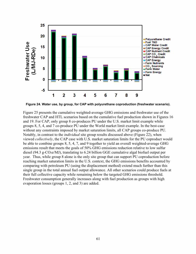
61

Figure 24. Water use, by group, for CAP with polyurethane coproduction (freshwater scenario).

Figure 25 presents the cumulative weighted-average GHG emissions and freshwater use of the freshwater CAP and HTL scenarios based on the cumulative fuel production shown in Figures 16 and 19. For CAP, only group 8 co-produces PU under the U.S. market limit example while groups 8, 5, 4, and 7 co-produce PU under the World market limit example. In the best-case without any constraints imposed by market saturation limits, all CAP groups co-produce PU. Notably, in contrast to the individual site group results discussed above (Figure 22), when viewed collectively, the CAP case with U.S. market saturation limits for the PU coproduct would be able to combine groups 8, 5, 4, 7, and 9 together to yield an overall weighted-average GHG emissions result that meets the goals of 50% GHG emissions reduction relative to low sulfur diesel (94.3 g-CO2e/MJ), translating to 6.24 billion GGE cumulative algal biofuel output per year. Thus, while group 8 alone is the only site group that can support PU coproduction before reaching market saturation limits in the U.S. context, the GHG emissions benefits accounted by comparing with petroleum PU (using the displacement method) extend much further than this single group in the total annual fuel output allowance. All other scenarios could produce fuels at their full collective capacity while remaining below the targeted GHG emissions threshold. Freshwater consumption generally increases along with fuel production as groups with high evaporation losses (groups 1, 2, and 3) are added.

62

Figure 25. Modeled scenarios showing cumulative weighted-average fuel production and corresponding GHG emissions and freshwater use for CAP and HTL conversion (freshwater

scenario). For CAP, three GHG emissions curves and three freshwater use curves are shown representing different coproduct market volume scenarios: (a) red curve—no market saturation limits for PU or related coproducts (i.e., expanding into additional markets such as polyols, epoxies, etc. such that market capacity exists over full site collection); (b) blue curve—PU is coproduced until hitting U.S. market consumption limit, after which point PU coproduction is eliminated and reverts to fuels-only for remainder of curve; (c) green curve—PU is coproduced until hitting world market consumption limit, after which point

PU coproduction is eliminated and reverts to fuels-only for remainder of curve. PU = polyurethanes.

Next, the LCA results for the saline cultivation scenario are discussed below, with the WTW GHG emissions, fossil energy use, and freshwater use presented in Figure 26. Results are shown for the CAP cases with and without coproducts, and for the HTL case. Groups 7 and 8 of the CAP cases with coproducts include two scenarios. The results denoted as Groups 7 and 8 represent the cases where both PU and SA are coproduced. Group 7* shows the CAP case with PU coproduction only as shown in the first point of the blue curve in Figure 17 while Group 8* represents the CAP case with limited PU coproduction after SA reaches its market capacity in the modeled scenario (represented as the third point of the green curve in Figure 17). Similar to the freshwater scenario for Group 8, Group 7 in this case does not have an instance without inclusion of coproducts, thus LCA results are not shown for Group 7 excluding coproducts.

Figure 26A again shows that the WTW GHG emissions for the CAP scenarios are highly dependent on the degree of inclusion of coproducts as well as the cultivation CC energy demand. The lowest GHG emissions are seen in the CAP cases with both PU and SA coproducts, which range from -514 to -510 g-CO2e/MJ at 0.63 MJe/kg-CO2 of CC energy demand and -482 to -478 g-CO2e/MJ at 1.0 MJe/kg-CO2 of CC energy demand. The highest GHG emissions are again observed in the CAP cases without coproducts ranging from 63.3 to 66.4 g-CO2e/MJ at 0.63 MJe/kg-CO2 of CC energy demand and 79.6 to 83.1 g-CO2e/MJ at 1.0 MJe/kg-CO2 of CC energy demand. The GHG emissions of group 7* and 8* (the CAP cases with only PU

63

coproduct) are -30.4 and 50.2 g-CO2e/MJ at 0.63 MJe/kg-CO2 of CC energy demand or -7.5 and 65.8 g-CO2e/MJ at 1.0 MJe/kg-CO2 of CC energy demand, respectively. The emissions for the HTL scenario fall within a more narrow range of 38.1 to 41.6 g-CO2e/MJ at 0.63 MJe/kg-CO2 of CC energy demand and 42.5 to 47.4 g-CO2e/MJ at 1.0 MJe/kg-CO2 of CC energy demand. Similar to the freshwater scenarios, most CAP cases with inclusion of coproducts and all HTL cases (except for Group 1 at 1.0 MJe/kg-CO2 CC energy demand) achieve the 50% GHG reduction target. Group 8* for the CAP case does not meet the 50% GHG reduction target, as it only produces a minimal amount of PU after SA has already been exhausted (although Group 7* does meet the GHG target with PU alone, it does so by maximizing the amount of PU produced per facility to reduce MFSP up to PU market saturation limits, while Group 8* produces a smaller amount of PU per facility given additional MFSP reductions enabled by the second SA coproduct in the modeled scenarios).

The fossil energy use follows the same trend as the GHG emissions, as shown in Figure 26B. The CAP cases with PU and SA coproducts and without coproducts consume -4.71 to -4.67 MJ and 0.74 to 0.77 MJ of fossil fuels per MJ of algal biofuel produced at 0.63 MJe/kg-CO2 of CC energy demand, respectively, increasing to -4.39 to -4.34 MJ/MJ and 0.90 to 0.94 MJ/MJ at 1.0 MJe/kg-CO2 of CC energy demand, respectively. The CAP cases with limited PU coproducts, or Groups 7* and 8* consume fossil energy at -0.69 and 0.56 MJ/MJ for the 0.63 MJe/kg-CO2 CC energy basis, respectively, or -0.46 and 0.72 MJ/MJ for the 1.0 MJe/kg-CO2 CC energy case, respectively. The HTL case exhibits a fossil energy consumption ranging from 0.48 to 0.52 MJ/MJ for the 0.63 MJe/kg-CO2 CC energy basis, and 0.53 to 0.58 MJ/MJ for the 1.0 MJe/kg-CO2 CC energy case. All conversion scenarios translate to lower fossil energy use than low sulfur diesel at 1.2 MJ/MJ.

The freshwater use, shown in Figure 26C, is significantly lower for the saline scenario than the freshwater scenario discussed above, given that the pond evaporation losses in this case are made up for by saline rather than fresh water, which is not counted in the freshwater consumption calculations. Thus, within a much smaller magnitude, the freshwater use appears to vary more strongly across the conversion technologies and coproducts (reflecting the water demands for the conversion processes) than variances by region of the country (reflecting local water evaporation rates for the cultivation step). The freshwater consumption in the CAP cases is again highest for those with maximum coproducts and minimum fuel yields, roughly 1.1 L/MJ, followed by those with limited PU coproduct (at 0.66 L/MJ for Group 7* and 0.50 L/MJ for Group 8*), then those without coproducts around 0.49 – 0.50 L/MJ. The HTL scenario has the lowest freshwater use at roughly 0.087 – 0.097 L/MJ, which is slightly higher than diesel. Again, the parasitic energy demand for CC does not exhibit visible impacts on freshwater consumption.

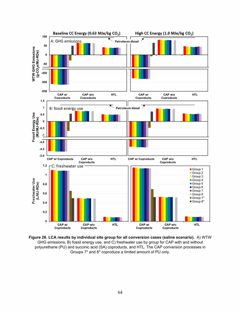
64

Figure 26. LCA results by individual site group for all conversion cases (saline scenario). A) WTW

GHG emissions, B) fossil energy use, and C) freshwater use by group for CAP with and without polyurethane (PU) and succinic acid (SA) coproducts, and HTL. The CAP conversion processes in

Groups 7* and 8* coproduce a limited amount of PU only.

65

More detailed breakdowns for the saline LCA results are presented in Figure 27, using group 6 as a representative example. The WTW GHG emissions for group 6 are the lowest for the CAP scenario that produces polyurethane and succinic acid at -513 g-CO2e/MJ for 0.63 MJe/kg-CO2 of CC energy demand and -481 g-CO2e/MJ for 1.0 MJe/kg-CO2 of CC energy demand (Figure 27A). These results are driven by the displacement credit for succinic acid at -577 g-CO2e/MJ. However, there are also noticeable contributions due to polyurethane displacement and CO2

sourcing at -88.1 g-CO2e/MJ, and 71.6 g-CO2e/MJ or 113 g-CO2e/MJ (at 0.63 or 1.0 MJe/kg-CO2 CC energy demand respectively). The large displacement credit for succinic acid is due to both the high GHG intensity of the petroleum-based adipic acid proxy at 5,200 g-CO2e/kg, and the total amount produced compared with other products, 1.15 kg of succinic acid for each kg of all other products (i.e., diesel, naphtha, and polyurethane). For this study, the displacement method was used for coproduct allocation. Another allocation method could be chosen, for example mass or a market-value-based method. As mentioned above however, there are currently no policy incentives for bioproducts that reduce GHG emissions relative to petroleum products, and the benefit of using the displacement method is that it explicitly credits the emissions reductions for producing bio-derived products through less energy/GHG-intensive routes, when compared with a benchmark scenario producing fuel, polyurethane, and adipic acid exclusively from petroleum.

The WTW GHG emissions for the group 6 CAP scenario with no coproduct inclusion is 64.0 g-CO2e/MJ at 0.63 MJe/kg-CO2 of CC energy demand and 80.5 g-CO2e/MJ at 1.0 MJe/kg-CO2 of CC energy demand, predominately driven by CO2 sourcing and conversion chemicals at 36.7–58.3 (for 0.63 and 1.0 MJe/kg-CO2 CC energy demand) and 27.6 g-CO2e/MJ, respectively. The group 6 emissions for HTL are 38.7 g-CO2e/MJ at 0.63 MJe/kg-CO2 of CC energy demand and 43.7 g-CO2e/MJ at 1.0 MJe/kg-CO2 of CC energy demand, mainly due to CO2 sourcing at 20.9–33.2 g-CO2e/MJ (for 0.63 and 1.0 MJe/kg-CO2 CC energy demand) as well as conversion energy use at 19.0 g CO2e/MJ.

The fossil energy use, Figure 27B, shows the same trend as the GHG emissions, with CAP including coproducts receiving a large credit from the succinic acid and polyurethane displacement. Although all conversion technologies require relatively little freshwater, there is a noticeable difference in the freshwater use across the conversion cases, as shown in Figure 27C. The CAP scenario with coproducts has the largest freshwater use at 1.1 L/MJ, driven primarily by conversion inputs (mainly process water). For CAP with no coproducts, the water consumption is also dominated by the conversion inputs at 0.50 L/MJ. HTL has a substantially lower freshwater consumption at 0.087 L/MJ, which is mostly due to conversion chemical and energy inputs, farm energy use, and CO2 sourcing at 0.035, 0.036, and 0.034 L/MJ, respectively.

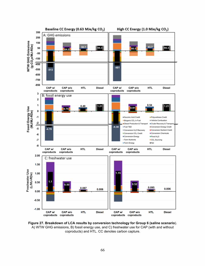
66

Figure 27. Breakdown of LCA results by conversion technology for Group 6 (saline scenario).

A) WTW GHG emissions, B) fossil energy use, and C) freshwater use for CAP (with and without coproducts) and HTL. CC denotes carbon capture.

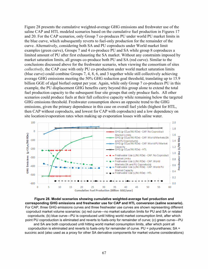
67

Figure 28 presents the cumulative weighted-average GHG emissions and freshwater use of the saline CAP and HTL modeled scenarios based on the cumulative fuel production in Figures 17 and 20. For the CAP scenarios, only Group 7 co-produces PU under world PU market limits in the blue curve, which subsequently reverts to fuel-only production for the remainder of the curve. Alternatively, considering both SA and PU coproducts under World market limit examples (green curve), Groups 7 and 4 co-produce PU and SA while group 8 coproduces a limited amount of PU after first exhausting the SA market. Without any constraints imposed by market saturation limits, all groups co-produce both PU and SA (red curve). Similar to the conclusions discussed above for the freshwater scenario, when viewing the consortium of sites collectively, the CAP case with only PU co-production under world market saturation limits (blue curve) could combine Groups 7, 4, 8, 6, and 3 together while still collectively achieving average GHG emissions meeting the 50% GHG reduction goal threshold, translating up to 15.9 billion GGE of algal biofuel output per year. Again, while only Group 7 co-produces PU in this example, the PU displacement GHG benefits carry beyond this group alone to extend the total fuel production capacity to the subsequent four site groups that only produce fuels. All other scenarios could produce fuels at their full collective capacity while remaining below the targeted GHG emissions threshold. Freshwater consumption shows an opposite trend to the GHG emissions, given the primary dependence in this case on overall fuel yields (highest for HTL, then CAP without coproducts, and lowest for CAP with coproducts) and a low dependency on site location/evaporation rates when making up evaporation losses with saline water.

Figure 28. Model scenarios showing cumulative weighted-average fuel production and corresponding GHG emissions and freshwater use for CAP and HTL conversion (saline scenario). For CAP, three GHG emissions curves and three freshwater use curves are shown representing different coproduct market volume scenarios: (a) red curve—no market saturation limits for PU and SA or related coproducts; (b) blue curve—PU is coproduced until hitting world market consumption limit, after which

point PU coproduction is eliminated and reverts to fuels-only for remainder of curve; (c) green curve—PU and SA are both coproduced until hitting world market consumption limits, after which point all

coproduction is eliminated and reverts to fuels-only for remainder of curve. PU = polyurethanes; SA = succinic acid (also used as a proxy for other SA derivative components for market volume considerations)

68

A key LCA driver in algae-based biofuel pathways is the pond circulation power. This study assumed that pond circulation consumes 27.8 KWh/ha/day including a 12-hour paddlewheel shutdown as noted in the beginning of this report. NREL’s algae farm design case [9] examined various pond designs with pond circulation power ranging from 41.5 to 75.5 kWh/ha/day without paddlewheel shutdown (based on various pond designs and sizes furnished by external consultants); specifically, the furnished values for pond circulation power were 63.0 and 75.5 kWh/ha/day for small 2-acre ponds circulated with paddlewheels, 70.0, 58.2, 48.0, and 44.0 kWh/ha/day for 10-acre ponds (the first three circulated with paddlewheels and the final circulated by pumping across a sloped raceway), and 41.5 and 44.0 kWh/ha/day for large 50-acre serpentine pond designs (both circulated by pumping). For a given circulation design, varying powers over the same pond size implies varying assumed efficiencies of the paddlewheels/pumps based on the consultants’ opinions on possible efficiencies. This range of power values would then translate to 20.8 – 37.8 kWh/ha/day for a 12-hour paddlewheel shutdown. The impacts of this variation in pond circulation power on overall life-cycle GHG emissions and fossil fuel consumption are briefly considered here. In the freshwater cases, the lowest pond circulation power value (20.8 kWh/ha/day) would reduce the life-cycle GHG emissions by 1.3-1.7, 0.9-1.2, and 0.6 g-CO2e/MJ for the CAP with PU, the CAP without PU, and the HTL scenarios, respectively. The highest pond circulation power value (37.8 kWh/ha/day) would increase the life-cycle GHG emissions by 2.0-2.6, 1.4-1.8, and 0.8-1.0 g-CO2e/MJ for the CAP with PU, the CAP without PU, and the HTL scenarios, respectively. In the saline cases, the lowest pond circulation power value reduces the life-cycle GHG emissions by 1.9-2.2, 1.0-1.5, and 0.6 g-CO2e/MJ, and the highest pond circulation power value increases the life-cycle GHG emissions by 2.9-3.4, 1.5-2.2, and 0.9 g-CO2e/MJ for the CAP with coproducts, the CAP without coproducts, and the HTL scenarios, respectively. The impacts of the pond circulation power decreases with higher fuel yields per hectare. Overall, the impacts of pond circulation power are smaller than other factors such as coproduct inclusions or CC energy use for cultivation CO2.

It should be noted that this study did not examine the impact of soil organic carbon (SOC) changes from pond construction that requires stripping top soil, scarification, and compaction assuming the ponds would be built on marginal land. The key factors determining SOC change include the SOC content of marginal land (which varies by region) and the emission factor (or conversion ratio of SOC into CO2 that depends on various factors, such as climate, soil depth, disposal method, etc.). Due to lack of data, quantifying these factors are difficult at this point. Assuming 50 tonne C/hectare of SOC content for marginal land within 100 cm depth, with each 10% of SOC loss, the impacts of SOC changes from pond construction would be 0.58 – 0.76 g-CO2e/MJ for CAP with PU, 0.43 – 0.54 g-CO2e/MJ for CAP without PU, and 0.25 – 0.29 g-CO2e/MJ for HTL in the freshwater scenario, when amortized over 30 years. In the saline case, the impacts increase to 0.87 – 1.00 g-CO2e/MJ for CAP with coproducts, 0.45 – 0.66 g-CO2e/MJ for CAP without coproducts, and 0.27 – 0.28 g-CO2e/MJ for HTL. For more reliable estimates on SOC change impacts, a more detailed and regional analysis for the algae pond sites is warranted.

69

Overall Output Summary Given the results presented above, the key harmonized model outputs are summarized for the CAP model below in Table 14 and for the HTL model in Table 15. The matrix for the CAP model represents one example scenario of coproduct market limitations, while other results for the other coproduct saturation scenarios are provided in Appendix A. In this case, Table 14 reflects the modeled scenarios with world market limits for the PU (freshwater and saline cases) and SA/derivatives (saline case) coproducts, after which point all other groups switch to producing fuels exclusively. Table 14 lists the cumulative fuel outputs, cumulative coproduct outputs, cumulative weighted average MFSP, and cumulative weighted average GHG emissions for the nine freshwater site groups and eight saline site groups. The groups are listed in order from lowest to highest MFSP. For freshwater, site groups 8, 5, 4, and 7 produce PU, while all remaining groups only produce fuels. On a GGE/ton basis, site groups that exclusively produce fuel can reach 109 GGE/ton algae yields, while PU reduces the fuel yield by 30%. GHG emissions are lower for the coproduct scenarios due to the credits given when using the displacement method with respect to petroleum-based counterparts, as discussed above. For the freshwater scenario, after reaching group 9 the cumulative MFSP and cumulative GHG emissions begin to increase due to more fuel-only sites contributing to overall results. Still, the final average freshwater MFSP and GHG emissions for the entire collection of all sites is $4.20/GGE and 26.7 g CO2e/MJ, respectively, for this example. Notably, if only taking the first 3.9 BGGE/yr of fuels, the average MFSP and GHG emissions for that subset would be $1.64/GGE and -31.0 g CO2e/MJ, respectively; or if expanding by one point to 5.0 BGGE/yr, the results would increase to $2.51/GGE and -9.2 g CO2e/MJ.

For saline, site groups 7, 4, and 8 produce PU while groups 7 and 4 also produce SA, with all remaining groups again reverting back to fuels without these two coproducts. The final average saline MFSP and GHG emissions for the entire collection of all sites is $6.04/GGE and -53.5 g CO2e/MJ, respectively. Similar to the freshwater results, if only taking a subset of the first 5.0 BGGE/yr, the average saline MFSP and GHG results would be $1.93/GGE and -513 g CO2e/MJ, respectively; or if expanding to 7.2 BGGE/yr those results would increase to $2.90/GGE and -343 g CO2e/MJ. A notable finding on the LCA results here is that although all individual site group cases that exceed the market volume limits and revert to fuel-only production carry a higher GHG emissions burden (lower GHG reductions versus petroleum), when viewing the entire consortium of sites as a whole, the overall weighted-average GHG emissions are still very low, easily exceeding the 50% GHG reduction goals, enabled by the large negative GHG credits for coproduct displacement even over the limited number of site groups which coproduce bioproducts. Put differently, if instead each individual site group were to coproduce these bioproducts in smaller amounts such that the overall coproduct inclusions could be maintained over the full consortium of sites, the average GHG emissions across the full site collection would exceed the 50% GHG reduction target, as would the GHG emissions for each individual site group as well.

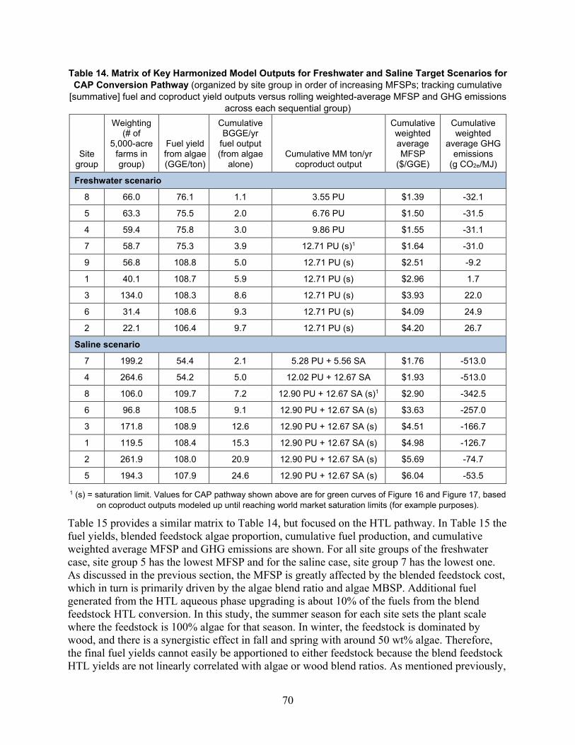
70

Table 14. Matrix of Key Harmonized Model Outputs for Freshwater and Saline Target Scenarios for CAP Conversion Pathway (organized by site group in order of increasing MFSPs; tracking cumulative

[summative] fuel and coproduct yield outputs versus rolling weighted-average MFSP and GHG emissions across each sequential group)

Site group

Weighting (# of

5,000-acre farms in group)

Fuel yield from algae (GGE/ton)

Cumulative BGGE/yr

fuel output (from algae

alone) Cumulative MM ton/yr

coproduct output

Cumulative weighted average MFSP

($/GGE)

Cumulative weighted

average GHG emissions

(g CO2e/MJ)

Freshwater scenario

8 66.0 76.1 1.1 3.55 PU $1.39 -32.1

5 63.3 75.5 2.0 6.76 PU $1.50 -31.5

4 59.4 75.8 3.0 9.86 PU $1.55 -31.1

7 58.7 75.3 3.9 12.71 PU (s)1 $1.64 -31.0

9 56.8 108.8 5.0 12.71 PU (s) $2.51 -9.2

1 40.1 108.7 5.9 12.71 PU (s) $2.96 1.7

3 134.0 108.3 8.6 12.71 PU (s) $3.93 22.0

6 31.4 108.6 9.3 12.71 PU (s) $4.09 24.9

2 22.1 106.4 9.7 12.71 PU (s) $4.20 26.7

Saline scenario

7 199.2 54.4 2.1 5.28 PU + 5.56 SA $1.76 -513.0

4 264.6 54.2 5.0 12.02 PU + 12.67 SA $1.93 -513.0

8 106.0 109.7 7.2 12.90 PU + 12.67 SA (s)1 $2.90 -342.5

6 96.8 108.5 9.1 12.90 PU + 12.67 SA (s) $3.63 -257.0

3 171.8 108.9 12.6 12.90 PU + 12.67 SA (s) $4.51 -166.7

1 119.5 108.4 15.3 12.90 PU + 12.67 SA (s) $4.98 -126.7

2 261.9 108.0 20.9 12.90 PU + 12.67 SA (s) $5.69 -74.7

5 194.3 107.9 24.6 12.90 PU + 12.67 SA (s) $6.04 -53.5

1 (s) = saturation limit. Values for CAP pathway shown above are for green curves of Figure 16 and Figure 17, based on coproduct outputs modeled up until reaching world market saturation limits (for example purposes).

Table 15 provides a similar matrix to Table 14, but focused on the HTL pathway. In Table 15 the fuel yields, blended feedstock algae proportion, cumulative fuel production, and cumulative weighted average MFSP and GHG emissions are shown. For all site groups of the freshwater case, site group 5 has the lowest MFSP and for the saline case, site group 7 has the lowest one. As discussed in the previous section, the MFSP is greatly affected by the blended feedstock cost, which in turn is primarily driven by the algae blend ratio and algae MBSP. Additional fuel generated from the HTL aqueous phase upgrading is about 10% of the fuels from the blend feedstock HTL conversion. In this study, the summer season for each site sets the plant scale where the feedstock is 100% algae for that season. In winter, the feedstock is dominated by wood, and there is a synergistic effect in fall and spring with around 50 wt% algae. Therefore, the final fuel yields cannot easily be apportioned to either feedstock because the blend feedstock HTL yields are not linearly correlated with algae or wood blend ratios. As mentioned previously,

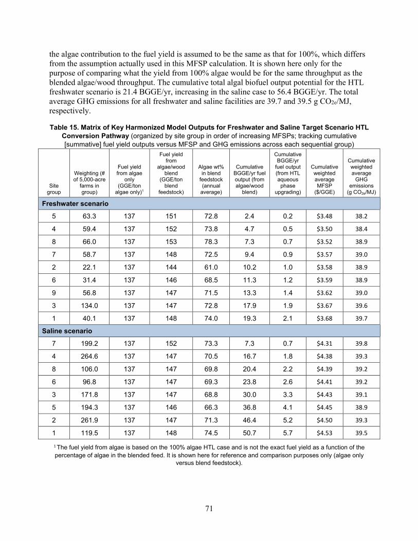
71

the algae contribution to the fuel yield is assumed to be the same as that for 100%, which differs from the assumption actually used in this MFSP calculation. It is shown here only for the purpose of comparing what the yield from 100% algae would be for the same throughput as the blended algae/wood throughput. The cumulative total algal biofuel output potential for the HTL freshwater scenario is 21.4 BGGE/yr, increasing in the saline case to 56.4 BGGE/yr. The total average GHG emissions for all freshwater and saline facilities are 39.7 and 39.5 g CO2e/MJ, respectively.

Table 15. Matrix of Key Harmonized Model Outputs for Freshwater and Saline Target Scenario HTL Conversion Pathway (organized by site group in order of increasing MFSPs; tracking cumulative [summative] fuel yield outputs versus MFSP and GHG emissions across each sequential group)

Site group


farms in group)

Fuel yield from algae

only (GGE/ton

algae only)1

Fuel yield from

algae/wood blend

(GGE/ton blend

feedstock)

Algae wt% in blend

feedstock (annual

average)

Cumulative BGGE/yr fuel output (from algae/wood

blend)

Cumulative BGGE/yr

fuel output (from HTL aqueous phase

upgrading)


($/GGE)

Cumulative weighted average

GHG emissions

(g CO2e/MJ)

Freshwater scenario

5 63.3 137 151 72.8 2.4 0.2 $3.48 38.2

4 59.4 137 152 73.8 4.7 0.5 $3.50 38.4

8 66.0 137 153 78.3 7.3 0.7 $3.52 38.9

7 58.7 137 148 72.5 9.4 0.9 $3.57 39.0

2 22.1 137 144 61.0 10.2 1.0 $3.58 38.9

6 31.4 137 146 68.5 11.3 1.2 $3.59 38.9

9 56.8 137 147 71.5 13.3 1.4 $3.62 39.0

3 134.0 137 147 72.8 17.9 1.9 $3.67 39.6

1 40.1 137 148 74.0 19.3 2.1 $3.68 39.7

Saline scenario

7 199.2 137 152 73.3 7.3 0.7 $4.31 39.8

4 264.6 137 147 70.5 16.7 1.8 $4.38 39.3

8 106.0 137 147 69.8 20.4 2.2 $4.39 39.2

6 96.8 137 147 69.3 23.8 2.6 $4.41 39.2

3 171.8 137 147 68.8 30.0 3.3 $4.43 39.1

5 194.3 137 146 66.3 36.8 4.1 $4.45 38.9

2 261.9 137 147 71.3 46.4 5.2 $4.50 39.3

1 119.5 137 148 74.5 50.7 5.7 $4.53 39.5

1 The fuel yield from algae is based on the 100% algae HTL case and is not the exact fuel yield as a function of the percentage of algae in the blended feed. It is shown here for reference and comparison purposes only (algae only

versus blend feedstock).

72

Finally, as noted previously, during final preparation of this report a budget bill was passed in February 2018 which expanded tax incentives under a program known as 45Q to include a carbon credit of $35 per ton ($38.59/metric tonne) CO2 for “recycling” or utilization of captured CO2 emissions, under which algal CO2 utilization would qualify [49]. Under such a scenario, when applying this credit to strictly the fraction of CO2 incorporated into algal biomass (excluding retention efficiency losses), all modeled TEA cost results presented above would be further reduced by the following amounts:

• All biomass cultivation cases (fresh and saline water): $70/ton MBSP • CAP cases excluding coproducts (fuels only): $0.49/GGE MFSP • Freshwater CAP cases with coproduction of PU: $0.69/GGE MFSP • Saline CAP cases with coproduction of PU and SA: $0.96/GGE MFSP • Freshwater HTL cases: $0.24/GGE • Saline HTL cases: $0.23/GGE

Concluding Remarks Based on the harmonized models across RA, cultivation TEA, conversion TEA, and system LCA, the work conducted here demonstrated the potential to produce up to 104 MM tons per year of freshwater algal biomass across a national consortium of 2.7 MM acres of cultivation area (532 individual 5,000-acre farms), contingent upon those sites being collectively able to achieve cultivation productivity targets of 26 g/m2/day annual average in the future. This potential increases substantially to 235 MM tons per year for saline algae based on 7.1 MM acres of available cultivation area (1,414 individual farms) at a similar overall average productivity, albeit at the expense of higher costs for salt management. Based on the underlying algal farm costs (dictated by CO2 sourcing and delivery via carbon capture of point-source flue gases; low-cost cultivation ponds, 10 acres each in size with minimal lining requirements for freshwater but fully lined for saline water; and low-cost dewatering technologies to concentrate the harvested biomass up to 20 wt% AFDW), these consortia of sites have the potential to provide algal biomass at an overall average cost of $472/ton for the freshwater scenario or $655/ton for the saline scenario. This outcome validates the decision to pursue carbon capture rather than bulk flue gas co-location, given the latter limited to 17 MM tons/year biomass potential (nearly an order of magnitude lower biomass potential), when constrained below a cap at $700/ton targeted cost thresholds, as previously presented in the Billion-Ton Report [12].

At the resulting modeled biomass cost scenarios, for the CAP pathway in the freshwater case, between 8 and 11 BGGE/yr algal biofuels could be produced nationally at a fuel cost between $1.99 and $5.68/GGE based on the degree to which high-value coproducts are included over the range of fuel outputs (both the fuel and the MFSP cost ranges are based on varying degrees of market saturation scenarios with an example polyurethane coproduct, for modeling purposes). For an example “world market” saturation limit (a modeling proxy for potential expansion into other coproduct markets beyond only polyurethanes), 5 BGGE/yr of fuels could be produced at an average MFSP of $2.51/GGE, or 9.7 BGGE/yr at $4.20/GGE in the freshwater scenario. For the CAP pathway in the saline scenario, between 15 and 28 BGGE/yr of algal fuels could be produced nationally at a cost between $2.59 and $7.45/GGE after introducing additional

73

coproduct options to offset the higher biomass costs (again, the ranges are reflective of different assumptions for coproduct specifics and supporting market volumes). Again, for both polyurethanes and succinic acid-related coproduct examples taken together modeled under “world market” limits, in the saline case roughly 5 BGGE/yr of fuels could be produced at an average MFSP below $2/GGE or 7 BGGE/yr below $3/GGE. For the HTL pathway, up to 21 and 56 BGGE/yr biofuels could be produced nationally from the freshwater and saline groups, respectively (including contributions from both blended woody feedstock biomass HTL conversion and aqueous phase upgrading). The corresponding average MFSPs are $3.68 and $4.53/GGE for the freshwater and saline groups, respectively. When more wood is added beyond the base case assumptions, the total feedstock cost drops and the conversion plant size doubles, thus allowing the MFSP to drop to $3/GGE for the freshwater groups.

LCA results from this study show that when viewing each site group location and conversion technology in isolation, the CAP cases with inclusion of coproducts and the HTL cases achieve the 50% GHG reduction goals relative to petroleum diesel, while the CAP cases without coproducts would not. When taken as a whole based on the entire collection of all site groups, the CAP pathway does also exceed the 50% GHG reduction goal over an expanded collection of coproduct and non-coproduct sites as the large GHG credits for the individual cases that do coproduce bioproducts maintain an overall weighted-average GHG profile that is lower than the individual sites producing only fuels. Production of a coproduct can exhibit a large influence on the LCA results depending on the LCA treatment method employed, showing that producing these products in comparison with petroleum-derived counterparts can provide large GHG emissions reductions when applying a displacement method to handle the chemical coproduct in the LCA. In instances where that method is valid (including ensuring that market volume limits are not exceeded for the given coproduct), these results support further research focus on identifying microalgae to fuel pathways that can also produce bioproducts in order to realize emissions reduction potentials alongside fuel cost reductions in ultimately moving towards viability goals for both metrics, as is likely to be required to ultimately achieve $2/GGE MFSP goals regardless of conversion pathway.

74

References 1. Davis, R., et al. Renewable Diesel from Algal Lipids: An Integrated Baseline for Cost, Emissions, and Resource Potential from a Harmonized Model. NREL/TP-5100-55431. Golden, CO: National Renewable Energy Laboratory (NREL), 2012. https://www.nrel.gov/docs/fy12osti/55431.pdf.

2. Davis, R., et al. "Integrated Evaluation of Cost, Emissions, and Resource Potential for Algal Biofuels at the National Scale." Environmental Science & Technology, 48, 2014; 6035-6042.

3. White, R., and R. Ryan. "Long-term cultivation of algae in open-raceway ponds: Lessons from the field." Industrial Biotechnology, 11(4), 2015; 213-220.

4. Knoshaug, E., et al. Use of Cultivation Data from the Algae Testbed Public Private Partnership as Utilized in NREL's Algae State of Technology Assessments. NREL/TP-5100-67289. Golden, CO: National Renewable Energy Laboratory (NREL), 2016. https://www.nrel.gov/docs/fy17osti/67289.pdf.

5. Quinn, J. C., and R. Davis. "The potentials and challenges of algae based biofuels: A review of the techno-economic, life cycle, and resource assessment modeling." Bioresource Technology, 184, 2015; 444-452.

6. Dong, T., et al. "Combined algal processing: A novel integrated biorefinery process to produce algal biofuels and bioproducts." Algal Research, 19, 2016; 316-323.

7. Laurens, L., et al. "Acid-catalyzed algal biomass pretreatment for integrated lipid and carbohydrate-based biofuels production." Green Chemistry, 17(2), 2015; 1145-1158.

8. Davis, R., et al. Process Design and Economics for the Conversion of Algal Biomass to Biofuels: Algal Biomass Fractionation to Lipid- and Carbohydrate-Derived Fuel Products. NREL/TP-5100-62368. Golden, CO: National Renewable Energy Laboratory (NREL), 2014. https://www.nrel.gov/docs/fy14osti/62368.pdf.

9. Davis, R., et al. Process Design and Economics for the Production of Algal Biomass: Algal Biomass Production in Open Pond Systems and Processing Through Dewatering for Downstream Conversion. NREL/TP-5100-64772. Golden, CO: National Renewable Energy Laboratory (NREL), 2016. http://www.nrel.gov/docs/fy16osti/64772.pdf.

10. Davis, R. "Algae Biofuels Techno-Economic Analysis 2017 Peer Review." Paper read at DOE Bioenergy Technologies Office (BETO) 2017 Peer Review, March 6, 2017, Denver, CO. https://www.energy.gov/sites/prod/files/2017/05/f34/algae_davis_131200.pdf.

11. Jones, S., et al. Process Design and Economics for the Conversion of Algal Biomass to Hydrocarbons: Whole Algae Hydrothermal Liquefaction and Upgrading. PNNL-23227. Richland, WA: Pacific Northwest National Laboratory (PNNL), 2014. http://www.pnnl.gov/main/publications/external/technical_reports/PNNL-23227.pdf.




http://www.nrel.gov/docs/fy16osti/64772.pdf

http://www.energy.gov/sites/prod/files/2017/05/f34/algae_davis_131200.pdf

http://www.pnnl.gov/main/publications/external/technical_reports/PNNL-23227.pdf

75

12. U.S. Department of Energy 2016 Billion-Ton Report: Advancing Domestic Resources for a Thriving Bioeconomy, Volume 1: Economic Availability of Feedstocks. M. H. Langholtz, B. J. Stokes, and L.M. Eaton (Leads), ORNL/TM-2016/160. Oak Ridge, TN: Oak Ridge National Laboratory, 2016. 448p. doi: 10.2172/1271651, http://energy.gov/eere/bioenergy/2016-billion-ton-report.

13. Pegallapati, A. K., et al. Supply Chain Sustainability Analysis of Whole Algae Hydrothermal Liquefaction and Upgrading. ANL/ESD-15/8. Argonne, IL: Argonne National Laboratory (ANL), 2015. http://www.ipd.anl.gov/anlpubs/2015/05/115882.pdf.

14. Pate, R., et al. "Resource demand implications for US algae biofuels production scale-up." Applied Energy, 88(10), 2011; 3377-3388.

15. Humbird, D., DWH Engineering, Personal communication, May 2017.

16. AECom, Engineering Consultant, Personal communication, 2017.

17. Nored, M., et al. Application Guideline for Electric Motor Drive Equipment for Natural Gas Compressors. San Antonio, TX: Gas Machinery Research Council, Southwest Research Institute, 2009.

18. U.S. Department of Energy (DOE). Bioenergy Technologies Office Multi-Year Program Plan, March 2016. Washington, DC: Bioenergy Technologies Office, 2016. http://energy.gov/sites/prod/files/2016/03/f30/mypp_beto_march2016_2.pdf.

19. U.S. Energy Information Administration (EIA). "Petroleum & Other Liquids." Cited April 30, 2018. https://www.eia.gov/dnav/pet/pet_cons_psup_dc_nus_mbbl_a.htm.

20. Office of Fossil Energy. "Carbon Capture R&D." Cited September 27, 2017. https://energy.gov/fe/science-innovation/carbon-capture-and-storage-research/carbon-capture-rd.

21. Fout, T., National Energy Technology Laboratory, Personal communication, May 2017.

22. "Algae Testbed Public-Private Partnership (ATP3)." Cited September 30, 2017. http://atp3.org/.

23. Wigmosta, M. S., et al. "National microalgae biofuel production potential and resource demand." Water Resources Research, 47(3), 2011.

24. Huesemann, M. H., et al. "A screening model to predict microalgae biomass growth in photobioreactors and raceway ponds." Biotechnology and Bioengineering, 110(6), 2013; 1583-1594.

25. Huesemann, M., et al. "A validated model to predict microalgae growth in outdoor pond cultures subjected to fluctuating light intensities and water temperatures." Algal Research, 13, 2016; 195-206.

http://energy.gov/eere/bioenergy/2016-billion-ton-report

http://energy.gov/eere/bioenergy/2016-billion-ton-report

http://www.ipd.anl.gov/anlpubs/2015/05/115882.pdf

http://energy.gov/sites/prod/files/2016/03/f30/mypp_beto_march2016_2.pdf

http://www.eia.gov/dnav/pet/pet_cons_psup_dc_nus_mbbl_a.htm

https://energy.gov/fe/science-innovation/carbon-capture-and-storage-research/carbon-capture-rd

http://atp3.org/

76

26. Huesemann, M., et al. "Estimating the maximum achievable productivity in outdoor ponds: microalgae biomass growth modeling and climate simulated culturing." In Microalgal Production for Biomass and High-Value Products, edited by S. P. Slocombe and J. R. Benemann: CRC Press, 2016; 113-137.

27. Tennant, D. L. "Instream flow regimens for fish, wildlife, recreation and related environmental resources." Fisheries, 1(4), 1976; 6-10.

28. Perkins, W., and M. Richmond. Modular Aquatic Simulation System in Two Dimensions Theory and Numerical Methods. PNNL-14820-1. Richland, WA: Pacific Northwest National Laboratory (PNNL), 2004. https://www.pnnl.gov/main/publications/external/technical_reports/PNNL-14820_1.pdf.

29. Huesemann, M., et al. "Climate-simulated raceway pond culturing: quantifying the maximum achievable annual biomass productivity of Chlorella sorokiniana in the contiguous USA." Journal of Applied Phycology, 30(1), 2018; 287-298.

30. Hadiyanto, H., et al. "Hydrodynamic evaluations in high rate algae pond (HRAP) design." Chemical Engineering Journal, 217, 2013; 231-239.

31. Edmundson, S. J., and M. H. Huesemann "The dark side of algae cultivation: Characterizing night biomass loss in three photosynthetic algae, Chlorella sorokiniana, Nannochloropsis salina and Picochlorum sp." Algal Research, 12, 2015; 470-476.

32. Venteris, E. R., et al. "A GIS Cost Model to Assess the Availability of Freshwater, Seawater, and Saline Groundwater for Algal Biofuel Production in the United States." Environmental Science & Technology, 47(9), 2013; 4840-4849.

33. Venteris, E. R., et al. "Siting algae cultivation facilities for biofuel production in the United States: Trade-offs between growth rate, site constructability, water availability, and infrastructure." Environmental Science & Technology, 48(6), 2014; 3559-3566.

34. Coleman, A. M., et al. "An integrated assessment of location-dependent scaling for microalgae biofuel production facilities." Algal Research, 5, 2014; 79-94.

35. U.S. Department of Energy National Energy Technology (NETL). "National Carbon Sequestration Database and Geographic Information System, NATCARB Sources v. 1502." 2015. https://www.netl.doe.gov/research/coal/carbon-storage/natcarb-atlas/co2-stationary-sources.

36. Middleton, R. S., et al. "CO2 deserts: Implications of existing CO2 supply limitations for carbon management." Environmental Science & Technology, 48(19), 2014; 11713-11720.

37. Church, R., and C. R. Velle. "The maximal covering location problem." Papers in Regional Science, 32(1), 1974; 101-118.

38. Marianov, V., and D. Serra. "Location problems in the public sector." Facility Location: Applications and Theory, 1, 2002; 119-150.

https://www.pnnl.gov/main/publications/external/technical_reports/PNNL-14820_1.pdf

http://www.netl.doe.gov/research/coal/carbon-storage/natcarb-atlas/co2-stationary-sources

http://www.netl.doe.gov/research/coal/carbon-storage/natcarb-atlas/co2-stationary-sources

77

39. Polo, G., et al. "Location-allocation and accessibility models for improving the spatial planning of public health services." PloS one, 10(3), 2015; e0119190.

40. Mohitpour, M., et al. Pipeline Design & Construction. New York, NY: ASME Press, 2003.

41. McCoy, S. T., and E. S. Rubin. "An engineering-economic model of pipeline transport of CO2 with application to carbon capture and storage." International Journal of Greenhouse Gas Control, 2(2), 2008; 219-229.

42. Zigrang, D., and N. Sylvester. "Explicit approximations to the solution of Colebrook's friction factor equation." AIChE Journal, 28(3), 1982; 514-515.

43. Parker, N. Using Natural Gas Transmission Pipeline Costs to Estimate Hydrogen Pipeline Costs. UCD-ITS-RR-04-35. Davis, CA: University of California, 2004. https://itspubs.ucdavis.edu/wp-content/themes/ucdavis/pubs/download_pdf.php?id=197

44. Bock, B., et al. Economic Evaluation of CO2 Storage and Sink Enhancement Options. DE-FC26-00NT40937. Knoxville, TN: Tennessee Valley Authority, 2003. https://www.osti.gov/servlets/purl/826435-GnUErF/native/.

45. Kuehn, N., et al. Current and Future Technologies for Natural Gas Combined Cycle (NGCC) Power Plants. DOE/NETL-341/061013. Pittsburgh, PA: National Energy Technology Laboratory (NETL), 2013. https://www.netl.doe.gov/research/energy-analysis/search-publications/vuedetails?id=607.

46. U.S. Department of Energy (DOE). Proceedings of the 2013 NETL CO2 Capture Technology Meeting, July 8-11, 2013, Pittsburgh, PA.

47. Gerdes, K., et al. "Current and future power generation technologies: pathways to reducing the cost of carbon capture for coal-fueled power plants." Energy Procedia, 63, 2014; 7541-7557.

48. Rubin, E. S., et al. "The cost of CO2 capture and storage." International Journal of Greenhouse Gas Control, 40, 2015; 378-400.

49. Jacobson, R. "Federal Budget Bill Includes Massive Tax Credit for Carbon Capture." TriplePundit, February 14, 2018.

50. Benemann, J., and MicroBio Engineering Team, Personal communication, 2017.

51. Lundquist, T. J., et al. A Realistic Technology and Engineering Assessment of Algae Biofuel Production. Berkeley, CA: Energy Biosciences Institute, 2010. http://digitalcommons.calpoly.edu/cenv_fac/188/

52. de Godos, I., et al. "Evaluation of carbon dioxide mass transfer in raceway reactors for microalgae culture using flue gases." Bioresource Technology, 153, 2014; 307-314.

https://itspubs.ucdavis.edu/wp-content/themes/ucdavis/pubs/download_pdf.php?id=197

https://www.osti.gov/servlets/purl/826435-GnUErF/native/

http://www.netl.doe.gov/research/energy-analysis/search-publications/vuedetails?id=607

http://www.netl.doe.gov/research/energy-analysis/search-publications/vuedetails?id=607

http://digitalcommons.calpoly.edu/cenv_fac/188/

78

53. Huesemann, M. "Microalgae Biofuels Production on CO2 from Air 2017 Peer Review." Paper read at DOE Bioenergy Technologies Office (BETO) 2017 Peer Review, March 6, 2017, Denver, CO. https://www.energy.gov/sites/prod/files/2017/05/f34/algae_huesemann_132900.pdf.

54. Hazlebeck, D. "Algae Production CO2 Absorber with Immobilized Carbonic Annhydrase 2017 Peer Review." Paper read at DOE Bioenergy Technologies Office (BETO) 2017 Peer Review, March 6, 2017, Denver, CO. https://www.energy.gov/sites/prod/files/2017/05/f34/algae_hazlebeck_132320.pdf.

55. Huntley, M. E., et al. "Demonstrated large-scale production of marine microalgae for fuels and feed." Algal Research, 10, 2015; 249-265.

56. Wortz, I., T. Lundquist, and J. Benemann, MicroBio Engineering, Personal communication, May 2015

57. Hazlebeck, D., Global Algal Innovations, Personal communication, May 2015

58. Negewo, B. D. Renewable Energy Desalination: An Emerging Solution to Close the Water gap in the Middle East and North Africa. Washington, DC: The World Bank, 2012.

59. McCurdy, R. "Underground injection wells for produced water disposal." Paper read at the U.S. Environmental Protection Agency (EPA) Technical Workshops for the Hydraulic Fracturing Study: Water Resources Management, March 29-30, 2011.

60. Burnett, D. "Desalinating brine from oil and gas operations in Texas." Southwest Hydrology, Nov.-Dec. 2005.

61. Tultz, A., and K. Bell. "PA prefers recycling brine, Ohio favors injection." The News Outlet - Partners in Engaging Journalism.

62. "Options to Help Oklahoma Alleviate Its Emerging Oilfield Water Crisis." Baker Energy Blog, March 22, 2016. https://www.lexology.com/library/detail.aspx?g=01ea6d64-17e5-4c50-9308-2def24ca38f5.

63. Laurens, L. M., et al. "Development of algae biorefinery concepts for biofuels and bioproducts; a perspective on process-compatible products and their impact on cost-reduction." Energy & Environmental Science, 10(8), 2017; 1716-1738.

64. Biddy, M. J., et al. Chemicals from Biomass: A Market Assessment of Bioproducts with Near-Term Potential. NREL/TP-5100-65509. Golden, CO: National Renewable Energy Laboratory (NREL), 2016. https://www.nrel.gov/docs/fy16osti/65509.pdf.

65. SRI Consulting. "1,4-butanediol." In Chemical Economics Handbook. Menlo Park, CA, 2016.

66. SRI Consulting. "Malic Anhydride." In Chemical Economics Handbook. Menlo Park, CA, 2015.

http://www.energy.gov/sites/prod/files/2017/05/f34/algae_huesemann_132900.pdf

http://www.energy.gov/sites/prod/files/2017/05/f34/algae_hazlebeck_132320.pdf

http://www.lexology.com/library/detail.aspx?g=01ea6d64-17e5-4c50-9308-2def24ca38f5

http://www.lexology.com/library/detail.aspx?g=01ea6d64-17e5-4c50-9308-2def24ca38f5

http://www.nrel.gov/docs/fy16osti/65509.pdf

79

67. SRI Consulting. "Tetrahydrofuran." In Chemical Economics Handbook. Menlo Park, CA, 2016.

68. SRI Consulting. "1,3-butadiene." In Chemical Economics Handbook. Menlo Park, CA, 2016.

69. SRI Consulting. "Adipic Acid." In Chemical Economics Handbook. Menlo Park, CA, 2017.

70. Wendt, L. "Algal Feedstock Logistics and Handling 2017 Peer Review." Paper read at DOE Bioenergy Technologies Office (BETO) 2017 Peer Review, March 7, 2017, Denver, CO. https://www.energy.gov/sites/prod/files/2017/05/f34/algae_wendt_133100.pdf.

71. Wendt, L., and B. Wahlen, Idaho National Laboratory, Personal communication, January 2018.

72. Wendt, L., and B. Wahlen, Idaho National Laboratory, Personal communication, June 2017.

73. Davis, R. "Biochemical Platform Analysis 2017 Peer Review." Paper read at DOE Bioenergy Technologies Office (BETO) 2017 Peer Review, March 7, 2017, Denver, CO. https://www.energy.gov/sites/prod/files/2017/05/f34/Biochemical%20Platform%20Analysis%20Project_0.pdf.

74. Biddy, M. J., et al. "The techno-economic basis for coproduct manufacturing to enable hydrocarbon fuel production from lignocellulosic biomass." ACS Sustainable Chemistry & Engineering, 4(6), 2016; 3196-3211.

75. Becker, J., et al. "Top value platform chemicals: Bio-based production of organic acids." Current Opinion in Biotechnology, 36, 2015; 168-175.

76. Van Heerden, C. D., and W. Nicol. "Continuous and batch cultures of Escherichia coli KJ134 for succinic acid fermentation: metabolic flux distributions and production characteristics." Microbial Cell Factories, 12(1), 2013; 80.

77. U.S. Deparment of Agriculture. U.S. Biobased Products: Market Potential and Projections Through 2025. Hauppauge, NY: Nova Science Publishers, 2010.

78. Wanasundara, U. N., et al. "Novel Separation Techniques for Isolation and Purification of Fatty Acids and Oil By‐Products." In Bailey's Industrial Oil and Fat Products, 2005.

79. Medina, A. R., et al. "Downstream processing of algal polyunsaturated fatty acids." Biotechnology Advances, 16(3), 1998; 517-580.

80. Bist, S., et al. "Method for separating saturated and unsaturated fatty acid esters and use of separated fatty acid esters." U.S. Patent 20090133462A1, 2008.

http://www.energy.gov/sites/prod/files/2017/05/f34/algae_wendt_133100.pdf

http://www.energy.gov/sites/prod/files/2017/05/f34/Biochemical%20Platform%20Analysis%20Project_0.pdf

http://www.energy.gov/sites/prod/files/2017/05/f34/Biochemical%20Platform%20Analysis%20Project_0.pdf

80

81. Sonnenschein, M. F. Polyurethanes: Science, Technology, Markets, and Trends. New York, NY: Wiley, 2014.

82. Junming, X., et al. "Preparation of polyester polyols from unsaturated fatty acid." Journal of Applied Polymer Science, 126(4), 2012; 1377-1384.

83. Gall, R. J. "In situ epoxidation of fatty acids." U.S. Patent 2810732A, 1957.

84. Nowak, J. A., et al. "Thin-film epoxidation of an unsaturated oil or alkyl fatty acid ester." U.S. Patent 6734315 B1, 2004.

85. SRI Consulting. "Bio-based Polyols." Menlo Park, CA, 2007.

86. Adam, N., et al. "Polyurethanes." In Ullmann’s Encyclopedia of Industrial Chemistry, New York, NY: Wiley, 2005.

87. Biobased-Solutions. "Innovative New Uses for Soy: Cargill's BiOH Polyols Breaks Barrier for Green Polyurethane." December 2008. http://soynewuses.org/wp-content/uploads/pdf/BiobasedSolutions_Soycouch.pdf.

88. Plastemart. "Developments in biobased polyols for polyurethane applications enhance product performance." October 13, 2014. http://www.plastemart.com/plastic-technical-articles/Developments-in-biobased-polyols-for-polyurethane-applications-enhance-product-performance-/2167.

89. Knoshaug, E., et al. Use of Cultivation Data from the Algae Testbed Public Private Partnership as Utilized in NREL's Algae State of Technology Assessments. NREL/TP-5100-67289. Golden, CO: National Renewable Energy Laboratory (NREL), 2016. https://www.nrel.gov/docs/fy17osti/67289.pdf.

90. Anderson, D. "Thermochemical Interface 2017 Peer Review." Paper read at DOE Bioenergy Technologies Office (BETO) 2017 Peer Review, March 7, 2017, Denver, CO. https://www.energy.gov/sites/prod/files/2017/05/f34/algae_anderson_134101.pdf.

91. Jarvis, J. M., et al. "FT-ICR MS analysis of blended pine-microalgae feedstock HTL biocrudes." Fuel, 216, 2018; 341-348.

92. Biller, P., and A. Ross "Potential yields and properties of oil from the hydrothermal liquefaction of microalgae with different biochemical content." Bioresource Technology, 102(1), 2011; 215-225.

93. Albrecht, K. O., et al. "Impact of heterotrophically stressed algae for biofuel production via hydrothermal liquefaction and catalytic hydrotreating in continuous-flow reactors." Algal Research, 14, 2016; 17-27.

94. Elliott, D. C., et al. "Process development for hydrothermal liquefaction of algae feedstocks in a continuous-flow reactor." Algal Research, 2(4), 2013; 445-454.

http://soynewuses.org/wp-content/uploads/pdf/BiobasedSolutions_Soycouch.pdf

http://soynewuses.org/wp-content/uploads/pdf/BiobasedSolutions_Soycouch.pdf

http://www.plastemart.com/plastic-technical-articles/Developments-in-biobased-polyols-for-polyurethane-applications-enhance-product-performance-/2167




http://www.energy.gov/sites/prod/files/2017/05/f34/algae_anderson_134101.pdf

81

95. Li, Y., et al. "Quantitative multiphase model for hydrothermal liquefaction of algal biomass." Green Chemistry, 19(4), 2017; 1163-1174.

96. Hu, M. "Advanced Membrane Separations to Improve Efficiency Thermochemical Conversion 2017 Peer Review." Paper read at DOE Bioenergy Technologies Office (BETO) 2017 Peer Review, March 8, 2017, Denver, CO. https://www.energy.gov/sites/prod/files/2017/05/f34/thermochem_hu_2.5.5.301-302.pdf.

97. Albrecht, K., et al. "Recovering and Upgrading Biogenic Carbon in Biomass-Derived Aqueous Streams 2017 Peer Review." Paper read at DOE Bioenergy Technologies Office (BETO) 2017 Peer Review, March 7, 2017, Denver, CO. https://www.energy.gov/sites/prod/files/2017/05/f34/themochem_albrecht_2.3.1.310-311.pdf.

98. Dunn, J. "Bioprocessing Separations Consortium 2017 Peer Review." Paper read at DOE Bioenergy Technologies Office (BETO) 2017 Peer Review, March 6, 2017, Denver, CO. https://www.energy.gov/sites/prod/files/2017/05/f34/Bioprocessing%20Seperations%20Consortium_0.pdf.

99. Canter, C. E., et al. "Infrastructure associated emissions for renewable diesel production from microalgae." Algal Research, 5, 2014; 195-203.

100. Koornneef, J., et al. "Life cycle assessment of a pulverized coal power plant with post-combustion capture, transport and storage of CO2." International Journal of Greenhouse Gas Control, 2(4), 2008; 448-467.

101. Modahl, I. S., et al. "Weighting of environmental trade-offs in CCS—An LCA case study of electricity from a fossil gas power plant with post-combustion CO2 capture, transport and storage." The International Journal of Life Cycle Assessment, 17(7), 2012; 932-943.

102. Black, J., et al. Cost and Performance of PC and IGCC Plants for a Range of Carbon Dioxide Capture. DOE/NETL-2011/1498. Pittsburgh, PA: National Energy Technology Laboratory (NETL), 2011. http://www.netl.doe.gov/energy-analyses/pubs/Gerdes-08022011.pdf.

103. Strube, R., and G. Manfrida "CO2 capture in coal-fired power plants—Impact on plant performance." International Journal of Greenhouse Gas Control, 5(4), 2011; 710-726.

104. Fout, T., et al. Cost and Performance Baseline for Fossil Energy Plants Volume 1a: Bituminous Coal (PC) and Natural Gas to Electricity, Revision 3. DOE/NETL-2015/1723. Pittsburgh, PA: National Energy Technology Laboratory (NETL), 2015. https://www.netl.doe.gov/File%20Library/Research/Energy%20Analysis/Publications/Rev3Vol1aPC_NGCC_final.pdf.

105. Supekar, S. D., and S. J. Skerlos "Sourcing of Steam and Electricity for Carbon Capture Retrofits." Environmental Science & Technology, 51(21), 2017; 12908-12917.

106. Supekar, S. D., et al. Analytical Models of Carbon Capture-Enabled Power Plant Configurations in GREET. Lemont, IL: Argonne National Laboratory, 2017. https://greet.es.anl.gov/files/ele_ccs_2017.

http://www.energy.gov/sites/prod/files/2017/05/f34/thermochem_hu_2.5.5.301-302.pdf

http://www.energy.gov/sites/prod/files/2017/05/f34/themochem_albrecht_2.3.1.310-311.pdf

http://www.energy.gov/sites/prod/files/2017/05/f34/Bioprocessing%20Seperations%20Consortium_0.pdf

http://www.energy.gov/sites/prod/files/2017/05/f34/Bioprocessing%20Seperations%20Consortium_0.pdf

http://www.netl.doe.gov/energy-analyses/pubs/Gerdes-08022011.pdf

https://www.netl.doe.gov/File%20Library/Research/Energy%20Analysis/Publications/Rev3Vol1aPC_NGCC_final.pdf

https://www.netl.doe.gov/File%20Library/Research/Energy%20Analysis/Publications/Rev3Vol1aPC_NGCC_final.pdf

https://greet.es.anl.gov/files/ele_ccs_2017

82

107. Cai, H., et al. "Life-cycle analysis of intergrated biorefineries with co-production of biofuels and biobased chemicals: Co-product handling methods and implications." Biofuels, Bioproducts and Biorefining (under review), 2018.

108. Adom, F., et al. "Life-cycle fossil energy consumption and greenhouse gas emissions of bioderived chemicals and their conventional counterparts." Environmental Science & Technology, 48(24), 2014; 14624-14631.

109. USLCI, et al. "Details for Toluene diisocyanate, at plant, CTR." Cited September 2017. https://uslci.lcacommons.gov/uslci/process/show/40181?qlookup=diisocyanate&qt=ldc&max=35&dtype=&hfacet=&hfacetCat=&loc=&year=&provider=&crop=&index=8&numfound=13&offset=&qa=&qp=&qn=&q=&st.

110. SRI Consulting. "Polyurethane Foams." In Chemical Economics Handbook. Menlo Park, CA, 2016.

111. Cai, H., et al. Supply Chain Sustainability Analysis of Renewable Hydrocarbon Fuels via Indirect Liquefaction, Fast Pyrolysis, and Hydrothermal Liquefaction: Update of the 2016 State-of-Technology Cases and Design Cases. ANL-17/04. Argonne, IL: Argonne National Laboratory (ANL), 2017. https://greet.es.anl.gov/files/renewable_hc_2016_update.

https://uslci.lcacommons.gov/uslci/process/show/40181?qlookup=diisocyanate&qt=ldc&max=35&dtype=&hfacet=&hfacetCat=&loc=&year=&provider=&crop=&index=8&numfound=13&offset=&qa=&qp=&qn=&q=&st



https://greet.es.anl.gov/files/renewable_hc_2016_update

83

Appendix A. Other Modeled Coproduct Market Scenarios for CAP Conversion with Coproducts Table 14 provided detailed site group values for one of the three example CAP conversion cases of MFSP versus cumulative fuel production shown in Figure 16. Table 14 displayed values for scenario (c) (the green curve in Figure 16) where the coproduct polyurethane was modeled against world market saturation limits. Here, we provide two more tables of additional information for the remaining fuel examples shown in Figure 16. Both Table A-1 and Table A-2 show the fuel yield per facility, cumulative fuel output, cumulative coproduct produced, cumulative MFSP, and the cumulative GHG emissions. Table A-1 represents the red curve in Figure 16 where a hypothetical market exists for polyurethane or related coproducts over the full yield curve. Comparatively, Table A-2 reflects the blue curve in Figure 16 and shows the resulting costs and yields for polyurethane modeled at the limit of U.S. market volumes. The final cumulative MFSP from Table A-1 is $1.99/GGE. This case produces the most polyurethane at 26.0 MM tons/year and the lowest cumulative fuel production of 7.9 billion GGE/year. On the other side, Table A-2 limits the amount of polyurethane to 3.6 million tons/year and results in the largest cumulative fuel production of 10.9 billion GGE/year at a cumulative MFSP of $5.68/GGE. Using cases 8, 5, 4, and 7 in Table A-2 would achieve 5 BGY of fuel at an MFSP of $4.82/GGE. Likewise, Table A-3 and Table A-4 present similar information for the two additional blue and red curves shown in Figure 17 under the saline case.

Table A-1. Red Curve Example in Figure 16: Matrix of Key CAP Model Outputs for Freshwater Scenario (organized by site group in order of increasing MFSPs; tracking cumulative [summative] fuel and coproduct outputs versus rolling weighted-average MFSP and GHG emissions across each group)

Site group

Weighting (# of 5,000-

acre farms in group)


Cumulative BGGE/yr fuel output (from algae alone)

Cumulative MM ton/yr coproduct

output

Cumulative weighted

average MFSP ($/GGE)

Cumulative weighted

average GHG emissions (g

CO2e/MJ)

8 66.0 76.1 1.1 3.55 PU $1.39 -32.1

5 63.3 75.5 2.0 6.76 PU $1.50 -31.5

4 59.4 75.8 3.0 9.85 PU $1.55 -31.1

7 58.7 75.3 3.9 12.71 PU $1.64 -31.0

9 56.8 75.0 4.7 15.39 PU $1.74 -30.8

1 40.1 74.9 5.2 17.32 PU $1.79 -30.4

3 134.0 74.6 7.1 23.63 PU $1.92 -29.5

6 31.4 74.8 7.6 25.09 PU $1.95 -29.5

2 22.1 73.2 7.9 26.04 PU $1.99 -29.3 1 Values for CAP pathway shown above are for red curve of Figure 16, based on polyurethane coproduction with a

model assumption of no market saturation limits over full fuel curve (for example purposes).

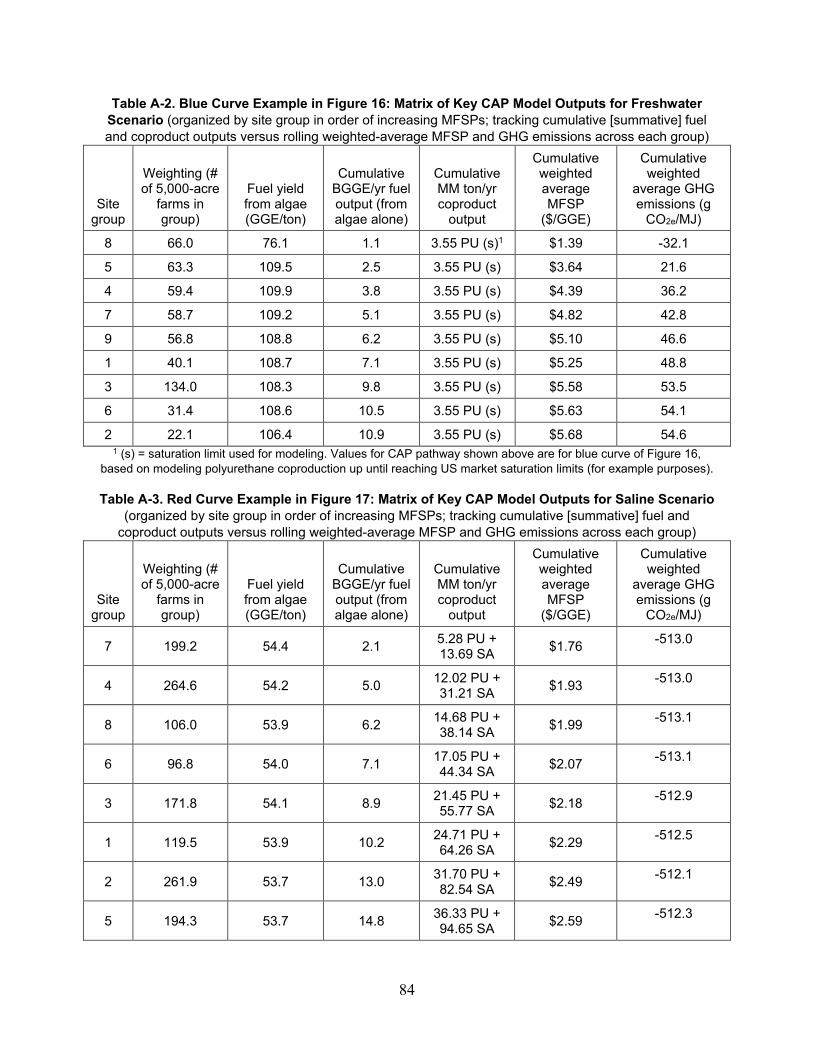
84

Table A-2. Blue Curve Example in Figure 16: Matrix of Key CAP Model Outputs for Freshwater Scenario (organized by site group in order of increasing MFSPs; tracking cumulative [summative] fuel and coproduct outputs versus rolling weighted-average MFSP and GHG emissions across each group)

Site group


farms in group)




output


($/GGE)

Cumulative weighted


CO2e/MJ)

8 66.0 76.1 1.1 3.55 PU (s)1 $1.39 -32.1

5 63.3 109.5 2.5 3.55 PU (s) $3.64 21.6

4 59.4 109.9 3.8 3.55 PU (s) $4.39 36.2

7 58.7 109.2 5.1 3.55 PU (s) $4.82 42.8

9 56.8 108.8 6.2 3.55 PU (s) $5.10 46.6

1 40.1 108.7 7.1 3.55 PU (s) $5.25 48.8

3 134.0 108.3 9.8 3.55 PU (s) $5.58 53.5

6 31.4 108.6 10.5 3.55 PU (s) $5.63 54.1

2 22.1 106.4 10.9 3.55 PU (s) $5.68 54.6 1 (s) = saturation limit used for modeling. Values for CAP pathway shown above are for blue curve of Figure 16,

based on modeling polyurethane coproduction up until reaching US market saturation limits (for example purposes).

Table A-3. Red Curve Example in Figure 17: Matrix of Key CAP Model Outputs for Saline Scenario (organized by site group in order of increasing MFSPs; tracking cumulative [summative] fuel and

coproduct outputs versus rolling weighted-average MFSP and GHG emissions across each group)

Site group


farms in group)




output


($/GGE)

Cumulative weighted


CO2e/MJ)

7 199.2 54.4 2.1 5.28 PU + 13.69 SA $1.76 -513.0

4 264.6 54.2 5.0 12.02 PU + 31.21 SA $1.93 -513.0

8 106.0 53.9 6.2 14.68 PU + 38.14 SA $1.99 -513.1

6 96.8 54.0 7.1 17.05 PU + 44.34 SA $2.07 -513.1

3 171.8 54.1 8.9 21.45 PU + 55.77 SA $2.18 -512.9

1 119.5 53.9 10.2 24.71 PU + 64.26 SA $2.29 -512.5

2 261.9 53.7 13.0 31.70 PU + 82.54 SA $2.49 -512.1

5 194.3 53.7 14.8 36.33 PU + 94.65 SA $2.59 -512.3

85

Table A-4. Blue Curve Example in Figure 17: Matrix of Key CAP Model Outputs for Saline Scenario (organized by site group in order of increasing MFSPs; tracking cumulative [summative] fuel and

coproduct outputs versus rolling weighted-average MFSP and GHG emissions across each group)

Site group


farms in group)




output


($/GGE)

Cumulative weighted


CO2e/MJ)

7 199.2 73.9 2.9 9.50 PU (s)1 $4.01 -30.4

4 264.6 109.1 8.3 9.50 PU (s) $6.10 31.0

8 106.0 108.5 10.5 9.50 PU (s) $6.41 37.7

6 96.8 108.5 12.4 9.50 PU (s) $6.63 41.8

3 171.8 108.9 15.9 9.50 PU (s) $6.90 46.8

1 119.5 108.4 18.5 9.50 PU (s) $7.06 49.5

2 261.9 108.0 24.2 9.50 PU (s) $7.33 53.4

5 194.3 107.9 27.9 9.50 PU (s) $7.45 55.0 1 (s) = saturation limit used for modeling. Values for CAP pathway shown above are for blue curve of Figure 17,

based on modeling polyurethane coproduction up until reaching US market saturation limits (for example purposes).

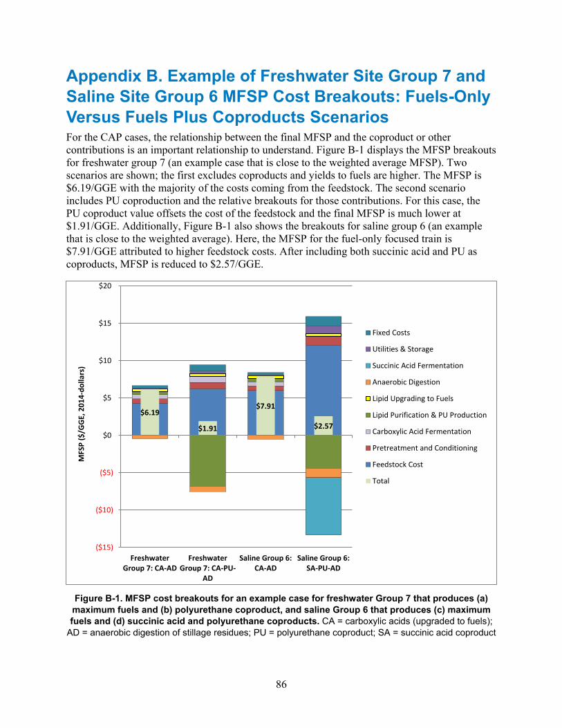
86

Appendix B. Example of Freshwater Site Group 7 and Saline Site Group 6 MFSP Cost Breakouts: Fuels-Only Versus Fuels Plus Coproducts Scenarios For the CAP cases, the relationship between the final MFSP and the coproduct or other contributions is an important relationship to understand. Figure B-1 displays the MFSP breakouts for freshwater group 7 (an example case that is close to the weighted average MFSP). Two scenarios are shown; the first excludes coproducts and yields to fuels are higher. The MFSP is $6.19/GGE with the majority of the costs coming from the feedstock. The second scenario includes PU coproduction and the relative breakouts for those contributions. For this case, the PU coproduct value offsets the cost of the feedstock and the final MFSP is much lower at $1.91/GGE. Additionally, Figure B-1 also shows the breakouts for saline group 6 (an example that is close to the weighted average). Here, the MFSP for the fuel-only focused train is $7.91/GGE attributed to higher feedstock costs. After including both succinic acid and PU as coproducts, MFSP is reduced to $2.57/GGE.

Figure B-1. MFSP cost breakouts for an example case for freshwater Group 7 that produces (a) maximum fuels and (b) polyurethane coproduct, and saline Group 6 that produces (c) maximum fuels and (d) succinic acid and polyurethane coproducts. CA = carboxylic acids (upgraded to fuels);

AD = anaerobic digestion of stillage residues; PU = polyurethane coproduct; SA = succinic acid coproduct

$6.19

$1.91

$7.91

$2.57

($15)

($10)

($5)

$0

$5

$10

$15

$20

FreshwaterGroup 7: CA-AD

FreshwaterGroup 7: CA-PU-

AD

Saline Group 6:CA-AD

Saline Group 6:SA-PU-AD

MFS

P ($

/GG

E, 2

014-

dolla

rs)

Fixed Costs

Utilities & Storage

Succinic Acid Fermentation

Anaerobic Digestion

Lipid Upgrading to Fuels

Lipid Purification & PU Production

Carboxylic Acid Fermentation

Pretreatment and Conditioning

Feedstock Cost

Total

87

Appendix C. Detailed Cost Data for Algae/Wood Blend Feedstock HTL and Upgrading Systems in Different Sites


Freshwater

Combined Freshwater - no

aq upgrading

Combined Freshwater - High Wood

Processing Area Cost Contributions & Key Technical Parameters MetricFuel sell ing price $/gge $3.83 $3.71 $3.81 $3.53 $3.48 $3.73 $3.70 $3.56 $3.76 $3.72 $3.79 $3.03Conversion Contribution $/gge $1.25 $1.27 $1.26 $1.16 $1.20 $1.25 $1.24 $1.16 $1.25 $1.24 $0.86 $1.28Production Diesel mm gge/yr 25 26 25 28 27 26 26 28 25 26 23 40 Production Naphtha mm gge/yr 13 15 14 15 15 14 14 14 14 14 11 29 Diesel Yield (AFDW feedstock basis) gge/US ton feedstock 96 90 95 99 99 94 96 101 95 96 84 75 Naphtha Yield (AFDW feedstock basis) gge/US ton feedstock 52 54 52 53 53 53 52 52 52 52 41 54 Diesel Yield (areal basis) gge/acre-yr 4,986 5,193 4,980 5,586 5,481 5,120 5,152 5,507 5,042 5,167 4,556 8,087 Naphtha Yield (areal basis) gge/acre-yr 2,696 3,082 2,720 2,964 2,929 2,875 2,809 2,832 2,772 2,814 2,192 5,821 Natural Gas Usage-drying (AFDW algae basis) scf/US ton feedstock 0 0 0 0 0 0 0 0 0 0 0 0 Natural Gas Usage-H2 gen (AFDW algae basis) scf/US ton feedstock 3,743 3,733 3,741 3,769 3,769 3,742 3,746 3,769 3,744 3,745 3,745 3,669 Carbon efficiency, C in products/C in feedstock % 74.8% 74.0% 74.6% 76.7% 76.7% 74.7% 74.9% 76.8% 74.8% 74.9% 63.2% 68.8%Feedstock Cost (AFDW basis) $/US ton blend $382 $351 $376 $359 $345 $363 $364 $366 $370 $367 $367 $225 Processing Area Cost Contributions

Feedstock $/gge fuel $2.59 $2.44 $2.56 $2.37 $2.28 $2.48 $2.46 $2.40 $2.51 $2.48 $2.93 $1.75 Algae Drying (summer & spring only) $/gge fuel $0.00 $0.00 $0.00 $0.00 $0.00 $0.00 $0.00 $0.00 $0.00 $0.00 $0.00 $0.00 HTL Biocrude Production $/gge fuel $0.43 $0.42 $0.43 $0.43 $0.43 $0.43 $0.43 $0.43 $0.43 $0.43 $0.52 $0.35 HTL Biocrude Hydrotreating to Finished Fuels $/gge fuel $0.17 $0.17 $0.17 $0.17 $0.17 $0.17 $0.17 $0.17 $0.17 $0.17 $0.20 $0.14 HTL Aqueous Phase Upgrading $/gge fuel $0.50 $0.52 $0.50 $0.42 $0.42 $0.50 $0.49 $0.42 $0.50 $0.49 $0.00 $0.70 Balance of Plant $/gge fuel $0.39 $0.38 $0.39 $0.37 $0.38 $0.38 $0.38 $0.37 $0.38 $0.38 $0.46 $0.35 Nutrient Recycle Credit $/gge fuel (0.24) (0.23) (0.23) (0.22) (0.20) (0.23) (0.23) (0.23) (0.24) (0.23) (0.33) (0.25)

Saline cases 1 2 3 4 5 6 7 8 Combined Saline

caseCombined Saline - no aq upgrading

Combined Saline -High Wood

Processing Area Cost Contributions & Key Technical Parameters MetricFuel sell ing price $/gge $4.80 $4.71 $4.51 $4.43 $4.54 $4.50 $4.31 $4.44 $4.55 $4.77 $3.50Conversion Contribution $/gge $1.22 $1.23 $1.24 $1.25 $1.26 $1.25 $1.18 $1.25 $1.24 $0.85 $1.28Production Diesel mm gge/yr 26 26 26 25 25 25 26 25 26 23 40 Production Naphtha mm gge/yr 14 15 15 14 14 14 14 14 14 11 29 Diesel Yield (AFDW feedstock basis) gge/US ton feedstock 96 95 94 95 93 94 99 95 95 84 75 Naphtha Yield (AFDW feedstock basis) gge/US ton feedstock 52 52 53 52 53 53 53 53 52 41 54 Diesel Yield (areal basis) gge/acre-yr 5,230 5,279 5,203 5,074 4,978 4,956 5,264 5,054 5,126 4,516 8,068 Naphtha Yield (areal basis) gge/acre-yr 2,816 2,911 2,909 2,803 2,838 2,766 2,803 2,808 2,835 2,213 5,840 Natural Gas Usage-drying (AFDW algae basis) scf/US ton feedstock 0 0 0 0 0 0 0 0 0 0 0 Natural Gas Usage-H2 gen (AFDW algae basis) scf/US ton feedstock 3,744 3,742 3,746 3,746 3,742 3,744 3,769 3,745 3,744 3,744 3,669

Carbon efficiency, C in products/C in feedstock % 74.9% 74.7% 74.9% 75.0% 74.6% 74.8% 76.7% 74.9% 74.8% 63.2% 68.8%Feedstock Cost (AFDW basis) $/US ton blend $530 $511 $481 $469 $478 $477 $474 $470 $487 $487 $286 Processing Area Cost Contributions

Feedstock $/gge fuel $3.58 $3.48 $3.27 $3.18 $3.28 $3.25 $3.13 $3.19 $3.31 $3.91 $2.22 Algae Drying (summer & spring only) $/gge fuel $0.00 $0.00 $0.00 $0.00 $0.00 $0.00 $0.00 $0.00 $0.00 $0.00 $0.00 HTL Biocrude Production $/gge fuel $0.43 $0.43 $0.43 $0.43 $0.43 $0.44 $0.44 $0.43 $0.43 $0.53 $0.35 HTL Biocrude Hydrotreating to Finished Fuels $/gge fuel $0.17 $0.17 $0.17 $0.17 $0.17 $0.17 $0.17 $0.17 $0.17 $0.21 $0.14 HTL Aqueous Phase Upgrading $/gge fuel $0.49 $0.50 $0.49 $0.49 $0.50 $0.50 $0.42 $0.49 $0.49 $0.00 $0.70 Balance of Plant $/gge fuel $0.38 $0.38 $0.38 $0.38 $0.39 $0.39 $0.38 $0.38 $0.38 $0.46 $0.35 Nutrient Recycle Credit $/gge fuel (0.25) (0.24) (0.23) (0.23) (0.23) (0.24) (0.23) (0.23) (0.23) (0.34) (0.26)

88

Appendix D. Life Cycle Inventory Data for the Pathways Examined Table D-1. LCI of Algae Cultivation

Freshwater Scenarios Group 1 2 3 4 5 6 7 8 9 Energy Electricity (kWh/kg afdw) 0.394 0.396 0.391 0.357 0.345 0.357 0.346 0.340 0.348 C/N/P

CO2 (kg/kg afdw) 2.67 2.67 2.67 2.67 2.67 2.67 2.67 2.67 2.67 Ammonia (kg/kg afdw) 0.02 0.02 0.02 0.02 0.02 0.02 0.02 0.02 0.02 (NH4)2HPO4 (kg/kg afdw) 0.01 0.01 0.01 0.01 0.01 0.01 0.01 0.01 0.01

Water Use

Fresh Water Lost to Evaporation (kg/kg afdw)

195 160 177 88 37 50 26 36 22

Fresh Water Lost to Blowdown (kg/kg AFDW)

13.6 13.1 13.3 6.3 2.4 3.5 1.5 2.9 2.0

CO2 Outgassing from Ponds (g/kg afdw) 665.8 666.0 665.8 665.7 665.5 665.5 665.5 665.5 665.4 Saline Water Scenarios

Group 1 2 3 4 5 6 7 8 Energy Electricity (kWh/kg afdw) 0.402 0.402 0.374 0.354 0.372 0.358 0.352 0.353 C/N/P

CO2 (kg/kg afdw) 2.68 2.68 2.67 2.67 2.67 2.67 2.67 2.67 Ammonia (kg/kg afdw) 0.02 0.02 0.02 0.02 0.02 0.02 0.02 0.02 (NH4)2HPO4 (kg/kg afdw) 0.01 0.01 0.01 0.01 0.01 0.01 0.01 0.01

CO2 Outgassing from Ponds (g/kg afdw) 667.4 667.4 666.5 665.9 666.2 665.9 665.9 665.9

89

Table D-2. LCI of CAP Conversion Technology (freshwater scenarios, Per MJ RDe) Group with PU coproduct 1 2 3 4 5 6 7 8 9 Products

Renewable Diesel (MJ) 0.360 0.361 0.360 0.359 0.359 0.360 0.359 0.359 0.360 Naphtha (MJ) 0.640 0.639 0.640 0.641 0.641 0.640 0.641 0.641 0.640

Polyurethane (kg) 0.025 0.025 0.025 0.025 0.025 0.025 0.025 0.025 0.025 Electricity Excess (kWh) 0.019 0.019 0.019 0.019 0.019 0.019 0.019 0.019 0.019

Inputs Algae Biomass (kg afdw) 0.103 0.108 0.104 0.101 0.102 0.104 0.102 0.100 0.103

Natural Gas (MJ) 0.070 0.068 0.066 0.071 0.069 0.069 0.070 0.069 0.070 Sulfuric Acid (kg) 0.004 0.004 0.004 0.004 0.004 0.004 0.004 0.004 0.004

Ammonia (kg) 0.001 0.001 0.001 0.001 0.001 0.001 0.001 0.001 0.001 (NH4)2HPO4 (kg) 0.001 0.001 0.001 0.001 0.001 0.001 0.001 0.001 0.001

Hexane (kg) 0.002 0.002 0.002 0.002 0.002 0.002 0.002 0.002 0.002 Hydrogen (kg) 0.001 0.001 0.001 0.001 0.001 0.001 0.001 0.001 0.001

Corn Steep Liquor (kg) 0.009 0.009 0.009 0.009 0.009 0.009 0.009 0.009 0.009 Water (gal) 0.165 0.164 0.167 0.173 0.170 0.165 0.170 0.171 0.165

Process Recovered Streams NH3 (kg) 0.002 0.002 0.002 0.002 0.002 0.002 0.002 0.002 0.002

(NH4)2HPO4 (kg) 0.001 0.001 0.001 0.001 0.001 0.001 0.001 0.001 0.001 Bioavailable N (kg Ca(NO3)2) 0.000 0.000 0.000 0.000 0.000 0.000 0.000 0.000 0.000

CO2 (Recovered) (kg) 0.071 0.072 0.071 0.071 0.071 0.071 0.071 0.070 0.071 Water Recycled (gal) 0.232 0.232 0.235 0.238 0.235 0.232 0.237 0.235 0.232

Group without PU coproduct 1 2 3 4 5 6 7 9 Products

Renewable Diesel (MJ) 0.508 0.509 0.508 0.508 0.508 0.508 0.508 0.508 Naphtha (MJ) 0.492 0.491 0.492 0.492 0.492 0.492 0.492 0.492

Electricity Excess (kWh) 0.015 0.014 0.014 0.014 0.014 0.014 0.014 0.014 Inputs

Algae Biomass (kg afdw) 0.072 0.076 0.073 0.071 0.071 0.073 0.072 0.072 Natural Gas (MJ) 0.021 0.005 0.003 0.005 0.005 0.006 0.003 0.005

Sulfuric Acid (kg) 0.003 0.003 0.003 0.003 0.003 0.003 0.003 0.003 Ammonia (kg) 0.001 0.001 0.001 0.001 0.001 0.001 0.001 0.001

(NH4)2HPO4 (kg) 0.001 0.001 0.001 0.001 0.001 0.001 0.001 0.001 Hexane (kg) 0.001 0.001 0.001 0.001 0.001 0.001 0.001 0.001

Hydrogen (kg) 0.001 0.001 0.001 0.001 0.001 0.001 0.001 0.001 Corn Steep Liquor (kg) 0.006 0.006 0.006 0.007 0.007 0.006 0.007 0.006

Water (gal) 0.100 0.098 0.101 0.105 0.103 0.099 0.103 0.100 Process Recovered Streams

NH3 (kg) 0.001 0.001 0.001 0.001 0.001 0.001 0.001 0.001 (NH4)2HPO4 (kg) 0.001 0.001 0.001 0.001 0.001 0.001 0.001 0.001

Bioavailable N (kg Ca(NO3)2) 0.000 0.000 0.000 0.000 0.000 0.000 0.000 0.000 CO2 (Recovered) (kg) 0.046 0.046 0.046 0.045 0.045 0.046 0.045 0.045 Water Recycled (gal) 0.156 0.156 0.158 0.160 0.158 0.156 0.159 0.156

90

Table D-3. LCI of CAP Conversion Technology (saline scenarios, Per MJ RDe) Group with PU and SA coproducts 1 2 3 4 5 6 7 8 7* 8* Products

Renewable Diesel (MJ) 0.705 0.704 0.704 0.704 0.704 0.704 0.704 0.704 0.358 0.462 Naphtha (MJ) 0.295 0.296 0.296 0.296 0.296 0.296 0.296 0.296 0.642 0.538

Polyurethane (kg) 0.018 0.018 0.018 0.018 0.018 0.018 0.018 0.018 0.025 0.003 Succinic Acid (kg) 0.048 0.048 0.048 0.048 0.048 0.048 0.048 0.048 0 0

Electricity Excess (kWh) 0.005 0.005 0.004 0.004 0.006 0.003 0.004 0.004 0.021 0.015 Inputs

Algae Biomass (kg afdw) 0.142 0.143 0.141 0.140 0.143 0.142 0.139 0.142 0.104 0.070 Natural Gas (MJ) 0.658 0.661 0.656 0.654 0.666 0.659 0.655 0.660 0.062 0.063

Sulfuric Acid (kg) 0.006 0.006 0.006 0.006 0.006 0.006 0.006 0.006 0.004 0.003 Ammonia (kg) 0.002 0.002 0.002 0.002 0.002 0.002 0.002 0.002 0.001 0.001

(NH4)2HPO4 (kg) 0.000 0.000 0.000 0.000 0.000 0.000 0.000 0.000 0.001 0.001 Hexane (kg) 0.002 0.002 0.002 0.002 0.002 0.002 0.002 0.002 0.002 0.001

Hydrogen (kg) 0.001 0.001 0.001 0.001 0.001 0.001 0.001 0.001 0.001 0.001 Corn Steep Liquor (kg) 0.003 0.003 0.003 0.003 0.003 0.003 0.003 0.003 0.009 0.006

Water (gal) 0.350 0.349 0.350 0.350 0.349 0.350 0.351 0.350 0.168 0.109 Process Recovered Streams

NH3 (kg) 0.003 0.003 0.003 0.003 0.003 0.003 0.003 0.003 0.002 0.001 (NH4)2HPO4 (kg) 0.001 0.001 0.001 0.001 0.001 0.001 0.001 0.001 0.001 0.001

Bioavailable N (kg Ca(NO3)2) 0.000 0.000 0.000 0.000 0.000 0.000 0.000 0.000 0.000 0.000 CO2 (Recovered) (kg) 0.103 0.104 0.103 0.103 0.104 0.103 0.103 0.104 0.072 0.048 Water Recycled (gal) 0.000 0.000 0.000 0.000 0.000 0.000 0.000 0.000 0.000 0.000

Group without coproducts 1 2 3 4 5 6 8 Products

Renewable Diesel (MJ) 0.508 0.509 0.508 0.508 0.509 0.508 0.508 Naphtha (MJ) 0.492 0.491 0.492 0.492 0.491 0.492 0.492

Electricity Excess (kWh) 0.014 0.014 0.014 0.014 0.014 0.014 0.014 Inputs

Algae Biomass (kg afdw) 0.073 0.073 0.072 0.072 0.074 0.073 0.073 Natural Gas (MJ) 0.008 0.008 0.008 0.008 0.007 0.007 0.008

Sulfuric Acid (kg) 0.003 0.003 0.003 0.003 0.003 0.003 0.003 Ammonia (kg) 0.001 0.001 0.001 0.001 0.001 0.001 0.001

(NH4)2HPO4 (kg) 0.001 0.001 0.001 0.001 0.001 0.001 0.001 Hexane (kg) 0.001 0.001 0.001 0.001 0.001 0.001 0.001

Hydrogen (kg) 0.001 0.001 0.001 0.001 0.001 0.001 0.001 Corn Steep Liquor (kg) 0.006 0.006 0.006 0.006 0.007 0.007 0.006

Water (gal) 0.101 0.101 0.100 0.100 0.102 0.102 0.101 Process Recovered Streams

NH3 (kg) 0.001 0.001 0.001 0.001 0.001 0.001 0.001 (NH4)2HPO4 (kg) 0.001 0.001 0.001 0.001 0.001 0.001 0.001

Bioavailable N (kg Ca(NO3)2) 0.000 0.000 0.000 0.000 0.000 0.000 0.000 CO2 (Recovered) (kg) 0.046 0.046 0.046 0.046 0.046 0.046 0.046 Water Recycled (gal) 0.000 0.000 0.000 0.000 0.000 0.000 0.000

91

Table D-4. LCI of HTL Conversion Technology (per MJ RDe)

Freshwater Group 1 2 3 4 5 6 7 8 9 Products

Renewable Diesel (MJ) 0.677 0.654 0.675 0.677 0.675 0.667 0.675 0.685 0.673 Naphtha (MJ) 0.323 0.346 0.325 0.323 0.325 0.333 0.325 0.315 0.327

Inputs Algae Biomass (kg afdw) 0.045 0.039 0.044 0.041 0.041 0.042 0.043 0.044 0.043

Electricity (kWh) 0.005 0.005 0.005 0.005 0.005 0.005 0.005 0.005 0.005 Natural Gas (MJ) 0.2267 0.2413 0.2290 0.2130 0.2134 0.2298 0.2249 0.2116 0.2272

Sulfuric Acid (kg) 0.002 0.002 0.002 0.002 0.002 0.002 0.002 0.002 0.002 HT Catalyst (kg) 3.2×10-6 3.2×10-6 3.2×10-6 3.2×10-6 3.2×10-6 3.2×10-6 3.2×10-6 3.2×10-6 3.2×10-6

Waste Wood (kg) 0.015 0.025 0.017 0.015 0.015 0.019 0.017 0.012 0.017 Water (gal) 0.0046 0.0048 0.0046 0.0043 0.0043 0.0046 0.0045 0.0042 0.0046

Process Recovered Streams NH3 (kg) 0.0008 0.0007 0.0008 0.0007 0.0007 0.0007 0.0007 0.0007 0.0007

(NH4)2HPO4 (kg) 0.0004 0.0003 0.0004 0.0003 0.0003 0.0003 0.0003 0.0004 0.0003 CO2 (Recovered) (kg) 0.0674 0.0755 0.0688 0.0593 0.0593 0.0686 0.0658 0.0590 0.0673 Water Recycled (gal) 0.0733 0.0781 0.0741 0.0681 0.0682 0.0742 0.0726 0.0677 0.0734

Saline Water Group 1 2 3 4 5 6 7 8 Products

Renewable Diesel (MJ) 0.678 0.672 0.668 0.671 0.663 0.669 0.676 0.670 Naphtha (MJ) 0.322 0.328 0.332 0.329 0.337 0.331 0.324 0.330

Inputs Algae Biomass (kg afdw) 0.044 0.043 0.041 0.042 0.040 0.041 0.043 0.042

Electricity (kWh) 0.005 0.005 0.005 0.005 0.005 0.005 0.005 0.005 Natural Gas (MJ) 0.223 0.226 0.225 0.224 0.228 0.226 0.222 0.225

Sulfuric Acid (kg) 0.002 0.002 0.002 0.002 0.002 0.002 0.002 0.002 HT Catalyst (kg) 3.2E-06 3.3E-06 3.3E-06 3.2E-06 3.3E-06 3.3E-06 3.2E-06 3.3E-06

Waste Wood (kg) 0.015 0.017 0.019 0.018 0.020 0.018 0.016 0.018 Water (gal) 0.0045 0.0045 0.0045 0.0045 0.0046 0.0045 0.0045 0.0045

Process Recovered Streams NH3 (kg) 0.001 0.001 0.001 0.001 0.001 0.001 0.001 0.001

(NH4)2HPO4 (kg) 0.000 0.000 0.000 0.000 0.000 0.000 0.000 0.000 CO2 (Recovered) (kg) 0.065 0.067 0.065 0.065 0.067 0.066 0.064 0.066

2017 algae harmonization study: evaluating the potential

Documents