20160706 abusing etfs accepted ssrn - fresh funds · pdf fileelectronic copy available at :...

Electronic copy available at: http://ssrn.com/abstract=2022442

Abusing ETFs

Forthcoming: Review of Finance

Utpal Bhattacharya, Benjamin Loos, Steffen Meyer, and Andreas Hackethal*

Abstract. Using data from a large German brokerage, we find that individuals investing in

passive exchange-traded funds (ETFs) do not improve their portfolio performance, even before

transaction costs. Further analysis suggests that this is because of poor ETF timing as well as

poor ETF selection (relative to the choice of low-cost, well-diversified ETFs). An exploration

of investor heterogeneity shows that though investors who trade more have worse ETF timing,

no groups of investors benefit by using ETFs, and no groups will lose by investing in low-cost,

well-diversified ETFs.

* Bhattacharya is affiliated with Hong Kong University of Science and Technology (Clear Water Bay, Kowloon

Hong Kong, [email protected], Phone 852-2358-8498), Loos is affiliated with University of Mannheim (L5, 2,

68131 Mannheim, [email protected], Phone +49 621 181 1516), Meyer is affiliated with Leibniz

University in Hannover (Königsworther Platz, 30167 Hannover, [email protected], Phone +49 511 762

4555), and Hackethal is affiliated with Goethe University Frankfurt (Grüneburgplatz 1, 60323 Frankfurt/Main,

[email protected], Phone +49 69 798 33700). For useful comments and discussions, we thank

Tyler Shumway, Dimitris Georgarakos, Craig Holden, Roman Inderst, Jose Martinez, Andrei Shleifer, Noah

Stoffman and Joachim Weber. Conference and seminar comments at the AEA meetings in Boston, American,

Cincinnati, the EFA meetings in Cambridge, the FIRS conference in Quebec City, the FMA meetings in Nashville,

GWU, Goethe University, Hong Kong University, IIM Ahmedabad, IIM Bangalore, IIM Kolkata, Indiana, ISB

Hyderabad, Lehigh, Minnesota, RSM Rotterdam, University of Melbourne, University of New South Wales,

University of Sydney, University of Technology at Sydney, Vanderbilt, WHU Otto Beisheim School of

Management, Yale and York significantly improved the paper.


JEL classification: D14, G11, G28

Keywords: household finance, ETFs, security selection, timing


Abusing ETFs†

Abstract. Using data from a large German brokerage, we find that individuals investing in

passive exchange-traded funds (ETFs) do not improve their portfolio performance, even before

transaction costs. Further analysis suggests that this is because of poor ETF timing as well as

poor ETF selection (relative to the choice of low-cost, well-diversified ETFs). An exploration

of investor heterogeneity shows that though investors who trade more have worse ETF timing,

no groups of investors benefit by using ETFs, and no groups will lose by investing in low-cost,

well-diversified ETFs.

JEL classification: D14, G11, G28

Keywords: household finance, ETFs, security selection, timing

† For useful comments and discussions, we thank Tyler Shumway, Dimitris Georgarakos, Craig Holden, Roman

Inderst, Jose Martinez, Andrei Shleifer, Noah Stoffman and Joachim Weber. Conference and seminar comments

at the AEA meetings in Boston, American, Cincinnati, the EFA meetings in Cambridge, the FIRS conference in

Quebec City, the FMA meetings in Nashville, GWU, Goethe University, Hong Kong University, IIM Ahmedabad,

IIM Bangalore, IIM Kolkata, Indiana, ISB Hyderabad, Lehigh, Minnesota, RSM Rotterdam, University of

Melbourne, University of New South Wales, University of Sydney, University of Technology at Sydney,

Vanderbilt, WHU Otto Beisheim School of Management, Yale and York significantly improved the paper.

1

1. Introduction

One of the most successful financial product innovations of the last twenty years is the

exchange-traded fund (ETF).1 The first ETF was launched in Canada in 1990. As of February

2016, 4,479 ETFs had been established, with approximately USD 2.7 trillion in assets under

management (roughly the same size as the global hedge fund industry).2

In this paper, we investigate whether or not ETFs provide benefits to a sample of

individual investors who include them in their portfolios.3 Given the paucity of studies on the

user effects of financial product innovations like ETFs, this is an important topic to analyze.

Frame and White (2004, p 116) state: “Everybody talks about financial innovation, but (almost)

nobody empirically tests hypotheses about it.” It is important to test whether ETFs benefit

individual investors because they attract a lot of them.4 In addition, employers are actively

1 An ETF is an index-linked security. These instruments aim to replicate the movements of a particular market

and therefore enable the investor to easily buy and sell a broadly-diversified portfolio of securities that mimic that

market. Investors can buy and sell ETF shares in public markets any time during the trading day.

2 ETFGI (Global ETF and ETP Directory, February 2016) and Hedge Fund Research (Global Hedge Fund

Industry Report, Year End 2015).

3 We examine only passive ETFs that aim to mimic an index. Active ETFs, which aim to outperform an index,

are not examined. Amongst passive ETFs, we do not differentiate whether ETFs are synthetic or fully replicating,

despite the fact that synthetic ETFs may entail additional risk (Ramaswamy, 2011). In unreported analyses, we

also look at passive index funds and find results similar to those for passive ETFs.

4 Charles Schwab, the largest U.S. discount brokerage, offers more than 200 commission-free ETFs to

individual investors (Schwab ETF OneSource,

http://www.schwab.com/public/schwab/investing/accounts_products/investment/etfs/schwab_etf_onesource).

2

seeking ways to include ETFs in 401(k) defined-contribution retirement plans5 and numerous

fin-tech startups promote standardized ETF portfolios to retail investors. Even some industry

regulators are promoting ETFs to individual investors.6

Our null hypothesis is that individual investors benefit by using passive ETFs. Classical

finance theory prescribes well-diversified and low-cost portfolios for investors.7 However,

many researchers document substantial portfolio underperformance by individual investors due

to poor diversification and costly over-trading in single stocks.8 Indeed, ETFs may help

5 “Are ETFs and 401(k) Plans a Bad Fit?” The Wall Street Journal, April 5, 2012.

6 The Securities and Markets Stakeholder Group of the European Securities and Markets Authority (ESMA) states

that “ETFs are a low cost and straightforward investment proposition for investors and, as such, ESMA should

investigate how to make indexed ETFs more offered to individual investors.” ESMA Report and Consultation

paper – Guidelines on ETFs and other UCITS issues. July 25, 2012,

http://www.esma.europa.eu/system/files/2012-474.pdf, p. 32.

7 Markowitz (1952) suggests we diversify by buying optimal portfolios. Tobin (1958) suggests that we require

only one optimal portfolio provided that a risk-free asset exists. Sharpe (1964) concludes that this optimal

portfolio was the market portfolio.

8 The portfolios of individual investors who participate in equity markets typically show suboptimal degrees of

diversification (e.g., Blume and Friend, 1975; Kelly, 1995; Goetzmann and Kumar, 2008) and concentration on

the home region (“home bias,” e.g., French and Poterba, 1991; Cooper and Kaplanis, 1994; Lewis, 1999;

Huberman, 2001; Zhu, 2002; Ahearne et al., 2004; Calvet et al, 2007). Individual investors are also shown to

trade too much (Odean, 1999; Barber and Odean, 2000).

3

investors attain theoretically sound portfolios.9 ETFs have other benefits, too. They trade in

real time and they offer tax advantages (Poterba and Shoven, 2002).

However, there is some evidence that investors may not be using index-linked products

wisely. Hortaçsu and Syverson (2004) find large fee dispersions among financially

homogeneous funds and Elton et al. Busse (2004) show that investors irrationally prefer more

expensive index funds.10 Second, it is possible that some ETFs, because they are highly

correlated with an index and are easy to trade, may enhance investors’ temptation to time the

underlying index.11 Third, investors may be overwhelmed by the sheer number of ETF products

and underlying market and sector indices (over 220 such indices in our sample alone) and end

up purchasing costly ETFs linked to rather undiversified single sectors or industries.

The key contribution of this paper to the literature (to our knowledge, the first of its

kind) is that we use the trading data of a large number of individual investors at a large German

brokerage firm during the 2005 to 2010 period to test whether ETFs benefit those who use

them.12 First, we examine who uses ETFs. We find that, compared to non-users, ETF users

9 Boldin and Cici (2010) review the entire empirical literature on index-linked securities and discuss their benefits.

French (2008) measures the benefits of passive investing and concluded, “the typical investor would increase his

average annual return by 67 basis points over the 1980-2006 period if he switched to a passive market portfolio.”

10 Choi et al., (2010) confirmed this behavior in an experiment and found that more financially sophisticated

investors pay lower fees.

11 In Germany, by 2009, the turnover in ETFs (data obtained from Deutsche Börse 2010) had become about the

same as the turnover in stocks (data obtained from the World Federation of Exchanges 2013).

12 We test whether the portfolio performance of individual investors improves after they purchase ETFs. An ex

4

are younger, wealthier in terms of both portfolio value and overall wealth, and have a shorter

relationship with the brokerage. Müller and Weber (2010), using a survey methodology, report

comparable results.

Second, we compare the portfolio performance of ETF users with all non-users in a

panel setting. We estimate the marginal contribution of ETFs to an individual’s portfolio

performance starting with the first month of ETF use. We examine raw returns as well as risk-

adjusted returns using one, two, four, and five risk factors.13 We use a panel setting with user

fixed effects to control for any time-invariant differences between users and non-users of ETFs.

We also control for observable demographics, lagged time-varying portfolio characteristics

like prior portfolio performance, and year fixed effects. We find that portfolio performance, as

measured by any of our measures using any benchmark index, does not increase with ETF use.

Third, and importantly, we examine why there is no performance improvement for ETF

users and what the performance improvement would have been had investors used ETFs

wisely. The basic idea is to compare actual portfolios with counterfactual portfolios. This

approach allows for inferences at the individual investor level, mitigating issues of self-

selection and endogeneity.

ante test like the one proposed by Calvet et al. (2007) will fail to incorporate the dynamic effects of actual trading.

13 For the market factor, we use a global index (MSCI All Country World Index “MSCI ACWI”), as well as the

broadest local index (CDAX). The former benchmark is for global investors and the latter benchmark is for local

investors. We use both indices for robustness. In our factor models that include a bond factor, we add the JP

Morgan Global Bond to the MSCI ACWI as a fixed income benchmark for global investors and the RDAX Return

Index to the CDAX Index as a fixed income benchmark for local investors.

5

We start with our first benchmark portfolio that is the non-ETF part of the portfolio. If

we add all the actual ETF trades of an investor, we are back at the full portfolio. The return

differential between the benchmark portfolio and the full portfolio is a statistically significant

−1.16% per year. We then examine what would happen if the actual ETFs were only bought,

but not sold, essentially emulating an ETF buy-and-hold strategy. This counterfactual portfolio

allows one to extract the contribution coming from ETF timing ability. We find that poor ETF

timing ability is responsible for -0.77 percentage points (statistically significant) of the total

return differential (-1.16%). ETF selection ability is not statistically significant. Examining

gross returns and risk-adjusted gross returns confirms that the actual portfolio returns of ETF

users are mainly adversely affected by poor ETF timing, though trading costs matter as well.

Focusing on portfolio efficiency alone, we find that the relative Sharpe ratio loss (RSRL)14

increases significantly with ETF use. This rules out that investors use ETFs mainly for hedging

or better diversification.

Our second benchmark portfolio is a prescription: we prescribe the investor a buy-and-

hold strategy in a low-cost ETF on the MSCI World Index. We find that investors are losing

a statistically significant -1.69% p.a. in net portfolio returns by not using this prescribed

portfolio. To decompose the above loss, we start with the actual portfolio of the investor. We

then examine what happens if we replace all ETF trades with trades in a low-cost ETF on the

MSCI World Index. This particular counterfactual portfolio isolates ETF selection (relative to

choosing the MSCI). We find that most of that -1.69% loss (-1.28%, statistically significant)

would have come from ETF selection (not choosing the low-cost ETF on the MSCI World

14 We measure the relative Sharpe ratio loss as defined in Calvet et al. (2007).

6

Index) and little (-0.41%, not statistically significant) from not employing a buy-and-hold

strategy. This result also holds for gross portfolio returns, gross risk-adjusted returns, and

diversification. We conclude that the average investor could have benefited from using ETFs

by following the guidelines of classical finance theory.

Finally, we explore investor heterogeneity in terms of overconfidence (proxied by

portfolio turnover) and financial sophistication (proxied by portfolio value and portfolio

diversification) to see if there are specific types of investors where our results are most

relevant. Our conclusion from sorting investors by overconfidence and sophistication:

though investors who trade more have worse ETF timing, no groups of investors benefit by

using ETFs, no matter which measure (performance, timing, selection, or diversification) or

sort (turnover, portfolio value, or diversification) we examine. We also find that no groups

will lose by investing in the right MSCI ETF.

Our sorting exercise also yields one potential explanation. Investors from virtually

all groups do not substantially adapt their trading behavior after ETF use. Those who traded

more before ETF use continue to trade more after ETF use, both in the ETF part of the

portfolio, as well as in the non-ETF part. Investors therefore appear to make the same

mistakes when they trade ETFs that they have made in trading non-ETFs.

Our overall conclusion is that our sample of ETF users does not improve their actual

portfolio performance after ETF use because they have both poor ETF timing as well as ETF

selection (relative to choosing a low-cost well-diversified ETF like the MSCI). Thus, although

passive ETFs are an important investment innovation, with an enormous potential to act as a

low-cost vehicle for diversification, in practice they may not help individual investors enhance

the efficiency of their portfolio, even before transaction costs. This would happen if individual

7

investors get tempted to trade too much in the ever-expanding choices of high-liquidity ETFs

based on narrow market indices. To conclude, more ETF choice may lead to abuse of ETFs.

We describe the data in Section 1 and examine which investors are most likely to

purchase ETFs in Section 2. In Section 3, we investigate whether ETF users improve their

portfolio performance compared with non-users. In Section 4, we examine why ETF users do

not improve their relative portfolio performance. We conclude in Section 5.

2. Data

1.1 ETFS AND INDEX-LINKED SECURITIES IN GERMANY

Individuals in Germany, as in the United States, who want to invest in index-linked

securities can choose ETFs and/or index mutual funds. Table I gives us a snapshot of both

markets at the end of a year. Panel A of Table I provides the data for index-linked securities in

Germany. Panel B provides this information for the U.S. Panel C provides the data for our

German sample. As a result of data availability, the three panels represent a snapshot of the

market at different times. For Germany and the U.S., the data for the end of 2011 are available,

whereas these data for our sample are available only for the end of 2009.

[INSERT TABLE I ABOUT HERE]

The leftmost column in Panels A and B of Table I show that the total assets under

management invested in index-linked securities relative to total active mutual fund

investments, a ratio of about 20%, is comparable between Germany and the U.S. Panels A and

B also show that the market in the U.S., as expected, is much larger as measured by both assets

under management and the number of products. Interestingly, in terms of assets under

management, the market is split almost evenly between passive ETFs and index mutual funds

in the U.S., whereas in Germany, passive ETFs comprise 84% of the market.

8

When Panel A of Table I (Germany) is compared with Panel C (our sample), in terms

of the proportion of assets under management in each security class, our sample seems to be

representative of the entire German market.

1.2 ETFS IN OUR SAMPLE

In this paper, we focus only on ETFs rather than index funds for two reasons. First, as

can be seen in Table I, ETFs are the predominant index-linked security in Germany, as well as

in our sample. Second, as the construction and trading of index funds are different from ETFs,

we do not bundle the two.15

Table II shows the rich diversity of ETFs in the portfolios in our sample. Panel A shows

that our investors have exposure to many different indices. Although the top 10 benchmark

indices constitute over 65% of the assets under management in ETFs, 224 other benchmark

indices make up the remainder. Note that the popular indices are connected to Germany,

Europe, and the world, which motivates us to select the local German index, CDAX, and a

global index, MSCI ACWI, as our two benchmark indices.

[INSERT TABLE II ABOUT HERE]

In Panel B of Table II, we examine the regional allocations of these ETFs. Europe is

the most popular, followed by Germany. Individual German investors, like individual investors

all over the world, exhibit home bias.

In Panel C of Table II, we examine the asset class of ETFs. We find that ETFs that are

15 The economic intuition of our paper, however, applies to both index funds and ETFs. Therefore, as mentioned

in footnote 3, we replicate all our tests for passive index funds. We find results similar to those for passive ETFs.

9

based on equity indices dominate (90.5% of assets under management), which further justifies

our use of equity indices like CDAX and MSCI ACWI as benchmarks. However, as there are

a few bond- and commodity-based ETFs as well, we will sometimes use a bond benchmark.

Panel A of Table II shows that many ETFs in our sample are linked to narrow indices,

so it is likely that they offer more choices for timing certain asset classes, sectors or countries,

rather than opportunities for broad diversification. If so, their beta loadings with respect to our

benchmarks, CDAX and MSCI ACWI, could be very different from 1. In Panel D of Table II,

we show the beta loadings of all ETFs in our sample with respect to the CDAX and the MSCI

ACWI. The mean beta loadings with respect to the CDAX and the MSCI ACWI are 0.72 and

0.88, respectively. Although these betas are statistically significantly different from 1, if we

narrow our sample to equity ETFs, the mean beta loading with respect to the MSCI ACWI

cannot be distinguished from 1, but the mean beta loading with respect to the CDAX is still

below 1. Further, although many of these ETFs may not be tracking the CDAX or MSCI

ACWI perfectly, Panel D of Table II shows that their alphas with respect to these indices are

indistinguishable from zero.

1.3 INDIVIDUAL INVESTORS IN OUR SAMPLE

The brokerage that we work with was founded as a direct bank with a focus on offering

brokerage services via telephone and the Internet. In 2009, to retain existing customers and

attract new ones, the brokerage introduced a financial advisory service, which offered free

financial advice to a random sample of about 8,000 investors. Approximately 96% of these

individuals refused the financial advice and continued trading as before.16 Our starting sample

16 Bhattacharya et al. (2012) analyze the same sample with a focus on the 4% of individual investors who accepted

10

is these 7,761 investors. The knowledge that these investors refused financial advice assures

us that our sample is composed of self-directed investors whose decisions are not distorted by

a third party. As our focus is on ETFs, we keep investors who invest in all securities except

index mutual funds. We additionally restrict our sample to investors who on average have at

least €5,000 in their portfolios. We do so to avoid a bias introduced by small play money

accounts. Our final sample has 6,949 investors in an unbalanced panel that begins in August

2005 and ends in March 2010. Of these 6,949 investors, 1,080 investors traded at least one

ETF during this period — the “users” — and 5,869 investors who traded no ETFs during this

period — the “non-users.”

Figure 1 shows the share of ETFs in the portfolio of an average individual investor in

our sample. It shows that after investors have switched to ETFs, their weight in the portfolio

hardly exceeds 20%. Figure 1 also shows the growing popularity of ETFs in our sample. The

sharp increase in ETF share in December 2008 is likely related to a tax change in Germany.

From 2009 onwards, all capital gains and losses, irrespective of the holding period, are subject

to taxation. Gains and losses from securities purchased before the end of 2008, if held for

longer than one year, are tax exempt. Thus, it is possible that some investors switched to ETFs

in December 2008 to ensure a tax advantage.

[INSERT FIGURE 1 ABOUT HERE]

The German brokerage provided us with investor demographics and account

characteristics for both ETF users and non-users for the sample period. Investor demographics

the offer.

11

include gender, age, and micro-geographic status. The micro-geographic status variable

measures the average wealth level of individuals who inhabit a given micro area (street-level

address). The variable has nine categories, with category one comprising the poorest

individuals and category nine the wealthiest individuals. This information is provided to the

German brokerage by a specialized data service that uses several factors (such as house type

and size, dominant car brands, rent per square meter, and the unemployment rate) to construct

it.

The account characteristics are primarily comprised of monthly position statements,

daily transaction data, and account transfers for the August 2005 to March 2010 period. We

use the transaction records to calculate portfolio turnover and number of trades per month, as

in Barber and Odean (2002). To compute daily position statements and portfolio values, we

proceed as follows. We multiply the beginning-of-month value of each security holding by the

corresponding daily price return (excluding dividends but considering any capital actions) for

that security to obtain its end-of-day holding value. These values are then adjusted for any

sales, purchases, and/or account transfers that occurred on that day to yield the position

statements for the beginning of the second day in the month. We repeat this procedure for each

trading day in a given month. The computed holdings on the last day of each month are then

reconciled with the true holdings in our dataset.

Daily portfolio returns are calculated as the weighted average return of all securities held,

purchased, and sold by the investor on that day. For securities held, we use total daily return

data from Datastream (they take into account dividend payments). For securities that are either

purchased or sold on that day, we compute daily returns based on exact transaction prices. Our

weighting factors for securities held or sold are closing prices of the previous day times the

number of securities held or sold. The weighting factors for securities purchased are the

12

corresponding transaction prices multiplied by the number of securities purchased. Since we

also obtained transaction costs, commissions, and fees from the bank, we are able to calculate

daily security and portfolio returns both on a gross (before transaction cost) and on a net (after

transaction cost) basis.

The account characteristics provided by the brokerage also include account opening

date and cash account balances at the beginning of the sample period and at the end of the

sample period. The account opening date gives us the length of the client relationship with the

brokerage, and the cash account balances enable us to calculate the share of risky securities in

the account with the brokerage (portfolio value plus cash value) for at least two dates.

Table III gives the sources of all the data described above, as well as of data obtained

from other sources. Finally, as we find that the typical investor in our sample only trades about

twice a month, we aggregate all daily returns and other statistics to the monthly level.

[INSERT TABLE III ABOUT HERE]

3. Who Uses ETFs?

Table IV provides summary statistics about the users and non-users of ETFs in the

sample. In this univariate setting, ETF users seem to be slightly younger and wealthier than

non-users. Moreover, they also have a shorter relationship with this brokerage, a higher share

of their portfolio in risky securities at the end of the sample period, a higher average portfolio

value during the sample period, more securities in their portfolio, and they trade more often

during the sample period. We also find a small difference in alpha over the entire sample

period, suggesting that ETF users appear to be more skilled investors than the non-users.

[INSERT TABLE IV ABOUT HERE]

13

Table V provides the results of a multivariate probit model to confirm the above

univariate results. The dependent variable is set to one if an investor opted to use ETFs at least

once in our sample period and is set to zero otherwise. The independent variables are the time-

invariant variables that we know at the start of our sample or on the first day an investor enters

the sample. The results in Table V confirm that younger and wealthier (in terms of portfolio

value) investors are more likely to use ETFs. This echoes the survey results in Müller and

Weber (2010) and is consistent with findings in the marketing literature (e.g., Dickerson and

Gentry 1983) that document early adopters to be younger and wealthier.

[INSERT TABLE V ABOUT HERE]

4. Do Individual Investors Benefit by Using ETFs?

We now examine whether individual investors benefit by using ETFs. We use data

from all ETF users and non-users in our sample. This allows us to exploit all of the information

in our panel dataset. We thus estimate the following model:

��,� =∝ +�∗ ��

�,�+ �

�∗ ��

�+ �

�∗

��+�� ∗ �� + ��∗ � ! + �

"∗ # !,$�−&�'�−() + *+,

(1)

where �,,- is the excess net return (excess over the 3-month Euribor rate and net of all

transaction cost) on investor i’s portfolio in month t, α denotes the constant,

��,,- is a dummy variable set to 1 in every month t after investor i has invested

in ETFs for the first time, User fixed effect is a dummy variable set to 1 if an investor holds an

ETF at any point in time during our observation period, and �� is a vector representing the

return of factors like the market factor in month t. Depending on the specification, this vector

14

may contain no factors, a market factor (CDAX or MSCI ACWI) or additional factors like

SMB (small-minus-big), HML (high-minus-low), MOM (Momentum) or a bond factor. ��

represents year fixed effects, which means that there is one year dummy for each year. � ! is

a demographic control vector for investor i. This vector contains gender, age, dummies for low

and high wealth, and length of relationship. # !,$�.&�'�.() is a vector of time-varying

characteristics (log of the portfolio value, alpha, turnover, and number of trades) of the portfolio

of investor i over the rolling window t-7 (months) to t-1. All these time-varying portfolio

characteristics of the investor are rolling moving averages calculated on a monthly basis at t

over the prior six months from t-7 to t-1 (6 months MA).

The use of year fixed effects is important in our context. These control for any events

in a given calendar year that change the propensity to purchase ETFs, such as the financial

crisis years of 2007-2009 or years in which the tax policy on investment profits changed. In

our sample, this is particularly important since a tax law change took place in Germany at the

end of 2008. From 2009 onwards, all capital gains and losses, irrespective of the holding

period, are subject to taxation. Gains and losses from securities purchased before the end of

2008, if held for longer than one year, are tax exempt. Because some investors may have

purchased ETFs to ensure a tax advantage in 2009 (see Figure 1), a year with above average

stock returns, the effect of buying ETFs for tax reasons in this year would indicate a spurious

benefit of ETF use.

Although the user fixed effects control for all time-invariant differences in

characteristics of users and non-users of ETFs, the criticism remains that the choice of using

an ETF may still be endogenous because we have not controlled for time-varying variables.

To mitigate this concern, we control for the following time-varying portfolio characteristics of

15

the investor that we can observe: log portfolio value, past performance as measured by a one-

factor Jensen (1968) alpha with the CDAX as the benchmark, and trading behavior measured

by number of trades and portfolio turnover. We use the rolling moving average of the previous

six trading months to calculate these four variables.

Finally, when running these panel regressions, we cluster standard errors by month in

all the regressions to address potential issues with cross-sectional correlation (Seasholes and

Zhu, 2010) and to be as conservative as possible. This level of clustering leads to lower t-stats

than a two-way cluster on investor and month, as suggested by Petersen (2009). If we had not

clustered standard errors by month, and would therefore have assumed independence of returns

between investors, the t-statistics would have been on average five times higher.

The independent variable of interest is First Use of ETFs. It is set to 0 on months before

ETFs were used, and switched to 1 after the first use of ETFs no matter whether investors held

any ETFs in subsequent periods. This allows us to compare portfolios of users before and after

the use of ETFs. So � measures the change in portfolio performance after an investor uses

ETFs for the first time. If we run Equation (1) without ��-, the coefficient � measures the

change in portfolio performance without risk adjusting, whereas if we run the equation with

��-, the coefficient measures the change in portfolio performance after risk adjustment. The

�� coefficients are the corresponding betas or factor sensitivities. The variable User fixed

effect, which is set to 1 if an investor holds an ETF at any point in time during our observation

period, allows us to compare ETF users with non-users. Their differential portfolio

performance is measured by ��. The �

� coefficients are the fixed effects of a given year, which

we do not show in Table VI for the sake of brevity. The �� coefficients are the effects of the

investor’s time-constant demographic characteristics. The �" coefficients are the effects of the

16

investor’s time-varying portfolio characteristics.

Although the above specification seems like a classic difference-in-difference research

design, it is not in our context. The reason is that it is not clear what the exact treatment and

control groups are. Certainly, investors who have never held an ETF in our sample are

unequivocally non-users and belong to the control group and investors who purchase ETFs for

the first time and then keep ETFs in their portfolio over the remaining sample period clearly

belong to the treatment group. However, if an investor held an ETF in the past but does not

hold an ETF in month t, should she be assigned to the control group of non-users or the

treatment group of users for month t? Questions like these are important, and it is for this

reason that we run Equation (1) in many ways.17 However, given the lack of an exogenous

shock, the myriad possible ways of running our panel regressions or doing a propensity score

matching, will still not give us a clean identification. Recognizing this limitation, and noting

that the results we obtain from our various tests are qualitatively similar, we show the results

17 We re-run regression (1) by restricting our sample only to users, and we define First Use of ETFs only for

investors who hold ETFs every month after first use or define First Use of ETFs only for investors who hold ETFs

sometimes after first use. Results are similar. Results are qualitatively unaltered if we add non-users to the sample

and re-run the above two tests. Results are qualitatively unaltered if we allow the factor exposures to be different

for ETF users and non-users. The logic is that ETFs, being a basket of well-diversified securities, may tend to

move the beta of the portfolios towards 1. Our results are qualitatively similar if we use the continuous fraction

of an investor’s portfolio value that is invested in ETFs instead of the dummy specification. Results are similar if,

instead of using the user fixed effect and demographic control variables as in Table VI, we use investor fixed

effects. We get the same qualitative result using a propensity scoring methodology. All results are available from

the authors upon request.

17

of just one of our tests in Table VI.

Column (1) in Table VI gives the results for raw net returns, whereas the other columns

give the results for risk-adjusted net returns. We risk adjust using the one-factor MSCI ACWI,

the MSCI ACWI factor and a world bond factor, the one-factor CDAX, the CDAX factor and

a German bond factor, the four-factor model that uses the CDAX factors, and the five-factor

model that uses the CDAX factors and a German bond factor, and present the results in columns

(2)-(7), respectively.

The most important result in Table VI is the observation that the portfolio performance

of ETF users does not improve after they start using ETFs; the coefficient on the First Use of

ETFs is negative in five models and positive in two models, but statistically insignificant in all

seven models. Table VI also shows that ETF users do no worse than non-users over the whole

sample; the coefficient on the User fixed effect is positive but insignificant in each of the seven

models. We interpret both these results to mean that although ETF users are insignificantly

better investors than non-users, ETFs do not improve their portfolio performance after use.

[INSERT TABLE VI ABOUT HERE]

We cannot completely control for unobserved heterogeneity. This is because we do not

have an exogenous shock (even the “exogenous” tax law change in Germany towards the latter

part of our sample period may affect ETF users differently in unpredictable ways) or good

instrumental variables to further refine our testing. We can rule out, however, one usual suspect

— investors using ETFs use all products sub-optimally, not just ETFs — from the results in

both Table IV (alphas are higher for ETF users) and Table VI (ETF users do no worse than

non-users in their portfolio performance as seen in the non-negative coefficient of the user

fixed effect).

18

5. Why Individual Investors Do Not Benefit by Using ETFs?

4.1 COUNTERFACTUAL PORTFOLIOS

We have shown above that individual investors do not benefit when they hold ETFs in

their portfolios. In this section, we use counterfactual portfolio analysis to determine why.

The basic idea is to compare the performance of actual portfolios with hypothetical

portfolios where we let the investor use a buy-and-hold ETF strategy (in this counterfactual

portfolio, we switch off ETF timing) or we let the investor replace all his ETF buys and sells

at time t with buys and sells in a MSCI World Index ETF at that same time t (in this

counterfactual portfolio, we switch off security selection), or we let the investor use a buy-and-

hold MSCI World Index ETF strategy (in this counterfactual portfolio, we switch off market

timing and security selection). These counterfactual portfolios can be constructed because we

know for each trade of each investor, the ISIN, the date, the value, and the associated fees of

that trade.

The counterfactual approach allows for inferences at the individual investor level,

mitigating issues of self-selection and endogeneity. This is because we look at the portfolio

performance changes for the same investor at the same point in time. Thereby, we can directly

draw conclusions on how a change in trading strategy or a different ETF selection changes

individual performance. In contrast to other approaches, we do not have to rely on a single

return series at the portfolio level to decompose portfolio returns into the components of

security selection and market timing.18 In comparison to Odean (1999), who uses individual

18 See Treynor and Mazuy (1966), Jensen (1968), Henriksson and Merton (1981), Pesaran and Timmermann

19

investors’ trading records to decompose the holding period returns of security purchases and

sales into market timing and security selection abilities, our counterfactual portfolio approach

does not require any assumptions on the weighting of trades or the lengths of holding periods.

Risk adjustment is also possible.19

These counterfactual portfolios, most importantly, allow us to test whether portfolio

performance changes because an investor trades the “right” ETF at the “wrong” point in time,

or because an investor trades the “wrong” ETF at the “right” point in time, or both. The wrong

point in time is when an investor buys high and sells low. The right ETF is difficult to

determine. As the ETF offerings are many, and are often based on narrow indices (see Panels

A, B, and C of Table II), a wrong ETF is one that promises suboptimal expected Sharpe ratios.

From an ex ante perspective, a single ETF (or alternatively, a basket of ETFs) that replicates

the market portfolio best would be the right ETF. Therefore, any ETF that tracks only a tiny

sub-market or has too large a tracking error with the market index is a wrong ETF. Given these

criteria, it seems that a sensible proxy for the right ETF in our context is an ETF on the MSCI

World Index.20

(1994), Gruber (1996), and Carhart (1997) for “top-down” approaches that use return series. See Jiang, Yao, and

Yu (2007), Kaplan and Sensoy (2008), and Elton et al. (2011, 2012) for “bottom-up” approaches that use changes

in returns in response to changes in portfolio holdings.

19 Odean (1999) weights trades equally, has different holding period lengths, and cannot risk-adjust in his

framework, whereas in counterfactual portfolios we retain the weighting of the original trade and can risk-adjust.

20 Calvet et al. (2007) also use the MSCI World Index as the market benchmark for Swedish investors holding

portfolios containing stocks, funds, bonds, and other marketable securities. The MSCI World Index is a

20

We start our analysis with the non-ETF part of an investor’s portfolio. This is called

the “benchmark” portfolio (BM) because we want to see how the performance of an investor’s

portfolio changes when ETFs are added to it. We then examine what would happen if ETFs

were added to this benchmark portfolio, but were just bought-and-held. So this first

counterfactual portfolio is an investor’s full portfolio that includes all non-ETFs and ETFs ever

bought where we assume that the investor buys and holds but never sells any ETF actually

purchased.21 This is called the buy-and-hold ETF portfolio (B&H). As it is a buy-and-hold

portfolio, it has no ETF timing. We then allow the ETFs to be traded, which is the actual full

portfolio (FULL) of the investor. By doing this, we introduce ETF timing.

It is apparent from the above construction of the portfolios that the difference in returns

between the full portfolio, FULL, and the non-ETF part portfolio, BM, is the change in returns

from adding ETFs to an investor’s portfolio. So FULL minus BM is the ETFs impact on

portfolio performance. The important task is to decompose this differential return into the

theoretically efficient choice from an ex ante perspective. This is because the MSCI World Index, as a proxy of

the market portfolio, promises the highest expected Sharpe ratio, assuming that investors do not have private

information and that capital markets are semi-strong form efficient. We choose the Vanguard Global Stock Index

Fund that tracks the MSCI World Index. We choose this fund for many reasons. First, this fund is well known

and would have been available at an expense ratio of 0.5% p.a. to our investors throughout our entire observation

period. Alternatives like a value-weighted portfolio of all assets held by all investors are not available as an ETF.

Other well-known funds have inception dates that do not cover our entire observation period. Note that all results

hold qualitatively if we use an investable ETF on the German DAX index instead of the MSCI World Index.

21 Results remain qualitatively unchanged if we create this first counterfactual portfolio using all non-ETFs and

only the first ETF ever bought. This means we disregard all purchases and sales of ETFs after the initial purchase.

21

contribution that is coming from ETF timing and the contribution that is coming from ETF

selection.

FULL minus BM, the ETF impact on portfolio performance, can be decomposed into

FULL minus B&H and B&H minus BM. As FULL is the actual full portfolio with actual ETF

buys and sells at different points in time, and B&H is the counterfactual full portfolio with a

buy-and-hold strategy for ETFs that switches off timing, it is clear that FULL minus B&H is

the contribution that is coming from an investor’s ETF timing ability. So we measure an

investor’s ETF timing ability using FULL minus B&H. B&H minus BM must then be the

contribution that is coming from ETF selection ability of the investor because it has no timing

in it. So we measure the ETF selection ability (relative to not choosing any ETFs) of an investor

using B&H minus BM.

The above decomposition, as it ignores what would happen if the investor who bought

a low-cost, well-diversified ETF — the strategy that is prescribed in classical finance theory

— is unable to analyze the opportunity loss by not doing so. It is for this reason that we do an

additional decomposition.

Using our full portfolio (FULL), we examine what would happen if we replace all ETF

trades with trades in a low-cost ETF on the MSCI World Index. This second counterfactual

portfolio is, therefore, the investor’s full portfolio where we replace all ETF buys and sells with

buy and sell trades in a Vanguard ETF that tracks the MSCI World Index. This is called the

Trade MSCI World (MSCI) portfolio. In this counterfactual portfolio, we get rid of selection,

because only investments in the ETF on the MSCI World Index are included.

We then examine what would happen to the MSCI counterfactual portfolio if we allow

the low-cost ETF on the MSCI World Index to be just bought-and-held instead of being traded.

22

This third counterfactual portfolio is, therefore, an investor’s full portfolio where we replace

all ETF purchases of an investor with purchases of a Vanguard ETF that tracks the MSCI World

Index, and where we disregard all ETF sales, emulating a pure buy-and-hold strategy of the

market portfolio. This is called the “market benchmark” (MBM) because we want to see what

happens when an investor buys and holds the ETF on the MSCI World Index (i.e. the “right”

ETF). This counterfactual portfolio has neither ETF timing nor selection in its ETF part. Table

VII provides an overview of the counterfactual portfolios.

[INSERT TABLE VII ABOUT HERE]

It is apparent from our discussion of the hypothetical portfolios that FULL minus MBM

is the “opportunity loss” that the investor incurs by deviating his actual full portfolio from a

theoretically sound full portfolio. FULL minus MBM, the opportunity loss, can be decomposed

into MSCI minus MBM and FULL minus MSCI. As the MSCI is the counterfactual full

portfolio with MSCI World Index buys and sells and the MBM is the counterfactual portfolio

with MSCI World Index buy-and-hold only, MSCI minus MBM is the change in returns caused

by trading instead of holding the MSCI World Index ETF. As the MSCI World Index is our

proxy for the market, this is the classical way to measure the impact of market timing on

portfolio performance, and following this tradition we call this measure “market timing.” Note

again that MSCI minus MBM is market timing (trading the MSCI ETF minus buying-and-

holding the MSCI ETF) and should not be confused with the previous ETF timing ability

(FULL minus B&H, i.e., trading selected ETFs minus buying-and-holding selected ETFs). As

FULL is the actual full portfolio with actual ETF buys and sells at different points in time, and

MSCI is the counterfactual full portfolio with MSCI World Index ETF buys and sells at the

same points in time, it is clear that FULL minus MSCI is the performance contribution that is

coming from choosing these particular ETFs instead of the MSCI World Index ETF. FULL

23

minus MSCI, therefore, might be considered the classical way (cf. e.g., Brinson et al., 1986) to

measure the impact of security selection on portfolio performance. So we call this measure

ETF selection ability (relative to choosing MSCI).

We notice above that there are many ways of decomposing our returns. These could be

confusing. To simplify, though we show all our decompositions in Tables VIII through XI, we

focus on mostly interpreting two of our most important decompositions: FULL minus B&H,

which measures an investor’s ETF timing ability, and FULL minus MSCI, which measures an

investor’s ETF selection ability relative to passive indices. Note that FULL minus MSCI

measures the impact of choosing a particular ETF instead of the “right” MSCI ETF; it should

not be confused with the previous B&H minus BM ETF selection, which measures ETF

selection ability with respect to not choosing any ETFs.

We use several metrics to compare portfolio performance: the mean of the return, the

standard deviation of returns, the RSRL22 (1 minus the quotient of the Sharpe ratio of an

investor’s portfolio over the Sharpe ratio of the MSCI World ACWI) over the sample period

in which ETFs are held, Jensen’s (1968) alpha, and the unsystematic variance share (average

of the ratio of idiosyncratic variance divided by the total variance of the portfolio return). To

compute Jensen’s alpha and the unsystematic variance share, we use the MSCI ACWI as the

benchmark. All measures are computed per investor and then averaged over the cross-section

of investors to make comparisons easier. Note that there are no qualitative differences if we

first average across investor per time period and then use the average over the different time

22 Calvet et al. (2007, 2009) suggest using the RSRL to measure the under-diversification in a household’s risky

portfolio.

24

periods.

A question that naturally arises is how to compute returns for the ETF part of the

portfolio during months in which a previous ETF user does not hold any ETFs. As we construct

the counterfactual portfolios based on the non-ETF part of the portfolio plus different strategies

in the ETF part, the ETF share in the counterfactual portfolios is zero in these months, while

the return on the total counterfactual portfolio is equal to the return of the non-ETF part. This

is equivalent to the assumption that when the investor sells ETFs, the cash goes toward

purchasing non-ETF risky securities. We use this option in all our tables with one notable

exception: computing the return on the ETF part of the portfolio. When we analyze only the

ETF part of the portfolio, another option becomes viable. We could assume that when the

investor bought (sold) ETFs, the cash came from (went to) the cash account. So we should use

zero as return, instead of the non-ETF return, for the ETF part of the portfolio in months without

ETF holdings. The two options give us different results for the ETF part of the portfolio. We

discuss these differences later.

4.2 RESULTS FROM COUNTERFACTUAL ANALYSIS

Table VIII shows the results of our portfolio return decomposition. Panel A shows the

results net of transaction costs and Panel B shows the results for gross returns. To compute the

net returns for the counterfactual portfolios that use the Vanguard MSCI World ETF, we retain

the costs of the original transactions. The transaction costs on the Vanguard MSCI World ETF

are likely to be lower.23

23 As all our qualitative results hold also for gross returns, this assumption is not critical.

25

[INSERT TABLE VIII ABOUT HERE]

Panel A of Table VIII, which displays net returns, shows that an ETF investor decreases

the net return of his portfolio from 3.91% (BM) to 2.74% (FULL) per year. This drop of -

1.16% (FULL minus BM)24 is statistically significant at the 10% level. However, if this

investor had just bought and held ETFs instead of trading in them, the increase in return would

be 0.77%. So the investor’s ETF timing ability is -0.77% (FULL minus B&H), which is

statistically significant at the 10% level. As the drop of 0.77% is the only part that is significant

in the overall drop of 1.16%, we conclude that it is mainly the investor’s poor ETF timing

ability that is adversely affecting portfolio’s return. If we adjust for risk and consider alphas,

we find that it is also the investor’s poor ETF timing ability that is adversely affecting the risk-

adjusted return of the portfolio [ETF timing ability expressed in alpha is -1.11% (FULL minus

B&H), which is statistically significant]. If we consider diversification and look at RSRL, we

find that most of the diversification loss of 9.15% is again coming from poor ETF selection

(6.33%) and both are statistically significant at 1% level.

We also examine what would happen if the investor chooses a MSCI World Index ETF.

The results are given at the bottom of Panel A of Table VIII. An investor would have improved

portfolio returns if all ETF trades had been replaced by a buy-and-hold strategy in a low-cost,

diversified ETF like the Vanguard MSCI World ETF. The opportunity loss for doing this is a

statistically significant -1.69% (FULL minus MBM). Most of this opportunity loss, -1.28%

(FULL minus MSCI), comes from ETF selection (relative to choosing MSCI), and this number

is statistically significant at the 5% level. If we adjust for risk and examine the alphas, we find

24 FULL minus BM has a rounding error.

26

an opportunity loss of -1.79% (FULL minus MBM). Most of this opportunity loss, -1.12%

(FULL minus MSCI), again comes from ETF selection (relative to choosing MSCI) and this

number is statistically significant at the 1% level. If we consider portfolio diversification and

look at RSRL, we also find that most of the 18.01% diversification loss is coming from ETF

selection (relative to choosing MSCI) (16.91%), and both are statistically significant at the 1%

level.

Panel B of Table VIII gives the results of the counterfactual analysis before transaction

costs (i.e., gross returns). An investor who uses ETFs decreases their gross portfolio returns

from 5.51% (BM) to 4.18% (FULL). This decline of -1.33% (FULL minus BM) is statistically

significant. However, if decomposed, none of the decomposed parts are statistically

significant. If we adjust for risk and consider the alphas, poor ETF timing seems to be

responsible for the decline.

When we examine opportunity loss at the bottom of Panel B in Table VIII, we find that

an investor would have higher portfolio returns if they had employed a buy-and-hold strategy

in a low-cost, diversified ETF like the Vanguard MSCI World ETF instead of conducting ETF

trades. The opportunity loss they incur by trading ETFs in terms of gross returns is a

statistically significant -1.23% (FULL minus MBM). Most of this opportunity loss, -1.29%

(FULL minus MSCI), comes from ETF selection (relative to choosing MSCI) and is statistically

significant. If we adjust for risk and examine the alphas, we also find an opportunity loss of -

1.29% (FULL minus MBM). Most of this opportunity loss, -1.12% (FULL minus MSCI), again

comes from poor ETF selection (relative to choosing MSCI) and is statistically significant. If

we consider portfolio diversification and look at RSRL, we find that most of the 16.43%

diversification loss is coming from poor ETF selection (relative to choosing MSCI) (16.62%)

and both are statistically significant.

27

To summarize, there are four major findings from Table VIII. First, an investor is

hurting his overall portfolio performance mostly by poor ETF timing. Second, the cost from

poor market timing cannot all be due to extra costs from excessive ETF trading because we see

the same result for gross returns. Third, if an investor had added a MSCI World Index ETF to

their portfolios and applied a buy-and-hold strategy, their net and gross returns would have

improved significantly. Most of that improvement would have come from replacing the ETFs

actually traded by the MSCI World Index ETF (security selection), rather than by

implementing a buy-and-hold strategy in the MSCI World Index ETF (market timing). Fourth,

the results for risk-adjusted returns (alphas) and portfolio diversification (RSRL) are

qualitatively similar to those for raw returns. Note that despite the fact that ETFs make up only

a fraction of 15% of the average investor’s full portfolio (see Figure 1), we do find that the

investor’s unwise use adversely and significantly affects the return of the full portfolio most of

the time.

4.3 DISCUSSION OF ALTERNATIVE EXPLANATIONS

The results in Table VIII allow us to rule out three alternative hypotheses as

explanations for our results. The first alternative hypothesis is that the non-ETF part of an ETF

investor’s portfolio is responsible for the lack of improvement of portfolio performance after

ETF use rather than the ETF part. The net return on the ETF part is -0.55% if we assume that

purchases (and sales) of ETFs are financed from the non-ETF part, as is the maintained

assumption in this table. This number changes to -1.46% (unreported result) if we assume that

purchases (and sales) of ETFs are financed from (finance) the cash account, the second option

we discuss above. Whether it is -0.55% or -1.46%, the net return on the ETF part of the

portfolio is lower than the net return on the non-ETF part (3.91%). Further tests show that they

28

are statistically significantly lower. This rules out that the non-ETF part is responsible for the

lack of improvement in portfolio performance after ETF use.

The second alternative hypothesis is that investors sacrifice returns by using ETFs as

hedges and benefit from substantial diversification effects. If ETFs were used for hedging, the

RSRL of the full portfolio should be smaller for the FULL portfolio than for the BM portfolio.

Note that the net RSRL is higher for the FULL portfolio (54.64) than it is for the BM benchmark

non-ETF portfolio (45.49).

The third alternative hypothesis is that investors simply trade more in ETFs than in

other securities and that extra trading costs are the main cause of deterioration in net returns.

If we assume that buys (and sells) of ETFs are financed from the non-ETF portion of the

portfolio, as is the assumption for Table VIII, the return net of transaction costs is –0.55% for

the ETF part of the portfolio (ETF) and 3.91% for the non-ETF part of the portfolio (BM). The

return before transaction costs is 1.02% for the ETF part of the portfolio (ETF) and 5.51%

(BM) for the non-ETF part of the portfolio. Although the drop in returns due to transactions is

marginally larger for the ETF part than for the non-ETF part, the important insight is that the

performance difference already exists for gross returns. Therefore, the costs that investors incur

in trading ETFs are not the only reason why the ETF part of the portfolio under-performs the

non-ETF part.25

25 We obtain the same conclusion if we assume that purchases (and sales) of ETFs are financed from (finance) the

cash part of the portfolio (results not tabulated). Then the after transaction costs return is -1.46% for the ETF part

of the portfolio and -2.10% for the non-ETF part of the portfolio; the return before transaction costs is -0.715%

for the ETF part and -0.722% for the non-ETF part.

29

4.4 IMPACT OF INVESTOR HETEROGENEITY

In this section, we explore the role of investor heterogeneity in the use of ETFs.

Specifically, we examine whether overconfident investors and/or financially unsophisticated

investors trade ETFs unwisely. The research design is to check whether there is a difference

in trading behavior and portfolio performance amongst ETF users sorted into quintiles along

these two dimensions.

Overconfident investors have higher portfolio turnover (e.g., Barber and Odean, 2000),

so we use turnover as our first sorting variable. Financially unsophisticated investors have

lower portfolio values, and are typically under-diversified (e.g., Goetzmann and Kumar, 2008).

We measure under-diversification using the RSRL. We use portfolio value and portfolio

diversification as our second and third sorting variables.

We use several metrics as measures of the trading behavior of ETF users. We first use

the portfolio turnover in ETF users’ portfolios before and after using ETFs. Then we

decompose the turnover after ETF use into turnover in the ETF part and turnover in the non-

ETF part of the portfolio. To measure the impact of portfolio performance, we use the same

return differentials as in Table VIII, but we focus our attention to ETF timing ability (FULL

minus B&H) and ETF selection (relative to choosing MSCI) (FULL minus MSCI). To check

for a portfolio diversification impact, we again resort to the change in RSRL.

In Table IX, ETF users are grouped into quintiles depending on their average portfolio

turnover before they start using ETFs. Quintile 1 has the lowest turnover whereas quintile 5

has the highest.

[INSERT TABLE IX ABOUT HERE]

30

ETF users, who trade more than other users before ETF use, also trade more than their

peers after ETF use. This holds for both the ETF part and for the non-ETF part of their

portfolio. Within each turnover quintile, ETF turnover is higher than the non-ETF turnover

after ETF use. Taken together, this suggests that the availability of ETFs induces the active

traders to remain active, but to shift some of their active trading from non-ETFs to ETFs.

Are there differences in performance, timing and selection abilities, or portfolio

diversification between the investor quintiles? Table IX shows some systematic relations.

First, no quintiles have statistically significant gains by trading ETFs (FULL minus BM).

However, overconfident investors, as measured by high portfolio turnover, have much worse

ETF timing abilities (FULL minus B&H), but actually have better ETF selection abilities.

Third, in terms of opportunity loss, almost all quintiles significantly lose by not buying and

holding the MSCI World Index ETF. However, turnover does not seem to be related to ETF

selection. Fourth, almost all quintiles worsen their portfolio diversification as measured by

RSRL.

Table X is analogous to Table IX except that ETF users are grouped into five quintiles

according to their average portfolio value before they start using ETFs. Quintile 1 has the

lowest portfolio value whereas quintile 5 has the highest. We find a negative relation between

investor sophistication as measured by portfolio value and trading before ETF use, but not after

ETF use. As in Table IX the level of turnover across all quintiles after ETF use is higher for

the ETF portion of the portfolio than for the non-ETF part.

[INSERT TABLE X ABOUT HERE]

We next examine whether wealth differences between users, as measured by portfolio

value, affect portfolio performance, timing and selection abilities, and portfolio diversification.

31

The results in Table X indicate no systematic relation. Nevertheless, we again find that there

is no distinct investor group that significantly benefits from ETF use or that experiences

significant increases in diversification (as measured by RSRL).

Table XI is analogous to Table X except that ETF users are grouped into five quintiles

depending on their RSRL before they start using ETFs. Quintile 1 has the lowest RSRL

(highest portfolio diversification), whereas quintile 5 has the highest RSRL (lowest portfolio

diversification). We find that with increasing RSRL, the portfolio turnover of ETF users’

increases. This positive relation exists before and after ETF use and is driven by trading in the

non-ETF part of the portfolio. Again, as in Table IX the level of portfolio turnover across all

quintiles after ETF use is much higher for the ETF portion of the portfolio than for the non-

ETF part.

[INSERT TABLE XI ABOUT HERE]

We next examine whether RSRL differences are related to performance, timing, and

selection abilities. The results in Table XI indicate no systematic relation. Though we find

that there is no quintile in which investors benefit from ETF use, and almost all quintiles lose

(sometimes significantly) by not buying and holding the MSCI World Index ETF, we do not

see significant cross-sectional differences across the quintiles in terms of performance, timing,

and selection abilities.

To summarize our exploration of investor heterogeneity, there is no distinct group of

investors whose portfolio performance is positively affected by the use of ETFs, no matter

which measure (performance, timing, selection, or RSRL) or sort (turnover, portfolio value,

or RSRL) we examine. We also find that no groups will lose by investing in the right MSCI

ETF. Our sorting exercise also yields one potential explanation. Investors from virtually all

32

groups do not substantially adapt their trading behavior after ETF use. Those who traded more before

ETF use continue to trade more after ETF use, both in the ETF portion of the portfolio, as well as in

the non-ETF part. Investors therefore appear to make the same mistakes when they trade ETFs that

they have made in trading non-ETFs.

6. Conclusion

In this paper, we investigate whether a sample of individual investors in Germany

benefit from using ETFs in the period 2005 to 2010. We find that the portfolio performance

of ETF users relative to non-users does not improve after ETF use. This is primarily due to

buying ETFs at the “wrong” time. There is also an opportunity loss that results mostly from

not choosing ETFs that are low-cost and well-diversified. Therefore, for the individual

investors in our sample, buying and holding well-diversified, low-cost ETFs would have been

a wise strategy. This strategy, of course, also saves transaction costs.

The innovation of passive ETFs, with its enormous potential to act as a low-cost and

liquid investment vehicle for diversification, may not help individual investors to enhance their

portfolio performance. Problems arise when they actively abuse passive ETFs by buying and

selling them at the “wrong” time or trading the “wrong” ETFs (buying and selling ETFs that

are linked to narrow indices). Ironically, the growth in the number of ETFs that track single

industries or countries seems to encourage this damaging behavior.

Our findings will make policymakers, regulators, consumer protection agencies,

companies with 401(k) plans, financial planners, and financial economists more cautious when

recommending ETF use. From a policy perspective, therefore, programs promoting savings in

well-diversified, low-cost ETFs that simultaneously limit the potential to actively trade in them

might be beneficial to individual investors.

33

References

Ahearne, A.G., Griever, W.L. and Warnock, F.E. (2004) Information Costs and Home Bias: An

Analysis of US Holdings of Foreign Securities, Journal of International Economics, 62,

313-336.

Barber, B.M. and Odean, T. (2000) Trading is Hazardous to Your Wealth: The Common Stock

Investment Performance of Individual Investors, The Journal of Finance, 55, 773-806.

Barber, B.M. and Odean, T. (2002) Online Investors: Do the Slow Die First?, Review of Financial

Studies, 15, 455-487.

Bhattacharya, U., Hackethal, A., Kaesler, S., Loos, B. and Meyer, S. (2012) Is Unbiased Financial

Advice to Retail Investors Sufficient? Answers from a Large Field Study, Review of

Financial Studies, 25, 975-1032.

Blume, M. and Friend, I. (1975) The Allocation of Wealth to Risky Assets – The Asset Structure

of Individual Portfolios and some Implications for Utility Functions, The Journal of

Finance, 30, 585-603.

Boldin, M.D. and Cici, G. (2010) The Index Fund Rationality Paradox, Journal of Banking &

Finance, 34, 33-43.

Brinson, G. P., Hood, L. R. and Beebower, G. L. (1986) Determinants of Portfolio Performance,

Financial Analysts Journal, 51, 133-138.

Calvet, L.E., Campbell, J.Y. and Sodini, P. (2007) Down or Out: Assessing the Welfare Costs of

Household Investment Mistakes, Journal of Political Economy, 115, 707-747.

Calvet, L.E., Campbell, J.Y. and Sodini, P. (2009) Measuring the Financial Sophistication of

Households. American Economic Review 99, 393–398.

34

Carhart, M.M. (1997) On Persistence in Mutual Fund Performance, The Journal of Finance, 52,

57-82.

Choi, J.J., Laibson, D. and Madrian, B.C. (2010) Why Does the Law of One Price Fail? An

Experiment on Index Mutual Funds, Review of Financial Studies, 23, 1405-1432.

Cooper, I. and Kaplanis, E. (1994) Home Bias in Equity Portfolios, Inflation Hedging and

International Capital Market Equilibrium, Review of Financial Studies, 7, 45-60.

Deutsche Börse (2010) facts & figures 10 Jahre ETF-Handel auf Xetra in 2013, Deutsche Börse,

Frankfurt.

Dickerson, M.D. and Gentry, J.W. (1983) Characteristics of Adopters and Non-Adopters of Home

Computers, Journal of Consumer Research, 10, 225-235.

Elton, E.J., Gruber, M.J. and Blake, C.R. (2011) Holdings Data, Security Returns and the

Selection of Superior Mutual Funds, Journal of Financial and Quantitative Analysis, 46,

341-367.

Elton, E.J., Gruber, M.J. and Blake, C.R. (2012) An Examination of Mutual Fund Timing Ability

Using Monthly Holdings Data, Review of Finance, 16, 619-645.

Elton, E.J., Gruber, M.J. and Busse, J.A. (2004) Are Investors Rational? Choices among Index

Funds, The Journal of Finance, 59, 261-288.

Fama, E.F. and French, K.R. (1993) Common Risk Factors in the Returns on Stocks and Bonds,

Journal of Financial Economics, 33, 3-56.

Frame, S.W. and White, L.J. (2004) Empirical studies of financial innovation: lots of talk, little

action?, Journal of Economic Literature, 42, 116-144.

35

French, K.R. (2008) Presidential Address: The Cost of Active Investing, The Journal of Finance,

63, 1537-1573.

French, K.R. and Poterba, J. (1991) Investor Diversification and International Equity Markets,

American Economic Review, 81, 222-226.

Goetzmann, W.N. and Kumar, A. (2008) Equity Portfolio Diversification, Review of Finance, 12,

433-463.

Gruber, M.J. (1996) Another Puzzle: The Growth in Actively Managed Mutual Funds, The

Journal of Finance, 51, 783-810.

Henriksson, R.D. and Merton, R.C. (1981) On Market Timing and Investment Performance II.

Statistical Procedures for Evaluating Forecasting Skills, Journal of Business, 54, 513-533.

Hortaçsu, A. and Syverson, C. (2004) Product Differentiation, Search Costs, and Competition in

the Mutual Fund Industry: A Case Study of S&P 500 Index Funds, The Quarterly Journal

of Economics, 119, 403-456.

Huberman, G. (2001) Familiarity Breeds Investment, Review of Financial Studies, 14, 659-680.

Jensen, M.C. (1968) The Performance of Mutual Funds in the Period 1945-1964, The Journal of

Finance, 23, 389-416.

Jiang, G.J., Yao, T. and Yu, T. (2007) Do Mutual Funds Time the Market? Evidence from

Portfolio Holdings, Journal of Financial Economics, 86, 724-758.

Kaplan, S.N. and Sensoy, B.A. (2008) Do Mutual Funds Time their Benchmarks?, mimeo.

Kelly, M. (1995) All Their Eggs in One Basket: Portfolio Diversification of U.S. Households,

Journal of Economic Behavior and Organization, 27, 87-96.

36

Lewis, K.K. (1999) Trying to Explain Home Bias in Equities and Consumption, Journal of

Economic Literature, 37, 571-608.

Markowitz, H.M. (1952) Portfolio Selection, The Journal of Finance, 7, 77-91.

Müller, S. and Weber, M. (2010) Financial Literacy and Mutual Fund Investments: Who Buys

Actively Managed Funds? Schmalenbach Business Review (sbr), 62, 126-153.

Odean, T. (1999) Do Investors Trade Too Much?, American Economic Review, 89, 1278-1298.

Pesaran, M.H. and Timmermann, A.G. (1994) A generalization of the non-parametric Henriksson-

Merton test of market timing, Economics Letters, 44, 1-7.

Petersen, M.A. (2009) Estimating standard errors in finance panel data sets: Comparing

approaches, Review of Financial Studies, 22, 435-480.

Poterba, J.M. and Shoven, J.B. (2002) Exchange-Traded Funds: A New Investment Option for

Taxable Investors, American Economic Review, 92, 422-427.

Ramaswamy, S. (2011) Market structures and systemic risks of exchange-traded funds, mimeo.

Seasholes, M.; Zhu, N. (2010) Individual investors and local bias, The Journal of Finance 65,

1987–2010.

Sharpe, W. (1964) Capital Asset Prices: A Theory of Market Equilibrium under Conditions of

Risk, The Journal of Finance, 19, 425-442.

Tobin, J. (1958) Liquidity Preference as Behavior towards Risk, Review of Economic Studies, 25,

65-86.

Treynor, J.L. and Mazuy, K.K. (1966) Can Mutual Funds Outguess the Market?, Harvard

Business Review, 44, 131-163.

37

World Federation of Exchanges (2013) Statistics - Annual Query Tool, retrieved from:

http://www.world-exchanges.org.

Zhu, N. (2002) The Local Bias of Individual Investors, mimeo.

38

Figure 1. ETF Use in Our Sample. The figure presents the usage of ETFs over time. The solid line shows the average

percentage share of ETFs in terms of euros in the portfolios of users (ETF share in %) and the dashed line shows the

cumulative number of users (Number of users of ETFs).

500

600

700

800

900

1000

C

ount

05

10

15

20

25

Per

centa

ge

Sep-05 Sep-06 Sep-07 Sep-08 Sep-09 Mar-10

Date

ETF share in % - left hand axis

Number of users of ETFs - right hand axis

39

Table I. Usage of Index-linked Securities: An Overview

This table provides an overview of the markets for ETFs and index funds in Germany (Panel A), the U.S. (Panel B), and within our sample (Panel C). For all panels, the latest

available year-end data are used. We report the number of products, as well as assets under management (AUM), in absolute numbers and in percentages. The last two columns

show the ETFs and index funds with active mutual funds in terms of the number of available products and assets under management (AUM).

1 As of December 31, 2011. Source: BVI, Deutsche Börse.

2 As of December 31, 2011. Source: Investment Company Institute Factbook 2012.

3 As of December 31, 2009.

Index-linked securities As % of active mutual funds

# of products % AUM in € m % # of products AUM

Panel A: Index-linked securities in Germany1

Passive ETFs 826 86% 99,311 84%

Index mutual funds 135 14% 18,353 16%

Total 961 100% 117,664 100% 17% 20%

Panel B: Index-linked securities in the US2

Passive ETFs 1,028 73% 934,216 46%

Index mutual funds 383 27% 1,094,296 54%

Total 1,411 100% 2,028,512 100% 23% 21%

Panel C: Index-linked securities held by our investors3

Passive ETFs 279 90% 17 95%

Index mutual funds 30 10% 1 5%

Total 309 100% 18 100% 17% 16%

40

Table II. The Kind of ETFs Investors in the Sample Buy

Panel A: This panel shows the average amount of euros invested per month in a passive ETF on a benchmark index

as a percentage of the total average amount of euros invested per month in all passive ETFs.

Panel B: This panel shows the average amount of euros invested per month in a region using passive ETFs as a

percentage of the total average amount of euros invested per month in all passive ETFs.

Benchmark index Share in %

DAX 25.0%

STOXX Europe 50 11.2%

STOXX Europe Select Dividend 5.7%

LevDAX 4.2%

MDAX 3.7%

TecDAX TRI 3.7%

MSCI World 3.3%

EONIA 3.2%

MSCI Emerging Markets 3.0%

STOXX Europe 600 2.5%

Other (224 indices) 34.4%

Total 100.0%

Country / region Share in %

Europe 42.1%

Germany 35.6%

Emerging markets 6.2%

World 3.5%

Japan 3.2%

U.S. 2.6%

China 1.8%

Brazil 1.2%

India 0.9%

Asia 0.8%

Other 2.2%

Total 100.0%

41

Panel C: This panel shows the average amount of euros invested per month in an asset class using passive ETFs as a

percentage of the total average amount of euros invested per month in all passive ETFs.

Panel D: This panel shows the distribution of beta, alpha, and tracking error of all ETFs (top panel) and ETFs based

on equity indices (bottom panel) that investors in our sample use. Beta, alpha, and tracking error (RMSE) result from

a regression of ETF returns on the MSCI ACWI or the German benchmark index CDAX and are estimated separately

for each ETF. p-values result from a t-test of betas and alphas against 1 and 0, respectively. ***, **, and * denote

statistical significance at the 1%, 5%, and 10% levels, respectively.

Asset class Share in %

Equity 90.5%

Bonds 6.5%

Commodities 3.0%

Other 0.1%

Total 100.0%

All ETFs

Metric N Mean p -value Median 10% 25% 75% 90%

Benchmark: MSCI World All Country

Beta 353 0.88 .002*** 1.03 -0.04 0.61 1.29 1.59

Alpha in % p.a. 353 0.84 .237 0.25 -12.27 -4.36 5.17 12.99

Tracking Error in % p.a. 353 3.63 3.16 1.27 2.16 4.70 6.21

Benchmark: CDAX

Beta 353 0.72 .000*** 0.83 -0.07 0.44 1.09 1.37

Alpha in % p.a. 353 0.11 .237 -0.36 -13.11 -6.30 5.66 13.41


ETFs on Equity Indices

Metric N Mean p -value Median 10% 25% 75% 90%

Benchmark: MSCI World All Country

Beta 284 1.05 .238 1.11 0.60 0.91 1.35 1.66

Alpha in % p.a. 284 0.67 .439 -0.07 -13.06 -4.84 5.45 14.21


Benchmark: CDAX

Beta 284 0.87 .000*** 0.93 0.44 0.69 1.15 1.40

Alpha in % p.a. 284 -0.17 .837 -2.03 -13.86 -6.67 5.95 13.91


42

Table III. Data Collected

The data are summarized in this table.

Type of data Data Frequency Source of data

Gender Time-invariant Bank

Date of birth (measure of age) Time-invariant Bank

Microgeographic status (measure of wealth) Time-invariant Bank

Actual position statements Monthly Bank

Actual transactions and transfers Daily Bank

Cash On start and end of dataset Bank

Account opening date (measure of length of relationship) Time invariant Bank

German Fama and French (1993) & Carhart (1997) factors Monthly Datastream / own calculation

MSCI World All Country Monthly Datastream

CDAX Monthly Datastream

RDAX Monthly Datastream

JP Morgan Global Bond Monthly Datastream

Individual security prices Monthly Datastream

Individual security properties Time-invariant Bank / Deutsche Börse

Client

demographics

Portfolio

characteristics

Market data

43

Table IV. Summary Statistics

This table reports summary statistics on investor demographics, investor characteristics, and portfolio characteristics. Investor demographics are comprised of statistics on the share

of male investors (Gender), the age of investors (Age), and the wealth of an investor measured by the micro-geographic status rating, one through nine, assessed by an external

agency (Wealth). Investor characteristics are comprised of statistics on the number of years the investor has been with the bank (Length of relation) and the proportion of risky

assets (Risky share) held with this brokerage at the beginning (08/2005) and at the end (03/2010) of our sample period. Portfolio characteristics are comprised of the following

statistics: the average risky portfolio value (Average risky portfolio value) of the customer, the average number of securities in the portfolio at the end of each month (Average

number of securities), the average number of trades per month (Average number of trades), the average portfolio turnover per month (Average portfolio turnover), and alphas net

of transaction costs for the MSCI ACWI and the CDAX (alpha). ***, **, and * denote statistical significance at the 1%, 5%, and 10% levels, respectively.

t -test

(users vs.

non-users)

Metric Measurement units Mean Median N Mean Median N p -value

Client demographics

Gender Dummy = 1 if male 80.9 100.0 1,080 82.0 100.0 5,869 .405

Age (08/2005) Years 47.8 45.0 1,080 49.8 48.0 5,869 .000***

Wealth (08/2005) Microgeographic status 6.5 7.0 952 6.3 6.0 5,164 .015**

Investor characteristics

Length of relationship with the bank (03/2010) Years since account opening 7.2 8.1 1,080 7.6 8.9 5,869 .000***

Risky share (08/2005) % 81.6 85.5 754 95.5 86.1 4,418 .653

Risky share (03/2010) % 78.0 86.7 1,043 73.4 82.2 5,381 .000***

Portfolio characteristics

Average risky portfolio value (08/2005 - 03/2010) € thousands 60.3 42.8 1,080 51.0 34.6 5,869 .000***

Average number of securities (08/2005 - 03/2010) Count 12.0 9.7 1,080 10.9 8.5 5,869 .001***

Average number of trades (08/2005 - 03/2010) Trades per month 2.1 1.4 1,080 1.6 0.9 5,869 .000***

Average portfolio turnover (08/2005 - 03/2010) %, monthly 7.4 4.4 1,080 6.5 3.5 5,869 .001***

Alpha (net) MSCI World All Country (08/2005 - 03/2010) %, yearly -0.9 0.0 1,080 -2.1 0.4 5,869 .091*

Alpha (net) CDAX (08/2005 - 03/2010) %, yearly -3.2 -2.3 1,080 -3.9 -2.8 5,869 .293

ETF users ETF non-users

44

Table V. ETF Users: A Probit Test

This table reports the marginal effects of a probit regression. The dependent variable is a dummy (Dummy user) set

to one for individual investors who hold at least one ETF during the sample period. For the estimation of the probit

model, our independent variables are time-invariant or measured at the beginning (08/2005) of our sample period or

at the first day an investor enters our sample. The independent variables are: a dummy that is equal to 1 if an investor

is male (Dummy male), the age of an investor (Age), a dummy that is equal to 1 if an investor falls into categories 1

to 3 of a micro-geographic status rating (Dummy low wealth), a dummy that is equal to 1 if an investor falls into

categories 7 to 9 of the micro-geographic status (Dummy high wealth), the risky portfolio value in euros of the investor

(Log portfolio value) on the day he enters the sample, years the investor has been with the bank (Length of relation),

and the proportion of risky assets in the account (Risky share) on the day the investor enters the sample.

Heteroscedasticity robust p-values are in parentheses ***, **, and * denote statistical significance at the 1%, 5%, and

10% levels, respectively.

Dummy user

(1) (2) (3) (4)

Dummy male -0.011 -0.012 -0.006 -0.013

(0.328) (0.313) (0.607) (0.351)

Age (08/2005) -0.002*** -0.002*** -0.002*** -0.002***

(0.000) (0.000) (0.000) (0.000)

Dummy low wealth (08/2005) -0.008 -0.008 -0.009 -0.011

(0.670) (0.678) (0.642) (0.602)

Dummy high wealth (08/2005) 0.015 0.014 0.014 0.005

(0.107) (0.112) (0.129) (0.626)

Log portfolio value (first day) 0.004 0.007** 0.015***

(0.114) (0.013) (0.000)

Length of relationship (08/2005) -0.005*** -0.001

(0.001) (0.575)

Risky share (08/2005) -0.000

(0.593)

Observations 6,949 6,949 6,949 5,172

Pseudo-R2

0.00470 0.00516 0.00715 0.00657

45

Table VI. Do ETFs Improve Portfolio Performance?

This table reports the results of a panel regression where the dependent variable is the net return of an investor

(model 1) or excess net return of an investor (models 2-7). Here excess net return is the excess return over the 3-

month Euribor rate. The sample includes all non-users and all users of ETFs. The independent variable of interest

is First Use of ETFs, which is set to one from the first month in which an investor holds an ETF. We also include

a user fixed effect using a dummy variable (User fixed effect), which is set to one if an investor holds an ETF

during our sample period. The regressions include the following independent variables: time-varying risk factors

(MSCI ACWI, World Bond, CDAX, German Bond, CDAX (SMB), CDAX (HML), and/or CDAX (MOM)), and time-

varying portfolio characteristics of the investor (the log of the risky portfolio value in euros (Log portfolio value),

the systematic risk-adjusted return (Alpha), portfolio turnover, and average number of trades). All these time-

varying portfolio characteristics of the investor are rolling moving averages calculated on a monthly basis at t

over the prior six months from t-7 to t-1 (6 months MA). “Alpha (net) 6 months MA” comes from a regression of

excess net portfolio returns on the German benchmark index CDAX in the t-7 to t-1 window, and is estimated

separately for each investor. The regression is estimated with demographic controls as well as year fixed effects.

Demographic controls, defined in Table IV, are: gender, age, dummy low and high wealth, and length of relation.

Standard errors are clustered by month. P-values are in parentheses. ***, **, and * denote statistical significance

at the 1%, 5%, and 10% levels, respectively.

46

Performance

(1) (2) (3) (4) (5) (6) (7)

Net return Excess net

return

Excess net

return

Excess net

return

Excess net

return

Excess net

return

Excess net

return

First Use of ETFs -0.687 0.628 1.358 -3.777 -4.144 -3.380 -3.774

(0.887) (0.895) (0.734) (0.222) (0.174) (0.276) (0.217)

User fixed effect 1.439 0.716 0.367 3.033 3.227 2.830 3.032

(0.594) (0.820) (0.890) (0.173) (0.130) (0.197) (0.155)

MSCI World All Country excess return 1.072*** 0.989***

(0.000) (0.000)

World bond index excess return -0.822***

(0.000)

CDAX excess return 0.837*** 0.807*** 0.918*** 0.911***

(0.000) (0.000) (0.000) (0.000)

German bond index excess return 0.670** 0.656***

(0.011) (0.008)

CDAX (SMB) 0.282*** 0.263***

(0.002) (0.003)

CDAX (HML) -0.035 -0.024

(0.756) (0.818)

CDAX (MOM) 0.012 0.062

(0.820) (0.327)

Dummy male -0.014 -0.014 -0.014 -0.014 -0.014 -0.015 -0.014

(0.521) (0.594) (0.588) (0.601) (0.608) (0.585) (0.596)

Age (08/2005) -0.965 -1.009 -0.944 -1.136 -1.147 -1.137 -1.152

(0.345) (0.422) (0.462) (0.375) (0.370) (0.376) (0.369)

Dummy low wealth (08/2005) 0.743 0.789 0.765 0.803 0.808 0.784 0.784

(0.350) (0.402) (0.427) (0.412) (0.413) (0.424) (0.427)

Dummy high wealth (08/2005) 0.485 0.510 0.489 0.509 0.503 0.504 0.501

(0.337) (0.405) (0.438) (0.424) (0.433) (0.430) (0.436)

Length of relationship (08/2005) 0.086 0.126 0.048 0.206 0.211 0.185 0.200

(0.720) (0.491) (0.790) (0.173) (0.152) (0.227) (0.171)

Log portfolio value 6 months MA -4.395*** -3.356*** -3.047*** -2.451*** -2.227*** -2.297*** -2.241**

(0.004) (0.000) (0.001) (0.003) (0.009) (0.006) (0.010)

Alpha (net) 6 months MA 1.308*** 0.929*** 0.898*** 0.896*** 0.896*** 0.867*** 0.873***

(0.000) (0.000) (0.000) (0.000) (0.000) (0.000) (0.000)

Portfolio turnover 6 months MA -28.931 -12.062 -21.323 -12.400 -13.884 -12.282 -12.304

(0.228) (0.448) (0.128) (0.288) (0.248) (0.254) (0.264)

Average number of trades 6 months MA -0.450 -0.568 -0.717* -0.476 -0.508 -0.519 -0.533

(0.402) (0.185) (0.071) (0.245) (0.209) (0.185) (0.173)

Constant 5.825 -1.035 -7.104 -9.711* -8.119 -5.101 -5.080

(0.645) (0.848) (0.214) (0.065) (0.114) (0.303) (0.213)

Observations 284,866 284,866 284,866 284,866 284,866 284,866 284,866

R-squared 0.194 0.435 0.461 0.476 0.480 0.482 0.485

Number of investors 6,893 6,893 6,893 6,893 6,893 6,893 6,893

Year fixed effect Yes Yes Yes Yes Yes Yes Yes

47

Table VII. Our Counterfactual Portfolios

BM, “Only non-ETF securities,” is the non-ETF portion of investors’ portfolios. This portfolio serves as the benchmark in our analysis. ETF, “Only ETF securities,” is the ETF

portion of investors’ portfolios. FULL is the actual full risky portfolio of investors. In B&H, “Non-ETF part + ETF part with B&H,” we disregard all ETF sell transactions. In

MSCI, “Non-ETF part + ETF part with MSCI”, each ETF transaction is replaced by a transaction in a Vanguard fund that tracks the MSCI World Index. In MBM, “Non-ETF

part + ETF part with B&H MSCI”, we disregard all ETF sell transactions and each ETF purchase is replaced by a purchase in a Vanguard fund that tracks the MSCI World

Index.

Portfolio Abbreviation Construction Description

Benchmark (Non-ETF part) BM Only non-ETF securities The non-ETF part of the full portfolio

ETF part ETF Only ETF securities The ETF part that of the full portfolio

Full portfolio FULL Non-ETF part + ETF part The actual full portfolio consisting of the ETF part and the non-ETF part

Full portfolio with B&H ETF B&H Non-ETF part + ETF part with B&H The full portfolio with only buy-and-hold ETFs

Full portfolio with MSCI ETF MSCI Non-ETF part + ETF part with MSCI The full portfolio with all ETFs replaced by MSCI

Market benchmark MBM Non-ETF part + ETF part with B&H MSCI The full portfolio with buy-and-hold MSCI

48

Table VIII. Counterfactual Portfolios and Performance Decomposition

This table reports the results from a portfolio performance decomposition using counterfactual analysis at the investor level. If no ETF is held on day t, we replace the return

with the return of the non-ETF part. Panel A displays results after transaction costs, whereas Panel B presents results before transaction costs. Portfolios in the top half of each

panel are created by either changing the securities considered (actual securities or Vanguard MSCI) or the trading strategy (actual behavior or B&H). The description of theses

portfolios is in Table VII. The performance metrics are: return p.a. (average of time series mean returns of individual investors), standard deviation p.a. (mean of the standard

deviations of time series returns of individual investors), the relative Sharpe ratio loss, and measures based on a one-factor model of performance evaluation using the MSCI

ACWI as the benchmark index. Alpha represents Jensen’s alpha, p-value is a test of the alpha against 0, beta is the coefficient on the market factor, and unsystematic variance

share is the fraction of the variance the model is unable to explain. The column “Return Difference from benchmark in %” is the difference in returns between the non-ETF

part of the portfolio (BM) and the respective portfolio. The column “p-value of return difference from benchmark” presents the results of a test of whether the difference is

statistically different from zero. The last column reports the number of investors. The bottom half of each Panel in Table VIII decomposes the return contribution of ETFs.

ETFs’ impact on portfolio performance is shown in row 1 (calculated as: FULL minus BM). The decomposition of row 1 into ETF timing ability (FULL minus B&H) and ETF

selection ability (relative to not choosing ETFs) (B&H minus BM) is shown in rows 2 and 3, respectively. The opportunity loss they have incurred by not investing into a

theoretically sound ETF is shown in row 4 (FULL minus MBM). The decomposition of row 4 into market timing (MSCI minus MBM) and ETF selection (relative to choosing

MSCI) (FULL minus MSCI) is shown in rows 5 and 6, respectively. The columns “p-value of return (RSRL, alpha) difference” presents p-values of a test of whether the return

(RSRL, alpha) difference is statistically different from zero. ***, **, and * denote statistical significance at the 1%, 5%, and 10% levels, respectively.

Panel A: Net of transaction costs

Portfolio Description

Return

p. a. in %

Standard

Deviation

p.a. in %

Relative Sharpe

Ratio Loss

in %

Alpha

p. a. in %

p-Value

of Alpha against 0 Beta

Unsystematic

Variance Share

in %

Return difference

from Benchmark

in %

p-Value of return

difference from

Benchmark N

BM Non-ETF part 3.91 23.48 45.49 -0.24 .710 0.75 39.41 0.00 n.a. 1,061

ETF ETF Part -0.55 24.37 85.40 -2.72 .000*** 0.75 39.52 -4.46 .000*** 1,061

FULL Non-ETF part + ETF part 2.74 21.96 54.64 -0.35 .526 0.74 34.54 -1.16 .058* 1,061

B&H Non-ETF part + ETF part with B&H 3.52 20.87 51.82 0.76 .054* 0.73 30.98 -0.39 .547 1,061

MSCI Non-ETF part + ETF part with MSCI 4.02 22.09 37.73 0.77 .190 0.75 33.66 0.12 .913 1,061

MBM Non-ETF part + ETF part with B&H MSCI 4.43 20.36 36.63 1.43 .000*** 0.73 30.03 0.52 .630 1,061

Difference Performance decomposition Return difference

p-Value of return

difference

RSRL

difference

p-Value of RSRL

difference Alpha difference

p-Value of alpha

difference

FULL - BM ETF's impact on portfolio performance -1.16 .058* 9.15 .000*** -0.11 .687

FULL - B&H ETF timing ability -0.77 .075* 2.82 .071* -1.11 .001***

B&H - BM ETF selection ability (relative to not choosing ETFs) -0.39 .547 6.33 .006*** 1.00 .018**

FULL - MBM Opportunity loss -1.69 .007*** 18.01 .000*** -1.79 .000***

MSCI - MBM Market timing -0.41 .236 1.10 .436 -0.67 .074*

FULL - MSCI ETF selection ability (relative to choosing MSCI) -1.28 .022** 16.91 .000*** -1.12 .000***

49

Panel B: Gross of transaction costs

Portfolio Description

Return

p. a. in %

Standard

Deviation

p.a. in %

Relative Sharpe

Ratio Loss

in %

Alpha

p. a. in %

p-Value

of Alpha against 0 Beta

Unsystematic

Variance Share

in %

Return difference

from Benchmark

in %

p-Value of return

difference from

Benchmark N

BM Non-ETF part 5.51 23.24 35.72 1.18 .041** 0.75 39.18 0.00 n.a. 1,061

ETF ETF Part 1.02 24.20 74.57 -1.24 .013** 0.75 39.25 -4.49 .000*** 1,061

FULL Non-ETF part + ETF part 4.18 21.78 45.15 0.97 .043** 0.74 34.27 -1.33 .033** 1,061

B&H Non-ETF part + ETF part with B&H 4.75 21.56 43.36 1.56 .000*** 0.75 31.57 -0.76 .234 1,061

MSCI Non-ETF part + ETF part with MSCI 5.47 21.92 28.53 2.09 .000*** 0.75 33.34 -0.04 .970 1,061

MBM Non-ETF part + ETF part with B&H MSCI 5.41 20.28 28.73 2.26 .000*** 0.73 29.67 -0.10 .927 1,061

Difference Performance decomposition Return difference

p-Value of return

difference

RSRL

difference

p-Value of RSRL

difference Alpha difference

p-Value of alpha

difference

FULL - BM ETF's impact on portfolio performance -1.33 .033** 9.43 .000*** -0.22 .415

FULL - B&H ETF timing ability -0.57 .215 1.80 .354 -0.59 .038**

B&H - BM ETF selection ability (relative to not choosing ETFs) -0.76 .234 7.63 .000*** 0.37 .265

FULL - MBM Opportunity loss -1.23 .045** 16.43 .000*** -1.29 .000***

MSCI - MBM Market timing 0.06 .839 -0.20 .884 -0.17 .542

FULL - MSCI ETF selection ability (relative to choosing MSCI) -1.29 .019** 16.62 .000*** -1.12 .000***

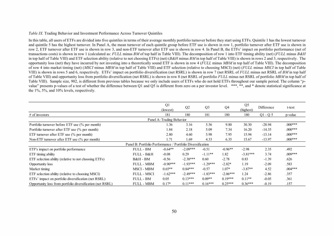
50

Table IX. Trading Behavior and Investment Performance Across Turnover Quintiles

In this table, all users of ETFs are divided into five quintiles in terms of their average monthly portfolio turnover before they start using ETFs. Quintile 1 has the lowest turnover

and quintile 5 has the highest turnover. In Panel A, the mean turnover of each quintile group before ETF use is shown in row 1, portfolio turnover after ETF use is shown in

row 2, ETF turnover after ETF use is shown in row 3, and non-ETF turnover after ETF use is shown in row 4. In Panel B, the ETFs’ impact on portfolio performance (net of

transactions costs) is shown in row 1 (calculated as: FULL minus BM of top half in Table VIII). The decomposition of row 1 into ETF timing ability (net) (FULL minus B&H

in top half of Table VIII) and ETF selection ability (relative to not choosing ETFs) (net) (B&H minus BM in top half of Table VIII) is shown in rows 2 and 3, respectively. The

opportunity loss (net) they have incurred by not investing into a theoretically sound ETF is shown in row 4 (FULL minus MBM in top half of Table VIII). The decomposition

of row 4 into market timing (net) (MSCI minus MBM in top half of Table VIII) and ETF selection (relative to choosing MSCI) (net) (FULL minus MSCI in top half of Table

VIII) is shown in rows 5 and 6, respectively. ETFs’ impact on portfolio diversification (net RSRL) is shown in row 7 (net RSRL of FULL minus net RSRL of BM in top half

of Table VIII) and opportunity loss from portfolio diversification (net RSRL) is shown in row 8 (net RSRL of portfolio FULL minus net RSRL of portfolio MBM in top half of

Table VIII). Sample size, 902, is different from previous tables because we only include users of ETFs who do not hold ETFs throughout our sample period. The column “p-

value” presents p-values of a test of whether the difference between Q1 and Q5 is different from zero on a per investor level. ***, **, and * denote statistical significance at

the 1%, 5%, and 10% levels, respectively.

Q1

(lowest)Q2 Q3 Q4

Q5

(highest)Difference t-test

# of investors 181 180 181 180 180 Q1 - Q 5 p-value

Panel A: Trading Behavior

Portfolio turnover before ETF use (% per month) 1.36 3.16 5.56 9.80 30.30 -28.94 .000***

Portfolio turnover after ETF use (% per month) 1.84 2.18 5.09 7.34 16.20 -14.35 .000***

ETF turnover after ETF use (% per month) 2.80 4.60 5.98 7.95 15.94 -13.14 .000***

Non-ETF turnover after ETF use (% per month) 1.71 1.69 4.33 6.35 15.67 -13.97 .000***

Panel B: Portfolio Performance / Portfolio Diversification

ETF's impact on portfolio performance FULL - BM -0.64** -2.09*** -0.51 -0.96** -2.98 2.35 .492

ETF timing ability FULL - B&H -0.08 0.29 -1.11** 1.82 -3.81*** 3.74 .009***

ETF selection ability (relative to not choosing ETFs) B&H - BM -0.56 -2.38*** 0.60 -2.78 0.83 -1.39 .626

Opportunity loss FULL - MBM -0.90*** -1.93*** -1.29*** -2.82* 1.19 -2.09 .583

Market timing MSCI - MBM 0.65** 0.84*** -0.57 1.07* -3.87** 4.52 .004***

ETF selection ability (relative to choosing MSCI) FULL - MSCI -1.62*** -2.49*** -1.83*** -2.06*** 1.24 -2.86 .357

ETFs’ impact on portfolio diversification (net RSRL) FULL - BM 0.05 0.13*** 0.09** 0.19*** 0.11** -0.05 .361

Opportunity loss from portfolio diversification (net RSRL) FULL - MBM 0.17* 0.11*** 0.16*** 0.25*** 0.36*** -0.19 .157

51

Table X. Trading Behavior and Investment Performance Across Portfolio Value Quintiles

In this table, all investors (users of ETFs and non-users of ETFs) divided into five quintiles in terms of their average monthly portfolio value before they start using ETFs.

Quintile 1 has the lowest value and quintile 5 has the highest value. In Panel A, the mean turnover of each quintile group before ETF use is shown in row 1, portfolio turnover

after ETF use is shown in row 2, ETF turnover after ETF use is shown in row 3, and non-ETF turnover after ETF use is shown in row 4. In Panel B (Portfolio Performance /

Portfolio Diversification), the ETFs’ impact on portfolio performance (net of transactions costs) is shown in row 1 (calculated as: FULL minus BM of top half in Table VIII).

The decomposition of row 1 into ETF timing ability (net) (FULL minus B&H in top half of Table VIII) and ETF selection ability (relative to not choosing ETFs) (net) (B&H

minus BM in top half of Table VIII) is shown in rows 2 and 3, respectively. The opportunity loss (net) they have incurred by not investing into a theoretically sound ETF is

shown in row 4 (FULL minus MBM in top half of Table VIII). The decomposition of row 4 into market timing (net) (MSCI minus MBM in top half of Table VIII) and ETF

selection (relative to choosing MSCI) (net) (FULL minus MSCI in top half of Table VIII) is shown in rows 5 and 6, respectively. ETFs’ impact on portfolio diversification (net

RSRL) is shown in row 7 (net RSRL of FULL minus net RSRL of BM in top half of Table VIII) and opportunity loss from portfolio diversification (net RSRL) is shown in row

8 (net RSRL of portfolio FULL minus net RSRL of portfolio MBM in top half of Table VIII). Sample size, 902, is different from previous tables because we only include users

of ETFs who do not hold ETFs throughout our observation period. The column “p-value” presents p-values of a test of whether the difference between Q1 and Q5 is different

from zero on a per investor level. ***, **, and * denote statistical significance at the 1%, 5%, and 10% levels, respectively.

Q1

(lowest)Q2 Q3 Q4

Q5




Portfolio turnover before ETF use (% per month) 13.78 11.85 8.74 8.56 7.16 6.62 .000***

Portfolio turnover after ETF use (% per month) 7.16 7.85 5.05 6.10 6.46 -0.70 .587

ETF turnover after ETF use (% per month) 6.97 7.58 7.10 7.42 8.19 1.23 .448

Non-ETF turnover after ETF use (% per month) 6.66 6.98 5.02 5.33 5.72 -0.94 .397


ETF's impact on portfolio performance FULL - BM -4.12 -0.79 -1.53*** 0.15 -0.87 -3.25 .333

ETF timing ability FULL - B&H -1.09 -1.55*** -0.87 0.84 -0.22 -0.86 .347

ETF selection ability (relative to not choosing ETFs) B&H - BM -3.03 0.75 -0.65 -0.69 -0.65 -2.38 .373

Opportunity loss FULL - MBM 1.07 -0.94 -2.23 -1.89 -1.76 -1.15 .447

Market timing MSCI - MBM 0.24 -0.54 -0.48 -1.07 -0.02 -0.37 .747

ETF selection ability (relative to choosing MSCI) FULL - MSCI -0.26 -1.95*** -2.62*** 0.02 -1.95*** 1.70 .571

ETFs’ impact on portfolio diversification (net RSRL) FULL - BM 0.15*** 0.09** 0.11*** 0.06* 0.17** -0.02 .799

Opportunity loss from portfolio diversification (net RSRL) FULL - MBM 0.39*** 0.20** 0.15*** 0.06 0.25*** 0.14 .305

52

Table XI. Trading Behavior and Investment Performance Across Relative Sharpe Ratio Loss Quintiles

In this table, all investors (users of ETFs and non-users of ETFs) are divided into five quintiles in terms of their average monthly relative Sharpe ratio loss (RSRL) before they

start using ETFs. Quintile 1 has the lowest RSRL while quintile 5 has the highest RSRL. In Panel A, the mean turnover of each quintile group before ETF use is shown in row

1, portfolio turnover after ETF use is shown in row 2, ETF turnover after ETF use is shown in row 3, and non-ETF turnover after ETF use is shown in row 4. In Panel B, the

ETFs’ impact on portfolio performance (net of transactions costs) is shown in row 1 (calculated as: FULL minus BM of top half in Table VIII). The decomposition of row 1

into ETF timing ability (net) (FULL minus B&H in top half of Table VIII) and ETF selection ability (relative to not choosing ETFs) (net) (B&H minus BM in top half of Table

VIII) is shown in rows 2 and 3, respectively. The opportunity loss (net) they have incurred by not investing into a theoretically sound ETF is shown in row 4 (FULL minus

MBM in top half of Table VIII). The decomposition of row 4 into market timing (net) (MSCI minus MBM in top half of Table VIII) and ETF selection (relative to choosing

MSCI) (net) (FULL minus MSCI in top half of Table VIII) is shown in rows 5 and 6, respectively. ETFs’ impact on portfolio diversification (net RSRL) is shown in row 7 (net

RSRL of FULL minus net RSRL of BM in top half of Table VIII) and opportunity loss from portfolio diversification (net RSRL) is shown in row 8 (net RSRL of portfolio

FULL minus net RSRL of portfolio MBM in top half of Table VIII). Sample size, 902, is different from previous tables because we only include users of ETFs who do not

hold ETFs throughout our sample period. The column “p-value” presents p-values of a test of whether the difference between Q1 and Q5 is different from zero on a per investor

level. ***, **, and * denote statistical significance at the 1%, 5%, and 10% levels, respectively.

Q1

(lowest)Q2 Q3 Q4

Q5




Portfolio turnover before ETF use (% per month) 9.54 7.82 9.90 11.38 11.47 -1.92 .166

Portfolio turnover after ETF use (% per month) 6.79 4.84 7.08 7.08 6.82 -0.04 .972

ETF turnover after ETF use (% per month) 6.74 6.21 7.15 9.33 7.82 -1.08 .426

Non-ETF turnover after ETF use (% per month) 6.20 4.10 7.47 5.70 6.24 -0.04 .969


ETF's impact on portfolio performance FULL - BM -0.52 -0.71 -1.55*** -3.83 -0.56 0.04 .972

ETF timing ability FULL - B&H 1.09 -1.76* -0.70 -1.26 -0.26 1.35 .488

ETF selection ability (relative to not choosing ETFs) B&H - BM -1.62 1.06 -0.85 -2.57 -0.30 -1.32 .566

Opportunity loss FULL - MBM -2.95 -1.57 -2.26 2.68 -1.62 -1.15 .449

Market timing MSCI - MBM -0.04 -1.83 -0.79 0.56 0.22 -0.37 .761

ETF selection ability (relative to choosing MSCI) FULL - MSCI -1.82*** -1.51 -2.18*** 0.86 -2.10*** 0.28 .763

ETFs’ impact on portfolio diversification (net RSRL) FULL - BM 0.13*** 0.03 0.16*** 0.08** 0.17** -0.04 .679

Opportunity loss from portfolio diversification (net RSRL) FULL - MBM 0.25*** 0.16*** 0.25*** 0.10*** 0.29** -0.05 .751

20160706 abusing etfs accepted ssrn - fresh funds · pdf fileelectronic copy available at :...

Documents