2016/01

■

A Dynamic Component Model for Forecasting High-Dimensional Realized Covariance Matrices

Luc Bauwens, Manuela Braione and Giuseppe Storti  

A dynamic component model for forecastinghigh-dimensional realized covariance matrices

L.Bauwens, M.Braione, G.Storti

Universite catholique de Louvain, CORE, and SKEMA Business School - Universite de Lille,luc.bauwens@uclouvain.be

Universite catholique de Louvain, CORE, manuela.braione@uclouvain.beUniversity of Salerno, DISES, storti@unisa.it

February 1, 2016

Abstract

The Multiplicative MIDAS Realized DCC (MMReDCC) model of Bauwens et al. [5] decom-poses the dynamics of the realized covariance matrix of returns into short-run transitoryand long-run secular components where the latter reflects the effect of the continuouslychanging economic conditions. The model allows to obtain positive-definite forecasts ofthe realized covariance matrices but, due to the high number of parameters involved, es-timation becomes unfeasible for large cross-sectional dimensions. Our contribution in thispaper is twofold. First, in order to obtain a computationally feasible estimation procedure,we propose an algorithm that relies on the maximization of an iteratively re-computedmoment-based profile likelihood function. We assess the finite sample properties of theproposed algorithm via a simulation study. Second, we propose a bootstrap procedurefor generating multi-step ahead forecasts from the MMReDCC model. In an empiricalapplication on realized covariance matrices for fifty equities, we find that the MMReDCCnot only statistically outperforms the selected benchmarks in-sample, but also improvesthe out-of-sample ability to generate accurate multi-step ahead forecasts of the realizedcovariances.

Keywords: Realized covariance, dynamic component models, multi-step forecasting,MIDAS, targeting, model confidence set.

1. Introduction

Building models for predicting the volatility of high dimensional portfolios is importantin risk management and asset allocation. Previous developments on time-varying covari-ances in large dimensions include the constant conditional correlation (CCC) model ofBollerslev [8], where the volatilities of each asset are allowed to vary through time but thecorrelations are time invariant, the RiskMetrics model by [27], and the DECO model byEngle and Kelly [18] who allow correlations to change over time and can be easily applied

1

in vast dimensions. Recently, Andersen et al. [2], Barndorff-Nielsen and Shephard [4] andBarndorff-Nielsen et al. [3], among others, opened up a new channel for increasing the pre-cision of covariance matrix estimates and forecasts by exploiting the information of highfrequency asset returns. This development has motivated several researchers to investigatemodels directly fitted to series of realized covariance matrices (see Gourieroux et al. [22],Jin and Maheu [25] and Chiriac and Voev [11], among others).

Despite the superiority of these models, illustrated for example by Hautsch et al. [24],there still remain technical and practical challenges one needs to deal with when con-structing covariance matrix forecasts for high-dimensional systems. First and foremost,the well-known “curse of dimensionality” problem, implying that the number of parame-ters grows as a power function of the cross-sectional model dimension. In order to saveparameters, a simple solution is represented by the so called covariance (or correlation)targeting approach of Engle [15], which consists in pre-estimating the constant interceptmatrix in the model specification by linking it to the unconditional covariance matrix ofreturns. This method can be applied under the stationarity assumption of the model andis one of the most widely employed techniques to simplifying parameter estimation andreducing the computational burden when the numerical maximization of the likelihoodfunction becomes difficult.

Recently, Bauwens et al. [5] investigated a wide class of multivariate models that simul-taneously account for short and long-term dynamics in the conditional (co)volatilities andcorrelations of asset returns, in line with the empirical evidence suggesting that their level ischanging over time as a function of the economic conditions (see, among others, Engle et al.[16]). Herein we focus on the Multiplicative MIDAS Realized DCC (MMReDCC) model,whose main ingredients are a multiplicative component structure, a Mixed Data Sampling(MIDAS) filter to modeling the secular dynamics and a DCC-type parameterization forthe short term component, directly inspired by the multivariate GARCH literature.1 Theextensive out-of-sample forecasting comparison performed by Bauwens et al. [5], althoughnot identifying a clear winner, shows that the MMReDCC model gives remarkably goodperformances in important financial applications such as Value-at-Risk forecasting andportfolio allocation. However, their results are limited to a relatively low dimensionalsetting (10 assets) and to a short-term forecasting horizon (1 day).

This paper extends the work by Bauwens et al. [5] along these directions: estimationfor high-dimensional systems and multi-step forecasting. We contribute to the first line ofresearch by developing of a computationally feasible procedure for the estimation of vastdimensional MMReDCC models. In this respect, it is important to remark that, althoughthe introduction of a dynamic secular component in the structure of the model adds a majorelement of flexibility and enables to obtain more accurate forecasts than standard modelsreverting to constant mean levels (see Bauwens et al. [5]), it also dramatically increases thenumber of parameters to be estimated. Specifically, the long term component incorporates

1We refer to Engle [14] and Ghysels et al. [20] as leading references for detailed discussions of the DCC

model and MIDAS regressions.

2

a scale intercept matrix with number of parameters equal to n(n+ 1)/2, where n denotesthe number of assets. In a vast dimensional framework, this quickly translates into theimpossibility of estimating the model since the intercept matrix cannot be directly targeted.

Therefore, we propose to overcome this estimation issue by proposing an iterative proce-dure inspired by the covariance targeting of Engle [15]. More precisely, based on a Methodof Moments estimator, we profile out the parameters of the intercept matrix and iterativelymaximize the likelihood in terms of the other parameters of interest. We refer to this asthe Iterative Moment-Based Profiling (IMP) estimator, as opposed to the Quasi MaximumLikelihood (QML) estimator which directly maximizes the likelihood with respect to thefull parameter vector.

It is worth noting that the proposed estimation procedure can be considered a switchingalgorithm in the sense discussed by Boswijk [9] and Cubadda and Scambelloni [13] since themaximization of the overall likelihood is obtained by switching between optimizations overdifferent blocks of parameters. This idea has a long standing tradition in the econometricanalysis of time series. A simple, well known example of switching algorithm is given bythe Cochrane-Orcutt iterative estimation procedure. Compared to conventional switchingalgorithms, the procedure that is here implemented incorporates an additional targetingstep. In particular, it reduces the dimension of the optimization problem to be solved byconcentrating out some of the parameters, the elements of the intercept matrix, by meansof an iteratively re-computed moment-based estimator. A comprehensive simulation studyis performed to assess the finite-sample properties of the proposed estimator which is foundto deliver unbiased estimates and to quickly converge, as no more than three iterations arerequired in general.

The second relevant contribution of the paper is the development of a resampling basedprocedure for the generation of multi-step ahead forecasts of the realized covariance matri-ces. The multiplicative component structure of the MMReDCC model makes the derivationof a closed-form expression for the h-step predictor impossible. Hence, to solve this issue weuse a distribution-free procedure based on a residual bootstrap method. The bootstrap hasbeen a standard tool for generating multi-step forecasts from non-linear and non-Gaussiantime series models for more than two decades (see e.g. Clements and Smith [12]). Its usehas been later extended to univariate volatility modeling (see e.g. Pascual and Ruiz [29];Shephard and Sheppard [31]). More recently, Fresoli and Ruiz [19] have proposed a simpleresampling algorithm that makes use of residual bootstrap to compute multi-step forecastsfrom DCC models. The bootstrap procedure which is implemented in this paper builds onthe work of Fresoli and Ruiz [19] but the algorithm is adapted to the dynamic modeling ofrealized covariance matrices.

Finally, the results of two different applications to real data are presented and discussed.In the first one, we focus on a low dimensional setting (ten assets), in which both the IMPand one-step QML estimation procedures are feasible, and compare the estimates obtainedby means of both algorithms. We find that the IMP-based estimates are sufficiently close tothe QML ones, so that using the IMP method in large dimensions is a sensible approach. Inthe second application the MMReDCC model estimated for fifty assets by the IMP methodis used to generate forecasts of the realized covariance matrix, up to twenty days ahead,

3

and compared to existing benchmarks not accounting for short and long term (co)volatilitydynamics. For the dataset considered, in correspondence of a forecasting horizon equal toone day, the MMReDCC model is outperformed by the benchmarks while it dominates forlonger horizons up to ten days.

The remainder of the paper is organized as follows. Section 2 briefly recalls the struc-ture of the MMReDCC model and explains the curse of dimensionality issue. Section 3introduces the IMP algorithm and Section 4 presents the results of a Monte Carlo experi-ment aimed at assessing the finite sample statistical properties of the proposed estimationalgorithm. The bootstrap procedure for computing multi-step ahead forecasts is explainedin Section 5. Section 6 contains the empirical results for the in-sample estimation com-parison and the out-of-sample forecasting exercise. Section 7 concludes with some finalremarks.

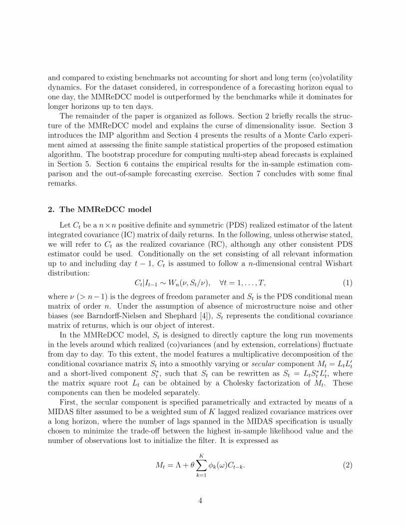
2. The MMReDCC model

Let Ct be a n×n positive definite and symmetric (PDS) realized estimator of the latentintegrated covariance (IC) matrix of daily returns. In the following, unless otherwise stated,we will refer to Ct as the realized covariance (RC), although any other consistent PDSestimator could be used. Conditionally on the set consisting of all relevant informationup to and including day t − 1, Ct is assumed to follow a n-dimensional central Wishartdistribution:

Ct|It−1 ∼ Wn(ν, St/ν), ∀t = 1, . . . , T, (1)

where ν (> n−1) is the degrees of freedom parameter and St is the PDS conditional meanmatrix of order n. Under the assumption of absence of microstructure noise and otherbiases (see Barndorff-Nielsen and Shephard [4]), St represents the conditional covariancematrix of returns, which is our object of interest.

In the MMReDCC model, St is designed to directly capture the long run movementsin the levels around which realized (co)variances (and by extension, correlations) fluctuatefrom day to day. To this extent, the model features a multiplicative decomposition of theconditional covariance matrix St into a smoothly varying or secular component Mt = LtL

′t

and a short-lived component S∗t , such that St can be rewritten as St = LtS∗tL′t, where

the matrix square root Lt can be obtained by a Cholesky factorization of Mt. Thesecomponents can then be modeled separately.

First, the secular component is specified parametrically and extracted by means of aMIDAS filter assumed to be a weighted sum of K lagged realized covariance matrices overa long horizon, where the number of lags spanned in the MIDAS specification is usuallychosen to minimize the trade-off between the highest in-sample likelihood value and thenumber of observations lost to initialize the filter. It is expressed as

Mt = Λ + θK∑k=1

φk(ω)Ct−k. (2)

4

In the right hand side of Eq.(2), the first term Λ is a n × n symmetric and semi-positivedefinite matrix of constant parameters, θ is a positive scalar and φk(·) is a weight functionparametrized according to the restricted Beta polynomial

φk(ω) =

(1− k

K

)ω−1∑Kj=1

(1− j

K

)ω−1 ,

The scalar parameter ω dictates the shape of the function and in order to achieve a time-decaying pattern of the weights, it is constrained to be larger than 1. For identification,the constraint

∑Kk=1 φk(ω) = 1 is imposed.

Second, the dynamics of the short term component S∗t is specified according to a scalarDCC parametrization that enables a separate treatment of conditional volatilities andcorrelations, thus allowing for a high degree of flexibility. Letting X be any square matrixof arbitrary size n, in the remainder the notation diag(X) is used to denote a n×n diagonalmatrix with non-zero elements equal to the diagonal elements of X. Therefore, assumingthat S∗t = D∗tR

∗tD∗t , where D∗t = diag{S∗t }1/2, their scalar specifications correspond to the

following equations:

S∗ii,t = (1− γi − δi) + γiC∗ii,t−1 + δiS

∗ii,t−1, ∀i = 1, . . . , n (3)

R∗t = (1− α− β)In + αP ∗t−1 + βR∗t−1, (4)

where γi > 0, δi ≥ 0, γi + δi < 1, α > 0, β ≥ 0, α + β < 1, C∗t = L−1t Ct(L

′t)−1 and

P ∗t = (diag{C∗t })−1/2C∗t (diag{C∗t })−1/2. The matrix C∗t is the realized covariance matrixpurged of its long term component and the matrix P ∗t is the corresponding short termrealized correlation matrix. Mean reversion to unity in Eq.(3) and to an identity matrixin Eq.(4) is needed for identification of the different components. Let γ = {γ1, ..., γn},δ = {δ1, ..., δn} for further use.

The parameters can be estimated by maximizing the following Wishart (quasi) log-likelihood function in one step:

`T (ψ) = −1

2

T∑t=1

{log |St(ψ)|+ tr

[St(ψ)−1Ct

]}. (5)

The finite-dimensional parameter vector ψ = {vech(Λ), θ, ω,γ, δ, α, β}2, has length {nΛ +2n+4} where nΛ = n(n+1)/2 = O(n2) denotes the number of unique parameters includedin the intercept matrix Λ of Eq.(2). It is obvious that, as n increases, the curse of dimen-sionality problem quickly arises, leading to the number of parameters listed in the first tworows of Table 1. Observe that estimation becomes already cumbersome after n = 20 andalmost impossible for n ≥ 50.

2Note that ψ do not include the degree of freedom parameter ν, as the first order conditions for the

estimation of the parameter vector ψ do not depend on ν by linearity in ν (see [5]).

5

Table 1: Number of parameters of MMReDCC models

n = 5 n = 10 n = 20 n = 50 n = 100

nΛ 15 55 210 1275 5050

ψ 29 79 254 1379 5254

ψ 14 24 44 104 204

Note: Entries report the number of parameters as a function of the dimension n; nΛ denotes the number of unique parameters

contained in the Λ matrix, ψ denotes the full vector of model parameters and ψ the vector of parameters excluding nΛ.

On the other hand, the last row of Table 1 shows that an intuitive way to keep themodel tractable is to avoid estimating the parameters of the matrix Λ. This would besufficient to reduce the order to 2n+ 4 = O(n), thus making the model estimable also forlarge n.In the following section we put forward a feasible estimation procedure that aims at over-coming the direct estimation of the long term component intercept matrix, thus cruciallymitigating the computational complexity of the model.

3. An Iterative Moment based Profiling (IMP) algorithm

In this section we discuss an iterative procedure for fitting the MMReDCC modelto large dimensional datasets. The basic idea underlying the proposed algorithm is toeliminate from the likelihood maximization the parameters of the intercept matrix Λ usinga technique that builds upon the covariance targeting discussed in Pedersen and Rahbek[30] for BEKK and Engle et al. [17] for DCC models. First of all, notice that from Eq.(2)and the following relation

Λ = E(Mt)− θK∑k=1

φk(ω)E(Ct−k),

a moment based estimator of the Λ intercept matrix is

Λ =1

T

T∑t=1

[Mt − θ

K∑k=1

φk(ω)Ct−k

]. (6)

Obviously, given the latent nature of Mt, the estimator in Eq.(6) cannot be computed inpractice and hence the covariance targeting approach cannot be applied in the usual way.It is worth noting that, if Lt and S∗t were assumed to be independent, given E(S∗t ) = In,it would hold that E(Ct) = E(Mt), implying that an asymptotically equivalent version ofEq.(6) could be explicitly computed replacing Mt by Ct. However, this is not the approachwe pursue, since the assumption of independence of the short and long term sources is

6

difficult to justify and would result in a rather counterintuitive and arbitrary constraint.Hence, we adopt a different method.

By noting from Eq.(6) that no estimate of Λ makes sense regardless of the value of(θ, ω), we make this dependence explicit and obtain an estimate of Λ as a function of(θ, ω), i.e. Λ(θ, ω). In this way, a different estimate of Λ is required for each different valueof the other two parameters. Therefore, by substituting Λ(θ, ω) for Λ in the Wishart QMLfunction stated in Eq.(5), the following moment based QML approximation is obtained:

˜T (ψ) = −1

2

T∑t=1

{log |Lt(θ, ω)S∗t (ψ)L′t(θ, ω)|+ tr

{[Lt(θ, ω)S∗t (ψ)L′t(θ, ω)

]−1Ct}}

(7)

with ψ = (ω, θ,ψS∗)′, ψ′S∗ = (γ, δ, α, β) and

Mt(θ, ω) = Lt(θ, ω)L′t(θ, ω) = Λ(θ, ω) + θK∑k=1

φk(ω)Ct−k. (8)

The method we propose consists of estimating the parameters in ψ by a block-wisemaximization of the moment-based QML function given in Eq.(7). First, conditional onsome reasonable initial guess of (θ, ω), ˜

T (ψ) is maximized with respect to the short termparameters ψS∗ and then, conditional on ψS∗ , the same function is maximized with respectto (θ, ω). The procedure is iterated for j = 0, . . . , J until some pre-specified convergencecriterion is met.

To initialize the algorithm at j = 0, one can reasonably use as starting values theparameter estimates obtained by fitting the model to low dimensional subsets of data;also, an initial guess for the long term component Mt,0 could be either provided in a naiveway, i.e. using the series of observed realized covariance matrices directly, or in a moresophisticated manner, by fitting to the data a nonparametric kernel smoother with anoptimized bandwidth parameter. Note that in order to guarantee the positive definitenessof Mt(θ, ω) in Eq.(8), it suffices to initialize Mt,0 from a PDS matrix and to impose θ > 0.

Given that the observed series of Ct, for every t, is PDS by definition, Λ(θ, ω) is assuredto be at least semi-positive definite at each iteration j > 0.

Once Λj(θj, ωj) has been computed at the initial iteration j = 0, for every j > 0 thesteps conducted in the algorithm are as follows:

Step 1 Plug Λj−1(θj−1, ωj−1) into Eq.(2), then get Mt,j and Lt,j = chol(Mt,j) for all t;Step 2 For each asset i = 1, ...n, obtain the short term GARCH(1,1) parameters of Eq.(3)

as follows{γi,j, δi,j} = arg max

{γi,δi}˜T (θj−1, ωj−1, αj−1, βj−1) ;

Step 3 Conditional on the estimated vectors γj = (γ1,j, . . . , γn,j)′ and δj = (δ1,j, . . . , δn,j)

′,maximize the same log-likelihood function with respect to the short term DCC cor-relation parameters:

{αj, βj} = arg max{α,β}

˜T

(θj−1, ωj−1,γj, δj

);

7

Step 4 Finally, conditional on the vector of short term parameter estimates φS∗ = {γj, δj, αj,βj}, maximize ˜

T with respect to {θj, ωj}; these estimates are used to compute anupdated version of Λj(θj, ωj);

Step 5 Check for convergence otherwise update all parameter estimates and go back to Step1.

It is worth to stress that although ˜T (ψ) looks like a profile likelihood, it is not since Λ(θ, ω)

is not a QML estimator but a feasible moment estimator. This motivates our choice to referto Steps 1− 5 as the Iterative Moment based Profiling algorithm, or IMP for short. Thisimplies that ψ is typically less efficient than the standard QML estimator that maximizesEq.(5) in one step. We come back to this issue in Section 6.1.

4. Simulation study

A Monte Carlo study is conducted to analyse the finite sample properties of the IMPestimator. We assume the MMReDCC to be the DGP and we generate 500 processes oflength T = 1000 and 2000 for n = 10, 20, 40 and 50, with true parameter values inspiredby the estimates given in Bauwens et al. [5], as summarized in Table 2.

It is important to stress that, in order to initialize the algorithm, parameter valueshave to be carefully chosen. This is a standard requirement in every optimization basedprocedure where the initial amount of information on the model parameters can be limitedor even null. In our situation we are mainly concerned with the impact that differentchoices of Mt,0, more than the remaining set of parameters, may have on the convergenceof the IMP algorithm. We evaluate this by performing a robustness check based on thetwo possible initializations of Mt,0 mentioned in Section 3.

In the first set of repetitions Mt,0 is computed by fitting to the series of simulated realizedcovariance matrices a Nadaraya-Watson kernel estimator with a single bandwidth param-eter for the whole covariance matrix. As in Bauwens et al. [5] and Bauwens et al. [6],the optimal bandwidth is selected by a least squares cross-validation criterion, where thesix-month rolling covariance is used as the reference for the computation of least squares.In the second (equivalent) simulation study, Mt,0 is obtained by substituting in Eq. (6)the observed Ct for the latent matrix Mt at each t. In both cases, the initial scalar modelparameters are set equal to the values listed in Panel B of Table 2.

The estimation bias is evaluated by the relative bias (RB), computed as 1500

∑500i=1

ψi−ψψ

,

along with the interquartile range (IQR), mean, minimum and maximum of the obtainedparameter estimates. To save space, we report averaged bias results for the parameters ofthe MIDAS intercept matrix in a separate table.

Table 3 reports results from the first simulation exercise. The emerging picture looksencouraging. As expected, the relative biases decrease as n or T increases. The biasesfor the parameters of the short term volatility and correlation components are very small,being smaller than five per cent in most of the cases, with one exception recorded for γ atT = 1000 for n = 10. As for the scalar parameters in the MIDAS specification, the bias

8

Table 2: Simulation setting

Panel A: Parameters

Long term component

θ 0.5

K 264

ω 15

Λ Λi,i = 0.02, Λi,j = 0.002 for i 6= j

Short term components

γi ∼ U(γ0 − 0.02, γ0 + 0.02), γ0 = 0.2

δi ∼ U(2δ0 + γi − 1 + 0.01, 1− γi − 0.01), δ0 = 0.7

α 0.2

β 0.7

General

ν 2n

T 1000, 2000

initial discarded observations 1000

convergence tolerance 0.0001

Panel B: Initial values

θ0 ω0 γi,0 δi,0 α0 β0

0.8 10 0.05 0.90 0.05 0.9

Note: In Panel A, for every i = 1, ..., n it holds {γi + δi} < 1. Entries of Panel B are scalar parameters chosen to initialize

the algorithm in both sets of simulation exercises.

for θ is negative in seven out of eight cases (the exception occurs for n = 10 at T = 2000)and ranging from the maximum of 5.8% (in absolute value) for n = 10 and T = 1000 tothe lowest value of 0.1% for n = 50 and T = 2000. The bias on the ω parameter, alsogenerally negative, tends to decrease with n but is usually of higher order (from 1.1 to 12%in absolute value). A similar behavior is observed for the IQR measure, which decreasesacross n and T but remains on higher values for the parameter ω. However, this doesnot represent a major concern as the Beta weight function is not very sensitive to smallvariations of this parameter and therefore we do not expect the likelihood function to beeither.

Table 4 gives an idea of the robustness of the results to the other initialization of thelong term component. Entries can be directly compared to those in Table 3. As hopedfor, the initial choice has a minor impact on the overall accuracy of the estimator, as theparameter biases are in the same range of magnitude and the comments made earlier arestill valid under this alternative scenario. Figure C.2 contains plots of the Monte Carlostandard deviations of the estimated θ, ω, α and β parameters against the cross-section size.

9

Table 3: Simulation exercise I: summary statistics

T= 1000 T= 2000

γ δ α β θ ω γ δ α β θ ω2

0.197 0.705 0.2 0.7 0.5 15 0.197 0.705 0.2 0.7 0.5 15

n=10 n=10

RB 0.098 -0.036 0.020 0.003 -0.058 -0.120 RB -0.039 -0.002 0.033 0.003 0.053 -0.095

IQR 0.048 0.093 0.006 0.010 0.044 1.641 IQR 0.032 0.068 0.006 0.008 0.037 1.819

Mean 0.202 0.699 0.204 0.702 0.475 14.820 Mean 0.2 0.713 0.207 0.702 0.526 13.58

Min 0.176 0.660 0.191 0.679 0.393 7.460 Min 0.153 0.669 0.183 0.523 0.072 1.949

Max 0.214 0.735 0.220 0.728 0.709 18.943 Max 0.22 0.803 0.37 0.817 1.000 17.74

n=20 n=20

RB 0.049 -0.009 0.019 0.001 -0.056 -0.110 RB 0.036 0.011 0.024 0.002 -0.014 -0.080

IQR 0.046 0.083 0.003 0.006 0.019 0.713 IQR 0.031 0.079 0.002 0.004 0.015 0.622

Mean 0.202 0.701 0.204 0.701 0.472 14.782 Mean 0.209 0.708 0.205 0.702 0.496 13.801

Min 0.171 0.633 0.197 0.687 0.430 12.802 Min 0.197 0.678 0.200 0.694 0.001 2.440

Max 0.219 0.744 0.211 0.711 0.532 16.759 Max 0.221 0.739 0.220 0.748 0.598 15.270

n=40 n=40

RB 0.028 0.023 0.015 0.002 -0.049 -0.080 RB 0.033 0.029 0.022 0.002 -0.014 -0.072

IQR 0.042 0.077 0.002 0.002 0.011 0.372 IQR 0.030 0.064 0.001 0.002 0.007 0.263

Mean 0.208 0.715 0.203 0.701 0.476 14.810 Mean 0.209 0.719 0.204 0.702 0.493 13.925

Min 0.190 0.656 0.060 0.695 0.446 3.735 Min 0.181 0.671 0.182 0.674 0.172 1.000

Max 0.217 0.762 0.222 0.799 0.705 16.500 Max 0.221 0.761 0.223 0.744 0.837 14.760

n=50 n=50

RB 0.027 0.011 0.016 0.001 -0.045 0.012 RB 0.029 0.027 0.017 0.001 -0.011 -0.037

IQR 0.042 0.076 0.001 0.002 0.008 0.293 IQR 0.030 0.056 0.001 0.002 0.007 0.220

Mean 0.208 0.716 0.203 0.701 0.473 15.182 Mean 0.208 0.720 0.203 0.701 0.494 14.442

Min 0.162 0.644 0.200 0.697 0.455 13.150 Min 0.191 0.657 0.199 0.695 0.474 12.089

Max 0.220 0.814 0.207 0.705 0.525 15.830 Max 0.222 0.763 0.207 0.707 0.529 16.238

Note: Summary statistics of the first set of simulations where Mt,0 is initialized using a nonparametric kernel estimator, see

Section 3. To save on space, γ and δ are reported as averaged values across series and replications. RB denotes the Relative

Bias computed over 500 replications. True parameter values used to simulate the process at the top of the table.

In all cases, standard deviations tend to decline as the cross-section dimension grows, witha faster decline when T = 2000. The two approaches produce similar parameter standarddeviations, with slightly bigger values recorded for θ and ω under the second simulationexperiment in correspondence with the higher cross-section sizes.

If we move to analyzing the bias results for the scale MIDAS intercept matrix, Table 5shows that under both sets of simulation exercises the estimator Λ(θ, ω) well approximatesthe true Λ matrix at all cross-section dimensions, with the parameter bias (averaged acrossdiagonal and off-diagonal elements) clearly improving with increasing n and T . Again, thedirect comparison of Panels A and B confirms that the algorithm initialized from the series

10

Table 4: Simulation exercise II: summary statistics

T= 1000 T= 2000

γ δ α β θ ω γ δ α β θ ω2

0.197 0.705 0.2 0.7 0.5 15 0.197 0.705 0.2 0.7 0.5 15

n=10 n=10

RB -0.077 0.013 0.019 0.002 -0.032 -0.007 RB 0.043 0.006 0.025 0.002 -0.012 -0.069

IQR 0.070 0.113 0.007 0.010 0.043 1.664 IQR 0.028 0.046 0.004 0.007 0.024 0.870

Mean 0.191 0.708 0.204 0.701 0.484 14.892 Mean 0.211 0.707 0.205 0.701 0.494 13.959

Min 0.107 0.588 0.191 0.678 0.393 6.678 Min 0.189 0.654 0.196 0.686 0.435 9.614

Max 0.231 0.833 0.218 0.723 0.927 19.237 Max 0.232 0.748 0.213 0.715 0.623 15.535

n=20 n=20

RB 0.048 -0.002 0.018 0.002 -0.045 -0.008 RB 0.006 0.039 0.023 0.002 -0.011 -0.064

IQR 0.042 0.085 0.003 0.005 0.021 0.719 IQR 0.030 0.060 0.002 0.004 0.013 0.510

Mean 0.207 0.702 0.204 0.701 0.477 14.887 Mean 0.206 0.721 0.205 0.701 0.494 14.047

Min 0.196 0.649 0.197 0.689 0.429 6.751 Min 0.164 0.680 0.199 0.692 0.467 11.108

Max 0.220 0.740 0.214 0.713 0.887 16.573 Max 0.225 0.772 0.209 0.710 0.555 15.241

n=40 n=40

RB 0.046 0.017 0.017 0.003 -0.045 0.005 RB 0.050 0.016 0.021 0.002 -0.012 -0.057

IQR 0.042 0.080 0.002 0.003 0.010 0.421 IQR 0.029 0.053 0.001 0.002 0.007 0.245

Mean 0.209 0.713 0.203 0.702 0.477 15.078 Mean 0.210 0.718 0.204 0.701 0.494 14.148

Min 0.197 0.682 0.193 0.696 0.116 6.895 Min 0.194 0.658 0.202 0.697 0.479 8.433

Max 0.219 0.756 0.216 0.807 0.955 49.985 Max 0.223 0.768 0.212 0.708 0.726 14.638

n=50 n=50

RB 0.029 0.028 0.016 0.002 -0.053 0.015 RB 0.028 0.018 0.020 0.002 -0.017 -0.048

IQR 0.041 0.071 0.001 0.002 0.009 0.342 IQR 0.030 0.061 0.001 0.001 0.005 0.195

Mean 0.208 0.715 0.203 0.701 0.473 15.225 Mean 0.208 0.721 0.204 0.701 0.492 14.278

Min 0.190 0.632 0.200 0.698 0.457 14.190 Min 0.184 0.674 0.202 0.698 0.437 11.178

Max 0.220 0.766 0.206 0.705 0.494 15.844 Max 0.216 0.766 0.209 0.713 0.508 14.742

Note: Summary statistics of the second set of simulations where Mt,0 is initialized from the series of realized covariance

matrices, see Section 3. To save on space, γ and δ are reported as averaged values across series and replications. RB denotes

the Relative Bias computed over 500 replications. True parameter values used to simulate the process at the top of the table.

of realized covariance matrices overall performs no worse than the one initialized from anonparametric smoother.

To summarize, the simulation study carried out in this section suggests that the pro-posed algorithm works quite accurately in finite samples and converges irrespective of theinitialization choice made. Overall, the moment-based estimator used for iteratively tar-geting the constant intercept matrix in the secular component does not create a severe biasproblem in the estimation of the other parameters, thus representing a feasible solutionto alleviate the curse of dimensionality issue that would otherwise prevent the use of theMMReDCC model in high dimensional applications. Both initialization methods for Mt,0

11

Table 5: Bias results for the scale MIDAS intercept matrix.

Panel A: Simulation exercise I

T=1000 T=2000

n=10 n=10

RB{i,i} 0.080 RB{i,i} 0.033

RB{i,j} 0.079 RB{i,j} 0.000

n=20 n=20

RB{i,i} 0.073 RB{i,i} 0.068

RB{i,j} 0.062 RB{i,j} 0.048

n=40 n=40

RB{i,i} 0.073 RB{i,i} 0.062

RB{i,j} 0.061 RB{i,j} 0.046

n=50 n=50

RB{i,i} 0.072 RB{i,i} 0.004

RB{i,j} 0.057 RB{i,j} 0.037

Panel B: Simulation exercise II

T=1000 T=2000

n=10 n=10

RB{i,i} 0.075 RB{i,i} 0.060

RB{i,j} 0.066 RB{i,j} 0.040

n=20 n=20

RB{i,i} 0.072 RB{i,i} 0.058

RB{i,j} 0.060 RB{i,j} 0.044

n=40 n=40

RB{i,i} 0.073 RB{i,i} 0.058

RB{i,j} 0.159 RB{i,j} 0.043

n=50 n=50

RB{i,i} 0.072 RB{i,i} 0.058

RB{i,j} 0.058 RB{i,j} 0.043

Note: RB{i,i} denotes averaged values over diagonal terms, while RB{i,j} denotes averages over off diagonal terms. Panel

(a) reports summary statistics of the first simulation exercise where Mt,0 is initialized from a nonparametric smoother while

Panel (b) reports results from the second simulation exercise where the series of observed realized covariance matrices are

used.

can be used in practice. In the empirical section, we have opted for the nonparametricsmoother.

5. Multi-step Forecasting

Models featuring short and long-run dynamics are particularly attractive for computingmulti-step-ahead predictions, as their component dynamic structure is possibly expectedto be beneficial for longer-term forecasts. The complex nonlinear structure of the MM-ReDCC model makes the analytical derivation of closed-form solutions impossible. In orderto overcome this problem, we propose to compute multi-step predictions by means of aprocedure based on bootstrap resampling.

At the outset, notice that Eq.(1) implies that E(Ct|=t−1) = St, so that Ct can berepresented as

Ct = S1/2t Ut(S

1/2t )′ (9)

where Ut is an element of a sequence of iid random matrices such that E(Ut) = In, and

S1/2t is any PDS matrix such that S

1/2t (S

1/2t )′ = St. The Wishart assumption of Eq.(1) is

recovered if Ut ∼ Wn(ν, In/ν), but this assumption is not needed to justify the bootstrapprocedure that we use for generating multi-step-ahead forecasts of the realized covariancematrix Ct. The procedure is described in the following six steps.

12

Step 1 Estimate the model on {Ct, t = 1, . . . , T} and obtain the estimated conditional co-variances St.

Step 2 Compute the estimated residuals

Ut = S−1/2t Ct(S

−1/2t )′, t = 1, . . . , T

and rescale them to enforce their sample mean to be equal to In, namely:

Ut = (E−1/2u )Ut(E

−1/2u )′,

where Eu = (1/T )∑T

t=1 Ut. The rescaled Ut can then be used to generate bootstrapreplicates of CT+j, for j = 1, . . . , h, where h denotes the chosen forecast horizon.

Step 3 Draw with replacement a bootstrap sample {UT+1|T , . . . , UT+h|T} of length h from

the empirical CDF of {Ut, t = 1, . . . , T}.Step 4 For j = 1 . . . , h, recursively generate a sequence of bootstrap replicates of CT+j as

follows

MT+j|T = Λ(θ, ω) + θK∑k=1

φk(ω)CT−k+j|T

LT+j|T = M1/2T+j|T

C∗T+j|T = LT+j|TCT+j(L′

T+j|T )−1

P ∗T+j|T = (diag{C∗T+j|T})−1/2C∗T+j|T (diag{C∗T+j|T})−1/2

S∗ii,T+j|T = (1− γi − δi) + γiC∗ii,T+j−1|T + δiS

∗ii,T+j−1|T

R∗T+j|T = (1− α− β)In + αP ∗T+j−1|T + βR∗T+j−1|T

S∗T+j|T = (diag{S∗T+j|T})1/2R∗T+j|T (diag{S∗T+j|T})1/2

ST+j|T = LT+j|TS∗T+j|TL

′T+j|T

CT+j|T = = (S1/2T+j|T )UT+j(S

1/2T+j|T )

′

Step 5 Repeat steps 3-4 B times, where B is set sufficiently large (e.g. B=10000). As a result

the procedure generates an array of h×B bootstrap replicates C(b)T+j|T (b = 1, . . . , B).

Step 6 Finally, the h-steps-ahead forecast can be computed as

ST,j =1

B

B∑b=1

C(b)T+j|T .

Even if our primary interest is in forecasting from MMReDCC models, the proposedforecasting procedure is very general and can be readily adapted to any model that admitsthe representation in Eq.(9), where St is modeled as a function of past information It−1.For example, in the empirical application which is being presented in Section 6.2, we alsouse it to generate multi-step ahead forecasts of Ct from the cRDCC model of Bauwenset al. [7]. To this purpose, the dynamic equations in step 4 must be replaced by thosepertaining to the specific model of interest.

13

6. Empirical Applications

This section contains two empirical applications. The first application provides theestimation results for the IMP estimator in comparison with the standard QML estimatorin the ideal case where both can be computed. The second one is performed in a largedimensional system and aims at evaluating both the full-sample fit of the model and itsforecasting performance. Specifically, we evaluate the ability of the MMReDCC model toprovide accurate multi-step-ahead covariance predictions against existing competitors notaccounting for time-varying long term dynamics.

6.1. Small sample accuracy comparison

As regards the in-sample performance, we are interested in comparing the estimatesprovided by the IMP method to the QML ones that are obtained by maximizing thelikelihood over the full parameter vector and can only be used in low dimensional cases(remember Table 1). For this purpose, we fix the cross-sectional dimension equal to tenassets and use three different datasets. An overview of the data being used is given inAppendix A. The first dataset comprises the assets used in Bauwens et al. [5] and includesseries of daily realized covariance matrices estimated on five minute intraday returns overthe period February 2001 to December 2009; the second and third sets comprise arbitraryselected subsamples of the dataset used in the work of Boudt et al. [10] which consists ofseries of daily realized covariance matrices obtained with the CholCov estimator over theperiod January 2007 to December 2012.3 As already mentioned before, the choice of therealized estimator is not an issue here as the model can be fitted to any series of realizedvariance-covariance matrices as long as they are guaranteed to be PDS.

Estimation results for the MMReDCC model by both the IMP and the QML estimatorsare reported in Table 6.

In the three datasets considered, both methods appear to deliver similar estimates.Short term GARCH coefficients tend to be quite homogeneous across assets and generallysignificant; the same applies to the short term correlation estimates. As for the parametersdriving the long term component, it can be noticed that the estimated θ and ω coefficientsare regularly lower for the IMP than for the QML method. This is in line with the prevail-ing negative bias reported from the simulation study. The QML estimator, as expected,performs slightly better than the IMP but the small differences in the log-likelihood valuesindicate that the loss, in terms of goodness of fit, is negligible and that the proposed IMPalgorithm represents an acceptable approach even when the model cannot be estimated byQML.

3Our analysis focuses on open-to-close covariance matrices, whereby noisy overnight returns have not

been included in the construction of the estimators. We refer to the cited papers for further details.

14

Table 6: Application I. In-sample parameter estimates

Dataset 1

QML IMPL

γi δi γi δi

0.36(0.04)

0.55(0.05)

0.38(0.06)

0.56(0.04)

0.35(0.63)

0.59(0.03)

0.41(0.07)

0.51(0.04)

0.34(0.04)

0.57(0.06)

0.37(0.05)

0.53(0.06)

0.33(0.04)

0.60(0.06)

0.31(0.04)

0.59(0.05)

0.34(0.03)

0.64(0.05)

0.33(0.04)

0.60(0.04)

0.26(0.03)

0.64(0.05)

0.25(0.03)

0.66(0.04)

0.38(0.03)

0.51(0.05)

0.37(0.03)

0.51(0.03)

0.38(0.04)

0.51(0.05)

0.37(0.03)

0.52(0.04)

0.37(0.04)

0.52(0.05)

0.39(0.04)

0.52(0.04)

0.36(0.04)

0.50(0.04)

0.37(0.04)

0.53(0.05)

α β α β

0.07(0.00)

0.84(0.01)

0.07(0.00)

0.88(0.00)

θ ω θ ω

0.91(0.05)

4.56(0.06)

0.88(0.05)

4.52(0.05)

Frobenius Norm

1.60

Loglik Loglik

-18317 -18323

Dataset 2

QML IMP

γi δi γi δi

0.15(0.03)

0.75(0.06)

0.18(0.05)

0.77(0.05)

0.23(0.05)

0.69(0.07)

0.23(0.05)

0.71(0.06)

0.24(0.06)

0.61(0.09)

0.26(0.06)

0.64(0.07)

0.20(0.28)

0.65(0.41)

0.19(0.08)

0.73(0.09)

0.22(0.1)

0.49(0.06)

0.19(0.08)

0.72(0.10)

0.18(0.09)

0.67(0.12)

0.18(0.06)

0.76(0.08)

0.18(0.2)

0.56(0.09)

0.08(0.04)

0.89(0.05)

0.18(0.09)

0.75(0.09)

0.18(0.04)

0.76(0.04)

0.18(0.06)

0.73(0.08)

0.18(0.05)

0.76(0.05)

0.14(0.04)

0.77(0.08)

0.13(0.04)

0.83(0.05)

α β α β

0.017(0.00)

0.80(0.1)

0.018(0.00)

0.91(0.05)

θ ω θ ω

0.84(0.18)

5.63(2.4)

0.81(0.18)

3.60(0.65)

Frobenius Norm

3.83

Loglik Loglik

-28571 -28576

Dataset 3

QML IMP

γi δi γi δi

0.20(0.05)

0.73(0.12)

0.18(0.07)

0.78(0.08)

0.21(0.06)

0.70(0.23)

0.22(0.04)

0.72(0.05)

0.25(0.05)

0.66(0.07)

0.22(0.06)

0.69(0.06)

0.12(0.07)

0.79(0.20)

0.05(0.01)

0.93(0.02)

0.18(0.14)

0.76(0.41)

0.16(0.03)

0.79(0.04)

0.29(0.10)

0.58(0.17)

0.24(0.07)

0.67(0.09)

0.14(0.05)

0.80(0.50)

0.20(0.13)

0.59(0.15)

0.21(0.10)

0.71(0.11)

0.22(0.06)

0.71(0.07)

0.22(0.06)

0.73(0.21)

0.17(0.10)

0.76(0.09)

0.15(0.06)

0.69(0.10)

0.02(0.08)

0.74(0.03)

α β α β

0.02(0.00)

0.96(0.01)

0.01(0.00)

0.90(0.04)

θ ω θ ω

0.90(0.14)

3.46(0.71)

0.80(0.22)

2.67(0.51)

Frobenius Norm

2.81

Loglik Loglik

-29026 -29056

Note: Each panel reports parameter estimates and corresponding standard errors in brackets. The Frobenius norm measures

the difference between the two long term MIDAS intercepts and is computed as√∑n

i,j=1 |ΛQMLi,j − ΛIMP

i,j |2, where the

superscripts QML, IMP denote respectively the one-step quasi-maximum likelihood and the iterative profile likelihood

estimators. Number of in-sample observations is 2242 for Dataset 1 and 1499 for Dataset 2 and 3.

6.2. Forecasting performance

In this subsection we push the analysis to higher dimensions, with the aim of assess-ing the usefulness of the MMReDCC model in a forecasting framework. As benchmarkswe consider the Consistent RDCC (cRDCC) model of Bauwens et al. [7] as the closestcompetitor and a simple Exponentially Weighted Moving Average (EWMA) model. Thesimple EWMA predictor appears a natural candidate due to its widespread diffusion amongpractitioners and in risk management systems like RiskMetrics. If applied to the realized

15

covariance matrices, it is defined by

St = (1− λ)Ct−1 + λSt−1,

where the λ parameter is set equal to the value 0.94 (see also Golosnoy et al. [21]).On the other hand, the choice of the cRDCC as a benchmark is supported by two

main reasons. First, it assumes that conditional volatilities and correlations mean revertto constant quantities, thus it can be considered as a simplified version of the MMReDCCmodel despite not being formally nested in it. Second, the findings of Boudt et al. [10]show that the cRDCC model favorably compares with some widely used competitors, suchas the HEAVY (Noureldin et al. [28]) and the cDCC (Aielli [1]) model, in forecastingValue-at-Risk. In order to estimate the cRDCC in high dimension, we apply a three stageQML estimation procedure as suggested by Bauwens et al. [7], where the constant longterm covariance matrix is consistently targeted by the unconditional covariance. Thisdrastically reduces the number of parameters to be estimated to 2n+ 2.

The dataset comprises fifty of the most liquid equities of the S&P 500 traded over theperiod May 1997 – July 2008, for a total of 2524 observations. Tickers and descriptivestatistics of the data are given in Appendix B.

Before turning to the out-of-sample analysis, it is worth first looking at the estimatesobtained by fitting the MMReDCC and cRDCC models over the full sample period. Asemerges from Panel A of Table 7, the MMReDCC outperforms the cRDCC in terms ofthe AIC and BIC criteria, which are both minimized for the MMReDCC. The univariateGARCH(1,1) parameters γ and δ, reported in averaged values across series, largely agreewith each other, while the correlation estimates are markedly different across the twomodels.

To closely examine the difference between the MMReDCC and cRDCC models, considerthe conditional correlations between two selected stocks, APOL and GCI, presented inFigure 1. The parameter estimates from the MMReDCC produce large and more persistentshifts in the conditional correlations, including a marked increase at the beginning of May,2007, lasting until the end of the sample. The cRDCC model, on the contrary, deliversconditional correlations that are nearly constant and exhibit little variation even near thespread of the financial crisis events in 2008. Given the close similarity between the models,this can be reasonably explained by the fact that the parameters θ and ω driving the longterm (co)volatilities dynamics allow much more flexibility of the MMReDCC model andthus for a better responsiveness of correlations in periods of higher market volatility.

To determine whether the MMReDCC model can lead to forecasting gains we computeforecasts of the conditional covariance matrix of daily returns at different horizons makinguse of the bootstrap procedure explained in Section 5. A similar approach is also appliedto the cRDCC model, while predictions from the EWMA are obtained analytically, sincethis model implies that E(Ct+h|=t) = E(Ct+h−1|=t).

To shorten the computational time, estimation is performed using a fixed-rolling windowscheme with window length equal to 2024 observations, that shifts forward every twentydays, over which parameter estimates are kept fixed. Given the full sample size of 2524

16

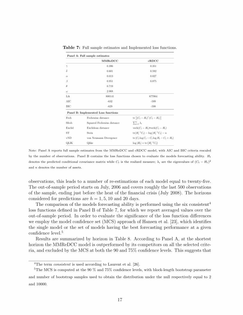
Table 7: Full sample estimates and Implemented loss functions.

Panel A: Full sample estimates

MMReDCC cRDCC

γ 0.396 0.351

δ 0.601 0.592

α 0.013 0.027

β 0.951 0.875

θ 0.719

ω 2.068

Lik 800141 677064

AIC -632 -599

BIC -629 -598

Panel B: Implemented Loss functions

Frob Frobenius distance tr[(Ct −Ht)

′ (Ct −Ht)]

Sfrob Squared Frobenius distance∑n

i=1 λi

Euclid Euclidean distance vech(Ct −Ht)′vech(Ct −Ht)

ST Stein tr(H−1t Ct)− log |H−1

t Ct| − n

vND von Neumann Divergence tr (Ct logCt − Ct logHt − Ct +Ht)

QLIK Qlike log |Ht|+ tr(H−1t Ct

)Note: Panel A reports full sample estimates from the MMReDCC and cRDCC model, with AIC and BIC criteria rescaled

by the number of observations. Panel B contains the loss functions chosen to evaluate the models forecasting ability. Ht

denotes the predicted conditional covariance matrix while Ct is the realized measure; λi are the eigenvalues of (Ct − Ht)2

and n denotes the number of assets.

observations, this leads to a number of re-estimations of each model equal to twenty-five.The out-of-sample period starts on July, 2006 and covers roughly the last 500 observationsof the sample, ending just before the heat of the financial crisis (July 2008). The horizonsconsidered for predictions are h = 1, 5, 10 and 20 days.

The comparison of the models forecasting ability is performed using the six consistent4

loss functions defined in Panel B of Table 7, for which we report averaged values over theout-of-sample period. In order to evaluate the significance of the loss function differenceswe employ the model confidence set (MCS) approach of Hansen et al. [23], which identifiesthe single model or the set of models having the best forecasting performance at a givenconfidence level.5

Results are summarized by horizon in Table 8. According to Panel A, at the shortesthorizon the MMReDCC model is outperformed by its competitors on all the selected crite-ria, and excluded by the MCS at both the 90 and 75% confidence levels. This suggests that

4The term consistent is used according to Laurent et al. [26].5The MCS is computed at the 90 % and 75% confidence levels, with block-length bootstrap parameter

and number of bootstrap samples used to obtain the distribution under the null respectively equal to 2

and 10000.

17

Figure 1: Estimated correlation of APOL-GCI.

Sep98 Nov00 Jan13 Apr05 Jun070

0.02

0.04

0.06

0.08

Realized Volatility of APOL

Sep98 Nov00 Jan13 Apr05 Jun070

5

10

x 10−3 Realized Volatility of GCI

Sep98 Nov00 Jan13 Apr05 Jun07

−0.5

0

0.5

Correlation estimates of APOL − GCI

cRDCC

MMReDCC

for the data at hand, accurate one-step-ahead predictions can be obtained by employingsimpler models that do not necessarily account for a time-varying long run level.6 At thisstage the choice between the EWMA and the cRDCC model appears almost indifferent,despite the latter being more often included in the MCS.

As we move further in time the situation is quickly reversed: at the 5-day horizon, theMMReDCC model minimizes five out of six loss functions while at the 10-day horizon itappears to deliver the optimal covariance forecasts according to the whole set of losses.This gain is confirmed by the inclusion of the model in the MCS resulting from all theselected criteria, differently from the competitors which are almost never included (EWMAand cRDCC are included three and two times, respectively, in the 75% MCS at h = 5,but never at h = 10). The predominance of the MMReDCC remains quite stable evenat the longest horizon (h = 20), but the difference in the forecast accuracy between theMMReDCC and the benchmarks becomes smaller, with the cRDCC performing almostas good as the MMReDCC in terms of MCS inclusions (cRDCC excluded only in the vonNeumann 75% MCS). These results appear to be in line with those of [21], where already atthe 10-ahead horizon the differences in the forecast accuracy between their best componentCAW model and the selected benchmarks were smaller than at shorter horizons.

Overall, the out-of-sample performance of the MMReDCC model in a moderatelyvolatile time period appears to be good relative to the competing models especially atmedium-term horizons, when it yields the most accurate forecasts. In light of these em-pirical results, it appears that the introduction of an additional component capturing thesecular movements in the volatility and covolatility dynamics is well justified and useful toenhance a higher forecasting accuracy.

6This result is quite different from that of Bauwens et al. [5] where models with a time-varying long-run

component dominate models with a constant long-run level at forecast horizon 1. The dataset of that

paper covers the turbulent period of 2008 and 2009.

18

Table 8: Multi-step-ahead forecast evaluation

Horizon 1 Horizon 5 Horizon 10 Horizon 20

MMReDCC EWMA cRDCC MMReDCC EWMA cRDCC MMReDCC EWMA cRDCC MMReDCC EWMA cRDCC

Panel A: Loss functions

Frob 0.133 0.125 0.126 0.138 0.135 0.139 0.144 0.148 0.148 0.158 0.167 0.160

Sfrob 0.040 0.034 0.037 0.036 0.036 0.036 0.037 0.038 0.038 0.041 0.042 0.043

Euclid 0.086 0.080 0.082 0.087 0.088 0.088 0.091 0.093 0.093 0.099 0.102 0.101

ST 65.159 59.018 55.449 59.227 61.684 60.245 61.522 63.611 63.289 67.748 66.269 66.667

vND 0.018 0.017 0.017 0.018 0.019 0.019 0.019 0.022 0.020 0.022 0.025 0.022

QLIK -370.64 -376.78 -380.35 -376.66 -374.20 -375.64 -374.43 -372.34 -372.67 -368.07 -369.55 -369.15

Panel B: 90 % MCS

Frob 0.014 0.689 1.000 0.486 1.000 0.232 1.000 0.001 0.015 0.224 0.619 1.000

Sfrob 0.044 0.259 1.000 0.614 1.000 0.614 1.000 0.052 0.052 0.547 0.547 1.000

Euclid 0.023 0.464 1.000 1.000 0.311 0.420 1.000 0.001 0.016 0.506 0.506 1.000

ST 0.000 0.000 1.000 1.000 0.000 0.018 1.000 0.000 0.003 1.000 0.000 0.281

vND 0.000 0.263 1.000 1.000 0.002 0.028 1.000 0.000 0.000 1.000 0.000 0.159

QLIK 0.000 0.000 1.000 1.000 0.000 0.017 1.000 0.000 0.004 1.000 0.000 0.275

Panel C: 75 % MCS

Frob 0.013 0.695 1.000 0.497 1.000 0.227 1.000 0.003 0.016 1.000 0.218 0.615

Sfrob 0.047 1.000 0.268 0.631 1.000 0.631 1.000 0.051 0.051 1.000 0.545 0.545

Euclid 0.018 0.461 1.000 1.000 0.315 0.429 1.000 0.001 0.015 1.000 0.511 0.511

ST 0.000 0.000 1.000 1.000 0.000 0.015 1.000 0.000 0.003 1.000 0.000 0.278

vND 0.000 0.265 1.000 1.000 0.002 0.029 1.000 0.000 0.000 1.000 0.000 0.160

QLIK 0.000 0.000 1.000 1.000 0.000 0.014 1.000 0.000 0.003 1.000 0.000 0.274

Note: Panel A reports averaged values of the loss functions listed in Table 7 over the out-of-sample period, where the best

performing model within each row is in bold. Entries in Panel B and C are p-values of the MCS with 10% and 25% size,

respectively. Included models in bold.

7. Conclusions

The estimation procedure proposed in the paper allows to extend the range of applica-bility of the MMReDCC model to large dimensional portfolios such as those encounteredin standard risk management practice. In order to reach this objective, we face two well-known challenges in multivariate time series modeling, namely high-dimensional estimationand multi-step ahead forecasting.

To face the former challenge, we implement a feasible estimation procedure, the Itera-tive Moment based Profiling (IMP) algorithm. It profiles out the parameters of the scaleMIDAS intercept matrix and iteratively maximizes the likelihood in terms of the other pa-rameters of interest. Whilst not providing an asymptotic inference theory for this method,we investigate the finite sample properties of the estimator via a simulation study, whichdemonstrates that the IMP estimator is comparable to the one-step QML ones in terms ofbias and accuracy. We also compare the one-step QML estimator with the IMP estimatoron real data sets of small dimension (ten) and find that not only the two estimators deliververy similar in-sample estimates, but also the loss of the IMP in terms of likelihood valuescan be considered as negligible. Another application illustrates the usefulness of the IMPalgorithm when the model is applied to the realized covariances of fifty stocks. From the

19

computational point of view, the IMP algorithm is found to be reliable and easy to ap-ply despite the large number of parameters involved in the MMReDCC model. Given itsflexibility, we fairly believe that it could be applied to datasets of larger dimensions.

As regards the second challenge, we develop a bootstrap approach to the generationof multi-step-ahead predictions. In an application to a portfolio of fifty stocks, we pro-vide compelling evidence that the MMReDCC model is useful for out-of-sample forecastingpurposes even when one has to work in such a dimension. If compared with existing multi-variate competitors not accounting for time-varying long-term dynamics, the MMReDCCis found to deliver the most accurate predictions especially at medium-term horizons, thusindicating the importance of allowing for a long-run component.

20

Appendix A. Application I: Descriptive statistics of daily realized variances.

Symbol Issue name Mean Max. Min. Std.dev. Skewness Kurtosis

Dataset 1: February, 2001 – December, 2009

AA Alcoa 5.458 277.308 0.074 16.811 7.178 72.570

AXP American Express 5.055 176.478 0.112 11.094 7.529 84.686

BAC Bank of America 1.934 57.543 0.075 3.362 7.319 85.006

KO Coca Cola 2.455 43.106 0.084 3.412 4.724 36.234

DD Du Pont 2.073 115.378 0.126 4.155 13.296 288.066

GE General Electric 4.944 160.241 0.294 8.935 7.635 92.124

IBM International Business Machines 4.420 201.879 0.077 9.154 8.536 133.699

JPM JP Morgan 2.529 63.874 0.163 3.728 6.442 68.505

MSFT Microsoft 3.196 114.256 0.097 7.114 7.232 75.484

XOM Exxon Mobil 1.414 56.505 0.039 2.254 9.715 180.206

Dataset 2: January, 2007 – December, 2012

ACAS American Capital 8.576 331.786 0.060 20.844 7.226 78.667

AET Aetna 8.163 771.525 0.109 26.593 17.882 467.969

AFL Aflac Incorporated 9.113 675.348 0.133 27.345 13.811 284.791

AIG American International Group 8.799 555.098 0.103 26.382 11.459 185.778

AIZ Assurant 8.613 325.167 0.101 23.230 7.712 79.082

ALL The Allstate Coprporation 8.213 543.714 0.186 24.593 11.277 189.052

AMP Ameriprise Financial 7.679 264.761 0.129 17.790 6.098 54.262

AXP American Express Company 8.076 945.750 0.095 30.571 21.795 618.891

BAC Bank of America 8.450 332.586 0.130 22.830 8.458 96.824

BBT BB&T Corporation 9.093 613.826 0.087 28.801 11.267 184.837

Dataset 3: January, 2007 – December, 2012

STI SunTrust Banks 8.510 388.707 0.086 22.765 8.088 94.838

STT State Street Corporation 8.985 315.656 0.039 23.192 7.265 74.391

TMK Torchmark Corporation 8.748 537.273 0.022 24.479 10.543 176.515

TROW T.Rowe Price Group 8.991 425.263 0.073 25.019 8.753 108.221

UNH UnitedHealth Group 8.344 378.667 0.130 21.065 8.534 112.479

UNM Unun Group 8.046 309.086 0.044 19.440 8.564 107.272

USB U.S.Bancorp 10.176 2534.073 0.079 69.496 32.392 1164.053

WFC Wells Fargo & Company 9.481 525.034 0.106 30.162 10.717 156.791

WU The Western Union Company 8.775 484.124 0.056 25.204 9.954 145.509

ZION Zions Bancorporation 15.302 6855.823 0.136 197.794 30.674 1005.621

21

Appendix B. Application II: descriptive statistics of daily realized variances.

Estimation sample: May 12, 1997 to July 17, 2006 (2024 observations)

Stock Mean (e-03) Max. Min.(e-03) Std.dev.(e-03) Skewness Kurtosis

ABT 0.434 0.025 0.026 0.948 15.958 333.606

AFL 0.491 0.027 0.020 1.208 13.097 225.997

APD 0.490 0.075 0.020 1.896 32.234 1221.466

AA 0.540 0.012 0.040 0.759 7.886 94.971

ALL 0.497 0.098 0.012 2.319 37.311 1554.460

AXP 0.549 0.041 0.014 1.553 16.921 374.949

AIG 0.391 0.073 0.027 1.724 38.011 1597.332

ADI 1.375 0.043 0.070 2.153 7.635 103.080

APOL 1.276 0.080 0.043 2.556 16.984 470.125

T 0.620 0.046 0.017 1.659 15.676 339.927

AZO 0.497 0.046 0.021 1.250 25.934 909.714

AVY 0.416 0.064 0.019 1.643 30.923 1136.941

BHI 1.000 0.098 0.060 3.284 23.106 603.142

BAC 0.477 0.054 0.015 1.681 20.789 578.406

BAX 0.447 0.059 0.022 1.884 22.785 609.476

BDX 0.481 0.036 0.021 1.109 19.322 541.972

BBBY 1.078 0.029 0.051 1.579 7.060 92.898

BMY 0.565 0.051 0.028 2.005 19.683 450.186

CPB 0.470 0.083 0.012 1.940 38.241 1616.776

COF 0.909 0.092 0.023 3.300 20.993 547.443

CAH 0.465 0.044 0.016 1.705 18.142 393.755

CTL 0.492 0.069 0.026 2.049 23.613 687.584

CTAS 1.104 0.113 0.018 2.839 31.100 1212.341

C 0.624 0.086 0.021 2.305 27.085 952.213

CLX 0.481 0.074 0.026 2.203 27.445 840.327

CMS 0.764 0.083 0.034 2.854 20.911 544.730

KO 0.314 0.009 0.015 0.464 7.565 101.565

CL 0.401 0.058 0.026 1.569 27.867 957.179

CMA 0.345 0.025 0.011 1.011 16.800 350.599

CSC 0.764 0.105 0.031 2.884 25.713 861.526

CAG 0.530 0.072 0.014 2.129 25.460 758.407

COST 0.773 0.135 0.042 3.358 33.314 1277.539

DOV 0.441 0.050 0.031 1.334 27.171 949.990

DOW 0.474 0.033 0.018 0.994 20.169 609.262

DTE 0.296 0.068 0.017 1.552 41.597 1818.052

EMN 0.432 0.089 0.027 2.141 35.535 1433.408

EIX 1.103 0.251 0.022 6.892 26.622 885.136

ETR 0.332 0.029 0.018 0.779 26.216 937.670

FDO 0.911 0.093 0.043 2.519 26.543 911.464

FISV 0.913 0.063 0.041 1.715 24.450 850.641

F 0.635 0.024 0.050 1.053 10.141 170.597

GCI 0.272 0.010 0.015 0.370 12.616 289.030

GPS 1.007 0.049 0.032 2.730 10.649 142.751

GE 0.445 0.037 0.013 1.233 19.948 515.188

GIS 0.231 0.008 0.013 0.334 9.989 181.369

GPC 0.427 0.089 0.018 2.039 40.541 1745.937

HNZ 1.240 0.075 0.030 2.547 19.600 511.929

HPQ 0.291 0.030 0.014 0.918 24.562 727.020

HD 0.902 0.047 0.022 1.965 11.388 195.042

HON 0.643 0.078 0.028 2.418 23.919 682.976

Forecasting sample: July 18, 2006 to July 18, 2008 (500 observations)

Stock Mean (e-03) Max. Min.(e-03) Std.dev.(e-03) Skewness Kurtosis

ABT 0.191 0.004 0.020 0.263 8.887 122.525

AFL 0.268 0.004 0.015 0.406 4.815 35.550

APD 0.261 0.003 0.013 0.292 4.633 38.977

AA 0.559 0.007 0.051 0.682 4.078 25.551

ALL 0.232 0.002 0.012 0.304 3.423 18.970

AXP 0.498 0.015 0.010 0.919 8.966 127.909

AIG 0.523 0.010 0.017 1.020 4.375 27.892

ADI 0.432 0.014 0.046 0.816 11.614 168.440

APOL 0.939 0.079 0.035 4.173 14.929 261.548

T 0.278 0.004 0.023 0.399 6.116 50.180

AZO 0.303 0.010 0.016 0.517 13.313 242.173

AVY 0.243 0.005 0.019 0.446 7.402 70.878

BHI 0.506 0.009 0.079 0.563 8.511 108.889

BAC 0.495 0.016 0.012 1.223 7.682 79.279

BAX 0.190 0.004 0.020 0.306 7.569 80.297

BDX 0.150 0.003 0.017 0.210 8.356 104.636

BBBY 0.464 0.010 0.029 0.627 7.907 106.865

BMY 0.303 0.007 0.017 0.521 7.153 72.678

CPB 0.152 0.002 0.011 0.206 4.746 30.567

COF 0.923 0.013 0.028 1.481 3.995 25.175

CAH 0.186 0.005 0.011 0.294 9.695 135.019

CTL 0.279 0.021 0.022 1.008 17.453 350.144

CTAS 0.293 0.006 0.034 0.395 8.196 99.256

C 0.648 0.014 0.019 1.276 5.411 41.978

CLX 0.153 0.007 0.012 0.416 13.180 203.335

CMS 0.219 0.003 0.020 0.242 5.684 49.133

KO 0.112 0.002 0.005 0.181 7.972 78.506

CL 0.125 0.004 0.015 0.212 11.526 172.718

CMA 0.632 0.023 0.017 1.400 9.231 131.210

CSC 0.285 0.005 0.025 0.412 6.514 62.089

CAG 0.179 0.005 0.016 0.313 9.470 120.784

COST 0.338 0.010 0.030 0.564 11.158 166.572

DOV 0.245 0.003 0.025 0.327 5.352 39.200

DOW 0.347 0.007 0.028 0.616 6.593 55.276

DTE 0.177 0.002 0.015 0.202 4.481 34.565

EMN 0.292 0.005 0.024 0.429 6.244 57.701

EIX 0.223 0.005 0.026 0.320 7.899 96.229

ETR 0.203 0.003 0.017 0.281 5.482 44.736

FDO 0.770 0.017 0.033 1.332 7.121 70.492

FISV 0.276 0.006 0.031 0.366 7.898 96.806

F 0.802 0.009 0.091 1.101 4.107 23.288

GCI 0.305 0.012 0.018 0.658 12.646 218.866

GPS 0.564 0.007 0.028 0.681 4.354 30.343

GE 0.213 0.016 0.016 0.718 19.569 416.499

GIS 0.108 0.002 0.011 0.137 6.537 58.387

GPC 0.182 0.002 0.017 0.189 5.554 49.714

HNZ 0.309 0.003 0.043 0.280 4.217 28.816

HPQ 0.121 0.002 0.016 0.138 5.344 43.491

HD 0.289 0.005 0.024 0.387 6.301 64.372

HON 0.394 0.004 0.042 0.469 3.953 25.552

22

Appendix C. Figures

Figure C.2: Standard deviation of the IMP Monte Carlo estimated scalar parameters θ, ω, α

and β against the cross-section dimension ranging from 10 to 50. Results from the two simulation

studies for T = 1000, 2000 jointly reported respectively in Panel (a) and (b).

(a) T = 1000

10 20 30 40 500

0.01

0.02

0.03

0.04

0.05

θ

sim I

sim II

10 20 30 40 500

0.5

1

1.5

ω

sim I

sim II

10 20 30 40 500

1

2

3

4

5

6x 10

−3 α

sim I

sim II

10 20 30 40 500

2

4

6

8x 10

−3 β

sim I

sim II

(b) T = 2000

10 20 30 40 500.01

0.011

0.012

0.013

0.014

0.015

0.016

0.017

0.018

0.019

0.02

θ

sim I

sim II

10 20 30 40 500.2

0.25

0.3

0.35

0.4

0.45

0.5

0.55

0.6

0.65

0.7

ω

sim I

sim II

10 20 30 40 500

0.002

0.004

0.006

0.008

0.01

0.012

0.014

0.016

α

sim I

sim II

10 20 30 40 500

0.005

0.01

0.015

0.02

0.025

β

sim I

sim II

23

[1] Aielli, G. P. [2013], ‘Dynamic conditional correlation: On properties and estimation’,Journal of Business & Economic Statistics 31, 282–299.

[2] Andersen, T., Bollerslev, T., Diebold, F. and Ebens, H. [2001], ‘The distribution ofrealized stock return volatility’, Journal of Financial Economics 61, 43–76.

[3] Barndorff-Nielsen, O. E., Hansen, P. R., Lunde, A. and Shephard, N. [2011], ‘Multi-variate realised kernels: consistent positive semi-definite estimators of the covariationof equity prices with noise and non-synchronous trading’, Journal of Econometrics162(2), 149–169.

[4] Barndorff-Nielsen, O. and Shephard, N. [2001], ‘Normal modified stable processes’,Theory of Probability and Mathematics Statistics 65, 1–19.

[5] Bauwens, L., Braione, M. and Storti, G. [2016], ‘Forecasting comparison of long termcomponent dynamic models for realized covariance matrices’, Annals of Economicsand Statistics, (Forthcoming) .

[6] Bauwens, L., Hafner, C. M. and Pierret, D. [2013], ‘Multivariate volatility modelingof electricity futures’, Journal of Applied Econometrics 28(5), 743–761.

[7] Bauwens, L., Storti, G. and Violante, F. [2012], Dynamic conditional correlation mod-els for realized covariance matrices. CORE DP 2012/60.

[8] Bollerslev, T. [1990], ‘Modeling the coherence in short-run nominal exchange rates: Amultivariate generalized arch model’, Review of Economics and Statistics 72, 498–505.

[9] Boswijk, H. P. [1995], ‘Identifiability of cointegrated systems’, Tinbergen InstituteWorking Paper (95/78).

[10] Boudt, K., Laurent, S., Lunde, A. and Quaedvlieg, R. [2014], ‘Positive semidefiniteintegrated covariance estimation, factorizations and asynchronicity’, Factorizationsand Asynchronicity (October 8, 2014) .

[11] Chiriac, R. and Voev, V. [2011], ‘Modelling and forecasting multivariate realizedvolatility’, Journal of Applied Econometrics 26, 922–947.

[12] Clements, M. P. and Smith, J. [1997], ‘The performance of alternative forecastingmethods for setar models’, International Journal of Forecasting 13, 463–475.

[13] Cubadda, G. and Scambelloni, E. [2015], Index-augmented autoregressive models:representation, estimation and forecasting. Paper presented at the CFE 2015, London.

[14] Engle, R. [2002], ‘Dynamic conditional correlation - a simple class of multivariateGARCH models’, Journal of Business & Economic Statistics 20, 339–350.

24

[15] Engle, R. F. [2009], ‘High dimension dynamic correlations’, The Methodology andPractice of Econometrics: A Festschrift in Honour of David F. Hendry: A Festschriftin Honour of David F. Hendry p. 122.

[16] Engle, R. F., Ghysels, E. and Sohn, B. [2013], ‘Stock market volatility and macroeco-nomic fundamentals’, Review of Economics and Statistics 95(3), 776–797.

[17] Engle, R. F., Shephard, N. and Sheppard, K. [2008], ‘Fitting vast dimensional time-varying covariance models’.

[18] Engle, R. and Kelly, B. [2012], ‘Dynamic equicorrelation’, Journal of Business &Economic Statistics 30, 212–228.

[19] Fresoli, D. E. and Ruiz, E. [In Press], ‘The uncertainty of conditional returns, volatil-ities and correlations in dcc models’, Computational Statistics & Data Analysis .

[20] Ghysels, E., Sinko, A. and Valkanov, R. [2007], ‘Midas regressions: Further resultsand new directions’, Econometric Reviews 26(1), 53–90.

[21] Golosnoy, V., Gribisch, B. and Liesenfeld, R. [2012], ‘The conditional autoregres-sive wishart model for multivariate stock market volatility’, Journal of Econometrics167(1), 211–223.

[22] Gourieroux, C., Jasiak, J. and Sufana, R. [2009], ‘The wishart autoregressive processof multivariate stochastic volatility’, Journal of Econometrics 150(2), 167–181.

[23] Hansen, P. R., Lunde, A. and Nason, J. M. [2011], ‘The model confidence set’, Econo-metrica 79(2), 453–497.

[24] Hautsch, N., Kyj, L. M. and Malec, P. [2015], ‘Do high-frequency data improve high-dimensional portfolio allocations?’, Journal of Applied Econometrics 30(2), 263–290.

[25] Jin, X. and Maheu, J. M. [2013], ‘Modeling realized covariances and returns’, Journalof Financial Econometrics 11(2), 335–369.

[26] Laurent, S., Rombouts, J. V. and Violante, F. [2013], ‘On loss functions and rankingforecasting performances of multivariate volatility models’, Journal of Econometrics173(1), 1–10.

[27] Morgan, J. [1994], ‘Introduction to riskmetrics’, New York: JP Morgan .

[28] Noureldin, D., Shephard, N. and Sheppard, K. [2012], ‘Multivariate high-frequency-based volatility (heavy) models’, Journal of Applied Econometrics 27(6), 907–933.

[29] Pascual, L., R. J. and Ruiz, E. [2006], ‘Bootstrap prediction for returns and volatilitiesin garch models’, Computational Statistics & Data Analysis 50(9), 2293–2312.

25

[30] Pedersen, R. S. and Rahbek, A. [2014], ‘Multivariate variance targeting in the bekk–garch model’, The Econometrics Journal 17(1), 24–55.

[31] Shephard, N. and Sheppard, K. K. [2010], ‘Realising the future: forecasting with high-frequency-based volatility (heavy) models.’, Journal of Applied Econometrics 25, 197–231.

26