2016 weather research and forecasting (wrf) modeling ... · ladco 2016 wrf modeling protocol 3 1...

2016 Weather Research and Forecasting (WRF) Modeling Protocol for the LADCO states Lake Michigan Air Directors Consortium 9501 W. Devon Ave., Suite 701 Rosemont, IL 60018 Wisconsin Department of Natural Resources 101 S. Webster St. Madison, WI 53707 February 13, 2018

LADCO 2016 WRF Modeling Protocol

i

CONTENTS

FIGURES ................................................................................................................................ ii

TABLES .................................................................................................................................. ii

1 Introduction ................................................................................................................... 3 1.1 Organization of the Modeling Protocol ...............................................................................3 1.2 Project Participants ............................................................................................................4 1.3 Related Studies ..................................................................................................................5 1.4 Overview of 2016 WRF Modeling Approach ........................................................................6

2 Model Selection ............................................................................................................. 6 2.1 Justification and Overview of Selected Models ...................................................................7

3 Domain Selection ........................................................................................................... 8 3.1 Horizontal Modeling Domain..............................................................................................8 3.2 Vertical Domain Structure ................................................................................................ 10

4 Meteorological Modeling ............................................................................................. 12 4.1 Model Selection and Application ...................................................................................... 12 4.2 Topographic Inputs .......................................................................................................... 12 4.3 Vegetation Type and Land Use Inputs ............................................................................... 12 4.4 Atmospheric Data Inputs .................................................................................................. 13 4.5 Time Integration .............................................................................................................. 13 4.6 Diffusion Options ............................................................................................................. 14 4.7 Lateral Boundary Conditions ............................................................................................ 14 4.8 Top and Bottom Boundary Conditions .............................................................................. 14 4.9 Sea Surface Temperature Inputs ....................................................................................... 14 4.10 FDDA Data Assimilation ................................................................................................... 14 4.11 WRF Physics Options ........................................................................................................ 14 4.12 WRF Output Variables ...................................................................................................... 17 4.13 WRF Simulation Methodology .......................................................................................... 17 4.14 Evaluation Approach ........................................................................................................ 17 4.15 Reporting......................................................................................................................... 18

5 Meteorological Model Performance Evaluation ............................................................ 19 5.1 Quantitative Evaluation using Surface Meteorological Observations ........................................ 19 5.2 Quantitative Evaluation using Upper Layer Meteorological Observations................................. 22 5.3 Qualitative Model Performance Evaluation ............................................................................. 22


ii

FIGURES

Figure 3-1. WRF 12/4/1.33-km grid structure for the LADCO 2016 meteorological modeling .... 10 Figure 5-1. Figure 5-4. Example quantitative model performance evaluation display using soccer

plots that compare monthly temperature performance (colored symbols) across the 36-km CONUS (top left), 12-km WESTUS (top right) and 4 km IMWD (bottom) domains with the simple and complex model performance benchmarks (rectangles). ................................... 22

Figure 5-2. Example comparison of PRISM analysis (left) and WRF modeling (right) monthly total precipitation amounts across the a 4km WRF domain for the months of January (top) and July (bottom) from a Western U.S. 2011 WRF simulation .................................................... 23

Figure 5-3. Example comparison of observed surface winds (left) and WRF modeling (right) on June 4th, 2011 at 4:00pm CDT from previous WRF model simulations in Wisconsin ........... 24

TABLES

Table 1-1. Key contacts for the LADCO 2016 modeling platform ................................................... 4 Table 3-1. Projection parameters for the LADCO 2016 WRF modeling domains ......................... 10 Table 3-2. WRF vertical layer specification ................................................................................... 11 Table 4-1. NLCD and MODIS landuse categories for the 2016 WRF modeling............................. 13 Table 4-2. Options proposed for the LADCO 2016 WRF modeling ............................................... 15 Table 4-3. Comparison of the LADCO 2016 WRF configuration to recent configurations for

modeling in the LADCO region .............................................................................................. 16 Table 5-1. Meteorological model performance benchmarks for simple and complex conditions

............................................................................................................................................... 21


3

1 Introduction

The Lake Michigan Air Directors Consortium (LADCO) was established by the states of Illinois, Indiana, Michigan, and Wisconsin in 1989. The four states and EPA signed a Memorandum of Agreement (MOA) that initiated the Lake Michigan Ozone Study (LMOS) and identified LADCO as the organization to oversee the study. Additional MOAs were signed by the states in 1991 (to establish the Lake Michigan Ozone Control Program), January 2000 (to broaden LADCO’s responsibilities), and June 2004 (to update LADCO’s mission and reaffirm the commitment to regional planning). In March 2004, Ohio joined LADCO. Minnesota joined the Consortium in 2012. LADCO consists of a Board of Directors (i.e., the State Air Directors), a technical staff, and various workgroups. The main purposes of LADCO are to provide technical assessments for and assistance to its member states, and to provide a forum for its member states to discuss regional air quality issues. LADCO is preparing a modeling platform for a 2016 base year to be used in planning modeling for O3, PM2.5, and regional haze (RH). Meteorological inputs are a key component for the LADCO modeling platform.

This document is a modeling protocol for the 2016 LADCO meteorological modeling. This protocol details the modeling inputs/outputs, modeling procedures, and evaluation procedures that will be used by the LADCO modeling team for meteorology modeling of 2016.

1.1 Organization of the Modeling Protocol

This document presents the LADCO protocol for simulating and evaluating year 2016 meteorology with the Weather Research Forecast Model (WRF). The structure and content of this protocol will follow EPA guidance for the use of models in planning applications. The results from the WRF modeling proposed here will likely be used as a basis for regulatory air quality modeling by the LADCO states. This LADCO 2016 WRF Modeling Protocol has the following sections:

1. Introduction: Presents a summary of the background, purpose, and objectives of the study.

2. Modeling Domain Specifications: Presents the modeling domains selected for the study

3. Modeling Specifications: Presents the modeling software selected for this study and how these models will be applied to simulate 2016 meteorology. This section describes how the meteorological modeling and the WRF model evaluation will be conducted.


4

4. Model Performance Evaluation: Provides the procedures for conducting the WRF model performance evaluation.

1.2 Project Participants

Cooperators on the project include Federal agencies and state Departments of Environmental Management. Contributions from Federal agencies include NOAA and EPA Region 5. The study is facilitated and managed by LADCO. The Wisconsin Department of Natural Resources (WI DNR) is conducting the meteorology modeling. WI DNR and LADCO will conduct an evaluation of the WRF modeling results. Key contacts and their roles in the LADCO 2016 WRF modeling are listed in Table 1-1.

Table 1-1. Key contacts for the LADCO 2016 modeling platform

Name Role Organization/Contact

Zac Adelman QA Manager Lake Michigan Air Directors Consortium (847) 720-7880 [email protected]

Tsengel Nergui LADCO Contact Lake Michigan Air Directors Consortium (847) 720-7881 [email protected]

David Bizot WI DNR Manager Bureau of Air Management Wisconsin Department of Natural Resources (608) 267-7543 [email protected]

Wusheng Ji WI DNR WRF Modeler

Bureau of Air Management Wisconsin Department of Natural Resources (608) 267-7583 [email protected]

Chris Misenis EPA WRF Advisor US EPA OAQPS

(919) 541-2046 [email protected]

Brad Pierce NOAA WRF Advisor National Oceanic and Atmospheric Administration Center for Satellite Applications and Research (608) 890-1892 [email protected]


5

1.3 Related Studies

There are numerous meteorological modeling and data analysis studies that are being used to guide the 2016 WRF modeling. The more recent and relevant studies are listed below.

1.3.1 Lake Michigan Ozone Study

The Lake Michigan Ozone Study (LMOS) began in May 2017 as an intensive atmospheric monitoring field campaign along the Western shore of Lake Michigan. The campaign used in-situ surface monitors, aircraft, ships, and satellite data to study the meteorology and chemical drivers of high ground-level ozone concentrations. With the conclusion of the field campaign, LMOS proceeded with a modeling study of the campaign period. The LMOS investigators used the data from the field campaign to evaluate different configurations of the WRF model with the objective of finding an optimal configuration for simulating the meteorology conditions that lead to high summer season ozone along the shores of Lake Michigan. The LMOS WRF modeling included a Continental US 12-km resolution (CONUS12) domain, a Great Lakes region 4-km domain, and a Lake Michigan 1.33 km domain. Detail on LMOS can be found at: https://www-air.larc.nasa.gov/missions/lmos/

1.3.2 2011 Iowa Department of Natural Resources Regional Modeling

The Iowa Department of Natural Resources (IA DNR), in collaboration with LADCO and WI DNR, completed annual WRF modeling for 2011 to support ozone and particulate matter air quality modeling. 1 These data represent a recent retrospective regional WRF simulation that was generated by agencies in the LADCO region for use in air quality planning. The IA DNR WRF modeling used a North American 36-km domain and a 12-km domain that spanned all of the US east of the Rocky Mountains.

1.3.3 Applications of US EPA WRF Modeling in the LADCO Region

The US EPA applied WRF for the entire year of 2011 to generate meteorological data to support air quality research and regulatory applications2. The EPA WRF simulation was done for CONUS 36 km and US 12 km domains. The EPA-generated 12 km resolution WRF outputs were used for air quality modeling to support attainment demonstration and SIP development for the 2008 ozone NAAQS in Wisconsin, Illinois, and Indiana3,4.

1 Brown, D. (2014) WRF Meteorology Modeling in Support of Regional Air Quality Modeling for the 2011

Base Year. Iowa Department of Natural Resources. Available online: http://www.iowadnr.gov/portals/idnr/uploads/air/insidednr/regmodel/wrf_tsd_2011.pdf 2 U.S. EPA (2014) Meteorological Model Performance for Annual 2011 WRF v3.4 Simulation. Available online: https://www3.epa.gov/ttn/scram/reports/MET_TSD_2011_final_11-26-14.pdf 3 LADCO Technical Support Document (2017) Modeling Demonstration for the 2008 Ozone National Ambient Air Quality Standard for the Lake Michigan Region. Available online: http://www.ladco.org/reports/ozone/post08/LADCO%20Ozone%20TSD%20FINAL%20(Feb%203%202017).pdf 4 Good, G. (2017) State Implementation Plan Submittal for Sheboygan County 2008 Ozone NAAQS Moderate Area Attainment Plan. Wisconsin Department of Natural Resources. Available online: http://dnr.wi.gov/topic/AirQuality/documents/SheboyganAttainmentPlan.pdf

https://www-air.larc.nasa.gov/missions/lmos/

http://www.iowadnr.gov/portals/idnr/uploads/air/insidednr/regmodel/wrf_tsd_2011.pdf

https://www3.epa.gov/ttn/scram/reports/MET_TSD_2011_final_11-26-14.pdf

http://www.ladco.org/reports/ozone/post08/LADCO%20Ozone%20TSD%20FINAL%20(Feb%203%202017).pdf

http://www.ladco.org/reports/ozone/post08/LADCO%20Ozone%20TSD%20FINAL%20(Feb%203%202017).pdf

http://dnr.wi.gov/topic/AirQuality/documents/SheboyganAttainmentPlan.pdf


6

1.3.4 WI DNR Fine Scale Modeling

Wisconsin DNR conducted WRF modeling to investigate the capabilities of the model to capture the lake breezes that drive high summertime ozone concentrations along the shores of Lake Michigan. The WRF modeling was done using a single domain with 1.33 km horizontal grid resolution.

1.4 Overview of 2016 WRF Modeling Approach

The WRF meteorological model will be applied for the 2016 calendar year using a one-way nested 12/4/1.33-km domain structure. The WRF modeling results for the 2016 annual period will be evaluated against surface and upper level meteorological observations of wind speed, wind direction, temperature, and humidity. Simulated precipitation fields will be compared against analysis fields from the National Center for Environmental Prediction, NOAA (NCEP) and the Parameter-elevation Relationships on Independent Slopes Model (PRISM) dataset. The 2016 WRF model results will be evaluated against meteorological modeling performance benchmarks and against results from recent regional WRF meteorological modeling studies in the LADCO region.

2 Model Selection

This section discusses the modeling software that will be used to estimate 2016 meteorology fields for the LADCO region. The modeling software selection methodology follows EPA’s guidance for regulatory modeling in support of ozone and PM2.5 attainment demonstration modeling.5 EPA recommends that models be selected for regulatory ozone, PM and visibility studies on a “case-by-case” basis with appropriate consideration given to the candidate model’s:

• Technical formulation, capabilities and features;

• Pertinent peer-review and performance evaluation history;

• Public availability; and

• Demonstrated success in similar regulatory applications.

All of these considerations should be examined for each class of models to be used (e.g., emissions, meteorological, and photochemical) in part because EPA no longer recommends a specific model or suite of photochemical models for regulatory application as it did twenty years ago in the first ozone SIP modeling guidance.6 Below we identify the most appropriate candidate models for the LADCO 2016 modeling requirements, discuss the

5 EPA. (2014) Guidance on the Use of Models and Other Analyses for Demonstrating Attainment of Air

Quality Goals for Ozone, PM2.5 and Regional Haze. U.S. Environmental Protection Agency, Research Triangle Park, NC. 6 EPA (1991) Guideline on the Regulatory Application of the Urban Airshed Model. U.S. Environmental Protection Agency, Office of Air Quality Planning and Standards, technical Support Division, Source Receptor Analysis Branch, Research Triangle Park, NC.

http://www.prism.oregonstate.edu/


7

candidate model attributes and then justify the model selected using the four criteria above. The science configurations recommended for each model in this study are introduced in Chapter 3.

2.1 Justification and Overview of Selected Models

There are two prognostic meteorological models that are routinely used in the U.S. in photochemical grid modeling studies:

• The fifth generation Mesoscale Model (MM5); and

• The Weather Research Forecasting (WRF) model.

Both MM5 and WRF were developed by the community, with the National Center for Atmospheric Research (NCAR) providing coordination and support. For many years the MM5 model was widely used by both the meteorological research as well as the air quality modeling community. Starting around the year 2000, the WRF model started to be developed as a technical improvement and replacement to MM5 and today NCAR no longer supports MM5.

Based on the following four selection criteria, we selected WRF for simulating the 2016 meteorology:

• Technical: WRF is based on more recent physics and computing techniques and represents a technical improvement over MM5. WRF has numerous new capabilities and features not available in MM5 and, unlike MM5, it is supported by NCAR.

• Performance: WRF is being used by thousands of users and has been subjected to a community peer-reviewed development process using the latest algorithms and physics. In general, it appears that WRF is better able to reproduce the observed meteorological variables so it performs better than MM5. WRF is amassing a rich publication and application history.

• Public Availability: WRF is publicly available and can be downloaded from the WRF website with no costs or restrictions. MM5 is also publicly available.

• Demonstrated Success: The 2011 LADCO WRF modeling produced meteorology fields that were sufficient for driving air quality model simulations (see Brown, D., 20141). The U.S. EPA Office of Air Quality Planning and Standards also routinely uses the WRF model for air quality planning modeling.

More details on the selected WRF meteorological model are provided below.

The non-hydrostatic version of the Advanced Research version of the Weather Research Forecast (WRF-ARW7) model (Skamarock et al. 2004; 2005; 2006; Michalakes et al. 1998; 2001; 2004) is a three-dimensional, limited-area, primitive equation, prognostic model that has been used widely in regional air quality model applications. The basic model has been under continuous development, improvement, testing and open peer-review for more than

7 All references to WRF in this document refer to the WRF-ARW


8

15 years and has been used world-wide by hundreds of scientists for a variety of mesoscale studies, including mesoscale convective complexes, urban-scale modeling, air quality studies, frontal weather, lake-effect snows, sea-breezes, orographically induced flows, and operational mesoscale forecasting. WRF is a next-generation mesoscale prognostic meteorological model routinely used for urban- and regional-scale photochemical, fine particulate and regional haze regulatory modeling studies. Developed jointly by the National Center for Atmospheric Research and the National Centers for Environmental Prediction, WRF is maintained and supported as a community model by researchers and practitioners around the globe. The code supports two modes: the Advanced Research WRF (ARW) version and the Non-hydrostatic Mesoscale Model (NMM) version. WRF-ARW has become the new standard model used in place of the older Mesoscale Meteorological Model (MM5) for regulatory air quality applications in the U.S. It is suitable for use in a broad spectrum of applications across scales ranging from hundreds of meters to thousands of kilometers.

3 Domain Selection

This section presents the model domain definitions for the 2016 WRF simulation, including the domain coverage, resolution, map projection, and nesting schemes for the high resolution sub-domains.

3.1 Horizontal Modeling Domain

We selected the modeling domains as a trade-off between the need to have high resolution modeling for sources in the Central Midwest versus the ability to perform regional ozone and particulate matter source apportionment modeling among all of the LADCO states. One recent modeling study indicated that the WRF model with a fine grid spacing of 1-km is capable of accurately yielding the near-surface temperatures and wind speeds associated with the lake breezes over the Chicago area adjoining Lake Michigan8. Another study also revealed the WRF model with a single 1-km grid domain is capable of capturing the fundamental surface wind convergence zones accompanying lake breezes near Great Salt Lake over Utah9. Consequently, the LADCO 2016 WRF modeling will use the same 12, 4 and 1.33-km domains as were used in the LMOS 2017 post-mission WRF-ARW model sensitivity studies10. The 2016 WRF simulation will use grids that are based on the standard Lambert Conformal Projection (LCP) used for continental U.S. modeling domains. Table 3-1 includes the specifications for the following domains:

• A 12-km continental U.S. (CONUS) domain that is the same as used by the Multi Jurisdictional Organizations (MJOs) and other recent modeling studies in the region, such as the Sheboygan Ozone SIP3. The outer domain is defined large

8 Sharma et al. Urban meteorological modeling using WRF: a sensitivity study. International Journal of Climatology. July 2016. (wileyonlinelibrary.com) DOI: 10.1002/joc.4819. 9 Blaylock et al, Impact of Lake Breezes on Summer Ozone Concentrations in the Salt Lake Valley. Journals Online, American Meteorological Society, February 2017. (https://doi.org/10.1175/JAMC-D-16-0216.1). 10 https://www-air.larc.nasa.gov/missions/lmos/


9

enough so that the outer boundaries are far away from our primary areas of interest (i.e., Central Midwest).

• A 4-km Great Lakes regional domain that contains all of the LADCO and adjacent states as well as extending into Canada.

• A 1.33-km Lake Michigan domain that focuses on coastal sites around the lake.

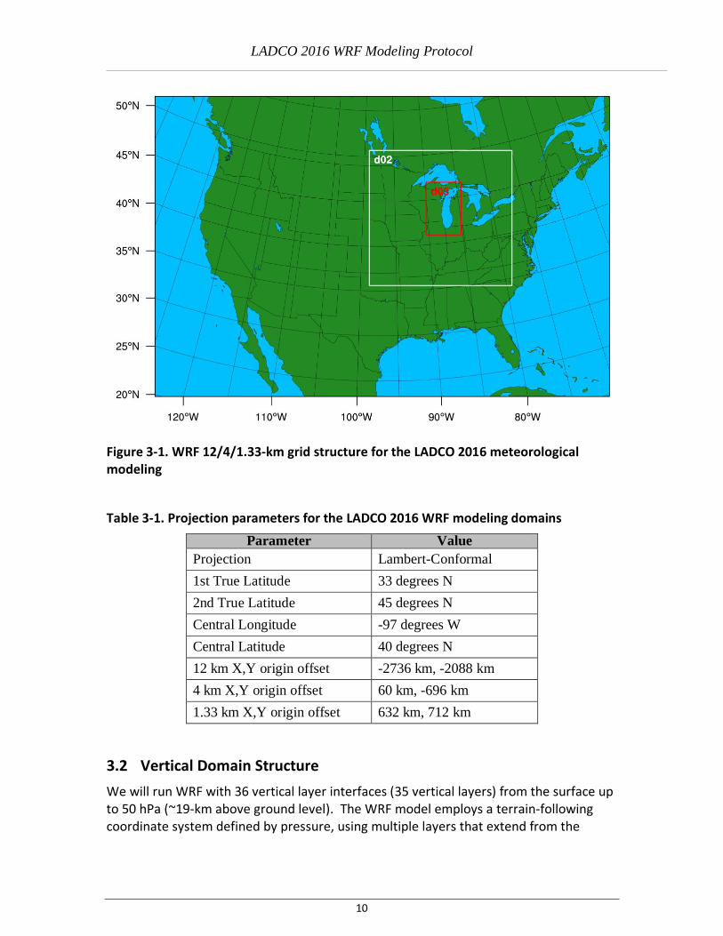
The WRF computational grid was designed so that it can generate photochemical grid model (PGM) meteorological inputs for the nested 12/4/1.33-km domains depicted in Figure 3-1. The WRF modeling domain was defined to be slightly larger than the PGM modeling domains to eliminate the occurrence of boundary artifacts in the meteorological fields used as input to the PGM. Such boundary artifacts can occur as the boundary conditions (BCs) for the meteorological variables come into dynamic imbalance with WRF’s atmospheric equations and numerical methods.

Figure 3-1 illustrates the horizontal modeling domains that will be used for the 2016 WRF modeling. The outer 12-km domain (D01) has 472 x 312 grid cells, selected to be consistent with the existing EPA modeling CONUS domain. The projection is Lambert Conformal with the national CONUS grid projection pole of 40o, -97o with true latitudes of 33o and 45o. The 4-km domain (D02) has 445 x 421 grid cells with offsets from the 12-km grid of 223 columns and 116 rows. The 1.33-km domain (D03) has 328 x 493 grid cells with offsets from the 4 km grid of 178 columns and 158 rows.


10

Figure 3-1. WRF 12/4/1.33-km grid structure for the LADCO 2016 meteorological modeling

Table 3-1. Projection parameters for the LADCO 2016 WRF modeling domains

Parameter Value

Projection Lambert-Conformal

1st True Latitude 33 degrees N

2nd True Latitude 45 degrees N

Central Longitude -97 degrees W

Central Latitude 40 degrees N

12 km X,Y origin offset -2736 km, -2088 km

4 km X,Y origin offset 60 km, -696 km

1.33 km X,Y origin offset 632 km, 712 km

3.2 Vertical Domain Structure

We will run WRF with 36 vertical layer interfaces (35 vertical layers) from the surface up to 50 hPa (~19-km above ground level). The WRF model employs a terrain-following coordinate system defined by pressure, using multiple layers that extend from the


11

surface to the model top. Table 3-2 illustrates the WRF layer structure that we will use for the LADCO 2016 modeling.

Table 3-2. WRF vertical layer specification

WRF Layer

Height (m)

Pressure (Pa)

Sigma

Thickness

(m) 36 17,556 5000 0.000 2776

35 14,780 9750 0.050 1958

34 12,822 14500 0.100 1540 33 11,282 19250 0.150 1280 32 10,002 24000 0.200 1101 31 8,901 28750 0.250 969 30 7,932 33500 0.300 868 29 7,064 38250 0.350 789

28 6,275 43000 0.400 722 27 5,553 47750 0.450 668 26 4,885 52500 0.500 621 25 4,264 57250 0.550 581 24 3,683 62000 0.600 547 23 3,136 66750 0.650 517

22 2,619 71500 0.700 393 21 2,226 75300 0.740 285 20 1,941 78150 0.770 276 19 1,665 81000 0.800 180 18 1,485 82900 0.820 177 17 1,308 84800 0.840 174

16 1,134 86700 0.860 170 15 964 88600 0.880 167 14 797 90500 0.900 83 13 714 91450 0.910 82 12 632 92400 0.920 81 11 551 93350 0.930 81

10 470 94300 0.940 80

9 390 95250 0.950 79 8 311 96200 0.960 79 7 232 97150 0.970 78 6 154 98100 0.980 39 5 115 98575 0.985 38 4 77 99050 0.990 39

3 38 99525 0.995 19 2 19 99763 0.9975 19

1 0 100000 1.000 0


12

4 Meteorological Modeling

This section describes the modeling software and approach that will be used for the 2016 WRF simulation. The WRF meteorological model will be applied for the 2016 calendar year using the 12/4/1.33-km domain structure described in Section 3. We will evaluate the WRF modeling results for the 2016 annual period against surface meteorological observations of wind speed, wind direction, temperature and humidity for each domain and compile model performance statistics on monthly basis. We will compare the 2016 WRF model performance against meteorological modeling benchmarks and with previous meteorological model performances in the region1,11. The WRF precipitation fields will be qualitatively assessed against gridded precipitation fields of the NCEP Environmental Modeling Center 4km Gridded Data (GRIB format) Gage-Only Analysis12 and PRISM datasets form PRISM Climate Group13.

4.1 Model Selection and Application

The 2016 WRF modeling will use WRF version 3.9.1.1. The WRF preprocessor programs GEOGRID, UNGRIB, and METGRID will be used to develop model inputs.

4.2 Topographic Inputs

Topographic information for the WRF will be developed using the National Land Cover Database (NLCD) 2011 Update available from the National Center for Atmospheric Research (NCAR) based on the 9 sec (~300 m) data14.

4.3 Vegetation Type and Land Use Inputs

We will use 2011 National Landcover Data (NLCD) for the vegetation and land use inputs to WRF. The NLCD is a 40-category, 30-meter resolution dataset of land-cover for the continental U.S. The WRF-compatible version of the NLCD is supplemented with the MODIS 20-category land cover data for regions outside of the U.S.

11 Bowden et al. (2016) Western State Air Quality Modeling Study WRF 2014 Meteorological Model Application/Evaluation. Available online: http://vibe.cira.colostate.edu/wiki/Attachments/Modeling/WAQS_2014_WRF_MPE_January2016.pdf 12 Lin, Y., 2006. GCIP/EOP Surface: Precipitation NCEP/EMC 4KM Gridded Data (GRIB) Gage-Only Analysis

(GAG) 1996-2001,Version 1.0. UCAR/NCAR - Earth Observing Laboratory. http://data.eol.ucar.edu/dataset/21.048. 13 PRISM Climate Group (2004), Oregon State Univ. Available at http://prism.oregonstate.edu 14 https://www.mrlc.gov/nlcd2011.php

http://dss.ucar.edu/

http://data.eol.ucar.edu/dataset/21.048


13

Table 4-1 lists the NLCD and MODIS landcover categories that will be available for this simulation.


14

Table 4-1. NLCD and MODIS landuse categories for the 2016 WRF modeling

MODIS NLCD Number Category Name Number Category Name

1 Evergreen Needleleaf Forest 22 Perennial Ice/Snow 2 Evergreen Broadleaf Forest 23 Developed Open Space 3 Deciduous Needleleaf Forest 24 Developed Low Intensity 4 Deciduous Broadleaf Forest 25 Developed Medium Intensity 5 Mixed Forests 26 Developed High Intensity 6 Closed Shrublands 27 Barren Land (Rock/Sand/Clay) 7 Open Shrublands 28 Deciduous Forest 8 Woody Savannas 29 Evergreen Forest 9 Savannas 30 Mixed Forest 10 Grasslands 32 Shrub/Scrub 11 Permanent Wetlands 33 Grassland/Herbaceous 12 Croplands 37 Pasture/Hay 13 Urban And Built Up 38 Cultivated Crops 14 Cropland/Natural Vegetation

Mosaic 39 Woody Wetlands

15 Permanent Snow and Ice 40 Emergent Herbaceous Wetlands

16 Barren or Sparsely Vegetated 17 IGBP Water

4.4 Atmospheric Data Inputs

The WRF simulation will be initialized with the 12-km (Grid #218) North American Model (NAM) archives available from the National Climatic Data Center (NCDC) National Operational Model Archive and Distribution System (NOMADS) server.

4.5 Time Integration

Third-order Runge-Kutta integration will be used (rk_ord = 3). The maximum time step, defined for the outer-most domain (12 km) only, should be set by evaluating the following equation:

𝑑𝑡 =6𝑑𝑥

𝐹𝑚𝑎𝑝

Where dx is the grid cell size in km, Fmap is the maximum map factor (which can be found in the output from the WRF program REAL.EXE), and dt is the resulting time-step in seconds. For the case of the 12-km domain, dx = 12 and Fmap = 1.08, so dt should be taken to be less than 200 seconds. Longer time steps typically lead to Courant-Friedrichs-Lewy (CFL) condition errors, associated with large vertical velocity values, which tend to occur in areas of steep terrain, especially during very stable conditions in winter.

For the 2016 modeling, we will use a fixed time step of 60 seconds for 12km grid domain, 20 seconds for 4km grid domain and 6.67 seconds for 1.33 km grid domain.


15

4.6 Diffusion Options

Horizontal Smagorinsky first-order closure (km_opt = 4) with sixth-order numerical diffusion (diff_6th_opt = 2) will be used.

4.7 Lateral Boundary Conditions

Lateral boundary conditions will be specified from the initialization dataset on the 12-km domain with continuous updates nested from the 12-km domain to the 4-km domain and from the 4-km domain to the 1.3-km domain, using one-way nesting (feedback = 0).

4.8 Top and Bottom Boundary Conditions

The no damping option will be selected for the top boundary condition and consistent with the model application for non-idealized cases, the bottom boundary condition will be selected as physical, not free-slip.

4.9 Sea Surface Temperature Inputs

A high resolution sea surface temperature (SST) from the Global Ocean Data Assimilation Experiment High Resolution Sea Surface Temperatures (GHRSST)15 will be used for all three domains. The 1 km resolution, daily average GHRSST fields will be re-gridded into each of the WRF modeling domain grids and interpolated to every 3 hours for integration into the WRF simulation through the surface boundary files.

4.10 FDDA Data Assimilation

The WRF model will be run with analysis nudging using Four Dimensional Data Assimilation (FDDA) for the 12-km and 4-km domains only. FDDA will not be used for the 1.33-km domain due to limited observations available over the Lake Michigan. We will use analysis nudging coefficients up to 3x10-4 s-1 for horizontal wind and temperature and analysis nudging coefficients up to 1.0x10-5 s-1 for water vapor mixing ratio, depending on domain. Only aloft nudging will be performed; no nudging will be applied for wind, temperature, and mixing ratio in the planetary boundary layer16.

4.11 WRF Physics Options

The WRF physics options for this WRF simulation will be based on the 2017 LMOS and 2011 IA DNR WRF configurations. The WRF sensitivity modeling for these studies found that the

15 Stammer, D., F.J. Wentz, and C.L. Gentemann (2003). Validation of Microwave Sea Surface Temperature Measurements for Climate Purposes. J. Climate, 16, 73-87. Available at: https://data.nodc.noaa.gov/ghrsst/L4/GLOB/JPL/MUR/ 16 Otte, T.L. (2008). The impact of nudging in the meteorological model for retrospective air quality simulations. Part II: Evaluating collocated meteorological and air quality observations. Journal of Applied Meteorology and Climatology, 47(7): 1868-1887.

https://data.nodc.noaa.gov/ghrsst/L4/GLOB/JPL/MUR/


16

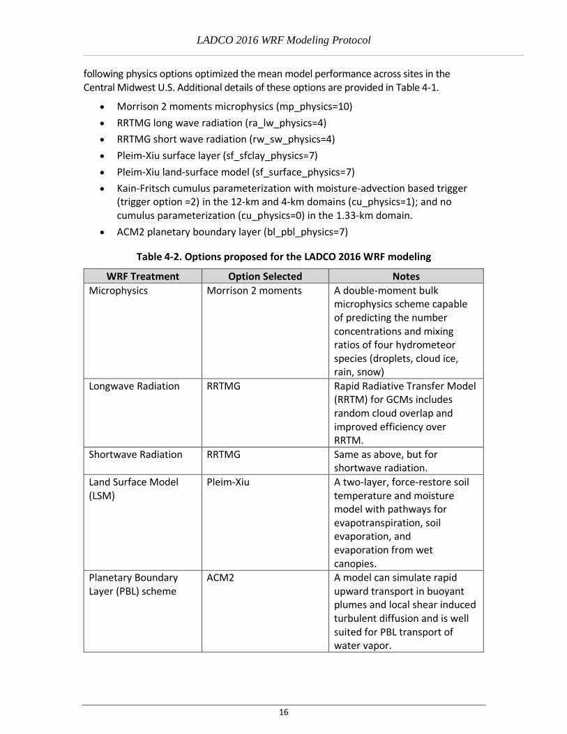
following physics options optimized the mean model performance across sites in the Central Midwest U.S. Additional details of these options are provided in Table 4-1.

• Morrison 2 moments microphysics (mp_physics=10)

• RRTMG long wave radiation (ra_lw_physics=4)

• RRTMG short wave radiation (rw_sw_physics=4)

• Pleim-Xiu surface layer (sf_sfclay_physics=7)

• Pleim-Xiu land-surface model (sf_surface_physics=7)

• Kain-Fritsch cumulus parameterization with moisture-advection based trigger (trigger option =2) in the 12-km and 4-km domains (cu_physics=1); and no cumulus parameterization (cu_physics=0) in the 1.33-km domain.

• ACM2 planetary boundary layer (bl_pbl_physics=7)

Table 4-2. Options proposed for the LADCO 2016 WRF modeling

WRF Treatment Option Selected Notes

Microphysics Morrison 2 moments A double-moment bulk microphysics scheme capable of predicting the number concentrations and mixing ratios of four hydrometeor species (droplets, cloud ice, rain, snow)

Longwave Radiation RRTMG Rapid Radiative Transfer Model (RRTM) for GCMs includes random cloud overlap and improved efficiency over RRTM.

Shortwave Radiation RRTMG Same as above, but for shortwave radiation.

Land Surface Model (LSM)

Pleim-Xiu A two-layer, force-restore soil temperature and moisture model with pathways for evapotranspiration, soil evaporation, and evaporation from wet canopies.

Planetary Boundary Layer (PBL) scheme

ACM2 A model can simulate rapid upward transport in buoyant plumes and local shear induced turbulent diffusion and is well suited for PBL transport of water vapor.


17

WRF Treatment Option Selected Notes

Cumulus parameterization

Kain-Fritsch in the 12-km and 4-km domains. None in the 1.33-km domain

1.33-km can explicitly simulate cumulus convection so parameterization not needed.

Analysis nudging Nudging applied to winds, temperature and moisture in the 12-km and 4-km domains

No nudging used within the PBL

Initialization Dataset 12 km North American Model (NAM)

Table 4-3. Comparison of the LADCO 2016 WRF configuration to recent configurations for modeling in the LADCO region

WRF Treatment LADCO 2016 LMOS 2017* WI DNR Fine Scale

2011

Diffusion Horizontal Smagorinsky first-order closure

Horizontal Smagorinsky first-order closure

Horizontal Smagorinsky first-order closure

Microphysics Morrison 2 moments Morrison 2 moments

Morrison 2 moments

LW Radiation RRTMG RRTMG RRTMG SW Radiation RRTMG RRTMG RRTMG

LSM Pleim-Xiu Pleim-Xiu LSM and NOAH LSM

Pleim-Xiu

PBL Scheme ACM2 ACM2 and YSU ACM2

Cumulus parameterization

Kain-Fritsch in the 12-km and 4-km domains. None in the 1.3-km domain.

Kain-Fritsch in the 12-km and 4-km domains. None in the 1.3-km domain.

Kain-Fritsch in 1.33-km domain

Analysis nudging uv, t, q in the 12-km and 4-km domains

uv, t, q in the 12-km and 4-km domains

uv, t, q in the 1.33-km domain

Analysis Nudging Coefficients

uv: 0.0003 (d01), 0.0001 (d02) t: 0.0003 (d01), 0.0001(d02) q: 0.00001

uv: 0.0001 t: 0.0001 q: 0.00001

uv: 0.0005 t: 0.0005 q: 0.00001

PBL Analysis Nudging

None None uv only

Obs Nudging None None None


18

WRF Treatment LADCO 2016 LMOS 2017* WI DNR Fine Scale

2011

Obs Nudging Coefficients

N/A N/A N/A

ICBC 12-km NAM 0.5o GFS 12-km NAM

LULC NLCD 2011 NLCD 2011 NLCD 2006

*For the LMOS 2017 Modeling, EPA Baseline configuration with Pleim-Xiu and NOAH LSM schemes, and ACM2 and YSU boundary layer options were evaluated.

4.12 WRF Output Variables

The WRF model will be configured to output additional variables to support air quality modeling with the Comprehensive Air Quality Model with Extensions (CAMx) and the Community Multiscale Air Quality Model (CMAQ). The following fields will be activated in the WRF output history files: fractional land use (LANDUSEF), aerodynamic resistance (RA), stomatal resistance (RS), vegetation fraction in the Pleim-Xiu LSM (VEGF_PX), roughness length (ZNT), inverse Monin-Obukhov length (RMOL).

4.13 WRF Simulation Methodology

The WRF model will be executed in 5.5-day blocks initialized at 12Z every 5 days with a 60-second integration time step. Model results will be output every 60 minutes and output files split at 24-hour intervals. Twelve hours of spin-up will be included in each 5.5-day block before the data are used in the subsequent evaluation. The model will be run at the 12-km, 4-km, and 1.33-km grid resolution from December 16, 2015 through January 1, 2017 using one-way grid nesting (i.e., the meteorological conditions are allowed to propagate from the coarser grid to the finer grid, but not vice versa). The namelist files for the WPS and WRF-ARW configurations that will be used for this study are included in Appendix A.

4.14 Evaluation Approach

The model evaluation approach will be based on a combination of qualitative and quantitative analyses. The quantitative analysis will be divided into monthly summaries of 2-m temperature, 2-m water vapor mixing ratio, and 10-m wind speed and direction using the boreal seasons to help generalize the model bias and error relative to a standard performance benchmark. The evaluation will focus on the 4-km and 1.33-km domains in the LADCO states and supplemented with select diurnal and time series analyses. Additional analysis will include a qualitative evaluation of the WRF daily and monthly precipitation fields against NCEP and PRISM fields. The National Oceanic and Atmospheric Administration (NOAA) Earth System Research Laboratory (ESRL) Meteorological Assimilation Data Ingest System (MADIS) will be used to evaluate the winds, temperatures, and water vapor mixing ratios in this simulation.

Calculating bulk statistics over a continental or regional scale domain is problematic because compensating errors and biases get averaged out when evaluating model performance


19

across a broad spectrum of physical and dynamical conditions. Evaluation across large spatial and temporal scales masks important sub-regional, local, and episodic features in the meteorology. Despite these issues, cursory statistics of domain wide, seasonal and monthly model performance provide a high-level overview of WRF’s ability to simulate meteorology conditions in the region. We will augment the 12/4/1.33-km domain-wide analysis with statistics by state. Particular attention will be paid to the model performance in the LADCO states.

Additional details of how we will conduct the model performance evaluation for this simulation are provided in Section 5.

4.15 Reporting

The 2016 WRF simulation and evaluation will be documented in a final report and through site-specific performance plots.


20

5 Meteorological Model Performance Evaluation

The WRF model evaluation approach will be based on a combination of qualitative and quantitative analyses. The qualitative approach compares the spatial distribution of the model-estimated precipitation with precipitation fields from the NCEP and PRISM17 precipitation analysis fields based on observations using graphical outputs, and a comparison of the WRF estimated cloud cover with satellite observations. The quantitative approach calculates model performance statistics using predicted and observed surface meteorological variables. We will compare the performance statistics for the 2016 WRF simulation with published performance benchmarks.

5.1 QUANTITATIVE EVALUATION USING SURFACE METEOROLOGICAL OBSERVATIONS

The statistical evaluation approach will examine tabular and graphical displays of the model bias and error for surface wind speed, wind direction, temperature, and water vapor mixing ratio. We will compare the 2016 WRF performance statistics to benchmarks developed based on a history of meteorological modeling as well as past meteorological model performance.18 Model performance will be evaluated at each meteorological station within the 12-km CONUS domain. The model performance statistics will be aggregated for each state for the 12-km CONUS, 4-km, and 1.33-km modeling domains.

MADIS is the observed database for winds, temperature, and water mixing ratio that will be used to evaluate WRF for this study.

The quantitative model performance evaluation of WRF using surface meteorological measurements will be performed using the publicly available Model Evaluation Tool (MET), METSTAT19 and the Atmospheric Model Evaluation Tool (AMET)20 evaluation tools. These tools calculate statistical performance metrics for bias, error, and correlation for surface winds, temperature, and mixing ratio and can produce time series of predicted and observed meteorological variables and performance statistics.

A full annual model evaluation is very difficult to summarize in a single document, especially a simulation that could be used for many different purposes. With this in mind, the WRF model evaluation report will present results for several sub-regions, even at the individual site level within the 1.33-km domain, leaving potential data users to independently judge the adequacy of the model simulation. Overall comparisons are offered to judge the model efficacy, but this review does not necessarily cover all potential user needs and applications.

17 http://www.prism.oregonstate.edu/ 18 Emery, C., E. Tai, and G. Yarwood, 2001. Enhanced Meteorological Modeling and Performance Evaluation for Two Texas Ozone Episodes. Prepared for the Texas Natural Resource Conservation Commission, prepared by ENVIRON International Corporation, Novato, CA. 31 August. (http://www.tceq.texas.gov/assets/public/implementation/air/am/contracts/reports/mm/EnhancedMetModelingAndPerformanceEvaluation.pdf). 19 http://www.camx.com/down/support.php 20 http://www.cmascenter.org

http://www.prism.oregonstate.edu/

http://www.camx.com/down/support.php


21

Statistical metrics will be presented for each LADCO state and for the U.S. portion of the 4-km and 1.33-km modeling domains. To evaluate the performance of the WRF 2016 simulation for the U.S., a number of performance benchmarks for comparison will be used. Emery et al. derived and proposed a set of daily performance “benchmarks” for typical meteorological model performance.21 These standards were based upon the evaluation of about 30 MM5 and RAMS meteorological simulations of limited duration (multi-day episodes) in support of air quality modeling study applications performed over several years. The simulations were ozone model applications for cities in the Eastern and Midwestern U.S. and Texas that were primarily simple (flat) terrain and simple (stationary high pressure causing stagnation) meteorological conditions. More recently, these benchmarks have been used in annual meteorological modeling studies that include areas with complex terrain and more complicated meteorological conditions; therefore, they must be viewed as being applied as guidelines and not bright-line numbers. That is, the purpose of these benchmarks is not to give a passing or failing grade to any one particular meteorological model application, but rather to put its results in context with other model applications and meteorological data sets.

Recognizing that these simple conditions benchmarks may not be appropriate for more complex conditions, McNally analyzed multiple annual runs that included complex terrain conditions and suggested an alternative set of benchmarks for temperature under more complex conditions.22 As part of the WRAP meteorological modeling of the western U.S., including the Rocky Mountain Region, as well as for complex terrain in Alaska, Kemball-Cook (2005b23) also came up with meteorological model performance benchmarks for complex conditions.

The objective of comparing the 2016 WRF model performance to the benchmarks is to understand how well the model performs relative to other retrospective WRF applications for the U.S. These benchmarks include bias and error benchmarks for temperature, wind direction and mixing ratio as well as the wind speed bias and Root Mean Squared Error (RMSE) between the models and databases. Table 5-1 lists the performance benchmarks for simple and complex conditions against which we will evaluate the WRF results from this study.

21 Emery, C., E. Tai, and G. Yarwood, 2001. “Enhanced Meteorological Modeling and Performance Evaluation for Two Texas Ozone Episodes.” Prepared for the Texas Natural Resource Conservation Commission, prepared by ENVIRON International Corporation, Novato, CA. 31-August. http://www.tceq.texas.gov/assets/public/implementation/air/am/contracts/reports/mm/EnhancedMetModelingAndPerformanceEvaluation.pdf 22 McNally, D. E., 2009. “12km MM5 Performance Goals.” Presentation to the Ad-Hoc Meteorology Group. 25-June. http://www.epa.gov/scram001/adhoc/mcnally2009.pdf 23 Kemball-Cook, S., Y. Jia, C. Emery and R. Morris. 2005. “Alaska MM5 Modeling for the 2002 Annual Period to Support Visibility Modeling” Prepared for Western Regional Air Partnership (WRAP). Prepared by Environ International Corporation. September. http://pah.cert.ucr.edu/aqm/308/docs/alaska/Alaska_MM5_DraftReport_Sept05.pdf

http://www.tceq.texas.gov/assets/public/implementation/air/am/contracts/reports/mm/EnhancedMetModelingAndPerformanceEvaluation.pdf

http://www.tceq.texas.gov/assets/public/implementation/air/am/contracts/reports/mm/EnhancedMetModelingAndPerformanceEvaluation.pdf

http://www.epa.gov/scram001/adhoc/mcnally2009.pdf

http://pah.cert.ucr.edu/aqm/308/docs/alaska/Alaska_MM5_DraftReport_Sept05.pdf


22

( )2

1

1

21

−

=

N

i

ii OPN

Table 5-1. Meteorological model performance benchmarks for simple and complex conditions

Parameter Simple Complex

Temperature Bias ≤ ±0.5 K ≤ ±2.0 K Temperature Error ≤ 2.0 K ≤ 3.5 K

Mixing Ratio Bias ≤ ±1.0 g/kg NA

Mixing Ratio Error ≤ 2.0 g/kg NA Wind Speed Bias ≤ ±0.5 m/s ≤ ±1.5 m/s

Wind Speed RMSE ≤ 2.0 m/s ≤ 2.5 m/s

Wind Direction Bias ≤ ±10 degrees NA

Wind Direction Error ≤ 30 degrees ≤ 55 degrees

The equations for bias, error, and root mean square error (RMSE) are given below.

Mean Bias (Bias) =

Mean Absolute Gross Error (Error) =

Root Mean Square Error (RMSE) =

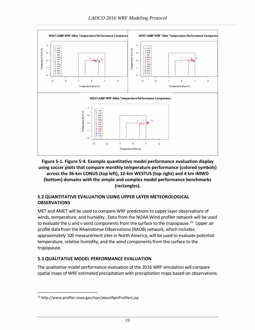
Figure 5-1 displays an example model performance soccer plot graphic from the WestJumpAQMS 2008 WRF run for monthly temperature performance within the three nested (36/12/4-km) modeling domains. The soccer plots shows the monthly temperature bias (x-axis) versus error (y-axis) as colored symbols with the simple and complex performance benchmarks24 represented by the rectangles. When the WRF monthly performance achieves the benchmark, it falls within the central rectangle. In this example we see the 2008 WRF simulation always achieves the complex benchmark in the 36-km domain and achieves the complex benchmark in 11 of 12 months over the 12-km domain, with just December falling just outside of the benchmark due to too warm temperatures. Across the 4-km domain, 7 of the 12 months achieve the complex benchmarks with 5 months failing due to overestimated temperatures.

24 Note that Figure 5-4 is using the McNally (2009) versions of the complex benchmark for temperature whereas we have adopted the Emory et. al (2001) versions for the temperature and wind benchmarks.

( )=

−N

i

ii OPN 1

1

=

−N

i

ii OPN 1

1


23

Figure 5-1. Figure 5-4. Example quantitative model performance evaluation display using soccer plots that compare monthly temperature performance (colored symbols)

across the 36-km CONUS (top left), 12-km WESTUS (top right) and 4 km IMWD (bottom) domains with the simple and complex model performance benchmarks

(rectangles).

5.2 QUANTITATIVE EVALUATION USING UPPER LAYER METEOROLOGICAL OBSERVATIONS

MET and AMET will be used to compare WRF predictions to upper layer observations of winds, temperature, and humidity. Data from the NOAA Wind profiler network will be used to evaluate the u and v wind components from the surface to the tropopause.25 Upper air profile data from the RAwindonse OBservations (RAOB) network, which includes approximately 100 measurement sites in North America, will be used to evaluate potential temperature, relative humidity, and the wind components from the surface to the tropopause.

5.3 QUALITATIVE MODEL PERFORMANCE EVALUATION

The qualitative model performance evaluation of the 2016 WRF simulation will compare spatial maps of WRF estimated precipitation with precipitation maps based on observations

25 http://www.profiler.noaa.gov/npn/aboutNpnProfilers.jsp


24

from NCEP and PRISM. One caveat of this analysis is that the PRISM analysis covers only the Continental U.S. and does not extend offshore or into Canada or Mexico.

Figure 5-2 displays example precipitation comparisons of WRF and PRISM fields from 2011 WRF simulations for the months of January and July and the continental U.S. For the LADCO 2016 WRF modeling, we will compare the model with PRISM for all months, for the 4-km and 1.33-km domains.

Figure 5-2. Example comparison of PRISM analysis (left) and WRF modeling (right) monthly total precipitation amounts across the a 4km WRF domain for the months of January (top) and July (bottom) from a Western U.S. 2011 WRF simulation

The model performance evaluation of the 2016 WRF simulation will also compare surface winds of WRF estimated with observations based on the dataset obtained from MADIS during the summer of 2016. The surface wind plots during summer days of 2016 will be


25

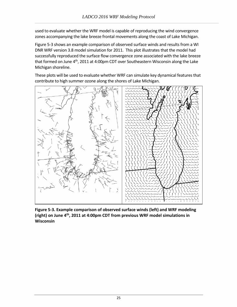
used to evaluate whether the WRF model is capable of reproducing the wind convergence zones accompanying the lake breeze frontal movements along the coast of Lake Michigan.

Figure 5-3 shows an example comparison of observed surface winds and results from a WI DNR WRF version 3.8 model simulation for 2011. This plot illustrates that the model had successfully reproduced the surface flow convergence zone associated with the lake breeze that formed on June 4th, 2011 at 4:00pm CDT over Southeastern Wisconsin along the Lake Michigan shoreline.

These plots will be used to evaluate whether WRF can simulate key dynamical features that contribute to high summer ozone along the shores of Lake Michigan.

Figure 5-3. Example comparison of observed surface winds (left) and WRF modeling (right) on June 4th, 2011 at 4:00pm CDT from previous WRF model simulations in Wisconsin


26

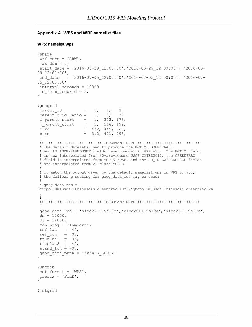
Appendix A. WPS and WRF namelist files WPS: namelist.wps &share

wrf_core = 'ARW',

max_dom = 3,

start_date = '2016-06-29_12:00:00','2016-06-29_12:00:00', '2016-06-

29_12:00:00',

end_date = '2016-07-05_12:00:00','2016-07-05_12:00:00', '2016-07-

05_12:00:00',

interval_seconds = 10800

io_form_geogrid = 2,

/

&geogrid

parent_id = 1, 1, 2,

parent_grid_ratio = 1, 3, 3,

i_parent_start = 1, 223, 178,

j_parent_start = 1, 116, 158,

e_we = 472, 445, 328,

e_sn = 312, 421, 493,

!

!!!!!!!!!!!!!!!!!!!!!!!!!!!! IMPORTANT NOTE !!!!!!!!!!!!!!!!!!!!!!!!!!!!

! The default datasets used to produce the HGT_M, GREENFRAC,

! and LU_INDEX/LANDUSEF fields have changed in WPS v3.8. The HGT_M field

! is now interpolated from 30-arc-second USGS GMTED2010, the GREENFRAC

! field is interpolated from MODIS FPAR, and the LU_INDEX/LANDUSEF fields

! are interpolated from 21-class MODIS.

!

! To match the output given by the default namelist.wps in WPS v3.7.1,

! the following setting for geog_data_res may be used:

!

! geog_data_res =

'gtopo_10m+usgs_10m+nesdis_greenfrac+10m','gtopo_2m+usgs_2m+nesdis_greenfrac+2m

',

!

!!!!!!!!!!!!!!!!!!!!!!!!!!!! IMPORTANT NOTE !!!!!!!!!!!!!!!!!!!!!!!!!!!!

!

geog_data_res = 'nlcd2011_9s+9s','nlcd2011_9s+9s','nlcd2011_9s+9s',

dx = 12000,

dy = 12000,

map_proj = 'lambert',

ref_lat = 40,

ref_lon = -97,

truelat1 = 33,

truelat2 = 45,

stand_lon = -97,

geog_data_path = '/y/WPS_GEOG/'

/

&ungrib

out_format = 'WPS',

prefix = 'FILE',

/

&metgrid


27

fg_name = 'FILE','SST',

io_form_metgrid = 2,

opt_metgrid_tbl_path = 'metgrid',

/

WRF: namelist.input

&time_control

start_year = 2016, 2016, 2016,

start_month = 06, 06, 06,

start_day = 29, 29, 29,

start_hour = 12, 12, 12,

start_minute = 00, 00, 00,

start_second = 00, 00, 00,

end_year = 2016, 2016, 2016,

end_month = 07, 07, 07,

end_day = 05, 05, 05,

end_hour = 00, 00, 00,

end_minute = 00, 00, 00,

end_second = 00, 00, 00,

interval_seconds = 10800

input_from_file = .true.,.true.,.true.,

fine_input_stream = 0, 2, 2,

history_interval = 60, 60, 60,

frames_per_outfile = 24, 24, 24,

restart = .false.,

restart_interval = 1440,

auxinput1_inname = "met_em.d<domain>.<date>"

io_form_history = 2

io_form_restart = 2

io_form_input = 2

io_form_boundary = 2

io_form_auxinput2 = 2

io_form_auxinput4 = 2

auxinput4_inname = "wrflowinp_d<domain>",

auxinput4_interval = 180, 180, 180,

/

&domains

time_step = 60,

time_step_fract_num = 0,

time_step_fract_den = 1,

max_dom = 3,

e_we = 472, 445, 328,

e_sn = 312, 421, 493,

e_vert = 36, 36, 36,

eta_levels = 1.0, 0.9975, 0.995, 0.99,

0.985, 0.98, 0.97, 0.96,

0.95, 0.94, 0.93, 0.92, 0.91,

0.9, 0.88, 0.86, 0.84, 0.82,

0.8, 0.77, 0.74, 0.7, 0.65,

0.6, 0.55, 0.5, 0.45, 0.4,

0.35, 0.3, 0.25, 0.2, 0.15,

0.1, 0.05, 0.0

p_top_requested = 5000,

num_metgrid_levels = 40,


28

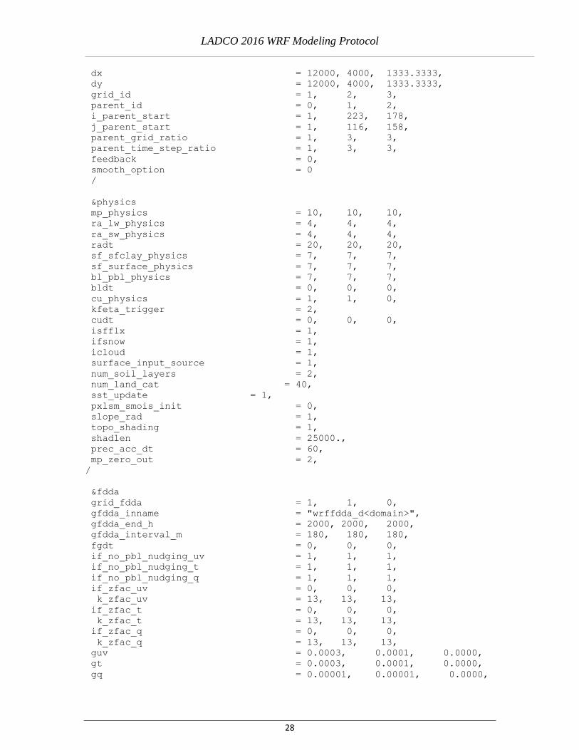
dx = 12000, 4000, 1333.3333,

dy = 12000, 4000, 1333.3333,

grid_id = 1, 2, 3,

parent_id = 0, 1, 2,

i_parent_start = 1, 223, 178,

j_parent_start = 1, 116, 158,

parent_grid_ratio = 1, 3, 3,

parent_time_step_ratio = 1, 3, 3,

feedback = 0,

smooth_option = 0

/

&physics

mp_physics = 10, 10, 10,

ra_lw_physics = 4, 4, 4,

ra_sw_physics = 4, 4, 4,

radt = 20, 20, 20,

sf_sfclay_physics = 7, 7, 7,

sf_surface_physics = 7, 7, 7,

bl_pbl_physics = 7, 7, 7,

bldt = 0, 0, 0,

cu_physics = 1, 1, 0,

kfeta_trigger = 2,

cudt = 0, 0, 0,

isfflx = 1,

ifsnow = 1,

icloud = 1,

surface_input_source = 1,

num_soil_layers = 2,

num_land_cat = 40,

sst_update = 1,

pxlsm_smois_init = 0,

slope_rad = 1,

topo_shading = 1,

shadlen = 25000.,

prec_acc_dt = 60,

mp_zero_out = 2,

/

&fdda

grid_fdda = 1, 1, 0,

gfdda_inname = "wrffdda_d<domain>",

gfdda_end_h = 2000, 2000, 2000,

gfdda_interval_m = 180, 180, 180,

fgdt = 0, 0, 0,

if_no_pbl_nudging_uv = 1, 1, 1,

if_no_pbl_nudging_t = 1, 1, 1,

if_no_pbl_nudging_q = 1, 1, 1,

if_zfac_uv = 0, 0, 0,

k_zfac_uv = 13, 13, 13,

if_zfac_t = 0, 0, 0,

k_zfac_t = 13, 13, 13,

if_zfac_q = 0, 0, 0,

k_zfac_q = 13, 13, 13,

guv = 0.0003, 0.0001, 0.0000,

gt = 0.0003, 0.0001, 0.0000,

gq = 0.00001, 0.00001, 0.0000,


29

if_ramping = 0,

dtramp_min = 60.0,

io_form_gfdda = 2,

/

&dynamics

w_damping = 1,

diff_opt = 1,

km_opt = 4,

diff_6th_opt = 2, 2, 2,

diff_6th_factor = 0.12, 0.12, 0.12,

damp_opt = 3,

base_temp = 290.

zdamp = 5000., 5000., 5000.,

dampcoef = 0.05, 0.05, 0.05

khdif = 0, 0, 0,

kvdif = 0, 0, 0,

non_hydrostatic = .true., .true., .true.,

moist_adv_opt = 2, 2, 2,

scalar_adv_opt = 2, 2, 2,

tke_adv_opt = 2, 2, 2,

/

&bdy_control

spec_bdy_width = 5,

spec_zone = 1,

relax_zone = 4,

specified = .true., .false.,.false.,

nested = .false., .true., .true.,

/

&grib2

/

&namelist_quilt

nio_tasks_per_group = 0,

nio_groups = 1,

/

2016 weather research and forecasting (wrf) modeling ... · ladco 2016 wrf modeling protocol 3 1...

Documents