2016-07 web
TRANSCRIPT

Robust Route Prediction inRaster Maps
Sebastian Fabian
MASTER’S THESIS | LUND UNIVERSITY 2016
Department of Computer ScienceFaculty of Engineering LTH
ISSN 1650-2884 LU-CS-EX 2016-07


Robust Route Prediction in Raster Maps
(Real Time Linear Topography for Look-Ahead Control)
Sebastian [email protected]
March 29, 2016
Master’s thesis work carried out at Scania CV AB.
Supervisors: Per Sahlholm, [email protected]
Flavius Gruian, [email protected]
Examiner: Jonas Skeppstedt, [email protected]


Abstract
By adapting gear changes and cruise control of a Heavy Duty Vehicle (HDV)to road inclination, fuel and time savings can be achieved. In this thesis is pre-sented a novel method of predicting the upcoming road topography, by con-structing a geographical and topographical self-learning map from which aroute prediction is made. The system is designed to simultaneously producethe desired road grade output in real time and update the map each time an areais driven through, making the map more accurate as more data is collected.Special considerations are given to the memory and processing constraints ofembedded automotive control hardware.
Keywords: raster map, route prediction, data structure, embedded, automotive, heatmap, GIS, topography

2

Acknowledgments
Thanks to Scania for giving me this opportunity.To my enthusiastic coworkers at REV at Scania R&D, for making my time there mem-
orable. I would like to especially thank Per Sahlholm for his guidance and inspiration.
3

4

Contents
1 Introduction 11
1.1 Problem definition . . . . . . . . . . . . . . . . . . . . . . . . . . . . . 131.2 Limitations . . . . . . . . . . . . . . . . . . . . . . . . . . . . . . . . . 131.3 Methodology . . . . . . . . . . . . . . . . . . . . . . . . . . . . . . . . 141.4 Delimitations . . . . . . . . . . . . . . . . . . . . . . . . . . . . . . . . 151.5 Report organization . . . . . . . . . . . . . . . . . . . . . . . . . . . . . 151.6 Contributions . . . . . . . . . . . . . . . . . . . . . . . . . . . . . . . . 15
2 Background 17
2.1 Theory . . . . . . . . . . . . . . . . . . . . . . . . . . . . . . . . . . . . 172.1.1 Coordinate mapping . . . . . . . . . . . . . . . . . . . . . . . . 172.1.2 Calculating distances in WGS84 . . . . . . . . . . . . . . . . . . 192.1.3 Quick calculation of arc length . . . . . . . . . . . . . . . . . . . 202.1.4 Splines . . . . . . . . . . . . . . . . . . . . . . . . . . . . . . . 202.1.5 Quadtrees . . . . . . . . . . . . . . . . . . . . . . . . . . . . . . 21
2.2 Technology . . . . . . . . . . . . . . . . . . . . . . . . . . . . . . . . . 222.2.1 Target platform . . . . . . . . . . . . . . . . . . . . . . . . . . . 222.2.2 Sample data . . . . . . . . . . . . . . . . . . . . . . . . . . . . . 23
2.3 Previous work . . . . . . . . . . . . . . . . . . . . . . . . . . . . . . . . 232.3.1 Map construction . . . . . . . . . . . . . . . . . . . . . . . . . . 242.3.2 Route prediction . . . . . . . . . . . . . . . . . . . . . . . . . . 272.3.3 Horizon length . . . . . . . . . . . . . . . . . . . . . . . . . . . 29
3 Implementation 31
3.1 Overview . . . . . . . . . . . . . . . . . . . . . . . . . . . . . . . . . . 313.2 Re-implementation of previous work . . . . . . . . . . . . . . . . . . . . 32
3.2.1 Discrete road grade format . . . . . . . . . . . . . . . . . . . . . 323.2.2 Directional route prediction . . . . . . . . . . . . . . . . . . . . 33
3.3 Map building . . . . . . . . . . . . . . . . . . . . . . . . . . . . . . . . 353.3.1 Data point interpolation . . . . . . . . . . . . . . . . . . . . . . 35
5

CONTENTS
3.3.2 Correcting pixel size . . . . . . . . . . . . . . . . . . . . . . . . 363.3.3 Planar road grade format . . . . . . . . . . . . . . . . . . . . . . 373.3.4 Decoupled road grade data . . . . . . . . . . . . . . . . . . . . . 40
3.4 Heat map based route prediction . . . . . . . . . . . . . . . . . . . . . . 403.4.1 Recording . . . . . . . . . . . . . . . . . . . . . . . . . . . . . . 413.4.2 Predicting . . . . . . . . . . . . . . . . . . . . . . . . . . . . . . 423.4.3 Aging . . . . . . . . . . . . . . . . . . . . . . . . . . . . . . . . 453.4.4 Loops . . . . . . . . . . . . . . . . . . . . . . . . . . . . . . . . 45
3.5 Distance calculation . . . . . . . . . . . . . . . . . . . . . . . . . . . . . 473.5.1 Linear interpolation . . . . . . . . . . . . . . . . . . . . . . . . . 473.5.2 Polynomial interpolation . . . . . . . . . . . . . . . . . . . . . . 473.5.3 Splines . . . . . . . . . . . . . . . . . . . . . . . . . . . . . . . 49
3.6 Heat as a quality measure . . . . . . . . . . . . . . . . . . . . . . . . . . 493.6.1 On a pixel level . . . . . . . . . . . . . . . . . . . . . . . . . . . 503.6.2 On a horizon level . . . . . . . . . . . . . . . . . . . . . . . . . 51
3.7 Filtering . . . . . . . . . . . . . . . . . . . . . . . . . . . . . . . . . . . 523.8 Horizon transmission . . . . . . . . . . . . . . . . . . . . . . . . . . . . 533.9 Data structures . . . . . . . . . . . . . . . . . . . . . . . . . . . . . . . 55
3.9.1 Using a quadtree . . . . . . . . . . . . . . . . . . . . . . . . . . 56
4 Results 57
4.1 Evaluation methodology . . . . . . . . . . . . . . . . . . . . . . . . . . 574.1.1 Performance assessment . . . . . . . . . . . . . . . . . . . . . . 574.1.2 Visualization . . . . . . . . . . . . . . . . . . . . . . . . . . . . 584.1.3 Reference routes . . . . . . . . . . . . . . . . . . . . . . . . . . 59
4.2 Design choices and parameters . . . . . . . . . . . . . . . . . . . . . . . 604.2.1 Pixel size . . . . . . . . . . . . . . . . . . . . . . . . . . . . . . 614.2.2 Distance calculation . . . . . . . . . . . . . . . . . . . . . . . . 614.2.3 Horizon length . . . . . . . . . . . . . . . . . . . . . . . . . . . 634.2.4 Heat map directions . . . . . . . . . . . . . . . . . . . . . . . . 644.2.5 Road grade format . . . . . . . . . . . . . . . . . . . . . . . . . 654.2.6 Loops and off-road conditions . . . . . . . . . . . . . . . . . . . 664.2.7 Aging . . . . . . . . . . . . . . . . . . . . . . . . . . . . . . . . 66
4.3 System performance . . . . . . . . . . . . . . . . . . . . . . . . . . . . 684.4 Horizon transmission . . . . . . . . . . . . . . . . . . . . . . . . . . . . 704.5 Heat as a quality measure . . . . . . . . . . . . . . . . . . . . . . . . . . 75
4.5.1 On a pixel level . . . . . . . . . . . . . . . . . . . . . . . . . . . 754.5.2 On a horizon level . . . . . . . . . . . . . . . . . . . . . . . . . 75
4.6 Decoupled road grade map . . . . . . . . . . . . . . . . . . . . . . . . . 764.7 Storage . . . . . . . . . . . . . . . . . . . . . . . . . . . . . . . . . . . 76
4.7.1 Tile based approach . . . . . . . . . . . . . . . . . . . . . . . . 774.7.2 Using a quadtree . . . . . . . . . . . . . . . . . . . . . . . . . . 77
6

CONTENTS
5 Discussion 79
5.1 System parameters . . . . . . . . . . . . . . . . . . . . . . . . . . . . . 795.1.1 Route prediction approach . . . . . . . . . . . . . . . . . . . . . 795.1.2 Pixel size . . . . . . . . . . . . . . . . . . . . . . . . . . . . . . 805.1.3 Number of heat maps . . . . . . . . . . . . . . . . . . . . . . . . 805.1.4 Road grade format . . . . . . . . . . . . . . . . . . . . . . . . . 805.1.5 Loops . . . . . . . . . . . . . . . . . . . . . . . . . . . . . . . . 815.1.6 Aging . . . . . . . . . . . . . . . . . . . . . . . . . . . . . . . . 815.1.7 Distance calculation . . . . . . . . . . . . . . . . . . . . . . . . 82
5.2 Horizon transmission . . . . . . . . . . . . . . . . . . . . . . . . . . . . 825.3 Computational considerations . . . . . . . . . . . . . . . . . . . . . . . 83
5.3.1 Lookup . . . . . . . . . . . . . . . . . . . . . . . . . . . . . . . 835.3.2 Recording . . . . . . . . . . . . . . . . . . . . . . . . . . . . . . 845.3.3 Horizon generation . . . . . . . . . . . . . . . . . . . . . . . . . 84
6 Conclusions 85
6.1 Summary . . . . . . . . . . . . . . . . . . . . . . . . . . . . . . . . . . 856.2 Storage . . . . . . . . . . . . . . . . . . . . . . . . . . . . . . . . . . . 876.3 Further study . . . . . . . . . . . . . . . . . . . . . . . . . . . . . . . . 88
Bibliography 88
7

CONTENTS
8

Glossary
ADAS
Advanced Driver Assistance System. Digital system to assist the driver by enhanc-ing, augmenting or simplifying driving functions.
HDV
Heavy Duty Vehicle
ECU
Electronic Control Unit. A generic designation for a digital computer unit in anautomotive context, typically used for ignition control, gearbox control and otherdigital functions of the vehicle.
Raster
A dot matrix data structure that stores information about some entity as a matrix ofdiscrete values, each representing a fixed size portion.
Pixel
The value that makes up the each element in a raster dot matrix.
Horizon
A predicted route of some length.
Tile
A square cluster of pixels, making up a subset of a raster dot matrix. A smallerportion than the entire raster dot matrix, although large than a single pixel.
Node map
A map system made up of interconnected nodes. Typically used in most commericalmap applications, including navigation.
GPS
Global Positioning System. A standard to determine one’s location upon the earthbased on triangulation with satellites.
9

CONTENTS
(Adaptive) cruise control
Automatic control system intended to control vehicle speed. Adaptive cruise controlsystems may change the speed setting to respond to surrounding conditions whereasplain cruise control keeps a set value.
CAN
Controller Area Network. Network connection standard for interconnected dis-tributed systems, typically used in vehicles to communicate between ECUs.
KDE
Kernel Density Estimation. A method of constructing graph-based maps.
GIS
Geographic Information Science. The discipline of geographic information systemstudy.
WGS84
World Geodetic System 84. Standardized coordinate system for mapping the earth.
GPS trace
A series of GPS coordinates, forming a single path of travel data.
Heat map
A map structure that consists of a single value for each point, typically visiting fre-quency.
KiB, MiB, GiB
Prefixed units for unambiguously describing amounts of data in prefix steps of 1024bytes, as described in IEC [1].
10

Chapter 1
Introduction
In today’s society of rising demand of transport services and their efficacy, fuel efficiencyand mechanical reliability are more important than ever before and are a vital part of theeveryday business for any logistics operation. In order to meet the needs of this increas-ingly global and connected society, smart ways to minimize fuel consumption and increasedependability of commercial fleets are highly desirable. This is evident by the rise of so-phisticated Advanced Driver Assistance Systems (ADAS), such as autonomous emergencybrakes and adaptive cruise control that meet a range of goals, such as minimizing humanerror and maximizing operational efficiency. Other approaches, that lack interaction fromthe driver, come in all shapes and forms, both digital and mechanical. Together, thesetechnologies represent a hallmark of the modern automotive industry.
One such non-interactive technology for saving fuel is road prediction and using de-rived data in the distributed network of Electronic Control Units (ECU) to improve severalintegrated functions of the vehicle. One such application is cruise control that adapts tothe road ahead. By, for instance, letting go of the throttle before a crest, velocity increasedue to the upcoming slope can be minimized which can prevent unnecessary braking andthus save fuel. Similarly, a throttle increase before an ascent can improve efficiency byminimizing the temporary slowdown. Another desirable application for such technologyis gear shift timing. By shifting down just before the ascent, a heavily loaded commer-cial vehicle can prepare for increased torque output beforehand which can, in some cases,eliminate the need for a mid-ascent gear shift. Additionally, by saving the time it takes toperform the actual shift, doing so in anticipation allows preservation of the current mo-mentum of the vehicle whereas shifting mid-ascent would cause a significant momentumloss.
Another application for this data is to determine whether to disengage the engine whilerolling downhill, or to keep it engaged. Disengaging the engine lets the HDV roll furthersince the gear no longer has to turn the engine, however does require more fuel sincediesel has to be injected to maintain idle. Overall, disengaged roll is preferred providedthat no additional braking is required, which of course depends on road grade, length of
11

1. Introduction
the downhill section and any upcoming road sections. If braking is required, predictingthis ahead of time and keeping the engine engaged, utilizing the engine brake, will serveto save the fuel required to keep the engine at idle.
That this type of look-ahead data can be useful for saving fuel is claimed by, amongother authors, Hellström et al. [8].
The technology described, and these applications, are already implemented in com-mercial vehicles by way of preprogrammed map data. A commercial road map, customar-ily stored in a refined node-based format, forms the foundation upon which such systemsoperate. Typically, raw data is collected by sensors in special data collection vehicles, andthen processed into a node form. Such a format consists of a number of conjoined nodes,each representing a point of the road network. By simplifying, through automatic or man-ual processes, the data, an unequivocal representation of the road network is obtained. Itis upon this data any further analysis is based. Due to its unambiguous nature, a singleexplicit path can be found with relative ease for the travel to a certain destination.
There are, however, shortcomings to this approach. Though useful, this type of com-mercial data typically contains large patches of incorrect or missing information. Certainportions of the map could contain erroneous information or could simply be absent. Thismay be due to inaccessibility of private roads or rapidly changing geography, such as quar-ries. Another situation for which the aforementioned strategy is insufficient, is off roadoperation which is common for many types of HDV usage. Yet another reason existingsystems are not completely ideal is due to a lack of coverage in certain geographical loca-tions. In certain countries, coverage may be lacking or available only in limited locations.Some situations where knowledge of the road ahead would be the most valuable, such asrough road conditions or mountain roads, may also be the locations where map data is themost likely to be unsatisfactory.
Operation on these types of areas are commonly performed with HDVs. As such, thisclass of vehicle is especially suited for an alternative approach to the problem.
A proposed solution to augment current inclination-aware navigation to adapt to suchconditions is to allow the vehicle to automatically collect road data and build its own mapdata. This is done by estimating the current road inclination based on input from severalsensors, as described by Sahlholm [18], the reason for which being that vehicles currentlyon the market are not actually equipped with sensors that can produce this result directly.
This would allow the vehicle to store information about any road encountered, and touse this information to its advantage each succeeding pass through that same area.
Historical data Prediction Road grade dataCurrent position
Predicted road grade
Figure 1.1: The desired system
By feeding the current location, as obtained from a GPS module in the vehicle, to thesystem, the desired final result is a function that represents the upcoming road inclinationfor a certain distance ahead, as illustrated in Figure 1.1.
12

1.1 Problem definition
Problem definition
The problem examined in this thesis is the construction of the system in Figure 1.1. Thissystem is to collect positional and road grade estimation data as input data and use it toincrementally construct a topographical map with statistical information about commonlytraveled paths. This map will be, simultaneously, used for real-time topographical predic-tion of the road ahead. In order to achieve this, the route needs to be predicted and thetopographical information fetched to predict the upcoming road grade.
Limitations
In order to realize the system mentioned above, several algorithmic solutions and datastructure designs are necessary. Furthermore, aside from solving a novel problem, theseneed to be developed with a certain focus on embedded ECUs. The main limitations areprocessing, memory, communication and storage constraints of the class of devices. It iscertainly possible to install hardware of sufficient capacity to house even a rather unopti-mized implementation of such a system, but this is undesirable for several reasons. Firstly,there are budgetary considerations. As HDVs are manufactured in large numbers, cost isto be kept down if possible. Furthermore, the commercial vehicle market is incrediblycompetitive. Secondly, there is a desire to be able to implement a self-learning inclinationprediction system in current hardware already in production. Lastly, any new hardwareintended for installation in an automotive system needs to meet strict demands in environ-mental ruggedness. The equipment will be subject to extreme temperature differences andvibrations, making regular consumer grade equipment unsuitable. This limits the choiceof hardware to equipment that is typically simpler in their technological capabilities.
Furthermore, the data bandwidth of the available communication means, i.e. the ex-isting CAN network, is severely limited. It is also shared by critical applications meaningthat brevity is of essence when carrying out communication. Another complication is thatthe length of the desired route prediction, the so-called horizon, is fairly long, as neededby certain applications of the data. This is further explained later on in this thesis.
The CAN message payload is a maximum of 8 bytes, which makes the sending of ahorizon a incremental endeavor. It follows, then, that having to discard the current predic-tion and start all over causes a penalty in terms of performance.
A self-learning route prediction system is useful for mainly these situations:
• Traditional roads not covered by the commercial map being used
• Information unavailable due to private land or land not of particular interest to thegeneral public
• Incorrect road inclination data in commercial map
• Potential high cost of commercial map data
An additional part to be considered is performance in open pit mines and other open areaswithout strictly defined road structures (falls within bullet point 2). These situations mightrequire a more flexible system than a node system would allow, because the path taken
13

1. Introduction
might be subject to larger perturbations between drives. This scenario will be especiallyconsidered when evaluating route prediction algorithms to make sure the end result isuseful.
The target hardware chosen is based on currently available hardware in productionvehicles. The capacity specified is not strict and may be subject to improvement (especiallystorage). Therefore, a scalable system is desirable, although the main focus is to achievea robust prediction. If this should require more resources than available, that would beacceptable provided other options have been exhausted.
Methodology
Since the objective of this thesis has a focus on algorithm evaluation, reference pointsand testing procedures are of importance. Python has been chosen as the environment forcarrying out simulations for this purpose, due to its brevity and clarity, which facilitatesrapid prototyping. Using this language means that experimentation on different algorithmswill be quicker and easier to change than, for example, embedded implementation in C.
The basis for evaluating algorithms and specific road conditions is raw CAN data cap-tures from actual vehicles. This collection of CAN bus recordings, carried out severaltimes over the same route, provides a data set to examine the performance of the chosenalgorithms. Measurement noise and natural variations in path are accurately captured. Avisualization of the roads covered by this data is viewable in Figure 1.2.
Figure 1.2: A visualization of the road network along which datahas been collected. Image: [16]. Map data: Google.
Evaluation is done by simulating driving from several complete traces in order to builda map. Another trace (not recorded in the previous) is then used to represent a unique newtravel through the area. This data is completely new to the system, and the prediction buildson the previous data. See Section 4.1 for further details on evaluation methodology.
14

1.4 Delimitations
Delimitations
This thesis does not aim to implement a fully functioning system on an embedded platform,however algorithms and data structures are to be chosen so that they are suitable for suchimplementation. This means that any code may be implemented in C or any other languageas long as a sufficient analysis is carried out to ascertain the suitability of implementationon an embedded target.
The main focus is route prediction, however auxiliary functions such as map data struc-ture and map generation will be delved into with the objective of enabling efficient routeprediction. The aim is to end up with a self-contained horizon generation system as an endresult, with a functionality as illustrated in Figure 1.1.
Report organization
The report is organized into five chapters.
1. Introduction. This chapter. Contains an overview of the problem and the work car-ried out as part of this thesis.
2. Background. Details on previous work and explanations of ancillary technologiesused for building the specified system.
3. Implementation. In-depth explanations of the implementation of various parts ofthe system, organized in a logical order such that a narrative for constructing thesystem is created.
4. Results. Presentation of results in the form of data and charts. Contains some im-plementation details and discussion in cases where they lay the basis for furtherinvestigation of results.
5. Discussion. An overview of the system that is developed within the scope of thisthesis. Conclusions and discussion regarding the chosen design and its parameters.
Contributions
This thesis contributes to the field of GIS with a novel method of route prediction througha raster based map, the heat map based route prediction method. In order to use this pre-diction method, a novel map format is developed that stores n heat maps, each representinga range of possible travel directions.
The novel heat map based route prediction method and its associated storage formatis explained in Section 3.4. By using a heat map based map, using the heat as a qualitymeasure is explored in Section 3.6.
Improvements compared to previous solutions in the field include a higher performinglinear distance calculation method, shown in Section 3.5, that calculates the average lineartravel distance between points in a sliding window. This is important for making sure thehorizon is properly aligned to the real world road slope.
15

1. Introduction
Means for controlling the bandwidth usage of the system is implemented, shown inSection 3.8, by controlling which points need to be re-sent and using the discoveries to sug-gest a new transmission standard. This is valuable when the generated horizons are used asinput data in a distributed ECU system interconnected by a bandwidth-constrained CANbus. Bandwidth performance is exhaustively explored, and a proposal for an approach thatworks within the current standard is made.
16

Chapter 2
Background
This chapter presents the reader with an overview of the theoretical background for theproblems examined in this thesis. The first section contains some underlying theory thatis used as a basis for building the system. Next is presented the technology with whichthe system is to be realized, and finally an overview of existing map building and routeprediction techniques from which inspiration has been drawn.
Theory
In this section, known theory that is used for realizing different parts of the desired system,is presented.
Coordinate mapping
In order to use the system for real-world applications, geographical coordinates are used insystem input and output signals. For ease of implementation, however, an internal Carte-sian coordinate system is used. This allows for fast and easy data addressing with standarddata formats, such as arrays.
The international standard for defining coordinates on the earth as well as the oneused by GPS technology is called World Geodetic System 84 (WGS84). A location asexpressed in WGS84 consists of a latitude and longitude, which are spherical coordinatesand the earth is modeled as an ellipsoid. The coordinates are expressed as an angle fromthe center of the earth, with latitude 0◦ at the equator. The range for the latitude coordinateis:
[−π
4,π
4
](2.1)
And for the longitude coordinate:
17

2. Background
Φ Δlat Δlong
0º 110.57 km 111.32 km15º 110.65 km 107.55 km30º 110.85 km 96.49 km45º 111.13 km 78.85 km60º 111.41 km 55.80 km75º 111.62 km 28.90 km90º 111.69 km 0.00 km
Table 2.1: The length of one degree of movement at different co-ordinates
[−π
2,π
2
](2.2)
If one divides the globe with equally spaced pieces in WGS84 coordinates (latitude andlongitude), the resulting pieces are not actually equilateral squares, but rather differ inheight and width (see Figure 2.1). The width of a one-degree differenceΔlong on a sphereof radius a can be expressed as:
∆long =π
180a cosΦ (2.3)
It then follows that the width on an ellipsoid would be:
∆long =πa cosΦ
180√
1 − e2sin2Φ(2.4)
where e is the eccentricity of the ellipsoid, defined using the equatorial and polar radii by:
e =a2 − b2
a2(2.5)
The longitude length is given by calculating the Meridian arc. The Meridian arc lengthfrom latitude φ (in radians) to the equator is given by:
m(φ) =
ˆ φ
0M (φ)dφ = a(1 − e2)
ˆ φ
0(1 − e2sin2φ)−
32 dφ (2.6)
where M(Φ) is the radius of curvature. It follows, then, that the height of a one-degreelatitude difference would be:
∆lat =πa(1 − e2)
180(1 − e2sin2φ)32
(2.7)
Evaluating the size of a one-degree difference in latitude and longitude for a few differentcoordinates yields the result in Table 2.1.
This means that division into quadrilateral pieces as expressed by WGS84 coordinatesare not actually equilateral squares, as seen in Figure 2.1. This can present a problem sinceit is desirable to optimize division size in terms of performance and memory usage, and
18

2.1 Theory
Figure 2.1: The earth divided into quadrilateral pieces as de-fined by equally spaced WGS84 coordinates. Image: Hellerick onWikipedia. Creative Commons Attribution-Share Alike 3.0 Un-ported license.
preferably keep the dimensions equal everywhere. The issue is the greatest with longitudecoordinates, and negligible for most intents in the latitude.
For the geographical vicinity of Sweden (since this is the area from which our sam-ple data is collected), this means a quadrilateral piece with an equal span of latitude andlongitude expressed in WGS84 standard format, will have a greater height compared to itswidth. Details of how this is dealt with is presented in Section 3.3.2.
Calculating distances in WGS84
To transform the representation of slope as a function of the data point to the slope asa function of the distance actually traveled, each slope data point is assigned a distancevalue. This value can be calculated as the accumulated distance traveled when passingthrough each pixel.
The simplest form of calculating such a distance is to use a linear approximation. Sincethe entry and exit points are already calculated, finding the distance between these give thedistance of linear travel at a fixed direction through each pixel.
These points are converted into a WGS84 coordinate representation and their distanceis calculated using the haversine formula. In formula 2.8, the distance between two pointson a sphere is denoted d, r is the radius, φ1and φ2 are the two latitude angles, and λ1 andλ2 are the longitude angles.
haversin
(
d
r
)
= harversin(φ2 − φ1) + cos(φ1)cos(φ2)haversin(λ1 − λ2) (2.8)
where the haversin(
φ)
function is defined as:
19

2. Background
haversin(φ) = sin2(
φ
2
)
=
1 − cos(φ)
2(2.9)
solving for d yields:
d = r haversin−1(h) = 2r arcsin(√
h)
(2.10)
where h is equal to:
h = haversin
(
d
r
)
(2.11)
Since this formula calculates the distance between points on a sphere, it is an approxima-tion compared to the WGS84 representation, which uses an ellipsoid to model the earth.However, the distances sought are very short, compared to the total circumference of theearth, which makes the approximation more accurate.
Quick calculation of arc length
Arc length calculation is necessary to obtain the route length as approximated by fittinga function to the data. In this thesis is explored doing so using polynomials. Here ispresented a computationally quick method of calculating the arc length for a polynomial,suitable for embedded implementation.
The arc length of a polynomial p(x) is written as:ˆ xn
x0
√
1 + (p′(x))2dx (2.12)
the derivative of which is trivially obtained from the polynomial.The integral can be calculated using Simpson’s rule, the origin of which is unknown
but popularized by and commonly attributed to Simpson [21].This is a numerical constant-time approximation of an integral:
ˆ xn
x0
f (x)dx ≈ xn − x0
6
(
f (x0) + 4 f
(
x0 + xn
2
)
+ f (xn)
)
(2.13)
Splines
A possible approach to calculating the route length is to construct a quadratic spline alongthe discrete points of the horizon.
A spline is a polynomial interpolation, but it is done in a piecewise fashion, first de-scribed by Schoenberg [20]. What this means is that a polynomial is fitted between twopoints at a time, giving a series of polynomials to interpolate all the points. When usinga quadratic polynomial spline, there are three unknowns (see Equation 3.32). This meansthat using two points to fit such a polynomial leaves one degree of freedom.
To make sure the spline smoothly transitions between the different polynomials, thisunknown is eliminated by choosing the polynomial such that its derivative matches thatof the previous polynomial. This ensures there are no sharp edges in the spline. Considertwo subsequent polynomials pi (x), pi+1(x) in a spline:
20

2.1 Theory
Figure 2.2: Points in a two dimensional space addressed using aquadtree. Image: David Eppstein. Public domain.
pi (x) | x ∈ [xi, xi+1] (2.14)
pi+1(x) | x ∈ [xi+1, xi+2] (2.15)
p′
i (xi+1) = p′
i+1(xi) (2.16)
Quadtrees
To address the sparse data created by traveling through a highly limited number of pointsthrough a large area (in essence, all of earth), some approach is needed to make the processboth computationally quick and efficient, storage-wise.
Quadtrees are a strategy to storing and quickly accessing items at coordinate points.It is an extension of the binary tree with four leaves at each node. It was first named byFinkel and Bentley [6] and although most applications (especially GIS) use quadtrees fortwo dimensional spaces, it is trivially extensible to any desired dimension.
A two dimensional quadtree, which will be relevant to the implementation in thisproject, divides the two dimensional plane in four quadrants at each level, making searchquick. It is a tree data structure where each node comprises four children. Each level thendivides its space into four new quadrants, and this sub division is continued for a numberof levels. The bottom most leaves in the tree, as a consequence of a limited number oflevels, can theoretically hold any amount of items. Therefore a trade-off is required inchoosing the number of levels. One does not want each node to contain too many items,as these need to be searched through by brute force to find the final desired item. On theother hand, too many levels also add additional time to find an item since more level needto be iterated through.
21

2. Background
The advantages of this data structure as compared to a two dimensional array is thatonly the regions that contain data need to be allocated. This is an important point becausethe self-recorded map data of a HDV is sparse. The quadtree still maintains the mainadvantage of two dimensional arrays; the ability to find an element quickly (although re-quiring a few more operations than a two dimensional array). Figure 2.2 visualizes a twodimensional space sparsely populated by points and how they are indexed by a quadtreedata structure. In this example, the maximum number of levels is 7, including the singletop node. Note that leaves not containing any points are not broken down further into anydeeper levels.
A quadtree, in its basic form, is non-discrete in that each node has four bordering sidesand any number of non-discrete points may fall within it (this will eventually trigger thecreation of deeper levels, provided the maximum limit is not reached). It supports storingany resolution of data.
Technology
This section describes notable technical components that are used in the context of thisthesis.
Target platform
The target platform is an embedded ECU for ADAS functionality that is present in pro-duction vehicles. The specifications of this ECU defines, roughly, the bounds by whichthe system should ideally conform. There is, however, some possibility for adjustments tothe hardware design before production of the system in question. Especially flash storagecan be expanded with relative ease.
This ECU features:
• 800 MHz 32-bit ARM CPU
• 512 MB RAM
• 4 GB flash storage
• Two CAN-buses
• Integrated GPS module
This ECU is shared with other functions, most notably Scania Active Prediction, which isthe production look-ahead system that uses commercial map data. The available storagedepends on the vehicle configuration, but is at least 1 GiB.
Another important limitation is the bandwidth limitation. In the production system, theCAN bus that connects the ECU housing the ADAS functionality and the ECUs utilizingthis data runs at 500 kbps. As is the case with the system resources, this is a sharedresource. The way the currently used protocol works (for Scania Active Prediction), thehorizon needs to be sent incrementally due to the low bandwidth, not to lock up othercommunication. This means that having to discard the horizon due to the driver choosing
22

2.3 Previous work
an unexpected route or noise results in a penalty. Therefore, an approach that generates anas robust as possible horizon is needed.
The software side follows the protocol detailed in Durekovic et al. [4]. This is a pro-prietary and confidential specification but the main take-away relevant to the scope of thisthesis is that the receiving client system is flexible in terms of what is possible to do. Thereis support for receiving multiple horizons or a horizon with splits of different probabilities,in other words a tree where each node represents a split. The receiving system can thenmake a decision on what to do based on this data.
It is, of course, also possible to perform the selection logic within the supplying systemand send the single horizon. This option will be explored in this thesis for the purpose ofsimulation.
Sample data
To simulate a driving vehicle, some sample data is needed. The data used for this thesisis recorded and processed raw data from the system that would actually be used as systeminput in the distributed HDV ECU network. The data is serial, sampled at 1 Hz, and eachdata point consists of, most notably:
• Latitude and longitude pairs
• Current slope estimation
• Time stamps
• Location and slope accuracy status
Since the slope estimation is inaccurate in some situations, such as while shifting gears,and the GPS location is subject to jitter, there are status flags that denote the assumedvalidity of these signals. A simple handling of the cases where data is deemed inaccurateusually solves this problem sufficiently, but may decrease data resolution in some areas ofthe map, depending on the approach used.
The data set consists of 34 traces in total, each representing a trip. The data sets werecollected with a tractor trailer combination vehicle with an approximate weight of 40 tons.Individual points along the trace may be referred to as the index of the corresponding datapoint.
Previous work
This thesis has its basis in previous work by Pivén and Ekstrand [16]. These parts are:
• Directional route prediction and associated map format
• Linear entry-exit point distance estimation technique
The road grade estimation used for creating the input data has its basis on work by Sahlholm[18]. The idea for implementing a self-learning map stems from previous internal researchat Scania CV AB. The input data used throughout this thesis was collected from ScaniaHDVs and provided by Scania CV AB.
23

2. Background
Map construction
There are several approaches to storing map data, the most widespread of which use anode representation. These are typically used in preprocessed commercial maps and gen-erated from large sets of data collected by special data collection vehicles, or aerial data.Such methods require large amounts of memory and processing power at the time of cre-ation, and are as such unsuitable for use in an embedded context. Furthermore, incre-mental update and improvement of the map was not a consideration in the developmentof these methods. There are, however, interesting proposals to node based incrementalmap building algorithms. Presented here is an overview of the most relevant methods forconstructing and using maps for topographical look-ahead.
Kernel Density Estimation
Kernel Density Estimation (KDE), is a method to derive a graph-based road map, indepen-dently attributed to Rosenblatt [17] and Parzen [15]. It takes a raster approach to collectingthe source data, by dividing the given area into a relatively fine-grained grid mesh. Eachlocation trace is then incorporated into this grid, in any of the available cells. This cellis then given a value based on the input data. There are two approaches to assigning thisvalue; point based or segment based. In a point based approach, the value of each cellrepresents the number of visits to this cell. A segment based approach, on the other hand,stores the number of traces passing through that particular cell.
The final result, in any case, is a density map from which road center lines can beextracted.
K-means
The K-means clustering method, first named by MacQueen [14] though originally at-tributed to Steinhaus [22], takes a slightly different approach by dividing the location datainto clusters. The algorithm begins by placing clusters in relation to the location points.Location points are then assigned to a cluster based on their proximity to the center of thecluster. Each time a new point is added to a cluster the cluster center is recalculated as theaverage position of its contained points. This incremental positional change of the clus-ters may cause certain point to no longer fulfill the criteria of belonging to this particularcluster. Such points are discarded and later assigned to another cluster. This process isiterated until all points belong to some cluster.
Trace merging
The concept of trace merging is to merge traces with each other until a suitable map den-sity is reached. Points are merged if they are sufficiently close to each other, and shareroughly the same bearing. This continues until there are no more candidates that fulfill therequirements of a merge. This point is then considered final, and made into a node on themap. Each node gets assigned a weight that increases each time more points are mergedinto it. By doing so, low-weight nodes can be discarded as likely erroneous. This methodis, in contrast to the previous two algorithms, incremental in nature. It is, however, sus-
24

2.3 Previous work
ceptible to errors for high-error data sets as investigated by Biagioni and Eriksson [2], Liuet al. [13].
Incremental trace merging
Hillnertz [10] examines the applicability of the trace merging algorithm for incrementalmap building and presents an approach for doing so.
For 888 km of road, this data structure uses 21 MiB of storage. Storing 50,000 kmof road would require 1182 MiB of storage space. Although possibly satisfactory, it issignificantly higher than the raster map structure by Pivén and Ekstrand [16]. Hillnertz [10]does mention that the quoted figure refers to a largely unoptimized system and thus may besubject to improvement. Computational performance is not investigated thoroughly, butit does seem to be slower than a raster map approach. This would need to be evaluatedfurther.
Raster map
This section presents the map format chosen by Pivén and Ekstrand [16]. Their thesisconcerns much of the same issues as this one, meaning many of the requirements on amap format are shared.
Rather than choosing a tried and true graph based map format, Pivén and Ekstrand [16]argue that such a map is less suitable for incremental updates under the given constraints,and opt for a raster based approach due to its supposed suitability for the task at hand. Theresulting raster map format combines very low storage and working memory requirements,as well as using a minimal amount of processing power.
Figure 2.3: The basic idea of the map construction used by Pivénand Ekstrand [16]. Image: [16].
25

2. Background
Figure 2.3 shows the basic idea behind the data structure of the map. The coverage areais divided into tiles of a fixed size, which are logical partitions of the map, the purposeof which is to enable memory swapping between RAM and storage. The actual data isstored as pixels, a certain number of which comprise each tile. Different sizes of pixelswere experimented with to try and find parameters to give a satisfactory granularity as wellas giving sufficiently low-noise results in route prediction and acceptable memory usage.The results of this investigation yields a pixel size of 20 by 20 meters.
The tiles are swapped between working memory and storage as shown in Figure 2.4.Using this strategy, the minimum possible length of a generated horizon is bounded bythe worst case scenario of being positioned on the edge of the middle tile with a predictedroute perpendicular to the side of the next tile facing the vehicle. This means that theminimum length of a predicted horizon will, assuming road data is available, be the lengthof the tile side.
Figure 2.4: Tile swapping as used by Pivén and Ekstrand [16].Image: [16].
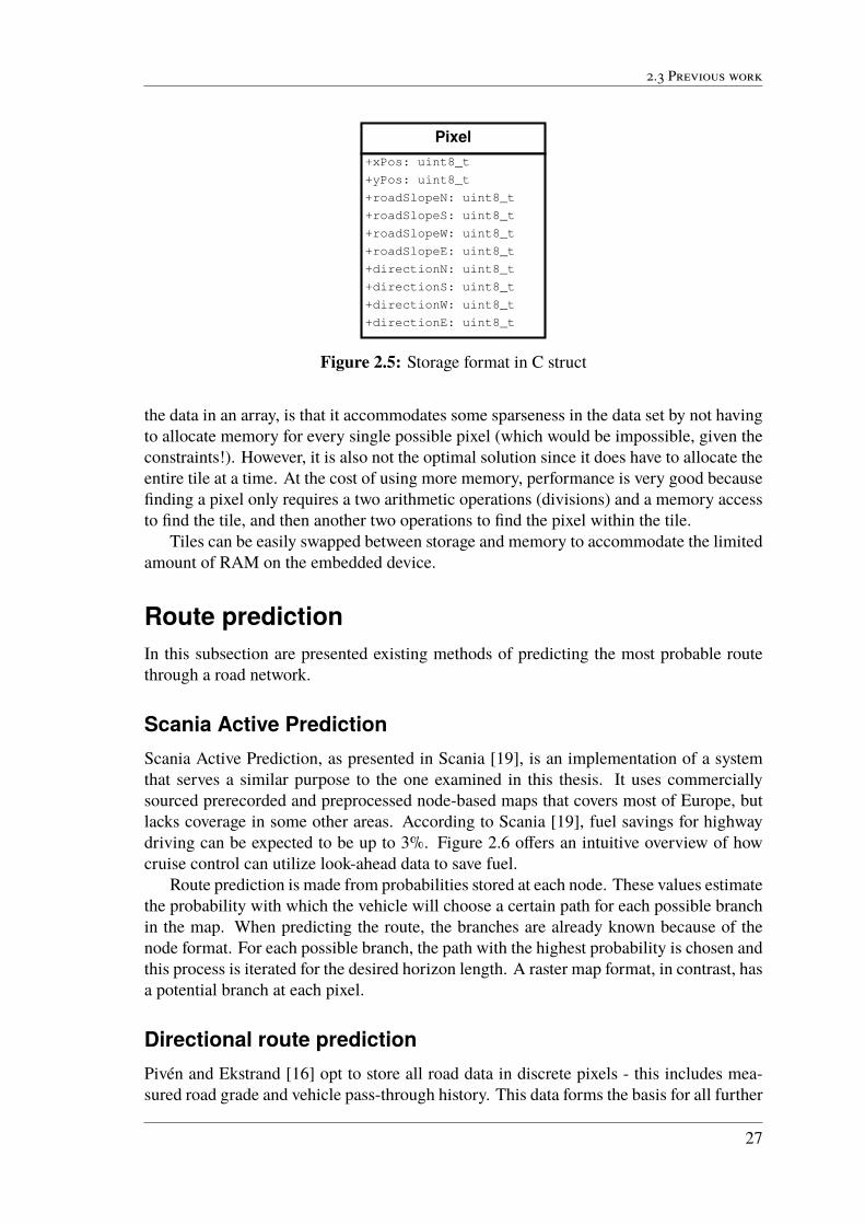
Road grade is stored as four values that represent road inclination in each of the fourdirections through the pixels. This simplified format means that very little processing isrequired when updating pixels. Figure 2.5 shows the data structure for an individual pixel.
Tile-based storage
Tile-based storage is used in Pivén and Ekstrand [16] to give some flexibility in storage,and ease of implementation. It can be compared to a quadtree with only one level, con-taining a high number of nodes. Each node then contains a high number of pixels. Like aquadtree, the correct tile to search for the pixel can be found quickly because it is spatiallymapped within the root node. When the correct tile is found, the pixel can be found withsimilar performance. The design parameter of the data structure is the number of pixelsper tile. The main advantage of this approach compared to the naïve approach of storing
26
2.3 Previous work
Pixel
+xPos: uint8_t
+yPos: uint8_t
+roadSlopeN: uint8_t
+roadSlopeS: uint8_t
+roadSlopeW: uint8_t
+roadSlopeE: uint8_t
+directionN: uint8_t
+directionS: uint8_t
+directionW: uint8_t
+directionE: uint8_t
Figure 2.5: Storage format in C struct
the data in an array, is that it accommodates some sparseness in the data set by not havingto allocate memory for every single possible pixel (which would be impossible, given theconstraints!). However, it is also not the optimal solution since it does have to allocate theentire tile at a time. At the cost of using more memory, performance is very good becausefinding a pixel only requires a two arithmetic operations (divisions) and a memory accessto find the tile, and then another two operations to find the pixel within the tile.
Tiles can be easily swapped between storage and memory to accommodate the limitedamount of RAM on the embedded device.
Route prediction
In this subsection are presented existing methods of predicting the most probable routethrough a road network.
Scania Active Prediction
Scania Active Prediction, as presented in Scania [19], is an implementation of a systemthat serves a similar purpose to the one examined in this thesis. It uses commerciallysourced prerecorded and preprocessed node-based maps that covers most of Europe, butlacks coverage in some other areas. According to Scania [19], fuel savings for highwaydriving can be expected to be up to 3%. Figure 2.6 offers an intuitive overview of howcruise control can utilize look-ahead data to save fuel.
Route prediction is made from probabilities stored at each node. These values estimatethe probability with which the vehicle will choose a certain path for each possible branchin the map. When predicting the route, the branches are already known because of thenode format. For each possible branch, the path with the highest probability is chosen andthis process is iterated for the desired horizon length. A raster map format, in contrast, hasa potential branch at each pixel.
Directional route prediction
Pivén and Ekstrand [16] opt to store all road data in discrete pixels - this includes mea-sured road grade and vehicle pass-through history. This data forms the basis for all further
27

2. Background
Figure 2.6: Illustration on how cruise control can be optimizedfor fuel efficiency using look-ahead technology as shown in Scania[19]
operations on the map.To enable route prediction through this data structure, pixel-by-pixel discrete statistics
are examined. The prediction is done by examining which pixel is the likely successorafter having visited the current pixel, as given by the current GPS location. This approachthus yields four possible succeeding pixels as shown in Figure 2.7, ignoring the diagonalcases, which are, depending on the implementation, technically not possible.
Figure 2.7: Succeeding pixel candidates in route prediction byPivén and Ekstrand [16]. Image: [16].
To give some granularity to the prediction and allow some support for road crossingsand lanes in opposite direction passing through the same squares, a probability is savedfor each side of each pixel. The vehicle is said to enter the pixel from south, north, westor east. The entrance side is then used to find the appropriate successor to the currentpixel, and this pixel is selected for the next step in the horizon. This is continued on apixel-per-pixel basis in order to produce a horizon of sufficient length.
28

2.3 Previous work
The driving statistics through each pixel is updated with each succeeding pass-through,using a weight.
Some noteworthy properties of the approach follow.
+ Memory usage is low at 10 bytes per pixel
+ Relatively simple solution
+ Yields satisfactory results for many cases
- Problems arise when roads fall on the edge of two rows or columns of pixels, and inthe worst case scenario the data needs to be duplicated to achieve the same predictionaccuracy, because the vehicle would need to pass through both cases and build datafor each one separately.
- Highly dependent on pixel size for route prediction. If the pixels are too small,the vehicle might stray into another pixel than the expected one, causing the entireroute prediction algorithm to fail and the horizon to be discarded, which is mostundesirable for this system as transmission capacity is severely limited.
- Road grade information and driving statistics are coupled, while the two might ben-efit from different parameters.
- Road grade granularity, route prediction accuracy and memory performance are allcoupled. Some trade-off needs to be chosen.
Horizon length
In an article by Hellström et al. [9], the optimal length of a horizon, with regards to fueleconomy, is examined. Cost of operation of a HDV is modeled and this model is used totest different horizon length for several routes. The results show that a horizon length of2.5 km is sufficient for a near-optimal prediction in terms of fuel savings for virtually allreal-world cases.
29

2. Background
30

Chapter 3
Implementation
This chapter presents explanations of the specific implementations made for the purposeof this thesis. First is presented an overview of how the two parts (map building and routeprediction) of the system work. Then follows an explanation of how the map buildingworks in detail, after which an explanation of how the route prediction works. Especiallyinteresting (in a performance perspective) implementation details are presented in theirown sections.
Overview
The system can be divided into two logical parts that run in series.
1. Incremental map building. The map is constructed using recorded sensor data foreach new data point sent to the input.
2. Horizon generation. The system predicts the upcoming road slope in real time (aperiod of one second was used in simulations).
Figure 3.1 shows an overview of the map building process. The inputs to this part arethe current GPS position and the current estimated road slope. The system uses the currentheading to find the correct heat map and the GPS position to find the corresponding pixelin the map. If the pixel does not exist, it is created at this point (only pixels with data arestored). The slope value is then recorded and stored, and the pixel heat is increased.
Find corresponding pixel
and heatmap
current GPS position
current road slope
Increase heat
Store slope
Figure 3.1: The map building part of the system
31

3. Implementation
current GPS positionFind corresponding
pixel
Calculate heading
and find heatmap
Find hottest
neighbor pixel
iterate until horizon length 2500m
Fetch slope
values for selected
pixels
Estimate travel
distance between
the points
Road slope horizon
as a function
of travel length
Figure 3.2: The horizon generating part of the system
Figure 3.2 shows an overview of the horizon generation process. The current GPSposition is used to find the corresponding pixel. The current heading is calculated bycomparing the position to the previously recorded GPS position, and the heading is usedto find the corresponding heat map. The neighboring pixels in this heat map are examinedto find the hottest pixel, as defined by their heat value. That pixel is then selected and thestep is iterated for the desired horizon length. After this step is done, the series of pixelsare examined to extract their road slope values. Finally, the travel distance between eachpoint in the horizon is estimated to generate a final road slope as a function of travel length.
Re-implementation of previous work
This section presents the reader with information of re-implementation of previous workfor the purpose of comparison and parameter tweaking in the simulator developed forobtaining the results in this thesis.
Discrete road grade format
This road grade format is re-implemented from Pivén and Ekstrand [16]. In their thesis,this format is used for storing road grade data in a pixel.
The discrete approach simply uses the recorded value and weighs it against the previousstored value with some inertial parameter α.
Φ(n + 1) = (1 − α)Φ(n) + αΦ(n − 1) (3.1)
where α is a constant. While not yielding the most accurate average value, this methodrequires a low amount of storage and processing power as only one value per directionneed be stored.
For the directional route prediction algorithm with four possible directions, this meansthat there are also four slope values stored for each pixel. An advantage of this approachis the low computational complexity. Each pass through a pixel requires only a multipli-cation and an addition to be performed to update the value, and recalling the value whenpredicting the upcoming road grade is simply a matter of fetching one of the stored values.
For the heat map based algorithm, the road grade is similarly stored as one value perdirectional heat map. This allows some flexibility in recall. Depending on the number of
32

3.2 Re-implementation of previous work
directional heat maps being used, values for the same pixel in several heat maps may beweighed together based on the amount of available data. This can improve performance insituations with few data points without sacrificing resolution when many data points areavailable.
Directional route prediction
This per-pixel directional route prediction has its basis in the algorithm described in Pivénand Ekstrand [16]. In order to collect data on the performance of this algorithm and easilytry out adjustments, it is re-implemented. This implementation calculates the most proba-ble next pixel for each pixel in the horizon based on historical direction through the pixel,when entered through one of the four possible edges. The process is iterated for the desiredprediction length, thus producing a string of pixels to pass through. Each pixel is dividedinto four areas; possible entrance from the north, east, south or west. For each possibleentrance direction, the most likely exit direction is stored, as is the road slope recordedin that particular direction. Both these variables are stored as a rolling average of eachrecorded data point, as described in Equation 3.1.
While not yielding the most accurate average value, this method requires a low amountof storage and processing power as only a single value need be stored. For each point inthe GPS trace, the pixel which contains the current coordinate is found and its northern,eastern, southern or western parameter pair is updated according to the formula above,inferring the current bearing of the vehicle by calculating the difference between the pre-vious coordinate pair and the one before that. The most current position is used to infer thesubsequent heading. Thus, three positional data points are used to update a single pixel.
To generate the horizon, the current GPS coordinate is compared to the previous one.This gives a current bearing and position. The latest position is converted into a decimalCartesian coordinate. By truncating the value into an integer, the current pixel in the map isfound. Subtracting the pixel position from the actual non-truncated Cartesian coordinatesyields the position of the vehicle inside the pixel itself, in the range [0, 1]. This internalposition is used as a starting point for trigonometric calculation in the route predictionalgorithm.
Finding entry and exit points
This method is a variation on the implementation used by Pivén and Ekstrand [16]. Todetermine the exit side from a pixel and entry side in the subsequent pixel, and to find themost plausible travel as determined by the method, exit and entry points (see Figure 3.3)need to be found.
In order to find the most probable subsequent pixel, a linear extrapolation from theinternal point in the current bearing is drawn. This is done by forming an expression ofthe line:
k =1
tan(γ)(3.2)
m = y0 − k ∗ x0 |x, y ∈ [0, 1] (3.3)
33

3. Implementation
(0,1) (1,1)
(0,0) (1,0)
(0,1) (1,1)
(0,0) (1,0)
entrance point
exit point / next entrance point
angle
new direction
new direction
Figure 3.3: Entrance and exit points within pixels of the map andtheir positions expressed in relative in-pixel coordinates
Algorithm 3.1 Transforming the exit point into the entrance point of the subsequent pixel
if x == 0:
x = 1
elif x == 1:
x = 0
elif y == 0:
y = 1
else :
y = 0
and using a first degree polynomial:
y = k x + m (3.4)
x =y − m
k(3.5)
to find the possible exit points for the assumed travel through the pixel. The exit points arecharacterized by being points on the border of the pixel, and thus must fulfill the followingcondition, which gives four possible points.
x ∨ y ⊆ {0, 1} (3.6)
The sought after point can be found by virtue of not being outside the pixel borders, aswell as conforming to the correct direction.
Once the exit point is found, the next pixel is known because it will be the pixel sharingthe same border as the one of the exit point. This pixel is then selected as the hypotheticalnext pixel to continue calculating the horizon from the previous pixel in the horizon.
In order to yield a correct result from now on, the entrance point of the pixel is usedas a starting point from which the route continues in the predicted direction through thatparticular pixel. Using the previous exit point, the entrance point is found using Algorithm3.1.
The system now works satisfactorily when running the same GPS trace twice, whichis to be expected since all passed coordinates will have data recorded. However, when
34

3.3 Map building
running a new GPS trace (which would be the case in real-life usage), an issue ariseswhere some pixels passed will be devoid of data because of never having been passedbefore. To alleviate this, a simple look-around algorithm is deployed. If a pixel is missingdata, its neighbors along the same direction are checked. If these are also empty, the currentheading is assumed and a line is extrapolated in the hope of finding upcoming pixels thatdo contain data.
The entry and exit points are used to approximate travel through a pixel as a linearsegment. Route length is estimated by taking the sum of each of these linear segments.
Map building
This section explains the incremental building and storage of the topographical and statis-tical map and its format. The resulting system corresponds to Figure 3.1.
Data point interpolation
The method of obtaining the raw data, as described by Sahlholm [18], is based on esti-mation from several input signals and unusable during certain circumstances such as inbetween gear changes. This means that some gaps in the stream of input data are to be ex-pected, resulting in “skipped” pixels, which will not be updated with historical route data.In order to rectify this, a line interpolation algorithm is utilized to calculate which pix-els were likely passed between two consecutive recorded points, and their data is updatedaccordingly.
The problem can be reduced to drawing a straight line between two points, on a meshgrid. This is done using the Bresenham [3] line drawing algorithm, which is commonlyused in computer graphics implementations for drawing non-anti aliased lines with highperformance. Because a line can be expressed as movement along the y axis and x axis ona two dimensional plane, if we define movement along the x axis to be constant, the linethen becomes a function of y. The line can be expressed as:
y =y1 − y0
x1 − x0(x − x0) + y0 (3.7)
for the starting point (x0, y0) and end point (x1, y1).When drawing the pixelated line, each pixel will contain a certain error from the actual
line. This error is calculated and the pixels that minimize the value are filled in. If anarbitrary line is approximated as a horizontal line, the error will increase linearly with thefollowing value at each point:
∆error =
�����∆y
∆x
�����(3.8)
The algorithm starts by drawing this horizontal line and accumulating the error. Whenthe error reaches 0.5, the y coordinate is either increased or decreased depending on thedirection of the line. This causes the cumulative (signed) error to decrease by one. Byiteration, the entire line is drawn.
35

3. Implementation
Algorithm 3.2 Python code for a simplified Bresenham line drawing algorithm
1for x in range (x0 , x1 +1) :
2points . append ((x,y))
3error += deltaerr
4if error > 0.5:
5y += 1
6points . append ((x,y))
7error -= 1
Note that the error fraction ∆error can be multiplied by an arbitrary scalar as long as thecondition for switching the y coordinate is multiplied by the same constant. Doing someans that implementing the Bresenham algorithm without floating point logic is easy.This makes the algorithm quick on a small microprocessor and highly suited for imple-mentation on an embedded ECU. Furthermore, the algorithm only has to run on eachsample (1 Hz in this case) and only if the speed is such that pixels are skipped.
In order to ensure compatibility with a raster map that disallows diagonal movement,a trivial modification to the algorithm makes sure that selected points are always horizon-tally or vertically adjacent. In the code in Algorithm 3.2, this modification consists of theaddition of program line (6). For the heat map based map, diagonal movement is allowed.
Figure 3.4 and 3.5 show the difference between a naïve and an interpolated approach.
Figure 3.4: A piece of a map constructed using each discrete GPSsample only. Map data: Google, Lantmäteriet/Metria.
Correcting pixel size
As mentioned in the Background chapter, dividing the earth into Cartesian coordinatesevenly along the longitude results in vastly different horizontal pixel sizes, meaning pixelsin for example Scandinavia will be smaller than those at the equator. For consistent per-formance, equal pixel sizes are desired. This is accomplished by a longitude correctionfactor. The number of pixels is calculated as:
36

3.3 Map building
Figure 3.5: The same map portion created from a single trace,with Bresenham interpolation. Map data: Google, Lantmäteri-et/Metria.
nlong = max
(
δcircum f erenceequatorial
sizepixel
, 1
)
(3.9)
for a correction factor δ. The correction factor uses a spherical approximation of the earth,with a cross-sectional circle:
x2+ y2
= r2, r = 1 (3.10)
setting r = 1 means that the pixel size, sizepixel , will approximately hold everywhere inour coordinate system. This means that:
δ = y =√
1 − x2 (3.11)
x =|latitude|
90(3.12)
− 90 ≤ latitude ≤ 90 (3.13)
Since the latitude ranges 90◦ in each direction as in Equation 3.13, assigning x as in Equa-tion 3.12 means that x will range from 0 at the poles of the earth, to 1 at the equator. Itfollows, then, that the pixel size (Equation 3.9) will be corrected by having fewer pixelscloser to the poles.
Precisely at the poles of the earth, the number of latitudinal pixels would be zero. Thisis avoided by setting the number of pixels to be at least one.
Planar road grade format
The planar approach to road grade storage stores the road grade in a pixel as a plane, asseen in Figure 3.6. Each pixel is initialized with a neutral road grade of 0◦ in all directions,giving a plane with the normal vector:
37

3. Implementation
Figure 3.6: Illustration of using a planar approach for storing theroad grade within a pixel
~n = [0, 0, 1] (3.14)
If we define a point:
p =
(
12,12, 0
)
(3.15)
that is in the center of the pixel (defined with dimensions (1, 1)), it, together with thenormal vector, defines the plane that represents the road grade in the pixel. If the point isconstant, only the three components of the normal vector need to be stored. Furthermore,by using a normalized vector, one of the points can be omitted as it can be calculated fromthe other two points at run time.
The advantage of this approach is mainly in data consistency. Rather than saving manygrade values, which may be internally inconsistent, a plane will at all times describe anunambiguous slope in three dimensions. It will also represent reality more accurately, andmake the most out of the limited input data. Two passes through the pixel in two differentdirections is sufficient to build a plane that perfectly represents reality within the givenlimitations (i.e. assumed linear road grade within each pixel), whereas storing four ormore directional road grades requires each direction to be passed through at least oncein order to gather enough data. The drawback, of course, is more intense computationalrequirements.
Each pass through the pixel will update the plane so as to contain the current trajectory,in three dimensions. In other words, fitting the plane to two points aentrance and aexit :
aentrance, aexit ∈ R3 (3.16)
constructed from the entrance and exit points, respectively.
pentrance, pexit ∈ R2 (3.17)
Two arbitrary points pentranceand pexit, are transformed the following way:
pi = (xi, yi) (3.18)
a = (xi, yi,±slope
2) (3.19)
38

3.3 Map building
So that the slope will be the different between the z-values of the 3-dimensional entranceand exit point.
This is an under-determined system which means that the plane will inherently retainsome previous data at each pass through.
Another advantage is granularity. The planar approach will not truncate different di-rections into one of n possible directions, but will allow a more accurate approximationof the road grade when passing through the pixel at a slightly different angle than the pre-vious time. Although this improved accuracy will, in most cases, be small for reasonablysmall pixels.
In order to determine the new plane after a new pass through, after aentranceand aexithavebeen calculated, the new plane is found by calculating its new normal vector. This is doneby first finding the vector of the two recorded points:
~v = aexit − aentrance (3.20)
A third vector:
~u | ~u⊥~v, ~u⊥~n (3.21)
is constructed by taking the cross product:
~u = ~n × ~v (3.22)
This gives the new normal vector as:
~n = ~u × ~v (3.23)
which together with the previously defined point p gives the new plane that passes throughthe desired points.
To reverse the process and obtain the slope, the two dimensional entrance and exitpoints to the pixel are calculated. Using the following description of a generic plane, andits relation to the normal vector:
ax + by + cz + d = 0 (3.24)
~n = [a, b, c] (3.25)
a, b, c ∈ R (3.26)
The x and y coordinates of each point is plugged into the plane description and the z
value is calculated. The value of the scalar d is calculated using the fixed point definedpreviously. The z value gives the distance from the plane to the imagined point on the twodimensional pixel. Adding the z values of both border points in the current direction givesthe slope in that direction.
39

3. Implementation
Decoupled road grade data
Since there are pixel size trade-offs between accuracy, sparseness and the number of prob-able paths, the ideal pixel size for predicting the route might not necessarily be the idealsize for storing the road grade data. Therefore, a decoupled road grade map is implementedthat makes use of an incremental trace merging approach, as described in Section 2.3.1.This is implemented as an alternative to storing the road grade on a per-pixel basis and anevaluation is presented in Section 4.6.
Slope values are stored in a separate map, without specific pixel sizes. Instead, theyare stored as nodes and the closest node for any given coordinate is the road grade at thatpoint. When another measurement is performed, it is merged into an existing node if thecoordinate is within a certain vicinity of an existing node, and the road grade differenceis lower than a certain threshold. When nodes are merged, their road grade values are av-eraged together, as are their coordinates. This means the nodes dynamically move aroundas they are merged into each other.
If the aforementioned conditions are not met, a new node is inserted into the map. Theidea is to store road grade information on an as-needed basis, allowing for more data inregions with varying road grade. This approach may be used with either the discrete roadgrade format, or the planar road grade format.
Three parameters govern the behavior of the algorithm:
• limdi f f is the maximum allowed road grade difference between nodes. If the abso-lute difference is smaller than this value, they are eligible for merging.
• limdist is the maximum allowed distance for merging nodes. If the distance betweenthem is smaller than this value, they are eligible for merging.
• mindist is the minimum distance between any two nodes. If the distance betweenthem is smaller than this value, they are unconditionally merged. The intent ofthis parameter is to counteract noisy data and avoid populating a very small areawith road grade values of wildly different values, as this most likely indicates mea-surement error. Instead, by merging those nodes, the measurement become moreaccurate.
Heat map based route prediction
A heat map (first named in a patent by Kinney [11]) is a raster matrix that stores a fre-quency value (“heat”) for each element. It is typically used for visualization of data sets,particularly to map frequency of a certain occurrence or prevalence in a two dimensionalplane. The name is derived from the common display of such heat maps as colored over-lays ranging from blue (cold) to red (hot), indicating a range of relative frequency. For aroute finding application, each time the pixel is passed through, this value in incremented.The heat, then, represents the probability of travel for that particular pixel in the map.
A novel approach to route prediction based on the historical frequency of travel througheach pixel is developed by constructing a number of heat maps, each representing a dif-ferent range of possible vehicle headings. When the vehicle travels through a pixel, its
40

3.4 Heat map based route prediction
Figure 3.7: A four component directional heat map. Map data:Google. Top to bottom: heading south, west, north and east.
heading is calculated and used to increase the heat in the heat map most closely corre-sponding to that direction. The number of such directional heat maps is adjustable. Agraphical representation of such a map is shown in Figure 3.7.
Recording
Figure 3.8 shows how the pixels are updated. When the vehicle passes through a pixel(when a data point is recorded), the corresponding heat map among the n directional heatmaps is found by calculating the heading of the two previous points (the previous recordedpoint and the one before that). Note that the spacing of the previous points, from whichthe direction is calculated, affects the course stability in routes predicted in the resultingmap. The directional heat map most closely matching this direction is selected and theheat value for this pixel is increased in the chosen heat map. Figure 3.8 shows, for a fourdirectional heat map, pixels that were updated in north bound direction (orange), westbound (blue, diagonally striped fill) and south bound direction (green, dotted fill). Notethat the heading is calculated with some delay, as shown by the north bound pixels.
The directional approach means that complex situation such as crossing paths will notinterfere, while still allowing complex path taking patterns and prediction. A variety ofparameters allow for tuning of performance in such situations.
41

3. Implementation
Figure 3.8: Updating directional heat map according to travel di-rection
Predicting
When the prediction is made, the corresponding directional heat map is used to calculatethe next likely pixel. First, the correct heat map is determined by calculating the currentheading and assigning it to one of the predefined directions, depending on the number ofdirections in the directional heat map.
For each possible next pixel candidate, the heat is computed as such:
heatcandidate = heatcurrent_direction
(
∠[~vcurrent,~vcandidate]π
+ α
)
(3.27)
where ~vcurrent is the current direction vector and ~vcandidate is a vector drawn between thecurrent pixel and the candidate pixel as in Equation 3.28. Take ∠[~vcurrent,~vcandidate] as theclosest absolute angle between the vectors, such that Equation 3.29 holds.
~vcandidate = pixelcurrent − pixelproposed (3.28)
0 ≤ ∠[~vcurrent,~vcandidate] ≤ π (3.29)
α is a parameter that sets a minimum multiplier. This means the heat of the directioncorresponding to the current heading will be multiplied by a factor:
α ≤(
∠[~vcurrent,~vcandidate]π
+ α
)
≤ α + 1 (3.30)
the purpose of which is to give priority to a prediction that continues the current headingapproximately, which is almost always true at a pixel level.
42

3.4 Heat map based route prediction
The current direction is calculated as a the angle between the current pixel and a pixeln places back (sliding window). This is kept track of using a queue. The distance n be-tween which the angle is calculated determines the granularity due to aliasing, and alsowillingness to change direction.
When the number of directions is set to, for example, four, the result is four separateheat maps, one for each direction, as seen in Figure 3.9. Each heat map represents the fre-quency through which each pixel is traveled, on the condition that the direction falls withinthe threshold. When doing a prediction, one of the four heat maps is chosen depending onthe current direction, and used to calculate the probability of the next pixel.
Figure 3.9 shows, starting in the upper left corner, the heat map for direction south,west, north and east. Travel in the specified direction will be evident as more heat (red) inthe portions of the map where travel in that direction is more commonplace.
Figure 3.9: The four components of a directional heat map withfour directions. Map data: Google. Left to right: heading south,west, north and east
Figure 3.10 illustrates the composition of the map system and how it is accessed to
43

3. Implementation
produce a route prediction. In the figure, one heat map is selected depending on the traveldirection and the pixel heat values of that heat map examined to find the most likely suc-ceeding pixel for travel.
Figure 3.10: Selecting one of several heat maps according totravel direction, and using heat values for predicting the route. Im-age: patent figure from patent by Fabian [5]
Even though the heat maps are directional, it may sometimes happen that the mostlikely route is one that loops around. Sometimes, this may be the desired behavior such aslow-speed situations in quarries and other tight navigational spots. At other times, how-ever, this may be unreasonable due to travel at highway speeds or simply unlikely depend-ing on the road conditions. To deal with this problem, a parameter is introduced to limitthe maximum allowed number of travels through the same pixel. By limiting this value,endless loops are minimized to essentially a single round-trip through two pixels, and thencontinuation in the correct direction. This essentially amounts to a work-around but it doeseliminate problematic situations in a reasonable way, error-wise. When considering thecomplete horizon, the remaining temporal error produced by such a loop is in most casesnegligible.
44

3.4 Heat map based route prediction
Algorithm 3.3 Local aging through scalar multiplication
let heat = heat in direction
if heat is at max bound then
for demote in heat_values_in_pixel do
demote = demote * 0.95
end
else
heat = heat + 1
endif
Algorithm 3.4 Local aging through subtraction
let heat = heat in direction
if heat is at max bound then
for demote in heat_values_in_pixel do
demote = demote - 1
end
else
heat = heat + 1
endif
Aging
Aging is the process of lowering the heat at each pixel through some method, the purposeof which is to keep all values from overflowing their data type. If the value was simplycapped, the steady state would be a map of equally hot pixels everywhere, which woulddefeat the purpose of such a map. Therefore, some type of aging is needed to preserve thedata.
Several approaches are possible. One might used a timer to globally decrease the heatafter a pixel has not been passed through in a certain time, or decrease the heat for borderpixels along the way. The problem with the first proposal is it requires a lengthy processingstep. It is perhaps conceivable to perform such a task when the vehicle is idle.
A simpler and more realistic solution to this problem is to perform the aging at a singlepixel when it is passed through. To do this, the heat of the current direction is calculated.If it is at the maximum bound of its data type, the other heat values in the pixel can bescaled back by some scalar as shown in Algorithm 3.3. This keeps the proportions intact,and prevents overflow in a manner with very low computational overhead. A conditionalstatement is added, which is bypassed the majority of time (depending on the scalar chosenand data type). Another possibility is to subtract all heat values in the pixel except thecurrent one, as per Algorithm 3.4.
Loops
To eliminate U-turns of the highway, endless loops and other problems, the number ofallowed visits to each pixel in a single horizon is limited.
The parameter governing the amount of visits per pixel allowed in each horizon hasa great impact on the predicted route. The reason for this is because this setting governs
45

3. Implementation
Figure 3.11: Loops disallowed (left) vs allowed (right). Map data:Google, Lantmäteriet/Metria.
the plausibility of loops in the predicted route. In Reference #3 (see Section 4.1.3), whendriving in a quarry, loops are comparatively common. Disallowing them (visitlim = 1)might be reasonable for regular roads and highway driving, in particular. The same settingsgives unexpected behavior, however, in Reference #3. By increasing the tolerance in thiscase, loops are again allowed. Figure 3.11 shows the prediction at a certain point withloops disallowed (left) and loops allowed (left) (visitlim = 3). The actual route takeninvolves looping around and returning the same way. With loops disallowed, however, thesystem selects the next most probably route, which is to keep the current heading (southin the picture).
For the on-road driving in Reference #2, however, allowing loops yields a sub optimalresult. To rectify this, a speed dependent setting is introduced such that:
visitlim =
α, speedcurrent > 40kph
β, otherwise(3.31)
46

3.5 Distance calculation
Distance calculation
Since the desired output of the system is the road grade as a function of distance, thelength of each point of the route needs to be determined. The result of the prediction is aseries of pixels that the HDV is predicted to pass through, but the exact distance at eachpoint is unknown. Using the pixel size would only yield a correct value for straight travelthrough the pixels (direction perpendicular to one of the pixel sides). Therefore, someapproximation is needed.
The desired result is an approximation of the travel distance for each and every pixel inthe horizon. To approximate the distance that the HDV is assumed to travel to reach a givenpoint, a way of converting WGS84 coordinates is a prerequisite. A method of determininga plausible fine-grained path between the pixels of the horizon can be accomplished in afew different ways:
• Linear travel through each pixel by interpolating linearly between the entry and exitpoint for each pixel. This is described by Pivén and Ekstrand [16].
• Linear approximation by calculating the distance between two pixels of some dis-tance in the horizon, and division by the same number of data points
• Polynomial fitting to select pixels
• Spline fitting to the entire horizon
Linear interpolation
One of the most straight-forward approaches to calculating the length of the distance isto linearly interpolate between two points. This is done by selecting two close pixels inthe horizon with some distance between them and calculating the linear distance betweenthem, as described previously. The pixel coordinates are used, which represents an aliasedversion of the assumed route. The distance between the center point of two subsequentpixels will not be a very accurate estimation of the actual distance traveled, but by takingtwo pixels of some distance along the horizon, the aliasing error is diminished.
This distance is then divided by the number of data points between the two pixels toobtain an average “distance per data point” value that is applied to the latest data point.This value can then be re-calculated for each point by using a queue that keeps track of thelast few points of the horizon, as it is being constructed.
This approach will give a good estimate for straight road segments, but introduce someerror in road segments with curvature.
Polynomial interpolation
Another possible approach to calculating the distance is to use a polynomial interpolationbetween some selected points, and then calculating the arc length of the polynomial, givingthe distance estimation.
Monotonic growth of the x axis is ensured by adding a small value to subsequent pointsif they are equal.
47

3. Implementation
A problem with polynomial fitting is that for cases of straight travel, the resulting poly-nomial is a very poor estimation of the route traveled. Figure 3.12 shows an example ofsuch a situation. Three points are plotted to the left, with piecewise linear interpolationshown, and to the right is the same plot with a second degree polynomial fit. Note thedifference in axis scale.
Figure 3.12: Second degree polynomial interpolation of threepoints
To try and rectify this, more points from the source data are used for the polynomialfit. A cubic polynomial has three unknowns:
p2(x) = a2x2+ a1x + a0 (3.32)
which means that three points is an exact determination of the corresponding polynomial.This is what causes the unwieldy shape of the curve. By adding more points to the sourcedata the system becomes over-determined and solving using the least squares method (Leg-endre [12]) yields a polynomial that is a more reasonable assumption of the route taken topass through the original points specified, as shown in Figure 3.13.
Figure 3.13: Least-squares fit of second degree polynomial tothree linearly interpolated points
Applying this to the simulated system gives the result in Figure 3.14, showing a secondand third order polynomial interpolation of five points, as well as the linear interpolation.
48

3.6 Heat as a quality measure
Note from this figure that the polynomial interpolations are disconnected from the end-points.
For sharp curvatures, the polynomial that fits within the x-axis that it is being evalu-ated inside, the length may be significantly shorter than the linear interpolation, causingan underestimation of the distance. A possible solution to this is to interpolate linearlybetween the endpoints of the polynomial and the start and end pixel.
Figure 3.14: Linear, quadratic and cubic least-squares interpola-tion of points
Splines
Yet another possible approach is to construct a quadratic spline along the points. Since aspline passes through every point specified, the set of pixels is thinned by discarding everynth point. Figure 3.15 shows an example of such a spline, with every fifth point used.
The spline differs in previously described approaches in that it is calculated once forthe horizon, and the same spline is used to estimate the travel distance at each point.
Heat as a quality measure
Quality implies several properties of a horizon generation system that are of importance.
• Making sure the system does not behave worse than the fallback case
• Minimizing route changes and route planning instability from one prediction to thenext
• Determining when to discard the horizon and start anew
49

3. Implementation
Figure 3.15: Predicted route approximated by using a quadraticspline
On a pixel level
One goal of the robustness is to prevent the incline prediction from deviating significantlyfrom actual road conditions. Returning a positive incline when the actual incline is nega-tive, or vice versa, is considered catastrophic, and in these cases one would like the systemto recognize its own uncertainty and fall back to a zero incline prediction.
By keeping track of the number of cold points in the horizon (defined as never havingbeen actually traveled through), and disallowing more than 5 cold points, a fallback is donewhere the rest of the horizon thereafter is a zero incline slope. This avoids the horizon fromdeviating from the road, finding another road and returning an incorrect slope predictionthat risks being far off the correct value.
One advantage of the heat map based route prediction approach is its inherent abilityto quantify the quality of a given horizon. This is done by summing the heat of each pixelthat makes up the horizon, producing a total heat value for the entire horizon. If this valueis zero, that means none of the pixels have ever been passed through, and the horizon willbe equivalent to a fallback with no incline. If the horizon is non-zero, but low, this likelymeans that the horizon “cuts off” somewhere, and we can resort to a fallback due to notfinding a viable path. This may be due to an unexpected path choice, incomplete dataor erroneous predicted route. In these cases, this uncertainty may be determined by thehorizon heat value. What this means practically is that a conscious choice regarding whento resort to a fallback can be taken based on this value.
To exploit the heat value as a quality measure in a meaningful way, several viablehorizons can be constructed to evaluate them on a few different metrics.
Defining the pixel certainty as:
certaintypixel =
���heathighest − heatnext_highest���
heathighest
(3.33)
50

3.6 Heat as a quality measure
0 ≤ certaintypixel ≤ 1 (3.34)
produces a value at each point in the horizon measuring the certainty of the path choice atthat particular point. Equation 3.33⇒ Equation 3.34. A value of 0 means that the secondhighest path, defined as a branch at this pixel, is just as likely as the one chosen, and avalue of 1 means that the chosen path is the only one that contains any data whatsoever.
When the certainty dips below a certain threshold, we consider the alternate pathby taking the next most probably branch and recursively calculating the horizon for thischoice. Using this method, several horizons of high likelihood are derived. They are com-pared to each other based on difference in road grade and total heat.
The difference in road grade matters because we are keen on avoiding predicting apositive incline when the actual slope in negative, and vice versa, especially for large valuepredictions. By avoiding making a prediction in cases when alternate routes differ greatlyin their predicted slope, the informed choice to fall back to a slope of 0◦ can be made. Bydoing so, the system will perform as if no prediction was made, rather than risk performingworse than no prediction.
On a horizon level
Something can be done to improve the system-wide robustness, meaning the series ofhorizons being produced and finally transmitted. By using the heat values as a basis, wecan measure the quality of a given horizon and make sure we always generate a plausibleroute.
The total horizon heat is used for determining the quality of each horizon. If the heatof a horizon is substantially lower than another one, this likely means that the lower heathorizon either cuts off somewhere, or simply is less traveled. When the heat differencereaches a certain threshold, the choice can be made to disregard the lower heat horizon infavor of a higher heat one. The results of this are explored in Section 4.5.
In order to avoid cold horizons, several horizons of descending likelihood are producedand weighed according to:
weighthorizon =heathorizon
i α + 1(3.35)
where i is the horizon number (0 being the first and most likely candidate) and α is aconstant. The horizon heat is defined as the sum of the heat of the pixels comprising thehorizon.
heathorizon =
∑
heatpixel (3.36)
The other horizons are then found by finding ambiguous points and branching off at thesepoints. The horizon of the highest weight, weighthorizon, is chosen.
Another possible strategy at this point is to revert to a fallback of zero incline. This isespecially useful if one of the horizons predicts a steep incline while the other predicts asteep decline, as this suggests the risk for error is high.
51

3. Implementation
Figure 3.16: Frequency response of a second order low pass filterwith a cut-off frequency of 0.2 Hz
Figure 3.17: Effects of the filters on a route prediction signal
Filtering
Signal noise and measurement uncertainty inherent due to the method of approximatingthe road slope (as described by Sahlholm [18]) cause the need for output signal filtering.The first step of this filter is a simple cutoff filter for rogue values since at some single pointserroneous data is presented either due to measurement noise or transitioning through pixelswith missing data. These are removed by considering three points at a time. The differencebetween the first and second points are calculated and if this values exceeds a threshold,the second point is replaced by a linear interpolation between the first and third points.
The data is then fed through a low-pass filter to smooth it. A second order filter is cho-sen to minimize phase shift. Figure 3.16 shows a low-pass filter with a cut-off frequencyof 0.2 Hz.
This effects of the two filters applied are shown in Figure 3.17.
52

3.8 Horizon transmission
Horizon transmission
Since the ECU that generates the horizon is not the ECU where the horizon will be uti-lized for gear selection and cruise control, it needs to be transmitted across a CAN buswith limited capacity. With this in mind, methods for limiting data transmission whilesimultaneously increasing robustness are developed.
A horizon that is robust enough that it does not need to be recalculated from scratch atevery point is desirable. To test this, a horizon h(x), defined as a function of a distance,with the function value representing road grade, can be generated at some point x0 alonga route. For a new horizon hnew (x) , generated further along the route x1, the followingshould hold:
h(x) ≈ hnew (x) ∀x ∈ [x0, x1] (3.37)
for some tolerance. The benefit of fulfilling this condition is that the horizon can hold forseveral points, and does neither need to be recalculated nor resent across the distributednetwork for every new GPS sample. This concerns the reliability of the horizon as a pre-dicted route.
As a first step towards achieving this, the new and old horizons need to be aligned. Thisis done by excising a number of data points at the start of the previous horizons, since theyare now presumably behind the vehicle, giving the new start index iprevious as the pointwith the smallest distance between the two horizons:
iprevious = i | min(���horizonnew (0) − horizonprevious (i)
���)
(3.38)
By examining the first few GPS coordinates, the start offset can be found quickly. If it isnot, this means the horizons are too far apart and the previous horizon should be discardedanyway. Although it depends on the horizon spacing, in reality usually only the first two orso points need to be examined. Figure 3.18 shows three non-aligned subsequent horizons,overlaid on top of each other, without alignment. From this figure is visible that they differonly by an offset. Remove the offset by aligning them and they differ only by their endpoints.
53

3. Implementation
Figure 3.18: Three subsequent horizons, overlaid on top of eachother
The desired end result, however, is not actually a prediction of the route; this is merelya means to and end. A road slope function is the final output from the system. Therefore,the other aspect of the horizon quality is to examine the predicted/recorded road slope.
As mentioned in Section 1.2, data transmission capability is severely limited. The idealcase would be building a perfect horizon and incrementally updating the tail of the horizonwith new data while removing old data at the head.
The solution for transmission is to replace all data points in the old horizon when∆i > tol with the corresponding data value of the new horizon. This way, only someselect data points are re-sent, along with some meta data to place them in the correct orderin the horizon, which is to be performed by the target ECU system. A suggested form ofmeta data for accomplishing this is the distance from the current position, which makesit trivial to find the correct data point to replace by comparing the values. By doing this,points can be sent in any order. This is done in the prototype to assemble the final horizonand measure its error.
The individual point resend strategy means that the distance needs to be recalculatedinside the receiving ECU, since the entire horizon is not retransmitted. The proposedsolution for this is to use a counter that starts out at zero, and increments by the differencebetween the distance from the current data point to the previous one at each point. Tosupport this, the difference in position between the current point and the previous one istransmitted, rather than the absolute value. Algorithm 3.5 shows the implementation inthe simulation environment.
Retransmission of single points, however, is not supported by the current ADAS In-terface Specification ([4]) and implementing this would thus require a custom interface.
54

3.9 Data structures
Algorithm 3.5 Recalculating point distances in modified horizon
if i > 0:
x_current += aligned_x [i] - aligned_x [i -1]
x_list . append ( x_current )
Because of this, an alternative approach of resending the entire horizon when any pointsdiffers is explored, which is supported in the current production system.
Since bandwidth is severely limited, it may be the case that not every point in the hori-zon can be sent in its 1 second sample interval. To handle this situation, the new horizon(where the mix of new and old horizon points are determined) is constructed and sent in-crementally. A maximum allowed number of points to be resent is implement to limit andcontrol bandwidth in edge cases. By adopting this strategy, the most important (closest tothe HDV) points are kept up-to-date and a complete horizon is always guaranteed at thereceiving ECU.
Data structures
The chosen data structure governs the memory usage of the map, and it is thus desirableto make it as compact as possible. To store a single pixel in the map, the following genericdata structure is used:
typedef struct {
uint32_t x;
uint32_t y;
uint16_t slope [ N_DIRECTIONS ];
uint8_t heat [ N_DIRECTIONS ];
} pixel_t ;
Note that the slope value accuracy has been increased compared to the previous implemen-tation (see Figure 2.5), because 8 bits are not enough to save the values with a satisfyinggranularity. The x and y coordinates, when using a quadtree, need to be remembered insidethe data structure.
Using the optimized algorithm using three heat maps with five bit heat values (seeSection 4.2.7) gives a possible data structure as such:
typedef struct {
uint32_t x;
uint32_t y;
uint16_t slope [3];
uint16_t heat ; % contains 3 heat values , bounded by
32
} pixel_t ;
for a total data storage requirement of 128 bits, or 16 bytes. This data structure is alignedon the 32 bit processor subject to host the implementation. For the planar based roadslope format, the slope data is replaced with two scalar values, giving it a lower storagerequirement but a larger computational overhead.
55

3. Implementation
Algorithm 3.6 Finding a pixel in the quadtree
def pixel_at (self , (x, y)):
x = int (x)
y = int (y)
global pixeltree
pixel = pixeltree . intersect ( bbox =[x -1 , y -1 , x+1 , y +1])
for candidate in pixel :
return candidate # there can be only one
pixel = Pixel ((x, y))
pixeltree . insert ( pixel ,
bbox =[x -0.1 , y -0.1 , x +0.1 , y +0.1])
return pixel
The heat values are then accessed as follows. By doing this, the heat values can bestored in a compact manner and accessed using bitwise AND operations and bit shifts:
heat1 = (0000000000011111 ∧ heat) (3.39)
heat2 = (0000001111100000 ∧ heat) ≫ 5 (3.40)
heat3 = (0111110000000000 ∧ heat) ≫ 10 (3.41)
Using a quadtree
To quickly find and address a desired pixel, a quadtree is utilized, as described in the Back-ground chapter. A quadtree is normally used for finding points on a continuous range (suchas WGS84 coordinates). Since discrete Cartesian coordinates are used in the implemen-tation, each pixel is given an arbitrary size that is sure to fit within its actual, discrete,dimensions. Algorithm 3.6 shows how storing and recalling pixels using a quadtree isimplemented.
56

Chapter 4
Results
In this chapter, results of different approaches and parameter settings are presented. Thefirst section explains the methodology with which the system is evaluated. The next sectionis concerned with finding the optimal (highest performance yielding) parameters for theheat map based system. Then follows sections with results of managing the horizon trans-mission strategy, horizon weighing using heat values and decoupled road grade storage.The last section contains an estimation of the storage requirements for the map.
Evaluation methodology
One of the core parts of this thesis has been to come up with a reliable evaluation method-ology in order to, as objectively as possible, compare the performance of different ap-proaches. This section presents the reader with an explanation of how this was accom-plished.
Performance assessment
The main basis on which system performance is measured is the average error for severalreference routes. A number of CAN logs (traces) collected from actual HDVs are playedback to the system, each comprising travel along a certain route. By doing this, drivingalong these routes the same number of times as the number of traces is simulated, creatingthe map as it would exist in the vehicle at this point.
After building the map, another, previously unused, CAN log (trace) is then used tosimulate novel driving along a similar, but not identical, route. At equally (temporally)spaced points along this trace, a horizon of a static length is generated and compared tocontinuation of the actual log, and the error between the predicted road grade and therecorded road grade of the trace is compared at each point. Finally, the average error iscalculated.
57

4. Results
erravg =
∑ni=0 |slopehorizon(i) − sloperecorded (i) |
n, dist(n) = 2500 (4.1)
As mentioned earlier, a horizon length of 2,500 meters is sufficient.
Visualization
A visual approach is used to display system characteristics. By doing so, route predictionchoices can been easily seen.
This chapter contains several visualized road segments and predictions. Figure 4.1shows an example of such a visualization. It consists of a data overlay on a map. The datais visualized as differently colored dots depending on what they represent.
• The large semi-transparent gray dot represents the current position of the HDV atthe current data point.
• Blue dots (behind the HDV dot) in decreasing size show the previous GPS locationsof the HDV.
• Red dots (slightly transparent) comprise the horizon as predicted from the currentposition. Points that are passed through more than once are opaque.
• Green dots (smaller than the red dots) are the actual positions that the HDV passedthrough after proceeding from the current data point. In the ideal case, the red dotsshould follow the path of the green ones.
Accuracy is measured by calculating the predicted slope function from the horizon andcomparing to the actual recorded slope when continuing (green dots). For data sets, theerror for each horizon is averaged.
Figure 4.1: Visualization of a road segment. Map data: Google,Lantmäteriet/Metria.
58

4.1 Evaluation methodology
Figure 4.2: Slope plot for the corresponding segment
Figure 4.2 shows the corresponding slope plot for the segment. In this plot, the pre-dicted road grade, produced from the horizon, is plotted in a blue color. The actual sloperecorded after proceeding in plotted in green. The average error is computed up to a de-sired horizon length as the absolute difference between the two plots. Choosing 2,500meters yields an average (per point) error of 0.182 percentage points for this particularsegment.
Reference routes
In order to measure system performance, a few references are defined which are used tocompare different algorithms and gather experimental data against a common baseline.
Reference #1: 10 manually selected segments along a route, containing road crossings,acceleration ramps and roundabouts. These points are especially challenging for routeplanning.
Reference #2: Data consisting of 250 minutes of driving, with the predicted horizon sam-pled every sixtieth second. The route taken starts in Södertälje and follows route 4 pastNyköping, makes a turn before Norrköping and passes Katrineholm and Mariefred on theway back to Södertälje. This route represents typical long haulage driving. Figure 4.3shows the data.
Reference #3: Data from driving in a quarry. This data set is challenging both becauseroutes contain many similar possible routes, as well as tight turns, and inclination differsgreatly, increasing the cost of incorrect prediction. It is also highly relevant, since it rep-resents a situation where commercial road and slope data is typically unavailable. Thereference covers 150 points, separated temporally by 60 seconds. Figure 4.4 shows thedata.
59

4. Results
Figure 4.3: Reference #2. Map data: Google.
Figure 4.4: Reference #3. Map data: Google, Lantmäteriet/Me-tria.
Design choices and parameters
In this section, approaches and parameters for the heat map based system are examinedindividually, to obtain comparative results. Unless otherwise stated, Reference #2, as de-scribed in the previous section, is used for calculating error figures, and the number ofhistorical traces is 10.
The baseline for the errors is the case where no prediction is used, which is analogousto assuming a constant slope of 0◦. This gives an average error of 1.28, which is definedas 100% error. Errors presented in this chapter are expressed as fractions of this value.Table 4.1 shows the baseline error figures for each of the reference routes. Note that thisvalue is the average absolute road slope along the route (i.e. the average deviation from0).
60

4.2 Design choices and parameters
route avg road slope
Reference #1 1.63 ≡ 100%Reference #2 1.28 ≡ 100%Reference #3 4.43≡ 100%
Table 4.1: Baseline values (errors when predicting a constant 0degree slope)
Pixel size (side, meters) average error
10 11% (0.145)15 10% (0.128)20 9.7% (0.124)25 13% (0.163)30 14% (0.181)35 17% (0.212)
Table 4.2: Error as a function of pixel size
Pixel size
The size of the pixels in the raster map has a great effect on several parameters of perfor-mance, and is also dependent on other parameters and the approach which is used for theprediction.
Overall, a balance between several different factors needs to be considered for a givenpixel size to work well.
Table 4.2 shows the effect of increasing pixel size on the predicted route accuracy inthe directional algorithm.
Distance calculation
The results of the chosen distance calculation approach is shown in Table 4.3. For allapproaches, five points are interpolated between. The least squares fit method is used tofind the polynomials. For the natural version, with no fixed endpoints, the 3rd degreepolynomial performs somewhat better because of its ability to get closer to the endpoints.For the version with linear interpolation between the endpoints of the polynomial, and thestart and end pixels, however, the second degree polynomial generally gives rise to morenatural-looking estimated curvatures, as evident if several interpolations are plotted andcompared to each other.
The approaches without fixed endpoints cause the polynomial to be significantly shorterthan the actual traveled distance for some curvatures. This effect is clearly visible whenplotting the slope horizon as in Figure 4.5. See also the visualizations in Section 4.7.
61

4. Results
approach avg error
linear interpolation 9.7% (0.124)2nd degree polynomial interpolation 41% (0.519)3rd degree polynomial interpolation 24% (0.312)2nd deg poly with linear endpoints 10% (0.133)3rd deg poly with linear endpoints 11% (0.135)
quadratic spline 17% (0.212)
Table 4.3: Distance calculation approaches
Figure 4.5: Second degree polynomial distance estimation: natu-ral (left), with linear endpoints (right)
62

4.2 Design choices and parameters
Figure 4.6: Error as a function of horizon length
Horizon length
The longer the predicted horizon, the higher the error will be. The reason for this istwofold:
1. Between each point pair in the horizon, a distance estimation has been made. Thisestimate will grow less and less accurate the further removed from the start positionof the horizon because some error is introduced at each point, depending on theaccuracy of the distance estimation method.
2. The number of route choices increases with travel length, meaning that our route isless certain the farther the travel.
Plotting the error as a function of the horizon length gives us Figure 4.6. To gather thedata for this chart, average errors are computed for separate runs with different horizonlengths.
To show a more meaningful correlation, the average error is again calculated, but eachhorizon is cut in 100 meter long pieces. The average error is calculated for each suchpiece (sliding window). The results of this are visualized in Figure 4.7. The result seemsto be a linear correlation between the distance between the piece and the horizon start,which seems reasonable (see also the linear trend line). Worth noting, however, is that thederivative is not very steep, meaning that long horizon may be used without introducing adramatical amount of error.
The data is also more valuable the more immediately useful it is, meaning the startof the horizon and its higher quality data carries more value than the data later on. Thisis because the most immediate prediction determines when an incline or slope will beginor end, making the timing important. But the more remote the data, the less importantthe exact timing of it. The knowledge of whether there will be an incline or slope andits approximate location is important, but the exact timing or height of the gradient is oflesser importance.
63

4. Results
Figure 4.7: Error for 100 meter sliding window segments of thehorizon, at different positions in the horizon
# directional heat maps average error
1 11% (0.140)2 14% (0.180)3 12% (0.152)4 14% (0.178)10 20% (0.256)
Table 4.4: Error as a function of heat map directions, for 5 traces
Heat map directions
For Reference #2 used as a basis for the data in Table 4.4, a single heat map gives the bestresult. This is interesting, as it would require less overhead. But when delving furtherinto this anomaly, it becomes apparent that the increased accuracy in the single heat mapcase stems from the fact that the five traces the map is based on all combine into moredata for the single heat map, rather than being spread out over several heat maps. Runningthe simulation again, this time with ten traces, indicates that this is the case. Results areshown in Table 4.5.
A single heat map is only effective when travel normally occurs only in one direction
# directional heat maps average error
1 15% (0.198)2 12% (0.159)3 9.7% (0.124)4 12% (0.153)10 20% (0.255)
Table 4.5: Error as a function of heat map directions, for 10 traces
64

4.2 Design choices and parameters
Figure 4.8: Acceleration ramp, with single heat map (left) andfour directional heat maps (right). Map data: Google, Lantmä-teriet/Metria.
# directional heat maps Reference #1 Reference #2 Reference #3
1 47% (0.773) 15% (0.198) 97% (4.28)3 26% (0.430) 9.7% (0.124) 48% (2.11)4 46% (0.752) 12% (0.153) 50% (2.22)
Table 4.6: Average error as a function of heat map directions,summary
in each pixel. In the recorded data set in Reference #2, travel is only performed in one di-rection at any given highway segment. However, when examining some more challengingroad situations, it becomes apparent that using a single heat map with any reasonable pixelsize means the predicted route tends to drift between opposing lanes.
This phenomenon is eliminated by increasing the number of heat maps, which meansthat, for example, an eastbound lane will not ever be selected when traveling west. SeeFigure 4.8 for a visualization of what happens when only using a single heat map for roadsituations other than straight highway travel, as opposed to four. In the single heat mapcase, the predicted horizon follows the acceleration ramp to the highway but decides totake an abrupt turn and return the same way it arrived, whereas with four directional heatmaps, the highway is entered correctly.
The results are confirmed for the other References in Table 4.6. Note that too manydirectional heat maps invoke a sparseness that degrades performance, which is furtherdiscussed in Section 5.1.3.
Road grade format
Two options for storing the road grade have been implemented; storing the slope as discretevalues, one per each heat map direction, or storing the road grade as a plane within eachpixel. The idea is that the plane will always guarantee consistent data, and might produce abetter grade prediction because it allows for entering pixels in any direction. This assumes
65

4. Results
road grade format avg error
Discrete (3 directions) 9.7% (0.124)Planar 15% (0.192)
Table 4.7: Average error as a function of heat map directions,summary
setting avg error Ref #3 avg error Ref #2
visitlim = 1 64% (2.84) 18% (0.236)visitlim = 3 48% (2.11) 12% (0.150)
visitlim =
1, speedcurrent > 40kph
3, otherwise48% (2.13) 18% (0.233)
visitlim =
2, speedcurrent > 40kph
3, otherwise48% (2.11) 9.7% (0.124)
Table 4.8: Error for different configurations of allowing or dis-allowing loops
a plane in a small enough pixel approximates the actual road topography well enough.Table 4.7 shows the performance of using the planar road grade format as compared toa discrete approach. Three directions are chosen because this gives the lowest error, asexplored in the previous section.
Loops and off-road conditions
To evaluate the system performance in off-road conditions, traces from driving in a quarryare examined. A major source of error in this case turns out to be the limited amount ofpermitted visits to a pixel in a single horizon, intended to eliminate loops.
By testing, the solution to allow different numbers of visits depending on travel speedis shown to produce the best results in both highway and quarry situations; allowed loopsin the quarry and disallowed loops at highway driving, see Table 4.8.
Overall system performance in Reference #3 is shown in Table 4.9. The average errorsare, in general, larger for Reference #3 than the previously examined cases, the reasonfor which being the steep slopes present in the quarry. There are inclines as steep as 15º.Horizon length is 500 meters.
The figure obtained in this table might seem excessively high, especially compared toprevious results. But consider the horizon plot in Figure 4.9. It is evident from this figurethat the high derivative of the (noisy) road grade is such a situation causes the error figureto grow large, which the predicted horizon still follows the actual slope.
Aging
The heat map based road map needs some sort of aging to avoid the heat values of eachpixel from exceeding the maximum possible value of the selected data type.
66

4.2 Design choices and parameters
algorithm avg error rel error
no prediction 4.43 100% (baseline)directional algorithm 3.42 77%heat map algorithm 2.11 48%
Table 4.9: System performance when driving in the quarry
Figure 4.9: Horizon plot for a segment in the quarry
67

4. Results
approach 30 traces 300 traces
no aging 13% (0.167) 14% (0.179)-1 when >16 11% (0.140) 12% (0.159)-1 when >32 10% (0.128) 12% (0.151)-1 when >64 13% (0.168) 12% (0.158)
*.95 when >16 11% (0.140) 15% (0.192)*.95 when >32 10% (0.128) 12% (0.155)*.95 when >64 13% (0.168) 12% (0.150)
Table 4.10: Effects of aging on accuracy
# previous traces avg error (directional) avg error (heat maps)
0 (no prediction) 100% (1.28) 100% (1.28)1 73% (0.934) 13% (0.164)5 53% (0.677) 12% (0.152)10 47% (0.604) 9.7% (0.124)
Table 4.11: Average error for the grade prediction of many roadsegments (Reference #2) for horizon length of 2500 meters
Both simple subtraction and multiplying with a scalar smaller than one when one ofthe heat values has reached a certain value, affects prediction accuracy. The chosen weigh-ing parameters for calculating the heat are tested on lower trace maps, and are thereforebiased in favor of values typically found in such maps. Therefore, the prediction actuallyperforms slightly worse as the number of GPS traces increases. Aging proves a useful toolin rectifying this problem. See Table 4.10 for a comparison. For the 300 trace run, the first30 traces were repeated 10 times.
The maximum value of 32 gives the best result according to simulations, which wouldrequire 5 bits to store (25
= 32). Since the ideal number of heat maps seems to be 3, thiswould require a total of 15 bits, meaning all three values could be saved as a single 16 bitinteger.
After some experimentation, the best approach seems to be subtracting all values ex-cept the current one if the current value is at its maximum, or otherwise increase by one.This is very computationally light as it only requires a handful of add operations.
System performance
Since the value of interest is the road slope, errors are calculated based on this measure.Running the directional algorithm implemented based on Pivén and Ekstrand [16] (secondcolumn, “avg error (directional)”) as well as the heat map based algorithm for Reference#2 yields the results in Table 4.11.
One advantage with that might not be obvious at first is the road length calculation inthe heat map based algorithm. Whereas the direction based algorithm constructs its pathbased on where the predicted position happens to end up according to the saved direction
68

4.3 System performance
Figure 4.10: Heat map based prediction (left) vs directional pre-diction (right)
Figure 4.11: Erratic behavior of directional algorithm in a selectsituation. Map data: Google, Lantmäteriet/Metria.
(which may be skewed; remember than passing through the same pixel at different anglesdifferent times will yield a final predicted direction as the average between these two di-rections, possibly pointing to some undesired middle ground position). This means thepath taken might cut corners too tight or too widely. The heat map based approach, on theother hand, since it gives priority to pixels most often traveled through, is more likely toproduce a pixel-level accurate prediction. This means that the predicted length of the roadis more accurate, yielding a predictive curve that is more closely aligned to the referencecurve, thus minimizing the average error.
Figure 4.10 shows the difference in prediction quality between the heat map algorithmand the directional algorithm when driving on a highway above another road segment, andthe predicted routes for this graph are shown in Figure 4.11 for the directional algorithmand Figure 4.12 for the heat map based algorithm.
Using a high pixel size introduces another phenomenon, namely subsequent locationpoints falling inside the same pixel, causing the heat counter to be increased multiple times.Through experimental tuning this is found to introduce an error. By checking the pixelagainst the previous recorded pixel and ignoring subsequent passes through, the systembehaves as expected with increasing number of traces (meaning that a higher amount ofhistorical traces does not lead to a decline in prediction accuracy).
Table 4.11 shows the effect of different number of traces on the prediction result and
69

4. Results
Figure 4.12: Heat map based algorithm in the same situation.Map data: Google, Lantmäteriet/Metria.
route avg error (directional) avg error (heat maps)
Reference #1 69% (1.13) 26% (0.430)Reference #2 13% (0.164) 9.7% (0.124)Reference #3 77% (3.42) 48% (2.11)
Table 4.12: Average error for the grade prediction of the referenceroutes, for 10 previous traces
compares system performance between the directional and heat map based prediction al-gorithms. The more often the vehicle has traveled a certain road, the more accurate futurepredictions along that road will be. In Table 4.12 is shown an overview of system per-formance for all three reference routes, using the optimal parameters as determined in theprevious section.
Horizon transmission
Since the route prediction is performed in one ECU but the data is utilized in another one,the horizon needs to be transmitted over CAN.
Horizons are produced continually, generating a completely new horizon at each point.It is however, desirable not to send the entire horizon every time because of bandwidthlimitations.
If the previous horizon (already sent) is determined to be accurate enough accordingto some tolerance, new data can be appended to the end of the current horizon. If, on theother hand, the new horizon differs significantly and it is determined that the difference islikely a permanent course change from the route prediction algorithm, the current horizonneeds to be discarded and re-sent.
By implementing some strategy to avoid re-sending the horizon at every single point,significant bandwidth is saved. Table 4.13 shows the difference in errors obtained and
70

4.4 Horizon transmission
strategy avg err payload bandwidth total TX resent points
(1) 0.119 4.69 kbps 7,617 KiB 100%(2) 0.167 0.21 kbps 334 KiB 0%
(3), for ∆i > 0.5 0.125 0.40 kbps 658 KiB 4.4%(3), for ∆i > 0.1 0.119 0.43 kbps 704 KiB 5.1%(3), for ∆i > 0.0 0.119 0.44 kbps 722 KiB 5.3%(4), for ∆i > 0.0 0.119 0.48 kbps 790 KiB 6.3%
Table 4.13: Effects of bandwidth management
the bandwidth by changing the bandwidth management strategy. The route driven is acomplete simulation of travel from Södertälje, passing Nyköping and traveling back (seeReference #2). Instead of sampling the horizon at certain interval, the horizon is contin-ually generated once per second (one for every sample point) to simulate the bandwidtheffects in a real-world scenario. This means that the values will be slightly different thanprevious figures.
All simulations are based on a horizon point size of 4 bytes. This fits one 16-bit un-signed integer that represents the distance and one 16-bit fixed point value for the roadinclination. This means that two data points fit inside the payload of a single CAN mes-sage.
A 1 Hz horizon request rate is assumed.These strategies are evaluated:
1. Always re-send. This is the naïve solution where a new horizon is generated forevery movement in the map, and then sent over the CAN network.
2. Only append new points. The old horizon is always kept and as the vehicle travelsfurther, new data points are simply appended at the end of the horizon, and passeddata points are routinely discarded as they are passed.
3. Re-send points with high difference. The new horizon is compared to the previousone and any road slope data points whose difference ∆i exceed a certain thresholdare re-sent individually. This is not supported by the current ADAS Interface Spec-ification ([4]). The distance for each point is recalculated as described in Section3.8.
4. Re-send entire horizon when a deviating point is found, according to the criterion in(3). This strategy is interesting only because it is supported by the ADAS InterfaceSpecification.
The figures in the table are inconsistent with other measurements on Reference #2,because the error is calculated for every single data point as opposed to points spaced by60 seconds, in order to produce horizons that can align. This was necessary to collectapplicable data.
The columns (from left to right) describe: the strategy used for the test, the absoluteaverage error, the required bandwidth for just the payload portion of the CAN message, thetotal amount of data transmitted for the complete loop between Södertälje and Norrköpingand lastly the fraction of data points that were ever re-sent.
71

4. Results
strategy avg err payload bandwidth total TX resent points
(1) 2.10 4.69 kbps 5,566 KiB 100%(2) 4.29 0.07 kbps 83 KiB 0%
(3), for ∆i > 0.0 2.09 0.80 kbps 955 KiB 16%(4), for ∆i > 0.0 2.08 1.25 kbps 1,481 KiB 25%
Table 4.14: Effects of bandwidth management on Reference #3
Figure 4.13: Plot showing the number of horizons (y axis) forwhich a given amount of points (x axis) were resent with strategy(3), for ∆i > 0.0, for Reference #2. Note the break in the y axis.
Trying out the bandwidth transmission management strategy for Reference #3 resultsin the figures presented in Table 4.14.
There is, however, a metric that is important to maintaining high system performancewhen it comes to the transmission strategy. If a 1 Hz horizon generation is used, in thecases where many points along the horizon need to be resent, there may not be enoughtime to resend all the points within the sample interval. This will lead to performancedegradation in the receiving ECU system. To try and measure this, the strategy used forrow 5 in Table 4.13 is used. When each horizon is considered, the number of points thathad to be resent is recorded. A plot is then made that shows the number of horizons as afunction of how many points in that plot had to be resent. The x axis shows the number ofpoints that had to be resent, and the y axis represents for how many horizons this numberof points had to be resent. It is thus desirable to have as low span of values as possible.Figure 4.13 shows the resulting plot. For more than 99% of all horizons, not a single pointneeded to be resent.
Figure 4.14 shows the same data calculated from the Reference #3 data set. This refer-ence route is more densely populated with crossings which gives rise to more uncertainty,as evident by the higher fraction of completely resent horizons. Still, the number of resent
72

4.4 Horizon transmission
Figure 4.14: Plot showing the number of horizons (y axis) forwhich a given amount of points (x axis) were resent with strategy(3), for ∆i > 0.0, for Reference #3. Note the break in the y axis.
points is low.
As seen in Figure 4.14, for the challenging data set in the quarry, all points of thehorizon were resent in roughly 200 of the produced horizons. This is a small fraction ofthe total amount of horizons generated, but is still undesirable. To avoid doing this, thenumber of allowed changes per horizon can be limited. By doing so, the points closest tothe vehicle will be prioritized, as the road grade most immediately ahead of the vehicle hasthe most bearing on system performance. In the case of a complete route change, this willensure that the horizon is smoothly replaced over the course of several cycles, each timeupdating the horizon. Table 4.15 shows the result of applying this strategy in conjunctionwith transmission strategy (3), for ∆i > 0.0.
Setting the limit, limresend , to for example eleven means that, since two points canbe sent per CAN message, one new point at the end of horizon plus eleven resent pointswill result in the transmission of a total of six CAN messages. The maximum desiredamount of CAN messages can be controlled by adjusting this parameter. In Figure 4.15 isshown corresponding graphs for the number of horizons as a function of how many pointswere resent, with different limits. Note that for limresend = 11, the number of horizonsin the first and second bar are almost equal. This is because the number of horizons with0 resent points decreases because refreshed points are instead transmitted more evenlyacross subsequent horizons.
73

4. Results
strategy avg err payload bandwidth total TX resent points
no limresend 2.10 0.80 kbps 955 KiB 16%limresend = 6 2.13 0.28 kbps 329 KiB 4.4%
limresend = 11 2.09 0.33 kbps 397 KiB 5.7%limresend = 31 2.10 0.47 kbps 562 KiB 8.7%limresend = 51 2.10 0.57 kbps 672 KiB 11%
Table 4.15: Effects of point resend limit on Reference #3
Figure 4.15: Resent points when limiting the maximum allowedpoints to resend, for Reference #3. From left to right: progres-sively lower resend limit.
74

4.5 Heat as a quality measure
approach avg error
always use the first horizon 9.7% (0.124)α = 0.5, certaintypixel < 0.2, 5 horizons 8.9% (0.114)
Table 4.16: Choosing among several horizon candidates
Heat as a quality measure
As explored in the previous chapter, the heat values of pixels and cumulative heat valuesfor horizons can serve as a sort of quality measure. This section presents the result ofapplying this to increase horizon quality.
On a pixel level
One goal of the robustness is to prevent the incline prediction from deviating significantlyfrom actual road conditions. Returning a positive incline when the actual incline is nega-tive, or vice versa, is considered catastrophic, and in these cases one would like the systemto recognize its own uncertainty and fall back to a zero incline prediction.
By keeping track of the number of cold points in the horizon (defined as never havingbeen actually traveled through, and consequently having heat values of zero), and disallow-ing more than five cold points, a fallback is done where the rest of the horizon thereafter isa zero incline slope. The idea is to avoid having the horizon deviate from the road, findinganother road and returning an incorrect slope prediction that risks being far off the correctvalue.
This strategy unfortunately also eliminates cases where the prediction loses its way andthen finds it again, and will discard such horizons due to their uncertainty. The end resultis a 3.9% increase in the average error on Reference #1, and unchanged performance onReference #2 and #3. Therefore, this idea was not investigated further.
On a horizon level
To find the most likely horizon in ambiguous situations, alternative horizons are made bygenerating the next most likely branch choices from ambiguous points along the horizon,as defined by the spread in heat values among neighboring pixels.
By experiment, overall system performance is increased for parameters α = 0.5 (inEquation 3.35) and allowing branches only when certaintypixel < 0.2 (in Equation 3.33).The results are in Table 4.16. The error is improved, but only marginally, the reason beingthe data is generally sufficient for the route. The horizon weighing mechanism is usefulfor cases where the horizon may go cold, which primarily happens due to missing data.On the other hand, since this approach requires generating five horizons for each point, aswell as needing to sum the heat for all pixels within each horizon, the computational loadis heightened.
75

4. Results
settings average error # pixels/nodes
slope in pixel (not decoupled) 9.7% (0.124) 36,600limdi f f = 0.1, limdist = 50m ,mindist = 5m 11% (0.138) 43,600limdi f f = 0.1, limdist = 50m ,mindist = 10m 10% (0.129) 32,500limdi f f = 0.1, limdist = 50m ,mindist = 25m 10% (0.132) 15,900limdi f f = 0.2, limdist = 50m ,mindist = 10m 11% (0.138) 33,200limdi f f = 0.0, limdist = 50m ,mindist = 10m 10% (0.134) 58,900limdi f f = 0.0, limdist = 50m ,mindist = 15m 10% (0.129) 29,500limdi f f = 0.0, limdist = 50m ,mindist = 25m 10% (0.131) 16,500limdi f f = 0.05, limdist = 50m ,mindist = 25m 10% (0.130) 16,200limdi f f = 0.05, limdist = 50m ,mindist = 5m 11% (0.135) 50,800
Table 4.17: The effects of using a decoupled trace merging ap-proach for road grade data
Decoupled road grade map
The use of a decoupled road grade data format is examined. The road grade is saved in aseparate quadtree with nodes containing only road slope values and coordinates. These aremanaged using the trace merging algorithm as described in Section 2.3.1. The parametersare limdi f f which is an upper limit for when merging two nodes is considered, and limdist
which is an upper limit for the maximum distance between two nodes to consider mergingthem. When both these conditions are fulfilled, the nodes are merged. The merging stepconsists of weighing the slope value with the previous value, as well as computing theaverage between the node position and the current position.
To avoid noise, when the distance between two nodes is smaller than mindist , theyare merged unconditionally. Table 4.17 shows the results of the decoupled road gradeapproach, for some combinations of parameters.
To conclude, no parameter configuration was found to increase performance by usinga decoupled road grade map. The reason might be that input data is too noisy, making thesystem keep points as separate points whereas the coupled approach will instead minimizethe error by unconditionally forming the average value of each data point in the same pixel.It is therefore very hard to find a trade-off that allows flexibility in the decoupled road gradestorage while being robust to noisy data.
Some storage can be saved by using a decoupled road grade format, but it does comeat a slight cost of accuracy. Since storage is generally not an issue, there does not seem tobe compelling reason to use such a format.
Storage
This section contains calculations that determine the storage needed to store a map for usein an HDV. In order to do this, the following assumption is made:
76

4.7 Storage
Assumption: A heavy duty vehicle travels 50,000 km of unique road during its lifetime (P.Sahlholm, Ph.D, personal communication).Equatorial circumference of the earth: 40,075 km.
All figures are quoted in IEC[1] standard format (KiB, MiB, GiB), in which storageprefixes are defined unambiguously as steps of 1024, as opposed to SI standards (KB, MB,GB) which may refer to either steps of 1024 or 1000.
Tile based approach
The tile-based storage used in Pivén and Ekstrand [16] uses 10 bytes per pixel and thenstores them in a two dimensional array (tile) within an overarching two dimensional array(the map). Each tile then contains a two dimensional array that contains nxn pixels. Thesize chosen for this parameter is 200x200, giving an adequate maximum horizon sizewithin a given set of 9 tiles in memory (see Section 2.3.1). This means each tile willreference 40,000 pixels. In a 32 bit system this means keeping track of 40,000 32 bit (4byte) memory pointers, for a total of 157 KiB of storage overhead for each tile.
The worst case scenario regarding the amount of tiles necessary is that they are nevertraveled through diagonally. This gives a minimum coverage of each tile a piece of roadof 4 km (using a pixel size of 20x20 meters). Assuming a lifetime travel of a HDV of50,000 km, the number of tiles needed to store this data is 12,500. This gives a totalstorage requirement of 12, 500 · 157 KiB ≈ 1917 MiB. The number of pixels within thesetiles would then be 50,000,000
20 = 2, 500, 000, giving us a storage requirement of 2, 500, 000 ·10 bytes + 1917 MiB ≈ 1940 MiB for the pixels and tiles. The overarching map needsto store a two dimensional array addressing each possible tile, giving us an additionalrequired 40,075 km
4 km· 4 bytes ≈ 39 KiB, which is a negligible amount.
This is a manageable amount, and could furthermore be reduced by purging old dataor exceptionally sparse tiles. However, the bulk of storage used consists of pointers thatare never used. It is therefore advised to use a smaller tile size if this storage method is tobe utilized.
Keep in mind that the calculated figure is a worst-case figure than assumes each tileis only traveled through along a single row or column of pixels. It is likely that each tilewould be traveled through in at least two different rows or columns (such as opposinghighway lanes), which would bring the data structure overhead to below 1 GiB. In eithercase, taking this approach will entail storing a large number of sparse matrices.
It is feasible that this amount could be compressed by some suitable compression al-gorithm thanks to its sparse nature. This can be utilized when swapping to disk, but addsa bit of computational overhead instead.
Using a quadtree
A more flexible and easy to use solution, however, is obtained through the use of a quadtree.It is especially suited to storing sparse data without adding massive memory or computa-tional overhead.
The border length in a quadtree node is halved for each subsequent level. This meansthat the border length at level i is 1
2i−1 , starting from level 1. Using a maximum number oflevels of 20, the bounding box side length of the bottom nodes is 40, 075, 000 m · 1
2nlevels−1 =
77

4. Results
40,075,000 m
219 ≈ 76 m. This bounding box will fit a maximum of 4 pixels along each side(worst case), for a total of 16 pixels per bottom node. This means in the worst case scenario,after finding the appropriate node, 15 pixels need to be searched and discarded beforefinding the correct one.
Using this data structure also means that additional memory needs to be included ineach pixel for storing their coordinate, as this is not unambiguously determined by theirlocation within the data structure. Since 216 <
40,075,000 m20 m
< 232, 32 bit unsigned integersmay be used for this.
Using the data structure as defined in Section 3.9, the final pixel size is 16 bytes. Thisgives a pixel storage requirement of 2, 500, 000 · 16 bytes ≈ 38 MiB for the same sizepixels.
The worst case scenario would be straight travel through the spatial area. With theprevious assumption of 50,000 km of traveled road, this means 3 of the top level nodeswould be traversed. The number of bottom nodes is nbottom =
⌈50,000,000 m
76 m
⌉= 657, 895.
The level above that is half that amount, and the one above that half again, etc. Giving usa total number of nodes:
ntotal =
Nlevels−1∑
i=0
nbottom
12i= nbottom
1 − ( 12 )Nlevels
1 − 12
(4.2)
Inserting our values gives the result ∼ 1, 320, 000. Each node consists of four 32 bitpointers, plus 3 pixel pointers per bottom node, bringing the data structure overhead to1, 320, 000 · 16 bytes + 658, 000 · (3 · 4) bytes ≈ 30 MiB. All in all, this map will useapproximately 73 MiB of storage.
78

Chapter 5
Discussion
This chapter contains discussion regarding the most suitable system for route predictionand self-learning map storage. It also presents the reader with a brief overview of theresults obtained in this thesis. This chapter can be read independently of the rest of thethesis, provided an understanding of the heat map based system explained in Section 3.4.
System parameters
This section contains discussion regarding the conclusions that were drawn from the sys-tem implemented. Since various approaches were implemented, these are compared toeach other.
Route prediction approach
A problem with the previous solution, the directional algorithm by Pivén and Ekstrand[16], is that a conflict in road data at the point where the highway passes over anotherroad arises. The same pixel is sometimes passed through on the highway, and sometimesbelow, each time updating the map with conflicting data. This ultimately leads to the wrongprediction of “jumping off” the highway, as seen in Figure 4.11. An inherent problem withthe directional route prediction approach is that the predicted new direction is an averageof historical recordings. This means that the predicted direction may be an angle that fallsin between two different valid paths, but is itself not a valid path to take, which is whathappens in the example. The heat map approach handles complex situations such as thisone more gracefully, as shown in Figure 4.12.
79

5. Discussion
Pixel size
A pixel size of 20x20 meters is shown to be the ideal size for the heat map based algorithm(see Section 4.2.1). Because slope data and prediction data are saved in the same pixels,varying the size has several effects. A lower pixel size gives more fine-grained road slopeassuming sensors are sensitive enough, and that the predicted route is exact enough to passthrough the correct pixel. A smaller pixel size also affects route prediction by spreadingthe same amount of data over more pixels, resulting in more sparse information to usefor route prediction. Another problem that increases as pixels shrink is that the numberof possible routes increase. This increases the risk of choosing the wrong path, choosinga dead end path or ending up in some uncommonly traveled through pixel that yields anincorrect prediction.
A larger pixel size, on the other hand, removes errors in route prediction by eliminatingthe tendency for slightly different routes. Overall, no beneficial effects were found fromdecoupling the road slope data and route prediction data, and it seems like the concludedsize is a reasonable choice for both.
Number of heat maps
For straight highway travel, when there are no road choices, a single heat map works verywell. This is because of the limited number of recordings done for each pixel, the fewerdirections, the more overdetermined the system will be, leading to more accurate data.When increasing the number of heat maps, the same amount of data is spread out overseveral layers of heat maps. On the other hand, using a single road map does not allow forintelligent road choice behavior, and for data sets containing road choices the performancewill be unsatisfactory.
The best system performance for all references is found for 3 directional heat maps(see Section 4.2.4), assuming the number of previous runs is at least 10. In cases of lowerprevious runs, the single heat map case may be better for simpler road situations. Thisis because a higher number of heat maps means spreading out the data more, resultingis more sparse data. Overall, 3 directional heat maps performs well for any amount ofprevious traces. The largest discrepancy is found for 5 previous traces, resulting in an 8%higher error for 3 heat maps as compared to a single one, for Reference #2, consistingmainly of road segments without crossings. For the other references, however, a singleheat map configuration performs significantly worse in all circumstances.
Road grade format
A planar format for storing the road grade as a plane in each pixel is explored (as explainedin Section 3.3.3), however turns out to produce a lower performance that the discrete ap-proach of simply storing a value for each directional heat map. One problem with theplanar approach is that opposing lanes that are close to each other, such as on rural roads,might have inconsistent road grade but still fall within the same pixel, since a 20 meterpixel width is enough to fit both lanes in the same pixel. This gives rise to inaccurate roadgrade data and a conflict depending on which direction is traveled most often.
80

5.1 System parameters
The discrete format, on the other hand, allows the storage of inconsistent data. A pixelshould ideally approximate a small enough portion of the road such that the road slope canbe considered a plane. However, the reality is such that road slope within a pixel of size20 meter might very well be inconsistent depending on the direction traveled. Therefore,the discrete approach outperforms that planar format.
Another advantage of the discrete road format lies in its computational lightness; itsimply requires recalling one of n values (typically 3), whereas the planar approach, whilemore theoretically elegant, requires numerical computations to find the plane and to recallthe road grade in any one direction.
As for the decoupled (node based) road grade format, no parameter configuration wasfound to increase performance (see Table 4.17). The reason is that the input data is toonoisy, making the system keep points as separate points whereas the coupled approachwill instead minimize the error by unconditionally forming the average value of each datapoint in the same pixel. It is therefore very hard to find a trade-off that allows flexibility inthe decoupled road grade storage while being robust to noisy data.
Some storage can be saved by using a decoupled road grade format, but it does comeat a slight cost of accuracy. Since storage is generally not an issue, there does not seem tobe compelling reason to use such a format.
Loops
A loop is defined as passing through the same pixel more than once, giving rise to a “loop”in the predicting route.
Disallowing loops is beneficial to eliminate the risk of looping around on the highway,which is rare, but can happen. However, this means that situations where loops actuallyoccur will now produce an erroneous route prediction. To find a balance between thesetwo design goals, a compromise is made by allowing loops below a certain speed (40 kphis found to be suitable). Experimentation further proves that by allowing a single loopalso at higher speeds, in some complex situations the route prediction actually becomesmore accurate by being able to loop around and find the correct road in case it temporarilygoes in the wrong direction. But limiting loops to one eliminates endless loops. For slowdriving (below 40 kph), such as quarries, a higher number of loops yields a better result.
Aging
The aging strategy proves crucial to system performance. It is of the highest importancethat the system consistently performs well on commonly traveled road networks. Yet still,an aging strategy is needed in order to keep values from overflowing their data types. Thehighest performance is achieved by demoting all neighboring heat values with 1 whena heat value reaches a maximum capacity of 32 (results in Section 4.2.7). This meansthat three heat values (for a 3 direction heat map) can be stored as a single 16-bit integer(explained in Section 3.9).
81

5. Discussion
Distance calculation
For calculating the length in the generated horizon, linear, polynomial and spline interpo-lation are evaluated (see explanations and figures in Section 3.5). Spline interpolation isdone by discarding some points in order not to fit exactly through every point. The problemwith this, however, is that curves are cut too tightly, and the distance is generally under-estimated. Linear and polynomial interpolation are used by fitting the function to pointswith some distance between them, calculating arc length and dividing by the number ofdata points between the selected evaluation points, and then moving this “sliding value”for each new data point. Choosing a distance of five data points proves to give the mostaccurate estimate.
Quadratic and cubic polynomial interpolation gives a very high error, in comparison,but this is mainly due to their endpoints not passing through actual start and end pixels.Compensating for this using linear interpolation between the end pixels and the polynomialendpoints make them a very close match to the linear approach. Ultimately, however, thelinear approach is slightly better and very quick, computationally.
To use spline fitting, some pixels have to be discarded, since the estimated route shouldnot pass the mid point of every single pixel in the horizon. Doing so yields a curve thatlooks like a reasonable approximation of a plausible route. However, depending on thecurvature, it tends to underestimate the travel distance because it cuts corners too early(because pixels are discarded regularly). A possible improvement to this may be a moreintelligent pixel dismissal algorithm that finds the pixels farthest into each corner. Seecomplete results in Section 4.2.2.
Horizon transmission
The rate at which the system is updated is coupled to the rate at which new horizons aregenerated internally. Since these are to be used in another ECU and another software sys-tem, they need to be transmitted across the CAN bus. Managing the transmission approachby only sending select messages brings two advantages:
1. Lower bandwidth usage
2. More stable behavior
That sending less data is equivalent to lowered bandwidth usage is obvious, but the secondpoint is more novel. If we re-send the horizon every time, this means the horizon needs tobe deleted from the ECU it is used at, and received anew. Because the low bandwidth ofthe CAN network, this causes a delay because only two data points can be sent per CANpacket. By only re-sending some of the points, or simply adding to the end of the horizon,these moments of missing data can be greatly reduced.
To accomplish this, the new horizon and the previous horizon are aligned so that theydata points overlap. This means the new horizon might have one or more new data pointsat the tail. These will need to be sent. The previous horizon might contain points at itshead that have been spatially passed by the vehicle. These will be removed.
The remaining points are examined. If all road slope values that are not identicalbetween the two horizons are replaced in favor of the newer value, performance is not
82

5.3 Computational considerations
degraded from the naïve approach, and transmission intensity is lowered by 90.5%, toa level of 0.44 kbps. In fact, performance is slightly higher. The reason for this is thatthe linear approximation method as described in Section 3.5 works more reliably whenworking on multiple data points, which makes the first few points of each horizon slightlyless accurate than the rest. But when moving forward in an existing horizon, the distancecalculation is unchanged and thus based on more data points than currently in the horizon.
This rate is easily maintained. As made evident by Figure 4.13 and 4.14, singularhorizons with a high number of retransmitted points are exceedingly uncommon, even forchallenging quarry conditions, making bottlenecks a non-issue.
Using this strategy for horizon transmission requires a modification to the ADAS Inter-face Specification, or the manufacturer specific implementation, as resending individualpoints is currently not supported by the standard. If one is to adhere strictly to the stan-dard, the entire horizon would need to be resent, which in normal highway driving doesnot affect results too much (see Table 4.13 and Figure 4.13). However, for the quarry driv-ing reference, which represents a more difficult data set, bandwidth is increased from 0.80kbps to 1.25 kbps, which is still well below the naïve version that transmits 4.69 kbps (seeTable 4.14).
The results confirm the natural assumption that subsequent horizons where the routeprediction was unchanged are simply moved forward by a new data point at the end. Inthese cases the other data points will be identical, which is why so much data can be savedby not re-transmitting these data points.
By limiting the maximum number of points to resend, performance in challengingconditions is improved by reducing the risk of a route prediction that changes frequently inuncertain situations. This reduces bandwidth usage dramatically, and allows for the precisecontrol of the maximum allowed number of CAN messages to send for each generatedhorizon (results in Table 4.15). In the quarry data set, bandwidth usage was somewhatsurprisingly reduced by more than half without degrading prediction performance. Thereason for this is that the prediction sometimes behaves erratically for a single data points.By disallowing the complete dismissal of the previous horizon at this point, when theprediction finds its way back to the original route, the amount transmitted is greatly limitedcompared to if a complete retransmission had been carried out.
Computational considerations
In this section are presented the computational requirements and an evaluation of suitabil-ity for using the system on the specified target platform.
Lookup
Lookup is performed both when recording data in a pixel and when doing predictions,once for each pixel in the horizon. This is performed using a quadtree data structure.
For each level, a number of comparisons need to be performed to determine whichquadrant the pixel falls within (three in the worst case), for a maximum of 60 compara-tive branches in a 20 level quadtree. At the bottom level, a linear O(n) brute-force search
83

5. Discussion
among the pixels is performed. The maximum possible amount of pixels in a single bot-tom node is very low, however (see calculations in Section 4.7), and this process can beconsidered constant O(1).
Recording
The recording step always works on the previously passed pixel in order to calculate acurrent direction as well as a previous direction. This requires one pixel lookup at thepreviously passed coordinates, and direction calculation between the previous pixel andcurrent pixel giving the current direction. The direction between the previous pixel andthe one before that is calculated to determine entrance direction into the previous pixel.In addition to this, linear interpolation between points is used if the vehicle has traveledfarther than into a neighbor of the previous pixel.
Each direction is calculated using an arctangent function call, two addition operationsand three multiplication operations.
Bresenham’s algorithm is then invoked, as explained in Algorithm 3.2. The previouspixel, as well as any “skipped” pixels are then looked up and recorded using the currentdirection and slope. Using the discrete slope approach, for each pixel, two multiplicationsare performed to weigh the slope and direction against previously kept values.
The planar approach, on the other hand, involves taking two cross products to findthe new normal vector of the plane, as described previously. This uses 6 floating pointoperations per cross product. This is more computationally intensive, but should be oflittle concern on the target platform, especially when performed only once a second. It isfeasible to implement this using fixed point arithmetic, in order to eliminate floating pointoperations, but this appear unnecessary.
Horizon generation
The horizon generation begins by finding the succeeding pixel to the one where the vehicleis currently situated. This is done by looking at the neighboring pixels (including diagonalneighbors) and calculating the appropriate heat value for these according to the formuladescribed previously.. Using the current direction, the appropriate heat map is selectedand a function call to each of the 8 neighbors performs the heat calculation. Finding theheat for a single pixel uses four multiplication operations and several addition operationsto weigh adjacent heat values in order to produce a more stable prediction. To calculateall heat values then requires 24 multiplication operations. They are then compared to eachother to find the greatest one. This process is repeated once for each pixel that is added tothe horizon, which for a 20 meter pixel size and desired horizon length of 2,500 meters isat most 125 pixels.
The horizon is the aligned with the previous horizon by looking at travel distance es-timation of the first few points and finding the most closely overlapping points in the oldand new horizons. Any previous values of the old horizons are then discarded. The restof the elements are iterated through and compared and all points that have changed fromthe previous horizon are marked for re-transmission and resent, along with one or severalnew data points that are appended at the end of the horizon. The number of such pointsdepends on the vehicle speed and sample frequency of the horizon generation.
84

Chapter 6
Conclusions
This chapter presents the viewer with a brief summary of the system developed in thisthesis, its performance and the conclusions drawn from this system. The last section inthis chapter concerns possible further work within this field.
Summary
After evaluation, the system that yields the highest performance is the novel heat mapbased map format with three directions of the type described in in detail in Section 3.4.This system predicts the most likely route by storing the frequency at which travel hashistorically occurred through a raster map in separate heat maps, depending on the currentdirection of travel. This yields a map system consisting of multiple heat maps, visualizedin Figure 6.1, each heat map representing the likelihood of travel, on a pixel level, for aparticular heading span.
When driving, the heading determines which one of the three directional heat mapsto select, and the heat for the current pixel is increased in this selected direction. Whenpredicting, the heading and heat is used to find the most likely pixel to travel to accordingto the relevant heat map, and this is iterated for the desired horizon length.
Along with the heat maps, the recorded road slope is also stored for each pixel, on a perdirection basis. When the route prediction has been made, the corresponding road slope,for those pixels, is recalled and this represents the final output of the system.
A pixel size of 20x20 meters yields a highly accurate prediction model, as well as mod-est storage requirements and low computational overhead. This system has been shown toaccomplish higher prediction performance than the previous direction based approach forevery scenario.
Table 6.1 shows an overview of the system performance using the parameter settingsthat were found to produce the smallest error. Sample rate is a fixed 1 Hz for both pre-diction and recording. The percentages cited are defined as fractions of the error when no
85

6. Conclusions
Figure 6.1: A four component directional heat map. Map data:Google. Top to bottom: heading south, west, north and east
86

6.2 Storage
Average error, crossings (Reference #1) 26%(
0.4301.63
)
Average error, highway and rural (Reference #2) 9.7%(
0.1241.28
)
Average error, quarry (Reference #3) 48%(
2.114.43
)
Total road length Reference #2 732 kmMap size Reference #2 (pixels) 36,600Map size Reference #2 (KiB) 787 KiB
Average bandwidth Reference #2 0.44 kbps
Table 6.1: Performance overview of preferred system
prediction is used. For complete details on the data and other parameters, see Section 4.2.The values were calculated by simulating driving along reference routes and using datacollected by HDVs when driving along those routes. See Section 4.1.3 for details on thereference routes.
The recommended data transmission approach is to, rather than send a new horizon ateach sample, align the new and old horizons so that their data points overlap as closely aspossible. Provided that the route prediction has not changed, this means the new horizonwill simple be further ahead spatially. Then, only the points whose slope value has changedare transmitted, including any new points at the tail end of the horizon. This results in avery low bandwidth requirement.
To transform the string of road slope values into a string of road slope values andspatial distance pairs, a travel length estimation is carried out. This is done as a linearinterpolation in a sliding window of length five, between the coordinates of the predictedpixels, as this proves to yield the most accurate estimate.
That the error figure for the quarry reference is so high can be explained by the highderivative (noise) of the road grade signal when driving in the quarry, even though thesystem predicts the route well, as shown in Figure 4.9.
The most common case of HDV operation, rural and highway driving, yields a predic-tion error of less than 10% in absolute road grade. To achieve this figure, ten previous runsalong the route were recorded as input to the system. This represents the performance ofthe system for a road portion that has been traveled ten times previously.
Storage
Table 6.2 shows a summary of estimated storage figures for using a predictive map through-out the service life of a HDV as calculated in Section 4.7.
The figures of using a quadtree to store the pixels show that storing such a map in thetarget platform specified in the Background chapter is realistic, and has room to grow. Pro-vided that the commercial map data currently residing in the system were to be removed,there would be room to fit the expected lifetime map of a HDV more than 60 times over,or 3,000,000 km worth of unique road.
This can be compared to the typical life expectancy of a HDV of at least 800,000 km,after which it is often sold and exported for continued use ([7]). All parts of the vehicle arespecified with a life expectancy of at least 2,000,000 km. Note, again, that the vehicle is
87

6. Conclusions
metric 20x20m tile-based 20x20m quadtree
pixel data 23 MiB 38 MiBoverhead 1917 MiB 30 MiB
total 1940 MiB 68 MiB
Table 6.2: Worst case storage use (uncompressed)
extremely unlikely never to pass the same road twice, in which case storage does not grow.A life expectancy of at the very least 3,000,000 km for this system is more than satisfactory.It is unrealistic to believe that storage may ever run out when using this system with 4 GiBof storage as specified by the target hardware.
Further study
All data used for simulation in this thesis is sampled from higher frequency data by se-lecting single data points. A more fine-grained simulation of letting the system averagehigher frequency data may be explored, in the pursuit of reducing sparseness.
The next logical step in the development of a self-learning road slope prediction systemfor the purpose to look-ahead control would be to implement and test the system shownto produce the highest performance. This would involve rewriting the system in C, takingcare to write efficient code, and to implement a CAN communication interface for horizontransmission.
The current production system of using preprogrammed commercial topography mapsperforms very well compared to the solutions of competitors, which is why an exhaustiveperformance evaluation compared to the current system is necessary, if a self-learningdesign is to replace the current system. Another possibility is to investigate the implemen-tation of a hybrid system that combines both approaches.
This thesis looks at using a node based road slope storage approach, but does not usesuch an approach for storing prediction data as this is incompatible with the algorithmdeveloped for this purpose. Further investigation into using a complete node-based systemfor prediction is another possible route for further investigation.
88

Bibliography
[1] Iec 80000-13:2008 quantities and units – part 13: Information science and technol-ogy.
[2] J. Biagioni and J. Eriksson. Inferring road maps from gps traces: Survey and compar-ative evaluation. 91st Annual Meeting of the Transportation Research Board, 2012.
[3] J. E. Bresenham. Algorithm for computer control of a digital plotter. IBM Systems
Journal 4, 1965.
[4] S. Durekovic, A. Bracht, B. Raichle, M. Rauch, J. Requejo, D. Toropov, A. Varch-min, D. Balzer, M. Griesbeck, J. Löwenau, S. Marwitz, M. Mittaz, C. Ress, N. Smith,S. T’Siobbel, and M. Wagner. Advanced driver assistance systems interface specifi-cations v2 protocol. ADASIS Forum, April 2010.
[5] S. Fabian. Se1650027-4s (self-learning map), 2016.
[6] R. A. Finkel and J. L. Bentley. Quad trees a data structure for retrieval on compositekeys. Acta Informatica vol 4 issue 1, 1974.
[7] T. Hällqvist. Scania performance specification - long haulage.
[8] E. Hellström, M. Ivarsson, L. Nielsen, and J. Åslund. Look-ahead control for heavytrucks to minimize trip time and fuel consumption. 5th IFAC Symposium on Advances
in Automotive Control, 2007.
[9] E. Hellström, J. Åslund, and L. Nielsen. Horizon length and fuel equivalents forfuel-optimal look-ahead control. 6th IFAC Symposium on Advances in Automotive
Control, 2010.
[10] F. Hillnertz. Incremental self learning road map. Master’s thesis, KTH, 2014.
[11] C. Kinney. Us75263259. 1991.
[12] A-M. Legendre. Nouvelles méthodes pour la détermination des orbites des comètes.F. Didot, 1805.
89

BIBLIOGRAPHY
[13] X. Liu, J. Biagioni, J. Eriksson, Y. Wang, G. Forman, and Y. Zhu. Mining large-scale, sparse gps traces for map inference: Comparison of approaches. Technicalreport, HP Labs, 2012.
[14] J. B. MacQueen. Some methods for classification and analysis of multivariate obser-vations. In Proceedings of 5th Berkeley Symposium on Mathematical Statistics and
Probability, 1967.
[15] E. Parzen. On estimation of a probability density function and mode. The Annals of
Mathematical Statistics, 1962.
[16] P. Pivén and O. Ekstrand. Grid based predictive roadmap. Master’s thesis, KTH,2015.
[17] M. Rosenblatt. Remarks on some nonparametric estimates of a density function. The
Annals of Mathematical Statistics, 1956.
[18] P. Sahlholm. Distributed road grade estimation for heavy duty vehicles. PhD thesis,KTH, 2011.
[19] Scania. Scania Active Prediction - presentation, 2011.
[20] I. S. Schoenberg. Contributions to the problem of approximation of equidistant databy analytic functions. Quarterly Applied Mathematics 4, 1946.
[21] T. Simpson. Doctrine and Application of Fluxions. Containing (besides what is com-
mon on the subject) a Number of New Improvements on the Theory. And the Solution
of a Variety of New, and very Interesting, Problems in different Branches of the Math-
ematicks. J. Nourse, 1750.
[22] H. Steinhaus. Sur la division des corps matériels en parties. Bulletin L’Académie
Polonaise des Science, Série des Sciences Mathématiques, Astronomiques et
Physiques, 1957.
90


To save fuel in trucks, the use of a self-learning map is explored. By predicting the path, and then the road grade for this path, fuel savings can be achieved via intelligent cruise control and gear shift timing.
As competition in the logistics industry hardens, pressure on heavy-duty truck manufacturers to save fuel, and thus costs, reaches unprecedented levels. Fuel-efficient engines no longer being enough, attention increasingly turns to intelligent software solutions. One idea for such a solution is to predict upcoming hills and crests for intelligent cruise control that saves fuel by driving smoothly and avoiding sudden braking. A self-learning map that uses statistical data to generate a route prediction, and from this prediction a road grade prediction, proves an efficient means to solve this problem. A unique feature of this system is its ability to build a complete map from scratch that contains information about statistical travel as well as topographical data. Each time the vehicle drives along the same road, the information is updated. After 10 such drives the upcoming road slope can be predicted up to 2,500 meters with an average error of less than 10 percent. As the vehicle drives through a known area, the road grade for the path ahead is predicted. To do this, the path the vehicle will take must be predicted. Then, the road grade for this path is predicted. The end result is a diagram that shows what road grade the vehicle will encounter. By using this information, and for example letting off the throttle before a crest, unnecessary fuel consumption is avoided.
At the heart of this system are directional heat maps that store data in frequency grids. The world is divided into small “pixels” of 20 by 20 meters. Each pixel has three lay-ers, divided into three direction ranges. Each pixel contains a value that represents the likelihood of travel through this pixel. The way this works is, when the vehicle drives th-rough a pixel, the pixel corresponding to the current po-sition is selected. Then the direction of travel determines which direction layer to use. Finally, the selected pixel has its value (“heat”) increased by one for this direction. When doing the prediction, the neighboring pixels are examined to find the one with the highest “heat” for the current driving direction. This pixel is selected as the next prediction, and the process is repeated for the desired pre-diction length. The main advantage of this system, as compared to other
solutions, is that it does not require any previous knowledge of the road network. This means that it can be used in areas and countries where topographical data is scarcely available. Furthermore, the system is designed in a light-weight manner such that it may be used in embedded automotive hardware already present in all Scania heavy-duty vehicles.
EXAMENSARBETE Robust Route Prediction in Raster Maps
STUDENT Sebastian Fabian
HANDLEDARE Flavius Gruian (LTH), Per Sahlholm (Scania CV AB)
EXAMINATOR Jonas Skeppstedt
Saving fuel using a self-learning mapPOPULÄRVETENSKAPLIG SAMMANFATTNING Sebastian Fabian
INSTITUTIONEN FÖR DATAVETENSKAP | LUNDS TEKNISKA HÖGSKOLA | PRESENTATIONSDAG 2016-03-18
A diagram showing the predicted road grade in percentage points and the actual road grade