2015_05_12 dissertation binder_vtantsyura

28 April, 2015

pg. 1 © 2015, Vadim Tantsyura, ALL RIGHTS RESERVED.

Impact of Study Size on Data Quality in Regulated Clinical Research:

Analysis of Probabilities of Erroneous Regulatory Decisions in the Presence of Data Errors

Vadim Tantsyura

A Doctoral Dissertation in the Program in Health Policy and Management

Submitted to the Faculty of the Graduate School of Health Sciences and Practice

In Partial Fulfillment of the Requirements

for the Degree of Doctor of Public Health

at New York Medical College

2015

vtantsyura

Pencil

28 April, 2015


Acknowledgements

I would like to thank my colleagues, friends and family who have provided support

throughout this journey. Thank you, Dr. Kenneth Knapp, for keeping this research focused.

With your guidance and foresight, goals became reachable. Dr. Imogene McCanless Dunn,

you stepped into my life many years ago and introduced me to the true meaning of scientific

inquiry. You were the first one who planted the seeds more than a decade ago that led to this

research. Your wisdom and ethics have helped me pull the pieces of this project together. I

thank you, Kaye Fendt, for introducing this research area to me, for ideas, and for bringing

this important issue forward so many people may benefit from. Your gentle touch changed

the direction of my thinking multiple times over the past ten years. I would like to express

my deepest gratitude to you, Dr. Jules Mitchel, for supporting me from my earlier years in

the industry, for shaping my views and writing style, and for your long-time mentorship and

regular encouragement. Your frame of reference allowed me to finalize my own thoughts,

and your impact on my work is much greater than you might think. Dr. Rick Ittenbach, I

greatly appreciate the time you took to listen, and I aspire to be someday as fair and wise as

you are. I would also like to thank Joel Waters and Amy Liu for “turning things around” for

me. I would especially like to thank my wonderful family, who allowed me to step away to

complete my journey. I will make up the lost time, I promise. I hope my children, Eva,

Daniel and Joseph, understand their education will go on for the rest of their lives. I hope

they enjoy their journeys as much as I have mine. I thank my parents, Volodymyr and Lyuba,

for their commitment to being role models for lifelong learning. Last, I would like to thank

my wife, Nadia. She has been a constant source of support through this process and fourteen

years of my other brainstorms. Thanks for understanding why I needed to do this.

28 April, 2015


Abstract.

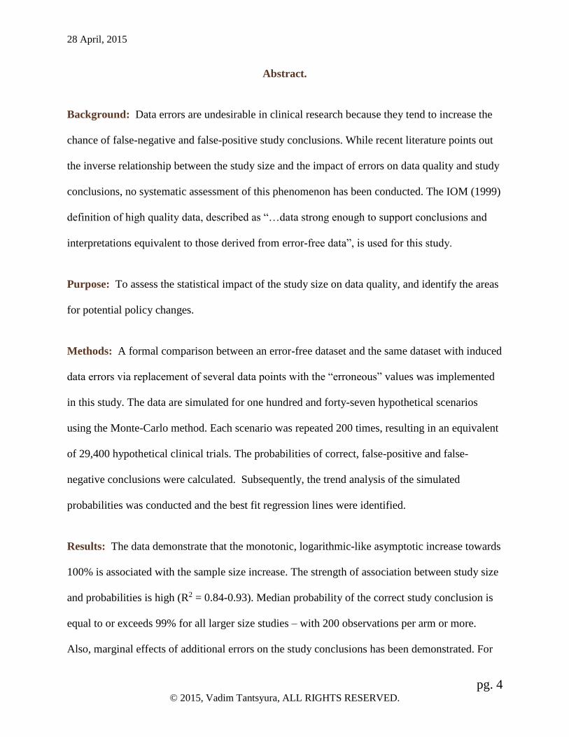
Background: Data errors are undesirable in clinical research because they tend to increase the

chance of false-negative and false-positive study conclusions. While recent literature points out

the inverse relationship between the study size and the impact of errors on data quality and study

conclusions, no systematic assessment of this phenomenon has been conducted. The IOM (1999)

definition of high quality data, described as “…data strong enough to support conclusions and

interpretations equivalent to those derived from error-free data”, is used for this study.

Purpose: To assess the statistical impact of the study size on data quality, and identify the areas

for potential policy changes.

Methods: A formal comparison between an error-free dataset and the same dataset with induced

data errors via replacement of several data points with the “erroneous” values was implemented

in this study. The data are simulated for one hundred and forty-seven hypothetical scenarios

using the Monte-Carlo method. Each scenario was repeated 200 times, resulting in an equivalent

of 29,400 hypothetical clinical trials. The probabilities of correct, false-positive and false-

negative conclusions were calculated. Subsequently, the trend analysis of the simulated

probabilities was conducted and the best fit regression lines were identified.

Results: The data demonstrate that the monotonic, logarithmic-like asymptotic increase towards

100% is associated with the sample size increase. The strength of association between study size

and probabilities is high (R2 = 0.84-0.93). Median probability of the correct study conclusion is

equal to or exceeds 99% for all larger size studies – with 200 observations per arm or more.

Also, marginal effects of additional errors on the study conclusions has been demonstrated. For

28 April, 2015


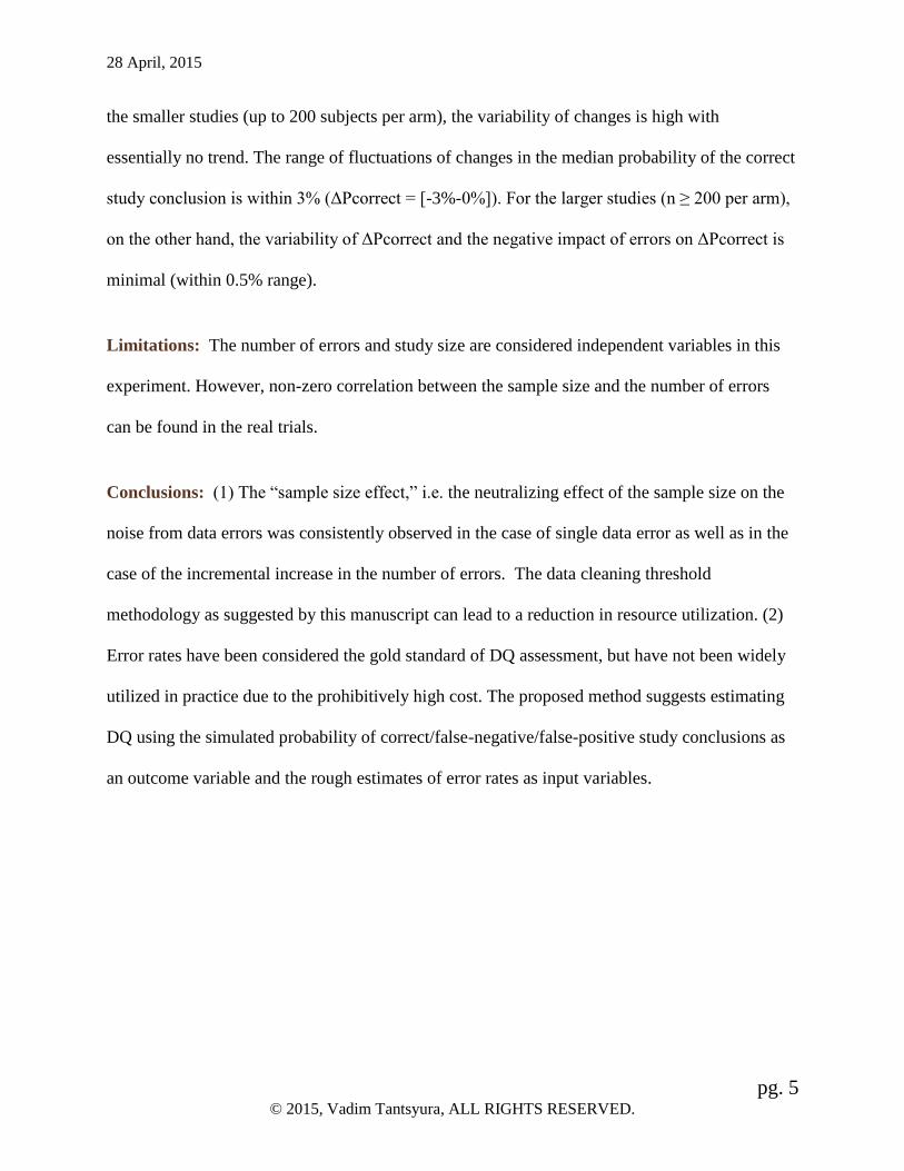
the smaller studies (up to 200 subjects per arm), the variability of changes is high with

essentially no trend. The range of fluctuations of changes in the median probability of the correct

study conclusion is within 3% (ΔPcorrect = [-3%-0%]). For the larger studies (n ≥ 200 per arm),

on the other hand, the variability of ΔPcorrect and the negative impact of errors on ΔPcorrect is

minimal (within 0.5% range).

Limitations: The number of errors and study size are considered independent variables in this

experiment. However, non-zero correlation between the sample size and the number of errors

can be found in the real trials.

Conclusions: (1) The “sample size effect,” i.e. the neutralizing effect of the sample size on the

noise from data errors was consistently observed in the case of single data error as well as in the

case of the incremental increase in the number of errors. The data cleaning threshold

methodology as suggested by this manuscript can lead to a reduction in resource utilization. (2)

Error rates have been considered the gold standard of DQ assessment, but have not been widely

utilized in practice due to the prohibitively high cost. The proposed method suggests estimating

DQ using the simulated probability of correct/false-negative/false-positive study conclusions as

an outcome variable and the rough estimates of error rates as input variables.

28 April, 2015


TABLE OF CONTENTS:

Section I. Introduction ................................................................................................................. 9

Section II. Background and Literature Review .......................................................................... 13

Basic Concepts and Terminology .................................................................................. 13

Measuring Data Quality ................................................................................................. 24

DQ in Regulatory and Health Policy Decision-Making ................................................ 28

Error-Free-Data Myth and the Multi-Dimensional Nature of DQ ................................. 31

Evolution of DQ Definition and Emergence of Risk-Based Approach to DQ .............. 32

Data Quality and Cost .................................................................................................... 34

Magnitude of Data Errors in Clinical Research ............................................................. 41

Source Data Verification, Its Minimal Impact on DQ and the Emergence

of Central/Remote Review of Data ................................................................................ 44

Effect of Data Errors on Study Results .......................................................................... 46

Study Size, Effect and Rational for the Study ............................................................... 46

Section III. Methods of Analysis ............................................................................................... 48

Objectives and End-Points ............................................................................................. 48

Synopsis ......................................................................................................................... 49

Main Assumptions ......................................................................................................... 50

Design of the Experiment .............................................................................................. 51

Data Generation ............................................................................................................. 53

Data Verification ............................................................................................................ 54

Analysis Methods ........................................................................................................... 55

Section IV. Results and Findings ............................................................................................... 57

28 April, 2015


Section V. Discussion ................................................................................................................ 66

Practical Implications ..................................................................................................... 67

Economic Impact ........................................................................................................... 72

Policy Recommendations ............................................................................................... 77

Study Limitations and Suggestions for Future Research ............................................... 80

Conclusions .................................................................................................................... 82

References .................................................................................................................................. 84

LIST OF APPENDIXES.

Appendix 1. Dimensions of DQ ..................................................................................... 93

Appendix 2. Simulation Algorithm ................................................................................ 94

Appendix 3. Excel VBA Code for Verification Program .............................................. 99

Appendix 4. Verification Program Output ................................................................... 105

Appendix 5. Simulation Results (SAS Output) ........................................................... 108

Appendix 6. Additional Verification Programming Results ........................................ 110

Appendix 7. Comparing the Mean in Two Samples .................................................... 113

LIST OF TABLES.

Table 1. Hypothesis Testing in the Presence of Errors .................................................. 15

Table 2. Risk-Based Approach to DQ – Principles and Implications ............................ 33

Table 3. R&D Cost per Drug ......................................................................................... 37

Table 4. Coding For “Hits” and “Misses” ..................................................................... 51

Table 5. Input Variables and Covariates ........................................................................ 52

Table 6. Summary of Data Generation .......................................................................... 52

28 April, 2015


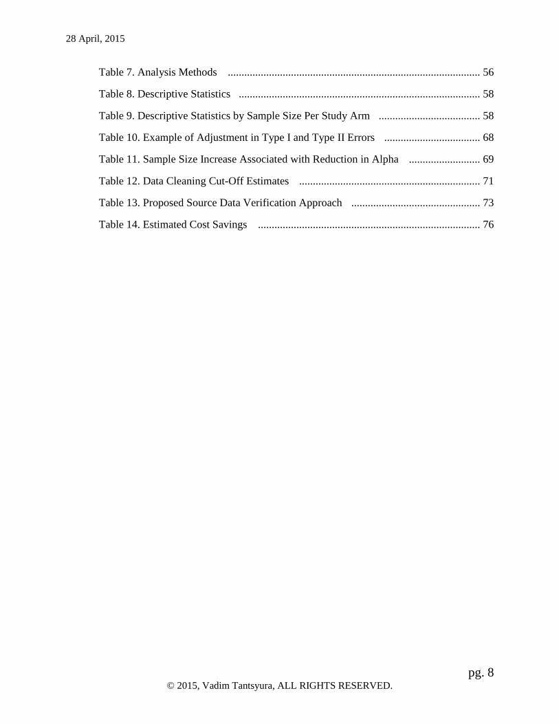
Table 7. Analysis Methods ............................................................................................ 56

Table 8. Descriptive Statistics ........................................................................................ 58

Table 9. Descriptive Statistics by Sample Size Per Study Arm ..................................... 58

Table 10. Example of Adjustment in Type I and Type II Errors ................................... 68

Table 11. Sample Size Increase Associated with Reduction in Alpha .......................... 69

Table 12. Data Cleaning Cut-Off Estimates .................................................................. 71

Table 13. Proposed Source Data Verification Approach ............................................... 73

Table 14. Estimated Cost Savings ................................................................................. 76

28 April, 2015


I. Introduction.

Because clinical research, public health, regulatory and business decisions are largely

determined by the quality of the data these decisions are based on, individuals, businesses,

academic researchers, and policy makers all suffer when data quality (DQ) is poor. Many cases

published in the news media and scientific literature exemplify the magnitude of the DQ

problems that health care organizations and regulators face every day1. Gartner estimates that

data quality problems cost the U.S. economy $600 billion a year. With regard to the

pharmaceutical industry, the issues surrounding DQ carry significant economic implications and

contribute to the large cost of pharmaceutical drug and device development. In fact, the cost of

clinical trials for medical product development has become prohibitive, and presents a significant

problem for future pharmaceutical research, which, in turn, may pose a threat to the public

health. This is why National Institute of Health (NIH) and Patient-Centered Outcome Research

Institute (PCORI) make investments in DQ research (Kahn et al., 2013; Zozus et al., 2015).

Data are collected during clinical trials on the safety and efficacy of new pharmaceutical

products, and the regulatory decisions that follow are based on these data. Ultimately,

reproducibility, the credibility of research, and regulatory decisions are only as good as the

underlying data. Moreover, decision makers and regulators often depend on the investigator’s

demonstration that the data on which conclusions are based are of sufficient quality to support

1 For example, the medical provider may change the diagnosis to a more serious one (especially when

doctors/hospitals feel that insurance companies do not give fair value for a treatment). Fisher, Lauria, Chngalur-

Smith and Wang (2006) site a study where “40% of physicians reported that they exaggerated the severity of patient

condition, changed billing diagnoses, and reported non-existent symptoms to help patients recover medical

expenses. The reimbursement for bacterial pneumonia averages $2500 more than for viral pneumonia. Multiplying

this by the thousands of cases in hundreds of hospitals will give you an idea of how big the financial errors in the

public health assessment field could be”. A new edition of the book (Fisher, et al., 2012) presents multiple examples

of poor quality: “In industry, error rates as high as 75% are often reported, while error rates to 30% are typical. Of

the data in mission-critical databases, 1% to 10% may be inaccurate. More than 60% of surveyed firms had

problems with DQ. In one survey, 70% of the respondents reported their jobs had been interrupted at least once by

poor-quality data, 32% experienced inaccurate data entry, 25% reported incomplete data entry, 69% described the

overall quality of their data as unacceptable, and 44% had no system in place to check the quality of their data.”

28 April, 2015


them (Zozus, et al., 2015). However, with the exception of newly emerging NIH Collaboratory

DQ assessment standards, no clear operational definition of DQ has been adopted to date. As a

direct consequence of the lack of agreement on such a fundamental component of the quality

system, data cleaning processes vary, conservative approaches dominate, and too many resources

are devoted to meeting unnecessarily stringent quality thresholds. According to DQ expert Kaye

Fendt (2004), the considerable financial impact of DQ-related issues on the U.S. health care

system is due to the following: (1) “Our medical-scientific-regulatory system is built upon the

validity of clinical observation,” and (2) “The clinical trials and drug regulatory processes must

be trusted by our society”. It would therefore be reasonable to conclude that the importance of

DQ in modern healthcare, health research, and health policy will continue to grow.

Several experts in the field have been emphasizing the importance of DQ research for

more than a decade. For instance, K. Fendt stated at the West Coast Annual DIA (2004): “We

need a definition (Target) of data quality that allows the Industry to know when the data are

clean enough.” Dr. J. Woodcock, FDA, Deputy Commissioner for Operations and Chief

Operating Officer, echoed this sentiment at the Annual DIA (2006): “…we [the industry] need

consensus on the definition of high quality data.” As a result of combined efforts over the past 20

years, the definition of high-quality data has evolved from a simple “error-free-data” to a much

more sophisticated “absence of errors that matter and are the data fit for purpose” (CTTI, 2012).

The industry, however, is slow in adopting this new definition of DQ. Experts agree that

the industry is so big that, for numerous reasons, it is always slow to change. Some researchers

“in the trenches” are simply not aware of the new definition. Others are not yet ready to embrace

it due to organizational inertia and rigidity of the established processes, as well as because of

insufficient knowledge, misunderstanding, and misinterpretation caused by the complexity of the

28 April, 2015


new paradigm. In addition, due to the fact that vendors and CROs make a lot of money on the

monitoring of sites, monitoring has long become the “holy grail” of the QC regulatory

requirement of operations at the site, regardless of its labor-intensive nature and low

effectiveness. The fact that monitoring findings have “no denominator” is another reason. Each

individual monitoring finding is given great attention, and not put in perspective with the other

hundreds of forms and data points that are good. Also, the prevailing industry belief in training

and certification of monitors might need reexamination. Perhaps it is time to shift resources in

training and certifying coordinators and investigators. Finally, the industry has not agreed on

what errors can be spotted by smart programs vs. what errors require review by monitors. In fact,

only one publication to date addressed this topic. The review by Bakobaki and colleagues (2012)

“determined that centralized [as opposed to manual / on-site] monitoring activities could have

identified more than 90% of the findings identified during on-site monitoring visits.”

Consequently, the industry continues to spend a major portion of the resources allocated for

clinical research on the processes and procedures related to the quality of secondary data – which

often have little direct impact on the study conclusions – while allowing some other critical

quality components (e.g., quality planning, triple-checking of critical variables, data

standardization, and documentation) to fall through the cracks. In my fifteen years in the

industry, I have heard numerous anecdotal accounts of similar situations and have witnessed

several examples firsthand. In a landmark new study, TransCelerate revealed what many clinical

research professionals suspected for a long time: that there is a relatively low proportion (less

than one-third) of data clarification queries that are related to “critical data” (Scheetz et al.,

2014). How much does current processes that arise from the imprecision in defining and

interpreting DQ cost the pharmaceutical and device companies? Some publications encourage

28 April, 2015


$4-9 billion annually in the U.S. (Ezekiel & Fuchs, 2008; Funning, Grahnén, Eriksson, & Kettis-

policy changes (Ezekiel, 2003; Lorstad, 2004) and others estimate the potential savings in the

neighborhood of Linblad, 2009; Getz et al., 2013; Tantsyura et al, 2015) Some cost savings are

likely to come from leveraging innovative computerized data validation checks and reduction in

manual efforts, such as source data verification (SDV). In previous decades, when paper case

report forms (CRFs) were used, the manual review component was essential in identifying and

addressing DQ issues. But with the availability of modern technology, this step of the process is

largely a wasted effort because the computer-enabled algorithms are able to identify data issues

much more efficiently.

Undoubtedly, an in-depth discussion of the definition of DQ is essential and timely.

Study size needs to be a key component of any DQ discussion. Recent literature points out the

inverse relationship between the study size and the impact of errors on the quality of the

decisions based on the data. However, the magnitude of this impact has not been systematically

evaluated. The intent of the proposed study is to fill in this knowledge gap. The Monte-Carlo

method was used to generate the data for the analysis. Because DQ is a severely under-

researched area, a thorough analysis of this important concept could lead to new economic and

policy breakthroughs. More specifically, if DQ thresholds can be established, or minimal impact

of data errors under certain conditions uncovered, then these advancements might potentially

simplify the data cleaning processes, free resources, and ultimately reduce the cost of clinical

research operations.

The primary focus of current research is the sufficient assurance of data quality in clinical

trials for regulatory decision-making. Statistical, economic, regulatory, and policy aspects of the

issue will be examined and discussed.

28 April, 2015


II. Background and Literature Review.

Basic Concepts and Terminology

A data error occurs when “a data point inaccurately represents a true value…” (GCDMP,

v4, 2005 p. 77). This definition is intentionally broad and includes errors with root causes of

misunderstanding, mistakes, mismanagement, negligence, and fraud. Similarly to GCDMP, the

NIH Collaboratory white paper (Zozus et al., 2015) uses the term “error” to denote “any

deviation from accuracy regardless of the cause.” Not every inaccuracy or deviation from the

plan or from a regulatory standard in a clinical trial constitutes a “data error.” Noncompliance of

procedures with regulations or an incomplete adherence of practices to written documentation

cannot be considered examples of data errors.

Frequently, for the monitoring step of Quality Control (QC), clinical researchers

“conveniently” choose to define data error as a mismatch between the database and the source

record (the document from which the data were originally captured). In the majority of cases,

perhaps in as many as 99% or more, the source represents a “true value,” and that prompts many

clinical researchers to assume mistakenly that the “source document” represents the true value,

as well. One should keep in mind that this is not always the case, as can be clearly demonstrated

in a situation where the recorded value is incompatible with life. This erroneous definition and

the conventional belief that it reinforces are not only misleading, but also bear costs for society.

From the statistical point of view, data errors are undesirable because they introduce

variability2 into the analysis, and this variability makes it more difficult to establish statistical

2 Generally speaking, variability is viewed from three different angles: science, statistics and experimental design.

More specifically, science is concerned with understanding variability in nature, statistics is concerned with making

28 April, 2015


significance and to observe a “treatment effect,” if one exists, because it reduces the standardized

treatment effect size (difference in means divided by standard deviation). When superiority trials

are affected by data errors, it becomes more difficult to demonstrate the superiority of one

treatment over another. Without loss of generality, to describe the fundamental framework for

hypothesis testing, it is assumed that there are two treatments, and the goal of the clinical study is

to declare that an active drug is superior to a placebo. In clinical trial research, generally the null

hypothesis expresses the hypothesis that two treatments are equivalent (or equal), and the

alternative hypothesis (sometimes called the motivating hypothesis) expresses that the two

treatments are not equivalent (or equal). Assuming an Aristotelian, 2-value logic system in

support, in the true, unknown state of nature, one of the hypotheses is true and the other one is

false. The goal of the clinical trial is to make a decision based on statistical testing that one

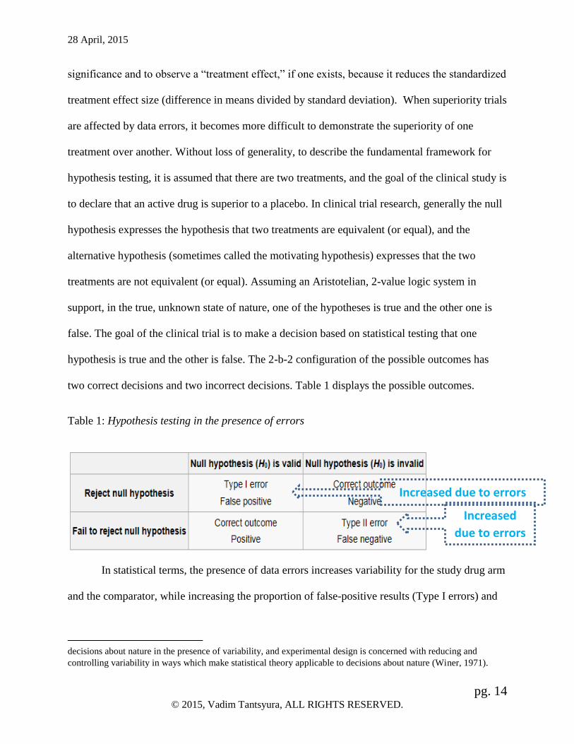
hypothesis is true and the other is false. The 2-b-2 configuration of the possible outcomes has

two correct decisions and two incorrect decisions. Table 1 displays the possible outcomes.

Table 1: Hypothesis testing in the presence of errors

In statistical terms, the presence of data errors increases variability for the study drug arm

and the comparator, while increasing the proportion of false-positive results (Type I errors) and

decisions about nature in the presence of variability, and experimental design is concerned with reducing and

controlling variability in ways which make statistical theory applicable to decisions about nature (Winer, 1971).

Increased

due to errors

Increased due to errors

28 April, 2015


false-negative results (Type 2 errors), thus reducing the power of the statistical test and the

probability of the right conclusion (as shown in Table 1). Because the definitions of the Type I

and Type II errors are reversed in non-inferiority trials relative to the superiority trials, the

treatment of interest in non-inferiority trials becomes artificially more similar to the comparator

in the presence of data errors.

DQ experts state that “DQ is a matter of degree, not an absolute” (Fendt, 2004) and

suggest reaching an agreement with regulators on acceptable DQ “cut-off” levels – similar to the

commonly established alpha and beta levels, 0.05 and 0.20 respectively. This thesis offers a

methodology to facilitate such discussion.

Each additional data error gradually increases the probability of a wrong study conclusion

(relative to the conclusion derived from the error-free dataset), but the results of this effect are

inconsistent. For one study, under one set of study parameters, a single data error could lead to a

reduction in the chance of the correct study conclusion from 100% to 99%. For another study of

a much smaller sample size, for example, the same error could lead to a reduction from 100% to

93.5%. For this reason DQ can be viewed as a continuous variable characterized by the

probability of the correct study conclusion in presence of errors. Obviously, such approach to

DQ is in direct contradiction with the common-sense belief that DQ is a dichotomous variable –

”good”/”poor” quality. This alternative (continuous and probabilistic) view of DQ reduces

subjectivity of “good/poor” quality assessment, quantifies the effect of data errors on the study

conclusions, and leads to establishing the probability cut-off level (X%), which distinguishes

between acceptable and not acceptable levels of the correct/false-positive/false-negative study

conclusions that satisfies regulators and all stakeholders.

28 April, 2015


Numerous sources and origins of data errors exist. There are errors in source documents,

such as an ambiguous question resulting in unintended responses, data collection outside of the

required time window, or the lack of inter-rater reliability (which occurs in cases where

subjectivity is inherently present or more than one individual is assessing the data). Transcription

errors occur in the process of extraction from a source document to the CRF or the electronic

case report form (eCRF). Additional errors occur during data processing, such as keying errors

and errors related to data integration issues. There are also database errors, which include the

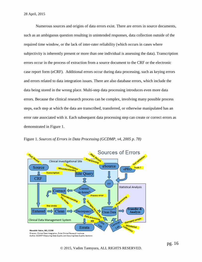
data being stored in the wrong place. Multi-step data processing introduces even more data

errors. Because the clinical research process can be complex, involving many possible process

steps, each step at which the data are transcribed, transferred, or otherwise manipulated has an

error rate associated with it. Each subsequent data processing step can create or correct errors as

demonstrated in Figure 1.

Figure 1. Sources of Errors in Data Processing (GCDMP, v4, 2005 p. 78)

28 April, 2015


Data errors can be introduced even after a study is completed and the database is

“locked.” Data errors and loss of information often occur at the data integration step of data

preparation, in cases of meta-analysis, or during the compilation of the integrated summary of

efficacy (ISE)/integrated safety summary (ISS) for a regulatory submission. This could be a

direct result of the lack of specific data standards. For example, if the code list for a variable has

two choices in one study and five choices in the other, considerable data quality reduction would

occur during the data integration step.

How data are collected plays an important role not only in what is collected by also “with

what quality.” It is known that if adverse events are elicited via checklists, there is an over-

reporting of minor events. If no checklist is used and no elicitation is used, it is known that

adverse events could be under-reported. Similarly, it is known that important medical events get

reported. The FDA guidance on safety reviews expresses views consistent with this known

result. For example, a patient may not recall episodes of insomnia or headaches that were not

particularly bothersome, but they may recall them when probed. Important, bothersome events,

however, tend to be remembered and reported as a result of open-ended questions. Checklists can

also create a mind-set: if questions relate to common ailments of headache, nausea, vomiting,

then the signs and symptoms related to energy, sleep patterns, mood, etc., may be lost, due to the

focus on physical findings.

Variability in the sources of data errors is accompanied by the substantial variation in

data error detection techniques. Some errors, such as discrepancies between the source

documents and the CRF, are easily detected at the SDV step of the data cleaning process. Other

errors, such as misunderstandings, non-compliance, protocol violations, and fraud are more

difficult to identify. The most frequently missed data error types include the data recorded under

28 April, 2015


the wrong subject number and data captured incorrectly from source records. Thus, data error

detection in clinical research is not as trivial as it may appear on the surface. Computerized edit

checks help identify illogical (such as visit two date is prior to visit one date), missing, or out of

expected range values much more efficiently than the manual data review.

Variability in the sources of data errors and the general complexity of this topic have

created substantial impediments to reaching a consensus as to what constitutes “quality” in

clinical research. The ISO 8000 (2012) focuses on data quality and defines “quality” as the

“…degree to which a set of inherent characteristics fulfills requirements.” Three distinct

approaches to defining data quality are found in the literature and in practice. “Error-free” or

“100% accurate” is the first commonly used definition that has dominated clinical research.

According to this definition, the data are deemed to be of high quality only if they correctly

represent the real world construct to which they refer. There are many weaknesses to this

approach. The lack of objective evidence supporting this definition, and prohibitively high cost

of achieving “100% accuracy” are two major weakness of this approach. Additionally, the

tedium associated with source-document verification and general quality control procedures

involved in the process of trying to identify and remove all errors is actually a distraction from a

focus on important issues. Humans are not very good at fending off tedium, and this reality

results in errors going undetected in the vast platforms of errorless data.

The “fit to use” definition, introduced by J.M. Juran (1986), is considered the gold

standard in many industries. It states that the data are of high quality "if they are fit for their

intended uses in operations, decision making and planning". This definition has been interpreted

by many clinical researchers as “the degree to which a set of inherent characteristics of the data

fulfills requirements for the data” (Zozus et al, 2015) or, simply, “meeting protocol-specified

http://www.answers.com/topic/operations

http://www.answers.com/topic/decision-making

http://www.answers.com/topic/planning

28 April, 2015


parameters.” Ambiguity and implementation challenges are the main impediments to a wider

acceptance of this definition. Unlike service or manufacturing environments, clinical trials vary

dramatically and are consequently more difficult to standardize. These inherent limitations have

resulted in the practice by many clinical research companies in the past three decades of using a

third definition – namely arbitrarily acceptable levels of variation per explicit protocol

specification (GCDMP, 2005). The development of objective data quality standards is more

important today than ever before. The fundamental question of “how should adequate data

quality be defined?” will require taking into consideration the study-specific scientific, statistical,

economic, and technological data collection and cleaning context, as well as the DQ indicators3.

As mentioned above, data cleaning and elimination of data errors reduces variability and

helps detect the “treatment effect.” On the other hand, the data cleaning process is not entirely

without flaws or unintended consequences. Not only does it add considerable cost to the clinical

trial conduct, it may potentially introduce bias and shift study conclusions. There are several

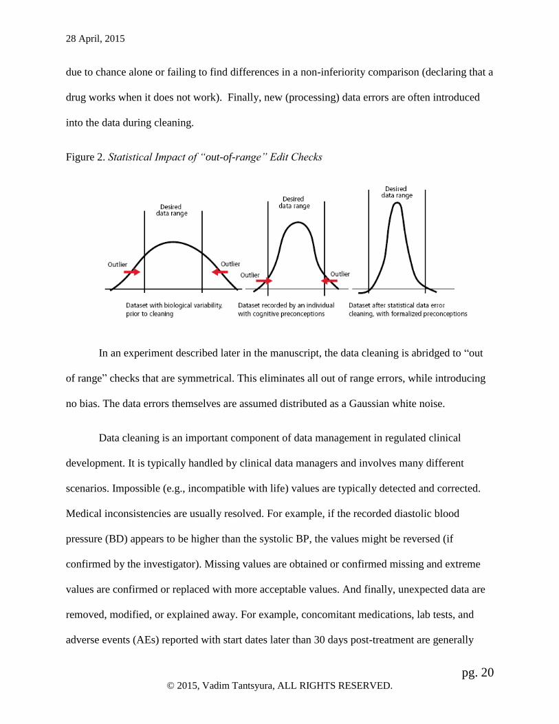
possible scenarios of bias being introduced via data cleaning. Systematically focusing on the

extreme values, when as many errors are likely to exist in the expected range (as shown in Figure

2), is one such scenario. Selectively prompting to modify or add non-numeric data to make the

(edited) data appear “correct,” even when the cleaning is fully blinded and well-intended, is

another example. Before selective cleaning, the data may be flawed, but the data errors are not

systematically concentrated, and, thus, introduce no bias. However, when the data cleaning is

non-random for any reason, it leads to a reduction of variance, and increases the Type I Error

Rate and the risk of making incorrect inferences, i.e., finding statistically significant differences

3 Multiple terms are used in the literature to describe DQ indicators – “quality criteria,” “attributes,” and

“dimensions.”

28 April, 2015


due to chance alone or failing to find differences in a non-inferiority comparison (declaring that a

drug works when it does not work). Finally, new (processing) data errors are often introduced

into the data during cleaning.

Figure 2. Statistical Impact of “out-of-range” Edit Checks

In an experiment described later in the manuscript, the data cleaning is abridged to “out

of range” checks that are symmetrical. This eliminates all out of range errors, while introducing

no bias. The data errors themselves are assumed distributed as a Gaussian white noise.

Data cleaning is an important component of data management in regulated clinical

development. It is typically handled by clinical data managers and involves many different

scenarios. Impossible (e.g., incompatible with life) values are typically detected and corrected.

Medical inconsistencies are usually resolved. For example, if the recorded diastolic blood

pressure (BD) appears to be higher than the systolic BP, the values might be reversed (if

confirmed by the investigator). Missing values are obtained or confirmed missing and extreme

values are confirmed or replaced with more acceptable values. And finally, unexpected data are

removed, modified, or explained away. For example, concomitant medications, lab tests, and

adverse events (AEs) reported with start dates later than 30 days post-treatment are generally

28 April, 2015


queried and removed. Subjects with AEs are probed for previously unreported medical history

details, which are then added to the database. Sites modify subjective assessments when the

direction of a scale is misinterpreted (e.g., one is selected instead of nine on a zero- to- ten scale).

All data corrections require the investigator’s endorsement and are subject to an audit trail.

Data cleaning is a time-consuming, monotonous, repetitive and uninspiring process. The

mind-numbing nature of this work makes it difficult for the data management professionals in

the trenches to maintain a broader perspective and refrain from over-analysing trivial details.

Data managers frequently ask the following question: If a site makes too many obvious

transcription errors in the case of outliers, why would one think that fewer errors are made within

the expected ranges? They use this as a justification to keep digging further, finding more and

more errors, irrespective of the relevance or the significance of those findings. The desire to

“fix” things that appear wrong is part of human nature, especially when one is prompted to look

for inconsistencies. Each new “finding” and data correction make data managers proud of their

detective abilities, but it costs their employers and society billions of dollars. Does the correction

of the respiratory rate from twenty two to twenty one make a substantial difference? More often

than not, the answer is no. As new research demonstrates, over two thirds of data corrections are

clinically insignificant and do not add any value to study results (Mitchel, Kim, Choi, Park,

Cappi, & Horn, 2011; TransCelerate, 2013; Scheetz et al., 2014). Unlike a generation ago, many

researchers and practitioners in the modern economic environment are facing resource

constraints. Therefore, they legitimately ask these types of questions in an attempt to gain a

better understanding of the true value of data cleaning, and to improve effectiveness and

efficiency in clinical trial operations.

28 April, 2015


The process of data collection has markedly transformed over the past 30 years. Manual

processes dominated the 1980s and 1990s, accompanied by the heavy reliance on the verification

steps of the process at that. As an example, John Cavalito (in his unpublished work at Burroughs

Wellcome in approximately 1985) found that a good data entry operator could key 99 of 100

items, without error. The conclusion was made that the data entry operator error rate was 1%.

With two data entry operators creating independent files, that would yield an error rate of

1/10,000 (.01 multiplied by .01 yields .0001, or 1/10,000). Similarly, Mei-Mei Ma’s dissertation

(1986) evaluated the impact of each step in the paper process, and discovered that having two

people work on the same file had a higher error rate than having the same person create two

different files (on different days); the rule for independence was unexpected. It was more useful

to separate the files than to use different people.

The introduction of electronic data capture technology (EDC) eliminated the need for

paper CRFs. Additionally, EDC had antiquated some types of extra work that was associated

with the traditional paper process4. More recently, introduction of eSource technologies such as

electronic medical records (EMRs) and direct data entry (DDE) has started the process of

eliminating paper source records, eradicating transcription errors and, as many believe, further

improving DQ. These events have also led to growing reliance on computer-enabled data

cleaning as opposed to manual processes such as SDV. While in the previous “paper” generation

the SDV component was essential in identifying and addressing issues, modern technology has

made this step of the process largely a redundant effort because the computer-enabled algorithms

4 Examples include (a) “None” was checked for “Any AEs?” on the AE CRF, but AEs were listed so the “None” is

removed, (b) data recorded on page 7a that belonged on page 4 is moved, (c) sequence numbers are updated, (d)

effort is spent cleaning data that will have little or no impact on conclusions and (e) comments recorded on the

margin that have no place in the database.

28 April, 2015


can identify over 90% of data issues much more efficiently (Bakobaki et al., 2012). Nevertheless,

some research professionals have expressed the opinion that the new technologies such as EDC,

EMR, DDE, and their corresponding data cleaning processes may result in a lower DQ,

compared to the traditional paper process, thus justifying their resistance to change. One

argument against the elimination of paper is that lay typists are not as accurate as trained data

entry operators (Nahm, Pieper, & Cunningham, 2008). The second argument, that EDC and DDE

use logical checks to “find & fix” additional “typing errors” by selectively challenging item

values (e.g., focusing on values outside of expected ranges) at the time of entry, also has some

merit. The clinical site personnel performing data entry, using one of the new technologies, is

vulnerable to the suggestion that a value may not be “right” and may unintentionally reject a true

value. In the final analysis, these skeptical arguments will not reverse the visible trend in the

evolution of clinical research that is characterized by greater reliance on technology. The

growing body of evidence confirms that, in spite of its shortcomings, DDE leads to the higher

overall data quality.

The DQ debate is not new. It attracts attention through discussions led by the Institute of

Medicine (IOM)5, the Food and Drug Administration (FDA), DQRI6, and MIT TDQM7, but

consensus in the debate over a definition of DQ has not been reached, nor have the practical

problems standing in the way of implementing that definition been solved. According to K.

5 “The Institute of Medicine serves as adviser to the nation to improve health. Established in 1970 under the charter

of the National Academy of Sciences, the Institute of Medicine provides independent, objective, evidence-based

advice to policymakers, health professionals, the private sector, and the public.” (http://www.iom.edu/; Accessed in

November, 2007) 6 The Data Quality Research Institute (DQRI) is a non-profit organization that existed in early 2000’s and provided

an international scientific forum for academia, healthcare providers, industry, government, and other stakeholders to

research and develop the science of quality as it applies to clinical research data. The Institute also had been

assigned an FDA liaison, Steve Wilson. (http://www.dqri.org/; Accessed in November, 2007) 7 MIT Total Data Quality Management (TDQM) Program: “A joint effort among members of the TDQM Program,

MIT Information Quality Program, CITM at UC Berkeley, government agencies such as the U.S. Navy, and industry

partners.” (See http://web.mit.edu/tdqm/ for more details.)

http://www.iom.edu/

http://www.dqri.org/

http://web.mit.edu/tdqm/

28 April, 2015


Fendt, a former Director of DQRI, the following aspects of DQ are fundamentally important: (1)

DQ is “a matter of degree; not an absolute,” (2) “There is a cost for each increment,” (3) There is

a need to determine “what is acceptable,” (4) “It is important to provide a measure of confidence

in DQ,” and (5) “Trust in the process” must be established. And the consequences of mistrust

are: “(1) “poor medical care based on non-valid data,” (2) “poor enrollment in clinical trials,” (3)

“public distrust” (of scientists/regulators), and (4) lawsuits.” (Fendt, 2004).

Measuring Data Quality

The purpose of measuring data quality is to identify, quantify, and interpret data errors,

so that quality checks can be added or deleted and the desired level of data quality can be

maintained (GCDMP, v 4, 2005, p. 80). The “error rate” is considered the gold standard metric

for measuring DQ, and for easier comparison across studies it is usually expressed as the number

of errors per 10,000 fields. It is expressed by the formula below. For the purpose of this thesis, it

is important to note that an increase in the denominator (i.e, the sample size) reduces the error

rate and dilutes the impact of data errors.

Inspected Fields

Found ErrorsRateError

ofNumber

ofNumber

“Measuring” DQ should not be confused with “assuring” DQ or “quality assurance”

(QA), which focuses on infrastructures and practices used to assure data quality. According to

the International Standards Organization (ISO), QA is the part of quality management focused on

providing confidence that the quality requirements will be met8 (ISO 9000:2000 3.2.11). As an

8 ICH GCP interprets this requirement as “all those planned and systematic actions that are established to ensure that

the trial is performed and the data are generated, documented (recorded), and reported in compliance with Good

Clinical Practice (GCP) and the applicable regulatory requirement(s).” (ICH GCP 1.16). Thus, in order for ICH to be

compatible with current ISO concepts, the word “ensure” should be replaced with “assure”. Hence the aim of

28 April, 2015


example, a QA plan for registries “should address: 1) structured training tools for data

abstractors; 2) use of data quality checks for ranges and logical consistency for key exposure and

outcome variables and covariates; and 3) data review and verification procedures, including

source data verification plans and validation statistics focused on the key exposure and outcome

variables and covariates for which sites may be especially challenged. A risk-based approach to

quality assurance is advisable, focused on variables of greatest importance” (PCORI, 2013).

Also, measuring DQ should not be confused with “quality control” (QC). According to ISO, QC

is the part of quality management focused on fulfilling requirements9. (ISO 9000:2000 3.2.10)

Auditing is a crucial component of Quality Assurance. An audit is defined as “a

systematic, independent and documented process for obtaining audit evidence objectively to

determine the extent to which audit criteria are fulfilled”10 (ISO 19011:2002, 3.1). The FDA

audits are called “inspections.” The scope of an audit may vary from “quality system” to

“process” and to “product audit.” Similarly, audits of a clinical research database may vary from

the assessment of a one-step process (e.g., data entry) to a multi-step (e.g., source-to-database)

audit. The popularity of one-step audits comes from their low cost. However, the results of such

one-step audits are often over-interpreted. For example, if a data entry step audit produces an

acceptably low error rate, it is sometimes erroneously concluded that the database is of a “good

quality.” The reality is that the low error rate and high quality of one step of the data handling

Clinical Quality Assurance should be to give assurance to management (and ultimately to the Regulatory

Authorities) that the processes are reliable and that no major system failures are expected to occur that would expose

patients to unnecessary risks, violate their legal or ethical rights, or result in unreliable data. 9 ICH GCP interprets these requirements as “the operational techniques and activities undertaken within the quality

assurance systems to verify that the requirements for quality of the trial have been fulfilled.” (ICH GCP 1.47) In

order for ICH language to be compatible with current ISO concepts, the word “assurance” should be replaced with

“management.” 10 ICH GCP interprets this requirement as “A systematic and independent examination of trial related activities and

documents to determine whether the evaluated trial related activities were conducted, and the data were recorded,

analyzed and accurately reported according to the protocol, the sponsor’s Standard Operating Procedures (SOPs),

Good Clinical Practice (GCP), and the applicable regulatory requirement(s). (ICH GCP 1.6)

28 April, 2015


process does not necessarily equate to a high quality/low error rate associated with the other

steps of data handling.

Audits are popular in many industries, such as manufacturing or services, for their ability

to provide tangible statistical evidence about the quality and reliability of products. However, the

utility of audits in clinical research is hindered by the substantial costs associated with them,

especially in the case of the most informative “source-to-database” audits. This accounts for the

reduction in error rate reporting in the literature in the past seven to ten years, since the

elimination of paper CRFs and the domination of EDC on the data collection market. At the

same time, such a surrogate measure of DQ as the rate of data correction has been growing in

popularity and reported in all recent landmark DQ-related studies (Mitchel et al., 2011, Yong,

2013; TransCelerate, 2013; Scheetz et al., 2014). Data corrections are captured in all modern

research databases (as required by the “audit-trail” stipulation of the FDA), making the rate of

data correction calculation an easily automatable and inexpensive benchmark for the DQ

research. The rates of data corrections were originally coined by statisticians as a measure of

“stability” of a variable, which is outside of the scope of this discussion.

Theoretically speaking, error rates calculated at the end of a trial and the rates of data

corrections are not substitutes one for the other, but rather complementary to each other. Ideally,

when all errors are captured via the data cleaning techniques, the error rate from a source-to-

database audit should be zero and the rate of corrections (data changes) should be equivalent to

the pre-data cleaning error rate. In a less than ideal scenario, when a small proportion of the total

errors is eliminated via data cleaning, the rate of data correction is less informative, leaving the

observer wondering how many errors are remaining in the database. The first (ideal) scenario is

closer to the real world of pharmaceutical clinical trials, where extensive (and extremely

28 April, 2015


expensive) data cleaning efforts lead to supposedly “error-free” databases. The second (less than

ideal) scenario is more typical of academic clinical research, where the amount of data cleaning

is limited for financial and other reasons. Thus, the rate of data changes is primarily a measure of

the reduction of the error rate (or DQ improvement) as a result of data cleaning, and a measure of

effectiveness of the data cleaning in a particular study. Low cost is the main benefit of the data

correction rates over the error rates, while obvious incongruence of data correction rates to the

error rates calculated via audits is the main flaw of this fashionable metric.

DQ in Regulatory and Health Policy Decision-Making

The amount of clinical research data has been growing exponentially over the past half

century. ClinicalTrials.gov currently lists 188,494 studies with locations in all 50 States and in

190 countries. BCC Research, predicted a growth rate of 5.8%, roughly doubling the number of

clinical trials every ten years (Fee, 2007).

Figure 3. The number of published trials, 1950 to 2007

28 April, 2015


This unprecedented growth, especially in the past decade, coupled with rising economic

constraints, places enormous pressure on regulators such as the FDA and the EMA. Regulators

ask and address a number of important questions in order to claim that the quality of decisions

made by policy makers and clinicians meets an acceptable level. There are numerous examples

of the regulatory documents that clarify and provide guidance in respect to many aspects of

Quality System and DQ (ICH Q8, 2009; ICH Q9, 2006; ICH Q10, 2009; FDA, 2013; EMA,

2013).

Fisher and colleagues reference Kingma’s finding that “even a suspicion of poor-quality

data influences decision making.” A lack of consumer confidence in data quality potentially

leads to a lack of trust in a study’s conclusions. (Kingma, 1996.) Thus, one of the most

important questions the policy-makers and regulators ask is to what extent do the data limitations

prohibit one from having confidence in the study conclusions. Some of these questions: What

methods were used to collect data? Are the sources of data relevant and credible? Are the data

reliable, valid and accurate? One hundred percent data accuracy is too costly, if ever achievable.

Would 99% accurate data be acceptable? Why or why not? Are there any other important

“dimensions” of quality, beyond “accuracy,” “validity,” and “reliability?” (Fisher, 2006; Fink

2005).

The DQ discussion (that is often spearheaded by regulators and regulatory experts) has

to date made progress on several fronts. There is a general consensus on the “hierarchy of errors”

(i.e. some errors are more important than others), and on the impossibility of achieving a

complete elimination of data errors. There will always be some errors that are not addressed by

quality checks, as well as those that slip through the quality check process undetected (IOM,

1999). Therefore, the clinical research practitioners’ primary goal should be to correct the errors

28 April, 2015


that will have an impact on study results (GCDMP, v4, 2005, p. 76). Quality checks performed

as part of data processing, such as data validation or edit checks, should target the fields that are

(1) critical to the analysis, (2) where errors frequently occur, and (3) where a high percent of

error resolution can be reasonably expected. “Because a clinical trial often generates millions of

data points, ensuring 100% completeness, for example, is often not possible; however it is not

necessary” (IOM, 1999) and “trial quality ultimately rests on having a well-articulated

investigational plan with clearly defined objectives and associated outcome measures” (CTTI,

2012) are the key message from the regulatory experts to the industry.

Furthermore, the growing importance of pragmatic clinical trials (PCT)11, the difficuty in

estimating error rates using traditional “audits,” and a deeper understanding of the multi-

dimensional nature of DQ (that is discussed next) have led to the development over the last

couple of years of novel approaches to DQ assessment. An NIH Collaboratory white paper,

which was supported by a cooperative agreement (U54 AT007748) from the NIH Common Fund

for the NIH Health Care Systems Research Collaboratory (Zozus et al., 2015) is the best example

of such innovative methodology that stresses the multi-dimensional nature of DQ assessment and

the determination of “fitness for use of research data.” The following statement by the authors

summarizes the rational, and approach taken by this nationally recognized group of thought

leaders:

Pragmatic clinical trials in healthcare settings rely upon data generated during routine

patient care to support the identification of individual research subjects or cohorts as well

as outcomes. Knowing whether data are accurate depends on some comparison, e.g.,

comparison to a source of “truth” or to an independent source of data. Estimating an error

or discrepancy rate, of course, requires a representative sample for the comparison.

Assessing variability in the error or discrepancy rates between multiple clinical research

11 PCT is defined as “a prospective comparison of a community, clinical, or system-level intervention and a relevant

comparator in participants who are similar to those affected by the condition(s) under study and in settings that are

similar to those in which the condition is typically treated.” (Saltz, 2014)

28 April, 2015


sites likewise requires a sufficient sample from each site. In cases where the data used for

the comparison are available electronically, the cost of data quality assessment is largely

based on time required for programming and statistical analysis. However, when labor-

intensive methods such as manual review of patient charts are used, the cost is

considerably higher. The cost of rigorous data quality assessment may in some cases

present a barrier to conducting PCTs. For this reason, we seek to highlight the need for

more cost-effective methods for assessing data quality… Thus, the objective of this

document is to provide guidance, based on the best available evidence and practice, for

assessing data quality in PCTs conducted through the National Institutes of Health (NIH)

Health Care Systems Research Collaboratory. (Zozus et al., 2015)

Multiple recommendations provided by this white paper (conditional upon the advances in data

standards or “common data elements”) lead in a new direction in the evolution of the data quality

assessment to support important public health policy decisions.

Error-Free-Data Myth and the Multi-dimensional Nature of DQ

In clinical research practice, DQ is often confused with “100% accuracy.” However,

“accuracy” is only one of very many attributes of DQ. For example, Wang and Strong (1996)

identified 16 dimensions and 156 attributes of DQ. Accuracy and precision, reliability, timeliness

and currency, completeness, and consistency are among the most commonly cited dimensions of

DQ in the literature (Wand & Wang, 1996; Kahn, Strong, & Wang, 2002; see Appendix 1 for

more details). The Code of Federal Regulation (21CFR Part 11, initially published in 1997,

revised in 2003 and 2013) emphasized the importance of “accuracy, reliability, integrity,

availability, and authenticity12" (FDA, 1997; FDA, 2003). Additionally, some experts and

regulators emphasize “trustworthiness” (Wilson, 2006), “reputation” and “believability” (Fendt,

2004) as key dimensions of DQ. More recently, Weiskopf and Weng (2013) identified five

dimensions that are pertinent to electronic health record (EHR) data used for research:

12 The original version of the document listed different attributes - Attributable-Legible-Contemporaneous-Original-

Accurate that were often called the ALCOA standards for data quality and integrity; eSource and “direct data entry”

exponentially increase their share and threaten to eliminate the paper source documents, making “Legible”

dimension of DQ an obsolete.

28 April, 2015


completeness, correctness, concordance, plausibility and currency, and NIH Collaboratory

stressed completeness, accuracy and consistency as the key DQ dimensions determining fitness

for use of research data where completeness is defined as “presence of the necessary data”,

accuracy as “closeness of agreement between a data value and the true value,” and consistency as

“relevant uniformity in data across clinical investigation sites, facilities, departments, units

within a facility, providers, or other assessors” (Zozus et al., 2015).

Even in the presence of its established multi-dimensional nature, DQ is still often

interpreted exclusively as data accuracy13. High data quality for many clinical research

professionals simply means 100% accuracy, which is costly, unnecessary, and frequently

unattainable. Funning et al. (2009) based on their survey of 97% (n=250) of phase III trials

performed in Sweden in 2005, concluded that significant resources are wasted in the name of

higher data quality. “The bureaucracy that the Good Clinical Practice (GCP) system generates,

due to industry over-interpretation of documentation requirements, clinical monitoring, data

verification etc. is substantial. Approximately 50% of the total budget for a phase III study was

reported to be GCP-related. 50% of the GCP-related cost was related to Source Data Verification

(SDV). A vast majority (71%) of respondents did not support the notion that these GCP-related

activities increase the scientific reliability of clinical trials.” This confusion between DQ and

“100% accuracy” contributes a substantial amount to the costs of clinical research and

subsequent costs to the public.

13 “Assessing data accuracy, primarily with regard to information loss and degradation, involves comparisons, either

of individual values (as is commonly done in clinical trials and registries) or of aggregate or distributional

statistics… In the absence of a source of truth, comprehensive accuracy assessment of multisite studies includes use

of individual value, aggregate, and distributional measures.” (Zozus et al., 2015)

28 April, 2015


Evolution of DQ Definition and Emergence of Risk-based (RB) Approach to DQ

Prior to 1999, there was no commonly accepted formal definition of DQ. As a result,

everyone interpreted the term “high-quality” data differently and, in most cases, these

interpretations were very conservative. The overwhelming majority of researchers of that time

believed (and many continue to believe) that all errors are equally bad. This misguided belief

leads to costly consequences. As a result of this conservative interpretation of DQ, hundreds of

thousands (if not millions) of man-hours have been spent attempting to ensure the accuracy of

every minute detail.

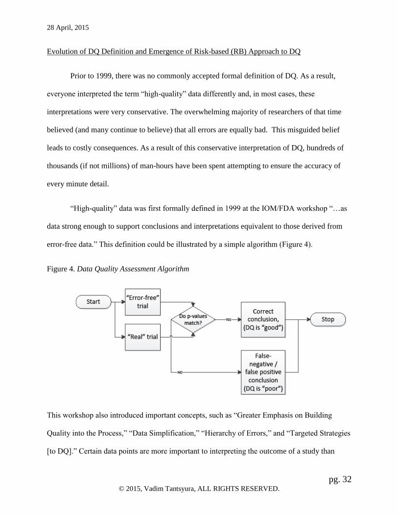
“High-quality” data was first formally defined in 1999 at the IOM/FDA workshop “…as

data strong enough to support conclusions and interpretations equivalent to those derived from

error-free data.” This definition could be illustrated by a simple algorithm (Figure 4).

Figure 4. Data Quality Assessment Algorithm

This workshop also introduced important concepts, such as “Greater Emphasis on Building

Quality into the Process,” “Data Simplification,” “Hierarchy of Errors,” and “Targeted Strategies

[to DQ].” Certain data points are more important to interpreting the outcome of a study than

28 April, 2015


others, and these should receive the greatest effort and focus. Implementation of this definition

would require agreement on data standards.

Below is a summary of the main DQ concepts reflected in the literature between 1998-

2010 (Table 2 is extracted from Tantsyura et. al, 2015):

Table 2. Risk-based approach to DQ –Principles and Implications

Fundamental Principles Practical and Operational Implications Data fit for use. (IOM, 1999) The Institute of Medicine defines quality data as “data that support

conclusions and interpretations equivalent to those derived from error-free data.” (IOM, 1999) “…the arbitrarily set standards ranging from a 0 to 0.5% error rate for

data processing may be unnecessary and masked by other, less quantified

errors.” (GCDMP, v4, 2005)

Hierarchy of errors. (IOM, 1999;

CTTI, 2009) “Because a clinical trial often generates millions of data points, ensuring

100 percent completeness, for example, is often not possible; however, it

is also not necessary.” (IOM, 1999) Different data points carry different

weights for analysis and, thus, require different levels of scrutiny to

insure quality. “It is not practical, necessary, or efficient to design a

quality check for every possible error, or to perform a 100% manual

review of all data... There will always be errors that are not addressed by

quality checks or reviews, and errors that slip through the quality check

process undetected” (GCDMP, 2008)

Focus on critical variables. (ICH E9,

1998; CTTI, 2009) Multi-tiered approach to monitoring (and data cleaning in general) is

recommended. (Khosla, Verma, Kapur, & Khosla, 2000; GCDMP v4, 2005;

Tantsyura et al., 2010)

Advantages of early error

detection. (ICH E9, 1998; CTTI,

2009)

“The identification of priorities and potential risks should commence at a

very early stage in the preparation of a trial, as part of the basic design

process with the collaboration of expert functions…” (EMA, 2013)

A decade later, two FDA officials (Ball & Meeker-O’Connell, 2011) had reiterated that

“Clinical research is an inherently human activity, and hence subject to a higher degree of

variation than in the manufacture of a product; consequently, the goal is not an error-free

dataset...” Recently, the Clinical Trials Transformation Initiative (CTTI), a public-private

partnership to identify and promote practices that will increase the quality and efficiency of

28 April, 2015


clinical trials, has introduced a more practical version of the definition, namely “the absence of

errors that matter.” Furthermore, CTTI (2012) stresses that “the likelihood of a successful,

quality trial can be dramatically improved through prospective attention to preventing important

errors that could undermine the ability to obtain meaningful information from a trial.” Finally, in

2013, in its Risk-Based Monitoring Guidance, the FDA re-stated its commitments, as follows:

“…there is a growing consensus that risk-based approaches to monitoring, focused on risks to

the most critical data elements and processes is necessary to achieve study objectives...” (FDA,

2013) Similarly, and more generally, a risk-based approach to DQ requires focus on “the most

critical data elements and processes.”

A risk-based approach to DQ is very convincing and understandable as a theoretical

concept. The difficulty comes when one attempts to implement it in practice and faces

surmounting variability among clinical trials. The next generation of DQ discussion should focus

on segregating different types of clinical trials and standard end-points, identifying acceptable

DQ thresholds and other commonalities in achieving DQ for each category.

Data Quality and Cost

If it is established that DQ is a “matter of degree, not an absolute,” then the next question

is where to draw the fine line between “good”/acceptable and “poor”/unacceptable quality. D.

Hoyle (1998, p. 28) writes in his “ISO 9000 Quality Systems Development Handbook”: “When a

product or service satisfies our needs we are likely to say it is of good quality and likewise when

we are dissatisfied we say the product or service is of poor quality. When the product or service

exceeds our needs we will probably say it is of high quality and likewise if it falls well below our

28 April, 2015


expectations we say it is of low quality. These measures of quality are all subjective. What is

good to one may be poor to another…”

Categorizing “good enough” and “poor” quality is a particularly crucial question for

clinical drug developers, because the answer carries serious cost implications. The objectively

defined acceptable levels of variation and errors have not yet been established. Despite the

significant efforts to eliminate inefficiencies in data collection and cleaning, there are still

significant resources devoted to low-value variables that have minimal to no impact on the

critical analyses. Focusing data cleaning efforts on “critical data” and establishing industry-wide

DQ thresholds are two of the main areas of interest. When implemented, there will be a major

elimination of waste in the current clinical development system.

A new area of research called the “Cost of Quality” suggests viewing costs associated

with quality as a combination of two drivers. According to this model, the presence of additional

errors carries negative consequences and cost (reflected in the monotonically decreasing “Cost of

poor DQ” line in the Figure 5). Thus, the first driver is a reflection of risk and the cost increase

due to the higher error rate/lower DQ. The second driver is the cost of data cleaning. Because the

elimination of data errors requires significant resources, it increases the costs, as manifested by

the monotonically increasing “Cost of DQ Maintenance” line in Figure 5. It is important to note

that the function is non-linear but asymptotic, i.e. the closer one comes to the “error-free” state

(100% accuracy), the more expensive each increment of DQ becomes. The “overall cost” is a

sum of both components, as depicted by the convex line in Figure 5. Consequently, there always

exists an optimal (lowest cost) point below the point that provides 100% accuracy. The “DQ

Cost Model” appears to be applicable and useful in pharmaceutical clinical development.

28 April, 2015


Figure 5. Data Quality Cost Model (Riain, and Helfert, 2005)

Pharmaceutical clinical trials are extremely expensive. On the surface, the clinical

development process appears to be fairly straight-forward – recruit a patient, collect safety and

efficacy data, and submit the data to the regulators for approval. In reality, only nine out of a

hundred of compounds entering pharmaceutical human clinical trials, ultimately get approved

and only two out of ten marketed drugs return revenues that match or exceed research and

development (R&D) costs (Vernon, Golec, & DiMasi, 2009). “Strictly speaking, a product’s

fixed development costs are not relevant to how it is priced because they are sunk (already

incurred and not recoverable) before the product reaches the market. But a company incurs R&D

costs in expectation of a product’s likely price, and on average, it must cover those fixed costs if

it is to continue to develop new products” (CBO, 2006).

28 April, 2015


According to various estimates, “the industry’s real (inflation-adjusted) spending on drug

R&D has grown between threefold and sixfold over the past 25 years—and that rise has been

closely matched by growth in drug sales.” (CBO, 2006) Most often quoted cost estimate by

DiMasi, Hansen and Grabowski (2003) states that the process of data generation costs more than

$800 million per approved drug14, up from $100 million in 1975 and 403 million US dollars in

2000 (in 2000 dollars). Some experts believe the real cost, as measured by the average cost to

develop one drug, to be closer to $4 billion (Miseta, 2013). However, this (high) estimate is

criticized by some experts for including the cost of drug failures but not the R&D Tax credit

afforded to the pharmaceutical companies. For some drug development companies the cost is

even higher – 14 companies spend in excess of $5 billion per new drug according to Forbes

(Harper, 2013) as referenced in the Table 3.

Table 3. R&D cost per drug (Liu, Constantinides, & Li, 2013)

14 “A recent, widely circulated estimate put the average cost of developing an innovative new drug at more than

$800 million, including expenditures on failed projects and the value of forgone alternative investments. Although

that average cost suggests that new-drug discovery and development can be very expensive, it reflects the research

strategies and drug-development choices that companies make on the basis of their expectations about future

revenue. If companies expected to earn less from future drug sales, they would alter their research strategies to lower

their average R&D spending per drug. Moreover, that estimate represents only NMEs developed by a sample of

large pharmaceutical firms. Other types of drugs often cost much less to develop (although NMEs have been the

source of most of the major therapeutic advances in pharmaceuticals)” (CBO, 2006).

28 April, 2015


In fact, the exponential growth of the clinical trial cost impedes progress in medicine and,

ultimately, may put the national public health at risk. CBO (2006) reported that the federal

government spent more than $25 billion on health-related R&D in 2005. Fee (2007), based on

the CMSInfo analysis, reported that national spending on clinical trials (including new

indications and marketing studies) in the United States was nearly $24 billion in 2005. The

research institute expected this number to rise to $25.6 billion in 2006 and $32.1 billion in

2011—growing at an average rate of 4.6% per year. The reality exceeded the initial projections.

It is believed that the nation spends over $50 billion per year on pharmaceutical clinical trials

(CBO, 2006; Kaitin, 2008). Research companies need to find a way to reduce these costs if the

industry to sustain growth and fund all necessary clinical trials.

Some authors question the effectiveness and efficiency of the processes employed by the

industry. Ezekiel (2003) pointed out more than a decade ago that a large proportion of the

clinical trial costs has been devoted to the non-treatment trial activities. More recently, Tufts

Center for the Study of Drug Development conducted an extensive study among a working group

of 15 pharmaceutical companies in which a total of 25,103 individual protocol procedures were

evaluated and classified using clinical study reports and analysis plans. This study uncovered

significant waste in clinical trial conduct across the industry. More specifically, the results

demonstrate that

…the typical later-stage protocol had an average of 7 objectives and 13 end points of

which 53.8% are supplementary. One (24.7%) of every 4 procedures performed per

phase-III protocol and 17.7% of all phase-II procedures per protocol were classified as

"Noncore" in that they supported supplemental secondary, tertiary, and exploratory end

points. For phase-III protocols, 23.6% of all procedures supported regulatory compliance

requirements and 15.9% supported those for phase-II protocols. The study also found that

on average, $1.7 million (18.5% of the total) is spent in direct costs to administer

Noncore procedures per phase-III protocol and $0.3 million (13.1% of the total) in direct

costs are spent on Noncore procedures for each phase-II protocol. Based on the results of

28 April, 2015


this study, the total direct cost to perform Noncore procedures for all active annual phase-

II and phase-III protocols is conservatively estimated at $3.7 billion annually. (Getz et al.,

2013)

A major portion of the clinical trial operation cost is devoted to “data cleaning” and other

data handling activities that are intended to increase the likelihood of drug approval. It appears

that the pharmaceutical industry (and society in general) continues to pay the price of not using a

clear-cut definition of DQ, in the hopes that 100% accuracy will make their approval less

painful. The title of Lörstad’s publication (2004) “Data Quality of the Clinical Trial Process –

Costly Regulatory Compliance at the Expense of Scientific Proficiency” summarizes the

concerns of the scientific community as they pertain to unintelligent utilization of resources. A

vital question– what proportion of these resources could be saved and how? – has been

frequently posed in the scientific literature over that past decade. Some authors estimate that

significant portion of the funds allocated for clinical research may be wasted, due to issues

related to data quality (DQ) (Ezekiel & Fuchs, 2008; Funning, 2009; Tantsyura et al, 2015).

Many recent publications focus on the reduction of barely efficient manual data cleaning

techniques, such as SDV. Typically, such over-utilization of resources is a direct result of the

conservative interpretation of the regulatory requirements for quality. Lörstad (2004) calls this

belief in the need for perfection of clinical data a “carefully nursed myth” and “nothing but

embarrassing to its scientifically trained promoters.”

The fundamental uniqueness of QA in clinical development relative to other industries

(manufacturing being the most extreme example), is the practical difficulty of using the classic

quality assurance approach, where a sample of “gadgets” is inspected, the probability of failure is

estimated, and the conclusions about quality are drawn. Such an approach to QA is not only

impractical in the pharmaceutical clinical trials because of the prohibitively high cost, but may

28 April, 2015


also be unnecessary. To further complicate the situation, the efficacy end-points and data

collection instruments and mechanisms are not yet standardized across the industry. This fact

makes almost every trial (and DQ context for this trial) unique, and thus requires intelligent

variation in the approaches to DQ from one trial to another in order to eliminate waste.

The industry does not appear to be fully prepared for such a cerebral and variable

approach to quality. Very often, from the senior management (allocating the data cleaning

resources) perspective, it is much safer, easier and surprise-free to stick to the uniformly

conservative interpretations of the regulatory requirements than allow a study team to determine

the quality acceptance criteria on a case-by-case basis. Study teams are not eager to change either

because of insufficient training and lack of motivation to change. Generalization and application

of DQ standards from one trial to another lead to imprecision in defining study-specific levels of

“good” and “poor” quality and, subsequently, to overspending in the name of high DQ. Thus, the

definition of DQ is at the heart of inefficient utilization of resources. An anticipated dramatic

reduction in reliance on manual SDV and its replacement with the statistically powered

computerized algorithms will lead to DQ improvements while reducing cost.

One can consider on-site monitoring, the most expensive and widely used element of the

process to assure DQ, as a vivid example of such inefficiency. The FDA has made it clear that

extensive on-site monitoring is no longer essential. In April 2011, the FDA withdrew a 1988

guidance on clinical monitoring (FDA, 1988) that emphasized on-site monitoring visits by the

sponsor or CRO personnel “because the 1988 guidance no longer reflected the current FDA

opinion” (Lindblad et al., 2014). A clinical monitoring guidance (FDA, 2013) encourages

sponsors to use a variety of approaches to meet their trial oversight responsibilities and optimize

the utilization of their resources

28 April, 2015


In my recent work (Tantsyura et al., 2015), I had estimated that over nine billion dollars

could be saved annually by the pharmaceutical industry if new standards for DQ process in

monitoring clinical trials are established and implemented by clinical trial operations across the

industry. Tantsyura et al. (2010), and Neilsen, Hyder, and Deng (2013) compared the cost

implications for several SDV models and concluded that a “mixed approach” (which is

characterized by a minimal amount of SDV relative to other alternatives) appears to be the most

efficient (Nielsen et al., 2013). In addition to site monitoring, new DQ standards would impact

all other functions, including data management, statistical programming, regulatory, quality, and

pharmacovigilance departments resulting in an even greater total potential savings.

Magnitude of Data Errors in Clinical Research

The error rates have long been an important consideration in analysis of clinical trials. As

discussed earlier, each data processing step in clinical trials may potentially introduce errors and

can be characterized by a corresponding “error rate.” For example, transcription (from the

“source document” to CRF) step is associated with a transcription error rate. Similarly, each data

entry step is associated with a data entry error rate. Subsequently, the overall (or “source-to-

database”) error rate is a sum of error rates introduced by each data processing step.

The historical contextual changes (when EDC eliminated the need for paper CRF and

thus eliminated the errors associated with data entry and, more recently, when eSource

technologies, such as EMR, DDE, began elimination of the paper source, thus eradicating the

transcription errors and further improving DQ) are important for understanding error rates

reported in the literature. Also, these evolutionary changes impacted the approaches to QA

audits. “Historically, only partial assessments of data quality have been performed in clinical

28 April, 2015


trials, for which the most common method measuring database error rates has been to compare

the case report forms (CRF) to database entries and count discrepancies” (Nahm et al., 2008). In

the contemporary data collection environment, even limited-in-scope single-step audits are rarely

used.

While actual error rates vary moderately from study to study due to multiple contextual

factors and are not assessed habitually, some reports on error rates are found in the literature. The

average source-to-database error rate in electronic data capture (EDC) – 14.3 errors per 10,000

fields or 0.143% – is significantly lower than the average published error rate (976 errors per

10,000 or 9.76%) calculated as a result of a literature review and analysis of 42 articles in the

period from 1981 to 2005, a majority of which were paper registries (Nahm, 2008).

Mitchel, Kim, Choi, Park, Schloss Markowitz and Cappi (2010) analyzed the proportion

of data corrections using a smaller sample for a paper CRF study and also found a very small

proportion (approx. 6%) of CRFs modified. In the most recent study by Mitchel and colleagues,

which used the innovative DDE system, the reported rate of error corrections is 1.44% (Mitchel

Gittleman, Park et al., 2014). Also, Medidata (Yong, 2013) analyzed the magnitude of data

modifications looking across a sample of 10,000+ clinical trials/millions data points. Many were

surprised by the tiny proportion of data points that were modified since the original data entry

was minimal – just under 3%. Grieve (2012) estimated data modification rates based on a

sample of 1,234 individual patient visits from 24 studies. His estimates were consistent with the

rate reported by Medidata. “The pooled estimate of the error rate across all projects was

approximately 3% with an associated 95% credible interval ranging from 2% to 4%.” [Note:

First, this imprecise use of term “error rate” is observed in several publications and likely a

reflection of the modern trend. Second, the methodology in the Mitchel et al. (2010) and

28 April, 2015


Medidata (Yong, 2013) studies were different – data-point-level vs. CRF level error correction.

As a result of these methodological differences, the numerator, denominator, and, ultimately, the

reported rates, were categorically different.]

The most recent retrospective multi-study data analysis by Transcelerate (Scheetz et al.,

2014) revealed that “only 3.7% of eCRF data are corrected following initial entry by site

personnel.” The difference between reported rates 3% (Yong, 2013) and 3.7% (Scheetz et al.,

2014) is primarily attributed to the fact that “the later estimates included cases of initially

missing data that were discovered and added later, usually as a result of monitoring activities by

CRA, which were not included as a separate category in the previous analysis (Tantsyura et al.,

2015). Overall, it has been established that the EDC environment with built-in real-time edit

checks has been reducing the error rate (and thus improving DQ) by a magnitude of 40-95%

(Bakobaki et al., 2012).

Now, when EDC is a dominant data acquisition tool in pharmaceutical clinical

development, and the data are collected not only much faster but with the higher quality (lower

error rates), and the first regulatory approval using DDE technology is on the horizon, the

important question is how much more data cleaning is necessary? What additional data cleaning

methods should or should not be used? Is investment in (expensive but still popular) human

source data verification effective and efficient, and does it produce a return commensurate with

its expense? Which processes truly improve the probability of a correct study conclusion and

drug approval, while reducing resource utilization at the same time?

28 April, 2015


Source Data Verification, Its Minimal Impact on DQ, and the Emergence of Central/Remote

Review of Data

Many authors look at SDV as an example of a labor-intensive and costly data-correction

method and present evidence on the effectiveness of SDV as it pertains to query generation and

data correction rates. All reviewed studies consistently demonstrated minimal effect of SDV-

related data corrections in respect to overall DQ.

More specifically, based on a sample of studies, TransCelerate (2013) calculated the

average percentage of SDV queries generated 7.8% of the total number of queries generated. The

average percentage of SDV queries that were generated in “critical” data exclusively was 2.4%.

A study by Cancer Research UK Liverpool Cancer Trials Unit assessed the value of SDV for

oncology studies and found it to be minimal (Smith et al., 2012). In this study data discrepancies

and comparative treatment effects obtained following 100% SDV were compared to those based

on data without SDV. In the sample of 533 subjects, baseline data discrepancies identified via

SDV varied from 0.6% (Gender), 0.8% (Eligibility Criteria), 1.3% (Ethnicity), 2.3% (Date of

Birth) to 3.0% (WHO PS), 3.2% (Disease Stage) and 9.9% (Date of Diagnosis).All discrepancies

were equally distributed across treatment groups and across sites, and no systematic patterns

were identified. The authors concluded that “in this empirical comparison, SDV was expensive

and identified random errors that made little impact on results and clinical conclusions of the

trial. Central monitoring using an external data source was a more efficient approach for the

primary outcome of overall survival. For the subjective outcome objective response, an

independent blinded review committee and tracking system to monitor missing scan data could

be more efficient than SDV.” Similarly to Mitchel et al. (2011), Smith and colleagues suggested

(as an alternative to SDV) “to safeguard against the effect of random errors might be to inflate

28 April, 2015


the target sample size…” This recommendation will be further explored in the “Practical

Implications” section of the discussion.

Mitchel, Kim, Hamrell et al. (2014) analyzed the impact of SDV and queries issued by

CRAs in a study with 180 subjects. In this study a total of 5,581 paper source records reviewed at

the site and compared with the clinical trial database. This experiment showed that only 3.9% of

forms were queried by CRAs and only 1.4% of forms had database changes as a result of queries

generated by CRAs (37% query effectiveness rate). Also, the “error rate” associated with SDV

alone was 0.86%.

The review by Bakobaki and colleagues “determined that centralized [as opposed to

manual/on-site] monitoring activities could have identified more than 90% of the findings

identified during on-site monitoring visits” [Bakobaki et al., 2012, as quoted by FDA RBM

guidance 2013]. This study leads to the conclusion that the manual data cleaning step is not only

too expensive, but also often unnecessary when and if a rigorous computerized data validation

process is employed.

Lindblad et al. (2013) attempted to “determine whether a central review by statisticians

using data submitted to the FDA… can identify problem sites and trials that failed FDA site

inspections.” The authors concluded that “systematic central monitoring of clinical trial data can

identify problems at the same trials and sites identified during FDA site inspections.”

In summary, SDV is the most expensive, but widely utilized, manual step in the data

cleaning process. However, multiple publications emphasized that while in the old 100% SDV

method, the SDV component was essential in identifying issues and addressing them, now,

utilizing modern technology, this step of the process is a largely wasted effort because computer-

enabled algorithms identify data issues much more efficiently.

28 April, 2015


Effect of Data Errors on Study Results

A recent study by Mitchel, Kim, Choi et al. (2011) uncovered the impact of data error

and error correction on study results by analyzing study data before and after data cleaning in a

study with 492 randomized subjects in a real pharmaceutical clinical development setting. In

this case, data cleaning did not change the study conclusions. Also, this study raised a legitimate

question: Does EDC, with its built-in on-line and off-line edit checks produce “good enough”

data with no further cleaning is necessary? More specifically, Mitchel and colleagues observed

the following three phenomena: (a) nearly identical means before and after data cleaning, (b) a

slight reduction in SD (by approximately 3%), and, most importantly, (c) the direct (inverse)

impact of the sample size on the “benefit” of data cleaning. [Further study of this last

phenomenon is the main focus of this dissertation thesis.]

Thus, regardless the systematic nature of data errors15, in presence of built-in edit checks,

some evidence demonstrates the very limited impact of data errors and data cleaning on study

results.

Study Size Effect and Rational for the Study

What are the factors that influence the validity, reliability and integrity of study

conclusions (i.e. DQ)? There are many. For example, the FDA emphasizes “trial-specific factors

(e.g., design, complexity, size, and type of study outcome measures)” (FDA, 1998). Recent

literature points out the inverse relationship between the study size and the impact of errors on

study conclusions (Mitchel et al., 2011; Tantsyura et al., 2015), as well as the diminishing (with

study size) return on investment (ROI) of DQ-related activities (Tantsyura et al. 2010, Tantsyura

15 With the exception of fraud, which is “rare and isolated in scope” (Helfgott, 2014).

28 April, 2015


et al., 2015). Mitchel, Kim, Choi and colleagues (2011) point out “the impact on detectable

differences [between the “original” and the “clean” data]…, is a direct function of the sample

size.”

However, the impact of study size on DQ has not been examined systematically in the

literature to date. This proposed study is intended to fill in this knowledge gap. Monte-Carlo

simulations will be used as a mechanism to generate data for analysis, as it has been suggested

by some literature (Pipino & Kopcso, 2004). Statistical, regulatory, economic and policy aspects

of the issue will be examined and discussed. The specific research questions this study will be

focusing on are: (1) “What is the statistical and economic impact of the study size on study

conclusions (i.e. data quality)?” and (2) “Are there any opportunities for policy changes to

improve the effectiveness and efficiency of the decision-making process?”

28 April, 2015


III. Analytical Section/Methods of Analysis.

Objectives and End-Points

Primary Objectives: Primary End-Points:

Estimate statistical impact of

the study size on study

conclusions in the presence of

data errors

Probability of the correct decision (i.e. match between

t-test by “error-free” data and t-test using “error-

induced” data) – Pcorrect;

Probability of the false-negative decision - Pfalse-neg;

Probability of the false-positive decision - Pfalse-pos.

Secondary Objectives: Secondary Endpoints:

Estimate the data cleaning

“cut-off point” for studies

with different sample sizes

Minimal sample size (n95%) to achieve 95%

probability of correct decision without data cleaning

(Pcorrect ≥ 95%);



(Pcorrect ≥ 98%);



(Pcorrect ≥ 99%).

Estimate the economic impact

of reduction in data cleaning

activities associated with

introduction of “data cleaning

cut-off” policy

Estimated cost savings (% cost reduction) associated with

reduced data cleaning.

Policy recommendations. Generate a list of recommendations for (potential) process

modification and regulatory policy changes to improve the

effectiveness and efficiency of the DQ-related decision-

making process.

Critical Concepts and Definitions:

“Accuracy” dimension of DQ is under investigation. Other dimensions are not

considered in this study.

Conceptual definition of DQ: “High-quality” data is formally defined “…as data strong

enough to support conclusions and interpretations equivalent to those derived from

error-free data.” (IOM, 1999)

Operational definition and measure of DQ: the probability of correct study conclusion

relative to “error-free data”. This definition is logically followed by the definitions of

(a) “increase in DQ” that is measured by an increase in probability of correct study

conclusion and (b) “reduction in DQ” that is measured by a decrease in probability of

correct study conclusion.

28 April, 2015


Synopsis:

Determine the impact of data errors on DQ and study conclusions for 147 hypothetical scenarios

while varying (1) the number of subjects per arm (n), (2) the effect size or difference between

means of active arm and comparator (delta), and (3) the number of errors per arm (e). Each trial

scenario is repeated 200 times and, thus, the results and probabilities calculated in this

experiment are based on 147 x 200 = 29400 trials. The input and output variables used in this

study are listed in the box below:

Input variables:

n – number of observations (pseudo-subjects) per arm

Co-variates:

e – number of induced errors per arm

d (delta) – effect size/difference between means of hypothetical “Pbo” and 7 different

“active” arms

Primary outcome variables of interest:

Pcorrect – probability of correct decision (i.e. match between t-test result from “error-

free” data and t-test from “error-induced” datasets)

Secondary outcome variables of interests:

Pfalse-neg – probability of false-negative decision

Pfalse-pos – probability of false-positive decision

Main Assumptions:

All 147 scenarios are superiority trials

Only one variable of analysis is considered for each simulated scenario

The distributions of values in ‘active’ and ‘Pbo’ arms are assumed normal. Also

o Variability for Pbo arm and seven “active” arms are assumed identical and fixed

(SD=1) for all 147 scenarios

28 April, 2015


Errors distributed as a Gaussian “white noise”

Out of range edit checks (EC) assume 100% effectiveness (catch 100% of errors) within

pre-specified range (4 SD). Overall, it is presumed that adequate process exists for

detecting important issues.

Number of errors in active and Pbo arms is assumed equal in all scenarios (0 v. 0, 1 v. 1,

2 vs. 2, 5 v. 5)

Number of errors (e) and number of observations per arm (n) are considered independent

variables.

Design of the Experiment:

The idea and design of this experiment comes directly from the IOM (1999) definition of

high quality data, which is described “as data strong enough to support conclusions and

interpretations equivalent to those derived from error-free data.” In fact, in a hypothetical trial,

this definition implies that the data is of “good enough” quality (no matter how many errors are

in the datasets) as long as clinical significance of a statistical test is on the same side of the

statistical threshold (typically 0.05). Furthermore, this definition suggests a formal comparison

between an error-free data set and the same data set with induced data errors (i.e. several data

points removed and replaced with the “erroneous” values), which is implemented in this study.

Figure 6. High-level Design of the Experiment

28 April, 2015


As the result of the experiment, the probabilities of “correct” (as well as “false-negative”

and “false-positive”) decisions are calculated 200 times for each of the 147 scenarios, producing

the equivalent of 29,400 hypothetical trials. [Note: The “correct” study conclusion, for the

purpose of this experiment, is defined as correct hypothesis acceptance or rejection (when the

“statistical significance” dictated by p-values in both erroneous and error-free datasets are the

same; denoted as code “0” in the table below). More specifically this probability is calculated as

a proportion of “matches” for p-values calculated from “error-free” and error-induced data-sets

with denominator 200, which reflects the number of Monte-Carlo iterations for each scenario.]

Similarly, the probability of incorrect (“false-negative” and “false-positive”) decisions are

calculated as well (codes “-1” and “+1” respectively). Table 4 is the visual demonstration of the

event coding for “hits” and misses.”

Table 4. Coding for ”Hits” and “Misses”

Erro

neo

us

pro

bab

ility

(Pd

_er)

True probability [P(d)]; d = 0, 0.05, 0.1, 0.2, 0.5, 1, 2

P(d) < 0.05 P(d) ≥ 0.05

Pd_er < 0.05 0 (correct) +1 (false-positive)

Pd_er ≥ 0.05 -1 (false-negative) 0 (correct)

Legend:

Correct decision (i.e. the statistical significance is not changed by induced error(s)):

o code “0”

Incorrect decision (i.e. the statistical significance is changed by induced error(s)):

o False positive decision: code “+1”

o False negative decision: code “-1”

28 April, 2015


The calculations are performed for 147 different scenarios (or hypothetical trials) while varying

the following one input variable and two covariates presented in Table 5 and Table 6. All

parameters are normalized. The standard deviation is assumed constant (SD = 1) for normal

distribution of the hypothetical active and Pbo arms for all scenarios.

Table 5. Input Variables and Covariates

Input variables Covariate

n – number of subjects per arm

e – number of errors per arm

d (delta) – effect size/difference between means of hypothetical “Pbo” and 7

“Active” arms

5, 15, 50, 100, 200, 500, 1000 1, 2, and 5 0 0.05SD, 0.1SD, 0.2SD, 0.5SD, 1SD, 2SD

Two-sided t-test is used to compare active and Pbo arms for each scenario.

Table 6. High-level Summary of Data Generation (Simulations) and Probability Calculations

Scenario # / simulation #

Study size

(n x 2)

Student t-test

(Seven scenarios for each study size; effect size (delta)

varies from 0 to 2 SD)

Number

of

errors

(e) per

arm

Probability of correct / false-positive / false-

positive decision erroneous decision(Pcorr

/ Pfalse-neg / Pfalse-pos)calculated for each

scenario

1 / 1-200

2 / 201-400

3 / 401-600

4 / 601-800

5 / 801-1000

6 / 1001-1200

7 / 1201-1400

5 x 2 = 10 T0: Pbo vs. Active 0

T0.05: Pbo vs. Active 0.05 SD




T1: Pbo vs. Active 1 SD


1

1

1

1

1

1

1

P1corr / P1false-neg / P2false-pos

P2corr / P2false-neg / P2false-pos

P4corr / etc.

P4corr / etc.

P5corr / etc.

P6corr / etc.

P7corr / etc.

28 April, 2015


8 / 1401-1600

9 / 1601-1800

10 / 1801-2000

11 / 2001-2200

12 / 2201-2400

13 / 2401-2600

14 / 2601-2800

15 x 2 = 30 T0: Pbo vs. Active 0







1

1

1

1

1

1

1

P8

P9

P10

P11

P12

P13

P14

15-21 / etc. 50 x 2 = 100 Etc. 1 Etc.

22-28 / etc. 100 x 2 = 200 Etc. 1 Etc.

… … … … …

141-147 / 29201-29400.

1000 x = 2000 Etc. 5 Etc.

Data Generation

High-level data generation algorithm includes the following steps:

1. Generate error-free data – normally distributed lists of 2 x n numbers (representing

individual 2n study subjects)

2. Generate uniformly distributed errors

3. Induce errors into the “error-free” data (by replacing some records (1, 2 or 5, depending

on the scenario) and thus creating the equivalent of “real” (as opposed to “error-free”)

datasets

4. Perform T.Test (Active arms v. Comparator) for “error-free” data

5. Perform T.Test (Active arms v. Comparator) for “real” (or “error-induced”) data

6. Compare p-values (produced by t-tests in steps above) from “error-free” and “real” data

7. Count “hits” and “misses” at each Monte-Carlo iteration

8. Repeat simulation 200 times

28 April, 2015


9. Calculate probabilities

10. Display results

Figure 7. Data generation algorithm

[Note: the flow-chart above shows only 2-arm experiment; however, 8-arm experiment, which

included 7 active arms and 1 control arm, as well as scenarios with different number of errors (0-

5), was executed in this study.] The fully detailed algorithm of the experiment is included in

Appendix 2.

Data Verification

Given that the data generation algorithm is long and complex, an additional data

verification step was conducted. In order to minimize the possibility of programming error, an

“independent” programming step (using Excel and VBA) and a manual comparison of the results

28 April, 2015


were performed. The programming algorithm (Excel/VBA) is included in Appendix 3. The

output of the validation programming is included in Appendix 4.

Analysis Methods

Analysis of data includes three sub-steps that are described below and summarized in the Table

7:

1. A visual review and descriptive statistics. More specifically, the following descriptive

statistics were examined for each subgroup:

Scatter plot (aggregate and by group)

Range (Min., Max.) (aggregate and by group)

Median, Mean (aggregate and by group)

2. Trend analysis and the best fit (multi-linear/polynomial/logarithmic) regression line

identification using n (number of records per arm) as a single input variable and a median

probability Pcorrect (and also Pfalse-neg/Pfalse-pos) as output variables. The strength of

correlation is calculated using R2. The regression line characterized by the higher value of

R2 is considered best fit.

3. Trend analysis and the best fit (multi-linear/polynomial/logarithmic) regression line

identification associated with the change in e (number of errors per arm) using n (number

of records per arm) as a single input variable and median change in probability Pcorrect

as output variables. The strength of correlation is calculated using R2. The regression line

characterized by the higher value of R2 is considered best fit.

a. Trend associated with errors change from 1 to 2 (1 additional error per arm) is

identified.

28 April, 2015


b. Trend associated with errors change from 2 to 5 (3 additional errors per arm) is

identified.

Table 7. Analysis Methods

Input variable Covariates Output variables

n (sample) e (errors) d (delta) Pcorr Pfalse-neg Pfalse-pos

Descriptive Stats n/a n/a n/a Yes Yes Yes

Best fit (Regression 1) Yes Yes Yes Yes Yes Yes

Best fit (Regression 2a & 2b)

Yes Δe Yes ΔPcorr No No

SAS 9.2, and MS Excel software were utilized for the calculations and the generation of graphical

output presented in this thesis.

28 April, 2015


IV. Results and Findings.

Figures 8a, 8b, and 8c present scatter plots for Pcorrect, Pfalse-negative and Pfalse-positive

decisions respectively. These three scatter plots demonstrate a high concentration of probabilities

Pcorrect around 90-100% and a high concentration of probabilities Pfalse-negatives and Pfalse-

positives around 0-5%. (Full simulation results can be found in Appendix 5.)

y = 3.155ln(x) + 79.334R² = 0.3139

0

20

40

60

80

100

120

1 10 100 1000

Pro

bab

ility

(%

)

Number of observations per arm

Figure 8a. Scatter-plot (Pcorrect)

Pcorrect Log. (Pcorrect)

y = -2.454ln(x) + 15.488R² = 0.2411

-20

0

20

40

60

80

1 10 100 1000

Pro

bab

ility

(%

)


Figure 8b. Scatter-plot (Pfalse-neg)

Pfalse-neg Log. (Pfalse-neg)

y = -0.701ln(x) + 5.178R² = 0.3309

0

5

10

15

1 10 100 1000

Pro

bab

ility

(%

)


Figure 8c. Scatter-plot (Pfalse-pos)

Pfalse-pos Log. (Pfalse-pos)

28 April, 2015


The summary of descriptive statistics can be found in the Tables 8 and 9.

Table 8. Descriptive Statistics (all scenarios aggregated; 200 simulations per scenario)

Pcorrect Pfalse-neg Pfalse-pos

min 30.5 0 0

max 100 66.5 10.5

median 96 2 1.5

mean 93.42 4.53 2.05

The summary statistics for individual subgroups (Min, Max, Median and Mean presented in the

Table 9) without exception demonstrate the monotonic increase towards 100% that is associated

with sample size increase (for each subgroup, e = 1, 2 and 5).

Table 9. Descriptive Statistics Pcorrect by sample size per arm (n) and by number of errors per

arm (e); 200 simulations per scenario

E (errors/arm) 1 1 1 1 1 1 1

n (per arm) 5 15 50 100 200 500 1000

min (%) 69 81 89.5 92 95.5 97 98

max (%) 97 99.5 100 100 100 100 100

median (%) 93.5 93 95.5 98 99.5 99.5 99

mean (%) 86.93 91.29 95.36 97.64 98.79 99.07 99.14

E (errors/arm) 2 2 2 2 2 2 2

n (per arm) 5 15 50 100 200 500 1000

min (%) 47 75.5 79 91.5 94.5 95.5 95

max (%) 95 99 100 100 100 100 100

median (%) 89.5 91 95 96 99 99 99

mean (%) 81.50 88.14 93.29 96.57 98.21 98.36 98.50

E (errors/arm) 5 5 5 5 5 5 5

n (per arm) 5 15 50 100 200 500 1000

min (%) 30.5 56.5 72.5 89 89 93.5 94

max (%) 91.5 91.5 100 100 100 100 100

median (%) 89 90.5 93 93 97.5 98 98.5

mean (%) 78.29 83.50 90.86 94.57 96.86 97.07 97.93

28 April, 2015


Subgroup analysis (presented in Figures 9a, 9b, 9c) demonstrated a strong (practically

monotonic) increase in the estimated probability of the correct decision along the sample size (n)

increase as well as a strong positive correlation of Pcorr with the sample size. Best fit analysis

for all 3 subgroups produces the logarithmic trend lines below. These regression lines are

characterized by R² = (0.84-0.94), which is a sign of a strong correlation between the data and

the regression line. The difference between these 3 scenarios (e = 1, 2 and 5 errors per arm) is

that in the presence of a larger number of errors (e.g. 2 vs. 1 or 5 vs. 2), the x% probability

threshold requires a slightly (but notably) larger sample size regardless the specific level of such

threshold.

y = 1.3779ln(x) + 90.705R² = 0.8446

91

92

93

94

95

96

97

98

99

100

101

0 200 400 600 800 1000 1200

Pro

bab

ility

, %

Sample size (n per arm)

Figure 9a. Median Probability Pcorrect (e = 1 error/arm)

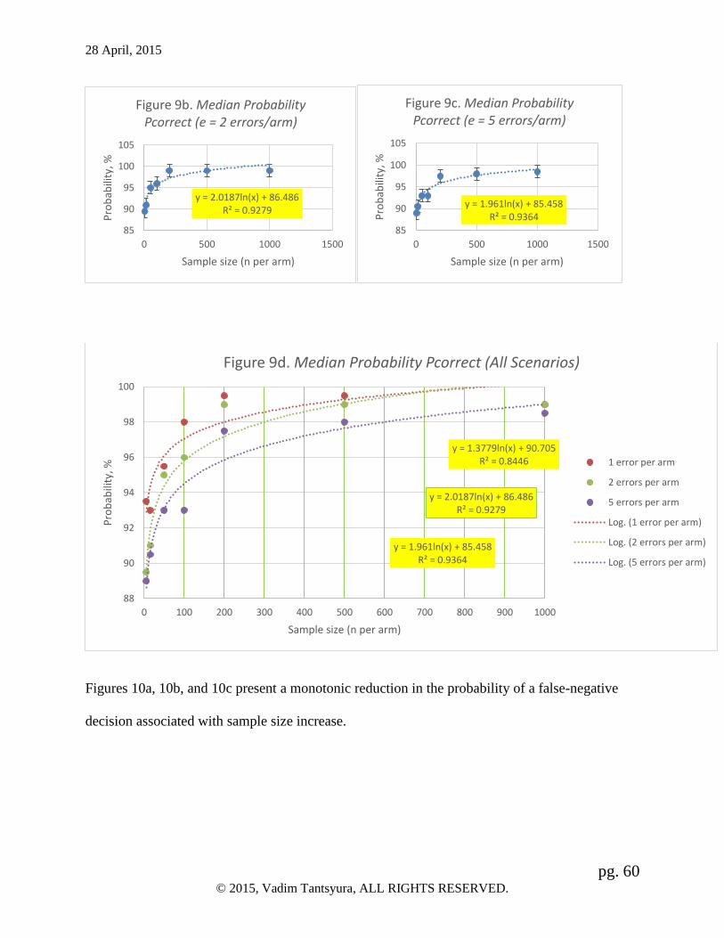
28 April, 2015


Figures 10a, 10b, and 10c present a monotonic reduction in the probability of a false-negative

decision associated with sample size increase.

y = 2.0187ln(x) + 86.486R² = 0.9279

85

90

95

100

105

0 500 1000 1500

Pro

bab

ility

, %


Figure 9b. Median Probability Pcorrect (e = 2 errors/arm)

y = 1.961ln(x) + 85.458R² = 0.9364

85

90

95

100

105

0 500 1000 1500

Pro

bab

ility

, %


Figure 9c. Median Probability Pcorrect (e = 5 errors/arm)

y = 1.3779ln(x) + 90.705R² = 0.8446

y = 2.0187ln(x) + 86.486R² = 0.9279

y = 1.961ln(x) + 85.458R² = 0.9364

88

90

92

94

96

98

100

0 100 200 300 400 500 600 700 800 900 1000

Pro

bab

ility

, %


Figure 9d. Median Probability Pcorrect (All Scenarios)

1 error per arm

2 errors per arm

5 errors per arm

Log. (1 error per arm)

Log. (2 errors per arm)


28 April, 2015


Figures 11a, 11b, and 11c present a monotonic reduction in the probability of a false-positive

decision associated with sample size increase. The logarithmic scale for n axis is used in these

data displays.

y = -0.836ln(x) + 5.3752R² = 0.9381

-1

0

1

2

3

4

5

6

0 200 400 600 800 1000 1200

Pro

bab

ility

%


Figure 10a. Median Pfalse-neg (e = 1 error/arm)

y = -1.212ln(x) + 7.6968R² = 0.9353

-2

0

2

4

6

8

0 500 1000 1500

Pro

bab

ility

%


Figure 10b. Median Pfalse-neg (e = 2 errors/arm)

y = -1.365ln(x) + 8.8787R² = 0.9343

-2

0

2

4

6

8

0 500 1000 1500

Pro

bab

ility

%


Figure 10c. Median Pfalse-neg (e = 5 errors/arm)

28 April, 2015


Interestingly, the intercepts of the trend lines are fairly stable / consistent among different

scenarios – 600 (per arm) for false-negative trend lines (Figures 10a, 10b and 10c) and 1000-

1200 (per arm) for false-positive trend lines (Figures 11a, 11b and 11c). This observation might

be indicative of a natural data cleaning cut-off points (i.e. virtually zero false negatives can be

expected in a study with 1200+ subjects and virtually zero false positives can be expected in a

study with 2400+ subjects). This phenomena needs further investigation.

y = -0.568ln(x) + 3.8239R² = 0.7705

-1

-0.5

0

0.5

1

1.5

2

2.5

3

3.5

4

1 10 100 1000

Pro

bab

ility

, %


Figure 11a. Median Pfalse-pos (e = 1 error/arm)

y = -0.82ln(x) + 5.5898R² = 0.8564

-1

0

1

2

3

4

5

1 10 100 1000

Pro

bab

ility

, %


Figure 11b. Median Pfalse-pos (e = 2 errors/arm)

y = -0.747ln(x) + 5.9083R² = 0.8365

0

1

2

3

4

5

6

1 10 100 1000

Pro

bab

ility

, %


Figure 11c. Median Pfalse-pos (e = 5 errors/arm)

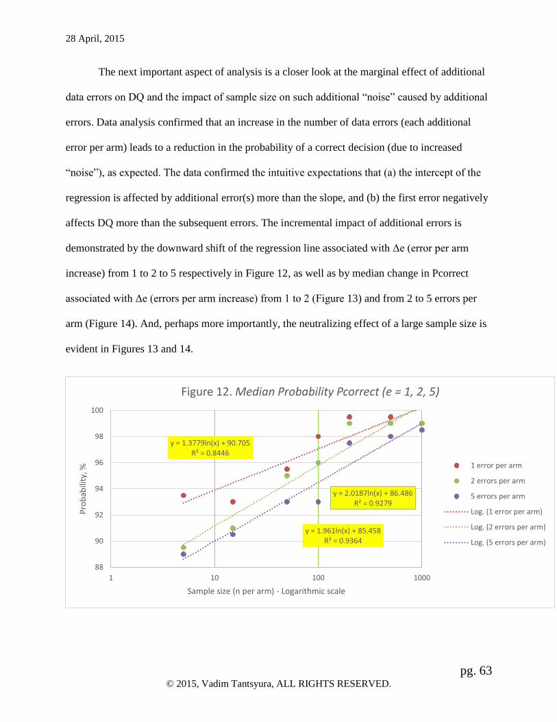
28 April, 2015


The next important aspect of analysis is a closer look at the marginal effect of additional

data errors on DQ and the impact of sample size on such additional “noise” caused by additional

errors. Data analysis confirmed that an increase in the number of data errors (each additional

error per arm) leads to a reduction in the probability of a correct decision (due to increased

“noise”), as expected. The data confirmed the intuitive expectations that (a) the intercept of the

regression is affected by additional error(s) more than the slope, and (b) the first error negatively

affects DQ more than the subsequent errors. The incremental impact of additional errors is

demonstrated by the downward shift of the regression line associated with Δe (error per arm

increase) from 1 to 2 to 5 respectively in Figure 12, as well as by median change in Pcorrect

associated with Δe (errors per arm increase) from 1 to 2 (Figure 13) and from 2 to 5 errors per

arm (Figure 14). And, perhaps more importantly, the neutralizing effect of a large sample size is

evident in Figures 13 and 14.

y = 1.3779ln(x) + 90.705R² = 0.8446

y = 2.0187ln(x) + 86.486R² = 0.9279

y = 1.961ln(x) + 85.458R² = 0.9364

88

90

92

94

96

98

100

1 10 100 1000

Pro

bab

ility

, %

Sample size (n per arm) - Logarithmic scale

Figure 12. Median Probability Pcorrect (e = 1, 2, 5)

1 error per arm

2 errors per arm

5 errors per arm

Log. (1 error per arm)



28 April, 2015


Figures 13 and 14 show the marginal effect of additional errors on the study conclusions as

measured by changes in Pcorrect (ΔPcorrect). The trend is positive towards zero for the large

sample size, however, R2 is relatively low (0.35-0.40) indicating a weak correlation between the

sample size n and the decrease in Pcorrect. A close look at the data reveals that for the smaller

studies (up to 200 subjects per arm), the variability of changes is high with essentially no trend.

The range of fluctuation of changes in Pcorrect associated with extra errors is within 3%

(ΔPcorrect = [-3%-0%]). For the larger studies (n > 200 per arm on the other hand, the variability

of ΔPcorrect and the negative impact of errors on ΔPcorrect is minimal (within 0.5% range for

number of error increase from 1 to 2 and within 1% range for number of errors increase from 2

to 5).

y = 0.002x - 1.5956R² = 0.3549

-4

-3.5

-3

-2.5

-2

-1.5

-1

-0.5

0

0.5

1

0 200 400 600 800 1000 1200

Ch

ange

in P

rob

abili

ty, %


Figure 13. Median change in Pcorrect (1 to 2 errors per arm increase)

28 April, 2015


It is noted that the negative incremental impact of each additional data error on the probability of

correct decision diminishes with each additional error. This phenomenon can be noted in the

reduction in slope between Figure 13 (0.002) and Figure 14 (0.0012), which is indicative of the

diminishing impact of additional data errors on Pcorrect. Such a diminishing impact of data

errors is similar to the famous economic law of “diminishing return” – in this case the lower

incremental per unit reduction in probability of correct study results (or “damage” to DQ) is

observed. This phenomenon can be explained by the fact that the uniform (Gaussian) distribution

of errors “regresses to the mean” and thus diminishes the “damage” to DQ with each additional

data error. (If this explanation is correct, then this (diminishing) effect from additional data errors

will likely disappear in a scenario in which the effect size (or difference between means of active

arm and comparator, delta) exceeds the assumed half-width of the uniform distribution that

represents “out-of range checks” (which is assumed 4SD in this study). However, such a scenario

is unlikely to occur in a real clinical trial.

y = 0.0012x - 1.6766R² = 0.4019

-3

-2.5

-2

-1.5

-1

-0.5

0

0 200 400 600 800 1000 1200C

han

ge in

Pro

bab

ility

, %


Figure 14. Median change in Pcorrect (2 to 5 errors per arm increase)

28 April, 2015


Discussion

The data clearly show that the impact of data errors in smaller size studies and larger

studies is unquestionably different. For smaller (n≤100 per arm) studies, the probability of a

correct decision in the presence of 1-5 errors is typically 90-98%, and for larger ones (n≥200 per

arm), the probability of a correct decision in the presence of 1-5 errors is typically 97.5-100%. At

the same time, the probability of the false-positive decision and the probability of the false-

negative decision are within 0-1% each for larger studies (n≥200 per arm). This leads to the

conclusion that the approaches to data cleaning for smaller and larger studies should vary

accordingly and be categorically different. It is evident that the amount of data cleaning activity

that is necessary to avoid false-positive or false-negative conclusions for the small studies is

notably higher than for the larger studies.

The first error in each arm does the most damage to DQ, as expected. The increase in the

number of errors per arm (from 1 to 2 and then to 5) has a diminishing impact on DQ (and the

reduction in probability of a correct study conclusion) in all simulated scenarios [combinations

of delta’s (d) and sample sizes (n)]. From the practical perspective, the most important

observation is that that the additional errors in the larger studies (n≥200 per arm) have virtually

no effect on the study conclusions.

An increase in the number of subjects per arm (n) has a profound effect on DQ. This

leads to the policy recommendation to reduce the data cleaning burden of the studies of larger

size and either (a) save these unused resources for future research or (b) invest these extra

resources in recruiting additional subjects for the study to increase statistical power as discussed

later. Also, the cut-off point (beyond which the data cleaning activities have minimal value)

28 April, 2015


varies depending on e (errors per arm) but does not change significantly between different effect

sizes (delta). The sliding scale for the data cleaning “cut-offs” is discussed later and is presented

in Table 12.

The slight difference in the effect of the data errors on the probabilities of false-positive

and false-negative decisions has been detected. The simulated data showed that the data errors

resulted in slightly more false-negative results (Median 2%, and Mean 4.53%) than false-positive

results (Median 1.5% and Mean 2.05%). This phenomena needs further investigation, and if

confirmed, at least on the surface, works in favor of public health. As indicated by their name,

error-provoked “false-negatives” will reduce the probability of an efficacious medical treatment

being approved. Therefore, it can be argued that this risk affects the sponsor more than the

public. On the other hand, in case of error-caused “false-positive” results, the probability of a

non-efficacious medical treatment being approved is higher, favoring the sponsor company, and

imposing a higher public health risk.

Practical implications

The fundamental question in planning activities for DQ, assessing/measuring and

assuring DQ is “how good is good enough.” How much should be invested in data cleaning to

get the most return on the investment of resources? Where is the cut-off point for the data

cleaning activities? This question is economic in nature and cannot be answered uniformly

across all types of variables, studies and economic conditions. However, the “cut-off point” for

data cleaning can be determined by study teams for each study individually. Empowered by the

results described in the previous section, the study teams have an opportunity to make study-

28 April, 2015


specific decisions based on the data (probabilities) rather than based on pure intuition. The

following section provides a blueprint for the main steps in such a decision making process.

Strategy 1. Elimination of data cleaning and statistical adjustment of the sample size to

compensate for data errors. This strategy carries no additional data quality related risk.

Step 1. Adjustment of alpha (type 1 error).

Since the data errors in larger studies (400 subjects or more) tend to increase the

probability of false-positive and false-negative decisions by up to 1% (depending on the

scenario/estimated sample size) each, one of the alternatives to data cleaning might be adjusting

alpha down from 5% to 4.0-4.9% as shown in Table 10 (and beta by up to 1% as well).

Table 10. Example of adjustment in Type I and Type II errors

Truth (for population studied)

Null Hypothesis True Null Hypothesis False

Decision (based on

sample)

Reject Null Hypothesis Type I Error (5%-0.5%) Correct Decision

Fail to reject Null

Hypothesis Correct Decision

Type II Error

(10/20%-0.5%)

Step 2. Such adjustment will inevitably lead to an increase in sample size. The following table

demonstrates the gradual sample size increase for several scenarios. The increase in sample size

typically varies from 0 to 6.3-6.8%

28 April, 2015


Table 11. Sample size increase associated with reduction in alpha

Effect size (delta)

alpha 0.05 0.1 0.2 0.3 0.5 1 2

0.050 12558 3140 786 350 126 32 8

0.049 12636 3159 790 351 126 32 8

0.048 12715 3179 795 353 127 32 8

0.047 12795 3199 800 355 128 32 8

0.046 12878 3219 805 358 129 32 8

0.045 12962 3241 810 360 130 32 8

0.044 13048 3262 816 362 130 33 8

0.043 13136 3284 821 365 131 33 8

0.042 13226 3307 827 367 132 33 8

0.041 13319 3330 832 370 133 33 8

0.040 13413 3353 838 373 134 34 8

Maximum sample size

increase 855 213 52 23 8 2 0

Maximum % increase in

sample size 6.81% 6.78% 6.62% 6.57% 6.35% 6.25% 0.00%

Step 3. Finally, the study team needs to determine the relative cost of sample size

increase versus “full scale” data cleaning. Per patient costs vary dramatically from study to

study, and in some studies per patient cost is much lower than in others. Therefore, it is

reasonable to expect that in some cases (when per patient cost is lower), the sample size increase

is a more economical alternative relative to such data cleaning activities as source data

verification. In such cases, the study team has sufficient evidence to convince the regulatory

agency that the elimination of expensive data cleaning activities carries no risk to the study’s

conclusions.

Strategy 2. Taking data quality risk and determining the data cleaning cut-off point when

the statistical impact of data cleaning can be viewed as marginal.

28 April, 2015


Step 1. Determining the cut-off point in terms of minimal acceptable probability (x%) of a

correct decision. One should not forget that 100% probability of a correct decision in presence of

errors is not practically possible and could be achieved only with either unrealistically high effect

sizes (delta) or unrealistically high sample sizes. Common sense dictates that data cleaning cut-

off does not imply complete elimination of data cleaning. It implies the elimination of most labor

intensive manual steps and reliance solely on inexpensive and intelligent computer-enabled data

cleaning processes and procedures. This objective can be accomplished by comparing the cost

(including opportunity cost/time component) of NDA/BLA rejection that is due to data errors

that are not captured by the sponsor or by the regulatory agencies. If, for instance, the cost of

regulatory rejection due to data errors is determined to be 40 times higher than the cost of data

cleaning (for instance, in case of a “me too” intervention with limited market potential), then the

cut-off point for data cleaning can be drawn as (100 - 100/40)% = 97.5%. However, if someone

is conducting a trial for a potential blockbuster drug, and the cost of rejection is 200 times or

more higher than the cost of additional investment in data cleaning (assuming the additional data

cleaning processes are extremely effective and catch a majority of the errors), then the cut-off

point might be determined as 99.5% (100-100/200)%.

Step 2. Converting the X% cut-off point into the sample size. DQ cut-off n(x%) for a particular

study can be simulated from the first principle using the algorithm presented in this thesis or

mathematically approximated from the data presented in Figure 12 above. The cut-off point

(beyond which the data cleaning activities bear minimal value) varies depending on the number

of errors per arm (e). Table 12 and Figure 15 below demonstrate the potential sliding scale for

the data cleaning activities and present three different data cleaning cut-off levels (95%, 98%,

and 99%) which are designed for three scenarios associated with three different risks – (a) low

28 April, 2015


risk/low expected error rates, (b) medium risk/medium expected error rates, and (c) high

risk/high expected error rates scenarios respectively. The data for this particular scenario

(presented in Appendix 6) were generated using the Excel-based simulation tool that was used to

verify SAS generated data presented earlier. For this particular simulation the effect size was

assumed e Δ=0.2, and the number of iterations in this simulation was 5,000. Two arms are

assumed for this simulation and, thus, the study sample size is two-fold relative to the size

reported in the previous tables and figures (N = 2n).

Table 12. Data cleaning cut-off estimates N(X%) for different number of errors (effect size

Δ=0.2, sample size N = 2n)

Errors per arm

1 2 3 4 5

N(95%) ≈60 ≈80 ≈100 ≈135 ≈180

N(98%) ≈250 ≈430 ≈700 ≈900 ≈950

N(99%) ≈400 ≈1200 ≈2000 ≈2500 ≈3000

60 80 100 135 180250430

700900 950

400

1200

2000

2500

3000

0

500

1000

1500

2000

2500

3000

3500

0 1 2 3 4 5 6

Tota

l nu

mb

er o

f su

bje

cts

(N=2

n)

Errors per arm (e)

Figure 15. 95%, 98% and 99% Estimated DQ Cut-off Lines

(effect size delta = 0.2 SD)

N(95%) N(98%) N(99%)

28 April, 2015


A precise calculations for a specific effect size (Δ) could be made by a study team using

algorithms presented in this manuscript. In the absence of a simulation tool (and based on the

observation that the probabilities of correct study conclusion (Pcorr) does not change

significantly among different effect sizes (Δ)) for their particular study, the study team could use

Table 12 and Figure 15 estimates for all values of the effect size (Δ) in their estimates of

different data cleaning cut-off levels (95%, 98%, and 99%).

Step 3. If one agrees to minimize the manual components of “data cleaning” efforts for study

sizes N > study-specific data cleaning threshold N(X%), then the next question is what practical

models can be used? Each sponsor company is likely to make its own decision. The author’s

recommended approach is to rely on standard computer-enabled (real-time or off-line) edit

checks and “statistical data surveillance” that are very inexpensive relative to the manual data

validation procedures so unjustifiably popular today. The queries produced by these computer-

enabled edit checks should become the focal points of the data error elimination process, while

leaving broad-brush manual activities such as SDV out of the scope.

Strategy 3. Focus on process optimization, SDV reduction and RBM.

The experiment above offers additional evidence to support the modern trend in

monitoring process optimization that is characterized by dramatic reduction of SDV, while

replacing it with the risk-based monitoring (RBM). RBM considers each clinical trial

holistically, identifies areas of increased risk, and uses that information as the basis for a

customized monitoring program. The proposed methodology, while estimating the probability of

erroneous study conclusions, provides study teams with an additional tool to measure ”risk.” If

the probability of false-positive or false-negative conclusions drops below a pre-specified level

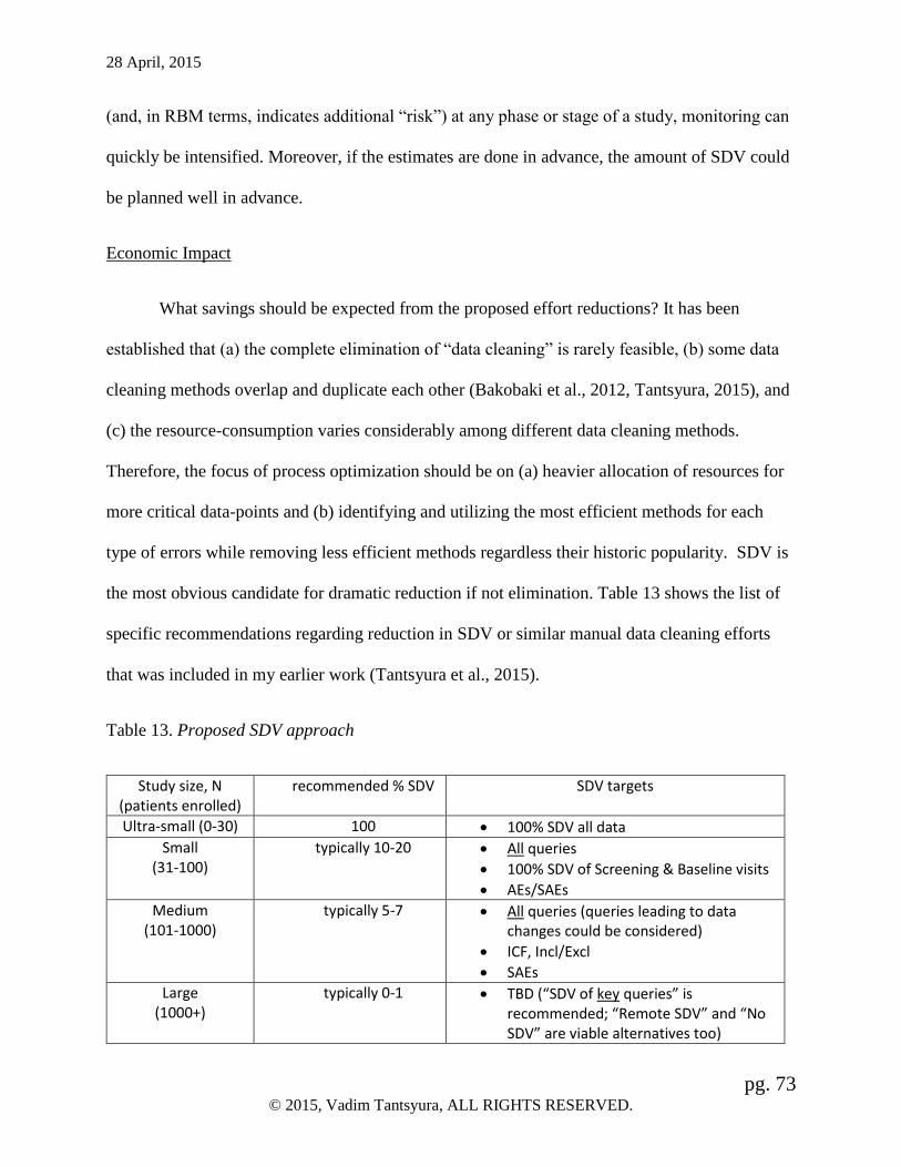
28 April, 2015


(and, in RBM terms, indicates additional “risk”) at any phase or stage of a study, monitoring can

quickly be intensified. Moreover, if the estimates are done in advance, the amount of SDV could

be planned well in advance.

Economic Impact

What savings should be expected from the proposed effort reductions? It has been

established that (a) the complete elimination of “data cleaning” is rarely feasible, (b) some data

cleaning methods overlap and duplicate each other (Bakobaki et al., 2012, Tantsyura, 2015), and

(c) the resource-consumption varies considerably among different data cleaning methods.

Therefore, the focus of process optimization should be on (a) heavier allocation of resources for

more critical data-points and (b) identifying and utilizing the most efficient methods for each

type of errors while removing less efficient methods regardless their historic popularity. SDV is

the most obvious candidate for dramatic reduction if not elimination. Table 13 shows the list of

specific recommendations regarding reduction in SDV or similar manual data cleaning efforts

that was included in my earlier work (Tantsyura et al., 2015).

Table 13. Proposed SDV approach

Study size, N (patients enrolled)

recommended % SDV SDV targets

Ultra-small (0-30) 100 100% SDV all data

Small (31-100)

typically 10-20 All queries

100% SDV of Screening & Baseline visits

AEs/SAEs

Medium (101-1000)

typically 5-7 All queries (queries leading to data changes could be considered)

ICF, Incl/Excl

SAEs

Large (1000+)

typically 0-1 TBD (“SDV of key queries” is recommended; “Remote SDV” and “No SDV” are viable alternatives too)

28 April, 2015


Will this change in approaches to data cleaning impact the study budgets and recruitment

strategies (and how?) is the next question. The answer to this question comes from recognition of

the distinction between the fixed and variable components of the data cleaning cost. Some data

cleaning efforts (that are correlated with the number of collected data points and subjects per

site), such as manual review of data, including SDV as an example, can be classified as

predominantly “variable cost.” At the same time, edit check specification writing and

programming edit checks are fixed and not impacted by the number of subjects and data points in

a study. This fact is probably the most important economic factor in designing the optimized data

cleaning process. Even some monitoring activities – GCP Compliance/Process Monitoring as an

example – are mostly “fixed” (per site) cost. Thus, with exception of small studies, the proposed

model demonstrates dramatic reduction of the variable component of cost (SDV) and

subsequently provides justification for perceiving monitoring cost as predominantly fixed (per

site) cost. This observation is consistent with anecdotal examples shared with the author when

the monitoring cost (per site) is prospectively pre-set at a certain level (e.g. $10K/year). The

following hypothetical chart is derived for the proposed SDV model and graphically represent

this relationship (exponential/asymptotic per subject effort reduction along with the increase in

the number of subjects). As shown in Figure 16, virtual disappearance of the variable component

of cost inevitably leads to the ceiling effect that puts a “cap” on the “per-site monitoring cost.”

Also, Figure 16 demonstrates that when and if the model presented in Table 13 is followed, in

the large studies with heavily discounted SDV (unlike in the traditional 100% SDV approach),

per patient costs drop dramatically along with the site enrollment. In other words, the first few

patients carry the cost load for the entire site and the cost associated with the subsequent subjects

is trivial because these additional subjects for a particular site do not require additional efforts in

28 April, 2015


training the sites, assuring the protocol compliance, following GCP, etc. The additional costs that

are “variable” in nature, associated with additional SDV or identification of non-computerizable

protocol violations, for example, are relatively minimal for the large studies, and thus do not

produce noteworthy cost increases. It makes the additional subject at a high-enrolling site a few

times less expensive relative to the cost of the additional subject at the low-enrolling site on a per

patient cost basis.

Figure 16. Reduced SDV: Monitoring Cost per Site and Ceiling Effect

This leads to the conclusion that the focus on high-enrollers produces additional savings

that are not present in a traditional SDV setting. It also creates economic pressure to eliminate

low-enrollers. In practical terms this theoretical conclusion means that a significant reduction in

the frequency of monitoring visits (that is a direct consequence of the reduced SDV burden for

CRA’s and sites and is already observed in the industry) has an even more profound effect on the

bottom line in the case of high-enrolling sites.

0

20

40

60

80

100

0 20 40 60 80 100 120

CO

ST

SUBJECTS PER SITE

Monitoring cost per site

Total cost per site Per patient cost Trend Line (Cost per patient)

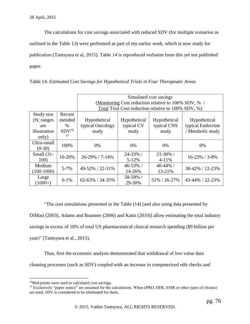
28 April, 2015


The calculations for cost savings associated with reduced SDV (for multiple scenarios as

outlined in the Table 13) were performed as part of my earlier work, which is now ready for

publication (Tantsyura et al, 2015). Table 14 is reproduced verbatim from this yet not published

paper.

Table 14. Estimated Cost Savings for Hypothetical Trials in Four Therapeutic Areas

Simulated cost savings

(Monitoring Cost reduction relative to 100% SDV, % /

Total Trial Cost reduction relative to 100% SDV, %)

Study size

(N; ranges

are

illustration

only)

Recom

mended

%

SDV16

17

Hypothetical

typical Oncology

study

Hypothetical

typical CV

study

Hypothetical

typical CNS

study

Hypothetical

typical Endocrine

/ Metabolic study

Ultra-small

(0-30) 100% 0% 0% 0% 0%

Small (31-

100) 10-20% 26-29% / 7-14%

24-33% /

5-12%

21-30% /

4-11% 16-23% / 3-8%

Medium

(100-1000) 5-7% 49-52% / 22-31%

46-53% /

14-26%

40-44% /

13-21% 38-42% / 12-23%

Large

(1000+) 0-1% 62-63% / 34-35%

58-59% /

29-30% 51% / 26-27% 43-44% / 22-23%

“The cost simulations presented in the Table (14) [and also using data presented by

DiMasi (2003), Adams and Brantner (2006) and Katin (2010)] allow estimating the total industry

savings in excess of 18% of total US pharmaceutical clinical research spending ($9 billion per

year)” (Tantsyura et al., 2015).

Thus, first the economic analysis demonstrated that withdrawal of low value data

cleaning processes (such as SDV) coupled with an increase in computerized edit checks and

16Mid-points were used to calculated cost-savings. 17 Exclusively “paper source” are assumed for the calculations. When ePRO, DDE, EMR or other types of eSource

are used, SDV is considered to be eliminated for them.

28 April, 2015


other centralized data review processes in large studies will not only improve DQ, but also

dramatically reduce costs. The potential savings vary from three to fourteen percent for the small

studies (under 100 subjects) to twenty two to thirty five percent for the large studies (over 1000

subjects) depending on the therapeutic area and other study parameters. Second, the economic

analysis demonstrated that reduction in any variable costs (such as SDV or manual review of

CRFs) inevitably leads to additional savings associated with the high enrolling sites that cannot

be realized in a traditional (100% SDV) paradigm. For this reason, it is anticipated that low

enrolling sites will be pushed out from participation in regulated clinical research, even more

than it has been in the past.

Policy recommendations.

Multiple papers recommended that the results of data quality assessments should be

reported with research results (Brown, Kahn, and Toh, 2013; Kahn, Brown, Chun et al., 2013;

Zozus et al., 2015). “Data quality assessments are the only way to demonstrate that data quality

is sufficient to support the research conclusions. Thus, data quality assessment results must be

accessible to consumers of research.” (Zozus et al., 2015) Because of the limited utility and high

cost of error rate estimation audits in clinical research, clinical trial simulations could replace DQ

audits as an alternative DQ assessment method. Such simulations can be almost completely

automated and relatively low cost as compared to DQ audits. The probability of the correct study

conclusion in the presence of errors (or simply “study DQ score”) could potentially be estimated

for virtually any clinical trial. Thus the first recommendation is to consider utilizing trial

simulation algorithms, analogous to the one presented in this thesis, by NDA reviewers and even

making such DQ assessment a requirement for the regulatory submissions after the error

simulation tools become widely available and inexpensive.

28 April, 2015


Perhaps most importantly, this experiment demonstrates the tremendous effectiveness of

trial simulation methodology. Modern practitioners and regulators rely almost exclusively on

very expensive and time-consuming “real” trials. Adaptive designs that have gained popularity

over the past decade is one of the examples of the leveraging power of modeling and

simulations. In addition, in many cases the trial simulation methodology offers even greater

advantages in many other areas of the clinical trial enterprise. It offers help and unparalleled

advantages in such areas as hypothesis generation, dosage finding, drug supply cost

minimization, and many other areas of clinical trial operations optimization.

Simulations are extensively used in many fields outside of medicine. One could take

military pilots’ training as an excellent example. Flight simulators were the first successful

implementation of simulation methodology in a larger scale, which led to saving billions of

dollars (and countless lives) over the past seventy years. It is quite obvious that the future

generation of clinical trial practitioners will find a way to capitalize on modern era computational

power and eliminate large numbers of unsuccessful trials with simulated trials. Such an approach

will not only lead to a reduction in new drug development cost and time, but will also allow the

investment of saved resources in other compounds and ultimately get more drugs to patients

more safely, more quickly and less expensively.

Perhaps, as a second policy recommendation, the regulators around the world might

initiate a discussion about drafting guidelines for the best practices in the trial simulations. The

recently issued guidance by the FDA on risk-based monitoring created a precedent. It was the

first time in the agency’s history that the focus of a guidance document was not protection of

public health per se, but on “elimination of waste” in the system, which is itself an important

component of public health improvement. Similarly, such new trial simulation guidance, if

28 April, 2015


drafted, would solidify this new trend in the FDA’s trial operations leadership, and would

ultimately lead, through system-wide reduction in time and resource consumption, to getting new

cures to the market quickly, inexpensively, and greatly to the benefit of public health.

The third policy recommendation comes from the fact that the majority of clinical trial

practitioners are not familiar with clinical trial simulation methods. Training and education

curriculums need to be adjusted to empower the next generation of practitioners with this

necessary knowledge.

One can reasonably conclude that modern computational power is under-utilized in

clinical research where “real” trials with human participants dominate the scene. There is no

doubt in my mind that the next generation of clinical trial practitioners will utilize trial

simulations as much as the military has come to use drones rather than pilot-operated aircraft.

Finally, looking in the future, I see the next generation of clinical research no longer

dependent on fixed assumptions, consistent and uniformly set rules, including such important

parameters as alpha and beta that determine acceptable levels of Type I & II errors across the

industry. XXI century public health will embrace and demand non-traditional, more intelligent,

less consistent, and inherently risk-based “rules of the game”. “Would the public health, and

society as a whole, suffer or benefit from the possible reduction in alpha for those clinical

indications, where multiple clinical choices already in place, relaxing alpha for orphan

designations or highly debilitating diseases where medical needs have not been met?” This is the

question next generation of public health researchers will inevitably ask. The proposed

methodology offers a big hand in answering this question.

28 April, 2015


Study limitations and Suggestions for Future Research

The current study assumed constant width of range edit check. The impact of variability

of range edit checks (3SD v. 4SD v. 5SD v. 10SD) on the DQ, as well as the impact of

asymmetrical edit checks need to be examined further. Particular interest for academic

researchers (given budgetary constraints in academic and government-sponsored research in

general) is assessment of the study size effect and data errors in the case of absence of out-of-

range checks. Similarly, the impact of “missing values” edit checks on DQ needs to be examined

in the future.

Continuous variables are analyzed in this study. However, the study conclusions need to

be validated using dichotomous variables and rank tests to make these conclusions completely

generalizable.

It is a documented fact that double data entry by professional typists produces

significantly higher accuracy (error rate under 0.1%, sometimes under 0.01%) relative to the

single data entry by “students” or “nurses” which is often the case, especially in academic

medical centers (error rate is 0.5-1%). The impact of irregular quality of initial data entry in the

new EDC/DDE environment on overall data quality needs to be examined further.

Also, in all simulated scenarios, I’ve assumed that the number of errors in “active” arm

and “comparator” are equal (1 v 1, 2 v 2, 5 v 5). However, a non-equal number of errors might

have an impact on DQ as well. For example, it would be beneficial to model a situation with no

errors in one arm versus at least one error in the other arm.

Given the growing number of drugs available on the market, non-inferiority trials keep

gaining popularity. The experiment described in this manuscript has not examined the impact of

28 April, 2015


study size on DQ for non-inferiority trials. In order to expand the conclusions, one needs to take

a close look at this type of trials.

The “borderline cases” (defined, for example, as the combined probability of error being

5% +/- 2%, i.e. Pfalse-neg + Pfasle-pos = 3-7%) can be selected and examined further using

sensitivity analysis.

Finally, in the described experiment, the number of errors (e) and number of observations

per arm (n) are considered independent variables. However, this assumption needs to be further

tested, and, if violated, alternative analysis methods might need to be considered. The next

advance in exploring this methodology will come from limiting options to only realistic

combinations of input variables and covariates – sample size, number of errors and effect size.

More specifically, the number of data entry errors per arm in real life is a function of

sample size – the typical proportion of errors in clinical trials is between 2% and 4% of the

sample size (Grieve, 2012; Yong, 2013; Scheetz, 2014) and up to 10% in registries (Nahm et al.,

2008). Thus, in the future experiments, the number of errors should be limited to 0.1-10%. Also,

the effect size and the sample size are directly linked, unlike in the discussed experiment

(Appendix 7 illustrates such relationship). Also, as an important side note, not all case report

forms (CRFs) and collected variables are equal in “producing” data errors. The universal “Pareto

Principle” (more often known as the 80/20 rule) certainly holds true in case of error rates for

different forms in clinical research. Historically, safety (Adverse Event and Concomitant

Medications) CRFs and variables are associated with much higher data entry error rates than

efficacy variables and forms. For instance, Mitchel et al., (2011) showed that a small number of

safety forms causes 70-80% of all data corrections in a study. This fact leads to the conclusion

28 April, 2015


that, in a typical study, the expected error rates for efficacy variables could be assumed below the

standard/expected 2-4% (0.5-2%, for example) and above the standard/expected 2-4% for safety

variables (for example around 4-8%).

Conclusion

The presented manuscript takes an important step in the directions of a better

understanding of the nature of DQ, a better informed health policy, a better clinical and

regulatory decision making process, and greater overall efficiency of the clinical research

enterprise. More specifically, it addresses the “sample size effect,” i.e. neutralizing the effect of

sample size on the noise from data errors was consistently observed in the case of single data

error as well as in the case of incremental increase in the number of errors. Perhaps, the most

important observation is that that the additional errors in the larger studies (n≥200 per arm) have

negligible effect on the study results as measured by the probability of the correct study

conclusion.

It is potentially a big relief for the industry that the simulations and the analyses show

that the impact of an error on analysis conclusion is less for larger sample sizes than for smaller

ones – all things being equal. This is certainly consistent with what one would expect and hope,

but it has been proved with data, simulations, and analysis. It is known that the impact of an

individual error is greater in a small study than a large one. If there are 10 patients in a study

(N=10), each one has a big impact, because each one is 10% of the sample size. If there are five

subjects with headaches as opposed to six subjects with headaches, it makes a difference. If there

are 10,000, there could be many subjects with headaches that are not counted, and it will have no

impact on the estimates of incidence of headaches. This is why regulators would rather have

28 April, 2015


high-level information on safety from a huge study than granular information from a small study.

Important things tend to be known and reported, regardless of the selected methods.

Since the impact of data errors in smaller size studies and larger studies is unquestionably

different, the approaches to data cleaning for smaller and larger studies should be categorically

different as well. The amount of data cleaning activity that is necessary to avoid false-positive or

false-negative conclusions for the smaller studies is notably higher than for the larger ones. Data

cleaning threshold methodology suggested by this manuscript can lead to reduction in resource

utilization. This study has demonstrated that the Monte-Carlo simulation method has the power

and utility to explore relationships and answer important clinical research questions. This study

is also intended to trigger a new wave of research using the Monte-Carlo Simulation method.

Error rates have been considered the gold standard of DQ assessment but are not widely

utilized in practice due to the prohibitively high cost. The proposed method suggests estimating

DQ by using simulated probability of a correct/false-negative/false-positive study conclusion as

the outcome variables and the estimates of error rates as the input variable. The probability of the

correct study conclusion (or simply “study DQ score”) could potentially be calculated for any

clinical trial. Such innovative paradigm shift has the potential to transform DQ assessment for

regulatory submissions and become a new gold standard as the “credit score” is the gold standard

in the financial world.

28 April, 2015


References:

Adams C.P., and Brantner W. (2006, Mar-Apr). Estimating the cost of new drug

development: is it really 802 million dollars? Health Aff (Millwood);25(2): 420-428.

Bakobaki JM, Rauchenberger M, Joffe N, McCormack S, Stenning S, Meredith S. (2012,

Apr). The potential for central monitoring techniques to replace on-site monitoring:

findings from an international multi-centre clinical trial, Clin Trials;9(2):257-64. doi:

10.1177/1740774511427325. Epub.

Ball L, and Meeker-O’Connell A. (2011). Building Quality into Clinical Trials: A

Regulatory Perspective, Quality by Design; available at:

http://www.beaufortcro.com/wp-content/uploads/2012/02/Monitor-

Quality_in_Clinical_Trials.pdf; Accessed on 14 December, 2013.

Brown J.S., Kahn M, Toh S. (2013). Data quality assessment for comparative

effectiveness research in distributed data networks. Med Care;51(8 suppl 3):S22–S29.

PMID: 23793049. doi: 10.1097/MLR.0b013e31829b1e2c.

Cavalito J. (approximately 1985). Unpublished research at Burroughs Wellcome.

Congressional Budget Office. (2006, October). A CBO study “Research and Development

in the Pharmaceutical Industry”; Available on

http://www.cbo.gov/sites/default/files/10-02-drugr-d.pdf

CTTI. (2009, November 4). Summary document – Workstream 2, Effective and efficient

monitoring as a component of quality in the conduct of clinical trials. Paper presented

at meeting of CTTI, Rockville, MD.

CTTI. (2012). “CTTI Quality By Design Workshops Project: Critical To Quality (CTQ)

Factors,” Working Group Document, Version 07January, 2012

DiMasi J.A., Hansen R.W., Grabowski H.G. (2003, Mar) The price of innovation: new

estimates of drug development costs, J Health Econ;22(2):151-85.

European Medicines Agency. (2013, November 18). Reflection paper on risk based

quality management in clinical trials. Available at:

http://www.ema.europa.eu/docs/en_GB/document_library/Scientific_guideline/2013/

11/ WC500155491.pdf. Accessed November 09, 2014.

http://www.beaufortcro.com/wp-content/uploads/2012/02/Monitor-Quality_in_Clinical_Trials.pdf

http://www.beaufortcro.com/wp-content/uploads/2012/02/Monitor-Quality_in_Clinical_Trials.pdf

http://www.cbo.gov/sites/default/files/10-02-drugr-d.pdf

28 April, 2015


Ezekiel E.J. (2003). Ethical and Regulatory Aspects of Clinical Research: Readings and

Commentary. Edited by: Ezekiel Emanuel, Robert Crouch, John Arras, Jonathan

Moreno and Christine Grady. Johns Hopkins University Press.

Ezekiel E.J. and Fuchs V.R. (2008, June 18). "The Perfect Storm of Overutilization",

Journal of the American Medical Association, Vol. 299 No. 23.

Food and Drug Administration. (1988, January). Guidance for Industry: Guideline for the

Monitoring of Clinical Investigations. Available at:

http://www.ahc.umn.edu/img/assets/19826/Clinical%20monitoring.pdf. Accessed

November 10, 2014.

Food and Drug Administration. (1997, June 9). General Principles of Software Validation;

Final Guidance for Industry and FDA Staff, Version 1.1, available at:

http://www.fda.gov/RegulatoryInformation/Guidances/ucm126954.htm; accessed on

November 9, 2014.

Food and Drug Administration. (1998, May). Guidance for Industry: Providing Clinical

Evidence of Effectiveness for Human Drug and Biological Products. Available at:

http://www.fda.gov/downloads/Drugs/.../Guidances/ucm078749.pdf . Accessed

November 10, 2014.

Food and Drug Administration. (2003). Regulation, 21 CFR Part 11, Electronic Records;

Electronic Signatures — Scope and Application, available at:

http://www.fda.gov/downloads/RegulatoryInformation/Guidances/ucm125125.pdf;

accessed on November 9, 2014

Food and Drug Administration. (2003). Guidance for Computerized Systems Used in

Clinical Trials (USFDA, April, 1999/updated in 2003 and May 2007); Available on

http://www.fda.gov/OHRMS/DOCKETS/98fr/04d-0440-gdl0002.pdf, accessed on 04

November, 2014

Food and Drug Administration. (2013, August). Guidance for Industry: Oversight of

Clinical Investigations — A Risk-Based Approach to Monitoring, Available at:

http://www.fda.gov/downloads/Drugs/.../Guidances/UCM269919.pdf. Accessed on

November 09, 2014.

http://www.ahc.umn.edu/img/assets/19826/Clinical%20monitoring.pdf

http://www.fda.gov/RegulatoryInformation/Guidances/ucm126954.htm

http://www.fda.gov/downloads/Drugs/.../Guidances/ucm078749.pdf

http://www.fda.gov/downloads/Drugs/.../Guidances/ucm078749.pdf

http://www.fda.gov/downloads/RegulatoryInformation/Guidances/ucm125125.pdf

http://www.fda.gov/OHRMS/DOCKETS/98fr/04d-0440-gdl0002.pdf

28 April, 2015


Fendt K. (2004, October). “Issues of Data Quality throughout the Data Life Cycle in

Clinical Research,” Presentation at the West Coast Annual DIA conference.

Fee R. (2007, March). The Cost of Clinical Trials, Drug Discovery and Development, Vol.

10, No. 3, p. 32.

Fink, A. (2005). Conducting Research Literature Reviews: From the Internet to Paper (2nd

ed.) Thousand Oaks, California: Sage Publications.

Fisher, C., Lauría, E., Chengalur-Smith, S. and Wang, R. (2006). Introduction to

Information Quality. MIT Information Quality Programme, New York.

Fisher, C., Lauria, E., Chngalur-Smith, S., Wang, R. (2012). Introduction to Information

Quality, An MITIQ Publication.

Funning, S., Grahnén, A., Eriksson, K., Kettis-Linblad, A. (2009, January). Quality

assurance within the scope of Good Clinical Practice (GCP)-what is the cost of GCP-

related activities? A survey within the Swedish Association of the Pharmaceutical

Industry (LIF)'s members, The Quality Assurance Journal; 12(1):3-7.

DOI:10.1002/qaj.433

Getz, K.A., Stergiopoulos, S., Marlborough, M., Whitehill, J., Curran, M., Kaitin, K.I.

(2013, February). Quantifying the Magnitude and Cost of Collecting Extraneous

Protocol Data. American journal of therapeutics; DOI:

10.1097/MJT.0b013e31826fc4aa

Good Clinical Data Management Practices (GCDMP) by Society for Clinical Data

Management v4, October 2005; accessed in 2007-08; no longer available.

Good Clinical Data Management Practices (GCDMP) by Society for Clinical Data

Management, Measuring Data Quality chapter, originally published in 2008.

Available at: http://www.scdm.org/sitecore/content/be-bruga/scdm/Publications.aspx

Grieve, A.P. (2012, February). Source Data Verification by Statistical Sampling: Issues in

Implementation, Drug Inf J;46(3):368-377.

Harper, M. (2013, August 11). How Much Does Pharmaceutical Innovation Cost? A Look

At 100 Companies, Forbes, available at

http://www.forbes.com/sites/matthewherper/2013/08/11/the-cost-of-inventing-a-new-

drug-98-companies-ranked/; accessed on 03/07/2015

http://www.scdm.org/sitecore/content/be-bruga/scdm/Publications.aspx

http://www.forbes.com/sites/matthewherper/2013/08/11/the-cost-of-inventing-a-new-drug-98-companies-ranked/

http://www.forbes.com/sites/matthewherper/2013/08/11/the-cost-of-inventing-a-new-drug-98-companies-ranked/

28 April, 2015


Helfgott, J. (2014, May 15). “Risk-Based Monitoring – Regulatory Expectations”

presented at DIA Webinar; available at https://diahome.webex.com/

Hoyle D. (1998, June 22). “ISO 9000 Quality Systems Development Handbook,”

Butterworth-Heinemann

International Conference on Harmonization (ICH). (1996, April). Guidance for Industry,

E6, “Good Clinical Practice: Consolidated Guidance,” available at:

http://www.fda.gov/downloads/Drugs/Guidances/ucm073122.pdf. Accessed

December 13, 2014.

International Conference on Harmonization (ICH). (1998, February). Harmonised

Tripartite Guideline: Statistical Principles for Clinical Trials E9. Available at:

http://www.ich.org/fileadmin/Public_Web_Site/ICH_Products/Guidelines/Efficacy/E

9/Step 4/E9_Guideline.pdf. Accessed November 09, 2014.

International Conference on Harmonization. (2009, November). Guidance for Industry,

Q8(R2) Pharmaceutical Development, Revision 2, available at:

http://www.fda.gov/downloads/Drugs/Guidances/ucm073507.pdf.

International Conference on Harmonization. (2006, June). Guidance for Industry, Q9

Quality Risk Management, available at:

http://www.fda.gov/downloads/Drugs/.../Guidances/ucm073511.pdf.

International Conference on Harmonization. (2009, April). Guidance for Industry, Q10

Pharmaceutical, Quality System, April 2009, available at:

http://www.fda.gov/downloads/Drugs/Guidances/ucm073517.pdf.

Institute of Medicine (IOM). (1999). Division of Health Sciences Policy, “Assuring Data

Quality and Validity in Clinical Trials for Regulatory Decision Making,” Workshop

Report, Roundtable on Research and Development of Drugs, Biologics, and Medical

Devices, edited by Davis JR, Nolan VP, Woodcock J, Estabrook RW, National

Academy Press, Washington, DC, available at:

http://www.nap.edu/openbook.php?record_id=9623.

International Organization for Standardization (ISO). (2000). 9000:2000 Quality

management systems -- Fundamentals and vocabulary; Originally issued in 2000,

revised in 2005.

https://diahome.webex.com/

http://www.fda.gov/downloads/Drugs/Guidances/ucm073122.pdf

http://www.ich.org/fileadmin/Public_Web_Site/ICH_Products/Guidelines/Efficacy/E9/Step%204/E9_Guideline.pdf

http://www.ich.org/fileadmin/Public_Web_Site/ICH_Products/Guidelines/Efficacy/E9/Step%204/E9_Guideline.pdf

http://www.nap.edu/openbook.php?record_id=9623

28 April, 2015


International Organization for Standardization (ISO). (2011). 19011:2011 Guidelines for

auditing management systems; Originally issued in 2002, revised in 2011.

International Organization for Standardization (ISO). (2012, June 15). ISO 8000-

2:2012(E) Data Quality – Part 2: Vocabulary. 1st ed.

Juran, J.M. (1986). The Quality Trilogy: A Universal Approach to Managing Quality,

Quality Progress: 19-24.

Kahn, B.K., Strong, D.M., and Wang, R.Y. (2002, April). Information Quality

Benchmarks: Product and Service Performance, Vol. 45, No. 4ve Communications of

ACM

Kahn, M.G., Brown, J., Chun, A., et al. (2013, December). A consensus-based data quality

reporting framework for observational healthcare data. Submitted to eGEMS Journal.

Draft version available at:

http://repository.academyhealth.org/cgi/viewcontent.cgi?article=1001&context=dqc.

Accessed February 2, 2015.

Kaitin, K.I. (2008). “Obstacles and opportunities in new drug development,” Clinical

Pharmacology and Therapeutics;83:210-212.

Khosla, R., Verma, D.D., Kapur, A., Khosla, S. (2000). Efficient source data verification.

Ind J Pharmacol;32:180–186.

Kingma, B.R. (1996). The Economics of Information: A guide to Economic and Cost-

Benefit Analysis for Information Professionals. Englewood, CO: Libraries Unlimited,

2000

Landray, M. (2013). “Clinical Trials: Rethinking How We Ensure Quality” presented at

DIA/FDA webinar.

Lindblad, A.S., Manukyan, Z., Purohit-Sheth, T., Gensler, G., Okwesili, P., Meeker-

O’Connell, A., Ball, L. and Marler, J.R. (2014). “Central site monitoring: Results

from a test of accuracy in identifying trials and sites failing Food and Drug

Administration inspection,” Clinical Trials; 11: 205–217. http://ctj.sagepub.com

Liu, C, Constantinides, P.P., Li, Y. (2014, April). Research and development in drug

innovation: reflections from the 2013 bioeconomy conference in China, lessons

learned and future perspectives, Acta Pharmaceutica Sinica B, Volume 4, Issue 2, pp.

112–119, doi:10.1016/j.apsb.2014.01.002, available at

http://repository.academyhealth.org/cgi/viewcontent.cgi?article=1001&context=dqc

28 April, 2015


http://www.sciencedirect.com/science/article/pii/S2211383514000045; accessed on

03/07/2015

Lörstad (2004, September). “Data Quality of the Clinical Trial Process – Costly

Regulatory Compliance at the Expense of Scientific Proficiency,” The Quality

Assurance Journal; 8(3):177 - 182. DOI: 10.1002/qaj.288

Mei-Mei Ma, J. (1986, December). A Dissertation submitted to the faculty of The

Department of Biostatistics, The University of North Carolina, “A modeling approach

to System Evaluation in Research Data Management,“ available at

http://www.stat.ncsu.edu/information/library/mimeo.archive/ISMS_1986_1822T.pdf

Mitchel, J.T., Kim, Y.J., Choi, J., Park, G., Schloss Markowitz, J.M. and Cappi, S. (2010,

Fall). “How Electronic Data Capture (EDC) Can Be Integrated into a Consolidated

Data Monitoring Plan”, Data Basics, Volume 16, Number 3.

Mitchel, J.T., Kim, Y.J., Choi, J., Park, G., Cappi, S., Horn, D., et al. (2011). Evaluation

of Data Entry Errors and Data Changes to an Electronic Data Capture Clinical Trial

Database, Inf J.;45:421–30. doi: 10.1177/009286151104500404.

Mitchel, J.T., Kim, Y.J., Hamrell, M.R., Carrara, D., Schloss Markowitz, J.M., Cho, T.,

Nora, S.D., Gittleman, D.A., Choi, J. (2014, January 17). Time to Change the Clinical

Trial Monitoring Paradigm: Results from a Multicenter Clinical Trial Using a Quality

by Design Methodology, Risk-Based Monitoring and Real-Time Direct Data Entry,

Appl Clin Trials.

Mitchel, J.T., Gittleman, D.A., Park, G., Harris, R., Schloss Markowitz, J.M., Jurewicz,

E., Cigler, T., Gittelman, M., Auerbach, S., Efros, M.D. (2014, Second Quarter). The

Impact on Clinical Research Sites When Direct Data Entry Occurs at the Time of the

Office Visit: A Tale of 6 Studies, InSite.

Miseta, E. (2013, April 08). The High Cost of Clinical Research – Who's To Blame And

What Can Be Done?, Outsourced Pharma, available at

http://www.outsourcedpharma.com/doc/the-high-cost-of-clinical-research-who-s-to-

blame-and-what-can-be-done-0001; accessed on 03/07/2015

Nahm, M.L., Pieper, C.F., Cunningham, M.M. (2008, Aug 25). “Quantifying Data Quality

for Clinical Trials Using Electronic Data Capture,” PLoS ONE. 2008; 3(8):e3049,

Published online.

http://www.sciencedirect.com/science/article/pii/S2211383514000045

http://www.outsourcedpharma.com/doc/the-high-cost-of-clinical-research-who-s-to-blame-and-what-can-be-done-0001

http://www.outsourcedpharma.com/doc/the-high-cost-of-clinical-research-who-s-to-blame-and-what-can-be-done-0001

28 April, 2015


Nielsen, E., Hyder, D., Deng, C. (2014). A Data-Driven Approach to Risk-Based Source

Data Verification, Drug Inf J.;48(2): 173-180.

The PCORI Methodology Report. (2013, November). Appendix A: Methodology

Standards; available at: http://www.pcori.org/assets/2013/11/PCORI-Methodology-

Report-Appendix-A.pdf

PCORI 3-year grant (awarded in 2013) “Building PCOR Value and Integrity with Data

Quality and Transparency Standards,” Principal Investigator Michael G. Kahn, MD,

PhD; details available at http://www.pcori.org/research-results/2013/building-pcor-

value-and-integrity-data-quality-and-transparency-standards; assessed on 03/20/2015

Pipino, L, and Kopcso, D. (2004).“Data Mining, Dirty Data, and Costs,” Research in

Progress, Proceedings of the Ninth International Conference on Information Quality

(ICIQ-04)

Riain, C.O., and Helfert, M. (2005). An Evaluation of Data Quality Related Problem

Patterns in Healthcare Information Systems, Research in Progress, School of

Computing, Dublin Citi University, Ireland.

Saltz, J. (2014). Report on Pragmatic Clinical Trials Infrastructure Workshop. Available

at:

https://www.ctsacentral.org/sites/default/files/documents/IKFC%201%204%202013.

pdf. Accessed July 28, 2014.

Sheetz, N., Wilson, B., Benedict, J., Huffman, E., Lawton, A., Travers, M., Nadolny, P.,

Young, S., Given, K., Florin, L. (2014, November). “Evaluating Source Data

Verification as a Quality Control Measure in Clinical Trials, Therapeutic Innovation

& Regulatory Science; Vol. 48, No. 6

Smith, C.T., Stocken, D.D., Dunn, J., Cox, T., Ghaneh, P., Cunningham, D., Neoptolemos,

J.P. (2012, December). The Value of Source Data Verification in a Cancer Clinical

Trial. PLoS ONE;7(12):e51623. December 12, 2012, DOI:

10.1371/journal.pone.0051623 Available at:

http://www.plosone.org/article/fetchObject.action?uri=info%3Adoi%2F10.1371%2Fj

ournal. pone.0051623&representation=PDF; Accessed November 10, 2014.

http://www.pcori.org/assets/2013/11/PCORI-Methodology-Report-Appendix-A.pdf

http://www.pcori.org/assets/2013/11/PCORI-Methodology-Report-Appendix-A.pdf

http://www.pcori.org/research-results/2013/building-pcor-value-and-integrity-data-quality-and-transparency-standards

http://www.pcori.org/research-results/2013/building-pcor-value-and-integrity-data-quality-and-transparency-standards

28 April, 2015


Tantsyura, V., Grimes, I., Mitchel, J., Fendt, K., Sirichenko, S., Waters, J., Crowe, J.,

Tardiff, B. (2010). RiskBased Source Data Verification Approaches: Pros and Cons,

Drug Inf J; 44:745-756.

Tantsyura, V., McCanless-Dunn, I., Fendt, K., Kim, Y.J., Waters, J., Mitchel, J. (2015,

Accepted for publication on March 06). Risk-Based Monitoring: A Closer Look at

Source Document Verification (SDV), Queries, Study Size Effects and Data Quality,

Therapeutic Innovations and Regulatory Science.

Tantsyura, V., McCanless Dunn, I., Waters, J., Fendt, K., Kim, Y.J., Viola, D., Mitchel,

J.T. (2015, not published yet, submitted for publication in April 2015). Practical

Approach to Risk-based Monitoring and Its Economic Impact on Clinical Trial

Operations. Therapeutic Innovation and Regulatory Science)

TransCelerate. (2013). Position Paper: Risk-Based Monitoring Methodology; Available at:

http://www.transceleratebiopharmainc.com/wp-

content/uploads/2013/10/TransCelerateRBM-Position-Paper-FINAL-

30MAY2013.pdf Accessed December 10, 2013.

Vernon, J.A., Golec, J.H., and DiMasi, J.A. (2010, August). “Drug Development Costs

When Financial Risk Is Measured Using the Fama-French Three-Factor Model,”

Health Econ.;19(8):1002-5. doi: 10.1002/hec.1538Woodcock, J, “Overview of the

HSP/BIMO Initiative and How It Relates to Critical Path,” presented at the Annual

DIA Conference, June 21, 2006

Wallin, J., Sjovall, J. (1981). Detection Of Adverse Drug Reactions in a Clinical Trial

using Two Types of Questioning, Clin Ther;3(6):450-2.

Wand, Y., and Wang, R.Y. (1996). Anchoring Data Quality Dimensions in Ontological

Foundations. Communications of the ACM, 39(11), 86-95.

Wang, R.Y., and Strong, D.M. (1996, Spring). Beyond Accuracy: What Data Quality

Means to Data Consumers, Journal of Management Information Systems, Vol. 12,

No. 4, pp.5-34

Weiskopf, N.G., and Weng, C. (2013). Methods and dimensions of electronic health

record data quality assessment: enabling reuse for clinical research. J Am Med Inform

Assoc;20:144–151. PMID: 22733976. doi: 10.1136/amiajnl-2011-000681.

http://www.transceleratebiopharmainc.com/wp-content/uploads/2013/10/TransCelerateRBM-Position-Paper-FINAL-30MAY2013.pdf



http://www.ncbi.nlm.nih.gov/pubmed/19655335

28 April, 2015


Wilson, S.E. (2006, June 21). “Data Integrity,” Presented at the Annual DIA Conference.

Winer, B.J. (1971, December). Statistical Principles in Experimental Design: International

Student Edition Hardcover. McGraw-Hill Publishing Co., Tokyo; Second Edition

Woodcock, J. (2006, June 21). “Overview of the HSP/BIMO Initiative and How It Relates

to Critical Path,” presented at the Annual DIA Conference

Yong, S. (2013, June 05). TransCelerate Kicks Risk-Based Monitoring into High Gear:

The Medidata Clinical Clout is Clutch., blog post 05 June 2013. Available at

http://blog.mdsol.com/transceleratekicks-risk-based-monitoring-into-high-gear-the-

medidata-clinical-cloud-is-clutch/. Accessed November 10, 2014.

Zozus, M.N., Hammond, W.E., Green, B.B., Kahn, M.G., Richesson, R.L., Rusincovitch,

S.A., Simon, G.E., Smerek, M.M. (2015). Assessing Data Quality for Healthcare

Systems Data Used in Clinical Research, (Version 1.0) An NIH Health Care Systems

Research Collaboratory Phenotypes, Data Standards, and Data Quality Core White

Paper

http://blog.mdsol.com/transcelerate-kicks-risk-based-monitoring-into-high-gear-the-medidata-clinical-cloud-is-clutch/




























28 April, 2015


APPENDIX 1. Dimensions of Data Quality (Kahn, Strong, and Wang, 2002)

28 April, 2015


APPENDIX 2. Programming Algorithm

PROGRAM TITLE: Monte-Carlo simulation of 147 Scenarios of hypothetical data errors for

hypothetical clinical trials and calculation of probabilities of erroneous t-test results associated

with such data errors.

*Generating lists of values representing (normal) distribution of true observations in the active

arm and Pbo arm for a hypothetical study. Each iteration (j = 1, 2, … 7 in step 2), will create a

study of a larger sample size. Each iteration (I = 1, 2, 5 in step 1) will introduce different number

of errors per arm. Step 3 is beginning of a loop representing simulation s (100 simulation for

each scenario will be used). Step 4 will generate data for error-free control arm. Step 5 will

generate 4 lists representing 4 different active arms of a study.*

1. Do Loop: Assign number of errors per arm e = 1, 2, 5 as follows

a. If i = 1, then e = 1 *first iteration*

b. If i = 2, then e = 2 *second iteration*

c. If i = 3, then e = 5 *third iteration*

*Question for myself: perhaps 1, 2, 3, 4, 5 should be used?*

2. Do Loop: Assign number of observations n(obs) = 5, 15, 50, 100, 200, 500, 1000 as

follows:

a. If j = 1, then n(obs) = 5 *first iteration*

b. If j = 2, then n(obs) = 15 *second iteration*

c. If j = 3, then n(obs) = 50 *third iteration*

d. If j = 4, then n(obs) = 100 *fourth iteration*

e. If j = 5, then n(obs) = 200 *fifth iteration*

f. If j = 6, then n(obs) = 500 *sixth iteration*

g. If j = 7, then n(obs) = 1000 *seventh iteration*

3. Do Loop: Assign simulation number (s):

a. s = 1, next

b. do until s = 200

4. Generate list of n(obs) normally distributed values [N(0,1)] with

a. mean = 0

b. standard deviation = 1

c. Save the list as L1

5. Generate 4 lists of n(obs) normally distributed values [N(0+delta,1)] with

a. standard deviation = 1

b. mean = 0 + delta,

i. for delta = 0 -> save the list as L2d0

ii. for delta = 0.5 -> save the list as L2d0_05

28 April, 2015


iii. for delta = 0.5 -> save the list as L2d0_1

iv. for delta = 0.5 -> save the list as L2d0_2

v. for delta = 0.5 -> save the list as L2d0_5

vi. for delta = 1 -> save the list as L2d1

vii. for delta = 2 -> save the list as L2d2

*Generating lists of values representing distribution of errors in the active arm and Pbo arms for

a hypothetical study. Uniform distribution of errors was selected as more impactful

(conservative) relative to normal distribution. Step 6 will generate errors for control arm. Step 7

will generate errors for 4 active arms.*

6. Generate list of n(obs) uniformly distributed values with

a. range = [-4;+4]

b. save the list as E1

7. Generate four lists of n(obs) uniformly distributed values with

c. For range = [-4.0;+4.0] -> save the list as E2d0 *this step 7a is intentionally the

same as Step 6*

d. For range = [-3.5;+4.5] -> save the list as E2d0_05

e. For range = [-3.5;+4.5] -> save the list as E2d0_1

f. For range = [-3.5;+4.5] -> save the list as E2d0_2

g. For range = [-3.5;+4.5] -> save the list as E2d0_5

h. for range = [-3.0;+5.0] -> save the list as E2d1

i. for range = [-2.0;+6.0] -> save the list as E2d2

*Replacing true values in L1 and L2’s (the active arms and Pbo arm for the hypothetical study)

by errors from lists of errors E1 and E2d’s*

8. Replace the first record in the list L1 by the first record/value from E1

a. Replace the 2nd record (if applicable)

b. Continue until all values (1, 2 or 5) replaced, then stop

c. Save this new list as L1er

9. Replace the first record in all 4 lists L2 by the first records/values from E2

a. Replace the 2nd record (if applicable)

b. Continue until all values (1, 2 or 5) replaced, then stop

c. Save this new list as L2d0er, L2d0_05er, L2d0_1er, L2d0_2er, L2d0_5er,

L2d1er, L2d2er

*Conducting t-test (without and with data errors), calculating p-value for each study (without and

with data errors) and saving/displaying the results in a table in Step 13. P0, P0_5, P1, P2

represent p-values for error-free studies, and P0-err, P0_5_err, P1_err, P2_err represent p-values

for studies with simulated errors.*

10. Calculate p-values for the following t-tests:

a. P0(L1 vs. L2d0), and

b. P0-er(L1er vs. L2d0er)

28 April, 2015


c. P0_5(L1 vs. L2d0_05), and

d. P0.5-er (L1er vs. L2d0_05er)

e. P0_5(L1 vs. L2d0_1), and

f. P0.5-er (L1er vs. L2d0_1er)

g. P0_5(L1 vs. L2d0_2), and

h. P0.5-er (L1er vs. L2d0_2er)

i. P0_5(L1 vs. L2d0_5), and

j. P0.5-er (L1er vs. L2d0_5er)

k. P1(L1 vs. L2d1), and

l. P1-er (L1er vs. L2d1er)

m. P2(L1 vs. L2d2), and

n. P2-er (L1er vs. L2d2er)

o. Save all 14 values (P0, P0_er, P0.05, P0.05 er,, etc.) for future use in Steps 11-12

11. Populate p-values (statistical significance indicator) for each iteration in the TABLE

12. Identify mismatches (Hit_misses) between P0 and P0-er, P0.05 and P0.05-er, P0.1 and P0.1-er,

P0.2 and P0.2-er, P0.5 and P0.5-er, P1 and P1-er, P2 and P2-er using new variable (“hit_miss”

using false-negative code -1, false-positive code 1, correct decision = 0) as follows:

a. Hit_miss(0) =-1 if P0 =< 0.05 and P0_er ≥ 0.05

i. Hit_miss(0) = +1 if P0 ≥ 0.05 and P0_er < 0.05

ii. Else Hit_miss(0) = 0

b. Hit_miss(0.05) = -1 if P0.05 <0.05 and P0.05_er ≥ 0.05

i. Hit_miss(0.05) = +1 if P0.05 ≥ 0.05 and P0.05_er < 0.05

ii. Else Hit_miss 0.05) = 0

c. Hit_miss(0.1) = …

i. …

ii. …

28 April, 2015


d. Hit_miss(0.2) = -…

i. …

ii. …

e. Hit_miss(0.5) = -…

i. …

ii. …

f. Hit_miss(1) = -…

i. …

ii. …

g. Hit_miss 2) = -1 if P2 <0.05 and P2-er ≥ 0.05

i. Hit_miss(2) = +1 if P2 ≥ 0.05 and P2-er < 0.05

ii. Else Hit_miss 2) = 0

*Here is the visual explanation of step 12 above*

Err

oneo

us

pro

bab

ilit

y (

Pl-

er) True probability (Pl); l = 0, 0.5, 1, 2

Pl < 0.05 Pl ≥ 0.05

Pl < 0.05 0 +1 (false-positive)

Pl_er ≥ 0.05 -1 (false-negative) 0

*End of comment*

13. Populate “Hit_miss”(0, 0.05, 0.1, 0.2, 0.5, 1, 2) variables for each iteration

14. Loop back to Step 3 and repeat the process for the next value of s (200 times).

15. Calculate / populate probability of correct decision for each scenario as follows:

a. Count number of lines in each scenario in the “Hit_miss” table (step 15) with

Hit_miss = 0 and

i. save this number as new variable (SCENARIOcor) *cor for “correct

decision”*

ii. Divide SCENARIOcor by number of iterations (200)

iii. Save this result (quotient) as Pcorrect(scenario #) = ? and populate it in a

table.

b. Count number of lines in each scenario in the “Hit_miss” table (step 15) with

Hit_miss = -1 (false-negatives) and

i. save this number as new variable (SCENARIOfalse-neg) *false-neg for

“false-negative decision”*

ii. Divide SCENARIOfalse-neg by number of iterations (200)

28 April, 2015


iii. Save this result (quotient) as Pfalse-neg(scenario #) = ? and populate it in

a table.

c. Count number of lines in each scenario in the “Hit_miss” table (step 15) with

Hit_miss = +1 (false-positives) and

i. save this number as new variable (SCENARIOfalse-pos) *false-pos for

“false-positive decision”*

ii. Divide SCENARIOfalse-pos by number of iterations (200)

iii. Save this result (quotient) as Pfalse-pos(scenario #) = ? and populate it in a

table.

16. Loop back to Step 2 and repeat the process for the next value of n(obs).

17. Loop back to Step 1 and repeat the process for the next value of e.

28 April, 2015


APPENDIX 3. VBA code for verification program in Excel

Option Explicit

Option Private Module

Sub RunIterationsCode()

' code linked to the RUN button to cycle through random numbers and collect error data in

green fields

Dim Row As Integer ' looping variable

Dim Col As Integer ' looping variable

Dim Itn As Long ' looping variable

' test Delta named range for empty, if so stop code

If Len(Range("Delta")) = 0 Then

MsgBox "ERROR! Please select a Delta value" & Chr(13) _

& "from the listbox.", vbCritical, "ERROR"

Range("Delta").Select

Exit Sub

End If

' test Iterations named range for empty, if so stop code

Dim Iterations As Variant

Iterations = Range("Iterations")

If Len(Iterations) = 0 Then

MsgBox "ERROR! Please select a number of iterations" & Chr(13) _

& "from the listbox.", vbCritical, "ERROR"

Range("Iterations").Select

28 April, 2015


Exit Sub

End If

' determine the number of cells in RandomNumbers range for inserting random numbers

Dim RandNbrMax As Integer ' number of random number cells

RandNbrMax = Range("Trial_End").Row - (Range("Trial_Top").Row + 1)

Dim Delta As Single

Delta = Range("Delta")

Dim LowerLimit As Single ' lower limit for random calculation

LowerLimit = 4 - Delta

Dim Step As Single

If Iterations <= 10 Then

Step = 0.1

ElseIf Iterations <= 100 Then

Step = 0.05

Else

Step = 0.01

End If

Dim PercStep As Single

PercStep = Iterations * 0.1

' array to collect error counts from each iteration

Dim ErrorCnt(7, 5) As Integer

' initialize array

28 April, 2015


For Row = 1 To 7

For Col = 1 To 5

ErrorCnt(Row, Col) = 0

Next Col

Next Row

Dim TestVal As Variant

Application.ScreenUpdating = False

Application.Calculation = xlCalculationManual

frmStatus.Show

For Itn = 1 To Iterations

For Row = 1 To RandNbrMax

' uniform error column for active and placebo columns

Range("Uniform_Active").Offset(Row, 0).Formula = "=" & Rnd & "*" & "8-" &

LowerLimit

Range("Uniform_Placebo").Offset(Row, 0).Formula = "=" & Rnd & "*" & "8-4"

' formula generation for zero to 5 error columns for active arm

Range("Uniform_Active").Offset(Row, 1).Formula = "=NORMINV(" & Rnd & "," &

Delta & ", 1)"

If Row > 1 Then Range("Uniform_Active").Offset(Row, 2).Formula = "=NORMINV("

& Rnd & "," & Delta & ", 1)"


& Rnd & "," & Delta & ", 1)"


& Rnd & "," & Delta & ", 1)"


& Rnd & "," & Delta & ", 1)"

28 April, 2015



& Rnd & "," & Delta & ", 1)"

' formula generation for zero to 5 error columns for placebo arm

Range("Uniform_Placebo").Offset(Row, 1).Formula = "=NORMINV(" & Rnd & ", 0,

1)"

If Row > 1 Then Range("Uniform_Placebo").Offset(Row, 2).Formula = "=NORMINV("

& Rnd & ", 0, 1)"


& Rnd & ", 0, 1)"


& Rnd & ", 0, 1)"


& Rnd & ", 0, 1)"


& Rnd & ", 0, 1)"

Next Row

DoEvents

Application.Calculate

For Row = 1 To 7

For Col = 1 To 5

TestVal = Range("ErrorCount_Top").Offset(Row, Col - 1)

If IsError(TestVal) Then

MsgBox "ERROR! Error counter resulted" & Chr(13) _

& "in an error. Please check.", vbCritical, "ERROR"

Range("ErrorCount_Top").Offset(Row, Col - 1).Select

Application.ScreenUpdating = True

Application.Calculation = xlCalculationAutomatic

Unload frmStatus

Exit Sub

28 April, 2015


End If

If IsNumeric(TestVal) = False Then

MsgBox "ERROR! Error counter resulted" & Chr(13) _

& "in a non-number. Please check.", vbCritical, "ERROR"

Range("ErrorCount_Top").Offset(Row, Col - 1).Select



Unload frmStatus

Exit Sub

End If

ErrorCnt(Row, Col) = ErrorCnt(Row, Col) + TestVal

Next Col

Next Row

If Itn >= PercStep Then

PercStep = PercStep + (Iterations * Step)

frmStatus.lblFront.Width = 250 * (PercStep / Iterations)

frmStatus.lblFront = Format(PercStep / Iterations, "##0%")

frmStatus.Repaint

End If

Next Itn

Unload frmStatus

' add data to results table

For Row = 1 To 7

28 April, 2015


For Col = 1 To 5

Range("Results_Top").Offset(Row, Col - 1) = ErrorCnt(Row, Col)

Next Col

Next Row



MsgBox "Calculations complete.", vbInformation, "NOTICE"

End Sub

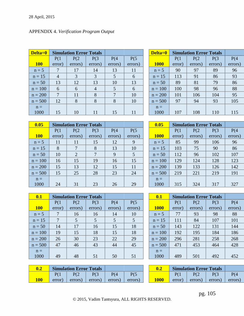
28 April, 2015


APPENDIX 4. Verification Program Output

Delta=0 Simulation Error Totals Delta=0 Simulation Error Totals

100

P(1

error)

P(2

errors)

P(3

errors)

P(4

errors)

P(5

errors) 1000

P(1

error)

P(2

errors)

P(3

errors)

P(4

errors)

P(5

errors)

n = 5 7 17 14 13 11 n = 5 90 97 89 96 97

n = 15 4 3 3 5 6 n = 15 113 91 86 93 92

n = 50 13 12 13 10 13 n = 50 89 81 79 86 83

n = 100 6 6 4 5 6 n = 100 100 98 96 88 107

n = 200 7 11 8 7 10 n = 200 101 106 104 95 91

n = 500 12 8 8 8 10 n = 500 97 94 93 105 96

n =

1000 15 10 11 15 11

n =

1000 107 108 110 115 90

0.05 Simulation Error Totals 0.05 Simulation Error Totals

100

P(1

error)

P(2

errors)

P(3

errors)

P(4

errors)

P(5

errors) 1000

P(1

error)

P(2

errors)

P(3

errors)

P(4

errors)

P(5

errors)

n = 5 11 11 15 12 9 n = 5 85 99 106 96 104

n = 15 8 7 8 13 10 n = 15 103 75 90 86 98

n = 50 10 2 7 9 5 n = 50 112 96 102 107 100

n = 100 16 15 19 16 15 n = 100 129 124 128 123 107

n = 200 15 13 12 15 11 n = 200 139 133 126 142 122

n = 500 15 25 28 23 24 n = 500 219 221 219 191 184

n =

1000 24 31 23 26 29

n =

1000 315 324 317 327 315


100

P(1

error)

P(2

errors)

P(3

errors)

P(4

errors)

P(5

errors) 1000

P(1

error)

P(2

errors)

P(3

errors)

P(4

errors)

P(5

errors)

n = 5 7 16 16 14 10 n = 5 77 93 98 88 99

n = 15 7 5 5 5 5 n = 15 111 84 107 101 107

n = 50 14 17 16 15 18 n = 50 143 122 131 144 125

n = 100 19 15 18 15 18 n = 100 192 195 184 186 168

n = 200 26 30 23 22 29 n = 200 296 281 258 268 261

n = 500 47 46 43 44 45 n = 500 471 453 464 428 405

n =

1000 49 48 51 50 51

n =

1000 489 501 492 452 451


100

P(1

error)

P(2

errors)

P(3

errors)

P(4

errors)

P(5

errors) 1000

P(1

error)

P(2

errors)

P(3

errors)

P(4

errors)

P(5

errors)

28 April, 2015


n = 5 14 7 14 13 16 n = 5 111 114 101 110 120

n = 15 18 18 19 15 19 n = 15 159 141 124 133 117

n = 50 27 29 25 28 30 n = 50 254 277 248 245 240

n = 100 46 35 41 52 46 n = 100 413 412 418 413 409

n = 200 52 45 50 61 48 n = 200 524 513 528 497 490

n = 500 17 17 15 18 22 n = 500 196 203 209 218 210

n =

1000 0 0 0 1 2

n =

1000 13 14 12 16 11


100

P(1

error)

P(2

errors)

P(3

errors)

P(4

errors)

P(5

errors) 1000

P(1

error)

P(2

errors)

P(3

errors)

P(4

errors)

P(5

errors)

n = 5 8 14 10 8 9 n = 5 133 139 123 130 139

n = 15 22 26 22 21 23 n = 15 206 188 179 176 173

n = 50 36 34 38 41 43 n = 50 423 414 389 423 383

n = 100 53 41 48 45 57 n = 100 487 501 494 531 516

n = 200 26 28 21 19 26 n = 200 278 282 263 283 294

n = 500 1 2 1 2 1 n = 500 5 2 5 8 5

n =

1000 0 0 0 0 0

n =

1000 0 0 0 0 0


100

P(1

error)

P(2

errors)

P(3

errors)

P(4

errors)

P(5

errors) 1000

P(1

error)

P(2

errors)

P(3

errors)

P(4

errors)

P(5

errors)

n = 5 13 17 17 17 16 n = 5 160 162 172 153 157

n = 15 39 30 36 30 33 n = 15 372 309 327 320 319

n = 50 45 50 56 51 51 n = 50 430 431 432 484 451

n = 100 12 9 13 10 14 n = 100 134 121 128 130 140

n = 200 0 1 1 0 0 n = 200 0 0 3 4 3

n = 500 0 0 0 0 0 n = 500 0 0 0 0 0

n =

1000 0 0 0 0 0

n =

1000 0 0 0 0 0

1 Simulation Error Totals 1 Simulation Error Totals

100

P(1

error)

P(2

errors)

P(3

errors)

P(4

errors)

P(5

errors) 1000

P(1

error)

P(2

errors)

P(3

errors)

P(4

errors)

P(5

errors)

n = 5 44 35 43 41 38 n = 5 381 365 356 351 346

n = 15 46 49 51 53 56 n = 15 451 464 486 532 555

n = 50 1 1 0 3 4 n = 50 1 5 3 13 15

n = 100 0 0 0 0 0 n = 100 0 0 0 0 0

n = 200 0 0 0 0 0 n = 200 0 0 0 0 0

n = 500 0 0 0 0 0 n = 500 0 0 0 0 0

28 April, 2015


n =

1000 0 0 0 0 0

n =

1000 0 0 0 0 0


100

P(1

error)

P(2

errors)

P(3

errors)

P(4

errors)

P(5

errors) 1000

P(1

error)

P(2

errors)

P(3

errors)

P(4

errors)

P(5

errors)

n = 5 53 44 55 54 55 n = 5 512 511 496 514 509

n = 15 7 14 22 22 30 n = 15 92 124 185 232 286

n = 50 0 0 0 0 0 n = 50 0 0 0 0 0

n = 100 0 0 0 0 0 n = 100 0 0 0 0 0

n = 200 0 0 0 0 0 n = 200 0 0 0 0 0

n = 500 0 0 0 0 0 n = 500 0 0 0 0 0

n =

1000 0 0 0 0 0

n =

1000 0 0 0 0 0

2 Simulation Error Totals 2 Simulation Error Totals

100

P(1

error)

P(2

errors)

P(3

errors)

P(4

errors)

P(5

errors) 1000

P(1

error)

P(2

errors)

P(3

errors)

P(4

errors)

P(5

errors)

n = 5 48 52 62 66 69 n = 5 510 570 610 653 683

n = 15 1 2 1 4 5 n = 15 4 20 39 56 75

n = 50 0 0 0 0 0 n = 50 0 0 0 0 0

n = 100 0 0 0 0 0 n = 100 0 0 0 0 0

n = 200 0 0 0 0 0 n = 200 0 0 0 0 0

n = 500 0 0 0 0 0 n = 500 0 0 0 0 0

n =

1000 0 0 0 0 0

n =

1000 0 0 0 0 0

28 April, 2015


Appendix 5. Full simulation results. (Legend: Prob2 = Pfals-neg; Prob0 = Pcorrect; Prob1 =

Pfals-pos)

N D E Prob2 Prob0 Prob1

5 0 1 3 97 0

5 0.05 1 4.5 94 1.5

5 0.1 1 3 94 3

5 0.2 1 3.5 93.5 3

5 0.5 1 7.5 86.5 6

5 1 1 15 74.5 10.5

5 2 1 30 69 1

15 0 1 3 95.5 1.5

15 0.05 1 2.5 93 4.5

15 0.1 1 4 90 6

15 0.2 1 3 95 2

15 0.5 1 15 81 4

15 1 1 13 85 2

15 2 1 0.5 99.5 0

50 0 1 1 96 3

50 0.05 1 2 95.5 2.5

50 0.1 1 4.5 95 0.5

50 0.2 1 5 92 3

50 0.5 1 7.5 89.5 3

50 1 1 0.5 99.5 0

50 2 1 0 100 0

100 0 1 1 97 2

100 0.05 1 1.5 97 1.5

100 0.1 1 1 98 1

100 0.2 1 5 92 3

100 0.5 1 0 99.5 0.5

100 1 1 0 100 0

100 2 1 0 100 0

200 0 1 0.5 99.5 0

200 0.05 1 0.5 99 0.5

200 0.1 1 1 97.5 1.5

200 0.2 1 1.5 95.5 3

200 0.5 1 0 100 0

200 1 1 0 100 0

200 2 1 0 100 0

500 0 1 0.5 99.5 0

500 0.05 1 0.5 99.5 0

500 0.1 1 2.5 97 0.5

28 April, 2015


500 0.2 1 1 97.5 1.5

500 0.5 1 0 100 0

500 1 1 0 100 0

500 2 1 0 100 0

1000 0 1 0 99 1

1000 0.05 1 1 98 1

1000 0.1 1 0 98 2

1000 0.2 1 0.5 99 0.5

1000 0.5 1 0 100 0

1000 1 1 0 100 0

1000 2 1 0 100 0

5 0 2 4.5 92 3.5

5 0.05 2 6 89.5 4.5

5 0.1 2 3 95 2

5 0.2 2 4 91 5

5 0.5 2 12.5 83.5 4

5 1 2 19.5 72.5 8

5 2 2 49.5 47 3.5

15 0 2 5 91 4

15 0.05 2 3 90.5 6.5

15 0.1 2 4 92 4

15 0.2 2 5.5 92.5 2

15 0.5 2 17.5 76.5 6

15 1 2 21 75.5 3.5

15 2 2 1 99 0

50 0 2 2.5 95 2.5

50 0.05 2 2 95.5 2.5

50 0.1 2 4.5 94.5 1

50 0.2 2 6.5 89.5 4

50 0.5 2 15.5 79 5.5

50 1 2 0.5 99.5 0

50 2 2 0 100 0

100 0 2 1.5 95.5 3

100 0.05 2 2 96 2

100 0.1 2 2.5 96 1.5

100 0.2 2 5.5 91.5 3

100 0.5 2 1 97 2

100 1 2 0 100 0

100 2 2 0 100 0

200 0 2 1.5 98.5 0

200 0.05 2 0.5 99 0.5

28 April, 2015


200 0.1 2 1.5 95.5 3

200 0.2 2 2.5 94.5 3

200 0.5 2 0 100 0

200 1 2 0 100 0

200 2 2 0 100 0

500 0 2 0.5 99 0.5

500 0.05 2 1 98.5 0.5

500 0.1 2 4 95.5 0.5

500 0.2 2 3 95.5 1.5

500 0.5 2 0 100 0

500 1 2 0 100 0

500 2 2 0 100 0

1000 0 2 0 98.5 1.5

1000 0.05 2 3 95 2

1000 0.1 2 1.5 97 1.5

1000 0.2 2 0.5 99 0.5

1000 0.5 2 0 100 0

1000 1 2 0 100 0

1000 2 2 0 100 0

5 0 5 4 91 5

5 0.05 5 6.5 89 4.5

5 0.1 5 4.5 91 4.5

5 0.2 5 4.5 91.5 4

5 0.5 5 13 82 5

5 1 5 21.5 73 5.5

5 2 5 66.5 30.5 3

15 0 5 6 90 4

15 0.05 5 2.5 91.5 6

15 0.1 5 5.5 90.5 4

15 0.2 5 5.5 91.5 3

15 0.5 5 18.5 74 7.5

15 1 5 40.5 56.5 3

15 2 5 9.5 90.5 0

50 0 5 3 93 4

50 0.05 5 2.5 93 4.5

50 0.1 5 5.5 93.5 1

50 0.2 5 9.5 85.5 5

50 0.5 5 19.5 72.5 8

50 1 5 1.5 98.5 0

50 2 5 0 100 0

100 0 5 2.5 92.5 5

28 April, 2015


100 0.05 5 3 96 1

100 0.1 5 4.5 91.5 4

100 0.2 5 7 89 4

100 0.5 5 5 93 2

100 1 5 0 100 0

100 2 5 0 100 0

200 0 5 2 97 1

200 0.05 5 0.5 97.5 2

200 0.1 5 1.5 94.5 4

200 0.2 5 6 89 5

200 0.5 5 0 100 0

200 1 5 0 100 0

200 2 5 0 100 0

500 0 5 0.5 98 1.5

500 0.05 5 1.5 94.5 4

500 0.1 5 4.5 93.5 2

500 0.2 5 5 93.5 1.5

500 0.5 5 0 100 0

500 1 5 0 100 0

500 2 5 0 100 0

1000 0 5 0 98 2

1000 0.05 5 3.5 94 2.5

1000 0.1 5 3 95 2

1000 0.2 5 0.5 98.5 1

1000 0.5 5 0 100 0

1000 1 5 0 100 0

1000 2 5 0 100 0

28 April, 2015


APPENDIX 6. Verification simulation results for effect size Δ=0.2, 5000 simulations

Δ=0.2 e n = 5 n = 15 n = 50 n = 100 n = 200 n = 500

n =

1000

P(1 error per arm) 1 93.92% 94.36% 96.70% 97.64% 98.98% 99.48% 99.44%

P(2 errors per arm) 2 92.10% 93.38% 95.80% 97.04% 97.98% 98.78% 99.20%

P(3 errors per arm) 3 91.24% 92.06% 94.94% 96.42% 97.54% 98.26% 98.90%

P(4 errors per arm) 4 90.94% 91.46% 94.52% 95.98% 96.92% 98.36% 98.62%

P(5 errors per arm) 5 90.38% 91.12% 93.56% 95.40% 96.84% 98.10% 98.58%

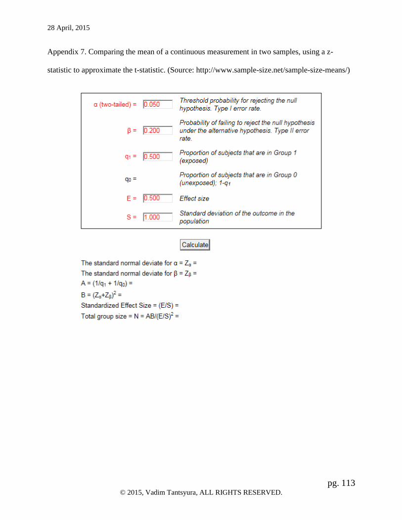
28 April, 2015


Appendix 7. Comparing the mean of a continuous measurement in two samples, using a z-

statistic to approximate the t-statistic. (Source: http://www.sample-size.net/sample-size-means/)

2015_05_12 dissertation binder_vtantsyura

Documents

data quality

data strong

impact of errors

errorfree data

impact of study size

research area

regulated clinical research

earlier years