2015 natural gas outlook -...

DOCKETED

Docket Number:

15-IEPR-03

Project Title: Electricity and Natural Gas Demand Forecast

TN #: 206501

Document Title: Draft Staff Report: 2015 Natural Gas Outlook

Description: This replaces TN206491 - 11.3.2015 IEPR Commissioner on the Revised Natural Gas Outlook Report

Filer: Raquel Kravitz

Organization: California Energy Commission

Submitter Role: Commission Staff

Submission Date:

11/3/2015 10:02:05 AM

Docketed Date: 11/3/2015

C ali f ornia Ene rgy C ommissi on

DRA FT STAFF REPORT

2015 NATURAL GAS OUTLOOK

CALIFORNIA ENERGY COMMISSION

Edmund G. Brown Jr., Governor

NO V E MB ER 20 15

CEC- 20 0 - 20 1 5- 0 0 7 - SD

CALIFORNIA ENERGY COMMISSION Leon Brathwaite Anthony Dixon Jorge Gonzales Melissa Jones Robert Kennedy Chris Marxen Peter Puglia Angela Tanghetti Primary Authors Chris Marxen Project Manager Ivin Rhyne Office Manager SUPPLY ANALYSIS OFFICE Sylvia Bender Deputy Director ENERGY ASSESSMENTS DIVISION Robert P. Oglesby Executive Director

DISCLAIMER Staff members of the California Energy Commission prepared this report. As such, it does not necessarily represent the views of the Energy Commission, its employees, or the State of California. The Energy Commission, the State of California, its employees, contractors and subcontractors make no warrant, express or implied, and assume no legal liability for the information in this report; nor does any party represent that the uses of this information will not infringe upon privately owned rights. This report has not been approved or disapproved by the Energy Commission nor has the Commission passed upon the accuracy or adequacy of the information in this report.

ACKNOWLEDGEMENTS

The authors would like to acknowledge the following individuals for their valuable contributions to this report:

Dr. Kenneth B. Medlock III, Ph. D., Institute for Public Policy, Baker Institute, Rice University, Houston, Texas, for assumption inputs, data, and guidance.

Angela Tanghetti, Energy Commission staff, for running and providing results of the production cost model, PLEXOS.

Melissa Jones, Energy Commission staff, for report review and edits.

Malachi Weng‐Gutierrez, Chris Kavalec, Asish Gautam, Keith O’Brien, and Andrea Gough, Energy Commission staff, for providing inputs on end‐use demand.

Catherine Elder of Aspen Environmental Group for report review and edits.

i

ABSTRACT

California Energy Commission staff produced the 2015 Natural Gas Outlook report to support the California Energy Commission’s 2015 Integrated Energy Policy Report. California Energy Commission staff, in consultation with industry experts, developed cases depicting future natural gas demand and supply trends under a variety of assumptions. The mid‐energy demand case represents a business‐as‐usual case in which staff based likely outcomes on current trends in natural gas markets, commercial activity, and economic developments. Staff created the high demand/low price and the low demand/high price cases by altering assumptions in ways that led to conditions that would move natural gas demand lower or higher than in the mid case. The results from this modeling effort are coordinated with other modeling efforts at the California Energy Commission.

Keywords: Natural gas supply, demand, infrastructure, storage, prices, exports, imports, shale, hydraulic fracturing, biomethane, liquefied natural gas

Brathwaite, Leon, Anthony Dixon, Jorge Gonzales, Melissa Jones, Robert Kennedy, Chris Marxen, Peter Puglia, Angela Tanghetti. 2015. 2015 Natural Gas Outlook Draft Staff Report. California Energy Commission. CEC‐200‐2015‐007‐SD.

ii

TABLE OF CONTENTS ACKNOWLEDGEMENTS .................................................................................................................... i

ABSTRACT ............................................................................................................................................. ii

EXECUTIVE SUMMARY ..................................................................................................................... 1

2015 IEPR Natural Gas Common Cases ........................................................................................ 1

Modeling Results ............................................................................................................................... 2

Natural Gas Prices .......................................................................................................................... 2

California Natural Gas Supply ..................................................................................................... 3

California Natural Gas Demand .................................................................................................. 4

Natural Gas Infrastructure ............................................................................................................... 5

North American Export and Import Issues ................................................................................ 6

Well Stimulation Technology Issues............................................................................................ 6

California Pipeline Safety Issues .................................................................................................. 7

Key Findings ....................................................................................................................................... 7

CHAPTER 1: Introduction ................................................................................................................... 9

Scope and Organization of Report ............................................................................................... 10

CHAPTER 2: 2015 Integrated Energy Policy Report Common Cases ......................................... 12

Modeling Approach ........................................................................................................................ 12

2015 IEPR Natural Gas Common Cases ...................................................................................... 14

Mid Demand Case ........................................................................................................................ 18

High Demand/Low Price Case ................................................................................................... 19

Low Demand/High Price Case ................................................................................................... 19

Modeling Results ............................................................................................................................. 20

Natural Gas Price Results ............................................................................................................ 20

Natural Gas Price Uncertainty ................................................................................................... 23

Supply Results .............................................................................................................................. 25

Demand Results ............................................................................................................................ 27

iii

CHAPTER 3: California End-Use Natural Gas Demand Forecast .............................................. 32

Statewide Baseline End-Use Natural Gas Forecast Results ..................................................... 32

Planning Area Baseline Results .................................................................................................... 35

Pacific Gas and Electric Planning Area ..................................................................................... 35

Southern California Gas Company Planning Area ................................................................. 38

San Diego Gas & Electric Planning Area .................................................................................. 41

CHAPTER 4: Natural Gas Resources and Infrastructure ............................................................. 44

Natural Gas Resources .................................................................................................................... 44

Natural Gas Reserves in the United States ............................................................................... 44

Hydraulic Fracturing and the Associated Environmental Concerns .................................... 45

Production Types and Trends .................................................................................................... 47

Biogas and Biomethane in California ........................................................................................ 54

Natural Gas Infrastructure ............................................................................................................. 54

Natural Gas Pipeline Changes .................................................................................................... 54

California Pipeline Safety .............................................................................................................. 56

California Storage ............................................................................................................................ 57

North American Export and Import Issues ................................................................................. 58

Mexico ............................................................................................................................................ 58

Canada ........................................................................................................................................... 59

Liquefied Natural Gas Exports ................................................................................................... 60

ACRONYMS......................................................................................................................................... 62

APPENDIX A: Electricity Dispatch Modeling Results ............................................................... A-1

Introduction .................................................................................................................................... A-1

Overview of Production Cost Modeling Assumptions .......................................................... A-2

Demand Assumptions .................................................................................................................. A-2

California 2015 to 2026 ............................................................................................................... A‐2

Rest of WECC 2015 to 2026 ....................................................................................................... A‐3

iv

Hydro Generation Forecast .......................................................................................................... A-4

WECC‐Wide ................................................................................................................................ A‐4

California Adjustments for 2015 and 2016 .............................................................................. A‐5

Renewable Portfolio Development 2015 – 2026 ....................................................................... A-5

Thermal Portfolio Development ................................................................................................. A-9

California Once‐Through‐Cooling Retirement Schedule ..................................................... A‐9

Non‐OTC Retirements and Additions .................................................................................. A‐11

California Non‐OTC Thermal Retirements .......................................................................... A‐12

California Thermal Additions ................................................................................................ A‐12

Rest of the WECC Thermal Retirements ............................................................................... A‐13

Rest of the WECC Thermal Additions .................................................................................. A‐14

California Renewable Curtailment ........................................................................................ A‐15

Natural Gas Demand for Electric Generation ...................................................................... A‐16

APPENDIX B: Development of a Monthly Model ...................................................................... B-1

APPENDIX C: Glossary .................................................................................................................... C-1

LIST OF FIGURES Figure 1: IEPR Common Cases for Henry Hub Pricing Point .......................................................... 3

Figure 2: Historical Natural Gas Cost Environments Using KLEMS Data .................................. 17

Figure 3: Composite Supply Cost Curve for the 2007 and 2015 IEPR Common Cases .............. 18

Figure 4: IEPR Common Cases for Henry Hub Pricing Point ........................................................ 21

Figure 5: Natural Gas Prices at Malin, Topock, and Henry Hub ................................................... 22

Figure 6: Prices Differentials (Point of Interest—Henry Hub) ....................................................... 22

Figure 7: 2015 IEPR Common Cases With Error Bands .................................................................. 24

Figure 8: U.S. EIA and Energy Commission Price Uncertainties ................................................... 25

Figure 9: United States Dry Natural Gas Production ...................................................................... 26

Figure 10: California 2025 Supply Portfolio (Mid Demand Case) ................................................. 27

v

Figure 11: U.S. Natural Gas Demand (All Sectors) .......................................................................... 28

Figure 12: U.S. Natural Gas Demand for Power Generation .......................................................... 28

Figure 13: California Natural Gas Demand (All Sectors) ................................................................ 29

Figure 14: California Natural Gas Demand in the Power Generation Sector .............................. 30

Figure 15: Statewide End‐Use Natural Gas Demand ...................................................................... 34

Figure 16: Statewide End‐Use Per Capita Natural Gas Consumption .......................................... 34

Figure 17: PG&E Planning Area Residential Natural Gas Demand .............................................. 36

Figure 18: PG&E Planning Area Commercial Natural Gas Demand ............................................ 37

Figure 19: PG&E Planning Area Industrial Natural Gas Demand ................................................ 37

Figure 20: So Cal Gas Planning Area Residential Natural Gas Demand ...................................... 39

Figure 21: So Cal Gas Planning Area Commercial Natural Gas Demand .................................... 40

Figure 22: So Cal Gas Planning Area Industrial Natural Gas Demand ........................................ 40

Figure 23: SDG&E Planning Area Residential Natural Gas Consumption .................................. 42

Figure 24: SDG&E Planning Area Commercial Natural Gas Consumption ................................ 43

Figure 25: SDG&E Planning Area Industrial Natural Gas Consumption .................................... 43

Figure 26: Proved and Potential Reserves in the United States ..................................................... 44

Figure 27: Total Shale Natural Gas Resources in the United States .............................................. 45

Figure 28: United States Historical and Projected Natural Gas Production by Resource Type .................................................................................................................................... 48

Figure 29: The Expanding Natural Gas Resource Base (2007 – 2015)............................................ 49

Figure 30: Total United States Natural Gas Production and Shale Natural Gas Production..... 50

Figure 31: Total United States Coalbed Methane Production ........................................................ 50

Figure 32: Total United States Tight Gas Sands Production ........................................................... 51

Figure 33: Total United States Associated Natural Gas Production .............................................. 52

Figure 34: Total United States Conventional Natural Gas Production ......................................... 53

Figure 35: Utility Storage Levels (2011 – 2015) ................................................................................. 58

Figure 36: Historical and Forecasted United States Exports to Mexico ........................................ 59

vi

Figure 37: Net Natural Gas Imports From Canada .......................................................................... 60

Figure 38: United States Net LNG Exports ....................................................................................... 61

Figure A‐1: WECC (Non‐CA) Electricity Load Forecast—All Cases (GWh)…………………...A‐4

Figure A‐2: California Thermal Power Plant Additions………………………………………....A‐13

Figure A‐3: Thermal Power Plant Retirements for the Rest of WECC…………………………A‐14

Figure A‐4: Thermal Power Plant Additions Rest of WECC……………………………………A‐15

Figure A‐5: California Natural Gas Demand for Electric Generation………………………….A‐16

Figure A‐6: Mid Demand Case Generation Fuel Sources 2015 – 2026…………………………A‐17

LIST OF TABLES Table 1: Actual and Modeled Natural Gas Demand for All Sectors in California (2013) ............. 5

Table 2: Assumptions for Common Cases ........................................................................................ 15

Table 3: Price Elasticity in NAMGas Model by Sector .................................................................... 16

Table 4: Actual and Modeled Natural Gas Demand for All Sectors in California (2013) ........... 31

Table 5: Statewide End‐Use Natural Gas Forecast Comparison .................................................... 33

Table 6: PG&E End‐Use Natural Gas Demand Forecast ................................................................. 35

Table 7: So Cal Gas End‐Use Natural Gas Demand Forecast ......................................................... 38

Table 8: SDG&E End‐Use Natural Gas Demand Forecast .............................................................. 41

Table 9: Summary of Changes in Production by Resource Type (2010 – 2020) ........................... 53

Table 10: Capacity Additions in the United States (2011 ‐ 2015) .................................................... 55

Table 11: Main Pipeline Systems Serving California ....................................................................... 56

Table A‐1: Production Cost Trends……………………………………………………………….....A‐2

Table A‐2: Counties by Region for the Solar Profiles………………………………………………A‐7

Table A‐3: WECC Renewables to Achieve Policy Goals (TWh)…………………………………..A‐8

Table A‐4: Summary of California RPS Goals, Operational Renewables, and Net Short Used to Generate Renewable Build in California (All Values in TWh)………………………..A‐8

Table A‐5: OTC Implementation Schedules for All IEPR Common Cases……………………..A‐10

vii

EXECUTIVE SUMMARY

California Energy Commission staff collects, analyzes, and publishes data on the operation of energy markets, including electricity, natural gas, petroleum, and alternative energy sources. This process is essential to serve the information and policy development needs of the Governor, the Legislature, public agencies, market participants, and the public (PRC Section 25300[c]). This report provides multiple plausible estimates of the natural gas market. These broad estimates are necessary due to the high complexity of the gas market, numerous options for decision‐makers, and deep uncertainties about future conditions. In 2015, staff is also publishing a companion document titled Assembly Bill 1257 Natural Gas Act Report: Strategies to Maximize the Benefits Obtained From Natural Gas as an Energy Source. Staff is addressing several topics covered in the 2013 Natural Gas Trends, Issues, and Outlook report, such as natural gas pipeline safety, methane emissions, and the southern system minimum flow issue, in the new report.

2015 IEPR Natural Gas Common Cases Staff examined historical trends in variables known to be major drivers in natural gas markets and then altered these variables by applying assumptions to project plausible future trends. Plausible changes are those that could occur with some level of certainty based upon past observances and the directives of current energy policies. Game‐changing events and unforeseen technological advances, such as horizontal drilling coupled with hydraulic fracturing, are unpredictable. History shows that these events can have a greater impact on natural gas markets than estimable variables. As such, the results of case analyses do not estimate with exact accuracy the future of the complex natural gas markets. Staff used a mix of plausible cases that incorporate transparent and vetted assumptions to model how the market may behave in the next two decades.

For this assessment, staff is using a modification of the Rice World Gas Trade Model, constructed specifically for the North American gas market. Staff refers to this as the North American Market Gas‐Trade Model. Staff developed natural gas cases around trends that represent three plausible futures: a business‐as‐usual or mid case, a high demand/low price case, and a low demand/high price case. Each case contains different assumptions about market and regulatory developments. Staff refers to these cases as “common” because they are common to several analyses performed for the 2015 Integrated Energy Policy Report across several Energy Commission offices. The mid case, or business‐as‐usual case, represents a future in which the economy, technology improvements, and cost environment proceed as they have done in the past. Staff created the high demand/low price case and low demand/high price case by altering assumptions in ways that would lead to plausible conditions that would move natural gas demand higher or lower than in the mid case. Assumptions that vary in each case include economic growth, technology improvements, percentage of renewable generation within the overall electricity generation portfolio, amount of generation in megawatts

1

historically provided by coal, the amount of expected coal‐fired generation retirement, cost, and several other assumptions.

Staff held public workshops on February 26, 2015, and May 21, 2015, to present the key assumptions used to build the cases and the preliminary modeling results. Staff also held a workshop on September 21, 2015, where staff presented the preliminary results of the modeling efforts undertaken as part of the Integrated Energy Policy Report process. Based on comments and feedback received at the workshop, staff made several refinements to the models and results. As a result, the charts and tables contained in this report may vary from those presented at the September workshop. A summary of the changes can be found in Chapter 1.

Modeling Results Natural Gas Prices The natural gas prices projected by staff’s North American Market Gas‐Trade Model for this outlook are estimates that use annual inputs to produce annual average prices. The North American Market Gas‐Trade Model does not account for fluctuations that occur in the natural gas market seasonally and daily. Figure 1 shows projected natural gas prices from 2015 to 2030. All prices are for natural gas traded at Henry Hub, which is the North American benchmark pricing point near Erath, Louisiana, and is the trading location used to price the New York Mercantile Exchange natural gas futures contracts. These prices reflect the estimated cost of producing natural gas, processing it for injection into the pipeline system, and transporting it to that hub. The North American Market Gas Trade Model used in this analysis produces annual average estimates of supply, demand and price; therefore, they are annual averages and do not account for temperature‐driven or other fluctuations that can occur in the natural gas market on a daily or seasonal basis.

For the projections from 2015 to 2019, staff blended the North American Market Gas Trade Model forecasts with the September 14, 2015, trade date information from New York Mercantile Exchange website in the following manner: • The 2015 and 2016 mid demand case values originated from the New York Mercantile

Exchange futures strip.

• The 2017, 2018, and 2019 mid demand case values combined the New York Mercantile Exchange futures strip and the North American Market Gas‐Trade Model projections. Staff averaged the New York Mercantile Exchange futures value and the North American Market Gas‐Trade Model values to determine the 2017, 2018, and 2019 mid demand case projections.

• Projections beyond 2019 originated from the North American Market Gas‐Trade Model.

In the high demand/low price case, the model high price values were blended with the blended mid demand case values from 2015 – 2019 to produce a reasonable slope to approach the

2

fundamentally higher price level for the high demand/low price case. The low demand/high price case uses North American Market Gas Trade model results exclusively. Staff produced all values from 2020 forward within the North American Market Gas‐Trade Model.

Figure 1: IEPR Common Cases for Henry Hub Pricing Point

Source: Energy Commission.

Henry Hub prices exhibit annual growth rates between 2.6 and 6.2 percent per year from 2015 to 2030 for the three cases. By 2030, prices in the high demand/low price case reach $4.08 (2014$) per thousand cubic feet, and prices in the low demand/high price case reach $6.87 (2014$) per thousand cubic feet. From 2015 to 2030, the gas market reflects traders’ expectations of slowly rising gas prices combined with fundamental market forces driving prices upward at an average rate of 4 percent per year. In the United States, natural gas is rising slowly, while excess production is diminishing, leading staff to expect prices to rebound from the 2015 low.

California Natural Gas Supply The three common cases estimate that by 2025 California continue to import about 98 percent of its natural gas. California’s natural gas enters the state at the northern hub of Malin, Oregon and the cluster of southern hubs located near Topock, Arizona. Gas entering at Malin comes from a combination of gas from Canada and the Rocky Mountains, while gas entering at the southern end of the state can come from the Rocky Mountains via the Kern River pipeline or from the San Juan basin via the pipelines entering at either Topock or Ehrenberg. Staff expects California to continue to import gas from the Canadian, Rocky Mountain, and San Juan basins, with varying amounts coming into the state from each source depending on the price and availability of gas.

0.001.002.003.004.005.006.007.008.00

Pric

e, 2

014$

per

Tho

usan

d Cu

bic

Feet

High Demand/ Low Price Mid Demand

EIA (Historical) Low Demand/ High Price

3

About half of the state’s gas will enter at the northern end via the Malin hub, with the remainder entering at the south via either Kern River or Topock and Ehrenberg. The remainder of the state’s gas supplies will come from gas production in state from the small, but long‐standing production basins located in the Sacramento and San Joaquin Valleys.

California Natural Gas Demand Staff produced the forecast of California end‐use natural gas demand using the Energy Commission’s end‐use demand models by the same staff that produces the end‐use electricity forecast. The end‐use forecast model encompass agriculture, commercial, industrial, residential, transportation (light‐duty vehicles, buses, medium and heavy‐duty trucks), communication, and utilities along three utility planning areas (Pacific Gas and Electric Company, Southern California Gas Company, and San Diego Gas & Electric Company).

These end‐use forecasts do not include natural gas for power generation and are used as inputs into the North American Market Gas Trade model. The new forecasts begin at a higher point in 2015, as actual natural gas demand in California was higher in 2015 than estimated in the California Energy Demand 2013 mid case and grow at a higher rate in all three cases from 2012 – 2024. Staff attributes the higher starting point and growth rates to an increase in natural gas demand for transportation followed by an increase in residential demand. Staff projects, by 2024, demand in the 2015 preliminary end‐use natural gas demand mid case to be around 10 percent higher compared to the California Energy Demand 2013 mid case.

The expected trend in natural gas demand for power generation in California differs from that of the United States. Staff produced this portion of the forecast by modeling the electricity dispatch in the Western United States using the PLEXOS production cost‐modeling platform. The implementation of renewable generation and the penetration of energy efficiency are suppressing natural gas demand in the state.

From North American Market Gas‐Trade model results, in the mid demand case, staff expects natural gas in California to decline at an annual rate of 1.1 percent between 2015 and 2026. After the full implantation of the Renewables Portfolio Standard and full penetration of energy efficiency, overall natural gas demand increases due to population growth and associated demand, reaching 5.92 billion cubic feet (Bcf) per day by 2030 in the mid demand case. However, natural gas demand in the state remains below the 2015 level.

The decline in natural gas demand becomes more apparent in the power generation sector where California’s Renewables Portfolio Standard has the greatest impact. While overall demand declines at an annual rate of 1.1 percent, the decline observed in the power generation sector is about 2.1 percent. In the mid demand case, after 2026, demand in power generation sector rebounds but, by 2030, remains below the 2015 level at about 1.7 Bcf per day. Table 1 shows natural gas demand by sector in California.

4

Table 1: Actual and Modeled Natural Gas Demand for All Sectors in California (2013)

Source: Energy Commission, Supply Analysis Office. Natural gas demand for residential, commercial, and industrial sectors were provided by the Demand Analysis Office.

Natural Gas Infrastructure Most of California’s natural gas supply comes from outside the state. The primary production areas for imported natural gas are the Southwest, the Rocky Mountains, and Canada, while the state produces less than 10 percent of its demand requirements.

Several interstate pipelines deliver the natural gas to the California border, and from there, intrastate pipelines take the natural gas to the Citygate 1and the local distribution pipelines or to storage facilities for later use. California has 13 operating natural gas storage facilities, all of

1 Citygate is a location where natural gas changes possession from one company to another. It can be a physical location such as a hub or compressor station, or a virtual location only.

Million Cubic Feet per DayLow Demand/ High Price Case 2013 2015 2020 2025 2030 % Change 2013‐2030Residential 1,369 1,450 1,502 1,521 11%Commercial 564 548 602 650 15%Industrial 1,627 1,592 1,543 1,537 ‐6%Transportation 22 29 60 147 568%Power Gen 2,821 2,626 1,721 1,260 1,378 ‐51%State Total 6,403 6,245 5,428 5,115 5,582 ‐13%

Mid Demand Case 2013 2015 2020 2025 2030Residential 1,369 1,451 1,472 1,453 6%Commercial 564 550 593 622 10%Industrial 1,627 1,608 1,563 1,557 ‐4%Transportation 22 30 67 164 645%Power Gen 2,821 2,695 1,918 1,702 1,773 ‐37%State Total 6,403 6,334 5,613 5,498 5,920 ‐8%

High Demand/ Low Price Case 2013 2015 2020 2025 2030Residential 1,369 1,452 1,488 1,481 8%Commercial 564 550 611 655 16%Industrial 1,627 1,641 1,637 1,650 1%Transportation 22 110 251 615 2695%Power Gen 2,821 2,822 2,811 2,337 2,478 ‐12%State Total 6,403 6,575 6,798 6,738 7,532 18%

5

which are depleted oil or gas production fields. The total current working gas capacity of these facilities is 349.3 billion cubic feet, with a maximum daily delivery of 8.56 billion cubic feet when the fields are full. These storage facilities, however, cannot all deliver at the maximum rate at any one time. In addition, some operate for purposes of supplier price arbitrage and others for utility reliability.

North American Export and Import Issues Demand for natural gas in the power generation sector in Mexico is growing. Mexico’s national energy ministry expects annual growth in this sector to exceed 5 percent over the next 10 years. At least six United States pipeline operators have proposed building pipelines to export natural gas to Mexico. The exporting of natural gas to Mexico could affect the availability of natural gas delivered to California. The vast quantities of reserves now available in the United States natural gas resource base, in part, motivate this activity.

United States operators are also seeking licenses to export liquefied natural gas from 22 proposed liquefaction facilities. Operators of these facilities have petitioned the United States Department of Energy; eight have received approval, and two facilities are under construction. On October 1, 2015, Sabine Pass, in Cameron, Louisiana, started receiving natural gas and expects to start exporting liquefied natural gas by the end of the year. In addition, Jordan Cove liquefied natural gas in Coos Bay, Oregon, received the final Federal Energy Regulatory Commission’s environmental impact report, with possible final approval in December 2015. Furthermore, Cameron LNG in Hackberry, Louisiana, filed to expand its liquefied natural gas export capacity.

Well-Stimulation Technology Issues The development of natural gas from shale formations has expanded the resource base and boosted United States natural gas production. However, the production from this resource type requires the use of well‐stimulation technologies. Horizontal drilling combined with the technique known as hydraulic fracturing, or more simply known as fracking, is the most commonly used well‐stimulation technology. Other forms of well‐stimulation technology include acid fracturing and acid matrix stimulation. Oil and gas operators have used some form of the fracking technique in the United States since 1947 on more than 1 million wells. In the last 20 years, the rate of use of the technique has accelerated and raised several environmental concerns. These concerns include greenhouse gas emissions, surface disturbances, water use, and disposal of wastewater, increased seismic activity, groundwater contamination, and socioeconomic impacts.

State and federal decision‐makers and regulators have developed regulatory frameworks to guide oil and natural gas activities within their jurisdictions. In California, efforts are continuing to develop the regulatory framework. In 2013, the State Legislature passed, and the Governor signed, Senate Bill 4 (Pavley, Chapter 313, Status of 2013). In November 2013, the California Department of Conservation began the formal rulemaking for Well Stimulation Treatment Regulations, scheduled to go into effect in 2015.

6

California Pipeline Safety Issues The explosion of a PG&E high‐pressure transmission pipeline in a residential neighborhood on September 9, 2010, killing eight people, injuring 58, and destroying or damaging more than 100 homes, has changed how citizens, energy regulators, and other public officials view natural gas pipeline safety. Lapses in pipeline safety led to that explosion. A natural gas system that does not protect the health and safety of Californians, by definition, does not satisfy the requirements of the Public Utilities Code and cannot meet California’s future need for natural gas. Staff discusses issues pertaining to pipeline safety such as the California Legislature’s response, the utilities and the California Public Utility Commission’s work towards insuring a safer natural gas system in detail in the companion report, Assembly Bill 1257 Natural Gas Act Report: Strategies to Maximize the Benefits Obtained From Natural Gas as an Energy Source.

Key Findings This report provides a comprehensive view of natural gas usage in California and the United States; staff believes the following are the most important findings or insights of the report:

• Staff estimates that in all three common cases, the United States’ pricing point (Henry Hub) will exhibit annual growth rates between 2.1 and 9.2 percent per year from 2015 to 2030.

• The negative price differential between Henry Hub and Malin, California’s main northern receiving hub, will persist. This difference reflects the fundamentally lower cost of gas production both in the Rocky Mountain and Canadian regions and competition between natural gas flowing south on the Gas Transmission Northwest pipeline and natural gas flowing west on the Ruby pipeline. The positive price differential between Henry Hub and Topock, California’s main southern receiving hub, persists throughout the outlook horizon. This positive price differential reflects relatively higher costs of resources produced in the San Juan basin and the added cost of transporting gas to the California border. The differential remains positive throughout the 20‐year horizon

• California imports about 90 percent of its natural gas demand, and staff expects imports to be about 98 percent in 2025. Staff expects California to receive gas imports through the Malin Hub (36 percent), the Southwest (47 percent) and the Rocky Mountains and Kern River (15 percent).

• Staff estimates natural gas demand for power generation in California to decline by about 37 percent over the forecasted period in the mid demand case, due to the implementation of renewable generation and the penetration of energy efficiency. This trend differs from the rest of the United States, where staff estimates natural gas demand for power generation to increase by about 13 percent due to aggressive coal retirements.

• Annual per capita demand for natural gas varies in response to annual temperatures and business conditions, but it has been generally declining since the late 1990s. Staff expects this trend to continue as population grows faster than total natural gas demand.

7

• Staff believes that meeting future natural gas demand system requirements in California will require more research, development, and deployment funding to projects that explore new technologies to monitor and address pipeline safety and integrity assessment.

8

CHAPTER 1: Introduction Natural gas has been an important part of California’s fuel mix for well over 150 years. Initially manufactured and used primarily for lighting, California now uses natural gas for heating, cooking, transportation fuel, industrial uses, and power generation.

As the state grows its renewable portfolio, the ways people use natural gas may be changing. The use of natural gas‐fired generation to smooth the intermittent nature of wind and solar energy has highlighted the need to assure that there is adequate supply for the power generation sector. Because of efforts to reduce air pollution, natural gas may provide new options in the fuel mix for the industrial and transportation sectors. Finally, the development of zero‐net‐energy buildings may present new opportunities for natural gas use in the residential sector.

Because natural gas continues to hold a large position in California’s energy mix, it is important to ensure reliable supplies and assess future natural gas demand, supply, prices, and infrastructure needs. Meeting such estimates requires an understanding of future issues and trends that could affect natural gas markets and disruptions in supply.

This report presents the results of the California Energy Commission 2015 analysis of natural gas supply, demand, prices, and infrastructure issues in California and North America. Energy Commission staff produced three cases based upon plausible and transparent assumptions to give planners and decision makers information about the possible supply, demand, and price of natural gas in the future.

As part of the overall Integrated Energy Policy Report (IEPR) process, staff has accepted input from stakeholders through workshops and written comments. This feedback has been invaluable to improving the overall forecast. On September 21, 2015, staff held a workshop presenting preliminary natural gas outlook results. Following that workshop, comments from stakeholders provided the impetus to make several small refinements. The net result of these changes was to reduce the overall price trajectory of the national natural gas market, lowering the expected price in 2030 from about $6.00 per thousand cubic feet to about $5.00 per thousand cubic feet (Mcf). In addition, small changes in nationwide natural gas demand also resulted. The key changes are as follows:

• The retirement of coal‐fired generation across the United States as a result of the new Part 111(d) rules put forward by the United States Environmental Protection Agency (U.S. EPA) were adjusted to be consistent with the Final Regulatory Impact Report released in July 2015.

• All states with renewable portfolio goals were estimated to meet those goals on time.

• Staff used the September Bidweek forward curve as the starting point for the model to align it with current market expectations.

• Postprocessing adjustments were made to address with minor modeling issues affecting the amount of natural gas imported from Canada.

9

• Adjustments to national residential, commercial, and industrial natural gas demand were made to align them more closely with the growth rates expected by the United States Energy Information Administration (U.S. EIA).

Decision makers can use this information to help determine near‐ and long‐term procurement needs and perform contingency planning. Staff believes the following are the most important findings of the report:

• Staff estimates that in all three common cases, the United States’ pricing point (Henry Hub) will exhibit annual growth rates between 2.1 and 9.2 percent per year from 2015 to 2030.

• The negative price differential between Henry Hub and Malin, California’s main northern receiving hub, will persist. This difference reflects the fundamentally lower cost of gas production both in the Rocky Mountain and Canadian regions and competition between natural gas flowing south on the Gas Transmission Northwest pipeline and natural gas flowing west on the Ruby pipeline. The positive price differential between Henry Hub and Topock, California’s main southern receiving hub, persists throughout the outlook horizon. This positive price differential reflects relatively higher costs of resources produced in the San Juan basin and the added cost of transporting gas to the California border. The differential remains positive throughout the 20‐year horizon

• California imports about 90 percent of its natural gas demand, and staff expects imports to be about 98 percent in 2025. Staff expects California to receive gas imports through the Malin Hub (36 percent), the southwest (47 percent) and the Rocky Mountains and Kern River (15 percent).

• Staff estimates natural gas demand for power generation in California to decline by about 37 percent over the forecasted period in the mid demand case, due to the implementation of renewable generation and the penetration of energy efficiency. This trend differs from the rest of the United States, where staff estimates natural gas demand for power generation to increase by about 13 percent due to aggressive coal retirements.

• Annual per capita demand for natural gas varies in response to annual temperatures and business conditions, but it has been generally declining since the late 1990s. Staff expects this trend to continue as population grows faster than total natural gas demand.

• Staff believes that meeting future natural gas demand system requirements in California will require more research, development, and deployment funding to projects that explore new technologies to monitor and address pipeline safety and integrity assessment.

Scope and Organization of Report

Chapter 2 presents the assumptions used to construct the three natural gas market common cases and model results. Staff presents results of the three IEPR common cases, high demand/low price, mid demand, and low demand/high price for natural gas price, supply, and demand and natural gas price uncertainty.

10

Chapter 3 presents the end‐use natural gas demand. Results for statewide and the three investor‐owned utility planning areas are compared in three cases: high demand/low price, mid demand, and low demand/high price.

Chapter 4 focuses on natural gas resource and infrastructure, including pipeline additions, pipeline safety, storage, and North American import and export issues.

11

CHAPTER 2: 2015 Integrated Energy Policy Report Common Cases Modeling Approach

In the 2015 IEPR, Energy Commission staff used the MarketBuilder platform2 to construct a natural gas market model. In this platform, staff developed the North American Market Gas‐Trade model (NAMGas), a general equilibrium resource model that simulates an interconnected network of economic agents3 seeking economic utility maximization. Building a model in the MarketBuilder platform requires defining a physical, geographic network or a topology for the natural gas market. Within the network, staff must define all natural gas demand centers, including large gas consumers such as power plants. Further, staff must locate all interconnecting interstate and intrastate pipelines, all import and export terminals, and all supply sources of natural gas.

Input assumptions for the network include the estimated demand for natural gas at all demand centers, each of which include five demand sectors. The model also includes:

• Price elasticities of demand for natural gas.

• Capacities and transportation costs along each route (or corridor) from supply to demand load.

• Size of the natural gas supply resources.

• Technological innovation rate.

• Cost over time to develop and extract natural gas resources.

• Investment criteria for the endogenous construction of new pipeline capacity.

Furthermore, staff must specify time‐points (periods) for the forecasting horizon of the model, which extends, in annual increments, from 2012 to 2050. The period allows the model to account for capital investment decisions. However, results presented in this report cover the 18‐year period from 2012 to 2030.

Further, staff considered the potential impact of relevant energy policy, such as the Renewables Portfolio Standard (RPS). In the 2015 IEPR, California and all other Western Electricity Coordinating Council (WECC) states construct generation portfolios that meet their individual RPS. In California, staff included, in all three cases, the requirement of 33 percent renewable generation by 2020. The PLEXOS production cost model provided the inputs for natural gas demand in the power generation sector in all WECC states. In addition, the penetration of

2 Platform owned by Deloitte LLP Market Point Services.

3 Economic agents are actors or decision‐makers in the marketplace.

12

http://r.search.yahoo.com/_ylt=A0SO81P.AHJVjH0ArnRXNyoA;_ylu=X3oDMTEydmk3aW5qBGNvbG8DZ3ExBHBvcwMxBHZ0aWQDQjAyNjVfMQRzZWMDc3I-/RV=2/RE=1433563519/RO=10/RU=http%3a%2f%2fwww.wecc.biz%2f/RK=0/RS=XxVpWHaJEnlTTXsAsdqLmalfYw0-

http://r.search.yahoo.com/_ylt=A0SO81P.AHJVjH0ArnRXNyoA;_ylu=X3oDMTEydmk3aW5qBGNvbG8DZ3ExBHBvcwMxBHZ0aWQDQjAyNjVfMQRzZWMDc3I-/RV=2/RE=1433563519/RO=10/RU=http%3a%2f%2fwww.wecc.biz%2f/RK=0/RS=XxVpWHaJEnlTTXsAsdqLmalfYw0-

energy efficiency, another variable affecting the outcomes of the model, varies among the cases. The low demand/high price case assumes the highest penetration and the high demand/low price case, the lowest. High penetration tends to lower natural gas demand, and low penetration achieves the reverse. Appendix A will provide more details about the energy efficiency assumptions.

The version of the NAMGas model now used by the Energy Commission requires annual starting (reference) demands and prices;4 and an econometric model provides these values. Staff refers to this as the “reference model.” The reference model consists of regression equations for each of the five demand sectors represented in the NAMGas model. The independent variables used in the regression equations for each end‐use sector appear below:

• Residential reference demand = recent historical demand for natural gas, population, natural gas price, income, heating oil price, and cold weather.

• Commercial reference demand = recent historical demand for natural gas, income, natural gas price, population, heating oil price, and cold weather.

• Industrial reference demand = recent historical demand for natural gas, natural gas price, coal price, industrial production, and cold weather.

• Power generation reference demand = total electricity generation, weather, natural gas price, fuel oil price, renewable electricity generation, and coal price.

• Transportation reference demand = recent historical transportation demand for natural gas, income, natural gas price, and population.

Performing a regression analysis5 using historical data for the variables by end‐use sector yields the coefficient estimates needed to calculate the reference demand quantities. These starting (reference) values extend through all the years of the forecasting horizon and through the geographic demand centers specified in the model. In addition to reference values generated by the regression analysis, the Natural Gas Unit uses California end‐use demand data from the Energy Assessments Division’s Demand Analysis Office. Staff also receives the WECC power generation demand from the Energy Assessments Division’s Procurement and Modeling Analysis Unit and obtains natural gas demand in the transportation sector from the Energy Assessments Division’s Transportation Fuels Unit.

With the specified topology and the input data, the NAMGas model iterates until it finds a solution that obeys basic economic principles for well‐behaved markets. Since every unit of natural gas produced from a supply basin shrinks the resource base, the model allows for advances in technology to offset this depletion effect, where necessary. At every iteration, the

4 This use of the term ”reference” does not mean ”reference case” but merely indicates that they are the starting input values.

5 Regression analysis is a statistical process for estimating the relationships among variables.

13

model seeks to balance supply and demand at the determined price. While the iteration procedure progresses, the NAMGas model:

• Adds pipeline capacity if economic conditions meet or exceed the investment criteria.

• Changes demand in response to price variations and the input price elasticities.

• Changes production in response to price variations, technology assumptions, and supply elasticity.

When the NAMGas model finds a final equilibrium, staff extracts a series of regional annual average natural gas prices, regional natural gas supply and demand, and interregional natural gas flows for the defined network. At this time, the model does not account for operational fluctuations or daily, monthly, and seasonal variations.

2015 IEPR Natural Gas Common Cases

Energy Commission staff created three common cases for the 2015 IEPR that staff uses across all the forecast models. These cases represent plausible cases of natural gas and electricity markets, and the Natural Gas Unit staff has incorporated elements of the demand forecast, transportation forecast, and electricity production cost forecast into propagation of the cases. The three common cases depict trends now seen in the natural gas market.

Table 2 summarizes assumptions used in the 2015 IEPR. However, the RPS, potential coal retirements, elasticity, and the cost environment play critical roles in the behavior and outcomes of the model. These assumptions simulate a range of plausible conditions that account for uncertainty in the natural gas market, in the economy, and in policy proposals and requirements.

14

Table 2: Assumptions for Common Cases

Assumptions Low Demand/High Price Case Mid Demand Case High Demand/Low

Price Case

GDP Growth Rate 2.0% 2.3% 3.5%

Natural Gas Technology Improvement Rate 1% 1% 2.5%

CA Meets 2020 RPS Target On Time On Time On Time

WECC Meets RPS Target On Time On Time On Time

Other States RPS Meet On Time On Time On Time

Additional U.S. Coal Generation Converts to Natural Gas Starting in 2016 (GW) 20 31 61

Elasticities Elasticities On (Except for CA and WECC Power Generation)

-0.5298 to -1.2364 (Except CA and all WECC Power Generation)

Elasticities On (Except for CA and WECC Power Generation)

Cost Environmenta High (P95) Mid (P50) Low (P5)

Source: Energy Commission, Supply Analysis Office, 2015.

a Refers to the assessment of the quantities of recoverable gas resources. By industry convention, the P50 assessments mean there is a 50 percent probability that at least this much gas is recoverable from that play using current technology. To increase the spread of resulting gas prices, additional cases were run assuming higher probability but lower resource amounts (a P95 case) and lower probability but higher resource amounts (a P5 case).

Staff developed three coal retirements converted to natural gas profiles, one for each case. In the high demand/low price case, coal retirements totaled to 61 gigawatts (GW), in the mid demand case, 31 GW, and in the low demand/high price case, 20 GW. To implement these assumptions, staff assumes that natural gas‐fired generation will replace the retiring coal. Since California uses little coal‐fired generation, the state experiences the impact of this assumption through price variations that occur outside the state. Price variations outside California affect natural gas flows to the state, which, in turn, influence price variations within the state.

Elasticities measure the responsiveness of price changes. As prices increase or decrease, the amount supplied or consumed will change. A key feature of NAMGas is the ability, as it

15

iterates, to adjust quantity demanded as prices change. Either the NAMGas model can let the price changes affect the demand for natural gas, or staff can turn off the elasticities, keeping demand at the input levels. In all three cases, staff turned off the elasticities for the power generation sector in California and the WECC to keep those values consistent with those produced by the production cost modeling activity. The natural gas demand for power generation originates from the PLEXOS model where the elasticities are considered. Table 3 displays the elasticity values used in the 2015 IEPR.

Table 3: Price Elasticity in NAMGas Model by Sector


Figure 2 displays the historical indexed combined cost of capitol, labor, energy, manufacturing, and service (KLEMS)(United States Department of Labor KLEMS database) between 1968 and 2013. These costs determine the cost environment6 of each unit of natural gas production in each case.

6 Staff placed the mid demand case in an averaged sustained cost environment. To construct the high and low demand cases, staff used the KLEMS data to place each of these two cases in a high‐sustained and low‐sustained cost environment, respectively.

16

Figure 2: Historical Natural Gas Cost Environments Using KLEMS Data

Source: Baker Institute, 2015.

Assumptions on the cost of producing natural gas and available reserves differ for each case. Staff placed the high demand/low price case in a low‐cost environment, placed the mid demand case in an average‐cost environment, and the low demand/high price case in the high‐cost environment. As shown in Figure 2, the average cost environment occurs at the P 50 line; for example, 50 percent of all cost environments fall below this line and 50 percent above the line. In addition, the high‐ and low‐cost environments occur at the P 95 and P 5 lines. Ninety‐five percent of all cost environments fall below the P 95 line, and, at the other end of the spectrum, 5 percent of all cost environments fall below the P 5 line. The index cost exhibited a sharp escalation after 2003. This resulted from the development of natural gas from shale formations. Each unit of natural gas recovered is costing less, but each well is recovering more natural gas; thus, total costs (unit cost x number of units) are increasing. Figure 2 reflects the index of total cost, not unit cost.

The supply cost curve, the most important variable of the NAMGas model, catalogs the amount of natural gas available and at what marginal cost. More than 400 supply cost curves, broken up by supply basin and formation depth, compete to satisfy the demand represented in the model. Figure 3 shows the aggregated (composite) supply cost curve. As depicted in Figure 3, cumulative natural gas reserve additions appear on the horizontal (x) axis and the marginal cost, on the vertical (y) axis. An example that best illustrates the relationship is displayed in Figure 3; a marginal cost of $4.00 generates 1,200 trillion cubic feet (Tcf) of available natural gas.

17

Figure 3: Composite Supply Cost Curve for the 2007 and 2015 IEPR Common Cases

Sources: Energy Commission; National Petroleum Council; Baker Institute, 2015.

The relative flatness observed on the front portion of the composite supply cost curve can limit the effect of changes in other variables. As shown, the curve reflects the vast quantities of natural gas available at lower cost relative to 2007. As such, minimal changes in marginal cost can expand the available natural gas at a rate that may appear disproportional. If marginal cost changes from $2.00 to $4.00, additional cumulative natural gas reserves available for production expand to 1,150 Tcf from about 300 Tcf. This phenomenon tends to dwarf the effect of other variables because, as the example shows, a doubling of the marginal cost quadruples the reserve additions. The development of shale formations has contributed to this economic behavior.

Mid Demand Case The mid demand case can also be referred to as the “business‐as‐usual case” because the current observable trend of all energy policies and market practices are adopted for the duration of the forecasting period. Staff did not assign a probability of occurrence to the assumptions imbedded in the mid case. As a result, this should not be considered “the expected case.”

In addition to the cost and price environments described above, the mid case assumes supply environments that differ from the other two common cases. Energy policies in effect will alter the amount of electricity generated from both coal and renewable fuel sources, which will affect

0.0

2.0

4.0

6.0

8.0

10.0

12.0

14.0

16.0

18.0

Mar

gina

l Cos

t, 20

14$/

Mcf

Cummulative Reserve Additions, Tcf Marginal Cost Curve (IEPR 2007)Approx. Marginal Cost Curve (IEPR 2015)

The composite supply cost curve depicts the relationship between available reserves and the marginal cost of producing an additional unit of natural gas.

18

the use of natural gas as an electricity generation source. The Lower 48 states generate about 300 GW of electricity from coal; however, in response to emission policies and lower natural gas prices, some coal‐fired generation will be retired. The mid demand case assumes that coal‐fired generation will start to retire in the Lower 48 states in 2016—until a total of 31 GW will be retired by 2025. Staff expects that renewable power will make up some of the generation loss from coal retirement. In the mid demand case it is assumed that California will meet its RPS mandate of having 33 percent of its load requirements met by renewable power sources by 2020. In addition, staff characterized regions outside California with RPS, or its equivalent within the model, as meeting their RPS targets on time. Gross domestic product (GDP) annual growth rate is 2.3 percent.

High Demand/Low Price Case This case combines a set of plausible assumptions to capture an environment of less expensive and more abundant natural gas that result in low prices, helping drive demand higher. This case forms the lower band of projected Henry Hub prices. The case assumes a low‐cost environment of P5 where costs of materials and labor are lower and there is only about a 5 percent chance that costs will fall below the P5 line based on historical data. A technology improvement rate of 1 percent limits the future amount of natural gas development.

The GDP growth rate of 3.5 percent and retirement of 61 GW of coal‐fired generation will create greater demand for natural gas. California will meet its RPS mandate of having 33 percent of its load requirements met by renewable power sources by 2020. In addition, staff characterized regions outside California with a renewable portfolio standard or its equivalent within the model as meeting their RPS targets on time.

Low Demand/High Price Case This case combines a set of assumptions that produce an environment of high costs for natural gas compared to the other two common cases. This case forms the upper band of projected Henry Hub prices among the three common cases. A high P95 cost environment, which assumes a 95 percent chance that cost will fall below this level based on historical data, causes higher production costs to create pressures to increase the price of natural gas. Staff embedded environmental regulation fees of $0.25/Mcf for all natural gas produced into the cost curves, increasing the production cost of natural gas and contributing to higher gas prices. The simulated supply reductions result in a given quantity of natural gas available at a higher price than for the other two cases.

California and the WECC region will meet RPS targets on time and other states will experience a 10‐year delay, the GDP growth rate is 2 percent, and 20 GW of assumed coal‐fired generation capacity will be retired. Combined, these produce an environment of naturally low demand/ high price, combined with higher prices, pushing demand lower.

19

Modeling Results

Natural Gas Price Results Figure 4 shows projected natural gas prices from 2015 to 2030. All prices are for natural gas traded at Henry Hub, which is the North American benchmark pricing point near Erath, Louisiana. These prices reflect the estimated cost of producing natural gas, processing it for injection into the pipeline system, and transporting it to that hub. The NAMGas model used in this analysis produces annual average estimates of supply, demand, and price; being annual averages, they do not account for temperature‐driven or other fluctuations that can occur in the natural gas market on a daily or seasonal basis.

For the projections from 2015 to 2019, staff blended the NAMGas forecasts with the September 14, 2015, trade date information from New York Mercantile Exchange (NYMEX) website in the following manner: • The 2015 and 2016 mid demand case values originated from natural gas Bidweek7 forward

prices.

• The 2017, 2018, and 2019 mid demand case values combined the Bidweek futures strip and the NAMGas model projections. Staff averaged the Bidweek futures value and the NAMGas model values to determine the 2017, 2018, and 2019 mid demand case projections.

• Projections beyond 2019 originated from the NAMGas model.

In the high demand/low price case, the model high price values were blended with the blended mid demand case values from 2015 – 2019 to produce a reasonable slope to approach the fundamentally higher price level for the high demand/low price case. The low demand/high price case uses NAMGas results exclusively. Staff produced all values from 2020 forward within the NAMGas model.

7 Bidweek is the last week of a month when producers are trying to sell their core production and consumers are trying to buy for their core natural gas needs for the upcoming month.

20

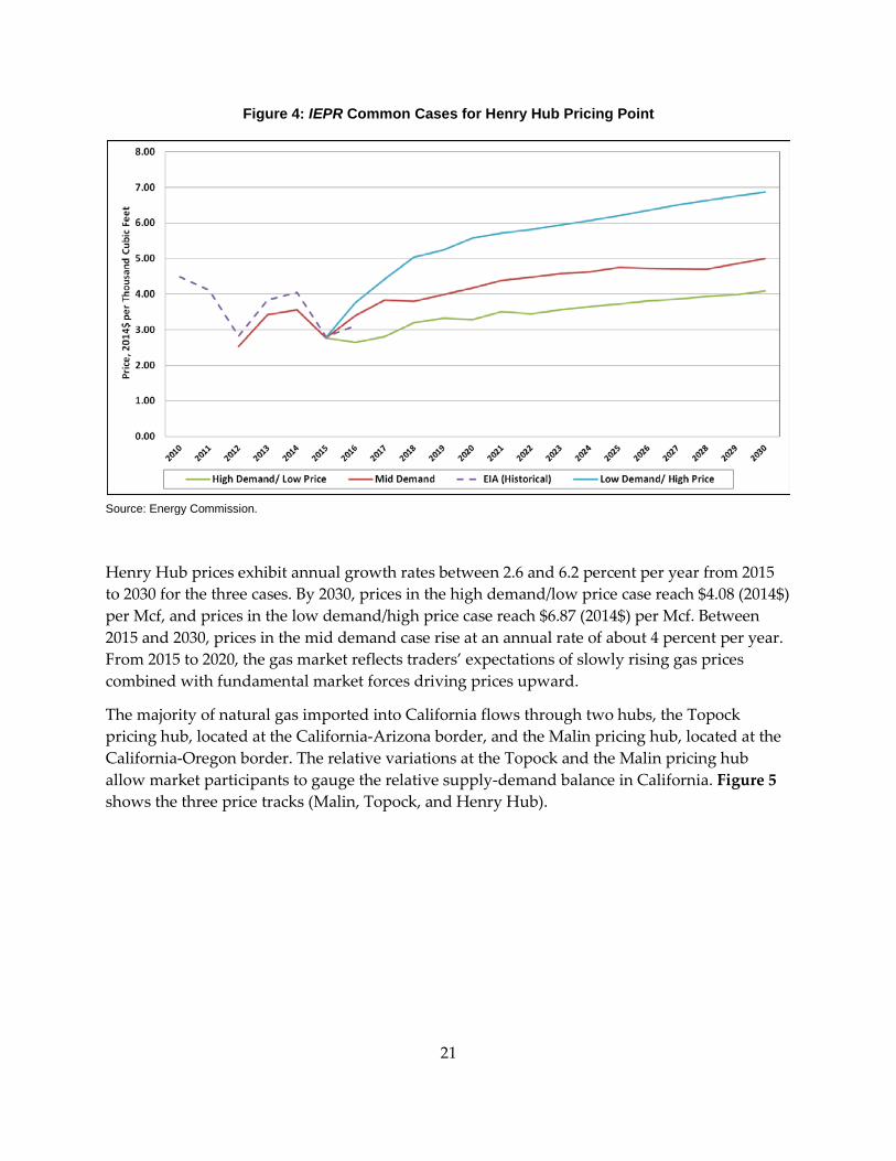
Figure 4: IEPR Common Cases for Henry Hub Pricing Point


Henry Hub prices exhibit annual growth rates between 2.6 and 6.2 percent per year from 2015 to 2030 for the three cases. By 2030, prices in the high demand/low price case reach $4.08 (2014$) per Mcf, and prices in the low demand/high price case reach $6.87 (2014$) per Mcf. Between 2015 and 2030, prices in the mid demand case rise at an annual rate of about 4 percent per year. From 2015 to 2020, the gas market reflects traders’ expectations of slowly rising gas prices combined with fundamental market forces driving prices upward.

The majority of natural gas imported into California flows through two hubs, the Topock pricing hub, located at the California‐Arizona border, and the Malin pricing hub, located at the California‐Oregon border. The relative variations at the Topock and the Malin pricing hub allow market participants to gauge the relative supply‐demand balance in California. Figure 5 shows the three price tracks (Malin, Topock, and Henry Hub).

21

Figure 5: Natural Gas Prices at Malin, Topock, and Henry Hub


While the patterns of price movements at the California pricing points parallel that of Henry Hub, California’s gas sources and Henry Hub gas are physically separate and linked only by the market influence Henry Hub has in the larger United States market. Figure 6 shows the price deviation of Malin and Topock relative to Henry Hub.

Figure 6: Prices Differentials (Point of Interest—Henry Hub)


22

The negative price differential between Henry Hub and Malin, California’s main northern receiving hub, will persist. This difference reflects the fundamentally lower cost of gas production both in the Rocky Mountain and Canadian regions and competition between natural gas flowing south on the GTN pipeline and natural gas flowing west on the Ruby pipeline. The positive price differential between Henry Hub and Topock, California’s main southern receiving hub, persists throughout the forecast horizon. This positive price differential reflects relatively higher costs of resources produced in the San Juan basin and the added cost of transporting gas to the California border. There are no new projects likely to disrupt the current market dynamics, and, therefore, staff does not expect this relative cost to change over the next decade. As a result, the differential remains positive throughout the outlook horizon.

Natural Gas Price Uncertainty Using Error Bands The forecasting of natural gas prices depends on many factors, including economic growth rates, expected rates of resource recovery, integration of renewable resources, retirement of coal‐fired power generation, and other factors. For example, higher rates of economic growth tend to lead to increased consumption of natural gas, leading to higher natural gas prices. Staff’s NAMGas model uses annual inputs to produce annual average prices; it does not account for fluctuations that occur in the natural gas market on a seasonal, monthly, or daily basis. Furthermore, it does not account for extreme weather, infrastructure accidents, and unforeseen technological advances.

To help account for inherent uncertainty in natural gas markets, staff used past natural gas forecast results generated by the Energy Commission to produce error bands around price results of the 2015 IEPR mid case. These error bands capture a much wider range of price uncertainty than seen in the price differential between the IEPR common cases as the error bands take into account events that staff cannot be model and ensure that staff bases the IEPR common cases on reasonable assumptions. Figure 7 shows the resulting error bands and the IEPR common cases.

23

Figure 7: 2015 IEPR Common Cases With Error Bands


Method for Creating Error Bands To produce the error bands, staff first collected previous natural gas price forecasts completed by the Energy Commission. These forecasts started in 2003 with the 2003 IEPR and concluded with the 2013 IEPR mid case. Staff used linear point‐to‐point interpolation to account for any missing data points. To simplify the mathematics, staff converted forecasted prices to nominal dollars and then calculated the percentage differences between actual Henry Hub prices and the forecasted prices for each year. Staff then aligned the values in an Excel® spreadsheet for years forecasted by placing all the forecasts one year out in line with each other, then two years out, and so on. For example, the 2003 IEPR Natural Gas Price Forecast first year forecasted is 2003, and the 2013 IEPR mid case is 2013. These two years plus the first year forecasted of the other forecasts would be in the first year forecasted column in the Excel spreadsheet.

Staff generated the error bands by using the statistical method of mean absolute percentage error (MAPE), which determines the goodness of fit of forecasts to actual prices. Staff then used the statistical method of MAPE on the year forecasted percentage difference values. This method determines the goodness of fit of forecasts to actual prices. Staff used only years forecasted with at least four values; due to statistical significance, this amounted to 10 years of MAPE values. Staff developed a linear regression equation using these MAPE values and then applied this linear equation to year forecasted to create percentage error. Staff then applied the percentage positively and negatively to the 2015 IEPR mid case to produce the error bands. Staff will continue to update the natural gas price error bands with the 2015 IEPR mid case for use in the next IEPR cycle.

24

United States Energy Information Administration Price Uncertainty The U.S. EIA also produces price uncertainty concerning natural gas prices in its ShortTerm Energy Outlook.8 U.S. EIA uses confidence intervals. The Short Term Energy Outlook forecasts out only 12 to 14 months and uses NYMEX Futures prices to forecast future prices of natural gas and price uncertainty. U.S. EIA also uses a more complex statistical and mathematical method to derive its price uncertainty. Due to these differences in forecasting and the plausible range of prices, Energy Commission’s and U.S. EIA’s forecasts are difficult to compare. Figure 8 shows a comparison of the Energy Commission’s and U.S. EIA’s forecast uncertainty. Even with differences in data and method, U.S. EIA’s Short-Term Energy Outlook and the IEPR mid case and lower error bands are close to each other.

Figure 8: U.S. EIA and Energy Commission Price Uncertainties

Source: Energy Commission, U.S. EIA.

Supply Results The net effect of any price variation involves a combination of the two responses: consumers can change the amount they purchase and suppliers can alter the amount they produce. Figure 9 displays the dry natural gas9 production for the three common cases. The NAMGas model does not simulate production; rather the model uses more than 400 supply cost curves, each of which portrays a relationship between the marginal cost of the next unit of natural gas

8 See http://www.eia.gov/forecasts/steo/.

9 Dry natural gas is natural gas that has been stripped of all natural gas liquids and impurities.

25

http://www.eia.gov/forecasts/steo/

and the amount of natural gas available. As a result, each curve competes with the other curves to satisfy the determined demand.

Figure 9: United States Dry Natural Gas Production


In general, the highest dry gas production in the United States arises from the high demand/low price case. Staff assumed a low‐cost environment in the high demand/low price case, and this assumption strengthens the competitiveness of United States production against Canadian imports.

Figure 10 shows that in the three common cases by 2025, California will import about 98 percent of its natural gas demand requirements. By 2025, staff expects California total natural gas demand to reach 5.52 billion cubic feet (Bcf) per day. Figure 10 represents the percentage of California’s demand that the associated supply source satisfies. California natural gas enters the state at the northern hub of Malin, Oregon, and the cluster of southern hubs located near Topock, Arizona. Gas entering at Malin comes from a combination of natural gas from Canada and the Rocky Mountains, while gas entering at the southern end of the state can come from the Rocky Mountains via the Kern River pipeline or from the San Juan basin via the pipelines entering at either Topock or Ehrenberg. Staff expects California to continue to import gas from the Canadian, Rocky Mountain, and San Juan basins, with varying amounts coming into the state from each source depending on the price and availability of gas. About half of the state’s gas will enter at the northern end via the Malin hub with the remainder entering at the south via either Kern River or Topock and Ehrenberg. The remainder of the state’s gas supplies will come from gas production in state from the small, but long‐standing production basins located

26

in the Sacramento and San Joaquin Valleys. With no new projects expected to disrupt the current market dynamics, staff expects this overall balance to continue for the foreseeable future.

Figure 10: California 2025 Supply Portfolio (Mid Demand Case)


Demand Results United States Demand Figure 11 shows the natural gas demand in all sectors in the United States. The sectors are industrial, commercial, residential, transportation, and power generation. Between 2015 and 2030, total natural gas demand in the mid demand case rises at an annual rate of about 0.3 percent. By 2030, demand in the mid demand case is about 68 billion cubic feet (Bcf) per day. Potential coal retirements in the power generation sector are contributing to the higher total natural gas demand, as well as increasing demand in the industrial sector.

27

Figure 11: U.S. Natural Gas Demand (All Sectors)


Figure 12 displays total United States natural gas demand in the power generation sector. In the high demand/ low price case, staff assumed aggressive coal retirements, totaling 61 GW by 2025. This assumption pushes demand for natural gas in the power generation sector higher. In the high demand/low price case, demand exceeds 33 Bcf per day by 2030.

Figure 12: U.S. Natural Gas Demand for Power Generation


28

California Demand The behavior of natural gas demand in California differs from that of the United States as a whole. The implementation of renewable generation and the penetration of energy efficiency are suppressing natural gas demand in the state. Figure 13 displays total natural gas demand in California. The sectors referred to are industrial, commercial, residential, transportation, and power generation.

Figure 13: California Natural Gas Demand (All Sectors)


In the mid demand case, staff expects natural gas in California to decline at an annual rate of 1.1 percent between 2015 and 2026. After the full implantation of the RPS and full penetration of energy efficiency, overall natural gas demand increases due to population growth and associated demand, reaching 5.92 Bcf per day by 2030 in the mid demand case. However, natural gas demand in the state remains below the 2015 level.

The decline in natural gas demand becomes more apparent in the power generation sector, where California’s RPS has the greatest impact. While overall demand declines at an annual rate of 1.1 percent, the decline observed in the power generation sector is about 2.1 percent. Figure 14 depicts the demand for natural gas in the power generation sector in California. In the mid demand case, after 2026, demand in power generation sector rebounds but, by 2030, remains below the 2015 level at about 1.7 Bcf per day.

Table 4 shows natural gas demand by sector.

012345678

Billi

on C

ubic

Fee

t per

Day

High Demand/ Low Price Case Mid Demand Case

Low Demand/ high Price Case EIA (Historical)

29

Figure 14: California Natural Gas Demand in the Power Generation Sector

Source: Energy Commission, Supply Analysis Office, 2015

0

200

400

600

800

1000

1200

2015 2016 2017 2018 2019 2020 2021 2022 2023 2024 2025 2026

Bcf

/ Yea

r

High Demand/ Low Price Mid Demand Low Demand/ High Price

30

Table 4: Actual and Modeled Natural Gas Demand for All Sectors in California (2013)

Source: Energy Commission, Supply Analysis Office. Natural gas demand for residential, commercial, and industrial sectors were provided by the Demand Analysis Office.

Million Cubic Feet per DayLow Demand/ High Price Case 2013 2015 2020 2025 2030 % Change 2013‐2030Residential 1,369 1,450 1,502 1,521 11%Commercial 564 548 602 650 15%Industrial 1,627 1,592 1,543 1,537 ‐6%Transportation 22 29 60 147 568%Power Gen 2,821 2,626 1,721 1,260 1,378 ‐51%State Total 6,403 6,245 5,428 5,115 5,582 ‐13%

Mid Demand Case 2013 2015 2020 2025 2030Residential 1,369 1,451 1,472 1,453 6%Commercial 564 550 593 622 10%Industrial 1,627 1,608 1,563 1,557 ‐4%Transportation 22 30 67 164 645%Power Gen 2,821 2,695 1,918 1,702 1,773 ‐37%State Total 6,403 6,334 5,613 5,498 5,920 ‐8%

High Demand/ Low Price Case 2013 2015 2020 2025 2030Residential 1,369 1,452 1,488 1,481 8%Commercial 564 550 611 655 16%Industrial 1,627 1,641 1,637 1,650 1%Transportation 22 110 251 615 2695%Power Gen 2,821 2,822 2,811 2,337 2,478 ‐12%State Total 6,403 6,575 6,798 6,738 7,532 18%

31

CHAPTER 3: California End-Use Natural Gas Demand Forecast This chapter presents preliminary baseline forecasts of end‐use natural gas demand, from demand forecasts, for California and Pacific Gas and Electric Company (PG&E), Southern California Gas Company (So Cal Gas), and San Diego Gas & Electric Company (SDG&E). Staff prepares these forecasts in parallel with its electricity demand forecasts, organized along electricity planning area boundaries. These forecasts do not include natural gas used by utilities or others for electric generation, but include projections for natural gas vehicle fuel use.

The end‐use natural gas demand forecast incorporates historical natural gas consumption data up through 2013. Three demand cases were forecast (high demand/low price, mid demand, and low demand/high price), with the same economic/demographic assumptions as used for electricity as presented in the February 23, 2015, workshop.10 Also similar to electricity, the high, mid, and low cases incorporated low, mid, and high assumptions, respectively, for natural gas prices and committed efficiency program impacts. The forecasts of end‐use natural gas demand encompass agriculture, commercial, industrial, residential, transportation (light‐duty vehicles, buses, medium‐ and heavy‐duty trucks), and transportation, communication, and utilities (TCU). 11 These forecasts do not include natural gas demand for power generation and, as such, differ from the forecasts of natural gas demand in the previous chapter.

Statewide Baseline End-Use Natural Gas Forecast Results

Table 5 compares the three end‐use natural gas demand baseline cases at the statewide level with the California Energy Demand 2013 (CED 2013) end‐use natural gas mid demand case for selected years. The new forecasts begin at a higher point in 2015, as actual natural gas consumption in California was higher in 2015 than forecasted in the CED 2013 mid case. Staff attributes this to an expected steep increase in forecasted prices that did not materialize. The new forecasts grow at a higher rate in all three cases from 2012 – 2024. Staff attributes the higher growth rates to an increase in natural gas demand for transportation, with heavy‐duty trucks having a large increase over the forecast period, followed by an increase in residential demand. The mid cases also include potential climate changes in the forecasts, while the high and low cases do not; this results in mid cases demand being lower than the low case in some instances.

10 See https://efiling.energy.ca.gov/Lists/DocketLog.aspx?docketnumber=15‐IEPR‐03 for presentation.

11 TCU is natural gas used to support the transportation system, such as natural gas used in an office building.

32

https://efiling.energy.ca.gov/Lists/DocketLog.aspx?docketnumber=15-IEPR-03

Table 5: Statewide End-Use Natural Gas Forecast Comparison

Demand (Billion Cubic Feet)

2013 CED End-

Use Natural Gas, Mid Demand

2015 End-Use Natural Gas,

High Demand/Low

Price

2015 End-Use Natural Gas, Mid Demand

2015 End-Use Natural Gas,

Low Demand/High

Price

1990 1,289 1,289 1,289 1,289

2000 1,391 1,391 1,391 1,391

2013 1,251 1,324 1,324 1,324

2015 1,268 1,356

1,343

1,336

2020 1,277 1,419

1,370

1,373

2024 1,280 1,484

1,418

1,434

Historical values are shaded. Average Annual Growth Rates

1990-2000 0.76% 0.72% 0.72% 0.72% 2000-2012 -0.71% -0.70% -0.70% -0.70% 2012-2015 -0.21% 1.81% 1.56% 1.41%

2012-2022 0.04% 1.32% 0.93% 1.01%

2012-2024 0.03% 1.34% 0.93% 1.04% Source: Energy Commission, Demand Analysis Office, 2015.

Staff projects by 2024 demand in the 2015 preliminary end‐use natural gas demand mid case to be around 11 percent higher compared to the CED 2013 mid case. Figure 15 shows historical use with the three cases and the CED 2013 mid case.

33

Figure 15: Statewide End-Use Natural Gas Demand

Source: Energy Commission, Demand Analysis Office, 2015

Figure 16 compares 2015 preliminary end‐use natural gas demand baseline per capita natural gas consumption with the CED 2013 mid case. Annual per capita demand varies in response to annual temperatures and business conditions, but it has been generally declining since the late 1990s. Staff expects this trend to continue as population grows faster than total natural gas demand. Per capita consumption in all three cases is higher in the 2015 forecasts than projected in the CED 2013 mid case due to the issues mentioned earlier.

Figure 16: Statewide End-Use Per Capita Natural Gas Consumption

Source: Energy Commission, Demand Analysis Office, 2015.

34

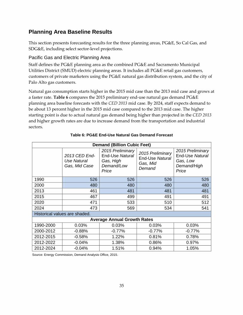
Planning Area Baseline Results

This section presents forecasting results for the three planning areas, PG&E, So Cal Gas, and SDG&E, including select sector‐level projections.

Pacific Gas and Electric Planning Area Staff defines the PG&E planning area as the combined PG&E and Sacramento Municipal Utilities District (SMUD) electric planning areas. It includes all PG&E retail gas customers, customers of private marketers using the PG&E natural gas distribution system, and the city of Palo Alto gas customers.

Natural gas consumption starts higher in the 2015 mid case than the 2013 mid case and grows at a faster rate. Table 6 compares the 2015 preliminary end‐use natural gas demand PG&E planning area baseline forecasts with the CED 2013 mid case. By 2024, staff expects demand to be about 13 percent higher in the 2015 mid case compared to the 2013 mid case. The higher starting point is due to actual natural gas demand being higher than projected in the CED 2013 and higher growth rates are due to increase demand from the transportation and industrial sectors.

Table 6: PG&E End-Use Natural Gas Demand Forecast


2013 CED End-Use Natural Gas, Mid Case

2015 Preliminary End-Use Natural Gas, High Demand/Low Price

2015 Preliminary End-Use Natural Gas, Mid Demand

2015 Preliminary End-Use Natural Gas, Low Demand/High Price

1990 526 526 526 526 2000 480 480 480 480 2013 461 481 481 481 2015 467 499 491 491 2020 471 533 510 512 2024 473 569 534 541 Historical values are shaded.

Average Annual Growth Rates 1990-2000 0.03% 0.03% 0.03% 0.03% 2000-2012 -0.88% -0.77% -0.77% -0.77% 2012-2015 -0.58% 1.22% 0.81% 0.78% 2012-2022 -0.04% 1.38% 0.86% 0.97% 2012-2024 -0.04% 1.51% 0.94% 1.05%


35

Figure 17 compares 2015 preliminary end‐use natural gas demand and CED 2013 mid case PG&E baseline residential forecasts. By 2024, the 2015 mid case forecast is about 5 percent higher than the 2013 mid case.

Figure 17: PG&E Planning Area Residential Natural Gas Demand


Commercial demand is about 2.8 percent lower in 2015 and in 2024 in the 2015 mid case compared to the 2013 mid case. This result is due to the impacts from building and appliance standards. Industrial is higher due to much higher projected growth in manufacturing output from the high‐tech sector. Figure 18 and Figure 19 show the forecasts for the PG&E commercial and industrial demand.

36

Figure 18: PG&E Planning Area Commercial Natural Gas Demand


Figure 19: PG&E Planning Area Industrial Natural Gas Demand


37

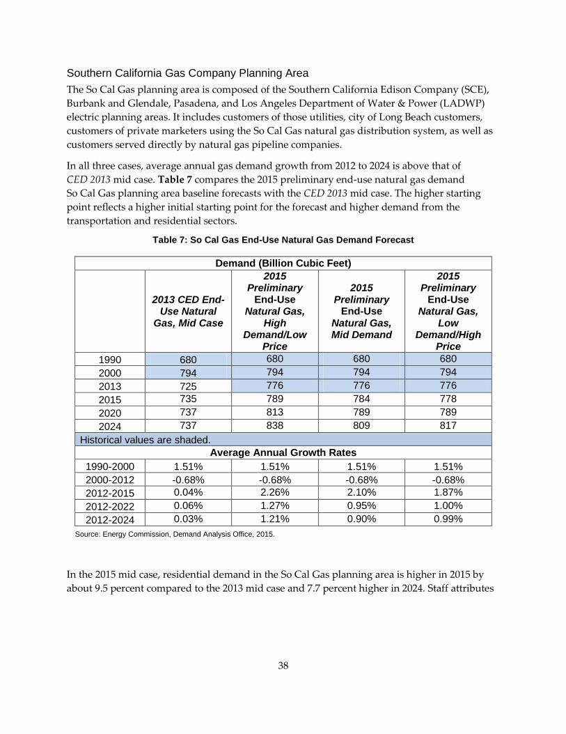
Southern California Gas Company Planning Area The So Cal Gas planning area is composed of the Southern California Edison Company (SCE), Burbank and Glendale, Pasadena, and Los Angeles Department of Water & Power (LADWP) electric planning areas. It includes customers of those utilities, city of Long Beach customers, customers of private marketers using the So Cal Gas natural gas distribution system, as well as customers served directly by natural gas pipeline companies.

In all three cases, average annual gas demand growth from 2012 to 2024 is above that of CED 2013 mid case. Table 7 compares the 2015 preliminary end‐use natural gas demand So Cal Gas planning area baseline forecasts with the CED 2013 mid case. The higher starting point reflects a higher initial starting point for the forecast and higher demand from the transportation and residential sectors.

Table 7: So Cal Gas End-Use Natural Gas Demand Forecast


2013 CED End-

Use Natural Gas, Mid Case

2015 Preliminary

End-Use Natural Gas,

High Demand/Low

Price

2015 Preliminary

End-Use Natural Gas, Mid Demand

2015 Preliminary


Low Demand/High

Price 1990 680 680 680 680 2000 794 794 794 794 2013 725 776 776 776 2015 735 789 784 778 2020 737 813 789 789 2024 737 838 809 817

Historical values are shaded. Average Annual Growth Rates

1990-2000 1.51% 1.51% 1.51% 1.51% 2000-2012 -0.68% -0.68% -0.68% -0.68% 2012-2015 0.04% 2.26% 2.10% 1.87% 2012-2022 0.06% 1.27% 0.95% 1.00% 2012-2024 0.03% 1.21% 0.90% 0.99%


In the 2015 mid case, residential demand in the So Cal Gas planning area is higher in 2015 by about 9.5 percent compared to the 2013 mid case and 7.7 percent higher in 2024. Staff attributes

38

the higher residential demand to adjustments made to heating degree‐days12 in the model. In the CED 2013 forecast, 2014 had fewer heating degree‐days than average in the model. The 2015 forecast for 2014 uses the average heating degree‐days, more heating degree‐days in the 2015 forecast increases the demand for natural gas for heating purposes. Figure 20 compares the 2015 preliminary end‐use natural gas demand mid case and CED 2013 So Cal Gas baseline residential forecasts.

Figure 20: So Cal Gas Planning Area Residential Natural Gas Demand


In the commercial sector, the three cases are similar to the CED 2013 mid case through 2017. Afterward, the cases show consumption growing at a slower rate for the rest of the forecast period due to additional efficiency savings, climate change, and rate impacts. By 2024, staff projects demand to be about 1.7 percent lower in the new mid case relative to the old. This lower starting is due to the same effect seen in the PG&E planning area; building and appliance standards are lowering demand.

The projections for industrial natural gas consumption reflect an expected long‐term decline in this sector output in the Los Angeles region in all three 2015 Preliminary End-Use Natural Gas Demand cases. By 2024, projected consumption is around 5.5 percent above the forecast in the CED 2013 mid case. The decreased demand is due to a projected decline in the resource

12 Heating degree days are indicators of household energy consumption for space heating. It is calculated by subtracting the daily average temperature from 65, the result is the number of heating degree days.

39

extraction sector compared to the 2013 forecast. Figure 21 and Figure 22 show the baseline forecasts for the So Cal Gas commercial and industrial sectors, respectively.

Figure 21: So Cal Gas Planning Area Commercial Natural Gas Demand


Figure 22: So Cal Gas Planning Area Industrial Natural Gas Demand


40

San Diego Gas & Electric Planning Area The SDG&E planning area contains SDG&E customers plus customers of private marketers using the SDG&E natural gas distribution system. Table 8 compares the 2015 preliminary end‐use natural gas demand SDG&E planning area baseline forecasts with the CED 2013 mid demand case. The new forecasts begin at a higher level due to actual demand in 2013 being higher than forecasted in the CED 2013 and grow at a faster rate from 2012 – 2024 in all three cases. By 2024, projected demand is about 9.7 percent higher in the new mid demand case relative to the old.

Table 8: SDG&E End-Use Natural Gas Demand Forecast


2013 CED End-

Use Natural Gas, Mid Case

2015 Preliminary


High Demand/Low

Price

2015 Preliminary

End-Use Natural Gas, Mid Demand

2015 Preliminary


Low Demand/High

Price 1990 72 72 72 72 2000 57 57 57 57 2013 49 53 53 53 2015 51 53 53 53 2020 52 58 56 57 2024 53 61 59 60 Historical values are shaded.

Average Annual Growth Rates

1990-2000 -1.92% -1.92% -1.92% -1.92% 2000-2012 -0.69% -0.69% -0.69% -0.69% 2012-2015 -0.51% 0.84% 0.71% 0.66% 2012-2022 0.31% 1.38% 1.05% 1.31% 2012-2024 0.32% 1.42% 1.08% 1.38%


Residential demand has a higher starting point in the 2015 forecast by about 2.9 percent compared to the 2013 forecast. Residential demand grows at a slower rate in the SDG&E planning area than the other two planning areas due to a projected increase in natural gas rates

41

compared to the two other planning areas. Figure 23 compares the 2015 preliminary end‐use natural gas demand mid case and CED 2013 mid case for SDG&E baseline residential forecasts.

Figure 23: SDG&E Planning Area Residential Natural Gas Consumption


Commercial demand grows at a faster rate in the SDG&E panning area compared to the other two planning areas due to projected growth in commercial floor space that more than offsets the savings from building and appliance standards. Projected industrial sector demand is flat throughout the forecast period and slightly above that estimated in the CED 2013 mid case. Figure 24 and Figure 25 show the baseline forecasts for the SDG&E commercial and industrial sectors.

42

Figure 24: SDG&E Planning Area Commercial Natural Gas Consumption


Figure 25: SDG&E Planning Area Industrial Natural Gas Consumption


43

CHAPTER 4: Natural Gas Resources and Infrastructure

Natural Gas Resources

Natural Gas Reserves in the United States The natural gas resource base, defined as the sum of the proved and potential natural gas reserves, has expanded between 2000 and 2014. Potential reserves include all undeveloped resources in the future. These resources, geologically known but with decreasing levels of certainty, require operating and maintenance costs and the full expenditures of capital dollars for the production of these resources. Staff expects that as total demand for natural gas grows, producers bring more of these resources on‐line, beginning with the lowest‐cost resources.

Figure 26 shows proved and potential reserves in the United States. Proved reserves comprise all resources with sufficient geological and engineering information that indicates with reasonable certainty oil and gas operators can recover such reserves with existing technology under existing economic and operating conditions. Production of proven resources requires the expenditure of operating and maintenance funds and few capital dollars.

Proved reserves in the United States grew at about 3.2 percent per year until 2004, and then increased to 7.4 percent per year. Although the United States produces more than 20 Tcf of natural gas each year, proved reserves still climbed to almost 340 Tcf in 2014 (blue part of Figure 26), up from just more than 150 Tcf in 2000. A growing percentage of the new proved reserves originate from the development of liquid‐rich shale resources.

Figure 26: Proved and Potential Reserves in the United States

Source: U.S. EIA; Potential Gas Committee (PGC).

Between 2000 and 2004, total potential resources rose at a rate of 0.5 percent per year. Because of the development of shale natural gas, however, the rate of expansion of the resource base accelerated, climbing to an annual rate of 8.4 percent between 2006 and 2014. Figure 27 shows

44

total shale natural gas resources. Between 2006 and 2014, the shale gas resource base expanded at an annual of rate 25.8 percent. Shale gas development technology increased the growth rate, resulting in the total United States resource base expanding to more than 2,850 Tcf in 2014.

Figure 27: Total Shale Natural Gas Resources in the United States

Source: U.S. EIA; PGC.

Hydraulic Fracturing and the Associated Environmental Concerns The development of natural gas from shale formations has expanded the resource base and boosted production. However, the production of this resource type requires the use of horizontal drilling combined with the technique known as hydraulic fracturing (fracking). Oil and gas operators have used some form of this technique in the United States since 1947. U.S. field operators have fractured more than 1 million wells. However, in the last 20 years, the technique level has accelerated and changed to incorporate new and different types of fracturing liquids and higher pressures. This has raised several environmental concerns:

• Greenhouse gas (GHG) emissions: Methane, the primary component of natural gas, contributes to GHG emissions.

• Surface disturbance: Development requires surface preparation and may create environmental stresses in some sensitive areas.

• Freshwater usage: Fracking requires between 2 million and 12 million gallons of freshwater per treatment; high usage may divert freshwater from other important and essential requirements.

• Disposal of retrieved water: After completion of a fracture treatment, operators retrieve about 30 percent to 70 percent of the injected fluid. Disposal of the retrieved water raises environmental concerns, such as spillage and groundwater contamination.

• Increased seismic activity: Ongoing studies are examining possible links between oil and gas operations and increased seismic activity in some areas of the United States.

45

• Groundwater contamination: Ongoing studies are examining possible links between hydraulic fracturing and groundwater contamination. All oil and gas operations pose some level of risk to groundwater aquifers.

• Socioeconomic impacts: Added noise and traffic are changing life in many communities that are first experiencing the “boom” conditions of shale gas development.

State and federal decision‐makers and regulators have developed, and continue to develop, regulatory frameworks to guide oil and natural gas activities within their jurisdictions. The protection of public health and the environment has collided, at times, with responsible development of natural resources. The State of New York, under which lies a portion of the Marcellus Shale, has banned all fracking activities. At the federal level, the Bureau of Land Management (BLM) is developing rules and regulations to:

• Strengthen existing well‐integrity standards.

• Require proper management of wastewater with the goal of minimizing environmental impacts.

• Require the disclosure of chemicals used in hydraulic fracturing.

This regulatory framework, when developed, will apply to oil and gas activities on federal lands managed by BLM. The Energy Policy Act of 2005 originally exempted the injection of fluids or propping agents, other than diesel, in fracking operations.13 Further, in February 2014, the United States Environmental Protection Agency (U.S. EPA) adopted additional regulations to restrict the use of diesel in all fracking stimulations.

State regulatory agencies are also developing frameworks. All states with major natural gas production have mandated the disclosure of chemicals used in fracking; however, the degree of disclosure varies from state to state. In general, regulatory frameworks that are shaping oil and gas activities include varying degrees of the following elements:

• Requirements for protecting and testing the groundwater

• Requirements for well testing before and after fracking stimulations

• Requirements for community notification

• Requirements for the disposal of wastewater

• Requirements to pay environmental mitigation fees

• Requirements for the “responsible development” of oil and gas subsurface formations

13 Energy Policy Act of 2005; see http://www.gpo.gov/fdsys/pkg/PLAW‐109publ58/pdf/PLAW‐109publ58.pdf.

46

http://www.gpo.gov/fdsys/pkg/PLAW-109publ58/pdf/PLAW-109publ58.pdf

http://www.gpo.gov/fdsys/pkg/PLAW-109publ58/pdf/PLAW-109publ58.pdf

In California, efforts are continuing to develop a workable regulatory framework. In 2013, the State Legislature passed, and the Governor signed, Senate Bill 4 (Pavley, Chapter 313, Statutes of 2013) (SB 4). In November 2013, the California Department of Conservation began the formal rulemaking process for Well Stimulation Treatment Regulations. As part of SB 4, on July 1, 2015, the Division of Gas and Geothermal Resources (DOGGR) certified the final environmental impact report, Analysis of Oil and Gas Well Stimulation Treatments in California.14 Also under SB 4, on July 9, 2015, the California Council on Science and Technology released its final reports on well stimulation, An Independent Scientific Assessment of Well Stimulation in California.15

An interim set of rules and regulations, taking effect in 2014, requires oil and gas well operators “…to submit notification of well stimulation treatments and various types of data associated with well stimulation operations, including chemical disclosure of well stimulation fluids, to the Division.” 16 In addition, the California Department of Conservation now compiles submitted information regarding these activities and makes such information available to the public in a searchable database.

In the oil and gas industry, innovators and stakeholders are adopting new techniques aimed at alleviating public health and environmental concerns. Producers are adopting waterless fracturing, reducing freshwater usage, and “greening” the ”fracking” fluids. Though not yet widespread, some oil and gas operators are now fracturing with a butane‐rich fluid instead of water. Further, oil and gas entrepreneurs are developing nontoxic agents that may replace the chemicals now in use in fracture treatments. These new agents contain food‐based products such as the sweetener maltodextrin and partially hydrogenated vegetable oil. The use of these more common and less expensive products may further lower the cost of fracking and further lower the overall supply costs going forward, as well as potentially address some of the environmental objections to fracturing.

Production Types and Trends The supply portfolio in the United States contains five main resource types:

• Shale natural gas: methane from shale formations17

• Tight sands natural gas: methane from low‐permeability18 sandstone formations

14 For more information on the EIR, see http://www.conservation.ca.gov/dog/Pages/SB4_Final_EIR_TOC.aspx.

15 For more information on combined‐cycle steam turbine’s (CCST) reports, see http://ccst.us/projects/hydraulic_fracturing_public/SB4.php.

16 California Department of Conservation website, http://www.conservation.ca.gov/dog/Pages/WellStimulation.aspx.

17 A formation is a rock strata that spreads over a geographic area in the earth's subsurface and contains natural gas.

18 Measures the ability of any fluid to flow through a rock formation.

47

http://www.conservation.ca.gov/dog/Pages/SB4_Final_EIR_TOC.aspx

http://ccst.us/projects/hydraulic_fracturing_public/SB4.php

http://www.conservation.ca.gov/dog/Pages/WellStimulation.aspx

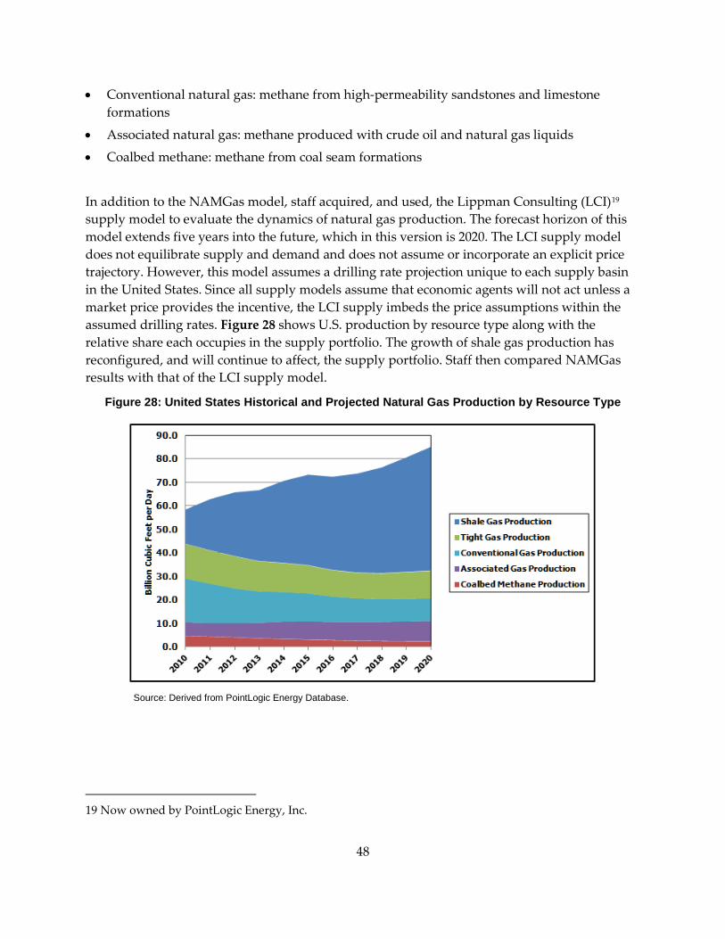
• Conventional natural gas: methane from high‐permeability sandstones and limestone formations

• Associated natural gas: methane produced with crude oil and natural gas liquids

• Coalbed methane: methane from coal seam formations

In addition to the NAMGas model, staff acquired, and used, the Lippman Consulting (LCI)19

supply model to evaluate the dynamics of natural gas production. The forecast horizon of this model extends five years into the future, which in this version is 2020. The LCI supply model does not equilibrate supply and demand and does not assume or incorporate an explicit price trajectory. However, this model assumes a drilling rate projection unique to each supply basin in the United States. Since all supply models assume that economic agents will not act unless a market price provides the incentive, the LCI supply imbeds the price assumptions within the assumed drilling rates. Figure 28 shows U.S. production by resource type along with the relative share each occupies in the supply portfolio. The growth of shale gas production has reconfigured, and will continue to affect, the supply portfolio. Staff then compared NAMGas results with that of the LCI supply model.

Figure 28: United States Historical and Projected Natural Gas Production by Resource Type

Source: Derived from PointLogic Energy Database.

19 Now owned by PointLogic Energy, Inc.

48

Figure 29 shows the expansion of the resource base is contributing to the lowering of natural gas prices in North America; Henry Hub prices now hover around $2.25/Mcf, about 79 percent lower than the 2008 peak.

Figure 29: The Expanding Natural Gas Resource Base (2007 – 2015)

Source: Energy Commission, Baker Institute; National Petroleum Council; Energy Commission.

Figure 30 demonstrates the growth of production from shale formations between 2010 and 2020. Staff compares results to 2020 as the LCI supply model ends in 2020. As shown in Figure 30, shale gas production rises and surpasses 50 Bcf per day by 2020. Natural gas from this resource type now dominates the supply portfolio. By 2020, total production should range between 84 and 93 Bcf per day, of which more than 60 percent should originate from shale gas formations. The oil and gas industry is investing more of its capital dollars in the development of shale resources. As a result, nearly all of the increase in natural gas production originates from shale development.

Technology is expanding the resource base and lowering cost

49

Figure 30: Total United States Natural Gas Production and Shale Natural Gas Production

Source: Derived from PointLogic Energy Database; Energy Commission.

Figure 31 shows the decline in coalbed methane production; both actual production and share of total production have dropped. In 2010, coalbeds in the United States produced about 4.7 Bcf per day; by 2020, the LCI supply model estimates this resource type to produce about 2.4 Bcf per day. The percentage share of total production provided by coalbed methane, depicted with an olive line on the right axis, has declined from 8.1 percent of total U.S. production to an expected value of 2.8 percent by 2020.

Figure 31: Total United States Coalbed Methane Production


50

The share of total production provided by tight gas sands20 has displayed similar erosion, though not as steep as coalbed methane. Figure 32 exhibits the actual production and the share of total production, both historical and forecasted, for tight gas sands. In 2010, tight gas sands in the U.S. produced 14.7 Bcf per day; by 2020, staff expects this resource type to contribute about 11.7 Bcf per day. The 2020 production value represents an increase from the low of 10.9 Bcf per day, expected to occur in 2017.

Figure 32: Total United States Tight Gas Sands Production


Even though production rises between 2017 and 2020, the share of production provided by tight gas sands declines in the same period. Since total production is rising faster than tight gas production, the share of this resource type continues to slide.

Associated natural gas production occupies between 9.3 percent and 10.8 percent throughout the forecast horizon. Figure 33 displays the production from this resource type. Associated natural gas production rises, expected to reach 8.7 Bcf per day by 2020. However, the production of this resource type is rising slower than total production. As a result, the share provided by this associated natural gas hovers in a narrow range.

20 “Tight Gas Sands” refers to natural gas obtained from very low permeability sand formations.

51

Figure 33: Total United States Associated Natural Gas Production


Conventional natural gas production, once dominant among resource types, supplied more than 30 percent of the total United States production in 2010. However, the development of natural gas from shale gas formations has shrunk the share of conventional gas production in the supply portfolio. Figure 34 shows the United States conventional gas production between 2010 and 2020. In 2010, conventional gas production totaled 18.5 Bcf per day. Staff expects, by 2020, that this resource type will produce about 9.6 Bcf per day and will command a market share of about 11.2 percent.

52

Figure 34: Total United States Conventional Natural Gas Production


Table 9 summarizes U.S. production by resource type. Two trends emerge from this table. First, the growth of shale gas production has positioned this resource type as the dominant element of the natural gas supply portfolio. Staff expects shale gas production to grow at an annual rate of 13.6 percent between 2010 and 2020, and to occupy about 62 percent of the supply portfolio by 2020.

Table 9: Summary of Changes in Production by Resource Type (2010 – 2020)


Second, coal seam, tight gas, and conventional gas production experience losses in both production and market share. The gains exhibited by associated natural gas result from the

53

development of shale gas resources. The oil and gas industry is expending vast quantities of capital dollars developing the so‐called wet shales (formations with above‐average quantities of liquids, such as crude oil and natural gas liquids). Because of the price differential between natural gas liquids and natural gas, producers are searching for liquid‐rich shale formations. These formation types, such as the Bakken Shale, contain three fossil fuel components: natural gas, natural gas liquids, and crude oil. As a result, the discovery of such formation types leads to the production of associated natural gas along with the other components.

Biogas and Biomethane in California Biogas is typically derived from organic fuel sources, such as biomass, digester gas, or landfill gas. Biogas is principally composed of methane and carbon dioxide. Biomethane is the treated product of biogas where CO2 and other contaminants are removed. Biogas is a by‐product of normal operations at many landfills (operating and closed), dairies, and wastewater treatment plants. Biogas can also be produced by stand‐alone facilities either directly through biochemical conversion processes (anaerobic digestion) or indirectly through gas reformation of producer gas from thermochemical conversion.

End‐use opportunities include electricity production, temperature control, and transportation fuel production. In each of these cases, biogas (or biomethane) can supplement or directly replace the use of natural gas. Biogas is not specifically modeled.

Natural Gas Infrastructure

Natural Gas Pipeline Changes The United States natural gas pipeline network consists of an interconnected and integrated transmission and distribution system that transports natural gas from numerous different producing basins to users all over the country via 305,000 miles of interstate and intrastate transmission lines. More than 1,400 compressor stations aid the flow of natural gas by maintaining pressure on the natural gas pipeline network. As a result, natural gas reaches the intended delivery points and intended demand centers, though not all supply areas are connected to all demand centers and bottlenecks and constraints arise at various locations that drive differences in regional natural gas market dynamics.

The development of shale natural gas has outpaced the expansion of the associated infrastructure. Bottlenecks in moving natural gas from supply basins to demand centers have spawned the building of capacity additions to the transmission and distribution network. The development of the Marcellus Shale (one of the largest shale gas plays21 in North America) in Pennsylvania is motivating the pipeline capacity expansion in the northeastern and midwestern United States. Table 10 shows the capacity additions in the United States between 2011 and 2015.

21 Common term for a geographic area where oil and gas development is occurring.

54

Table 10: Capacity Additions in the United States (2011 - 2015)

Source: U.S. EIA.

Recent additions of pipeline capacity across the country have allowed access to new shale gas supplies. Capacity added since 2011 totals more than 30 Bcf per day. While the northeastern United States is experiencing the most pipeline building activity, shale gas development in the Southwest has required the construction of some larger natural gas pipelines, such as the Eagle Ford Shale Pipeline system with capacity of 2.3 Bcf per day. In addition, developers in the Utica and Bakken Shales have announced projects to alleviate their bottlenecks. The Utica Ohio River Project, with an anticipated capacity addition of 2.1 Bcf per day, expects to first flow natural gas in late 2015.

Interstate pipelines listed in Table 11 connect California to gas supply basins located elsewhere in North America. The state produces less than 10 percent of its demand requirements, which averages about 6 Bcf per day; about 90 percent of natural gas demand requirements reach the state through the interstate pipeline system. Table 11 displays the eight main interstate pipeline serving California.

55

Table 11: Main Pipeline Systems Serving California

Source: Compiled from various sources, including the California Gas Report.

Together, these pipelines provide the state with a total capacity of 11.74 Bcf per day, far exceeding the state's average consumption of about 6.0 Bcf per day. The internal pipeline capacity within California, however, restricts how much of the interstate capacity can serve California at any time. This in‐state receipt capacity equals about 7.7 Bcf per day.22

California Pipeline Safety

The explosion of a PG&E high‐pressure transmission pipeline in a residential neighborhood on September 9, 2010, killing eight people, injuring 58, and destroying or damaging more than 100 homes, has changed how citizens, energy regulators, and other public officials view natural gas pipeline safety. Lapses in pipeline safety led to that explosion. A natural gas system that does not protect the health and safety of Californians, by definition, does not satisfy the requirements of the Public Utilities Code and cannot meet California’s future need for natural gas. Staff

22 Estimated using data from the 2014 California Gas Report, 2014.

56

discusses issues pertaining to pipeline safety such as the California Legislature’s response and the utilities’ and the California Public Utility Commission’s (CPUC) work toward insuring a safer natural gas system in detail in the companion report, Assembly Bill 1257 Natural Gas Act Report: Strategies to Maximize the Benefits Obtained From Natural Gas as an Energy Source.23 This report includes a discussion of So Cal Gas’ southern system minimum flow issues and the alternative solutions to address the issue.

California Storage

Underground storage of natural gas plays a vital role in balancing California’s demand requirements with supply availability. California has 14 natural gas storage facilities: four owned by So Cal Gas, three by PG&E, and seven by independent operators.24 The 14 storage facilities have a working gas capacity of 374.3 Bcf and a maximum daily delivery of 8.56 Bcf.25 As of late August 2015, the inventory of working gas in storage averaged 208 Bcf, about 3 Bcf above the previous month and 36 Bcf higher than the same time last year.26 Figure 35 shows California’s utilities’ storage level over the last five years. Throughout 2015, natural storage inventories in California have tracked above the five‐year average. A milder‐than‐expected winter left inventory levels in the state higher than the five‐year historical average.

23 The Draft AB 1257 can be found at http://docketpublic.energy.ca.gov/PublicDocuments/15‐IEPR‐04/TN206126_20150916T124857_AB_1257_Natural_Gas_Act_Report_Strategies_to_Maximize_the_Benef.pdf.

24 The independent facilities are Wild Goose Storage, Central Valley Storage, Gill Ranch Storage, and Lodi Gas Storage. Lodi Gas Storage operates four storage reservoirs. U.S. EIA, Field Level Storage Data. See http://www.eia.gov/cfapps/ngqs/ngqs.cfm?f_report=RP7.

25 U.S. EIA, Field Level Storage Data. See http://www.eia.gov/cfapps/ngqs/ngqs.cfm?f_report=RP7.

26 U.S. EIA, Weekly Storage Report (May 22, 2015).

57

http://docketpublic.energy.ca.gov/PublicDocuments/15-IEPR-04/TN206126_20150916T124857_AB_1257_Natural_Gas_Act_Report_Strategies_to_Maximize_the_Benef.pdf



http://www.eia.gov/cfapps/ngqs/ngqs.cfm?f_report=RP7

http://www.eia.gov/cfapps/ngqs/ngqs.cfm?f_report=RP7

Figure 35: Utility Storage Levels (2011 – 2015)

Source: California Envoy, PG&E Piperanger.

Inventories of the private storage operators are not published or known. Those facilities operate based on market price dynamics, whereas the gas utility fields operate to provide system balancing service and winter reliability protection.

California’s gas storage infrastructure has seen growth over the past decade with the addition of new storage capacity from independent owners. The current low gas prices create few arbitrage opportunities and are unlikely to spur new construction in the gas storage arena. As a result, gas storage capacity is expected to remain constant absent more volatile seasonal prices or some circumstance that cannot be foreseen.

North American Export and Import Issues

Mexico The increasing quantity of reserves available in the United States resource base, in part, is motivating natural gas producers to seek new markets. Demand for natural gas in the power generation sector in Mexico is soaring. As a result, pipeline exports to Mexico have doubled between 2008 and 2014. Several U.S. pipeline operators have proposed the building of cross‐border pipelines to export natural gas from the United States to Mexico. Figure 36 shows historical and forecasted exports to Mexico from the United States.

58

Figure 36: Historical and Forecasted United States Exports to Mexico

Source: U.S. EIA; Energy Commission.

By 2020, the mid demand case shows U.S. exports to Mexico reaching about 4.3 Bcf per day. The mid and high demand/low price cases stabilize exports between 4.7 and 5.2 Bcf per day; however, around 2028 exports drop off as Mexico develops its natural gas resources. In the low demand/high price case, exports drop off much earlier, starting in 2020. Low‐cost gas production in the high demand/low price case is offering incentives for exports to Mexico and, as a result, exports to Mexico in the high demand/low price case continue to grow for a longer period before Mexican gas resources become economically competitive.

Mexico also has three liquefied natural gas (LNG) import terminals, though only two of these are operating. Sempra Energy’s Costa Azul LNG terminal in Ensenada, Baja California, Mexico, was placed into service in 2008 but has been underused. Many LNG shipments have been redirected to Asia, where prices are higher; Southern California markets have shown little interest due to cheaper supply being available from interstate pipelines. Given the cost of LNG versus the cost of pipeline imports from the United States, LNG imports are not expected to rise anytime soon; therefore, imports from the United States are Mexico’s cheapest and best option in the near term.

Canada Natural gas produced in Canada has served several markets in the Lower 48 states, some for more than 50 years. At least six pipelines (GTN, Northern Natural, Northern Border, Alliance, Great Lakes, Iroquois, and Maritimes & Northeast) transport natural gas from supply basins in

59

Canada to demand centers in the United States. Figure 37 displays the historical and forecasted natural gas imports from Canada.

Figure 37: Net Natural Gas Imports From Canada


As stated in Chapter 2, in general, the highest dry gas production in the United States arises in the high demand/low price case. Staff assumed a low‐cost environment in the high demand/low price case, and this assumption strengthens the competitiveness of United States production against Canadian imports. As a result of this increased competitiveness, Canadian imports in the high demand/low price case fall to the point of leading to net exporting of gas to Canada by the end of the forecast horizon. In both the mid demand and low demand/high price cases, imports from Canada decline consistent with recent trends.

Liquefied Natural Gas Exports The boom in shale gas production and resulting low gas prices have motivated the United States natural gas producers to seek international markets through LNG exports. Ten years ago, most market observers believed that the Lower 48 would become a LNG importer; however, the vast quantities of shale gas now available have changed that prognosis. Figure 38 shows modeled net LNG exports. To date, the United States Department of Energy (U.S. DOE) has approved eight LNG liquefaction terminals:

• Alaska LNG Project with maximum capacity of 2.55 Bcf per day

• Cameron LNG Terminal with maximum capacity of 1.7 Bcf per day

60

• Corpus Christi Liquefaction Project with maximum capacity of 2.1 Bcf per day

• Cove Point LNG with maximum capacity of 0.77 Bcf per day

• Freeport LNG Terminal with maximum capacity of 1.8 Bcf per day

• Lake Charles LNG Terminal with maximum capacity of 2.0 Bcf per day

• Oregon LNG Project with maximum capacity of 1.25 Bcf per day

• Sabine Pass LNG with maximum capacity of 2.2 Bcf per day.

Together, these facilities total 14.4 Bcf per day of export capacity. Several applications with total capacity of about 14 Bcf per day await approval. All approved export licenses limit LNG sales only to countries having free trade agreements with the United States. Two facilities, Cameron and Corpus Christi, have begun construction. On October 1, 2015, Sabine Pass started receiving natural gas and expects to start exporting liquefied natural gas by the end of the year.27 In addition, Jordan Cove LNG in Coos Bay, Oregon, received its final Federal Energy Regulatory Commission’s (FERC) environmental impact report, with possible final approval in December 2015.28 Furthermore, Cameron LNG in Hackberry, Louisiana, filed to expand its liquefied natural gas export capacity.29 Figure 38 shows estimated U.S. LNG exports.

Figure 38: United States Net LNG Exports

Source: Compiled by Energy Commission staff from NAMGas model results and U.S. EIA data.

27 See https://client.pointlogicenergy.com/#article‐detail/pipelines/5666.

28 See http://www.naturalgasintel.com/articles/103855‐jordan‐cove‐lng‐project‐gets‐final‐ferc‐environmental‐review.

29 See http://www.naturalgasintel.com/articles/103851‐cameron‐lng‐files‐at‐ferc‐for‐trains‐4‐5.

61

https://client.pointlogicenergy.com/%23article-detail/pipelines/5666

http://www.naturalgasintel.com/articles/103855-jordan-cove-lng-project-gets-final-ferc-environmental-review

http://www.naturalgasintel.com/articles/103855-jordan-cove-lng-project-gets-final-ferc-environmental-review

http://www.naturalgasintel.com/articles/103851-cameron-lng-files-at-ferc-for-trains-4-5

ACRONYMS Acronym Proper Name

AAEE Additional achievable energy efficiency AB 1257 Assembly Bill 1257 BAA Balancing area authorities Bcf Billion cubic feet, BLM Bureau of Land Management California ISO California Independent System Operator CED California Energy Demand CHP Combined heat and power CPUC California Public Utilities Commission EE Energy efficiency Energy Commission California Energy Commission Fracking Hydraulic fracturing GDP Gross domestic product GHG Greenhouse gas GT Natural gas-fired turbines GTN Gas Transmission Northwest Company GW Gigawatt GWh Gigawatt hours IEPR Integrated Energy Policy Report IOU Investor-owned utility LADWP Los Angeles Department of Water and Power LCI Lippman Consulting, Inc. LNG Liquefied natural gas MAPE Mean absolute percentage error MMBtu Million British thermal unit MW Megawatt NAMGas North American Market Gas-Trade Model NGCC Natural gas combined-cycle NYMEX New York Mercantile Exchange OTC Once-through cooling PEMEX Petróleos Mexicanos PG&E Pacific Gas and Electric Company POU Publicly owned utilities PSEP Pipeline Safety Enhancement Plan PV Photovoltaic QFER Quarterly Fuels and Energy Report RPS Renewables Portfolio Standard SB 4 Senate Bill 4

62

Acronym Proper Name SCE Southern California Edison Company SDG&E San Diego Gas & Electric Company SMUD Sacramento Municipal Utility District So Cal Gas Southern California Gas Company SWRCB State Water Resources Control Board Tcf Trillion cubic feet TEPPC Transmission Electric Planning and Policy Committee U.S. United States U.S. EPA United States Environmental Protection Agency U.S. EIA United States Energy Information Administration WECC Western Electricity Coordinating Council

63

APPENDIX A: Electricity Dispatch Modeling Results Introduction

In the 2015 IEPR, the Energy Commission staff continued its use of the PLEXOS production cost model30 to provide an estimate of natural gas demand in the power generation sector for the WECC.31 In this platform, staff developed a WECC‐wide production simulation model dataset covering the years 2015‐2026 for the three IEPR common cases. California’s electricity supply and demand assumptions reflect current policy and mandates. For the rest of the WECC, staff begins with the Transmission Electric Planning and Policy Committee’s (TEPPC) 2024 common case32 and the most current year (2013) of historical supply and demand data to develop the 2015 – 2026 details missing from the single year TEPPC common case.

The PLEXOS simulation dataset developed to provide fuel demand for natural gas generation for 2015 – 2026 uses two major sets of assumptions, California‐specific and those for the rest of the WECC. Each set has a set of electricity load forecasts and supply portfolios.

California has two basic types of electricity utilities characterized in the PLEXOS dataset: investor‐owned and publicly owned utilities located throughout the state. For instance, SDG&E, SCE, LADWP, and Imperial Irrigation District are three examples of utilities that serve the southern portion of the state, while SMUD, Turlock Irrigation District, and PG&E are three examples that serve the northern portion.33

California’s electricity supply portfolio is composed of in‐state and out‐of‐state generation resources, providing a combined total of more than 292,000,000 megawatt hours (MWh) of electricity in 2014. Various conventional and renewable types of generation resources supply California including, but not limited to, natural gas‐fired, hydroelectric, solar, wind, nuclear, biomass, and coal‐fired. Staff projects the composition of each type of generation resource to change by the mid‐2020s. Imports of coal‐fired generation are expected to decline as many of the utilities in California have begun divesting themselves from coal plants and in anticipation of the proposed U.S. EPA’s Clean Power Plan. Renewable generation is expected increase

30 Platform owned by Energy Exemplar Ltd.

31 The WECC Region extends from Canada to Mexico and includes the provinces of Alberta and British Columbia in Canada, the northern portion of Baja California, Mexico, and all, or portions of, 14 western states in the United States of America.

32 The TEPPC, a WECC Board of Directors committee, guides WECC’s Transmission Expansion Planning (TEP) process and working groups consisting of stakeholders throughout the WECC to create this common case on a biannual basis.

33 There are other utilities and other entities such as community choice aggregators MCE (formerly Marin Clean Energy) and Sonoma Clean Power.

A‐1

contributions to California’s electricity supply. However, staff expects natural gas‐fired generating resources to stay the largest type of resource serving California throughout the forecast period. This is due to the current amount of installed gas‐fired capacity, future gas‐fired additions for maintaining planning reserve margins, the availability of low‐cost natural gas, and restrictions on the development of nuclear and coal‐fired generation technologies in California.

Overview of Production Cost Modeling Assumptions

Table A-1 outlines specific production cost dataset trends for the 2015 IEPR common cases. Not only are the forecasts of high, low, or mid demand, energy efficiency, GHG prices and supply portfolios key, it is vital to understand how these assumptions are combined in developing each of the 2015 IEPR common cases.

Table A-1: Production Cost Trends

Key Assumptions Specific to Production

Cost Model

High Demand/Low Price Case

Mid Demand

Case

Low Demand/High

Price Case Demand Forecast High Mid Low Renewable Generation High Mid Low Energy Efficiency Low Mid High New CHP None Mid High Carbon Price Low Mid High Coal Price Low Mid High Natural Gas Price Low Mid High

Source: Energy Commission staff presentation at https://efiling.energy.ca.gov/Lists/DocketLog.aspx?docketnumber=15-IEPR-03Demand Assumptions.

Demand Assumptions

California 2015 to 2026 Staff used the preliminary 2015 California low, mid, and high demand/low price cases posted on July 3, 2015.34 Compared to the adopted CED 2014 update, all demand cases are lower throughout the forecast period. The main driver for these lower projections is behind‐the‐meter photovoltaic (PV). The preliminary 2015 CED includes the 2013 additional achievable energy efficiency (AAEE) projections for investor‐owned utilities (IOUs).

34 Preliminary CED 2015 at https://efiling.energy.ca.gov/Lists/DocketLog.aspx?docketnumber=15‐IEPR‐03. See Docket TN# 205236‐1, 205236‐2 and 205236‐3.

A‐2

https://efiling.energy.ca.gov/Lists/DocketLog.aspx?docketnumber=15-IEPR-03Demand%20Assumptions



For the publicly owned utilities (POUs) incremental energy efficiency projections, staff used the 2015 Supply Form filings.35 These projections are incremental to what has been removed from the demand forecast. The 2015 POU incremental energy efficiency projections are slightly less than 2013 projections for the mid and low demand/high price cases, while the 2015 projections are slightly higher for the high demand/low price case.

Rest of WECC 2015 to 2026 Data submitted to the WECC by balancing area authorities (BAA) for the historical year 2013 and the WECC TEPPC 2024 common case36 load forecast were used as “bookends” to estimate the non‐California BAA load. Staff used a compound annual growth rate formula to calculate the peak and energy demand for the intervening years (2015 to 2023). The period for PLEXOS simulations extended beyond the TEPPC common case year of 2024, so staff used the compound annual growth rate to extrapolate the forecast by two years to 2026. The annual peak and energy forecasts were inputs to PLEXOS, and staff developed hourly hourly energy profiles for each year using the “build”37 function embedded in the PLEXOS software.

Staff developed peak and energy forecasts for the high and low demand/high price cases using different multipliers for each BAA. To calculate the high demand/low price case energy, gigawatt hours (GWh) forecast, staff increased annual loads by an average of 1.15 percent above the mid demand case for each year. This was based on 2013 IEPR out‐of‐state load forecasts. Staff used these load modifiers in the interest of time. Staff decreased the low demand/high price case annual energy forecast below the mid demand case by 8 percent, on average. Figure A‐1 displays the annual WECC (Non‐CA) load forecast in GWh for the period of 2015 – 2026 for all three common cases. Staff calculated annual peak demand for each BAA using the same method.

35 POU high and low incremental EE forecast were developed by applying the same variability as observed between the mid case in comparison to the high and low case AAEE forecast.

36 See http://www.wecc.biz/committees/BOD/TEPPC/Pages/TAS_Datasets.aspx.

37 Linear programming model that uses the peak and energy forecast and an average hourly load profile for load‐serving entities in the WECC to develop hourly profiles for 2015 – 2026.

A‐3

http://www.wecc.biz/committees/BOD/TEPPC/Pages/TAS_Datasets.aspx

Figure A-1: WECC (Non-CA) Electricity Load Forecast—All Cases (GWh)

Source: Energy Commission staff.

Hydro Generation Forecast

WECC-Wide In a departure from the previous IEPR modeling technique, staff developed WECC‐wide hydroelectric generation forecasts using a shorter and more recent set of historical hydro generation data from the U.S. EIA38 and the Energy Commission’s Quarterly Fuels and Energy Report (QFER) database.39 Staff did this to reflect the overall trend of reduced hydroelectric generation due to persistent or semipersistent drought conditions in the western United States and to reflect changes in hydroelectric operations due to federal and state regulations concerning water flows for fish protection.

Historically, staff has used the hydroelectric generation data from 1991 to the most recent year for which data are available (currently 2014). For this IEPR cycle, staff used hydroelectric generation data from 2001 to 2014 to calculate the average monthly generation by state. Using this much shorter and recent period resulted in a decrease of about 6 percent to annual hydro generation on a WECC‐wide basis. Due to a lack of available data, staff did not update the Canadian hydroelectric generation forecast for Alberta and British Columbia.

38 Seehttp://www.eia.gov/electricity/monthly/.

39 See http://energyalmanacca.gov/electricity/web_qfer/.

-

100,000

200,000

300,000

400,000

500,000

600,000

700,000

800,000

2015 2016 2017 2018 2019 2020 2021 2022 2023 2024 2025 2026

High Case

Mid Case

Low Case

A‐4

http://www.eia.gov/electricity/monthly/

http://energyalmanacca.gov/electricity/web_qfer/

California Adjustments for 2015 and 2016 The monthly projections for California hydroelectric generation are an average based on plant level 2000 – 2014 monthly historical generation. Since actual 2015 California hydro generation is not available, staff derated the 2015 and 2016 average monthly hydro generation projections. Staff projects 2015 hydro generation to equal the lower‐than‐average actual 2014 monthly generation, while the 2016 monthly projections match the also lower‐than‐average actual 2013 historic monthly hydro generation. Staff derated the projections to reflect current hydro generation conditions and thereby natural gas use for electric generation forecasts for these two near‐term years. Similar derates were not made for the rest of WECC.

Renewable Portfolio Development 2015 – 2026

Staff assumes that California meets current RPS legislation and mandates and then develops annual estimates for new renewable generation for each of the common cases. Staff refers to this as renewable portfolio development.

The method used to develop the renewable portfolio for California and the rest of the WECC was similar for all three common cases. The resource portfolio essentially adds new renewable generation such that the magnitude of renewable generation achieves policy and development assumptions across the WECC. The assumptions used include the following:

• California achieves and maintains RPS of 33 percent by 2020 as a floor through 2026. Staff also assumed other WECC states achieve their RPS targets, growing linearly until the target is achieved. Staff chose new projects using input from CPUC’s RPS calculator and load‐serving entities RPS procurement contracts. Staff assumed in‐state renewables to continue provide 70 to 85 percent of the total RPS mandated procurement, consistent with historical generation and out‐of‐state procurement.

• For each state without an RPS target or mandate, staff assumed existing renewable energy generation to continue generating. Staff also added additional renewable generators following general assumptions regarding new development in the WECC TEPPC 2024 common case Version 1.5.

• Staff assumed existing renewables continue operating at average historical levels except where information about facility retirement, refurbishment, or repowering was available. Staff used annual generation reported to the QFER to infer operation characteristics (such as net capacity rating, scheduled maintenance outages, and so forth) of biomass and geothermal projects.

• High and low demand/high price cases:

o Renewable portfolios were adjusted from the mid case both in‐ and out‐of‐state to meet higher or lower RPS goals consistent with the high or low demand/high price case. Staff allocated new capacity to maintain the general assumption that 70 to 85 percent of

A‐5

renewable procurement will come from in‐state resources. For all cases, staff used the renewable build in the WECC TEPPC 2024 common case Version 1.5 as a guide.

o Staff assumed that new out‐of‐state renewable builds would be influenced by higher and lower energy demands in California.40 In the high demand/low price case, generic out‐of‐state renewable projects used in the mid demand case were assumed to expand primarily in regions with RPS targets. For the low demand/high price case, staff assumed generic out‐of‐state renewables lower than the mid case. Staff assumed either renewables with a higher relative capital cost, according to the CPUC RPS Calculator, to be built or the scale was reduced to reflect the lower demand for the generation.

The production cost model used by the Energy Commission allows generation profiles, or shapes, as an input. These shapes represent hourly output levels and are used to represent the generation profiles for variable renewable generators, such as wind and solar. The output of wind and solar projects can vary significantly in different geographic regions because of differences in weather patterns. Staff updated wind and solar generation hourly profiles for the 2015 IEPR simulation runs. The recent surge in solar generation and continuing growth in the wind industry necessitated special attention to the profiles used to model these resources. In addition, technology preferences and development strategies continue to evolve in the wind and solar industries, which affect generation profiles. Recent changes in industry practices include the following:

• Many existing wind generators are repowering older turbines with larger and more efficient turbines and relocation of individual turbines to minimize bird and bat mortality.

• Solar photovoltaic development has surged to more than 3,000 megawatts (MW) of interconnected generation in California. The magnitude of capacity will provide meaningful impacts to the dispatch of natural gas generators and is highly correlated to the region of the state in which the PV is located due to the natural variability of sunlight. Staff found that capacity factors for these PV resources could range from 20 percent to 30 percent, depending on solar resource, technology configuration, location, and local climate conditions. In addition, PV development has evolved to maximize generation over more hours of the day using tracking systems and modified inverter loading ratios. Staff expects these development strategies to continue.

• New solar thermal projects now operating, each with a particular operating profile, can vary based on facility‐specific factors such as the thermal medium, solar‐collecting technology, and use of fossil fuel. In addition, new solar thermal projects under development include the use of thermal storage, significantly altering the generation profile and shifting generation by up to six hours.

40 Higher and lower energy demands, relative to the mid, directly affect the RPS targets in each case.

A‐6

The California Independent System Operator (California ISO) collects and maintains five‐minute operational data for most of the operating wind and solar projects in California. However, since the facility‐specific data are confidential, staff gathered the data by region, as defined by Table A-2, using a capacity‐weighted average to protect its confidentiality. This approach is appropriate for modeling solar and wind generation by region because the regional climate and the technology deployment in the region are intrinsic factors. For example, wind resources have very different profiles based on the geographic region. Table A-2 summarizes the counties by region for the solar profiles.

Table A-2: Counties by Region for the Solar Profiles

Region County

Bay Area Contra Costa San Francisco

Cascade-Sierra

Mariposa Mono Shasta Tuolumne

Central Coast San Luis Obispo

Central Coast Inland San Benito Santa Clara

North Coast Sonoma

North Coast Inland Napa Lake

Sacramento Valley Solano Yolo Sacramento

San Joaquin Valley

Fresno Kern Kings San Joaquin Tulare

South Coast Los Angeles San Diego

Southeast Interior

Imperial Inyo Riverside San Bernardino


For out‐of‐state projects, staff opted to use wind and solar profiles developed for the WECC TEPPC 2024 common case. Staff made adjustments to ensure these renewable profiles correlated

A‐7

with the synthetic41 hourly load profiles used in staff’s PLEXOS dataset. The TEPPC 2024 common case profile for solar thermal with 6‐hour storage was also used to model in‐state and out‐of‐state planned solar thermal projects. The differences in profiles are in the development of the profiles. TEPPC used a National Renewable Energy Laboratory model to determine approximate shapes based on weather patterns, wind and solar resource, and geographic factors. Energy Commission staff used production levels to infer the output levels. Table A-3 shows WECC renewables to achieve policy goals, and Table A-4 shows California specific goals for all three cases.

Table A-3: WECC Renewables to Achieve Policy Goals (TWh)

2015 2016 2017 2018 2019 2020 2021 2022 2023 2024 2025 2026 WECC States With - No RPS 17.05 17.53 18.02 18.51 19.00 19.49 19.98 20.47 20.96 21.45 21.94 22.43 AZ* 3.54 4.07 4.60 5.14 5.67 6.20 6.73 7.26 7.79 8.33 8.86 9.39 CO* 9.10 9.36 9.62 9.88 10.14 10.41 10.67 10.93 11.19 11.45 11.71 11.98 MT 0.88 0.90 0.92 0.94 0.96 0.98 1.00 1.02 1.04 1.06 1.08 1.10 NM 1.30 1.49 1.68 1.88 2.07 2.26 2.45 2.64 2.84 3.03 3.22 3.41 NV 6.69 6.88 7.07 7.26 7.45 7.65 7.84 8.03 8.22 8.41 8.60 8.79 OR 4.92 5.66 6.41 7.15 7.89 8.63 9.37 10.11 10.85 11.59 12.33 13.07 TX 0.00 0.05 0.10 0.15 0.19 0.24 0.29 0.33 0.38 0.43 0.48 0.52 UT 0.64 1.18 1.72 2.26 2.80 3.34 3.88 4.42 4.96 5.50 6.04 6.58 WA 8.68 9.14 9.60 10.06 10.52 10.98 11.44 11.90 12.36 12.82 13.28 13.74 Total Other

WECC (No CA)

52.81 56.29 59.76 63.23 66.71 70.18 73.65 77.12 80.60 84.07 87.54 91.02

Source: Energy Commission staff using the renewables goals in the WECC TEPPC 2024 common case Version 1.5 to develop a linear trajectory for 2026. See https://www.wecc.biz/TransmissionExpansionPlanning/Pages/Default.aspx.

Table A-4: Summary of California RPS Goals, Operational Renewables, and Net Short Used to Generate Renewable Build in California (All Values in TWh)

2015 2016 2017 2018 2019 2020 2021 2022 2023 2024 2025 2026

Low-RPS Goal 57.22 61.10 65.26 67.08 73.11 76.05 74.44 72.96 71.22 69.55 67.69 66.23 Mid-RPS Goal 57.91 62.30 67.10 69.65 76.78 81.32 80.93 80.72 80.36 79.91 79.40 78.93 High-RPS Goal 58.06 63.16 68.68 71.87 80.21 86.22 86.97 87.75 88.30 88.78 89.27 89.70 Operational Renewables 65.95 65.95 65.95 65.95 65.54 65.54 65.54 65.39 64.91 64.42 63.80 63.59


41 TEPPC 2024 Common Case used the year 2005 hourly load profiles, while Energy Commission staff created a synthetic load shape based on hourly load profiles for 2002 – 2007.

A‐8

https://www.wecc.biz/TransmissionExpansionPlanning/Pages/Default.aspx

Thermal Portfolio Development

The fleet of natural gas generators in California is changing as the State Water Resources Control Board (SWRCB) policy for once‐through‐cooling (OTC) in power plants is implemented. To meet the OTC policy, generators are retiring and/or repowering power plants.

California Once-Through-Cooling Retirement Schedule The SWRCB approved an OTC policy that included many grid reliability recommendations made by the California ISO, as well as a joint implementation proposal developed by the Energy Commission, CPUC, and California ISO that became effective regulation on October 1, 2010. See Table A-5 for specific retirement assumptions common to all IEPR cases.

The OTC regulation affected 19 California power plants. Of those, 16 power plants totaling about 17,500 MW are in the California ISO balancing area, and 3 are in the LADWP balancing area. The original regulatory compliance dates ranged from 2010 to 2024. In July 2011, LADWP obtained the SWRCB consent to delay compliance for its three units until 2029. In return, LADWP agreed to exceed the ocean water best available control technology embodied in the OTC policy by eliminating use of ocean water for its repowered facilities.

A‐9

Table A-5: OTC Implementation Schedules for All IEPR Common Cases

Facility & Units NQC SWRCB Compliance D t

IEPR Common Case Assumption Humboldt Bay 1, 2 135 Dec. 31, 2010 Retired Sept. 30, 2010 Potrero 3 206 Oct. 1, 2011 Retired Feb. 28, 2011 South Bay 296 Dec. 31, 2011 Retired Dec. 31, 2010 Haynes 5,6 535 Dec. 31, 2013 Repowered as Air Cooled June 1, 2013 El Segundo 3 335 Dec. 31, 2015 Repowered as Air Cooled July 27, 2013 El Segundo 4 335 Dec. 31, 2015 Retire on Dec. 31, 2015 Morro Bay 3, 4 650 Dec. 31, 2015 Retired Feb. 5, 2014 Scattergood 3 450 Dec. 31, 2015 Repowered as 309 MW Air Cooled Jan 1

Encina 1,2,3,4,5 946 Dec. 31, 2017 Retire on Dec. 31, 2017 Contra Costa 6, 7 674 Dec. 31, 2017 Retired April 30, 201342 Pittsburg 5,6,7 1,307 Dec. 31, 2017 Retire on Dec. 31, 201743 Moss Landing 1,2 1,020 Dec. 31, 2017 NQC de-rated by 15% Dec. 31,202044 Moss Landing 6,7 1,510 Dec. 31, 2017 Retire Dec. 31, 202045 Huntington Beach

452 Dec. 31, 2020 Retire Dec 31, 202046

Huntington Beach

452 Dec. 31, 2020 Retired Nov. 1, 2012 Redondo 5,7 354 Dec. 31, 2020 Retire Dec 31, 2020 Redondo 6,8 989 Dec. 31, 2020 Retire Dec 31, 2020 Alamitos 1,2 350 Dec. 31, 2020 Retire Dec 31, 2020 Alamitos 3,4 668 Dec. 31, 2020 Retire Dec 31, 2020 Alamitos 5,6 993 Dec. 31, 2020 Retire Dec 31, 2020 Mandalay 1,2 430 Dec. 31, 2020 Retire Dec 31, 2020 Ormond Beach 1,2 1,516 Dec. 31, 2020 Retire Dec 31, 2020 San Onofre 2,3 2,246 Dec. 31, 2022 Retired Jan. 31, 2011 Scattergood 1,2 367 Dec. 31, 2024 Repower With 2x100 MW NGCT Dec.

Diablo Canyon 1,2 2,240 Dec. 31, 2024 Assumed Operational Through Forecast Haynes 1,2 444 Dec. 31, 2026 Beyond Common Case Forecast Period

Harbor 1, 2, 5 229 Dec. 31, 2029 Beyond Common Case Forecast Period Haynes 8 - 10 575 Dec. 31, 2029 Beyond Common Case Forecast Period Source: Energy Commission.

42 Although NRG retired Contra Costa 6‐7, the Marsh Landing facility was constructed beside it. 12 Unit 7 (682 MW) cannot operate independently of Units 5‐6.

43 Unit 7 (682 MW) cannot operate independently of Units 5‐6.

44 Staff assumed units 1 and 2 will continue operations with a compliance parasitic load of about 15 percent of net qualifying capacity (NQC). See Dynegy/SWRCB Settlement Agreement, http://www.swrcb.ca.gov/water_issues/programs/ocean/cwa316/docs/energy_comp/settlement_dynegy_2014.pdf.

45 Ibid.

46 AES Huntington Beach, letter to SWRCB, November 8, 2013.

47 The OTC requirements for Diablo Canyon may be affected by an upcoming study of mitigation options overseen by the SWRCB’s Review Committee for Nuclear Fueled Power Plants.

A‐10

http://www.swrcb.ca.gov/water_issues/programs/ocean/cwa316/docs/energy_comp/settlement_dynegy_2014.pdf

http://www.swrcb.ca.gov/water_issues/programs/ocean/cwa316/docs/energy_comp/settlement_dynegy_2014.pdf

Non-OTC Retirements and Additions Thermal power plant additions and retirements come from a number of sources. Staff uses utility integrated resource plans, POU supply form filings, various decisions from the CPUC 2014 long‐term procurement plan, a combined heat and power (CHP) special study48 in support of the IEPR and the QFER database to determine recent and future power plant additions and retirements. ABB’s Energy Velocity Suite, an online data subscription service, also provides planned power plant additions and retirements. Lastly, staff uses the CPUC 2014 LTPP planning guidance on nonrenewable, non‐OTC retirement planning assumptions to set expected retirement dates of thermal power that have operated more than 40 years.49 Table A-5 in the previous section covers the OTC plant retirement schedules.

Following these identified portfolio additions and retirements, staff ran annual production cost simulations to identify any reserve deficits by transmission area. If reserves drop below currently observed levels, staff added natural gas‐fired turbines (GT) and natural gas combined‐cycle plants (NGCC) electric generators to transmission areas with deficits.50 Staff used GTs to meet peak and intermediate loads, while NGCCs serve forecasted baseload energy requirements. In addition, staff includes new grid‐connected and onsite CHP plants in support of Governor Edmund G. Brown, Jr.’s CHP goals outlined in the Clean Energy Jobs Plan.51 About 2,700 MW of installed CHP by 2026 added between 2019 and 2026 for the IOUs, Los Angeles, SMUD, and the Turlock Irrigation District. After examining load profiles and simulation results, staff can choose between types of resources that best meet any identified need or simulated operating deficits. For example, staff may include a generic GT in a certain geographic area if that area is deficient in generation for a few hours of the year during peak load periods. Alternatively, staff may consider including a generic NGCC in an area that is deficient generation for many hours of the year.

48 Hedman, Bruce, Ken Darrow, Eric Wong, Anne Hampson. Combined Heat and Power: 2011‐2030 Market Assessment. California Energy Commission ICF International, Inc. 2012. CEC‐200‐2012‐002.

49 See http://docs.cpuc.ca.gov/PublishedDocs/Efile/G000/M091/K181/91181771.PDF. See page 27, “other retirements.”

50 By this stage, staff has exhausted its pool of preferred resources; for example, there is no additional energy efficiency or renewable energy resources available. In addition, staff adds GTs and NGCCs to meet electricity system reliability and to provide flexibility for integration of renewable energy resources. Staff does not add additional renewable resources beyond California’s RPS targets.

51 Governor Edmund G. Brown, Jr.’s Clean Energy Plan. Available at http://gov.ca.gov/docs/Clean_Energy_Plan.pdf.

A‐11

http://docs.cpuc.ca.gov/PublishedDocs/Efile/G000/M091/K181/91181771.PDF

http://gov.ca.gov/docs/Clean_Energy_Plan.pdf

California Non-OTC Thermal Retirements Non‐OTC thermal retirement information is consistent with the assumptions set forth in the 2014 long‐term procurement plan assigned commission ruling dated 5‐14‐2014.52 All cases include 100 MW of GT capacity retirements in 2015 and by 2026; cumulative GT capacity retirements reach 1,550 MW. All cases also include 205 MW of steam boiler capacity retirement by 2022.

California Thermal Additions All cases include the under‐construction thermal resources expected to be operational by the end of 2015. This equals 300 MW of new NGCC capacity and 316 MW of GT capacities by the end of 2015. By 2026 cumulative additions for all cases included 1,239 MW of NGCCs and 404 MW of new GTs to meet load expectations. New generic onsite and grid‐connected CHP, consistent with the Governor’s CHP goals53, are added in the low and mid demand cases starting in 2019, while the high demand/low price case includes no new CHP beyond that embedded in the preliminary 2015 CED.

For the low demand/high price case, only new generic CHP is added to this case. There is not a need for additional generic GTs or NGCCs for reliability in this low demand/high price case. Beginning in 2019, 262 MW of new generic grid‐connected CHP is added to this case and increases to 2,023 MW by 2026. New generic onsite CHP capacity of 292 MW is included in 2019, increasing to 2,629 MW by 2026.

By 2026, the mid case includes cumulative additions of 1,260 MW of new generic NGCCs and 1,000 MW new generic CTs. New grid‐connected CHP capacity is 194 MW in 2019 and increases to 1,471 MW by 2026. Generic onsite CHP capacity of 183 MW is added in 2019 and increased to 1,359 MW by 2026.

The high case use includes cumulative generic additions by 2026 of 1,726 MW and 4,000 MW, of NGCCs and natural gas combustion turbines (NGCT), respectively. No new CHP is added in this case beyond the amounts included in the 2015 CED.

Figure A-2 shows assumed thermal power plant capacity additions in California for 2015 and the cumulative amounts by 2026. All three common cases include identical capacity additions in 2015. The high demand/low price case includes more NGCC and GT capacity than the mid and the low cases; however, the low case adds more CHP capacity than the mid and high cases. This is due to the higher energy prices in the low case, which offer incentives for large energy users to develop more CHP for their needs, as well as create opportunities for sales to the grid.

52 See http://pgera.azurewebsites.net/Regulation/ValidateDocAccess?docID=304572.

53 Governor Edmund G. Brown’s Clean Energy Plan. Available at http://gov.ca.gov/docs/Clean_Energy_Plan.pdf.

A‐12

http://pgera.azurewebsites.net/Regulation/ValidateDocAccess?docID=304572

http://gov.ca.gov/docs/Clean_Energy_Plan.pdf

Figure A-2: California Thermal Power Plant Additions


Rest of the WECC Thermal Retirements All three common cases include only one NGCC and steam boiler retirement of 82 MW and 267 MW, respectively, throughout the forecast period. By 2026, cumulative coal capacity retirements reach 4,901 MW and CT retirements reach 4,462 MW. The high demand/low price includes an additional 2,250 MW of coal retirements in 2023. Figure A-3 shows thermal plant capacity retirements for the remainder of the WECC territory.

0500

100015002000250030003500400045005000

Cap

acity

Add

ed (

MW

)Low Mid High

A‐13

Figure A-3: Thermal Power Plant Retirements for the Rest of WECC


Rest of the WECC Thermal Additions The TEPPC 2024 common case includes new capacity additions of 5,075 MW of NGCC, 991 MW of GT, 1,110 MW of grid‐connected CHP, and 428 MW of coal capacity by 2024.

For the low demand/high price case, by 2026 an additional 988 MW of GT capacity is added, while the mid demand case includes 4,028 MW of generic NGCC and 1,340 MW of GT capacity. The high demand/low price case includes more than double the total generic resources added to the mid case. In the high case, 7,534 MW of NGCC and 4,019 MW of GT capacity are included by 2026.

Figure A-4 shows thermal power plant capacity additions for the rest of WECC. Year 2015 represents additions for that year, while 2026 shows cumulative additions. In 2015, all resource types have the same amount of capacity added in each of the three common cases. In 2026, more GT and NGCC capacity is added in the high case than in either the mid or the low cases. Added CHP capacity is the same across the three common cases for 2015 and 2026.

-

1,000

2,000

3,000

4,000

5,000

6,000

7,000

8,000C

apac

ity R

etire

d (M

W)

Low Mid High

A‐14

Figure A-4: Thermal Power Plant Additions Rest of WECC


California Renewable Curtailment Much discussion and analysis have focused on the issue of renewable curtailment or over‐generation in California. A review of the most recent summaries provided by the California ISO on this topic reveal 12 days over the past 17 months with manual renewable curtailment. Since April 12, 2014, no instances of supply/demand type of curtailments have been reported, only renewable curtailments due to transmission outages or transmission congestion.

In simulation modeling, renewable curtailment can be measured by the amounts of dump energy or ancillary service violations. Dump energy in production cost simulation is due to lack of transmission or transmission constraints, as well as constraints imposed on generation within a given node. In a recent analysis by the California ISO using PLEXOS, a transmission constraint was included that created instances of renewable curtailment or dump energy as reported in simulation results. The transmission constraint that was imposed to create this overgeneration is referred to as no net exports. Specifically, the modeling convention for this constraint is that California cannot export more energy than is imported across all interties in all hours of the year. Energy Commission staff is gathering data to analyze if this is a reasonable simulation modeling constraint for use in production cost modeling. Given the shift toward an energy imbalance market and the possibility of more regional coordination with the proposed U.S. EPA Clean Power Plan, staff did not include this California specific transmission constraint in model

-

2,000

4,000

6,000

8,000

10,000

12,000

Cap

acity

Add

ed (

MW

)

Low Mid High

A‐15

runs. Staff will revisit this assumption in a workshop setting once the data gathering and analysis are complete. In the meantime, no instances of dump energy or renewable curtailment were observed in any of the IEPR common cases.

Natural Gas Demand for Electric Generation Natural gas demand for power generation was estimated using electricity production cost modeling for electric generation in the WECC area, which includes California. Staff used these natural gas demand projections as fixed values in the NAMGas model in a similar fashion to the way staff used natural gas end‐use demand. Natural gas demand for power generation for areas outside the WECC was estimated using the NAMGas model. Figure A-5 shows California natural gas demand for electric generation, along with new demand‐side CHP for the high, low, and mid demand cases. In all three cases in California, natural gas demand for power generation falls over the period of the forecast. This decline is driven by increases in alternative generation sources, such as renewable energy, that reduce the need for power from fossil‐fueled sources. Figure A-6 shows the breakdown of generation sources by type for the mid cases.

Figure A-5: California Natural Gas Demand for Electric Generation


0

200

400

600

800

1000

1200

2015 2016 2017 2018 2019 2020 2021 2022 2023 2024 2025 2026

Bcf

/ Yea

r

High Demand/ Low Price Mid Demand Low Demand/ High Price

A‐16

Figure A-6: Mid Demand Case Generation Fuel Sources 2015 – 2026


0

25000

50000

75000

100000

125000

150000

175000

200000

225000

250000

275000

2015 2016 2017 2018 2019 2020 2021 2022 2023 2024 2025 2026

GW

h

Wind

Solar

Geothermal

Biomass

AAEE

Gas

Coal

Nuclear

Hydro

A‐17

APPENDIX B: Development of a Monthly Model As discussed in Chapter 2, staff, with the assistance of its consultant, developed the NAMGas model in the MarketBuilder platform. This version of the model uses annual time points to specify the forecast horizon. The NAMGas model, as now constructed, produces only interyear variations of model output and generates only annual values of demand, supply, prices, and price differentials. This representation limits staff's ability to use this modeling tool for short‐term analysis; for example, evaluation of the behavior of natural gas storage in California.

The model cannot capture, nor address, the intrayear dynamic of natural gas storage; for example, staff assumes annual net natural gas injections of zero. While this assumption eases the computational complexities in an annual environment, zero net injections contradict reality.

As a result, staff has decided to build a monthly model. This will require three tasks:

• Break down the time horizon into monthly increments (subtime points).

• Add storage nodes at all represented locations in North America.

• Build a data set with the associated monthly values and shapes.

With the monthly NAMGas model operational, staff will no longer assume zero year‐to‐year storage variation, and the output of the model will include intrayear variations of demand, supply, price, and net storage injections. In general, the new model will evaluate the intrayear dynamic of storage and produce an improved natural gas balance.

Staff will begin beta testing the monthly model in 2016.

B‐1

APPENDIX C: Glossary Absorbed gas: Methane molecules attached to organic material contained within solid matter.

Aquifer: An underground formation that usually contains water.

Baseload generation: A power plant that produced electricity to meet minimum demand requirements.

Biogas: Typically refers to gas that is a mixture of methane and carbon dioxide that results from the decomposition of organic matter, often from landfills.

Burner tip prices: Refers to the price paid for the end use of natural gas at its point of consumption, which includes items such as stoves and heaters. This price reflects all the costs throughout the process, such as exploration, development, and transportation, along with the price of the natural gas.

Cap and trade: Used to refer to environmental policy that places a limit, or cap, on emissions, while allowing sources to trade for extra credits in order to exceed the cap.

Carbon footprint: The total set of GHG emissions caused by the direct and/or indirect action of an individual, organization, event, or product.

Carrier pipeline: A pipeline in a system that transports gas to another region or local delivery system.

Casing pipe: Set with cement in a hole drilled in the earth.

Clean energy: An energy source that results in little to no environmental impacts. An example would be renewable energy.

Coal generation conversion : The process of switching energy dependence on coal generation to another resource.

Coal-bed methane (CBM): Natural gas from coal deposits.

Combined heat and power generation: A form of generation that creates electricity and uses the heat that is produced during electric generation.

Compressed natural gas (CNG): Natural gas that has been subject to a high amount of pressure that lowers the volume.

Curtailment: The restriction of natural gas usage.

Demand response: The responsiveness of consumer demand to changes in the market price.

C‐1

Digester gas: Methane that is derived from the decomposition of organic matter, usually agricultural waste.

Drilling: The process of boring a hole in the earth to find and remove subsurface fluids, such as oil and natural gas.

Electric generation: Creating electricity for use.

Energy imbalance market: An energy market formed by California ISO and PacifiCorp that determines and reconciles system energy imbalances. An energy imbalance is the difference between load and generation.

Energy-intensive, trade-exposed (EITE) industries: Industries with considerable energy usage that face market competition.

Environmental impact: Adverse effect upon natural ambient conditions.

Equilibrium: A balancing point.

Error bounds: A statistical measure that establishes a range that an estimate can reasonably lie within.

Finding and development (F&D): The cost associated with exploring for and developing a resource.

Firm gas delivery: A contract agreement that reserves pipeline capacity for delivery of natural gas, causing it to be available during a period.

Flex Alerts: An emergency alert that urges Californians to save energy.

Formation: A bed or rock deposit composed, in whole, of substantially the same kind of rock; also called reservoir or pool.

Fuel-switching capabilities: The ability to switch from one type of fuel to another in an efficient manner.

Gas shippers: Anyone who owns rights on a natural gas distribution system

Greenhouse effect: Greenhouse gases, such as carbon dioxide, methane, and nitrous oxide, trap radiant energy from the Earth’s surface.

Greenhouse gas emissions: Gases, primarily carbon dioxide, methane, and nitrous oxide, that are released and contribute to the greenhouse effect.

Groundwater Water in the Earth’s subsurface used for human activities, including drinking.

Groundwater contamination: Pollution of water resources, specifically groundwater.

Henry Hub: Located in Southern Louisiana, it is a major pricing point in the Lower 48.

C‐2

Horizontal well: A hole at first drilled vertically and then horizontally for a significant distance (500 feet or more).

Hub price: A pricing point.

Hydraulic fracturing: The forcing into a formation of a proppant‐laden liquid under high pressure to crack open the formation, thus creating passages for oil and natural gas to flow through and into the wellbore.

Hydroelectric generation: Creating electricity using hydrologic resources.

Infrastructure: The structures needed to support civilization, specifically pipelines, LNG compressor stations.

Interruptible supply: A contract agreement that allows service to be unavailable for a period.

Interstate pipeline system: Pipeline systems that run from state to state.

Intrastate pipelines: Pipeline systems that run within a state.

Iterative process: A function that is performed repeatedly.

Liquefied natural gas: Natural gas that has been cooled to a certain temperature or subjected to pressure to change it from a gas to a liquid. This reduces the volume of the gas and makes it easier to transport.

Local distribution companies: Utility companies that distribute gas to consumers, after receiving it from transmission lines.

Locally distributed generation: The production of electricity from local sources.

Mitigation costs: Costs that offset existing or potential environmental impact.

Moratorium: The restriction or banning of a proposed activity.

Natural gas nominations: The act of declaring how much natural gas will be needed during a specific time period.

Natural gas-fired generation: Creating electricity from natural gas.

Net present value: The process of finding the current‐date value of a stream of cash flows occurring in multiperiods. Present value of revenues minus present value of costs gives the net present value.

Nondisclosure clause: A confidentiality agreement.

Nuclear generation: Creating electricity using radioactive elements.

Once-through cooling: The process of using water from a nearby water source to cool the pipes in a power plant. The water is then returned to the source from which it came.

C‐3

Open season process: The process where interested parties submit bids for new transportation capacity to pipelines companies.

Operating and maintenance cost: The variable cost of producing natural gas.

Original gas-in-place : The total initial volume (both recoverable and nonrecoverable) of oil and/or natural gas in‐place in a rock formation.

Oversupply: An abundance of supply.

Permeability: The ability of a fluid (such as oil or natural gas) to flow within the interconnected pore network of a porous medium (such as a rock formation).

Petroleum coke: A by‐product of oil refinery or cracking that comes in different grades, some of which can be used for fuel.

Pipeline capacity: The amount of gas that can be safely transported through a pipeline.

Pipeline-quality methane: Gas that meets certain quality specifications that make it suitable for transportation in a pipeline.

Porosity: The condition of a rock formation by which it contains many pores that can store hydrocarbons.

Power generation portfolio: The different energy sources used to generate electricity.

Price elasticities: A measure of how responsive a commodity is to changes in price.

Procurement: The acquisition of a resource, for example, would be obtaining fuels for electricity generation.

Production decline profile: A chart demonstrating the depletion of a producing well.

Proppant: A granular substance (sand grains, walnut shells, or other material) carried in suspension by a fracturing fluid that keep the cracks in the shale formation open after the well operator retrieves the fracturing fluid.

Ramping: The ability to increase or decrease electricity generation in order to meet load requirements.

Recoverable reserves: The unproduced but recoverable oil and/or natural gas in‐place in a formation.

Regression analysis: The statistical method of finding a trend line from data, then using this information to determine a relationship between the variables.

Renewable generation: Creating electricity from hydro, solar, or wind energy sources. These sources are renewable, meaning they are easily and naturally replenished.

Renewables Portfolio Standard: A regulation that determines how much energy should be produced from renewable resources.

C‐4

Rig count: The number of drilling rigs actively punching holes in the earth.

Salt cavern: A salt dome formation that is flushed with water to create caverns.

Shale: A fine‐grained sedimentary rock whose original constituents were clay minerals or mud.

Shale gas: Natural gas produced from shale formations.

Shoulder season: The period between peak and off‐peak season.

Spot market: A market in which natural gas is bought and sold for immediate or very near‐term delivery, usually for a period of 30 days or less. The transaction does not imply a continuing agreement between the buyers and sellers. A spot market is more likely to develop at a location with numerous pipeline interconnects, thus allowing for a large number of buyers and sellers. The Henry Hub in Southern Louisiana is the best‐known spot market for natural gas.

Stimulation: The process of using methods and practices to make a well more productive.

Technological innovation: The improvement of existing technology.

Tight gas: Natural gas from very low permeability rock formations.

Unconventional production: Natural gas from tight formations or from coal deposits or from shale formations.

Well: A hole in the earth caused by the process of drilling.

Well completion: The activities and methods necessary to prepare a well for the production of oil and natural gas.

Well stimulation technologies: Use of different injection fluids such as petroleum, acid, or steam to release oil and natural gas trapped underground.

Wellbore: The hole made by drilling. It may be cased, i.e., pipe set by cement within the hole.

Wellhead: The mouth of the gas well.

Wind turbines: The rotating blades that are used to generate electricity.

C‐5