201448 pap

8/12/2019 201448 Pap

http://slidepdf.com/reader/full/201448-pap 1/55

Finance and Economics Discussion SeriesDivisions of Research & Statistics and Monetary Affairs

Federal Reserve Board, Washington, D.C.

QE Auctions of Treasury Bonds

Zhaogang Song and Haoxiang Zhu

2014-48

NOTE: Staff working papers in the Finance and Economics Discussion Series (FEDS) are preliminarymaterials circulated to stimulate discussion and critical comment. The analysis and conclusions set forthare those of the authors and do not indicate concurrence by other members of the research staff or theBoard of Governors. References in publications to the Finance and Economics Discussion Series (other thanacknowledgement) should be cleared with the author(s) to protect the tentative character of these papers.

8/12/2019 201448 Pap


QE Auctions of Treasury Bonds∗

Zhaogang Song† Haoxiang Zhu‡

June 16, 2014

Preliminary. Comments welcome

Abstract

The Federal Reserve (Fed) uses a unique auction mechanism to purchase U.S. Trea-

sury securities in implementing its quantitative easing (QE) policy. In this paper, we

study the outcomes of QE auctions and participating dealers’ bidding behaviors from

November 2010 to September 2011, during which the Fed purchased $780 billion Trea-

sury securities. Our data include the transaction prices and quantities of each traded

bond in each auction, as well as dealers’ identities. We find that: (1) In QE auctions

the Fed tends to exclude bonds that are liquid and on special, but among included

bonds, purchase volumes gravitate toward more liquid bonds; (2) The auction costs

are low on average: the Fed pays around 0.7 cents per $100 par value above the sec-

ondary market ask price on auction dates; (3) The heterogeneity of Fed’s costs across

bonds relates to their liquidity and specialness, suggesting that dealers respond to

both valuation and information uncertainties; (4) Dealers exhibit strong heterogeneity

in their participation, trading volumes, and profits in QE auctions; (5) Auction bidding

variables forecast bond returns only one day after the auction, suggesting that dealers

have price-relevant information but the information decays quickly.

Key Words: Auction, Federal Reserve, Quantitative Easing, Specialness, Treasury Bond

JEL classification: G12, G13

∗For helpful discussions and comments, we thank Hui Chen, Jim Clouse, Glenn Haberbush, JenniferHuang, Jeff Huther, Leonid Kogan, Debbie Lucas, Laurel Madar, Andrey Malenko, Jun Pan, JonathanParker, Tanya Perkins, Simon Potter, Tony Rodrigues, Adrien Verdelhan, Jiang Wang, Min Wei, RobZambarano, and Hao Zhou as well as seminar participants at CKGSB, Tsinghua PBC, and MIT. Theopinions expressed in this paper do not necessarily reflect those of the Federal Reserve System.

†Board of Governors of the Federal Reserve System, Mail Stop 165, 20th Street and Constitution Avenue,Washington, DC, 20551. E-mail: [email protected].

‡MIT Sloan School of Management and NBER, 100 Main Street E62-623, Cambridge, MA [email protected].

8/12/2019 201448 Pap


QE Auctions of Treasury Bonds

June 16, 2014

Abstract

The Federal Reserve (Fed) uses a unique auction mechanism to purchase U.S. Treasury

securities in implementing its quantitative easing (QE) policy. In this paper, we study the

outcomes of QE auctions and participating dealers’ bidding behaviors from November 2010

to September 2011, during which the Fed purchased $780 billion Treasury securities. Our

data include the transaction prices and quantities of each traded bond in each auction,

as well as dealers’ identities. We find that: (1) In QE auctions the Fed tends to exclude

bonds that are liquid and on special, but among included bonds, purchase volumes gravitate

toward more liquid bonds; (2) The auction costs are low on average: the Fed pays around

0.7 cents per $100 par value above the secondary market ask price on auction dates; (3) The

heterogeneity of Fed’s costs across bonds relates to their liquidity and specialness, suggesting

that dealers respond to both valuation and information uncertainties; (4) Dealers exhibitstrong heterogeneity in their participation, trading volumes, and profits in QE auctions; (5)

Auction bidding variables forecast bond returns only one day after the auction, suggesting

that dealers have price-relevant information but the information decays quickly.

8/12/2019 201448 Pap


1 Introduction

One of the most dramatic events in the history of the U.S. Treasury market is the Federal

Reserve’s large-scale asset purchase programs of long-term Treasury securities since the 2008

financial crisis, commonly known as “quantitative easing” (QE).1 The QE program was

introduced in response to the tightening financial and credit conditions during the financial

market turmoil, while the federal funds rate—the usual tool of monetary policy—was stuck

at the zero lower bound. Through September 2011, the end of the sample period in our study,

the Federal Reserve (Fed) purchased $1.19 trillion of Treasury debt. These purchases are

equivalent to about 28% of the total outstanding stock of these securities at the beginning of

the QE program of Treasury securities in March 2009, and about 15% of the total outstanding

stock of these securities in September 2011.

Clearly, shifting such large amounts of Treasury bonds from investors to the Fed requires

a well-structured mechanism. The mechanism used by the Fed is QE auctions—a series of multi-object, multi-unit, and discriminatory-price auctions, conducted with primary dealers

recognized by the Fed. The principal purpose of this study is to empirically characterize the

outcomes of QE auctions and primary dealers’ strategic behaviors, guided by auction theory.

An microeconomic understanding of QE auctions is important for a few reasons. First, the

sheer size of the Fed’s purchase may raise concerns of price-impact costs. Do QE auctions

execute the Fed’s purchases effectively, at reasonable costs? Second, the analysis of QE

auctions sheds light on the strategic behaviors of dealers, who act as key intermediaries

between the Fed and investors in U.S. Treasury markets. To what extent do dealers differ in

their participation, offers, trading volumes, and profits? What economic channels determine

this difference? Third, QE auctions reveal information regarding dealers’ bidding strategy

in addition to the purchase amounts. What information do auction variables contain in

forecasting post-auction bond returns and liquidity?

We seek answers to these questions in this study, guided by auction theory of strategic

behavior of auction participants. To the best of our knowledge, this paper provides the first

analysis of the QE purchase auctions of Treasury securities.2 Our data includes the 139

purchase auctions of nominal Treasury securities from November 12, 2010, to September 9,

2011, with a total purchased amount of $780 billion (in par value). This amount includes1The large-scale asset purchase programs began with the purchasing of agency mortgage-backed securities

and agency debt announced in November 2008. Since our study focuses on purchases of Treasury bonds, weshall use QE for purchase operations of Treasury securities throughout the paper.

2A recent paper Pasquariello, Roush, and Vega (2014) studies how the Fed’s open market operations innormal times affect the Treasury market microstructure, using only the purchase amount.

1

8/12/2019 201448 Pap


the entire purchase of the “QE2” program, $600 billion, as well as the $180 billion reinvest-

ment by the Fed of the principal payments from its agency debt and agency MBS holdings.

The distinguishing feature of our study is the use of detailed data of each accepted offer,

including dealers’ identities, released by the Fed in accordance with the Dodd-Frank Wall

Street Reform and Consumer Protection Act (Dodd-Frank Act), passed in July 2010. Thisallows us to study not only the auction outcomes at the aggregate level, but also the granular

heterogeneity of Treasury bonds and primary dealers.3

The unique QE auction mechanism and theory

While the objective of the QE program is to provide monetary policy stimulus to the economy,

the outright purchase operations need be conducted in a manner that encourages competitive

pricing to avoid excessive burdens on U.S. taxpayers (Potter (2013)). However, the Federal

Reserve might have been expected to incur significant costs in executing its QE programsgiven the sheer size of the purchases ($780 billion), conducted in a relatively short time

window (around 10 months). In fact, the purchase operations of the $600 billion of the

“QE2” program from November 2010 to July 2011 “involve the Federal Reserve purchasing,

over an eight-month period, more Treasury securities than the amount currently held by the

entire U.S. commercial banking system” (Sack (2011)).

The Fed uses a unique (reverse) auction mechanism to purchase Treasury securities. The

auctions are conducted on its FedTrade system and implemented by the Open Market Trad-

ing Desk at the Federal Reserve Bank of New York. Specifically, for each purchase operation,

the Fed announces a range of total amount and a maturity bucket of the Treasury bonds

to be purchased, but specifies neither the exact total amount nor the amount for individual

bonds. Each operation is organized as a multi-object, multi-unit, and discriminatory-price

auction, which allows participants to place multiple offers (up to nine on each bond) across

all eligible securities simultaneously. Only primary dealers, the trading counterparties rec-

ognized by the Federal Reserve Bank of New York, are eligible to participate in the QE

auctions directly, but investors can sell securities to the Fed through the primary dealers.

The submitted offers are assessed by the Fed based on a combination of prevailing sec-

ondary market prices at the close of the auction and the Fed’s internal spline-based prices.4

3Technically, only Treasury securities with maturities of 20 to 30 years at issuance are Treasury bonds,whereas those with maturities of 2 to 10 years at issuance are Treasury notes. We call them Treasury bondswithout making a distinction for convenience.

4According to the Federal Reserve Bank of New York, this internal spline-based price is calculated froma spline model fitted through the prices of Treasury securities across CUSIPs (Sack (2011)). The Fed does

2

8/12/2019 201448 Pap


The Fed’s internal spline prices serve as a benchmark for evaluating the relative attractive-

ness of offers on different CUSIPs. On the one hand, once these spline-based prices are

taken into account, different Treasury bonds (CUSIPs) become perfectly substitutable, and

the Fed can take the relatively attractive offers (i.e. with lower prices) among many different

eligible bonds. This flexibility should reduce the Fed’s purchase costs. On the other hand,this internal spline-based price can also exacerbate the winner’s curse problem and induce

strategic responses from the primary dealers. Moreover, dealers with sufficient experience

in the Treasury market may be able to (approximately) reverse-engineer the Fed’s internal

spline-based price. These incentives can increase the Fed’s purchase cost.

To guide our empirical investigation, we construct a stylized model of QE auctions and

characterize dealers’ equilibrium bidding strategies. We aim to capture dealers’ heterogeneity

in two dimensions. First, dealers differ in their valuations for the same Treasury bonds. In

our context, valuation heterogeneity is a proxy for heterogeneity in dealers’ inventories, risk-

bearing capacities, or intermediation activities in Treasury market. Second, some dealers

could have better information regarding the Fed’s internal spline prices than others. In

equilibrium, each dealer offers to sell the bond at its value plus a markup, where the markup

depends on the distribution of other dealers’ valuations and private information regarding

the Fed’s internal spline prices. This two-dimensional heterogeneity serves as our guiding

principal in conducting the empirical analysis and interpreting our findings.

Eligible Treasury bonds, transaction volumes, and offer dispersion

We first examine the behavior of the Fed as auctioneer. As planned, 86% of the QE purchases

concentrate on four maturity buckets: 2.5–4 year, 4–5.5 year, 5.5–7 year, and 7–10 year. The

purchase quantities across the four buckets are roughly equal. Only 6% of the total purchased

Treasury securities have maturities beyond 10 years, and only 5% of the total purchases

happen in the 1.5–2.5 year bucket. Treasury Inflation-Protected Securities (TIPS), which

we exclude in our study, account for only 3% of the total purchases.

Within the maturity bucket of each auction, the Fed decides which bonds (CUSIPs)

to exclude and communicates this choice to dealers. We find that the Fed tends to exclude

liquid bonds with the highest specialness (the specialness of a Treasury bond is the differencebetween the general repo rate and the special repo rate on that bond), lowest bid-ask spread,

and the longest time to maturity. This behavior is consistent with the Fed’s communication

not publish their spline-based prices, but market participants can implement a similar method to measurethe bond values along the curve.

3

8/12/2019 201448 Pap


to the public that it will avoid buying bonds trading on special in repo markets or the

cheapest-to-deliver bonds for futures contracts.

Among the included bonds, however, there is strong evidence that transaction volumes

gravitate toward more liquid bonds. For example, if one CUSIP has a relative bid-ask spread

that is one basis point narrower than that of another, the Fed would on average purchase$130 million more of the first CUSIP than the second. A Treasury security with a $10 billion

higher outstanding balance is associated with a $110 million higher purchase amount in QE

auctions. If we only consider bonds that are actually purchased (i.e. excluding eligible bonds

with a zero purchase amount), the magnitudes become even larger. The higher transaction

volume of more liquid bonds could be due to the relative ease dealers have in locating them.

Next, we examine the bidding behavior of primary dealers. We find that the dispersion

of dealers’ offers on a bond is higher if that bond has a higher bid-ask spread or a lower

outstanding balance (suggesting that the bond is less liquid). Interestingly, dealers’ offer

dispersion is also higher on bonds with a higher specialness (suggesting that the bond is more

liquid). These seemingly contrasting patterns, however, are consistent with implications from

auction theory that the heterogeneity of offers reflects the heterogeneity of valuations and

information. On the one hand, less liquid bonds are harder to value, and the heterogeneity

of dealers’ valuations about them is higher. On the other hand, a high specialness on a

Treasury bond may reflect the fact that dealers find it more difficult to reverse-engineer the

Fed’s internal spline-based price on this bond, as it falls far away from the spline fitted by the

Fed. As a result, the heterogeneity of dealers’ information of the Fed’s internal spline-based

price on (more liquid) bonds with high specialness will be high.

Costs to the Federal Reserve and dealer profitability

An important measure for the effectiveness of QE auctions is their costs. We measure the

costs to the Fed by the difference between the accepted offer prices and the secondary market

prices of the same bonds at the time the auctions are closed, all weighted by the accepted

quantity. Overall, the costs to the Fed appear low. On average, the Fed pays about 0.7 cents

per $100 par value more than the ask price in the secondary market. Relative to the mid

quotes, the Fed pays 2.1 cents per $100 par value higher. Moreover, the aggregate costs varysubstantially across the 139 QE auctions, with the standard deviation of costs to mid quote

being 11 cents per $100 par value.

Further, we find that the Fed’s costs are heterogeneous among the purchased bonds. The

Fed’s costs relative to ask prices are higher if the bonds are more special. If benchmarked

4

8/12/2019 201448 Pap


against the bid quotes or mid quotes in the secondary markets, the Fed’s purchase costs are

also higher if the bonds are more illiquid, measured by a higher bid-ask spread or a lower

outstanding balance. For example, if the bid-ask spread on a bond is one basis point higher,

the Fed’s cost relative to mid quote is 0.6 cents higher per $100 par value. If the outstanding

balance of a bond is $10 billion less, the Fed’s cost to the mid quote is 0.76 cents higher per$100 par value. These patterns are consistent with implications of auction theory that dealers

respond strategically to the uncertainty regarding bond values or the Fed’s internal spline-

based prices. As discussed above, high illiquidity may imply high bond value uncertainty

faced by dealers, and high specialness may reflect high uncertainty of dealers regarding the

Fed’s internal spline prices. In consequence, dealers may strategically increase their offer

prices, leading to higher costs on illiquid bonds and (liquid) bonds with high specialness.5

The flip side of the Fed’s cost is the profit of primary dealers. Since the fixed costs of the

dealers in providing liquidity are unobservable, we measure dealers’ profits as the prices of

accepted offers less the secondary market prices (bid, ask, and mid), weighted by accepted

quantities. The identities of the dealers in our data enable us to disaggregate the dealers’

profits, dealer by dealer. We find a striking dispersion in the profits of primary dealers.

Among the 20 primary dealers that participated in QE auctions in our sample period, the

top five dealers sold 54% of the $780 billion total Fed purchases. And they account for

96% of all the dealers’ profits, if measured against the ask quotes in the secondary market.

These fractions are smaller, at 70% and 65%, if the profits are measured against the mid and

bid quotes in secondary markets. Their profit margins (dollar profits divided by purchase

amounts) are also higher than the average. By contrast, the bottom few dealers sell muchsmaller amounts of Treasuries to the Fed and make much less profit (in fact a collective loss,

if measured against the ask quote).

What contributes to dealers’ heterogeneous profits? We find that a dealer’s profit margin

to the ask quote does not significantly correlate with the characteristics of the bonds the

dealer sells. However, if we measure the profit margin relative to the bid or mid quotes,

a dealer’s profit is higher if he manages to sell bonds that are less liquid, with a lower

outstanding balance or a wider bid-ask spread. This pattern is consistent with the evidence

above that the Fed’s costs on more illiquid bonds are higher, reflecting these dealers’ abilities

to locate those illiquid bonds.

5Alternatively, bonds that are deeply on special or are very illiquid can be difficult for a dealer to source.In this case, the higher purchase costs of the Fed on those bonds may reflect the higher costs incurred bydealers in acquiring them.

5

8/12/2019 201448 Pap


Effects of QE auctions on Treasury prices and liquidity

A key objective of the Fed’s purchase program is to put a downward pressure on long-term

yields, but avoid market dysfunctions in implementing the purchases. The last question we

examine is the effect of QE auctions on Treasury prices and liquidity. For this purpose,

a pure time-series analysis is hard to interpret because of the confounding effects of other

market news and policy initiatives during the crisis. Instead, we run a panel regression of

the post-auction bond returns on the purchase amounts and the auction outcomes across

CUSIPs.

We find that dealers’ bidding behavior, such as offer per dealer, number of dealers,

and number of offers, can positively forecast bond returns one day after the auction, but

not over longer horizons. This finding suggests that the competitiveness of primary dealers

reveals information regarding bond returns, but this information decays quickly. By contrast,

purchase amount is only significant over longer horizons. For example, if the purchase amounton a CUSIP is $1 billion higher than that of another in the same auction, the cumulative

return of the first bond is higher than that of the second by about 29 basis points over the

next 5 business days. We caution, however, that this magnitude should not be taken literally

as we cannot rule out the possibility that certain bonds are bought more by the Fed because

they are perceived as “undervalued.”

A similar analysis suggests that the Fed’s purchase of Treasuries securities does not have

any material effect on bond liquidity, measured by bid-ask spread. For example, a $1 billion

higher purchase of a CUSIP is associated with a higher bid-ask spread of 0.05 bps after 5

days. These are much smaller than the average bid-ask spread of 2.4 bps in our sample

period.

Related literature

The most directly related paper to our work is Han, Longstaff, and Merrill (2007), who

study the Treasury’s buyback auctions of long-term debt from March 2000 to April 2002.

Our study of QE auctions differs in at least two important aspects. First, though both

are discriminatory-price auctions and involve different CUSIPs, QE auctions have an ex-

plicitly announced mechanism, whereas the mechanism of the Treasury’s buyback auctions

is opaque. A transparent and explicit mechanism gives us some guideline to interpret the

results. Second, our data include individual accepted offers and dealer identities on each

CUSIP in each auction, which are more comprehensive than the CUSIP-level aggregate auc-

tion data used by Han, Longstaff, and Merrill (2007). Dealer-level data enable us to look

6

8/12/2019 201448 Pap


into the heterogeneity of dealers, as suggested by auction theory.

Our analysis of the effect of QE auctions on bond prices and liquidity complements

the growing literature on the overall effects of quantitative easing on interest rates. The

vast majority of this literature use event studies, time-series regressions, or term structure

models to estimate the effect of QE on interest rates and the relevant channels. Paperstaking this approach include Krishnamurthy and Vissing-Jorgensen (2011), Gagnon, Raskin,

Remanche, and Sack (2011), Hancock and Passmore (2011), Swanson (2011), Wright (2012),

D’Amico, English, Lopez-Salido, and Nelson (2012), Hamilton and Wu (2012), Christensen

and Rudebusch (2012), Stroebel and Taylor (2012), Bauer and Rudebusch (2013), and Li

and Wei (2013), among others. Another group of studies, such as D’Amico and King (2013)

and Meaning and Zhu (2011), estimate the effect of QE through a panel data analysis using

CUSIP-level data on Fed purchases.

The objective of our paper is different from that of the QE literature mentioned above.

Instead of estimating the overall effect of QE on interest rates, we provide a focused study of

the mechanism that implements QE policy. An important distinction between our paper and

those mentioned above is that we take into account the explicit auction mechanism by which

the Fed purchases the Treasury bonds from private investors. With an explicit auction

protocol, we use auction theory to guide our empirical analysis and the interpretation of

the results. For example, we investigate the explanatory power of auction variables, which

directly depend on the information held by the Fed and primary dealers, for post-auction

bond returns and liquidity. Moreover, using primary dealers’ identifiers in our dataset, we

show that dealers have highly heterogeneous profitability and trading volumes with the Fed.This heterogeneity, in turn, shed lights on the process by which primary dealers intermediate

trades between the Fed and the rest of the market. To the best our knowledge, this type of

dealer-level results are the first in the literature on quantitative easing. Thus, our paper and

the existing literature on QE are complementary.

Our paper is also related to the large literature on Treasury issuance auctions, such as

Cammack (1991), Simon (1994), and Nyborg and Sundaresan (1996), who use aggregate

auction-level data, and Umlauf (1993), Gordy (1999), Nyborg, Rydqvist, and Sundaresan

(2002), Keloharju, Nyborg, and Rydqvist (2005), Hortacsu and McAdams (2010), Kastl

(2011), and Hortacsu and Kastl (2012), who use bid-level data.6 QE auctions differ in that

each auction involves multiple substitutable CUSIPs, whereas each issuance auction has a

6Theoretical and experimental studies of Treasury issuance auctions include Bikhchandani and Huang(1989), Chatterjee and Jarrow (1998), Goswami, Noe, and Rebello (1996), and Kremer and Nyborg (2004),among others.

7

8/12/2019 201448 Pap


single CUSIP at a time. Moreover, our data include dealer identities on each CUSIP in each

auction, allowing us to study the heterogeneity of dealers’ equilibrium bidding strategies and

profitability in a panel data analysis. Studies of issuance auctions either do not have dealer

identities or only have masked identifiers.

2 Institutional Background

From November 12, 2010, to September 9, 2011, the Federal Reserve conducted a series

of 156 purchase auctions of U.S. Treasury securities, including Treasury notes, bonds, and

Inflation-Protected Securities (TIPS). These auctions cover two Fed programs. The first,

so-called QE2, is the $600 billion purchase program of Treasury securities, announced on

November 3, 2010, and finished on July 11, 2011. The second program is the reinvestment of

principal payments from agency debt and agency MBS into longer-term Treasury securities,

announced on August 10, 2010, with a total purchase size of $180 billion over our sample

period.7 (We discuss our data and sample period shortly.) These actions are expected to

maintain downward pressure on longer-term interest rates, support mortgage markets, and

help to make broader financial conditions more accommodative, as communicated by the

Federal Open Market Committee (FOMC).

The QE auctions are designed as a series of sealed-offer, multi-object, multi-unit, and

discriminatory-price auctions. Transactions are conducted on the FedTrade platform. Direct

participants of QE auctions only include the primary dealers recognized by the Federal

Reserve Bank of New York, although other investors can indirectly participate throughthe primary dealers. In the first half of our sample period until February, 2, 2011, there

are 18 primary dealers, including BNP Paribas Securities Corp (BNP Paribas), Bank of

America Securities LLC (BOA), Barclays Capital Inc (Barclays Capital), Cantor Fitzgerald

& Co (Cantor Fitzgerald), Citigroup Global Markets Inc (Citigroup), Credit Suisse Securities

USA LLC (Credit Suisse), Daiwa Securities America Inc (Daiwa), Deutsche Bank Securities

Inc (Deutsche Bank), Goldman Sachs & Co (Goldman Sachs), HSBC Securities USA Inc

(HSBC), Jefferies & Company, Inc (Jefferies), J. P. Morgan Securities Inc (J. P. Morgan),

Mizuho Securities USA Inc (Mizuho), Morgan Stanley & Co. Incorporated (Morgan Stanley),

Nomura Securities International, Inc (Nomura), RBC Capital Markets Corporation (RBC),

RBS Securities Inc (RBS), and UBS Securities LLC (UBS). On February 2, 2011, MF Global

7Principal payments from maturing Treasury securities are also invested into purchases of Treasury secu-rities in auctions.

8

8/12/2019 201448 Pap


Inc (MF Global) and SG Americas Securities, LLC (SG Americas) were added to the list

of primary dealers, making the total number of primary dealers 20 in the second half our

sample period.8

Figure 1 describes the timeline of QE auctions, including pre-auction announcement,

auction execution, and post-auction information release. To initiate the asset purchase op-eration, the Fed publishes a pre-auction announcement on or around the eighth business

day of each month. The announcement includes an anticipated total amount of purchases

expected to take place between the middle of the current month and the middle of the fol-

lowing month.9 Most importantly, this announcement also includes a schedule of anticipated

Treasury purchase operations, including operation dates, settlement dates, security types to

be purchased (nominal coupons or TIPS), the maturity date range of eligible issues, and an

expected range for the size of each operation. Therefore, the announcement identified the

set of eligible bonds to be included as well as the minimum and maximum total notional

amount (across all bonds) to be purchased in each planned auction. While the purchase

amount has to reach the minimum expected size, the Fed reserves the option to purchase

less than the maximum expected size.

[Figure 1 about here.]

On the auction date, each dealer submits up to nine offers per security or CUSIP, with

both the minimum offer size and the minimum increment as $1 million. Each offer consists

of a price-quantity pair, specifying the par value the dealer is willing to sell to the Fed at

a specific price. The auctions happen mostly between 10:15am to 11:00am Eastern Time.

Occasionally, the auctions happen between 10:40am and 11:30am, 11:25am and 12:05pm,

and 1:15pm and 2:00pm.

In a discriminatory-price auction, offers are either accepted or rejected at the specified

prices, and for each accepted offer, the dealer sells its offering amount of bonds to the Fed

at its offer price. Since each auction involves a set of heterogeneous securities/CUSIPs, an

algorithm is needed to compare the relative attractiveness of offers on different CUSIPs. To

make this comparison, the Fed announces that it will compare each offer with a combination

of the secondary market prices of similar securities at the close of the auction and its internal8See the website of the Federal Reserve Bank of New York for the historical list of primary dealers.9This amount is determined by the part of the $600 billion purchases that are planned to be completed

over the coming monthly period, and the sum of the approximate amount of principal payments from agencyMBS expected to be received over the monthly period, and the amount of agency debt maturing betweenthe seventh business day of the current month and the sixth business day of the following month. All thepurchases are conducted as one consolidated purchase program.

9

8/12/2019 201448 Pap


spline-based prices (Sack (2011)). Thus, the combination of secondary market prices and

the Fed’s internal spline-based prices makes different CUSIPs essentially perfect substitutes

from the Fed’s perspective. From the dealers’ perspectives, however, information regarding

the Fed’s internal spline-based prices is valuable for their strategic bidding across different

CUSIPs. To the extent that the internal spline-based prices of the Fed also influence the Fed’sopen market operations and other policy initiatives, these prices can also contain valuable

information regarding the returns of different CUSIPs.

Within a few minutes after the closing of the auction, the Fed announces the auction

results publicly on the Federal Reserve Bank of New York website, including the total number

of offers received, total number of offers accepted, and the amount purchased per CUSIP. At

the same time, participating dealers receive their accepted offers via FedTrade. At the end of

each scheduled monthly period, coinciding with the release of the next period’s schedule, the

Fed publishes certain auction pricing information. The pricing information released includes

the weighted-average accepted price, the highest accepted price, and the proportion accepted

of each offer submitted at the highest accepted price, for each security purchased in each

auction. Finally, in accordance with the Dodd-Frank Act, detailed auction results including

the offer price, quantity, and dealer identity for each accepted individual offer will be released

two years after each quarterly auction period.

3 Implications of Auction Theory for QE Auctions

QE auctions are multiple-object, multiple-unit and discriminatory-price auctions. To thebest of our knowledge, this unique combination of institutional features is not yet addressed

in existing auction models. In fact, even for a single-object, multiple-unit auction, multiple

Bayesian-Nash equilibria can exist, so that no definitive theoretical predictions can be made

about the equilibrium bidding strategies and auction outcomes (see, for example, Bikhchan-

dani and Huang (1993); Back and Zender (1993); Ausubel, Cramton, Pycia, Rostek, and

Weretka (2013)). The complications of multiple objects and internal spline-based prices in-

volved in QE auctions make a thorough theoretical treatment of QE auctions much more

challenging.

Instead of pursuing a full-fledged theory, which is beyond the empirical focus of this paper,

we characterize equilibrium strategies of a substantially simplified model in this section.

The model we present at this stage is not solved explicitly in closed form, so directional

predictions are not obtained. Nonetheless, this model is still useful in highlighting the

10

8/12/2019 201448 Pap


strategic considerations of dealers participating in QE auctions; it also helps to guide our

empirical explorations and the interpretation of the data. This approach is also employed

in empirical studies of Treasury issuance auctions, such as Cammack (1991), Umlauf (1993),

Gordy (1999), and Keloharju, Nyborg, and Rydqvist (2005).

A stylized model. There are N dealers selling a single indivisible bond to the Fed.

The indivisibility assumption is not far-fetched for discriminatory-price auctions. Back and

Zender (1993) and Ausubel, Cramton, Pycia, Rostek, and Weretka (2013) show that, in

discriminatory-price auctions of divisible assets and under natural conditions, it is an equi-

librium for each bidder to bid as if he were in an auction of indivisible assets.10

Dealers have private values {vi} for owning the bonds, where {vi} are i.i.d. with distri-

bution function F : [v, v̄] → [0, 1] and density f . The Fed’s value, or “reserve price,” v0, has

the distribution G : [v, v̄] → [0, 1], with the density g. The Fed is willing to buy the bond

as long as the lowest offer is lower than v0. The difference in valuations among dealers can

reflect the heterogeneous hedging needs and customer demands. For example, if a dealer has

bought a large bond inventory from its clients in anticipation of selling those bonds to the

Fed, this deal may have a low value for holding these bonds. The Fed assigns a potentially

different value on the bond because its objective as a central bank can be distinct from

that of the dealers. We emphasize that by “independence” of values, we mean conditional

independence, where the conditional information is the information available to the dealers

prior to the auction date (e.g. prices of interdealer trades). Moreover, although this model

does not explicitly have multiple bonds, we interpret the distribution functions F and G asproxies for bond characteristics. For example, if a bond is less liquid, we expect its value

distribution F and G to have a higher variance.

Lastly, dealers have heterogeneous information about the Fed’s reserve price v0. For

example, some dealers may trade more with the Fed and learn the Fed’s valuation methods

better than other dealers. In particular, among the N dealers, dealers 1, 2,...,M perfectly

observe v0, whereas dealers M + 1,...,N do not observe v0 at all. We refer to the first group

as informed dealers, and the second group as uninformed dealers. Clearly, this informed-

uninformed dichotomy is a simplification, but it captures the qualitative effect we want to

model.

10In discriminatory-price auctions, bidders pay their bids on each unit of the asset, regardless of the priceson other units. Therefore, bidders have little incentive to “shade” (i.e. reduce) the bid. By contrast, indivisible auctions with uniform prices, bidders have strong incentives to lower their their bid to make theprices on all units more favorable. This latter incentive is analyzed by Wilson (1979), Back and Zender(1993), and Ausubel, Cramton, Pycia, Rostek, and Weretka (2013), among others.

11

8/12/2019 201448 Pap


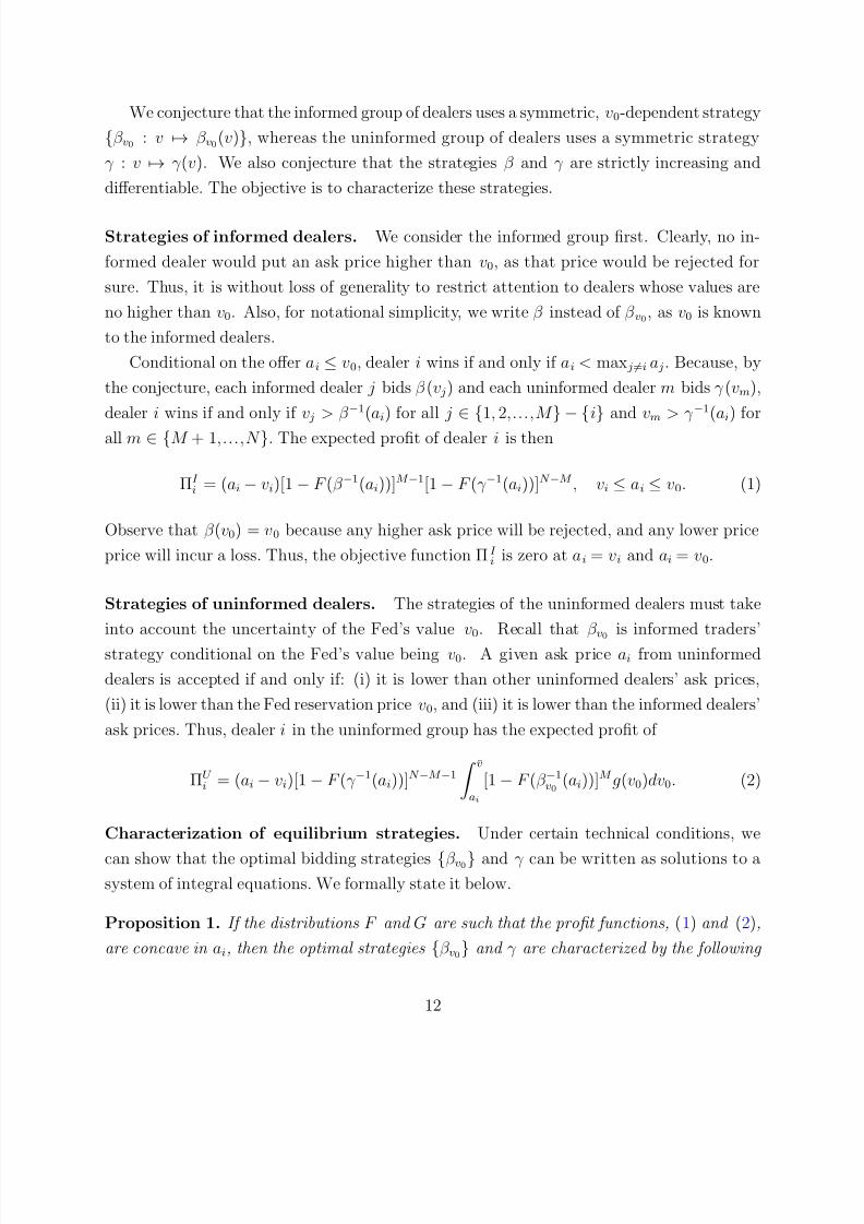
We conjecture that the informed group of dealers uses a symmetric, v0-dependent strategy

{β v0 : v → β v0(v)}, whereas the uninformed group of dealers uses a symmetric strategy

γ : v → γ (v). We also conjecture that the strategies β and γ are strictly increasing and

differentiable. The objective is to characterize these strategies.

Strategies of informed dealers. We consider the informed group first. Clearly, no in-

formed dealer would put an ask price higher than v0, as that price would be rejected for

sure. Thus, it is without loss of generality to restrict attention to dealers whose values are

no higher than v0. Also, for notational simplicity, we write β instead of β v0, as v0 is known

to the informed dealers.

Conditional on the offer ai ≤ v0, dealer i wins if and only if ai < max j=i a j. Because, by

the conjecture, each informed dealer j bids β (v j) and each uninformed dealer m bids γ (vm),

dealer i wins if and only if v j > β −1(ai) for all j ∈ {1, 2,...,M } − {i} and vm > γ −1(ai) for

all m ∈ {M + 1,...,N }. The expected profit of dealer i is then

ΠI i = (ai − vi)[1 − F (β −1(ai))]M −1[1 − F (γ −1(ai))]N −M , vi ≤ ai ≤ v0. (1)

Observe that β (v0) = v0 because any higher ask price will be rejected, and any lower price

price will incur a loss. Thus, the objective function ΠI i is zero at ai = vi and ai = v0.

Strategies of uninformed dealers. The strategies of the uninformed dealers must take

into account the uncertainty of the Fed’s value v0. Recall that β v0 is informed traders’

strategy conditional on the Fed’s value being v0. A given ask price ai from uninformed

dealers is accepted if and only if: (i) it is lower than other uninformed dealers’ ask prices,

(ii) it is lower than the Fed reservation price v0, and (iii) it is lower than the informed dealers’

ask prices. Thus, dealer i in the uninformed group has the expected profit of

ΠU i = (ai − vi)[1 − F (γ −1(ai))]N −M −1

v̄ai

[1 − F (β −1v0

(ai))]M g(v0)dv0. (2)

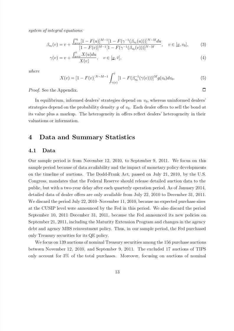
Characterization of equilibrium strategies. Under certain technical conditions, we

can show that the optimal bidding strategies {β v0} and γ can be written as solutions to asystem of integral equations. We formally state it below.

Proposition 1. If the distributions F and G are such that the profit functions, (1) and (2),

are concave in ai, then the optimal strategies {β v0} and γ are characterized by the following

12

8/12/2019 201448 Pap


system of integral equations:

β v0(v) = v +

v0u=v

[1 − F (u)]M −1[1 − F (γ −1(β v0(u)))]N −M du

[1 − F (v)]M −1[1 − F (γ −1(β v0(v)))]N −M , v ∈ [v, v0], (3)

γ (v) = v + v̄u=v

X (u)du

X (v) , v ∈ [v, v̄], (4)

where

X (v) = [1 − F (v)]N −M −1

v̄γ (v)

[1 − F (β −1v0

(γ (v)))]M g(v0)dv0. (5)

Proof. See the Appendix.

In equilibrium, informed dealers’ strategies depend on v0, whereas uninformed dealers’

strategies depend on the probability density g of v0. Each dealer offers to sell the bond at

its value plus a markup. The heterogeneity in offers reflect dealers’ heterogeneity in theirvaluations or information.

4 Data and Summary Statistics

4.1 Data

Our sample period is from November 12, 2010, to September 9, 2011. We focus on this

sample period because of data availability and the impact of monetary policy developments

on the timeline of auctions. The Dodd-Frank Act, passed on July 21, 2010, by the U.S.Congress, mandates that the Federal Reserve should release detailed auction data to the

public, but with a two-year delay after each quarterly operation period. As of January 2014,

detailed data of dealer offers are only available from July 22, 2010 to December 31, 2011.

We discard the period July 22, 2010–November 11, 2010, because no expected purchase sizes

at the CUSIP level were announced by the Fed in this period. We also discard the period

September 10, 2011–December 31, 2011, because the Fed announced its new policies on

September 21, 2011, including the Maturity Extension Program and changes in the agency

debt and agency MBS reinvestment policy. Thus, in our sample period, the Fed purchased

only Treasury securities for its QE policy.

We focus on 139 auctions of nominal Treasury securities among the 156 purchase auctions

between November 12, 2010, and September 9, 2011. The excluded 17 auctions of TIPS

only account for 3% of the total purchases. Moreover, focusing on auctions of nominal

13

8/12/2019 201448 Pap


bonds makes the bond characteristics, such as coupon rates and returns, comparable across

CUSIPs. These 139 auctions were conducted on 136 days, with two auctions on November

29, 2010, December 20, 2010, and June 20, 2011, and only one auction on all the other days.

Our empirical analysis combines the auction data released by the Federal Reserve and

three CUSIP-level data sets of Treasury securities, including the secondary market intradayprice quotes, the specific collateral repo rates, and the outstanding quantity. The auction

data include: (1) the expected total purchase size range, the total par amount offered, and

the total par amount accepted for each auction; (2) the indicator of whether a CUSIP was

included or excluded, the par amount accepted, the weighted average accepted price, and

the least favorable accepted price for each CUSIP in each auction; and (3) the offered par

amount, offer (clean) price, and dealer identity for each accepted offer on each CUSIP in

each auction.

To the best of our knowledge, the individual-offer data we use is the first set of auction

data at the individual bid level that has been ever analyzed for U.S. Treasury securities. Pre-

vious studies of issuance auctions and buyback auctions of U.S. Treasury securities, including

Cammack (1991), Simon (1994), Nyborg and Sundaresan (1996), and Han, Longstaff, and

Merrill (2007), have used data only at the aggregate auction level or at the CUSIP level at

best.11

Our secondary market price data contain indicative bid and ask quotes from the New

Price Quote System (NPQS) by the Federal Reserve Bank of New York, as well as the

corresponding coupon rate, original maturity at issuance, and remaining maturity, which

are also used by D’Amico and King (2013). We choose the NPQS quotes because the thesedata cover off-the-run securities that are mainly involved in QE auctions. (The BrokerTec

data used in recent studies such as Fleming and Mizrach (2009) and Engle, Fleming, Ghysels,

and Nguyen (2012) mainly contain prices of mostly on-the-run securities.) The NPQS data

have four pairs of bid and ask quotes each day, which are the best bid and ask prices across

different trading platforms of Treasury securities made at 8:40am, 11:30am, 2:15pm, and

3:30pm. Since the auction close time is one of 11:00am, 11:30am, 12:05pm, and 2:00pm, we

use the 11:30am NPQS quotes for the first three auction closing times and the 2:15pm NPQS

quotes for the last auction closing time when comparing the auction price with secondary

market price. A daily when-issued-count number is also included to signal whether the

security is on-the-run or off-the-run, and how off-the-run it is: the number is 0 if the security

11Studies of Treasury auctions in other countries have used bid-level data, such as Umlauf (1993), Gordy(1999), Nyborg, Rydqvist, and Sundaresan (2002), Keloharju, Nyborg, and Rydqvist (2005), Hortacsu andMcAdams (2010), Kastl (2011), and Hortacsu and Kastl (2012).

14

8/12/2019 201448 Pap


is on-the-run, and 1 is added each time a security with the same original maturity and

coupon rate is issued.

We obtain the CUSIP-level special collateral repo rates from the BrokerTec Interdealer

Market Data that averages quoted repo rates across different platforms between 7am and

10am each day (when most of the repo trades take place). We then calculate the CUSIP-level repo specialness as the difference between the General Collateral (GC) repo rate and

specific collateral repo rate, measured in percentage points. This specialness measure re-

flects the value of a specific Treasury security used as a collateral for borrowing (see Duffie

(1996); Jordan and Jordan (1997); Krishnamurthy (2002); Vayanos and Weill (2008)). We

also obtain the outstanding par amount of Treasury securities each day from the Monthly

Statement of the Public Debt (MSPD) of the Treasury Department.

4.2 Descriptive statistics of QE auctionsFigure 2 presents descriptive statistics on the number of bonds and auction size for these 139

QE auctions (of nominal Treasury securities). The top left panel shows that the number of

eligible bonds in an auction varies between 15 and 36, with a mean of 26. On average, one

CUSIP is excluded in each auction, with the minimum and maximum number of excluded

CUSIPs being 0 and 4, respectively. This leaves the number of eligible (included) bonds

between 13 and 34, averaging 25 per auction, as presented in the top right panel. Among

these included bonds, 14 (11) bonds were (not) purchased by the Fed on average in each

auction, with the minimum and maximum number of bonds purchased (not purchased) being

2 (0) and 26 (28), respectively. Across all 139 auctions, only 186 CUSIPs have ever been

purchased by the Fed, among the 215 included CUSIPs.


The bottom left panel shows that the (par) amount of submitted offers varies between

$4 and $43 billion, averaging $21 billion per auction, while the amount of offers accepted

by the Fed varies between $0.7 and $8.9 billion, averaging $5.6 billion per auction. The

ratio between submitted and accepted offer amounts was on average 4.2. In addition, from

the bottom right panel, the accepted offers always have a par value that falls between the

expected minimum and maximum purchase sizes.


15

8/12/2019 201448 Pap


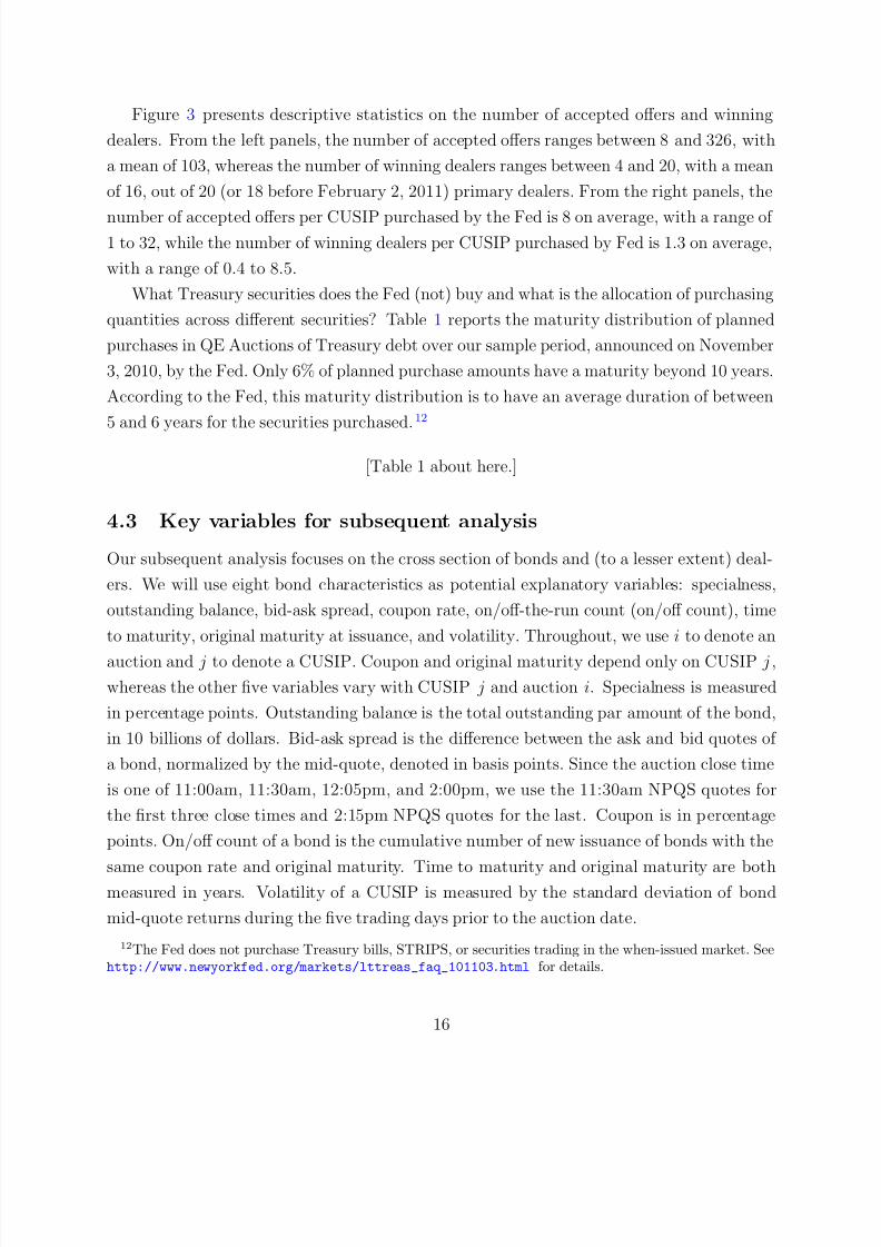
Figure 3 presents descriptive statistics on the number of accepted offers and winning

dealers. From the left panels, the number of accepted offers ranges between 8 and 326, with

a mean of 103, whereas the number of winning dealers ranges between 4 and 20, with a mean

of 16, out of 20 (or 18 before February 2, 2011) primary dealers. From the right panels, the

number of accepted offers per CUSIP purchased by the Fed is 8 on average, with a range of 1 to 32, while the number of winning dealers per CUSIP purchased by Fed is 1.3 on average,

with a range of 0.4 to 8.5.

What Treasury securities does the Fed (not) buy and what is the allocation of purchasing

quantities across different securities? Table 1 reports the maturity distribution of planned

purchases in QE Auctions of Treasury debt over our sample period, announced on November

3, 2010, by the Fed. Only 6% of planned purchase amounts have a maturity beyond 10 years.

According to the Fed, this maturity distribution is to have an average duration of between

5 and 6 years for the securities purchased.12

[Table 1 about here.]

4.3 Key variables for subsequent analysis

Our subsequent analysis focuses on the cross section of bonds and (to a lesser extent) deal-

ers. We will use eight bond characteristics as potential explanatory variables: specialness,

outstanding balance, bid-ask spread, coupon rate, on/off-the-run count (on/off count), time

to maturity, original maturity at issuance, and volatility. Throughout, we use i to denote an

auction and j to denote a CUSIP. Coupon and original maturity depend only on CUSIP j ,

whereas the other five variables vary with CUSIP j and auction i. Specialness is measured

in percentage points. Outstanding balance is the total outstanding par amount of the bond,

in 10 billions of dollars. Bid-ask spread is the difference between the ask and bid quotes of

a bond, normalized by the mid-quote, denoted in basis points. Since the auction close time

is one of 11:00am, 11:30am, 12:05pm, and 2:00pm, we use the 11:30am NPQS quotes for

the first three close times and 2:15pm NPQS quotes for the last. Coupon is in percentage

points. On/off count of a bond is the cumulative number of new issuance of bonds with the

same coupon rate and original maturity. Time to maturity and original maturity are bothmeasured in years. Volatility of a CUSIP is measured by the standard deviation of bond

mid-quote returns during the five trading days prior to the auction date.

12The Fed does not purchase Treasury bills, STRIPS, or securities trading in the when-issued market. Seehttp://www.newyorkfed.org/markets/lttreas_faq_101103.html for details.

16

http://www.newyorkfed.org/markets/lttreas_faq_101103.html


8/12/2019 201448 Pap



Table 2 reports the correlations of these variables across CUSIP/Auction. Panel A reports

the correlations by pooling the observations across CUSIP/Auction, while Panel B reports

correlations by first computing the correlation matrix across CUSIPs for each auction andthen taking averages across auctions in order to control for the effect of panel data. In

Panel A, only specialness has a consistently weak correlation with other bond characteristics.

Outstanding balance, bid-ask spread spread, coupon rate, on/off count, and original maturity

are highly correlated with each other. The average auction-level correlations, shown in panel

B, exhibit a similar pattern of high correlation among some bond characteristics. Because of

potential multicellularity concerns, in our empirical strategies we will run multiple univariate

regressions, instead of multi-variate regressions.

5 Behavior of Auction Participants

In this section, we analyze the behavior of the Fed as auctioneer and the bidding behaviors

of primary dealers throughout the QE auction process. More specifically, we study the Fed’s

decision to include or exclude certain CUSIPs in the auctions, the transaction volumes, and

the dispersion of dealers’ offers. We relate these three quantities to bond characteristics.

The prices of dealers’ offers, as well as associated costs to the Fed, are covered in Section 6.

5.1 The decision to include or exclude bonds

As presented earlier, on average, one CUSIP is excluded out of 26 eligible bonds in each

auction. According to Fed communications to the public, excluded bonds are those trading

with heightened specialness in the repo market, or cheapest to deliver into the front-month

Treasury futures contracts.13 Presumably, the reason for excluding these bonds is to avoid

exacerbating supply shortages in repo and futures markets. To formally explore the Fed’s

decision to include or exclude certain CUSIPs, we estimate a panel logit regression in which

the dependent variable, indexed by auction i and CUSIP j , takes the value of one if the j th

13The Fed also excludes CUSIPs by the size limit for purchase amount per security according to thepercentage of the outstanding issuance and the Fed’s existing holdings of this security. See the websiteof Federal Reserve Bank of New York for details (http://www.newyorkfed.org/markets/lttreas_faq_101103.html). We do not study this criterion as the Fed purchase rarely hit the size limit in our sample.In addition, communications with the Fed confirm that primary dealers have almost perfect foresight aboutwhich securities will be excluded before the auction.

17





8/12/2019 201448 Pap


CUSIP is included in the ith auction, and zero otherwise. Although the set of CUSIPs varies

with the auction number i, we suppress the dependence of j on i for notation simplicity.


Table 3 reports the results from the panel Logit regression, controlling for auction fixed

effects. As many bond characteristic variables are correlated, we run multiple univariate

regressions including one explanatory variable at a time to avoid the multi-collinearity prob-

lem. We observe from Table 3 that the regression coefficient of specialness is significantly

negative, confirming that the Fed did exclude bonds trading at heightened specialness. More-

over, illiquid bonds with higher bid-ask spreads are more likely to be included, implying that

the Fed may also try to improve the market liquidity for relatively illiquid bonds. Finally, the

Fed also tends to include bonds with shorter time to maturity, consistent with the pattern

shown in Table 1.

5.2 Auction outcomes: volumes and offer dispersion

Now we turn to the analysis of auction outcomes, after the Fed determines the set of in-

cluded bonds. We emphasize that because the Fed’s internal spline prices on various CUSIPs

are unobservable to us, the auction outcomes necessarily reflect both the primary dealers’

propensity to sell particular bonds and the Fed’s propensity to buy them.14

Purchase amounts and bond characteristics. We run a panel regression of the paramount accepted, in billions of dollars, for each bond included in an auction on a number of

explanatory variables.

The panel “Purchase Amount (Included Bonds)” of Table 4 reports the results from the

panel regressions for all included bonds (with both zero and positive purchase amounts), con-

trolling for auction fixed effects. As before, we run multiple univariate panel regressions (to

prevent the multi-collinearity problem). Robust t-statistics that correct for serial correlation

in the residuals clustered at the auction level are reported in parentheses.

As shown in Table 4, the five variables that are highly significant all suggest that the

Fed and the dealers have a combined preference of transacting more liquid bonds. For

14To better separate the behaviors of the dealers from that of the Fed, one would need to observe theentire supply curves of dealers on each CUSIP, including both accepted and rejected offers. Comparing the

just-accepted offers and just-rejected offers would give us valuable information regarding the Fed’s internalspline price across CUSIPs. Unfortunately, such detailed data are unavailable.

18

8/12/2019 201448 Pap


example, the Fed has purchased more bonds with a higher outstanding balance, a narrower

bid-ask spread, and a lower on/off count. Original maturity and coupon rates are pure bond

characteristics that are invariant of time, but in our sample they are highly correlated with

bid-ask spread, a measure of illiquidity (see Table 2). The economic magnitudes are also

large. If the bid-ask spread of a bond is 1 basis point wider than that of another, the Fed’spurchase of the first bond is on average $130 million less than that of the second bond. If a

bond has an outstanding balance that is $10 billion larger than another, the Fed’s purchase of

the first bond is on average $110 million higher than that of the second. Overall, though the

Fed tends to exclude the most liquid bonds in its purchase operations, among the included

bonds the Fed’s purchases tilt toward more liquid ones.

To check that these results are not driven entirely by bonds with zero purchase amounts,

we repeat the regressions only for bonds that have strictly positive purchased amounts. The

results, reported in the panel “Purchase Amount (Purchased Bonds)” of Table 4, confirm

that the Fed and dealers have a combined preference of trading more liquid bonds or bonds

with lower transaction costs. The bond characteristics are still statistically significant, and

their economic magnitudes also become larger. For example, a one basis point wider spread

implies a smaller Fed purchase by $190 million, whereas a $10 billion higher outstanding

balance implies a larger Fed purchase by $160 million. The coefficient on specialness also

becomes significantly positive and economically large. A 10 basis points increase in repo

specialness on a CUSIP is associated with an increase in Fed purchase of $253 million on

that CUSIP.


Offer dispersions and bond characteristics. Now, we turn to the relation between

offer dispersions and bond characteristics. This exercise is useful because, as auction theory

suggests, the dispersion of offers is an indication of heterogeneous valuations or information

among dealers.

Specifically, suppose that the oth winning offer price and par amount of dealer d for

CUSIP j in auction i are pi,j,d,o and q i,j,d,o, respectively. Then we define the Offer Dispersion

for the CUSIP j of auction i as

Offer Dispersion =

d,o

pi,j,d,o − pi,j

2· q i,j,d,o

d,o q i,j,d,o, (6)

19

8/12/2019 201448 Pap


where pi,j =

d,o pi,j,d,o · q i,j,d,o

/

d,o q i,j,d,o

is the quantity-weighted average auction

price for CUSIP j in auction i.

The panel “Offer Dispersion (Purchased Bonds)” of Table 4 reports the results from the

panel regression of offer dispersion for each bond purchased by the Fed on the same set

of eight explanatory variables, controlling for auction fixed effects. Offer Dispersion has asignificant correlation with almost all the explanatory variables. Offer dispersion is higher

if a bond has a higher specialness, a lower outstanding balance, a wider bid-ask spread, a

larger coupon, a larger on/off count, or a longer original maturity. With the exception of

specialness, these variables generally point to illiquidity and uncertainty of bond value, which

we find intuitive. The positive correlation between offer dispersion and specialness may be

due to the fact that bonds on special tend to trade at a yield away from otherwise similar

bonds. Thus, dealers may find it more difficult to guess or “model” the Fed’s internal spline

prices, leading to a higher dispersion in offers.

6 Costs of the Federal Reserve and Dealer Profitability

In this section, we study the cost to the Fed of purchasing the large amount of Treasury se-

curities ($780 billion) in implementing its QE polices from November 12, 2010, to September

9, 2011. We relate these costs to bond characteristics and disaggregate the profits of primary

dealers who participate in these auctions. Our measure of costs and profits is relative to the

secondary market prices on the days the auctions are closed. Using same-day market prices

mitigates the effects of markets events that are hard to control in the time series.

6.1 The costs of the Federal Reserve

To compute the Fed’s cost in an individual auction, we first calculate the purchase cost on

individual CUSIPs and then take the average costs for all CUSIPs purchased in that auction,

weighted by the par amount purchased. We measure the cost to the Fed of purchasing a

bond as the difference between the weighted average of accepted prices in QE auctions and

the corresponding secondary market price of that bond at the time the auction is closed. 15

15We also measure the cost of purchasing a bond as the difference between the least favorable priceaccepted by the Fed (also known as the stop-out price) and the corresponding secondary market price. Thiscost measure quantifies the maximum price the Fed is willing to tolerate to achieve its minimum purchaseamount. The cost measure based on stop-out price is around 2 cents per $100 par value higher than thatbased on the weighed average price, and the correlation between the two measures is as high as 99%. Becauseof their high correlation, we only report results based on the average purchase price.

20

8/12/2019 201448 Pap


As the secondary market quotes are valid only up to a standardized quantity, it is quite

possible that the Fed will create price impacts and pay an average purchase price above the

ask quote in secondary markets. In addition to the ask quote, we also calculate the costs

to the Fed based on the mid quote and the bid quote in the secondary market. The bid is

the price at which the Fed can in principle implement its purchases by posting limit orders,at the risk of not being able to execute the target purchases in time. The mid price is a

measure of the fair value of the bonds.

Figure 4 and Table 5 present the cost, in cents per $100 par value, to the Fed for the 139

auctions in our sample. The average cost over all purchase auctions, weighted by auction

size, is 0.71, 2.09, and 3.46 cents relative to the ask, mid, and bid quotes in the secondary

Treasury market, respectively. To put these average costs into perspective, we observe that

the weighted average bid-ask spread for the purchased bonds (weighted by the par amount

purchased) is 2.56 cents per $100 par value during our sample period. Therefore, the average

cost to ask of 0.71 cents is only about 28% of the average bid-ask spread. These results reveal

that the Fed suffers little market-impact costs in purchasing the huge amount ($780 billion)

of Treasury securities in its QE auctions.16



Equally interesting is the large dispersion of costs across auctions. The quantity-weighted

standard deviations of the Fed’s costs to ask, mid, and bid quotes are 11.05, 11.01, and11.00 cents per $100 par value, respectively. The average cost to ask for the individual

auctions ranges between -43.12 and 46.46. The cost to mid and cost to bid have similarly

large ranges. Moreover, the average cost is positive for 46.76%, 55.40%, and 66.91% of the

auctions measured using the ask, mid, and bid quotes, respectively. This result suggests

that sometimes the Fed receives a more favorable price in QE auctions than in the secondary

market.

16It may be tempting to argue that this measured cost underestimates the true costs to the Fed, if Treasuryprices increase between the announcement date and implementation date of each auction. However, to the

extent that the QE policy aims to reduce Treasury yields, a price increase in the secondary market isprecisely what the Fed wants and in our view should not be part of the cost calculation. What clearly shouldbe counted as a cost is how much the Fed pays above the prevailing secondary market price at the time of the auctions. We use the same logic in our calculation of dealers’ profits. This is different from Lou, Yan,and Zhang (2013) who compare issuance auction prices of the Treasury and secondary market prices fivedays pre-auction.

21

8/12/2019 201448 Pap


It is informative to compare the costs of the Fed in QE auctions to the costs of Treasury

auctions. Han, Longstaff, and Merrill (2007) report that the Treasury’s buyback auctions

from March 2000 to April 2002 incur the average cost of 4.38 cents per $100 par value, which

is about 70% of the average bid-ask spread of the auctioned bonds. Moreover, the average

par amount per auction of the Treasury’s buyback operations is $1.5 billion, whereas theaverage par amount per auction of the Fed’s QE purchases in our sample period is more than

three times as large, at $5.6 billion. The average cost in QE auctions also compares well with

those in issuance auctions of Treasury securities estimated by prior studies. For example,

among others, Goldreich (2007) estimates that the average issuance cost of Treasury notes

and bonds from 1991 to 2000 is about 3.5 cents per $100 par value, while Cammack (1991)

and Nyborg and Sundaresan (1996) provide similar estimates for T-bill issuance auctions.

How does the cost to the Fed vary across different bonds? To answer this question, we

estimate panel regressions of the average auction cost of each purchased bond on two sets of

explanatory variables. The first set contains the eight bond characteristics. The second set

contains three variables of auction outcomes, for each purchased CUSIP and each auction:

offer per dealer (the number of winning offers divided by the number of winning dealers),

offer dispersion (defined in (6)), and purchase amount (par amount purchased, in $billions).

As before, the panel regressions are univariate.

Table 6 reports the results of panel regressions of the average auction cost of each bond

purchased by Fed, controlling for auction fixed effects. Among the bond characteristics,

only specialness has a significant effect on cost to ask. This result suggest that the Fed’s

selection criterion based on internal spline-based prices offsets any detectable effect of bondcharacteristics, except specialness. If specialness is 1% higher on a particular bond, the cost

to the Fed to buy this bond increases by about 7 cents per $100 par value, which seems

quite large economically. Moreover, the cost to ask on a bond is higher if dealers submit

more offers on that bond and if dealers’ offers are more dispersed. To the extent that offer

dispersion measures the heterogeneity of dealers’ values or information, we would expect a

higher adverse selection or “bid shading” in the dealers’ supply curve, thus a higher cost.

Cost to mid and cost to bid are correlated with most of the bond characteristics. Because

cost to ask is equal to cost to bid less the bid-ask spread on each CUSIP, these results may

merely reflect the high correlation between bond characteristics and the bid-ask spread. Offer

per dealer does not significantly correlate with cost to mid or cost to bid, but offer dispersion

does.


22

8/12/2019 201448 Pap


Lastly, in unreported results, we run OLS regressions of the average cost of each auction

on weighted average versions of the explanatory variables used in Table 6. Almost none of

the variables are significant, suggesting that even if dealers have any propensity to charge a

higher spread on any type of bonds, the Fed substitutes into cheaper offers on other bonds

according to the ranking by its internal spline-based prices, leading to comparable costsacross bonds.17

6.2 Dealer profitability

In this section, we study the profitability of primary dealers in QE auctions. In interpreting

the results throughout this section, we use the intuition from Section 3 that the heterogeneity

in dealers’ profits reflects heterogeneous valuations or information.

For each dealer, we compute the profit margin as

Profit Margin =

i,jo ( pi,j,d,o − P i,j) · q i,j,d,o

i,j,o q i,j,d,o, (7)

where pi,j,d,o and q i,j,d,o are the oth winning offer price and par amount of dealer d for CUSIP

j in auction i, respectively, and P i,j is the secondary market price of the CUSIP j at the time

auction i is closed. That is, the profit margin is the average, weighted by the amount of each

accepted offer, of the differences between the offer price and the corresponding secondary

market price of the bond for that offer at the time the auction is closed. We use both the

ask and bid prices as the secondary market prices. The profit margin to bid measures theprofitability of dealers in selling bonds to the Fed through the QE auctions, rather than

selling bonds to investors on the secondary market at the bid price without delay. The profit

margin to ask measures the profitability of dealers who buy bonds on the secondary market

at the ask price without delay and then sell them to the Fed in the QE auctions. We also

use the mid-price to compute dealers’ profit margin.

With the profit margins, we calculate the aggregate profit of each dealer as

Aggregate Profit = Profit Margin × Offer Amount Accepted, (8)

where the profit margin can be relative to secondary market bid, mid, and ask prices.

17To control for the possibility that dealers learn about the bond values or the Fed’s internal spline-basedprices over time, we also include the auction number in the OLS regression as an explanatory variable(Milgrom and Weber (1982), Ashenfelter (1989), and Han, Longstaff, and Merrill (2007)). We do not findany time trend in the data.

23

8/12/2019 201448 Pap



Table 7 summarizes the dealer-by-dealer profitability across the 139 QE auctions in our

sample period. The first column lists the profitability rankings according to dealers’ aggre-

gate profits to bid prices, while the dealer identities are provided in the second column. The

third column presents the aggregate par amount each dealer sold to the Fed in billions of

dollars. The rest of the columns provides the profit margin in cents per $100 par amount

and the aggregate profit in millions of dollars of each dealer, relative to the secondary market

bid, mid, and ask prices, respectively.

Complementary to Table 7, Table 8 reports bidding characteristics of each dealer, sorted

by their aggregate profits to bid prices. For each dealer, we consider four bidding character-

istics: number of auctions participated, number of CUSIPs sold, number of winning offers

per auction, and number of winning offers per CUSIPs accepted.


Table 7 reveals that the aggregate profits to bid are positive for all dealers. Among

the 20 dealers, only one has a negative average profit to mid, and eight have an average

negative profit to ask. The concentration of aggregate profits and aggregate amounts of

accepted offers among dealers is striking. The top five dealers, Goldman Sachs, Morgan

Stanley, Barclays Capital, BNP Paribas, and J.P. Morgan, account for 65% of the $268.8

million total profit to bid of all dealers participating in the 139 QE auctions. The ratio is

even higher, about 70% and 96%, if aggregate profits are measured using mid and ask prices,respectively. These five dealers also accounted for 54% of the $776.6 billion total purchases.

By contrast, the bottom five dealers (Nomura, Jefferies, Daiwa, Cantor Fitzgerald, and

Mizuho, excluding SG Americas and MF Global who participated in QE auctions only after

February 2, 2011) account for only 6% of the $268.8 million total profit to bid and 6.6% of

the $776.6 billion total par amount purchased. Furthermore, we see in Table 8 that the top

five dealers sold bonds to the Fed in over 128 of the 139 QE auctions, and had winning offers

on over 129 of 186 CUSIPs purchased by the Fed, with the highest number of winning offers

both per auction and per CUSIP. These results strongly suggest the existence of information

asymmetry across dealers.

The profit margins reveal further patterns regarding the heterogeneity of dealers. Certain

dealers have high profit margins but low aggregate profits due to their lower number of

winning offers. For example, RBC, Merrill Lynch, and Daiwa have profit margins to bid

over 4.4 cents per $100 par amount, which are above the average profitability of 3.15 cents,

24

8/12/2019 201448 Pap


but their aggregate profits to bid are all significantly lower than the top five dealers. This

pattern suggests that the quantity of offers accepted and the profitability on these offers could

be two separate dimensions. For example, as suggested by the stylized model of Section 3,

dealers’ profit margins margins may well be related to asymmetric information regarding

the Fed’s internal spline-based prices, whereas the total sale volume may reflect a dealer’sactivity in Treasuries markets.

To better understand the heterogeneity of dealer profitability, we regress dealers’ profit

margins on two sets of explanatory variables, at the auction/dealer level (i.e. aggregating

CUSIP information). The first set contains the weighted average (by the CUSIP-specific

par amount accepted) of bond characteristics: specialness, outstanding balance, bid-ask

spread, coupon rate, on/off count, time to maturity, original maturity, and volatility. The

second contains two bidding variables: offer per CUSIP and weighted average bid dispersion.

We control for auction fixed effects, and report robust t-statistics that correct for serial

correlation in the residuals clustered at the auction level in the parentheses.


Table 9 reports the results. Most of the weighted average bond characteristic variables

are highly significant in explaining variations of dealers’ profit margins to bid and mid. The

signs of these significant variables imply that certain dealers have higher profitability because

they manage to sell bonds that are less liquid (e.g. those with higher bid-ask spreads or larger

on/off count) or more difficult to locate (e.g. those with lower outstanding balances). Once

the spread component is eliminated, margin to ask is not explained by any of those variables.

It seems reasonable to say that dealers’ profitability in QE auctions is partly correlated with

their market-making profits, measured by the bid-ask spread.

Do different dealers show different bidding behaviors? The heterogeneity of dealers’

profits suggests that they should. To answer this question, we estimate panel regressions of

two bidding variables, offer per CUSIP and weighted average offer dispersion, on a set of

explanatory variables across dealer/auction. The offer per CUSIP is the ratio between the

total number of winning offers and the total number of CUSIPs purchased by a dealer d in

auction i. For each dealer d in auction i, the weighted average offer dispersion is obtainedby computing first the offer dispersion measure for each CUSIP using dealer d’s accepted

offers on this CUSIP similar to (6), and then the weighted average of such CUSIP-specific

dispersion measures using the CUSIP-specific quantity. The explanatory variables are the

weighted average of (by the CUSIP-specific par amount accepted) specialness, outstanding

25

8/12/2019 201448 Pap


balance (in 10 billions of dollars), bid-ask spread, coupon rate, on/off count, time to maturity,

original maturity, and volatility.


Table 10 reports the results from the panel regression of offer per CUSIP and weighted

average offer dispersion. Most of the weighted-average bond characteristics are highly signif-

icant in explaining variations of offer per CUSIP. Generally, dealers submit fewer offers on

bonds that are less liquid, suggesting that either (a) they face a higher uncertainty of bond

value or the Fed’s internal spline-based price, or (b) their offers on these bonds are more

unattractive, so the Fed substitutes them with more liquid ones. Dealers’ weighted average

offer dispersion is only mildly correlated with the weighted averages of coupon, on/off count,

and original maturity, suggesting that lower liquidity coincides with only marginally higher

heterogeneity in dealers’ valuations or information.

7 Post-Auction Bond Returns and Liquidity

In this section, we explore the granular cross-section information in our data and study the

connection between auction outcomes and post-auction bond prices and liquidity.

Specifically, we run panel regressions of bond returns from before to after auction dates

on auction variables, across CUSIP/auction, and controlling for both auction and CUSIP

fixed effects. For each auction date t, we calculate the bond return from one day before to

one day after the auction, log(P t+1) − log(P t−1), and the bond return from one day before to

five days after the auction, log(P t+5)−log(P t−1), in percentage points.18 All days are business

days. For each CUSIP and auction, the right-hand variables include total purchased amount

(in billions of dollars), offer dispersion, offer per dealer, number of offers, number of dealers,

and profit margin to mid.19 Note that purchase amounts and profit margin to mid reflect

the information of both the Fed and the dealers, whereas all other auction variables only

reflect the information of the dealers. This panel-regression approach is broadly similar to

that of D’Amico and King (2013), but the auction variables are unique to our study.

18We stop at the five-day horizon because QE auctions for the same maturity bucket are conducted aboutevery five business days. Longer-horizon returns of a particular bond will likely cover two or more auctionsinvolving that bond, making the results difficult to interpret.

19We also run regressions using margin to bid and margin to ask (and also margins based on stop-outprices), and find similar results. It is also the case for the regressions of bond liquidity changes reportedin Table 12. In addition, we also run regressions of both bond price and liquidity changes using purchaseamount divided by outstanding balance (for each CUSIP) and find similar results.

26

8/12/2019 201448 Pap


Table 11 reports the results. Interestingly, auction variables can significantly forecast

bond returns. Offer per dealer, number of offers, and number of dealers positively forecast

bond returns from one day before to one day after the auction date, suggesting that a higher

competitiveness of dealers conveys positive information regarding bond returns in the short

term. Purchase amount is either statistically insignificant or significant but small.20By contrast, the return from t − 1 to t + 5 is only significantly forecasted by purchase

amount. If the Fed’s purchase amount of a particular CUSIP is $1 billion more than the

purchase of another, the first CUSIP tends to have a cumulative return that is 28–38 basis

points higher than that of the second, depending on the particular estimation model. No

other auction variable can forecast bond returns beyond the purchase amount, suggesting

that information contained in dealers’ offers delays quickly.

We caution that the 28–38 bps bond return five days after the auction date should not be

taken literally, for two reasons. First, since we do not observe the Fed’s demand function (or

its internal spline method), we cannot rule out the possibility that certain bonds are bought

more because they are perceived as “undervalued” by the Fed. The post-auction returns for

those “undervalued” bonds would naturally be higher. Second, each auction is immediately

followed by a few other auctions for different maturity buckets, so the five-day return pattern

can be partly affected by the outcomes of these immediately subsequent auctions.


Do Fed purchases affect liquidity in Treasury markets? To answer this question, we run a

similar regression of the cumulative changes in bond liquidity, proxied by the bid-ask spread

in basis points, on the same right-hand variables, again controlling for CUSIP and auction

fixed effects. A wider bid-ask spread implies worse liquidity. Table 12 reports the results

on the change in liquidity, from one day before to one day after the auction (Panel A) and

from one day before to five days after the auction (Panel B). We observe that none of the

auction variables significantly forecast bond liquidity change, whether it is from t − 1 to

t + 1 or from t − 1 to t + 5. In contrast, purchase amount is positively significant for bond

liquidity changes from one day before to five days after auctions. That is, if the Fed buys a

larger amount of a particular bond in QE auctions, that bond tends to become less liquid.However, the negative effect on liquidity is small. If the Fed purchases $1 billion more of a

particular bond, the bond’s spread tends to widen by 0.04–0.05 basis points five days later,

20In unreported results, we also find that the same auction variables alone can predict bond returns up tothree days after the auction, but this predictability is not statistically significant once the purchase amountsare included on the right-hand side.

27

8/12/2019 201448 Pap


a very small amount relative to the average bid-ask spread (2.4 basis points) of Treasury

market in our sample period.


8 Conclusion

The large scale purchase of Treasury securities by the Federal Reserve, commonly known as

quantitative easing (QE), is one of the most dramatic events in the U.S. Treasury market.

The Fed uses QE auctions—multi-object, multi-unit, and discriminatory-price auctions—to

implement its QE policy. This paper provides an empirical analysis of the outcomes and

dealers’ strategic behaviors of QE auctions. During our sample period of November 2010

to September 2011, the Fed purchased around $780 billion of Treasury securities, a large

fraction of the outstanding amount. Our findings can be summarized as follows:

1. The Fed tends to exclude from QE auctions the most liquid Treasury securities and

securities with heightened specialness in repo markets.

2. Among Treasury securities included in QE auctions, transaction volumes tilt toward

more liquid ones. In the cross-section, and controlling for the auction fixed effect, a one

basis point increase in the relative bid-ask spread of a Treasury bond is associated with

a $130 million reduction in the purchase of that bond. A $10 billion higher outstanding

balance of a Treasury bond is associated with a $110 million higher purchase.

3. Primary dealers submit heterogeneous offer prices, and the dispersion of these offers

is higher on bonds with a wider bid-ask spread and a lower outstanding amount (less

liquid ) and on bonds with a higher specialness (more liquid ).

4. The average costs to the Fed appear low. Relative to secondary market ask quotes

at the close of the auction, the Fed pays an additional 0.7 cents per $100 par value

on average. The total dollar value of this cost is about $55 million. Across auctions,

the standard deviation of the Fed’s costs, measured against to second-market prices,

is about 11 cents per $100 par value.

5. Primary dealers on average make profits by selling Treasury securities to the Fed. The

top five dealers account for about 96% of all dollar profits made by primary dealers, if

measured against the ask quotes in the secondary markets. This figure is 65% and 70%

if measured against the bid and mid quotes in the secondary markets, respectively.

28

8/12/2019 201448 Pap


6. The profits of primary dealers relative to bid or mid quotes increase in bond illiquidity.

This suggests that dealers that make more profits tend to sell more illiquid bonds to

the Fed.

7. Treasury returns one day after the auction can be forecasted by the dealers’ bidding

behavior in the auctions, whereas five-day returns are only predictable by the purchase

amount.

8. QE auctions do not seem to have an economically significant effect on bond liquidity.

This paper does not answer all questions on QE auctions, but we believe it is a start. We

can see two potential directions to investigate further. One is to construct a more thorough

model and derive specific theoretical predictions that can be tested. Structural parameters

can then be estimated and used for answering market-design questions. For example, what

is the best design of QE auctions to maximize competition among dealers and minimize the

Fed’s costs? Should the Fed decide to reverse its QE policy, what is the best design to sell

its Treasury inventories?

The second potential direction is to dig deeper into the effect of QE auctions on Treasury

markets by further exploring the cross-section information in the data. So far, post-auction

bond prices are necessarily the joint results of the dealers’ supply curves and the Fed’s

internal spline-based prices. For example, a higher purchase on certain CUSIPs may reflect

the Fed’s perception or information that these bonds are undervalued. Disentangling the

dealers’ supply and the Fed’s demand is likely to require additional data, such as dealers’offers that are rejected by the Fed. We leave these questions for future research.

29

8/12/2019 201448 Pap


Appendix

A Proof of Proposition 1

Under the technical condition of concavity, the first-order condition would give us the optimalstrategy.

To derive the optimal strategy β , we take the first-order condition of ΠI i and get

0 = dΠI

i

dai= [1 − F (β −1(ai))]M −1[1 − F (γ −1(ai))]N −M (9)

+ (ai − vi)

−(M − 1)[1 − F (β −1(ai))]M −2f (β −1(ai))

dβ −1(ai)

dai[1 − F (γ −1(ai))]N −M

+ (ai − vi)

−[1 − F (β −1(ai))]M −1(N − M )[1 − F (γ −1(ai))]N −M −1f (γ −1(ai))

dγ −1(ai)

dai

.

Substituting in ai = β (vi) and using the fact that dβ −1(ai)/dai = 1/β (vi), we have the

differential equation:

[1 − F (v)]M −1[1 − F (γ −1(β (v)))]N −M β (v) (10)

= (β (v) − v)

(M − 1)[1 − F (v)]M −2f (v)[1 − F (γ −1(β (v)))]N −M

+ (β (v) − v)

[1 − F (v)]M −1(N − M )[1 − F (γ −1(β (v)))]N −M −1f (γ −1(β (v)))γ −1

(β (v))β (v)

.

The above equation can be written as

d

β (v)[1 − F (v)]M −1[1 − F (γ −1(β (v)))]N −M

= v d

[1 − F (v)]M −1[1 − F (γ −1(β (v)))]N −M

.

(11)

Integrating the above equation from v to v0 and rearranging, we obtain (3).

To derive the optimal strategy γ , we take the first-order condition of ΠU i and get

0 = dΠU

i

dai= [1 − F (γ −1(ai))]N −M −1

v̄ai

[1 − F (β −1v0

(ai))]M g(v0)dv0 (12)

− (ai − vi)[1 − F (γ −1

(ai))]N −M −1 v̄

ai M [1 − F (β −1

v0 (ai))]M −1

f (β −1

v0 (ai))

dβ −1v0(ai)

dai g(v0)dv0

− (ai − vi)(N − M − 1)[1 − F (γ −1(ai))]N −M −2f (γ −1(ai))dγ −1(ai)

dai

v̄ai

[1 − F (β −1v0

(ai))]M g(v0)dv0.

− (ai − vi)[1 − F (γ −1(ai))]N −M −1[1 − F (β −1ai

(ai))]M g(ai).

30

8/12/2019 201448 Pap


Substituting in ai = γ (vi) and using the fact that dγ −1(ai)/dai = 1/γ (vi), we have the

differential equation:

[1 − F (v)]N −M −1γ (v)

v̄γ (v)

[1 − F (β −1v0

(γ (v)))]M g(v0)dv0 (13)

= − (γ (v) − v)[1 − F (v)]N −M −1γ (v)

v̄γ (v)

M [1 − F (β −1v0(γ (v)))]M −1f (β −1v0

(γ (v)))β −1

v0(γ (v))g(v0)dv0

− (γ (v) − v)(N − M − 1)[1 − F (v)]N −M −2f (v)

v̄ai

[1 − F (β −1v0(ai))]M g(v0)dv0.

− (γ (v) − v)[1 − F (v)]N −M −1γ (v)[1 − F (β −1γ (v)(γ (v)))]M g(γ (v)).

As in the case of informed dealers, the differential equation can be rewritten as

d[γ (v)X (v)] = v dX (v). (14)

In particular, X (v̄) = 0. Integrating from v to v̄ and rearranging, we obtain (4).

References

Ashenfelter, O. 1989. How auctions work for wine and art. Journal of Economic Perspectives 3: 23–36.

Ausubel, L., Cramton, P., Pycia, M., Rostek, M., and Weretka, M. 2013. Demand Reductionand Inefficiency in Multi-Unit Auctions. Working paper.

Back, K., and Zender, J. 1993. Auctions of divisible goods: On the rationale for the Treasuryexperiment. Review of Financial Studies 6: 733–764.

Bauer, M., and Rudebusch, G. 2013. The Signaling Channel for Federal Reserve Bond Pur-chases. International Journal of Central Banking forthcoming.

Bikhchandani, S., and Huang, C. 1989. Auctions with Resale Markets: A Model of TreasuryBill Auctions. Review of Financial Studies 2: 311–340.

Bikhchandani, S., and Huang, C. 1993. The economics of Treasury securities markets. Journal of Economic Perspectives 7: 117–134.

Cammack, E. 1991. Evidence on bidding strategies and the information in Treasury billauctions. Journal of Political Economy 99: 100–130.

Chatterjee, A., and Jarrow, R. 1998. Market manipulation, price bubbles, and a model of the US Treasury securities auction market. Journal of Financial and Quantitative Analysis 33: 255–290.

31

8/12/2019 201448 Pap


Christensen, J., and Rudebusch, G. 2012. The Response of Interest Rates to US and UKQuantitative Easing. Economic Journal 122: 385–414.

D’Amico, S., English, W., Lopez-Salido, D., and Nelson, E. 2012. The Federal Reserve’sLarge-Scale Asset Purchase Programs: Rationale and Efects. Economic Journal 122: 415–

226.D’Amico, S., and King, T. 2013. Flow and Stock Effects of Large-Scale Treasury Purchases:

Evidence on the Importance of Local Supply. Journal of Financial Economics 108: 425–448.

Duffie, D. 1996. Special repo rates. Journal of Finance 51: 493–526.

Engle, R., Fleming, M., Ghysels, E., and Nguyen, G. 2012. Liquidity, Volatility, and Flightsto Safety in the U.S. Treasury Market: Evidence from a New Class of Dynamic OrderBook Models. Federal Reserve Bank of New York Staff Reports no. 590.

Fleming, M., and Mizrach, B. 2009. The Microstructure of a U.S. Treasury ECN: TheBrokderTech Platform. Federal Reserve Bank of New York Staff Reports no. 381.

Gagnon, J., Raskin, M., Remanche, J., and Sack, B. 2011. The Financial Market Effectsof the Federal Reserve’s Large-Scale Asset Purchases. International Journal of Central Banking 7-1: 3–44.

Goldreich, D. 2007. Underpricing in discriminatory and uniform-price Treasury auctions.Journal of Financial and Quantitative Analysis 42 (2): 443–466.

Gordy, M. 1999. Hedging Winner’s Curse with Multiple Bids: Evidence from the PortugueseTreasury Bill Auction. Review of Economics and Statistics 81: 448–465.

Goswami, G., Noe, T., and Rebello, M. 1996. Collusion in Uniform-Price Auctions: Experi-mental Evidence and Implications for Treasury Auctions. Review of Financial Studies 9:757–785.

Hamilton, J. D. D., and Wu, J. C. 2012. The Effectiveness of Alternative Monetary PolicyTools in a Zero Lower Bound Environment. Journal of Money, Credit and Banking 44:3–46.

Han, B., Longstaff, F., and Merrill, C. 2007. The U.S. Treasury Buyback Auctions: TheCost of Retiring Illiquid Bonds. Journal of Finance 62: 2673–2693.

Hancock, D., and Passmore, W. 2011. Did the Federal Reserve’s MBS Purchase ProgramLower Mortgage Rates?. Journal of Monetary Economics 58-5: 498–514.

Hortacsu, A., and Kastl, J. 2012. Informational Advantage: A Study of Canadian TreasuryAuctions. Econometrica 80 (6): 2511–2542.

32

8/12/2019 201448 Pap


Hortacsu, A., and McAdams, D. 2010. Mechanism Choice and Strategic Bidding in DivisibleGood Auctions: An Empirical Analysis of the Turkish Treasury Auction Market. Journal of Political Economy 118 (5): 833–865.

Jordan, B., and Jordan, S. 1997. Special repo rates: An empirical analysis. Journal of

Finance 52: 2051–2072.Kastl, J. 2011. Discrete Bids and Empirical Inference in Divisible Good Auctions. Review of

Economic Studies 78: 978–1014.

Keloharju, M., Nyborg, K., and Rydqvist, K. 2005. Strategic behavior and underpricing inuniform price auctions: Evidence from Finnish Treasury auctions. Journal of Finance 60:1865–1902.

Kremer, I., and Nyborg, K. 2004. Underpricing and Market Power in Uniform-Price Auctions.Review of Financial Studies 17: 849–877.

Krishnamurthy, A. 2002. The bond/old-bond spread. Journal of Financial Economics 66:463–506.

Krishnamurthy, A., and Vissing-Jorgensen, A. 2011. The Effects of Quantitative Easing onInterest Rates. Brookings Papers on Economic Activity (Fall).

Li, C., and Wei, M. 2013. Term Structure Modeling with Supply Factors and the FederalReserve’s Large-Scale Asset Purchase Programs. International Journal of Central Banking 9(1): 3–39.

Lou, D., Yan, H., and Zhang, J. 2013. Anticipated and Repeated Shocks in Liquid Markets.Review of Financial Studies 18: 981–1020.

Meaning, J., and Zhu, F. 2011. The Impact of Recent Central Bank Asset Purchase Pro-grammes. BIS Quarterly Review December: 73–83.

Milgrom, P., and Weber, R. 1982. A theory of auctions and competitive bidding. Economet-rica 50: 1089–1122.

Nyborg, K., Rydqvist, K., and Sundaresan, S. 2002. Bidder behavior in multiunit auctions-Evidence from Swedish Treasury auctions. Journal of Political Economy 110: 394–424.

Nyborg, K., and Sundaresan, S. 1996. Discriminatory versus uniform Treasury auctions:Evidence from when-issued transactions. Journal of Financial Economics 42: 63–104.

Pasquariello, P., Roush, J., and Vega, C. 2014. Government Intervention and Strategic Trad-ing in the U.S. Treasury Market. Working paper.

Potter, S. 2013. The Implementation of Current Asset Purchases. Remarks at the Annual Meeting with Primary Dealers (New York City).

33

8/12/2019 201448 Pap


Sack, B. 2011. Implementing the Federal Reserve’s Asset Purchase Program. Remarks at Global Interdependence Center Central Banking Series Event, Federal Reserve Bank of Philadelphia .

Simon, D. 1994. Markups, quantity risk, and bidding strategies at Treasury coupon auctions.

Journal of Financial Economics 35: 43–62.Stroebel, J., and Taylor, J. 2012. Estimated Impact of the Federal Reserve’s Mortgage-

Backed Securities Purchase Program. International Journal of Central Banking 8-2.

Swanson, E. T. 2011. Let’s Twist Again: A High-Frequency Event-Study Analysis of Op-eration Twist and Its Implications for QE2. Working paper Federal Reserve Bank of SanFrancisco.

Umlauf, S. 1993. An empirical study of the Mexican Treasury bill auction. Journal of Fi-nancial Economics 33: 313–340.

Vayanos, D., and Weill, P.-O. 2008. A search-based theory of the on-the-run phenomenon.Journal of Finance 63: 1361–1398.

Wilson, R. 1979. Auctions of shares. Quarterly Journal of Economics 93: 675–689.

Wright, J. H. 2012. What does Monetary Policy do to Long-Term Interest Rates at the ZeroLower Bound?. The Economic Journal 122 (November): 447–466.

34

8/12/2019 201448 Pap


List of Figures

1 Example of Timeline of QE Auctions . . . . . . . . . . . . . . . . . . . . . . 362 QE Auction: Number of Bonds and Auction Size . . . . . . . . . . . . . . . 373 QE Auction: Number of Offers and Dealers . . . . . . . . . . . . . . . . . . 38

4 Auction Cost . . . . . . . . . . . . . . . . . . . . . . . . . . . . . . . . . . . 39

35

8/12/2019 201448 Pap


Figure 1: Example of Timeline of QE Auctions

36

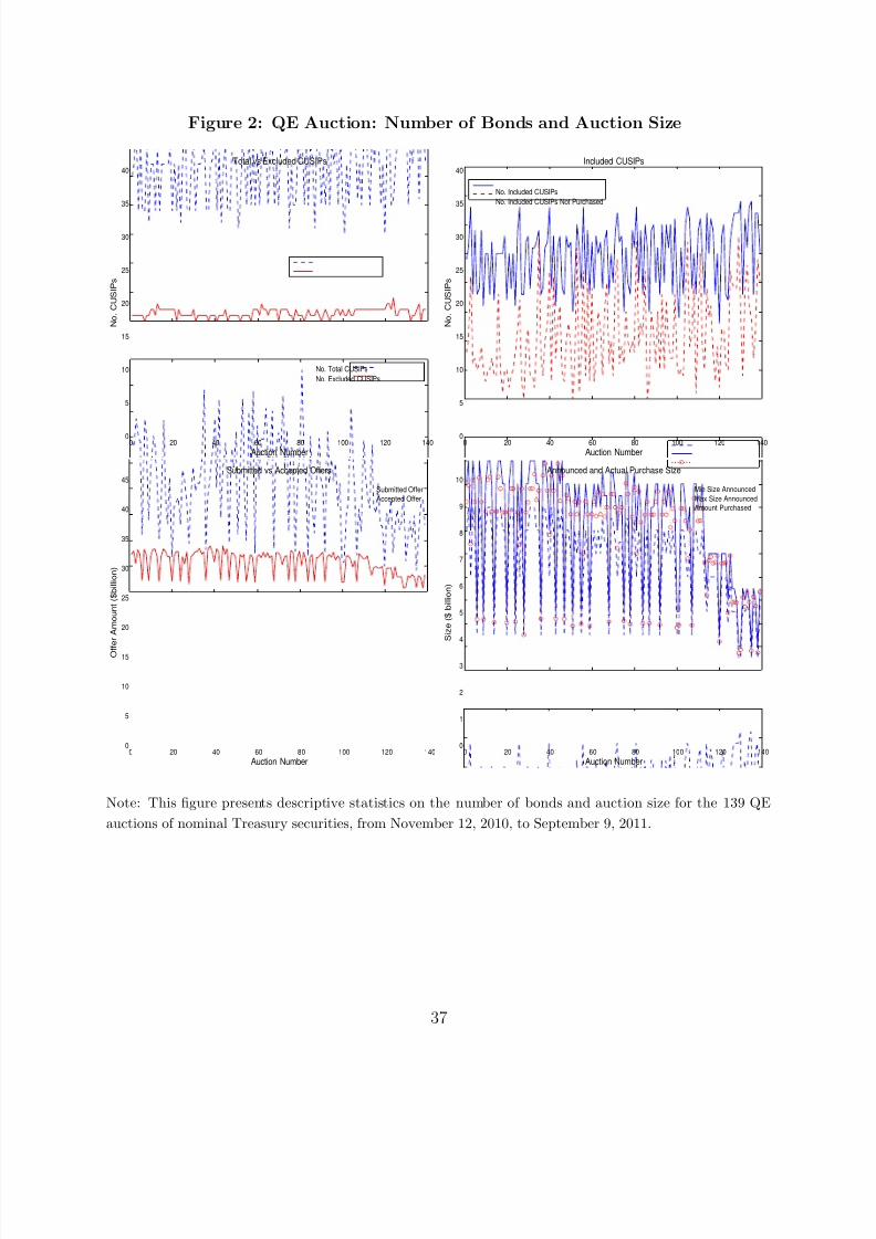
8/12/2019 201448 Pap


Figure 2: QE Auction: Number of Bonds and Auction Size

0 20 40 60 80 100 120 1400

5

10

15

20

25

30

35

40

Auction Number

N o .

C U S I P s

Total vs Excluded CUSIPs

No. Total CUSIPs

No. Excluded CUSIPs

0 20 40 60 80 100 120 1400

5

10

15

20

25

30

35

40

Auction Number

N o .

C U S I P s

Included CUSIPs

No. Included CUSIPs

No. Included CUSIPs Not Purchased

0 20 40 60 80 100 120 1400

5

10

15

20

25

30

35

40

45

Auction Number

O f f e r A m o u n t ( $ b i l l i o n )

Submitted vs Accepted Offers

Submitted Offer

Accepted Offer

0 20 40 60 80 100 120 1400

1

2

3

4

5

6

7

8

9

10

Auction Number

S i z e

( $

b i l l i o n )

Announced and Actual Purchase Size

Min Size Announced

Max Size Announced

Amount Purchased

Note: This figure presents descriptive statistics on the number of bonds and auction size for the 139 QE

auctions of nominal Treasury securities, from November 12, 2010, to September 9, 2011.

37

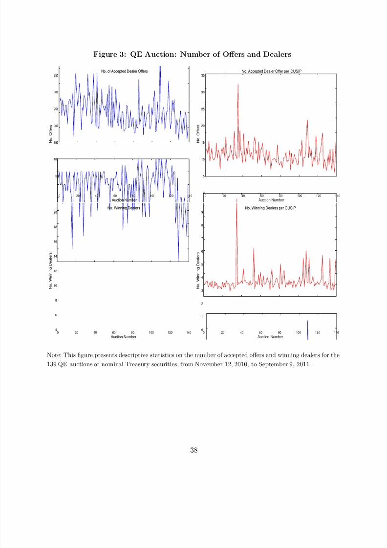
8/12/2019 201448 Pap


Figure 3: QE Auction: Number of Offers and Dealers

0 20 40 60 80 100 120 1400

50

100

150

200

250

300

350

N o .

O f f e r s

Auction Number

No. of Accepted Dealer Offers

0 20 40 60 80 100 120 1400

5

10

15

20

25

30

35

N o .

O f f e r s

Auction Number

No. Accepted Dealer Offer per CUSIP

0 20 40 60 80 100 120 1404

6

8

10

12

14

16

18

20

N

o .

W i n n i n g D e a l e r s

Auction Number

No. Winning Dealers

0 20 40 60 80 100 120 1400

1

2

3

4

5

6

7

8

9

N

o .

W i n n i n g D e a l e r s

Auction Number

No. Winning Dealers per CUSIP

Note: This figure presents descriptive statistics on the number of accepted offers and winning dealers for the

139 QE auctions of nominal Treasury securities, from November 12, 2010, to September 9, 2011.

38

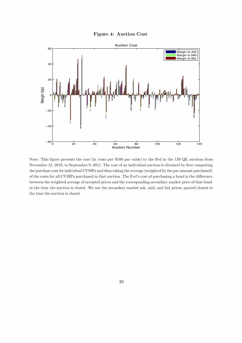
8/12/2019 201448 Pap


Figure 4: Auction Cost

0 20 40 60 80 100 120 140−60

−40

−20

0

20

40

60

M a r g i n ( b p )

Auction Number

Auction Cost

Margin to Ask

Margin to Mid

Margin to Bid

Note: This figure presents the cost (in cents per $100 par value) to the Fed in the 139 QE auctions from

November 12, 2010, to September 9, 2011. The cost of an individual auction is obtained by first computing

the purchase cost for individual CUSIPs and then taking the average (weighted by the par amount purchased)

of the costs for all CUSIPs purchased in that auction. The Fed’s cost of purchasing a bond is the difference

between the weighted average of accepted prices and the corresponding secondary market price of that bond

at the time the auction is closed. We use the secondary market ask, mid, and bid prices, quoted closest to

the time the auction is closed.

39

8/12/2019 201448 Pap


8/12/2019 201448 Pap


Table 1: Maturity Distribution of Planned Purchases in QE Auctions

Maturity Sectors for QE Auctions of Treasury Securities

Nominal Coupon Securities TIPS

Maturity Sector (Years) 1.5–2.5 2.5–4 4–5.5 5.5–7 7–10 10–17 17–30 1.5–30Percentage 5% 20% 20% 23% 23% 2% 4% 3%

Note: This table provides the maturity distribution of planned purchases in QE Auctions of Treasury debt

over our sample period (November 12, 2010–September 9, 2011), announced on November 3, 2010 by the

Fed. The on-the-run 7-year note will be considered part of the 5.5- to 7-year sector, and the on-the-run

10-year note will be considered part of the 7- to 10-year sector.

41

8/12/2019 201448 Pap


Table 2: Correlations of CUSIP-Level Variables

A: Pooled Correlation

Outstanding Bid- On/Off Time to Original

Specialness Balance Ask Coupon Count Maturity MaturitySpecialness 1.00

Outstanding Balance -0.12 1.00

Bid-Ask Spread 0.07 -0.78 1.00

Coupon 0.22 -0.84 0.84 1.00

On/Off Count 0.17 -0.57 0.69 0.79 1.00

Time to Maturity -0.13 -0.52 0.43 0.35 -0.10 1.00

Original Maturity 0.11 -0.84 0.82 0.87 0.55 0.71 1.00

Volatility -0.14 -0.48 0.40 0.34 -0.08 0.80 0.60

B: Average of Auction-Level Correlation

Specialness 1.00Outstanding Balance -0.23 1.00

Bid-Ask Spread 0.05 -0.61 1.00

Coupon 0.15 -0.65 0.73 1.00

On/Off Count 0.05 -0.66 0.82 0.87 1.00

Time to Maturity -0.11 0.05 0.07 0.09 -0.04 1.00

Original Maturity 0.10 -0.62 0.72 0.86 0.82 0.20 1.00

Volatility -0.22 0.36 -0.21 -0.24 -0.34 0.83 -0.12

Note: This table reports the correlations of bond characteristic variables. Panel A reports the correlations

by pooling the observations across CUSIP/Auction, while Panel B reports correlations by first computing

the correlation matrix across CUSIPs for each auction and then taking averages across auctions in order tocontrol for the effect of panel data. Specialness is the difference between the general repo rate and special

repo rate on the CUSIP, in percentage points. Outstanding balance is the total outstanding par amount

of the bond (in 10 billions of dollars). Bid-ask spread is the difference between the secondary market ask

and bid quotes of a bond normalized by the mid-quote, denoted in basis points. Coupon is in percentage

points. On/off count of a bond is the cumulative number of new issuance of bonds with the same coupon

rate and original maturity. Time to maturity and original maturity are both measured in years. Volatility is

the standard deviation of bond returns, using the series of mid-prices of secondary market quotes each day,

during the five trading days prior to the auction date. The secondary market prices have the closest quoting

time to the close of auction. The sample period is from November 12, 2010, to September 9, 2011.

42

8/12/2019 201448 Pap


Table 3: Panel Logit Regression for the Inclusion of Bonds in QE Auctions

Explanatory Variable Estimate N Pseudo R2

Specialness -7.376** 3,127 0.0540

(-2.683)

Outstanding Balance 0.031 3,127 0.0276

(0.321)

Bid-Ask Spread 0.233** 3,127 0.0373

(2.922)

Coupon 0.072 3,127 0.0295

(1.374)

On/Off Count 0.001 3,127 0.0275

(0.226)

Time to Maturity -0.078** 3,127 0.0299

(-3.445)

Original Maturity 0.013 3,127 0.0282(0.905)

Note: This table reports the results from the panel logit regression of whether a bond is included in an

auction (yes=1, no=0) on a set of explanatory variables, with z-statistics in the parentheses. The auction

fixed effects are included. Specialness is the difference between the general repo rate and special repo rate on

the CUSIP, in percentage points. Outstanding balance is the total outstanding par amount of the bond in

10 billions of dollars. Bid-ask spread is the difference between the secondary market ask and bid quotes of a

bond normalized by the mid-quote, denoted in basis points. Coupon is in percentage points. On/off count of

a bond is the cumulative number of new issuance of bonds with the same coupon rate and original maturity.

Time to maturity and original maturity are both measured in years. The secondary market prices have the

closest quoting time to the close of auction. The sample period is from November 12, 2010, to September 9,2011. We exclude bonds for which no quotations of special repo rates are available. Significance levels: ∗∗

for p < 0.01, ∗ for p < 0.05, and + for p < 0.1, where p is the p-value.

43

8/12/2019 201448 Pap


Table 4: Panel Regression for Purchase Amount and Bidding Behavior acrossCUSIP/Auction

Explanatory Variable Purchase Amount Purchase Amount Offer Dispersion

(Included Bonds) (Purchased Bonds) (Purchased Bonds)Estimate R2 Estimate R2 Estimate R2

Specialness 0.89 0.03 2.53* 0.11 2.78* 0.39

(1.44) (2.03) (2.40)

Outstanding Balance 0.11** 0.06 0.16** 0.13 -0.10** 0.39

(16.24) (9.19) (-3.52)

Bid-Ask Spread -0.13** 0.11 -0.19** 0.21 0.06* 0.39

(-15.75) (-13.76) (2.32)

Coupon -0.06** 0.07 -0.10** 0.15 0.06** 0.40

(-19.31) (-14.61) (3.68)

On/Off Count -0.01** 0.11 -0.02** 0.21 0.01** 0.39

(-16.27) (-15.89) (3.17)Time to Maturity 0.01 0.03 0.01 0.10 0.02 0.39

(0.15) (1.50) (1.13)

Original Maturity -0.02** 0.06 -0.03* 0.15 0.02** 0.40

(-20.35) (-16.08) (3.53)

Volatility -0.02 0.03 0.32 0.10 -0.86 0.39

(-0.13) (0.88) (-1.39)

N 3261 1854 1854

Note: This table reports the panel regressions of the par amount accepted (in billions of dollars) of each

bond included in an auction, as well as Offer Dispersion of each bond purchased by Fed, on a number of

potential explanatory variables, controlling for auction fixed effects. Robust t-statistics that correct for

serial correlation in the residuals clustered at the auction level are reported in parentheses. Specialness

is the difference between the general repo rate and special repo rate on the CUSIP, in percentage points.

Outstanding balance is the total outstanding par amount of the bond (in 10 billions of dollars). Bid-ask

spread is the difference between the secondary market ask and bid quotes of a bond normalized by the mid-

quote, denoted in basis points. Coupon is in percentage points. On/off count of a bond is the cumulative

number of new issuance of bonds with the same coupon rate and original maturity. Time to maturity and

original maturity are both measured in years. Volatility is the standard deviation of bond returns, using the

series of mid-prices of secondary market quotes each day, during the five trading days prior to the auction

date. The secondary market prices have the closest quoting time to the close of auction. The sample periodis from November 12, 2010, to September 9, 2011. The first panel, denoted “Included Bonds”, uses the

sample of all included bonds with both zero and nonzero purchase amounts, while the second and third

panels, denoted “Purchased Bonds”, use the sample of bonds with nonzero purchase amounts. We exclude

bonds for which no quotations of special repo rates are available. Significance levels: ∗∗ for p < 0.01, ∗ for

p < 0.05, and + for p < 0.1, where p is the p-value.

44

8/12/2019 201448 Pap


Table 5: Auction Cost

Quantity-Weighted Mean Quantity-Weighted Min Max

Standard Deviation

Cost to Ask 0.71 11.05 -43.12 46.46

Cost to Mid 2.09 11.01 -40.99 48.92Cost to Bid 3.46 11.00 -38.86 51.39

Note: This table presents summary statistics of the cost (in cents per $100 par value) to the Fed in the 139

QE auctions from November 12, 2010, to September 9, 2011. The cost of an individual auction is obtained

by first computing the purchase cost for individual CUSIPs and then taking the average (weighted by the

par amount purchased) of the costs for all CUSIPs purchased in that auction. The Fed’s cost of purchasing

a bond is the difference between the weighted average of accepted prices and the corresponding secondary

market price of that bond at the time the auction is closed. We use the secondary market ask, mid, and bid

prices, quoted closest to the time the auction is closed. The quantity-weighted mean and standard deviation

is computed as the mean and standard deviation across the 139 QE auctions, weighted by auction sizes.

45

8/12/2019 201448 Pap


Table 6: Panel Regression of Auction Cost across CUSIP/Auction

Explanatory Variables Cost to Ask Cost to Mid Cost to Bid

(N=1854) Estimate R2 Estimate R2 Estimate R2

Specialness 7.02* 0.94 14.14** 0.95 21.27** 0.93

(2.22) (3.50) (4.00)

Outstanding Balance 0.06 0.95 -0.76** 0.95 -1.57** 0.94

(0.42) (-4.92) (-8.86)

Bid-Ask Spread -0.13 0.95 0.60** 0.95 1.33** 0.95

(-1.18) (5.34) (11.32)

Coupon 0.05 0.95 0.52** 0.95 0.98** 0.95

(0.60) (6.07) (11.14)

On/Off Count -0.00 0.95 0.07** 0.95 0.14** 0.95

(-0.27) (5.58) (10.83)

Time to Maturity 0.18 0.95 0.12 0.95 0.06 0.93

(1.48) (1.00) (0.49)Original Maturity 0.02 0.95 0.16** 0.95 0.30** 0.95

(0.87) (5.99) (11.00)

Volatility 1.81 0.95 -3.38 0.95 -8.58* 0.93

(0.47) (-0.93) (-2.24)

Offer per Dealer 0.47* 0.95 0.34+ 0.95 0.22 0.93

(2.22) (1.66) (1.00)

Offer Dispersion 0.60** 0.95 0.72** 0.95 0.85** 0.93

(4.56) (5.32) (5.52)

Note: This table reports results from panel regressions of the average auction cost of each bond purchased

by Fed on a set of explanatory variables, across CUSIP/auction, controlling for auction fixed effects. Robustt-statistics that correct for serial correlation in the residuals clustered at the auction level are reported in

parentheses. The cost of an individual auction is obtained by first computing the purchase cost for individual

CUSIPs and then the average (weighted by the par amount purchased) of the costs for all CUSIPs purchased

in that auction. The cost to Fed of purchasing a bond is the difference between the weighted-average accepted

price and the corresponding secondary market (ask, mid, and bid) price. Specialness is the difference between

the general repo rate and special repo rate on the CUSIP, in percentage points. Outstanding balance is the

total outstanding par amount of the bond (in 10 billions of dollars). Bid-ask spread is the difference between

the secondary market ask and bid quotes of a bond normalized by the mid-quote, denoted in basis points.

Coupon is in percentage points. On/off count of a bond is the cumulative number of new issuance of bonds

with the same coupon rate and original maturity. Time to maturity and original maturity are both measured

in years. Volatility is the standard deviation of bond returns, using the series of mid-prices of secondary

market quotes each day, during the five trading days prior to the auction date. The secondary market prices

have the closest quoting time to the close of auction. Offer per dealer is the total number of winning offers

divided by the total number of winning dealers, for each bond of each auction. Offer Dispersion is defined as

in (6). The sample period is from November 12, 2010, to September 9, 2011. Bonds with no quotations of

special repo rates are excluded. Significance levels: ∗∗ for p < 0.01, ∗ for p < 0.05, and + for p < 0.1, where

p is the p-value.46

8/12/2019 201448 Pap


T a b l e 7 : D e a l e r P r o fi t a b i l i t y

R a n k b y

A g g r e g a t e

P r o fi t

A g g r e g a t e

P r o fi t

A g g r e g a t e

P r o fi t

A g g r e g a t e

A g g r e g a t e

P r o fi t

M a r g i n t o B i d

P r o fi t

M a r g i n t o M i d

P r o fi t

M a r g i n t o A s k

P r o fi t s

O ff e r

t o B i d

( C e n t s p e r

t o

M i d

( C e n t s p e r

t o A

s k

( C e n t s p e r

t o B i d

D e a l e r

( $ b i l l i o n )

( $

m i l l i o n )

1 0 0 d o l l a r s )

( $ m

i l l i o n )

1 0 0 d o l l a r s )

( $ m i l l i o n )

1 0 0 d o l l a r s )

1

G o l d m a n S a c h s

1 4 3 . 6 1

5 7 . 7 4

4 . 0 2

3 8

. 5 2

2 . 6 8

1 9 . 3

0

1 . 3 4

2

M o

r g a n S t a n l e y

1 2 5 . 8 8

5 3 . 3

4 . 2 3

3 7

. 9 9

3 . 0 2

2 2 . 6

7

1 . 8 0

3

B a r c l a y s C a p i t a l

6 9 . 5 7

2 5 . 1 5

3 . 6 2

1 1

. 1 9

1 . 6 1

- 2 . 7

7

- 0 . 4 0

4

B N

P P a r i b a s

4 8 . 4 9

2 0 . 2 4

4 . 1 7

1 3

. 9 3

2 . 8 7

7 . 6 1

1 . 5 7

5

J . P

. M o r g a n

3 2 . 9 1

1 7 . 8 2

5 . 4 1

1 2

. 1 4

3 . 6 9

6 . 4 5

1 . 9 6

6

C r e

d i t S u i s s e

8 2 . 9 7

1 7 . 4 1

2 . 1 0

8 . 3 5

1 . 0 1

- 0 . 7

2

- 0 . 0 9

7

R B

S

5 9 . 2 7

1 5 . 5 5

2 . 6 2

7 . 4 6

1 . 2 6

- 0 . 6

3

- 0 . 1 1

8

D e u t s c h e B a n k

2 4 . 2 4

1 0 . 1 1

4 . 1 7

5 . 3 4

2 . 2 0

0 . 5 7

0 . 2 4

9

R B

C

1 7 . 9 2

7 . 8 9

4 . 4 0

5 . 4 3

3 . 0 3

2 . 9 7

1 . 6 6

1 0

M e r r i l l L y n c h

1 6 . 7 8

7 . 5 1

4 . 4 7

4 . 8 9

2 . 9 1

2 . 2 6

1 . 3 5

1 1

C i t

i g r o u p

4 9 . 6 1

7 . 3 5

1 . 4 8

0 . 4 3

0 . 0 9

- 6 . 5

- 1 . 3 1

1 2

H S B C

2 2 . 5 5

6 . 5 4

2 . 9

4 . 1 1

1 . 8 2

1 . 6 7

0 . 7 4

1 3

U B

S

2 5 . 6 1

5 . 3 6

2 . 1 0

2 . 2 8

0 . 8 9

- 0 . 8

0

- 0 . 3 1

1 4

N o m u r a

1 9 . 0 8

4 . 8 6

2 . 5 5

2 . 7 7

1 . 4 5

0 . 6 8

0 . 3 6

1 5

J e ff

e r i e s

1 2 . 9 2

4 . 7 6

3 . 6 9

2 . 9 9

2 . 3 2

1 . 2 2

0 . 9 4

1 6

D a i w a

8 . 7 1

3 . 8 4

4 . 4 1

2 . 8 1

3 . 2 3

1 . 7 7

2 . 0 4

1 7

C a n t o r F i t z g e r a l d

5 . 8 0

1 . 8 3

3 . 1 6

1 . 1 0

1 . 8 9

0 . 3 6

0 . 6 2

1 8

M i z u h o

4 . 7 4

0 . 8 3

1 . 7 6

0 . 3 2

0 . 6 8

- 0 . 1

9

- 0 . 4 1

1 9

S G

A m e r i c a s

3 . 7 7

0 . 5 1

1 . 3 7

0 . 1 5

0 . 4 0

- 0 . 2

1

- 0 . 5 6

2 0

M F

G l o b a l

2 . 2 1

0 . 1 0

0 . 4 4

- 0

. 1 2

- 0 . 5 5

- 0 . 3

4

- 1 . 5 3

A v e r a g e

3 8 . 8 3

1 3 . 4 4

3 . 1 5

8 . 1 0

1 . 8 2

2 . 7 7

0 . 5 0

N o t e : T h i s t a b l e s u m m a r i z e s t h e d e a l e r p r o fi t a b i l i t y

a c r o s s t h e 1 3 9 Q E

a u c t i o n s i n o u r s a m p l e p e r i o d . F o r e a c h d e a l e r

, w e c o m p u t e t h e

p r o fi t m a r g i n a s t h

e a v e r a g e ( w e i g h t e d b y t h e a m o u n t o f e a c h a c c e p t e d o ff e r ) o f t h e d i ff e

r e n c e s b e t w e e n t h e o ff e r p r i c e a n d

t h e c o r r e s p o n d i n g

s e c o n d a r y m a r k e t ( b i d , m i d , a n d a s k ) p r i c e o f t h e b o n d f o r t h a t o ff e r a t t h e t i m e t h e a u c t i o n i s c l o s e d . T h e a g g r e g a t e p r o fi

t o f e a c h d e a l e r i s

c o m p u t e d a s t h e p

r o d u c t b e t w e e n t h e p r o fi t m a r g i n a

n d o ff e r a m o u n t a c c e p t e d . T h e p r o

fi t a b i l i t y r a n k i n g s o f d e a l e r s a r e d e

t e r m i n e d b y t h e i r

a g g r e g a t e p r o fi t s t o b i d p r i c e s . T h e s e c o n d a r y m a r k e t

p r i c e s e m p l o y e d h a v e t h e c l o s e s t q u

o t i n g t i m e t o t h e c l o s e o f a u c t i o n . T h e s a m p l e p e r i o d

i s f r o m

N o v e m b e r 1 2 , 2 0 1 0 , t o S e p t e m b e r 9 , 2 0 1 1 .

47

8/12/2019 201448 Pap


T a b l e 8 : B i d d i n g C h a r a c t e r i s t i c s a c r o

s s D e a l e r s

D e a l e r R a n k b y

N u m b e r o f

N u m b e r o f

A g g r e g a t e P r o fi t s

N u m b e r o f

N u m b e r o f

B i d s

B i d s

t o B i d

D e a l e r

A u c t i o n s

C U S I P s

p e r A u c t i o n

p e r C U S I P

1

G o l d m a n S

a c h s

1 3 8

1 4 7

1 1 . 7 0

1 0 . 9 9

2

M o r g a n S t a n l e y

1 2 8

1 2 9

5 . 8 7

5 . 8 2

3

B a r c l a y s C a p i t a l

1 3 1

1 4 4

7 . 1 8

6 . 5 3

4

B N P P a r i b a s

1 3 1

1 7 4

3 1 . 6 1

2 3 . 8

5

J . P . M o r g a n

1 3 1

1 3 7

4 . 8 7

4 . 6 6

6

C r e d i t S u i s

s e

1 3 2

1 4 0

5 . 7 0

5 . 3 7

7

R B S

1 2 0

1 2 0

4 . 9 1

4 . 9 1

8

D e u t s c h e B

a n k

1 1 3

1 2 5

4 . 6 0

4 . 1 6

9

R B C

1 0 3

1 2 7

4 . 2 4

3 . 4 4

1 0

M e r r i l l L y n

c h

1 1 4

1 3 0

4 . 7 6

4 . 1 8

1 1

C i t i g r o u p

1 2 4

1 3 5

5 . 3 1

4 . 8 8

1 2

H S B C

1 1 7

1 1 4

3 . 3 3

3 . 4 2

1 3

U B S

1 0 6

1 1 7

4 . 3 3

3 . 9 2

1 4

N o m u r a

1 1 6

1 1 7

3 . 3 1

3 . 2 8

1 5

J e ff e r i e s

1 1 6

1 0 8

3 . 3 1

3 . 5 6

1 6

D a i w a

8 9

8 1

2 . 9 7

3 . 2 6

1 7

C a n t o r F i t z g e r a l d

1 0 1

9 6

3 . 3 5

3 . 5 2

1 8

M i z u h o

9 0

8 0

3 . 2 9

3 . 7 0

1 9

S G

A m e r i c a s

5 1

4 5

2 . 4 5

2 . 7 8

2 0

M F G l o b a l

4 0

4 4

1 . 9 8

1 . 8 0

A v e r a g e

1 1 0

1 1 6

5 . 9 5

5 . 4 0

N o t e : T h i s t a b l e p

r e s e n t s b i d d i n g c h a r a c t e r i s t i c s o f d

e a l e r s , r a n k e d b y t h e i r a g g r e g a t e p r o fi t s t o s e c o n d a r y m a r k e t b i d p r i c e s . F o u r b i d d i n g

c h a r a c t e r i s t i c v a r i a

b l e s a r e i n c l u d e d , i n c l u d i n g t h e n u m b e r o f a u c t i o n s , n u m b e r o f C U S I P

s , n u m b e r o f w i n n i n g o ff e r s p e r a u c t i o n , a n d n u m b e r

o f w i n n i n g o ff e r s p

e r C U S I P s a c c e p t e d , f o r e a c h d e a l e r . T h e s e c o n d a r y m a r k e t p r i c e s e m

p l o y e d h a v e t h e c l o s e s t q u o t i n g t i

m e t o t h e c l o s e o f

a u c t i o n . T h e s a m p

l e p e r i o d i s f r o m

N o v e m b e r 1 2 , 2 0 1

0 , t o S e p t e m b e r 9 , 2 0 1 1 .

48

8/12/2019 201448 Pap


Table 9: Panel Regression of Dealer Profitability across Dealer/Auction

Explanatory Variable Margin to Bid Margin to Mid Margin to Ask

(N=1962) Estimate R2 Estimate R2 Estimate R2

Weighted Average Specialness -0.009 0.963 0.010 0.968 0.030 0.971

(-0.295) (0.418) (1.325)

Weighted Average Outstanding Balance -0.017** 0.966 -0.009** 0.969 -0.001 0.971

(-5.756) (-3.685) (-0.320)

Weighted Average Bid-Ask Spread 0.132** 0.969 0.063** 0.970 -0.007 0.971

(7.178) (3.540) (-0.388)

Weighted Average Coupon 0.011** 0.970 0.006** 0.971 0.001 0.971

(6.948) (3.925) (0.754)

Weighted Average On/Off Count 0.001** 0.969 0.001** 0.970 0.000 0.971

(7.198) (3.815) (0.100)Weighted Average Time to Maturity -0.001 0.963 -0.001 0.968 0.000 0.971

(-0.887) (-0.423) (0.059)

Weighted Average Original Maturity 0.003** 0.969 0.001** 0.970 0.000 0.971

(6.082) (3.252) (0.340)

Weighted Average Volatility -0.113** 0.964 -0.078** 0.969 -0.042 0.971

(-3.952) (-2.755) (-1.350)

Offer per CUSIP -0.003** 0.964 -0.002** 0.969 -0.001+ 0.971

(-3.963) (-3.074) (-1.924)

Weighted Average Offer Dispersion 0.001 0.963 0.001 0.969 0.001 0.971

(0.744) (0.644) (0.516)

Note: This table reports the results for panel regressions of the dealer profit margins on a set of explanatory

variables across dealer/auction, controlling for auction fixed effects. Robust t-statistics that correct for se-

rial correlation in the residuals clustered at the auction level are reported in parentheses. The explanatory

variables include the weighted averages (by the CUSIP-specific par amount accepted) of CUSIP-level spe-

cialness, outstanding balance (in 10 billions of dollars), bid-ask spread, coupon rate, on/off count, time to

maturity, original maturity, and volatility, as well as offer per CUSIP and weighted average offer dispersion.

The secondary market prices employed have the closest quoting time to the close of auction. The sample

period is from November 12, 2010, to September 9, 2011. We exclude bonds for which no quotations of

special repo rates are available. Significance levels: ∗∗ for p < 0.01, ∗ for p < 0.05, and + for p < 0.1, where

p is the p-value.

49

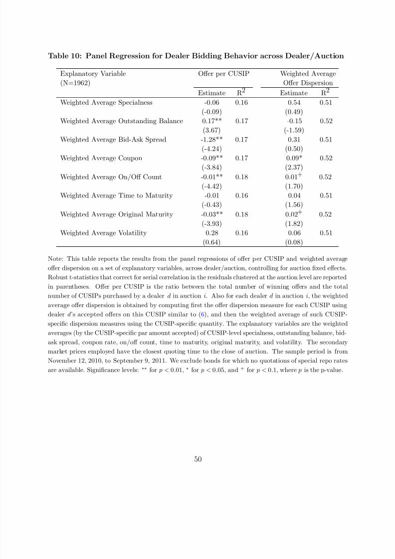
8/12/2019 201448 Pap


Table 10: Panel Regression for Dealer Bidding Behavior across Dealer/Auction

Explanatory Variable Offer per CUSIP Weighted Average

(N=1962) Offer Dispersion

Estimate R2 Estimate R2

Weighted Average Specialness -0.06 0.16 0.54 0.51

(-0.09) (0.49)

Weighted Average Outstanding Balance 0.17** 0.17 -0.15 0.52

(3.67) (-1.59)

Weighted Average Bid-Ask Spread -1.28** 0.17 0.31 0.51

(-4.24) (0.50)

Weighted Average Coupon -0.09** 0.17 0.09* 0.52

(-3.84) (2.37)

Weighted Average On/Off Count -0.01** 0.18 0.01+ 0.52

(-4.42) (1.70)

Weighted Average Time to Maturity -0.01 0.16 0.04 0.51(-0.43) (1.56)

Weighted Average Original Maturity -0.03** 0.18 0.02+ 0.52

(-3.93) (1.82)

Weighted Average Volatility 0.28 0.16 0.06 0.51

(0.64) (0.08)

Note: This table reports the results from the panel regressions of offer per CUSIP and weighted average

offer dispersion on a set of explanatory variables, across dealer/auction, controlling for auction fixed effects.

Robust t-statistics that correct for serial correlation in the residuals clustered at the auction level are reported

in parentheses. Offer per CUSIP is the ratio between the total number of winning offers and the total

number of CUSIPs purchased by a dealer d in auction i. Also for each dealer d in auction i, the weighted

average offer dispersion is obtained by computing first the offer dispersion measure for each CUSIP using

dealer d’s accepted offers on this CUSIP similar to (6), and then the weighted average of such CUSIP-

specific dispersion measures using the CUSIP-specific quantity. The explanatory variables are the weighted

averages (by the CUSIP-specific par amount accepted) of CUSIP-level specialness, outstanding balance, bid-

ask spread, coupon rate, on/off count, time to maturity, original maturity, and volatility. The secondary

market prices employed have the closest quoting time to the close of auction. The sample period is from

November 12, 2010, to September 9, 2011. We exclude bonds for which no quotations of special repo rates

are available. Significance levels: ∗∗ for p < 0.01, ∗ for p < 0.05, and + for p < 0.1, where p is the p-value.

50

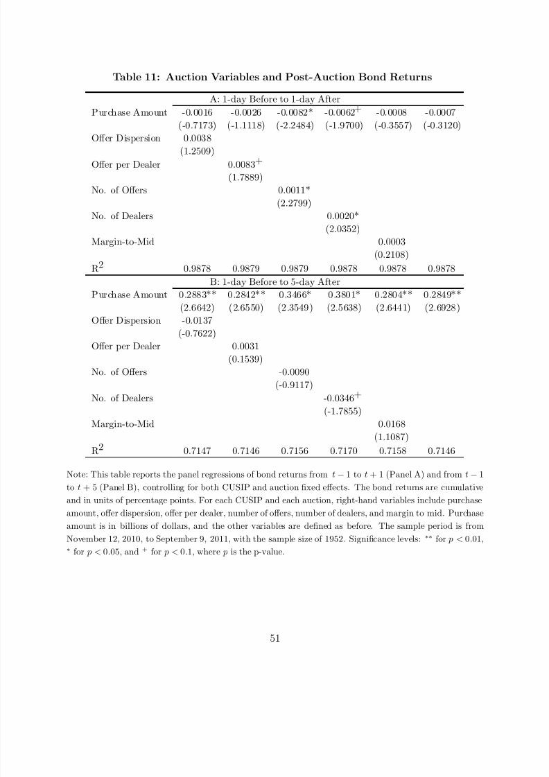
8/12/2019 201448 Pap


Table 11: Auction Variables and Post-Auction Bond Returns

A: 1-day Before to 1-day After

Purchase Amount -0.0016 -0.0026 -0.0082* -0.0062+ -0.0008 -0.0007

(-0.7173) (-1.1118) (-2.2484) (-1.9700) (-0.3557) (-0.3120)

Offer Dispersion 0.0038(1.2509)

Offer per Dealer 0.0083+

(1.7889)

No. of Offers 0.0011*

(2.2799)

No. of Dealers 0.0020*

(2.0352)

Margin-to-Mid 0.0003

(0.2108)

R2

0.9878 0.9879 0.9879 0.9878 0.9878 0.9878B: 1-day Before to 5-day After

Purchase Amount 0.2883** 0.2842** 0.3466* 0.3801* 0.2804** 0.2849**

(2.6642) (2.6550) (2.3549) (2.5638) (2.6441) (2.6928)

Offer Dispersion -0.0137

(-0.7622)

Offer per Dealer 0.0031

(0.1539)

No. of Offers -0.0090

(-0.9117)

No. of Dealers -0.0346+

(-1.7855)Margin-to-Mid 0.0168

(1.1087)

R2 0.7147 0.7146 0.7156 0.7170 0.7158 0.7146

Note: This table reports the panel regressions of bond returns from t − 1 to t + 1 (Panel A) and from t − 1

to t + 5 (Panel B), controlling for both CUSIP and auction fixed effects. The bond returns are cumulative

and in units of percentage points. For each CUSIP and each auction, right-hand variables include purchase

amount, offer dispersion, offer per dealer, number of offers, number of dealers, and margin to mid. Purchase

amount is in billions of dollars, and the other variables are defined as before. The sample period is from

November 12, 2010, to September 9, 2011, with the sample size of 1952. Significance levels: ∗∗ for p < 0.01,∗ for p < 0.05, and + for p < 0.1, where p is the p-value.

51

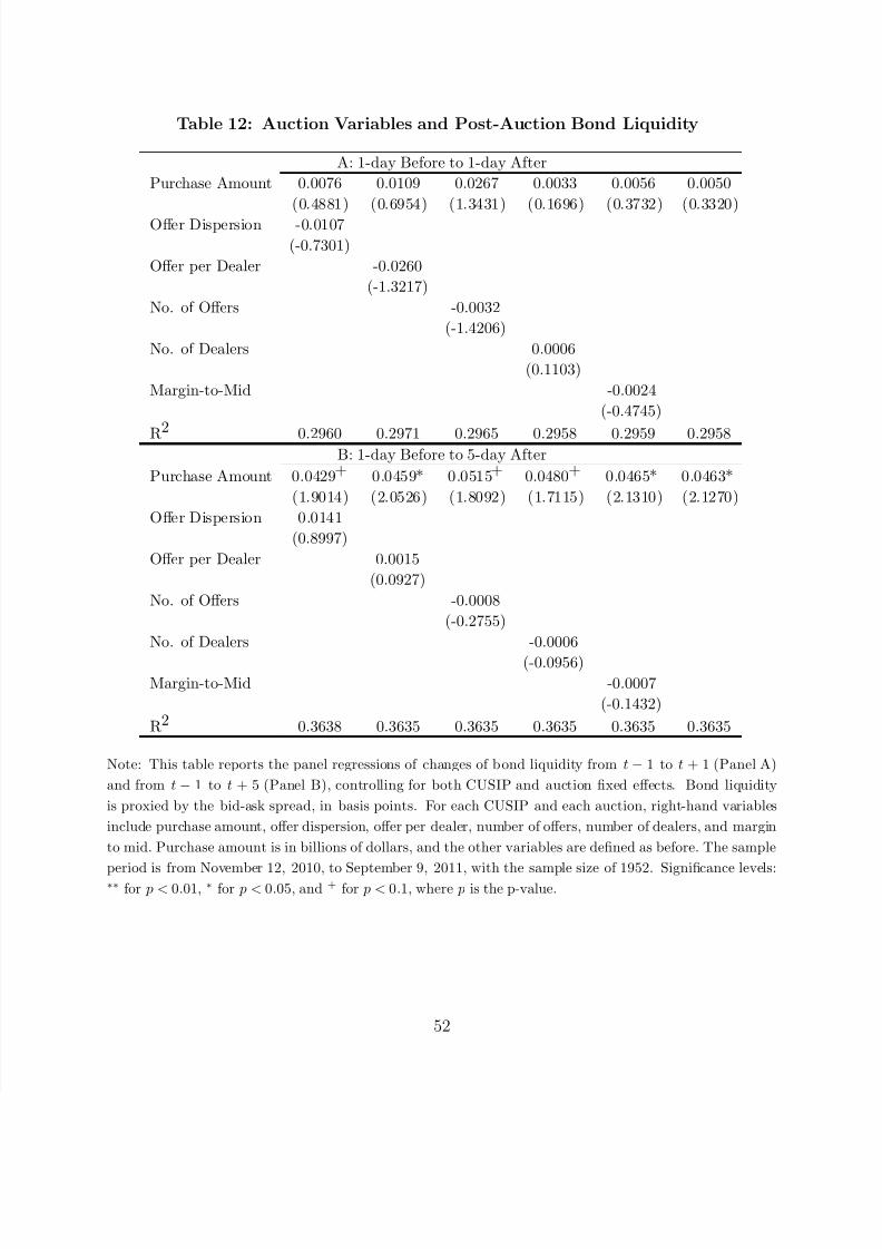
8/12/2019 201448 Pap


Table 12: Auction Variables and Post-Auction Bond Liquidity

A: 1-day Before to 1-day After

Purchase Amount 0.0076 0.0109 0.0267 0.0033 0.0056 0.0050

(0.4881) (0.6954) (1.3431) (0.1696) (0.3732) (0.3320)

Offer Dispersion -0.0107

(-0.7301)

Offer per Dealer -0.0260

(-1.3217)


(-1.4206)

No. of Dealers 0.0006

(0.1103)

Margin-to-Mid -0.0024

(-0.4745)

R2

0.2960 0.2971 0.2965 0.2958 0.2959 0.2958B: 1-day Before to 5-day After

Purchase Amount 0.0429+ 0.0459* 0.0515+ 0.0480+ 0.0465* 0.0463*

(1.9014) (2.0526) (1.8092) (1.7115) (2.1310) (2.1270)

Offer Dispersion 0.0141

(0.8997)

Offer per Dealer 0.0015

(0.0927)


(-0.2755)

No. of Dealers -0.0006

(-0.0956)

Margin-to-Mid -0.0007

(-0.1432)

R2 0.3638 0.3635 0.3635 0.3635 0.3635 0.3635

Note: This table reports the panel regressions of changes of bond liquidity from t − 1 to t + 1 (Panel A)

and from t − 1 to t + 5 (Panel B), controlling for both CUSIP and auction fixed effects. Bond liquidity

is proxied by the bid-ask spread, in basis points. For each CUSIP and each auction, right-hand variables

include purchase amount, offer dispersion, offer per dealer, number of offers, number of dealers, and margin

to mid. Purchase amount is in billions of dollars, and the other variables are defined as before. The sample

period is from November 12, 2010, to September 9, 2011, with the sample size of 1952. Significance levels:∗∗ for p < 0.01, ∗ for p < 0.05, and + for p < 0.1, where p is the p-value.

201448 pap

Documents