THERMOLUMINESCENCE: MATERIALS AND APPLICATIONS

by

JENNIFER MARY ODUKO

r

A thesis submitted to the Faculty'of'Science

at the University of Surrey in fulfillment of '

the requirements for the degree of

Doctor of Philosophy

June 1992

Department of Physics

University of Surrey

Guildford, Surrey

CONTENTS

Summary

Acknowledgements

1. Introduction 1

1.1 Historical Background 1

1.2 State of the Art 5

1.3 Present Work 9

2. Theory 12

2.1 Model of a Simple Ionic Crystal 12

2.2 First-Order Kinetics 18

2.3 Second-Order Kinetics 22

2.4 Methods of Determining Trap Parameters 25

3. Equipment 29

3.1 TLD Readers 29

3.1.1 Toledo 29

3.1.2 Solaro 32

3.1.3 Reader for TL of Foodstuffs 35

3.1.4 Discussion 37

3.2 Data Recording Equipment 40

3.2.1 Multichannel Analysers 40

3.2.2 SWT6800 Computer 41

3.2.3 PC with MCA Card 41

3.2.4 Solaro Glowcurve Recording 41

3.2.5 Discussion 42

3.3 Irradiators

3.3.1

3.3.2

3.3.3

3.3.4

3.3.5

3.4 Other

3.4.1

90Y/9OSr Irradiator

137Cs Irradiator

X-ray Irradiator

60CO Irradiator

Discussion

Equipment

Handling

3.4.2 Storage

3.4.3 Ovens

3.5 Conclusions

4. Materials

4.1 Introduction

4.2 Lithium Fluoride

4.3 Magnesium Borate

4.4 Lithium Borate

4.5 Beryllium Oxide

4.6 Calcium Sulphate

5. Computerised Glowcurve Deconvolution

5.1 Introduction

5.2 The Program

5.3 Some Results

5.3.1 LiF: MgjT1

5.3.2 LIF: Cu, Mg, P

5.3.3 MgB407: DY

5.3.4 L12B407: Mn

5.3.5 BeO: Na

5.3.6 CaS04: Mn

44

44

46

47

47

48

48

48

49

50

50

51

51

53

54

55

56

57

58

58

60

65

66

71

71

76

76

84

6. 1

Applications in Medical Physics 86

6.1 Introduction 86

6.2 Applications In Radiotherapy 90

6.2.1 International Intercomparlsons 91

6.2.2 Phantom Measurements 93

6.2.3 In-Vivo Measurements 95

6.3 Radiation Protection 97

6.3.1 Personal Dosimetry 97

6.3.2 Diagnostic Radiology 100

6.3.3 Measurements in Diagnostic Radiology104

6.3.4 Other Measurements ill

7. Environmental Monitoring 115

7.1 Introduction 115

7.2 Requirements for Environmental Dosimetry 118

7.3 International Intercomparlsons 122

7.4 Environmental Monitoring in Surrey 125

8. Thermoluminescence of Foodstuffs 146

8.1 Introduction 146

8.2 Review 149

8.3 Results 155

8.3.1 Spices 155

8.3.2 Chicken 157

8.3.3 Fish and Fish Oils 165

8.3.4 Fruit and Vegetables 166

8.3.5 Egg 169

8.4 Discussion 169

9. Conclusions 170

References 175

Summary

Thermoluminescence dosimetry (TLD) is a widely

used method of measuring ionising radiation. In this

thesis the properties of a wide range of TLD materials

are presented, with one (magnesium borate) described in

some detail. A computer program has been developed for

the analysis of TL glowcurves into their component

peaks. This is based on first-order kinetics, described

in the chapter on theory, which has been found to apply

to most of the materials studied and analysed.

A number of practical applications of TLD are

described. These include the successful use of TLD

measurements to test whether foodstuffs have been

irradiated. In some cases the TL signal is due to

traces of dust or soil in the food, but the existence

of clear TL signals from irradiated fats and fatty

foods was an unexpected finding. Further work Is

required to elucidate the TL mechanism in fats.

A programme of environmental monitoring with TLD

measurements was carried out in Surrey for two years.

This Involved monthly measurements at 26 sites spread

over the county. Results indicated a normal range (for

UK) of background gamma radiation, with slight

variation over the county corresponding to changes In

geology.

Some results are presented for measurements of

patient absorbed dose In diagnostic radiology. These

are preliminary results from a large study currently

being carried out. The small amount of data gathered so

far indicates that the entrance surface dose values are

well. below theýnational guidelines.

A -wide range of other applications of TLD is

reviewed. - Lessons drawn from 'experience with a wide

range of -TLD 'equipment., some specially developed for

this work, are presented.

1. Introduction

Certain substances- emit visible or ultra-violet

light when heated after having been exposed to, ionizing

radiation. This effect is. called thermoluminescence.,

and the substance which has this property is known as a

phosphor. This chapter comprises -a history of early

observations. and scientific study of this phenomenon,

up to the middle of the twentieth century; a survey of

the major fields of interest in thermoluminescence

research and applications; and an outline of the scope

and relevance of the work described In this thesis.

1.1 Historical Background

In considering the history of the subject, it is

tempting to speculate, with Scharmann (1981)-and Becker

(1986), that observations of thermoluminescence were

probably first made by prehistoric, cavemen. McKinlay

(1981) - notes that there are many references to

luminescence phenomena- in classical -literature, , and

according to Becker (1973),, mediaeval alchemists knew

that fluorite and some other minerals showed a

transient glow when heated in the dark. However, the

earliest recorded scientific observations of

thermoluminescence phenomena were those of Boyle

(1663), who wrote about his experiments with a diamond:

"Eleventhly., I also brought It to some kind of

glimmering light., by taking it into bed with me, and

holding It a good while upon a warm part of my naked

1

body.

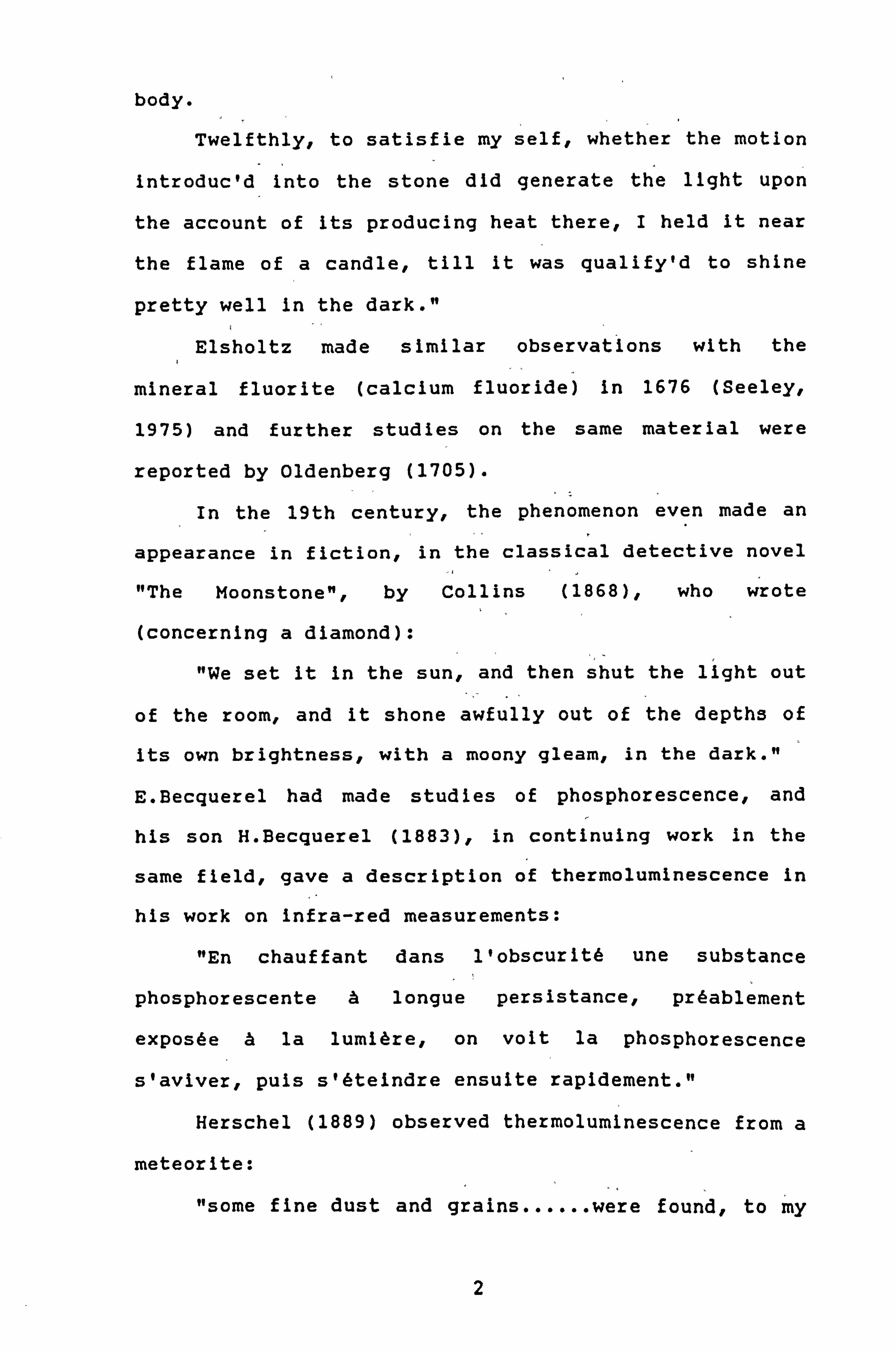
Twelfthly., to satisfie my self, whether the motion

introducId into the stone did generate the light upon

the account of Its producing heat there, I held It near

the flame of a candle, till it was qualify'd to shine

pretty well in the dark. "

Elsholtz made similar observations with the

mineral fluorite (calcium fluoride) in 1676 (Seeley.,

1975) and further studies on the same material were

reported by Oldenberg (1705).

In the 19th century, the phenomenon even made an

appearance In fiction, in the classical detective novel

"The Moonstone". by Collins (1868)., who wrote

(concerning a diamond):

"We set It in the sun.. and then shut the light out

of the room, and it shone awfully out of the depths of

its own brightness, with a moony gleam, in the dark. "

E. Becquerel had made studies of phosphorescence, and

his son H. Becquerel (1883), in continuing work in the

same field, gave a description of thermoluminescence in

his work on infra-red measurements:

"En chauffant dans l1obscurlt6 une substance

phosphorescente A longue persistance, pr6ablement

expos6e A la luml6re, on volt la phosphorescence

slaviver, puis sl6telndre ensuite rapidement. 11

Herschel (1889) observed thermoluminescence from a

meteorite:

"some f ine dust and grains ...... were found, to my

2

considerable surprise, to glow quite distinctly, though

not very brightly, with yellowish-white light, when

sprinkled ...... on a piece of nearly red-heated iron in

the dark. "

All these early observations were of naturally-

occurring materials, whose thermoluminescence resulted

from the absorbed dose they had received from natural

background radiation. Considerable progress towards

thermoluminescence as it is used today was made by

Wiedemann and Schmidt (1895). They studied a wide range

of inorganic compounds as well as natural minerals, and

used a beam of electrons for the Initial irradiation

of the phosphors. Trowbridge and Burbank (1898) showed

that X-rays could restore the property of

thermoluminescence to fluorite which had been heated to

remove the emission due to environmental radiation.

Curie (1904) described the use of radium for the same

purpose In her doctoral thesis:

"Certain bodies, such as fluorite, become luminous

when heated; they are thermoluminescent. Their

luminosity disappears after some time, but the capacity

of becoming luminous afresh through heat is restored to

them by the action of a spark and also by the action of

radiation. Radium can thus restore to these bodies

their thermo-luminescent property. "

Morse (1905) Investigated the thermoluminescence

of. fluorite, in particular the spectrum of the emitted

light. Wick (1924,1925) described thermoluminescence

stimulated in fluorite and many other materials by X-

3

rays. He observed that the emission of light occurred at

lower temperatures following exposure to X-rays, than

following natural (environmental) irradiation. (This is

due to more rapid fading of the lower-temperature peaks

at ambient temperature, although Wick merely noted the

effect and did not offer an explanation. )

Urbach (1930) reported on the thermoluminescence

of alkali halides, and suggested that the temperature

of maximum light emission was related to the electron

trap depth. This was more fully developed, and the

foundations of thermoluminescence theory laid, by

Randall and Wilkins (1945a, b) and by Garlick and Gibson

(1948). They gave expressions for the shape of a glow-

peak In terms of temperature, heating-rate, and the two

parameters characteristic of the trap associated with

the peak the trap depth E and the "frequency factor"

s. Their theories of first and second order kinetics,

respectively, are discussed In more detail In chapter

2.

Daniels et al (1953) discussed thermoluminescence

materials, apparatus, mechanisms, and a wide range of

potential applications Including dosimetry,

Identification of minerals., studies of catalysis and

radiation damage.. thermoluminescence stratigraphy and

age determination of rocks and pottery. This paper was

the source of the often repeated claim that of over

3000 rocks and minerals studied, about 75 per cent

showed visible thermoluminescence. The authors also

4

recommended the use of lithium fluoride from the Harshaw

chemical company. Thus this paper can be seen as the

foundation of much of modernresearch and development

in thermoluminescence dosimetry.

1.2 State of the Art.

The basic theory and practice of

thermoluminescence dosimetry (TLD) are both well

established. However, there still exists some degree

of "darkness ..... the myste rious ..... problems and

confusion" In the field (Becker, 1986). one goal whi ch

had not yet been attained Is the ability to produce a

phosphor to meet certain specifications., Just as

effectively as electronic circuits are designed and

produced. Becker (1973) lists the following desirable

properties of a TLD phosphor:

a. High concentration of traps and high

efficiency of light emission

b. No disturbing fading even during

extended storage at ambient or slightly higher

temperatures. (This usually implies a main peak

temperature between 180 and 2500C. )

C. Spectrum of emitted light well

suited to photomultiplier response, (Generally,

wavelengths between 300 and 500nm are suitable. )

d. Simple trap distribution, without

rapidly-fading low-temperature peaks., or high-

temperature peaks which are difficult to remove by

annealing. Annealing should effectively restore the

5

original properties of the phosphor.

e. Resistant to potentially disturbing

environmental factors: light., humidity, organic

solvents., common fumes and gases.

f. For most applications, low effective

atomic number and linear response over a wide dose-

range.

9. The phosphor should be cheap,,

non-toxic, chemically and physically stable, and

preferably easily made In a chemical laboratory. _

Nearly 20 years later, although new phosphors have been

developed and much studied, none really fulfils all

these conditions. LiF: Mg, Ti with its complex glowcurve

structure and complicated annealing requirements, Is

still more widely used than any other phosphor.

With several hundred papers published each year on

thermoluminescence, the research worker is forced to

specialise. A broad view of the subject is presented in

a number of good books. Cameron et al (1968) and Becker

(1973) present much of the earlier work. In the 1980's,

McKinlay (1981), Horowitz (1984) and McKeever (1985)

all provide wide coverage of the field, with particular

emphasis on their own special Isations. Most recently,

Mahesh et al (1989) cover all aspects of

thermoluminescence, with a particularly large section

on applications. In addition, three books cover more

specialised topics: Fleming (1979) on

thermoluminescence techniques in archaeology, McDougall

6

(1968) on thermoluminescence of geological materials,

and Aitken (1985) on thermoluminescence dating.

The wide range of research Interests in all fields

of thermoluminescence research Is conveniently

presented in the proceedings of the international

conferences on Luminescence/Solid State Dosimetry held

every three years since 1965. (Although other dosimetry

topics are now included, thermoluminescence still

predominates. ) Editorials to the 1983 (Ottawa) and 1986

(oxford) conference proceedings both claimed that a

steady state had been reached, in terms of numbers of

papers and participants. The 1989 (Vienna) conference

proceedings contained almost twice as many papers as

the previous two, but this reflects the considerably

Increased participation from Eastern European countries

rather than substantial growth In TLD research.

The main fields of research in thermoluminescence

are the following: basic principles and mechanisms,

characteristics of materials, Instrumentation, personal

dosimetry, environmental dosimetry, clinical dosimetry,

high level dosimetry, charged particle and neutron

dosimetry, geological and archaeological dating. Most

of these will be discussed In later chapters, but a few

recent developments may be mentioned briefly here. The

most exciting new material introduced in the last few

years was the highly sensitive LIF(Mg, Cu, P), described

by De Werd et al (1983). There has been much recent

interest In this material, see for example, Wang et al

(1986), Piters and Bos (1990), Wang et al (1990),

7

Horowitz and Horowitz (1990), Azorin et al (1990). Its

one disadvantage Is the extreme sensitivity to

temperature of the valence state of the phosphorus ion.

This means that extremely careful control of

temperature is required during phosphor production and

dosemeter readout. Such close control Is difficult to

attain, so that good batch reproducibility, and

continued good performance of the dosemeters in use,

are hard to achieve (Curry, 1990).

Another relatively new material, carbon-loaded

lithium fluoride, has been reported by Needham (1989),

Francis et al (1989) and Burgkhardt and Klipfel (1990).

These papers describe relatively new commercially

available dosemeters, but the Idea of using carbon-

loaded lithium fluoride was proposed much earlier by

Koczynski et al'(1974) and Robertson (1975). The carbon

absorbs the light emitted from all but the surface

layers of the dosemeter, making it suitable for beta

dosimetry. It is, of course, necessary to avoid

annealing these dosemeters at 4000C (as usual for

lithium fluoride) In air, otherwise the carbon from the

surface layer would be removed by oxidation, and the

dosemeter properties would be changed.

There has been an Increasing trend towards

automation of TLD readers, with the requirements of

large personal dosimetry services chiefly in mind. The

other main trend In instrumentation has been towards

computer control of the TLD reader, data storage and

8

record keeping. This has been made possible by the

Increasing availability and decreasing cost of personal

computers over the last f ive years or so. Several

companies now produce such computer-controlled readers,

e. g., the Solaro reader from Vinten Instruments (now NE

Technology) and the 8000C from Harshaw. This last now

has an option for practically on-line analysis (in 8s)

of a glow-curve Into Its component peaks., by

computerised glow-curve deconvolution, described by

Moscovitch (1986).

To summarise, the state of the art is that

thermoluminescence theory continues to be developed;

Instrumentation continues to be improved; new materials

continue to be Investigated In the search for a better,

or even the Ideal thermoluminescence material; and new

applications continue to be developed. At the same

time, well-established techniques and applications and

materials such as lithium fluoride and calcium

sulphate, continue in widespread use.

1.3 Present Work

The work described in this thesis began as an

study of various less common phosphors provided for

investigation by Vinten Instruments Ltd. of Weybridge,

Surrey. LIF: Mg. Ti was mostly excluded, except where

used in comparison with other materials. Fading

measurements were made., with the Intention of

determining E and s values. In addition, it was hoped

that one of these materials might prove to be the ideal

9

phosphor - or at least better than lithium f. luoride,

with its complicated glowcurve structure and annealing

requirements. Magnesium borate appeared to be a

promising material, but several disadvantages for

practical use also emerged In the study of its

properties (Oduko, Harris and Stewart 1984).

Attempts to use peak shape and peak maximum

positions to determine trapping parameters did not

yield the expected straight lines. The possibility

emerged that what looked like single peaks in the

glowcurve were actually more complex, consisting of two

or more overlapping peaks. This was confirmed when the

technique of computerised glowcurve deconvolution was

applied to the materials studied., The author had helped

to develop this technique during a visit to Israel

(Moscovitch, Horowitz & Oduko, 1983).

An interest In applications of thermoluminescence

dosimetry also developed. In particular, work with some

M. Sc. students at the University of Surrey led to the

development of techniques for detecting whether certain

foodstuffs had been Irradiated (Moriarty, Oduko &

Spyrou, 1988 Oduko & Spyrou 1990). The proposed

irradiation of foodstuffs aroused considerable public

and political Interest (Hansard, 1988). The weight of

public opinion is against It, since irradiation is

perceived as harmful; the test is therefore promising

for widespread application now that the irradiation of

foodstuffs has been permitted by the Food (Control of

10

Irradiation) Regulations 1990 which came into force on

1 January 1991. With the complete removal of European

trade barriers at the end of 1992 it Is likely that

more irradiated food will be offered for sale in the

U. K., and tests will probably be required for effective

monitoring and control.

The author has participated In an environmental

dosimetry survey of Surrey, using calcium sulphate

dosemeters and a Solaro TLD reader. Preliminary results

for the first two years of measurement (Ramsdale &

Oduko, 1991) are presented.

Finally, the author is involved in a programme of

measuring entrance surface dose to patients in

diagnostic radiology. Lithium fluoride dosemeters are

used for this at present, although a change to lithium

borate Is envisaged. A very large programme of

measurements is under way, and preliminary results from

the first two hospitals are presented.

11

2. Theor-Y

The existence of electron traps -associated with

the thermoluminescence process was mentioned briefly in

Chapter 1. For a material to ýxhibit

thermoluminescence, it must actually contain traps for

electrons and holes,, and recombination centres where

the electrons and holes recombine, with the emission of

light. These traps and centres are associated with

various kinds of defects in the material.

Most thermoluminescent materials are crystalline

solids (although some more complex biological materials

also exhibit thermoluminescence, as described in

chapter 8). A simple model for thermoluminescence Is

therefore presented for a simple crystalline material,

an alkali halide. Different assumptions about electron

trapping lead to different mathematical theories of

thermoluminescence, namely f lrst,, second and general

order kinetics. These are then 'related to different

experimental methods of determining trap parameters.

2.1 Model of a Simnle Ionic Crystal

Both halogens and alkali metals are monovalent, so

the perfect alkali halide crystal consists of equal

numbers of singly charged positive and negative ions.,

as shown In figure 2.1(a). Any real crystal, however,

contains defects or Imperfections; two of the simplest

of these shown In Figure 2.1(b). They are:

12

(D G G) 0 (D (1)

G) 0 G G e e e G G G) e G

G G 0

Figur e 2.1 (a) Figur e 2.1 (b)

Perfect alkal i halide Imperfec t alkali halide

cr ystal. crystal with vacancy

and inte rstitial.

ee ee

E)

E) 0 q) E) G)

Figur e 2.1 (c) Figur e 2.1 (d)

Alkali halide crystal Alkali h alide crystal

with di valent ion and with F centre

v acancy *= electron)

a)

e C) e 9 (E)

0G (i) ", 6" 0 0 6) '1, - "0 G0

e, G)

(D G E) 0 T

Figur e 2.1 (e) Figure 2.1 (f)

Alkali halide with Vk Alkali halide crystal

centre (0= hole) with R centre

13

(I) a vacancy or missing ion, shown by a square at

the top of figure 2.1(b). (This is also called a

Schottky defect)

(Ii) an Interstitial ion., which is an extra one

inserted between the normal ionic sites,, - shown at the

bottom right of figure 2.1(b) (This is also called a

Frenkel defect).

McKinlay (1981) lists three types of lattice

defects:

- Intrinsic or thermal defects

- Extrinsic defects or substitutional Impurity

Ions

- Radiation-induced defects

and points out that the number of intrinsic defects

increases as the temperature increases. If a hot

crystal Is cooled very rapidly, there is insufficient

time for the number of defects to decrease to that

appropriate to the lower temperature, so that the

number of defects present at the higher temperature Is

"frozen in". (This helps to explain the Increased

sensitivity of lithium fluoride cooled very rapidly

after annealing).

An example of an extrinsic defect Is the divalent

Ion (++) shown In Figure 2.1(c). To maintain electrical

neutrality in the crystal there must be two missing

positive ions. The divalent ion occupies the site of

one of them,, while the other Is shown as an adJacent

Schottky defect.

14

When an alkali halide crystal Is irradiated, free

electrons and holes are produced in it. A negative Ion

vacancy Is a region of excess positive charge (since

the surrounding positive ions are not fully neutralised

as they are in the perfect crystal); It therefore acts

as a potential trap for a free electron. An electron

trapped at a negative Ion vacancy is called a 'colour

centrel or F centre, from the German 'farbel (colour);

It Is shown In Figure 2.1(d). This arises from the

absorption of visible light of a certain wavelength

when the electron moves from Its ground state to an

excited state In the trap. This selective absorption of

light makes the crystal appear coloured.

It might be supposed that a hole would be trapped

In a similar way at a positive ion vacancy. Although

this has been given the name VF centre It is- thought

to have no real existence. Instead, a hole is trapped

by two adjacent negative ions, as shown In Figure

2.1(e). The two ions therefore become a singly charged

halogen molecule, such as 12_ or C12-. Two holes may be

trapped at a negative ion vacancy, and this Is referred

to as a V3 centre.

Trapping centres may cluster together in small

groups, and these have been given different names. Thus

an M centre is two F centres, and an R centre Is three

F centres, as shown in Figure 2.1(f). These centres

may also trap extra electrons, and if F, M or R centres

do so, they are known as F', MI or RI centres,

15

respectively (Mahesh et al, 1989).

The numbers., types and clustering of traps in a

crystal are affected by its thermal-history. Thus for a

phosphor to have reproducible properties, it Is

important that the annealing time, temperature and

cooling rateare exactly reproducible.

The traps described above represent 'different

energy levels, which lie between the valence and

condýctlon bands on an energy level diagram, as shown

in Figure 2.2(a). E and H represent the electron and

hole traps, respectively,, while L Is a luminescence

centre. The steps involved In thermoluminescence are

shown In Figures 2.2(b) to (d). In (b), Ionising

radiation incident on the crystal creates an electron-

hole pair. The electron is free -to- wander in -the

conduction band,, and is then trapped at E. The hole

wanders through the valence'band until it is trapped at

H. Many hole traps are unstable at room temperature and

decay*'rapidly (McKinlay, 1981) so that the hole Is

released., as shown in Figure 2.2(c). The electron in

Its trap is more stable; it ; emains there until the

crystal is heated. The thermal energy raises it to the

conduction band., as in Figure 2.2(d), - and -then the

electron can recombine with a hole at the luminescence

centre, with the associated emission of visible or

ultra-violet light.

16

Conduction band

E Ionisinc.

Radiatioi

L H-

Valence band

Figure 2.2(a)

Energy levels in

alkali halide

Heat 11

UT

Figure 2.2(c)

Hole released from

trap

Figure 2.2(b)

Irradiation and

trapping

Figure 2.2(d)

y

Light

Recombination of hole

and electron, with

light emitted

17

It should be noted that only a small percentage of

electron-hole pairs produced by Irradiation give rise

to thermoluminescence. Some pairs recombine almost

immediately (i. e. in less than 10-8s), with or'without

the emission of light; if light is emitted, the effect

is called fluorescence. If the electron and hole traps

are shallow, so that substantial recombination (with

emission of light) occurs at room temperature, the

effect is called phosphorescence. only if the electrons

are stable in the traps for longer periods (of the

order of a day or more) Is It called

thermoluminescence.

Information on defects and traps is obtained from

experimental measurements, Including:

thermoluminescence (for example, changes In the

glowcurves after heating the material or exposing it to

light or infra-red radiation to empty some traps),

electron spin resonance (ESR)., thermally stimulated

conductivity (TSC).. thermally stimulated electron

emission (TSEE) and optical properties of the material.

2.2 First-Order-Kinetics.

There are several forms of the equations

describing the thermoluminescence process and the shape

of the glow-peak. These correspond to different sets of

underlying assumptions. The theory of first'order

kinetics was first described by Randall and Wilkins

(1945a, b). It is based on the assumption that there is

18

no re-trapping of electrons after they are released

from traps., i. e. if an electron Is 'liberated from a

trap it always goes straight to a luminescence centre.

Three additional simplifying assumptions are also made:

a. Only the trapping and release of electrons is

considered. (The treatment of holes would be exactly

similar. )

b. only one kind of trap and one kind of

recombination centre are Involved.

c. The temperature increases at a constant rate

during readout.

Since the electrons In the traps have a Maxwellian

distribution of thermal energies, the probability per

unit time of an electron escaping from a trap of depth

E below the conduction band Is

p=s exp(-E/kT) (2.1)

where k is Boltzmann's constant, T is the absolute

temperature, and s is a constant (which may, however,

vary slowly with temperature, according to Randall and

Wilkins, 1945a). Following Mott and Gurney (1940), s is

interpreted by regarding the trap as a potential box;

then s is the product of the frequency with which the

electron strikes the sides of the box, and the

reflection coefficient. s has units seconds-'.. and Is

called the frequency factor. Its value is expected to

be somewhat less than the vibrational frequency of the

crystal, typically 1012 S-1.

If there are n electrons In the traps at time t

19

then from equation 2.1,

dn/dt = -pn -ns exp(-E/kT) (2.2)

The thermoluminescence emission intensity I is

proportional to the number of electrons recombining

with holes per second, I. e. to dn/dt. If the units are

chosen such that the constant of proportionality is 1,

then

I -dn/dt = ns exp(-E/kT) (2.3)

Rearranging terms gives

dn/n = -s exp(-E/kT) dt (2.4)

The heating rate 0 dT/dt Is constant, thus

dt = (1/0) dT

Substituting this In equation 2.4 and integrating

gives

ln (n/no) (1/0) s exp(-E/kT) dT,

where there are no trapped electrons at tempera ture To.

Thus

n= no expl-f WO) exp(-E/kT) dT1 (2.5)

and then from equation 2.3, the intensity of the glow-

peak Is

I= nos exp(-E/kT)exp[-f (s/O)exp(-E/kT)dT] (2.6)

This represents an asymmetric glow peak, as shown

In Figure 2.3(a). An important feature is that I is

proportional to the Initial concentration of trapped

electrons, no. Thus for first-order kinetics the peak

shape remains the same when no is varied, i. e. when the

phosphor is irradiated to different levels of absorbed

dose. Equation 2.6 also shows that the area under the

20

g-low-peak is proportional to no.

At the low-temperature side of the curve, where T

is close to To, the term in square brackets is close to

zero and I varies approximately as exp(-E/kT). At

higher temperatures, the term In square brackets

decreases rapidly and tends to zero, so that I

decreases to zero on the high-temperature side.

light

output

temperature

Figure 2.3(a) First-order kinetics glow curve

light

output

temperature

Figure 2.3(b) Second-order kinetics glow curves

21

I

The temperature of the peak maximum, Tmax, can be

found from equation 2.6 by differentiating and pVtting

dI/dT 0 at T= Tmax, From the form of equation 2.6,

it is easier to differentiate ln I than I., and this

would be equivalent since

d(lnI)/dT = (1/I) (dI/dT)

Thus from equation 2.6,

d(lnI)/dT 0 -E /kTmax 2_ (s/0) exp('-E /kTmax)

which gives

OE/kTmax 2s exp(-E/kTmax) -02.7)

This does not contain no, so the positljon . of

the maximum does not depend on the absorbed radiation

dose. The equation shows that Tmax does depend, -, on

the heating rate; it can be shown that as 13 increases,

Tmax also increases.

2.3 Second-Order Kinetics.

If it Is assumed that electrons released from

traps have an equal probability of combining with holes

In recombination centres and of being re-trapped., the

theory known as second-order kinetics is developed.

This was first given by Garlick and Gibson (1948),

although the suggestion that the two probabilities

might be approximately equal was taken from Randall and

Wilkins (1945b).

If there are a total of N electron traps in the

phosphor, and n are filled by electrons at some

instant., then N-n are empty. There are also n hol-es in

22

luminescence centres, since equal numbers of electrons

and holes were originally produced by Irradiation. Then

the probability of an electron recombining with a hole

at a luminescence centre, rather than being re-trapped,

is

n/l(N n) + n] = n/N (2.8)

Combining equation 2.8 with equation 2.3 then I

gives the second-order equation 112

I -dn/dt = (n IN)s exp(-E/kT) (2.9)

It Is usual to express sIN as a constant s'; this

pre-exponential factor does not exactly correspond to

the frequency factor s of first-order kinetics, as It

has units m3s-1. Using sl, equation 2.9 becomes

I= -dn/dt = sln2 exp(-E/kT) (2.10)

as before, the heating rate J3 dT/dt is

constant, the equation of the glow-peak becomes

I= n02sIexp(-E/kT)1l+(nO'sI/O)f exp(-E/kT)dT, -2

(2.11)

Unlike the first-order case, this represents a

peak which Is nearly symmetric.. as shown in Figure

2.3(b). The Intensity I Is not simply proportional to

no, as it was in the case of first-order kinetics. This

means that the shape of the peak depends on no,, and

therefore on the absorbed dose received by the

phosphor.

On the low-temperature side of the peak where T Is

close to To, the teim in square brackets is practically

equal to 1, thus I varies approximately as exp(-E/kT).

23

This is the same result as for first-order kinetics;

similarly, at higher temperatures, the second function

becomes more Important., and approaches zero.

Conveniently for dosimetric use, however, the

total area under the glow-peak is proportional to the

absorbed radiation dose. This is shown in a simple way

by Chen (1984):

since I= -dn/dt from equation 2.10, integrating

with respect to time from zero to infinity gives

Idt (dn/dt)dt dn no - n.

But n,, =0 since the traps are all empty at very high

temperatures, so that the Integral is equal to no (or

proportional to no If some different choice of units

had been made).

The temperature of the peak maximum can be found

by differentiating I from equation 2.11, and setting

dI/dT = 0. Chen (1969) has shown that this gives

(nos'/O)j exp(-E/kT)dT +1

(2kTmax 2nos'/OE) exp(-E/kTmax) (2.12)

This is not a simple relation5hip, but it is

obvious that Tmax depends on no (unlike the first-order

case). If no Increases, Tmax decreasesll as I seen in'the

curves of Figure 2.3(b).

Chen (1984) shows that the peak maximum intensity

Imax also varies with n0j, as follows:

Imax no'r (2.13)

where -c DE exp(E/kTmax)/(nokTma x 2SI)

24

But It can be shown that

23 1+ 2x X max - 6xmax + 24xmax . #. #*

where xmax m kTmax/E. Since generally xmax < 0-1., this

shows that Imax in equation 2.13 is slightly

supralinear with dose. Thus there is some small error

in assuming that peak heights and peak areas are

proportional, unlike the first-order kinetics case.

In general, the order of kinetics may be neither 1

nor 2., but some general number a. This is treated in

some detail by, for example, Mahesh and Furetta (1989)

and will noý be discussed here. Naturally the equations

reduce to first- and second-order kinetics in the cases

of 1 and a= 21 respectively.

2.4 Methods for Determining Trag Parameters

The trap parameters E and s (and the order of

kinetics) may be determined from experimental

measurements by a variety of different methods. For

detailed discussion of these methods see Chen (1976),

Chen (1984)., Mahesh and et al (1989). In addition,

Taylor- and Lilley (1978) describe several of these

methods and Illustrate their use by determining trap

parameters for lithium fluoride. The methods described

below generally apply to measurements made with linear

heating of the dosemeter. If, however, a TLD reader can

be programmed to give a hyperbolic heating profile,

then the method of Colvin and Gilboy (198s) can be

applied to determine E, s and the order of kinetics.

25

The simplest method of determining E is the method of

Urbach (1948), who found empirically for KC1 that

E(eV) = 23kTm

Similar equations, with different numerical values,

have been suggested for some other materials. These are

only approximate, and are based on an implied value of

s (not given).

The initial rise method uses the fact that the

low-temperature side of a first-order peak varies

approximately as exp(-E/kT), as noted in section 2.2.

Thus a plot of ln I against l/T gives a straight line

of slope -E/k, so that E can be found. This method can

be used if there are no lower peaks overlapping the one

to be studied.

Peak shape methods use the full width at half

maximum (w) of a glow peak and its component parts on

the low- and high-temperature sides as shown in Figure

2.4.

IM

1,, /a

Figure 2.4 FWHM w and component parts t, d

26

T2.

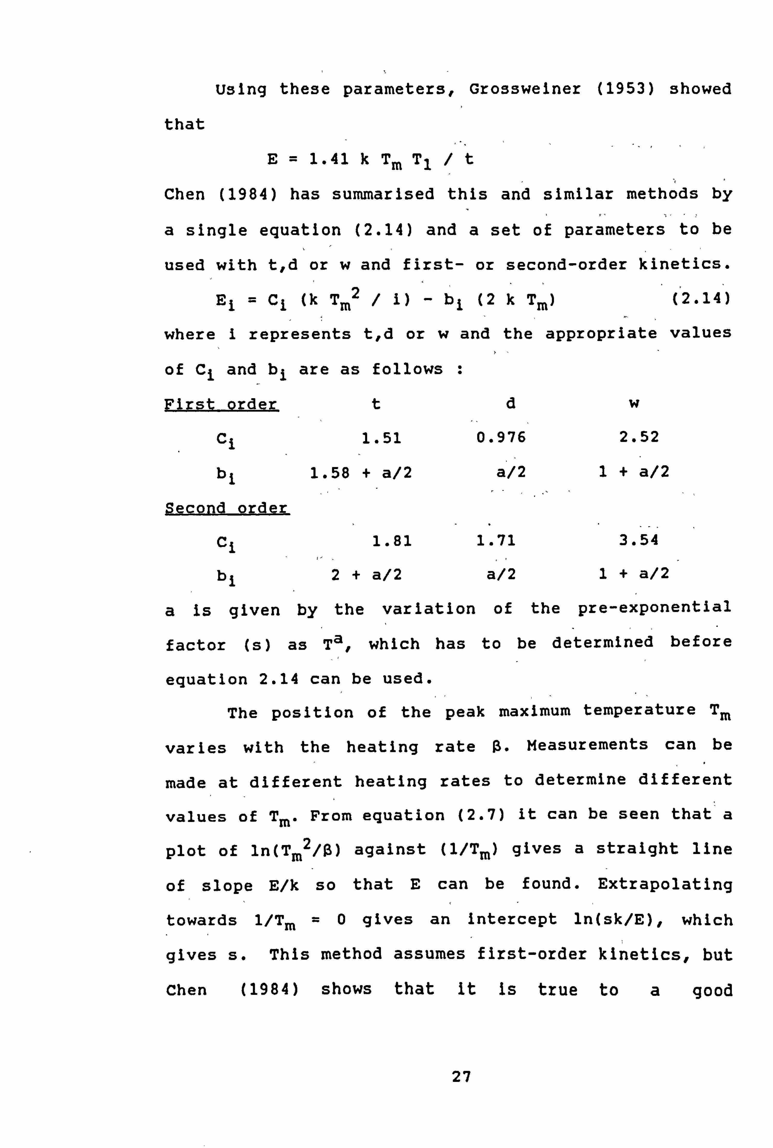
using these parameters, Grosswelner (1953) showed

that

E=1.41 k Tm Tj t

Chen (1984) has summarised this and similar methods by

a single equation (2.14) and a set of parameters to be

used with t, d or w and first- or second-order kinetics.

El = Ci (k Tm2 / I) bi (2 k Tm) 2.14)

where I represents t, d or w and the appropriate values

of C, and bi are as follows

First order tdw

Ci 1.51 0.976 2.52

bi 1.58 + a/2 a /2 1+ a/2

. gecond order

Ci 1.81 1.71 3.54

bi 2+ a/2 a/2 1+ a/2

a Is given by the variation of the pre-exponential

f actor (s) as Ta., which has to be determined before

equation 2.14 can be used.

The position of the peak maximum temperature Tm

varies with the heating rate 13. Measurements can be

made at different heating rates to determine different

values of Tm. From equation (2.7) it can be seen that a

plot of ln(TM2/a) against (1/Tm) gives a straight line

of slope E/k so that E can be found. Extrapolating

towards 1/Tm =0 gives an Intercept ln(sk/E), which

gives s. This method assumes first-order kinetics, but

Chen (1984) shows that It Is true to a good

27

approximation In other cases also.

If, a TL material Is heated and held at a constant

temperature,, light Is emitted (phosphorescence) as 'the

traps are emptied. Chen (1984). shows that the slope of

the graph ' of ln I -(where I Is the phosphorescence

intensity) against time t'is'equal to 4ý-'= s exp(-E/kT).

If the decay Is measured-t at several ' different

temperatures, a 'plot of ln ot against l/T gives a

straight line of slope -E/k.. - hence E. This applies to

first-order, kinetics.

If a material' has a complicated glowcurve -with

overlapping peaks, - none of these methods may be applied

directly. One may attempt to remove the overlapping

peaks by the use of light, uv or infra-red. Sometimes,

however, these means may cause new peaks to appearl An

alternative method is thermal bleaching, -that 'is,

heating the material to'a certain temperature so that

any peaks below that temperature are removed. 'This may

be useful, but it zeduces the main, peak Intensity

considerably.,

Lastlyl' peak parameters may be determined from the

results of computerised fitting-of overlapping peaks to

a complex glowcurve. This is discussed in detail in

chapter 5. Care must be -taken that the results are

meaningful, ie that the fitted peaks have real physical

meaning so that the whole procedure Is not just a

mathematical exercise.

28

3. Equivment

Three basic pieces of equipment- are required -for

TLD research or applications -a TLD reader, equipment

for recording (and possibly storage, and analysis) of

data, and an Irradiator. For - -some- purposes. 9 an

annealing oven is also required. In addition, various

small items- are used for proper storage,, handling and

cleaning of dosemeters and equipment. In the course

for this work, several different pieces of equipment In

each category have been used. These are briefly

described and a critical appraisal Is presented, in the

following sections.

3.1 TLD Readers

3.1.1 Toledo

The Toledo 654 TLD reader was - manufactured by

D. L. Pitman Ltd.. - later Vinten Instruments. It has been

widely used.. especially in the U. K. and Europe,, - for

many years, proving well suited for both routine and

research work (see, for example, Knipe (1984)1 Driscoll

et al (1984),, Holzapfel et al- -(1986).. Furetta et al

(1990), Dutt et al (1990)). Its development and

construction are described In detail by Robertson

(1975).. The reader's sensitivity can be adjusted over

three decades , to suit, , different dosemeters ' and

different ranges of absorbed dose. It comes in two

modules, standard and research. The standard module,

which is the. simpler of the two, offers a choice of two

29

read times and temperatures and two anneal t emperatures

with an optional preheat. The Interchangeable research

module offers a wide choice of times for the preheat,

read and anneal stages, with heating rate and

temperature also capable of being varied. With the

preheat and anneal stages switched out a linear

heating ramp can be obtained. This module, as the name

implies, is more suited to research p urposes, whereas

the standard module Is more convenient for most simple

or routine applications. Heating is electrical, with

the stainless steel strip heater raised into contact

with the dosemeter tray during a heating cycle. The

trays, also of stainless steel can readily be removed

for cleaning or replacement, so that trays need never

be used when dirty or tarnished, as this would affect

the efficiency of the light collection system. A flow

of oxygen-free nitrogen over the tray and dosemeter is

maintained during readout. This helps to suppress

triboluminescence, blows any airborne dust off the tray

and dosemeter, prevents oxidation of any traces of dirt

or grease during heating, and helps to cool the

photomultiplier and drawer assembly. The Internal light

source (ILS) Is an important feature which helps to

keep the response of the TLD reader stable. It consists

of 14C mixed with a plastic scintillator. Initial

problems with such light sources (Burgkhardt Plesch,

1981) were overcome by sealing a glass cover over the

ILS (Pitman, 1980). The ILS comes Into position under I-r

30

the photomultiplier tube (PMT) whenever the drawer is

opened to load or unload a dosemeter. A variable

negative feedback system Is used to adjust the high

voltage supply to the PMT so that the measured output

from the ILS remains constant. This compensates for

temperature-related changes in the PMT and the"'signal

measurement circuits. The compensation Is not quite

perfect, as a change in mean ILS reading of the order

of 1% is observed when reading large numbers of

dosemeters, such as 300 in one day. In these

circumstances, the dark current also Increases

substantially being typically of the order of, 8. to'60

counts on maximum sensitivity; - such an increase 'is to

be expected as the PMT becomes hotter, and readings can

be easily adjusted to compensate, for this. It should

also be noted-that the intensity of the ILS decreases

by about 2% when it is exposed to daylight, if , the

reader is opened for cleaning or maintenance. The

Intensity returns to normal after about 5 days, so this

should be taken into account if absolute measurements

are made, within this time. Many TLD measurements are

relative to calibration doses' or dosemeters so this

variation would not constitute a source of error in

such a case.

The Toledo used for the patient dosimetry

measurements which Is described later had, an attached"

automatic sample changer. This, can hold up to'30-trays

and dosemeters, 'and can be left unattended for the 20

31

to 30 minutes that it takes for them to be read out.

3.1.2 Solgro

The Solaro, originally from Vinten Instruments but

now supplied by NE Technology., is basically a

modernised, computer -control led version of the Toledo;

it consequently has various advantages and

disadvantages when compared with the Toledo. The

reader's operation is controlled by' an Opus III

personal computer (PC) with the TLD reader circuits and

mechanisms built Into the processor unit; - the computer

monitor, keyboard and printer stand separately. The

opus III computer Is now quite outdated compared with

currently available PC's, as is its 5' 1/4" single

density floppy drive, but there seems to be no

immediate prospect of the manufacturer updating it. The

menu-driven software is relatively easy, to use after'a

short (1-2 weeks) familiarisation period. ''Heating

rates, F times and temperatures are selected from 'the

appropriate menu and up to 10 different heating

programmes can be stored for selection as required. In

this and other functions, such as measurement of the

ILS and dark current at intervals.. the computer has

thus taken over the functions previously performed

manually by the operator of a Toledo. This simplifies

operation In some ways, so that a relatively 'unskilled

person may carry out routine readout of dosemeters

without neglecting any essential procedures. --However,

32

It also means that the physicist -loses the opportunity

for'exercising Initiative and flexibility - the Solaro,

for example, checks the ILS every 15 minutes and the

dark current every- hour,, and uses the measured values

to calculate "corrected readings". These are based on

the measured "raw counts" (PMT output) which-are-then

corrected for changes in dark current-and ýILS reading

(i. e. sensitivity).

The ILS readings are-relatively stable'with time,

as for the Toledo, but- -increases in- the dark current

sometimes give rise to misleading values of "corrected

readings" because' of the'dark ýcurrent being measured

only every hour. For example, on a hot day, the dark

current may be 1 count , at the start of readout, 4

counts one hour later, and 11 counts one hour-, later

again. This difference Is negligible compared with

dosemeter readings in most cases, typically 250 counts

for example for a site dosemeter- In - environmental

monitoring (see Chapter 7). In a few cases., however,

the difference Is large compared with the reading. A

background dosemeter from the environmental monitoring

programme may typically give a reading of 10-12 counts.

Hollaway (1990) has reported similar- problems, In

measurements with the- Solaro using Vinten personnel

dosimetry cards.

Such pzoblems are affected by both- hardware and

software considerations. The dark current Increases as

the reader becomes substantially hotter during use in

33

summer. In the winter the increase is marginal so the

problem could obviously be overcome by air-conditioning

the room where the TLD reader is located.

Unfortunately, financial considerations usually exclude

this alternative. The software could alternatively ýbe

changed to measure the dark current more often and to

apply corrections before the changes become-too large.

It Is not generally possible for the user/physicist 'to

make such a change as the software supplied is In

machine code and Inaccessible. The manufacturers, while

ready to listen to suggestions, may take 1-2 years to

Implement them (if at all) due to the size of the task

of producing a new version of the software. Ideally.,

what Is required of a computer-controlled TLD reader Is

a greater degree of flexibility of control by the

physicist. Parameters such as frequency of ILS and dark

current checks- should be controllable from menus or

set-up parameter tables, just as heating cycle

parameters are.

It should be noted that there are usually ways of

overcoming practical problems such as that posed by

measuring the dark current only every hour. One could,

in this case, quit the readout programme and then

restart It, forcing a new measurement of the dark

current every 15 minutes. However, because of the time

taken for further ILS checks -and writing various

information to the hard disk, this would take at least

five minutes, adding considerably to the overall time

34

taken for readout.

Apart from computer control.. the main difference

between the Toledo and the Solaro is that the latter

contains two carefully matched PM tubes and two heaters.

Thus It can simultaneously read either two loose

dosemeters or two TL elements incorporated In a card.

This potentially halves the readout time for a number

of dosemeters, although less time Is saved in practice

if glowcurves are being saved, as is generally

desirable for quality control (and error investigation)

purposes. There is a version of the -Solaro which

incorporates a turntable and automatic loading,, readout

and unloading of dosemeters. This-is known as a Rialto,

and Is in other respects Identical to the Solaro.

Although the two PM tubes are carefully matched, and

the heaters are carefully adjusted to perform in the

same way, there are Inevitably slight differences In

performance between the two "channels" (PMTs and

heaters) of the Solaro or Rialto. Measurements by the

author with LIF chips have confirmed the manufacturer's

precision of about 2% for the Rialto, as compared with

1% for the Toledo with its single PM-tube.

3.1.3 Reader for TL of Foodstuffs

The reader used for measuring the

thermoluminescent response of foodstuffs (chapter 8)

was designed and built in 1973 In the Physics

Department, University of Surrey. Moriarty. (1987),

35

Ndonye (1990) and Walker (1991) give details of various

aspects of this reader. Although originally used for

archaeological dating measurements, it has proved very

suitable for the measurement of the TL'of foodstuffs,

as its construction allows for easy escape"of smoke and

oily vapours produced when they are heated. The easily

accessible glass cover of the PM tube window can be

cleaned with-'alcohol. Cleaning"Is necessary at frequent

Intervals to 'remove deposits of smoke or oil which

build up on this glass cover. The PM tube assembly -is

surrounded' by 'black cloth during this procedure to

exclude ambient light., and in addition no E. H. T. Is

applied to the PM tube during this procedure.

At the author's suggestion; better results were

obtained In later studies "than In earlier work

(Moriarty, 1987) by introducing two changes in

technique. Firstly, surrounding the PM tube-assembly

with black'clotfi at all 'times during readout reduced

slight light leaks which were causing -variable "and

sometimes large background signals. Secondly,, sliding

the PM tube'over to the ILS during the last few seconds

of each readout cycle enabled- all results to be

normalised to' a standard ILS output level. This com-

pensated'for temperature induced changes-in the-gain of

the PM tube. '

This reader offered a choice of heating, rates- and

maximum temperature set; this maximum temperature was

then held for 30 seconds before cooling at the end of

36

the cycle. A heating rate of 811C per second ý and a

maximum set temperature-of 30011C were found to be

suitable for work'with'most foodstuffs. Walker, (1991)

measured the temperature of the removable sample tray

during a heat cycle and found the peak temperature to

be 184 ± 50C. In reasonable agreement with a mean

result of 178"C'from Moriarty (1987). The poor-agree-

ment with 3000C Is probably due to poor thermal contact)

of the tray with the-heater block. The selected heat

cycle was well suited to the foodstuffs being studied,

as shown by the glowcurves.

3.1.4 Discussion

I The TL readers described here reflect the general

trend of improvement In reliability, flexibility,

sophistication, and moves towards-computer control, which

have emerged In the-last two, decades. The Toledo offers

much better performance than earlier readers such as

the reader for TL of foodstuffs, and it Is still widely

used today. The Solaro or Rialto offer computer control

of many functions, managing some routine measurements

and -calculations; there is, however some resultant lack

of freedom for the physicist to keep some functions

within his control., The author's current work (not

reported here) uses a Panasonic UD-716 reader utillsing

optical heating (Yamamoto et al, 1982); the software to

control this reader runs on any IBM-compatible PC,

which is an advantage over the outdated PC In the

37

Solaro or Rialto. Perhaps what Is most required with

such readers Is more user-friendliness, I. e greater

opportunity for the physicist to control the reader to

suit his exact needs.

The readers described above are those the author

has personally used. A similar trend of development

from basic readers In earlier years to recent more

advanced computer-controlled models Is evident In

readers from other manufacturers, e. g. H arshaw. the

Harshaw TLD system 8800 (Moscovitch et al, 1990) Is

computer-controlled, and uses a stream of hot gas to

produce linear heating. This enables computerised

glowcurve analysis (Moscovitch., Horowitz and Oduko,

1984) to be used on the resulting glowcurves, which was

not possible In earlier constant-temperature hot-gas

readers due to non-linear heating. Computer control Is

also used In recen tly developed readers u sing laser

heating, described by Braunlich (1990) and Bloomsburg

et al (1990). Computer control and record-keeping is

obviously essential for automated readers; Duftschmid

and Strachotinsky (1990) review the performance of four

such systems from maJor manufacturers, Alnor, Harshaw,

Panasonic and Vinten. A similar study by Casal et al

(1990) covers the same four manufacturers' systems and

also Teledyne.

computers are useful not only for controlling TLD

readers but also to record glowcurves, results and

other data, as discussed further in section 3.2.

38

Finally., the question of different light

measurement systems for TLD readers may ..

be briefly

considered. Since this work used commercially available

TLD readers and one already constructed, the question

of choice of light measurement systems did not arise,

but It Is relevant at the design stage of a reader.

Robertson (1975) describes the three options available

photon counting, digital counting and analogue

measurement. In photon counting each output pulse

corresponds to a single photon arriving at the PMT

photocathode. Photon counting can only be used over a

restricted range of absorbed dose (due to pulse pile-

up) and is therefore not generally used In commercially

available TLD readers. The Panasonic UD-716 reader

mentioned earlier uses photon counting at low levels of

absorbed dose, switching to digital counting at higher

levels.

Digital counting Involves converting the PMT current to

pulses (using a charge-to frequency convertor) and

counting the pulses with a scaler. This method can

operate over a much wider range of absorbed dose and so

Is generally pre ferred for commercial TLD readers,

including the Toledo and Solaro. The dark current Is

slightly higher for this type of reader than f or one

using photon-counting, but since background readings

are subtracted In most dosimetric applications this is

not a serious drawback.

Analogue measurement is effectively obsolete now,

39

since there are difficulties in measuring both

glowcurves and integrated output simultaneously, and

the range of measurement Is quite limited unless

switching between different ranges Is used.

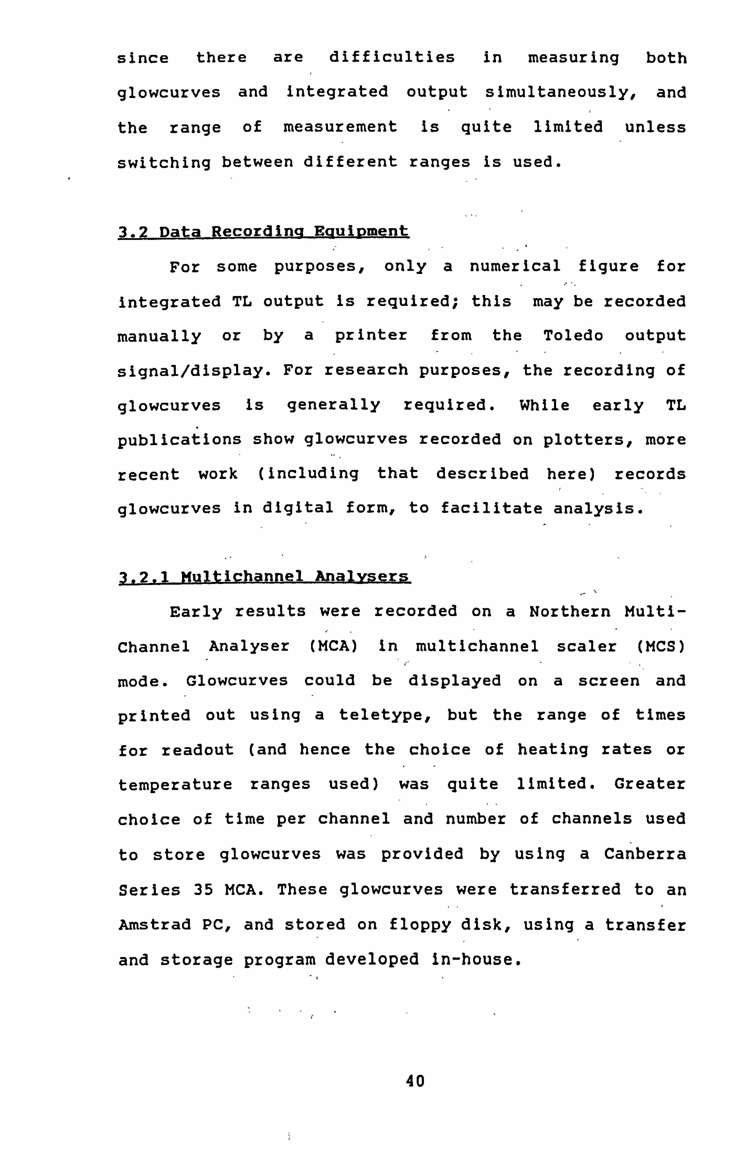
3.2 Data Recording Eguipment

For some purposes, only a numerical figure for

integrated TL output Is required; this may be recorded

manually or by a printer from the Toledo output

signal/display. For research purposes, the recording of

glowcurves Is generally required. While early TL

publications show glowcurves recorded on plotters, more

recent work (including that described here) records

glowcurves in digital form, to facilitate analysis.

3.2.1 Multichannel Analysers

Early results were recorded on a Northern Multi-

Channel Analyser (MCA) In multichannel scaler (MCS)

mode. Glowcurves could be displayed on a screen and

printed out using a teletype, but the range of times

for readout (and hence the choice of heating rates or

temperature ranges used) was quite limited. Greater

choice of time per channel and number of channels used

to store glowcurves was provided by using a Canberra

Series 35 MCA. These glowcurves were transferred to an

Amstrad PC, and stored on floppy disk, using a transfer

and storage program developed In-house.

40

3.2.2 SWTGOOO ComDuter

A program had been developed in the Physics

Department to receive output pulses from the Toledo,,

store them in the computer memory and write the

glowcurve to a floppy disk at the end of the readout

cycle. A wide range of time per channel was available,

while the fixed 200 channels per glowcurve was found

suitable for all cases. Simple and later more complex

analysis of the glowcurves was performed on the same

computer.

3.2.3 PC with MCA Card

For the measurement of TL of foodstuffs, a MCA was

at f irst used, but subsequently a dedicated Amstrad PC

was purchased. This incorporated a MCA card (MCS mode)

from Nucleus Inc. for data acquisition and limited

analysis. The glowcurve data was stored on the

computer's hard disk, offering considerably greater

storage capacity than earlier systems.

3.2.4 Solaro Clowcuxve Recording

Part of the Solaro software-- package is a system

for recording and storage of up to 800 glowcurves, on a

designated part of the hard disk. When this Is full.,

the glowcurves can be transferred to floppy disk for

long-term storage If required, and the hard disk area

wiped clean to make room for new glowcurves. Analysis

is quite limited,, allowing only subtraction of two

41

curves, multiplication by a constant and moving the

boundaries between preheat, read and anneal regions

over which the glowcurve areas are summed. The heating

(thermocouple output) Is also recorded with the

glowcurve; this has proved useful on occasion in

detecting heater or thermocouple faults which have

caused anomalous absorbed dose readings.

The same glowcurve recording package is used on

the Rialto, and Is also available as an option for use

with the Toledo 654 reader.

3.2.5 Discussion

The gradual trend towards improved technology,

greater sophistication and computer control, noted

earlier for TL readers.. is also apparent In digital

recording of glowcurves. Improvements In speed and

storage capacity of PCs', combined with steadily

decreasing prices, have made their use widespread. The

storage of glowcurve data on computer facilitates

analysis, but most commer cially available systems offer

little more than summing different regions under the

glowcurve. Only the-more -recent Harshaw readers offer

computerised glowcurve deconvolution to separate

overlapping peaks; this Is described In more detail In

Chapter 5. With PCs now more widely used In

thermoluminescence dosimetry, it is expected In that

development of software by physicists for research

purposes and applications will become more widespread.

42

perspex shield

Source holder

perspex

90Y/9OSr foil

/// // /�_

rotating disk

/

////v

Figure 3.1 90Y/90Sr Irradiator

43

source in

3.3 irradiators

3.3.1 90Y/9OSr Irradiator

For the first few months of the work described In

this thesis, a Pitman Model 623 Irradiator was

available on loan from the company. This is described

(and illustrated) by Oberhofer, 1981. It has two

90 90 carefully matched Y/ Sr sources above and below a

rotating turntable which can hold 30 dosemeters. The

sources are shielded and can be shut off from the

turntable by shutters. Dosemeters can be loaded and

left to be Irradiated automatically until a preset.

number of revolutions has elapsed.

When this Irradiator was no longer available., an

irradiator to operate in a similar manner was designed

and built for this work. This Is shown in Figure 3.1.

Like the Model 623, the moving parts were based on a

record player turntable. A 90Y/9OSr source (140 MBq on

1.1.91) In the form of a rectangular foil was bent Into

a U-shape and fixed In a perspex holder., so as to

Irradiate the dosemeters both from above and below.

Dosemeters were placed In circular depressions machined

around the perimeter of a perspex disc so that they

passed through the middle of the U-shaped curve when

the disc rotated. The source assembly was enclosed In a

2 cm thick perspex box, which was adequate shielding

for the 0.6 and 2.2 MeV beta-particles from 90Y/90Sr.

Instead of counting revolutions, Irradiations were

timed with a stopwatch. Care was taken that the doseme-

44

ters were always well away from the source when

rotation stopped at the end of an Irradiation, so that

the dosemeters were all Irradiated equally.

McKinlay (1981) describes how a 90Y/90sr

Irradiator is the most suitable for routine laboratory

irradiation as It meets three requirements:

(1) reproducibility of absorbed dose,

(2) fixed numerical relationship between

laboratory irradiation and calibration absorbed

dose,

and (3) convenience of use.

The Irradiator described above has fulfilled these

criteria. and operated reliably over a period of 10

years. Results are .

reproducible, although over long

periods correction must be made for the decay of the

source (half-life 28 years). A calibration figure was

produced in May 1982 by measuring the response of LIF-

Teflon dosemeters Irradiated In the Irradiator. The

dosemeters had been previously calibrated by

Irradiating them overnight at a known distance from a

6OCo source. Results showed that irradiation in the

90Y/90Sr Irradiator for one hour gave a response equal

to that from 20.3 ± 1.0 mGy In air absorbed dose from

6OCo. Further measurements with the dosemeters in

different positions confirmed that Irradiation was

uniform for these positions, I. e. that there were no

geometrical or, mechanical errors In the arrangement or

operation of the irradiator. It has certainly fulfilled

45

the criterion of convenience of use: the source is well

shielded so that the Irradiator can be located In the

laboratory; also dosemeters can be irradiate d to a

convenient absorbed dose of approximately 5 mGy In

approximately 15-20 minutes. This may be compared to

several hours or overnight irradiation which would be

required for the same absorbed dose from the ý-sources

available in the laboratory.

137 3.3.2_ Cs Irradiator

The environmental monitoring programme described

in Chapter 7 requires the use of an Irradiator

containing a 137Cs source, nominally 50 mcl, with

calibration traceable to NPL standards. Up to 30

dosemeter cards can be Irradiated in badges mounted in

" circle radius 40 cm. The source is normally stored In

" lead pot approximately 40 cm -below the badges. It is

raised into irradiation position by a small motor

(designed for raising a car aerial) and returned to the

lead pot after one hour of irradiation, controlled by a

programmable timer. In one hour the dosemeters are

Irradiated to approximately 900 )1Gy in air; the exact

value of absorbed dose Is corrected on each occasion

for decay of the source.

This irradiator is situated in a small room with

walls 1-2 m from the source, so there may be errors in

absorbed dose due to scatter. This is a common problem

46

with 137CS Irradiators of this type (Maiello et ý al,

1990) and requires ' further Investigation. , "It' is

expected that the problem will be overcome by moving

the irradiator in the' near future to a much larger

room.

3.3-. 3 X-ray Irradiators,

LiF dosemeters used for patient dose measurements,

as described In chapter 6, were calibrated with a

Garantix diagnostic medical X-ray set In the John Perry

Metrology laboratory (a NAMAS accredited secondary

standard facility)-. For patient dosimetry, irradiation

was at 60 or 80 kVp as- appropriate, for- the procedure

being monitored. It -is Important to - use the

appropriate kVp due 'to 'the' sl Ight, over-response , of LIF

compared with tissue at diagnostic energies (Bassi et

al,, 1976). Dosemeters were arranged on a3 cm thick

tissue-equivalent block at approximately 1.5 m from the

focus of the X-ray tube. They-were confined to-a region

approximately 10 x 10 cm within which the field was

known to be uniform, to within ± 1%; -- -the absorbed dose

was measured with a calibrated 11mdh11- electrometer,, the

reading being corrected to standard temperature and

pressure.

3.3.4 GoCo Irradiator

For the Irradiation of foodstuffs wh ose TL

response Is described In Chapter 8, a high dose-rate

47

irradiator was required, as an absorbed dose-of several

kGy is typically used for Irradiation of ., foodstuffs.

For this application,, a Thompson-I'Super-Hot Spot" 6OCo

irradiator was used. The dose rate varied over the

period of the experiment described due to decay-of the

source, but was for example 0.13 ± 0.01 kGy/h (Walker,

1991) so that Irradiation times of 24 to 48 hours were

typically used.

3.3.5 Discussion

Four very different irradiation facilities have

been described above. They cover a wide range of

energies and dose rates, and each has been found

convenient In use and well suited to Its respective

application. There is little scope (or need) for maJor

improvements in irradiation facilities for TLD.

3.4 Other EcuiiDment -I

The most important Items of TLD equipment have

been described In the previous sections. Here, various

items needed for correct storage,, handling and thermal

treatment of TL materials-are briefly described.

3.4.1 Handlinq

Dosemeters were always handled with care and

protected as much as possible from dust., dirt and light

to avoid their becoming dirty and/or showing high

48

background signals. They were usually handled with

vacuum tweezers, which cause less scratch Ing or surface

deterioration than manual tweezers. The latter were

however used where necessary, mainly for packaging and

Inserting dosemeters In positions not readily

accessible to vacuum tweezers. Robertson (1975) and

McKinlay (1981) discuss various factors associated with

good practice In storage and handling of dosemeters.

Dosemeters and trays were cleaned when necessary

with ethanol or methanol., followed by rinsing In de-

Ionised water. When not used entirely within the

laboratory, they were sealed In plastic sachets or

packets of various types to protect them from dirt and

allow the packets to be positioned by hand for the

various applications.

3.4.2 Storage

Dosemeters were stored in darkness, since many TL

materials show a response to visible light or UV light.

This could cause errors In measured response to

ionising radiation if dosemeters were exposed to light.

Hygroscopic materials were kept in a desiccator; this

was particularly Important for foodstuffs prepared by

freeze-drying or drying in an incubator.

Where a constant temperature some 10 or 200C above

or below room temperature was required, materials were

stored In sealed containers in a refrigerator, or loose

on the shelves of an incubator In the laboratory.

49

3.4.3 Ovens

Ovens were at times required for annealing, or for

maintaining dosemeters at temperatures well above room

temperature for extended -periods of time. --Oberhofer

(1981) describes and illustrates several, types of ovens

, for use in TLD. Of these, the Pitman programmable

annealing block was used for early work.. ' a small oven

(Thermolyne Type 1300) for later studies, and a larger

programmable, Pickstone oven with fan-assisted air flow

for the environmental monitoring and, patient dosimetry

studies. Scarpa (1990) reviews the characteristics of

various types of ovens used in Italy for some TLD

applications and concludes that programmable -fan-

assisted ovens give -the best performance In terms of

temperature , uniformity within the oven, and

reproducibility of the heating cycle.,

3.5 Conclusions

In this chapter the equipment used (purchased or

developed) has been described in some, detail; trends

and improvements have been noted- in the, discussion at

the end of each section. The overall picture Is one of

steady improvement In ý instrumentation,, as might

be expected. Increasing use of computers to control the

equipment have not greatly reduced the amount of work

involved In making TLD measurements, but enabled larger

studies to be carried out and more reliable results to

be presented. ý11

so

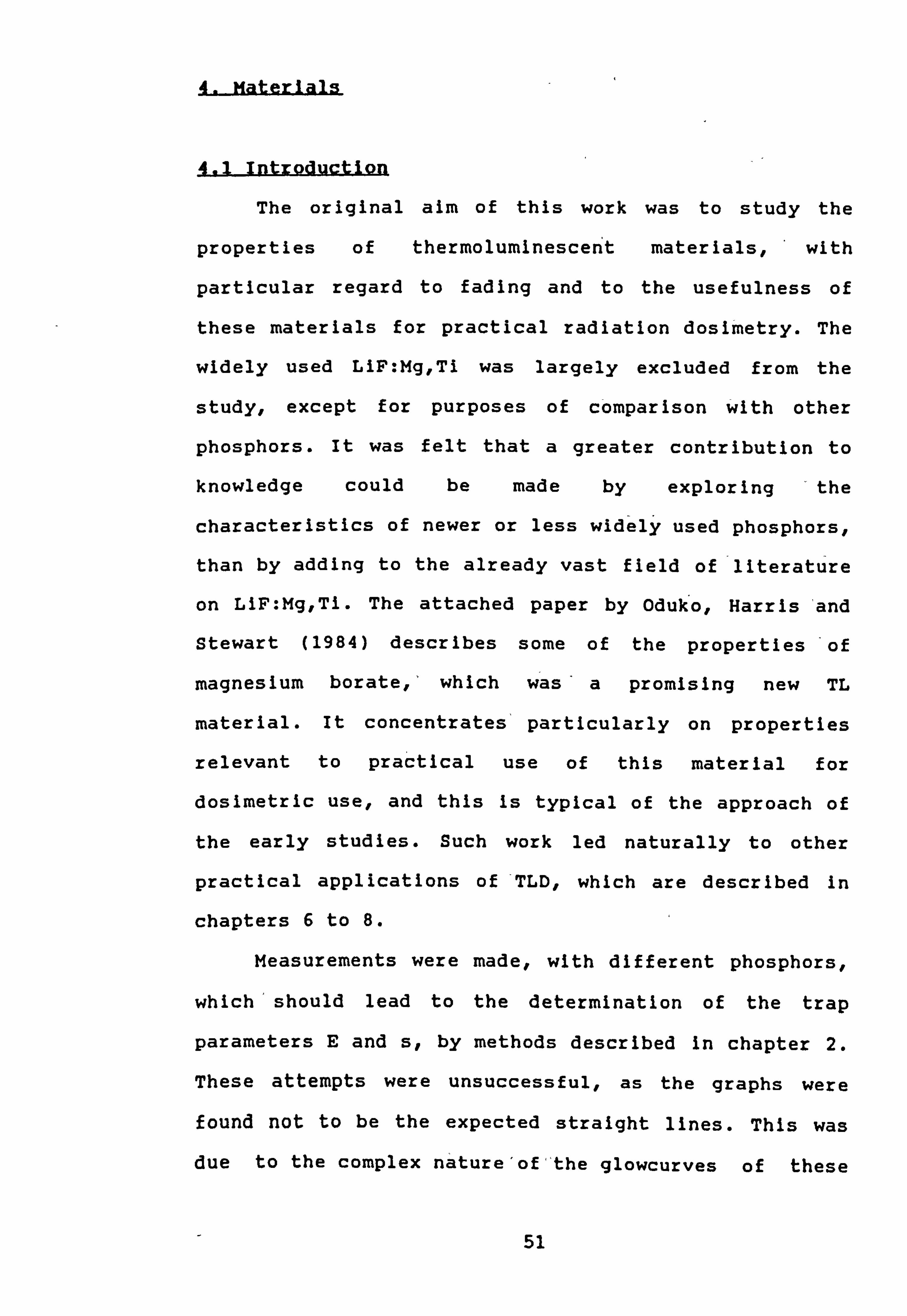
4.1 Introduction

The original aim of this work was to study the

properties of thermoluminescent materials, ' with

particular regard to fading and to the usefulness of

these materials for practical radiation dosimetry. The

widely used LIF: Mg, Ti was largely excluded from the

study, except for purposes of comparison with other

phosphors. It was felt that a greater contribution to

knowledge could be made by exploring -the

characteristics of newer or less widely used phosphors,

than by adding to the already vast field of literature

on LiF: Mg, Ti. The attached paper by Oduio., Harris 'and

Stewart (1984) describes some of the properties 'of

magnesium borate, ' which was' a promising new TL

material. It concentrates particularly on properties

relevant to practical use of this material for

dosimetric use, and this Is typical of the approach of

the early studies. Such work led naturally to other

practical applications of _TLD., which are described in

chapters 6 to 8.

Measurements were made, with different phosphors,

which ' should lead to the determination of the trap

parameters E and s, by methods described In chapter 2.

These attempts were unsuccessful, as the graphs were

found not to be the expected straight lines. This was

due to the complex nature'of-the glowcurves of these

51

materials, as was made clearer by the computerised

glowcurve analysis technique described In chapter 5.

Thus, for example, the shift of the main peak

temperature in magnesium borate heated at different

rates results from different relative shifts, of its

component single peaks. Attempts to separate the peaks

by experimental means met with little success. , Full

interpretation of these results, which include,

measurements of hundreds of glowcurves, awaits the

completion of computerised glowcurve deconvolution of

the glowcurves. As explained In detail In chapter, 5,

the program could not run on the SWT6800 microcomputer

on which most of the glowcurves were stored. Transfer

to the Opus III microcomputer, on which the program

runs, is at present by the slow means of keying In the

data for each channel of each glowcurve. On completion

of this process (preferably by developing some faster

means of data transfer), the glowcurves will be

analysed and the data Interpreted and results

published. Values of E and s for the peaks can also be

determined, when the peak parameters have been reliably

established by analysis of a series of glowcurves.

In the rest of this chapter, the properties of the

TL materials studied will be briefly reviewed. For an

early study comparing the properties of most of these

materials (ie excluding magnesium borate and copper-

doped lithium fluoride which are relatively new) see

Attix et al (1968). More recently, Portal (1986) has

52

reviewed the properties of all the phosphors discussed

here.

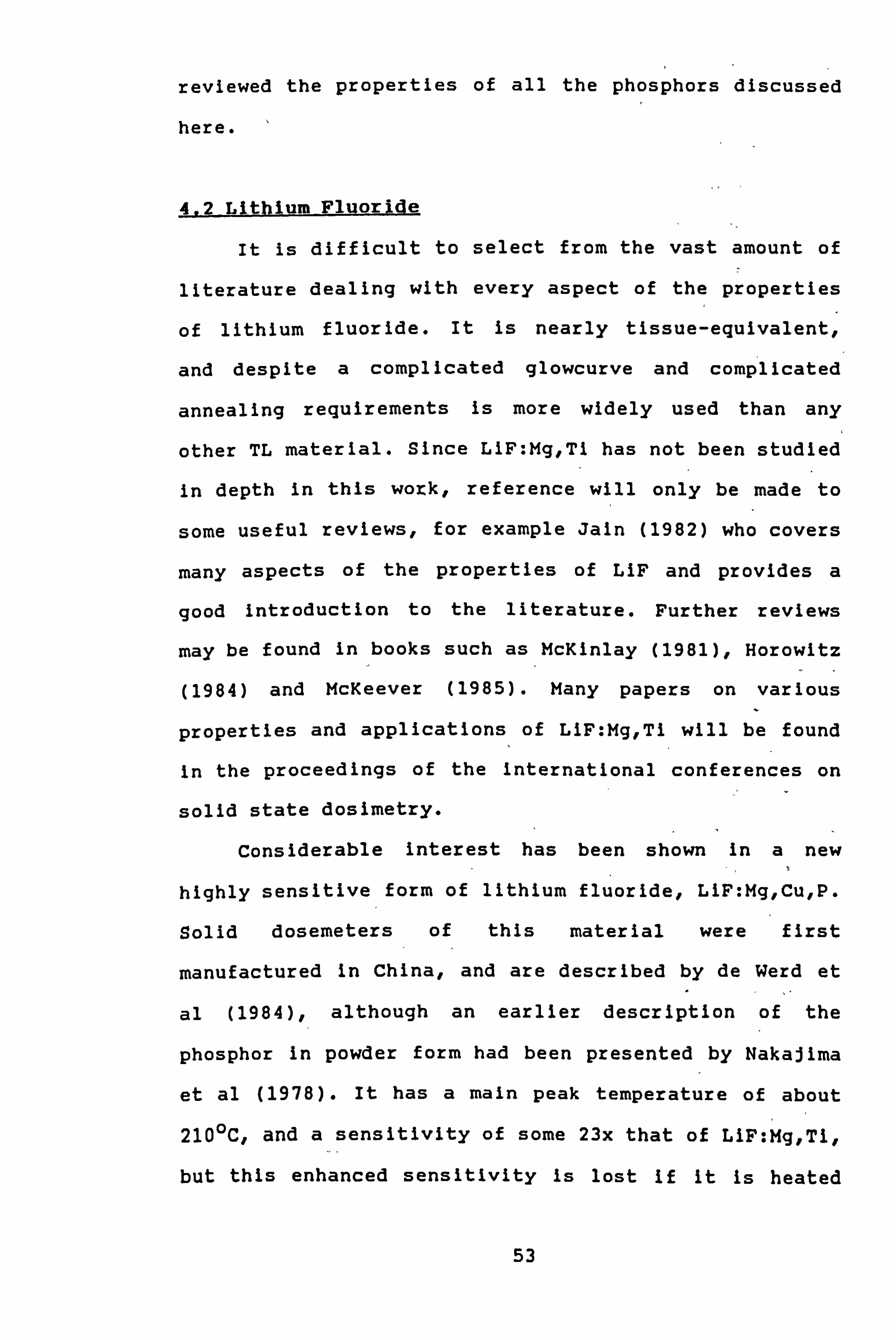
4.2 Lithium Fluoride

It is difficult to select from the vast amount of

literature dealing with every aspect of the properties

of lithium fluoride. It Is nearly tissue-equivalent,

and despite a complicated glowcurve and complicated

annealing requirements is more widely used than any

other TL material. Since LIF: Mg, TI has not been studied

in depth in this work, reference will only be made to

some useful reviews, for example Jain (1982) who covers

many aspects of the properties of LiF and provides a

good introduction to the literature. Further reviews

may be found In books such as McKinlay (1981), Horowitz

(1984) and McKeever (1985). Many papers on various

properties and applications of LIF: Mg, Ti will be found

In the proceedings of the International conferences on

solid state dosimetry.

Considerable Interest has been shown in a new

highly sensitive form of lithium fluoride, LiF: Mg, Cu, P.

Solid dosemeters of this material were first

manufactured In China, and are described by de Werd et

al (1984), although an earlier description of the

phosphor in powder form had been presented by Nakajima

et al (1978). It has a main peak temperature of about

2100C, and a sensitivity of some 23x that of LiF: Mg, TI,

but this enhanced sensitivity Is lost if It is heated

53

to a temperature above about 2500C. The dependence of

Its properties on concentrations of mg, Cu and P have

been studied by Shoushan (1988), while Wang et al

(1990) and Fang et al (1990) describe the use of this

material for neutron dosimetry and skin dose

measurements respectively. Piters and Bos (1990)

discuss the influence of cooling rate on the

repeatability of the dosemeters' performance, while

Horowitz and Horowitz (1990) discuss annealing

considerations. Despite their promising

characteristics, these dosemeters, have not yet come

Into widespread use, and are not yet commercially

available in the UK.

4.3 Maqnesium Borate

While Kazanskaya et al (1974) described an early

form of magnesium borate dosemeters,, the material of

interest in recent years has been that made at the

Boris Kidric Institute and described by Prokic

(1980,1982). The magnesium borate is doped with Dy or

Tm, and made into sintered pellets. It was Introduced

as a very promising new material for dosimetry, because

of its simple glowcurve, simple annealing requirements

and near tissue-equivalence. Studies by Barbina et al

(1981) and Driscoll et al (1981) reported some

disadvantages high fading, significant light-induced

fading and considerable variation In sensitivity within

a batch. Improvements in the performance of the

54

magnesium borate dosemeters have recently been reported

(Prokic, 1990) and a carbon-loaded form for beta

dosimetry has been developed (Prokic, 1984).

Some MgB407: Dy dosemeters from the Boris Kidric

Institute were supplied to the author by Vinten

Instruments and their properties were studied In some

detail. Reference is made to the attached paper (Oduko,

Harris and Stewart, 1984) which reports the results

they will not be repeated in detail here. The

dosemeters were found to be sensitive to light and uv,

and some of them had poor physical properties. However,

re-estimation of absorbed dose by re-reading (at a

higher temperature) was shown to be possible. This

would be useful for personal dosimetry.

4.4 LitLAum Borate

Lithium borate is an attractive material for

dosimetry because of its good tissue-equivalence

(effective atomic number 7.4). L12B407: Mn was first

described by Schulman et al (1965). It has a relatively

simple glowcurve, and simple annealing, but the

disadvantages of being hygroscopici, and of having low

sensitivity,, approximately 1/10 that of LiF. This is

because of its emission of orange light, to which

ordinary PM tubes are less sensitive, whereas LiF emits

blue light. Some early studies of L'213407: Mn Include

Jayachandran (1970), Driscoll et al- (1984). Studies of

its suitability for use in patient dosimetry are

55

reported by Langmead and Wall (1976),, and wall et al

(1982).

Several of these papers also compare the

properties of L12B407: Mn with L12B407: Cu, a more

sensitive form of lithium borate because of Its

emission of blue light. Takenaga et al (1983) describe

this phosphor, which has been manufactured in a special

encapsulated form for use with Panasonic TLD readers

(Yamamoto et al, 1982). The encapsulation overcomes the

problem of hygroscopicity. A recent study of further

properties of this phosphor Is reported by Ben-Shachar

et al (1989).

4.5 Beryllium Oxide

Beryllium oxide is nearly tissue-equivalent, with

effective atomic number 7.13. It Is cheap, due to its

manufacture on a large scale for other purposes (in

electronics), but the glowcurve structure depends -on

the impurities present. Considerable interest in this

material in the 1970s (Scarpa 1970, Scarpa et al 1971,

Becker et al 1970, Crase and Gammage 1975) did not lead

to its widespread acceptance and use except In Italy

where it continues to be used routinely for personal

d'Osimetry (Busuoli et al 1984, Scarpa et al 1990). The

dosemeters are highly sensitive to uv, which causes

photo-transferred thermoluminescence. This Is useful

for dose re-estimation in personal dosimetry.

56

4.6 Calcium SuljRhate

Calcium sulphate Is not tissue-equIvalent

(effective atomic number 15.3)., but It Is highly

sensitive and has- been widely used for this reason.,

especially for environmental monitoring. Itý may be

doped with Dy, Tm or Mn., the latter being the most

sensitive but suffering, from the disadvantage of

extremely high fading. Many studies on CaS04 have -been

published (though not, as many as on LIN ;a review Is

provided by Sunta (1984). Yamashita et al (1971) report

the Introduction of CaS04: Dy and Tm as new materials

with, less fading than CaS04: Mn. Papers on properties

and applications of calcium sulphate phosphors continue

to appear eg Kasa (1990), Morgan and, Stoebe., (1990).

They also have some usefulness for uv dosimetry (Nambi

and Higashimural 1971) ; uv affects the dosimetry peak

and creates new- peaks In the glowcurve (Chakrabarti et

al, 1990).

The properties of these selected materials have

been presented only briefly here. Some glowcurves which

have been recorded for them, and results of preliminary

analysis of these glowcurves, are presented In chapter

5.

57

5. Comvuterlsed Glowcurve'Deconvolution

5.1 Introduction

In October-November 1982, the, author spent several

weeks at the Radiation Physics, Laboratory, Ben Gurion

University of the' Negev,, ' Beersheva,, 'Israel., and

contributed to the development of a computer program

for' the deco'nvolution of glowcurves Into separate

p7eaks. The program Is described by Moscovitch, Horowitz

and Oduko (1984). The paper shows -how, the use of the

program on tIF glowcurves gave Improved precision of

measurement over the standard technique 'of background

subtraction by using a second readout.

The program has 'subsequently been used In various

studies' with 'LIF, Including measurements at very, high

and very low ranges' of absorbed, dose (Horowitz and

Moscovitch, 1986alb and Horowitz, Moscovitch and Wilt,

1986). It was also used to estimate the time between

irradiation and readout-from the ratios of, peak 20; 3 and

5 of LiF (Moscovitch., 1986). -Other recent appfications

with LIF are given 'by MoscoVitch et al (1990) and

Horowitz and Shachar (1990). Applications of the

program to other TLD 'materials has been limited, but

Horowitz and Horowitz (1990) used it for LiF: Cu,, Mg., P

and Shachar and Horowitz'-(1988) for CaF2: Tm. The

program has recently been Incorporated 'Into data

analysis software for use with Harshaw-readers.

other authors have more recently developed

computerised methods for analysis of glowcurves into

58

separate peaks. Sahre (1987) describes such a- program

and its use for CaS04: Dy dosemeters In environmental

monitoring. He uses Gaussian curves.. however,, to fit

the peaks, following the suggestion of Mangla et al

(1977), although there Is little physical basis-for the

choice of the Gaussian. Peto (1990) describes the

analysis of A1203 glowcurves with a program he has

developedl which has the advantage of including peaks

of both first and second-order kinetics. Perks and

Marshall-(1990,, 1991) describe and compare three methods

for glowcurve analysis. -The first, like the program of

moscovitch, Horowitz and Oduko (1984) uses Podgorsak's

equation for first-order kinetics peaks (Podgorsak et

all 1972). The second method involves - dividing an

experimental glowcurve by a reference glowcurve. The

third uses successive subtractions of the most

prominent peaks.. using the results of the first two

methods. de Vries and Bos (1990) and Bos et al (1990)

describe the use of their own glowcurve analysis

program on measurements with LIF MD-100). They do not

disclose the- equation 'used for the -, peaks., but it

Involves four parameters for each peak (order of

kinetics., trap depth, frequency factor and number of

traps). Delgado and Gomez Ros (1990) and Delgado et al

(1992) describe a s. implified method of partial

glowcurveýanalysisj as applied to measurements with LiF

at low dose and In - photo-transferred

thermoluminescence, respectively. This method involves

59

fitting the background tail of the glowcurve with the

exponential function suggested by Moscovitch, Horowitz

and Oduko (1984), subtracting this background from the

glowcurve, and then summing the curve overý certain

regions rather than fitting separate peaks to it. It Is

likely that further development of such techniques for

analysis will be carried out as personal computers are

becoming cheaper and'more powerful. -

5.2 The-Progra

The program Is described only briefly here., but

reference- should be made to the attached paper by

Moscovitch, Horowitz and Oduko. (Greater detail cannot

be given due --to an agreement between 'the authors of

this paper,, and because the program has been

incorporated In the Harshaw software package).

The peaks are fitted by an equation for a lst

order kinetics peak, suggested by Podgorsak et al,

1972.

P= Imexpll+(T-Tm)/Tm*E/kTm-exp((T-Tm)/TM*E/kTm)I (5.1)

where E Is the activation energy of the peak, T Is the

temperature,, Tm Is the temperature of the glow-peak

maximum, Im is the Intensity of the glow curve at

temperature Tm, and k is Boltzmann's constant.

An equation was chosen to fit the background,

which increases for higher temperatures forming a

60

"tall" on the glowcurve.

B=a exp (T/b) +c (5.2)

where a, -b and 'c' are constants chosen to give 'a good

fit to the background. This exponential form is purely

empirical, but it has proved suitable for use In a wide

range of experiments. The constant term c corresponds

to the low level of background noise at the beginning

of a glowcurve. The values of a and bf ound by curve-

fitting depend on how much of the background tall Is

taken into account. The background is only'fitted and

then subtracted In practical use, so this variation'of

a and b values Is not a problem.

The whole glowcurve Is then f Itted to the sum of

the background B and as many peaks P, as are

appropriate for the application, e. g. for LIF up to

30011C

y" P2 + P3 + P4 + P5 +B (5.3)

where the subscripts denote the usual peak numbering

for'LIF. (Peak 1 decays rapidly at room temperature and

is not normally seen). Each term on the right hand side

of equation 5.3 Is -characterised by 3 parameters, which

are the height, width and peak temperature (or channel

number) for each peak P, and the parameters a, b and c

for the background term B. The task of the program Is

to find the optimum values of these parameters'(15 -in

61

the example of equation 5.3) to fit ,a glowcurve of

typically 200 experimental points.. The fitting is

carried out by repeated iterations on the computer,

using a combination of the, Newton-Raphson method and a

search for the minimum)(? value. Further ý -details are

given in the original paper (Horowitz, Moscovitch and

Oduko, ý1984).

The original program was developed in Basic on an

Apple microcomputer. The ' author .,, made some

modifications, to make it better suited to the Toledo's

output glowcurves, and to run on the SWT6800 computer

used for recording glowcurves. - Despite considerable

efforts, the program was unable to run to completion (a

good fit to the experimental points) without

"crashing". This reflects the limitations of the

SWT6800 computer, so the program was then modified to

run on a Opus III microcomputer. This version has

proved successful, and analysis has been performed on a

number of glowcurves to date. Results are presented In

section 5.3. '

The values of the starting parameters fed into the

program are, very important in obtaining a good final

fit. If they are poorly chosen the program may stop

when the series is no longer converging, and no good

fit Is obtained to the experimental data. (A good -fit

is one for which the final value of 'X? is not much

greater than 1). The process may beývisuallsed as a

search for the minimum value of 0 in n-dimensional

62

space, where n Is the number of parameters being varied

and Q is the sum of the squares of the differences

between the computed and the experimental points. If

the starting parameters are too far from the correct

values for the glowcurve, the search may lead to a

local minimum value of 0 rather than the true (overall)

minimum value. The peak height (IM) and the temperature

of the glowpeak maximum (Tm) are easy to estimate for

well-defined single peaks, but the peak width parameter

is less obvious. In the case of overlapping peaks.,

choosing initial values of all three may prove

difficult. As mentioned earlier, the constant c may be

found from the beginning of the glowcurve, but choice

of values for the constants a and b also presents some

difficulty.

A procedure was developed to use a Lotus 123

spreadsheet, with Its associated graphical display

facility, to obtain reasonably good starting parameters

before using the computer program. The experimental

data and the equations of the Individual peaks were

stored In different columns of the spreadsheet, while

the graph displayed the experimental data and the sum

of the calculated peaks. Then the peak parameters

invariably gave a good fit in a small number of

iterations of the computer program (except where first-

order kinetics was not appropriate, as described

later). This process is recommended for use when

fitting the glowcurve of any new material with the

63

program. The spreadsheet peak-fitting procedure

replaces an earlier technique for finding good starting

parameters for the program. This involved fixing some

of the parameters, such as the peak heights and

positions of easily resolved peaks which could be read

from the glowcurve, and allowing the others to'vary In

a preliminary run of the program. Only part 'of the

glowcurve might be used In this process. The results of

this run (or several such runs, in stages) could then

be used as starting parameters for the main run-of the

program, in which all the peak and background

parameters were allowed to vary. The results of this

process were generally satisfactory, but It-was much

more time-consuming than the use of the spreadsheet. It

should be noted that most of the work already published

using this program concerns LIF, for which the values

of starting parameters (apart from peak heights, which

are dose-dependent) were already well known. ' The

spreadsheet procedure is not needed in such cases.

The results of analysis of a number of glowcurves

are presented In section 5.3, to Illustrate the use of

the program. The reasons for presenting only a limited

number are (1) the time-consuming nature of the

spreadsheet/graph fitting process described above, and

(2) the glowcurve data had to be typed manually into

the Opus III microcomputer. Ideally some means of data

transfer from the SWT6800 to the Opus III should be

developed, or else the process of keying 'in data

64

manually may be continued, although this is obviously

very time-consuming. Further work Is In progress to

complete the analysis of hundreds of glowcurves which

have been recorded for various different TLD materials.

It may be useful in future that the program is running

on an Opus III computer., since this Is the computer

used to run the Solaro and the Rialto TLD readers. It

would be easy, therefore, to run the program as it is

on glowcurves recorded on a Solaro or Rialto.

The computer program Is a purely mathematical

technique, and could be used to fit almost any curve if

a large enough number of peaks were chosen. Care must

be taken In its use and In the Interpretation of the

results so that they are physically meaningful and

consistent. Peak heights vary with absorbed dose, but

the other peak parameters should remain the same for

different values of absorbed dose, and after fading at

different temperatures and for different times (unless

a peak has faded completely). Some preliminary results

indicate that this is the case. When used

intelligently, the program is, a powerful tool for the

analysis of glowcurves, especially when the peaks

overlap to an extent that makes experimental methods of

peak separation relatively unsuccessful.

5.3 Some Results

Figures 5.1 to 5.14 illustrate the process and

results of computerised glowcurve deconvolution, for 6

65

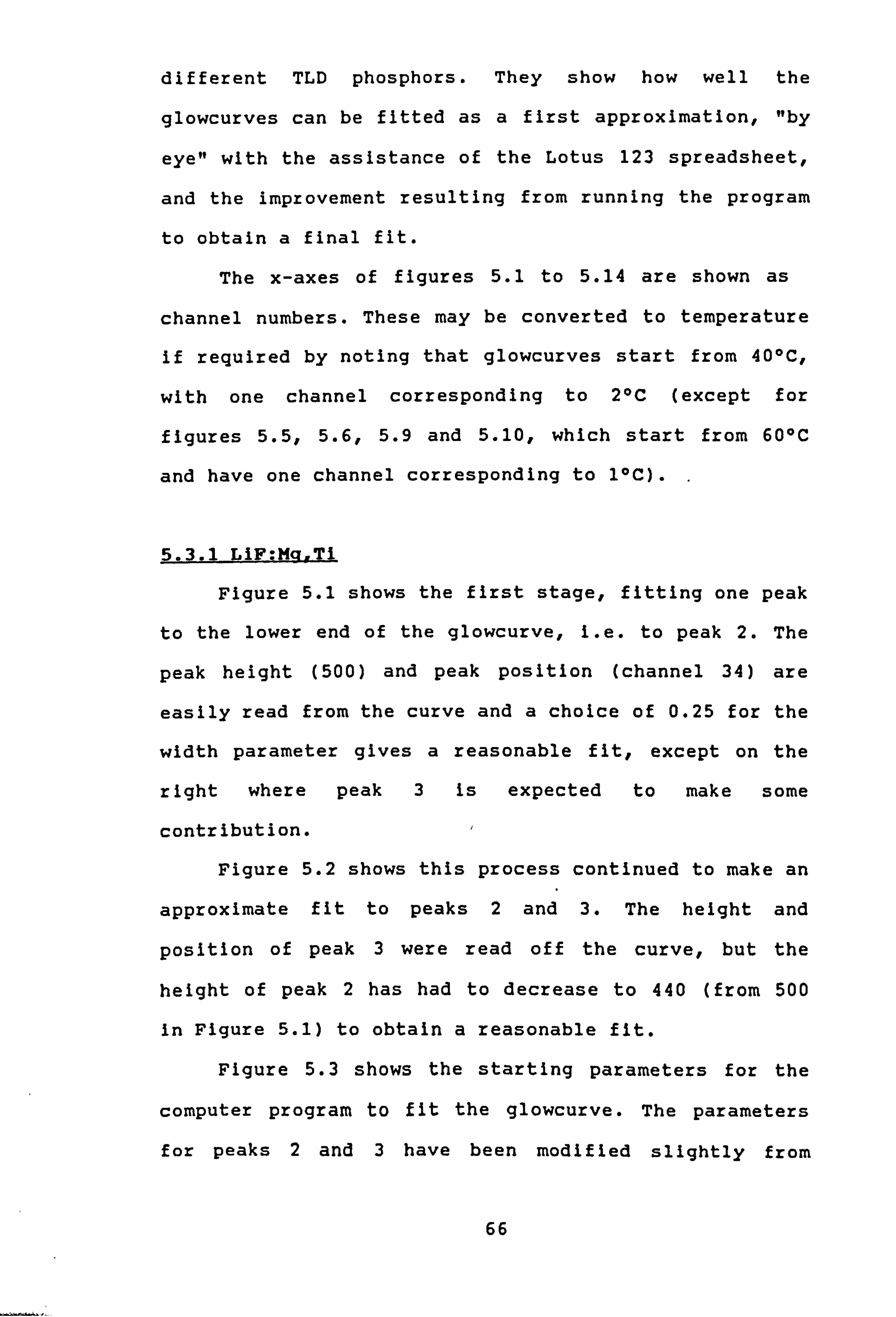
different TLD phosphors. They show how well the

glowcurves can be fitted as a first approximation., "by

eye" with the assistance of the Lotus 123 spreadsheet,

and the improvement resulting from running the program

to obtain a final fit.

The x-axes of figures 5.1 to 5.14 are shown as

channel numbers. These may be converted to temperature

if required by noting that glowcurves start from 400C,

with one channel corresponding to 20C (except for

figures 5.5., 5.6,5.9 and 5.10, which start from 6011C

and have one channel corresponding to 10C). .

5.3.1 LIF: Mg,, Ti

Figure 5.1 shows the first stage, fitting one peak

to the lower end of the glowcurve, I. e. to peak 2. The

peak height (500) and peak position (channel 34) are

easily read from the curve and a choice of 0.25 for the

width parameter gives a reasonable fit, except on the

right where peak 3 is expected to make some

contribution. I

Figure 5.2 shows this process continued to make an

approximate fit to peaks 2 and 3. The height and

position of peak 3 were read off the curve., but the

height of peak 2 has had to decrease to 440 (from 500

In Figure 5.1) to obtain a reasonable fit.

Figure 5.3 shows the starting parameters for the

computer program to fit the glowcurve. The parameters

for peaks 2 and 3 have been modified slightly from

66

0

0 0 LO

, 11 C-

L6 C14

. qr NO

CL

sanioA i,

Figure 5.1 Fitting Peak 2 of LIF: Mg, Tl

0 0 c6 rn

0

0 0>

X r4)

CL x LLJ

00 0 1.6 C14

0 0 Cý C14

67

0000 000 LO n

LO

Cý 0

C14

C'4 0-

sanjoA ),

Figure 5.2 Fitting Peaks 2 and 3 of LiF: Mg, Ti

0 0 4 Ln

0 0 6

Ln

0 0 L6 t

0 0 Cý , It

0 0 00 to V)

(U

0>

Cý x 't r4)

ä M)

0

0 0

Cý CN

0- x LU

0

68

0000000

Ln

LLI

(I.

Ln r- cli CN

00

L6

C14 i

0

le 0-

(3) I-t

clý LO L. r)

0-

Lfi Cý

C: ý le

Cl-

0 00

0 LU

6

0 C14

0

ýN o) 00 r- Lo LO t ff) N 0) 00 r- Lo Ln 't r) C, 4 , 66666666

(spuosnoL41) Indlno IqBl-l

Figure 5.3 Fitting LiF: Mg, Ti Clowcurve:

Starting Parameters

CL

tr)

LLJ 0-

(14 V

Lli CL

0 -J 0

x LLJ

ID

69

(. 0

LC)

0ý LO 0)

Lh le

CL

Pr) , It f-i LO

as 00 CN

Cý

(. 0 r*: ý Nr le n 00 Ln M

0 0 Cý P-i It 0 Lr) r; -i

04 L

LO

0 00

0 (D

0

0 C'4

0

6ý ý CN 0) 00 r- LO 1-t rt) N 0) 00 r- to LO 0

Ne 0- Cý

(s pu os no L4_L) Indlno It451-1

Figure 5.4 Fitting LiF: Mg, Ti Glowcurve:

Final Fit

LO

V LLJ a-

-ýt

V LLJ

(I

LLI

6

C14

bi n

0 -J 0

12-

0

70

those of Figure 5.2. The smooth curve which is the sum

of the individual peaks Is an approximate, but not very

good, fit to the experimental points.,

Figure 5.4 shows the final f It. All 12 parameters

have been allowed to vary, and although they have not

changed very much from those of Figure 5.31 the

calculated curve Is now a good fit to all the

experimental points except the last 6. (Possibly a

small peak 6 contribution or the start of the

background tail should be added In for these points).

The value of -X2 for this final fit was 3.57 - rather

high for a good fit, but this Is probably mostly due to

the last 6 points.

5.3.2 LIF: Cu, Mg, P

Figure 5.5 shows the starting parameters. Although

peak 2 at channel 35 Is hardly visible In this f Igure,

it is clearly seen on a larger scale.

Figure 5.6 shows the final fit, which again passes

through all the points., except for 2 at the extreme

right. The parameters were all varied, but do not

differ greatly from those of Figure 5.5. Peak 6 Is

perhaps Inappropriate., It might be replaced with an

exponential tail. X2 was 4.77 for the final fit.

5.3.3 MgB4Q7**Dv

Figure 5.7 shows the starting parameters, with a

good fit already obtained as the curve passes through

all the points, but not quite symmetrically.

71

C, 4

0-

0 Lo

C) CD N r-

CL (. 0

0 0

OL

LO

Ln _EI

ri

0 (D oo r- (. 0 LO e mý CN - 0 C, CO r, - (, 0 Lo e M) CN - CD C, j

(spuosnotAl)

Indlno lqbl-l

Figure 5.5 Fitting LiF: Mg, CuP Glowcurve:

Starting Parameters

LO

\1 CD < 00 LU

0

(. 0

< LU

0

00

0 (D

LU

c;

C, 4

LU 0-

C-) -J C-)

0

x LJ

0

72

N

LO LO (. 0 00

00 C, 4

C, 4

00 LO QD

Lb

C, 4 C, 4

CD

00

Lf)

0- Co LO r1

CN 0 C (M Co (0 U') t vý C, 4 0 al 00 r- ýc (f) e m) CN

----------

(spuosnoLij_) 4nd4no ýq5cl

Figure 5.6 Fitting LiF: Mg, Cu, P Glowcurve:

Final Fit

Ln y

0< 00 Li

< Lli

< Lii

d 0-

Z

C) Co C)

C, 4

Li

o

6 -J

0 N

0

ü- x LU

13

73

Cd

0-

C)

Co

LO

LO

cý to

C, 4

00

cý LO

00

N m) 00 (0 e CN N 00 1,0 tN 00 ýo -t CN 0

cý cý cý cý 0 c5 ä c;

(spuosnoL4 I) Indlno IL451-1

Figure 5.7 Fitting MgB407: Dy Glowcurve:

Starting Parameters

0

0

0 0

0 00

0 (D

0

0 C14

0

114-

0-

NO

V Ld a-

LLJ

0-

Q) c c

LLJ a-

U -J 0

0- x LL)

0

74

LO

Ln 0

T (D Lii LO 't

0- r- CN

CN (. 0 <

't uý

(D

0- 0 N

C: ) < Lii 00

00

uý ýo _r_

LU ü- (1-

(D C) C

C, 4

(_O i

1A x 00 04 ýO 00 (. 0 'It CN CN 00 (0 , 1- CN 00 LO -, I- C-4 0 It . C) ff) Cý Cý Cý Cý 1ý 1-2 6666

0 (spuosnot4 I indlno It4bl-1

Q- Figure 5.8 Fitting MgB407: Dy Clowcurve:

Final Fit

75

Figure 5.8 shows the final fit, for which X? =

3.54. The use of only lines here shows how 'very close

the calculated curve Is to the experimental points.

5.3.4 L1211407. Mn

There is considerable degree of scatter on the

points for this glowcurve, which is relatively

Insensitive to ionising radiation (approximately 20% of

the response of LIF) . This is due to its emission of

orange light to which the photomultiplier Is less

sensitive. The technique still gives a good, fit. Figure

5.9 shows the starting parameters.

Figure 5.10 shows the final fit., In which the

region between channels 140 and 160 Is particularly

improved to a smooth curve.

5.3.5 BeO: Na ,

Figure 5.11 shows the starting parameters. The fit

to the first peak Is not very close, though an earlier

attempt to f It just one peak to this was even poorer.

This glowcurve extends to higher temperatures than the

others, and an exponential tail (labelled I-R) has been

f itted. This was not needed in the curves previously

shown.

Figure 5.12 shows the final fit. The first peak of

the glowcurve Is shown to consist of two peaks., of

comparable size. 'X? 0.33 for these final values, the

best of the examples presented here.

76

Ul) (D

LO

6 0 0

(7) ,,: I-

C4

0 Ln

a_ 00 N

00 0 0 0 0 0 7 C14 __y Cl-

LO

0

0

al

-Y

a-

(spuosnoqi) ; nd4no 4qbl-l

Figure 5.9 Fitting L'2B407: Mn Glowcurve:

Starting Parameter5

0 0 CN

LAJ

0 00

0 1-0

0

LU

CD . 0- 0

Z

C) 00 LLJ

0

x LLJ

0 C14

0

1: 1

77

CNI (3) 00 r- w LO le V) C, 4 0

Cd 00

0

6 Cý Q6 CC) 4 -Y

U-) Lri , -I-

a) 00 0 7 (D . 1i

06

00 (. 6 C14

M 00 00 r- 0 6

C5 06 Ln 00

Ln

0) 0

0

LLJ

Cl.

0

00

LLJ

0 CL

0

V

LJ

0 ch

0z

0

00

(. 0

0 CN

0

LO Cli (3) Co LO CD 6

CN

(spuosnoL4 I) Ind4no ItABI-I

Figure 5.10 Fitting L'2B407: Mn Glowcurve:

Final Fit

x LL)

0

78

(. 0

Co u-)

rý 00 LLJ

CD

LO

03 (D

cli

ü-

u-)

Cý CD

Ci- r43

C) uý P. r) C, 4

LU 0-

0 (N

0 0

LLJ

(I

0 0z 00

c c

Uv 0< LLJ

a_

0 C'4

0

000 CD 0000000000 00 ý1- CN 0 00 CN 0 00 (D 14, C14 cli NNN---

Indlno jqbi-1

Figure 5.11 Fitting BeO: Na Glowcurve:

Starting Parameters

79

0- x LL)

c

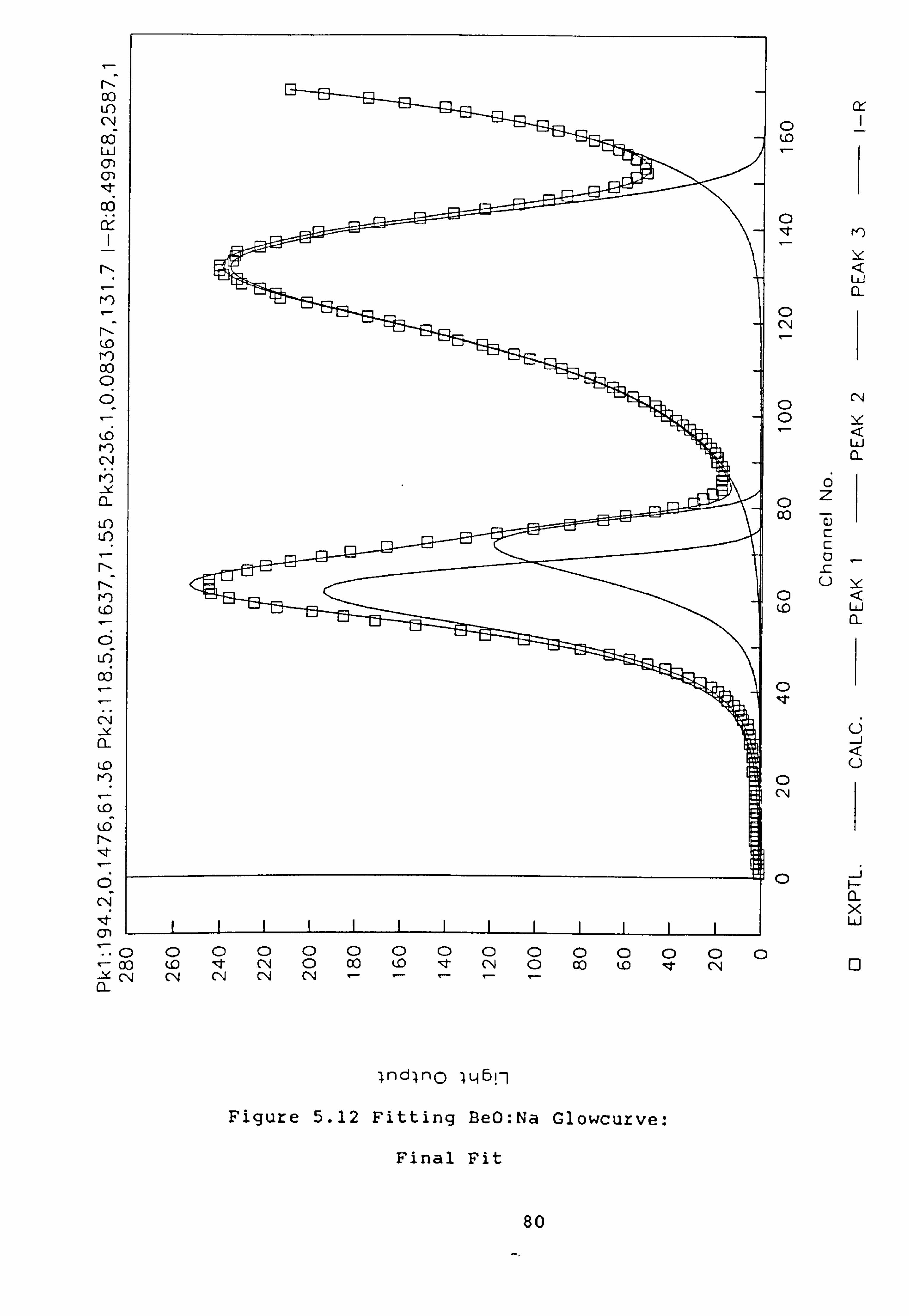
Co u-) C, 4 Cd LU

(M

00 cr

QD fle) 00

C)

LD

LO LO

Lo

LO 00

(. 0

cli

lt (71

(D (D C) 00 C) 00 (D C) 00 C) 0 00 (0 't cq C) 00 (0 't (N 0 00 ýo le C, 4

--Y C'4 cli C-4 cli n

Ind; no jq5rj

Figure 5.12 Fitting BeO: Na Glowcurve:

Final Fit

(. 0

C)

LU

0 cli

LLJ CL

0

cc) 0z

y 0< LO

LLJ

a-

0

0 C14

0 ü- x LU

ID

80

E) -

C: ) CN

0-

0 cl 0

0 00

G EI EI EI

0

0 G

0 -J

x LLI

0

0 CN

1,10

Lo LO t ff) C14 0 o) oo r- (. o Ln -q- in c, 4

(spuosnoLAI)

4ndlno IL45rl

Figure 5.13 Fitting Ca S04: Hn Glowcurve:

Main Peak

81

C r, )

0

00 Iýi 00 LO r- C

00

-Y 0- C'ý

00 00 00 0

C; cli 0 cli 111)

a_

C; C(5 00 0 r-

Cd t') r4

, It

0W 0

0 c"i

LU 0-

0

(N

0< 00 LU

c; n Z

ü-

CD e1

0 C4

(D LO It r") C**4 0 0) 00 P- (D Lr) zt V) C, 4

CT

U') C, (spuosnoL4_L)

4nd4no IL46rl -Y

Figure 5.14 Fitting CaS04: Mn Glowcurve:

Starting Parameters

0

x LLI

ID

82

C

co

Ln __y a- 0

0-

0 0

C14

Cl-

L. r) LO

C) 0 0 LO C14 \1

C) 0 0 Lr) C',

Lo Lo r-1) CN

(D 00

0 LD

C) CN

0

, It V

Li a-

r-1)

LLJ a-

LLJ

0-

0 -J 0

Cl- x LLJ

0

(spuosnoql) Indlno IL451-1

Figure 5.15 Fitting CaS04: Mn Glowcurve:

Final Fit

83

0 C) 00 r- LO Lr) I- to CN -0

5.3.6 Ca6-Q4,. Mn

This material appears unsuitable from the start

for fitting with first-order peaks. The shape of the

large main peak Is more symmetrical than the single

first-order peak shown In Figure 5.13, suggesting that

second-order peaks might be more suitable, (they are

more symmetrical).,

Figure 5.14 shows the starting parameters for an

attempted, fit. The fit Is particularly poor for

channels 0-25,50-80 and 120-150.

Figure 5.15 shows the final fit., the best that

could be obtained with repeated Iterations of the

program. _Xý was 36.8 for the final fit.. considerably

greater than for any of the others shown here and

indicating a very poor, fit. The poor- fit, Is visually

obvious, especially for channels 0-30. The undulations

in the curve from channel 50 to channel 110 look

unconvincing, although the curve passes through almost

every point. This example Illustrates that It Is not

possible to fit any glowcurve with enough first-order

kinetics peaks., Increasing confidence in the goodness

of fit shown previously.

The examples given Illustrate the successful

application of computerised glowcurve analysis to

several different materials., and the failure of the

technique in a case where it Is thought to be

inappropriate. It is Intended that its continued

application, to many more glowcurves, will clarify the

84

behaviour of these materials with respect to thermal and

light induced fading, dose response, etc. It should

also Increase the precision of measurements at low

values of absorbed dose.

The aim of this chapter was to demonstrate the

application of the glowcurve deconvolution program to a

variety of materials, In proceeding beyond such

demonstration to practical applications in research and

routine measurements, the question of errors of

measurement and analysis arises. one aspect of this is

repeatability. The analysis of, say, 5 or 10 glowcurves

obtained from the same material under identical

conditions of irradiation and readout will yield an

estimate of the statistical spread of results resulting

from errors In measurement and analysis. There may also

be systematic errors giving rise to uncertainties in

the temperature scale and the ligh t output scale. These

have been reduced, as far as possible, by design

considerations in the development of the Toledo 654

reader (Robertson., 1975). For the particular Toledo

used In these measurements., the planchet temperature

was checked in early work by the use of temperature-

indicating wax strips. The temperature difference

between the planchet and the dosemeter, however, Is an

unknown quantity In this as In most TLD research. It Is

minimised by the use of powder or thin dosemeters and

slow heating rates (McKeever, 1985).

85

6. ADDlications In-Medical Physics

The early paper by Daniels et al (1953) on

practical applications of thermoluminescence included a

medical application,, the u5e of lithium fluoride for

dosimetry In cancer patients: "The crystals were

swallowed by the patients, recovered one or two days

later, and the accumulated dosage in roentgens was

measured". It is fortunate that this procedure did not

come into common use, as lithium fluoride Is now known

to be toxic (McKinlay, 1981). By. the 19701s, many

medical applications were reported, both in

radiotherapy (e. g Ruden, 1971, Suntharalingam and

Mansfield, 1971) and in diagnostic radiology (e. g.

Langmead et al, 1976).

For medical applications, tissue-equivalence is a

highly desirable property of TLD materials. Both

lithium fluoride and lithium borate have been widely

used, although LiF, with photon effective atomic number

8.21 Is not as close to tissue (Zeff = 7.4) as Zeff =

L12B407: Mn, as shown by Langmead and Wall (1976). The

main disadvantage of L12B407: Mn is that It emits orange

light, whereas LiF emits blue light. The detection

efficiency of PM tubes is much less in the orange than

the blue, so that L12B407: Mn dosemeters are found in

practice to be considerably less sensitive than LiF.

Wall et al (1982) compared the properties of three

different lithium borate phosphors with different

86

dopants. L12B4071Cu emits blue light and is

consequently considerably more sensitive (7.8 times)

than L12B407: Mn. Both showed a small under-response

compared with muscle at 1 30 keV. Of L12B407 dosemeters

commercially available today, L12B407: Mn from Alnor is

several times less sensitive than LIF.. due to Its

emission of orange light, and L12B407: Cu is only

available In a form foruse In the Panasonic TLD reader

(Yamamoto et al, 1982). Consequently, LiF continues to

be widely used, although because of the over-response

at lower energies (in the diagnostic range) care should

be taken to perform appropriate calibration

Irradiations. They should be made at the same X-ray

energy and with similar backscatter conditions as for

the dosimetric irradiation.

TLD materials are available In various physical

forms which are suitable for different applications.

Loose powder presents considerably more practical

difficulties In use than solid forms, but may be useful

where the shape of available solid forms is not

suitable for a given application. Extremity dosemeters

consist of a thin layer of powder attached to a

suitable tape base. LiF-Teflon dosemeters are available

as 13 mm, diameter discs or 6 mm long.. 1 mm diameter

microrods. These should not be annealed above 3000C as

Teflon softens at 32711 C. Solid LIF dosemeters are

available as 3 mm square (0.9 mm thick) chips or 3-4 mm

diameter discs and L12B407 dosemeters as 4 mm diameter

87

discs. The small size of dosemetersý thus -allows

measurements to be made at numerous points within

phantoms.

The d if f erent physical forms of - dosemeters have

different sensitivity to ionising radiation. TLD

readers can also be set to different ranges of

sensitivity for readout. With the right combination of

dosemeter and reader sensitivity, absorbed dose may be

measured between say 10-5 Gy and 10 Gy,, covering the

whole range required for personnel . dosimetry.,

diagnostic radiology and radiotherapy. Sensitisation

may occur In dosemeters which have received very, high

radiation doses. If this cannot be removed. by adequate

annealing (for example, for Teflon-based dosemeters),,

care must be-taken to re-calibrate them before re-use.

Dosemeters need, to be encapsulated In some way

before use in medical applications. For use on the

skin, they may be sealed Into plastic sachets which

should. preferably exclude, light. Black plastic sachets

have been widely used. Aluminised plastic film Is the

best material currently available (from NE Technology)

as the sachets made, from It can be easily labelled with

a marker pen. Plastic sachets, black on one side and

transparent on the other were. wIdely used In, the past,

but these were found to leave a slight sticky film from

the plastic on the dosemeters. For measurements In

blo'od vessels or body cavities, dosemeters are normally

Inserted In catheters, usually with some small metal

88

markers to make them visible on radiographs. once sealed

in sachets or catheters, the whole package may be

sterilised chemically or with ultraviolet light,, but

autoclaving is unsuitable for the TL materials

(McKinlay, 1981).

Some effort is required to ensure that the

carefully prepared dosemeters are used as Intended, in

the right positions, and Indeed that they are used at

all (and not lost). If the cooperation of radiographers

is not gained, it may be found that they are too busy

performing their work to use dosemeters on the

patients. Similarly, a clear and simple record-keeping

system must be set up; without this the results of TLD

measurements are meaningless.

Calibration with X-rays for diagnostic radiology

measurements has been described In Chapter 3. For

radiotherapy measurements, calibration irradiations

should be made on the dosemeters before use. To avoid

taking much machine time.. a cross-comparlsonmay be

made with a 90Y/90Sr irradiator, which can then be used

for subsequent calibrations. Dosemeters may be

Individually calibrated, but it is often extremely

difficult to keep track of Individual dosemeters

(except for LiF-Teflon discs which can be numbered with

Indian Ink). Even if they have been kept carefully In

numbered positions, when several dosemeters are loaded

into a sachet or catheter, it is not possible to know

which one is which when they are removed from it after

89

use. More usually a batch calibration is used. A large

number of dosemeters Is purchased and given several

calibration irradiations. Dosemeters- showing large

variation In response are discarded, then the remaining

ones are sorted Into batches whose response varies by

not more than 5%, say, for diagnostic radiology

measurements, or 1% or less, for radiotherapy where

greater precision Is required (Portal, - 1986). ý the

dosemeters are -thený used In 'separate batches-, for

various uses, with' a, few from each batch used for

calibration and background for every application. The

whole batch should be annealed and read out together,

and any receiving very large radiation doses discarded,

so-that the properties of the batch remain, uniform as

far as possible. Usually 3 or 4 dosemeters are used In

a sachet for one measurement., The mean reading Is thus

more accurate than that of a single dosemeter, in view

of the batching described above. This also allows the

occasional spurious reading (due to reader malfunction

or dirt on the tray or dosemeter) to be discarded, as

such a reading is clearly different from that of the

others In the sachet.

6.2 Applications In Radlotheragy I il

In radiotherapy., it Is extremely important that

the prescribed radiation absorbed dose Is delivered to

the tumour with high precision and accuracy. If the

absorbed dose is too high there is a risk of

90

complications arising from damage to surrounding healthy

tissue.. whereas If - It Is too low tumours may not -be

completely destroyed., -resulting in Increased patient

morbidity and mortality. While the radiologist

prescribes the absorbed dose, the physicist's task

Involves calibration and measurement to ensure that the

correct dose Is delivered. TLD is highly suitable for

such * measurements., although lonisation chambers and

silicon diode detectors are also used. The European

Organisation for Research and Treatment of Cancer

(EORTC) states that acceptable practice Is 11 ±3% on the

calibration of therapy units and ±5% on the prescribed

dose" (Johansson et al, 1988). TLD is used for

International Intercomparlsons of absorbed dose

delivered by radiotherapy machines, for In-vivo

measurements, and for measurements on phantoms, as

dsescribed below.

6.2.1 International Intercomparlsons

The International Atomic Energy Agency (IAEA) and

World Health Organisation (WHO) have run as

international intercomparlson programme for 60CO

radlotherapy, units since 1968, using LIF powder sent by

post to various centres. Results have'been published In

various studies, for example,, Eisenlohr and Jayaraman

(1977), Biaerngard and Kase (1980), Boyd et al (1982).

Results for 1969-1987 are presented by Svensson (1990);

within this period, 1984 results were obtained from a

91

total of 686 radiotherapy centres throughout the world.

98% were within ±30%, and for these the mean deviation

of results was -0.25%, standard deviation 6.7%. Figure

6.1 illustrates the procedure followed in

Irradiation PSDL 2 Gy

........................................................................

IAEA Virgin -irradiation I I Dosimetry TL Annealing

(

a. calibration EVALUATION in E\ X

powder Laboratory curve Irradiation --m- -2 Gy ........................................... SmIJ

4f

lab. ref.

Radiotherapy centres .............................. .........................................

Irradiation 2 Gy

week Time scale 0-1

Several About Between days 2 months 2 and 11 months

Figure 6.1 Flowchart of IAEA/WHO International

Intercomparison Service for 60CO teletherapy

units. (from Svensson et al, 1990).

92

the intercomparlsons (PSDL denotes Primary Standard

Dosimetry Laboratory) It should be noted that each

centre receives not only LiF powder to be irradiated to

2 Gy, but also a sample of unirradiated LiF and another

sample, already Irradiated to 2 Gy, so that allowance

can be made for background, transit dose and fading.

6.2.2 Phantom Measurements

Measurements can be made at any desired point In a

phantom of tissue-equivalent material, whereas in the

patient., measurement can only be made at accessible

points. Phantoms are of two type - anatomical and

simple geometrical shapes such as rectangular blocks of

plastic or tanks of water.

Complex calculations are made on computers for

treatment planning In radiotherapy. These make use of

depth dose data and isodose curves, which may be

determined by measurements with Ion chambers or TL

dosemeters (McKinlay,, 1987). A considerable amount of

data Is required, as beam size and geometry, radiation

quality, distance to the surface of patient or phantom,

source size and the use of wedges or filters in the

beam all affect the value of absorbed dose at a given

point. Lindskoug and Lundberg (1984) describe various

studies using LIF in geometrical phantoms to

Investigate problems of build-up at air/tissue ý .1

equivalent interfaces, the dose distribution around a 90Y/90Sr source, absorbed dose distributions in

93

computerised interstitial after-loading techniques, and

checks on radioactive needles and seeds. Kosunen and

Jarvinen (1990) describe the use of L12B407 dosemeters

in a water phantom to test the performance of a

radiotherapy treatment planning system. They conclude

that TLD measurements are suitable for regular quality

control of treatment planning systems.

Anatomical phantoms represent the whole or parts

of a human body with varying degrees of accuracy. Some

are simple shapes of tissue equivalent material, others

contain bone substitute or real bones, air spaces for

lungs and sinuses, etc. Oduko (1979) describes the use

of a simple slice of a cylinder of a tissue-equivalent

wax mixture,, -representing the post-mastectomy* chest

wall. LiF-Teflon microrods were used to check the

accuracy of the Isodose curves produced by the

computerised treatment planning system. Differences

between calculated and measured values were found to be

up to 6% for a single beam,, but only up to 3% with

opposed fields, as errors partially cancelled -out.

Lindskoug and Lundberg (1984) suggest that

discrepancies of 20% or even 30% are not unusual when

comparing measurements and treatment' planning

calculations. Aget et al (1977) describe the results of

TLD measurements in whole-body Irradiation of a Rando

phantom'(Irradiated with 25 MV photons) and compare

with the results of computer calculations. Binder et al

(1990) describe the use of 2x1 x'l mm LiF crystals

94

cut from standa rd Harshaw TLD-100 chips to measure the

dose distribution in an eye phantom irradiated with a

10GRu applicator. These examples indicate the wide

variety of measurements reported using TLD to measure

absorbed dose in phantoms.

6.2.3 In-Vivo Measurements

In-vivo TLD measurements are carried out at many

radiotherapy centres, for example at Radiumhemmet in

Stockholm measurements are carried out each time a

patient Is Irradiated (Lindskoug and Lundberg,, 1984).

In-vivo measurements have been carried out for many

years In the Scandinavian countries and many published

studies originate from there. Outside Scandinavia, such

studies are less common and mostly restricted to

special treatments., such as total body irradiation.

Lewis at al (1984) describe the use of TLD-100 LIF

chips in holders taped to the patients's skin, during

total body Irradiation for acute leukaemia at the Royal

Marsden Hospitalr Sutton. 120 LiF chips are used at

various sites on the body and for controls,, and the

results are used to ensure that the planned absorbed

dose Is correctly delivered to the patient, within

5%.

Svenss on et al (1984) give three reasons for in-

vivo TLD measurements In radiotherapy:

(a) to prevent mistakes due to human error

(b) to provide rapid Indication of changes or faults

95

In the radiation facility

(c) to indicate problems In treatment planning or

reproducibility of, patient set-up.

Patients, are normally irradiated several times in

a course of treatment. If errors are detected, as

above., corrections may be made on subsequent

irradiations to ensure that the overall treatment is

close to that prescribed. -

McKinlay (1981) lists four classes of In-vivo

measurements for which TLD may be used:

(a) Entrance absorbe d dose measurements

(b) Exit absorbed dosemeasurements

. (c) Intra-cavitary absorbed dose measuremnts

(d) Individual spared organ absorbed dose measurements.

He discusses special considerations for each, and the

type of information that each provides, and gives

'examples and Ill ustrations of various types of

measurements. Lindskoug and Lundberg (1984) also give

numerous illustrations of results of In-vivo TLD

measurements. Further examples of TLD measurements are

given by Ruden (1971), Ruden (1976), Gooden and

Brickner (1971), Suntharalingam (1980) and McKeever

(1985). An interesting recent development is described

'by Jones et al. (1990). In this prototype instrument for

in-vivo radiotherapy dosimetry, CaS04: Mn_ and CaF2: Tm

phosphors were used"to measure gamma and gamma+neutron

radiation.

96

Af ibre-optic system was used to couple the phosphors

to a Nd-YAG laser used for remote stimulation of,

thermoluminescence, the light output passing along the

optical fibre to a PMT for detection. Results. were very

promising, although actual In-vivo use, has not yet been

reported.

6.3 Radiation Protection

This section encompasses measurements in

diagnostic radiology, Including measurements in

dentistry and computerised. --, tomography (CT) scanner

checks., and also personal dosimetry, a- large field

which might have occupied-a, whole chapter by itself,

but does comprise a part of radiation protection

services.,, Some results of measurements carried out by

the author are also presented.

6.3.1 Personal Doslmetry. ý .G

- While the earliest -personal dosimetry services

used photographic film.,, and some still use it today,

TLD systems began to be widely used from the 1970's.

onwards. Becker (1973) lists 18 TLD personal dosimetry

services In 6 countries; most, used LIF: Mg, Ti and about

half of them had automatic readout of dosemeters. The

NRPB's automatic system was described by Dennis et al

(1974) while , other large automatic services . are

described by Duftschmid (1980) and Grogan et al (1980)

In the proceedings of the 6th International Conference

97

I",, on Solid State Dosimetry. At the same time, Marshall et

al (1980) discussed the performance of the NRPB

thermoluminescent dosemeter, and McKinlay et al (1980)

described the use of u Itra-violet radiation (the

photo-transferred thermoluminescence technique) for re-

assessment of absorbed dose in the NRPB automated

system. Interestingly, further progress is reported

principally by the same authors in the proceedings of

the 7th, 8th and 9th International Conferences on Solid

state Dosimetry. Thus Grogan (1983) describes some

problems encountered In seven years of operation of the

Canadian TLD service., while Grogan (1986) discusses

some of the technical and administrative anomalies

encountered. The earlier CEC directive In 1975 had

prescribed the measurement of skin absorbed dose and

body absorbed dose at depths of 5-10 mg cm-2 and 400-

1000 mg cm-2. Duftschmid and Strachotinsky (1986) and

Bartlett et al (1986) relate the performance of the TL

dosemeters used in the Austrian and British personal

dosimetry services, respectively, to the new quantities

defined in ICRU Report 39. Grogan (1990) reviews 14

years of experience with the Canadian TLD service,

discusses variations in sensitivity of the TL

dosemeters and suggests that periodic recalibration Is

desirable. Bartlett et al (1990) discuss factors

relating to the calibration of personal dosemeters

including the new ICRU quantities and the ICRU sphere

phantom.

98

The above selective review of a very wide field is

not intended to imply that the work of other authors Is

not of value, rather that by selecting publications by

just a few authors over a decade one may In this case

follow the general trends and issues of the period. A

worldwide perspective for 1990 is reflected In Griffith

et al (1990) which describes an IAEA intercomparlson

f or personal monitoring., Including both TLD and film

services. 21 laboratories from 19 different countries

participated in the study, and six different TLD

phosphors were used of which LIF was the most common. A

study of dosimetry services (film and TLD) in the UK is

presented by Clark et al (1991). Another International

Intercomparison, within the EEC, is described by

Ambrosi et al (1992); this again Includes both TLD and

film services. The references section of this last

paper reflects the growing concern In the 1990's for

quality assurance and quality control. These are

further discussed by McDonald et al (1992) and Bohm et

al (1992) who point out the need for dosimetry services

to be accredited, and clarify some of the Issues

Involved.

This brief review has not explicitly covered

special areas of personal monitoring such as beta-

particle, neutron and extremity monitoring. The first

two are Included within the last few references; for a

general discussion of these aspects see, for example.,

McKinlay (1981), Mahesh et al (1989), Hufton (1984).

99

The author's current work In the field of personal

dosimetry includes quality assurance for a hospital-

based personal dosimetry system using TLD, and the

development of convenient dosemeters to be worn on the

head, for the measurement of eye doses.

6.3.2 Diagnostig Raýdioiogy

While man-made sources of radiation contribute

only 15% of the collective effective dose to the UK

populat'ion, some 90% of this amount Is due to medical

X-rays. A national survey of doses to patients

undergoing X-ray examinations was carried out in

England in 1983. TLD was used to measure entrance skin

dose for simple radiographs.. while dose-area product

meters were used for measurements In more complex

radiographic procedures such as barium meals., barium

enemas and intravenous urography. The results are

reported by Shrimpton et al (1986). A recent report

(NRPB., 1990) on patient dose reduction recommends that

pat I ient entrance skin - d6se should be measured

periodically as part of a quality assurance programme,

while the protocol for such measurements (IPSM,, 1991)

specifies that thermoluminescent dosemeters should be

used for such' measurements. These reports do not

Include computerised tomography (CT) which constitutes

only 2% of X-ray examinations In the UK but contributes

some 20% of the effective dose to the population. TLD

measurements are also made In quality assurance checks

100

of CT scanners, as described later. Thus there is at

this time a rapidly expanding demand for TLD

measurements in hospitals, in the interests - of

radiation protection for patients.

McKinlay- (1981) describes the gains which , may

result from diagnostic absorbed dose measurements:

1) Improving the design of equipment to reduce patient

absorbed dose 1

2) Improving radlographers techniques to reduce patient

absorbed dose

3) providing a measurement base for epidemiological

analysis of population radiation absorbed dose from

diagnostic radiology.

It is to be hoped that TLD measurementsýwould not

have to be used to Justify changes- whose -results are

already well known. For example, changing to rare-earth

screens would certainly reduce patient skin dose, as

was indeed found in a recent study with TLD (Waldron et

al, 1992). Conversely,, use of say 50 kVp X-rays when

70kVp would be more suitable, would give Increased skin

dose; simple gathering of information would highlight.

this factor more quickly than TLD measurements. Quality

assurance programmes for X-ray -equipment and film

processors, and film reject analysis., are , other,

measures which can help to reduce patient , absorbed

dose, before a TLD measurement programme -is commenced

so that further reductions can be made.

Some resultsi of patient dosimetry measurements,

101

with TLD are presented in the next section. As a

practical matter, It is important to have the

dosemeters used correctly and appropriate records kept,

otherwise considerable effort in calibrating and

preparing the dosemeters is wasted. Cost is another

consideration, as users might not realise that such

small insignificant-looking packets cost several pounds

each. Best results have been obtained by entrusting the

TLDs to a keen and willing superintendent or quality

assurance radlographer, or a radiography student

wishing to use the results of the survey as part of an

educational project. Clear sheets of Instructions must

be supplied to anyone who will be Involved in using the

TLDs on the patients, and the record forms must also be

clear and readily available. Samples of forms are

provided In an appendix of IPSM 1991.

Patient weight is one important - piece of

information which needs to be recorded, as higher

absorbed dose to the patient Is required to produce

acceptable radiographs of larger patients. Hart and

Shrimpton (1991) suggest that a linear relationship

holds approximately between patient weight and entrance

surface -dose, although the relationship varies for

different rooms and examinations. In summary, they

suggest that the difficulty of making corrections. for

weight may be avoided-by choosing patients, of weight 70

±5 kg for patient dosimetry measurements. IPSM-(1991)

suggests that this might be relaxed to approximately 70

102

±10 kg., so that less patients would be excluded from the

study.

This leads to consideration of a further

difficulty. The protocol (IPSM, 1991) suggests that

measurements should be made for at least 10 patients

per type of radiograph. The radiographs suggested for

TLD measurements of entrance surface dose are

Lumbar spine AP

Lat

LSJ

Abdomen AP

Pelvis AP

Chest PA

Lat

Skull AP/PA

Lat

(A = Anterior.. P= Posterior, Lat = Lateral, LSJ

lumbo-sacral Joint) -

A choice of only 5 from this list, with 10

patients each, and 3 dosemeters in each, sachet, would

mean 150 dosemeters would be needed, with say 10 more

for calibration and background. This would be for Just

one room, as X-ray equipment In every room is

different'. The demands on time and resources to make

such measurements In a large hospital are very great.

For smaller hospitals.,, the difficulties lie -An finding

10 patients of the right weight for each examination.

It might take many months to accumulate enough data for

103

0-

a study.

As well as the recent programmes described above,

TLD measurements In diagnostic radiology have been

carried out for many years. McKinlay (1981), McKeever

(1985) and Mahesh et al (1989) describe various

applications, including measurements with phantoms and

on patients. For examples of TLD measurements-'in

speciallsed fields, which have not' been discussed

above, see for example Fitzgerald 'et al (1981), '

describing me asurements In mammography, and' Chapple 'et'

al (1992) for paediatric radiology.

6.3.3 Some Measurements In Dlaqnostic Radlolo

Square LIF chips were used for this study. They

had previously been calibrated and sorted Into 'batches

of 50, with sensitivity within :t 5% in each batch.

They were annealed before use for 2 hours at 40011C

followed by 16 hours at 8011C., In anodised aluminium

annealing blocks. Cooling was in the oven., for repro-

ducibility from one cycle to another. The TLD reader.,

the oven and the X-ray Irradiation equipment for cali-

bration have been described in Chapter 3.

Dosemeters were packed in groups of 2 or 3 Into

small plastic sachets, sealed and numbered. They were

sent to hospitals P and R by post., with each group

accompanied by a sachet of background dosemeters, not

to be used. No fading dosemeters were used, as previous

work had shown fading to be negligible under these

104

. 1. conditions. on return from the hospitals, the dosemeters

were read out, along with a set of calibrated

dosemeters from the same batch., and background doseme-

ters which had been kept in the laboratory. Results are

presented on the following pages, Tables 6.1,6.2 and

6.3.

In these examples the hospitals were quite small

and the results Indicate the difficulty of obtaining

sufficient measurements, of each type over a period of a

few months. Further measurements will be made at these

hospitals to Increase the numbers of patients for each

examination. Patient entrance surface dose in tissue is

shown in the results for each chip., then the average

value Is also converted to entrance surface dose In

air. Discarding results for patients outside the weight

range 70 ± 15 kg yields the data shown In Table 6.4

for the examinations of which several were measured.

Reference values of entrance surface dose, which

are the rounded values of the third quartile of

measurements, reported In, the national survey (Shrimpton

et al, 1986) are as shown in Table 6.5.

105

Dose Estivates: lospital P

Sarface Average Average Sachet Reading Dose Dose Dose %S. D. Rooroltaiiiatiot ILD ky W FFD AEC Veigsel Age

go. (icy) (Icy) (air, IGI) go. Positiol (cl) Rg) Urs)

81 To? 0.114 0.113 0.107 5.8 2 cil PA. Kidliie 63 5.6 200 71 ,K 24 721 0.119 35143 T? 683 0.106

82 575 0.069 0.071 0.070 10.7 1 CIR PA Kidlhe 66 5.0 200 60 P 39 576 0.070 35143 T6 616 0.083

23 389 0.006 0.003 0.003 97.7 10 record 370 0.000 382 0.004

B4 9845 3.216 3.276 3.091 1.9 1 W. E. Sphe ledial to 73 115 Yes 71 1 25 10220 3.343 30110 1 I. S. I. S 10008 3.271

is 48569 16.36 16-68 15.74 4.6 1 Lit. L. Spile literior 81 100 115 71 1 25 47896 16.13 2(130 to L3 52105 ITX

B6 105250 35.60 32.83 30.98 11.2 1 Lit. LS/Sl Posterior 90 115 res 71 F 25 101280 31.25 18124 to D-1 84807 28.66

17 7920 2.562 2.554 2-09 1.2 5 I. P. Pellis Xidliae 70 26.0 115 71 K 69 8201 2.658 35143 above pubis 7563 2.441

B8 799 0.145 0.135 0.127 1.7 5 M. CIR Over T6 66 7.0 200 74 1 6i 768 0.135 3514311 738 0.125

39 3808 1.17 1.14 1.07 3.1 5 W. L. Sphe Xidlhe 70 IS. 5 115 60 1 42 3647 1.11 30140 U

BIO 7091 2.23 2.28 2.15 0.1 5 Lit. L. Spile U 15 17.5 115 60 F 42 7108 2.29 21130 7095 2.28

211 16198 5.37 1.92 1.65 9.6 5 lit. Uphe B/I 85 39 115 Tes 60 F 42 15023 4.97 18124 nd D-1 13413 4.43

Table 6.1 Patient entrance surface doses

for hospital P(l)

106

Dose Estintes: NOW p (2)

Sarface Average Average Sachet teading Dose Dose Dose IS-D. Room Elalilation TLD il 118 FFD AEC Veight Sei Age

10. - (IGI) (OGY) (air, IGI) go. Position (Cal (ill (its)

DI 63337 25-424 25-514 24-070 0.5 1 L-Spiie LSISI A. S. I. S. Ievel 85 110 Yes 74 K 46 63784 25.601 18124 on R side

D2 339 -0.008 -0.002 -0.002 -58M 2 Supine Abdoi. Kidline level 70 22.0 100 SI K 60 372 0.005 35143 Iliac Crest

D3 6208 2.361 2.333 2.201 1.1 1 A. P. L. Spiae Kidline V to 1 71 IN Yes 55 F 20 6069 2.305 24130 Lower cost. iarg.

D4 5682 2.149 2.162 2.00 0.9 2 A. P. U. Spine Kidline 70 100 Yes 46 F 32 5748 2.115 35118 Level N

D5 8094 3.12 3.13 2.96 0.5 2 Lit. 7h. Spine Kidline axilla 70 25 100 46 F 32 8154 3.15 30140 Level T6

D6 6966 2.67 2.68 2.52 0.5 2 I. P. L. Spine Kidline lover 13 110 Yes 74 K 46 7012 2.69 30140 costal margin

D7 3075 1.096 1.066 1.006 (. 0 1 Tovaes Skill gairline sid TO 115 Yes 57 F 63 '2927 1.036 24130 forehead

Do 2453 0.845 0.856 0.808 1.9 2 A. P. L. Spine Xidliie 81 100 Yes 46 F 32 2509 0.868 2400 Level LCK

D9 6825 2.61 2.60 2.46 0.3 2 Lat-L-Spiae Kidline axilla 85 100 Yes 46 F 32 6799 2.60 24130 Level LCK

DII 30221 12.05 11.79 11.12 3.2 2 Lat. L. Spine Lover costal 81 110 Yes 14 K 46 28906 11-52 30140 margin R. side

D12 34230 13.61 13.83 13.05 1.6 2 Sapiie Abd. Kldliie Iliac 70 90.5 100 110 K 72 35018 13.99 35143 Crest level

D13 C02 0.10 0.09 0.09 9.3 1 P. A. CIR Kidliae 63 6.3 200 6 Ir F 50 572 0.09 35135 T?

D14 77685 31-216 31-680 29-887 2.1 5 Spot US Kidpoint ISIS 91 110 Yes HF 20 79986 32.145 18121 ud PSIS

D15 13729 5.397 5.381 5.076 0.4 2 Lat-L$ Joint- Level I. S. I. S. 90 100 Yes 16 1 32 1360 MES Spice 18121 on Raide

D16 368 0.00 0.03 0.03 12S. 5 1 P. A. C11 Xidline 60 5.0 200 50 1 39 502 0.06 35135 T7

D17 2426 0.83 0.84 0.79 1.4 1 P. A. Skill 20deg Kid-siall TO 115 Yes I'll FV 206 OJS down 2400

D18 1848 0.60 0.62 0.58 3.4 1 Lit. Ska II 3ca above 66 150 Tes 1.7 F 63 1922 0.63 24130 1.1.1.

Table 6.2 Patient entrance surface doses

for hospital P(2)

107

Dose Estimates: Hospital

Sachet No. Reading Surface Dose Average Dose Average Dose %S. D. Examination kV mA s FFD Weight Sex Age (mGy) (@Gy) (air, mGy) (cl) (kg) (yrs)

CI 3711 1.32 1.31 1.24 1.1 O. M. 4 95 200 0.04 96 64 M so 3660 1.30 Left Lateral 90 200 0.02 96

C2 1043 0.30 0.30 0.28 1.8 A. P. chest 90 200 0.06 180 78 H 40 -1023 0.29

C3 932 0.26 0.28 0.26 10.5 A. P. chest 90 200 0.05 180 78 M 40 1040 0.30

C4 525 0.10 0.09 0.09 17.7 P. A. chest 82 200 0.02 180 (stall) F 60 465 0.08 (Min)

CS 783 0.20 0.21 0.20 4.4 A. P. knees 52 200 0.04 90 70 M 52 817 0.21

C6 631 0.14 0.13 0.13 11.2 A. P. chest 82 200 0.03 180 67, M 26 576 0.12

C7 4677 1.69 1.62 1.53 5.7 A. P. abdomen . 90 200 0.04 90 61 N 26 4332 1.56

C8 3916 1.40 1.39 1.31 1.0 A. P. pelvis 90 200 0.04 90 61 H 26 3866 1.38

C9 771 0.20 0.19 0.18 6.6 Chest 82 0.03 180 61 M 29 725 0.18

CIO 5120 1.86 1.85 1.75 0.6 Abdomen 92 0.06 100 63 M 29 5080 1.84

CII 272 0.01 0.00 0.00 -433.1 (unused) 223 -0.01

C12 234 -0.01 -0.01 -0.01 -58.1 (unused) 204 -0.02

C13 210 -0.02 -0.02 -0.01 -19.4 (unused) 221 -0.01

C14 213 -0.02 -0.01 -0.01 -32.8 (unused) 229 -0.01

Table 6.3 Patient entrance surface doses

for hospital R

108

HosDital P (1 & 2)

Average Entrance Surface

Examination Dose in Tissue (mGy) Mean s. d.

Chest PA 0.113

0.074

0.135

0.09 0.103 0.027

Lumbar Spine AP 3.28

1.14

2.33

2.68 -

0.86 2.06 1.03

Lumbar Spine Lat 16.68

2.28

4.92

2.61*

ll. '80 7.66 6.33

Table' 6., 4' Entrance Doses for some Examinations

from Tables 6.1,6.2

109

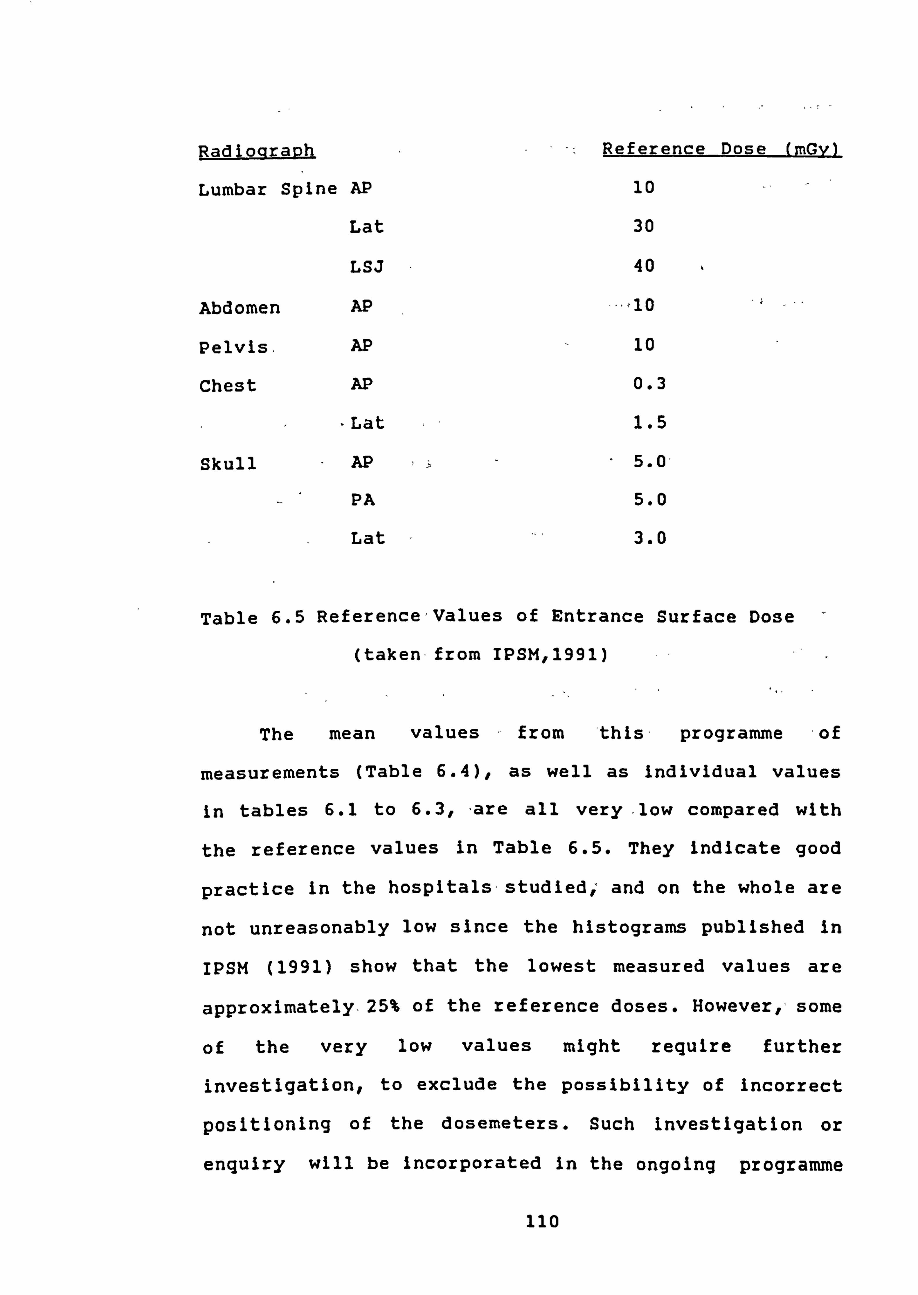
Radloqraph Reference Dose (mGv)

Lumbar Spine AP 10

Lat 30

LSJ 40

Abdomen AP

Pelvis. AP 10

Chest AP 0.3

-Lat 1.5

Skull AP 5.01

PA 5.0

Lat 3.0

Table 6.5 Reference, Values of Entrance Surface Dose

(taken-from IPsm., 1991)

The mean values - from 'this, programme of

measurements (Table 6.4), as well as individual values

in tables 6.1 to 6.3., are all very low compared with

the reference values in Table 6.5. They indicate good

practice In the hospitalsýstudied; and on the whole are

not unreasonably low since the histograms published in

IPSM (1991) show that the lowest measured values are

approximately, 25% of the reference doses. However.., some

of the very low values might require further

investigation, to exclude the possibility of incorrect

positioning of the dosemeters. Such Investigation or

enquiry will be incorporated In the ongoing programme

110

for further measurements. The need for fading dosemeters

will also be re-examined. One further point Illustrated

by Tables 6.1 to 6.3 Is that there are some practical

difficulties occurring In a patient dosimetry programme

such as this - incomplete or missing data., lost or

unused dosemeters, wrong views (knees), etc. Attempts

will also be made to minimise these in future work.

6.3.4 Other Measurements

Some other areas of radiation protection which use

TLD measurements may be briefly considered.

Computerised tomography (CT) is one such area.

Shrimpton (1992) presents results of a survey of CT

practice in the UK, showing that CT examinations

contribute approximately 20% of the annual collective

dose of 20,000 man Sv, as a result of the 5.3 mSv mean

contribution per CT examination. He also shows how much

greater the effective dose equivalent is for CT as

compared with the conventional X-ray examinations of

head, chest, abdomen, spine, etc. Wall at al (1979)

used L12B407 powder to measure CT absorbed dose In a

phantom. LiF dosemeters are also used routinely for

acceptance and routine checks on CT scanners as part of

a quality assurance system. They are stacked in

cylindrical perspex holders and Irradiated on the

scanner, either In phantoms or free In air, to produce

dose profiles such as that shown In figure 6.2, taken

from Faulkner and Moores (1984).

ill

.5 a:

0

distance

Figure 6.2 CT Dose Profile

The full width at half maximum (FWHM) of this

curve gives the slice thickness and the computed

tomography dose index (CTDI) can be determined from the

prof ile by integration. This and other parameters used

for quality assurance in CT are discussed by Shope et

al (1981). The process of stacking the LiF chips in the

perspex holder, and unpacking them for readout, are

extremely difficult and time-consuming. As an

alternative, the continuous dosemeter technique

described by Lindskoug and Lundberg (1984) is very

attractive, but unfortunately this requires a special

112

type of TLD reader.

In dentistry, some studies have been carried out

with TLD to determine the absorbed dose to various

parts of the body during dental X-ray examination. Wall

et al (1979b) and McKlveen - (1980) Aescribe the results

of such studiesl, lncluding measurements on., patients and

on phantoms., In quality assurance measurements,, on

dental X-ray setse LIF dosemeters are routinely used. to

measure the output at the slit of the ortho-

pantomographic (OPG) sets. Current work Anvolves

developing a pack, of TLD dosemeters under filters to

measure the kVp of the X-rays, since the motion, of the

set precludes*the use of normal kVp meters.

Thermoluminescence also has some relevance In

accident dosimetry, where estimation of the total

absorbed dose to the victim is useful for clinical

management. For example., Majborn (1984) describes the

measurement of TL from watch jewels to determine the

absorbed dose received by a worker who died. Jewel-

movement watches are now uncommon, however, and

studies by NajakIma (1988) show that quartz elements

now commonly used in watches are not sensitive enough

for use as emergency dosemeters. Haskell and Bailiff

(1990) and Furetta et al (1986) Indicate the

possibility of determining when an accident occurred by

the studying the relative changes In glow peaks of

thermoluminescent materials In personal dosemeters.

Lastly, some attempts have been made to apply

113

thermoluminescence for the measurement of ultra-violet

(uv) radiation. Either the Intrinsic response of the

phosphor to uv or the effect of exposure, toýboth uv and

ionisIng radiation may be measured. Nambi and

Higashimura. (1971) report the response of CaS04: Dy and

CaS04: Tm to uv, while, Busuoli (1983) examines the

response of several different phosphors, 'including

LIF.

A recent study by Lidakis (1991) showed a clear

response of natural CaF2 to uv, but results were not

promising for uv dosimetry. Oberhofer (1984) discusses

the use of TLD for uv dosimetry, and concludes that It

Is not very promising.. especially when compared - with-

polysulphone film which has-. been, more widely used In

recent years.

114

7. Environmental Monitorinq

7.1 Introduction

Natural background radiation accounts for some, 87%-

of the genetically significant Aose received by the

population - of Great Britain (Wall et al., 1981). .

The

Chernobyl incident highlighted the importance of

measuring natural background levels so as to assess the

relative Impact of Increases due to accidental release

of radioactivity. ' Environmental monitoring is often

carried out near reactors and other nuclear

Installations to monitor the effect of any release of.

radioactivity. , TLD has been used for environmental

monitoring for many ýyears. TL phosphors act as

integrating dosemeters which are read out at Intervals,

e. g. monthly. Instruments which-give an instantaneous

readingle. g. Geiger counters, may also be used In

conjunction with ' TLD. TLD measurements, give an

Indication of the levels of environmental gamma

radiation; there are also other programmes of

environmental monitoring to determine contributions

from radon lný homes and radioactivity in food and

drink.

The gamma radiation--in the environment-arises from

the decay of long-lived radionuclides-in soil-and rocks

and from the decay of radon released from the rocks and

the- soil and diffusing into the atmosphere. TLD

measurements will detect this gamma radiation, but also

a contribution due to cosmic rays. At sea level, --cosmic

115

rays consist, of mostly muons, -electrons and positrons

arising from interactions of the primary particles

(mostly protons) with the, atmosphere. The levels of

radiation from cosmic rays vary with latitude (less

near the equator) and altitude (less at sea level), and

also with levels of sun-spot activity. _

The measured

radiation. contribution from rocks.. soil and radon, is

found, to vary with weather conditions, being affected

by snow cover and by levels of water in the soil. -.

Studies of environmental gamma radiation In

different parts of - the ýworld indicate considerable

variation,, with particularly high values in some parts

of Indlaýand Brazil. Al-Hussan and Wafa (1992), quoting

results from a number of studies, give somevalues for

natural background radiation In mSv y-l as follows:

UK 0.70

Riyadh City 0.60

USA 0.65 - 2.35.

France (granite areas) 1.80 - 3.50

Brazil (coastal strips) -5.0

India (Kerala and Madras) 13.0

World average 0.65

The earliest, reported use of TLD for environmental

monitoring is probablyýthat of Roser and Cullen (1965).

Becker et al J1971) report the superiority of TLD

materials over photographic film for environmental and

personal monitoring under tropical conditions. Jones et

al (1971) describe the use of CaF2: Dy for environmental

116

monitoring. -Becker (1972) shows that CaS04: Dy 'performs

better than, LIF (more sensitive) and CaF2: Dy (less

fading) for environmental monitoring. Some other early

studies. reporting the use of TLD for environmental

monitoring are Kramer- et al (1977), Piesch and

Burgkhardt (1977) and Tuyn (1977),, the last of which

reports measurements around a high- energy proton

accelerator. These, last three form part of the

proceedings of the 5th International Conference on

Luminescence Dosimetry. A small number (2 or 3) of

papers on environmental monitoring were presented , at

the , 6th,, 7th., 8th conferences In 1980., 1983 and, 1986,

respectively. Some of these are discussed - In - section

7.3 below. One paper (Driscoll and Green, 1984)

discussed the use of LIF to measure natural gamma'

radiation in homes In the UK, in conjunctionýwith radon

measurements. Botter-Jensen et al (1986) described a

CaS04: Dy dosemeter used to estimate the energy

distribution of environmental -gamma radiation as well

as the dose-rate. The 9th International Conference In

1989 showed a considerably increased interest I n'

environmental monitoring with a whole section devoted

to papers on it, 12 of them dealing with TLD. Of these,

Wernli (1990) discusses a dosemeter, -to measure ICRU

dose quantities H*(10) and H'(0.07), while 5 papers

deal with monitoring around reactors or other nuclear

Installations. (Szabo et al (1990), Dies et al (1990),

Abdul, Ahad (1990), Segovia et al (1990), Mollah et al

117

(1990)). This increased interest in TLD for

environmental monitoring was probably stimulated by the

Chernobyl Incident, mentioned earlier, as was the study

described in more detail in section 7.4.

Lastly, one further promising application of TLD

in environmental monitoring may be noted. Siegel (1991)

reports the use of LIF _and

CaS04 dosemeters to survey

large areas of land cheaply for promising oil fields.

Measurements were carried out In China from 1985

onwards., with dosemeters buried, In plastic bottles In

the ground at one per square km, and left for 110 days.

Water ascending through the ground is blocked by

deposits of oil, but becomes slightly contaminated with

radioactive materials at the edge of the oil deposit.

As this reaches the surface., the boundary of the oil

deposit is indicated by a ring of higher TLD readings

mapped after readout.

7.2 Reguirements for Environmental Dostmetry Systems

There are various requirements to be fulfilled If

environmental monitoring Is to be carried out

satisfactorily. Piesch (1981) lists the following:

(a) good precision and reproducibility of measurement

over the exposure range of Interest (10-100 mrem)

(b) low fading over the field exposure period (3-12

months)

(c) insensitivity to environmental parameters, i. e.

temperature, moisture, humidity, light

118

(d) approximate tissue equivalence in dose reading

(e) low self -irradiation due, to natural radionuclides in

the TLD phosphor or holder,

(f) encapsulation in a plastic holder to provide

secondary electronic equilibrium, shielding against

beta-rays and light as well as water tightness,

(g) calibration techniques for each f leld cycle to

guarantee ý the highest precision for the conversion- to

exposure and to correct- for fadings, transit exposure

and zero-dose reading.

He discusses these requirements in terms the

American National -Standard (ANSI., , 1975). which, quotes

numerical values for-the aspects of performance listed

above. It also quotes for - overall measurement error

under field conditions a figure of ± 30% at the 95%

confidence level. CaS04: Dy has been -one of- the most

widely, used materials -for environmental monitoring. It

does not meet the requirement of tissue equivalence by

Itself, but can be made to do so by use in, a suitable-

badge or holder with metal filters, as described In

section , 7.4, for example. The use of metal filters

provides additional information about the radiation

measured. If this were partly due to a man-made source,

the ratio of- the response of filtered ýto- unfiltered

dosemeters would be different to the ratio for normal

background radiation. Thus tampering with the

measurement may be detected.

The degree of fading occurring In a measurement

119

programme depends on the temperature of the dosemeters.

Differences between summer and winter are expected, but

temperatures reached may be higher than expected.

Gesell et al (1980) used thermocouples to measure the

temperature of dosemeters in packaging of various kinds

and colours. Dosemeters reached temperatures as high as

4311C, while the air temperature was only 250C.

Correction Is made for fading by the use of fading

dosemeters, but a suitable packaging (white or

reflective) should be chosen to minimlse this effect.

Bacci et al (1988) present data on the fading of CaS04

and CaF2 dosemeters used In environmental monitoring.

A more recent standard for environmental dosimetry

Is that of ISO (1985), as-follows:.

1. Batch Homoqeneity

The evaluated dose for any one dosemeter shall not

differ from the evaluated dose for any other

dosemeter In the batch by more than 30%, for a

dose equal to 10 x the required minimum detectable

limit.

For environmental dosemeters this is equivalent to

300 pSv ±15 ASv.

2. Rel2roducibility

cr of the evaluated dose shall not exceed 7.5% for

each dosemeter and all n dosemeters collectively

for a dose of 200 JjSv.

3. Linearity

The response shall not vary by more than 5% over

120

the range 30 jjSv to 100 mSv.

4. Stability

The evaluated dose of dosemeters Irradiated at the

beginning or end of the storage period shall not

differ from the conventional true dose by more

than: 20% for 30 days storage at 400C and 65%

relative humidity.

5. Detection Threshold

The detection threshold shall not exceed 30 gSv.

6. Self Irradiation

After a storage period of 30 days, the zero point

shall not exceed 50 pSv.

7. Residue

The detection threshold shall not change by more

than 20% and the response shall not change by more

than 10% at a dose level of 0.1 mSv after

irradiation with a conventional true dose of 10

msv.

8. Energy Response

When irradiated by photons In the range 30 keV to

3 MeV the evaluated dose shall not differ from the

true dose by more than 30%.

In addition to criteria for the monitoring system,

there are certain requirements for the monitoring

sites. A height of 1m above ground level Is generally

used as standard. The_sIte should be on open ground at

121

least 30m from any buildings, bridges, etc and well

clear of roads to avoid contamination by spray. It

should be well clear of any body of water and not on

the ground which may become flooded or water-logged, or

near bushes or trees. It should also be a reasonably

secure site to minimise problems due to vandalism.

Normal rules of good practice In TLD should also

be followed., i. e. -all instruments and dosemeters kept

clean, handling with tweezers, nitrogen flow in the TLD

reader, reproducible annealing, and readout In subdued

lighting with minimal exposure time to light If the

phosphor Is light-sensitive.

7.3 International IntercomDarlsons

An Interesting view of experience, trends and

problems -in environmental dosimetry with TLD may be

gained from publications reporting a series of

International comparisons (principal authors G de

Planque, and TF Gesell). A pilot study was carried out

in 1973, the first International Intercomparlson In

1974 (Gesell et' al, 1976) and subsequent

Intercomparlsons at approximately 2-yearly intervals up

to the eighth in 1985-6 (reported- by Maiello et al.,

1990). Participation was international from the start,

with 41 groups from 11 countries participating in the

first Intercomparison, Increasing to, 132 groups from 30

countries in the -- 8th. In the earlier studies,,

participants sent- 6 dosemeters by mail to the

122

organisers In the USA. These were used as two field

dosemeters given a known radiation exposure In the

laboratory, and two control dosemeters. In later

studies, 8 dosemeters were sent, allowing for pre-

Irradiation of some dosemeters or field irradiation at

two different sites. Dosemeters were kept at the field

sites for 3 months. Half way through this period the

calibration dosemeters were Irradiated to a known

response In the laboratory. At the end of the 3 months,

dosemeters were returned to the participants for

readout and calculation. Results were reported as

exposure in mR.. as surprisingly even up to the 8th

Intercomparlson this is still the most popular choice

amongst participants, mostly in the USA but also

worldwide (de Planque and Gesell, 1986)

The series of Intercomparisons aimed to assess the

state of the art of environmental dosimetry, to allow

participants to assess the quality of their

performance, and to conduct experiments directed at

specific problems. General conclusions are presented by

de Planque and Gesell (1986), including the following

points:

- LiF is used more than any other phosphor, with CaS04

and CaF2 also widely used.

- Harshaw readers are most widely used. 137

- Use of Cs irradiators has become more widespread,

while use of 226Ra and 60Co has decreased.

- Results of over 85% of participants are within t 30%

123

of the estimated delivered exposures (with about half

within ±10%).

- Participants who calibrate with 137Cs tend to under-

estimate the delivered exposure by about 5%.

This last unexpected result was further

Investigated In a special mini-intercomparison (Malello

et al,, 1990). This involved 43 participants who were

able to calibrate with both 6OCo and 137Cs. Despite

considerable effort this problem has not yet been

solved, although It Is suggested that scattering or

energy-dependent fading may _be

responsible. Other

special experiments forming part of the main series of

Intercomparisons involved the use of a field site

contaminated with 137 Cs, the use of high and low

exposure sites,, problems of fading and cosmic ray

contributions.

A European Intercomparlson of environmental

dosimetry with TLD (McKInlay et al., 1986) followed a

similar pattern except that more dosemeters were

involved because each participant was asked to provide

two sites at which their own and other participants'

dosemeters could be exposed for 7 months. The aim was

to extend the intercomparison to situations more like

real practical field conditions. The cosmic ray

contribution was specially measured using dosemeters

just below the surface of a lake 10 m deep, 100 m from

the shore. Interesting results from this study Included

124

sources of error from corrections for fading and for

the low-energy response of dosemeters.

These International intercomparisons have provided

a wealth of information for participants but also for

others Involved in environmental monitoring,, offering

opportunities for Improving practice and reducing

sources of error.

7.4 Environmental Moni: Loring in Surrey

The author has carried out environmental

monitoring with TLD In Surrey from April 1990 to

December 1991. Reference Is made to the attached paper

describing the monitoring -programme _

and results, .

for

1990 (Ramsdale and Oduko, 1991).

Following the Chernobyl Incident In 1986, the UK

Government introduced a plan to cater for the

consequences of such accidents overseas. This included

a monitoring __system,

the Radioactive Incident

Monitoring Network# RIMNET, to detect and monitor

radiation and provide information and advice locally

and nationally (DoE, 1988). Since there was little

coverage of local sites within the RIMNET scheme,

Surrey County Council with Surrey environmental health

officers, decided to introduce comprehensive

monitoring of food and non-food Items for

radioactivity., as well as measuring the environmental

gamma dose rate with TLD and with direct-reading dose

rate monitors (Mini -Instruments Type 6-80). The latter

measurements were taken once a month by environmental

125

health officers, at the TLD measurement sites. The

readings are denoted by INS (instantaneous) on the

results presented later.

The site locations are shown In Figure 7.1.26

sites were selected to fit within a 10 km grid across

Surrey, and to meet criteria for sites as given In

section 7.2. Most of the sites (23) were located In

schools for educational purposes. Dosemeters were

sealed in aluminised plastic and placed 1m above the

ground, on the underside of wooden "bird tables".. and

changed every month. Dosemeter preparation and readout

were carried out at the South West Thames Regional

Radiation Protection Service, St Luke's Hospital,

Guildford, using equipment described In Chapter 3.

The dosemeter, from Vinten Instruments, (now NE

Technology), consisted of four CaS04: Dy/Teflon discs

mounted with kapton film In an aluminium card,, with

attached bar-code for Instant identification. The card

is inserted In a badge, having 4 mm PTFE as filter for

two elements and 0.9 mm aluminium +3 mm copper for the

other two. These are subsequently referred to as

plastic and metal filters. By combining the response of

the dosemeters under both filters, a response

satisfying the E(30) ISO requirement is found. The

combined response is

D30 0.1D P+0.9Dm

126

w

10 at 0

0 0

LLJ

U)

uj

m x

cr c

IX

C-1 ul -j

0 z

C;

3: 9 uj

OK 0

vi 0z

0 LL

0

U,

w

m Oo

m 17 cc

w

z cc

9

- F-

.0

I

60

F i(gure 7.1 Locat iOlls Of Ellvirolimental Moni tor ing Sites

127

where D30 true dose from 30 keV to 3 MeV

DP dose Indicated under plastic filters

Dm dose Indicated under metal filters

Figures 7.2 and 7.3 show the response of the dosemeters

under the plastic and metal filters, and the combined

response, respectively.

The manufacturer's specifications for the

dosemeter show that it meets the ISO requirements

listed 1 to 8 in section 7.2, as follows:

1. Standard deviation of a batch of CaS04 dosemeters

= ±5%

The average of two dosemeters Is used a= 5/12

= 3.5%

Individual calibration may reduce this to 12%.

2. Standard deviation of any n dosemeters =± 5% and

for any one dosemeter read-out ten times 2%.

3. Response over range better than 5%.

4. All evidence shows CaS04 as the most stable of all

TL materials up to 500C, fading in 30 days < 3%.

5. Detection threshold.

Defined as 3xa of background immediately after

anneal Is equivalent to < 10 pSv.

6. There Is no detectable self-irradiation In

CaS04: Dy discs.

7. If annealed correctly i. e. 3000C for 2 to 3 hours

after use there Is no change In residue.

8. Response of holder shows that It complies with

± 30% requirement.

128

Figure 7.2 Response of CaS04: Dy teflon dosemeters

under filters In free air

129

as I- to in " en rw C? 0

LELSO 01 3AIIV'138 3SNOdS38 -

0 C. Ct

Figure 7.3 Graph of D=0.9 Dm + 0.1 Dp against energy

130

C3 3SNOdS38

One important omission from the ISO specification

Is the angular response of the filtered dosemeters.

(This Is, however, included in the more recent IEC 1066

specification. ) Radiation incident at other than normal

Incidence passes through a greater thickness of filter

materials, and so is attenuated more; the angular

response of the dosemeter may also not be uniform, so

experimental measurements are'needed to investigate the

angular response of the dosemeters In the badges. In

addition, the directional distribution of radiation

needs to be considered. The contribution from cosmic

rays is approximately isotropic, while the ground may

be -approximated by an Infinite plane 'of u niform

radioactive content, irradiating the dosemeter in a

horizontal badge_l m above ground level.

The CaS04 glowcurve is recorded by the Solaro TLD

reader during readout. 'Figure 7.4 shows a glowcurve

obtained during, environmental monitoring, and also'the

temperature. The heating cycle used was preheat 12 s at

180 OC, read 16 s at 3000C. For comparison, Figure 7.5

shows a glowcurve of the same material heated with a

linear ramp, which Is the normal CaS04: Dy glowcurve

shape.

A total of 48 badges with dosemeters were used

each month. All were annealed -immediately. before use

for 2 hours at 300*C (the maximum temperature suitable

for Teflon), hanging freely In air in the oven to avoid

discolouration. 26 were sent to measurement sites. 5

131

Soo

9 L

43 a L a CL E

Primary and Secondary

4) C

0 U

0 460

30 Time (S)

Figure 7.4 Glowcurve of CaS04: Dy (normal readout)

IOB3

132

ca A

4-0 a

SOO

41313

Sias

20a

14313

/Z eoe. 00,

11C

Time (5)

Figure 7.5 Glowcurve of CaS04: Dy (linear ramp heating)

IL3

128

133

SURREY RADIATION MONITORING SCHEME

Final Report of TILD and Instantaneous Dose Measurements 1990

All Doses in uGy/h

SITE APR MAY JUN JUL AUG SEP OCT NOV DEC AVG

1 OXTED TLD 0.062 0,064 0.065 0.069 0.065 0.067 0.065 0.057 0.060 0.064 INS 0.053 0.057 0.057 0.057 0.057 0.056 0.051 0.052 0.054 0.055

2 LINGFIELD TLD 0.071 - 0.072 0.073 0.075 0.081 0.074 0.079 0.069 0.074 INS 0.057 0.052 0.056 0.055 0.057 0.050 0.056 0.056 0.058 0.055

3 CATERHAM TLD 0.064 0.058 0.066 0.061 0.068 0.064 - 0.066 0.064 0.064 INS 0.053 0.052 0.053 0.055 0.053 0.055 0.052 0.054 0.055 0.054

4 BANSTEAD TLD 0.055 0.054 0.055 0.057 0.056 - 0.057 0.052 0.056 0.055 INS 0.051 0.048 0.050 0.057 0.047 0.049 0.053 0.052 - 0.051

5 REDHILL TLD 0.055 - 0.062 0.072 0.065 0.069 0.066 0.065 0.067 0.065 INS 0.058 0.052 0.053 0.051 0.054 0.052 0.056 0.056 - 0.054

6 HORLEY TLD 0.071 0.069 0.070 0.075 0.073 0.078 0.072 0.068 0.067 0.071 INS 0.056 0.061 0.060 0.057 0.055 0.055 0.058 0.055 - 0.057

7 EWELL TLD 0.053 0.051 0.055 0.054 0.054 0.052 0.054 0.049 0.054 0.053 INS 0.046 0.047 0.048 0.048 0.047 0.048 0.045 0.045 0.045 0.047

8 LEATHERHEAD TLD 0.067 0.065 0.070 0.070 0.070 0.067 0.070 0.069 0.064 0.068 INS 0.057 0.058 0.058 0.051 0.059 0.060 0.060 0.071 0.058 0.059

9 DORKING TLD 0.059 0.058 0.058 0.061 0.060 0.061 0.060 0.062 0.060 0.060 INS 0.051 0.052 0.053 0.049 0.052 0.054 0.055 0.054 0.055 0.053

10 CAPEL TLD 0.075 0.076 0.078 0.079 0.081 0.080 0.081 0.073 0.077 0.078 INS 0.064 0.070 0.062 0.059 0.061 0.061 0.064 0.070 0.058 0.063

11 ESHER TLD 0.058 0.055 - 0.059 0.062 0.058 - 0.058 INS 0.057 0.055 0.054 0.057 - 0.056 0.056 0.055 0.059 0.056

12 W. HORSLEY TLD 0.060 0.058 0.062 0.062 0-063 0.059 0.062 0.060 O-OS9 0.061 INS 0.049 0.053 0.055 0.055 0.055 0.055 0.054 0.055 0.052 0.054

13 STAINES TLD 0.066 - 0.066 0.067 0.066 0.065 0.066 0.063 0.064 0.065 INS 0.055 0.054 0.055 0.055 0.055 0.054 0.065 0.067 0.054 0.057

Invalid re sults which have been discarded.

Table 7.1 Environmental monitoring results (1990)

134

SURREY RADIATION MONITORING SCHEME

Final Report of TLD and Instantaneous Dose Measurements 1990

All Doses in uGy/h

SITE APR MAY JUN JUL AUG SEP OCT NOV DEC AVG

14 ADDLESTONE TLD 0.057 0.052 0.057 0.056 0.060 0.054 0.055 0.0ral 0.055 O. OS6 INS 0.051 0.049 0.051 0.050 0.049 0.047 0.052 0.050 0.049 O. Ow

15 SHERE TLD 0.056 0.054 0.058 0.059 0.059 0.057 0.058 0.058 0.056 0.057 INS 0.050 0.049 0.054 0.052 0.052 0.052 0.051 0.052 0.049 0.051

16 CRANLEIGH TLD 0.067 0.061- 0.068 0.065 0.071 - 0.071 0.066 0.064 0.067 INS 0.055 0.058 0.054 0.057 0.057 0.059 0.057 0.053 0.056 0.056

17 WOKING TLD 0.059 0.057 0.062 0.062 0.062 0.058 0.062 0.059 0.059 0.060 INS 0.051 0.055 0.054 0.054 0.055 0.057 O-OS5 0.057 0.054 0.055

18 ENGLEFIELD GN TLD 0.054 0.050 0.055 0.057 0.058 0.055 0.059 0.052 0.054 0.055 INS 0.047 0.048 0.049 0.050 0.050 0.046 0.048 0.049 0.050 0.049

,J BURPHAM TLD 0.068 0.061 0.070 - 0.073 0.072 0.062 0.059 0.059 0.066 INS 0.054 0.059 0.057 0.057 0.055 0.058 0.064 0.055 0.058 0.057

20 GODALMING TLD 0.045 0.039 0.046 0.047 0.047 0.044 0.047 0.041 0.043 0.044 INS 0.042 0.044 0.041 0.045 0.042 0.041 0.042 0.042 0.044 0.043

21 WINDLESHAM TLD 0.050 0.046 0.051 0.052 0.053 0.049 0.054 0.044 0.050 0.050 INS 0.048 0.046 0.046 0.045 0.047 0.046 0.046 0.044 0.045 0.046

22 CHIDDINGFOLD TLD 0.066 0.064 0.069 - - 0.074 0.076 0.063 0.067 0.068 INS 0.056 0.058 0.057 0.059 0.061 0.060 0.058 0.055 0.054 0.058

23 CAMBERLEY TLD 0.054 0.051 0.056 0.057 0.055 0.053 0.056 0.052 0.054 0.054 INS 0.049 0.049 0.051 0.048 0.048 0.047 0.049 0.046 0.048 0.046

24 ASH TLD 0.060 0.056 0.061 - 0.062 0.062 0.062 0.056 0.060 0.060 INS 0.051 0.052 0.056 0.047 0.050 0.053 0.052 0.056 0.049 0.052

25 HASLEMERE TLD 0.049 0.046 0.048 0.049 0.051 0.047 0.050 0.047 0.047 0.048 INS 0.043 0.045 0.040 0.040 0.046 0.047 0.047 0.047 0.047 0.04S

2A FARNHAM TLD 0.055 0.049 0.055 0.068 0.056 - 0.055 0.051 0.056 0.056 INS 0.046 0.048 0.052 0.050 0.048 0.046 0.050 0.047 0.048 0.048

AVERAGE TLD 0.060 0.056 0.061 0.062 0.063 0.062 0.062 0.059 0.059 0.061 (ALL SITES) INS 0.052 0.053 0.053 0.052 O. OS2 0.052 0.054 0.054 0.052 0.053

Table 7.1(cont. )Environmental monitoring results (1990)

135

«2 1-r Wlb s2

-r %A p-. t

v. 0- 3 Vb

%A - 6A

W% -0- - pý Wb

m P. 2ý

CD cý ýo 0%

Ch 0" 10 WN c cm! ýo

. c20 c3 c20 0 ch CD, 92 ci c: i ch c: i c: i ci c: i cý c: i c: i ci c: i ci c: i ö c: i

de 0. -0 - ob &A @0 c: b P- &A UN -0 b. 1 %A bA -4 %A P- idb Ir < ce 9 19 19 ce 19 C! 19 c3 c> 80 00 44 ý 0 c> C» 0 CD Cb 0 ci 16 ci ci ci

94 &A %A cý ýo f% P- > w% NA r. WN .4 lib In &A -4 UN -0 bob 6A w. Z IR 9 a

. 45 19

. C,

.9 ce le

c> 0 0 cm 0 c3 CD 43 0 CD CD 0 00 0 CD ci

u %A ýo CD c 0e f4 Co UN 0 ýa wb ". Co CD ui -0 WN 0 , %01 -0 2 %Ob -r -v- 40b %0% "r 0

C> CD i i

99 cý cý IC! cý IC:! Q 00 0 42 90 CD c: c c> ci CD q> 042 cý 4: ) a cý c: i ci ee

l> bm Co 0 e4 - p. &A 0 ýo en p CN Co (714 0 le

c3 (D 2 bm 23 C>

ýo VN 00

ýc c

ýo c bol %n --r q. %ON %M e.

Z cs c; ci ci d cý :!

42 9 0

c! d Ch

0 43 ci d c> cm! d0 99

00 V)

Pv f. N ýc Co ýo r4 r4 ri ýo CD %A -r u ýo IC!

NA IR

&A -0 42 (2 00

F, bm (2 ca

%0% Z c %A

c

0 CD c2h Ch 0 0 CD c: i c; ci d ci c i 9

; i CD

w : 0 c> c c ci cý LU ýo 0 Cb l- --r 44 CP. v- v. .p0 NA Ch 40 Nn c2h WN 0 6A -KI, ID cý 3g 9 g -, c:! c:! -- -r C C: --r --r C CD ,, 42 0 c: i ci 0d e ci c: i c> ci ! ! ! 41 (L) Q 0 CD 0 c2h 0 cý ci ci -A r vi zy 0) CK

1-" %A CD cm WN Wb .0 Ub

. c, WN p. WN "- %A

CK e a) V) Z 90 CDP 99 . IC:! Ct Cý IC! &A &A -0 ýb c! - -ql -e- CD im

e» CD CD vi %n m < c: i ci CD 0 00 ID Q o ci i i ; C ! c c c 00

:l en t2

bo% -, Z: P.

e4 ýo tý w%

- w- -0 ., P. ' '- ., `r 94 -4

0 CD C) cm Ce C) 0 ýo

13 m c:! WN "- 99 w» "-

cý c:! ;32 w ' 0 c: i ci ci e d Ics cý c> ci c> c2h C> 0 C> 012 d ci 0

2 r_ . 44 4.3 V) Z

f-. WN

f" 0-% Net IA w% %A

ý ob Co 4 04 r4 0 c:! c:! CM! d:! 0 C> ýo CD o 6A

C) 0 rý VN CD 0 0 40

q- 0 43

10 %A 0 CD

0

CD c20 CO 0 c: i ci ci e e ci ci c; cs ci dd c: i d E Z wl .

5 P-4 0 .

< fu

n CY CD ýo C> C> c21 0 Ct 9 9 cý q I Clh

ji

r: Z ci d d cý d ci CD CD 00 9

C> c3 9 R 10 c3 99

CD 0 r: ce (V

ein

ce %A VN &A p% (4 -A wl N

«e ew CD 0

9 Ch qo 12 0 CD M

C> WN ý Cb C)

ýo tn C> CD

-0 C) CD

c: i ci ci ci ci 9:: i cý ci ci c; ci ci > 0

LU 0- m tn oý rt lw 0-

c

f4 NX 0 C! 9 pl C! -" W% ce C!

10 0

%0% Clh

"- -r da

-0 ýo Z;

vi

CD CD CD 0 CD 42 d ci C>

ci ci 42 ID

ci ci CD C>

ci d

CY 1 - cil C» ' UN pý f4 en Co &A oý CD m -r 0 v hn

42 in CD CD 10

ZA UN 00

wl %Ob 40 Cl>

"- CD C>

6A CD C)

6A ýo 42 ýo 0 Ch cý cý cý ci cý c: i ci ci c: i d

- E- Z

cm ob M wl r wi sý ffl j; UN ýo ri ch ýo ". Co 0 c) 0- < 99 0 0 c3 C> 10 V%

00 rý WN

00 bot

CD 0 P, 0

CD CD ýa 2

CD CD dd ci d cs cý C>

0 CA F -- ?Z

21m 2A tn Z

2 2 Z-

23 2Z

ý-

< < :

ul tu t;; CIK rz ; pl UA k- a Z < ui

m ac c12 k 0

CD «" 13 6

Co fý CD ýo ý "' "- *0 5: ý; Z fl 0 c> bm UN «>

C IC c eb 0ý -0 0% -

! k 9 cý e9 99 Ct 9 c:! IC:! 99, - C» CD CD C> c20 CD CD 0 C> 0 0Q Cb c2b co c> , ci c;

r4 -le fý %A pý ýo CN d> f% In we w% Wb %ob co 9 ce 19 0a 4:! 9 0

0 C> 0 Cb 00

Ir 0. 0- ", an e4 Pt Co %A le- 69 bA 14 6A 14 &A %A -r

22 .9C! C! 9 19 Ct c> ID Co Z c> c21 c31 C, c> C» 4D c31 0 ci c; c; ci 46 ci ci 0 ci

0 LU 13

0% 0 z

u 0 LLJ

LLI 44 CL

u V)

z A) 0

2 o

0 Z o

4) r 0 to

z z 0 <

cc cc

0 ui cc :D

0 cn ce- co

ob bft Co pý pý - -q» ýc F% 94 hn 0 -r 0" CD ýo r4 44 P. ýc %A hm biN tn %0% WN vt w% &A hm t^ ýo 4. M %A %A C> C> CD C> CD cl- Ct cý Ct CD R CD C> CD C) C> c> ci cý e ci c: i e 00 00 d0 c: i ci ci ci ci ci , i

ce C! C! C> (2 ci, c! 0 c> c! 00 C> C> CD C> cb CD o ci c; c: i 0e c: i 0 ci d ci c> ci c; d ci

0- 0. UN 10 UN r* ýo toN -

ýo 0 CD m m ýc %0 CD In ! r-1

r% -0 0 ßob ý UN -w bm sn %n &A &A -0 &M ýo %0% . 9 zi CD c:! cý C! C> 42 V tD CD C) C> C> C> 9 c3 IC! c:! ci ö Q c> cý ci ci ci de ci c$ ci c> c; Q C2N ul

Co %A ,' 10 pý Z; --r f-N oý cý 40b " cb CD A %A 94 ew m l. tn

C, C: e c: e ce g:! C! 0 C! C! ab c ce

;e c Q :

ci 0 CD CD Q C> 0 0 C> . CQ o ci CD C t 4:, ö c: i

Z

0 1-r e4 CD %M "- C> 94 2 pý 43. ro Ir mZ 2 @A &A rý ýo C> c:!

ýa bm C!

%A hob WN C!

-W- c! ch

. Ob %A C) c!

; 6A ce c:!

z

C> c> Z

c3, c ci o CD CD C> C> CD Q 0 cý 0 0 CD cs ci !

cs co 0

tot 0 t', e4 -r rt P- c> c:!

^ WN

C! d:! -0 bm

99 hm

9 4A

C! C: i -0 WN 0 C)

A WN

d c> cl, C> c: N C> ci Ch 0Q ci c; ä c; 2 q ci c> fo

-- pý pý - 43' In 10 W% Co Co c> CD - -r ". oý UN (V c:! C! c2 cs

cý o Q C> c; CD 00 0 i i ; C! C, C>

CD c c c c2, Q ci C , 0

W

CD %A -r %0 92 Z; 0 ýo 2 %A -r 0. to% ýo cý ". - P. -4 Co ýa

C! C! ýo

c:! Ck t- ý

0 0 c! aý ýa &M

C: ) ce ýa 6n 0 42 0

4 c: > r:

42 42 C2P CD C2N c: i ci ci d c2h 0 ci ci ci ci 1 !

c3 CD

oý CD M. Ch CD CM- %M CD w` to ýo c:! cý C! C! c:! 9q 9 c20 CD CD C) Q C> 42 c20 Cb CD 0 Ch 0 Ch 0 cý ci c: i

ä 'c; 0 u

CP. fl. f" "- CD P-N 4> hA - Z- n0 c- PN rý -r CD rq ýa A 99

hm %A

C! c:! bA V,

ce 9 w% W-b 00 , NM

0 C> 0 Ch IN %A bm 6A

Z &A 0

C> 40 qm C) C) 42 ci ci d c: i ci Ci- CD ci ci 9 C! cl, 40

9 C! 0 CD

;Z 4- Co p. :2 �r . sý Z; CD f4 05 e" en Or% F% ; 1111 9

6m eb &M q ýv UN ý

, ýo hm ýo NON

Z; -- v

.. 0 CD Ch Q C> C) Q 0 ci ci

cl CD ci d cl, C>

d c; 40 42 dd Ct 9 (0

4: ) C>

tn Co r4 h. e4 0 9 C!

ýa ý,

IR C! W%

c:! c> ýo

C) 0 ul

CD -0

C) C ýo ýa

C) ýD CD C> do ci e ci d D ci ci

C) 9 e0 c:! 0

C! 9 l- c CD

- 3 Z 9 Z i3 IA

Z fA

)- - ; - ý- - r- Z

LU Lu Cie

>- ui t4

- z

ui z

R ui cc 2 Z

ui !M 0 <

%U

u

S2 0 ý: -

L6

z tu

13

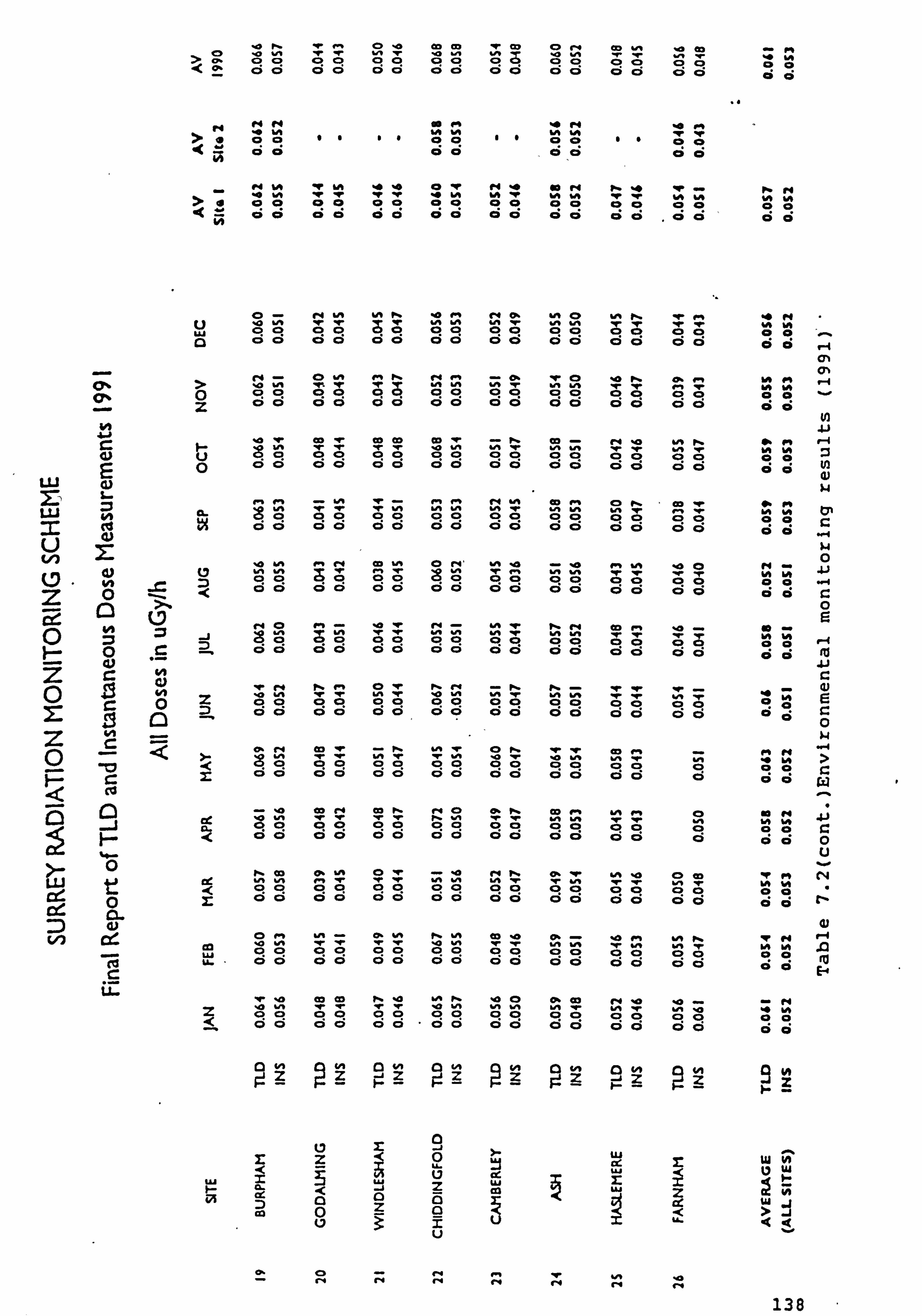
-0 pl -4- ý C> ýo Co Co -r CKP C> r4 03 ul ýa Co

c, - C'm Z 3: c3 ;3 ýI Z 2ý :ý2 9 C> CD e ! Q CD 9 ý 0 CD C> CD cý

99 92 CD

C! 9 c20 C> ý 9 c:!

c21 CD

rt e4 f4 r4 -4 >0

ý 0 %A

0Q %A

Ch c> -Ir 9D

< ci ci ci d , c; c; c; ci

ed %A «r 6A -4 14 43 lw ei -4 40 m pý 0 IN- .4 %A

D -e Ir 43 0

-p -p 0 c3.

.4 NA c31 0

hA le 43

'. ' bm -p n- Z

WN 0

:2 CD C ci ci ci d cý d ci ci

0 ci 16

Q 43 d ci

c21 im ci ci

c3 43 ci ci &4 .

Z "t

Ol

ci

P. - M

d c;

W cý c:! CD C>

04 bilt Ir -r 99 412 0

W-b P% lw Z ce

ID Q

ýo 0--b %0% WN t:! c:! 00

«4 Z &A 0 CD c; ci

UN C> 0% %A

(3 CD ci ci

eý pý le,

C> C> d ci

n» 4.. b ýr "- CD CD e ci

-4

an

ci

re

1101

ci --

doN

C%

> 0

4-4 '0 6A 99 C) 0

42 l" Ir C! C: t Q0

p. r ;ý

IC! 0 (2

rt f-N

00

CN

00

le c: b wli ßON 99 00

ýr 1-r cm! -0

c> ci

CN f.. b 0" -q- 42 C)

ci cý

ha

0

ci

f% b* 0

c;

1:, :Z vi ul

z2

Z

0

In

L- Z

4A

ce

V)

4v c: 2 ,4

(-q

401 0

0

CL

tg

3 -

-2

43 Q

en en ;e UN c:!

0 C>

'0 WN

od --! cio

4. CD ch c;

ýo UN IC!

0 CD

Co

42 42

- &A -r "- IR c:! CD 0

94 4- 9

ci 0

d" -

CD ci c: i

ýr l" 9 Ct c), CD

Co (0

cý Ch 0d

-r - ýr NM c:! 9 00

Cb &A ý n. c:! cý 0 CD

ýa w.

C> CD ci ö

LM ýr C! x:! 00,

CD

CDO d c: i

0" f" &A 9

c2h 0

r4' %A 9

00

r4 -

9 Ck CD CD

ýo vt c: ý IC! c> C. 2h

CD Ch d dmi

rt 4A UN -q- 9 IR Q CD

boN ýa w» ý 9 C! Ch c20

t^ --r

9 Ch ci Ch

%0% -r 0 R 00

Co Vb tn

CD 92

ci e

CO en im q 0 ci

- 10 UN %ob c:! Cm! cl, 40

rý e4

9 c:! 90 c20

LA UN qR 0Q

f4 10 Ir Ir

CD Clh

ci ci

CD P- im -v-

Cgi g

42

fn UN r M- ce c:!

CD CD

CD r"

ci ci cs ci

"- -q- 9 ýo 0d

vt p. beb -q- C> 4: )

cý e

, Co In- A ýf- 9-

c> cý

ýo 0 ýr 14» C! C! 010

ýo - 42 e0

4^ -4- CD 40 ci ci

ob än 0

G 0- &A 0

ci f4 Wb 19 Cb

40 w% C» ci

0 Ci

f% tot 0

ci F% %Ob 0

e;

Z; 9 Cb

- %A 0 ci

bob 9

43 r-i

ul

-41 --, r_

tu

E

r:

0

Gl

.5 < 22 f4

3 6n IC! c> CD

c13 -r --r w-

cý C) c> cý

- eý %A -r

CD CD e ci

4A n- 191 2 0

cý ci

c2 mý ýo lw

q9 0 CD

0. -, r ýo WN c:, 9 ci 42

en en

C> 92

ci d

- %A 42

ci

P% -4 c: A

ci

pf A 0

d

-4

ci CD ci

03 pl w- "- 00

d ci

ri CD r, ýA ce c2

ci d v c2

cý cý

Co 0% 6A 6m 9 c:: t CD C>

0--b lw, c3

c: i d

43 -Ob 0 ci

da 1., 0 ci

rt %A 0 6 0

CY-

:D

0

0

ce ic 99

40 Q ce ce

CD 0 cý c:!

00 0 010 0 c: i 10

ci ci 12 0

e ci

bot 0

ci

w% 0

ci

V') cir. 02 LU

0 0--b ýc UN C:! C! Q c2h

%0% :; llr cý C! CD 0 0 C>

%A Nn

c:! 9 00

e3 ýo `r -W- 99 CD 0

CN - %A %ON IR C! 0 9: )

ýo 0" -v- WN cý c:! 10 40

6A beb 9 CD CD

lw 6A C! 0

9-4 wt C! c3

ýa '0 ýb ce c:! CD CD

Co CD ý-r -e- 9 c:!

0

-e ýr cý c:! CD 0

f. 10 %A II:! C!

00

-4 0 bm wl

C)

xý

ob 03 6A q- q 42 ci d

r4 ýo bot -q- C], c> c: i ci

-4 %A ýa c2 ch ö ci

.6 0 ci

w% 0 ci

12 CA 0 4A 0 KA KA Cl tn j3 V) 0A

ua 1-- CL.

ct 0

ui -i

Z

cr. ui c12 ul

w v' w

u

138

_r_ >c 0

. wvv4NWYI

3W3W3-B'YH

C) C)

I- 0

U, 0, U, 0 0 0 -J I- a,

Cl,

MY

AM32wv,. )

M040"Ool"o ~310NIM

! )NI14woo! )

WVP. fdni

NO (3-13113n! )N3

ONNOM

HDITIN"D

3W31-6

3NOISIIO(3v

S3t4rV. LS

ATI"OKM

)j*43 13dy: )

! )Nrxwoo 0

cv3"w3HIyn : Ll

-n3tA3

A Yrd OH TIJH03*d

cry3lsNyv W-vl4wllv: )

M31IONn

aILXO

CC) C: ) Cý C: ) 0 ci C) c;

Cq C: ) 0 Ci 6

Figure 7.6 Environmental monitoring TLD results (1991)

139

I,

-a S

a

-a E S

r-

a) cr)

0

0

0

0

z

V

I-

E 41

a- ýx

-c C 0

V C D

z

Z

X

-0 ýf

C

Figure 7.7 Environmental monitoring results (1991)

140

cr) co r- (D U') '4t: r Cl) C14

C; Cý Cý q Cý Cý q Cý Cý

C) C) 0000

. jq/Agn

were fading dosemeterss, irradiated after annealing to

approximately 900 pGy In air and also sent -to

selected

sites. 2 weretransit dosemeters, which accompanied the

previous sets on each of two Journeys, through east and

west Surrey, for placement and collection of dosemeters

on each of these routes. 5 were calibration dosemeters,

kept In the laboratory for the month In a lead-lined

box, and irradiated mid-month to approximately 900 WGy

in air. 5 were calibration zero dosemeters, which

accompanied the previous 5 at all times except for the

irradiation. 5 were zero dosemeters, annealed again at

the end of the month Immediately before readout of the

collected dosemeters and used to Indicate dosemeter TLD

reader zero reading. A diagram Illustrating the whole

process Is shown In Figure 1 of Ramsdale and Oduko

(1991) - Results for 1990 (April to December) and 1991 are

shown In Tables 7.1, and 7.2, and Illustrated In Figures

2 and 3 of Ramsdale and Oduko (1991) and Figures 7.6

and 7.7. Results marked INS refer to Instantaneous

readings of gamma dose-rate taken by environmental

health off Icers. They are In reasonable agreement with

the TLD results. It Is not expected that they should be

equal, since these are taken at one point In the month

(a 600 Is

reading) while the TLD measurements integrate

over a whole month.

The results show some variation across the sites,

as is expected for varying geology, with a tendency to

141

higher values in the south-east of Surrey. The highest

readings are found in Capell the lowest in Godalming,

but all are within the expected range. The overall

average environmental gamma dose rate In air was f ound

(with TLD) to be 0.061 JACy/h in 1990 and 0.057 pGy/h In

1991., giving annual rates of 0.53 mGy/ y and 0.50 mGy/y

respectively. These are approximately equivalent to 0.6

mSv/y, a little lower than the UK average of 0.7 mSv/y

quoted earlier (section 7.1). The results were

calculated from the TLD readings by the Solaro

Environmental Monitoring Software package, and by a

Lotus Symphony (later Microsoft Excel) spreadsheet as a

backup. The advantage of the spreadsheet Is that one

can follow through all stages of the calculation, check

equations and data and find any errors., and so have

considerable confidence In the result. The software

package is something of a "black box".. as detailed

information on how it calculates the results is not

available. For the first 9 months the results of both

systems were in close agreement. Then a new version of

the software was Installed, and results were poor

compared with those from the spreadsheet; missing

dosemeters were also not treated correctly in the

calculations. It Is hoped that better agreement would

be found again with the latest software Installed in

June 1992.

A number of problems emerged during the operation

of the monitoring programme. One of these was the loss

142

of dosemeters from a number of sites, mostly

corresponding to a- on the tables of results. At some

sites these losses occurred once only, but at other

sites repeated losses of dosemeters led to a decision

to change the sites. The new sites (shown as Site 2 in

the penultimate column of Table 7.2) were In old

peoples' homes, and no dosemeters have been lost since

these changes were made.

A small number of TLD readings at one site were

extremely high, although the Instantaneous readings

from the site remained normal. The ratio of readings

from dosemeters under the metal and plastic filters

Indicated that this was due to a man-made radiation

source. Subsequently a small radioactive source

(probably from a smoke detector) was found In the

container with the dosemeter on one occasion. This more

sophisticated form of vandalism also led to some true

results being lost, and the site was changed.

Some problems arose due to the reader becoming

hotter and dark current increasing substantially on hot

summer days. The manufacturers recommend a fixed-

temperature (200C) environment for the Solaro, but It

was not always possible to provide this. The effect of

this on some readings has been discussed in Chapter 3.

On another occasion, a fault In one of the two heaters

of the Solaro was detected. This caused unreasonable

readings from a few dosemeters, with abnormalities

visible in the glowcurves. After repair of the heater,

143

the heating efficiency was changed., resulting in a'step

change of sensitivity of approximately 20% for that

channel of the reader, so that all the dosemeters had

to be re-calibrated.

The dosemeters were all calibrated before the

start of the monitoring programme, for selection

purposes. (For example, those with the most

reproducible readings were chosen 'for calibration

dosemeters) . The overall results gave 1 s. d. as 10%.,

compared with less than 5% claimed by the manufacturer.

The manufacturer offered to replace them, but by that

time Individual calibrations for each dosemeter had

been entered into the reader's software,, for use in

calculations, so that replacement did not seem

worthwhile, and would have involved further substantial

effort In calibration. Other aspects of the dosemeter

performance were satisfactory (see Ramsdale and Oduko,

1991). Although a full error analysis has not been

carried out, due to the difficulty of separating

various parts of the complex process, initial estimates

suggest a value considerably less than the requirement

of the ISO standard, ±30%. Further work is required in

this respect. Errors arising from scatter In the

Irradiation facility could be Investigated when It is

moved to a more spacious location. Provision of several

badges at one site for a month would allow some

statistical analysis of the spread of results to be

made. An intercomparlson of results with the East

144

Sussex monitoring programme, using shared sites, is

currently being carried out. Results should provide an

initial check on the accuracy of the measurements,

which could be further tested by participation In an

international Intercomparison programme.

The overall purpose of the measurements has been

achieved, that Is., (1) assuring the people of Surrey

that the background radiation levels are low and safe,

and (2) establishing a baseline of measurements so

that,, should any accident involving radioactive

contamination of the environment occur in future, Its

effect can be evaluated.

145

8-. -

Thermoluminescence of Foodstuffn

8.1 Introduction

The use of irradiation for the preservation of

food has been introduced relatively recently., due to

post-war advances in technology which have made it

possible on a large scale. The-subject still arouses

some controversy, however., due to public mistrust- of

any process associated with radiation. Irradiation of

foodstuffs has been permitted in -the UK since 1st

January 1991, when the Food (Control of Irradiation)

Regulations 1990 and the Food Labelling JAmendment)

(Irradiated Food) Regulations 1990, came -Into effect.

Under these regulations Isotron pic of Swindon was

granted the first licence to Irradiate foodstuffs in

the UK on 12 June 1991. An earlier government statement

(Hansard, 1988) had suggested that the availability of

tests for Irradiated foodstuffs would be an important

consideration before Irradiation of foodstuffs, was

permitted. Work has been carried out in the Physics

Department, University of Surrey since 1987 on

developing the -use of TLD as a test for Irradiated

foodstuffs. Reference should be made to the attached

publications (Moriarty, Oduko and Spyrou (1988), Oduko

and Spyrou (1990)) which summarise some of the work. Of

the results presented in' this chapter, most are from

the work of various students for M. Sc. projects. The

author was closely involved in directing this research

as a supervisor. Most of the study of strawberries, the

146

measurement of 'chicken bone in the Toledo reader, and

the longer-term measurements of spices., however, are

entirely the author's own work.

The recent UK legislation was based on the

findings of the government's Advisory Committee on

Irradiated and Novel Foods (ACINF, 1987) which 'in turn

took much of Its information from the report of JECFI

(1981) w- "' the Joint Expert Committee on the

Wholesomeness of Irradiated Foods. (The Joint'committee

Is that of the United Nations Food and Agricultural

Organisation, the lnýernational Atomic Energy Agency

and the World Health Organisation). The worldwide

perspective Is one of widespread use of , Irradiation as

a food preservation technique. IAEA (1988) reports the

use of food Irradiation facilities In 21 countries,

while -35 countries had approved the - process. With

Increasing world trade, and differing regulations, the

need for a test remains. Besides TLD, various other

methods have been used with some success to detect

whether foodstuffs have been Irradiated. -These Include

electron spin resonance (ESR), changes In viscosity.,

lyoluminescence, gas chromatography, enzyme analysis,,

spectrophotometry and colorimetry. Each has been found

promising In tests of only a few different foodstuffs.

Irradiation of food has been used to produce

various effects (Moriarty, 1987):

(1) Radurisation (low dose - less than 1 kGy)

This includes inhibition of sprouting of vegetables

147

(onions, potatoes), delaying the ripening of fruits to

extend their shelf-life, and killing Insect pests In

grains and fruit

(2) Radicidation (medium dose - 1-10 kGy)

This reduces the numbers of microorganisms (bacteria,

mould, yeast) to reduce food spoilage and the risk of

food poisoning.

(3) RadaDDertisation (high dose - over 10 kGy)

This completely sterilises food by killing all bacteria

and viruses, but is not recommended except for special

medical. reasons (for people with Immune deficiency

problems).

The ranges of absorbe d dose recommended for

irradiation of different foodstuffs are as follows

(ACINF, 1987):

Abs. -Dose

Range (kgy),

Inhibition of sprouting 0.05-0.15

Delaying ripening of fruit 0.2-0.5

Insect disinfestation 0.2-1.0

Elimination of parasites 0.03-6.0

Reduction of microbial load 0.5-5.0

for shelf life extension

Elimination of non-sporing 3.0-10.0

pathogens

Bacterial sterillsation up to 50.0

Table 8.1 Ranges of absorbed dose recommended for food for various processes

148

one reason for the need for a test of irradiated

food ls_so that these recommended values should not be

exceeded. This might occur If food is irradiated more

than once,, in error. In addition, It is not Intended

that irradiation should be used to make "safe" food

which Is unfit for human consumption. (For example,

Irradiation might kill the bacteria but food would

still contain toxins produced by them) . Even If this

has not occurred, the consumer has a right to know

whether food has been Irradiated, so as to make his own

choice.

8.2 Review

Although almost all research in TLD deals with

inorganic phosphors, a number of materials of

biological origin have been shown to exhibit

thermoluminescence, for example bone, fish scales and

seeds (Horowitz, 1984). Two early papers report

thermoluminescence of bone Wasinska and Niewladomski

(1970), Christodoulides and Fremlin (1971)), but these

were principally with a view to archaeological dating.

W. B6gl and L. Heide have published a large number of

studies on the Identification of Irradiated spices

using thermoluminescence., lyoluminescence (which they

call chemiluminescence) and changes in the viscosity of

a suspension of spices in water. Most of these papers

are in German, but the following (in English) give some

idea of the scope of their extensive studies: B8gl and

149

Heide (1985), Heide and B8gl (1987), Heide et al (1990).

Farkas et al (1990) also measured the viscosity of

suspensions of spices In water.

Electron spin resonance (ESR) has been

successfully used to detect irradiated fish and meat by

measuring the ESR signals from the bones. Lea et al

(1988) describe the use of this method for, chicken,,

goose, turkey and duck bones, while Dodd et al measured

ESR signals from pork, chicken and cod bones. Stevenson

and Cray (1989) measured ESR signals from Irradiated

chicken bone. The only disadvantage of ESR for such a

test Is that the equipment Is large and expensive, as

compared with that for TLD.

The considerable variation in the TLD response of

different samples of spices may be explained by their

dust content, as suggested by Sanderson et al (1989a,

b). The dust presumably originates from the soils In

the different countries of origin. Autio and PInnIoja

(1990) have made similar studies of the TL signal of

dust separated from spices and potatoes and compared

them with glowcurves of common minerals (quartz,

limestone and feldspar).

Kolbak (1988) and Goksu et al (1990) point out the

possible Interfering effects of uv-Induced signals If

the spices have been exposed to light as well as

Ionising radiation. Some more general studies of food

Irradiation and dosimetry have been reported by Laizier

et al (1990) and Crahn (1990).

150

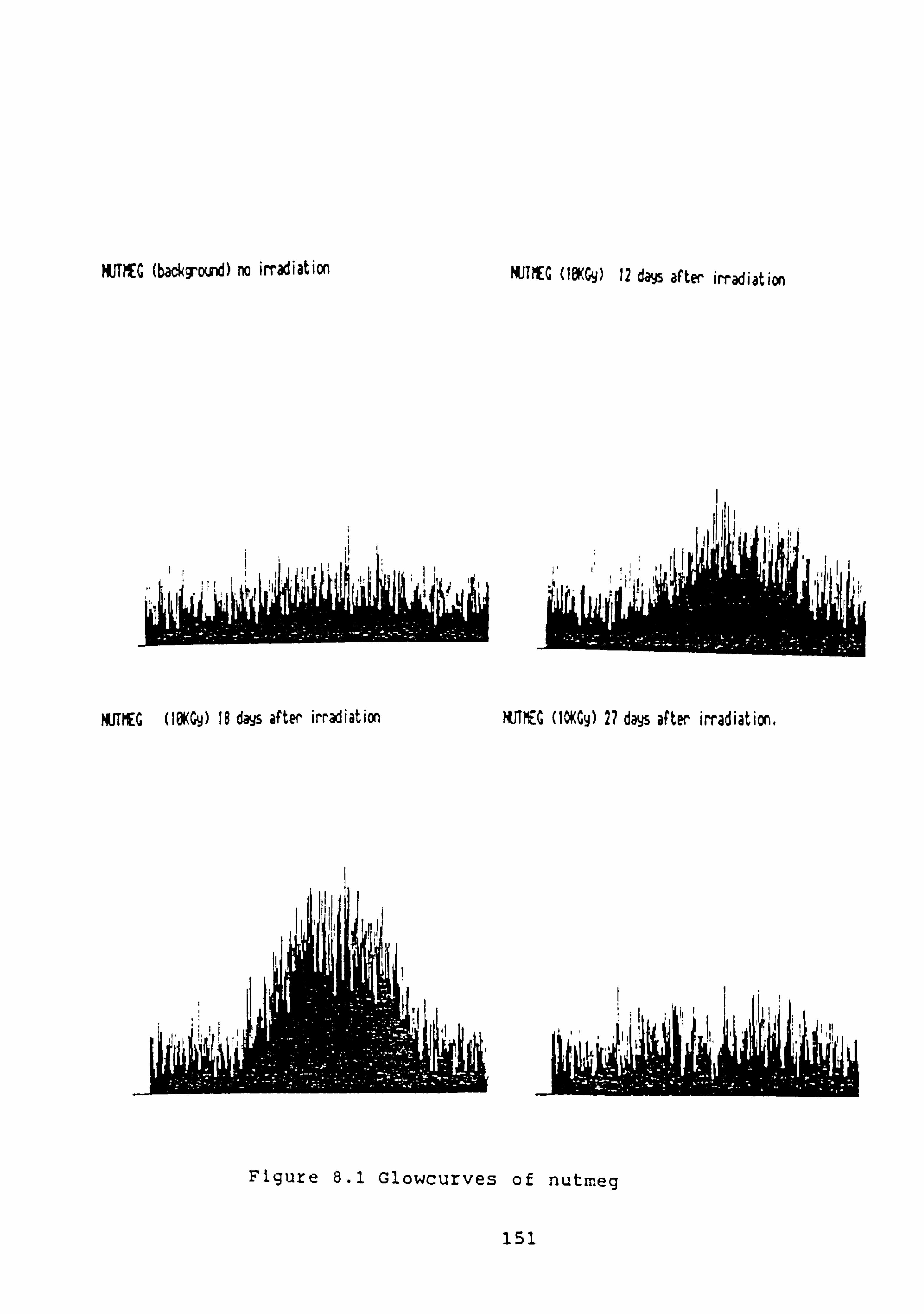
NUT? EC (background) no irradiation NUTIC OOKG9) 12 dags after irradiation

SIR

NUTMEG (IOKG9) 18 days after irradiation NUTMEG (IOKGy) 27 days after irradiation,

Figure 8.1 Clowcurves of nutmeg

151

PWRIKA (background) no irradiation PWRIKA (IBKCy) 12 days after irradiation,

PAPRIKA OOKGy) 18 days after irradiation. PAPRIKA (10 KGy) 27 days after irradiation.

Figure 8.2 Glowcurves of paprika

152

Blad( pepper ( backround ) no irradiation

Black Pepper (181(Gy) 18 *s after irradiation

Black Pepper (10KOO 12 dags after irradiation,

Black Pepper OOKGO 27 dags after irradiation

Figure 8.3 Glowcurves of black pepper

153

CUMIN ( background ) no irradiation. CUMIN (IOKGY) 12 days after irradiation,

CUMIN OB KGY) 18 days after irradiation, CUMIN (10 KGY) 27 days after irradiation,

Figure 8.4 Glowcurves of cumin

154

8.3 Results

8.3.1 Spices

Moriarty (1987) irradiated 7 different spices to 5

and 10 kGy. The TL glowcurves from these spices showed

clear peaks which were not present when Irradiated

samples were read out. Except In the case of nutmeg,

the peaks were still clearly visible 27 days after

irradiation. It may be noted that whole nutmegs are

extremely hard and smooth, so that presumably little or

no dust adheres to them. The TL signal of nutmeg may be

due to its own material, fading to background levels in

less than 27 days., whereas for the other spices the.

persistent signals would be expected from their content

of minerals in the form of dust. Figures 8.1 to 8.4

show glowcurves from 4 of the spices studied by

Moriarty (1987). They are not all to the same scale:

relative responses are shown by the histogram in Oduko

and Spyrou (1990). Some of the changes In peak height

may, be'due to differences in sample size, or changes in

sensitivity of the photomultiplier tube# but the

difference between irradiated and unirradiated samples

is clear. Further measurements up to 80 days after

irradiation (Moriarty., Oduko and Spyrou,, 1988) showed

that the response stabilised at a level well above that

of the unirradiated samples. Longer-term measurements

(Oduko and Spyrou, 1990) have shown that there is still

a clear difference between glowcurves of these

irradiated and unirradiated spices (except for nutmeg)

155

12

10

-13 I, - :3 CL

4-0 :3 0

4-

2

0

I.

(XIO)

30 60 90 time (s)

Figure 8.5 Glowcurves of 3 different brands of paprika,

4 days after irradiation to 10 kGy

156

20 months after Irradiation. This suggests that TLD Is

a suitable test for irradiated spices over periods

appropriate for their shelf-life.

Manetou (1988) studied TL signals for only 3

spices (chili powder, paprika and black pepper) but

took 2 or 3 samples of each from different

manufacturers. Clowcurves from 3 different samples of

paprika, for example, were clearly different, as shown

in Figure 8.5. The difference between Irradiated and

unirradiated samples was still clear at 30 days after

irradiation. Measurements with chili powder indicated a

linear dose-response relationship up to 10 kGy.

8.3.2 Chicken

Chicken is a likely candidate for irradiation, due

to the possibility of contamination with salmonella

which could cause outbreaks of food-poisoning.

Irradiation of chicken and turkey has been put Into use

on an industrial scale in France, using a linear

accelerator to produce 7 MeV electrons for Irradiation

(Sadat and Vassenaux, 1990).

Initially, attempts were made to obtain TL signals

from Irradiated samples of chicken bone (Manetou, *

1988), since TL had previously been observed In bone

samples (Jasinska and Niewladomski (1970),

Christodoulides and Fremlin (1971)). Although Driver

(1979) suggested the use of thin slices of bone (and a

complex chemical treatment before readout), better

157

results were obtained from powdered bone than from

slices. Chicken thigh bones were freeze dried and then

powder was . produced by filing them. Nitrogen flow

dur'Ing readout suppressed triboluminescence,, which is

greater for powder than for solid slices. The

measurements could not clearly distinguish Irradiated

from unirradiated samples from a single reading, but

repeated readout of a sample (up to 20 times) produced

curves which were higher for the irradiated samples.

Appropriate sample preparation Is very Important

for measurements of TL of bone. Measurements by the

author (Oduko and Spyrou, 1990) of bone ground to

powder and then dried with phosphorus pentoxide (Lea et

al, 1988), clearly distinguished between irradiated and

. -unirradiated samples. Oladeji (1989) observed a similar

but smaller difference , but Walker (1991a) was unable

to reproduce these results. Clearly more work Is needed

to specify exactly the best sample preparation

technique for TL of bone measurements.

OlaaejI (1989) was able to clearly distinguish

between '- Irradiated and unirradiated chicken by

measuring the TL of skin and fat. The samples were

dried before measurement by several methods - in

sunlight, in an Incubator, freeze dried, and with

phosphorus pentoxide. Figure 8.6 shows the marked

differences In the glowcurves of irradiated and

unirradiated samples. The TL signals from fat (and

158

(a) skin dried in sunlight

(b) skin dried with P205

(d) freeze-dried skin

(e) freeze dried fat

(c) skin dried in incubator (f) oil squeezed

from fatty tissue

Figure 8.6 Clowcurves of chicken samples irradiated to 5 kGy

-- irradiated -- unirradiated

159

(a)

(6)

(c)

Figure 8.7 Glowcurves of chicken samples irradiated to

5 kGy (a) fatty tissue (b) flesh (c) bone marrow

-- irradiated --- unirradiated

160

(a)

(b')

(c)

Figure 8.8 Glowcurves of fats and oils (a) olive oil

(b) sunflower oil (c) lard

irradiated -- unirradiated

161

chicken skin, which has a high fat content) were

unexpected, as one Is accustomed to think of TL In

terms of energy levels in inorganic materials such as

LIF. Presumably some parts of the complex fat molecules

are able to act as trapping and luminescence centres,

although further work Is needed to clarify this.

Further work on fatty parts of chicken and other

fats and oils, was carried out by Rayson (1990). Figure

8.7 shows his results for fatty tissue, flesh and bone

marrow of freeze-dried samples. His results for skin

samples were similar to those of Oladeji. He also

measured Irradiated and unirradiated olive oil,

sunflower oil and lard, as shown in Figure 8.8. The

oils showed only slight differences between irradiated

and unirradiated samples, but the lard glowcurve showed

a much higher peak for the Irradiated than for the

unirradiated sample. This shows that saturated animal

fats are associated with the TL signal, while the

effect is much less marked for unsaturated oils.

Walker (1991a, b) continued studies on chicken

f lesh,, fat and skin and f ound similar results.

Measurements on pheasant skin showed results similar to

chicken, but lower in magnitude, probably due to lower

fat content in pheasant skin. After cooking (30 minutes

boiling), irradiated skin samples still showed a

response 3 to 6 times that of unirradiated samples..

although the response was reduced compared with that of

uncooked irradiated skin. Thus TLD may still be usable

as a test of Irradiated chicken even after cooking.

162

(a)

(W

(c)

Figure 8.9 Glowcurves of fish flesh irradiated to 3 kGy

(a) cod (b) trout (c) sprat

irradiated unirradiated 163

X106 6-

5

4

3

rý

Ln

0 u

LLJ Or-ý -cx:: Lij

CD I

CD

0

A- IRRADIATED r -V- CON.

[3- IRRADIATED (with some oil

- C) - CONTROL j extracted)

L

/

-- ' 0--

Background

5 10 SAMPLE MASS [mg]

15

Figure 8.10 Graph of area under glowcurve vs sample

mass for irradiated and unirradiated sprat flesh

164

8.3.3 Fish and Fish Oils

Further studies relating to fats and oils in food

were carried out by Ndonye (1990). He measured the

response of freeze-dried cod,, trout and sprat flesh,

prawn shells and various fish oils. The freeze-dried

flesh was pulverised and formed into thin flat pellets

before readout: this seems to be a very suitable sample

preparation procedure. The results of the study showed

a TL response related to the fat content of the fish

samples. For cod (0.6% fat) there was no observable

difference between glowcurves of Irradiated and

unirradiated samples, while for trout and sprat (36%

and 38% fat, respectively) the glowcurves of the

irradiated samples showed large clear peaks absent from

those of unirradiated samples (see Figure 8.9). The

area under the glowcurves increased linearly with

sample mass up to 12 mg, as shown in Figure 8.10.

Surprisingly, measurements with fish oils (cod and

halibut liver oil, and oils extracted from the flesh of

trout and sprat) showed very little difference between

the signals obtained from Irradiated and unirradiated

samples. Possibly both fish flesh and oil molecules

must be present to allow some kind of

thermoluminescence process to occur. Measurements with

the shell (cuticle) of prawns showed the response of

the Irradiated samples to be about twice that of

unirradiated samples. The difference Is probably not

165

large enough to enable this effect to be used as a

definite test for Irradiated prawns.

Walker (1991) carried out further studies on

irradiated fish, using coley.. tuna and mackerel. None

of these showed a difference In response of irradiated

and unirradiated samples, although one might have been

expected for tuna and mackerel which are oily fish.

This may have been due to the sample preparation

technique, which was drying In an Incubator Instead of

freeze drying.

8.3.4 Fruit and Veqetables

A large number of fruits and a few vegetables have

been tested for thermoluminescence response. On the

whole., the results have not been very promising for

detection of Irradiated samples. Oladeji (1989) tested

various parts of two fruits, mango and papaya. One

piece of mango stem gave a signal 6 times greater for

irradiated than unirradiated samples, but no difference

was noticeable for any of the other samples. Possibly

the stem carried some unseen contaminant which had a

large response to ionising radiation.

Oduko and Spyrou (1990) shows the difference in

glowcurves of crushed seeds from Irradiated (5 kGy) and

unirradiated strawberries., the result of measurements

carried out by the author. Similar but smaller

differing signals were obtained from the dried sepals

attached to the fruit. The glowcurve from grains of

166

(a)

()

Figure 8.11 Glowcurves of irradiated (0.2kGy) and

unirradiated samples of (a) new potato skin

(b) yam skin

irradiated -- -unirradiated

167

sand removed from these strawberries was several orders

of magnitude greater and completely different in shape,

as also shown in Oduko and Spyrou (1990). This suggests

that the response of strawberry seeds (unlike spices)

Is not due to the presence of adhering soil particles.

Vincent (1989) obtained similar differences in response

of irradiated and unirradiated strawberry seeds, while

Walker (1991b) could demonstrate such a difference with

10 strawberry seeds but not with smaller samples. There

appears to be quite a large degree of variation in

response between different samples of strawberries.

Walker (1991b) could distinguish irradiated samples

most clearly by measuring the TL response of soil

removed from the surface of the strawberries, a result

which one would expect.

Oladeji (1989) showed the different TL responses

of yam skin and new potato skin, irradiated to 0.2 kGy

and unirradiated (see Figure 8.11). The TL signals of

Irradiated samples faded with half-lives of about 26

days (potato) and 10 days (yam) , and were shown to be

due to the presence of soil on the surface of the

vegetables, by removing this and measuring it

separately.

Walker (1991b) also tested Irradiated and

unirradiated flesh, seeds and skin of the following

fruits: apples, pears, redcurrants, blackcurrants,

gooseberries, oranges. He found no difference In the

measured TL signals for any of these fruits.

168

8.3.5 Ecia

Vincent (1989) measured the TL response of

Irradiated eggshell, as there was considerable media

attention' at the time concerning salmonella in eggs.

Eggs were Irradiated to 1 or 5 kGy, and small fragments

of shell were read out in the Toledo TLD reader. (Their

mainly mineral composition made this permissible. ) The

glowcurve of irradiated eggshell was clearly different

to that of unirradiated eggshell, as shown in Oduko and

Spyrou (1990).

8.4 Discussion

-These extensive measurements, only 'briefly

summarised here, have shown that thermoluminescence

measurements are promising for the detection of some

Irradiated foodstuffs. For other foodstuffs tested, the

method is not suitable. This also applie's to many other

tests for Irradiated foodstuffs, but 'TLD 'has the

advantage of being a relatively quick, easy and

Inexpensive method of testing.

- The TLD reader has recently been Improved by the

Incorporation of a charge Integrator In its circuitry.

Consideration might be given to replacing the PM-tube,

whose output is now not very stable from day to day,

and to making the heating cycle linear. Further 'and

improved studies of thermoluminescence signals from

various foodstuffs might then be fruitfully carried

out.

169

9. Conclusions

The work presented in this thesis includes several

maJor parts which each present a significant

contribution to the study of thermoluminescence

materials and their practical applications. These

comprise a study of magnesium borate dosemeters.. the

development of a computerised glowcurve deconvolution

technique, environmental monitoring measurements with

TLDý In Surrey.. and the use of thermoluminescence as a

test-for Irradiated foodstuffs. Each of these has been

published and the papers are attached.

Besides the detailed results presented, - for

magnesium borate, hundreds of other glowcurves ý have

been recorded for different materials. Their, analysis

(with the aid of the glowcurve deconvolution program)

has not yet been completed, due to the present slow

rate of manual data transfer, discussed in chapter -5.,

on completion of the analysis It is expected that these

will also be published. The development of some more

suitable means of data transfer, to speed up this

process., is a high priority. Nevertheless, the

usefulness of the program has been demonstrated in

chapter 5 by applying it to 6 different materials.

These range from LiF: MgTi, for which its use is well

established, to a low-dose glowcurve of lithium borate

with considerable scatter on the points. Glowpeaks of

several materials, which would appear to be single

peaks, are shown to have a more complex structure.

170

Lastly, the unsuccessful use of the program to fit-a

calcium' sulphate glowcurve shows clearly that the

method Is discriminating, it cannot be used simply to

fit any number of first-order peaks to any curve. The

shape ofý the calcium sulphate glowcurve appears to be

more- 'suited-- to second-order kinetics, and future

development' of the program to, include second-order

kinetics, is envisaged. The program in Its present form

is' highly- suitable for running on a Solaro-or Rialto

TLD reader since it runs on the same computer-as they

do. I

' The program needs fairly good starting parameters

for', easy running to a good fit. An interactive

display/adjust procedure, using a spreadsheet, is

described. This assists In the process of determining

reasonable starting parameters for any new material.

One such new material of current Interest is a: Al203: C

(Akselrod et al, 1990), a study of which Is planned.

A considerable amount of work was Involved In

setting up and running the TLD measurement part of the

environmental monitoring programme in Surrey. Levels of

background gamma radiation for the county were

established over two years. These should prove useful

for reference In case of any future Incident, meanwhile

the population of Surrey has been reassured of Its

safety. Apart from the lessons learned about security

of sites and dosemeters., the Interesting question of

under-response associate with 137Cs calibration arose

171

during this study. While the author Is no longer

involved. in the Surrey environmental monitoring

programme., It may be Interesting to look into this

question in future, using 137Cs calibration facilities

which are planned for the John Perry Metrology

Laboratory, St-George's Hospital, Tooting. I-

TLD has been demonstrated as a promising tool for

the detection of 'certain Irradiated foodstuffs. Like

other methods (eg ESR) it Is only successful for a

certain range of foods, but some of these are

surprising. The evidence for some kind of

thermoluminescence effect in fatty foods is quite

clear. The details of this effect, however, are

definitely deserving of further study to elucidate the

mechanism. Differences in response of different. classes

of fats, and oils are particularly Interesting. For some

foods the measured thermoluminescence Is due to their

dust or soil content,, but even without separation of

the dust, TLD remains a straightforward simple

technique for checking whether they have, been

Irradiated. Some recent Improvement In the food TL

equipment has been noted, and further suggestions for

improvement are made. There is considerable scope for

further work In this field, so that a reliable routine

test for some Irradiated foods can be developed

(although public interest In the matter seems to have

decreased considerably since legislation In the UK

permitted the irradiation of foodstuffs).

172

A very few preliminary results have been presented

for patient dose monitoring in diagnostic radiology.

Some of the practical difficulties of such a programme

have already emerged. The preliminary studies are the

first of a large measurement programme which the author

Is Involved In developing. Although lithium fluoride

dosemeters are currently used, a change to L12B407: Cu

dosemeters designed for use with the Panasonic

automatic TLD reader Is expected to be made, 'when 'a

study of their relevant properties Is complete. They

have the advantages of tissue equivalence.. ' higher

sensitivity than L12B407: Mn, and the excellent

reliability of the TLD reader. Future work planned In

this field involves the development of light-weight

"user-friendly" dosemeter packages for use on the

forehead, to measured absorbed dose to the eyes during

medical procedures, and the use of TLD In some

measurements of dental X-ray sets.

An in-depth review of various TLD equipment which

the author has used Is also presented. The 90Y/90Sr

irradiator was developed specially for use in this

work. The trend towards increasing computerisation of

reader control and data recording Is discussed.

Suggestions are made concerning the need for the

computer control to be a tool to aid the physicist, and

under his control, rather than limiting the

measurements he wishes to carry out because of the way

173

the 'software is written. It is hoped that the increasing

use of computers will lead to Increasingly more

accurate, reliable and powerful systems in which TLD is

applied for research purposes , and practical

applications, such as have been presented In this

thesis.

Many practical applications of TLD have been

reviewed, although some other fields such as

archaeology, geology, neutron and heavy ' charged

particle dosimetry have not been discussed at all.

Nevertheless, TLD has been presented as a practical

tool, using a wide variety of materials, for both

research purposes and a wide range of 'practical

applications.

174

Abdul Ahad Y K, All H H, Abdalla MM 1990 Radiat. Prot.

Dosim. 34,215-218

ACINF 1987 "Report on the safety and Wholesomeness of

Irradiated Food", M. A. F. F. London: HMSO

Aget H,, Van Dyk J, Leung MK 1977 Radiology 1.23-, 747

Aitken MJ 1985 Thermoluminescence Dating (New York:

Academic Press)

Akselrod M S, Kortov V S, Kravetsky D J, Gotlib VI

1990 Radiat. Prot. Dosim. 2_1,119-122

Al-Hussan KA and Wafa NF 1992 Radiat. Prot. Dosim. ýU

59-61

Ambrosi P, Buchholz G, Marshall T 0, Roberts P J,

Thompson IMG 1992 Radiat. Prot. Dosim. AD, 9-16

ANSI 1975 American National Standard "Performance,

testing and procedural specifications for

themoluminescence dosimetry (environmental

applications)" ANSI N545-1975 (re-affirmed 1982)

Attix F H, West E J, Nash A El Corbics S C, Johnson TL

1968 Rep. NRL Progress, 1-11

Autio T and Pinnioja S 1990 Z Lebensm Unters Forsch

1-9-" 177-180

Morin J, Gutidrrez A, Niewadomski T and GonzAlez p

1990 Radlat. Prot. Dosim. 23,283-286

Bacci C, Furetta C, Rispoli B, Roubaud G, Tuyn JWN

1988 Radlat. Prot. Dosim. 25,43-48

Barbina V, Contento G, Furetta C, Malisan M, Padovani R

1981 Radlat. Eff. Lett. 67.55-62

175

Bartlett DT, Burgess P H, Francis T M, Dutt J C,

Dimbylow PJ 1986 Radlat. Prot. Dosim. 17,29-31

Bartlett D T, Dimbylow P J, Francis TM 1990 Radiat.

Prot. Dosim. 34,119-121

Bassi P,, Busuoli C, Rlmondl 0 1976 Int. J. Appl. Rad.

and Isotopes 27, p 291

Becker K 1973 Solid State Dosimetry (Cleveland, Ohio:

CRC Press)

Becker K 1986 Radiat. Prot. Dosim. 12,531-53

Becker K, Lu R H-W, Weng P-S 1971 Proc. 3rd Int.

Conf. Lum. Dos., Riso Re'port 249., Rlso, Denmark.,

960-977

Becker K, Cheka J S, Oberhofer M 1970 Health Phys. 119,

391-403

Becquerel H 1883 Ann. Chim. Phys. 5e s6rie XXX, 5

Ben-Shachar B, Catchen C L, Hoffman J M, 1989 Radiat.

Prot. Dosim. 27,121-124

Binder W, Chlari A, Aginger H 1990 Radlat. Prot. Dosim.

2-L 275-278

Bjaerngard BE and Kase KR 1980 Med. Phys. 7(5),

560-565

Bloomsburg C D, Braunlich P, Hegland J E, Hopelscher i

W and Tetzlaff W 1990 Radlat. Prot. Dosim. 2. L

365-368

BOgl W and Heide L 1985 Radiat. Phys. Chem. 2_5., 173-185

Bohm J, McDonald J C, Swinth K L, Selby J M, Thompson I

MG 1992 Radiat. Prot. Dosim. J. O_, 5-8

176

Bos AJJ, Piters T M, de Vries W, Hoogenbloom JE 1990

Radlat. Prot. Dosim. 33 7-10

Botter-Jensen L, Furuta S, Nielsen SP 1986 Radiat.

Prot. Dosim. 17.205-210

Boyd A W, Elsenlohr H H, Girzikowsky R 1982 Med. Phys.

911-1,112-113

Boyle R 1663 (1964) Experiments and Considerations

Touching Colours, p413

Braunlich P 1990 Radlat. Prot. Dosim. 34,345-351

Burgkhardt B and Kllpfel A 1990 Radlat. Prot. Dosim.

33., 275-278

Burgkhart B and Piesch E 1981 Health Phys. 40,549-557

Busuoli G, Lembo L, Nanni R, Sermenghi 1 1984 Radiat.

Prot. Dosim. 6,317-320

Cameron J R, Suntharalingam N and Kenney GN 1968

Thermoluminescent Dosimetry (Madison, USA:

University of Wisconsin Press)

Casal E., Gil J A, Llorca N, Martinez JH 1990 Radiat.

Dosim. a, 23-31

Chakrabarti K, Mathur V K, Abbundi R J, Hill MD 1990

Radlat. Prot. Dosim. 33,35-38

Chapple C-L, Faulkner K, Lee REJ, Hunter EW 1992

Brit. J. Radlol. L! j, 225-231

Chen R 1976 J. Mat. Sci. 11,1521-1541

Chen R 1984 "Kinetics of Thermoluminescence Glow Peaks"

in: Thermoluminescence and Thermoluminescent

Dosimetry, ed YS Horowitz, Boca Raton, Florida :

177

CRC Press

Chris todoulides C and Fremlin JH 1971, Nature,

257-258

Clark M J, Burgess P H, Young T 0, Gray RC 1991,1

Radiol. Prot. 11.117-126

Collins W 1868 The Moonstone (London: JM Dent, 1944

edn. ), p56

Colvin GG and Gilboy WB 1985 J. Phys. D: Appl.

Phys. 18,283-289

Crase K W, Gammage R B, 1975 Health Phys. 29,739-746

Curie M 1904 (1961) Radioactive Substances (New York:

Philosophical Library)

Curry R 1990 , personal communication

Daniels F, Boyd C A, Saunders DF 1953 Science, 117,

343-349

Delgado A and Gomez Ros JM 1990 Radiat. Prot. Dosim.

. Z4,357-360

Delgado A, Gomez Ros J M, Muniz J L, Portillo JC 1992

Health Phys. 62.228-234

Dennis J A, Marshall T 0, Shaw KB 1974 The NRPB

Automated Thermoluminescent Dosemeter and Dose

Record Keeping System, Harwell, National

Radiological Protection Board NRPB R 32, London:

HMSO

De Werd L A, Cameron J R, Wu Da-Ke, Papini T and Das I

J 1983 Radiat. Prot. Dosim. L 350-352

Dies X, Ortega X, Rosell J 1990 Radiat. Prot. Dosim.

3A, 211-214

Dodd NJF, Lea J S, Swallow AJ 1988 Nature, 334,387

178

DoE 1988 Nuclear Accidents Overseas. The National

Response Plan and Radioactive Incident Monitoring

Network (RIMNET). Dept of Environment, Her

Majesty's Inspectorate of Pollution. London: HMSO

Driscoll CMH, McKinlay A F, Smith PA 1984 Radiat.

Prot. Dosim. 6,117-120

Driscoll CMH, Mundy S J, Elliot JM 1981 Radiat.

Prot. Dosim. L 135-137

Driscoll CMH, Fisher E S, Furetta C, Padovani R 1984

Radiat. Prot. Dosim. fi, 305-308

Driver HST 1979 P. A. C. T. 3,290-297

Duftschmid KE and Strachotinsky Ch 1986 Radlat. Prot.

Dosim. 17,21-23

Duftschmid KE and Strachotinsky Ch 1990 Radiat. Prot.

Dosim. 34,339-343

Duftschmid KE 1980 NuCl. Instrum. Meth. 135,162-165

Dutt J C, Iles W J, Bartlett DT 1990 Radiat. Prot.

Dosim. 33.303-306

Eisenlohr HH and Jayaraman S 1977 Phys. Med. Blol.

22-Cl 1,18 -28

Fang W., Ziying Z, Jian L, Zhongmei Z 1990 Radiat. Prot.

Dosim. 33.331-334

Farkas J, Sharif M M, Koncz A 1990 Radiat. Phys. Chem.

36,621-627

Faulkner K and Moores BM 1984 "The Measurement of

Radiation Dose in Computed Tomography using

Lithium Fluoride" in : Practical Aspects of

Thermoluminescence Dosimetryl CRS-431 London:

179

Hospital Physicists Association

Fitzgerald M, White D R, White E, Young J 1981 Brit. J.

Radiol. 5_4,212-220

Fleming SJ 1979 Thermoluminescence Techniques In

Archaeology (Oxford Clarendon Press)

Francis T M. O'Hagan J B, Williams S M, Driscoll CMH,

Bartlett DT 1989 Radiat. Prot. Dosim. 2L 201-205

Furetta C, Bacci C, Rispoli B, Sanipoli C, Scacco A

1990 Radiat. Prot. Dosim. 2_L 107-110

Garlick GFJ and Gibson AF 1948 Proc. Phys. Soc.

60.574-590

Gesell T F, de Planque Burke G, Becker K 1976 Health

Phys 2Z 125-133

Coksu H Y, Regulla D F, Hietel B, Popp G 1990 Radiat.

Prot. Dosim. 34.319-322

Gooden DS and BricknerIT J, Proc. 3rd Int. Conf. Lum.

Dos., Riso Report 249, Rlso, Denmark, 793-814

Grahn Ch. 1990 Radiat. Phys. Chem. U, 679-682

Griffith R V, Bohm J, Herrmann D, Strachotinsky c,

Thompson IMC 1990 Radiat. Prot. Dosim. . 1j, 115-

118

Grogan D, Bradley R P, - Ashmore J P, Scott iG 1980

Nucl. Instrum. Meth. 1.2-5., 166-168

Grogan D, Bradley R P, Ashmore iP 1983 Radiat. Prot.

Dosim. 5,233-236

Grogan D, Bradley R P, Scott iG 1986 Radiat. Prot.

Dosim. 12,33-37

Grogan D, Bradley R P, Mattioli A 1990 Radiat. Prot.

180

Dosim. 34.99-102

Grossweiner L1 1953 J. Appl. Phys. 2A, 1306

Hansard 1988 House of Commons Official Report of

Parliamentary Debates (Hansard) 126,4 February ca

762 (written)

Haskell E H, I

Bailiff IK 1990 Radiat. Prot. Dosim.

195-197

HeidelL and B6gl W 1987 Int. J. Food Sci. Tech. 22,93-

103_

Heide L, Nurnberger E, B8gl W 1990 Radiat. Phys. Chem.

36,613-619

Herschel AS 1889 Nature, 60,29

Hollaway PB 1990 M. Sc Dissertation, University of

Surrey

Holzapfel G, Lesz J, Petel M and Scharmann A 1986

Radiat. Prot. Dosim. 17.71-75

Horowitz A and Horowitz YS 1990 Radlat. Prot. Dosim. I

IL 267-270

Horowitz YS (ed) 1984 Thermohuminescence and

Thermoluminescence Dosimetry, Vol I-III (Florida

: CRC Press)

Horowitz YS and'Horowitz A 1990 Radlat. Prot. Dosim.

33j, 279-282

Horowitz Y S, Moscovitch M 1986a Radlat. Prot. Dosim.

IL 263-266

Horowitz YSI Moscovitch M 1986b Nucl. Instrum. Meth.

A243 207-214

181

-, r Horowitz Y S, Moscvovitch M, Wilt M 1984 Nucl. Instrum.

Meth. A244,556-564

Horowitz YS and Shachar BB 1990 Radiat. Prot. Dosim.

33,263-266

Hufton AP (ed) 1984 Practical Aspects of

Thermoluminescence Dosimetry, CRS-43, London:

Hospital Physicists Association

IAEA 1988., IAEA News Features 5,1-12

IPSM 1991 National Protocol for Patient Dose

Measurements in Diagnostic Radiology

ISO 1985 Thermoluminescent Dosimetry for Personnel and

Environmental Monitoring. Draft Proposal ISO/DP

8034.2 Document No ISO/TC85/sc 2N360

Jain VK 1982 Radiat. Prot. Dosim. Z, 141-167

Jasinska M and Niewladomski T 1970 Nature, 22L 1159-

1160

Jayachandran CA 1970 Phys. Med. Biol. U, 325-33_4

JECFI 1981, "Wholesomeness of Irradiated Food", JECFI

Tech. Report Series 659, Geneva: World Health

Organisation.

Johansson K-Al Hanson W F, Horlot JC 1988, Radiother.

Oncol. "l 201-203, quoted in Svensson et al

(1990)

Jones S C, Hegland i E, Hoffmann J M, Braunlich PF

1990 Radlat. Prot. Dosim. 24 , 279-282

Jones D E, Lindeken C L, McMillen RE 1971 Proc. 3rd

Int. Conf. Lum. Dos., Riso Report 249, Risol

Denmark, 985-1001

14 182

Kasa 1 1990 Radiat. Prot. Dosim. 33,299-302

Kazanskaya V A, Kuzmin V V, Minaeva E E, Sokolov AD I

1974 Proc. 4th Int. Conf. Lum. Dos., Krakow, 581-

591

Knipe_A D 1984 Radiat. Prot. Dosim. -6,75-78

Koczynski A, Wolsa-Witer M, Botter-Jensen L,

Christensen P 1974 Proc. 4th Int. Conf. Lum. Dos., F

Krakow, 641-651

Kolbak D 1988 Radiat. Prot. Dosim. 22,201-202

Kosunen A and Jarvinen H 1990 Radiat. Prot. Dosim. 34,

257-260

Kramer R, Regulla D F, Drexler G 1977 Proc. 5th Int.

Conf. Lum. Dos., Sao Paulo, 298-312

Laizier J, Erhart F, Vuillemey R 1990 Radiat. Phys.

Chem. 2§-, 667-678

Langmead WA and Wall BF 1976 Phys. Med. Biol. 21,

39-51

Langmead WA and Wall BF 1976 Phys. Med. Blol. 2.7,

1023-1034

Lea J S.. Dodd NJF, Swallow AJ 1989 Int. J. Food Sci.

Tech. 23.625-632

Lewis M A, Povall J M, Rosenbloom M E, Pickling P A,

MacHardy JD 1984 11 A TLD System for Total Body

Irradiation Dosimetry" in: Practical Aspects of

Thermoluminescence Dosimetry CRS-43, ed AP

Hufton, London: Hospital Physicists Association

Lindskoug BA and Lundberg L-M 1984 "ClInIcal Applica-

tions of Thermoluminescent Dosimetry", In

183

Thermoluminescence and Thermoluminescent Dosim

etry, Vol III, ed. Y. S. Horowitz, Boca

Raton, Florida: CRC Press.

Mahesh K, Weng PS and Furetta C 1989

Thermoluminescence in Solids and its applications

(Ashford, Kent: Nuclear Technology Publishing)

Maiello M L, Gulbin JF de Planque G, Gesell TF 1990

Radlat. Prot. Dosim. 32.91-98

Maiello M L, Culbin J F, de Planque C, Heaton HT 1990

Radiat. Prot. Dosim. 2A, 175-178

Majborn B 1984 Radlat. Prot. Dosim. 6,129-132

Manetou A, 1988, M. Sc. Dissertalon, University of

Surrey

Mangla M, Olivierl E, Fionella 0 1977 Proc. 5th Int.

Conf. Lum. Dos. Sao Paulo, 29-39

Marshall T 0., Pattison R J, Turyman A, Preston H E,

Stewart JC 1980 Nucl. Instrum. Meth. 147-149

McDougall DJ (ed)1968 Thermoluminescence of Geological

Materials (London: Academic Press)

McKeever SWS 1985 Thermoluminescence of Solids,

Cambridge: Cambridge University Press

McKinlay AF 1981 Thermoluminescence Dosimetry

(Bristol: Adam Hilger Ltd)

McKinlay A F, Bartlett D T, Smith PA 1980, Nucl.

Instrum. Meth. 175,57-59

McKlveen iW 1980 Nucl. Instrum. Meth. 175,201-204

mollah A S, Rahman M M, Molla MAR, Das SC Akan Y

Radiat. Prot. Dosim. ý4,223-224

184

Morgan MD and Stoebe TG 1990 Radiat. Prot. Dosim. 33,

31-33

Moriarty TF 1987, M-Sc. Dissertation, University of

Surrey

Moriarty T, Oduko JM and Spyrou NMS 1988 Nature 332,

22

Morse HW 1905 Astrophys. J. 21,410

Moscovitch M 1986 Radiat. Prot. Dosim. J_L 165-169

Moscovitch M, Horowitz YS and Oduko J 1984 Radiat.

Prot. Dosim. 6,157-159

Moscovitch M, Szalanczy A, Bruml W W, Velbeck K il

Tawil RA 1990, Radiat. Prot. Dosim. 34.361-364

Nakajima T 1988 Radiat. Prot. Dosim. ZZ, 119-122

Nambi KSV and Higashimura T 1971 Proc. 3rd Int. Conf.

Lum. Dos., Rlso, Rlso Report 249,1107-1117

Needham A 1989 Radiation Protection - Theory and

Practice, Proc. 4th Int. Symp.

Ndonye PK 1990 M. Sc. Dissertation, University of

Surrey

NRPB 1990 Patient Dose Reduction in Diagnostic

Radiology , Documents of the NRPBI L3

Oberhofer M 1981 "Accessory Instrumentation" in

"Applied Thermoluminescence Dosimetry",, eds M

Oberhofer and A Scharmann, (Bristol: Adam Hilger

Ltd)

Oduko JM 1979, M. Sc Dissertation, University of

Surrey

Oduko JM, Harris SJ and Stewart JC 1984 Radiat.

185

Prot. Dosim. 8,257-260

Oduko JM and Spyrou NMS 1990 Radlat. Phys. Chem.

603-607

Oladeji T0 1989, M. Sc. Dissertation, University of

Surrey

Oldenberg H 1705 Phil. Trans. Abrdg. 1,345

Perks CA and Marshall M 1990 Radiat. Prot. Dosim. 2_L

103-106

Perks CA and Marshall M 1991 Radiat. Prot. Dosim. 21,

261-269

Peto A 1990 Radiat. Prot. Dosim. . 23... 103-106

Piesch E 1981 "Application of TLD Systems for

Environmental Monitoring" in: Applied

Themoluminescence Dosimetry ed. M Oberhofer and A

Scharmann, Bristol: Adam Hilger, 197-228

Piesch E and Burgkhardt B 1977 Proc. 5th Int. Conf.

Lum. Dos., Sao Paulo, 335-341

Piters TM and Bos AJJ 1990 Radiat. Prot. Dosim.

33., 91-94

Pitman DA Ltd 1980 Technical Information: Low

Intensity Solid State Light Sources

de Planque G and Gesell TF 1984 Radiat. Prot. Dosim.

J. L 193-200

Podgorsak E B, Moran P R, Cameron JR 1971 Proc. 3rd

Int. Conf. Lum. Dos. Rlso Report 249, Riso, Denmark

1-8

Portal G 1986, Radiat. Prot. -Dosim. 17.. 351-357

Prokic M 1980 Nucl. Instrum. Meth. jjý, 57-59

18G

Prokic M 1982 Health Phys. JL 849-855

Prokic M 1984 Radiat. Prot. Dosim. J, 133-136

Prokic M 1990 Radiat. Prot. Dosim. J. L 99-102

Ramsdale ML and Oduko JM 1991 Paper presented at

5th International Symposium on the Natural

Radiation Environment, Salzburg and to be

published in Radiat. Prot. Dosim.

Randall JF and Wilkins MHF 1945a Proc. R. Soc. A184,

366-389

Randall JF and Wilkins MHF 1945b Proc. R Soc.

A184 390-407

Rayson MJ 1990 M. Sc. Special Project Report,

University of Surrey

Robertson MEA 1975 Ph. D Thesis, University of Surrey

Roser FX and Cullen TL 1965 Science 138 145

Ruden B-I 1976 Acta Radiol. Ther. Phy. Blol. U, 447-464

Ruden B-I 1971 Proc. 3rd Int. Conf. Lum. Dos., Riso

Report 249, Riso, Denmark, 781-792

Sadat T and Vassenaix M 1990 Radiat. Phys. Chem. 2_E,

661-665

Sahre P 1987 Radiat. Prot. Dosim. U, 19-23

Sanderson DCW, Slater C, Cairns KJ 1989a Nature 2AO,

23

Sanderson DCW, Slater C, Cairns KJ 1989b Radiat.

Phys. Chem. 2_L 915-924

Scarpa G, Caporali C, Moscati M 1990 Radiat. Prot.

Dosim. 2_L 343-346

Scarpa G 1970 Phys. Med. Biol. 15,667-672

187

Scarpa G, Benincasa G, Ceravolo L 1971 Proc. 3rd Int.

Conf. Lum. Dos., Riso, Riso Report 249,427-441

Scarpa G, Alberici A, Ledda S, Klamert V 1990 Radiat.

Prot. Dosim. 2_3,323-326

Scharman A 1981 History, In Applied Thermoluminescence

Dosimetry, ed. M. Oberhofer and A Scharmann

(Bristol: Adam Hilger Ltd)

Schulman J H, Kirk R D, West E J, 1965 Proc. Int. Conf.

Lum. Dos., Stanford, 113-118

Seeley MA 1975 J Archaeol. Sci. 2.17

Segovia N, Gaso M I, Chavez A, Tejera A, Gutierrez A,

Azorin J, Balcazar M, Lopez A, Tamez E, Cervantes

L, Monnin M 1990 Radiat. Prot. Dosim. 34,219-222

Shachar BB and Horowitz YS 1988 Radiat. Prot. Dosim.

22,87-96

Shope T B, Cange R, Johnson GC 1981 Med. Phys. 1,488-

495

Shoushan W 1988 Radiat. Prot. Dosim. 25,133-136

Shrimpton PC 1992 NRPD Radiol. Prot. Bull. JZ2,4-11

Shrimpton P C, Wall B F, Jones D G, Fisher ES Hillier

M C,, Kendall GM 1986 A National Survey of Doses

to Patients Undergoing a Selection of Routine X-

ray Examinations In English Hospitals, Chilton,

National Radiological Protection Board, NRPB R2001

London: HMSO

Stevenson MH and Gray R 1989 J. Scl. Food Agric.

269-274

Sunta CM 1984 Radiat. Prot. Dosim. E., 25-44

188

Suntharalingam N 1980 Nucl. Instrum. Meth. 175,191-

192

Suntharalingam W and Mansfield CM 1971 Proc 3rd Int.

Conf. Lum. Dos., Riso, Riso Report No 249 p. 816

Svenssson H, Nette P, Zsdansky K 1990 Radlat. Prot.

Dosim. 34.241-247

Szabo P P, Feher I, German E 1990 Radiat. Prot. Dosim.

2j, 191-194

Takenaga M, Yamamoto 0, Yamashita T 1983 Health Phys.

44 387-393 L-L. f Taylor GC and Lilley E 1978 J. Phys. D: Appl. Phys.

11.567

Trowbridge J and Burbank JE 1898 Am. J. Scl. ser 4,

5,55

Tuyn JWN 1977 Proc. 5th Int. Conf. Lum. Dos., Sao

Paulo, 288-297

Urbach G 1930 Wien. Ber. IIa M, 363

Urbach G 1948 Storage and Release of Light by

Phosphors, New York: John Wiley

Vincent L 1989 M. Sc. Special Project Report, University

of Surrey

de Vries W and Bos AJJ, 1990 Radlat. Prot. Dosim.

251-253

Waldron L, Wade J P, Goldstone K 1992, Radiography

Today 5B, 659,9-10

Walker MW 1991a, M. Sc Special ProJect Report,

University of Surrey

189

Walker MW 1991b M. Sc Dissertation, University of

Surrey

Wall B F,, Driscoll CMH, Strong J C, Fisher ES 1982

Phys. Med. Biol 27,1023-1034

Wall B F, Green DAC, Veerappan R 1979a, Br. J.

Radiol. JL 189

Wall B F, Fisher E S, Paynter R, Hudsen A, Bird P D,

1979b, Br. J. Radiol. ý2-, 727

Wall B F., Rae S, Darby S C, Kendall GM 1989 Br. J

Radiol. _54,779

Wang S, Chen G, Wu F, Ll Y, Zha S, Zhu j 1986 Radiat.

Prot. Dosim. " 223-227

Wang S, Cai G C, Zhou KQ and Zhou RX 1990 Radiat.

Prot. Dosim 23,247-250

Wernli C 1990 Radiat. Prot. Dosim. 34,199-202

Wick FG 1924 Phys. Rev. 2L 272

Wick FG 1925 Phys. Rev. 2-5,588

Yamamoto 0, Yasuno Y, Minamide S, Hasegawa Sp Tsutsui

H,, Takenaga M, Yamashita T 1982 Health Phys.

IL 383-390

190

Uj'IjVERSjTYUrýOW46j6fAMA amio'iiAhl