Summaries of Wildlife Research Findings

2012

Minnesota Department of Natural Resources Division of Fish and Wildlife

Wildlife Populations and Research Unit

SUMMARIES OF WILDLIFE RESEARCH FINDINGS

2012

Edited by: Lou Cornicelli

Michelle Carstensen Marrett D. Grund Michael A. Larson

Jeffrey S. Lawrence

Minnesota Department of Natural Resources Division of Fish and Wildlife

Wildlife Populations and Research Unit 500 Lafayette Road, Box 20

St. Paul, MN 55155-4020 (651) 259-5202

©September 2013 State of Minnesota, Department of Natural Resources

For more information contact:

DNR Information Center 500 Lafayette Road

St. Paul, MN 55155-4040 (651) 296-6157 (Metro Area)

1 888 MINNDNR (1-888-646-6367)

TTY (651) 296-5484 (Metro Area) 1 800 657-3929

http://www.mndnr.gov

This volume contains interim results of wildlife research projects. Some of the data and interpretations may change as a result of additional findings or future, more comprehensive analysis of the data. Authors should be contacted regarding use of any of their data. Printed in accordance with Minn. Stat. Sec. 84.03 Equal opportunity to participate in and benefit from programs of the Minnesota Department of Natural Resources is available to all individuals regardless of race, color, creed, religion, national origin, sex, marital status, status with regard to public assistance, age, sexual orientation, membership or activity in a local commission, or disability. Discrimination inquiries should be sent to MN DNR, 500 Lafayette Road, St. Paul, MN 55155-4031; or the Equal Opportunity Office, Department of the Interior, Washington, DC 20240. Printed on recycled paper containing a minimum of 30% post-consumer waste and soy-based ink.

TABLE OF CONTENTS

Farmland Wildlife Research Group

Evaluating Preferences of Hunters and Landowners for Managing White-tailed Deer in Southwest Minnesota – A Progress Report

Gino J. D’Angelo and Marrett D. Grund…………………………………………………….…1

Establishment of Forbs in Existing Grass Stands

Nicole Davros, Molly Tranel, Greg Hoch, and Kurt Haroldson………………………………6

Forest Wildlife Research Group

Ecology and Population Dynamics of Black Bears In Minnesota

David L. Garshelis, Karen V. Noyce, and Mark A. Ditmer………………………………….13

Measuring The Apparent Decline of a Bear Population in the Core of Minnesota’s Bear Range

David L. Garshelis, Karen V. Noyce………………………………………………………….27

Helicopter Capture of Newborn Moose Calves in Northeastern Minnesota: An Evaluation

Glenn D. DelGiudice, William J. Severud, and Robert G. Wright…………………………40

Evaluating the Use of GPS-Collars to Determine Moose Calving and Calf Mortalities in Northeastern Minnesota

William J. Severud, Glenn D. DelGiudice, and Robert G. Wright………………………....52

Assessing Nutritional Restriction of Moose in Northeastern Minnesota, Winter 2013: A Pilot

Glenn D. DelGiudice, Erika Butler, Michelle Carstensen, and William J. Severud……...63

A Long-Term Assessment of the Effect of Winter Severity on the Food Habits of White-Tailed Deer

Glenn D. DelGiudice, Barry A. Sampson, and John H. Giudice ………………………….74

A Long-Term Assessment of the Variability in Winter Use of Dense Conifer Cover By Female White-Tailed Deer

Glenn D. DelGiudice, John R. Fieberg, and Barry A. Sampson………….……………….75

Wildlife Health Program

Bovine Tuberculosis in White-Tailed Deer in Northwest Minnesota: A 7-Year Effort to Restore Minnesota’s Disease-Free Accreditation

Michelle Carstensen, Erika Butler, Erik Hildebrand, and Lou Cornicelli…………………76

Northeast Minnesota Moose Herd Health Assessment 2007–2012

Erika A. Butler, Michelle Carstensen, Erik C. Hildebrand, and John H. Giudice ……......86

Determining Causes of Death in Minnesota’s Declining Moose Population: A Progress Report

Erika A. Butler, Michelle Carstensen, Erik C. Hildebrand, and David C. Pauly……….…97

The Ecology of Eastern Equine Encephalitis Virus in Wildlife and Mosquitoes in Minnesota

Amy Kinsley, Erika A. Butler, Roger Moon, Kirk Johnson, Michelle Carstensen,

David Nietzel, and Meggan Craft …………………………………………………………...107

Transmission of Newcastle Disease Virus in Double-crested Cormorants

LeAnn White, Jeffrey Hall, Daniel Walsh, Paul Wolf, David C. Pauly, Erik C. Hildebrand,

Michelle Carstensen, Erika Butler ……………………………………………………….…109

Congenital Transmission of Neospora caninum in White-Tailed Deer (Odocoileus virginianus)

J. P Dubey, M. C. Jenkins, O.C.H Kwok, L. R. Ferreira, S. Choudhary, S. K. Verma,

I. Villena, E. Butler, and M. Carstensen ……………………………………………………112

Biometrics Unit and Surveys

Quantifying the Effect Of Habitat Availability On Species Distributions

Geert Aarts, John Fieberg, Sophie Brasseur, and Jason Matthiopoulos………………..114

Estimating Population Abundance Using Sightability Models: R Sightabilitymodel Package

John R. Fieberg…………………………………………………………………………….…115

Abundance Estimation with Sightability Data: A Bayesian Data Augmentation Approach

J. Fieberg, M. Alexander, S. Tse, and K. St. Clair……………………………………..116

Using Time-of-Detection to Evaluate Detectability Assumptions in Temporally Replicated Aural Count Indices: An Example with Ring-Necked Pheasants

John H. Giudice, Kurt J. Haroldson, Alison Harwood, Brock R. McMillan……………117

A Comparison of Models Using Removal Efforts to Estimate Animal Abundance

Katherine St. Clair, Eric Dunton, and John Giudice ………………………………….…118

Wetland Wildlife Research Group

Modeling And Estimation Of Harvest Parameters And Annual Survival Rates Of Wood Ducks In Minnesota. Phase I: A Comparison Of The Effectiveness Of Three Types Of Traps

James B. Berdeen………………………………………………………………………..…119

Efficacy of CO2 as a Fish Piscicide: Final Report For The Winter 2013 Pilot CO2 Study

Kyle D. Zimmer, Jim B. Cotner, Mark A. Hanson, and Brian R. Herwig ……..….…..123

Shallow lake rehabilitation: still lots to learn?

Mark A. Hanson, Brian R. Herwig, Kyle D. Zimmer, Patrick G. Welle, Nicole

Hansel-Welch, and William O. Hobbs ……………………………………….………….133

Nesting Ecology of Ring-Necked Ducks in The Boreal Forest of Northern Minnesota

Charlotte Roy ……………………………………………………………………….……....134

Investigation of Trematodes and Faucet Snails Responsible for Lesser Scaup Die-Offs

Charlotte Roy …………………………………………………………………………….....142

Publications ………………………………………………………………………………………….152

Farmland Wildlife Populations and Research Group

35365 800th Avenue Madelia, Minnesota 56062-9744

(507) 642-8478 Ext. 221

Evaluating Preferences of Hunters and Landowners for Managing White-tailed Deer in Southwest Minnesota – A Progress Report

Gino J. D’Angelo and Marrett D. Grund

SUMMARY OF FINDINGS

We mailed questionnaires to 3,600 hunters and 4,400 landowners in southwest

Minnesota to evaluate their experiences and attitudes regarding white-tailed deer (Odocoileus virginianus) densities, hunting opportunities, and potential regulations for deer hunting. This paper summarizes findings from 2 of 3 mailings that were completed. We expect final results will be available in summer 2013. Preliminary results suggested hunters were satisfied with deer densities, but would prefer to see a higher proportion of bucks in the population and more older-aged bucks. Most landowners believed deer populations were too high or about right, and 46% of landowners wished to see deer densities reduced. The results of these surveys will help evaluate the 2012 deer goal-setting process in southwest Minnesota, and will help inform decisions about future management of deer in southwest Minnesota.

INTRODUCTION

During 2012, Minnesota Department of Natural Resources (MNDNR) conducted a deer

goal-setting process to gather public input to aid in setting deer population goals for 3 blocks of deer permit areas (DPAs) in the state, including southwest Minnesota, the Grand Rapids area, and the Hibbing area (Thorson 2012). The goal-setting process included development of recommendations for deer population goals by stakeholder teams and an online survey of voluntary participants. Stakeholder teams from the respective blocks represented hunters, landowners, local government officials, and other people with an interest in deer. Stakeholder teams were presented with information about deer biology and management in their region. After discussion among the stakeholders, the team developed recommendations for deer population goals.

Online surveys were available on the MNDNR public website and were announced through news releases. Online surveys were open for a period of 26 days. Participants in the online survey were voluntary, and they were asked to select 1 block of DPAs that was of interest to them. These participants were presented with a slide show of information specific to the block of DPAs, including the recommendations for deer population goals from the stakeholder teams. Participants then completed a survey about deer management in their area, and were asked at what level the deer population should be managed in the block of DPAs.

Online respondents indicated they would like deer populations to be increased in all 3 blocks of DPAs. In both the Grand Rapids area and the Hibbing area, >60% of respondents felt that deer numbers were too low. The results were less clear in the southwest block of DPAs with 46% of respondents indicating that deer numbers were about right and 50% of respondents indicating that deer numbers were too low. With no plurality of opinion about deer population levels in southwest Minnesota, the results of the goal-setting process were difficult to apply to management. In addition, only 36% of online respondents were satisfied with the goal-setting process. Thus, the purpose of our study was to obtain detailed public input data to aid in setting deer population goals for southwest Minnesota.

OBJECTIVES

1) To evaluate the satisfaction of deer hunters with regards to their hunting experiences in southwest Minnesota;

2) To identify the preferences of hunters for potential regulations to manage deer in southwest Minnesota;

Page 1

3) To evaluate the experiences and attitudes of landowners in southwest Minnesota about deer relative to land use on their property and perceptions of deer damage to agriculture;

4) To evaluate the satisfaction of landowners that hunt with regards to their hunting experiences in southwest Minnesota; and

5) To identify the preferences of landowners for potential regulations to manage deer in southwest Minnesota.

METHODS

The surveys focused on southwest Minnesota, including the counties of Brown,

Cottonwood, Jackson, Lac qui Parle, Lincoln, Lyon, Martin, Murray, Nobles, Pipestone, Redwood, Rock, Watonwan, and Yellow Medicine. To evaluate potential geographic differences in experiences and attitudes of respondents, the region was stratified into 2 sub-regions. Sub-region 1 was generally north of U.S. Route 14, including DPAs 252, 279, 286, 288, 289, and 296. Sub-region 2 was generally south of U.S. Route 14, including DPAs 234, 237, 238, 250, 294, and 295.

We selected a random sample of 3,600 hunters from the MNDNR Electronic Licensing System. All Minnesota hunters were asked to indicate which DPA they intended to hunt when they purchased a license for hunting deer in 2012. Our survey population included adult, resident firearms deer hunters who indicated they intended to hunt in 1 of the DPAs within the study area. We randomly selected 1,800 hunters in each sub-region for this survey. We created a database of landowners from tax records of the counties in our study area and selected landowners who owned at least 1 property >160 acres. We then randomly selected 2,200 landowners for each sub-region for a total of 4,400 landowners.

We mailed individuals a self-administered questionnaire with a postage-paid return envelope. Accompanying the survey was a cover letter, which requested participation in the survey, outlined the goals of the survey, and assured individuals that their participation, contact information, and answers would remain confidential. We conducted 3 mailings beginning on 21 February 2013 with 4 weeks between the first and second mailing, and 6 weeks between the second and third mailings.

The survey of hunters was 8 pages and included questions about their hunting participation and behaviors, satisfaction with their hunting experiences, opinions about deer population levels, and preferences for potential regulations. The survey of landowners was 12 pages and included questions about land ownership, perceptions of wildlife damage, strategies used to reduce wildlife damage, opinions about deer population levels, and preferences for potential regulatory changes. Landowners who indicated they hunted were directed to the same questions asked in the survey of hunters, including their hunting participation and behaviors, and satisfaction with their hunting experiences. Potential regulations for deer hunting presented in the survey were: 1) an early youth-only season, 2) buck-only hunting when deer densities were considered below goal in a DPA, 3) buck permit lottery with youth exemption, 4) antler point restriction with youth exemption, 5) prohibit cross-tagging of bucks, 6) prohibit cross-tagging of antlerless deer, 7) earlier start of the firearm season, and 8) delayed start of the firearm season.

RESULTS and DISCUSSION

Two of 3 mailings were completed at the time of this report and we expect final results

will be available in summer 2013. The preliminary results we present in Tables 1-5 include data from the first 2 mailings for the survey of hunters and landowners. Estimated response rates from these 2 mailings were >50% and >44% for hunters and landowners, respectively.

Preliminary results suggested about 60% of hunters in southwest Minnesota were satisfied with the number of antlerless deer and the total number of deer seen while hunting, but hunters were less satisfied with the quantity and quality of bucks in the population (Table 1). Although only 6% of hunters believed too many either-sex licenses were being offered by the

Page 2

MNDNR (Table 2) and most hunters believed deer densities were about right (Table 3), approximately 52% of hunters responded that they would still like to have deer densities increased (Table 4). In contrast, 31% of landowners were satisfied with current deer numbers (Table 4) but 42% of landowners believed deer numbers were too high (Table 3) and 46% of landowners would prefer to see deer densities decreased (Table 4). Thus, our preliminary results indicated the majority of hunters and landowners were satisfied with current deer numbers and believed the number of either-sex permits issued by the MNDNR has been appropriate, but hunters want more deer and landowners want fewer deer in the future.

About half of the hunters we surveyed were not satisfied with the number or quality of bucks in the southwest Minnesota deer population (Table 1). As demonstrated in southeast Minnesota and in other states, an antler-point restriction regulation reduces harvest mortality rates of young bucks thereby allowing bucks to reach older-age classes and grow larger racks. Previous hunter surveys conducted in Minnesota suggest buck harvest mortality would slightly decrease if hunters were not able to cross-tag bucks with their hunting licenses. There is a perception that bucks would be less vulnerable to being harvested if the deer hunting season were held after the rut. Our preliminary results suggest a majority of hunters support an antler-point restriction regulation but there was strong opposition from hunters about prohibiting the cross-tagging of deer or holding the deer hunting season after the rut (Table 5). Based on these preliminary findings, we believe wildlife managers should consider implementing an antler-point restriction to address satisfaction levels associated with the quantity and quality of bucks in southwest Minnesota deer populations.

ACKNOWLEDGEMENTS

We appreciate the input of L. Cornicelli, W. Krueger, R. Markl, L. McInenly, S. Merchant, B. Schuna, E. Thorson, and K. Varland. Their knowledge of issues regarding deer and public involvement in deer management in southwest Minnesota was integral to designing the surveys. We thank T. Klinkner, J. Luttrell, K. McCormick, and A. McDonald for diligently entering data from returned surveys. The county governments of southwest Minnesota cooperatively provided landowner data. We are indebted to the many hunters and landowners who took the time to complete surveys. Their experiences and opinions will help guide the responsible management of deer in southwest Minnesota. LITERATURE CITED Thorson, E. 2012. 2012 Minnesota deer goal-setting report. Unpublished report. Division

of Fish and Wildlife, Minnesota Department of Natural Resources, St. Paul, Minnesota. 11 pp.

Page 3

Table 1. Satisfaction of hunters and landowners in southwest Minnesota with deer population demographics, 2012 (Note: Answers of “Don’t know” were removed from these analyses, and if landowners indicated they did not hunt, they were not asked these questions).

Survey population n Strongly

disagree Slightly disagree Neutral Agree Strongly

agree

Satisfaction with number of legal bucks

Hunters 1,705 24% 25% 10% 27% 14%

Landowners 456 24% 22% 11% 24% 18%

Satisfaction with quality of bucks

Hunters 1,711 28% 24% 12% 24% 12%

Landowners 462 33% 19% 11% 22% 14%

Satisfaction with number of antlerless deer

Hunters 1,731 11% 14% 12% 23% 40%

Landowners 465 14% 16% 13% 16% 41%

Satisfaction with total number of deer

Hunters 1,745 12% 18% 10% 30% 30%

Landowners 474 11% 19% 12% 22% 37%

Table 2. Opinions of hunters and landowners in southwest Minnesota about the number of either-sex permits provided for their area for the 2012 deer season (Note: If landowners indicated they did not hunt, they were not asked this question).

Survey population n Too low About

right Too high Don’t know

Hunters 1,774 27% 49% 6% 18%

Landowners 504 27% 50% 8% 15%

Table 3. Opinions of hunters and landowners in southwest Minnesota about the level of the deer population in their area, 2012.

Survey population n Too low About

right Too high Don’t know

Hunters 1,781 36% 42% 15% 7%

Landowners 1,742 11% 31% 42% 16%

Table 4. Opinions of hunters and landowners in southwest Minnesota during 2012 about future management of the deer population in their area.

Survey population n Decrease

50% Decrease 25%

Decrease 10% No change Increase

10% Increase 25%

Increase 50%

Hunters 1,755 3% 7% 10% 28% 26% 20% 6%

Landowners 1,560 18% 16% 12% 29% 11% 9% 5%

Page 4

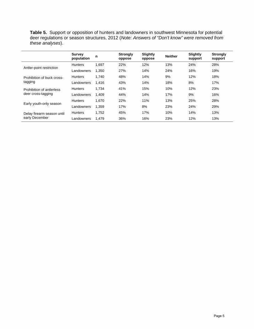
Table 5. Support or opposition of hunters and landowners in southwest Minnesota for potential deer regulations or season structures, 2012 (Note: Answers of “Don’t know” were removed from these analyses).

Survey population n Strongly

oppose Slightly oppose Neither Slightly

support Strongly support

Antler-point restriction Hunters 1,697 22% 12% 13% 24% 28%

Landowners 1,350 27% 14% 24% 16% 19%

Prohibition of buck cross-tagging

Hunters 1,740 48% 14% 9% 12% 18%

Landowners 1,416 43% 14% 18% 8% 17%

Prohibition of antlerless deer cross-tagging

Hunters 1,734 41% 15% 10% 12% 23%

Landowners 1,409 44% 14% 17% 9% 16%

Early youth-only season Hunters 1,670 22% 11% 13% 25% 28%

Landowners 1,359 17% 8% 23% 24% 29%

Delay firearm season until early December

Hunters 1,752 45% 17% 10% 14% 13%

Landowners 1,479 36% 16% 23% 12% 13%

Page 5

ESTABLISHMENT OF FORBS IN EXISTING GRASS STANDS Nicole Davros, Molly Tranel, Greg Hoch, and Kurt Haroldson SUMMARY OF FINDINGS Interseeding native forbs into reconstructed grasslands could restore plant species diversity and improve wildlife habitat, yet many managers report having limited experience with interseeding and poor success with a few early attempts. Survival of forbs interseeded directly into existing vegetation may be enhanced by management treatments that reduce competition from established grasses. In 2009, we initiated a study to investigate the effects of two mowing and two herbicide treatments on diversity and abundance of forbs interseeded into established grasslands on 15 sites across southern Minnesota. Each site was burned and interseeded in fall 2009 (n=8) or spring 2010 (n=7), and two mowing treatments (Mow 1, Mow 2) and two grass-selective herbicide treatments (Herbicide Low, Herbicide High) were applied during the 2010 growing season. By summer 2011, we observed 24 (83%) of the 29 native, seeded forbs in study plots, but there was no significant difference in seeded species abundance among treatments. Differences in percent cover of native and exotic grasses varied slightly among treatments, but percent cover of native forbs and exotic forbs did not vary among treatments. We will survey sites during summer 2013 to determine the extent of forb establishment and persistence. We will also determine if it is more effective to restore forbs through interseeding compared to completely eliminating all vegetation then re-establishing grasses and forbs into wildlife management areas. These findings will then be used to determine if additional research is warranted. INTRODUCTION

Minnesota Department of Natural Resources (MNDNR) wildlife managers indicated a need for more information on establishing and maintaining an abundance and diversity of forbs in reconstructed grasslands (Tranel 2007). A diversity of forbs in grasslands provides the heterogeneous vegetation structure needed by many bird species for nesting and brood rearing (Volkert 1992, Sample and Mossman 1997). Forbs also provide habitat for invertebrates, an essential food for breeding grassland birds and their broods (Buchanan et al. 2006).

The forb component in many restored grasslands has been lost or greatly reduced. Managers interested in increasing the diversity and quality of forb-deficient grasslands are faced with the costly option of completely eliminating the existing vegetation and planting into bare ground, or attempting to interseed forbs directly into existing vegetation. Management techniques that reduce competition from established grasses may provide an opportunity for forbs to become established in existing grasslands (Collins et al. 1998, McCain et al. 2010). Temporarily suppressing dominant grasses may increase light, moisture, and nutrient availability to seedling forbs, ultimately increasing forb abundance and diversity (Schmitt-McCain 2008, McCain et al. 2010). Williams et al. (2007) found that frequent mowing of grasslands in the first growing season after interseeding increased forb emergence and reduced forb mortality. Additionally, Hitchmough and Paraskevopoulou (2008) found that forb density, biomass, and richness were greater in meadows where a grass herbicide was used.

In this study, we examine the effects of two mowing and two herbicide treatments on diversity and abundance of forbs interseeded into established grasslands in southern

Page 6

Minnesota. Results will be used to help guide future management decisions made by wildlife managers. METHODS

We selected study sites (n=15) throughout the southern portion of Minnesota’s prairie/farmland region on state- and federally-owned wildlife areas. Each site was ≥4 ha and characterized by relatively uniform soils, hydrology, and vegetative composition. All sites were dominated by relatively uniform stands of native grasses with few forbs, most of which were non-native species [e.g., sweet clover (Melitotus alba, M. officinalis)].

Eight sites were burned in October-November 2009 and frost interseeded during December 2009 and March 2010, whereas 7 sites were burned and interseeded during April and May 2010. The same 30-species mix of seed was broadcast seeded at all sites at a rate of 239 pure live seeds/m2. Seed used on spring-burned sites was cold-moist stratified for 3-5 weeks in wet sand to stimulate germination during spring 2010; seed used on fall-burned sites was not cold-moist stratified prior to interseeding.

Treatments

We divided sites into 10 study plots of approximately equal size and randomly assigned each of 4 treatments and the control. Each site received all treatments to account for variability among sites, and the control and each treatment was replicated twice at each site. The following treatments, designed to suppress grass competition, were applied during the first growing season after interseeding (2010) while the forbs were becoming established:

• Mow 1: mowed once to a height of 10-15 cm when vegetation reached 25-35 cm in height.

• Mow 2: mowed twice to a height of 10-15 cm when vegetation reached 25-35 cm in height.

• Herbicide Low: applied grass herbicide Clethodim (Select Max®) at 108 mL/ha (9 oz/A) when vegetation reached 10-15 cm.

• Herbicide High: applied grass herbicide Clethodim (Select Max®) at 215 mL/ha (18 oz/A) when vegetation reached 10-15 cm.

Sampling Methods

2011 – We visited all sites once between 25 July – 27 September. Twenty randomly-distributed sampling points within each study plot were chosen a priori using ArcGIS 10.1 (ESRI, Redlands, California) and loaded onto a Global Positioning System (GPS) receiver to locate them in the field. We estimated presence of seeded forbs in a 76 x 31 cm2 quadrat at each sampling point. In addition, we estimated litter depth and percent cover (Daubenmire 1959) of native grasses, exotic grasses, native forbs, exotic forbs, bare ground, and duff within each sampling quadrat. We estimated percent cover within 6 classes: 0-5%, 5-25%, 25-50%, 50-75%, 75-95%, and 95-100%. Finally, we recorded visual obstruction readings (VOR; Robel et al. 1970) in the 4 cardinal directions at the 5th, 10th, 15th, and 20th quadrats in each plot to determine vegetation vertical density.

2012 – Field protocols used in 2012 differed from those used in 2011 in the following

ways: • Only 10 of the 15 sites were visited.

Page 7

• Several flags and markers disappeared or fell down between seasons, and plot corners were not remarked or reflagged prior to the start of data collection. As a result, plot boundaries were difficult to determine in the field.

• The start of data collection was >30 days later in 2012. Data were collected between 28 August – 23 September 2012.

• Sampling points were not relocated with a GPS receiver. Instead, 20-30 new points were randomly chosen in the field at the time of data collection.

• Robel pole readings were only taken at 7 of the 10 sites. Due to these deviations from the 2011 protocol, we have not included the 2012 data in our analyses. Post-Treatment Management To aid forb establishment and persistence, managers conducted prescribed burns at 14 sites during April and May 2013. One site was not burned due to time constraints and adverse weather conditions. RESULTS

One year following treatments, we observed 24 (83%) of the 29 native, seeded forbs in the study plots (Table 1). Black-eyed Susan (Rudbeckia hirta) was the most common seeded forb species (forming 40% of all seeded forb observations), followed by wild bergamot (Monarda fistulosa, 16%), golden Alexander (Zizia aurea, 10%), common milkweed (Asclepias syriaca, 8%), and yellow coneflower (Ratibida pinnata, 7%). Differences in seeded forb abundance were not significant among treatments and the control (P > 0.05; Table 1).

Native grasses formed the greatest component of canopy cover, averaging 48% cover across all treatments (Table 2). Big bluestem (Andropogon gerardi) tended to dominate the study plots, occurring in 82% of the quadrats regardless of treatment (P >0.05). Cover of native grasses was slightly less in the Mow 2 treatment than the Mow 1 treatment. In contrast, cover of exotic grasses was slightly greater in the Mow 2 treatment than other treatments except Herbicide Low (Table 2). Treatments did not significantly affect cover of native forbs or exotic forbs (Table 2). DISCUSSION

Although the mowing and herbicide treatments were effective in suppressing grasses during the first growing season after application (Tranel 2009), the grasses had recovered by 2011. Most of the seeded forb species became established in low numbers, but we detected no benefit of treatments in supporting greater forb establishment 1 year after interseeding. Williams et al. (2007) also observed similarly abundant seeded forbs in mowed and control treatments at the end of the second growing season, but seeded forbs were twice as abundant in mowed treatments by the beginning of year 5. Hitchmough and Paraskevopoulou (2008) found that, in treatments where grass was suppressed with a graminoid herbicide, sown forb density was higher in the second and third year after treatment and forb richness was greater 3 years after treatment.

We will remark all plot boundaries before the summer 2013 field season and follow the vegetation protocols that were used in 2011 so that direct comparisons can be made to

Page 8

measure changes in forb establishment and persistence. In addition, we will determine if it is more effective to completely eliminate all vegetation and plant forbs and grasses into bare ground compared to interseeding forbs into existing grasslands.

MANAGEMENT IMPLICATIONS

The use of the pre-emergent grass selective herbicide Clethodim (Select Max®) at 108 mL/ha (9 oz/A) and 215 mL/ha (18 oz/A) was effective at suppressing well-established native and exotic grasses at the pilot site (Tranel 2009). Growth of grass was stunted but grass mortality was not observed even at the high application rate at any of the study sites. Clethodim is an inexpensive herbicide that requires only 1 application per growing season. Therefore, Clethodim may be an alternative for managers to consider when repeated mowing is needed to keep grasses suppressed. Additional management may still be needed in subsequent years, however, to further suppress dominant grasses and allow forbs to establish and compete for resources.

ACKNOWLEDGMENTS

This project was funded by the Minnesota Department of Natural Resources. The Minnesota Department of Natural Resources and U.S. Fish and Wildlife Service managers provided study sites, equipment, and labor for prepping, treating, and burning the sites. J. Zajac suggested the idea behind this study. J. Fieburg and J. Giudice provided valuable advice and assistance on the study design and analysis. S. Betzler, A. Krenz, M. Miller, H. Rauenhorst, J. Swanson, and K. Zajak conducted most of the field work. M. Grund provided comments on an earlier draft of this report. LITERATURE CITED Buchanan, G.M., M.C. Grant, R.A. Sanderson, and J.W. Pearce-Higgins. 2006. The contribution

of invertebrate taxa to moorland bird diets and the potential implications of land-use management. Ibis 148:615-628.

Collins, S.L., A.K. Knapp, J.M. Briggs, J.M. Blair, and E.M. Steinauer. 1998. Modulation of diversity by grazing and mowing in native tallgrass prairie. Science 280:745-747.

Daubenmire, R.F. 1959. Canopy coverage method of vegetation analysis. Northwest Science 33:43-64.

Hitchmough, J. and A. Paraskevopoulou. 2008. Influence of grass suppression and sowing rate on the establishment and persistence of forb dominated urban meadows. Urban Ecosystems 11:33-44.

McCain, K.N.S., S.G. Baer, J.M. Blair, and G.W.T. Wilson. 2010. Dominant grasses suppress local diversity in restored tallgrass prairie. Restoration Ecology 18:40-49.

Robel, R.J., J.N. Briggs, A.D. Dayton, and L.C. Hulbert. 1970. Relationships between visual obstruction measurements and weight of grassland vegetation. Journal of Range Management 23:295-297.

Sample, D.W. and M.J. Mossman. 1997. Managing habitat for grassland birds, a guide for Wisconsin. Wisconsin Department of Natural Resources, Bureau of Integrated Science Services, Madison, Wisconsin.

Schmitt-McCain, K.N. 2008. Limitations to plant diversity and productivity in restored tallgrass prairie. Thesis. Kansas State University, Manhattan, USA.

Page 9

Tranel, M.A. 2007. Management focused research needs of Minnesota’s wildlife managers- grassland management activities. In MW DonCarlos, RO Kimmel, JS Lawrence, and MS Lenarz (eds.). Summaries of Wildlife Research Findings. Minnesota Department of Natural Resources, St. Paul, Minnesota.

Tranel, M.A. 2009. Establishment and maintenance of forbs in existing grass stands- pilot season update. In MW DonCarlos, RO Kimmel, JS Lawrence, and MS Lenarz (eds.). Summaries of Wildlife Research Findings. Minnesota Department of Natural Resources, St. Paul, Minnesota.

Volkert, W.K. 1992. Response of grassland birds to a large-scale prairie planting project. Passenger Pigeon 54: 191-195.

Williams, D.W., L.L. Jackson, and D.D. Smith. 2007. Effects of frequent mowing on survival and persistence of forbs seeded into a species-poor grassland. Restoration Ecology 15:24-33.

Page 10

Table 1. Frequency of seeded forb species by treatment type on 15 study sites across southern Minnesota during 2011 (1 year post treatment). Maximum possible frequency was 3,000 (15 sites x 5 treatments x 2 replicates x 20 quadrats).

Herbicide Herbicide % of

Seeded Forb Control Mow 1 Mow 2 Low High Sum Total

Alumroot 0 0 0 0 0 0 0 0 0 2 2 0.12

Aster, Heath 2 1 0 8 13 1 0 7 9 0 41 2.39

Aster, New England 1 1 0 1 0 1 0 1 1 0 6 0.35

Aster, Sky Blue 0 1 0 0 0 0 0 0 0 0 1 0.06

Bergamot, Wild 28 29 25 22 29 30 22 35 37 26 283 16.47

Black-eyed Susan 68 59 54 74 81 59 61 92 68 75 691 40.22

Blazingstar, Prairie 0 0 1 0 0 0 1 0 0 0 2 0.12

Blazingstar, Rough 0 0 0 0 0 0 0 0 0 0 0 0.00

Canada Milk Vetch 6 3 5 2 4 6 7 5 5 7 50 2.91

Closed Bottle Gentain 0 0 0 0 0 1 0 0 0 0 1 0.06

Coneflower, N. L. Purple 0 1 0 2 1 7 1 0 2 1 15 0.87

Coneflower, Yellow 11 10 13 8 17 19 7 7 14 18 124 7.22

Culver's Root 0 0 0 0 0 0 0 0 0 0 0 0.00

False Sunflower 0 1 1 3 1 2 0 0 1 3 12 0.70

G. Alexander, Heart Leaf 0 1 0 0 0 0 0 0 1 1 3 0.17

Golden Alexander 16 15 21 27 22 14 2 20 23 13 173 10.07

Goldenrod, Stiff 1 3 0 3 1 0 0 3 0 3 14 0.81

Leadplant 0 0 0 0 0 0 0 0 0 0 0 0.00

Maximilian Sunflower 0 0 0 0 0 0 0 0 0 2 2 0.12

Milkweed, Common 18 17 11 8 11 19 17 9 14 13 137 7.97

Partridge Pea 0 0 0 0 1 0 1 2 0 3 7 0.41

Prairie Cinquefoil 10 3 7 7 5 6 4 4 10 9 65 3.78

Prairie Clover, Purple 1 0 2 2 1 0 2 1 1 1 11 0.64

Prairie Clover, White 0 0 1 1 0 0 0 1 1 2 6 0.35

Prairie Coreopsis 0 0 0 0 0 0 0 0 0 0 0 0.00

Prairie Onion 0 0 0 0 0 0 0 0 0 0 0 0.00

Showy Tick Trefoil 0 0 1 0 1 0 0 0 1 0 3 0.17

Vervain, Blue 9 2 2 9 3 8 2 2 3 5 45 2.62

Vervain, Hoary 2 0 3 3 3 1 2 2 6 2 24 1.40

Sum 173 147 147 180 194 174 129 191 197 186 1718 100.00

Page 11

Table 2. Comparison of estimated percent cover of native grasses, exotic grasses, native forbs, and exotic forbs on 15 study sites across southern Minnesota during 2011 (1 year post treatment).

Native Grasses Exotic Grasses Native Forbs Exotic Forbs

Treatment Mean SD 95% CI Mean SD 95% CI Mean SD 95% CI Mean SD 95% CI

Control 49.08 27.81 46.85-51.31 31.19 33.08 28.54-33.84 21.62 31.97 19.06-24.18 21.25 30.89 18.78-23.72

Mow 1 50.49 27.43 48.30-52.68 33.21 33.45 30.53-35.89 21.48 31.45 18.96-24.00 19.27 26.75 17.13-21.41

Mow 2 45.62 29.4 43.27-47.97 39.35 35.07 36.54-42.16 21.26 32.3 18.68-23.84 20.78 28.77 18.48-23.08

Herbicide low 47.63 27.72 45.41-49.85 36.42 35.07 33.61-39.23 22.37 32.23 19.79-24.95 18.4 28.58 16.11-20.69

Herbicide high 48.11 27.32 45.92-50.30 31.11 33.26 28.45-33.77 24.98 31.98 22.42-27.54 18.19 24.41 16.24-20.14

All 48.12 34.04 22.34 19.58

Page 12

Forest Wildlife Populations and Research Group 1201 East Highway 2

Grand Rapids, Minnesota 55744 (218) 327-4432

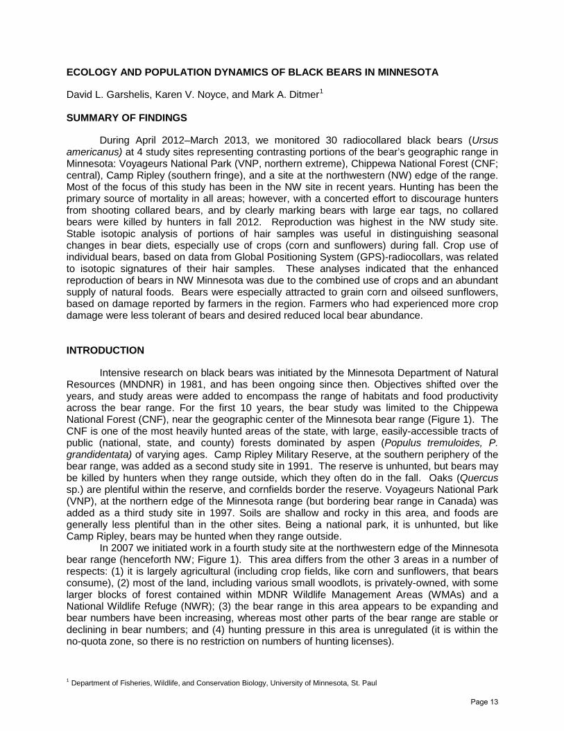
ECOLOGY AND POPULATION DYNAMICS OF BLACK BEARS IN MINNESOTA David L. Garshelis, Karen V. Noyce, and Mark A. Ditmer1 SUMMARY OF FINDINGS

During April 2012–March 2013, we monitored 30 radiocollared black bears (Ursus americanus) at 4 study sites representing contrasting portions of the bear’s geographic range in Minnesota: Voyageurs National Park (VNP, northern extreme), Chippewa National Forest (CNF; central), Camp Ripley (southern fringe), and a site at the northwestern (NW) edge of the range. Most of the focus of this study has been in the NW site in recent years. Hunting has been the primary source of mortality in all areas; however, with a concerted effort to discourage hunters from shooting collared bears, and by clearly marking bears with large ear tags, no collared bears were killed by hunters in fall 2012. Reproduction was highest in the NW study site. Stable isotopic analysis of portions of hair samples was useful in distinguishing seasonal changes in bear diets, especially use of crops (corn and sunflowers) during fall. Crop use of individual bears, based on data from Global Positioning System (GPS)-radiocollars, was related to isotopic signatures of their hair samples. These analyses indicated that the enhanced reproduction of bears in NW Minnesota was due to the combined use of crops and an abundant supply of natural foods. Bears were especially attracted to grain corn and oilseed sunflowers, based on damage reported by farmers in the region. Farmers who had experienced more crop damage were less tolerant of bears and desired reduced local bear abundance.

INTRODUCTION

Intensive research on black bears was initiated by the Minnesota Department of Natural Resources (MNDNR) in 1981, and has been ongoing since then. Objectives shifted over the years, and study areas were added to encompass the range of habitats and food productivity across the bear range. For the first 10 years, the bear study was limited to the Chippewa National Forest (CNF), near the geographic center of the Minnesota bear range (Figure 1). The CNF is one of the most heavily hunted areas of the state, with large, easily-accessible tracts of public (national, state, and county) forests dominated by aspen (Populus tremuloides, P. grandidentata) of varying ages. Camp Ripley Military Reserve, at the southern periphery of the bear range, was added as a second study site in 1991. The reserve is unhunted, but bears may be killed by hunters when they range outside, which they often do in the fall. Oaks (Quercus sp.) are plentiful within the reserve, and cornfields border the reserve. Voyageurs National Park (VNP), at the northern edge of the Minnesota range (but bordering bear range in Canada) was added as a third study site in 1997. Soils are shallow and rocky in this area, and foods are generally less plentiful than in the other sites. Being a national park, it is unhunted, but like Camp Ripley, bears may be hunted when they range outside.

In 2007 we initiated work in a fourth study site at the northwestern edge of the Minnesota bear range (henceforth NW; Figure 1). This area differs from the other 3 areas in a number of respects: (1) it is largely agricultural (including crop fields, like corn and sunflowers, that bears consume), (2) most of the land, including various small woodlots, is privately-owned, with some larger blocks of forest contained within MDNR Wildlife Management Areas (WMAs) and a National Wildlife Refuge (NWR); (3) the bear range in this area appears to be expanding and bear numbers have been increasing, whereas most other parts of the bear range are stable or declining in bear numbers; and (4) hunting pressure in this area is unregulated (it is within the no-quota zone, so there is no restriction on numbers of hunting licenses).

1 Department of Fisheries, Wildlife, and Conservation Biology, University of Minnesota, St. Paul

Page 13

OBJECTIVES 1. Quantify temporal and spatial variation in cub production and survival; 2. Assess causes of bear mortality in different parts of the bear range; 3. Evaluate use of crops by bears living along the edge of the range; 4. Assess damage caused by bears to various crops along the edge of the bear range, and

corresponding attitudes of farmers toward bears. METHODS

We previously attached radiocollars with breakaway and/or expandable devices to bears either when they were captured during the summer or when they were handled as yearlings in the den with their radiocollared mother. We used VHF collars in CNF, Camp Ripley, and VNP, and GPS in the NW study site. We used both GPS “pods” (Telemetry Solutions, Concord, CA) that were bolted onto standard VHF collars, and GPS-Iridium collars (Vectronic Aerospace, Berlin, Germany). The latter collars uploaded location data to an Iridium satellite, which was then transmitted to us daily by email. The location data stored in the pods were retrievable only by physically connecting the pod to a computer when we handled bears in dens.

During December–March, we visited all radio-instrumented bears once or twice at their den site. We immobilized bears in dens with an intramuscular injection of Telazol, administered with a jab stick or Dan-Inject dart gun. Bears were then removed from the den for processing. We measured lengths and girths, body weight, body fat (using biolelectrical impedance analysis), and took blood and hair samples. We changed or refit the collar, as necessary. All collared bears had brightly-colored, cattle-size ear tags (7x6 cm; Dalton Ltd., UK) that would be plainly visible to hunters. Bears were returned to their dens after processing.

We assessed reproduction by observing cubs in dens of radiocollared mothers. We sexed and weighed cubs without drugging them. We evaluated cub mortality by examining dens of radiocollared mothers the following year: cubs that were not present as yearlings with their mother were presumed to have died.

We did not monitor survival of bears during the summer. Mortalities, though, were reported to us when bears were shot as a nuisance, hit by a car, or killed by a hunter. Prior to the hunting season (1 September–mid-October), hunters were mailed a letter requesting that they not shoot collared bears with large ear tags.

We plotted GPS locations downloaded from collars on bears in the NW study site. We used a Geographic Information System (GIS) overlay to categorize the covertypes of GPS locations, including types of crop fields. We compared the proportion of time that bears spent in cropfields to stable isotopic signatures of carbon (C) and nitrogen (N) in their hair (Colorado Plateau Stable Isotope Laboratory, Northern Arizona University, Flagstaff, AZ). We sectioned hair in two pieces representing two periods of growth: spring-summer (distal half) and fall. We collected various types of bear foods from the NW study site, including herbaceous vegetation, fleshy fruits, nuts, ants, deer, corn, soybeans, and sunflowers, and obtained their isotopic signatures for C and N (Department of Geology and Geophysics, University of Minnesota, Minneapolis, MN). We used the Stable Isotope Analysis package in Program R (SIAR) to solve mixing models for the isotopic data within a Bayesian framework, and thereby generated distributions for the probabilities that different individual bears consumed and assimilated given proportions of certain types of foods.

We interviewed farmers in the NW study site to gauge the amount of bear-related damage to various crops, and whether their attitudes toward bears changed accordingly. Growers were asked to subjectively rate levels of bear damage to their crops based on a scale of 0 (no damage) to 5 (major damage). We asked how tolerant the grower was of bear-related damage to crops and asked if they would prefer fewer, the same, or more bears in the region. We also inquired about any attempted hunting of bears on their property either as a direct response to crop damage or as a means to reduce the general number of bears near the crop

Page 14

land. Initial interviews were conducted with growers who reported damage to local Minnesota Department of Natural Resources offices, as well as growers who owned fields in which GPS-collared bears were known to have visited. After these interviews, other interview subjects were added.

RESULTS AND DISCUSSION Radiocollaring and Monitoring Since 1981 we have handled >800 individual bears and radiocollared >500. As of April 2012, the start of the current year’s work, we were monitoring 30 radiocollared bears: 5 in the CNF, 8 at Camp Ripley, 4 in VNP, and 13 in the NW (Table 1). We did not trap any new bears this year. We collared one additional bear whose den was found by a hunter near the western edge of the range, but the GPS unit failed shortly afterwards. One VHF collar also failed. Two bears dropped collars: 1 of these was not handled during the winter of 2011–2012, so the breakaway on the collar deteriorated and severed (as it should have); the other had an expandable device that expanded too much. We could not find 1 CNF bear. Mortality

Legal hunting has been the dominant cause of mortality among radiocollared bears from all study sites (Table 2). However, no bears were shot by hunters during 2012, as they respected our request not to shoot them. One NW study bear was hit by a car, and a yearling collared in a den in VNP in March 2012 apparently died of natural mortality (we found its collar chewed by wolves). One adult female who was denned in an open nest with her yearlings died after drugging, despite a normal drug dose and the bear being in apparent good health.

The oldest bear on our study, a 39-year-old female in the CNF (as of January 2013) survived another year. Reproduction

Eleven collared females gave birth to 28 cubs in 2013. Nearly all bears maintained a 2-year reproductive cycle. All 8 females that produced cubs 2 years ago produced cubs again this year; 1 female whose litter died last year produced a litter this year; and 2 females produced their first litters (1 at 3 years old, 1 at 4 years old).

Since 1982, we have checked 269 litters with 689 cubs ( x = 2.6 cubs/litter), of which 52% were male (Tables 3–6). Mortality of cubs during their first year of life averaged 21%, with mortality of male cubs (26%) exceeding that of females (16%; χ2 = 7.3, P < 0.01). The timing and causes of cub mortality are unknown.

Reproductive rates were highest in the NW study area, and lowest in VNP (Figure 2). The reproductive rate (cubs/female 4+ years old) combines litter size, litter frequency, and age of first reproduction into a single parameter. Reproductive rate was higher for 7+ year-old bears than 4–6 year-old bears because many bears in this younger age group either had not yet reproduced or had their first litter, which tended to be smaller. Reproductive rates for 7+ year-old bears in the CNF and Camp Ripley were similar, although Camp Ripley bears tended to mature earlier (Figure 2). Litter size averaged ≥3.0 cubs only for 7+ year-olds in the NW.

Page 15

Crop Use by NW Bears

We were able to separate stable isotope signatures of bear foods into 5 groups: natural vegetation (herbaceous, berries, and nuts), ants, deer, corn, and sunflowers (Figure 3). Isotopic signatures of portions of bear hair representing spring-summer growth clustered around natural vegetation and varying amounts of ants and deer; samples with enriched nitrogen indicated use of ants or deer (CIs for ants and deer overlapped so could not be readily distinguished). Some spring-summer samples also had enriched carbon, indicative of use of corn by some animals, likely obtained from unharvested fields or spillage during fall harvest. Portions of bear hair representing fall growth had more variation in C and N signatures due to varying use of corn and sunflowers. Males made the most extreme use of these crops, but a number of females also used crops in fall, based on enriched C and/or N (Figure 3). However, the relatively high reproductive rate of females in this area was not solely due to crop use, as this analysis showed that most of them fed mainly on natural vegetation; abundant hazelnuts (Corylus americana, C. cornuta) probably contributed largely to their high reproductive output. Extent of cropfield use by GPS-collared bears was related to isotopic signatures of their hair (Figures 4,5), thus confirming the use of stable isotopes to assess crop use.

Crop Damage by NW Bears During 2009–2012 we conducted 38 interviews with growers (36) and apiarists (2) in the NW study area. Most were long-time residents of the area (average ~30 years). Growers reported differing amounts of bear damage among crops and crop varieties (Table 7). Among the 25 survey participants who had grown corn in recent years, 91% reported damage from bears. Those who grew hybrid/grain corn reported more bear-related damage than those who grew field corn for silage (Table 7). Among 19 sunflower growers, 16 had grown oil sunflowers (used for cosmetics, cooking, birdseed), 9 confection sunflowers (used for human consumption, birdseed) and 6 had experience with both varieties. The mean level of bear damage in oil sunflower fields was significantly higher than confectionary sunflower fields (Table 7). Bears are likely attracted to the black oilseed for its high fat content (Figure 6). Apiarists (2 of 2, but highly dependent on year) and oat growers (9 of 9) also reported significant amounts of bear damage. Of 25 growers of soybeans, the crop with the most areal coverage, only 1 reported bear damage (rated as minor). Those who grew wheat, canola, barley, alfalfa, sugar beets, and rye grass, grains, or hay reported low or no distinguishable bear damage. Tolerance toward bear damage was largely related to the perceived level of past damage: 5 of 26 growers had not incurred any bear damage and all considered themselves tolerant of bears; among 21 respondents that had incurred bear damage, only 6 (29%) classified themselves tolerant, 8 (38%) had tolerance “contingent on level of damage” and 7 (33%) were classified as having no tolerance for bear damage. Accordingly, 5 of 7 (71%) growers who did not report any damage from bears had not killed or attempted to kill bears and 50% said they would prefer the same or more bears in the region. Conversely, of 16 growers who reported crop losses to bears, 10 (63%) had attempted nuisance killing or additional hunting pressure and 73% indicated that they would prefer fewer or no bears in the region. ACKNOWLEDGMENTS

We thank the collaborators in this study: Brian Dirks, who conducted the fieldwork and provided all materials for the work at Camp Ripley; Dr. Paul Iaizzo at the University of Minnesota, and Dr. Tim Laske at Medtronic, Inc., who assisted with fieldwork and provided the GPS-Iridium radiocollars, and Spencer Rettler who assisted in isotope sample preparation and data entry. Agassiz NWR kindly provided use of their bunkhouse and assistance from staff during the winter fieldwork.

Page 16

Table 1. Fates of radiocollared black bears in 4 study sites (Chippewa National Forest, Camp Ripley, Voyageurs National Park, and northwestern Minnesota), April 2012−March 2013.

CNF Camp Ripley VNP NW

Collared sample April 2012 5 8 4 13

Killed as nuisance

Killed in vehicle collision 1

Killed by Minnesota hunter

Natural mortality 1

Dropped collar 2

Failed radiocollar 1

Lost contacta 1

Died in denb 1

Collared in den 1

Collared sample April 2013 4 8 3 9 a Due to radiocollar failure, unreported kill, or long-distance movement. b Due to handling. Table 2. Causes of mortality of radiocollared black bears ≥1 year old in 4 Minnesota study sites, 1981–2012. Bears did not necessarily die in the area where they usually lived (e.g., hunting was not permitted within Camp Ripley or VNP, but bears were killed by hunters when they traveled outside these areas).

CNF Camp Ripley VNP NW All combined

Shot by hunter 223 11 15 12 261

Likely shot by huntera 8 1 0 4 13

Shot as nuisance 22 2 1 3 28

Vehicle collision 12 8 1 3 24

Other human-caused death 9 1 0 0 10

Natural mortality 7 3 5 0 15

Died from unknown causes 4 2 0 3 9

Total deaths 285 28 22 25 360 a Lost track of during the bear hunting season, or collar seemingly removed by a hunter.

Page 17

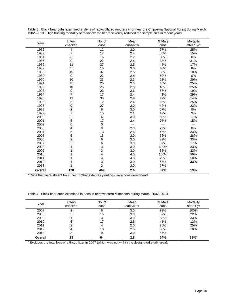
Table 3. Black bear cubs examined in dens of radiocollared mothers in or near the Chippewa National Forest during March, 1982–2013. High hunting mortality of radiocollared bears severely reduced the sample size in recent years.

Year Litters checked

No. of cubs

Mean cubs/litter

% Male cubs

Mortality after 1 yra

1982 4 12 3.0 67% 25% 1983 7 17 2.4 65% 15% 1984 6 16 2.7 80% 0% 1985 9 22 2.4 38% 31% 1986 11 27 2.5 48% 17% 1987 5 15 3.0 40% 8% 1988 15 37 2.5 65% 10% 1989 9 22 2.4 59% 0% 1990 10 23 2.3 52% 20% 1991 8 20 2.5 45% 25% 1992 10 25 2.5 48% 25% 1993 9 23 2.6 57% 19% 1994 7 17 2.4 41% 29% 1995 13 38 2.9 47% 14% 1996 5 12 2.4 25% 25% 1997 9 27 3.0 48% 23%

1998 2 6 3.0 67% 0% 1999 7 15 2.1 47% 9% 2000 2 6 3.0 50% 17% 2001 5 17 3.4 76% 15% 2002 0 0 — — — 2003 4 9 2.3 22% 0% 2004 5 13 2.6 46% 33% 2005 6 18 3.0 33% 28% 2006 2 6 3.0 83% 33% 2007 2 6 3.0 67% 17% 2008 1 3 3.0 100% 33% 2009 1 3 3.0 33% 33% 2010 1 4 4.0 100% 50% 2011 1 4 4.0 25% 50% 2012 1 3 3.0 67% 33% 2013 1 3 3.0 67%

Overall 178 469 2.6 52% 19% a Cubs that were absent from their mother’s den as yearlings were considered dead. Table 4. Black bear cubs examined in dens in northwestern Minnesota during March, 2007–2013.

Year Litters checked

No. of cubs

Mean cubs/litter

% Male cubs

Mortality after 1 yr

2007 2 6 3.0 33% 100%

2008 5 15 3.0 67% 22% 2009 1 3 3.0 33% 33% 2010 6 17 2.8 41% 13% 2011 2 4 2.0 75% 25% 2012 4 10 2.5 60% 10% 2013 3 9 3.0 67%

Overall 23 64 2.8 54% 28%a a Excludes the total loss of a 5-cub litter in 2007 (which was not within the designated study area).

Page 18

Table 5. Black bear cubs examined in dens in or near Camp Ripley Military Reserve during March, 1992–2013.

Year Litters checked

No. of cubs

Mean cubs/litter

% Male cubs

Mortality after 1 yra

1992 1 3 3.0 67% 0% 1993 3 7 2.3 57% 43% 1994 1 1 1.0 100% — 1995 1 2 2.0 50% 0% 1996 0 0 — — —

1997 1 3 3.0 100% 33%

1998 0 0 — — —

1999 2 5 2.5 60% 20% 2000 1 2 2.0 0% 0% 2001 1 3 3.0 0% 33% 2002 0 0 — — —

2003 3 8 2.7 63% 33% 2004 1 2 2.0 50% —

2005 3 6 2.0 33% 33% 2006 2 5 2.5 60% — 2007 3 7 2.3 43% 0% 2008 2 5 2.5 60% 0% 2009 3 7 2.3 29% 29% 2010 2 4 2.0 75% 25% 2011 3 8 2.7 50% 25% 2012 1 2 2.0 100% 0% 2013 6 14 2.3 50%

Overall 40 94 2.4 52% 21% a Blanks indicate no cubs were born to collared females or collared mothers with cubs died before the subsequent den visit to assess cub survival. Table 6. Black bear cubs examined in dens in Voyageurs National Park during March, 1999–2013. All adult collared females were killed by hunters in fall 2007, so no reproductive data were obtained during 2008–2009.

Year Litters checked

No. of cubs

Mean cubs/litter

% Male cubs

Mortality after 1 yra

1999 5 8 1.6 63% 20% 2000 2 5 2.5 60% 80% 2001 3 4 1.3 50% 75% 2002 0 — — —

2003 5 13 2.6 54% 8% 2004 0 — — —

2005 5 13 2.6 46% 20% 2006 1 2 2.0 50% 0% 2007 3 9 3.0 44% — 2008 0 2009 0 2010 1 2 2.0 50% 0% 2011 1 2 2.0 0% 0% 2012 1 2 2.0 0% 50% 2013 1 2 2.0 50%

Overall 28 62 2.2 48% 27% a Blanks indicate no cub mortality data because no cubs were born to collared females.

Page 19

Table 7. Extent of black bear-related damage to cropfields in NW Minnesota perceived by interviewed farmers, 2009–2012. Growers were asked to subjectively rate levels of bear damage to their crops based on a scale of 0 (no damage) to 5 (major damage).

Crop Number of interviewees

Bear damage rating

Mean 95% CI

Hybrid/grain corn 13 3.61 2.71 – 4.51

Silage corn 10 1.83 1.30 – 2.68

Oilseed sunflowers 15 2.20 1.17 – 3.23

Confection sunflowers 9 0.28 0.04 – 0.52

Oats 9 2.94 1.96 – 3.93

Page 20

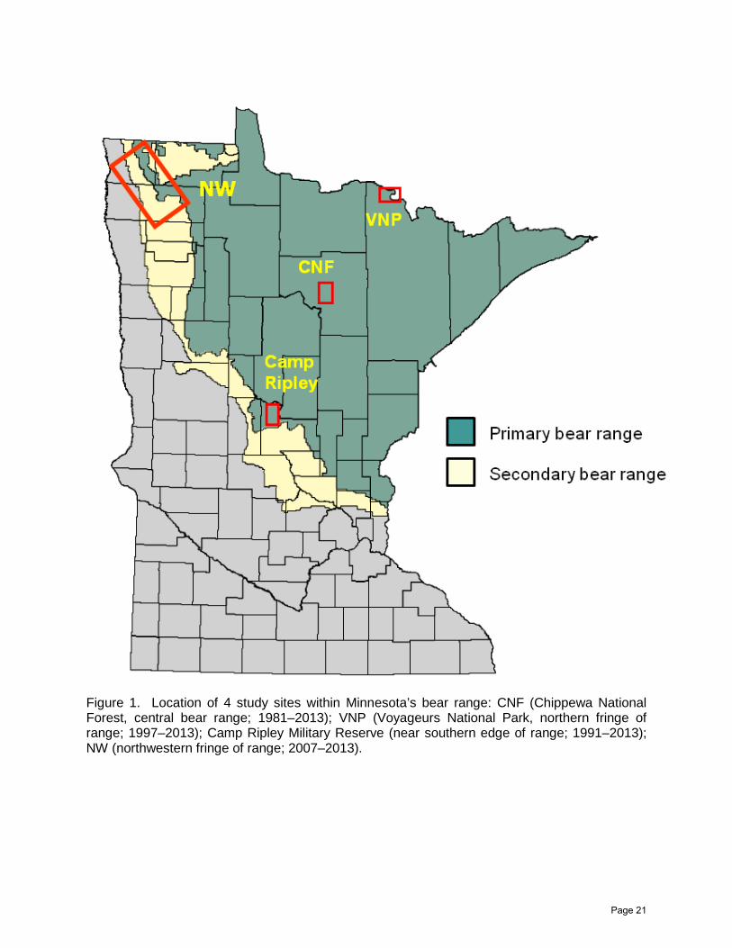
Figure 1. Location of 4 study sites within Minnesota’s bear range: CNF (Chippewa National Forest, central bear range; 1981–2013); VNP (Voyageurs National Park, northern fringe of range; 1997–2013); Camp Ripley Military Reserve (near southern edge of range; 1991–2013); NW (northwestern fringe of range; 2007–2013).

Page 21

Figure 2. Reproductive rates of radiocollared bears within 4 study sites (see Figure 1) through March 2013. Sample sizes refer to the number of female bear-years of monitoring in each area for each age group. Data include only litters that survived 1 year (even if some cubs in the litter died). Some bears in CNF, Camp Ripley, and NW produced cubs at 3 years old, but are not included here.

0.0

0.5

1.0

1.5

2.0

VNP CNF Ripley NW

Rep

ro ra

te (c

ubs/

adul

t F)

4-6 yr-old F 7-25 yr-old F

n=24

n=26

n=43

n=14n=38

n=35

n=153

n=262

Page 22

Figure 3. Stable isotope signatures obtained from hair samples of collared black bears in NW Minnesota, 2007–2012 (n = 58 female bear-years, 52 male bear-years; 21 different females, 30 different males) compared to mean isotope signatures (and 95%CI) of seasonal bear foods. Hair samples were divided into 2 sections representing spring-summer growth (assimilated diet during April–July; top panel) and fall growth (diet during August–denning; bottom panel). Samples with more enriched C and/or N in fall represent diets with increased use of corn or sunflowers. Corn in spring diet is from spillage and unharvested fields. Natural vegetation is season-specific (herbaceous plants and fleshy fruits in spring-summer; mainly nuts in fall).

0 5 10 15 20 25

-30

-25

-20

-15

-10

-5

d15NPl

d13C

Pl

AntsCorn

Deer

EarlyVeg

Group 1

Group 2

Carb

on (δ

13C)

Nitrogen (δ15N)

AntsCornDeer

Natural veg.

Males

Females

0 5 10 15 20 25

-30

-25

-20

-15

-10

-5

d15NPl

d13C

Pl

Sun_cutCornFallVegGroup 1Group 2

Nitrogen (δ15N)

Carb

on (δ

13C)

SunflowersCornNatural veg. (fall)

Males

Females

Spring-summer

Fall

Page 23

Figure 4. Isotopic values of carbon in fall growth of hair samples from GPS-collared black bears in NW Minnesota, 2007–2012 (n = 38 bear-years from 10 male and 12 female bears) compared to each individual’s use of corn (measured as the summed proportion of GPS locations in cornfields each month, August-denning). Bears that spent more time in cornfields had more enriched carbon (r2 = 0.434, P < 0.001; grey area represents ±SE of regression), indicating that stable isotope analysis portrayed the use of this crop.

Carb

on (δ

13C)

Cumulative Proportion Fall Corn Use

Page 24

Figure 5. Isotopic values of nitrogen in fall growth of hair samples from GPS-collared black bears in NW Minnesota, 2007–2012 (n = 38 bear-years from 10 male and 12 female bears) compared to each individual’s use of sunflowers and corn (measured as the summed proportion of GPS locations in these cropfields each month, August-denning). Bears that spent more time in sunflower and corn fields had more enriched nitrogen (r2 = 0.554, P < 0.001; grey area represents ±SE of regression), indicating that stable isotope analysis portrayed the use of these crops.

Nitr

ogen

(δ15

N)

Cumulative Proportion Fall Sunflower+Corn Use

Page 25

Figure 6. Bears were especially attracted to oilseed sunflower fields. Fields like this one provide rich, abundant food for bears during the hyperphagic period prior to hibernation, as well as nearby cover and shade.

Page 26

MEASURING THE APPARENT DECLINE OF A BEAR POPULATION IN THE CORE OF MINNESOTA’S BEAR RANGE David L. Garshelis, Karen V. Noyce SUMMARY OF FINDINGS Bear abundance in the Chippewa National Forest (CNF) appears to have been declining for the past 2 decades, due to heavy hunting pressure. During the summer of 2012, we conducted a genetic capture–mark–recapture (CMR) estimate of abundance using hair snares to ascertain how much the population has declined. We will compare this estimate to CMR estimates from the 1980s and 1990s, which employed radiocollars as marks. We set 121 barbed wire hair snares in the same study site as used in the 1980s and 1990s. We checked snare sites 6 times, at 10-day intervals. Visitation by bears was high (55% of site-session checks), yielding 2784 hair samples, of which 1120 were submitted for genetic analysis. At the same time, we conducted a bait-station survey through the central study area, patterned after surveys conducted during the 1980s: bear visitation in 2012 was only 2%, compared to 35–70% during the 1980s. After completion of genetic analysis and computation of a population estimate we will learn whether the high visitation at hair traps represented a higher than expected abundance of bears, or a few bears visiting many traps.

INTRODUCTION

In 1981 we initiated a bear research project near the geographic center of the bear range, mainly within the Chippewa National Forest (henceforth CNF; Figure 1). A primary objective of this study was to monitor population dynamics in an area considered representative of much of the north-central part of the state in terms of habitat and hunting pressure. Radio-telemetry provided the central means of collecting population-related data on bears in the CNF during the 1980s. Population estimates were obtained through capture–mark−recapture (CMR), where marks were radiocollars (Garshelis 1992). Due to budgetary constraints, trapping was discontinued after 1989, at which time 7 population estimates had been obtained (1983−89); these suggested an increasing population trend (Figure 2). An upward trend also was observed for bears captured per unit effort, an index of bear density (Figure 2). We also conducted a bait-station survey through the middle of the study area in early July each year, consisting of 50 baits spaced at 0.5-mi intervals along dirt roads; the percent of baits taken by bears after 1 week was supposed to be another index of population size, but population trend gleaned from this survey did not match the trapping data (Figure 2).

A second series of population estimates was obtained in the mid-1990s (1994−1996), again using collared bears as marked animals, but instead of physical captures, we employed cameras (Noyce et al. 2001). These estimates were consistently lower than obtained in the late-1980s, suggesting that the population had declined (Figure 2).

Concurrent with these estimates, we observed a decline in the age of harvested female bears taken from the bear management unit (BMU) that contains the CNF study area, possibly indicating an over-harvest. These data were obtained from teeth submitted by hunters each year.

Periodic trapping during 2000−2005, while not sufficient to provide an estimate of density, indicated that the effort required to catch a bear in the CNF was 2−5x higher than it had been in the late 1980s (Figure 2). A bait-station survey conducted through the CNF in 2009 yielded a bear visitation rate of only 6%, <20% that of the late 1980s.

All of these indicators point to a population decline in the CNF resulting from an excessive harvest. Harvest is controlled by a quota, which was purposefully reduced during the past decade to lessen hunting pressure in response to a perceived population decline. Nevertheless, it appears that the population declined faster than expected, meaning that each

Page 27

year’s reduced harvest may still be an over-harvest. Whereas collectively these data are strongly indicative of population trend, it is not possible to ascertain the true magnitude of population decline without an actual density estimate.

Since our work with physical CMR in the 1980s and camera-captures in the mid-1990s, a good deal of effort has gone into the development of genetic CMR approaches. The basic technique was first outlined by Woods et al. (1999). It involves stringing barbed wire around trees, thereby enclosing a small area. A scent lure and(or) suspended bait in the middle of the barbed-wire enclosure is used to entice bears to crawl under the wire, whereupon a clump of hair is plucked from their back; this hair is genetically analyzed to differentiate individuals. Many modifications of this basic procedure have been tried and compared (e.g., Boulanger et al. 2006, Tredick et al. 2007, Dreher et al. 2009, Robinson et al. 2009, Proctor et al. 2010, Pederson et al. 2012).

Genetic CMR has many advantages over marking bears through physical captures and radiocollaring. Because bears are not handled, checking hair traps requires a lower level of skill; more traps can be set because they do not have to be checked daily; and bears likely have less aversion to the traps, so are more likely to be recaptured; thus capture samples are apt to be larger and less biased. Moreover, radiocollaring necessitates later den checks to adjust or remove collars. For these reasons, we elected to employ genetic CMR to obtain a new population estimate on the CNF. OBJECTIVES

1. Obtain an estimate of bear numbers on the CNF study site with sufficient precision to discern a decline of ≥50% during the past 20 years.

2. Obtain an estimate of bear density on the CNF with sufficient precision to guide management.

3. Obtain a reliable estimate of the sex ratio of bears on the CNF. METHODS

The study area was same CNF study site where previous CMR estimates were obtained. It contains good access via 2 main paved roads, smaller unimproved roads, and forest roads. Ownership is mainly national and state forest, with additional county lands and private lands.

Hair traps were erected the third week of May, 2012, and removed the third week of July. We erected hair-snare traps using 2 strands of 4-pronged barbed wire wrapped around trees, 1 at 45 cm and 1 at 75 cm off the ground (Figure 3). We erected 1 trap in each square-mile section (121 mi2). We set traps in what we perceived as good bear habitat to maximize visitation. We set traps at least 100m from main roads, but often along trails that we suspected bears would use.

We suspended a bag of bacon and a scent lure from a wire (above the reach of a bear) in the middle of each trap, and put bait and scent lure on a pile of brush in the middle of the enclosure (Figure 3). Baits and lures were refreshed at each trap visit. We added different types of lures at each trapping session to maintain novelty for the bears. We checked all traps 6x at intervals of 10 days. We did not move traps between sessions. At each trap check, all bear hair was removed from the wire. Each clump of hairs on a barb was collected in a separate envelope, and labeled as to proximity to other barbs with hair, trap number, and date (Figure 4). We coded barbs of hair that were adjacent (next to, or on the wire above/below) as being from the same cluster.

We set camera traps at some of the hair traps that were visited by bears to gauge whether cubs of the year left hair on wires, and to assess the responses of different bears to the wires and the baits.

Page 28

During the first week of July, 2012, we conducted a bait-station survey, using the same technique and route through the study area as in our previous bait-station surveys. We wired 50 1-lb sacks of bacon to trees, spaced at 0.5-mile intervals, and checked them for visitation 1 week later. RESULTS AND DISCUSSION

We checked all 121 hair traps 5 times (605 site-sessions), then dismantled 36 traps that were never visited by a bear, leaving 85 to be checked in session 6. Of 690 total site-sessions, 377 (55%) had bear hair (Table 1). Bear visitation was low in the first session (late May), then increased, possibly as bears became more accustomed to the traps and scents.

We collected a total of 2784 barbs of hair (Table 1). We did not collect hairs from barbs with fewer than 3 hairs because it would have been unlikely to yield enough DNA for genetic analysis. Our budget was not sufficient to analyze all collected hair samples, so we subsampled the collection. In subsampling we made an attempt to maximize the number of different bears that visited the sites. Thus, we initially chose (randomly) 1 barb from each of the 377 site-sessions with hair. We chose additional samples that, where possible, were not within the same cluster of barbs as the initial sample. We chose 737 samples from among the remaining 1265 clusters, yielding a total of 1114 samples for processing. Not all of these samples will yield sufficient DNA for genetic analysis.

We also submitted hair samples from 4 radiocollared bears and their current offspring living on the study area (collected during den visits) to determine whether they visited the hair traps.

Camera trap photos showed that individual bears visited traps multiple times within sessions, and also visited multiple traps. Individual bears entered and left traps at various locations along the wires, and different bears entered and left at some of the same locations (Figures 5,6). Thus, our presumption may not be correct that clusters of adjacent barbs are likely to be the same bear; also, some barbs may have collected hair from >1 bear. This will not affect the population estimate, as hairs from multiple bears on a single barb would be genetically discernible. Some photographed bears seemed reluctant to cross the wire (Figure 7), but we assume that most or all of these eventually did so, given the ease and frequency with which other identifiable bears entered the enclosure.

Camera traps also revealed that some bears learned how to reach the suspended bait, either by climbing nearby trees (Figure 8), or pulling down the string on which the bait was suspended. Despite consumption of this bait, the stations remained attractive to bears due to the lingering odors of the scents on the brush pile in the middle.

Only 1 of 50 baits on the bait-station survey was taken by a bear, 3 were taken by raccoons or fishers, yielding a bear visitation rate of 1/(50-3) = 2%. This is the lowest visitation rate ever measured in this area (Figure 2). This low rate of visitation appears inconsistent with the high visitation at the hair traps. The difference may have been due to (1) the location of hair traps in good bear habitat, distant from roads, and (2) the use of strong, attractive scents and more bait at hair traps. We will not know until after completion of genetic analysis and computation of a population estimate whether the high visitation at hair traps represented a higher than expected abundance of bears, or few bears visiting many traps.

ACKNOWLEDGMENTS

We sincerely thank the 2 volunteers who checked traps and meticulously collected hair: Chris Anderson and Chih-Chien (Jerry) Huang. We also thank the individuals who allowed us to set and check traps on their private land: Bradley Box, Mark Hawkinson, Dale Juntenen, Brad and Mary Nett, Jack Rajala, Scherer Brothers Lumber Company, and Thomas Schultz.

Page 29

LITERATURE CITED Boulanger, J., M. Proctor, S. Himmer, G. Stenhouse, D. Paetkau, and J. Cranston. 2006. An

empirical test of DNA mark–recapture sampling strategies for grizzly bears. Ursus 17:149–158.

Dreher, B.P., G.J.M. Rosa, P.M. Lukacs, K.T. Scribner, and S.R. Winterstein. 2009. Subsampling hair samples affects accuracy and precision of DNA-based population estimates. Journal of Wildlife Management 73:1184–1188.

Garshelis, D.L. 1992. Mark-recapture density estimation for animals with large home ranges. Pages 1098-1111 in D. R. McCullough and R. H. Barrett, editors. Wildlife 2001:Populations. Elsevier Applied Science, London.

Noyce, K.V., D.L. Garshelis, and P. L. Coy. 2001. Differential vulnerability of black bears to trap and camera sampling and resulting biases in mark–recapture estimates. Ursus 12:211–226.

Pederson, J.C., K. D. Bunnell, M. M. Conner, and C. R. McLaughlin. 2012. A robust-design analysis to estimate American black bear population parameters in Utah. Ursus 23:104–116.

Proctor, M., B. McLellan, J. Boulanger, C. Apps, G. Stenhouse, D. Paetkau, and G. Mowat. 2010. Ecological investigations of grizzly bears in Canada using DNA from hair, 1995–2005: a review of methods and progress. Ursus 21:169-188.

Robinson, S.J., L.P. Waits, and I.D. Martin. 2009. Estimating abundance of American black bears using DNA-based capture–mark–recapture models. Ursus 20:1–11.

Tredick, C.A., M.R. Vaughan, D.F. Stauffer, S.L. Simek, and T. Eason. 2007. Sub-sampling genetic data to estimate black bear population size: a case study. Ursus 18:179–188.

Woods, J.G., D. Paetkau, D. Lewis, B.N. McLellan, M. Proctor, and C. Strobeck. 1999. Genetic tagging of free-ranging black and brown bears. Wildlife Society Bulletin 27:616–627.

Page 30

Table 1. Bear hair collected at 121 barbed wire hair snares in the CNF during summer 2012.

Session Dates Number of snares with haira

Number of barbs with hair

Number of barb clustersb

1 25 – 31 May 30 298 149

2 5 – 10 June 63 626 308

3 15 – 21 June 65 470 279

4 25 – 30 June 79 650 392

5 5 – 10 July 76 448 303

6 13 – 19 July 64 292 211

Total 377 2784 1642 a Each hair-snare was checked in each of sessions 1 – 5. Snares that were never visited by bears during that period (n = 36) were dismantled prior to session 6. b Barbs with bear hair that were adjacent to each other, either on the same or different wires, were considered a cluster, possibly representing a single bear entering or leaving a hair snare.

Page 31

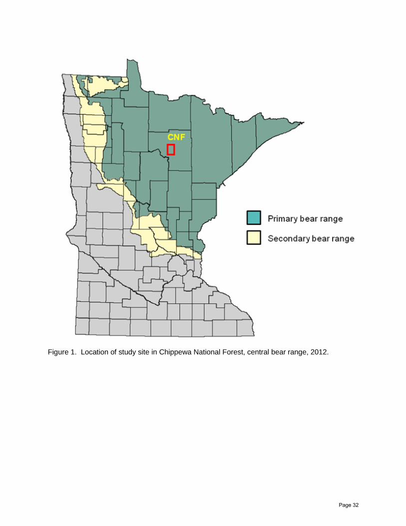
Figure 1. Location of study site in Chippewa National Forest, central bear range, 2012.

Page 32

Figure 2. Indicators of bear population trend on the CNF study site, 1981–2009: density estimates derived from mark−recapture of radiocollared bears (physical captures in the 1980s, camera captures in the 1990s); bear visitation to baits on a standardized route through the study area; and bears caught (trapped) per unit effort.

0

15

30

45

60

75

90

105

120

0

5

10

15

20

25

30

35

40

1981 83 85 87 89 91 93 95 97 99 01 03 05 07 09

Bai

t sta

tion

visi

tatio

n (%

)

B

ears

cau

ght/1

000

trap

nigh

ts

Bea

rs/1

00 k

m2

Physical mark-recapture

Bait station visitation

Capture success

Page 33

Figure 3. Set-up of barbed wire hair snare, showing 2 strands of barbed wire, central pile of bait and scent, and suspended bait and scent cup.

Page 34

Figure 4. Volunteer Chris Anderson collecting bear hair from a barb. Each sample was placed in an individual envelope indicating the date, trap number, and location relative to other barbs with hair.

Page 35

Figure 5. Radiocollared and eartagged adult female bear entering and then leaving hair snare at same site (1 minute apart), going between wires on 1 pass, and below lower wire on second pass. The other bears in the photos are her yearlings, 1 of which passed through the wires at the same spot as the mother.

Page 36

Figure 6. Marked adult female bear, probably in estrus, followed under the same spot in the wire hair snare by an unmarked young male about 1 hour later. Prior to the arrival of this male, a much larger male was photographed consorting with this female inside the enclosure. That male exited a different way.

Page 37

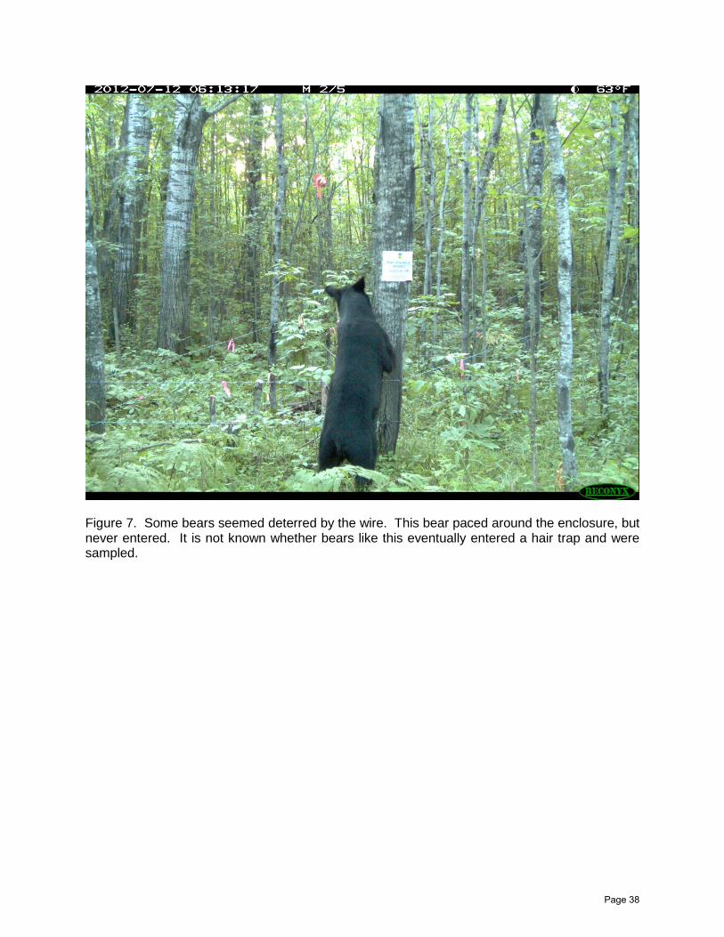
Figure 7. Some bears seemed deterred by the wire. This bear paced around the enclosure, but never entered. It is not known whether bears like this eventually entered a hair trap and were sampled.

Page 38

Figure 8. Some bears discovered clever ways of reaching the suspended “inaccessible” bait. The disappearance of this bait became increasingly common through the summer sampling period.

Page 39

HELICOPTER CAPTURE OF NEWBORN MOOSE CALVES IN NORTHEASTERN MINNESOTA: AN EVALUATION Glenn D. DelGiudice, William J. Severud, and Robert G. Wright1 SUMMARY OF FINDINGS

Important to our new study of moose (Alces alces) calf survival and cause-specific mortality in northeastern Minnesota, our objective here is to evaluate helicopter capture of newborn moose calves to better understand its value for fulfilling our primary research goal and to assess risks to the welfare of the captured calves. On 1 May 2013, we began monitoring the locations and movements of 52 pregnant global positioning system (GPS)-collared females to determine when they made their “calving move.” We allowed an average of 54 hours of dam-calf bonding time before capture. We captured 49 (25 females, 24 males) newborn calves of 31 dams during 8-17 May 2013. Mean birth-date of captured neonates was 11 May 2013 and mean capture-date was 13 May. The overall twinning rate was 58% (18 of 31 dams). Mean rectal temperature, body mass, and hind leg length were 101.6o F, 16 kg, and 46.2 cm, respectively. Capture operations yielded 38 GPS-collared calves suitable for studying survival and natural mortality. We unexpectedly documented a relatively high level of abandonment of calves by their dams during capture operations. Seven of a total of 31 dams abandoned 9 calves, possibly prompted most directly by the helicopter. Female calves were 2 times as likely to be abandoned as males (6 females, 3 males), but otherwise our examination of numerous factors revealed no relationships with the unpredictable abandonment behavior of the dams. We are discussing several considerations and ideas for attempting to reduce capture-related abandonment and mortality in the future.

INTRODUCTION

The moose population in northeastern Minnesota has been declining since at least 2005 from an estimated 8,160 moose to the current (2013) estimate of 2,760 (Lenarz et al. 2009, 2010; DelGiudice 2013). Annual aerial moose surveys have indicated an estimated decline of 52% from 2010 to 2013 (DelGiudice 2013). Climate change (i.e., warming temperatures) has been implicated in the population’s decline, as well as for the population in northwestern Minnesota (Murray et al. 2006; Lenarz et al. 2009, 2010). In the latter, malnutrition and pathogens were identified as contributing factors to the population’s diminution, but in the northeast associated specific causes of natural mortality remain largely unknown (Lenarz et al. 2009, 2010). Mean annual natural mortality rates of adults were similarly high in the northwest and northeast (21%, Murray et al. 2006, Lenarz et al. 2009), and currently remain elevated (R. A. Moen, Natural Resources Research Institute [NRRI], Duluth, MN, personal communication). Further, the long-term stochastic growth rate for the northeastern population was estimated at 0.85 and was most sensitive to estimated adult survival rates (Lenarz et al. 2010). These findings collectively have prompted the Minnesota Department of Natural Resources (MNDNR) to launch a new study focused on determining the specific causes of adult mortality (Butler et al. 2011).

Adult survival has a greater impact on ungulate population dynamics than that of juveniles; however, high annual variability in juvenile survival also can have a pronounced influence on a population’s growth rate (Gaillard et al. 1998, 2000). Across much of moose range in Ontario, Canada, declining moose numbers and winter calf:cow ratios have been a cause for concern since the 1990s (Patterson et al. 2013). These authors reported that overall, natural causes _________________ 1Wildlife GIS Specialist, Minnesota Information Technology Services @ Department of Natural Resources, Section of Wildlife, 5463-C West Broadway, Forest Lake, MN 55025.

Page 40

were the leading mortality forces, primarily predation by black bears (Ursus americanus) and wolves (Canis lupus) in Algonquin Provincial Park, and malnutrition, exposure, and tick-related mortality in a Wildlife Management Area where hunting was permitted and accounted for 16% of calf mortality.

Average pregnancy rates have been relatively high (83%) in northeastern Minnesota, but annually it has been variable (range of 55-100%; Lenarz, unpublished data). Recently, Lenarz et al. (2010) reported an average annual survival rate of 0.40 for calves in the northeastern population. These crude estimates were based on fixed-wing flights conducted during May-June to determine whether radiocollared cows had newborn calves present, and again in April-May of the following year to determine if calves were still present. Further, based on the MNDNR’s annual aerial moose survey conducted in January, the calf:cow ratio has declined from 0.52 in 2005 to 0.36 in 2012, and has been as low as 0.24 (2011, Lenarz 2012).

The average annual survival rate of northeastern Minnesota moose was consistent with estimates from moose populations elsewhere where black bears and wolves were common (Hauge and Keith 1981), yet black bear predation on moose calves can be highly variable across North America (see Ballard’s 1992 review). Determination of cause-specific mortality of calves was not part of the Lenarz et al. (2009, 2010) study design, consequently very little is known about the specific causes or potential contributing factors.

The goal of our recently initiated moose calf research in northeastern Minnesota, a companion study to the MNDNR’s adult moose study, is to enhance our understanding of the seasonal and annual survival of calves, specific causes of mortality and contributing factors, and to assess the potential quantitative impact of calf mortality on the declining trend of the population. The hazard, or instantaneous probability of death, for northern ungulates is highest at birth, and although it declines sharply during the first 12 months, it is markedly higher than during the subsequent prime years of its life (DelGiudice et al. 2002, 2006; Lenarz et al. 2010). Fulfilling the primary goal of the calf study requires 3 things, the ability to: 1) capture and GPS-collar a sample of newborn moose calves representative of the population in northeastern Minnesota, 2) closely monitor the movements and survival of moose calves, and 3) rapidly respond to calf mortalities to investigate and maximize our collection of site and carcass data and other evidence to most accurately determine the specific cause of death and assess the influence of contributing factors. To efficiently and cost-effectively obtain a sample size of 50 newborn calves during the spring of 2013, we opted for capture and handling by an experienced helicopter capture crew (Quicksilver, Inc., Fairbanks, AK, and Peyton, CO). Having captured more than 600 newborn moose calves, as well as neonates of numerous other ungulate species, this company is considered one of the leading helicopter capture outfits with respect to this type of work.

OBJECTIVE

1. To evaluate helicopter capture of newborn moose calves in northeastern Minnesota to better understand its value for fulfilling our primary research goal and to assess risks to the welfare of the captured calves. In a companion research summary (please see Severud, DelGiudice, and Wright), we describe and evaluate our process for monitoring the GPS-collared calves and their dams and rapidly responding to investigate mortalities. STUDY AREA

The 6,068-km2 study site for this calf research is the same as that of the Environmental and Natural Resources Trust Fund (ENRTF)-supported research addressing survival and cause-specific mortality of adult moose in northeastern Minnesota (Figure 1). This area has been classified as the Northern Superior Upland region (MNDNR 2007) and is characterized by a variety of wetlands, including bogs, swamps, lakes, and streams; lowland conifer stands, including northern white cedar (Thuja occidentalis), black spruce (Picea mariana), and tamarack (Larix laricina); and upland conifers of balsam fir (Abies balsamea) and jack (Pinus banksiana), white (P. strobus), and red pines (P. resinosa). Trembling aspen (Populus tremuloides) and

Page 41

white birch (Betula papyrifera) occur on the uplands, often intermixed with conifers. Open lands included lowland and upland deciduous shrub and sedge meadows. Potential predators of adult moose and their calves include gray wolves and black bears (Fritts and Mech 1981, Erb 2008, Lenarz et al. 2009, Garshelis and Noyce 2011, Patterson et al. 2013). White-tailed deer (Odocoileus virginianus) share most of the study area with moose; their pre-fawning densities are managed at ≤10 deer per square mile (MNDNR 2011).

The State moose hunt in northeastern Minnesota has been restricted to adult bulls-only since 2007 and accounts for 1.1-1.9% of the overall population (Lenarz 2011). A total of 87 licenses were purchased this year for the State moose hunt, and 46 adult bulls were harvested. Due to rapidly declining numbers, the State moose hunting season has been cancelled beginning in 2013 until further notice.

METHODS

Beginning 1 May 2013, we began monitoring closely the locations and movements of 52 GPS-collared (Iridium GPS collars, Vectronic Aerospace, Berlin, Germany) adult female moose, which were determined to be pregnant during winter capture by serum progesterone concentrations (≥2.0 ng/mL, Murray et al. 2006). Additionally, we similarly monitored 7 collared adult females not blood-sampled during winter capture and so assigned an “unknown” pregnancy status. Our primary monitoring objective was to record when and where individual pregnant females made their “calving move” (Bowyer et al. 1999; McGraw et al., in review). This is a variable but atypical, long distance move that often occurs an estimated 12 hours before calving, after which the dam’s movements become very clustered or localized for up to 7-10 days.

We expected at least 80% of moose calving in northeastern Minnesota to occur during the middle 2 weeks of May (Patterson et al. 2013; Moen, unpublished data). Consequently, the Iridium collars of the adults were programmed to record an hourly fix during the month of May, rather than the normal 4-hour rate. Adult location fixes, and subsequently calf fixes, were transmitted 3-4 and 6 times per day, respectively, to our base station located about 59 km north of the Twin Cities, and we had continuous computer access to the base station. We had 3 sources of data and information for monitoring the hourly locations and movements of the dams, and subsequently of their GPS-collared calves. We have a shared network computer drive (M-drive) with the location coordinates and calculated hourly distances of all of the GPS-collared adult moose; the Vetronics website, which allowed us to observe the locations (and associated information) overlaid on GoogleEarth maps and aerial imagery at various scales; and an automated report produced by J. Forester (University of Minnesota, St. Paul), which plotted mean hourly distances moved for up to 10 days at a time and GPS coordinates of fixes and paths of movement for the most recent 5 days. This report was updated every 4 hours and provided locations and paths of movement for the past 24 hours overlaid on GoogleEarth coverage, as well as calculations of speed and displacement distance (see the research summary of Severud, DelGiudice, and Wright for additional details). Using fixes and hourly distances moved on our M-drive, we calculated and graphed the average hourly distance moved by cows by 3-hour intervals (R. A. Moen and A. McGraw, NRRI, Duluth, MN, personal communication), and identified times of the calving move and capture for estimating bonding time for individual dams and their calves (see example in Figure 2).

We began capture operations with a planning meeting involving the entire capture team (researchers and helicopter capture crew) the day before actually beginning calf captures to ensure that everyone was informed about safety, the monitoring process, criteria for targeting captures, limits on pursuit and handling time, capture-related abandonment and associated issues, and other logistical considerations. We operated our base station for calf captures out of the Ely Municipal Airport.

We assumed that once cows made their calving move, they calved within 12 hours. We then allowed an additional 24 hours for bonding between the dam and her calf or calves for an estimated minimum total bonding time of 24-36 hours. Once monitored females had calved and

Page 42

were allowed this bonding time with their newborn(s), the calves were identified as ready for capture and handling. Each morning our team provided the commercial capture crew with a list of females (ear-tag numbers, GPS collar number, and VHF radio frequency) and their most recent GPS coordinates.

The helicopter capture crew located the target dam from the air and then landed some distance away to allow the handler(s) to disembark and approach calves on foot. The calf handling protocol included slipping an expandable Globalstar GPS collar (440 g, Vectronic Aerospace, Berlin, Germany) over the head; fixing ear-tags; collecting 25 ml of blood by syringe from the jugular vein into 1 EDTA tube for hematology and into 2 serum tubes for laboratory analyses for chemistries, metabolites, electrolytes, and metabolic and reproductive hormones; weighing the calf to the nearest 0.5 kg; recording several morphological measurements (hind leg length, body length, girth, and neck circumference) and a rectal temperature (oF); and a physical examination to record any noteworthy injuries or abnormalities. The calf collars were programmed to record a fix hourly. Time expended in attempting to capture a calf or calves for handling while dealing with an aggressive dam was to be limited to 10 minutes. Also, to minimize risk of abandonment, if a chase was necessary to capture a calf, it was limited to one attempt per calf. We planned the complete handling protocol to require about 5-6 minutes per calf to limit separation from the dam (Keech et al. 2011), and that in the case of twins, an attempt would be made to handle both calves. Our intention was to learn more about overall health at birth, survival, and cause-specific mortality by not excluding one of the twins. Further, extensive experience had indicated to the capture crew that handling both members of a twin set limited the risk of the dam abandoning the twin being handled with the one not being handled (M. A. Keech, Quicksilver, Inc., Fairbanks, AK, personal communication). An important field objective, when possible, was to capture, handle, and release twins together (Keech et al. 2011); ultimately the handling crew achieved this during our operations with 100% success. All captures and handling protocols followed requirements of the Institutional Animal Care and Use Committee for the University of Minnesota (Protocol 1302-30328A).

RESULTS AND DISCUSSION

Mean birth-date of captured neonates was 11 May 2013 (range = 5-15 May) and mean capture-date was 13 May 2013 (range = 8-17 May). Keech et al. (2011) reported a mean capture-date of 24 May during a 7-year study of newborn moose calves in western Interior Alaska. We captured 49 (25 females, 24 males) newborn calves of 31 dams. With only a few exceptions, dams were relatively non-aggressive during the capture and handling of their calves, particularly compared to dams of captured neonates in Alaska and Ontario (Keech et al. 2011, Patterson et al. 2013). Additionally, our process for monitoring and determining when GPS-collared dams had calved and met our minimum threshold of bonding time with their calves was very successful.

Our overall twinning rate was unusually high at 58% (18 of 31 dams); 11, 4, and 3 were female/male, female/female, and male/male sets of twins. Thirteen adult females had singletons (6 females, 7 males). Patterson et al. (2013) reported an overall twinning rate of 16.7% in a 4-year study of moose calves in central Ontario. Keech et al. (2011) observed an overall average twinning rate of 42% (24-52%) for collared cows ≥3 years old during their 7-year study. The long-term average annual twinning rate in northeastern Minnesota may be about 29% (Schrage, unpublished data), whereas in northwestern Minnesota, Murray et al. (2006) reported an average twinning rate of 19%. The high twinning rate we documented this year likely had much to do with beginning our capture of newborn calves early in the calving season, when the birthing of twins is most likely to occur. From 8 to 15 May, our twinning rate was 71.4%, but during 16-17 May, the twinning rate declined to 30% (70% singletons). An additional contributing factor to the elevated twinning rate may be that the mild winter of 2011-2012 may have allowed for a somewhat higher than normal proportion of cows to enter the rut (2012) in good body condition, increasing the probability that many would conceive twins (Schwartz 2007). This also suggests that a population is below carrying capacity (Gasaway et al. 1992).

Page 43

Although the distance of the “calving move” was quite variable among individuals, average hourly movements prior to calving and the clustering of locations which occurred immediately following it, allowed us to identify this important behavior with a high degree of confidence (see Figure. 2). Further, having a time associated with “the move” allowed us to estimate dam-calf bonding time with a relatively high degree of certainty. Mean bonding time was 54 hours (n = 49, SE = 2.7, range = 31-116 hr), so on average, these calves were just over 2 days old at capture. Patterson et al. (2013) recently reported bonding times before capture of 9.5-58 hours (median = 19 hr) on their WMU49 site and <48 hours (48%) and 48-120 hours (52%) at Algonquin Provincial Park. In Interior Alaska, Keech et al. (2011) reported estimated mean age of newborns at capture (i.e., bonding times) of 2.6 days (62 hr) and a range of 0.5-11 days (12-264 hr). Typically, our handling time was 2-4 minutes per calf. Although the data did not indicate that handling time might be contributing to capture-related abandonment, after the first 2 cases, we limited our handling protocol to collaring, ear-tagging, measuring body weight, and recording rectal temperature.

Mean rectal temperature was 101.6o F (n = 43, SE = 0.1, range = 99-103.4oF). Apparently, these are the first rectal temperature data reported for free-ranging moose calves, and they are not dissimilar from rectal temperatures of free-ranging, adult white-tailed deer (Odocoileus virginianus, DelGiudice et al. 2005). Mean body mass of our captured calves was 16 kg (n = 43, SE = 0.3, range = 12.5-20.5 kg) and mean hind leg length (same as hind foot length) was 46.2 cm (n = 49, SE = 0.2, range = 42-49 cm). As adults, Minnesota moose (Alces alces andersoni) tend to be somewhat smaller than Alaskan moose (Alces alces gigas, Bubenik 2007); however, generally, body masses of the calves were unexpectedly similar (mean = 17.4 at <3 days old, Keech et al. 2011). In Ontario, mean body mass for calves <48 hours old was 15.4 kg (Patterson et al. 2013). Recording body mass of neonates can be of value to understanding their survival because generally neonates of the deer family at the low end of the birth-mass distribution may be more vulnerable to a variety of mortality factors (Thorne et al. 1976). However, presently such information for moose is sparse. We documented 2 cases of capture-related mortality not associated with dam abandonment. One neonate was accidentally stepped on by the dam, causing a head trauma. This was the smallest neonate (12.5 kg) of all 49. The second calf appeared healthy; however, it had the lowest rectal temperature (99oF), had a relatively low body mass (14.0 kg), and a necropsy showed that its gastrointestinal tract contained no milk.

We unexpectedly documented a relatively high level of capture-related abandonment of calves by their dams during our operations. In these cases the dam would flee at the approach of the helicopter and/or handler(s) and not return for any length of time to the calf or calves. We observed 7 (23%) of 31 dams abandon 9 (18% of) calves, apparently prompted by capture-related activities. Female calves were 2 times as likely to be abandoned as males (6 females, 3 males), but otherwise there were no discernible patterns associated with abandonment events. Abandonment involved 2 cases of both calves of twins, 3 cases of 1 calf of twins, and 2 cases of singletons. All twins were captured, handled, and released together. This was exactly what we had hoped for because, according to the capture crew, this would minimize the risk of the dam abandoning a calf being handled with the one not being handled, even during the brief handling periods required. We examined a number of factors (birth-date, capture-date, bonding time, rectal temperature, calf body weight, and hind leg length) in an attempt to understand what might have influenced or prompted a dam to abandon her calf(ves), including an overall comparison to calves not abandoned and to calves which died from other causes, but there were no clear differences (Table 1). Additionally, we found no spatial pattern of the capture-related abandonments; they occurred throughout the study area. In the Alaskan study, researchers similarly used helicopters to capture 422 moose neonates and experienced 32 (7.6%) captured-related abandonments or mortalities (Keech et al. 2011).

The number of mortalities associated with capture-related abandonment was distributed as follows: May 10th (1), 12th (1), 15th (1), 16th (1), 17th (3), 19th (1), and 20th (1). Because this was the first study of free-ranging moose neonates fit with GPS collars, it permitted nearly

Page 44

continuous monitoring of the calves and their GPS-collared dams. Indeed, unlike in other studies employing VHF telemetry, there was almost no way abandonment could be underestimated unless the collars malfunctioned. Using VHF telemetry, Patterson et al. (2013) reported only 4 (4.6%) capture-related calf abandonments in a study which spanned 4 springs; all of their newborn calves were captured without the use of helicopters. They observed no relationship between body mass of the calves (indicative of their condition or development) and abandonment. Ground capture may limit the obtainable annual sample size of collared calves, but it also may at least partially account for the relatively low estimated number of abandonments in their study.

Movement behavior of dams which abandoned calves during and immediately post-capture/handling varied markedly. For example, in our study twin calves of dam number 12607 were captured on 14 May at 1216 hours. The dam made her first movement away from the calves about 15 hours later, moving about 2 km southwest. About 9.5 hours after that she made a 600-m move north, but was still more than 1 km from the calves. On 16 May at 0045 hours this dam made a large movement back to within 20-40 m of the calves, but then only about an hour later she moved 200 m west away from the calves, and then by 0255 hours she was about 1.5 km northwest of the calves. Finally, on 17 May (0215 hr), 12607 moved eastward again towards her twins, but only to within 200 m, and never actually returned. Shortly thereafter, she moved northwest and settled down about 1 km from her calves.

A second example involved dam number 12569, which also abandoned twins (captured/handled on 15 May at 1020 hr). This dam first moved about 500 m away from the calves at 1624 hours, but then made a 200-m move southwest and then a large movement back to the calves at 1830 hours to within 40 m. But then at 2143 hours the dam moved 700 m northeast away from the calves, followed by a movement that put her 1.5 km directly north of her calves. On 17 May (0225 hr), she moved back to within 100-200 m, but subsequently was located 2 km away from the calves. Finally, on 19 May the dam returned to the calves’ location, but they had died on 17 May. These are just 2 examples of the 7 dams that abandoned their calves during capture operations, but the unpredictability of the timing and distance of their movements reflect the difficult challenge of deciding if, when, and how researchers should intervene.

Considerations for Future Capture Operations

Overall, this year’s capture operations for newborn moose calves were successful in that they allowed us to better understand calf productivity at the population level and to learn about seasonal and annual survival and the primary natural mortality forces impacting this vulnerable age class. At the individual level, the operations were less successful as reflected by the unexpected high rate of dam abandonment (7 of 31) apparently associated with the capture operations, and possibly most specifically with the helicopter component. What we have learned from our preliminary examination of data from all 49 calf captures is that presently abandonment behavior is not at all predictable or well understood. Previous winter condition of the dams, assessed during their capture, was “normal” to “fat” for all but one “thin animal.” Further, the development and condition of the calves as assessed during handling (e.g., body mass, hind leg length, and rectal temperature) did not appear to be influential factors. We hope to learn more from the ages of the 31 dams once those data are available from the analysis of last incisors extracted when they were captured during January-February 2013. It is conceivable that young or old dams may be most likely to abandon their newborns when disturbed, but presently this is unknown.

For next year’s capture operations we will consider all the information gathered from our review of this year’s data in an effort to markedly limit and minimize capture-related abandonments and mortalities. This may involve including a certain proportion of ground captures; higher-altitude approaches by the helicopter and greater landing distances from the dam and calves to be handled, with a 2-day capture protocol (one day for simply observing the location of a dam and its calf[ves] and planning a cautious approach and landing, and a second

Page 45

day for the actual capture); capture operations which span more of the calving period (later in May); and an abandonment response plan. ACKNOWLEDGMENTS

We thank R. Moen, M. Schrage, J. Forester, K. Foshay, T. Enright, J. Lodel, T. Obermoller, B. Betterly, A. Jones, K. Miedtke, and S. Larson, the adult moose study team (E. Hildebrand, D. Pauly, E. Butler, M. Carstensen, M. Dexter), and L. Cornicelli for technical assistance and cooperative efforts in planning capture operations and securing equipment. We are grateful for the flying, capture, and calf handling skills and efforts of R. Swisher and M. Keech (Quicksilver, Inc.). A. Buchert and L. Ettle provided expert piloting of the fixed-wing aircraft for safety backup during a portion of capture operations. This study is funded by the Section of Wildlife’s Wildlife Populations and Research Unit.

LITERATURE CITED Ballard, W. B. 1992. Bear predation on moose: a review of recent North American studies and

their management implications. Alces Supplement 1:162-176. Bowyer, R. T., V. Van Ballenberghe, J. G. Kie, and J. A. K. Maier. 1999. Birth-site selection by

Alaskan moose: maternal strategies for coping with a risky environment. Journal of Mammalogy 80:1070–1083.

Bubenik, A. B. 2007. Evolution, taxonomy, and morphophysiology. Pages 77-123 in A. W.

Franzmann and C. C. Schwartz, editors. Ecology and management of the North American moose. Second edition. Smithsonian Institution Press, Washington, D. C., USA.

Butler, E., M. Carstensen, and G. D. DelGiudice. 2011. Determining causes of death in a

declining moose population. Environmental and Natural Resources Trust Fund proposal. Project number 009-A1. July 2011. St. Paul, Minnesota.

DelGiudice, G. D. 2013. 2013 Aerial moose survey. Unpublished report. Minnesota

Department of Natural Resources, Wildlife Populations and Research Unit, St. Paul, Minnesota. 6pp.

DelGiudice, G. D., M. R. Riggs, P. Joly, and W. Pan. 2002. Winter severity, survival and

cause-specific mortality of female white-tailed deer in north central Minnesota. Journal of Wildlife Management 66:698-717.

DelGiudice, G. D., B. A. Sampson, D. W. Kuehn, M. Carstensen Powell, and J. Fieberg. 2005.

Understanding margins of safe capture, chemical immobilization, and handling of free-ranging white-tailed deer. Wildlife Society Bulletin 33:677-687.

DelGiuduce, G. D., J. Fieberg, M. R. Riggs, M. Carstensen Powell, and W. Pan. 2006. A long-

term age-specific survival analysis of female white-tailed deer. Journal of Wildlife Management 70:1556-1568.

Erb, J. 2008. Distribution and abundance of wolves in Minnesota, 2007-2008. Department of

Natural Resources, St. Paul, USA. Fritts, S. H., and L. D. Mech. 1981. Dynamics, movements, and feeding ecology of a newly

protected wolf population in northwestern Minnesota. Wildlife Monographs No. 80.

Page 46

Gaillard, J.-M., M. Festa-Bianchet, and N. G. Yoccoz. 1998. Population dynamics of large herbivores: variable recruitment with constant adult survival. Trends in Ecology and Evolution 13:58-63.

Gaillard, J.-M., M. Festa-Bianchet, and N. G. Yoccoz, A. Loison, and C. Toigo. 2000. Temporal

variation in fitness components and population dynamics of large herbivores. Annual Review of Ecology and Systematics 31:367-393.

Garshelis, D., and K. Noyce. 2011. Status of Minnesota black bears, 2010. Final Report to

Bear Committee. Minnesota Department of Natural Resources, St. Paul, USA. Gasaway, W. C., R. D. Boertje, D. V. Granaard, D. G. Kelleyhouse, R. O. Stephenson, and D.

G. Larsen. 1992. The role of predation in limiting moose at low densities in Alaska and Yukon and implications for conservation. Wildlife Monographs 120.

Hauge, T. M., and L. B. Keith. 1981. Dynamics of moose populations in northeastern Alberta. Journal of Wildlife Management 45:573-597.

Keech, M. S., M. S. Lindberg, R. D. Boertje, P. Valkenburg, B. D. Taras, T. A. Boudreau, and K.

B. Beckmen. 2011. Effects of predator treatments, individual traits, and environment on moose survival in Alaska. Journal of Wildlife Management 75:1361-1380.

Lenarz, M. S. 2011. 2011 Minnesota moose harvest. Minnesota Department of Natural

Resources, St. Paul, USA. Lenarz, M. S. 2012. 2012 Aerial moose survey. Minnesota Department of Natural Resources,

St. Paul, USA. Lenarz, M. S., M. E. Nelson, M. W. Schrage, and A. J. Edwards. 2009. Temperature mediated

moose survival in northeastern Minnesota. Journal of Wildlife Management 73:503-510. Lenarz, M. S., J. Fieberg, M. W. Schrage, and A. J. Edwards. 2010. Living on the edge:

viability of moose in northeastern Minnesota. Journal of Wildlife Management 74:1013-1023.

McGraw, A. M., J. Terry, and R. Moen. In review. Pre-parturition movement patterns and birth-

site characteristics of moose in northeastern Minnesota. Alces. Minnesota Department of Natural Resources (MNDNR). 2007. Ecological Classification

System. Minnesota Department of Natural Resouces, St. Paul, USA. http://www.dnr.state.mn.us/ecs/index.html.

Minnesota Department of Natural Resources (MNDNR). 2011. Minnesota moose research and

management plan. Division of Fish and Wildlife, St. Paul. Murray, D. L., E. W. Cox, W. B. Ballard, H. A. Whitlaw, M. S. Lenarz, T. W. Custer, T. Barnett,

and T. K. Fuller. 2006. Pathogens, nutritional deficiency, and climate influences on a declining moose population. Wildlife Monographs No. 166.

Patterson, B. R., J. F. Benson, K. Middel, K. J. Mills, M. E. Obbard. 2013. Moose calf mortality

in central Ontario, Canada. Journal of Wildlife Management 77:832-841.

Page 47

Schwartz, C. C. 2007. Reproduction, natality, and growth. Pages 141-171 in A. W. Franzmann and C. C. Schwartz, editors. Ecology and management of the North American moose. Second edition. Smithsonian Institution Press, Washington, D. C., USA.

Thorne, E. T., R. E. Dean, and W. G. Hepworth. 1976. Nutrition during gestation in relation to

successful reproduction in elk. Journal of Wildlife Management 40:330-335.

Page 48

Table 1. Comparison of capture-related factors (8-17 May 2013) which might influence dam abandonment of newborn calves, northeastern Minnesota (as of 2 July 2013).

Mean (±95% CI)__________________________________________________________

Groupa Birth-date Capture-date Bonding time (hr) Rectal temperature (F) Body mass (kg) Hind leg length (cm)

Calves abandoned

during capture 20130511 (2) 20130514 (2) 60 (9.2) 101.6 (0.6) 16.4 (1.0) 46.1 (1.4)

All others a 20130511 (1) 20130513 (1) 53 (6.4) 101.6 (0.4) 16.0 (0.8) 46.2 (0.6)

Survivors 20130510 (1) 20130512 (1) 62 (13.8) 101.7 (0.4) 16.6 (1.4) 46.3 (1.0)

Capture-related

mortalityb 20130511 (6) 20130513 (6) 43 (17.0) 99.0 13.3 (2.2) 44.5 (4.2)

Predator-killed 20130512 (1) 20130514 (1) 46 (6.0) 101.7 (0.4) 15.8 (1.0) 46.4 (0.8)

Other natural 20130508 (2) 20130511 (3) 65.7 (18.0) 101.8 (2.2) 14.3 (6.4) 45.7 (4.0)

Slipped collar 20130513 (3) 20130515 (3) 41 (4.2) 101.7 (1.0) 16.8 (2.4) 46.3 (0.6)

_______________________________________________________________________________________________________________________________________________

aCapture and handling circumstances did not always allow collection of all data for each calf; therefore sample sizes varied as follows: capture-related abandonment (8-9), “all

others” (35-40), survivors (12-15), capture-related mortality (1-2), predator-kill (13-15), “other natural” (2-3), and slipped collar (4); the maximum was the total handled per

group. bOne calf, the smallest (12.5 kg) was fatally wounded by its dam during the capture process. A second calf, a singleton, appeared healthy during the capture and handling,

but died 4 hours later of unknown causes. The handling was brief and largely uneventful, except this calf exhibited the lowest rectal temperature (99oF) of all the neonates. The

dam stayed close before, during, and post-capture, including when the carcass was recovered. Despite the dam’s proximity, necropsy showed that the calf’s gastrointestinal tract

contained no milk. We are awaiting pathology results.

Page 49

Figure 1. Study area for the study of moose calf survival and cause-specific mortality, northeastern Minnesota, 2013-2017.

Page 50

Figure 2. Calculated mean hourly distances moved by pregnant, adult female moose number 12500 from 12:04 am, 1 May to 1:42 pm, 8 May 2013. The elevated peak at Tick 88 represents the dam’s primary “calving move” (about 800 m), but she didn’t localize completely until after Tick 97. We used the latter as indicative of calving so as not to over-estimate bonding time, which was measured during the interval between then and capture time (Tick 172).

Page 51

EVALUATING THE USE OF GPS-COLLARS TO DETERMINE MOOSE CALVING AND CALF MORTALITIES IN NORTHEASTERN MINNESOTA William J. Severud, Glenn D. DelGiudice, and Robert G. Wright1

SUMMARY OF FINDINGS

Adult survival is an important driver of large herbivore population dynamics; however, low and variable recruitment also can have a strong influence on population trajectory. The northeastern Minnesota moose (Alces alces) population has been exhibiting a downward trend since 2005. Neonate and seasonal survival rates and specific causes of mortality (e.g., predation, undernutrition, disease) of calves are largely unknown. Our research is investigating survival rates and specific causes of mortality. We monitored 73 adult female moose fitted with global positioning system (GPS) collars (50 confirmed pregnant at capture by progesterone concentrations, 6 unknown, 17 not pregnant) beginning 1 May 2013, looking for long-distance pre-calving movements followed by localization. We confirmed the presence of calves with a helicopter capture crew for 31 of 38 cows suspected of calving. Of these 31 dams, 28 were confirmed pregnant by progesterone levels during winter adult capture, and 3 did not have blood drawn and were of unknown pregnancy status. Forty-nine neonates from 31 dams (58% twinning rate) were fitted with expandable GPS collars during May 2013 and are being tracked intensely throughout their first year. We are retrieving collars from calf mortalities and estimating proximate causes of mortality on site. Mean elapsed time between estimated time of death and mortality investigation ranges from 34 to 60 hours, dependent upon accessibility and functioning of individual collars. Thirty mortalities have occurred (with 4 slipped collars) during 8 May-2 July 2013, leaving 15 calves “on air” to date. After censoring 4 slipped collars, 9 capture-related abandonments, and 2 capture-related mortalities, 19 of 34 calves have died (56%). Natural abandonment (n = 2), abandonment of unknown cause (1), drowning (1), black bear (Ursus americanus)-kills (4), and wolf (Canis lupus)- or possible wolf-kills (11) are preliminary causes of death. Identifying specific causes of calf mortality and understanding their relations to various landscape and other extrinsic factors should yield insight into mechanisms contributing to the declining moose population in northeastern Minnesota and serve as a basis for an ecologically-sound management response.

INTRODUCTION

The moose (Alces alces) is an iconic species of northern Minnesota, which has afforded valuable hunting and viewing opportunities (Minnesota Department of Natural Resources 2012 [MNDNR]). In its most recent draft of proposed revisions to Minnesota’s List of Endangered, Threatened and Special Concern Species, the MNDNR proposed moose for listing as a Species of Special Concern (http://files.dnr.state.mn.us/input/rules/ets/SONAR_all_species.pdf). Recently, the northwestern population declined precipitously to less than 100 moose due to a variety of natural factors (Murray et al. 2006). The northeastern moose population is in decline and is experiencing adult mortality rates similar to those of the northwestern population as it decreased (Lenarz et al. 2009, 2010).

Large herbivore population growth (λ) is most sensitive to variation in adult survival (Gaillard et al. 1998, 2000; Lenarz et al. 2010). Juvenile survival has less of an impact on overall population growth, but differences in temporal variation of juvenile survival may be important in accounting for between-year variation in λ (Gaillard et al. 2000). Fecundity and calf survival ultimately determine recruitment rates which are important to more fully understanding population dynamics (Van Ballenberghe and Ballard 2007). When viable populations of predators are present, predation can be a primary cause of mortality of temperate ungulate neonates (Linnell et al. 1995). Less is known about other specific ultimate or proximate sources of moose calf mortality or factors which may be contributing to predation _________________ 1Wildlife GIS Specialist, Minnesota Information Technology Services @ Department of Natural Resources, Section of Wildlife, 5463-C West Broadway, Forest Lake, MN 55025.

Page 52

and other sources of mortality. It also is unclear when predation is compensatory or additive to other sources of mortality (Franzmann et al. 1980, Linnell et al. 1995), although a recent study documented additive effects of predation in Alaska (Keech et al. 2011). The degree of predation’s impact on calf survival depends on the extant predator guild and relative densities of predator and prey (Eriksen et al. 2011, Patterson et al. 2013).

Particularly after the calves’ first summer, wolves (Canis lupus) can have a range of impacts on their survival (Patterson et al. 2013). Wolves are more adept at killing calves in deep snow (DelGiudice et al. 2009, Sand et al. 2012, Sivertsen et al. 2012), but wolves in an Alaskan study also were responsible for calf mortalities in fall (Keech et al. 2011). Typically, bear-caused (Ursus spp.) mortality of calves is greatest closer to parturition, more immediately following emergence from winter dens (Bastille-Rousseau et al. 2011). Once bears enter dens, their impact on calf mortality decreases dramatically (Garneau et al. 2008, Bastille-Rousseau et al. 2011). Cows in poor nutritional condition may defend calves less vigorously (Patterson et al. 2013). Further, risk of predation is not independent of maternal care and experience (Ozoga and Verme 1986, Gaillard et al. 2000). The importance of natural non-predatory causes of calf mortality likely vary during different times of the year, such as malnutrition and exposure in spring, or malnutrition and tick-related deaths in winter (Patterson et al. 2013). The extent to which diseases drive calf mortality is not well understood, although diseases have led to poor recruitment in moose (O’Hara et al. 2001, Murray et al. 2006). Juvenile animals are more predisposed to parasites than adults, and pathology related to parasite infection may be an important source of mortality for moose calves (Jenkins et al. 2001, Murray et al. 2006). Further, small calves may not be tall enough to efficiently nurse, leading to malnutrition (Murray et al. 2006). Drowning and climate have been known to affect moose calves more than predation in some regions (Crête and Courtois 2009). In winter, temperature and snow depth can be more important causes of mortality than predation (Keech et al. 2011).

Pregnant cow moose tend to move long distances (mean = 6 km) prior to localizing to give birth (McGraw et al., in review). These distances are typically much longer than movements between foraging and bedding sites. Following a long movement, calving localizations as measured by global positioning system (GPS) collars, resemble mortality localizations. A cow and calves may stay within a 1.2-ha area for up to 4 days.

Expandable GPS collars have until now not been fitted to moose neonates, and have only recently been used on other ungulate neonates (white-tailed deer [Odocoileus virginianus], Long et al. 2010; fallow deer [Dama dama], Kjellander et al. 2012). Observable fine-scale movement patterns and habitat use of moose calves, made possible by GPS collars, will enable us to examine landscape factors important for calf survival, and to closely track calves and their dams so we can quickly investigate mortality events to assign proximate causes and gather evidence for ultimate causes and contributing factors. Having dam and calf(ves) fitted with GPS collars also allows us to study the importance of proximity of dam and offspring to juvenile survival.

OBJECTIVES

1. Evaluate monitoring of movement behavior of GPS-collared adult female moose to determine timing and location of calving; and

2. Evaluate remote tracking of GPS-collared calves and dams to determine and investigate calf mortalities and to assign cause.

METHODS Our study area is the same as that of the Environmental and Natural Resources Trust Fund

(ENRTF)-supported study focused on survival and cause-specific mortality of adult moose in northeastern Minnesota (see Figure 1, research summary of DelGiudice, Severud, and Wright). As part of the companion adult moose mortality study, 111 adult moose (84 females, 27 males) were captured and fitted with Iridium GPS collars (Vectronic Aerospace, Berlin, Germany) during January 2013 (Butler et al. 2011). Blood was collected and tested for pregnancy; ≥2.0 ng/mL was the progesterone concentration threshold indicative of pregnancy. We monitored cow movements during pre-parturition and calving, with particular attention afforded to pregnant

Page 53

cows. We looked for movement patterns indicative of calving, including a long-distance movement followed by localization (Bowyer et al. 1999; McGraw et al., in review).

We began monitoring 73 collared adult female moose (50 confirmed pregnant at capture by progesterone concentrations, 6 unknown, 17 not pregnant) on 1 May 2013. Cow collars were programmed to collect hourly locations during May and transmit these locations 3-4 times per day. An automated R program (J. D. Forester, University of Minnesota, Twin Cities, unpublished data) generated emailed reports 6 times daily (0400, 0800, 1200, 1600, 2000, 2400 hr), which contained a document (pdf format) displaying various movement and location metrics for each collared cow, and table (csv format) and map (kml format) files with all recent locations of each animal. The .pdf reports contained a rough map of northeastern Minnesota with all cows displayed and a summary table of all animal locations and distances moved in the last 24 and 48 hours. The metrics for each cow included the date and time of the last location, movement path of the last 5 days, movement path of the last 24 hours overlaid on Google Earth imagery, a plot showing 3-hour average distances moved, and each cow’s data on a single page (Figure 1). The distance plot showed peaks in movements that we then monitored for possible dampening of movements. If the cow moved <100 m over 36 hours after making a long-distance movement (dam-calf bonding time), the program flagged that cow as “localized,” and that cow was put on the eligible list for visitation by the helicopter capture crew. When a cow was eligible for capture, we also checked her movement path on the Vectronic website (https://www.vectronic-wildlife.com; Figure 2). As a third way to check that the cow’s movements were restricted, we plotted distances between fixes using data directly from the satellite base station using Excel (see Figure 2 in research summary of DelGiudice, Severud, and Wright). After capture, dams and calves were paired for the automated reports, and an additional plot was included (proximity between dam and calf, Figure 3). This plot was monitored for possible abandonments. Calves also were added to the report and had a page similar to that of the cows displaying their location and movement metrics.

Once a cow was identified at a calving site, a capture crew (Quicksilver, Inc., Fairbanks, AK) searched for the pregnant cow and calf(ves) by helicopter (see research summary of DelGiudice, Severud, and Wright). Each captured calf was fitted with an expandable Globalstar GPS collar (440 g; Vectronic Aerospace, Berlin, Germany) and 2 ear-tags, and was weighed (kg). Collars were programmed to take a fix hourly. Twins each received a collar and ear-tags. As feasible relative to the dam’s behavior, the crew also made morphometric measurements (neck circumference, girth, total body length, hind leg length), collected blood, and measured a rectal temperature. All captures and handling protocols followed requirements of the Institutional Animal Care and Use Committee for the University of Minnesota (Protocol 1302-30328A) and were consistent with guidelines recommended by the American Society of Mammalogists (Gannon et al. 2007).

We will monitor each collared calf daily until mortality or until its collar drops off (designed to be about 400 days). We relied upon the collars to send mortality alert notification to cell phones via text message (i.e., SMS) when mortalities occurred, but after several mortalities went unnoticed (see below), we began using the Vectronic website and GPS Plus X software to check if calf collars were far from dam collars or in mortality mode. Each morning all dam and calf groups are checked and monitored closely throughout the day if separated by >100 m.

When we receive a mortality alert or determine a mortality may have occurred, we dispatch a necropsy team to collect the collar and carcass remains and to determine the cause of death (Ballard et al. 1979). To avoid possible investigation-induced abandonment, investigations are delayed if the dam is still in the area, especially if she is with a twin. Our primary field objective is to recover the entire carcass and deliver it to the University of Minnesota’s Veterinary Diagnostics Laboratory (VDL) for necropsy. If the carcass cannot be extracted and transported, we perform a detailed field necropsy. If scavenged, fresh organ and tissue samples are collected and shipped to the VDL as feasible (Butler et al. 2011). Care is taken to haze off predators and scavengers when approaching the mortality site; bear repellent spray and firearms are available as a last resort for protection, but their use is not necessarily anticipated (Smith et al. 2008, 2012). We postpone the investigation when predators are sighted on the

Page 54

carcass; return is dependent on the age and size of the carcass as an indication of how long the predator or scavenger may feed.

Once we begin a thorough investigation of the site, we are careful not to disturb potential evidence. We photograph tracks and scat and collect scat when identification is uncertain. We note the presence of puncture wounds on the neck, skull, or hind quarters and claw marks across the body and take photographs of all wounds. When the hide is present, we note if it is inverted, which may indicate a bear was feeding on the carcass. We document the consumption of viscera, the rumen, or its contents. Wolves may chew on ribs and ends of long bones, whereas bears are more likely to cache pieces of the carcass. To determine if the calf was alive or dead when consumed, we look for subdermal hemorrhaging or sprays of blood on the collar or on broken or matted vegetation. We take note of the position of the carcass (lateral or sternal), and the distribution of body parts (scattered or near the carcass). An odor of decomposition or many fecal pellets in the area may indicate scavenging versus predation.

If we found a GPS collar without a carcass or other evidence of predation, we backtracked to the last known locations of the calf and its dam to examine a larger area in an expanded search. The Iridium collars are more accurate than the calf collars, so we use the cow’s locations from the approximate time of death of the calf to look for a kill-site or evidence of the cause of mortality. We determined a collar to be slipped rather than a possible mortality if the breakaway section was frayed and/or the bolts holding the breakaway section were loose, coupled with both an absence of blood on the collar and lack of evidence within a 30-m radius of the collar.

RESULTS

We deployed 49 expandable GPS collars on the first neonates observed and captured from 31 dams (58% twinning rate) during 8-17 May 2013 (Figure 4; see research summary of DelGiudice, Severud, and Wright for additional details). Of the 31 dams, 28 were confirmed pregnant by progesterone, and 3 were unknown. Once we deployed 49 collars, we ceased capture operations, so it is not known whether the remaining cows calved or not. We visited 7 cows (4 pregnant, 3 not pregnant) which exhibited movement patterns indicative of calving, yet no calf was observed. We visited 4 dams more than once because no calf was observed during the first visit, yet the dam was behaving as if a calf was near, or she remained localized following the first visit. During a subsequent visit the helicopter crew observed and captured a calf or twins with each of these 4 dams.

As of 2 July 2013, we have documented 30 mortalities (Figure 5) and 4 slipped collars; 15 collared calves remain “on air.” Capture-related activities accounted for 11 mortalities (see research summary of DelGiudice, Severud, and Wright). Of the remaining 19 mortalities, there were 2 natural abandonment (dam and calf were together after capture activities for 2-3 days before abandonment), 1 abandonment of unknown cause, 1 drowning, 4 bear-kills, and 11 wolf- or possible wolf-kills. Histological and disease-screening results from the VDL are pending. After censoring the capture-related mortalities and slipped collars, 19 of 34 calves have died (56%) as of 2 July 2013, with 15 of those preyed upon by wolves or bears.

Of the 28 mortalities we have investigated on site, 11 of the collars failed to send a mortality alert text message. Three of these collars were buried and never transmitted a mortality message to the satellite base station (and stopped sending GPS fixes); 1 was on a drowned animal in slightly flowing water (causing collar movement); 5 sent mortality transmissions to the base station, but the base station did not send an email or text alert; and 2 simply did not send a mortality transmission to the base station. It is unknown whether the collars that never sent a mortality transmission to the base station were in VHF mortality mode, because this was not checked in the field in these instances.

Mean elapsed time between estimated time of death and mortality investigation was 59 hours (range = 0-577 hr, n = 34). A collar that was inaccessible for 24 days (located on an island with the surviving twin and dam) was an extreme outlier at 577 hours. With this outlier excluded the mean time to investigation was 44 hours. The mean response-time was 60 hours

Page 55

(range = 10-577 hr, n = 20) when we received a mortality alert text message. With the island collar omitted, the mean was 34 hours (range = 10-80, n = 19).

DISCUSSION

Tracking GPS-collared cow movements was a highly reliable way to estimate whether or not a cow had calved. Of the 38 dams suspected of calving and subsequently visited, 31 were with a calf (82% success rate). We do not know for certain whether the 7 dams observed without calves had given birth. The calves may have been stillborn, abandoned, or preyed upon before we visited. Our study objective was to fit GPS collars to 50 newborns. We decided to track cows during May to look for movement patterns indicative of calving rather than fit vaginal implant transmitters (VITs) to pregnant cows for several reasons. Fitting VITs would have required determining pregnancy status during winter captures, which would have added significant expense and time to the handling of the adult females. Monitoring pregnant cows (determined later in the lab by serum progesterone concentration) for a “calving move” did not limit us to only those 50 pregnant females which would have been fitted with a VIT; the latter also would have required the expense of monitoring from a fixed-wing aircraft. Finally, twinning, unknown at adult capture, would mean that ultimately we would not be collaring neonates from all 50 cows fitted with a VIT. Indeed, this year’s high twinning rate (58%) meant that newborns of only 31 dams were captured and collared; so the expense, time, and effort of fitting and monitoring VITs in 19 of the dams would have been wasted relative to calf capture operations. Monitoring calving movements will be invaluable next year as we plan to capture calves from collared cows that we will not need to recapture during winter to determine pregnancy.

We observed and handled many sets of twins at the beginning of calving, but over half of our singletons were handled the last 2 days of captures. To more accurately represent the northeastern population next year we will attempt to spread out capture efforts throughout the calving season. In northeastern Minnesota, mean calving date was 14 May (range 3-27 May), with 70% of births happening 9-20 May (McGraw et al, in review). We will need to balance attempting to catch later-born calves with loss of visibility due to leaf-out (see research summary of DelGiudice, Severud, and Wright).

To date we have had 4 collars slip off. In each instance the breakaway section of the collar was frayed and bolts were loose. There was no tearing or blood on the collars or sign of a struggle at the collar location. This may be a design flaw that will need to be addressed before next year’s captures.

When collars did not send mortality alert text notifications, our response-time increased from 35 to 45 hours. Some collars were not sending text messages after calf release, consequently, we began to closely monitor cow and calf(ves) proximities and GPS Plus X software to alert us to possible mortalities rather than relying only on text messages. Bears caching collars or calves drowning and remaining in flowing water may either keep the collars from transmitting or keep the collars in normal mode due to movement. Similarly, predators or scavengers may “play” with the collar and keep it in normal mode long after mortality has occurred. These all will be considerations next year for how we monitor the calves and their dams from the beginning of capture operations.

ACKNOWLEDGMENTS

We would like to thank J. Forester, R. Moen, M. Schrage, K. Foshay, T. Enright, the adult moose mortality study team (E. Butler, M. Carstensen, E. Hildebrand, D. Pauly, and M. Dexter), pilots A. Buchert and L. Ettle, and volunteers B. Betterly, T. Obermoller, J. Lodel, A. Jones, K. Miedtke, and S. Larson. This study is funded by the Section of Wildlife’s Wildlife Populations and Research Unit.

Page 56

LITERATURE CITED Ballard, W. B., A. W. Franzmann, K. P. Taylor, T. H. Spraker, C. C. Schwartz, and R. O.

Peterson. 1979. Comparison of techniques utilized to determine moose calf mortality in Alaska. Alces 15:362–387.

Ballard, W. B., T. H. Spraker, and K. P. Taylor. 1981. Causes of neonatal moose calf mortality in south central Alaska. Journal of Wildlife Management 45:335–342.

Ballard, W. B. 1992. Bear predation on moose: A review of recent North American studies and their management implications. Alces Supplement 1:162–176.

Bastille-Rousseau, G., D. Fortin, C. Dussault, R. Courtois, and J. P. Ouellet. 2011. Foraging strategies by omnivores: are black bears actively searching for ungulate neonates or are they simply opportunistic predators? Ecography 34:588–596.

Bertram, M. R., and M. T. Vivion. 2002. Moose mortality in eastern interior Alaska. Journal of Wildlife Management 66:747–756.

Boer, A. H. 1988. Moose, Alces alces, calf mortality in New Brunswick. The Canadian Field-Naturalist 102:74–75.

Bowyer, R. T., V. Van Ballenberghe, J. G. Kie, and J. A. K. Maier. 1999. Birth-site selection by Alaskan moose: maternal strategies for coping with a risky environment. Journal of Mammalogy 80:1070–1083.

Bowyer, R. T., V. Van Ballenberghe, and J. G. Kie. 1998. Timing and synchrony of parturition in Alaskan moose: long-term versus proximal effects of climate. Journal of Mammalogy 79:1332–1344.

Butler, E., M. Carstensen, and G. D. DelGiudice. 2011. Proposal title: Determining causes of death in declining moose population. Environmental and Natural Resources Trust Fund-LCCMR. Wildlife Populations and Research Unit, Minnesota Department of Natural Resources, St. Paul.

Cook, R. C., J. G. Cook, T. R. Stephenson, W. L. Myers, S. M. Mccorquodale, D. J. Vales, L. L. Irwin, P. B. Hall, R. D. Spencer, and S. L. Murphie. 2010. Revisions of rump fat and body scoring indices for deer, elk, and moose. Journal of Wildlife Management 74:880–896.

Crête, M., and R. Courtois. 2009. Limiting factors might obscure population regulation of moose (Cervidae: Alces alces) in unproductive boreal forests. Journal of Zoology 242:765–781.

DelGiudice, G. D., K. R. McCaffery, D. E. Beyer, and M. E. Nelson. 2009. Prey of Wolves in the Great Lakes Region. Pages 155–173 in A. P. Wydeven, T. R. Deelen, and E. J. Heske, editors. Recovery of Gray Wolves in the Great Lakes Region of the United States. Springer New York, New York, NY.

DelGiudice, G. D., B. A. Sampson, M. S. Lenarz, M. W. Schrage, and A. J. Edwards. 2011. Winter body condition of moose (Alces alces) in a declining population in northeastern Minnesota. Journal of Wildlife Diseases 47:30–40.

DelGiudice, G. D. 2012. 2012 Minnesota moose harvest. Minnesota Department of Natural Resources, St. Paul, USA.

Eriksen, A., P. Wabakken, B. Zimmermann, H. P. Andreassen, J. M. Arnemo, H. Gundersen, O. Liberg, J. Linnell, J. M. Milner, H. C. Pedersen, H. Sand, E. J. Solberg, and T. Storaas. 2011. Activity patterns of predator and prey: a simultaneous study of GPS-collared wolves and moose. Animal Behaviour 81:423–431.

Franzmann, A. W., C. C. Schwartz, and R. O. Peterson. 1980. Moose calf mortality in summer on the Kenai Peninsula, Alaska. Journal of Wildlife Management 44:764–768.

Franzmann, A. W. 1977. Condition assessment of Alaskan moose. Proceedings of the North American Moose Conference Workshop 13:119–127.

Gaillard, J. M., M. Festa-Bianchet, N. G. Yoccoz, A. Loison, and C. Toigo. 2000. Temporal variation in fitness components and population dynamics of large herbivores. Annual Review of Ecology and Systematics 31:367–393.

Gaillard, J.-M., M. Festa-Bianchet, and N. G. Yoccoz. 1998. Population dynamics of large herbivores: variable recruitment with constant adult survival. Trends in Ecology and Evolution 13:58–63.

Page 57

Gannon, W. L., R. S. Sikes, and The Animal Care and Use Committee of the American Society of Mammalogists. 2007. Guidelines of the American Society of Mammalogists for the use of wild mammals in research. Journal of Mammalogy 88:809–823.

Garneau, D. E., T. Boudreau, M. Keech, and E. Post. 2008. Black bear movements and habitat use during a critical period for moose calves. Mammalian Biology-Zeitschrift für Säugetierkunde 73:85–92.

Jenkins, A., K. Handeland, S. Stuen, L. Schouls, I. van de Pol, R. T. Meen, and B. E. Kristiansen. 2001. Ehrlichiosis in a moose calf in Norway. Journal of Wildlife Diseases 37:201–203.

Keech, M. A., M. S. Lindberg, R. D. Boertje, P. Valkenburg, B. D. Taras, T. A. Boudreau, and K. B. Beckmen. 2011. Effects of predator treatments, individual traits, and environment on moose survival in Alaska. Journal of Wildlife Management 75:1361–1380.

Kjellander, P., I. Svartholm, U. A. Bergvall, and A. Jarnemo. 2012. Habitat use, bed-site selection and mortality rate in neonate fallow deer Dama dama. Wildlife Biology 18:280–291.

Lenarz, M. S., J. Fieberg, M. W. Schrage, and A. J. Edwards. 2010. Living on the edge: Viability of moose in northeastern Minnesota. Journal of Wildlife Management 74:1013–1023.

Lenarz, M. S., M. E. Nelson, M. W. Schrage, and A. J. Edwards. 2009. Temperature mediated moose survival in northeastern Minnesota. Journal of Wildlife Management 73:503–510.

Linnell, J. D. C., R. Aanes, and R. Andersen. 1995. Who killed Bambi? The role of predation in the neonatal mortality of temperate ungulates. Wildlife Biology 1:209–223.

Long, E. S., D. R. Diefenbach, B. D. Wallingford, and C. S. Rosenberry. 2010. Influence of roads, rivers, and mountains on natal dispersal of white-tailed deer. Journal of Wildlife Management 74:1242–1249.

McGraw, A.M., J. Terry, and R. Moen. In review. Pre-parturition movement patterns and birth site characteristics of moose in northeast Minnesota. Alces.

Messier, F. 1994. Ungulate population models with predation: a case study with the North American moose. Ecology 75:478–488.

Minnesota Department of Natural Resources. 2012. Minnesota moose research and management plan. Division of Fish and Wildlife, St. Paul, USA.

Murray, D. L., E. W. Cox, W. B. Ballard, H. A. Whitlaw, M. S. Lenarz, T. W. Custer, T. Barnett, and T. K. Fuller. 2006. Pathogens, nutritional deficiency, and climate influences on a declining moose population. Wildlife Monographs 166:1–30.

O’Hara, T. M., G. Carroll, P. Barboza, K. Mueller, J. Blake, V. Woshner, and C. Willetto. 2001. Mineral and heavy metal status as related to a mortality event and poor recruitment in a moose population in Alaska. Journal of Wildlife Diseases 37:509–522.

Ozoga, J. J., and L. J. Verme. 1986. Relation of maternal age to fawn-rearing success in white-tailed deer. Journal of Wildlife Management 50:480–486.

Patterson, B. R., J. F. Benson, K. R. Middel, K. J. Mills, A. Silver, and M. E. Obbard. 2013. Moose calf mortality in central Ontario, Canada. Journal of Wildlife Management 77:832-841.

Sand, H., C. Wikenros, P. Ahlqvist, T. H. Strømseth, and P. Wabakken. 2012. Comparing body condition of moose (Alces alces) selected by wolves (Canis lupus) and human hunters: consequences for the extent of compensatory mortality. Canadian Journal of Zoology 90:403–412.

Sivertsen, T. R., A. Mysterud, and H. Gundersen. 2012. Moose (Alces alces) calf survival rates in the presence of wolves (Canis lupus) in southeast Norway. European Journal of Wildlife Research 58:863–868.

Smith, T. S., S. Herrero, T. D. Debruyn, and J. M. Wilder. 2008. Efficacy of bear deterrent spray in Alaska. Journal of Wildlife Management 72:640–645.

Smith, T. S., S. Herrero, C. S. Layton, R. T. Larsen, and K. R. Johnson. 2012. Efficacy of firearms for bear deterrence in Alaska. The Journal of Wildlife Management 76:1021–1027.

Page 58

Testa, J. W., E. F. Becker, and G. R. Lee. 2000. Temporal patterns in the survival of twin and single moose (Alces alces) calves in southcentral Alaska. Journal of Mammalogy 81:162–168.

Van Ballenberghe, V., and W. B. Ballard. 2007. Population dynamics. Pages 223–245 in. Ecology and Management of the North American Moose. Second Edition. University Press of Colorado, Boulder.

Zager, P., and J. Beecham. 2006. The role of American black bears and brown bears as predators on ungulates in North America. Ursus 17:95–108.

Figure 1. Example report for adult female moose number 12569 from 20:00 hours, 14 May 2013, northeastern Minnesota, showing movement paths for the last 5 days and 24 hours, and 3-hour average hourly distances moved. Green circle represents the start of the 5-day period, green triangle the start of the 24-hour period, and red triangle the most recent location. Red dots indicate location when the collar was “localized.” We visited this cow at 7 days since 4 May (12 May), but she had not yet calved. She made a “calving move” ~9 days after 4 May 2013 (14 May) and then localized. She was visited on 15 May and her twins were collared.

Page 59

Figure 2. Vectronic website (https://www.vectronic-wildlife.com) map interface showing the path of adult female moose number 12569, 12–14 May 2013, northeastern Minnesota. The green square represents the start of the interval, and the red square depicts the end of the interval. The cow’s movement pattern in the southwestern corner of the map indicates typical bedding and foraging, whereas the cluster in the southeastern corner of the map indicates a tight localization which followed a long-distance movement. This cluster is likely the calving ground.

Figure 3. Distance plot displaying both 3-hour average distance moved and proximity of adult female moose number 12569 to calf number 13090, northeastern Minnesota. Line displays the distance the dam has moved; dots with circles represent the distance between the dam and calf collar.

Page 60

Figure 4. Number of moose dams with single and twin calves captured and handled, 8-17 May 2013, northeastern MN.\

Page 61

Figure 5. Number of moose calf mortalities by day and cumulative mortality by day, 10 May – 2 July 2013, northeastern MN.

Page 62

ASSESSING NUTRITIONAL RESTRICTION OF MOOSE IN NORTHEASTERN MINNESOTA, WINTER 2013: A PILOT Glenn D. DelGiudice, Erika Butler, Michelle Carstensen, and William J. Severud SUMMARY OF FINDINGS

The moose (Alces alces) population in northeastern Minnesota has declined an estimated 66% since 2005. As in northwestern Minnesota, a number of factors, such as malnutrition, pathogens, and predation may be contributing to this recent dramatic decline. Nutrition is centrally related to all other aspects of an animal’s ecology. Winter nutritional restriction of moose and other northern ungulates may be physiologically assessed by serial collection and chemical analysis of fresh urine in snow (snow-urine). Urinary urea nitrogen:creatinine (UN:C) ratios have shown the most potential as a metric of winter nutritional status and have been associated with changes in the moose population on Isle Royale. Serial collection and chemical analysis of moose snow-urine in northeastern Minnesota during winter 2012-2013 served as a pilot study for assessing nutritional restriction and to better understand the feasibility of the associated logistics. Our prediction was that winter nutritional restriction would be relatively severe in this declining population. During 23 January-25 March, 124 snow-urine samples of moose were collected randomly during 5, 2-week sampling intervals. During 13 February-25 March, 112 specimens were collected from 35 (31 females, 4 males) target Global Positioning System (GPS)-collared moose; each individual was sampled during 1-3, 2-week sampling intervals. According to our random sampling, overall, the mean UN:C ratio for the entire winter was 3.7 mg:mg (SE = 0.4, n = 123), and the percentage of snow-urine specimens collected with UN:C ratios indicative of severe nutritional restriction (≥3.5 mg:mg) of moose was 32%. Mean urinary UN:C ratios indicated that nutritional restriction on average was “normal” or modest during late January, but was severe throughout February and early March, and still moderately severe during late March. Overall, about 41% of the UN:C values of total snow-urine specimens collected tracking target moose indicated moose were experiencing moderately severe (21.4%) to severe (20.0%) dietary restriction; the remaining 58.6% reflected normal or modest winter restriction. From late February through late March, the percentage of snow-urine specimens reflecting normal restriction was stable at about half (53.8-57.7%); however, the percentage of samples indicative of severe restriction doubled from late February (19.2%) to late March (38.5%), and those reflecting moderately severe restriction decreased from 28.0 to 7.7%. The random sampling approach involved specimens from a large number of moose during each 2-week sampling interval and should be continued as part of the adult moose mortality study in northeastern Minnesota. Beginning sampling during early December (rather than January) when moose are in relatively peak condition should be an important consideration for future assessments. Monitoring the nutritional status of these animals long-term at the population level should facilitate a better understanding of important relationships to other aspects of their ecology, including movements, habitat use, and population performance.

INTRODUCTION

Since 2005, when the aerial moose (Alces alces) survey in northeastern Minnesota was more completely standardized and a sightability model included, the population has decreased 66% (from 8,160 to 2,760 moose; Lenarz et al. 2009, 2010; DelGiudice 2013). The decreasing trajectory has been similar to that documented recently for the moose population in northwestern Minnesota (Murray et al. 2006, Lenarz et al. 2009). This poses a complex and immediate management challenge, which must rely largely on relatively new accumulating research findings to expedite effective responses. As in northwestern Minnesota, the recent decline is likely attributable to a number of factors. Climate change (i.e., warming temperatures)

Page 63

has been implicated in the decline of both populations (Murray et al. 2006; Lenarz et al. 2009, 2010). In northwestern Minnesota, malnutrition and pathogens were identified as contributing factors to the population’s decrease, whereas in the northeast specific causes of natural mortality have been largely unknown (Lenarz et al. 2009, 2010), but currently are being investigated aggressively (Butler et al. 2011). Mean annual natural mortality rates of adults were similarly high in the northwest and northeast (21%) and have the strongest impact on population growth rates (Murray et al. 2006, Lenarz et al. 2009). Currently, these adult mortality rates remain elevated in northeastern Minnesota (R. A. Moen, unpublished data; Butler et al., unpublished data).

“Knowledge of wildlife nutrition, as a component of both wildlife ecology and management, is central to understanding the survival and productivity of all wildlife populations…” (Robbins 1993). Whereas current investigations may discover that a number of factors, such as disease, parasites, or predation are contributing significantly to the decline of moose in northeastern Minnesota, there also is little doubt that seasonal nutrition may be playing a key role. For northern ungulates, winter dietary restriction due to natural reductions of forage abundance, availability, and quality reflects the most apparent annual nutritional bottleneck with which they must contend, but generally have adapted (DelGiudice et al. 1989, Robbins 1993, Schwartz 2007). Moose and other members of the deer family may withstand losses of 33% of their peak fall body mass while they rely heavily on all of their fat reserves and up to 33% of their endogenous protein (mostly as lean body mass) to compensate for natural dietary restriction and attempt to fulfill their energy and protein requirements. However, severity of nutritional restriction of ungulates may be mediated by a variety of environmental factors, including diet composition, disease, parasites, and density of the target species (DelGiudice et al. 1997, 2001, 2010; Schwartz 2007).

Winter nutritional restriction of moose and other northern ungulates may be physiologically assessed by serial collection and chemical analysis of fresh urine samples in snow (snow-urine; DelGiudice et al. 1988, 1997, 2001, 2010; Moen and DelGiudice 1997, Ditchkoff and Servello 2002). Urea nitrogen (UN) is one of many chemistries investigated for its potential value as an indicator of nutritional restriction, and it has shown the most promise in studies of white-tailed deer (Odocoileus virginianus), moose, elk (Cervus elaphus), and bison (Bison bison). Its value is related to its role as an end-product of protein metabolism, both dietary crude protein and endogenous protein, and how its values change in response to diminishing intake of crude protein and digestible energy and accelerated catabolism of endogenous protein as dietary restriction becomes increasingly serious and fat reserves are depleted.

On Isle Royale winter nutritional restriction of moose was assessed by collection and analysis of snow-urine for 7 years. Urea N:creatinine (UN:C) ratios were strongly related to winter tick (Dermacentor albipictus) infestation and population change of moose, including significant declines and historic high numbers. Collection and chemical analysis of snow-urine also elucidated relationships between winter nutritional restriction, winter severity, and mortality rates of deer in northern Minnesota and Maine, and elk and bison in Yellowstone National Park (DelGiudice et al. 1989, 1997, 2001, 2010; Ditchkoff and Servello 2002).

This year’s (winter 2012-2013) field effort served as a pilot study for assessing nutritional restriction of moose by serial collection and chemical analysis of fresh snow-urine and to better understand the challenges of the associated logistics. Our prediction is that winter nutritional restriction is relatively severe in the declining moose population in northeastern Minnesota. OBJECTIVE

1. To estimate the proportion of the northeastern moose population experiencing severe nutritional restriction during winter 2012-2013 as indicated by urinary UN:C ratios >3.5 mg:mg.

Page 64

STUDY AREA The 6,068-km2 study site for this research is the same as that of the Environmental and

Natural Resources Trust Fund (ENRTF)-supported research addressing survival and cause-specific mortality of adult moose in northeastern Minnesota (Figure 1). This area has been classified as the Northern Superior Upland region (MNDNR 2007). Additional details are provided in the research summary of DelGiudice, Severud, and Wright, also included in this issue. METHODS

We collected fresh snow-urine specimens of moose during 23 January-25 March 2013. We

began snow-urine sampling according to a random design then transitioned (beginning 13 February) into targeting known Global Positioning System (GPS)-collared moose, while continuing the random sample collections. Our field team drove (by truck or snowmobile) a 201-km (125-mile) route designated for wolf (Canis lupus) scat and moose snow-urine collections. The route was divided into 4 legs to distribute the sampling throughout the study area; the team was not restricted to this route. Our field team used handheld GPS units loaded with several land coverages (R. Wright, Minnesota Information Technology @ Minnesota Department of Natural Resources, Section of Wildlife), a Superior National Forest map (U. S. Forest Service), and the Vectronic Aerospace website (https://www.vectronic-wildlife.com/index.php) with GoogleEarth to locate and navigate to target GPS-collared moose for sampling.

To be able to associate urine chemistry data of randomly collected snow-urines and nutritional assessments with specific temporal windows, sampling generally was conducted within 7 days of a fresh snowfall, but most often within 2-4 days. Upon observing fresh moose sign (e.g., tracks, pellets), the team tracked the individual(s) on foot as necessary until they came to a fresh specimen(s). The primary objective for the random collections was to sample adult (>1 year old) moose (indicated by track and bed size), because once capture operations were completed, our expanded sampling included GPS-collared adults.

After the first week of sampling known or target GPS-collared adult moose and being more aware of the logistical challenges involved, we concentrated our efforts on sampling adult females, because they have a greater potential impact on population dynamics through nutritional effects of the dam on reproductive success. We focused primarily on the adult age class to maximize sample sizes (i.e., they are more abundant) and to facilitate optimum comparability of data. Typically juveniles begin winter with far less fat reserves than adults, thus their physiological (urinary UN:C) data are less likely to occur on a temporal scale comparable to that of adults, which could confound interpretations at the population level. Recent GPS locations of target collared moose were used to locate areas where relatively fresh snow-urine specimens might be located. Multiple known locations were used to increase confidence that a sample was from the target individual. Snow-urine specimens of target individuals were not always collected with 100% certainty based on the evidence (e.g., GPS locations, sets of tracks, beds, number of individuals in a group). The estimated degree of certainty was recorded. When the sampling team encountered multiple fresh specimens which could have been voided by the target moose or other moose traveling closely with the target, and distinguishing between them was not 100% certain, all were collected and analyzed. When sampling target individuals, additional random specimens (i.e., not associated specifically with the GPS-collared moose) were collected opportunistically and data were included with those of the other specimens collected randomly.

Specimens were collected and handled as described by DelGiudice et al. (1991, 1997). A GPS waypoint was recorded for each snow-urine specimen collected. Date of the most recent snowfall and comments describing the presence of moose and “other” sign in the area also were recorded.

Snow-urine specimens were analyzed for UN (mg/dL) and C (mg/dL) by a Roche Cobas Mira autoanalyzer (Roche Diagnostics Systems, Inc., Montclair, NJ) in the Forest Wildlife

Page 65

Populations and Research Group’s laboratory. One specimen from random sampling and 1 from sampling target GPS-collared moose were excluded, because UN or C concentrations were below the threshold of sensitivity of the autoanalyzer due to dilution by snow. Data are compared as UN:C ratios to correct for differences in hydration, body size, and dilution in snow (DelGiudice 1995, DelGiudice et al. 1988).

The winter collection period (23 Jan-25 Mar) was divided into 5, 2-week sampling intervals (15-31 Jan, 1-15 Feb, 16-28 Feb, 1-15 Mar, and 16-31 Mar). Sample sizes for the random snow-urine collections varied by interval due to variability of weather conditions, equipment availability, logistical challenges, and ease of finding samples. Mean (± SE) UN:C values are reported by sampling intervals for snow-urine specimens collected randomly. Additionally, based on past work, urinary UN:C values were assigned to 1 of 3 levels of nutritional restriction: modest or “normal,” 0.5-2.9 mg:mg; moderately severe, 3.0-3.5 mg:mg; and severe, ≥3.5 mg:mg (DelGiudice et al. 1997, 2001, 2010). Because sampling of known GPS-collared moose began rather late in winter and access to areas where these animals occurred was often quite challenging, the number of snow-urines per individual was limited to 1-3 specimens for the winter. RESULTS AND DISCUSSION

During 23 January-25 March, 124 snow-urine samples of moose were collected randomly

during all 5, 2-week sampling intervals using our designated route and by opportunistically collecting additional random specimens while sampling target individuals. During 13 February-25 March, 112 specimens were collected from 35 target GPS-collared moose, 1-3 times each (i.e., 1-3, 2-week sampling intervals), for a total of 69 known individual-sampling interval combinations. Forty-three of these specimens were collected with 100% certainty that they were voided by the target individual for a 62% success rate. Specimens associated with the remaining 26 target-sampling interval combinations were collected with a reasonable amount of confidence (≥50%). When multiple specimens were collected for a target moose within a sampling interval and location with less than 100% certainty, the mean UN:C ratio of the specimens was used to represent that individual.

According to our random sampling, overall, the mean UN:C ratio for the entire winter was 3.7 mg:mg (SE = 0.4, n = 123), and the percentage of snow-urine specimens collected with UN:C ratios indicative of severe nutritional restriction (≥3.5 mg:mg) of moose was 32%. Mean urinary UN:C ratios indicated that nutritional restriction was normal or modest (0.5-2.9 mg:mg) during late January, but was severe (≥3.5 mg:mg) throughout February and early March, and still moderately severe (3.0-3.4 mg:mg) during late March (Figure 2). As severe nutritional restriction of individuals progresses with winter, they may be under-sampled as they urinate less to conserve water and electrolytes or begin to succumb. Percentage of samples with urinary UN:C ratios indicative of severe nutritional restriction was relatively high throughout winter (Figure 3). These very elevated values (≥3.5 mg:mg) were associated with starvation or fasting in controlled nutrition studies of white-tailed deer and free-ranging elk, bison, and moose (DelGiudice et al. 1987, 1991, 1997, 2001). The percentage of snow-urine specimens with UN:C ratios indicative of moderately severe to severe nutritional restriction throughout the winter was 45.9%.

The greatest value of the mean UN:C values from randomly sampled snow-urines and the percentage of specimens indicative of moderately severe to severe nutritional restriction comes from our comparison to data from previously studied Isle Royale moose (DelGiudice et al. 1997). During that 7-year study, mean annual UN:C ratios of several winters hovered at about 3.0 mg:mg were associated with severe winter tick infestations and a significant 26% population decline from winters 1988 to 1990. Additionally, our nutritional assessment showed that restriction was markedly more severe on the east side of the island, which was dominated by balsam fir (Abies balsamea); the west end was characterized by more diverse woody browse. As the Isle Royale moose numbers steadily recovered to a new estimated historic high (1,880) during winter 1992-1993, and remained elevated during winter 1993-1994 (1,770), mean annual

Page 66

UN:C ratios were stable at about 2.0 mg:mg, (see Figure 4 in DelGiudice et al. 1997). During the 3 winters of the Isle Royale moose decline, the percentage of snow-urine samples with UN:C ratios indicative of severe nutritional restriction varied between 50 and 60%, but during the subsequent years of recovery, ≤ 12% were indicative of severe restriction. The percentage of snow-urine samples collected randomly with UN:C ratios indicative of severe nutritional restriction also was significantly related (r2 = 0.52, P = 0.013) to percent winter mortality of white-tailed deer during a long-term study in north-central Minnesota (DelGiudice et al. 2010) and to elevated winter mortality of elk and bison during a severe winter immediately following historic (300-year) fires which had burned much of their winter range (DelGiudice et al. 2001).

We sampled 35 target GPS-collared adult moose (31 females, 4 males) 1 to 3 times each from mid-February to late-March (Table 1). Overall, about 41% of the UN:C values of total snow-urine specimens collected while tracking target moose indicated moose were experiencing moderately severe (21.4%) to severe (20.0%) dietary restriction; the remaining 58.6% reflected normal winter restriction. During early February, 100% of the UN:C ratios of target moose were indicative of normal restriction, but the sample size of snow-urines was small (n = 4) as we began transitioning to sampling target moose. From late February through late March, the percentage of snow-urines reflecting normal restriction was stable at about half (53.8-57.7%); however, during those 3 sampling intervals, the percentage of samples indicative of severe restriction doubled from late February (19.2%) to late March (38.5%).

Of the 35 target moose sampled 1-3 times for fresh snow-urine from early February to late March (including moose numbers 12577 and 12486 traveling together and considered 1 target animal for 1 sampling), 19 (54.3%) were represented by at least 1 specimen with a UN:C ratio indicative of moderately severe to severe nutritional restriction. Nine of these (25.7% of total 35 targets) were restricted severely during at least 1 sampling (Table 1).

At capture, 10 (31.3%) of the 32 adults assessed by body condition scoring (3 were not assessed at capture) were classified as “thin” or “very thin” (Butler and Carstensen, unpublished data) (Table 1). Of these 10 adults, 8 yielded at least 1 snow-urine specimen indicative of moderately severe nutritional restriction subsequent to capture and release (Table 1); a ninth moose sampled only once, had a UN:C value (2.9) just below the moderately severe threshold. Five (50%) of the 10 thin or very thin moose had UN:C values reflecting severe undernutrition later during winter. Of the 22 moose classified at capture as being in normal condition (21) or fat (1), 13 (59.0%) yielded snow-urine specimens during all 1-3 sampling intervals with UN:C ratios indicative of normal dietary restriction (i.e., none of their samples indicated moderately severe or severe restriction as winter progressed, Table 1). Only 2 (9.1%) of the 22 moose in normal condition yielded at least 1 snow-urine sample with a UN:C value indicating the animal was experiencing severe restriction at some point subsequent to capture, whereas 7 (31.8%) of these moose went on to experience moderately severe dietary restriction during at least 1 of the 2-week intervals in which they were sampled.

Seven of the adult moose captured during late January-early February subsequently died from a variety of causes (Butler and Carstensen, unpublished data) during April-July 2013. Three and 1 of these adults yielded at least 1 snow-urine UN:C value indicative of severe and moderately severe winter nutritional restriction, respectively (Table 1).

At the individual level, UN:C ratios in fresh snow-urine of moose have value in distinguishing whether an individual moose is experiencing modest to severe nutritional restriction at a given point in time. Clearly, collecting 1-3 specimens from an individual over time is not going to allow us to reliably predict whether that individual is going to be in poor, average, or good condition by late winter. However, if we can sample target moose once per week or biweekly throughout the winter, then our ability to relate their nutritional status to environmental conditions (e.g., severity of weather, habitat types) or to estimate physical condition by physiological modeling would be greatly enhanced. Accomplishing this would also allow us to examine relationships of specific pregnant females to calf productivity, reproductive success, and calf survival; however, the daily logistical challenges and intermittent inefficiency experienced with accessing these specific target individuals to collect their urine specimens prompts us to afford additional consideration to the feasibility of this approach in the field.

Page 67

At the population level, random sampling and chemical analysis of snow-urine of moose and other ungulates serially throughout winter has repeatedly demonstrated significant value in relating nutritional assessments to winter severity, winter tick infestations, major fire disturbances, temporally and spatially to distinctly different ranges, and to mortality rates (DelGiudice et al. 1989, 1997, 2001). The random sampling approach involved specimens from a large number of moose during each 2-week sampling interval, is more feasible compared to individual-level sampling, and should be continued as part of the adult moose mortality study in northeastern Minnesota. This population approach should continue to generate data amenable to application of our physiological model for condition assessments which can then be related to survival and pregnancy rates, calf productivity, and reproductive success. Importantly, concentrating greater resources would allow sampling to begin during early December (rather than January) when moose are in relatively peak condition. The longer we can monitor the nutritional restriction and condition of these animals at the population level, the better we will come to understand relationships to their habitat and other aspects of their ecology.

ACKNOWLEDGMENTS

We thank K. Foshay and R. Peterson for their diligence and strong efforts necessary to

sampling these free-ranging moose; the associated logistical and physical challenges typically were greater than immediately apparent. We also are grateful to T. Rusch, D. Plattner, M. Meskill, L. Cassioppi, M. Magnuson, and N. Thom for their assistance and cooperation in setting up office space and securing key equipment. We also gratefully acknowledge the laboratory support of C. Humpal. This study was supported largely by a grant from the Environmental and Natural Resources Trust Fund (ENRTF). Support was augmented by the Minnesota Department of Natural Resources Section of Wildlife.

LITERATURE CITED Butler, E., M. Carstensen, and G. D. DelGiudice. 2011. Determining causes of death in a

declining moose population. Environmental and Natural Resources Trust Fund proposal. Project number 009-A1. July 2011. St. Paul, Minnesota, USA.

DelGiudice, G. D. 1995. Assessing winter nutritional restriction of northern deer with urine in

snow: consideration, potential, and limitations. Wildlife Society Bulletin 23:687-693. DelGiudice, G. D. 2013. 2013 Aerial moose survey. Minnesota Department of Natural

Resources, St. Paul. Minnesota, USA. 6pp. DelGiudice, G. D., L. D. Mech, and U. S. Seal. 1988. Comparison of chemical analyses of deer

bladder urine and urine collected from snow. Wildlife Society Bulletin 16:324-326. DelGiudice, G. D., L. D. Mech, and U. S. Seal. 1989. Physiological assessment of deer

populations by analysis of urine in snow. Journal of Wildlife Management 53:284-291. DelGiudice, G. D., L. D. Mech, U. S. Seal, and P. D. Karns. 1987. Winter fasting and refeeding

effects on urine characteristics in white-tailed deer. Journal of Wildlife Management 51:860-864.

DelGiudice, G. D., R. A. Moen, F. J. Singer, and M. R. Riggs. 2001. Winter nutritional

restriction and simulated body condition of Yellowstone elk and bison before and after the fires of 1988. Wildlife Monographs No. 147.

Page 68

DelGiudice, G. D., R. O. Peterson, and W. M. Samuel. 1997. Trends of winter nutritional restriction, ticks, and numbers of moose on Isle Royale. Journal of Wildlife Management 61:895-903.

DelGiudice, G. D., R. O. Peterson, and U. S. Seal. 1991. Differences in urinary chemistry

profiles of moose on Isle Royale during winter. Journal of Wildlife Diseases 27:407-416. DelGiudice, G. D., B. A. Sampson, and J. Fieberg. 2010. Increasing our understanding of the

effects of winter severity and conifer cover on winter distribution, movements, and survival of female white-tailed deer in north-central Minnesota. Pages 55-67 in J. S. Lawrence, R. O. Kimmel, and M. S. Lenarz, editors. Summaries of wildlife research findings, 2009. Minnesota Department of Natural Resources, St. Paul, Minnesota, USA.

DelGiudice, G. D., U. S. Seal, and L. D. Mech. 1991. Indicators of severe undernutrition in

urine of free-ranging elk during winter. Wildlife Society Bulletin 19:106-110. Ditchkoff, S. S., and F. A. Servello. 2002. Patterns in winter nutritional status of white-tailed

deer Odocoileus virginianus populations in Maine, USA. Wildlife Biology 8:137-143. Lenarz, M. S., J. Fieberg, M. W. Schrage, and A. J. Edwards. 2010. Living on the edge:

viability of moose in northeastern Minnesota. Journal of Wildlife Management. 74:1013-1023.

Lenarz, M. S., M. E. Nelson, M. W. Schrage, and A. J. Edwards. 2009. Temperature mediated

moose survival in northeastern Minnesota. Journal of Wildlife Management 73:503-510. Minnesota Department of Natural Resources (MNDNR). 2007. Ecological Classification

System. Minnesota Department of Natural Resouces, St. Paul, USA. http://www.dnr.state.mn.us/ecs/index.html.

Moen, R. A., and G. D. DelGiudice. 1997. Simulating nitrogen metabolism and urinary urea

nitrogen:creatinine ratios in ruminants. Journal of Wildlife Management 61:881-894. Murray, D. L., E. W. Cox, W. B. Ballard, H. A. Whitlaw, M. S. Lenarz, T. W. Custer, T. Barnett,

and T. K. Fuller. 2006. Pathogens, nutritional deficiency, and climate influences on a declining moose population. Wildlife Monographs No. 166.

Robbins, C. T. Wildlife feeding and nutrition. Academic Press, New York, New York, USA.

Page 69

Table 1. Assessment of nutritional restriction of known Global Positioning System (GPS)-collared moose by serial collection and chemical analysis of fresh urine in snow (snow-urine), northeastern Minnesota, February-March 2013. Moose Condition at 2-week IDa Sexb capturec intervald Sampling date Urinary UN:C

(mg:mg)e 12479 F Thin

3 28-Feb 4.1

4 13-Mar 2

12485 F Thin

3 1-Mar 3.5

4 13-Mar 3.3

12486 F Thin

5 22-Mar 3

12489 F Normal

3 21-Feb 3.9

4 8-Mar 2.2

5 22-Mar 4.7

12490 (Mort) F Very thin

3 21-Feb 6.8

4 8-Mar 3.2

5 25-Mar 6.4

12495 (Mort) F Normal

3 19-Feb 2.5

4 11-Mar 1.9

12497 F Normal

4 11-Mar 2.4

5 25-Mar 2.4

12499 (Mort) F Normal

3 18-Feb 2.5

4 6-Mar 2.1

5 21-Mar 1.9

12503 F Normal

3 26-Feb 2.8

4 15-Mar 2.9

12553 F Normal

2 15-Feb 2.6

4 14-Mar 2

12560 F Thin

4 8-Mar 3.8

5 22-Mar 4.8

12563 (Mort) F Normal

3 18-Feb 2

4 6-Mar 2.5

5 21-Mar 2.2

12564 (Mort) F NR

3 22-Feb 2.9

4 6-Mar 3

5 21-Mar 4.7

12567 F Normal

3 18-Feb 3

4 6-Mar 3.2

5 20-Mar 2.9

12569 F Normal

3 22-Mar 2

12572 F Normal

3 26-Feb 2

4 15-Mar 2.6

12573 F Fat

3 1-Mar 3.2

Page 70

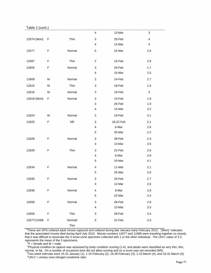
Table 1 (cont.)

4 13-Mar 3

12574 (Mort) F Thin

3 25-Feb 4

4 12-Mar 4

12577 F Normal

5 22-Mar 2.6

12587 F Thin

2 15-Feb 2.9

12605 F Normal

3 26-Feb 1.7

4 15-Mar 2.5

12609 M Normal

2 14-Feb 2.7

12615 M Thin

3 18-Feb 1.5

12618 M Normal

3 19-Feb 3

12619 (Mort) F Normal

2 13-Feb 1.9

3 26-Feb 1.6

4 15-Mar 3.2

12624 M Normal

3 19-Feb 3.1

12625 F NR

3 18-22 Feb 2.1

4 6-Mar 2.6

5 20-Mar 2.2

12628 F Normal

3 28-Feb 2.3

4 13-Mar 3.5

12629 F Thin

3 22-Feb 2.6

4 6-Mar 3.9

5 20-Mar 4.1

12634 F Normal

4 11-Mar 2.1

5 25-Mar 2.6

12635 F Normal

3 25-Feb 2.7

4 12-Mar 2.6

12636 F Normal

4 8-Mar 2.8

5 22-Mar 3.4

12658 F Normal

3 28-Feb 2.8

4 13-Mar 3.3

12659 F Thin

3 28-Feb 3.4

12577/12486 F Normal/

3 21-Feb 3.3

Thin aThese are GPS-collared adult moose captured and collared during late January-early February 2013. “(Mort)” indicates that the associated moose died during April-July 2013. Moose numbers 12577 and 12486 were traveling together so closely that it was difficult to associate the 3 snow-urine specimen collected with 1 or the other individual. The UN:C value of 3.3 represents the mean of the 3 specimens. bF = female and M = male. cPhysical condition at capture was assessed by body condition scoring (1-4), and adults were classified as very thin, thin, normal, or fat. On a number of occasions time did not allow scoring and so a score was not recorded (NR). dTwo-week intervals were 15-31 January (1), 1-15 February (2), 16-28 February (3), 1-15 March (4), and 16-31 March (5). eUN:C = urinary urea nitrogen:creatinine ratio.

Page 71

Figure 1. Study area for assessing nutritional restriction of moose by serial sampling and chemical analysis of urine voided in snow (snow-urine), northeastern Minnesota, late January-March 2013 (5, 2-week sampling intervals). (This includes all randomly collected samples and specimens from “known” GPS-collared moose.)

Page 72

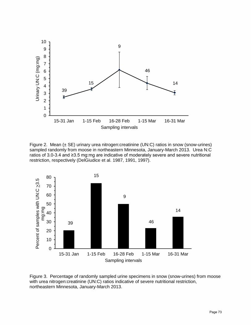
Figure 2. Mean (± SE) urinary urea nitrogen:creatinine (UN:C) ratios in snow (snow-urines) sampled randomly from moose in northeastern Minnesota, January-March 2013. Urea N:C ratios of 3.0-3.4 and ≥3.5 mg:mg are indicative of moderately severe and severe nutritional restriction, respectively (DelGiudice et al. 1987, 1991, 1997).

Figure 3. Percentage of randomly sampled urine specimens in snow (snow-urines) from moose with urea nitrogen:creatinine (UN:C) ratios indicative of severe nutritional restriction, northeastern Minnesota, January-March 2013.

0123456789

10

15-31 Jan 1-15 Feb 16-28 Feb 1-15 Mar 16-31 Mar

Urin

ary

UN

:C (m

g:m

g)

Sampling intervals

39 15

9

46

14

0

10

20

30

40

50

60

70

80

15-31 Jan 1-15 Feb 16-28 Feb 1-15 Mar 16-31 Mar

Perc

ent o

f sam

ples

with

UN

:C >

3.5

mg:

mg

Sampling intervals

39

15

9

46

14

Page 73

A LONG-TERM ASSESSMENT OF THE EFFECT OF WINTER SEVERITY ON THE FOOD HABITS OF WHITE-TAILED DEER1 Glenn D. DelGiudice, Barry A. Sampson, and John H. Giudice ABSTRACT Nutrition is a critical link between environmental and population variation in northern populations of free-ranging white-tailed deer (Odocoileus virginianus). Yet, there are few studies of winter food habits of northern free-ranging deer and all of these were short-term studies (1-2 winters). Consequently, little information is available on the effect of inter-annual variation in winter severity on browse availability and diet composition of free-ranging deer. We describe winter browse use by white-tailed deer on 4 study sites in northern Minnesota during 1991-2005. We also tested several a priori predictions about how browse use and availability would change as a function of winter severity. We collected browse data from 1,028 feeding trails and recorded 38 available browse species or species groups. The 4 most common browse species (beaked hazel [Corylus cornuta], mountain maple [Acer spicatum], trembling aspen [Populus tremuloides], and speckled alder [Alnus incana]) accounted for 76% of total available stems, and beaked hazel and mountain maple accounted for 68% of total used stems. As expected, browse use and availability distributions were very similar (i.e., deer utilized many of the available browse resources). Mean number of browse species used did not increase (decreased selection) with snow depth. However, mean browse rate (functional response) increased with increasing snow depth, and use of speckled alder (“starvation food”) increased when snow depth exceeded 40 cm. In addition, the number of browse species along feeding trails declined and stem abundance increased, on average, with increasing snow depth. Deep snow and increased use of dense conifer cover in northern Minnesota may restrict deer to greater use of lower quality feeding sites. In landscapes where this may occur, habitat management should attempt to minimize over-browsing on feeding sites in proximity to dense conifer cover by maximizing browse abundance and availability, particularly for beaked hazel and mountain maple. Managers also should consider enhancing alternative early winter feeding sites.

___________________________________________ 1Abstract from paper accepted by the Journal of Wildlife Management

Page 74

A LONG-TERM ASSESSMENT OF THE VARIABILITY IN WINTER USE OF DENSE CONIFER COVER BY FEMALE WHITE-TAILED DEER1 Glenn D. DelGiudice, John R. Fieberg, and Barry A. Sampson ABSTRACT Backgound: Long-term studies allow capture of a wide breadth of environmental variability and a broader context within which to maximize our understanding of relationships to specific aspects of wildlife behavior. The goal of our study was to improve our understanding of the biological value of dense conifer cover to deer on winter range relative to snow depth and ambient temperature. Methodology/Principal Findings: We examined variation among deer in their use of dense conifer cover during a 12-year study period as potentially influenced by winter severity and cover availability. Female deer were fitted with a mixture of very high frequency (VHF, n = 267) and Global Positioning System (GPS, n = 24) collars for monitoring use of specific cover types at the population and individual levels, respectively. We developed habitat composites for four study sites. We fit multinomial response models to VHF (daytime) data to describe population-level use patterns as a function of snow depth, ambient temperature, and cover availability. To develop alternative hypotheses regarding expected spatio-temporal patterns in the use of dense conifer cover, we considered two sets of competing sub-hypotheses. The first set addressed whether or not dense conifer cover was limiting on the four study sites. The second set considered four alternative sub-hypotheses regarding the potential influence of snow depth and ambient temperature on space use patterns. Deer use of dense conifer cover increased the most with increasing snow depth and most abruptly on the two sites where it was most available, suggestive of an energy conservation strategy. Deer use of dense cover decreased the most with decreasing temperatures on the sites where it was most available. At all four sites deer made greater daytime use (55 to >80% probability of use) of open vegetation types at the lowest daily minimum temperatures indicating the importance of thermal benefits afforded from increased exposure to solar radiation. Date-time plots of GPS data (24 hr) allowed us to explore individual diurnal and seasonal patterns of habitat use relative to changes in snow depth. There was significant among-animal variability in their propensity to be found in three density classes of conifer cover and other open types, but little difference between diurnal and nocturnal patterns of habitat use. Conclusions/Significance: Consistent with our findings reported elsewhere that snow depth has a greater impact on deer survival than ambient temperature, herein our population-level results highlight the importance of dense conifer cover as snow shelter rather than thermal cover. Collectively, our findings suggest that maximizing availability of dense conifer cover in an energetically beneficial arrangement with quality feeding sites should be a prominent component of habitat management for deer.

1Abstract from published paper: DelGiudice, G. D., J. R. Fieberg, and B. A. Sampson. A long-term assessment of the variability in winter use of dense conifer cover by female white-tailed deer. PLoS ONE 8(6):e65368. Doi: 10.1371/journal.pone.0065368

Page 75

Wildlife Health Program Wildlife Populations and Research Group

5463 - C West Broadway Forest Lake, Minnesota 55025

(651) 296-5200

BOVINE TUBERCULOSIS IN WHITE-TAILED DEER IN NORTHWEST MINNESOTA: A 7-YEAR EFFORT TO RESTORE MINNESOTA’S DISEASE-FREE ACCREDITATION Michelle Carstensen1, Erika Butler, Erik Hildebrand, and Lou Cornicelli SUMMARY OF FINDINGS

A total of 10,667 white-tailed deer (Odocoileus virginianus) were tested for bovine tuberculosis (bTB) in northwest Minnesota from 2005 to 2012. Fall 2012 marked the 7th consecutive year that the Minnesota Department of Natural Resources (MNDNR) conducted surveillance for this disease in deer since 2005, when bTB was first detected in a northwest cattle farm. The disease has since been found in a total of 12 cattle operations and 27 free-ranging white-tailed deer. Both deer and cattle had the same strain of bTB, which has been identified as one that is consistent with the disease found in cattle in the southwestern United States and Mexico. The Board of Animal Health (BAH) has been leading efforts to eradicate the disease in Minnesota’s cattle, which have included the depopulation of all infected herds, a buy-out program that removed 6,200 cattle from the affected area, and mandatory fencing of stored feeds on remaining farms. No new infections have been detected in either cattle or deer since 2009. A total of 323 hunter-harvested deer were sampled in fall 2012, with no positive cases of bTB detected. This marked the 3rd consecutive year that MNDNR has conducted bTB surveillance in hunter-harvested deer in the bTB outbreak area and failed to find any new cases of the disease. The state regained its bTB-Free accreditation in October 2011; however, some testing requirements remained on cattle herds within the endemic area until the infection in deer could be determined as nonexistent. While MNDNR is unable to declare the local deer herd entirely disease-free, the cumulative years of intensive surveillance efforts aimed at bTB detection of prevalence >0.5% with 99% confidence, provided solid evidence that this disease is no longer within these detectable levels in the deer population. MNDNR has now suspended any futures efforts to monitor for bTB in the state. INTRODUCTION

Bovine tuberculosis (bTB) is an infectious disease that is caused by the bacterium Mycobacterium bovis. Bovine tuberculosis primarily affects cattle; however, other mammals may become infected. The disease was first discovered in 5 cattle operations in northwest Minnesota in 2005. Since that time, 7 additional herds were found infected; resulting in a reduction of the state’s bTB accreditation to Modified Accredited in early 2008. In fall 2008, Minnesota was granted a split-state status for bTB accreditation that maintained only a small area (2,670mi2) in northwest Minnesota as “Modified Accredited,” allowing the remainder of the state to advance to “Modified Accredited Advanced.” In total, 27 wild deer have been found infected with the disease in northwest Minnesota, which can be attributed to a spillover of the disease from infected cattle. In 2010, The United States Department of Agriculture (USDA) upgraded Minnesota’s bTB accreditation to Modified Accredited Advanced within the split-state zone and bTB-Free throughout the remainder of the state. With no new infections discovered in MN cattle in 2009 and 2010, USDA upgraded the split-state portion to bTB-Free in October 2011. Although bTB was once relatively common in U.S cattle, it has historically been a very rare disease in wild deer. Prior to 1994, only 8 wild white-tailed and mule deer (O. hemionus) had been reported with bTB in North America. In 1995, bTB was detected in wild deer in Michigan and do serve as a reservoir of the disease in that state. Bovine tuberculosis is a progressive, chronic disease. It is spread primarily through the exchange of respiratory secretions between infected and uninfected animals. This transmission usually happens when animals are in close contact with each other. Animals may also become infected with bTB by ingesting the bacteria from contaminated feed. Incubation periods 1Corresponding author’s email: michelle.carstensen@state.mn.us

Page 76

can vary from months to years from time of infection to the development of clinical signs. The lymph nodes in the animal’s head usually show infection first and as the disease progresses, lesions (yellow or tan, pea-sized nodules) will begin to develop throughout the thoracic cavity. In severely infected deer, lesions can usually be found throughout the animal’s entire body. Hunters do not always readily recognize small lesions in deer, as they may not be visible when field dressing deer. In fact, most infected deer appear healthy. While it is possible to transmit bTB from animals to people, the likelihood is extremely low. Most human tuberculosis is caused by the bacteria M. tuberculosis, which is spread from person to person and rarely infects animals. METHODS

During falls 2005–2012 a hunter-harvested surveillance strategy was developed to

collect samples from the bTB Management Zone, which is approximated by Deer Management Area (DMA) 101. Sampling goals varied by year, dependent on frequency of new infections as well as existing Memorandums of Understanding (MOU) with United States Department of Agriculture, signed by both MNDNR and BAH. To that end, MNDNR was committed to ensuring the disease is not present in wild deer within the bTB Management Zone at >1.0% with 99% confidence.

At the registration stations, hunters were asked to voluntarily submit lymph node (LN) samples for bTB testing. Hunter information was recorded, including the hunter’s name, telephone number, MNDNR number, and location of kill. Maps were provided to assist the hunters in identifying the location (Township, Range, Section, and Quarter-section) of the kill. Cooperating hunters were given a cooperator’s patch and entered into a raffle for a firearm donated by the Minnesota Deer Hunter’s Association (MDHA). In addition, the Roseau River chapter of MDHA raffled additional firearms and a life-time deer hunting license for hunters that submitted samples from within the bTB Management Zone or bTB Core Area.

Sampling procedures included a visual inspection of the chest cavity of the hunter-killed deer. Three pairs of cranial LNs (parotid, submandibular, and medial retropharyngeal) were visually inspected for presence of gross lesions and collected for further testing. Samples were submitted to the Veterinary Diagnostic Laboratory (VDL) at the University of Minnesota for histological examination and acid-fast staining (when lesions are present only). All samples were then pooled in groups of 5 and sent to the National Veterinary Services Laboratories (NVSL) in Ames, IA for culture. Any suspect carcasses (e.g., obvious lesions in chest cavity or head) were voluntarily surrendered at the registration stations and the hunter was issued a replacement deer license at no charge. Suspect carcasses were transported in their entirety to the VDL for further testing.

Additionally, MNDNR implemented efforts to further reduce deer numbers in the post-hunting season in the bovine 140-mi2 TB-infected Core Area, through the use of ground sharpshooters (USDA-Wildlife Services). During Feb–April of 2007–2010, sharpshooter-harvested deer were transported intact to a central processing facility at Thief Lake Wildlife Management Area. Sample collection and handling was similar to that described above. Carcasses were salvaged for venison and available to the public. The ground sharpshooting effort was augmented with the addition of aerial gunning during winters 2008 and 2009.

In early winter of 2007–2012, MNDNR conducted an aerial survey of the bTB Core Area to assess deer numbers and distribution. This information was used to guide future management activities and estimate the percentage of deer removed from the area through hunting and agency culling.

RESULTS AND DISCUSSION

In 2005, Minnesota began a 7-year effort to attempt to eradicate bTB from the state’s cattle and free-ranging deer in the northwest corner of the state. Minnesota DNR, having

Page 77

learned valuable lessons from Michigan’s bTB outbreak, adopted an aggressive surveillance and management effort to prevent an establishment of a wildlife reservoir (Carstensen and Doncarlos 2011). To date, our efforts appear successful and the “Minnesota Model” of bTB response as received both national and international attention.

From 2005 to 2012, a total of 10,667 white-tailed deer were tested for bTB in northwest Minnesota, including hunter-harvested (n = 7,839), sharpshooting (n = 2,613), and landowner shooting permits (n = 215) (Table 1). There have been a total of 27 confirmed bTB-positive deer, all within a limited geographic area that extended in a 10-mile radius from Skime, MN (Fig 1). In fall 2012, MNDNR collected 323 samples from hunter-harvested deer in DPA 101 (including deer tested just outside this area). Testing of all lymph node samples at NVSL has confirmed that there were no positive cases of bTB, marking 2012 as the 3rd consecutive year that no new cases of bTB have been detected in wild deer. Apparent prevalence of bTB in the local deer population, sampled throughout a 1,730 to 2,670mi2 Surveillance Zone, indicates a significant decreasing trend from 2006–2012 (Table 1, Figure 2). Further, disease prevalence in the bTB Core Area has decreased dramatically from 2007 to 2010 (Table 1, Figure 2). Although disease prevalence estimates in the TB Core Area are biased due to the limited geographic distribution of bTB-positive deer and the increased probability of detecting a positive individual, the decreasing trend is consistent with the large-scale surveillance of the local deer population.

Aerial survey results from 2007 to 2012 demonstrated an overall decline in the deer population in the bTB Core Area (Table 2, Figure 3). This was expected, given the intensive removal efforts that occurred through ground and aerial sharpshooting; however, it was surprising that it took 4 consecutive years (2007 to 2010) of these removal operations to detect a significant difference in deer numbers (55% decline from the 2007 estimate) (Figure 3). Also of interest, is that more deer were shot in the bTB Core Area during winter removal efforts than counted in both 2008 and 2009 aerial surveys (Tables 1 and 2). There are a couple reasons for this apparent discrepancy. First, the aerial survey occurs at one point in time, typically at the end of January or beginning of February, prior to the start of the deer removal operations in mid-late February that occurred over 8-10 weeks. Second, it is likely that the bTB Core Area is home to both migratory and resident deer, some of which may move out of the zone to spring-summer-fall or winter ranges during the year. It is further likely that deer from the surrounding area are immigrating into the bTB Core Area as deer numbers are reduced and habitat availability increases. In a pilot study involving radio-collared deer south of the bTB Management Zone, mean home range size for deer (n = 9) surviving through the end of the study was 46.7 km2 (SE = ±10.1); 7 of these deer were migratory, traveling 4–20 km to distinct winter ranges over 2-3 day periods (Carstensen et al. 2011). This fluid environment within the bTB Core Area suggests deer move in and out of this zone relative to season, food resources, and predator pressure. Thus, a deer survey that generates a point estimate of deer abundance at one point in time only cannot account for these changes that occur over time. Deer are also very prolific and mild winters, in combination with abundant food resources (natural or artificial) will grow a herd rapidly. We have demonstrated that continued pressure on a deer herd is needed to reduce overall deer densities and yield a significant long-term reduction in the local population.

Another interesting question is whether or not the intensive deer removal efforts in DPA 101 affected hunter effort and success? While MNDNR-sponsored removal efforts (sharpshooting and aerial gunning) were very effective at reducing deer numbers and targeting bTB-infected individuals, it was also expensive ($390 and $960 per deer, respectively) and unpopular with the local residents. Eventhough we were told by local hunters that many would discontinue hunting in DPA 101 as a result of unpopular bTB management efforts, hunting number remained stable from 2007 to 2011, at >1,500 hunters/year (Figure 4). Total harvest and hunter success rates did decline after 2007, which suggests less deer were available to hunters in DPA 101 as a result of the intensive bTB management efforts.

Recent work being conducted at NVSL on genetic isolates from bTB-positive deer and cattle is helping to further explain Minnesota’s outbreak. The proximity of the bTB-infected deer

Page 78

to infected cattle herds, the strain type, and the fact that disease prevalence (<0.1%) was low, supports our theory that this disease spilled-over from cattle to wild deer in this area of the state. Further, the lack of infected yearlings or fawns and limited geographic distribution of infected adults further supports that deer are not a wildlife reservoir for this disease in Minnesota (Carstensen and DonCarlos, 2011). MNDNR is currently working with BAH, USDA, and NVSL on 2 manuscripts that detail the epidemiology of the outbreak in the northwest and magnitude of the response that was necessary to regain the state’s TB-Free accreditation within 7 years. With the recent upgrade in status to bTB-Free across the state and a lack of available funding to continue support payments to farms that participated in the buy-out program, BAH allowed farms to repopulate with cattle within the bTB Management Zone beginning July 1, 2012. Now that MNDNR completed its 3rd consecutive year with no new cases of the disease detected in deer and announced the suspension of further surveillance efforts, BAH discontinued whole-herd testing within the bTB Management Zone. ACKNOWLEDGMENTS

There is no way to complete a project of this scale without the assistance and leadership

from St. Paul and regional staff (some recently retired), including Ed Boggess, Mike DonCarlos, Dennis Simon, Paul Telander, and John Williams. For all the help with field collections, we’d like to thank area staff from Thief Lake, Red Lake, Roseau River, and Thief River Falls, as well as students and faculty from the University of Minnesota, College of Veterinary Medicine. Also thanks to Bob Wright and John Heineman for conducting a deer survey within the bTB Core Area. Also thanks to John Giudice for analyzing the survey data. GIS support was provided by Julie Adams, Bob Wright, and Chris Scharenbroich. Lastly, we thank USDA-Wildlife Services for their excellent work during sharpshooting operations. REFERENCES Carstensen, M. and M. W. DonCarlos. 2011. Preventing the establishing of a wildlife disease

reservoir: a case study of bovine tuberculosis in wild deer in Minnesota, USA. Veterinary Medicine International, Volume 2011, Article ID 413240, 10 pages, doi:10.4061/2011/413240.

Carstensen, M., D. J, O’ Brien, and S. M. Schmitt. 2011. Public acceptance as a determinant of management strategies for bovine tuberculosis in free-ranging U.S. wildlife. Veterinary Microbiology 151 (2011): 200–204, doi:10.1016/j.vetmic.2011.02.046.

Carstensen, M. J. R. Lima, E. Hildebrand, R. Wright, L. Cornicelli, S. Wells, and M. Grund. 2011. Spatial patterns of white-tailed deer movements related to bovine tuberculosis transmission risk in northwest Minnesota. Pages 98–108 in L. Cornicelli, M. Carstensen, M. Grund, M. Larsen, and J. Lawrence. Summaries of wildlife research findings, 2011. Minnesota Department of Natural Resources, Wildlife Populations and Research Unit, St. Paul.

Miller, R., J. B. Kaneene, S. D. Fitzgerald, and S.M. Schmitt. 2003. Evaluation of the influence of supplemental feeding of white-tailed deer (Odocoileus virginianus) on the prevalence of Bovine tuberculosis in the Michigan wild deer population. Journal of Wildlife Diseases 39: 84-95.

Minnesota Bovine Tuberculosis Management Plan. 2006. Minnesota Department of Agriculture, Minnesota Department of Natural Resources, Minnesota Board of Animal Health, United States Department of Agriculture, Unpubl. Rept.

O’Brien, D. J., S. D. Fitzgerald, T. J. Lyon, K. L. Butler, J. S. Fierke, K. R. Clarke, S. M. Schmitt, T. M. Cooley, and D. E. Berry. 2001. Tuberculous lesions in free-ranging white-tailed deer in Michigan. Journal of Wildlife Diseases 37: 608-613.

Page 79

O’Brien, D. J., S. M. Schmitt, J. S. Fierke, S. A. Hogle, S. R. Winterstein, T. M. Cooley, W. E. Moritz, K. L. Diegel, S. D. Fitzgerald, D. E. Berry, and J. B. Kaneene. 2002. Epidemiology of Mycobacterium bovis in free-ranging whitetailed deer, Michigan, USA, 1995-2000. Preventive Veterinary Medicine 54: 47-63.

Schmitt, S. M., S. D. Fitzgerald, T. M. Cooley, C. S. Bruning-Fann, L. Sullivan, D. Berry, T. Carlson, R. B. Minnis, J. B. Payeur, and J. Sikarskie. 1997. Bovine tuberculosis in free- ranging white-tailed deer from Michigan. Journal of Wildlife Diseases 33: 749-758.

Page 80

Table 1. Number of deer sampled for bovine tuberculosis (bTB) and testing results listed by sampling strategy, 2005 to 2012, northwestern Minnesota. Sampling strategy 2005 2006 2007 2008 2009 2010 2011 2012 Totals Hunter-harvested (Oct-Jan) 474 942 1,166 1,246 1,488 1,639 561 323 7,839 # bTB-positive 1 5 5 0 1 0 0 0 Apparent prevalence 0.21% 0.53% 0.43% 0.0% 0.07% 0.0% 0.0% 0.0% Sharpshooting (Feb-May) n/a n/a 488 937 738 450 n/a n/a 2,613 # bTB-positive 6 6 2 0 Apparent prevelance 1.23% 0.64% 0.27% 0.0% Landowner/tenant n/a 90 n/a 125 n/a n/a n/a n/a 215 # bTB-positive 1 0 Total deer tested 474 1,032 1,654 2,308 2,226 2,089 561 323 10,667 Total # bTB-positive 1 6 11 6 3 0 0 0 27

Table 2. Population estimatesa and 95% confidence intervalsb of deer within the Bovine Tuberculosis Core Area, 2007–2012, northwest Minnesota. Year Aircraft Design Var.est n N Srate Svar SE Xbar SE 95%CI PopEst SE 95% CI CV(%) RP(%) 2007 OH-58 StRS3 SRS 72 164 0.439 NA NA 5.7 0.46 4.9-6.5 935 76.0 784-1086 8.1 16.2 2008 OH-58 GRTS.SRS Local 72 164 0.439 21.94 4.53 4.9 0.56 3.8-6.0 807 75.2 659-954 9.3 18.3 2009 Enstrom GRTS.stRS2 Local 79 164 0.482 20.63 2.56 4.1 0.27 3.5-4.6 664 44.4 577-751 6.7 13.1 2010 OH-58 GRTS.SRS Local 72 164 0.439 29.30 6.70 2.6 0.39 1.8-3.3 422 64.4 296-548 15.3 30.0 2011 OH-58 GRTS.SRS Local 72 164 0.439 21.01 2.80 3.2 0.30 2.7-3.8 531 48.6 436-627 9.2 18.0 2012 OH-58 GRTS.SRS Local 72 164 0.439 3.06 0.57 1.0 0.14 0.7-1.3 160 22.3 120-210 13.6 26.7 aPopulation estimate = estimated minimum number of deer present during the sampling interval. Estimates are not adjusted for detectability (but intensive survey is designed to minimize visibility bias) and deer movement between sample plots is assumed to be minimal or accounted for via survey software. b95%CI’s based on sampling variance only (adjusted for spatial correlation in 2008-2011); they do not include uncertainty associated with detectabilty or animal movements (temporal variation due to animals moving onto or off the study area).

Page 81

Figure 1. Locations of all white-tailed deer found infected (n = 27) with bovine tuberculosis (bTB) since fall 2005 in northwest Minnesota, with the 12 previously-infected cattle operations are also included.

Page 82

a)

b) Figure 2. Prevalence of bovine tuberculosis (bTB) in hunter-harvested deer from 2005–2012 in the bTB Surveillance Zone (a) and disease prevalence from sharpshooter removed deer from 2007–2010 in the bTB Core Area (b), northwest Minnesota.

Page 83

Figure 3. Population estimate of deer within the Bovine Tuberculosis Core Area, winters 2007–2012, northwest Minnesota.

Page 84

Figure 4. Changes in hunter effort and success in deer permit area 101, from fall 2007 to fall 2011, northwest Minnesota.

Page 85

NORTHEAST MINNESOTA MOOSE HERD HEALTH ASSESSMENT 2007–2012 Erika A. Butler, Michelle Carstensen, Erik C. Hildebrand, and John H. Giudice SUMMARY OF FINDINGS

This project, which began in 2007, represents the second phase (2010–2012) of an

overall health assessment of hunter-harvested moose (Alces alces) in northeastern Minnesota. The objectives of this project were to: (1) screen hunter-harvested (and presumably healthy) moose for select disease agents and combine results from phase 1 of the project (2007-2009) to asses if there was any spatial or temporal variation in prevalence rates, (3) assess the clinical impacts of liver fluke (Fascioloides magna) infection on moose, and (4) determine the frequency of histological lesions consistent with brainworm (Parelaphostrongylus tenuis) infection. Samples were collected from 643 moose during 2007-2012 (average annual n = 107; range = 63-131). Moose were screened for West Nile virus, eastern equine encephalitis, western equine encephalitis, St. Louis encephalitis, malignant catarrhal fever, borreliosis (Borrelia burgdorferi), anaplasmosis (Anaplasma phagocytopila, formerly Ehrlichia phagocytophila) and 6 serovars of leptospirosis. There was evidence of exposure to West Nile Virus (30.1%), eastern equine encephalitis (4.1%) malignant catarrhal fever (23.3%), borreliosis (21.9%), and leptospirosis (0.5-6.4%). Portions of brain, cerebral spinal fluid, whole blood, and serum were submitted for polymerase chain reaction (PCR) for Flavivirus ribonucleic acid (RNA) (2011 only). Whole livers and brains were examined grossly and histologically for evidence of brainworm and liver fluke infections; both parasites were documented. Full serum chemistry profiles were conducted on 211 moose and will be used to determine if a correlation exists between liver fluke damage and serum liver enzymes. Whole blood samples from 217 moose were submitted for evaluation for tick-borne illnesses; anaplasmosis and piroplasma infections were also documented.

INTRODUCTION

Aerial survey data indicate a declining moose population in northeastern MN (DelGiudice 2013) and annual survival and reproductive rates during 2002-2007 were substantially lower than documented elsewhere in North America (Lenarz et al. 2007). Estimated at 2,760, the 2013 moose population estimate is significantly lower (35%) than the 2012 estimate and time series analysis of estimates since 2005 indicate a significant downward trend (DelGiudice 2013). Previous and ongoing research has been unable to determine proximate and ultimate cause(s) of non-hunting moose mortality and the possible related impacts to the long-term viability of the northeastern MN population. In 2007, the MN Department of Natural Resources (MNDNR) began a 3-year moose health assessment project to determine which diseases moose are being exposed to in northeastern MN and to establish baseline hepatic mineral levels. We believed that hunter-harvested moose would represent “healthy” animals; thus, data from these animals could be compared to known sick moose to increase our understanding of what might be considered “normal” for northeastern moose. We found that hunter-harvested moose in northeastern MN had been exposed to a variety of disease agents such as West Nile virus (WNV), eastern equine encephalitis (EEE), malignant catarrhal fever (MCF), anaplasmosis, borreliosis, and leptospirosis (Butler et al. 2010). While these findings were illuminating, additional research was needed to determine (1) the role liver damage (due to liver flukes) plays in non-hunting mortality, 2) the impact of arboviruses and how their prevalence may vary temporally, and (3) the impact of brainworm on moose survival, due to the difficulty in interpreting brain lesions caused by this parasite. The second phase of the moose health assessment project (started in 2010) will help to address these questions.

Murray et al. (2006) concluded that moose in northwestern MN were dying from high liver fluke loads. However, assessing the extent of liver damage caused by flukes can be subjective. In order to determine if liver damage caused by flukes has clinical implications, serum liver enzymes should be evaluated. Beginning in 2009, we asked hunters to collect

Page 86

whole livers for evaluation and they were ranked for liver fluke loads by a board-certified veterinary pathologist. In 2009, the first year of liver examinations, we found that 35% of livers had fluke-induced lesions with some having nearly 100% of the liver parenchyma affected (Butler et al. 2010). However, poor blood- collection techniques prevented assessment of the clinical impacts of the damage caused by the liver fluke infections. In 2010 we asked hunters to alter their blood collection strategies and began collecting the whole liver and assessing serum liver enzymes, with the goal of determining whether results of gross evaluation of the liver correlated with enzyme indicators of liver function.

Our moose health assessment during 2007–2009 indicated that moose are being exposed to a variety of arboviruses, including EEE, WNV, borreliosis, and anaplasmosis (Butler et al. 2010). As climate changes, the density and distribution of capable arthropod vectors is expected to change as well (Gould and Higgs 2009). Climate is known to play a key role in determining the geographical and temporal distribution of arthropods, characteristics of arthropod lifecycles, dispersal patterns of associated arboviruses, evolution of arboviruses, and the efficiency with which they are transmitted from arthropods to vertebrate hosts (Gould and Higgs 2009). For example, there has been a substantial increase in tick-borne encephalitis in Sweden since the mid-1980s related to milder winters and earlier arrival of spring (Lindgren and Gustafson 2001). In Phase 2 of the moose health assessment study, serum was screened for these arboviruses and a few additional disease agents. Combined with results from our 2007–2009 sampling, we have 6 years of data on the incidence of arbovirus exposure in our moose herd to evaluate temporal variation in prevalence. Additionally, in 2011 only, we screened moose for western equine encephalitis (WEE) and St. Louis encephalitis (SLE).

Diagnostics have shown that moose are dying from brainworm in MN. It is also known that moose are able to survive low-dose infections of brainworm and even develop immunity to subsequent infections (Lankester 2002). Researchers have hypothesized that brainworm was responsible for historic declines in moose populations (Karns 1967, Prescott 1974, Lankester 1987), but it is questionable whether brainworm represents a major threat to the northeastern MN population. In 2008, we began collecting whole brains from hunter-harvested moose to determine the frequency of brain lesions consistent with past brainworm infections in presumably healthy moose. These data would allow for better interpretation of migration tracts and could prevent pathologists from wrongly assigning brainworm as the cause of death based solely on the presence of migration tracts. We continue to collect whole brains to increase our sample size and to quantify the number of presumably healthy moose that have parasitic migration tracts. METHODS Hunters (tribal and state) were asked to collect whole livers, blood, hair, and a central incisor from their harvested moose. State hunters were only allowed to harvest bulls, whereas some tribal hunters were able to take either bulls or cows. Wildlife Health Program staff provided a presentation and instructions on the moose health assessment project at the mandatory MNDNR Moose Hunt Orientation sessions and at tribal natural resource offices. Hunters were given a sampling kit at the sessions and were asked to drop off completed sampling kits at official registration stations at the time of moose registration. Sampling kits included a cooler, 1-60-cc syringe for blood collection, 6-15-cc serum separator tubes, 2-5-cc ethylenediaminetetraacetic acid (EDTA) blood tubes for whole blood collection, 1 heavy-duty bag for liver storage, 2 coin envelopes for the tooth and hair collected, data sheet, protocol, Sharpie marker, 1 pair of large vinyl gloves, and 1 icepack. Hunters collected blood using the 60-cc syringe after incising the jugular vein as soon after death as possible and recorded time of death and blood collection. Blood was placed in serum-separator tubes and in an EDTA tube and kept cool until they were delivered to official MNDNR registration stations or tribal natural resource offices. Livers were placed in heavy-duty, pre-labeled bags.

At the registration stations or tribal offices, serum-separator tubes were centrifuged and the serum decanted. Blood spinning time was recorded. Portable refrigerators were located in

Page 87

advance at the registration stations to maintain the tissue samples. One whole blood sample (EDTA tube) and 1 mL of serum were refrigerated and submitted every 2-3 days to the University of MN (UMN)-College of Veterinary Medicine-Clinical Pathology Laboratory for a full large-animal serum chemistry profile. The remaining whole blood sample was submitted every 2-3 days to the UMN-Department of Entomology for testing for tick-borne illnesses. Remaining serum and the whole livers were frozen. Cerebral spinal fluid was collected when possible (2011 only). Whole brains were removed with the hunter’s permission and placed in formalin. A 1x1x1” piece of brain was removed and frozen (2011 only). The serum, whole liver, and whole brains were submitted to the UMN Veterinary Diagnostic Laboratory (UMN VDL, St. Paul, MN). The 1x1x1” piece of brain, cerebral spinal fluid, whole blood, and 1 mL of serum were submitted to the Minnesota Department of Health (MDH) for PCR for Flavivirus RNA (2011 only). Serum samples were also submitted to the National Veterinary Services Laboratory (NVSL) in Ames, Iowa.

Serum was tested for WNV, EEE, and WEE with a plaque reduction neutralization test (PRNT) and SLE with a serum neutralization test at NVSL. Serum was screened for leptospirosis (microscopic agglutination test), borreliosis (immunofluorescence assay), anaplasmosis (card test), and MCF via peroxidase-linked assay (PLA) with positive PLA tests further tested with a virus neutralization test (VN) at the UMN VDL. The livers were ranked by a board-certified veterinary pathologist based on parenchymal damage due to liver flukes; ranking included no fluke-induced lesions (no evidence of fluke migration), mild infection (<15% of liver parenchyma is affected with mild prominence/fibrosis of bile ducts and few smaller nodules characterized by peripheral fibrosis and central presence of opaque brown pasty material), moderate infection (15-50% of the liver parenchyma affected by nodules and fibrosis), and marked infection (51-100% of the liver parenchyma affected with deformation of the entire liver by larger nodules with widespread fibrosis). Brains were examined histologically with 4 complete coronary brain, cerebellum, and brain stem sections processed from each moose. An average of 25 histological slides per animal were examined, including the frontal, temporal, parietal, and occipital lobes and the basal nuclei, thalamus, mesencephalon, and brain stem. Central incisors of moose were submitted to Mattson’s Laboratory (Milltown, Montana) for aging by cementum annuli (Sergeant and Pimlott 1959). RESULTS AND DISCUSSION

We obtained samples from 643 hunter-harvested moose during 2007-2012 and the samples were well distributed throughout moose hunting zones (Figure 1.). The average age of hunter-harvested moose during 2007-2011 (results from 2012 are pending) was 4.4 years (n = 533, median = 4, range: 0.5-14; Fig. 2).

Eastern Equine Encephalitis

Evidence of exposure to EEE was detected in 23/557 (4%, 95% CI: 3-6%) moose sampled from 2007–2012 (Figure 3). Due to the small number of positive animals in each year and county, we were unable to accurately estimate the magnitude of spatial or temporal variation in EEE prevalence rates (other than to conclude that they were low).

A total of 65 moose were sampled (frozen brain, cerebral spinal fluid, serum, and whole blood) by the MDH by PCR for evidence of any Flavivirus RNA in 2011. Positive results would indicate that the moose actually had virus present in the tissues sampled. All results were negative.

Mosquitoes spread EEE, which can cause neurologic signs and often death. It poses a greater mortality threat for most species than WNV, although the effects of EEE infection have not been studied in moose. A titer that is greater than 100 is considered a very strong positive and means the serum was able to neutralize nearly 100% of the virus. Titers >100 were observed in 9% of positive samples.

Page 88

West Nile Virus

Evidence of exposure to WNV was detected in 171/557 (30%, 95% CI: 27-35%) moose sampled from 2007–2012 (Figure 4). There appeared to be an increase in prevalence in adult moose from east to west (Cook County: 27%, CI: 21-35%; Lake County: 39%, 95% CI: 32-48%; St. Louis County: 53.1%, CI: 41.3-68.2%). There also was some evidence (z = -2.099, p =0.035) that the log odds of exposure in adult moose was lower in 2011 than in 2007-2010 (𝜷� = -0.563, 95% CI: -1.177 to -0.084), although the biological significance of estimated differences in exposure rates is unknown (e.g., 𝒑� = 0.156 vs. 0.274 in Cook county). Furthermore, this model was fit after exploring the data and, therefore, estimates of effect sizes are likely optimistic (i.e., exploratory models tend to overfit the data and predict poorly on new data). Finally, positive serological results indicate that animals were exposed to the WNV, but it does not necessarily indicate illness. Similar to EEE, a titer that is greater than 100 is considered a very strong positive. Titers of 100 or greater were found in 5% of positive samples. Western Equine Encephalitis and St. Louis Encephalitis Of the 64 sera samples submitted for WEE and SLE testing (2011 only), none tested positive. Both of these diseases are mosquito-borne. Western equine encephalitis is known to occur infrequently in MN, although when it does, it is often part of a regional outbreak. Testing was performed at the suggestion of the Minnesota Department of Health as part of our collaborative project investigating arboviral prevalence rates in Minnesota’s wildlife.

Malignant Catarrhal Fever Virus

Evidence of exposure to MCF was detected in 129/553 (23.3%, CI: 19.9-27.1%) moose

sampled from 2007–2012. Follow-up testing with VN was negative for 110/129, 18 were unsuitable for testing, and one was weakly positive (likely a false positive). The PLA test is more sensitive than VN, meaning it is much better at identifying true positives, whereas VN is more specific and thus better at identifying true negatives. Malignant Catarrhal Fever is a gammaherpes virus, of which there are multiple strains (e.g., wildebeest strain of MCF, sheep strain of MCF, deer strain of MCF). The PLA reacts with multiple gammaherpes viruses. A PLA positive does not indicate the strain of exposure. The VN test only screens for the wildebeest strain (which is exotic to the U.S.) and would be negative if other strains are present. This means a sample that was positive on PLA and negative on VN was likely exposed to MCF, but not the wildebeest strain. There were some large differences in estimated probability of MCF exposure in adults by year (e.g., 𝒑� 4% in 2007 vs. 72%in 2008), but we found no evidence that probability of exposure varied significantly by location or age.

Gammaherpes viruses have been documented to cause serious illness and death in moose and other ruminants. The clinical symptoms can mimic brainworm infection, including neurological deficits, blindness, and thrashing on the ground prior to death. While infection with MCF frequently results in death, carrier status can occur and is identified with serology. Zarnke et al. (2002) found serologic evidence of exposure in numerous species across Alaska and reported 1% prevalence in moose. Anaplasmosis Evidence of exposure to anaplasmosis was detected in 1/426 (0.2%, CI: 0-2%) moose sampled from 2007–2010 (testing was no longer available in 2011). Results indicate that exposure to this bacterium is likely occurring, albeit at a very low rate.

Page 89

Moose are thought to be susceptible to infection with A. phagocytophilum. In Norway, anaplasmosis was diagnosed in a moose calf, which displayed apathy and paralysis of the hind-quarters (Jenkins et al. 2001). This moose was concurrently infected with Klebseilla pneumonia, to which the calf’s death was attributed, though the Klebseilla infection was most likely secondary to and facilitated by the primary infection with A. phagocytophilum. In sheep, this disease produces significant effects on the immunological defense system, increasing their susceptibility to disease and secondary infections (Larsen et al. 1994). Borreliosis

Evidence of exposure to borreliosis was detected in 120/546 (22%, CI: 19-26%) moose sampled from 2007–2012. There were some large differences in estimated probability of borreliosis exposure in adults by year (e.g., 2% in 2008 vs. 30% in 2010), but again we found no evidence that probability of exposure varied significantly by location or age. Borreliosis is a tick-borne bacterial disease that is maintained in a wildlife/tick cycle involving a variety of species, including mammals and birds. While evidence of natural infection in wildlife exists, there has been no documentation of clinical disease or lesions reported in wildlife species. Leptospirosis

A total of 559 samples were screened for 6 serovars of Leptospira interrogans. Results per serovar are as follows:

L. interrogans bratislava: o 7/559 (1.3%, CI: 0.5-2.6%)

L. interrogans canicola: o 3/559 (0.5%, CI 0.1-1.7%)

L. interrogans grippothyphosa: o 9/559 (1.6%, CI: 0.8-3.1%)

L. interrogans hardjo: o 3/559 (0.5%, CI: 0.1-1.7%)

L. interrogans icterohaemorrhagicae: o 24/559 (4.3%, CI: 2.8-6.4%)

L. interrogans pomona: o 36/559 (6.4%, CI: 4.7-8.8%)

We found no evidence of higher exposure rates among adults vs. juveniles and no evidence of a year effect on prevalence rates. We did find a significant (p < 0.05) positive correlation between infection with L. interrogans pomona and L. interrogans grippothyphosa (φ2 = 0.37, 95% CI: 0.18-0.53) and L. interrogans hardjo and L. interrogans icterohaemorrhagicae ( φ2 = 0.34, 95% CI: 0.19-.051).

Leptospirosis is a bacterial disease that can infect a wide variety of mammals, both domestic and wild. Moose could be at an increased risk for leptospirosis, as it is often propagated by mud and water contaminated with urine, not uncommon in moose habitat. General Tick-Borne Illness Screening Whole blood samples from 217 (n = 109, 59, 49 in 2010, 2011, and 2012, respectively) moose were submitted to the UMN Department of Entomology, where we are collaborating with Dr. Ulrike Munderloh to determine if hunter-harvested moose are infected with tick-borne illnesses. Samples were screened with a variety of PCR techniques. Results, only available for the 2010 samples, indicate that 10% of the moose were infected with anaplasmosis and 32% were positive for prioplasma primers. A hemolytic Mycoplasma was also identified in 19 of the samples. Further analysis is pending.

Page 90

Brain Histopathology Whole brains from 151 moose were collected since 2008 (n =23, 24, 40, 31, and 33 in 2008, 2009, 2010, 2011, and 2012, respectively) and 118 have been examined (results from 2012 are pending). No lesions were found in 101 (85.6%) of the brains, 12 (10.1%) had lymphocytic infiltration (unspecific chronic inflammatory lesion), and 5 (4.2%) had lesions consistent with larval migration tracts (mild to moderate meningitis, axonal degeneration, and secondary demyelination). Whole Liver Evaluation Whole livers were collected from 271 (n = 57, 108, 61, and 45 in 2009, 2010, 2011, and 2012, respectively) and have been submitted for gross examination. Of these livers, 192 (70.8%) had no fluke-induced lesions, 42 (15.5%) had mild infection, 28 (10.3%) had moderate infection, and 9 (3.3%) had marked infection. Additionally, beginning in 2010, serum was submitted for a serum chemistry profile in an attempt to correlate serum liver enzyme levels with the level of fluke-induced damage. Analyses of these results are pending. Serum Chemistries A total of 211 (n = 95, 63, and 53 in 2010, 2011 and 2012, respectively) serum samples were submitted for a full large animal serum chemistry profile. Analysis of these results is pending. The purpose of collecting these data is to determine if there is a correlation between the liver ranking and serum liver enzymes, as well as to establish baseline “normals” for animals in this population. ACKNOWLEDGMENTS

This project would not have been possible without assistance from a number of MNDNR personnel, tribal biologists, and volunteers. We would like to especially thank our crews that worked moose registrations stations: T. Rusch, J. Hines, D. Ingebrigtsen, B. Kirsch, N. Gellerman, W. Gessler, D. Litchfield, D. Pauly, M. Minchak, P. Backman, K. Carlisle, M. Dexter, and J. Hines. J. Hines also made our area maps. We also would like to thank tribal biologists M. Schrage, A. Edwards, L. Overland, and S. Moore for their help with the project. LITERATURE CITED Butler, E., M. Carstensen, E. Hildebrand, J. Giudice, R. Wright, and M. Schrage. 2010.

Preliminary results from the 2007-2009 moose herd health assessment project. Pages 150-163 in J. S. Lawrence, R. O. Kimmel, and M. S. Lenarz, eds. Summaries of wildlife research findings, 2009. Minnesota Department of Natural Resources, Wildlife Populations and Research Unit, St. Paul.

DelGiudice, G.D. 2013. 2013 Aerial Moose Survey Final Results. Minnesota Department of Natural Resources [MNDNR]. http://files.dnr.state.mn.us/recreation/hunting/moose/moose_survey_2013.pdf

Gould, E. A., and S. Higgs. 2009. Impacts of climate change and other factors on emerging arbovirus disease. Royal Society of Tropical Medicine and Hygeine 103:109-121.

Jenkins, A., K. Handeland, S. Stuen, L. Schouls, I. Van de Pol, R. T. Meen, and B. E. Kristiansen. 2001. Ehrlichiosis in a Moose calf in Norway. Journal of Wildlife Diseases 37:201-203.

Karns, P. D. 1967. Pneumostrongylus tenuis in deer in Minnesota and implications for moose. Journal of Wildlife Management 32:299-303.

Page 91

Lankester, M. W. 1987. Pests, parasites and diseases of moose (Alces alces) in North America. Swedish Wildlife Research Supplement 1:461-489.

Lankester, M. W. 2002. Low-dose meningeal worm (Paralaphostrongylus tenuis) infections in moose (Alces alces). Journal of Wildlife Disease 38:789-795.

Larsen, H. J. S., G. Overnes, H. Waldeland, and G. M. Johansen. 1994. Immunosuppression in sheep experimentally infected with Ehrlichia phagocytophila. Research in Veterinary Science 56:216-224.

Lenarz, M. S. 2011. 2011 Aerial moose survey. Unpublished report. Minnesota Department of Natural Resources, St. Paul.

Lenarz, M. S. 2011. 2012 Aerial moose survey. Unpublished report. Minnesota Department of Natural Resources, St. Paul.

Lenarz, M. S., J. Fieberg, M. W. Schrage, and A. J. Edwards. 2010. Living on the edge: viability of moose in northeastern Minnesota. Journal of Wildlife Management 74:1013-1023.

Lenarz, M. S., M. W. Schrage, A. J. Edwards, and M. E. Nelson. 2007. Moose population dynamics in northeastern Minnesota. Pages 346-348 in M. W. DonCarlos, R. O. Kimmel, J. S. Lawrence, and M. S. Lenarz, eds. Summaries of wildlife research findings, 2005. Minnesota Department of Natural Resources, Wildlife Populations and Research Unit, St. Paul.

Lindgren, E., and R. Gustafson. 2001. Tick-born encephalitis in Sweden and climate change. The Lancet 358:16-18.

Murray, D. L., E. W. Cox, W. B. Ballard, H. A. Whitlaw, M. S. Lenarz, T. W. Custer, T. Barrnett, T. K. Fuller. 2006. Pathogens, nutritional deficiency, and climate influence on a declining moose population. Wildlife Monographs 166.

Prescott, W. H. 1974. Interrelationships of moose and deer of the genus Odocoileus. Naturaliste Canadien 101:493-504.

Sergeant, D. W., and D. H. Pimlott. 1959. Age determinationin moose from sectioned incisor teeth. Journal of Wildlife Management 23:315-321.

Zarnke, R. L., H. Li, and T. B. Crawford. 2002. Serum antibody prevalence of malignant catarrhal fever viruses in seven wildlife species from Alaska. Journal of Wildlife Diseases 38:500-504.

Page 92

Figure 1. Harvest locations of hunter-harvested moose (n=628) included in the 2007–2012 moose health assessment project, northeastern Minnesota.

Page 93

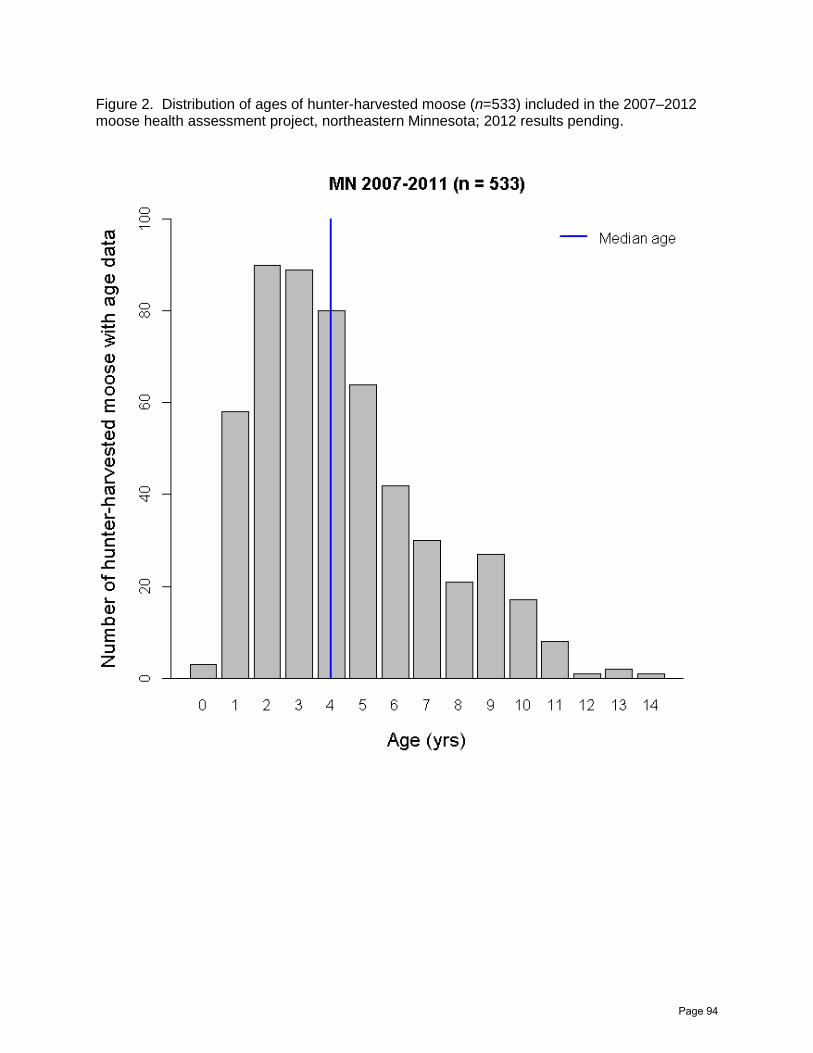
Figure 2. Distribution of ages of hunter-harvested moose (n=533) included in the 2007–2012 moose health assessment project, northeastern Minnesota; 2012 results pending.

Page 94

Figure 3. Locations of hunter-harvested moose (n=554) tested for eastern equine encephalitis included in the 2007–2012 moose health assessment project, northeastern Minnesota. Three moose were not included due to insufficient location data.

Page 95

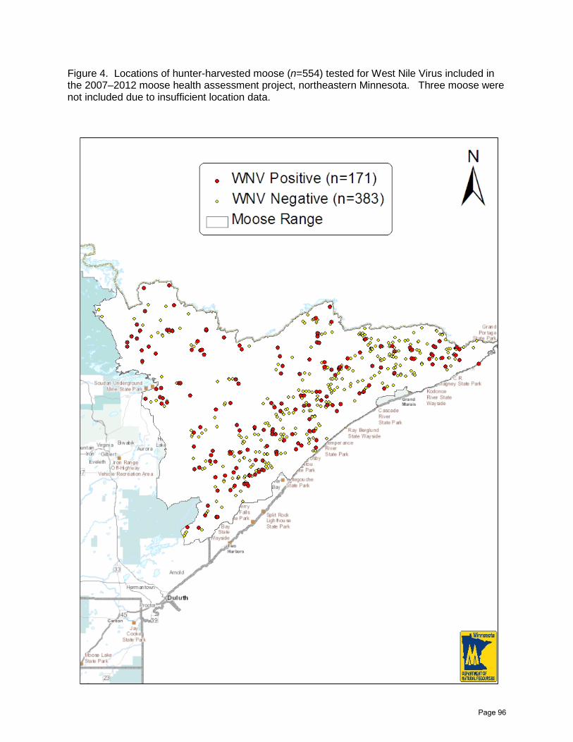
Figure 4. Locations of hunter-harvested moose (n=554) tested for West Nile Virus included in the 2007–2012 moose health assessment project, northeastern Minnesota. Three moose were not included due to insufficient location data.

Page 96

DETERMINING CAUSES OF DEATH IN MINNESOTA’S DECLINING MOOSE POPULATION: A PROGRESS REPORT Erika A. Butler, Michelle Carstensen, Erik C. Hildebrand, and David C. Pauly SUMMARY OF FINDINGS The primary goal of this project is to improve our understanding of non-anthropogenic (i.e., health-related) mortality of the northeastern Minnesota moose population. Our objectives are to determine causes of non-hunting mortality (i.e., identify specific disease and parasite agents), and assess the role nutrition plays as a potential contributing factor. To accomplish this, it is crucial that mortalities be investigated within 24 hours of death notification. From January 20- February 7, 2013, 111 moose were captured, radio-collared and released in northeastern MN. Serologic evidence of exposure to West Nile Virus, malignant catarrhal fever, various serovars of Leptospira interrogans, and Borreilia was documented. Nearly 1/3 of the 103 moose where body condition was assessed at capture were classified as thin or very thin. Serum progesterone levels indicated a 75% pregnancy rate. Mortalities investigated as of 20 June, 2013 (n=15) included 5 wolf kills, 2 wolf-related injuries with secondary lethal infections, one brainworm (Parelaphostrongylus tenuis), 3 winter ticks (Dermacentor albopictus), and 4 health-related causes with results pending.

INTRODUCTION Historically, moose were found throughout the forested zone of northern Minnesota. By the 1960’s there were two distinct populations, the northwest (NW) population of the aspen parklands and northeast (NE) population of the boreal forest (Fuller 1986). In the mid-1980’s the NW population began a precipitous decline, falling from 4,000 to <100 animals (Murray et al. 2006, Lenarz 2007). Murray et al. (2006) identified pathogens, including liver flukes (Fascioloides magna) and brainworm (Paralaphostrongylus tenius), as the principal cause of death for 37-62% of radio-collared animals; 25% of additional mortalities were likely pathogen-induced, but limited necropsy evidence was inconclusive. They also observed that many moose in NW MN dying of natural causes were malnourished, as evidenced by 51.4% of carcasses having bone marrow fat (BMF) contents below a critical threshold (< 30%) and trace mineral deficiencies (i.e., copper and selenium). No age or sex affects were identified.

Subsequently, in NE MN, Lenarz et al. (2009) reported a 21% average non-hunting mortality rate for radiocollared males and females, which was much higher than the 8-12% reported for moose elsewhere in North America (Larsen et al. 1989, Ballard 1991, Kufeld and Bowden 1996). Specific causes of most of the non-anthropogenic mortality (89%) could not be determined, as assessing cause-specific mortality was not the primary objective of the study (Lenarz et al. 2009). Many of the deaths appeared health-related, with prime age animals dying during unusual times of the year or carcasses found intact with little evidence of scavenging.

Aerial surveys also indicate the NE population is declining. Since the estimated peak at 8,840 moose in 2006, the 2013 estimated moose population (2,760) is significantly lower (35%) than the 2012 estimate and time series analysis of estimates since 2005 indicate a significant

Page 97

downward trend (DelGiudice 2013). Butler et al. (2010) documented evidence of exposure of NE MN moose to a variety of disease agents (e.g., West Nile Virus, eastern equine encephalitis, malignant catarrhal fever), which could be potential mortality factors. Additionally, sick moose reported by the public have been found to be infected with a variety of disease agents, including brainworm (Parelaphostrongylus tenuis), liver flukes (Fascioloides magna), arterial worm (Elaeophora schneiderei), and Setaria sp. (Minnesota Department of Natural Resources [MNDNR], unpublished data). Brainworm and arterial worm are known mortality factors of moose elsewhere in the U.S. (Anderson 1964, Worley et al. 1972, Pessier et al. 1998). Researchers have hypothesized that brainworm was responsible for historic declines in moose populations (Karns 1967, Prescott 1974, Lankester 1987), but it is questionable whether brainworm currently represents a major threat to the NE MN population; clinical signs consistent with brainworm infection were first reported in MN moose in 1912 (Fenstermacher and Olson 1942). Lenarz et al. (unpublished data) found that brainworm may have caused an average 19% (0-32%) of the population’s total annual mortality.

The relationship between diseases, parasites, and nutritional restriction of ungulates can be very complex, and moose numbers may be influenced by interactions among these factors (DelGiudice et al. 1997). All can act either singularly or in concert to negatively affect survival. Poor body condition, potentially related to nutritional deficiencies, was reported in some NE MN moose (Lenarz et al. 2009). Using ultrasonographic measurements of rump fat and body condition scoring, DelGiudice et al. (2011) found that 21.1% of radiocollared adult females may have been seriously challenged by poor condition in 2003. A strong relationship exists between maximum depth of rump fat (Maxfat) and ingesta-free body fat (IFBF) of moose; when rump fat is depleted, IFBF is no more than 5.6% (Stephenson et al. 1998). Cook et al. (2004) reported that the probability of winter survival for northern Yellowstone elk with >5.0% IFBF during February-March was good to excellent. Urine collected from snow (snow-urine) can be chemically analyzed for urea nitrogen (UN), potassium (K), and creatinine (C). Urinary UN:C and K:C ratios have been used to assess the degree of nutritional restriction and endogenous protein catabolism in Isle Royale moose (DelGiudice et al. 1997) and Yellowstone elk (Cervus elaphus) and bison (Bison bison) (DelGiudice et al. 2001). DelGiudice et al. (1997) showed that UN:C data indicated abnormally severe nutritional restriction in a high proportion of moose from 1988 to 1990, coinciding with a 26% decline in the population, and they reported a negative correlation between population rate-of-increase and UN:C ratios, suggesting that nutritional restriction and an associated winter tick (Dermacentor albpictus) infestation may have contributed to the population decline on Isle Royale during 1988-1990. Assessment of body condition at the individual and population levels is essential to better understand relations of seasonal heat stress, body condition, habitat use, demographic parameters and performance of this population (DelGiudice et al. 2011).

The primary goal of this project is to improve our understanding of non-anthropogenic (i.e., health-related) mortality of the NE MN moose population. Our objectives are to determine causes of non-hunting mortality (i.e., identify specific disease and parasite agents), and assess the role nutrition plays as a potential contributing factor. To accomplish this, it is crucial that mortalities be investigated in within 24 hours of death notification. The technology being utilized in this study to facilitate rapid responses to mortalities is the first of its kind.

Page 98

METHODS The study area (Figure 1) is classified as the Northern Superior Upland region (MNDNR 2007), and includes a variety of wetlands (e.g., bogs, swamps, lakes, streams) and multiple species of conifers, such as northern white ceder (Thuja occidentalis), black spruce (Picea mariana), and tamarack (Larix laricina) in the lowlands and balsam fir (Abies balsamea) and jack (Pinus banksiana), white (P. strobes), and red pines (P. resinosa) in the uplands. Deciduous trees, including quaking aspen (Populus tremuloides) and white birch (Betula papyrifera) are intermixed with conifers on uplands. Potential predators of moose include wolves (Canis lupus) and black bears (Ursus americanus).

Moose were captured by aerial darting with carfentanil (4.5 mg or 6.0 mg) and xylazine (100 mg or 150 mg) from a helicopter; immobilizations were reversed with naltrexone and tolazoline. Blood (serum and whole blood) was collected at capture by venipuncture of the jugular vein. Serum was screened for evidence of exposure to 10 disease agents following the same protocol as described by Butler et al. (2010). Additionally, serum was submitted for a full large animal serum chemistry profile for chemistries and reproductive hormones to assess physiological status, overall health, and pregnancy status (Franzmann and LeResche 1978, Haig et al. 1982, Duncan et al. 1994). Serum progesterone levels were determined by the Smithsonian Institute; levels >2.0 ng/mL were considered pregnant. Whole blood in Ethylenediaminetetraacetic acid (EDTA) was used to make blood smears and complete and differential blood cell counts were performed, which may be indicative of condition and health status (Duncan et al. 1994), presence of tick-borne illnesses, and evaluation for the presence of microfilaria. An incisor (I4) was removed for aging by cementum annuli (Sergeant and Pimlott 1959). A general fecal floatation examination for parasites was performed. Rump Maxfat (cm) was measured by ultrasound to assess body condition and nutritional status (Cook et al. 2010, DelGiudice et al. 2011). A thorough physical examination was performed, including assessment of body condition score (very thin, thin, normal, fat), winter tick load, and hair loss. Total body length, girth, and hind leg length (cm) were measured (Franzman et al. 1978) and used to estimate body weight of moose and to standardize estimates of IFBF from Maxfat (Stephenson et al. 1998, Cook et al. 2010).

Moose were fitted with Irridium Global Positioning System (GPS) radiocollars manufactured by Vectronic Aerospace (Berlin, Germany). The DNR purchased 100 collars, and 10 collars were purchased by a researcher at the University of Minnesota, James Forrester, to be incorporated into our adult mortality project. Collars were programmed to obtain a location approximately once every 4 hours with one transmission per day. The Irridium component allows remote programming of these collars. The location fix schedule and transmission schedule were changed in the month of May (1 fix every 1 hour, 3 minutes, and 44 seconds, with 3-4 transmissions/day) to assist with the calf study (a corresponding research project assessing the proximate and ultimate causes of mortality in calves born to cows collared as part of this project). Battery life of 3-4 years is expected. Collars include a mortality signal triggered by a motion-sensitive switch. In turn, the mortality signal triggers a text message to be sent to the moose mortality response team, alerting us that the moose has died. A program was also developed to analyze locations, and if they are within a 20 m radius, a “localization notification” is generated. This is useful in detecting sick animals that are potentially moribund. Mortality implant transmitters (MITs), which are manufactured by Vectronics, were placed orally into the

Page 99

reticulum of a subset of the captured moose. These devices are similar to a cow magnet in size, log internal temperatures every 15 minutes, and transmit a subset of this data to the collar. Additionally, MITs are meant to provide immediate notification of mortality via detection of minimal internal activity (e.g., lack of a heart beat) and this notification is also made via text message to the moose mortality response team. Temperature loggers (Hobo TibdbiTv2) were affixed to the GPS collar and were programmed to collect ambient temperature every 60 minutes.

Any mortalities that occurred within two weeks of the capture date were censored from the study.

Necropsy response teams were organized and have undergone extensive necropsy training. Responders were on-call and were ready to respond quickly in the event of a notification. If a moose is found to be alive, but obviously ill, it was euthanized and necropsied. Every effort will be made to remove carcasses intact and deliver them to the University of Minnesota Veterinary Diagnostic Laboratory (UM VDL) for a complete necropsy by a board-certified pathologist. If carcass extraction is not possible a thorough and complete field necropsy was performed, guided by an established protocol, and samples were submitted to the UM VDL for diagnostics.

RESULTS AND DISCUSSION Capture Summary From Jan 20 – Feb 7, 2013, 111 moose (84 females, 27 males) were captured and fitted with GPS collars (Figure 1). Four moose (2 females, 2 males) died within 2 weeks of capture and were censored; this corresponds to a 3.6% capture-related mortality rate. Though mortality rates < 2% are the goal for any wild ungulate capture, this assumes a routine capture within a healthy population (Arnemo et al., 2003). There are indications that MN’s moose herd was not healthy; thus the observed capture-related mortality rate was not higher than expected. In fact, Roffe et al. (2001) reported mortality rates in moose captured with Carfentanil combinations range from 6-19%. At necropsy, one of the capture-related mortalities was found to have parasitic tracts in its brain (likely due to P. tenuis infection); thus suggesting that other contributing factors may have been involved in these deaths.

Collar and MIT Functioning Of the 100 collars purchased by the MN DNR, 26 have had mortality switch malfunctions resulting in the collars being locked in mortality mode. To address this, we worked with the collar manufacturer to develop a localization program, which evaluates all the locations and generates a text message notification if the GPS fixes are within a 20 m radius. This program is currently functioning on both our locked-in-mortality collars (notification generated if fixes from the past 12 hours are within a 20 m area) and our properly functioning collars (notification generated if the fixes from the past 24 hours are within a 20 m area). This program has actually increased our ability to recognize animals that are moribund, but are not actually dead, allowing us to euthanize the animal. This allows never before documented clinical signs to be observed and key samples (e.g., fresh blood) to be collected, which is vital when trying to determine cause of death. This program has also helped us identify wolf-kills faster, as wolves will feed under the collar and prevent it from going into mortality until they have left the carcass.

Page 100

Initially, we deployed 9 MITS; however, Vectronics discovered that the acceleration function malfunctioned (though the temperature sensor was still functioning) and requested that all remaining MITs be returned to them for reprogramming. While replacements were returned to DNR, we did not receive all of them in time for deployment prior to the end of the capture operation. In total, we deployed 28 MITs (9 of the first generation, 19 of the second generation). The first generation MITs are only collecting temperature data, while the other 19 should be functioning as designed. Unfortunately, 6 MITs were regurgitated by the animals soon after deployment and are no longer functioning. Three moose with MITs have died; 2 of which functioned as designed and generated an immediate notification of mortality. The other was a second generation and did not notify us of the mortality but recorded internal temperatures. Currently, there are currently 11-2nd generation and 8-1st generation MITs remaining in moose. Body Condition Score and Rump Fat Measurement at Capture The body condition score of each animal was evaluated and recorded whenever possible. Nearly 1/3 of the 103 moose assessed were classified as either very thin (4, 3.8%) or thin (30, 29.1%). Sixty-seven were categorized as normal (65%) and 2 (1.9%) were identified as being fat. Serum Progesterone Results Serum from 75 females were screened for progesterone levels. Fifty-six (74.6%) cows were identified as pregnant. Disease and Parasite Screening at Capture Evidence of exposure to West Nile Virus (WNV) was detected in 15/96 (15.6%) moose at capture. These results were lower than those reported during the MN hunter harvested moose surveillance project (34.8%; Butler et al. 2010). Any titer ≥10 was considered positive and indicates that animals were exposed to the WNV, but does not necessarily indicate illness. A titer that is greater than 100 is considered a very strong positive and means that the serum was able to neutralize nearly 100% of the virus. Multiple hunter-harvested animals had titers ≥100; however, at capture the only positive titers were 10. This could indicate that the antibody response to WNV in moose is not very long lived. Evidence of exposure to eastern equine encephalitis (EEE) was not detected in any of the 96 moose tested at capture. The lack of detection was unexpected as an average exposure rate of 6.1% was documented during the MN hunter-harvested moose surveillance project (Butler et al. 2010). This could indicate that the antibody response to WNV in moose is not very long lived. Like WNV, mosquitoes spread EEE, which can cause neurologic signs and often death. It poses a greater mortality threat for most species than WNV, although the effects of EEE infection have not been studied in moose. Evidence of exposure to malignant catarrhal fever (MCF) was detected in 48/96 (50%) moose sampled at capture. Follow-up testing with virus neutralization was negative for all moose, indicating that they were not exposed to the wildebeest strain of MCF. These results are higher than what we reported from 2007 to 2009 during the MN hunter-harvested moose surveillance project (35%; Butler et al. 2010). Malignant catarrhal fever is a gammaherpes virus, of which there are multiple strains (e.g., wildebeest strain of MCF, sheep strain of MCF, deer strain of MCF). Gammaherpes viruses have been documented to cause serious illness and death in moose and other ruminants (Neimanis et al. 2009). Clinical symptoms mimic brainworm

Page 101

infection, including neurological deficits, blindness, and thrashing on the ground prior to death. While infection with MCF frequently results in death, carrier status can occur and is identified with serology.

Evidence of exposure to Borreilia was detected in 22/96 (22.9%) moose sampled at capture. These results are similar to results from 2007 to 2009 during the MN hunter-harvested moose surveillance project (23%, Butler et al. 2010). Borreliosis is a tick-borne bacterial disease that is maintained in a wildlife/tick cycle involving a variety of species, including mammals and birds. While evidence of natural infection in wildlife exists, there has been no documentation of clinical disease or lesions reported in wildlife species.

BA total of 96 moose were screened for 6 serovars of Leptospira interrogans. Results per serovar are as follows:

L. interrogans bratislava: o 0/96 (0%)

L. interrogans canicola: o 0/96 (0%)

L. interrogans grippothyphosa: o 1/96 (1.0%)

L. interrogans hardjo: o 0/96 (0%)

L. interrogans icterohaemorrhagicae: o 3/96 (3.1%)

L. interrogans pomona: o 8/96 (8.3%)

While the prevalences are lower for most of the serovars compared with data from the MN hunter-harvested moose surveillance project, the prevalence of L. pomona was slightly higher (Butler et al. 2010). Leptospirosis is a bacterial disease that can infect a wide variety of mammals, both domestic and wild. Moose could be at an increased risk for leptospirosis, as it is often propagated by mud and water contaminated with urine, not uncommon in moose habitat. Fecal floatation was used to screen moose at capture for parasites. A total of 84 animals were sampled, with 31 (36.9%) infections identified. Nematodirus sp. was found in 20 moose, Strongyle-type ova were identified in 6 moose, Moniezia sp. was found in one moose, two moose were coinfected with Nematodirus sp and and Strongyle-type ova, one had Moniezia and Nematodirus, and one had Moniezia and Strongyle-type ova. This is a higher rate than found during the MN DNR hunter-harvested moose health assessment project (12.9%, Butler et al. 2010) and is likely due to a change in methods (feces were no longer frozen, but submitted chilled) as freezing can cause ova to lyse and make identification difficult or impossible. Analysis of the CBC and serum chemistry results is pending. Central incisors have been submitted for aging, but results aren’t expected until mid-summer. Moose Mortalities to Date As of 25 June, 2013, 15 of 107 (14%; 11 females, four males) collared moose have died. Causes of death are as follows: 5 wolf kills, 2 wolf-caused injuries with secondary lethal

Page 102

infections, one P. tenuis (with a worm in both the brain and an eye, likely with partial blindness), 3 winter ticks, and 4 health-related mortalities with results pending. Two of the moose were found alive and euthanized (the P. tenuis case and one of the wolf-caused injuries with a secondary bacterial infection), 4 carcasses were extracted intact and delivered to the UM VDL for a complete necropsy, and 11 were necropsied in the field. The causes of mortalities determined to-date have not been unexpected. Spring is the most stressful time of year for moose (i.e., lack of adequate forage, very little remaining fat reserves) and coupled with snow conditions that favored wolves and winter ticks, these types of mortalities are not unusual. As this study continues, we expect mortalities to occur in late summer and early fall, as was documented by previous studies (Mike Schrage, Fond du Lac Resource Management Division, personal communication), and these cases may be more illuminating as to what health-related pathogens may be driving this moose decline. Mortality Response Times Response time has varied, though the majority of responses (53%) have occurred within 24 hours of mortality notification, 4 (27%) were within 32 hours and 3 (20%) ranged from 33-96 hours. Three of the wolf-killed moose had a delayed response time (31, 46, and 60 hours) because the wolf activity at the death site prevented the collar from going into mortality mode (thereby, no notification was generated) until they left the carcass remains. The new localization program will hopefully minimize this lag affect in the future. The moose with a 96 hour response time had sent a localization notification, but no mortality notification. While viewing the GPS location data for this moose, the moose response team believed it was alive and making small- movements; clearly, this was not the case and we have altered our response strategy accordingly. ACKNOWLEDGEMENTS This project is very demanding and would not be possible without the assistance of the following groups and individuals: the Environmental and Natural Resources Trust Fund for funding the majority of this project, Glenn DelGiudice for his input in study design and methodology and assistance at captures, Arno Wuenshmann and Anibal Armien (UM VDL) for their diagnostic investigations of the mortalities, Mike Schrage (Fond du Lac Resource Management Division) and Andy Edwards (1854 Treaty Authority) for their assistance in the field and purchase of MITs, Richard Gerhold and Caroline Grunenwald (University of Tennessee) for assisting with the identification of microfilaria, Ulrike Munderloh (University of MN, Department of Entomology) for testing samples for tick-borne illness, J. P. Dubey (USDA, ARS) for neospora testing, Robert Wright (MNIT) for his GIS and technical assistance, our team of primary responders (Nancy Gellerman, Dave Ingebrigtsen, Dawn Plattner, and Margaret Dexter; MN DNR), our team of secondary responders (Tom Rusch, John Giudice, Bob Kirsch, John Giudice, and Jeff Hines; MN DNR), Dan Ryan (US Forest Service), Brandon Seitz (Grand Portage National Monument) and Katie Foshey (MNDNR volunteer) for their assistance in the field, Larissa Minicucci (University of Minnesota, College of Veterinary Medicine) for training us how to place MITs, the MN DNR enforcement pilots (Jason Jenson, John Heineman, and Tom Bucker) for their assistance during captures, and Amanda McGraw (University of MN) for her assistance with data management and gearing-up for captures.

Page 103

LITERATURE CITED Anderson, R.C. 1964. Neurologic disease in moose infected experimentally with

Pneumostrongylus tenuis from white-tailed deer. Pathologica Veterinaria. 1:289-322. Arnemo J. M., T.J. Kreeger, and T. Soveri. 2003. Chemical immobilization of free-ranging

moose. Alces 39:243-253. Ballard, W.B., J.S. Whitman, and D.J. Reed. 1991. Population dynamics in south-central

Alaska. Wildlife Monograph 114. Butler, E.A., M. Carstensen, E. Hildebrand, J. Giudice, R. Wright, and M. Schrage. 2010.

Preliminary results from the 2007-2009 moose herd health assessment project. Minnesota Department of Natural Resources [MNDNR]. http://www.dnr.state.mn.us/publications/wildlife/research2010.html

Cook, R.C., J.G. Cook, and L.D. Mech. 2004. Nutritional condition of northern Yellowstone elk. Journal of Mammalogy 85:714-722.

Cook, R.C., J.G. Cook, T.R. Stephenson, W.L. Myers, S.M. Mccorquodale, D.J. Vales, L.L. Irwin, P. Briggs Hall, R.D. Spencer, S.L. Murphie, K. A. Schoenecker, and P.J. Miller. 2010. Revisions of rump fat and body scoring indices for deer, elk, and moose. Journal of Wildlife Management 74:880-896.

DelGiudice, G.D., R.O. Peterson, and W.M. Samuel. 1997. Trends of winter nutritional restriction, ticks, and numbers of moose on Isle Royale. Journal of Wildlife Management 61:895-903.

DelGiudice, G. D., R. A. Moen, F. J. Singer, and M. R. Riggs. 2001. Winter nutritional restriction and simulated body condition of Yellowstone elk and bison before and after the fires of 1988. Wildlife Monographs No. 147. 60pp.

DelGiudice, G. D., B. A. Sampson, M. S. Lenarz, M. W. Schrage, and A. J. Edwards. 2011. Winter body condition of moose (Alces alces) in a declining population in northeastern Minnesota. Journal of Wildlife Disease 47:30-40.

DelGiudice, G.D. 2013 Aerial Moose Survey Final Results. Minnesota Department of Natural Resources [MNDNR]. http://files.dnr.state.mn.us/recreation/hunting/moose/moose_survey_2013.pdf

Duncan, J.R., K.W. Trasse, and E.A. Mahaffey. 1994. Veterinary laboratory medicine 3rd edition. Iowa State Univeristy, Ames, USA.

Fenstermacher, R. and O.W. Olson. 1942. Furthers studies of diseases affecting moose III. Cornell Veterinarian 32:241-254.

Franzmann, A.W. and R.E. LeResche. 1978. Alaskan moose blood studies with emphasis on condition evaluation. Journal of Wildlife Management 42:334-351.

Franzmann, A.W., R.E. LeResche, R.A.Rausch, and J.D. Oldemeyer. 1978. Alaskan moose measurements and weights and measurement-weight relationships. Canadian Journal of Zoology 56:298-306.

Fuller, T.K. 1986. Observations of moose, Alces alces, in peripheral range in northcentral Minnesota. Canadian Field Naturalist 100:359-362.

Haigh, J.C., E. H. Kowal, W. Runge, and G. Wobeser. 1982. Pregnancy diagnosis as a management tool for moose. Alces 18:45-53.

Karns, P.D. 1967. Pneumostrongylus tenuis in deer in Minnesota and implications for moose. Journal of Wildlife Management 32:299-303.

Kufeld, R.C., and D.C. Bowden. 1996. Survival rates of Shiras moose (Alces alces shirasi) in Colorado. Alces 32:9-13.

Lankester, M.W. 1987. Pests, parasites and diseases of moose (Alces alces) in North America. Page 104

Swedish Wildlife Research Supplement 1:461-489. Larsen, D.G., D.A. Gauthier, and R.L. Markel. 1989. Cause and rate of moose mortality in

the southwest Yukon. Journal of Wildlife Management 53:457-481. Lenarz, M. S., M. W. Schrage, A. J. Edwards, and M. E. Nelson. 2007. Moose population

dynamics in northeastern Minnesota. Pages 346-348 in M. W. DonCarlos, R. O. Kimmel, J. S. Lawrence, and M. S. Lenarz, eds. Summaries of wildlife research findings, 2005. Minnesota Department of Natural Resources, Wildlife Populations and Research Unit, St. Paul.

Lenarz, M.S., M.E. Nelson, M.W. Schrage, A.J. Edwards. 2009. Temperature mediated moose survival in northeastern Minnesota. Journal of Wildlife Management 73:503-510.

Murray, D.J., E.W. Cox, W.B. Ballard, H.A. Whitlaw, M.S. Lenarz, T.W. Custer, T. Barnett, and T.K. Fuller. 2006. Pathogens, nutritional deficiency, and climate influences on a declining moose population. Wildlife Monographs 116:1-30.

Neimanis, A.S., J.E. Hill, C.M. Jardine, and T.K. Bollinger. 2009. Sheep-associated malignant catarrhal fever in free-ranging moose (Alces alces) in Saskatchewan, Canada. Journal of Wildlife Disease 45:213-217.

Pessier, A.P, V.T. Hamilton, W.J. Foreyt, S. Parish, and T. L. McElwain. 1998. Probable elaeophorosis in a moose (Alces alces) from eastern Wasthington state. Journal of Veterinary Diagnostic Investigation 10:82-84.

Prescott, W. H. 1974. Interrelationships of moose and deer of the genus Odocoileus. Naturaliste Canadien 101:493-504.

Roffe, T.J., K. Coffin, and J. Berger. 2001. Survival and immobilizing moose with carfentanil and xylazine. Wildlife Society Bulletin 29:1140-1146.

Sergeant, D.W., and D.H. Pimlott. 1959. Age determinationin moose from sectioned incisor teeth. Journal of Wildlife Management 23:315-321.

Stephenson, T.R., K.J. Hundertmanrk, C.C. Schwartz, and V. Van Ballenbergehe. 1998. Predicting body fat and body mass in moose with ultrasonography. Canadian Journal of Zoology 76:717-722.

Worley, D.E., C.K. Anderson, and K.R. Greer. 1972. Elaeophorosis in moose from Montana. Journal of Wildlife Diseases 8:242-244.

Page 105

Figure 1. Locations of moose captured (n=111) during Jan 20- Feb 7, 2013 in northeast Minnesota.

Page 106

The ecology of eastern equine encephalitis virus in wildlife and mosquitoes in Minnesota

Amy Kinsley (University of MN-Dept of Veterinary Population Medicine), Erika Butler, Roger Moon (University of MN-Dept of Entomology), Kirk Johnson (Metropolitan Mosquito Control District), Michelle Carstensen, David Neitzel (Minnesota Department of Health), and Meggan Craft (University of MN-Dept of Veterinary Population Medicine)

INTRODUCTION

Eastern equine encephalitis virus (EEEV) is a reemerging arbovirus endemic in North America. In the United States, EEEV cases have been reported in and around freshwater hardwood swamps in Eastern and Midwestern states. Wild birds serve as the primary reservoir host; they provide long-term maintenance of the virus and exchange infection between competent mosquitoes during blood meals. The highly ornithophilic mosquito species, Culiseta melanura, acts as the primary enzootic vector, providing stable transmission of the virus between the reservoir hosts. Species of the genera Culex, Aedes and Coquilletidia are thought to act as bridge vectors, leading to incidental infections in dead-end hosts, which move the virus beyond the endemic hardwood swamp habitat. EEEV is considered to be one of the most severe arbovirus infections with estimated human and equine mortality rates of 50-75% and 70-90%, respectively.

In this study, elk and moose serological surveys were used to calculate EEEV seroprevalence in the northwestern and northeastern portions of Minnesota. The serological surveys were conducted as part of the annual moose and elk herd health assessment plans conducted by the Minnesota Department of Natural Resources (MNDNR) from 2007-2011. Specific trapping sites were selected based on elk and moose seroprevalence, proximity to bog habitat and vehicular accessibility. This resulted in 2 trapping sites in the northwest and 10 trapping sites in the northeast. METHODS Mosquitoes were collected weekly at each of the trapping sites using Clarke® CO2 baited ABC basic light traps that operated overnight. The trapping began in June 2012 and continued to September 2012. At each trapping site, a trap was placed at ground level and another at the canopy to maximize the amount of mosquitoes caught. The mosquitoes were transferred from the field to a freezer to be preserved until identification by taxonomic key. Samples larger than 100 mosquitoes were volumetrically subsampled and rare species in the larger samples were individually identified. Species were separated by location and date into pools of ≤ 50 mosquitoes. The mosquito pools were tested for EEEV at the Minnesota Department of Health Public Health Laboratory by Reverse Transcriptase Polymerase Chain Reaction (RT-PCR). RESULTS AND DISCUSSION In total 54,319 adult female mosquitoes, comprised of 5 genera and 29 species were trapped during the summer of 2012. An average of 315 mosquitoes were trapped per trap-night. A total of 79 Culiseta melanura were found across 11 of the 12 trapping locations. Cs. melanura was trapped in all of the locations except moose hunting zone 30. Coquillletidia perturbans was the most abundant species trapped and was present through the entire trapping period. An average

Page 107

of 241 Cq. perturbans were trapped per trap night. Other abundant mosquitoes trapped were Aedes abserratus, Aedes canadensis, Aedes intrudens, Aedes sticticus, Aedes vexans, Culex restuans/pipiens and Culiseta morstians. Of these abundant species, Aedes canadensis, Aedes sticticus, Aedes vexans, Culex restuans/pipiens and Culiseta morstians have tested positive for EEEV in previous studies.

To date, 240 mosquito pools have tested negative for EEEV. There are 300 samples in the process of testing and we anticipate those results to arrive in the next month. By understanding the mosquito populations in northwestern and northeastern Minnesota, we can begin to unravel the multifarious ecological conditions that have lead to elk and moose EEEV exposure.

Page 108

Transmission of Newcastle Disease Virus in Double-crested Cormorants

LeAnn White (USGS-National Wildlife Health Center), Hon Ip (USGS-National Wildlife Health Center), Jeffrey Hall (USGS-National Wildlife Health Center), Daniel Walsh (USGS-National Wildlife Health Center), Paul Wolf (USDA-Wildlife Services), David C. Pauly, Erik C. Hildebrand, Michelle Carstensen, Erika A. Butler INTRODUCTION Newcastle Disease, a reportable disease in poultry, was last detected in US poultry flocks in California in 2002, but continues to cause mortality events in wild birds, particularly double-crested cormorants (DCCO). The frequency of DCCO mortality events caused by the Newcastle Disease Virus (NDV) appears to be increasing in the Midwest with at least one epizootic of NDV occurring from 2006-2010 (NWHC, unpub data) compared to the 11 year period between the first documented event in 1992 and second event in 2003. In this study we determined age-specific immune and infection status for adults and two juvenile age groups (1–3 week olds and 4–6 week olds) of DCCOs at study sites in Minnesota which have a history of ND outbreaks. The age-specific prevalence data will be used to evaluate the hypothesis that prevalence of maternal antibodies drives episodic ND outbreaks in DCCOs. This project involved collaboration between US Geological Survey-National Wildlife Health Center, US Department of Agriculture-Wildlife Services, Minnesota Department of Natural Resources, and Leech Lake Band of Ojibwe, all of which are involved with the monitoring and/or management of cormorant populations and have identified understanding the transmission dynamics of NDV as important for developing management strategies for this wildlife disease.

Clinical signs and mortality are most often reported in the 4–6 week old age group (Meteyer et al., 1997. Avian Dis 41:171-180). By this stage, maternal antibodies is thought to have waned leaving this age group susceptible to circulating or introduced virus. Juveniles in this age class also become mobile and regularly leave the nest to form crèches (congregate), thereby increasing contact rates and possibly virus transmission. The accumulation of a sufficiently large population of susceptible juveniles at a breeding colony may be a driving factor in NDV episodic events. It is possible that when a larger portion of the adult population is naïve to NDV or has low antibody levels, the passive transfer of antibodies to the juvenile population is insufficient for protection. Understanding the role of maternal antibodies in the transmission dynamics of Newcastle Disease virus was the primary objective of this study. Adults were examined as a potential source of NDV because although mortality and clinical signs in adult cormorants have not been reported during ND outbreaks, they may still be capable of being infected and transmitting virus.

Since 2011 was a non-epizootic year and based on the 2-3 year pattern of large-scale epizootic events observed during the 2000’s in the Midwest, we predicted 2012 to be an outbreak year. This was indeed the case, and a NDV outbreak occurred on one (Leech Lake) of the three Minnesota study sites. The data in this report pertains to the work that occurred on Marsh Lake and Wells Lake with some general discussion of findings from Leech Lake for comparative purposes. This study was planned as a multi-year longitudinal study to better understand the prevalence of NDV in various age classes during both epizootic and non-epizootic years. Nevertheless, the 2012 data provided important information that is being used to examine and further refine our hypotheses and design field and laboratory experiments to test these hypotheses. The overall goal of this research is to develop a sufficient understanding of NDV dynamics to predict epizootic events, and provide managers with a scientific basis to take management actions to prevent or reduce epizootic events in DCCO.

Page 109

METHODS The study sites were cormorant breeding colonies at Wells Lake (Rice County, MN) and Marsh Lake (Lac Qui Parle County, MN). During 2012 we also sampled Leech Lake (Cass County, MN) and Pilot Island (Door County, Wisconsin) and these data are presented in reports to Leech Lake Band of Ojibwe and USFWS.

Juvenile cormorants were captured by hand and adult cormorants were captured using reduced tension foot-hold traps or were culled during management activities. Lethal sampling was also used to sample adults at the end of the summer when they were no longer tied to nests. Live captured birds were banded to allow for data collection on disease and other parameters through time if the individuals were recaptured during additional sampling periods or years. Capture locations were recorded with a handheld GPS when possible.

Sex was determined on adult-lethal-sampled birds by gonadal inspection. Morphological characteristics (wingchord, culmen depth, culmen length, weight, and tarsus length) were recorded on all adult birds and will be used to develop morphometric predictor of sex in live sampled adult birds. Morphological characteristics (wingchord, ulna, weight, and feather measurements) were measured on all juvenile birds to assist with age class stratification. Blood volume not exceeding 1% of body weight (~ 2-3 mL in adults, < 1 mL in juveniles) was taken. When lethal sampling was used blood was collected from the heart and/or body cavity. Oral-pharyngeal and cloacal swabs were placed together in a single cryovial containing viral transport media.

Blood was centrifuged within 24 hours and serum was stored in cryovials and frozen until testing was performed. Serum was tested at NWHC with the ID Screen® Newcastle Disease Competition ELISA (IDVET Innovative Diagnostics, Montpellier, France) which can detect all APMV-1, including NDV. Oral-pharyngeal and cloacal swabs from each bird were combined and screened with a NDV matrix gene RT-PCR assay. Virus isolation in embryonating chicken eggs was performed on RT-PCR-positive samples, and hemagglutination positive isolates were sequenced using primers that cover the region containing the NDV fusion protein gene protease cleavage site to determine virus virulence. RESULTS AND DISCUSSION A total of 643 blood and swab samples were collected from double-crested cormorants from Marsh Lake and Wells Lake. Adults were difficult to sample during the late season (August) since they were no longer tied to nests. We attempted both nighttime dip netting of birds on the water, noose carpet trapping, and lethal sampling of adults at Marsh Lake but was unable to obtain the goal of 125 adult birds during this sample period. We therefore sampled young of the year birds (>10 weeks old) at Marsh Lake during August as well as adults.

We predicted that lower maternal antibody levels in a population could result in a smaller portion of the juvenile population protected (i.e., a larger susceptible juvenile class) thereby allowing an epizootic in juveniles to occur in a population. According to our hypothesis an outbreak would have been more likely at Marsh Lake where early season seroprevalence in adults was the lowest among the sampled sites. Instead, an outbreak occurred at the Leech Lake site where early season adult seroprevalence was higher. High adult seroprevalence did not seem to be reflected in the 1–3 week olds as seroprevalence in this age group was <15% at Marsh Lake, and was not significantly different between the outbreak (Leech Lake) and non-outbreak site (Marsh Lake). Furthermore, we found no difference in seroprevalence in the 4–6 week old age class between the outbreak and non-outbreak sites, although the seroprevalence was lower as expected between in the 4-6 week old compared to the 1–3 week olds at each site.

Page 110

The seroprevalence data based on the ELISA test do not currently support the proposed hypothesis that maternal antibodies drive episodic events of NDV in cormorants; however, the ELISA used, and whose results are reported herein, is a general, non-species specific test for AMPV-1. APMV-1 strains other than NDV also belong to this group of viruses, and occur in DCCOs. Thus, the ELISA provides only a measure of seroprevalence to this entire group of viruses. Therefore, additional serology work using more specific tests is underway to further characterize the ELISA positive cormorants ithat had antibodies to NDV. This will provide a clearer understanding of NDV seroprevalence results and maternal antibody protection. We are continuing data collection at these sites in 2013 to help determine if the differences in early season adult seroprevalence at Leech Lake (2012 outbreak site) compared to Marsh and Wells Lakes (both 2012 non-outbreak sites) were due to NDV transmission dynamics of the disease. There may exist site-specific characteristics (e.g., spatial structure of the colony, location of wintering sites, etc.) that play a critical role in NDV transmission dynamics, and require within colony comparisons between epizootic and non-epizootic years to adequately assess the role of maternal antibodies in NDV epizootics. The 2013 field study will contribute to a better assessment of the validity of between colony comparisons. Additionally, experimental work using captive DCCOs is on-going to test whether adults are functional carriers of NDV. Together this project is the most detailed study of NDV transmission in double crested cormorants to date and our results will help to improve the understand of NDV transmission dynamics in cormorants.

Page 111

CONGENITAL TRANSMISSION OF NEOSPORA CANINUM IN WHITE-TAILED DEER (ODOCOILEUS VIRGINIANUS) J. P Dubey, M. C. Jenkins, O.C.H Kwok, L. R. Ferreira, S. Choudhary, S. K. Verma, I. Villena, E. Butler, and M. Carstensen ABSTRACT Neosporosis is an important cause of bovine abortion worldwide. Many aspects of transmission of Neospora caninum in nature are unknown. The white-tailed deer (Odocoileus virginianus) is considered one of the most important wildlife reservoirs of N. caninum in the USA. During the hunting seasons of 2008, 2009, and 2010, brains of 155 white-tailed deer fetuses were bioassayed in mice for protozoal isolation. Viable N. caninum (NcWTDMn1, NcWTDMn2) was isolated from the brains of two fetuses by bioassays in mice, and subsequent propagation in cell culture. Dams of these two infected fetuses had antibodies to N. caninum by Neospora agglutination test at 1:100 serum dilution. DNA obtained from culture-derived N. caninum tachyzoites of the two isolates with Nc5 PCR confirmed diagnosis. Results prove congenital transmission of N. caninum in the white tailed deer for the first time.

1Veterinary Parasitology, Volume 2013, http://dx.doi.org/10.1016/j.vetpar.2013.03.004, in press

Page 112

Biometrics Unit and Surveys

North Metro Area Office 5463 - C West Broadway

Forest Lake, Minnesota 55025 (651) 296-5200

QUANTIFYING THE EFFECT OF HABITAT AVAILABILITY ON SPECIES DISTRIBUTIONS1 Geert Aarts2,3, John Fieberg, Sophie Brasseur2, and Jason Matthiopoulos4

SUMMARY 1. If animals moved randomly in space, the use of different habitats would be proportional to their availability. Hence, deviations from proportionality between use and availability are considered the tell-tale sign of preference. This principle forms the basis for most habitat selection and species distribution models fitted to use-availability or count data (e.g. MaxEnt and Resource Selection Functions). 2. Yet, once an essential habitat type is sufficiently abundant to meet an individual’s needs, increased availability of this habitat type may lead to a decrease in the use/availability ratio. Accordingly, habitat selection functions may estimate negative coefficients when habitats are superabundant, incorrectly suggesting an apparent avoidance. Furthermore, not accounting for the effects of availability on habitat use may lead to poor predictions, particularly when applied to habitats that differ considerably from those for which data have been collected. 3. Using simulations, we show that habitat use varies non-linearly with habitat availability, even when individuals follow simple movement rules to acquire food and avoid risk. The results show that the impact of availability strongly depends on the type of habitat (e.g. whether it is essential or substitutable) and how it interacts with the distribution and availability of other habitats. 4. We demonstrate the utility of a variety of existing and new methods that enable the influence of habitat availability to be explicitly estimated. Models that allow for non-linear effects (using b-spline smoothers) and interactions between environmental covariates defining habitats and measures of their availability were best able to capture simulated patterns of habitat use across a range of environments. 5. An appealing aspect of some of the methods we discuss is that the relative influence of availability is not defined a priori, but directly estimated by the model. This feature is likely to improve model prediction, hint at the mechanism of habitat selection, and may signpost habitats that are critical for the organism’s fitness.

______________________________ 1Abstract from paper accepted for publication in Journal of Applied Ecology. 2 IMARES Wageningen UR, PO Box 167, 1790AD, Den Burg, The Netherlands; 3Department of Aquatic Ecology and Water quality Management, Wageningen UR, PO Box 47, 6700AA, Wageningen, the Netherlands; 4 Institute of Biodiversity, Animal Health and Comparative Medicine, College of Medicine, Veterinary & Life Sciences, University of Glasgow, Graham Kerr Building, Glasgow G12 8QQ, UK

Page 114

ESTIMATING POPULATION ABUNDANCE USING SIGHTABILITY MODELS: R SIGHTABILITYMODEL PACKAGE1

John R. Fieberg ABSTRACT Sightability models are binary logistic-regression models used to estimate and adjust for visibility bias in wildlife-population surveys (Steinhorst and Samuel 1989). Estimation proceeds in 2 stages: (1) Sightability trials are conducted with marked individuals, and logistic regression is used to estimate the probability of detection as a function of available covariates (e.g., visual obstruction, group size). (2) The fitted model is used to adjust counts (from future surveys) for animals that were not observed. A modified Horvitz-Thompson estimator is used to estimate abundance: counts of observed animal groups are divided by their inclusion probabilities (determined by plot-level sampling probabilities and the detection probabilities estimated from stage 1). We provide a brief historical account of the approach, clarifying and documenting suggested modifications to the variance estimators originally proposed by Steinhorst and Samuel (1989). We then introduce a new R package, SightabilityModel, for estimating abundance using this technique. Lastly, we illustrate the software with a series of examples using data collected from moose (Alces alces) in northeastern Minnesota and mountain goats (Oreamnos americanus) in Washington State.

_____________________ 1 Abstract from published paper: Fieberg, J. 2012. Estimating population abundance using sightability models: R SightabilityModel package. Journal of Statistical Software 51:1-20.

Page 115

ABUNDANCE ESTIMATION WITH SIGHTABILITY DATA: A BAYESIAN DATA AUGMENTATION APPROACH1

J. Fieberg, M. Alexander2, S. Tse2, and K. St. Clair2 SUMMARY 1. Steinhorst & Samuel (1989) showed how logistic-regression models, fit to detection data collected from radiocollared animals, can be used to estimate and adjust for visibility bias in wildlife-population surveys. Population abundance is estimated using a modified Horvitz-Thompson (mHT) estimator in which counts of observed animal groups are divided by their estimated inclusion probabilities (determined by plot-level sampling probabilities and detection probabilities estimated from radiocollared individuals). The sampling distribution of the mHT estimator is typically right skewed, and statistical inference relies on asymptotic theory that may not be appropriate with small samples. 2. We develop an alternative, Bayesian model-based approach which we apply to data collected from moose (Alces alces) in Minnesota. We model detection probabilities as a function of visual obstruction (VO), informed by data from 124 sightability trials involving radiocollared moose. These sightability data, along with counts of moose from a stratified random sample of aerial plots, are used to estimate moose abundance in 2006 and 2007 and the log rate of change between the two years. 3. Unlike traditional design-based estimators, model-based estimators require assumptions regarding stratum-specific distributions of the detection covariates, the number of animal groups per plot, and the number of animals per animal group. We demonstrate numerical and graphical methods for assessing the validity of these assumptions and compare two different models for the distribution of the number of animal groups per plot, a beta-binomial model and a logistic-t model. 4. Estimates of the log-rate of change (95%CI) between 2006 and 2007 were -0.21 (-0.53, 0.12), -0.24 (- 0.64, 0.16), and -0.25 (-0.64, 0.15) for the beta-binomial model, logistic-t model, and mHT estimator, respectively. Plots of posterior-predictive distributions and goodness-of-fit measures both suggest the beta-binomial model provides a better fit to the data. 5. The Bayesian framework offers many inferential advantages, including the ability to incorporate prior information and perform exact inference with small samples. More importantly, the model-based approach provides additional flexibility when designing and analyzing multi-year surveys (e.g., rotational sampling designs could be used to focus sampling effort in important areas, and random effects could be used to share information across years).

____________________________ 1 Abstract from paper accepted for publication in Methods in Ecology and Evolution. 2 Department of Mathematics, Carleton College, Northfield, MN 55057, USA

Page 116

USING TIME-OF-DETECTION TO EVALUATE DETECTABILITY ASSUMPTIONS IN TEMPORALLY REPLICATED AURAL COUNT INDICES: AN EXAMPLE WITH RING-NECKED PHEASANTS 1 John H. Giudice, Kurt J. Haroldson, Alison Harwood2,3, Brock R. McMillan4 ABSTRACT The validity of treating counts as indices to abundance is based on the assumption that the expected detection probability, E(p), is constant over time or comparison groups or, more realistically, that variation in p is small relative to variation in population size that investigators seek to detect. Unfortunately, reliable estimates of E(p) and var(p) are lacking for most index methods. As a case study, we applied the time-of-detection method to temporally replicated (within season) aural counts of crowing male Ring-necked Pheasants (Phasianus colchicus) at 18 sites in southern Minnesota in 2007 to evaluate the detectability assumptions. More specifically, we used the time-of-detection method to estimate E(p) and var(p), and then used these estimates in a Monte Carlo simulation to evaluate bias-variance tradeoffs associated with adjusting count indices for imperfect detection. The estimated mean detection probability in our case study was 0.533 (SE = 0.030) and estimated spatial variation in E(p) was 0.081 (95% CI: 0.057–0.126). On average, both adjusted (for �̂�) and unadjusted counts of crowing males qualitatively described the simulated relationship between pheasant abundance and grassland abundance, but the bias-variance tradeoff was smaller for adjusted counts (MSE = 0.003 vs. 0.045, respectively). Our case study supports the general recommendation to use, whenever feasible, formal population-estimation procedures (e.g., mark-recapture, distance sampling, double sampling) to account for imperfect detection. However, we caution that interpreting estimates of absolute abundance can be complicated, even if formal estimation methods are used. For example, the time-of-detection method was useful for evaluating detectability assumptions in our case study and the method could be used to adjust aural count indices for imperfect detection. Conversely, using the time-of-detection method to estimate absolute abundances in our case study was problematic because the biological populations and sampling coverage could not be clearly delineated. These estimation and inference challenges may also be important in other avian surveys that involve mobile species (whose home ranges may overlap several sampling sites), temporally replicated counts, and inexact sampling coverage.

____________________________ 1 Abstract from published paper: Giudice et al. 2013. Using time-of-detection to evaluate detectability assumptions in temporally replicated aural count indices: an example with Ring-necked pheasants. Journal of Field Ornithology.84(1):98-112. 2 Department of Biological Sciences, Minnesota State University, Mankato, Minnesota 56001. 3 Present address: WSB & Associates, 701 Xenia Ave S., Suite 300, Minneapolis, MN 55416. 4 Department of Plant and Wildlife Sciences, Brigham Young University, Provo, Utah 84602.

Page 117

A COMPARISON OF MODELS USING REMOVAL EFFORTS TO ESTIMATE ANIMAL ABUNDANCE 1 Katherine St. Clair2, Eric Dunton3, and John Giudice SUMMARY OF FINDINGS This paper compares methods for modeling the probability of removal when variable amounts of removal effort are present. A hierarchical modeling framework can produce estimates of animal abundance and detection from replicated removal counts taken at different locations in a region of interest. A common method of specifying variation in detection probabilities across locations or replicates is with a logistic model that incorporates relevant detection covariates. As an alternative to this logistic model, we propose using a catch–effort (CE) model to account for heterogeneity in detection when a measure of removal effort is available for each removal count. This method models the probability of detection as a nonlinear function of removal effort and a removal probability parameter that can vary spatially. Simulation results demonstrate that the CE model can effectively estimate abundance and removal probabilities when average removal rates are large but both the CE and logistic models tend to produce biased estimates as average removal rates decrease.We also found that the CE model fits better than logistic models when estimating wild turkey abundance using harvest and hunter counts collected by the Minnesota Department of Natural Resources during the spring turkey hunting season.

____________________________ 1 Abstract from published paper: St. Clair et al. 2013. A comparison of models using removal efforts to estimate animal abundance. Journal of Applied Statistics 40(3):527-545. 2 Department of Mathematics, Carleton College, Northfield, Minnesota 55057. 3 Present address: Shiawassee National Wildlife Refuge, U.S. Fish and Wildlife Service, Saginaw, Michigan 48601.

Page 118

Wetland Wildlife Populations and Research Group

102 – 23rd Street Northeast Bemidji, Minnesota 56601

(218) 308-2282

MODELING AND ESTIMATION OF HARVEST PARAMETERS AND ANNUAL SURVIVAL RATES OF WOOD DUCKS IN MINNESOTA PHASE I: A COMPARISON OF THE EFFECTIVENESS OF THREE TYPES OF TRAPS James B. Berdeen INTRODUCTION

There has been concern about the recent liberalization of harvest regulations on the wood duck (Aix sponsa) population in Minnesota. Consequently, I conducted preliminary analyses of band and recovery data to: (1) examine the influence of harvest regulations on harvest parameters and annual survival rates of wood ducks in Minnesota, and (2) estimate the sample size of banded individuals needed to generate precise estimates of these parameters (Berdeen 2012). Results suggested that a greater sample size of banded individuals from most cohorts was needed, and that the greatest spatial need was in the Laurentian Mixed Forest ecological province (Hanson and Hargrave 1996).

Because the target sample size of banded individuals from most cohorts is unlikely to be obtained regularly with current banding efforts, it is necessary to identify and develop more efficacious capture methods to generate more precise estimates and gain a better understanding of the effects of regulatory change. Therefore, I conducted a pilot field study to identify which of 3 trap types was most effective with regard to capturing wood ducks and dabbling ducks in general. The specific objectives to: (1) compare the number of wood ducks captured per trap-day among trap types, (2) compare the number of trapping mortalities of waterfowl per trap-day among trap types, (3) provide project costs, and (4) provide ancillary information that may be used to improve the capture methodology for wood ducks. If this study is successful, funding may be sought to capture and band wood ducks at additional sites in Minnesota. The knowledge gained in this pilot study should benefit future banding efforts and increase the likelihood that sample size targets for each cohort of interest will be attained. STUDY AREA

This pilot project was conducted in the Laurentian Mixed Forest ecological province near Bemidji. This location was chosen because there is a need to increase the sample size of banded wood ducks in this ecological province (Berdeen 2012). Further, it was logistically and economically more feasible to administer this project out of the Wetlands Wildlife Research and Populations Group office in Bemidji (i.e., purchasing trap materials, supervising seasonal employees on 2 projects, minimizing travel and housing costs for employees). METHODS

The 3 trap types examined were Benning II traps (Dieter et al. 2009), oval trap with a lead panel (Dieter et al. 2009), and floating y-traps (Rowell 1984). Sites that appeared to be consistent with habitats attractive to wood ducks were identified, and bait (corn) was placed at 12 locations to concentrate ducks near potential trap sites. Wood duck use was sufficient to justify the deployment of traps at 9 prebaited sites. Traps were deployed 4–5 days per week and checked daily when operational.

It would have been advantageous from the perspective of study design and analysis to deploy each type of trap at every trapping site, but this was not logistically possible. Specifically, wetlands had receded in spatial extent because of the long-term drought, thus making it difficult to feasibly situate multiple traps in some wetlands. It also would have been difficult to deploy and check those types of traps (i.e., Benning II, oval with leads) that rested on

Page 119

the substrate of wetlands with especially soft bottoms. It was most practical to deploy floating y-traps at such locations. Further, it was difficult to transport materials used in heavier or bulkier trap types (i.e., Benning II, floating y) to sites at which relatively thick vegetation and soft bottom substrate negatively influenced access. RESULTS

Capture efforts occurred for 68 trap-days at 9 sites (Table 1), with no capture mortalities of waterfowl occurring. Substantial raccoon activity was detected near traps at 3 sites, and black bear activity destroyed a trap at another site. Field personnel captured and banded a small number of ducks during this pilot study, with the species composition (0.75) skewed toward the target species (Table 1).

I did not conduct formal data analyses because the small sample size of banded ducks precluded findings of significantly different numbers of duck captures per trap-day among trap types or sites. However, summary statistics and field observations provide insights regarding the methods that were successful under field situations and study approaches that can be improved upon.

The number of wood ducks captured per trap-day was greatest for floating y-traps, followed by Benning II traps, and finally oval traps with leads (Table 2). There also appeared to be site-specific variation of the total number of ducks captured per trap-day. Specifically, there no ducks were captured at 5 of 9 sites, but between 0.056 and 1.000 duck per trap-day at 4 other sites (Table 3).

Project costs were as follows: $5119.36 for the wages of one seasonal employee (310 hours [271 regular, 8 holiday, 31 overtime]), $1573.89 for one loaner vehicle (3263 miles and 2 months rental), $135.87 for bait (corn), and $2363.61 for trap materials. The total cost of the pilot project was $9192.73. However, this cost was conservative because fencing material from earlier projects was used in trap construction and seasonal employees from the summer waterfowl banding project assisted with trap construction. Seasonal employees spent approximately 120 hours building 18 traps, with a disproportionate amount of this time allotted to constructing floating y-traps. DISCUSSION

It is difficult to reliably determine the effectiveness of each trap type because of the relatively small sample size of captured and banded wood ducks. However, the limited information available suggests that the floating y-trap was the most effective of those examined with regard to numbers of wood ducks captured per trap-day (Table 2). This trap type seems especially well-suited for use at wetland sites with bottom substrate that is too soft to traverse, and therefore must be checked via boat. It should be emphasized that y-traps required more time to construct than the others we examined and was difficult to transport to wetlands with poor access because of its bulkiness. Further, floating y-traps required some assembly after being transported to the trapping site.

The difference in the number of captured ducks per trap-day among trapping sites (Table 3) suggests that there were site-specific differences in the number of ducks using these sites. Further, field personnel observed that duck use of each wetland varied temporally, and that many more ducks were observed swimming and feeding near some traps than were caught. Thus, it is necessary to identify the potential sources of such spatiotemporal variation and the variables that may have limited capture success. Disturbance from potential predators and field personnel, temporal changes of food availability (e.g., the ripening of rice during late summer) on the landscape, and the long-term drought may have negatively influenced the number of ducks using capture sites over time. Also, it may be necessary to slightly alter traps

Page 120

to capture a greater number of ducks. Field personnel closely followed schematic plans during trap construction and assembly in the field, but the number of ducks that were near the trap but did not enter suggest that capture efforts may have been more effective if trap doors were widened and bait was distributed differently. RECOMMENDATIONS

Information regarding the spatiotemporal distribution of wood ducks in Minnesota during August and September currently is not available, but could benefit future capture efforts. This would be especially important for capture efforts in the Laurentian Mixed Forest ecological province, where wood ducks did not appear to have been concentrated during the study period yet a greater sample size of banded individuals is needed.

Once wetlands that are attractive to wood ducks have been identified, it may be important to bait such sites during the early phase of fieldwork to encourage site-fidelity in ducks so that they will be available for capture and banding throughout the field season. It also may be important to identify those sites that are frequented by predators relatively early in the field season, and deal with this situation in an appropriate manner. I will consider modifying trap plans to: (1) use a smaller size of wire mesh to reduce the likelihood that captured ducks escape, and (2) decrease the overall dimensions of the relatively bulky types of traps to facilitate transportation in the field.

During the 2012 field season, primarily one person was assigned to the wood duck banding project and 4 other seasonal personnel assisted as time permitted. To remain within budgetary constraints, the person assigned primarily to wood duck banding could work only 4–5 days per week. Thus, the time that traps were operational ultimately was limited by this constraint. The availability of 2 full-time field personnel would have permitted traps to be operational for 7 days per week, facilitated the moving of traps when necessary, and increased likelihood of increasing the number of wood ducks captured. ACKNOWLEDGEMENTS I thank J. Norenberg, L. Burlingame, A. Fojtik, and J. Gable for assistance with trap construction and field work. J. Lawrence and J. Norenberg reviewed earlier drafts of this report.

LITERATURE CITED

Berdeen, J. B. 2012. Modeling and estimation of harvest parameters and annual survival rates of wood ducks in Minnesota, 1996–2010. Unpublished Report. Minnesota Department of Natural Resources, Section of Wildlife, Wildlife Populations and Research Unit, Saint Paul, USA.

Dieter, C. D., R. J. Murano, and D. Galster. 2009. Capture and mortality rates of ducks in selected trap types. Journal of Wildlife Management 73:1223–1228.

Hanson, D. S., and B. Hargrave. 1996. Development of a multilevel Ecological Classification System for the state of Minnesota. Environmental Monitoring and Assessment 39:75–84.

Rowell, W. 1984. 1983 Wood duck trapping. Michigan Department of Natural Resources Report 2981, Lansing, Michigan, USA.

Page 121

Table 1. Numbers of 3 species of ducks captured in 3 types of traps placed at 9 study sites in northcentral Minnesota, 2012.

Number captured Site

Trap type

Number of trap-days

Bluewinged teal

Mallard

Wood duck

106 Benning II 7 2 1 Oval 5 1 Buena Vista wetland Benning II 3 Oval 3 Burns Lake Benning II 5 Oval 8 1 Y 5 Cub impoundment Benning II 3 1 Oval 2 Y 2 Ekstrom wetlands Benning II 2 Y 4 Hart Lake N/Aa Hubbard Lake N/Aa Lake Andrusia N/Aa MRS Oval 4 Ose Lake Benning II 4 Tax Forfeit Lake Y 6 6 Tower Lake Y 5 a Sites were baited but traps were not deployed at these sites.

Table 2. Species-specific captures per trap-day using 3 types of traps in northcentral Minnesota, 2012.

Species-specific captures per trap-day Trap type Blue-winged teal Mallard Wood duck Benning II 0.083 0 0.083 Oval with leads 0 0.045 0.045 Floating y 0 0 0.273

Table 3. Total number of ducks captured per trap-day at 9 study sites in northcentral Minnesota, 2012.

Site

Number of ducks captured

Number of trap-days

Number of ducks captured per trap-day

106 4 12 0.333 Buena Vista wetland 0 6 0 Burns Lake 1 18 0.056 Cub Impoundment 1 7 0.143 Ekstrom wetlands 0 6 0 MRS 0 4 0 Ose Lake 0 4 0 Tax Forfeit Lake 6 6 1.000 Tower Lake 0 5 0

Page 122

EFFICACY OF CO2 AS A FISH PISCICIDE: FINAL REPORT FOR THE WINTER 2013 PILOT CO2 STUDY Kyle D. Zimmer1, Jim B. Cotner2, Mark A. Hanson, and Brian R. Herwig3

SUMMARY OF FINDINGS Lake managers are in need of additional tools to control undesirable fish populations in lakes. Injection of CO2 under the ice during winter has great potential due to its lack of environmental persistence and effectiveness as a fish toxicant. However, application at a whole-lake level has never been attempted, and there are several unknowns, including whether it’s even logistically possible to elevate CO2 levels high enough to be lethal to fish, how long CO2 levels would remain elevated, and how well CO2 will mix in lake water under the ice. In winter 2013 collaborators from the University of Minnesota, University of St. Thomas, and the Minnesota Department of Natural Resources conducted a pilot study to assess the efficacy and logistics of using CO2 as a piscicide. We added 545 kg of dry ice to a 0.40 ha pond with a mean depth of 0.5 m on 13 February 2013. We used 2 sondes and 1 CO2 meter deployed under the ice to make multiple daily estimates of water temperature, pH, and CO2 levels for 5 days before the treatment and for 26 days afterwards. Our goal was to double CO2 levels in the lake to approximately 150 mg/L, a level thought to be toxic to fish. Results showed that the addition of the dry ice raised CO2 levels in the lake from the initial concentration of 19 mg/L to 204 mg/L within three hours, and reached a maximum level of 274 mg/L within one week of application. Similar results were obtained with all sensors, indicating the CO2 mixed well under the ice. Additionally, CO2 levels remained above 200 mg/L for 26 days, indicating the technique works well in terms of exposing fish to high CO2 levels for long periods of time. Assessing toxicity on resident fish and invertebrate populations was not part of this project, but a visual survey of the pond by DNR staff after ice out found dead fish and many dead snails, indicating the CO2 did create a lethal environment. Overall this study found that adding CO2 to lakes was logistically possible, the CO2 mixed well under the ice and went into solution very well, and stayed at elevated levels for a long time. Thus, we recommend the DNR or others take the next steps in developing CO2 as a fish piscicide. Key questions that need to be addressed in subsequent research include identifying specific CO2 levels toxic to target fish, assessing how lake chemistry (alkalinity etc.) will impact the amount of CO2 needed to reach toxic levels, and whole-lake assessment on effects of elevated CO2 on target fish populations and non-target animals such as aquatic invertebrates.

___________________________________________________________________________ 1Department of Biology, University of St. Thomas, 2115 Summit Avenue, St. Paul, MN 55105 2Department of Ecology, Evolution, and Behavior, University of Minnesota, 100 Ecology Building, 1987 Upper Buford Circle, St. Paul, MN 55108 3Fisheries Research, Populations and Community Ecology Group, MDNR, 2114 Bemidji Ave, Bemidji, MN 56601

Page 123

BACKGROUND

Extensive drainage of wetlands and shallow lakes in Minnesota (hereafter shallow lakes) has placed a priority on managing the remaining basins in ways that optimize ecosystem services. Shallow lakes provide numerous ecosystem services, but providing habitat to waterfowl and other species is of particular importance to natural resource managers. Thus, shallow lake management in Minnesota and elsewhere has often focused on maximizing the suitability of shallow lakes as habitat for shallow lake dependent species. One primary method for improving habitat quality of shallow lakes is to manage them to be in a clear-water state. Shallow lakes exhibit two alternative stable states; a clear-water state dominated by submerged macrophytes versus a turbid-water state dominated by phytoplankton (Scheffer et al. 1993). The proportion of lakes in a turbid state appears to vary spatially in Minnesota. Zimmer et al. (2009) studied 72 shallow lakes dispersed across Grant and Polk counties in Minnesota, and found that 51% of the sites in Grant were turbid, compared to just 11% in Polk. Current research at a nearly state-wide scale indicates relatively high proportion of lakes in turbid states in the Windom, Twin Cities, and Alexandria areas, with lower proportions observed in Itasca State Park and in the Chippewa National Forest (Zimmer et al. unpublished data). Taken together, these data suggest a north-south statewide gradient where the proportion of turbid lakes is highest in south and lowest in the north, and that a large number of lakes are turbid across large portions of Minnesota. Shallow lakes do shift between states, with a shift from clear to turbid states driven by a loss of submerged macrophytes due to increased water depth, nutrient loading, or abundance of benthivorous fish. Similarly, reduced abundance of planktivorous and benthivorous fish, or introduction of piscivorous fish, can cause a lake to shift from turbid to clear (reviewed by Scheffer 1998). Higher abundance of macrophytes and aquatic invertebrates increases the suitability of clear-water lakes as habitat for waterfowl and amphibians (Scheffer et al. 2006), and waterfowl use of shallow lakes has increased in response to lakes shifting from turbid to clear (Hanson and Butler 1994). Work in Minnesota and elsewhere has shown that turbid states are often associated with planktivorous and benthivorous fish (Søndergaard et al. 1997, Zimmer et al. 2002), and that reducing abundance of these fish via biomanipulation can improve water clarity and induce a shift to the clear state (Hanson and Butler 1994, Potthoff et al. 2008). Thus, sharp reduction of these fish is potentially a powerful management tool for lake managers in Minnesota and elsewhere.

Managing these shallow lakes for waterfowl is of increased importance recently due to the fact that many of the shallow lakes have been drained in the past 100 years and eutrophication has pushed many of the remaining lakes into a turbid (less desirable) state. In fact, DNR recently proposed a collaborative plan to improve habitat for waterfowl and this approach calls for restoration of 1,800 shallow lakes statewide (Duck Plan Highlights). The current methods for biomanipulation include reverse winter aeration, stocking piscivorous fish, water-level drawdown, and application of fish toxicants such as rotenone. Reverse aeration consists of pumping air under the ice to circulate anoxic water from the bottom and thereby cause a sudden drop in dissolved oxygen to kill fish. This method was assessed by Shroyer (2007), and he reported the technique achieved little success killing species such as black bullhead and fathead minnows and was not recommended for general use. Stocking piscivorous fish has been tested in Minnesota and elsewhere, and has produced mixed success. Søndergaard et al. (1997) found that stocking northern pike improved water clarity, but effects were short lived. Similarly, Potthoff et al. (2008) reported stocking walleye in lakes with fathead minnows improved water clarity, but results suggested stocking would need to done for at least three consecutive years to ensure a shift to the clear water state. Friederichs et al. (2010) examined piscivore effects in shallow Minnesota lakes, and concluded

Page 124

phytoplankton would only be reduced by piscivores in lakes limited to soft-rayed planktivore species (e.g. no bullheads). However, recent surveys have indicated lakes limited to soft-rayed planktivore species comprise just 5% of shallow lakes in western Minnesota (K.D. Zimmer unpublished data), suggesting piscivore stocking will have limited application. Water-level drawdown is commonly done in Minnesota by the DNR, but hydrological considerations limit the number of lakes where it can be used. Rotenone is the most common fish toxicant used in Minnesota and elsewhere, and its application is most often used to achieve biomanipulation in the state. Use of rotenone by Minnesota DNR Fisheries and Wildlife varies year to year, but probably averages 3-5 lakes treated per year (Todd Call MN DNR, personal communication). However, success in reducing fish populations with rotenone has been mixed, especially for species such as fathead minnow. Zimmer at al. (2001) observed average population declines of just 66% following rotenone application to 11 lakes with fathead minnows, and only one lake shifted to a stable clear-water state. Moreover, environmental concerns have been raised regarding ingredients in liquid rotenone formulations, making the long-term availability of the chemical unknown. Given the limitations of reversed aeration, piscivore stocking, drawdown, and rotenone application, there is a pressing need for additional tools for lake managers to control planktivorous and benthivorous fish in Minnesota's shallow lakes. One proposed new technique for biomanipulation is to inject CO2 under the ice in winter. The lethal effects of CO2 on fish have been known for quite some time, but research on CO2 levels influencing fish has historically focused on its application as an anesthetic (e.g. Bernier and Randall 1998). High concentrations of CO2 in waters causes fish narcosis and mortality through several mechanisms including hypercapnia and acidosis. Hypercapnia occurs when the CO2 concentrations are high enough that exchange of O2 and CO2 on hemoglobin cannot occur effectively at the gills. Acidosis occurs when the CO2 (or any other environmental acid) levels are high enough to lower the pH of the blood. One of the best understood toxicity pathways is respiratory acidosis, which leads to Root effect reductions in blood-oxygen capacity, even in high oxygen environment (Bernier and Randall 1998). In addition, metabolic acidosis also develops, and can become a principal contributing factor to the acid-base imbalance. The metabolic acidosis leads to increased H+ levels in the blood and is more difficult to recover from than respiratory acidosis (Bernier and Randall 1998). Recent studies suggest acid-base imbalance may not be the main mechanism for CO2 lethality, and that hypercapnia may cause a heart failure via an unknown mechanism that is linked to the decrease in stroke volume, and drop in a blood pressure (Lee et al. 2003). Although research on fish physiology indicates CO2 should be an effective fish toxicant, its use at the ecosystem scale of entire lakes or ponds has not been attempted and its use may face several logistical constraints. Here we report the results of a pilot study designed to test whether its logically possible to elevate CO2 levels under the ice in lakes, whether the CO2 goes into solution or is mainly lost to the atmosphere, how well the CO2 is mixed throughout the lake water column, and the length of time CO2 remains elevated. METHODS

Our preliminary research on CO2 application indicated using liquid CO2 would require customized equipment (hoses, valves) that would not be available in the timeframe of the current pilot project. Thus, we decided to use solid CO2 (dry ice). Moreover, dry ice may be especially effective due to its “boiling” effect when placed in water, as this turbulence likely helps mix the CO2 into the entire water column. We selected a 0.4 ha pond on the property of the Carlos Avery DNR facility near Forest Lake, MN (Figure 1). This site was chosen because of its size (because application to a water body < than 1 ac need not be permitted by EPA) and restricted public access. The pond had a maximum depth of 1.3 m (including ice), an average depth of 0.5 m, and on the day of CO2

Page 125

application an ice thickness of 0.3 m. Budget and time constraints precluded us from assessing the fish and non-target communities prior to the treatment, but we observed black bullheads, central mudminnows, and fathead minnows on the day of application. We deployed two sondes (which measured water temperature, pH, and dissolved oxygen every 2 hours) and one CO2 meter (which measured CO2 every 30 minutes) at three locations in the center of the pond spaced equal distances apart from each other. The sondes and CO2 meter were deployed at the midpoint between the bottom of the ice and sediment surface. The CO2 meter measured CO2 directly, while the sondes estimate CO2 indirectly based on lake pH and alkalinity (measured directly when the sondes were deployed). Thus, the two estimates are independent of each other and serve as cross validation on the accuracy of our estimates. The three monitors were deployed on 8 February, five days before the CO2 application, to get background data. We also collected water samples on 8 February to measure pH, alkalinity, and dissolved inorganic carbon (DIC) back in the lab as a validation of estimates from the three meters at the beginning of the experiment. Similarly, water samples were also collected when the meters were removed after 26 days of deployment to serve as a validation of the meters at the end of the experiment.

Based on the literature regarding toxicity of CO2 to fish, we set a target concentration of 150 mg/L. We collected water samples in January to estimate lake alkalinity, DIC, and pH, which were used to estimate of CO2 concentrations and the amount of CO2 required to raise lake levels to 150 mg/L. However, these estimates weren’t available before we ordered the dry ice, so we assumed CO2 and alkalinity would be similar to other lakes we’ve worked in. We also assumed some CO2 would be lost in transport, and some would be lost to the atmosphere before the application holes refroze. Based on these considerations, we purchased 545 kg of dry ice CO2 (hereafter CO2) through the UStores at the University of Minnesota.

The CO2 was applied to the lake on 13 February 2013. The CO2 arrived in two large coolers on wheels, minimizing loss when being transported. The logistics were also relatively easy, as the coolers were transferred from the delivery truck to DNR trucks without use of any heavy equipment. At the lake we drilled a grid of holes spaced 10 m apart, for a total of 48 holes across the 0.4 ha lake. The holes were placed the maximum distance (5m) from the three meters to test how well the CO2 mixed under the ice. Holes were drilled at a 45 degree angle to minimize loss of CO2 to the air and to reduce turbulence from the dry ice keeping the hole from refreezing. Additionally, we used an HVAC pipe inserted into the hole down to the sediment to deploy the ice as far from the hole as possible (Figure 2). We split the 24x24 cm blocks with a spud to get them small enough to fit into the drilled holes. We put ca. 11.3 kg of CO2 into each of the 48 holes to get a uniform application. We had 2 people drill the holes with power augers, and seven people inserted the CO2 into the holes. We initially used sleds to move the CO2 from the truck out on to the pond, but a six-wheel ATV made the job much easier. RESULTS

The application took just over two hours from start to finish, with a considerable amount of this time used for initial planning since this had never been done. As expected, the CO2 caused enormous turbulence in the water, even though the holes were drilled at an angle. On several occasions the CO2 caused bubbling in holes 10 m away. CO2 could be seen sublimating from the holes, but we found that packing the holes immediately with ice and snow effectively sealed each hole. It should be noted that the air temperature was at the freezing point on the day of the application, so holes would refreeze more quickly with colder, more seasonal air temperatures. The treated pond was checked weekly for any signs the CO2 was effecting the surface ice or was being released through cracks. Nothing unusual was observed. A period of warm weather forced us to remove the three meters 26 days after CO2 application. When drilling

Page 126

holes in the ice to retrieve the 3 meters we noticed the water appeared to be carbonated (“bubbly”), and we saw several dead fish. Results from both the CO2 meter and the sonde indicated the application was highly successful (Figure 3a). Within three hours after application, CO2 levels went from the background level of 19 mg/L to over 204 mg/L, and reached a maximum of 274 mg/L one week after application. Additionally, levels stayed above 200 mg/L for the entire 26 days. Assuming the CO2 rate of decline stayed constant and the lake remained frozen, CO2 levels would have remained above 150 mg/L for a total of 45 days. The CO2 addition also dropped the lake pH from 7.03 to 5.97 within three hours of application and it remained below 6.0 for all 26 days (Figure 3b). Finally, the water temperature in the lake dropped 2oC after CO2 addition, and didn’t warm to pre-treatment levels until two weeks later (Fig. 3b). We note the peak CO2 level of 274 mg/L was 83% higher than our target level of 150 mg/L, due to both lower lake alkalinity and less water volume than we expected when we ordered the dry ice. A formal assessment of the fish and community response to the CO2 addition were beyond the scope of this pilot study. However, we asked a DNR staff member from Carlos Avery to walk the perimeter of the treated pond after ice out and look for evidence of mortality from the CO2 application. He reported: “I walked around the pond today and saw 4 dead minnows that have been dead a while, 1 painted turtle that seemed very fresh, a crayfish claw that has been there a while, and what I estimate to be a couple thousand dead snails. I also walked around the adjacent pond and saw only a dozen or so dead snails. I did not note any live creatures in the water today.” Although anecdotal, his observations indicate CO2 levels were lethal. DISCUSSION AND CONCLUSIONS Results of this study indicate under-ice CO2 application to shallow lakes is logistically feasible, that CO2 mixes well under the ice, that it can reach levels high to be potentially lethal to fish, and that high CO2 concentrations persist for several weeks following treatment. Thus, our recommendation is that the DNR or other interested parties take the next steps in testing the efficacy of CO2 as a fish toxicant. We think the key remaining questions are: 1) What CO2 concentration and duration are required to kill target fish such as bullhead and fathead minnow? 2) Is it more effective to apply CO2 early or late in the winter due to adjustments of fish physiology to increasing CO2 as the winter progresses? 3) How will the five-fold variability in lake alkalinity known for lakes across the state influence efficacy of CO2 addition? 4) What are the non-target impacts of CO2 addition on invertebrates, amphibians, etc.? Related, how fast will lake chemistry recover, and will changes in pH influence mercury dynamics? It should also be noted that any future research that scales up to lakes larger than 0.42 ha (1 ac) will require special permits from the US EPA. Requirements for obtaining permits will necessitate planning at least a year in advance of application. Finally, we have a few other observations based on our experiences with this project. Future CO2 applications will be quicker and will require staff on site when ATVs or snowmobiles are used to transport CO2 around the lake. We expect that CO2 dispersal would be just as

Page 127

extensive with far fewer holes drilled in a given lake, and more CO2 added to each hole. Based on our observations, CO2 generated extreme turbulence under the ice, and we think the resulting mixing will extend over distances much larger than we tested, probably in the range of 25 m or more. This will save a lot of time and effort in a CO2 application, as drilling numerous holes in the ice at an angle was the hardest part. Overall results of this pilot study indicate that CO2 has good promise as a tool to control populations of undesirable fish in Minnesota lakes. ACKNOWLEDGEMENTS We thank DNR staff from the Carlos Avery Area Office, and especially Jim LaBarre, for help with numerous aspects of this project, and especially with assistance in permitting, arranging for equipment needs, and conducting follow-up observations at the treatment pond. Ray Norrgard, Fred Bengtson, and Charles Anderson helped with various aspects of the project including transporting equipment, adding CO2 to holes, and clean-up, and other logistical support. Funds supporting the project were provided by the Section of Wildlife, Minnesota DNR, and the University of St. Thomas.

Page 128

Figure 2. Application strategy showing how angled hole in ice and HVAC pipe minimized dry ice turbulence from reaching the hole in the ice.

Figure 1. Location of the study pond at the MN DNR Carlos Avery station.

Figure 2. Application strategy showing how angled hole in ice and HVAC pipe minimized dry ice turbulence from reaching the hole in the ice.

Page 129

a) CO2 response

day

Mon 04 Mon 11 Mon 18 Mon 25 Mon 04 Mon 11

CO2

mg

L-1

0

50

100

150

200

250

300

sonde estimateCO2 meter estimate

February 2013 March 2013

CO2 addition February 13th

equipment removed from lake 11 Marchtarget CO2 level

day

Mon 04 Mon 11 Mon 18 Mon 25 Mon 04 Mon 11

wat

er te

mpe

ratu

re (C

)

0.5

1.0

1.5

2.0

2.5

3.0

pH

5.8

6.0

6.2

6.4

6.6

6.8

7.0

7.2

sonde estimated water temperaturesonde estimated pH

February 2013 March 2013

CO2 addition February 13th

equipment removed from lake 11 March

b) water temperature and pH response

CO2 levels exceed meters range

Figure 3. (a) Reponse of CO2 to dry ice addition as estiamted by both sondes and the CO2 meter. (b) Reponse of water temperature and pH to dry ice addition as measured by sondes.

Page 130

LITERATURE CITED Bernier, N.J., and D.J. Randall. 1998. Carbon dioxide anesthesia in rainbow trout: effects of

hypercapnic level and stress on induction and recovery from anesthetic treatment. Journal of Fish Biology 52:621–637.

Friederichs, S.J., K.D. Zimmer, B. R. Herwig, M. A. Hanson, and J. R. Fieberg. 2010. Total

phosphorus and piscivore mass as drivers of food web characteristics in shallow lakes. Oikos 120: 756-765.

Hanson, M. A. and M. G. Butler. 1994. Responses to food web manipulation in a shallow

waterfowl lake. Hydrobiologia 279-280:457-466 Herwig, B. R., K. D. Zimmer, M. A. Hanson, M. L. Konsti, J. A. Younk, R. W. Wright, S. R.

Vaughn, and M. H. Haustein. 2010. Factors influencing fish distributions and community structure in shallow lakes within prairie and prairie-parkland regions of Minnesota, USA. Wetlands 30:609-619.

Lee, K, Kita J., Ishimatsu A. 2003. Effects of Lethal Levels of Environmental Hypercapnia on

Cardiovascular and Blood-Gas Status in Yellowtail, Seriola quinqueradiata. Zoological Science 20:417-422.

Potthoff, A. J., B. R. Herwig, M. A. Hanson, K. D. Zimmer, M. G. Butler, J. R. Reed, B. G.

Parsons, and M. C. Ward. 2008. Cascading food-web effects of piscivore introductions in shallow lakes. Journal of Applied Ecology 45:1170-1179.

Scheffer, M. 1998. Ecology of shallow lakes. Kluwer Academic Publishers, Dordrecht. Scheffer, M., S. H. Hosper, M.-L. Meijer, B. Moss, and E. Jeppesen. 1993. Alternative equilibria

in shallow lakes. Trends in Ecology and Evolution 8:275-279. Scheffer, M., G. J. van Geest, K. D. Zimmer, E. Jeppesen, M. Søndergaard, M. G. Butler, M. A.

Hanson, S. Declerck, and L. De Meester. 2006. Small habitat size and isolation can promote species richness: second-order effects on biodiversity in shallow lakes and ponds. Oikos 112:227-231.

Shroyer, S. M. 2007. Induced winterkill as a managment tool for reclaiming Minnesota walleye

rearing ponds. Minnesota Department of Natural Resources Special report 527, St Paul, MN.

Søndergaard, M., E. Jeppesen, and S. Berg. 1997. Pike (Esox lucius L.) stocking as a

biomanipulation tool 2. Effects on lower trophic levels in Lake Lyng, Denmark. Hydrobiologia 342/343:319-325.

Zimmer, K. D., M. A. Hanson, and M. G. Butler. 2001. Effects of fathead minnow colonization

and removal on a prairie wetland ecosystem. Ecosystems 4:346-357. Zimmer, K. D., M. A. Hanson, and M. G. Butler. 2002. Effects of fathead minnows and

restoration on prairie wetland ecosystems. Freshwater Biology 47:2071-2086.

Page 131

Zimmer, K. D., M. A. Hanson, B. R. Herwig, and M. L. Konsti. 2009. Thresholds and stability of alternative regimes in shallow prairie-parkland lakes of central North America. Ecosystems 12:843–852.

Page 132

*Shallow lake rehabilitation: still lots to learn? Mark A. Hanson, Brian R. Herwig1, Kyle D. Zimmer2, Patrick G. Welle3, Nicole Hansel-Welch4, and William O. Hobbs5 Shallow lake rehabilitation is complex and often produces unexpected-even disappointing-results. Relatively few management tools are available to lake managers and commonly used general approaches have changed little during the past 50 years. The most widely used strategies are drawdown, removal of undesirable fishes, or combinations of both approaches. These efforts are complicated by multiple factors. For example, inducing drawdown can be confounded by high precipitation, extensive surface water connectivity, and expectations of recreational lake users. Fish removal is also difficult and usually requires application of chemical toxicants, and fish typically re-colonize lakes within a few years after treatment. Restoration of grasslands or other native vegetation within lake watersheds is thought to favor improved water quality in shallow lakes, but these projects are extremely costly and benefits are slow to develop (if they occur at all). We review results of shallow lake restorations and 12 case study lakes and suggest the following generalizations. Shallow lake rehabilitation often triggers improved water quality and habitat suitability for wildlife, but deteriorated conditions typically recur within 5-10 years. Lake sediments show evidence of greatly increased nutrient loading since European settlement. While restoration of upland cover within lake watersheds has many beneficial effects, in-lake characteristics are difficult to link with watershed-scale land cover variables. Accelerated monitoring is critical if managers hope to refine current rehabilitation methods and planning strategies for shallow lakes in Minnesota.

__________________________________________________________________ 1Fisheries Research, Minnesota Department of Natural Resources, Bemidji, MN 2Biology Department, University of St. Thomas, St. Paul, MN 3Department of Economics and Environmental Studies, Bemidji State University, Bemidji, MN 4Shallow Lakes Program, Minnesota Department of Natural Resources, Brainerd, MN 5St. Croix Watershed Research Station, Science Museum of Minnesota, Marine on St. Croix, MN *Abstract of paper presented at the Annual Meeting of the Minnesota Chapter of the Wildlife Society, February 2013

Page 133

NESTING ECOLOGY OF RING-NECKED DUCKS IN THE BOREAL FOREST OF NORTHERN MINNESOTA Charlotte Roy SUMMARY OF FINDINGS

We have completed 5 years of fieldwork on this research project. We searched 147 wetlands, located 115 ring-necked duck (Aythya collaris) nests, marked 66 hens, and followed 32 broods. Nest success during this study ranged from 0.12-0.46, which is comparable to previous studies in Minnesota. Hen survival during the breeding season has not been previously estimated in Minnesota, and ranged 0.54-0.88. Brood survival also has not been estimated previously in Minnesota and was 0.22 for 2008-2012. INTRODUCTION

The ring-necked duck is a characteristic and important species for the Laurentian Mixed Forest province of Minnesota (Minnesota Department of Natural Resources [MNDNR] 2006), also known as the Boreal or Coniferous Forest biome. Recent surveys near Bemidji have indicated declines in ring-necked duck numbers, despite increases elsewhere in their breeding range (Zicus et al. 2005). Unfortunately, basic information on nest success, hen survival, and brood survival in north-central Minnesota are unavailable, limiting informed interpretation of these local survey data and our understanding of how vital rates affect population growth of ring-necked ducks in the forest. These data are particularly pertinent given the increasing development and recreational use in the forest (MNDNR 2006) and predictions that the spruce-fir forest will shift north of Minnesota as a result of global climate change (Iverson and Prasad 2001).

Nest success, hen survival, and brood survival in the boreal forest are largely unknown. Some data are available for nest success and brood survival in the boreal forest in north-central Minnesota (Hohman and Eberhardt 1998), Michigan (Sarvis 1972) and Maine (McAuley and Longcore 1988, 1989), but this data was collected decades ago. Limited data are available for nest success outside the forest; Maxson and Riggs (1996) studied nest success of ring-necked ducks in the forest-prairie transition during 1985−1987, and Koons and Rotella (2003) compared nest success of ring-necked ducks to that of lesser scaup (Aythya affinis) in the parkland of Manitoba. However, neither study examined hen or brood survival during the breeding season. In general, nesting and brood-rearing information for diving ducks are limited in comparison to the data available for dabbling ducks (Yerkes 2000).

Gathering information on vital rates during the breeding season is an important first step to understanding recent population patterns of ring-necked ducks in Minnesota. Although sensitivity analyses of vital rates on population growth rates are not available for ring-necked ducks, sensitivity analyses for mid-continent mallards indicated that nest success explained the most variation (43%) in population growth rates (Hoekman et al. 2002). A similar analysis for the Great Lakes Region indicated that duckling survival (32%) and nest success (16%) accounted for the greatest variation in mallard population growth rates during the breeding season (Coluccy et al. 2008). =

OBJECTIVES

1. To obtain baseline information on ring-necked duck nest success, hen survival, and brood survival before fledging in the forest.

2. To examine how these vital rates vary along a gradient of development and recreational

use (e.g., number of dwellings, boat access, proximity to roads).

Page 134

METHODS

We used multiple methods and data sources to identify lakes to search, including locations of pairs and lone males from a ring-necked duck helicopter survey conducted during 2004−2010 and ground surveys conducted on 10−14 lakes in the Bemidji area beginning in 1969. The survey data were used to identify land cover attributes of wetlands that ring-necked ducks used (US Geological Survey Gap Analysis Program [GAP] types 12 and 13 surrounded by GAP types 10, 14, and 15). We identified 103 lakes within a 40-km (25-mile) radius of Bemidji with land cover attributes similar to those used in the 2 surveys. In 2009, we scouted wetlands in early spring and focused nest-searching efforts on the wetlands where ring-necked ducks had been seen. We excluded lakes considered unsafe to search or where we had been denied access. Each year we added wetlands where we observed ring-necked ducks. During the 5 years of the study, 147 wetlands were searched (Fig. 1).

To locate nests, we searched emergent vegetation on floating bog mats and along wetland margins using bamboo poles and nest drags. When a nest was located, we determined the stage of incubation by candling eggs (Weller 1956) and from the appearance of new eggs in the nest. Nests were monitored every 4−7 days to determine fate (abandoned, depredated, or successful) and Mayfield nest success (Mendall 1958, Mayfield 1975). We determined water depth and distance to open water at each nest after it hatched or failed.

We trapped hens on nests with Weller traps (Weller 1957) to attach radio-transmitters late in incubation. Because we were initially concerned that a surgical transmitter attachment method might be too disruptive to incubating hens, we tried a bib-type transmitter attachment method, which had been used with previous success in wood ducks (Montgomery 1985). This attachment method was faster and less invasive than surgical methods. Hens received a transmitter fastened to a Herculite® fabric bib with dental floss and superglue (total weight of approximately 11 g). We modified the method used unsuccessfully with redheads (Aythya americana) by Sorenson (1989) by securing the bib more tightly and by preening the bib into the breast feathers as in Montgomery (1985). After the transmitter was in place, we trimmed any excess fabric so that feathers concealed the transmitter. Due to concerns about low hen survival in 2009 and low brood survival during 2008 and 2009, we changed the transmitter attachment method in 2010. We tried the surgical transmitter attachment method that we had been using for the MNDNR-funded study on post-fledging ring-necked ducks (Korschgen et al. 1996). However, we used a local anesthetic (i.e., lidocaine) instead of isoflurane so that we could do surgeries in the field (Corcoran et al. 2007). We also used propofol, injected intravenously, to reduce nest abandonment (Rotella and Ratti 1990, Machin and Caulkett 2000) on 6 hens in 2010 and on all hens in 2011 and 2012. When propofol was used, hens were placed on nests rather than being released from the edge of the wetland.

After nests hatched, we attempted to monitor broods every 3−7 days. During each observation, we counted the ducklings present, and when possible, aged them from a distance based on plumage characteristics (Gollop and Marshall 1954). Broods were monitored until ducklings reached age Class III (39-49 days old) or until total brood loss occurred. We considered hens to have lost their entire brood when hens were observed without any ducklings for 3 consecutive observations or if the hen was found >16 km (10 miles) from the nesting lake. We continued to monitor hens after the brood-rearing period for as long as they could be tracked before migration to examine their survival using the Kaplan-Meier method (Kaplan and Meier 1958).

In 2011, the state government shutdown occurred 1-20 July, during peak weeks of ring-necked duck hatching. We were still finding nests and 5 nests were still active at the time of the shutdown. We attempted to check nests that had been active and locate broods when state government activities resumed. However, the shutdown precluded data collection according to the methods described above.

Page 135

RESULTS

We located 115 active nests, marked 66 hens, and followed 32 broods. We searched for nests on 37 wetlands for a total of 67 searches (17 wetlands searched once and 20 wetlands searched >1 time) between 22 May and 22 July 2008, 37 wetlands searched 55 times (21 wetlands once and 16 wetlands searched >1 time) between 29 May and 22 July 2009, 72 wetlands searched 128 times (33 wetlands once and 39 wetlands searched >1 time) between 19 May and 12 July 2010, and 76 wetlands were searched 107 times (54 wetlands once and 22 wetlands searched >1 time) between 23 May and 30 June 2011. We searched 79 wetlands 140 times (35 wetlands once, and 44 wetlands searched >1 time) between 15 May and 10 July 2012. Nest Survival

We located 14 active ring-necked duck nests on 10 wetlands in 2008, 20 active nests on

11 wetlands in 2009, 32 active nests on 17 wetlands in 2010, 22 active nests on 16 wetlands in 2011, and 27 active nests on 14 wetlands in 2012. In 2008, 8 nests hatched, 3 were depredated, and 3 nests were flooded by rising water levels following rain events. Average clutch size for nests that were incubated was 9.1 + 0.6 (mean + SE, range = 7−15, n = 12 nests with 109 eggs) and 86.6 + 0.1% of eggs hatched in successful nests. In 2009, 7 nests hatched, 9 were depredated, and 4 were abandoned, with at least 2 cases of abandonment likely due to trapping and 1 due to flooding. The average clutch size for incubated nests was 8.3 ± 0.3 (range = 7−11, n = 19 nests with 158 eggs) and 89.5 ± 0.6% of the eggs hatched in nests that were successful. In 2010, 13 nests hatched, 9 were depredated, 6 were abandoned after trapping and transmitter attachment, and 2 were abandoned for other reasons. We could not determine the outcome of 1 nest based on evidence at the nest site, and 1 failed because the hen died during transmitter-implantation surgery. We began using propofol on all hens captured later in the field season because 5 of 13 hens marked without propofol had abandoned their nests. Average clutch size for incubated nests was 8.3 + 0.3 (range = 5−10, n = 30 nests with 250 eggs) and 84.5 + 0.1% of eggs hatched. In 2011, 6 nests hatched, 3 were abandoned (2 to investigator disturbance and 1 for unknown reasons), and 13 were depredated. Average clutch size was 8.8 + 0.4 (range = 4-11, n = 19 nests with 166 eggs) and hatching success was 85.0 + 0.2%. In 2012, 11 nests hatched, 5 were abandoned (1 to investigator disturbance, 2 to flooding), 7 were depredated, 1 was unviable, 2 hens were killed before the nest could hatch, and 1 fate was unknown. Average clutch size was 7.8 + 0.3 (range = 4-10, n = 27 nests with 210 eggs) and hatching success was 85.2 + 8.4%. Mayfield nest success for a 35-day period of laying and incubation was 30% in 2008, 27% in 2009, 46% in 2010, 12% in 2011, and 23% for 2012. Hen Survival

We radio-marked 8 hens in 2008, 14 in 2009, 19 in 2010, 9 in 2011, and 16 in 2012. In

2008, 2 hens died due to predation during the tracking season; 1 lost her nest late in incubation and the other had a brood. Both of these birds had been observed preening more than other birds with transmitters, although this behavior occurred during the first 2 weeks after marking and then subsided. Both deaths occurred after this period, one 3 weeks post-marking and the other 4 weeks post-marking. All birds in 2008 continued to nest and rear broods after transmitter attachment, with the exception of birds that lost their nests to flooding. In 2009, 6 hens died during the monitoring period (17, 20, 32, 33, 55, and 84 days post-marking). Evidence obtained at the recovery sites indicated that radioed birds were either depredated or scavenged by avian predators (3) or by mammalian predators (1). Additionally, there were 2 cases in which a probable cause of death could not be determined, because the transmitter was underwater and no carcass was found. All of the hens that died did not have broods at the time

Page 136

of death; 3 lost their nest late in incubation, 1 abandoned her nest due to trapping, and 2 lost broods early after hatching. In 2010, only 1 hen died during the monitoring period. She died 17 days after marking and appeared to have been killed by a mammalian predator. She did not have a brood. Twelve of 19 transmitters dehisced 55.1 + 6.0 days (range = 30−121 days) after attachment. In 2011, 2 hens were depredated, one by a mink and the other by an unknown predator. One hen did not recover from anesthesia and her nest was censored. Another hen dehisced her transmitter in mid-August, 53 days after marking. In 2012, 2 hens were depredated during incubation and one was depredated during brood-rearing by unknown predators. One hen did not recover from propofol and her nest was censored. Three transmitters dehisced 42.7 + 8.4 days (range = 28-53 days) after marking. Hen survival through mid-September was 0.80 + 0.18, 0.54 + 0.08, 0.88 + 0.11 for 2008-2010, respectively. In 2011 and 2012, tracking was terminated in mid-August because few birds were located in the study area. In previous years, tracking success was higher because a concurrent telemetry study on post-fledging ring-necked ducks allowed for a larger search area at no additional cost. Hen survival through mid-August in 2011 and 2012 was 0.69 + 0.19 and 0.70 + 0.10 respectively. Brood and Duckling Data

In 2008, 7 radio-marked hens had broods (n = 57 ducklings). One brood survived to

fledge 5 ducklings. Other broods dwindled slowly, with total brood loss at the IA (1), IB (1), IC (1), and IIA (2) age classes (Gollop and Marshall 1954). The fate of 1 brood could not be determined, because the hen died when the brood was at the IIA stage, and we could no longer relocate the ducklings without the marked hen. We also monitored the brood of 1 unmarked hen that was not trapped in time to give her a transmitter. Her brood made it to the IC stage, but they were not observed again and their fate was uncertain.

Seven broods were monitored in 2009 (n = 56 ducklings). Total brood losses occurred at IA (3), IB (1), and IC (1) age classes. One brood fledged 2 young. Another brood matured to IIA before the hen left the wetland, after which time 1 duckling was seen on the wetland and no hens were present.

We observed 6 broods in 2010 (n = 40 ducklings); 3 broods survived to age Class III and likely fledged 14 ducklings, 1 brood was located as Class IA ducklings, but the hen was not located again, 1 brood survived until age Class 1A, and another brood survived to age Class IB. Seven marked hens were believed to have hatched ducklings, but were not located with broods before total brood loss.

In 2011, following the government shutdown, we were able to locate 5 hens and follow 2 broods that were still alive. Both broods fledged; one brood of 3 ducklings made it to flight (50 days) and the other had 6 ducklings survive until at least class III (42 days, and most likely flight).

In 2012, we observed 7 broods (n = 39 ducklings); 2 broods were last observed as IA ducklings, 1 brood made it to Class IB, 3 broods made it to Class IIA, and 1 brood survived to Class III and likely fledged 4 ducklings. Two additional broods were never observed and were likely lost as Class IA ducklings. Thus, brood survival to fledging for all years was 0.22 + 0.07.

Brood movements also were observed during various stages of brood-rearing (Classes I and II). Distances moved ranged 148-2,273 m but were generally less than 860 m (n = 8). Movements were to both larger and smaller wetlands in the vicinity of nests. DISCUSSION

Our success finding nests was comparable to that in other studies that found ring-necked duck nests (45 nests in 3 years, Maxson and Riggs 1996; 35 nests in 2 years, Koons and Rotella 2003, 188 nests in 6 years by R. T. Eberhardt). Our nest survival rates were lower than Eberhardt’s estimates of 44% during 1978-1984 in northern Minnesota (n = 188, Hohman and Eberhardt 1998), but more similar to the 34.1% reported by Maxson and Riggs (1996) for west central Minnesota during 1985-1987, n = 26). Interestingly, nest success was lower for all

Page 137

diving ducks in the 80’s than in the 60’s (43.3% reported by Jessen et al. 1964 vs. 32.7% reported by Maxson and Riggs 1996). However, early estimates of nest success did not adjust for the stage at which nests were found, and thus early estimates are likely biased high (Mayfield 1975). If we did not correct for nesting stage, our nest success estimate was 44%, which was the same as Eberhardt’s earlier estimate. Thus, nest success appeared to be comparable to historical levels in Minnesota.

The causes of nest failure in our study (11% flooding, 75% depredation, 11% abandonment, 3.5% unknown fate, and 1.8% unviable) were similar to other studies (16−24% flooding, 67−80% depredation, and 5% abandonment; Mendall 1958, McAuley and Longcore 1989), when we exclude nests where abandonment was attributed to investigator disturbance (following nest trapping or surgery). Abandonment may have been slightly higher than other studies, but losses to flooding and abandonment might have been slightly confounded if flooding was interpreted as abandonment because signs of flooding were temporary. Thus, we believe that the causes of nest failure in our study were comparable to other studies.

Estimates of egg hatching success appeared to be lower than those of Eberhardt’s previous study in north-central Minnesota (94%, Hohman and Eberhardt 1998), as well as studies in Maine (91%, McAuley and Longcore 1989) and Michigan (90%, Sarvis 1972). Springs during this study were wet and rainy, which may have chilled and flooded some eggs in nests. However, we found evidence that some eggs may have been unviable when laid. For example, we found a clutch where candling indicated that 2 of 5 eggs were not viable the day it was found, and this was later confirmed when only 3 eggs hatched. Similarly, we were able to tell that 1 egg of 7 was bad during the first visit of another nest. This nest was later depredated. Other instances of eggs not developing were also noted, but were not immediately detected when the nest was first found. For example, in a nest of 15 eggs we observed small dark spots in several eggs when candling midway through incubation and only 4 eggs hatched. Another case occurred with a clutch of 9 eggs where candling indicated that some eggs were not developing and it was later abandoned. In another nest of 4 eggs that was abandoned, we opened the eggs and it was obvious that no development had occurred while the hen was incubating. We did not open most eggs that did not hatch, so we do not know how common this was. Parasitism may have also contributed to poor hatching success; 15 eggs is a very large clutch for a ring-necked duck. Further investigation would be necessary to understand the factors influencing egg viability and any role of parasitism.

Hen survival rates for the period June−mid-September were comparable to reports for hen mallards during April−September (0.80, Cowardin et al. 1985; 0.60, Blohm et al. 1987; 0.67, Brasher et al. 2006). However, given the shorter duration of measurement in our study, we expected hen survival to be higher. Furthermore, mortality was expected to be greatest during incubation, and hens were not marked for the entirety of incubation, so survival was lower than expected. Brood survival rates also seemed low. Brood survival in ring-necked ducks has only been examined previously in Maine (77% to 45 days, n = 64, McAuley and Longcore 1988). Duckling survival in the same study was 37% (n = 381).

Fieldwork for this study was completed in 2012. Data are being proofed and analyzed for a final report and manuscript preparation. Results should be viewed as preliminary and are subject to change.

Page 138

LITERATURE CITED Blohm, R. J., R. E. Reynolds, J. P. Bladen, J. D. Nichols, J. E. Hines, K. H. Pollock, and R. T.

Eberhardt. 1987. Mallard mortality rates on key breeding and wintering areas. Transactions of the North American Wildlife and Natural Resources Conference. 52:246-257.

Brasher, M. G., T. W. Arnold, J. H. Devries, and R. M. Kaminski. 2006. Breeding-season

survival of male and female mallards in Canada’s prairie-parklands. Journal of Wildlife Management 70:805-811.

Coluccy, J. M., T. Yerkes, R. Simpson, J. W. Simpson, L. Armstrong, and J. Davis. 2008.

Population dynamics of breeding mallards in the Great Lakes states. Journal of Wildlife Management 72:1181-1187.

Corcoran, R. M., J. R. Lovvorn, M. R. Bertram, and M. T. Vivion. 2007. Lesser scaup nest

success and duckling survival on the Yukon flats, Alaska. Journal of Wildlife Management 71:127-134.

Cowardin, L. M., D. S. Gilmer, and C. W. Shaiffer. 1985. Mallard recruitment in the agricultural

environment of North Dakota. Wildlife Monographs 92. 37pp.

Gollop, J. B., and W. H. Marshall. 1954. A guide to aging duck broods in the field. Unpublished report. Mississippi Flyway Council Technical Section, Online. http://www.npwrc.usgs.gov/resource/birds/ageduck/index.htm last accessed 10/14/11.

Hoekman, S. T., L. S. Mills, D. W. Howerter, J. H. Devries, I. J. Ball. 2002. Sensitivity analyses of the life cycle of mid-continent mallards. Journal of Wildlife Management 66:883-900.

Hohman, W. L., and R. T. Eberhardt. 1998. Ring-necked Duck (Aythya collaris). In The Birds of

North America, No. 329 A. Poole and F. Gill, eds. The Birds of North America, Inc., Philadelphia, Pennsylvania. 32 pp.

Iverson, L. R., and A. M. Prasad. 2001. Potential changes in tree species richness and forest

community types following climate change. Ecosystems 4:186-199. Jessen ,R. L., J. P. Lindmeier, and R. E. Farmes. 1964. A study of duck nesting and production

as related to land use in Mahnomen County. Pages 26-85 in Ducks and land use in Minnesota. (J. B. Moyle, ed.) in Minnesota Department of Conservation Technical Bulletin. No. 8.

Kaplan, E. L., and P. Meier. 1958. Nonparametric estimation from incomplete observations.

Journal of the American Statistical Association 53:457-481. Koons, D. N., and J. J. Rotella. 2003. Comparative nesting success of sympatric lesser scaup

and ring-necked ducks. Journal of Field Ornithology 74:222-229. Korschgen, C. E., K. P. Kenow, W. L. Green, M. D. Samuel, and L. Sileo. 1996. Technique for

implanting radiotransmitters subcutaneously in day-old ducklings. Journal of Field Ornithology 67:392-397.

Page 139

Machin, K. L., and N. A. Caulkett. 2000. Evaluation of isoflurane and propofol anesthesia for intra-abdominal transmitter placement in nesting female canvasback ducks. Journal of Wildlife Diseases 36:324-334.

Maxson, S. J., and M. R. Riggs. 1996. Habitat use and nest success of overwater nesting

ducks in westcentral Minnesota. Journal of Wildlife Management 60:108-119. Mayfield, H. F. 1975. Suggestions for calculating nest success. The Wilson Bulletin 87:456-466. Mendall, H. L. 1958. Ring-necked duck in the Northeast. University of Maine Orono, study no.

73, Bulletin 60(16): 317 pp. McAuley, D. G., and J. R. Longcore. 1988. Survival of juvenile ring-necked ducks on wetlands

of different pH. Journal of Wildlife Management 52:169-176. McAuley, D. G., and J. R. Longcore. 1989. Nesting phenology and success of ring-necked

ducks in east-central Maine. Journal of Field Ornithology 60:112-119. Minnesota Department of Natural Resources. 2006. A vision for wildlife and its use – goals and

outcomes 2006–2012. Minnesota Department of Natural Resources, St. Paul. http://files.dnr.state.mn.us/aboutdnr/reports/strategic-documents/wildlife-stategic-plan05-12.pdf Last accessed 17 February 2010.

Montgomery, J. 1985. A collar radio-transmitter attachment for wood ducks and other avian

species. Proceedings of the International Conference on Wildlife Biotelemetry 5:19-27. Rotella, J. J., and J. T. Ratti. 1990. Use of methoxyflurane to reduce nest abandonment in

mallards. Journal of Wildlife Management 54:627-628. Sarvis, J. E. 1972. The breeding biology and ecology of ring-necked ducks in northern

Michigan. M. S. thesis, Utah State University, Logan. Sorenson, M. D. 1989. Effects of neck collars on female redheads. Journal of Field Ornithology

60:523-528. Weller, M. W. 1956. A simple field candler for waterfowl eggs. Journal of Wildlife Management

20:111-113. Weller, M. W. 1957. An automatic nest-trap for waterfowl. Journal of Wildlife Management

21:456-458. Yerkes, T. 2000. Nest-site characteristics and brood-habitat selection of redheads: an

association between wetland characteristics and success. Wetlands 20:575-580. Zicus, M. C., D. P. Rave, J. Fieberg, J. Giudice, and R. Wright. 2005. Minnesota’s ring-necked

ducks: a pilot breeding pair survey. Pages 137–158 in P. J. Wingate, R. O. Kimmel, J. S. Lawrence, and M. S. Lenarz, eds. Summaries of wildlife research findings, 2004. Minnesota Department of Natural Resources, Wildlife Populations and Research Group, St. Paul.

Page 140

Figure 1. Wetlands searched for ring-necked duck nests in north-central Minnesota during 2008−2012.

Page 141

INVESTIGATION OF TREMATODES AND FAUCET SNAILS RESPONSIBLE FOR LESSER SCAUP DIE-OFFS Charlotte Roy

SUMMARY OF FINDINGS

Two waterfowl die-offs occurred on Lake Winnibigoshish in 2012. During spring, several hundred lesser scaup (Aythya affinis) were observed moribund, unable to fly and/or keep their heads up, and necropsy later confirmed trematodiasis. During the fall of 2012, few lesser scaup were observed on Winnibigoshish, but those that were observed were sick. Trematodiasis was again confirmed through necropsy of dead individuals. We also observed <100 sick birds at Bowstring and Round lakes, but we were unable to collect birds from these locations.

The invasive faucet snail is the only known first host of the trematodes that cause the die-offs, so we sampled faucet snails at all sites where they were known to occur in interior Minnesota; Lake Winnibigoshish, Upper and Lower Twin lakes, the Shell River, First Crow Wing Lake, and the Crow Wing River. In 2012, several new sites were added due to new detections of the faucet snails. We added Second Crow Wing Lake and several ponds on the White Earth Nation. We also sampled Bowstring and Round lakes for faucet snails, because these lakes are known to be important to migrating lesser scaup. We report the first detection of faucet snails in Bowstring Lake.

INTRODUCTION

During the autumns of 2007 and 2008, thousands of lesser scaup and hundreds of American coots (Fulica americana) died on Lake Winnibigoshish in north-central Minnesota. These deaths were attributed to trematodiasis caused by non-native intestinal trematodes (Cyathocotyle bushiensis, Sphaeridiotrema spp., and Leyogonimus polyoon) and concerned both waterfowl hunters and non-consumptive users.

The trematode species responsible for the die-offs have a complex life cycle that involves two intermediate hosts. The faucet snail (Bithynia tentaculata), a non-native species from Europe (Sauer et al. 2007), is the only known first intermediate host of these trematodes in the Midwest and also serves as the second host for C. bushiensis and Sphaeridiotrema spp. The second host of L. polyoon is one of a variety of larval aquatic insects, including damselflies (Zygoptera) and dragonflies (Odonata) (US Geological Survey, National Wildlife Health Center (NWHC), unpubl. data). Adult trematodes develop in waterfowl after they consume infected snails and in American coots (Fulica americana) and common moorhens (Gallinula chloropus) after consumption of infected insects. Parasite eggs are then defecated by sick birds and later ingested by snails, continuing the cycle. Because of this complex life cycle, the dynamics of faucet snail distribution and transmission of these parasites to lesser scaup and other birds are poorly understood.

The first U.S. detection of the faucet snail was in Lake Michigan in 1871 (Mills et al. 1993). It has since been documented in the mid-Atlantic states, the Great Lakes Region, and Montana, and undoubtedly will continue to spread (Sauer et al. 2007). In 2002, the faucet snail was detected in the Upper Mississippi River. Since then, trematodiasis has killed an estimated 52,000-65,000 waterbirds, primarily lesser scaup and American coots, but also dabbling ducks such as blue-winged teal (Anas discors), northern shoveler (Anas clypeata), mallard (Anas platyrhynchos), American black duck (Anas rubripes), and northern pintail (Anas acuta); diving ducks such as ring-necked ducks (Aythya collaris) and redheads (Aythya americana); and other waterfowl such as ruddy ducks (Oxyura jamaicensis), buffleheads (Bucephala albeola), and tundra swans (Cygnus columbianus, R. Cole, NWHC, pers. comm.).

Page 142

The faucet snail was detected in Lake Winnibigoshish in the spring of 2008, following the loss of 7,000 Lesser Scaup and a few hundred coots to trematodiasis the previous fall (Lawrence et al. 2008). In 2008, 2,000 more birds died (Lawrence et al. 2009). The severity of the outbreaks seems to have lessened in Lake Winnibigoshish over time. This may be because fewer birds are stopping over on the lake during migration or there may be another explanation related to the disease cycle. In any event, these outbreaks are highly visible and attract the media, which can spur public concern and a desire for action.

In recent years, new areas have been designated as infested with faucet snails in north central Minnesota. The faucet snail was first detected in Upper and Lower Twin lakes and the Shell River in 2009. In 2010, the Crow Wing River was designated as infested with faucet snails, and in 2011, First Crow Wing Lake and Second Crow Wing Lake were added to the list of waters infested with faucet snails. In 2012, several new ponds were designated as infested on the White Earth Nation. These newly designated sites may afford us additional opportunities to learn about this disease cycle.

We examined the factors associated with faucet snail abundance and distribution, parasite prevalence within snails, and the influence of snail densities and site attributes (e.g., water depth, distance from shore, substrate composition) on lesser scaup foraging. For example, depth influences the amount of work that scaup have to do against buoyancy. Shallow depths are thus important to foraging scaup (Jones and Drobney 1986, Mitchell 1992). If such depths are also preferred by faucet snails, then the potential for exposure will be much higher than if snails prefer dissimilar water depths. The profitability of food items will vary as a function of depth, density, and prey type among other things (Lovvorn and Jones 1991, Lovvorn et al. 1991, Beauchamp et al. 1992, de Leeuw and van Eerden 1992, Lovvorn 1994).

OBJECTIVES

1- Improve understanding of lesser scaup foraging as it relates to faucet snail and other food source distribution and density, including water depth, distance from shore, and substrate composition

2- Examine factors (e.g., temperature, substrate, vegetation, other snail species) that are associated with the distribution and movement of faucet snails

3- Examine the factors that influence the prevalence of the parasites in faucet snails (e.g., snail density, temperature, microhabitat, time of year)

4- Examine how faucet snail distribution varies during spring, summer, and fall

METHODS

During 2012, we sampled faucet snails at the same locations sampled in 2011, and we added sampling sites at the newly designated First Crow Wing Lake, Crow Wing River, and Second Crow Wing Lake (Figure 1a,b). New faucet snail infestations were discovered in ponds at the White Earth Nation during the summer of 2012, so we added these ponds to our sampling schedule in the fall of 2012 (Figure 1c). We sampled during spring, summer, and fall at the same points within a lake or river (Table 1a,b). In small lakes (<405 ha), we used transects that traversed the entire length of the lake and across a range of depths. In large lakes, we used index areas with points stratified by depth for sampling. In Lake Winnibigoshish, we had 2 index areas, the West Winni Index Area and the East Winni Index Area, which were 5-6 km along the longest dimension and approximately 2 km in width. In rivers, we sampled points at regular intervals (500 m) along the infested corridor for a maximum length of 10 km. In small ponds, we placed sample points ~100 m apart in such a way as to attempt to maximize the number of sampling locations in each pond (diameter 75-320 m).

We used 2 sampling methods; we used a bottomless sampling cylinder (0.2 m2) at 30 and 60 cm depths for comparisons with an ongoing study on the Upper Mississippi River, and we also sampled

Page 143

with a benthic sled to standardize our protocol for all depths. We dragged the sled a distance of 1.2 m at deeper depths to examine how snail distribution varied within a water body. We collected data on microhabitat variables at each point to examine relationships to snail distribution, the snail community, and parasite prevalence. These included substrate (e.g., silt, rock, sand, vegetated, muck), temperature (Co), water depth (cm), and a secchi depth (cm) reading was taken 8 times (4 times on the way down and 4 times on the way up) from the shaded side of the boat and averaged. At each snail collection site, we determined pH, dissolved oxygen (mg/L), conductivity (μS/cm), and salinity (o/oo) with a Hach Company (Loveland, Colorado) HQd portable meter that was calibrated daily for pH and weekly for conductivity. Flow (mps) was measured at 60% of the total depth (from the surface) with a Global Water Instrumentation (Gold River, California) flow probe when flow was detectable and averaged over a 40 s interval (the USGS “6 tens method”).

Invertebrate samples were stored in the refrigerator until processed. We used a magnifying lens and microscope as needed to identify all invertebrates to Order and noted their presence in each sample. We identified all snails to genus and counted their numbers in each sample. We determined the size of B. tentaculata and similarly sized Amnicola spp. with calipers, as measured along the central axis from the apex. Parasite prevalence was determined for all samples possessing at least 50 B. tentaculata (R. Cole, NWHC, unpubl. data). For samples possessing 10-49 B. tentaculata, we collected additional snails while in the field from the same location at the same time to increase the number of samples for which we could do prevalence. These additional snails were not used in the determination of snail abundance at the site. Trematode stages (cercariae or metacercariae), species (C. bushiensis, S. globulus, L. polyoon), and numbers were also recorded in the lab.

Each season, we collected a water sample at each sample pond, lake, or river and sent it to the Minnesota Department of Agriculture for analysis. Total phosphorus (ppm), nitrite plus nitrate nitrogen (ppm), chlorophyll a (ppb), total alkalinity (ppm), ammonia nitrogen (ppm), and calcium (ppm) were quantified but have not yet been interpreted.

We also identified sites where lesser scaup foraged and collected benthic samples at these locations. These sites were identified through observations of birds from shore or from a boat. We determined the location of rafts of scaup using a compass from 2-3 observation points, which was plotted in ArcMap version 10 (Environmental Systems Research Institute, Inc., Redlands, California) to determine the area occupied by the birds. We then placed a transect through this area and sampled at 100 m intervals. Food densities, water depths, distance from shore, lake size, and substrate composition at these foraging locations were recorded using the same techniques as snail sampling.

We also collected scaup carcasses during die-offs at study lakes for confirmation of trematodiasis by the NWHC in Madison, Wisconsin. Additionally, Bowstring and Round lakes are known for having large number of scaup, particularly in the fall, and have been the sites of trematodiasis die-offs in the past. We monitored Bowstring and Round lakes for scaup die-offs during the spring and fall. Staff from the Minnesota Department of Natural Resources-Grand Rapids office also made regular visits to Winnibigoshish, Round, and Bowstring lakes throughout the fall season to check for sick birds.

RESULTS

Faucet snails

We detected faucet snails at both index areas on Lake Winnibigoshish, Upper and Lower Twin lakes, the Shell River, First Crow Wing Lake, Crow Wing River, and the newly sampled White Earth Ponds (Tables 1a,b). We also report the first detection of faucet snails in Bowstring Lake.

Preliminary analysis indicates that faucet snails are more abundant during the summer than other seasons. Faucet snails also appear to move into shallower depths in the summer, perhaps to reproduce on vegetation, with a return to deeper depths in fall and spring. Additional data collection will

Page 144

help determine whether this is a robust seasonal pattern. At the Twin lakes, populations of faucet snails may be expanding and increasing. Further data collection will be necessary to determine whether separation of population growth and expansion from seasonal patterns is possible. More formal analyses will be included in subsequent reports. Trematodes

Both C. bushiensis and Sphaeridiotrema spp. were detected on Lake Winnibigoshish, Lower Twin Lake, the Shell River, Bowstring Lake, First Crow Wing Lake, the Crow Wing River, and the White Earth ponds. Only C. bushiensis was detected in samples from Upper Twin Lake this year, likely because snails are not abundant there yet and thus samples sizes were small. Sphaeridiotrema spp. has been detected there in previous years of this study. Prevalence (proportion of snails infected) of C. bushiensis was generally higher than that of Sphaeridiotrema spp. within a water body. Prevalence was generally highest at the West Winni Index Area and Shell River. The intensity (number of parasites in infected snails) of parasite infections was also highest at these two locations.

Scaup

We observed large rafts of scaup during our visits to Bowstring, Round, and Winnibigoshish lakes (Table 2). Foraging was always confirmed in the spring, but in the fall we were not always able to confirm foraging before the birds began to flush. Two die-offs occurred on Lake Winnibigoshish in 2012. During spring 2012 a raft of 2,000 birds were observed on the west side and several hundred sick birds were documented (Table 2). Nine birds (2 greater scaup, 7 lesser scaup) were collected and sent to the NWHC. Trematodiasis was confirmed. During fall 2012, few birds were observed on Winnibigoshish but sick lesser scaup were observed at two locations; near Mallard Point on the east side of Lake Winnibigoshish and north of Sugar Lake on the west side of Winnibigoshish. Five lesser scaup were collected from this die-off and sent to the NWHC. Again, trematodiasis was confirmed. Sick birds were also observed at Bowstring (n ~ 25) and Round (n ~ 50-75) lakes but birds could not be collected for confirmation of trematodiasis because they were still able to swim away at the time of site visits.

DISCUSSION

This report summarizes activities for the second year of field work (spring, summer and fall

2012). Fall 2010, a pilot season, and the 2011 field season were included in earlier reports. Data entry and analysis are preliminary and still underway. More formal analyses will be included in subsequent reports. We plan to continue using the same methodology, adding additional lakes with faucet snails as they become known, through fall 2013.

LITERATURE CITED

Beauchamp, G., M. Guillemette, and R. Ydenberg. 1992. Prey selection while diving in common

eiders, Somateria mollissima. Animal Behaviour 44:417-426.

de Leeuw, J. J., and M. R. van Eerden. 1992. Size selection in diving tufted ducks Aythya fuligula explained by differential handling of small and large mussels Dreissena polymorpha. Ardea 80:353-362.

Jones, J. J., and R. D. Drobney. 1986. Winter feeding ecology of scaup and common goldeneye in Michigan. Journal of Wildlife Management 50:446-452.

Page 145

Lawrence, J. S., S. D. Cordts, R. A. Cole, and P. Loegering. 2008. Determining gastropod hosts of trematodes and monitoring lesser scaup and coot mortality in north central Minnesota. Unpublished Phase 1 Proposal, Minnesota Department of Natural Resources, Wildlife Research.

Lawrence, J. S., P. Loegering, R. A. Cole, and S. D. Cordts. 2009. Scaup and coot die-off at Lake Winnibigoshish-2008 Update. Minnesota Department of Natural Resources, Section of Wildlife, unpublished report, Minnesota Department of Natural Resources, Wildlife Research.

Lovvorn, J. R., and D. R. Jones. 1991. Effects of body size, body fat, and change in pressure with depth on buoyancy and costs of diving in ducks. Canadian Journal of Zoology 69:2879-2887.

Lovvorn, J. R., D. R. Jones, and R. W. Blake. 1991. Mechanics of underwater locomotion in diving ducks: Drag, buoyancy and acceleration in a size gradient of species. Journal of Experimental Biology 159:89-108.

Lovvorn, J. R. 1994. Biomechanics and foraging profitability: An approach to assessing trophic needs and impacts of diving ducks. Hydrobiologia 279/280:223-233.

Mills, E. L., J. H. Leach, J. T. Carlton, and C. L. Seacor. 1993. Exotic species in the Great Lakes: A history of biotic crises and anthropogenic introductions. Journal of Great Lakes Research 19(1):1–54.

Mitchell, C. A. 1992. Water depth predicts Redhead distribution in the Lower Laguna Madre, Texas. Wildlife Society Bulletin 20:420-424.

Sauer, J.S., R. A. Cole, and J. M. Nissen. 2007. Finding the exotic faucet snail (Bithynia tentaculata): Investigation of water bird die-offs on the Upper Mississippi River National Wildlife and Fish Refuge. U.S. Geological Survey Open-File Report 2007–1065, 3 p.

Page 146

Table 1a. Sampling sites for faucet snails in infested northern Minnesota water bodies during spring, summer, and fall 2012. Number of points refers to the number of points sampled each season of sampling.

Location No. seasons sampled

No. sample points Faucet snails detected

East Winni Index Area 3 80 Yes

West Winni Index Area 3 80 Yes

Upper Twin Lake 3 24 Yes

Lower Twin Lake 3 39 Yes

First Crow Wing Lake 3 37 Yes

Second Crow Wing Lake 3 18 No

Crow Wing River 3 18 Yes

White Earth Ponds 1(Fall) 24 Yes

Shell River 3 22 Yes

Total 978

Table 1b. Sampling sites for faucet snails associated with lesser acaup in northern Minnesota water bodies during spring and fall 2012. Number of points refers to the number of points sampled each season of sampling.

Location Season sampled No. sample points Faucet snails detected

Lake Winnibigoshish Spring 10 Yes

Crow Wing River Spring 1 Yes

Bowstring Lake Spring/Fall 6,14 Yes

Round Lake Spring/Fall 12,13 No

Total 56

Page 147

Table 2. Reports of scaup observed by Minnesota Department of Natural Resources staff on lakes in northern Minnesota during spring and fall 2012. Scaup that failed to escape approach or had drooping heads were considered to be sick; dead birds were typically found along the shoreline.

Location Date Total no. of scaup observed

No. of sick or dead scaup observed

SPRING

Winnibigoshish 4/4/12 60 Nonea

Lower Twin 4/5/12 2 0

Winnibigoshish 4/12/12 700-800 Nonea

Lower Twin 4/14/12 64 None

Winnibigoshish 4/17/12 3,500 Nonea

Winnibigoshish 4/22/12 5,000 35 sickb, 200 suspect

Winnibigoshish 4/23/12 3,500 1 deada

First Crow Wing 4/29/12 60-70 Nonea

Winnibigoshish (Third River) 5/3/12 2,500 50 sick

Bowstring 5/3/12 250 Nonea

Round 5/3/12 450 Nonea

Winnibigoshish (Third River) 5/5/12 200-250 3 sicka

Bowstring 5/5/12 560 None

Round 5/5/12 360 Nonea

Bowstring 5/9/12 300 None

Round 5/9/12 350 Nonea

FALL

Winnibigoshish 10/19/12 Not reported Sick scaup

Bowstring 10/24/12 2,000 Nonea

Round 10/24/12 4,000 50a

Winnibigoshish 10/24/12 Few scaup Sick scaup reported by hunterb

Winnibigoshish 10/27/12 Few scaup Dead scaupb

Bowstring 10/31/12 1,100 25 sick, ~100 suspecta

Round 11/3/12 1,500-2,000 Nonea

Winnibigoshish 11/5/12 0 20 dead scaup, few suspect

Round 11/7/12 500-600 15-20 sick scaupa

Winnibigoshish 11/12/12 No raft <25 sick scaup

Bowstring, Round 11/13/12 Freezing up None observed a Benthic samples collected below scaup. b Scaup were collected and sent to the NWHC to be tested for trematodiasis.

Page 148

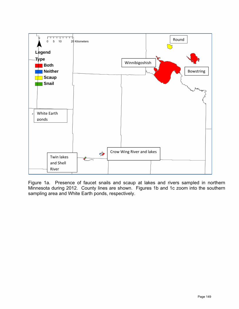
Figure 1a. Presence of faucet snails and scaup at lakes and rivers sampled in northern Minnesota during 2012. County lines are shown. Figures 1b and 1c zoom into the southern sampling area and White Earth ponds, respectively.

LegendType

BothNeitherScaupSnail

0 10 205 Kilometers¯Winnibigoshish 

Round 

Bowstring 

Crow Wing River and lakes Twin lakes and Shell River 

White Earth ponds 

Page 149

Figure 1b. Presence of faucet snails and scaup in lakes and rivers sampled in the southern portion of the sampling area in north-central Minnesota during 2012.

LegendType

BothNeitherScaupSnail

0 2 41 Kilometers¯

Second Crow Wing Lake 

First Crow Wing Lake 

Crow Wing River 

Upper Twin Lake 

Lower Twin Lake 

Shell River 

Page 150

Figure 1c. Infested ponds on the White Earth Nation of northern Minnesota that were sampled for faucet snails and their trematodes during 2012. Scaup were not observed at these ponds during our visits.

LegendType

BothNeitherScaupSnail

0 0.25 0.50.125 Kilometers¯

Page 151

Publications

2012 Biometrics Publications

Aarts, G, J. Fieberg, S. Brasseur, and J. Matthiopoulos. In press. Quantifying the effect of habitat availability on species distributions. Journal of Animal Ecology.

** DelGiudice, G. D., J. R. Fieberg, and B. A. Sampson. In press. A long-term assessment of the variability in winter use of dense conifer cover by female white-tailed deer. PLOS ONE.

** DelGiudice, G. D., B. A. Sampson, and J. H. Giudice. In press. A long-term assessment of the effect of winter severity on the food habits of white-tailed deer. Journal of Wildlife Management.

Fieberg, J. 2012. Estimating Population Abundance Using Sightability Models: R SightabilityModel Package. Journal of Statistical Software 51:1-20.

Fieberg, J. and L. Börger. 2012. Could you please phrase home range as a question? Journal of Mammalogy 93:890-902.

Fieberg, J. and M. Ditmer. 2012. Understanding the causes and consequences of animal

movement: a cautionary note on fitting and interpreting regression models with time-dependent covariates. Methods in Ecology and Evolution 3:983–991.

Fieberg, J., M. Alexander, S. Tse, and K. St. Clair. In press. Abundance estimation with sightability data: a Bayesian data augmentation approach. Methods in Ecology and Evolution.

Giudice, J. H., K. J. Haroldson, A. Harwood, and B. R. McMillan. 2013. Using time-of-detection to evaluate detectability assumptions in temporally replicated aural count indices: an example with Ring-necked pheasants. Journal of Field Ornithology.84(1):98-112.

** Hanson, M., B. R. Herwig, K. D. Zimmer, J. Fieberg, S. R. Vaughn, R. G. Wright, and, J. A. Younk. 2012. Comparing Effects of Lake- and Watershed-Scale Influences on Communities of Aquatic Invertebrates in Shallow Lakes. PlosONE 7(9): e44644. doi:10.1371/journal.pone.0044644.

Jenkins, K. J., Happe, P.J., Beirne, K.F, Hoffman, R.A., Griffin, P.C., Baccus, W. T., and J. Fieberg. 2012. Recent population trends in mountain goats in the Olympic mountains. Northwest Science 86:264-275.

** Rave, D. P., J. Fieberg, and K. Kotts. In press. Comparison of a fall biomass harvest to a

spring prescribed burn in restored native grass fields. Wildlife Society Bulletin.

** Rave, D. P., M. C. Zicus, J. R. Fieberg, L. Savoy, K. Regan. In Press. Trends in eggshell thickness and mercury in Common Goldeneye and Hooded Merganser eggs. Wildlife Society Bulletin.

St. Clair, K., E. Dunton, and J. Giudice. 2013. A comparison of models using removal efforts to estimate animal abundance. Journal of Applied Statistics 40(3):527-545.

“*” Indicates biological paper that are located with one of the specific research units.

Page 152

2012 Forest Wildlife Publications

DelGiudice, G. D., J. R. Fieberg, and B. A. Sampson. A long-term assessment of the variability in winter use of dense conifer cover by female white-tailed deer. PLoS ONE 8(6):e65368. Doi: 10.1371/journal.pone.0065368

DelGiudice, G. D., B. A. Sampson, and J. H. Giudice. 2013. A long-term assessment of the effect of winter severity on the food habits of white-tailed deer. Journal of Wildlife Management Accepted.

Iaizzo, P. A., T. G. Laske, H. J. Harlow, C. B. McClay, and D.L. Garshelis. 2012. Wound healing during hibernation by black bears (Ursus americanus) in the wild: elicitation of reduced scar formation. Integrative Zoology 7:77–89.

Kouffeld, M. J., M. A. Larson, and R. J. Gutiérrez. 2013. Selection of landscapes by male ruffed grouse during peak abundance. Journal of Wildlife Management 77(6):1192–1201.

Steinmetz, R., D. L. Garshelis, W. Chutipong, N. Seauturien. 2013. Feeding ecology and coexistence of two species of bears in seasonal tropical forests, Thailand. Journal of Mammalogy 94:1–18.

Page 153

2012 Wetland Wildlife Publications

Berdeen, J. B., and D. G. Krementz. In Press. Observations of unusual courtship behaviors by male American woodcock. Southeastern Naturalist.

Berkman, L, K., C. K. Nielsen, C. L. Roy, and E. J. Heist. In press. Population genetic structure among bobwhite in an agriculturally modified landscape. Journal of Wildlife Management.

Berkman, L, K., C. K. Nielsen, C. L. Roy, and E. J. Heist. 2013. Resistance is futile: Effects of landscape genetic features on gene flow of the northern bobwhite. Conservation Genetics 14(2):323-332.

Bischof, M., M.A. Hanson, M.R. Fulton, R.K. Kolka, S.D. Sebestyen, and M.G. Butler. 2013. Invertebrate community patterns in seasonal ponds in Minnesota, USA: response to hydrologic and environmental variability. Wetlands DOI.1007/s13157-012-0374-0.

*Denton, J. C., C. L. Roy, G. Soulliere, and B. Potter. 2012. Change in density of duck nest cavities at forests in the North Central United States. Journal of Fish and Wildlife Management 3(1):76-88.

Gorman, M.W., K.D. Zimmer, B.R. Herwig, M.A. Hanson, R.G. Wright, S.R. Vaughn, and J.A. Younk. Phosphorus, fish biomass, and watersheds as drivers of phytoplankton abundance in shallow lakes. Science of the Total Environment In Review.

*Hanson, M.A., B. R. Herwig, K. D. Zimmer, J. Fieberg, S. R. Vaughn, R. G. Wright, and J. A. Younk. 2012. Comparing effects of lake- and watershed-scale influences on communities of aquatic invertebrates in shallow lakes. PLoS ONE 7(9): e44644. DOI:10.1371/journal.pone.0044644.

*Heinrich, K., M. Whiles, and C. L. Roy. In press, available online. Cascading Ecological Responses to an In-stream Restoration Project in a Midwestern River. Restoration Ecology.

*Herwig, B. R., L. W. Schroeder, K. D. Zimmer, M. A. Hanson, D. F. Staples, R. G. Wright, and J. A. Younk. 2013. Fish influences on amphibian presence and abundance in prairie and parkland landscapes of Minnesota, U.S.A. Journal of Herpetology. In Press.

Kissoon, L., D.L. Jacob, M.A. Hanson, B.R. Herwig, S. Bowe, and M.L. Otte. 2013. Macrophytes in shallow lakes: relationships with water, sediment, and watershed characteristics. Aquatic Botany 109: 39-48.

Labarbenchon, C., R. Poulson, K. Shannon, J. Slagter, M. J. Slusher, B. R. Wilcox, J. Berdeen, G. A. Knutsen, C. J. Cardona, and D. E. Stallknecht. In Press. Isolation of influenza A viruses from wild ducks and feathers in Minnesota (2010-2011). Avian Diseases.

Nelson, M. D., and C. Roy. 2012. Estimating tree cavity distributions from historical FIA data. Pages 199-203 in Moving from Status to Trends: Forest Inventory and Analysis Symposium 2012. USDA, Forest Service, Northern Research Station General Technical Report, NRS-P-105. 478 pp.

Page 154

Rave, D. P., J. R. Fieberg, and K. Kotts. In Press. Comparison of an autumn biomass harvest with a spring prescribed burn in restored native grass fields. Wildlife Society Bulletin.

Rave, D. P., M. C. Zicus, J. R. Fieberg, L. Savoy, and K. Regan. In Press. Trends in eggshell thickness and mercury in common goldeneye and hooded merganser eggs. Wildlife Society Bulletin.

*Roy, C. L., C. M. Herwig, W. L. Hohman, R. T. Eberhardt. 2012. The Ring-necked Duck (Aythya collaris), The Birds of North America online. (A. Poole, ed.) Ithaca Cornell Lab of Ornithology.

Roy, C. L., C. M. Herwig, and P. Doherty. In press, available online. Mortality and refuge use of young ring-necked ducks before and during hunting season in north-central Minnesota. Journal of Wildlife Management

Schroeder S. A., D. C. Fulton, J. S. Lawrence, and S. D. Cordts. 2013. Identity and Specialization as a Waterfowl Hunter, Leisure Sciences: An Interdisciplinary Journal, 35:3, 218-234.

*Schroeder, S. A., D. C. Fulton, J. S. Lawrence, and S. D. Cordts. 2012. An Application and Extension of the Constraints-Effects-Mitigation Model to Minnesota Waterfowl Hunting. Human Dimensions of Wildlife: An International Journal. 17(3):174-192.

Schroeder, S. A., J.S. Lawrence, and S. D. Cordts. 2012. The 2011 Waterfowl Hunting Season in Minnesota: A Study of Hunters’ Opinions and Activities. University of Minnesota, Minnesota Cooperative Fish and Wildlife Research Unit, Dept. of Fisheries, Wildlife, and Conservation Biology. 120 pp.

Schroeder, S. A., J.S. Lawrence, and S. D. Cordts. 2012. The 2010 Waterfowl Hunting Season in Minnesota: A Study of Hunters’ Opinions and Activities. University of Minnesota, Minnesota Cooperative Fish and Wildlife Research Unit, Dept. of Fisheries, Wildlife, and Conservation Biology. 146 pp.

2012 Wildlife Health Publications

Dubey, J.P., M. Jenkins, O. Kwok, L Ferreira, S Choudhary, S Verma, I Villena, E. Butler, M. Carstensen. 2013. Congenital transmission of Neospora caninum in white tailed deer (Odocoileus virginianus). Vet Parasitol. 2013 Sep 23;196 (3-4):519-22. doi: 10.1016/j.vetpar.2013.03.004. Epub 2013 Mar 14

Dubey, J.P., P Dennis, S Verma, S Chaudhary, L Ferreira, S Oliveira, O Kwok, E Butler, M Carstensen, C Su. 2013. Epidemiology of toxoplasmosis in white tailed deer (Odocoileus virginianus): occurrence, congenital transmission, correlates of infection, isolation, and genetic characterization of Toxoplasma gondii. Veterinary Parasitology: In press

Dubey, J.P., S Choudhary; L Ferreira; O Kwok; E Butler; M Carstensen; L yu; C Su. 2013. Isolation and genetic characterization of Toxoplasma gondii from the Gray wolf (Canis lupus). Veterinary Parasitology: In press

Page 155