©2012 sutapat thiprungsri all rights reserved
TRANSCRIPT

©2012
Sutapat Thiprungsri
ALL RIGHTS RESERVED

CLUSTER ANALYSIS FOR ANOMALY DETECTION IN ACCOUNTING
By Sutapat Thiprungsri
A dissertation submitted to the
Graduate School – Newark
Rutgers, The State University of New Jersey
in partial fulfillment of requirements
for the degree of
Doctor of Philosophy
Graduate Program in Management
Written under the direction of
Professor Miklos A. Vasarhelyi
and approved by
_____________________________________________
Dr. Miklos A. Vasarhelyi
_____________________________________________
Dr.Alexander Kogan
_____________________________________________
Dr. Michael Alles
_____________________________________________
Dr.Jianming (Jimmy) Ye
Newark, New Jersey
January, 2011

II
ABSTRACT
Cluster Analysis for Anomaly Detection in Accounting
By Sutapat Thiprungsri
Dissertation Advisor: Dr. Miklos A. Vasarhelyi
Cluster Analysis is a useful technique for grouping data points such that points
within a single group or cluster are similar, while points in different groups are different.
The objective of this study is to examine the possibility of using clustering technology for
auditing. Automating fraud filtering can be of great value to continuous audits.
In the first paper, cluster analysis is used to group transactions from a transitory
account of a large international bank. Transactions are clustered based on the open
comments field. Major types of transactions are discovered. These results provide a new
knowledge about the nature of transactions that flow into transitory accounts.
In the second paper, cluster analysis is applied to wire payments within an
insurance company. Different anomaly detection techniques are examined. No wire
transfer is flagged by all techniques. These results do not necessarily indicate that there is
no real anomaly in the dataset, but that different assumptions, parameters or settings
should be examined.
In the third paper, cluster analysis is applied to group life insurance claims.
Individual claims which have significantly different characteristic from other members in
the same cluster as well as clusters which comprise of less than 2% of the population are
III
identified as possible anomalies. Moreover, rule-based detection techniques are used to
assist internal auditors in selecting claims for further investigation. Cluster analysis and
rule-based detection can be combined for the efficiency and effectiveness of the
implementation by internal auditors.
Cluster analysis has been used extensively in marketing as a way to understand
market segments and customer behavior. This study examines the application of cluster
analysis in the accounting domain. It can be used for exploratory data analysis (EDA),
but also can be used for anomaly detection (i.e. for audit purposes). The results provide a
guideline and evidence for the potential application of this technique in the field of audit.

IV
DEDICATION
To My Parents, Nakorn and Rampai Thiprungsri
For their love and support throughout my life.
This dissertation would not exist without countless sacrifices they have made for me.

V
ACKNOWLEDGEMENTS
I would like to express my gratitude to my advisor, Dr. Miklos A. Vasarhelyi, for
introducing me to the field of Continuous Auditing, and for his guidance, suggestions and
patience throughout my Ph.D. study at Rutgers. Finishing up this dissertation would not
have been possible without the tremendous support and encouragement from him.
I am very grateful to Dr. Alexander Kogan and Dr .Michael Alles for their advice,
suggestion, and comment. I am in debt to their guidance. I also appreciate all constructive
suggestions on this research work from my outside committee member, Dr. Jianming
(Jimmy) Ye.
I would like to express my special appreciation to my Rutgers colleagues,
Yongbum Kim, David Chan, Siripan Kuenkaikaew and Vasundhara Chakraborty for the
life-long friendships we have established. Their supports had made my stressful work
very enjoyable. Many thanks go to Danielle Lombardi, Rebecca Bloch, Victoria Chiu,
J.P. Krahel for their help during the writing process. I also thank for all the friends at
CARLAB: Ryan Teeter, Qi Liu, Hussein Issa, for all useful comment on my study and
my Ph.D. life.
I owe more than many thanks to my supportive friends who have always been
there for me: Atchara Santiwiriyapiboon, Araya Eakpisankit, Aroonsuda Vilalux,
Buntharika Suchodayon, Jirarat Pipatnarapong, Nathan Overmann, Piya-on Vinijsanun,
Porntip Cheumchaitrakul, Savitri Somboonchan, Dr.Tarinee Huang, Tip-upsorn
Kamlangarm and Wannapa Saikwan. I also thank for all my Thai friends at Rutgers:
P‘Note, P‘Tum, P‘Na,N‘Poom, N‘Pom, N‘Nan, P‘Oh, Tony, Chok, P‘A, Off, Joe for all
the fun time we had together.

VI
Special thanks go to my beloved grandma and my sister, Arpanchanok
Thiprungsri for their constant supports and loves.
Last but not least, my most special thanks are to Wantinee Viratyaporn for
patience, comfort, support, and encouragement that have given me the strength to get me
where I am.
THANK YOU!

VII
TABLE OF CONTENT
Chapter 1 Introduction ........................................................................... 1
1.1 Background ........................................................................................................... 1
1.2 Fraud ..................................................................................................................... 2
1.2.1 Type of Fraud ................................................................................................. 2
1.2.2 Error and Anomaly ........................................................................................ 6
1.3 Cluster Analysis .................................................................................................... 8
1.3.1 Basic concept ................................................................................................. 8
1.3.2 Steps in Cluster Analysis ............................................................................... 9
1.3.3 Clustering Evaluation ................................................................................... 11
1.4 References ........................................................................................................... 14
Chapter 2 Literature Review ............................................................... 16
2.1 Cluster Analysis .................................................................................................. 16
2.1.1 Methodological issues in Clustering ............................................................ 16
2.1.1.1 Number of Clusters ............................................................................... 16
2.1.1.2 Clustering Algorithm ............................................................................ 17
2.1.1.3 Characteristics of the data set and attributes ......................................... 18
2.1.1.4 Noise and outlier ................................................................................... 18
2.1.1.5 Number of data objects ......................................................................... 19
2.1.1.6 Number of attributes ............................................................................. 19
2.1.1.7 Algorithm consideration ....................................................................... 20
2.1.2 Anomaly Detection ...................................................................................... 20
2.1.3 Application of Clustering ............................................................................. 21
2.2 Fraud prediction using data mining techniques .................................................. 23
2.2.1 Management Fraud Prediction ..................................................................... 23
2.2.2 Other Types of Fraud Prediction .................................................................. 26
2.3 Continuous Auditing ........................................................................................... 27
2.4 Conclusion and Research Question .................................................................... 36
2.5 References ........................................................................................................... 38
Chapter 3 : Cluster Analysis for Exploratory Data Analysis in Auditing
................................................................................................................ 46
3.1 Introduction ......................................................................................................... 46
3.2 Exploratory Data Analysis ............................................................................. 46
3.3 Cluster Analysis for Data Exploratory Purposes ............................................ 47
3.4 The Audit Problem ......................................................................................... 51

VIII
3.5 Data ................................................................................................................ 52
3.5.1 General Information ..................................................................................... 52
3.5.2 Attributes ...................................................................................................... 53
3.5.3 Transitory Account for Debit Reclassification of Checking Account ......... 56
3.6 Parsing Procedure ........................................................................................... 57
3.6.1 Banks processing system ............................................................................. 59
3.6.1.1 System Identification ............................................................................ 59
3.7 Clustering Procedure ...................................................................................... 61
3.8 Results ............................................................................................................ 62
3.9 Conclusions .................................................................................................... 75
3.10 References ......................................................................................................... 77
Chapter 4 Cluster Analysis for Anomaly Detection ............................ 79
4.1 Introduction ......................................................................................................... 79
4.2 Anomaly Detection ............................................................................................. 80
4.3 Cluster Analysis for Anomaly Detection ............................................................ 82
4.4 The Audit Problem .............................................................................................. 83
4.5 Data ..................................................................................................................... 85
4.5.1 General Information ..................................................................................... 85
4.5.2 Description and Distribution of Attributes .................................................. 87
4.6 Methodology ....................................................................................................... 97
4.6.1 Clustering Procedure .................................................................................... 97
4.6.2 Anomaly Detection ...................................................................................... 98
4.7 Results ............................................................................................................... 103
4.8 Conclusions ....................................................................................................... 113
4.9 References ......................................................................................................... 116
Chapter 5 Cluster Analysis and Rule Based Anomaly Detection ..... 119
5.1 Introduction ....................................................................................................... 119
5.2 Anomaly and Anomaly Detection .................................................................... 120
5.3 Cluster Analysis for Anomaly Detection .......................................................... 121
5.4 The Audit Problem ............................................................................................ 123
5.5 Data ................................................................................................................... 126
5.5.1 General Information ................................................................................... 126
5.5.2 Attributes .................................................................................................... 128
5.6 Methodology ..................................................................................................... 132
5.6.1 Clustering Procedure .................................................................................. 132
5.6.2 Anomaly Detection .................................................................................... 134
5.6.3 Rule-Based Anomaly Detection................................................................. 135
5.7 Results ............................................................................................................... 139
5.8 Conclusions ....................................................................................................... 153
5.9 References ......................................................................................................... 155

IX
Chapter 6 Summary, conclusions, paths for further research,
limitations ............................................................................................ 158
6.1 Summary of the results and implications .......................................................... 158
6.1.1 Cluster Analysis ......................................................................................... 158
6.1.2 Anomaly detection using cluster analysis .................................................. 158
6.2 Primary Contribution ........................................................................................ 159
6.3 Limitations ........................................................................................................ 161
6.4 Future Research ................................................................................................ 162
6.5 References ......................................................................................................... 165

X
LISTS OF TABLES
Table 2.1 Revised Deadlines for Filing Periodic Reports................................................. 31
Table 3.1 Detail Information of the Transitory Accounts ................................................. 52
Table 3.2 Frequency Distribution of Transactions ........................................................... 53
Table 3.3 Attribute Information ........................................................................................ 54
Table 3.4 Distribution of four remaining attributes .......................................................... 57
Table 3.5 Content of the Comment Fields in Each Cluster .............................................. 66
Table 3.6 Number of Transactions by Clusters ................................................................ 69
Table 3.7 Distribution of the Transaction into Clusters by Top 20 Branches .................. 70
Table 3.8 Percentage of Transactions Grouped into Clusters for the Top 20 Branches ... 72
Table 4.1 Attribute Information ........................................................................................ 87
Table 4.2 Number of Wire Transfer by WireType ........................................................... 88
Table 4.3 Number of Wire Transfers by Payee ................................................................ 89
Table 4.4 Number of Wire Transfer by Initiator............................................................... 90
Table 4.5 Number of Wire Transfer by Approver ............................................................ 91
Table 4.6 Number of Wire Transfer by Trantype ............................................................. 92
Table 4.7 Number of Wire Transfers by COSTCTR ........................................................ 95
Table 4.8 Number of Wire Transfer by AutoIni ............................................................... 96
Table 4.9 Number of Wire Transfer by AutoApp............................................................. 97
Table 4.10 Number of Wire Transfer by Number of Approvers ...................................... 97
Table 4.11 Probability of an Observation Belonging to Each Cluster, Calculated and
Presented by WEKA Filtering Procedure, ―Clustermembership‖ .................................. 102
Table 4.12 Number of Wire Transfer in Each Cluster by DBSCAN.............................. 104
Table 4.13 Number of Wire Transfer in Each Cluster by DBSCAN 2........................... 105
Table 4.14 Distribution of Wire Transfer by Clusters .................................................... 107
Table 4.15 Average and Stand deviation of the Monetary amount of Wire Transfer .... 108
Table 4.16 Distribution of Possible Anomalies as Identified by Distance-Based Outliers
......................................................................................................................................... 109
Table 4.17 Distribution of Possible Anomalies by Cluster Statistics ............................. 110
Table 4.18 Comparison of the Number of Anomalies Identified ................................... 111
Table 4.19 Number of Wire Transfer flagged as possible Anomalies ............................ 112
Table 4.20 Outliers Identified by Each Technique ......................................................... 113
Table 5.1 Example of Tests Performed by Internal Auditors ......................................... 125
Table 5.2 Distribution of Claim by Quarter .................................................................... 128
Table 5.3 List of Remaining Attributes .......................................................................... 131
Table 5.4 Result of Cluster Analysis using Two Attributes from WEKA (Enhanced) .. 140
Table 5.5 Result of Cluster Analysis using Four Attribute from WEKA (Enhanced) ... 145
Table 5.6 Summary of the Results from Cluster Analysis.............................................. 148
Table 5.7 Number of Claims fails the test (rule-based filtering) .................................... 150
Table 5.8 Suspicious Score Distribution by Cluster: Two Attributes ............................. 151
Table 5.9 Suspicious Score Distribution by Cluster: Four Attributes ............................ 152
XI
LISTS OF FIGURES Figure 1.1 Fraud Triangle. .................................................................................................. 4
Figure 1.2 An Outline of Cluster Analysis Procedure. (Kachigan, 1991) ........................ 10
Figure 2.1 Automatic Fraud Detection ............................................................................. 26
Figure 3.1 Data Structure .................................................................................................. 58
Figure 3.2 Parsing Procedure ............................................................................................ 59
Figure 3.3 Example of System Identification String in the Comment .............................. 60
Figure 3.4 Comment Coding Illustration .......................................................................... 61
Figure 3.5: Clustering Result from using the four remaining attributes ........................... 64
Figure 3.6 Visualization of Clustering Results (LANVFCDFUNC and LANVFCDORLC) 65
Figure 3.7 Assigned clusters and the value in part1 and part3 of the comment field. ...... 67
Figure 3.8 Assigned Clusters and the value of part3 and part4 of the comment field(2). 68
Figure 3.9 Distribution of Transactions into clusters by top 20 branches ........................ 73
Figure 4.1 Wire Transfer Process ..................................................................................... 84
Figure 4.2 Illustration of Core Point, Border Point and Noise (Tan et al, 2011) ............ 100
Figure 4.3 DBSC AN Algorithm (Tan et al, 2011)......................................................... 101
Figure 5.1Group Life Claim Process .............................................................................. 127
Figure 5.2 Summary of Attribute Information ................................................................ 130
Figure 5.3Number of Clusters and Resulting Sum of Squared Error: 2 Attributes ........ 139
Figure 5.4 Visualization of the Cluster Assignment for 2 attributes clustering;
N_Percentage and N_AverageDTH_PMT. .................................................................... 141
Figure 5.5 Visualization of the Clustering Result (Two Attributes) with Cluster Marked
......................................................................................................................................... 142
Figure 5.6Number of Clusters and Resulting Sum of Squared Errors: 4 Attributes....... 144
Figure 5.7 Visualization of the Cluster Assignment for 4 attributes clustering:
N_Percentage, N_AverageDTH_PMT, N_AverageCLM_PMT, N_DTH_CLM. ......... 147
Figure 5.8 Visualization of the Clustering Result (Four Attributes) with Marks ........... 147

1
Chapter 1 Introduction
1.1 Background
Clustering is an unsupervised learning algorithm, which means that there
is no label (class) for the data (Kachigan, 1991). Clustering is a useful technique for
grouping data points such that points within a single group or cluster are similar, while
points in different groups are different. In general, the greater similarity within a group
and the greater differences between groups mean the better clustering results. There is no
absolute best clustering technique (Kachigan, 1991). User‘s needs are also an important
factor in evaluating the clustering technique. The best techniques are those that could
provide the results which are useful for the user‘s purposes. Moreover, cluster evaluation
is quite subjective because the results could be interpreted in different ways. Several
factors should be considered when deciding upon which type of clustering technique to
use. These factors are, for example, type of clustering techniques, type of cluster,
characteristic of clusters, characteristics of the dataset and attributes, noise and outlier,
number of data objects, number of attributes, cluster description, and algorithm
considerations (Tan et al, 2006).
Clustering as an unsupervised learning algorithm is a good candidate as a fraud
and anomaly detection technique. It is difficult to identify suspicious transactions.
Clustering can be used to group transactions so that different treatment and strategies can
be applied to each different cluster. The purpose of this study is to examine the possibility
of using clustering techniques for auditing. Cluster Analysis will be applied to three
datasets. The first dataset encompasses transitory accounts from a bank. The second and

2
third datasets, a wire transfer and a group life insurance claim file, are from an insurance
company.
In the first paper, cluster analysis has been used to group transactions from a
transitory account of a bank. Transactions are grouped or clustered based on the open
comment field. Seven clusters representing seven types of transactions are formed. In the
second paper, cluster analysis has been applied to wire transfers within an insurance
company. Four detection techniques are used to identify possible anomalies. In the third
paper, cluster based outliers have been examined. Group life insurance claims have been
grouped. Those clusters with small populations have been flagged for further
investigation.
This dissertation is organized into six parts. The next section of the introduction
gives a summary of fraud detection in accounting and the basic idea of cluster analysis.
Then the literature review sections outline some methodological issues found in
clustering analysis, the fraud detection using data mining techniques, continuous
auditing, and research questions. The later parts of this dissertation comprise of three
research studies done on three different dataset to demonstrate the possible usage of
cluster analysis. The final chapter outlines the summary of findings, discusses the
shortcomings of this approach, suggests continuation and further research in this area and
draws conclusions for this dissertation.
1.2 Fraud
1.2.1 Type of Fraud
There are many definitions of fraud. Webster‘s New World Dictionary (1964)
states:

3
Fraud is a generic term and embraces all the
multifarious means which human ingenuity can
devise, which are resorted to be one individual, to
get an advantage over another by false
representations. No definite and invariable rule can
be laid down as a general proposition in defining
fraud, as it includes surprise, trickery, cunning and
unfair ways by which another is cheated. The only
boundaries defining it are those which limit human
knavery.
Fraud always involves deception, confidence and trickery. Albrecht et al (2006)
define that the most common way to classify fraud is to divide frauds into 1) those
committed against an organization and 2) those committed on behalf of an organization.
For fraud committed against an organization, or occupational fraud, the
employee‘s organization is the victim. This type of fraud can be anything from security
break abuses to serious high-tech schemes. The Association of Certified Fraud Examiners
defines this type of fraud as, ―The use of one‘s occupation for personal enrichment
through the deliberate misuse or misapplication of the employing organization‘s
resources or assets‖ (Association of Certified Fraud Examiners, 1996).
The most common fraud committed on behalf of organization is fraudulent
financial reporting. It is usually committed through actions of top management. These
frauds are committed to make the companies‘ financial statements look better for various
reasons such as to increase stock‘s price, to ensure a larger year-end bonus for executives,
to get better financing terms and etc. Management fraud is distinguished from other types
of fraud both by the nature of the perpetrators and by the method of deception (Albrecht
et al, 2006).

4
Based on a series on interviews, Cressey (1953) introduces the fraud risk factor
theory, called ―fraud triangle‖. Cressey concludes that frauds generally share three
common traits: pressure, opportunity, and rationalization. These three key traits can be
used to identify factors that are always present in any given fraud. Whether the fraud is
an employee fraud or management fraud, these three elements will always be present.
Figure 1.1 Fraud Triangle.
Albrecht et al (2006) explains the fraud triangle theory which will be summarized
in this section. The first element is pressure. It is increased when financial stability or
profitability is threatened by economic, industry, the firms operating conditions and / or
the third parties. Management or other employees may have incentive or be under
pressure, which provides a motivation to commit fraud. The second element is a
perceived opportunity to commit fraud, to conceal it, or to avoid being punished.
Opportunity is increased by factors such as industry characteristics, ineffective
monitoring of management, insufficiency and or inefficiency of internal controls.
Circumstances can exist, for example, the absence of controls, ineffectiveness of the
existing controls and ability of management to override the controls, which provide the
opportunities for fraud to occur. Rationalization is the attitudes or rationale by board
Pressure
Rationalization
Opportunity

5
members, management and/or employee that allow them to committee fraud. Fraudsters
need a way to rationalize their actions as acceptable. They tend to believe that their
actions are for a good cause; hence, they are acceptable. Some individuals possess an
attitude, set of ethical values, or character, that motivates/allows/facilitates/justifies them
to knowingly and intentionally commit fraud.
The fraud triangle theory described above is widely accepted and adopted by the
American Institute of CPA‘s (AICPA) in the Statement on Auditing Standards (SAS)
No.99, ―Consideration of Fraud in a Financial Statement Audit‖. SAS No. 99 states in
paragraph .31 as following
Because fraud is usually concealed, material misstatements
due to fraud are difficult to detect. Nevertheless, the auditor
may identify events or conditions that indicate
incentive/pressure to perpetrate fraud, opportunities to carry
out fraud, or attitudes/rationalizations to justify a fraudulent
action. Such events or conditions are referred to as “fraud risk
factors”. Fraud risk factors do not necessarily indicate the
existence of fraud; however, they often are present in
circumstances where fraud exists.
SAS No. 99 also gives examples of fraud risk factors to guide practitioners. Not
all of examples are relevant in all circumstances. Some may be at greater or lesser
significances in entities of different size, with different organizational characteristics or
circumstances.
Despite the popularity of the fraud triangle theory, little is known about the
dynamic relationship among each aspect of the fraud triangle. Loebbecke et al (1989)
find that when all three components are present concurrently, it is likely that management
fraud exists. If only one component is present, there is lower likelihood of fraud. These
findings do not help much in understanding the dynamic of the relationships.

6
Albrecht et al (2006) believes that the three elements are interactive. For example,
the greater the perceived opportunity or the more intense the pressure, the less
rationalization it takes to motivate someone to commit fraud. On the other hand, the more
dishonest a perpetrator is, the less opportunity and/or pressure it takes to motivate fraud.
There is little research evidence to back up the claim.
How do all aspects affect each other? A better understanding of the relationship
among of three aspects, opportunity/condition, pressure/incentive, and
rationalization/attitude, is needed.
The fraud triangle theory is well accepted and adopted in many disciplines.
Albrecht et al (2004) combine the fraud triangle theory with agency theory from
economic literature and stewardship theory from psychology literature. This is later
known as ―the Broken Trust‖ theory (named by Choo et al, 2007). The theory describes
corporate management fraud using corporate executive behavior, compensation and
corporate structures. . Choo et al (2007) extend the broken trust theory with the
―American Dream‖ theory from sociology literature. Three high profile management
fraud events in the United States (Enron, WorldCom, and Cendant) are used as anecdotal
evidences to support the theory.
1.2.2 Error and Anomaly
According to American Heritage College dictionary (2004),
Error n. 1.An act, assertion, or belief that unintentionally deviates from
what is correct, right or true. 2. The conditional of having incorrect or
false knowledge. 3. The act of an instance of deviating from an accepted
code of behavior. 4. A mistake.
Anomaly n. 1.Deviation or departure from the usual or common order, form or rule. 2. One that is peculiar, irregular, abnormal, or difficult to
classify.

7
Based on fraud triangle theory, the distinguishing factor between fraud and error
is the intention. Error is the deviation from the usual behavior. It does not have the
element of intention to deviate. Therefore, a deviation or anomaly could be a result of an
error or an intention to commit fraud.
Anomalies are generated from many reasons; for example, data may come from
different classes, natural variation in the data and data measurement or collection error
(Tan et al, 2006). The first reason, data coming from different classes, is probably the
most important type of the anomaly. It is the focal point of anomaly detection in data
mining. For examples, fraudulent transactions belong to a different class from normal
transactions, i.e. fraudulent transactions are initiated by hackers. They usually are
generated from different source, i.e. fraudulent customers. The data can also have natural
variations. In other words, most data will be near the center (or the average); while the
further away from the center, the lesser number of observations will be present. Errors
and anomalies can also come from errors in measurement. The data may be incorrectly
recorded because the equipment malfunctions and/or human error. For example, a weight
scale always reads out 1 pound less than the real weight, a researcher reads out the
temperature a few degrees higher than the real temperature because he/she misread the
scale and etc. This type of data will provide no useful information. It should be cleaned in
the preprocessing step (or data cleaning step).
8
1.3 Cluster Analysis
1.3.1 Basic concept
Cluster analysis groups the objects or databases only on information found in the
data that describes the objects and their relationships (Tan et al, 2006). Each object is
very close or similar to other objects in the same group (the closer, the better), but
different from objects in the other groups, (the greater differences, the better). It begins
with a single group, follows by attempt to form subgroups which are different on selected
variables. To determine what variables to be used is not an easy task. Even if there is a
clear answer to the preceding question, the following question will be how it should be
measured. Clustering can be used for data exploration and also to understand the structure
of data. Without the prior knowledge about the data, cluster analysis can be used to
search for common characteristics of sub groups in the data.
The two major steps in cluster analysis are 1) selecting measures of similarities or
dissimilarities, and 2) selecting the procedures for cluster formations (Kachigan, 1991).
There are several options or techniques available for these steps, making cluster analysis
as much as art as a science. It is not simple to choose and interpret the results. Moreover,
while running simulations on cluster analysis, Milligan et al (1985) find that that
performance of some cluster analysis procedures can also be data dependent. Generally
the purpose of performing cluster analysis is to ask the question whether a given group
can be partitioned into subgroups which have different characteristics. The subgroups or
clusters can be named or defined using the common characteristics of the group members
such as group mean for the numeric values as the representative of the observations in the
group, or using the most common or majority values in the subgroups. For example, in

9
marketing, customer segments (or clusters) are defined using demographic information
(Erdogan et al, 2006). Different marketing strategies would be developed and applied to
each customer segments or clusters.
Cluster analysis techniques can be categorized as following (Tan et al, 2006)
1) Hierarchical vs. Partitional (nest or un-nested): Hierarchical techniques
produce a nested sequence or partitions with a single all inclusive cluster at
the top and single clusters of individual points at the bottom. It is organized as
a tree. Partitional techniques create one-level non –overlapping or un-nested
partitioning of data. Each data object is in exactly one subset or subgroup.
2) Exclusive vs. Overlapping vs. Fuzzy: All exclusive clustering is when each
object is assigned to a single cluster. If an object can simultaneously be
assigned to more than one group, it is overlapping or non-exclusive clustering.
It is used when an object can equally be assigned to any of the groups. Fuzzy
clustering assigns membership weight between 0(absolutely doesn‘t belong)
and 1(absolutely belongs) for every object to every cluster.
3) Complete vs. Partial: A complete clustering assigns every object to a cluster;
while a partial clustering does not (Tan et al, 2006). The objects which are not
assigned to any clusters can possible represent noises or outliers.
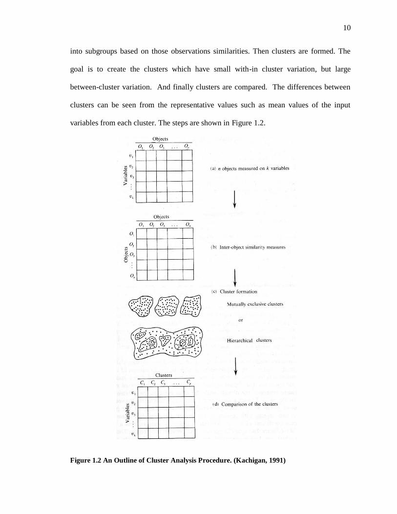
1.3.2 Steps in Cluster Analysis
Cluster analysis is generally started with observation measurements. Observations
are measured on K variables. Observation similarity distances between each pair of
observations are measured. Some algorithm will be employed to group the observations
10
into subgroups based on those observations similarities. Then clusters are formed. The
goal is to create the clusters which have small with-in cluster variation, but large
between-cluster variation. And finally clusters are compared. The differences between
clusters can be seen from the representative values such as mean values of the input
variables from each cluster. The steps are shown in Figure 1.2.
Figure 1.2 An Outline of Cluster Analysis Procedure. (Kachigan, 1991)

11
Unlike other data analysis methods, cluster analysis has been developed
throughout the years in many disciplines; for examples, management sciences, marketing
management, biomedical sciences, and computer sciences. There is no single dominant
discipline. The purposes or the benefit of the cluster analysis depend on the type of the
applications. For example, in marketing, cluster analysis may be used mainly to learn
about market segments and to seek a better understanding of buyer behaviors by
identifying homogeneous groups of buyers (Punj et al, 1983), in medical science, patients
can be clustered based on symptoms to understand the causes and to help finding
alternative therapies (McLachlan, 1992). In psychology, Clutter (2006) uses cluster
analysis to understand the relationship between health risk and college students‘ health
behaviors.
1.3.3 Clustering Evaluation
Selecting techniques or parameters for cluster analysis is not an easy task.
Moreover, Morrison (1967) states that some of the methods that give statistically
meaningful results will not necessarily give managerially meaningful results. Clustering
is an unsupervised learning algorithm. There is no label (class) for the data. Its goal is
trying to determine to which group each data in unlabeled data set belongs. There is no
absolute best criterion to decide which clustering algorithms give the best clusters. It
must depend on user‘s need. The best clustering techniques are those that can provide the
results which are useful for the user‘s purposes. Cluster evaluation and interpretation are
quite subjective. Though the clustering results can also be interpreted in different ways,
the meaning of each cluster should be intuitive.

12
Each clustering technique defines its own type of cluster and requires different
type of evaluations (Tan et al, 2006). Most clustering techniques have focused on
numerical data. One of the popular cluster analysis techniques is K-means clustering.
With numeric values, the definition of clustering does generally suggest the notion of
similarity, dissimilarity or distance between data objects. Its goal is to minimize the
distance between data objects in the same clusters and maximize the distance between
data objects from different clusters. The K-means clustering can be evaluated using Sum
of Squares for Errors (SSE). However, there are more difficulties in clustering with
categorical data because there is neither real nor natural distance between categorical
data. When there is no obvious distance, it can be ―defined‖. However, it is not always
easy especially in multidimensional spaces.
In general, a good cluster algorithm is the one that produces clusters which the
intra cluster similarity is high, while inter cluster similarity is low. However, the measure
of the similarity is also a challenge. There are several techniques and measurement for
similarity to choose from. The type of similarity measure should fit the type of data (Tan,
et al, 2006). Some measurement may be good for one dataset but not for the other. A
cluster algorithm can also be applied to a data set with a natural cluster and produce poor
quality clusters simply because a wrong similarity measures have been chosen.
When good quality clusters are defined, to get a general idea of how the clusters
are different, the means and the variances of each cluster should be compared (Kachigan,
1991). Examining the representative values of the clusters will help in understanding the
distinguishing values and characteristics of each cluster.

13
All clusters should have enough observations to be meaningful for the
interpretation. Having too small or too big clusters can mean that that number of cluster
selected is not appropriate for the dataset (Garson, 2009). Not only a small cluster can
mean that the number of clusters selected is too large, but the small cluster can be an
outlier or anomaly. On the other hand, having a cluster which is too large dominating the
results can mean that the number of cluster selected is too small.

14
1.4 References
Albrecht, W. S., C. C. Albrecht and C. O. Albrecht. 2006. Fraud Examination 2nd
Edition. Thomson South Western. U.S.A.
Albrecht, W. S., C. C. Albrecht. 2004. Fraud and Corporate Executives: Agency,
Stewardship and Broken Trust. Journal of Forensic Accounting: 109-130.
American Heritage College Dictionary. 2004. U.S.A. p.58, p.475
Association of Certified Fraud Examiners. 1996. The Report to the Nation on Occupation
Fraud and Abuse. ACFE. p.4
Choo, F. and K. Tan. 2007. An American Dream Theory of Corporate Executive Fraud.
Accounting Forum 31: 203-215
Clutter, J. E. 2006. Describing College Students' Health Behaviors: A Cluster-Analytical
Approach. The Ohio State University. 98 pages; AAT 3238221
Cressey, D. 1953. Other People‘s Money: A Study in the Social Psychology of
Embezzlement, Free Press.
Erdogan, B. Z., S. Deshpande and S. Tagg. 2007. Clustering Medical Journal Readership
Among GPs: Implications for Media Planning. Journal of Medical Marketing 7(2): 162-
168.
Garson, G. D. 2009. http://faculty.chass.ncsu.edu/garson/PA765/cluster.htm, Accessed on
12/3/09.
Kachigan, S. K. 1991. Multivariate Statistical Analysis: a Conceptual Introduction,
Radius Press. New York, NY, USA.

15
Loebbecke, J.K., M.M. Eining, and J.J. Willingham. 1989. Auditors‘ Experience with
Material Irregularities: Frequency, Nature, and Detectability, Auditing: A Journal of
Practice & Theory 9 (1): 1-28.
McLachlan, G.J. 1992. Cluster Analysis and Related Techniques in Medical Research.
Stat Methods Med Res (March 1992) 1: 27-48.
Milligan, G.W. and M. C. Cooper. 1985. An Examination of Procedures for Determining
the Number of Clusters in a Data Set. Psychometrika 50(2): 159-79.
Morrison, D. G. 1967. Measurement Problems in Cluster Analysis. Management Science
13(12) Series B Managerial (Aug, 1967): B775-B780.
Punj, G. and D.W. Stewart. 1983. Cluster Analysis in Marketing Research: Review and
Suggestion for Application. Journal of Marketing Research Vol. XX (May 1983): 134-
148.
Tan, P-N, M. Steinbach and V. Kumar. 2006. Introduction to Data Mining. Pearson
Education, Inc.
Webster‘s New World Dictionary, College Edition. 1964. Cleveland and New York:
World, p. 380.

16
Chapter 2 Literature Review
2.1 Cluster Analysis
2.1.1 Methodological issues in Clustering
Selecting what clustering technique to be used and/or what parameter to set are
not trivial tasks. Several factors should be considered when performing cluster analysis.
There is no formula for determining the proper technique (Tan et al, 2006). Moreover,
sometimes the intended application can influence the type of clustering to choose. Some
factors worth considering are as follows:
2.1.1.1 Number of Clusters
Choosing the number of clusters is one of the most important decisions in
performing cluster analysis. Clustering always finds subgroups or clusters; however,
determining which groups are meaningful is the significant task. Several techniques can
be used for estimating the number of clusters. Some of which are very straightforward,
while others are quite subjective. Alpaydin (2004) outlines some techniques for selecting
the number of clusters as follows:
– The data can be plotted into two –three dimensional space and examined,
– Reconstruction error or log likelihood as a function of numbers of clusters can
be plotted,
– Validation of the groups can be done manually by checking for the
meaningfulness of the groups, in some simple dataset,
– Looking at differences between levels in the tree, a good split can be
identified in hierarchical clustering.

17
Milligan et al (1985) examine procedures for determining the number of clusters
in a dataset by running a Monte Carlo simulation on artificial datasets. Based on the
assumption that the true numbers of clusters in the datasets are known, four hierarchical
clustering methods and many stopping rules are examined using simulation. Some
procedures work well, while others do not. The results from Milligan‘s study provide
clear evidence that the performance of some cluster analyses may be data dependent.
Therefore, researchers may have to try alternative techniques and specification to see
which one will work best. Research is needed to guide on this process.
2.1.1.2 Clustering Algorithm
There are many algorithms available in the literature such as K-mean clustering,
fuzzy C-mean clustering and hierarchical clustering. These algorithms are mainly for
quantitative values. It has been shown that traditional algorithms are not appropriate for
categorical data and many other algorithms have been introduced for categorical values.
Ohn Mar Sun et al (2004) propose an alternative to k-mean clustering for categorical
data; which is using the notion of ―cluster center‖ to formulate the cluster problems for
categorical data as a partitioning problem. Guta et al (1999) propose a novel concept of
links (called ROCK) to measure the similarity/proximity between a pair of data points for
Boolean and categorical attributes. The concept is naturally extended to non-metric
similarity measures that are relevant in situations where a domain expert/similarity table
is the only source of knowledge.
Ganti et al (1999) introduce ―CACTUS‖; which is a formalization of a cluster for
categorical attributes by generalizing a definition of a cluster for numerical attributes.
The technique requires two scans of the dataset and is a fast summarization based
18
algorithm. Zengyou et al (2002) suggest another clustering method for categorical
attributes called ―SQUEEZER‖. The algorithm reads each tuple or record t in sequence
then either assigning t to an existing cluster (initially none), or creating t as a new cluster,
which is determined by the similarities between t and clusters. It is extremely suitable for
data stream.
2.1.1.3 Characteristics of the data set and attributes
There are various types of data, such as structured, graphed or ordered. Attributes
are also 1) quantitative or nominal and 2) binary, discrete or continuous. The type of data
set and attributes can dictate the type of algorithm to use. Similarity/Dissimilarity
measures should be appropriate for the type of data being considered (Punj et al, 1983).
For example, K-means algorithm can only be used on data for which an appropriate
proximity measure is available and that allows meaningful computation of cluster
centroids (Tan et al, 2006). For other algorithms, such as many agglomerative
hierarchical approaches, the nature of dataset and attributes is less important. Some
algorithms may not be suitable for some data type. Morrison (1967) shows how the scale
used in measuring input variables will affect the results. Sometimes, data must be
processed (i.e. to discretized or binarized) so that the similarity matrix can be calculated.
The problem will become more complicated when the dataset have a mixture of different
attribute types.
2.1.1.4 Noise and outlier
Outliers or noise can affect the performance of the clustering algorithms. In some
techniques such as single linkage, outliers can result in joining clusters which should not
be joined. Therefore, data might have to be preprocessed to remove outliers before

19
performing cluster analysis. Some algorithms, such as DBSCAN, Density-Based Spatial
Clustering of Applications with Noise, can detect or identify objects as noise and move
them from clustering procedure (Tan et al, 2006).
2.1.1.5 Number of data objects
Clustering can be affected by the number of data objects. Cluster analysis requires
powerful computing because computations can be extensive; especially as the number of
objects increases. To include or exclude a certain observation can have an effect on the
clusters‘ forms. Ideally, all observations, assuming no outliers, should be included in the
clustering procedure so that the cluster results are a true representation of the dataset.
2.1.1.6 Number of attributes
Algorithms that work well in low dimensions may not work well in high dimensions. In
other words, algorithms that work well when there are fewer attributes, such as 1-20
attributes, may not give a great result when there are a larger number of attributes such as
a hundred different attributes. The relationship among attributes can also create
difficulties in cluster analysis. Moreover, using a small number of attributes may be
easier for clustering procedures; however, the results may not be useful. On the other
hand, using many attributes at the same time may complicate the procedures. For
example, Green et al (1967) discuss that while using only one attribute (such as income
levels) is not enough; however, using 10-15 attributes (such as education, ethnic
composition, physical distribution, etc.) for clustering may actually be very difficult to
process. The algorithm will produce clusters; but, the resulting clusters may be useless in
representing real data structures.

20
2.1.1.7 Algorithm consideration
Each clustering algorithm is different. The theories and idea behind each
procedure make one algorithm good to one dataset/or purpose, but not the other. Several
decisions must be made. For example, simple K-mean algorithm requires the
specification of the number of clusters, while expectation maximization algorithm does
not have this requirement. There are also techniques to define the values of various
parameters, such as number of clusters. The theoretical support of the algorithm that
performs the cluster analysis is important. Otherwise, the clustering results, even though
the algorithm can produce an optimal cluster, will not be meaningful. Moreover,
clustering algorithms usually have one or more parameters which should be set or
selected by users; for example, choosing the number of clusters in simple K-mean
clustering. Several trial and error attempts should be conducted in order to find suitable
values for those parameters. This process of selecting parameter can become even more
complicated because a small change in a parameter value can significantly change the
clustering results. (Tan at el, 2006)
2.1.2 Anomaly Detection
Anomaly detection is the procedure of identifying observations whose
characteristics are significantly different from the rest of the data or the population (Tan
et al, 2006). These observations are called outliers or anomalies because they have
attribute values that deviate significantly from the expected or typical attribute values.
Applications of anomaly detection include fraud detection, credit card fraud detection,
network intrusion, etc. Regardless of the domain, anomaly detection procedures generally
involve three basic steps: 1) identify normality or what is normal by calculating some
―signature‖ of the data, 2) determine some metric to calculate an observation‘s degree of

21
deviation from the signature or how much it is different or deviate from normal data, and
3) set some criteria/threshold which, if exceeded by an observation‘s metric measurement
means the observation is anomalous (Davidson, 2002). A variety of methods or an option
for each step has been used in various applications in many fields.
2.1.3 Application of Clustering
Clustering is a widely used technique in the area of marketing research, especially
market segmentation, market structure analysis, and study of customer behavior. In the
review of cluster analysis in marketing research, Punj et al (1983) have listed many
marketing studies prior to 1983; which applied cluster analysis as their methodologies for
understanding the market segments and buyer behaviors. Market segmentation using
cluster analysis have been examined in many different industries, for instance, finance
and banking (Anderson et al, 1976, Calantone et al, 1978), automobile (Kiel et al, 1981),
education (Moriarty et al, 1978), consumer product (Sexton, 1974, Schaninger et al,
1980) and high technology (Green et al, 1968).
Another examination of the usefulness of cluster analysis is for test market
selection. Green et al (1967) use cluster analysis for test marketing to ensure
projectability (or predictability) of the test marketing results. The responses or the results
of the test program in the area selected for marketing tests provide a reasonable and
accurate indication of the results or responses from customers in the larger geographic
area. Therefore, cluster analysis is used for choosing an appropriate set of test cities or
areas.
Cluster analysis can be used to extract information about markets and customers.
Erdogan et al (2006) use cluster analysis to understand the readership patterns of the

22
medical journal. Shih et al (2003) study the customer relationship management using k-
means clustering methodology to group customers with similar lifetime value or loyalty
in hardware retailer business. The results can help companies to gain a better
understanding of clusters so they can allocate the appropriate resources to ensure the
effectiveness of marketing investment.
Cluster analysis can also be used to extract information from a single group or
segment; such as to define characteristics or behaviors or members in sub-groups. For
example, Lim et al (2006) use the case survey methodology to study the characteristic of
international marketing strategies of a multinational firm and to group them by using
hierarchical clustering via Ward‘s method. Wziatek-Kubiak et al (2009) use cluster
analysis to investigate the differences in innovation behaviors among manufacturing
firms in three countries in Europe. Five types of innovation patterns are detected and
similarities and differences are highlighted.
Using different attributes as inputs for cluster analysis can create many useful and
interesting results. For example, Srivastava et al (1981) use hierarchical clustering
approach to cluster the products based on substitution-in-use in market structure analysis.
Two important factors for the analysis are the degree of substitutability of the product and
method used to analyze. Morwitz et al (1992) examine sales forecasts based on purchase
intentions utilizing various methods of partitioning to determine whether segmentation
methods can improve on the aggregate forecasts. Chang et al (2005) try to investigate the
expression modes typically used by consumers by using hierarchical clustering analysis
to re-categorize the total set of expression categories. They are clustered into meaningful
and distinct expression modes to help in the understanding consumers‘ expressions.

23
These research studies demonstrate that various types of attributes can be used as
inputs for cluster analysis. In the social sciences, cluster analysis is used similarly to
market segmentation in Marketing. For example, Hirschberg et al (1991) with attributes
related to social and political factors (i.e. political rights, real domestic product, life
expectancy, etc) apply cluster analysis for measuring welfare and quality of life across
countries. Ferro-Luzzi et al (2006) use cluster analysis in combination with factor
analysis and logistic regression to help in the measurement of poverty. Factor analysis is
used to find the common factors for some aspect of multidimensional poverty. Cluster
analysis then determines subgroups by using the factor derived. The determinant of
poverty is identified by using logistic regression.
Cluster Analysis has been extensively used in marketing and many other fields to
understand the patterns and behaviors of the dataset. Though, there is much potential in
the usage of cluster analysis to understand the nature of accounting transactions as very
few studies have been performed.
2.2 Fraud prediction using data mining techniques
2.2.1 Management Fraud Prediction
Research on fraud prediction models is discussed in this section. For predicting
management fraud, most models employ either logistic regression or Neural Networks.
Bell et al (2000) develop a model useful in predicting fraudulent financial
reporting. The authors propose a working discriminant function for the conceptual model
from Loebbecke et al (1989). Using a sample of 77 fraud, and 305 non fraud control
firms, they develop and test a logistic regression model to estimate the likelihood of

24
fraudulent financial reporting for an audit client, conditioned on the presence of fraud-
risk factors.
Fanning et al (1995) propose an alternative approach, Artificial Neural Networks
(ANNs), for detection of management fraud. Neural networks are designed using both
generalized adaptive neural network architectures (GANNA) and the Adaptive Logic
Network (ALN). Using the same data set as Bell et al (2000), the prediction accuracy is
89% for GANNA and 90% from ALN.
Green et al (1997) examine the use of neural networks (NN) as a means of
detecting financial statement fraud in the revenue and collection cycle of publicly held
manufacturing and merchandising companies. Five ratios (Allowance for doubtful
account/ Net sales, Allowance for doubtful account/ AR, Net sales/ AR, Gross Margin/
Net sales, AR/ TA) and three accounts (Net sales, AR, Allowance for doubtful account)
are used. Eighty six (86) fraudulent firms and 86 non-fraudulent firms are used as
samples. Models‘ performances or accuracy are ranked from 32% to 62%.
Deshmukh et al (1997) develop membership functions and fuzzy rules for
assessing risk of management fraud using the statistical significance of each red flag and
theoretical model. Using the same data set as Bell et al (2000), this model gives a similar
result.
Fanning et al (1998) propose the use of self-organizing Artificial Neural Network
(ANN), AutoNet, to develop a model for detecting management fraud using publicly
available financial information. From twenty possible indicators of fraudulent financial
statement, the neural network model selects a discriminant function that was statistically
successful on a holdout sample. The model‘s prediction accuracy is 63%. The neural net

25
model performs better than linear and quadratic discriminant analysis and logistic
regression.
Lin et al (2003) evaluate the utility of an integrated fuzzy neural network (FNN)
for fraud detection. FNNs are a class of hybrid intelligent systems that integrate fuzzy
logic with Artificial Neural Network. All of the variables used are financial ratios. The
FNN developed in this research outperformed most statistical models and artificial neural
networks (ANNs) with approximately 76% accuracy.
Though, several fraud prediction models mentioned previously can give very
good prediction performance, the majority of papers extend the work of Bell et al (1991).
Three papers (Bell et al, 2000, Fanning et al, 1995, Deshmukh et al., 1997) use the same
data set to test model performance. The data used consists of a set of questions
administered to KPMG partners. These models have two major disadvantages, which
were derived from the use of this data set. First, these three models‘ performance could
have been overstated due to possible hindsight bias inherent in the judgment made by the
auditors associated with fraud engagements (Bell et al, 2000). Secondly, the data is not
publicly available. Therefore, the application of these models to general cases may be
difficult, if not impossible, and it might not be cost effective to do.
Prediction in other models is generally in the 50-65% range. This level of
prediction performance is not high. Though Lin et al (2003) give a generally high
prediction performance; the use of only groups of variables related to account receivables
is a limitation. Moreover, the fraud sample size is small. Account receivables have
already been proven as a good predictor of fraud. Using variations of the AR ratios would

26
not be much of a contribution to the literature. Better and more accurate models for fraud
prediction are needed.
2.2.2 Other Types of Fraud Prediction
There are numerous automated techniques for fraud detection frequently being
developed in many business fields, such as credit card fraud detection,
telecommunication fraud detection, and computer intrusion detection. Phua et at (2005)
present the bar chart of the academic papers categorized by fraud types in Figure 2.1.
Figure 2.1 Automatic Fraud Detection
Credit card transactional fraud detection has received the most attention from
researchers. Research papers are mainly from the computer, information system, or
engineering domains. Phua et al (2005), a comprehensive survey of Data Mining-based
Fraud detection Research, is also a paper from the information systems domain. Though
there are some weaknesses in the paper regarding management fraud, this survey presents
a couple of interesting points. First, the management data sets are smaller comparing to
Automatic Fraud Detection
Phua, C., V. Lee, K. Smith and R. Gaylor, 2005, A Comprehensive Survey of Data Mining based
Fraud Detection Research, available at http://www.bsys.monash.edu.au/people/cphua
Credit card transaction
TelecommunicationInsurance

27
other data sets in credit card fraud, telecommunication fraud, etc. All research in
management fraud has less than 500 observations in the sample, while credit card
transaction data and telecommunication data have over millions as the sample size.
Second, the number of specific attributes and variables used for detecting management
fraud is also small and mainly a specific type of information. Management fraud data is
typically financial ratios, using information such as account receivables, allowance of bad
debts, and net sales. The data used in other fraud types is more varied.
2.3 Continuous Auditing
Continuous auditing (CA) is a methodology that enables independent auditors to
provide written assurance on a subject matter using a series of auditors‘ reports issued
simultaneously with, or a short period of time after, the occurrence of events underlying
the subject matter (CICA/AICPA 1999).
While the ultimate objectives of traditional and continuous auditing are the same,
continuous auditing has a number of distinct advantages over the traditional audit. Firstly,
continuous auditing may be deployed more frequently to improve the timeliness and
relevance of results. Secondly, the incremental cost of verifying more transactions is
relatively small. And thirdly, it may improve the quality of audit evidence by increasing
the scope of transactions tested and providing evidence about these transactions in a more
timely fashion (Brown et al, 2007).
Advanced information technology and electronization of business drives the need
for continuous auditing and the use of technology in the auditing process (Vasarhelyi et
al, 2003, Braun et al, 2003, Kogan et al, 1999, Rezaee et al, 2002., Vasarhelyi et al,
2004). The accounting profession, the regulatory agencies and investors are demanding

28
firms to release more accurate, timely, and detailed information concerning their
operations. Information technology nowadays has advanced to the point where users can
get more relevant and reliable information in or close to real-time.
Hunton et al (2002) find that more frequent reporting enhances the usefulness of
information for decision making, improves the quality of earnings, reduces
management‘s aggressiveness to manage earnings, and reduces the stock price volatility.
Their study provides evidence of a positive correlation between frequent reporting and
usefulness of the report to the decision maker. Rezaee et al (2002), Flowerday et al
(2005), and Alles et al (2004) suggest that real-time financial reporting will necessitate
continuous auditing. Also increasing frequency of disclosures will drive the nature of the
audit process to ensure the reliability of the disclosure (Elliott, 2002).
Braun et al (2003) suggest that computer-assisted audit tools and technologies
may help enabling detection of problems (i.e. errors and/or anomalies) as they occur,
rather than at the end of the period. Then management will be able to find the solutions or
strategies to eliminate or reduce the problem in the timely manner. Moreover, an
improved quality of reports and the availability of the information will help the investors
as well as analysts to monitor the firms more effectively. More timely detection of
anomalies within business and accounting processes is a distinct benefit of continuous
auditing (Brown et al. 2007).
The complexity of the business operation is also another factor driving the
demand for the continuous auditing. Outsourcing and Electronic Data Interchange (EDI)
have amplified the need for integrity of the transaction (Van Decker, 2004, Vasarhelyi et
al, 2004). Information systems from business partners are usually linked or

29
interconnected so that it can facilitate their operations and cooperation. They need to be
able to rely on the data received from or forwarded to their business partners. Therefore,
the integrity and reliability of the data is important making continuous auditing a
progressively increasing necessity.
The change in the legislation, (i.e. especially Sarbanes-Oxley Act of 2002) is
another factor that drives the demand for continuous auditing. SOX section 404 intended
to force companies to document and test their internal controls over financial reporting
and assign management the responsibility for ensuring the accuracy and the effectiveness
of the internal controls. With this rule, the management‘s internal control report will:
1) State the responsibility of management for establishing and maintaining an
adequate internal control structure and procedures for financial reporting; and
2) Contain an assessment, as of the end of the fiscal year, of the effectiveness of the
internal control structure and procedures for financial reporting.
This certification should be included in annual and quarterly SEC filings. Section
404 might be considered the most critical part of SOX. Therefore, senior management
should be willing to invest in technology solutions (e.g., business performance
management solutions, internal compliance dashboards/portals, enabling workflow,
replacing/upgrading financial systems, and consolidating ERP systems) to improve
compliance with the SOX. Because of SOX section 404‘s requirements; it is believed that
continuous auditing will facilitate the overall evaluation and testing of internal financial
reporting controls. It will provide the necessary assurance to the key executives who will
have to make the Section 404 certification. Compliance with Section 404 may initially be
interpreted as the requirement of documenting internal controls; however, management

30
will later realize that an integrated view of controls is needed for their efficiency and
effectiveness of their operation. Warren et al (2003) find that internal auditors are
interested in continuous auditing techniques and how it can assist their work; however,
they need guidance in the implementation. In the future, internal controls will be
continuously monitored.
Vasarhelyi et al (2004) suggest that continuous auditing and analytic monitoring
techniques may assist SOX section 404 compliance by
(1) Providing evidence that controls are functioning and providing understanding
of the consequences of ineffective or nonoperational controls,
(2) Repeating data operations to assure controls are working and
(3) Querying specially designed controls to assure that they are operating.
SOX section 409 mentioned the need for ―real-time reporting.‖ Currently, it is
interpreted as a requirement for the acceleration of periodic Securities Exchange Act of
1934 filings (e.g. quarterly report Form). Though ―real-time‖ is not considered in the
same sense as in information technology domain just yet, it will become closer and closer
in the future. For example, Securities and Exchange Commission (SEC) voted on
December 2005 to revise deadlines for filing periodic reports and create a new category
of large accelerated filers. The revised deadlines are listed in Table 2.1. This section may
be further interpreted as the rule requiring deadlines even closer to real time reporting in
the future. This section could be seen as a catalyst for continuous auditing. The greater
the need of the real-time reporting leads to increased demand for continuous auditing.

31
Table 2.1 Revised Deadlines for Filing Periodic Reports
Vasarhelyi et al (2004) develop a theoretical framework for continuous auditing.
This framework consists of a four level of analysis, (1. transaction evaluation, 2.
measurement rule assurance estimate assurance, 3. consistency of aggregate measures,
and 4. judgment assurance), characterized by audit objectives, procedures, level of
automation and paradigms used. Vasarhelyi et al (2004) also identify tools used in new
continuous auditing assurance technology to detect variances or exceptions from systems‘
norms. These tools are as following.
Continuity Equations: Using business process knowledge and related performance
measures to evaluate the reasonableness of actual transactional information.
Transaction tagging : Identifying transaction by using tags allowing the
transaction flow from one application to the next to be evaluated for data accuracy
and integrity
Time-series and cross-sectional statistical analyses: Developing models to compare
against actual results.
Category of Filer
Revised Deadlines For Filing Periodic Reports
Form 10-K Deadline Form 10-Q Deadline
Large Accelerated Filer
75 days for fiscal years ending before December 15, 2006 and 60 days for
fiscal years ending on or after
December 15, 2006 40 days($700MM or more)
Accelerated Filer
75 days 40 days
($75MM or more and less
than $700MM)
Non-accelerated Filer
90 days 45 days(less than $75MM)
Accessed from: http://www.sec.gov/answers/form10k.htm

32
Automatic confirmations: Vasarhelyi et al (2004) assert that automatic confirmation
procedures have the potential to change the nature, scope, and procedures of an audit
because of their ability to fulfill audit objectives at the transaction level.
Control tags: Containing a range of information can help mark data paths or serve
other audit purposes to provide assurance about transaction processing.
Groomer et al (1989) examine the use of an Embedded Audit Module (EAM)
approach to capture information about exceptions and violations to the defined data
access restrictions in continuous auditing of database application. With EAMs, violation
and exception information can be detected on a real-time basis. All events (transactions)
can be screened and the extent of compliance testing may be reduced.
Debreceny et al (2003) outline the development of embedded audit module alerts
for ten potential types of fraud and present the evidence that some of the alerts interfered
with smooth operation of the accounting system. Dull at al. (2004) proposed an
application of control charts previously used for manufacturing process monitoring to
continuous auditing.
Examining the effects of adding continuous auditing processing loads to the
overall system, Murthy (2004) concludes that aggregate function controls have very
detrimental effects on system performance; therefore, system capacity planning is
important.
Several enabling technologies, including belief functions, databases, expert
systems, intelligent agents, neural networks, real-time accounting, and XBRL/XML, have
been identified for continuous auditing (Brown et al, 2007).

33
Belief functions can be a good method for aggregating audit evidence (Sun et al,
2006; Gillett et al, 2000; Srivastava et al, 2000; Srivastava et al, 1992; Shafer et al, 1990).
Shafer et al (1990) compare the Bayesian formalism with the belief-function formalism
from the perspective for auditing to suggest that it can be an alternative choice for
auditors. Shafer et al (1992) go on to relate or to suggest using - belief functions for
structuring audit risk. Gillett et al (2000) demonstrate how statistical audit evidence
obtained by attribute sampling may be represented as belief functions. Srivastava et al
(2000) describe the evidential network using a belief function model and a decision-
theoretic model for Web Trust assurance services. Sun et al (2006) provide the examples,
from the perspective of auditors, of how the Dempster-Shafer Theory of Belief Functions
can be implemented for information system security risk analysis. Because of the
complexity of the environment where continuous auditing must cooperate, the belief
function framework provides a structured, yet tractable approach to risk assessment and
proves useful for continuous auditing (Brown et al, 2007)
Kogan et al (1999) suggest that continuous auditing is only possible if the
implementation is fully automated and the system allows instant access to relevant events
and their outcomes. Rapid improvement in the information technology and the reducing
cost of hardware can help facilitate the growth of continuous auditing.
Rezee et al (2002), realizing the complexity and challenges concerning the
standardization of data sources in building continuous auditing capacity, propose a model
that does not require an ERP data warehouse, but require an audit data mart. Data will be
collected, transformed and stored in an audit data server for data marts for easy access,
analysis and report. Rezee et al (2002) also outline the characteristics of an integrated

34
audit data mart as follows; 1) provide integrated query analysis and reporting, 2) have an
easy-to-use product line, but powerful enough for sophisticated users, 3) can export the
result of the queries to common spreadsheets and database systems, 4) have a query
engine capable of retrieving and processing large volume of data, 5) have data
aggregation and multidimensional database capability, 6) can perform advanced
statistical modeling and data exploration, 7) have data visualization capability for data
mining exploration and identification of patterns and trends in the data set. Murthy et al
(2004) suggest a similar list of necessary characteristics for continuous auditing,
including 1) a highly reliable client system which can provide necessary information to
the auditor in a timely manner, 2) the electronically accessible audited subjects, 3) auditor
who is proficient in information systems computer technology and what is to be audited,
4) automated procedures reliably providing the needed audit evidence, and 5) high level
management or executive who champion continuous auditing.
An expert system is one of the enabling technologies which has been applied in a
variety of auditing tasks. The applications have been developed for tasks in many steps of
the audit process. Gillett (1993) proposes a system called ―ADAPT‖, an automated
dynamic audit program tailoring using an expert system. A number of expert systems
were developed and used in accounting firms including Deloitte Touche‘s Audit Planning
Advisor (Zhao et al 2004, Brown 1991), Price Waterhouse‘s Planet (Zhao et al 2004,
Brown 1991), Arthur Andersen‘s WinProcess (Zhao et al 2004, Brown 1991) and
KPMG‘s KRisk (Zhao et al 2004; Bell et al 2002; Brown 1991). Baldwin et al (1993)
study the impact of expert system audit tools on auditing firms and find that successful
35
application of AI to auditing tasks are mostly for structured repetitive tasks where the
human expertise is not extremely hard to acquire.
An intelligent agent is another enabling technology that can facilitate - continuous
auditing. FRAANK (Financial Reporting and Auditing Agent with Net Knowledge)
system is an example of intelligent agent, which acquire, parse, and covert financial
information available on the WEB to XBRL and can automatically be processed to
achieve the audit objectives (Kogan et al, 2002). Woodroof et al (2001a, 2001b) describe
the usage of an intelligent agent to continuously assure debt covenant compliance. These
systems provide evidence that intelligent agents can be used in continuous auditing.
Another type of intelligent agent used in continuous auditing is a Neural Network.
Although the black box nature of neural networks poses some issues, the ability of neural
networks to quickly tag unusual transactions for additional screening could prove useful
in minimizing the impact of continuous auditing on the performance of accounting
systems (Brown et al, 2007). Neural networks have long been used in transaction
screening by banks, credit card companies and insurance companies (Baker 2005; Viaene
et al. 2002). Several studies in the field of continuous auditing propose the use of Neural
Networks for error and fraud detection (Lin et al, 2003, Fanning and Cogger, 1998,
Fanning et al. 1995). Some studies examine the use of this technique for analytical
review. Coakley et al (1993) seed material errors in the monthly data and applied the
artificial neural network to the ratio analysis for error detections. Koskivaara (2000)
compares the analytical procedure using regression and the integrated analytical
procedure using the Artificial Neural Network (ANN) which is embedded in the
continuous auditing environment. In addition to error and fraud detection, neural

36
networks have also been used in making control risk assessment. Ramamoorti et al
(1999) investigate whether the neural network can enhance internal auditors‘ risk
assessments. Davis (1997) also proposes a similar line of work, a prototype expert
network to support a complex audit judgment task (the internal control risk assessment).
2.4 Conclusion and Research Question
Never ending demands from users have always been the driving force of the
technology development. When existing needs are fulfilled, users start to develop new
and usually more complicated needs. For examples, in the early years of computer
systems, with the limitation of the system capability, users may only wish and obtain
weekly or monthly summary information. When the weekly or monthly information was
obtained, the users may start to develop the need for daily, hourly and eventually for on-
demand summary information. The availability of the information technology and user
needs have created the need for more innovative ideas.
The accounting profession is not an exception. The audit profession started to
look for more advanced and innovative ideas to be adopted in performing the audit tasks.
Several advanced and computation intensive techniques have been tested or applied with
accounting data (such as Artificial Neural Network, Belief functions, etc.). On one hand,
new technologies can be developed out- of-the box, tested and implemented. However,
this process can take long time. On the other hand, another possible alternative is to
borrow techniques which are popular from other disciplines. One of such technique that
has not often been applied to the accounting is cluster analysis. It is promising not only as
a method to acquire information (as in data exploration) but also a method to detect
anomalies.
37
The research question that this dissertation deals with is:
―How can we apply cluster analysis in auditing?‖
Three examples will demonstrate to the readers how this technology can be
implemented in the audit using real world data from real companies. First example, using
the data from an international bank, will demonstrate how the cluster analysis can be used
for data exploration to gain additional knowledge about the data set. The second and the
third examples, using the data from an insurance company, will provide readers with the
first look of how the auditor can use this technique for the auditing tasks.
The ultimate purpose of this dissertation is to provide guideline of how the cluster
analysis can be implemented with accounting data, how the results can be interpreted and
utilized.

38
2.5 References
Alles, M., A. Kogan, and M. A. Vasarhelyi. 2004. Real Time Reporting and Assurance:
Have Their Time Come? Institute of Chartered Financial Analysts of India. ICFAI
Reader (Special Issue—Finance in 2004).
Alpaydin, E. 2004. Introduction to Machine Learning (Adaptive Computation and
Machine Learning). The MIT Press. USA.
Anderson, W. T. Jr., E. P. Cox, III and D. G. Fulcher. 1976. Bank Selection Decisions
and Market Segmentation. Journal of Marketing, 40:40-45
Baker, N. 2005. Fraud and Artificial Intelligence. Internal Auditor 61 (1): 29–31.
Baldwin-Morgan, A. A. 1993. The Impact of Expert System Audit Tools on Auditing
Firms in The Year 2001: A Delphi Investigation, Journal of Information Systems 7 (1):
16–34.
Bell, T.B., S. Szykowny and J.J. Willingham. 1991. Assessing the Likelihood of
Fraudulent Financial Reporting: A Cascaded Logit Approach. Working paper, KPMG
Peat Marwick. Montvale. NJ.
Bell, T.B. and J.V., Carcello. 2000. A Decision Aid for Assessing the Likelihood of
Fraudulent Financial Reporting. Auditing: A Journal of Practice and Theory 19(1): 169-
184
Bell, T. B., J. C. Bedard, K. M. Johnstone, and E. F. Smith. 2002. KRisk: A
Computerized Decision Aid for Client Acceptance and Continuance Risk Assessments,
Auditing: A Journal of Practice &Theory 21 (2): 97–113
Braun, R. L., and H. E. Davis. 2003. Computer-Assisted Audit Tools and Techniques:
Analysis and Perspectives. Managerial Auditing Journal 18 (9): 725–731.
Brown, C. E., J. Wong, and A.A. Baldwin. 2007. A Review and Analysis of The Existing
Research Streams in Continuous Auditing. Journal of Emerging Technologies in
Accounting 4(1), 1-28

39
Brown, C. E. 1991. Expert Systems in Public Accounting: Current Practice and Future
Directions. Expert Systems with Applications 3 (1): 3–18.
Calantone, R. J. and A. G. Sawyer. 1978. Stability of Benefit Segments. Journal of
Marketing Research 15(August):395-404.
Canadian Institute of Chartered Accountants, 1999. Research Report on Continuous
Auditing. Toronto, Canada.
Chang, H., H. H. Lai and Y.M. Chang. 2006. Expression Modes Used by Consumers in
Conveying Desire for Product Form: A Case Study of a Car. International Journal of
Industrial Ergonomics 36: 3-10.
Coakley, J. R., and C. E. Brown. 1993. Artificial Neural Networks Applied to Ratio
Analysis in The Analytical Review Process. International Journal of Intelligent Systems
in Accounting, Finance and Management 2 (1): 19–39.
Davidson, I. 2002. Visualizing Clustering Results. Proceeding SIAM International
Conference on Data Mining April 2002. University of Illinois at Chicago.
Davis, J. T., A. P. Massey, and R. E. R. Lovell. 1997. Supporting Complex Audit
Judgment Tasks: An Expert Network Approach. European Journal of Operations
Research 103 (2): 350–372.
Debreceny, R., and G. Gray, W.-L. Tham, K.-Y. Goh, and P.-L. Tan. 2003. The
Development of Embedded Audit Modules to Support Continuous Monitoring in The
Electronic Commerce Environment. International Journal of Auditing 7 (2): 169–185.
Deshmukh, A. and T. Talluru. 1997. A Rule Based Fuzzy Reasoning System for
Assessing the Risk of Management Fraud. Journal of Intelligent Systems in Accounting,
Finance & Management 7(4): 669-673.
Dull, R. B., and D. P. Tegarden. 2004. Using Control Charts to Monitor Financial
Reporting of Public Companies. International Journal of Accounting Information
Systems (5): 109–127.

40
Elliott, R. K. 2002. Twenty-First Century Assurance. Auditing: A Journal of Practice &
Theory 21 (1):139–146.
Erdogan, B. Z., S. Deshpande and S. Tagg. 2007. Clustering Medical Journal Readership
Among GPs: Implications for Media Planning. Journal of Medical Marketing7( 2): 162-
168.
Fanning, K., K. O. Cogger, and R. Srivastava. 1995. Detection of Management Fraud: A
Neural Network Approach. International Journal of Intelligent Systems in Accounting,
Finance & Management 4 (2): 113–126.
Fanning, K. and K. O. Cogger. 1998. Neural Network Detection of Management Fraud
Using Published Financial Data. International Journal of Intelligent Systems in
Accounting, Finance & Management 7 (1):21–41.
Ferro-Luzzi, G., Y. Fluckiger, and S. Weber. 2006. A Cluster Analysis of
Multidimensional Poverty in Switzerland. Working Paper. CRAG-Haute Ecole de
Gestion de Geneve. Access from http://ssrn.com/abstract=918744. Nov. 2011.
Flowerday, S., and R. von Solms. 2005. Continuous Auditing: Verifying Information
Integrity and Providing Assurances for Financial Reports. Computer Fraud & Security 7
(July): 12–16.
Ganti, V., J. Gehrke and R. Ramakrishnant. 1999. CACTUS-Clustering Categorical Data
Using Summaries. Proceedings of the fifth ACM SIGKDD international conference on
Knowledge discovery and data mining. San Diego, CA: 73-83
Gillett, P. 1993. Automated Dynamic Audit Programme Tailoring: An Expert System
Approach. Auditing: A Journal of Practice & Theory 12 (1): 173–189.
Gillett, P. and R. P. Srivastava. 2000. Attribute Sampling: A Belief-Function Approach to
Statistical Audit Evidence. Auditing: A Journal of Practice & Theory 19 (1): 145–155.
Green, B. and J Choi. 1997. Assessing the Risk of Management Fraud Through Neural
Network Technology. Auditing: A Journal of Practices & Theory 16(1): 14-28.

41
Green, P. E., R. E. Frank and P. J. Robinson. 1967. Cluster Analysis in Test Market
Selection. Management Science 13(8) Series B. Managerial (Apr.1967): B387-B400.
Green, P. E. and F. J. Carmone. 1968. The Performance Structure of the Computer
Market: A Multivariate Approach. Economic and Business Bulletin, 20:1-11.
Groomer, S. M., and U. S. Murthy. 1989. Continuous Auditing of Database Applications:
An Embedded Audit Module Approach. Journal of Information Systems 3 (2): 53–69.
Guha, S., R. Rastogi, K. Shim. 1999. ROCK: A Robust Clustering Algorithm for
Categorical Attributes. Proceeding 1999 International Conference in Data Engineering:
512-521, Australia.
Hirschberg, J., E. Maasoumi, and D. J. Slotte. 1991. Cluster Analysis of Measuring
Welfare and Quality of Life across Countries. Journal of Econometrics 50(3): 131-50
Hunton, J., A. Wright, and S. Wright. 2002. Assessing the Impact of More Frequent
External Financial Statement Reporting and Independent Auditor Assurance on Quality
of Earnings and Stock Market Effects. Working paper. Presented at the Fifth Continuous
Auditing Symposium.
Kiel, G. C. and R. A. Layton. 1981. Dimensions of Consumer Information Seeking
Behavior. Journal of Marketing Research 18(May):233-9.
Kogan, A., E. F. Sudit, and M. A. Vasarhelyi. 1999. Continuous Online Auditing: A
Program of Research. Journal of Information Systems 13 (2): 87–103.
Kogan, A., K. M. Nelson, R. P. Srivastava, M. A. Vasarhelyi, and M. Bovee. 2002.
Design and Applications of An Intelligent Financial Reporting and Auditing Agent with
Net Knowledge (FRAANK). KU ScholarWorks: 1–37. Available at: https: /
/kuscholarworks.ku.edu/dspace/handle/1808/141
Koskivaara, E. 2000. Artificial Neural Network Models for Predicting Patterns in
Auditing Monthly Balances. Journal of the Operational Research Society 51 (9): 1060–
1069.

42
Lim, L., F. Acito and A. Rusetski. 2006. Development of Archetypes of International
Marketing Strategy. Journal of International Business Studies 37: 499-524.
Lin, J. W., M. I. Hwang, and J. D. Becker. 2003. A Fuzzy Neural Network for Assessing
the Risk of Fraudulent Financial Reporting. Managerial Auditing Journal 18 (8): 657–
665.
Loebbecke, J.K., M.M. Eining, and J.J. Willingham. 1989. Auditors‘ Experience with
Material Irregularities: Frequency, Nature, and Detectability. Auditing: A Journal of
Practice & Theory 9 (1): 1-28
Milligan, G.W. and M. C. Cooper. 1985. An Examination of Procedures for Determining
the Number of Clusters in a Data Set. Psychometrika 50(2): 159-79.
Moriarty, M. and M. Venkatesan. 1978. Concept Evaluation and Market Segmentation.
Journal of Marketing 42:82-86.
Morrison, D. G. 1967. Measurement Problems in Cluster Analysis. Management
Science13(12) Series B Managerial (Aug., 1967): B775-B780
Morwitz, V. G. and D. Schmittlein. 1992. Using Segmentation to Improve Sales
Forecasts Based on Purchase Intent: Which ―Intenders‖ Actually Buy? Journal of
Marketing Research29: 391-405.
Murthy, U. S. 2004. An Analysis of The Effects of Continuous Monitoring Controls on
E-commerce System Performance. Journal of Information Systems 18 (2): 29–47.
Murthy, U. S, and S. M. Groomer. 2004. A Continuous Auditing Web Services Model for
XML-Based Accounting Systems. International Journal of Accounting Information
Systems 5 (2): 139–163.
Ohn Mar San, V. N. Huynh, Y. Nakamori. 2004. An Alternative Extension of The k-
MEANS Algorithm for Clustering Categorical Data. International Journal of Applied
Mathematics of Computer Science 14(2): 241–247

43
Phua, C., V. Lee, K. Smith and R. Gaylor. 2005. A Comprehensive Survey of Data
Mining Based Fraud Detection Research. Artificial Intelligence Review.
Punj, G. and D.W. Stewart. 1983. Cluster Analysis in Marketing Research: Review and
Suggestion for Application. Journal of Marketing Research Vol. XX(May 1983): 134-
148.
Ramamoorti, S., A. D. Bailey, Jr., and R. O. Traver. 1999. Risk Assessment in Internal
Auditing: A Neural Network Approach. International Journal of Intelligent Systems in
Accounting, Finance and Management 8 (3): 159–180.
Rezaee, Z., W. Ford, and R. Elam. 2000. Real-Time Accounting Systems. Internal
Auditor 57 (2): 62–67.
Rezaee, Z, A. Sharbatoghlie, R. Elam, and P. L McMickle. 2002. Continuous Auditing:
Building Automated Auditing Capability. Auditing: A Journal of Practice & Theory 21
(1): 147–163.
Schaninger, C.M., V.P. Lessig, and D. B. Panton. 1980. The Complementary Use of
Multivariate Procedures to Investigate Nonlinear and Interactive Relationships between
Personality and Product Usage. Journal of Marketing Research 17(February): 119-24.
Securities and Exchange Commission. 2005. Revisions to Accelerated Filer Definition
and Accelerated Deadlines for Filing Periodic Reports, Release No: 33-8644. Accessed
from http://www.sec.gov/rules/final/33-8644.pdf
Sexton, D. E. Jr.1974. A Cluster Analytic Approach to Market Response Functions.
Journal of Marketing Research, 11(February):109-114.
Shafer, G. R., and R. P. Srivastava. 1990. The Bayesian and Belief-Function Formalisms:
A General Perspective for Auditing. Auditing: A Journal of Practice & Theory 9
(Supplement): 110–137.
Shafer, G. R., and R. P. Srivastava. 1992. Belief-Function Formulas for Audit Risk.
working paper

44
Shih, Y.Y. and C.-Y. Liu. 2003. A Method for Customer Lifetime Value Ranking-
Combining the Analytic Hierarchy Process and Clustering Analysis. Database Marketing
& Customer Strategy Management 11( 2): 159-172.
Srivastava, R. K., R. P. Leone and A. D. Shocker. 1981. Market Structure Analysis:
Hierarchical Clustering of Products Based on Substitution-in-use. Journal of Marketing
45: 38-48.
Srivastava, R. P., and G. R. Shafer. 1992. Belief-Function Formulas for Audit Risk. The
Accounting Review 67 (2): 249–282.
Srivastava, R. P., and T. J. Mock. 2000. Evidential Reasoning for Webtrust Assurance
Services. Journal of Management Information Systems 16 (3): 11–32.
Sun, L., R. P. Srivastava, and T. J. Mock. 2006. An Information Systems Security Risk
Assessment Model Under the Dempster-Shafer Theory of Belief Functions. Journal of
Management Information Systems 22 (4): 109–142.
Tan, P-N, M. Steinbach and V. Kumar. 2006. Introduction to Data Mining. Pearson
Education, Inc.
Van Decker, J. 2004. The need for continuous controls monitoring. Delta 2951:
METAgroup. Available at: http:
//www.metagroup.com/webhost/ONLINE/739743/d2951.htm.
Vasarhelyi, M. A., and M. L. Greenstein. 2003. Underlying Principles of the
Electronization of Business: A Research Agenda. International Journal of Accounting
Information Systems 4 (1): 1–25.
Vasarhelyi, M. A., M. Alles, and A. Kogan. 2004. Principles of Analytic Monitoring for
Continuous Assurance. Journal of Emerging Technologies in Accounting 1 (1): 1–21.
Viaene, S., R. A. Derrig, B. Baesens, and G. Dedene. 2002. A Comparison of State-of-
the-Art Classification Techniques for Expert Automobile Insurance Claim Fraud
Detection. Journal of Risk & Insurance 69 (3): 373–421.

45
Warren, J. D., and X. L. Parker. 2003. Continuous Auditing: Potential for Internal
Auditors. The Institute of Internal Auditors Research Foundation. September 2003.
Woodroof, J., and D. Searcy. 2001a. Audit Implications of Internet Technology:
Triggering Agents Over the Web in the Domain of Debt Covenant Compliance. 34th
Hawaii International Conference on System Sciences (HICSS), Hawaii.
Woodroof, J., and D. Searcy. 2001b. Continuous Audit: Model Development and
Implementation within a Debt Covenant Compliance Domain. International Journal of
Accounting Information Systems 2 (3): 169–191.
Wziatek-Kubiak, A., E. Balcerewicz, and M. Peczkowski. 2009. Differentiation of
Innovation Behavior of Manufacturing Firms in the New Member States. Cluster
Analysis on Firm-Level Data. Case Network Studies & Analyses No. 394. CASE- Center
for Social and Economic Research . Access from http://ssrn.com/abstract=1518349. Nov
2011.
Zengyou, H., X. Xiaofei and D. Shengchun. 2002. Squeezer: An Efficient Algorithm for
Clustering Categorical Data. Journal of Computer Science and Technology 17(5), 611-
624
Zhao, N., D. C. Yen, and I.-C. Chang. 2004. Auditing in the E-commerce Era.
Information Management & Computer Security 12 (5): 389–400.

46
Chapter 3 : Cluster Analysis for Exploratory Data Analysis in Auditing
3.1 Introduction
Understanding the data is an important step in any analysis. When planning an
audit, auditors need to understand the client and their data in order to plan effective and
efficient audit procedures. There are several methods that auditors can use to obtain
information and knowledge about the client. For example, auditors can calculate
statistical values such as maximum, minimum, median and standard deviation. In
addition to these classic statistical methods, powerful data mining methods are gaining
popularity as computer systems become less expensive. For example, cluster analysis is
used as an important exploratory tool for knowledge discovery.
This research study applies a conceptual clustering tool to a dataset from a real
company. The objective is to demonstrate the usage of this method for Exploratory Data
Analysis (EDA) in a real world setting. The chapter begins by providing an explanation
of exploratory data analysis, and discussing how cluster analysis can be used for data
exploratory purposes by outlining the audit problems the sample company is facing. The
structure of data set, the research methodology, and the results are then presented.
3.2 Exploratory Data Analysis
Practical data analysis can be divided into two phases: exploratory and
confirmatory (Tukey, 1977). Exploratory data analysis emphasizes flexible searching for
clues and evidence, whereas confirmatory data analysis stresses evaluating the available
evidence (Hoaglin et al, 1983). The method of choice for evaluating data is a matter of
philosophy. Exploratory data Analysis (EDA) can be characterized as a search for

47
regularity or structure among objects in an environment, and the subsequent
interpretation of discovered regularity (Fisher et al., 1986; Tukey, 1977). The most
common forms of exploratory data examination are classical statistical and special
graphics displays. Many different tools can be used for representing structures in data,
using the classical method; for example, numeric summaries (i.e. in the form of means,
median, min, max, summation and etc) and statistical distributions (i.e. stem-and-leaf
displays, bar graphs, and various kinds of graphs).
With the advent of advanced technologies and the decreasing cost of computer
systems, a technique of using a series of Artificial Intelligence (AI) methods for
exploratory data analysis is becoming more popular. These techniques use AI for
machine learning. The major distinction between methods of machine learning and
statistical data analysis is primarily due to differences in the way techniques of each type
represent data and structure within the data (i.e. Methods of machine learning are
strongly biased toward symbolic data representation.) (Fisher et al, 1986). Whether using
statistical or machine learning methods, the objective of the data exploratory task is to
construct classification schemes over an initially unclassified set of data.
3.3 Cluster Analysis for Data Exploratory Purposes
One alternative to using machine learning methods for data exploratory purposes is
to use cluster analysis. Fisher et al (1986) defines the task, ―the abstract clustering task‖,
as follows:
The Abstract Clustering Task
Given: A set of object, 0.
Goal: Distinguish clusters (i.e., subsets of O) S1,…, Sn, such that intra
cluster object similarity of each Si tends to be maximized, and the inter-cluster object

48
similarity over all Sj’s tends to be minimized. A collection of clusters is termed a
clustering.
Michalski (1980) considers conceptual clustering as an extension to the method of
numerical taxonomy. Sokal et al (1963) define numerical taxonomy as a classification
system in biological systematic which deals with grouping by numerical methods of
taxonomic units based on their character states rather than using subjective evaluation of
properties. The similarity between two objects is the value of a numeric function applied
to the descriptions of the two objects (Everitt, 1980).
The numerical taxonomy technique implicitly assumes that objects (or observations)
can be represented using continuous values. However, not all objects (or observations)
can be measured in term of continuous values. There are four general levels of
measurement (nominal, ordinal, interval and ratio) which lead to four kinds of scales
(Kerlinger et al, 2000). The lowest level of measurement is nominal measurement,
which is for nominal categories. For example, gender can be categorized into male and
female; religion can be categorized into Catholic, Protestants, Buddhist, Muslim, and
others. The second level of measurement is ordinal measurement. It requires that the
objects of a set can be rank ordered on an operationally defined characteristic or property
(Kerlinger et al, 2000). For example, customer satisfaction can be ranked using high,
medium and low. In this example, it is possible to say high > medium>low. However, it
does not give information on how different each scale is from others. The third level of
measurement is interval measurement. In addition to having the characteristics of
nominal and ordinal scales, interval has numerically equal distances between each level
of the interval scale for the property being measured (Kerlinger et al, 2000) and can be

49
added and subtracted. For example, height, weight and age can be considered as interval
measures. The highest level of measurement is ratio measurement. In addition to
containing characteristics of nominal, ordinal, and interval measures, ratio has an
absolute or natural zero. It means if an object is measured as zero on the ratio
measurement, it has none of the property being measured.
Some objects can be measured using multiple measurements; for example, if the
object is a person, values (or variables, or attributes) of interest can be age, height,
weight, marriage status, educational background, race, etc. Some of these variables are
ordinal measures (i.e. age, height and weight) and others are nominal values (i.e.
marriage status, education background and race). To use a numerical taxonomy to
represent similarity among people will be a challenge because these objects are
represented with several types of measures.
Moreover, though the numerical taxonomy techniques are very useful, the resulting
clusters or groups may not be easily characterized in a generalized conceptual language
that can be used to hypothesize about future observations (Fisher et al, 1986). Michalski
(1980) addresses the problem of determining conceptual representations of object clusters
and defines conceptual clustering.
Given a set of concepts, C, which may be used to describe structures within a object
set O, Michalski(1980) defines the similarity between two objects, A and B, as
),',','(),( COBAfBASimilarity .
To explain in simple terms, the similarity between two objects depends on the quality
of concepts used to describe them. The conceptual clustering defines the similarity
between objects as a set of values common to all object of an object group.

50
Cluster Analysis has been extensively used in marketing and many other fields to
understand the patterns and behavior of the dataset. For example, Erdogan et al (2006)
examine consumer media habits by utilizing cluster analysis to understand readership
patterns of a medical journal. The results of this type of study help interested parties such
as the pharmaceutical industry to allocate appropriate resources to their marketing
campaigns. Chang et al (2005) try to investigate the expression modes typically used by
consumers by using hierarchical clustering analysis to re-categorize the total set of
expression categories. The categories are clustered into meaningful and distinct
expression modes. Lim et al (2006) use the case survey methodology to study the
characteristics of international marketing campaigns of multinational firms and to group
them using hierarchical clustering via Ward‘s method. Srivastava et al (1981) use a
hierarchical clustering approach to cluster products based on a substitution-in-use in
market structure analysis. Two important factors for the analysis are the degree of
substitution of the product and the method. Morwitz et al (1992) examine sales forecasts
based on purchase intentions utilizing various methods of partitioning to determine
whether segmentation methods can improve the aggregate forecasts. Shih et al (2003)
study the customer relationship management using k-means clustering methodology to
group customers with similar lifetime value or loyalty in hardware retailer business.
Although there is much potential in using the cluster analysis on accounting data to
understand the nature of transactions, there have been very few studies using this
approach. Therefore more research is needed in this area.

51
3.4 The Audit Problem
This research study deals with a large international bank that identified transitory
accounts as a major area of risk. Transitory accounts acts as a temporary resting places
for bank transactions that cannot be completed immediately after being entered into the
bank‘s system. The transaction is kept in a transitory account until the issue is resolved.
Problems involving the transitory accounts may include a non-existent destination
account for money transfers, higher transaction amount than the balance of the account,
an inactive account, etc. Once the problem is resolved, the transaction is cleared. The
remaining balance should then be ―0‖.
The audit / management questions involve:
Why does a transaction end up in transitory account?
What was done to resolve the issue with the transaction?
Was the appropriate action/change taken for the transaction proper?
Questions about what happens to transactions posted to transitory accounts are of
great concern to the bank. Large incorrect entries could eventually create materially
incorrect financial statements and substantive losses due to fraud or error. Consequently
transitory accounts are included in a continuous auditing program aimed at monitoring
key accounts and filtering potentially fraudulent transactions.
Little information is known about the transitory account‘s regularity and/or
behavior. Therefore, it is a suitable scenario for exploratory data analysis. The auditor
will gain understanding about these transitory accounts and identify possible risks and
problems with the system.

52
3.5 Data
3.5.1 General Information
The sample transaction dataset covers the period from Jan 2008-Dec 2008. It
encompasses information from 16 transitory accounts that have been pre-selected by the
bank as the accounts of interest. A detailed description of each account given by the bank
is listed in Table 3.1. The purpose and origin of each transitory account is different. For
example, account 302 is for operations in process (which is a form of inter-departmental
transfer); account 61930 is for wire transfers for financial applications; account 70050
and 70068 are for return of inter-departmental transfer. No matter where these
transactions originated from, they are posted to the transitory account because the system
cannot complete the transactions at the time they are presented. The problems can be for
various reasons, including incomplete account numbers, incorrect account number,
insufficient funds, etc.
Table 3.1 Detail Information of the Transitory Accounts
Account Number Description
302 Operations in process : inter-departmental transfer
1155 Banker's check still outstanding
5738 (-) DAV (clearance) debit reclassification : checking acct
21776 Return of the check paid by clearing house
21830 Adjustment DAD (clearance of compensation) TITULOS/check/DOC
32360 Incorrect cash in treasury (maybe bulky multi-purpose acct)
45136 FAI : Pending operations in process
58122 SPB (cleaning house for TED) : credits between banks resubmitted
60836 Rejected received TED
61042 Clearance credit reclassfication
61930 Wire transfer for financial application
66613 (-) reclassification of debit CY (name of system) to correct wrong classification
68128 USB (department of process) occurences debtors
70050 Returns of inter-departmental transfer : one dept charges the other and turned out to be wrong so returned.
70068 Returns of inter-departmental transfer : one dept charges the other and turned out to be wrong so returned.
94870 Value received Bandeirantes TED STR

53
The frequency distribution of transactions in each account is presented in Table 3.2.
Table 3.2 Frequency Distribution of Transactions
3.5.2 Attributes
There are 16 attributes extracted from each transaction. The attributes are shown
in Table 3.3.
Account Number (LANVFCDPCB) Frequency Percent
302 5652 1.41%
1155 688 0.17%
5738 49539 12.37%
21776 28741 7.18%
21830 23926 5.98%
32360 67187 16.78%
45136 73375 18.32%
58122 20395 5.09%
60836 91660 22.89%
61042 12114 3.03%
61930 1042 0.26%
66613 2426 0.61%
68128 19565 4.89%
70050 2715 0.68%
70068 889 0.22%
94870 503 0.13%
Total 400417 100.00%

54
Table 3.3 Attribute Information
The first three attributes, LANVFCDUNID, LANVFCDPCB, and
LANVFNUNSUE, are identification types. They provide the branch number, account
number and transaction number. Four of the attributes provide information related to
date and monetary value when the transaction is originally posted and when the
transaction is last posted on the transitory account. These attributes are LANVFDTLANC
(original date), LANVFVLLANC (original monetary value posted), LANVFDTULBX
(last date posted) and LANVFVLSALD (remaining balance).
Attribute Name Description
LANVFCDUNID Bank Unit No. Branch or administrator
LANVFCDPCB Internal Acct #, Old branch #, and the table name
LANVFNUNSUE (unique) Transaction #
LANVFDTLANC Date of Entry in the table
LANVFDCCOMP Comment
LANVFINDBCR 8 for debit, 9 for credit
LANVFVLLANC Amount
LANVFVLSALD (residual) amt (=balance)
LANVFDTULBX Date of last entry on the balance
LANVFCDFUNC Both 0 and 999999999 for automatic entry
LANVFCDORLC
System of origin that feeds the table. Validating from what system it is coming from. (Not used any more)
LANVFINRESP Manual entry indicator (Not used any more)
LANVFCDSTPR Status of processing (Not used anymore): 0-sent but not processed, 1-processed.
LANVFINEXCE Account overage (Not used and more)
LANCDMULIUNID Multi-Branch data (Not used any more)
LANCDEVENNEGO Manual entry indicator (Not used any more)

55
Six of the attributes are no longer used by the bank; i.e. LANVFCDORLC,
LANVFINRESP, LANVFCDSTPR, LANVFINEXCE, LANCDMULIUNID and
LANCDEVENNEGO.
Two of the attributes give information on the nature of the transaction.
LANVFINDBCR provides the information if the transaction is debit (8) or credit (9)
type. LANVFCDFUNC specifies if the transaction is automatically entered or manually
entered.
The attribute which appears to contain the most detailed information related to the
transaction is the comment field or LANVFDCCOMP. This attribute is rich with
information content. It can contain much of details such as account number, branch
number, dates, reasons why the transaction is posted to the transitory account and etc.
This information can be automatically entered by the system, manually entered by an
employee of the bank, or a combination of both (i.e. partially automatic or partially
manual). Generally, there is no pre-fixed format of how the comment should/could be
entered. Though this attribute appears to contain valuable information, it is extremely
difficult if not impossible to process the information for further analysis due to its free-
field format. Therefore, a parsing procedure is developed to make the attribute readable
and understandable to the computer system. The parsing procedure aims at breaking the
comment into smaller and more manageable forms.
Because the structures of the comment are very different from account to account,
(i.e. comment belonging to account #302 is totally different from those belonging to
account #5738); the parsing procedure is tailored to a specific account. Once the

56
procedure is fully developed, it can be a prototype for developing such a procedure for
other accounts.
3.5.3 Transitory Account for Debit Reclassification of Checking Account
Because of the differences in the structure of each comment, the parsing
procedure developed is specific to the account. The account selected for this study is
5738. It is a transitory account for debit reclassification of a checking account. The
reasons for selecting the account are the number of observations, which are large enough
for the analysis, and the organized structure of the comment, which make it possible for
the parsing procedures to be developed.
Each attribute is closely examined to determine if it can be used as the input for
clustering procedures. Four attributes, LANVFINDBCR, LANVFCDSTPR,
LANVFINEXCE, and LANCDMULIUNID, have only one possible value. Two date
attributes, LANVFDTLANC and LANVFDTULBX, are shown with errors. They have
―1900‖ as the year value. Therefore, they are excluded for the analysis. One attribute,
LANVFDCCOMP, contains a free format field with comments from employees
concerning the particular transactions. Two attributes, LANVFVLLANC and
LANVFVLSALD are continuous values. Four attributes, LANVFCDFUNC,
LANVFCDORLC, LANVFINRESP, and LANCDEVENNEGO from the total of 17
attributes are the remaining candidates for conceptual clustering. Therefore, the cluster
analysis is performed on these remaining four attributes. The frequency distribution for
this data is shown in Table 3.4.

57
Table 3.4 Distribution of four remaining attributes
The parsing procedure for the account is presented in the next section, followed
by the clustering procedure and the analysis of the results.
3.6 Parsing Procedure
The structure of the data file and an example of the values is presented in the
Figure 3.1. The open comment attribute, LANVFDCCOMP, is rich with additional
information. It is either automatically entered by the system, manually entered by a bank
employees or a combination of both. In addition to account and branch number,
LANVFDCCOMP generally contains information related to reasons why the specific
transaction could not be completed and was consequently transferred to the transitory
account. Possible reasons include incomplete account number, insufficient funds, inactive
account, etc. When the information is passed on through computer systems, the data in
this field is combined, making it unusable for further analysis. Therefore, the comment
LANVFCDFUNC LANCDEVENNEGO
0 49316 603 49307
1120423 208 30397 6
1173444 12(blank) 226
1180885 3Total 49539
Total 49539
LANVFINRESP LANVFCDORLC
A 3 11 222
U 223 15 109
(blank) 49313 29 3
Total 49539 41 49199
51 6
Total 49539

58
field would be parsed so that the individual comment items would be used. Perl 5.10 is
used for the parsing.
Figure 3.1 Data Structure
The automatic or partially automatic comments are comprised of 2 -5 pre-set strings.
These preset strings are separated from each other by blank spaces. Therefore, the blank
spaces are used as the criteria for parsing these automatic and partially automatic
comments.
The open comment attribute, LANVFDCCOMP, is separated from the other
attributes for the parsing procedure. After the comment attribute is parsed into a set of
smaller and understandable attributes, they are integrated back into the original list of
attribute. The maximum of five (5) attributes would be created for each comment field.
They are named ―part1‖, ―part2‖, ―part3‖, ―part4‖, and ―part5‖. The parsing procedure is
shown in Figure 3.2.
LANVFCDUNID LANVFCDPCB LANVFNUNSUE LANVFDTLANC LANVFCDTPTR LANVFDCCOMP LANVFINDBCR LANVFVLLANC LANVFVLSALD LANVFDTULBX LANVFCDFUNC LANVFCDORLC LANVFINRESP LANVFCDSTPR LANVFINEXCE LANCDMULIUNID LANCDEVENNEGO
1 5738 10200001941 15-Jan-08 0
AGENCIA = 1 CONTA = 2121828
72 - LCTO BLOQUEADO P/ CONTA PARALISADA
02030 DEVOLUCAO CHEQUE DEPOSITADO
CN0001212182820080115994062BCN21DA 8 900 0 16-Jan-08 0 41 1 0 0 603
1 5738 20200001941 15-Jan-08 0
AGENCIA = 1 CONTA = 2121828
72 - LCTO BLOQUEADO P/ CONTA PARALISADA
02030 DEVOLUCAO CHEQUE DEPOSITADO
CN0001212182820080115994063BCN21DA 8 805 0 17-Jan-08 0 41 1 0 0 603
46 5738 20800046941 15-Jan-08 0
AGENCIA = 46 CONTA = 2023243
03449 *ASSINATURA EDITORA ABRIL
IB 88497554244039810310361601081501 8 51.4 0 18-Jan-08 0 41 1 0 0 603

59
Figure 3.2 Parsing Procedure
3.6.1 Banks processing system
In addition to the pre-set strings, the comment field also includes a string which
appears to be coded information transferred between various computer systems.
The main system of the bank is created from hundreds of smaller systems
including legacy and newer systems. Therefore, the system has created a coding system
for the between computer system transferring so that the system analyst can identify
where and which system the information is from.
3.6.1.1 System Identification
The characteristic of this alphanumeric string is that it normally begins with
characters and is followed by a string of numbers. An example of the system
identification string is shown in Figure 3.3. The characters are a code name for a specific
system, while a numeric string appears to have a structure or format. However, at present,
it is not possible to parse the numeric string in order to get to the real information
LA N V FC D U N ID LA N V FC D PC B LA N V FN U N SU E LA N V FD TLA N C LA N V FC D TPTR LA N V FD C C OM P LA N V FIN D B C R LA N V FV LLA N C LA N V FV LSA LD LA N V FD TU LB X LA N V FC D FU N C LA N V FC D OR LC LA N V FIN R ESP LA N V FC D STPR LA N V FIN EX C E LA N C D M U LIU N ID LA N C D EV EN N EGO
1 5738 10200001941 15-Jan-08 0
AGENCIA = 1 CONTA = 2121828
72 - LCTO BLOQUEADO P/ CONTA PARALISADA
02030 DEVOLUCAO CHEQUE DEPOSITADO
CN0001212182820080115994062BCN21DA 8 900 0 16-Jan-08 0 41 1 0 0 603
1 5738 20200001941 15-Jan-08 0
AGENCIA = 1 CONTA = 2121828
72 - LCTO BLOQUEADO P/ CONTA PARALISADA
02030 DEVOLUCAO CHEQUE DEPOSITADO
CN0001212182820080115994063BCN21DA 8 805 0 17-Jan-08 0 41 1 0 0 603
46 5738 20800046941 15-Jan-08 0
AGENCIA = 46 CONTA = 2023243
03449 *ASSINATURA EDITORA ABRIL
IB 88497554244039810310361601081501 8 51.4 0 18-Jan-08 0 41 1 0 0 603
part6 part7
X X
X X
X X
Part1 Part2 Part3 Part4 Part5
A C 72cat 02030cat SYS
A C 72cat 02030cat SYS
A C 03449cat SYS -
02030 DEVOLUCAO CHEQUE DEPOSITADO
02030 DEVOLUCAO CHEQUE DEPOSITADO
IB 88497554244039810310361601081501
CN0001212182820080115994063BCN21DA
CN0001212182820080115994062BCN21DA
X
part5
AGENCIA = 1
AGENCIA = 1
AGENCIA = 46
CONTA = 2121828
CONTA = 2121828
CONTA = 2023243
72 - LCTO BLOQUEADO P/ CONTA PARALISADA
72 - LCTO BLOQUEADO P/ CONTA PARALISADA
03449 *ASSINATURA EDITORA ABRIL
LANVFDCCOMP
AGENCIA = 1 CONTA = 2121828 72 - LCTO BLOQUEADO P/ CONTA PARALISADA 02030 DEVOLUCAO CHEQUE DEPOSITADO CN0001212182820080115994062BCN21DA
AGENCIA = 1 CONTA = 2121828 72 - LCTO BLOQUEADO P/ CONTA PARALISADA 02030 DEVOLUCAO CHEQUE DEPOSITADO CN0001212182820080115994063BCN21DA
AGENCIA = 46 CONTA = 2023243 03449 *ASSINATURA EDITORA ABRIL IB 88497554244039810310361601081501
part1 part2 part3 part4
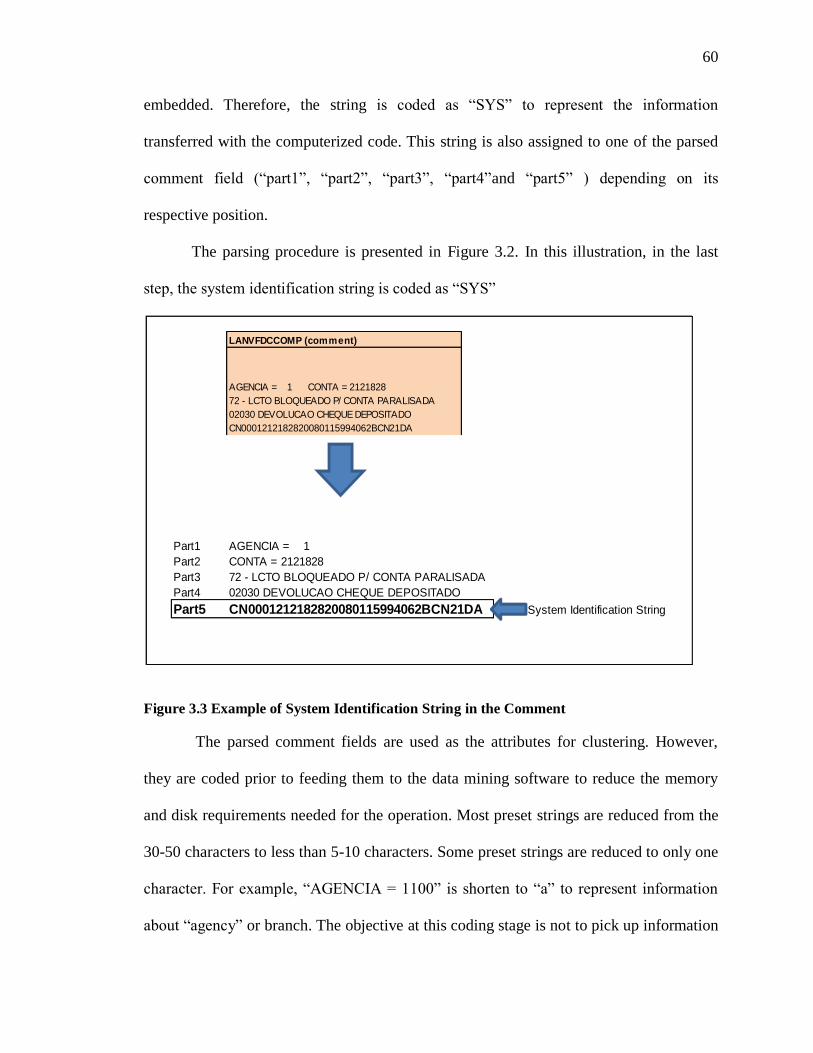
60
embedded. Therefore, the string is coded as ―SYS‖ to represent the information
transferred with the computerized code. This string is also assigned to one of the parsed
comment field (―part1‖, ―part2‖, ―part3‖, ―part4‖and ―part5‖ ) depending on its
respective position.
The parsing procedure is presented in Figure 3.2. In this illustration, in the last
step, the system identification string is coded as ―SYS‖
Figure 3.3 Example of System Identification String in the Comment
The parsed comment fields are used as the attributes for clustering. However,
they are coded prior to feeding them to the data mining software to reduce the memory
and disk requirements needed for the operation. Most preset strings are reduced from the
30-50 characters to less than 5-10 characters. Some preset strings are reduced to only one
character. For example, ―AGENCIA = 1100‖ is shorten to ―a‖ to represent information
about ―agency‖ or branch. The objective at this coding stage is not to pick up information
LANVFDCCOMP (comment)
AGENCIA = 1 CONTA = 2121828
72 - LCTO BLOQUEADO P/ CONTA PARALISADA
02030 DEVOLUCAO CHEQUE DEPOSITADO
CN0001212182820080115994062BCN21DA
Part1 AGENCIA = 1
Part2 CONTA = 2121828
Part3 72 - LCTO BLOQUEADO P/ CONTA PARALISADA
Part4 02030 DEVOLUCAO CHEQUE DEPOSITADO
Part5 CN0001212182820080115994062BCN21DA System Identification String

61
on specific identity such as to pick up ―1100‖ from the string ―AGENCIA = 1100‖ but to
recognize the pattern that this string refers to or gives information on agency number or
branch number. In addition, as mentioned in previous section, the alphanumeric string
representing the computer-coded information transferred between computer systems are
coded as ―SYS‖. The steps taken to code the comment are shown in Figure 3.4.
Figure 3.4 Comment Coding Illustration
3.7 Clustering Procedure
The parsed comment field is used as the input variable for clustering. Because
neither the distribution of the input variables nor other parameters necessary for cluster
analysis is known, the EM algorithm will be adopted for the clustering (Witten et al,
2005). EM algorithm, or expectation-maximization, involves two steps; 1) ―expectation‖
is the calculation of the cluster probabilities, and 2) ―maximization‖ of the likelihood of
the distributions given the data. For this method, only the cluster probabilities, not the
cluster themselves, that are known for each observation. They could be considered as
LANVFDCCOMP (comment)
AGENCIA = 1 CONTA = 2121828
72 - LCTO BLOQUEADO P/ CONTA PARALISADA
02030 DEVOLUCAO CHEQUE DEPOSITADO
CN0001212182820080115994062BCN21DA
Part1 AGENCIA = 1 A
Part2 CONTA = 2121828 C
Part3 72 - LCTO BLOQUEADO P/ CONTA PARALISADA 72CAT
Part4 02030 DEVOLUCAO CHEQUE DEPOSITADO 02030CAT
Part5 CN0001212182820080115994062BCN21DA SYS

62
weights. Witten et al (2005) state if wi is the probability that observation i belongs to
cluster A, the mean and standard deviation for cluster A are
n
nnA
n
nnA
www
xwxwxw
www
xwxwxw
....
)(....)()(
.....
.......
21
22
22
2
112
21
2211
The EM algorithm converges toward a fixed point, which can be identified by calculating
the overall likelihood that the data came from this dataset, given the values for all
parameters. However, it will never actually get to that point. This likelihood can be
calculated by multiplying the probabilities of the individual observation i:
i
iBiA BxpAxp ])|Pr[|Pr(
Where the probabilities given the cluster A and B are determined from the normal
distribution function ),;( xf (Witten et al, 2005). The likelihood is a measurement of
the goodness of the clustering process. This number should be increased after each
iteration.
3.8 Results
Though the most commonly used techniques for exploratory data analysis are a
multitude of statistical methods and in particular graphical displays, cluster analysis can
also be used for EDA. As earlier discussed, cluster analysis is a technique that can be
used for finding the common characteristics in a data set. Understanding the
characteristics of a data set can assist the user in making sense of the data. There are
many possible uses for this technique including developing specific strategies, policy,
anomaly detection techniques, etc.

63
Using the four original attributes, LANVFCDFUNC, LANVFCDORLC,
LANVFINRESP, and LANCDEVENNEGO with the EM algorithm for conceptual
clustering creates three clusters. The result is shown in Figure 3.5. From using the four
original attributes, 99% (49,199) of transactions are grouped into the same cluster,
cluster0. Only 223 and 117 transactions are grouped into cluster1 and cluster2. When
observing the original dataset, it becomes clear that cluster1 and cluster2 are transactions
of which comments are manually entered. Though the reason given for those transactions
are varied, the nature of the comment is the same, they are manual comments. They could
have been entered manually partially or completely.
Figure 3.6 shows that when the four original attributes are used as the clustering
attributes, this data set can be grouped to a set of meaningful clusters. Dots with the same
color are the transactions in the same cluster. The more homogeneous the colors in the
group are; the clearer or better the clustering results appear to be.

64
Figure 3.5: Clustering Result from using the four remaining attributes
=== Run information ===
Scheme: weka.clusterers.EM -I 100 -N -1 -M 1.0E-6 -S 100
Relation: 5738Main
Instances: 49539
Attributes: 7
LANVFCDFUNC
LANVFCDORLC
LANVFINRESP
LANVFCDSTPR
LANCDEVENNEGO
Test mode: evaluate on training data
=== Model and evaluation on training set ===
EM
==
Number of clusters selected by cross validation: 3
Cluster
Attribute 0 1 2
(0.99) 0 0
LANVFCDFUNC
mean 0 1124089.5 0
std.dev. 75255.23 13675.25 3.4191
LANVFCDORLC
mean 41 11.0179 17.2051
std.dev. 2.3463 0.2673 8.1624
LANVFINRESP
U 49200 224 115
A 1 1 4
[total] 49201 225 119
LANVFCDSTPR
mean 1 1 0.9487
std.dev. 0.011 0.011 0.2206
LANCDEVENNEGO
mean 603 606.6251 2130.9904
std.dev. 327.8754 0 6571.7138
Clustered Instances
0 49199 ( 99%)
1 223 ( 0%)
2 117 ( 0%)
Log likelihood: -16.99899

65
Figure 3.6 Visualization of Clustering Results (LANVFCDFUNC and LANVFCDORLC)
Though the resulting cluster is clear (i.e. unseen observations can be classified
into groups easily) and meaningful, it may not necessarily be useful. For example, in this
clustering result, it is possible to tell which transactions are manually entered. Whether
the knowledge about the nature of the transaction is useful is an important question to
consider.
When using open comment attribute with the EM algorithm, seven clusters are
created. Dominant characteristics or the content of the comment in each cluster are
summarized in the Table 3.5.

66
Table 3.5 Content of the Comment Fields in Each Cluster
Cluster
No Content of the comment fields
Cluster0 70 - RESOLUCAO 2025-CLIENTE NAO RECADASTRADO with other message
Cluster1
02 - VALOR LANCTO MAIOR QUE O SALDO with 01902 *TAXA ADMINISTRATIVA
OR
02 - VALOR LANCTO MAIOR QUE O SALDO with 06246 *DEB AUT REVISTA
SELECOES
Cluster2 01 - CONTA INEXISTENTE with other message
Cluster3
Transaction with the comment that have only one message (in addition to the agencia, conta, and
the alphanumeric phase generated from the system)AND the alphanumeric phase generated from
the system
Cluster4 50 - LANC.INVALIDO P/PRODUTO HOT-OVER OU COMPROR with other message
Cluster5 71 - LCTO BLOQUEADO P/ CONTA NAO HABILITADA with other message
72 - LCTO BLOQUEADO P/ CONTA PARALISADA with other message
Cluster6
02 - VALOR LANCTO MAIOR QUE O SALDO with other message
but NOT 01902 *TAXA ADMINISTRATIVA OR
06246 *DEB AUT REVISTA SELECOES
- Transaction with only one message (in addition to AGENCIA and CONTA) WITHOUT
alphanumeric phase generated from the system
- Transaction that have the massages too varied to parsed
Transactions with similar comments are grouped together. For example, the
transaction with the inexistent accounts (01 - CONTA INEXISTENTE) would be in
cluster2. There is additional information relating to the inexistent accounts presented in
the part4. These clusters represent different reasons that the transactions are transferred to
this transitory account. The visualization of the assigned clusters is shown in Figure 3.7
and Figure 3.8. With the limitations of the visualizations in this paper, the attributes and

67
their relationships can be shown in at most three dimensions; the x-axis, y-axis and the
color. Therefore, even though cluster analysis is a multidimensional analysis (i.e. several
attributes can be used as the input at the same time), only three dimensions (of the input
attributes and the results) can be shown. The assigned clusters are visualized by using
color; while other two attributes would be visualized using the x and y axis. The use of
color will make the distinction and/or the interpretation of the results easier. By observing
dots (or observations) in different colors, the reader would easily understand that they are
different groups or clusters.
Figure 3.7 Assigned clusters and the value in part1 and part3 of the comment field.

68
Figure 3.8 Assigned Clusters and the value of part3 and part4 of the comment field(2).
Though the free form comment field has no standardized format, it could be
parsed or separated into four parts. Most transactions have the branch (AGENCIA) and
account number (CONTA) as the first two parts of the free form comment. The
remaining two parts are mainly coded messages (coded number and written message).
Because the first two parts of the comment are mostly (but not all) the same, it is
justifiable to select part3 and part4 for visualization purposes.
Transactions having similar comments are grouped into the same clusters. From
the graphical visualization, it shows that there are clusters. Dots represent individual
transactions where the same colors represent the same clusters. Figure 3.8 highlights that
the most grouped transactions create large areas of a single color. There are areas for

69
yellow, green, purple, red, light blue, blue. The x-axis represents part3 of the comment,
while y-axis represents part4. The large areas of single color demonstrate that the
transactions from the same clusters have the same values in part3 and part4.
Table 3.6 Number of Transactions by Clusters
Cluster name Number of Transaction Percentage cluster0 491 0.99% cluster1 4010 8.09% cluster2 19005 38.36% cluster3 2575 5.20% cluster4 4277 8.63% cluster5 3408 6.88% cluster6 15773 31.84% Grand Total 49539 100.00%
Numbers of transactions in each cluster are shown in Table 3.6. The majority of
transactions (70.20%) are in cluster2 (38.36%) and cluster6 (31.84%). The cluster with
the smallest number of transactions is cluster0 (0.99%). The remaining clusters, which
are cluster1, clsuter3, cluser4 and cluster5, have 8.09%, 5.20%, 8.63% and 6.88%
respectively.
This dataset consists of transactions entered into a single transitory account
(account 5738) by over 1,000 branches (AGENCIA) of a major foreign bank. Some
branches (AGENCIA) are bigger and originate more transactions than others. The
number of transactions by branches ranges from 1 to over 1,500 transactions. The top 20
branches (AGENCIA) in term of number of transactions originated comprise 20% of the
total number of transactions in the transitory account number 5738. In order to gain a
better understanding of the dataset, the clustering results by branch is examined. The

70
distribution of the clustered transactions of the top 20 branches (AGENCIA) is examined.
It is organized by branch.
Table 3.7 Distribution of the Transaction into Clusters by Top 20 Branches
Table 3.7 shows that different branches have different dominating types of
comments. For example, branch 7227, 1715 and 986 originate many transactions which
are in cluster4; while branch 90 and 444 originate many transactions which are either 02 -
VALOR LANCTO MAIOR QUE O SALDO+ an additional comment, comment with
one message, or comment which are impossible to parse. Some branches have originated
two dominating type of comments or reasons; for example, branch329, 130, 7335 and
811. These branches have two dominating type of comments or reasons (i.e. 01 - CONTA
INEXISTENTE + additional comment AND transactions with incomplete comment).
Branch cluster0 cluster1 cluster2 cluster3 cluster4 cluster5 cluster6 Total
7227 6 78 1560 5 38 1687
1715 5 1003 1 7 1016
90 5 5 26 2 1 12 954 1005
7246 9 865 1 6 23 904
329 4 324 1 539 868
444 6 48 1 1 470 526
927 457 22 1 480
201 377 51 2 16 9 7 462
379 9 393 7 2 411
130 234 3 3 3 142 385
529 4 6 286 1 1 5 58 361
986 5 48 290 7 8 358
7335 12 183 2 111 308
870 3 277 2 6 288
206 254 6 3 12 275
562 3 239 31 273
811 9 74 3 184 270
351 12 219 9 5 4 249
126 4 233 10 1 248
1693 21 185 2 3 35 246

71
There can be explanations to why such concentration exists. For example, all
branches use the same transitory account for the different types of pending transactions
(i.e. account 5738 could be for transactions without account number, while account
60836 could be for transactions with insufficient funds, etc). A transitory account is
supposed to be used for the same purpose for all branches.
Examining transactions from a particular transitory account in a particular branch,
there should be only one cluster. Transactions from clusters other than the one with the
highest population may be considered an anomaly.
From the dataset, there are 1016 transactions generated from branch 1715. These
transactions are grouped into cluster2 (5), cluster4 (1003), cluster5 (1) and cluster6 (7).
More than 98% of transactions are in cluster4. The remaining transactions (which are 5
transactions from cluster2, 1 transaction from cluster5 and 7 transactions from cluster6)
are the minority. Using this rationale to evaluate the clustering results of account 5738,
thirteen transactions from branch 1715 can be flagged as possible anomalies. The total
number and the percentage of transactions in these remaining groups are so small that
they are suspicious of being illegitimate. Though the reasons or explanation related to the
transactions may seem valid, the small volume can lead to the doubt of their presences.
Further investigation and/or tests are needed to check the legitimacy of the transactions.

72
Table 3.8 Percentage of Transactions Grouped into Clusters for the Top 20 Branches
The distributions of transactions grouped into clusters are presented in Table 3.8
and Figure 3.9. The table lists branch and how its transactions are distributed into
clusters. Looking at the top 20 branches by the number of transactions indicates that
most branches have one or two dominating types of transactions. For example, branch
927 and 201 have over 80% of transactions in cluster1 (02 - VALOR LANCTO MAIOR
QUE O SALDO); branch 7246, 379, 529, 870, 206, 562, 351 and 1693 have over 75% of
transactions in cluster2 (01 - CONTA INEXISTENTE); branch 126 has over 93% of
transactions in cluster3; branch 7227, 1715 and 986 have over 80% of transactions in
cluster4(50 - LANC.INVALIDO P/PRODUTO HOT-OVER OU COMPROR); branch
90 and 444 have over 89% of transactions in cluster6 (incomplete comment). There is no
branch in the top 20 group that originates the majority of the transaction in cluster0 (70 -
RESOLUCAO 2025-CLIENTE NAO RECADASTRADO) and cluster5 (71 - LCTO
Branch cluster0 cluster1 cluster2 cluster3 cluster4 cluster5 cluster6 Total
7227 0.3557% 4.6236% 92.4718% 0.2964% 2.2525% 100%
1715 0.4921% 98.7205% 0.0984% 0.6890% 100%
90 0.4975% 0.4975% 2.5871% 0.1990% 0.0995% 1.1940% 94.9254% 100%
7246 0.9956% 95.6858% 0.1106% 0.0000% 0.6637% 2.5442% 100%
329 0.4608% 37.3272% 0.1152% 62.0968% 100%
444 1.1407% 9.1255% 0.1901% 0.1901% 89.3536% 100%
927 95.2083% 4.5833% 0.2083% 100%
201 81.6017% 11.0390% 0.4329% 3.4632% 1.9481% 1.5152% 100%
379 2.1898% 95.6204% 1.7032% 0.4866% 100%
130 60.7792% 0.7792% 0.7792% 0.7792% 36.8831% 100%
529 1.1080% 1.6620% 79.2244% 0.2770% 0.2770% 1.3850% 16.0665% 100%
986 1.3966% 13.4078% 81.0056% 1.9553% 2.2346% 100%
7335 3.8961% 59.4156% 0.6494% 36.0390% 100%
870 1.0417% 96.1806% 0.6944% 2.0833% 100%
206 92.3636% 2.1818% 1.0909% 4.3636% 100%
562 1.0989% 87.5458% 11.3553% 100%
811 3.3333% 27.4074% 1.1111% 68.1481% 100%
351 4.8193% 87.9518% 3.6145% 2.0080% 1.6064% 100%
126 1.6129% 93.9516% 4.0323% 0.4032% 100%
1693 8.5366% 75.2033% 0.8130% 1.2195% 14.2276% 100%

73
BLOQUEADO P/ CONTA NAO HABILITADA; 72 - LCTO BLOQUEADO P/
CONTA PARALISADA). From this knowledge, it is possible to write a program to
detect if the incoming transaction does not have similar characteristics as the others.
Figure 3.9 Distribution of Transactions into clusters by top 20 branches
Using simple expressions in Perl programming can change the complex fields
which is originally impossible to be analyzed into a computable form. After the field is
parsed, the patterns and other information can be revealed. Data mining on this data can
then be performed.
Cluster Analysis can be used for the exploratory data analysis. At the first glance,
it might appear as if the simple counting can be applied and used for this purpose. For
cluster0
cluster1
cluster2
cluster3
cluster4
cluster5
cluster6

74
example, transactions with the phrase ―70 - RESOLUCAO 2025-CLIENTE NAO
RECADASTRADO‖ can be grouped into cluster1, transactions with the phrase ―50 -
LANC.INVALIDO P/PRODUTO HOT-OVER OU COMPROR‖ can be grouped into
cluster4. However, cluster analysis is able to group the transactions with similar mistakes
into the same groups in such a way that a simple counting of frequency distribution
cannot. It incorporates more than one attribute in the consideration of grouping.
For example, transactions with the message ―02 - VALOR LANCTO MAIOR
QUE O SALDO‖ are grouped into 2 separated groups by cluster analysis. First group of
02 - VALOR LANCTO MAIOR QUE O SALDO transactions are in cluster1; while the
second group are in cluster6. The difference between the two (2) clusters is that cluster1
represents 02 - VALOR LANCTO MAIOR QUE O SALDO with either 01902 *TAXA
ADMINISTRATIVA or 06246 *DEB AUT REVISTA SELECOES as the second part of
the comment; while 02 - VALOR LANCTO MAIOR QUE O SALDO transaction in
cluster6 does not have either 01902 *TAXA ADMINISTRATIVA or 06246 *DEB AUT
REVISTA SELECOES. Moreover, some 02 - VALOR LANCTO MAIOR QUE O
SALDO transactions which are grouped into cluster6, represent the transaction where the
first phase of the comment was entered as 02 - VALOR LANCTO MAIOR QUE O
SALDO and the additional information (or 2nd
phrase) is missing. If the 02 - VALOR
LANCTO MAIOR QUE O SALDO transactions have either 01902 *TAXA
ADMINISTRATIVA or 06246 *DEB AUT REVISTA SELECOES as the second (2nd
)
phrase, they will be grouped into cluster1.
Though the results from clustering using the four original attributes and using the
parsed comments are not equivalent, there are some points that should be noted. Firstly,

75
clustering using the four original attributes can generate three clusters, two of which are a
subset of cluster results from the parsed comment. Transactions which are grouped in
cluster1 and cluster2 from using four original attributes are grouped into cluster6 from
using parsed comment field. Secondly, most transactions (99%) are grouped into cluster0
when four original attributes are used despite the fact that the transactions are of a
different nature. Therefore, it might be worth noting that the open comment attribute once
parsed can be a very useful variable for conceptual clustering.
3.9 Conclusions
Cluster analysis is used extensively in marketing as a technique to discover
market segments. In this aspect, it is used to discover hidden patterns and structures such
as market segments. The end benefits depend on the objective of the clustering. For
example, after identifying market segments, a marketer may use the information to
develop marketing strategies to serve some specific market segments or develop several
strategies targeted for each individual segment. Without prior knowledge about the
dataset, cluster analysis may be used as a tool to help discover some hidden information.
Using the real dataset from an international bank, this study provides the
illustration on how cluster analysis may be applied by auditors to gain knowledge about a
dataset. This dataset consists of transactions that are posted onto transitory accounts.
These transactions cannot be completed at the time they are entered into the system. The
transactions are transferred or posted to transitory accounts temporarily before employees
can find the solution to the problem. Once the issue is resolved, the transaction is cleared
leaving the ending balance of the transaction as zero. There is very little information
relating to the nature of these transitory accounts. Therefore, cluster analysis is an

76
excellent method for exploring this type of dataset. The clustering technique Expectation
Maximization (EM) is performed, resulting in seven clusters. The resulting clusters may
be considered as major sub-groups. As a result, better understanding about the dataset
may be developed and this knowledge may be useful in the audit planning process.
Cluster analysis is a useful technique for exploratory data analysis. Using a real
dataset from a company, the EM technique is applied and major sub-groups of
transactions are discovered. The end benefits of the cluster analysis depend on the
objective of the clustering and how the resulting clusters are used.

77
3.10 References
Chang, H., H. H. Lai and Y.M. Chang. 2006. Expression Modes Used by Consumers in
Conveying Desire for Product Form: A Case Study of a Car. International Journal of
Industrial Ergonomics 36: 3-10.
Erdogan, B. Z., S. Deshpande and S. Tagg. (2007). Clustering Medical Journal
Readership Among GPs: Implications for Media Planning. Journal of Medical Marketing
7(2): 162-168.
Fisher, D. and P. Langley. 1985. Conceptual Clustering and Its Relation to Numerical
Taxonomy. Workshop on Artificial Intelligence and Statistics. AT&T Bell Laboratories,
Princeton, N.J.
Kerlinger, F. N., H. B. Lee. 2000. Foundations of Behavioral Research (Fourth Edition).
Harcourt College Publishers. USA.
Lim, L., F. Acito and A. Rusetski. 2006. Development of Archetypes of International
Marketing Strategy. Journal of International Business Studies37: 499-524.
Michalski, R. 1980. Knowledge Acquisition through Conceptual Clustering: A
Theoretical Framework and Algorithm for Participating Data into Conjunctive Concepts.
International Journal of Policy Analysis and Information Systems 4(3)219-243.
Morwitz, V. G. and D. Schmittlein. 1992. Using Segmentation to Improve Sales
Forecasts Based on Purchase Intent: Which ―Intenders‖ Actually Buy? Journal of
Marketing Research 29: 391-405.
Shih, Y.Y. and C.-Y. Liu. 2003. A Method for Customer Lifetime Value Ranking-
Combining the Analytic Hierarchy Process and Clustering Analysis. Database Marketing
& Customer Strategy Management 11(2): 159-172.
Sokal, R. R. and P. H. A. Seneath. 1963. Principles of Numerical Taxonomy. W.H.
Freeman. San Francisco, USA

78
Srivastava, R. K., R. P. Leone and A. D. Shocker. 1981. Market Structure Analysis:
Hierarchical Clustering of Products Based on Substitution-in-use. Journal of
Marketing45: 38-48.
Tukey, J. W. 1977. Exploratory Data Analysis. Addison-Wesley Publishing Company
Inc. USA.
Witten, I. H. and E. Frank. 2005. Data Mining: Practical Machine Learning Tools and
Techniques. Morgan Kafmann Publishers, USA.

79
Chapter 4 Cluster Analysis for Anomaly Detection
4.1 Introduction
Cluster Analysis is a very popular technique used in marketing for the purpose of
market segmentation (Erdogan et al, 2006, Lim et al, 2006, Morwitz et al, 1992, Shih et
al, 2003). It could be used to group the data such as customers and/or products into
groups or segments in order to develop marketing strategies specifically to each segment,
for example. In addition to grouping, cluster analysis is used for outlier identification.
Outliers can be a by-product of cluster analysis (Agrawal et al, 1998, Aggarwal et al,
1999). Even though clustering and anomaly detection appear to be fundamentally
different, several clustering based anomaly detection techniques have been developed in
the literature (Chandola et al, 2009).
This study uses data of a major insurance company. It aims at developing a
continuous audit or automatic fraud detection process for its electronic wire transfer
system. The company would like to develop the monitoring process for the wire
payments transferred within and out of the company‘s system. Funds have been
transferred continuously to and from many divisions or business unit. The frequency and
volume of the transferred funds are significant in business operations. Several controls
are implemented in the systems; for example, requiring several approvers for
transactions, setting fund limits for approvers and initiators of the transactions, setting
specific bank account for specific type of transactions, etc. The process of the wire
transfers is not extremely complicated; however, its high volume has significant impact
on business operations. Therefore, depending on only good controls may not be
sufficient. With the business world growing more complicated with time, having good

80
controls in place may not be enough. As a result, management is hoping to find a more
effective, innovative, and up-to-date method to monitor the wire transfers.
The objective of this study is to examine the use of cluster analysis as an
alternative and innovative anomaly detection technique in the wire transfer system.
Several clustering techniques are applied to detect possible anomalous wire transfers. The
results are compared and evaluated in terms of understanding the type of possible
outcome cluster analysis delivers as well as how it can be used by internal auditors. This
study provides a guideline for the usage of this technology in auditing process.
4.2 Anomaly Detection
Outliers are observations that deviate significantly from other observations to the
point that they arouse suspicion that they were generated by a different mechanism
(Hawkins, 1980). Anomalies occur for many reasons, for example, different classes of
data, natural variation in the data and data measurement, and collection error (Tan et al,
2006).
Chandola et al (2009) suggest that anomalies can be classified into three
categories: point anomaly, contextual anomaly, and collective anomaly. Point anomaly is
a simple form of anomaly that identifies an individual data instance as anomalous in
respect to the remaining of data. Contextual anomaly occurs when a data instance is
anomalous in specific context. For example, a temperature of 35F is considered normal in
winter but rather anomalous in summer. Collective anomaly is the case when a collection
of related data instances are anomalous. Duan et al (2009) suggest that there is a
possibility that many abnormal events have both temporal and spatial locality, which
might form small clusters that also need to be deemed as outliers. In other words, not
81
only single points but also small clusters can probably be considered as outliers. This
type of outlier is called a ―cluster-based outlier‖.
Anomaly detection is the task of identifying observations whose characteristics
are significantly different from the rest of the data (Tan et al, 2006). These observations
are called outliers or anomalies because they have attribute values that deviate
significantly from the expected or typical attribute values. Application of anomaly
detection includes fraud detection, credit card fraud detection, network intrusion, etc.
Regardless of the applied domain, anomaly detection generally involves three basic steps;
1) identify normality by calculating the ―signature‖ of the data, 2) determine the metric
to calculate an observation‘s degree of deviation from the signature, and 3) set some
criteria/threshold to identify anomalous observations which metric measurements are
higher than the threshold (Davidson, 2000). A variety of methods for each step have been
used in various applications in all fields.
Chondala et al (2009) suggest that with respect to the extent to which the labels
are available, anomaly detection techniques can operate in one of three modes:
supervised anomaly detection, semi-supervised anomaly detection and unsupervised
anomaly detection. Supervised anomaly detection assumes the availability of a training
data set which has instances labeled as normal as well as anomaly classes. Semi-
supervised anomaly detection assumes that the training data set has labeled instances for
only the normal classes. A model corresponding to the normal behavior will be build and
used for identifying the anomalous instances in the test data. Unsupervised anomaly
detection does not require training data set. It assumes that anomalous instances are far
less than the normal instances.

82
4.3 Cluster Analysis for Anomaly Detection
Chandola et al (2009) propose that clustering based techniques can be grouped
into three categories. The first group relies on the assumption that normal data instances
belong to a cluster in the data while anomalies do not belong to any cluster(Chandola et
al (2009); for example, DBSCAN - Density-Based Spatial Clustering of Applications
with Noise (Ester et al, 1996), ROCK-Robust Clustering using links (Guha et al, 2000),
SNN cluster - Shared Nearest Neighbor Clustering (Ertoz et al, 2003), FindOut algorithm
(Yu et al, 2002) and WaveCluster algorithm (Sheik-Holeslami et al, 1998). Basically
these techniques apply a clustering algorithm to the data set and declare any data
instances that do not belong to any cluster as anomalous.
The second group relies on the assumption that normal data instances lie close to
their closest cluster centroid while anomalies are far away from their closest cluster
centroid (Chandola et al, 2009). Self-Organizing Maps (SOM) introduced by Kohonen
(1997) is widely used for anomaly detection in many different applications; for example,
fraud detection in automobile bodily injury insurance claims (Brockett et al, 1998) and
network intrusion detection (Labib et al, 2002, Smith et al, 2002, Ramadas et al,
2003).The techniques in this group basically involve two steps; firstly, grouping data into
clusters and secondly calculating distances from cluster centroid to identify anomaly
scores.
The third group relies on the assumption that normal data instances belong to
large and dense clusters, while anomalies either belong to small or sparse clusters
(Chandola et al, 2009). He et al (2003) propose a technique called FindCBLOF to find

83
size of the cluster to which the data instance belongs and the distance of the data instance
to its cluster centroid. These two values make up the score called Cluster-Based Local
Outlier Factor (CBLOF). Applying the technique to detect anomalies in astronomical
data, Chaudhary et al (2002) propose an anomaly detection model using k-d trees
providing partitions of data in linear time. Sun et al (2004) propose a technique called
CD-trees. Both techniques define sparse clusters as anomalies; in other words, they
determine anomalies based on the density and distance from other clusters.
4.4 The Audit Problem
The insurance company is aiming at developing a continuous audit / fraud
detection process. Therefore, the internal audit team of the company has cooperated with
the research team to develop automatic models or methodologies that could be used in
parallel with the internal audit process. The wire transfer process is selected for model
development because of a number of factors as follows. Firstly, the data is available for
the analysis. Secondly, the internal audit team identifies that wire transfer is an important
process which involves a large number of transaction in the system. Thirdly, a
knowledgeable and competent internal audit team is available to assist in the model
building process.
The wire transfer process in the company consists of three stages: initiation,
approval and payment. First, users in the line of business initiate or request the payment.
The request is then needed to be approved by appropriate approvers. Depending on the
type and nature of the wires, some may require more approvers than others. After the
request is approved, the payment is then made to the payee. Though wire transfer is a
significant process, it does not seem yet to have a very good control set in place. There

84
are cases where the crucial information is missing such as approvers‘ identification.
Specific controls that exist in the system are, for example, users are assigned to a specific
transaction and bank account group; therefore they can conduct a certain type of
transaction thru specific bank account groups.
Figure 4.1 Wire Transfer Process
Recognizing the importance of the wire transfer system; the company has been
cooperating with an academic institution to create a model for fraud or anomaly
identification that can be used along side with their normal internal auditing process.
Several indicators are created using statistical methods such as prediction interval test,
correlation test and frequency test. For the prediction interval test, the model involves
stratifying payees into four categories: 1) payees with one wire payment (P1), 2) payees
with two wire payments (P2), 3) payees with three to twenty-nine wire payments (P3),
and 4) payees with thirty or more wire payment (P4). Alpha prediction intervals of 90%,
95% and 99% are created to identify outliers. With the statistical nature of these
indicators, numbers of transactions are of great concern. For payees with thirty or more
Initiation
Approval
Payment

85
wires (P4), calculating alpha prediction intervals is not an issue. For payees with only one
wire payment (P1), a prediction interval can be estimated by grouping them with other
payees who also have only one wire payment and calculating the value as a whole. There
exist difficulties at this stage dealing with payees who have only two wire payments (P2)
and those with three to twenty nine payments (P3). The former group has more than one
wire payment, making it impossible to be added to the combined pool with payees that
has only one payment. The latter group with three to twenty nine payments does not have
the required number of transactions for statistical tests. Therefore, the company is looking
for the other alternative methods for detecting outliers for this group of wire transfers.
The company does not seem to have available the record of previously identified
frauds or anomalies. However, lacking of such a record does not necessarily mean that
there is no fraud in the wire transfer process. Due to the lack of previous fraud history for
model development process, applying an unsupervised method is appropriate. The
objective of this research is to create an unsupervised model for potential anomaly
detection in wire transfer system. The results from the model, which are potential
anomalies identified, will be investigated further by the internal audit team.
4.5 Data
4.5.1 General Information
The data obtained from an insurance company consists of wire transactions for a
period of time from 2008 to 2010. It includes information on each wire transfer such as
its approvers, initiators, senders, receivers; the department or group it belongs to; the
amount it has transferred; the designated location it will be sent to as well as its other
description or information, etc. The attributes are listed in Table 4.1. It is noticeable that

86
most attributes are mainly for identification purposes (for examples, initiator id, approver
id, cost center id, initiator name, account number, routing number). Though they are very
informative, they are not useful for classification. Therefore, based on the original
attributes list and additional consultation with the internal auditors, attributes that
represent characteristics of the wire transfers are created.
While the insurance company provided data for approximately two years in this
project, cluster analysis has been done quarterly due to the following reasons: 1) the data
size is large enough for the analysis and not too large to be processed for a reasonable
amount of time and 2) the analysis corresponds with the quarterly internal audit process.
The result will be presented in detail for one quarter.

87
Table 4.1 Attribute Information
4.5.2 Description and Distribution of Attributes
Attributes Used:
From the original attributes, the attributes selected and/or created are as follows:
WireType: There are four type of wire transfer: random, repetitive, concentration,
and batch. The categories are based on the number of payments and on operational
All_wires Detail Information
ACCTBIZUNIT The Line of Business that owns the bank account from which the funds are disbursed
AMOUNT Amount of each wire (stored as negative number)
APPROVER1ID User (employee) id of (first) approver
APPROVER1LOB Cost center of (first) approver
APPROVER1NAME Fullname of (first) approver (includes phone number)
APPROVER2ID User (employee) id of (second) approver
APPROVER2LOB Cost center of (second) approver
APPROVER2NAME Fullname of (second) approver (includes phone number)
COUNTBIZUNIT The Line of Business that owns the bank account to which the funds are being sent
CURRENCY Standard currency code of disbursed funds (e.g. USD, MXN, EUR, etc.)
DATASOURCE Indicates wire source (system)
EFFDATE Effective date of funds disbursal
INITIATEDDATE Date the wire was initiated
INITIATORID User (employee) id of initiator
INITIATORLOB Cost center of initiator
INITIATORNAME Fullname of initiator (including phone number)
INTTRANIND Identifies whether the wire was between 2 MetLife bank accounts
PAYEE Payee Name
PAYEEACCTNUM Payee Bank Account
RANDREP Indicates whether wire is random or repetitive (i.e. source is line number template)
RECORDTYPE Type of Record??
REPREF Reference to the Repetitive Wire Template
ROUTINGNUM ABA, Fed Wire or Swift Code
SOURCEACCTNUM Bank account from which funds are disbursed
TRANREF Descriptive information entered along with the wire
TRANTYPE TWS transaction type assigned to each wire
WIREID Unique id for each wire transaction

88
effectiveness and efficiency. These wire transfers have different characteristics.
Therefore, it is reasonable to assume that they may have different behaviors. The brief
description of different types of wire transfers is given below.
Random: infrequent wire transfer,
Repetitive: Regular and repeated wire transfer such as monthly
installments, weekly payments and etc,
Concentration: Transfer between departments such as transfers
between different business units and or branches,
Batch: Batch wire transfer such as transfers which have been
entered at various times during the day but have been processed
only at the end of the day.
Table 4.2 Number of Wire Transfer by WireType
Payee: Type of payee (Individual who receives wire transfers)
Payees are categorized by the number of payment that he or she received
throughout the period. Payees are stratified into four categories:
P1: if the payee receives only one payment;
P2 : if the payee receives two payments;
P3: if the payee receives from three to twenty-nine payment;
P4: if the payee receives thirty or more.
WireType Count
Bat 7495
Ran 1594
Rep 358
Grand Total 9447

89
The objective of this study is to find an alternative method for anomaly
detection that could be applied to wire transfer when the types of payee are P2 and P3, in
other words, when the payee receives between two to twenty-nine payments. Therefore,
among the originally stratified four payee categories, the values of this attribute that
appears in this dataset will be only P2 and P3.
The payees are categorized based on the number of payment received due
to statistical reasons mentioned in the previous section (The Audit Problem). It is also
reasonable to assume that payees from different groups may have different characteristics
and/or different behaviors. In order to derive statistical values such as means, median and
etc, of a group of values, it is conventional belief that at least 30 observations are needed
(Kutner et al, 2004). Therefore, payees who receive 30 or more payments are grouped
into P4; while payees who receive less 30 payments are classified into 3 groups based on
the number of payments.
Table 4.3 Number of Wire Transfers by Payee
Ini: Type of Initiator (Individual who initiates wire transfers)
Type of Initiator is identified by the number of wire transfer he or she
initiates throughout the period. Initiator is stratified to four categories:
I1: if the initiator initiates only one wire transfer;
I2 : If the initiator initiates two wire transfers;
Patron Count
P2 888
P3 8559
Grand Total 9447
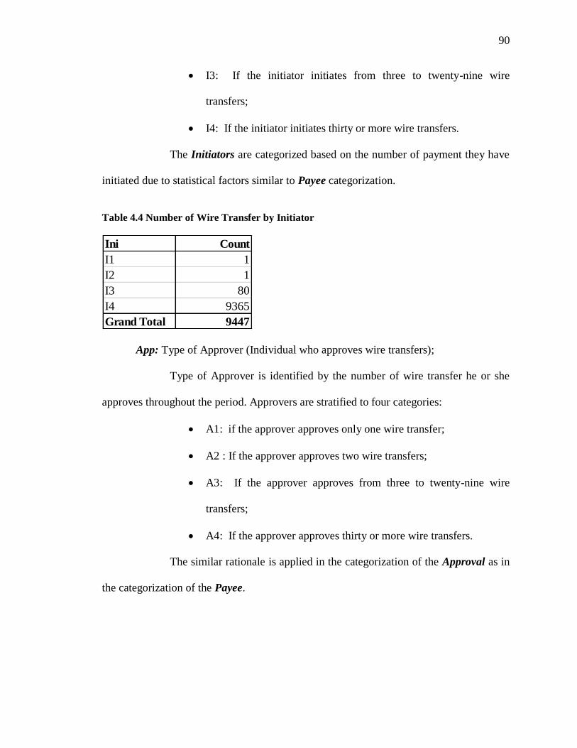
90
I3: If the initiator initiates from three to twenty-nine wire
transfers;
I4: If the initiator initiates thirty or more wire transfers.
The Initiators are categorized based on the number of payment they have
initiated due to statistical factors similar to Payee categorization.
Table 4.4 Number of Wire Transfer by Initiator
App: Type of Approver (Individual who approves wire transfers);
Type of Approver is identified by the number of wire transfer he or she
approves throughout the period. Approvers are stratified to four categories:
A1: if the approver approves only one wire transfer;
A2 : If the approver approves two wire transfers;
A3: If the approver approves from three to twenty-nine wire
transfers;
A4: If the approver approves thirty or more wire transfers.
The similar rationale is applied in the categorization of the Approval as in
the categorization of the Payee.
Ini Count
I1 1
I2 1
I3 80
I4 9365
Grand Total 9447
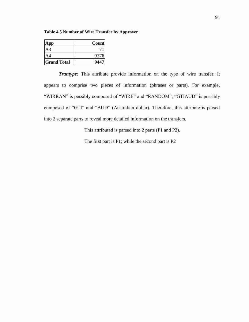
91
Table 4.5 Number of Wire Transfer by Approver
Trantype: This attribute provide information on the type of wire transfer. It
appears to comprise two pieces of information (phrases or parts). For example,
―WIRRAN‖ is possibly composed of ―WIRE‖ and ―RANDOM‖; ―GTIAUD‖ is possibly
composed of ―GTI‖ and ―AUD‖ (Australian dollar). Therefore, this attribute is parsed
into 2 separate parts to reveal more detailed information on the transfers.
This attributed is parsed into 2 parts (P1 and P2).
The first part is P1; while the second part is P2
App Count
A3 71
A4 9376
Grand Total 9447

92
Table 4.6 Number of Wire Transfer by Trantype
COSTCTR: Cost center is the relationship between the initiator and approvers of
the wire transfers. Cost center provides information related to the group or center that the
specific employee belongs to for cost management purposes. Different cost center
represents different branches or different business lines, etc. There are three different
P1 P2 COUNT P1 P2 COUNT
ACH REP 72 INTERCO SWT 5
ACH REPTXP 5 INTERCO (blank) 2
CM WIRE 4 INTRACOREP 11
GTI AUD 6 INTRACO(blank) 9
GTI CAD 20 IRE EURSEM 1
GTI CHF 3 IRE GBP 1
GTI EUR 13 IRE GBPSEM 5
GTI GBP 22 UK GBP 1
GTI JPY 15 UK GBPSEM 37
GTI MXN 7 WIR AGLN 113
GTI NZD 4 WIR RAN 7223
GTI PLN 4 WIR RANAP 4
GTI SEK 6 WIR RANARM 28
GTI USD 1 WIR RAND 7
GTR AUDFXC 4 WIR RANEVB 711
GTR CADFXC 11 WIR RANM 179
GTR CHFFXC 3 WIR REP 233
GTR EURFXC 5 WIR REPARM 5
GTR GBPFXC 7 WIR RSWTO 5
GTR JPYFXC 2 WIR SEM 74
GTR MXNFXC 1 WIR SEMAG 5
GTR NOKFXC 1 WIR SEMARM 3
GTR PLNFXC 3 WIR SWT 113
GTR SEKFXC 3 WIR SWTAP 8
GTR TRYFXC 2 WIRE SWT 18
GTS CHF 5 WIRE (blank) 409
GTS GBP 3 Grand Total 9447
GTS NOK 1
GTS PLN 2
GTS USD 2

93
types of cost center information in this dataset: 1) Initiators‘ cost center, 2) Approver1‘s
cost center, and 3) Approver2‘s cost center. Depending on the transaction type, there
should be different relationship between Initiator‘s cost center and Approvers‘ cost
center. This attribute is created to represent the relationship between initiators and
approvers. It shows how close they are (i.e. if they are from the same cost center, etc).
The cost center relationship can be grouped into eleven categories:
When cost center information is not available
A: InitiatorLOB = "" AND Approver1LOB = "" AND Approver2LOB =
"" then COSTCTR="A" – Information on cost center of Initiator,
Approver1 and Approver2 is not available.
When cost center information is available for initiator and approver1
(Only one approver needed for the transaction)
((InitiatorLOB = Approver1LOB) AND (Approver2LOB="")) then
COSTCTR="C" – Initiator and Approver1 are from the same cost center
but the information on cost center of Approver2 is not available.
((InitiatorLOB <> Approver1LOB) AND (Approver2LOB="")) then
COSTCTR="D" – Initiator and Approver1 are NOT from the same cost
center but the information on cost center of Approver2 is not available.
When cost center information is available for initiator, approver1 and
approver2

94
InitiatorLOB = Approver1LOB =Approver2LOB then COSTCTR="B" –
Initiator, Approver1 and Approver2 are from the same cost center.
((InitiatorLOB <> Approver1LOB) AND (Approver2LOB <>"") AND
(InitiatorLOB <> Approver2LOB) AND (Approver1LOB
<>Approver2LOB)) then COSTCTR="E" – Initiator and Approver1 are
NOT from the same cost center; Initiator and Approver2 are NOT from
the same cost center.
((InitiatorLOB <> Approver1LOB) AND (Approver2LOB <>"") AND
(InitiatorLOB = Approver2LOB)) then COSTCTR="F"; – Initiator and
Approver1 are NOT from the same cost center; Initiator and Approver2
are from the same cost center.
((InitiatorLOB = Approver1LOB) AND (Approver2LOB <>"") AND
(InitiatorLOB <>Approver2LOB)) then COSTCTR="G"; – Initiator and
Approver1 are from the same cost center; Initiator and Approver2 are
NOT from the same cost center.
((InitiatorLOB <>Approver1LOB) AND (Approver2LOB
=Approver1LOB) AND (InitiatorLOB <> Approver2LOB)) then
COSTCTR="H"; – Initiator are NOT from the same cost center as
Approver1 and Approver2; however, Approver1 and Approver2 are from
the same cost center.
When cost center information is available for approver1 and
approval2

95
((InitiatorLOB = "") AND (Approver1LOB=Approver2LOB)) then
COSTCTR="I"; – The information of initiator‘s cost center is not
available. Approver1 and Approver 2 are from the same cost center.
((InitiatorLOB = "") AND (Approver1LOB <> Approver2LOB)) then
COSTCTR="J"; – The information of initiator‘s cost center is not
available. Approver1 and Approver 2 are NOT from the same cost center.
When cost center information is available only for initiator
K. ((InitiatorLOB <> "") AND (Approver1LOB = "") AND
(Approver2LOB = "") then COSTCTR="K" – Information on cost center
is only available for Initiator.
Table 4.7 Number of Wire Transfers by COSTCTR
AutoIni : This attribute indicates whether the initiator is an automatic system or a
person. It is defined by using the characteristic of the initiator identification. For a regular
person, the identification would be numbers. An identification of an automatic system
can be alphanumeric. In addition to the aforementioned two major types of initiators,
management level employee appears to be another special type of initiator. High ranking
COSTCTR Count
A 0
B 7149
C 279
D 232
E 757
F 98
G 214
H 497
I 220
J 1
Grand Total 9447

96
management occasionally initiates, as well as approves wire transfer. The identification
of this group of people is mainly represented by their short names.
If the Initiator is the automatic system, the AutoIni= ‗Y‘.
If the Initiator is not the automatic system, the AutoIni=‘N‘.
If the Initiator is a person but he/she has an ID similar to the automatic
system, the AutoIni= ‗O‘ (e.g. example of the type of id is ―JHNDOE‖).
Table 4.8 Number of Wire Transfer by AutoIni
AutoApp: This attribute indicates whether the approver is an automatic system or
a person. It is defined by using the characteristic of the approver identification. For a
regular person, the identification would be numbers. An identification of an automatic
system can be alphanumeric. In addition to the aforementioned two major types of
approver, management level employee appears to be another special type of approver.
High ranking management occasionally initiates, as well as approves, wire transfer. The
identification of this group of people is mainly represented by their short names.
If the Approver is the automatic system, the AutoApp= ‗Y‘.
If the Approver is not the automatic system, the AutoApp=‘N‘.
If the Approver is a person but he/she has an id similar to the automatic
system, the AutoApp= ‗O‘ (e.g. The example of the type of id is
―JHNDOE‖).
AutoIni Count
N 2079
Y 7368
Grand Total 9447

97
Table 4.9 Number of Wire Transfer by AutoApp
NApp: This attribute provide information on the number of approvers for each wire
transfer. Depending on the nature and type of wire transfer, different number of
approvers is needed. It is reasonable to assume that the higher the risk of wire transfer
transaction is, the larger number of approvers is required.
Table 4.10 Number of Wire Transfer by Number of Approvers
4.6 Methodology
4.6.1 Clustering Procedure
Since neither the distribution of the input variables nor other necessary parameters
for cluster analysis is known, the EM algorithm is adopted for clustering (Witten et al,
2005). The EM algorithm, or expectation-maximization, involves two steps; 1)
―expectation‖ is the calculation of the cluster probabilities, and 2) ―maximization‖ of the
likelihood of the distribution given the data. For this method, only the cluster
probabilities, not the cluster themselves, are known for each observation. They could be
considered as weights. Witten et al (2005) states if wi is the probability that observation i
belongs to cluster A, the mean and standard deviation for cluster A are
AutoApp Count
N 2811
Y 6636
Grand Total 9447
NApp Count
1 511
2 8936
Grand Total 9447

98
n
nnA
n
nnA
www
xwxwxw
www
xwxwxw
....
)(....)()(
.....
.......
21
22
22
2
112
21
2211
The EM algorithm converges toward a fixed point which can be identified by calculating
the overall likelihood of the data being in this dataset, given the values of all parameters.
However, it will never reach that exact point. This likelihood can be calculated by
multiplying the probabilities of individual observation i:
i
iBiA BxpAxp ])|Pr[|Pr(
Where the probabilities given the cluster A and B are determined by the normal
distribution function ),;( xf (Witten et al, 2005). Likelihood is a measurement of the
goodness of the clustering process. This number should be increased along the iteration
process.
4.6.2 Anomaly Detection
How to define an outlier or anomaly is considered a controversial issue in
research. Different research questions and domain knowledge can lead to different
definitions of what an outlier or anomalous observation is. When dealing with data with
continuous values and a normal distribution, an outlier could be values which are two (2)
standard deviations above and below the mean values (MEAN ±2STD). When data are
categorical, however, defining values above or below the mean would be impossible.
In the wire transfer dataset, most data are categorical. The clustering procedure
was done using the combination of categorical and numeric attributes. In order to identify
anomalous activities in the wire transfer dataset, four identification methods are used.
First Method: DBSCAN

99
The first method of detection is based on the assumption that normal data
instances belong to a cluster in the data; while anomalies do not belong to any cluster.
There are several clustering techniques that can be classified into this group. In this
research, however, DBSCAN proposed by Ester et al (1996) is used because of its
availability in the software selected.
DBSCAN stands for Density-Based Spatial Clustering of Applications with Noise
(Ester et al, 1996). It is a type of density-based clustering and does not require an input of
the number of clusters in the analysis. Moreover, it can find arbitrarily shaped clusters.
Because it also has a notion of noise, it can also be used for anomaly detection..
DBSCAN requires two parameters: ε (Eps) and the minimum number of points
required to form a cluster (minPts). It starts with an arbitrary starting point. Then points
in its ε-neighborhood are retrieved. Once it contains sufficient points, a cluster is formed.
Otherwise, the point is labeled as noise. A point is a core point if it has more than a
specified number of points (minPts) within ε (Eps); while a border point has fewer than
minPts within Eps, it is still in the neighborhood of a core point. Figure 4.2 illustrates the
concept of core point, border point and noise. When the parameters are Eps=1 and
minPts=5, point A is a core point. On the other hand, point B is a border point because it
does not have enough points in its neighborhood to be a core point but it is located in the
core point‘s neighborhood. Point C is noise as shown in Figure 4.2.

100
Figure 4.2 Illustration of Core Point, Border Point and Noise (Tan et al, 2011)
Any two core points that are close to an extent within a distance Eps of one
another are considered in the same cluster. A noise point is any point that is neither a
core point nor a border point. Noise points are usually discarded. The point originally
found as noise might later be found in sufficiently sized ε-environment of a different
point. Therefore, it can become part of the cluster.

101
Figure 4.3 DBSC AN Algorithm (Tan et al, 2011)
Because of the notion of noise, DBSCAN has been used for anomaly detection.
Observations which cannot be grouped into any cluster are identified as noise or possible
anomalies.

102
Second Method: Distance-Based Outliers
They are individual wires (observations) which are far/different from other wires
(observations) in the same cluster. This individual wire is identified using WEKA
filtering procedure called ―Clustermembership.‖ The procedure calculates the probability
of the observations belonging to each cluster. If the probability of the wire belonging in
the assigned cluster is less than 0.6, it would be flagged as a possible outlier. The
example of the probability calculated and presented by the filtering procedure
―Clustermembership‖ is shown in Table 4.11.
Table 4.11 Probability of an Observation Belonging to Each Cluster, Calculated and
Presented by WEKA Filtering Procedure, “Clustermembership”
Third Method: Cluster-Based Outliers
Clusters which are populated by less than 2% of the total wire transfers are
identified as possible outliers. The percentage is set arbitrarily based upon evaluating the
results. For consistency of the evaluation, throughout the study, cluster which comprises
of less than 2% of the total population are considered as possible outliers.
Fourth Method: Statistical-Based Outliers
Statistical-based outliers are the wires which amount is more than 2 std. or less
than -2 std. away from the mean (of the transfer amount of each cluster). After grouping
wires into clusters, the mean, standard deviation, and Z-values of all wire transferred in
CLM_ID Cluster0 Cluster1 Cluster2 Cluster3
20808005145 0.00021 0.806916 0.000961 0.191913
20808005307 0 0.114174 0.002238 0.883588
20808005512 0.000075 0.973995 0.000095 0.025835
20808007974 0.96161 0.036733 0.000011 0.001646
….. … … … ..

103
each clusters are calculated. If the Z-value of the transfer amount is less than -2 or more
than 2, the wire would be identified as possible outlier. The continuous attribute
―AMOUNT‖ which was a part of original set of attributes but not a part of the attributes
selected as clustering attributes is used. External variables for which information is
available on the cluster members, but which was not used in the clustering procedure
could be used for cluster comparison (Ketchigan, 1991). The wire transfers are grouped
based on the clustering results. The ―AMOUNT‖ is examined.
Outliers identified from all techniques (which are DBSCAN, distance based,
cluster based and statistical based outlier) are examined. Four (4) indicators would be
assigned for clustering results. If the wire transfers are identified by 4, 3, 2 or 1
techniques, it would be given a score of 4, 3, 2 or 1, respectively.
4.7 Results
The first type of anomaly detection technique is based on the assumption that
normal observation will be grouped into clusters, while anomalies would be discarded.
The first set of the results finds forty nine clusters based on DBSCAN technique. The
largest cluster consists of 60.86% of the population. The remaining clusters each
comprise between 0% - 10% of the population. Five clusters contain more than 1% but
less than 5% of the population (3.12%, 1.65%, 1.69%, 2.23% and 1.03%). Two clusters
contain more than 5% but less than 10% of the population (6.02% and 6.02%). DBSCAN
considers single observation or point as noise. The algorithm evaluates each individual
point as core point, border point or noise. The clustering results show that 341 wire
transfers (3.61%) are discarded as noise.

104
Table 4.12 Number of Wire Transfer in Each Cluster by DBSCAN
If this study was based on another different assumption that very small clusters
can be identified as possible anomalies then the number of anomaly clusters and wire
transfers identified would greatly increase. The disadvantage of applying this assumption
is that the findings are neither useful to internal auditors nor cost efficient to investigate
manually a large number of observations. Some small clusters can possibly be anomalies
Cluster No of Member Percentage Cluster No of Member Percentage
0 295 3.1227% 25 22 0.2329%
1 5749 60.8553% 26 89 0.9421%
2 569 6.0231% 27 22 0.2329%
3 569 6.0231% 28 10 0.1059%
4 48 0.5081% 29 75 0.7939%
5 84 0.8892% 30 19 0.2011%
6 156 1.6513% 31 19 0.2011%
7 37 0.3917% 32 97 1.0268%
8 8 0.0847% 33 33 0.3493%
9 14 0.1482% 34 6 0.0635%
10 57 0.6034% 35 7 0.0741%
11 66 0.6986% 36 25 0.2646%
12 15 0.1588% 37 7 0.0741%
13 44 0.4658% 38 70 0.7410%
14 57 0.6034% 39 9 0.0953%
15 160 1.6937% 40 30 0.3176%
16 89 0.9421% 41 8 0.0847%
17 43 0.4552% 42 9 0.0953%
18 27 0.2858% 43 9 0.0953%
19 211 2.2335% 44 7 0.0741%
20 25 0.2646% 45 24 0.2540%
21 6 0.0635% 46 8 0.0847%
22 16 0.1694% 47 10 0.1059%
23 30 0.3176% 48 88 0.9315%
24 28 0.2964% NOISE 341 3.6096%

105
i.e. group of anomalies. The number of wire transfers in each cluster and noise
observations are presented in Table 4.12.
Though the noise or possible anomalies as identified by DBSCAN may appear to
be reasonable in number, other concerns are raised. As the previously shown DBSCAN
results, a large number of clusters are considered as small clusters, such as those
populated by less than 2% of the observations. Therefore, DBSCAN clustering is re-
examined with a different specification. This specification assumes that a cluster should
comprise of at least 2% of the population. Therefore, the minimum size of clusters from
DBSCAN is set at 189 observations and no lower (approximately 2% of 9447
observations). Under this assumption, five clusters are formed and more than 20% of the
wire transfers are identified as noise. Since the level of the noise or possible anomalies is
extremely large, it is unlikely that all identified noise observations are real anomalies.
Table 4.13 Number of Wire Transfer in Each Cluster by DBSCAN 2
With no benchmark to compare with, the knowledge of the domain expert, in this
case- the internal auditor, is needed to evaluate the results. The expert can provide
feedback on whether the flagged transactions are indeed real anomaly, only with
Cluster No of Member Percentage
0 295 3.12%
1 5750 60.87%
2 569 6.02%
3 569 6.02%
4 211 2.23%
NOISE 2053 21.73%
Total 9447 100.00%

106
suspicious characteristics but in fact normal, or with suspicious characteristics and worth
performing further investigation.
The real interpretation of the results derives from the understanding of the data.
The wire transfers which are identified as noise have to be checked to see if they are truly
anomalous. Some small clusters may be suspicious. For example, a person can commit
fraud or generate a small number of suspicious transactions, in other words, there can be
a number of suspicious transactions with similar characteristics.
Other anomaly detection techniques are derived from a single cluster analysis.
This clustering technique is different from DBSCAN in the aspect of anomaly detection
since identifying anomaly/noise/outlier are not its main purposes. In other words, it does
not initially identify some transactions as outliers or noise. After clustering, several
anomaly detection techniques are implemented on the initial results. The second, third
and forth detection methods are applied to the same clustering result. This part of the
research will illustrate how similar and/or different each detection technique will identify
wire transfers as anomalous one.
The clustering results of using the Expectation Maximization with the wire
transfer for the first quarter of 2010 are presented in Table 4.14. The number of clusters
generated by EM clustering is fourteen. Over 60% of the wire transfers are grouped into
cluster0. The remaining percentage is distributed among the remaining twelve clusters
which includes four clusters with less 1% of the population (cluster1: 0.25%, cluster4:
0.41%, cluster11: 0.05% and cluster13: 0.34%). Five clusters with 1-5% of the
populations. These clusters are cluster5: 3.97%, cluster6: 3.40%, cluster7: 1.03%,

107
cluster8: 4.38%, cluster10: 2.33% and cluster12: 1.12%); and two clusters with more than
5% of the population, cluster2 (8.33%) and cluster9 (7.49%).
Table 4.14 Distribution of Wire Transfer by Clusters
The average and standard deviation of the amount of the wire transfer in monetary
value is presented in Table 4.15. By examining the average and standard deviation, it can
be noticed quite clearly that the amount of the wire transfer fluctuates substantially. The
standard deviations are very high. All clusters with an exception of cluster0 have the
standard deviations of the amount higher than the average. In many cases, the standard
deviations of the amount are more than two to three times of the average of the amount in
the same clusters; for example, cluster4, the average is 560,820,174.20, while the
standard deviation is 2,048,154,558.56.
Cluster Number of wire transfer Percentage
0 6319 66.89%
1 24 0.25%
2 787 8.33%
4 39 0.41%
5 375 3.97%
6 321 3.40%
7 97 1.03%
8 414 4.38%
9 708 7.49%
10 220 2.33%
11 5 0.05%
12 106 1.12%
13 32 0.34%
Total 9447 100.00%

108
Table 4.15 Average and Stand deviation of the Monetary amount of Wire Transfer
In the second detection method, possible anomalies that are identified as clusters
are those smaller in size such as having less than 2% of the population as the member of
clusters. The clusters, which fell into this category, are Cluster1, Cluster4, Cluster7,
Cluster11, Cluster12 and Cluster13 with cluster members as 24(0.25%), 39(0.41%),
97(1.03%), 5(0.05%), 106(1.12%) and 32(0.34%).
In the third detection method, possible anomalies are identified as single wire
transfers that have low probabilities of belonging to its assigned clusters. The
―Clustermembership‖ filtering algorithm from WEKA is applied to provide such
probabilities. The distribution of the anomalies by clusters as identified by this method is
presented in Table 4.16.
Row Labels Average of amount StdDev of amount
cluster0 220,404.43 140,586.10
cluster1 5,539,783.70 18,789,154.95
cluster2 1,920,884.98 6,672,814.49
cluster4 560,820,174.20 2,048,154,558.56
cluster5 67,021,229.80 659,558,588.44
cluster6 2,079,378.25 16,959,186.68
cluster7 86,042.74 170,314.74
cluster8 17,401,415.99 270,847,828.01
cluster9 391,898.44 4,840,719.35
cluster10 1,393,105.01 6,988,986.20
cluster11 172,598.29 212,731.04
cluster12 51,913.36 346,500.70
cluster13 2,987,894.22 5,092,731.53
Grand Total 6,203,907.40 196,917,603.81
Values

109
Table 4.16 Distribution of Possible Anomalies as Identified by Distance-Based Outliers
In the fourth method, means and standard deviation of the wire transfer amount of
each cluster are calculated. The wire transfers which have the amount above and below 2
standard deviations of the cluster mean are identified as possible anomalies. The results
are shown in Table 4.17. It is understandable that in this case the larger cluster will
naturally yield many possible anomalies. On the other hand, even though, some clusters
are very small, there can also be possible anomalies present; for example, Cluster1,
Cluster4, Cluster7, Cluster12 and Cluster13.
Cluster Number of Anomalies
Cluster0 0
Cluster1 0
Cluster2 164
Cluster4 10
Cluster5 9
Cluster6 9
Cluster7 0
Cluster8 0
Cluster9 0
Cluster10 9
Cluster11 2
Cluster12 6
Cluster13 0
Total 209
Distribution of Possible Anomalies:
By Distance -Based Outliers

110
Table 4.17 Distribution of Possible Anomalies by Cluster Statistics
Based on the clustering procedures selected and anomaly detection specified in
the previous section, the comparison of wire transfers flagged as possible anomalies is
presented in Table 4.18. This table presents the result of different specifications of the
anomalies on a single clustering result. The Expectation Maximization clustering is
applied first and the clustering result is then examined. Three different assumptions of
anomalies are used to identify some observations as possible anomalies/outliers. The
results are shown by clusters.
Cluster Number of Anomalies
cluster0 253
cluster1 1
cluster2 29
cluster4 2
cluster5 4
cluster6 1
cluster7 3
cluster8 1
cluster9 2
cluster10 5
cluster11 0
cluster12 2
cluster13 2
Grand Total 305
Distribution of Possible Anomalies:
By Cluster Statistics

111
Table 4.18 Comparison of the Number of Anomalies Identified
In addition to Expectation Maximization clustering, DBSCAN clustering is
examined as mentioned previously at the beginning of the section. The results of each
clustering procedures and the anomaly detection are combined and examined.
From the total of 9,447 wire transfers from quarter one in 2010, there are 927 wire
transfers flagged by one technique; 81 wire transfers are flagged by two techniques; and
23 wire transfers are flagged by three techniques. The remaining 8,416 wire transfers are
not flagged by any of the method. There is no wire transfer flagged by all four
techniques. The result is shown in Table 4.19
Cluster Distance-Based Cluster-Based Cluster Statistics
cluster0 0 0 253
cluster1 0 24 1
cluster2 164 0 29
cluster4 10 39 2
cluster5 9 0 4
cluster6 9 0 1
cluster7 0 97 3
cluster8 0 0 1
cluster9 0 0 2
cluster10 9 0 5
cluster11 2 5 0
cluster12 6 106 2
cluster13 0 32 2
Grand Total 209 303 305
Comparison of Number of Anomalies Identified

112
Table 4.19 Number of Wire Transfer flagged as possible Anomalies
These flagged wires will be given anomaly scores accordingly. The flagged wire
and the assigned anomaly scores will be assigned to the other score set of rule-based
detection technique to arrive at the final detection scores. A number of flagged wires will
be selected for further investigation to check if they are real anomalies.
The comparison of the results is presented in Table 4.20. Though DBSCAN is a
well known technique for anomaly detection, it may not be suitable for this dataset. To
get a number of outliers comparable to other techniques, DBSCAN will produce several
small clusters. If DBSCAN is set to produce clusters which have comparable sizes to
those clusters produced by other clustering techniques, it will identify a large number of
observations as outliers. The number of outliers will be too large to be useful for further
analysis.
Result Number of Wire Transfer
Wire Transfer -Not flagged by any Technique 8416
Wire Transfer -flagged by ONE Technique 927
Wire Transfer - Flagged by TWO Techniques 81
Wire Transfer - Flagged by THREE Techniques 23
Grand Total 9447

113
Table 4.20 Outliers Identified by Each Technique
4.8 Conclusions
This study explores the use of cluster analysis for anomaly detection. Four
anomaly detection techniques based on cluster analysis are performed. In addition to the
three techniques based on Chandola et al (2009), anomalies based on cluster‘s statistical
values are also presented.
DBSCAN technique is applied to the dataset as the first anomaly detection
technique. By applying this technique, 341 wire transfers are identified as noise or
possible outliers or possible anomalous transactions. For the remaining detection
techniques, Expectation Maximization Algorithm is applied to the dataset to cluster the
wire transfers. After wire transfers are clustered, three anomaly detection techniques are
then applied to the dataset. Two techniques are based on the remaining two techniques
from Chandola et al (2009) and the last technique is based on statistical values.
The second technique assumes that normal data instances belong to large, dense
clusters, while anomalies belong to small or sparse clusters (Chandola et al, 2009). For
this technique, clusters which with less than 2% of the population are identified as
possible anomalous wire transfers.
Clustering Technique Detection Techniques No. of Outliers
DBSCAN DBSCAN (Setting minimum number of obserations in each cluster= 6) 322
DBSCAN (Setting minimum number of observations in each cluster=189) 2053
Expectation Maximization Distance-based outliers: 209
Using Clustermembership Filtering (Probability less than 0.6)
Cluster-based outliers: 303
membership less than 2% of population
Statistical based outiers: 305
Amount +/- 2 Standard Deviation

114
The third technique assumes that normal data instances lie closer to the nearest
cluster centroid (or center) while anomalies are far away from the nearest cluster centroid
(Chandola et al, 2009). For this technique, possible anomalies are identified as single
wire transfers that have low probabilities of belonging to clusters they are assigned to.
The fourth technique considers the use of statistical values in order to find
possible anomalous wire transfers. The wire transfers with the amount above and below 2
standard deviations from the clusters‘ mean are identified as possible anomalies.
By comparing the results from different detection techniques, the wire transfers
flagged by all of the methods are not very similar, i.e. from Table 4.19, only 23 wires
transfers are flagged by three methods. There is no wire transfer transaction flagged by
all methods. There are many possible explanations. Firstly, on the extremely positive
side, there are no real anomalous wire transfers; however, each technique still has to
identify something as possible outliers/anomalous transfers. Secondly, the assumption
underlying the detection techniques are different. Applying different assumptions,
different anomalous wire transfers will be identified. Thirdly, the choices in the model
building process can be the main reason. The choice of the clustering technique selection,
parameters usage and/or attributes input can have great impact on the outcome. In sum, if
different clustering algorithm is selected or different parameters are set, the results can be
completely different from the results presented in this research.
Without a labeled dataset, it is very difficult to evaluate the results. It is
impossible to justify which technique is the better one. One possible alternative to
evaluate the detection technique when a labeled dataset is not available is to use
simulation. An experiment can be set up similar to Milligan et al (1985). Under the

115
assumption that the original dataset is free from error and/or anomalies, synthetic errors
may be seeded or added. Each technique will then be evaluated by how well it is able to
detect or identify the seeded error. A better technique will be the one that is able to
identify the most seeded errors. However, the results should be examined with care. It
also depends on the synthetic error generation process that one detection technique is
better than the other.
Without either the labeled data or the application of simulation, in order to
evaluate if one clustering technique can produce better results than others techniques, the
knowledge from domain experts will be required. The experts will use their expertise and
knowledge about the subject matters for evaluation. The question of whether one
technique is better than others also depends greatly on different usage. One technique
may be good / suitable for one purpose but not others.

116
4.9 References
Aggarwal, C.C., C. Procopiuc, J. L. Wolf, P. S. Yu and J. S. Park. 1999. Fast Algorithms
for Projected Clustering. Proceeding of ACM SIGMOD Conference 1999.
Agrawal, R., J. Gehrke, D. Gunopulos and P. Raghavan. 1998. Automatic Subspace
Clustering of High Dimensional Data for Data Mining Applications. Proceeding of the
1998 ACM SIGMOD International Conference on Management of data 27(2).
Brockett, P. L., X. Xia and R. A. Derrig. 1998. Using Kohonen‘s Self-Organizing Feature
Map to Uncover Automobile Bodily Injury Claims Fraud. Journal of Risk and Insurance
65(2): 245-274.
Chandola, V., A. Banerjee and V. Kumar. 2009. Anomaly Detection: A Survey. ACM
Computing Surveys41 (3): Article 15.
Chaudhary, A., A. S. Szalay and A. W. Moore. 2002. Very Fast Outlier Detection in
Large Multidimensional Data Sets. Proceeding of ACM SIGMOD Workshop in Research
Issues in Data Mining and Knowledge Discovery (DMKD). ACM Press.
Davidson, I. 2002. Visualizing Clustering Results. Proceeding SIAM International
Conference on Data Mining April 2002. University of Illinois at Chicago.
Duan, L., L. Xu, Y. Liu and J. Lee. 2009. Cluster-Based Outlier Detection. Annuals of
Operational Research 168: 151-168.
Erdogan, B. Z., S. Deshpande and S. Tagg. 2007. Clustering Medical Journal Readership
among GPs: Implications for Media Planning. Journal of Medical Marketing 7( 2): 162-
168.
Ertoz, L., M., Steinbach, and V. Kumar. 2003. Finding Topics in Collections of
Documents: A Shared Nearest Neighbor Approach. Clustering and Information
Retrieval: 83-104.

117
Ester, M., H. P. Kriegel, J. Sander and X. Xu. 1996. A Density-Based Algorithm for
Discovering Clusters in Large Spatial Databases with Noise., Proceeding of Second
International Conference on Knowledge Discovery and Data Mining: 226-231.
Guha, S., R. Rastogi, and K.Shim. 2000. ROCK, A Robust Clustering Algorithm for
Categorical Attributes. Information Systems 25(5): 345-366.
Hawkins, D. 1980. Identification of Outliers. Chapman and Hall. London, UK.
He, Z., X. Xu, and S. Deng. 2003. Discovering Cluster-Based Local Outliers. Pattern
Recognition Letters 24(9-10): 1641-1650
Kachigan, S. K. 1991. Multivariate Statistical Analysis: a Conceptual Introduction.
Radius Press. New York, NY, USA.
Kohonen, T. 1997. Self-Organizing Maps. Springer-Verlag New York Inc. Secaucus, NJ,
USA.
Kutner, M, C. Nachtsheim, J. Neter and W. Li. 2004. Applied Linear Statistical Models
5th
edition. McGraw-Hill/Irwin. USA.
Labib, K. and R.Vemuri. 2002. Nsom: A Real-Time Network-Based Intrusion Detection
using Self-Organizing Maps. Networks and Security.
Lim, L., F. Acito and A. Rusetski. 2006. Development of Archetypes of International
Marketing Strategy. Journal of International Business Studies 37:499-524.
Milligan, G.W. and M. C. Cooper.1985.An Examination of Procedures for Determining
the Number of Clusters in a Data Set. Psychometrika 50(2): 159-79.
Morwitz, V. G. and D. Schmittlein. 1992. Using Segmentation to Improve Sales
Forecasts Based on Purchase Intent: Which ―Intenders‖ Actually Buy? Journal of
Marketing Research 29: 391-405.

118
Ramadas, M., S. Ostermann, and B. C. Jeden. 2003. Detecting Anomalous Network
Traffic with Self-Organizing Maps. Proceeding of Recent Advances in Intrusion
Detection: 36-54.
Sheikholeslami, G., S. Chatterjee, and A. Zhang. 1998. Wavecluster: A Multi-resolution
Clustering Approach for Very Large Spatial Databases., Proceedings of the 24rd
International Conference on Very large Data Bases: 428-439. Morgan Kaufmann
Publishers Inc. San Francisco, CA, USA.
Shih, Y.Y. and C.-Y. Liu. 2003. A Method for Customer Lifetime Value Ranking-
Combining the Analytic Hierarchy Process and Clustering Analysis. Database
Marketing & Customer Strategy Management 11(2): 159-172.
Smith, R., A. Bivens, M. Embrechts, C. Palagiri and B. Szymanski. 2002. Clustering
Approaches for Anomaly Based Intrusion Detection. Proceedings of Intelligent
Engineering Systems through Artificial Neural Networks: 579-584. ASME Press.
Sun, H., Y. Bao, F., Zhao, G. Yu and D. Wang. 2004. Cd-trees: An Efficient Index
Structure for Outlier Detection, Proceeding of the 5th
International Conference on Web-
Age Information Management(WAIM): 600-609.
Tan, P-N, M. Steinbach and V. Kumar. 2006. Introduction to Data Mining. Pearson
Education Inc. USA.
Tan, P-N, M. Steinbach and V. Kumar. 2011. Chapter 6: Cluster Analysis. Accessed from
http://www.cse.msu.edu/~cse980/lecture/ch6_draft.pdf, A Chapter of A Book in
Progress, 5/13/2011
Witten, I. H. and E. Frank. 2005. Data Mining: Practical Machine Learning Tools and
Teachniques. Morgan Kafmann Publishers. USA.
Yu, D., G. Sheikholeslami and A. Zhang. 2002. Findout: Finding Outliers in Very Large
Datasets, Knowledge and Information Systems 4(4): 387-412.

119
Chapter 5 Cluster Analysis and Rule Based Anomaly Detection
5.1 Introduction
Clustering is an unsupervised learning algorithm, which means that there is no
label or class for the data (Kachigan, 1991). Clustering is a useful technique for grouping
data points such that points within a single group or cluster are similar, while points in
different groups are dissimilar. There is no absolute best clustering technique. The most
appropriate technique is simply the one that provides the results that are most useful for
the user‘s purposes. Moreover, the cluster evaluation is quite subjective because the
results can be interpreted in different ways.
Clustering as an unsupervised learning algorithm is a good candidate for fraud
and anomaly detection. Automating fraud filtering can be of great value for continuous
audits. I apply cluster analysis to a unique dataset provided by a major insurance
company in the United States and examine the cluster-based outliers. Cluster-based
outliers help auditors focus their efforts when evaluating group life insurance claims.
Claims with similar characteristics have been grouped together and those clusters with
small population have been flagged for further investigations. Some dominant
characteristics of those clusters are, for example, large beneficiary payment, large interest
amount and long time between claim and disbursement.
This study examines the application of cluster analysis in accounting domain.
The results provide a guideline and evidence for the potential application of this
technique in the field of audit.

120
5.2 Anomaly and Anomaly Detection
Outliers are observations that deviate so much from other similar observations
that they arouse suspicion that they were generated by a different mechanism (Hawkins,
1980). Anomalies occur for many reasons. For example, data may come from different
classes, natural variations in data and data measurement, or collection error (Tan et al,
2006).
Chandola et al (2009) suggest that anomalies can be classified into three
categories: point anomalies, contextual anomalies, and collective anomalies. A point
anomaly is the simplest type of anomaly. It is simply an individual data instance which is
identified as anomalous in respect to the rest of the data. A contextual anomaly is a data
instance that is only anomalous in a specific context. For example, a temperature of 35F
is considered normal in winter, but anomalous in summer. A collective anomaly is an
anomalous collection of related data instances. Duan et al (2009) suggest that there is a
possibility that many abnormal events have both temporal and spatial locality, which
might form small clusters that also need to be deemed as outliers. In other words, not
only single points but also small clusters can probably be considered outliers. This type
of outlier is called a ―cluster-based outlier‖.
Anomaly detection is the task of identifying observations whose characteristics
are significantly different from the rest of the data (Tan et al, 2006). These observations
are called outliers or anomalies because they have attribute values that deviate
significantly from the expected or typical attribute values. Regardless of the domain,
anomaly detection generally involves three basic steps (Davidson, 2000):
1) identify normality by calculating some ―signature‖ of the data,

121
2) determine some metric to calculate an observation‘s degree of deviation from
the signature, and
3) set some criteria/threshold which, if exceeded by an observation‘s metric
measurement, indicates an anomaly.
A variety of methods or options for each step have been used in various
applications in many areas of knowledge.
Chondola et al (2009) suggest that with respect to the extent to which labels are
available, anomaly detection techniques can operate in one of three modes: supervised
anomaly detection, semi-supervised anomaly detection and unsupervised anomaly
detection. Supervised anomaly detection assumes the availability of a training data set
which has instances labeled as either normal or anomalous. Semi-supervised anomaly
detection assumes that the training data set has labeled instances for only the normal
class. A model corresponding to the normal behavior will be built and used for
identifying anomalous instances in the test data. Unsupervised anomaly detection does
not require a training data set.
5.3 Cluster Analysis for Anomaly Detection
Chandola et al (2009) proposes that clustering based techniques can be grouped
into three categories:
The first group relies on the assumption that normal data instances belong to a
cluster in the data while anomalies do not belong to any cluster (Chandola et al, 2009);
examples include DBSCAN (Ester et al, 1996), ROCK (Guha et al, 2000), SNN cluster
(Ertoz et al, 2003), FindOut algorithm (Yu et al, 2002) and WaveCluster algorithm

122
(Sheik-Holeslami et al, 1998). These techniques apply a clustering algorithm to the data
set and declare any data instances that do not belong to any cluster as anomalous.
The second group relies on the assumption that normal data instances lie close to
their closest cluster centroid while anomalies are far away from their closest cluster
centroid (Chandola et al, 2009). Self-Organizing Maps (SOM) introduced by Kohonen
(1997) is widely used to for anomaly detection in many different applications; for
example, fraud detection in automobile bodily injury insurance claims (Brockett et al,
1998) and network intrusion detection (Labib et al, 2002, Smith et al, 2002, Ramadas et
al, 2003) .The techniques in this group involve two steps; grouping data into clusters,
then calculating distances from cluster centroids to develop anomaly scores.
The third group relies on the assumption that normal data instances belong to
large and dense clusters, while anomalies belong to either small or sparse clusters
(Chandola et al, 2009). He et al (2003) propose a technique called FindCBLOF to find
size of the cluster to which the data instance belongs and the distance of the data instance
to its cluster centroid. These two values make up the score called Cluster-Based Local
Outlier Factor (CBLOF). Applying the technique to detect anomalies in astronomical
data, Chaudhary et al (2002) propose an anomaly detection model using k-d trees
providing partitions of data in linear time. Sun et al (2004) propose a technique called
CD-trees. Both techniques define sparse clusters as anomalies.
Some of these techniques mentioned in this section will be applied to the dataset
from a real company. Results will be examined to determine if these detection techniques
can identify anomalies in dataset.

123
5.4 The Audit Problem
This study is related to the group life insurance product offered by a major
insurance firm to employees of other companies in the United States. Group life is
typically marketed directly to corporations.
Group life insurance differs from individual life insurance in many ways. For
example, group life insurance is sold to companies in volume (i.e. Company A buys
group life insurance for 100 employees); while individual life insurance is sold
individually to the insured (i.e. Mr. A purchases a policy for himself). From the
perspective of the insurance provider, the purchasing company is the customer in the
former case; while the insured is the customer in the latter. Companies that purchase
group life insurance offer the insurance to their employees as part of work benefits. The
employees might also have the option to purchase additional life insurance. Because of
the differences mentioned, the insurance company manages policies and claims from
these two types of life insurance differently. Unlike individual life insurance, group
insurance providers will not initially keep the information on a particular insured
individual. That information is entered into the system only when a claim is received.
When Company A submits a claim, the insurance provider accepts the
information from the company as–is, with little or no verification. For example, if
Company A submits a claim for John Doe, the insurance provider will check if John Doe
is listed in the Social Security Administration‘s death file (SSA death file). There is
neither further verification on the real existence of that employee in the company nor any
other verification.
The type of risk, the description of tests, and the follow-up actions currently
performed by internal auditors are presented in Table 5.1. The tests performed are simple,

124
ineffective, and often vague. Some tests are very vague. For example, there is a review
for fictitious insured‘s name or fictitious beneficiary‘s name. Internal auditor will check
for fictitious names in the claim payment system. However, the definition of ―fictitious
name‖ and how the fictitious names are defined is not clear. Internal auditors use
personal judgment to identify a name as fictitious one.
Because of the poor data quality as a result of manual inputs, some tests do not
give very useful results. For example, the test for improper or incorrect data entry by
checking the date related data such as birth date, death date, hiring dates, could yield
useless results. Given the wrong dates of birth and death of an individual, the resulting
ages could be invalid. For example, there are several cases where an insured age‘s
derived from the calculation ((Death date-Birth date)/365) is one digit (0-9 years old).
The result would be inconclusive if the data is for normal life insurance. However, an
insured cannot be younger than the legal working age for group life insurance.

125
Table 5.1 Example of Tests Performed by Internal Auditors
The nature of group life insurance carries many risks for policy administration
and audit. Internal auditors are well aware of the problems and shortcoming of their audit
procedures. Therefore, the insurance company is seeking innovative solutions to control
and reduce the risk of fraudulent claims.
# Risk Test Description Follow-up Actions
1 Duplicate payments are made. Perform duplicate tests by checking the life claim payment f ile
to see if there was more than one payment for the insured by
SSN.
Line of business auditor to review output to
ensure the payments are duplicate
payments.
2 Duplicate payments are made. Perform duplicate tests by checking the life claim payment f ile
to see if there was more than one payment for the insured by
insured's f irst and last name.
Line of business auditor to review output to
ensure the payments are duplicate
payments.
3 Fictitious Insured's name was
entered into the claim payment
system.
Perform testing by reviewing the insured's names for f ictitious
names
A claim noted with a factitious insured will
have the back-up review and also Accurint
will be reviewed.
4 Fictitious Benef iciary's name was
entered into the claim system.
Perform testing by reviewing the benef iciary's names for
f icticious names
A claim noted with a factitious benef iciary
will have the back-up review and also
Accurint will be reviewed.
5 Insured does not appear on the SSA
Death File.
Compare the insured in the claims f ile to the SSA
administrative death f ile and look at the insureds that do not
appear on the report.
Individuals who do not appear on the report
will be reviewed.
6 Insured does not appear on the SSA
Death File.
Compare the insured f rom the last audit to the SSA
administrative death f ile and look at insured that do not appear
on the report.
Individuals who do not appear on the report
will be reviewed.
7 Benef iciary for survivor income
benef it payments does not appear on
the SSA death f ile.
Compare the benef iciary for the survivor income benef it
payments to social security administrative death f ile.
Benef iciaries who appear on the social
security administrative death f ile report will
be reviewed.
8 Benef iciary for survivor income
benef it payments has not remarried.
For selected claims review Accurint information to note if the
benef iciary has remarried.
Benef iciaries who appear to be remarried
in Accurint will be reviewed.
9 Improper or incorrect information is
entered into the claim payment
system
Compare the date of birth, date of death to the date claim that
was submitted.
All claims will be reviewed.
10 Claims are paid out for benef its in the
additional insurance policy system.
Compare the benef it amounts for group f rom the additional
insurance policy system to the amount paid on the claims on
the claim payment system.
All outputs will be reviewed.
11 Amount of paid claim is signif icantly
dif ferent f rom other paid claims f rom
the same group
Compare the payment to other payments in the group to f ind
outliers (payments that are substantially above/below the
normal payment).
All outputs will be reviewed.
12 Interest payments are not calculated
accurately.
Take the interest rates payment and recalculate it by taking the
interest rates by states and multiplying it by the benef it amount.
All outputs will be reviewed.
13 Claim payment data does not balance
to the general ledger.
Take random days of claim payments and trace it to the
general ledger.
All outputs will be reviewed.
14 Security access individuals have
update capabilities to the eligibility
system and the claim payment
system.
Compare the individuals with update capabilities in the claim
payment system to individuals with update capabilities in
eligibility system.
Follow-up with system administrator about
individuals who have update capabilities in
both systems.
15 Inappropriate or unauthorized activity
is performed in the claim payment
system.
Compare the current system access to an active HR listing. Follow-up with system administrator about
individuals who are terminated and have
system access.
16 Benef it amount is not correct Compare the eligible benef it information to the claim benef it
amount.
All outputs will be reviewed.

126
5.5 Data
5.5.1 General Information
Figure 5.1depicts the group life claim process. The insurance company receives
the data in paper format. The insurance company then scans the claim document into the
system as a PDF file. The information will be input into the claim payment systems
manually, resulting in several potential errors, (e.g. wrong date, typographical error, and
misspelling). Some mistakes can be considered as unintentional ones. For example,
several date attributes are entered carelessly. There are several instances where the birth
date entered would make the claimant a toddler when deceased. In the case of group life
claims offered to working people, these values (young age) are clearly invalid.
There are cases where the insured‘s death dates are prior to birth date and/or
employment dates. Other mistakes may not be easily identified. For example, by using
the data, a calculated age of the insured can be reasonable (i.e. they could legally be
employed); however, another attribute indicated that they are retired from the company
and/or died of natural causes. Some may argue that the retired date can be used to
estimate the age and/or birth date. However, one insured can retire at age 60; while
another retires at age 50. It is thus impossible to determine age, and therefore claim
validity, from retirement date.
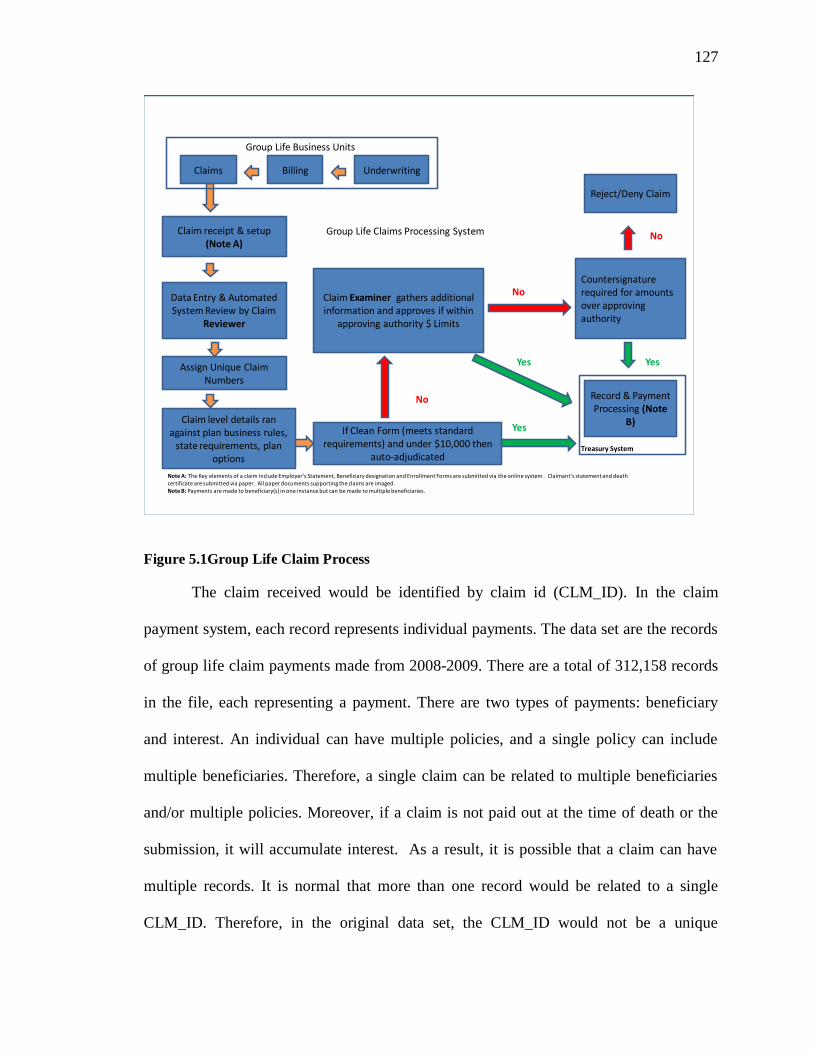
127
Group Life Claims Processing System Claim receipt & setup(Note A)
If Clean Form (meets standard requirements) and under $10,000 then
auto-adjudicated
Note A: The Key elements of a claim include Employer’s Statement, Beneficiary designation and Enrollment Forms are submitted via the online system . Claimant’s statement and death certificate are submitted via paper. All paper documents supporting the claims are imaged. Note B: Payments are made to beneficiary(s) in one instance but can be made to multiple beneficiaries.
Data Entry & Automated System Review by Claim
Reviewer
Assign Unique Claim Numbers
Claim level details ran against plan business rules,
state requirements, plan options
Record & Payment Processing (Note
B)
Claim Examiner gathers additional information and approves if within
approving authority $ Limits
Yes
No
Yes
NoCountersignature required for amounts over approving authority
Yes
Reject/Deny Claim
Claims UnderwritingBilling
No
Group Life Business Units
Treasury System
Figure 5.1Group Life Claim Process
The claim received would be identified by claim id (CLM_ID). In the claim
payment system, each record represents individual payments. The data set are the records
of group life claim payments made from 2008-2009. There are a total of 312,158 records
in the file, each representing a payment. There are two types of payments: beneficiary
and interest. An individual can have multiple policies, and a single policy can include
multiple beneficiaries. Therefore, a single claim can be related to multiple beneficiaries
and/or multiple policies. Moreover, if a claim is not paid out at the time of death or the
submission, it will accumulate interest. As a result, it is possible that a claim can have
multiple records. It is normal that more than one record would be related to a single
CLM_ID. Therefore, in the original data set, the CLM_ID would not be a unique

128
identifier of the record. However, each claim is referred to by CLM_ID. They are
approved, denied or frozen by CLM_ID. Therefore, the analysis will be performed on and
presented by CLM_ID
From the 312,158 records, there are 181,176 claims in the data set. The
distribution of claim by quarter is listed in Table 5.2
Table 5.2 Distribution of Claim by Quarter
5.5.2 Attributes
The data is comprised of 208 attributes related to information of group life claims.
The attributes are categorized into 6 groups.
o Insured.
o Dependent
o Coverage
o Group / Company
o Beneficiary
o Payment.
Many attributes are left blank, either because the fields have not been filled in, or because
the attributes are not used. From the total 208 attributes, 92 attributes have more than
15% missing values, 21 attributes have a single value, 15 attributes are identification
Period Number of Claim
Q1 2008 36208
Q2 2008 36408
Q3 2008 34316
Q4 2008 34164
Q1 2009 40080

129
type(i.e. Name, Last name, Tax ID, Customer ID, Employee ID and etc.), and 8 attributes
contain date related data. If the date related attributes are not related directly to the
payment, they are known to be inaccurate. In other words, if the date is not a payment
date (either interest or beneficiary payment), its accuracy cannot be guaranteed. Though
there might be some input controls to ensure that improper and/or incorrect information
was not entered into the database, the input controls may not be able to detect when
employees are deliberately entering inaccurate data. Therefore, these attributes should be
excluded from the analysis. A summary of this basic information is presented in Figure
5.2. The remaining attributes are those attributes which do not have these shortcomings.
The absence of these deficiencies cannot guarantee that they will be useful for all
analysis. The list of these attributes is shown in Table 5.3 .
After checking the values of the remaining attributes, other data quality problems
become apparent. Several attributes are designed to store coverage information. There are
two main types of coverage amount: flat and multiple factor. Flat coverage refers to a
fixed dollar amount. Multiple factor coverage can be based on many different factors
such as 2X monthly salary, 1X annual income, etc. The data will be easily interpreted if
the company uses a certain or fixed number of attributes to collect this information.
There are several attributes supposedly holding the coverage information; for example,
coverage flat amount, coverage multiple factor, coverage percentage, coverage benefit
percentage, and coverage benefit flat amount. The company‘s recording policies are not
consistent. The same data element may be recorded in one of many attributes. In addition,
there are cases where the coverage is fixed; however, the information on multiple factors

130
is also present. Therefore, it is impossible to derive the exact amount of payment by
combining or calculating values from attributes holding related information.
After multiple examinations of the raw data file and consultation with the domain
experts (internal auditors), suggestions on attribute selection were developed. Based on
current control tests (see Table 5.1), the major concern of this group life business unit is
the payment. Several existing tests relate to the reasonableness of the interest payment
and the beneficiary payment. In addition, the internal auditors specifically communicate
that they are in search of better and more useful techniques to test the reasonableness of
the values.
Figure 5.2 Summary of Attribute Information
All Attributes 208
Less:
Attributes with more than 15% missing values -92
Attributes with single values -22
Identification type of attributes (TAXID, CUSTOMER ID, EMPLOYEE ID
and etc) -15
Date information (such as birthdate, hiring date, final work date and etc.) -8
Remaining attributes 71

131
Table 5.3 List of Remaining Attributes
Attribute Name Expanded Attribute Name Attribute Name Expanded Attribute Name
CLM_ID Claim ID Insured_CLI_CITY_NM_TXT CITY
CLM_STAT_CD Claim Status Code Beneficiary_CLI_PSTL_CD ZIPCODE
BASE_ANN_INCM_AMT Base Annual Income Amount Insured_CLI_ADDR_LN_1_TXT ADDRESS
TEAM_CD Team assigned to claim in Oriskany Company_Division_CLI_CTRY_CDCOUNTRY
COMB_RSK_POOL_AMT Combined Risk Pool Amount MULT_LVL_INCR_IND Multiple Level Increase Ind
BNFY_TYP_CD Beneficiary - Type XCES_RSK_POOL_IND Excess Risk Pool Indicator
Beneficiary_CLI_CTRY_CD US COMB_RSK_POOL_IND Combined Risk Pool Indicator
FRGN_RES_IND Foreign Resident Indicator SITUS_ST_CD Situs State code
PAYE_TYP_CD Payee Type code Insured_CLI_CRNT_LOC_CD STATE
PMT1_AMT Payment Amount 1 PMT1_MTHD_CD Payment method payment 1
PMT_DT Payment Date Beneficiary_CLI_CRNT_LOC_CD STATE
PMT_STAT_CD Payment Status Code DLAY_PMT_INT_CD delay payment interest code
SIB_INS_IND SIBI Insurance Indicator Insured_CLI_SEX_CD Sex
Beneficiary_CLI_CITY_NM_TXT CITY Insured_CLI_PSTL_CD ZIPCODE
BNFY_REL_INSRD_CD Beneficiary Relation to the insured CUST_CITY_TXT CITY
PMT_MTHD_CD__T5BEN_ Payment Method CUST_STATE_CD STATE
ABS_ASIGN_IND Absolute Assignment Indicator PMT_MTHD_CD__T5CVG_ Payment Method code
INS_CNCL_IND Insurance ever Cancelled Indicator INSRD_JOB_STAT_CD Job Status Code
CLMT_STMT_SIGN_IND Claimant Statement Sign indicator CUST_ADDR_LN_1_TXT ADDRESS
BCKUP_WTHLD_IND Backup Withhold Indicator CUST_PSTL_CD ZIPCODE
MAIL_TO_EMPLR_IND Mail to Employer Indicator MULT_PMT_MTHD_IND Multiple Payment method indicator
W8_BNFY_IND W8 Beneficiary Indicator SEND_CHK_TO_CD Send Check to code
ADDL_PMT_IND Additional Payment Indicator Beneficiary_CLI_SEX_CD Sex
CVG_NUM Coverage Number Insured_CLI_INDV_TITL_TXT Title
CVG_DESC_TXT Coverage Discription PERF_DY_DUR Performance Guarantee indicator
CLM_CVG_AMT Claim Coverage Amount NOTI_CLM_PMT_IND Notification of Claim Payment Ind
CVG_STAT_CD Coverage Status code PARTY_3RD_ADM_IND TPA Indicator
BASE_CVG_NUM Base Coverage Number FORM_712_IND 712 Form Indicator
CVG_FLAT_AMT Coverage Flat Amount Insured_CLI_MARIT_STAT_CD Marital Status
CVG_MULT_FCT Coverage Muliple Factor Beneficiary_CLI_INDV_TITL_TXT Title
CVG_PCT Coverage percent MINR_BNFY_IND Minor Beneficiary Indicator
CVG_BNFT_PCT Coverage benefit percent SPCL_HNDL_IND Special Handling required
CVG_BNFT_FLT_AMT coverage benefit flat amount Insured_LOSS_TYP_CD Loss Type Code
BNFY_DESGNT_CD Beneficiary Designation code Insured_MANNER_LOSS_CD Manner of Loss Code
HLD_HRMLESS_IND Hold Harmless Indicator Insured_CAUSE_LOSS_CD Cause of Loss code
PAR_IND Par/Non-Par indicator

132
Because of data quality issues and after consulting with internal auditors, a new
dataset was created based on the original data. Four newly created attributes were
selected for clustering:
Percentage: Total interest payment / Total beneficiary payment
AverageCLM_PMT: Average number of days between claims received date and
the payment date (a weighted average is used because a claim could have multiple
payment dates)
DTH_CLM: Number of days between death date and claim received date.
AverageDTH_PMT: Average number of days between death date and payment
date (a weighted average is used because a claim could have multiple payment
dates).
These attributes were normalized so they could be compared, minimizing the effect of
scale differences. These attributes will be used for cluster analysis.
5.6 Methodology
5.6.1 Clustering Procedure
Internal auditors perform quarterly audits. In order to mesh with the internal audit
analysis, the clustering procedure will be performed using the data by quarter. For this
initial work, the latest data, Q1 of 2009 will be used for the analysis.
Because all attributes are numeric, simple K-mean clustering is selected as the
clustering procedure. K-mean is a simple, well-known algorithm for clustering. It is less
computer intensive than many other algorithms, making it a preferable choice for large
datasets (Tan et al, 2006).

133
Because K-mean does not have the option to automatically use the number of
clusters to group the data, the number of clusters must be pre-selected. No matter how
many number of clusters the data set must be grouped to, the following steps would
generally the same.
The second step for K-mean clustering is to place each observation into a cluster.
This step can be done randomly or systematically. Centroids (or Center of cluster) must
be selected, then each observation is assigned to the closest centroid.
The third step would be to compute the distance between each observation and
the centroid. If the observation is not currently a member of the cluster with the closest
centroid, the observation must be reassigned to the new cluster, then new centroids will
be recalculated. The process from step three will repeat until there is no new assignment.
The steps in K mean clustering could be explained as follows (Roiger et al, 2003):
Here is the algorithm
1. Choose a value for K, the total number of clusters to be determined.
2. Choose K instances (data points) within the dataset at random. These
are the initial cluster centers.
3. Use simple Euclidean distance to assign to remaining instances to
their closest cluster center.
4. Use the instances in each cluster to calculate a new mean for each
cluster.
5. If the new mean values are identical to the mean values of the previous
iteration the process terminates. Otherwise, use the new means as
cluster center and repeat steps 3-5.
One way to measure the quality of a clustering is to use sum of squared error
(SSE) by computing the error of each data instance to its closest centroid, then computing
the total sum of the squared error (Tan et al, 2006). Clusters produce the lowest SSE
when the number of clusters is equal to the number of instances. An obvious and
probably simplest way to reduce SSE is to increase the number of clusters. Adding the

134
first cluster will decrease the SSE substantially. The higher number of clusters, the lower
SSE. However, at some point the marginal gain (the decreasing SSE) will be dropped. An
ideal number of clusters should be the one where adding an additional cluster will not
substantially reduce the SSE. A graph should be plotted to show the relationship between
the number of clusters and the resulting SSE in order to find ―elbow‖ (Alpaydin, 2004).
The drop in the marginal gain will create the elbow in the graph. Several numbers of
clusters have been tried. The resulting sums of squared errors are used to plot the graph to
find the suitable number of clusters. The number of clusters which create the elbow in the
graph is selected. Observations are grouped to a cluster. For the first combination,
representing the interest and total length of time in the claim payment process (i.e.
interest and death to payment), Percentage and AverageDTH_PMT are used. For the
second combination, representing the interest and the length of time in the claim payment
process in greater detail (i.e. interest, death to claim, death to payment, claim to
payment), all four variables are used.
The software packages used are WEKA1 and SAS. The data set will be cleaned
and transformed using SAS. The clean data is then exported into CSV format and then
converted into ARFF format in order to feed into WEKA.
5.6.2 Anomaly Detection
This research examines both individual observations and small clusters as
possible outliers. Most data points in the dataset should not be outliers. The outliers are
then identified in three ways:
1 WEKA (Waikato Environment for Knowledge Analysis), developed by The University of Waikato,
New Zealand, is an open source for machine learning written in Java. It is available at
http://www.cs.waikato.ac.nz/ml/weka/. It contains a large collection of tools for standard data mining tasks
such as data preprocessing, feature selection, classification and clustering. More details on WEKA can be
found at the website and Hall et al (2009).

135
First, observations that have low probability of being a member of a cluster
(i.e. are far away from other members of the clusters) are identified as outliers.
The probability of 0.6 is used as a cut-off point.
Second, clusters with small populations should be considered outliers. In this
aspect, clusters populated with less than 1% of the whole population are
considered as outliers.
Third, rule based extraction will be developed to aid anomaly detection.
Most clusters have large populations. Some well-populated clusters may still have
suspicious characteristic. Therefore, in addition to cluster-based outliers, rule-based
extraction might be applied in order to select a number of observations from highly
populated clusters and flag them as suspicious. These rules can be developed by
consulting with business managers with domain knowledge and internal auditors with
experience auditing the unit.
Based on the previous experiences, rules can be created. Internal auditors learn
from previously detected frauds how they were committed, then attempt to create
detection and protection for such incidents. Business rules and policy are set up as
guidance. If the rules are not observed by employees, company can suffer losses.
Therefore, testing if the business rules and policies are followed is important. Previous
fraud cases and business rules are used in creating a rule based detection system.
5.6.3 Rule-Based Anomaly Detection
Some rules were derived from examination of the data. Internal auditor found that
some data fields have been entered carelessly. Some information can be verified with
government issued data. However, some wrong dates can be identified easily without any

136
external help. For instance, the insured‘s calculated age should not be lower than sixteen,
the legal minimum employment age. After a simple calculation of the insured age, errors
in data entry have been uncovered in many claims.
In order to further identify suspicious claims, the following indicators/rules were
created.
• Age related rules:
– Age1= ―Y‖ if Birthday and/or Death date is available, otherwise Age1=
―N‖
– Age2= ―Y‖ if the calculated age is proper.
For example, If the insured‘s age, calculated from birth date – death date,
is lower than 16, Age2= ―N‖
If the insured age is lower than 50 and the INSRD_JOB_STAT_CD is
―R‖(for retired employee), then Age2= ―N‖
• Causes/Manner of loss relation
– CAUSE1= ―Y‖ if both Insured_MANNER_LOSS_CD AND
Insured_CAUSE_LOSS_CD are available
– CAUSE2= ―Y‖ if the relationship between manner and cause of loss are
reasonable.
Insured_MANNER_LOSS_CD is related to the manner that a
person died. It is divided into 4 groups.
AC: Accident
HO: Homicide
NC: Natural Causes
137
PI: Pending Investigation
SU: Suicide
UD: Undetermined
Insured_CAUSE_LOSS_CD is related to the specific reason that a
person died such as specific disease, type of accident and etc. In order to
check the relationship of manner and cause of death the possible cause are
divided into 4 groups
Diseases causes
Accidental causes
Undetermined causes
Suicidal causes
If the manner is ―AC‖, the cause should not be diseases OR suicidal.
If the manner is ―HO‖, the cause should not be diseases OR suicidal.
If the manner is ―NC‖, the cause should not be accidental OR suicidal.
– CAUSE3= ―Y‖ if the manner is NOT ―PI-pending investigation‖ OR
―UN-undetermined‖ OR the cause of loss is ―UNDT-undetermined‖
The claim relating to unresolved death or pending investigation should not
be paid.
Date Related
– DATE1= ―Y‖ if the payment date is AFTER the claim received date.
Payment date should come after the claim received date. However,
some payment date appeared to precede their respective the received dates.
– DATE2= ―Y‖ if the claim is received AFTER the death date.

138
Life claim should be received, in most case, after a person died.
However, in some case, the claim is received before the death if the insured is
terminally ill.
– DATE3= ―Y‖ if, in the case of SUICIDE, the payment date is at least 2
years AFTER the death date.
Company policy dictates that payout will not occur until two years
after death in the case of suicide.
• Beneficiary Tax ID
– BID= ―Y‖ if the beneficiary has a tax id.
When the beneficiary does not have a tax id, a default number
‗99999999‘ is assigned to the beneficiary. If the default number has been
used, it would be extremely difficult to verify the duplication or the existence
of the specific beneficiary. It is possible to create a fictitious person to receive
a claim.
Having failed any specific test does not guarantee that a claim is fraudulent. There
can be legitimate reasons for such discrepancies. For example, if a beneficiary is a
foreigner, he/she will not have a tax id. If a claim is an accelerated benefit, the claim will
be received legitimately before death.
Failing these rules, however, can be an indicator of possible deceit. Each test
failure will be given a suspicious score of ―1‖. If it passes (―Y‖), the score would be ―0‖.
If it fails, the score will be ―1‖. The higher the score, the more suspect is the claim.

139
Different clusters can have different score distributions. The highest score for one
cluster can be different from another. Selecting cut-off points for the cluster will require
input from the domain experts, such as business managers and internal auditors.
5.7 Results
The 40,080 claims paid in the first quarter of 2009 are used in the analysis. Two
different combinations of attributes are used for clustering. First, the Percentage and
AverageDTH_PMT are used for initial clustering. Several numbers of clusters have been
tested. The relationship between the number of clusters and resulting sum of squared
errors is plotted as shown in Figure 5.3. From the graph, it is clear that adding an
additional cluster will reduce the SSE. However, at some point, the SSE will be reduced
at significantly lower rate. When the number of clusters is eight, adding an additional
cluster will insignificantly reduce the SSE from 3.9 (in eight clusters) to 3.4 (in nine
clusters). Therefore, in this particular dataset, the number of clusters selected should be
eight.
Figure 5.3Number of Clusters and Resulting Sum of Squared Error: 2 Attributes
0
2
4
6
8
10
12
14
16
18
20
2 3 4 5 6 7 8 9 10
SSE
No. of Clusters
Sum of Squared Error

140
The results from WEKA are represented in Table 5.4.
Table 5.4 Result of Cluster Analysis using Two Attributes from WEKA (Enhanced)
For the first set of clusters using two attributes, eight clusters are formed. About
90% of claims are clustered into cluster7 and 6% are in cluster0 (as shown in Table 5.4).
Three clusters (cluster1, cluster2, and cluster5) have membership of less than 1% of the
total. The numbers of claims in those clusters are 54, 84 and 31 respectively. Examining
the characteristics of these less populated clusters, some suspicious characteristics should
=== Run information ===
Cluster centroids:
Cluster#
Attribute Full Data 0 1 2 3 4 5 6 7
(40080) (2523) (54) (84) (222) (295) (31) (768) (36103)
N_AverageDTH_PMT 0 0.6374 15.177 3.5419 6.9858 0.8778 10.9006 2.7806 -0.1937
N_percentage 0 0.2666 1.8334 9.3405 0.5042 3.4637 26.6913 0.3185 -0.1057
Clustered Instances
0 2523 ( 6%)
1 54 ( 0%)
2 84 ( 0%)
3 222 ( 1%)
4 295 ( 1%)
5 31 ( 0%)
6 768 ( 2%)
7 36103 ( 90%)
Relation: TestSetPayment2
Scheme: weka.clusterers.SimpleKMeans -N 8 -A "weka.core.EuclideanDistance -R first-last" -I 500 -S 10
CLM_ID
Ignored:
N_percentage
N_AverageDTH_PMT
Attributes: 3
Instances: 40080
Missing values globally replaced with mean/mode
Within cluster sum of squared errors: 3.9256036521001687
Number of iterations: 55
Test mode: evaluate on training data
=== Model and evaluation on training set ===
kMeans
======
Clusters with small number of population

141
be mentioned. Claims in these clusters have high interest/beneficiary payment percentage
and/or claims with a long period of time from death dates to payment dates. Claims in
cluster5 have high interest / beneficiary payment percentage and a long period between
the death dates and the payment date. Cluster1 claims have long period from death to
payment dates. Claims in cluster2 have high interest/beneficiary payment. The total
number of claims identified as possible anomalies from cluster-based outliers is 169. In
addition to identifying small clusters, the probability of individual observations‘ cluster
membership is examined. The claims, which have lower than 0.6 probabilities of
belonging to the cluster they are assigned to, are identified as possible anomalies. 568
claims fit this criterion. The visualized results are shown in Figure 5.4.
Figure 5.4 Visualization of the Cluster Assignment for 2 attributes clustering; N_Percentage and
N_AverageDTH_PMT.

142
Figure 5.5 Visualization of the Clustering Result (Two Attributes) with Cluster Marked
It is clear that cluster1, cluster2 and cluster5 have fewer members and are sparser.
Characteristics of claims in these clusters are different from the majority of claims in
other clusters. Having different characteristics does not necessarily signal abnormality or
fraud. There are possibly legitimate reasons; for example, a claim may have high interest
because it was in the system for a long time. If the insured died a long time before the
claims are submitted; accumulated interests will be high. These legitimate reasons,
however, should be considered with caution. Several questions should be asked. For
example,
– If the claim was in the system for a long time
o Why were the claims in the system for that long?
Document issues
Cluster 1
Cluster 5
Cluster 2

143
Was it because the document was incomplete?
What document was it?
Why did it take long time?
Beneficiary issues
Was it because difficulty in tracking down the
beneficiaries?
Why was it difficult?
Were they out of the country?
Did they have their name changed?
What were the dollar amounts they received?
– If the insured died a long time before the claim was submitted
o Why did it take time? Was it because the beneficiaries were
unaware of the policy?
o Who were the beneficiaries? What were the dollar amounts they
received?
Answers to these questions should not be taken lightly. Knowledge of such a
policy, if fell into wrong hands, might create an opportunity for someone to commit
insurance fraud. For example, if it has taken a long time to collect the document because
the beneficiaries are out of reach, how can we be sure that the individuals who appear to
be the previously unreachable beneficiaries are the person who they say they are? What if
someone else is hired to pretend to be the missing beneficiaries? What if the real
beneficiaries are unaware of the policy, but someone else pretends to be them and cash
out the payment? When an insurance claim is submitted but not paid for a long time, or it

144
has taken a long time to submit, and then one day it gets paid, the internal auditor should
exert caution. There are several possibilities and opportunities for fraud.
Internal auditor should check not only those claims with no explanation, but also
those with unsound explanation.
For the second set of cluster analysis, four attributes are used. Several numbers of
clusters have been tested to find the suitable one. For this data set with four attributes,
number of cluster selected is thirteen. The Figure 5.6 illustrates that when an additional
number of clusters is added, the resulting sum of squared error is decreased, until a
certain point similar to the previous case with two attributes..
Figure 5.6Number of Clusters and Resulting Sum of Squared Errors: 4 Attributes
0
5
10
15
20
25
5 6 7 8 9 10 11 12 13 14 15
SSE
No. of Clusters
Sum of Squared Error

145
Table 5.5 Result of Cluster Analysis using Four Attribute from WEKA (Enhanced)
About 81% of claims fall into cluster8. Six clusters are populated with less than
1% of the claims (from Table 5.5). These are cluster2, cluster3, cluster5, cluster10,
cluster11 and cluster12. The numbers of claims in those clusters are 194, 98, 30, 39, 110
and 97, respectively. Because of time and budget constraints, it is impractical to follow
up on all of the claims in the suspicious clusters. Therefore, not all small clusters are
selected for further investigation. Not all available explanation will sound reasonable. All
the small clusters should be closely examined. From these six small clusters, the one that
has interesting characteristics and should be selected for the follow up in greater details is
=== Run information ===
Scheme: weka.clusterers.SimpleKMeans -N 13 -A "weka.core.EuclideanDistance -R first-last" -I 500
-S 10
Relation: TestSetPayment4
Instances: 40080
Attributes: 6
N_AverageCLM_PMT
N_DTH_CLM
N_AverageDTH_PMT
N_percentage
Test mode: evaluate on training
data
=== Model and evaluation on training set ===
kMeans
======
Number of iterations: 110
Within cluster sum of squared errors:
8.938107429242356
Missing values globally replaced with
mean/mode
Cluster centroids:
Cluster#
Attribute Full Data 0 1 2 3 4 5 6 7 8 9 10 11 12
(40080) (510) (343) (194) (98) (3699) (30) (1275) (741) (32658) (286) (39) (110) (97)
======================================================================================================================
=============
N_AverageCLM_PMT 0 3.3277 5.847 1.1228 0.9334 0.2657 1.0787 1.4446 -0.0175 -0.2593 0.3256 1.2762 9.8053 4.0441
N_DTH_CLM 0 0.0465 0.2918 5.6314 9.2662 -0.0994 11.5083 -0.1067 0.8305 -0.1278 2.8859 17.3103 0.3974 0.4875
N_AverageDTH_PMT 0.0004 1.2373 2.3694 5.638 8.9342 0.0078 11.0603 0.399 0.7809 -0.211 2.7915 16.5008 3.8038 1.9042
N_percentage -0.0013 0.2109 0.1571 1.7843 0.6634 0.1131 26.8887 0.5127 0.4848 -0.1232 1.0013 2.2243 0.3016 7.7798
Clustered Instances
0 510 (1%)
1 343 (1%)
2 194 (0%)
3 98 (0%)
4 3699 (9%)
5 30 (0%)
6 1275 (3%)
7 741 (2%)
8 32658 (81%)
9 286 (1%)
10 39 (0%)
11 110 (0%)
12 97 (0%)
Clusters with small number of population

146
cluster12. This cluster has a high interest/beneficiary percentage, while the length of time
from the death to payment date is not as high. The length of time is a very important
factor for determining the amount of interest. The important question the internal auditor
should ask is why the interest rate is high. The explanation given should also be reviewed
to check for its validity.
In addition to identifying small clusters as possible anomalies, the probability of
individual observations‘ cluster membership is examined. A distance-based outlier in a
dataset is a data instance having a distance far away from the center of the cluster.
Probability distribution over the clusters for each data instance is calculated. The data
instance which has the highest probability lower than the cut-off point will be identified
as possible outliers. Using probability of 0.6 as the cutoff point, 325 claims and 547
claims are identified as possible anomalies from two attributes and four attributes
clustering results respectively.

147
Figure 5.7 Visualization of the Cluster Assignment for 4 attributes clustering: N_Percentage,
N_AverageDTH_PMT, N_AverageCLM_PMT, N_DTH_CLM.
Figure 5.8 Visualization of the Clustering Result (Four Attributes) with Marks
Cluster 12

148
The results from these two settings (two and four attributes) for cluster analysis
and its two anomaly detection are presented inTable 5.6.
Table 5.6 Summary of the Results from Cluster Analysis
Suspicious claims should be investigated further by the internal auditor to
determine the efficacy of the clustering effort. The results from the follow up would help
to improve the model.
Time and budget constraints prohibit investigation of all claims in all suspicious
clusters. Moreover, some suspicious clusters may be highly populated. Therefore, in
addition to cluster-based outliers, rule-based extractions would be used to filter claims for
further investigation.
The results from the cluster analysis would be used for this step. All claims would
be tested by using the rules in the previous section. The total possible score is nine. The
claims which did not pass this filter are summarized in Table 5.7. The results demonstrate
that this dataset has quality issues. Several important pieces of information are missing or
incorrect (for example, birth date and death date). Some information is not updated (for
example, the manner of lose is still shown as pending, while, the payment is made- A
claim payment should not be made if the case is still under investigation).
Inquiries regarding these issues did not result in satisfactory conclusion. For
example, the company acknowledges the data quality issues; however, instead of
expressing an interest in minimizing or eliminating the problems, they accept the bad
Cluster Analysis
Cluster-Based
Outliers
Distance-Based
Outliers
Cluster Analysis with 2 Attributes 169 325
Cluster Analysis with 4 Attributes 568 547
149
quality data and try to work with it. When questions about cases under investigation are
asked, the company responds that it is highly likely that the cases have already been
concluded but the data have not been updated.
In some cases, failing the rules indicates that domain knowledge is required and
further investigation is needed. Cases where claim dates precede death date, for instance,
might arouse suspicion. However, if an insured is terminally ill, he/she may need
accelerated benefit payments to cover hospital expenses. Therefore, the claim should be
submitted, reviewed and paid before the insured dies. For this kind of situation, the
insurance company relies on the opinion of the doctor who is taking care of the insured.
If the doctor provides proof that the insured is terminally ill, the insurance company will
accept the doctor‘s opinion and approve the payment. If a claim fails this rule test, the
internal auditor should first check to see if the insured is terminally ill. If the insured is
indeed seriously ill, the claim should not be flagged.

150
Table 5.7 Number of Claims fails the test (rule-based filtering)
The score distribution is presented in Table 5.8 and Table 5.9. The highest scores
for each cluster are widely distributed. It appears that no single claim fails multiple rules.
Therefore, there is no claim shown with a score higher than 4, and only 16 claims have a
total score of 3. Because the highest scores in each cluster are not the same, the
investigation thresholds for each cluster should not be the same. For example, only five
clusters have the highest score of 3. If the score of three is used as universal cutoff point,
there will be only claims from those five clusters. Judgment can also be made if a
Rules Number of Claims
If Birthday and/or Death date is NOT available 13
If a proper age CAN NOT be calculated from the
information 18
If both Insured_MANNER_LOSS_CD AND
Insured_CAUSE_LOSS_CD are NOT available 269
If the relationship between manner and cause of loss
are NOT reasonable. 31
If the manner is ―PI-pending investigation‖ OR ―UN-
undetermined‖ OR the cause of loss is ―UNDT-
undetermined 197
If the beneficiary has NO tax id 402
If the payment date is BEFORE the claim received
date 12
If the claim is received BEFORE the death date 72
If, in the case of SUICIDE, the payment date is at
LESS THAN 2 years AFTER the death date 107

151
universal cut off point is desired. For example, if the score of two is used as a universal
cutoff point, there will be a total of 157 claims flagged: 141 claims with the score of 2
and 16 claims with the score of 3. The number of flagged claims from cluster0 and
cluster6 can be considered too many for the internal auditor to do the detailed follow-up.
If it is more reasonable that some claims from each cluster should be flagged, different
cutoff points should then be applied for each cluster.
Table 5.8 Suspicious Score Distribution by Cluster: Two Attributes
Table 5.8 and Table 5.9 show that suspicious score has no relation with clusters
(i.e. 16 claims have the score of 3 from both clustering results). At this stage the rules are
created using general business rules and policy. Therefore, the clustering results have no
effect on the score. With no rule created from cluster analysis, the potential usages for
cluster analysis with these results are that the results can be used for setting the cutoff
points.
SCORE
CLUSTER 0 1 2 3 Grand Total
cluster0 2181 289 46 7 2523
cluster1 45 5 4 54
cluster2 83 1 84
cluster3 183 33 5 1 222
cluster4 278 16 1 295
cluster5 31 31
cluster6 534 169 61 4 768
cluster7 35095 980 24 4 36103
Grand Total 38430 1493 141 16 40080

152
Table 5.9 Suspicious Score Distribution by Cluster: Four Attributes
SCORE
CLUSTER 0 1 2 3 Grand Total
cluster0 336 136 35 3 510
cluster1 192 110 40 1 343
cluster2 169 19 6 194
cluster3 81 14 2 1 98
cluster4 3468 219 9 3 3699
cluster5 30 30
cluster6 1042 210 17 6 1275
cluster7 706 33 2 741
cluster8 31949 694 15 32658
cluster9 264 19 1 2 286
cluster10 34 2 3 39
cluster11 67 33 10 110
cluster12 92 4 1 97
Grand Total 38430 1493 141 16 40080

153
5.8 Conclusions
As information technology has never stopped advancing, business processes are
also getting more complicated. Deception and fraudulent actions also increase in
complexity. Simple observation and traditional detection techniques can no longer
recognize such activities. Companies are not only having to find new and innovative way
to run their businesses, but they are facing more difficult tasks in control and monitoring
their advanced business processes. Manual, quarterly and annually audit activities are no
longer enough to protect the integrity of their financial information system. To keep up
with technological advancement, businesses need to find new and innovative ways to
control and monitor their processes. Technology and techniques from other discipline
have been adopted and applied in business. Borrowed from other business fields, cluster
analysis as an unsupervised learning algorithm is a good candidate for fraud and anomaly
detection techniques. It makes use of the powerful information system, receives input
from transaction systems, performs the analysis and provide the results to the internal
auditor for the follow up or further investigation. Clustering can be used to group
transactions so that different attention and efforts could be applied to each cluster so that
it will reduce time and efforts required in the audit process.
This study examines the possibility of using clustering technique for auditing.
Cluster analysis is applied to a data set from a major life insurance company in the United
States. Group life insurance claims were grouped into clusters of claims. Claims with
similar characteristics were grouped together. Clusters with small populations were
flagged for further investigation.
154
Using cluster analysis to identify possible anomalies in the dataset of group life
insurance, claims with suspicious characteristics are identified. These are the claims
which have been in the systems for an extended period of time before approval and
payment, or for which the insured is dead for a long period of time before a claim is
submitted. In most cases, there are valid reasons to explain the anomalous characteristics.
The possible reasons are for example;
Required documents are missing,
Beneficiaries cannot be contacted,
Families are unaware of the insurance policy, or
Cases are on hold pending investigation.
Though the reasons mentioned above are valid, it is undeniably that it worthwhile
to take time to evaluate some of these cases. There is no real anomalous claim found
from this dataset; however, the suspicious characteristics of these claims are of interest to
the internal auditor.
Several parameters are available to researchers in order to perform cluster
analysis. One may select different options from others. Moreover, the resulting groups
may not be meaningful for further analysis. To clearly evaluate the results, researchers
need helps from people with domain knowledge.
This study is a preliminary step toward applying the cluster analysis in the field of
auditing. It shows that cluster analysis may be a useful technology for accounting.

155
5.9 References
Alpaydin, E. 2004. Introduction to Machine Learning (Adaptive Computation and
Machine Learning). The MIT Press. USA.
Brockett, P. L., X. Xia and R. A. Derrig. 1998. Using Kohonen‘s Self-organizing Feature
Map to Uncover Automobile Bodily Injury Claims Fraud. Journal of Risk and Insurance
65(2): 245-274.
Chandola, V., A. Banerjee and V. Kumar. 2009. Anomaly Detection: A Survey, ACM
Computing Surveys 41(3): Article 15.
Chaudhary, A., A. S. Szalay and A. W. Moore. 2002. Very Fast Outlier Detection in
Large Multidimensional Data Sets. Proceeding of ACM SIGMOD Workshop in Research
Issues in Data Mining and Knowledge Discovery (DMKD), ACM Press.
Davidson, I. 2002. Visualizing Clustering Results. Proceeding SIAM International
Conference on Data Mining April 2002. University of Illinois at Chicago.
Duan, L., L. Xu, Y. Liu and J. Lee. 2009. Cluster-based Outlier Detection. Annuals of
Operational Research 168: 151-168.
Ertoz, L., M., Steinbach, and V. Kumar. 2003. Finding Topics in Collections of
Documents: A Shared Nearest Neighbor Approach. Clustering and Information
Retrieval: 83-104.
Estor, M., H. P. Kriegel, J. Sander and X. Xu. 1996. A Density-Based Algorithm for
Discovering Clusters in Large Spatial Databases with Noise, Proceeding of Second
International Conference on Knowledge Discovery and Data Mining: 226-231. E.
Simoudis, J. Han, and U. Fayyad, Eds. AAAI Press. Portland, Oregon.
Guha, S., R. Rastogi, and K.Shim. 2000. ROCK, A Robust Clustering Algorithm for
Categorical Attributes. Information Systems 25(5): 345-366.
Hall, M., E. Frank, G. Holmes, B. Pfahringer, P. Reutemann, I. H. Witten. 2009. The
WEKA Data Mining Software: An Update. SIGKDD Explorations 11 (1).

156
Hawkins, D. 1980. Identification of Outliers. Chapman and Hall. London, UK.
He, Z., X. Xu, and S. Deng. 2003. Discovering Cluster-Based Local Outliers. Pattern
Recognition Letters 24(9-10): 1641-1650.
Kachigan, S. K. 1991. Multivariate Statistical Analysis: a Conceptual Introduction.
Radius Press. New York, NY, USA.
Kohonen, T. 1997. Self-Organizing Maps. Springer-Verlag New York Inc. Secaucus, NJ,
USA.
Labib, K. and R.Vemuri. 2002. Nsom: A Real-Time Network-Based Intrusion Detection
using Self-Organizing Maps. Networks and Security.
Ramadas, M., S. Ostermann, and B. C. Jeden. 2003. Detecting Anomalous Network
Traffic with Self-Organizing Maps. Proceeding of Recent Advances in Intrusion
Detection: 36-54.
Roiger R. J. and M. W. Geatz. 2003. Data Mining: A Tutorial-Based Primer
(International Edition). Pearson Education, USA.
Sheikholeslami, G., S. Chatterjee, and A. Zhang. 1998. Wavecluster: A Multi-Resolution
Clustering Approach for Very Large Spatial Databases, Proceedings of the 24rd
International Conference on Very large Data Bases: 428-439. Morgan Kaufmann
Publishers Inc. San Francisco, CA, USA.
Smith, R., A. Bivens, M. Embrechts, C. Palagiri and B. Szymanski. 2002. Clustering
Approaches for Anomaly Based Intrusion Detection. Proceedings of Intelligent
Engineering Systems through Artificial Neural Networks: 579-584, ASME Press.
Sun, H., Y. Bao, F., Zhao, G. Yu and D. Wang, 2004, Cd-trees: An Efficient Index
Structure for Outlier Detection, Proceedings of the 5th
International Conference on Web-
Age Information Management (WAIM): 600-609.

157
Tan, P-N, M. Steinbach and V. Kumar. 2006. Introduction to Data Mining. Pearson
Education, Inc, USA.
Yu, D., G. Sheikholeslami and A. Zhang. 2002. Findout: Finding Outliers in Very Large
Datasets, Knowledge and Information Systems 4(4): 387-412.

158
Chapter 6 Summary, conclusions, paths for further research, limitations
6.1 Summary of the results and implications
6.1.1 Cluster Analysis
Clustering as an unsupervised learning algorithm is a good candidate for fraud
and anomaly detection. Without further investigation, there is no way to know for sure
that a particular transaction is fraudulent. In other words, the transactions are not clearly
identified as fraudulent or legitimate. It is often difficult to identify suspicious
transactions. Clustering could be used to group transactions so that different attention
and strategies could be applied to each different cluster. Outliers or anomalies could be
identified.
This study examines the possibility of using the cluster analysis in auditing. The
result shows that it is a useful technique for the accounting profession. It could be used in
the area of automatic detection and continuous control and monitoring.
6.1.2 Anomaly detection using cluster analysis
Theoretically, outliers are a by-product of cluster analysis (Ester et al, 1996,
Agrawal et al, 1998, Aggarwal et al, 1999). Regarding to the use of cluster analysis for
anomaly detection; however, there is no study in the literature conducted using real world
data. Several studies have been using synthetic data or seeded errors. Considering the
nature of the technique, it is understandable why a researcher has to choose the type of
data set. Anomaly detection is a subjective matter. What will be defined as anomaly?
What will be the definition of outliers? These problems require the knowledge of domain
experts. Because of the unsupervised nature of the cluster analysis, it is extremely
difficult, if not impossible, to evaluate the results. Expert feedback is needed. With the

159
unique knowledge that the experts have about the domain, they will be able to provide the
insight or information useful in the model building process.
Without the help from domain experts, researchers will have very difficult time to
evaluate results. Therefore, using seeded errors seems to be reasonable choices.
6.2 Primary Contribution
Prior literature suggests many fraud detection techniques using data mining
(Fanning et al, 1995, Green et al. 1997, Deshmukh et al, 1997, Fanning et al, 1998, Lin et
al, 2003 Bakar et al, 2006). These models identify fraudulent firms using Accounting and
Auditing Enforcement Releases (AAER) by the U.S. Securities and Exchange
Commission or private datasets.
Because these models require fraud samples (i.e. fraud/none fraud firms) and/or
use the data that is unique and not easily obtained, the models are not easily applicable in
other real world settings. The main problem of inapplicability comes from the fact that it
is extremely difficult, if not impossible, to identify fraudulent firms or transactions with
total confidence. Therefore, if a fraud detection model can be developed that can sidestep
this difficulty it will be very useful. Consequently, cluster analysis, an unsupervised
learning algorithm, which does not require the knowledge of fraud/non fraud sample is a
good candidate for fraud and anomaly detection.
This study examines the possibility of using clustering techniques for auditing.
Cluster analysis is applied to three datasets, one dataset is from an international bank and
two datasets are from a major life insurance company in the United States.

160
In the first setting, cluster analysis is used to uncover seven major types of
transactions in transitory accounts. These major types or groups of transactions from
branches were not previously known to the bank. Therefore, the clustering results provide
new knowledge about transactions. This knowledge can possibly be used for creating
new controls or detection rules in the transitory account system.
In the second setting, four anomaly detections techniques from cluster analysis are
examined using a wire transfer dataset. There is no wire identified as possible anomaly
by all four methods. Twenty-three and Eighty-one wire transfers are identified by three
and two techniques respectively. No wire identified by all method can mean no real
anomalous wires in the dataset. However, this explanation is highly unlikely. Because of
underlining assumptions in each detection technique, different wire transfers are
identified. Therefore, using different parameters, clustering techniques, and/or
assumption can create significantly different results.
In the third setting, anomaly detection based on cluster analysis is applied to
group life insurance claim. Clusters of claims with suspicious characteristics (i.e. being in
the claim payment system for a long time before payment, and having a large interest
payment) are identified as possible anomalies. Though these claims may not be real
anomalies, they possess characteristics which are worth for internal audit to investigate
further.
Overall, this study is only a preliminary step toward applying cluster analysis in
the field of auditing. It shows that cluster analysis may be a useful audit technology.
Automating fraud filtering can be of great value to audits.

161
Cluster analysis is a very promising technique that can be integrated into a
schema of continuous system monitoring and assurance. Archival studies of data trends
will reveal acceptable clusters and problematic ones, Experience, judgment, and
monitoring procedures will evaluate these clusters, and categorize data. Progressively,
clustering findings can be impounded into a priori processing filters and block
transactions with bad weightings from processing. These filtered transactions will be
routed to auditors (Vasarhelyi et al, 2010; Vasarhelyi et al, 1991) for review and
subsequent action. Clustering results will provide an innovative and unique group of
transactions for auditors to follow up. Therefore, traditional views for looking at results
may not be enough.
From the introduction of the first application of continuous auditing in AT&T
Bell Laboratories in 1989 (Vasarhelyi et al, 1991) to newer applications in a health
organization and in an international bank (Vasarhelyi et al, 2010), audit tasks become
increasingly automatic and more computer intensive. Newer and more advanced
technology is needed.
6.3 Limitations
There are several options (i.e. distances or similarity measures, clustering
algorithms) and/or parameters available for a researcher to choose when performing
cluster analysis. Therefore, for the same dataset, one researcher may choose a different
distance measurements and/or different clustering algorithm from another researcher. It
does not necessarily mean that one is right and the other is wrong. While one may select
different options from others, there is no one correct method. A technique/parameter may

162
be selected because it would make more sense/ produce a clearer/better interpretation of
the results.
Cluster analysis is a very computationally intensive process. It can take unusual
long time to run and provide results. To perform the analysis on a large dataset, a very
powerful computer system is needed. Such a system can be extremely expensive. It can
create problems for small companies wishing to try the technology. Pre-processing the
dataset is also an alternative to speed up the analysis. Attributes can be transformed so
that they take shorter time to be processed. Though the transformation can speed up the
analysis, it can distort the meaning of the attributes. The transformed attributes may or
may not have influences on how results will be interpreted. Therefore, results should be
interpreted with care.
Cluster analysis will always produce grouping. However, a result may be
statistically meaningful, while, at the same time, it does not provide any useful meaning.
Given the nature of cluster analysis, to evaluate if results are useful requires the help from
domain experts. It may or may not prove to be useful for the purpose that it is intended.
The grouping may be useful or useless is a question of the application. Researchers need
the expertise of people with domain knowledge for proper evaluation and interpretation
of results. Without help and support from internal auditors, domain experts, good and
useful clustering results will be difficult to obtain.
6.4 Future Research
This study, as an initial examination of the usage of clustering technology for
auditing, is a good starting point. There are many possibilities for future research.

163
1. Cluster analysis can be used together with rule-based extractions in order
to build the automatic fraud detection. There should be a study to combine
the two methods or techniques together. Some possibilities are as follows:
a. To use cluster analysis to create groups and, from the clustering
results, to use rule-based extractions to create rules to detect
possible anomaly in clusters.
b. To use results from cluster analysis as one of the rule to detect
anomalous transaction
c. To use several rules to test or evaluate the dataset and use cluster
analysis as an alternative technique to conclude the results from the
rule.
2. Other algorithms and techniques in cluster analysis can also be tested.
There are several clustering techniques available for the researcher to
choose from. Some techniques may be appropriate for one dataset but not
the other. Moreover, within one technique selected, there are a number of
parameters to specify or to select. This study is only a preliminary trial of
cluster analysis in the field of auditing. With the limitation on time and the
availability of the technique in the software, only a number of techniques
and parameter set have been selected. Therefore, other algorithms and
techniques should also be examined in order to evaluate the suitability of
this methodology in the field of auditing.

164
3. Other attributes and/or combinations of attributes can be used to
investigate the usefulness of these techniques. In this study, because of
data quality issues, only a few fields are recorded correctly or with care;
hence they are considered as - unreliable. Domain experts know and
accept the issues. They mention that they are working toward improving
the quality of the data entered into the system. Upon the improved quality
of data, with different data set, other attributes or combination of attributes
can be used; therefore possibly greater varieties and specification of the
clustering model can be examined.
4. Other data transformation techniques can be used to transform input
attributes. Several attributes are transformed for the ease of processing.
Transformation can affect results. Therefore, with different choices of
techniques, different results will be produced.
Cluster analysis is a very promising area for accounting research. There are
several possibilities that researchers should explore. With enough attention and support,
this technology would become as popular as it has been in the field of marketing.

165
6.5 References
Aggarwal, C.C., C. Procopiuc, J. L. Wolf, P. S. Yu and J. S. Park. 1999. Fast Algorithms
for Projected Clustering. Proceeding of ACM SIGMOD Conference 1999.
Agrawal, R., J. Gehrke, D. Gunopulos and P. Raghavan. 1998. Automatic Subspace
Clustering of High Dimensional Data for Data Mining Applications, Proceeding of the
1998 ACM SIGMOD international conference on Management of data 27(2).
Bakar, Z. A, R. Mohemad, A. Ahmad and M. M. Deris. 2006.A Comparative Study for
Outlier Detection Techniques in Data Mining. Proceeding of IEEE Conference on
Cybernetics and Intelligent Systems 2006.
Deshmukh, A. and T. Talluru. 1997. A Rule Based Fuzzy Reasoning System for
Assessing the Risk of Management Fraud. Journal of Intelligent Systems in Accounting,
Finance & Management 7(4): 669-673.
Ester, M., H.-P.Kriegel, J. Sander and X. Xu. 1996. A Density-Based Algorithm for
Discovering Clusters in Large Spatial Databases with Noise. Proceedings of Second
International Conference on Knowledge Discovery and Data Mining: 226-231.
Fanning, K., K. O. Cogger, K. O. and R. Srivastava. 1995. Detection of Management
Fraud: A Neural Network Approach. International Journal of Intelligent Systems in
Accounting, Finance & Management. 4(2): 113-126.
Fanning, K. M. and K. O. Cogger. 1998. Neural Network Detection of Management
Fraud Using Published Financial Data. International Journal of Intelligent Systems in
Accounting, Finance & Management 7: 21-41.
Green, B. and J Choi. 1997. Assessing the Risk of Management Fraud through Neural
Network Technology. Auditing: A Journal of Practices & Theory 16(1): 14-28.
Lin, J. W., M. I. Hwang, and J. D. Becker. 2003. A Fuzzy Neural Network for Assessing
the Risk of Fraudulent Financial Reporting. Managerial Auditing Journal 18(8): 657-665.

166
Vasarhelyi, M.A. and F. Halper. 1991. The Continuous Audit of Online Systems.
Auditing: A Journal of Practice and Theory 10 (1): 110-125.
Vasarhelyi, M.A., M. Alles, and K.T. Williams. 2010. Continuous Assurance for the Now
Economy. A Thought Leadership Paper for the Institute of Chartered Accountants in
Australia, Melbourne, May 2010.

167
CURRICULUM VITAE
Sutapat Thiprungsri
09/1977 Born in Uthai Thani/ Thailand
05/1996 Satri Nakhon Sawan, School
12/1999 Thammasat University, Bachelor of Science in
Accounting (International Program)
01/2003 College of Management, Mahidol University,
Master of Management in Entrepreneurship
Management
01/2012 Rutgers, The State University of New Jersey,
Ph.D. in Accounting Information Systems, Rutgers
Business School.