2012 state of the climate
DESCRIPTION
Climate Change state year 2012. Bulletin of American Metereological Society august 2013TRANSCRIPT
STATE OF THE CLIMATE IN 2012
Editors
Jessica Blunden Derek S. Arndt
Ahira Sánchez-Lugo
Wassila M. Thiaw
Peter W. Thorne
Scott J. Weaver
Kate M. Willett
Howard J. Diamond
A. Johannes Dolman
Ryan L. Fogt
Margarita C. Gregg
Bradley D. Hall
Martin O. Jeffries
Michele L. Newlin
James A. Renwick
Jacqueline A. Richter-Menge
Ted A. Scambos
Chapter Editors
AmericAn meteorologicAl Society
Technical Editor
Mara Sprain
HOW TO CITE THIS DOCUMENT
Citing the complete report:
Blunden, J., and D. S. Arndt, Eds., 2013: State of the Climate in 2012. Bull. Amer. Meteor. Soc., 94 (8), S1–S238.
Citing a chapter (example):
Jeffries, M. O., and J. Richter-Menge, Eds., 2013: Arctic [in “State of the Climate in 2012”]. Bull. Amer. Meteor. Soc., 94 (8), S111–S146.
Citing a section (example):
Tedesco, M., and Coauthors, 2013: [Arctic] Greenland ice sheet [in “State of the Climate in 2012”]. Bull. Amer. Meteor. Soc., 94 (8), S121–S123.
Cover Credits:
Front: Kate stafford — 2012 rUsALCA expedition, rAs-noAA, Wrangel island in the early morning
BACK: terry Callaghan, eU-interact/sergey Kirpotin, tomsk state University — trees take hold as permafrost thaws near the Altai Mountains in russia

SiAUGUST 2013STATE OF THE CLIMATE IN 2012 |
EDITOR & AUTHOR AFFILIATIONS (ALphABetiCAL By nAme)
Achberger, Christine, Department of Earth Sciences, University
of Gothenburg, Sweden
Ackerman, Stephen A., Cooperative Institute for Meteorologi-
cal Satellite Studies, University of Wisconsin Madison, Madison,
WI
Albanil, Adelina, National Meteorological Service of Mexico,
Mexico
Alexander, P., Department of Earth and Atmospheric Sciences,
City College of New York, New York, NY
Alfaro, Eric J., Center for Geophysical Research and School of
Physics, University of Costa Rica, San José, Costa Rica
Allan, Rob, Met Office Hadley Centre, Exeter, United Kingdom
Alves, Lincoln M., Centro de Ciencias do Sistema Terrestre
(CCST), Instituto Nacional de Pesquisas Espaciais (INPE),
Cachoeira Paulista, Sao Paulo, Brazil
Amador, Jorge A., Center for Geophysical Research and School
of Physics, University of Costa Rica, San José, Costa Rica
Ambenje, Peter, Kenya Meteorological Department (KMD),
Nairobi, Kenya
Andrianjafinirina, Solonomenjanahary, Direction de la Me-
teorologie Nationale de Madagascar, Tananarive, Madagascar
Antonov, John, NOAA/NESDIS National Oceanographic Data
Center, Silver Spring, MD; and University Corporation for
Atmospheric Research, Boulder, CO
Aravequia, Jose A., Centro de Previsão de Tempo e Estudos
Climáticos, INPE, Cachoeira Paulista, Sao Paulo, Brazil
Arendt, A., Geophysical Institute, University of Alaska Fairbanks,
Fairbanks, AK
Arévalo, Juan, Instituto Nacional de Meteorología e Hidrología de
Venezuela (INAMEH), Caracas, Venezuela
Arndt, Derek S., NOAA/NESDIS National Climatic Data Center,
Asheville, NC
Ashik, I., Arctic and Antarctic Research Institute, St. Petersburg,
Russia
Atheru, Zachary, IGAD Climate Prediction and Applications
Centre (ICPAC), Nairobi, Kenya
Banzon, Viva, NOAA/NESDIS National Climatic Data Center,
Asheville, NC
Baringer, Molly O., NOAA/OAR Atlantic Oceanographic and
Meteorological Laboratory, Miami, FL
Barreira, Sandra, Argentine Naval Hydrographic Service, Buenos
Aires, Argentina
Barriopedro, David E., Universidad Complutense de Madrid
(UCM), Spain
Beard, Grant, Bureau of Meteorology, Australia
Becker, Andreas, Global Precipitation Climatology Centre,
Deutscher Wetterdienst (DWD), Offenbach, Germany
Behrenfeld, Michael J., Oregon State University, OR
Bell, Gerald D., NOAA/NWS Climate Prediction Center, College
Park, MD
Benedetti, Angela, European Centre for Medium-Range
Weather Forecasts, Reading, United Kingdom
Bernhard, Germar, Biospherical Instruments, San Diego, CA
Berrisford, Paul, NCAS Climate, European Centre for Medium-
Range Weather Forecasts, Reading, United Kingdom
Berry, David I., National Oceanography Centre, Southampton,
United Kingdom
Bhatt, U., Geophysical Institute, University of Alaska Fairbanks,
Fairbanks, AK
Bidegain, Mario, Dirección Nacional de Meteorología, División
de Climatología, Uruguay
Bindoff, Nathan, Antarctic Climate and Ecosystems Cooperative
Research Centre, Hobart, Australia; and CSIRO Marine and
Atmospheric Laboratories, Hobart, Australia
Bissolli, Peter, Deutscher Wetterdienst, Germany
Blake, Eric S., NOAA/NWS National Hurricane Center, Miami,
FL
Blunden, Jessica, ERT Inc., NOAA/NESDIS National Climatic
Data Center, Asheville, NC
Booneeady, Raj, Mauritius Meteorological Services
Bosilovich, Michael, NASA/GSFC, Global Modeling and Assimila-
tion Office, Greenbelt, MD
Box, J. E., Geological Survey of Denmark and Greenland, Copen-
hagen, Denmark; and Byrd Polar Research Center, The Ohio
State University, Columbus, OH
Boyer, Tim, NOAA/NESDIS National Oceanographic Data Cen-
ter, Silver Spring, MD
Braathen, Geir O., WMO Atmospheric Environment Research
Division, Geneva, Switzerland
Bromwich, David H., Byrd Polar Research Center, The Ohio
State University, Columbus, OH
Brown, R., Environment Canada, Climate Research Division,
Montreal, Quebec, Canada
Brown, L., Climate Research Division, Environment Canada,
Downsview, Ontario, Canada
Bruhwiler, Lori, NOAA/OAR Earth System Research Laboratory,
Boulder, CO
Bulygina, Olga N., Russian Institute for Hydrometeorological
Information, Obninsk, Russia
Burgess, D., Geological Survey of Canada, Natural Resources
Canada, Ottawa, Ontario, Canada
Burrows, John, University of Bremen, Bremen, Germany
Calderón, Blanca, Center for Geophysical Research, University
of Costa Rica, San José, Costa Rica
Camargo, Suzana J., Lamont-Doherty Earth Observatory, Co-
lumbia University, Palisades, NY

Sii aUGUST 2013|
Campbell, Jayaka, Department of Physics, University of the
West Indies, Jamaica
Cao, Y., Ocean University of China, Qingdao, China
Cappelen, J., Danish Meteorological Institute, Copenhagen,
Denmark
Carrasco, Gualberto, Servicio Nacional de Meteorología e
Hidrología de Bolivia (SENAMHI), La Paz, Bolivia
Chambers, Don P., College of Marine Science, University of
South Florida, St. Petersburg, FL
Chang’a, L., Tanzania Meteorological Agency, Dar es Salaam,
Tanzania
Chappell, Petra, National Institute of Water and Atmospheric
Research, Ltd., Auckland, New Zealand
Chehade, Wissam, University of Bremen FB1, Bremen, Germany
Cheliah, Muthuvel, NASA/GSFC, Global Modeling and Assimila-
tion Office, Greenbelt, MD
Christiansen, Hanne H., Geology Department, University
Centre in Svalbard, UNIS, Norway; and Department of Geosci-
ences, University of Oslo, Oslo, Norway
Christy, John R., University of Alabama in Huntsville, Huntsville,
AL
Ciais, Phillipe, Laboratoire des Sciences du Climat et de
l’Environnement (LSCE), CEA-CNR-UVSQ, Gif-sur-Yvette,
France
Coelho, Caio A. S., CPTEC/INPE Center for Weather Forecasts
and Climate Studies, Cachoeira Paulista, Brazil
Cogley, J. G., Department of Geography, Trent University, Peter-
borough, Ontario, Canada
Colwell, Steve, British Antarctic Survey, Cambridge, United
Kingdom
Cross, J.N., School of Fisheries and Ocean Sciences, University of
Alaska Fairbanks, Fairbanks, AK
Crouch, Jake, NOAA/NESDIS National Climatic Data Center,
Asheville, NC
Cunningham, Stuart A., Scottish Marine Institute Oban, Argyll,
United Kingdom
Dacic, Milan, Republic Hydrometeorological Service of Serbia,
Belgrade, Serbia
De Jeu, Richard A.M., Department of Earth Sciences, Faculty of
Earth and Life Sciences, VU University Amsterdam, Amster-
dam, Netherlands
Dekaa, Francis S., Nigerian Meteorological Agency, Abuja,
Nigeria
Demircan, Mesut, Turkish State Meteorological Service, Ankara,
Turkey
Derksen, C., Environment Canada, Climate Research Division,
Toronto, Ontario, Canada
Diamond, Howard J., NOAA/NESDIS National Climatic Data
Center, Silver Spring, MD
Dlugokencky, Ed J., NOAA/OAR Earth System Research Labora-
tory, Boulder, CO
Dohan, Kathleen, Earth and Space Research, Seattle, WA
Dolman, A. Johannes, Department of Earth Sciences, Faculty of
Earth and Life Science, VU University Amsterdam, Amsterdam,
Netherlands
Domingues, Catia M., Antarctic Climate and Ecosystems Coop-
erative Research Centre, Hobart, Australia
Dong, Shenfu, NOAA/OAR Atlantic Oceanographic and Meteo-
rological Laboratory, Miami, FL; and Cooperative Institute for
Marine and Atmospheric Science, Miami, FL
Dorigo, Wouter A., Department of Geodesy and Geoinforma-
tion, Vienna University of Technology, Vienna, Austria
Drozdov, D. S., Earth Cryosphere Institute, Tumen, Russia
Duguay, Claude R., Interdisciplinary Centre on Climate Change
& Department of Geography and Environmental Management,
University of Waterloo, Waterloo, Ontario, Canada
Dunn, Robert J. H., Met Office Hadley Centre, Exeter, United
Kingdom
Dúran-Quesada, Ana M., Center for Geophysical Research and
School of Physics, University of Costa Rica, San José, Costa
Rica
Dutton, Geoff S., Cooperative Institute for Research in Environ-
mental Sciences, University of Colorado, Boulder, CO
Ehmann, Christian, Institute for Meteorology und Climate
Research (IMK), Karlsruhe Institute of Technology (KIT), Karl-
sruhe, Germany
Elkins, James W., NOAA/OAR Earth System Research Labora-
tory, Boulder, CO
Euscátegui, Christian, Instituto de Hidrología de Meteorología y
Estudios Ambientales de Colombia (IDEAM), Bogotá, Colombia
Famiglietti, James S., Department for Earth System Science,
University of California, Irvine, CA
Fang, Fan, Goddard Earth Sciences Data and Information Services
Center (ADNET), NASA, Greenbelt, MD
Fauchereau, Nicolas, National Institute of Water and Atmo-
spheric Research, Ltd., Auckland, New Zealand; and Ocean-
ography Department, University of Cape Town, Rondebosh,
South Africa
Feely, Richard A., NOAA/OAR Pacific Marine Environmental
Laboratory, Seattle, WA
Fekete, Balázs M., CUNY Environmental CrossRoads Initiative,
The City College of New York at CUNY, New York, NY
Fenimore, Chris, NOAA/NESDIS National Climatic Data Center,
Asheville, NC
Fioletov, Vitali E., Environment Canada, Measurements and
Analysis Research Section, Toronto, Ontario, Canada
Fogarty, Chris T., Environment Canada, Canadian Hurricane
Centre, Dartmouth, Nova Scotia, Canada
SiiiAUGUST 2013STATE OF THE CLIMATE IN 2012 |
Fogt, Ryan L., Department of Geography, Ohio University,
Athens, OH
Folland, Chris K., Met Office Hadley Centre, Exeter, United
Kingdom
Foster, Michael J., Cooperative Institute for Meteorological Sat-
ellite Studies, University of Wisconsin Madison, Madison, WI
Frajka-Williams, Eleanor, National Oceanography Centre,
Southampton, United Kingdom
Franz, Bryan A., NASA Goddard Space Flight Center, Greenbelt,
MD
Frith, Stacey H., NASA Goddard Space Flight Center, Greenbelt,
MD
Frolov, I., Arctic and Antarctic Research Institute, St. Petersburg,
Russia
Ganter, Catherine, Bureau of Meteorology, Melbourne, Australia
Garzoli, Silvia, NOAA/OAR Atlantic Oceanographic and Meteo-
rological Laboratory, Miami, FL; and Cooperative Institute for
Marine and Atmospheric Science, Miami, FL
Geai, M.-L., Department of Earth and Atmospheric Sciences,
University of Alberta, Edmonton, Alberta, Canada
Gerland, S., Norwegian Polar Institute, Fram Centre, Tromsø,
Norway
Gitau, Wilson, Department of Meteorology, University of Nai-
robi, Kenya
Gleason, Karin L., NOAA/NESDIS National Climatic Data Cen-
ter, Asheville, NC
Gobron, Nadine, European Commission, Joint Research Centre,
Institute for Environment and Sustainability, Italy
Goldenberg, Stanley B., NOAA/OAR Atlantic Oceanographic
and Meteorological Laboratory, Miami, FL
Goni, Gustavo, NOAA/OAR Atlantic Oceanographic and Meteo-
rological Laboratory, Miami, FL
Good, Simon A., Met Office Hadley Centre, Exeter, United
Kingdom
Gottschalck, Jonathan, NOAA/NWS Climate Prediction Cen-
ter, College Park, MD
Gregg, Margarita C., NOAA/NESDIS National Oceanographic
Data Center, Silver Spring, MD
Griffiths, Georgina, National Institute of Water and Atmospher-
ic Research, Ltd., Auckland, New Zealand
Grooß, Jens-Uwe, Forschungszentrum Jülich, Jülich, Germany
Guard, Charles “Chip”, NOAA/NWS Weather Forecast Office,
Guam
Gupta, Shashi K., Science Systems Applications, Inc., Hampton,
VA
Hall, Bradley D., NOAA/OAR Earth System Research Labora-
tory, Boulder, CO
Halpert, Michael S., NOAA/NWS Climate Prediction Center,
College Park, MD
Harada, Yayoi, Climate Prediction Division, Japan Meteorological
Agency, Tokyo, Japan
Hauri, C., School of Fisheries and Ocean Sciences, University of
Alaska Fairbanks, Fairbanks, AK
Heidinger, Andrew K., Cooperative Institute for Meteorological
Satellite Studies, University of Wisconsin, Madison, WI
Heikkilä, Anu, Finnish Meteorological Institute, Helsinki, Finland
Heim, Richard R., Jr., NOAA/NESDIS National Climatic Data
Center, Asheville, NC
Heimbach, Patrick, Massachusetts Institute of Technology,
Boston, MA
Hidalgo, Hugo G., Center for Geophysical Research and School
of Physics, University of Costa Rica, San José, Costa Rica
Hilburn, Kyle, Remote Sensing Systems, Santa Rosa, CA
Ho, Shu-peng (Ben), UCAR COSMIC, Boulder, CO
Hobbs, Will R., Scripps Institution of Oceanography, University
of California, San Diego, La Jolla, CA
Holgate, Simon, Sea Level Research, Liverpool, United Kingdom
Hovsepyan, Anahit, Climate Research Division, Armstatehy-
dromet, Armenia
Hu, Zeng-Zhen, NOAA/NWS Climate Prediction Center, Col-
lege Park, MD
Hughes, P., NOAA/NESDIS National Climatic Data Center,
Asheville, NC
Hurst, Dale F., Cooperative Institute for Research in Environ-
mental Sciences, University of Colorado, Boulder, CO
Ingvaldsen, R., Institute of Marine Research, Bergen, Norway
Inness, Antje, European Centre for Medium-Range Weather
Forecasts, Reading, United Kingdom
Jaimes, Ena, Servicio Nacional de Meteorología e Hidrología de
Perú (SENAMHI), Lima, Perú
Jakobsson, Martin, Department of Geological Sciences, Stock-
holm University, Stockholm, Sweden
James, Adamu I., Nigerian Meteorological Agency, Abuja, Nigeria
Jeffries, Martin O., Office of Naval Research, Arlington, VA; and
Geophysical Institute, University of Alaska Fairbanks, Fairbanks,
AK
Johns, William E., Rosenstiel School of Marine and Atmospheric
Science, Miami, FL
Johnsen, Bjorn, Norwegian Radiation Protection Authority,
Østerås, Norway
Johnson, Gregory C., NOAA/OAR Pacific Marine Environmental
Laboratory, Seattle, WA
Johnson, Bryan, NOAA/OAR Earth System Research Labora-
tory, Global Monitoring Division; and University of Colorado,
Boulder, CO
Jones, Luke T., European Centre for Medium-Range Weather
Forecasts, Reading, United Kingdom
Jumaux, Guillaume, Météo France, Réunion

Siv aUGUST 2013|
Kabidi, Khadija, Direction de la Météorologie Nationale du
Maroc, Rabat, Morocco
Kaiser, Johannes W., King’s College London, London, United
Kingdom; European Centre for Medium-Range Weather Fore-
casts, Reading, United Kingdom; and Max-Planck-Institute for
Chemistry, Mainz, Germany
Kamga, Andre, African Centre of Meteorological Applications for
Development, Niamey, Niger
Kang, Kyun-Kuk, Interdisciplinary Centre on Climate Change &
Department of Geography and Environmental Management,
University of Waterloo, Waterloo, Ontario, Canada
Kanzow, Torsten O., Helmholtz-Centre for Ocean Research Kiel
(GEOMAR), Kiel, Germany
Kao, Hsun-Ying, Earth & Space Research, Seattle, WA
Keller, Linda M., Department of Atmospheric and Oceanic Sci-
ences, University of Wisconsin-Madison, Madison, WI
Kennedy, John J., Met Office Hadley Centre, Exeter, United
Kingdom
Key, J., NOAA/NESDIS Center for Satellite Applications and
Research, Madison, WI
Khatiwala, Samar, Lamont-Doherty Earth Observatory, Colum-
bia University, Palisades, NY
Kheyrollah Pour, H., Interdisciplinary Centre on Climate Change
& Department of Geography and Environmental Management,
University of Waterloo, Waterloo, Ontario, Canada
Kholodov, A. L., Geophysical Institute, University of Alaska
Fairbanks, Fairbanks, AK
Khoshkam, Mahbobeh, Islamic Republic of Iranian Meteorologi-
cal Organization (IRIMO), Iran
Kijazi, Agnes, Tanzania Meteorological Agency, Dar es Salaam,
Tanzania
Kikuchi, T., Japan Agency for Marine-Earth Science and Technol-
ogy, Tokyo, Japan
Kim, B.-M., Korea Polar Research Institute, Incheon, Korea
Kim, S.-J., Korea Polar Research Institute, Incheon, Korea
Kimberlain, Todd B., NOAA/NWS National Hurricane Center,
Miami, FL
Knaff, John A., NOAA/NESDIS Center for Satellite Applications
and Research, Fort Collins, CO
Korshunova, Natalia N., All-Russian Research Institute of Hy-
drometeorological Information – World Data Center, Obninsk,
Russia
Koskela, T., Finnish Meteorological Institute, Helsinki, Finland
Kousky, Vernon E., NOAA/NWS Climate Prediction Center,
College Park, MD
Kramarova, Natalya, Science Systems and Applications, Inc.,
NASA Goddard Space Flight Center, Greenbelt, MD
Kratz, David P., NASA Langley Research Center, Hampton, VA
Krishfield, R., Woods Hole Oceanographic Institution, Woods
Hole, MA
Kruger, Andries, South African Weather Service, Pretoria, South
Africa
Kruk, Michael C., ERT Inc., NOAA/NESDIS National Climatic
Data Center, Asheville, NC
Kumar, Arun, NOAA/NWS Climate Prediction Center, College
Park, MD
Lagerloef, Gary S. E., Earth & Space Research, Seattle, WA
Lakkala, K., Finnish Meteorological Institute, Arctic Research
Centre, Sodankylä, Finland
Lander, Mark A., University of Guam, Mangilao, Guam
Landsea, Chris W., NOAA/NWS National Hurricane Center,
Miami, FL
Lankhorst, Matthias, Scripps Institution of Oceanography, Uni-
versity of California, San Diego, La Jolla, CA
Laurila, T., Finnish Meteorological Institute, Helsinki, Finland
Lazzara, Matthew A., Space Science and Engineering Center,
University of Wisconsin-Madison, Madison, WI
Lee, Craig, Applied Physics Laboratory, University of Washington,
Seattle, WA
Leuliette, Eric, NOAA/NESDIS Laboratory for Satellite Altim-
etry, Silver Spring, MD
Levitus, Sydney, NOAA/NESDIS National Oceanographic Data
Center, Silver Spring, MD
L’Heureux, Michelle, NOAA/NWS Climate Prediction Center,
College Park, MD
Lieser, Jan, Antarctic Climate and Ecosystems Cooperative
Research Center (ACE CRC), University of Tasmania, Hobart,
Tasmania, Australia
Lin, I-I, National Taiwan University, Taipei, Taiwan
Liu, Y. Y., School of Civil and Environmental Engineering, Univer-
sity of New South Wales, Sydney, Australia
Liu, Y., Cooperative Institute for Meteorological Satellite Studies,
University of Wisconsin, Madison, WI
Liu, Hongxing, Department of Geography, University of Cincin-
nati, Cincinnati, OH
Liu, Yanju, National Climate Center, China Meteorological Ad-
ministration, Beijing, China
Lobato-Sánchez, Rene, National Meteorological Service of
Mexico, Mexico
Locarnini, Ricardo, NOAA/NESDIS National Oceanographic
Data Center, Silver Spring, MD
Loeb, Norman G., NASA Langley Research Center, Hampton,
VA
Loeng, H., Institute of Marine Research, Bergen, Norway
Long, Craig S., NOAA/NWS National Center for Environmental
Prediction, College Park, MD

SvAUGUST 2013STATE OF THE CLIMATE IN 2012 |
Lorrey, Andrew M., National Institute of Water and Atmospher-
ic Research, Ltd., Auckland, New Zealand
Luhunga, P., Tanzania Meteorological Agency, Dar es Salaam,
Tanzania
Lumpkin, Rick, NOAA/OAR Atlantic Oceanographic and Meteo-
rological Laboratory, Miami, FL
Luo, Jing-Jia, Centre for Australian Weather and Climate Re-
search, Melbourne, Australia
Lyman, John M., NOAA/OAR Pacific Marine Environmental
Laboratory, Seattle, WA; and Joint Institute for Marine and
Atmospheric Research, University of Hawaii, Honolulu, HI
Macdonald, Alison M., Woods Hole Oceanographic Institution,
Woods Hole, MA
Maddux, Brent C., AOS/CIMSS University of Wisconsin Madison,
Madison, WI; and KNMI (Royal Netherlands Meteorological
Institute) De Bilt, Netherlands
Malekela, C., Tanzania Meteorological Agency, Dar es Salaam,
Tanzania
Manney, Gloria, Northwest Research Associates, Socorro, NM;
and New Mexico Institute of Mining and Technology, Socorro,
NM
Marchenko, S. S., Geophysical Institute, University of Alaska
Fairbanks, Fairbanks, AK
Marengo, Jose A., Centro de Ciencias do Sistema Terrestre
(CCST), Instituto Nacional de Pesquisas Espaciais (INPE),
Cachoeira Paulista, Sao Paulo, Brazil
Marotzke, Jochem, Max-Planck-Institut für Meteorologie, Ham-
burg, Germany
Marra, John J., NOAA/NESDIS National Climatic Data Center,
Honolulu, HI
Martínez-Güingla, Rodney, Centro Internacional para la Inves-
tigación del Fenómeno El Niño (CIIFEN), Guayaquil, Ecuador
Massom, Robert A., Australian Antarctic Division and Antarctic
Climate and Ecosystems Cooperative Research Center (ACE
CRC), University of Tasmania, Hobart, Tasmania, Australia
Mathis, Jeremy T., NOAA/OAR Pacific Marine Environmental
Laboratory, Seattle, WA
McBride, Charlotte, South African Weather Service, Pretoria,
South Africa
McCarthy, Gerard, National Oceanography Centre, Southamp-
ton, United Kingdom
McVicar, Tim R., CSIRO Land and Water, Canberra, Australia
Mears, Carl, Remote Sensing Systems, Santa Rosa, CA
Meier, W., National Snow and Ice Data Center, Cooperative
Institute for Research in Environmental Sciences, University of
Colorado, Boulder, CO
Meinen, Christopher S., NOAA/OAR Atlantic Oceanographic
and Meteorological Laboratory, Miami, FL
Menéndez, Melisa, Environmental Hydraulic Institute, Universi-
dad de Cantabria, Santander, Spain
Merrifield, Mark A., Joint Institute Marine and Atmospheric
Research, University of Hawaii, Honolulu, HI
Mitchard, Edward, School of Geosciences, University of Edin-
burgh, United Kingdom
Mitchum, Gary T., College of Marine Science, University of
South Florida, St. Petersburg, FL
Montzka, Stephen A., NOAA/OAR Earth System Research
Laboratory, Boulder, CO
Morcrette, Jean-Jacques, European Centre for Medium-Range
Weather Forecasts, Reading, United Kingdom
Mote, Thomas, Department of Geography, University of Geor-
gia, Athens, GA
Mühle, Jens , Scripps Institution of Oceanography, University of
California San Diego, La Jolla, CA
Mühr, Bernhard, Lacunosa Weather Services, Karlsruhe, Ger-
many
Mullan, A. Brett, National Institute of Water and Atmospheric
Research, Ltd., Wellington, New Zealand
Müller, Rolf, Forschungszentrum Jülich, Jülich, Germany
Nash, Eric R., Science Systems and Applications, Inc., NASA God-
dard Space Flight Center, Greenbelt, MD
Nerem, R. Steven, Department of Aerospace Engineering Sci-
ences, University of Colorado, Boulder, CO
Newlin, Michele L., NOAA/NESDIS National Oceanographic
Data Center, Silver Spring, MD
Newman, Paul A., Laboratory for Atmospheres, NASA Goddard
Space Flight Center, Greenbelt, MD
Ng’ongolo, H., Tanzania Meteorological Agency, Dar es Salaam,
Tanzania
Nieto, Juan José, Centro Internacional para la Investigación del
Fenómeno El Niño (CIIFEN), Guayaquil, Ecuador
Nishino, S., Japan Agency for Marine-Earth Science and Technol-
ogy, Tokyo, Japan
Nitsche, Helga, Climate Monitoring Satellite Application Facility,
Deutscher Wetterdienst (DWD), Offenbach, Germany
Noetzli, Jeannette, Department of Geography, University of
Zürich, Zürich, Switzerland
Oberman, N.G., MIREKO, Syktyvkar, Russia
Obregón, Andre’, Deutscher Wetterdienst (DWD), Offenbach,
Germany; and WMO RA VI Regional Climate Centre on Cli-
mate Monitoring, Offenbach, Germany
Ogallo, Laban A., IGAD Climate Prediction and Applications
Centre (ICPAC), Nairobi, Kenya
Oludhe, Christopher S., Department of Meteorology, Univer-
sity of Nairobi, Nairobi, Kenya
Omar, Mohamed I, Egyptian Meteorological Authority, Cairo,
Egypt

Svi aUGUST 2013|
Overland, James, NOAA/OAR Pacific Marine Environmental
Laboratory, Seattle, WA
Oyunjargal, Lamjav, Institute of Meteorology and Hydrology,
National Agency for Meteorology, Hydrology and Environmen-
tal Monitoring, Ulaanbaatar, Mongolia
Parinussa, Robert M., Department of Earth Sciences, Faculty of
Earth and Life Sciences, VU University Amsterdam, Amster-
dam, Netherlands
Park, Geun-Ha, NOAA/OAR Atlantic Oceanographic and Me-
teorological Laboratory, Miami, FL
Park, E-Hyung, Korea Meteorological Administration (KMA),
Republic of Korea
Parker, David, Met Office Hadley Centre, Exeter, United King-
dom
Pasch, Richard J., NOAA/NWS National Hurricane Center,
Miami, FL
Pascual-Ramírez, Reynaldo, National Meteorological Service of
Mexico, Mexico
Pelto, Mauri S., Nichols College, Dudley, MA
Penalba, Olga, Departamento de Ciencias de la Atmósfera y los
Océanos, Facultad de Ciencias Exactas y Naturales, Universidad
de Buenos Aires, Argentina
Peng, L., UCAR COSMIC, Boulder, CO
Perovich, Don K., USACE, ERDC, Cold Regions Research and
Engineering Laboratory, Hanover, NH; and Thayer School of
Engineering, Dartmouth College, Hanover, NH
Pezza, Alexandre B., Melbourne University, Melbourne, Aus-
tralia
Phillips, David, Environment Canada, Toronto, Canada
Pickart, R., Woods Hole Oceanographic Institution, Woods Hole,
MA
Pinty, Bernard, European Commission, Joint Research Centre,
Institute for Environment and Sustainability, Italy
Pitts, Michael C., NASA Langley Research Center, Hampton, VA
Purkey, Sarah G., School of Oceanography, University of Wash-
ington, Seattle, WA; and NOAA/OAR Pacific Marine Environ-
mental Laboratory, Seattle, WA
Quegan, Shaun, Centre for Terrestrial Climate Dynamics, Uni-
versity of Sheffield, Sheffield, United Kingdom
Quintana, Juan, Dirección Meteorológica de Chile, Chile
Rabe, B., Alfred Wegener Institute, Bremerhaven, Germany
Rahimzadeh, Fatemeh, Atmospheric Science and Meteorologi-
cal Research Center (ASMERC), Tehran, Iran
Raholijao, Nirivololona, Direction de la Météorologie Nationale
de Madagascar, Tananarive, Madagascar
Raiva, I., African Centre of Meteorological Applications for Devel-
opment, Niamey, Niger
Rajeevan, Madhavan, National Atmospheric Research Labora-
tory, Gadanki, India
Ramiandrisoa, Voahanginirina, Direction de la Météorologie
Nationale de Madagascar, Tananarive, Madagascar
Ramos, Alexandre, Instituto Dom Luiz, Universidade de Lisboa
Campo Grande, Lisboa, Portugal
Ranivoarissoa, Sahondra, Direction de la Météorologie Natio-
nale de Madagascar, Tananarive, Madagascar
Rayner, Nick A., Met Office Hadley Centre, Exeter, United
Kingdom
Rayner, Darren, National Oceanography Centre, Southampton,
United Kingdom
Razuveav, Vyacheslav N., All-Russian Research Institute of
Hydrometeorological Information, Obninsk, Russia
Reagan, James, NOAA/NESDIS National Oceanographic Data
Center, Silver Spring, MD
Reid, Phillip, Australian Bureau of Meteorology and Centre for
Australian Weather and Climate Research, Tasmania, Australia
Renwick, James, Victoria University of Wellington, New Zealand
Revedekar, Jayashree, Indian Institute of Tropical Meteorology,
Pune, India
Richter-Menge, Jacqueline, USACE, ERDC, Cold Regions Re-
search and Engineering Laboratory, Hanover, NH
Rivera, Ingrid L., Center for Geophysical Research, University of
Costa Rica, San José, Costa Rica
Robinson, David A., Rutgers University, Piscataway, NJ
Rodell, Matthew, Hydrological Sciences Laboratory, NASA God-
dard Space Flight Center, Greenbelt, MD
Romanovsky, Vladimir E., Geophysical Institute, University of
Alaska Fairbanks, Fairbanks, AK
Ronchail, Josyane, University of Paris, Paris, France
Rosenlof, Karen H., NOAA/OAR Earth System Research Labora-
tory, Boulder, CO
Sabine, Christopher L., NOAA/OAR Pacific Marine Environ-
mental Laboratory, Seattle, WA
Salvador, Mozar A., Instituto Nacional de Meteorología, INMET,
Brasilia, DF, Brazil
Sánchez-Lugo, Ahira, NOAA/NESDIS National Climatic Data
Center, Asheville, NC
Santee, Michelle L., NASA Jet Propulsion Laboratory, Pasadena,
CA
Sasgen, I., GFZ German Research Centre for Geosciences, Pots-
dam, Germany
Sawaengphokhai, P., Science Systems Applications, Inc., Hamp-
ton, VA
Sayouri, Amal, Direction de la Météorologie Nationale du Maroc,
Rabat, Morocco
Scambos, Ted A., National Snow and Ice Data Center, University
of Colorado, Boulder, CO
Schauer, U., Alfred Wegener Institute, Bremerhaven, Germany

SviiAUGUST 2013STATE OF THE CLIMATE IN 2012 |
Schemm, Jae, NOAA/NWS Climate Prediction Center, College
Park, MD
Schlosser, P., Lamont-Doherty Earth Observatory of Columbia
University, Palisades, NY
Schmid, Claudia, NOAA/OAR Atlantic Oceanographic and
Meteorological Laboratory, Miami, FL
Schreck, Carl, Cooperative Institute for Climate and Satellites,
NC State University, Asheville, NC
Semiletov, Igor, International Arctic Research Center, University
of Alaska Fairbanks, Fairbanks, AK
Send, Uwe, Scripps Institution of Oceanography, University of
California, San Diego, La Jolla, CA
Sensoy, Serhat, Turkish State Meteorological Service, Kalaba,
Ankara, Turkey
Setzer, Alberto, National Institute for Space Research, Sao Jose
dos Compos-SP, Brazil
Severinghaus, Jeffrey, Scripps Institution of Oceanography,
University of California San Diego, San Diego, CA
Shakhova, Natalia, International Arctic Research Center, Uni-
versity of Alaska Fairbanks, Fairbanks, AK
Sharp, M., Department of Earth and Atmospheric Sciences, Uni-
versity of Alberta, Edmonton, Alberta, Canada
Shiklomanov, Nicolai I., Department of Geography, George
Washington University, Washington, DC
Siegel, David A., University of California, Santa Barbara, Santa
Barbara, CA
Silva, Viviane B. S., NOAA/NWS Office of Climate, Water, and
Weather Services, Silver Spring, MD
Silva, Frabricio D. S., Instituto Nacional de Meteorología, IN-
MET, Brasilia, DF, Brazil
Sima, Fatou, Division of Meteorology, Department of Water
Resources, Banjul, The Gambia
Simeonov, Petio, National Institute of Meteorology and Hydrol-
ogy, BAS, Sofia, Bulgaria
Simmonds, I., School of Earth Sciences, University of Melbourne,
Melbourne, Australia
Simmons, Adrian, European Centre for Medium-Range Weather
Forecasts, Reading, United Kingdom
Skansi, Maria, Servicio Meteorológico Nacional, Buenos Aires,
Argentina
Smeed, David A., National Oceanography Centre, Southampton,
United Kingdom
Smethie, W. M., Lamont-Doherty Earth Observatory of Colum-
bia University, Palisades, NY
Smith, Adam B., NOAA/NESDIS National Climatic Data Center,
Asheville, NC
Smith, Cathy, NOAA/OAR Earth System Research Laboratory
Physical Sciences Division, Boulder, CO; and Cooperative Insti-
tute for Research in Environmental Sciences, Climate Diagnos-
tics Center, Boulder, CO
Smith, Sharon L., Geological Survey of Canada, Natural Resourc-
es Canada, Ottawa, Ontario, Canada
Smith, Thomas M., NOAA/NESDIS Center for Satellite Ap-
plications and Research, College Park, MD; and Cooperative
Institute for Climate and Satellites, University of Maryland,
College Park, MD
Sokolov, V., Arctic and Antarctic Research Institute, St. Peters-
burg, Russia
Srivastava, A. K., India Meteorological Department, Pune, India
Stackhouse Jr., Paul W., NASA Langley Research Center, Hamp-
ton, VA
Stammerjohn, Sharon, Institute of Arctic and Alpine Research,
University of Colorado, Boulder, CO
Steele, M., Applied Physics Laboratory, University of Washington,
Seattle, WA
Steffen, Konrad, Swiss Federal Research Institute WSL, Birmens-
dorf, Switzerland
Steinbrecht, Wolfgang, DWD (German Weather Service),
Hohenpeissenberg, Germany
Stephenson, Tannecia, Department of Physics, University of the
West Indies, Jamaica
Su, J., Ocean University of China, Qingdao, China
Svendby, T., Norwegian Institute for Air Research, Kjeller, Nor-
way
Sweet, William, NOAA/NOS Center for Operational Oceano-
graphic Products and Services, Honolulu, HI
Takahashi, Taro, Lamont-Doherty Earth Observatory, Columbia
University, Palisades, NY
Tanabe, Raymond M., NOAA/NWS Central Pacific Hurricane
Center, Honolulu, HI
Taylor, Michael A., Department of Physics, University of the
West Indies, Jamaica
Tedesco, Marco, Department of Earth and Atmospheric Sciences,
City College of New York, New York, NY
Teng, William L., Goddard Earth Sciences Data and Information
Services Center (ADNET), NASA, Greenbelt, MD
Thépaut, Jean-Noel, European Centre for Medium-Range
Weather Forecasts, Reading, United Kingdom
Thiaw, Wassila M., NOAA/NWS Climate Prediction Center,
College Park, MD
Thoman, R., NOAA/NWS Weather Forecast OFfice, Fairbanks,
AK
Thompson, Philip, Joint Institute Marine and Atmospheric Re-
search, University of Hawaii, Honolulu, HI
Thorne, Peter W., Cooperative Institute for Climate and Satel-
lites, NC State University, Asheville, NC
Timmermans, M.-L., Yale University, New Haven, CT
Tobin, Skie, Australian Bureau of Meteorology, Melbourne,
Australia

Sviii aUGUST 2013|
Toole, J., Woods Hole Oceanographic Institution, Woods Hole,
MA
Trewin, Blair C., Australian Bureau of Meteorology, Melbourne,
Australia
Trigo, Ricardo M., Instituto Dom Luiz, Universidade de Lisboa
Campo Grande, Lisboa, Portugal
Trotman, Adrian, Caribbean Institute for Meteorology and
Hydrology, Bridgetown, Barbados
Tschudi, M., Aerospace Engineering Sciences, University of Colo-
rado, Boulder, CO
van de Wal, Roderik S. W., Institute for Marine and Atmo-
spheric Research Utrecht, Utrecht University, Utrecht, The
Netherlands
Van der Werf, Guido R., Department of Earth Sciences, Faculty
of Earth and Life Sciences, VU University Amsterdam, Amster-
dam, Netherlands
Vautard, Robert, Laboratoire des Sciences du Climat et de
l’Environnement (LSCE), CEA-CNR-UVSQ, Gif-sur-Yvette,
France
Vazquez, J. L., National Meteorological Service of Mexico, Mexico
Vieira, Gonçalo, Department of Geography, University of Lisbon,
Portugal
Vincent, Lucie, Environment Canada, Toronto, Canada
Vose, Russ S., NOAA/NESDIS National Climatic Data Center,
Asheville, NC
Wagner, Wolfgang W., Department of Geodesy and Geoinfor-
mation, Vienna University of Technology, Vienna, Austria
Wahr, John, Department of Physics & Cooperative Institute for
Research in Environmental Sciences, University of Colorado,
Boulder, CO
Walsh, J., International Arctic Research Center, University of
Alaska Fairbanks, Fairbanks, AK
Wang, Junhong, Earth Observing Laboratory, NCAR, Boulder,
CO; and Department of Atmospheric & Environmental Sci-
ences, University at Albany, SUNY, Albany, NY
Wang, Chunzai, NOAA/OAR Atlantic Oceanographic and Me-
teorological Laboratory, Miami, FL
Wang, M., Joint Institute for the Study of the Atmosphere and
Ocean, University of Washington, Seattle, WA
Wang, Sheng-Hung, Byrd Polar Research Center, The Ohio State
University, Columbus, OH
Wang, Lei, Department of Geography and Anthropology, LA State
University, Baton Rouge, LA
Wanninkhof, Rik, NOAA/OAR Atlantic Oceanographic and
Meteorological Laboratory, Miami, FL
Weaver, Scott, NOAA/NWS Climate Prediction Center, College
Park, MD
Weber, Mark, University of Bremen FB1, Bremen, Germany
Werdell, P. Jeremy, NASA Goddard Space Flight Center, Green-
belt, MD
Whitewood, Robert, Environment Canada, Toronto, Canada
Wijffels, Susan, CSIRO Marine and Atmospheric Laboratories,
Hobart, Australia
Wilber, Anne C., Science Systems Applications, Inc., Hampton,
VA
Wild, J. D., NOAA/NWS Climate Prediction Center, College
Park, MD
Willett, Kate M., Met Office Hadley Centre, Exeter, United
Kingdom
Williams, W., Fisheries and Oceans Canada, Institute of Ocean
Sciences, Sidney, British Columbia, Canada
Willis, Joshua K., Jet Propulsion Laboratory, California Institute
of Technology, Pasadena, CA
Wolken, G., Alaska Division of Geological & Geophysical Surveys,
Fairbanks, AK
Wong, Takmeng, NASA Langley Research Center, Hampton, VA
Woodgate, R., Applied Physics Laboratory, University of Wash-
ington, Seattle, WA
Worthy, D., Environment Canada, Climate Research Division,
Toronto, Ontario, Canada
Wouters, B., Department of Physics, University of Colorado
Boulder, Boulder, CO; and School of Geographical Sciences,
University of Bristol, Bristol, England, United Kingdom
Wovrosh, Alex J., Department of Geography, Ohio University,
Athens, OH
Xue, Yan, NOAA/NWS Climate Prediction Center, College Park,
MD
Yamada, Ryuji, Tokyo Climate Center, Climate Prediction Divi-
sion, Japan Meteorological Agency, Tokyo, Japan
Yin, Zungang, ERT Inc., NOAA/NESDIS National Climatic Data
Center, Asheville, NC
Yu, Lisan, Woods Hole Oceanographic Institution, Woods Hole,
MA
Zhang, Liangying, Earth Observing Laboratory, NCAR, Boulder,
CO
Zhang, Peiqun, Beijing Climate Center, Beijing, China
Zhao, Lin, Cold and Arid Regions Environmental and Engineering
Research Institute, Lanzhou, China
Zhao, J., Ocean University of China, Qingdao, China
Zhong, W., Ocean University of China, Qingdao, China
Ziemke, Jerry, NASA Goddard Space Flight Center, Greenbelt,
MD
Zimmermann, S., Fisheries and Oceans Canada, Institute of
Ocean Sciences, Sidney, British Columbia, Canada

SixAUGUST 2013STATE OF THE CLIMATE IN 2012 |
List of authors and affiliations ..................................................................................................................................... iAbstract ........................................................................................................................................................................xiv1. INTRODUCTION ............................................................................................................................................1 sideBAr 1.1: essentiAL CLimAte vAriABLes: WhAt Are they exACtLy, Where did they Come From, And WhAt pUrpose do they serve? .............................................................................................................................4
2. GLOBAL CLIMATE .........................................................................................................................................7 a. Overview .............................................................................................................................................................7 b. Temperature .....................................................................................................................................................11 1. Surface temperature ...................................................................................................................................11 2. Lower tropospheric temperature...........................................................................................................12 3. Lower stratospheric temperature ..........................................................................................................14 c. Cryosphere .......................................................................................................................................................15 I. Permafrost thermal state ...........................................................................................................................15 2. Northern Hemisphere continental snow cover extent ....................................................................16
3. Alpine glaciers ..............................................................................................................................................17 d. Hydrological cycle ...........................................................................................................................................18 1. Surface humidity ..........................................................................................................................................18 2. Total column water vapor ........................................................................................................................19 3. Precipitation ................................................................................................................................................. 20 4. Cloudiness .....................................................................................................................................................21 5. River discharge ............................................................................................................................................ 22 6. Terrestrial water storage ..........................................................................................................................24 7. Soil moisture .................................................................................................................................................24 e. Atmospheric circulation ............................................................................................................................... 25 1. Mean sea level pressure ............................................................................................................................ 25 2. Surface winds .............................................................................................................................................. 27 f. Earth radiation budget at the top-of-atmosphere .................................................................................. 30 g. Atmospheric composition .............................................................................................................................31 1. Atmospheric chemical composition .......................................................................................................31 2. Aerosols ........................................................................................................................................................ 34 3. Stratospheric ozone .................................................................................................................................. 36 4. Stratospheric water vapor ........................................................................................................................37 sideBAr 2.1: tropospheriC ozone ...................................................................................................................... 38 h. Land surface properties ................................................................................................................................41 1. Forest biomass and biomass change .......................................................................................................41 2. Land surface albedo dynamics ................................................................................................................ 42 3. Fraction of absorbed photosynthetically active radiation dynamics ............................................. 43 4. Global biomass burning ............................................................................................................................ 43
3. GLOBAL OCEANS..........................................................................................................................................47 a. Overview ...........................................................................................................................................................47 b. Sea surface temperatures .............................................................................................................................47 c. Ocean heat content ....................................................................................................................................... 50 d. Ocean surface heat fluxes ............................................................................................................................ 53 sideBAr 3.1: Argo–providing systemAtiC oBservAtions oF the sUBsUrFACe gLoBAL oCeAn ...................... 54 e. Sea surface salinity ..........................................................................................................................................57 f. Subsurface salinity .......................................................................................................................................... 60 g. Surface currents ............................................................................................................................................. 62
TABLE OF CONTENTS
Sx aUGUST 2013|
1. Pacific Ocean ............................................................................................................................................... 62 2. Indian Ocean ............................................................................................................................................... 63 3. Atlantic Ocean ............................................................................................................................................ 64 h. Meridional overturning circulation and heat transport observations in the Atlantic Ocean .... 65 sideBAr 3.2: sLoWdoWn oF the LoWer, soUthern LimB oF the meridionAL overtUrning CirCULAtion in reCent deCAdes ...................................................................................................................... 68 i. Sea level variability and change .................................................................................................................... 68 j. Global ocean carbon cycle ............................................................................................................................ 72 1. Sea-air carbon dioxide fluxes .................................................................................................................. 72 2. Ocean carbon inventory .......................................................................................................................... 73 3. Anthropogenic ocean acidification .........................................................................................................74 4. Global ocean phytoplankton ................................................................................................................... 75
4. TROPICS ............................................................................................................................................................ 79 a. Overview .......................................................................................................................................................... 79 b. ENSO and the tropical Pacific .................................................................................................................... 79 1. Oceanic conditions .................................................................................................................................... 79 2. Atmospheric circulation: Tropics ............................................................................................................81 3. Temperature and precipitation impacts ............................................................................................... 82 c. Tropical intraseasonal activity ..................................................................................................................... 83 d. Tropical cyclones ............................................................................................................................................ 84 1. Overview ...................................................................................................................................................... 84 2. Atlantic Basin ............................................................................................................................................... 85 3. Eastern North Pacific Basin ..................................................................................................................... 89 4. Western North Pacific Basin .................................................................................................................. 92 5. Indian Ocean Basins ................................................................................................................................... 94 6. Southwest Pacific Basin ............................................................................................................................ 96 7. Australian Region Basin............................................................................................................................. 98 e. Tropical cyclone heat potential .................................................................................................................. 99 1. Background, overview, and basin highlihghts for 2012 ..................................................................... 99 2. Examples of TC intensification associated with TCHP .................................................................. 100 f. Intertropical convergence zones ............................................................................................................... 101 1. Pacific ........................................................................................................................................................... 101 2. Atlantic ........................................................................................................................................................ 103 g. Atlantic warm pool ...................................................................................................................................... 103 h. Indian Ocean dipole ..................................................................................................................................... 105 sideBAr 4.1: the doUBLe LiFe oF hUrriCAne sAndy–And A CLimAtoLogiCAL perspeCtive oF these post-tropiCAL giAnts ..................................................................................................................................... 109
5. THE ARCTIC .................................................................................................................................................. 111 a. Overview ......................................................................................................................................................... 111 b. Air temperature, atmospheric circulation, and clouds ....................................................................... 111 1. Mean annual surface air temperature .................................................................................................. 111 2. Seasonal air temperatures ......................................................................................................................112 3. Severe weather ..........................................................................................................................................113 4. Cloud cover ................................................................................................................................................113 sideBAr 5.1: the extreme storm in the ArCtiC BAsin in AUgUst 2012 ......................................................114 c. Ozone and UV radiation .............................................................................................................................114 d. Carbon dioxide and methane ....................................................................................................................116 e. Terrestrial snow ............................................................................................................................................117

SxiAUGUST 2013STATE OF THE CLIMATE IN 2012 |
f. Glaciers and ice caps (outside Greenland) ..............................................................................................119 g. Greenland Ice Sheet .....................................................................................................................................121 1. Satellite observations of surface melting and albedo .......................................................................121 2. Satellite observations of ice mass loss ................................................................................................ 122 3. Surface mass balance observations along the K-Transect ............................................................. 122 4. Surface air temperature observations ................................................................................................ 122 5. Marine-terminating glaciers ................................................................................................................... 123 h. Permafrost...................................................................................................................................................... 123 i. Lake ice ............................................................................................................................................................ 124 j. Sea ice cover ................................................................................................................................................... 126 1. Sea ice extent ............................................................................................................................................ 126
2. Spatial distribution of sea ice ................................................................................................................ 127 3. Sea ice age .................................................................................................................................................. 127 k. Ocean temperature and salinity ............................................................................................................... 128 1. Upper ocean .............................................................................................................................................. 128
2. Atlantic Water layer ................................................................................................................................ 129 3. Pacific Water layer ................................................................................................................................... 129 l. Ocean acidification ........................................................................................................................................ 130 sideBAr 5.2: toWArd An internAtionAL netWorK oF ArCtiC oBserving systems .................................... 130
6. ANTARCTICA .............................................................................................................................................. 133 a. Overview ........................................................................................................................................................ 133 b. Circulation ..................................................................................................................................................... 133 c. Surface manned and automatic weather station observations ........................................................ 135 d. Net precipitation (P–E) .............................................................................................................................. 137 sideBAr 6.1: reCent AntArCtiC WArming ConFirmed By iCe BorehoLe thermometrys ............................ 138 e. 2011/12 seasonal melt extent and duration ........................................................................................... 139 f. Sea ice extent and concentration ..............................................................................................................141 g. Ozone depletion ........................................................................................................................................... 142 sideBAr 6.2: the 2012 AntArCtiC ozone hoLe ............................................................................................. 145
7. REGIONAL CLIMATES ........................................................................................................................... 147 a. Overview ........................................................................................................................................................ 147 b. North America ............................................................................................................................................. 147 1. Canada ......................................................................................................................................................... 147 2. United States ............................................................................................................................................. 149 sideBAr 7.1: BiLLion-doLLAr WeAther And CLimAte disAsters: 2012 in Context .......................................151 3. Mexico ......................................................................................................................................................... 152 c. Central America and the Caribbean ....................................................................................................... 154 1. Central America ....................................................................................................................................... 154 2. The Caribbean .......................................................................................................................................... 156 d. South America .............................................................................................................................................. 157 1. Northern South America and the tropical Andes ........................................................................... 158 2. Tropical South America east of the Andes ....................................................................................... 159 3. Southern South America ........................................................................................................................ 160 sideBAr 7.2: the 2012 severe droUght over northeAst BrAziL ................................................................. 162 e. Africa ............................................................................................................................................................... 163 1. Northern Africa ........................................................................................................................................ 163 2. West Africa ................................................................................................................................................ 164

Sxii aUGUST 2013|
EDITORIAL AND PRODUCTION TEAM
sideBAr 7.3: AFriCA: the FLoods oF the sAheL in 2012 ................................................................................ 164 3. Eastern Africa ............................................................................................................................................ 166 4. Southern Africa ......................................................................................................................................... 168 5. Western Indian Ocean countries ......................................................................................................... 170 f. Europe and the Middle East .........................................................................................................................171 1. Overview .....................................................................................................................................................171 2. Central and Western Europe ............................................................................................................... 173 3. Nordic and Baltic countries ................................................................................................................... 175 4. Iberian Peninsula ........................................................................................................................................176 5. Mediterranean, Italy, Balkan States ..................................................................................................... 178 6. Eastern Europe ......................................................................................................................................... 179 7. Middle East ................................................................................................................................................. 180 g. Asia ................................................................................................................................................................... 181 1. Overview .................................................................................................................................................... 181 sideBAr 7.4: CoLd speLL in eUrAsiA in Winter 2011/12 ................................................................................. 182 2. Russia ........................................................................................................................................................... 184 3. East Asia ...................................................................................................................................................... 187 4. South Asia .................................................................................................................................................. 188 5. Southwest Asia.......................................................................................................................................... 190 h. Oceania ........................................................................................................................................................... 192 1. Overview .................................................................................................................................................... 192 2. Northwest Pacific and Micronesia ....................................................................................................... 192 3. Southwest Pacific ...................................................................................................................................... 194 4. Australia ...................................................................................................................................................... 196 5. New Zealand ............................................................................................................................................. 198 sideBAr 7.5: A very WArm end to the AUstrAL spring For soUtheAst AUstrALiA .................................... 198
APPENDIX 1: Seasonal Summaries .......................................................................................................... 201APPENDIX 2: Relavent Datasets and Sources .................................................................................... 205ACKNOWLEDGMENTS .................................................................................................................................213ACRONYMS AND ABBREVIATIONS .....................................................................................................214REFERENCES ........................................................................................................................................................216
Hyatt, Glenn M., Graphics Production, NOAA/NESDIS National Climatic Data Center, Asheville, NC
Love-Brotak, S. Elizabeth, Graphics Support, NOAA/NESDIS Na-tional Climatic Data Center, Asheville, NC
Misch, Deborah J., Graphics Support, LMI, Inc., NOAA/NESDIS Na-tional Climatic Data Center, Asheville, NC
Riddle, Deborah, Graphics Support, NOAA/NESDIS National Climatic Data Center, Asheville, NC
Sprain, Mara, Technical Editor, LMI, Inc., NOAA/NESDIS National Climatic Data Center, Asheville, NC
Veasey, Sara W., Lead Graphics Production, NOAA/NESDIS National Climatic Data Center, Asheville, NC

SxiiiAUGUST 2013STATE OF THE CLIMATE IN 2012 |

Sxiv aUGUST 2013|
ABSTRACT—J. Blunden and d. S. arndt
For the first time in several years, the El Niño-Southern Oscillation did not dominate regional climate conditions around the globe. A weak La Niña dissipated to ENSO-neutral conditions by spring, and while El Niño appeared to be emerging during summer, this phase never fully developed as sea surface temperatures in the eastern equatorial Pacific uncharacteristically returned to neutral conditions. Nevertheless, other large-scale climate patterns and extreme weather events impacted various regions during the year. A negative phase of the Arctic Oscillation from mid-January to early February contributed to frigid conditions in parts of northern Africa, eastern Europe, and western Asia. A lack of rain during the 2012 wet season led to the worst drought in at least the past three decades for northeastern Brazil. Central North America also experienced one of its most severe droughts on record. The Caribbean observed a very wet dry season and it was the Sahel’s wettest rainy season in 50 years.
Overall, the 2012 average temperature across global land and ocean surfaces ranked among the 10 warmest years on record. The global land surface temperature alone was also among the 10 warmest on record. In the upper atmosphere, the average stratospheric temperature was record or near-record cold, depending on the dataset. After a 30-year warming trend from 1970 to 1999 for global sea surface temperatures, the period 2000–12 had little further trend. This may be linked to the prevalence of La Niña-like conditions during the 21st century. Heat content in the upper 700 m of the ocean remained near record high levels in 2012. Net increases from 2011 to 2012 were observed at 700-m to 2000-m depth and even in the abyssal ocean below. Following sharp decreases in global sea level in the first half of 2011 that were linked to the effects of La Niña, sea levels rebounded to reach records highs in 2012. The increased hydrological cycle seen in recent years continued, with more evaporation in drier locations and more precipitation in rainy areas. In a pattern that has held since 2004, salty areas of the ocean surfaces and subsurfaces were anomalously salty on average, while fresher areas were anomalously fresh.
Global tropical cyclone activity during 2012 was near average, with a total of 84 storms compared with the
1981–2010 average of 89. Similar to 2010 and 2011, the North Atlantic was the only hurricane basin that experienced above-normal activity. In this basin, Sandy brought devastation to Cuba and parts of the eastern North American seaboard. All other basins experienced either near- or below-normal tropical cyclone activity. Only three tropical cyclones reached Category 5 intensity–all in the Western North Pacific basin. Of these, Super Typhoon Bopha became the only storm in the historical record to produce winds greater than 130 kt south of 7°N. It was also the costliest storm to affect the Philippines and killed more than 1000 residents.
Minimum Arctic sea ice extent in September and Northern Hemisphere snow cover extent in June both reached new record lows. June snow cover extent is now declining at a faster rate (-17.6% per decade) than September sea ice extent (-13.0% per decade). Permafrost temperatures reached record high values in northernmost Alaska. A new melt extent record occurred on 11–12 July on the Greenland ice sheet; 97% of the ice sheet showed some form of melt, four times greater than the average melt for this time of year.
The climate in Antarctica was relatively stable overall. The largest maximum sea ice extent since records begain in 1978 was observed in September 2012. In the stratosphere, warm air led to the second smallest ozone hole in the past two decades. Even so, the springtime ozone layer above Antarctica likely will not return to its early 1980s state until about 2060.
Following a slight decline associated with the global financial crisis, global CO2 emissions from fossil fuel combustion and cement production reached a record 9.5 ± 0.5 Pg C in 2011 and a new record of 9.7 ± 0.5 Pg C is estimated for 2012. Atmospheric CO2 concentrations increased by 2.1 ppm in 2012, to 392.6 ppm. In spring 2012, for the first time, the atmospheric CO2 concentration exceeded 400 ppm at 7 of the 13 Arctic observation sites. Globally, other greenhouse gases including methane and nitrous oxide also continued to rise in concentration and the combined effect now represents a 32% increase in radiative forcing over a 1990 baseline. Concentrations of most ozone depleting substances continued to fall.

S1AUGUST 2013STATE OF THE CLIMATE IN 2012 |
observing systems throughout the world. We often comment that the State of the Climate series not only offers annual snapshots of the climate’s state, but also of our capacity to monitor it. The loss of lake tem-perature and level information from the demise of the ENVISAT platform is a reminder that observing systems, both ground-based and space-based, need to be healthy to support even a minimal understanding of this rich, complex, dynamic climate system and all the phenomena embedded within it.
The following ECVs, included in this edition, are considered “fully monitored”, in that they are ob-served and analyzed across much of the world, with a sufficiently long-term dataset that has peer-reviewed documentation:
• Atmospheric Surface: air temperature, pre-cipitation, air pressure, water vapor.
• Atmospheric Upper Air: earth radiation bud-get, temperature, water vapor.
• Atmospheric Composition: carbon dioxide, methane, other long-lived gases, ozone.
• Ocean Surface: temperature, salinity, sea level, sea ice, current, ocean color, phyto-plankton.
• Ocean Subsurface: temperature, salinity.• Terrestrial: snow cover, albedo.ECVs in this edition that are considered “partially
monitored”, meeting some but not all of the above requirements, include:
• Atmospheric Surface: wind speed and direc-tion.
• Atmospheric Upper Air: cloud properties.• Atmospheric Composition: aerosols and their
precursors.• Ocean Surface: carbon dioxide, ocean acidity.• Ocean Subsurface: current, carbon.• Terrestrial: soil moisture, permafrost, glaciers
and ice caps, river discharge, groundwater, ice sheets, fraction of absorbed photosynthetical-ly-active radiation, biomass, fire disturbance.
ECVs that are expected to be added in the future include:
• Atmospheric Surface: surface radiation budget.
• Atmospheric Upper Air: wind speed and direction.
• Ocean Surface: sea state.• Ocean Subsurface: nutrients, ocean tracers,
ocean acidity, oxygen.• Terrestrial: water use, land cover, lakes, leaf
area index, soil carbon.
1. INTRODUCTION─d. S. arndt, J. Blunden, and K. M. WillettThis is the 23rd edition of the annual State of the
Climate series, from its origin as NOAA’s Climate Assessment, and the 18th consecutive year of its association with the Bulletin of the American Me-teorological Society (BAMS). As always, its primary goals are to place the weather and climate events of the year into accurate historical perspective, and to provide information on the state, trends, and vari-ability of the climate system’s many variables and phenomena.
For the first time in several years, this year was not dominated by a strong ENSO signal and its consequences. The year clearly started in La Niña, then transitioned into neutral conditions. A brief foray into warm conditions in the late boreal sum-mer was captured differently by the many metrics and perspectives that look upon ENSO. We have generally left the author’s language intact regarding this episode. Please be advised that this means that different sections of this document may have slightly different language to characterize this period.
On the topic of interrupting multiyear trends, after many years of rapid growth, this issue of State of the Climate is the first issue shorter than the pre-vious year’s since 1999. This is due to a concerted effort by the chapter editors to reduce the bulk and improve the organization of the document. We are grateful for their patience and their effort in stream-lining what has become a very comprehensive and anticipated series.
The rapid change in the Arctic was our choice for this issue’s cover images. As with any piece of the climate system, the Arctic itself is beautifully and even frustratingly complex. To observe significant change, on the water, in the water, on the ground, and under the ground underscores the complexity and connectedness of the Arctic and the climate system as a whole.
Beginning this year, time series of major climate indicators are presented in this introductory chap-ter. Many of these indicators are essential climate variables (ECVs), originally defined in GCOS 2003 and updated again by GCOS in 2010. Sidebar 1.1 discusses the origins of this way of organizing data and information about the climate system, and how this approach has successfully been applied in other earth sciences and even life sciences disciplines.
Although the sidebar does not directly address the issue, it is important to note that the data with which these ECVs are assessed come from the many

S2 aUGUST 2013|
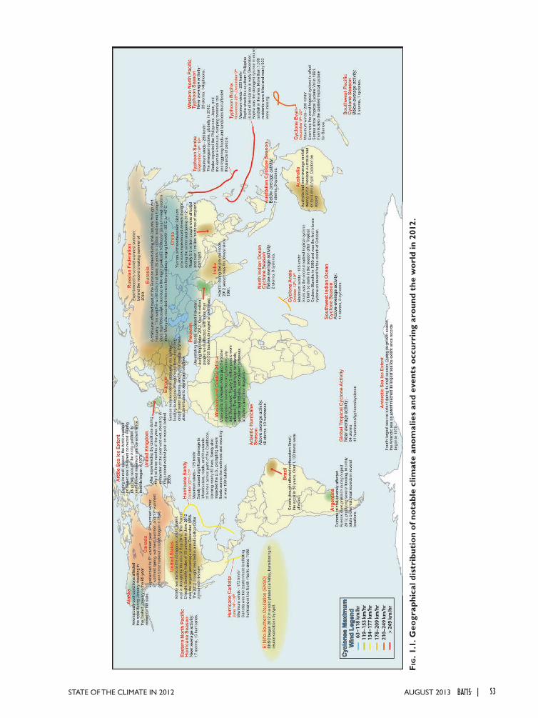
An overview of findings is presented in the Ab-stract and Fig. 1.1. Chapter 2 features global-scale climate variables; Chapter 3 highlights the global oceans; and Chapter 4 includes tropical climate phe-nomena including tropical cyclones. The Arctic and Antarctic respond differently through time and are reported in separate chapters (5 and 6, respectively). Chapter 7 provides a regional perspective authored largely by local government climate specialists. Sidebars included in each chapter are intended to provide background information on a significant climate event from 2012, a developing technology, or
an emerging dataset germane to the chapter’s content. A list of relevant datasets and their sources for all chapters is again provided as an Appendix.
This series is consciously conservative with state-ments of attribution regarding drivers of events on the scale of climate variability and change. Only widely-understood and established attribution re-lationships, such as those for ENSO’s influence, are employed here. However, for the second consecutive year, BAMS will publish an annual collection of such analyses, allowing this series to continue its focus as a chief scorekeeper of the climate’s evolving state.
S3AUGUST 2013STATE OF THE CLIMATE IN 2012 |
Fig
. 1.1
. Geo
grap
hica
l dis
trib
utio
n of
not
able
clim
ate
anom
alie
s an
d ev
ents
occ
urri
ng a
roun
d th
e w
orld
in 2
012.

S4 aUGUST 2013|
SIDEBAR 1.1: ESSENTIAL CLIMATE VARIABLES: WHAT ARE THEY EXACTLY, WHERE DID THEY COME FROM, AND WHAT PURPOSE DO THEY SERVE?—h. J. diaMond
In 1990, the First Assessment Report of the Inter-governmental Panel on Climate Change (IPCC) was published. In addition to its findings on the state of the climate system, the IPCC made the following statement on the observing system: Systematic long term observations of the system are of vital importance for understanding the natural variability of the Earth’s climate system, detecting whether man’s activities are changing it, parameterizing key processes for models, and verifying model simulations (Houghton et al. 1990, p. xxxii). This was the first step in creating the Global Climate Observing System (GCOS) program, which was a key outcome of the Second World Climate Conference held in 1990 and led to the formal establishment of GCOS in 1992.
In 2003, The Second Report on the Adequacy of the Global Observing Systems for Climate in Support of the UNFCCC (GCOS 2003) first documented the concept of Essential Climate Variables (ECVs). The focus of this seminal report was to establish a set of ECVs that were feasible for global implementation and had high impact with respect to the requirements of both the United Nations Framework Convention for Climate Change (UNFCCC) and the IPCC.
These 44 ECVs covered the atmospheric, oceanic, and terrestrial domains. While not covering every pos-sible variable, they were selected as being a reasonably achieved set of key variables that could best meet critical climate observing needs. In 2010, with the publication of the Implementation Plan for the Global Observing System for Climate in Support of the UNFCCC (GCOS 2010), the list of ECVs was expanded to 50 (http://gosic.org/ios/MATRICES/ECV/ECV-matrix.htm). Both satellite and in situ observations are essential to fully understand the nature of the global climate system and both types of observations contribute to the composition of ECVs. In situ observations provide the long-term historical record for most variables and serve a vital role in satellite cali-bration; and in some cases, such as in the deep ocean, they are the only currently viable observing technology available.
The observations and supporting information encom-pass a broad spectrum, including (a) routine weather observations, collected consistently over a long period of time; (b) observations collected as part of research investigations or one-time satellite missions to elucidate
climate processes or demonstrate the technical feasibility of particular observations; (c) highly precise, sustained observations collected for the express purposes of de-tailed documentation of local changes and calibration of other observations, from a limited set of sites sampling different climatic regimes; (d) climate observations de-signed to document more generally the changing state of the oceans, atmosphere, sea ice, and land systems; (e) proxy information based on documentary records and natural paleoclimatic data, used to extend the instrumen-tal climate record to remote regions and back in time; and (f) observations of climate forcing constituents, such as greenhouse gases and aerosols. The importance of observing these ECVs was presented to the World Cli-mate Conference 3 (WWC-3) in 2009 (Karl et al. 2010).
The true success of the ECV concept is to focus at-tention and provide a systematic approach to organizing a wide global effort such as GCOS. For example, the organization and coordination of satellite observations in support of climate is a complicated and costly effort, and in this regard, having ECVs as an organizing focus has been useful (Schulz et al. 2009). In fact, the concept of ECVs has become such a well-recognized and success-ful effort that it has been picked up by other thematic communities. For example, in developing a Framework for Ocean Observing at the OceanObs’09 conference, in September 2009, a task team was established to develop a set of Essential Ocean Variables (see http://www.oceanobs09.net/foo/FOO_Report.pdf). And the biodiversity community, responding to the challenge of developing a global observation system in support of the UN Convention on Biological Diversity, developed a set of Essential Biodiversity Variables (EBVs), modeled upon the ECV concept. The goal of EBVs is to help observation communities harmonize the monitoring of biodiversity by identifying how variables should be sampled and mea-sured (Pereira et al. 2013).
The ECV concept has not only demonstrated its value to the climate community as a useful organizing mecha-nism to better organize the complicated nature of global climate observing, but has also been valuable to other scientific thematic areas. This successful framework has also assisted in the evolution and progress of the annual State of the Climate reports.

S5AUGUST 2013STATE OF THE CLIMATE IN 2012 |
PlAte 1.1. Global (or representative) average time series for essential climate variables. Anomalies are shown relative to the base period in parentheses although original base periods may differ. Data products are colored black for in situ (IS), red for satellite (S), and blue for reanalyses (R). (a) Northern Hemisphere lower strato-spheric ozone in March (1IS, 2S); (b) Southern Hemisphere lower stratospheric ozone in October (1IS, 2S); (c) Lower stratospheric temperature (4IS, 3S, 3R); (d) Lower tropospheric temperature (4IS, 2S, 4R); (e) Surface temperature (4IS, 5R); (f) Land surface wind speed (2IS); (g) Ocean surface wind speed (1IS,1S, 5R); (h) North-ern Hemisphere continental snow cover extent (1S); (i) Precipitation over land (3IS); (j) Lower stratospheric water vapor over Boulder, CO (1IS, 1S); (k) Surface specific humidity over land (4IS, 5R); (l) Surface specific humidity over ocean (3IS, 5R); (m) Surface relative humidity over land (3IS, 4R); (n) Surface relative humidity over ocean (2IS, 4R); (o) Arctic sea ice extent (1IS); (p) Antarctic sea ice extent (1IS); (q) Glacier cumulative mean specific balance (1IS); (r) Precipitation over ocean (3S); (s) Cloudiness (1IS, 5S); (t) Total column water vapor over land (2IS, 1S); (u) Total column water vapor over ocean (2S[k1]); (v) Soil moisture (1S); (w) Ocean heat content (0–700 m) (4IS); (x) Sea level rise (1S); (y) Terrestrial groundwater storage (1S); (z) FAPAR (1S); (aa) Land surface albedo in the visible spectrum (1S).

S6 aUGUST 2013|

S7STATE OF THE CLIMATE IN 2012 |AuguST 2013
2. GLOBAL CLIMATE—K. M. Willett, A. J. Dolman, B. D. Hall, and P. W. Thorne, Eds.
a. Overview—P. W. Thorne, K. M. Willett, A. J. Dolman, and B. D. HallUnlike the preceding two years, the climate of
2012 was not dominated by the phase of the El Niño Southern Oscillation. The La Niña that began in fall 2011 rapidly dissipated in early 2012. During the sum-mer of 2012 an El Niño appeared to be building but by year’s end the ENSO state was neutral again. This lack of a strong large-scale dynamic forcing of the global system led to a return to more average global-mean conditions for many variables and a greater degree of regional heterogeneity within many aspects of the climate system. (See Chapter 7 for details of regional behavior.)
Depending on the dataset, 2012 was eighth or ninth warmest in the record since 1850 at the surface and eighth to eleventh warmest since 1979 in the troposphere. All top ten years in both records have occurred since the large El Niño event of 1998. The stratosphere was cooler than the long-term average. Cryospheric indicators showed declines in spring snow cover and glacial mass, continuing long-term trends which are consistent with observed surface and tropospheric temperature change. Glacial mass balance likely was negative globally for the 22nd consecutive year.
Globally averaged, anomalies in elements of the hydrological cycle were unremarkable in nature. But this masks large regional anomalies such as drought over much of North America and southeastern
Europe. Meanwhile several other areas experienced substantially above-average rainfall or started the year in drought and ended with significant flooding (e.g., northwestern Europe).
Greenhouse gas concentrations continued to increase and ozone depleting gases continued to decrease in concentration. Stratospheric ozone exhib-ited values closer to pre-ozone levels in the Southern Hemisphere, primarily attributable to an early break down of the circumpolar vortex and associated polar stratospheric warming. For the first time, an assess-ment of tropospheric ozone is included in this year’s chapter. Tropospheric ozone is a gas of both natural and anthropogenic origin (Sidebar 2.1), having a posi-tive radiative balance and potential human health and ecological impacts. Globally, it has slightly increased.
Maps of anomalies of many of the variables described in this chapter are available in Plate 2.1. Time series from variables in this chapter and some from other chapters are shown in Plate 1.1. Wher-ever possible a standard 1981–2010 climatology has been used which covers the period of many satellite observations and all reanalyses products. A number of sections refer to online figures that can be found here: http://dx.doi.org/10.1175/2013BAMSStateoftheClimate.2, alongside alternative figure versions ex-ploring structural uncertainties arising from the use of different data sources and data processing choices. Finally, owing to the demise of the ENVISAT satellite which carried the AATSR instrument, lake surface temperatures cannot be included this year.
(a) Return to more neutral ENSO conditions; (b) global surface temperature anomalies with North America warmth; (c) continued glacier loss; (d) continued greenhouse gas accumulation. See Plate 2.1c and Figs. 2.22b, 2.9, and 2.32 for more information.
(a)
(b)
(c)
(d)
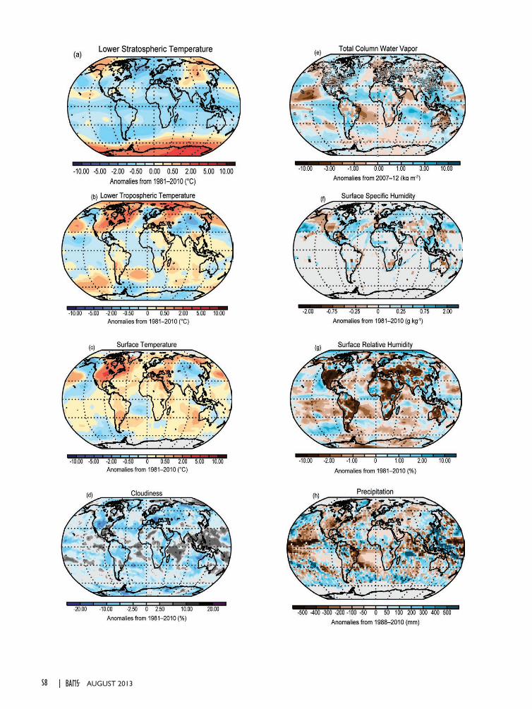
S8 | august 2013

S9STATE OF THE CLIMATE IN 2012 |AuguST 2013

S10 | august 2013
Plate 2.1. a) ERA-Interim 2012 anomalies of MSU Channel 4 equivalent for the lower stratospheric temperature.b) ERA-Interim 2012 anomalies of MSU Channel 2LT equivalent for the lower tropospheric temperature.c) NOAA NCDC 2012 anomalies of surface temperature.d) PATMOS-x 2012 anomalies of cloudiness. e) SSMIS (ocean) and COSMIC (land) with radiosonde (triangles) and ground based GPS (circles); (land) 2012 anomalies of total column water vapor.f) HadISDH (land) and NOCS v2.0 (ocean) 2012 anomalies of surface specific humidity.g) ERA-Interim 2012 anomalies of surface relative humidity.h) RSS and GHCN precipitation 2012 anomalies.i) Water balance model analysis by authors showing 2012 anomalies of river discharge over continents.j) GRACE satellite observations of 2012 minus 2011 annual mean terrestrial water storage (the sum of groundwater, soil water, surface water, snow, and ice, as an equivalent depth of water in cm). k) ESA’s CCI ESV SM satellite observations of 2012 anomalies of soil moisture.l) HadSLP2r 2012 anomalies of sea level pressure.m) Satellite radiometer (ocean), ERA-Interim (land and ocean where satellite estimates are unavail-able), and in situ sites (land) from ISD-LITE and Australian stations (from McVicar et al. 2008) 2012 anomalies of surface wind speed.n) MACC reanalysis for 2012 anomalies of total aerosol optical depth.o) GOME/SCIAMACHY/GOME2 2012 anomalies of stratospheric ozone.p) MODIS White Sky broadband 2012 anomalies of land surface albedo from the visible spectrum.q) MODIS White Sky broadband 2012 anomalies of land surface albedo from the near-infrared spectrum.r) Combined SeaWiFS, MERIS, and MODIS 2012 anomalies of Fraction of Absorbed Photosynthetically Active Radiation (FAPAR).s) MACC GFAS processed MODIS observations for 2012 anomalies of biomass burning in terms of annual carbon emission per unit area.
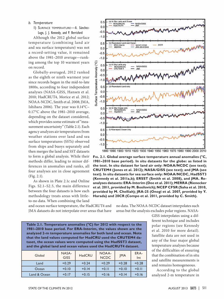
S11STATE OF THE CLIMATE IN 2012 |AuguST 2013
b. Temperature1) Surface temperature—A. Sánchez-
Lugo, J. J. Kennedy, and P. BerrisfordAlthough the 2012 global surface
temperature (combining land air and sea surface temperature) was not a record-setting value, it remained above the 1981–2010 average—rank-ing among the top 10 warmest years on record.
Globally-averaged, 2012 ranked as the eighth or ninth warmest year since records began in the mid-to-late 1800s, according to four independent analyses (NASA-GISS, Hansen et al. 2010; HadCRUT4, Morice et al. 2012; NOAA-NCDC, Smith et al. 2008; JMA, Ishihara 2006). The year was 0.14°C–0.17°C above the 1981–2010 average, depending on the dataset considered, which provides some estimate of “mea-surement uncertainty” (Table 2.1). Each agency analyzes air temperatures from weather stations over land and sea surface temperatures (SSTs) observed from ships and buoys separately and then merges the land and SST datasets to form a global analysis. While their methods differ, leading to minor dif-ferences in anomalies and ranks, all four analyses are in close agreement (Fig. 2.1).
As shown in Plate 2.1c and Online Figs. S2.1–S2.5, the main difference between the four datasets is how each methodology treats areas with little-to-no data. When combining the land and ocean surface temperature, the HadCRUT4 and JMA datasets do not interpolate over areas that have
no data. The NOAA-NCDC dataset interpolates such areas but the analysis excludes polar regions. NASA-
GISS interpolates using a dif-ferent technique and includes polar regions (see Kennedy et al. 2010 for more detail). Satellite data are not used in any of the four major global temperature analyses because of the difficulties of ensuring that the combination of in situ and satellite measurements is and remains homogeneous.
According to the global analyzed 2-m temperature in
Table 2.1. Temperature anomalies (°C) for 2012 with respect to the 1981–2010 base period. For ERA-Interim, the values shown are the analyzed 2-m temperature anomalies for both land and ocean. Note that the land values computed for HadCRU used the CRUTEM4 da-taset, the ocean values were computed using the HadSST3 dataset, and the global land and ocean values used the HadCRUT4 dataset.
GlobalNASA-GISS
HadCRUNOAA-NCDC
JMAERA-Int
Land +0.29 +0.24 +0.29 +0.28 +0.28
Ocean +0.10 +0.14 +0.11 +0.10 +0.11
Land & Ocean +0.17 +0.15 +0.16 +0.14 +0.16
Fig. 2.1. Global average surface temperature annual anomalies (°C, 1981–2010 base period). In situ datasets for the globe: as listed in the text. In situ dataset for land air only: NOAA/NCDC (see text); CRUTEM4 (Jones et al. 2012); NASA/GISS (see text); and JMA (see text). In situ datasets for sea surface only: NOAA/NCDC, HadSST3 (Kennedy et al. 2011a,b); ERSST (Smith et al. 2008), and JMA. Re-analyses datasets: ERA-Interim (Dee et al. 2011); MERRA (Rienecker et al. 2011, provided by M. Bosilovich); NCEP CFSR (Saha et al. 2010, provided by M. Chelliah); JRA-25 (Onogi et al. 2007, provided by Y. Harada) and 20CR (Compo et al. 2011, provided by C. Smith).

S12 | august 2013
the ERA-Interim reanalysis, 2012 was 0.16°C above the 1981–2010 average, making the year the ninth warmest since 1979. The 2-m temperature for the year was 0.12°C below the highest value in ERA-Interim, which occurred in 2005. Other reanalyses are in generally close agreement.
La Niña conditions in late 2011 dissipated in early 2012 and SSTs in the tropical Pacific approached El Niño thresholds by late July. However, conditions had returned to near neutral by the end of the year. The effects of the 2011 La Niña were seen in early 2012, with global average temperatures in the first quarter being cooler than the remainder of the year. Global average temperatures for 2012 were slightly higher than in 2011, which had two La Niña episodes (Fig. 2.2; Online Figs. S2.6–S2.8).
The year was characterized by unusual warmth that affected most of the globe’s land areas, with the most prominent warmth across the Northern Hemi-sphere higher latitudes, specifically the contiguous United States, the eastern half of Canada, southern Europe, western Russia, and the Russian Far East (Plate 2.1c; Fig. 2.2; Online Figs. S2.1–S2.8). Cooler-than-average conditions affected Alaska, western parts of Canada, eastern Australia, and parts of cen-tral Asia. The globally-averaged annual temperature over land was 0.24°C–0.29°C above average, ranking between sixth and ninth warmest on record, depend-ing on the dataset. For ERA-Interim, the average temperature over land was 0.28°C above average, making 2012 the 10th warmest year on record. The ocean surface was warmer than average except across parts of the northeastern and central equatorial Pa-cific Ocean, parts of the southern Atlantic Ocean, and some regions of the southern oceans. The ERA-Interim (Online Fig. S2.4) shows an additional swath of cooler-than-average conditions across the North Atlantic Ocean, which could ref lect a difference
between the air temperatures (as represented in ERA-Interim) and sea surface temperatures (as represented in the other datasets). Averaged globally, the ocean temperature was 0.10°C–0.14°C above average, the ninth to eleventh warmest year on record, depending on the dataset, and the sixth warmest according to ERA-Interim.
2) Lower tropoSpheric temperature—J. R. ChristyThe 2012 annual, globally-averaged temperature
of the lower troposphere (the atmosphere below 10 km altitude or roughly the lower 70 percent by mass) was approximately 0.15°C above the 1981–2010 mean and near the value of 2011. This placed 2012 between eighth and eleventh warmest of the past 34 years, depending on dataset (Fig. 2.3).
The year began with a dissipating La Niña in the tropical Pacific, which contributed to a below-average global tropospheric temperature for the first two months of the year (Fig. 2.4). These conditions ended during boreal spring and a warm phase El Niño appeared to gather strength mid-year with the heat signature in the troposphere appearing about two months later, in September and October. However, the warm SST anomalies faded to near average by year-end, and the global tropospheric temperature anomaly decreased as well.
Regionally, central and eastern North America and the entire Arctic experienced much-above-average
Fig. 2.2. HadCRUT4 monthly mean anomalies (°C; 1981–2010 base period) for surface temperature by latitude. Gray areas indicate regions where data are unavailable.
Fig. 2.3. Global average lower tropospheric tempera-ture annual anomalies (°C; 1981–2010 base period) for the MSU 2LT equivalent layer. Radiosondes: HadAT2 (Thorne et al. 2005; 465 day, 384 night stations), RATPAC (Free et al. 2005; 85 stations), RAOBCORE (Haimberger et al. 2012; 1184 stations), and RICH-obs (Haimberger et al. 2012; 1184 stations). Satellites: UAHv5.5 (Christy et al. 2011) and RSSv3.3 (Mears and Wentz 2009). Reanalyses: as described in Fig. 2.1. Major volcanic eruptions, which cause 2–3 year cool-ing episodes, are indicated by triangles in 1963, 1982, and 1991.

S13STATE OF THE CLIMATE IN 2012 |AuguST 2013
temperatures, while northern China and the Gulf of Alaska saw much-below-average temperatures (Plate 2.1b). The tropical belt, while cooler than average at the start of the year and warmer than average mid-year, finished near average overall. The southern midlatitudes, in general, were above average (Fig. 2.4).
The long-term trend based on radiosondes (start-ing in 1958) is +0.15°C decade-1 and satellites (starting in 1979) is +0.14 ± 0.02°C decade-1 where the range represents the variation among the different datasets and serves as an estimate of mea-surement uncertainty (Fig. 2.3). Ap-plying standard statistical methods to take into account the magnitude of the year-to-year variations pro-duces a statistical confidence range of ±0.06°C decade-1, meaning the trends are significantly greater than zero. Part of the upward trend is due to major volcanic events (1963, 1981, and 1992). The resulting period of cooler temperatures at those times affected the early part of the tro-pospheric temperature record, the satellite period especially, enhanc-ing the upward trend. Since 2002 there has been a relative plateau of anomalies, averaging about +0.2°C (+0.5°C) above the 1981–2010 (1961–90) average.
Basic lapse-rate theory indi-cates the tropospheric temperature should experience greater magni-tudes in annual f luctuations and in long-term trends than surface temperature (National Academy of Sciences 2003). For the globe (trop-ics), this amplification of the surface trend in the bulk tropospheric layer
measured by satellites is expected to be about 1.2 (1.4). Over the satellite era (1979 to present), trends in observations indicate a troposphere-to-surface ratio close to or slightly less than 1.0 for both global and tropical domains (Table 2.2). Over the longer radiosonde era (1958 to present), the observed results are nearer theoretically-expected values. Seidel et al. (2012) examined the “within-troposphere” tropical lapse rate finding the trends at an upper level at 200 hPa (~12 km altitude) were generally less than those at a lower level at 700 hPa (~3 km altitude). However, trends for an upper level of 300 hPa (~9 km altitude) were generally greater than those at 700 hPa, being closer to the theoretically-expected “within-tropo-sphere” relationship.
Direct measurement of the lower atmosphere bulk temperature utilizes radiosonde datasets from 1958 and satellites from late 1978. Radiosondes are balloon-borne instrument packages that monitor the temperature of the air as the balloon ascends through the atmosphere. Satellites monitor the intensity of up-welling microwave emissions of atmospheric oxygen that are proportional to temperature. Temperature
Fig. 2.4. ERA-Interim monthly mean anomalies (°C; 1981–2010 base period) of lower tropospheric tempera-ture MSU channel 2LT equivalent by latitude.
Globe 1979–2012 Globe 1958–2012
RATPAC-B +0.128 +0.136
HadAT2 +0.163 +0.159
RICHv1.5 +0.142 +0.150
RAOBCOREv1.5 +0.125 +0.147
UAHv5.5 LT +0.138 -
RSSv3.3 LT +0.131 -
Median LT +0.135 +0.149
NCDC Sfc +0.152 +0.129
HadCRUT4 Sfc +0.161 +0.124
20°S–20°N 1979–2012 20°S–20°N 1958–2012
RATPAC-B +0.090 +0.123
HadAT2 +0.111 +0.135
RICHv1.5 +0.120 +0.128
RAOBCOREv1.5 +0.085 +0.160
UAHv5.5 LT +0.066 -
RSSv3.3 LT +0.113 -
Median LT +0.101 +0.132
NCDC Sfc +0.110 +0.114
HadCRUT4 Sfc +0.109 +0.098
Table 2.2. Trend values of the tropospheric datasets utilized in this report with surface values indicated by ‘Sfc’.

S14 | august 2013
variations in the troposphere are relatively large-scale when averaged over a month or year due to mixing by the large atmospheric wind systems. Hence, fewer spatial points (i.e., radiosondes) are needed to create a reasonable estimate of the global average compared to the more inhomogeneous surface. However, as at the surface, the instrumentation on both the radiosondes and satellites has changed through the years and so adjustments to the data are required to produce homogeneous time series for climate analysis. The different choices made in homogenizing the raw series lead to slightly different results (i.e., termed “measurement uncertainty” above.)
In addition to radiosonde and satellite estimates, five reanalyses products are also shown (Fig. 2.3). Re-analyses assimilate multiple data sources, including radiosondes and satellites, which are then assimilated into a global circulation model that seeks to balance the observations for dynamic and thermodynamic consistency. ERA-Interim shows good agreement with satellite estimates and is used here to provide the spatial depictions (Plate 2.1b; Fig. 2.4).
3) Lower StratoSpheric temperature—C. S. Long and J. R. Christy
Global-average temperatures in the lower strato-sphere for 2012 were below the 1981–2010 climatol-ogy (Fig. 2.5). How the global-average temperature for 2012 ranked in comparison with previous years varies with the observation system. The satellite datasets ranked 2012 as either the coldest year since 1979 (RSS and STAR) or the third coldest (UAH). Two of the four radiosonde datasets agreed with the
satellite that 2012 was either the coldest (RATPAC) or nearly the coldest (HadAT2) in their record. The other two radiosonde datasets ranked 2012 as the sixth coldest (RAOBCORE) and the eighth coldest (RICH-obs). The annually averaged cool signal was widespread, covering the southern midlatitudes, tropics, and northern midlatitudes (Plate 2.1a; Fig. 2.6). The northern high latitudes exhibited a wave-1 pattern in which the northern Atlantic and European regions were cooler than climatology and the Asian and Canadian regions were warmer than climatol-ogy. This pattern was most dominant in the boreal winter months. The southern high latitudes were much warmer than climatology, especially in October and November of 2012. The cooler-than-climatology temperatures in the tropics can be attributed to a thermal response to the descending quasi-biennial os-cillation (QBO) easterly winds. Typically, the tropical temperature anomaly minima occur at progressively later times from 10 hPa down to 70 hPa, as shown by Online Fig. S2.9. The timing of the tropical tempera-ture anomaly minima agrees well with the easterly phase of the QBO at that level (Online Fig. S2.10). Conversely, 2011 saw a westerly phase of the QBO, resulting in a warm tropical lower stratosphere (Long and Christy 2012). Because ENSO conditions were not outstanding in 2012, there was little influence of the Pacific SST forcing upon the lower stratospheric temperatures. For most of the extratropics, the tem-perature anomalies are a response to the elevated tro-popause driven by the warm temperature anomalies in the troposphere (section 2b.2). In early October in the Southern Hemisphere, an amplified wave-1 in the middle stratosphere resulted in a large pulse of heat flux from the southern midlatitudes into the southern high latitudes, contributing to an early break down of the polar vortex; the resulting temperatures were well above normal in the lower stratosphere post-September. This played a role in the high levels of stratospheric ozone over the Antarctic in October and November 2012. This is in contrast to very low levels of ozone over Antarctica in 2011 in response to cool stratospheric temperatures in the polar region.
Global lower stratospheric temperatures as deter-mined by radiosonde, satellite, and reanalysis show resumed cooling since 2010 (Fig. 2.5). The three sat-ellite estimates of the cooling trend since 1979 differ slightly from each other, with the UAH time series having the greatest cooling trend (-0.371°C decade-1). The RSS (-0.299°C decade-1) and STAR (-0.320°C decade-1) cooling trends are slightly weaker. How-ever, these estimates are generally equivalent (range:
Fig. 2.5. Global average lower stratospheric tempera-ture annual anomalies (°C; 1981–2010 base period) for the MSU channel 4 equivalent layer. Radiosondes, satellites, and reanalyses are as shown in Fig. 2.3 plus (satellite) STAR (Zou and Wang 2010). Major volcanic eruptions, which cause 2–3 year warming episodes, are indicated by triangles in 1963, 1982, and 1991.
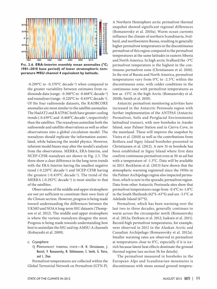
S15STATE OF THE CLIMATE IN 2012 |AuguST 2013
-0.299°C to -0.370°C decade-1) when compared to the greater variability between estimates from ra-diosonde data (range: -0.300°C to -0.468°C decade-1) and reanalyses (range: -0.220°C to -0.419°C decade-1). Of the four radiosonde datasets, the RAOBCORE anomalies are most similar to the satellite anomalies. The HadAT2 and RATPAC both have greater cooling trends (-0.439°C and -0.468°C decade-1, respectively) than the satellites. The reanalyses assimilate both the radiosonde and satellite observations as well as other observations into a global circulation model. The reanalyses should replicate the information assimi-lated, while balancing the model physics. However, inherent model biases may alter the model’s analysis from the observations. MERRA, ERA-Interim, and NCEP-CFSR reanalyses are shown in Fig. 2.5. The three show a clear difference in the long-term trends with the ERA-Interim having the smallest negative trend (-0.220°C decade-1) and NCEP-CFSR having the greatest (-0.419°C decade-1). The trend of the MERRA (-0.292°C decade-1) is most similar to that of the satellites.
Observations of the middle and upper stratosphere are not yet sufficient to constitute their own State of the Climate section. However, progress is being made toward understanding the differences between the UKMO and NOAA long-term SSU datasets (Thomp-son et al. 2012). The middle and upper stratosphere is where the various reanalyses disagree the most. Progress is being made towards understanding how best to assimilate the SSU and top AMSU-A channels (Kobayashi et al. 2009).
c. Cryosphere1) permafroSt thermaL State—H. H. Christiansen, J.
Noetzli, V. Romanovsky, N. Shiklomanov, S. Smith, G. Vieira, and L. Zhao
Permafrost temperatures are collected within the Global Terrestrial Network on Permafrost (GTN-P).
A Northern Hemisphere arctic permafrost thermal snapshot showed significant regional differences (Romanovsky et al. 2010a). Warm ocean currents influence the climate of northern Scandinavia, Sval-bard, and northwestern Russia, resulting in generally higher permafrost temperatures in the discontinuous permafrost of this region compared to the permafrost temperatures at the same latitudes in eastern Siberia and North America. In high arctic Svalbard the -3°C permafrost temperature is the highest in the con-tinuous permafrost zone (Christiansen et al. 2010). In the rest of Russia and North America, permafrost temperatures vary from 0°C to -2.5°C within the discontinuous zone, with colder conditions in the continuous zone with permafrost temperatures as low as -15°C in the high Arctic (Romanovsky et al. 2010b; Smith et al. 2010).
Antarctic permafrost monitoring activities have increased in the Antarctic Peninsula region with further implementation of the ANTPAS (Antarctic Permafrost, Soils and Periglacial Environments) latitudinal transect, with new boreholes in Amsler Island, near Palmer Station and in Cierva Cove, in the mainland. These will improve the snapshot by Vieira et al. (2010) as well as the contributions from Rothera and Signy Island boreholes presented in Christiansen et al. (2012). A new 31-m borehole has been established in Signy Island where first data confirm continuous permafrost even at 30-m asl but with a temperature of -1.3°C. Data will be available in 2013. Bockheim et al. (2013) have shown that the atmospheric warming registered since the 1950s in the Palmer Archipelago region also impacted perma-frost, which is now in the sporadic permafrost region. Data from other Antarctic Peninsula sites show that permafrost temperatures range from -0.4°C to -1.8°C in the South Shetlands (62°S–63°S) and are -3.1°C at Adelaide Island (67°S).
Permafrost, which has been warming over the last two to three decades, generally continues to warm across the circumpolar north (Romanovsky et al. 2012a; Derksen et al. 2012; Isaksen et al. 2011). Record-high permafrost temperatures, for example, were observed in 2012 in the Alaskan Arctic and Canadian Archipelago (Romanovsky et al. 2012a). Smaller warming rates are observed in permafrost at temperatures close to 0°C, especially if it is ice-rich because latent heat effects dominate the ground thermal regime (see section 5h for details).
The permafrost measured in boreholes in the European Alps and Scandinavian mountains is discontinuous with mean annual ground tempera-
Fig. 2.6. ERA-Interim monthly mean anomalies (°C; 1981–2010 base period) of lower stratospheric tem-perature MSU channel 4 equivalent by latitude.

S16 | august 2013
ture mostly between 0°C and -3°C (Haeberli et al. 2010). The steep topography, heterogeneous surface characteristics, and snow cover result in high spatial variability of the ground thermal conditions. Decadal records (Fig. 2.7) for European mountain permafrost show a general warming trend, with smaller increases in temperature where permafrost temperatures are close to 0°C (Isaksen et al. 2007; Haeberli et al. 2010; PERMOS 2010). Permafrost temperature anomalies associated with extreme warm years (2003, 2009, and 2011) are superimposed on the warming trend (PER-MOS 2010; Phillips et al. 2009; Zenklusen-Mutter et al. 2010). More pronounced are trends observed in Scandinavia (Isaksen et al. 2011). The observed trends in permafrost temperatures are consistent with changes in air temperatures, but snow cover, soil properties (including ice and moisture content), and vegetation, also determine the magnitude of the changes in ground temperature changes (e.g., Hae-berli et al. 2010; Romanovsky et al. 2010a).
In the warm permafrost of the higher altitudes of central Asia, ground temperatures have increased by up to 0.5°C decade-1 since the early 1990s, with a general increase in active layer thickness (ALT; e.g., Zhao et al. 2010).
Decadal trends in ALT vary by region. Permafrost has disappeared in several of the Circumpolar Ac-tive Layer Monitoring (CALM) sites. A progressive increase in ALT has been observed since the 1990s in all regions, with the exception of northern Alaska, western Canadian Arctic, and West Siberia. Smaller increases have been observed in Scandinavian sites such as Arctic Sweden and Svalbard compared to East Siberia, the Russian Far East, and Greenland. In North America a progressive increase of ALT is observed only at sites in the Alaskan Interior, whereas
ALT on the Alaskan North Slope was relatively stable over the 1995–2011 period.
2) NortherN hemiSphere SNow cover—D. A. RobinsonAnnual snow cover extent (SCE) over Northern
Hemisphere (NH) lands averaged 24.6 million km2 in 2012. This is 0.3 million km2 less than the 1967–2012 average and ranks 2012 as having the 12th least ex-tensive cover in the 46-year period of record (Table 2.3; Fig. 2.8). This evaluation considers snow over the continents, including the Greenland ice sheet. The SCE in 2012 ranged from 47.8 million km2 in February to 2.3 million km2 in July. Monthly SCE is calculated at the Rutgers Global Snow Lab from daily SCE maps produced by meteorologists at the National Ice Center (a US joint NOAA, Navy, and Coast Guard facility), who rely primarily on visible satellite imagery to construct the maps.
The first three months of 2012 saw the extent of snow cover over Eurasia (EU) rank as the third (Feb-ruary) and ninth (January and March) most extensive of the past 46 years. Meanwhile, North American (NA) extents were well below average, ranking third, sixteenth, and fourth lowest in January, February, and March, respectively. This resulted in hemispheric extents lying close to average in January and March and eighth most extensive in February.
Spring snow coverage declined rapidly over EU, with the April ranking plummeting to seventh least extensive and May and June extents the lowest on record. With the low extents continuing over NA, the NH melt season continued the precipitous mid-to-late spring decline of recent years when compared to the long-term average.
While off to a rather slow start in September, fall snow extents over EU and NA expanded explosively
in October and remained well above average through December. This included EU and NA rankings no lower than thirteenth most exten-sive in any month, and NH rankings of eighth in Octo-ber, fifth in November, and most extensive on record in December.
Persistent ridging across much of the United States resulted in below-average snow coverage from January through melt out in May. January, March, and April
Fig. 2.7. Observed permafrost temperatures (°C) from (a) 10-m and (b) 20-m depth for selected boreholes in European mountains. Data for Swiss sites are provided by PERMOS and for Norwegian sites by the Norwegian Meteorological Institute. (Modified from Haeberli et al. 2010, figure 4).

S17STATE OF THE CLIMATE IN 2012 |AuguST 2013
coverage ranked as third or fourth least extensive on record, while Febru-ary was fourteenth, and May eighth lowest. Fall cover was below average in October, close to av-erage in November and ranked fourteenth most extensive in December.
Maps depicting daily, week ly, and monthly conditions, daily and monthly anomalies, and monthly climatologies for the entire period of record may be viewed at the Rutgers Global Snow Lab website (http://snowcover.org). Month-ly SCE for the NH, EU, NA, the contiguous US, Alaska, and Canada are also posted, along with information on how to
access weekly areas and the weekly and monthly gridded products.
3) aLpiNe gLacierS—M. S. PeltoAlpine glaciers have been studied as sensitive
indicators of climate for more than a century, most commonly focusing on changes in terminus position and mass balance. The worldwide retreat of moun-tain glaciers is one of the clearest signals of ongoing climate change (Haeberli et al. 2000). The retreat is a reflection of strongly negative mass balances over the last 30 years (WGMS 2012). Glacier mass balance is the difference between accumulation and ablation. The recent rapid retreat and prolonged negative bal-ances have led to some glaciers disappearing and others fragmenting (Pelto 2010).
The World Glacier Monitoring Service (WGMS) record of mass balance and terminus behavior (WGMS 2012) provides a global index for alpine glacier behavior. Annual mass balance was -766 mm water equivalent (w.e.) in 2011, negative for the 21st consecutive year. Preliminary data for 2012 from Austria, Norway, New Zealand, Nepal, and the United States indicate it is highly likely that 2012 will be the 22nd consecutive year of negative annual balances. The loss of glacier area is leading to declining runoff; the importance of this is indicated by Schaner et al.
Fig. 2.8. Twelve-month running anomalies of monthly snow cover extent over NH lands (including Green-land) as a whole and Eurasia and North America sepa-rately between Nov 1966 and Dec 2012. Anomalies are calculated from NOAA snow maps. Mean hemispheric snow extent is 25.0 × 10⁶ km2 for the full period of record. Monthly means for the period of record are used for 9 missing months between 1968 and 1971 in order to create a continuous series of running means. Missing months fall between Jun and Oct; no winter months are missing.
Table 2.3. Monthly and annual climatological information on Northern Hemisphere and continental snow extent between Nov 1966 and Dec 2012. Included are the numbers of years with data used in the calculations, means, standard deviations, 2012 values and rankings. Areas are in millions of square kilometers. 1968, 1969, and 1971 have 1, 5, and 3 missing months respectively, thus are not included in the annual (Ann) calculations. North America (N. Am.) includes Greenland. Ranks are from most extensive (1) to least (ranges from 43 to 47 depending on the month).
Yrs Mean Std. Dev. 2012 2012 NH rank Eurasia rank
N. Am. rank
Jan 46 46.7 1.5 46.9 21 9 44
Feb 46 45.7 1.8 47.8 8 3 31
Mar 46 40.4 1.8 40.4 23 9 43
Apr 46 30.4 1.7 28.2 43 40 39
May 46 19.4 1.9 15.9 45 46 39
Jun 45 9.9 2.3 4.8 45 45 45
Jul 43 4.1 1.2 2.3 43 43 43
Aug 44 3.1 0.7 2.3 42 42 37
Sep 44 5.3 0.9 4.3 36 32 40
Oct 45 18.0 2.5 19.9 8 11 7
Nov 47 33.7 2.0 36.0 5 8 12
Dec 47 43.3 1.9 46.3 1 2 13
Ann 43 24.9 0.8 24.6 32 15 39

S18 | august 2013
(2012) who determined that, globally, 370 million people live in river basins where glaciers contribute at least 10% of river discharge on a seasonal basis.
The cumulative mass balance loss since 1980 is 15.7 m w.e. the equivalent of cutting a 17-m thick slice off the top of the average glacier (Fig. 2.9). The trend is remarkably consistent from region to region (WGMS 2011). WGMS mass balance results based on 30 reference glaciers with 30 years of record is not appreciably different, -15.5 m w.e. The decadal mean annual mass balance was -198 mm w.e. in the 1980s, -382 mm w.e. in the 1990s, and -740 mm w.e. for 2000–10. The declining mass balance trend during a period of retreat indicates alpine glaciers are not approaching equilibrium and retreat will continue to be the dominant terminus response.
In 2012, slightly-above-average winter accumula-tion in the Alps was offset by extreme summer abla-tion, yielding mass balances that were negative. In Austria, Mullwitzkees had a mass balance of -1461 mm w.e. and Hallstätter Gletscher a mass balance of -1944 mm w.e. (Fischer 2012). The Austrian Glacier inventory in 2011 examined 90 glaciers: 87 were in retreat and 3 were stationary. Average terminus change was -17 m, reflecting the continued negative mass balances of the region. In Italy, a large deposit of World War I ammunition melted out of the glacier on Ago Di Nardis Peak during August 2012. The Swiss Glacier Monitoring Network noted in 2011 92 glaciers retreating, 1 advancing, and 3 stationary. The one advancing glacier had retreated the previous five years. The 2012 data are not complete, but retreat was again dominant.
In Norway, terminus f luctuation data from 25 glaciers for 2012 with ongoing assessment indicate 21 retreating, 2 stable, and 2 advancing. The average terminus change was -12.5 m (Elvehøy 2012). The
retreat rate is less than 2011. Mass balance surveys found deficits on all Norwegian glaciers.
In the North Cascades, Washington La Niña con-ditions during the winter led to a wet winter and a cool and wet spring. Summer was drier and warmer than normal. This led to nearly equilibrium condi-tions on North Cascade glaciers, with mass balance positive on five glaciers and negative on four glaciers. (Pelto 2013)
In southeast Alaska, the same La Niña conditions prevailed and led to the highest snow totals in several decades. Glacier snowlines were more than 100 m below average on Lemon Creek and Taku Glaciers of the Juneau Icefield indicative of moderate positive mass balance (Pelto 2013).
In New Zealand, the annual end of summer snow-line survey on 50 glaciers found snowlines that were approximately 120 m above the elevation for glacier equilibrium. This indicates strong mass balance losses (NIWA 2012).
In Nepal, the International Centre for Integrated Mountain Development measured the mass balance of Yala and Rikha Samba Glaciers in 2012 and found both to be significantly negative (Mishra 2012). Pelto (2012) reported that the extensive inventories are better validated than GRACE (Jacob et al. 2012) for Himalayan glacier volume change. This conclusion has been confirmed by Bolch et al. (2012).
d. Hydrological cycle1) Surface humidity—K. M. Willett, D. I. Berry, and A.
SimmonsSurface humidity can be monitored in two differ-
ent ways: specific humidity, which is a quantitative measure of water vapor in the atmosphere, and rela-tive humidity, which describes how close the atmo-sphere is to saturation. Based on in situ observations, HadISDH (Willett et al. 2013) over land and NOCS v2.0 (Berry and Kent 2009, 2011) over the oceans, the global average specific humidity for 2012 was similar to 2011, with values higher than the long-term average but not record breaking (Fig. 2.10). Relative humidity over land, as shown by ERA-Interim (Dee et al. 2011), remains well below the long-term average, continuing the recent relative drying over land. The dry anomaly over the United States was the most extreme feature in 2012 (Plate 2.1g). Over the oceans, relative humidity during 2012 was similar to 2011. For both land and ocean, the in situ data coverage concentrates in the Northern Hemisphere (Plate 2.1f) such that global averages are dominated by changes here.
Fig. 2.9. Mean annual balance (bars) reported for the 30 reference glaciers to the WGMS and cumulative annual balance (red line) during 1980–2011.

S19STATE OF THE CLIMATE IN 2012 |AuguST 2013
Currently, HadISDH is the only in situ monitor-ing product for land specific humidity. The data have been quality controlled and then homogenized. HadISDH agrees well with existing products and with ERA-Interim (Willett et al. 2008, 2013; Simmons et al. 2010; Dai 2006). Hence, ERA-Interim can also be used for monitoring. However, a slight dry bias in ERA-Interim is apparent from 2000 onwards relative to the in situ record. This is likely linked to a change to the source of assimilated SST at that time (Simmons et al. 2010). Currently, ERA-Interim is the only validated product available to monitor land surface relative humidity. However, estimates from the MERRA, NCEP-CFSR, 20CR, and JRA-25 reanalyses are also shown for comparison. JRA-25/JCDAS humidity fields suffered a large discontinuity due to absence of precipitable water retrieval data from microwave imagers since October 2011. The reanalyses generally
agree in the overall increasing specific humidity over land but show quite large year-to-year differences in the more recent record.
For ocean, NOCS v2.0 pro-vides quality-controlled and bias- and height-adjusted spe-cific humidity data over all ice-free regions of the globe from ships. Only regions with high confidence are used in this as-sessment, predominantly the shipping lanes in the North-ern Hemisphere. Confidence in the in situ data decreases post-2006 due to reducing numbers of observations and loss of call sign information in the source data (Woodruff et al. 2011), which removes the ability to reliably link ob-servations to their metadata (e.g., Kent et al. 2007). For the first time, a satellite estimate of marine specific humidity from HOAPS-3.2 (Hamburg Ocean Atmosphere Param-eters and Fluxes from Satellite Data derived from SSM/I pas-sive microwave radiometers; Bentamy et al. 2003; Anders-son et al. 2010) is also included, although the period of record
is limited to 1987–2008. This does not match the curve of NOCS v2.0 but does include full spatial coverage. Reanalysis estimates are provided from ERA-Interim, MERRA, NCEP-CFSR, 20CR, and JRA-25.
Spatial anomalies for 2012 are shown in Plates 2.1f and 2.1g with comparisons from some reanalysis products as Online Figs. S2.11–S2.13. As expected, these are similar to other components of the hydrolog-ical cycle (see Plate 2.1). Following the mixed ENSO signals during the year, unlike 2011, no dominant ENSO feature is apparent.
2) totaL coLumN water vapor—C. Mears, J. Wang, S. Ho, L. Zhang, and L. Peng
Global total column water vapor (TCWV) over oceans and land was slightly above average for the majority of observational estimates (Fig. 2.11); how-ever, there is considerable variability between the
Fig. 2.10. Global average surface humidity annual anomalies (1979–2003 base period). For the in situ datasets, 2-m surface humidity is used over land and ~10-m over the oceans. For the reanalyses, 2-m humidity is used over the whole globe. For ERA-Interim only, points over open sea are evaluated and background forecast values are used as opposed to analysis values because of unreliable use of ship data in producing the analysis. HadCRUH and Had-CRUHext use the 1974–2003 base period. Dai uses the 1976–2003 base pe-riod. All reanalyses products use the 1981–2010 base period. NOCS 2.0 uses a 1979–2003 base period. HOAPS have been calculated using a 1988–2008 base period. All data have been adjusted to have a mean of zero over the common period 1979–2003 to allow direct comparison with HOAPS given a zero mean over the 1988–2003 period. ERA values over land are from ERA-40 prior to 1979 and ERA-Interim thereafter. (Data provided by authors A. Dai, M. Bosilovich, Y. Harada, M. Chelliah, and C. Smith.)

S20 | august 2013
different observing products and the short period of overlap results in a short baseline for comparing anomalies to an average (2007–12). Over the ocean, the TCWV anomaly time series (Fig. 2.11a) from the satellite-borne microwave radiometers (SSM/I, SSMIS, AMSR-E, and WindSat; Wentz 1997; Wentz el al. 2007) shows maxima in 1987–88, 1997–98, and 2009–10, associated with El Niño events, as well as a more subtle increasing trend corresponding with increasing global temperatures. Minima are apparent in Northern Hemisphere winters during the La Niña events of 1988–89, 1992–93, 1999–2000, 2000–08, and late 2010 (note that the eruption of Mt. Pinatubo may also have contributed to cooling in 1992–93). The ocean-only COSMIC GPS-RO data (Ho et al. 2010a,b) also show a strong increase late in 2012, which is only partly reproduced in the radiometer data. An increase during 2012 is also shown in the COSMIC data over land, and in ground-based GPS measurements over land (Wang et al. 2007), but not in the homogenized radiosonde data (Dai et al. 2011; Fig. 2.11b). A hov-muller plot derived from the satellite radiometers (Fig. 2.12) shows that the long-term increase in TCWV is occurring at nearly all latitudes.
The map of TCWV anomalies for 2012 (Plate 2.1e) includes data from radiometers (ocean), COSMIC (land), radiosonde (land), and the ground-based GPS measurements (land). In general, the products agree well. There are pronounced dry anomalies south of the Hawaiian Islands, east of South America, and over most of Australia. Over the oceans, there are wet anomalies in the western and eastern edges of the tropical Pacific, the subtropical Indian, and the northern tropical Atlantic. Many of the same features are present in the 2012 precipitation and surface hu-
midity anomalies (Plate 2.1). The pattern in TCWV anomalies over ocean is also confirmed by COSMIC ocean measurements (Ho et al. 2010a).
3) precipitatioN—R. S. Vose, K. Hilburn, X. Yin, M. Kruk, and A. Becker
Globally, land precipitation was near the 1961–90 average in 2012, in contrast to the above-normal totals of the previous two years (Fig. 2.13a). This conclusion is based primarily on station records in the Global Historical Climatology Network (GHCN) Monthly version 2 (Peterson and Vose 1997), which was about 5 mm above normal, and the Global Precipitation Climatology Centre (GPCC) Monitoring Product version 4 (Schneider et al. 2011a; Becker et al. 2013),
Fig. 2.11. (a) Anomaly time series of TCWV over ocean from satellite-borne microwave radiometers and COS-MIC. The reference period for both measurements is 2007–12. (b) Anomaly time series of TCWV over land from radiosondes, ground-based GPS, and COSMIC. Except for COSMIC, the reference period is 1997–2012. The COSMIC land anomalies are calculated relative to a 2007–12 COSMIC land climatology. For (a) and (b) the time series have been smoothed to remove vari-ability on time scales shorter than 6 months.
Fig. 2.12. Time-latitude plot of TCWV anomalies calculated using a 1997–2010 base period. The data (SSM/I, SSMIS, AMSR-E, and WindSat measurements) have been smoothed in the time direction to remove variability on time scales shorter than 4 months. Gray areas indicate regions where data are unavailable.
Fig. 2.13. Globally averaged precipitation anomalies (1961–90 base period over land, 1988–2012 base period over oceans) for (a) three in situ datasets over land and (b), (c) three satellite-based datasets over ocean. Global ocean averages cover 60°N–60°S using a com-mon definition of “ocean”. Panel (c) shows low-pass filtered time series by convolution with a Gaussian distribution with 4-month width at half-peak power whereas panel (b) shows annual averages of this for comparison with land data.

S21STATE OF THE CLIMATE IN 2012 |AuguST 2013
which was about 5 mm below normal. Historically, GHCN and GPCC have been similar on an annual ba-sis, though GHCN has higher interannual variability due to its smaller network. Land data for a blended satellite-in situ product, the Global Precipitation Climatology Project (GPCP) version 2.1 (Adler et al. 2003), suggest that 2012 may have been somewhat be-low normal, though GPCP has generally been slightly drier than the other two products in recent years.
Land anomaly patterns for 2012 (Plate 2.1h) exhibit some notable changes from 2011. For instance, the dry conditions over central North America expanded in 2012. Areas of below-normal precipitation became apparent in eastern South America, the Sahara desert, southern Africa, central Asia, and central Australia (all of which were above normal the previous year). The dryness in parts of Europe and southern China abated in 2012, with a few small areas experiencing wetter-than-normal conditions. The Maritime Con-tinent was much wetter than normal, as was much of Greenland (though the latter should be viewed cau-tiously because of the statistically in-filled estimates in that area).
In contrast to the land datasets, the ocean products are often somewhat dissimilar in their global anoma-lies, a tendency that continued in 2012. For instance, ocean precipitation was above the 1988–2010 average in 2012 based on intercalibrated passive microwave rain retrievals in the Remote Sensing Sytems (RSS; Hilburn and Wentz 2008) version 7 product, and it was below average in the GPCP blended satellite-in situ product (Fig. 2.13b,c). Ocean data for an addi-tional product, the Climate Prediction Center Merged Analysis of Precipitation (CMAP; Xie and Arkin 1997), are not yet available for 2012. Very generally, the datasets concur on lower precipitation in 2011 relative to 2010, and an increase thereafter (at least in RSS and GPCP). RSS has been consistently wetter since about 2008.
As over land, ocean anomaly patterns for 2012 (Plate 2.1h) exhibit some notable changes since 2011, reflecting the decline of La Niña. For instance, the dry anomalies in the central Pacific were weaker and less extensive than in 2011, and the dry anomalies in the southeast Pacific abated significantly, becoming wet anomalies over limited areas. Likewise, the dryness in the North Atlantic faded and was less extensive, while much of the South Atlantic reversed its pattern entirely, e.g., from wet to dry off the Brazilian coast. The wet anomaly in the Bay of Bengal became a weak dry anomaly while a new wet anomaly appeared in
the central Indian Ocean. The wet anomaly in the East China Sea strengthened.
4) cLoudiNeSS—M. J. Foster, S. A. Ackerman, A. K. Heidinger, and B. C. Maddux
Global mean annual cloudiness anomalies are estimated from five satellite data records (Fig. 2.14). For 2012, both PATMOS-x (Pathfinder Atmospheres Extended) and MODIS (Moderate Resolution Imag-ing Radiospectrometer) show an increase of roughly 0.5% from 2011. MISR (Multi-angle Imaging Spec-troRadiometer) shows a slight drop in cloudiness of 0.2%. ISCCP (International Satellite Cloud Climatol-ogy Project) and HIRS (High Resolution Infrared Sounder) data are currently unavailable for 2012 but their records are shown for reference. The time series illustrate the general year-to-year stability of the global annual cloud amount and the lack of con-sensus of these climate records on the presence of any systematic trend.
Much of the year-to-year variability in the global cloudiness record corresponds with the positive and negative phases of ENSO (Fig. 2.15) though its inter-action with other large-scale patterns also plays an important role. Global cloudiness in 2012 was affected by La Niña conditions receding during the beginning of the year, moving to El Niño conditions mid-year and then transitioning into ENSO-neutral conditions
Fig. 2.14. Annual global cloudiness anomalies for five satellite datasets spanning 1981–2012. The anomaly is defined as the annual value minus the 2000–07 mean, a period common to all of the satellite records included here. The datasets include MODIS (Ackerman et al. 2008) and MISR (Di Girolamo et al. 2010) instruments, which are located on NASA’s Terra satellite and span from 2000 to present (a MODIS instrument is also lo-cated on NASA’s Aqua satellite and is included in the climatology from 2003); ISCCP (Rossow and Schiffer 1999) data derived from the imaging radiometers on the operational weather satellites of several nations for the period from 1983 to 2008; and HIRS (Wylie et al. 2005) and PATMOS-x AVHRR (Heidinger et al. 2013, manuscript submitted to Bull. Amer. Meteor. Soc.), which are instruments located on the NOAA polar orbiting satellite series.

S22 | august 2013
for the rest of the year. Similarly, the Arctic Oscilla-tion began in a positive phase and transitioned to a neutral/slightly negative phase by mid-year. Several statistically significant continental anomalies oc-curred, corresponding to severe drought or flooding conditions. The primary dataset, PATMOS-x, used for this analysis is a 32-year record of cloud retriev-als taken from the Advanced Very High Resolution Radiometers (AVHRR).
Over the oceans, La Niña conditions in early 2012 resulted in enhancement of large-scale convection in the western Pacific and Indonesia, with a correspond-ing reduction of convection in the central Pacific. This was driven by lower-than-normal SSTs in the central equatorial Pacific and higher-than-normal temperatures around Indonesia, along with posi-tive low-level easterly wind anomalies at that time. This resulted in large negative maritime cloudiness anomalies in the central equatorial and southeastern Pacific and positive anomalies in the western tropi-cal Pacific and near Indonesia, as seen in Plate 2.1d. However, because the conditions existed for just part of the year, only small portions of the negative annual anomalies in the central equatorial and southeastern Pacific were significant at the 5% level (greater than two standard deviations). Other significant maritime anomalies included negative anomalies off the west coast of Australia coupled with positive anomalies off the east coast of Africa, indicative of a positive phase of the Indian Ocean dipole. Statistically significant negative anomalies were also seen in the subtropical South Atlantic. These may in part be attributable to a positive phase of the Antarctic Oscillation present in the beginning of the year.
Noteworthy continental cloudiness events in-cluded negative anomalies over large portions of the United States, Eurasia, Europe, Brazil, and southern Africa. These anomalies commonly relate to pre-cipitation patterns; in the United States, Europe, and
Brazil, negative cloudiness anomalies corresponded with drought conditions. In Eurasia, the reduced cloudiness corresponded with a severe cold wave in the beginning of the year. The geographic breadth of a statistically significant event is often relative to the duration of the event. For example, the United States experienced drought conditions throughout much of the year and consequently quite large portions of the negative cloudiness anomalies were statistically significant. The causes for some of these anomalies are in part attributable to large-scale weather pat-terns. The negative annual anomalies over Europe were consistent with the positive phases of the Arctic Oscillation while those in the southern United States were consistent with La Niña. Statistically significant positive anomalies occurred over western and central Africa as well as Argentina, and corresponded with flooding conditions.
Clouds are also modulators of the global radiative energy budget and cloudiness by itself is not sufficient to gauge heating/cooling effects. To illustrate this point, seasonal maps of total cloudiness anomalies and outgoing longwave radiation (OLR) are shown in Online Figs. S2.14, S2.15. Negative cloudiness anomalies persisted throughout much of the year over the United States and coincided with positive OLR anomalies. While this relation between cloudiness and OLR radiation is common, it is not universal, as evidenced by the negative cloudiness anomalies experienced over Eurasia early in the year with no coincident positive anomalies in OLR because the clear skies were associated with cold weather.
5) river diScharge—B. M. FeketeDue to the continuing lack of real-time report-
ing from the global discharge monitoring network (Fekete et al. 2012a), global-scale hydrological mod-eling remains the primary means to assess the state of riverine water fluxes globally. The Water Balance Model (WBM) analysis (Fekete et al. 2010, 2012b; Fekete and MacDonald 2011) was carried out using the same WBM configuration (Vörösmarty et al. 1998; Wisser et al. 2010a,b) as in previous State of the Climate issues, driven by daily air temperature from the NCEP/NCAR Reanalysis (Kalnay et al. 1996; Kistler et al. 2001) and monthly precipitation forcing from the Global Precipitation Climate Center (GPCC) down-scaled to daily time steps by partitioning of the monthly precipitation based on the NCEP Reanalysis. The runoff variations of the last four years (2009–12) are compared to the 1948–2010 baseline using the same forcing data. This represents a departure from
Fig. 2.15. Annual global cloudiness anomalies (%) from the PATMOS-x record calculated using the same meth-od as Plate 2.1d but zonally for each degree latitude.

S23STATE OF THE CLIMATE IN 2012 |AuguST 2013
the 1900–2000 baseline from Wisser et al. (2010a) used in previous years, but offers more consistent comparison since the NCEP/NCAR Reanalysis is only available 1948 onward. The previous 1900–2000 simu-lations were based on air tem-perature forcing from Climate Research Unit (New et al. 1999, 2000).
The continental and receiv-ing ocean basin summaries (Fig. 2.16) are based on the same continent and ocean wa-tershed masks used in previous years. For the global average, 2012 was the driest year in the last four years. Only Austra-lia and small islands around the world experienced more runoff than the 1948–2010 average, while Asia and Europe encountered average runoff conditions.
The impacts of the droughts in North and South America and Africa are clearly visible from the nega-tive anomalies in the runoff from the watersheds dis-charging to the Atlantic Ocean. Only the Arctic and the Pacific Oceans received more runoff than average. The positive runoff anomalies on arheic (land-locked) basins are limited to Australia since other continents with large arid areas experienced drier-than-average conditions.
Plate 2.1i and Online Fig. S2.16 reveal that the av-erage runoff conditions over the European continent were actually a result of drier-than-average conditions in central Europe (largely discharging into the Black Sea), and wetter-than-average conditions in northern Europe and the European part of Russia.
Water Balance Model simulations were validated against 47 discharge gauges across the United States available through the National Water Information System (NWIS; http://waterdata.usgs.gov/nwis) from the U.S. Geological Survey. The NWIS archive contains discharge time series for over 26 000 gauges nationwide out of which almost 9500 are updated operationally (Fekete et al. 2012a). The 47 discharge gauges selected have observation records 1948–pres-ent and monitor a catchment area of at least 25 000 km2 that was found to be the lowest threshold that the 30-minute gridded network (STN-30p providing the
basis of both the modeling and the spatial summaries) can represent (Vörösmarty et al. 2000).
The observed and simulated annual discharges averaged over the 1948–2010 baseline period compare well for the wetter years (Fig. 2.17). However, there are some deficiencies. These are partially due to inaccura-cies in delineating the catchment areas but are domi-nated by other sources such as erroneous forcings and inadequate WBM parameterization. However, these deficiencies appear to diminish over larger river basins, giving confidence in the continental analysis.
Fig. 2.16. Water Balance Model runoff estimates: (a), (b) over continents and (c), (d) by receiving oceans. (a), (c) Annual runoff and (b), (d) annual anomalies (relative to 1948–2010) for 2009, 2010, 2011, and 2012.
Fig. 2.17. Scatterplot of observed (USGS) and simu-lated (WBMplus) mean annual average discharge at 47 gauge sites compared to 1948–2010.
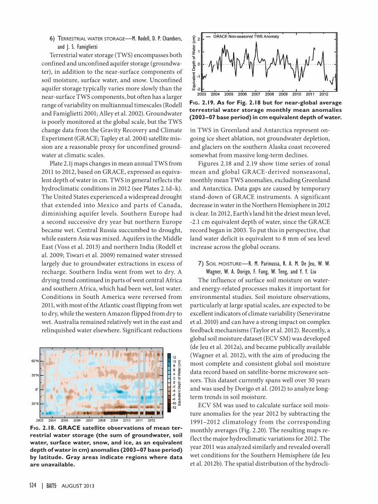
S24 | august 2013
6) terreStriaL water Storage—M. Rodell, D. P. Chambers, and J. S. Famiglietti
Terrestrial water storage (TWS) encompasses both confined and unconfined aquifer storage (groundwa-ter), in addition to the near-surface components of soil moisture, surface water, and snow. Unconfined aquifer storage typically varies more slowly than the near-surface TWS components, but often has a larger range of variability on multiannual timescales (Rodell and Famiglietti 2001; Alley et al. 2002). Groundwater is poorly monitored at the global scale, but the TWS change data from the Gravity Recovery and Climate Experiment (GRACE; Tapley et al. 2004) satellite mis-sion are a reasonable proxy for unconfined ground-water at climatic scales.
Plate 2.1j maps changes in mean annual TWS from 2011 to 2012, based on GRACE, expressed as equiva-lent depth of water in cm. TWS in general reflects the hydroclimatic conditions in 2012 (see Plates 2.1d–k). The United States experienced a widespread drought that extended into Mexico and parts of Canada, diminishing aquifer levels. Southern Europe had a second successive dry year but northern Europe became wet. Central Russia succumbed to drought, while eastern Asia was mixed. Aquifers in the Middle East (Voss et al. 2013) and northern India (Rodell et al. 2009; Tiwari et al. 2009) remained water stressed largely due to groundwater extractions in excess of recharge. Southern India went from wet to dry. A drying trend continued in parts of west central Africa and southern Africa, which had been wet, lost water. Conditions in South America were reversed from 2011, with most of the Atlantic coast flipping from wet to dry, while the western Amazon flipped from dry to wet. Australia remained relatively wet in the east and relinquished water elsewhere. Significant reductions
in TWS in Greenland and Antarctica represent on-going ice sheet ablation, not groundwater depletion, and glaciers on the southern Alaska coast recovered somewhat from massive long-term declines.
Figures 2.18 and 2.19 show time series of zonal mean and global GRACE-derived nonseasonal, monthly mean TWS anomalies, excluding Greenland and Antarctica. Data gaps are caused by temporary stand-down of GRACE instruments. A significant decrease in water in the Northern Hemisphere in 2012 is clear. In 2012, Earth's land hit the driest mean level, -2.1 cm equivalent depth of water, since the GRACE record began in 2003. To put this in perspective, that land water deficit is equivalent to 8 mm of sea level increase across the global oceans.
7) SoiL moiSture—R. M. Parinussa, R. A. M. De Jeu, W. W. Wagner, W. A. Dorigo, F. Fang, W. Teng, and Y. Y. Liu
The influence of surface soil moisture on water- and energy-related processes makes it important for environmental studies. Soil moisture observations, particularly at large spatial scales, are expected to be excellent indicators of climate variability (Seneviratne et al. 2010) and can have a strong impact on complex feedback mechanisms (Taylor et al. 2012). Recently, a global soil moisture dataset (ECV SM) was developed (de Jeu et al. 2012a), and became publically available (Wagner et al. 2012), with the aim of producing the most complete and consistent global soil moisture data record based on satellite-borne microwave sen-sors. This dataset currently spans well over 30 years and was used by Dorigo et al. (2012) to analyze long-term trends in soil moisture.
ECV SM was used to calculate surface soil mois-ture anomalies for the year 2012 by subtracting the 1991–2012 climatology from the corresponding monthly averages (Fig. 2.20). The resulting maps re-flect the major hydroclimatic variations for 2012. The year 2011 was analyzed similarly and revealed overall wet conditions for the Southern Hemisphere (de Jeu et al. 2012b). The spatial distribution of the hydrocli-
Fig. 2.18. GRACE satellite observations of mean ter-restrial water storage (the sum of groundwater, soil water, surface water, snow, and ice, as an equivalent depth of water in cm) anomalies (2003–07 base period) by latitude. Gray areas indicate regions where data are unavailable.
Fig. 2.19. As for Fig. 2.18 but for near-global average terrestrial water storage monthly mean anomalies (2003–07 base period) in cm equivalent depth of water.

S25STATE OF THE CLIMATE IN 2012 |AuguST 2013
matic variations 2012 clearly shows the capacity of the soil moisture dataset to capture drought and flood events. In contrast with 2011, there was no distinct division between hemispheres in 2012 (Plate 2.1k).
There was major flooding of the Murrumbidgee River, a large tributary of the Murray River in south-east Australia, in March 2012. New South Wales was hardest hit and Queensland and Victoria were also significantly impacted. Flooding events in Australia are associated with La Niña. The most prominent drought in 2012 was in the central United States and Canada (see section 7b; Plate 2.1k). It resulted from a shortage of snow melt in spring followed by a severe summer heat wave, yielding year round negative soil moisture anomalies. Also, the ongoing drought in
the southern United States, most prominent in the state of Texas, is evident. Another region suffering year round drought was northeastern Brazil, a region intensely used for agriculture. Droughts in these regions have been ascribed to La Niña (Mar-lon et al. 2012). Significant drought in parts of southern Europe resulted from both low precipitation and high temperatures. (See Chapter 7 for more regional flooding and drought details.)
Figure 2.21 shows month-ly mean soil moisture anoma-lies 1991–2012 time series for each hemisphere. Fluctua-tions over the entire analysis period reveal much larger deviations in the Southern Hemisphere compared to the Northern Hemisphere. This difference is likely the result of the smaller land area in the Southern Hemi-sphere. The year 2011 was the wettest on record for the
Southern Hemisphere. In contrast, 2012 shows soil moisture conditions slightly below average for both hemispheres. The standard deviation (not shown) of the sample used to calculate the monthly mean soil moisture anomalies exhibited a record high value in 2012, suggesting an increase in extreme conditions compared to the reference time series.
e. Atmospheric circulation1) meaN Sea LeveL preSSure—R. Allan and C. K FollandAtmospheric Southern Oscillation index (SOI)
values and oceanic SST anomalies show that the protracted La Niña episode, which developed in mid-2010, terminated in early 2012 (Fig. 2.22a). This episode resulted in major precipitation and tempera-
ture impacts across the entire Indo-Pacific region and at higher latitudes in both hemi-spheres (http://www.ncdc.noaa.gov/sotc/service/global/significant-extremes/201113.
Fig. 2.20. Selected 2012 monthly soil moisture anomaly images derived from the multidecadal satellite soil moisture dataset. The anomalies (m3 m-3) are relative to 1979–2012 base period. Images are based on WindSat, TMI, and ASCAT observations. Gray areas indicate regions where data are unavailable.
Fig. 2.21. Hemispheric monthly mean soil moisture anomalies (m3 m-3) for 1991–2012; the anomalies are relative to 1979–2012 base period.

S26 | august 2013
gif; http://poleshift.ning.com/profiles/blogs/2012-significant-climate-anomalies-and-events).
El Niño and La Niña can be measured by the SOI, the normalized mean sea level pressure (MSLP) dif-ference between Tahiti and Darwin (Allan et al. 1996). Other indices, employing SST are also commonly used (Kaplan 2011). El Niños (negative SOI) and La Niñas (positive SOI) vary in magnitude, duration, and evolution, with no two events or episodes exactly the same. There is also the propensity in the climate system for the occasional development of protracted El Niño and La Niña episodes (Allan et al. 2003), when a La Niña (El Niño) event appears to be ending and/or moving into an El Niño (La Niña) only to be revi-talized and continue as an La Niña (El Niño). Figure 2.22a shows the presence of such episodes in the SOI record since 1876, and that they can last up to six years (e.g., the 1990–95 protracted El Niño).
The SOI trace since 2009 highlights the shift from El Niño to strong La Niña conditions around mid-2010, a decline in the event by mid-2011 and its resurgence and continuation until its demise in early 2012 (Fig. 2.22b). Major El Niño and La Niña events can be near-global in their influence on world weather patterns, owing to ocean-atmosphere interactions across the Indo-Pacific region with teleconnections to higher latitudes in both hemispheres.
The Northern Hemisphere winters of 2010/11, 2011/12, and 2012/13 experienced contrasting North Atlantic Oscillation (NAO)/Arctic Oscillation (AO) conditions (Fig. 2.23). In 2010/11, the NAO/AO in-dices were dominated by long periods of extremely negative values, with positive pressure anomalies over higher latitudes and negative anomalies over the midlatitudes, and an associated reduction in the westerlies over the North Atlantic-European sector. This contrasted markedly with the 2011/12 boreal
winter, when opposite conditions prevailed. During 2012/13, the boreal winter began with positive NAO/AO conditions, favoring a westerly regime, but this was succeeded by a predominantly negative NAO/AO leading to reduced westerlies and colder, snowy weather over western Europe in early 2013 (Fig. 2.23f).
In the main boreal summer months of July and August, the summer NAO (SNAO), which has a northward displaced pattern compared to the winter NAO (Folland et al. 2009), continued the generally negative phase observed since summer 2007. Figure 2.24a shows daily SNAO values for July and August 2012. This negative phase is reflected in the pattern shown in the North Atlantic and Europe MSLP anomaly map for July and August (Fig. 2.24b). Recent cyclonic northwest Europe summers are likely related in part to the current warm North Atlantic phase of
Fig. 2.22. The Southern Oscillation Index (SOI) time series from (a) 1876 to early 2013 and (b) 1998 to early 2013. [Data from HadSLP2r (Allan and Ansell 2006).]
Fig. 2.23. NAO patterns in mean sea level pressure anomalies (hPa) and daily index (hPa) for (a), (d) win-ter 2010/11; (b), (e) winter 2011/12; and (c), (f) winter 2012/13.

S27STATE OF THE CLIMATE IN 2012 |AuguST 2013
the Atlantic multidecadal oscillation (AMO; Folland et al. 2009; Sutton and Dong 2012), a pattern also seen in the HadCM3 coupled model (Knight et al. 2006). June has also followed this MSLP anomaly tendency in recent years, although historically June tends to behave differently from July and August (Folland et al. 2009). A strong multidecadal fluctuation from generally positive SNAO values in the late twentieth century to the current negative phase is illustrated by Fig. 2.24c; some differences in the location of the center of recent negative anomaly patterns from that of the standard SNAO pattern (shown in Allan and Folland 2012) may underestimate the recent cyclonic tendency near the United Kingdom. Similarly, in 2012 the cyclonic anomaly center is displaced west of the SNAO center.
Globally in 2012, f luctuations in midlatitude circulation patterns and tropical monsoon regimes saw the warmest boreal summer in Canada since 1948, major drought conditions in the United States, the coldest Eurasia mid-January–February period in the last 26 years, the lowest premonsoon rainfall in India since 1901, severe July–September f lood-ing across western to central Africa, and the third driest April–October period in Western Australia (see Chapter 7 for further detail; http://poleshift.ning.com/profiles/blogs/2012-significant-climate-anomalies-and-events). Annual average anomalies of MSLP appear in Plate 2.1l.
2) Surface wiNdS
(i) Land surface wind speed—T. R. McVicar, R. Vautard, J.-N. Thépaut, P. Berrisford, and R. J. H. Dunn
2012 was the second weakest land surface winds year since monitoring began in 1981 (Fig. 2.25a). In each continental region of the Northern Hemisphere, mean surface wind speed was low, especially over Asia (record low over central Asia, third lowest over East Asia). Over North America, the mean wind speed was third lowest and it was tenth lowest over Europe. In the Southern Hemisphere, 2012 mean wind speed over Australia was also record low. Continued declin-ing observed trends during 2012 are similar to those reported for the two previous years (see Peterson et al. 2011; Vautard et al. 2012).
The NOAA ISD-LITE database (quality controlled as per Vautard et al. 2010) is the primary dataset uti-lized for this analysis. Station wind speeds from Had-
Fig. 2.24. Summer NAO patterns for the North At-lantic European region. (a) Daily values of the SNAO (hPa) for Jul and Aug 2012 based on the daily SNAO pattern. (b) Mean sea level pressure anomalies (hPa) for summer (Jul–Aug) 2012. (c) Annual values of the SNAO (hPa) averaged over Jul and Aug 1850–2012 and a centered 11-year running mean. All anomalies and indices are relative to 1981–2010 base period.
Fig. 2.25. Global and regional average annual mean land wind speed calculated using the augmented NOAA ISD-LITE database (solid) and the augmented HadISD database (dotted). (a) Anomalies (m s-1; 1981–2010 base period), (b) frequency of wind speeds >3 m s-1, and (c) frequency of wind speeds >10 m s-1. Regional means and trends are shown in Table 2.4. Occurrence frequencies were not calculated for Australia in (b) and (c).

S28 | august 2013
ISD (Dunn et al. 2012) are also shown for comparison. Both are augmented with higher quality independent Australian data (McVicar et al. 2008), replacing their own Australian stations. The quality control leads to an objective selection of at least 1400 stations globally with observations over 1981–2012. While many of the ISD-LITE and HadISD source stations are the same, processing methodologies differ.
Partitioning wind speeds into >3 m s-1 and >10 m s-1 also shows declining wind speeds. Globally, the ISD-LITE 2012 frequency of wind speeds >3 m s-1 (52.0%) is 3% lower than the corresponding 1981 value and close to the record low (51.8%) of 2010 (Fig. 2.25b). For stronger wind speeds (>10 m s-1), the 2012 frequency is 25% below the frequencies found in 1981. For central Asia, such strong winds occurred 2.3% of the time in 1981 but only 0.7% of the time in 2012 (Fig. 2.25c). Exactly how these changes relate to wind speeds aloft remains an interesting research question, with potential implications for renewable wind energy production (Bakker et al. 2012; Holt and Wang 2012).
The spatial patterns of linear wind speed trends (m s-1 yr-1) for 1981–2012 are shown for both the aug-mented ISD-LITE (Fig. 2.26a) and for the augmented HadISD (Fig. 2.26b; Table 2.4). Despite methodologi-cal differences, the general spatial patterns are similar. Uncertainty in the wind speed trends is quantified by differencing the trends in the two global datasets (Fig. 2.26c). At the 876 common sites the average difference (ISD-Lite minus HadISD) is -0.001 m s-1 yr-1 with a standard deviation of 0.001 m s-1 yr-1. The differences in the per-site 1981–2012 wind speed climatologies have an average and standard deviation of 0.019 m s-1 and 0.110 m s-1, respectively (Online Fig. S2.17; Table 2.4). These differences are generally smaller than the trends shown, suggesting that the observed trends are not influenced by different data process-ing protocols and quality control procedures, though there are some differences in the frequency of strong winds (Fig. 2.25b,c).
Using the ERA-Interim (Dee et al. 2011) output in addition to ISD-LITE, the 2012 land surface wind anomaly pattern resembled that of 2010 and 2011 (Plate 2.1m; Online Figs. S2.18, S2.19 for comparison using other products; see Peterson et al. 2011; Vau-tard et al. 2012), with strong negative anomalies over eastern North America, central Europe, central Asia, eastern China, and Japan, contrasting with positive anomalies found for South America, Republic of South Africa, and west Africa. Results for Australia are mixed. There is overall good agreement between ERA-Interim anomalies and those from the ISD-LITE
Fig. 2.26. Global distributions of the land wind speed trends (m s-1 yr-1) for 1981–2012 calculated using (a) the augmented NOAA ISD-LITE database and (b) augmented HadlSD dataset. (c) Trend differences between the two, calculated as (a)-(b).
Table 2.4. Global and regional average wind speeds and trends for 1981–2012 using the augmented NOAA ISD-LITE database. Values in brackets are from the augmented HadlSD dataset.
Region Mean Wind Speed (m s-1)
Trend (m s-1 yr-1)
Number of Stations
Globe 3.5 [3.3]-0.0070[-0.0111]
1453 [1400]
Europe 3.9 [3.8]-0.0066[-0.0118]
511 [332]
Central Asia 2.6 [3.0]-0.0074
[-0.0169]57 [137]
East Asia 2.8 [2.7]-0.0069
[-0.0093]259 [303]
North America 3.8 [3.7]-0.0106
[-0.0142]379 [391]
Australia 2.1 [2.1]-0.0072
[-0.0072]41 [41]

S29STATE OF THE CLIMATE IN 2012 |AuguST 2013
observations. This is consistent with Vautard et al. (2010) who showed that the interannual variability of surface winds is fairly well reproduced in reanalyses, although trends are underestimated. The dissimilar-ity in trends has been noted in both the Northern (Pryor et al. 2009) and Southern Hemispheres (McVicar et al. 2008). Many global climate models also do not concur with observed land winds (Chen et al. 2012a; Johnson and Sharma 2010; McInnes et al. 2011). These differences suggest that use of these outputs to model trends of atmospheric evaporative demand over land remains questionable (McVicar et al. 2012a). In all cases (observations, models, and re-analyses), more research is needed to characterize and improve estimates of the land surface wind speeds.
Land surface winds have a major inf luence on many physical and biological processes, such as the water cycle and plant production, and inf luence land-surface exchanges with the lower atmosphere. Although long-term wind changes are challeng-ing to characterize (as measurements may undergo changes in location, observation protocols, and/or techniques, and local surface roughness) many re-gional studies report declining surface wind speeds in the midlatitudes and the tropics of ~-0.01 m s-1 yr-1 (see McVicar et al. 2012b for a global review). A major part of this trend in the Northern Hemisphere appears attributable to land cover changes (Vautard et al. 2010; Wever 2012) and increasing aerosol levels (Jacobson and Kaufman 2006), though for specific regions other factors are important (Bichet et al. 2012; Chen et al. 2012b).
(ii) Ocean surface wind speed—C. MearsGlobally-averaged winds over the oceans for
2012 were close to average and a little lower than in 2011. Estimates were obtained from satellite-borne microwave radiometers (Wentz 1997; Wentz et al. 2007; Fig. 2.27). The record exhibits a maximum in 1988–89, followed by a broad minimum in 1991–97. Winds were stronger than average from 1998 to 2000 and in 2006–07. In 2008–09, global wind speed fell slightly, followed by a partial recovery in 2010–11, and another fall in late 2012. Both the global time series and the Hovmuller diagram of wind speed anomalies (Fig. 2.28) are dominated by short-term variability making multidecadal-scale changes difficult to evalu-ate. Other long-term records exist from WASwinds (Tokinaga and Xie 2011), which uses wave and an-emometer measurements from ships corrected for changing ship heights. This dataset covers 1987–2008. The WASwinds global average is in good agreement
with the satellite data between 1993 and 2007 but, un-like the satellite data, it shows a conspicuous positive trend over the period (Fig. 2.27). Ocean surface wind speeds can also be obtained from reanalyses; these are also shown in Fig. 2.27. With the exception of NCEP-CFSR, the reanalyses show increasing trends.
During 2012, ocean surface winds showed large positive anomalies in the central tropical Pacific, the South Pacific south of about 40°S, and in the Gulf of Alaska. Positive anomalies around Cape Horn in southern Chile concur with those over land as shown by ERA-Interim and ISD-LITE station data. Most other areas showed negative anomalies (Plate 2.1m)
Fig. 2.27. Surface wind speed anomalies (m s-1) over the global ice-free oceans as measured by (a) Remote Sensing Systems using satellite-borne microwave radiometers SSM/I, AMSR-E, SSMIS, and WindSat; (b) WASwind ship anemometers; and (c) reanalyses (over all ocean) as described in Fig. 2.1. The satellite time series has been smoothed to remove variability on time scales shorter than 4 months. The reference period for the combined measurements is 1988–2010 although all have been given a zero mean over the common period 1988–2008.
Fig. 2.28. Hovmuller plot of surface wind speed anomalies (m s-1; reference period 1988–2010) over the ice-free oceans. Data have been smoothed in time to remove variability on time scales shorter than 4 months. Gray areas indicate regions where data are not available.
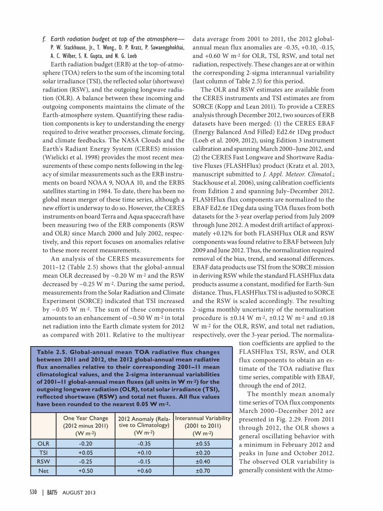
S30 | august 2013
f. Earth radiation budget at top of the atmosphere— P. W. Stackhouse, Jr., T. Wong., D. P. Kratz, P. Sawaengphokhai, A. C. Wilber, S. K. Gupta, and N. G. LoebEarth radiation budget (ERB) at the top-of-atmo-
sphere (TOA) refers to the sum of the incoming total solar irradiance (TSI), the reflected solar (shortwave) radiation (RSW), and the outgoing longwave radia-tion (OLR). A balance between these incoming and outgoing components maintains the climate of the Earth-atmosphere system. Quantifying these radia-tion components is key to understanding the energy required to drive weather processes, climate forcing, and climate feedbacks. The NASA Clouds and the Earth's Radiant Energy System (CERES) mission (Wielicki et al. 1998) provides the most recent mea-surements of these compo nents following in the leg-acy of similar measurements such as the ERB instru-ments on board NOAA 9, NOAA 10, and the ERBS satellites starting in 1984. To date, there has been no global mean merger of these time series, although a new effort is underway to do so. However, the CERES instruments on board Terra and Aqua spacecraft have been measuring two of the ERB components (RSW and OLR) since March 2000 and July 2002, respec-tively, and this report focuses on anomalies relative to these more recent measurements.
An analysis of the CERES measurements for 2011–12 (Table 2.5) shows that the global-annual mean OLR decreased by ~0.20 W m-2 and the RSW decreased by ~0.25 W m-2. During the same period, measurements from the Solar Radiation and Climate Experiment (SORCE) indicated that TSI increased by ~0.05 W m-2. The sum of these components amounts to an enhancement of ~0.50 W m-2 in total net radiation into the Earth climate system for 2012 as compared with 2011. Relative to the multiyear
data average from 2001 to 2011, the 2012 global-annual mean flux anomalies are -0.35, +0.10, -0.15, and +0.60 W m-2 for OLR, TSI, RSW, and total net radiation, respectively. These changes are at or within the corresponding 2-sigma interannual variability (last column of Table 2.5) for this period.
The OLR and RSW estimates are available from the CERES instruments and TSI estimates are from SORCE (Kopp and Lean 2011). To provide a CERES analysis through December 2012, two sources of ERB datasets have been merged: (1) the CERES EBAF (Energy Balanced And Filled) Ed2.6r 1Deg product (Loeb et al. 2009, 2012), using Edition 3 instrument calibration and spanning March 2000–June 2012, and (2) the CERES Fast Longwave and Shortwave Radia-tive Fluxes (FLASHFlux) product (Kratz et al. 2013, manuscript submitted to J. Appl. Meteor. Climatol.; Stackhouse et al. 2006), using calibration coefficients from Edition 2 and spanning July–December 2012. FLASHFlux flux components are normalized to the EBAF Ed2.6r 1Deg data using TOA fluxes from both datasets for the 3-year overlap period from July 2009 through June 2012. A modest drift artifact of approxi-mately +0.12% for both FLASHFlux OLR and RSW components was found relative to EBAF between July 2009 and June 2012. Thus, the normalization required removal of the bias, trend, and seasonal differences. EBAF data products use TSI from the SORCE mission in deriving RSW while the standard FLASHFlux data products assume a constant, modified for Earth-Sun distance. Thus, FLASHFlux TSI is adjusted to SORCE and the RSW is scaled accordingly. The resulting 2-sigma monthly uncertainty of the normalization procedure is ±0.14 W m-2, ±0.12 W m-2 and ±0.18 W m-2 for the OLR, RSW, and total net radiation, respectively, over the 3-year period. The normaliza-
tion coefficients are applied to the FLASHFlux TSI, RSW, and OLR f lux components to obtain an es-timate of the TOA radiative f lux time series, compatible with EBAF, through the end of 2012.
The monthly mean anomaly time series of TOA flux components March 2000–December 2012 are presented in Fig. 2.29. From 2011 through 2012, the OLR shows a general oscillating behavior with a minimum in February 2012 and peaks in June and October 2012. The observed OLR variability is generally consistent with the Atmo-
One Year Change(2012 minus 2011)
(W m-2)
2012 Anomaly (Rela-tive to Climatology)
(W m-2)
Interannual Variability(2001 to 2011)
(W m-2)
OLR -0.20 -0.35 ±0.55TSI +0.05 +0.10 ±0.20
RSW -0.25 -0.15 ±0.40
Net +0.50 +0.60 ±0.70
Table 2.5. Global-annual mean TOA radiative flux changes between 2011 and 2012, the 2012 global-annual mean radiative flux anomalies relative to their corresponding 2001–11 mean climatological values, and the 2-sigma interannual variabilities of 2001–11 global-annual mean fluxes (all units in W m-2) for the outgoing longwave radiation (OLR), total solar irradiance (TSI), reflected shortwave (RSW) and total net fluxes. All flux values have been rounded to the nearest 0.05 W m-2.
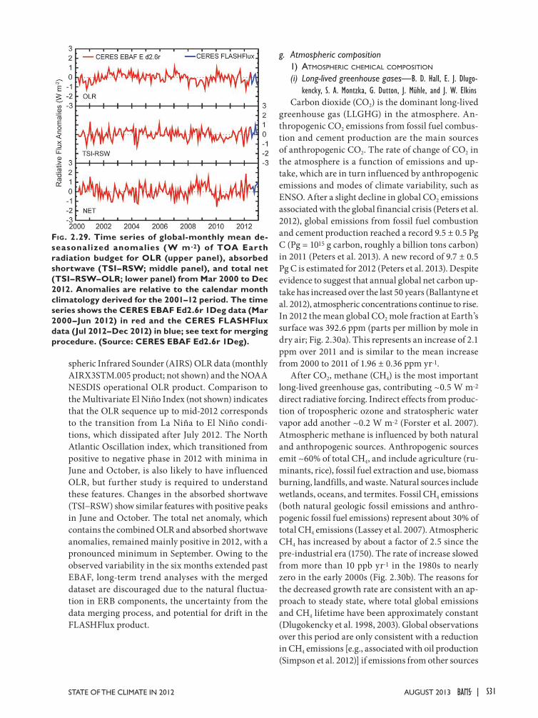
S31STATE OF THE CLIMATE IN 2012 |AuguST 2013
spheric Infrared Sounder (AIRS) OLR data (monthly AIRX3STM.005 product; not shown) and the NOAA NESDIS operational OLR product. Comparison to the Multivariate El Niño Index (not shown) indicates that the OLR sequence up to mid-2012 corresponds to the transition from La Niña to El Niño condi-tions, which dissipated after July 2012. The North Atlantic Oscillation index, which transitioned from positive to negative phase in 2012 with minima in June and October, is also likely to have influenced OLR, but further study is required to understand these features. Changes in the absorbed shortwave (TSI−RSW) show similar features with positive peaks in June and October. The total net anomaly, which contains the combined OLR and absorbed shortwave anomalies, remained mainly positive in 2012, with a pronounced minimum in September. Owing to the observed variability in the six months extended past EBAF, long-term trend analyses with the merged dataset are discouraged due to the natural fluctua-tion in ERB components, the uncertainty from the data merging process, and potential for drift in the FLASHFlux product.
g. Atmospheric composition1) atmoSpheric chemicaL compoSitioN
(i) Long-lived greenhouse gases—B. D. Hall, E. J. Dlugo-kencky, S. A. Montzka, G. Dutton, J. Mühle, and J. W. Elkins
Carbon dioxide (CO2) is the dominant long-lived greenhouse gas (LLGHG) in the atmosphere. An-thropogenic CO2 emissions from fossil fuel combus-tion and cement production are the main sources of anthropogenic CO2. The rate of change of CO2 in the atmosphere is a function of emissions and up-take, which are in turn influenced by anthropogenic emissions and modes of climate variability, such as ENSO. After a slight decline in global CO2 emissions associated with the global financial crisis (Peters et al. 2012), global emissions from fossil fuel combustion and cement production reached a record 9.5 ± 0.5 Pg C (Pg = 1015 g carbon, roughly a billion tons carbon) in 2011 (Peters et al. 2013). A new record of 9.7 ± 0.5 Pg C is estimated for 2012 (Peters et al. 2013). Despite evidence to suggest that annual global net carbon up-take has increased over the last 50 years (Ballantyne et al. 2012), atmospheric concentrations continue to rise. In 2012 the mean global CO2 mole fraction at Earth’s surface was 392.6 ppm (parts per million by mole in dry air; Fig. 2.30a). This represents an increase of 2.1 ppm over 2011 and is similar to the mean increase from 2000 to 2011 of 1.96 ± 0.36 ppm yr-1.
After CO2, methane (CH4) is the most important long-lived greenhouse gas, contributing ~0.5 W m-2 direct radiative forcing. Indirect effects from produc-tion of tropospheric ozone and stratospheric water vapor add another ~0.2 W m-2 (Forster et al. 2007). Atmospheric methane is influenced by both natural and anthropogenic sources. Anthropogenic sources emit ~60% of total CH4, and include agriculture (ru-minants, rice), fossil fuel extraction and use, biomass burning, landfills, and waste. Natural sources include wetlands, oceans, and termites. Fossil CH4 emissions (both natural geologic fossil emissions and anthro-pogenic fossil fuel emissions) represent about 30% of total CH4 emissions (Lassey et al. 2007). Atmospheric CH4 has increased by about a factor of 2.5 since the pre-industrial era (1750). The rate of increase slowed from more than 10 ppb yr-1 in the 1980s to nearly zero in the early 2000s (Fig. 2.30b). The reasons for the decreased growth rate are consistent with an ap-proach to steady state, where total global emissions and CH4 lifetime have been approximately constant (Dlugokencky et al. 1998, 2003). Global observations over this period are only consistent with a reduction in CH4 emissions [e.g., associated with oil production (Simpson et al. 2012)] if emissions from other sources
Fig. 2.29. Time series of global-monthly mean de-seasonalized anomalies (W m-2) of TOA Earth radiation budget for OLR (upper panel), absorbed shortwave (TSI–RSW; middle panel), and total net (TSI–RSW–OLR; lower panel) from Mar 2000 to Dec 2012. Anomalies are relative to the calendar month climatology derived for the 2001–12 period. The time series shows the CERES EBAF Ed2.6r 1Deg data (Mar 2000–Jun 2012) in red and the CERES FLASHFlux data (Jul 2012–Dec 2012) in blue; see text for merging procedure. (Source: CERES EBAF Ed2.6r 1Deg).
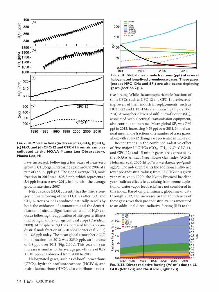
S32 | august 2013
have increased. Following a few years of near-zero growth, CH4 began increasing again around 2007 at a rate of about 6 ppb yr-1. The global average CH4 mole fraction in 2012 was 1808.5 ppb, which represents a 5.4 ppb increase over 2011, in line with the average growth rate since 2007.
Nitrous oxide (N2O) currently has the third stron-gest climate forcing of the LLGHGs after CO2 and CH4. Nitrous oxide is produced naturally in soils by both the oxidation of ammonium and the denitri-fication of nitrate. Significant emission of N2O can occur following the application of nitrogen fertilizers (including manure) on agricultural crops (Davidson 2009). Atmospheric N2O has increased from a pre-in-dustrial mole fraction of ~270 ppb (Forster et al. 2007) to ~325 ppb today. The mean global atmospheric N2O mole fraction for 2012 was 325.0 ppb, an increase of 0.8 ppb over 2011 (Fig. 2.30c). This year-on-year increase is similar to the average growth rate of 0.79 ± 0.01 ppb yr-1 observed from 2000 to 2012.
Halogenated gases, such as chlorofluorocarbons (CFCs), hydrochlorof luorocarbons (HCFCs), and hydrofluorocarbons (HFCs), also contribute to radia-
tive forcing. While the atmospheric mole fractions of some CFCs, such as CFC-12 and CFC-11 are decreas-ing, levels of their industrial replacements, such as HCFC-22 and HFC-134a are increasing (Figs. 2.30d, 2.31). Atmospheric levels of sulfur hexafluoride (SF6), associated with electrical transmission equipment, also continue to increase. Mean global SF6 was 7.60 ppt in 2012, increasing 0.29 ppt over 2011. Global an-nual mean mole fractions of a number of trace gases, along with 2011–12 changes are presented in Table 2.6.
Recent trends in the combined radiative effect of five major LLGHGs (CO2, CH4, N2O, CFC-11, and CFC-12) and 15 minor gases are expressed by the NOAA Annual Greenhouse Gas Index (AGGI; Hofmann et al. 2006; http://www.esrl.noaa.gov/gmd/aggi/). The index represents the additional influence (over pre-industrial values) from LLGHGs in a given year relative to 1990, the Kyoto Protocol baseline year. Indirect effects (e.g., arising from ozone deple-tion or water vapor feedbacks) are not considered in this index. Based on preliminary, global mean data through 2012, the increases in the abundances of these gases over their pre-industrial values amounted to an additional direct radiative forcing (RF) to the
Fig. 2.30. Mole fractions (in dry air) of (a) CO2, (b) CH4, (c) N2O, and (d) CFC-12 and CFC-11 from air samples collected at the NOAA Mauna Loa Observatory, Mauna Loa, HI.
Fig. 2.31. Global mean mole fractions (ppt) of several halogenated long-lived greenhouse gases. These gases (except HFC-134a and SF6) are also ozone-depleting gases (section 2gii).
Fig. 2.32. Direct radiative forcing (W m-2) due to LL-GHG (left axis) and the AGGI (right axis).

S33STATE OF THE CLIMATE IN 2012 |AuguST 2013
atmosphere totaling 2.88 W m-2. This compares with 2.18 W m-2 in 1990 (Fig. 2.32), resulting in an index value of 1.32. Thus, the accumulation of LLGHGs in the atmosphere since 1990 has resulted in a 32% increase in RF. The change in the RF from LLGHGs
considered in the index was 1.26% between 2011 and 2012, which is similar to the average change from 2000 to 2012 (1.24%). In fact, since 2000 only one year (2009) showed an increase of less than 1%.
Table 2.6. Mole fractions, radiative efficiencies and lifetimes of chemicals considered in the AGGI (CO2 mixing ratios are in ppm, N2O and CH4 in ppb, and all others in ppt).
Industrial Designation or Common Name
Chemical Formula AGGI ODGI
Radiative Efficiency
(W m-2 ppb-1)a
Mean Surface Mole Fraction, 2012 [change
from prior year]b
Lifetime(years)
Carbon Dioxide CO2 Y N 1.41 × 10⁻⁵ 392.6[+2.1] c
Methane CH4 Y N 3.7 × 10⁻⁴ 1808.5[+5.4] c 9.1
Nitrous oxide N2O Y N 3.03 × 10⁻³ 325.0[+0.8] 131
ChlorofluorocarbonsCFC-11 CCl3F Y Y 0.25 236.8[-2.1] c 45
CFC-12 CCl2F2 Y Y 0.32 525.3[-2.6] c 100
CFC-113 CCl2FCClF2 Y Y 0.30 74.7[-0.7] c 85
HydrochlorofluorocarbonsHCFC-22 CHClF2 Y Y 0.20 212.7[+8.7] c 11.9
HCFC-141b CH3CCl2F Y Y 0.14 21.3[+0.9] c 9.2
HCFC-142b CH3CClF2 Y Y 0.20 20.9[+0.8] c 17.2
Hydrofluorocarbons
HFC-134a CH2FCF3 Y N 0.16 62.6[+5.4] c 14.2
HFC-152a CH3CHF2 Y N 0.09 6.5[+0.4] c 1.5
HFC-143a CH3CF3 Y N 0.13 11.1[+1.0] c 47.1
HFC-125 CHF2CF3 Y N 0.23 9.7[+1.4] c 28.2
HFC-23 CHF3 Y N 0.19 25.0[+0.9] c 222
Chlorocarbons
Methyl Chloroform CH3CCl3 Y Y 0.06 6.3[-1.3] 5.0
Carbon Tetrachloride CCl4 Y Y 0.13 85.8[-1.1] 26
Methyl Chloride CH3Cl N Y 0.01 537[-3] 1.0
Bromocarbons
Methyl Bromide CH3Br N Y 0.01 7.0[-0.03] c 0.8
Halon 1211 CBrClF2 Y Y 0.30 4.0[-0.1] c 16.0
Halon 1301 CBrF3 Y Y 0.32 3.2[+0.04] c 65
Halon 2402 CBrF2CBrF2 Y Y 0.33 0.45[-0.01] c 20
Fully fluorinated species
Sulfur Hexafluoride SF6 Y N 0.52 7.60[+0.29] 3200
PFC-14 CF4 N N 0.10 79.7[+0.7] c > 50 000
PFC-116 C2F6 N N 0.26 4.25[+0.08] c > 10 000
a Radiative efficiencies and lifetimes are taken from Daniel et al. (2011), Montzka et al. (2011), and Prather at al. (2012). For CO2, numer-ous removal processes complicate derivation of a lifetime.
b Mole fractions are global surface means determined from the NOAA global cooperative air sampling network (Hofmann et al. 2006), except for PFC-14, PFC-116, and HFC-23, which were measured by the AGAGE group (Mühle et al. 2010; Miller et al. 2010). Changes indicated in brackets are the differences between the 2012 and 2011 global mean mole fractions.
c Preliminary estimate for 2012.

S34 | august 2013
(ii) Ozone-depleting gases—B. D. Hall, S. A. Montzka, G. Dutton, and J. W. Elkins
In addition to their direct radiative forcing, long-lived gases containing chlorine and bromine also influence RF indirectly through destruction of strato-spheric ozone. Production of many halocarbons has been substantially reduced in recent years through amendments and adjustments to the 1987 Montreal Protocol on Substances that Deplete the Ozone Layer. As a result, atmospheric mole fractions of many of the most potent ozone-depleting gases have been declin-ing at Earth’s surface (Figs. 2.30d, 2.31).
While mole fractions of many ozone-depleting substances (ODS) are declining, those of some ha-logenated gases continue to increase globally (Fig. 2.31). The most rapid increases are observed for hydrochlorofluorocarbons (HCFCs) and hydrofluo-rocarbons (HFCs), which are common replacements for chlorofluorocarbons (CFCs), and halons. HCFCs contain chlorine and contribute to ozone depletion, while HFCs do not.
Progress towards stratospheric halogen declining back to the 1980 level, often used as a benchmark, can be assessed with the NOAA Ozone-Depleting Gas In-dex (ODGI; Table 2.6; Hofmann and Montzka 2009). This index is derived from surface measurements of ozone-depleting substances together with an estimate of their potential to destroy stratospheric ozone, for example bromine is 60–65 times more effective than chlorine (Montzka et al. 2011). Factors also include transit time from Earth’s surface to the stratosphere, mixing during transit, and photolytic reactivity (Schauff ler et al. 2003; Newman et al. 2007). The weighted sum of chlorine and bromine, combined with these factors yields a quantity known as Equiva-lent Effective Stratospheric Chlorine (EESC), which is an estimate of reactive halogen mole fraction in the stratosphere (Fig. 2.33a). The ODGI is the change in EESC from its peak, relative to that needed to reach the 1980 value (Fig. 2.33b). An updated NOAA ODGI was released in January 2013. The update includes improved methods of accounting for transport and reactions with solar radiation to form reactive halo-gen in the stratosphere (see http://www.esrl.noaa.gov/gmd/odgi/).
The EESC is calculated for two stratospheric regions: Antarctica and midlatitudes. EESC was ~1670 ppt and ~3900 ppt at the beginning of 2012 for the midlatitudes and Antarctica, respectively. Current EESC values in the midlatitudes are smaller than those in the Antarctic because the liberation of reactive halogen from halocarbons is substantially
less in the midlatitude stratosphere compared to the Antarctic. The ODGI for Antarctica was 87.2 at the beginning of 2012 (Fig. 2.33b). Thus, reactive halogen levels in the Antarctic stratosphere have progressed 13% of the way towards the 1980 benchmark. By con-trast, the ODGI for midlatitudes was 65.4, indicating substantial progress towards the 1980 benchmark.
2) aeroSoLS—A. Benedetti, L. T. Jones, A. Inness, J. W. Kaiser, and J. J. MorcretteAtmospheric aerosols have received considerable
attention in climate studies, especially due to large uncertainties in the relative impacts and amounts of reflecting and absorbing aerosols. Most aerosols have a general cooling impact because they reflect incoming solar radiation back to space. However, black carbon has a warming effect through absorp-tion of radiation at visible wavelengths. Bond et al. (2013) recently reviewed the climate impacts of black carbon (BC), indicating that the climate-warming ef-fect of BC is second only to that of carbon dioxide. In addition to anthropogenic aerosols, natural aerosols such as volcanic ash and desert dust are recognized
Fig. 2.33. (a) Equivalent Effective Stratospheric Chlo-rine (EESC), and (b) the NOAA Ozone-Depleting Gas Index (ODGI). The ODGI represents the relative mole fractions of reactive halogen in the midlatitude and Antarctic stratosphere scaled such that ODGI = 100 at maximum EESC and zero in 1980. Both EESC and ODGI are derived from NOAA surface measurements of ozone-depleting substances (symbols) or WMO scenarios (dashed lines; Daniel et al. 2011).

S35STATE OF THE CLIMATE IN 2012 |AuguST 2013
to have a large impact on regional and global climate (Haywood et al. 2005).
Atmospheric composition products currently derived from reanalyses have limited utility for trend analysis because of their short time histories, unknown bias in the modeled emission and removal processes, and limited availability of constraining satellite observations. However, they represent a use-ful tool for assessing the current state of climate and the interannual variability of important atmospheric constituents. In fact, it is difficult to infer the vari-ability of individual aerosol species from satellite data because satellites observe the integrated effect of the total aerosol amounts on radiation at the top of the at-mosphere. Aerosol reanalysis data products combine information from models and observations to provide an assessment of aerosol fields and aerosol types.
ECMWF has recently completed a 10-year re-analysis of atmospheric composition from 2003 to 2012 which includes aerosols, reactive gases, and greenhouse gases, under the EU-funded project MACC-II (Peuch and Engelen 2012). The MACC-II aerosol analysis (Morcrette et al. 2011) is based on 4DVAR assimilation of aerosol optical depth (AOD) observations at 550 nm from the MODIS sensors, including a global adaptive bias correction. Compari-sons of multiyear averages of AOD over the period 2003–10 from the MACC-II reanalysis and from the MISR sensors onboard the Terra satellite indicate good qualitative agreement (not shown). However, it is apparent that AODs in the MACC-II reanalysis may be overestimated in some regions, such as East Asia, while desert dust over the Sahara is underes-timated owing to the lack of constraining data and model deficiencies. Estimates of biomass burning aerosols benefit from fire emissions computed from fire radiative power observations (Global Fire As-similation System inventory, Kaiser et al. 2012; see section 2h4). Unbiased anomalies can be estimated when subtracting the annual mean for a given year from the multiyear average.
A map of the time-averaged total AOD anomaly for 2012 is shown in Plate 2.1n (long-term average shown as Online Fig. S2.20). The anomaly map for total AOD shows the extensive burning that occurred in Russia and Siberia during the boreal summer and the active dust season that induced increased trans-port over the Atlantic Ocean, particularly in the dust outflow area. It also shows an unusual bull's-eye of positive values in central Africa. The feature was caused by the eruption of volcano Nyiragongo (DR Congo, 1.52°S, 29.25°E), with an additional plume
from nearby volcano Nyamuragira (DR Congo, 1.41°S, 29.2°E). The Toulouse Volcanic Ash Advisory Centre reported that Nyiragongo had been emitting volcanic ash more vigorously starting on 3 July. In the current version of the MACC-II reanalysis, vol-canic aerosols are not included. Hence, the observed AOD signal from volcanic ash is attributed to other species in the reanalysis. In the specific case of the Nyiragongo, the volcanic ash signal has been attrib-uted mainly to dust and carbonaceous aerosols, since these are the aerosol types which dominate the area. Volcanic ash will be introduced in the next version of the MACC-II reanalysis.
Figure 2.34a shows the dust anomaly for March–May. This season was extremely active for dust, with large positive anomalies over the northern tropical Atlantic, the Arabian Peninsula, and the northern Indian Ocean. There was also a positive dust anomaly over the central United States, possibly as a result of dry winter and spring conditions (see section 7b2).
Figure 2.34b shows anomalies of carbonaceous aerosols in June–August. The signature of the strong fire season in Siberia is particularly striking. Also identifiable is the anomaly in biomass burning aero-sols in the western United States, as a result of one of the worst summers on record for wildfires in those
Fig. 2.34. MACC aerosol optical depth anomaly in (a) desert dust for Mar–May 2012 and (b) biomass burning for Jun–Aug 2012.

S36 | august 2013
areas. At the beginning of July, the area around Se-attle, Washington, experienced hazy skies. However the MACC-II analyses for biomass burning aerosols show that this smoke originated from the large wild fires in Asia (as opposed to fires in Colorado) and was transported over long distances at altitudes around 3 km (Online Figs. S2.21, S2.22). In particular, Online Fig. S2.22 shows a comparison between the MACC-II aerosol fields with data from the CALIOP lidar onboard the CALIPSO satellite (Winker et al. 2007). The correspondence between model cloud and aerosol fields and observations is extremely good.
3) StratoSpheric ozoNe—M. Weber, W. Chehade, V. E. Fioletov, S. M. Frith, C. S. Long, W. Steinbrecht, and J. D. Wild
The global distribution of total ozone (troposphere and stratosphere) in 2012 was similar to 2000–09, except in the Southern Hemisphere polar region and areas of the midlatitude Northern Hemisphere. About 90% of the ozone in the total column is of stratospheric origin. Total ozone values 25 DU–50 DU higher than average were observed above Ant-arctica, and values 10 DU–15 DU lower than average were observed above central Europe and the North Atlantic and Central Pacific Oceans (Plate 2.1q). The bands of positive ozone anomalies in the subtropics (25°–30°) and negative anomalies at the equator are a typical dynamical pattern caused by the easterly phase of the quasi-biennial oscillation (QBO). The positive anomalies in Antarctica are related to the small ozone hole observed in 2012 (see section 6g). While values in the Arctic polar region in March were close to the mean of the last decade, Antarctic values in austral spring from SBUV satellite measurements were the second largest since 1990 (see Fig. 2.35).
In Fig. 2.36, time series of total ozone since 1970 are shown for various zonal bands: global (60°S–60°N), middle latitudes in both hemispheres (30°–60°), and the tropics (25°S–25°N). The global average in 2012 is at the high end of ranges of values observed since the late 1990s. As in the tropics, a quasi-biennial variation is also evident in the extratropics. The midlatitude losses between 1980 and the early 1990s were followed by a period of stable but interannually varying values in the Southern Hemisphere and a rapid increase and subsequent leveling off in the Northern Hemisphere. The substantial minimum in the Northern Hemi-sphere in the early 1990s arose from additional ozone loss associated with the eruption of Mount Pinatubo and a series of unusually cold Arctic stratospheric winters (e.g., Dhomse et al. 2006; Steinbrecht et al. 2011).
Despite the considerable variability in extratropi-cal ozone, there is evidence that ozone has slowly started recovering in accordance with the Montreal Protocol and amendments phasing out ozone deplet-ing substances (see section 2g1ii; e.g., Mäder et al. 2010; Weber et al. 2011). The estimated ozone evolu-tion according to changes in Equivalent Effective Stratospheric Chlorine (EESC; Newman et al. 2007) is shown in Fig. 2.36 for various zonal bands. These curves were obtained from multivariate linear regres-sions of the data from the period 1964–2011 (Fioletov et al. 2002, 2008) against factors important to ozone change: EESC, solar cycle, QBO, Arctic Oscillation (only in the Northern Hemisphere), stratospheric aerosols, and seasonal variations (Steinbrecht et al. 2011). Only the EESC influence is shown in Fig. 2.36. In the extratropics, the anthropogenic recovery has been a modest 2 DU–3 DU during the last decade. The EESC-related changes in the tropics during the same period are statistically insignificant. In contrast, the variability in the middle latitudes can amount to up to ±15 DU from year to year.
Fig. 2.35. Mar and Oct polar total ozone (in Dobson units, DU) in the N. and S. Hemisphere, respectively. WOUDC ground-based measurements combining Brewer, Dobson, and filter spectrometer data (red; Fioletov et al. 2002, 2008); the merged satelliterecord BUV/SBUV MOD V8.6 (blue; Stolarski and Frith 2006), and satellite GOME/SCIAMACHY/GOME-2 “GSG” (green; Weber et al. 2007). The 2012 WOUDC data are preliminary as not all ground data have been submitted as of this publication date.
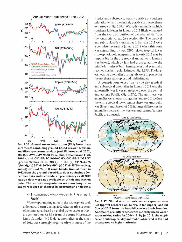
S37STATE OF THE CLIMATE IN 2012 |AuguST 2013
4) StratoSpheric water vapor—D. F. Hurst and K. Rosenlof
Water vapor mixing ratios in the stratosphere took a downward turn during 2012 after nearly six years of net increase. Based on global water vapor retriev-als centered on 82 hPa from the Aura Microwave Limb Sounder (MLS) data, anomalies at the start of 2012 were strongly negative (dry) in most of the
tropics and subtropics, weakly positive at southern midlatitudes and moderately positive in the northern extratropics (Fig. 2.37a). Weak, dry anomalies at high southern latitudes in January 2012 likely emanated from the seasonal outf low of dehydrated air from the Antarctic vortex (see section 6b). The tropical and subtropical dry anomalies in January 2012 were a complete reversal of January 2011 when this zone was extraordinarily wet. QBO-related tropical lower stratospheric cold temperatures in early 2012 may be responsible for the dry tropical anomalies in January (see below), which by July had propagated into the middle latitudes of both hemispheres and eventually reached northern polar latitudes (Fig. 2.37b). The larg-est negative anomalies during July were in patches in the northern subtropics and midlatitudes.
A conspicuous exception to the dry tropical and subtropical anomalies in January 2012 was the abnormally wet lower stratosphere over the central and eastern Pacific (Fig. 2.37a). Though these wet anomalies were not as strong as in January 2011, when the entire tropical lower stratosphere was unusually wet (Hurst and Rosenlof 2012), large differences in anomalies between the western and central/eastern Pacific are unusual.
Fig. 2.37. Global stratospheric water vapor anoma-lies (ppmv) centered on 82 hPa in Jan (upper) and Jul (lower) 2012 from the Aura Microwave Limb Sounder. Anomalies are differences from monthly mean water vapor mixing ratios for 2004–12. By Jul 2012, the tropi-cal and subtropical dry anomalies observed in Jan had propagated to higher latitudes.
Fig. 2.36. Annual mean total ozone (DU) from mea-surements combining ground-based Brewer, Dobson, and filter spectrometer data (red; Fioletov et al. 2002, 2008), BUV/SBUV MOD V8.6 (blue; Stolarski and Frith 2006), and GOME/SCIAMACHY/GOME-2 “GSG” (green; Weber et al. 2007), in the (a) 60°N–60°S (global), (b) 30°N–60°N (NH), (c) 25°N–25°S (tropics), and (d) 30°S–60°S (SH) zonal bands. Annual mean in 2012 from the ground-based data does not include De-cember data and is considered preliminary as all 2012 station data were not available as of this publication date. The smooth magenta curves show long-term ozone response to changes in stratospheric halogens.

S38 | august 2013
SIDEBAR 2.1: TROPOSPHERIC OZONE—O. COOPER AND J. ZIEMKE
Tropospheric ozone (O3) is a short-lived trace gas that either originates naturally in the stratosphere (Stohl et al. 2003) or is produced in situ by photochemical reactions involving sunlight and ozone precursor gases such as nitrogen oxides (NOx), non-methane volatile organic compounds, methane, and carbon monoxide (The Royal Society 2008; Monks et al. 2009). Ozone precursors can originate from natural sources including wildfires, biogenic hydrocarbon emissions, lightning NOx, and biogenic NOx emissions from soils, and from anthropogenic sources such as fossil fuel and biofuel combustion, or crop burning. The global distribution of tropospheric ozone is highly vari-able by season, location, and altitude. In addition to impacting human health and vegetation (Na-tional Research Council 1991; The Royal Society 2008), tropospheric ozone is also a greenhouse gas that produces a globally-averaged radiative forcing most recently estimated to be 0.40 W m-2 (Stevenson et al. 2013).
Little information on pre-industrial ozone concentrations exists and only limited point measurements are available from the late 19th century (Bojkov 1986; Volz and Kley 1988; Marenco et al. 1994; Pavelin et al. 1999). Therefore, atmospheric chemistry/climate models are the only method for estimating the pre-industrial tropospheric ozone burden. Multimodel analyses have calculated a tropospheric ozone burden of 244 ± 39 Tg (mean and standard deviation; Tg = 1012 g) in 1850, increasing by 36% to a present day value of 332 ± 22 Tg, largely due to growth in anthropogenic ozone precursor emissions (Young et al. 2013). The ozone burden not only changes with precursor emission rates but can also vary interannually due to circulation changes caused by ENSO. Tropospheric column ozone (TCO; the total mass of ozone present throughout the tropospheric column) decreases in the central and east Pacific and increases in the west Pacific/Indonesia in response to circulation and convective changes during El Niño conditions, and overall the global tropospheric ozone burden is slightly greater (~4%) during La Niña years (Doherty et al. 2006).
Today, near-surface ozone is measured routinely at thou-sands of sites around the world. Routine vertical profiling is limited to a few dozen ozonesonde (balloon) and lidar sites and a few airports that are frequented by commercial aircraft
equipped with air pollution monitoring equipment (Europe's IAGOS program; Dentener et al. 2011). Broad regions of the globe such as the oceans, polar regions, and sparsely populated areas have few or no in situ ozone measurements. However, satellite measurements can provide a global survey of TCO. A current satellite-based TCO climatology shows that ozone peaks in the Northern Hemisphere during boreal summer at 35°N–40°N with the strongest enhancements stretching from the eastern United States to southern Europe, and from East Asia into the western North Pacific (Ziemke et al. 2011). The Southern Hemisphere peak occurs in austral spring at 25°S–30°S within a band stretching from Brazil eastward to Australia. On an annual basis Northern Hemisphere TCO exceeds the Southern Hemisphere by 4%, 12%, and 18% at low (0°–25°), mid- (25°–50°), and high (50°–60°) latitudes, respectively.
Because the satellite record of tropospheric ozone profiles is short (Bowman et al. 2006), long-term ozone trends at the surface and at specific levels in the free troposphere must be determined from in situ measurements that are available at a limited number of sites. The longest continuous time series stretch back to the 1970s, and in two cases, the 1950s. Nine-teen such surface sites or regions exist around the globe, all
Fig. SB2.1. Ozone trends at the surface or within the lower troposphere between 1990 and 2010, based on yearly average ozone values. Vectors indicate the ozone rate of change at each site (ppb yr-1), as shown in the legend. Most of the sites are in rural locations so that they are represen-tative of regional air quality; however, many of the Asian sites are urban. Red dots indicate sites with a statistically significant positive ozone rate of increase, while pink, light blue and dark blue dots indicate trends that are insignificant positive, insignificant negative, and significant negative, respectively. Trend values are from Helmig et al. 2007; Ding et al. 2008; Wang et al. 2009; Tarasova et al. 2009; Li et al. 2010; Lin et al. 2010; Cooper et al. 2012; Parrish et al. 2012; Oltmans et al. 2013.

S39STATE OF THE CLIMATE IN 2012 |AuguST 2013
Fig. SB2.2. OMI/MLS tropospheric column ozone for (top) summer (JJA) 2012 and (bottom) averaged for 2005–12.
SIDEBAR 2.1: TROPOSPHERIC OZONE—O. COOPER AND J. ZIEMKE
exhibiting positive trends through 2000 or 2010, with 14 sites having statistically significant positive trends over a 25+ year period (Lelieveld et al. 2004; Oltmans et al. 2013; Parrish et al. 2012). Free tropospheric monitoring since the 1970s is even more limited. The available data from ozonesondes or aircraft show significant positive trends above some sites (Schnadt et al. 2009; Oltmans et al. 2013), with no site recording a significant negative trend.
Over the past few decades, ozone precursor emission rates have decreased in Europe and North America and increased in Asia (Granier et al. 2011), impacting ozone production on regional and hemispheric scales (Jacob et al. 1999; Dentener et al. 2011; Stevenson et al. 2013; Young et al. 2013). Over the period 1990–2010 surface ozone trends vary regionally (Fig. SB2.1). In Europe ozone generally increased through much of the 1990s but has leveled off or decreased since 2000 at rural and mountaintop sites and at the maritime Mace Head site in Ireland (Tarasova et al. 2009; Logan et al. 2012; Parrish et al. 2012; Oltmans et al. 2013). In North America surface ozone has increased in eastern and Arctic Canada, but is unchanged in central and western Canada (Oltmans et al. 2013). Surface ozone has increased in baseline air masses coming ashore along the US west coast (Parrish et al. 2012) and at half of the rural sites in the western United States during spring (Cooper et al. 2012). In the eastern United States, surface ozone has decreased strongly in summer, is largely unchanged in spring, and has increased in winter (Lefohn et al. 2010; Cooper et al. 2012). East Asian surface ozone is generally increasing (Ding
et al. 2008; Wang et al. 2009; Li et al. 2010; Lin et al. 2010; Parrish et al. 2012; Oltmans et al. 2013). Downwind from Asia, ozone is increasing at Mauna Loa, Hawaii, but decreasing at Minamitorishima, Japan (Oltmans et al. 2013). In the Southern Hemisphere ozone has increased at all eight available sites, although trends are not significant at four sites (Helmig et al. 2007; Oltmans et al. 2013).
In the free troposphere post-1990, ozone has decreased above Europe since 1998 (Logan et al. 2012) and is largely unchanged above Japan (Oltmans et al. 2013). Otherwise, the rest of the regions with measurements (North America, North Pacific Ocean, Southern Hemisphere) show a mix of positive trends (both significant and insignificant) depending on altitude, with no site having a negative trend at any altitude. Significant positive annual trends are most consistent above Canada (Olt-mans et al. 2013) and western North America during spring (Cooper et al. 2012).
An assessment of the global tropospheric ozone burden for 2012 is derived from instruments onboard NASA’s polar orbiting Aura satellite that has monitored stratospheric ozone and tropospheric trace gases since 2004. The Ozone Monitor-ing Instrument (OMI) science team combines OMI total ozone measurements (troposphere and stratosphere) with Microwave Limb Sounder (MLS) stratospheric column ozone measure-ments to produce global maps of OMI/MLS TCO (Ziemke et al. 2006). The tropospheric ozone burden from 60°N to 60°S derived from OMI/MLS averaged 270 Tg from October 2004 through October 2012, with yearly (November–October) av-erage values in the range 266 Tg–278 Tg. The burden calculated from November 2011 to October 2012 was 276 Tg, slightly above average. These burden values are approximately 20% lower than the model-derived global tropospheric ozone bur-den (Young et al. 2013). However the model values are for the entire globe and use a different definition of the tropopause. A direct comparison of the model output to the OMI/MLS product indicates that the average 60°N–60°S tropospheric ozone burdens are similar but with competing model biases in both hemispheres (Young et al. 2013).
Figure SB2.2 compares 2012 summertime TCO across the Northern Hemisphere to the 2005–12 mean, showing that ozone was enhanced above East Asia and the north Africa/Mediterranean/Middle East region in 2012. A full understanding of the tropospheric ozone anomalies in 2012 requires detailed photochemical modeling using a global scale chemical transport model, an endeavor that has not yet been undertaken.

S40 | august 2013
Water vapor variations in the tropical lower strato-sphere are dominated by the annual cycle of tropical tropopause temperatures (Fig. 2.38a) and only after this cycle is filtered out are QBO-induced interannual variations readily apparent (Fig. 2.38b). After a weak QBO-induced dry phase in tropical water vapor in 2010 and an extreme wet phase in early 2011, there is evidence of a QBO-driven dry anomaly beginning in early 2012. This dry anomaly was brief; by May it had vanished and remained absent until its robust reap-pearance in October (Fig. 2.38b). Note that the lack of QBO-driven dry anomalies in the tropical lower stratosphere during mid-2012 is not at odds with Fig. 2.37b because the strong dry anomalies had moved out of the tropical belt by July.
The data records generated by balloon-borne frost point hygrometers at four long-term monitoring sta-tions are in good general agreement with zonal aver-ages of MLS retrievals at 82 hPa (Fig. 2.39). Monthly soundings are conducted at Boulder, Colorado; Hilo, Hawaii; and Lauder, New Zealand, using the NOAA frost point hygrometer (FPH; Hurst et al. 2011) and at San Jose, Costa Rica, using the cryogenic frost point hygrometer (CFH; Vömel et al. 2007).
Anomalies at each of these four stations show a net increase from 2004 to 2011, but then a significant decline during 2011–12. At the two tropical stations (Hilo and San Jose), the decline began earlier and was more severe than at the two midlatitude stations. In the tropics, the anomalies reached their maxima in early 2011 and by the end of 2012 had fallen by ~1 ppmv. Decreases at Boulder and Lauder began near the end of 2011 and were only 0.4 ppmv–0.5 ppmv. These differences in timing and severity indicate that the decline in water vapor originated from the tropical lower stratosphere and propagated to the midlatitudes, precisely as depicted in Fig. 2.37.
The key feature of note during 2012 was a change in trend, with stratospheric water vapor decreasing over most of the globe after increasing since ~2006. Strong dry anomalies in the tropics and subtropics ap-parent during January had spread to the midlatitudes and even northern polar latitudes by July. The occur-
Fig. 2.38. Time series of MLS vertical profiles of monthly mean mixing ratios (upper) and anomalies (lower) in the tropical band 15°N–15°S. QBO-induced dry anomalies in the lower stratosphere, strong dur-ing 2004–08 but largely absent during 2010, robustly appeared during the last quarter of 2012.
Fig. 2.39. Lower stratospheric water vapor anomalies at 82 hPa (ppmv; differences from 2004–12 monthly averages) at four stations with routine soundings by balloon-borne frost point (FP) hygrometers. Anoma-lies of FP data from individual soundings (black) and zonal averages of MLS retrievals within ±2° lat of each station (red) are shown. The higher resolution FP data were averaged between 70 hPa and 100 hPa to emulate the averaging kernel used for MLS retrievals at 82 hPa. The Boulder period of record is now 33 years but only anomalies since 2004 are shown for comparison.
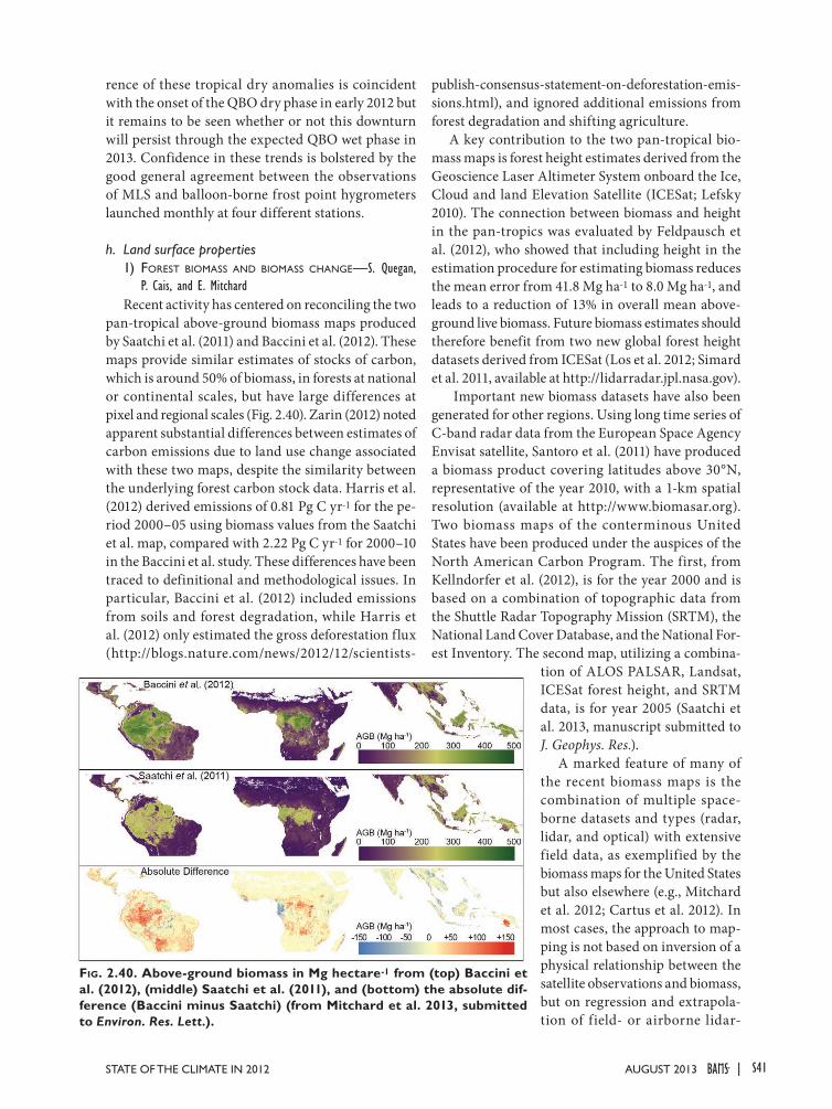
S41STATE OF THE CLIMATE IN 2012 |AuguST 2013
rence of these tropical dry anomalies is coincident with the onset of the QBO dry phase in early 2012 but it remains to be seen whether or not this downturn will persist through the expected QBO wet phase in 2013. Confidence in these trends is bolstered by the good general agreement between the observations of MLS and balloon-borne frost point hygrometers launched monthly at four different stations.
h. Land surface properties1) foreSt biomaSS aNd biomaSS chaNge—S. Quegan,
P. Cais, and E. Mitchard Recent activity has centered on reconciling the two
pan-tropical above-ground biomass maps produced by Saatchi et al. (2011) and Baccini et al. (2012). These maps provide similar estimates of stocks of carbon, which is around 50% of biomass, in forests at national or continental scales, but have large differences at pixel and regional scales (Fig. 2.40). Zarin (2012) noted apparent substantial differences between estimates of carbon emissions due to land use change associated with these two maps, despite the similarity between the underlying forest carbon stock data. Harris et al. (2012) derived emissions of 0.81 Pg C yr-1 for the pe-riod 2000–05 using biomass values from the Saatchi et al. map, compared with 2.22 Pg C yr-1 for 2000–10 in the Baccini et al. study. These differences have been traced to definitional and methodological issues. In particular, Baccini et al. (2012) included emissions from soils and forest degradation, while Harris et al. (2012) only estimated the gross deforestation flux (http://blogs.nature.com/news/2012/12/scientists-
publish-consensus-statement-on-deforestation-emis-sions.html), and ignored additional emissions from forest degradation and shifting agriculture.
A key contribution to the two pan-tropical bio-mass maps is forest height estimates derived from the Geoscience Laser Altimeter System onboard the Ice, Cloud and land Elevation Satellite (ICESat; Lefsky 2010). The connection between biomass and height in the pan-tropics was evaluated by Feldpausch et al. (2012), who showed that including height in the estimation procedure for estimating biomass reduces the mean error from 41.8 Mg ha-1 to 8.0 Mg ha-1, and leads to a reduction of 13% in overall mean above-ground live biomass. Future biomass estimates should therefore benefit from two new global forest height datasets derived from ICESat (Los et al. 2012; Simard et al. 2011, available at http://lidarradar.jpl.nasa.gov).
Important new biomass datasets have also been generated for other regions. Using long time series of C-band radar data from the European Space Agency Envisat satellite, Santoro et al. (2011) have produced a biomass product covering latitudes above 30°N, representative of the year 2010, with a 1-km spatial resolution (available at http://www.biomasar.org). Two biomass maps of the conterminous United States have been produced under the auspices of the North American Carbon Program. The first, from Kellndorfer et al. (2012), is for the year 2000 and is based on a combination of topographic data from the Shuttle Radar Topography Mission (SRTM), the National Land Cover Database, and the National For-est Inventory. The second map, utilizing a combina-
tion of ALOS PALSAR, Landsat, ICESat forest height, and SRTM data, is for year 2005 (Saatchi et al. 2013, manuscript submitted to J. Geophys. Res.).
A marked feature of many of the recent biomass maps is the combination of multiple space-borne datasets and types (radar, lidar, and optical) with extensive field data, as exemplified by the biomass maps for the United States but also elsewhere (e.g., Mitchard et al. 2012; Cartus et al. 2012). In most cases, the approach to map-ping is not based on inversion of a physical relationship between the satellite observations and biomass, but on regression and extrapola-tion of field- or airborne lidar-
Fig. 2.40. Above-ground biomass in Mg hectare-1 from (top) Baccini et al. (2012), (middle) Saatchi et al. (2011), and (bottom) the absolute dif-ference (Baccini minus Saatchi) (from Mitchard et al. 2013, submitted to Environ. Res. Lett.).

S42 | august 2013
derived biomass over forested landscapes identified by satellite observations. As a result, as long as systematic measurements from a dedicated satellite with strong sensitivity to forest structure and biomass are not available, existing biomass mapping efforts suffer from large uncertainties.
2) LaNd Surface aLbedo dyNamicS—B. PintyLand surface albedo represents the fraction of
solar radiation scattered backward by land surfaces. In the presence of vegetation, surface albedo results from complex nonlinear radiation transfer processes determining the amount of radiation that is scattered by the vegetation and its background, transmitted through the vegetation layer, or absorbed by the veg-etation layer and its background (Pinty 2012).
The geographical distributions of visible and near-infrared surface albedo for 2012 are shown in Plates 2.1p and 2.1q as normalized anomalies rela-tive to a 2003–12 base period for which two MODIS sensors are available. Anomalies in mid- and high latitude regions of the Northern Hemisphere result mainly from interannual variations in snow cover extent and duration in winter and spring. The large negative anomalies over the United States reflect the lack of snowfall and snowpack over the Rockies, the Midwest, and much of the eastern half of the country. This contrasts with the strong positive anomalies in southeastern Europe around the Black Sea. The am-plitude of these changes can reach ±30% in relative units, and are larger in the visible than in the near-infrared. Snow-free regions experienced dramatic variations with noticeable negative anomalies in both spectral domains in Australia and the western part of southern Africa. These were associated with more fa-vorable vegetation growing conditions by comparison to previous years (section 2h3). Mexico and north-eastern Brazil had strong positive anomalies in the visible domain. More subtle variations in albedo affected South America, China, and Russia as well as central Africa. These variations are attributed to vegetation dynamics under stress from ambient conditions although in-terannual variations in tropical cloud cover may also influence the surface albedo record.
Analysis of the zonally-averaged albedo anomalies in the visible (Fig. 2.41a) and near-infrared (Fig. 2.41b) spectral domain shows considerable interannual variations related to snow
cover in winter and spring at mid- and high latitudes but also to summer vegetation. Persistent negative anomalies are noticeable since 2010 between 20°S and 40°S.
The globally averaged normalized anomalies (Fig. 2.42) range within ±7% (3%) in the visible (near-infrared) domain. Antarctica is excluded. As in 2011, negative anomalies predominate in 2012 although positive anomalies are discernible in boreal spring and winter, especially at the end of 2012 when
Fig. 2.41. Zonal means of the MODIS White Sky broadband surface albedo normalized anomalies in the (a) visible and (b) near-infrared domain relative to a 2003–12 base period. Gray areas indicate regions where data are unavailable.
Fig. 2.42. Globally averaged MODIS White Sky broadband surface albedo normalized anomalies in the (a) visible and (b) near-infrared domain relative to a 2003–12 base period.
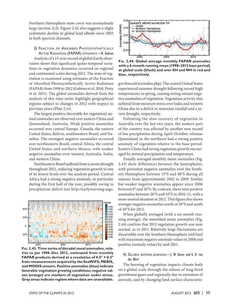
S43STATE OF THE CLIMATE IN 2012 |AuguST 2013
Northern Hemisphere snow cover was anomalously large (section 2c2). Figure 2.42 also suggests a slight systematic decline in global land albedo since 2003 in both spectral channels.
3) fractioN of abSorbed photoSyNtheticaLLy active radiatioN (fapar) dyNamicS—N. Gobron
Analysis of a 15-year record of global Earth obser-vation shows that significant spatio-temporal varia-tions in vegetation dynamics occurred on regional and continental scales during 2012. The state of veg-etation is examined using estimates of the Fraction of Absorbed Photosynthetically Active Radiation (FAPAR) from 1998 to 2012 (Gobron et al. 2010; Pinty et al. 2011). The global anomalies derived from the analysis of this time series highlight geographical regions subject to changes in 2012 with respect to previous years (Plate 2.1r).
The largest positive (favorable for vegetation) an-nual anomalies are observed over eastern China and Queensland, Australia. Weak positive anomalies occurred over central Europe, Canada, the eastern United States, Bolivia, southwestern Brazil, and Na-mibia. The strongest negative anomalies occurred over northeastern Brazil, central Africa, the central United States, and northern Mexico, with weaker negative anomalies over western Australia, India, and western China.
Northeastern Brazil suffered from a severe drought throughout 2012, reducing vegetation growth to one of its lowest levels over the analysis period. Central Africa had a strong negative anomaly, in particular during the first half of the year, possibly owing to precipitation deficit (see http://earlywarning.usgs.
gov/fews/africa/index.php). The central United States experienced summer drought following record high temperatures in spring, causing strong annual nega-tive anomalies of vegetation. Vegetation activity also suffered from moisture stress over India and western China due to a deficit in monsoon rainfall and a se-vere drought, respectively.
Following the slow recovery of vegetation in Australia over the last two years, the western part of the country was affected by another new record of low precipitation during April–October, whereas Queensland in the northeast had a strong positive anomaly of vegetation relative to the base period. Eastern China had strong vegetation growth encour-aged by normal precipitation and temperature.
Zonally averaged monthly mean anomalies (Fig. 2.43) show differences between the hemispheres, with persistent negative anomalies over the South-ern Hemisphere between 15°S and 40°S during all seasons from approximately 2002 to 2009. Similar but weaker negative anomalies appear since 2006 between 0° and 20°S. By contrast, there were positive anomalies between 20°S and 45°S in 2010–11, with a more neutral situation in 2012. This figure also shows stronger negative anomalies north of 20°S and south of 40°S for 2012.
When globally averaged (with a six-month run-ning average), the smoothed mean anomalies (Fig. 2.44) confirm that 2012 vegetation growth was near normal, as in 2011. Relatively large fluctuations are discernible over the Southern Hemisphere (red line) with maximum negative anomaly values in 2008 and positive anomaly values by mid-2011.
4) gLobaL biomaSS burNiNg—J. W. Kaiser and G. R. van der Werf
The burning of vegetation impacts climate both on a global scale through the release of long-lived greenhouse gases and regionally due to emissions of aerosols, and by changing land surface characteris-
Fig. 2.43. Time series of decadal zonal anomalies, rela-tive to Jan 1998–Dec 2012, estimated from monthly FAPAR products derived at a resolution of 0.5° × 0.5° from measurements acquired by the SeaWiFS, MERIS, and MODIS sensors. Positive anomalies (blue) indicate favorable vegetation growing conditions; negative val-ues (orange) are markers of vegetation under stress. Gray areas indicate regions where data are unavailable.
Fig. 2.44. Global average monthly FAPAR anomalies with a 6-month running mean (1998–2012 base period) at global scale (black) and over SH and NH in red and blue, respectively.

S44 | august 2013
tics. Although fires occur in most biomes, they exhibit large spatial variability and information on global scale fire activity is derived mostly from satellites.
The Global Fire Assimilation System (GFAS; Kaiser et al. 2012) uses MODIS satellite observations from fires that burn during the satellite overpass. Converting the radiative energy released by these fires to biomass consumed produces emissions estimates in near-real time, yielding daily emissions estimates since 2003. These estimates have been calibrated with an alternative method where satellite detections of burned area (Giglio et al. 2010) are combined with biogeochemical modeling to estimate fuel loads (van der Werf et al. 2010).
Broadly speaking, most fires burn in the subtrop-ics where fire is used as a tool to manage savannas and convert forests to land for cultivation. Humans ignite most of the fires here but this does not neces-sarily mean that humans increase fire activity; the increase in ignitions may be offset by a decrease in land available for burning (van der Werf et al. 2013). Fires occur less frequently in temperate and boreal regions, where the ignition source can be from hu-
mans or lightning. In general, these fires burn more frequently and consume larger areas when climate is favorable.
On average, fires consumed about 2 Pg of carbon (C) per year over the period 2003–11 with a range of 1.7 Pg C–2.3 Pg C yr-1. This is about 7% of the car-bon that is sequestered by photosynthesis each year, or about 20% of total global fossil fuel emissions. Fires, however, are a net source of carbon dioxide only when the combusted carbon is not subsequently sequestered. This is the case when fire is used in the deforestation process or when areas see an increase in fire activity.
In most years, almost 90% of total carbon emis-sions originate in the tropics and subtropics; however, the large biomass burning regions in Africa and South America experienced a negative biomass burning anomaly in 2012 (see Table 2.7; Plate 2.1s; Fig. 2.45). In South America (-26%), this is the continuation of a declining trend related to reduced rates of deforesta-tion since 2004 (INPE 2012).
In 2012 Australia experienced its strongest fire season (+110%) in the GFAS record, following the pre-
Fig. 2.45. Global map of biomass burning in terms of carbon emission (gC m-2 yr-1) during (a) 2003–11 and (b) 2012. Gray areas indicate regions where data are unavailable.
Fig. 2.46. Daily fire activity in terms of carbon con-sumption (Tg C day-1) for Australia (top), Siberia (middle), and the western United States (bottom), 2003–12.

S45STATE OF THE CLIMATE IN 2012 |AuguST 2013
Table 2.7. Annual continental-scale biomass burning budgets in terms of carbon emission (Tg C yr-1) reported in GFASv1.0.
Time Period 2003–11 2012 2012 w.r.t. 2003–11
Quantity Mean Range ValueAbsolute Anomaly
Relative Anomaly
Global 2037 1774–2312 2163 +126 +6%
N America 101 71–138 103 +3 +3%
C America 66 53–91 49 -17 -25%
SH America 340 177–458 252 -87 -26%
Europe and Mediterranean
35 26–62 31 -5 -26%
NH Africa 413 331–458 367 -46 -11%
SH Africa 526 488–591 507 -19 -4%
N Asia 197 105–470 356 +159 +81%
SE Asia 130 95–162 126 -4 -3%
Tropical Asia 91 22–218 83 -8 -9%
Australia 137 52–273 288 +151 +110%
Western US 21 8–38 42 +21 +101%
Siberia 144 61–414 319 +175 +122%
vious strong fire season in 2011. The anomaly in 2012 was mostly in the arid western interior, i.e., farther southwest than in 2011. Particularly striking were a strong peak on 23 October, when daily carbon emis-sions reached levels not seen in any other year, and a delay of the fire season relative to 2011 (Fig. 2.46).
Strong positive anomalies affected several temper-ate and boreal regions. The western United States experienced its fiercest fire season (+101%) in the GFAS record. However, low fire activity in Canada and Alaska led to a negligible overall fire activity anomaly for North America (+3%).
The fire season was also strong in Northern Asia (+81%), including Siberia (+122%). Most of the fire
activity started in early June and persisted until early August, i.e., relatively late in the season (Fig. 2.46). Large smoke plumes from these fires traveled across the Pacific to the North American west coast (section 2g2; ECMWF 2012).
The strong negative and positive anomalies of biomass burning are also observed as corresponding anomalies of aerosol optical depth (section 2g2). The large positive anomalies in Siberia and Australia more than compensated the negative ones in Africa and South America, such that the total global fire activity in 2012 was about 2.2 Pg C yr-1 or 6% above average.

S46 | august 2013
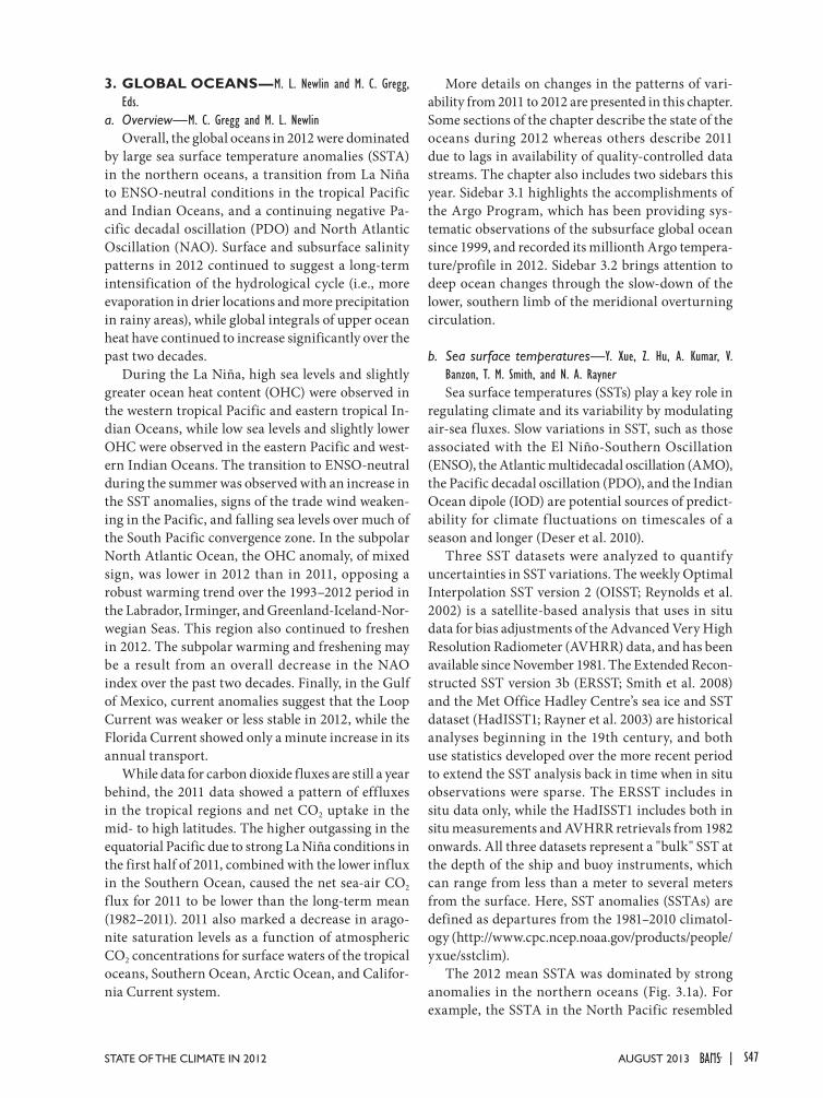
S47STATE OF THE CLIMATE IN 2012 |AuguST 2013
3. GLOBAL OCEANS—M. L. Newlin and M. C. Gregg, Eds.
a. Overview—M. C. Gregg and M. L. NewlinOverall, the global oceans in 2012 were dominated
by large sea surface temperature anomalies (SSTA) in the northern oceans, a transition from La Niña to ENSO-neutral conditions in the tropical Pacific and Indian Oceans, and a continuing negative Pa-cific decadal oscillation (PDO) and North Atlantic Oscillation (NAO). Surface and subsurface salinity patterns in 2012 continued to suggest a long-term intensification of the hydrological cycle (i.e., more evaporation in drier locations and more precipitation in rainy areas), while global integrals of upper ocean heat have continued to increase significantly over the past two decades.
During the La Niña, high sea levels and slightly greater ocean heat content (OHC) were observed in the western tropical Pacific and eastern tropical In-dian Oceans, while low sea levels and slightly lower OHC were observed in the eastern Pacific and west-ern Indian Oceans. The transition to ENSO-neutral during the summer was observed with an increase in the SST anomalies, signs of the trade wind weaken-ing in the Pacific, and falling sea levels over much of the South Pacific convergence zone. In the subpolar North Atlantic Ocean, the OHC anomaly, of mixed sign, was lower in 2012 than in 2011, opposing a robust warming trend over the 1993–2012 period in the Labrador, Irminger, and Greenland-Iceland-Nor-wegian Seas. This region also continued to freshen in 2012. The subpolar warming and freshening may be a result from an overall decrease in the NAO index over the past two decades. Finally, in the Gulf of Mexico, current anomalies suggest that the Loop Current was weaker or less stable in 2012, while the Florida Current showed only a minute increase in its annual transport.
While data for carbon dioxide fluxes are still a year behind, the 2011 data showed a pattern of effluxes in the tropical regions and net CO2 uptake in the mid- to high latitudes. The higher outgassing in the equatorial Pacific due to strong La Niña conditions in the first half of 2011, combined with the lower influx in the Southern Ocean, caused the net sea-air CO2 flux for 2011 to be lower than the long-term mean (1982–2011). 2011 also marked a decrease in arago-nite saturation levels as a function of atmospheric CO2 concentrations for surface waters of the tropical oceans, Southern Ocean, Arctic Ocean, and Califor-nia Current system.
More details on changes in the patterns of vari-ability from 2011 to 2012 are presented in this chapter. Some sections of the chapter describe the state of the oceans during 2012 whereas others describe 2011 due to lags in availability of quality-controlled data streams. The chapter also includes two sidebars this year. Sidebar 3.1 highlights the accomplishments of the Argo Program, which has been providing sys-tematic observations of the subsurface global ocean since 1999, and recorded its millionth Argo tempera-ture/profile in 2012. Sidebar 3.2 brings attention to deep ocean changes through the slow-down of the lower, southern limb of the meridional overturning circulation.
b. Sea surface temperatures—Y. Xue, Z. Hu, A. Kumar, V. Banzon, T. M. Smith, and N. A. RaynerSea surface temperatures (SSTs) play a key role in
regulating climate and its variability by modulating air-sea fluxes. Slow variations in SST, such as those associated with the El Niño-Southern Oscillation (ENSO), the Atlantic multidecadal oscillation (AMO), the Pacific decadal oscillation (PDO), and the Indian Ocean dipole (IOD) are potential sources of predict-ability for climate f luctuations on timescales of a season and longer (Deser et al. 2010).
Three SST datasets were analyzed to quantify uncertainties in SST variations. The weekly Optimal Interpolation SST version 2 (OISST; Reynolds et al. 2002) is a satellite-based analysis that uses in situ data for bias adjustments of the Advanced Very High Resolution Radiometer (AVHRR) data, and has been available since November 1981. The Extended Recon-structed SST version 3b (ERSST; Smith et al. 2008) and the Met Office Hadley Centre’s sea ice and SST dataset (HadISST1; Rayner et al. 2003) are historical analyses beginning in the 19th century, and both use statistics developed over the more recent period to extend the SST analysis back in time when in situ observations were sparse. The ERSST includes in situ data only, while the HadISST1 includes both in situ measurements and AVHRR retrievals from 1982 onwards. All three datasets represent a "bulk" SST at the depth of the ship and buoy instruments, which can range from less than a meter to several meters from the surface. Here, SST anomalies (SSTAs) are defined as departures from the 1981–2010 climatol-ogy (http://www.cpc.ncep.noaa.gov/products/people/yxue/sstclim).
The 2012 mean SSTA was dominated by strong anomalies in the northern oceans (Fig. 3.1a). For example, the SSTA in the North Pacific resembled

S48 | august 2013
the negative phase of the PDO pattern (Mantua et al. 1997), with the mean of normalized monthly PDO index at -1.4 in 2012 (Fig. 3.2c). In the North Atlantic, positive SSTA greater than +1.5°C was largely to the north of the Gulf Stream (GS) and its extension. In contrast, the 2012 mean SSTA in the tropical Pacific was weak, negative SSTA in the central Pacific and positive in the southeast Pacific. There was a weak positive SSTA in the tropical North Atlantic, as well as a subtropical dipole in the South Atlantic (Venegas et al. 1997). In the Indian Ocean, there was a weak posi-tive IOD pattern (Saji et al. 1999) and positive SSTA in the southeast subtropical Indian Ocean.
The 2012 minus 2011 SSTA differences (Fig. 3.1b) show that the SST in the tropical Pacific increased substantially in the central-eastern tropical Pacific due to the transition from La Niña to ENSO-neutral (see section 4b for details). There was a moderate cooling in the Bering Sea and north of the Bering Strait, and a substantial warming in the mid- and high latitudes of the North Atlantic. In the southern oceans, SSTA differences were dominated by wave-like patterns, particularly in the South Pacific and South Atlantic.
The temporal evolution of seasonal mean SSTA in 2012 is shown in Fig. 3.3. The winter 2011/12 (Decem-ber–February) was dominated by La Niña conditions in the tropical Pacific and a negative PDO pattern in the North Pacific. With the weakening of La Niña,
negative SSTA weakened and retreated to north of the equator in spring 2012, while the positive SSTA in the southeast Pacific strengthened to exceed +2 standard deviation (STD; Fig. 3.3b). El Niño-like conditions, positive SSTA exceeding +0.5°C in the central-eastern Pacific, emerged during summer 2012 (Fig. 3.3c). However, these conditions were short-lived and by fall 2012 SST returned to near-normal except in a small area near 160°E (Fig. 3.3d).
The warming along the GS strengthened and expanded into the subpolar North Atlantic during summer and fall 2012 with values exceeding +2 STD. Positive SSTA exceeding +2 STD covered most of the Arctic Ocean, consistent with the historically low value of Arctic sea ice extent during the period (see section 5j). The positive SSTA in the subtropical North Atlantic also increased during summer and fall, which is favorable for North Atlantic hurricane activity. The subtropical SST dipole in the South Atlantic persisted throughout the year. The Indian Fig. 3.1. (a) Yearly mean OISST anomaly (°C, relative
to 1981–2010 average) in 2012; (b) 2012 minus 2011 OISST anomaly.
Fig. 3.2. (a) Monthly standardized NAO index (bar) and average SSTA in the box shown in Fig. 3.3c (red line); (b) 5-month running mean of NAO (black line) and average SSTA in the box (red line); (c) monthly normalized PDO index (bar) and Niño-3.4 index (av-erage SSTA in 170°W–120°W, 5°S–5°N, red line); (d) 5-month running mean of PDO and Niño-3.4 index (red line). SSTA is relative to 1981–2010 average (°C).
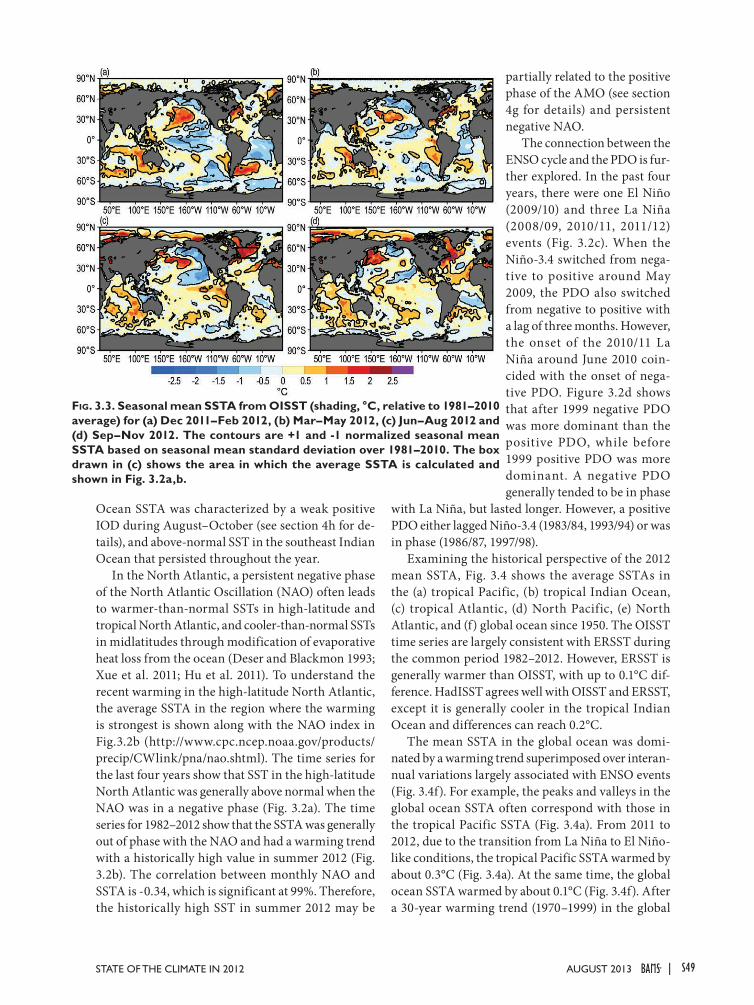
S49STATE OF THE CLIMATE IN 2012 |AuguST 2013
Ocean SSTA was characterized by a weak positive IOD during August–October (see section 4h for de-tails), and above-normal SST in the southeast Indian Ocean that persisted throughout the year.
In the North Atlantic, a persistent negative phase of the North Atlantic Oscillation (NAO) often leads to warmer-than-normal SSTs in high-latitude and tropical North Atlantic, and cooler-than-normal SSTs in midlatitudes through modification of evaporative heat loss from the ocean (Deser and Blackmon 1993; Xue et al. 2011; Hu et al. 2011). To understand the recent warming in the high-latitude North Atlantic, the average SSTA in the region where the warming is strongest is shown along with the NAO index in Fig.3.2b (http://www.cpc.ncep.noaa.gov/products/precip/CWlink/pna/nao.shtml). The time series for the last four years show that SST in the high-latitude North Atlantic was generally above normal when the NAO was in a negative phase (Fig. 3.2a). The time series for 1982–2012 show that the SSTA was generally out of phase with the NAO and had a warming trend with a historically high value in summer 2012 (Fig. 3.2b). The correlation between monthly NAO and SSTA is -0.34, which is significant at 99%. Therefore, the historically high SST in summer 2012 may be
partially related to the positive phase of the AMO (see section 4g for details) and persistent negative NAO.
The connection between the ENSO cycle and the PDO is fur-ther explored. In the past four years, there were one El Niño (2009/10) and three La Niña (2008/09, 2010/11, 2011/12) events (Fig. 3.2c). When the Niño-3.4 switched from nega-tive to positive around May 2009, the PDO also switched from negative to positive with a lag of three months. However, the onset of the 2010/11 La Niña around June 2010 coin-cided with the onset of nega-tive PDO. Figure 3.2d shows that after 1999 negative PDO was more dominant than the positive PDO, while before 1999 positive PDO was more dominant. A negative PDO generally tended to be in phase
with La Niña, but lasted longer. However, a positive PDO either lagged Niño-3.4 (1983/84, 1993/94) or was in phase (1986/87, 1997/98).
Examining the historical perspective of the 2012 mean SSTA, Fig. 3.4 shows the average SSTAs in the (a) tropical Pacific, (b) tropical Indian Ocean, (c) tropical Atlantic, (d) North Pacific, (e) North Atlantic, and (f) global ocean since 1950. The OISST time series are largely consistent with ERSST during the common period 1982–2012. However, ERSST is generally warmer than OISST, with up to 0.1°C dif-ference. HadISST agrees well with OISST and ERSST, except it is generally cooler in the tropical Indian Ocean and differences can reach 0.2°C.
The mean SSTA in the global ocean was domi-nated by a warming trend superimposed over interan-nual variations largely associated with ENSO events (Fig. 3.4f). For example, the peaks and valleys in the global ocean SSTA often correspond with those in the tropical Pacific SSTA (Fig. 3.4a). From 2011 to 2012, due to the transition from La Niña to El Niño-like conditions, the tropical Pacific SSTA warmed by about 0.3°C (Fig. 3.4a). At the same time, the global ocean SSTA warmed by about 0.1°C (Fig. 3.4f). After a 30-year warming trend (1970–1999) in the global
Fig. 3.3. Seasonal mean SSTA from OISST (shading, °C, relative to 1981–2010 average) for (a) Dec 2011–Feb 2012, (b) Mar–May 2012, (c) Jun–Aug 2012 and (d) Sep–Nov 2012. The contours are +1 and -1 normalized seasonal mean SSTA based on seasonal mean standard deviation over 1981–2010. The box drawn in (c) shows the area in which the average SSTA is calculated and shown in Fig. 3.2a,b.

S50 | august 2013
ocean SST (rising 0.11°C per decade in ERSST and 0.06°C per decade in HadISST), the period 2000–12 had little further trend. This may be linked to the prevalence of La Niña-like conditions during the 21st century (Meehl et al. 2011).
The tropical Indian Ocean SSTA is dominated by an upward trend of +0.9°C from 1950 to 2010, when the historically high value was reached (Fig. 3.4b). The interannual variations correspond well with those in the tropical Pacific SSTA due to the remote influences of ENSO. From 2011 to 2012, the tropical Indian Ocean SSTA increased slightly. In the tropical Atlantic, SSTA was mostly negative before 1995, and warmed significantly from -0.43°C in 1992 to +0.31°C in 2003. The positive SSTA largely persisted from 2003 to 2009, then suddenly increased to the histori-cally high value +0.46°C in 2010 (Fig. 3.4c), due to the combined influences of El Niño, the long-persistent negative phase of NAO, and the underlying long-term trend (Hu et al. 2011). Since 2010, the tropical Atlantic SST cooled substantially and became weakly below normal in 2012. The North Pacific SSTA trended
downward from 1950 to 1987, rebounded from -0.5°C in 1987 to +0.31°C in 1990, staying persistently positive since (Fig. 3.4d). The North Atlantic SSTA trended downward from 1951 to early 1970s, then trended upward, reached a historically high value in 2006 relative to the 1950–2011 period. From 2006 to 2010, the SSTA had a downward trend, but rebounded from +0.05°C in 2011 to +0.49°C in 2012, reaching a new historical high (Fig. 3.4e).
c. Ocean heat content—G. C. Johnson, J. M. Lyman, J. K. Willis, S. Levitus, T. Boyer, J. Antonov, S. A. Good, C. M. Domingues, S. Wijffels, and N. BindoffStorage and transport of heat in the ocean are
central to aspects of climate such as ENSO (Roem-mich and Gilson 2011), the North Atlantic Oscillation (Curry and McCartney 2001), hurricanes (Mainelli et al. 2008), sea level rise (Johnson and Wijffels 2011), the global energy budget (Church et al. 2011), and constraining global warming scenarios (Knutti and Tomassini 2008).
An estimate of upper (0–700 m) ocean heat content anomaly (OHCA) for 2012 (Fig. 3.5a) is computed from a combination of in situ ocean temperature data and satellite altimetry data (hereafter referred to as the combined estimate). In situ data are from Hadley Center EN3 V2a (Ingleby and Huddleston 2007), derived mostly from the World Ocean Database (e.g., Boyer et al. 2009), but with a January 2013 download of Argo (see Sidebar 3.1) data. Updated mechanical and expendable bathythermograph (MBT and XBT) bias corrections from Ishii and Kimoto (2009) are applied. Since OHCA changes are related to depth-integrated ocean temperature changes, increases in OHCA are sometimes referred to here as warming and OHCA decreases as cooling. Some of the data used in this analysis are preliminary; however, strong regional signals are unlikely to change upon data finalization.
Upper OHCA in 2012 (Fig. 3.5a) shows typical eddy and meander signatures (e.g., Johnson et al. 2012a). Similarly, differences of upper OHCA between 2012 and 2011 (Fig. 3.5b) exhibit typical interannual variability. OHCA variability (and net increases) are also found from 700 m to 2000 m in depth (Levitus et al. 2012) and even in the abyssal ocean below (e.g., Purkey and Johnson 2010). These variations, as well as salinity and mass signals, all contribute to local sea level anomalies (Llovel et al. 2009). Despite these additional factors, there are many large-scale visual similarities between the combined estimate of upper OHCA (Fig. 3.5a) and sea level (see Fig. 3.27) fields
Fig. 3.4. Yearly mean SSTA (°C, relative to 1981–2010 average) from ERSST (bar) and HadISST (blue line) for 1950–2012 (bar) and OISST for 1982–2012 (black line) averaged over the (a) tropical Pacific, (b) tropical Indian Ocean, (c) tropical Atlantic, (d) North Pacific, (e) North Atlantic, and (f) global ocean.

S51STATE OF THE CLIMATE IN 2012 |AuguST 2013
in 2012. This similarity ref lects mostly the large contribution of upper OHCA variations to sea level variations, but also to a lesser extent the influence of the altimeter data in the combined estimate (Willis et al. 2004).
Large-scale patterns are evident in the combined estimate of upper OHCA for 2012 (Fig. 3.5a) and its difference from 2011 (Fig. 3.5b). The pattern of annual mean OHCA (Fig. 3.5a) on the equator in the Pacific exhibits slightly cool values in the east and slightly warm values in the west. This pattern arises from a transition during 2012 from La Niña to more neutral conditions (section 3b).
In 2012, the North Pacific (Fig. 3.5a) shows a pat-tern of anomalous warmth in the central Pacific and cold in the subpolar, eastern subtropical, and eastern tropical Pacific that is typical of the negative phase of the Pacific decadal oscillation (PDO; Mantua et al. 1997). Extratropical SST anomalies in 2012 exhibit a similar pattern (see Fig. 3.1). Furthermore, zonal anomalies along the Kuroshio Extension are
associated with an anomalously northward position of that current in 2012 (see Fig. 3.17). The band of anomalously warm upper OHCA in the South Pacific extending from the Solomon Islands in the west to about 30°S, 100°W (Fig. 3.5a) has been present at various latitudes since 2006 (see Johnson et al. 2012a and previous State of the Climate reports). The band of cooling between 2011 and 2012, just north of the warm band, is associated with an increase in Ekman suction (anomalous upwelling) owing to changes in the winds (see Fig. 3.9b)
Indian Ocean upper OHCA anomalies remained mostly warm in 2012 (Fig. 3.5a) compared to the base-line period. The upper ocean warmed between 2011 and 2012 south of Oman and west of Australia (Fig. 3.5b). The warming from 2011 to 2012 in the central Indian Ocean near 10°S (Fig. 3.5b) may be associated with a large freshening in sea surface salinity in the region (see Fig. 3.11).
In the subpolar North Atlantic, small portions of the Labrador Sea were anomalously cold in upper OHCA in 2012 (Fig. 3.5a), having cooled since 2011 (Fig. 3.5b), and even more since 2010 (see Johnson et al. 2012a). This regional ocean cooling is consonant with a slightly less negative NAO index since the low values in the winter of 2009/10 (see Fig. 3.8). Much of eastern subpolar North Atlantic also cooled from 2011 to 2012 (Fig. 3.5b), consistent with surface salinity freshening over that same period (see Fig. 3.11), suggesting that subtropical inf luences that were strong there in recent years (e.g., Johnson and Gruber 2007) may be lessening. In 2012, a meridional dipole of OHCA along the Gulf Stream extension—warm to the north and cool to the south—suggests a weaker-than-average eastward current there in 2012, although that reduction was small in 2012 zonal surface current anomalies (see Fig. 3.17). While the tropical Atlantic mostly cooled from 2011 to 2012 (Fig. 3.5b) it remained warmer than the 1993–2012 average (Fig. 3.5a).
A few distinct (Fig. 3.6a) and statistically sig-nificant (Fig. 3.6b) regional patterns stand out in the 1993–2012 local linear trends of upper OHCA. In the Indian Ocean, the warming trend is widespread except for a patch south of the equator in the center of the basin and statistically significant in many locations.
In the Atlantic Ocean, the Labrador, Irminger, and Greenland-Iceland-Norwegian Seas have all trended warmer over 1993–2012 (Fig. 3.6a), reflecting a robust regional warming trend over the interval despite some cooling from 2011 to 2012 (Fig. 3.6b). These
Fig. 3.5. (a) Combined satellite altimeter and in situ ocean temperature data estimate of upper (0–700 m) ocean heat content anomaly (OHCA; 109 J m-2) for 2012 analyzed following Willis et al. (2004), but using an Argo monthly climatology and displayed relative to a 1993–2012 baseline. (b) The difference of 2012 and 2011 combined estimates of OHCA expressed as a local surface heat flux equivalent (W m-2). For panel comparisons, note that 95 W m-2 applied over one year results in a 3 × 10⁹ J m-2 change of OHCA.

S52 | august 2013
changes may result from an overall decrease in the NAO index from 1993 to 2012. Eastern portions of the subtropical Atlantic and most of the tropics also trend warmer across both hemispheres. Statistically significant cooling trends in the Atlantic are limited to the Gulf Stream extension, probably related to a southward shift in that current over the past few years. As discussed in previous reports (e.g., Johnson et al. 2012a), this shift is also expected with an overall declining NAO index.
Statistically significant (Fig. 3.6b) 1993–2012 regional trends in the Pacific Ocean (Fig. 3.6a) in-clude warming in the western tropical Pacific and extra-equatorial cooling in the east, consistent (via the geostrophic relation) with general strengthen-ing of the interior subtropical-tropical circulation attributed to trade-wind intensification (Merrifield and Maltrud 2011). The statistically significant warm-ing in the central North Pacific and cooling south of Alaska and off the west coast of North America are also consistent with an overall downward trend in
the PDO index from 1993 to 2012. There is a similar trend pattern in the South Pacific.
The overall 1993–2012 trends in Southern Ocean upper OHCA are towards warming, consistent with previous analyses (e.g., Böning et al. 2008), but with some cooling trends in localized regions, most no-tably around South America and near Antarctica in the Indian Ocean (Fig. 3.6a). The apparent trends adjacent to Antarctica are located in both in situ and altimeter data-sparse regions and may not be as ro-bust as suggested by the statistics (Fig. 3.6b).
Four different upper (0–700 m) ocean estimates of globally integrated in situ OHCA (Fig. 3.7) reveal a large increase in global integrals of that quantity since 1993. While each of the curves appears to show
Fig. 3.6. (a) Linear trend from 1993–2012 of the com-bined satellite altimeter and in situ ocean temperature data estimate of upper (0–700 m) OHCA (W m-2) analyzed following Willis et al. (2004) but relative to a monthly Argo climatology. Areas with statistically significant trends are outlined in black. (b) Signed ratio of the linear trend to its 95% uncertainty estimate, with increasing color intensity showing regions with increasingly statistically significant trends.
Fig. 3.7. Time series of annual average global integrals of in situ estimates of upper (0–700 m) OHCA (1021 J, or ZJ) for 1993–2012 with standard errors of the mean. The CSIRO/ACE CRC estimate (smoothed by a 3-year running mean) and its uncertainties are up-dated following Domingues et al. (2008). The PMEL/JPL/JIMAR estimate is a weighted integral (Lyman and Johnson 2008) using data and instrument bias corrections described in the text with uncertainty estimate methodology following Lyman et al. (2010). The NODC estimate (http://www.nodc.noaa.gov/OC5/indprod.html) follows Levitus et al. (2012). Un-certainties are estimated solely from the variance of quarterly estimates of OHCA. The Hadley estimate is computed from gridded monthly temperature anoma-lies (relative to 1950–2012) calculated from EN3 v2a data following Palmer et al. (2007). An updated version of the instrument bias corrections of Gouretski and Reseghetti (2010; V. Gouretski, personal communica-tion) was applied. Uncertainty estimates follow Palmer and Brohan (2011). For comparison, all estimates have been individually offset (vertically on the plot), first to their individual 2004–12 means (the best sampled time period), and then to their collective 1993–2012 mean (the record length).

S53STATE OF THE CLIMATE IN 2012 |AuguST 2013
interannual to decadal variability in upper ocean heat content, they do not always agree in the details. These details differ for a variety of reasons including dif-ferences in climatology and base period, treatment of the seasonal cycle, mapping methods, instrument bias corrections, quality control, and other factors (Ly-man et al. 2010). Some of these factors are not taken into account in some of the displayed uncertainties, and the offsets applied to the curves for display are arbitrary. Uncertainties in annual estimates of global upper OHCA only permit statistically significant trends to be estimated over about 10 years or longer (Lyman 2012). Nonetheless, the warming of the upper ocean accounts for a large portion of the global energy imbalance, at least since 1970 (Church et al. 2011).
d. Ocean surface heat fluxes—L. Yu and P. W. Stackhouse Jr.The net heat f lux (Qnet) at the ocean surface is
the sum of solar radiation (SW), longwave radia-tion (LW), turbulent latent heat (LH), and sensible heat (SH) fluxes. The balance of these heat exchange processes is fundamental to the understanding of the role of the ocean in mitigating radiative perturbations and modulating the global climate. Global maps of surface f luxes are now produced regularly using satellite observations and numerical weather pre-diction models. The net heat flux presented here is a combination of surface fluxes produced by two f lux proj-ects. One is the Objectively Analyzed air-sea Fluxes (OA-Flux) project (http://oaflux.whoi.edu) at the Woods Hole Oceanographic Institution (Yu and Weller 2007) that provides turbulent LH and SH estimates from objec-tive blending of satellite re-trievals and atmospheric reanalyses. The averaged root-mean-square (rms) er-ror is 9.6 W m-2 (8%) for LH and 2.6 W m-2 (15%) for SH (Yu et al. 2008). The other project is the CERES (Clouds and Earth’s Radiant Energy Systems) Fast Longwave And SHortwave Radiative Fluxes (FLASHFlux) project (http://f lashf lux.larc.nasa.gov) at the NASA Langley Research Center (Stackhouse et al.
2006) that delivers global daily surface SW and LW flux products in near real-time (within 1 week). This output data product uses simplified calibration as-sumptions with fast radiation algorithms (Kratz et al. 2010) in processing Terra and Aqua observations from CERES and cloud property retrievals from the MODerate-resolution Imaging Spectroradiometer (MODIS). The rms error is 29.3 W m-2 (15.7%) for downward SW and 18.6 W m-2 (6.0%) for downward LW (with the bias in the net surface heat flux being about 25 W m-2).
The annual mean Qnet in 2012 is displayed in Fig. 3.8a. The regions of net heat gain (positive Qnet) and net heat loss (negative Qnet) are in broad agreement with the climatological mean pattern (Josey et al. 1999). On the annual-mean basis, the tropical oceans receive heat from the atmosphere, with the maximum heat gain (>120 W m-2) in the equatorial cold tongues in the eastern Pacific and Atlantic. The subtropics and high latitudes experience net heat loss, with the maximum heat loss (<-140 W m-2) over the western boundary currents (WBCs) regions. The primary mechanism of excessive net heat loss in the vicinity of the WBCs is latent and sensible heat fluxes in the fall and winter seasons (Yu and Weller 2007).
The 2012 minus 2011 difference plot of Qnet (Fig. 3.8b) shows several large-scale changes with
Fig. 3.8. (a) Annual mean net heat flux into the ocean (Qnet) in 2012. Positive (negative) values denote ocean heat gain (loss). (b) Annual mean difference in Qnet between 2012 and 2011. The 2012 minus 2011 mean difference in surface radiation (SW + LW) and turbulent heat fluxes (LH + SH) are shown in (c) and (d), respectively. In (b)–(d), positive (negative) values denote ocean gains more (loses less) heat in 2012 compared to 2011.

S54 | august 2013
SIDEBAR 3.1: ARGO—PROVIDING SYSTEMATIC OBSERVATIONS OF THE SUBSURFACE GLOBAL OCEAN—THE ARGo STEERiNG TEAM
The Argo Program is the first global subsurface ocean ob-serving system, complementing satellite observations of the sea surface with comparable coverage of the subsurface oceans. Systematic global observations of the oceans are essential for describing and understanding climate variability and change because the oceans and atmosphere interact through a broad spectrum of climate-related phenomena. These range from rapid weather events, such as tropical cyclones, to multidecadal trends in heat and freshwater that are key indices of climate change. They include seasonal exchanges of heat and freshwater on hemispheric scales, water mass formation processes embed-ded in the seasonal cycle, interannual climate phenomena such as El Niño/La Niña, and decadal variability in the Pacific decadal oscillation and the southern annular mode. For all of these, it is important to study not only air-sea interactions, but their cumulative impact on ocean properties, including temperature and salinity. The ocean is the climate system’s dominant res-ervoir for storage of heat and water, which it exchanges with the atmosphere and transports through ocean circulation. The ocean’s great capacity for storage and its slow circulation provide long time scales in the climate system, smoothing the rapid changes of the atmosphere forcing.
Subsurface ocean observations were, until very recently, almost exclusively made from ships. The earliest global-scale observations were in the 1870s from HMS Challenger; from then on, measurements have continued to be made using instru-ments lowered from ships or by expendable probes deployed from merchant vessels. Such ship-dependent measurements re-main few in number, are seasonally biased (few at high latitudes in winter), and leave large areas unobserved. The high point in ship-based global-scale oceanography was the 1990–97 World Ocean Circulation Experiment (WOCE) survey in which many research vessels together collected about 8000 top-to-bottom temperature and salinity profiles along trans-ocean lines.
For WOCE, the first neutrally buoyant floats capable of being tracked globally were developed. These floats were deployed to reveal the flow field at 1-km depth and were later modified to measure profiles of temperature and salinity as they ascended to the surface for satellite tracking. Profiling floats opened the possibility of a global-scale network routinely col-lecting temperature/salinity (T/S) profiles, and the Argo project was designed for this purpose (Argo Science Team 1999). (The name Argo reflected the complementarity of the float array with the Jason altimeter satellites). Argo’s goal was to obtain over 100 000 T/S profiles per year, 0–2000 m depth, from 3300 floats spaced every 3° of latitude and longitude and profiling every 10 days (Fig. SB3.1).
Argo is large and complex, requiring coordination by its multinational partnership to oversee implementation and to guide the consistent processing and distribution of data in two streams (near real-time and higher quality delayed mode). Argo floats are operated through nationally-funded programs of greatly differing size. The first deployments were in late 1999 and as float lifetimes improved (presently around four to five years), large-scale deployments from research, commercial, and dedicated chartered vessels followed in 2004. A 3000-float global array, operated by more than 30 nations, was achieved in late 2007 (Fig. SB3.2), and float numbers have been maintained since then. Argo has surpassed its initial goals in terms of float lifetime, data quality, and speed of delivery, and the milestone of the millionth Argo T/S profile was reached in late 2012 (Fig. SB3.3). To put this achievement in context, since the late 19th century ships have collected just over 500 000 T/S profiles to a depth of 1 km and only 200 000 to 2 km. Argo profiles are now being collected at a rate of 11 000 each month and a cost of about $170 (US dollars) per profile.
In its short life, the Argo data stream has become an indis-pensable resource for ocean and climate research, with over 200 refereed publications per year using Argo data at pres-ent, and many PhD and Master’s theses. It has also become a mainstay of national and international climate assessments,
Fig. SB3.1. Schematic diagram of a single Argo float cycle.

S55STATE OF THE CLIMATE IN 2012 |AuguST 2013
Fig. SB3.2. Location of 3675 active Argo floats in Nov 2012, color–coded by nation. (Source: Argo Information Center.)
Fig. SB3.3. (Top) Number of Argo temperature/salin-ity profiles per 1° square. (Bottom) All years, World Ocean Database shipboard temperature/salinity profiles per 1° square to at least 1 km depth. Median values are 23 Argo profiles per 1° square compared with 2 for shipboard data.
ocean reanalysis, short-term forecasting, and seasonal-to-decadal ocean and coupled prediction. Argo has been of particular value in the study of ocean heat storage, with its implications for sea-level rise, and in providing insights into changes in the global hydro-logical cycle. Argo’s compre-hensive temporal and spatial coverage provides a means of assessing ocean changes over the period since earlier sparse measurements.
Argo remains focused on its core open-ocean T/S and velocity mission, but the basic technology and data delivery system are adaptable and robust, and as a consequence, many enhancements to the program have been endorsed and are being developed (Freeland et al. 2010). These include profiling to the ocean bottom and incorporating sensors to observe biogeochemical and ecosystem impacts of climate variability and change, as well as sampling in ice-covered regions, marginal seas, and western boundary regions, and providing improved vertical resolution and surface-layer sampling. These enhance-ments have been made possible through improvements in energy efficiency and capabilities of profiling floats, increased communication bandwidth, and the development of novel sensors.
Argo has become a major community resource for research, operational activities, and as an education and outreach tool. There is a strong case that it should be maintained and refined to meet the needs of an ever growing and broadening body of users. Argo is now a central element of the Global Ocean Observing System, continuing its synergy with satellite obser-vations and providing an essential framework into which other ocean observations (both ship-based and from autonomous platforms such as drifters and gliders) can be integrated. Fur-ther information about Argo and access to all Argo data can be found at http://www.argo.net.

S56 | august 2013
organized patterns. The most significant change is observed in the Labrador and Irminger Seas, at 45°N–65°N in the North Atlantic, where the ocean surface received more than 30 W m-2 extra heat from the atmosphere in 2012. To the south of this area of large heat gain lies a band of negative anomalies (en-hanced ocean heat loss) in the midlatitudes, stretch-ing from the Gulf Stream pathway northeastward to the Norwegian Sea, and a band of positive anomalies (enhanced ocean heat gain) in the subtropics between the equator and 30°N. This tripole pattern of heat flux anomalies in the North Atlantic is related to the atmospheric conditions of a generally negative NAO phase that is opposite to the relatively positive phase in 2011 (see Fig. 3.2) To some degree, the anomalies in the Labrador and Irminger Seas reflect a regional rectification of excessive turbulent heat loss in 2011. The tripole pattern is shown in both surface net radia-tion SW+LW (Fig. 3.8c) and turbulent LH+SH (Fig. 3.8d), but LH+SH anomalies were about five times larger than SW+LW anomalies and thus dominated the tripole pattern and magnitude of Qnet anomalies.
A good pattern correlation between SW+LW and LH+SH difference anomalies is also seen in the South Atlantic, where there was a net oceanic heat gain be-tween 20°S and 60°S, with maximum heating located along 30°S. The net heat gained in the region ranges between 5 W m-2 and 15 W m-2, of which 2 W m-2–3 W m-2 is due to increased downward solar radiation and about 5 W m-2–10 W m-2 due to reduced LH+SH loss from the ocean. At the latitude of 30°S where heating was largest, SST difference anomalies had a positive sign (see Fig. 3.1), an indication that the extra heating received at the ocean surface contributed to an increase of local SST. The positive correlation between SST and Qnet anomalies in midlatitudes of the North and South Atlantic suggests that Qnet was a forcing for SST anomalies.
On the other hand, Qnet difference anomalies generally correlate negatively with SST difference anomalies in the tropical oceans. This is most evi-dent in the tropical eastern Pacific where the air-sea conditions in 2012 were influenced by ENSO-neutral conditions, which were a contrast to the La Niña conditions in 2011. The sea surface warmed by more than 0.5°C compared to 2011. However, the source of heating was not directly from Qnet, as net heating in this region was reduced due primarily to enhanced LH+SH loss (negative anomalies) from the ocean to the atmosphere (Fig. 3.8d). It is known that ENSO SSTs are governed by ocean dynamics through wind-driven upwelling of cold water from the thermocline
(Wyrtki 1981). The upwelling in the eastern Pacific is weakened during ENSO-neutral conditions, causing anomalous warming of the ocean surface (positive SST anomalies) that in turn leads to more evaporation cooling (negative LH anomalies) and reduces the total Qnet into the region. This SST-LH-Qnet relationship explains the occurrence of negative Qnet anomalies in the eastern Pacific in 2012. It appears that Qnet acted as a damping mechanism to existing SST anomalies, suppressing the growth of ENSO SSTs.
The tropical Indian Ocean dipole index was near normal in 2012. However, the basin-averaged SST was abnormally higher (see Fig. 3.1), which might be related to the Indian Ocean response to the ENSO warm conditions in the first half of 2012. The net heating in 2012 was reduced in the basin, an indica-tion that Qnet was a damping mechanism for SST anomalies. Similar negative correlation between Qnet and SST anomalies was also observed in the tropical Atlantic Ocean.
The PDO index continued its negative phase in 2012. There was a reduction in the net heating into the North Pacific, with the exception of a narrow band of anomalous heating that was aligned in the northeast-southwest direction with maximum Qnet anomalies (~15 W m-2) in the western tropical Pacific near 10°N. The Qnet in the South Pacific changes with latitudes; an enhanced Qnet was observed for regions poleward of 30°S while a reduced Qnet was shown in the subtropical region between 15°S and 30°S. The changing patterns of Qnet with latitudes demonstrate that the global climate system is ruled by intricate feedbacks between the ocean and the atmosphere.
Figure 3.9 shows the 2012 global mean pattern of surface wind stress vectors superimposed onto the mean pattern of Ekman vertical velocity, wEK. These changes can also be seen by looking at the near-surface wind stress, a fundamental quantity in discus-sions of the upper ocean circulation. Spatial variations of wind stress cause divergences and convergences of the Ekman transport. Convergent flow drives down-welling, and divergent f low drives upwelling. This vertical motion, denoted Ekman pumping/sucking, brings the interior of the ocean into motion and sets the wind-driven gyre circulation. The wind forc-ing leads to Ekman downwelling over much of the midlatitude subtropical gyres and Ekman upwelling over much of the high-latitude subpolar gyres, some coastal boundaries, and the equatorial region. Major changes in 2012 surface wind stress and wEK (Fig. 3.9) are most notable in the tropical Indian and Pacific Oceans, where the large positive differences of wEK

S57STATE OF THE CLIMATE IN 2012 |AuguST 2013
suggest a weakening of downwelling in the tropi-cal Pacific and a strengthening of upwelling in the tropical Indian Ocean. Changes at latitudes poleward of 50° are also observed; the predominant negative differences, particularly in the South Pacific and North Atlantic, suggest a weakening of the subpolar upwelling.
Yearly variability of Qnet over the global oceans is induced primarily by the LH+SH component. The long-term perspective of the change in 2012 LH+SH can be assessed from the annual mean time series of the LH+SH averages over the global oceans for 1958–2012 (Fig. 3.10). The 2012 mean value was slightly lower than the 2011 mean, continuing the downward trend that started around 2000. The tendency toward reversing the upward trend that dictated the decades of 1980s and 1990s holds strong, which further enhances the perspective that LH+SH has distinct multidecadal variability. During the past 55 years, LH+SH showed a minimum at 99 W m-2 in 1977 and a maximum at 109 W m-2 in 1999, with LH
being the major contributor. It is worth noting that LH is not only an important component in the global heat and energy balance but also a key component of the freshwater flux over the oceans that contributes to the change of ocean surface salinity (see Fig. 3.12).
e. Sea surface salinity—G. C. Johnson, J. M. Lyman, G. S. E. Lagerloef, and H.-Y. KaoOcean storage and transport of freshwater are
intrinsic to aspects of global climate, including the water cycle (e.g., Schanze et al. 2010), El Niño (e.g., Roemmich and Gilson 2011), and anthropogenic climate change (e.g., Held and Soden 2006). Since 2004, the achievement of near-global coverage by Argo (see Sidebar 3.1) has allowed an annual assess-ment of upper ocean salinity and its complement, freshwater, usually measured within a few meters of the ocean surface. Although somewhat less accurate, the Aquarius satellite (http://aquarius.nasa.gov/index.html) has measured sea surface salinity (SSS) for the top cm of the global ocean with greater temporal and spatial resolution since August 2011. These two complementary data sources are used to examine an-nual and seasonal SSS variability, respectively.
The in situ data, downloaded from an Argo Global Data Assembly Center in January 2013, are a mix of real-time (preliminary) and delayed-mode (scientific quality-controlled). The estimates presented here could change after all the data have been subjected to careful scientific quality control. Analysis proce-dures for Argo follow Johnson and Lyman (2012). For Aquarius, SSS release V2.0 swath data interpolated to 1° × 1° monthly maps with a bilinear fit and 150-km radius are used.
Climatological SSS patterns are correlated with surface freshwater f lux—the sum of evaporation, precipitation, and river runoff (e.g., Schanze et al.
Fig.3.10. Year-to-year variations of global averaged an-nual mean latent plus sensible heat flux (black curve), latent heat flux (LHF; red curve), and sensible heat flux (SHF; blue curve). The shaded areas indicate the error bars of the flux estimates at the 95% confidence level.
Fig. 3.9. (a) The 2012 mean pattern of Ekman verti-cal velocity (wEK, unit: cm day-1; colored background) superimposed with mean wind stress vectors. Positive values denote upwelling and negative downwelling. (b) The 2012 minus 2011 difference anomalies in wEK (col-ored background) and wind stress (vectors). Positive anomalies denote enhanced upwelling and negative enhanced downwelling.

S58 | august 2013
2010)—but advection and mixing are also important in many locations on seasonal (Yu 2011) and longer (Lagerloef et al. 2010) time scales. In each ocean ba-sin, subtropical salinity maxima centered between roughly 20° and 25° in latitude (Fig. 3.11, gray con-tours) are signatures of the predominance of evapora-tion over precipitation. Conversely, in most regions where climatological surface salinities are relatively fresh, such as the high latitudes and the intertropical convergence zones (ITCZs), precipitation generally dominates over evaporation.
The 2012 SSS anomalies (Fig. 3.11a, colors) reveal some large-scale patterns that also hold from 2004 to 2012. The regions around the subtropical salinity maxima are salty with respect to World Ocean Atlas (WOA) 2009 (Antonov et al. 2010). Most of the high-latitude climatologically fresh regions appear fresher overall than WOA 2009, including in the vicinity of the Antarctic Circumpolar Current near 50°S and the subpolar gyre of the North Pacific. These multiyear
patterns are consistent with an increase in the hydrological cycle (that is, more evaporation in drier locations and more precipitation in rainy areas) as seen in simulations of global warming, which suggest this signal might be discernible since the 1980s (Held and Soden 2006). While anomalous ocean advection could influence the SSS pattern over decadal time scales, changes observed at the local extrema are presumably relatively insensitive to such effects. This SSS anomaly pattern and its interpretation are consistent with other analyses (Boyer et al. 2005; Hosoda et al. 2009; Durack and Wijffels 2010). Changes in ocean interior salinity values also appear consistent with an increase in the hydrological cycle (Helm et al. 2010; section 3f).
While still mostly anomalously salty in 2012 with respect to WOA 2009 (Fig. 3.11a, colors), the surface of the subpolar North Atlantic and Nordic Seas have mostly freshened in 2012 relative to 2011 (Fig. 3.11b, colors). This freshening, together with warming (see Fig. 3.5), may herald a reduction in the notably warm and salty influence of subtropical gyre waters in the northeastern North Atlantic in recent years (Häk-kinen et al. 2011). The eastern tropical Pacific warm pool, the Caribbean Sea, the northern Bay of Bengal, and the South China Sea were all noticeably fresher in 2012. Finally La Niña is associated with an anoma-lously strong Indonesian Throughf low (England and Huang 2005), hence the prolonged and strong 2010–2012 La Niña may be partly responsible for the fresh conditions observed northwest of Australia (Fig. 3.11a, colors), as the throughflow does bring relatively fresh water into the Indian Ocean.
Sea surface salinity changes from 2011 to 2012 (Fig. 3.11b, colors) strongly reflect 2012 anomalies in precipitation (see Plate. 2.1h) and to a lesser extent year-to-year changes in evaporation, with the latter being closely related to latent plus sensible heat flux changes (Fig. 3.8d). For instance, the salinification under the Pacific ITCZ in 2012 is associated with a remarkably low amount of precipitation under that feature, whereas the freshening in the central Indian Ocean south of the equator is associated with anoma-lously strong precipitation, anomalously warm SST (see Fig. 3.1), and anomalous heat flux from ocean to atmosphere (Fig. 3.8b). Advection by anomalous ocean currents (see Fig. 3.17) also plays a role in sea surface salinity changes. In addition, the South Pa-cific convergence zone (SPCZ) appears to have shifted northward from 2011 to 2012, consistent with the dipole salinity changes centered around 10°S in the southwest tropical Pacific.
Fig. 3.11. (a) Map of the 2012 annual surface salinity anomaly estimated from Argo data (colors in PSS-78) with respect to monthly climatological salinity fields from WOA 2009 (yearly average, gray contours at 0.5 PSS-78 intervals). (b) The difference of 2012 and 2011 surface salinity maps estimated from Argo data [colors in PSS-78 yr-1 to allow direct comparison with (a)]. White ocean areas are too data-poor to map. While salinity is often reported in practical salinity units, or PSU, it is actually a dimensionless quantity reported on the 1978 Practical Salinity Scale (PSS-78; Fofonoff and Lewis 1979).
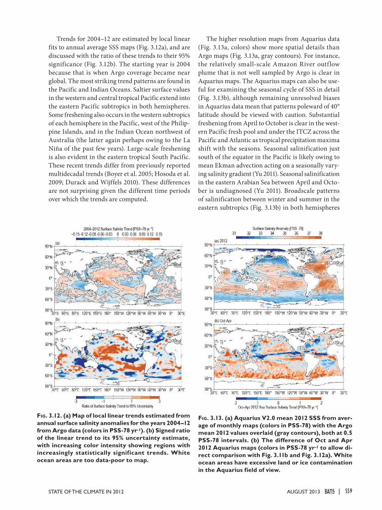
S59STATE OF THE CLIMATE IN 2012 |AuguST 2013
Trends for 2004–12 are estimated by local linear fits to annual average SSS maps (Fig. 3.12a), and are discussed with the ratio of these trends to their 95% significance (Fig. 3.12b). The starting year is 2004 because that is when Argo coverage became near global. The most striking trend patterns are found in the Pacific and Indian Oceans. Saltier surface values in the western and central tropical Pacific extend into the eastern Pacific subtropics in both hemispheres. Some freshening also occurs in the western subtropics of each hemisphere in the Pacific, west of the Philip-pine Islands, and in the Indian Ocean northwest of Australia (the latter again perhaps owing to the La Niña of the past few years). Large-scale freshening is also evident in the eastern tropical South Pacific. These recent trends differ from previously reported multidecadal trends (Boyer et al. 2005; Hosoda et al. 2009; Durack and Wijffels 2010). These differences are not surprising given the different time periods over which the trends are computed.
The higher resolution maps from Aquarius data (Fig. 3.13a, colors) show more spatial details than Argo maps (Fig. 3.13a, gray contours). For instance, the relatively small-scale Amazon River outf low plume that is not well sampled by Argo is clear in Aquarius maps. The Aquarius maps can also be use-ful for examining the seasonal cycle of SSS in detail (Fig. 3.13b), although remaining unresolved biases in Aquarius data mean that patterns poleward of 40° latitude should be viewed with caution. Substantial freshening from April to October is clear in the west-ern Pacific fresh pool and under the ITCZ across the Pacific and Atlantic as tropical precipitation maxima shift with the seasons. Seasonal salinification just south of the equator in the Pacific is likely owing to mean Ekman advection acting on a seasonally vary-ing salinity gradient (Yu 2011). Seasonal salinification in the eastern Arabian Sea between April and Octo-ber is undiagnosed (Yu 2011). Broadscale patterns of salinification between winter and summer in the eastern subtropics (Fig. 3.13b) in both hemispheres
Fig. 3.12. (a) Map of local linear trends estimated from annual surface salinity anomalies for the years 2004–12 from Argo data (colors in PSS-78 yr-1). (b) Signed ratio of the linear trend to its 95% uncertainty estimate, with increasing color intensity showing regions with increasingly statistically significant trends. White ocean areas are too data-poor to map.
Fig. 3.13. (a) Aquarius V2.0 mean 2012 SSS from aver-age of monthly maps (colors in PSS-78) with the Argo mean 2012 values overlaid (gray contours), both at 0.5 PSS-78 intervals. (b) The difference of Oct and Apr 2012 Aquarius maps (colors in PSS-78 yr-1 to allow di-rect comparison with Fig. 3.11b and Fig. 3.12a). White ocean areas have excessive land or ice contamination in the Aquarius field of view.
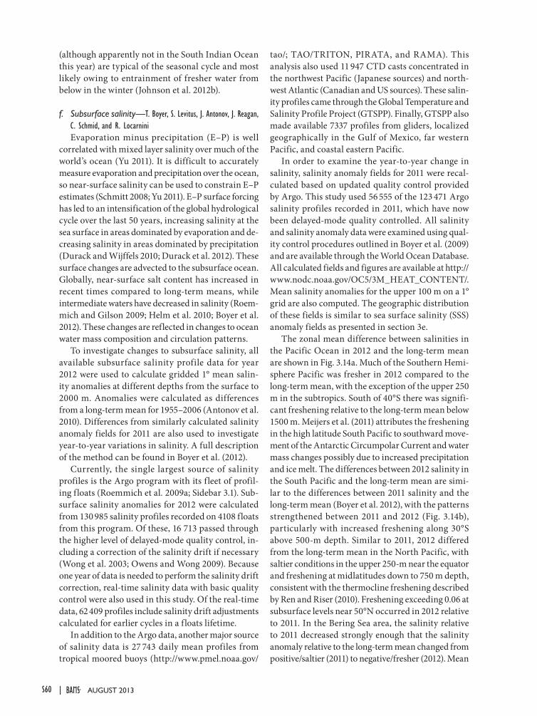
S60 | august 2013
(although apparently not in the South Indian Ocean this year) are typical of the seasonal cycle and most likely owing to entrainment of fresher water from below in the winter (Johnson et al. 2012b).
f. Subsurface salinity—T. Boyer, S. Levitus, J. Antonov, J. Reagan, C. Schmid, and R. LocarniniEvaporation minus precipitation (E–P) is well
correlated with mixed layer salinity over much of the world’s ocean (Yu 2011). It is difficult to accurately measure evaporation and precipitation over the ocean, so near-surface salinity can be used to constrain E–P estimates (Schmitt 2008; Yu 2011). E–P surface forcing has led to an intensification of the global hydrological cycle over the last 50 years, increasing salinity at the sea surface in areas dominated by evaporation and de-creasing salinity in areas dominated by precipitation (Durack and Wijffels 2010; Durack et al. 2012). These surface changes are advected to the subsurface ocean. Globally, near-surface salt content has increased in recent times compared to long-term means, while intermediate waters have decreased in salinity (Roem-mich and Gilson 2009; Helm et al. 2010; Boyer et al. 2012). These changes are reflected in changes to ocean water mass composition and circulation patterns.
To investigate changes to subsurface salinity, all available subsurface salinity profile data for year 2012 were used to calculate gridded 1° mean salin-ity anomalies at different depths from the surface to 2000 m. Anomalies were calculated as differences from a long-term mean for 1955–2006 (Antonov et al. 2010). Differences from similarly calculated salinity anomaly fields for 2011 are also used to investigate year-to-year variations in salinity. A full description of the method can be found in Boyer et al. (2012).
Currently, the single largest source of salinity profiles is the Argo program with its fleet of profil-ing floats (Roemmich et al. 2009a; Sidebar 3.1). Sub-surface salinity anomalies for 2012 were calculated from 130 985 salinity profiles recorded on 4108 floats from this program. Of these, 16 713 passed through the higher level of delayed-mode quality control, in-cluding a correction of the salinity drift if necessary (Wong et al. 2003; Owens and Wong 2009). Because one year of data is needed to perform the salinity drift correction, real-time salinity data with basic quality control were also used in this study. Of the real-time data, 62 409 profiles include salinity drift adjustments calculated for earlier cycles in a floats lifetime.
In addition to the Argo data, another major source of salinity data is 27 743 daily mean profiles from tropical moored buoys (http://www.pmel.noaa.gov/
tao/; TAO/TRITON, PIRATA, and RAMA). This analysis also used 11 947 CTD casts concentrated in the northwest Pacific (Japanese sources) and north-west Atlantic (Canadian and US sources). These salin-ity profiles came through the Global Temperature and Salinity Profile Project (GTSPP). Finally, GTSPP also made available 7337 profiles from gliders, localized geographically in the Gulf of Mexico, far western Pacific, and coastal eastern Pacific.
In order to examine the year-to-year change in salinity, salinity anomaly fields for 2011 were recal-culated based on updated quality control provided by Argo. This study used 56 555 of the 123 471 Argo salinity profiles recorded in 2011, which have now been delayed-mode quality controlled. All salinity and salinity anomaly data were examined using qual-ity control procedures outlined in Boyer et al. (2009) and are available through the World Ocean Database. All calculated fields and figures are available at http://www.nodc.noaa.gov/OC5/3M_HEAT_CONTENT/. Mean salinity anomalies for the upper 100 m on a 1° grid are also computed. The geographic distribution of these fields is similar to sea surface salinity (SSS) anomaly fields as presented in section 3e.
The zonal mean difference between salinities in the Pacific Ocean in 2012 and the long-term mean are shown in Fig. 3.14a. Much of the Southern Hemi-sphere Pacific was fresher in 2012 compared to the long-term mean, with the exception of the upper 250 m in the subtropics. South of 40°S there was signifi-cant freshening relative to the long-term mean below 1500 m. Meijers et al. (2011) attributes the freshening in the high latitude South Pacific to southward move-ment of the Antarctic Circumpolar Current and water mass changes possibly due to increased precipitation and ice melt. The differences between 2012 salinity in the South Pacific and the long-term mean are simi-lar to the differences between 2011 salinity and the long-term mean (Boyer et al. 2012), with the patterns strengthened between 2011 and 2012 (Fig. 3.14b), particularly with increased freshening along 30°S above 500-m depth. Similar to 2011, 2012 differed from the long-term mean in the North Pacific, with saltier conditions in the upper 250-m near the equator and freshening at midlatitudes down to 750 m depth, consistent with the thermocline freshening described by Ren and Riser (2010). Freshening exceeding 0.06 at subsurface levels near 50°N occurred in 2012 relative to 2011. In the Bering Sea area, the salinity relative to 2011 decreased strongly enough that the salinity anomaly relative to the long-term mean changed from positive/saltier (2011) to negative/fresher (2012). Mean

S61STATE OF THE CLIMATE IN 2012 |AuguST 2013
salinity in the upper 100 m (not shown, but closely resembles Fig. 3.11a) shows a large positive salinity anomaly relative to the long-term mean under the South Pacific convergence zone (SPCZ), although this feature has weakened compared to 2011 (not shown, but closely resembles Fig. 3.11b). The western equato-rial Pacific south of the equator has freshened since 2011, but otherwise the tropical Pacific waters in the upper 100 m are saltier than the long-term mean and this positive salinity anomaly increased from 2011 to 2012 between the equator and 15°N (not shown, but closely resembles Fig. 3.11b).
For the most part, 2012 salinity anomalies with respect to the long-term mean (Fig. 3.15a) in the subtropical and sub-polar North Atlantic agree with the salinity increase reported by Boyer et al. (2007) and Wang et al. (2010), with the exception of a reversal around 45°N. However, most of the North Atlantic freshened between 2011 and 2012 (Fig. 3.15b). North of 40°N, this freshening was consistent down to 500 depth. South of 40°N, freshening was generally exceeding 0.02 above 200-m depth, with anomalies exceeding 0.01 m to 500-m depth in the tropics. 2012 experienced a mostly negative North Atlantic Oscil-lation (NAO) index, while 2011 had mostly a positive NAO index, with the exception of the months May–July; Tropical Rainfall Measuring Mission (TRMM) recorded greater precipitation in 2012 than in 2011 from 30°N to 40°N, while from the equator to 25°N less precipitation was recorded. (No data are available outside 40°S–40°N.) These factors could contribute to the observed freshening, at least in the mixed layer. Another factor could be changes in the ice melt (both
Arctic Ocean and Greenland). It remains to be seen if this freshening is a short-term phenomenon or a reversal of the signal present over the last 15 years. In contrast, the southern Atlantic salinity signal for 2012, compared to the long-term trend, strengthened with respect to the same signal for 2011. Positive salinity anomalies exceeding 0.04, compared to the long-term trend, are found for 2012 down to 250 m in depth from the equator to 40°S, with anomalies exceeding 0.02 down below 500 m between 30°S and 40°S. South of 40°S in the Atlantic Ocean, a deep freshening is observed, to depths exceeding 700 m, shoaling to the south, where the freshening is lim-ited to the upper 200-m depth. These trends were strengthened and deepened between 2011 and 2012 (Fig. 3.15b) over most of the South Atlantic, with the exception of the high latitudes, where conditions were saltier in the upper 200 m in 2012 than 2011.
In the Indian Ocean, the difference between 2012 salinity zonal means and the long-term mean (Fig. 3.16a) includes deep (below 1000 m) freshening south of the equator, interrupted by increased salinity in the midlatitude South Indian Ocean from the surface to at least 250-m depth. In the upper 100 m (not shown, but closely resembles Fig. 3.11a), the positive/salty anomaly at latitudes north of 30°S is confined to the western half of the Indian Ocean, with freshening in the eastern Indian Ocean. South of 30°S, the positive anomaly extends across the entire basin. The salinity change from 2011 to 2012 in the South Indian Ocean was small (Fig. 3.16b). Most of the North Indian Ocean zonal mean anomalies for 2012 are positive/salty compared to the long-term mean to depths ex-
Fig. 3.14. Zonally averaged (a) 2012 salinity anomaly and (b) 2012 minus 2011 salinity f ield for the Pa-cific Ocean. Blue shading represents negative (fresh) anomalies <-0.01, red shading represents positive (salty) anomalies >0.01. The contour interval for the anomalies is 0.02. In the background of each figure (thick blue contours) is the zonally-averaged clima-tological mean salinity (WOA09). Contour intervals for the background are 0.4. All values are on the PSS.
Fig. 3.15. Zonally averaged (a) 2012 salinity anomaly and (b) 2012 minus 2011 salinity field for the Atlan-tic Ocean. Blue shading represents negative (fresh) anomalies <-0.01, red shading represents positive (salty) anomalies >0.01. The contour interval for the anomalies is 0.02. In the background of each figure (thick blue contours) is the zonally-averaged clima-tological mean salinity (WOA09). Contour intervals for the background are 0.4. All values are on the PSS.
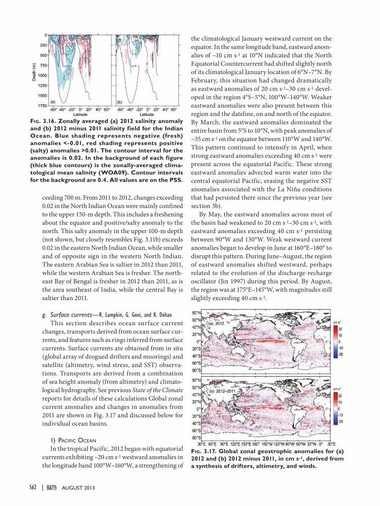
S62 | august 2013
Fig. 3.17. Global zonal geostrophic anomalies for (a) 2012 and (b) 2012 minus 2011, in cm s-1, derived from a synthesis of drifters, altimetry, and winds.
ceeding 700 m. From 2011 to 2012, changes exceeding 0.02 in the North Indian Ocean were mainly confined to the upper 150-m depth. This includes a freshening about the equator and positive/salty anomaly to the north. This salty anomaly in the upper 100-m depth (not shown, but closely resembles Fig. 3.11b) exceeds 0.02 in the eastern North Indian Ocean, while smaller and of opposite sign in the western North Indian. The eastern Arabian Sea is saltier in 2012 than 2011, while the western Arabian Sea is fresher. The north-east Bay of Bengal is fresher in 2012 than 2011, as is the area southeast of India, while the central Bay is saltier than 2011.
g. Surface currents—R. Lumpkin, G. Goni, and K. DohanThis section describes ocean surface current
changes, transports derived from ocean surface cur-rents, and features such as rings inferred from surface currents. Surface currents are obtained from in situ (global array of drogued drifters and moorings) and satellite (altimetry, wind stress, and SST) observa-tions. Transports are derived from a combination of sea height anomaly (from altimetry) and climato-logical hydrography. See previous State of the Climate reports for details of these calculations Global zonal current anomalies and changes in anomalies from 2011 are shown in Fig. 3.17 and discussed below for individual ocean basins.
1) Pacific Ocean
In the tropical Pacific, 2012 began with equatorial currents exhibiting ~20 cm s-1 westward anomalies in the longitude band 100°W–160°W, a strengthening of
the climatological January westward current on the equator. In the same longitude band, eastward anom-alies of ~10 cm s-1 at 10°N indicated that the North Equatorial Countercurrent had shifted slightly north of its climatological January location of 6°N–7°N. By February, this situation had changed dramatically as eastward anomalies of 20 cm s-1–30 cm s-1 devel-oped in the region 4°S–5°N, 100°W–140°W. Weaker eastward anomalies were also present between this region and the dateline, on and north of the equator. By March, the eastward anomalies dominated the entire basin from 5°S to 10°N, with peak anomalies of ~35 cm s-1 on the equator between 110°W and 140°W. This pattern continued to intensify in April, when strong eastward anomalies exceeding 40 cm s-1 were present across the equatorial Pacific. These strong eastward anomalies advected warm water into the central equatorial Pacific, erasing the negative SST anomalies associated with the La Niña conditions that had persisted there since the previous year (see section 3b).
By May, the eastward anomalies across most of the basin had weakened to 20 cm s-1–30 cm s-1, with eastward anomalies exceeding 40 cm s-1 persisting between 90°W and 130°W. Weak westward current anomalies began to develop in June at 160°E–180° to disrupt this pattern. During June–August, the region of eastward anomalies shifted westward, perhaps related to the evolution of the discharge-recharge oscillator (Jin 1997) during this period. By August, the region was at 175°E–145°W, with magnitudes still slightly exceeding 40 cm s-1.
Fig. 3.16. Zonally averaged (a) 2012 salinity anomaly and (b) 2012 minus 2011 salinity field for the Indian Ocean. Blue shading represents negative (fresh) anomalies <-0.01, red shading represents positive (salty) anomalies >0.01. The contour interval for the anomalies is 0.02. In the background of each figure (thick blue contours) is the zonally-averaged clima-tological mean salinity (WOA09). Contour intervals for the background are 0.4. All values are on the PSS.
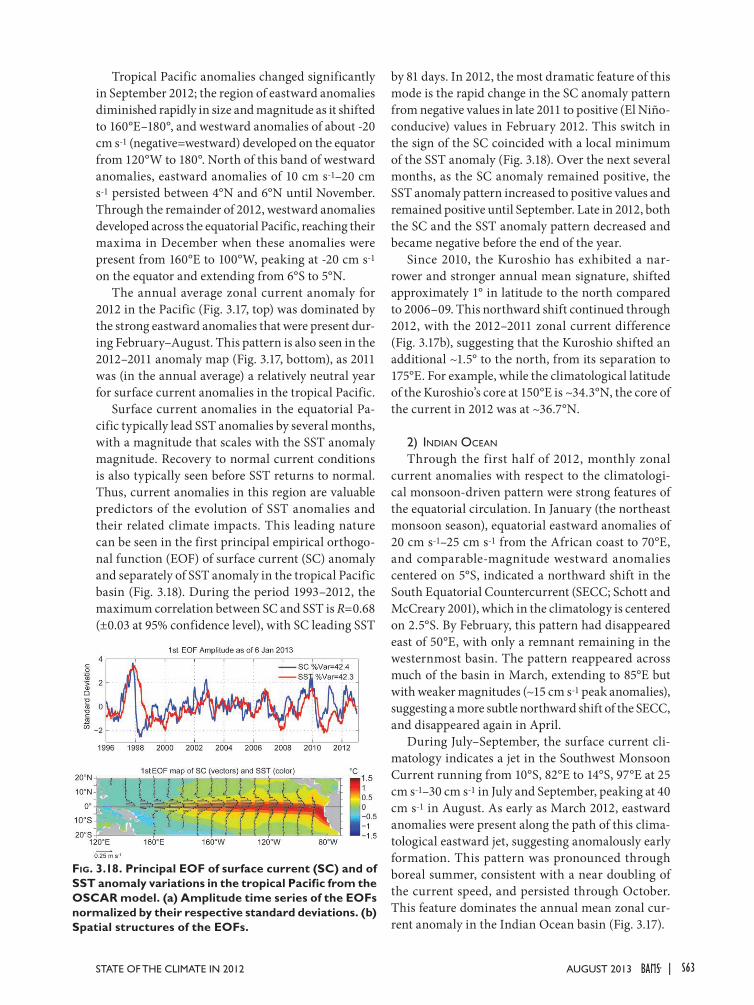
S63STATE OF THE CLIMATE IN 2012 |AuguST 2013
Tropical Pacific anomalies changed significantly in September 2012; the region of eastward anomalies diminished rapidly in size and magnitude as it shifted to 160°E–180°, and westward anomalies of about -20 cm s-1 (negative=westward) developed on the equator from 120°W to 180°. North of this band of westward anomalies, eastward anomalies of 10 cm s-1–20 cm s-1 persisted between 4°N and 6°N until November. Through the remainder of 2012, westward anomalies developed across the equatorial Pacific, reaching their maxima in December when these anomalies were present from 160°E to 100°W, peaking at -20 cm s-1 on the equator and extending from 6°S to 5°N.
The annual average zonal current anomaly for 2012 in the Pacific (Fig. 3.17, top) was dominated by the strong eastward anomalies that were present dur-ing February–August. This pattern is also seen in the 2012–2011 anomaly map (Fig. 3.17, bottom), as 2011 was (in the annual average) a relatively neutral year for surface current anomalies in the tropical Pacific.
Surface current anomalies in the equatorial Pa-cific typically lead SST anomalies by several months, with a magnitude that scales with the SST anomaly magnitude. Recovery to normal current conditions is also typically seen before SST returns to normal. Thus, current anomalies in this region are valuable predictors of the evolution of SST anomalies and their related climate impacts. This leading nature can be seen in the first principal empirical orthogo-nal function (EOF) of surface current (SC) anomaly and separately of SST anomaly in the tropical Pacific basin (Fig. 3.18). During the period 1993–2012, the maximum correlation between SC and SST is R=0.68 (±0.03 at 95% confidence level), with SC leading SST
by 81 days. In 2012, the most dramatic feature of this mode is the rapid change in the SC anomaly pattern from negative values in late 2011 to positive (El Niño-conducive) values in February 2012. This switch in the sign of the SC coincided with a local minimum of the SST anomaly (Fig. 3.18). Over the next several months, as the SC anomaly remained positive, the SST anomaly pattern increased to positive values and remained positive until September. Late in 2012, both the SC and the SST anomaly pattern decreased and became negative before the end of the year.
Since 2010, the Kuroshio has exhibited a nar-rower and stronger annual mean signature, shifted approximately 1° in latitude to the north compared to 2006–09. This northward shift continued through 2012, with the 2012–2011 zonal current difference (Fig. 3.17b), suggesting that the Kuroshio shifted an additional ~1.5° to the north, from its separation to 175°E. For example, while the climatological latitude of the Kuroshio’s core at 150°E is ~34.3°N, the core of the current in 2012 was at ~36.7°N.
2) indian Ocean
Through the first half of 2012, monthly zonal current anomalies with respect to the climatologi-cal monsoon-driven pattern were strong features of the equatorial circulation. In January (the northeast monsoon season), equatorial eastward anomalies of 20 cm s-1–25 cm s-1 from the African coast to 70°E, and comparable-magnitude westward anomalies centered on 5°S, indicated a northward shift in the South Equatorial Countercurrent (SECC; Schott and McCreary 2001), which in the climatology is centered on 2.5°S. By February, this pattern had disappeared east of 50°E, with only a remnant remaining in the westernmost basin. The pattern reappeared across much of the basin in March, extending to 85°E but with weaker magnitudes (~15 cm s-1 peak anomalies), suggesting a more subtle northward shift of the SECC, and disappeared again in April.
During July–September, the surface current cli-matology indicates a jet in the Southwest Monsoon Current running from 10°S, 82°E to 14°S, 97°E at 25 cm s-1–30 cm s-1 in July and September, peaking at 40 cm s-1 in August. As early as March 2012, eastward anomalies were present along the path of this clima-tological eastward jet, suggesting anomalously early formation. This pattern was pronounced through boreal summer, consistent with a near doubling of the current speed, and persisted through October. This feature dominates the annual mean zonal cur-rent anomaly in the Indian Ocean basin (Fig. 3.17).
Fig. 3.18. Principal EOF of surface current (SC) and of SST anomaly variations in the tropical Pacific from the OSCAR model. (a) Amplitude time series of the EOFs normalized by their respective standard deviations. (b) Spatial structures of the EOFs.
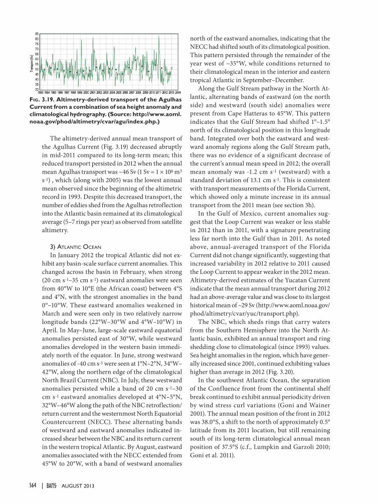
S64 | august 2013
The altimetry-derived annual mean transport of the Agulhas Current (Fig. 3.19) decreased abruptly in mid-2011 compared to its long-term mean; this reduced transport persisted in 2012 when the annual mean Agulhas transport was ~46 Sv (1 Sv = 1 × 10⁶ m3 s-1) , which (along with 2005) was the lowest annual mean observed since the beginning of the altimetric record in 1993. Despite this decreased transport, the number of eddies shed from the Agulhas retroflection into the Atlantic basin remained at its climatological average (5–7 rings per year) as observed from satellite altimetry.
3) atlantic Ocean
In January 2012 the tropical Atlantic did not ex-hibit any basin-scale surface current anomalies. This changed across the basin in February, when strong (20 cm s-1–35 cm s-1) eastward anomalies were seen from 40°W to 10°E (the African coast) between 4°S and 4°N, with the strongest anomalies in the band 0°–10°W. These eastward anomalies weakened in March and were seen only in two relatively narrow longitude bands (22°W–30°W and 4°W–10°W) in April. In May–June, large-scale eastward equatorial anomalies persisted east of 30°W, while westward anomalies developed in the western basin immedi-ately north of the equator. In June, strong westward anomalies of -40 cm s-1 were seen at 1°N–2°N, 34°W–42°W, along the northern edge of the climatological North Brazil Current (NBC). In July, these westward anomalies persisted while a band of 20 cm s-1–30 cm s-1 eastward anomalies developed at 4°N–5°N, 32°W–46°W along the path of the NBC retroflection/return current and the westernmost North Equatorial Countercurrent (NECC). These alternating bands of westward and eastward anomalies indicated in-creased shear between the NBC and its return current in the western tropical Atlantic. By August, eastward anomalies associated with the NECC extended from 45°W to 20°W, with a band of westward anomalies
north of the eastward anomalies, indicating that the NECC had shifted south of its climatological position. This pattern persisted through the remainder of the year west of ~35°W, while conditions returned to their climatological mean in the interior and eastern tropical Atlantic in September–December.
Along the Gulf Stream pathway in the North At-lantic, alternating bands of eastward (on the north side) and westward (south side) anomalies were present from Cape Hatteras to 45°W. This pattern indicates that the Gulf Stream had shifted 1°–1.5° north of its climatological position in this longitude band. Integrated over both the eastward and west-ward anomaly regions along the Gulf Stream path, there was no evidence of a significant decrease of the current’s annual mean speed in 2012; the overall mean anomaly was -1.2 cm s-1 (westward) with a standard deviation of 13.1 cm s-1. This is consistent with transport measurements of the Florida Current, which showed only a minute increase in its annual transport from the 2011 mean (see section 3h).
In the Gulf of Mexico, current anomalies sug-gest that the Loop Current was weaker or less stable in 2012 than in 2011, with a signature penetrating less far north into the Gulf than in 2011. As noted above, annual-averaged transport of the Florida Current did not change significantly, suggesting that increased variability in 2012 relative to 2011 caused the Loop Current to appear weaker in the 2012 mean. Altimetry-derived estimates of the Yucatan Current indicate that the mean annual transport during 2012 had an above-average value and was close to its largest historical mean of ~29 Sv (http://www.aoml.noaa.gov/phod/altimetry/cvar/yuc/transport.php).
The NBC, which sheds rings that carry waters from the Southern Hemisphere into the North At-lantic basin, exhibited an annual transport and ring shedding close to climatological (since 1993) values. Sea height anomalies in the region, which have gener-ally increased since 2001, continued exhibiting values higher than average in 2012 (Fig. 3.20).
In the southwest Atlantic Ocean, the separation of the Confluence front from the continental shelf break continued to exhibit annual periodicity driven by wind stress curl variations (Goni and Wainer 2001). The annual mean position of the front in 2012 was 38.0°S, a shift to the north of approximately 0.5° latitude from its 2011 location, but still remaining south of its long-term climatological annual mean position of 37.5°S (c.f., Lumpkin and Garzoli 2010; Goni et al. 2011).
Fig. 3.19. Altimetry-derived transport of the Agulhas Current from a combination of sea height anomaly and climatological hydrography. (Source: http://www.aoml.noaa.gov/phod/altimetry/cvar/agu/index.php.)

S65STATE OF THE CLIMATE IN 2012 |AuguST 2013
h. Meridional overturning circulation and heat transport observations in the Atlantic Ocean—M. o. Baringer, W. E. Johns, G. McCarthy, J. Willis, S. Garzoli, M. Lankhorst, C. S. Meinen, U. Send, W. R. Hobbs, S. A. Cunningham, D. Rayner, D. A. Smeed, T. o. Kanzow, P. Heimbach, E. Frajka-Williams, A. Macdonald, S. Dong, and J. MarotzkeThe meridional overturning circulation (MOC)
is typically defined as the maximum of the zonally-integrated mass transport stream function. In the Atlantic Ocean the MOC is the large-scale circulation that transports warm near-surface water northward, thereby transferring heat to the atmosphere and returning southward as colder, denser, deeper water. The actual f lows are more complicated than this simple description and for further details the reader should see previous State of the Climate reports (e.g., Baringer et al. 2011, 2012) or the recent reviews of Srokosz et al. (2012) or Lozier (2012).
The longest time series of a major ocean current contributing to the strength of the MOC is NOAA’s Florida Current (FC) data, which began continuous daily measurements in 1982. The full record (Fig. 3.21) shows substantial variability on all measured time scales (Meinen et al. 2010; Baringer and Larsen 2001). The 1982–2012 median transport of daily values is 32.0 ± 0.27 Sv (standard error of the mean based on an integral time scale of about 20 days) with a minimal downward trend of -0.23 ± 0.06 Sv decade-1 (90% confidence). In 2012 the annual median was 31.6 ± 1.5 Sv, with the annual mean transport slightly below the average since 2007 (Baringer et al. 2012). However, the 2012 median is within the middle 50% of all annual means. The 2012 daily values of FC transport do show some unusual periods. The daily FC transport values as compared to all previous years (Fig. 3.21, top) indicate that 2012 was unusual in that there were several low transport values (LTP) start-
ing 27 October and ending 24 November. The lowest transport observed occurred on 28 October, reaching only 17.2 Sv. This low value is similar to the lowest transport recorded since 1982 (17.3 Sv on 3 October 1983). The 2012 LTP was preceded by the only high transport event during 2012 that exceeded the 95% confidence limits. This transport exceeded 38 Sv from 3 to 4 October. Low values in the October–November time frame are consistent with the average annual cycle of FC transport (e.g., Meinen et al. 2010). In the last week of October low values are consistent with the passage of Hurricane Sandy northward offshore of the US East Coast. Previous studies have shown that southerly along-shore wind stress can cause a reduction in FC strength, leading to increased sea level along the coast (e.g., Ezer et al. 2013; Sweet et al. 2009). Ezer et al. (2013) quantified this effect using
Fig. 3.21. (a) Daily estimates of the transport of the Florida Current during 2012 (red solid line) compared to 2011 (dashed blue line). The daily values of the Florida Current transport for other years since 1982 are shown in light gray and the 95% confidence inter-val of daily transport values computed from all years is shown in black (solid line); the long-term annual mean is dashed black. The 2012 median transport (31.6 ± 1.5 Sv) lies slightly below the long-term median for the daily values of the Florida Current transport (32.0 Sv). (b) Daily estimates of the Florida Current transport for the full time series record (light gray), and a smoothed version of transport (heavy black line; using a 12-month second-order Butterworth filter) and the mean transport for the full record (dashed black).
Fig. 3.20. Space-time diagram of deseasoned sea height anomaly (SHR) values along the NBC ring corridor during 2008–12. (Source: http://www.aoml.noaa.gov/phod/altimetry/cvar/nbc.)

S66 | august 2013
a numerical model to show that a 1 Sv decrease in transport corresponds to a 1 cm increase in coastal sea level near these latitudes (see also Boon 2012; Sal-lenger et al. 2012; Ezer and Corlett 2012).
The only complete daily time series of basin-wide MOC strength at a particular latitude currently available is from the in situ mooring array, RAPID-MOC/MOCHA/WBTS (Fig. 3.22). This mooring array spans the Atlantic Ocean roughly along 26°N (Rayner et al. 2010; Kanzow et al. 2008a). The mean MOC transport centered on this low MOC event (1 April 2009–31 March 2010, referred to as 2009/10) was 12.7 Sv. After this 2009/10 low, the annual mean transport increased to 16.9 Sv in 2010/11, only slightly lower than the 2004–11 mean of 17.5 ± 1.6 Sv (± standard error of annual means). Although the mean transport for 2010/11 represents an increase, there is still a statistically significant (p=0.95) MOC minimum from 13 November–29 December 2010. This MOC minimum is preceded by three minima in low Florida Current transport occurring between 4 October and 10 December 2010 (Fig 3.22). Similar
to the December–March 2009/10 low MOC event, the November 2010–December 2011 low MOC appears most coincident with the unusual and significantly low Ekman transport compared to a mean of 3.2 Sv (2–29 December 2010). In December–March 2009/10, the slowing of the MOC (low FC and Ek-man transports) was preceded by a weakening of the upper ocean southward flow east of 77°W (aka the interior transport, Fig. 3.22; 5 October–2 December, mean -11.1 Sv) and followed by a strengthening of the interior southward flow 29 January–6 February 2011. Wunsch and Heimbach (2013) estimate the frequency of occurrence of such monthly extremes to be 14 months in a 1992–2010 monthly transport time series that is assumed to represent a station-ary Gaussian process. Overall, however, the interior transport was stronger southward in both 2009 and 2010 (hence contributing to the low MOC transport in those years). In these two years there was interest-ing phasing between anomalous interior, FC, and Ekman transport. It is the sum of these components that makes up the MOC at this latitude and therefore a clear understanding of this phasing is fundamental to the understanding of the physical mechanisms supporting MOC transport variability (McCarthy et al. 2012).
The North Atlantic MOC is also being monitored by somewhat less direct and complete time series at 41°N and 16°N (Fig. 3.23). Near 41°N, Willis and Fu (2008) developed a technique using Argo profiling f loats combined with satellite altimetry and the ECCO2 state estimate (Menemenlis et al. 2005) to estimate the upper ocean circulation with the zonally and vertically integrated upper ocean flow represent-ing the upper layer of the MOC. The 41°N time series shows a similar low MOC event slightly preceding the 26°N winter 2009 low MOC. Near 16°N, a mooring array of inverted echo sounders, current meters, and dynamic height moorings that measures the deep circulation across most of the basin has been in place since 2000 (Kanzow et al. 2008b). Interestingly, the 16°N time series has a high southward flow (hence a large MOC) in the winter of 2009 (13 December 2009–23 January 2010). The three-month low-pass filtering of these time series highlights the seasonal cycles found in all three. There are different phases for each, with 16°N having a maximum MOC in May–July, 26°N having a broad maximum in July–November (Kanzow et al. 2010), and 16°N having a maximum southward flow (and hence stronger MOC) in November–January. Using these time series, vari-ous authors have reported MOC trends ranging from
Fig. 3.22. Daily estimates of the strength of the meridi-onal overturning circulation (MOC; blue line) and its components, the Florida Current (FC; green), wind-driven Ekman transport (Ek; red) and the geostrophic interior (Int; black), as measured by the UK National Environmental Research Council Rapid Climate Change Program (RAPID-WATCH), the National Sci-ence Foundation’s Meridional Overturning and Heat transport Array proposal, and the NOAA Western Boundary Time Series project (WBTS). The interior volume transport estimate (accurate to 1 Sv, Cunning-ham et al. 2007) is based on the upper ocean transport from April 2004 to April 2011 (see also Rayner et al. 2010; Kanzow et al. 2010), with a 10-day low pass filter applied to the daily transport values. Annual means of the MOC transport starting 1 April of each year are shown in blue text (in Sv).

S67STATE OF THE CLIMATE IN 2012 |AuguST 2013
zero (Willis 2010 at 41°N) to a 10% decrease per de-cade (Send et al. 2011 at 16°N). Using the overlapping time period of these observations (1 April 2004−10 December 2010), the trend in MOC is -7.1 ± 5.7 Sv decade-1 at 41°N and -6.7 ± 5.9 Sv decade-1 at 26°N, suggesting a weakening MOC (barely significant at 95% confidence limits). However, at 16°N the deep southward flow is increasing, which is equivalent to an increase in the MOC at -7.7 ± 9.3 Sv decade-1 (not significantly different from zero at 95% confidence limits). Using the full time series from either 41°N or 16°N reduces the discrepancy largely by eliminating any significant MOC trend (-1.2 ± 1.7 Sv decade-1 at 41°N and 0.5 ± 0.4 Sv decade-1 at 16°N). Given the large variability in these short underlying time series and the low transport in the winter of 2009, it is dif-ficult at the present time to determine unambiguously whether the large-scale low-frequency MOC circula-tion has a trend in the North Atlantic.
In the South Atlantic there is an ongoing estima-tion of the MOC using upper ocean measurements from expendable bathythermograph sections that measure the upper ocean temperature approximately every three months (Garzoli et al. 2012). The MOC estimate from that data along 35°S since 2002 has suggested no significant trend in the MOC (Dong et al. 2009).
The MOC is related to the meridional transport of heat (MHT) in the oceans, and the variability of MHT can impact heat storage, sea-level rise, and air-sea fluxes, and hence influence local climate on land. MHT has been inferred using the time series data at 41°N (Hobbs and Willis 2012) and 26°N (Johns et al. 2008). Near 41°N, the time series mean MHT is 0.50 ± 0.10 PW (1PW = 1015 W) and near 26°N is 1.26 ± 0.40 PW (Fig. 3.24). In the South Atlantic, MHT has been estimated using a combination of expendable bathythermograph (XBT) data and Argo profiling f loats (Garzoli et al. 2012; Garzoli and Baringer 2007). The mean MHT near 35°S is 0.55 ± 0.3 PW (±1 standard deviation). Note that the mean MHT from the ECCO-PROD and SODA assimilating models are higher than those computed directly from observa-tions at 41°N, lower near 26°N, and bracket the direct MHT estimates at 35°S. In a detailed intercomparison
Fig. 3.24. Observed time series of meridional heat transport (MHT) at 41°N (profiling floats), 26°N (mooring/hydrography) and 35°S (XBTs) in the At-lantic compared to the monthly estimates from the ECCO-PROD version 4 (FH12, blue line; Forget et al. 2012, unpublished manuscript) and the Soda version 2.2.4 (red line; Carton and Giese 2008) models. (Top) The black line is the estimate MHT and the gray lines represents the error in the estimate (Hobbs and Wil-lis 2012). (Middle) The black line is the observed data filtered with a 30-day boxcar filter and the gray lines are the underlying 12-hourly data. (Bottom) The gray line is the quarterly estimated MHT from XBTs and the black line is a yearly boxcar filter to those quarterly estimates.
Fig. 3.23. Estimates of the MOC in the Atlantic Ocean from the Argo/Altimetry estimate at 41°N (black; Wil-lis 2010), the RAPID-WATCH/MOCHA/WBTS 26°N array (red; Cunningham et al. 2007), and the German/NOAA MOVE array at 16°N (blue; Send et al. 2011) are shown versus year. All time series have a three-month second-order Butterworth low pass filter applied. Horizontal lines are the mean transport during similar time periods as listed in the corresponding text. For the MOVE data, the net zonal and vertical integral of the deep circulation represents the lower limb of the MOC (with a negative sign for the southward flow).
S68 | august 2013
examining the RAPID/MOCHA/WBTS array near 26°N with two climate models, Msadek et al. (2013) found that the low MHT in the models was due to an overly diffuse thermocline rather than a weak MOC. In terms of variability, the low MOC winter of 2009/10 corresponds to a low MHT near both 26°N and 41°N. Both models capture the 26°N event, but not the 41°N event. Near 35°S the assimilation estimates have a much larger MHT seasonal cycle than observations (and, surprisingly, have larger variability). More work is needed to understand the causes of the underlying differences between direct-observation-based and data-assimilating-model estimates of MHT/MOC.
i. Sea level variability and change—M. A. Merrifield, P. Thompson, R. S. Nerem, D. P. Chambers, G. T. Mitchum, M. Menéndez, E. Leuliette, J. J. Marra, W. Sweet, and S. HolgateFour aspects of sea level variability during 2012 are
examined. First updated time series of global mean sea level (GMSL) as determined from satellite altim-eter observations are considered. GMSL provides a measure of the temporal change in ocean volume, which is affected by changes in density and the net heat content of the ocean, and by the mass transfer of water between the continents and the oceans via land ice melt and shifting evaporation-precipitation pat-terns. Second, seasonal anomalies of regional sea level based on satellite altimetry and tide gauge observa-
SIDEBAR 3.2: SLOWDOWN OF THE LOWER, SOUTHERN LIMB OF THE MERIDIONAL OVERTURNING CIRCULATION IN RECENT DECADES—G. C. JoHNSoN AND S. G. PURKEY
The Atlantic Meridional Overturning Circulation (AMOC), fed by sinking of North Atlantic Deep Water (NADW), has been continuously monitored for possible changes in the sub-tropical North Atlantic since 2006 (see section 3h). Annual means of the measured transport of the AMOC range from 13 Sv to 20 Sv between 2006 and 2010 (McCarthy et al. 2012). However, the AMOC is only the upper northern limb of the global meridional overturning circulation (MOC; Lumpkin and Speer 2007). The lower southern limb of the MOC, fed by sinking of Antarctic Bottom Water (AABW), has a transport of similar magnitude (Lumpkin and Speer 2007). In fact, AABW fills more of the world oceans than NADW, including much of the Southern Ocean as well as the deep Indian, Pacific, and western South Atlantic Oceans (Johnson 2008).
There is growing evidence that this lower southern limb is changing over recent decades, including statistically significant warming of deep waters of Antarctic origin nearly globally since circa 1990 (Kouketsu et al. 2011; Purkey and Johnson 2010), as well as freshening of bottom waters near Antarctica in the Indian (Rintoul 2007) and Pacific (Swift and Orsi 2012) sectors of the Southern Ocean. While there is no equivalent of the subtropical North Atlantic AMOC observation system (see section 3h) for the lower southern limb of the meridional overturning circulation, many studies, summarized below, have inferred consistent, worldwide reductions in the strength of this limb by comparing various oceanographic section data from the Global Ship-Based Hydrographic Investigations Program (http://www.go-ship.org/) with data from earlier oceanographic sections occupied during the 1980s and 1990s as part of the World Ocean Circulation Experiment (WOCE) Hydrographic Program.
Changes in the inventories of the coldest, deepest waters around the globe using oceanographic section data from the 1980s to present suggest a strong contraction of the coldest varieties of AABW (Fig. SB3.4; Purkey and Johnson 2012). Their results suggest that deep Southern Ocean waters with potential temperatures below 0°C are disappearing at a rate of over 8 Sv. At 35°S, the northward flow of bottom waters of southern origin is estimated to be slowing down by about 0.7 Sv decade-1 from 1968 to 2005 in the Pacific and 0.4 Sv decade-1 in the western Atlantic Ocean over the same time interval from a numerical model assimilating these data (Kouketsu et al. 2011). The same assimilation finds no change in the deep Indian Ocean, but oceanographic section data are sparser there since the completion of WOCE. While classic AABW (potential temperatures <0°C) is only found in the Argentine Basin of the western Atlantic at this latitude (Fig. SB3.4), the AABW influence is still strong in the bottom waters of all three oceans (Johnson 2008).
In the Northern Hemisphere, inverse model calculations in the Pacific using data from repeat hydrographic sections along 24°N suggest that the deep northern transport of waters of Southern Ocean origin lessened by 1.5 Sv between 1985 and 2005 (Kouketsu et al. 2009), consistent with results in the South Pacific. In the North Atlantic Ocean at 24°N, one analy-sis based on geostrophic calculations inferred a remarkable slowdown of northward flow of 4 Sv from four hydrographic sections occupied between 1981 and 2004 (Johnson et al. 2008); although another set of inverse estimates using different reference levels, integration areas, and data extrapolation into u-sampled areas found a slowdown of only 1.3 Sv over those same times, with a resurgence of 0.4 Sv between 2004 and
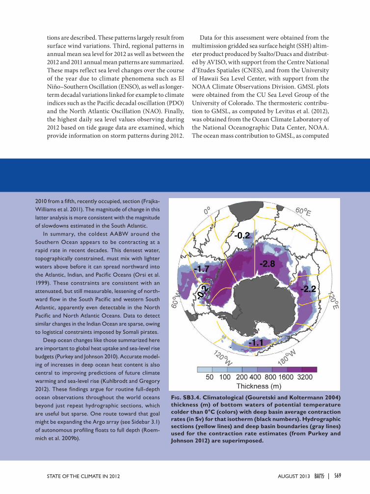
S69STATE OF THE CLIMATE IN 2012 |AuguST 2013
tions are described. These patterns largely result from surface wind variations. Third, regional patterns in annual mean sea level for 2012 as well as between the 2012 and 2011 annual mean patterns are summarized. These maps reflect sea level changes over the course of the year due to climate phenomena such as El Niño–Southern Oscillation (ENSO), as well as longer-term decadal variations linked for example to climate indices such as the Pacific decadal oscillation (PDO) and the North Atlantic Oscillation (NAO). Finally, the highest daily sea level values observing during 2012 based on tide gauge data are examined, which provide information on storm patterns during 2012.
Data for this assessment were obtained from the multimission gridded sea surface height (SSH) altim-eter product produced by Ssalto/Duacs and distribut-ed by AVISO, with support from the Centre National d’Etudes Spatiales (CNES), and from the University of Hawaii Sea Level Center, with support from the NOAA Climate Observations Division. GMSL plots were obtained from the CU Sea Level Group of the University of Colorado. The thermosteric contribu-tion to GMSL, as computed by Levitus et al. (2012), was obtained from the Ocean Climate Laboratory of the National Oceanographic Data Center, NOAA. The ocean mass contribution to GMSL, as computed
Fig. SB3.4. Climatological (Gouretski and Koltermann 2004) thickness (m) of bottom waters of potential temperature colder than 0°C (colors) with deep basin average contraction rates (in Sv) for that isotherm (black numbers). Hydrographic sections (yellow lines) and deep basin boundaries (gray lines) used for the contraction rate estimates (from Purkey and Johnson 2012) are superimposed.
2010 from a fifth, recently occupied, section (Frajka-Williams et al. 2011). The magnitude of change in this latter analysis is more consistent with the magnitude of slowdowns estimated in the South Atlantic.
In summary, the coldest AABW around the Southern Ocean appears to be contracting at a rapid rate in recent decades. This densest water, topographically constrained, must mix with lighter waters above before it can spread northward into the Atlantic, Indian, and Pacific Oceans (Orsi et al. 1999). These constraints are consistent with an attenuated, but still measurable, lessening of north-ward flow in the South Pacific and western South Atlantic, apparently even detectable in the North Pacific and North Atlantic Oceans. Data to detect similar changes in the Indian Ocean are sparse, owing to logistical constraints imposed by Somali pirates.
Deep ocean changes like those summarized here are important to global heat uptake and sea-level rise budgets (Purkey and Johnson 2010). Accurate model-ing of increases in deep ocean heat content is also central to improving predictions of future climate warming and sea-level rise (Kuhlbrodt and Gregory 2012). These findings argue for routine full-depth ocean observations throughout the world oceans beyond just repeat hydrographic sections, which are useful but sparse. One route toward that goal might be expanding the Argo array (see Sidebar 3.1) of autonomous profiling floats to full depth (Roem-mich et al. 2009b).

S70 | august 2013
by Chambers et al. (2010), was obtained from the Satellite Oceanography Laboratory of the University of South Florida.
The 20-year GMSL record is constructed by com-bining TOPEX, Jason-1, and Jason-2 satellite altimeter SSH observations (Fig. 3.25a). The SSH data have been corrected for the inverse barometer effect as well as for changes in ocean volume associated with glacial isostatic adjustment (GIA). The positive linear trend in GMSL of 3.2 ± 0.4 mm yr-1 during the altimetry record is due to the combined effect of increasing
ocean heat content (thermosteric rise) and increas-ing ocean mass primarily resulting from melting of terrestrial ice (Fig. 3.25a). Linear trend values for GMSL, thermosteric, and ocean mass change over the span of each measurement (Fig. 3.25a) and are con-sistent within the errors for each trend value. Trends in GMSL are smaller during the shorter intervals spanning time series of the individual contributions, but the differences are not statistically significant as the error bars about each value overlap. During the 2005–12 period for which all three measurements are available, the ocean mass contribution to the trend is dominant and more than twice that of the ther-mosteric contribution. The sum of the trends in the two individual contributions closes the GMSL trend budget within the error.
In addition to the positive linear trend in GMSL, there are substantial residual variations about the trend. In particular, the SSH residual exhibited low values relative to the trend during 2010–11, with a return to high values in 2012. The detrended GMSL time series has been shown to correlate significantly with the multivariate ENSO index (MEI; Nerem et al. 2010), although the relationship is not linear and may vary from event to event due to other factors. The agreement between detrended GMSL and the MEI during 2010–11 (Fig. 3.25b) suggests the decrease in GMSL relative to the trend during this period was due to La Niña. The influence of ENSO on GMSL during La Niña occurs both through lower ocean heat con-tent, as well as an increase in precipitation rates over land, which transfers ocean mass to the continents and leads to a short-term lowering of GMSL (Llovel et al. 2011). In the case of the 2010–11 La Niña, negative GMSL anomalies were almost entirely the result of ocean mass transfer to the continents (Boening et al. 2012), which is supported by the coincident decrease in ocean mass (Fig. 3.25a). In contrast, anomalies about the trend in the thermosteric contribution to GMSL are small during 2010–11.
Maps of regional sea level, averaged over three-month time spans, show the transition from La Niña dominant conditions at the beginning of the year, with high levels in the western tropical Pacific and eastern tropical Indian Oceans and low levels in the eastern Pacific and western Indian Oceans (Fig. 3.26a), to more ENSO-neutral conditions during the last quarter of 2012 (Fig. 3.26d). The early 2012 pat-tern represents the last stages of La Niña conditions that began in 2010. In the Indian Ocean, the La Niña-related high sea level anomaly along the west coast of Australia at the beginning of the year (Fig. 3.26a)
Fig. 3.25. (a) Time series of global mean sea level (GMSL) since 1993 obtained from the TOPEX, Jason-1, and Jason-2 satellite altimeters. GMSL exhibits a linear trend of 3.2 ± 0.4 mm yr-1. Seasonal signals have been removed from the data and the inverse barometer and global isostatic adjustment corrections have been applied (see Nerem et al. 2010). Recent estimates of ocean mass (Chambers et al. 2010) and thermosteric (Levitus et al. 2012) contributions to GMSL are in-cluded for comparison. (b) GMSL (detrended) versus the multivariate ENSO index (MEI). Time series have been normalized by their standard deviations.

S71STATE OF THE CLIMATE IN 2012 |AuguST 2013
migrated westward as Rossby waves over the course of the year (Fig. 3.26b–d).
2012 began with the continuation of a positive NAO phase, which was ref lected in negative sea level anomalies in the Mediterranean and positive anomalies in the Baltic Sea (Fig. 3.26a). The NAO index switched to negative values through the middle of the year with near-neutral conditions by the end of the year. Regional sea level patterns in the North Atlantic remained somewhat static throughout this period. Negative anomalies were noticeable in the South Atlantic for most of the year.
Annually-averaged sea level during 2012 reflects the La Niña pattern that dominated the tropical Pa-cific and Indian Oceans at the start of the year (Fig. 3.27a). The Pacific decadal oscillation (PDO) index was consistently negative throughout 2012, as it has been since mid-2010. The 2012 sea level field is char-acteristic of a negative PDO phase with low sea level anomalies along the eastern boundary that extend westward across the basin, particularly at low lati-tudes (Merrifield et al. 2012; Zhang and Church 2012). At midlatitudes in the North Pacific, high sea levels occurred associated with anomalous wind forcing in the Aleutian Low region. Over the Southern Ocean, a broad region of negative sea levels persisted west of the southern tip of South America. Annual sea levels were generally high in the tropical Indian Ocean. Sea level in the Atlantic Ocean was high north of the Gulf Stream extension and low south of this region.
The difference between the 2012 and 2011 annual means shows signs of the trade wind weakening in the
Pacific associated with the wan-ing La Niña and falling sea levels over much of the South Pacific convergence zone (SPCZ; Fig. 3.27b). A region of strong posi-tive change in the Indian Ocean largely reflected a strong negative sea level anomaly in 2011 that was absent in 2012. Zonal bands of rising and falling sea level appeared in the Atlantic, which partly reflect wind changes as-sociated with the switch from negative to positive NAO phase in 2011, and then back from posi-tive to neutral in 2012.
The maximum daily-averaged sea level during 2012 at each tide gauge station, relative to the an-nual mean of that station, shows
the general pattern of higher amplitude values in the mid- to high latitudes and weaker values in the tropics
Fig. 3.27. (a) The 2012 annual mean SSH anomaly from the 1993–2012 baseline compared with the 2012 sea level anomaly computed from tide gauges (dots). (b) The difference between 2012 and 2011 annual means.
Fig. 3.26. Seasonal SSH anomalies for 2012 relative to the 1993–2012 base-line average, obtained using the multimission gridded sea surface height altimeter product produced by Ssalto/Duacs and distributed by AVISO, with support from CNES (http://www.aviso.oceanobs.com).

S72 | august 2013
(Fig. 3.28a). The historic context for the 2012 annual maxima is presented in terms of the return period/averaged recurrence interval (years), computed using a generalized extreme value fit for tide gauges with at least 30 years of records (Fig. 3.28b). The annual maxima at the majority of stations (75 of 79) corre-spond to return periods of less than 8 years, with 2 stations in the 12–16 year range (Pensacola, Florida, and Naha, Japan). The impact of Hurricane Sandy is clearly evident at two stations in the northeastern United States: Atlantic City, New Jersey, and Newport, Rhode Island. The annual maxima at these locations are 96 cm and 73 cm above the annual mean sea level, respectively, corresponding to return periods of 39 and 276 years. It is noted that these levels do not include the contribution of high tides during the storm. The Hurricane Sandy storm tide heights are discussed in detail in Peterson et al. 2013 (manuscript submitted to Bull. Amer. Meteor. Soc.). The daily mean sea level during Hurricane Sandy is the highest over the 82-year record at Newport and the second high-est over the 101-year record at Atlantic City. (The record highest is 120 cm during the "Perfect Storm" of 1991.) The annual maximum at Pensacola (73 cm)
occurred in late August 2012 during the landfall of Hurricane Isaac, while in the same month Typhoon Bolaven caused significant damage at Naha and the Okinawa Island.
j. Global ocean carbon cycle—R. A. Feely, R. Wanninkhof, C. L. Sabine, J. T. Mathis, T. Takahashi, S. Khatiwala and G.-H. Park1) Sea-air carbOn diOxide fluxeS
The large increase in surface carbon dioxide (CO2) measurements and updated compilations are improving sea-air carbon dioxide f lux estimates. A community-based effort under auspices of the International Ocean Carbon Coordination Project (IOCCP; http://www.ioccp.org) released its first data product in 2011, SOCAT version 1.4. The second release, SOCAT version 2.0, is scheduled for the sum-mer of 2013. However, there are still delays with the availability of quality-controlled data streams, and surface sea-air CO2 fluxes reported in the State of the Climate reports are a year behind.
The global ocean sea-air CO2 flux estimate for 2011 is based on the approach described in Lee et al. (1998) and Park et al. (2006, 2010a,b). The monthly surface water CO2 partial pressure (pCO2SW) climatol-ogy on a 4° by 5° grid from Takahashi et al. (2009) is the basis to estimate interannual variability in sea-air CO2 f luxes (http://www.ldeo.columbia.edu/res/pi/CO2/carbondioxide/pages/air_sea_flux_2009.html). Subannual relationships are determined between SST and pCO2SW from this climatology and used to cal-culate the monthly pCO2SW for the other years from the SST anomaly compared to the SST for reference year 2000. SST is the optimal interpolated NOAA SST product (http://www.cdc.noaa.gov/data/gridded/data.noaa.oisst.v2.html).
Following this approach the anthropogenic sea-air CO2 flux estimate for 2011 using the CCMP winds is -1.95 Pg C yr-1, while for the NCEP-II winds the value is -2.30 Pg C yr-1. The difference in global fluxes is caused by the NCEP-II winds being systematically lower than the CCMP winds in the equatorial Pacific where the CO2 flux is out of the ocean, and higher in the Southern Ocean where the CO2 flux is into the ocean (Wallcraft et al. 2009).
The global ocean monthly average flux for 2011 and the anomaly from the 1982–2011 mean are shown in Fig. 3.29. The monthly trend and magnitude for 2011 is similar to the 30-year mean. On average, the global ocean CO2 uptake in 2011 was about 9% less than the long-term mean, after removing the long-term trend.
Fig. 3.28. (a) Highest daily-averaged sea level at tide gauges during 2012. (b) Return period/averaged recur-rence interval (years) associated with the highest daily sea level during 2012 at each station. Inset shows the highest daily sea level measured at Atlantic City, NJ, during Hurricane Sandy in late Oct 2012.

S73STATE OF THE CLIMATE IN 2012 |AuguST 2013
The contemporary sea-air f luxes in June and December 2011, panels on the left in Fig. 3.30, show a pattern of effluxes in the tropical regions and net CO2 uptake in mid- to high latitudes. The sinks at high northern latitudes in early summer are due to biological productivity while the sinks in the sub-tropical regions and subpolar Southern Ocean are caused by seasonal cooling. The patterns are similar for December 2011 except that the drivers switch,
with the pCO2 sinks in the Northern Hemisphere caused by seasonal cooling and the Southern Ocean sink being driven by biological productivity. The maximum inf lux in the Southern Ocean moves further south and is greatest in the Atlantic sector. The efflux in tropical regions is significantly greater in June than December. Upwelling in the equatorial Pacific is stronger in June, particularly in 2011 with the occurrence of the La Niña phase of ENSO. The high CO2 effluxes in response to upwelling during the southwest monsoon in the Arabian Sea are also apparent in June.
Anomalies in sea-air f luxes are often related to large-scale climate reorganizations, with the ENSO being the most prominent. The multivariate ENSO index (MEI; http://www.esrl.noaa.gov/psd/enso/mei/table.html) shows that the first half of 2011 experi-enced strong La Niña conditions with the remainder of the year weak to neutral conditions (see Fig. 3.3). The La Niña caused enhanced outgassing in the equatorial Pacific as is observed in the anomaly maps. Other features of note are the positive anomalies in the Pacific sector of the Southern Ocean in June and to a lesser extent in December, which means that this sink region took up less CO2 in 2011. This is attributed to a combination of SST anomalies in the region and higher winds. The higher outgassing in the equato-rial Pacific, combined with the lower influx in the Southern Ocean, caused the net sea-air CO2 flux for 2011 to be lower than the long-term mean.
2) Ocean carbOn inventOry
The U.S. CLIVAR/CO2 Repeat Hydrography Pro-gram continues to provide new insights about the
uptake and storage of carbon within the ocean interior. Two different data-based approaches for calculating anthropogenic carbon inventories exist: the ΔC* method (Gruber 1998; Sa-bine et al. 2002, 2004), and the transit time distribution (TTD) method (Waugh et al. 2006). These observations-based ap-proaches use tracer information and assume steady state ocean circulation. The anthropogenic carbon inventories inferred from these different methods agree well with each other with-in the limits of their uncertain-ties. A recent compilation of
Fig. 3.29. Monthly sea-air CO2 fluxes (Pg C yr-1) for 2011. The red solid line shows the monthly fluxes, the black dashed line is the 30-year mean, and the open squares are the monthly anomalies compared to the 30-year mean. (Source: http://cwcgom.aoml.noaa.gov/erddap/griddap/aomlcarbonfluxes.graph. Note: this utility does not include the coastal areas, or account for changing atmospheric CO2 but rather provides an open ocean contemporary flux.)
Fig. 3.30. Sea-air CO2 flux for Jun 2011 (a,b) and Dec 2011 (c,d). (a) and (b) show the net fluxes while (c) and (d) indicate the anomaly for each 4° × 5° pixel. The color bar is at the bottom with fluxes expressed in mol m-2 yr-1.

S74 | august 2013
inventories of anthropogenic carbon (Cant) from these methods combined with some model results indicate a global ocean inventory of Cant from 1750 to 2010 of 155 ± 26 PgC (Khatiwala et al. 2013).
The storage rate of Cant can also be assessed by calculating the change in concentration between two time periods. Regional observations of the storage rate are in general agreement with that expected from the increase in atmospheric CO2 concentrations and with the tracer-based estimates (Fig. 3.31). However, there are significant spatial and temporal differences in the degree to which the inventory of Cant tracks change in the atmosphere. For example, the subpo-lar North Atlantic is an area with high variability in circulation and deep water formation, influencing the Cant inventory. Large differences in storage rates have been observed on decadal and subdecadal time scales (Wanninkhof et al. 2010; Khatiwala et al. 2013). Pérez et al. (2010) found that the Cant storage rate in the North Atlantic was dependent on the NAO, with highest Cant storage rates occurring during the pos-itive phase of NAO and low storage rates during the negative phase of NAO. Ocean observations are in-sufficient to assess whether there has been a change in the rate of total (anthropogenic plus natural) carbon uptake by the global ocean. In the Pacific Ocean there are higher Cant storage rates in the South Pacific as compared with the North Pacific (Murata et al. 2007; Sabine et al. 2008). In the Indian Ocean the largest
Cant storage rates are observed south of the equator where Cant increases to 1800 m have been observed (Murata et al. 2010; Álvarez et al. 2011).
3) anthrOPOgenic Ocean acidificatiOn
Over the past two and a half centuries, the release of carbon dioxide (CO2) from human industrial and agricultural activities has resulted in an increase in atmospheric CO2 concentrations by about 110 ppm. During this period, the ocean has absorbed about 155 billion metric tons of carbon as CO2 from the atmosphere, or about a quarter of the total carbon emissions. The pH (total scale) of surface waters ranges from 7.8 to 8.4 in the open ocean, so the ocean remains mildly basic (pH > 7) under present condi-tions (Caldeira and Wickett 2003; Orr et al. 2005; Feely et al. 2009). Ocean uptake of CO2 results in gradual decrease in the pH of seawater, a process com-monly referred to as “ocean acidification” (Broecker and Clark 2001; Caldeira and Wickett 2003).
Monthly observations of oceanic pCO2SW and pH reflect changes in both the natural carbon cycle and the uptake of anthropogenic CO2 from the at-mosphere. Ocean time-series stations in the North Atlantic and North Pacific record decreasing pH (Fig. 3.32), with rates averaging about -0.0018 yr-1. The pH changes in Southern Ocean surface waters are less certain because of the paucity of long-term time-series observations.
Fig. 3.31. (Top) Maps of storage rate distribution of anthropogenic carbon (mol m-2 y-1) for the three ocean basins (left to right: Atlantic, Pacific, and Indian Oceans) averaged over 1980–2005 estimated by the Green’s function approach (Khatiwala et al. 2009). (Bottom) Corresponding storage rates as observed from repeat hydrography cruises. Measurements for the Northern Hemisphere are drawn as solid lines, the tropics as dash-dotted lines, and dashed lines for the Southern Hemisphere; the color schemes refer to different studies. Estimates of un-certainties are shown as vertical bars with matching colors. The solid black line represents the basin average storage rate using the same Green function approach (Khatiwala et al. 2009). (Source: Khatiwala et al. 2013.)
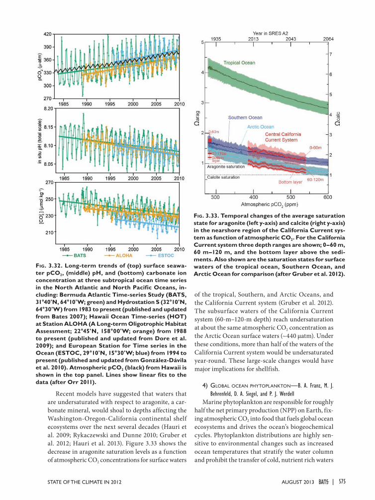
S75STATE OF THE CLIMATE IN 2012 |AuguST 2013
Recent models have suggested that waters that are undersaturated with respect to aragonite, a car-bonate mineral, would shoal to depths affecting the Washington-Oregon-California continental shelf ecosystems over the next several decades (Hauri et al. 2009; Rykaczewski and Dunne 2010; Gruber et al. 2012; Hauri et al. 2013). Figure 3.33 shows the decrease in aragonite saturation levels as a function of atmospheric CO2 concentrations for surface waters
of the tropical, Southern, and Arctic Oceans, and the California Current system (Gruber et al. 2012). The subsurface waters of the California Current system (60-m–120-m depth) reach undersaturation at about the same atmospheric CO2 concentration as the Arctic Ocean surface waters (~440 µatm). Under these conditions, more than half of the waters of the California Current system would be undersaturated year-round. These large-scale changes would have major implications for shellfish.
4) glObal Ocean PhytOPlanktOn—B. A. Franz, M. J. Behrenfeld, D. A. Siegel, and P. J. Werdell
Marine phytoplankton are responsible for roughly half the net primary production (NPP) on Earth, fix-ing atmospheric CO2 into food that fuels global ocean ecosystems and drives the ocean’s biogeochemical cycles. Phytoplankton distributions are highly sen-sitive to environmental changes such as increased ocean temperatures that stratify the water column and prohibit the transfer of cold, nutrient rich waters
Fig. 3.32. Long-term trends of (top) surface seawa-ter pCO2, (middle) pH, and (bottom) carbonate ion concentration at three subtropical ocean time series in the North Atlantic and North Pacific Oceans, in-cluding: Bermuda Atlantic Time-series Study (BATS, 31°40'N, 64°10'W; green) and Hydrostation S (32°10'N, 64°30'W) from 1983 to present (published and updated from Bates 2007); Hawaii Ocean Time-series (HOT) at Station ALOHA (A Long-term Oligotrophic Habitat Assessment; 22°45'N, 158°00'W; orange) from 1988 to present (published and updated from Dore et al. 2009); and European Station for Time series in the Ocean (ESTOC, 29°10'N, 15°30'W; blue) from 1994 to present (published and updated from González-Dávila et al. 2010). Atmospheric pCO2 (black) from Hawaii is shown in the top panel. Lines show linear fits to the data (after Orr 2011).
Fig. 3.33. Temporal changes of the average saturation state for aragonite (left y-axis) and calcite (right y-axis) in the nearshore region of the California Current sys-tem as function of atmospheric CO2. For the California Current system three depth ranges are shown; 0–60 m, 60 m–120 m, and the bottom layer above the sedi-ments. Also shown are the saturation states for surface waters of the tropical ocean, Southern Ocean, and Arctic Ocean for comparison (after Gruber et al. 2012).
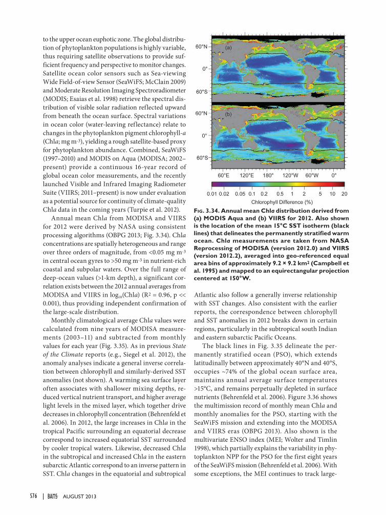
S76 | august 2013
to the upper ocean euphotic zone. The global distribu-tion of phytoplankton populations is highly variable, thus requiring satellite observations to provide suf-ficient frequency and perspective to monitor changes. Satellite ocean color sensors such as Sea-viewing Wide Field-of-view Sensor (SeaWiFS; McClain 2009) and Moderate Resolution Imaging Spectroradiometer (MODIS; Esaias et al. 1998) retrieve the spectral dis-tribution of visible solar radiation reflected upward from beneath the ocean surface. Spectral variations in ocean color (water-leaving reflectance) relate to changes in the phytoplankton pigment chlorophyll-a (Chla; mg m-3), yielding a rough satellite-based proxy for phytoplankton abundance. Combined, SeaWiFS (1997–2010) and MODIS on Aqua (MODISA; 2002–present) provide a continuous 16-year record of global ocean color measurements, and the recently launched Visible and Infrared Imaging Radiometer Suite (VIIRS; 2011–present) is now under evaluation as a potential source for continuity of climate-quality Chla data in the coming years (Turpie et al. 2012).
Annual mean Chla from MODISA and VIIRS for 2012 were derived by NASA using consistent processing algorithms (OBPG 2013; Fig. 3.34). Chla concentrations are spatially heterogeneous and range over three orders of magnitude, from <0.05 mg m-3 in central ocean gyres to >50 mg m-3 in nutrient-rich coastal and subpolar waters. Over the full range of deep-ocean values (>1-km depth), a significant cor-relation exists between the 2012 annual averages from MODISA and VIIRS in log10(Chla) (R2 = 0.96, p << 0.001), thus providing independent confirmation of the large-scale distribution.
Monthly climatological average Chla values were calculated from nine years of MODISA measure-ments (2003–11) and subtracted from monthly values for each year (Fig. 3.35). As in previous State of the Climate reports (e.g., Siegel et al. 2012), the anomaly analyses indicate a general inverse correla-tion between chlorophyll and similarly-derived SST anomalies (not shown). A warming sea surface layer often associates with shallower mixing depths, re-duced vertical nutrient transport, and higher average light levels in the mixed layer, which together drive decreases in chlorophyll concentration (Behrenfeld et al. 2006). In 2012, the large increases in Chla in the tropical Pacific surrounding an equatorial decrease correspond to increased equatorial SST surrounded by cooler tropical waters. Likewise, decreased Chla in the subtropical and increased Chla in the eastern subarctic Atlantic correspond to an inverse pattern in SST. Chla changes in the equatorial and subtropical
Atlantic also follow a generally inverse relationship with SST changes. Also consistent with the earlier reports, the correspondence between chlorophyll and SST anomalies in 2012 breaks down in certain regions, particularly in the subtropical south Indian and eastern subarctic Pacific Oceans.
The black lines in Fig. 3.35 delineate the per-manently stratified ocean (PSO), which extends latitudinally between approximately 40°N and 40°S, occupies ~74% of the global ocean surface area, maintains annual average surface temperatures >15°C, and remains perpetually depleted in surface nutrients (Behrenfeld et al. 2006). Figure 3.36 shows the multimission record of monthly mean Chla and monthly anomalies for the PSO, starting with the SeaWiFS mission and extending into the MODISA and VIIRS eras (OBPG 2013). Also shown is the multivariate ENSO index (MEI; Wolter and Timlin 1998), which partially explains the variability in phy-toplankton NPP for the PSO for the first eight years of the SeaWiFS mission (Behrenfeld et al. 2006). With some exceptions, the MEI continues to track large-
Fig. 3.34. Annual mean Chla distribution derived from (a) MODIS Aqua and (b) VIIRS for 2012. Also shown is the location of the mean 15°C SST isotherm (black lines) that delineates the permanently stratified warm ocean. Chla measurements are taken from NASA Reprocessing of MODISA (version 2012.0) and VIIRS (version 2012.2), averaged into geo-referenced equal area bins of approximately 9.2 × 9.2 km2 (Campbell et al. 1995) and mapped to an equirectangular projection centered at 150°W.

S77STATE OF THE CLIMATE IN 2012 |AuguST 2013
Fig. 3.36. Long-term (15-year) multimission record of Chla averaged over the permanently stratified ocean for SeaWiFS (black), MODISA (blue), and VIIRS (red). (a) shows the independent record from each mission and (b) shows the monthly anomaly after subtraction of the monthly climatological mean (SeaWiFS relative to SeaWiFS climatology, MODISA and VIIRS rela-tive to MODISA climatology). The gray region in (b) shows the averaged difference between SeaWiFS and MODISA over the common mission lifetime. Green diamonds show the Multivariate ENSO Index, inverted and scaled to match the range of the Chla anomalies.
Fig. 3.35. Spatial distribution of summed monthly Chla anomalies for (a) MODIS and (b) VIIRS, where monthly differences were derived relative to the 9-year monthly climatology of MODISA (2003–11), expressed as % difference relative to the climatology, and aver-aged over 2012. Panel (c) shows the difference between the MODISA and VIIRS anomaly images. Also shown in each panel is the location of the mean 15°C SST isotherm (black lines) delineates the permanently stratified ocean (PSO).
scale PSO temporal variability over the multimission Chla record. A strong El Niño to La Niña transition occurred in 2010, with commensurate reduction in stratification of the tropical Pacific that is clearly re-flected by a rapid increase in the Chla anomaly trend (Fig. 3.35a,b). After 2010, correlation between PSO Chla anomalies and MEI is less clear, but this devia-tion from the long-term pattern may be indicative of increased uncertainty in sensor calibration rather than a fundamental change in the functioning of the ocean biology-climate system.
Globally, for 2012, the MODISA and VIIRS Chla anomalies exhibit a strong correspondence (Figs. 3.35a,b; R2 = 0.66, p << 0.001), thus adding confir-
mation to the large-scale anomaly patterns; and the VIIRS Chla record shows good agreement with MODISA for the PSO, with mean absolute difference in monthly anomalies of 2.4% (Fig. 3.36), suggesting that the consistently-processed VIIRS record may well be able to extend the Chla time series at a level of qual-ity consistent with MODISA. There are, however, sig-nificant regional differences in annual anomalies for the two missions (Fig. 3.35c) that provide an indica-tion of uncertainty and raise questions about whether existing technologies will be able to accurately detect the subtle variations in ocean phytoplankton that may be associated with long-term climate change. The goal is to resolve long-term trends in Chla anomalies with a precision approaching 0.1% per year (Siegel and Franz 2010; Siegel et al. 2013). When averaged over all deep-water locations, the annual Chla anomalies for MODISA and VIIRS agree to within 1%, but with a standard deviation of ±30%. These relatively large regional differences are due in part to calibration errors that will likely be reduced in subsequent repro-
S78 | august 2013
cessing: VIIRS is a new instrument and its calibra-tion is not yet well understood, while MODISA is an aging instrument and its calibration is increasingly challenging (Turpie et al. 2012; Meister et al. 2012). However, both VIIRS and MODISA suffer from sev-eral design choices that reduce accuracy for ocean color science relative to SeaWiFS, including reduced spectral coverage in the green leading to degraded accuracy of Chla retrievals in coastal waters, lack of tilting capabilities that results in reduced sampling due to Sun glint contamination (specular reflection from the surface), and significant sensitivity to atmo-spheric polarization that increases complexity and uncertainty in modeling the atmospheric signal that dominates observed radiance and must be accurately removed to retrieve ocean color (e.g., McClain 2009; Werdell et al. 2009; Siegel and Franz 2010; National Research Council 2011).
In addition to the aforementioned technical chal-lenges, there are more fundamental limitations in the interpretation of satellite ocean color data as a biological response to climate change. Key among these is the assumption that Chla is a good proxy for phytoplankton abundance (Siegel et al. 2013). Phy-
toplankton adjust their cellular chlorophyll content in response to environmental changes in light and nutrient availability. This physiological response can contribute an order of magnitude variability in Chla and is ultimately responsible for the monthly to inter-annual variations in PSO anomalies. As such, changes in the satellite time series (e.g., from 2011 to 2012) can be interpreted as either a reflection of physiological variability or as absolute abundance changes, and this ambiguity has major implications for the subsequent interpretation of ocean productivity time series. This is further complicated by limitations in our ability to separate optical signals of phytoplankton abundance from colored dissolved organic matter, which is sim-ply assumed to covary in the traditional band-ratio algorithms employed here (e.g., Siegel et al. 2013). Fully resolving these issues and thereby increasing our scientific understanding of Earth’s biological response to climate change remains problematic with heritage ocean color sensors (such as MODISA and VIIRS). Moving forward will require advanced observational capabilities that expand the range of measurement wavelength (near-ultraviolet to near-infrared) and increase spectral resolution.

S79STATE OF THE CLIMATE IN 2012 |AUGUST 2013
4. THE TROPICS—H. J. Diamond, Ed.a. Overview—H. J. Diamond
From the standpoint of ENSO, the year began with well-coupled La Niña conditions which by March had dissipated and led to a period of ENSO-neutral condi-tions through May. From June through October, while a warming trend was favorable for the reemergence of El Niño conditions, this did not happen. In fact, the latter portion of the year was characterized by an abrupt cooling period which was unprecedented in the historical record, and the year ended with ENSO-neutral conditions.
Overall, global tropical cyclone (TC) activity dur-ing 2012 was below average with a total of 84 storms (the 1981–2010 global average is 89). However, the 2012 activity was higher than in the previous two seasons, which featured the lowest numbers of global TCs since the start of the satellite era (generally con-sidered to have begun after 1970). Only the North Atlantic Basin experienced above-normal activity in 2012; all other basins were either at or below normal levels. Globally, only three TCs reached the Saffir-Simpson Category 5 intensity level, all occurring in the western North Pacific Basin. This tied with 2011 as the lowest global number of Category 5 storms re-corded since the Dvorak intensity estimation method was introduced in the 1980s (Diamond 2012).
This chapter consists of seven sections: (1) ENSO and the Tropical Pacific; (2) tropical intraseasonal activity; (3) seasonal TC activity in the seven TC basins: the North Atlantic, Eastern North Pacific, Western North Pacific, North Indian and South Indian Oceans, Southwest Pacific, and Australia; (4) TC heat potential, which aids in summarizing the section for TCs from an ocean heat perspective; (5) intertropical convergence zone behavior in the Pacific and Atlantic basins; (6) the Indian Ocean dipole; and (7) the Atlantic warm pool (AWP). The AWP section is new and replaces the Atlantic multidecadal oscilla-tion (AMO) section, which was included in the BAMS State of the Climate in 2010 and 2011 (Diamond 2011, 2012). This complements some of the other work re-lated to Atlantic hurricane activity, ENSO, the IOD, and the Madden-Julian Oscillation. Finally, a sidebar article detailing the unique and destructive nature of the Atlantic basin’s Hurricane Sandy is also included. b. ENSO and the Tropical Pacific—M. Halpert, G. D. Bell,
and M. L’Heureux1) Oceanic cOnditiOns
The El Niño-Southern Oscillation (ENSO) is a coupled ocean-atmosphere phenomenon over the
tropical Pacific Ocean. Opposite warm and cool phases of ENSO, called El Niño and La Niña, respec-tively, are classified by NOAA’s Climate Prediction Center (CPC) using the Niño-3.4 index, which is based on the area-averaged sea surface temperature (SST) anomalies in the east-central equatorial Pacific (5°N–5°S, 170°W–120°W). The Oceanic Niño Index (ONI) is a three-month running average of the Niño-3.4 index and is used by NOAA to classify ENSO events historically1.
A time series of the weekly Niño-3.4 index for 2012 shows that SSTs were below average during the Northern Hemisphere (NH) winter, with the largest negative values reaching -1.2°C during January (Fig. 4.1a). These below-average SSTs dissipated rapidly after January 2012, followed by a period of positive values beginning in May through November. The largest positive weekly values were observed dur-ing August and September and exceeded 0.75°C.
1 For historical purposes, the CPC classifies an El Niño (La Niña) episode when the ONI is greater- (less-) than or equal to +0.5°C (-0.5°C) for five consecutive overlapping seasons (as measured by the ERSST-v3b dataset; Smith et al. 2008); see http://www.cpc.ncep.noaa.gov/products /analysis_monitoring/ensostuff/ensoyears.shtml.
Fig. 4.1. Time series of (a) weekly SST anomalies (°C) in the Niño-3.4 region (5°N–5°S, 170°W–120°W) and (b) the Oceanic Niño Index (°C) from DJF 2010/11 through OND 2012. Values in (a) represent departures from the 1981–2010 weekly adjusted OI climatology (Smith and Reynolds 1998). Values in (b) are derived from the ERSST-v3b dataset (Smith et al. 2008).
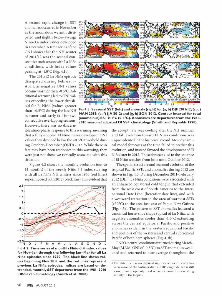
S80 | AUGUST 2013
A second rapid change in SST anomalies occurred in November as the anomalous warmth dissi-pated, and slightly below-average Niño-3.4 index values developed in December. A time series of the ONI shows that the NH winter of 2011/12 was the second con-secutive such season with La Niña conditions, with index values peaking at -1.0°C (Fig. 4.1b).
The 2011/12 La Niña episode dissipated during February–April, as negative ONI values became warmer than -0.5°C. Ad-ditional warming led to ONI val-ues exceeding the lower thresh-old for El Niño (values greater than +0.5°C) during the late NH summer and early fall for two consecutive overlapping seasons. However, there was no discern-ible atmospheric response to this warming, meaning that a fully-coupled El Niño never developed. ONI values then dropped below the +0.5°C threshold dur-ing October–December (OND) 2012. While there in fact may have been responses to this warming, they were just not those we typically associate with this situation.
Figure 4.2 shows the monthly evolution (out to 14 months) of the weekly Niño-3.4 index starting with all La Niña NH winters since 1950 (red lines) superimposed with 2012 (black line). It is evident that
the abrupt, late year cooling after the NH summer and fall evolution toward El Niño conditions was unprecedented in the historical record. Most dynami-cal model forecasts at the time failed to predict this evolution, and instead favored the development of El Niño later in 2012. Those forecasts led to the issuance of El Niño watches from June until October 2012.
The spatial structure and seasonal evolution of the tropical Pacific SSTs and anomalies during 2012 are shown in Fig. 4.3. During December 2011–February 2012 (DJF), La Niña conditions were associated with an enhanced equatorial cold tongue that extended from the west coast of South America to the Inter-national Date Line2 (hereafter date line), and with a westward retraction in the area of warmest SSTs (>30°C) to the area just east of Papua New Guinea (Fig. 4.3a). The pattern of SST anomalies featured a canonical horse-shoe shape typical of La Niña, with negative anomalies cooler than -1.0°C extending across the central equatorial Pacific and positive anomalies evident in the western equatorial Pacific and portions of the western and central subtropical Pacific of both hemispheres (Fig. 4.3b).
ENSO-neutral conditions returned during March–May (MAM; ONI of -0.3°C) as SST anomalies weak-ened and returned to near average throughout the
2 The date line has no physical significance as it merely tra-verses around the Antimeridian at 180° longitude, but is still a useful and popularly used reference point for describing activity in the tropics.
Fig 4.2. Time series of monthly Niño-3.4 index values for Nov–Jan through the following Jan–Mar for all La Niña episodes since 1950. The black line shows val-ues beginning Nov 2011 and the red lines represent previous La Niña episodes. Indices are based on de-trended, monthly SST departures from the 1981–2010 ERSSTv3b climatology (Smith et al. 2008).
Fig 4.3. Seasonal SST (left) and anomaly (right) for (a, b) DJF 2011/12; (c, d) MAM 2012; (e, f) JJA 2012; and (g, h) SON 2012. Contour interval for total (anomalous) SST is 1°C (0.5°C). Anomalies are departures from the 1981–2010 seasonal adjusted OI SST climatology (Smith and Reynolds 1998).

S81STATE OF THE CLIMATE IN 2012 |AUGUST 2013
tropical Pacific (Figs. 4.3c,d). Additional warming during June–August (JJA) led to above-average SSTs across the east-central and eastern equatorial Pacific, with departures exceeding +1.0°C in some locations (Figs. 4.3e,f). However, below-average SSTs persisted in the off-equatorial central and eastern North Pa-cific. For the September–November (SON) season, the positive SST anomalies in the eastern half of the equa-torial Pacific weakened as the equatorial cold tongue returned to near-average strength (Fig. 4.3g), and only small regions with departures exceeding +0.5°C were evident for the season as a whole (Fig. 4.3h).
Consistent with this evolution, the subsurface temperature structure (from 50 m to 450 m) varied considerably during the year, reflecting La Niña early in the year, trending toward El Niño during the NH summer, and returning to near average during the
NH fall (Fig. 4.4). In DJF, temperatures were 2°C–4°C below average from the surface to 150 m depth east of 160°W, and above average (anomalies exceeding +3°C) in the western Pacific between 100 m and 200 m depth (Fig. 4.4a). This overall anomaly pattern is typi-cal of La Niña, and reflected a shallower (deeper) than average thermocline in the eastern (western) Pacific.
During MAM, subsurface temperatures returned to near average across the eastern half of the equato-rial Pacific and the area of above-average tempera-tures largely persisted in the western half of the basin (Fig. 4.4b). This evolution reflects the transition to ENSO-neutral conditions and occurred partly in as-sociation with the downwelling phase of an equatorial oceanic Kelvin wave (see Fig. 4.8). The JJA season featured above-average subsurface temperatures in the eastern half of the Pacific, as the oceanic thermo-cline deepened in association with increasingly warm SST anomalies. However, these anomalies failed to further intensify during SON, as would be expected if El Niño were to develop, and instead subsurface temperatures returned to near average across the entire Pacific (Fig. 4.4d).
2) atmOspheric circulatiOn: trOpics
During DJF, La Niña featured a strong coupling between the ocean and the overlying atmospheric circulation. For example, convection was strongly suppressed over the central equatorial Pacific and enhanced over Indonesia (Figs. 4.5a, 4.6a). Enhanced lower level (850-hPa) easterly winds and enhanced upper level (200-hPa) westerly winds across the central Pacific reflects an increased strength of the equatorial Walker circulation, as is characteristic of La Niña. The upper-level wind pattern also featured an anomalous cyclonic couplet centered in the sub-tropics of both hemispheres flanking the region of suppressed convection, which is consistent with a suppressed Hadley circulation over the central Pacific and is also typical of La Niña.
Although equatorial Pacific Ocean temperatures returned to near average during MAM, many aspects of the tropical atmospheric circulation retained their La Niña characteristics, but with lesser intensity. For example, convection in the central tropical Pa-cific remained suppressed just north of the equator, while convection over the Maritime continent was enhanced (Figs. 4.5b, 4.6b). In addition, the enhanced lower-level easterlies (Fig. 4.5b) and upper-level west-erlies (Fig. 4.6b) persisted across the central tropical Pacific, but with reduced strength.
Fig. 4.4. Equatorial depth-longitude section of ocean temperature anomalies (°C) averaged between 5°N and 5°S during (a) DJF 2011/12, (b) MAM 2012, (c) JJA 2012, and (d) SON 2012. The 20°C isotherm (thick solid line) approximates the center of the oceanic thermocline. The data are derived from an analysis system that assimilates oceanic observations into an oceanic GCM (Behringer et al. 1998). Anomalies are departures from the 1981–2010 monthly means.

S82 | AUGUST 2013
Atmospheric conditions even retained some weak La Niña characteristics during JJA, despite the ap-parent SST evolution toward El Niño (Figs. 4.1, 4.3e). These conditions included slightly enhanced convec-tion over the far western Pacific and suppressed con-vection over the central Pacific north of the equator (Figs. 4.5c, 4.6c). They also included a continuation of the tropical wind anomalies noted previously (Figs. 4.5c, 4.6c). These conditions finally dissipated during SON (Figs. 4.5d, 4.6d).
In the extratropics, the circulation during DJF over the NH was not particularly consistent with La Niña, but rather with the positive phase of the Arctic Oscillation (AO), with below-average heights at high latitudes and above-average height in the midlatitudes (Fig. Appendix 1.2). However, the circulation over the Southern Hemisphere (SH) during austral summer strongly reflects the positive phase of the Antarctic Oscillation (AAO), with below-average heights over the polar region and above-average heights in the
midlatitudes (Fig. Appendix 1.2). The positive phase of the AAO is known to be consistent with La Niña (L’Heureux and Thompson 2006).
During MAM, the 500-hPa circulation over the Pacific-North American (PNA) sector featured above-average heights over the central Pacific, below-average heights in the Gulf of Alaska, and above-average heights in the central and eastern United States (Fig Appendix 1.4). This pattern reflects the negative phase of the PNA teleconnection pattern, and is often observed in association with La Niña.
3) temperature and precipitatiOn impacts
During DJF, the precipitation patterns typically associated with La Niña (Ropelewski and Halpert 1989; http://www.cpc.ncep.noaa.gov/products/precip/CWlink/ENSO/regressions) were observed over many parts of the world. These included below-average precipitation over the equatorial western and cen-tral Pacific Ocean, much of the southern tier of the
Fig. 4.6. Anomalous 200-hPa wind vector and speed (contours, m s-1) and anomalous OLR (shaded, W m-2) during (a) DJF 2011/12, (b) MAM 2012, (c) JJA 2012, and (d) SON 2012. Anomalies are departures from the 1981–2010 monthly means.
Fig. 4.5. Anomalous 850-hPa wind vector and speed (contours, m s-1) and anomalous OLR (shaded, W m-2) during (a) DJF 2011/12, (b) MAM 2012, (c) JJA 2012, and (d) SON 2012. Anomalies are departures from the 1981–2010 monthly means.
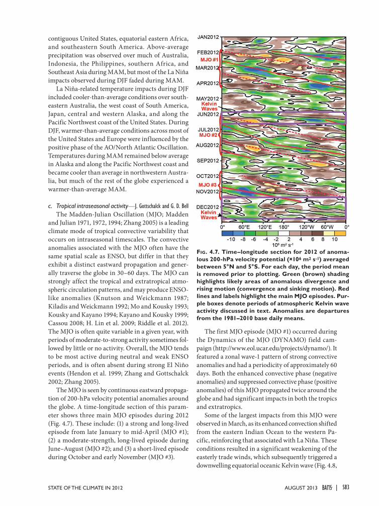
S83STATE OF THE CLIMATE IN 2012 |AUGUST 2013
contiguous United States, equatorial eastern Africa, and southeastern South America. Above-average precipitation was observed over much of Australia, Indonesia, the Philippines, southern Africa, and Southeast Asia during MAM, but most of the La Niña impacts observed during DJF faded during MAM.
La Niña-related temperature impacts during DJF included cooler-than-average conditions over south-eastern Australia, the west coast of South America, Japan, central and western Alaska, and along the Pacific Northwest coast of the United States. During DJF, warmer-than-average conditions across most of the United States and Europe were influenced by the positive phase of the AO/North Atlantic Oscillation. Temperatures during MAM remained below average in Alaska and along the Pacific Northwest coast and became cooler than average in northwestern Austra-lia, but much of the rest of the globe experienced a warmer-than-average MAM.
c. Tropical intraseasonal activity—J. Gottschalck and G. D. BellThe Madden-Julian Oscillation (MJO; Madden
and Julian 1971, 1972, 1994; Zhang 2005) is a leading climate mode of tropical convective variability that occurs on intraseasonal timescales. The convective anomalies associated with the MJO often have the same spatial scale as ENSO, but differ in that they exhibit a distinct eastward propagation and gener-ally traverse the globe in 30–60 days. The MJO can strongly affect the tropical and extratropical atmo-spheric circulation patterns, and may produce ENSO-like anomalies (Knutson and Weickmann 1987; Kiladis and Weickmann 1992; Mo and Kousky 1993; Kousky and Kayano 1994; Kayano and Kousky 1999; Cassou 2008; H. Lin et al. 2009; Riddle et al. 2012). The MJO is often quite variable in a given year, with periods of moderate-to-strong activity sometimes fol-lowed by little or no activity. Overall, the MJO tends to be most active during neutral and weak ENSO periods, and is often absent during strong El Niño events (Hendon et al. 1999; Zhang and Gottschalck 2002; Zhang 2005).
The MJO is seen by continuous eastward propaga-tion of 200-hPa velocity potential anomalies around the globe. A time-longitude section of this param-eter shows three main MJO episodes during 2012 (Fig. 4.7). These include: (1) a strong and long-lived episode from late January to mid-April (MJO #1); (2) a moderate-strength, long-lived episode during June–August (MJO #2); and (3) a short-lived episode during October and early November (MJO #3).
The first MJO episode (MJO #1) occurred during the Dynamics of the MJO (DYNAMO) field cam-paign (http://www.eol.ucar.edu/projects/dynamo/). It featured a zonal wave-1 pattern of strong convective anomalies and had a periodicity of approximately 60 days. Both the enhanced convective phase (negative anomalies) and suppressed convective phase (positive anomalies) of this MJO propagated twice around the globe and had significant impacts in both the tropics and extratropics.
Some of the largest impacts from this MJO were observed in March, as its enhanced convection shifted from the eastern Indian Ocean to the western Pa-cific, reinforcing that associated with La Niña. These conditions resulted in a significant weakening of the easterly trade winds, which subsequently triggered a downwelling equatorial oceanic Kelvin wave (Fig. 4.8,
Fig. 4.7. Time–longitude section for 2012 of anoma-lous 200-hPa velocity potential (×106 m2 s-1) averaged between 5°N and 5°S. For each day, the period mean is removed prior to plotting. Green (brown) shading highlights likely areas of anomalous divergence and rising motion (convergence and sinking motion). Red lines and labels highlight the main MJO episodes. Pur-ple boxes denote periods of atmospheric Kelvin wave activity discussed in text. Anomalies are departures from the 1981–2010 base daily means.
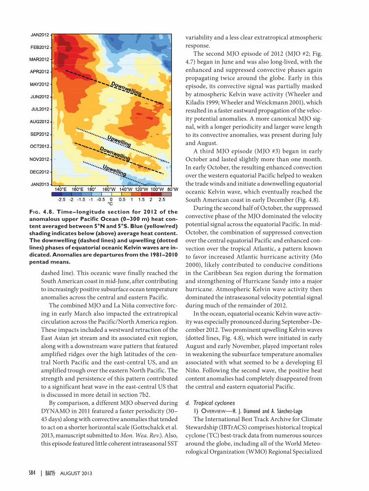
S84 | AUGUST 2013
dashed line). This oceanic wave finally reached the South American coast in mid-June, after contributing to increasingly positive subsurface ocean temperature anomalies across the central and eastern Pacific.
The combined MJO and La Niña convective forc-ing in early March also impacted the extratropical circulation across the Pacific/North America region. These impacts included a westward retraction of the East Asian jet stream and its associated exit region, along with a downstream wave pattern that featured amplified ridges over the high latitudes of the cen-tral North Pacific and the east-central US, and an amplified trough over the eastern North Pacific. The strength and persistence of this pattern contributed to a significant heat wave in the east-central US that is discussed in more detail in section 7b2.
By comparison, a different MJO observed during DYNAMO in 2011 featured a faster periodicity (30–45 days) along with convective anomalies that tended to act on a shorter horizontal scale (Gottschalck et al. 2013, manuscript submitted to Mon. Wea. Rev.). Also, this episode featured little coherent intraseasonal SST
variability and a less clear extratropical atmospheric response.
The second MJO episode of 2012 (MJO #2; Fig. 4.7) began in June and was also long-lived, with the enhanced and suppressed convective phases again propagating twice around the globe. Early in this episode, its convective signal was partially masked by atmospheric Kelvin wave activity (Wheeler and Kiladis 1999; Wheeler and Weickmann 2001), which resulted in a faster eastward propagation of the veloc-ity potential anomalies. A more canonical MJO sig-nal, with a longer periodicity and larger wave length to its convective anomalies, was present during July and August.
A third MJO episode (MJO #3) began in early October and lasted slightly more than one month. In early October, the resulting enhanced convection over the western equatorial Pacific helped to weaken the trade winds and initiate a downwelling equatorial oceanic Kelvin wave, which eventually reached the South American coast in early December (Fig. 4.8).
During the second half of October, the suppressed convective phase of the MJO dominated the velocity potential signal across the equatorial Pacific. In mid-October, the combination of suppressed convection over the central equatorial Pacific and enhanced con-vection over the tropical Atlantic, a pattern known to favor increased Atlantic hurricane activity (Mo 2000), likely contributed to conducive conditions in the Caribbean Sea region during the formation and strengthening of Hurricane Sandy into a major hurricane. Atmospheric Kelvin wave activity then dominated the intraseasonal velocity potential signal during much of the remainder of 2012.
In the ocean, equatorial oceanic Kelvin wave activ-ity was especially pronounced during September–De-cember 2012. Two prominent upwelling Kelvin waves (dotted lines, Fig. 4.8), which were initiated in early August and early November, played important roles in weakening the subsurface temperature anomalies associated with what seemed to be a developing El Niño. Following the second wave, the positive heat content anomalies had completely disappeared from the central and eastern equatorial Pacific.
d. Tropical cyclones1) Overview—H. J. Diamond and A. Sánchez-LugoThe International Best Track Archive for Climate
Stewardship (IBTrACS) comprises historical tropical cyclone (TC) best-track data from numerous sources around the globe, including all of the World Meteo-rological Organization (WMO) Regional Specialized
Fig. 4.8. Time–longitude section for 2012 of the anomalous upper Pacific Ocean (0–300 m) heat con-tent averaged between 5°N and 5°S. Blue (yellow/red) shading indicates below (above) average heat content. The downwelling (dashed lines) and upwelling (dotted lines) phases of equatorial oceanic Kelvin waves are in-dicated. Anomalies are departures from the 1981–2010 pentad means.
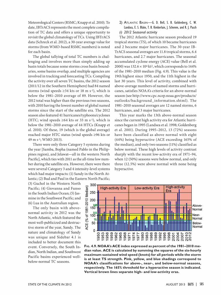
S85STATE OF THE CLIMATE IN 2012 |AUGUST 2013
Meteorological Centers (RSMC; Knapp et al. 2010). To date, IBTrACS represents the most complete compila-tion of TC data and offers a unique opportunity to revisit the global climatology of TCs. Using IBTrACS data (Schreck et al. 2012), a 30-year average value for storms (from WMO-based RSMC numbers) is noted for each basin.
The global tallying of total TC numbers is chal-lenging and involves more than simply adding up basin totals because some storms cross basin bound-aries, some basins overlap, and multiple agencies are involved in tracking and forecasting TCs. Compiling the activity over all seven TC basins, the 2012 season (2011/12 in the Southern Hemisphere) had 84 named storms (wind speeds ≥34 kts or 18 m s-1), which is below the 1981–2010 average of 89. However, the 2012 total was higher than the previous two seasons, with 2010 having the lowest number of global named storms since the start of the satellite era. The 2012 season also featured 41 hurricanes/typhoons/cyclones (HTC; wind speeds ≥64 kts or 33 m s-1), which is below the 1981–2010 average of 44 HTCs (Knapp et al. 2010). Of these, 19 (which is the global average) reached major HTC status (wind speeds ≥96 kts or 49 m s-1; WMO 2013).
There were only three Category 5 systems during the year [Samba, Bopha (named Pablo in the Philip-pines region), and Jelawat—all in the western North Pacific], which ties with 2011 as the all-time low num-ber during the satellite era. However, there were there were several Category 3 and 4 intensity-level systems which had major impacts: (1) Sandy in the North At-lantic; (2) Bud and Paul in the Eastern North Pacific; (3) Guchol in the Western North Pacific; (4) Giovanna and Funso in the South Indian Ocean; (5) Jas-mine in the Southwest Pacific; and (6) Lua in the Australian region.
The only basin with above-normal activity in 2012 was the North Atlantic, which featured the most well-publicized and destruc-tive storm of the year, Sandy. The nature and climatology of Sandy was unique and Sidebar 4.1 is included to better document this event. Conversely, the South In-dian, North Indian, and Southwest Pacific basins experienced well-below-normal TC seasons.
2) atlantic Basin—G. D. Bell, S. B. Goldenberg, C. W. Landsea, E. S. Blake, T. B. Kimberlain, J. Schemm, and R. J. Pasch
(i) 2012 Seasonal activity The 2012 Atlantic hurricane season produced 19
tropical storms (TS), of which 10 became hurricanes and 2 became major hurricanes. The 30-year IB-TrACS seasonal averages are 11.8 tropical storms, 6.4 hurricanes, and 2.7 major hurricanes. The seasonal accumulated cyclone energy (ACE) value (Bell et al. 2000) was 132.6 × 10⁴ kt2, which corresponds to 144% of the 1981–2010 median (Fig. 4.9). This value is the 19th highest since 1950, and the 11th highest in the last 30 years. This level of activity, combined with above-average numbers of named storms and hurri-canes, satisfies NOAA’s criteria for an above-normal season (see http://www.cpc.ncep.noaa.gov/products/outlooks/background_information.shtml). The 1981–2010 seasonal averages are 12 named storms, 6 hurricanes, and 3 major hurricanes.
This year marks the 13th above-normal season since the current high activity era for Atlantic hurri-canes began in 1995 (Landsea et al. 1998; Goldenberg et al. 2001). During 1995–2012, 13 (72%) seasons have been classified as above normal with eight (44%) being hyperactive (ACE exceeding 165% of the median), and only two seasons (11%) classified as below normal. These high levels of activity contrast sharply with the recent low-activity era of 1971–94, when 12 (50%) seasons were below normal, and only three (12.5%) were above normal with none being hyperactive.
Fig. 4.9. NOAA’s ACE index expressed as percent of the 1981–2010 me-dian value. ACE is calculated by summing the squares of the six-hourly maximum sustained wind speed (knots) for all periods while the storm is at least TS strength. Pink, yellow, and blue shadings correspond to NOAA’s classifications for above-, near-, and below-normal seasons, respectively. The 165% threshold for a hyperactive season is indicated. Vertical brown lines separate high- and low-activity eras.

S86 | AUGUST 2013
(ii) Storm tracksAugust–October (ASO) is typically the peak
period of the season, and all but four named storms (including one hurricane) during 2012 formed in ASO. During above-normal seasons, much of the ASO activity is linked to storms that first develop in the main development region (MDR, green boxed region in Fig. 4.10, which encompasses the tropical Atlantic Ocean and Caribbean Sea between 9.5°N and 21.5°N; Goldenberg et al. 2001).
During ASO 2012, nine tropical storms formed within the MDR (Fig. 4.10, brown lines), with six becoming hurricanes and one becoming a major hurricane (Sandy; http://www.nhc.noaa.gov/data/tcr/AL182012_Sandy.pdf). These storms accounted for 67% of the seasonal ACE value. Three of these hur-ricanes made landfall at hurricane strength, including Ernesto (Yucatan Peninsula), Isaac (Louisiana), and Sandy (Jamaica, Cuba as a major hurricane, and New Jersey3). This high level of MDR activity was related in part to weak vertical wind shear (Fig. 4.10, green shading) and above-average SSTs (Fig. 4.11a) across much of that region. These conditions are consistent with the ongoing high-activity era for Atlantic hur-ricanes (Goldenberg et al. 2001; Bell and Chelliah 2006; Bell et al. 2011, 2012).
3 When Sandy made landfall near Brigantine, NJ, it was a post-tropical cyclone.
Also during 2012, two named storms formed over the Gulf of Mexico. Debby made landfall in Florida as a tropical storm and Helene made landfall in Mexico as a tropical depression. (Helene actually first developed in the MDR over the central Atlantic, dis-sipated, and then reformed over the Gulf of Mexico.) Eight named storms (four tropical storms and four hurricanes, with one becoming Major Hurricane Michael) formed north of the MDR over the open North Atlantic, and remained at sea throughout their life cycle. Michael was only the fifth major hurricane in the satellite era to develop from a disturbance of non-tropical origin (http://www.nhc.noaa.gov/data/tcr/AL132012_Michael.pdf).
Sandy became a Category 3 storm with maxi-mum sustained winds of 100 kt (51 m s-1) as it made landfall in eastern Cuba before quickly weakening to a Category 1 hurricane while moving through the central and northwestern Bahamas, only to reach a secondary peak intensity with maximum sustained winds of 85 kt (44 m s-1) while it turned northwest-ward toward the mid-Atlantic region of the United States. On average, three to four named storms form in the southwestern Caribbean region per season, and roughly two become hurricanes.
The increased 2012 activity north of the MDR re-flected a strong mid- and upper-level ridge across the subtropical North Atlantic, along with an extensive region of weak vertical wind shear (Fig. 4.10). These conditions were part of a larger-scale anomalous wave pattern that featured amplified troughs over the eastern US and the eastern North Atlantic. A similar eastern US trough, along with its associated strong southwesterly steering flow over the western North Atlantic, was also evident during ASO 2010 and ASO 2011 (Bell et al. 2011, 2012). In all three years, these conditions contributed to a large number of named storms that stayed well east of North America (Blake et al. 2011).
(iii) Atlantic sea surface temperaturesSea surface temperatures in the MDR were above
average during ASO 2012, with the largest departures (between +0.5°C and +1.0°C) observed across the north-central and northeastern MDR (Fig. 4.11a). The mean SST departure within the MDR was +0.41°C (Fig. 4.11b), which is 0.40°C warmer than the average departure for the entire global tropics (Fig. 4.11c).
This anomalous warmth compared to the remain-der of the global tropics has been present since 1995 in association with the warm phase of the Atlantic multidecadal oscillation (AMO; Enfield and Mestas-
Fig 4.10. Aug–Oct 2012 500-hPa heights (contours, m) and anomalies (shading), mean wind vectors (m s-1) for the 600 hPa–300 hPa layer, and regions where the magnitude of vertical wind shear is less than 8 m s-1 (light green shading). Atlantic named storm tracks that formed after 1 Aug are shown in brown, beginning with tropical depression strength. Tracks for storms that formed during May–Jul are shown in yellow. Green box denotes the MDR. Vector scale is below right of color bar. Anomalies are with respect to the 1981–2010 monthly means.

S87STATE OF THE CLIMATE IN 2012 |AUGUST 2013
Nuñez 1999; Goldenberg et al. 2001; Vecchi et al. 2008; Bell et al. 2011, 2012). A similar signal was ob-served during the previous warm AMO phase of the 1950s and 1960s. Conversely, the MDR was generally cooler than the global tropics during the cold AMO phase (and reduced Atlantic hurricane activity) of the 1970s through the early 1990s.
(iv) Atmospheric circulationThe sharp transition in 1995 to the current high
activity era reflects a phase change in the AMO and in the corresponding tropical multidecadal signal (Goldenberg et al. 2001; Bell and Chelliah 2006; Bell et al. 2007). This signal links atmospheric variability across the central and eastern MDR to multidecadal fluctuations in the AMO and the strength of the West African monsoon.
Consistent with this ongoing multidecadal signal, the atmospheric circulation during ASO 2012 again featured an interrelated set of conditions known to be exceptionally conducive for tropical cyclone forma-tion and intensification within the MDR (Landsea et al. 1998; Goldenberg and Shapiro 1996; Goldenberg et al. 2001; Bell and Chelliah 2006; Kossin and Vimont 2007; Bell et al. 2012). Similar ASO conditions have been present throughout the period 1995–2011, and a yearly archive of these conditions is shown in previ-ous State of the Climate reports.
In the lower atmosphere, the MDR conditions conducive for cyclogenesis during ASO included weaker trade winds, a deep layer of anomalous cross-equatorial flow, and below-average heights/sea level pressure (Fig. 4.12a). Across the tropical Atlantic and sub-Saharan Africa, the low-level westerly anomalies extended above 700-hPa, the approximate level of the African easterly jet (AEJ; Fig. 4.12b), and were associ-ated with an anomalous northward shift of the AEJ core (thick black arrow).
As a result, the bulk of the African easterly wave energy (Reed et al. 1977) during ASO was often cen-tered well within the MDR. The AEJ also featured increased cyclonic shear along its equatorward flank (red shading), which dynamically favors stronger easterly waves. These conditions have generally prevailed since 1995 and are opposite to those seen during the low activity era of 1971–94 (Figs. 4.12c,d).
Also during ASO 2012, enhanced upper-level ridges spanned the subtropical Atlantic and Africa in both hemispheres (Fig. 4.13a). This interhemispheric symmetry is consistent with an enhanced West Afri-can monsoon system (Fig. 4.13b), both of which are prominent features of the current high activity era.
In addition to weaker trade winds, these condi-tions contributed to anomalous upper-level easterly flow across the MDR. The result was weak vertical wind shear (less than 8 m s-1) across the southern MDR (Fig. 4.10), with the most anomalously weak shear located over the central tropical Atlantic and eastern Caribbean Sea (Fig. 4.14a). These conditions were part of a larger-scale pattern that included increased shear over both the eastern equatorial Atlantic and the eastern tropical North Pacific (blue shading), which is also typical of other above-normal seasons since 1995 (Bell and Chelliah 2006; Bell et al. 2011).
The question then arises as to why there was so little major hurricane activity in 2012. Only two six-hourly periods were observed with storms at major hurricane strength this year, which corresponds to
Fig 4.11. (a) Aug–Oct (ASO) 2012 SST anomalies (°C). (b) Time series during 1950–2012 of ASO area-averaged SST anomalies in the MDR [green box in (a)]. (c) Time series showing the difference between ASO area-averaged SST anomalies in the MDR and those for the entire global tropics (30°N–30°S). Anomalies are departures from the ERSST-v3b (Smith et al. 2008) 1981–2010 monthly means.

S88 | AUGUST 2013
one-half of a major hurricane day4. This value is the lowest since 1995, and is even lower than for 79% of the years during the recent low-activity era (1971–94). Some reasons for this low major hurricane activi-ties are evident. First, many storms remained over the central North Atlantic in an area of relatively cool SSTs throughout their life. Second, of the five named storms that moved over the Caribbean Sea, two became hurricanes (Ernesto and Sandy) and both of these made landfall shortly thereafter.
This minimal hurricane and major hurricane activity over the Caribbean Sea was partly related to exceptionally dry air during July–October, which can be linked to anomalous northerly low-level winds (Fig. 4.15a). This ob-servation is consistent with the strong
historical relationship between these parameters (Fig. 4.15b). Conditions over the Caribbean Sea were es-pecially non-conducive to major hurricane formation during September, in response to a nearly complete disappearance of the normal ascending motion (Fig. 4.15c, negative values) that led to record anomalies of descending motion throughout the lower and mid-troposphere (not shown; see also Klotzbach and Gray 2012). A time-longitude section of velocity potential (Fig. 4.7) shows that this anomalous sinking mo-tion was related to a quasi-stationary intraseasonal f luctuation characterized by anomalous ascending motion near the date line and anomalous descend-ing motion across the central tropical Atlantic and Caribbean Sea.
The full analysis indicates that all of the key in-terrelated features of the active Atlantic phase of the tropical multidecadal signal were again present dur-ing 2012 (Figs. 4.11–4.14). Therefore, there was neither an apparent weakening of the conditions conducive for cyclogenesis that have prevailed since 1995, nor is there any evidence to suggest that the current high-activity era for Atlantic hurricane activity might be ending soon.
4 The measure "major hurricane days", also known as "intense hurricane days" (Gray et al. 1993), is the sum of all of the six-hourly periods that storms were at major hurricane status, with each period counting as 0.25 major hurricane days.
Fig 4.12. (Left) Aug–Oct 2012 anomalies of (a) 1000-hPa heights (shad-ing, m) and wind vectors (m s-1), and (b) 700-hPa relative vorticity (shading, ×10-6 s-1) and wind vectors, with thick black arrow showing the axis of the AEJ. Vector scales are below right of color bars. Green boxes denote the MDR. Anomalies are with respect to the 1981–2010 monthly means. (Right) Historical time series showing yearly ASO values of area-averaged (c) 700-hPa zonal wind (m s-1) and (d) 700-Pa relative vorticity (×10-6 s-1). Blue curve shows unsmoothed values and red curve shows a five-point running mean. Averaging regions are shown in the insets.
Fig 4.13. Aug–Oct 2012 200-hPa circulation and anoma-lies: (a) streamfunction (contours, interval is 10 × 106
m2 s-1) and anomalies (shaded) and (b) anomalous velocity potential (shading, ×106 m2 s-1) and divergent wind vectors (m s-1). In (a) anomalous ridges are indi-cated by positive values (orange/red) in the NH and negative values (blue) in the SH. Anomalous troughs are indicated by negative values in the NH and positive values in the SH. In (b) vector scale is below right of color bar. Green boxes denote the MDR. All departures are with respect to the 1981–2010 monthly means.
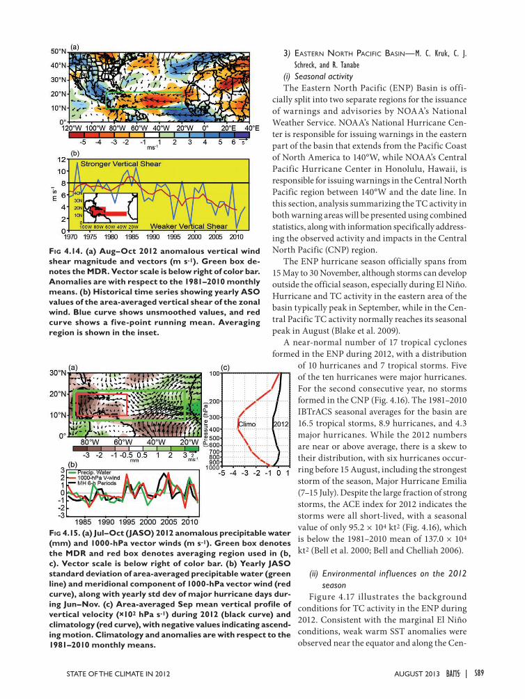
S89STATE OF THE CLIMATE IN 2012 |AUGUST 2013
3) eastern nOrth pacific Basin—M. C. Kruk, C. J. Schreck, and R. Tanabe
(i) Seasonal activityThe Eastern North Pacific (ENP) Basin is offi-
cially split into two separate regions for the issuance of warnings and advisories by NOAA’s National Weather Service. NOAA’s National Hurricane Cen-ter is responsible for issuing warnings in the eastern part of the basin that extends from the Pacific Coast of North America to 140°W, while NOAA’s Central Pacific Hurricane Center in Honolulu, Hawaii, is responsible for issuing warnings in the Central North Pacific region between 140°W and the date line. In this section, analysis summarizing the TC activity in both warning areas will be presented using combined statistics, along with information specifically address-ing the observed activity and impacts in the Central North Pacific (CNP) region.
The ENP hurricane season officially spans from 15 May to 30 November, although storms can develop outside the official season, especially during El Niño. Hurricane and TC activity in the eastern area of the basin typically peak in September, while in the Cen-tral Pacific TC activity normally reaches its seasonal peak in August (Blake et al. 2009).
A near-normal number of 17 tropical cyclones formed in the ENP during 2012, with a distribution
of 10 hurricanes and 7 tropical storms. Five of the ten hurricanes were major hurricanes. For the second consecutive year, no storms formed in the CNP (Fig. 4.16). The 1981–2010 IBTrACS seasonal averages for the basin are 16.5 tropical storms, 8.9 hurricanes, and 4.3 major hurricanes. While the 2012 numbers are near or above average, there is a skew to their distribution, with six hurricanes occur-ring before 15 August, including the strongest storm of the season, Major Hurricane Emilia (7–15 July). Despite the large fraction of strong storms, the ACE index for 2012 indicates the storms were all short-lived, with a seasonal value of only 95.2 × 10⁴ kt2 (Fig. 4.16), which is below the 1981–2010 mean of 137.0 × 10⁴ kt2 (Bell et al. 2000; Bell and Chelliah 2006).
(ii) Environmental inf luences on the 2012 season
Figure 4.17 illustrates the background conditions for TC activity in the ENP during 2012. Consistent with the marginal El Niño conditions, weak warm SST anomalies were observed near the equator and along the Cen-
Fig 4.14. (a) Aug–Oct 2012 anomalous vertical wind shear magnitude and vectors (m s-1). Green box de-notes the MDR. Vector scale is below right of color bar. Anomalies are with respect to the 1981–2010 monthly means. (b) Historical time series showing yearly ASO values of the area-averaged vertical shear of the zonal wind. Blue curve shows unsmoothed values, and red curve shows a five-point running mean. Averaging region is shown in the inset.
Fig 4.15. (a) Jul–Oct (JASO) 2012 anomalous precipitable water (mm) and 1000-hPa vector winds (m s-1). Green box denotes the MDR and red box denotes averaging region used in (b, c). Vector scale is below right of color bar. (b) Yearly JASO standard deviation of area-averaged precipitable water (green line) and meridional component of 1000-hPa vector wind (red curve), along with yearly std dev of major hurricane days dur-ing Jun–Nov. (c) Area-averaged Sep mean vertical profile of vertical velocity (×102 hPa s-1) during 2012 (black curve) and climatology (red curve), with negative values indicating ascend-ing motion. Climatology and anomalies are with respect to the 1981–2010 monthly means.

S90 | AUGUST 2013
tral American coast (Fig. 4.17a). Cold anomalies oc-curred to the north and west. Most of the TCs formed over areas where the SSTs were near to slightly above normal. Convection was somewhat enhanced over the eastern part of the basin where the storms developed (Fig. 4.17b). Meanwhile the ITCZ was suppressed over the CNP, which also experienced larger-than-normal vertical wind shear (Fig. 4.17c). The combination of cooler SSTs, suppressed convection, and enhanced shear likely led to the lack of TCs in the CNP this year.
Figure 4.17d shows a broad area of 850-hPa west-erly anomalies near the equator, with easterly anoma-lies to the north. This combination produced the region of enhanced cyclonic vorticity within which most of ENP storms developed. Many of these storms developed where the enhanced vorticity intersected the westerly anomalies. The westerlies could have strengthened easterly wave activity in this region through barotropic energy conversion and wave ac-cumulation (Maloney and Hartmann 2001; Aiyyer and Molinari 2008).
Eastern North Pacific TC activity was strongly influenced by the MJO during the 2012 season (Ma-loney and Hartmann 2001; Aiyyer and Molinari 2008; Slade and Maloney 2013), and recent studies have also found a greater role for convectively coupled Kelvin waves in modulating tropical cyclogenesis (Schreck and Molinari 2011; Ventrice et al. 2012a,b). Figure 4.18
Fig. 4.16. Seasonal TC statistics for the ENP basin for 1970–2012: (top) number of named storms, hurricanes, and major hurricanes, and (bottom) the ACE index with the seasonal total of 2012 highlighted in red. The time series shown includes the corresponding 1981–2010 means for each parameter.
Fig. 4.17. Maps of May–Nov 2012 anomalies of (a) SST (°C), (b) OLR (W m-2), (c) 850–200-hPa vertical wind shear vector (arrows) and scalar (shading, m s-1) anomalies, and (d) 850-hPa winds (arrows) and zonal wind (shading, m s-1) anomalies. Anomalies are relative to the annual cycle from 1981–2010, except for SST which is relative to 1982–2010 due to data availability. Hurricane symbols denote where each TC attained tropical storm strength. (Wind data are obtained from the NCEP–DOE Reanalysis 2.)

S91STATE OF THE CLIMATE IN 2012 |AUGUST 2013
employs outgoing longwave radiation (OLR) data to examine the evolution of convection during the 2012 ENP hurricane season. Following Kiladis et al. (2005, 2009), the black contours identify the MJO-filtered anomalies, while the green contours are filtered for Kelvin waves. Easterly waves are also apparent in the unfiltered anomalies (shading) as westward moving features, such as those leading up to Tropical Storms Hector and John.
The MJO is thought to have played a role in the formation of Hurricane Gilma and Tropical Storm Hector during August and for both Tropical Storm Olivia and Major Hurricane Paul in October. The MJO often transitions to a Kelvin-like structure as it traverses the Pacific (Straub et al. 2006; Sobel and Kim 2012). Such a transition could explain the Kel-vin wave that coincided with Tropical Storm Olivia’s genesis. In contrast, Hurricane Lane developed in association with a Kelvin wave that did not stem from the larger MJO envelope.
(iii) TC impacts During the 2012 season, 5 of the 17 tropical storms
had direct impacts on the western coast of Mexico and Baja Peninsula. The first was Major Hurricane Bud
(21–26 May), which had maximum sustained winds of 100 kt (51 m s-1) and a minimum central pressure of 960 hPa. Bud impacted western Mexico as a strong Saffir-Simpson Category 2 hurricane, but impacts were rather minimal.
Nearly a month later, from 14 to 17 June, Hur-ricane Carlotta developed and was the easternmost storm in the basin this season, with maximum sus-tained winds at peak intensity near 90 kt (46 m s-1) and a mean central pressure of 973 hPa. The satellite representation of Carlotta (not shown) indicated a classic hurricane with a clearly visible eye on 15 June. By late in the day on the 15th, Carlotta made landfall near Puerto Escondido, Oaxaca. The storm resulted in approximately seven fatalities (see http://www.thejakartapost.com/news/2012/06/16/hurricane-carlotta-makes-landfall-mexico.html). The hurricane also caused widespread power outages, roof collapses, and small landslides. In San Juan Bautista, Tuxtepec, over 350 mm of rain fell from Carlotta.
The next storm to impact the western Mexican coastline was Hurricane Fabio (12–18 July), which had peak winds of 90 kt (46 m s-1) and a mean central pressure of 966 hPa. Fabio developed rapidly, growing from a tropical depression to a Category 1 hurricane in just 24 hours. As quickly as the storm intensified, it weakened as it began to ingest dry air and eventually lost its hurricane characteristics as it drifted over the Baja Peninsula; few, if any, impacts were reported.
The 14th named storm of the season, Tropical Storm Norman, lasted from 28 to 29 September and although it never intensified above tropical storm status, it brought stormy weather to Cabo San Lucas and record rainfall to Texas. Extremely heavy rainfall was the primary impact from Norman, with precipi-tation ranging from 200 mm to 500 mm of rainfall across the areas of Colima, Jalisco, Nayarit, Sinaloa, Durango, and Zacatecas in Mexico. Coastal ports were also closed due to wave heights of 4 m–6 m.
Finally, Major Hurricane Paul was a mid- to late-season storm, occurring 13–17 October, and was the last storm to impact Mexico during the season. Paul was also the fifth major hurricane of the season, but the only one to affect land areas. Winds peaked at 105 kt (54 m s-1), and a mean central pressure of 960 hPa was observed. Paul moved northward toward the Baja California peninsula as it rounded a deep-layer ridge to its east. It encountered enhanced vertical south-westerly shear as it approached land, and weakened to minimal hurricane status. Paul’s close brush to the Baja Peninsula caused numerous power and water outages and damage to local infrastructure. Paul was
Fig. 4.18. Longitude–time Hovmöller of OLR averaged 10°N–20°N. Unfiltered anomalies from a daily clima-tology are shaded. Black contours denote MJO-filtered anomalies at +10 W m-2 (dashed) and -10 W m-2 (solid). Kelvin-filtered anomalies are contoured in green at -10 W m-2. Letters indicate the genesis points of ENP TCs.

S92 | AUGUST 2013
also blamed for landslides and damage to roads in the city of La Paz.
4) western nOrth pacific Basin—S. J. Camargo
The TC season in the west-ern North Pacific (WNP) for 2012 was either slightly below normal or near normal, de-pending on the measure and source of TC activity consid-ered. According to the Joint Typhoon Warning Center (JTWC) there were a total of 27 TCs, which is equal to the 25th percentile of the climato-logical distribution. Twenty-five became tropical storms, sixteen of which became ty-phoons, and four became super typhoons, as noted in Fig 4.19a. The Regional Spe-cialized Meteorological Cen-ter, Tokyo, operated by the Japan Meteorological Agency (JMA), compiled tracks for a total of 25 TCs (below the median JMA climatological distribution of 27), with 3 tropical storms, 8 noted as severe tropical storms, and 14 typhoons. The climatologi-cal average numbers of TCs (1951–76) or tropical storms, severe tropical storms and typhoons (1977–2012) ac-cording to JMA are depicted in Fig. 4.19b5. The 30-year (1981–2010) IBTrACS sea-sonal averages for the basin are 25.9 tropical storms, 16.6 typhoons, and 8.8 major typhoons.
The 2012 season started in February with Tropi-cal Depression 01W, followed in March by Tropical Storm Pakhar. Typhoon Sanvu formed in mid-May
5 It is well known that there are many differences between the JMA and JTWC datasets and the reasons have been discussed in the literature (e.g., Wu et al. 2006; Nakazawa and Hoshino 2009; Song et al. 2010; Ying et al. 2011; Kang and Elsner 2012; Yu et al. 2012).
and Typhoon Mawar at the end of May6. Three TCs had genesis in June: Typhoon Guchol, and Tropical Storms Talim and Doksuri, with Guchol reaching super typhoon intensity, a rare occurrence in June.
6 In this analysis, if a storm forms in the last two days of a month, and lasts at least two days into the following month, it is counted for the following month. This was the case in 2012 for Tropical Storm Mawar (formed on 31 May), as well as for Tropical Storms Maliksi and Gaemi (both formed on 29 September).
Fig. 4.19. (a) Number of tropical storms (TS), typhoons (TY), and super ty-phoons (STY) per year in the WNP for 1945–2012 based on the JWTC best-track dataset. (b) Number of all storms which reach tropical storm intensity or higher (TC) from 1951 to 1976; number of tropical storms (TS), severe tropical storms (STS), and typhoons (TY) from 1977 to 2012 based on the JMA best-track dataset. (c) Cumulative number of TCs with tropical storm intensity or higher (named storms), per month in the WNP: 2012 (black line), and climatology (1971–2010) as box plots [interquartile range: box; median: red line; mean: blue asterisk; values in the top or bottom quartile: blue crosses; high (low) records in the 1945–2011 period: red diamonds (circles)]. Panels (d), (e), and (f) show the number of named storms, typhoons, and super typhoons, respectively, per month in 2012 (black line) and the climatologi-cal mean (blue line); the blue “+” signs denote the maximum and minimum monthly historical records and the red error bars show the climatological interquartile range for each month (in the case of no error bars, the upper and/or lower percentiles coincide with the median). [Sources: 1945–2011 JTWC best-track dataset, 2012 JTWC preliminary operational track data for panels (a), (c), (d), (e), and (f); 1951–2012 RSMC-Tokyo, JMA best-track dataset for panel (b).]
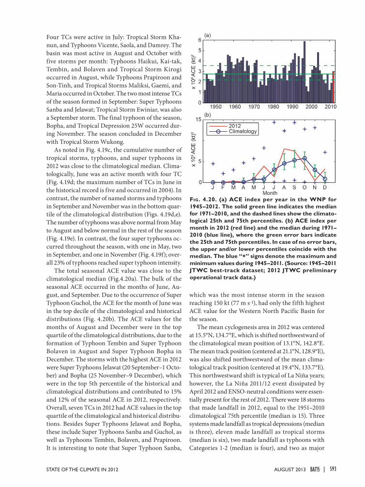
S93STATE OF THE CLIMATE IN 2012 |AUGUST 2013
Four TCs were active in July: Tropical Storm Kha-nun, and Typhoons Vicente, Saola, and Damrey. The basin was most active in August and October with five storms per month: Typhoons Haikui, Kai-tak, Tembin, and Bolaven and Tropical Storm Kirogi occurred in August, while Typhoons Prapiroon and Son-Tinh, and Tropical Storms Maliksi, Gaemi, and Maria occurred in October. The two most intense TCs of the season formed in September: Super Typhoons Sanba and Jelawat; Tropical Storm Ewiniar, was also a September storm. The final typhoon of the season, Bopha, and Tropical Depression 25W occurred dur-ing November. The season concluded in December with Tropical Storm Wukong.
As noted in Fig. 4.19c, the cumulative number of tropical storms, typhoons, and super typhoons in 2012 was close to the climatological median. Clima-tologically, June was an active month with four TC (Fig. 4.19d; the maximum number of TCs in June in the historical record is five and occurred in 2004). In contrast, the number of named storms and typhoons in September and November was in the bottom quar-tile of the climatological distribution (Figs. 4.19d,e). The number of typhoons was above normal from May to August and below normal in the rest of the season (Fig. 4.19e). In contrast, the four super typhoons oc-curred throughout the season, with one in May, two in September, and one in November (Fig. 4.19f); over-all 23% of typhoons reached super typhoon intensity.
The total seasonal ACE value was close to the climatological median (Fig.4.20a). The bulk of the seasonal ACE occurred in the months of June, Au-gust, and September. Due to the occurrence of Super Typhoon Guchol, the ACE for the month of June was in the top decile of the climatological and historical distributions (Fig. 4.20b). The ACE values for the months of August and December were in the top quartile of the climatological distributions, due to the formation of Typhoon Tembin and Super Typhoon Bolaven in August and Super Typhoon Bopha in December. The storms with the highest ACE in 2012 were Super Typhoons Jelawat (20 September–1 Octo-ber) and Bopha (25 November–9 December), which were in the top 5th percentile of the historical and climatological distributions and contributed to 15% and 12% of the seasonal ACE in 2012, respectively. Overall, seven TCs in 2012 had ACE values in the top quartile of the climatological and historical distribu-tions. Besides Super Typhoons Jelawat and Bopha, these include Super Typhoons Sanba and Guchol, as well as Typhoons Tembin, Bolaven, and Prapiroon. It is interesting to note that Super Typhoon Sanba,
which was the most intense storm in the season reaching 150 kt (77 m s-1), had only the fifth highest ACE value for the Western North Pacific Basin for the season.
The mean cyclogenesis area in 2012 was centered at 15.5°N, 134.7°E, which is shifted northwestward of the climatological mean position of 13.1°N, 142.8°E. The mean track position (centered at 21.1°N, 128.9°E), was also shifted northwestward of the mean clima-tological track position (centered at 19.4°N, 133.7°E). This northwestward shift is typical of La Niña years; however, the La Niña 2011/12 event dissipated by April 2012 and ENSO-neutral conditions were essen-tially present for the rest of 2012. There were 18 storms that made landfall in 2012, equal to the 1951–2010 climatological 75th percentile (median is 15). Three systems made landfall as tropical depressions (median is three), eleven made landfall as tropical storms (median is six), two made landfall as typhoons with Categories 1-2 (median is four), and two as major
Fig. 4.20. (a) ACE index per year in the WNP for 1945–2012. The solid green line indicates the median for 1971–2010, and the dashed lines show the climato-logical 25th and 75th percentiles. (b) ACE index per month in 2012 (red line) and the median during 1971–2010 (blue line), where the green error bars indicate the 25th and 75th percentiles. In case of no error bars, the upper and/or lower percentiles coincide with the median. The blue “+” signs denote the maximum and minimum values during 1945–2011. (Source: 1945–2011 JTWC best-track dataset; 2012 JTWC preliminary operational track data.)

S94 | AUGUST 2013
typhoons with Categories 3-5 (mean is 0.7). The high number of landfalls as tropical storms and intense typhoons are in the 95th and 90th percentiles of their climatological and historical distributions, respec-tively, while the two landfalls as weak typhoons are in the bottom quartile of these distributions.
Figure 4.21 shows the environmental conditions associated with the activity in 2012. The SST anoma-lies in the period July–October (JASO; Fig. 4.21a) were small in the basin, with exception of a positive anomaly near Japan. The maximum extension of the monsoon trough zonal winds (Fig. 4.21b) was just east of the Philippines, and together with the 600-hPa relative humidity positive anomalies in the western part of the basin (Fig. 4.21c), explains the westward shift in the cyclogenesis activity in the basin. Not sur-prisingly, the genesis potential index (Emanuel and Nolan 2004; Camargo et al. 2007) also had positive anomalies in the western part of the basin.
Typhoon Vicente and Super Typhoon Bopha made landfall as typhoons with Categories 4 and 5 strength in southern China and the southern Philippines, respectively. The largest impacts in the region for the season were caused by Super Typhoon Bopha; the storm had devastating effects to the island of Mindanao, f lattening coastal villages, and causing mudslides and f loods that destroyed plantations. Bopha made landfall three times while crossing the sprawling archipelago of the southern Philippines, resulting in over 1000 deaths, and nearly as many
missing; the storm also displaced over 835 000 people. Bopha was the costliest typhoon to ever affect the Philippines, resulting in excess of $1 billion US dollars in economic loss. Bopha was a low-latitude storm, one of three typhoons in the historical record to reach over 110 kt (57 m s-1) south of 5°N latitude, and the only typhoon in the historical record to reach over 130 kt (67 m s-1) south of 7°N. Thus, this rare low-latitude intense typhoon impacted an area not as prone to typhoons compared with compared with Philippine islands (e.g., Luzon) further to the north.
5) indian Ocean Basins
(i) North Indian Ocean—M. C. Kruk and K. L. GleasonThe North Indian Ocean (NIO) TC season typi-
cally extends from April to December, with two peaks in activity during May–June and in November when the monsoon trough is positioned over tropical waters in the basin. Tropical cyclones in the NIO basin nor-mally develop over the Arabian Sea and Bay of Bengal between latitudes 8°N and 15°N. These systems are usually short-lived and relatively weak, and often quickly move into the Indian subcontinent.
According to the Joint Typhoon Warning Center (JTWC), the 2012 TC season produced four tropical storms, no cyclones, and no major cyclones (Fig. 4.22a). The 1981–2010 IBTrACS seasonal averages for the basin are 3.9 tropical storms, 1.4 cyclones, and 0.6 major cyclones. The season produced a relatively low ACE index value of 5.7 × 10⁴ kt2, which is well
below the 1981–2010 mean of 12.5 × 10⁴ kt2 (Fig. 4.22b), and was the lowest ACE in the basin since 1989. Typically, there is enhanced TC activity, especially in the Bay of Bengal, during the cool phase of ENSO (Singh et al. 2000); however, most of this season was char-acterized by near-neutral ENSO conditions.
The NIO season started late this year, with the first storm occurring 24–25 Octo-ber. Murjan developed in the Arabian Sea and began a slow westward track towards the Horn of Africa. The storm made landfall on 25 October with maximum sustained winds of 35 kt (18 m s-1) and produced heavy rains in Somalia, particularly resulting in much needed rainfall for the Bari region in the northeastern portion of Somalia. No other major impacts were reported.
One of the most noteworthy storm of the season was Nilam, which formed relatively close to the Indian subcontinent on 28 Oc-tober in the Bay of Bengal. The storm made
Fig. 4.21. (a) SST anomalies for Jul–Oct (JASO) 2012. (b) Zonal winds in JASO 2012 (positive contours are shown in solid lines, negative contours in dash dotted lines, and the zero contour in a dotted line). (c) Relative humidity 600-hPa anomalies in JASO 2012. (d) Genesis potential index anomalies in JASO 2012. [Source: atmospheric variables: NCEP/NCAR Reanalysis data (Kalnay et al. 1996); SSTs (Smith and Reynolds 2005).]

S95STATE OF THE CLIMATE IN 2012 |AUGUST 2013
landfall with winds of 55 kt (28 m s-1) near Mahab-alipuram, Sri Lanka, on 31 October with heavy rains. The Kala Oya River overflowed its banks and one woman was killed when a large rock fell on her house; all local area schools were closed for three days as they were used as storm shelters (http://www.colombopage.com/archive_12A/Oct29_1351524597KA.php). The circulation around Nilam brought a 6°C drop in tem-perature to Bangalore, India, as the storm tapped into cool, dry air from Russia (http://articles.timesofindia.indiatimes.com/2012-10-31/bangalore/34836037_1_temperature-moderate-rainfall-cold-weather).
The final two storms of the season, Tropical Storms 03B and 04A, both formed in an environ-ment with highly favorable SSTs and moderate wind shear. However, for both systems, shortly after they were termed “deep depressions”, the storms’ low-level centers became exposed owing to increased vertical shear and the systems quickly dissipated with little, if any, impact on the basin.
(ii) South Indian Ocean—K. L. Gleason and M. C. KrukAccording to the Joint Typhoon Warning Center
(JTWC), the Southern Indian Ocean (SIO) Basin extends south of the equator from the east African coastline to 105°E7, with most cyclones developing south of 10°S. The SIO TC season extends from July of one year to June of the following year; the 2012 season is comprised of storms from July 2011 to June 2012. The peak activity typically occurs from De-cember to April when the ITCZ is located south of, and migrating towards, the equator. Historically, the vast majority of landfalling cyclones in the Southern Indian Ocean impact Madagascar, Mozambique, and the Mascarene Islands, including Mauritius and La Réunion.
The historical SIO TC data is probably the least reliable of all the TC basins (Atkinson 1971), pri-marily due to a lack of historical record keeping by individual countries and no centralized monitoring agency; however, the historical dataset for the region has been updated (Knapp et al. 2010). The historical data are noticeably deficient before reliable satellite data were operationally implemented in the region beginning about 1983.
The 2011/12 SIO season storm numbers were near average with 12 tropical storms, 6 of these becoming cyclones, and 2 of those becoming major cyclones (Fig. 4.23a). The 1981–2010 IBTrACS seasonal aver-ages are 8.7 tropical storms, 4.0 cyclones, and 1.2 major cyclones. The 2011/12 season ACE index of 52.6 × 10⁴ kt2, was less than the 1981–2010 average of 55.9 × 10⁴ kt2 (Fig. 4.23b). Despite the near-average number of TCs for the season, the below-average ACE value implies that the overall strength and/or duration of the storms during the season were below average. This is the fourth consecutive year with below-average ACE values.
Two named storms and one cyclone made landfall during the season: Tropical Storms Chanda and Irina made landfall in Madagascar during January and March, respectively, and Major Cyclone Giovanna made landfall in February. Giovanna was the stron-gest cyclone of the season and caused significant damage as it made landfall in Madagascar. Giovanna was also the first intense TC to impact Madagascar since Bingiza in February 2011.
Giovanna began as a tropical wave on 7 February. Two days later, the storm strengthened into a de-pression as it moved southwestward towards central Madagascar. Giovanna intensified rapidly on 13 Feb-ruary and became a major cyclone with peak winds
7 In order to generate consistent basin statistics, the SIO Basin boundary overlaps with the Australian Bureau of Meteorol-ogy’s operational warning area from 90°E to 105°E.
Fig. 4.22. Annual TC statistics for the NIO for 1970–2012: (a) number of named storms, cyclones, and major cyclones and (b) the estimated annual ACE Index (in kt2 × 104) for all TCs during which they were at least tropical storm strength or greater intensity (Bell et al. 2000). The 1981–2010 means are included in both (a) and (b).

S96 | AUGUST 2013
of 125 kt (64 m s-1), equivalent to a Saffir-Simpson Category 4 hurricane. Later that day, Giovanna made landfall near Andovoranto, Madagascar, and weak-ened rapidly once on land. After moving back into open waters of the Mozambique Channel, Giovanna tracked counterclockwise around the southern tip of the island and intensified briefly as it moved over warmer water. Giovanna eventually dissipated east of Madagascar on 21 February. Strong winds and flood-ing associated with Giovanna caused widespread damage across much of central Madagascar. Thou-sands of homes were destroyed and some villages on nearby islands were decimated. In addition to damage across Madagascar, La Réunion Island reported waves up to 8 m, which caused erosion and swept one person out to sea. More than 30 fatalities were reported as a direct result from this storm.
A second intense TC formed off the coast of Mo-zambique and became Cyclone Funso on 20 January.
Nearly stationary off the coast, Funso continued to intensify and brought damaging winds and torren-tial rainfall to more than three million people across Mozambique and Malawi. After making a loop in the Mozambique Channel, Funso began a south-ward track and reached peak intensity with winds sustained at 119 kt (61 m s-1) as it slowly pulled away from the coast and out into open ocean waters. On 28 January, Funso transitioned into an extratropical storm and weakened rapidly before dissipating. At least 40 people perished as a result of Funso despite the fact that it never officially made landfall.
6) sOuthwest pacific Basin—A. M. Lorrey, N. Fauchereau, P. Chappell, and H. J. Diamond
(i) Seasonal activityFrom an official WMO perspective, the South-
west Pacific Basin is an area defined from 160°E to 120°W. However, from a climatological perspective (Diamond et al. 2012), the region is better defined as spanning the area from 135°E to 120°W. The long-term climatological averages justifying these boundaries are documented in the South Pacific Enhanced Archive of Tropical Cyclones (SPEArTC; Diamond et al. 2012). As such, and according to data from the Fiji Meteorological Service, New Zealand MetService, and Australian Bureau of Meteorology, the 2011/12 TC season for this basin had 16 tropical depressions (including tropical lows), five tropical cyclones, and one major tropical cyclone (Fig. 4.24) based on the Australian TC intensity scale (http://www.bom.gov.au/cyclone/about/intensity.shtml). The 1981–2010 SPEArTC seasonal averages are 1.9 tropical depressions8, 10.4 tropical cyclones, and 4.3 major tropical cyclones. The relatively low conversion rate for tropical depressions that failed to achieve at least a Category 1 status did not mean the TC season was uneventful. The few tropical cyclones that developed across the basin had significant impacts in terms of destructive winds, amplified wave climate, and large effects from heavy rainfall that caused flooding and landslides, severely damaging agriculture and civil infrastructure across the South Pacific Islands region. Two of the tropical depressions also caused 13 deaths, including one storm that killed 5 people in the New Zealand sector after it underwent extratropical transi-tion (Sinclair 2002).
8 Historical information on TDs in the SPEArTC dataset is not as reliable as with named storms and therefore this number is most probably artificially low.
Fig. 4.23. Annual TC statistics for the Southern Indian Ocean for 1970–2012: (a) number of named storms, cyclones, and major cyclones, and (b) the estimated annual ACE index (in kt2 × 104) for all TCs during which they were at least tropical storm strength or greater intensities (Bell et al. 2000). The 1981–2005 means are included in both (a) and (b) as the horizontal lines. Note that the ACE Index is estimated due to a lack of consistent six-hour-sustained winds for every storm.

S97STATE OF THE CLIMATE IN 2012 |AUGUST 2013
(ii) Landfalling and other significant TCsThe first TC of the season, Fina, began as a tropi-
cal low within the South Pacific convergence zone (SPCZ) on 18 December near Papua New Guinea. This system tracked southwest, and was categorized as a Category 1 storm on 20 December. Tropical Cy-clone Fina was short-lived, with maximum sustained winds of 35 kt (18 m s-1), and a mean central pressure of 994 hPa. The storm dissipated and was classified as an extratropical system on 22 December, but the decaying system still generated tropical storm winds across parts of coastal Queensland, Australia.
Tropical Cyclone Grant, a Category 2 storm with maximum sustained winds of 54 kt (28 m s-1) and a mean central pressure of 978 hPa, was initiated to the north of Darwin, Australia, as a tropical low on 21 December. The system moved south, building rapidly to maximum strength by 25 December and bringing gale force winds as it crossed the north Australian coastline. After making landfall, the system tracked east and across the Gulf of Carpentaria, the Cape York Peninsula, and then into the Coral Sea where it dissipated on 2 January.
In early February, Tropical Cyclone Cyril, a Category 2 storm with maximum sustained winds of 51 kt (26 m s-1) and a mean central pressure of 985 hPa, began as a tropical disturbance south of Fiji. The system tracked east across Fijian territory before it became a named storm on 6 February as it
reached Tonga. The storm then moved southeast and became extratropical on 8 February. Cyril generated strong winds and heavy rainfall across north-ern islands in the Fijian group during early stages of activity. Gale force winds and torrential rainfall occurred in association with Cyril damaged banana and breadfruit trees in Vava’u in the northern area of Tonga.
Later in February, Tropical Cyclone Jasmine, a Category 4 storm (and the only major TC of the season) formed with maximum sustained winds of 100 kt (51 m s-1) and a mean central pressure of 942 hPa. It was the fourth system to affect the region, and was a unique system for the season in terms of strength (strongest overall),
morphology that the storm evolved into, and storm duration (19 days). Jasmine was classified as an an-nular TC system for one portion of its life, and these systems are rare (approximately 3% of all named TCs in the Southwest Pacific Basin have ever been categorized in this manner). Annular TCs are char-acterized by a well-defined eye wall, intense and broad convection across much of the breadth of the storm, and a highly symmetrical radius which lacks strongly-defined rain band splays that typically extend obliquely away from the edge of the system in spiral-form fashion (Knaff et al. 2012). Jasmine began in the Gulf of Carpentaria, where it brought heavy rainfall to Queensland, then tracked east-ward across the Coral Sea and to the north of New Caledonia. Jasmine produced heavy rainfall to the south and east of the Solomon Islands and northern New Caledonia, and contributed to submergence of subsistence agriculture plots, kumara (sweet potato) vine rot, landslides, and destruction of homes. After Jasmine moved to the southeast (south of Fiji), it caused significant damage, including crop destruc-tion in Vanuatu and Tonga.
The combination of Tropical Cyclones Jasmine and Cyril within the same month meant that Tonga received 200%–300% of its normal rainfall (with monthly totals ranging from 424 mm to 627 mm) at five out of six of their stations that are regularly discussed in the monthly Island Climate Update
Fig. 4.24. Named TCs in the Southwest Pacific Basin. Solid black lines indi-cate each storm track. SST anomalies (°C), 4 m s-1 steering wind, surface pressure (geopotential at 1000 hPa), and the location of the SPCZ (purple line) are shown. Omega (used to define the core location of the SPCZ) and the 4 m s-1 steering wind contour are taken from the 500-hPa geopotential height. SST anomalies are plotted relative to the austral warm season (Nov–Apr) 1981–2010 climatology. Geopotential height contours are in meters. (Source: NCEP 1 reanalysis and the NOAA Optimum Interpola-tion SST dataset.)

S98 | AUGUST 2013
southwest Pacific seasonal climate forecast forum. The breadth of damage and impacts from Jasmine resulted in the retirement of that name from further use in the basin.
Tropical Cyclone Daphne, a Category 2 storm with maximum sustained winds of 51 kt (26 m s-1) and a mean central pressure of 985 hPa, was the last named storm of the season in the basin. It formed from a tropical depression that was located south of the Solomon Islands on 31 March before reaching Category 1 status on 2 April. The storm tracked to the southeast and became extratropical on 3 April, but not before causing damage to the Nadi Airport in Fiji, which included a power outage.
7) australian regiOn Basin—B. C. Trewin (i) Seasonal activityAccording to the Australian Bureau of Meteorol-
ogy, the 2011/12 TC season was somewhat below normal in the broader Australian Basin (areas south of the equator and between 90°E and 160°E9, which includes Australian, Papua New Guinean, and Indo-nesian areas of responsibility). The season produced 7 TCs, below the 1983/84–2010/11 average (the average coincides with comprehensive satellite coverage of the region) of 10.8, and somewhat counter to the above-normal TC activity typical of La Niña seasons in the Australian region. (An eighth system was named operationally but downgraded on post-analysis). The 1981–2010 IBTrACS seasonal averages for the basin are 8.4 named storms, 4.5 tropical cyclones, and 1.7 major tropical cyclones, which compares with the 2011/12 counts of 7, 4, and 1, respectively.
There was one tropical cyclone in the eastern sector10 of the Australian region (which reached its peak intensity after moving into the Southwest Pacific region), one in the northern sector, and five tropical cyclones in the western sector. Three systems made landfall in Australia as tropical cyclones, while one was dissipating when it made landfall on the coast of Western Australia.
9 The Australian Bureau of Meteorology’s warning area overlaps both the southern Indian Ocean and Southwest Pacific.
10 The western sector covers areas between 90°E to 125°E. The eastern sector covers areas east of the eastern Australian coast to 160°E, as well as the eastern half of the Gulf of Carpentaria. The northern sector covers areas from 125° E east to the western half of the Gulf of Carpentaria.
(ii) Landfalling and other significant TCsThe most intense tropical cyclone of the season
in the Australian region was Lua, which reached tropical cyclone intensity on 13 March off the Pilbara coast near 19°S, 115°E, and initially moved northwest before turning on 15 March and moving southeast towards the coast of Western Australia, ultimately making landfall near Pardoo Station, about 150 km east of Port Hedland, on 17 March. Lua reached Cat-egory 4 intensity (on the Australian tropical cyclone intensity scale) with maximum sustained winds of 90 kt (46 m s-1), and made landfall near peak intensity. Lua dissipated over the interior of Western Australia, bringing heavy rain as far south as Kalgoorlie and Norseman. The region where it made landfall is sparsely populated; therefore, damage was minimal despite Lua’s intensity.
Tropical Cyclone Grant, the only storm of the sea-son in the northern region of Australia, as discussed in section d6ii of this chapter, reached tropical cyclone intensity northeast of Darwin, near 11°S, 132°E, early on the morning of 25 December. It intensified dur-ing the day and reached its peak intensity of 55 kt (28 m s-1) that evening as it moved south. Grant crossed the Cobourg Peninsula as a Category 2 system and made landfall east of Point Stuart on the morning of 26 December. The remnant low pressure system then moved southeast across Arnhem Land, bringing heavy rain to the region. Edith Falls Ridge, north of Katherine, received 385 mm of rain within 24 hours on 26–27 December, with four other sites exceeding 200 mm. The rains resulted in major flooding in the Katherine area, causing a train derailment when a bridge was washed out and closing the main Adelaide-Darwin railway for more than a month. The remnants of Grant moved east over the Gulf of Carpentaria on 28 December, but failed to regain TC intensity.
Tropical Cyclone Heidi reached TC intensity late on 10 January north of the western Australian coast, near 16°S, 119°E. It intensified to Category 2 on 11 January as it tracked south, and made landfall just east of Port Hedland early on 12 January, near its peak intensity of 65 kt (33 m s-1). The system contin-ued to move south over land, and was downgraded to a tropical low late on 12 January near Tom Price, with the remnants bringing heavy rainfall and some flooding to the Pilbara and Gascoyne regions over the following two days. There was some minor wind damage in the Port Hedland area, and offshore oil and gas production was disrupted.

S99STATE OF THE CLIMATE IN 2012 |AUGUST 2013
The season’s last landfalling storm was Tropical Cyclone Iggy, which made landfall as a dissipating system near Jurien Bay, north of Perth, on 2 Febru-ary. Iggy reached tropical cyclone intensity early on 26 January, about 960 km northwest of Exmouth near 16°S, 108°E. It initially moved southeast towards the Pilbara coast and reached Category 2 intensity, peak-ing as a 55 kt (28 m s-1) system on 28 January. On 29 January, the storm became near-stationary off the coast near 20°S, 111°E, and weakened before mov-ing southwest and re-intensifying to Category 2 on 30 January. Iggy recurved east and weakened before making landfall. There was moderate rainfall in the landfall area, with Lancelin receiving 73 mm within 24 hours on 2–3 February.
No other tropical cyclones made landfall, or reached Category 3 or higher intensity within the Australian region, although Alenga (December) did so before entering the Australian region from the west, and Jasmine (February) did so after moving into the Southwest Pacific Basin. The circulation as-sociated with the development of Jasmine (discussed in more detail in section d6ii of this chapter) caused some minor wind damage in the Cairns area.
e. Tropical cyclone heat potential—G. J. Goni, J. A. Knaff, and I-I Lin 1) BackgrOund, Overview, and Basin highlights fOr
2012This section summarizes the seven previously
described TC basins from the standpoint of tropical cyclone heat potential (TCHP), by focusing on upper ocean temperature conditions during the season with respect to average values. TCHP (Goni and Trinanes 2003), defined as the ocean heat content contained between the sea surface and the depth of the 26°C isotherm (D26), has been shown to be more closely linked to intensity changes of tropical cyclones than SST alone (Shay et al. 2000; Goni and Trinanes 2003; I-I Lin et al. 2008, 2009a), provided that atmospheric conditions are also favorable. In general, fields of TCHP show high spatial and temporal variability associated with oceanic mesoscale features that can be globally detected with satellite altimetry (Lin et al. 2008; Goni et al. 2009; Goni et al. 1996). Additionally, areas with high TCHP values can be an important factor in the rapid intensification of tropical cyclones (Shay et al. 2000; Mainelli et al. 2008; I-I Lin et al. 2009b). Satellite-derived fields of TCHP are usually validated using Argo and XBT fields (Goni et al. 1996; Pun et al. 2007). It has also been shown that mesoscale features with high values of TCHP can
be an important factor for the rapid intensification of TCs (e.g., Shay et al. 2000; Mainelli et al. 2008; I-I Lin et al. 2009b).
Tropical cyclone heat potential is an important seasonal factor since large cooling could affect the intensification for subsequent TCs in the same region and may also inf luence the upper ocean thermal structure on regional scales within weeks to months after the passage of a TC (Emanuel 2001; Hart et al. 2007; Dare and McBride 2011; Knaff et al. 2013).
To examine TCHP interannual variability, Fig. 4.25 shows anomalies during the months of TC activ-ity in each hemisphere: June through November in the Northern Hemisphere and November through April in the Southern Hemisphere. Anomalies are defined as departures from the mean TCHP calculated dur-ing the same months for the period 1993–2012. These anomalies show large variability within and among the TC basins. During the 2012 season, the basins exhibited the following TCHP anomalies:• The Atlantic Basin displayed generally weak
positive anomalies while the Gulf of Mexico (Fig. 4.25, lower right box) showed patterns indicative of variability of the Loop Current. The central region of the Gulf of Mexico, which is typically characterized by high TCHP values, exhibited negative values. In the tropical Atlantic, condi-tions remained mostly average, but with larger regions exhibiting positive anomaly values (see http://www.aoml.noaa.gov/phod/regsatprod/atln/index.php). It should be noted that there were warm SST anomalies in the Atlantic, and SSTs do not necessarily equate to TCHP values.
• The Western North Pacific (WNP) Basin con-tinues to see an increase in D26 and TCHP by
Fig. 4.25. Global anomalies of TCHP corresponding to 2012 computed as described in the text. The numbers above each box correspond to the number of Category 1 and above TCs that traveled within each box. The Gulf of Mexico conditions during Jun–Nov 2012 are shown in the insert shown in the lower right corner.

S100 | AUGUST 2013
approximately 10%, as compared to the early 1990s. The sea surface area under very high D26 (>110 m) or very high TCHP (>110 kJ cm-2) has increased by ~13% (Pun et al. 2013). This has been found to be significant, as areas with high D26 and TCHP values are often associated with the development of super typhoons (Lin et al. 2008; Goni et al. 2009; Pun et al. 2013). During 2012, positive anomalies predominated in the WNP MDR in this basin, and TCHP values approached 90 kJ cm-2, making 2012 slightly warmer than average.
• As in 2011, the Southwest Pacific Basin had both positive and negative spatial anomalies (Fig. 4.25), although the basin predominately exhib-ited high positive anomaly values.
• In contrast with 2011, in the NIO, the Bay of Bengal exhibited a decrease in TCHP values with negative anomalies during 2012, while the Arabian Sea exhibited mostly positive anomaly values.
• Differences in each basin in 2012 with respect to the 2011 conditions (Fig. 4.26) indicate that the east Pacific Ocean and central SIO exhibited larger values (>20 kJ cm-2) of TCHP in most areas in 2012.
2) examples Of tc intensificatiOn assOciated with tchp
Hurricane Sandy (see Sidebar 4.1) was the most intense storm of the 2012 Atlantic season to make landfall and the largest known Atlantic hurricane in gale wind force diameter on record. Originating as a tropical wave in the Caribbean Sea on 19 October, by 24 October Sandy reached Category 3 strength while crossing over a region north of Cuba with TCHP values above 75 kJ cm-2 (Fig. 4.27a). The cooling produced by this storm, even after strengthening,
reached values lower than the typically observed 3C under its track.
In the Mozambique Channel of the Southern In-dian Ocean, Tropical Cyclone Funso (Fig. 4.27e) was classified as a tropical depression on 19 January. This is a preferred region for anticyclonic/warm ocean ed-dies that can interact and influence TCs. The storm initially moved slowly west while rapidly intensifying, reaching an intensity of 100 kt (51 m s-1) on 21 Janu-ary. At this time the storm was nearly stationary and the eyewall was interacting with the coast of Africa. The upwelling of cooler water, coupled with its in-teraction with land, caused Funso to weaken slightly as the storm moved slowly eastward and back over the warm Mozambique Channel. Then its steering changed and the storm started moving more steadily, albeit slowly, southward in an environment that was favorable for intensification. During this period of slow southward movement, Funso tracked around the periphery of a warm ocean eddy that had values of TCHP exceeding 75 kJ cm-2. The combination of favorable atmospheric conditions and high TCHP values allowed Funso to intensify to 115 kt (59 m s-1) on 24 January, and it maintained this intensity for 18 hours. As Funso left the influence of this warm eddy, it began the first of two eyewall replacement cycles, resulting in a slight weakening and the formation of a larger eyewall. By this time, Funso was moving more rapidly southward and again re-intensified to 115 kt (59 m s-1) on 26 January after encountering higher TCHP values to the west. After this interaction, Funso began its final eyewall replacement cycle and began to weaken as it moved over the cooler oceanic conditions to the south.
Super Typhoon Sanba was the most intense TC observed in the WNP in 2012. On 13 September, it underwent rapid intensification over a region of high TCHP of >130 kJ cm-2 (Fig. 4.27d). Within 18 hours, its intensity increased by 60 kt (31 m s-1) to its peak at maximum sustained winds of 150 kt (77 m s-1). This rapid rate of intensification is more than 2.5 times the rapid intensification threshold value of 30 kt (15 m s-1) in a 24-hour period as described by Kaplan and DeMaria (2003). Sanba was able to maintain this peak intensity for 18 hours while it remained over the high TCHP region that was >130 kJ cm-2. However, as Sanba moved northward away from the higher TCHP region into a southern-eddy-rich zone, it encountered a pre-existing cold ocean eddy. With corresponding significantly lower TCHP values in the range of 60 kJ cm-2 –90 kJ cm-2, Sanba’s intensity decreased to 110 kt (57 m s-1) within 18 hours.
Fig. 4.26. Differences between the TCHP fields in 2012 and 2011.

S101STATE OF THE CLIMATE IN 2012 |AUGUST 2013
On 13 September, Super Typhoon Jelawat (Fig. 4.27b) followed a track similar to Sanba. Jelawat in-tensified from a Category 1 to a Category 5 storm in only two days and maintained that strength for one day. As it moved away from the high TCHP area and passed over the cold water wake region left by Sanba, its intensity decreased significantly.
Another notable case of intensification was also observed in the WNP with Super Typhoon Bopha, a late boreal fall/early boreal winter storm. Bopha (Fig. 4.27c) was also the only December typhoon to have reached a Category 5 status in the past decade. Bopha had a low-latitude track around 4°N–5°N for much of its existence. Typhoon Bopha formed at a low latitude and in a region where TCHP values are typically
above 100 kJ cm-2, and its maximum intensification rates were coincident with a typhoon tracking through a region with TCHP values exceeding 85 kJ cm-2. On 1 December, Bopha had maximum sus-tained winds of 115 kt (59 m s-1), and by 3 December, it reached its peak intensity of 140 kt (72 m s-1). However, the storm in-tensified more slowly than Sanba. Bopha made landfall in Mindanao, Philippines, soon after reaching its peak intensity. As noted in section 4d4, Mindanao is not a region that experiences frequent TC land-falls and Bopha was the most devastating typhoon to affect the southern Philippines in the last 20 years.
f. Intertropical convergence zones 1) pacific—A. B. Mullan The intertropical convergence zone
(ITCZ) lies approximately parallel to the equator with a slight north-easterly tilt, and varies in position from around 5°N–7°N in February–May to 7°N–10°N in August–November. The South Pacific convergence zone (SPCZ) extends diago-nally from around Solomon Islands (10°S, 160°E) to near 30°S, 140°W, and is most active during November–April. In the far western Pacific, these two convergence bands merge into the Australian and East Asian monsoon trough.
The Pacific convergence zones are strongly influenced by the status of ENSO; as the year began, a mature La Niña was in place. This event dissipated during April 2012 and warmer-than-normal tropical
SSTs developed in the second half of the year, but did not display sufficient amplitude or persistence to qualify as an El Niño. Thus, SST anomalies in the tropical Pacific were not extreme during 2012 nor were the precipitation variations in the convergence zones, other than exceptions as noted below.
Figure 4.28 summarizes the convergence zone behavior for 2012, and relates the seasonal variation to the longer-term climatology. Rainfall transects over 20°N to 30°S are presented for each quarter of the year, averaged across successive 30° longitude bands, starting in the western Pacific at 120°E–150°E. The rainfall data are taken from the Tropical Rainfall Monitoring Mission (TRMM) analysis (Huffman et al. 2007), using the 0.25° resolution 3B43 dataset
Fig. 4.27. (Left) Oceanic TCHP and surface cooling given by the difference between post- and pre-storm values of (center) TCHP and (right) SST for TCs (a) Sandy, (b) Jelawat, (c) Bopha, (d) Sanba, and (e) Funso. The TCHP values correspond to two days before each TC reaches its maximum intensity value.

S102 | AUGUST 2013
except for December 2012 where the 0.5° 3A12 data was substituted (the 3B43 data was not available at the time this climate summary was prepared). The 3B43 data are based on the version 7 algorithm and start in 1998. The period 1998–2011 is used as the climatology for comparison with the 2012 transects.
Starting with the westernmost sector of Fig. 4.28, in what might be considered the monsoon trough region, seasonal rainfall for the first half of 2012 was close to normal. During July–September, convection was above normal at all latitudes of this sector, a situation that reversed in the following quarter. In particular, the normal southward progressive in convection over New Guinea and northern Australia was delayed. These convection anomalies observed in the TRMM data accord with rainfall anomalies reported in Australia (http://www.bom.gov.au/climate/current/index.shtml) and in Micronesia (http://www.prh.noaa.gov/peac/).
The seasonal variation in ITCZ convection can be seen in Fig. 4.28 in the three sectors starting at 150°E, 180°, and 150°W. In the first quarter of 2012, the ITCZ was disorganized and weak, especially between the date line and 150°W; this is unusual for a La Niña period. Figure 4.29 shows the TRMM rainfall in the tropical Pacific for February 2012 and the break in ITCZ convection east of the date line is evident. Figure 4.30 illustrates the 2012 situation in comparison to other La Niña seasons in the TRMM
observational period. According to NOAA’s Oceanic Niño Index (ONI), there are eight years in the TRMM archive where the January–March quarter qualifies as a La Niña period. Rainfall east of the date line (180°–150°W sector) between about 5°N and 15°N in 2012 is by far the lowest of any of the La Niña years. The only drier January-March quarters in the TRMM archive occur during El Niño periods (1998, 2003, and 2010), when convection is typically much greater than the long-term average between about 10°S and 5°N, but much less than average between 5°N and 15°N.
A double ITCZ was present in March and April, with a fairly prominent southern branch between 150°W and 90°W, as is typical of La Niña years (Masunaga and L’Ecuyer 2010). During the second half of 2012, when tropical Pacific SSTs were generally warmer than normal, the ITCZ was well organized and equatorward of its normal position (Fig. 4.28).
In the f irst quarter of 2012, SPCZ rainfal l was higher than normal and the maximum was
not iceably southward of its climatological position (Fig. 4.28). As ENSO-neutral c o n d i t i o n s d e v e l o p e d , t h e S P C Z c o n v e c t i o n bec a me re lat ive ly wea k and disorganized, but this is typical during April to September. In the last quarter of 2012, the SPCZ maximum was more sharply peaked than normal and equatorward of its climatological position. This is evident in the 180°–150°W sector (lower right panel of Fig. 4.28), and coincided with low rainfalls observed in the South Pacific Islands east of the date line at about 20°S. For example, the October–December rainfall at Niue’s Hanan Airport (19°S, 170°W) was only 36% of normal, and
Fig. 4.29: TRMM 3B43 rainfall (mm day-1) for Feb 2012.
Fig. 4.28: (a-d) Rainfall rate (mm day-1) from TRMM analysis (3B43 version 7) for the four quarters of 2012. The separate panels for each quarter show the 2012 rainfall cross-section between 20°N and 30°S (solid line) and the 1998–2011 climatology (dotted line) for four 30° sectors from 120°E–150°E to 150°W–120°W.

S103STATE OF THE CLIMATE IN 2012 |AUGUST 2013
at Rarotonga (21°S, 160°W) in the southern Cook Islands it was 53% of normal (http://www.niwa.co.nz/climate/icu). These islands typically experience dry conditions during El Niño periods.
2) atlantic—A. B. Pezza and C. A. S. CoelhoThe Atlantic ITCZ is a well-organized convective
band that oscillates approximately between 5°N and 12°N during July–November and 5°N and 5°S during January–May (Waliser and Gautier 1993; Nobre and Shukla 1996). Equatorial Kelvin waves can modu-late the ITCZ intraseasonal variability (Wang and Fu 2007; Mounier et al. 2007; and Mekonnen et al. 2008); and ENSO is also known to influence it on the seasonal time scale (Münnich and Neelin 2005). In 2012 the prevailing equatorial Pacific scenario was a moderate La Niña that began retreating in March, leading to slightly warm to neutral conditions for the remaining of the year. The ITCZ responded to this pattern and presented a noticeable enhancement in January and February, with negative outgoing longwave radiation (OLR) anomalies in most of the western sector of the equatorial Atlantic surrounding South America (Fig. 4.31a). This pattern contributed to above-average rainfall in the Amazon sector of Brazil, Peru, Colombia, and Venezuela, but it was not sufficiently strong to produce significant rainfall in the drought-prone area of northeastern Brazil during the first three months of 2012 (Fig. 4.31b).
The ending of La Niña conditions in March helped enhance the ITCZ via Kelvin wave-induced upper level divergence in the western Atlantic sector dur-ing January and February. For the remainder of the year the ITCZ presented a near-normal convective intensity, with occasional bursts of severe convection towards the Caribbean Sea. This anomalous activity to the west responded to a cooler-than-average SST pattern in both the North and South Atlantic (Fig.
4.32a) prevailing until austral winter. Such an SST pattern favored the ITCZ predominant location to the north of its climatological position particularly dur-ing the first four months of the year. During boreal summer, the North Atlantic warmed up considerably and remained warm until the end of the year. The interplay of the SST gradient between the South and North Atlantic is seen by the Atlantic Index (see Fig. 4.32b caption for definition), which shows a return to negative conditions (unfavorable for convection with-in the ITCZ) contrasting with parts of 2010 and 2011, yet not as severe as in early 2010. Within this scenario, the ITCZ oscillated north of its average climatological position for most of the year, with precipitation well below average over most of northeastern Brazil (Fig. 4.33; see Sidebar 7.2 for more details on the drought in this region).
g. Atlantic warm pool—C. WangThe Atlantic warm pool (AWP) is a large body of
warm water in the lower latitudes of the North Atlan-tic, comprising the Gulf of Mexico, the Caribbean Sea, and the western tropical North Atlantic (Wang and Enfield 2001, 2003). Previous studies have shown that the AWP plays an important role in Atlantic tropical cyclone activity, and in rainfall in the central United States (Wang et al. 2006, 2008a, 2011). Unlike the Indo-Pacific warm pool, which straddles the equator, the AWP is entirely north of the equator. In addition to the large seasonal cycle, AWP variability occurs on both interannual and multidecadal timescales, and
Fig. 4.30. South-north cross-sections of Jan–Mar rain-fall anomalies (% of 1998–2011) for all La Niña seasons since 1998, averaged over the sector 180° to 150°W. The black line represents 2012, and the blue lines the years 1999, 2000, 2001, 2006, 2008, 2009, and 2011.
Fig. 4.31. (a) Atlantic NOAA interpolated OLR (Lieb-mann and Smith 1996) anomalies (W m-2) for Jan–Feb 2012 and (b) TRMM anomalous precipitation rate (mm day-1) for Jan–Mar 2012. Anomalies are based on the climatology for (a) 1975–2011 and (b) 1998–2011.

S104 | AUGUST 2013
has exhibited a long-term warming trend (Wang et al. 2006, 2008b). Figures 4.34a and b depict the long-term total and detrended June–November AWP area anomalies. The multidecadal variability (Fig. 4.34c) shows that the AWP was larger during the period 1930–60, as well as after the late 1990s; and smaller during the periods of 1905–25 and 1965–95. The periods for large and small AWPs coincide with the warm and cool phases of the AMO (Delworth and Mann 2000; Enfield et al. 2001). Wang et al. (2008b) showed that the influences of the AMO on tropical cyclone activity and climate might operate through the atmospheric changes induced by the AWP. The spatial distribution of AWP-related global SST anomalies is shown in Fig. 4.35, which depicts the AWP varied with the global SST on both interannual and multidecadal time scales.
In 2012, the AWP during the Atlantic hurricane season was larger than its climatological mean, with the largest AWP occurring in September (Fig. 4.36a). The large AWP in 2012 was associated with an active 2012 hurricane season in the North Atlantic, and consistent with that, a large AWP is generally associ-ated with a reduction in vertical wind shear and an increase in atmospheric instability in the MDR—two factors favoring tropical cyclone development (Wang et al. 2008a). Spatially, the AWP started to develop in June in the Gulf of Mexico (Fig. 4.36b). By July and August, the AWP was well developed in the Gulf of Mexico and Caribbean Sea and reached eastward to the western tropical North Atlantic (Figs. 4.36c,d). By September, the AWP had further expanded southeast-ward and the isotherm of 28.5°C covered the entire tropical North Atlantic by crossing to the coast of
Fig. 4.32. (a) Atlantic ITCZ position inferred from OLR during Apr 2012. The colored thin lines indicate the approximate position for the six pentads of Apr 2012. The black thick line indicates the Atlantic ITCZ climatological position. The SST anomalies (°C; Reyn-olds et al. 2002) for Apr 2012 based on the 1982–2011 climatology are shaded. The two boxes indicate the areas used for the calculation of the Atlantic Index in (b). (b) Monthly SST anomaly time series averaged over the South American sector (SA region, 5°S–5°N, 10°W–50°W) minus the SST anomaly time series av-eraged over the tropical coast of northern Africa (NA region, 5°N–25°N, 20°W–50°W) for 2010–12 forming the Atlantic Index. The positive phase of the index indicates favorable conditions for enhanced Atlantic ITCZ activity.
Fig. 4.33. Northeastern Brazil average 2012 precipi-tation anomaly (mm) with respect to 1961–90 clima-tology based on high resolution station data. [Data sources: federal and regional networks (CMCD/INPE, INMET, SUDENE, ANEEL, FUNCEME/CE, LMRS/PB, EMPARN/RN, LAMEPE/ITEP/PE, CMRH/SE, SEAAB/PI, SRH/BA, CEMIG/SIMGE/MG, SEAG/ES)].
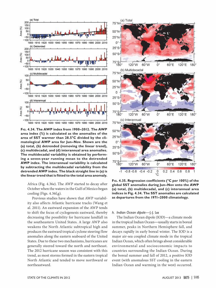
S105STATE OF THE CLIMATE IN 2012 |AUGUST 2013
Africa (Fig. 4.36e). The AWP started to decay after October when the waters in the Gulf of Mexico began cooling (Figs. 4.36f,g).
Previous studies have shown that AWP variabil-ity also affects Atlantic hurricane tracks (Wang et al. 2011). An eastward expansion of the AWP tends to shift the focus of cyclogenesis eastward, thereby decreasing the possibility for hurricane landfall in the southeastern United States. A large AWP also weakens the North Atlantic subtropical high and produces the eastward tropical cyclone steering flow anomalies along the eastern seaboard of the United States. Due to these two mechanisms, hurricanes are generally steered toward the north and northeast. The 2012 hurricane season was consistent with this trend, as most storms formed in the eastern tropical North Atlantic and tended to move northward or northeastward.
h. Indian Ocean dipole—J.-J. Luo
The Indian Ocean dipole (IOD)—a climate mode in the tropical Indian Ocean—usually starts in boreal summer, peaks in Northern Hemisphere fall, and decays rapidly in early boreal winter. The IOD is a major air-sea coupled climate mode in the tropical Indian Ocean, which often brings about considerable environmental and socioeconomic impacts to countries surrounding the Indian Ocean. During the boreal summer and fall of 2012, a positive IOD event (with anomalous SST cooling in the eastern Indian Ocean and warming in the west) occurred.
Fig. 4.34. The AWP index from 1900–2012. The AWP area index (%) is calculated as the anomalies of the area of SST warmer than 28.5°C divided by the cli-matological AWP area for Jun–Nov. Shown are the (a) total, (b) detrended (removing the linear trend), (c) multidecadal, and (d) interannual area anomalies. The multidecadal variability is obtained by perform-ing a seven-year running mean to the detrended AWP index. The interannual variability is calculated by subtracting the multidecadal variability from the detrended AWP index. The black straight line in (a) is the linear trend that is fitted to the total area anomaly.
Fig. 4.35. Regression coefficients (°C per 100%) of the global SST anomalies during Jun–Nov onto the AWP (a) total, (b) multidecadal, and (c) interannual area indices in Fig. 4.34. The SST anomalies are calculated as departures from the 1971–2000 climatology.

S106 | AUGUST 2013
Fig. 4.36. (a) The monthly AWP area in 2012 (1012 m2; blue) and the climatological AWP area (red). Spatial distributions of the 2012 AWP in (b) Jun, (c) Jul, (d) Aug, (e) Sep, (f) Oct, and (g) Nov. The AWP is defined by SST larger than 28.5°C. The black contours in (b–g) are the climatological AWP normals based on 1971–2000.
This Indian Ocean dipole was short-lived: it began in July and dissipated in November. Its peak intensity in August was greater than two standard deviations and became the fourth strongest event over the past three decades (Fig. 4.37b). However, unlike the three extreme events in 1994, 1997, and 2006, which were predominantly determined by strong cooling in the eastern IO, the warming in the western Indian Ocean contributed more than the cooling in the east to the 2012 IOD (Fig. 4.37a). This may be related to the fact that the mean tropical Indian Ocean Basin SST has risen rapidly in recent decades, two to three times faster than that of the Pacific (Luo et al. 2012). The east cooling-west warming SST dipole structure is well-linked with stronger-than-normal surface easterlies in the central equatorial IO (Fig. 4.37b); this is a typical air-sea coupled feature of the IOD. In contrast to the positive IOD in 2011, which occurred with a La Niña, the 2012 positive IOD occurred with a weak El Niño-like condition.
Associated with the 2011/12 La Niña, anomalous easterlies in the western-central Pacific and westerlies in the Indian Ocean converged in the Indonesia area. This produced stronger-than-normal rainfall in the eastern Indian-western Pacific during late 2011 and into early 2012 (Figs. 4.38a,b). The La Niña also caused wet conditions in southeastern Australia. Meanwhile, warm water piled up in the western Pacific, due to the Pacific easterly anomalies, and penetrated into the IO via the Indonesian throughflow. The warm water propagated southward along the west coast of Australia via coastal Kelvin waves and extended westward via Rossby waves (Fig. 4.39). The oceanic downwelling Rossby waves induced basinwide SST warming in the South Indian Ocean with a shape being oriented in the southeast-northwest direction (Fig. 4.38). The SST warming promoted strong-than-normal rainfall and local surface wind convergence. As a result of the atmospheric Rossby wave response to the SST warming, a cyclonic wind anomaly formed with its center always shifted poleward of the SST warming.
Following the 2011/12 La Niña, weak El Niño conditions developed in the second half of 2012. Equatoria l SST warming showed a westward propagation consistent with this El Niño condition.
Fig. 4.37. (a) Monthly anomalies of SST (°C) in the eastern (IODE; 90°E–110°E, 10°S–0°, blue lines) and western poles (IODW; 50°E–70°E, 10°S–10°N, red lines) of IOD. (b) As in (a), but for the IOD index (°C; measured by the SST difference between IODW and IODE, green line) and surface zonal wind anomaly (m s-1) in the central equatorial IO (Ucio), from 70°E–90°E, 5°S–5°N (black line). The anomalies were cal-culated relative to the 1982–2011 climatology; based on the NCEP optimum interpolation SST (Reynolds et al. 2002) and JRA-25 atmospheric reanalysis (Onogi et al. 2007).
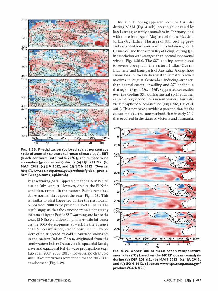
S107STATE OF THE CLIMATE IN 2012 |AUGUST 2013
Peak warming (>1°C) appeared in the eastern Pacific during July–August. However, despite the El Niño condition, rainfall in the western Pacific remained above normal throughout the year (Fig. 4.38). This is similar to what happened during the past four El Niños from 2000 to the present (Luo et al. 2012). The result suggests that the atmosphere was not greatly influenced by the Pacific SST warming and hence the weak El Niño conditions might have little influence on the IOD development as well. In the absence of El Niño’s influence, strong positive IOD events were often triggered by cold subsurface anomalies in the eastern Indian Ocean, originated from the southwestern Indian Ocean via off-equatorial Rossby wave and equatorial Kelvin wave propagations (e.g., Luo et al. 2007, 2008, 2010). However, no clear cold subsurface precursors were found for the 2012 IOD development (Fig. 4.39).
Fig. 4.38. Precipitation (colored scale, percentage ratio of anomaly to seasonal mean climatology), SST (black contours, interval 0.25°C), and surface wind anomalies (green arrows) during (a) DJF 2011/12, (b) MAM 2012, (c) JJA 2012, and (d) SON 2012. (Source: http://www.cpc.ncep.noaa.gov/products/global_precip/html/wpage.cams_opi.html.)
Initial SST cooling appeared north to Australia during MAM (Fig. 4.38b), presumably caused by local strong easterly anomalies in February, and with those from April–May related to the Madden-Julian Oscillation. The area of SST cooling grew and expanded northwestward into Indonesia, South China Sea, and the eastern Bay of Bengal during JJA, in association with stronger-than-normal monsoonal winds (Fig. 4.38c). The SST cooling contributed to severe drought in the eastern Indian Ocean-Indonesia, and large parts of Australia. Along-shore anomalous southeasterlies west to Sumatra reached maxima in August–September, inducing stronger-than-normal coastal upwelling and SST cooling in that region (Figs. 4.38d, 4.39d). Suppressed convection over the cooling SST during austral spring further caused drought conditions in southeastern Australia via atmospheric teleconnection (Fig 4.38d; Cai et al. 2011). This may have provided a precondition for the catastrophic austral summer bush fires in early 2013 that occurred in the states of Victoria and Tasmania.
Fig. 4.39. Upper 300 m mean ocean temperature anomalies (°C) based on the NCEP ocean reanalysis during (a) DJF 2011/12, (b) MAM 2012, (c) JJA 2012, and (d) SON 2012. (Source: www.cpc.ncep.noaa.gov/products/GODAS/.)

S108 | AUGUST 2013
In summary, the 2012 positive Indian Ocean dipole was not caused by either El Niño or Indian Ocean subsurface conditions. Instead, local coupling among along-shore winds, coastal upwelling, and SST
west to Sumatra are thought to have played a crucial role in this year’s IOD development.

S109STATE OF THE CLIMATE IN 2012 |AUGUST 2013
SIDEBAR 4.1: THE DOUBLE LIFE OF HURRICANE SANDY – AND A CLIMATOLOGICAL PERSPECTIVE OF THESE POST-TROPICAL GIANTS—C. T. FoGARTy AND E. S. BLAKE
Fig. SB4.1. Hurricane Sandy’s structural history as represented within the TC Phase Space using 0.5° GFS model initial (00HR) fields. The x-axis indicates the storm symmetry (B) while the y-axis is a measure of the cold/warm-core structures of the system (right hand side of diagram corresponds to thermal wind -|VT
L | > 0 for warm core) as described in Hart (2003). Time moves forward from A to C/Z, the start and end of the TC life cycle resolvable within the available dataset and its geographic boundaries. The size of the TC (mean radius of the 925-hPa gale force winds) corresponds to the size of the solid circles along the phase trajectory (largest shown is approximately 300 km). Circle color corresponds to the intensity of the TC, with purple for the weaker end of the scale and orange/magenta for the most intense. The track of the TC is plotted in the inset.
Fig. SB4.2. GOES enhanced water vapor satellite im-agery of Hurricane Sandy from tropical (a) through post-tropical (d) stages. Upper tropospheric short-wave troughs (dry air = warm colors) are indicated by numbered dashed lines. Minimum sea level pressure (hPa) is indicated near the storm center.
Hurricane Sandy—more commonly referred to in the me-dia as “Superstorm” Sandy—of October 2012 will go down in the record books as a truly giant and destructive storm in the eastern United States and Canada. Like nearly half of named tropical storms and hurricanes in the Atlantic Ocean (Hart and Evans 2001), Sandy underwent extratropical transition (ET) to a post-tropical storm. But occasionally hurricanes merge with cyclogentically-favorable regions of the subtropical or midlatitudes and grow into large, more energetic post-tropical storms. The destructive impact of Sandy is well known, but how did this level of destruction come to be, and where does it fit into the historical record and context of similar events?
Sandy had a complex life that can be described using the TC phase space diagram (Hart 2003) shown in Fig. SB4.1. Sandy began as a disturbance in the southern Caribbean Sea on 22
October and quickly intensified into a Category 3 hurricane that made landfall in Cuba early on 25 October. This period of the storm’s life is represented in the lower right portion of the phase diagram. As Sandy moved through Cuba, noted as “trough #1”, and as depicted on the satellite water vapor image in Fig. SB4.2a, the ET process was initiated (the series of green circles in the asymmetric warm core portion of the phase diagram). A second upper-level trough as depicted in Fig. SB4.2b ironically delayed the ET process by enhancing the outflow above the storm as described by Hanley et al. (2001) while it remained over warm water. This phase of the storm is depicted by the phase trajectory migrating back toward the symmetric warm core portion of the diagram (highlighted with an ellipse in Fig. SB4.1). From the morning of 27 October to the afternoon of 29 October, Sandy re-intensified to Category 2 status while a series of upper-level troughs (numbered 3–5 in Fig. SB4.2c) acted to reshape the storm’s outer circulation. Es-sentially the overall storm was undergoing ET, with a hurricane “cocooned” within, until trough #6 penetrated the core as the highly distorted large-scale flow brought the storm center into New Jersey during the evening of 29 October (Fig. SB4.2d). By the time of landfall, the storm was still well within the asym-metric warm core phase, at least based upon the GFS 00-HR model fields depicted in Fig. SB4.1. Surface weather station data (not shown) clearly indicated that frontal structures had formed and connected to the storm center.

S110 | AUGUST 2013
CON'T SIDEBAR 4.1: THE DOUBLE LIFE OF HURRICANE SANDY – AND A CLIMATOLOGICAL PERSPECTIVE OF THESE POST-TROPICAL GIANTS—C. T. FoGARTy AND E. S. BLAKE
Fig. SB4.3. Tracks of all hurricanes over the past 100 years (1911–2012) that trans-formed from hurricane to hurricane-strength post-tropical [i.e., extratropical (ET) in legend] TC. Intensity of the tropical phase of the storms is represented with various colors in the upper left portion of the map. Standard intensity convention: H5 = hurricane strength Category 5, etc. Gray portion of the track represents the ET phase.
The ET of hurricanes dir-ectly into extratropical [a.k.a. post-tropical (PT)] storms, while maintaining hurricane-force winds, are not rare occurrences in the Atlantic Basin. Figure SB4.3 shows nearly 40 of these storm tracks and the percentage of hurricanes by decade (inset) that made a transition directly to hurricane-strength PT status; this is based on the HURDAT dataset (http://www.aoml.noaa.gov/hrd/hurdat/) over the past 100 years. Storms depicted in Fig.SB4.3 are ones that main-tained hurricane strength for a least six hours after ET was declared, and had maximum sustained winds that were at least 75 kt (39 m s-1) at the point of ET, (and/or exhibited a leftward hook). This leftward hook or bend during transition is the hallmark signature of strong midlatitude trough interaction (as noted in Fig. SB4.2). Only four of these storms (not in-cluding earlier stage events over Florida) have made landfall in the eastern United States over the past 100 years. They include the “Long Island Express” storm of 1938, Hurricanes Carol and Hazel in 1954, and Sandy in 2012.
Primary factors affecting the occurrence of these types of PT events include the: (a) latitudinal extent of the midlatitude baroclinic zone; (b) poleward extent of warm, hurricane-sup-porting SSTs; and (c) size/intensity of the hurricane moving into the midlatitudes. It is during October and November in the Atlantic Ocean Basin when the baroclinic zone is closest to the standard hurricane-supporting 26° “tropical zone” (Hart and Evans 2001, figure 7). There is a greater likelihood of a TC transitioning to a strong PT storm under these conditions. Also, given that intense and/or large hurricanes take longer to dissipate than smaller ones (Kimball et al. 2004), they can exist for a longer period while moving into the midlatitudes. Me-teorologists tasked with forecasting ET are cognizant of these
factors. They may be important considerations for understand-ing change in the frequency of their occurrence over time and raise several questions. For instance, was the relatively more frequent occurrence of these storm types during the 1950s and 1960s (Fig. SB4.3 inset) an artifact of the absence of satellite monitoring, or was it a true difference in the nature of storm tracks and/or state of the baroclinic environment?
In summary, there are still many questions that need to be answered, including how the increase in the frequency of such storms over the past three to four decades can be explained. One thing that is known is that global sea level rise, coupled with the increase of coastal populations and infrastructure increases vulnerability to high wind and storm surge inun-dation from such events, and therefore, makes studying and understanding the behavior of storms like Sandy imperative for the TC community.

S111STATE OF THE CLIMATE IN 2012 |AUGUST 2013
5. THE ARCTIC—M. O. Jeffries and J. Richter-Menge, Eds.a. Overview—M. O. Jeffries and J. Richter-Menge
The climate of the Arctic in 2012 was dominated by continued significant changes in the cryosphere. There were new records for minimum sea ice extent and permafrost warming in northernmost Alaska. And, a negative North Atlantic Oscillation (NAO) in spring and summer, which promoted southerly airflow into the Arctic, had a major impact on lake ice break-up, snow cover extent, Greenland Ice Sheet melt extent and albedo, and mass loss from the ice sheet and from Canadian Arctic glaciers and ice caps.
Lake ice break-up was up to three weeks earlier in Arctic Canada and up to one month earlier in Eurasia, consistent with changes in spring snow cover extent. A new record low Northern Hemisphere snow cover extent occurred in June, and June snow cover extent is now declining at a faster rate (-17.6% per decade) than September sea ice extent (-13.0% per decade).
The strong negative NAO caused persistent high sea level pressure over Greenland, a feature of the last six summers, and record air temperatures in June, July, and August (JJA). Consequently, new ice sheet surface melt and albedo records occurred. A rare 97% melt extent on 11–12 July was almost four times the mean melt extent during 1981–2010. The mass loss, -627 ± 89 Gt, from the Greenland Ice Sheet in JJA was a new record. The atmospheric circulation responsible for the extraordinary events in Greenland also af-fected Canadian Arctic glaciers and ice caps, where the mass loss for balance year 2011/12, -106 ± 27 Gt, equaled the record set the previous year.
Sea surface temperatures (SST) in Baffin Bay, between Greenland and the Canadian Arctic, were >2°C higher in August than the mean August SST during 1982–2006. Similar August SST anomalies occurred in the Arctic Ocean. The exception was a negative SST anomaly in the Chukchi Sea, where lo-cally extensive ice cover remained, even as the main body of the pack ice retreated northward and reached a new record minimum extent of 3.41 × 10⁶ km2 in mid-September. An intense cyclone (ranked 13 out of 19 625 such storms that have occurred since 1979 in the Arctic) in early August contributed to the sea ice retreat.
A contrast in aragonite saturation state, a measure of ocean acidification, was observed between the Chukchi Sea and the Beaufort Sea/Canada Basin, where surface waters were almost undersaturated with respect to aragonite. The Beaufort Gyre, Canada Basin, continued to have the maximum freshwater content in the Arctic Ocean, the 2012 value being
similar to that of 2011. The heat content of the Beau-fort Gyre in 2012 was also similar to 2011, both aver-aging ~25% more in summer compared to the 1970s.
At the southern boundary of the Beaufort Sea, on the North Slope of Alaska, new record high tempera-tures occurred at 20 m below the surface at most per-mafrost observatories. The record temperatures are part of a ~30-year warming trend that began near the coast in the 1970s and which now appears to be propa-gating inland. Throughout the Arctic, cold, coastal permafrost has been warming for several decades, while the temperature of warmer, inland permafrost has been relatively stable or even decreasing slightly.
Atmospheric CO2 and CH4 concentrations con-tinue to rise, and the former exceeded 400 ppm at a number of Arctic sites for the first time. Notwith-standing the permafrost warming trends, there is no evidence that increasing Arctic atmospheric CH4 concentrations are due to increasing emissions from Arctic sources.
Atmospheric total ozone columns were consider-ably higher than those in spring 2011, when unprec-edented chemical ozone losses occurred. Ultraviolet radiation levels during the first half of 2012 were generally within the range observed during the last two decades.
b. Air temperature, atmospheric circulation, and clouds— J. Overland, J. Key, B.-M. Kim, S.-J. Kim, Y. Liu, J. Walsh, M. Wang, U. Bhatt, and R. Thoman1) Mean annual surface air teMperature
In contrast to the period 2001–11, when large posi-tive Arctic-wide temperature anomalies occurred, 2012 had relatively weak positive annual temperature anomalies in the central Arctic, with a small region of maximum positive temperature anomalies over the coast of subarctic central Siberia and adjacent waters (Fig. 5.1a). However, the Arctic continues to show local monthly extremes, with several Alaska stations reporting the coldest month on record in January, and Barrow, in northernmost Alaska, recording the warmest October in more than nine decades of unbroken climate observations. Record summer temperatures over Greenland (section 5g) were another regional/seasonal extreme.
On a decadal timescale, substantial positive tem-perature anomalies have been observed everywhere across the central Arctic during the period 2001–12 relative to a 1971–2000 reference period (Fig. 5.1b; Overland et al. 2011a; Stroeve et al. 2012, updated). This temperature pattern is a manifestation of "Arctic amplification", which is characterized by temperature

S112 | AUGUST 2013
increases 1.5°C greater than (more than double) the increases at lower latitudes. Since the mid-1960s, mean annual surface air temperature over Arctic land areas has increased about 2°C (Overland et al. 2012a).
2) seasonal air teMperatures
Consistent with the annual average temperatures (Fig. 5.1), each seasonal near-surface air temperature anomaly distribution shows generally positive depar-tures across the Arctic, with regional maxima often centered in the subarctic (Fig. 5.2). Winter 2012 was characterized by a positive North Atlantic Oscilla-tion (NAO), which promotes the warm temperature anomaly over the Barents and Kara Seas (Fig. 5.2a) through warm air advection and increased storm activity downstream of the stronger winds and lower pressures of the Icelandic low pressure center. The temperature pattern in 2012 was unlike the Warm Arctic/Cold Continents pattern (e.g., Overland et al. 2010, 2011b) associated with a negative Arctic Oscil-lation (AO) climate pattern over the central Arctic, which dominated fall 2009 and 2010, and winter 2010 and 2011.
In contrast to the positive winter NAO, spring and summer had a negative NAO, with its more meridional (north-south, south-north) wind pattern. This had significant consequences for snow cover duration (section 5e), lake ice break-up (section 5i), and the extent of melting on the Greenland Ice Sheet (section 5g). Spring also saw the early formation of an Arctic dipole pattern, with high pressure on the North American side of the Arctic and low pressure on the Siberian side (Fig. 5.3a). In the previous five years this did not occur until June (Overland et al. 2012b). The Arctic dipole pattern supported increased
winds across the Arctic and warmer temperature anomalies over the East Siberian Sea and western Greenland (Fig. 5.2b). In contrast to previous years, and especially 2007, the Arctic dipole in 2012 was short-lived, with summer mostly characterized by low pressure centered on the Pacific Arctic sector (Figs. 5.2c and 5.3b), similar to climate conditions of the late 20th century. An unusually strong summer storm in early August (Sidebar 5.1) contributed to the summer low pressure average, with the exception of Greenland (Fig. 5.3b).
Despite the early deterioration of the Arctic di-pole pattern, high sea level pressure persisted over Greenland (Fig. 5.3b). This has been a feature of early summer for the last six years. Higher pres-sures over Greenland and their influence on Arctic and subarctic wind patterns, a so-called blocking pattern, suggests physical connections between the wind patterns and reduced North American snow cover in May and June (section 5e), loss of Greenland and Canadian Arctic glacier ice (sections 5f and 5g), reduced Arctic sea ice in the summer (section 5j), and, potentially, extremes in mid-latitude weather (Overland et al. 2012b).
Fall was dominated by warm air anomalies lying primarily over regions that were sea ice free in late summer, i.e., the Barents, East Siberian, and Beau-
Fig. 5.2. Seasonal anomaly patterns for near-surface air temperatures in 2012 relative to the reference period 1981–2010: winter (a), spring (b), summer (c), and fall (d). (Source: NOAA/ESRL, http://www.esrl.noaa.gov/psd/.)
Fig. 5.1. (a) Annual average near-surface air tem-perature anomalies for 2012 relative to the 1981–2010 reference period. (b) Annual average near-surface air temperature anomalies for the period 2001–12 relative to the reference period 1971–2000. (Source: NOAA/ESRL, http://www.esrl.noaa.gov/psd/.)

S113STATE OF THE CLIMATE IN 2012 |AUGUST 2013
fort Seas and northern Baffin Bay (Fig. 5.2d). The AO index was again negative in fall, similar to 2009 and 2010, favoring a more meridional wind pattern and potentially increased Arctic-subarctic weather linkages (Francis and Vavrus 2012; J. Liu et al. 2012). These linkages are a controversial topic and an area of active research.
3) severe weather
The year 2012 was notable for two severe weather events. One, an extreme cyclone in August in the Pacific Arctic sector, is described by Simmonds (Sidebar 5.1).
The other severe weather event was in late Janu-ary–early February, when a warm center occurred over the Kara and Laptev Seas and broader, severe cold anomalies occurred over the northern Eurasian subarctic during a brief period of negative AO. There was a sharp contrast in surface temperature anoma-lies between North America and Eurasia. The United States experienced its fourth warmest winter since national records began in 1895, whereas extremely low temperatures occurred across parts of Eurasia during 24 January–14 February (see Sidebar 7.4). This was Europe's worst cold spell in at least 26 years, and more than 650 people died as a result of frigid conditions in Russia, Ukraine, and Poland. Snow fell across the affected areas, resulting in the third largest February snow cover extent (http://www.ncdc.noaa.gov/sotc/global-snow/2012/2).
4) cloud cover
Unlike 2011, when Arctic cloud cover was some-what higher than normal in winter and lower in the summer, Arctic cloud cover in 2012 was, overall, average compared to the period 2001–10. However, there were significant monthly anomalies that war-rant closer examination, as the spatial patterns varied in important ways on the regional scale.
While clouds influence the surface energy budget, they also respond to changes in the ice cover (Y. Liu et al. 2012; Schweiger et al. 2008). As in recent years, positive cloud cover anomalies (more cloud) over the Arctic Ocean correspond to negative sea ice concen-tration anomalies (less ice). This was particularly evident in the winter months in the Barents and Kara Seas region, and in the summer months from the East Siberian Sea to the Beaufort Sea. An example for September 2012 is shown in Fig. 5.4.
Large-scale advection of heat and moisture and the frequency of synoptic scale systems also influ-ence cloud cover (Liu et al. 2007). For example, positive cloud anomalies over Alaska in September correspond to southerly f low on the eastern side of the monthly mean cyclonic circulation pattern, while negative cloud anomalies over Russia during the same month correspond to northerly f low and the Siberian High. Positive cloud anomalies over the Chukchi Sea in June also appear to be related more to changes in circulation than to changes in sea ice cover. These circulation patterns are evident in the 500 hPa geopotential height and wind anomalies (not shown), and can be inferred from the surface temperature fields in Fig. 5.2.
Fig. 5.3. (a) Sea level pressure for Apr–Jun 2012 showing the Arctic dipole pattern, with high pressure on the North American side of the Arctic and low pressure on the Eurasian side. (b) Sea level pressure anomaly for Jul and Aug 2012 relative to the reference period 1981–2010, with extensive low pressure centered on the Pacif ic Arctic sector and high pressure over Greenland. (Source: NOAA/ESRL, http://www.esrl.noaa.gov/psd/.)
Fig. 5.4. Cloud cover (a) and sea ice concentration (b) anomalies (in %) in September 2012 relative to the corresponding monthly means for the period 2002–10. (Source: MODIS on the Aqua satellite.)

S114 | AUGUST 2013
c. Ozone and UV radiation—G. Bernhard, V. Fioletov, J.-U. Grooß, A. Heikkilä, B. Johnsen, T. Koskela, K. Lakkala, G. Manney, R. Müller, and T. Svendby Total ozone columns in the Arctic measured by
satellites and ground-based instruments during 2012 were, by and large, within the typical range observed during the first decade of the 21st century, but notably below those of the 1979–88 reference period (Fig. 5.5). The 2012 ozone columns were considerably higher than those in the spring of 2011, when unprecedented chemical ozone losses occurred (Manney et al. 2011). The minimum total ozone column for March 2012, averaged over the "equivalent latitude" (Butchart and Remsberg 1986) band 63°N–90°N, was 372 DU (Dobson Units). The 2011 record low was 302 DU. The average for 2000–10 is 359 DU, 13 DU below the value for 2012, and the average for 1979–88 is 397 DU.
Comparing the monthly mean total ozone col-umns for February–May 2012 compiled by Environ-ment Canada (2013) with data from the reference period 1979–88, notable differences are observed during certain periods and for certain regions.
During February 2012, total ozone at Svalbard was more than 30% below the monthly mean. Regions with monthly mean ozone levels ≥10% below the
Fig. 5.5. Time series of area-averaged minimum to-tal ozone for March in the Arctic, calculated as the minimum of daily average column ozone poleward of 63° equivalent latitude. Winters in which the Arctic vortex broke up before March (1987, 1999, 2001, 2006, and 2009) are shown as open symbols. Ozone in those years was relatively high because of mixing with air from lower latitudes. Figure adapted from Müller et al. (2008), updated using Version 2.8 of the combined total column ozone database produced by Bodeker Scientific (http://www.bodekerscientific.com/data/total-column-ozone). The area-averaged minimum total ozone quantity is explained by Müller et al. (2008).
SIDEBAR 5.1: THE EXTREME STORM IN THE ARCTIC BASIN IN AUGUST 2012—I. SIMMONDS
In late summer 2012, a remarkable storm formed over Si-beria on 2 August, moved across the Arctic Basin, and finally decayed in the Canadian Arctic Archipelago on 14 August. This cyclone occurred when the sea ice extent was on the way to reaching a new all-time low during the satellite observation era (1979–present; see section 5j), and attracted a great deal of scientific and media interest.
The cyclone has been analyzed using the Melbourne Uni-versity cyclone tracking scheme (Simmonds and Keay 2002), an algorithm that calculates a broad range of morphological characteristics of the storms it identifies; these include central pressure, radius, depth, vorticity, and lifetime. The scheme was applied to the 6-hourly sea level pressure analyses of the Na-tional Centers for Environmental Prediction (NCEP) Climate Forecast System Reanalysis (CFSR; Saha et al. 2010). One of the significant advantages of CFSR for analysis in the polar regions is that it includes atmosphere-ocean coupling, assimilates sea ice concentration data, and is run at high resolution (horizontal: ~38 km; vertical: 64 sigma-pressure hybrid levels).
It is natural to ask what were the connections, if any, be-tween the record low sea ice extent and the occurrence of this intense storm in August 2012? Analysis indicates that the storm behavior was strongly influenced by baroclinicity (as
measured by the Eady growth rate) and by the presence of a long-lived tropopause polar vortex. These are characterized, in part, by the downward intrusion of stratospheric air to about 500 hPa and beyond, and hence have the potential to influence surface development (Kew et al. 2010; Cavallo and Hakim 2012). Baroclinicity was a key factor associated with the rapid decrease in central pressure when the storm crossed into the East Siberian Sea. The surface system formed in a deep southward trough associated with the tropopause polar vortex. After four days, the centers of the tropopause polar vortex and cyclone became vertically aligned, and remained so until the latter’s demise over the Canadian Arctic Archipelago.
Detailed analysis reveals that there is little evidence to sug-gest that the large negative sea ice extent anomaly had any substantial impact on the cyclone (Simmonds and Rudeva 2012). It should be noted that in late summer the surface fluxes of latent and sensible heat (sources of energy for cyclone devel-opment) are quite modest, and anomalous sea ice conditions would not be expected to affect these significantly (a different picture of ice-atmosphere interaction would have emerged had this storm occurred in winter).
In contrast, the storm had an immediate and significant effect on the ice distribution. Satellite-based observations indicate

S115STATE OF THE CLIMATE IN 2012 |AUGUST 2013
historical reference encompassed the North Pole, the North Sea, northern Siberia, northern Greenland, Scandinavia, Iceland, the British Isles, Denmark, the Netherlands, and northern Germany. Above-average ozone levels were observed over the Aleutian Islands in the North Pacific Ocean. In March, the area with total ozone 10% below the mean was centered on the North Sea and extended towards southern Scandi-navia, the British Isles, France, and central Europe. Much of eastern Canada, the eastern United States, and southern Alaska were also affected by below-average total ozone columns. In April, Arctic regions with lower-than-historic ozone included the northern part of Canada (Victoria Island) and southern Green-land. Extended areas with large deviations from the historical measurements were not observed in the Arctic between May and November 2012. Departures from the mean (either up or down) were larger for individual days. For example, deviations exceeding -35% were observed in the western part of Russia as late as the second half of April.
Arctic stratospheric temperatures in December 2011 were among the lowest on record, but rose to near average in late December. The low temperatures facilitated the formation of polar stratospheric clouds (PSC), which play an important role in activating stratospheric chlorine, which then destroys ozone in catalytic cycles. According to data from the Micro-wave Limb Sounder (MLS) on the Aura satellite, a sudden stratospheric warming in late January 2012 halted PSC formation and hence the activation of chlorine, leading to conditions that did not allow chemical ozone loss to be sustained into spring. Stratospheric ozone concentrations increased slightly through mid-March as vertical motions transported higher ozone down from above.
The distribution of total ozone column over the Arctic on 3 April of the years 1981 (a year with a long-lasting and cold Arctic vortex, and relatively low stratospheric chlorine concentrations), 2002 (long-lasting warm vortex, high total chlorine loading), 2011 (long-lasting cold vortex, high chlorine), and 2012 (warm vortex, high chlorine) is illustrated in
that the storm caused the separation of an expanse of 0.4 × 10⁶
km2 of ice from the main pack, which melted completely and accounted for 57% of the difference between the 2007 and 2012 ice extent minima (Parkinson and Comiso 2013). The loss of this region of ice also left the main pack more exposed to wind and waves, facilitating further decay. Even with this evidence, researchers continue to debate the role the storm played in achieving the record low sea ice extent. For instance, a recent model study by Zhang et al. (2013) suggests that 2012 would have produced a record minimum ice extent without the August storm. More consistent is the expectation that as Arctic sea ice becomes less extensive and thinner it will be more vulnerable to intense storms (e.g., Overeem et al. 2011; Screen et al. 2011; Asplin et al. 2012).
Fig. SB5.1. Mean sea level pressure field at 18UTC on 6 August 2012 and the 6-hourly positions of the cyclone from its formation in Siberia (2 Aug) to its demise in the Canadian Arctic Archipelago (14 Aug). The contour interval is 5 hPa. The labels indicate the location of the cyclone at 00UTC on almost every day.
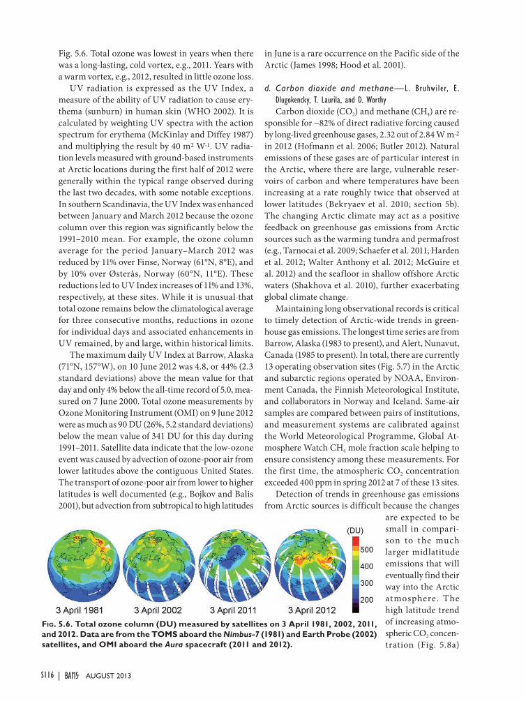
S116 | AUGUST 2013
Fig. 5.6. Total ozone was lowest in years when there was a long-lasting, cold vortex, e.g., 2011. Years with a warm vortex, e.g., 2012, resulted in little ozone loss.
UV radiation is expressed as the UV Index, a measure of the ability of UV radiation to cause ery-thema (sunburn) in human skin (WHO 2002). It is calculated by weighting UV spectra with the action spectrum for erythema (McKinlay and Diffey 1987) and multiplying the result by 40 m2 W-1. UV radia-tion levels measured with ground-based instruments at Arctic locations during the first half of 2012 were generally within the typical range observed during the last two decades, with some notable exceptions. In southern Scandinavia, the UV Index was enhanced between January and March 2012 because the ozone column over this region was significantly below the 1991–2010 mean. For example, the ozone column average for the period January–March 2012 was reduced by 11% over Finse, Norway (61°N, 8°E), and by 10% over Østerås, Norway (60°N, 11°E). These reductions led to UV Index increases of 11% and 13%, respectively, at these sites. While it is unusual that total ozone remains below the climatological average for three consecutive months, reductions in ozone for individual days and associated enhancements in UV remained, by and large, within historical limits.
The maximum daily UV Index at Barrow, Alaska (71°N, 157°W), on 10 June 2012 was 4.8, or 44% (2.3 standard deviations) above the mean value for that day and only 4% below the all-time record of 5.0, mea-sured on 7 June 2000. Total ozone measurements by Ozone Monitoring Instrument (OMI) on 9 June 2012 were as much as 90 DU (26%, 5.2 standard deviations) below the mean value of 341 DU for this day during 1991–2011. Satellite data indicate that the low-ozone event was caused by advection of ozone-poor air from lower latitudes above the contiguous United States. The transport of ozone-poor air from lower to higher latitudes is well documented (e.g., Bojkov and Balis 2001), but advection from subtropical to high latitudes
in June is a rare occurrence on the Pacific side of the Arctic (James 1998; Hood et al. 2001).
d. Carbon dioxide and methane— L . Bruhwi ler, E. Dlugokencky, T. Laurila, and D. WorthyCarbon dioxide (CO2) and methane (CH4) are re-
sponsible for ~82% of direct radiative forcing caused by long-lived greenhouse gases, 2.32 out of 2.84 W m-2 in 2012 (Hofmann et al. 2006; Butler 2012). Natural emissions of these gases are of particular interest in the Arctic, where there are large, vulnerable reser-voirs of carbon and where temperatures have been increasing at a rate roughly twice that observed at lower latitudes (Bekryaev et al. 2010; section 5b). The changing Arctic climate may act as a positive feedback on greenhouse gas emissions from Arctic sources such as the warming tundra and permafrost (e.g., Tarnocai et al. 2009; Schaefer et al. 2011; Harden et al. 2012; Walter Anthony et al. 2012; McGuire et al. 2012) and the seafloor in shallow offshore Arctic waters (Shakhova et al. 2010), further exacerbating global climate change.
Maintaining long observational records is critical to timely detection of Arctic-wide trends in green-house gas emissions. The longest time series are from Barrow, Alaska (1983 to present), and Alert, Nunavut, Canada (1985 to present). In total, there are currently 13 operating observation sites (Fig. 5.7) in the Arctic and subarctic regions operated by NOAA, Environ-ment Canada, the Finnish Meteorological Institute, and collaborators in Norway and Iceland. Same-air samples are compared between pairs of institutions, and measurement systems are calibrated against the World Meteorological Programme, Global At-mosphere Watch CH4 mole fraction scale helping to ensure consistency among these measurements. For the first time, the atmospheric CO2 concentration exceeded 400 ppm in spring 2012 at 7 of these 13 sites.
Detection of trends in greenhouse gas emissions from Arctic sources is difficult because the changes
are expected to be small in compari-son to t he much larger midlatitude emissions that will eventually find their way into the Arctic atmosphere. The high latitude trend of increasing atmo-spheric CO2 concen-tration (Fig. 5.8a)
Fig. 5.6. Total ozone column (DU) measured by satellites on 3 April 1981, 2002, 2011, and 2012. Data are from the TOMS aboard the Nimbus-7 (1981) and Earth Probe (2002) satellites, and OMI aboard the Aura spacecraft (2011 and 2012).
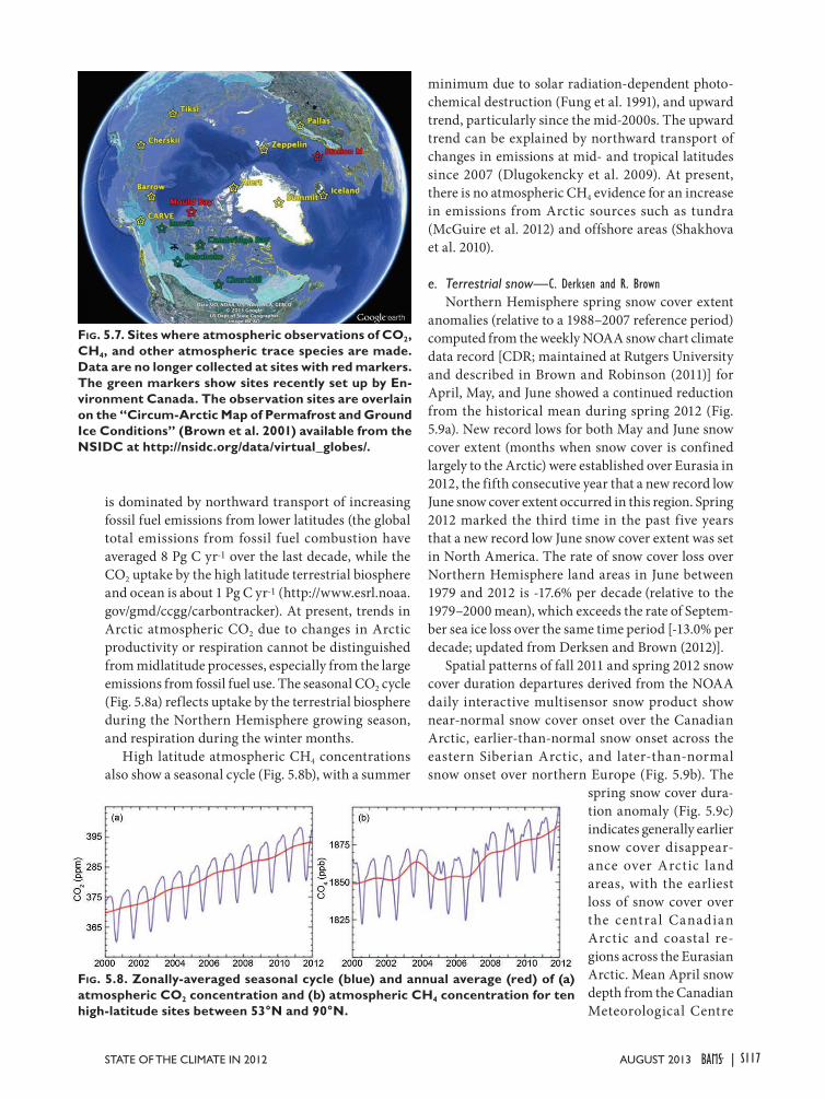
S117STATE OF THE CLIMATE IN 2012 |AUGUST 2013
is dominated by northward transport of increasing fossil fuel emissions from lower latitudes (the global total emissions from fossil fuel combustion have averaged 8 Pg C yr-1 over the last decade, while the CO2 uptake by the high latitude terrestrial biosphere and ocean is about 1 Pg C yr-1 (http://www.esrl.noaa.gov/gmd/ccgg/carbontracker). At present, trends in Arctic atmospheric CO2 due to changes in Arctic productivity or respiration cannot be distinguished from midlatitude processes, especially from the large emissions from fossil fuel use. The seasonal CO2 cycle (Fig. 5.8a) reflects uptake by the terrestrial biosphere during the Northern Hemisphere growing season, and respiration during the winter months.
High latitude atmospheric CH4 concentrations also show a seasonal cycle (Fig. 5.8b), with a summer
minimum due to solar radiation-dependent photo-chemical destruction (Fung et al. 1991), and upward trend, particularly since the mid-2000s. The upward trend can be explained by northward transport of changes in emissions at mid- and tropical latitudes since 2007 (Dlugokencky et al. 2009). At present, there is no atmospheric CH4 evidence for an increase in emissions from Arctic sources such as tundra (McGuire et al. 2012) and offshore areas (Shakhova et al. 2010).
e. Terrestrial snow—C. Derksen and R. BrownNorthern Hemisphere spring snow cover extent
anomalies (relative to a 1988–2007 reference period) computed from the weekly NOAA snow chart climate data record [CDR; maintained at Rutgers University and described in Brown and Robinson (2011)] for April, May, and June showed a continued reduction from the historical mean during spring 2012 (Fig. 5.9a). New record lows for both May and June snow cover extent (months when snow cover is confined largely to the Arctic) were established over Eurasia in 2012, the fifth consecutive year that a new record low June snow cover extent occurred in this region. Spring 2012 marked the third time in the past five years that a new record low June snow cover extent was set in North America. The rate of snow cover loss over Northern Hemisphere land areas in June between 1979 and 2012 is -17.6% per decade (relative to the 1979–2000 mean), which exceeds the rate of Septem-ber sea ice loss over the same time period [-13.0% per decade; updated from Derksen and Brown (2012)].
Spatial patterns of fall 2011 and spring 2012 snow cover duration departures derived from the NOAA daily interactive multisensor snow product show near-normal snow cover onset over the Canadian Arctic, earlier-than-normal snow onset across the eastern Siberian Arctic, and later-than-normal snow onset over northern Europe (Fig. 5.9b). The
spring snow cover dura-tion anomaly (Fig. 5.9c) indicates generally earlier snow cover disappear-ance over Arctic land areas, with the earliest loss of snow cover over the centra l Canadian Arctic and coastal re-gions across the Eurasian Arctic. Mean April snow depth from the Canadian Meteorological Centre
Fig. 5.8. Zonally-averaged seasonal cycle (blue) and annual average (red) of (a) atmospheric CO2 concentration and (b) atmospheric CH4 concentration for ten high-latitude sites between 53°N and 90°N.
Fig. 5.7. Sites where atmospheric observations of CO2, CH4, and other atmospheric trace species are made. Data are no longer collected at sites with red markers. The green markers show sites recently set up by En-vironment Canada. The observation sites are overlain on the “Circum-Arctic Map of Permafrost and Ground Ice Conditions” (Brown et al. 2001) available from the NSIDC at http://nsidc.org/data/virtual_globes/.

S118 | AUGUST 2013
daily gridded global snow depth analysis (Brasnett 1999) shows large regions of positive April snow depth anomalies over both the North American and Eur-asian Arctic (Fig. 5.9d). This suggests the record setting loss of spring snow cover in 2012 was driven by rapid snow ablation rather than anomalously low snow accumulation.
Estimates of historical variability in pan-Arctic maximum seasonal snow water equivalent (SWEmax) anomalies over land for 1980–2012 were calculated by averaging anomalies f rom four datasets: (1) GlobSnow, an assimilation of surface observations of snow depth and satellite retrievals from passive mi-crowave data (Takala et al. 2011); (2) a gridded global snow depth analysis based on optimal interpolation of surface snow depth ob-servations (Brasnett 1999; Brown et al. 2003); (3) a snow cover reconstruction driven with temperature and precipitation from the ERA-interim atmospher-ic reanalysis (Dee et al. 2011); and (4) diagnosed SWE from the MERRA reanalysis (Rienecker et al. 2011). The multidata-set anomaly time series for North America (Fig. 5.9e) shows decadal-scale vari-ability with no significant linear trend. The Eurasian SWEmax anomaly for 2012 is consistent with a step change to lower SWE ob-served since 2000.
Atmospheric circulation during the spring 2012 Arc-
Fig. 5.9. (a) Monthly Arctic snow cover extent standardized (and thus unitless) anomaly time series (with respect to 1988–2007) from the NOAA snow chart CDR for Apr, May, and Jun, 1967–2012 (solid lines denote 5-yr moving average); (b) and (c) Snow cover duration departures (with respect to 1998–2010) from the NOAA Interactive Multisensor Snow data record for the 2011 fall season and the 2012 spring season, respectively; (d) Apr 2012 snow depth anomaly (% of 1999–2010 average) from the CMC snow depth analysis; and (e) time series of multidataset average monthly SWEmax standardized anomalies (± the standard error) relative to 1988–2007 (solid lines denote 5-yr moving average).

S119STATE OF THE CLIMATE IN 2012 |AUGUST 2013
tic snow melt season was characterized by a strongly negative North Atlantic Oscillation (NAO) which reached a low of -2.25 in June (see section 5b). A negative NAO is associated with enhanced southerly air flow into the Arctic which contributes to warm temperature anomalies and rapid ablation of the snowpack. The only other year since 1950 to have a June NAO value lower than -2.0 was 1998 (Atkinson et al. 2006), when warm temperature anomalies were also present across Arctic land areas.
f. Glaciers and ice caps (outside Greenland)—G. Wolken, M. Sharp, M-L. Geai, D. Burgess, A. Arendt, and B. Wouters. With data contributions from J. G. Cogley and I. Sasgen. Mountain glaciers and ice caps cover an area
of over 400 000 km2 in the Arctic, and are a major contributor to global sea level change (Meier et al. 2007; Gardner et al. 2011; Jacob et al. 2012). They gain mass by snow accumulation, and lose mass by surface melt and runoff, and by iceberg calving where they terminate in water (ocean or lake). The climatic mass balance (Bclim, the difference between an-nual snow accumulation and annual runoff) is a widely used index of how glaciers respond to climate variability and change.
As Bclim measurements for the 2011/12 balance year are not yet available, we sum-marize measurements of 24 Arctic glaciers for 2010/11 (World Glacier Monitoring Service 2013). The glaciers are located in Alaska (three), Arctic Canada (four), Iceland (six), Svalbard (four), Nor-way (two), and Sweden (five) (Table 5.1). All but three of the glaciers (Dyngjujökull, Brúarjökull, and Eyjabak-kajökull in eastern Iceland) had a negative annual bal-ance (i.e., loss of ice mass). Mass balances of glaciers in Svalbard and northern Scan-dinavia were very negative in 2010/11. In the Canadian
Arctic, the 2010/11 balances were the most negative on record for all four glaciers. In this region, between five and nine of the most negative mass balance years in the 49–52 year record have occurred since 2000. The mean annual mass balance for the period 2000/11 is between three (Melville South Ice Cap) and eight (Meighen Ice Cap) times as negative as the 1963–99 average for each ice cap. This is a result of strong summer warming over the region that began around 1987 (Gardner and Sharp 2007) and acceler-ated significantly after 2005 (Sharp et al. 2011). For the monitored Arctic glaciers as a whole, mass bal-ance year 2010/11 continues a trend of increasingly negative cumulative balances (Fig. 5.10).
Trends of increasingly negative cumulative bal-ances are also evident in regional total mass balance estimates (ΔM, which includes mass losses by iceberg
Table 5.1. Measured annual climatic mass balances (Bclim) of glaciers in Alaska, the Canadian Arctic, Iceland, Svalbard, Norway, and Sweden for 2009/10 and 2010/11. Mass balance data for all glaciers are from the World Glacier Monitoring Service (2013).
Region Glacier Length of Record (yr)
Net Balance 2009/10
(kg m-2 yr-1)
Net Balance 2010/11
(kg m-2 yr-1)Alaska Wolverine 46 -85 -1070
Lemon Creek 59 -580 -720Gulkana 46 -1832 -1290
Arctic-Canada Devon Ice Cap 51 -417 -683
Meighen Ice Cap
50 -387 -1310
Melville S. Ice Cap
49 -939 -1339
White 49 -188 -983
IcelandLangjökull S. Dome
15 -3800 -1279
Hofsjökull E 21 -2830Hofsjökull N 22 -2400Hofsjökull SW 21 -3490Köldukvislarjökull 19 -2870 -754Tungnaarjökull 20 -3551 -1380Dyngjujökull 14 -1540 +377Brúarjökull 19 -1570 +515Eyjabakkajökull 20 -1750 +525
Svalbard Midre Lovenbreen 44 -200 -920Austre Brogger-breen
45 -440 -1004
Kongsvegen 25 +130 -434Hansbreen 23 -14 -280
Norway Engabreen 42 -520 -910Langfjordjøkulen 21 -760 -1257
Sweden Marmaglaciaren 22 -500 -1450Rabots Glaciar 30 -1080 -2110Riukojietna 25 -960 -1080Storglaciaren 66 -690 -1060Tarfalaglaciaren 17 -1060 -1820

S120 | AUGUST 2013
calving), derived using GRACE satellite gravimetry (Fig. 5.11). Available for the 2011/12 balance year, estimated ΔM of all the glaciers and ice caps in the Canadian Arctic Archipelago (CAA) was -106 ± 27 Gt, while in the Gulf of Alaska region ΔM was +51.9 ± 16.3 Gt. The CAA estimate matches the record negative value of the previous year (2010/11), and the Gulf of Alaska region estimate is the most positive for the region during the GRACE observation period,
2003–12 (Fig. 5.11). The higher rates of mass loss in the CAA (Fig. 5.11), and the strongly negative Bclim values reported in the previous paragraph, confirm the growing importance of glaciers and ice caps in this region as contributors to global sea level rise (Gardner et al. 2011).
Variability in mean summer temperature accounts for much of the interannual variability in Bclim in cold, dry regions like the Canadian high Arctic while, in more maritime regions, like Iceland and the Gulf of Alaska region, variability in winter precipitation is also a factor. Land surface temperature (LST) over ice in summer may serve as a proxy for Bclim of gla-ciers across the Arctic. Moderate to large positive LST anomalies over glaciers and ice caps occurred throughout the Arctic during summer 2012, particu-larly in the Canadian high Arctic (Fig. 5.12). Summer mean LSTs in 2012 were the warmest in the 13-year record on northern Ellesmere and Agassiz ice caps—exceeding the record set the previous year—and the second warmest on the Axel Heiberg Island, Prince of Wales (eastern Ellesmere Island), and Penny (south-ern Baffin Island) ice caps. Elsewhere in the Arctic, summer mean LSTs in 2012 equaled the 2011 record on Franz Josef Land, and were the second and fourth warmest in Severnaya Zemlya and Novaya Zemlya, respectively. In contrast, 2012 summer mean LSTs were only the eighth warmest in the 13-year long record in Iceland and the tenth warmest in southern Alaska (Fig. 5.12), where Bclim and ΔM, respectively, were positive.
Data from the NCEP/NCAR R1 reanalysis were also used as indicators of climatic conditions over the major glaciated regions of the Arctic during the 2011/12 mass balance year. Relative to the 1948–2008
Fig. 5.10. Mean annual climatic mass balance (Bclim) from 1989 to 2011 (red) and cumulative climatic mass balance relative to 1989 (blue) based on available an-nual measurements (count) for 24 glaciers monitored in the Arctic (World Glacier Monitoring Service 2013).
Fig 5.12. Comparison of 2010, 2011, and 2012 summer mean land surface temperature (LST) anomalies (rela-tive to 2000–10) for 16 glaciated regions of the Arctic based on the MODIS MOD11A2 LST product (ORNL DAAC 2010).
Fig. 5.11. Cumulative mass balances of Canadian Arctic Archipelago (CAA) and Gulf of Alaska region (GoA) glaciers, determined from the GRACE satellites. CAA data are unpublished estimates derived from monthly Stokes coefficients from the Center for Space Re-search fifth release (CSR RL5) and processed following methods in Gardner et al. (2011) and Wouters and Sch-rama (2007). The GoA data are unpublished estimates updated from Sasgen et al. (2012) and derived from a composite of monthly Stokes coefficients from the CSR, the Jet Propulsion Laboratory, and the German Research Center for Geosciences processing centers.
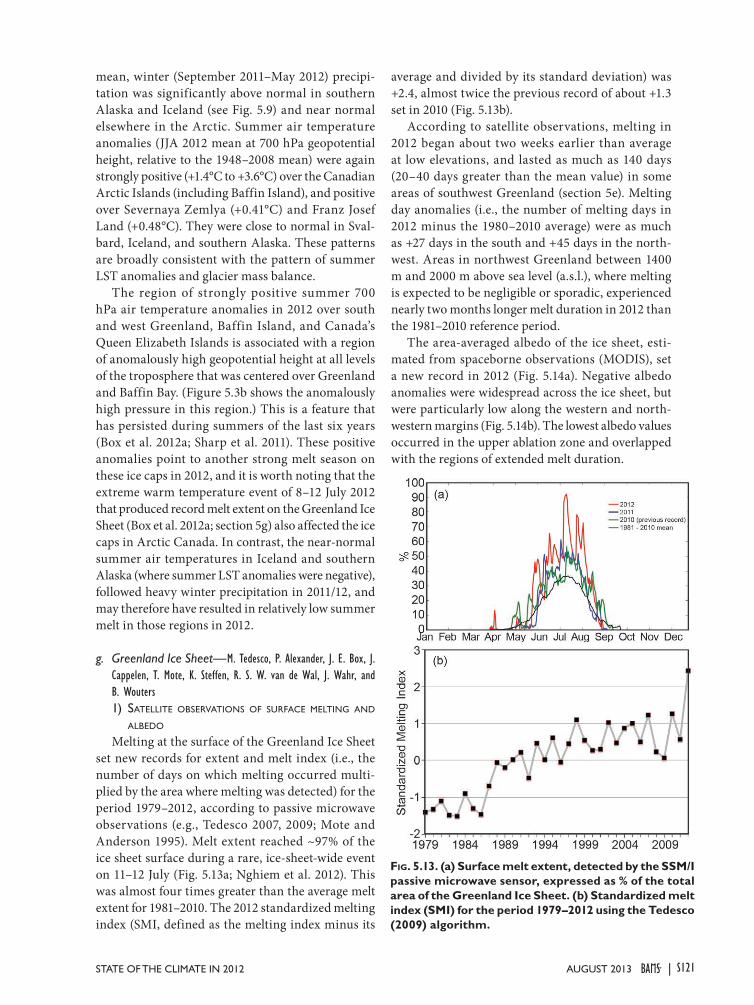
S121STATE OF THE CLIMATE IN 2012 |AUGUST 2013
mean, winter (September 2011–May 2012) precipi-tation was significantly above normal in southern Alaska and Iceland (see Fig. 5.9) and near normal elsewhere in the Arctic. Summer air temperature anomalies (JJA 2012 mean at 700 hPa geopotential height, relative to the 1948–2008 mean) were again strongly positive (+1.4°C to +3.6°C) over the Canadian Arctic Islands (including Baffin Island), and positive over Severnaya Zemlya (+0.41°C) and Franz Josef Land (+0.48°C). They were close to normal in Sval-bard, Iceland, and southern Alaska. These patterns are broadly consistent with the pattern of summer LST anomalies and glacier mass balance.
The region of strongly positive summer 700 hPa air temperature anomalies in 2012 over south and west Greenland, Baffin Island, and Canada’s Queen Elizabeth Islands is associated with a region of anomalously high geopotential height at all levels of the troposphere that was centered over Greenland and Baffin Bay. (Figure 5.3b shows the anomalously high pressure in this region.) This is a feature that has persisted during summers of the last six years (Box et al. 2012a; Sharp et al. 2011). These positive anomalies point to another strong melt season on these ice caps in 2012, and it is worth noting that the extreme warm temperature event of 8–12 July 2012 that produced record melt extent on the Greenland Ice Sheet (Box et al. 2012a; section 5g) also affected the ice caps in Arctic Canada. In contrast, the near-normal summer air temperatures in Iceland and southern Alaska (where summer LST anomalies were negative), followed heavy winter precipitation in 2011/12, and may therefore have resulted in relatively low summer melt in those regions in 2012.
g. Greenland Ice Sheet—M. Tedesco, P. Alexander, J. E. Box, J. Cappelen, T. Mote, K. Steffen, R. S. W. van de Wal, J. Wahr, and B. Wouters1) satellite observations of surface Melting and
albedo
Melting at the surface of the Greenland Ice Sheet set new records for extent and melt index (i.e., the number of days on which melting occurred multi-plied by the area where melting was detected) for the period 1979–2012, according to passive microwave observations (e.g., Tedesco 2007, 2009; Mote and Anderson 1995). Melt extent reached ~97% of the ice sheet surface during a rare, ice-sheet-wide event on 11–12 July (Fig. 5.13a; Nghiem et al. 2012). This was almost four times greater than the average melt extent for 1981–2010. The 2012 standardized melting index (SMI, defined as the melting index minus its
average and divided by its standard deviation) was +2.4, almost twice the previous record of about +1.3 set in 2010 (Fig. 5.13b).
According to satellite observations, melting in 2012 began about two weeks earlier than average at low elevations, and lasted as much as 140 days (20–40 days greater than the mean value) in some areas of southwest Greenland (section 5e). Melting day anomalies (i.e., the number of melting days in 2012 minus the 1980–2010 average) were as much as +27 days in the south and +45 days in the north-west. Areas in northwest Greenland between 1400 m and 2000 m above sea level (a.s.l.), where melting is expected to be negligible or sporadic, experienced nearly two months longer melt duration in 2012 than the 1981–2010 reference period.
The area-averaged albedo of the ice sheet, esti-mated from spaceborne observations (MODIS), set a new record in 2012 (Fig. 5.14a). Negative albedo anomalies were widespread across the ice sheet, but were particularly low along the western and north-western margins (Fig. 5.14b). The lowest albedo values occurred in the upper ablation zone and overlapped with the regions of extended melt duration.
Fig. 5.13. (a) Surface melt extent, detected by the SSM/I passive microwave sensor, expressed as % of the total area of the Greenland Ice Sheet. (b) Standardized melt index (SMI) for the period 1979–2012 using the Tedesco (2009) algorithm.

S122 | AUGUST 2013
2) satellite observations of ice Mass loss
In 2012, new records for summertime and annual ice mass loss, as estimated from the GRACE satellite mission (e.g., Velicogna and Wahr 2006), occurred. Between June and August, the mass loss was -627 ± 89 Gt, 2 standard deviations below the 2003–12 mean of -414 Gt (Fig. 5.15; Tedesco et al. 2012). The previous
record mass loss, -516 ± 89 Gt, 0.8 standard devia-tion below the mean, occurred in 2010. The trend of summer mass change during 2003–12 is -29 ± 11 Gt yr−1. Excluding the mass loss in summer 2012, the trend is -20 ± 13 Gt yr−1. The annual mass loss from mid-September 2011 to mid-September 2012, -575 ± 89 Gt, 2 standard deviations below the mean, also set a new record, exceeding the previous record, set only two years earlier, by +152 Gt.
3) surface Mass balance observations along the K-transect
The original K-Transect is located in western Greenland near Kangerlussuaq at 67°N and between 340 m and 1500 m a.s.l. (van de Wal et al. 2005). During the period 1991–2012, 1500 m a.s.l. was the average equilibrium line altitude (ELA; i.e., the high-est altitude at which winter snow survives). In 2012, the ELA reached 2687 m a.s.l., 3.7 standard deviations above the mean (van de Wal et al. 2012). The surface mass balance in 2012, between 340 m and 1500 m a.s.l., was the second lowest since measurements began in 1991. However, a weighted mass balance that includes a site above the former 1500 m ELA indicates that the 2011/12 mass balance year was the most negative in 21 years. At the highest station in 2012, 1847 m, almost 350 m higher than the former ELA, the surface mass balance was estimated to be -0.74 m water equivalent. Below 1500 m elevation, surface mass balance values decreased gradually to normal values near the ice margin.
4) surface air teMperature observations
The extensive surface melting and ice mass loss observed in 2012 occurred in conjunction with record summer (June, July, and August: JJA) air temperatures. The ice sheet-wide JJA surface tem-perature estimated from space by MODIS increased Fig. 5.14. (a) Area-averaged albedo of the Greenland
Ice Sheet each Jul from 2000 to 2012, and (b) geo-graphic variability of the Jun–Aug 2012 albedo anomaly expressed as % of the mean anomaly of the 2000–11 reference period. All data are derived from MODIS MOD10A1 observations. Figures are after Box et al. (2012b).
Fig. 5.15. Cumulative mass anomaly in Gt of the Green-land Ice Sheet derived from GRACE satellite data between April 2002 and September 2012.

S123STATE OF THE CLIMATE IN 2012 |AUGUST 2013
3.4°C between 2000 and 2012, from an average value of -9°C in 2000 to -5.6°C in 2012 (Tedesco et al. 2012). Applying a linear fit, this suggests an increase in ice sheet-wide surface temperature of +0.16°C yr-1. Other than Tasiilaq, in southeast Greenland, where June 2012 was the coldest it had been since records began in 1895, record-setting warm JJA surface air temperatures occurred at long-term meteorological stations (records began in 1873) along the western and southern margins of the island and at the ice sheet summit. The Greenland Climate Network (GC-Net) automatic weather station at Summit (3199 m a.s.l.) measured hourly-mean air temperatures above 0°C for the first time since measurements began in 1996. Such a melt event is rare; the last significant event occurred in 1889, according to the analysis of ice core data (Nghiem et al. 2012).
Seasonally-averaged upper air temperature data available from twice-daily radiosonde observations show anomalous warmth throughout the troposphere in summer 2012 (section 5f). This is consistent with an overall warming pattern near the surface between 850 hPa and 1000 hPa. The recent warming trend is seen in the long-term air temperature reconstruction for the ice sheet, which also shows that mean annual air temperatures in all seasons are now higher than they have been since 1840 (Box et al. 2012a).
5) Marine-terMinating glaciers
Forty marine-terminating glaciers have been surveyed daily since 2000 using cloud-free MODIS visible imagery (Box and Decker 2011; http://bprc.osu.edu/MODIS/). The net area change of the 40 glaciers during the period of observation has been -1775 km2, with the 18 northernmost (>72°N) glaciers alone contributing to half of the net area change. In 2012, the northernmost glaciers lost a collective area of 255 km2, or 86% of the total net area change of the 40 glaciers surveyed. The six glaciers with the largest net area loss in 2012 were Petermann (-141 km2), 79 glacier (-27 km2), Zachariae (-26 km2), Steenstrup (-19 km2), Steensby (-16 km2, the greatest retreat since observations began), and Jakobshavn (-13 km2). While the total area change was negative in 2012, the area of four of the forty glaciers did increase relative to the end of the 2011 melt season. The anomalous advance of these four glaciers is not easily explained, as the mechanisms controlling the behavior of individual glaciers are uncertain due to their often unique geographic settings.
h. Permafrost—V. E. Romanovsky, A. L. Kholodov, S. L. Smith, H. H. Christiansen, N. I. Shiklomanov, D. S. Drozdov, N. G. Oberman, and S. S. MarchenkoSystematic observations of permafrost tempera-
ture at many sites in Alaska, Canada, and Russia since the middle of the 20th century provide several decades of continuous data, which allow decadal changes in permafrost temperatures to be assessed. A general increase in temperatures has been observed during the last several decades in Alaska, northern Canada, and Siberia (Smith et al. 2010; Romanovsky et al. 2010a,b). During the last four to five years, all these regions show similar temporal and spatial vari-ability of permafrost temperature. As illustrated for selected sites in Russia (Fig. 5.16), although tempera-ture has been generally increasing continuously in colder permafrost located close to the Arctic coasts (Romanovsky et al. 2012a), the temperatures of warmer permafrost in the continental interior have been relatively stable or even decreasing slightly. Permafrost temperature has increased by 1°C–2°C in northern Russia during the last 30 to 35 years, but this trend was interrupted by colder conditions in summer 2009 and winters 2009/10 and 2010/2011 at many locations in the Russian Arctic, especially in the western sector (Fig. 5.16). However, the warming trend resumed in 2012.
In 2012, new record high temperatures at 20-m depth were measured at most permafrost observato-ries on the North Slope of Alaska, i.e., north of the Brooks Range (Fig. 5.17a), where measurements began in the late 1970s. The exceptions were the coastal sites, West Dock, and Deadhorse (Fig. 5.17b), where tem-peratures in 2012 were the same as the record-high temperatures observed in 2011 (Fig. 5.17b). Changes in permafrost temperatures at 20-m depth are typi-cally lagging by one year compared to the changes in surface temperatures. The data suggest that a coastal warming trend has propagated southward towards the northern foothills of the Brooks Range, where a noticeable warming in the upper 20 m of permafrost has become evident since 2008 (Romanovsky et al. 2012b). Record high temperatures were also observed in 2012 in the Brooks Range (Chandalar Shelf) and in its southern foothills (Coldfoot). However, permafrost temperatures in Interior Alaska (e.g., Healy, Birch Lake, College Peat, and Old Man; Fig. 5.17c) were still decreasing in 2012. These distinct patterns of permafrost warming on the North Slope and a slight cooling in the Alaska Interior in 2010–11 are in good agreement with air temperature patterns observed in the Arctic and the sub-Arctic over the last five years
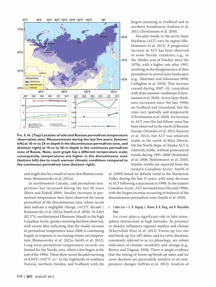
S124 | AUGUST 2013
and might also be a result of snow distribution varia-tions (Romanovsky et al. 2012a).
In northwestern Canada, cold permafrost tem-perature has increased during the last 40 years (Burn and Kokelj 2009). Smaller increases in per-mafrost temperature have been observed for warm permafrost of the discontinuous zone, where recent data indicate a negligible change, (<0.2°C decade-1; Romanovsky et al. 2012a; Smith et al. 2010). At Alert (82.5°N, northernmost Ellesmere Island) in the high Canadian Arctic, greater warming has been observed, with recent data indicating that the steady increase in permafrost temperature since 2000 is continuing largely in response to increasing winter air tempera-ture (Romanovsky et al. 2012a; Smith et al. 2012). Long-term permafrost temperature records are limited for the Nordic area, where a few began at the end of the 1990s. These show recent decadal warming of 0.04°C–0.07°C yr-1 in the highlands of southern Norway, northern Sweden, and Svalbard, with the
largest warming in Svalbard and in northern Scandinavia (Isaksen et al. 2011; Christiansen et al. 2010).
Decadal trends in the active layer thickness (ALT) vary by region (Shi-klomanov et al. 2012). A progressive increase in ALT has been observed in some Nordic countries, e.g., in the Abisko area of Sweden since the 1970s, with a higher rate after 1995, resulting in the disappearance of thin permafrost in several mire landscapes (e.g., Åkerman and Johansson 2008; Callaghan et al. 2010). This increase ceased during 2007–10, coincident with drier summer conditions (Chris-tiansen et al. 2010). Active layer thick-ness increased since the late 1990s on Svalbard and Greenland, but the rates vary spatially and temporarily (Christiansen et al. 2010). An increase in ALT over the last fifteen years has been observed in the north of Russian Europe (Drozdov et al. 2012; Kaverin et al. 2012), but ALT was relatively stable in the north of West Siberia. On the North Slope of Alaska ALT is relatively stable, without pronounced trends during 1995–2008 (Streletskiy et al. 2008; Shiklomanov et al. 2010). Similar results are reported from the western Canadian Arctic. Smith et
al. (2009) found no definite trend in the Mackenzie Valley during the last 15 years, with some decrease in ALT following a maximum in 1998. In the eastern Canadian Arctic, ALT increased since the mid-1990s, with the largest increase occurring in bedrock of the discontinuous permafrost zone (Smith et al. 2010).
i. Lake ice—C. R. Duguay, L. Brown, K.-K. Kang, and H. Kheyrollah PourIce cover plays a significant role in lake-atmo-
sphere interactions at high latitudes. Its presence or absence influences regional weather and climate (Kheyrollah Pour et al. 2012). Freeze-up (ice-on) and break-up (ice-off) dates, and ice cover duration, commonly referred to as ice phenology, are robust indicators of climate variability and change (e.g., Brown and Duguay 2010). There is ample evidence that the timing of freeze-up/break-up dates and ice cover duration are particularly sensitive to air tem-perature changes (Jeffries et al. 2012). Analysis of
Fig. 5.16. (Top) Location of selected Russian permafrost temperature observation sites. Measurements during the last five years: (bottom left) at 10-m to 24-m depth in the discontinuous permafrost zone, and (bottom right) at 10-m to 26-m depth in the continuous permafrost zone of Russia. Note, each graph has a different temperature scale; consequently, temperatures are higher in the discontinuous zone (bottom left) due to much warmer climatic conditions compared to the continuous permafrost zone (bottom right).

S125STATE OF THE CLIMATE IN 2012 |AUGUST 2013
for most lakes located in the southern portion of northern Europe. The positive North Atlan-tic Oscillation (NAO) of fall 2011 and winter 2012 (section 5b) was the likely cause for the late freeze-up in the latter re-gion and early freeze-up in the Canadian Arctic. A positive NAO is asso-ciated with higher tem-peratures over Europe and lower-than-normal values over northeastern Canada. The NAO has previously been shown to affect lake ice phe-nology in northeastern Canada, Scandinavia, and northwestern Rus-sia (Bonsal et al. 2006).
With few exceptions, break-up in 2012 occurred several days earlier in Arctic Canada and Eurasia compared to the 2004–11 mean (Fig. 5.18b). Break-up dates were, on average, as much as 3 weeks earlier throughout Arctic Canada and up to 1 month earlier in Eurasia. The few lakes that experienced later break-up (e.g., southern portion of northern Europe) showed small deviations from the mean (1 week on average). The earlier break-up in eastern Siberia and much of Arctic Canada is consis-tent with the record-low June 2012 snow cover extent (section 5e). The strong negative NAO of spring and summer 2012 (section 5b), which promoted southerly air flow into the Arctic, had a significant impact on lake ice break-up dates and other components of the cryosphere (sections 5e, 5g).
Compared to the 2004–11 mean, ice cover duration in 2011/12 was ~2–5 weeks shorter in central Arctic Canada, western Siberia, southern Scandinavia, and parts of northwestern Russia. On the other hand, ice cover duration was 1–4 weeks longer in eastern Arctic Canada (i.e., Baffin Island and both sides of near-coastal regions of northern Hudson Bay) and 1–8 weeks longer in Norway (Fig. 5.18c). Longer ice cover duration in the northeastern Canadian Arc-tic and shorter ice duration in northern Eurasia is typically associated with positive phases of the NAO (Prowse et al. 2011).
limited in situ and satellite records (1950s–2004) from northern Canada shows increasingly later freeze-up and earlier break-up dates and, consequently, shorter ice cover duration (Duguay et al. 2006; Latifovic and Pouliot 2007). Although ice cover duration over the Arctic has decreased significantly, largely in response to increasingly warmer conditions during the 20th century, the patterns have varied regionally, primar-ily due to climate impacts associated with large-scale atmospheric and oceanic oscillations (e.g. Prowse et al. 2011). Ice year 2011/12 provides a good illustration of the influence of teleconnection patterns on the ice regime of Arctic lakes.
Freeze-up and break-up dates, and ice cover dura-tion were derived at the grid-cell level for the largest lakes of the Arctic (4 km × 4 km or larger) using the NOAA Interactive Multisensor Snow and Ice Map-ping System 4 km resolution daily product (National Ice Center 2008) for the complete length of the avail-able record (2004–12). (See Helfrich et al. 2007 for details). Freeze-up, break-up, and ice cover duration anomalies (expressed as number of days) between ice year 2011/12 and mean conditions for the reference period 2004–10 were then calculated.
Freeze-up in 2011/12 was earlier than the 2004–11 mean by 10–30 days in eastern and part of central Arctic Canada, Norway, and eastern Siberia (Fig. 5.18a). Freeze-up occurred almost a full month later
Fig. 5.17. (a) Map of Alaska showing the continuous and discontinuous permafrost zones (separated by the broken blue line) and location of a north-south transect of permafrost temperature measurement sites; (b) and (c) time series of mean annual temperature at depths 20 m and 15 m below the surface, respectively.

S126 | AUGUST 2013
j. Sea ice cover—D. K. Perovich, W. Meier, M. Tschudi, S. Gerland, and J. Richter-Menge1) sea ice extent
There is an accurate record of sea ice extent de-termined from satellite-based passive microwave instruments since 1979. There are two months each year that are of particular interest: September, at the end of summer, when the ice reaches its annual mini-mum extent, and March, at the end of winter, when the ice is at its maximum extent. Ice extent in March 2012 and September 2012 are illustrated in Fig. 5.19.
Based on estimates by the National Snow and Ice Data Center, on 16 September 2012, the sea ice cover reached its minimum extent for the year of 3.41 mil-lion km2. This was the lowest in the satellite record, 18% lower than in 2007, when the previous record of 4.17 million km2 was recorded (Fig. 5.20). Overall, the 2012 minimum was 3.29 million km2 (49%) be-low the 1979–2000 average minimum of 6.71 million km2. The last six years, 2007–12, have the six lowest minimum extents since satellite observations began.
In March 2012 ice extent reached a maximum value of 15.24 million km2 (Fig. 5.20), 4% below the 1979–2000 average. Although this was the highest maximum in nine years, the period 2004–12 has the nine lowest maximum extents since 1979. The relatively large maximum extent in March 2012 was due to conditions in the Bering Sea, where ice extent was at or near record levels throughout the winter and spring.
After reaching maximum extent, the seasonal de-cline began slowly, particularly in the Bering Sea, and around mid-April extent was close to the 1979–2000
Fig. 5.18. (a) Freeze-up, (b) break-up, and (c) ice cover duration anomalies in 2011/12 relative to the 2004–11 reference period from the NOAA Interactive Multi-sensor Snow and Ice Mapping System 4 km product.
Fig. 5.19. Sea ice extent (in white) in Mar 2012 and Sep 2012, the winter maximum and summer minimum, respectively. The magenta line shows the median maximum and minimum ice extents in Mar and Sep for the period 1979–2000. (Source: NSIDC Sea Ice Index, http://nsidc.org/data/seaice_index.)

S127STATE OF THE CLIMATE IN 2012 |AUGUST 2013
average for the time of year. However, soon after that the decline accelerated and was faster than any sum-mer retreat on record. August 2012 was a period of particularly rapid ice loss, in part due to the cyclone that passed through the region at the beginning of the month (Sidebar 5.1). Overall, 11.83 million km2 of ice was lost between the maximum and minimum ex-tents. This is the largest seasonal decline in the record and 1 million km2 less ice than in any previous year.
Sea ice extent has decreasing trends in all months and virtually all regions (the exception being the Bering Sea during winter). The September monthly average trend is now -91 600 km2 per year or -13.0% per decade relative to the 1979–2000 average (Fig. 5.20). The magnitude of the trend has increased every year since 2001. Trends are smaller during March, but still decreasing and statistically significant. The March trend is -2.6% per decade.
Four time periods of the average ice extent for each month are compared in Fig. 5.21: the reference period 1979–2000, 2001–06, the last six years (2007–12) be-ginning with the previous record minimum of 2007, and 2012. The 1979–2000 period has the largest ice extent for every month, with the greatest difference between the time periods occurring in September. Comparing the two 21st century periods shows that ice extent is similar in winter and spring, but summer values are significantly lower in 2007–12. Figure 5.21 also emphasizes how extreme the ice retreat was in summer 2012.
2) spatial distribution of sea ice
In 2007, when the previous record minimum extent occurred, persistent winds through the sum-
mer, created by an Arctic dipole circulation pattern (see Arctic Report Card 2007, figure A3), resulted in a compact ice cover and an ice edge far to the north on the Pacific side of the Arctic. However, the circula-tion also pushed ice onto the coast in the Laptev Sea, completely blocking the Northern Sea Route. In the years since 2007, the pattern of ice loss has varied, but a tongue of older ice in the East Siberian Sea has persisted through the summer (Fig. 5.22). This tongue was particularly evident in 2010 and 2011. In 2012, that tongue of ice mostly melted away, aided by the August storm (Sidebar 5.1), and ice retreated significantly around the entire perimeter of the ice pack (Fig. 5.19, right). This includes the Atlantic side, north of Svalbard, where extents had been near nor-mal in recent years. Overall, compared to 2007 there was more ice in 2012 in the central Arctic north of the Bering Strait, but less ice nearly everywhere else.
A major storm that moved across the Arctic Basin in early August 2012 (Sidebar 5.1) accelerated ice loss in the Chukchi and East Siberian Seas and helped to quickly remove ice from the region. The storm blew the mostly first-year ice southward into warmer water, where satellite observations indicated that it melted in a few weeks (Parkinson and Comiso 2013). As the ice melted and diverged, ice concentration quickly fell below the detection limit of passive microwave sensors, though small amounts of ice were observed for a couple of weeks afterwards by operational ice analysts using other imagery.
3) sea ice age
The age of the ice is another key descriptor of the state of the sea ice cover. Older ice tends to be thicker
Fig. 5.20. Time series of ice extent anomalies in Mar (the month of ice extent maximum) and Sep (the month of ice extent minimum) in % relative to the mean value for 1979–2000. The black and red lines are least squares linear regression lines with slopes indicating ice losses of -2.6% and -13.0% per decade in Mar and Sep, respectively.
Fig. 5.21. Mean monthly sea ice extent for 2012 and three periods: the reference period 1979–2000, 2001–06, and 2007–12. The vertical bars represent one std dev about the mean value for each month.
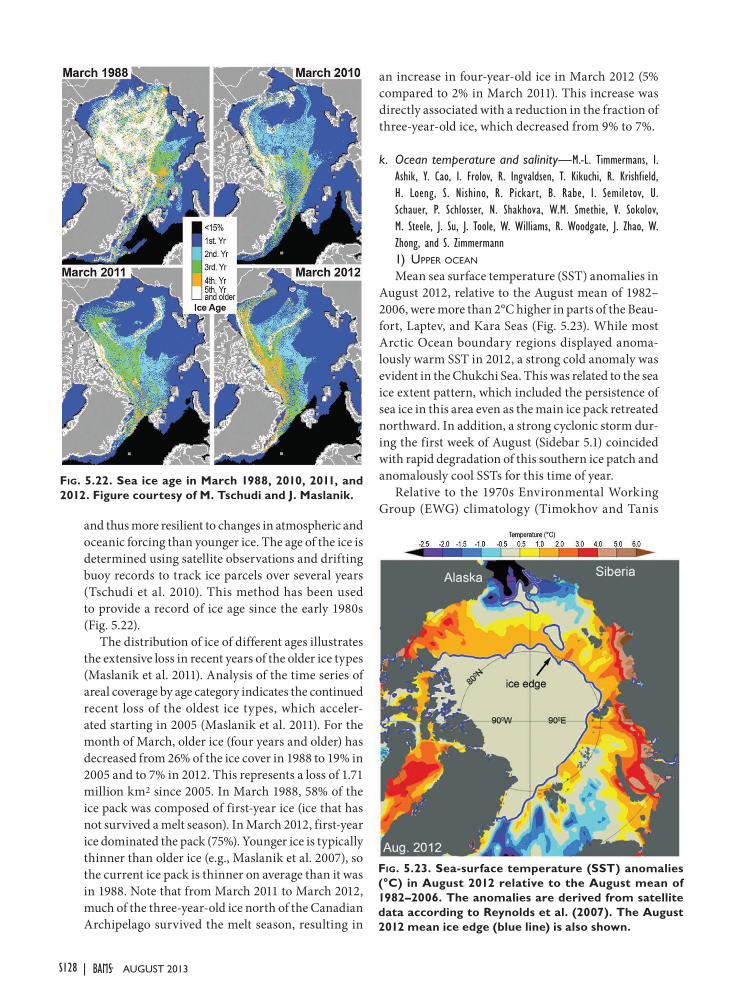
S128 | AUGUST 2013
and thus more resilient to changes in atmospheric and oceanic forcing than younger ice. The age of the ice is determined using satellite observations and drifting buoy records to track ice parcels over several years (Tschudi et al. 2010). This method has been used to provide a record of ice age since the early 1980s (Fig. 5.22).
The distribution of ice of different ages illustrates the extensive loss in recent years of the older ice types (Maslanik et al. 2011). Analysis of the time series of areal coverage by age category indicates the continued recent loss of the oldest ice types, which acceler-ated starting in 2005 (Maslanik et al. 2011). For the month of March, older ice (four years and older) has decreased from 26% of the ice cover in 1988 to 19% in 2005 and to 7% in 2012. This represents a loss of 1.71 million km2 since 2005. In March 1988, 58% of the ice pack was composed of first-year ice (ice that has not survived a melt season). In March 2012, first-year ice dominated the pack (75%). Younger ice is typically thinner than older ice (e.g., Maslanik et al. 2007), so the current ice pack is thinner on average than it was in 1988. Note that from March 2011 to March 2012, much of the three-year-old ice north of the Canadian Archipelago survived the melt season, resulting in
an increase in four-year-old ice in March 2012 (5% compared to 2% in March 2011). This increase was directly associated with a reduction in the fraction of three-year-old ice, which decreased from 9% to 7%.
k. Ocean temperature and salinity—M.-L. Timmermans, I. Ashik, Y. Cao, I. Frolov, R. Ingvaldsen, T. Kikuchi, R. Krishfield, H. Loeng, S. Nishino, R. Pickart, B. Rabe, I. Semiletov, U. Schauer, P. Schlosser, N. Shakhova, W.M. Smethie, V. Sokolov, M. Steele, J. Su, J. Toole, W. Williams, R. Woodgate, J. Zhao, W. Zhong, and S. Zimmermann1) upper ocean Mean sea surface temperature (SST) anomalies in
August 2012, relative to the August mean of 1982–2006, were more than 2°C higher in parts of the Beau-fort, Laptev, and Kara Seas (Fig. 5.23). While most Arctic Ocean boundary regions displayed anoma-lously warm SST in 2012, a strong cold anomaly was evident in the Chukchi Sea. This was related to the sea ice extent pattern, which included the persistence of sea ice in this area even as the main ice pack retreated northward. In addition, a strong cyclonic storm dur-ing the first week of August (Sidebar 5.1) coincided with rapid degradation of this southern ice patch and anomalously cool SSTs for this time of year.
Relative to the 1970s Environmental Working Group (EWG) climatology (Timokhov and Tanis
Fig. 5.22. Sea ice age in March 1988, 2010, 2011, and 2012. Figure courtesy of M. Tschudi and J. Maslanik.
Fig. 5.23. Sea-surface temperature (SST) anomalies (°C) in August 2012 relative to the August mean of 1982–2006. The anomalies are derived from satellite data according to Reynolds et al. (2007). The August 2012 mean ice edge (blue line) is also shown.

S129STATE OF THE CLIMATE IN 2012 |AUGUST 2013
1997), the major upper-ocean salinity differences in 2012 (Fig. 5.24a) were saltier waters in the central Eurasian Basin and a fresher Canada Basin in general. The upper waters of the Barents and Kara Seas were predominantly anomalously salty relative to climatol-ogy, although the magnitude of the salinity difference was smaller than in the central Arctic Basin. In the re-gion to the north of Greenland and Ellesmere Island, upper-ocean salinity in 2012 was only slightly less than the 1970s climatology, although small changes can be attributed in part to gaps in sampling.
The maximum freshwater content anomaly is cen-tered in the Beaufort Gyre (BG), Canada Basin (Fig. 5.24c). The BG accumulated more than 5000 km3 of freshwater during 2003–12, a gain of approximately 25% (update to Proshutinsky et al. 2009) relative to climatology of the 1970s (Fig. 5.24b). In 2012, the BG freshwater content was comparable to that in 2011, although 2012 saw a shift in the center of freshwater content to the northwest relative to 2011, consistent with the large-scale wind forcing (see Timmermans et al. 2012, figures 2.7, 2.11). The strong freshwater accumulation trend in the Beaufort Gyre has been linked to an increase in strength over the past decade of the large-scale anticyclonic wind forcing (e.g., Proshutinsky et al. 2009). Shifts in major freshwater
pathways also influence BG freshwater (Morison et al. 2012), while freshwater transported offshore during storms in the southern Beaufort Sea can also ac-count for a significant fraction of the observed year-to-year variability in freshwater content of the BG (Pickart et al. 2013). The BG heat content in 2012 (see Timmermans et al. 2012, figure 2.11) also remained approximately com-parable to 2011 conditions, with ~25% more heat on average in the summer compared to the 1970s.
2) atlantic water layer
Warm water of North Atlantic origin, lying below the halocline at depths between about 200 m and 900 m (shallower in the vicinity of Fram Strait), is characterized by tem-peratures >0°C and salinities >34.5. In 2012 in the southern Barents Sea, Atlantic Water temperatures reached a maximum (since 1951) of up to 6°C, about 1.4°C higher than the long-term mean (1951–2010) and about 1.2°C
higher than in 2011 (Trofimov and Ingvaldsen 2012). In other regions, no significant changes were observed in 2012 in this layer compared to 2011 conditions. Relative to 1970s climatology, maximum Atlantic Water temperature anomalies are high-est on the Eurasian side of the Lomonosov Ridge, with maximum anomalies 2°C in Fram Strait (see Proshutinsky et al. 2012, figure 5.22b). Warming is less pronounced in the Canada Basin, with Atlantic Water cooler now than in the 1970s in the region to the north of Ellesmere Island.
3) pacific water layer
The Pacific Water layer in the Arctic Ocean originates from the Bering Strait inflow and resides in the Canada Basin at depths between about 50 m and 150 m. Data from ice-tethered profilers that sampled in the central Canada Basin during 2004–12 indicate Pacific Water warming in recent years that is broadly congruent with freshening. The maximum temperature of the Pacific Water layer increased by about 1.5°C over this time, with corresponding in-creases in heat content.
In 2011, the most recent year for which data are avail-able, Pacific Water inflow through the Bering Strait was about 1.1 Sv (Woodgate et al. 2012), significantly
Fig. 5.24. (a) Anomalies of salinity at 20-m depth in 2012 relative to 1970s climatology. Contour lines show the 500-m and 2500-m isobaths. (b, c) Freshwater content (m) calculated relative to a ref-erence salinity of 34.8: (b) freshwater content in the Arctic Ocean based on 1970s climatology (Timokhov and Tanis 1997); (c) freshwa-ter content in the Beaufort Gyre (the region enclosed by the black box in the top panel) based on hydrographic surveys (black dots depict station locations) in 2012.
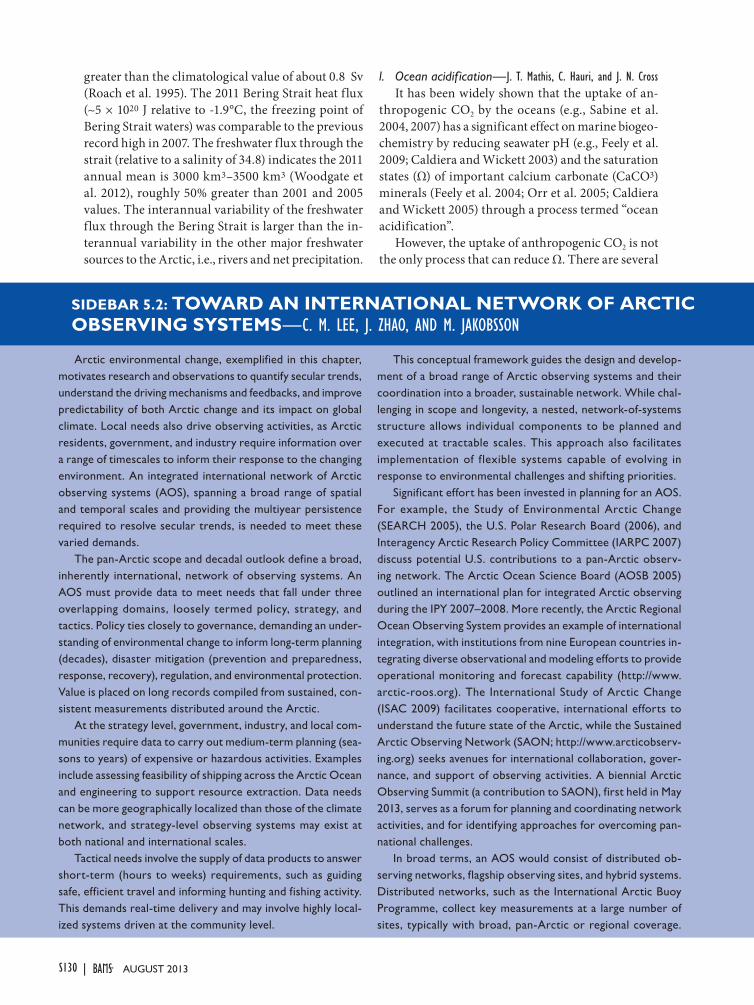
S130 | AUGUST 2013
greater than the climatological value of about 0.8 Sv (Roach et al. 1995). The 2011 Bering Strait heat flux (~5 × 10²⁰ J relative to -1.9°C, the freezing point of Bering Strait waters) was comparable to the previous record high in 2007. The freshwater flux through the strait (relative to a salinity of 34.8) indicates the 2011 annual mean is 3000 km3–3500 km3 (Woodgate et al. 2012), roughly 50% greater than 2001 and 2005 values. The interannual variability of the freshwater flux through the Bering Strait is larger than the in-terannual variability in the other major freshwater sources to the Arctic, i.e., rivers and net precipitation.
l. Ocean acidif ication—J. T. Mathis, C. Hauri, and J. N. CrossIt has been widely shown that the uptake of an-
thropogenic CO2 by the oceans (e.g., Sabine et al. 2004, 2007) has a significant effect on marine biogeo-chemistry by reducing seawater pH (e.g., Feely et al. 2009; Caldiera and Wickett 2003) and the saturation states (Ω) of important calcium carbonate (CaCO3) minerals (Feely et al. 2004; Orr et al. 2005; Caldiera and Wickett 2005) through a process termed “ocean acidification”.
However, the uptake of anthropogenic CO2 is not the only process that can reduce Ω. There are several
SIDEBAR 5.2: TOWARD AN INTERNATIONAL NETWORk OF ARCTIC OBSERVING SySTEMS—C. M. LEE, J. ZHAO, AND M. JAKOBSSON
Arctic environmental change, exemplified in this chapter, motivates research and observations to quantify secular trends, understand the driving mechanisms and feedbacks, and improve predictability of both Arctic change and its impact on global climate. Local needs also drive observing activities, as Arctic residents, government, and industry require information over a range of timescales to inform their response to the changing environment. An integrated international network of Arctic observing systems (AOS), spanning a broad range of spatial and temporal scales and providing the multiyear persistence required to resolve secular trends, is needed to meet these varied demands.
The pan-Arctic scope and decadal outlook define a broad, inherently international, network of observing systems. An AOS must provide data to meet needs that fall under three overlapping domains, loosely termed policy, strategy, and tactics. Policy ties closely to governance, demanding an under-standing of environmental change to inform long-term planning (decades), disaster mitigation (prevention and preparedness, response, recovery), regulation, and environmental protection. Value is placed on long records compiled from sustained, con-sistent measurements distributed around the Arctic.
At the strategy level, government, industry, and local com-munities require data to carry out medium-term planning (sea-sons to years) of expensive or hazardous activities. Examples include assessing feasibility of shipping across the Arctic Ocean and engineering to support resource extraction. Data needs can be more geographically localized than those of the climate network, and strategy-level observing systems may exist at both national and international scales.
Tactical needs involve the supply of data products to answer short-term (hours to weeks) requirements, such as guiding safe, efficient travel and informing hunting and fishing activity. This demands real-time delivery and may involve highly local-ized systems driven at the community level.
This conceptual framework guides the design and develop-ment of a broad range of Arctic observing systems and their coordination into a broader, sustainable network. While chal-lenging in scope and longevity, a nested, network-of-systems structure allows individual components to be planned and executed at tractable scales. This approach also facilitates implementation of flexible systems capable of evolving in response to environmental challenges and shifting priorities.
Significant effort has been invested in planning for an AOS. For example, the Study of Environmental Arctic Change (SEARCH 2005), the U.S. Polar Research Board (2006), and Interagency Arctic Research Policy Committee (IARPC 2007) discuss potential U.S. contributions to a pan-Arctic observ-ing network. The Arctic Ocean Science Board (AOSB 2005) outlined an international plan for integrated Arctic observing during the IPY 2007–2008. More recently, the Arctic Regional Ocean Observing System provides an example of international integration, with institutions from nine European countries in-tegrating diverse observational and modeling efforts to provide operational monitoring and forecast capability (http://www.arctic-roos.org). The International Study of Arctic Change (ISAC 2009) facilitates cooperative, international efforts to understand the future state of the Arctic, while the Sustained Arctic Observing Network (SAON; http://www.arcticobserv-ing.org) seeks avenues for international collaboration, gover-nance, and support of observing activities. A biennial Arctic Observing Summit (a contribution to SAON), first held in May 2013, serves as a forum for planning and coordinating network activities, and for identifying approaches for overcoming pan-national challenges.
In broad terms, an AOS would consist of distributed ob-serving networks, flagship observing sites, and hybrid systems. Distributed networks, such as the International Arctic Buoy Programme, collect key measurements at a large number of sites, typically with broad, pan-Arctic or regional coverage.
S131STATE OF THE CLIMATE IN 2012 |AUGUST 2013
other drivers in the western Arctic Ocean, such as sea ice melt (Yamamoto-Kawai et al. 2009), respiration of organic matter (Bates and Mathis 2009), upwell-ing (Mathis et al. 2012), and riverine inputs (Mathis et al. 2011), that can exacerbate ocean acidification at different temporal and spatial scales. These pro-cesses, combined with the fact that the Arctic Ocean is already pre-conditioned to have relatively low Ω compared to the global ocean due to lower tem-peratures and unique physical and biogeochemical processes (Fabry et al. 2009), make the region highly vulnerable to further reductions in seawater pH, with
unknown, but likely detrimental, consequences for certain marine organisms.
Unfortunately, there are no long-term observa-tions of carbonate chemistry in the Arctic Ocean, as these properties were not measured until the early 2000s. Over the past several years, the number of observations has increased substantially (e.g., Mathis et al. 2012; Cai et al. 2010; Bates et al. 2009), although a number of questions remain regarding spatial variability and the seasonally varying controls on carbonate mineral saturation states.
In October 2012, an unprecedented survey was conducted in the Beaufort and Chukchi Seas from the USCGC Healy, with thousands of observations made of the carbonate system across the broadest area to date (Fig. 5.25). All four carbonate parameters (dissolved inorganic carbon, total alkalinity, pH, and the partial pressure of CO2) were directly measured at the surface, and three (dissolved inorganic carbon, total alkalinity, and pH) were directly measured in the water column.
The broad extent of these observations shows that there is a contrast in aragonite saturation states between the Chukchi Sea region and areas of the Beaufort Sea to the east. These spatial differences reveal the varying degree of impacts that primary production, ice melt, and river water can have on carbonate mineral concentrations and ocean acidification in the region. High rates of primary production over the Chukchi shelf consume dissolved inorganic carbon at the surface and cause a significant increase in pH and carbonate mineral satura-tion states (i.e., anti-ocean acidification) dur-ing spring and summer; these effects can be seen throughout the open-water season. Rates of primary production are much lower in the Beaufort Sea due to nutrient limitations; ac-cordingly, the saturation states near the surface are lower. In the Canada Basin, where ice melt is most prevalent and rates of primary production are minimal, the surface waters are near un-dersaturation (Ω < 1) with respect to aragonite. Low Ω waters were also observed north of the Bering Strait, where the Alaska Coastal Cur-rent (ACC) brings low salinity, carbonate-poor waters northward from the Bering Sea.
Water column measurements in 2012 confirmed previous observations (Bates and Mathis 2009) that subsurface waters over the Chukchi shelf, particularly in the region of Bar-
In contrast, flagship observatories focus resources on critical locations to provide extensive suites of measurements, albeit with limited spatial extent. Examples include the Zackenburg, Greenland, ecosystem research and observing station, and the arrays of heavily instrumented moorings at Bering, Fram, and Davis straits that quantify exchanges between the Arctic and subarctic oceans at critical gateways. The International Arctic Systems for Observing the Atmosphere (IASOA), a network of ten flagship atmospheric observatories distributed around the Arctic Ocean rim, is an example of a hybrid system. These systems share a common characteristic: all were designed to deliver regular, climate-quality measurements sustained over time spans of years to decades. The AOS also requires an improved geospatial frame-work (e.g., coastlines, seafloor bathymetry, and land topography) to support modeling, interpretation, and understanding. Focused, intensive, short-term studies also play a significant role, advancing understanding of key processes at scales that long-term measure-ments cannot resolve.
Cooperation is essential to achieve a sustained, integrated AOS. At the local level, this should include community-based monitoring and indigenous observations. At the national level, agencies responsible for basic research and operational observ-ing must cooperate to develop models for supporting long-term, integrated measurement efforts capable of meeting the immedi-ate, tactical needs of Arctic stakeholders while also producing the broadly distributed, long time series needed to investigate climate change and its impacts. International coordination will be required to optimize these national plans for fit within the broader scope of the pan-Arctic network, to facilitate shared logistics and ensure the open sharing of data. International collaboration and coordina-tion will also play a critical role in identifying sustainable funding models, optimizing activities across diverse observing systems and securing pan-Arctic access for the basic scientific research performed by the network (Calder et al. 2009).

S132 | AUGUST 2013
row Canyon (Fig. 5.25), can become undersaturated due to the accumulation of remineralized dissolved inorganic carbon. The waters on the western side of the canyon were highly undersaturated with respect to aragonite, which is consistent with the understand-ing of patterns of primary production and export of organic matter in the region (Mathis et al. 2007; Grebmeier et al. 2012). Figure 5.26 shows that the east-ern part of the transect across Barrow Canyon was dominated by ACC water that was warmer, fresher and had lower total alkalinity. This riverine water is also low in inorganic nutrients and therefore limits primary production at the sur-face. However, observations on the western side of this transect were more indicative of central Chukchi Sea waters that are re-plete with nutrients and support high rates of primary produc-tion. The respiration signal is present near the bottom, with high dissolved inorganic carbon concentrations on the western side of the canyon.
The long-term drivers of ocean acidification in the west-ern Arctic will continue to be the loss of seasonal sea ice, which will allow greater interaction with the anticipated higher at-mospheric CO2 concentrations and will directly reduce car-bonate mineral concentrations through dilution at the surface.
In addition, the loss of ice will allow for increases in the frequency, intensity, and duration of wind-driven upwelling events that have been shown to bring wa-ters that are undersaturated in carbonate minerals to the surface (Mathis et al. 2012). The changes in the carbonate system caused by these drivers will be reinforced by natural respiration processes related to the production and export of organic matter, both of which will likely increase in a warmer, sea ice-depleted Arctic (Arrigo and van Dijken 2011). It will be critical to understand the timing, duration, and spatial extent of undersaturation events both at the surface and in bottom waters, particularly as they relate to species distribution and sensitive life stages of calcifying organisms.
Fig. 5.25. Aragonite saturation states (Ω) in October 2012 at the surface of the Beaufort and Chukchi Seas. When Ω = 1, seawater is exactly in equilibrium or saturation with respect to aragonite. When Ω > 1, the seawater is supersaturated with respect to aragonite and it precipitates. When Ω < 1, the seawater is under-saturated with respect to aragonite and it dissolves.
Fig. 5.26. Cross-sections of (a) temperature, (b) salinity and several car-bonate parameters [(c) pH, (d) total alkalinity (TA), (e) dissolved inorganic carbon (DIC), and (f) aragonite saturation state (Ω)] in Oct 2012 midway along Barrow Canyon (Fig. 5.25). The plots are scaled such that the middle area is the deepest part of the canyon viewed from the south, i.e., looking northward towards the mouth of the canyon and the Arctic Ocean.

S133STATE OF THE CLIMATE IN 2012 |AuguST 2013
6. AntArcticA— R. L. Fogt and T. A. Scambos, Eds.a. Overview—R. L. Fogt and T. A. Scambos
The climate of Antarctica during 2012 was char-acterized by anomalous conditions during January, a relatively near-normal period for several following months, and anomalous conditions again at the end of year, starting in September. The beginning and end of the year were marked by opposing climate anomalies, which—coupled with the near-average conditions during mid-year—led to a weak annual mean surface pressure and 2-m temperature anomaly across the continent, as shown in Fig. 6.1. The Ross Ice Shelf observed above-average temperatures for the year, while some regions of the East Antarctic Plateau experienced below-average temperatures. The overall weak circulation anomalies in 2012 gave rise to near-normal conditions at most staffed and automatic weather station locations, as well as near-normal snow accumulation and surface melt. Yet, despite the overall normal year, a few new records were set, mainly at the beginning or end of the year. Notable Antarctic climate events during 2012 include:
• Below-average pressure and temperature (with a few station records) in January and June–July across much of the continent as well as stronger circumpolar zonal winds.
• Pronounced above-average temperatures in the stratosphere in October, which propa-gated downward to the middle and lower troposphere in November–December. These anomalously warm conditions were associ-ated with above-average geopotential heights throughout the troposphere, weaker circum-polar winds, above-average pressures in the Amundsen Sea, below-average surface tem-
Fig. 6.1. 2012 annual mean (a) surface pressure and (b) 2-m temperature anomalies based on the ErA-interim reanalysis. the shading represents how many std devs the anomalies are from the 1981–2010 mean. contour interval is 0.5 hPa for (a) and 1°c for (b).
peratures along the Antarctic Peninsula, and above-average surface temperatures across much of East Antarctica.
• More intense melting across the Antarctic Peninsula during the 2011/12 melt season than in 2010/11; however, across the entire Antarctic continent the 2011/12 melt season was less intense than the previous two years.
• A new record maximum total sea ice extent set in September, but otherwise weakly positive total sea ice extent anomalies were present throughout the year, except in December, when sea ice extent was slightly below normal.
• The Antarctic ozone hole was the second smallest since the 1990s, with only the 2002 ozone hole being smaller in area.
Although the Antarctic climate in 2012 was rela-tively stable overall, a study by Bromwich et al. (2013), using a recalibrated and patched record from Byrd station, confirmed that West Antarctica is undergoing a rapid warming. Their study confirmed the warming in the annual mean and austral winter and spring, but also observed a statistically significant warming in austral summer, i.e., during the melt season.
b. Circulation—A. J. Wovrosh, S. Barreira, R. L. Fogt, and T. A. ScambosNear-average circulation features dominated the
cold-season months of 2012 across Antarctica and the high southern latitudes. However, significantly below-average pressure was present across the con-tinent during January, and in the latter part of the year a marked stratospheric anomaly emerged that propagated into the troposphere by late austral spring. This pattern produced a negative southern annular mode (SAM) index in November (Fig. 6.2). However, the arrangement of anomalous high pressure over the Amundsen-Bellingshausen Seas sector and low pres-sure areas in the midlatitudes resembles a zonal wave-number (ZW3) pattern for the end-of-year period.
The circulation anomalies in 2012 are examined in Fig. 6.2 using a vertical cross section of geopotential height extending from the troposphere to the strato-sphere, temperature anomalies averaged over the polar cap (60°S–90°S), and circumpolar (50°S–70°S) averaged zonal wind anomalies. To investigate the Antarctic surface circulation anomalies more closely, the year was divided into (somewhat subjective) monthly-periods that exhibited consistent circulation anomalies. For 2012, the periods were January, Febru-ary–May, June–September, and October–December. The mean surface pressure and 2-m temperature

S134 | August 2013
anomalies for each period are plotted in Fig. 6.3. Here, anomalies as well as the standard deviation are defined using the base period 1981–2010 in all cases.
The beginning of 2012 was characterized with geopotential heights ~100 m below the climatologi-cal mean throughout the troposphere (most marked at ~1000 hPa–200 hPa at <-2.0 standard deviations), which extended into the stratosphere but were less significant. In January (Fig. 6.3a), surface pressure anomalies of -8 hPa were observed across the en-tire Antarctic continent, which were more than 2.5 standard deviations below the climatological mean. Positive circumpolar zonal wind anomalies are also
evident during January, reaching 4 m s-1 (>1.5 stan-dard deviations above the 1981–2010 mean) from 1000 hPa to ~50 hPa. In terms of surface temperature, the strongest January anomaly was a pronounced region of below-average temperatures throughout the northern Weddell Sea (Fig. 6.3b).
February–May was marked mainly by strato-spheric cooling down to ~50 hPa (Fig. 6.2b) despite a relatively weak polar vortex (Fig. 6.2c), while above-average temperature anomalies emerged within the troposphere. During winter, and especially July, a positive SAM index resulted from persistent low pres-sure systems located west of the Antarctic Peninsula
Fig. 6.3. (Left) Surface pressure anomaly and (right) 2-m temperature anomaly contours [every 4 hPa with an additional contour at ±2 hPa and every 2°c, respectively, except for (b) and (h) at every 1°c] rela-tive to 1981–2010 for (a) and (b) Jan 2012; (c) and (d) Feb–May 2012; (e) and (f) Jun–Sep 2012; and (g) and (h) Oct–Dec 2012. the shaded regions correspond to std dev from the 1981–2010 mean. (Source: ErA-interim reanalysis.)
Fig. 6.2. Area-weighted averaged climate parameter anomalies for the southern polar region in 2012 rela-tive to 1981–2010: (a) polar cap (60°S–90°S) averaged geopotential height anomalies (m); (b) polar cap aver-aged temperature anomalies (°c); and (c) circumpolar (50°S–70°S) averaged zonal wind anomalies (m s-1). the shading represents std dev from the 1981–2010 mean. red vertical bars indicate the four separate climate periods shown as spatial climate anomalies in Fig. 6.3; the dashed lines near Dec 2011 and Dec 2012 indicate circulation patterns wrapping around the calendar year. Primary contour interval is 50 m in (a), 1°c in (b), and 2 m s-1 in (c). Values for the SAM index are shown along the bottom in black and red. (Source: ErA-interim reanalysis.)

S135STATE OF THE CLIMATE IN 2012 |AuguST 2013
and cold frontal areas that remained active in the South Atlantic convergence zone. This can also be seen by below-average pressure anomalies over the Bellingshausen Sea and Drake Passage (Fig. 6.3e), +2 m s-1 circumpolar zonal wind anomalies, and mid-tropospheric cooling over the Antarctic continent during winter (Figs. 6.2b,c).
A significant stratospheric circulation anomaly over Antarctica developed during September and subsequently propagated into the troposphere in Oc-tober, persisting there for the remainder of the year. Of particular note are the above-average temperatures in the upper troposphere and stratosphere for No-vember–December, with the anomaly exceeding 2.5 standard deviations between 300 hPa and 500 hPa. These are coupled with strongly positive geopotential height departures and negative circumpolar zonal wind anomalies (Fig. 6.2), all of which are consistent with a negative SAM index during November–De-cember, as indicated by the monthly Marshall (2003) SAM index (values shown below Fig. 6.2c). From October through December, pressure anomalies up to +8 hPa (2 standard deviations above the mean) were observed over the Amundsen-Bellingshausen (AB) Seas, along with below-average pressure anoma-lies (-4 hPa) between 1 and 2.5 standard deviations below the climatological mean across the southern Pacific, Indian, and Atlantic Oceans. These features weakly resemble a ZW3 pattern (Fig 6.3g), which was accompanied by an equatorward displacement of the low pressure belt due to the higher pressure anomalies over the Antarctic continent and AB Seas. Geostrophic circulation around the anomalous region of high pressure in the AB Seas at this time led to above-average temperatures across the Ross Sea and extending to Pine Island Bay (due to northerly winds; Fig. 6.3h). Rain events were reported by field teams on lower Pine Island Glacier in December. In contrast, the Antarctic Peninsula experienced average tempera-tures of around 1°C below normal (more than 2 stan-dard deviations below the climatological mean; Fig. 6.3h) associated with southerly flow there. This also partially explains the positive sea ice extent anomaly that was observed in the eastern Bellingshausen Sea and Weddell Sea sectors at this time. Above-average pressure (+1 hPa to +2 hPa) and temperature (+1°C to +2°C and up to 2.5 standard deviations above the mean) anomalies were present over East Antarctica at the end of the year.
c. Surface manned and automatic weather station observations—S. Colwell, L. M. Keller, M. A. Lazzara, and A. SetzerThe overall circulation anomalies outlined in
section 6b are ref lected in observations at staffed and automatic weather stations (AWS). A map of key locations described in this section and throughout the chapter is displayed in Fig. 6.4. Climate data from two staffed stations (Rothera and Neumayer) and two AWS (Ferrell and Dome C II) that reflect regional conditions are displayed in Figs. 6.5a–d.
Monthly mean temperatures on the central west-ern side of the Antarctic Peninsula were near-average for most of the year, although Rothera did experience above-average temperatures during July, August, and September (Fig. 6.5a). Temperatures at Marambio station on the northeastern side of the Peninsula, as well as many stations on its northern tip, showed a below-average period from August onwards where the monthly mean temperature was 2°C–3°C colder than the 1981–2010 mean. The Antarctic Peninsula region did experience low pressures during June, with Rothera station recording a record-low monthly mean pressure of 976.7 hPa, Bellingshausen 978.4 hPa, and Marambio 979.9 hPa. All of these were close to 15 hPa below the long-term mean. In the northern part of the Peninsula, the overall colder conditions in 2012, together with 2011, 2009, and 2007, continued to reduce the warming trend observed over the last 30 years (McGrath and Steffen 2012). Sea level pressure in the region was above average for 2012, reversing the below-average period of 2008–10.
In the Weddell Sea region, the annual mean tem-peratures at Halley and Neumayer stations were about average, but the monthly values varied considerably with Neumayer reporting a record-low monthly mean
Fig. 6.4. Map identifying locations of automatic and staffed Antarctic weather stations described in this chapter.

S136 | August 2013
mean pressure values at Amundsen-Scott were close to the long-term averages except for January, which had a record-low monthly mean value of 680.2 hPa (9.4 hPa below the long-term m o n t h l y m e a n) . Consistent with the low pressures across East Antarctica in January (Fig. 6.3a), Vostok station also had a record-low monthly mean pres-sure of 626.5 hPa in this month (as well as many other AWS, not shown). These strong negat ive pressure anomalies over the Antarctic continent (except the Antarctic Peninsula) were asso-
ciated with the strong positive SAM index at this time.Temperatures were less extreme than 2011 for the
AWS network around the Ross Sea embayment and West Antarctica. The only record-high mean tem-perature in this region was at Gill (-13.6°C reported in February). May was also warmer than normal at Byrd, Ferrell, Marble Point, Gill, and Possession Is-land. While no monthly mean records were broken, temperatures were 4°C–8°C above normal, with the warmest conditions centered on the Ross Ice Shelf (i.e., Fig. 6.5c at Ferrell). As a note, the Byrd AWS tem-perature anomalies are based on the newly-corrected time series (Bromwich et al. 2013).
Continuing the pattern from December 2011, record-low monthly mean pressures for January 2012 were reported for Byrd, Dome C II, Ferrell, Marble Point, and Gill. The values at these stations were 10 hPa–11 hPa below normal (Figs. 6.5c–d). While Possession Island did not break a record for January, monthly mean pressure there was also below normal. Monthly mean pressures generally remained below normal for the first half of the year, except at Dome C II, where pressures were below normal for almost the whole year. By November, stations in the Ross Sea area (Marble Point, Gill, Ferrell, and Possession Island) were reporting higher-than-normal pressures
Fig. 6.5. (a)–(d) 2012 Antarctic climate anomalies at four representative stations [two staffed: (a) and (b), and two automatic: (c) and (d)]. Monthly mean anomalies for temperature (°c), MSLP (hPa), and wind speed (m s-1) are shown, + denoting record anomalies for a given month at each station in 2012. climatological data start in 1976 for rothera, 1981 for neumayer and Ferrell, and 1980 for Dome c ii. the base period for calculating anomalies is 1981–2010 for all stations.
temperature of -24.8°C in April, which was 7.3°C below the mean, and below-average temperatures in July (Fig. 6.5b). From September onwards, the monthly mean temperatures were above average with a record-high monthly mean of -7.0°C reported in November at Neumayer. There were also several wind speed records set at Neumayer, with monthly aver-ages in April and July having record-low wind speeds and February and September observing record-high wind speeds in 2012 (Fig. 6.5b). At Halley station, no temperature records were broken but March, July, and August were considerably colder than average, and June and October were considerably warmer than average. Record-low monthly mean pressure values were reported at both Halley and Neumayer in January, with the values being around 10 hPa below the long-term mean.
Around the coast of East Antarctica, the annual temperatures at Mawson and Casey were about aver-age with the winter temperatures being slightly below average. Record-low monthly mean pressure values were recorded at both Mawson and Casey in January with values around 9 hPa below the long-term mean.
The annual mean temperature at Amundsen Scott station was close to average, with individual months f luctuating above and below the mean. Monthly

S137STATE OF THE CLIMATE IN 2012 |AuguST 2013
(6 hPa–8 hPa above normal), with a record-high monthly mean pressure at Ferrell. Wind speeds were near average at most AWS sites, reflected in the green lines in Figs. 6.5c–d.
d. Net precipitation (P–E)—D. H. Bromwich and S.-H. WangPrecipitation minus evaporation (P–E) closely ap-
proximates the surface mass balance over Antarctica, except for the steep coastal slopes (e.g., Bromwich et al. 2011; Lenaerts and van den Broeke 2012). Precipi-tation variability is the dominant term for P–E changes at regional and larger scales over the Antarc-tic continent. Precipitation and evaporation/sublimation fields from the Japanese Reanalysis (JRA; Onogi et al. 2007) were examined to assess Antarctic net precipitation (P–E) behavior for 2012. The evaporation in JRA was calculated from the surface latent heat flux variable. In comparison to other long-term global reanalyses (e.g., NCEP1 and NCEP2), JRA has higher model resolution, both horizon-tally and vertically, greater use of observational data, and a more advanced model configuration (Bromwich et al. 2007). Nicolas and Bromwich (2011) show that the reliability of JRA P–E is highly ranked in relation to other global reanalyses.
Figure 6.6 shows the JRA an-nual anomalies of P–E and mean sea level pressure (MSLP) for 2012 (Figs. 6.6a,c) and 2011 (Figs. 6.6b,d) to demonstrate the simi-larities and major changes be-tween these two years. As noted in section 6a, annual anomalies in 2012 over the high interior of the continent were small (within ±50 mm yr-1), consistent with the low snow accumulation in this region, although there were rather large positive P–E anoma-lies across much of the Southern Ocean (Fig. 6.6a). Most coastal regions in Antarctica during 2012 display qualitatively similar
spatial patterns to 2011 P–E anomalies, but exhibit weaker signals. The positive P–E anomalies over the Ross Ice Shelf (between 150°W and 170°E) in 2011 were much weaker and covered a smaller area in 2012. The largest positive P–E anomaly over Dron-ning Maud Land (between 0° and 50°E) in 2011 was replaced by weak positive and negative anomalies in 2012. The annual P–E anomaly triplet (negative-positive-negative) between Wilkes Land and Victoria Land (between 90°E and 170°E) in 2011 was also
Fig. 6.6. Annually-averaged (a) 2012 P–E anomalies (mm); (b) 2011 P–E anomalies (mm); (c) 2012 MSLP anomalies (hPa); and (d) 2011 MSLP anoma-lies (hPa) with respect to the 1981–2010 mean. (e) Monthly total P–E (mm; red) for the West Antarctic sector bounded by 75°S–90°S, 120°W–180°, along with the SOi (blue, from nOAA climate Prediction center) and SAM [black, from Marshall (2003)] index since 2008. centered annual running means are plotted as solid lines.
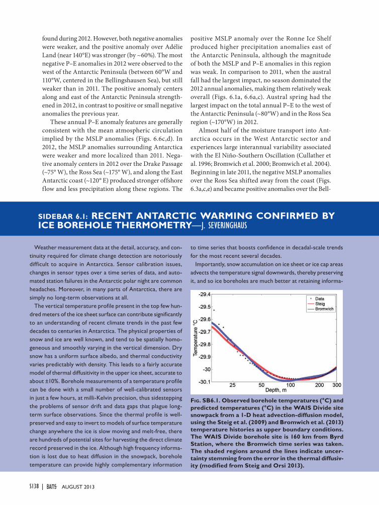
S138 | August 2013
found during 2012. However, both negative anomalies were weaker, and the positive anomaly over Adélie Land (near 140°E) was stronger (by ~60%). The most negative P–E anomalies in 2012 were observed to the west of the Antarctic Peninsula (between 60°W and 110°W, centered in the Bellingshausen Sea), but still weaker than in 2011. The positive anomaly centers along and east of the Antarctic Peninsula strength-ened in 2012, in contrast to positive or small negative anomalies the previous year.
These annual P–E anomaly features are generally consistent with the mean atmospheric circulation implied by the MSLP anomalies (Figs. 6.6c,d). In 2012, the MSLP anomalies surrounding Antarctica were weaker and more localized than 2011. Nega-tive anomaly centers in 2012 over the Drake Passage (~75° W), the Ross Sea (~175° W), and along the East Antarctic coast (~120° E) produced stronger offshore flow and less precipitation along these regions. The
positive MSLP anomaly over the Ronne Ice Shelf produced higher precipitation anomalies east of the Antarctic Peninsula, although the magnitude of both the MSLP and P–E anomalies in this region was weak. In comparison to 2011, when the austral fall had the largest impact, no season dominated the 2012 annual anomalies, making them relatively weak overall (Figs. 6.1a, 6.6a,c). Austral spring had the largest impact on the total annual P–E to the west of the Antarctic Peninsula (~80°W) and in the Ross Sea region (~170°W) in 2012.
Almost half of the moisture transport into Ant-arctica occurs in the West Antarctic sector and experiences large interannual variability associated with the El Niño-Southern Oscillation (Cullather et al. 1996; Bromwich et al. 2000; Bromwich et al. 2004). Beginning in late 2011, the negative MSLP anomalies over the Ross Sea shifted away from the coast (Figs. 6.3a,c,e) and became positive anomalies over the Bell-
SiDEbAr 6.1: rEcEnt AntArctic WArMinG cOnFirMED bY icE bOrEHOLE tHErMOMEtrY—J. SEVERINGHAUS
Weather measurement data at the detail, accuracy, and con-tinuity required for climate change detection are notoriously difficult to acquire in Antarctica. Sensor calibration issues, changes in sensor types over a time series of data, and auto-mated station failures in the Antarctic polar night are common headaches. Moreover, in many parts of Antarctica, there are simply no long-term observations at all.
The vertical temperature profile present in the top few hun-dred meters of the ice sheet surface can contribute significantly to an understanding of recent climate trends in the past few decades to centuries in Antarctica. The physical properties of snow and ice are well known, and tend to be spatially homo-geneous and smoothly varying in the vertical dimension. Dry snow has a uniform surface albedo, and thermal conductivity varies predictably with density. This leads to a fairly accurate model of thermal diffusitivity in the upper ice sheet, accurate to about ±10%. Borehole measurements of a temperature profile can be done with a small number of well-calibrated sensors in just a few hours, at milli-Kelvin precision, thus sidestepping the problems of sensor drift and data gaps that plague long-term surface observations. Since the thermal profile is well-preserved and easy to invert to models of surface temperature change anywhere the ice is slow moving and melt-free, there are hundreds of potential sites for harvesting the direct climate record preserved in the ice. Although high frequency informa-tion is lost due to heat diffusion in the snowpack, borehole temperature can provide highly complementary information
to time series that boosts confidence in decadal-scale trends for the most recent several decades.
Importantly, snow accumulation on ice sheet or ice cap areas advects the temperature signal downwards, thereby preserving it, and so ice boreholes are much better at retaining informa-
Fig. Sb6.1. Observed borehole temperatures (°c) and predicted temperatures (°c) in the WAiS Divide site snowpack from a 1-D heat advection-diffusion model, using the Steig et al. (2009) and bromwich et al. (2013) temperature histories as upper boundary conditions. the WAiS Divide borehole site is 160 km from byrd Station, where the bromwich time series was taken. the shaded regions around the lines indicate uncer-tainty stemming from the error in the thermal diffusiv-ity (modified from Steig and Orsi 2013).

S139STATE OF THE CLIMATE IN 2012 |AuguST 2013
ingshausen Sea in October 2012 (Fig. 6.3g). Previous studies suggest that these anomaly features are con-sistent with simultaneously weak La Niña and positive SAM index values (Fogt and Bromwich 2006; Fogt et al. 2011), which were observed throughout much of 2012 prior to November. Figure 6.6e shows the time series of average monthly total P–E over Marie Byrd Land-Ross Ice Shelf (75°S–90°S, 120°W–180°) and monthly Southern Oscillation index (SOI) and SAM index (with 12-month running means). It is clear that the SOI and SAM index are positively correlated but have opposite behavior to P–E in most months from 2008 to mid-2011. After this period, the SOI decreases and SAM index increases (anti-correlated) into 2012. The correlation coefficients between monthly P–E and index values (from 2008 to 2012) are SOI -0.22 (-0.38 for annual running mean) and SAM index -0.29 (-0.71 for annual running mean), respectively.
e. 2011/12 Seasonal melt extent and duration—L. Wang and H. LiuAntarctic surface snow melt during the 2011/12
austral summer was estimated from daily brightness temperature data acquired by Defense Meteorological Satellite Program (DMSP-17) satellite with the on-board Special Sensor Microwave/Imager (SSM/I). The 19-GHz horizontally polarized channel acquired in the ascending pass of the polar orbit of DMSP-17 (Zwally and Fiegles 1994; Armstrong et al. 2013; Liu et al. 2005) was used for analysis. The melt onset and end dates were tracked using the algorithm in Liu et al. (2005), and the number of melting days enclosed by the onset and end pairs during the melt season were recorded. The total number of melting days in a year is calculated by accumulating all the melt onset and end pairs in the time series. The first and last melt days in the year are recorded as the start and end days
tion than terrestrial boreholes, especially in high-accumulation sites. High accumulation rates also advect the geothermal gradient down into the lower half of the ice sheet, removing this potential complication, although variations in accumula-tion can add an additional one. West Antarctica is one such high-accumulation region [22 cm yr-1 at the West Antarctic Ice Sheet (WAIS) Divide site], and the Antarctic Peninsula is another (up to 3 m yr-1 at the Bruce Plateau). Fortunately, the accumulation rate history at the WAIS Divide site is well known from the ice core recently drilled there, and this information is incorporated into the heat transport model.
Four recent borehole temperature studies confirm an accelerated pace of warming in recent decades in the Antarctic Peninsula, West Antarctica, and the Dronning Maud Land in East Antarctica (Barrett et al. 2009; Muto et al. 2011; Zagorodnov et al. 2012; Orsi et al. 2012). All find recent warming of order 1°C in the last few decades, confirming time series measurements from Byrd Station (Bromwich et al. 2013) and other temporal records (Steig et al. 2009; Steig and Orsi 2013).
When these time series measurements are run through a forward model of heat advection and diffusion to predict the temperature profile in the snowpack, they can be compared directly to the borehole data from the WAIS Divide site (Fig. SB6.1). The observed match of model and data is a powerful test of the validity of the borehole inversion methodology and should eliminate
any remaining doubt that West Antarctica is warming rapidly. When the data are inverted for the temperature history at the site (Fig. SB6.2), the result shows consistency with other published records, although the non-unique nature of the inver-sion causes a loss of resolution going back in time (indicated by the spread of 6000 Monte Carlo simulations). The success of the Muto et al. (2011) study from Dronning Maud Land, show-ing a similar level of warming at four different sites, suggests the scientific potential for borehole studies in other areas of East Antarctica.
Fig. Sb6.2. central West Antarctic temperature history (°c) inferred from the inversion of borehole temperature measurements. the light gray shaded region represents ±1 std dev. Adapted from Orsi et al. (2012).

S140 | August 2013
of the melt season. Based on the calculation, maps were generated for the melt start day (Fig. 6.7a), melt end day (Fig. 6.7b), and melt duration (Fig. 6.7c) of surface snow on the Antarctic Ice Sheet. Melt extent and melt index (Zwally and Fiegles 1994; Torinesi et al. 2003; Liu et al. 2006) values were derived from the maps. Melt extent is the total area that experienced surface melt for at least one day, and the melt index is the accumulated melt extent for the number of days of melt over the entire continent of Antarctica or an Antarctic region.
Surface snow melt during the 2011/12 austral summer across the Antarctic continent exhibits a coherent spatial pattern. Lengthy and contiguous melt mainly occurred on the ice shelves of the Antarctic Peninsula. The melt index in this area is 50% of the total melt for the entire continent. The melt index of the Antarctic Peninsula in 2011/12 (16 036 875 day km2) is much greater than in 2010/11 (14 215 625 day km2), indicating that the recent melt season was longer than in 2010/11. The spatial distribution of surface melt duration is shown in Fig. 6.7c. Areas with
intensive melt duration (>45 days) include the Larsen Ice Shelf, Wilkins Ice Shelf, and Abbot Ice Shelf (Fig. 6.7c), mainly equatorward of 75°S. Areas of moderate melt duration (16–45 days) are on the ice shelves of Dronning Maud Land, West Ice Shelf, Shackleton, Wilkes Land, and Amery Ice Shelf. Short-term melt (<16 days) occurred on the coast of Dronning Maud Land and Ross Ice Shelf. Ephemeral surface melt in Ross Ice Shelf extended to 85°S. Such ephemeral melt in this region has not been observed in recent years. Sporadic early melt events in the middle of October 2011 are found at the tip of the Antarctic Peninsula (Fig. 6.7a). The main melt period (Fig. 6.7d) over the continent started at the end of November 2011. Melt area reached its peak on 23 December 2011, and a record warm day was observed by multiple AWSs near the South Pole two days later (Colwell et al. 2012). The main melt season ended on 7 February 2012. A minor melt event began on 2 March 2012, and peaked on 10 March, with melt areas confined mainly to the Antarctic Peninsula and Abbot Ice Shelf (Fig. 6.7b). This second melt period ended by 16 March.
In comparison with previous years, the 2011/12 melt season had a relatively small melt extent across all of Antarct ica . The overall melt extent was 944 375 km2, lower t ha n t he prev ious year (1 069 375 km2; Wang and Liu 2012), a lmost the same as in the 2009/10 aus-tral summer (945 000 km2; Wang and Liu 2011), and well below the 25-year median value (1 277 500 km2) reported in Liu et al. (2006). Total melt in-dex for the 2011/12 season is 29 006 250 day km2, significantly lower than the past two years. Given the similar melt extent, the average melt du-ration in the 2011/12 austral year was about 25% shorter than the
Fig. 6.7. Maps for (a) melt start day, (b) melt end day, and (c) melt duration of Ant-arctic ice sheet during 2011/12 austral summer. Daily melt area is plotted in (d) with two peak days labeled.

S141STATE OF THE CLIMATE IN 2012 |AuguST 2013
previous two years. However, the Antarctic melt index shows a positive trend since its record low in the 2008/09 melt season (Tedesco 2009; Tedesco and Monaghan 2009).
f. Sea ice extent and concen-tration—R. A. Massom, P. Reid, S. Stammerjohn, S. Barreira, J. Lieser, and T. ScambosAntarctic sea ice in 2012
was characterized by generally above-average area and extent throughout the year, compared to the 1981–2010 mean, with the exception of late May through early June and late November through much of December (Fig. 6.8a). A new maximum sea ice extent was recorded during September (since satellite re-cords began in 1978; see http://nsidc.org/arcticseaicenews). Regionally, the pattern of sea ice variability throughout the year was closely associated with variations in large-scale atmo-spheric and oceanic circulation patterns and related local sea surface temperatures.
The sea ice pattern during the early months of 2012 (Janu-ary–May) was predominantly characterized by three regions of above-average sea ice extent and concentration: most of the Weddell Sea, much of East Antarctic/western Ross Sea (120°E–180°), and for a short period, the coastal area in the Bel l ingshausen/Amundsen Sea (~90°W–120°W; Fig. 6.8b). These regions were associated with lower-than-normal at-mospheric temperatures (Figs. 6.3b,d) and SSTs, for this time of the year and adjacent to the ice edge (Fig. 6.8d). During this period, below-average sea ice extent occurred mostly in two areas: eastern Ross Sea and
Fig. 6.8. (a) Plot of daily anomaly (black line) from the 1981–2010 mean of daily SH sea ice extent for 2012, based on satellite passive microwave ice concentration data from the GSFc bootstrap Version 2 dataset (comiso 2008). blue banding represents the range of daily values for 1981–2010, while the red line represents ±2 std devs. numbers at the top are monthly-mean extent anomalies (×106 km2). (b) and (c) Sea ice concentration anomaly maps for Jan and Sep 2012 derived versus the monthly means for 1981–2010, with monthly-mean contours of AccESS MSLP. bell is bellingshausen Sea. (d) and (e) Maps of monthly-mean sea ice concentration for Jan and Sep 2012, respectively, with mean ice edge/extent contours for 1981–2010 (black lines) and SSt anomaly contours superimposed. the SSt anomalies were calcu-lated against the 1981–2010 mean and are based on data from the Optimal interpolation SSt version 2 dataset (reynolds et al. 2002; Smith et al, 2008). (f) Sea ice duration anomaly for 2012/13, and (g) duration trend (see Stam-merjohn et al. 2008). both the climatology (for computing the anomaly) and trend are based on 1981/82 to 2010/11 data (comiso 2008), while the 2012/13 duration-year data are from the nASA team near-real-time Sea ice (nrtSi) dataset (Maslanik and Stroeve 1999).

S142 | August 2013
parts of East Antarctica (80°E–110°E). These patterns of anomalous sea ice concentrations reflect the timing of the 2011/12 retreat season (Massom et al. 2012). As the austral summer transitioned into fall (~March–May) in 2012, most areas of the Southern Ocean sea ice zone began to advance earlier (later) where they had previously retreated later (earlier).
During the latter part of the sea ice advance season (June–September), the pattern of anomalous sea ice extent changed from that of earlier in the year. Par-ticularly strong and persistent cyclonic activity in the Bellingshausen-Amundsen Seas and Dronning Maud Land regions during July and August was responsible for an increase in sea ice extent in the eastern Ross Sea and Dronning Maud Land. Above-average sea ice extents along parts of the East Antarctic coast (110°E–130°E) were synonymous with strong compac-tion and thickening of the ice by northerly winds in this region, as well as a dynamic build-up of sea ice behind large icebergs (as observed on the SIPEX-2 in September–October; see also Massom et al. 2001). In situ observations also suggested heavy snowfall and extreme snow accumulation on the sea ice in this re-gion of East Antarctica (and this is partially corrobo-rated by the snow accumulation analysis in section 6c and Fig. 6.6a). On the other hand, relatively warm northerly winds in July and August were responsible for inhibiting sea ice advance and subsequent lower-than-normal sea ice extents in the far eastern East Antarctic (150°E–180°) and the western Weddell Sea. Overall, the regions of above-average sea ice extents off East Antarctica, the Ross Sea, and Dronning Maud Land were sufficient to contribute to a new record-high overall sea ice extent during late September (since 1979) of about 19.45 million km2 (Figs. 6.8c,e).
The 2012 early sea ice retreat season (October–December) saw yet another change in the pattern of sea ice extent anomalies. During October through November, the Amundsen Sea Low (ASL) stayed west in the Ross Sea (Fig. 6.3g), contributing to more zonal conditions farther east, particularly in October. This in turn contributed to a late sea ice retreat in the outer pack ice of the western Weddell-Bellingshausen Seas region (~100°W–40°W). In contrast and immediately east of the ASL, strong northerly winds and warmer-than-normal SSTs (advected south from the central Pacific) contributed to below-average sea ice extents and an early sea ice retreat over most of the Amundsen Sea (~100°W–160°W). Similarly, the juxtaposition of low pressure systems across East Antarctica produced contrasting retreat anomalies, with late retreat of the
outer pack ice in the East Antarctic/western Ross Sea area (from ~90°E–160°W), and early retreat of the outer pack ice in the eastern Weddell Sea (~0°–30°E) and Indian Ocean (~80°E–90°E).
Sea ice concentration and extent patterns for the first few months of 2012 (January–May) were gen-erally consistent with the overall long-term trend (Comiso 2010), with the exception of the areas of East Antarctica (at around 90°E), the far western Ross Sea, and the Bellingshausen-Amundsen Seas (~60°W–160°W). The latter was east of anomalously low sea level pressure system in the Antarctic Pen-insula-western Weddell Sea region during February. An overall exception to the often-observed opposing retreat/advance anomalies was an area in the Indian Ocean (~20°E–60°E), where sea ice retreat and ad-vance were both earlier. The earlier advance appeared to be related to favorable southerly winds west of a low pressure system that intensified throughout the austral autumn and into June (not shown).
The 2012 ice season, with positive ice season duration anomalies (Fig. 6.8f) everywhere except in the Amundsen Sea (~100°W–160°W) and in East Antarctica (~80°E–100°E), reflects the general influ-ence of strengthened westerly winds (positive SAM index) and a strengthened ASL (La Niña/positive SAM index) in the first half of the year, followed by a strengthened wave-3 pattern and negative SAM index later in the year. Because the ASL was farther west than usual during the transition seasons in 2012, the Antarctic Peninsula-Bellingshausen Sea region was given a reprieve from strong northerly winds. Thus, an unusually long ice season was observed there, opposing the strong negative trend recorded for 1980/81–2010/11 (Fig. 6.8g; Stammerjohn et al. 2012). Otherwise and elsewhere, the ice season duration anomalies in 2012 more or less reflected the 30-year trends (see Stammerjohn et al. 2012).
g. Ozone depletion—P. A. Newman, N. Kramarova, E. R. Nash, C. S. Long, M. C. Pitts, B. Johnson, M. L. Santee, J. Burrows, and G. O. BraathenThe 2012 Antarctic ozone hole was significantly
weaker than average in comparison to the typical ozone hole over the 1990–2011 period. Figure 6.9 displays October total ozone from GOME, GOME-2, and SCIAMACHY. Prior to 1980, severe Antarctic ozone depletion was not clearly evident. After 1990, every year has shown severe depletion. The 2012 hole (Fig. 6.9, bottom middle) shows weak losses that are still large in comparison to pre-1985 levels

S143STATE OF THE CLIMATE IN 2012 |AuguST 2013
(not shown). Only 2002 (marked by a strong stratospheric warming and a vortex split) was weaker than 2012 in the 1990–2012 period.
The 2012 hole was the second smallest over the 1990–2012 period; the 2002 hole was the smallest at 12.0 million km2 (see Sidebar 6.2 for more information). Measurements from the Suomi National Polar-orbiting Partnership (S-NPP) satellite’s Ozone Mapper and Profiler Suite Nadir Map-per (OMPS NM) showed a single-day maximum area of 20.9 million km2 on 22 September 2012, with a time-average (7 September–13 October) of 17.6 million km2. The lowest OMPS value of 124 Dobson Units (DU) was observed on 1 October, with a time average (21 September–16 October) of 139 DU. The 2012 polar vortex was relatively short-lived, keeping the ozone hole below previous years' daily maximum area values from mid-September through mid-November.
The minimum ozone is shown in Fig. 6.10 using the OMPS Limb Profiler (OMPS LP) ozone measurements at locations chosen to be near the polar vortex center. The vortex is defined using potential vortic-ity fields on the 460 K potential temperature surface, calculated from the NASA Global Model-ing and Assimilation Office (GMAO) Modern-era Retro-spective Analysis for Research and Applications (MERRA; Rienecker et al. 2011). The low-est total column ozone near the vortex center (shown in Fig. 6.10a) is accompanied by a corresponding profile (Fig. 6.10b). Figure 6.10c shows the profile and column minimum locations. The vortex split into two parts in early November, so the larger mass of vortex air that maintained itself was followed
Fig. 6.9. October averages of total column ozone derived from the GOME, GOME-2, and SciAMAcHY instruments from 1995 to 2012.
Fig. 6.10. OMPS ozone observations from a location near the center of the polar vortex: (a) total column ozone (in DU) and (b) daily ozone profiles (in ppmv). Values have been smoothed in time using a 1-2-1 filter. (c) the circles show vortex daily location with every fifth day numbered. the blue, green, and red circles indicate Sep, Oct, and nov, respectively.

S144 | August 2013
in Fig. 6.10c. The minimum ozone observed on 1 October 2012 was followed by steady recovery over the October–November period.
Early October Antarctic ozone profiles show a near 100% depletion over small vertical layers in the lower stratosphere. South Pole ozonesonde measurements show the 14 km–21 km average ozone plummeting from 150 DU on 1 September to approximately 20 DU by early October. While the lowest total ozone occurred on 1 October (Fig. 6.10a), the lowest mixing ratio (density of ozone divided by the total density of all atmospheric gases) values were found during the 6–13 October 2012 period below about 18 km (Fig. 6.10b), in general agreement with these South Pole ozonesondes. The hole filled in quite rapidly (in terms of total column) as large amounts of ozone advected over Antarctica at altitudes above 25 km during the October–November period.
Chlorine- and bromine-containing compounds cause Antarctic ozone depletion. Ozone-depleting substances (ODSs) over Antarctica have only de-creased by about 0.25 ppb, to 3.80 ppb from the peak levels in the 2000–12 pe-riod (4.05 ppb). This amounts to a 13% drop towards the 1980 level of 2.11 ppb.
The ozone hole resu lt s f rom conversion of chlorine molecules from nonreactive forms into ozone-destroying forms on polar strato-spheric clouds (PSCs) surfaces (i.e,
) . T h e springtime rising sun photolyzes molecular chlorine, and this chlorine (combined with bromine) drives cata-lytic ozone loss. CALIPSO satellite ob-servations indicate that May–October 2012 total PSC volume was the smallest in comparison to the 2006–11 Antarc-tic period (not shown). June PSC levels were near average, and much below average during July–October (update from Pitts et al. 2009).
The Aura Microwave Limb Sounder (MLS) measures nonreactive HCl (Fig. 6.11a, top panel) and ozone-destroying ClO (Fig. 6.11a, bottom panel), thus tracking chlorine activation and de-activation. In June–July, HCl decreases as temperatures drop and PSCs form. As noted above, PSCs convert HCl
and ClONO2 into reactive chlorine (mainly ClO and Cl2O2). As a result of high levels of PSCs, ClO increas-es from June through August, and this chlorine is confined within the vortex. ClO peaks in September from the continued presence of PSCs and the rising sun over Antarctica. In late September, the complete destruction of ozone and evaporation of PSCs causes ClO (rapid decrease) to be converted back to HCl (rapid increase). Figure 6.11a shows that, consistent with the picture seen in ozone and temperature, the degree of chlorine activation in 2012 was slightly below average.
Antarctic stratospheric temperatures modulate the year-to-year ozone hole severity. Below- (above-)
Fig. 6.11. (a) Daily time series of Antarctic vortex-averaged Hcl (top panel) and clO (bottom panel) from the Aura MLS, in ppbv. the averages are made inside the polar vortex on the 485°c potential temperature surface (~21 km altitude or 40 hPa). Gray shading shows Antarctic values for 2004–10. Updated from Manney et al. (2011). (b) Sep monthly mean temperature at 50 hPa, 60°S–90°S from MErrA data. in 2012, the average temperature was about 2°c above the MErrA average. the trend in (b) is not statistically significant.

S145STATE OF THE CLIMATE IN 2012 |AuguST 2013
Above-average air temperatures high above the Antarctic led to the second smallest ozone hole in 20 years in 2012. At its peak, the ozone hole stretched to 21.2 million km2, slightly smaller than the total area of North America. In comparison, the largest ozone hole recorded to date was in 2000 at 29.9 million km2.
Figures SB6.3 and SB6.4 show the development of the 2012 ozone hole over South Pole Station from balloon-borne ozonesonde measurements. Total column ozone dropped from an average pre-depletion value of 279 Dobson Units (DU) to a minimum value of 136 DU on 5 October. This was significantly higher than the 1986–2011 average minimum of 116 ± 20 DU. The main ozone depletion layer from 12 km to 20 km plummeted from 141 DU to 19 DU, but zero ozone was only observed within the 16 km–18 km layer. For comparison, the deepest layer of zero ozone measured over South Pole was in 2006 when the 14 km–21
Fig. Sb6.3. Selected ozonesonde profiles from South Pole Station in 2012 showing the progression of the ozone hole. the pre-ozone hole profile (blue), in mid-June to mid-August, shows an average total column ozone of 279 Dobson units (DU), which drops to 180 by 15 Sep (green) and reaches a minimum of 136 DU on 5 Oct (red). the partial column values within the 12 km–20 km region are also in the legend. (Figure from bryan Johnson of nOAA.)
Fig. Sb6.4. Stratospheric air temperature (red) and ozone values for 2012 (blue) vs. historic average (envelope) at 16 km–18 km above the South Pole. Prior to 25 September, the average envelopes rep-resent ±1 std dev; after this date they represent an approximate (non-statistical) average to be used only as a guide. Figure from bryan Johnson of nOAA.
km layer was nearly 100% depleted and total column ozone was near record lows at 93 DU. Figure SB6.4 indicates that the minimum in early October was followed by a fast rebound to much higher-than-average ozone and temperature values. Several early ozonesonde measurements made from 1966 to 1971 are plotted in Fig. SB6.4 as single points to show typical ozone and temperatures before significant springtime deple-tion began. Increased stratospheric temperatures correlate to an earlier breakup of the 2012 ozone hole. Historically, mid-October ozone values in the 16 km–18 km layer show the greatest depletion and can be at, or near, zero.
Even 25 years after an international agreement was signed to regulate production of ozone-depleting chemicals, the ozone hole still forms each year. In fact, it could be another 5–10 years before scientists can confirm early signs of Antarctic ozone layer recovery. The springtime ozone layer above Antarctica likely will not return to its early 1980s state until about 2060. The length of time needed for this full recovery is mainly due to the large quantity and long lifetime of ozone-depleting sub-stances in the atmosphere. Climate change may also affect the rate of ozone recovery by altering transport and cooling the stratosphere, which has several competing effects on ozone depletion. Monitoring the state of ozone in Antarctica, and globally, will remain important for decades to come.
SiDEbAr 6.2: tHE 2012 AntArctic OZOnE HOLE
S146 | August 2013
average temperatures result in large and deep (small and shallow) ozone holes. Figure 6.11b shows Antarc-tic (60°S–90°S) September 50 hPa monthly means. September lower stratospheric temperatures were 2°C above average (also see Fig. 6.2b). Above-average temperatures were consistent with smaller amounts of PSCs and less chlorine activation.
The Antarctic stratosphere is warmed by the return of sunlight at the end of the winter and by large-scale weather systems (planetary-scale waves) that form in the troposphere and move upward into the stratosphere. Easterly momentum deposition from these waves decelerates the stratospheric jet and causes a poleward and downward circulation. This downward circulation adiabatically warms the Antarctic lower stratosphere. Wave events during the
2012 Antarctic winter and spring were particularly strong. This caused a warmer-than-normal vortex (Fig. 6.11b; see also Fig. 6.3b) and a weaker ozone hole. Low ozone values disappeared quite early in 2012 in comparison to previous years.
In summary, the 2012 Antarctic ozone hole was significantly weaker than average in comparison to the typical ozone hole over the 1990–2011 period. This weakness was from dynamical effects that warmed the Antarctic lower stratosphere and ad-vected higher ozone concentrations over Antarctica. Activated chlorine levels were still high, and estimates of Antarctic inorganic chlorine levels have yet to significantly decrease. Severe ozone depletion was again observed from ground, balloon, and satellite observations in comparison to the pre-1985 period.
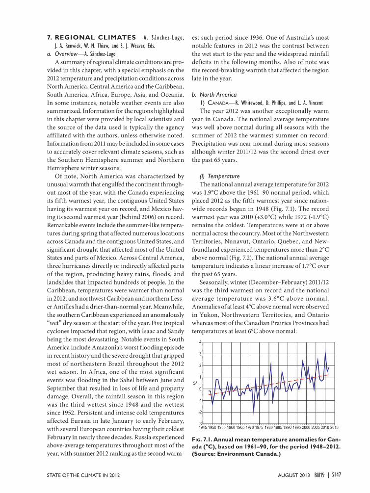
S147STATE OF THE CLIMATE IN 2012 |AuguST 2013
7. Regional Climates—A. Sánchez- Lugo , J. A. Renwick, W. M. Thiaw, and S. J. Weaver, Eds.
a. Overview—A. Sánchez-LugoA summary of regional climate conditions are pro-
vided in this chapter, with a special emphasis on the 2012 temperature and precipitation conditions across North America, Central America and the Caribbean, South America, Africa, Europe, Asia, and Oceania. In some instances, notable weather events are also summarized. Information for the regions highlighted in this chapter were provided by local scientists and the source of the data used is typically the agency affiliated with the authors, unless otherwise noted. Information from 2011 may be included in some cases to accurately cover relevant climate seasons, such as the Southern Hemisphere summer and Northern Hemisphere winter seasons.
Of note, North America was characterized by unusual warmth that engulfed the continent through-out most of the year, with the Canada experiencing its fifth warmest year, the contiguous United States having its warmest year on record, and Mexico hav-ing its second warmest year (behind 2006) on record. Remarkable events include the summer-like tempera-tures during spring that affected numerous locations across Canada and the contiguous United States, and significant drought that affected most of the United States and parts of Mexico. Across Central America, three hurricanes directly or indirectly affected parts of the region, producing heavy rains, f loods, and landslides that impacted hundreds of people. In the Caribbean, temperatures were warmer than normal in 2012, and northwest Caribbean and northern Less-er Antilles had a drier-than-normal year. Meanwhile, the southern Caribbean experienced an anomalously “wet” dry season at the start of the year. Five tropical cyclones impacted that region, with Isaac and Sandy being the most devastating. Notable events in South America include Amazonia’s worst flooding episode in recent history and the severe drought that gripped most of northeastern Brazil throughout the 2012 wet season. In Africa, one of the most significant events was flooding in the Sahel between June and September that resulted in loss of life and property damage. Overall, the rainfall season in this region was the third wettest since 1948 and the wettest since 1952. Persistent and intense cold temperatures affected Eurasia in late January to early February, with several European countries having their coldest February in nearly three decades. Russia experienced above-average temperatures throughout most of the year, with summer 2012 ranking as the second warm-
est such period since 1936. One of Australia’s most notable features in 2012 was the contrast between the wet start to the year and the widespread rainfall deficits in the following months. Also of note was the record-breaking warmth that affected the region late in the year.
b. North America1) Canada—R. Whitewood, D. Phillips, and L. A. VincentThe year 2012 was another exceptionally warm
year in Canada. The national average temperature was well above normal during all seasons with the summer of 2012 the warmest summer on record. Precipitation was near normal during most seasons although winter 2011/12 was the second driest over the past 65 years.
(i) Temperature The national annual average temperature for 2012
was 1.9°C above the 1961–90 normal period, which placed 2012 as the fifth warmest year since nation-wide records began in 1948 (Fig. 7.1). The record warmest year was 2010 (+3.0°C) while 1972 (-1.9°C) remains the coldest. Temperatures were at or above normal across the country. Most of the Northwestern Territories, Nunavut, Ontario, Quebec, and New-foundland experienced temperatures more than 2°C above normal (Fig. 7.2). The national annual average temperature indicates a linear increase of 1.7°C over the past 65 years.
Seasonally, winter (December–February) 2011/12 was the third warmest on record and the national average temperature was 3.6°C above normal. Anomalies of at least 4°C above normal were observed in Yukon, Northwestern Territories, and Ontario whereas most of the Canadian Prairies Provinces had temperatures at least 6°C above normal.
Fig. 7.1. annual mean temperature anomalies for Can-ada (°C), based on 1961–90, for the period 1948–2012. (source: environment Canada.)

S148 | August 2013
The national average temperature for spring 2012 was 1.6°C above normal, which made it the ninth warmest spring since 1948. Southern Manitoba, most of Ontario, and southern Quebec experienced temperatures that were more than 3°C above normal.
Summer 2012 was the warmest on record since nation-wide records began in 1948, with the national average temperature 1.9°C above normal. The previ-ous record of 1.7°C above normal was set in 1998. The whole country experienced above-normal warmth, especially the Northwest Territories, Nunavut, north-ern Prairies Provinces, Ontario, Quebec, Labrador, and Newfoundland, which had temperatures at least 2°C above normal. Only British Columbia (B.C.) had temperatures close to normal.
Fall 2012 was the 17th warmest on record with a national average temperature of 1.2°C above normal. The Northwest Territories, Nunavut, southern B.C., northern Quebec, and Atlantic Canada had tempera-tures at least 1°C above normal. However, southern Yukon, northern B.C., most of Alberta, southern
Saskatchewan, and southern Manitoba experienced cooler-than-normal temperatures.
(ii) PrecipitationOverall, Canada experienced near-normal pre-
cipitation in 2012. It was the 33rd wettest year in the 65 years of record with the national precipitation value 1% above the 1961–90 normal (Fig. 7.3). The wettest year was 2005 (15% above normal) and the driest was 1956 (12% below normal). Most of the country received near-normal annual precipitation amounts. Areas in southern B.C., Saskatchewan, and Manitoba, along with northern Quebec and eastern Nunavut, received slightly higher-than-normal pre-cipitation (Fig. 7.4). Northern Northwest Territories, western Nunavut, central B.C., south-central Alberta, southern Ontario, and Newfoundland and Labrador had slightly drier-than-normal conditions.
Winter 2011/12 was characterized by drier-than-normal conditions (18% below normal) and ranked as the second driest out of the 65 years of record. Almost the entire country saw drier-than-normal conditions. The Prairie Provinces, northern Northwest Territo-ries, and northern Quebec experienced conditions at least 40% drier than normal. Only two areas had above-normal precipitation: the region running from northern Manitoba up through eastern Nunavut and a small region along the B.C. coast.
National average precipitation was generally near normal during the rest of the year. Spring 2012 ranked as 24th wettest and the national average precipitation was 3% above normal. Conditions at least 40% wet-ter than normal were found in the Canadian Prairie Provinces, southern Yukon and Northwest Territories, and northern Ontario. Areas of drier-than-normal conditions included Nunavut, southern Ontario, and Atlantic Canada.
Fig. 7.4. 2012 annual total precipitation anomalies for Canada (percent departure from 1961–90 average). (source: environment Canada.)
Fig. 7.2. 2012 annual mean temperature anomalies for Canada (°C) based on 1961–90. (source: environment Canada.)
Fig. 7.3. annual total precipitation anomalies for Canada (percent of 1961–90 average) for the period 1948–2012. (source: environment Canada.)

S149STATE OF THE CLIMATE IN 2012 |AuguST 2013
Summer 2012 was 4% above normal and ranked as the 19th wettest since 1948. Slightly above-normal precipitation was found in small areas in southern B.C., Saskatchewan, Yukon, Northwest Territories, and northern Quebec. Below normal precipitation was observed in northern B.C., northern Northwest Territories, Ontario, southern Quebec, Newfoundland and Labrador, and Nova Scotia.
During fall, the national average precipitation remained near normal (2% below normal), ranking as the 30th driest since 1948. Drier-than-normal conditions were observed in central B.C., southern Alberta and Saskatchewan, most of Nunavut, and the northern Northwest Territories. Southern B.C., northeastern B.C., northern Alberta, northern Sas-katchewan, most of Manitoba, northern Quebec, and part of the Maritimes all experienced wetter-than-normal conditions.
(iii) Notable eventsHot temperature events dominated the list of the
major Canadian weather stories in 2012. The year 2012 featured a winter that went missing, a March with broken records, and a summer that was the warmest of the warm seasons.
In 2012, Canadians witnessed an almost total absence of winter. In Toronto, snowfall was a record low 41.8 cm; there were no days with measurable snow after March 1 and only nine days with more than 1 cm of snow from November to April. In Montreal, overnight lows never dipped below -20°C (the mark of a cold Canadian day), which was a first for the record books. The average afternoon temperature for Saskatoon in December and January hit -3.2°C, which was the warmest in records going back to the 1880s.
In March, summer-like temperatures affected numerous locations across Canada. Fort Frances reached 26°C and on 19 March the town recorded a minimum temperature of 15.1°C. Winnipeg reg-istered a maximum temperature of 20.9°C on 19 March, its earliest recording of temperature above 20°C in a calendar year. Halifax reported a maximum temperature of 27.2°C on 22 March, shattering its previous record of 11.8°C set in 1983. On 21 March, Petawawa recorded a maximum temperature of 28.8°C—the highest temperature ever recorded in Ontario in March.
Flooding due to intense precipitation events were also among the major weather events in 2012. Late on 26 May, a low-pressure system that moved from North Dakota and sat on Thunder Bay brought be-tween 35 mm and 120 mm of rain (including 71 mm
in less than six hours). The ensuing flash flood caused washouts on numerous roads and trails, cut power to homes and businesses, and filled thousands of base-ments with up to two meters of dirty sewage water.
On 29 May, a pair of rainstorms combined to de-liver more than 100 mm rain to much of Montreal, producing widespread flooding and power outages in the area. The first storm brought up to 40 mm of rain and twelve hours later a brief but more power-ful storm dumped an additional 50 mm to 80 mm of rain on the city. The storms also caused power failures affecting 28 000 people. On 22 July, an intense downpour in Hamilton dumped 140 mm on the city in less than four hours.
2) United StateS—J. Crouch, R. R. Heim Jr., P. Hughes, and C. Fenimore
Based on preliminary data, the annual aver-age temperature in 2012 for the contiguous United States (CONUS) was 13.0°C, which is 1.8°C above the 1901–2000 average and the warmest year since records began in 1895 (Fig. 7.5). 2012 sur-passed the previous record warm year of 2006 by 0.6°C. The nationally-averaged precipitation dur-ing 2012 was 674.9 mm, 65.3 mm below average.
(i) Temperature Anomalous warmth dominated much of 2012,
with each state in the CONUS having above-normal temperatures and many locations having record warm annual temperatures (Fig. 7.6a). Winter (De-cember–February) 2011/12 was the third warmest on record for the nation with a seasonally-averaged
Fig 7.5. annual mean temperature for the contiguous United states for the period 1895–2012. the filter is a weighted average used to smooth the year-to-year changes in the data values which may help identify the presence/absence of trends throughout the data record. (source: noaa/nCDC.)

S150 | August 2013
temperature 2.2°C above average. Warmer-than-average temperatures were present for most of the nation, with near-average temperatures across parts of the West. Spring (March–May) was the warmest on record with an average temperature 2.9°C above average and consisted of a record warm March, third warmest April, and second warmest May. Record warmth occurred in 34 states from the Rockies to New England. Only Oregon and Washington had near-normal spring temperatures. The nationally-averaged summer (June–August) temperature was the second warmest on record, slightly cooler than the summer of 1936, at 1.4°C above average, and consisted of the 11th warmest June, record warmest July (and warmest month of any month on record), and the 13th warmest August. Much of the central and northeastern United
States were warmer than normal, while the Southeast and Northeast were near-normal. The CONUS fall (September–November) temperature was 0.6°C above average, with above-normal temperatures in the West and below-normal temperatures in the East. Nevada had its warmest fall on record.
(ii) PrecipitationPrecipitation for the CONUS in 2012 was below
normal and ranked as the 15th driest year on record and the driest since 1988. The year was character-ized by drier-than-average conditions for much of the central United States and the central East Coast. It was the driest year on record for Colorado, Montana, Nebraska, and Wyoming. The Northwest, central Gulf Coast, and parts of the Northeast were wetter than average. The year began with 32% of the CONUS in moderate to exceptional drought (based on the U.S. Drought Monitor), mainly across the Southern Rockies and Plains, Upper Midwest, and the Southeast. By the end of 2012, nearly 58% of the CONUS was experiencing drought conditions. Win-ter precipitation was below normal. The Southern Plains were wetter-than-average, helping to ame-liorate drought conditions that impacted the region during much of 2011. Drier-than-average conditions occurred along the West Coast, Canadian border, and Eastern Seaboard. The warm and dry winter, particularly across the western and northern United States, limited winter snow cover extent to the third smallest in the 46-year satellite record. At the end of the winter season, mountain snowpack was less than 50% of normal across the Great Basin and Central and Southern Rockies. Above-normal snowpack occurred in the Cascades and Northern Rockies. Spring was slightly drier than average for the CONUS. Below-normal precipitation occurred in the central Rockies and Midwest. Six states in those two regions had seasonal precipitation totals ranking among their 10 driest. Above-normal precipitation occurred in the Pacific Northwest and Upper Midwest. Minne-sota, Oregon, and Washington each had a top 10 wet spring. Summer was the 14th driest on record with precipitation 88% of normal. Above-normal precipi-tation occurred in New England, the Far West. and along the Gulf Coast. Florida had its wettest summer on record, with 137% of normal, partially attributable to Tropical Storm Debby and Hurricane Isaac. The central Rockies and Midwest were much drier than average. Nebraska and Wyoming each had their driest summer on record, with seasonal precipitation 40% and 44% of average, respectively. The spatial extent
Fig. 7.6. Climate division ranks of annual 2012 (a) tem-perature and (b) precipitation. Record coldest/warm-est or driest/wettest is defined as the smallest/largest annual value for that climate division in the 1895–2012 period of record. above-normal temperature/precipi-tation is defined as occurring in the warmest/wettest third of recorded years. Whereas, much-below-normal temperature/precipitation falls in the bottom 10% of coolest/driest years since 1895, and below normal is defined as the coolest/driest third of the distribution. (source: noaa/nCDC.)
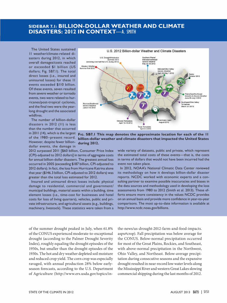
S151STATE OF THE CLIMATE IN 2012 |AuguST 2013
of the summer drought peaked in July, when 61.8% of the CONUS experienced moderate-to-exceptional drought (according to the Palmer Drought Severity Index), roughly equaling the drought episodes of the 1950s, but smaller than the drought episodes of the 1930s. The hot and dry weather depleted soil moisture and reduced crop yield. The corn crop was especially ravaged, with annual production 28% below early-season forecasts, according to the U.S. Department of Agriculture (http://www.ers.usda.gov/topics/in-
the-news/us-drought-2012-farm-and-food-impacts.aspx#crop). Fall precipitation was below average for the CONUS. Below-normal precipitation occurred for most of the Great Plains, Rockies, and Southeast, with above-normal precipitation in the Northwest, Ohio Valley, and Northeast. Below-average precipi-tation during consecutive seasons and the expansive drought resulted in near-record low water levels along the Mississippi River and western Great Lakes slowing commercial shipping during the last months of 2012.
siDebaR 7.1: billion-DollaR WeatHeR anD Climate DisasteRs: 2012 in ConteXt—A. SMiTH
The United States sustained 11 weather/climate-related di-sasters during 2012, in which overall damages/costs reached or exceeded $1 bill ion (US dollars; Fig. SB7.1). The total direct losses (i.e., insured and uninsured losses) for these 11 events exceeded $110 billion. Of these events, seven resulted from severe weather or tornado events, two were related to hur-ricanes/post-tropical cyclones, and the final two were the year-long drought and the associated wildfires.
The number of billion-dollar disasters in 2012 (11) is less than the number that occurred in 2011 (14), which is the largest of the 1980–present record. However, despite fewer billion-dollar events, the damage in 2012 surpassed 2011 [$60 billion, Consumer Price Index (CPI)-adjusted to 2012 dollars] in terms of aggregate costs for annual billion-dollar disasters. The greatest annual loss occurred in 2005 (exceeding $187 billion, CPI-adjusted to 2012 dollars). In fact, the loss from Hurricane Katrina alone that year ($146.3 billion, CPI-adjusted to 2012 dollars) was greater than the total loss estimated for 2012.
Insured and uninsured direct losses include: physical damage to residential, commercial and government/municipal buildings, material assets within a building, time element losses (i.e., time-cost for businesses and hotel costs for loss of living quarters), vehicles, public and pri-vate infrastructure, and agricultural assets (e.g., buildings, machinery, livestock). These statistics were taken from a
wide variety of datasets, public and private, which represent the estimated total costs of these events—that is, the costs in terms of dollars that would not have been incurred had the event not taken place.
In 2012, NOAA's National Climatic Data Center reviewed its methodology on how it develops billion-dollar disaster reports. NCDC worked with economic experts and a con-sulting partner to examine possible inaccuracies and biases in the data sources and methodology used in developing the loss assessments from 1980 to 2012 (Smith et al. 2013). These ef-forts ensure more consistency in the values NCDC provides on an annual basis and provide more confidence in year-to-year comparisons. The most up-to-date information is available at http://www.ncdc.noaa.gov/billions.
Fig. sb7.1 this map denotes the approximate location for each of the 11 billion-dollar weather and climate disasters that impacted the United states during 2012.

S152 | August 2013
(iii) Notable EventsTornado activity during 2012 was much below
average, with 925 tornadoes being confirmed dur-ing the year, compared to the 1991–2010 average of approximately 1200 tornadoes annually. This is the least number of tornadoes to impact the United States since 1989. Of the 68 tornado-related fatalities during 2012, at least 62 resulted during above-average activ-ity in February, March, and April. Following those initial large outbreaks, tornado activity was relatively quiet for the rest of 2012. Less than half of the average number of tornadoes occurred during May and June, typically the most active tornado months of the year.
During 2012, approximately 67 265 fires burned over 3.7 million hectares across the United States The total area burned was the third most on record, and the low total number of fires resulted in the largest average fire size in the 13-year period of record. The largest fire in New Mexico’s history charred nearly 120 500 hectares, while Colorado was impacted by two devastating fires. One destroyed approximately 350 homes making it the most destructive fire in Colo-rado’s history and the other was the second largest, in terms of acreage burned, on record for the state.
Post-tropical cyclone Sandy made landfall along the New Jersey coast in late October with sustained winds of 67 kts (34.7 m s-1). The storm’s large size contributed to a significant storm surge along the Northeast coast, where several locations experienced record high water levels, including the Battery in New York City. Sandy also brought record early-season snowfall to the central Appalachians. The storm re-sulted in 159 direct and indirect fatalities and at least $70 billion (US dollars) in damages (see Sidebar 4.1 for further details on this storm).
3) MexiCo—R. Pascual, A. Albanil, J. L. Vazquez, and R. LobatoAfter exceptional drought conditions in 2011,
near-normal precipitation was observed in Mexico during 2012; nonetheless, the moisture deficit that persisted during the previous 24 months did not van-ish completely. An initial estimate of total precipita-tion for 2012 in Mexico was about 742 mm, below the long-term mean since 1941, whereas the mean annual temperature was 22.0°C, +1.2°C above normal (1971–2000 base period).
(i) TemperatureMean temperature in Mexico observed in 2012
(22.0°C) was above normal (+1.2°C), ranking as the second warmest year on record since 1971 (Fig. 7.7), exceeded only by 2006. All months except February
(-0.3°C) recorded a mean temperature above normal. The highest positive anomaly occurred in August (+2.7°C). The above-normal pattern was also ob-served in quarterly analyses. April–June (+1.5°C) and July–September (+1.9°C) ranked as third warmest for their respective periods whereas October–December (+2°C) ranked as warmest in record for that period since 1971 (Fig. 7.8).
Northeastern states such as Coahuila, Nuevo León, and Tamaulipas reported the highest anoma-lies in mean temperature (+2.7°C, +2.6°C, +2.9°C, respectively), as did Chihuahua (+2.6°C) in northern Mexico. A similar pattern was observed in southeast-ern states such as Quintana Roo (+1.7°C), Campeche (+1.4°C), Chiapas (+1.2°C), Tabasco (+1.0°C), and Yucatan (+0.8°C). However, near-normal mean tem-peratures were observed in northwestern and central states, where positive temperature anomalies were relatively small (Sonora and Sinaloa, +0.5°C; Puebla, +0.3°C). Temperatures in central and eastern Mexico remained within the normal range (Fig. 7.9a).
(ii) PrecipitationAverage annual precipitation in 2012 was approxi-
mately 742.3 mm, 4.4% below the long-term mean (25th driest since 1941). About 49% of the country, mostly in the north, observed below-normal precipi-tation (less than 85%); 35% of the country received near-normal precipitation (between 85% and 115% of the long-term mean) and 15% observed above-normal precipitation (Fig. 7.9b).
Fig 7.7. annual mean temperature anomaly (°C) in mexico (bars) and linear trend. Departures are de-picted as deviations from the 1971–2012 mean. (source: national meteorological service of mexico, smn.)
Fig 7.8. Daily mean temperature (°C) in mexico ob-served along 2012 (solid line) compared to the mean (dotted line) and a range of ±2 std dev (shaded area). anomalies are derived from 1971–2000 base period. (source: smn.)
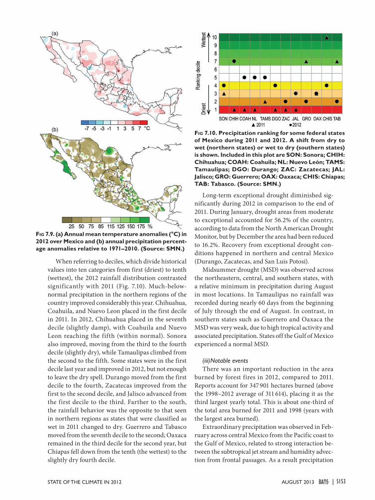
S153STATE OF THE CLIMATE IN 2012 |AuguST 2013
When referring to deciles, which divide historical values into ten categories from first (driest) to tenth (wettest), the 2012 rainfall distribution contrasted significantly with 2011 (Fig. 7.10). Much-below-normal precipitation in the northern regions of the country improved considerably this year. Chihuahua, Coahuila, and Nuevo Leon placed in the first decile in 2011. In 2012, Chihuahua placed in the seventh decile (slightly damp), with Coahuila and Nuevo Leon reaching the fifth (within normal). Sonora also improved, moving from the third to the fourth decile (slightly dry), while Tamaulipas climbed from the second to the fifth. Some states were in the first decile last year and improved in 2012, but not enough to leave the dry spell. Durango moved from the first decile to the fourth, Zacatecas improved from the first to the second decile, and Jalisco advanced from the first decile to the third. Farther to the south, the rainfall behavior was the opposite to that seen in northern regions as states that were classified as wet in 2011 changed to dry. Guerrero and Tabasco moved from the seventh decile to the second; Oaxaca remained in the third decile for the second year, but Chiapas fell down from the tenth (the wettest) to the slightly dry fourth decile.
Long-term exceptional drought diminished sig-nificantly during 2012 in comparison to the end of 2011. During January, drought areas from moderate to exceptional accounted for 56.2% of the country, according to data from the North American Drought Monitor, but by December the area had been reduced to 16.2%. Recovery from exceptional drought con-ditions happened in northern and central Mexico (Durango, Zacatecas, and San Luis Potosi).
Midsummer drought (MSD) was observed across the northeastern, central, and southern states, with a relative minimum in precipitation during August in most locations. In Tamaulipas no rainfall was recorded during nearly 60 days from the beginning of July through the end of August. In contrast, in southern states such as Guerrero and Oaxaca the MSD was very weak, due to high tropical activity and associated precipitation. States off the Gulf of Mexico experienced a normal MSD.
(iii) Notable eventsThere was an important reduction in the area
burned by forest fires in 2012, compared to 2011. Reports account for 347 901 hectares burned (above the 1998–2012 average of 311 614), placing it as the third largest yearly total. This is about one-third of the total area burned for 2011 and 1998 (years with the largest area burned).
Extraordinary precipitation was observed in Feb-ruary across central Mexico from the Pacific coast to the Gulf of Mexico, related to strong interaction be-tween the subtropical jet stream and humidity advec-tion from frontal passages. As a result precipitation
Fig 7.9. (a) annual mean temperature anomalies (°C) in 2012 over mexico and (b) annual precipitation percent-age anomalies relative to 1971–2010. (source: smn.)
Fig 7.10. Precipitation ranking for some federal states of mexico during 2011 and 2012. a shift from dry to wet (northern states) or wet to dry (southern states) is shown. included in this plot are son: sonora; CHiH: Chihuahua; CoaH: Coahuila; nl: nuevo león; tams: tamaulipas; Dgo: Durango; ZaC: Zacatecas; Jal: Jalisco; gRo: guerrero; oaX: oaxaca; CHis: Chiapas; tab: tabasco. (source: smn.)
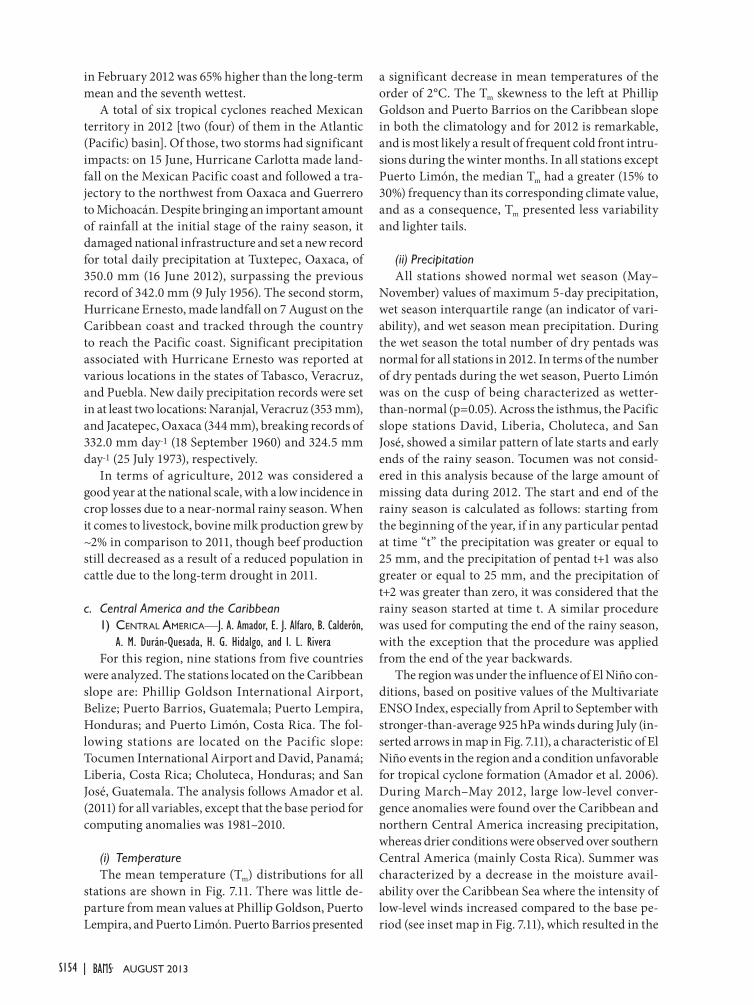
S154 | August 2013
in February 2012 was 65% higher than the long-term mean and the seventh wettest.
A total of six tropical cyclones reached Mexican territory in 2012 [two (four) of them in the Atlantic (Pacific) basin]. Of those, two storms had significant impacts: on 15 June, Hurricane Carlotta made land-fall on the Mexican Pacific coast and followed a tra-jectory to the northwest from Oaxaca and Guerrero to Michoacán. Despite bringing an important amount of rainfall at the initial stage of the rainy season, it damaged national infrastructure and set a new record for total daily precipitation at Tuxtepec, Oaxaca, of 350.0 mm (16 June 2012), surpassing the previous record of 342.0 mm (9 July 1956). The second storm, Hurricane Ernesto, made landfall on 7 August on the Caribbean coast and tracked through the country to reach the Pacific coast. Significant precipitation associated with Hurricane Ernesto was reported at various locations in the states of Tabasco, Veracruz, and Puebla. New daily precipitation records were set in at least two locations: Naranjal, Veracruz (353 mm), and Jacatepec, Oaxaca (344 mm), breaking records of 332.0 mm day-1 (18 September 1960) and 324.5 mm day-1 (25 July 1973), respectively.
In terms of agriculture, 2012 was considered a good year at the national scale, with a low incidence in crop losses due to a near-normal rainy season. When it comes to livestock, bovine milk production grew by ~2% in comparison to 2011, though beef production still decreased as a result of a reduced population in cattle due to the long-term drought in 2011.
c. Central America and the Caribbean1) Central aMeriCa—J. A. Amador, E. J. Alfaro, B. Calderón,
A. M. Durán-Quesada, H. G. Hidalgo, and i. L. RiveraFor this region, nine stations from five countries
were analyzed. The stations located on the Caribbean slope are: Phillip Goldson International Airport, Belize; Puerto Barrios, Guatemala; Puerto Lempira, Honduras; and Puerto Limón, Costa Rica. The fol-lowing stations are located on the Pacific slope: Tocumen International Airport and David, Panamá; Liberia, Costa Rica; Choluteca, Honduras; and San José, Guatemala. The analysis follows Amador et al. (2011) for all variables, except that the base period for computing anomalies was 1981–2010.
(i) TemperatureThe mean temperature (Tm) distributions for all
stations are shown in Fig. 7.11. There was little de-parture from mean values at Phillip Goldson, Puerto Lempira, and Puerto Limón. Puerto Barrios presented
a significant decrease in mean temperatures of the order of 2°C. The Tm skewness to the left at Phillip Goldson and Puerto Barrios on the Caribbean slope in both the climatology and for 2012 is remarkable, and is most likely a result of frequent cold front intru-sions during the winter months. In all stations except Puerto Limón, the median Tm had a greater (15% to 30%) frequency than its corresponding climate value, and as a consequence, Tm presented less variability and lighter tails.
(ii) PrecipitationAll stations showed normal wet season (May–
November) values of maximum 5-day precipitation, wet season interquartile range (an indicator of vari-ability), and wet season mean precipitation. During the wet season the total number of dry pentads was normal for all stations in 2012. In terms of the number of dry pentads during the wet season, Puerto Limón was on the cusp of being characterized as wetter-than-normal (p=0.05). Across the isthmus, the Pacific slope stations David, Liberia, Choluteca, and San José, showed a similar pattern of late starts and early ends of the rainy season. Tocumen was not consid-ered in this analysis because of the large amount of missing data during 2012. The start and end of the rainy season is calculated as follows: starting from the beginning of the year, if in any particular pentad at time “t” the precipitation was greater or equal to 25 mm, and the precipitation of pentad t+1 was also greater or equal to 25 mm, and the precipitation of t+2 was greater than zero, it was considered that the rainy season started at time t. A similar procedure was used for computing the end of the rainy season, with the exception that the procedure was applied from the end of the year backwards.
The region was under the influence of El Niño con-ditions, based on positive values of the Multivariate ENSO Index, especially from April to September with stronger-than-average 925 hPa winds during July (in-serted arrows in map in Fig. 7.11), a characteristic of El Niño events in the region and a condition unfavorable for tropical cyclone formation (Amador et al. 2006). During March–May 2012, large low-level conver-gence anomalies were found over the Caribbean and northern Central America increasing precipitation, whereas drier conditions were observed over southern Central America (mainly Costa Rica). Summer was characterized by a decrease in the moisture avail-ability over the Caribbean Sea where the intensity of low-level winds increased compared to the base pe-riod (see inset map in Fig. 7.11), which resulted in the

S155STATE OF THE CLIMATE IN 2012 |AuguST 2013
decrease of the moisture transport that contributes to precipitation over Central America. Note that the in-tensification of the Caribbean low-level jet enhances the trans-isthmic transport. The second part of the rainy season started with a marked decrease in the moisture availability for southern Central America (September). A generalized drier-than-normal peak during the second part of the rainy season (October) was observed in the interim reanalysis data.
(iii) Notable eventsThe year 2012 was near average for tropical storms
in the Caribbean Sea (6°N−24°N, 92°W−60°W). In this basin there were four named storms, two hur-ricanes, and no major hurricanes. Hurricane Ernesto made landfall in Belize, but the main impact was to Guatemala where it produced intense rain, forcing 150 people to evacuate their homes due to f loods
and power cuts and damaging 30 houses. Guate-mala reported drought conditions July–August with estimated losses over $10 million (US dollars). A low pressure system (18–29 May) and an upper-level trough (16–20 June) impacted Honduras, causing six and two fatalities, respectively. Costa Rica suffered through a “temporal” (a period of rain of variable intensity, lasting for several days and affecting a synoptic-scale region), that caused three fatalities during 27–30 June. Two more casualties were reported in early August due to the passage of an intense tropi-cal wave. The indirect effects of Hurricane Isaac [see Peña and Douglas (2002) for mechanisms] were felt in Costa Rica around 15 October, causing floods in the north, the Central Pacific, and the Central Valley. Temporal conditions in Costa Rica (21–25 October), associated with the indirect effect of Hurricane Sandy, produced intense rainfalls over the nation’s
Fig 7.11. mean surface temperature (tm) frequency and accumulated pentad precipitation (P) time series shown for the 9 stations (blue dots depict station location) in Central america: (1) Phillip goldson international air-port, belize; (2) Puerto barrios, guatemala; (3) Puerto lempira, Honduras; (4) Puerto limón, Costa Rica; (5) tocumen international airport, Panama; (6) David, Panama; (7) liberia, Costa Rica; (8) Choluteca, Honduras; and (9) san José, guatemala. the blue line represents the 1981–2010 mean and the red line shows 2012. Wind anomaly vectors at 925 hPa, based on 1981–2010 base period for July, are also shown. map also shows regional elevation (m). (source: noaa/nCDC.)
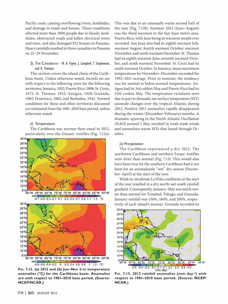
S156 | August 2013
Pacific coast, causing overflowing rivers, landslides, and damage to roads and houses. These conditions affected more than 3000 people due to floods, land-slides, obstructed roads and fallen electrical wires and trees, and also damaged 922 houses in Panama. Heavy rainfalls resulted in three casualties in Panama on 25–29 November.
2) the Caribbean—M. A. Taylor, J. Campbell, T. Stephenson, and A. Trotman
This section covers the island chain of the Carib-bean basin. Unless otherwise noted, records set are with respect to the following years for the following territories: Jamaica, 1952; Puerto Rico, 1898; St. Croix, 1972; St. Thomas, 1953; Antigua, 1928; Grenada, 1985; Dominica, 1982; and Barbados, 1942. Normal conditions for these and other territories discussed are estimated from the 1981–2010 base period, unless otherwise noted.
(i) TemperatureThe Caribbean was warmer than usual in 2012,
particularly over the Greater Antilles (Fig. 7.12a).
This was due to an unusually warm second half of the year (Fig. 7.12b). Summer 2012 (June–August) was the third warmest in the San Juan metro area, Puerto Rico, with June being its warmest month ever recorded. San Juan also had its eighth warmest July, warmest August, fourth warmest October, warmest November, and ninth warmest December. St. Thomas had its eighth warmest June, seventh warmest Octo-ber, and ninth warmest November. St. Croix had its ninth warmest October. In Jamaica, mean maximum temperatures for November–December exceeded the 1992–2011 average. Prior to summer, the tendency was for normal to below-normal temperatures. An-tigua had its 3rd coldest May and Puerto Rico had its 11th coolest May. The temperature variations were due in part to dramatic sea surface temperature (SST) anomaly changes over the tropical Atlantic during 2012. Positive 2011 anomalies rapidly disappeared during the winter (December–February) months. A dramatic upswing in the North Atlantic Oscillation (NAO) around 1 May resulted in weak trade winds and anomalous warm SSTs that lasted through Oc-tober.
(ii) PrecipitationThe Caribbean experienced a dry 2012. The
northwest Caribbean and northern Lesser Antilles were drier than normal (Fig. 7.13). This would also have been true for the southern Caribbean had it not been for an anomalously “wet” dry season (Decem-ber–April) at the start of the year.
Weak-to-moderate La Niña conditions at the start of the year resulted in a dry north-wet south rainfall gradient. Consequently, January–May was much wet-ter than normal for Trinidad, Tobago, and Grenada. January rainfall was 156%, 184%, and 200%, respec-tively of each island’s normal. Grenada recorded its
Fig. 7.12. (a) 2012 and (b) Jun–nov 2-m temperature anomalies (°C) for the Caribbean basin. anomalies are with respect to 1981–2010 base period. (source: nCeP/nCaR.)
Fig. 7.13. 2012 rainfall anomalies (mm day-1) with respect to 1981–2010 base period. (source: nCeP/nCaR.)

S157STATE OF THE CLIMATE IN 2012 |AuguST 2013
wettest dry season (January–May) in 27 years (245% of normal relative to a 1985–2012 base period) while Barbados recorded rainfall that was 159% of normal. In contrast, the northwest Caribbean was dry. Ja-maica received 69% of normal rainfall in January and 55% of normal in February, relative to a 1971–2000 baseline. Similarly, 52% of Cuba experienced moder-ate to severe drought conditions in January, followed by 42% in February.
As the Pacific rapidly transitioned in early 2012 to ENSO-neutral conditions, wetter conditions spread northward. St. Vincent, St. Lucia, Barbados, Domi-nica, St. Thomas, Antigua, Puerto Rico, and Jamaica all reported two or more months between February and May that were wetter than average. Records include the second wettest March in St. Thomas, St. Croix, and Puerto Rico (San Juan metro area), the fifth wettest March since 1961 for Jamaica, the third wettest April since 2002 in Antigua, the second wet-test May in Grenada, and the eighth wettest May in St. Thomas and Puerto Rico.
A drier regime was observed beginning in June, the start of the Caribbean wet season. June and Sep-tember were notable for records set. It was the driest June (3.1 mm) in 60 years for St. Maarten and the driest for San Juan, Puerto Rico (4.1 mm). June was the second driest for St. Thomas, the third driest for St. Croix, Barbados, and Antigua, and the fifth driest for Dominica. Grenada, St. Vincent, St. Lucia, and Jamaica also recorded below-normal June rainfall. September was the driest for St. Thomas, St. Maarten (since 1986), and Antigua (since 1978) and the sixth driest for Puerto Rico. Trinidad, Tobago, Grenada, St. Vincent, St. Lucia, Barbados, Dominica, Jamaica, and Cuba reported below- or well-below-normal September rainfall. Almost all reporting countries recorded below-normal rainfall in November. Bar-bados (Grantley Adams Airport) had its fifth lowest November rainfall.
Tropical storm activity accounted for rainfall re-ceived in August and October. Three of eight named storms in August moved through the Lesser Antilles. The rain bands of Tropical Storms Ernesto and Isaac provided more than half of Barbados’ August rainfall, which was the highest since 2000. Ernesto and Isaac increased rainfall amounts over the southern half of Puerto Rico, and Isaac also produced significant rain over Cuba. Hurricane Rafael accounted for more than half of the October rainfall recorded in Antigua, which was 200% of normal and the second highest October rainfall.
(iii) Notable eventsTropical storms impacting the Caribbean were
clustered in August and October. Of the five systems that impacted the region (Isaac, Ernesto, Tropical Depression #7, Sandy, and Rafael), Isaac and Sandy were the most devastating. Isaac passed over the southwestern peninsula of Haiti and Cuba, and produced heavy rainfall across Puerto Rico and the Dominican Republic. In Haiti at least 24 people died, 12 houses were destroyed, and 269 houses damaged. Agricultural losses were estimated at $242 million (US dollars) and damage to electrical infrastructure reached $7.9 million (US dollars). In the Dominican Republic, authorities evacuated nearly 7800 people from low-lying areas, and river flooding and storm surge cut off 90 towns. Five fatalities were reported and agricultural losses were estimated at $30 million (US dollars). Damages were less severe in Cuba. The storm destroyed 4 houses and damaged 19 homes in Baracoa, and 72 homes were flooded by the Sagua de Tánamo River in Holguín province.
Hurricane Sandy made landfall near Kingston, Jamaica, as a Category 1 storm and strengthened to Category 2 as it re-emerged in the Caribbean Sea. On 25 October, Sandy hit Cuba, before weakening to Category 1 and moving through the Bahamas. In Jamaica, Sandy left 70% of residents without electric-ity, killed one person, and caused damages estimated at $55.23 million (US dollars). In Haiti, Sandy’s outer bands triggered floods that killed at least 54 people and left about 200 000 homeless. In the Dominican Republic, two people died. In Cuba, approximately 15 000 homes were destroyed and 11 people were killed; damage was estimated at $2 billion (US dol-lars). In the Bahamas, two died and an estimated $300 million (US dollars) in damage was done.
d. South AmericaThe 2012 annual mean temperature was predomi-
nantly above normal in South America. Persistent positive anomalies (1°C–2°C above the 1971–2000 average) were observed over northern South Amer-ica, Brazil, Paraguay, and northern Argentina (Fig. 7.14a). Precipitation was above normal during January–March along northern South America, the Peru-Chile-Bolivia border, and parts of central and southern Argentina with anomalies ranging from 50 mm to 250 mm. In contrast, during most of the year, below-normal precipitation was observed in central, northeast, and southern Brazil, central Chile, and northwestern Argentina (Fig. 7.14b).

S158 | August 2013
1) northern SoUth aMeriCa and the tropiCal andeS—R. Martínez, J. Arévalo, G. Carrasco, C. Euscategui, E. Jaimes, and J. Nieto
In this section, unless otherwise noted, normals and anomalies are based upon a 1971–2000 average.
(i) TemperatureTemperatures in Colombia were normal to above
normal during most of the year. Positive temperature anomalies ranged between 2°C and 5°C across parts of the central region of the country. In southern Ecuador, maximum temperatures were above nor-mal during April and September–November, while minimum temperatures were below normal during January–February and August. The temperature in Peru showed positive anomalies of up to 2.5°C along the coast during May–June and up to 4.5°C (in Cayalti-Lambayeque) during July–September. Be-tween July and August, below-average temperatures were registered in the Andean zone and the Peruvian Amazonia. On 19 September, in Peru’s Ponaza valley in San Martin region, a heat wave brought tempera-tures as high as 40°C, resulting in a new temperature record for September. In Bolivia, historical maximum temperatures were observed during October 2012, with new maximum temperature records reported in Reyes, San Matías, San José, Puerto Suárez, Co-chabamba, and Potosi. During March, Puerto Suárez recorded its lowest minimum temperature since 1987.
(ii) PrecipitationDuring January–March, above-normal precipita-
tion was observed across most of Venezuela, except
for parts of the west and southeast where negative anomalies were registered. Overall, the dry season (De-cember–May) ended with above-normal precipitation. The rainy season (June–November) was marked by below-normal precipitation. The largest rivers of Venezu-ela (Orinoco and Caroní) re-corded below-normal levels during May and June. Dur-ing August and September, as a consequence of the tran-sit of tropical storms Ernes-to, Helene, and Isaac, many stations along the coast and the islands recorded heavy
rainfall. The most extreme precipitation was 215.2 mm day-1 in Isla de Aves station, with other stations reporting more than 50 mm day-1.
Dry conditions were recorded in the Andean re-gion of Colombia during the second half of the year. In contrast, tropical waves and/or tropical cyclones produced unexpected rainfall in the Caribbean coast-al zone, which is typically dry. The frequent intrusion of Amazonian moisture and its interaction with the cyclonic activity generated above-average precipita-tion in Colombia’s Orinoquia and Amazonia regions.
In Ecuador, precipitation during January–March, was near normal in the central coast, central and southern highlands, and eastern Amazonia. Dur-ing October–November, precipitation records were registered in southern highlands (140% to 200% of normal).
In Peru, intense and frequent precipitation during the first half of the year across the northern coast and southern highlands caused rivers to flow as high as 211% and 400% of normal, respectively. In contrast, during July–September, precipitation was below nor-mal. During October–December, precipitation was 200% of normal in northern and central zones of the country, while in the southern zones precipitation was normal to below normal. On 4 April a rainfall event of 37 mm was registered near Chosica—the highest daily precipitation total of the last 20 years. One person was killed, many people were injured and severe damage to houses and basic infrastructure was reported.
In Bolivia, precipitation was generally above nor-mal in the Altiplano region. The most significant anomaly was registered in Oruro with an annual
Fig. 7.14. (a) 2012 annual mean temperature anomalies (°C) and (b) 2012 an-nual precipitation anomalies (%) for south america (1971–2000 base period). (sources: Data from 1173 stations provided by national meteorological ser-vices of argentina, brazil, bolivia, Chile, Colombia, ecuador, Paraguay, Peru, suriname, Uruguay, and Venezuela. the data was compiled and processed by CiiFen.)

S159STATE OF THE CLIMATE IN 2012 |AuguST 2013
anomaly of +150.7 mm. Along the Valles, precipita-tion was close to normal except in Cochabamba where the annual anomaly was 167% of normal. At the Villa Montes station, an annual anomaly of 266.1 mm (134% of normal) was registered. In contrast, most of the Llanos Orientales region experienced negative precipitation anomalies. In Puerto Suárez the annual precipitation was 60% of normal.
2) tropiCal SoUth aMeriCa eaSt of the andeS—J. A. Marengo, J. Ronchail, and L. M. Alves
In this section, unless otherwise noted, normals and anomalies are based upon a 1961–90 average.
(i) TemperatureAccording to data from the INPE and INMET in
Brazil, across most of tropical South America, east of the Andes, the monthly mean temperatures were about 1°C warmer than average. In northern Paraguay and southern Bolivia seasonal temperature anomalies were as high as +3°C between August–October. Some extreme hot days were recorded during 2012. On 18 September, the maximum temperature soared to 34.1°C in São Paulo, Brazil, the highest during the last 57 years (the September mean maximum temperature is about 24°C). In contrast, on 25 September the situ-ation changed and temperatures dropped as low as 0.7°C in southern Brazil, and snow was reported in some cities in this region. On 28–31 October, south-eastern Brazil experienced high temperature records: 43°C in the city of Ribeirão Preto on 28 October and 42°C in São Paulo on 31 October. The mean maxi-mum temperature for that region is between 19°C and 22°C. Brazil’s most important record high tem-perature of 2012 occurred on 26 December in Rio de Janeiro, where temperatures reached 43.2°C, the high-est temperature detected for any month since 1915.
From May to August, six cold surges affected southeastern South America, especially southern Amazonia and southern Brazil. In May, air tempera-tures dropped to 0°C in southern Brazil, and a cold air intrusion dropped temperatures to -4.3°C at Bom Jesus, in extreme southern Brazil on 7 June and -9.3°C on 8 June—Brazil’s lowest temperature of 2012. On 8 June, the cold air reached western Amazonia where temperatures dropped to 12.7°C. This system also af-fected the southern Peruvian Andes, causing extreme cold weather events with some areas reporting below- freezing temperatures.
(ii) PrecipitationDuring 2012, rainfall was above average between
January and April (50 mm–100 mm above the 1961–90 average) across the 5°S–15°S latitude bands in South America. Rainfall was well-above-normal in Bolivia, Paraguay, and southeastern Brazil between May and July (50 mm above normal). Wet condi-tions prevailed in Amazonia during austral spring and summer (300 mm above normal). Many rainfall records were broken during this period. In contrast, dry conditions prevailed in northeast Brazil, from January to May (100 mm below normal), due to an anomalously northward displacement of the ITCZ over the Atlantic and an unfavorable phase of the MJO for convective activity and precipitation, re-sulting in the worst drought in the region in over 30 years (Sidebar 7.2). After April, deficit expanded from northeast towards the west and north, compromising the northern tropical rainy season. From August to December, rainfall deficits were observed in most regions from southern Brazil to the northern tip of South America (Sidebar 7.2).
In January 2012, heavy rains produced landslides and floods in Minas Gerais, in southeastern Brazil, affecting 53 cities and killing 7 people, and in Feb-ruary the intense rains in Acre, western Amazonia, generated floods that affected 13 000 people. In Ecua-dor, heavy rains occurred in the provinces of Guayas and El Oro, and left nearly 20 000 people affected by floods. Floods and landslides in Bolivia left 13 people dead and almost 14 000 affected. Also in January, the Paraguayan government declared a state of food security emergency due to drought as 263 800 families suffered crop losses. On 8 January, 12 people died as consequence of intense rains in the central region of Rio de Janeiro, Brazil.
In March, floods in 18 of Colombia’s 32 depart-ments affected more than 66 000 people, and in July, f loods affected the Putumayo region. Heavy rains, f loods, and mudslides affected Paraguay’s Chaco region in April. In the Sierra of Rio de Janeiro, in-tense rainfall affected the region of Teresopolis on 7 April, killing seven people. In October, floods and landslides occurred in Colombia, leaving 10 people dead and almost 200 families affected. In contrast, the La Niña phenomenon was blamed for the drought that affected parts of southern Brazil, which began in November 2011 and lasted through November 2012. Of note, on 17 September the city of São Paulo had its 62nd consecutive day without rainfall—its longest dry spell during the last 50 years. December was a dry month in most of central Brazil.
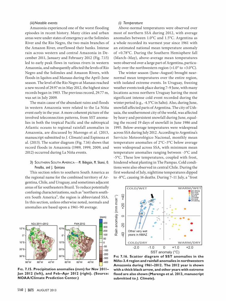
S160 | August 2013
(iii) Notable eventsAmazonia experienced one of the worst flooding
episodes in recent history. Many cities and urban areas were under states of emergency as the Solimões River and the Rio Negro, the two main branches of the Amazon River, overflowed their banks. Intense rain across western and central Amazonia in De-cember 2011, January and February 2012 (Fig. 7.15) led to early peak flows in various rivers in western Amazonia, and subsequently affected the levels of Rio Negro and the Solimões and Amazon Rivers, with floods in Iquitos and Manaus during the April–June season. The level of the Rio Negro at Manaus reached a new record of 29.97 m in May 2012, the highest since records began in 1903. The previous record, 29.77 m, was set in July 2009.
The main cause of the abundant rains and floods in western Amazonia were related to the La Niña event early in the year. A more coherent picture of the involved teleconnection patterns, from SST anoma-lies in both the tropical Pacific and the subtropical Atlantic oceans to regional rainfall anomalies in Amazonia, are discussed by Marengo et al. (2013, manuscript submitted to J. Climate) and Espinoza et al. (2013). The scatter diagram (Fig. 7.16) shows that record f loods in Amazonia (1989, 1999, 2009, and 2012) occurred during La Niña events.
3) SoUthern SoUth aMeriCa—M. Bidegain, M. Skansi, O. Penalba, and J. Quintana
This section refers to southern South America as the regional name for the combined territory of Ar-gentina, Chile, and Uruguay, and sometimes adjacent areas of far southeastern Brazil. To reduce potentially confusing characterizations, such as “northern south-ern South America”, the region is abbreviated SSA. In this section, unless otherwise noted, normals and anomalies are based upon a 1961–90 average.
(i) TemperatureAbove-normal temperatures were observed over
most of northern SSA during 2012, with average anomalies between 1.0°C and 1.5°C. Argentina as a whole recorded its warmest year since 1961 with an estimated national mean temperature anomaly of +0.78°C. During the Southern Hemisphere fall (March–May), above-average mean temperatures were observed over a large part of Argentina, particu-larly over the northwestern region (+1.0° to +3.0°C).
The winter season (June–August) brought near-normal mean temperatures over the entire region, with isolated extreme events. In Uruguay, freezing weather events took place during 7–9 June, with many locations across northern Uruguay having the most significant intense cold event recorded during the winter period (e.g., -4.5°C in Salto). Also, during June, snowfall affected parts of Argentina. The city of Ush-uaia, the southernmost city of the world, was affected by heavy and persistent snowfall during June, equal-ing the record 19 days of snowfall in June 1986 and 1995. Below-average temperatures were widespread across SSA during July 2012. According to Argentina’s Servicio Meteorológico Nacional, monthly mean temperature anomalies of 2°C–3°C below average were widespread across SSA, with minimum mean temperature anomalies ranging between -3°C and -5°C. These low temperatures, coupled with frost, hindered wheat planting in The Pampas. Cold condi-tions were also observed in central Chile. During the first weekend of July, nighttime temperatures dipped to -8°C, causing 16 deaths. During 7–11 July, a “frost
Fig 7.16. scatter diagram of sst anomalies in the niño-3.4 region and rainfall anomalies in northwestern amazonia during 1961–2012. the 2012 year is shown with a thick black arrow, and other years with extreme flood are also shown (marengo et al. 2013, manuscript submitted to J. Climate).
Fig. 7.15. Precipitation anomalies (mm) for nov 2011–Jan 2012 (left), and Feb–apr 2012 (right). (source: noaa/Climate Prediction Center.)

S161STATE OF THE CLIMATE IN 2012 |AuguST 2013
period” was recorded throughout Uruguay, charac-terized by the persistence of at least five consecutive days with temperatures below freezing level. The low-est minimum temperature on 7 July was in Mercedes (-4.9°C). On 11 July, below freezing temperatures were observed across the entire country with values as low as -3.0°C in Mercedes and Florida. On 30 July, the last frost was accompanied by extremely low tempera-tures in central and southern Uruguay, with -6.0°C recorded in Florida and -5.2°C in Mercedes. Over the entire SSA, significant positive anomalies were observed during the Southern Hemisphere spring (September–November), with temperature anomalies as high as +3°C across northern and northwestern Argentina. Argentina, as a whole, observed its warm-est spring since 1961.
(ii) PrecipitationDuring the first quarter of 2012, below-average
precipitation across SSA was driven by a La Niña episode which began in 2011. From December 2011 to February 2012, the regions most affected by rain deficiencies were northeastern Argentina, eastern Uruguay, and southern Brazil. The year 2012 was the fourth consecutive year with below-average precipita-tion across central and northern Chile (65% of normal and 30% of normal, respectively).
During 1–9 February 2012, abundant precipitation fell across western Uruguay and Entre Ríos province (Argentina). In several locations, the total rainfall accumulated was over 200 mm, with Quebracho recording 315 mm—the largest amount in Uruguay. The heavy precipitation brought relief to areas that had experienced below-average precipitation since November 2011.
Drier-than-average conditions prevailed across SSA during March–July 2012. Parts of eastern central Argentina reported their driest July in more than 50 years, including the towns of Laboulaye, Pehuajó, and Dolores. Similar conditions were observed in central and southern Chile, which experienced their driest July in 11 years.
In August, extreme rainfall affected Buenos Aires province (Argentina), producing severe f looding. Monthly totals broke historical records in several locations. During August, new rainfall records were set in the Argentine Pampas. The largest anomalies occurred in southeastern Buenos Aires province, but records were also set in northern parts of the prov-ince, west of La Pampa, south of Cordoba, southern Santa Fe, and Entre Ríos. According to Argentina’s Servicio Meteorológico Nacional, the monthly rain-
fall was the most significant in at least 51 years. Nota-bly, in Tandil, Azul, Tres Arroyos, and Nueve de Julio, the rains were the most significant in over 100 years. The city of Buenos Aires and surrounding areas, also had extreme rainfall, with a monthly total of 228.0 mm—the second largest August total since 1906.
Significant rainfall was also observed during August in Uruguay, particularly across the southern, southwestern, western, and central regions. The high-est values reported were between 200 mm and 250 mm in the western region and 386 mm in Durazno.
During the second half of 2012, positive SST anomalies were present across the tropical Pacific Ocean, favoring positive rainfall anomalies in SSA during October–December 2012. Eastern Argen-tina, Uruguay, southern Brazil, and southern Chile experienced intense rainfall during the last three months of 2012. These conditions favored better water conditions for pastures and summer crops (soybean, maize, and rice).
(iii) Notable eventsAfter experiencing drought conditions at the be-
ginning of the year, the northwest region of Buenos Aires province reported heavy rains that caused floods and affected summer crops. In February, heavy rain was recorded in the province of Entre Ríos and in northeastern Buenos Aires. The region north of 40°S experienced severe heavy rains during May, October, November, and December.
There were two extreme rain events in Chile. The first was 26 May, when 108 mm of precipitation fell in San Fernando due to a warm frontal system which concentrated its maximum intensity in the O’Higgins Region (135 km south of Santiago). The second epi-sode occurred in southern Chile between 22 and 24 December, with a cumulative amount of 151 mm in Valdivia. In this region, the daily maximum of 79.3 mm occurred on 23 December. This was the most severe episode in December since 1950.
January and March were the warmest months ever recorded in the southern and central Chile. In January, Coyhaique recorded its highest average maximum temperature since 1961, with an anomaly of 4.8°C and in March, central Chile recorded the warmest average maximum temperature since 1910 when the Quinta Normal Santiago station maxi-mum temperature soared to 30.6°C, 3.2°C above the 1971–2000 average.

S162 | August 2013
siDebaR 7.2: tHe 2012 seVeRe DRoUgHt oVeR noRtHeast bRaZil—V. B. S. SiLVA, V. E. KOuSKy, F. D. S. SiLVA, M. A. SALVADOR, AND J. A. ARAVEQuiA
Northeast Brazil experienced severe drought during the 2012 wet season, which followed several years of near- to above-normal rainfall. During the rainy season of 2012, many areas received less than 50% of the average rainfall for the season, leading many municipalities to declare states of emergency. Lack of rain dried up rivers and damaged crops, which boosted food prices.
The rainy season over Northeast Brazil varies from region to region: December–February (DJF) or November–January (NDJ) in southern sections, January–March (JFM) in central sections, February–April (FMA) in northern sections, and May–July (MJJ) along the eastern coast. The 2012 precipitation anomalies for NDJ and FMA (see Fig. 7.15) show below-average rainfall over Northeast Brazil during both periods, with the largest deficits occurring in FMA when rainfall is usually a maxi-mum over northern Northeast Brazil. The rainfall deficits in FMA extended over most of Brazil, except for the western and northern portions of the Amazon Basin where above-average rainfall was observed.
The El Niño–Southern Oscillation (ENSO) phenomenon has a significant impact on rainfall over tropical Brazil. The impacts on Northeast Brazil partly depend on the intensity and dis-tribution of the SST departures in the tropical Pacific Ocean. Often, below-average rainfall over the central/eastern Amazon and the Northeast is associated with warmer-than-average SSTs (El Niño) in the equatorial Pacific, while above-average rainfall in those regions is associated with colder-than-average SSTs (La Niña). Other factors, such as the distribution of SST anomalies in the tropical Atlantic and, consequently, the posi-tion and intensity of the ITCZ, and transient systems (e.g, cold fronts and upper-level subtropical cyclonic vortices) are also important, and affect rainfall variability in Northeast Brazil. The 2012 Northeast drought was unexpected, since below-average SSTs were present in the central equatorial Pacific (La Niña).
The observed data for some selected stations, from the Brazilian National Weather Service, INMET, indicate that several Northeast stations had FMA 2012 precipitation deficits
greater than 400 mm, indicating strong drought conditions, es-pecially during March and April. Figure SB7.2 top p a n e l s s h o w monthly precipi-tation anomalies ca lcu lated for the period July 2011–June 2012 in two selected 5° by 5° boxes: 1 ) N o r t h e r n Northeast Brazil (NNEBR, 2°S–10 ° S , 37 ° W –45°W) and 2) Southern North-east Brazil (SNE-BR, 10°S–18°S, 40°W–48°W). It is clear that pre-cipit at ion was be low normal between December 2011 and May 2012 in both regions, with maximum deficits occurring in March and April. The FMA average daily precipitation for each year during 1979–2012 in the two selected boxes (Fig. SB7.2, bottom panels) shows that 2012 was the driest FMA period in the entire 34-year record for both NNEBR and SNEBR. The preceding years (2006–11) were generally quite wet for both regions.
The pattern of outgoing-longwave radiation (OLR) for FMA 2012 (Fig. SB.7.3a) shows negative anomalies (enhanced convective activity) in the tropical Atlantic north of the equa-tor, indicating that the ITCZ had shifted northward from its normal position. This is consistent with below-average SSTs in the tropical Atlantic Ocean (Fig. SB.7.3b). The OLR pattern also shows enhanced convective activity over the northern Amazon Basin and over the eastern tropical Pacific where SSTs were above average.
A longitude-height cross section of the anomalous diver-gent circulation for the latitude band from the equator to 10°S (Fig. SB.7.3c) shows anomalous sinking motion in the mid-troposphere (400 hPa to 700 hPa) over Northeast Brazil (30°W–40°W) and anomalous rising motion over the Amazon Basin and the extreme eastern Pacific, consistent with the patterns of OLR and SST anomalies. This suggests that the distribution of SST anomalies in the tropical Atlantic and Pacific may have caused a westward shift in the divergent circulation cell (regional Walker circulation cell) from its normal position, contributing to the Northeast Brazil drought and heavy rainfall in the western Amazon Basin.
Fig. sb.7.3. (a) anomalous outgoing longwave radiation (olR, W m-2), (b) sea surface temperatures (ssts, °C), and (c) zonal divergent circulation, for Feb–apr 2012. (source: nCeP/nCaR.)
Fig. sb.7.2. (top) monthly precipitation anoma-lies (mm) for Jul 2011–Jun 2012, for nnebR (left) and snebR (right). anomalies are computed with respect to 1981–2010. (bottom) average daily pre-cipitation (mm) for Feb–mar in the two regions for 1979–2012. the orange lines indicate the 1981–2010 mean daily precipitation.
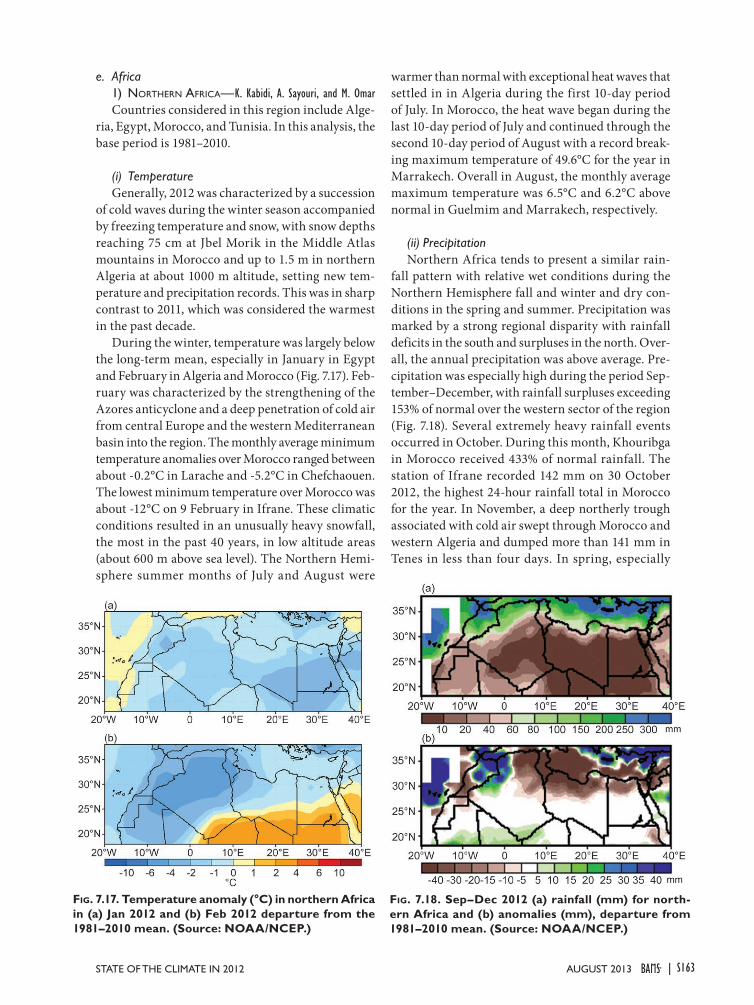
S163STATE OF THE CLIMATE IN 2012 |AuguST 2013
e. Africa1) northern afriCa—K. Kabidi, A. Sayouri, and M. Omar Countries considered in this region include Alge-
ria, Egypt, Morocco, and Tunisia. In this analysis, the base period is 1981–2010.
(i) TemperatureGenerally, 2012 was characterized by a succession
of cold waves during the winter season accompanied by freezing temperature and snow, with snow depths reaching 75 cm at Jbel Morik in the Middle Atlas mountains in Morocco and up to 1.5 m in northern Algeria at about 1000 m altitude, setting new tem-perature and precipitation records. This was in sharp contrast to 2011, which was considered the warmest in the past decade.
During the winter, temperature was largely below the long-term mean, especially in January in Egypt and February in Algeria and Morocco (Fig. 7.17). Feb-ruary was characterized by the strengthening of the Azores anticyclone and a deep penetration of cold air from central Europe and the western Mediterranean basin into the region. The monthly average minimum temperature anomalies over Morocco ranged between about -0.2°C in Larache and -5.2°C in Chefchaouen. The lowest minimum temperature over Morocco was about -12°C on 9 February in Ifrane. These climatic conditions resulted in an unusually heavy snowfall, the most in the past 40 years, in low altitude areas (about 600 m above sea level). The Northern Hemi-sphere summer months of July and August were
warmer than normal with exceptional heat waves that settled in in Algeria during the first 10-day period of July. In Morocco, the heat wave began during the last 10-day period of July and continued through the second 10-day period of August with a record break-ing maximum temperature of 49.6°C for the year in Marrakech. Overall in August, the monthly average maximum temperature was 6.5°C and 6.2°C above normal in Guelmim and Marrakech, respectively.
(ii) PrecipitationNorthern Africa tends to present a similar rain-
fall pattern with relative wet conditions during the Northern Hemisphere fall and winter and dry con-ditions in the spring and summer. Precipitation was marked by a strong regional disparity with rainfall deficits in the south and surpluses in the north. Over-all, the annual precipitation was above average. Pre-cipitation was especially high during the period Sep-tember–December, with rainfall surpluses exceeding 153% of normal over the western sector of the region (Fig. 7.18). Several extremely heavy rainfall events occurred in October. During this month, Khouribga in Morocco received 433% of normal rainfall. The station of Ifrane recorded 142 mm on 30 October 2012, the highest 24-hour rainfall total in Morocco for the year. In November, a deep northerly trough associated with cold air swept through Morocco and western Algeria and dumped more than 141 mm in Tenes in less than four days. In spring, especially
Fig. 7.17. temperature anomaly (°C) in northern africa in (a) Jan 2012 and (b) Feb 2012 departure from the 1981–2010 mean. (source: noaa/nCeP.)
Fig. 7.18. sep–Dec 2012 (a) rainfall (mm) for north-ern africa and (b) anomalies (mm), departure from 1981–2010 mean. (source: noaa/nCeP.)

S164 | August 2013
in April, isolated storms soaked local areas such as Bouarfa in Morocco with rainfall amounts about 509% of normal. In Egypt, rainfall was near average with all station totals averaging 40 mm, about 90% of the climatological mean. All the annual rainfall oc-curred during the rainy season from November 2011 to March 2012. Dry conditions prevailed during the remainder of the year.
(iii) Notable eventsSevere and unusually cold wave conditions pre-
vailed over the region during the winter, particularly in January and February, claiming about 30 lives in Algeria. Several temperature records were established. The freezing temperatures were accompanied by record-breaking snow storms. In contrast, intense heat waves occurred during the summer season. The heat associated with predominant easterly winds fa-vored the outbreak of several bush fires burning over 10 000 ha in Morocco and Algeria.
2) WeSt afriCa—F. Sima, A. Kamga, i. Raiva, F. S. Dekaa, and A. i. James
West Africa is defined here as the region from the Guinea coastline to about 20°N and from the tropical North Atlantic coast in Guinea to Chad. Climatologi-
cally, it consists of two distinct but inherently linked sub regions: (1) The Sahel to the north from about 12°N to 17°N, spanning countries from Senegal and The Gambia in the west to Chad in the east; and (2) the Gulf of Guinea region to the south from about 4°N to 10°N encompassing the Guineas to the west along the east Atlantic coast and Nigeria and Cameroon to the east. Unless otherwise specified, the climatologi-cal base period for both temperature and precipitation is 1981–2010.
(i) TemperatureAnnual temperature was about average across
West Africa, except for the north central region, where anomalies exceeded 1°C over northwestern Ni-ger (Fig. 7.19). Temperature was less than 0.5°C above normal over northern Mali, eastern Mauritania, and eastern Senegal. However, during February–April 2012, temperature anomalies averaged 2°C above nor-mal over northeastern Mali and much of Niger, with peaks of 3°C above normal in Niger. Temperature was slightly below normal in pockets over northeastern Nigeria and in local areas in central Sahel including western Niger and eastern Burkina Faso. Local areas in Nigeria recorded the most frequent highest daily maximum temperatures, averaging 42°C–47°C in
siDebaR 7.3: aFRiCa: tHe FlooDs oF tHe saHel in 2012—W. M. THiAW
Fig. sb 7.4. Rainfall anomalies (mm) across the sahel during (a) Jun, (b) Jul, (c) aug, and (d) sep 2012.
In the heart of West Africa, The Sahel, a narrow band of land sand-wiched between the Sahara desert and the Savanna lands in the Gulf of Guinea region, and roughly between 12°N–15°N and 18°W–25°E, experi-enced extremely heavy rains during June–October 2012. This marked a continuation of the increased rainfall trend that has been observed since early in the 21st century. Overall, the rainfall season was the third wettest since 1948 and the wettest since 1952 according to NOAA’s Climate Prediction Center gauge-only grid-ded precipitation dataset (PREC/L). The regional average rainfall amount exceeded 400 mm and was about 120 mm above the 1948–2012 mean. Rain-fall surpluses were observed across the region, except for a few localities, where totals were near average. The areas that registered the strongest

S165STATE OF THE CLIMATE IN 2012 |AuguST 2013
February–May. Maximum daily temperatures at the station of Yola were above 42°C for 60 consecutive days.
(ii) PrecipitationPrecipitation was above average, except for the
Guinea coast, which registered near-average rainfall based on the CPC PREC/L data (Chen et al. 2002). The West African monsoon season was once again very active. Rainfall totals during June–September 2012 ranged from 100 mm to 300 mm in the north-ern Sahel to over 1200 mm in the areas of maximum
precipitation, including the western Guinean coast, coastal Nigeria, and along the southern border with Cameroon (Fig. 7.20a). The 300 mm-isohyet for June–September, defining the strength of the mon-
Fig. 7.19. annual temperature anomaly (°C) for West africa, departure from 1981–2010 mean. (source: noaa/nCeP.)
Fig. 7.20. Jun–sep 2012 (a) rainfall (mm) for West africa and (b) anomalies (mm), departure from 1981–2010 mean. (source: noaa/nCeP.)
anomalies over 200 mm above the 1981–2010 climatological mean included northeastern Nigeria and parts of the central and western sectors of the Sahel. The torrential rains and associated persistent flooding hit the western Sahel hard-est in areas that included western Mali, the southern half of Senegal, and the Guineas. The rainfall season was off to an excellent start in June with surpluses across the region. Anomalies exceeded 100 mm in northern Nigeria, and ranged between 20 mm and 50 mm above average in the central and western sectors of the Sahel (Fig. SB7.4). The heaviest rain storms occurred during July–September. The western end of The Sahel was the most affected with monthly surpluses exceeding 100 mm along the coastal areas of Senegal and the Guineas. For this sub-region, 2012 was the second wettest season, after 2010, since 1948 with totals averaging over 850 mm, or 300 mm above the 1948–2012 mean.
Many extreme events were reported. The station of Dakar on coastal Senegal in the far western end of the Sahel registered a record-breaking 152 mm on 26 August, causing the government to launch a rescue plan to assist victims. This extreme heavy rainfall event, which claimed the lives of 18 people and injured 42, followed other deadly storm events
that occurred earlier during August. A storm on 13 August dropped about 75 mm and resulted in nine deaths when a fac-tory wall collapsed onto residential homes following the heavy rains. The flooding was exacerbated by saturated soils from the active 2012 monsoon onset. Additionally, the water table in this region has become high due to persistent extremes since 2005. According to news reports, downpours in central Nigeria’s Plateau State on 13 August washed away bridges, destroyed farmland, and left hundreds of people homeless. The floods were associated with above-normal sea surface temperatures (SSTs) in the northern tropical and subtropi-cal Atlantic and overall below-normal SSTs in the southern Atlantic and especially along the Guinea coast. This positive dipole mode is known to enhance (suppress) precipitation in the Sahel (Gulf of Guinea region). Consistent with the tropi-cal Atlantic warming, the low level westerly jet across the eastern Atlantic into West Africa was prominent and marked by anomalies of 4 m s-1 or more at its core region. This jet converged with the southerly outflow from the St. Helena high pressure system in the southern Atlantic to create favorable conditions for moisture to penetrate and persist in West Africa causing the devastating flood episodes.

S166 | August 2013
soon system, stretched from southern Mauritania to Chad along the latitude band north of 15°N. The 2012 rainy season featured above-average rainfall across the Sahel and portions of the Gulf of Guinea region (Fig. 7.20b). Rainfall anomalies for June–September exceeded 50 mm in the northern Sahel, and surpluses were above 300 mm along the coastal Guineas. Rain-fall was also much above average over northeastern Nigeria and southern Chad. Daily rainfall totals were 100 mm or higher at several locations between May and August. The Lagos area in the southern part of Nigeria registered a 24-hour rainfall total between 170 mm and 226 mm in June, while the northern states of Gombe, Kano, and Zaria were soaked with 24-hour rainfall totals of 120 mm, 143 mm, and 158 mm, respectively, during August. In central Sahel, there were pockets where rainfall was near average for the season. In contrast, moisture deficits prevailed in the southern sector of the Gulf of Guinea region over eastern Liberia, Cote d’Ivoire, and Ghana.
(iii) Notable eventsThe heavy rains in the Sahel caused f looding
that resulted in loss of life and property damage. In Burkina Faso, repeated flooding events between June and September affected nearly 50 000 people with 33 wounded and 18 killed. In Mali, heavy rains in August resulted in flooding in many localities in the south. It was reported that 2 800 houses collapsed, thousands of people were left homeless, and crops were destroyed in local areas. Five people died from flood-related injuries. In Niger, it was reported that 65 people lost their lives and 125 000 people were dis-placed from their homes during the summer season. Torrential rains also inundated local areas in Senegal and The Gambia, displacing thousands of people and killing at least 20 people. Ni-geria experienced the worst f looding in more than 40 years as a result of the heavy rains, elevated rivers, and the release of water from dams during the last week of August. Nearly the entire country was affected and millions of people across 14 states suffered severe economic losses. In Chad, heavy rains in early August caused f looding in many parts of the country. By Sep-
tember, the floods had affected 466 000 people (kill-ing 34), 96 000 houses were destroyed, and 255 000 ha of crops flooded. The downpours cut off major humanitarian supply routes to some localities, leading to hundreds of people in need of emergency support. In Cameroon, 10 people died and hundreds were left homeless due to the flooding.
3) eaStern afriCa—W. Gitau, C. Oludhe, L. Ogallo, Z. Atheru, and P. Ambenje
Countries considered in this analysis encompass the Greater Horn of Africa, extending from Tanzania in the south to Sudan in the north, and from the west-ern Indian Ocean coastline to the boundary between Uganda and Congo. Unless otherwise stated in this section, the base period of 1961–90 has been used.
(i) TemperatureOverall, temperature was above normal over
much of the Greater Horn of Africa (GHA). In May, minimum temperature (Fig. 7.21a) was more than 1°C above normal over much of North Sudan, parts of western Eritrea, northwestern and eastern Ethiopia, southern Somalia, much of Kenya, Rwanda, Burundi, and northwestern and northeastern Tanzania. Mini-mum temperature anomalies were more than 2°C above normal over northern Sudan and in pockets over the Darfur region, southwestern Kenya, and along the border between Kenya and Somalia. How-ever near- to below-normal minimum temperatures were observed over southern Tanzania and in parts of northwestern Kenya and central Uganda. In October, maximum temperatures were normal to above nor-mal across much of the region (Fig. 7.21b), except for pockets in central Kenya and southeastern Tanzania,
Fig. 7.21. (a) minimum temperature anomaly (°C) for may 2012 and (b) maxi-mum temperature anomaly (°C) for east africa (base period: 1961–90). (source: iCPaC.)

S167STATE OF THE CLIMATE IN 2012 |AuguST 2013
where maximum temperature anomalies ranged be-tween normal and 1°C below normal. The maximum temperature anomaly was greater than 1°C over much of North Sudan, Ethiopia, Somalia, and eastern Ke-nya. Maximum temperature anomaly exceeded 1°C in pockets over western and eastern Ethiopia.
(ii) PrecipitationWith respect to the rainfall regimes, the GHA sub-
region can be divided into three sectors: the North, the equatorial sector, and the South. The northern sector includes northern Somalia, Ethiopia, Eritrea, and Sudan. The equatorial sector covers southern So-malia, Kenya, Uganda, Burundi, Rwanda, and north-ern Tanzania. The southern sector covers central and southern Tanzania. December–February marks the main rainfall season over the southern sector and the hottest season over the equatorial sector. March–May marks the main rainfall season (the “Long Rains” season) over the equatorial sector while a second rainfall season (the “Short Rains” season) is observed from late September to early December. June to early Sep-tember marks the rainfall season over the northern sector and the coldest season over the equatorial sector. The western highlands and coastal parts of Kenya also experience significant rain-fall during this season.
Observed cumulative 10-day rainfall at stations rep-resentative of the northern, equatorial, and southern sec-tors suggested that rainfall was considerably below aver-age in the latter, while near or above average in central Kenya and in Ethiopia, i.e., the northern and equatorial sectors (Fig. 7.22).
March was marked with a delayed onset of the sea-sonal rainfall over most of the equatorial sector of the GHA. However, from mid-April to May, torrential rains pounded this region, espe-cially over the highland areas of Kenya and to the west,
resulting in an overall near-average March–May rain-fall season in the equatorial sector. Overall, less than 75% of the expected rainfall total was received over much of Ethiopia, much of Somalia, eastern Kenya, and much of Tanzania. Northwestern and western Kenya, the southwestern tip of Uganda, much of Rwanda, and the northern tip of Tanzania recorded between 125% and 175% of the climatological mean rainfall for March–May.
June–August marks the main rainfall season in the northern and western equatorial sectors. During this time, intrusion of cold winter air from the Mascarene High into the equatorial region was prevalent. Moder-ate to heavy rains in June in the central and north-western parts of the equatorial sector, the southern tip of Sudan, and western Ethiopia resulted in near- to above -average conditions. In July and August, the moisture spread over much of the central and west-ern parts of the northern sector and extended to the northwestern equatorial sector, resulting in near- to
Fig. 7.22. Cumulative decadal rainfall (mm) for (a) Combolcha in northern sector, (b) Dagoretti in central equatorial sector, and (c) Kigoma in north-western southern sector for the year 2012. (source: iCPaC.)

S168 | August 2013
above-average rainfall. Less than 75% of the mean rainfall for the period was received over southern and central Tanzania, eastern Kenya, much of Somalia, southeastern and eastern Ethiopia, and northern and northeastern Sudan during the June–August season. Western and southern Sudan, parts of northern and northeastern Tanzania, portions of southern Uganda, and central and southern Kenya received more than 125% of the expected long-term mean rainfall for the season.
September–November marks the second rainfall season (commonly referred to as the short rainfall season) over the equatorial sector, while December marks the onset of the rainfall season over the south-ern sector. In September, significant rains fell over the central and northern areas of the equatorial sector. Following the timely onset of the rains in October, heavy downpours were reported over the western and central parts of the equatorial sector. Rainfall was near- to above average over much of the equato-rial sector, the western part of the northern sector, and parts of the southern sector. Significant rains in December resulted in near- to above-average condi-tions over the central, western, and southwestern parts of the equatorial sector, and in most areas in the southern sector.
4) SoUthern afriCa — A. Kruger, C. McBride, A. Kijazi, L. Chang’a, H. Ng’ongolo, P. Luhunga, and C. Malekela
This region includes the countries south of about 5°S with more specific details provided for South Africa and Tanzania. The mean temperature and precipitation were generally near normal across southern Africa based on the analysis of the NOAA global historical climatological network (GHCN) and the Climate Prediction Center (CPC) global precipita-tion for land only (PREC/L) datasets with respect to the 1981–2010 base period.
(i) TemperatureAnnual mean temperature anomalies ranged be-
tween +0.5°C and +1°C along the eastern seaboard of South Africa and locally along coastal Namibia, and west of Lake Malawi. There was a pocket of below-normal temperatures just southeast of Lake Malawi in northern Mozambique. For South Africa, the an-nual mean temperature anomaly was about 0.23°C, based on the preliminary analysis of data from 21 climate stations using the 1961–90 reference period. A warming trend of 0.14°C decade-1 is indicated by the data, statistically significant at the 95% level. This temperature trend was consistent with that
registered in Tanzania (Fig. 7.23), where the analysis of maximum and minimum temperature indicates that 2012 was also anomalously warmer than normal in most parts of the country. There has been a steady increase in temperature since 1990 and this trend has been found to be more pronounced in minimum temperature than maximum temperature.
(ii) PrecipitationPrecipitation was generally near average, except
for portions of the eastern sector including parts of Mozambique, Zimbabwe, and northern South Africa, where rainfall anomalies for the year were about 0.5 mm day-1 below average.
Southern Africa receives the bulk of its annual rainfall during the Southern Hemisphere summer months of November–March with a peak in De-cember–February. Rainfall was overall near average, except for pockets in central Mozambique, northern Zimbabwe, the Zambia-Democratic Republic of Congo border, and central Tanzania, where rainfall surpluses approached 200 mm in some localities (Fig. 7.24). Rainfall was below average over much of north-eastern South Africa, including the Maize Triangle, southern Tanzania, and northwestern Angola with moisture deficits ranging between 50 mm and 200 mm for the season.
For South Africa, Fig. 7.25 presents the rainfall anomalies for 2012 compared to the reference period of 1961–90. Above-average rainfall was observed over the areas encompassing the western and southern interior, while below-average rainfall prevailed in the central and northern interior. A more detailed analy-sis of the rainfall distribution suggested that the first three months were characterized by below-average rainfall over the central and northeastern interior and the Western Cape Province, but wetter than nor-
Fig. 7.23. mean annual maximum and minimum 2-m temperature anomalies (°C) from 1971 to 2012 and their respective trends for tanzania. (source: tanzania meteorological agency.)

S169STATE OF THE CLIMATE IN 2012 |AuguST 2013
mal elsewhere. The second quarter showed a similar rainfall pattern. In the third quarter, wet conditions were experienced in general with some areas receiv-ing more than twice the long term mean rainfall. The exception, however, was the central interior which was relatively dry with rainfall amounts averaging less that 25% of average rainfall in some localities. The last quarter showed above-average rainfall for most of the country, except for isolated parts in the central interior, the southwestern Cape, and the far northeastern interior. The Standard Precipitation Index for 2012 (not shown) indicated severe dryness in the northern sector of South Africa.
(iii) Notable eventsExtreme weather events once again characterized
the climate of South Africa in 2012. These included severe thunderstorms and lightning, hailstorms, extremely strong winds, extensive flooding, tropical storms, snowfall, and wildfires. A severe hailstorm destroyed 20 houses in Berseba (a village near Rusten-burg in northwestern South Africa) on 17 October. Thousands of families were housed in local halls and schools after a hailstorm destroyed more than 1600 houses in Ladysmith and Estcourt, KwaZulu-Natal on 9 December. Eight people died and 76 were injured after a tornado struck the Free State Province on 23 June. Also in June, extensive flooding in Cape Town and Port Elizabeth displaced thousands of people.
Lightning-related deaths were also prevalent. Two endangered mountain bongos at the National Zoo-logical Gardens in Pretoria were killed when struck by lightning during the weekend of 14–15 January. Two people died after they were struck by lightning in Ndwedwe, north of Durban on 29 October, while four people were killed near Pietermaritzburg in KwaZulu-Natal on 28 August. One man died and two others sustained minor injuries when struck by lightning near Witpoort, Limpopo Province, on 21 November. Three people were struck and killed by lightning in the northwest and in KwaZulu-Natal in December.
Additionally, rare severe snow events were re-ported. The snowfall of 7 August that was associated with a cold air outbreak stranded many people who had to be airlifted by helicopter to the nearest town.
Southwestern Tanzania experienced strong winds and hailstorms that severely damaged crops and for-
Fig. 7.24. nov 2011–apr 2012 (a) rainfall (mm) for southern africa and (b) rainfall anomalies (mm), de-parture from 1981–2010. (source: noaa/nCeP.)
Fig. 7.25. Rainfall anomaly expressed as a percentage of the 1961–90 mean for south africa for 2012. (source: south african Weather service.)

S170 | August 2013
est plantations. On 16 March, the Iringa region and many villages in the Mufindi district also experienced unusually heavy snow that affected crops and forests.
5) WeStern indian oCean CoUntrieS — N. Raholijao, S. Ranivoarissoa, V. Ramiandrisoa, S. Andrianjafinirina, G. Jumaux, and Raj Booneady
This region is comprised of many islands grouped into five countries: Comoros, Madagascar, Mauritius, Seychelles, and Réunion (France). In this analysis, the base period is 1971–2000.
(i) Temperature In Madagascar, 2012 was the third warmest year
since 1971, with an overall mean temperature of 23.34°C, about 0.5°C above normal. Mean annual temperatures were above normal across the country, except at three locations where negative anomalies were observed: Maevatanana, Sambava, and Be-salampy registered temperature about 0.5°C, 0.4°C, and 0.1°C below normal, respectively (Fig. 7.26). The
highest positive anomalies—about 1°C—were ob-served at the central highland station of Fianarantsoa and the southwestern station of Toliary. However, the mean seasonal temperatures during the January–March summer months were below normal along the southwestern coast of Madagascar, with the highest negative anomalies observed in Morondava (-1.1°C), Toliary (-0.8°C), and Morombe (-0.76°C). Maevata-nana, located farther inland and one of the warmest cities in Madagascar, also experienced below-normal mean seasonal temperature (-0.83°C). The highest negative anomalies were recorded in January in Mo-rondava (-2.2°C).
The austral winter (June–August) mean seasonal temperatures were above normal, except along the northeastern coast and at two locations in the north-western region. The highest positive anomalies were recorded along the southwestern coast at Toliary (1.7°C), Morombe (1.6°C), and Morondava (1.5°C).
In Réunion, 2012 was the fourth warmest year on record since 1971, with an annual mean tempera-ture anomaly of +0.65°C. Minimum and maximum temperature anomalies were +0.4°C and +0.9°C, re-spectively. Temperatures were generally near normal during the first half of the year and above normal in the latter half, particularly during the months of July, August, and October. Annual temperature was also above normal over the Mauritius Islands with anomalies ranging between +0.5°C and +1.4°C at St. Brandon.
(ii) PrecipitationThe mean annual rainfall was near to below aver-
age across Madagascar, except for the western coast and at two locations in the central highlands, where the mean annual rainfall was above average (Fig. 7.27). In the Southern Hemisphere summer months (January–March), mean seasonal rainfall was above average in the southern highlands and along the western coast and below average elsewhere. The cli-matologically dry winter season (June–August) was drier than normal across the island.
In Réunion, annual rainfall was 92% of the long-term average, despite a wet March, when amounts averaged about 180% of the long term mean. In fact, a severe drought affected the southern areas of the island from May to October. The lowest rainfall total over Réunion in 2012 was recorded in the southern region at Pierrefonds (405 mm) whereas the highest was recorded in the eastern highlands at Hauts-de-Sainte-Rose (10 557 mm). In Mauritius the annual rainfall was below the long-term mean. However, Fig. 7.26. annual temperature anomaly (°C) departure
from the 1971–2000 mean. (source: Dgm madagascar.)

S171STATE OF THE CLIMATE IN 2012 |AuguST 2013
rainfall was above average at St. Brandon from Au-gust to November, peaking at 113 mm (about 390% of normal) in October, while Agalega registered 540 mm (about 300% of normal rainfall) in December.
(iii) Notable eventsNineteen tropical storms developed over the
southern Indian Ocean during 2012. Four major storms entered or formed in the southwestern Indian Ocean. Tropical Storm Chanda, Category 4 Tropical Cyclone Giovanna, and Tropical Storm Irina all made landfall in Madagascar, while Category 4 Tropical Cyclone Funso cruised along the Mozambique Chan-nel. Together the storms caused over $100 million (US dollars) in damages in Madagascar alone. Tropical Storm Chanda, with maximum sustained winds of about 35 kt (18 m s-1), made landfall between the coastal communities of Morombe and Toliara along the western coast of Madagascar on 9 January, dump-ing more than 275 mm of rainfall in 48 hours. Also in January, Tropical Cyclone Funso brought torrential
rains, f looding, high winds, and elevated waves to the northern Zambezia Province of Mozambique, causing 12 fatalities and major property damage. Persistent rains in upstream neighboring countries also increased river levels flowing into Mozambique. The Komati River flooded and destroyed 50 m of Mo-zambique’s main North-South highway. Funso was preceded by Subtropical Depression Dando, which formed east of Madagascar and struck southern Mo-zambique with heavy rains that triggered significant flooding. The January storms caused thousands of people in Mozambique to lose their homes and crops, and schools and shops were inaccessible for days. Im-pacts were also felt in parts of Zimbabwe, Swaziland, and South Africa.
In February 2012, powerful Tropical Cyclone Giovanna made landfall along the east coast of Madagascar, crossed the country, and exited on the west coast into the Mozambique Channel. The storm left 65 people dead and 11 000 people home-less according to news reports. Property damage in Madagascar included one hospital, four health cen-ters, and five schools, mostly in Brickaville. Giovanna had little impact on Mozambique, which already had been drenched a few weeks before by Dando, which had pounded the country with f looding rains and damaging winds near the capital city of Maputo. It was reported that at least 22 people were killed and thousands abandoned their homes.
f. Europe and the Middle EastThroughout this section, normal is defined as the
1961–90 average for both temperature and precipita-tion, unless otherwise specified. European countries conform to different standards applied by the national weather services. All seasons mentioned in this sec-tion refer to the Northern Hemisphere.
More detailed information can be found in the Monthly and Annual Bulletin on the Climate in RA VI – Europe and the Middle East, provided by the WMO RA VI Pilot Regional Climate Centre on Climate Monitoring (RCC-CM; http://www.dwd.de/rcc-cm).
1) overvieW—B. Mühr, C. Ehmann, P. Bissolli, A. Obregón, H. Nitsche, and D. Parker
As in recent years, 2012 was warmer than normal across nearly all of Europe and the Middle East (Fig. 7.28). Temperature anomalies were up to +1°C in most regions except in the Arctic. Southern Europe was mostly 1°C–2°C above normal. According to the CRUTEM4 dataset (Jones et al. 2012) the land surface
Fig. 7.27. annual total precipitation expressed as percentage above or below normal based on the 1971–2000 mean. (source: Dgm madagascar.)

S172 | August 2013
air temperature for the European region (35°N–75°N, 10°W–30°E) was 0.86°C ± 0.11°C above average (Fig. 7.29). This makes it very likely to be between the 12th and 16th warmest year since 1850. The E-OBS dataset (van der Schrier et al. 2013), based on a different data-set and an area that extends farther south (into North Africa, Fig. 7.30), yielded an anomaly of +0.91°C.
Annual precipitation was relatively high in the northeast and north of Europe while the south and the Middle East were drier (Fig. 7.31). Southern Finland had precipitation totals greater than 150% of normal (in the top 5% on record), while Portugal was much drier than normal with only 20 to 30% of normal in some areas (in the bottom 5% on record).
In winter (December 2011–February 2012) tem-
peratures deviated strongly below normal in southern Europe and the Middle East (Fig. 7.32). January was warmer and wetter than normal especially in central Europe due to dominant westerly flows (positive NAO phase), but an exceptional cold wave affected many parts of Europe in the first half of February due to the westward extension of an unusually strong high pressure system over Russia.
An unusually strong Azores high was displaced to the northeast in early 2012 (Figs. 7.33, 7.34), lead-ing to drought conditions in southwestern Europe. This high pressure inf luence extended to almost all of Europe in March, resulting in a warm spring, especially in March. Some countries recorded their
Fig. 7.29. annual average land surface air temperature anomaly (°C) for europe (35°n–75°n, 10°W–30°e) from 1850–2012, relative to the 1961–90 base period. blue bars show the annual average anomaly values and black error bars indicate the 95% confidence range of the uncertainties. the green bar is the annual value for 2012. the smooth orange line shows the annual values after smoothing with a 21-point binomial filter. the dashed portion of the line indicates where the smoothed curve is affected by the choice of endpoint padding and is liable to change in future. the hatched orange area indicates the 95% confidence range on the smoothed values. [source: CRUtem4 dataset (Jones et al. 2012).]
Fig. 7.30. annual land surface air temperature anomaly (°C) for europe, similar to Fig. 7.29, but based on the e-obs dataset (van der schrier et al. 2013) from 1950 to 2012. [source: Knmi (Royal national meteorologi-cal institute) netherlands.]
Fig. 7.31. european precipitation totals (% of normal, 1961–90 base period) for 2012. Hatched areas indicate regions where precipitation is higher (lower) than the 95th percentile (5th percentile) of the 1961–90 distri-bution. only grid points with annual normals above 15 mm month-1 are represented. [source: global Precipi-tation Climatology Centre ( schneider et al. 2011b).]
Fig. 7.28. anomaly of annual mean air temperature (°C) from normal in 2012. (source: DWD.)

S173STATE OF THE CLIMATE IN 2012 |AuguST 2013
warmest and driest March in many years. However, above-normal rain in spring was recorded in western Scandinavia where repeated northwesterly flows led to heavy precipitation on the windward slopes of the Scandinavian mountains. Also, much of the United Kingdom had an exceptionally wet April.
One of the hottest summers in history was ex-perienced in southeastern Europe and parts of the Middle East, associated with very high 500-hPa geo-potential heights (Fig. 7.33). Warm and dry conditions stretched into the Mediterranean countries (Fig. 7.34). In contrast, summer in northwestern and northern Europe was cool and wet, with low mean sea level pressures. Pressure anomalies southwest of the British Isles were in the lowest 5% on record.
Fall continued to be colder than normal in north-western Europe and was significantly wetter in north-eastern Europe (Finland, Russia) with widespread low MSL pressure (Fig. 7.34) while it was exceptionally
dry in the Caucasus region and the eastern shores of the Black Sea due to a long-lasting upper-air ridge.
In the first half of December, low pressure systems often trav-eled from northwestern Europe to the southeast, bringing heavy precipitation to western Europe. In the second half of the month the continental high over Rus-sia moved westwards and on its southern flank cold continental air advanced to eastern Europe. However, at Christmas westerly to northwesterly winds brought mild air to western and central Europe.
2) Central and WeStern eU-rope—B. Mühr, C. Ehmann, P. Bissolli, D. Parker, and J. Kennedy
This region includes Ireland, the United Kingdom (UK), the Netherlands, Belgium, Luxem-bourg, France, Germany, Swit-zerland, Austria, Poland, Czech Republic, Slovakia, and Hungary.
(i) TemperatureYearly mean temperatures for
2012 were slightly above normal in both western and central Eu-
Fig. 7.32. seasonal winter 2011/12 (DJF) anomalies (°C, 1961–90 base period) of gridded land surface temperature for europe. [source: CRUtem4 dataset (Jones et al. 2012).]
Fig. 7.33. seasonal anomalies (1961–90 base period) of 500-hPa geopoten-tial height (contour, gpm) and 850-hPa temperature (shading, °C) using data from the nCeP/nCaR reanalysis. (DJF) winter (Dec 2011–Feb 2012), (mam) spring (mar–may 2012), (JJa) summer (Jun–aug 2012) and (son) fall (sep–nov 2012). stippled areas indicate regions where 500 hPa geo-potential is larger (lower) than the 95th percentile (5th percentile) of the 1961–90 distribution, while hatched areas represent the corresponding thresholds but for 850-hPa temperature. [source: global Precipitation Climatology Centre (schneider et al. 2011b).]
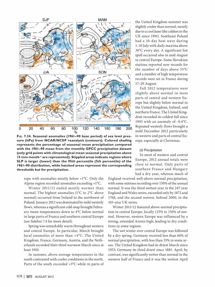
S174 | August 2013
rope with anomalies mostly below +1°C. Only the Alpine region recorded anomalies exceeding +1°C.
Winter 2011/12 ended mostly warmer than normal. The highest anomalies (1°C to 2°C above normal) occurred from Ireland to the northwest of Poland. January 2012 was dominated by mild westerly flows, whereas a significant cold snap brought Febru-ary mean temperatures down to 4°C below normal in large parts of France and southern central Europe (see Sidebar 7.4 for more detail).
Spring was remarkably warm throughout western and central Europe. In particular, March brought local anomalies of more than +4°C. The United Kingdom, France, Germany, Austria, and the Neth-erlands recorded their third warmest March since at least 1910.
In summer, above-average temperatures in the south contrasted with cooler conditions in the north. Parts of the south exceeded +3°C while in parts of
the United Kingdom summer was slightly cooler than normal, mostly due to a cool June (the coldest in the UK since 1991). Southeast Poland had a 10-day heat wave during 1–10 July with daily maxima above 36°C every day. A significant hot spell occurred also in mid-August in central Europe. Some Slovakian stations reported new records for the number of days above 35°C and a number of high temperature records were set in France during 17–20 August.
Fall 2012 temperatures were slightly above normal in most parts of central and western Eu-rope but slightly below normal in the United Kingdom, Ireland, and northern France. The United King-dom recorded its coldest fall since 1993 with an anomaly of -0.4°C. Repeated westerly flows brought a mild December 2012 particularly in western and parts of central Eu-rope, especially at Christmas.
(ii) PrecipitationIn most of western and central
Europe, 2012 annual totals were close to normal. Only parts of southern France and Hungary had a dry year, whereas much of
England received well-above-normal precipitation, with some stations recording over 150% of the annual normal. It was the third wettest year in the 247-year England and Wales series, exceeded only by 1872 and 1768, and the second wettest, behind 2000, in the 103-year UK series.
Winter 2011/12 featured above-normal precipita-tion in central Europe, locally 125% to 150% of nor-mal. However, western Europe was influenced by a strong, extended Azores high, leading to dry condi-tions in some regions.
The wet winter over central Europe was followed by a dry spring. Germany received less than 60% of normal precipitation, with less than 35% in some ar-eas. The United Kingdom had its driest March since 1953; Germany its third driest since 1881. April, by contrast, was significantly wetter than normal in the western half of France and it was the wettest April
Fig. 7.34. seasonal anomalies (1961–90 base period) of sea level pres-sure (hPa) from nCaR/nCeP reanalysis (contours). Colored shading represents the percentage of seasonal mean precipitation compared with the 1961–90 mean from the monthly gPCC precipitation dataset (only grid points with climatological mean seasonal precipitation above 15 mm month-1 are represented). stippled areas indicate regions where slP is larger (lower) than the 95th percentile (5th percentile) of the 1961–90 distribution, while hatched areas represent the corresponding thresholds but for precipitation.

S175STATE OF THE CLIMATE IN 2012 |AuguST 2013
in the 103-year UK series and also the wettest in the 247-year England and Wales series.
Summer was drier than normal in southern Po-land, Slovakia, and Hungary, but was exceptionally wet in the United Kingdom and Ireland. The major-ity of stations in Ireland recorded their wettest June since regular measurements began. It was the wettest June in the 247-year England and Wales series. In the United Kingdom, the last summer which was wetter was in 1912. In July, severe thunderstorms contributed to record July precipitation totals at some stations in Austria.
Wet conditions continued into fall in most of the United Kingdom whereas parts of Germany and southern France received much less than normal pre-cipitation. England experienced its wettest fall since 2000 and wettest December since 1978. In eastern Scotland it was the wettest since 1929. Locations in northern France reported 200% to 300% of normal precipitation in December.
(iii) Notable eventsIn early January, intense low pressure systems
“Ulli” and “Andrea” crossed northern central Europe. Violent storm gusts were reported from the United Kingdom to Poland and the Czech Republic with Aberdaron, Wales, recording 81 kt (42 m s-1).
In late April, subtropical air brought temperature records to central Europe. On 28 April, two stations set April temperature records for Germany at 32.9°C. Slubice, Poland, recorded 31.6°C. St. Gallen, Switzer-land, reported a nighttime minimum of 22.9°C, the highest April minimum temperature ever recorded in Switzerland. On 30 June, the mountain-top obser-vatory at Sonnblick, Austria (3109 m), recorded its highest temperature since 1886: 15.3°C.
Mid-August brought a short, albeit extreme, hot spell across large parts of central and western Europe, setting daytime maxima and daily mean tempera-tures records at some stations. Dobřichovice set an all-time record for the Czech Republic with 40.4°C on 20 August. This was also the beginning of a 6-week drought in Poland, causing the lowest river water levels in 45 years. In France, Auzances (Limousin region) recorded a new all-time record of 41.6°C on 18 August, shattering the previous record of 37.2°C (records began in 1947).
In the second half of October, an unusual weather pattern brought extremely warm air to central Eu-rope. Daily maxima up to 28°C were recorded in Germany. Thirteen Austrian stations reported record
daily maximum temperatures, including 22.7°C at Feuerkogel Mountain (1618 m).
Just one week after the record warmth, an early cold-air outbreak brought snow to the lowlands in the southern and eastern parts of the region. At St. Gallen, Switzerland, a snow depth of 33 cm was noted, 15 cm above the previous October record set in 1974. Some stations in Germany also recorded record snow depths for October and, in the clear nights that followed, many stations had record low minimum October temperatures.
An unusually cold and snowy first half of De-cember was followed by a massive thaw up to the high alpine regions and subsequent flooding. Later, Germany, Austria, and Switzerland experienced their warmest Christmas since the start of the observa-tional record.
3) nordiC and baltiC CoUntrieS—C. Achberger, B. Mühr, C. Ehmann, P. Bissolli, D. Parker, and J. Kennedy
This region includes Iceland, Norway, Denmark, Sweden, Finland, Estonia, Latvia, and Lithuania.
(i) TemperatureAveraged over the year, temperatures in the Nordic
and Baltic Regions were 0.5°C to 0.7°C above normal. Western Iceland was warmer at +1.2°C anomaly.
Winter temperatures (DJF 2011/12) were well above normal over most of the region. The highest anomalies (+3°C to +4°C) occurred in central Sweden and northern Finland. However, a strong and persis-tent high pressure system in late January and early February led to a significant cold spell, particularly in eastern parts of the region.
Spring temperatures were 0.5°C to 2°C above normal, mainly due to a combination of prolonged high pressure in southern parts and warm air ad-vection on the eastern f lank of Atlantic lows. The highest seasonal anomalies (+2°C) were measured in Denmark. Norway experienced its warmest March since measurements started in 1900. April and May, in contrast, were colder than normal across most of Norway and Sweden though Norway saw some record daytime maxima in late May.
Iceland, Denmark, and the Baltic states had a slightly above-normal summer while much of Scan-dinavia was colder than normal. An advance of cold Arctic air in late May and early June established a persistent trough of low pressure over northern Europe. For Denmark and Sweden it was the coldest June since 1991. In Finland, the number of June days >25°C was only half of normal.

S176 | August 2013
While Iceland and western Norway experienced a colder-than-normal fall, Finland and the Baltic states were 1°C to 2°C warmer than normal. In late October, very warm air masses from central Europe reached southern Sweden where some stations reported un-usually high temperatures of almost 20°C. Only six days later, a strong cold front brought snow as far south as Denmark.
In December, a cold continental high over Rus-sia extended westward to Scandinavia. Apart from Iceland, all areas finished the month with below-normal temperatures. Finland was most extreme with anomalies down to -5°C.
(ii) Precipitation In general, it was wetter than normal across most
of the Nordic and Baltic countries. In many places in Finland, 2012 was the wettest year in the past 50 years.
Winter 2011/12 precipitation was well above nor-mal in many parts of the Nordic and Baltic countries. Southern Iceland and the Norwegian southwest coast received far more precipitation than usual; areas bor-dering the Baltic received more than 150% of normal.
Spring was dominated by westerly f low with well-above-normal rain in most of the Nordic and Baltic countries, particularly along the Norwegian coast. Totals were mostly between 110% and 150% of normal, with the majority falling in March where monthly totals up to 300 mm were recorded. Iceland and Denmark were mostly drier than average.
Summer was very dry in the west of the Nordic countries, but wet in other parts. Iceland was unusu-ally dry with many areas recording only 30% to 70% of the long-term mean. The drought caused vegeta-tion to suffer in some areas. In western Iceland, it was the driest summer in almost 100 years. Stykkishólmur received only 0.6 mm of rain in June, which marked the driest June since measurements began in 1856. On the other hand, Sweden, Finland, and the Baltic states had precipitation surpluses, especially in June and July. Parts of Finland received a summer total of 150% of normal, and parts of Sweden saw twice as much rain as normal.
Precipitation in fall was again distributed uneven-ly. It was particularly wet in western Finland (above 150% of normal), northeastern Sweden, and northern Norway (locally almost twice normal) with daily or monthly precipitation records set at some stations.
In December, the dominant high pressure influ-ence meant that western Norway had significantly less precipitation than normal. Many stations reported
100-year or longer record minimum precipitation totals for December.
(iii) Notable eventsAn exceptional cold spell gripped northern Europe
in early February (see Sidebar 7.4). Extremely warm air reached southern Iceland at
the end of March, with Kvisker setting a monthly record for Iceland with 20.5°C on 29 March.
In early July, thunderstorms hit parts of southern and central Sweden and the Baltic states causing local flooding. Lääne-Nigula, Estonia, received 93.5 mm in 12 hours on 7 July, the highest 12-hour value in Estonia since 1964.
Northern Iceland was hit by a severe snowstorm from 9 to 11 September. Snowdrifts up to 2 m deep were observed at inland farms, which is unusual so early in the season. Farmers lost thousands of sheep. Icing on power lines caused considerable damage and power outages.
October brought intense rain to northern Sweden and western Finland. In some areas, more than 100 mm fell within one week. Flooding in Finland caused around 6 million Euros (approx. $7.6 million US dol-lars) of damage. Such severe flooding had previously been recorded only during 1981 and 1984.
An exceptionally early cold air outbreak brought snow cover of 18 cm to Lääne-Nigula, Estonia, on 27 October. This was the greatest October snow depth recorded there since 1964.
At the end of November, a blizzard brought over 20 cm of snow to the southern coastline of Finland. The storm was one of the strongest observed in the Gulf of Finland with 10-minute mean wind speeds reaching 29 m s-1. The storm damaged trees and left tens of thousands of homes without power.
4) iberian peninSUla—R. Trigo, D. Barriopedro, A. M. Ramos, D. Parker, B. Mühr, C. Ehmann, P. Bissolli, and J. Kennedy
This region includes Spain and Portugal. Unless otherwise noted, anomalies refer to a base period of 1971–2000.
(i) TemperatureBoth Iberian countries registered slightly above-
average annual temperatures with the highest anoma-lies in eastern Spain of +1°C to +2°C.
The 2011/12 winter season was cool with mean temperature anomalies of -1.2°C in Portugal and -0.6°C in Spain. The mean minimum temperature for Portugal was the third lowest since 1931. The
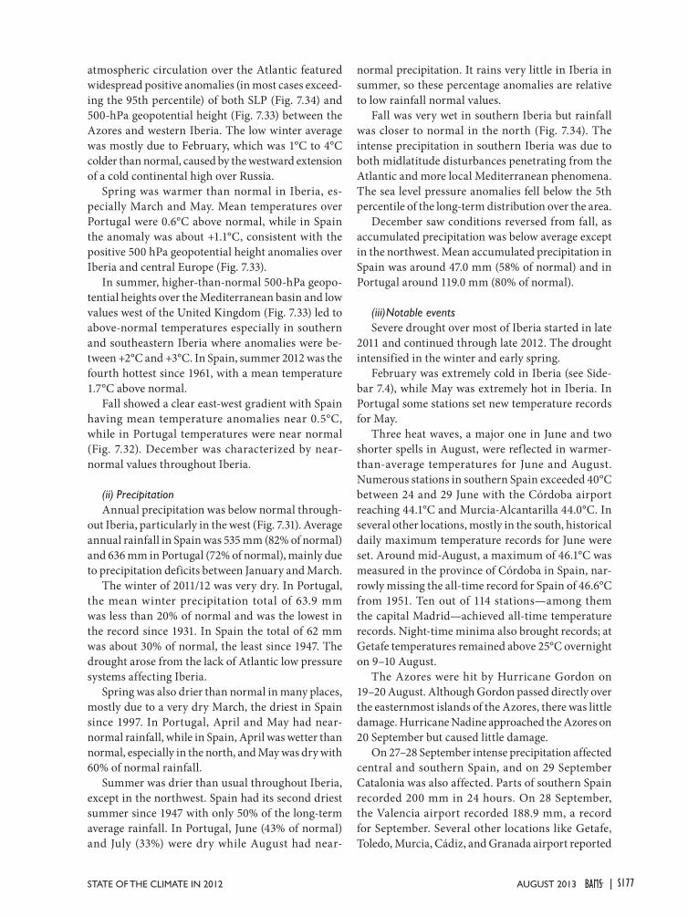
S177STATE OF THE CLIMATE IN 2012 |AuguST 2013
atmospheric circulation over the Atlantic featured widespread positive anomalies (in most cases exceed-ing the 95th percentile) of both SLP (Fig. 7.34) and 500-hPa geopotential height (Fig. 7.33) between the Azores and western Iberia. The low winter average was mostly due to February, which was 1°C to 4°C colder than normal, caused by the westward extension of a cold continental high over Russia.
Spring was warmer than normal in Iberia, es-pecially March and May. Mean temperatures over Portugal were 0.6°C above normal, while in Spain the anomaly was about +1.1°C, consistent with the positive 500 hPa geopotential height anomalies over Iberia and central Europe (Fig. 7.33).
In summer, higher-than-normal 500-hPa geopo-tential heights over the Mediterranean basin and low values west of the United Kingdom (Fig. 7.33) led to above-normal temperatures especially in southern and southeastern Iberia where anomalies were be-tween +2°C and +3°C. In Spain, summer 2012 was the fourth hottest since 1961, with a mean temperature 1.7°C above normal.
Fall showed a clear east-west gradient with Spain having mean temperature anomalies near 0.5°C, while in Portugal temperatures were near normal (Fig. 7.32). December was characterized by near-normal values throughout Iberia.
(ii) PrecipitationAnnual precipitation was below normal through-
out Iberia, particularly in the west (Fig. 7.31). Average annual rainfall in Spain was 535 mm (82% of normal) and 636 mm in Portugal (72% of normal), mainly due to precipitation deficits between January and March.
The winter of 2011/12 was very dry. In Portugal, the mean winter precipitation total of 63.9 mm was less than 20% of normal and was the lowest in the record since 1931. In Spain the total of 62 mm was about 30% of normal, the least since 1947. The drought arose from the lack of Atlantic low pressure systems affecting Iberia.
Spring was also drier than normal in many places, mostly due to a very dry March, the driest in Spain since 1997. In Portugal, April and May had near-normal rainfall, while in Spain, April was wetter than normal, especially in the north, and May was dry with 60% of normal rainfall.
Summer was drier than usual throughout Iberia, except in the northwest. Spain had its second driest summer since 1947 with only 50% of the long-term average rainfall. In Portugal, June (43% of normal) and July (33%) were dry while August had near-
normal precipitation. It rains very little in Iberia in summer, so these percentage anomalies are relative to low rainfall normal values.
Fall was very wet in southern Iberia but rainfall was closer to normal in the north (Fig. 7.34). The intense precipitation in southern Iberia was due to both midlatitude disturbances penetrating from the Atlantic and more local Mediterranean phenomena. The sea level pressure anomalies fell below the 5th percentile of the long-term distribution over the area.
December saw conditions reversed from fall, as accumulated precipitation was below average except in the northwest. Mean accumulated precipitation in Spain was around 47.0 mm (58% of normal) and in Portugal around 119.0 mm (80% of normal).
(iii) Notable eventsSevere drought over most of Iberia started in late
2011 and continued through late 2012. The drought intensified in the winter and early spring.
February was extremely cold in Iberia (see Side-bar 7.4), while May was extremely hot in Iberia. In Portugal some stations set new temperature records for May.
Three heat waves, a major one in June and two shorter spells in August, were reflected in warmer-than-average temperatures for June and August. Numerous stations in southern Spain exceeded 40°C between 24 and 29 June with the Córdoba airport reaching 44.1°C and Murcia-Alcantarilla 44.0°C. In several other locations, mostly in the south, historical daily maximum temperature records for June were set. Around mid-August, a maximum of 46.1°C was measured in the province of Córdoba in Spain, nar-rowly missing the all-time record for Spain of 46.6°C from 1951. Ten out of 114 stations—among them the capital Madrid—achieved all-time temperature records. Night-time minima also brought records; at Getafe temperatures remained above 25°C overnight on 9–10 August.
The Azores were hit by Hurricane Gordon on 19–20 August. Although Gordon passed directly over the easternmost islands of the Azores, there was little damage. Hurricane Nadine approached the Azores on 20 September but caused little damage.
On 27–28 September intense precipitation affected central and southern Spain, and on 29 September Catalonia was also affected. Parts of southern Spain recorded 200 mm in 24 hours. On 28 September, the Valencia airport recorded 188.9 mm, a record for September. Several other locations like Getafe, Toledo, Murcia, Cádiz, and Granada airport reported

S178 | August 2013
record 24-hour precipitation. The torrential precipita-tion caused 10 deaths and severe damage to Spanish infrastructure.
On 16 November an F3 tornado hit the southern coast of Portugal (Carvoeiro, Lagoa, and Silves). On its 31 km track it caused 1 fatality, 12 injuries, and major damage to houses and cars.
5) Mediterranean, italy, balkan StateS—B. Mühr, C. Ehmann, P. Bissolli, S. Sensoy, M. Demircan, P. Simeonov, A. Obregón, J. Kennedy, D. Parker, and M. Dacic
This region includes Italy, Malta, Slovenia, Croa-tia, Serbia, Montenegro, Bosnia and Herzegovina, Albania, Macedonia, Greece, Bulgaria, and Turkey.
(i) TemperatureThe 2012 annual average temperature was warmer
than normal in the western Mediterranean and the Balkans, with parts of Slovenia and the north of Croa-tia exceeding 2°C above the 1961–90 average. Bulgaria had its third warmest year since 1901.
Temperatures in winter 2011/12 ranged from slightly to significantly below normal. Anomalies down to -3°C were measured in Turkey where a cold January with frequent outbreaks of arctic air was fol-lowed by a cold snap in early February. In Bulgaria, February was 4.3°C below normal. February was the coldest month at 15 stations in Serbia. Snow depths reached 1.5 m. Temperature anomalies in Macedo-nia in January and February ranged from -2.3°C to -4.5°C.
Spring was warmer than normal apart from some areas in the western and eastern areas of Turkey. The largest positive anomalies (up to +3°C) occurred in northern Italy, Slovenia, and northern Croatia. The high temperatures in the vicinity of the Alps were due to dominant high pressure and frequent foehn events along the southern slopes of the Alps.
Summer was unusually warm throughout the region. Serbia and Bosnia and Herzegovina had their warmest summers of the last 120 years. Serbia experienced several hot spells, arising from recur-rent outbreaks of subtropical and very warm air originating in northern Africa, each lasting for six days or more. There were 62 tropical days (where daily maximum temperature exceeds 30°C) and 52 tropical nights (where daily minimum temperature exceeds 20°C) recorded in Belgrade. Slovenia and northern Italy both had the second warmest summer on record. Turkey experienced maxima above 40°C at 40 stations; the highest was 47°C. In Bulgaria, July was 4.5°C above normal.
Fall was warmer than normal in the central Medi-terranean and the Balkans. Anomalies from Croatia, Greece, and western Turkey exceeded +4°C in places. This resulted from frequent cyclonic developments over the northern Mediterranean. On their eastern f lank, warm air of subtropical origin spread over southeastern Europe.
However, December was colder than normal with anomalies down to -2°C in parts of Albania and Bul-garia. This was the result of cold air outbreaks from the north in the first half of the month and a cold northeasterly flow on the southern side of a conti-nental high pressure system over Russia.
(ii) PrecipitationIn northern Italy and northern parts of the Bal-
kans, 2012 was characterized by below-average rain-fall (60%–80% of normal). Southern areas were wetter than normal, especially along the Turkish Mediterra-nean coast and in southern Bulgaria, where rainfall in some places was almost twice the long-term average.
Northern Italy had a dry winter, with some areas recording 150 mm less precipitation than normal, about two-thirds of the long-term mean. The dry conditions were caused by frequent advances of high pressure from the Azores, exacerbated by foehn events. Vigorous low pressure activity over the Mediterranean in the first half of February led to a significant precipitation surplus in southern Italy and Greece where the winter was wetter than normal in places. Eastern and southern parts of the Balkans and Turkey were also wetter than normal.
Spring was slightly drier than normal around the Adriatic Sea, in the northern Balkans, and in south-eastern Turkey. Upper lows in April and May led to a slight wet anomaly in the north of Greece, in Bulgaria, and around the Bosporus.
Summer was quite dry in southeastern Europe. In several places in northern Italy no rain was recorded during almost the whole summer. August precipita-tion was only 20% of normal in southern Croatia and in Bosnia and Herzegovina, with several sites receiving no rain. Summer totals amounted to only 35% of the mean. Slovenia and Serbia also experienced extreme drought in August. Some areas around the Black Sea recorded a wet summer due to intense con-vective precipitation in July and August.
Well-above-normal precipitation was observed in all three fall months around the north Adriatic Sea. Western Turkey was mostly dry in September and November with precipitation only 10% and 45% of normal, respectively.
S179STATE OF THE CLIMATE IN 2012 |AuguST 2013
In December, the distribution was reversed with a rather dry north and a wet southeast due to pronounced low pressure activity over the eastern Mediterranean.
(iii) Notable eventsIn late January and early February an extreme
cold spell occurred, ending with heavy snowfalls (see Sidebar 7.4). Dust-red snow fell on 8 February in Sirnak, Turkey.
In mid-April, a strong gale ravaged the Aegean Sea and western Turkey. Storm gusts caused heavy dam-age and four people died. Istanbul was particularly affected with gusts of 29 m s-1. Six road construc-tion workers in Elazig died in a tornado on 9 April. Saharan dust was seen on 18 April in western and central Turkey.
An unusually severe cold snap brought the lat-est snow cover since 1962 to Sarajevo, Bosnia and Herzegovina, with the city reporting 14 cm on the morning of 14 May; up to 50 cm of fresh snow fell on nearby mountains.
Dust storms affected eastern Turkey on 30 May, 30 July, and 1 August. Mud rain fell on 1 August in Kars.
Heavy rain on 22–23 October caused f looding in several places in Turkey. Late October and early November brought violent storms to Italy and Croa-tia. The northeast of Italy was especially affected, with Venice reporting the 11th highest water level recorded there.
Heavy rain fell on 4–5 November on the Austrian–Slovenian border, where 100 mm–200 mm of rain fell within 24 hours. Kredarica, Slovenia, reported 225 mm. The snow line was very high at around 2500 m resulting in heavy snow melt and flooding.
Northern Italy experienced intense rain in mid-November resulting in flooding and mudslides. Chie-volis reported 368 mm within 17 hours. Hundreds of inhabitants in Tuscany and Liguria had to be rescued. Venice reported the sixth highest water level (1.5 m) recorded in the city’s history.
Five heat waves were registered across Serbia dur-ing 2012 lasting 6–10 days on average. At the begin-ning of summer, prolonged high air temperatures and low precipitation caused severe to extreme drought across the whole of Serbia.
6) eaStern eUrope—B. Mühr, C. Ehmann, P. Bissolli, D. Parker, J. Kennedy, and R. Trigo
This region includes the European part of Russia, Belarus, Ukraine, Moldavia, and Romania.
(i) TemperatureEastern Europe had a warmer than normal 2012.
In Romania and Ukraine anomalies were between +1°C and +2°C. Western Russia and Belarus had mostly below +1°C.
A warmer-than-normal winter was observed in the northern regions of eastern Europe with positive anomalies of more than 4°C in the northeast of Eu-ropean Russia. On the other hand, parts of southern Ukraine, Moldavia, and Romania were slightly colder than normal. A recurrent southwesterly flow brought mild Atlantic air far into eastern Europe. High pres-sure inf luence, which often dominates the winter in eastern Europe, developed in February with sea level pressure anomalies between +12 hPa and +16 hPa over Russia. The advection of cold continental air associated with the high brought the anomaly for the winter as a whole closer to normal.
With the exception of Russia, spring was 1°C to 2°C warmer than normal. The highest anomalies were in Ukraine, particularly the east and south, where anomalies exceeded +4°C. Mid-May brought the first summer weather patterns to the region with the advection of warm air from the Black Sea area.
The south of the region experienced a much warm-er-than-normal summer with anomalies exceeding +4°C in places. An unusually warm July contributed to the overall warm anomaly with a persistent sub-tropical ridge of high pressure extending far to the northeast.
Fall continued with warmer-than-normal con-ditions. The western parts of Russia, Belarus, and Ukraine had anomalies of +1°C to +2°C while Mol-davia and Romania reached +2°C to +3°C. November was particularly warm with warm air advancing along the eastern flank of deep troughs of low pres-sure over the western Mediterranean, leading to large areas between 2°C and 3°C above normal. The mild setup ended abruptly in mid-December when high pressure in the east gained inf luence. In western Russia mean sea level pressure was more than 16 hPa above the long-term mean in December.

S180 | August 2013
(ii) PrecipitationPrecipitation totals in 2012 were near average
across large parts of eastern Europe. In European Russia, however, some regions received almost 200% of the long-term mean.
The larger part of eastern Europe had a near-normal winter, but the western parts of Russia and eastern Belarus were slightly wetter than normal (110% to 150%) due to a wet December with dominat-ing Atlantic low pressure influence.
Spring was near normal despite large deviations in individual months. In Romania, May was a very wet month with 200% of normal precipitation. Parts of Russia were also slightly wet (110% to 150% of nor-mal), while eastern Ukraine was drier than normal in places.
Belarus and northern Ukraine received well-above-normal rain totals in summer with some areas getting between 90 mm and 150 mm (130% to 150% of normal). The majority of the surplus was due to an unusually strong low, established in mid-August near the Belarus-Ukraine border. Moldavia and Ro-mania were drier than normal under the influence of a recurrent ridge of high pressure that also affected the Balkan area.
In fall, well-above-normal precipitation totals were observed in the European part of Russia. Anomalies were between 90 mm and 150 mm (150%–225% of normal). The wettest month, relatively speaking, was October, which was under the influence of low pressure. December started wetter than normal in parts of Ukraine, Moldavia, and Romania. However Northern Russia was somewhat drier.
(iii) Notable eventsThe cold spell during the end of January and early
February led to new minimum temperature records in many areas of eastern Europe (see Sidebar 7.4).
Late April brought record-setting warmth to eastern Europe. Several eastern European locations, including Minsk, Belarus; Moscow, Russia; and the Ukrainian cities of Kiev and Odessa, had their warm-est day recorded in April.
Extensive rain lasting several days led to major f looding along the Russian Black Sea border. The abundant precipitation was caused by an abnormally strong and persistent low pressure system. Some areas received nearly 300 mm of rain; locally, four to five times the normal July monthly precipitation fell within 12 hours. In the region of Krasnodar at least 140 people drowned in the floods.
Along the boundary between continental cold and dry air and milder and moister air in the west, huge snowfalls were reported in many parts of eastern Europe. Kiev recorded the largest snow depth ever recorded for mid-December: on three consecutive days from 13 December snow depths of 54 cm were measured.
7) Middle eaSt—B. Mühr, C. Ehmann, P. Bissolli, A. Hov-sepyan, D. Parker, and J. Kennedy
This region includes Israel, Cyprus, Jordan, Leba-non, Syria, West Kazakhstan, Armenia, Georgia, and Azerbaijan.
(i) TemperatureIn the Middle East average temperatures for 2012
were 1°C to 2°C above normal.Winter 2011/12 was colder than the long-term
mean. In western Kazakhstan, at the Caspian Sea, and in the south Caucasus temperatures were locally 2°C to 3°C below average. December was mostly under a high pressure influence and therefore colder than normal while January was milder (especially in the east) under the inf luence of low pressure systems, resulting in a warmer-than-normal month. February again was colder with well-below-normal temperatures in the entire region and anomalies down to -4°C.
Spring brought slightly above-normal tempera-tures to most areas; in western Kazakhstan tem-peratures were moderately above normal. March was significantly colder than normal across the entire area, and Armenia saw its coldest March since 1965. In April, however, the general flow veered to south-westerly and positive departures of more than +4°C were observed, especially in western Kazakhstan and in the Caucasus range. May was again a warm month, the third warmest since 1966 in Armenia.
Summer was significantly warmer than normal throughout the area with anomalies between +1°C and +3°C, and near +4°C along part of the eastern border of the Mediterranean. Anomalies were highest in June. A persistent upper low in the first days of July brought cool and cloudy weather conditions, eventu-ally easing off in the second half of the month. July was cooler than normal in Armenia, despite a very warm spell towards the end of the month. In Israel, summer tied 2010 as the warmest on record.
Fall finished with generally above-normal temper-atures with each month having an anomaly between +1°C and +3°C. In the South Caucasus October was 3°C–4°C above average. Far western Georgia expe-
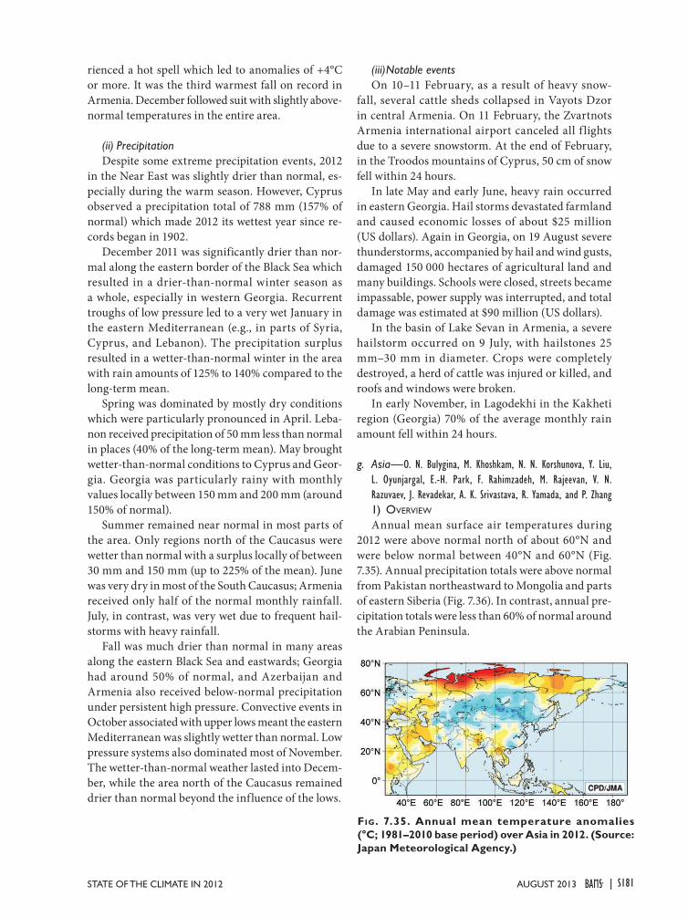
S181STATE OF THE CLIMATE IN 2012 |AuguST 2013
rienced a hot spell which led to anomalies of +4°C or more. It was the third warmest fall on record in Armenia. December followed suit with slightly above-normal temperatures in the entire area.
(ii) PrecipitationDespite some extreme precipitation events, 2012
in the Near East was slightly drier than normal, es-pecially during the warm season. However, Cyprus observed a precipitation total of 788 mm (157% of normal) which made 2012 its wettest year since re-cords began in 1902.
December 2011 was significantly drier than nor-mal along the eastern border of the Black Sea which resulted in a drier-than-normal winter season as a whole, especially in western Georgia. Recurrent troughs of low pressure led to a very wet January in the eastern Mediterranean (e.g., in parts of Syria, Cyprus, and Lebanon). The precipitation surplus resulted in a wetter-than-normal winter in the area with rain amounts of 125% to 140% compared to the long-term mean.
Spring was dominated by mostly dry conditions which were particularly pronounced in April. Leba-non received precipitation of 50 mm less than normal in places (40% of the long-term mean). May brought wetter-than-normal conditions to Cyprus and Geor-gia. Georgia was particularly rainy with monthly values locally between 150 mm and 200 mm (around 150% of normal).
Summer remained near normal in most parts of the area. Only regions north of the Caucasus were wetter than normal with a surplus locally of between 30 mm and 150 mm (up to 225% of the mean). June was very dry in most of the South Caucasus; Armenia received only half of the normal monthly rainfall. July, in contrast, was very wet due to frequent hail-storms with heavy rainfall.
Fall was much drier than normal in many areas along the eastern Black Sea and eastwards; Georgia had around 50% of normal, and Azerbaijan and Armenia also received below-normal precipitation under persistent high pressure. Convective events in October associated with upper lows meant the eastern Mediterranean was slightly wetter than normal. Low pressure systems also dominated most of November. The wetter-than-normal weather lasted into Decem-ber, while the area north of the Caucasus remained drier than normal beyond the influence of the lows.
(iii) Notable eventsOn 10–11 February, as a result of heavy snow-
fall, several cattle sheds collapsed in Vayots Dzor in central Armenia. On 11 February, the Zvartnots Armenia international airport canceled all f lights due to a severe snowstorm. At the end of February, in the Troodos mountains of Cyprus, 50 cm of snow fell within 24 hours.
In late May and early June, heavy rain occurred in eastern Georgia. Hail storms devastated farmland and caused economic losses of about $25 million (US dollars). Again in Georgia, on 19 August severe thunderstorms, accompanied by hail and wind gusts, damaged 150 000 hectares of agricultural land and many buildings. Schools were closed, streets became impassable, power supply was interrupted, and total damage was estimated at $90 million (US dollars).
In the basin of Lake Sevan in Armenia, a severe hailstorm occurred on 9 July, with hailstones 25 mm–30 mm in diameter. Crops were completely destroyed, a herd of cattle was injured or killed, and roofs and windows were broken.
In early November, in Lagodekhi in the Kakheti region (Georgia) 70% of the average monthly rain amount fell within 24 hours.
g. Asia—O. N. Bulygina, M. Khoshkam, N. N. Korshunova, y. Liu, L. Oyunjargal, E.-H. Park, F. Rahimzadeh, M. Rajeevan, V. N. Razuvaev, J. Revadekar, A. K. Srivastava, R. yamada, and P. Zhang1) overvieW
Annual mean surface air temperatures during 2012 were above normal north of about 60°N and were below normal between 40°N and 60°N (Fig. 7.35). Annual precipitation totals were above normal from Pakistan northeastward to Mongolia and parts of eastern Siberia (Fig. 7.36). In contrast, annual pre-cipitation totals were less than 60% of normal around the Arabian Peninsula.
Fig. 7.35. annual mean temperature anomalies (°C; 1981–2010 base period) over asia in 2012. (source: Japan meteorological agency.)

S182 | August 2013
siDebaR 7.4: ColD sPell in eURasia in WinteR 2011/12— B. MüHR, C. EHMANN, P. BiSSOLLi, D. PARKER, J. KENNEDy, S. TANAKA, AND K. yOSHiMATSu
In the second half of winter 2011/12, Eurasia experienced significantly lower-than-normal temperatures due to strong cold-air inflow (Fig. SB7.5). The influence of cold air extended to the whole of Europe as well as to all of eastern and central Asia in early February. In contrast to other wintertime cold spells in recent years, this event was not driven by a negative North Atlantic Oscillation excursion.
Siberian HighIn mid-January, a high pressure system was enhanced over
western Siberia, in association with the large meander of the upper-level westerly jet stream, and a significantly cold air mass over central and eastern Siberia flowed into Mongolia and Kazakhstan along the south flank of the high pressure. At Ulaanbaatar in Mongolia and Astana in Kazakhstan, the daily mean temperatures decreased considerably. On 2 February, the daily mean temperature at Astana was -35°C (about 21°C below normal).
During the cold spell, the high pressure system intensified and expanded over northwestern Russia and northern Europe. A surface air pressure of more than 1060 hPa was recorded over the Baltic countries on 29 January. The cold air mass flowed farther westward and reached eastern and central Europe in early February. Temperatures well below 0°C lasted for more than one week across these areas. The lack of snow at the beginning of the cold spell prevented the development of even colder temperatures near the surface. At the end of the first week of February a small low pressure system emerged from the planetary frontal zone over northern Scandinavia. This low pressure system affected particularly the eastern parts of central Europe, and again, a very cold continental air mass spread to the southwesterly by 9 February.
In the meantime, several intense low pressure systems developed over the Mediterranean Sea. From 11 February onwards, the high pressure area over Europe weakened sig-nificantly and shifted to the south. Frontal systems from the Atlantic Ocean, with mild air, began to enter central Europe and finally brought the cold spell to an end, first in western and later in eastern parts of Eurasia. In Mongolia and Kazakhstan, lower-than-normal temperatures continued until the end of February. This weather pattern was extremely persistent, especially in these places.
Unusually intense and long cold spell in much of EuropeDespite a milder second half of the month, some European
countries reported their coldest February in about three de-cades. Unlike other winters of the recent past which were also cold, the weather conditions in February 2012 were character-ized by both extremely low temperatures and highly persistent cold air, even in central Europe. This fact is illustrated by the data from mountain weather stations. On top of the Feldberg Mountain in southwestern Germany (1493 m) the temperature did not exceed -10°C between 1 and 7 February (average daily
temperature is -3.4°C). On 4 February, the maximum tem-perature was -17.9°C. Only five days since recordings began in 1945 had lower daily maximum temperatures. The average temperature for the first 10 days of the month in Germany was 10.3°C below the monthly mean for February (1961–90). These days were even colder than those in February 1956, which set the previous record with an anomaly of -10.0°C.
The unusual and intense cold wave affected almost all of Europe. In Portugal, mean minimum temperature anomalies were the second lowest since 1931, and several stations in Portugal and Spain set new records for minimum temperature. Portugal also had its driest February in the record for 1931–present. In Spain even the larger cities measured minimum temperatures well below 0°C, e.g., Granada with -9.7°C on 13 February. A weather station at the University of Palma de Mallorca (Balearics) reported the lowest temperature in 40 years, where the temperature dropped to -5.7°C on 6 Febru-ary. France reported the most striking cold wave since 1987; in large parts of the country even daytime temperatures stayed well below 0°C. Minima reached nearly -30°C in Poland. In Gomel, in southeastern Belarus, temperatures dropped to -34.3°C on the night of 11/12 February, a new all-time record for the entire country since 1956. Moscow also experienced a very cold episode with temperatures exceeding -10°C on only two days in the first half of February; the night 12/13 February brought a minimum temperature of -28.5°C. The cold snap claimed several hundred lives in eastern Europe.
Southeastern Europe, too, was affected by extremely low temperatures. In extensive areas of Bosnia and Herzegovina,
Fig. sb7.5. Weekly temperature anomalies (°C) in the northern Hemisphere for (top) 15–21 Jan, (middle) 22–28 Jan, and (bottom) 29 Jan–4 Feb 2012. anoma-lies are deviations from normal (1981–2010 average). symbol "a" is Ulaanbaatar, mongolia, and "b" is astana, Kazakhstan. [source: interpolated from sYnoP re-ports (Japan meteorological agency).]

S183STATE OF THE CLIMATE IN 2012 |AuguST 2013
the months of February 1929 and 1956 were both associated with significantly lower daily minimum temperatures, whereas the first two weeks of February 2012 turned out to be a little colder than the peak of the February 1986 cold spell.
Anomalous seasonal mean pattern in winter 2011/12The 500-hPa height field for the boreal winter 2011/12 (Fig.
SB7.6a) shows distinct wave trains from the North Atlantic to Eurasia with positive anomalies over the North Atlantic and western Siberia, and negative anomalies over eastern Europe and northeastern Asia, indicating a significant meandering of the polar front jet stream. This wavy pattern with quasi-stationary Rossby wave packets propagating only slowly from the North Atlantic eastward persisted throughout the winter. In the sea level pressure field (Fig. SB7.6b), positive anomalies can be seen over the eastern North Atlantic and across north-ern Eurasia, especially over western Siberia. The Siberian High was significantly enhanced and expanded, reaching its strongest level since 1979/80. The Siberian High intensification was asso-ciated with upper-level ridges over western Siberia (Takaya and Nakamura 2005a,b). The enhanced Siberian High contributed also to an intensification of the East Asian winter monsoon, which strengthened cold air advection over the region. In the 850-hPa temperature field (Fig. SB7.6c), negative anomalies were seen in the Eurasian midlatitudes, especially over central and eastern Asia and over large parts of Europe except parts of the north and west (where either the duration of the cold spell was shorter or the anomalies less extreme). The extremely below-normal temperatures in the lower troposphere in central Asia and Mongolia in relation with subsidence in front of the upper-air ridge further enhanced the Siberian High. In northeastern Europe, temperatures in 850 hPa dropped to below -25°C in early February. The -10°C-isotherm temporar-ily was pushed as far as southern Spain, even parts of North Africa were affected by the cooling (see section 7f).
the first 10 days of February were the coldest in the last 120 years. Erzurum (Turkey) measured -35°C on 3 February.
In northern Europe, some new records for February were set in Norway (e.g., Hammerfest -19.9°C). Sweden recorded the lowest temperature since 2001 with -42.8°C, and in Lat-via minima dropped to below -30°C on five consecutive days (2–6 February). This has happened only twice before—in 1956 and 1996. In Kittila (northern Finland), which is the national low-temperature record holder (-51.5°C in January 1999), temperatures fell to -41.6°C.
In contrast to the Eurasian continent, warm and moist air was carried into the Arctic region by a strong southwesterly flow. On 29 and 30 January, Ny Ålesund on Svalbard observed a new daily precipitation record: 98 mm of rain fell within 24 hours, the most since July 1974, and its January mean temperature was 10.3°C above normal.
Heavy snowfall around the MediterraneanHeavy snowfall and record snow depths occurred around the
eastern and central Mediterranean Sea, especially in the central and southern parts of Italy and in the Balkan countries. Near Rome, the town of Frosinone (185 msl) reported a snow depth of 40 cm. St. Peter’s Square (Vatican) was covered by snow, for the first time since 1991. Bologna (Italy) saw its highest accumulated snow for 100 years. In the Apennines Mountains snow accumulation locally was more than 1 m.
Southeastern Europe recorded heaviest snowfalls at the end of the cold spell in mid-February. At the International Airport of Bucharest, Romania, snow depth was 63 cm, Belgrade in Serbia received 52 cm, and Bulgaria’s capital, Sofia, measured 48 cm. The greatest snow depths in the past 120 years were recorded in Bosnia and Herzegovina with values between 85 cm (Mostar) and 107 cm (Sarajevo)—both record values for the respective stations. The already difficult conditions were exac-erbated by snow drifts with heights of 6 m. Even Turkey saw snow (e.g., 150 cm in Sirnak, 8 cm in Ankara). Farther to the east, avalanches caused more than 40 fatalities in Afghanistan.
Comparison with former cold spellsEurope’s past February extreme cold
spells occurred in 1929, 1956, and 1986. All these events have in common the penetration of extremely cold air from northeastern Europe or western Asia at all tropospheric levels, driven either by middle and upper tropospheric troughs or cold air pools aloft. In each, a strong and extended surface high pressure area was established over northern Europe, Scandinavia, and northwestern Russia. The extremely low daily mean tem-peratures of February 1929 and 1956, at least in Germany, were not exceeded in February 1986 or 2012. Furthermore,
Fig. sb7.6. three-month mean (a) 500-hPa height (m), (b) sea level pres-sure, (hPa) and (c) 850-hPa temperature (°C) for Dec 2011–Feb 2012. the contour intervals are (a) 60 m, (b) 4 hPa and (c) 4°C. the shading indicates respective anomalies from the 1981–2010 average. Contours and shading are not shown for areas with altitudes >1600 m. [source: JRa/JCas re-analysis data (onogi at al. 2007.)]
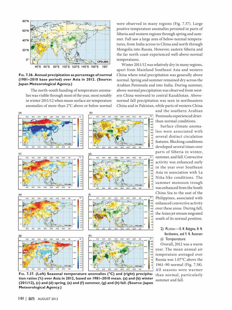
S184 | August 2013
The north-south banding of temperature anoma-lies was visible through most of the year, most notably in winter 2011/12 when mean surface air temperature anomalies of more than 2°C above or below normal
were observed in many regions (Fig. 7.37). Large positive temperature anomalies persisted in parts of Siberia and western regions through spring and sum-mer. Fall saw a large area of below-normal tempera-tures, from India across to China and north through Mongolia into Russia. However, eastern Siberia and the far north coast experienced well-above-normal temperatures.
Winter 2011/12 was relatively dry in many regions, apart from Mainland Southeast Asia and western China where total precipitation was generally above normal. Spring and summer remained dry across the Arabian Peninsula and into India. During summer, above-normal precipitation was observed from west-ern China westward to central Kazakhstan. Above-normal fall precipitation was seen in northeastern China and in Pakistan, while parts of western China
and the southern Arabian Peninsula experienced drier-than-normal conditions.
Surface climate anoma-lies were associated with several distinct circulation features. Blocking conditions developed several times over parts of Siberia in winter, summer, and fall. Convective activity was enhanced early in the year over Southeast Asia in association with La Niña-like conditions. The summer monsoon trough was enhanced from the South China Sea to the east of the Philippines, associated with enhanced convective activity over these areas. During fall, the Asian jet stream migrated south of its normal position.
2) rUSSia—O. N. Bulygina, N. N. Korshunova, and V. N. Razuvaev
(i) TemperatureOverall, 2012 was a warm
year. The mean annual air temperature averaged over Russia was 1.07°С above the 1961–90 normal (Fig. 7.38). All seasons were warmer than normal, particularly summer and fall.
Fig. 7.36. annual precipitation as percentage of normal (1981–2010 base period) over asia in 2012. (source: Japan meteorological agency.)
Fig. 7.37. (left) seasonal temperature anomalies (°C) and (right) precipita-tion ratios (%) over asia in 2012, based on 1981–2010 mean. (a) and (b) winter (2011/12), (c) and (d) spring, (e) and (f) summer, (g) and (h) fall. (source: Japan meteorological agency.)
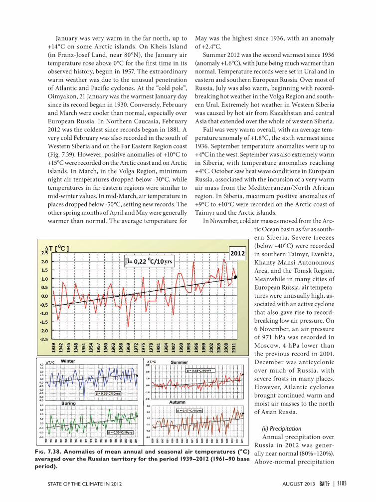
S185STATE OF THE CLIMATE IN 2012 |AuguST 2013
January was very warm in the far north, up to +14°C on some Arctic islands. On Kheis Island (in Franz-Josef Land, near 80°N), the January air temperature rose above 0°С for the first time in its observed history, begun in 1957. The extraordinary warm weather was due to the unusual penetration of Atlantic and Pacific cyclones. At the “cold pole”, Oimyakon, 21 January was the warmest January day since its record began in 1930. Conversely, February and March were cooler than normal, especially over European Russia. In Northern Caucasia, February 2012 was the coldest since records began in 1881. A very cold February was also recorded in the south of Western Siberia and on the Far Eastern Region coast (Fig. 7.39). However, positive anomalies of +10°C to +15°С were recorded on the Arctic coast and on Arctic islands. In March, in the Volga Region, minimum night air temperatures dropped below -30°С, while temperatures in far eastern regions were similar to mid-winter values. In mid-March, air temperature in places dropped below -50°C, setting new records. The other spring months of April and May were generally warmer than normal. The average temperature for
May was the highest since 1936, with an anomaly of +2.4°С.
Summer 2012 was the second warmest since 1936 (anomaly +1.6°С), with June being much warmer than normal. Temperature records were set in Ural and in eastern and southern European Russia. Over most of Russia, July was also warm, beginning with record-breaking hot weather in the Volga Region and south-ern Ural. Extremely hot weather in Western Siberia was caused by hot air from Kazakhstan and central Asia that extended over the whole of western Siberia.
Fall was very warm overall, with an average tem-perature anomaly of +1.8°С, the sixth warmest since 1936. September temperature anomalies were up to +4°C in the west. September was also extremely warm in Siberia, with temperature anomalies reaching +4°С. October saw heat wave conditions in European Russia, associated with the incursion of a very warm air mass from the Mediterranean/North African region. In Siberia, maximum positive anomalies of +9°C to +10°С were recorded on the Arctic coast of Taimyr and the Arctic islands.
In November, cold air masses moved from the Arc-tic Ocean basin as far as south-ern Siberia. Severe freezes (below -40°C) were recorded in southern Taimyr, Evenkia, Khanty-Mansi Autonomous Area, and the Tomsk Region. Meanwhile in many cities of European Russia, air tempera-tures were unusually high, as-sociated with an active cyclone that also gave rise to record-breaking low air pressure. On 6 November, an air pressure of 971 hPa was recorded in Moscow, 4 hPa lower than the previous record in 2001. December was anticyclonic over much of Russia, with severe frosts in many places. However, Atlantic cyclones brought continued warm and moist air masses to the north of Asian Russia.
(ii) PrecipitationAnnual precipitation over
Russia in 2012 was gener-ally near normal (80%–120%). Above-normal precipitation
Fig. 7.38. anomalies of mean annual and seasonal air temperatures (°C) averaged over the Russian territory for the period 1939–2012 (1961–90 base period).
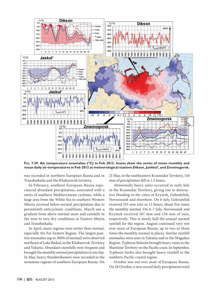
S186 | August 2013
was recorded in northern European Russia and in Transbaikalia and the Khabarovsk territory.
In February, southern European Russia expe-rienced abundant precipitation, associated with a series of southern Mediterranean cyclones, while a large area from the White Sea to southern Western Siberia received below-normal precipitation due to persistently anticyclonic conditions. March saw a gradient from above-normal snow and rainfalls in the west to very dry conditions in Eastern Siberia and Transbaikalia.
In April, many regions were wetter than normal, especially the Far Eastern Region. The largest posi-tive anomalies (up to 300% of normal) were observed northeast of Lake Baikal, in the Khabarovsk Territory and Yakutia. Abundant snowfalls were frequent and brought the monthly normal precipitation in one day. In May, heavy thundershowers were recorded in the mountain regions of southern European Russia. On
21 May, in the southeastern Krasnodar Territory, 110 mm of precipitation fell in 1.5 hours.
Abnormally heavy rains occurred in early July in the Krasnodar Territory, giving rise to destruc-tive f looding in the cities of Krymsk, Gelendzhik, Novorossisk and elsewhere. On 6 July, Gelendzhik received 253 mm rain in 12 hours, about five times the monthly normal. On 6–7 July, Novorossisk and Krymsk received 187 mm and 156 mm of rain, respectively. This is nearly half the annual normal rainfall for the region. August continued very wet over most of European Russia, up to two or three times the monthly normal in places. Similar rainfall anomalies were seen in Yakutia and in the Magadan Region. Typhoon Bolaven brought heavy rains to the Maritime Territory on the Pacific coast. In September, Typhoon Sanba also brought heavy rainfall to the southern Pacific coastal region.
October was wet over most of European Russia. On 28 October, a new record daily precipitation total
Fig. 7.39. air temperature anomalies (°C) in Feb 2012. insets show the series of mean monthly and mean daily air temperatures in Feb 2012 at meteorological stations Dikson, Jashkul’, and Zmeinogorsk.

S187STATE OF THE CLIMATE IN 2012 |AuguST 2013
for October (39 mm) was established in Moscow, the highest 1-day total since 1895 (the previous record was 26.8 mm). Southern Kamchatka and the southern Far Eastern Region also recorded a very wet October.
The year ended drier than normal in many re-gions. In November, anticyclonic conditions left East-ern Siberia with only 30% to 70% of monthly normal precipitation. December also saw little precipitation across much of Siberia. However, Transbaikalia and the southeast of Siberia received much-above-normal precipitation during November and December.
(iii) Notable eventsOn 27 January the Novorossisk bora, with winds
up to 38 m s-1, resulted in a massive power cut. On 8 February, a severe storm on the Black Sea coast of the Krasnodar Territory brought wind speeds of up to 45 m s-1–50 m s-1. The wind damaged cars, and brought down trees and roofs. Damage in Gelendzhik was estimated to be about $650 000 (US dollars). Tens of thousands of people were left without electricity, heat-ing, or hot water. Childcare centers and schools were closed. On 23–26 March, a blizzard with wind speeds up to 33 m s-1 persisted for 70 hours in the Anadyr Region of the Chukotka Autonomous District, with visibility reduced to 50 m.
On 6–7 July, catastrophic floods in the southern Krasnodar Territory (Krymsk, Gelendzhik, Novo-rossisk, and other cities) killed 171 people and inun-dated more than 5500 houses. The infrastructure in Krymsk was completely destroyed.
On 29 August, Typhoon Bolaven brought hur-ricane-force winds to Vladivostok, toppling trees, damaging power lines, and destroying other infra-structure. Thousands of houses in the south of the city lost electricity and water. On 17–18 September, Typhoon Sanba brought torrential rains to the Mari-time Territory (extreme southeastern Russia). Roads, basements of houses and farmland were inundated, and power supplies were interrupted.
On 10 October, Derbent (Dagestan) received 55 mm of precipitation in five hours, causing severe floods in the city and suburbs. Six people were killed, 320 houses were inundated, and gas, water, and power supply was interrupted.
3) eaSt aSia—P. Zhang, y. Liu, R. yamada, E-Hyung Park, and L. Oyunjargal
Countries considered in this section include China, Japan, Korea, and Mongolia. Unless otherwise noted, anomalies are relative to a normal period of 1981–2010.
(i) TemperatureAnnual mean temperatures across East Asia are
visible in Fig. 7.35. The annual mean temperature over China was 9.4°C, 0.2°C below normal, and 0.3°C lower than 2011. Mean temperatures were lower than normal in winter and fall, but persistently higher than normal in spring and summer. Apart from above-nor-mal conditions in the southwest and below-normal conditions in the north and northeast, annual mean temperatures were near normal over most of China. Annual mean temperatures were 0.5°C–1.0°C above normal in some parts of Yunnan, Sichuan, Qinghai, and northeast of Heilongjiang provinces. They were 0.5°C–1.0°C below normal in Jilin, Liaoning, eastern Inner Mongolia, and northern Guizhou provinces.
The average surface temperature over Japan (averaged over 17 observatories confirmed as being relatively unaffected by urbanization) was 0.06°C above normal. While annual mean temperatures were near normal, interseasonal f luctuations were large, with below-normal temperatures in winter and above-normal temperatures in summer.
The annual mean surface temperature over South Korea was 12.3°C (averaged over 45 weather stations), 0.2°C below normal. The seasonal mean surface tem-peratures (anomalies) were -3.7°C, 12.2°C, 24.7°C, and 13.7°C (-4.3°C, +0.5°C, +1.1°C, and -0.4°C) for winter, spring, summer, and fall, respectively.
The annual mean temperature for Mongolia was -0.5°C, 1.0°C below normal. Although temperatures were 3.7°C–3.9°C below normal in most of the country in winter, near-normal temperatures were recorded from April to October.
(ii) Precipitation Figure 7.36 shows 2012 annual precipitation as a
percentage of normal over the whole of Asia.The mean annual total precipitation in China
was 669.3 mm, 106.3% of normal and 20% higher than 2011. The seasonal total precipitation was below normal in winter, but much above normal in spring, summer, and fall. In 2012, the summer came earlier than normal with a strong East Asian monsoon and the rain belt lay much farther north than normal during the flood season. Although the precipitation during Mei-Yu (the major summer rainfall period along the middle and lower reaches of the Yangtze River basin, usually occurring between 19 June and 9 July; also known as Baiu in Japan and Changma in Korea) was much below normal, the annual precipita-tion in northeast China, north China, the middle and low reaches of Yangtze River basin, northwest China,

S188 | August 2013
and south China were all above normal. In particular, precipitation was the highest in the past 62 years in northeast China (131.5% of normal) and in the past 35 years in north China, Beijing, and Tianjin.
In Japan, annual precipitation was significantly above normal in Okinawa/Amami and above normal over most of eastern and western Japan. Summer pre-cipitation amounts were significantly above normal on the Pacific side of western Japan and Okinawa/Amami due to some heavy rain events by Baiu fronts (see note in previous paragraph) and frequent pas-sages of typhoons.
In South Korea, the mean annual precipitation was 1478.9 mm, 113% of normal, which ranked as the eighth highest since 1973 (the highest was 142% of normal in 2003). The seasonal mean precipitation was 62.8 mm, 256.5 mm, 770.6 mm, and 363.3 mm (72%, 106%, 106%, and 142% of normal) for winter, spring, summer, and fall, respectively.
In Mongolia, the annual precipitation was 241.5 mm, 116% of normal. Above-normal precipitation prevailed over the northern part of the western re-gion, and whole areas of central and southern regions. While January and February precipitation was far less than normal, the country had near-normal pre-cipitation in spring and above-normal precipitation in summer. In November and December, snowfall was above normal (176%–204% of normal) in most of the country and, as a result, snow covered more than 80% of the country.
(iii) Notable eventsIn January and February, East Asia experienced
significantly below-normal temperatures due to strong cold-air inf low. The daily minimum tem-perature reached -51.2°C in Telmen, Mongolia, in January. In South Korea, record-breaking minimum temperatures were reported on 2 and 3 February.
In spring, China was affected by 10 dust and sand events, much fewer than the normal of 17. There was an average of 1.3 dust days in northern China (2.7 days less than normal), the fewest since 1961. The first event was observed on 20 March, which was the latest since 2001. In Mongolia in spring, dust and snow storms frequently occurred with winds of more than 28 m s-1. On 21–23 April, a strong dust and snow storm with wind speeds of 16 m s-1 –34 m s-1 affected much of the country, causing widespread damage.
On 21–23 June, an intense cold front moved through northern Mongolia bringing cold rain and wet snow in northern part of the central region. The event cost the lives of 6100 head of livestock.
In early summer, South Korea experienced abnor-mally hot weather and substantial rainfall deficit (50% of monthly normal) due to migratory anticyclones and the Okhotsk high. The Okhotsk high not only induced Föhn winds but also prevented the north-ward movement of the Changma front (see Mei-Yu note, previous section).
On 11–14 July, northern Kyushu (western Japan) experienced extremely heavy rainfall due to an active Baiu front, with significant damage. Four-day total precipitation exceeded 800 mm in Aso City, 143% of the monthly normal.
Typhoons Damrey, Saola, and Haikui made land-fall in China in quick succession during one week in early August, affecting 15 provinces (or autonomous regions and municipalities). Regional low tempera-tures, overcast skies, and rainy weather occurred frequently, with severe impacts on agriculture.
In South Korea, from mid- to late August, heavy rainfall occurred in central and southern regions; when combined with rainfall associated with Ty-phoons Bolaven and Tembin, it was the fifth wettest August since 1973. It was unprecedented that two typhoons hit the Korean Peninsula within 43 hours.
Northern and eastern Japan experienced extreme-ly high temperatures in late summer due to the sig-nificantly enhanced North Pacific high. Record-high area-averaged temperatures were set over northern Japan for three consecutive 10-day periods from late August to mid-September. Northern Japan’s 10-day period temperature anomaly for 11–20 September was 5.5°C above normal.
In China, many rainstorms caused regional and flash floods and major landslides. Large-scale floods developed successively in the Yangtze, Yellow, and Haihe River basins, and others. Flash f loods and landslides occurred in some areas of Beijing, Gansu, Chongqing, Yunnan, Guizhou, Ningxia, Qinghai, and Xinjiang provinces.
4) SoUth aSia—A. K. Srivastava, J. Revadekar, and M. RajeevanCountries considered in this section include:
Bangladesh, India, Pakistan, and Sri Lanka. Climate anomalies are taken relative to the 1961–90 normal, unless otherwise stated.
(i) TemperatureOn average, south Asia experienced warm condi-
tions in 2012. The annual mean temperature for India was 0.5°C above normal, the ninth warmest year since records began in 1901 (Fig. 7.40). Abnormally warm temperatures during the summer monsoon season

S189STATE OF THE CLIMATE IN 2012 |AuguST 2013
(June–September), related to subdued monsoon activ-ity, were the main contribution to the warmer annual temperatures. Mean air temperature over India for the summer monsoon season was 0.6°C above nor-mal, making 2012 the third warmest monsoon year since 1901, after 2009 and 1987 (+0.8°C).
Mean air temperatures over Pakistan were gener-ally close to their normal values. Much-above-normal maximum temperatures and heat wave conditions were reported over central and southern parts of Pakistan during the last few days of May and the first week of June. Mohenjo-daro and Larkana each reported a maximum temperature of 49.5°C on 31 May, while Dadu reported 49.5°C on 4 June.
(ii) PrecipitationFor India, the long-term average (LTA) of the sum-
mer monsoon (June to September) rainfall, calculated using all the data from 1951 to 2000, is 890 mm. For 2012, the summer monsoon seasonal rainfall averaged over the country as a whole was 93% of its LTA. While the central regions of India and the northern plains experienced near-normal rainfall activity, below-normal rainfall was reported from north-ea ster n pa r t s a nd south peninsula (Fig. 7.41). The monsoon onset over southern parts of India was on 5 June, four days later than the climatologi-cal date. Subsequently, the monsoon steadily adva nced unt i l 21 June covering central and northern parts of
the country. After a hiatus of 11 days, beginning on 3 July the monsoon advanced rapidly and covered the whole country on 11 July, about four days earlier than its climatological date.
During the monsoon season, rainfall over the country was unevenly distributed. The first half of the season saw suppressed monsoon activity. Rain-fall was just 72% and 87% of LTA during June and July respectively. At the end of July, the deficiency of all-India rainfall was 19%, threatening drought conditions over the country. However, during the second half, monsoon circulation regained strength and above-normal rainfall was reported over the country. Monthly rainfall was normal in August and above normal in September (111% of LTA). The revival may be attributed to weakening of the warm-ing trend over the central Pacific and development of colder sea surface temperature anomalies over the east equatorial Indian Ocean (positive Indian Ocean dipole event, see Chapter 4).
During the monsoon season, of the 36 meteoro-logical subdivisions, one received above-normal rain-fall, 22 received normal rainfall, and the remaining 13 received below-normal rainfall. On the daily time scale, for the country as a whole, average rainfall was generally below normal on most days during the first two months of the season and above or near normal during the remaining two months (Fig. 7.42). During the monsoon season, 10 low pressure systems formed over the north Indian Ocean, though none of them intensified into a monsoon depression. This is con-sistent with the observed trend toward decreasing frequency of monsoon depressions over the north Indian Ocean. Climatologically, five to six monsoon depressions form over the north Indian Ocean.
During the winter (January–February) season, rainfall over India was 96% of LTA. During the pre-monsoon season (March–May), rainfall was below
Fig. 7.40. annual mean temperature anomalies (°C, with respect to 1961–90 mean) averaged over india for 1901–2012. the smoothed time series (9-point binomial filter) is shown as a continuous line.
Fig. 7.41. spatial distribution of monsoon seasonal (Jun–sep) rainfall (mm) over india in 2012.

S190 | August 2013
LTA by 31%, which is the lowest since 1901, while dur-ing the post-monsoon season (October–December), rainfall was 79% of LTA.
In Pakistan, the most significant feature of the 2012 monsoon season was subdued monsoon activity during July (54% of normal) and moderately deficient rainfall in August (75% of normal) and well-above-normal rainfall during September (427% of normal). The 2012 monsoon seasonal rainfall averaged over Pakistan was 257% of the LTA. Sindh (1100% of normal), Punjab (405% of normal), and Baluchistan (338% of normal) provinces experienced exceptional-ly heavy rainfall during September. Most of the heavy rains fell during the week of 6–12 September, appar-ently caused by interaction of moist monsoon flow and a trough in extratropical westerly f low. Many stations in Sindh and Punjab provinces experienced severe f loods. Khanpur (Punjab) received record rainfall of 291 mm during 6–12 September, against the long-term normal of 15 mm during this period. Jacobabad (Sindh) received record 481 mm of rainfall in 48 hours on 10 and 11 September. The devastating floods in Pakistan affected around 3 million people, damaged thousands of hectares of agricultural crops, and claimed approximately 450 lives.
Bangladesh received normal rainfall during the monsoon season. However, the country experienced severe f loods during July and again in September. The July flood events were triggered by exceptionally heavy rainfall in the last week of June. On 27 June, Chittagong reported a record-breaking 24-hr rainfall of 463 mm.
Sri Lanka faced one of its worst droughts during 2012. Most of northern, central, and southeastern parts of the country fell under the grip of severe drought as both the summer and northeast mon-soons failed. However, during the formation stage of Cyclone Nilam, northern parts of Sri Lanka received heavy rainfall and f looding during 28 October–2 November. In the third week of November, there were floods due to heavy rainfall over southern parts
of the country. Overall, approximately 40 people lost their lives and one million people were affected due to flood-related events.
(iii) Notable eventsSevere cold wave conditions prevailed over most
of India during January. Maximum temperatures were more than 5°C below normal in much of the country during this period. Many stations in the Kashmir valley reported sub-zero temperatures on 13 January: -19.6°C at Kargil, -18.2°C at Leh, and -16.5°C at Gulmarg, and Srinagar reported -3.6°C on 14 January. The peninsular parts of the country also experienced cold wave conditions during the last week of February.
Cold wave conditions also prevailed across much of the country during the last 10 days of December 2011. Fog-related incidents alone claimed over 90 lives in northern India’s Uttar Pradesh province during this period.
On 16 March, Mumbai recorded its lowest mini-mum temperature 12.9°C (departure of -9.6°C from normal) for that day. Some other cities of the west coast of India also recorded record low minimum temperatures in early March.
Several intense heat wave events occurred during late May and early June over parts of northern India, where maximum temperatures were frequently over 45°C (6°C–7°C above normal). These heat wave events claimed more than 500 lives.
There were severe f loods in Assam (Northeast region) due to heavy rainfall events in the last week of June and again in the second fortnight of September which cost around 150 lives.
A cloudburst and associated flash flood in Utta-rakhand on the night of 13 September washed away many houses from four villages and claimed at least 70 lives.
Floods over southeastern parts of India (Tamil Nadu and Andhra Pradesh) associated Tropical Cyclone Nilam in November caused heavy damage to agricultural crops and claimed at least 100 lives.
5) SoUthWeSt aSia—M. Khoshkam and F. Rahimzadeh This subsection covers only Iran. Turkey is incor-
porated in the Europe subsection. Climate anomalies are relative to the 1981–2010 normal, unless otherwise stated.
(i) TemperatureOverall, surface air temperature anomalies varied
in 2012. Temperatures were below normal during
Fig. 7.42. Daily standardized rainfall time series aver-aged over the monsoon core zone india (1 Jun–30 sep 2012).

S191STATE OF THE CLIMATE IN 2012 |AuguST 2013
winter and above normal during fall. Temperatures also varied strongly with location, in all seasons. No-tably, anomalies in winter 2011/12 ranged from -9.8°C in Kahnooj Kerman province to +1.8°C in Kohrang, with much of the country up to 3°C below normal. However parts of the Zagross mountains area were warmer than normal (Fig. 7.43a).
In spring, average temperatures were 1°C–2°C above normal in many northern and central regions, and in the west and south of the country. Eastern regions recorded temperatures around 1°C below the long-term normal. Summer temperature anomalies (Fig. 7.43b) were below normal in central regions and in the northeast, while the west and south were warmer than normal. In fall, warmer-than-normal conditions occurred in most parts of the country.
(ii) PrecipitationIn general in 2012, Iran experienced wetter-than-
normal conditions in summer and fall, with a mixed pattern in winter and spring. In total, the average precipitation in 2012 was below the long-term normal but above the previous year.
During winter 2010/11 (Fig.7.44a) in central, southern, and southeastern Iran, rainfall was less than 25 mm. Most of the country received between 30% and 60% of normal precipitation. Areas with normal or above-normal rainfall (up to 170%) were confined to the south of the area across the Caspian Sea and parts of the northwest. In spring (Fig. 7.44b), precipitation amounts were between 30% and 90% of normal in most parts of the country , but up to 170% of normal in some central and eastern areas.
Fig. 7.43. iran seasonal mean surface temperature anomalies (°C ) in (a) winter 2011/12 (Dec–Feb), and (b) summer 2012 (Jun–aug).
Fig. 7.44. iran seasonal mean rainfall anomalies (per-cent of normal) for (a) winter 2011/12 (Dec–Feb) and (b) spring 2012 (mar–may).

S192 | August 2013
During the summer, one-third of the country (south and central areas) received no measured rainfall. Many other regions received less than 25 mm precipitation. Only the north of the country, including areas near the Caspian Sea and the Alborz mountains, experienced more than 50 mm precipita-tion (above normal). The highest recorded summer precipitation was in Bandar Anzali (650.2 mm). This is the third consecutive year that Bandar Anzali has recorded the highest summer precipitation total in Iran. During fall, precipitation amounts were between 30% and 90% of normal in the south and up to 170% of normal in the northern half of the country.
h. Oceania—G. Beard, P. R. Chappell, C. Ganter, G. M. Griffiths, C. P. Guard, M. A. Lander, and S. TobinThis region includes the tropical northwest Pacific,
southwest Pacific, Australia, and New Zealand.
1) overvieW The Pacific basin began 2012 in La Niña condi-
tions that quickly evolved to ENSO-neutral. During the Northern Hemisphere summer 2012, the ocean began to show signs of El Niño with observed warm-ing of the equatorial SST and sub-surface waters. The atmosphere, however, showed few signs of moving towards an El Niño state. The evolution of the Pacific climate system through the Northern Hemisphere fall 2012 saw all indices of ENSO move to well within the boundaries of ENSO-neutral.
La Niña conditions brought above-average rainfall to some western parts of the region, notably Australia, during the first three months of the year. The South-ern Annular Mode (SAM) was positive for much of the year, bringing reduced westerly winds on average to New Zealand and southern Austra-lia. Annually averaged temperatures were close to average in most places.
2) northWeSt paCifiC and MiCro-neSia—M. A. Lander and C. P. Guard
This assessment covers the area from the International Date Line west to 130°E, between the equator and 20°N. It includes the U.S.-Affiliated Islands of Micronesia, but excludes the western islands of Kiribati and nearby northeastern islands of In-donesia. In this Pacific region, the climate is strongly influenced by the phase of ENSO. Unless specifically indicated, anomalies are based on
1981–2010 normals (http://www.ncdc.noaa.gov/land-based-station-data/climate-normals/1981-2010-normals-data).
In mid-2012, the western north Pacific monsoon was weak or absent at low latitudes, and tropical cyclone (TC) activity occurred mostly in the region to the west and north of average. Sea levels remained near or just below their 2011 La Niña high stands across Micronesia. By mid-October, the western North Pacific monsoon retreated early, trade winds became firmly established across most of Micronesia, and TC activity slowed, with Super Typhoon Bopha (November–December) a notable exception. In De-cember 2012 some of the Republic of the Marshall Islands (RMI) became persistently dry.
In summary, the climate of the western North Pacific basin during 2012 included a slight reduction of TCs in the basin, a substantial reduction of TCs across the Micronesia region, a weaker-than-normal monsoon trough in Micronesia, and an early retreat of the summer monsoon. Near-average annual rainfall was recorded at most sites. Temperatures were mostly above average.
(i) TemperatureThe 2012 temperatures across Micronesia were
mostly above normal. During the first half of the year, positive temperature anomalies were largest in the west and north, at islands such as Guam, Palau, and Saipan (see Table 7.1). In the second half of the year, positive temperature anomalies were largest in the eastern islands of Micronesia, inluding Pohnpei Island, Kosrae, and Majuro. Average monthly maxi-mum temperatures (maxT) and minimum tempera-tures (minT) across most of Micronesia have been
Fig. 7.45. time series of maxt anomaly at Kwajalein, majuro, and at guam aaFb. Values are a 12-month moving average of the monthly averages. the aaFb time series is representative of islands in the western half of micronesia. the time series at Kwajalein and majuro more closely share interannual variations that are not present at aaFb. ordinate is offset for aaFb for ease of comparison.

S193STATE OF THE CLIMATE IN 2012 |AuguST 2013
rising for several decades at a rate close to the global average of + 0.74°C in the last century (Guard and Lander 2012). The temperature time series of Kwaja-lein and Majuro in the eastern portion of Micronesia are similar to each other, but different than at other Micronesia locations. Though they exhibit a rising trend, the interannual behavior is different (Fig. 7.45).
(ii) PrecipitationMost of the rainfall totals throughout Micronesia
during 2012 were close to normal, except at Kapinga-marangi, where the 2012 annual total of 4351.8 mm was 156% of normal (Table 7.1). Elsewhere, Yap and Chuck were slightly wet, while Pohnpei, Majuro, and Kwajalein were slightly dry. At the Reagan Test Site on Kwajalein Atoll in the RMI, there was a 24-hour rainfall of 173.2 mm in mid-December. This was the eighth highest 24-hour rainfall total in their climate record and one of the largest not associated with a
tropical cyclone. Even with this heavy rain day and a very wet December, the 2012 annual total of 2222 mm at Kwajalein was still below average (86%). Kwajalein, Majuro, and most other atolls of the northern RMI (e.g., Wotje and Utirik) had below-average 2012 annual rainfall amounts which, by the end of the year, began to cause problems with the availability of drinking water. The 6-month and annual rainfall values for selected locations across Micronesia are summarized in Table 7.1.
(iii) Notable eventsFor the past decade, ENSO behavior has shifted
to become more dominated by La Niña. The last strong El Niño occurred in 1997/98, after which time surface easterly wind flow became persistently strong throughout Micronesia (more like La Niña). Strong easterly winds have caused the sea level to remain high across Micronesia since 1998 (Merrifield 2011).
Table 7.1. maximum and minimum temperature anomalies and rainfall anomalies for selected micronesian locations. “n” is the normal rainfall taken from the 1981–2010 base period. loca-tions (latitude and longitude) are approximate. na indicates that the temperature normals are not available from noaa’s national Climatic Data Center (nCDC). Kapinga stands for Kapin-gamarangi atoll in Pohnpei state, Federated states of micronesia (Fsm).
locationmax tempmin temp
Rainfall
Jan–Jun
Jul–Dec
Jan–Jun
Jan–Jun
Jan–Jun
Jul–Dec
Jul–Dec
Jul–Dec
Jan–Dec
Jan–Dec
°C mo-1
°C mo-1 N mm
2012mm
% N mm2012mm
%2012mm
%
Saipan15°N,146°E
+2.43+1.18
+2.42+1.80
449.1 389.1 86.7 1322.8 1486.6 111.0 1801.4 100.8
Guam13°N,145°E
+0.50+0.20
+0.56+0.34
691.6 790.2 114.3 1788.4 1726.2 96.5 2516.4 101.5
Yap9°N,138°E
+0.67-0.002
+0.53 +0.05
1169.7 1129.5 96.6 1902.0 2394.0 125.9 3523.7 114.7
Palau7°n,134°e
+0.44+0.07
+0.34-0.06
1717.6 1608.1 93.6 1816.1 2612.1 89.4 3424.2 91.3
Chuuk7°N,152°E
+1.34+0.53
+0.32+0.23
1584.2 1716.8 108.4 1833.1 2334.2 127.2 4049.0 118.5
Pohnpei7°N,158°E
+0.29-0.16
-0.008+1.62
2266.4 2108.2 93.0 2336.5 2012.7 86.1 4120.9 89.5
Kapinga1°N,155°E
NANA
NANA
1670.8 2189.5 131.0 1123.7 2162.3 190.2 4351.8 155.7
Kosrae5°N,163°E
-0.16+1.38
-0.43+1.39
2567.9 2261.1 88.1 2342.9 2567.9 109.6 4829.0 98.3
Majuro7°N,171°E
+0.25+0.61
+0.46+1.18
1368.3 1256.5 91.8 1868.2 1467.6 78.6 2724.2 84.2
Kwajalein9°N,168°E
+0.48+0.14
+0.57+0.34
801.4 804.7 100.4 1579.1 1418.1 89.8 2222.8 93.4
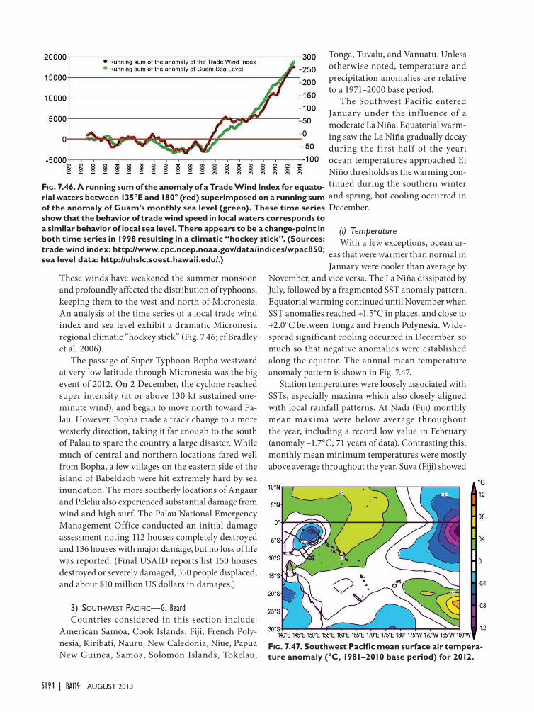
S194 | August 2013
These winds have weakened the summer monsoon and profoundly affected the distribution of typhoons, keeping them to the west and north of Micronesia. An analysis of the time series of a local trade wind index and sea level exhibit a dramatic Micronesia regional climatic “hockey stick” (Fig. 7.46; cf Bradley et al. 2006).
The passage of Super Typhoon Bopha westward at very low latitude through Micronesia was the big event of 2012. On 2 December, the cyclone reached super intensity (at or above 130 kt sustained one-minute wind), and began to move north toward Pa-lau. However, Bopha made a track change to a more westerly direction, taking it far enough to the south of Palau to spare the country a large disaster. While much of central and northern locations fared well from Bopha, a few villages on the eastern side of the island of Babeldaob were hit extremely hard by sea inundation. The more southerly locations of Angaur and Peleliu also experienced substantial damage from wind and high surf. The Palau National Emergency Management Office conducted an initial damage assessment noting 112 houses completely destroyed and 136 houses with major damage, but no loss of life was reported. (Final USAID reports list 150 houses destroyed or severely damaged, 350 people displaced, and about $10 million US dollars in damages.)
3) SoUthWeSt paCifiC—G. BeardCountries considered in this section include:
American Samoa, Cook Islands, Fiji, French Poly-nesia, Kiribati, Nauru, New Caledonia, Niue, Papua New Guinea, Samoa, Solomon Islands, Tokelau,
Tonga, Tuvalu, and Vanuatu. Unless otherwise noted, temperature and precipitation anomalies are relative to a 1971–2000 base period.
The Southwest Pacific entered January under the inf luence of a moderate La Niña. Equatorial warm-ing saw the La Niña gradually decay during the first half of the year; ocean temperatures approached El Niño thresholds as the warming con-tinued during the southern winter and spring, but cooling occurred in December.
(i) TemperatureWith a few exceptions, ocean ar-
eas that were warmer than normal in January were cooler than average by
November, and vice versa. The La Niña dissipated by July, followed by a fragmented SST anomaly pattern. Equatorial warming continued until November when SST anomalies reached +1.5°C in places, and close to +2.0°C between Tonga and French Polynesia. Wide-spread significant cooling occurred in December, so much so that negative anomalies were established along the equator. The annual mean temperature anomaly pattern is shown in Fig. 7.47.
Station temperatures were loosely associated with SSTs, especially maxima which also closely aligned with local rainfall patterns. At Nadi (Fiji) monthly mean maxima were below average throughout the year, including a record low value in February (anomaly –1.7°C, 71 years of data). Contrasting this, monthly mean minimum temperatures were mostly above average throughout the year. Suva (Fiji) showed
Fig. 7.46. a running sum of the anomaly of a trade Wind index for equato-rial waters between 135°e and 180° (red) superimposed on a running sum of the anomaly of guam’s monthly sea level (green). these time series show that the behavior of trade wind speed in local waters corresponds to a similar behavior of local sea level. there appears to be a change-point in both time series in 1998 resulting in a climatic “hockey stick”. (sources: trade wind index: http://www.cpc.ncep.noaa.gov/data/indices/wpac850; sea level data: http://uhslc.soest.hawaii.edu/.)
Fig. 7.47. southwest Pacific mean surface air tempera-ture anomaly (°C, 1981–2010 base period) for 2012.

S195STATE OF THE CLIMATE IN 2012 |AuguST 2013
similar temperature variations, although maxima were above average in five months. Overnight warmth was more pronounced, however, with mean minima being ranked in the top four in several months, in-cluding a new record in October (anomaly +2.0°C, 71 years of data).
Temperatures in Vanuatu were mostly above aver-age; at Analgauhat there was only one negative anom-aly (August minima) among the 24 mean monthly maxima and minima combined, while at Pekoa there were six. Maximum temperatures were particularly high, with near records set in several months at both sites. Pekoa set a new record mean maximum for March (+1.2°C anomaly, 53 years of data).
(ii) Precipitation Rainfall across the region responded to changes
in ENSO and to f luctuations in the South Pacific Convergence Zone (SPCZ). Convection was sup-pressed near the equatorial date line during January and February. Tarawa (Kiribati) received 121 mm of rain during these two months, only 30% of average. This followed a dry spell from October to December 2011 (73 mm, 16% of average). In contrast, most other countries in the region began 2012 with near- or above-average rainfall in response to an active SPCZ.
Rainfall was generally near or above normal over the region during March to May. However, below-average precipitation was more prevalent in April, especially in eastern or southern areas such as the Cook Islands and Niue. The remainder of the year was
mainly characterized by above-average rainfall in the north and southwest of the region, and below-average totals in central to southeastern parts. Enhanced activity in the SPCZ favored the Solomon Islands, Vanuatu, Fiji, and Tonga, while a zone of suppressed convection affected Tuvalu, Samoa, Niue, and the Cook Islands.
Niue and Rarotonga (southern Cook Islands) were particularly dry; with the exception of May in Niue and July in Rarotonga, monthly rainfall was below average from April onwards. Niue recorded 652 mm (52% of average, fourth driest of 63-year record) for the nine months, while Rarotonga had 801 mm (65% of average, fifth driest of 84-year record). Representa-tive annual totals are shown in Table 7.2.
(iii) Notable eventsFrom 21 to 26 January, intense rainfall and severe
f looding occurred over northern and western Fiji. Over 500 mm of rain fell during 22–24 January, including more than 800 mm at some sites. Severe flooding occurred in the major towns of Nadi, Ba, and Rakiraki. A similar event in late March set several monthly and daily rainfall records for the month.
A tropical depression on 9 December, about 700 km northwest of Suva, Tropical Cyclone Evan intensified and tracked eastward, affecting the French islands of Wallis and Futuna. Reaching Category 1 tropical cyclone status on 11 December, it maintained an easterly track towards Samoa and American Samoa. Between 12 and 14 December,
Evan slowed considerably near Samoa (resulting in severe impacts) as it first recurved northward, then westward. The areas sur-rounding Apia, Samoa, received over 400 mm of rain on 13 December, while wind gusts reached 113 kt (58.3 m s-1) at Faleolo Air-port, Apia.
C yc lone Ev a n a l s o caused widespread damage across the Island of Upolu. Four people were killed, mostly from flooding, and 10 were unaccounted for at year’s end. In addition, about 7 500 people were temporarily displaced. Se-
Table 7.2: Rainfall totals for 2012, percent of average, and rank (starts at 1 for lowest; years of record also shown) for representative stations across the southwest Pacific.
station annual total (mm)
Percent of average
Rank (Posi-tion/Years of
Record)
Port Moresby (PNG) 1411 131 93/107
Honiara (Solomon Islands) 2537 130 49/56
Port Vila (Vanuatu) 2126 100 31/60
Tarawa (Kiribati) 1775 87 38/77
Nadi Airport (Fiji) 3548 189 69/69 (highest)
Nuku’alofa (Tonga) 2616 152 66/67
Apia (Samoa) 2437 82 31/123
Alofi (Niue) 2050 105 30/63
Rarotonga (Cook Islands) 1405 76 8/84

S196 | August 2013
vere f looding in the Vaisigano catchment was re-ported as the worst on record.
In addition to destroying community facilities such as schools and churches, Evan severely damaged 2 088 houses across 164 villages. There was major damage and disruption to transportation, power, wa-ter, and communications infrastructures. There was also widespread damage to crops such as bananas, taro, and breadfruit. The total cost of damage and losses from this disaster is $479.8 million Samoan Tala ($209 million US dollars), which is equivalent to 29.3% of the country’s GDP in 2011. The cyclone did not cause any damage on Savaii Island.
As Evan continued on its westward path, Wallis and Futuna Islands were affected for a second time, with extensive damage at the former. By 16 Decem-ber, Evan’s path was more southwesterly as it headed directly for Fiji. With one-minute sustained winds of 124 kt (63.9 m s-1) and a central pressure of 943 hPa (Category 4 severe tropical cyclone, Category 4 hur-ricane), peak intensity was reached on 17 December as Evan skirted the northern coast of Vanua Levu (Fiji). There were no reports of casualties in Fiji, although there was extensive damage and flooding.
4) aUStralia—C. Ganter and S. TobinUnless otherwise noted, Australian temperature
anomalies are reported using a 1961–90 base period.
(i) TemperatureAustralia’s mean temperature anomaly for 2012
was +0.11°C, 36th warmest of 103 years of record. Maximum temperatures (Fig. 7.48) were above nor-mal while minimum temperatures (Fig. 7.49) were below, with anomalies of +0.51°C (12th warmest) and
–0.28°C (43rd coolest), respectively. All states and territories recorded a positive maximum temperature anomaly, with Western Australia, South Australia, and Tasmania all observing their ninth warmest years (anomalies of +0.66°C, +0.97°C and +0.56°C, respec-tively). Minimum temperatures were less significant with Tasmania, at 10th warmest, the only state in the warmest/coolest ten. The diurnal temperature range nationally was the fifth highest on record. The four years with a greater range all occurred during periods of major drought.
Maximum temperatures were broadly above normal across most of the country, with parts of the tropical north slightly below normal. Anomalies exceeded +0.5°C over parts of the Top End of the Northern Territory, the northern tip of the Cape York Peninsula, and in a broad area stretching across most of the southern half of Australia, except for parts of the east. Large areas of southern and coastal Western Australia topped +1.0°C, as did a few small areas of central Australia. The largest anomalies, which were between +1.5°C and +2.0°C, were confined to small areas of Western Australia.
Maximum temperatures were broadly cooler than normal until July, mostly an effect from the widespread cloud cover and rainfall brought from La Niña. The first three months of the year were 17th coolest nationally, with some part of the country ex-periencing anomalies of at least –4.0°C during each of these months.
From August onwards, maximum temperature anomalies became increasingly positive. The last four months were exceptionally warm; the national September–December anomaly of +1.61°C was the highest on record. Each of the last four months had
Fig. 7.49. australian mean annual maximum tempera-ture anomalies (°C, 1961–90 base period) for 2012.
Fig. 7.48. australian mean annual minimum tempera-ture anomalies (°C, 1961–90 base period) for 2012.

S197STATE OF THE CLIMATE IN 2012 |AuguST 2013
some part of the country observing anomalies higher than +4.0°C, with the largest area of +4.0°C and above experienced during November (see Sidebar 7. 5).
In contrast to maximum temperatures, minimum temperatures for the year were largely below normal, with the exception of western parts of Western Aus-tralia, Tasmania, and the coastal southern regions of the mainland. Anomalies cooler than –0.5°C were measured over the Kimberley region in Western Australia, most of the Northern Territory, and large patches through Queensland and New South Wales. The largest anomalies, between –1.5°C and –2.0°C were found in small areas over northern Australia.
(ii) PrecipitationRainfall averaged over Australia for the year was
475 mm (102% of normal), ranking 39th wettest since records began in 1900. Annual rainfall was normal to above normal across most of the country, with parts of the far tropical north and most of the south below normal (Fig. 7.50).
In stark contrast to the two years prior, the annual total for 2012 for the majority of Australia was close to normal. South Australia was the only state with annual rainfall more than 10% away from normal (77% of normal).
Only a small percentage of the country received precipitation in deciles one and ten (both 4.2%), with areas of above-average precipitation recorded over the northwest of the country, extending through much of the inland eastern mainland. Other regions generally received below-average precipitation.
Rainfall in 2012 was characterized by two very different periods, the wet initial three months under La Niña’s influence, and the far drier remaining nine months, as ENSO became neutral. The January–March period was very wet over parts of the east and
northwest. Areas in southern New South Wales and northeast Victoria experienced record high rainfall for the three-month total, mostly the result of one very wet week. Nationally, it was the seventh wettest January–March on record.
With the breakdown of La Niña during austral fall, Australia shifted into a different rainfall pattern, namely, below-average rainfall across southern Aus-tralia and seasonally dry weather over the northern tropics. Central Australia was particularly dry, with Alice Springs Airport recording no measurable rain for 157 consecutive days (25 April to 28 September), the longest such spell in the site’s 57-year history. For southern Australia (south of 26°S), it was the ninth driest April–December period on record. The tropics experienced a poor start to the wet season at the end of 2012, with no monsoon onset by the year’s end.
(iii) Notable eventsThe most notable aspect of 2012 for Australia was
the contrast between the cool and wet start to the year and the widespread rainfall deficits in the months following, together with record-breaking warmth late in the year.
The 2011/12 La Niña continued to bring persistent heavy rain in the first three months of the year, result-ing in flooding in many parts of eastern Australia and the tropics. Following flooding in southern and southeast Queensland and northern New South Wales in January and February, one of the most ex-treme multiday rainfall events in southeast Australia’s history brought daily totals above 100 mm to the inland southeast between 27 February and 4 March. The Murrumbidgee, Upper Murray, and Lachlan catchments all nearly doubled their previous record weekly rainfall. Flooding was widespread and neces-sitated extensive evacuations in many rural towns.
A number of storms brought significant rainfall, damage, or both to parts of Australia in 2012:
• An East Coast Low on 3–5 June caused f looding in southern Victoria, with daily totals more than twice the monthly average across the Otway Ranges. Very large waves were observed in Bass Strait and New South Wales waters.
• Multiple intense cold fronts and storms over southwest Western Australia between 7 and 13 June caused the worst damage on record to the Western Australian electricity network and set a new storm surge record of 1.0 m at Fremantle.Fig. 7.50. australian annual rainfall deciles (since 1900)
for 2012.

S198 | August 2013
• Several periods of damaging winds associated with low pressure systems were reported in the southeastern states during August and September.
• Severe thunderstorms occurred in southeast Queensland and northern New South Wales on 17 and 18 November.
• Heavy precipitation fell across Western Aus-tralia between 10 and 13 December, causing some flooding in the southwest.
Two notable cold outbreaks affected southeastern Australia during the year. One in early April brought storms to Tasmania, snow at high elevations on the mainland, and cold nights as far north as Queensland. The other, in the second week of October, brought snow to Adelaide and the surrounding hills before combining with an East Coast Low to bring severe
weather to eastern New South Wales south of New-castle, including 15 cm–25 cm of snow in parts of the Blue Mountains (the heaviest snowfall at any time of year since 1984).
From August onwards temperature maxima tracked well above average, resulting in numerous winter and spring heat records. A number of sites in central Australia tied or set new early season records, while eastern Australia experienced one of the most significant spring heat waves on record at the end of November (see Sidebar 7.5).
5) neW Zealand—P. R. Chappell and G. M. GriffithsIn the following discussion the base period is
1981–2010, unless otherwise noted. All statistics are based on data available as of 9 January 2013.
siDebaR 7.5: a VeRY WaRm enD to tHe aUstRal sPRing FoRsoUtHeast aUstRalia
One of the most significant spring heat waves on record hit large parts of southeast Australia during the last week of November (Fig. SB7.7). This heat wave was comprised of a sequence of extreme heat events in the region during austral spring. A very hot air mass developed over central Australia by 25 November. Northerly winds dragged this air towards the southeast, with the peak heat intensity occurring on 29 November, covering most of Victoria, inland New South Wales, northern and eastern South Australia, and western Tasmania. On that day, 18 long-term stations across Victoria, New South Wales, and South Australia had their hottest spring day on record. More broadly, a spring maximum temperature record was set over 33.8% of Victoria, 10.4% of New South Wales, and 1.2% of South Australia.
Most significantly, at Ouyen, the temperature reached 45.8°C, the hottest Victorian spring temperature on record. The previous record, 44.5°C, set at Mildura on 17 November 1980 was also broken by four other sites: Mildura (45.5°C); Swan Hill (45.2°C); Hopetoun (45.0°C); and Walpeup (44.7°C).
As cloud cover increased ahead of an approaching trough, very high overnight minimum temperatures occurred on the night of 29–30 November. The air mass, which was already un-usually moist for a spring heatwave, became even more humid, with some particularly high dewpoints measured. Record-high minimum temperatures were measured at a number of sites near the New South Wales–Victoria border, over northeast and central Victoria, and southern Tasmania.
The extreme heat was relatively short-lived over southeast Australia. However, it was persistent over inland areas, with weekly temperature anomalies in excess of +10°C over inland southeast Australia (Fig. SB7.7). Some sites tied their respec-tive November records for an extended hot spell. For ex-ample, Birdsville, in Queensland, tied its November record of 10 consecutive days above 40°C from 21–30 November, while Oodndatta in South Australia also tied its overnight record of six consecutive nights above 25°C from 25 to 30 November.
Fig. sb7.7. maximum temperature anomalies (°C, 1961–90 base period) for 24–30 nov 2012.
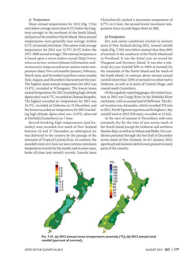
S199STATE OF THE CLIMATE IN 2012 |AuguST 2013
(i) TemperatureMean annual temperatures for 2012 (Fig. 7.51a)
were below average (more than 0.5°C below the long-term average) in the northeast of the South Island, and parts of the southern North Island. Mean annual temperatures were generally near average (within 0.5°C of normal) elsewhere. The nation-wide average temperature for 2012 was 12.5°C (0.1°C below the 1971–2000 annual average). The national temperature is based upon a seven-station record (http://www.niwa.co.nz/our-science/climate/information-and-resources/nz-temp-record/seven-station-series-tem-perature-data). Five cool months (January, February, March, June, and November) and three warm months (July, August, and December) characterized the year. The highest mean annual temperature for 2012 was 15.8°C, recorded at Whangarei. The lowest mean annual temperature for 2012 (excluding high altitude alpine sites) was 6.7°C, recorded at Chateau Ruapehu. The highest recorded air temperature for 2012 was 34.5°C, recorded at Gisborne on 19 December, and the lowest recorded air temperature for 2012 (exclud-ing high altitude alpine sites) was -11.8°C, observed at Darfield (Canterbury) on 7 June.
Record-breaking high temperatures (and hu-midity) were recorded over much of New Zealand between 22 and 27 December, as subtropical air was delivered to the country by the passage of the remnants of Tropical Cyclone Evan. In contrast, the snowfall event on 6 June set new extreme minimum temperature records for the month, and in some cases, broke all-time (any month) records. Lincoln (near
Christchurch) reached a maximum temperature of 0.7°C on 6 June, the second lowest maximum tem-perature since records began there in 1881.
(ii) PrecipitationDry and sunny conditions existed in western
areas of New Zealand during 2012. Annual rainfall totals (Fig. 7.51b) were below normal (less than 80% of normal) in the southwest of the North Island and in Fiordland. It was the driest year on record for Wanganui and Secretary Island. It was also a rela-tively dry year (rainfall 80% to 100% of normal) for the remainder of the North Island and for much of the South Island. In contrast, above-normal annual rainfall (more than 120% of normal) was observed in Gisborne, as well as in parts of Central Otago, and coastal south Canterbury.
Of the regularly reporting gauges, the wettest loca-tion in 2012 was Cropp River in the Hokitika River catchment, with an annual total of 9630 mm. The dri-est location was Alexandra, which recorded 378 mm in 2012. North Egmont experienced the highest 1-day rainfall total in 2012 (336 mm), recorded on 15 July.
At the start of summer (1 December), soils were extremely dry for the time of year across much of the North Island (except for Gisborne and northern Hawkes Bay), as well as in Nelson and Buller. Dry con-ditions persisted through the first half of December across much of New Zealand. As of 1 January 2013, significant soil moisture deficits were present in many parts of the country.
Fig. 7.51. (a) 2012 annual mean temperature anomaly (°C); (b) 2012 annual total rainfall (percent of normal).

S200 | August 2013
(iii) Notable eventsOne significant snowfall event occurred in 2012.
On 6 June, a low over the Tasman Sea and a trough to the south of the country brought a broad area of cold, moist air over the South Island that produced heavy snowfall to low levels over most of the South Island (Fig. 7.52). Afternoon temperatures in many places set new low records for the month, and in some cases broke all-time (any month) records. Maximum temperatures on 6 June in Canterbury struggled to reach even 1°C, with heavy snow falling throughout the daylight hours. This event closed major and mi-nor roads, schools, and universities, and disrupted air traffic.
A rapidly deepening low migrated eastwards across the southern North Island on 4 March, bring-ing heavy rain and extremely strong winds to the southern North Island and Nelson, felling trees, clos-ing roads, and causing property damage. On 19–20
March, heavy rain caused f looding in Northland, especially affecting the township of Kaeo, where roughly twice the normal rainfall for March fell in 35 hours (284 mm, average March rainfall is 120 mm). Gisborne was all but isolated by landslides and flooding. On 5–6 June, the northwest South Island was affected by record-breaking rain, again associated with a rapidly deepening low over the Tasman Sea. Greymouth Airport had 151 mm of rain in 24 hours, the highest June daily rainfall total in the record there since 1947.
On 6 December, an active trough line contain-ing thunderstorms passed over Auckland. A tor-nado touched down in west Auckland, felling trees, damaging roofs, and causing power outages. Three people were killed by falling slabs of concrete at a construction site from this event, and several others were injured.
Fig. 7.52. notable weather events and climatic extremes for new Zealand in 2012.

S201STATE OF THE CLIMATE IN 2012 |AUGUST 2013
appendix 1: SeaSOnaL SUMMaRieS—M. Halpert
Fig
. a
1.1.
dec
201
1–Fe
b 20
12 (
top)
sur
face
tem
pera
ture
ano
mal
ies
(°C
) an
d (b
otto
m)
prec
ipit
atio
n pe
rcen
tile
s ba
sed
on a
gam
ma
dist
ribu
tion
fit
to t
he 1
981–
2010
bas
e pe
riod
. T
empe
ratu
re a
nom
alie
s (1
981–
2010
bas
e pe
riod
) ar
e ba
sed
on s
tati
on d
ata
over
land
and
sea
sur
face
tem
pera
ture
da
ta o
ver
wat
er. p
reci
pita
tion
dat
a w
ere
obta
ined
from
the
Ca
MS
-Op
i da-
tase
t tha
t is
a co
mbi
nati
on o
f rai
n ga
uge
obse
rvat
ions
and
sat
ellit
e-de
rive
d es
tim
ates
(Ja
now
iak
and
xie
199
9). a
naly
sis
was
om
itte
d in
dat
a-sp
arse
re
gion
s (w
hite
are
as).
Fig
. a1.
2. d
ec 2
011–
Feb
2012
(to
p) n
orth
ern
Hem
isph
ere
and
(bot
tom
) So
uthe
rn H
emis
pher
e 50
0 hp
a ge
opot
enti
al h
eigh
ts (9
-dam
con
tour
inte
r-va
l) a
nd a
nom
alie
s (s
hadi
ng)
dete
rmin
ed fr
om t
he 1
981–
2010
bas
e pe
riod
m
eans
. dat
a is
from
the
Cd
aS
/Rea
naly
sis
pro
ject
(K
alna
y et
al.
1996
).

S202 | AUGUST 2013
Fig
. a
1.3.
Mar
–May
201
2 (t
op)
surf
ace
tem
pera
ture
ano
mal
ies
(°C
) an
d (b
otto
m) p
reci
pita
tion
per
cent
iles
base
d on
a g
amm
a di
stri
buti
on fi
t to
the
1981
–201
0 ba
se p
erio
d. T
empe
ratu
re a
nom
alie
s (1
981–
2010
bas
e pe
riod
) ar
e ba
sed
on s
tati
on d
ata
over
lan
d an
d se
a su
rfac
e te
mpe
ratu
re d
ata
over
wat
er. p
reci
pita
tion
dat
a w
ere
obta
ined
fro
m t
he C
aM
S-O
pi
data
-se
t th
at is
a c
ombi
nati
on o
f rai
n ga
uge
obse
rvat
ions
and
sat
ellit
e-de
rive
d es
tim
ates
(Ja
now
iak
and
xie
199
9). a
naly
sis
was
om
itte
d in
dat
a-sp
arse
re
gion
s (w
hite
are
as).
Fig
. a1.
4. M
ar–M
ay 2
012
(top
) nor
ther
n H
emis
pher
e an
d (b
otto
m) S
outh
-er
n H
emis
pher
e 50
0 hp
a ge
opot
enti
al h
eigh
ts (9
-dam
con
tour
inte
rval
) and
an
omal
ies
(sha
ding
) de
term
ined
from
the
198
1–20
10 b
ase
peri
od m
eans
. d
ata
is fr
om t
he C
da
S/R
eana
lysi
s p
roje
ct (
Kal
nay
et a
l. 19
96).

S203STATE OF THE CLIMATE IN 2012 |AUGUST 2013
Fig
. a1.
5. J
un–a
ug 2
012
(top
) su
rfac
e te
mpe
ratu
re a
nom
alie
s (°
C)
and
(bot
tom
) pr
ecip
itat
ion
perc
enti
les
base
d on
a g
amm
a di
stri
buti
on f
it
to t
he 1
981–
2010
bas
e pe
riod
. Tem
pera
ture
ano
mal
ies
(198
1–20
10 b
ase
peri
od) a
re b
ased
on
stat
ion
data
ove
r la
nd a
nd s
ea s
urfa
ce t
empe
ratu
re
data
ove
r w
ater
. pre
cipi
tati
on d
ata
wer
e ob
tain
ed fr
om t
he C
aM
S-O
pi
data
set
that
is
a co
mbi
nati
on o
f ra
in g
auge
obs
erva
tion
s an
d sa
telli
te-
deri
ved
esti
mat
es (
Jano
wia
k an
d x
ie 1
999)
. a
naly
sis
was
om
itte
d in
da
ta-s
pars
e re
gion
s (w
hite
are
as).
Fig
. a1.
6. Ju
n–a
ug 2
012
(top
) nor
ther
n H
emis
pher
e an
d (b
otto
m) S
outh
ern
Hem
isph
ere
500
hpa
geop
oten
tial
hei
ghts
(9-
dam
con
tour
int
erva
l) a
nd
anom
alie
s (s
hadi
ng)
dete
rmin
ed f
rom
the
198
1–20
10 b
ase
peri
od m
eans
. d
ata
is fr
om t
he C
da
S/R
eana
lysi
s p
roje
ct (
Kal
nay
et a
l. 19
96).
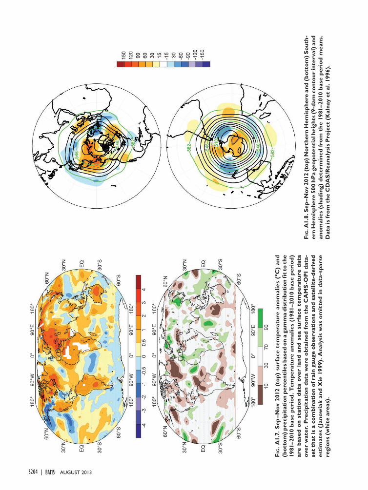
S204 | AUGUST 2013
Fig
. a
1.7.
Sep
–nov
201
2 (t
op)
surf
ace
tem
pera
ture
ano
mal
ies
(°C
) an
d (b
otto
m) p
reci
pita
tion
per
cent
iles b
ased
on
a ga
mm
a di
stri
buti
on fi
t to
the
1981
–201
0 ba
se p
erio
d. T
empe
ratu
re a
nom
alie
s (1
981–
2010
bas
e pe
riod
) ar
e ba
sed
on s
tati
on d
ata
over
lan
d an
d se
a su
rfac
e te
mpe
ratu
re d
ata
over
wat
er. p
reci
pita
tion
dat
a w
ere
obta
ined
from
the
Ca
MS
-Op
i da
ta-
set
that
is a
com
bina
tion
of r
ain
gaug
e ob
serv
atio
ns a
nd s
atel
lite-
deri
ved
esti
mat
es (
Jano
wia
k an
d x
ie 1
999)
. ana
lysi
s w
as o
mit
ted
in d
ata-
spar
se
regi
ons
(whi
te a
reas
).
Fig
. a1.
8. S
ep–n
ov 2
012
(top
) nor
ther
n H
emis
pher
e an
d (b
otto
m) S
outh
-er
n H
emis
pher
e 50
0 hp
a ge
opot
enti
al h
eigh
ts (9
-dam
con
tour
inte
rval
) and
an
omal
ies
(sha
ding
) de
term
ined
fro
m t
he 1
981–
2010
bas
e pe
riod
mea
ns.
dat
a is
from
the
Cd
aS
/Rea
naly
sis
pro
ject
(K
alna
y et
al.
1996
).

S205STATE OF THE CLIMATE IN 2012 |AUGUST 2013
General Variable or Phenomenon
Specific Dataset or Variable Source Section
AerosolsAERONET data (NASA)
http://aeronet.gsfc.nasa.gov/ 2g2
Aerosol products http://www.gmes-atmosphere.eu/data/ 2g2
Air-sea fluxes
Woods Hole Oceano-graphic Institute (WHOI) OAFlux Project
http://oaflux.whoi.edu 3d
Albedo MODIS http://ladsweb.nascom.nasa.gov/ 2h2,5f
Biomass Burning Biomass Burning http://www.globalfiredata.org/ 2h4
Clouds, Cloudiness
HIRS No known public portal 2d4
ISCCP D2 http://isccp.giss.nasa.gov 2d4
MISR http://eosweb.larc.nasa.gov/PRODOCS/misr/level3 /overview.html
2d4
MODIS Cloud Mask http://ladsweb.nascom.nasa.gov/ 2d4,5b
PATMOS-x http://www.ncdc.noaa.gov/cdr/operationalcdrs.html 2d4
SOBS http://www.atmos.washington.edu/~ignatius/CloudMap 2d4
Evaporation JRA-25 http://jra.kishou.go.jp 6d
FAPAR FAPAR http://fapar.jrc.ec.europa.eu/ 2h3
Geopotential Height
ERA-Interim http://www.ecmwf.int/research/era 6b
Glacier Mass orVolume
Glacier Mass Balance http://www.geo.uzh.ch/microsite/wgms/mbb/sum10.html 5e
GRACE http://www.csr.utexas.edu/grace/ 2c3
Humidity, [Near] Surface
20th Century Reanalysis
http://www.esrl.noaa.gov/psd/data/20thC_Rean/ 2d1
Dai by email to [email protected] 2d1
ERA-Interim http://www.ecmwf.int/research/era 2d1
HadCRUH http://www.metoffice.gov.uk/hadobs/hadcruh 2d1
JRA-25 Atmospheric Reanalysis
http://jra.kishou.go.jp/JRA-25/index_en.html 2d1
MERRA http://gmao.gsfc.nasa.gov/merra/ 2d1
NCEP CFSR http://cfs.ncep.noaa.gov 2d1
NOCS 2.0 http://www.noc.soton.ac.uk/noc_flux/noc2.php 2d1
Isotherm depthNCEP Global Ocean Data Assimilation System
http://www.cpc.ncep.noaa.gov/products/GODAS 4h
Lake Ice NOAA IMS, 4m Daily http://nsidc.org/data/g02156.html 5h
Lake Levels
Altimetric Lake level Products, USDA
http://www.pecad.fas.usda.gov/cropexplorer /global_reservoir/index.cfm
2d8
ESA http://tethys.eaprs.cse.dmu.ac.uk/RiverLake/shared/main 2d8
LEGOS http://www.legos.obs-mip.fr/soa/hydrologie/hydroweb/ 2d8
Lake TemperatureARCLAKE http://hdl.handle.net/10283/88, http://www.geos.ed.ac.uk
/arclake/2b4
IWBP http://largelakes.jpl.nasa.gov 2b4
APPENDIx 2: RELEVANT DATASETS AND SouRCES
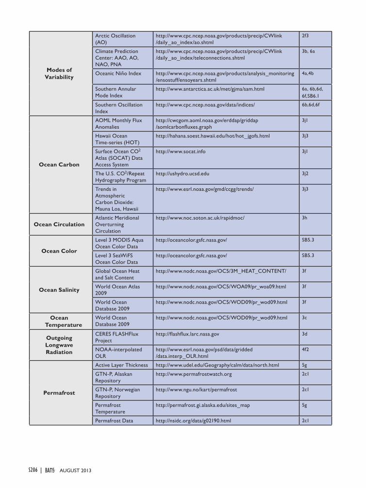
S206 | AUGUST 2013
Modes of Variability
Arctic Oscillation (AO)
http://www.cpc.ncep.noaa.gov/products/precip/CWlink /daily_ao_index/ao.shtml
2f3
Climate Prediction Center: AAO, AO, NAO, PNA
http://www.cpc.ncep.noaa.gov/products/precip/CWlink /daily_ao_index/teleconnections.shtml
3b, 6a
Oceanic Niño Index http://www.cpc.ncep.noaa.gov/products/analysis_monitoring /ensostuff/ensoyears.shtml
4a,4b
Southern Annular Mode Index
http://www.antarctica.ac.uk/met/gjma/sam.html 6a, 6b,6d,6f,SB6.1
Southern Oscillation Index
http://www.cpc.ncep.noaa.gov/data/indices/ 6b,6d,6f
ocean Carbon
AOML Monthly Flux Anomalies
http://cwcgom.aoml.noaa.gov/erddap/griddap /aomlcarbonfluxes.graph
3j1
Hawaii Ocean Time-series (HOT)
http://hahana.soest.hawaii.edu/hot/hot_jgofs.html 3j3
Surface Ocean CO2 Atlas (SOCAT) Data Access System
http://www.socat.info 3j1
The U.S. CO2/Repeat Hydrography Program
http://ushydro.ucsd.edu 3j2
Trends in Atmospheric Carbon Dioxide: Mauna Loa, Hawaii
http://www.esrl.noaa.gov/gmd/ccgg/trends/ 3j3
ocean CirculationAtlantic Meridional Overturning Circulation
http://www.noc.soton.ac.uk/rapidmoc/ 3h
ocean Color
Level 3 MODIS Aqua Ocean Color Data
http://oceancolor.gsfc.nasa.gov/ SB5.3
Level 3 SeaWiFS Ocean Color Data
http://oceancolor.gsfc.nasa.gov/ SB5.3
ocean Salinity
Global Ocean Heat and Salt Content
http://www.nodc.noaa.gov/OC5/3M_HEAT_CONTENT/ 3f
World Ocean Atlas 2009
http://www.nodc.noaa.gov/OC5/WOA09/pr_woa09.html 3f
World Ocean Database 2009
http://www.nodc.noaa.gov/OC5/WOD09/pr_wod09.html 3f
ocean Temperature
World Ocean Database 2009
http://www.nodc.noaa.gov/OC5/WOD09/pr_wod09.html 3c
outgoing Longwave Radiation
CERES FLASHFlux Project
http://flashflux.larc.nasa.gov 3d
NOAA-interpolated OLR
http://www.esrl.noaa.gov/psd/data/gridded /data.interp_OLR.html
4f2
Permafrost
Active Layer Thickness http://www.udel.edu/Geography/calm/data/north.html 5g
GTN-P, Alaskan Repository
http://www.permafrostwatch.org 2c1
GTN-P, Norwegian Repository
http://www.ngu.no/kart/permafrost 2c1
Permafrost Temperature
http://permafrost.gi.alaska.edu/sites_map 5g
Permafrost Data http://nsidc.org/data/g02190.html 2c1

S207STATE OF THE CLIMATE IN 2012 |AUGUST 2013
Phytoplankton, ocean Color
MERIS 3rd Data Reprocessing
http://earth.eo.esa.int/pcs/envisat/meris/documentation /meris_3rd_reproc/MERIS_3rd_Reprocessing_Changes.pdf
3j4
Ocean Color Documents: MODIS-Aqua Reprocessing 2010.0
http://oceancolor.gsfc.nasa.gov/WIKI/OCReproc20100MA.html
3j4
Precipitation
CMAP http://www.esrl.noaa.gov/psd/data/gridded /data.ncep.reanalysis.html
2d3
GHCN http://www.ncdc.noaa.gov/temp-and-precip /ghcn-gridded-products.php
2d3
Global Precipitation Climatology Project (GPCP)
http://precip.gsfc.nasa.gov 2d3,4h
GPCC http://www.gpcc.dwd.de/ 2d3
SSM/I, TMI, and AMSR-E Data
http://www.remss.com 2d3
TRMM 3A12 http://disc.sci.gsfc.nasa.gov/precipitation/documentation /TRMM_README/TRMM_3A12_readme.shtml
4f2
TRMM 3B43 Rainfall http://disc.sci.gsfc.nasa.gov/precipitation/documentation /TRMM_README/TRMM_3B43_readme.shtml
4f1, 4f2
Precipitation (net) JRA-25 Atmospheric Reanalysis
http://jra.kishou.go.jp/JRA-25/index_en.html 6d
Pressure, Sea Level or Near-Surface
ACCESS http://www.bom.gov.au/nwp/access/NWPData.shtml 6f
AMRC (Antarctic Me-teorological Research Center) AWS
http://amrc.ssec.wisc.edu/data/ 6c,SB6.1
ERA-Interim http://www.ecmwf.int/research/era 6a,6b,6c
HadSLP2r http://www.metoffice.gov.uk/hadobs 2e1
JRA-25 Atmospheric Reanalysis
http://jra.kishou.go.jp/JRA-25/index_en.html 6d
READER http://www.antarctica.ac.uk/met/READER/ 6c
River Discharge
Arctic-RIMS1 River Discharge
http://rims.unh.edu 2d5
Dartmouth Flood Observatory
http://floodobservatory.colorado.edu 2d5
River Discharge http://waterdata.usgs.gov/nwis - USGS2 2d5
Sea Ice Concentration
Nimbus-7 SMMR and DMSP SSM/I
http://nsidc.org/data/nsidc-0051.html 5b, SB5.2
Nimbus-7 SMMR and DMSP SSM/I (Bootstrap)
http://nsidc.org/data/docs/daac/nsidc0079_bootstrap_seaice .gd.html
6f
Sea Ice DurationNear-Real-Time DMSP SSM/I-SSMIS Daily Polar Gridded
http://nsidc.org/data/nsidc-0081.html 6f
Sea Ice Extent
Nimbus-7 SMMR and DMSP SSM/I (Bootstrap)
http://nsidc.org/data/docs/daac /nsidc0079_bootstrap_seaice.gd.html
6f
NOAA IMS, 4km Daily http://nsidc.org/data/g02156.html 5i
Sea Ice Index
Sea Ice Concentration from DMSP SSM/I-SS-MIS Passive Microwave Data
http://nsidc.org/data/seaice_index/archives/index.html 5i

S208 | AUGUST 2013
Sea Level
Arctic Sea Level http://www.whoi.edu/science/PO/arcticsealevel/data.html 5j
Ssalto/Duacs Multimission Altimeter Products
http://www.aviso.oceanobs.com/en/data /product-information/duacs/index.html
3g
University of Hawaii Sea Level Center
http://uhslc.soest.hawaii.edu/ 3i
Sea Surface Salinity
Aquarius http://aquarius.nasa.gov SB3.1
World Ocean Atlas 2009
http://www.nodc.noaa.gov/OC5/WOA09/pr_woa09.html 3e
Sea Surface Temperature
Climate Prediction Center's Monthly Ocean Briefing
http://www.cpc.ncep.noaa.gov/products/GODAS 3b
ERSST-v3b http://www.esrl.noaa.gov/psd/data/gridded/data.noaa.ersst.html
4b1,4d,4g
HadSST2 http://www.metoffice.gov.uk/hadobs/hadsst2 2b1
NOAA Optimum Interpolation SST (OISST) v2
http://www.esrl.noaa.gov/psd/data/gridded /data.ncep.oisst.v2.html
4f2,4h,
5j2,6f
Snow CoverSnow Cover Extent and Duration
http://climate.rutgers.edu/snowcover/ 2c2,5d
SSM/I http://www.nsidc.org 6e
Snow Depth
Canadian Meteorological Centre Daily Gridded
http://nsidc.org/data/docs/daac/nsidc0447_CMC_snow_depth/index.html
5d
Snow Water Equivalent
ERA-interim Atmospheric Reanaly-sis
http://www.ecmwf.int/research/era 5d
GlobSnow N. Hemisphere Snow Water Equivalent
http://www.globsnow.info/ 5d
Soil Moisture GRACE http://www.esa-soimoisture-cci.org/ 2d6
Solar Transmission Mauna Loa Solar Transmission
http://www.esrl.noaa.gov/gmd/grad/mloapt.html SB2.3
Stratospheric ozone
Calipso (Polar Stratospheric Clouds)
http://eosweb.larc.nasa.gov/PRODOCS/calipso /table_calipso.html
6g
GOME/SCIAMACHY/GOME2 Total Ozone datasets, GSG Merged Data
http://www.iup.uni-bremen.de/gome/wfdoas 2g3, 6g
KNMI OMI http://ozoneaq.gsfc.nasa.gov 6g
Multi Sensor Reanalysis (MSR) of Total Ozone
http://www.temis.nl/protocols/O3global.html 2g3
NASA Aura Micro-wave Limb Sounder
http://aura.gsfc.nasa.gov/instruments/mls.html 6g
OMI Total Ozone (OMTO3)
http://mirador.gsfc.nasa.gov/cgi-bin/mirador /presentNavigation.pl?tree=project&project=OMI
2g3
Ozonesonde http://www.esrl.noaa.gov/gmd/dv/spo_oz/ 6g
WOUDC Ground-based Ozone
ftp://ftp.tor.ec.gc.ca/Projects-Campaigns/ ZonalMeans/ 2g3

S209STATE OF THE CLIMATE IN 2012 |AUGUST 2013
Stratospheric Water Vapor
Boulder Water Vapor Balloon Data
ftp://ftp.cmdl.noaa.gov/ozwv/water_vapor/Boulder_New/ 2f4
HALOE Data http://haloe.gats-inc.com/home/index.php 2f4
MLS Data http://disc.sci.gsfc.nasa.gov/Aura/data-holdings/MLS/index.shtml
2f4
Surface Current
Long Term Time Series of Surface Cur-rents
http://www.aoml.noaa.gov/phod/altimetry/cvar 3g
Long Term Time Series of Surface Currents: Agulhas Current
http://www.aoml.noaa.gov/phod/altimetry/cvar/agu/index.php
3g2
Long Term Time Series of Surface Cur-rents: Brazil-Malvina Region
http://www.aoml.noaa.gov/phod/altimetry/cvar/mal/BM_ts.php
3g3
Ocean Surface Current Analysis - Real time (OSCAR)
http://www.oscar.noaa.gov/ 3g
PO.DAAC Physical Oceanography Distrib-uted Active Archive Center
http://podaac.jpl.nasa.gov/ 3g
Ssalto/Duacs Multimission Altimeter Products
http://www.aviso.oceanobs.com/en/data/product-informa-tion /duacs/index.html
3i
The Global Drifter Program, Satellite-tracked Surface Drift-ing Buoys
http://www.aoml.noaa.gov/phod/dac/gdp.html 3g
Tropical Atmosphere Ocean Project
http://www.pmel.noaa.gov/tao/ 3g
Temperature,[Near]Surface
AMRC (Antarctic Me-teorological Research Center) AWS
http://amrc.ssec.wisc.edu/data/ 6c,SB6.1
Berkeley Land Temperature
http://berkeleyearth.org/analysis/ 2b1
CRUTEM3 http://www.metoffice.gov.uk/hadobs/crutem3 2b1, 5b
CRUTEM4 http://www.metoffice.gov.uk/hadobs/crutem4 2b1
ERA-Interim http://www.ecmwf.int/research/era 6a,6b,6c
HadCRUT3 Global Temperature
http://www.metoffice.gov.uk/hadobs/hadcrut3 2b1
JMA Global Temperature
http://ds.data.jma.go.jp/tcc/tcc/products/gwp/temp/map /download.html
2b1
JRA-25 Atmospheric Reanalysis
http://jra.kishou.go.jp/JRA-25/index_en.html 2b1
MERRA http://gmao.gsfc.nasa.gov/merra/ 2b1, 6g
NASA/GISS Global Temperature
http://data.giss.nasa.gov/gistemp/ 2b1
NCEP/NCAR Reanalysis
http://www.esrl.noaa.gov/psd/data/gridded/data.ncep .reanalysis.html
5b
NCEP-CFSR http://cfs.ncep.noaa.gov 2b1
NOAA/NCDC Global Temperature
http://www.ncdc.noaa.gov/cmb-faq/anomalies.html 2b1
READER http://www.antarctica.ac.uk/met/READER/ 6c, SB6.1

S210 | AUGUST 2013
Temperature,upper
Atmosphere
20th Century Reanalysis
http://www.esrl.noaa.gov/psd/data/20thC_Rean/ 2b2
ERA-Interim http://www.ecmwf.int/research/era 2b2,2b3,
6b
HadAT2 http://www.metoffice.gov.uk/hadobs 2b2,2b3
JRA-25 Atmospheric Reanalysis
http://jra.kishou.go.jp/JRA-25/index_en.html 2b2
MERRA http://gmao.gsfc.nasa.gov/merra/ 2b2,2b3
NCEP/DOE Reanalysis 2
http://www.esrl.noaa.gov/psd/data/gridded/data.ncep .reanalysis2.html
6g
RAOBCORE, RICH http://imgw.univie.ac.at/en/products 2b2,2b3
RATPAC http://www.ncdc.noaa.gov/oa/climate/ratpac 2b2,2b3
RSS http://www.remss.com 2b2,2b3
UAH MSU http://vortex.nsstc.uah.edu/public/msu/ 2b2,2b3
ToA Earth Radiation Budget
CERES EBAF Ed2.6r 1Deg
http://ceres.larc.nasa.gov/sitemap_ceres.php 2f
Total Column ozone
TOMS and OMI Sensors
http://ozoneaq.gsfc.nasa.gov/ 5c,6g
Total Column Water Vapor
andHumidity, upper Air
COSMIC Land and Ocean Total Column Water Vapor
http://cosmic-io.cosmic.ucar.edu/cdaac/index.html 2d2
GPS Ground-Based Total Column Water Vapor
http://dss.ucar.edu/datasets/ds721.1/ 2d2
NCEP/NCAR Reanalysis
http://www.esrl.noaa.gov/psd/data/gridded /data.ncep.reanalysis.html
4d4
SSM/I -AMSR-E Ocean Total Column Water Vapor
http://www.remss.com 2d2
TCWV Radiosonde Junhong Wang, Earth Observing Laboratory, NCAR, Boulder, CO.
2d2
Trace Gases
Atmospheric Green-house Gas Index (AGGI)
http://www.esrl.noaa.gov/gmd/aggi/ 2g1
Carbon Dioxide http://www.esrl.noaa.gov/gmd/dv/iadv/ 2g1,SB5.1
Carbon Monoxide http://www.esrl.noaa.gov/gmd/dv/iadv/ 2g1
JPL MLS (HCl,ClO) http://mls.jpl.nasa.gov/index.php 6g
Methane http://www.esrl.noaa.gov/gmd/dv/iadv/ 2g1,SB5.1
Nitrous Oxide http://www.esrl.noaa.gov/gmd/hats/combined/N2O.html 2g1
ODGI http://www.esrl.noaa.gov/gmd/odgi/ 2g1
Perfluorocarbons http://agage.eas.gatech.edu/ 2g1
Sulphur Hexafluoride http://www.esrl.noaa.gov/gmd/hats/combined/SF6.html 2g1
SCIAMACHY (OClO, NO2)
http://www.sciamachy.org/ 6g
Tropical Cyclone Data
International Best Track Archive for Climate Stewardship (IBTrACS)
http://www.ncdc.noaa.gov/oa/ibtracs/ 4d
JTWC Best-track Dataset (2011 preliminary)
http://www.usno.navy.mil/NOOC/nmfc-ph/RSS/jtwc /best_tracks/
4d4
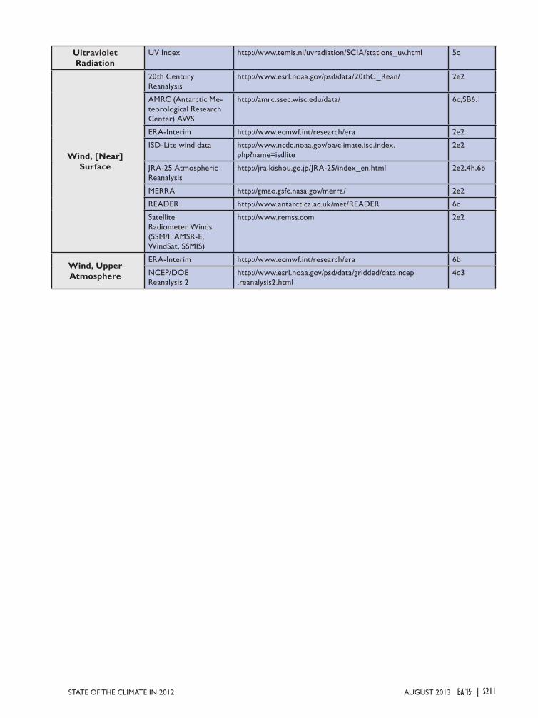
S211STATE OF THE CLIMATE IN 2012 |AUGUST 2013
ultraviolet Radiation
UV Index http://www.temis.nl/uvradiation/SCIA/stations_uv.html 5c
Wind, [Near] Surface
20th Century Reanalysis
http://www.esrl.noaa.gov/psd/data/20thC_Rean/ 2e2
AMRC (Antarctic Me-teorological Research Center) AWS
http://amrc.ssec.wisc.edu/data/ 6c,SB6.1
ERA-Interim http://www.ecmwf.int/research/era 2e2
ISD-Lite wind data http://www.ncdc.noaa.gov/oa/climate.isd.index.php?name=isdlite
2e2
JRA-25 Atmospheric Reanalysis
http://jra.kishou.go.jp/JRA-25/index_en.html 2e2,4h,6b
MERRA http://gmao.gsfc.nasa.gov/merra/ 2e2
READER http://www.antarctica.ac.uk/met/READER 6c
Satellite Radiometer Winds (SSM/I, AMSR-E, WindSat, SSMIS)
http://www.remss.com 2e2
Wind, upper Atmosphere
ERA-Interim http://www.ecmwf.int/research/era 6b
NCEP/DOE Reanalysis 2
http://www.esrl.noaa.gov/psd/data/gridded/data.ncep .reanalysis2.html
4d3
Temperature,upper
Atmosphere
20th Century Reanalysis
http://www.esrl.noaa.gov/psd/data/20thC_Rean/ 2b2
ERA-Interim http://www.ecmwf.int/research/era 2b2,2b3,
6b
HadAT2 http://www.metoffice.gov.uk/hadobs 2b2,2b3
JRA-25 Atmospheric Reanalysis
http://jra.kishou.go.jp/JRA-25/index_en.html 2b2
MERRA http://gmao.gsfc.nasa.gov/merra/ 2b2,2b3
NCEP/DOE Reanalysis 2
http://www.esrl.noaa.gov/psd/data/gridded/data.ncep .reanalysis2.html
6g
RAOBCORE, RICH http://imgw.univie.ac.at/en/products 2b2,2b3
RATPAC http://www.ncdc.noaa.gov/oa/climate/ratpac 2b2,2b3
RSS http://www.remss.com 2b2,2b3
UAH MSU http://vortex.nsstc.uah.edu/public/msu/ 2b2,2b3
ToA Earth Radiation Budget
CERES EBAF Ed2.6r 1Deg
http://ceres.larc.nasa.gov/sitemap_ceres.php 2f
Total Column ozone
TOMS and OMI Sensors
http://ozoneaq.gsfc.nasa.gov/ 5c,6g
Total Column Water Vapor
andHumidity, upper Air
COSMIC Land and Ocean Total Column Water Vapor
http://cosmic-io.cosmic.ucar.edu/cdaac/index.html 2d2
GPS Ground-Based Total Column Water Vapor
http://dss.ucar.edu/datasets/ds721.1/ 2d2
NCEP/NCAR Reanalysis
http://www.esrl.noaa.gov/psd/data/gridded /data.ncep.reanalysis.html
4d4
SSM/I -AMSR-E Ocean Total Column Water Vapor
http://www.remss.com 2d2
TCWV Radiosonde Junhong Wang, Earth Observing Laboratory, NCAR, Boulder, CO.
2d2
Trace Gases
Atmospheric Green-house Gas Index (AGGI)
http://www.esrl.noaa.gov/gmd/aggi/ 2g1
Carbon Dioxide http://www.esrl.noaa.gov/gmd/dv/iadv/ 2g1,SB5.1
Carbon Monoxide http://www.esrl.noaa.gov/gmd/dv/iadv/ 2g1
JPL MLS (HCl,ClO) http://mls.jpl.nasa.gov/index.php 6g
Methane http://www.esrl.noaa.gov/gmd/dv/iadv/ 2g1,SB5.1
Nitrous Oxide http://www.esrl.noaa.gov/gmd/hats/combined/N2O.html 2g1
ODGI http://www.esrl.noaa.gov/gmd/odgi/ 2g1
Perfluorocarbons http://agage.eas.gatech.edu/ 2g1
Sulphur Hexafluoride http://www.esrl.noaa.gov/gmd/hats/combined/SF6.html 2g1
SCIAMACHY (OClO, NO2)
http://www.sciamachy.org/ 6g
Tropical Cyclone Data
International Best Track Archive for Climate Stewardship (IBTrACS)
http://www.ncdc.noaa.gov/oa/ibtracs/ 4d
JTWC Best-track Dataset (2011 preliminary)
http://www.usno.navy.mil/NOOC/nmfc-ph/RSS/jtwc /best_tracks/
4d4

S212 | AUGUST 2013
S213AUGUST 2013STATE OF THE CLIMATE IN 2012 |
Acknowledgments
The editors thank the staff of the Bulletin of the American Meteorological Society for their professionalism and assistance. Melissa Fernau provided valuable editorial advice and logisti-cal support. As always, the guidance and leadership of Bryan Hanssen and Jeff Rosenfeld was essential. The chapter editors enthusiastically thank their respective internal reviewers, and anonymous external reviewers, for working on very tight time-tables to improve the document.
Chapter 2:• Various reanalysis datasets were provided by Paul Ber-
risford and Hitoshi Sato (ERA-Interim), Mike Bosilovich (MERRA), Muthuvel Chelliah (NCEP CFSR), Yayoi Harada (JRA-25/JCDAS), and Cathy Smith (20CR).
• Kate Willett was supported by the Joint DECC/Defra Met Office Hadley Centre Climate Programme (GA01101).
Chapter 3:• The Hadley Ocean Heat Content estimate was supported by
the Joint DECC/Defra Met Office Hadley Centre Climate Programme (GA01101). The CSIRO/ACE CRC estimate (http://www.cmar.csiro.au/sealevel/sl_data_cmar.html) was supported by the Australian Government’s Coopera-tive Research Centres Programme, the Australian Climate Change Program, and the CSIRO Wealth from Oceans Flagship.
Chapter 4:• Charles “Chip” Guard, NOAA/NWS/Guam Weather Fore-
cast Office, Mark Lander, University of Guam, and Ryuji Yamada, Tokyo Climate Center, Climate Prediction Divi-sion, Japan Meteorological Agency are thanked for their contributions to and assistance with the section dealing with tropical cyclones in the Western North Pacific basin.
• Bill Ward, NOAA/NWS/Pacific Region Headquarters, Honolulu, Hawaii, is thanked for his detailed and very helpful internal review of the chapter.
Chapter 5:• Martin Jeffries and Jackie Richter-Menge thank the Office
of Naval Research and the NOAA Arctic Research Office, respectively, for continuing support for co-editing the Arctic section.
• The Ozone and UV Radiation essay was supported by NSF grants ARC-0856268 and ARC-1203250 (Ultraviolet Radia-tion in the Arctic) and the European Commission Seventh Framework Programme grant RECONCILE-226365-FP7-ENV-2008-1 (RECONCILE project).
• The Permafrost essay was supported by NSF grants ARC-0520578, ARC-0632400, ARC-0612533, ARC-0856864, and ARC-1002119.
• The NOAA authors note that, with respect to their con-tributions, “The views, opinions, and findings contained in this report are those of the author(s) and should not be construed as an official National Oceanic and Atmospheric Administration or U.S. Government position, policy, or decision.”
Chapter 6:• Rob Massom and Jan Lieser acknowledge support from
the Australian Government’s Cooperative Research Centre programme through the ACE CRC, and contribution to Project CPC18 and AAS Project 4116.
• Ted Scambos was supported under NASA grant NNX-09AM78G.
• Sharon Stammerjohn was supported under NSF/OPP 0217282.
Chapter 7:• The editors acknowledge and thank the numerous Na-
tional Hydrological and Hydrometeorological Services for collecting and providing data (and many authors) for this report.

S214 AUGUST 2013|
Acronyms And AbbreviAtions
AAO Antarctic OscillationACE NOAA’s Accumulated Cyclone Energy
IndexAGGI NOAA’s Annual Greenhouse Gas IndexALT active layer thicknessAMO Atlantic Multidecadal OscillationAMSR-E Advanced Microwave Scanning
Radiometer for Earth Observing SystemAMSU Advanced Microwave Sounding UnitAO Arctic OscillationAOD aerosol optical depthATSR Along-Track Scanning RadiometersAVHRR Advanced Very High Resolution
RadiometerAVISO Archiving, Validating, and
Interpretation of Satellite Oceanographic data
CAMS Climate Anomaly Monitoring SystemCDR climate data recordCERES Clouds and the Earth’s Radiant Energy
SystemCPC NOAA’s Climate Prediction CenterCPHC NOAA’s Central Pacific Hurricane
CenterCRU Hadley Centre’s Climate Research UnitDU Dobson UnitE–P evaporation minus precipitationECMWF European Centre for Medium-Range
Weather Forecasts ECV essential climate variableEECl effective equivalent chlorineEESC effective equivalent stratospheric
chlorineEOS Earth Observatory SystemERB Earth radiation budgetERBE Earth Radiation Budget ExperimentERSST Extended Reconstructed Sea Surface
TemperatureESA European Space AgencyESRL Earth System Research LaboratoryFAPAR Fraction of Absorbed Photosynthetically
Active RadiationFLASHflux Fast Longwave and Shortwave Radiative
FluxesGCOS Global Climate Observing SystemGHCN Global Historical Climatology NetworkGHG greenhouse gasGISS NASA’s Goddard Institute of Space
StudiesGOME Global Ozone Monitoring Experiment
GPCC Global Precipitation Climatology Centre
GPCP Global Precipitation Climatology Project
GRACE Gravity Recovery and Climate Experiment
GTN-P Global Terrestrial Network on Permafrost
HadAT Hadley Centre’s radiosonde temperature product
HadCRUT Hadley Centre/CRU gridded monthly temperatures dataset
HadISST Hadley Centre’s sea ice and SST datasetHIRS-W High Resolution Infrared SounderIBTrACS International Best Track Archive for
Climate StewardshipICD ice cover durationIOD Indian Ocean dipoleISCCP International Satellite Cloud
Climatology ProjectJMA Japanese Meteorological AgencyJPL Jet Propulsion Laboratory JRA Japanese ReanalysisJTWC U.S. Navy’s Joint Typhoon Warning
CenterLHF latent heat fluxLLGHG long-lived greenhouse gasMDR Main Development RegionMEI multivariate ENSO indexMERIS Medium Resolution Imaging
SpectrometerMISR Multiangle Imaging SpectroRadiometerMLS Microwave Limb SounderMOC meridional overturning currentMOCHA Meridional Overturning Circulation
Heat Transport Array MODIS Moderate Resolution Imaging
SpectroradiometerMSLP mean sea level pressureMSU Microwave Sounding UnitNAO North Atlantic OscillationNASA National Aeronautics and Space
AdministrationNCAR National Center for Atmospheric
ResearchNCDC NOAA’s National Climatic Data CenterNCEP NOAA’s National Center for
Environmental PredictionNERC National Environmental Research
Council
S215AUGUST 2013STATE OF THE CLIMATE IN 2012 |
NOAA National Oceanic and Atmospheric Administration
NSIDC National Snow and Ice Data CenterOAFlux Objectively Analyzed Air-Sea FluxesODGI Ozone Depleting Gas IndexODS ozone depleting substanceOHCA ocean heat content anomalyOISST Optimal Interpolation SSTOLR outgoing longwave radiationOMI Ozone Monitoring InstrumentONI NOAA’s Oceanic Niño Index OPI OLR precipitation indexP–E precipitation minus evaporationPATMOS (-x) Pathfinder Atmospheres (Extended
Product)PDO Pacific decadal oscillationPSC polar stratospheric cloudsPSS practical salinity scaleQBO Quasi-biennial oscillationQuikSCAT Quick ScatterometerRAOBCORE Radiosonde Observation CorrectionRATPAC Radiosonde Atmospheric Temperature
Products for Assessing ClimateRICH Radiosonde Innovation Composite
HomogenizationRSS Remote Sensing SystemsSAM Southern annular mode
SCD snow covered durationSCE snow cover extentSCIAMACHY Scanning Imaging Absorption
Spectrometer for Atmospheric Chartography
SeaWiFS Sea-viewing Wide Field of ViewSHF Sensible heat fluxSLP Sea level pressureSOI Southern Oscillation index SPCZ South Pacific convergence zoneSSM/I Special Sensor Microwave ImagerSSH Sea surface heightSSS Sea surface salinitySSTA Sea surface temperature anomalySWE Snow water equivalentTCHP Tropical cyclone heat potential TCWV Total column water vaporTOA Top of atmosphereTOMS Total Ozone Mapping SpectrometerTRMM Tropical Rainfall Measuring MissionWBM Water Balance Modelw.e. water equivalentWGMS World Glacier Monitoring ServiceWMO World Meteorological OrganizationWOA World Ocean Atlas WOCE World Ocean Circulation Experiment

S216 AUGUST 2013|
reFerences
Ackerman, S. A., R. E. Holz, R. Frey, E. W. Eloranta, B. C. Maddux, and M. McGill, 2008: Cloud detection with MODIS. Part II: Validation. J. Atmos. Oceanic Technol., 25, 1073–1086.
Adler, R. F., and Coauthors, 2003: The version 2 Global Precipitation Climatology Project (GPCP) monthly precipitation analysis (1979-present). J. Hydrometeor., 4, 1147–1167.
Aiyyer, A., and J. Molinari, 2008: MJO and tropical cyclogenesis in the Gulf of Mexico and eastern Pacific: Case study and idealized numerical modeling. J. Atmos. Sci., 65, 2691–2704.
Åkerman, H. J., and M. Johansson, 2008: Thawing permafrost and thicker active layers in sub-arctic Sweden. Permafrost Periglacial Processes, 19, 279–292, doi:10.1002/ppp.626.
Allan, R. J., and T. J. Ansell, 2006: A new globally complete monthly historical gridded mean sea level pressure data set (HadSLP2): 1850-2004. J. Climate, 19, 5816–5842.
—, and C. K. Folland, 2012: [Global climate] Mean sea level pressure [in “State of the Climate in 2011”]. Bull. Amer. Meteor. Soc., 93 (7), S35–S36.
—, J. A. Lindesay, and D. E. Parker, 1996: El Niño Southern Oscillation and Climatic Variability. CSIRO Publications, 405 pp.
—, C. J. C. Reason, J. A. Lindesay, and T. J. Ansell, 2003: 'Protracted' ENSO episodes and their impacts in the Indian Ocean region. Deep-Sea Res. II, 50, 2331–2347.
Alley, W. M., R. W. Healy, J. W. LaBaugh, and T. E. Reilly, 2002: Flow and storage in groundwater systems. Science, 296, 1985–1990.
Álvarez, M., T. Tanhua, H. Brix, C. Lo Monaco, N. Metzl, E. McDonagh, and H. L. Bryden, 2011: Decadal biogeochemical changes in the subtropical Indian Ocean associated with Subantarctic Mode Water. J. Geophys. Res., 116, C09016, doi:10.1029/2010JC006475.
Amador, J. A., E. J. Alfaro, O. G. Lizano, and V. O. Magaña, 2006: Atmospheric forcing of the eastern tropical Pacific: A review. Progr. Oceanogr., 69, 101–142.
—, —, H. G. Hidalgo, and B. Calderón, 2011: [Regional climates] Central America [in “State of the Climate in 2010”]. Bull. Amer. Meteor. Soc., 92 (6), S182–S183.
Andersson, A., K. Fennig, C. Klepp, S. Bakan, H. Graßl, and J. Schulz, 2010: The Hamburg Ocean Atmosphere Parameters and Fluxes from Satellite Data - HOAPS-3. Earth Syst. Sci. Data, 2, 215–234, doi:10.5194/essd-2-215-2010.
Antonov, J. I., and Coauthors, 2010: Salinity. World Ocean Atlas 2009, Vol.2, NOAA Atlas NESDIS 69, 184 pp.
AOSB, 2005: The Integrated Arctic Ocean Observing System (iAOOS): An AOSB-CliC observing plan for the International Polar Year. Arctic Ocean Science Board, Vienna, VA, 16 pp.
Argo Science Team, 1999: On the Design and Implementation of Argo: An Initial Plan for a Global Array of Profiling Floats.
International CLIVAR Project Office (ICPO) Report 21, GODAE Report 5, 32 pp. [Available online at http://www .argo.ucsd.edu/argo-design.pdf.]
Armstrong, R. L., K. W. Knowles, M. J. Brodzik, and M. A. Hardman, updated 2013: DMSP SSM/I-SSMIS Pathfinder daily EASE-grid brightness temperatures. Version 2. Southern Hemisphere. National Snow and Ice Data Center, Boulder, CO, digital media. [Available online at http://nsidc .org/data/docs/daac/nsidc0032_ssmi_ease_tbs.gd.html.]
Arrigo, K. R., and G. L. van Dijken, 2011: Secular trends in Arctic Ocean net primary production. J. Geophys. Res., 116, C09011, doi:10.1029/2011JC007151.
Asplin, M. G., R. Galley, D. G. Barber, and S. Prinsenberg, 2012: Fracture of summer perennial sea ice by ocean swell as a result of Arctic storms. J. Geophys. Res., 117, C06025, doi:10.1029/2011JC007221.
Atkinson, D. E., and Coauthors, 2006: Canadian cryospheric response to an anomalous warm summer: A synthesis of the climate change action fund project “The state of the Arctic cryosphere during the extreme warm summer of 1998”. Atmos.—Ocean, 44, 347–375.
Atkinson, G. D., 1971: Forecasters’ guide to tropical meteorology. U.S. Air Force Tech. Rep. 240, 360 pp.
Baccini, A., and Coauthors, 2012: Estimated carbon dioxide emissions from tropical deforestation improved by carbon-density maps. Nature Climate Change, 2, 182–185, doi:110.1038/nclimate1354.
Bakker, A. M. R., B. J. J. M. Van den Hurk, and J. P. Coelingh, 2012: Decomposition of the windiness index in the Netherlands for the assessment of future long-term wind supply. Wind Energy, in press, doi:10.1002/we.1534.
Ballantyne, A. P., C. B. Alden, J. B. Miller, P. P. Tans, and J. W. C. White, 2012: Increase in observed net carbon dioxide uptake by land and oceans during the past 50 years. Nature, 488, doi:10.1038/nature11299.
Baringer, M. O., and J. Larsen, 2001: Sixteen years of Florida Current transport at 27°N. Geophys. Res. Lett., 28, 3179–3182.
—, and Coauthors, 2011: [Global oceans] Meridional overturning circulation observations in the subtropical North Atlantic [in “State of the Climate in 2010”]. Bull. Amer. Meteor. Soc., 92 (6), S95–S98.
—, and Coauthors, 2012: [Global oceans] Meridional overturning circulation observations in the subtropical North Atlantic [in “State of the Climate in 2011”]. Bull. Amer. Meteor. Soc., 93 (7), S78–S81.
Barrett, B. E., K. W. Nicholls, T. Murray, A. M. Smith, and D. G. Vaughan, 2009: Rapid recent warming on Rutford Ice Stream, West Antarctica, from borehole thermometry. Geophys. Res. Lett., 36, L02708. doi:10.1029/2008GL036369.

S217AUGUST 2013STATE OF THE CLIMATE IN 2012 |
Bates, N. R., 2007: Interannual variability of the oceanic CO2 sink in the subtropical gyre of the North Atlantic Ocean over the last 2 decades. J. Geophys. Res., 112, C09013, doi:10.1029/2006JC003759.
—, and J. T. Mathis, 2009: The Arctic Ocean marine carbon cycle: Evaluation of air-sea CO2 exchanges, ocean acidification impacts and potential feedbacks. Biogeosciences, 6, 2433–2459.
—, —, and L. W. Cooper, 2009: Ocean acidification and biologically induced seasonality of carbonate mineral saturation states in the western Arctic Ocean. J. Geophys. Res., 114, C11007, doi:10.1029/2008JC004862.
Becker, A., P. Finger, A. Meyer-Christoffer, B. Rudolf, K. Schamm, U. Schneider, and M. Ziese, 2013: A description of the global land-surface precipitation data products of the Global Precipitation Climatology Centre with sample applications including centennial (trend) analysis from 1901–present. Earth Syst. Sci. Data, 5, 71–99, doi:10.5194/essd-5-71-2013.
Behrenfeld, M. J., and Coauthors, 2006: Climate-driven trends in contemporary ocean productivity. Nature, 444, 752–755.
Behringer, D. W., M. Ji, and A. Leetmaa, 1998: An improved coupled model for ENSO prediction and implications for ocean initialization. Part I: The ocean data assimilation system. Mon. Wea. Rev., 126, 1013–1021.
Bekryaev, R., I. V. Polyakov, and V. A. Alexeev, 2010: Role of polar amplification in long-term surface air temperature variations and modern Arctic warming. J. Climate, 23, 3888–3906.
Bell, G. D., and M. Chelliah, 2006: Leading tropical modes associated with interannual and multidecadal fluctuations in north Atlantic hurricane activity. J. Climate, 19, 590–612.
—, and Coauthors, 2000: The 1999 North Atlantic and eastern North Pacific hurricane season [in “Climate Assessment for 1999”]. Bull. Amer. Meteor. Soc., 81, S19–S22.
—, and Coauthors, 2007: Tropical cyclones: Atlantic basin [in “State of the Climate in 2006”]. Bull. Amer. Meteor. Soc., 88 (6), S48–S51.
—, and Coauthors, 2011: Tropical cyclones: Atlantic basin [in “State of the Climate in 2010”]. Bull. Amer. Meteor. Soc., 92 (6), S115–S121.
—, and Coauthors, 2012: Tropical cyclones: Atlantic basin [in “State of the Climate in 2011”] Bull. Amer. Meteor. Soc., 93 (7), S99–S105.
Bentamy, A., K. B. Katsaros, A. M. Mestas-Nuñez, W. M. Drennan, E. B. Forde, and H. Roquet, 2003: Satellite estimates of wind speed and latent heat flux over the global oceans. J. Climate, 16, 637–656.
Berry, D. I., and E. C. Kent, 2009: A new air-sea interaction gridded dataset from ICOADS with uncertainty estimates. Bull. Amer. Meteor. Soc., 90, 645–656.
—, and —, 2011: Air-sea fluxes from ICOADS: the construction of a new gridded dataset with uncertainty estimates. Int. J. Climatol., 31, 987–1001, doi:10.1002/joc.2059.
Bichet, A., M. Wild, D. Folini, and C. Schär, 2012: Causes for decadal variations of wind speed over land: Sensitivity studies with a global climate model. Geophys. Res. Lett., 39, L11701, doi:10.1029/2012GL051685.
Blake, E., and Coauthors, 2009: Tropical Cyclones of the Eastern North Pacific Basin, 1949-2006. Historical Climatology Series 6-5, NOAA National Climatic Data Center, 162 pp.
—, C. W. Landsea, and E. J. Gibney, 2011: The deadliest, costliest, and most intense United States tropical cyclones from 1851 to 2010. NOAA Tech. Memo. NWS NHC-6, NOAA National Hurricane Center, 47 pp. [Available online at http://www.nhc.noaa.gov/Deadliest_Costliest.shtml.]
Bockheim, J., G. Vieira, M. Ramos, J. López-Martínez, E. Serrano, M. Guglielmin, K. Wilhelm, A. Nieuwendam, 2013: Climate warming and permafrost dynamics in the Antarctic Peninsula region. Global Planet. Change, 100, 215–223.
Boening, C., J. K. Willis, F. W. Landerer, R. S. Nerem, and J. Fasullo, 2012: The 2011 La Niña: So strong, the oceans fell. Geophys. Res. Lett., 39, L19602, doi:10.1029/2012GL053055.
Bojkov, R. D., 1986: Surface ozone during the second half of the nineteenth century. J. Climate Appl. Meteor., 25, 343–352.
—, and D. S. Balis, 2001: Characteristics of episodes with extremely low ozone values in the northern middle latitudes 1957-2000. Ann. Geophys., 19, 797–807.
Bolch, T., and Coauthors, 2012: The state and fate of Himalayan glaciers. Science, 336, 310–314.
Bond, T., and Coauthors, 2013: Bounding the role of black carbon in the climate system: A scientific assessment J. Geophys. Res. Atmospheres, in press, doi:10.1002/jgrd.50171.
Böning, C. W., A. Dispert, M. Visbeck, S. R. Rintoul, and F. U. Schwarzkopf, 2008: The response of the Antarctic Circumpolar Current to recent climate change. Nature Geosci., 1, 864–869.
Bonsal, B. R., T. D. Prowse, C. R. Duguay, and M. P. Lacroix, 2006: Impacts of large-scale teleconnections on freshwater-ice duration over Canada. J. Hydrol., 330, 340–353.
Boon, J. D., 2012: Evidence of sea level acceleration at U.S. and Canadian tide stations, Atlantic coast, North America. J. Coastal Res., 28, 1437–1445, doi:10.2112/JCOASTRES-D-12-00102.1.
Bowman, K. W., and Coauthors, 2006: Tropospheric emission spectrometer: Retrieval method and error analysis. IEEE Trans. Geosci. Remote Sens., 44, 1297–1307, doi:10.1109/TGRS.2006.871234.
Box, J. E., and D. T. Decker, 2011: Greenland marine-terminating glacier area changes: 2000-2010. Ann. Glaciol., 52 (59), 91–98.
S218 AUGUST 2013|
—, and Coauthors, 2012a: Greenland ice sheet. Arctic Report Card 2012, M. O. Jeffries, J. A. Richter-Menge, and J. E. Overland, Eds., NOAA Rep., 146–158. [Available online at http://www.arctic.noaa.gov/reportcard.]
—, X. Fettweis, J. C. Stroeve, M. Tedesco, D. K. Hall, and K. Steffen, 2012b: Greenland ice sheet albedo feedback: thermodynamics and atmospheric drivers. Cryosphere, 6, 821–839, doi:10.5194/tc-6-821-2012.
Boyer, T. P., J. I. Antonov, S. Levitus, and R. Locarnini, 2005: Linear trends of salinity for the world ocean, 1955-1998. Geophys. Res. Lett., 32, L01604, doi:1029/2004GL021791.
—, S. Levitus, J. Antonov, R. Locarnini, A. Mishonov, H. Garcia, and S. A. Josey, 2007: Changes in freshwater content in the North Atlantic Ocean 1955–2006. Geophys. Res. Lett., 34, L16603, doi:10.1029/2007GL030126.
—, and Coauthors, 2009: Introduction. World Ocean Database 2009, NOAA Atlas NESDIS 66, 18–43.
—, S. Levitus, J. I. Antonov, J. R. Reagan, C. Schmid, and R. Locarnini, 2012: [Global oceans] Subsurface salinity [in “State of the Climate in 2011”]. Bull. Amer. Meteor. Soc., 93 (7), S72–S75.
Bradley, R. S., M. K. Hughes, and M. E. Mann, 2006: Authors were clear about hockey-stick uncertainties. Nature, 442, 627.
Brasnett, B., 1999: A global analysis of snow depth for numerical weather prediction. J. Appl. Meteor., 38, 726–740.
Broecker, W., and E. Clark, 2001: A dramatic Atlantic dissolution event at the onset of the last glaciation. Geochem. Geophys. Geosys., 2, 1065, doi:10.1029/2001GC000185.
Bromwich, D. H., A. N. Rogers, P. Kallberg, R. I. Cullather, J. W. C. White, and K. J. Kreutz, 2000: ECMWF analysis and reanalysis depiction of ENSO signal in Antarctic precipitation. J. Climate, 13, 1406–1420.
—, A. J. Monaghan, and Z. Guo, 2004: Modeling the ENSO modulation of Antarctic climate in the late 1990s with Polar MM5. J. Climate, 17, 109–132.
—, R. L. Fogt, K. I. Hodges, and J. E. Walsh, 2007: A tropospheric assessment of the ERA-40, NCEP, and JRA-25 global reanalyses in the polar regions. J. Geophys. Res., 112, D10111, doi:10.1029/2006JD007859.
—, J. P. Nicolas, and A. J. Monaghan, 2011: An assessment of precipitation changes over Antarctica and the Southern Ocean since 1989 in contemporary global reanalyses. J. Climate, 24, 4189–4209.
—, —, —, M. A. Lazzara, L. M. Keller, G. A. Weidner, and A. B. Wilson, 2013: Central West Antarctica among the most rapidly warming regions on Earth. Nature Geosci., 6, 139–145, doi:10.1038/ngeo1671.
Brown, J., O. J. Ferrians, Jr., J. A. Heginbottom, and E. S. Melnikov, revised 2001: Circum-arctic map of permafrost and ground ice conditions. National Snow and Ice Data Center, Boulder,
CO, digital media. [Available online at http://nsidc.org/data/docs/fgdc/ggd318_map_circumarctic/index.html.]
Brown, L. C., and C. R. Duguay, 2010: The response and role of ice cover in lake-climate interactions. Prog. Phys. Geogr., 34, 671–704.
Brown, R., and D. Robinson, 2011: Northern Hemisphere spring snow cover variability and change over 1922–2010 including an assessment of uncertainty. Cryosphere, 5, 219–229.
—, B. Brasnett, and D. Robinson, 2003: Gridded North American monthly snow depth and snow water equivalent for GCM evaluation. Atmos.—Ocean, 41, 1–14.
Burn, C. R., and S. V. Kokelj, 2009: The environment and permafrost of the Mackenzie Delta area. Permafrost Periglacial Processes, 20, 83–105.
Butchart, N., and E. E. Remsberg, 1986: The area of the stratospheric polar vortex as a diagnostic for tracer transport on an isentropic surface. J. Atmos. Sci., 43, 1319–1339.
Butler, J. H., 2012: The NOAA annual greenhouse gas index. [Available online at http://www.esrl.noaa.gov/gmd/aggi/.]
Cai, W-J., and Coauthors, 2010: Decrease in the CO2 uptake capacity in an ice-free Arctic Ocean basin. Science, 329, 556–559.
—, P. van Rensch, T. Cowan, and H. H. Hendon, 2011: Teleconnection pathways of ENSO and the IOD and the mechanisms for impacts on Australian rainfall. J. Climate, 24, 3910–3923.
Caldeira, K., and M. E. Wickett, 2003: Anthropogenic carbon and ocean pH. Nature, 425, 365.
—, and —, 2005: Ocean model predictions of chemistry changes from carbon dioxide emissions to the atmosphere and ocean. J. Geophys. Res., 110, C09S04, doi:10.1029/2004JC002671.
Calder, J., and Coauthors, 2009: An integrated international approach to Arctic Ocean observations for society (A legacy of the International Polar Year). Proc.OceanObs ’09: Sustained Ocean Observations and Information for Society (Vol. 2), Venice, Italy, J. Hall et l. Eds., ESA Publication WPP-306, Community White Paper.
Callaghan, T. V., F. Bergholm, T. R. Christensen, C. Jonasson, U. Kokfelt, and M. Johansson, 2010: A new climate era in the sub-Arctic: Accelerating climate changes and multiple impacts. Geophys. Res. Lett., 37, L14705, doi:10.1029/2009GL042064.
Camargo, S. J., K. A. Emanuel, and A. H. Sobel, 2007: Use of a genesis potential index to diagnose ENSO effects on tropical cyclone genesis. J. Climate, 20, 4819–4834.
Campbell, J. W., 1995: The lognormal distribution as a model for bio-optical variability in the sea. J. Geophys. Res., 100 (C7), 13 237–13 254.
Carton, J. A., and B. S. Giese, 2008: A reanalysis of ocean climate using Simple Ocean Data Assimilation (SODA). Mon. Wea. Rev., 136, 2999–3017.

S219AUGUST 2013STATE OF THE CLIMATE IN 2012 |
Cartus, O., J. Kellndorfer, M. Rombach, and W. Walker, 2012: Mapping canopy height and growing stock volume using airborne lidar, ALOS PALSAR and Landsat ETM+. Remote Sens., 4, 3320–3345, doi:10.3390/rs4113320.
Cassou, C., 2008: Intraseasonal interaction between the Madden Julian Oscillation and the North Atlantic Oscillation. Nature, 455, 523–527, doi:10.1038/nature07286.
Cavallo, S. M., and G. J. Hakim, 2012: Radiative impact on tropopause polar vortices over the Arctic. Mon. Wea. Rev., 140, 1683–1702.
Chambers, D. P., J. Wahr, M. E. Tamisiea, and R. S. Nerem, 2010: Ocean mass from GRACE and glacial isostatic adjustment. J. Geophys. Res., 115, B11415, doi:10.1029/2010JB007530.
Chen, L., D. Li, and S. C. Pryor, 2012a: Wind speed trends over China: Quantifying the magnitude and assessing causality. Int. J. Climatol., in press, doi:10.1002/joc.3613.
—, S. C. Pryor, and D. Li, 2012b: Assessing the performance of Intergovernmental Panel on Climate Change AR5 climate models in simulating and projecting wind speeds over China. J. Geophys. Res., 117, D24102, doi:10.1029/2012JD017533.
Chen, M., P. Xie, J. Janowiak, and P. A. Arkin, 2002: Global land precipitation: A 50-yr analysis based on gauge observations. J. Hydrometeor., 3, 249–266.
Christiansen, H. H., and Coauthors, 2010: The thermal state of permafrost in the Nordic area during IPY 2007-2009. Permafrost Periglacial Processes, 21, 156–181.
—, M. Guglielmin, J. Noetzli, V. Romanovsky, N. Shiklomanov, S. Smith, and L. Zhao, 2012: [Global climate] Permafrost thermal state [in “State of the Climate in 2012”]. Bull. Amer. Meteor. Soc., 93 (7), S19–S21.
Christy, J. R., R. W. Spencer, and W. B Norris, 2011: The role of remote sensing in monitoring global bulk tropospheric temperatures. Int. J. Remote Sens. 32, 671–685, doi:10.1080/01431161.2010.517803.
Church, J. A., and Coauthors, 2011: Revisiting the Earth's sea-level and energy budgets from 1961 to 2008. Geophys. Res. Lett., 38, L18601, doi:10.1029/2011GL048794.
Colwell, S., L. M. Keller, and M. A. Lazzara, 2012: [Antarctica] Surface manned and automatic weather station observations [in “State of the Climate in 2011”]. Bull. Amer. Meteor. Soc., 93 (7), S151–S153.
Comiso, J., updated 2008: Bootstrap sea ice concentrations from NIMBUS-7 SMMR and DMSP SSM/I. National Snow and Ice Data Center, Boulder, CO, digital media. [Available online at http://nsidc.org/data/nsidc-0079.html.]
—, 2010: Variability and trends of the global sea ice cover. Sea Ice, 2nd ed., D. N. Thomas, and G. S. Dieckmann, Eds., Wiley-Blackwell, 205–246.
Compo, G. P., and Coauthors, 2011: The Twentieth Century Reanalysis Project. Quart. J. Roy. Meteor. Soc., 137, 1–28, doi:10.1002/qj.776.
Cooper, O. R., R.-S. Gao, D. Tarasick, T. Leblanc, and C. Sweeney, 2012: Long-term ozone trends at rural ozone monitoring sites across the United States, 1990–2010. J. Geophys. Res., 117, D22307, doi:10.1029/2012JD018261.
Cullather, R. I., D. H. Bromwich, and M. L. Van Woert, 1996: Interannual variations in Antarctic precipitation related to El Niño-Southern Oscillation. J. Geophys. Res., 101, 19 109–19 118.
Cunningham, S. A., and Coauthors, 2007: Temporal variability of the Atlantic meridional overturning circulation at 26.5°N. Science, 312, 935–938, doi: 10.1126/science.1141304.
Curry, R. G., and M. S. McCartney, 2001: Ocean gyre circulation changes associated with the North Atlantic oscillation. J. Phys. Oceanogr., 31, 3374–3400.
Dai, A., 2006: Recent climatology, variability, and trends in global surface humidity. J. Climate, 19, 3589–3606.
—, J. Wang, P. W. Thorne, D. E. Parker, L. Haimberger, and X. L. Wang, 2011: A new approach to homogenize daily radiosonde humidity data. J. Climate, 24, 965–991.
Daniel, J. S., and Coauthors, 2011: A focus on information and options for policymakers. Scientific Assessment of Ozone Depletion: 2010, Global Ozone Research and Monitoring Project Rep. 52, World Meteorological Organization, 5.1–5.56.
Dare, R. A., and J. L. McBride, 2011: Sea Surface temperature response to tropical cyclones. Mon. Wea. Rev., 139, 3798–3808.
Davidson, E. A., 2009: The contribution of manure and fertilizer nitrogen to atmospheric nitrous oxide since 1860. Nature Geosci., 2, 659–662, doi:10.1038/NGEO608.
De Jeu, R. A. M., W. A. Doringo, R. M. Parinussa, W. W. Wagner, Y. Y. Liu, D. Chung, and D. Fernández-Prieto, 2012a: [Global climate] Building a climate record of soil moisture from historical satellite observations [in “State of the Climate in 2011”]. Bull. Amer. Meteor. Soc., 93 (7), S32–S33.
—, —, —, —, and D. Chung, 2012b: [Global climate] Soil moisture [in “State of the Climate in 2011”]. Bull. Amer. Meteor. Soc., 93 (7), S30–S31, S34.
Dee, D. P., and Coauthors, 2011: The ERA-Interim reanalysis: Configuration and performance of the data assimilation system. Quart. J. Roy. Meteor. Soc., 137, 553–597, doi:10.1002/qj.828.
Delworth, T. L., and M. E. Mann, 2000: Observed and simulated multi-decadal variability in the Northern Hemisphere. Climate Dyn., 16, 661–676.
Dentener, F., T. Keating, and H. Akimoto, Eds., 2011: Hemispheric Transport of Air Pollution 2010. Part A: Ozone and Particulate Matter. Air Pollution Studies, no. 17, United Nations, 278 pp.
Derksen, C., and R. Brown, 2012: Spring snow cover extent reductions in the 2008-2012 period exceeding climate

S220 AUGUST 2013|
model projections. Geophys. Res. Lett., 39, L19504, doi:10.1029/2012GL053387.
—, and Coauthors, 2012: Variability and change in the Canadian cryosphere. Climatic Change, 115, 59–88.
Deser, C., and M. L. Blackmon, 1993: Surface climate variations over the North Atlantic Ocean during winter: 1900–1989. J. Climate, 6, 1743–1753.
—, M. A. Alexander, S.-P. Xie, and A. S. Phillips, 2010: Sea surface temperature variability: Patterns and mechanisms. Ann. Rev. Marine Sci., 2, 115–143.
Dhomse, S., M. Weber, J. P. Burrows, I. Wohltmann, and M. Rex, 2006: On the possible cause of recent increases in NH total ozone from a statistical analysis of satellite data from 1979 to 2003. Atmos. Chem. Phys., 6, 1165–1180.
Di Girolamo, L., A. Menzies, G. Zhao, K. Mueller, C. Moroney, and D. J. Diner, 2010: Multi-angle imaging spectroradiometer level 3 cloud fraction by altitude algorithm theoretical basis document. JPL Publ. D-62358, Jet Propulsion Laboratory, 23 pp.
Diamond, H. J., Ed., 2011: Tropics [in "State of the Climate in 2010"]. Bull. Amer. Meteor. Soc., 92 (7), S109–S142.
—, Ed., 2012: Tropics [in "State of the Climate in 2011"]. Bull. Amer. Meteor. Soc., 93 (7), S93–S125.
—, A. M. Lorrey, K. R. Knapp, and D. H. Levinson, 2012: Development of an enhanced tropical cyclone tracks database for the Southwest Pacific from 1840-2010. Int. J. Climatol., 32, 2240–2250, doi:10.1002/joc.2412.
Ding, A. J., T. Wang, V. Thouret, J.-P. Cammas, and P. Nédélec, 2008: Tropospheric ozone climatology over Beijing: analysis of aircraft data from the MOZAIC program. Atmos. Chem. Phys., 8, 1–13.
Dlugokencky, E. J., K. A. Masarie, P. M. Lang, and P. P. Tans, 1998: Continuing decline in the growth rate of atmospheric methane. Nature, 393, 447–450.
—, S. Houweling, L. Bruhwiler, K. A. Masarie, P. M. Lang, J. B. Miller, and P. P. Tans, 2003: Atmospheric methane levels off: Temporary pause or a new steady-state? Geophys. Res. Lett., 30, 1992, doi:10.1029/2003GL018126.
—, and Coauthors, 2009: Observational constraints on recent increases in the atmospheric CH4 burden. Geophys. Res. Lett., 36, L18803, doi:10.1029/2009GL039780.
Doherty, R. M., D. S. Stevenson, C. E. Johnson, W. J. Collins, and M. G. Sanderson, 2006: Tropospheric ozone and El Niño–Southern Oscillation: Influence of atmospheric dynamics, biomass burning emissions, and future climate change. J. Geophys. Res., 111, D19304, doi:10.1029/2005JD006849.
Domingues, C. M., J. A. Church, N. J. White, P. J. Gleckler, S. E. Wijffels, P. M. Barker, and J. R. Dunn, 2008: Improved estimates of upper-ocean warming and multi-decadal sea-level rise. Nature, 453, 1090–1093, doi:10.1038/nature07080.
Dong, S., S. L. Garzoli, M. O. Baringer, C. S. Meinen, and G. J. Goni, 2009: The Atlantic meridional overturning circulation
and its northward heat transport in the South Atlantic. Geophys. Res. Lett., 36, L20606, doi:10.1029/2009GL039356.
Dore, J. E., R. Lukas, D. W. Sadler, M. J. Church, and D. M. Karl, 2009: Physical and biogeochemical modulation of ocean acidification in the central North Pacific. Proc. Natl. Acad. Sci. USA, 106, 12 235–12 240.
Dorigo, W., R. de Jeu, D. Chung, R. Parinussa, Y. Y. Liu, W. W. Wagner, and D. Fernández-Prieto, 2012: Evaluating global trends (1988–2010) in harmonized multi-satellite surface soil moisture. Geophys. Res. Lett., 39, L18405, doi:10.1029/2012GL052988.
Drozdov, D. S., G. V. Malkova, N. G. Ukraintseva, and Yu. V. Korostelev, 2012: Permafrost monitoring of southern tundra landscapes in the Russian European North and West Siberia. Proc. 10th Int. Conf. on Permafrost, Vol. 2, Salekhard, Russia, 65–70.
Duguay, C. R., T. D. Prowse, B. R. Bonsal, R. D. Brown, M. P. Lacroix, and P. Ménard, 2006: Recent trends in Canadian lake ice cover. Hydrolog. Processes, 20, 781–801.
Dunn, R. J. H., K. M. Willett, P. W. Thorne, E. V. Woolley, I. Durre, A. Dai, D. E. Parker, and R. S. Vose, 2012: HadISD: a quality-controlled global synoptic report database for selected variables at long-term stations from 1973-2011. Climate Past, 8, 1649–1679, doi:10.5194/cp-8-1649-2012.
Durack, P. J., and S. E. Wijffels, 2010: Fifty-year trends in global ocean salinities and their relationship to broad-scale warming. J. Climate, 23, 4342–4362.
—, —, and R. J. Matear, 2012: Ocean salinities reveal strong global water cycle intensification during 1950 to 2000. Science, 336, 455–458.
ECMWF, 2012: Skillful forecast of wildfire smoke. ECMWF News, 13 July 2012. [Available online at http://www.ecmwf.int/publications/cms/get/ecmwfnews/298.]
Elvehøy, H., 2012: Glacier length change table 2000–2012. Norwegian Water Resources and Energy Directorate. [Available online at http://www.nve.no/GlobalVann20og20vassdrag /Hydrologi/Bre/Nedlastinger/Length_Change_Table_2000-2012v2.pdf?epslanguage=no.]
Emanuel, K. A., 2001: The contribution of tropical cyclones to the oceans' meridional heat transport. J. Geophys. Res., 106 (D14), 14 771–14 781.
—, and D. S. Nolan, 2004: Tropical cyclone activity and the global climate system. Proc. 26th Conf. on Hurricanes and Tropical Meteor., Amer. Meteor. Soc., 10A.2, 240–241.
Enfield, D. B., and A. M. Mestas-Nuñez, 1999: Multi-scale variabilities in global sea surface temperatures and their relationships with tropospheric climate patterns. J. Climate, 12, 2719–2733.
—, —, and P. J. Trimble, 2001: The Atlantic Multidecadal Oscillation and its relationship to rainfall and river flows in the continental US. Geophys. Res. Lett., 28, 2077–2080.

S221AUGUST 2013STATE OF THE CLIMATE IN 2012 |
England, M. H., and F. Huang, 2005: On the interannual variability of the Indonesian Throughflow and its linkage with ENSO. J. Climate, 18, 1435–1444.
Environment Canada, cited 2013: Select ozone maps. [Available online at http://es-ee.tor.ec.gc.ca/cgi-bin/selectMap.]
Esaias, W. E., and Coauthors, 1998: An overview of MODIS capabilities for ocean science observations. IEEE Trans. Geosci. Remote Sens., 36, 1250–1265, doi:10.1109/36.701076.
Espinoza, J. C., J. Ronchail, F. Frappart, W. Lavado, W. Santini, and J. L. Guyot, 2013: The major floods in the Amazonas River and tributaries (Western Amazon basin) during the 1970–2012 period: A focus on the 2012 flood. J. Hydrometeor., in press, doi:10.1175/JHM-D-12-0100.1.
Ezer, T., and W. B. Corlett, 2012: Is sea level rise accelerating in the Chesapeake Bay? A demonstration of a novel new approach for analyzing sea level data. Geophys. Res. Lett., 39, L19605, doi:10.1029/2012GL053435.
—, L. P. Atkinson, W. B. Corlett, and J. L. Blanco, 2013: Gulf Stream’s induced sea level rise and variability along the U.S. mid-Atlantic coast. J. Geophys. Res. Oceans, 118, 685–697, doi:10.1002/jgrc.20091.
Fabry, V. J., J. B. McClintock, J. T. Mathis, and J. M. Grebmeier, 2009: Ocean acidification at high latitudes: The bellwether. Oceanography, 22 (4), 160–171.
Feely, R. A., C. L. Sabine, K. Lee, W. Berelson, J. Keypas, V. J. Fabry, and F. J. Millero, 2004: Impact of anthropogenic CO2 on the CaCO3 system in the oceans. Science, 305, 362–266.
—, S. C. Doney, and S. R. Cooley, 2009: Ocean acidification: Present conditions and future changes in a high-CO2 world. Oceanography, 22 (4), 36–47.
Fekete, B. M., and A. M. MacDonald, 2011: [Global climate] River discharge [in “State of the Climate in 2010”]. Bull. Amer. Meteor. Soc., 92 (6), S46–S48.
—, R. B. Lammers, A. M. MacDonald, L. C. Bowling, and R. Lawford, 2010: [Global climate] River discharge [in “State of the Climate in 2009”]. Bull. Amer. Meteor. Soc., 91 (7), S35.
—, U. Looser, and R. D. Robarts, 2012a: Rationale for monitoring discharge on the ground. J. Hydrometeor., 13, 1977–1986.
—, R. B. Lammers, and G. R. Brakenridge, 2012b: [Global climate] River discharge [in “State of the Climate 2011”]. Bull. Amer. Meteor. Soc., 93 (7), S28–S29.
Feldpausch, T. R., and Coauthors, 2012: Tree height integrated into pantropical forest biomass estimates. Biogeosciences, 9, 3381–3403, doi:10.5194/bg-9-3381-2012.
Fioletov, V. E., G. E. Bodeker, A. J. Miller, R. D. McPeters, and R. Stolarski, 2002: Global and zonal total ozone variations estimated from ground-based and satellite measurements: 1964–2000. J. Geophys. Res., 107 (D22), 4647, doi:10.1029/2001JD001350.
—, and Coauthors, 2008: The performance of the ground-based total ozone network assessed using satellite data. J. Geophys. Res., 113, D14313, doi:10.1029/2008JD009809.
Fischer, A., 2012: Gletscherbericht 2010/2011. Sammelbericht über die Gletschermessungen des Österreichischen Alpenvereins im Jahre 2011. Letzter Bericht: Bergauf 02/2011, Jg. 66 (136).
Fofonoff, N. P., and E. L. Lewis, 1979: A practical salinity scale. J. Oceanogr. Soc. Japan, 35, 63–64, doi:10.1007/BF02108283.
Fogt, R. L., and D. H. Bromwich, 2006: Decadal variability of the ENSO teleconnection to the high latitude South Pacific governed by coupling with the Southern Annular Mode. J. Climate, 19, 979–997.
—, —, and K. M. Hines, 2011: Understanding the SAM influence on the South Pacific ENSO teleconnection. Climate Dyn., 36, 1555–1576, doi:10.1007/s00382-010-0905-0.
Folland, C. K., J. Knight, H. W. Linderholm, D. Fereday, S. Ineson, and J. W. Hurrell, 2009: The summer North Atlantic oscillation: Past, present and future. J. Climate, 22, 1082–1103.
Forster, P., and Coauthors, 2007: Changes in atmospheric constituents and in radiative forcing. Climate Change 2007: The Physical Science Basis, S. Solomon et al., Eds., Cambridge University Press, 129–234.
Frajka-Williams, E., S. A. Cunningham, H. Bryden, and B. A. King, 2011: Variability of Antarctic Bottom Water at 24.5°N in the Atlantic. J. Geophys. Res., 116, C11026, doi:10.1029/2011JC007168.
Francis, J. A., and S. J. Vavrus, 2012: Evidence linking Arctic amplification to extreme weather in mid-latitudes. Geophys. Res. Lett., 39, L06801, doi:10.1029/2012GL051000.
Free, M., D. J. Seidel, J. K. Angell, J. R. Lanzante, I. Durre, and T. C. Peterson, 2005: Radiosonde Atmospheric Temperature Products for Assessing Climate (RATPAC): A new dataset of large-area anomaly time series. J. Geophys. Res., 110, D22101, doi:10.1029/2005JD006169.
Freeland, H., and Coauthors, 2010: Argo - A decade of progress. Proc. OceanObs’09: Sustained Ocean Observations and Information for Society (Vol. 2), Venice, Italy, J. Hall et al., Eds., ESA Publication WPP-306, doi:10.5270/OceanObs09.cwp.32.
Fung, I., J. John, J. Lerner, E. Matthews, M. Parther, L. P. Steele, and P. J. Fraser, 1991: Three-dimensional model synthesis of the global methane cycle. J. Geophys. Res., 96, 13 033–13 065.
Gardner, A. S., and M. Sharp, 2007: Influence of the Arctic circumpolar vortex on the mass balance of Canadian high arctic glaciers. J. Climate 20, 4586–4598.
—, and Coauthors, 2011: Sharply increased mass loss from glaciers and ice caps in the Canadian Arctic Archipelago. Nature, 473, 357–360.
Garzoli, S. L., and M. O. Baringer, 2007: Meridional heat transport using expandable bathythermographs Part II:

S222 AUGUST 2013|
South Atlantic transport. Deep Sea Res. I, 54, 1402–1420, doi:10.1016/j.dsr.2007.04.013.
—, —, S. Dong, R. C. Perez, and Q. Yao, 2012: South Atlantic meridional fluxes. Deep-Sea Res. I, 71, 21–32, doi:10.1016/j.dsr.2012.09.003.
GCOS, 2003: The second report on the adequacy of the global observing systems for climate in support of the UNFCCC. GCOS-82 (WMO/TD no. 1143). World Meteorological Organization, 74 pp. [Available online at http://www.wmo.int/pages/prog/gcos/Publications/gcos-82_2AR.pdf.]
—, 2010: Implementation plan for the global observing system for climate in support of the UNFCCC (2010 Update). GCOS-138 (GOOS-184, GTOS-76, WMO-TD/No. 1523). World Meteorological Organization, 180 pp. [Available online at http://www.wmo.int/pages/prog/gcos/Publications/gcos-138.pdf.]
Giglio, L., J. T. Randerson, G. R. van der Werf, P. S. Kasibhatla, G. J. Collatz, D. C. Morton, and R. S. DeFries, 2010: Assessing variability and long-term trends in burned area by merging multiple satellite fire products. Biogeosciences, 7, 1171–1186.
Gobron, N., A. S. Belward, B. Pinty, and W. Knorr, 2010: Monitoring biosphere vegetation 1998-2009. Geophys. Res. Lett., 37, L15402, doi:10.1029/2010GL043870.
Goldenberg, S. B., and L. J. Shapiro, 1996: Physical mechanisms for the association of El Niño and West African rainfall with Atlantic major hurricane activity. J. Climate, 9, 1169–1187.
—, C. W. Landsea, A. M. Mestas-Nuñez, and W. M. Gray, 2001: The recent increase in Atlantic hurricane activity: Causes and implications. Science, 293, 474–479.
Goni, G. J., and I. Wainer, 2001: Investigation of the Brazil Current front dynamics from altimeter data. J. Geophys. Res., 106 (C12), 31 117–31 128.
—, and J. A. Trinanes, 2003: Ocean thermal structure monitoring could aid in the intensity forecast of tropical cyclones. Eos, Trans. Amer. Geophys. Union, 84, 573–578.
—, S. Kamholz, S. Garzoli, and D. Olson, 1996: Dynamics of the Brazil-Malvinas confluence based on inverted echo sounders and altimetry. J. Geophys. Res., 101 (C7), 16 273–16 289.
—, and Coauthors, 2009: Applications of satellite-derived ocean measurements to tropical cyclone intensity forecasting. Oceanography, 22 (3), 176–183.
—, F. Bringas, and P. N. Di Nezio, 2011: Observed low frequency variability of the Brazil Current front. J. Geophys. Res., 116, C10037, doi:10.1029/2011JC007198.
González-Dávila, M., J. M. Santana-Casiano, M. J. Rueda, and O. Llinas, 2010: The water column distribution of carbonate system variables at the ESTOC site from 1995 to 2004. Biogeosciences, 7, 3067–3081.
Gouretski, V. V., and K. P. Koltermann, 2004: WOCE global hydrographic climatology. Berichte des bundesamtes für
seeshifffahrt und hydrographie 35, 52 pp. [Available online at http://icdc.zmaw.de/woce_climatology.html?&L=1.]
—, and F. Reseghetti, 2010: On depth and temperature biases in bathythermograph data: Development of a new correction scheme based on analysis of a global ocean database. Deep-Sea Res. I, 57, 812–833, doi:10.1016/j.dsr.2010.03.0111.
Granier, C., and Coauthors, 2011: Evolution of anthropogenic and biomass burning emissions of air pollutants at global and regional scales during the 1980–2010 period. Climatic Change, 109, 163–190, doi:10.1007/s10584-011-0154-1.
Grebmeier, J., and Coauthors, 2012: Ecosystem observations in Barrow Canyon: A focus for the international Distributed Biological Observatory (DBO). Arctic Report Card 2012, M. O. Jeffries, J. A. Richter-Menge, and J. E. Overland, Eds., NOAA Rep., 68–72. [Available online at http://www.arctic.noaa.gov/reportcard.]
Gruber, N., 1998: Anthropogenic CO2 in the Atlantic Ocean. Global Biogeochem. Cycles, 12, 165–191.
—, C. Hauri, Z. Lachkar, D. Loher, T. L. Frölicher, and G.-K. Plattner, 2012: Rapid progression of ocean acidification in the California Current system. Science, 337, 220–223, doi:10.1126/science.1216773.
Guard, C., and M. A. Lander, 2012: [Regional climates: Oceania] Northwest Pacific, Micronesia [in "State of the Climate in 2011"]. Bull. Amer. Meteor. Soc., 93 (7), S215–S218.
Haeberli, W., J. Cihlar, and R. Barry, 2000: Glacier monitoring within the Global Climate Observing System. Ann. Glaciol, 31, 241–246.
—, and Coauthors, 2010: Mountain permafrost - development and challenges of a young research field. J. Glaciol., 56, 1043–1058
Haimberger, L., C. Tavolato, and S. Sperka, 2012: Homogenization of the global radiosonde temperature dataset through combined comparison with reanalysis background series and neighboring stations. J. Climate, 25, 8108–8131.
Häkkinen, S., P. B. Rhines, and D. L. Worthen, 2011: Warm and saline events embedded in the meridional circulation of the northern North Atlantic. J. Geophys. Res., 116, C03006, doi:10.1029/2010JC006275.
Hanley, D., J. Molinari, and D. Keyser, 2001: A composite study of the interactions between tropical cyclones and upper-tropospheric troughs. Mon. Wea. Rev., 129, 2570–2584.
Hansen, J., R. Ruedy, M. Sato, and K. Lo, 2010: Global surface temperature change. Rev. Geophys., 48, RG4004, doi:10.1029/2010RG000345.
Harden, J. W., and Coauthors, 2012: Field information links permafrost carbon to physical vulnerabilities of thawing. Geophys. Res. Lett., 39, L15704, doi:10.1029/2012GL051958.
Harris, N. L., and Coauthors, 2012: Baseline map of carbon emissions from deforestation in tropical regions. Science, 336, 1573, doi:10.1126/science.1217962.
S223AUGUST 2013STATE OF THE CLIMATE IN 2012 |
Hart, R., 2003: A cyclone phase space derived from thermal wind and thermal asymmetry. Mon. Wea. Rev., 131, 585–616.
—, and J. L. Evans, 2001: A climatology of the extratropical transition of Atlantic tropical cyclones. J. Climate, 14, 546–564.
—, R. N. Maue, and M. C. Watson, 2007: Estimating local memory of tropical cyclones through MPI anomaly evolution. Mon. Wea. Rev., 135, 3990–4005.
Hauri, C., N. Gruber, G.-K. Plattner, S. Alin, R. A. Feely, B. Hales, and P. A. Wheeler, 2009: Ocean acidification in the California Current system. Oceanography, 22 (4), 60–71, doi:10.5670/oceanog.2009.97.
—, and Coauthors, 2013: Spatiotemporal variability and long-term trends of ocean acidification in the California Current system. Biogeosciences, 10, 193–216, doi:10.5194/bg-10-193-2013.
Haywood, J., R. Allan, I. Culverwell, T. Slingo, S. Milton, J. Edwards, and N. Clerbaux, 2005: Can desert dust explain the outgoing longwave radiation anomaly over the Sahara during July 2003? J. Geophys. Res, 110, D05105, doi:10.1029/2004JD005232.
Held, I. M., and B. J. Soden, 2006: Robust response of the hydrological cycle to global warming. J. Climate, 19, 5686–5699.
Helfrich, S. R., D. McNamara, B. H. Ramsay, T. Baldwin, and T. Kasheta, 2007: Enhancements to, and forthcoming developments in the Interactive Multisensor Snow and Ice Mapping System (IMS). Hydrol. Processes, 21, 1576–1586.
Helm, K. P., N. L. Bindoff, and J. A. Church, 2010: Changes in the global hydrological-cycle inferred from ocean salinity. Geophys. Res. Lett., 37, L18701, doi:10.1029/2010GL044222.
Helmig, D., S. J. Oltmans, D. Carlson, J.-F. Lamarque, A. Jones, C. Labuschagne, K. Anlauf, and K. Hayden, 2007: A review of surface ozone in the polar regions. Atmos. Environ., 41, 5138–5161.
Hendon, H., C. Zhang, and J. Glick, 1999: Interannual variation of the Madden-Julian Oscillation during austral summer. J. Climate, 12, 2538–2550.
Hilburn, K. A., and F. J. Wentz, 2008: Intercalibrated passive microwave rain products from the unified microwave ocean retrieval algorithm (UMORA). J. Appl. Meteor. Climatol., 47, 778–794.
Ho, S.-P., Y.-H. Kuo ,W. Schreiner, X. Zhou, 2010a: [Global climate] Using SI-traceable global positioning system radio occultation measurements for climate monitoring [in “State of the Climate in 2009”]. Bull. Amer. Meteor. Soc., 91 (7), S36–S37.
—, X. Zhou, Y.-H. Kuo, D. Hunt, and J.-H. Wang, 2010b: Global evaluation of radiosonde water vapor systematic biases using GPS radio occultation from COSMIC and ECMWF analysis. Remote Sens., 2, 1320–1330.
Hobbs, W., and J. K. Willis, 2012: Estimates of North Atlantic heat transport from satellite and drifter data. J. Geophys. Res., 117, C01008, doi:10.1029/2011JC007039.
Hofmann, D. J., and S. A. Montzka, 2009: Recovery of the ozone layer. Eos, Trans. Amer. Geophys. Union, 90, 1–2, doi:10.1029/2009EO010001.
—, J. H. Butler, E. J. Dlugokencky, J. W. Elkins, K. Masarie, S. A. Montzka, and P. Tans, 2006: The role of carbon dioxide in climate forcing from 1979-2004: Introduction of the Annual Greenhouse Gas Index. Tellus, 58B, 614–619. [Updated annually at: http://www.esrl.noaa.gov/gmd/aggi.]
Holt, E., and J. Wang, 2012: Trends in wind speed at wind turbine height of 80 m over the contiguous United States using the North American Regional Reanalysis (NARR). J. Appl. Meteor. Climatol., 51, 2188–2202.
Hood, L. L., B. E. Soukharev, M. Fromm, and J. P. McCormack, 2001: Origin of extreme ozone minima at middle to high northern latitudes. J. Geophys. Res., 106 (D18), 20 925–20 940, doi:10.1029/2001JD900093.
Hosoda, S., T. Suga, N. Shikama, and K. Mizuno, 2009: Global surface layer salinity change detected by Argo and its implication for hydrological cycle intensification. J. Oceanogr., 65, 579–586, doi:10.1007/s10872-009-0049-1.
Houghton, J. T., G. J. Jenkins, and J. J. Ephraums, Eds., 1990: Climate Change: The IPCC Scientific Assessment. Cambridge University Press, 410 pp.
Hu, Z.-Z., A. Kumar, B. Huang, Y. Xue, W. Wang, and B. Jha, 2011: Persistent atmospheric and oceanic anomalies in the North Atlantic from Summer 2009 to Summer 2010. J. Climate, 24, 5812–5830.
Huffman, G. J., and Coauthors, 2007: The TRMM multi-satellite precipitation analysis: Quasi-global, multi-year, combined-sensor precipitation estimates at fine scale. J. Hydrometeor., 8, 38–55.
Hurst, D., and K. Rosenlof, 2012: [Global Climate] Stratospheric water vapor [in “State of the Climate in 2011”]. Bull. Amer. Meteor. Soc., 93 (7), S48–S49.
—, S. J. Oltmans, H. Vömel, K. H. Rosenlof, S. M. Davis, E. A. Ray, E. G. Hall, and A. F. Jordan, 2011: Stratospheric water vapor trends over Boulder, Colorado: Analysis of the 30 year Boulder record. J. Geophys. Res., 116, D02306, doi:10.1029/2010JD015065.
IARPC, 2007: Arctic Observing Network: Toward a U.S. Contribution to Pan-Arctic Observing. Arctic Research of the United States, Vol. 21, National Science Foundation, 94 pp. [Available online at http://www.nsf.gov/pubs/2008/nsf0842/index.jsp.]
Ingleby, B., and M. Huddleston, 2007: Quality control of ocean temperature and salinity profiles — historical and real-time data. J. Marine Sys., 65, 158–175, doi:10.1016/j.jmarsys.2005.11.019.

S224 AUGUST 2013|
INPE, 2012: Divulgaçao da estimativa da Taxa de Desmatamento por Corte Raso do PRODES 2012 (in Portuguese). Instituto Nacional de Pesquisas Espaciais [Brasil], 6 pp. [Available online at http://www.inpe.br/noticias/arquivos/pdf/prodes2012estimativa.pdf.]
Isaksen, K., J. L. Sollid, P. Holmlund, and C. Harris, 2007: Recent warming of mountain permafrost in Svalbard and Scandinavia. J. Geophys. Res., 112, F02S04, doi:10.1029/2006JF000522.
—, and Coauthors, 2011: Degrading mountain permafrost in southern Norway - spatial and temporal variability of mean ground temperatures 1999–2009. Permafrost Periglacial Processes, 22, 361–377.
Ishihara, K., 2006: Calculation of global surface temperature anomalies with COBE-SST. Sokkō-jihō [Weather Service Bull.], 73 Special Issue, S19–S25, (in Japanese).
Ishii, M., and M. Kimoto, 2009: Revaluation of historical ocean heat content variations with time-varying XBT and MBT depth bias corrections. J. Oceanogr., 65, 287–299, doi:10.1007/s10872-009-0027-7.
Jacob, D. J., J. A. Logan, and P. P. Murti, 1999: Effect of rising Asian emissions on surface ozone in the United States. Geophys. Res. Lett., 26, 2175–2178, doi:10.1029/1999GL900450.
Jacob, T., J. Wahr, W. T. Pfeffer, and S. Swenson, 2012: Recent contributions of glaciers and ice caps to sea level rise. Nature, 482, 514–518.
Jacobson, M. Z., and Y. J. Kaufman, 2006: Wind reduction by aerosol particles. Geophys. Res. Lett., 33, L24814, doi:10.1029/2006GL027838.
James, P. M., 1998: A climatology of ozone mini-holes over the northern hemisphere. Int. J. Climatol., 18, 1287–1303.
Jeffries, M. O., K. Morris, and C. R. Duguay, 2012: Floating ice: Lake ice and river ice. Satellite Image Atlas of Glaciers of the World. Vol.A: State of the Earth's Cryosphere at the Beginning of the 21st Century: Glaciers, Global Snow Cover, Floating Ice, and Permafrost and Periglacial Environments. U.S. Geological Survey Professional Paper 1386-A, A381–A424.
Jin, F.-F., 1997: An equatorial ocean recharge paradigm for ENSO. Part I: Conceptual model. J. Atmos. Sci., 54, 811–829.
Johns, W. E., L. M. Beal, M. O. Baringer, J. R. Molina, S. A. Cunningham, T. Kanzow, and D. Rayner, 2008: Variability of shallow and deep western boundary currents off the Bahamas during 2004-2005: Results from the 26°N RAPID-MOC array. J. Phys. Oceanogr., 38, 605–623.
Johnson, F., and A. Sharma, 2010: A comparison of Australian open water body evaporation trends for current and future climates estimated from Class A evaporation pans and general circulation models. J. Hydrometeor., 11, 105–121.
Johnson, G. C., 2008: Quantifying Antarctic Bottom Water and North Atlantic Deep Water volumes. J. Geophys. Res., 113, C05027, doi:10.1029/2007JC004477.
—, and N. Gruber, 2007: Decadal water mass variations along
20°W in the northeastern Atlantic Ocean. Prog. Oceanogr., 73, 277–295, doi: 10.1016/j.pocean.2006.03.022.
—, and S. E. Wijffels, 2011: Ocean density change contributions to sea level rise. Oceanography, 24 (2), 112–121, doi:10.5670/oceanog.2011.31.
—, and J. M. Lyman, 2012: [Global oceans] Sea surface salinity [in “State of the Climate in 2011”]. Bull. Amer. Meteor. Soc., 93 (7), S68–S69, S72.
—, S. G. Purkey, and J. M. Toole, 2008: Reduced Antarctic meridional overturning circulation reaches the North Atlantic Ocean. Geophys. Res. Lett., 35, L22601, doi:10.1029/2008GL035619.
—, J. M. Lyman, J. K. Willis, S. Levitus, T. Boyer, J. Antonov, and S. A. Good, 2012a: [Global oceans] Ocean heat content [in “State of the Climate in 2011”]. Bull. Amer. Meteor. Soc., 93 (7), S62–S65.
—, S. Schmidtko, and J. M. Lyman, 2012b: Relative contributions of temperature and salinity to seasonal mixed layer density changes and horizontal density gradients. J. Geophys. Res., 117, C04015, doi:10.1029/2011JC007651.
Jones, P. D., D. H. Lister, T. J. Osborn, C. Harpham, M. Salmon, and C. P. Morice, 2012: Hemispheric and large-scale land surface air temperature variations: An extensive revision and an update to 2010. J. Geophys. Res., 117, D05127, doi:10.1029/2011JD017139.
Josey, S. A., E. C. Kent, and P. K. Taylor, 1999: New insights into the ocean heat budget closure problem from analysis of the SOC air–sea flux climatology. J. Climate, 12, 2856–2880.
Kaiser, J. W., and Coauthors, 2012: Biomass burning emissions estimated with a global fire assimilation system based on observed fire radiative power. Biogeosciences, 9, 527–554.
Kalnay, E., and Coauthors, 1996: The NCEP/NCAR 40-year reanalysis project. Bull. Amer. Meteor. Soc., 77, 437–471.
Kang, N.-Y., and J. B. Elsner, 2012: Consensus on climate trends in western North Pacific tropical cyclones. J. Climate, 25, 7564–7573.
Kanzow, T., and Coauthors, 2008a: A prototype system for observing the Atlantic Meridional Overturning Circulation – scientific basis, measurement and risk mitigation strategies, and first results. J. Operational Oceanogr., 1, 19–28.
—, U. Send, and M. McCartney, 2008b: On the variability of the deep meridional transports in the tropical North Atlantic. Deep-Sea Res. I, 55, 1601–1623, doi:10.1016/j.dsr.2008.07.011.
—, and Coauthors, 2010: Seasonal variability of the Atlantic meridional overturning circulation at 26.5°N. J. Climate, 23, 5678–5698.
Kaplan, A., 2011: [Introduction] Patterns and indices of climate variability [in “State of the Climate in 2010”]. Bull. Amer. Meteor. Soc., 92 (6), S20–S25.

S225AUGUST 2013STATE OF THE CLIMATE IN 2012 |
Kaplan, J., and M. DeMaria, 2003: Large-scale characteristics of rapidly intensifying tropical cyclones in the North Atlantic basin. Wea. Forecasting, 18, 1093–1108.
Karl, T. R., and Coauthors, 2010: Observation needs for climate information, prediction and application: Capabilities of existing and future observing systems. Procedia Environ. Sci., 1, 192–205.
Kaverin, D., G. Mazhitova, A. Pastukhov, and F. Rivkin, 2012: The transition layer in permafrost-affected soils, Northeast European Russia. Proc. 10th Int. Conf. on Permafrost, Vol. 2, Salekhard, Russia, 145–148.
Kayano, M., and V. Kousky, 1999: Intra-seasonal (30-60 day) variability in the global tropics: Principal modes and their evolution. Tellus, 51A, 373–386.
Kellndorfer, J., W. Walker, K. Kirsch, G. Fiske, J. Bishop, L. LaPoint, M. Hoppus, and J. Westfall, 2012: NACP Aboveground Biomass and Carbon Baseline Data (NBCD 2000), U.S.A., 2000. Oak Ridge National Laboratory, Oak Ridge, TN, digital media. [Available online at http://dx.doi.org/10.3334/ORNLDAAC/1081.]
Kennedy, J. J., and Coauthors, 2010: [Global climate] How do we know the world has warmed? Bull. Amer. Meteor. Soc., 91 (7), S26–S27.
—, N. A. Rayner, R. O. Smith, D. E. Parker, and M. Saunby, 2011a: Reassessing biases and other uncertainties in sea surface temperature observations since 1850: Part 1: Measurement and sampling uncertainties. J. Geophys. Res., 116, D14103, doi:10.1029/2010JD015218.
—, —, —, —, and —, 2011b: Reassessing biases and other uncertainties in sea surface temperature observations since 1850: Part 2: Biases and homogenisation. J. Geophys. Res., 116, D14104, doi:10.1029/2010JD015220.
Kent, E. C., S. D. Woodruff, and D. I. Berry, 2007: Metadata from WMO Publication No. 47 and an assessment of voluntary observing ship observation heights in ICOADS. J. Atmos. Oceanic Technol., 24, 214–234.
Kew, S. F., M. Sprenger, and H. C. Davies, 2010: Potential vorticity anomalies of the lowermost stratosphere: A 10-yr winter climatology. Mon. Wea. Rev., 138, 1234–1249.
Khatiwala, S., F. Primeau, and T. Hall, 2009: Reconstruction of the history of anthropogenic CO2 concentrations in the ocean. Nature, 462, 346–349.
—, and Coauthors, 2013: Global ocean storage of anthropogenic carbon. Biogeosciences, 10, 2169–2191, doi:10.5194/bg-10-2169-2013.
Kheyrollah Pour, H., C. R. Duguay, A. Martynov, and L. C. Brown, 2012: Simulation of surface temperature and ice cover of large northern lakes with 1-D models: A comparison with MODIS satellite data and in situ measurements. Tellus, 64A, 17614, doi:10.3402/tellusa.v64i0.17614.
Kiladis, G., and K. Weickmann, 1992: Circulation anomalies associated with tropical convection during northern winter. Mon. Wea. Rev., 120, 1900–1923.
—, K. H. Straub, and P. T. Haertel, 2005: Zonal and vertical structure of the Madden–Julian oscillation. J. Atmos. Sci., 62, 2790–2809.
—, M. C. Wheeler, P. T. Haertel, K. H. Straub, and P. E. Roundy, 2009: Convectively coupled equatorial waves. Rev. Geophys., 47, RG2003, doi:10.1029/2008RG000266.
Kimball, S., K. Madhuri, and S. Mulekar, 2004: A 15-year climatology of North Atlantic tropical cyclones. Part I: Size parameters. J. Climate, 17, 3555–3575.
Kistler, R., and Coauthors, 2001: The NCEP/NCAR 50-year reanalysis: Monthly means CD-ROM and documentation. Bull. Amer. Meteor. Soc., 82, 247–267.
Klotzbach, P. J., and W. M. Gray, 2012: Summary of 2012 Atlantic tropical cyclone activity and verification of author's seasonal and two-week forecasts. Colorado State Univ., Dept. of Atmospheric Science, 79 pp. [Available online at http://hurricane.atmos.colostate.edu/Forecasts/2012/nov2012/nov2012.pdf.]
Knaff, J. A., J. P. Kossin, and M. DeMaria, 2012: Annular Hurricanes. Wea. Forecasting, 18, 204–223.
—, M. DeMaria, C. R. Sampson, J. E. Peak, J. Cummings, and W. H. Schubert, 2013: Upper oceanic energy response to tropical cyclone passage. J. Climate, 26, 2631–2650.
Knapp, K. R., M. C. Kruk, D. H. Levinson, H. J. Diamond, and C. J. Neumann, 2010: The International Best Track Archive for Climate Stewardship (IBTrACS). Bull. Amer. Meteor. Soc., 91, 363–376.
Knight, J. R., C. K. Folland, and A. A. Scaife, 2006: Climate impacts of the Atlantic Multidecadal Oscillation. Geophys. Res. Lett., 33, L17706, doi:10.1029/2006GL026242.
Knutson, T., and K. Weickmann, 1987: 30-60 day atmospheric oscillations: Composite life cycles of convection and circulation anomalies. Mon. Wea. Rev., 115, 1407–1436.
Knutti, R., and L. Tomassini, 2008: Constraints on the transient climate response from observed global temperature and ocean heat uptake. Geophys. Res. Lett., 35, L09701, doi:10.1029/2007GL032904.
Kobayashi, S., M. Matricardi, D. Dee, and S. Uppala, 2009: Toward a consistent reanalysis of the upper stratosphere based on radiance measurements from SSU and AMSU-A. Quart. J. Roy. Meteor. Soc., 135, 2086–2099, doi:10.1002/qj.514.
Kopp, G., and J. L. Lean, 2011: A new, lower value of total solar irradiance: Evidence and climate significance. Geophys. Res. Lett., 38, L01706, doi:10.1029/2010GL045777.
Kossin, J. P., and D. J. Vimont, 2007: A more general framework for understanding Atlantic hurricane variability and trends. Bull. Amer. Meteor. Soc., 88, 1767–1781.

S226 AUGUST 2013|
Kouketsu, S., M. Fukasawa, I. Kaneko, T. Kawano, H. Uchida, T. Doi, M. Aoyama, and K. Murakami, 2009: Changes in water properties and transports along 24°N in the North Pacific between 1985 and 2005. J. Geophys. Res., 114, C01008, doi:10.1029/2008JC004778.
—, and Coauthors, 2011: Deep ocean heat content changes estimated from observation and reanalysis product and their influence on sea level change. J. Geophys. Res., 116, C03012, doi:10.1029/2010JC006464.
Kousky, V., and M. Kayano, 1994: Principal modes of outgoing longwave radiation and 250-mb circulation for the South American sector. J. Climate, 7, 1131–1143.
Kratz, D. P., S. K. Gupta, A. C. Wilber, and V. E. Sothcott, 2010: Validation of the CERES Edition 2B surface-only flux algorithms. J. Appl. Meteor. Climatol., 49, 164–180.
Kuhlbrodt, T., and J. M. Gregory, 2012: Ocean heat uptake and its consequences for the magnitude of sea level rise and climate change. Geophys. Res. Lett., 39, L18608, doi:10.1029/2012GL052952.
Lagerloef, G., R. Schmitt, J. Schanze, and H.-Y. Kao, 2010: The ocean and the global water cycle. Oceanography, 23 (4), 82–93, doi:10.5670/oceanog.2010.07.
Landsea, C. W., G. D. Bell, W. M. Gray, and S. B. Goldenberg, 1998: The extremely active 1995 Atlantic hurricane season: Environmental conditions and verification of seasonal forecasts. Mon. Wea. Rev., 126, 1174–1193.
Lassey, K. R., D. C. Lowe, and A. M. Smith, 2007: The atmospheric cycling of radiomethane and the “fossil fraction” of the methane source. Atmos. Chem. Phys., 7, 2141–2149, doi:10.5194/acp-7-2141-2007.
Latifovic, R., and D. Pouliot, 2007: Analysis of climate change impacts on lake ice phenology in Canada using the historical satellite data record. Remote Sens. Environ., 106, 492–508.
Lee, K., R. Wanninkhof, T. Takahashi, S. Doney, and R. A. Feely, 1998: Low interannual variability in recent oceanic uptake of atmospheric carbon dioxide. Nature, 396, 155–159.
Lefohn, A. S., D. Shadwick, and S. J. Oltmans, 2010: Characterizing changes in surface ozone levels in metropolitan and rural areas in the United States for 1980-2008 and 1994-2008. Atmos. Environ., 44, 5199–5210.
Lefsky, M. A., 2010: A global forest canopy height map from the Moderate Resolution Imaging Spectroradiometer and the Geoscience Laser Altimeter System. Geophys. Res. Lett., 37, L15401, doi:10.1029/2010GL043622.
Lelieveld, J., J. van Aardenne, H. Fischer, M. de Reus, J. Williams, and P. Winkler, 2004: Increasing ozone over the Atlantic Ocean. Science, 304, 1483–1487.
Lenaerts, J. T. M., and M. R. van den Broeke, 2012: Modeling drifting snow in Antarctica with a regional climate model: 2. Results. J. Geophys. Res., 117, D05109, doi:10.1029/2010JD015419.
Levitus, S., and Coauthors, 2012: World ocean heat content and thermosteric sea level change (0–2000 m), 1955–2010. Geophys. Res. Lett., 39, L10603, doi:10.1029/2012GL051106.
L'Heureux, M. L., and D. W. J. Thompson, 2006: Observed relationships between the El Niño/Southern Oscillation and the extratropical zonal-mean circulation. J. Climate, 19, 276–287.
Li, H. C., K. S. Chen, C. H. Huang, and H. K. Wang, 2010: Meteorologically adjusted long-term trend of ground-level ozone concentrations in Kaohsiung County, southern Taiwan. Atmos. Environ., 44, 3605–3608.
Liebmann, B., and C.A. Smith, 1996: Description of a complete (interpolated) outgoing longwave radiation dataset. Bull. Amer. Meteor. Soc., 77, 1275–1277.
Lin, H., G. Brunet, and J. Derome, 2009: An observed connection between the North Atlantic Oscillation and the Madden-Julian oscillation. J. Climate, 22, 364–380.
Lin, I-I, C. C. Wu, I.-F Pun, and D.-S Ko, 2008: Upper-ocean thermal structure and the western North Pacific category 5 yyphoons. Part I: Ocean features and the category 5 typhoons’ intensification. Mon. Wea. Rev., 136, 3288–3306.
—, C.-H. Chen, I.-F. Pun, W. T. Liu, and C.-C. Wu, 2009a: Warm ocean anomaly, air sea fluxes, and the rapid intensification of tropical cyclone Nargis (2008). Geophy. Res. Lett., 36, L03817, doi:10.1029/2008GL035815.
—, I.-F. Pun, and C.-C. Wu, 2009b: Upper ocean thermal structure and the western North Pacific category-5 typhoons Part II: Dependence on translation speed. Mon. Wea. Rev., 137, 3744–3757.
Lin, Y.-K., T.-H. Lin, and S.-C. Chang, 2010: The changes in different ozone metrics and their implications following precursor reductions over northern Taiwan from 1994 to 2007. Environ. Monit. Assess., 169, 143–157, doi:10.1007/s10661-009-1158-4.
Liu, H., L. Wang, and K. Jezek, 2005: Wavelet-based edge detection approach to derivation of snow-melt onset, duration and extent from satellite passive microwave measurements. Int. J. Remote Sens., 26, 4639–4660.
—, —, and —, 2006: Spatio-temporal variations of snow melt zones in Antarctic Ice Sheet derived from satellite SMMR and SSM/I data (1978-2004). J. Geophys. Res., 111, F01003, doi:10.1029/2005JF000318.
Liu, J., J. A. Curry, H. Wang, M. Song, and R. M. Horton, 2012: Impact of declining Arctic sea ice on winter snowfall. Proc. Natl. Acad. Sci. USA, 109, 4074–4079, doi:10.1073/pnas.1114910109.
Liu, Y., J. Key, J. Francis, and X. Wang, 2007: Possible causes of decreasing cloud cover in the Arctic winter, 1982-2000. Geophys. Res. Lett., 34, L14705, doi:10.1029/2007GL030042.
—, —, Z. Liu, X. Wang, and S. J. Vavrus, 2012: A cloudier Arctic expected with diminishing sea ice. Geophys. Res. Lett., 39, L05705, doi:10.1029/2012GL051251.
S227AUGUST 2013STATE OF THE CLIMATE IN 2012 |
Llovel, W., S. Guinehut, and A. Cazenave, 2009: Regional and interannual variability in sea level over 2002–2009 based on satellite altimetry, Argo float data and GRACE ocean mass. Ocean Dyn., 60, 1193–1204.
—, and Coauthors, 2011: Terrestrial waters and sea level variations on interannual time scale. Global Planet. Change, 75, 76–82, doi:10.1016/j.gloplacha.2010.10.008.
Loeb, N. G., B. A. Wielicki, D. R. Doelling, G. L. Smith, D. F. Keyes, S. Kato, N. Manalo-Smith, and T. Wong, 2009: Toward optimal closure of the Earth’s tp-of-amosphere radiation budget. J. Climate, 22, 748–766.
—, S. Kato, W. Su, T. Wong, F. Rose, D. R. Doelling, and J. Norris, 2012: Advances in understanding top-of-atmosphere radiation variability from satellite observations. Surv. Geophys., 33, 359–385, doi:10.1007/s10712-012-9175-1.
Logan, J. A., and Coauthors, 2012: Changes in ozone over Europe: Analysis of ozone measurements from sondes, regular aircraft (MOZAIC) and alpine surface sites. J. Geophys. Res., 117, D09301, doi:10.1029/2011JD016952.
Long, C., and J. R. Christy, 2012: [Global climate] Lower stratospheric temperature [in “State of the Climate in 2011”]. Bull. Amer. Meteor. Soc., 93 (7), S16–S18.
Los, S. O., and Coauthors, 2012: Vegetation height and cover fraction between 60°S and 60°N from ICESat GLAS data. Geosci. Model Dev., 5, 413–432, doi:10.5194/gmd-5-413-2012.
Lozier, M. S., 2012: Overturning in the North Atlantic. Ann. Rev. Marine Sci., 4, 291–315, doi:10.1146/annurev-marine-120710-100740.
Lumpkin, R., and K. Speer, 2007: Global ocean meridional overturning. J. Phys. Oceanogr., 37, 2550–2562.
—, and S. Garzoli, 2010: Interannual to decadal changes in the southwestern Atlantic’s surface circulation. J. Geophys. Res., 116, C01014, doi:10.1029/2010JC006285.
Luo, J.-J., S. Masson, S. Behera, and T. Yamagata, 2007: Experimental forecasts of Indian Ocean dipole using a coupled OAGCM. J. Climate, 20, 2178–2190.
—, S. Behera, Y. Masumoto, H. Sakuma, and T. Yamagata, 2008: Successful prediction of the consecutive IOD in 2006 and 2007. Geophys. Res. Lett., 35, L14S02, doi:10.1029/2007GL032793.
—, R. Zhang, S. K. Behera, Y. Masumoto, F.-F. Jin, R. Lukas, and T. Yamagata, 2010: Interaction between El Niño and extreme Indian Ocean dipole. J. Climate, 23, 726–742.
—, W. Sasaki, and Y. Masumoto, 2012: Indian Ocean warming modulates Pacific climate change. Proc. Natl. Acad. Sci. USA, 109, 18 701–18 706.
Lyman, J. M., 2012: Estimating global energy flow from the global upper ocean. Surv. Geophys., 33, 387–393, doi:10.1007/s10712-011-9167-6.
—, and G. C. Johnson, 2008: Estimating global upper ocean heat content despite irregular sampling. J. Climate, 21, 5629–5641.
—, S. A. Good, V. V. Gouretski, M. Ishii, G. C. Johnson, M. D. Palmer, D. A. Smith, and J. K. Willis, 2010: Robust warming of the global upper ocean. Nature, 465, 334–337, doi:10.1038/nature09043.
Madden, R., and P. Julian, 1971: Detection of a 40-50 day oscillation in the zonal wind in the tropical Pacific. J. Atmos. Sci., 28, 702–708.
—, and —, 1972: Description of global-scale circulation cells in the tropics with a 40-50 day period. J. Atmos. Sci., 29, 1109–1123.
—, and —, 1994: Observations of the 40-50 day tropical oscillation: A review. Mon. Wea. Rev., 122, 814–837.
Mäder, J. A., J. Staehelin, T. Peter, D. Brunner, H. E. Rieder, and W. A. Stahel, 2010: Evidence for the effectiveness of the Montreal Protocol to protect the ozone layer. Atmos. Chem. Phys., 10, 19 005–19 029, doi:10.5194/acpd-10-19005-2010.
Mainelli, M., M. DeMaria, L. Shay, and G. Goni, 2008: Application of oceanic heat content estimation to operational forecasting of recent Atlantic category 5 hurricanes. Wea. Forecasting, 23, 3–16.
Maloney, E. D., and D. L. Hartmann, 2001: The Madden–Julian oscillation, barotropic dynamics, and North Pacific tropical cyclone formation. Part I: Observations. J. Atmos. Sci., 58, 2545–2558.
Manney, G. L., and Coauthors, 2011: Unprecedented Arctic ozone loss in 2011 echoed the Antarctic ozone hole. Nature, 478, 469–475.
Mantua, N. J., S. R. Hare, Y. Zhang, J. M. Wallace, and R. C. Francis, 1997: A Pacific interdecadal climate oscillation with impacts on salmon production. Bull. Amer. Meteor. Soc., 78, 1069–1079.
Marenco, A., H. Gouget, P. Nédélec, and J.-P. Pagés, 1994: Evidence of a long-term increase in tropospheric ozone from Pic du Midi series: consequences: positive radiative forcing J. Geophys. Res., 99 (D8), 16 617–16 632.
Marlon, J. R., and Coauthors, 2012: Long-term perspective on wildfires in the western USA. Proc. Natl. Acad. Sci. USA, 109, E535–E543, doi:10.1073/pnas.1112839109.
Marshall, G. J., 2003: Trends in the Southern Annular Mode from observations and reanalyses. J. Climate, 16, 4134–4143.
Maslanik, J., and J. Stroeve, 1999: Near-real-time DMSP SSM/I daily polar gridded sea ice concentrations. National Snow and Ice Data Center, Boulder, CO, digital media. [Available online at http://nsidc.org/data/nsidc-0081.html.]
—, C. Fowler, J. Stroeve, S. Drobot, J. Zwally, D. Yi, and W. Emery, 2007: A younger, thinner Arctic ice cover: Increased potential for rapid, extensive sea-ice loss. Geophys. Res. Lett., 34, L24501, doi:10.1029/2007GL032043.

S228 AUGUST 2013|
—, J. Stroeve, C. Fowler, and W. Emery, 2011: Distribution and trends in Arctic sea ice age through spring 2011. Geophys. Res. Lett., 38, L13502, doi:10.1029/2011GL047735.
Massom, R. A., K. K. Hill, V. I. Lytle, A. Worby, and I. Allison, 2001: Effects of regional fast-ice and iceberg distributions on the behavior of the Mertz Glacier Polynya, East Antarctica. Ann. Glaciol., 33, 391–398.
—, P. Reid, S. Stammerjohn, S. Barreira, and T. Scambos, 2012: [Antarctica] Sea ice extent and concentration. [in “State of The Climate in 2011”]. Bull. Amer. Meteor. Soc., 93 (7), S157–S159.
Masunaga, H., and T. S. L’Ecuyer, 2010: The southeast Pacific warm band and double ITCZ. J. Climate, 23, 1189–1208.
Mathis, J. T., D. A. Hansell, D. Kadko, N. R. Bates, and L. W. Cooper, 2007: Determining net dissolved organic carbon production in the hydrographically complex western Arctic Ocean. Limnol. Oceanogr., 52, 1789–1799.
—, J. N. Cross, and N. R. Bates, 2011: Coupling primary production and terrestrial runoff to ocean acidification and carbonate mineral suppression in the eastern Bering Sea. J. Geophys. Res., 116, C02030, doi:10.1029/2010JC006453.
—, and Coauthors, 2012: Storm-induced upwelling of high pCO2 waters onto the continental shelf of the western Arctic Ocean and implications for carbonate mineral saturation states. Geophys. Res. Lett., 39, L07606, doi:10.1029/2012GL051574.
McCarthy, G. E., and Coauthors, 2012: Observed interannual variability of the Atlantic meridional overturning circulation at 26.5°N. Geophys. Res. Lett., 39, L19609, doi:10.1029/2012GL052933.
McClain, C. R., 2009: A decade of satellite ocean color observations. Ann. Rev. Marine Sci., 1, 19–42.
McGrath, D., and K. Steffen, 2012: [Antarctica] Recent cooler conditions on the northern Antarctic Peninsula. [in “State of The Climate in 2011”]. Bull. Amer. Meteor. Soc., 93 (7), S154–S155.
McGuire, A. D., and Coauthors, 2012: An assessment of the carbon balance of Arctic tundra: comparisons among observations, process models, and atmospheric inversions. Biogeosciences, 9, 3185–3204, doi:10.5194/bg-9-3185-2012.
McInnes, K. L., T. A. Erwin, and J. M. Bathols, 2011: Global climate model projected changes in 10 m wind speed and direction due to anthropogenic climate change. Atmos. Sci. Lett., 12, 325–333.
McKinlay, A. F., and B. L. Diffey, 1987: A reference action spectrum for ultraviolet induced erythema in human skin. CIE Res. Note, 6 (1), 17–22.
McVicar, T. R., T. G. Van Niel, L. T. Li, M. L. Roderick, D. P. Rayner, L. Ricciardulli, and R. J. Donohueet, 2008: Wind speed climatology and trends for Australia, 1975-2006: Capturing the stilling phenomenon and comparison with
near-surface reanalysis output. Geophys. Res. Lett., 35, L20403, doi:10.1029/2008GL035627.
—, M. L. Roderick, R. J. Donohue, and T. G. Van Niel, 2012a: Less bluster ahead? Ecohydrological implications of global trends of terrestrial near-surface wind speeds. Ecohydrology, 5, 381–388.
—, and Coauthors, 2012b: Global review and synthesis of trends in observed terrestrial near-surface wind speeds: Implications for evaporation. J. Hydrol., 416/417, 182–205.
Mears, C. A., and F. J. Wentz, 2009: Construction of the RSS V3.2 lower tropospheric temperature records from the MSU and AMSU microwave sounders. J. Atmos. Oceanic Technol., 26, 1492–1509.
Mekonnen, A., C. D. Thorncroft, A. R. Aiyyer, and G. N. Kiladis, 2008: Convectively coupled Kelvin waves over tropical Africa during the boreal summer: Structure and variability. J. Climate, 21, 6649–6667.
Meehl, G. A., J. M. Arblaster, J. T. Fasullo, A. Hu and K. E. Trenberth, 2011: Model-based evidence of deep-ocean heat uptake during surface-temperature hiatus periods. Nature Climate Change, 1, 360–364, doi:10.1038/NCLIMATE1229.
Meier, M. F., M. B. Dyurgerov, U. K. Rick, S. O’Neel, W. T. Pfeffer, R. S. Anderson, S. P. Anderson, and A. F. Glazovsky, 2007: Glaciers dominate eustatic sea level rise in the 21st century. Science, 317, 1064–1067.
Meijers, A. J. S., N. L. Bindoff, and S. R. Rintoul, 2011: Frontal movements and property fluxes: Contributions to heat and freshwater trends in the Southern Ocean. J. Geophys. Res., 116, C08024, doi:10.1029/2010JC006832.
Meinen, C. S., M. O. Baringer, and R. F. Garcia, 2010: Florida Current transport variability: An analysis of annual and longer-periods. Deep Sea Res. I, 57, 835–846, doi:10.1016/j.dsr.2010.04.001.
Meister, G., B. A. Franz, E. J. Kwiatkowska, and C. R. McClain, 2012: Corrections to the calibration of MODIS aqua ocean color bands derived from SeaWiFS data. IEEE Trans. Geosci. Remote Sens., 50, 310–319.
Menemenlis, D., I. Fukumori, and T. Lee, 2005: Using Green’s functions to calibrate an ocean general circulation model. Mon. Wea. Rev., 133, 1224–1240.
Merrifield, M. A., 2011: A shift in western tropical Pacific sea level trends during the 1990s. J. Climate, 24, 4126–4138.
—, and M. E. Maltrud, 2011: Regional sea level trends due to a Pacific trade wind intensification. Geophys. Res. Lett., 38, L21605, doi:10.1029/2011GL049576.
—, P. R. Thompson, and M. Lander, 2012: Multidecadal sea level anomalies and trends in the western tropical Pacific. Geophys. Res. Lett., 39, L13602, doi:10.1029/2012GL052032.
Miller, B. R., and Coauthors, 2010: HFC-23 (CHF3) emission trend response to HCFC-22 (CHClF2) production and recent HFC-23 emission abatement measures. Atmos. Chem. Phys., 10, 7875–7890.
S229AUGUST 2013STATE OF THE CLIMATE IN 2012 |
Mishra, U., 2012: Research and training expedition to Yala Glacier in Nepal builds the capacity of partners and students. International Centre for Integrated Mountain Development (ICIMOD). [Available online at http://www.icimod.org/?q=9079.]
Mitchard, E. T. A., and Coauthors, 2012: Mapping tropical forest biomass with radar and spaceborne LiDAR in Lopé National Park, Gabon: Overcoming problems of high biomass and persistent cloud. Biogeosciences, 9, 179–191, doi:10.5194/bg-0-179-2012.
Mo, K. C., 2000: The association between intraseasonal oscillations and tropical storms in the Atlantic Basin. Mon. Wea. Rev., 128, 4097–4107.
—, and V. E. Kousky, 1993: Further analysis of the relationship between circulation Anomaly anomaly patterns and tropical convection. J. Geophys. Res., 98 (D3), 5103–5113.
Monks, P. S., and Coauthors, 2009: Atmospheric composition change — global and regional air quality. Atmos. Environ., 43, 5268–5350.
Montzka, S. A., and Coauthors, 2011: Ozone-depleting substances (ODSs) and related chemicals. Scientific Assessment of Ozone Depletion: 2010, Global Ozone Research and Monitoring Project Rep. 52, World Meteorological Organization, 1.1–1.108.
Morcrette, J.-J., A. Benedetti, L. Jones, J. W. Kaiser, M. Razinger, and M. Suttie, 2011: Prognostic aerosols in the ECMWF IFS: MACC vs GEMS aerosols. ECMWF Tech. Memo. 659, 32 pp. [Available online at http://www.ecmwf.int/publications/library/ecpublications/_pdf/tm/601-700/tm659.pdf.]
Morice, C. P., J. J. Kennedy, N. A. Rayner, and P. D. Jones, 2012: Quantifying uncertainties in global and regional temperature change using an ensemble of observational estimates: The HadCRUT4 dataset. J. Geophys. Res., 117, D08101, doi:10.1029/2011JD017187.
Morison, J., R. Kwok, C. Peralta-Ferriz, M. Alkire, I. Rigor, R. Andersen and M. Steele, 2012: Changing Arctic Ocean freshwater pathways. Nature, 481, 66–70, doi:10.1038/nature10705.
Mote, T. L., and M. R. Anderson, 1995: Variations in melt on the Greenland ice sheet based on passive microwave measurements. J. Glaciol., 41, 51–60.
Mounier, F., G. N. Kiladis, and S. Janicot, 2007: Analysis of the dominant mode of convectively coupled Kelvin waves in the West African monsoon. J. Climate, 20, 1487–1503.
Msadek, R., W. E. Johns, S. G. Yeager, G. Danabasoglu, T. L. Delworth, and A. Rosati, 2013: The Atlantic Meridional Heat transport at 26.5°N and its relationship with the MOC in the RAPID array and the GFDL and NCAR coupled models. J. Climate, in press, doi:10.1175/JCLI-D-12-00081.1.
Mühle, J., and Coauthors, 2010: Perfluorocarbons in the global atmosphere: Tetrafluoromethane, hexafluoroethane, and octafluoropropane. Atmos. Chem. Phys., 10, 5145–5164.
Müller, R., J.-U. Grooß, C. Lemmen, D. Heinze, M. Dameris, and G. Bodeker, 2008: Simple measures of ozone depletion in the polar stratosphere. Atmos. Chem. Phys., 8, 251–264.
Münnich, M., and J. D. Neelin, 2005: Seasonal influence of ENSO on the Atlantic ITCZ and equatorial South America. Geophys. Res. Lett., 32, L21709, doi:10.1029/2005GL023900.
Murata, A., Y. Kumamoto, S. Watanabe, and M. Fukasawa, 2007: Decadal increases of anthropogenic CO2 in the South Pacific subtropical ocean along 32°S. J. Geophys. Res., 112, C05033, doi:10.1029/2005JC003405.
—, —, K. Sasaki, S. Watanabe, and M. Fukasawa, 2010: Decadal increases in anthropogenic CO2 along 20°S in the South Indian Ocean. J. Geophys. Res., 115, C12055, doi:10.1029/2010JC006250.
Murray, M. S., and Coauthors, 2009: The International Study of Arctic Change: Science Plan. International Study of Arctic Change Program Office, 58 pp.
Muto, A., T. A. Scambos, K. Steffen, A. G. Slater, and G. D. Clow, 2011: Recent surface temperature trends in the interior of East Antarctica from borehole firn temperature measurements and geophysical inverse methods. Geophys. Res. Lett., 38, L15502, doi:10.1029/2011GL048086.
Nakazawa, T., and S. Hoshino, 2009: Intercomparison of Dvorak parameters in the tropical cyclone datasets over the western North Pacific. SOLA, 5, 33–36, doi:10.2151/sola.2009-009.
National Academy of Sciences, 2003: Cloud, water vapor, and lapse rate feedbacks. Understanding Climate Change Feedbacks. National Academies Press, 21–40.
National Ice Center, 2008, updated daily: IMS daily Northern Hemisphere snow and ice analysis at 4 km and 24 km resolution. National Snow and Ice Data Center, Boulder, CO, digital media. [Available online at http://nsidc.org/data/docs/noaa/g02156_ims_snow_ice_analysis/index.html.]
National Research Council, 1991: Rethinking the Ozone Problem in Urban and Regional Air Pollution. National Academies Press, 500 pp.
National Research Council, 2011: Assessing the Requirements for Sustained Ocean Color Research and Operations. National Academies Press, 126 pp.
Nerem, R. S., D. P. Chambers, C. Cho, and G. T. Mitchum, 2010: Estimating mean sea level change from the TOPEX and Jason altimeter missions. Marine Geodesy, 33, 435–446. doi:10.1080/01490419.2010.491031.
New, M., M. Hulme, and P. D. Jones, 1999: Representing twentieth century space-time climate variability: I. Development of a 1961-1990 mean monthly terrestrial climatology. J. Climatol., 12, 829–856.
—, —, and —, 2000: Representing twentieth century space-time climate variability: II. Development of 1901-1996 monthly grids of terrestrial surface. J. Climatol., 13, 2217–2238.
S230 AUGUST 2013|
Newman, P. A., J. S. Daniel, D. W. Waugh, and E. R. Nash, 2007: A new formulation of equivalent effective stratospheric chlorine (EESC). Atmos. Chem. Phys., 7, 4537–4552.
Nghiem, S. V., and Coauthors, 2012: The extreme melt across the Greenland Ice Sheet in 2012. Geophys. Res. Lett., 39, L20502, doi:10.1029/2012GL053611.
Nicolas, J. P., and D. H. Bromwich, 2011: Precipitation changes in high southern latitudes from global reanalyses: A cautionary tale. Surv. Geophys., 32, 475–494, doi:10.1007/s10712-011-9114-6.
NIWA, 2012: Understanding New Zealand’s Mountain Climate. National Institute of Water and Atmospheric Research, 22 pp. [Available online at http://www.niwa.co.nz/sites/default/files/umc_program_and_abstracts_2012.pdf.]
Nobre, P., and J. Shukla, 1996: Variations of sea surface temperature, wind stress and rainfall over the tropical Atlantic and South America. J. Climate, 9, 2464–2479.
OBPG, cited 2013: Ocean color data reprocessing. [Available online at http://oceancolor.gsfc.nasa.gov/WIKI/OCReproc.html.]
Oltmans, S. J., and Coauthors, 2013: Recent tropospheric ozone changes - A pattern dominated by slow or no growth. Atmos. Environ., 67, 331–351.
Onogi, K., and Coauthors, 2007: The JRA-25 Reanalysis. J. Meteor. Soc. Japan, 85, 369–432.
ORNL DAAC, 2010: MODIS subsetted land products, Collection 5. Oak Ridge National Laboratory Distributed Active Archive Center, Oak Ridge, TN, digital media. [Available online at http://daac.ornl.gov/MODIS/MODIS-menu/products.html.]
Orr, J. C., 2011: Recent and future changes in ocean carbonate chemistry. Ocean Acidification, J.-P. Gattuso and L. Hansson, Eds., Oxford University Press, 41–66.
—, and Coauthors, 2005: Anthropogenic ocean acidification over the twenty-first century and its impact on calcifying organisms. Nature, 437, 681–686, doi:10.1038/nature04095.
Orsi, A. H., G. C. Johnson, and J. L. Bullister, 1999: Circulation, mixing, and production of Antarctic Bottom Water. Prog. Oceanogr., 43, 55–109.
Orsi, A. J., B. D. Cornuelle, and J. P. Severinghaus, 2012: Little Ice Age cold interval in West Antarctica: Evidence from borehole temperature at the West Antarctic Ice Sheet (WAIS) Divide. Geophys. Res. Lett., 39, L09710, doi: 10.1029/2012GL051260.
Overeem, I., R. S. Anderson, C. W. Wobus, G. D. Clow, F. E. Urban, and N. Matell, 2011: Sea ice loss enhances wave action at the Arctic coast. Geophys. Res. Lett., 38, L17503, doi:10.1029/2011GL048681.
Overland, J., M. Wang, and J. Walsh, 2010: Atmosphere. Arctic Report Card 2010, J. Richter-Menge, and J. E. Overland, Eds., NOAA Rep. 8–15. [Available online at http://www.arctic.noaa.gov/report10/atmosphere.html.]
— U. Bhatt, J. Key, Y. Liu, J. Walsh, and M. Wang, 2011a: Temperature and clouds. Arctic Report Card 2011, J. Richter-Menge, M. O. Jeffries, and J. E. Overland, Eds., NOAA Rep., 11–19. [Available online at http://www.arctic.noaa.gov/report11/temperature_clouds.html.]
—, K. R. Wood, and M. Wang, 2011b: Warm Arctic-cold continents: Impacts of the newly open Arctic Sea. Polar Res., 30, 15787, doi:10.3402/polar.v30i0.15787.
—, J. Key, B.-M. Kim, S.-J. Kim, Y. Liu, J. Walsh, M. Wang, and U. Bhatt, 2012a: Air temperature, atmospheric circulation and clouds. Arctic Report Card 2012, M. O. Jeffries, J. A. Richter-Menge, and J. E. Overland, Eds., NOAA Rep., 13–21. [Available online at http://www.arctic.noaa.gov/reportcard.]
—, J. A. Francis, E. Hanna, and M. Wang, 2012b: The recent shift in early summer arctic atmospheric circulation. Geophys. Res. Lett., 39, L19804, doi:10.1029/2012GL053268.
Owens, W. B., and A. P. S. Wong, 2009: An improved calibration method for the drift of the conductivity sensor on autonomous CTD profiling floats by theta-S climatology. Deep-Sea Res. I, 56, 450–457.
Palmer, M. D., and P. Brohan, 2011: Estimating sampling uncertainty in fixed-depth and fixed-isotherm estimates of ocean warming. Int. J. Climatol., 31, 980–986, doi:10.1002/joc.2224.
—, K. Haines, S. F. B. Tett, and T. J. Ansell, 2007: Isolating the signal of ocean global warming. Geophys. Res. Lett., 34, L23610, doi:10.1029/2007GL031712.
Park, G.-H., K. Lee, R. Wanninkhof, and R. A. Feely, 2006: Empirical temperature-based estimates of variability in the oceanic uptake of CO2 over the past 2 decades. J. Geophys. Res., 111, C07S07, doi:10.1029/2005JC003090.
—, and Coauthors, 2010a: Variability of global net sea-air CO2 fluxes over the last three decades using empirical relationships. Tellus, 62B, 352–368.
—, R. Wanninkhof, and J. Trinanes, 2010b: Procedures to create near real-time seasonal air-sea CO2 flux maps. NOAA Tech. Memo. 98 OAR AOML, 21 pp.
Parkinson, C. L., and J. C. Comiso, 2013: On the 2012 record low Arctic sea ice cover: Combined impact of preconditioning and an August storm. Geophys. Res. Lett., 40, 1356–1361, doi:10.1002/grl.50349.
Parrish, D. D., and Coauthors, 2012: Long-term changes in lower tropospheric baseline ozone concentrations at northern mid-latitudes. Atmos. Chem. Phys., 12, 11 485–11 504, doi:10.5194/acp-12-11485-2012.
Pavelin, E. G., C. E. Johnson, S. Rughooputh, and R. Toumi, 1999: Evaluation of pre-industrial surface ozone measurements made using Schönbein’s method. Atmos. Environ., 33, 919–929.
Pelto, M., 2010: Forecasting temperate alpine glacier survival from accumulation zone observations. Cryosphere, 4, 67–75.

S231AUGUST 2013STATE OF THE CLIMATE IN 2012 |
—, 2012: [Global climate] Alpine glaciers [in “State of the Climate in 2011”]. Bull. Amer. Meteor. Soc., 93 (7), S22–S23.
—, cited 2013: North American glacier mass balance. [Available online at http://www.nichols.edu/departments/glacier/north%20american%20glacier%20mass%20balance.htm.]
Peña, M., and M. W. Douglas, 2002: Characteristics of wet and dry spells over the Pacific side of Central America during the rainy season. Mon. Wea. Rev., 130, 3054–3073.
Pereira, H. M., and Coauthors, 2013: Essential biodiversity variables. Science, 339, 277–278.
Pérez, F. F., M. Vázquez-Rodríguez, H. Mercier, A. Velo, P. Lherminier, and A. F. Ríos, 2010: Trends of anthropogenic CO2 storage in North Atlantic water masses. Biogeosciences, 7, 1789–1807, doi:10.5194/bg-7-1789-2010.
PERMOS, 2010: Permafrost in Switzerland: 2006/2007 and 2007/2008. Glaciological Report (Permafrost) No. 8/9, 68 pp. [Available online at http://www.permos.ch/downloads/permos06-08.pdf.]
Peters, G. P., G. Marland, C. Le Quere, T. Boden, J. G. Canadell, and M. Raupauch, 2012: Rapid growth in CO2 emissions after the 2008-2009 global financial crisis. Nature Climate Change, 2, 2–4, doi:10.1038/nclimate1332.
—, and Coauthors, 2013: The challenge to keep global warming below 2°C. Nature Climate Change, 3, 4–6.
Peterson, T. C., and R. S. Vose, 1997: An overview of the Global Historical Climatology Network temperature database. Bull. Amer. Meteor. Soc., 78, 2837–2849.
—, R. Vautard, T. R. McVicar, J.-N. Thépaut, and P. Berrisford, 2011: [Global climate] Surface winds over land [in “State of the Climate in 2010”]. Bull. Amer. Meteor. Soc., 92 (6), S57.
Peuch, V.-H., and R. Engelen, 2012: Towards an operational GMES Atmosphere Monitoring Service. ECMWF Newsletter, No. 132, 20–25.
Phillips, M., E. Zenklusen, M. Kern-Lütschg, and M. Lehning, 2009: Rapid degradation of grounbd ice in a ventilated talus slope: Flüela Pass, Swiss Alps. Permafrost Periglacial Processes, 20, 1–14.
Pickart, R. S., M. A. Spall, and J. T. Mathis, 2013: Dynamics of upwelling in the Alaskan Beaufort Sea and associated shelf–basin fluxes. Deep-Sea Res. I, 76, 35–51, doi:10.1016/j.dsr.2013.01.007.
Pinty, B., 2012: [Global climate] Land surface albedo [in “State of the Climate in 2011”]. Bull. Amer. Meteor. Soc., 93 (7), S52–S53.
—, and Coauthors, 2011: Exploiting the MODIS albedos with the Two-stream Inversion Package (JRC-TIP): 2. Fractions of transmitted and absorbed fluxes in the vegetation and soil layers. J. Geophys. Res., 116, D09106, doi:10.1029/2010JD015373.
Pitts, M. C., L. R. Poole, and L. W. Thomason, 2009: CALIPSO polar stratospheric cloud observations: Second-generation
detection algorithm and composition discrimination. Atmos. Chem. Phys., 9, 7577–7589, doi:10.5194/acp-9-7577-2009.
Polar Research Board, 2006: Toward an Integrated Arctic Observing Network. National Academies Press, 116 pp.
Prather, M. J., C. D. Holmes, and J. Hsu, 2012: Reactive greenhouse gas scenarios: Systematic exploration of uncertainties and the role of atmospheric chemistry. Geophys. Res. Lett., 9, L09803, doi:10.1029/2012GL051440.
Proshutinsky, A., and Coauthors, 2009: Beaufort Gyre freshwater reservoir: State and variability from observations. J. Geophys. Res., 114, C00A10, doi:10.1029/2008JC005104.
—, and Coauthors, 2012: [The Arctic] Ocean [in "State of the Climate in 2011"]. Bull. Amer. Meteor. Soc., 93 (7), S57–S92.
Prowse, T., and Coauthors, 2011: Past and future changes in lake and river ice. Ambio, 40 (Suppl. 1), 53–62, doi:10.1007/s13280-011-0216-7.
Pryor, S.C., and Coauthors, 2009: Wind speed trends over the contiguous United States. J. Geophys. Res., 114, D14105, doi:10.1029/2008JD011416.
Pun, I.-F., I-I Lin, C. R. Wu, D. S. Ko, and W. T. Liu, 2007: Validation and application of altimetry-derived upper ocean thermal structure in the western North Pacific ocean for typhoon intensity forecast. IEEE Trans. Geosci. Remote Sens. 45, 1616–1630.
—, —, and M.-H. Lo, 2013: Recent increase in high tropical cyclone heat potential area in the western North Pacific Ocean. Geophys. Res. Lett., in press, doi:10.1002/grl.50548.
Purkey, S. G., and G. C. Johnson, 2010: Warming of global abyssal and deep Southern Ocean waters between the 1990s and 2000s: Contributions to global heat and sea level rise budgets. J. Climate, 23, 6336–6351.
—, and —, 2012: Global contraction of Antarctic Bottom Water between the 1980s and 2000s. J. Climate, 25, 5830–5844.
Rayner, D., and Coauthors, 2010: Monitoring the Atlantic meridional overturning circulation. Deep-Sea Res. II, 58, 1744–1753, doi: 10.1016/j.dsr2.2010.10.056.
Rayner, N. A., D. E. Parker, E. B. Horton, C. K. Folland, L. V. Alexander, D. P. Rowell, E. C. Kent, and A. Kaplan, 2003: Global analyses of sea surface temperature, sea ice, and night marine air temperature since the late nineteenth century. J. Geophys. Res., 108 (D14), 4407, doi:10.1029/2002JD002670.
Reed, R. J., D. C. Norquist, and E. E. Recker, 1977: The structure and properties of African wave disturbances as observed during Phase III of GATE. Mon. Wea. Rev., 105, 317–333.
Ren, L., and S. Riser, 2010: Observations of decadal-scale salinity changes in the thermocline of the North Pacific Ocean. Deep-Sea Res. II, 57, 1161–1170.
Reynolds, R. W., N. A. Rayner, T. M. Smith, D. C. Stokes, and W. Wang, 2002: An improved in situ and satellite SST analysis for climate. J. Climate, 15, 1609–1625.
S232 AUGUST 2013|
—, T. M. Smith, C. Liu, D. B. Chelton, K. S. Casey, and M. G. Schlax, 2007: Daily high-resolution-blended analyses for sea surface temperature. J. Climate, 20, 5473–5496.
Riddle, E., M. Stoner, N. Johnson, M. L'Heureux, D. Collins, and S. Feldstein, 2012: The impact of the MJO on clusters of wintertime circulation anomalies over the North American region. Climate Dyn., 40, 1749–1766, doi:10.1007/s00382-012-1493-y.
Rienecker, M. M., and Coauthors, 2011: MERRA: NASA's Modern-Era Retrospective Analysis for Research and Applications. J. Climate, 24, 3624–3648.
Rintoul, S. R., 2007: Rapid freshening of Antarctic Bottom Water formed in the Indian and Pacific Oceans. Geophys. Res. Lett., 34, L06606, doi:10.1029/2006GL028550.
Roach, A. T., K. Aagaard, C. H. Pease, S. A. Salo, T. Weingartner, V. Pavlov, and M. Kulakov, 1995: Direct measurements of transport and water properties through the Bering Strait. J. Geophys. Res., 100 (C9), 18 443–18 457.
Rodell, M., and J. S. Famiglietti, 2001: An analysis of terrestrial water storage variations in Illinois with implications for the Gravity Recovery and Climate Experiment (GRACE). Water Resour. Res., 37, 1327–1340.
—, I. Velicogna, and J. S. Famiglietti, 2009: Satellite-based estimates of groundwater depletion in India. Nature, 460, 999–1002, doi:10.1038/460789a.
Roemmich, D., and J. Gilson, 2009: The 2004–2008 mean and annual cycle of temperature, salinity, and steric height in the global ocean from the Argo Program. Prog. Oceanogr., 82, 81–100, doi:10.1016/j.pocean.2009.03.004.
—, and —, 2011: The global ocean imprint of ENSO. Geophys. Res. Lett., 38, L13606, doi:10.1029/2011GL047992.
—, and Coauthors, 2009a: The Argo Program: Observing the global ocean with profiling floats. Oceanography, 22 (2), 34–43.
—, and Coauthors, 2009b: Argo: The challenge of continuing 10 years of progress. Oceanography, 22 (3), 46–55.
Romanovsky, V. E., S. L. Smith, and H. H. Christiansen, 2010a: Permafrost thermal state in the polar Northern Hemisphere during the International Polar Year 2007-2009: A synthesis. Permafrost Periglacial Processes, 21, 106–116.
—, and Coauthors, 2010b: Thermal state of permafrost in Russia. Permafrost Periglacial Processs, 21, 136–155.
—, S. L. Smith, H. H. Christiansen, N. I. Shiklomanov, D. S. Drozdov, N. G. Oberman, A. L. Kholodov, and S. S. Marchenko, 2012a: Permafrost. Arctic Report Card 2012, M. O. Jeffries, J. A. Richter-Menge, and J. E. Overland, Eds., NOAA Rep., 159–169. [Available online at http://www.arctic.noaa.gov/reportcard.]
—, —, —, —, —, —, —, and —, 2012b: [The Arctic] Permafrost [in “State of the Climate in 2011”]. Bull. Amer. Meteor. Soc., 93 (7), S137–S138.
Ropelewski, C. F., and M. S. Halpert, 1989: Precipitation patterns associated with the high index phase of the Southern Oscillation. J. Climate, 2, 268–284.
Rossow, W. B., and R. A. Schiffer, 1999: Advances in understanding clouds from ISCCP. Bull. Amer. Meteor. Soc., 11, 2261–2287.
Rykaczewski, R. R., and J. P. Dunne, 2010: Enhanced nutrient supply to the California Current ecosystem with global warming and increased stratification in an earth system model. Geophys. Res. Lett., 37, L21606, doi:10.1029/2010GL045019.
Saatchi, S. S., and Coauthors, 2011: Benchmark map of forest carbon stocks in tropical regions across three continents. Proc. Natl. Acad. Sci. USA, 108, 9899–9904.
Sabine, C. L., and R. A. Feely, 2007: The oceanic sink for carbon dioxide. Greenhouse Gas Sinks, D. Reay et al., Eds., CABI Publishing, 31–49.
—, and Coauthors, 2002: Distribution of anthropogenic CO2 in the Pacific Ocean. Global Biogeochem. Cycles, 16, 1083, doi:10.1029/2001GB001639.
—, and Coauthors, 2004: The oceanic sink for anthropogenic CO2. Science, 305, 367–371.
—, R. A. Feely, F. J. Millero, A. G. Dickson, C. Langdon, S. Mecking, and D. Greeley, 2008: Decadal changes in Pacific carbon. J. Geophys. Res., 113, C07021, doi: 10.1029/2007JC004577.
Saha, S., and Coauthors, 2010: The NCEP climate forecast system reanalysis. Bull. Amer. Meteor. Soc., 91, 1015–1057.
Saji, N. H., B. N. Goswami, P. N. Vinayachandran, and T. Yamagata, 1999: A dipole mode in the tropical Indian Ocean. Nature, 401, 360–363.
Sallenger, A. H., K. S. Doran, and P. Howd, 2012: Hotspot of accelerated sea-level rise on the Atlantic coast of North America. Nature Climate Change, 2, 884–888, doi:10.1038/NCLIMATE1597.
Santoro, M., C. Beer, O. Cartus, C. Schmullius, A. Shvidenko I. McCallum, U. Wegmüller, and A. Wiesmann, 2011: Retrieval of growing stock volume in boreal forest using hyper-temporal series of Envisat ASAR ScanSAR backscatter measurements. Remote Sens. Environ., 115, 490–507.
Sasgen, I., V. Klemann, and Z. Martinec, 2012: Towards the inversion of GRACE gravity fields for present-day ice-mass changes and glacial-isostatic adjustment in North America and Greenland. J. Geodyn., 59-60, 49–63, doi:10.1016/j.jog.2012.03.004.
Schaefer, K., T. Zhang, L. Bruhwiler, and A. P. Barrett, 2011: Strength and timing of the permafrost carbon feedback. Tellus, 63B, 165–180, doi:10.1111/j.1600-0889.2011.00527.x.
Schaner, N., N. Voisin, B. Nijssen, and D. P. Lettenmaier, 2012: The contribution of glacier melt to streamflow. Environ. Res. Lett., 7, 034029, doi:10.1088/1748-9326/7/3/034029.
S233AUGUST 2013STATE OF THE CLIMATE IN 2012 |
Schanze, J. J., R. W. Schmitt, and L. L. Yu, 2010: The global oceanic freshwater cycle: A state-of-the-art quantification. J. Marine Res., 68, 569–595.
Schauffler, S. M., and Coauthors, 2003: Chlorine budget and partitioning during the Stratospheric Aerosol and Gas Experiment (SAGE) III Ozone Loss and Validation Experiment (SOLVE). J. Geophys. Res., 108, 4173, doi:10.1029/2001JD002040.
Schmitt, R., 2008: Salinity and the global water cycle. Oceanography, 21 (1), 12–19.
Schnadt, C. P., J. Staehelin, D. Brunner, V. Thouret, H. De Backer, and R. Stübi, 2009: Long-term changes in UT/LS ozone between the late 1970s and the 1990s deduced from the GASP and MOZAIC aircraft programs and from ozonesondes. Atmos. Chem. Phys., 9, 5343–5369.
Schneider, U., A. Becker, P. Finger, A. Meyer-Christoffer, B. Rudolf, and M. Ziese, 2011a: GPCC monitoring product: Near real-time monthly land-surface precipitation from rain-gauges based on SYNOP and CLIMAT data. Deutscher Wetterdienst, Offenbach/Main, Germany, digital media. [Available online at http://dx.doi.org/10.5676/DWD_GPCC/MP_M_V4_100.]
—, —, A. Meyer-Christoffer, M. Ziese, and B. Rudolf, 2011b: Global precipitation analysis products of the GPCC. Global Precipitation Climatology Centre (GPCC), Deutscher Wetterdienst. [Available online at http://gpcc.dwd.de.]
Schott, F., and J. P. McCreary, 2001: The monsoon circulation of the Indian Ocean. Prog. Oceanogr., 51, 1–123.
Schreck, C. J., and J. Molinari, 2011: Tropical cyclogenesis associated with Kelvin waves and the Madden–Julian oscillation. Mon. Wea. Rev., 139, 2723–2734.
—, J. P. Kossin, K. R. Knapp, and P. A. Hennon, 2012: Global tropical cyclone climatology using IBTrACS. 30th Conf. Hurricanes and Tropical Meteor., Ponte Vedra Beach, FL, Amer. Meteor. Soc., 1B.4. [Available online at http://ams.confex.com/ams/30Hurricane/webprogram/Paper204685.html.]
Schrier, G. van der, E. J. M. van den Besselaar, A. M. G. Klein Tank, and G. Verver, 2013: Monitoring European averaged temperature based on the E-OBS gridded dataset. J. Geophys. Res. Atmospheres, in press, doi:10.1029/JGRD.504444.
Schulz, J., and Coauthors, 2009: Operational climate monitoring from space: The EUMETSAT Satellite Application Facility on Climate Monitoring (CM-SAF). Atmos. Chem. Phys., 9, 1687–1709.
Schweiger, A. J., R. W. Lindsay, S. Vavrus, and J. Francis, 2008: Relationships between Arctic sea ice and clouds during autumn. J. Climate, 21, 4799–4810.
Screen, J. A., I. Simmonds, and K. Keay, 2011: Dramatic interannual changes of perennial Arctic sea ice linked to abnormal summer storm activity. J. Geophys. Res., 116, D15105, doi:10.1029/2011JD015847.
SEARCH, 2005: Study of Environmental Arctic Change: Plans for Implementation During the International Polar Year and Beyond. Arctic Research Consortium of the United States (ARCUS), 104 pp.
Seidel, D. J., M. Free and J. S. Wang, 2012: Reexamining the warming of the tropical upper troposphere: Models versus radiosonde observations. Geophys. Res. Lett., 39, L22701, doi:10.1029/2012GL053850.
Send, U., M. Lankhorst, and T. Kanzow, 2011: Observation of decadal change in the Atlantic meridional overturning circulation using 10 years of continuous transport data. Geophys. Res. Lett., 38, L24606, doi:10.1029/2011GL049801.
Seneviratne, S. I., T. Corti, E. L. Davin, M. Hirschi, E. B. Jaeger, I. Lehner, B. Orlowsky, and A. J. Teuling, 2010: Investigating soil moisture-climate interactions in a changing climate: A review. Earth-Sci. Rev., 99, 125–161, doi:10.1016/j.earscirev.2010.02.004.
Shakhova, N., I. Semiletov, A. Salyuk, V. Yusupov, D. Kosmach, and O. Gustafsson, 2010: Extensive venting the atmosphere from sediments of the East Siberian Arctic shelf. Science, 327, 1246–1250, doi:10.1126/science.1182221.
Sharp, M., D. O. Burgess, J. G. Cogley, M. Ecclestone, C. Labine, and G. J. Wolken, 2011: Extreme melt on Canada’s Arctic ice caps in the 21st century. Geophys. Res. Lett., 38, L11501, doi:10.1029/2011GL047381.
Shay, L. K., G. J. Goni, and P. G. Black, 2000: Effects of a warm oceanic feature on Hurricane Opal. Mon. Wea. Rev., 128, 1366–1383.
Shiklomanov, N. I., D. A. Streletskiy, F. E. Nelson, R. D. Hollister, V. E. Romanovsky, C. E. Tweedie, J. G. Bockheim, and J. Brown, 2010: Decadal variations of active-layer thickness in moisture-controlled landscapes, Barrow, Alaska. J. Geophys. Res., 115, G00I04, doi:10.1029/2009JG001248.
—, —, and —, 2012: Northern Hemisphere component of the global Circumpolar Active Layer Monitoring (CALM) program. Proc. 10th Int. Conf. on Permafrost, Vol. 1, Salekhard, Russia, 377–382.
Siegel, D. A., and B. A. Franz, 2010: Oceanography: A century of phytoplankton change. Nature, 466, 569–570.
—., and Coauthors, 2012: [Global oceans] Global ocean phytoplankton [in “State of the Climate in 2011”]. Bull. Amer. Meteor. Soc., 93 (7), S107–S110.
—, and Coauthors, 2013: Regional to global assessments of phytoplankton dynamics from the SeaWiFS mission. Remote Sens. Envir., 135, 77–91, doi:10.1016/j.rse.2013.03.025.
Simard, M., N. Pinto, J. B. Fisher, and A. Baccini, 2011: Mapping forest canopy height globally with spaceborne lidar. J. Geophys. Res., 116, G04021, doi:10.1029/2011JG001708.
Simmonds, I., and K. Keay, 2002: Surface fluxes of momentum and mechanical energy over the North Pacific and North Atlantic Oceans. Meteor. Atmos. Phys., 80, 1–18.

S234 AUGUST 2013|
—, and I. Rudeva, 2012: The Great Arctic Cyclone of August 2012. Geophys. Res. Lett., 39, L23709, doi:10.1029/2012GL054259.
—, C. Burke, and K. Keay, 2008: Arctic climate change as manifest in cyclone behavior. J. Climate, 21, 5777–5796.
Simmons, A. J., K. M. Willett, P. D. Jones, P. W. Thorne, and D. P. Dee, 2010: Low-frequency variations in surface atmospheric humidity, temperature and precipitation: Inferences from reanalyses and monthly gridded observational datasets. J. Geophys. Res., 115, D01110, doi:10.1029/2009JD012442.
Simpson, I. J., M. P. S. Andersen, S. Meinardi, L. Bruhwiler, N. J. Blake, D. Helmig, F. S. Roland, and D. R. Blake, 2012: Long-term decline of global atmospheric ethane concentrations and implications for methane. Nature, 488, 490–494, doi:10.1038/nature11342.
Sinclair, M. R., 2002: Extratropical transition of Southwest Pacific tropical cyclones. Part I: Climatology and mean structure changes. Mon. Wea. Rev., 130, 590–609.
Singh, O. P., T. M Ali Khan, and S. Rahman, 2000: Changes in the frequency of tropical cyclones over the North Indian Ocean. Meteor. Atmos. Phys., 75, 11–20.
Slade, S. A., and E. D. Maloney, 2013: An intraseasonal prediction model of Atlantic and east Pacific tropical cyclone genesis. Mon. Wea. Rev., 141, 1925–1942.
Smith, A. B., and R. W. Katz, 2013: U.S. billion-dollar weather and climate disasters: Data sources, trends, accuracy, and biases. Natural Hazards, 67, 387–410, doi: 0.1007/s11069-013-0566-5.
Smith, S. L., S. A. Wolfe, D. W. Riseborough, and F. M. Nixon, 2009: Active-layer characteristics and summer climatic indices, Mackenzie Valley, Northwest Territories, Canada. Permafrost Periglacial Processes, 20, 201–220, doi:10.1002/ppp.651.
—, V. E. Romanovsky, A. G. Lewkowicz, C. R. Burn, M. Allard, G. D. Clow, K. Yoshikawa, and J. Throop, 2010: Thermal state of permafrost in North America - A contribution to the International Polar Year. Permafrost Periglacial Processes, 21, 117–135.
—, J. Throop, and A. G. Lewkowicz, 2012: Recent changes in climate and permafrost temperatures at forested and polar desert sites in northern Canada. Can. J. Earth Sci., 49, 914–924.
Smith, T. M., and R. W. Reynolds, 1998: A high-resolution global sea surface temperature climatology for the 1961–90 base period. J. Climate, 11, 3320–3323.
—, and —, 2005: A global merged land air and sea surface temperature reconstruction based on historical observations (1880-1997). J. Climate, 18, 2021–2036.
—, —, T. C. Peterson, and J. Lawrimore, 2008: Improvements to NOAA’s historical merged land-ocean surface temperature analysis (1880-2006). J. Climate, 21, 2283–2296.
Sobel, A. H., and D. Kim, 2012: The MJO-Kelvin wave transition. Geophys. Res. Lett., 39, L20808, doi:10.1029/2012GL053380.
Song, J.-J, Y. Wang, and L. Wu, 2010: Trend discrepancies among three best track data sets of western North Pacific tropical cyclones. J. Geophys. Res., 115, D12128, doi:10.1029/2009JD013058.
Srokosz, M., M. Baringer, H. Bryden, S. Cunningham, T. Delworth, S. Lozier, J. Marotzke, and R. Sutton, 2012: Past, present and future change in the Atlantic meridional overturning circulation. Bull. Amer. Meteor. Soc., 93, 1663–1676.
Stackhouse, P. W., Jr., D. P. Kratz, G. R. McGarragh, S. K. Gupta, and E. B. Geier, 2006: Fast Longwave and Shortwave Radiative Flux (FLASHFlux) products from CERES and MODIS measurements. Proc. 12th Conf. Atmospheric Radiation, Madison, WI, Amer. Meteor. Soc., P1.10. [Available online at http://ams.confex.com/ams/pdfpapers/113479.pdf.]
Stammerjohn, S. E., D. G. Martinson, R. C. Smith, X. Yuan, and D. Rind, 2008: Trends in Antarctic annual sea ice retreat and advance and their relation to El Niño–Southern Oscillation and Southern Annular Mode variability. J. Geophys. Res., 113, C03S90, doi:10.1029/2007JC004269.
—, R. Massom, D. Rind, and D. Martinson, 2012: Regions of rapid sea ice change: An inter-hemispheric seasonal comparison. Geophys. Res. Lett., 39, L06501, doi:10.1029/2012GL050874.
Steig, E. J., and A. Orsi, 2013: The heat is on in Antarctica. Nature Geosci., 6, 87–88.
—, D. P. Schneider, S. D. Rutherford, M. E. Mann, J. C. Comiso, and D. T. Shindell, 2009: Warming of the Antarctic ice-sheet surface since the 1957 International Geophysical Year. Nature, 457, 459–462, doi:10.1038/nature07669.
Steinbrecht, W., U. Köhler, H. Claude, M. Weber, J. P. Burrows, and R. J. van der A, 2011: Very high ozone columns at northern mid-latitudes in 2010. Geophys. Res. Lett., 38, L06803, doi:10.1029/2010GL046634.
Stevenson, D. S., and Coauthors, 2013: Tropospheric ozone changes, radiative forcing and attribution to emissions in the Atmospheric Chemistry and Climate Model Inter-comparison Project (ACCMIP). Atmos. Chem. Phys., 13, 3063–3085, doi:10.5194/acp-13-3063-2013.
Stohl, A., and Coauthors, 2003: Stratosphere-troposphere exchange: A review, and what we have learned from STACCATO. J. Geophys. Res., 108, 8516, doi:10.1029/2002JD002490.
Stolarski, R. S., and S. Frith, 2006: Search for evidence of trend slow-down in the long-term TOMS/SBUV total ozone data record: The importance of instrument drift uncertainty and fingerprint detection. Atmos. Chem. Phys., 6, 4057–4065.
Straub, K. H., G. N. Kiladis, and P. E. Ciesielski, 2006: The role of equatorial waves in the onset of the South China Sea summer

S235AUGUST 2013STATE OF THE CLIMATE IN 2012 |
monsoon and the demise of El Niño during 1998. Dyn. Atmos. Oceans, 42, 216–238, doi:10.1016/j.dynatmoce.2006.02.005.
Streletskiy, D. A, N. I. Shiklomanov, F. E. Nelson, and A. E. Klene, 2008: 13 Years of observations at Alaskan CALM sites: Long-term active layer and ground surface temperature trends. Proc. Ninth Int. Conf. Permafrost, Fairbanks, AK, Vol. 2, 1727–1732.
Stroeve, J. C., M. C. Serreze, M. M. Holland, J. E. Kay, J. Maslanik, and A. P. Barrett, 2012: The Arctic's rapidly shrinking sea ice cover: a research synthesis. Climatic Change, 110, 1005–1027, doi 10.1007/s10584-011-0101-1.
Sutton, R. T., and B.-W. Dong, 2012: Atlantic Ocean influence on a shift in European climate in the 1990s. Nature Geosci., 5, 788–792, doi:10.1038/ngeo1595117
Sweet, W., C. Zervas, and S. Gill, 2009: Elevated East Coast sea level anomaly: June–July 2009. NOAA Technical Report NOS CO-OPS 051, 30 pp.
Swift, J. H., and A. H. Orsi, 2012: Sixty-four days of hydrography and storms: RVIB Nathaniel B. Palmer's 2011 S04P cruise. Oceanography, 25 (3), 54–55.
Takahashi, T., and Coauthors, 2009: Climatological mean and decadal change in surface ocean pCO2, and net sea-air CO2 flux over the global oceans. Deep-Sea Res. II, 56, 554–577.
Takala, M., K. Luojus, J. Pulliainen, C. Derksen, J. Lemmetyinen, J-P Kärnä, and J. Koskinen, 2011: Estimating northern hemisphere snow water equivalent for climate research through assimilation of space-borne radiometer data and ground-based measurements. Remote Sens. Environ., 115, 3517–3529.
Takaya, K., and H. Nakamura, 2005a: Mechanisms of intraseasonal amplification of the cold Siberian high. J. Atmos. Sci., 62, 4423–4440.
—, and —, 2005b: Geographical dependence of upper-level blocking formation associated with intraseasonal amplification of the Siberian high. J. Atmos. Sci., 62, 4441–4449.
Tapley, B. D., S. Bettadpur, J. C. Ries, P. F. Thompson, and M. M. Watkins, 2004: GRACE measurements of mass variability in the Earth system. Science, 305, 503–505.
Tarasova, O. A., I. A. Senik, M. G. Sosonkin, J. Cui, J. Staehelin, and A. S. H. Prévôt, 2009: Surface ozone at the Caucasian site Kislovodsk High Mountain Station and the Swiss Alpine site Jungfraujoch: data analysis and trends (1990-2006). Atmos. Chem. Phys., 9, 4157–4175, doi:10.5194/acp-9-4157-2009.
Tarnocai, C., J. G. Canadell, E. A. G. Schuur, P. Kuhry, G. Mazhitova, and S. Zimov, 2009: Soil organic carbon pools in the northern circumpolar permafrost region. Global Biogeochem. Cycles, 23, GB2023, doi:10.1029/2008GB003327.
Taylor, C. M., R. A. M. de Jeu, F. Guichard, P. P. Harris and W. A. Dorigo, 2012: Afternoon rain more likely over drier soils. Nature, 489, 423–426, doi:10.1038/nature11377.
Tedesco, M., 2007: Snowmelt detection over the Greenland ice sheet from SSM/I brightness temperature daily variations. Geophys. Res. Lett., 34, L02504, doi:10.1029/2006GL028466.
—, 2009: Assessment and development of snowmelt retrieval algorithms over Antarctica from K-band spaceborne brightness temperature (1979-2008). Remote Sens. Environ., 113, 979–997.
—, and A. J. Monaghan, 2009: An updated Antarctic melt record through 2009 and its linkages to high-latitude and tropical climate variability. Geophys. Res. Lett., 36, L18502, doi:10.1029/2009GL039186.
—, X. Fettweis, T. Mote, J. Wahr, P. Alexander, J. Box, and B. Wouters, 2012: Evidence and analysis of 2012 Greenland records from spaceborne observations, a regional climate model and reanalysis data. The Cryosphere Discuss., 6, 4939–4976.
The Royal Society, 2008: Ground-level ozone in the 21st century: Future trends, impacts and policy implications. Science Policy Rep. 15/08, 132 pp. [Available online at http://royalsociety.org/Report_WF.aspx?pageid57924&terms5ground-level1ozone.]
Thompson, D. W. J., and Coauthors, 2012: The mystery of recent stratospheric temperature trends. Nature, 491, 692–697, doi:10.1038/nature11579.
Thorne, P. W., D. E. Parker, S. F. B. Tett, P. D. Jones, M. McCarthy, H. Coleman, and P. Brohan, 2005: Revisiting radiosonde upper-air temperatures from 1958 to 2002. J. Geophys. Res., 110, D18105, doi:10.1029/2004JD005753.
Timmermans, M.-L. and Coauthors, 2012: Ocean. Arctic Report Card 2012, M. O. Jeffries, J. A. Richter-Menge, and J. E. Overland, Eds., NOAA Rep., 43–55. [Available online at http://www.arctic.noaa.gov/reportcard.]
Timokhov, L., and F. Tanis, Eds., 1997: Arctic Climatology Project: Environmental Working Group Joint U.S.-Russian Atlas of the Arctic Ocean. National Snow and Ice Data Center, Boulder, CO, digital media. [Available online at http://dx.doi.org/10.7265/N5H12ZX4.]
Tiwari, V. M., J. Wahr, and S. Swenson, 2009: Dwindling groundwater resources in northern India, from satellite gravity observations. Geophys. Res. Lett., 36, L18401, doi:10.1029/2009GL039401.
Tokinaga, H., and S.-P. Xie, 2011: Wave and Anemometer-based Sea-surface Wind (WASWind) for climate change analysis. J. Climate, 24, 267–285.
Torinesi, O., M. Fily, and C. Genthon, 2003: Variability and trends of the summer melt period of Antarctic ice margins since 1980 from microwave sensors. J. Climate, 16, 1047–1060.
Trofimov, A., and R. Ingvaldsen, 2012: Hydrography. Survey Rep. from the Joint Norwegian/Russian Ecosystem Survey in the Barents Sea August-October 2012, E. Eriksen, Ed., IMR/PINRO Joint Report Series, No. 2/2012, 7–15.

S236 AUGUST 2013|
Tschudi, M. A., C. W. Fowler, J. A. Maslanik, and J. C. Stroeve, 2010: Tracking the movement and changing surface characteristics of Arctic sea ice. IEEE J. Selected Topics in Earth Obs. Remote Sens., 3, 536–540, doi:10.1109/JSTARS.2010.2048305.
Turpie, K. R., and Coauthors, 2012: Suomi NPP VIIRS ocean color data product early mission assessment. Earth Observing Systems XVII, J. J. Butler et al., Eds., International Society for Optical Engineering (SPIE Proceedings, Vol. 8510), 85101H. [Available online at http://dx.doi.org/10.1117/12.931113.]
van de Wal, R. S. W., W. Greuell, M. R. van den Broeke, C. H. Reijmer, and J. Oerlemans, 2005: Surface mass-balance observations and automatic weather station data along a transect near Kangerlussuaq, West Greenland. Ann. Glaciol., 42, 311–316.
—, W. Boot, C. J. P. P. Smeets, H. Snellen, M. R. van den Broeke, and J. Oerlemans, 2012: Twenty-one years of mass balance observations along the K-transect, West Greenland. Earth Sys. Sci. Data, 4, 31–35, doi:10.5194/essd-4-31-2012.
van der Werf, G. R., and Coauthors, 2010: Global fire emissions and the contribution of deforestation, savanna, forest, agricultural, and peat fires (1997–2009). Atmos. Chem. Phys., 10, 11 707–11 735, doi:10.5194/acp-10-11707-2010.
—, W. Peters, T. T. van Leeuwen, and L. Giglio, 2013: What could have caused pre-industrial biomass burning emissions to exceed current rates? Climate Past, 9, 289–306, doi:10.5194/cp-9-289-2013.
Vautard, R., J. Cattiaux, P. Yiou, J.-N. Thépaut, and P. Ciais, 2010: Northern Hemisphere atmospheric stilling partly attributed to increased surface roughness. Nature Geosci., 3, 756–761.
—, T. R. McVicar, J.-N. Thépaut, and M. L. Roderick, 2012: [Global climate] Atmospheric circulation: Surface winds: Land surface winds and atmospheric evaporative demand [in “State of the Climate in 2011”]. Bull. Amer. Meteor. Soc., 93 (7), S36–S38.
Vecchi, G. A., K. L. Swanson, and B. J. Soden, 2008: Whither hurricane activity? Science, 322, 687, doi:10.1126/science.1164396.
Velicogna, I., and J. Wahr, 2006: Acceleration of Greenland ice mass loss in spring 2004. Nature, 443, 329–331, doi:10.1038/Nature05168.
Venegas, S. A., L. A. Mysak, and D. N. Straub, 1997: Atmosphere-ocean coupled variability in the South Atlantic. J. Climate, 10, 2904–2920.
Ventrice, M. J., C. D. Thorncroft, and M. A. Janiga, 2012a: Atlantic tropical cyclogenesis: A three-way Interaction between an African easterly wave, diurnally varying convection, and a convectively coupled atmospheric Kelvin wave. Mon. Wea. Rev., 140, 1108–1124.
—, —, and C. J. Schreck, 2012b: Impacts of convectively coupled Kelvin waves on environmental conditions for
Atlantic tropical cyclogenesis. Mon. Wea. Rev., 140, 2198–2214.
Vieira, G., and Coauthors, 2010: Thermal state of permafrost and active-layer monitoring in the Antarctic: advances during the International Polar Year 2007-09. Permafrost Periglacial Processes, 21, 182–197.
Volz, A., and D. Kley, 1988: Evaluation of the Montsouris series of ozone measurements made in the nineteenth century. Nature, 332, 240–242.
Vömel, H., D. E. David, and K. Smith, 2007: Accuracy of tropospheric and stratospheric water vapor measurements by the cryogenic frost point hygrometer: Instrumental details and observations. J. Geophys. Res., 112, D08305, doi:10.1029/2006JD007224.
Vörösmarty, C. J., C. A. Federer, and A. L. Schloss, 1998: Potential evaporation functions compared on US watersheds: Possible implications for global-scale water balance and terrestrial ecosystem modeling. J. Hydrol., 207, 147–169.
—, B. M. Fekete, M. Meybeck, and R. B. Lammers, 2000: Geomorphometric attributes of the global river system of rivers at 30-minute spatial resolution. J. Hydrol., 237, 17–39.
Voss, K. A., J. S. Famiglietti, M. Lo, C. de Linage, M. Rodell, and S. C. Swenson, 2013: Groundwater depletion in the Middle East from GRACE with implications for transboundary water management in the Tigris-Euphrates-Western Iran region. Water Resour. Res., 49, doi:10.1002/wrcr.20078.
Wagner, W., W. Dorigo, R. de Jeu, D. Fernandez, J. Benveniste, E. Haas, and M. Ertl, 2012: Fusion of active and passive microwave observations to create an essential climate variable data record on soil moisture. ISPRS Annals Photogrammetry, Remote Sens. Spatial Information Sci., Vol. I-7, 315–321.
Waliser, D. E., and C. Gautier, 1993: A satellite-derived climatology of the ITCZ. J. Climate, 6, 2162–2174.
Wallcraft, A. J., A. B. Kara, C. N. Barron, E. J. Metzger, R. L. Pauley, and M. A. Bourassa, 2009: Comparisons of monthly mean 10 m wind speeds from satellites and NWP products over the global ocean. J. Geophys. Res., 114, D16109, doi:10.1029/2008JD011696.
Walter A., K. M., P. Anthony, G. Grosse, and J. Chanton, 2012: Geologic methane seeps along boundaries of Arctic permafrost thaw and melting glaciers. Nature Geosci., 5, 419–426, doi:10.1038/NGEO1480.
Wang, C., and D. B. Enfield, 2001: The tropical Western Hemisphere warm pool. Geophys. Res. Lett., 28, 1635–1638.
—, and —, 2003: A further study of the tropical Western Hemisphere warm pool. J. Climate, 16, 1476–1493.
—, and X. Wang, 2013: Classifying El Niño Modoki I and II by different impacts on rainfall in southern China and typhoon tracks. J. Climate, 26, 1322–1338.
—, D. B. Enfield, S.-K. Lee, and C. W. Landsea, 2006: Influences of the Atlantic warm pool on Western Hemisphere summer rainfall and Atlantic hurricanes. J. Climate, 19, 3011–3028.
S237AUGUST 2013STATE OF THE CLIMATE IN 2012 |
—, S.-K. Lee, and D. B. Enfield, 2008a: Climate response to anomalously large and small Atlantic warm pools during the summer. J. Climate, 21, 2437–2450.
—, —, and —, 2008b: Atlantic warm pool acting as a link between Atlantic multidecadal oscillation and Atlantic tropical cyclone activity. Geochem. Geophys. Geosyst., 9, Q05V03, doi:10.1029/2007GC001809.
—, S. Dong, and E. Munoz, 2010: Seawater density variations in the North Atlantic and the Atlantic meridional overturning circulation. Climate Dyn., 34, 953–968, doi:10.1007/s00382-009-0560-5.
—, H. Liu, S.-K. Lee, and R. Atlas, 2011: Impact of the Atlantic warm pool on United States landfalling hurricanes. Geophys. Res. Lett., 38, L19702, doi:10.1029/2011GL049265.
Wang, H., and R. Fu, 2007: The influence of Amazon rainfall on the Atlantic ITCZ through convectively coupled Kelvin waves. J. Climate, 20, 1188–1201.
Wang, J., L. Zhang, A. Dai, T. Van Hove, and J. Van Baelen, 2007: A near-global, 8-year, 2-hourly atmospheric precipitable water dataset from ground-based GPS measurements. J. Geophys. Res., 112, D11107, doi:10.1029/2006JD007529.
Wang, L., and H. Liu, 2011: [Antarctica] 2009/2010 Seasonal melt extent and duration [in “State of the Climate in 2010”]. Bull. Amer. Meteor. Soc., 92 (6), S167.
—, and —, 2012: [Antarctica] 2010/2011 Seasonal melt extent and duration [in “State of the Climate in 2011”]. Bull. Amer. Meteor. Soc., 93 (7), S156–S157.
Wang, T., X. L. Wei, A. J. Ding, C. N. Poon, K. S. Lam, Y. S. Li, L. Y. Chan, and M. Anson, 2009: Increasing surface ozone concentrations in the background atmosphere of Southern China, 1994-2007. Atmos. Chem. Phys., 9, 6217–6227.
Wanninkhof, R., S. C. Doney, J. L. Bullister, N. M. Levine, M. Warner, and N. Gruber, 2010: Detecting anthropogenic CO2 changes in the interior Atlantic Ocean between 1989 and 2005. J. Geophys. Res., 115, C11028, doi: 10.1029/2010JC006251.
Waugh, D. W., T. M. Hall, B. I. McNeil, R. M. Key, and R. J. Matear, 2006: Anthropogenic CO2 in the oceans estimated using transit-time distributions. Tellus, 58B, 376–390.
Weber, M., L. N. Lamsal, and J. P. Burrows, 2007: Improved SCIAMACHY WFDOAS total ozone retrieval: Steps towards homogenising long-term total ozone datasets from GOME, SCIAMACHY, and GOME2. Proc. Envisat Symposium 2007, ESA SP-636, Montreux, Switzerland, European Space Agency, 5 pp. [Available online at http://envisat.esa.int/envisatsymposium/proceedings/posters/3P4/463281we.pdf]
—, S. Dikty, J. P. Burrows, H. Garny, M. Dameris, A. Kubin, J. Abalichin, and U. Langematz, 2011: The Brewer-Dobson circulation and total ozone from seasonal to decadal time scales. Atmos. Chem. Phys., 11, 11 221–11 235, doi:10.5194/acp-11-11221-2011.
Wentz, F. J., 1997: A well calibrated ocean algorithm for special sensor microwave/imager. J. Geophys. Res., 102 (C4), 8703–8718.
—, L. Ricciardulli, K. Hilburn, and C. Mears, 2007: How much more rain will global warming bring? Science, 317, 233–235.
Werdell, P. J., S. W. Bailey, B. A. Franz, L. W. Harding Jr., G. C. Feldman, and C. R. McClain, 2009: Regional and seasonal variability of chlorophyll-a in Chesapeake Bay as observed by SeaWiFS and MODIS-Aqua. Remote Sens. Environ., 113, 1319–1330.
Wever, N., 2012: Quantifying trends in surface roughness and the effect on surface wind speed observations. J. Geophys. Res., 117, D11104, doi:10.1029/2011JD017118.
WGMS, 2011: Glacier Mass Balance Bulletin No. 11 (2008–2009). World Glacier Monitoring Service, Zurich, Switzerland, 102 pp.
—, 2012: Preliminary glacier mass balance data 2010. World Glacier Monitoring Service. [Available online at http://www.geo.uzh.ch/microsite/wgms/mbb/sum11.html.]
Wheeler, M., and G. N. Kiladis, 1999: Convectively coupled equatorial waves: Analysis of clouds and temperature in the wavenumber-frequency domain. J. Atmos. Sci., 56, 374–399.
—, and K. M. Weickmann, 2001: Real-time monitoring and prediction of modes of coherent synoptic to intra-seasonal tropical variability. Mon. Wea. Rev., 129, 2677–2694.
WHO, 2002: Global Solar UV Index: A Practical Guide. World Health Organization, 28 pp. [Available online at: http://www.who.int/uv/publications/en/UVIGuide.pdf.]
Wielicki, B. A., and Coauthors, 1998: Clouds and the Earth's Radiant Energy System (CERES): algorithm overview. IEEE Trans. Geosci. Remote Sens., 36, 1127–1141.
Willett, K. M., P. D. Jones, N. P. Gillett, and P. W. Thorne, 2008: Recent changes in surface humidity: development of the HadCRUH dataset. J. Climate, 21, 5364–5383.
—, C. N. Williams Jr., R. J. H. Dunn, P. W. Thorne, S. Bell, M. de Podesta, P. D. Jones, and D. E. Parker, 2013: HadISDH: An updatable land surface specific humidity product for climate monitoring. Climate Past, 9, 657–677, doi:10.5194/cp-9-657-2013.
Willis, J. K., 2010: Can in situ floats and satellite altimeters detect long-term changes in Atlantic Ocean overturning? Geophys. Res. Lett., 37, L06602, doi:10.1029/2010GL042372, 2010.
—, and L.‐L. Fu, 2008: Combining altimeter and subsurface float data to estimate the time‐averaged circulation in the upper ocean. J. Geophys. Res., 113, C12017, doi:10.1029/2007JC004690.
—, D. Roemmich, and B. Cornuelle, 2004: Interannual variability in upper ocean heat content, temperature, and thermosteric expansion on global scales. J. Geophys. Res., 109, C12036, doi:10.1029/2003JC002260.

S238 AUGUST 2013|
Winker, D.M., H. H. Hunt, and M. J. McGill, 2007: Initial performance assessment of CALIOP. Geophys. Res. Lett., 34, L19803, doi:10.1029/2007GL030135.
Wisser, D., B. M. Fekete, C. J. Vörösmarty, and A. H. Schumann, 2010a: Reconstructing 20th century global hydrography: A contribution to the Global Terrestrial Network- Hydrology (GTN-H). Hydrol. Earth Syst. Sci., 14, 1–24, doi:10.5194/hess-14-1-2010.
—, S. E. Frolking, E. M. Douglas, B. M. Fekete, A. H. Schumann, and C. J. Vörösmarty, 2010b: The significance of local water resources captured in small reservoirs for crop production - a globalscale analysis. J. Hydrol., 384, 264–275.
WMO, 2013: Statement on the status of the global climate in 2012. WMO-No. 1108, World Meteorological Organization, 33 pp. [Available online at http://www.wmo.int/pages/prog/wcp/wcdmp/statement.php.]
Wolter, K., and M.S. Timlin, 1998: Measuring the strength of ENSO - how does 1997/98 rank? Weather, 53, 315–324.
Wong, A. P. S., G. C. Johnson, and W. B. Owens, 2003: Delayed-mode calibration of autonomous CTD profiling float salinity data by theta-S climatology. J. Atmos. Oceanic Technol., 20, 308–318.
Woodgate, R. A., T. J. Weingartner, and R. Lindsay, 2012: Observed increases in Bering Strait oceanic fluxes from the Pacific to the Arctic from 2001 to 2011 and their impacts on the Arctic Ocean water column. Geophys. Res. Lett., 39, L24603, doi:10.1029/2012GL054092.
Woodruff, S. D. and Coauthors, 2011: ICOADS release 2.5: Extensions and enhancements to the surface marine meteorological archive. Int. J. Climatol., 31, 951–967, doi:10.1002/joc.2103.
World Glacier Monitoring Service, cited 2013: Preliminary glacier mass balance data 2010 and 2011. Update release: 24 January 2013. [Available online at http://www.geo.uzh.ch/microsite/wgms/mbb/sum11.html.]
Wouters, B., and E. J. O. Schrama, 2007: Improved accuracy of GRACE gravity solutions through empirical orthogonal function filtering of spherical harmonics. Geophys. Res. Lett., 34, L23711, doi:10.1029/2007GL032098.
Wu, M. C., K. H. Yeung, and W. L. Chang, 2006: Trends in western North Pacific tropical cyclone intensity. Eos, Trans. Amer. Geophys. Union, 87, 537–538.
Wunsch, C., and P. Heimbach, 2013: Two decades of the Atlantic meridional overturning circulation: Anatomy, variations, prediction, and overcoming its limits. J. Climate, in press, doi: 10.1175/JCLI-D-12-00478.1.
Wylie, D. P., D. L. Jackson, W. P. Menzel, and J. J. Bates, 2005: Global cloud cover trends inferred from two decades of HIRS observations. J. Climate, 18, 3021–3031.
Wyrtki, K., 1981: An estimate of equatorial upwelling in the Pacific. J. Phys. Oceanogr., 11, 1205–1214.
Xie, P., and P. A. Arkin, 1997: Global precipitation: A 17-Year monthly analysis based on gauge observations, satellite estimates and numerical model outputs. Bull. Amer. Meteor. Soc., 78, 2539–2558.
Xue, Y., R. W. Reynolds, V. Banzon, T. Smith, and N. Rayner, 2011: [Global oceans] Sea surface temperature [in “State of the Climate in 2010”]. Bull. Amer. Meteor. Soc., 92 (6), S78–S81.
Yamamoto-Kawai, M., F. A. McLaughlin, E. C. Carmack, S. Nishino, and K. Shimada, 2009: Aragonite undersaturation in the Arctic Ocean: Effects of ocean acidification and sea ice melt. Science, 326, 1098–1100.
Ying, M., Y. H. Yang, B. D. Chen, and W. Zhang, 2011: Climatic variation of tropical cyclones affecting China during the past 50 years. Sci. China Earth Sci., 54, 1226–1237, doi:10.1007/s11430-011-4213-2.
Young, P. J., and Coauthors, 2013: Pre-industrial to end 21st century projections of tropospheric ozone from the Atmospheric Chemistry and Climate Model Intercomparison Project (ACCMIP). Atmos. Chem. Phys., 13, 2063–2090, doi:10.5194/acp-13-2063-2013.
Yu, H., Y. Lu, P-Y. Chen, W.C. Zhou, 2012: Intensity change characteristics of tropical cyclones in the western North Pacific as revealed by three different datasets. J. Trop. Meteor. 18, 119–126.
Yu, L., 2011: A global relationship between the ocean water cycle and near‐surface salinity. J. Geophys. Res., 116, C10025, doi:10.1029/2010JC006937.
—, and R. A. Weller, 2007: Objectively Analyzed air-sea heat Fluxes (OAFlux) for the global ocean. Bull. Amer. Meteor. Soc., 88, 527–539.
—, J. Xin, and R. A. Weller, 2008: Multidecade global flux datasets from the Objectively Analyzed Air-sea Fluxes (OAFlux) Project: Latent and sensible heat fluxes, ocean evaporation, and related surface meteorological variables. OAFlux Project Tech. Rep. OA-2008-01, 64 pp. [Available online at http://oaflux.whoi.edu/pdfs/OAFlux_TechReport_3rd_release.pdf.]
Zagorodnov, V., O. Nagornov, T. A. Scambos, A. Muto, E. Mosley-Thompson, E. C. Pettit, and S. Tyuflin, 2012: Borehole temperatures reveal details of 20th century warming at Bruce Plateau, Antarctic Peninsula. Cryosphere, 6, 675–686, doi:10.5194/tc-6-675-2012.
Zarin, D. J., 2012: Carbon from tropical deforestation. Science, 336, 1518, doi:10.1126/science.1223251.
Zenklusen-Mutter, E., J. Blanchet, and M. Phillips, 2010: Analysis of ground temperature trends in Alpine permafrost using generalized least squares. J. Geophys. Res., 115, F04009, doi:10.1029/2009JF001648.
Zhang, C., 2005: Madden-Julian oscillation. Rev. Geophys., 43, 1–36.

S239AUGUST 2013STATE OF THE CLIMATE IN 2012 |
—, and J. Gottschalck, 2002: SST anomalies of ENSO and the Madden Julian oscillation in the equatorial Pacific. J. Climate, 15, 2429–2445.
Zhang, J., R. Lindsay, A. Schweiger, and M. Steele, 2013: The impact of an intense summer cyclone on 2012 Arctic sea ice retreat. Geophys. Res. Lett., 40, 720–726, doi:10.1002/grl.50190.
Zhang, X., and J. A. Church, 2012: Sea level trends, interannual and decadal variability in the Pacific Ocean. Geophys. Res. Lett., 39, L21701, doi:10.1029/2012GL053240.
Zhao, L., Q. Wu, S. S. Marchenko, and N. Sharkhuu, 2010: Thermal state of permafrost and active layer in Central Asia during the International Polar Year. Permafrost Periglacial Processes, 21, 198–207.
Ziemke, J. R., S. Chandra, B. N. Duncan, L. Froidevaux, P. K. Bhartia, P. F. Levelt, and J. W. Waters, 2006: Tropospheric ozone determined from Aura OMI and MLS: Evaluation of measurements and comparison with the Global Modeling Initiative's chemical transport model. J. Geophys. Res., 111, D19303, doi:10.1029/2006JD007089.
—, S. Chandra, G. J. Labow, P. K. Bhartia, L. Froidevaux, and J. C. Witte, 2011: A global climatology of tropospheric and stratospheric ozone derived from Aura OMI and MLS measurements. Atmos. Chem. Phys., 11, 9237–9251.
Zou, C.-Z., and W. Wang, 2010: Stability of the MSU-derived atmospheric temperature trend. J. Atmos. Oceanic Technol., 27, 1960–1971.
Zwally, H. J., and S. Fiegles, 1994: Extent and duration of Antarctic surface melting. J. Glaciol., 40, 463–476.

S240 AUGUST 2013|

Libraries: Please file with the Bulletin of the American Meteorological Society, Vol. 94, Issue 8