Linear Algebra and its Applications 434 (2011) 1444–1467

Contents lists available at ScienceDirect

Linear Algebra and its Applications

journal homepage: www.elsevier .com/locate/ laa

Random orthogonal matrix simulation<

Walter Ledermanna, Carol Alexanderb,∗, Daniel Ledermannb

aUniversity of Sussex, Brighton BN1 9RH, UK

bICMA Centre, University of Reading, Reading RG6 6BA, UK

A R T I C L E I N F O A B S T R A C T

Article history:

Received 21 August 2009

Accepted 28 October 2010

Available online 25 November 2010

Submitted by T. Laffey

AMS classification:

C14

C15

C63

Keywords:

Simulation

Orthogonal matrix

Randommatrix

Ledermann matrix

L matrices

Multivariate moments

Volatility clustering

Value-at-risk

This paper introduces a method for simulating multivariate sam-

ples that have exact means, covariances, skewness and kurtosis. We

introduce a new class of rectangular orthogonalmatrixwhich is fun-

damental to themethodology andwe call thesematrices Lmatrices.

Theymay be deterministic, parametric or data specific in nature. The

targetmomentsdetermine the Lmatrix then infinitelymany random

samples with the exact same moments may be generated by mul-

tiplying the L matrix by arbitrary random orthogonal matrices. This

methodology is thus termed “ROM simulation”. Considering certain

elementary types of random orthogonal matrices we demonstrate

that they generate samples with different characteristics. ROM sim-

ulation has applications to many problems that are resolved using

standard Monte Carlo methods. But no parametric assumptions are

required (unless parametric Lmatrices are used) so there is no sam-

pling error causedby thediscrete approximationof a continuousdis-

tribution, which is a major source of error in standard Monte Carlo

simulations. For illustration, we apply ROM simulation to determine

the value-at-risk of a stock portfolio.

© 2010 Elsevier Inc. All rights reserved.

Introduction

Parametric Monte Carlo simulation is the ubiquitous tool for generating multivariate random sam-

ples. However, unless the sample size is very large there can be substantial differences between the

targetdistributionand theempirical distributionsof the simulations. But generatingvery large samples

< The publication of this paper is timed to coincide with the centennial of Walter Ledermann’s birth on 18 March 1911 in Berlin.

As a researcher, teacher and writer he was one of the most influential mathematicians of the twentieth century. This is Walter’s last

research paper. He died soon after publishing his ‘Encounters of a Mathematician’, aged 98.∗ Corresponding author.

E-mail addresses: c.alexander@icmacentre.rdg.ac.uk (C. Alexander), d.ledermann@icmacentre.rdg.ac.uk (D. Ledermann).

0024-3795/$ - see front matter © 2010 Elsevier Inc. All rights reserved.

doi:10.1016/j.laa.2010.10.023

W. Ledermann et al. / Linear Algebra and its Applications 434 (2011) 1444–1467 1445

can be extremely time-consuming. For instance, when Monte Carlo simulation is applied to financial

risk assessment it is standard to use at least 100,000 simulations, and for each simulation a valua-

tion model must be applied to each instrument in the portfolio. A typical portfolio held by a large

bank contains many thousands of financial instruments, and when the portfolio contains exotic or

path-dependent contingent claims the valuation models themselves require very large numbers of

simulations. Thus, assessing portfolio risk via simulation usually takes many hours of computational

time, even though most banks have highly sophisticated computers. 1

This paper introduces a new method for multivariate simulation based on random orthogonal

matrices, which we call “ROM simulation”. The focus of ROM simulation is to eliminate sampling

error in the sample mean vector, covariance matrix and the Mardia [23] multivariate skewness and

kurtosis measures, so that in each simulation they are exactly equal to their target values. Methods for

matching the moments of a multivariate simulation have undergone many recent developments. In

particular, Lyhagen [19] constructsmultivariate samplesusing linear combinationsof randomvariables

with known multivariate distributions. Although the distribution of this sum may be unknown, the

coefficients of the combination may be optimised in order to control the moments of the multivariate

simulation. This approach is applied to the analysis of non-normal residuals, which are observed

frequently in empirical finance. Date et al. [7] consider symmetricmultivariate distributions and focus

on matching marginal kurtosis. They achieve this via an optimisation algorithm which constrains the

probabilities of simulated scenarios and applications to portfolio risk management in finance and

sigma point filtering in engineering are discussed.

The methods of Lyhagen [19] and Date et al. [7] are statistical in nature. We attempt to solve the

same type of problem using linear algebra. By introducing L matrices, a new class of rectangular

orthogonal matrices that are fundamental to ROM simulation, we provide constructive algorithms for

generating exact moment simulations. We believe that ROM simulation, like Monte Carlo simulation,

will have numerous applications across many different disciplines. In quantitative finance alone there

are immediate applications to three very broad areas: exotic option pricing and hedging, portfolio

risk assessment and asset allocation techniques. Since this paper focuses on introducing the class of

L matrices and describing the basic theoretical properties of ROM simulation, there is only space to

include a brief example of one such application.

To motivate our research, consider the multivariate normal (MVN) case where we have a target

mean vector, μn and a target covariance matrix, Sn for n random variables. We want to generate a

random sample Xmn, which containsm observations on the n random variables and where the sample

mean vector and sample covariance matrix of Xmn match the target mean vector μn and covariance

matrix Sn.2 That is, 3

m−1(Xmn − 1mμ′n)′(Xmn − 1mμ′n) = Sn. (1)

Clearly, setting

Xmn = Zmn + 1m(μ′n − z′n),where Zmn is a MVN simulation with sample mean zn, yields a simulation with mean μn. However,

at first, it is not immediately obvious that a matrix Xmn satisfying (1) will exist, for any covariance

matrix Sn. But since Sn is positive semi-definite we can find a decomposition Sn = A′nAn, where An is

a Cholesky matrix, for example. 4 Then by considering the transformation

1 This samplingerrorproblemhas spawnedavoluminous literatureonmethods for increasing the speedandreducing the sampling

error when Monte Carlo methods are applied to financial problems. See [10] for a review.2 Throughout this paper we will use the following notation, unless stated otherwise: Vectors, will be columns vectors, written

in lowercase bold with a single index, e.g. an . Rectangular matrices will be uppercase bold with a row and column index, e.g. Amn .

Square matrices will have a single index, e.g. An .3 For ease of expositionwe ignore anybias adjustments in samplemoments, so thatm rather thanm−1appears in thedenominator

of the sample variances and covariances of our random variables.When samplesmoments are bias-adjusted the equivalent formulae

in our theoretical results are available from the authors on request.4 Another alternative would be to set Sn = Qn�nQ

′n where �n is the diagonal matrix of eigenvalues, and Qn is the orthogonal

matrix of eigenvectors of Sn , so that An = �− 1

2n Q ′n .

1446 W. Ledermann et al. / Linear Algebra and its Applications 434 (2011) 1444–1467

Lmn = m−1/2(Xmn − 1mμ′n)A−1n , (2)

it is clear that solving (1) is equivalent to finding a matrix Lmn which satisfies

L′nmLmn = In with 1′mLmn = 0′n. (3)

By solving (3) and inverting transformation (2) we will be able to produce exact MVN samples Xmn,

given any desired sample mean μn and covariance matrix Sn.

Any matrix satisfying (3) will be referred to as an L matrix in memory of Walter Ledermann, who

motivated this work by finding an explicit, deterministic solution to (3) at the age of 97. The condition

(3) actually turns out to be fundamental to our simulation methodology, in which many different

types of L matrices have since been applied. Thus, we shall begin by categorising the L matrices that

are considered in this paper.

Characterising a sample via it’smean and covariancematrix is sufficient forMVN randomvariables,

but it is not necessarily sufficient for more complex multivariate distributions. Moreover, in some ap-

plications it may not be advantageous to assume any particular parametric form for the distribution of

Xmn. For example, when assessing portfolio risk, most financial institutions prefer to perform simula-

tions that are based on historical data; this is the so-called “historical simulation” approach. Here the

portfolio return distribution is characterised by fitting a kernel to an historical distribution, or by the

moments of this distribution. 5 Therefore, the main focus of our research is to introduce methods for

generating exact covariance sampleswhich alsomatch theMardiamultivariate skewness and kurtosis

of the random variables in question. In this framework there is no need to specify a parametric form

for the distribution function.

Thepaper is outlinedas follows. Section1provides a classificationof thedifferent typesof Lmatrices

that we consider in this paper. Deterministic, parametric and data-specific techniques are described

for constructing L matrices and within each construction many different types of L matrices exist. For

the sake of brevity, here we specify only three distinct types, being of increasing complexity. Section

2 develops exact moment simulation algorithms which combine L matrices with other, random, or-

thogonal matrices. We have given the name “random orthogonal matrix (ROM) simulation" to this

approach. We characterise the skewness and kurtosis of ROM simulations and, by focusing on a par-

ticular type of deterministic L matrix, we investigate how different orthogonal matrices can affect the

dynamic and marginal characteristics of ROM simulated samples. In Section 3 we apply ROM simula-

tion to estimate the value-at-risk for a portfolio invested in Morgan Stanley Country Indices (MSCI).

Section 4 concludes. Some proofs are in the Appendix.

1. Classification of L matrices

A square matrix Qn is orthogonal if and only if its inverse is equal to its transpose. That is

Q ′nQn = QnQ′n = In. (4)

This is equivalent to saying that the rows of Qn form an orthonormal set of vectors, as do the columns

of Qn. However for our work we need to extend definition (4) to rectangular matrices. We do this in

the obvious way, stating that Qmn is a (rectangular) orthogonal matrix if and only if

Q ′nmQmn = In. (5)

From this definition, and the rank-nullity Theorem, it follows that we must have m ≥ n. Then (5)

implies that the column vectors of the matrix Qmn are orthonormal. 6

5 A recent survey found that, of the 65% of firms that disclose their value-at-risk methodology, 73% used historical simulation, see

[25].6 However, (5) does not necessarily imply that the row vectors of Qn are orthonormal.

W. Ledermann et al. / Linear Algebra and its Applications 434 (2011) 1444–1467 1447

We can now begin to think geometrically about the condition (3) which defines an Lmatrix. Essen-

tially, in order to satisfy (3) wemust find n orthonormal vectors inRm, which all lie on the hyper-plane

H = {(h1, . . . , hm)′ ∈ R

m | h1 + · · · + hm = 0}.

CertainlyH containsm− 1 linearly independent vectors and sinceH ⊂ Rm, it follows that dim(H) =

m−1. So, provided thatm > n, wewill be able to select n vectors from an orthonormal basis forH. By

allocating these n vectors to the columns of a matrix Lmn, we will have at least one solution fulfilling

(3). Therefore the key to defining an Lmatrix lies in finding an orthonormal set within the hyper-plane

H.

Fortunately, we have the Gram-Schmidt procedure at our disposal, which provides a sequential

method for finding an orthonormal set from a set of linearly independent vectors. 7 Formally, let

{v1, . . . , vn} be a set of linearly independent vectors, equippedwith an inner product. A set of orthog-

onal vectors {u1, . . . , un} can be found via the Gram-Schmidt procedure where

u1 = v1

u2 = v2 − proju1(v2)

...

un = vn −n−1∑i=1

projui(vn), (6)

and where, at each step, the projection operator proju : Rm→ Rm, is defined as

proju(v) := 〈u, v〉〈u, u〉u.

Our final step is to map this orthogonal set to an orthonormal set {w1, . . . ,wn}, using the standard

normalisation

wi = 〈ui, ui〉−1/2ui for 1 ≤ i ≤ n. (7)

For simplicity we write this transformation of n linearly independent vectors Vmn = {v1, . . . , vn} ton orthonormal vectors Wmn = {w1, . . . ,wn} as

Wmn = GS(Vmn).

With this notation we will often refer to Wmn as the GS image of Vmn and Vmn as the GS pre-image of

Wmn.

It is well known that the Gram-Schmidt procedure is subspace preserving. That is, if Wmn =GS(Vmn) then span(Vmn) = span(Wmn), where span(Vmn) denotes the subspace of R

m spanned

by the n columns ofVmn. So, in particular, if the linearly independent columns ofVmn belong toH, then

we may writeWmn = Lmn since it will satisfy (3).

The rest of this section explores a range of possible solutions to (3) that can be found by spec-

ifying different linearly independent sets within the hyper-plane H ⊆ Rm. Typically, solutions are

constructed as follows:

• Take a pair (m, n) ∈ Z2+ with m > n and pick N(m) linearly independent vectors in H to form a

matrix Vm,N(m), where m > N(m) ≥ n.• Apply the Gram-Schmidt procedure to Vm,N(m) and hence find an orthonormal basis whose ele-

ments form the columns ofWm,N(m).• Select n columns from Wm,N(m) to form a matrix Lmn.

7 Orthogonalisation methods employing [14] reflections or [9] rotations are also available.

1448 W. Ledermann et al. / Linear Algebra and its Applications 434 (2011) 1444–1467

In general, the properties of an L matrix are inherited from the linearly independent vectors which

are used in it’s construction. In Section 1.1 we specify these vectors non-randomly, using zeros, ones

and integer parameters. These vectors produce deterministic L matrices, whose properties are deter-

mined by the parameters specifying the vectors. This contrasts with parametric L matrices, which are

defined in Section 1.2. Here linearly independent vectors are generated randomly, using parametric

multivariate distributions. Properties of these L matrices are dependent upon the type of distribution

used. Section 1.3 relies on existing sample data to generate linearly independent vectors. These pro-

duce “data-specific” L matrices, whose properties, as the name suggests, are determined by the data

in question.

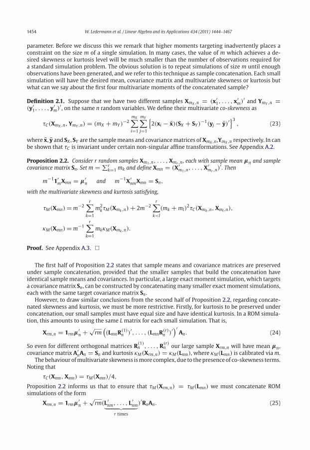
1.1. Deterministic L matrices

To construct a deterministic Lmatrixwe take apair (m, n) ∈ Z2+withm > n and setN(m) = m−1.

Then define a matrix Vm,N(m) = (v1, . . . , vN(m)) whose columns are specified as

vj = [0, . . . , 0︸ ︷︷ ︸j−1

, 1,−1, 0, . . . , 0︸ ︷︷ ︸m−1−j

]′ for 1 ≤ j ≤ N(m).

It is clear that {v1, . . . , vN(m)} is a linearly independent set and that vj ∈ H for 1 ≤ j ≤ N(m).We then

construct Lmn using the last n columns from Wm,N(m), the GS image of Vm,N(m). After some algebraic

manipulation we find thatWm,N(m) takes the following form:⎛⎜⎜⎜⎜⎜⎜⎜⎜⎜⎜⎜⎜⎜⎜⎜⎜⎜⎜⎜⎜⎜⎜⎜⎜⎜⎝

1√2

1√6· · · 1√

j(j+1) · · · · · · 1√(m−1)m

−1√2

1√6

......

0 −2√6

......

... 0. . .

......

......

. . . −j√j(j+1)

...

...... 0

. . ....

......

.... . .

. . ....

0 0 · · · 0 · · · 0−(m−1)√(m−1)m

⎞⎟⎟⎟⎟⎟⎟⎟⎟⎟⎟⎟⎟⎟⎟⎟⎟⎟⎟⎟⎟⎟⎟⎟⎟⎟⎠

. (8)

We remark that the matrix Wm,N(m) above is the last m − 1 columns of a type of m × m gener-

alised Helmert matrix. 8 Interestingly, it has been applied to change coordinate systems for geometric

morphometric analysis, by Mardia and Walder [22], Mardia and Dryden [21] and others.

The last n columns of the matrix (8) form the L matrix Lmn which Walter Ledermann first defined

as an explicit solution to (3). If we write Lmn = (�1, . . . , �n), then for 1 ≤ j ≤ n,

�j = [(m− n+ j − 1)(m− n+ j)]−1/2(1, . . . , 1︸ ︷︷ ︸m−n+j−1

,−(m− n+ j − 1), 0, . . . , 0︸ ︷︷ ︸n−j

)′. (9)

Few other Lmatrices have a simple closed form such as (9), so it will be convenient to use this Lmatrix

for illustrating the main concepts of ROM simulation. For this reason in the following we shall refer to

this particular L matrix as the “Ledermann matrix”.

8 After the German geodecist Friedrich Helmert, 1843–1917. A standard Helmert matrix is an n× n matrix in which all elements

occupying a triangle below the first row and above the principal diagonal are zero, i.e. H = (hij) where hij = 0 for j > i > 1. If

further h1j > 0 for all j,∑n

1 h2ij = 1, and hij > 0 for j < i thenH is a Helmert matrix in the strict sense. Generalised Helmert matrices

are square orthogonal matrices that can be transformed by permutations of their rows and columns and by transposition and by

change of sign of rows, to a form of a standard Helmert matrix. See [17] for further details.

W. Ledermann et al. / Linear Algebra and its Applications 434 (2011) 1444–1467 1449

The remainder of this section defines other Lmatrices, written Lkmn where k is an additional integer

parameter, which generalise the Ledermann matrix in the sense that Lmn = L1mn or L0mn. As is clear

from (9), the entries of Lmn only depend on the matrix dimensionm and n. Now to define Lk-matrices

we consider triples of the form (m, n, k) ∈ Z3+. Each triple must satisfy m > n. Restrictions on k

may also be imposed. With the introduction of a “free” parameter k these Lk-matrices may be quite

complex to express explicitly. In the following we suggest three types of Lk-matrices, although there

are endless possibilities.

Type I

For Type I matrices we allow only those triples with 2k ≤ m+ 1− n and set N(m) = m+ 1− 2k,

so n ≤ N(m). We define the Type I matrix Vm,N(m) = (v1, . . . , vN(m)) by setting

vj = [0, . . . , 0︸ ︷︷ ︸j−1

, 1,−1, . . . , 1,−1︸ ︷︷ ︸2k

, 0, . . . , 0︸ ︷︷ ︸m+1−2k−j

]′ for 1 ≤ j ≤ N(m). (10)

Again it is straightforward to check that the columns of Vmn form a linearly independent set in H.

Now the Lkmn matrix of Type I is the last n columns of the GS image of Vm,m+1−2k , defined above. By

considering GS pre-images it is clear that L1mn is indeed the Ledermann matrix. For k > 2 one can

easily check that Lkmn will solve Eq. (3), but it is less easy to write down the form of Lkmn explicitly. A

direct specification of Type I, Lk-matrices is available from the authors on request.

Type II

Again we start with a triple (m, n, k) ∈ Z3+, now satisfying the condition N(m) = m − k ≥ n. In

this case the GS pre-image matrix Vm,N(m) = (v1, . . . , vN(m)) is defined by

vj = [0, . . . , 0︸ ︷︷ ︸j−1

, 1, . . . , 1︸ ︷︷ ︸k

,−k, 0, . . . , 0︸ ︷︷ ︸m−k−j

]′ for 1 ≤ j ≤ N(m). (11)

We now define an L matrix of Type II as the last n columns of the GS image of Vm,m−k , defined above.

Once again this coincides with the Ledermann matrix when k = 1, but for k > 1 we have another

type of L matrix which is distinct from the Type I L matrices defined above. At this stage an explicit

specification of Type II L matrices has not been found.

Type III

In this case our triple (m, n, k) ∈ Z2+ × Z is only constrained by m and n since we simply set

N(m) = m− 2, and require that n ≤ N(m). Now define Vm,N(m) = (v1, . . . , vN(m)) where

vj = [0, . . . , 0︸ ︷︷ ︸j−1

, k,−1, 1− k, 0, . . . , 0︸ ︷︷ ︸m−2−j

]′ for 1 ≤ j ≤ N(m). (12)

Taking the last n columns of the GS image of the above yields L matrices of Type III. Note that, unlike

the Type I and Type II definitions, k is no longer restricted to the positive integers, provided it is real.

The case k = 0 corresponds to the Ledermann matrix, otherwise we have another distinct class of L

matrices.

It is easy to generalise Type III Lk-matrices further to allow for more free parameters. For example,

the GS pre-image columns could be defined as

vj = [0, . . . , 0︸ ︷︷ ︸j−1

, k1,−k2, k2 − k1, 0, . . . , 0︸ ︷︷ ︸m−2−j

]′ for 1 ≤ j ≤ N(m). (13)

This would then produce a matrix Lk1,k2mn which solves (3) with the flexibility of two parameters. Con-

tinuing in this way, an abundance of interesting solutions can be found. Although some will be rather

complex, every matrix constructed in this way is an L matrix.

1450 W. Ledermann et al. / Linear Algebra and its Applications 434 (2011) 1444–1467

1.2. Parametric L matrices

In this section we construct linearly independent sets inH from elliptical probability distributions.

This method can be interpreted as Monte Carlo simulation, adjusted to achieve exact covariance. In

this approach, the columns of our GS pre-image matrix Vmn = (v1, . . . , vn) are random vectors.

We assume that these vectors are drawn from a zero mean elliptical multivariate distribution, whose

marginal components are independent. That is,

Vmn ∼ D(0n, In),

where D is an elliptical distribution. Of course, Vmn is just m random observations on the n random

variables, whose population distribution is D. So in particular, the sample mean of our observations

will only satisfy the approximation

vn ≈ 0n,

and hence the columns ofVmn will not necessarily bemembers ofH. However, we can simply re-define

Vmn← Vmn − 1mv′n,

so that the column vectors of Vmn do indeed lie in H. 9 We would like to transform these vectors into

an orthonormal set using the Gram-Schmidt procedure. However we can only do this if our column

vectors are linearly independent. Once again, althoughwe assumed independence for ourmultivariate

distribution D, the sample covariance matrix of Vmn will only satisfy the approximation

m−1V′nmVmn ≈ In. (14)

We now normalise the columns of Vmn by re-defining10

vj ← vj〈vj, vj〉−1/2.Since the vectors of Vmn now have unit length, approximation (14) can be written more explicitly as

V′mnVmn = In + εPn, (15)

where ε is a small number, sometimes written as ε � 1, and Pn is a square matrix with zeros on the

diagonal. Due to sampling error, ε �= 0 almost always.

Recall that our aim is to show that the columns of Vmn are linearly independent. We first note that

a key result in linear algebra states that the columns of a matrix, Vmn, are linearly independent if and

only if its corresponding Gramian matrix, GV , is non-singular, where

GV = V′mnVmn.

Therefore for the classification of linear independencewemust calculate the determinant of thematrix

GV . Now using (15), and a perturbation result for determinants, we know that

det(GV ) = det(In + εPn) = 1+ tr(Pn)ε + ◦(ε2).

Since tr(Pn) = 0 we have that det(GV ) = 1 + ◦(ε2) �= 0. Therefore the n column vectors of the

matrixVmn = (v1, . . . , vn) are linearly independent and theGram-Schmidt algorithmmay be applied

to them. If we let LPmn = GS(Vmn), then we have yet another L matrix.

If we use this matrix for exact covariance simulation, assuming a target mean of 0n and covariance

matrix In, then from (2) our sample will simply be

Xmn = m1/2LPmn.

Since LPmn = GS(Vmn − 1mv′n) we have

Vmn − 1mv′n = LPmnRn, (16)

9 Other authors, such asMeucci [24], augment their samples using negative complements in order to achieve a zeromean sample.10 Normalisation at this step is applied to aid the argument of linear independence. In practise, it is superfluous at this point, since

the Gram-Schmidt algorithm, which is employed later, includes a normalisation.

W. Ledermann et al. / Linear Algebra and its Applications 434 (2011) 1444–1467 1451

where Rn is an upper (or right) triangular matrix. 11 Now, from the approximation (14) and the or-

thogonality of LPmn we have R′nRn ≈ mIn. But In is diagonal so R′nRn ≈ RnR′n. We require the following

lemma:

Lemma 1.1. Suppose thatUn is an upper triangularmatrix satisfyingU′nUn = UnU′n. ThenUn is a diagonal

matrix. In particular, if Un is orthogonal, then Un = diag(±1, . . . ,±1).Proof. See [26, Chapter III, Section 17], for example. �

Using an approximate form of Lemma 1.1 we deduce that Rn ≈ diag(±√m, . . . ,±√m). Now, by

inspecting the Gram-Schmidt procedure further, we find that the diagonal elements of Rn must be

positive. Hence, Rn ≈ m1/2In and, after inverting (16), we arrive at the approximation

Xmn ≈ Vmn − 1mv′n.

HenceXmn is in fact very close tomeandeviations of our original sampleVmn. This shows that paramet-

ric L matrices generate simulations that are a small adjustment to standard parametric Monte Carlo

simulations.

1.3. Data-specific L matrices

We now introduce a method for exact covariance simulation when the covariance matrix is esti-

mated from existing data. It is applicable to both cross-section and time-series data, but for the sake

of exposition we shall assume that we observe a multivariate time series on n random variables. The

advantage of this approach is that the properties of an exact moment simulation will closely resemble

the corresponding properties of the original sample, if one exists.

Suppose that we have a sample matrix Ymn representing m historical observations on n random

variables. The columns of this matrix need not have zero sample mean, so define

Vmn = Ymn − 1my′n,

whose columns will lie in H. We assume the columns of Vmn are linearly independent. 12 Clearly,

LDmn = GS(Vmn) is an L matrix. Now, given a target mean μn and covariance matrix Sn, we use this

data-specific solution to form an exact sample

Xmn = m1/2LDmnAn + 1mμ′n,where A′nAn = Sn.

It is straightforward to show that Xmn = Ymn when the target moments μn and Sn are chosen to

match themoments of the existing dataYmn.13 However onemay generate exact covariance simulated

samples that differ from the existing sample by targeting moments that are different from the sample

moments. For instance, one very useful application to financial risk management is to “stress” the

elements of a covariance matrix, while keeping other, less quantifiable characteristics of the existing

data unchanged.

1.4. Hybrid L matrices

A data-specific solution LDmn can be combined with deterministic and/or parametric L matrices to

produce “hybrid” L matrices which reflect both existing and hypothetical properties of the data. Of

course, in situations where little or no existing data are available only deterministic and parametric

L matrices are applicable. For instance, we may construct a hybrid L matrix which utilises both the

deterministic and parametric L matrix methodologies, using the following lemma (its proof is direct).

11 This is an example of a Thin QR Decomposition, see [11].12 If any variable in the system is a linear combination of other variables then it is not necessary to simulate this variable separately,

and it should be removed.13 This assumes that the covariance matrix of Ymn is positive definite.

1452 W. Ledermann et al. / Linear Algebra and its Applications 434 (2011) 1444–1467

Lemma 1.2. Suppose we have k rectangular matrices Q 1mn, . . . ,Q

kmn ∈ R

mn satisfying

(Q imn)′(Q j

mn) = δijIn for all 1 ≤ i, j ≤ k,

where δij is the Kronecker delta function. Then, given k non-zero scalars α1, . . . , αk ∈ R, the linear

combination of matrices

Smn =⎛⎝ k∑

i=1α2i

⎞⎠−

12 k∑

i=1αiQ

imn,

is a rectangular orthogonal matrix.

Let Lmn be a deterministic L matrix, which is constructed using one of the techniques from Section

1.1. Also let Vmn be a random sample from an elliptical distribution D(0n, In). Assuming that Vmn has

been adjusted to have a zero sample mean, we construct the augmented matrix

Am,2n = (Lmn,Vmn).

We then apply the Gram-Schmidt procedure, setting Am,2n = GS(Am,2n) where

Am,2n = (Lmn, Vmn).

Because of the sequential nature of the Gram-Schmidt algorithm, and since Lmn is already orthogonal,

we know that Lmn = Lmn. Furthermore, thematrix Vmn will not only be orthogonal butwill also satisfy

L′mnVmn = 0. Therefore we can apply Lemma 1.2, so that for any ε the matrix

LPmn =1√

1+ ε2

(Lmn + εVmn

), (17)

will be rectangular orthogonal. Since the columns of Am,2n lie inH, the subspace preserving property

of the Gram-Schmidt process ensures that the columns of Am,2n are also in H. Therefore LPmn defined

by (17) is another L matrix. The parameter ε controls the mix between deterministic and random

structure in thematrix. If it is small the hybrid Lmatrix approximates the deterministic characteristics

of Lmn.

2. ROM simulation

The motivation for the research presented in this section is that, if Lmn is an L matrix then so is

LmnRn, for any square orthogonal matrix Rn. Also, if Qm is a permutation matrix then QmLmn is an L

matrix, since 1′mQm = 1′m. Together, these two observations lay the foundation for a new approach to

simulating infinitely many random samples that have identical sample mean vectors and covariance

matrices. Each random sample is generated as

Xmn = 1mμ′n +√

mQmLmnRnAn, (18)

where Lmn is an Lmatrix,Qm is a randompermutationmatrix,Rn is any random orthogonalmatrix,μn

is the target mean vector and A′nAn = Sn, where Sn is the target covariance matrix. Thus, (18) provides

a novel and very flexible method for generating random samples. 14

Any deterministic, parametric or data-specific L matrix of type I, II or III may be applied in (18)

but in this section for simplicity we shall work with the Ledermann matrix (9), since it is available

in an elegant closed form. The purpose of this section is to investigate how the characteristics of the

simulated sample are affected when we choose different types of random orthogonal matrices Rn

in (18).

14 Many thanks to Prof. Nick Higham for recently pointing us towards the paper by Li [18] where a special case of (18) is proposed

in which n = m − 1, Qm is the identity matrix and Lmn is the matrix (8), or any matrix such that (m−1/21m, Lmn) is an orthogonal

matrix.

W. Ledermann et al. / Linear Algebra and its Applications 434 (2011) 1444–1467 1453

2.1. Skewness and kurtosis

There are many ways to measure the skewness and kurtosis, even of a univariate sample, as dis-

cussed by Cramer [6]. For our applications we require a statistic for the skewness and kurtosis of

a multivariate sample, and there are also many different definitions of multivariate skewness and

kurtosis, see [15]. In the following we employ the definitions introduced by Mardia [23]. However,

as highlighted by Gutjahr et al. [12], samples from different distributions may have identical Mardia

characteristics. Even so,we choose toworkwithMardia’smultivariatemoments since, as scalar-valued

measurements, they are highly tractable.

Given a random sample Xmn = (x′1, . . . , x′m)′, written using row vector notation where xi =(xi1, . . . , xin) for 1 ≤ i ≤ m, Mardia [23] proposes the following measures for the multivariate

skewness and kurtosis of Xmn:

τM(Xmn) = m−2m∑i=1

m∑j=1

{(xi − x)S−1X (xj − x)′

}3,

κM(Xmn) = m−1m∑i=1

{(xi − x)S−1X (xi − x)′

}2where SX is the n × n sample covariance matrix of Xmn and x is the row vector of sample means.

Mardia [23] proves that thesemeasures are invariant under non-singular, affine transformations. That

is, τM(Ymn) = τM(Xmn) and κM(Ymn) = κM(Xmn), whenever

Ymn = XmnBnn + 1mbn, (19)

where Bnn is any invertible matrix and bn is any row vector. This invariance property is of particu-

lar significance in ROM simulation, since the transformation (18) is a (random) non-singular affine

transformation of the L matrix Lmn. Therefore τM(Lmn) and κM(Lmn) will determine the multivariate

skewness and kurtosis of all ROM simulated samples Xmn.

Proposition 2.1. Let Lmn be the Ledermann matrix, defined by (9). Then

τM(Lmn) = n[(m− 3)+ (m− n)−1

]=: f (m, n), (20)

κM(Lmn) = n[(m− 2)+ (m− n)−1

]=: g(m, n). (21)

Proof. See Section A.1 of the appendix. �

BycomparingEqs. (21) and (20)wesee that avery simple relationship links themultivariatekurtosis

and multivariate skewness of the Ledermann matrix. That is, for m > n, we have

κM(Lmn)− τM(Lmn) = n.

The expected skewness and kurtosis of MVN variables are also closely linked, since their ratio is a

simple function of n and m. See Proposition 2.3 below.

We now study the asymptotic behaviour of the Mardia skewness and kurtosis derived from large

samples that are generated using Ledermann matrices. For a fixed n and a comparatively large m,

writtenm� n, we have that (m− n)−1 ≈ 0. Hence we can approximate (20) and (21) as

f (m, n) ≈ n(m− 3), g(m, n) ≈ n(m− 2) for m� n. (22)

So the functions g(m, n) and f (m, n) are asymptotically linear, with gradient n, and will become

unbounded as m becomes large. It is also true that if n2 > n1 then f (m, n2) > f (m, n1) for all

m > max{n1, n2} and that f (m, n2) will tend to infinity faster than f (m, n1), as m tends to infinity,

and similarly for g(m, n).Note that if we use a Ledermann matrix in ROM simulation then we can target either skewness or

kurtosis but not both, by choosing an appropriate valuem, since the number of variables n is typically

fixed. To target bothmoments we shall need to use a generalised Lmatrix, with at least one additional

1454 W. Ledermann et al. / Linear Algebra and its Applications 434 (2011) 1444–1467

parameter. Before we discuss this we remark that higher moments targeting inadvertently places a

constraint on the size m of a single simulation. In many cases, the value of m which achieves a de-

sired skewness or kurtosis level will be much smaller than the number of observations required for

a standard simulation problem. The obvious solution is to repeat simulations of size m until enough

observations have been generated, andwe refer to this technique as sample concatenation. Each small

simulation will have the desired mean, covariance matrix and multivariate skewness or kurtosis but

what can we say about the first four multivariate moments of the concatenated sample?

Definition 2.1. Suppose that we have two different samples XmX ,n = (x′1, . . . , x′m)′ and YmY ,n =(y′1, . . . , y′m)′, on the same n random variables. We define their multivariate co-skewness as

τC(XmX ,n, YmY ,n) = (mX + mY )−2

mX∑i=1

mY∑j=1

{2(xi − x)(SX + SY )

−1(yj − y)′}3

, (23)

where x, y and SX , SY are the samplemeans and covariancematrices ofXmX ,n,YmX ,n respectively. In can

be shown that τC is invariant under certain non-singular affine transformations. See Appendix A.2.

Proposition 2.2. Consider r random samples Xm1,n, . . . ,Xmr ,n, each with sample mean μn and sample

covariance matrix Sn. Set m = ∑rk=1 mk and define Xmn = (X′m1,n

, . . . ,X′mr ,n)′. Then

m−11′mXmn = μ′n and m−1X′nmXmn = Sn,

with the multivariate skewness and kurtosis satisfying,

τM(Xmn)=m−2r∑

k=1m2

kτM(Xmk,n)+ 2m−2r∑

k<l

(mk + ml)2τC(Xmk,n,Xml,n),

κM(Xmn)=m−1r∑

k=1mkκM(Xmk,n).

Proof. See Appendix A.3. �

The first half of Proposition 2.2 states that sample means and covariance matrices are preserved

under sample concatenation, provided that the smaller samples that build the concatenation have

identical samplemeans and covariances. In particular, a large exactmoment simulation, which targets

a covariancematrix Sn, can be constructed by concatenatingmany smaller exact moment simulations,

each with the same target covariance matrix Sn.

However, to draw similar conclusions from the second half of Proposition 2.2, regarding concate-

nated skewness and kurtosis, we must be more restrictive. Firstly, for kurtosis to be preserved under

concatenation, our small samples must have equal size and have identical kurtosis. In a ROM simula-

tion, this amounts to using the same L matrix for each small simulation. That is,

Xrm,n = 1rmμ′n +√

rm((LmnR

(1)n )′, . . . , (LmnR

(r)n )′

)′An. (24)

So even for different orthogonal matrices R(1)n , . . . , R

(r)n our large sample Xrm,n will have mean μn,

covariance matrix A′nAn = Sn and kurtosis κM(Xrm,n) = κM(Lmn), where κM(Lmn) is calibrated viam.

Thebehaviour ofmultivariate skewness ismore complex, due to thepresenceof co-skewness terms.

Noting that

τC(Xmn,Xmn) = τM(Xmn)/4,

Proposition 2.2 informs us that to ensure that τM(Xrm,n) = τM(Lmn) we must concatenate ROM

simulations of the form

Xrm,n = 1rmμ′n +√

rm(L′nm, . . . , L′nm︸ ︷︷ ︸r times

)′RnAn. (25)

W. Ledermann et al. / Linear Algebra and its Applications 434 (2011) 1444–1467 1455

Since (25) is a special case of (24), Xmn will still have sample mean μn and covariance matrix Sn, with

multivariate kurtosis satisfying κM(Xrm,n) = κM(Lmn).Wehave defined amethod for generating large samples of size rm, with exact target first and second

moments and third and fourth moments that are determined by the skewness and kurtosis of the L

matrix used in (25). With n fixed, the skewness and kurtosis of a matrix Lkmn is a function ofm and k. In

general, these functions are not available in closed form, so a numerical optimisation must be applied

to calibrate the values ofm and kwhich achieve the target skewness and kurtosis. With thesemoment

targeted, a simulation of the form (25) ensures that thesemoments are preserved in large simulations.

We now study the skewness and kurtosis of ROM simulationswhich employ parametric Lmatrices,

as defined in Section 1.2. Recall that a parametric L matrix LPmn is a Gram-Schmidt orthogonalisation

of a random sample Vmn, drawn from an elliptical multivariate distribution. One can show this or-

thogonalisation process in an invertible affine transformation and hence the skewness and kurtosis of

LPmn will equal the skewness and kurtosis of Vmn. Unlike the deterministic case, τM(LPmn) and κM(LPmn)depend on a random sample Vmn, and will therefore be random quantities themselves. However, if

Vmn is drawn from a multivariate normal distribution, then we can use the following result of Mardia

[23], to find the expected values of τM(LPmn) and κM(LPmn).

Proposition 2.3. Let Vmn be a random sample drawn from any multivariate normal distribution

N(μn, �n). Then

E[τM(Vmn)] = n(n+ 1)(n+ 2)m−1,E[κM(Vmn)] = n(n+ 2)(m− 1)(m+ 1)−1.

Therefore for largem the skewness and kurtosis of a parametric Lmatrix generated from amultivariate

normal distribution will be:

E

[τM(LPmn)

]≈ 0,

E

[κM(LPmn)

]≈ n(n+ 2).

Hence, the skewness and kurtosis in a parametric ROM simulation is restricted by the underlying

distribution, and these moments are also prone to sampling error.

By contrast, when using deterministic L matrices in ROM simulations one can target a range of

different skewness and kurtosis levels. There will also be no sampling error since the deterministic

values τM(Lmn) and κM(Lmn) fix the multivariate skewness and kurtosis of all ROM simulated sam-

ples. One can also concatenate deterministic L matrix ROM simulations and parametric L matrix ROM

simulations and the moments of this concatenated sample may be estimated using Proposition 2.2.

Example 1. Concatenating deterministic and parametric ROM simulations. Using the same target

mean and covariance matrix, suppose we use ROM simulation to generate two samples Xm1,n and

Xm2,n. The first sample is simulated from the Ledermannmatrix and the second sample is a simulated

from a normally distributed parametric Lmatrix. Assuming thatm1 andm2 are large, the multivariate

kurtosis of the concatenated sample Xmn = (X′m1,n,X′m2,n

)′, has approximate expected value

E[κM(Xmn)] ≈ (m1 + m2)−1 {m1n(m1 − 2)+ m2n(n+ 2)} .

Concatenation is not the only way of combining deterministic and parametric ROM simulations. One

can also use perturbed L matrices, as defined in (17).

Example 2. Kurtosis of perturbed Lmatrices. Let LPmn be a ε-perturbation of the deterministic Lmatrix

Lmn. Then, provided that ε is small, it is straightforward to derive the approximation

κM(LPmn) ≈κM(Lmn)

(1+ ε2)2.

1456 W. Ledermann et al. / Linear Algebra and its Applications 434 (2011) 1444–1467

Finally, we note that the skewness and kurtosis of data-specific Lmatrices are completely determined

by theunderlyingdata. So, similar to parametric ROMsimulations, thehighermoments of data-specific

ROM simulations are limited. However, if desired, one can affect these limits while maintaining some

characteristics of the existing data by using a concatenation or perturbation approach.

2.2. Orthogonal matrices and sample characteristics

In Section 2.1 we used the multivariate skewness and kurtosis measures of Mardia [23] to quantify

how different L matrices affect ROM simulations. We now turn our attention to the random square

orthogonal matrices which pre- or post-multiply a given L matrix during a ROM simulation. Geomet-

rically, square orthogonal matrices fall into three categories: permutations, reflections and rotations.

Methods for generating such matrices are numerous, particularly in the latter case. We choose to

focus on rotation matrices which appear in upper Hessenberg form. However techniques involving

skew-symmetric matrices and [3] transforms, or the matrix exponential function, may also be used

to generate random, rotation matrices, see [5]. For the sake of clarity and because this matrix has a

relatively simple explicit form, Lmn will again denote the Ledermann matrix defined by (9), unless

otherwise specified. Continuing the notation of (18), we shall now investigate how random permu-

tation, reflection and other random orthogonal matrices can alter the characteristics of multivariate

time series ROM simulations.

Permutation matrices are the primary means of controlling the time ordering of observations in

multivariate time series ROM simulation. Such a matrix, denoted by Qm, is a square matrix of order

m, which has exactly one entry 1 in every row and every column, and has entries 0 everywhere else.

Pre-multiplying any m× n matrix Amn with Qm permutes the rows of Amn. For example,

QmAmn =

⎛⎜⎜⎜⎝

0 1 0

0 0 1

1 0 0

⎞⎟⎟⎟⎠⎛⎜⎜⎜⎝

a11 a12

a21 a22

a31 a32

⎞⎟⎟⎟⎠ =

⎛⎜⎜⎜⎝

a21 a22

a31 a32

a11 a12

⎞⎟⎟⎟⎠ .

To see how permutation matrices can affect ROM simulations we first recall the structure of Lmn, in-

ferred from (8). From this we see that the largest values in Lmn appear on the diagonal of it’s lowest

n × n block. Therefore, when the Ledermann matrix is applied to ROM simulations without permu-

tations, large values only appear at the end of the simulated sample paths. However, by including a

random permutationmatrixQm in (18) we can ensure that these large values are randomly positioned

throughout the whole sample path. Furthermore, by restricting the permutation matrix, and hence

controlling the rows of the L matrix that are fixed and those that are randomly permuted, we can

influence the random times at which these large values appear.

In time series analysis one regularly observes areas of large changes (positive or negative) followed

by areas of small changes. This phenomenon is referred to as volatility clustering. 15 Cyclic permutation

matrices enable us to produce ROM samples which exhibit this volatility clustering feature. When

a random cyclic permutation matrix pre-multiplies a matrix the rows of the matrix are all offset

downwards by means of a random shift, thus maintaining their ordering. By using random cyclic

permutations in ROM simulation the large values of the Ledermann matrix can be made to appear

together in a random cluster. Alternatively, to remove the volatility clustering that is implicit in the L

matrix, a general random permutation matrix can be used.

To illustrate these effects, Fig. 1 exhibits plots for three different simulated sample paths. Each

simulation has the form (18), with Rn fixed as the identity. However, in the top path Qm is also the

identity, in the middle path Qm is a random cyclic permutation and in the bottom path Qm is a general

random permutation matrix.

The assertion in (18) thatQn must be a permutationmatrix, while Rn can be any orthogonalmatrix,

is made for the following reason. Let Xmn be a ROM simulated sample, generated from Lmn. In order

for the sample mean of Xmn to be μn, we must have that

1′mQmLmnRnAn = 0′n. (26)

15 In finance, these volatility clusters are often apparent in historical returns series, see [20].

W. Ledermann et al. / Linear Algebra and its Applications 434 (2011) 1444–1467 1457

−1

−0.5

0

0.5

1−1

−0.5

0

0.5

1

−1

−0.5

0

0.5

1

Fig. 1. Threeplotsdemonstratinghowpermutationmatrices affect volatility clustering in samplepaths simulated fromtheLedermann

matrix.

Now, since Lmn is an L matrix, given by (3), we know that 1′mLmn = 0′n. If Qm is a permutation matrix

then 1′mQm = 1′m and (26) will hold regardless of the form of Rn. However, this may not be the case if

Qm is not a permutationmatrix. So now, assuming thatQm is a permutationmatrix,we discuss possible

choices for the random orthogonal matrix Rn.

Although we have examined the multivariate kurtosis of ROM simulations, as defined by Mardia

[23],we have not yet discussedmarginal kurtosis, that is, the kurtosis of the individual variableswithin

the simulation. Since permutation matrices only re-order our samples, we must find orthogonal ma-

trices which can affect the magnitude of our simulated observations. An upper Hessenberg matrix Hn

of degree n is a matrix with zero entries below the first sub-diagonal. Berry et al. [2], Gemignani [8]

and many other authors show that we can construct orthogonal upper Hessenberg matrices using

Givens rotation matrices. A Givens rotation Gj(θj) is the identity matrix except for the 2× 2 principal

sub-matrix

Gj[j, j + 1; j, j + 1] =⎛⎝ cos(θj) sin(θj)

− sin(θj) cos(θj)

⎞⎠ . (27)

Orthogonal upperHessenbergmatricesHn can be constructed as a product of n−1Givens rotations via

Hn = G1(θ1)G2(θ2) . . .Gn−1(θn−1). (28)

In order to produce random orthogonal upper Hessenbergmatrices we allow the arguments of (28) to

be stochastic, choosing θj in the interval [0, 2π) for 1 ≤ j ≤ n− 1 at random.16 An example of a low-

dimensional Hessenberg matrix is given below, where we simplify notation by setting ci = cos(θi)and si = sin(θi) for 1 ≤ i ≤ 3.

H4 =

⎛⎜⎜⎜⎜⎜⎜⎝

c1 −s1 0 0

s1 c1 0 0

0 0 1 0

0 0 0 1

⎞⎟⎟⎟⎟⎟⎟⎠

⎛⎜⎜⎜⎜⎜⎜⎝

1 0 0 0

0 c2 −s2 0

0 s2 c2 0

0 0 0 1

⎞⎟⎟⎟⎟⎟⎟⎠

⎛⎜⎜⎜⎜⎜⎜⎝

1 0 0 0

0 1 0 0

0 0 c3 −s30 0 s3 c3

⎞⎟⎟⎟⎟⎟⎟⎠

=

⎛⎜⎜⎜⎜⎜⎜⎝

c1 −s1c2 s1s2c3 −s1s2s3s1 c1c2 −c1s2c3 c1s2s3

0 s2 c2c3 −c2s30 0 s3 c3

⎞⎟⎟⎟⎟⎟⎟⎠ .

16 Random orthogonal Hn can be generated quickly in MatLab using the function gallery(’randhess’,n), see [13].

1458 W. Ledermann et al. / Linear Algebra and its Applications 434 (2011) 1444–1467

−0.5

0

0.5

−0.5

0

0.5

−0.5

0

0.5

Fig. 2. Three plots demonstrating how upper Hessenberg and permutation matrices affect the characteristics of sample paths simu-

lated from the Ledermann matrix.

In ROM simulation we can use products of random upper Hessenbergmatrices to form the orthogonal

matrix Rn, which post-multiplies the L matrix appearing in (18). Recall that the magnitudes of the

elements of an L matrix depend on its degree, which depends on the number of observations m we

want to simulate. When m is large, the large elements on the lowest diagonal of the L matrix create a

“pulse”, where clusters of large positive and negative observations are interspersedwith “flat” periods

of less activity in the sample (see the third plot in Fig. 1 for example). Permutation matrices only

control the timing of such pulses, butwemay also like to affect theirmagnitude and have the potential

to eliminate the flat periods. Crucially, unlike permutation matrices, post-multiplying an L matrix

with many random Hessenberg matrices diminishes and dissipates the effect of the large elements,

randomly throughout the sample. Fig. 2 showshow the three samples paths shown in Fig. 1 are affected

by post-multiplication with random Hessenberg matrices.

The number of Hessenberg matrices used in the orthogonal product affects the marginal kurtosis

of the random variables. The bottom n× n block of an L matrix Lmn is upper triangular. Furthermore,

the number of non-zero elements in each column of Lmn increases by one every timewe post-multiply

Lmn by a random upper Hessenberg matrix. Therefore, to remove all zeros from Lmn we must include

the product of at least n− 1 upper Hessenberg matrices in the random orthogonal matrix Rn of (18).

Having looked at multivariate skewness in Section 2.1, we now show how to induce some degree

of positive or negative marginal skewness into ROM simulations. For this we will use an orthogonal

matrix Bn of the form

Bn = diag{(−1)d1 , . . . , (−1)dn

}, (29)

where each index di is either zero or one. When the indices are realisations of Bernoulli variables, we

call such a matrix a random sign matrix. It will multiply the rows of any matrix it pre-multiplies by

plus or minus one.

Suppose Rn is chosen in (18) to be a product of random upper Hessenberg matrices. This matrix

pre-multiplies a matrix An, which realises the target covariance matrix Sn. We write this product as

Tn = RnAn.

Now Tn will be a randommatrix containing both positive andnegative entries. Since Tn post-multiplies

Lmn in (18), large positive elements of Tn will combine with the large negative diagonal elements of

the L matrix to form large negative observations in our simulated sample matrix Xmn. Similarly, large

negative elements of Tn cause large positive observations in the sample. However, pre-multiplying Tn

W. Ledermann et al. / Linear Algebra and its Applications 434 (2011) 1444–1467 1459

by a random sign matrix Bn affects these large negative or positive values. 17 Without this extra pre-

multiplication, large positive andnegative elements appear equally often in Tn, resulting in a simulated

samplewhich is approximately symmetric. A judicious choice for theBernoulli probabilities can ensure

that the product BnTn has more large negative elements then large positive elements (or vice versa).

Thus positive (or negative) marginal skewness is introduced into ROM simulated samples. 18

There are many ways to influence skewness by altering the Bernoulli probabilities. For instance,

letting ti denote the ith row of Tn, if Tn has at least one negative entry we can set

pi =∣∣∣∣∣minj

{min(tij, 0) : tij ∈ ti

}mini,j

{tij : tij ∈ Tn

}∣∣∣∣∣ . (30)

Then, randomly selecting r ∈ (0, 1), assign:

di =⎧⎨⎩ 1, if r < pi

0, otherwisefor 1 ≤ i ≤ n.

If there is a large negative entry in row ti then the Bernoulli probability pi will be close to one. Therefore

the index di is more likely to take the value 1 and hence row ti will change sign when Tn is pre-

multiplied by Bn. Thus this particular Bernoulli sign matrix converts large negative elements of Tn to

large positive elements. As a result negativemarginal skewness is introduced into simulations. Positive

marginal skewness can be introduced by defining the pi using maxima rather than minima in (30).

This section has shown how different classes of orthogonal matrices affect the characteristics of

ROM simulated samples in very different ways. Although we have focussed on the Ledermannmatrix,

the above techniques can also be applied to ROM simulations involving other Lmatrices. Investigating

these more general ROM simulations, and exploring further classes of orthogonal matrices, is left to

future research.

3. Application to value-at-risk

ROM simulation has applications to virtually any problem that may be resolved using Monte Carlo

simulation. Generally, such problems require the forecasting of future multivariate distributions, us-

ing historical or scenario sample data. In finance these problems include the pricing and hedging of

complex options, any decision problem based on a future distribution such as portfolio optimisation,

and financial risk assessment where, since its introduction during the 1990’s, the value-at-risk (VaR)

of a portfolio has become the industry benchmark. This section demonstrates how ROM simulation

may be applied to VaR estimation.

The portfolio VaR is the loss that would be equalled or exceeded, with a given probability α, over

a certain period of time (which is called the “risk horizon”) if the portfolio is left un-managed during

this interval. Measured as a percentage of the current portfolio value, the 100α% h-day VaR is minus

the α-quantile of the distribution of the portfolio’s h-day returns, in present value terms. For example,

if the h-day excess returns on the portfolio’s risk factors have a multivariate normal distribution and

the portfolio return is a linear function of it’s risk factor returns, the 100α% h-day VaR, expressed as a

percentage of the current portfolio value is: 19

VaR(α, h) = −−1(α)σh (31)

where −1(α) is the lower α-quantile of a standard normal distribution and σh is the standard devi-

ation of the normal h-day portfolio returns distribution.

However, a multivariate normal assumption is not usually appropriate and many portfolios have

returns that are non-linear functions of the risk factor returns, so it is very common to use simulation to

17 Algebraically, we are simply including a sign matrix into the Hessenberg product which comprises Rn .18 If there are more large positive elements in BmTmn than large negative elements, the samples will have negative skewness. If

there are more large negative elements in BmTmn than large positive elements, the samples will have positive skewness.19 This formula applies if the portfolio is expected to return the discount rate over the risk horizon. Otherwise, a small mean

adjustment applies. See [1, Section IV.1.5].

1460 W. Ledermann et al. / Linear Algebra and its Applications 434 (2011) 1444–1467

estimate portfolio VaR. Monte Carlo simulation assumes a parametric multivariate risk factor returns

distribution and thus generates i.i.d. simulations on each risk factor. To each simulation we then apply

the portfolio mapping, which gives the portfolio value as a function of the returns on its risk factors,

to obtain a simulated h-day return. Repeating the simulations many times generates a distribution for

the portfolio’s h-day return and theMonte Carlo VaR, expressed as a percentage of the portfolio value,

is estimated as minus the α-quantile of this distribution. However, in addition to the sampling error

described in the introduction, the parametric assumptions underlying Monte Carlo simulation pose a

significant source ofmodel risk. That is, different distributional assumptions typically give rise to quite

different VaR estimates. It is well known that the empirical characteristics of financial asset returns

are often misrepresented by multivariate normal or Student-t distributions, yet it is usually not clear

what distributional assumption is most appropriate.

For these reasons historical simulation is by far the most common VaR resolution method used

in the finance industry. Standard historical simulation uses a large number of historical returns on

the portfolio to build an empirical distribution and hence estimate the VaR from a lower quantile. An

advantage is that it does not make parametric assumptions regarding the risk factor returns; a major

disadvantage is data limitation. A long historical samplemay be difficult to obtain for all risk factors, or

may be thought to be inappropriate since market behaviour has changed considerably in recent years.

Thus the empirical distribution is typically built using only 3–5 years of daily returns, i.e. a sample

size of around 750–1250 data points, so the accuracy of the quantile estimator is severely impaired. 20

Moreover, due to lack of sufficient weekly or monthly historical data, 1-day historical VaR estimates

are usually scaled up to h-day estimates for h > 1 and for this crude assumptions are commonly

made, such as a “square-root-of-time” scaling rule. Although square-root scaling is very common, it

is not justified because it requires the portfolio returns to be independent and identically normally

distributed. Hence the scaling of historical VaR to risk horizons longer than 1 day is a significant source

of model risk, especially in options portfolios. 21

3.1. ROM VaR methodology

Using ROM simulation to estimate portfolio value-at-risk can circumvent the disadvantages of

existing VaRmethodologies summarised above. Suppose thatwe have a portfoliowith n assets. Similar

to elliptical Monte Carlo VaR, ROM VaR starts by targeting a mean vector μhn and covariance matrix

Shn for the h-day returns on risk factors under examination. We then simulate a sample Xhmn, using a

ROM simulation of the form (18). This matrix Xhmn representsm observations for the h-day returns on

the portfolio’s n risk factors. Since ROM simulation is an exact covariance simulation technique, the

samplemean and covariancematrix of the simulated risk factor returnsXhmn, will match the targetsμh

n

and Shn exactly. Assuming a portfolio mapping, π : Rn → R, we construct a vector of h-day portfolio

returns, Yhm = (y1, . . . , ym)′, defining

yi = π(xi) for 1 ≤ i ≤ m

where xi denotes the ith row of Xhmn. So given the α-quantile estimator qα : Rm → R, we calculate

ROM VaR as

VaR(α, h) = −qα(Yhm). (32)

Typically the covariance matrix Shn will have a large influence on ROM VaR. 22 But VaR, being a lower

quantile of the portfolio returns distribution, is alsomuch affected by the skewness and kurtosis of the

risk factor returns, and this is one reason why the (non-parametric) historical VaR model is favoured

by many practitioners. However, the limitation of using only one realisation of the risk factors – i.e.

the one that was observed historically – is that it assumes that history will repeat itself, in the sense

20 Some practitioners bootstrap the sample, i.e. they re-sample randomly many times from the same set of returns, but this only

serves to make the tails of the distribution blunt, as no new information is added. See [1, Section IV.3.2].21 See [1, Section IV.6.2].22 This is similar to normal VaR, and to Student-t VaR where Shn affects the VaR through the portfolio variance σh .

W. Ledermann et al. / Linear Algebra and its Applications 434 (2011) 1444–1467 1461

that the risk factor returns distribution over the risk horizon will be identical to their distribution in

the historical sample.

With ROM VaR we can simulate a very large number of realisations for the risk factor returns, each

being consistent with the sample moments that were observed in the historical sample. Alternatively,

when stress testing a portfolio for extreme realisations of its risk factors, we can target other sample

moments that are consistent with periods of financial crisis. As we saw in Sections 1 and 2, different

L matrices and different orthogonal matrices will affect the characteristics of a ROM simulation in

different ways. In particular, the effect of skewness and kurtosis can be incorporated into ROM VaR

through a judicious choice of these matrices. 23

ROMsimulationhasnumerousapplications toVaRestimation. For example, in stress-testingportfo-

lios a riskmanager would hypothesise values for samplemoments that are believed to reflect stressful

market conditions, apply ROM simulations to generate samples that have exactly these moments, and

compute the stress-VaR as a lower quantile of the simulated distribution. In general, ROM VaR can be

thought of as an extension of historical VaR, or a form of scenario VaR, where there is no need for the

crude time-scaling approximations that are normally used because definition (32) does not explicitly

depend on h; the risk horizon is implicit within each of the ROM simulations (18).

Suppose a portfolio manager holds a large portfolio of n assets and would like to gauge his risk

exposure by calculating VaR. The only information available is an historical sample on the portfolio risk

factor returns,whichwedenoteHmn. Empirically he discovers that the historical data does not strongly

resemble any elliptical multivariate distribution. In particular, the multivariate historical kurtosis is

much larger than the kurtosis of amultivariate normal distribution. The lengthm of the historical data

is typically too small to be confident in the accuracy of historical quantile estimates, especially for small

α. Anyway, themanager does not believe that historywill repeat itself exactly, only that the risk factor’s

sample moments are related to those observed in the historical sample. He is not performing a stress

test, so he will use ROM simulations that target exactly the historical sample means and covariance

matrix of the risk factor returns. However, given the recent crisis in the banking industry, investors

are now seeking quite conservative estimates of potential losses, andwant to be careful to incorporate

large outliers into the VaR simulations. For this reason he would like the multivariate kurtosis of the

simulated weekly returns to be 100β% greater than the historical kurtosis level.

Given the scenariopaintedabove,wechoose to adopt a technique forROMVaRwhere the Lmatrix of

our simulations is chosen to reflect themanager’s views on kurtosis, while preserving other properties

of the historical data. Starting with the historical sample Hmn we calculate the historical mean vector

μn, the historical covariance matrix Sn, and the historical multivariate kurtosis κ = κM(Hmn) of the

weekly returns. As in Section 1.3, we orthogonalise our historical sample to produce a data-specific

L matrix LDmn = GS(Hmn). We also construct a deterministic L matrix, Lpn, of the form (9), where the

integer parameter pwill be determined by our kurtosis target.

First, targeting the historical mean vector and covariance matrix, the ROM simulated risk factor

returns take the form

Xm+p,n =⎛⎜⎝ 1mμ′n

1pμ′n

⎞⎟⎠+

⎛⎜⎝√

m LDmn

√p LpnRn

⎞⎟⎠An, (33)

where Rn is a product of random orthogonal matrices and A′nAn = Sn. Within Rn we include n −1 random upper Hessenberg matrices and a random sign matrix, which induces negative marginal

skewness, to convey the specific concern for large negative returns. By applying proposition 2.2 to the

concatenated sample Xm+p,n, and recalling the invariance property of Mardia’s measures, we deduce

that

(m+ p)κM(Xm+p,n) = mκM(LDmn) + pκM(Lpn).

The kurtosis of LDmn, by definition, equals the historical kurtosis κ . But we would like the kurtosis of

our simulated sample to be 100β% more than the historical value. That is, κM(Xm+p,n) = (1 + β)κ .

23 This contrasts with Monte Carlo methods, where parametric assumptions place strong restrictions on the higher moments.

1462 W. Ledermann et al. / Linear Algebra and its Applications 434 (2011) 1444–1467

This will be achieved through an appropriate choice of p. Using approximation (22) for κM(Lmn), we

find that pmust satisfy:

(m+ p)(1+ β)κ = mκ + pn(p− 2). (34)

Provided that β is positive, this quadratic equation always yields a positive solution p+. Taking the

closest integer part of this solution, we set p = int(p+), and use Lpn for our ROM simulations (33).

Now the portfolio risk manager knows that the ROM VaR simulations will resemble historical data

through LDmn, while representing his views on kurtosis via Lpn. Targeting kurtosis in this way would

not be possible with parametric VaR. And the presence of random orthogonal matrices in (33) ensures

that we are not simply relying on our single historical sample, as we are forced to do with histori-

cal VaR.

3.2. Empirical results

In this sectionwecompare fourVaRmodels. Thefirst is theROMVaRmethoddescribedabove,which

utilises deterministic and historical L matrices. The second and third are parametric Monte Carlo VaR,

based on multivariate normal and Student-t distributions for the risk factors. Since ROM VaR is based

on an exact covariance simulationmethod, we will adjust our Monte Carlo VaR simulations to achieve

this same precision. This is equivalent to using parametric L matrices in (18), without any random

orthogonal matrices. Our final method is standard historical VaR, which will form the benchmark of

our investigation.

In order to test the accuracy of the different VaRmethodswe assume that the portfolio riskmanager

holds a portfolio of 10 MSCI World country indices. 24 For this portfolio we will calculate 1-day and 5-

day (or1-week)VaRsat0.1%, 1%and5% levels. 25 Ourhistorical sample spans theperiod January1995 to

July 2009 (3789 days, 757weeks). Starting in January 2000wewill use the first 5 years (1300 days, 260

weeks) of the historical sample to calculate historical means, covariances and higher moments of our

weekly risk factor returns. We assume that we have an equally weighted portfolio, which corresponds

to the portfolio mapping:

π : (x1, . . . , xn) �−→ (x1 + · · · + xn)/n.

Assuming that β = 0.1 the kurtosis of future returns will be 10% more than that of the historical

returns, so we solve (34) for p and use ROM simulations of the form (33) to generate 10,000 returns

on each of our 10 risk factors. 26 The mean and covariance matrix of our simulated sample will match

the corresponding historical moments exactly. We then use our equally weighted portfolio mapping

π to form 10,000 observations for the total portfolio return and then apply the quantile function, as

in (32), to obtain the ROM VaR.

To test the accuracy of the VaR models we employ unconditional coverage tests, introduced by

Kupiec [16], and the independence and conditional coverage tests, introduced by Christoffersen [4]. To

perform these testswefirst determine the number of “exceedances”, i.e. the number of days (orweeks)

when theportfolio lostmore than theVaR thatwas estimated for that period.Under thenull hypothesis

of the unconditional coverage test, the proportion of exceedances should equal α. Over the period

January 2000 to July 2009 there are 2489 daily observations in total period, the ROMVaRmodel yields

4 exceedances of the 0.1% VaR, 36 exceedances of the 1%VaR and 162 exceedances of the 5%VaR; that is

the proportion of exceedance was 0.2%, 1.5% and 6.5% respectively. Out of 497weekly observations the

number of exceedances at the 0.1%, 1% and 5% levels were 1, 11 and 31 respectively, which correspond

to exceedance proportions of 0.2%, 2.2% and 6.2%. This indicates that ROM simulation performswell, in

general, for VaR estimation. However, one of the assumptions underlying the unconditional coverage

test is that exceedances are independent events. If they are not, VaR estimates could be exceededmany

24 We include indices for the United States, United Kingdom, Japan, Germany, France, India, China, Switzerland, South Africa and

Australia in the portfolio.25 Very often weekly rather than daily historical data are used by portfolio managers for allocation decisions. This is because re-

balancing is rarely done on a daily basis and, without the external regulatory control placed upon investment banks, risk assessment

may be performed on a weekly rather than daily basis.26 A minimum of 10,000 simulations are standard in the VaR models used by the financial industry.

W. Ledermann et al. / Linear Algebra and its Applications 434 (2011) 1444–1467 1463

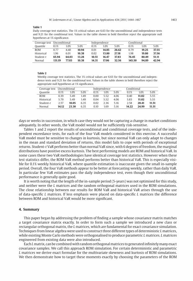
Table 1

Daily coverage test statistics. The 1% critical values are 6.63 for the unconditional and independence tests

and 9.21 for the conditional test. Values in the table shown in bold therefore reject the appropriate null

hypotheses at 1% significance.

Coverage test Unconditional Independence Conditional

Quantile 0.1% 1.0% 5.0% 0.1% 1.0% 5.0% 0.1% 1.0% 5.0%

ROM 0.77 4.40 10.94 0.01 14.85 26.62 0.79 19.25 37.55

Historical 1.96 6.01 10.38 0.02 13.80 27.18 1.98 19.80 37.56

Student-t 65.94 64.03 13.28 10.51 16.47 37.83 76.45 80.49 51.11

Normal 131.19 77.83 10.38 14.31 17.06 32.56 145.50 94.89 42.94

Table 2

Weekly coverage test statistics. The 1% critical values are 6.63 for the unconditional and indepen-

dence tests and 9.21 for the conditional test. Values in the table shown in bold therefore reject the

appropriate null hypotheses at 1% significance.

Coverage test Unconditional Independence Conditional

Quantile 0.1% 1.0% 5.0% 0.1% 1.0% 5.0% 0.1% 1.0% 5.0%

ROM 0.39 5.49 1.49 0.00 5.52 4.06 0.40 11.02 5.55

Historical 5.79 5.49 1.49 0.04 5.52 4.06 5.83 11.02 5.55

Student-t 2.57 18.05 6.35 0.02 2.36 5.16 2.58 20.41 11.51

Normal 14.12 23.30 6.35 0.10 1.69 5.16 14.22 24.99 11.51

days or weeks in succession, in which case they would not be capturing a change inmarket conditions

adequately. In other words, the VaR model would not be sufficiently risk-sensitive.

Tables 1 and 2 report the results of unconditional and conditional coverage tests, and of the inde-

pendent exceedance tests, for each of the four VaR models considered in this exercise. A successful

VaR model must be sensitive to changes in kurtosis, but since normal VaR can only adapt to changes

in the mean and standard deviation of returns, this model fails to cope with periods of exceptional

returns. Student-t VaRperforms better than normal VaR since,with 6 degrees of freedom, themarginal

distributions have positive excess kurtosis. The best performingmodels are ROM and historical VaR. In

some cases these two VaR methodologies have identical coverage test statistics. However when these

test statistics differ, the ROM VaR method performs better than historical VaR. This is especially visi-

ble for 0.1% weekly historical VaR, where quantile estimation is inaccurate given the small in-sample

period. Overall, the four VaRmethods appear to be better at forecasting weekly, rather than daily VaR.

In particular few VaR estimates pass the daily independence test, even though their unconditional

performance is generally quite good.

It is worth noting that the length of the in-sample period (5-years) was not optimised for this study,

and neither were the L matrices and the random orthogonal matrices used in the ROM simulations.

The close relationship between our results for ROM VaR and historical VaR arises through the use

of data-specific L matrices. If less emphasis were placed on data-specific L matrices the difference

between ROM and historical VaR would be more significant.

4. Summary

This paper began by addressing the problem of finding a sample whose covariance matrix matches

a target covariance matrix exactly. In order to form such a sample we introduced a new class or

rectangular orthogonalmatrix, the Lmatrices, which are fundamental for exact covariance simulation.

Techniques from linear algebrawere used to construct three different types of deterministic Lmatrices,

while existingMonte Carlomethodswere orthogonalised to produce parametric Lmatrices. Lmatrices

engineered from existing data were also introduced.

Each Lmatrix, canbecombinedwith randomorthogonalmatrices togenerated infinitelymanyexact

covariance samples. We call this approach ROM simulation. For certain deterministic and parametric

L matrices we derive exact formulae for the multivariate skewness and kurtosis of ROM simulations.

We then demonstrate how to target these moments exactly by choosing the parameters of the ROM

1464 W. Ledermann et al. / Linear Algebra and its Applications 434 (2011) 1444–1467

simulation appropriately. That is, in addition to exact covariance simulation, we have no simulation

error for these higher moments. There is an extremely small rounding error which arises when many

large matrices are multiplied together, but this is minuscule. However, since Monte Carlo methods are

parametric, simulation errors may still have a significant influence on the higher moments for ROM

simulations based on parametric L matrices.

We also explored the effect that some elementary classes of orthogonal matrices have on the

dynamic sample characteristics, and on the features of marginal distributions. Note that the multi-

variate sample moments are left invariant by these ROMs, so we can generate many different types

of sample paths that have the exactly the same multivariate moments. Features such as volatil-

ity clustering, or mimicking certain features of marginal distributions, may be important in some

applications.

Finally we carried out an empirical study that compared four different methods for computing the

value-at-risk (VaR) of a stock portfolio; this demonstrated some clear advantages of ROM simulation

as a VaR resolution methodology. Clearly, the application of ROM simulation to VaR estimation – and

by extension to portfolio optimisation – will be a productive area for future research. The ability of

ROM simulation to produce infinitely many random samples which capture historical and/or hypo-

thetical characteristics may also have great significance in other areas of finance whenever simulation

is required. And there is much scope for further investigation into the applications of ROM simulation

to other disciplines.

A. Appendix

A.1. Proof of Proposition 2.1

(1) Kurtosis

We start by expressing the Ledermannmatrix in row vector notation, writing Lmn = (�′1, . . . , �′m)′.Our objective is to evaluate κM(Lmn), for all n < m. Now since Lmn is an L matrix we know that it has

sample mean vector μn = 0n and sample covariance matrix Sn = m−1In. Simply observing that

S−1n = mIn, we deduce the following:

κM(Lmn)= 1

m

m∑i=1

{�imIn�

′i

}2

=m

m∑i=1

{�i�′i

}2.

Recall that Lmn is obtained by deleting the first r = m − 1 − n columns of the L matrix Lm,m−1,displayed in (8). We first consider the rows �i where r + 2 ≤ i ≤ m. The first i− r − 2 entries of row

i are all zero. Therefore

�i�′i =

( −(i− 1)√(i− 1)i

)2

+m−1∑k=i

(1√

k(k + 1)

)2

= i− 1

i+ m− i

mi

= m− 1

mfor r + 2 ≤ i ≤ m.

For the remaining rows �i, with 1 ≤ i ≤ r + 1 we have that

�i�′i =

m−1∑k=r+1

(1√

k(k+ 1)

)2

= m− (r + 1)

m(r + 1). (A.1)

W. Ledermann et al. / Linear Algebra and its Applications 434 (2011) 1444–1467 1465

Replacing r with n we calculate that

κM(Lmn)=m

[(m− n)n2

m2(m− n)2+ n(m− 1)2

m2

]

= n[(m− 2)+ (m− n)−1

].

(2) Skewness

Once again, knowing the sample mean and covariance matrix of Lmn exactly we can write:

τM(Lmn)= 1

m2

m∑i=1

m∑j=1

{�imIn�

′j

}3

=m

m∑i=1

{�i�′i

}3 + 2m

m∑i<j

{�i�′j

}3.

As with the evaluation of kurtosis, we consider two cases separately. Firstly, for 1 ≤ i, j ≤ r + 1, we

observe that �i = �j and hence, using (A.1), we deduce that

�i�′j =

m− (r + 1)

m(r + 1)for 1 ≤ i, j ≤ r + 1.

Our second case concerns rows �i and �j such that r + 2 ≤ j ≤ m and i < j. In this case we see that

�i�′j =−(j − 1)

(j − 1)j+

m−1∑k=j

(1√

k(k + 1)

)2

=−1

j+ m− j

mj

=− 1

m.

Combining all these terms, and after some simplification, we calculate that

τM(Lmn)=m

[(m− n)n3

m3(m− n)3+ n(m− 1)3

m3+ 2

{(m− n)(m− n− 1)n3

2m3(m− n)3+ n(2m− n− 1)

2m2

}]

= n[(m− 3)+ (m− n)−1

].

A.2. Invariance of co-skewness

Let us begin with two different samples XmX ,n = (x′1, . . . , x′m)′ and YmY ,n = (y′1, . . . , y′m)′, onthe same n random variables. Let x, y and SX , SY denote the sample means and covariance matrices of

XmX ,n,YmX ,n respectively. Given any invertible matrix Bn and column vector bn we define

XmX ,n = XmX ,nBn + 1mXb′n and YmY ,n = YmY ,nBn + 1mY

b′n. (A.2)

Now the means of XmX ,n and YmY ,n are xBn + b′n and yBn + b′n, while the covariance matrices are

B′nSXBn and B′nSYBn. So, noticing that{2(xiBn + b′n − xBn − b′n)B−1n (SX + SY )

−1(B−1n )′(yjBn + b′n − yBn − b′n)′}3

={2(xi − x)(SX + SY )

−1(yj − y)′}3

,

1466 W. Ledermann et al. / Linear Algebra and its Applications 434 (2011) 1444–1467

we deduce that τC(XmX ,n, YmY ,n) = τC(XmX ,n, YmY ,n). Hence τC is invariant under non-singular affine

transformations of the form (A.2).

A.3. Proof of Proposition 2.2

Our proposition begins with r random samples Xm1,n, . . . ,Xmr ,n, each with sample mean μn and

sample covariance matrix Sn. We adopt the following row vector notation

Xmk,n =

⎛⎜⎜⎜⎜⎝

xk1

...

xkmk

⎞⎟⎟⎟⎟⎠ for 1 ≤ k ≤ r, (A.3)

and settingm = ∑rk=1 mk , we write our concatenated sample as

Xm,n = (X′m1,n, . . . ,X′mr ,n

)′.Throughout this proof we will use the dot product notation

x · y =⎧⎨⎩ xy′ for row vectors,

x′y for column vectors.

(1) Concatenated mean vector

The mean of our concatenated sample Xmn is

m−11′mXmn = m−1r∑

k=11′mk

Xmk,n = m−1r∑

k=1mkμn = μn.

(2) Concatenated covariance matrix

Having established the mean of our concatenated sample, we can calculate the covariance matrix

of Xmn as

m−1X′mnXmn = m−1r∑

k=1X′mk,n

Xmk,n = m−1r∑

k=1mkSn = Sn.

(3) Concatenated skewness

We now calculate the Mardia [23] skewness of the concatenated sample Xmn in terms of the skew-

ness of the sample components Xm1,n, . . . ,Xmr ,n. Since we know that Mardia’s measure are invariant

under non-singular affine transformations, we begin by defining

Zmn = (Xmn − 1mμ′n)A−1n ,

where A′nAn = Sn. Then we can write Zmn = (Z′m1,n, . . . , Z′mr ,n

)′, where each component

Zmk,n = (Xmk,n − 1mkμ′n)A−1n .

As a result of these non-singular affine transformations Zmn will have sample mean vector 0n and

covariance matrix In. This will also be the case for each component Zmk,n, for 1 ≤ k ≤ r. Adopting a

row notation equivalent to (A.3), we can express

τM(Zmn)=m−2m∑i=1

m∑j=1

(zi · zj)3

=m−2⎡⎣ r∑k=1

⎧⎨⎩

mk∑i=1

mk∑j=1

(zki · zkj )3⎫⎬⎭+ 2

r∑k<1

⎧⎨⎩

mk∑i=1

mk∑j=1

(zki · zlj)3⎫⎬⎭⎤⎦

=m−2r∑

k=1m2

kτM(Zmk,n)+ 2m−2r∑

k<1

(mk + ml)2τC(Zmk,n, Zml,n).

W. Ledermann et al. / Linear Algebra and its Applications 434 (2011) 1444–1467 1467

The third statement of the proposition follows immediately from the non-singular affine invariance

property of τM and τC .(4) Concatenated kurtosis

For Mardia’s kurtosis we calculate that

κM(Zmn)=m−1m∑i=1

(zi · zi)2

=m−1r∑

k=1

⎧⎨⎩

mk∑i=1

(zki · zki )2⎫⎬⎭

=m−1r∑

k=1mkκM(Zmk,n).

Applying the non-singular affine invariance property of κM yields the final expression of the proposi-

tion.

References

[1] C. Alexander, Market Risk Analysis Volume IV, Value-at-Risk Models, Wiley, 2008.[2] M. Berry, J. Dongarra, Y. Kim, A highly parallel algorithm for the reduction of a non-symmetricmatrix to block upper-Hessenberg

form, Parallel Comput. 21 (1995) 1189.

[3] A. Cayley, Sur quelques propriétés des déterminants gauches, J. Reine Angew. Math. (Crelle’s J.) 32 (1846) 119–123.[4] P. Christoffersen, Evaluating interval forecasts, Internat. Econom. Rev. 39 (1998) 841–862.

[5] R. Courant, D. Hilbert, Wiley, 1999.[6] H. Cramer, Mathematical Methods of Statistics, Princeton University Press, 1946.

[7] P. Date, R. Mamon, L. Jalen, A new moment matching algorithm for sampling from partially specified symmetric distributions,Oper. Res. Lett. 36 (2008) 669–672.

[8] L. Gemignani, A unitaryHessenbergQR-based algorithmvia semiseparablematrices, J. Comput. Appl.Math. 184 (2005) 505–517.

[9] W. Givens, Computation of plane unitary rotations transforming a generalmatrix to triangular form, SIAM J. Appl.Math. 6 (1958)26–50.

[10] P. Glasserman, Monte Carlo Methods in Financial Engineering, Springer, 2004.[11] G. Golub, C. Loan, Matrix Computations, third ed., Johns Hopkins University Press, Baltimore, 1996.

[12] S. Gutjahr, N. Henze,M. Folkers, Shortcomings of generalized affine invariant skewnessmeasures, J. Multivariate Anal. 71 (1999)1–23.

[13] N. Higham, Accuracy and Stability of Numerical Algorithms, Society for Industrial and Applied Mathematics, 1996.[14] A. Householder, Unitary triangularization of a non-symmetric matrix, J. ACM 5 (1958) 339–342.

[15] T. Kollo, Multivariate skewness and kurtosis measures with an application in ICA, J. Multivariate Anal. 99 (2008) 2328–2338.

[16] P. Kupiec, Techniques for verifying the accuracy of risk measurement models, J. Derivatives 2 (1995) 173–184.[17] H. Lancaster, The Helmert matrices, Amer. Math. Monthly 72 (1) (1965) 4–12.

[18] K.-H. Li, Generation of random matrices with orthonormal columns and multivariate normal variates with given sample meanand covariance, J. Statist. Comput. Simulation 43 (1992) 11–18.

[19] J. Lyhagen, A method to generate multivariate data with the desired moments, Comm. Statist. Simulation Comput. 37 (2008)2063–2075.

[20] B. Mandelbrot, A. Fisher, L. Calvet, A multifractal model of asset returns, Cowles Foundation Discussion Paper, 1997.

[21] K. Mardia, I. Dryden, The statistical analysis of shape data, Biometrika 76 (2) (1989) 271–281.[22] K. Mardia, A.N. Walder, Shape analysis of paired landmark data, Biometrika 81 (1) (1994) 185–196.

[23] K.V. Mardia, Measures of multivariate skewness and kurtosis with applications, Biometrika 57 (3) (1970) 519.[24] A. Meucci, Simulations with exact means and covariances, Risk Mag. 22 (2009) 89–91.

[25] C. Perignon, D. Smith, The level and quality of value-at-risk disclosure by commercial banks, J. Banking Finance 34 (2010)362–377.

[26] V. Prasolov, Problems and Theorems in Linear Algebra, vol. 134American Mathematical Society, Providence, RI, 1994.