2010-11-08 cugs advanced course
TRANSCRIPT

2010-11-08
1
Heuristic Algorithms for
C bi t i l O ti i ti P bl
Heuristic Algorithms for
C bi t i l O ti i ti P bl
CUGS Advanced CourseCUGS Advanced Course
Combinatorial Optimization ProblemsCombinatorial Optimization Problems
Petru Eles and Zebo Peng
Embedded Systems Laboratory (ESLAB)Linköping University
Petru Eles and Zebo Peng
Embedded Systems Laboratory (ESLAB)Linköping University
ObjectivesObjectives
Introduction to combinatorial optimization problems.
Basic principles of heuristic techniques.
Modern heuristic algorithms:
Simulated annealing.
Tabu search.
Genetic algorithms.
Evaluation of heuristic algorithms.
22Zebo Peng, IDA, LiTHZebo Peng, IDA, LiTH
Evaluation of heuristic algorithms.
Application of heuristic techniques to design automation and software engineering.

2010-11-08
2
Course OrganizationCourse Organization
Introductory lectures Lectures in 3 blocks.
• The future time slots?• The future time slots?
Mostly on principles and basic algorithms.
Project part: Implementation of one or two heuristic algorithms.
You can select the application area, e.g., related to
33Zebo Peng, IDA, LiTHZebo Peng, IDA, LiTH
pp , g ,your current research topic.
Documentation of the implementation work in a term paper.
Presentation of the results in a common seminar.
Reference LiteratureReference Literature
C. R. Reeves, "Modern Heuristic Techniques for Combinatorial Problems," Blackwell Scientific P bli ti 1993Publications, 1993.
Z. Michalewicz, "Genetic Algorithms + Data Structures = Evolution Programs" Spinger-Verlag, 1992.
A. H. Gerez, "Algorithms for VLSI Design Automation," John Wiley & Sons, 1999.
44Zebo Peng, IDA, LiTHZebo Peng, IDA, LiTH

2010-11-08
3
Additional PapersAdditional Papers
A. Colorni et al., “Heuristics from Nature for Hard Combinatorial Optimization Problems,” Int. Trans. Operations Research Vol 3 No 1 1996Operations Research, Vol. 3, No. 1, 1996.
S. Kirkpatrick et al., “Optimization by Simulated Annealing,” Science, Vol. 220, No. 4598, 1983.
… (to be distributed in each lecture block).
L
55Zebo Peng, IDA, LiTHZebo Peng, IDA, LiTH
Lecture notes.
Lecture ILecture I
Combinatorial optimization
Overview of optimization heuristics
Neighborhood search
66Zebo Peng, IDA, LiTHZebo Peng, IDA, LiTH
Evaluation of heuristics

2010-11-08
4
IntroductionIntroduction
Many computer science problems deal with the choice of a best set of parameters to achieve some goal.
E Pl t d ti bl i VLSI d iEx. Placement and routing problem in VLSI design:
Given a set of VLSI cells, with ports on the boundaries, and a collection of nets, which are sets of ports that need to be wired together
Find a way to place the cells and run the wires so that the total wiring distance is minimized and each wire is
77Zebo Peng, IDA, LiTHZebo Peng, IDA, LiTH
gshorter than a given constant.
Placement and RoutingPlacement and Routing
A
CB
88Zebo Peng, IDA, LiTHZebo Peng, IDA, LiTH
CB

2010-11-08
5
Design Space ExplorationDesign Space Exploration
The majority of design space exploration tasks can be viewed as optimization problems:
To findTo find the architecture (type and number of processors, memory modules,
and communication blocks, as well as their interconnections),
the mapping of functionality onto the architecture components, and
the schedules of basic functions and communications,
such that
99Zebo Peng, IDA, LiTHZebo Peng, IDA, LiTH
a cost function (in terms of implementation cost, performance, power, etc.) is minimized; and
a set of constraints are satisfied.
Mathematical OptimizationMathematical Optimization The optimization problems can usually be formulated as to
Minimize f(x)Subject to gi(x) bi; i = 1, 2, ..., m;
wherex is a vector of decision variables;f is the cost (objective) function;gi’s are a set of constraints.
If f and gi’s are linear functions, we have a Linear
1010Zebo Peng, IDA, LiTHZebo Peng, IDA, LiTH
a d gi s a e ea u ct o s, e a e a eaProgramming problem.
LP problems can be solved by, e.g., the simplex algorithm, which is an exact method, i.e., it will always identify the optimal solution if it exists.

2010-11-08
6
Type of SolutionsType of Solutions
A solution to an optimization problem specifies the values of the decision variables, x, and therefore also the value of the objective function f(x)the value of the objective function, f(x).
A feasible solution satisfies all constraints.
An optimal solution is feasible and gives the best objective function value.
A near-optimal solution is feasible and provides a superior objective function value but not necessarily
1111Zebo Peng, IDA, LiTHZebo Peng, IDA, LiTH
superior objective function value, but not necessarily the best.
Combinatorial Optimization (CO)Combinatorial Optimization (CO)
There are two types of optimization problems: Continuous, with an infinite number of feasible
solutions;
Combinatorial, with a finite number of feasible solutions.
In an CO problem, the decision variables are discrete, i.e., where the solution is a set, or a sequence, of integers or other discrete objects.
Ex System partitioning can be formulated as follows:
1212Zebo Peng, IDA, LiTHZebo Peng, IDA, LiTH
Ex. System partitioning can be formulated as follows:
Given a graph with costs on its edges, partition the nodes into k subsets no larger than a given maximum size, to minimize the total cost of the cut edges.

2010-11-08
7
The System Partitioning ProblemThe System Partitioning Problem
5
35
2
45
5
35
5
5665
20
40
15
A feasible solution for the k-way partitioning can be
8
35
3 4
35
624 6723
Two-way partitioning
1313Zebo Peng, IDA, LiTHZebo Peng, IDA, LiTH
represented as:
xi = j; j {1, 2, ..., k}, i = 1, 2, ..., n.
Features of CO ProblemsFeatures of CO Problems
Most CO problems, e.g., system partitioning with constraints, for digital system designs are NP-compete.
The time needed to solve an NP-compete problem grows The time needed to solve an NP-compete problem grows exponentially with respect to the problem size n.
For example, to enumerate all feasible solutions for a scheduling problem (all possible permutation), we have: 20 tasks in 1 hour (assumption);
21 tasks in 20 hour;
1414Zebo Peng, IDA, LiTHZebo Peng, IDA, LiTH
22 tasks in 17.5 days;
...
25 tasks in 6 centuries.

2010-11-08
8
An Exact Approach to COAn Exact Approach to CO
Many CO problems can be formulated as an Integer Linear Programming (ILP) problem, and solved by an ILP solverILP solver.
It is inherently more difficult to solve an ILP problem than the corresponding Linear Programming problem.
Because there is no derivative information and the surface are not smooth.
1515Zebo Peng, IDA, LiTHZebo Peng, IDA, LiTH
The size of problem that can be solved successfully by ILP algorithms is an order of magnitude smaller than the size of LP problems that can be easily solved.
Simple Simple vsvs Hard Problems Hard Problems
Few decision variables
Independent variables
Many decision variables
Dependent variables Independent variables
Single objective
Objective easy to calculate (additive)
No or light constraints
Dependent variables
Multi objectives
Objective difficult to calculate
Severely constraints
1616Zebo Peng, IDA, LiTHZebo Peng, IDA, LiTH
Feasibility easy to determine
Deterministic
Feasibility difficult to determine
Stochastic

2010-11-08
9
Approach to COApproach to CO
Why not solve the corresponding LP and round the solutions to the closest integer?
Ex if x = 2 75 x will be set of 3 Ex. if x1 = 2,75, x1 will be set of 3.
This will be plausible if the solution is expected to contain large integers and therefore is insensitive to rounding.
Otherwise, rounding could be as hard as solving the
1717Zebo Peng, IDA, LiTHZebo Peng, IDA, LiTH
original problem from scratch, since rounding does not usually even give a feasible solution!
The RoundingThe Rounding--Off ProblemOff Problem
Ex. To maximize f(x1, x2) = 5x1+8x2
subject to x1 + x2 ≤ 6,
5 +9 ≤ 455x1 +9x2≤ 45,
x1, x2 ≥ 0, and be integers.
Continuous optimum
Round off Nearest feasible point
Integer optimum
1818Zebo Peng, IDA, LiTHZebo Peng, IDA, LiTH
x1 2.25 2 2 0
x2 3.75 4 3 5
f 41.25 Infeasible solution
34 40

2010-11-08
10
The Traveling Salesman ProblemThe Traveling Salesman Problem
A salesman wishes to find a route which visits each of ncities once and only once at minimal cost.
813
2048 7
24
17
148
15
347
2
6
1919Zebo Peng, IDA, LiTHZebo Peng, IDA, LiTH
A feasible solution can be represented as a permutation of the numbers from 1 to n.The size of the solution space is therefore (n - 1)!
ILP Formulation of TSPILP Formulation of TSP
A solution can be expressed by:
xij = 1 if he goes from city i to j, with Cij as cost;
0 th i0 otherwise.
The problem can be formulated as:
n
i
n
jijij xc
1 1
minimize
) 21( 1 , ...,n, jxn
ij
1
1
1
1
1
xij
subject to
2020Zebo Peng, IDA, LiTHZebo Peng, IDA, LiTH
) 2121( 0
) 21( 11
1
, ..., n, , ...,n; j, ix
, ...,n, ix
ij
n
jij
i
11
(Each city should be visited once and only once.)

2010-11-08
11
Additional TSP Constraints Additional TSP Constraints
12
To avoid disjoint sub-tours, (2n - 1) additional constraints must be added.
Ex
347
6
2121Zebo Peng, IDA, LiTHZebo Peng, IDA, LiTH
Ex.
.14,73,71,74,63,61,64,23,21,2 xxxxxxxxx
The BranchThe Branch--andand--Bound ApproachBound Approach
Traverse an implicit tree to find the best leaf (solution).
4-City TSP0
y
0 1 2 3
0 3 6 41
0 40 5
0 4
0
1
2
3
3
40
41
0
1
2222Zebo Peng, IDA, LiTHZebo Peng, IDA, LiTH
0 3
423
Total cost of this solution = 88

2010-11-08
12
BranchBranch--andand--Bound ExBound Ex0 1 2 3
0 3 6 41
0 40 5
0 4
0
0
1
2
3 {0}
Low-bound on the cost function.
Search strategy
0
{0,1}
{0,1,2}
L 0
L 3
{0,1,3}
{0,2}L 6
{0,2,1}
{0,3}L 41
{0,2,3} {0,3,1} {0,3,2}
2323Zebo Peng, IDA, LiTHZebo Peng, IDA, LiTH
{0,1,2,3}L = 88
L 43
{0,1,3,2}
L 8
L = 18
L 46
{0,2,1,3}L = 92
{0,2,3,1}
L 10
L = 18{0,3,1,2} {0,3,2,1}
L 46 L 45
L = 92 L = 88
Some ConclusionsSome Conclusions
The integer programming problem is inherently more difficult to solve than the simple linear programming problemproblem.
We need heuristics, which seek near-optimal solutions at a reasonable computational cost without being able to guarantee either feasibility or optimality.
Heuristic techniques are widely used to solve many NP-hard problems.
2424Zebo Peng, IDA, LiTHZebo Peng, IDA, LiTH
a d p ob e s

2010-11-08
13
Lecture ILecture I
Combinatorial optimization
Overview of optimization heuristics
Neighborhood search
2525Zebo Peng, IDA, LiTHZebo Peng, IDA, LiTH
Evaluation of heuristics
Heuristic: adj. & n.Heuristic: adj. & n.
Webster’s 3rd New International Dictionary:
Greek heuriskein: to find.
“providing aid or direction in the solution of a problem but otherwise unjustified or incapable of justification.”
“of or relating to exploratory problem-solving techniques that utilize self-educating techniques to improve performance.”
2626Zebo Peng, IDA, LiTHZebo Peng, IDA, LiTH
The Concise Oxford Dictionary:
“serving to discover; (of computer problem-solving) proceeding by trial and error.”

2010-11-08
14
Why HeuristicsWhy Heuristics
Many exact algorithms involve a huge amount of computation effort.
The decision variables have frequently complicated The decision variables have frequently complicated interdependencies. To improve a design, e.g., one might have to simultaneously change
the values of several parameters.
We have often nonlinear cost functions and constraints, even no mathematical functions.
Ex The cost function f can for example be defined by a computer
2727Zebo Peng, IDA, LiTHZebo Peng, IDA, LiTH
Ex. The cost function f can, for example, be defined by a computer program (e.g., for power estimation).
Approximation of the model for optimization. A near optimal solution is usually good enough and could be even
better than the theoretical optimum.
Heuristic Approaches to COHeuristic Approaches to COProblem specific Generic methods
• Clustering• List scheduling
• Branch and bounductiv
e
• List scheduling• Left-edge algorithm
• Divide and conquer
Con
str
atio
nal
ovem
ent
• Kernighan-Lin • Neighborhood search
Si l t d li
2828Zebo Peng, IDA, LiTHZebo Peng, IDA, LiTH
Tra
nsfo
rma
(Ite
rativ
e im
pro e g a
algorithm• Simulated annealing• Tabu search• Genetic algorithms

2010-11-08
15
List SchedulingList Scheduling Resource-constrained (RC) scheduling problem:
To find a (optimal) schedule for a set of operations that obeys the data dependency and utilizes only the available functional units.
For each control step the operations that are available to be scheduled For each control step, the operations that are available to be scheduled are kept in a list.
The list is ordered by some priority function:
The length of path from the operation to the end of the block;
Mobility: the number of control steps from the earliest to the latest feasible control step.
Each operation on the list is scheduled one by one if the resources it needs are free; otherwise it is deferred to the next control step
2929Zebo Peng, IDA, LiTHZebo Peng, IDA, LiTH
needs are free; otherwise it is deferred to the next control step.
Until the whole schedule is constructed, no information about the schedule length is available.
11
22
List Scheduling ExampleList Scheduling Example
++ ** **++++11 22 33 44 55
++ 11**
33
++ 44 55
Con
trol
Ste
psC
ontr
ol S
teps
33
55
44
22++
++
**
--
**
++66 77 88
99 1010
++ 22
++ **
-- 66
++ 88**
99
3030Zebo Peng, IDA, LiTHZebo Peng, IDA, LiTH
55
66 ++ 77**
1010

2010-11-08
16
The KernighanThe Kernighan--Lin Algorithm (KL)Lin Algorithm (KL)
A graph is partitioned into two clusters of arbitrary size, by minimizing a given objective function.
KL is based on an iterative partitioning strategy: KL is based on an iterative partitioning strategy: The algorithm starts with two arbitrary clusters C1 and
C2.
The partitioning is then iteratively improved by moving nodes between the clusters.
At each iteration, the node which produces the minimal value of the cost function is moved; this value can
3131Zebo Peng, IDA, LiTHZebo Peng, IDA, LiTH
value of the cost function is moved; this value can, however, be greater than the value before moving the node.
KL Execution Trace ExampleKL Execution Trace Example
165000
170000
150000
155000
160000
165000
Cos
t fu
nctio
n va
lue
3232Zebo Peng, IDA, LiTHZebo Peng, IDA, LiTH
140000
145000
0 5 10 15 20 25 30 35 40 45
Number of iterations

2010-11-08
17
BranchBranch--andand--Bound ExBound Ex0 1 2 3
0 3 6 41
0 40 5
0 4
0
0
1
2
3 {0}
Low-bound on the cost function.
Search strategy
0
{0,1}
{0,1,2}
L 0
L 3
{0,1,3}
{0,2}L 6
{0,2,1}
{0,3}L 41
{0,2,3} {0,3,1} {0,3,2}
3333Zebo Peng, IDA, LiTHZebo Peng, IDA, LiTH
{0,1,2,3}L = 88
L 43
{0,1,3,2}
L 8
L = 18
L 46
{0,2,1,3}L = 92
{0,2,3,1}
L 10
L = 18{0,3,1,2} {0,3,2,1}
L 46 L 45
L = 92 L = 88
Lecture ILecture I
Combinatorial optimization
Overview of optimization heuristics
Neighborhood search
3434Zebo Peng, IDA, LiTHZebo Peng, IDA, LiTH
Evaluation of heuristics

2010-11-08
18
Search as HeuristicsSearch as Heuristics
Search the term used for constructing or improving solutions to obtain the optimum or near-optimum.
S l ti E di ( ti th l ti ) Solution Encoding (representing the solution).
Neighborhood Nearby solutions (in the encoding or solution space).
Move Transforming current solution to another (usually neighboring) solution.
E l i T h l i ’ f ibili d
3535Zebo Peng, IDA, LiTHZebo Peng, IDA, LiTH
Evaluation To compute the solutions’ feasibility and objective function value.
Local search based on greedy heuristic (local optimizers).
Neighborhood Search MethodNeighborhood Search Method Step 1(Initialization)
(A) Select a starting solution xnow X.(B) xbest = xnow, best_cost = c(xbest).
Step 2 (Choice and termination)Choose a solution xnext N(xnow).If no solution can be selected or the terminating criteria apply, then the
method stop.
Step 3 (Update)R t now next
3636Zebo Peng, IDA, LiTHZebo Peng, IDA, LiTH
Re-set xnow = xnext.If c(xnow) < best_cost, perform Step 1(B). Goto Step 2.
N(x) denotes the neighborhood of x, which is a set of solutions reachable from x by a simple transformation (move).

2010-11-08
19
Neighborhood Search MethodNeighborhood Search Method
The neighborhood search method is very attractive for many CO problems as they have a natural neighborhood structure, which can be easily defined and evaluated.
E Graph partitioning s apping t o nodes Ex. Graph partitioning: swapping two nodes.
5
8
35
2
3
45
5
435
5
6
5665
24
20
40
67
15
23
3737Zebo Peng, IDA, LiTHZebo Peng, IDA, LiTH
5
8
35
2
3
45
5
4
35
5
6
5665
24
20
40
67
15
23
The Descent MethodThe Descent Method Step 1(Initialization)
Step 2 (Choice and termination)Choose xnext N(xnow) such that c(xnext) < c(xnow) and terminate if noChoose x N(x ) such that c(x ) < c(x ), and terminate if no
such xnext can be found.
Step 3(Update)
C t
The descent process can easily be stuck at a local optimum:
3838Zebo Peng, IDA, LiTHZebo Peng, IDA, LiTH
Cost
Solutions

2010-11-08
20
Many Local Optima Many Local Optima
21
23
25
27
3939Zebo Peng, IDA, LiTHZebo Peng, IDA, LiTH2 1
2,7
3,3
3,9
45,65,
8
6
15
17
19
Dealing with Local OptimalityDealing with Local Optimality
Enlarge the neighborhood.
Start with different initial solutions.T ll “ hill ” To allow “uphill moves”: Simulated annealing Tabu search
Cost
4040Zebo Peng, IDA, LiTHZebo Peng, IDA, LiTH
Cost
SolutionsX

2010-11-08
21
Heuristics from NatureHeuristics from Nature
Model (loosely) a phenomenon existing in nature, derived from physics, biology and social sciences:
Annealing Annealing.
Evolution.
Usually non-deterministic, including some randomness features.
Often has implicit parallel structure or enable parallel
4141Zebo Peng, IDA, LiTHZebo Peng, IDA, LiTH
implementation.
Some Heuristics from NatureSome Heuristics from Nature
Genetic algorithms evolution process of nature.
Simulated annealing heat treatment of materials.
Tabu search search and intelligent uses of memory.
Neural nets mimic biological neurons.
Ant system ant colony.
Simulating the behavior of a set of agents that cooperate to solve an optimization problem by means
4242Zebo Peng, IDA, LiTHZebo Peng, IDA, LiTH
of very simple communications.
Ants leave trails on paths they visit, which will be followed by other ants, probabilistically.
The shorter paths will be enhanced by many ants.

2010-11-08
22
Advantages of MetaAdvantages of Meta--HeuristicsHeuristics
Very flexible
Often global optimizersg p
Often robust to problem size, problem instance and random variables
May be the only practical alternative
4343Zebo Peng, IDA, LiTHZebo Peng, IDA, LiTH
Lecture ILecture I
Combinatorial optimization
Overview of optimization heuristics
Neighborhood search
4444Zebo Peng, IDA, LiTHZebo Peng, IDA, LiTH
Evaluation of heuristics
2010-11-08
23
Evaluation of HeuristicsEvaluation of Heuristics
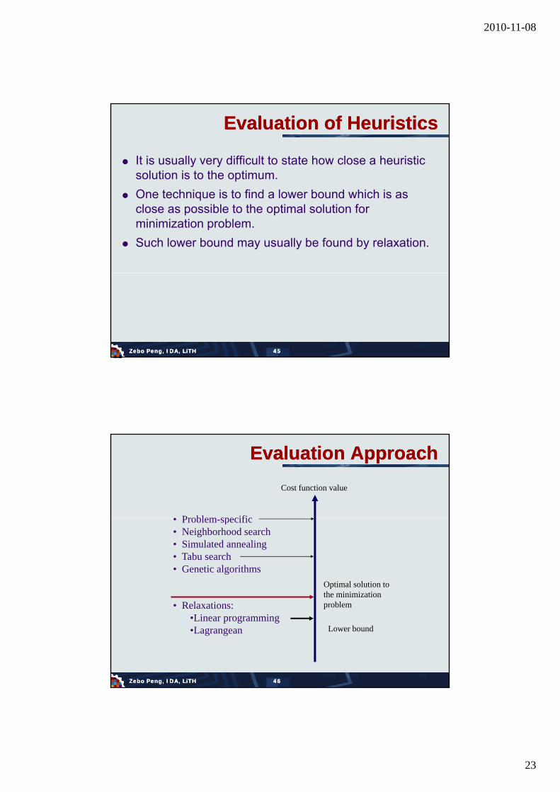
It is usually very difficult to state how close a heuristic solution is to the optimum.
One technique is to find a lower bound which is as close as possible to the optimal solution for minimization problem.
Such lower bound may usually be found by relaxation.
4545Zebo Peng, IDA, LiTHZebo Peng, IDA, LiTH
Evaluation ApproachEvaluation Approach
Cost function value
• Problem specific
Optimal solution tothe minimization
bl
• Problem-specific• Neighborhood search• Simulated annealing• Tabu search• Genetic algorithms
R l ti
4646Zebo Peng, IDA, LiTHZebo Peng, IDA, LiTH
problem• Relaxations:•Linear programming•Lagrangean Lower bound

2010-11-08
24
SummarySummary
Combinatorial optimization is the mathematical study of finding an optimal arrangement, grouping, ordering, or selection of discrete objects usually finite inor selection of discrete objects usually finite in numbers.
- Lawler, 1976
In practice, combinatorial problems are often very difficult to solve, because there is no derivative i f ti d th f t th
4747Zebo Peng, IDA, LiTHZebo Peng, IDA, LiTH
information and the surfaces are not smooth.
We need therefore to develop heuristic algorithms that seek near-optimal solutions.