20. 7. 2003 1

II–4 Microscopic View of Electric Currents

20. 7. 2003 2

Main Topics

• The Resistivity and Conductivity.

• Conductors, Semiconductors and Insulators.

• The Speed of Moving Charges.

• The Ohm’s Law in Differential Form.

• The Classical Theory of Conductivity.

• The Temperature Dependence of Resistivity

• The Thermocouple

20. 7. 2003 3

The Resistivity and Conductivity I

• Let’s have an ohmic conductor i.e. the one which obeys the Ohm’s law:

V = RI• The resistance R depends both on the geometry

and the physical properties of the conductors. If we have a homogeneous conductor of the length l and the cross-section A we can define the resistivity and its reciprocal the conductivity by:

A

l

A

lR

1

20. 7. 2003 4

The Resistivity and Conductivity II

• The resistivity is the ability of materials to defy the electric current. With the same geometry a stronger field is necessary if the resitivity is high to reach a certain current.

• The SI unit of resistivity is 1 m. • The conductivity is the ability to conduct the

electric current. • The SI unit of conductivity is 1 -1m-1. • A special unit siemens exists 1 Si = --1.

20. 7. 2003 5

Mobile Charge Carriers I

• Generally, they are charged particles or pseudo-particles which can move freely in conductors.

• They can be electrons, holes or various ions. • The conductive properties of materials depend

on how freely their charge carriers can move and this depends on deep structure properties of the particular materials.

20. 7. 2003 6

Mobile Charge Carriers II

• E.g. in solid conductors each atom shares some of its electrons, those least strongly bounded, with the other atoms.

• In zero electric field these electrons normally move chaotically at very high speeds and undergo frequent collisions with the array of atoms of the solid. It resembles thermal movement of gas molecules electron gas.

20. 7. 2003 7

Mobile Charge Carriers III

• In non-zero field the electrons also have some relatively very low drift speed in the opposite direction then has the field.

• The collisions are the predominant mechanism for the resistivity (of metals at normal temperatures) and they are also responsible for the power loses in conductors.

20. 7. 2003 8

Differential Ohm’s Law I

• Let us again have a conductor of the length l and the cross-section A and consider only one type of charged carriers and a uniform current, which depends on their:• density n i.e. number in unit volume

• charge q

• drift speed vd

20. 7. 2003 9

Differential Ohm’s Law II

• Within some length x of the conductor there is a charge:

Q = n qx A• The volume which passes some plane in 1 second

is Ax/t = vd A so the current is:

I = Q/t = n q vd A = j A• Where j is so called current density. Using Ohm’s

law and the definition of the conductivity:I = j A = V/R = El A/l j = E

20. 7. 2003 10

Differential Ohm’s Law III

j = E• This is Ohm’s law in differential form. • It has a similar form as the integral law but

it contains only microscopic and non-geometrical parameters.

• So it is a the starting point of theories which try to explain conductivity.

• Generally, it is valid in vector form: Ej

20. 7. 2003 11

Differential Ohm’s Law IV

• Its meaning is that the magnitude of the current density is directly proportional to the field and that the charge carriers move along the field lines.

• For deeper insight it is necessary to have at least rough ideas about the magnitudes of the parameters involved in the Ohms law.

20. 7. 2003 12

An Example I

• Let us have a current of 10 A running through a copper conductor with the cross-section of 3 10-6 m2. What is the charge density and drift velocity if every atom contributes by one free electron? • The atomic weight of Cu is 63.5 g/mol. • The density = 8.95 g/cm3.

20. 7. 2003 13

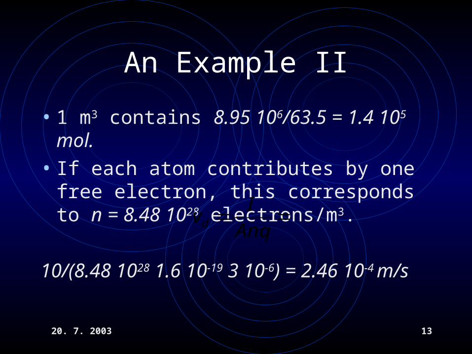
An Example II

• 1 m3 contains 8.95 106/63.5 = 1.4 105 mol.

• If each atom contributes by one free electron, this corresponds to n = 8.48 1028 electrons/m3.

10/(8.48 1028 1.6 10-19 3 10-6) = 2.46 10-4 m/s

Anq

Ivd

20. 7. 2003 14

The Internal Picture

• The drift speed is extremely low. It would take the electron 68 minutes to travel 1 meter! In comparison, the average speed of the chaotic movement is of the order of 106 m/s.

• So we have currents of the order of 1012 A running in random directions and so compensating themselves and relatively a very little currents caused by the field.

• It is similar as in the case of charging something a very little un-equilibrium.

20. 7. 2003 15

A Quiz

• The drift speed of the charge carriers is of the order of 10-4 m/s.

Why it doesn’t take hours before a bulb lights when we switch on the light?

20. 7. 2003 16

The Answer

• By switching on the light we actually connect the voltage across the wires and the bulb and thereby create the electric field which moves the charge carriers. But the electric field spreads with the speed of light c = 3 108 m/s, so all the charges start to move (almost) simultaneously.

20. 7. 2003 17

The Classical Model I

• Let’s try to explain the drift speed using more elementary parameters. We suppose that during some average time between the collision the charge carriers are accelerated by the field. And non-elastic collision stops them.

• Using what we know from electrostatics:

vd = qE/m

20. 7. 2003 18

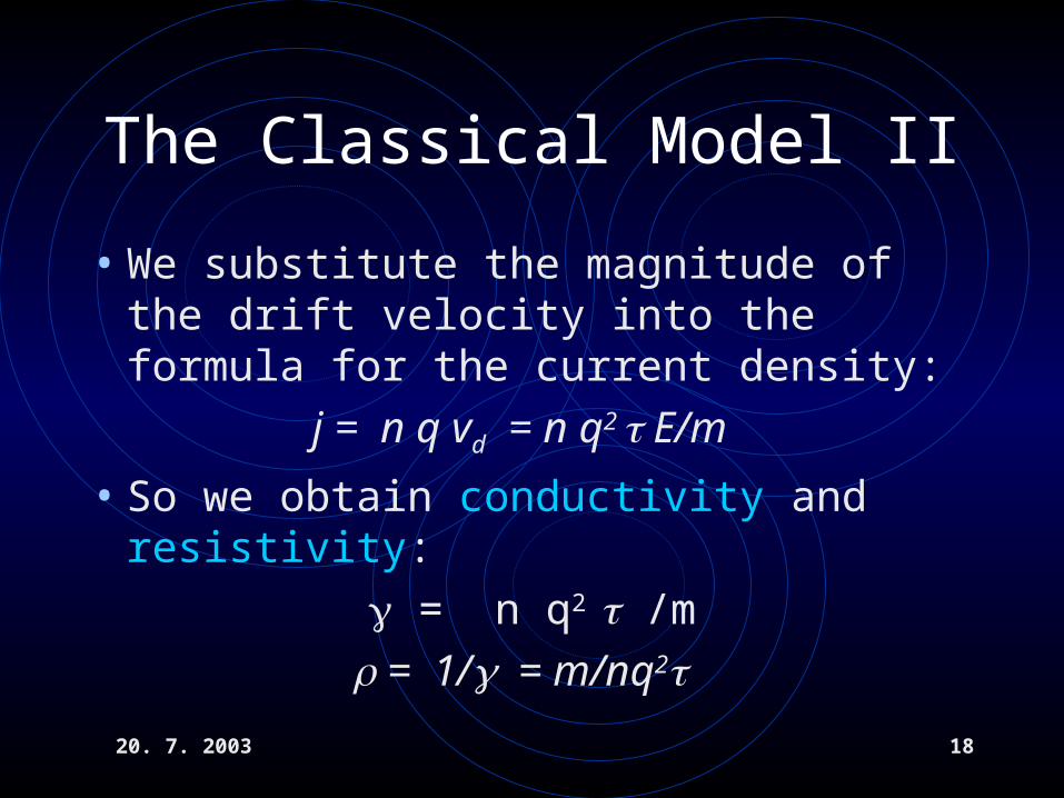
The Classical Model II

• We substitute the magnitude of the drift velocity into the formula for the current density:

j = n q vd = n q2 E/m

• So we obtain conductivity and resistivity:

= n q2 /m

= 1/ = m/nq2

20. 7. 2003 19

The Classical Model III

• It may seem that we have just replaced one set of parameters by another.

• But here only the average time is unknown and it can be related to mean free path and the average thermal speed using well established theories similar to those studying ideal gas properties.

• This model predicts dependence of the resistivity on the temperature but not on the electric field.

20. 7. 2003 20

Temperature Dependence of Resistivity I

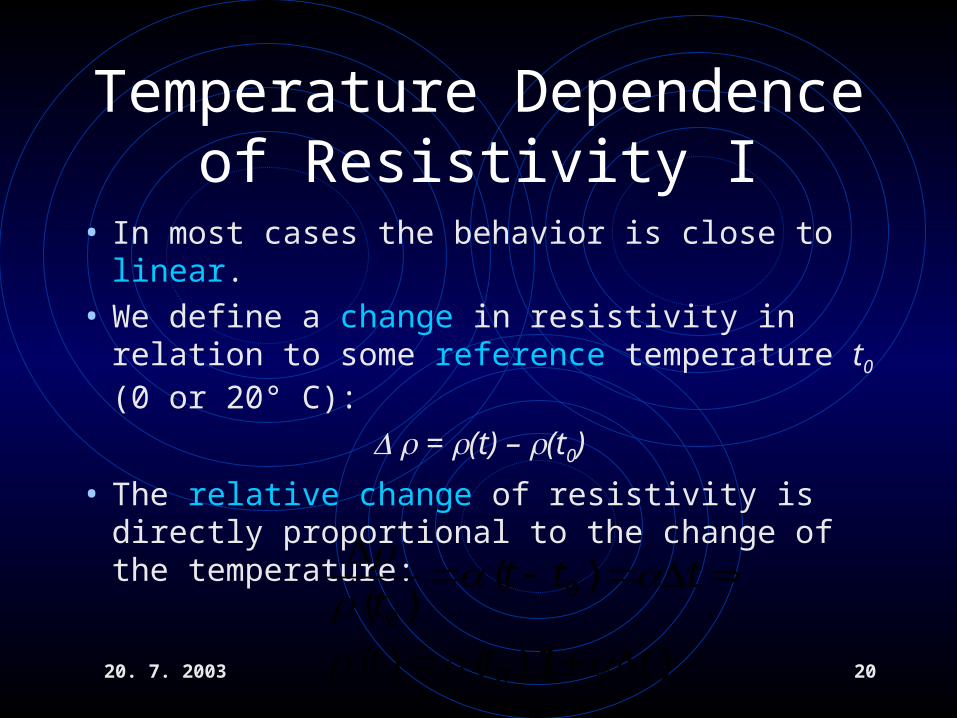
• In most cases the behavior is close to linear.

• We define a change in resistivity in relation to some reference temperature t0 (0 or 20° C):

= (t) – (t0)

• The relative change of resistivity is directly proportional to the change of the temperature:

)1)(()(

)()(

0

00

ttt

tttt

20. 7. 2003 21

Temperature Dependence of Resistivity II

[K-1] is the linear temperature coefficient.• It is given by the temperature dependence of n and vd.

• It can be negative e.g. in the case of semiconductors (but exponential behavior).

• In larger temperature span we have to add a quadratic term etc.

/(t0) = (t – t0) = t + (t)2 + …

(t) = (t0)(1 + t + (t)2 + …)

20. 7. 2003 22

The Thermocouple I• The thermocouple is an example of a

transducer, a device which transfers some physical quality (here temperature) to an electrical one.

• Unlike other temperature sensors e.g. the platinum thermometer or thermistor which use the thermal conductivity change of metals or semiconductors, the thermocouple is a power-source.

20. 7. 2003 23

The Thermocouple II• It is based on thermoelectric or Seebeck

(Thomas 1821) effect : If we keep a difference of temperature on two ends of a conductive wire also potential difference appears between these ends.

• This voltage is proportional to the temperature difference and some a material parameter Seebeck’s coefficient.

20. 7. 2003 24

The Thermocouple III• Let’s connect two conductors A and B in one

point, which we keep at temperature t1.

• The other ends, which are at room temperature t0 will have voltages with respect to their contact point :

VA=kA(t1-t0) and VB=kB(t1-t0)

• A voltmeter connected between these ends shows :

VAB = VB - VA= (kB - kA)(t1 - t0)

20. 7. 2003 25

The Thermocouple IV• As a thermocouple two wires with sufficiently

different Seebeck’s coefficient can be used.

• Usually around ten selected pairs of materials are frequently used. They are named J, K … and their calibration parameters are known. They differ e.g. in temperature span where they are used.

• When using one thermocouple its voltage depends on room temperature which is not a very convenient property.

20. 7. 2003 26

The Thermocouple V• A simple possibility to get rid of this dependence

is to use a pair of thermocouples.• Let use make a second connection of conductors A and

B and place it into known temperature t2.

• The we cut one of the conductors (e.g. B) in a place on room temperature t0. The voltages of the points of disconnection X and Y with respect to the first common point is : VX = kB(t1 - t0)

VY = kA(t1 - t2) + kB(t2 - t0)

20. 7. 2003 27

The Thermocouple VI• And the voltage between these points is :

VXY = VY - VX = kA(t1 - t2) + kB(t2 - t0) - kB(t1 - t0)

so finally : VXY = (kA- kB)(t1 - t2)

• The dependence on the room temperature has really vanished. The price is the necessity to use a bath with the reference temperature t2. Usually some well defined phase transitions e.g. (melting of ice in water) are used. But care has to be taken e.g. for pressure dependence.

20. 7. 2003 28

The Thermocouple VII• Modern instruments (equipped with

microprocessors) usually measure the room temperature, so they can simulate the “cold junction” (reference junction) and using only one thermocouple is sufficient.

• They can be, however, only used with the types of thermocouples for which they are preprogrammed and instructions how to precisely connect the thermocouple have to be obeyed.

20. 7. 2003 29

Peltier’s Effect• Thermoelectric effect works also the other way. If

current flows through a junction of two different materials, heat can be transferred into or from this junction.

• This is so called Peltier effect (Jean 1834).• Peltier cells are commercially available.

• They can be used to control conveniently temperature of some volume of interest in a temperature span of circa – 50 to 200 °C. They can both heat and cool!

• In special cases e.g. in space ships they can even be used as power sources.

20. 7. 2003 30

Homework

• 26 – 3, 4, 10, 11, 40

• Study guides

20. 7. 2003 31

Things to read

• This lecture covers :

Chapter 25 – 4, 8, 9 and 26 – 6

• Advance reading

Chapters 21 – 26 except 25 – 7, 26 – 4

• See demonstrations: http://buphy.bu.edu/~duffy/semester2/semester2.html