2 sw simulation overview - rice university · 2 sw simulation overview ... shape memory materials,...

FEA Concepts: SW Simulation Overview J.E. Akin

Draft 13.0. Copyright 2009. All rights reserved. 21

2 SW Simulation Overview

2.1 Simulation Study Capabilities

The SW Simulation software offers several types of linear studies including:

Buckling: A buckling study calculates a load factor multiplier for axial loads to predict when the axial loads will cause sudden, large catastrophic transverse displacements. Slender structures subject to axial loads can fail due to buckling at load levels far lower than those required to cause material failure.

Drop Test: Drop test studies evaluate the impact effect of dropping the design on a rigid floor. You can specify the dropping distance or the velocity at the time of impact in addition to gravity. The program solves a dynamic problem as a function of time using explicit integration methods. After the analysis is completed, you can plot and graph the time history of the displacements, velocities, accelerations, strains, and stresses.

Dynamic Analysis: This type of time‐history study assumes that the materials are linear. Mass and inertia effects are included and damping is available. The applied loads are time‐dependent. The loads can be deterministic (periodic, non‐periodic), or non‐deterministic (random) which means that they cannot be precisely predicted but they can be described statistically.

Fatigue: Fatigue studies evaluate the consumed life of an object based on fatigue events. Repeated loading weakens materials over time even when the induced stresses are low. The number of cycles required for failure depends on the material and the stress fluctuations. Those data are provided by the material S‐N curve, which depicts the number of cycles that cause failure for different stress levels.

Frequency: A body tends to vibrate at natural, or resonant, frequencies. For each natural frequency, the body takes a certain shape called the mode shape. Frequency analysis calculates the natural frequencies and their associated mode shapes.

Optimization: Optimization studies automate the search for a local optimum design based on an initial geometric design and analysis state. Optimization studies require the definition of the following: Objective. State the objective of the study, for example, the minimum material to be used. Design Variables. Select the dimensions that can change and set their allowed ranges. Behavior Constraints. Set the conditions that the optimum design must satisfy. For example, you can

require that a stress component does not exceed a certain value and the natural frequency be within a specified range.

Pressure Vessel Design: The results of multiple static studies are combined with the desired load factors. This study combines the results algebraically using a linear combination or the square root of the sum of the squares.

Random Vibration: The loads are described statistically by power spectral density (psd) functions. After running the study, you can plot root‐mean‐square (RMS) values, or psd results of stresses, displacements, velocities, etc. at a specific frequency or graph results at specific locations versus frequency values.



Static: Static (or Stress) studies calculate displacements, reaction forces, strains, stresses, failure criterion, factor of safety, and error estimates. Available loading conditions include point, line, surface, acceleration (volume) and thermal loads are available. Elastic orthotropic materials are available.

Thermal: Thermal studies calculate temperatures, temperature gradients, heat flux, and total heat flow based on internal heat generation, conduction, convection, contact resistance and radiation conditions. Thermal orthotropic materials are available.

The SW Simulation software offers several types of nonlinear studies including:

Nonlinear Static: When the assumptions of linear static analysis do not apply, you need to use nonlinear studies to solve the problem. The main sources of nonlinearity are: large displacements, nonlinear material properties, and contact. Nonlinear studies calculate displacements, reaction forces, strains, and stresses at incrementally varying levels of loads and restraints. Common special options available in SW Simulation include: creeping materials, elastoplastic materials, hyperelastic materials, large displacements, shape memory materials, and viscoelastic materials.

Nonlinear Thermal: SW Simulation solves a nonlinear thermal problem based on temperature dependent material properties, restraints and sources.

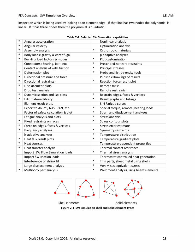
Like most commercial finite element systems SW Simulation has many capabilities and the average user only utilizes a few of them. Table 2‐1 lists those abilities that the author thinks are most useful. Those with an asterisk are illustrated in this book. SW Simulation comes with a very good set of tutorials. Here SW Simulation will be introduced by examples intended to show basis capabilities generally not covered in the tutorials. Also some tutorials focus on which icons to pick, and do not have the space to discuss good engineering practice. Here, one goal is to introduce such concepts based on the author’s decades of experience in applying finite element (FE) methods. For example, you should always try to validate a FE calculation with approximate analytic solutions and/or a different type of finite element model. This is true for even experienced persons using a program with which they have not had extensive experience. Sometimes you might just misunderstand the supporting documentation and make a simple input error.

In the author’s opinion, the book by Adams and Askenazi [1] is one of the best practical overviews of the interaction of modern solid modeling (SM) software and general finite element software (such as SW Simulation), and the many pitfalls that will plague many beginners. It points out that almost all FE studies involve assumptions and approximations and the user of such tools should be conscious of them and address them in any analysis or design report. You are encouraged to read it.

2.2 Element Types and Shapes

SW Simulation currently includes solid continuum elements, curved surface shell elements (thin and thick) and truss and frame line elements. The shells are triangular with three vertex nodes or three vertex and three mid‐edge nodes (Figure 2‐1). The solids are tetrahedra with four vertex nodes or four vertex and six mid‐edge nodes. They use linear and quadratic interpolation for the solution based on whether they have two or three nodes on an edge. The linear elements are also called simplex elements because their number of vertices is one more than the dimension of the space.

You should always examine the mesh before starting an analysis run. The size of each element indicates a region where the solution is approximated (piecewise) by a spatial polynomial. Most finite element systems, including SW Simulation, use linear or quadratic complete polynomials in each element. You can tell by



inspection which is being used by looking at an element edge. If that line has two nodes the polynomial is linear. If it has three nodes then the polynomial is quadratic.

Table 2‐1: Selected SW Simulation capabilities

* Angular acceleration Nonlinear analysis * Angular velocity Optimization analysis * Assembly analysis * Orthotropic materials * Body loads: gravity & centrifugal p‐adaptive analyses * Buckling load factors & modes * Plot customization Connectors (Bearing, bolt, etc.) * Prescribed nonzero restraints Contact analysis of with friction * Principal stresses * Deformation plot * Probe and list‐by‐entity tools * Directional pressure and force Publish eDrawings of results * Directional restraints * Reaction force result plot * Displacement plots Remote mass Drop test analysis Remote restraints * Dynamic section and iso‐plots * Restrain edges, faces & vertices * Edit material library * Result graphs and listings Element result plots S‐N Fatigue curves Export to ANSYS, NASTRAN, etc. * Special torque, remote, bearing loads Factor of safety calculation & plot * Strain and displacement analyses Fatigue analysis and plots * Stress analysis * Fixed restraints on faces * Stress contour plots * Force on edges, faces & vertices Stress error estimate * Frequency analyses * Symmetry restraints h‐adaptive analyses * Temperature distribution * Heat flux result plots * Temperature gradient plots * Heat sources Temperature‐dependent properties * Heat transfer analysis Thermal contact resistance Import SW Flow Simulation loads * Thermal stress analysis Import SW Motion loads Thermostat controlled heat generation Interference or shrink fit * Thin parts, sheet metal using shells Large displacement analysis * Von Mises equivalent stress * Multibody part analysis * Weldment analysis using beam elements

Shell elements Solid elements Figure 2‐1 SW Simulation shell and solid element types



2.3 Element Interpolations

Let T(x, y, z) denote an entity to be interpolated within an element and let x, y, and z be the local element edge coordinates. You can relate the number of nodes on an element to the number of polynomial coefficients ( ) in the local element spatial approximation, as outlined below:

1. Linear element type:

Straight edge line, or straight bar – 2 nodes, ; Straight edged triangle shell, or tetrahedron face – 3 nodes, , ; Straight edged, flat faced, tetrahedron – 4 nodes, , , , . Therefore, the solution gradient (first derivatives) in this type of element is constant and many elements are required to get good results. In SW Simulation a mesh of linear elements is called a "Draft Mesh". These are also called complete linear elements.

2. Quadratic element type:

Edge line – 3 nodes, ; Curved triangular shell, or tetrahedron face – 6 nodes,

, General curved tetrahedron – 10 nodes,

, , These are called complete quadratic elements because there are no terms missing in the quadratic polynomial. Their gradients are complete linear polynomials in three‐dimensional space. Therefore, the solution gradient, and strains and heat fluxes, in these elements vary piecewise linearly in space and fewer quadratic elements are required for a good solution. SW Simulation refers to quadratic elements as a "Quality Mesh". The above comments refer to flat shells loaded only in their plane. When flat or curved shells are loaded normal to their surface a more complicated set of interpolations are used to include their transverse bending behavior.

Note that if you set z = 0 in the quadratic (10 DOF) solid, to restrict the interpolation to a particular face triangular of the element, you obtain the previous (6 DOF) quadratic triangle. Likewise, if you set both z and y to zero, to restrict the interpolation to a particular edge of the element, you obtain the previous quadratic (3 DOF) line element. Clearly, all of the elements can interpolate data that happen to be constant (like a RBM) with 0, 2. It is less clear, but easy to prove, that all of the quadratic interpolations can reduce to the corresponding (line, surface, volume) linear interpolation if that is the exact solution.

These polynomial interpolations within an element mean that the primary unknown (displacement or temperature) is continuous within the element (has an infinite number of derivatives, C∞) and across the element interfaces (but only the value is shared with its neighbor, C0). But, the gradient of the primary unknown is discontinuous across elements, whereas the exact gradient value is continuous in a homogeneous material. The amount of discontinuity between element gradients is reduced as the element size is reduced. For example, the two colored quadratic surfaces in Figure 2‐2 could represent the temperature distribution through the two lower adjacent (white) elements. Tangent to the common edge, the temperature and its tangential slope would both be continuous, but the slope normal to that interface is not continuous. Thus, the temperature gradient is discontinuous across each interface, but continuous everywhere inside any single element. Actually, the element interpolations are also used to determine the shape of each element by interpolating between the global position vectors of their nodes.

For a quadratic shell, the SolidWorks sends the physical x, y, z coordinates of each the six nodes to SW Simulation for building the shell geometry, as seen on the left of Figure 2‐3. Similarly, the element nodes on all



surfaces of a solid are defined by SolidWorks and then the SW Simulation mesh generator builds the interior tetrahedrons by working in from the bounding surfaces. While the edges seen in Figure 2‐3 would be defined exactly in SolidWorks as circles, and they “look like” circles in the finite element mesh they are actually piecewise approximations of a circle. In other words, the quadratic edge of an element is a segment of a parabola passing through the three edge nodes that is used to approximate a segment of a circular arc through the same three nodes. The geometric error is easy to compute and it increases rapidly with the enclosed angle for the edge.

Figure 2‐2 Exploded view of two quadratic faces

Figure 2‐3 Piecewise quadratic surface and solid elements

2.4 Common Modeling Errors

As noted above, FE models often have small geometric errors. They can be reduced by mesh refinement and are usually much less important than other sources of error. Probably the most common source of error is in selecting the restraint approximations to be applied to a model. Usually a restraint is applied to a region where surrounding material has been removed and it is necessary to replace the missing material with a restraint. Keep in mind that the removed material must be capable of supplying the assumed restraint or you may introduce a very large error. Sometimes you should move the restraints further away from the part of main interest by including a small region of the supporting material to which you apply the restraints.

Many tutorials and examples assume fixed supports for simplicity. True fixed supports are extremely rare. They require zero movement of the support region. That in turn means that the removed supporting material (represented by the restraint) must be able to develop large reaction forces (and/or moments). A fixed support assumes the material can convey both tension and compression reaction forces locally as needed. Yet some supports can only convey tension while others can only resist compression. Fixed support assumptions tend to under estimate the stresses in the part of interest, but over estimate the resisting stresses (reactions) in the removed material replaced by our simplified engineering assumptions (the restraint type).



Loadings are also not as clear elementary examples suggest. Is a force applied as a point load, a line load, a surface load, etc. That is, where and how a load is applied is usually an assumption. Likewise, the magnitude of a force or other load source may be a reasonable guess or it may be given by established design codes. In thermal studies the source terms, like convection coefficients, vary over a wide range and you may have to run different studies with the high and low values. If two or more regions have different convection fluids then you may have to consider many studies using a Monte Carlo approach to combining the different ranges of data to find the likely worst case.

The nature of the equations being solved is such that the computed reactions are essentially always equal and opposite to the resultant actual applied loads, not necessarily the loads you though that you applied. Reaction data are available in SW Simulation and you should always check them.

Common “standardized” materials have mechanical and thermal properties that are relatively well known and are built into the SW Simulation materials library. However, even those materials have some range in their values that are not represented in a single number stored in a table. Many important properties, like the modulus of elasticity, are experimentally measured to only two or three significant figures. Yet a materials table frequently gives average values or values converted from other units to a misleading six or seven significant figures. So usually the computed displacements are only accurate to three or four digits and the stresses to two or three digits.

2.5 Infinite Corner Gradients

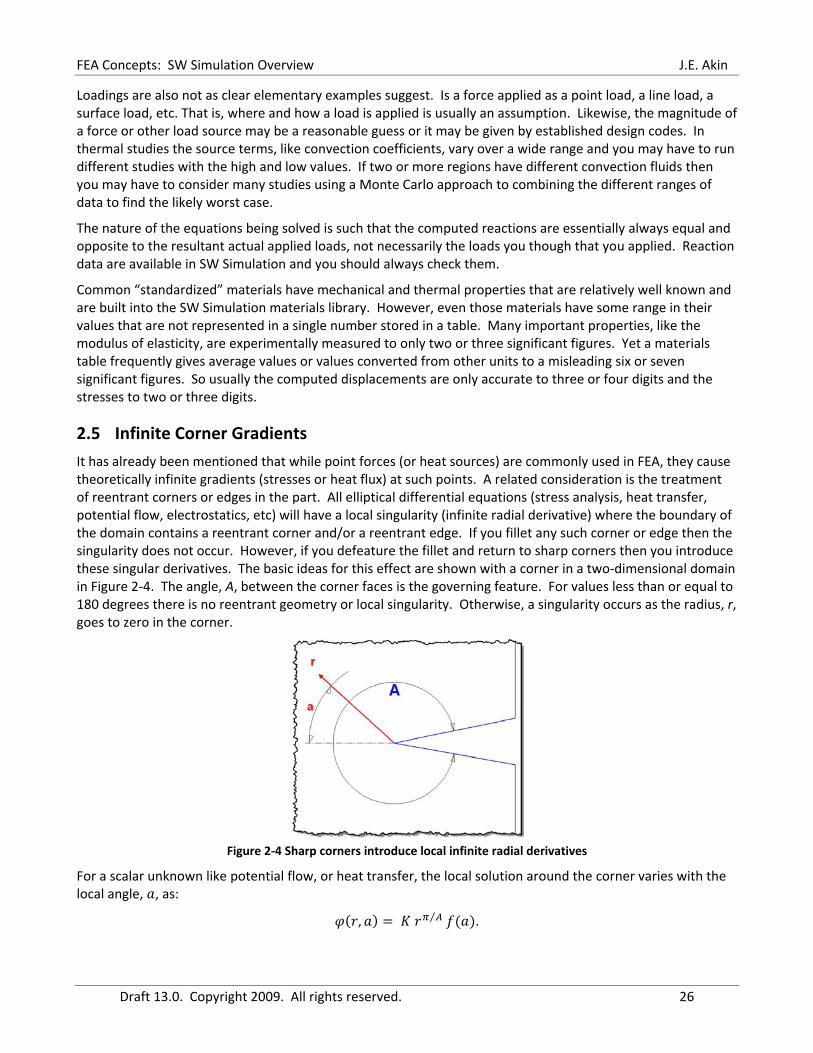
It has already been mentioned that while point forces (or heat sources) are commonly used in FEA, they cause theoretically infinite gradients (stresses or heat flux) at such points. A related consideration is the treatment of reentrant corners or edges in the part. All elliptical differential equations (stress analysis, heat transfer, potential flow, electrostatics, etc) will have a local singularity (infinite radial derivative) where the boundary of the domain contains a reentrant corner and/or a reentrant edge. If you fillet any such corner or edge then the singularity does not occur. However, if you defeature the fillet and return to sharp corners then you introduce these singular derivatives. The basic ideas for this effect are shown with a corner in a two‐dimensional domain in Figure 2‐4. The angle, A, between the corner faces is the governing feature. For values less than or equal to 180 degrees there is no reentrant geometry or local singularity. Otherwise, a singularity occurs as the radius, r, goes to zero in the corner.

Figure 2‐4 Sharp corners introduce local infinite radial derivatives

For a scalar unknown like potential flow, or heat transfer, the local solution around the corner varies with the local angle, , as:

, ⁄ .



Where K is the intensity (importance) of the singularity and / is the strength of the singularity. A right angle corner ( 3 /2) is relatively weak ( 2/3 while a slit or crack ( 2 ) is the strongest with

1/2. The radial gradient, in polar coordinates, will go to infinite any time the angle is more than 180 degrees ( 1):

For a crack the radial gradient is proportional to one over the square root of the radius:

1⁄

Therefore, the radial gradient goes to infinite as the radius r goes to zero at the corner. Since the local error in a FE solution is proportional to the product of the gradient and the element size, in theory you need to have very small element sizes (almost zero) at such reentrant geometries. In practice, most corners are not mathematically sharp and some small radius develops during manufacture. Still, the gradients can be very large. When the solid part has a mathematically sharp corner, the false infinite stresses (or strains, or heat flux) develops at the corner point. When you contour singular results the false high values may lead you to overlook real high gradient values at other locations. To avoid that, at times you will need to reduce the automatically selected maximum contour level in your plots.

The actual intensity (importance), K, of the corner singularity depends on how the far field solution is distributed relative to the centerline of the corner. Corners with the same angle will have different importance depending on whether the far field solution is changing parallel‐to or perpendicular‐to the corner centerline. This is illustrated graphically in the following figures where there are six 90 degree corners and two with larger interior angles. In this case, the default plot labels refer to temperatures and heat flux, but the same Poisson equation would apply to ideal fluid flow where is the velocity potential and the gradient is the speed (listed as heat flux magnitude) and the gradient vectors would be the actual fluid velocity vectors (listed here as the heat flux vectors).



Figure 2‐5 Sharp reentrant corners have less effect on the primary unknown

Figure 2‐6 Sharp reentrant corners can have large effects on the solution gradient



Figure 2‐7 Gradient vectors must change direction and magnitude as the pass around corners

As can be seen from the last two figures, reentrant corner singularities usually affect the solution gradients, but their importance depends on their location in the part. Apply reasonable mesh refinements near all such corner regions.

2 sw simulation overview - rice university · 2 sw simulation overview ... shape memory materials,...

Documents