1

Scaling estimates of vegetation structure in Amazonian tropical forests using 1

multi-angle MODIS observations 2

3

Yhasmin Mendes de Moura1* 4

Thomas Hilker2, 3 5

Fabio Guimarães Goncalves4 6

Lênio Soares Galvão1 7

João Roberto dos Santos1 8

Alexei Lyapustin5 9

Eduardo Eiji Maeda6 10

Camila Valéria de Jesus Silva1 11

12

1Instituto Nacional de Pesquisas Espaciais (INPE), Divisão de Sensoriamento Remoto, 13

12245-970, São José dos Campos, SP, Brazil. 14

2Oregon State University, College of Forestry, Corvallis, OR, 97331, USA. 15

3University of Southampton, Department of Geography and Environment, 16

Southampton, SO17 1BJ, United Kingdom 17

4Agrosatelite Geotecnologia Aplicada, Florianópolis, SC, 88032-005, Brazil. 18

5NASA Goddard Space Flight Center, Greenbelt, MD, 20771, USA. 19

6University of Helsinki, Department of Geosciences and Geography, P.O. Box 68, FI-20

00014, Helsinki, Finland 21

22

*Corresponding author: yhas.mendes@gmail.com 23

https://ntrs.nasa.gov/search.jsp?R=20170003716 2018-06-20T14:18:33+00:00Z

2

Abstract. Detailed knowledge of vegetation structure is required for accurate modelling 24

of terrestrial ecosystems, but direct measurements of the three dimensional distribution 25

of canopy elements, for instance from LiDAR, are not widely available. We investigate 26

the potential for modelling vegetation roughness, a key parameter for climatological 27

models, from directional scattering of visible and near-infrared (NIR) reflectance 28

acquired from NASA’s Moderate Resolution Imaging Spectroradiometer (MODIS). We 29

compare our estimates across different tropical forest types to independent measures 30

obtained from: (1) airborne laser scanning (ALS), (2) spaceborne Geoscience Laser 31

Altimeter System (GLAS)/ICESat, and (3) the spaceborne SeaWinds/QSCAT. Our 32

results showed linear correlation between MODIS-derived anisotropy to ALS-derived 33

entropy (r2= 0.54, RMSE=0.11), even in high biomass regions. Significant relationships 34

were also obtained between MODIS-derived anisotropy and GLAS-derived entropy 35

(0.52≤ r2≤ 0.61; p<0.05), with similar slopes and offsets found throughout the season, 36

and RMSE between 0.26 and 0.30 (units of entropy). The relationships between the 37

MODIS-derived anisotropy and backscattering measurements (σ0) from 38

SeaWinds/QuikSCAT presented an r2 of 0.59 and a RMSE of 0.11. We conclude that 39

multi-angular MODIS observations are suitable to extrapolate measures of canopy 40

entropy across different forest types, providing additional estimates of vegetation 41

structure in the Amazon. 42

43

Keywords: canopy roughness, multi-angle, MODIS, MAIAC, LiDAR, anisotropy 44

45

46

3

1. Introduction 47

48

Terrestrial vegetation plays a significant role in the re-distribution of moisture and 49

heat in the surface boundary layer, as well as in the energy balance of the planet 50

(Bastiaanssen et al., 1998a). Land-atmosphere interactions are driven by the three-51

dimensional structure of vegetated land cover, including surface roughness, leaf area 52

and canopy volume (Vourlitis et al., 2015; Domingues et al., 2005). Canopy roughness, 53

defined as vertical irregularities in the height of the canopy (Chapin et al., 2011), plays a 54

key role in earth system modelling. For instance, evapotranspiration is controlled much 55

more by canopy roughness (and therefore aerodynamic conductance) than by canopy 56

leaf area or maximum stomatal conductance (Chapin et al., 2011). 57

At stand level scales, significant advances have been made measuring canopy 58

vegetation structure from Light Detection and Ranging (LiDAR). LiDAR allows direct 59

measurements of the three-dimensional distribution of vertical vegetation elements from 60

ground-based (Strahler et al., 2008), airborne (Wulder et al., 2012) and orbital platforms 61

(Sun et al., 2008). To date, most vegetation related LiDAR applications rely on airborne 62

platforms for data acquisition, with measurements acquired at altitudes between 500 and 63

3000 m (Hilker et al., 2010). Due to cost and practical considerations, the availability of 64

airborne LiDAR is currently limited to specific research sites and data are not available 65

across the landscape. 66

The Geoscience Laser Altimeter System (GLAS), onboard the Ice, Cloud, and land 67

Elevation Satellite (ICESat), has provided certain capability to map vegetation 68

characteristics across broader areas from space (Zwally et al., 2002). GLAS is a large-69

footprint, waveform-recording LiDAR that measures the timing and power of the 1064 70

nm laser energy returned from illuminated surfaces (Schutz et al., 2005). While not 71

configured for vegetation characterization, the GLAS instrument allows quantification 72

4

of the vertical distribution of plant components relative to the ground over vegetated 73

terrain (Harding, 2005; Yu et al., 2015, Morton et al., 2014). GLAS data has been 74

successfully used to discriminate forest structure across various biome types (Boudreau 75

et al., 2008; Gonçalves, 2014; Lefsky et al., 2005; Pang et al., 2008) and to estimate 76

canopy light environments and forest productivity (Stark et al., 2014; Rap et al., 2015; 77

Morton et al., 2016). While GLAS provides larger spatial coverage, its footprint is still 78

spatially discrete and importantly a lack of repeated measurements prevents its use for 79

estimation of climate related responses of vegetation. 80

Perhaps complimentary to structural observations, optical remote sensing available 81

from satellite data, provide global coverage at frequent time steps but can generally not 82

deliver accurate information on the vertical organization of plant canopies. For instance, 83

vegetation indices provide general information on canopy “greenness” but their ability 84

to detect changes in high-biomass areas is limited due to a well-documented saturation 85

effect (Carlson and Ripley, 1997). Although VIs have been employed as proxies for 86

vegetation structure, including roughness lengths for turbulent transfer, field estimates 87

of vegetation structure attributes are often only moderately correlated with VIs and their 88

derivatives (Glenn et al., 2008). 89

As an alternative to conventional, mono-angle observations, the combination of 90

multiple view angles may provide new opportunities for modelling the structure of 91

vegetated land surfaces (Breunig et al., 2015; Shaw & Pereira, 1982) from optical 92

remote sensing. Changes in canopy structure including changes in tree crown size, 93

shape, density and spatial distribution of leaves, affect the directional scattering of light 94

(Chen et al., 2005). Multi-angle observations of this scattering may therefore allow us to 95

describe the three-dimensional structure of vegetation (Chen and Leblanc, 1997; 96

Strahler & Jupp, 1990). Multi-angular scattering of surface reflectance (anisotropy) has 97

5

been linked to optical properties and geometric structure of the target (Widlowski et al., 98

2004; Widlowski et al., 2005), including canopy roughness (Strahler, 2009), leaf angle 99

distribution (Roujean, 2002), leaf area index (LAI) (Walthall, 1997) and foliage 100

clumping (Chen et al., 2005; Chopping et al., 2011). Such estimates may even be made 101

in dense canopies (Moura et al., 2015), as observations acquired from multiple view 102

angles decrease the dispersion and saturation effect in geometrically complex vegetation 103

(Zhang et al., 2002). 104

105With the advent of multi-angular sensors such as the Multi-angle Imaging 106

SpectroRadiometer (MISR) (Breunig et al., 2015) and POLDER (Roujean, 2002), the 107

dependence of reflectance on observation angles has been documented (Barnsley et al., 108

2004) and modelled (Roujean et al., 1992; Wanner et al., 1995). Recent progress using 109

the Multi-Angle Implementation of Atmospheric Correction Algorithm (MAIAC) has 110

allowed the acquisition of multi-angle reflectance across large areas and at high 111

observation frequencies by combining satellite imagery obtained from NASA’s 112

Moderate Resolution Imaging Spectroradiometer (MODIS) Terra and Aqua platforms 113

during a few overpasses (Lyapustin et al., 2012a; Moura et al., 2015). Such observations 114

could potentially allow periodic and spatially contiguous estimates of vegetation 115

structure and its response to changes in climate variables. When correlated with more 116

direct measurements of canopy structure by other instruments, such as LiDAR, this may 117

then allow us to extrapolate canopy roughness and other structural estimates in space 118

and time, thereby filling key data gaps for improving our understanding of ecosystem 119

structure and functioning. Further validation may be provided by scatterometer 120

observations over dense forests. For instance, the SeaWinds microwave radar, onboard 121

NASA’s QuikSCAT satellite, was primarily designed to measure near-surface wind 122

speed and direction over the oceans. However, due to its high sensitivity to water 123

6

content that drives canopy dielectric properties, it has been also used to study canopy 124

structure (Frolking et al., 2011; Saatchi et al., 2013). 125

In this study, we used estimates of canopy roughness obtained from 1) airborne 126

laser scanning (ALS), 2) spaceborne LiDAR GLAS, and 3) the spaceborne SeaWinds 127

scatterometer, to evaluate the potential of multi-angular MODIS observations for 128

modelling vegetation roughness from directional scattering of visible and near-infrared 129

(NIR) reflectance. We implemented a spatial scaling approach, from airborne to orbital 130

levels of data acquisition, to model continuous coverage of roughness across tropical 131

forests of the Xingu basin area in the Brazilian Amazon. Our objective was to test 132

whether multi-angle MODIS reflectance can be used as a proxy for canopy roughness 133

over Amazonian tropical forests, including different forest types such as Dense and 134

Open ombrophilous Forests, and Semi-Deciduous Forest. 135

136

2. Methods 137

2.1. Study area 138

The study area is located in the southeast part of the Amazon, including the Xingu 139

basin and adjacent areas (Figure 1). Figure 1 also shows the GLAS transects for the 140

study area (Schutz et al., 2005) as well as the ALS and the field data plots. The study 141

area presents a south-north gradient with respect to climate. Following the Kӧppen 142

classification, the southern portion of the study area is dominated by tropical wet and 143

dry climate (Aw), while the north portion is characterized by tropical monsoon climate 144

(Am). Length and duration of the dry season, defined as months with rainfall less than 145

100 mm or less than one third of precipitation range (Asner & Alencar, 2010; Myneni et 146

al., 2007), also varies across the study area. In the southern parts, the dry season lasts 147

about five months, from May to September (Moura et al., 2012). In the northern parts, a 148

7

drier climate prevails between July and November (Vieira et al., 2004). The area is 149

characterized by three predominant forest types: Dense Ombrophilous Forest (Dse), 150

Open Ombrophilous Forest (Asc) and Semi-Deciduous Forest (Fse) (IBGE, 2004). 151

152

(Figure 1) 153

154

2.2. Field inventory data 155

Estimates of vegetation structure were derived for each of the three different forest 156

types using available inventory plots across the region. For two vegetation types, Open 157

Ombrophilous Forest (Asc) and Semi-decidiuous Forest (Fse), surveys were provided 158

by the Sustainable Landscapes Brazil project in collaboration with the Brazilian 159

Agricultural Research Corporation (EMBRAPA), the US Forest Service, the USAID, 160

and the US Department of State (http://mapas.cnpm.embrapa.br/paisagenssustentaveis/). 161

The Asc forest type was represented by 22 plots of 40 m x 40 m each. All the trees with 162

a diameter at breast height (DBH) equal to or greater than 10 cm were measured within 163

each plot. For Fse, 10 sample plots (20 m x 500 m) were used. The field data for the 164

Dense Ombrophilous Forest (Dse) were obtained in 2012 and are described in Silva et 165

al. (2015). The floristic and structural surveys included seven sample plots of 25 m x 166

100 m over mature forests. Trees with DBH equal to or greater than 10 cm were 167

measured within each plot. 168

169

2.3. Airborne Laser Scanning (ALS) data 170

ALS data were acquired by GEOID Ltd. using an Altm 3100/Optech instrument 171

and provided by the Sustainable Landscapes Brazil project. The positional accuracy (1σ) 172

of the LiDAR measurements was approximately 0.10 m horizontally and 0.12 m 173

8

vertically (http://mapas.cnpm.embrapa.br/paisagenssustentaveis/). We focussed our 174

analysis on undisturbed, non-degraded research plots. Structural information was 175

obtained in the Tapajós National Forest, Pará State (September to November 2012), in 176

São Félix do Xingu municipality, Pará state (August 2012) and in Canarana/Querência 177

municipality, Mato Grosso State (August 2012), to represent Dse, Asc and Fse, 178

respectively. Table 1 shows the specifications of LiDAR data for each site. 179

(Table 1) 180

ALS data were delivered as classified LAS-formatted point clouds, along with 1-m 181

resolution bare earth digital terrain models (DTM). For comparison with GLAS, 182

discrete-return data were aggregated produce pseudo-waveforms. Coops et al. (2007) 183

demonstrated that canopy profiles, analogue to those derived from full waveform 184

systems, can be derived from discrete return LiDAR when aggregating returns into three 185

dimensional voxel spaces and comparing the amount of discrete returns contained in 186

each voxel layer to the voxel layers below and above. In this study, waveforms were 187

synthesized by sub-setting the LiDAR point cloud co-located with each field plot and 188

counting the number of points observed in vertical bins of 50 cm and at a horizontal 189

resolution of 100 x100m. 10 by 10 pixels of LiDAR metrics were then averaged to 190

match the 1x1km MODIS pixel size. ALS based entropy was then computed to 191

determine canopy structural diversity and approximate canopy roughness (Palace et al., 192

2015; Stark et al., 2012). The method is described in detail in the next section (2.4) and 193

is analogue to that applied from GLAS observations. In addition to ALS entropy, we 194

also calculated canopy volume models (CVMs) to quantify the three-dimensional 195

structure of the forest canopies based on the incident radiation levels and196

photosynthetic potential (Coops et al., 2007; Hilker et al., 2010). The method is197

9

describedindetailin(Lefskyetal.,2005).CVMs divide the canopy space into sunlit and 198

shaded vegetation elements as well as gap spaces enclosed within. 199

200

2.4. GLAS/ICESat data and structural metrics from vertical profiles 201

GLAS profiles were obtained across the Xingu basin (Figure 1) between 2006 and 202

2008 (laser operating periods 3E through 2D) (Gonçalves, 2014). Each GLAS footprint 203

is elliptical in shape, spaced at approximately 170-m intervals along-track. GLAS 204

LiDAR profiles characteristics varied between the campaigns across the study area. The 205

near-infrared elliptical footprint and eccentricity varied between 51.2 (±1.7) to 58.7 206

(±0.6), and 0.48 (±0.02) to 0.59 (±0.01), respectively. The horizontal and vertical 207

geolocation accuracy varied between 0.00 (±3.41) to 1.72 (±7.36), and 0.00 (±2.38) to 208

1.2 (±5.14), depending on the campaign and respective data product. 209

Because GLAS observations are able to penetrate optically thin clouds (Schulz et 210

al., 2005), processing of the GLAS profiles included additional cloud screening to 211

improve the data quality. The technique is described in detail in Smith et al. (2005). 212

Briefly, the approach takes advantage of the fact that returns unaffected by saturation or 213

forward scattering resemble narrow Gaussian pulses that are similar to the transmitted 214

pulse (Smith et al., 2005). To process GLAS waveforms, we used parameters reported 215

in the GLA01, GLA05, and GLA14 data products following methods described by 216

(Gonçalves, 2014). First, the waveforms were filtered by convolution with a discrete 217

Gaussian kernel with the same standard deviation as the transmitted laser pulse. This 218

procedure reduced the background noise, while preserving an adequate level of detail 219

for characterization of the canopy (Sun et al., 2008). Second, GLAS waveforms used in 220

this study were calibrated and digitized into 1000 discrete bins at a time resolution of 1 221

ns (~15 cm). The locations of the highest (signal start) and lowest (signal end) detected 222

10

surfaces within the 150-m waveform were determined, respectively, as the first and last 223

elevations at which the amplitude exceeded a threshold level, for a minimum of n 224

consecutive bins. The peak of the ground return was determined as the lowest peaks in 225

the smoothed waveforms with at least the same width as the transmitted laser pulse, 226

after taking into account the mean noise level. In order to minimize the effect of 227

different output energy levels of the 2E and 3E Laser flight campaigns, all profiles were 228

then normalized to unity by dividing by the maximum amplitude. This correction 229

approach assumes that differences in measurement campaigns affect the overall amount 230

of energy but do not significantly change the waveforms (i.e. the vertical scale of energy 231

output) of our entropy calculation (Gonçalves, 2014). 232

We utilized GLAS estimates of entropy (Sz), a measure of canopy structural 233

diversity sensitive to crown depth and leaf area (Palace et al., 2015; Stark et al., 2012), 234

as a proxy of canopy roughness. Sz was calculated using Equations 1 and 2 (Harding & 235

Carabajal, 2005, Nelson et al., 2009, Treuhaft et al., 2009, Gonçalves, 2014): 236

237

𝑆" = − 𝑝(𝑤()ln 𝑝(𝑤()-.

(/0

,𝑤𝑖𝑡ℎ 238

(1) 239

𝑝 𝑤( =𝑤( 𝑧𝑤( 𝑧 𝑑𝑧

80999

240

(2) 241

where nb is the number of vertical bins from the ground peak to the signal start defined 242

as the vertical distance between the ground peak and the signal start; w(z) is the laser 243

power received from the 1m bin centered at height z; H100 is the maximum canopy 244

11

height, defined as the vertical distance between the ground peak and the signal start 245

(Gonçalves, 2014). 246

247

2.5. SeaWinds/QuikSCAT data 248

Estimates of canopy structure were independently also obtained from SeaWinds 249

Scatterometer data, provided by NASA’s Scatterometer Climate Record Pathfinder 250

project. The SeaWinds Scatterometer operates at microwave frequency of 13.4 GHz 251

(Ku-band) with mean incidence angle of 54º for V-polarization and 46º for H-252

polarization. The sensitivity of radar data to variations in vegetation canopy structure 253

can be explained by the dependence of radar backscatter to surface dielectric properties, 254

which are strongly dependent on the liquid water content of the canopy constituents 255

(Frolking et al., 2006). Given that the SeaWinds instrument operates at a higher 256

frequency and higher incidence angle than other similar sensors, it has lower penetration 257

into forest canopy, and therefore almost no interference from soil moisture variations in 258

densely vegetated forested areas (Saatchi et al., 2013). 259

The backscatter product (σ0) used in this study combines ascending (morning) and 260

descending (evening) orbital passes, and is based on SeaWinds "egg" images (Frolking 261

et al., 2006).The nominal image pixel resolution for egg images is 4.45 km/pixel. Only 262

backscatter data for horizontal (H) polarization were used, as previous assessments had 263

indicated that results using vertical (V) polarization show no significant differences 264

(Saatchi et al., 2013). We used data obtained from January 2001 to November 2009, 265

when the sensor stopped collecting data due to failure in the scanning capability. To 266

match the spatial resolution of the SeaWinds instrument, we averaged the corresponding 267

anisotropy observations from the MODIS instrument to match the 268

SeaWinds/QuikSCAT pixels. 269

12

2.6. Determination of surface anisotropy from multi-angle MODIS data 270

MODIS observations are acquired at different solar and view zenith angles, 271

depending on the orbital overpass and time of the year. Pixel-based algorithms often 272

assume a Lambertian reflectance model, which reduces the anisotropy of the derived 273

surface reflectance (Lyapustin, 1999; Wang et al., 2010), thus decreasing the ability to 274

detect directional scattering (Hilker et al., 2009). In this study, we use the MAIAC 275

algorithm because it preserves the multi-angle character of MODIS observations, 276

providing a means to estimate the anisotropy of surface reflectance (Chen et al., 2005), 277

a surrogate for structure of vegetation and shaded parts of the canopy (Myneni et al., 278

2002; Chen et al., 2003; Gao et al., 2003). MAIAC is a cloud screening and atmospheric 279

correction algorithm that uses an adaptive time series analysis and processing of groups 280

of pixels to derive atmospheric aerosol concentration and surface reflectance. A detailed 281

description of the technique can be found in Lyapustin et al. (2011) and Lyapustin et al. 282

(2012). Previous results (Hilker et al., 2012, 2015) have shown that while the MAIAC 283

cloud mask is less conservative, it is also more accurate, improving the number of 284

observations and data quality in tropical environments. 285

For retrieval of the surface bi-directional reflectance distribution function (BRDF), 286

MAIAC accumulates data over 4-16 days (Lyapustin et al., 2011, 2012). Assuming that 287

vegetation is relatively stable during this period, the surface directional scattering can be 288

characterized using the Ross-Thick Li-Sparse (RTLS) bidirectional reflectance 289

distribution function (BRDF) model (Roujean, et al., 1992). 290

Using the RTLS model (Wanner et al., 1995), we characterized the BRDF of each 1 291

km x 1 km grid cell of MODIS data. Based on the RTLS BRDF model, we derived 292

MODIS backscatter (Solar Zenith Angle (SZA) = 45°, View Zenith Angle (VZA) = 35°, 293

Relative Azimuth Angle (RAA) = 180°) and forward scatter (SZA = 45°, VZA = 35°, 294

13

RAA = 0°) observations (4-16 days of observations) for a fixed view and sun angle. The 295

advantage of using the RTLS model rather than reflectance directly is to keep constant 296

sun-observer geometry and extrapolate measurements to the principal plane. In addition, 297

the modelled reflectance can be based on all multi-angle MODIS data, which should 298

yield a more representative characterization of the reflectance properties. We selected a 299

VZA of 35° rather than the hotspot location at VZA = 45° in order to keep the modelled 300

reflectance closer to the actual range of angles observed by MODIS, thereby 301

minimizing potential errors resulting from extrapolation of the BRDF. 302

We used estimates of anisotropy (defined as the difference between BRDF 303

modelled backscattering (SZA = 45°, VZA = 35°, RAA = 180°) and BRDF modelled 304

forward scattering (SZA = 45°, VZA = 35°, RAA = 0°) based on the Enhanced 305

Vegetation Index (EVI) to describe roughness of the surface for different vegetation 306

types across the study area (Moura et al., 2015). The objective of using EVI rather than 307

surface reflectance of a given band was to minimize the effect of non-photosynthetically 308

active elements (i.e. soil fraction component) while optimizing the sensitivity to green 309

canopy structure (Moura et al., 2015). 310

MODIS-derived anisotropy values were then regressed against ALS-derived 311

entropy, GLAS-derived entropy and SeaWinds/QuikSCAT backscatter (σ0, Frolking et 312

al., 2006), which were estimated on a per-pixel-basis to generate time series profiles of 313

entropy for each forest type in the study area. 314

315

3. Results 316

The Xingu basin contains a number of different forest types. However, vegetation is 317

dominated by Asc and Dse forest types in the north, and by Fse vegetation in the south, 318

14

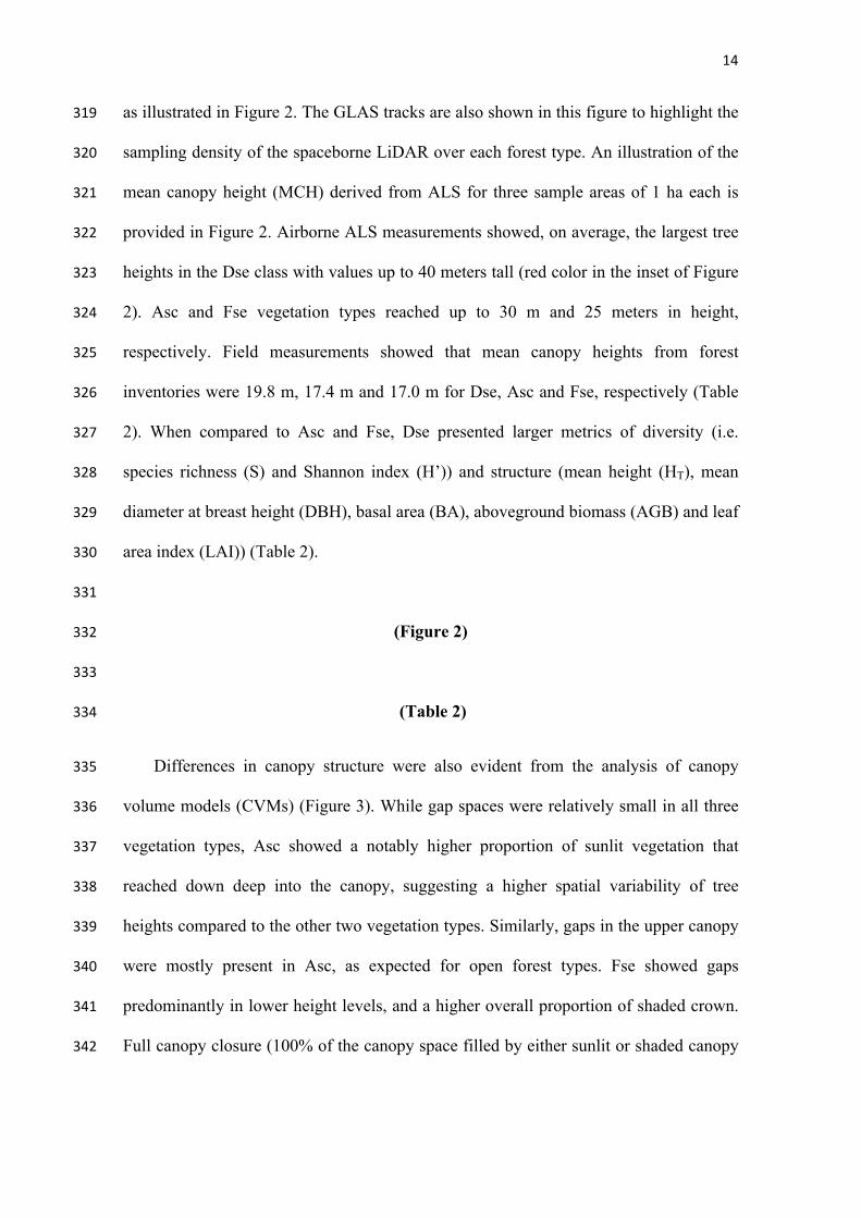
as illustrated in Figure 2. The GLAS tracks are also shown in this figure to highlight the 319

sampling density of the spaceborne LiDAR over each forest type. An illustration of the 320

mean canopy height (MCH) derived from ALS for three sample areas of 1 ha each is 321

provided in Figure 2. Airborne ALS measurements showed, on average, the largest tree 322

heights in the Dse class with values up to 40 meters tall (red color in the inset of Figure 323

2). Asc and Fse vegetation types reached up to 30 m and 25 meters in height, 324

respectively. Field measurements showed that mean canopy heights from forest 325

inventories were 19.8 m, 17.4 m and 17.0 m for Dse, Asc and Fse, respectively (Table 326

2). When compared to Asc and Fse, Dse presented larger metrics of diversity (i.e. 327

species richness (S) and Shannon index (H’)) and structure (mean height (HT), mean 328

diameter at breast height (DBH), basal area (BA), aboveground biomass (AGB) and leaf 329

area index (LAI)) (Table 2). 330

331

(Figure 2) 332

333

(Table 2) 334

Differences in canopy structure were also evident from the analysis of canopy 335

volume models (CVMs) (Figure 3). While gap spaces were relatively small in all three 336

vegetation types, Asc showed a notably higher proportion of sunlit vegetation that 337

reached down deep into the canopy, suggesting a higher spatial variability of tree 338

heights compared to the other two vegetation types. Similarly, gaps in the upper canopy 339

were mostly present in Asc, as expected for open forest types. Fse showed gaps 340

predominantly in lower height levels, and a higher overall proportion of shaded crown. 341

Full canopy closure (100% of the canopy space filled by either sunlit or shaded canopy 342

15

elements or fully enclosed gap space) was reached at about 15 m height for both Asc 343

and Dse, and at about 20 m height for Fse. 344

(Figure 3) 345

346

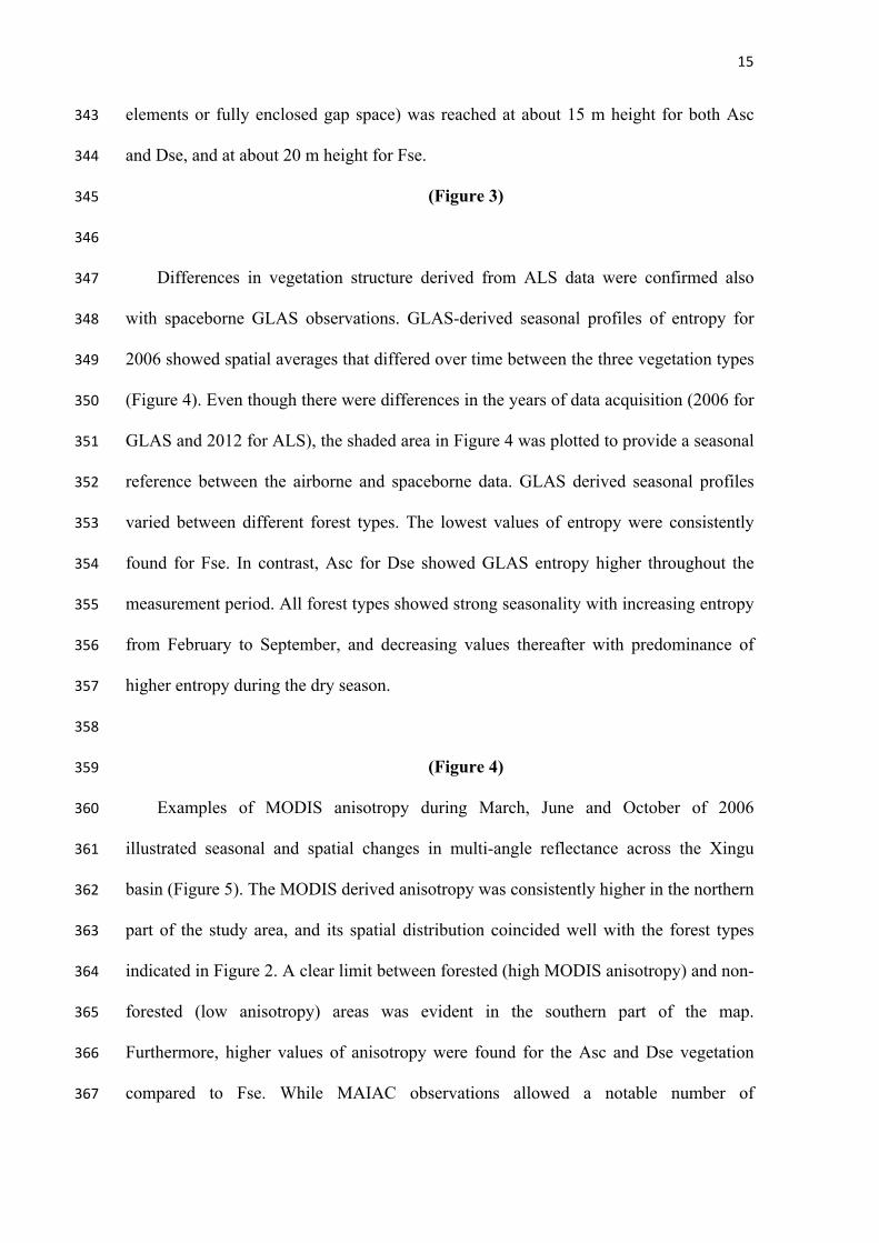
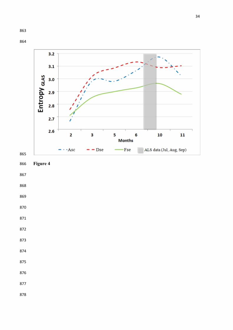
Differences in vegetation structure derived from ALS data were confirmed also 347

with spaceborne GLAS observations. GLAS-derived seasonal profiles of entropy for 348

2006 showed spatial averages that differed over time between the three vegetation types 349

(Figure 4). Even though there were differences in the years of data acquisition (2006 for 350

GLAS and 2012 for ALS), the shaded area in Figure 4 was plotted to provide a seasonal 351

reference between the airborne and spaceborne data. GLAS derived seasonal profiles 352

varied between different forest types. The lowest values of entropy were consistently 353

found for Fse. In contrast, Asc for Dse showed GLAS entropy higher throughout the 354

measurement period. All forest types showed strong seasonality with increasing entropy 355

from February to September, and decreasing values thereafter with predominance of 356

higher entropy during the dry season. 357

358

(Figure 4) 359

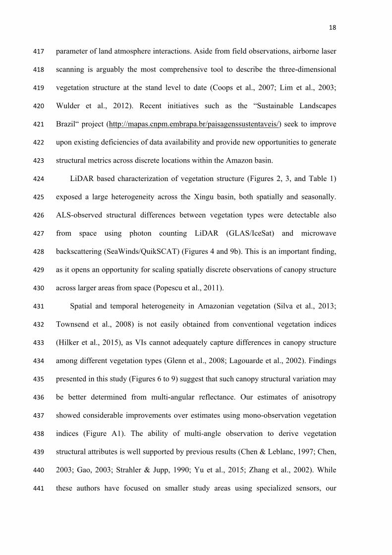
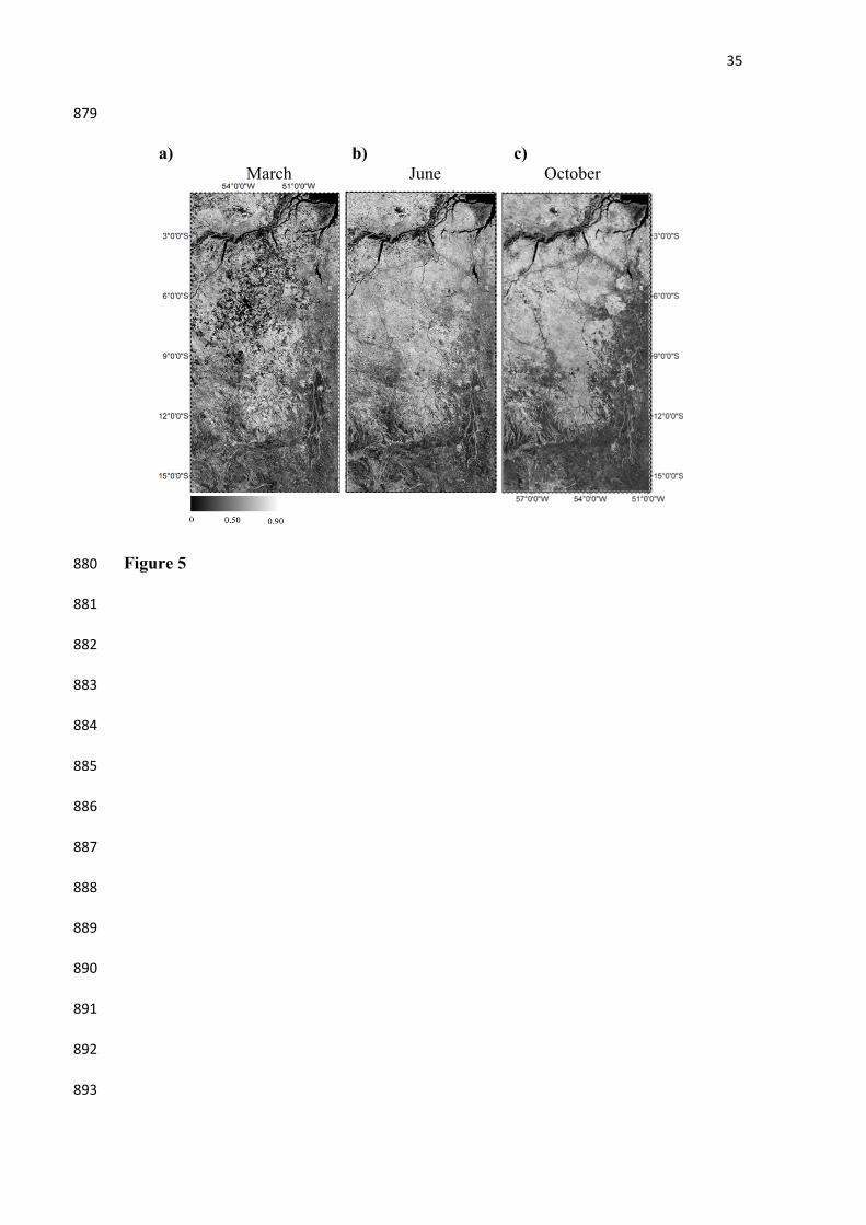
Examples of MODIS anisotropy during March, June and October of 2006 360

illustrated seasonal and spatial changes in multi-angle reflectance across the Xingu 361

basin (Figure 5). The MODIS derived anisotropy was consistently higher in the northern 362

part of the study area, and its spatial distribution coincided well with the forest types 363

indicated in Figure 2. A clear limit between forested (high MODIS anisotropy) and non-364

forested (low anisotropy) areas was evident in the southern part of the map. 365

Furthermore, higher values of anisotropy were found for the Asc and Dse vegetation 366

compared to Fse. While MAIAC observations allowed a notable number of 367

16

measurements of anisotropy between June (Figure 5b) and October (Figure 5c), some 368

data gaps were observed in March (Figure 5a) due to cloud cover in the rainy season. 369

(Figure 5) 370

MODIS-derived anisotropy was linearly correlated to ALS-derived entropy 371

(Figure 6). The coefficient of determination (r2) of the relationship between all 828 372

MODIS pixels that coincided with existing ALS observations was 0.54 with an RMSE 373

of 0.11 units of entropy. Much of the scattering presented in Figure 3 was limited to 374

lower values of entropy, while residuals were notably smaller for the higher entropy 375

range. 376

(Figure 6) 377

Significant relationships were also found between MODIS anisotropy and 378

GLAS measured entropy using all observations that contained five or more GLAS shots 379

within the 1 km x 1 km MODIS pixels (Figure 7). In order to examine seasonal 380

variability in the relationship, we performed the regressions separately for March 381

(Figure 7a), June (Figure 7b) and October (Figure 7c) of 2006. The r2 varied between 382

0.52 for March and 0.61 for June (p<0.05) with similar slopes and offsets found 383

throughout the observation period. RMSE varied between 0.26 and 0.30 units of entropy. 384

The highest noise levels were observed in March, which is corresponding also to the 385

larger amount of data gaps during the rainy season (Figure 5). The availability of GLAS 386

data was somewhat limited during June, but the relationships were still highly 387

significant and consistent with those observed during other months of the year. A 388

comparison between conventional VI estimates using directionally normalized EVI 389

from MAIAC and LiDAR derived Entropy is shown in the appendix (Figure A1). 390

(Figure 7) 391

17

A strong relationship between the MODIS-derived anisotropy and the 392

backscattering measurements (σ0) from SeaWinds/QuikSCAT was also observed 393

(Figure 8). The relationship was obtained for 10.000 randomly sampled MODIS pixels 394

and corresponding SeaWinds/QuikSCAT (σ0) observations across the Xingu basin for 395

all available QuikSCAT data between 2001 and 2009. Note, however, that when using 396

radar observations, the relationship to MODIS-derived anisotropy was non-linear 397

(r2=0.59, RMSE=0.11). 398

(Figure 8) 399

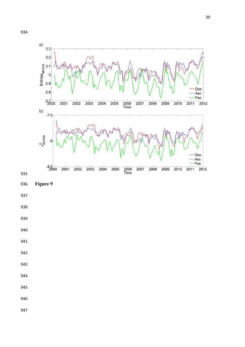
Time series profiles of MODIS-derived entropy estimated from the regression 400

model of Figure 7c and of MODIS-derived QuikSCAT-σ0 estimated from model of 401

Figure 8 were plotted as spatial averages for Dse, Asc and Fse (Figure 9). All three 402

forest types displayed notable seasonal cycles. The Ombrophilous Forests (Dse and Asc) 403

consistently showed high values of entropy with less seasonal variation. In contrast, the 404

seasonal cycles were much more pronouced in the Fse, as expected for semi-decidous 405

vegetation. Both models (GLAS-derived entropy and QScat-derived σ0) yielded very 406

similar seasonal patterns, in terms of temporal variation as well as in terms of 407

differences between vegetation types. The results presented in Figure 9 were consistent 408

also with those shown in Figure 5. A small negative trend in both entropy and σ0 was 409

observed from 2000 until 2009 and a positive trend in all three vegetation types was 410

found from 2010 onwards. This trend was especially pronounced for the canopy entropy 411

based on GLAS observations. 412

(Figure 9) 413

4. Discussion 414

This study investigated the potential of multi-angle reflectance obtained from 415

MODIS to derive estimates of vegetated surface roughness as an important structural 416

18

parameter of land atmosphere interactions. Aside from field observations, airborne laser 417

scanning is arguably the most comprehensive tool to describe the three-dimensional 418

vegetation structure at the stand level to date (Coops et al., 2007; Lim et al., 2003; 419

Wulder et al., 2012). Recent initiatives such as the “Sustainable Landscapes 420

Brazil“ project (http://mapas.cnpm.embrapa.br/paisagenssustentaveis/) seek to improve 421

upon existing deficiencies of data availability and provide new opportunities to generate 422

structural metrics across discrete locations within the Amazon basin. 423

LiDAR based characterization of vegetation structure (Figures 2, 3, and Table 1) 424

exposed a large heterogeneity across the Xingu basin, both spatially and seasonally. 425

ALS-observed structural differences between vegetation types were detectable also 426

from space using photon counting LiDAR (GLAS/IceSat) and microwave 427

backscattering (SeaWinds/QuikSCAT) (Figures 4 and 9b). This is an important finding, 428

as it opens an opportunity for scaling spatially discrete observations of canopy structure 429

across larger areas from space (Popescu et al., 2011). 430

Spatial and temporal heterogeneity in Amazonian vegetation (Silva et al., 2013; 431

Townsend et al., 2008) is not easily obtained from conventional vegetation indices 432

(Hilker et al., 2015), as VIs cannot adequately capture differences in canopy structure 433

among different vegetation types (Glenn et al., 2008; Lagouarde et al., 2002). Findings 434

presented in this study (Figures 6 to 9) suggest that such canopy structural variation may 435

be better determined from multi-angular reflectance. Our estimates of anisotropy 436

showed considerable improvements over estimates using mono-observation vegetation 437

indices (Figure A1). The ability of multi-angle observation to derive vegetation 438

structural attributes is well supported by previous results (Chen & Leblanc, 1997; Chen, 439

2003; Gao, 2003; Strahler & Jupp, 1990; Yu et al., 2015; Zhang et al., 2002). While 440

these authors have focused on smaller study areas using specialized sensors, our 441

19

findings confirm such multi-angle potential to be acquired from the MODIS instrument 442

and across the Amazon basin (Moura et al., 2015). Our previous work also confirmed 443

the consistency of monthly anisotropy measurements and its statistical significance for 444

estimating seasonal changes in vegetation structure across the Amazon (Moura et al., 445

2015). This is an important advancement, as it allows structural estimates over large 446

areas and at high temporal frequencies from space, complementing the data analysis of 447

orbital LiDAR data. 448

Anisotropy derived from multiple overpasses of MODIS imagery may therefore 449

provide new insights into structural variability of Amazon forests as it increases the 450

sensitivity to changes in vegetation structure across dense vegetation types. As 451

demonstrated in previous work (Moura et al., 2015), seasonal changes in observed 452

anisotropy cannot be explained by bi-directional effects, as all observations have been 453

normalized to a fixed forward and backscatter geometry (Lyapustin et al., 2012b). In 454

addition, Moura et al. (2015) demonstrated that standard deviations between observed 455

and modelled MAIAC reflectance were about 10% of the observed variation in 456

anisotropy, thus confirming the ability of our approach to detect seasonal and inter-457

annual changes. Differences between forward and backscatter observations as utilized in 458

this paper are largely driven by the different directional scattering behaviour of red and 459

NIR reflectance (Moura et al., 2015, Hilker et al., 2015). The modelled near hotspot and 460

near darkspot locations were designed to maximize the range of resulting anisotropy, 461

thereby seeking to increase the sensitivity with respect to changes in vegetation 462

structure. 463

While the range of view angles acquired by MODIS is relatively small, as the 464

instrument was not specifically designed for multi-angle acquisitions, MODIS-derived 465

anisotropy still provided an effective means to characterize vegetation structure across 466

20

large areas from space. Within the Amazon basin (or tropics in general), this is partially 467

facilitated by the fact that MODIS view geometry comes very close to the principal 468

plane twice a year. As a result, our BRDF model is representative of the angles used in 469

this study. Consequently, modelled anisotropy is close to its maximum range of possible 470

values. The contrary occurs in mid-latitudes where observations are further from the 471

principal plane. In these cases, other geometric configurations might be preferable. 472

Modelling MODIS anisotropy using the RTLS BRDF model further allowed us to 473

derive anisotropy independent of the sun-observer geometry (Roujean et al., 1992). As a 474

limitation to this approach, changes in sun-sensor configuration over the year do not 475

always allow modelling of forward and backscattering observations within the sampling 476

range of the MODIS instruments. Therefore, higher uncertainties may be observed 477

during some times of the year than during others. 478

The strong, positive correlation found between GLAS-measured entropy and 479

MODIS anisotropy (Figure 6) may be explained by geometric scattering of individual 480

tree crowns (Chopping et al., 2011; Li, X., Strahler, 1986). For instance, a large 481

variability in canopy heights (high canopy roughness) will increase the geometric 482

scattering component, especially of NIR reflectance. Other structural changes may, 483

however, also influence seasonal patterns of anisotropy. In addition to canopy 484

roughness, anisotropy is also affected by leaf angle distribution (Roujean, 2002) and 485

foliage clumping (Chen et al., 2005) among other variables related to the floristic 486

variability, which tends to be high in tropical forests. The interaction between these 487

variables and multi-angle scattering is not straightforward, requiring further 488

investigation, especially in the components of scattering determined in the RTLS model. 489

For example, increases in leaf area may increase the volumetric scattering component 490

(Ross, 1981; Roujean, et al., 1992) of multi-angle reflectance, but at the same time 491

21

decrease the surface roughness, at least within a certain range of values. Therefore, the 492

results presented in here should be understood as a first demonstration of the technique. 493

Due to the complexities described as well as other limitations in terms of footprint 494

size, and range of angular sampling, MODIS-derived estimates of canopy structure 495

should not be understood as a replacement for direct 3D measures of vegetation, but 496

rather as a complimentary approach for scaling such observations in space and time. 497

The consistency in the modelled relationship obtained from GLAS LiDAR and 498

SeaWinds/QuikSCAT backscattering is encouraging in this respect, as it suggests that 499

such scaling approaches may be built on opportunistically sampled observations across 500

platforms. For instance, MODIS data can help interpret estimates of canopy roughness 501

in between GLAS footprints, as well as fill missing observations in time, enabling more 502

comprehensive seasonal and spatial analysis. Upcoming new LiDAR instruments, such 503

as the Global Ecosystem Dynamics (GEDI) mission (Dubayah et al., 2014; Stysley et al., 504

2015), will allow further improvements in the measures of canopy structure as well as 505

biomass. 506

507

5. Conclusions 508

Our analysis has demonstrated that multi-angular MODIS observations are suitable 509

to determine canopy entropy at different scales of LiDAR measurements across the 510

study area in the Amazon. The sparseness of existing, highly detailed LiDAR 511

observations currently imposes severe restriction on accuracy of modeled carbon and 512

water fluxes, particularly in remote regions such as the Amazon basin. Complementary 513

measures of vegetation structure from optical satellites are therefore highly desirable to 514

extrapolate spatially or temporally sparse estimates of canopy structure across the 515

22

landscape. Such approaches will be crucial for improving our understanding of climate 516

tolerance and responses to Amazonian forests to extreme events. 517

518

Acknowledgements 519

We are grateful to the NASA Center for Climate Simulation (NCCS) for 520

computational support and access to their high performance cluster. MAIAC data for 521

the amazon basin are described and available for download at 522

ftp://ladsweb.nascom.nasa.gov/MAIAC. LiDAR data were acquired by the Sustainable 523

Landscapes Brazil project supported by the Brazilian Agricultural Research Corporation 524

(EMBRAPA), the US Forest Service, and USAID, and the US Department of State. 525

Thanks are also to CAPES (Coordenação de Aperfeiçoamento de Pessoal de Nível 526

Superior) grant number 12881-13-9; and CNPq (Conselho Nacional de 527

Desenvolvimento Científico e Tecnológico), grant number PVE 401025/2014-4. Dr 528

Eduardo Maeda was supported by a research grant from the Academy of Finland. 529

530

References 531

Asner, G. P., & Alencar, A. (2010). Drought impacts on the Amazon forest: the remote 532sensing perspective. The New Phytologist, 187(3), 569–78. doi:10.1111/j.1469-5338137.2010.03310.x 534

Barnsley, M. J., Settle, J. J., Cutter, M. A., Lobb, D. R., & Teston, F. (2004). The 535PROBA/CHRIS mission: a low-cost smallsat for hyperspectral multiangle 536observations of the Earth surface and atmosphere. IEEE Transactions on 537Geoscience and Remote Sensing, 42(7), 1512–1520. 538doi:10.1109/TGRS.2004.827260 539

BOUDREAU, J., NELSON, R., MARGOLIS, H., BEAUDOIN, A., GUINDON, L., & 540KIMES, D. (2008). Regional aboveground forest biomass using airborne and 541spaceborne LiDAR in Québec. Remote Sensing of Environment, 112(10), 3876–5423890. doi:10.1016/j.rse.2008.06.003 543

Breunig, F. M., Galvão, L. S., dos Santos, J. R., Gitelson, A. A., de Moura, Y. M., Teles, 544T. S., & Gaida, W. (2015). Spectral anisotropy of subtropical deciduous forest 545using MISR and MODIS data acquired under large seasonal variation in solar 546zenith angle. International Journal of Applied Earth Observation and 547

23

Geoinformation, 35, 294–304. doi:10.1016/j.jag.2014.09.017 548

Carlson, T. N., & Ripley, D. A. (1997). On the relation between NDVI, fractional 549vegetation cover, and leaf area index. Remote Sensing of Environment, 62(3), 241–550252. doi:10.1016/S0034-4257(97)00104-1 551

Chapin, F. I., Matson, P., & Vitousek, P. (2011). Principles of terrestrial ecosystem 552ecology. Retrieved from 553https://books.google.com/books?hl=en&lr=&id=68nFNpceRmIC&oi=fnd&pg=PR5545&dq=principles+of+terrestrial+ecosystem+ecology+stuart&ots=V1DZdx8sni&si555g=d5RF0D75OjOWRvQpqdU9k1hxqkI 556

Chen, J. M., & Leblanc, S. G. (1997). A four-scale bidirectional reflectance model 557based on canopy architecture. IEEE Transactions on Geoscience and Remote 558Sensing, 35(5), 1316–1337. doi:10.1109/36.628798 559

Chen, J. M., Liub, J., Leblanc, S. G., Lacazec, R., & Roujean, J. L. (2003). Multi-560angular optical remote sensing for assessing vegetation structure and carbon 561absorption. 562

Chen, J. M., Menges, C. H., & Leblanc, S. G. (2005). Global mapping of foliage 563clumping index using multi-angular satellite data. Remote Sensing of Environment, 56497(4), 447–457. doi:10.1016/j.rse.2005.05.003 565

Chopping, M., Schaaf, C. B., Zhao, F., Wang, Z., Nolin, A. W., Moisen, G. G., 566Martonchik, J. V., & Bull, M. (2011). Forest structure and aboveground biomass in 567the southwestern United States from MODIS and MISR. Remote Sensing of 568Environment, 115(11), 2943–2953. doi:10.1016/j.rse.2010.08.031 569

Coops, N. C., Hilker, T., Wulder, M. A., St-Onge, B., Newnham, G., Siggins, A., & 570Trofymow, J. A. (Tony). (2007). Estimating canopy structure of Douglas-fir forest 571stands from discrete-return LiDAR. Trees, 21(3), 295–310. doi:10.1007/s00468-572006-0119-6 573

Domingues, T. F., Berry, J. A., Martinelli, L. A., Ometto, J. P. H. B., & Ehleringer, J. R. 574(2005). Parameterization of Canopy Structure and Leaf-Level Gas Exchange for an 575Eastern Amazonian Tropical Rain Forest (Tapajós National Forest, Pará, Brazil). 576Earth Interactions, 9(17), 1–23. doi:10.1175/EI149.1 577

Dubayah, R., Goetz, S. J., Blair, J. B., Fatoyinbo, T. E., Hansen, M., Healey, S. P., 578Hofton, M. A., Hurtt, G. C., Kellner, J., Luthcke, S. B., & Swatantran, A. 579(2014). The Global Ecosystem Dynamics Investigation. American Geophysical 580Union. Retrieved from http://adsabs.harvard.edu/abs/2014AGUFM.U14A..07D 581

Frolking, S., Milliman, T., McDonald, K., Kimball, J., Zhao, M., & Fahnestock, M. 582(2006). Evaluation of the Sea Winds scatterometer for regional monitoring of 583vegetation phenology. Journal of Geophysical Research: Atmospheres, 111(17), 1–58414. doi:10.1029/2005JD006588 585

Frolking, S., Milliman, T., Palace, M., Wisser, D., Lammers, R., & Fahnestock, M. 586(2011). Tropical forest backscatter anomaly evident in SeaWinds scatterometer 587morning overpass data during 2005 drought in Amazonia. Remote Sensing of 588Environment, 115(3), 897–907. doi:10.1016/j.rse.2010.11.017 589

Gao, F. (2003). Detecting vegetation structure using a kernel-based BRDF model. 590Remote Sensing of Environment, 86(2), 198–205. doi:10.1016/S0034-5914257(03)00100-7 592

Glenn, E. P., Huete, A. R., Nagler, P. L., & Nelson, S. G. (2008). Relationship between 593

24

remotely-sensed vegetation indices, canopy attributes and plant physiological 594processes: What vegetation indices can and cannot tell us about the landscape. 595Sensors, 8(4), 2136–2160. doi:10.3390/s8042136 596

Gonçalves, F. G. (2016, January). Vertical structure and aboveground biomass of 597tropical forests from lidar remote sensing. 598

Harding, D. J. (2005). ICESat waveform measurements of within-footprint topographic 599relief and vegetation vertical structure. Geophysical Research Letters, 32(21), 600L21S10. doi:10.1029/2005GL023471 601

Hilker, T., Leeuwen, M., Coops, N. C., Wulder, M. A., Newnham, G. J., Jupp, D. L. B., 602& Culvenor, D. S. (2010). Comparing canopy metrics derived from terrestrial and 603airborne laser scanning in a Douglas-fir dominated forest stand. Trees, 24(5), 819–604832. doi:10.1007/s00468-010-0452-7 605

Hilker, T., Lyapustin, A. I., Hall, F. G., Myneni, R., Knyazikhin, Y., Wang, Y., Tucker, 606C. J., & Sellers, P. J. (2015). On the measurability of change in Amazon vegetation 607from MODIS. Remote Sensing of Environment, 166, 233–242. 608doi:10.1016/j.rse.2015.05.020 609

Hilker, T., Wulder, M. A., Coops, N. C., Linke, J., McDermid, G., Masek, J. G., Gao, F., 610& White, J. C. (2009). A new data fusion model for high spatial- and temporal-611resolution mapping of forest disturbance based on Landsat and MODIS. Remote 612Sensing of Environment, 113(8), 1613–1627. doi:10.1016/j.rse.2009.03.007 613

IBGE. (2004). Manual Tecnico da vegetacao brasileira. 614

Jing M. Chena, Jane Liub, Sylvain G. Leblancb, Roselyne Lacazec, J.-L. R. (2002). 615Multi-angular optical remote sensing for assessing vegetation structure and carbon 616absorption. Remote Sensing of Environment, 84, 516–525. 617

Lagouarde, J.-P., Jacob, F., Gu, X. F., Olioso, A., Bonnefond, J.-M., Kerr, Y., John 618Mcaneney, K., & Irvine, M. (2002). Spatialization of sensible heat flux over a 619heterogeneous landscape. Agronomie, 22(6), 627–633. doi:10.1051/agro:2002032 620

Lefsky, M. A., Harding, D. J., Keller, M., Cohen, W. B., Carabajal, C. C., Del Bom 621Espirito-Santo, F., Hunter, M. O., & de Oliveira, R. (2005). Estimates of forest 622canopy height and aboveground biomass using ICESat. Geophysical Research 623Letters, 32(22), L22S02. doi:10.1029/2005GL023971 624

Li, X., Strahler, A. H. (1986). Geometric-Optical Bidirectional Reflectance Modeling of 625a Conifer Forest Canopy, (6), 906–919. 626

Lim, K., Treitz, P., Wulder, M., St-Onge, B., & Flood, M. (2003). LiDAR remote 627sensing of forest structure. Progress in Physical Geography, 27(1), 88–106. 628doi:10.1191/0309133303pp360ra 629

LYAPUSTIN, A. I., & MULDASHEV, T. Z. (1999). METHOD OF SPHERICAL 630HARMONICS IN THE RADIATIVE TRANSFER PROBLEM WITH NON-631LAMBERTIAN SURFACE. Journal of Quantitative Spectroscopy and Radiative 632Transfer, 61(4), 545–555. doi:10.1016/S0022-4073(98)00041-7 633

Lyapustin, A. I., Wang, Y., Laszlo, I., Hilker, T., G.Hall, F., Sellers, P. J., Tucker, C. J., 634& Korkin, S. V. (2012a). Multi-Angle Implementation of Atmospheric Correction 635for MODIS (MAIAC). Part 3: Atmospheric Correction. Remote Sensing of 636Environment, 127, 385–393. doi:10.1016/j.rse.2012.09.002 637

Lyapustin, A., Wang, Y., Laszlo, I., & Hilker, T. (2012b). Multi-Angle Implementation 638

25

of Atmospheric Correction for MODIS (MAIAC). Part 3: Atmospheric Correction. 639Remote Sensing of Environment, 127, 385–393. Retrieved from 640http://ntrs.nasa.gov/search.jsp?R=20120017006 641

Moura, Y. M. de, Hilker, T., Lyapustin, A. I., Galvão, L. S., dos Santos, J. R., Anderson, 642L. O., de Sousa, C. H. R., & Arai, E. (2015). Seasonality and drought effects of 643Amazonian forests observed from multi-angle satellite data. Remote Sensing of 644Environment, 171, 278–290. doi:10.1016/j.rse.2015.10.015 645

Moura, Y. M., Galvão, L. S., dos Santos, J. R., Roberts, D. a., & Breunig, F. M. (2012). 646Use of MISR/Terra data to study intra- and inter-annual EVI variations in the dry 647season of tropical forest. Remote Sensing of Environment, 127, 260–270. 648doi:10.1016/j.rse.2012.09.013 649

Myneni, R. ., Hoffman, S., Knyazikhin, Y., Privette, J. ., Glassy, J., Tian, Y., Wang, Y., 650Song, X., Zhang, Y., Smith, G. ., Lotsch, A., Friedl, M., Morisette, J. ., Votava, P., 651Nemani, R. ., & Running, S. . (2002). Global products of vegetation leaf area and 652fraction absorbed PAR from year one of MODIS data. Remote Sensing of 653Environment, 83(1-2), 214–231. doi:10.1016/S0034-4257(02)00074-3 654

Myneni, R. B., Yang, W., Nemani, R. R., Huete, A. R., Dickinson, R. E., Knyazikhin, 655Y., Didan, K., Fu, R., Negrón Juárez, R. I., Saatchi, S. S., Hashimoto, H., Ichii, K., 656Shabanov, N. V, Tan, B., Ratana, P., Privette, J. L., Morisette, J. T., … 657Salomonson, V. V. (2007). Large seasonal swings in leaf area of Amazon 658rainforests. Proceedings of the National Academy of Sciences of the United States 659of America, 104(12), 4820–3. doi:10.1073/pnas.0611338104 660

Palace, M. W., Sullivan, F. B., Ducey, M. J., Treuhaft, R. N., Herrick, C., Shimbo, J. Z., 661& Mota-E-Silva, J. (2015). Estimating forest structure in a tropical forest using 662field measurements, a synthetic model and discrete return lidar data. Remote 663Sensing of Environment, 161, 1–11. doi:10.1016/j.rse.2015.01.020 664

Pang, Y., Lefsky, M., Sun, G., Miller, M. E., & Li, Z. (2008). Temperate forest height 665estimation performance using ICESat GLAS data from different observation 666periods, 37. 667

Popescu, S. C., Zhao, K., Neuenschwander, A., & Lin, C. (2011). Satellite lidar vs. 668small footprint airborne lidar: Comparing the accuracy of aboveground biomass 669estimates and forest structure metrics at footprint level. Remote Sensing of 670Environment, 115(11), 2786–2797. doi:10.1016/j.rse.2011.01.026 671

Ross, I. (1981). The radiation regime and architecture of plant stands. 672

Roujean, J. J.-L., Leroy, M., & Deschamps, P.-Y. (1992). A bidirectional reflectance 673model of the Earth’s surface for the correction of remote sensing data. Journal of 674Geophysical Research, 97(D18), 20455–20468. doi:10.1029/92JD01411 675

Roujean, J.-L. (2002). Global mapping of vegetation parameters from POLDER 676multiangular measurements for studies of surface-atmosphere interactions: A 677pragmatic method and its validation. Journal of Geophysical Research, 107(D12), 6784150. doi:10.1029/2001JD000751 679

Saatchi, S., Asefi-Najafabady, S., Malhi, Y., Aragão, L. E. O. C., Anderson, L. O., 680Myneni, R. B., & Nemani, R. (2013). Persistent effects of a severe drought on 681Amazonian forest canopy. Proceedings of the National Academy of Sciences of the 682United States of America, 110(2), 565–70. doi:10.1073/pnas.1204651110 683

Schutz, B. E., Zwally, H. J., Shuman, C. A., Hancock, D., & DiMarzio, J. P. (2005). 684

26

Overview of the ICESat Mission. Geophysical Research Letters, 32(21), L21S01. 685doi:10.1029/2005GL024009 686

Shaw, R. H., & Pereira, A. . (1982). Aerodynamic roughness of a plant canopy: A 687numerical experiment. Agricultural Meteorology, 26(1), 51–65. doi:10.1016/0002-6881571(82)90057-7 689

Silva, F. B., Shimabukuro, Y. E., Aragão, L. E. O. C., Anderson, L. O., Pereira, G., 690Cardozo, F., & Arai, E. (2013). Large-scale heterogeneity of Amazonian 691phenology revealed from 26-year long AVHRR/NDVI time-series. Environmental 692Research Letters, 8(2), 024011. doi:10.1088/1748-9326/8/2/024011 693

Stark, S. C., Leitold, V., Wu, J. L., Hunter, M. O., de Castilho, C. V, Costa, F. R. C., 694McMahon, S. M., Parker, G. G., Shimabukuro, M. T., Lefsky, M. A., Keller, M., 695Alves, L. F., Schietti, J., Shimabukuro, Y. E., Brandão, D. O., Woodcock, T. K., 696Higuchi, N., … Chave, J. (2012). Amazon forest carbon dynamics predicted by 697profiles of canopy leaf area and light environment. Ecology Letters, 15(12), 1406–69814. doi:10.1111/j.1461-0248.2012.01864.x 699

Strahler, A. H. (2009). Vegetation canopy reflectance modeling—recent developments 700and remote sensing perspectives∗ . Remote Sensing Reviews, 15(1-4), 179–194. 701doi:10.1080/02757259709532337 702

Strahler, A. H., Jupp, D. L. ., Woodcock, C. E., Schaaf, C. B., Yao, T., Zhao, F., Yang, 703X., Lovell, J., Culvenor, D., Newnham, G., Ni-Miester, W., & Boykin-Morris, W. 704(2008). Retrieval of forest structural parameters using a ground-based lidar 705instrument (Echidna ® ). Canadian Journal of Remote Sensing, 34(S2), S426–706S440. doi:10.5589/m08-046 707

Strahler, A. H., & Jupp, D. L. B. (1990). Modeling bidirectional reflectance of forests 708and woodlands using boolean models and geometric optics. Remote Sensing of 709Environment, 34(3), 153–166. doi:10.1016/0034-4257(90)90065-T 710

Stysley, P. R., Coyle, D. B., Kay, R. B., Frederickson, R., Poulios, D., Cory, K., & 711Clarke, G. (2015). Long term performance of the High Output Maximum 712Efficiency Resonator (HOMER) laser for NASA׳s Global Ecosystem Dynamics 713Investigation (GEDI) lidar. Optics & Laser Technology, 68, 67–72. 714doi:10.1016/j.optlastec.2014.11.001 715

SUN, G., RANSON, K., KIMES, D., BLAIR, J., & KOVACS, K. (2008). Forest 716vertical structure from GLAS: An evaluation using LVIS and SRTM data. Remote 717Sensing of Environment, 112(1), 107–117. doi:10.1016/j.rse.2006.09.036 718

Townsend, A. R., Asner, G. P., & Cleveland, C. C. (2008). The biogeochemical 719heterogeneity of tropical forests. Trends in Ecology & Evolution, 23(8), 424–31. 720doi:10.1016/j.tree.2008.04.009 721

Vieira, S., de Camargo, P. B., Selhorst, D., da Silva, R., Hutyra, L., Chambers, J. Q., 722Brown, I. F., Higuchi, N., dos Santos, J., Wofsy, S. C., Trumbore, S. E., & 723Martinelli, L. A. (2004). Forest structure and carbon dynamics in Amazonian 724tropical rain forests. Oecologia, 140(3), 468–79. doi:10.1007/s00442-004-1598-z 725

Vourlitis, G. L., de Souza Nogueira, J., de Almeida Lobo, F., & Pinto, O. B. (2015). 726Variations in evapotranspiration and climate for an Amazonian semi-deciduous 727forest over seasonal, annual, and El Niño cycles. International Journal of 728Biometeorology, 59(2), 217–30. doi:10.1007/s00484-014-0837-1 729

Walthall, C. L. (1997). A Study of Reflectance Anisotropy and Canopy Structure Using 730

27

a Simple Empirical Model. Remote Sensing of Environment, 128(May 1995), 118–731128. 732

Wang, Y., Lyapustin, A. I. A., Privette, J. J. L., Cook, R. B., SanthanaVannan, S. K., 733Vermote, E. F., & Schaaf, C. L. (2010). Assessment of biases in MODIS surface 734reflectance due to Lambertian approximation. Remote Sensing of …, 114(11), 7352791–2801. doi:10.1016/j.rse.2010.06.013 736

Wanner, W., Li, X., & Strahler, A. H. (1995). On the derivation of kernels for kernel-737driven models of bidirectional reflectance. Journal of Geophysical Research, 738100(D10), 21077. doi:10.1029/95JD02371 739

WIDLOWSKI, J.-L., PINTY, B., GOBRON, N., Verstraete, M. M., Diner, D. J., & 740Davis, A. B. (2004). Canopy Structure Parameters Derived from Multi-Angular 741Remote Sensing Data for Terrestrial Carbon Studies. Climatic Change, 67(2-3), 742403–415. doi:10.1007/s10584-004-3566-3 743

Widlowski, J.-L., Pinty, B., Lavergne, T., Verstraete, M. M., & Gobron, N. (2005). 744Using 1-D models to interpret the reflectance anisotropy of 3-D canopy targets: 745issues and caveats. IEEE Transactions on Geoscience and Remote Sensing, 43(9), 7462008–2017. doi:10.1109/TGRS.2005.853718 747

Wulder, M. a., White, J. C., Nelson, R. F., Næsset, E., Ørka, H. O., Coops, N. C., Hilker, 748T., Bater, C. W., & Gobakken, T. (2012). Lidar sampling for large-area forest 749characterization: A review. Remote Sensing of Environment, 121, 196–209. 750doi:10.1016/j.rse.2012.02.001 751

Yu, Y., Yang, X., & Fan, W. (2015). Estimates of forest structure parameters from 752GLAS data and multi-angle imaging spectrometer data. International Journal of 753Applied Earth Observation and Geoinformation, 38, 65–71. 754doi:10.1016/j.jag.2014.12.013 755

Zhang, Y., Tian, Y., Myneni, R. B., Knyazikhin, Y., & Woodcock, C. E. (2002). 756Assessing the information content of multiangle satellite data for mapping biomes. 757Remote Sensing of Environment, 80(3), 418–434. Retrieved from 758http://www.sciencedirect.com/science/article/pii/S0034425701003224 759

Zwally, H. J., Schutz, B., Abdalati, W., Abshire, J., Bentley, C., Brenner, A., Bufton, J., 760Dezio, J., Hancock, D., Harding, D., Herring, T., Minster, B., Quinn, K., Palm, S., 761Spinhirne, J., & Thomas, R. (2002). ICESat’s laser measurements of polar ice, 762atmosphere, ocean, and land. Journal of Geodynamics, 34(3-4), 405–445. 763doi:10.1016/S0264-3707(02)00042-X 764

765

766

767

768

769

770

28

LIST OF TABLES 771

772

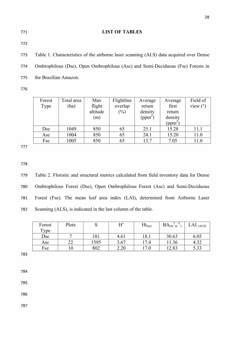
Table 1. Characteristics of the airborne laser scanning (ALS) data acquired over Dense 773

Ombrophilous (Dse), Open Ombrophilous (Asc) and Semi-Deciduous (Fse) Forests in 774

the Brazilian Amazon. 775

776

Forest Type

Total area (ha)

Max flight

altitude (m)

Flightline overlap

(%)

Average return

density (ppm2)

Average first

return density (ppm2)

Field of view (°)

Dse 1049 850 65 25.1 15.28 11.1 Asc 1004 850 65 24.1 15.20 11.0 Fse 1005 850 65 13.7 7.05 11.0

777

778

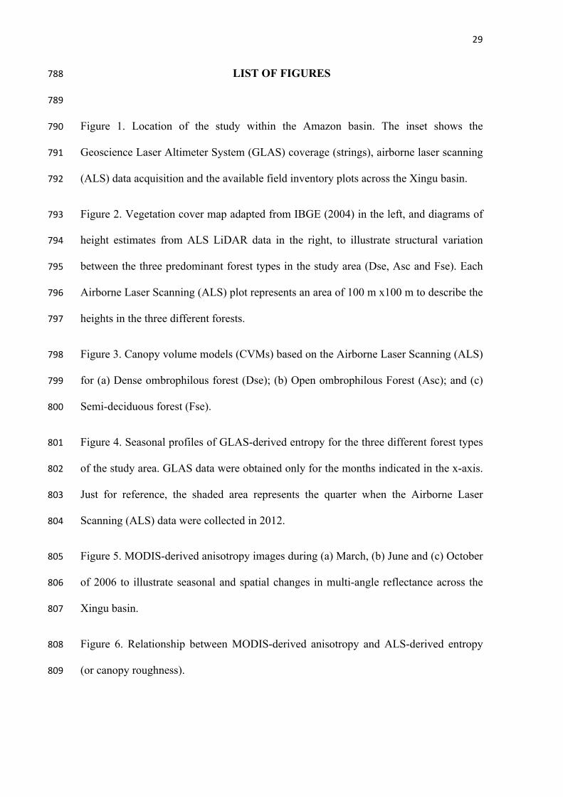
Table 2. Floristic and structural metrics calculated from field inventory data for Dense 779

Ombrophilous Forest (Dse), Open Ombrophilous Forest (Asc) and Semi-Deciduous 780

Forest (Fse). The mean leaf area index (LAI), determined from Airborne Laser 781

Scanning (ALS), is indicated in the last column of the table. 782

Forest Type

Plots S H’ Ht(m) BA(m2

m-2

) LAI (ALS)

Dse 7 181 4.61 18.1 30.63 6.05 Asc 22 1595 3.67 17.4 11.36 4.32 Fse 10 802 2.20 17.0 12.83 5.33

783

784

785

786

787

29

LIST OF FIGURES 788

789

Figure 1. Location of the study within the Amazon basin. The inset shows the 790

Geoscience Laser Altimeter System (GLAS) coverage (strings), airborne laser scanning 791

(ALS) data acquisition and the available field inventory plots across the Xingu basin. 792

Figure 2. Vegetation cover map adapted from IBGE (2004) in the left, and diagrams of 793

height estimates from ALS LiDAR data in the right, to illustrate structural variation 794

between the three predominant forest types in the study area (Dse, Asc and Fse). Each 795

Airborne Laser Scanning (ALS) plot represents an area of 100 m x100 m to describe the 796

heights in the three different forests. 797

Figure 3. Canopy volume models (CVMs) based on the Airborne Laser Scanning (ALS) 798

for (a) Dense ombrophilous forest (Dse); (b) Open ombrophilous Forest (Asc); and (c) 799

Semi-deciduous forest (Fse). 800

Figure 4. Seasonal profiles of GLAS-derived entropy for the three different forest types 801

of the study area. GLAS data were obtained only for the months indicated in the x-axis. 802

Just for reference, the shaded area represents the quarter when the Airborne Laser 803

Scanning (ALS) data were collected in 2012. 804

Figure 5. MODIS-derived anisotropy images during (a) March, (b) June and (c) October 805

of 2006 to illustrate seasonal and spatial changes in multi-angle reflectance across the 806

Xingu basin. 807

Figure 6. Relationship between MODIS-derived anisotropy and ALS-derived entropy 808

(or canopy roughness). 809

30

Figure 7. Relationship between MODIS-derived anisotropy and GLAS-derived entropy 810

using observations for (a) March, (b) June and (c) October of 2006. 811

Figure 8. Relationship between MODIS-derived anisotropy and backscattering (σ0) 812

measurements from SeaWinds/QSCAT over Amazonian tropical forests considering the 813

period 2001 to 2009. 814

Figure 9. Time series profiles of MODIS-derived (a) GLAS entropy estimated using the 815

regression model of Figure 7c, and (b) MODIS-derived SeaWinds/QuikSCAT 816

backscattering (σ0) from the model of Figure 8. Results are shown as spatial average for 817

Dense (Dse) and Open (Asc) Ombrophilous Forests and the Semi-Deciduous Forest 818

(Fse) between 2000 and 2012 for the Xingu basin. 819

820

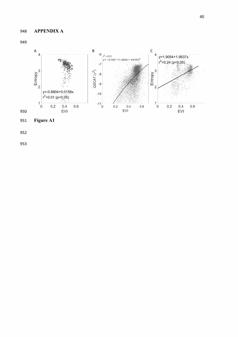
Figure A1. Comparison between MODIS-MAIAC EVI (normalized for directional 821

effects) and estimates of canopy entropy derived from ALS (a), GLAS (b) and 822

QuikSCAT (c). The vegetation index was significantly less suited to describe canopy 823

structural parameters than Anisotropy. 824

825

31

826

Figure 1 827

828

32

829

Figure 2 830

831

832

833

834

835

836

837

838

839

840

841

842

33

843

844

845

Figure 3 846

847

848

849

850

851

852

853

854

855

856

857

858

859

860

861

862

34

863

864

865

Figure 4 866

867

868

869

870

871

872

873

874

875

876

877

878

35

879

a) March

b) June

c) October

Figure 5 880

881

882

883

884

885

886

887

888

889

890

891

892

893

36

894

895

Figure 6 896

897

898

899

900

901

902

903

904

905

906

907

908

37

909

910

Figure 7 911

912

913

914

915

916

917

38

918

919

Figure 8 920

921

922

923

924

925

926

927

928

929

930

931

932

933

39

934

935

Figure 9 936

937

938

939

940

941

942

943

944

945

946

947

40

APPENDIX A 948

949

950

Figure A1 951

952

953