CONTROL ENGINEERING LABORATORY

Simulation in Pulp and Paper Industry

Kauko Leiviskä

Report A No 2, February 1996

University of Oulu Control Engineering Laboratory Report A No 2, February 1996

Simulation in Pulp and Paper Industry

Kauko Leiviskä

University of Oulu, Control Engineering Laboratory

Abstract: Mathematical models and simulation are used in several areas of systems engineering. In research and development they are used in studies of process internal phenomena like flow, mixing, reactions, heat and mass transfer, etc. to gain a thorough understanding of what is really going on inside the process. In product design models are used in defining effects of variables on product quality and amount. In process design, modelling, simulation and optimization methods are nowadays used in studying alternatives for process equipment and connections, to optimize process operation and to find best ways to utilize raw materials and energy. Equipment sizing also utilizes models and simulation. In control engineering, models and simulation are utilized in determining control strategies for the process. Simulation is also an interesting tool for process operation. It is employed in disturbance and alarm analysis, in start-up and shut-down planning, in real time control and optimization and in operator training. This material was written for the Process Simulation Course given to two graduate schools during winter 1996: Graduate School in Chemical Engineering (GSCE) and International Ph.D. Program in Pulp and Paper Science and Technology

Keywords: process simulation, production scheduling, pulp and paper industry ISBN 951-42-4374-9 University of Oulu ISSN 1238-9390 Control Engineering Laboratory Linnanmaa FIN- 90570 OULU

1. INTRODUCTION A model is an abstract description of its object system. It includes the essential features that are defined by its purpose. The model replaces the system under study in the conditions that it is designed to describe. According to standard dictionaries simulation is often said to give the appearance of, to fake or in general to mean something unreal [Wahlström and Leiviskä, 1986]. In terms of systems engineering, the word is used for the task of building a mathematical model of a system and to use that model for a systematic investigation of the actual system. Process simulation systems are program packages used for the simulation of one separate process or a whole mill with standard tools. Flowsheeting is a term that is generally used in the connection of specific computer programs to solve steady-state material and energy balances for design and cost estimation. The word simulation is then not restricted to the solution of the model equations but it is thought to encompass the whole process of model construction, model validation and model use. Models have been used by mankind since the very beginning and the early models were characterized by superstition and wishful thinking. A more systematic use of models emerged after the second world war as initiated by advances in the systems theory. The theory of feedback and the use of differential equations to describe the technical systems of interest were in the 50s triggering a very rapid development in the field of simulation. The introduction of analog computer also had its impact on the whole field and simulation once meant the use of analog computation for the solution of engineering problems. [Wahlström and Leiviskä, 1986] The present development in the field of computers and software has however, made the analog computer obsolete, but the simulation method in general forms is still as young as it was when it was born. What has been happening during the years is that the technology driven development has been offering a multitude of new possibilities for the old method. It could even be said that today there are possibilities to do what ever our colleagues in the 50s were wishing to do. The rapid development has really made it possible to use simulation with a quite larger confidence than earlier and new applications are due to be introduced at a rapid pace. [Wahlström and Leiviskä, 1986] Mathematical models are used in several areas of systems engineering. In research and development mathematical models are used in studies of process internal phenomena like flow, mixing, reactions, heat and mass transfer, etc. to gain a thorough understanding what is really going on inside the process. In product design of process industries different kind of models are used in defining effects of variables on product quality and amount. Process optimization is also done often in the early stages of the design project. In process design, modelling and simulation methods are nowadays used in studying alternatives for process equipment and connections, to optimize process operation and to find best ways to utilize raw materials and energy. Equipment sizing also utilizes models and

2

simulation. In control engineering, models and simulation are utilized in determining control strategies for the process. Simulation is also an interesting tool for process operation. It is employed in disturbance and alarm analysis, in start-up and shut-down planning, in real time control and optimization and in operator training. The users of simulation vary in the same degree. Consulting engineers, designers and equipment vendors use flowsheeting in the process design. The engineers in the research department use it in process studies trying to understand a process and evaluating relationships between process variables. This is done in order to test operating alternatives, for sensitivity studies, energy optimization, etc. Control engineers and control system vendors use simulation in the design of control systems and also in some cases in the operator training. Operators and engineers at the mill site use models and simulation included in the process and production control systems. In pulp and paper industry simulation is used on four typical levels [Jutila and Leiviskä, 1981]: forest sector (regional, national and international), corporate, mill and process. In this paper the main interest is directed to mill and process level. Mill models can be used for following purposes [Jutila and Leiviskä,1981]: (1) Optimal mill design models and simulation are used in selection of equipment, in process capacity planning and also in storage capacity planning. (2) Overall optimization of the mill can be done using economic models. The selection of optimum operation control can also be obtained using simulation models, for instance, the determination of preferable chemical concentrations for each process, the optimal energy usage, etc. Especially in closed mill studies the effects of accumulation of different chemicals in recycling processes must be considered. (3) With the help of production control models optimal scheduling of the processes, optimal utilization of the storage tanks and the planning of rate and grade changes using simulation can be carried out. Usually mill models are formulated in a modular way starting from the process models. It has an advantage that standard main programs and process standard programs can be utilised.

3

2. SIMULATION BASICS When using simulation, one should always be aware of the inherent limitations in the model. A model may be seen as an artefact of the real world, i.e. it is a simplification which is stressing some characteristics of the real system and disregarding the others. The strength and limitations of the model are in the simplification. It makes it possible to concentrate on the relevant characteristics not considering the multitude of aspects that have no interest in the framework of problem definition. The simplification, however, means that important behaviour is not included in the model and this simply means that the model can not be used outside the very narrow range of validity. When starting a simulation project one should always be very well aware of the final objectives of the simulation study. If they are too broad, the simulation will be too expensive in comparision with the potential benefit. If, on the other hand, they are too narrow, the model can not describe all the behaviour relevant for the study. This means that to a large extend, simulation project is governed by the objectives and new objectives after completing the study will probably make a new model necessary. This chapter is, more or less, an updated and edited version of Chapter 2 in [Wahlström and Leiviskä, 1986]. 2.1 Model classification There are plenty of ways to classify models according to different aspects. The model is always developed to fulfil a certain purpose and the model structure and contents must be defined in the beginning in as detailed way as possible. The purpose and the application area define the model type. The actual model formulation, on the other hand, depends on the model type and available data. Different models are also used in different stages of modelling; usually simple models are used in the beginning and, if needed, more complicated models are resulted in the later stages of the simulation project. Classification according to the model structure According to the model structure one can speak about physical and symbolic models. Physical models like small scale models, pilot plants, prototypes and analog models are descriptive and versatile ways to study the process, but their costs can rise high. Usually prototypes and pilot models are used at the final stage of the simulation project after studies with symbolic models; usually mathematical models; have already confirmed the feasibility of the studied system.

4

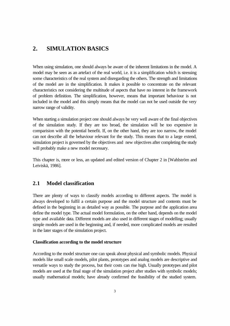
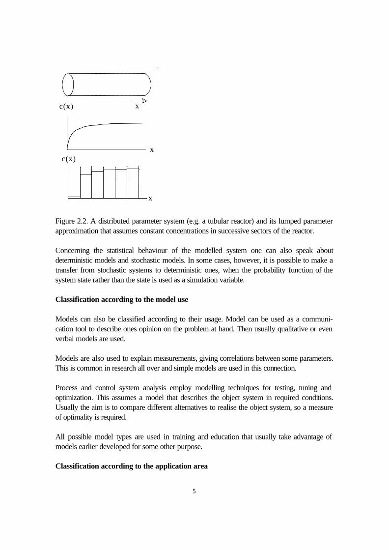
Mathematical models can be further divided into analytical and numerical ones based on the principle of solution. Classification according to the model behaviour According to the time behaviour one can speak about steady-state and dynamic models. Steady-state models are used in the case time dependent behaviour is not of great importance or when the system has enough time to settle to an equilibrium. They have found a permanent use in e.g. flowsheet simulators common in the chemical engineering. Dynamic models; further classified as continuous and discrete ones; are necessary when time dependent behaviour is deemed important, e.g. in the case when time constants are playing an important role. Discrete event simulation is used when only quantum changes in the system state are considered important. Typical examples are the simulation of queuing systems and other Markovian systems. Continuous systems are characterized by differential equations and in this case, time is advanced as a continuous variable in the simulation. Dynamic models are widely used in diversified engineering fields e.g. in control system design and in training simulators. Figure 2.1 describes the difference between continuous and discrete dynamic models.

t

y( t)

kT

y(kT)

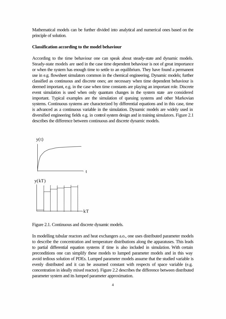
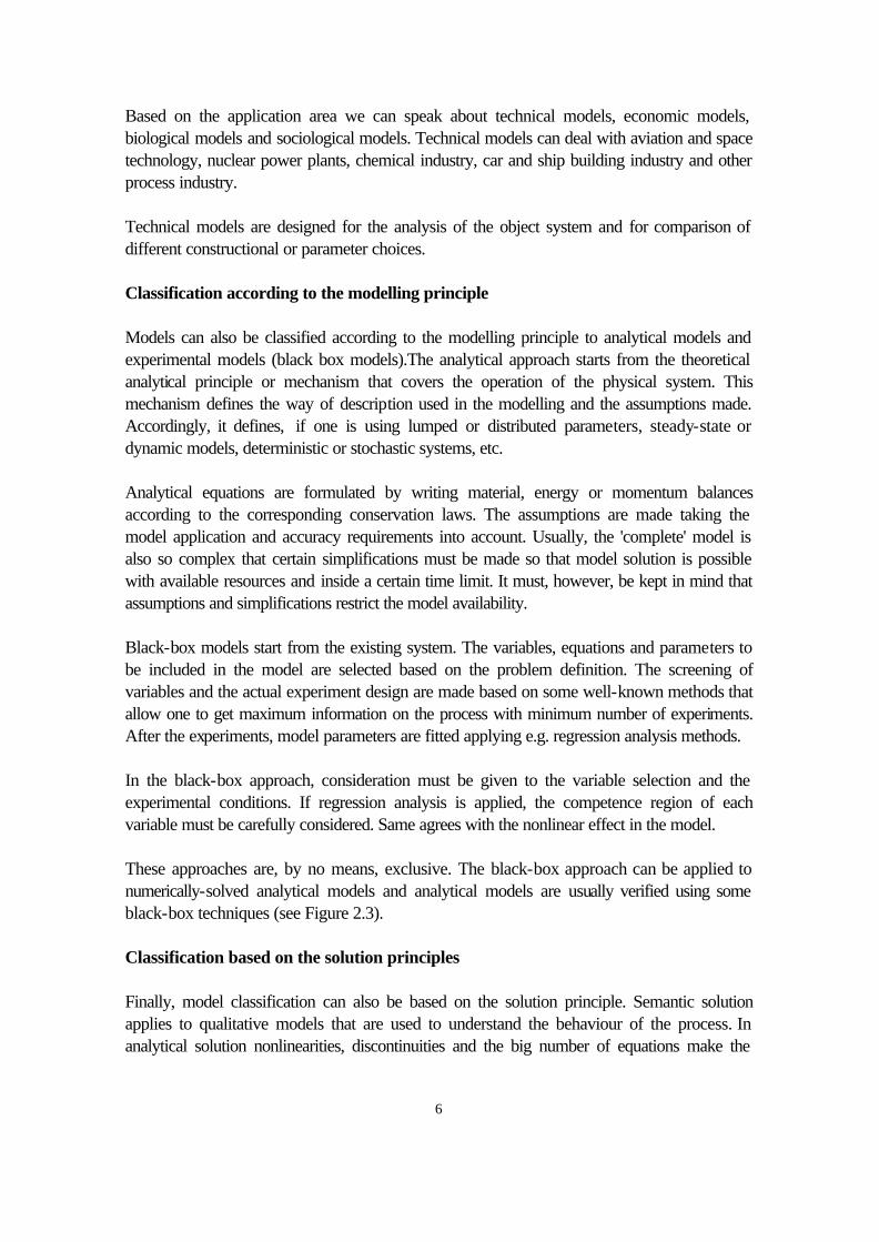
Figure 2.1. Continuous and discrete dynamic models. In modelling tubular reactors and heat exchangers a.o., one uses distributed parameter models to describe the concentration and temperature distributions along the apparatuses. This leads to partial differential equation systems if time is also included in simulation. With certain preconditions one can simplify these models to lumped parameter models and in this way avoid tedious solution of PDEs. Lumped parameter models assume that the studied variable is evenly distributed and it can be assumed constant with respects of space variable (e.g. concentration in ideally mixed reactor). Figure 2.2 describes the difference between distributed parameter system and its lumped parameter approximation.

5

c(x)

x

x

c(x)

x

Figure 2.2. A distributed parameter system (e.g. a tubular reactor) and its lumped parameter approximation that assumes constant concentrations in successive sectors of the reactor. Concerning the statistical behaviour of the modelled system one can also speak about deterministic models and stochastic models. In some cases, however, it is possible to make a transfer from stochastic systems to deterministic ones, when the probability function of the system state rather than the state is used as a simulation variable. Classification according to the model use Models can also be classified according to their usage. Model can be used as a communi-cation tool to describe ones opinion on the problem at hand. Then usually qualitative or even verbal models are used. Models are also used to explain measurements, giving correlations between some parameters. This is common in research all over and simple models are used in this connection. Process and control system analysis employ modelling techniques for testing, tuning and optimization. This assumes a model that describes the object system in required conditions. Usually the aim is to compare different alternatives to realise the object system, so a measure of optimality is required. All possible model types are used in training and education that usually take advantage of models earlier developed for some other purpose. Classification according to the application area

6

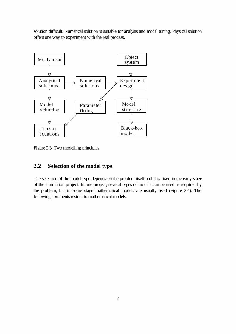
Based on the application area we can speak about technical models, economic models, biological models and sociological models. Technical models can deal with aviation and space technology, nuclear power plants, chemical industry, car and ship building industry and other process industry. Technical models are designed for the analysis of the object system and for comparison of different constructional or parameter choices. Classification according to the modelling principle Models can also be classified according to the modelling principle to analytical models and experimental models (black box models).The analytical approach starts from the theoretical analytical principle or mechanism that covers the operation of the physical system. This mechanism defines the way of description used in the modelling and the assumptions made. Accordingly, it defines, if one is using lumped or distributed parameters, steady-state or dynamic models, deterministic or stochastic systems, etc. Analytical equations are formulated by writing material, energy or momentum balances according to the corresponding conservation laws. The assumptions are made taking the model application and accuracy requirements into account. Usually, the 'complete' model is also so complex that certain simplifications must be made so that model solution is possible with available resources and inside a certain time limit. It must, however, be kept in mind that assumptions and simplifications restrict the model availability. Black-box models start from the existing system. The variables, equations and parameters to be included in the model are selected based on the problem definition. The screening of variables and the actual experiment design are made based on some well-known methods that allow one to get maximum information on the process with minimum number of experiments. After the experiments, model parameters are fitted applying e.g. regression analysis methods. In the black-box approach, consideration must be given to the variable selection and the experimental conditions. If regression analysis is applied, the competence region of each variable must be carefully considered. Same agrees with the nonlinear effect in the model. These approaches are, by no means, exclusive. The black-box approach can be applied to numerically-solved analytical models and analytical models are usually verified using some black-box techniques (see Figure 2.3). Classification based on the solution principles Finally, model classification can also be based on the solution principle. Semantic solution applies to qualitative models that are used to understand the behaviour of the process. In analytical solution nonlinearities, discontinuities and the big number of equations make the

7

solution difficult. Numerical solution is suitable for analysis and model tuning. Physical solution offers one way to experiment with the real process.

Numericalsolut ions

Mechanism

Analyt icalsolut ions

Modelreduction

Transferequat ions

Parameterfitt ing

Objectsystem

Experimentdesign

Mo delstructure

Black-bo xmodel

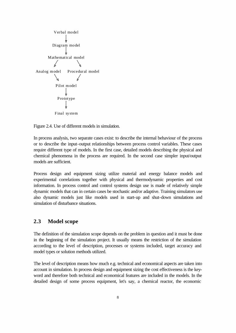
Figure 2.3. Two modelling principles. 2.2 Selection of the model type The selection of the model type depends on the problem itself and it is fixed in the early stage of the simulation project. In one project, several types of models can be used as required by the problem, but in some stage mathematical models are usually used (Figure 2.4). The following comments restrict to mathematical models.

8

Verbal model

Diagram model

Mathematical model

Analog model Procedural model

P ilot model

Prototype

Final system Figure 2.4. Use of different models in simulation. In process analysis, two separate cases exist: to describe the internal behaviour of the process or to describe the input-output relationships between process control variables. These cases require different type of models. In the first case, detailed models describing the physical and chemical phenomena in the process are required. In the second case simpler input/output models are sufficient. Process design and equipment sizing utilize material and energy balance models and experimental correlations together with physical and thermodynamic properties and cost information. In process control and control systems design use is made of relatively simple dynamic models that can in certain cases be stochastic and/or adaptive. Training simulators use also dynamic models just like models used in start-up and shut-down simulations and simulation of disturbance situations. 2.3 Model scope The definition of the simulation scope depends on the problem in question and it must be done in the beginning of the simulation project. It usually means the restriction of the simulation according to the level of description, processes or systems included, target accuracy and model types or solution methods utilized. The level of description means how much e.g. technical and economical aspects are taken into account in simulation. In process design and equipment sizing the cost effectiveness is the key-word and therefore both technical and economical features are included in the models. In the detailed design of some process equipment, let's say, a chemical reactor, the economic

9

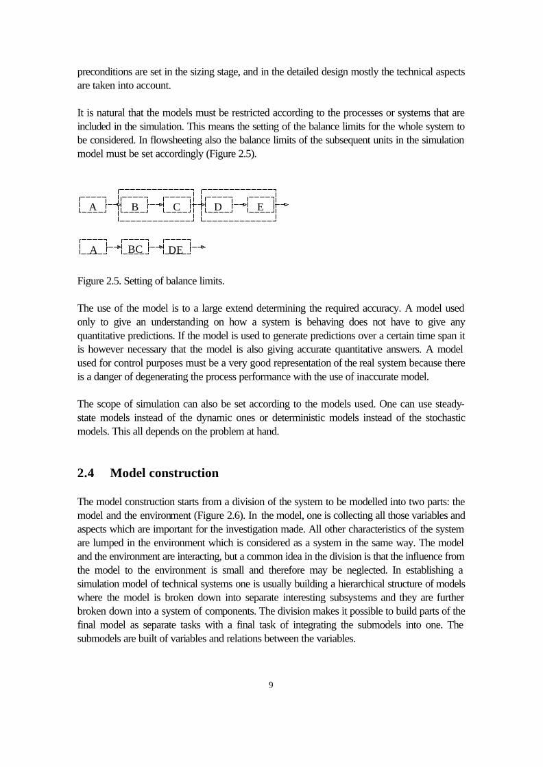
preconditions are set in the sizing stage, and in the detailed design mostly the technical aspects are taken into account. It is natural that the models must be restricted according to the processes or systems that are included in the simulation. This means the setting of the balance limits for the whole system to be considered. In flowsheeting also the balance limits of the subsequent units in the simulation model must be set accordingly (Figure 2.5).

A B C D E

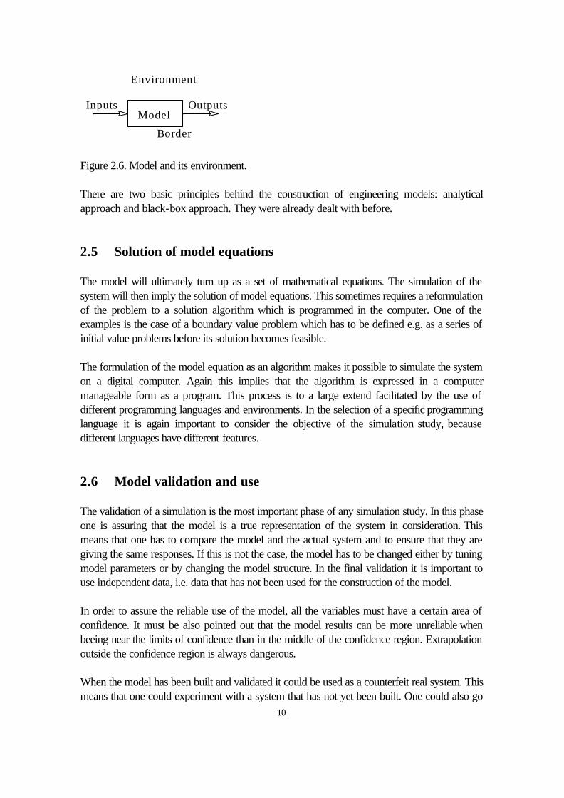
A BC DE Figure 2.5. Setting of balance limits. The use of the model is to a large extend determining the required accuracy. A model used only to give an understanding on how a system is behaving does not have to give any quantitative predictions. If the model is used to generate predictions over a certain time span it is however necessary that the model is also giving accurate quantitative answers. A model used for control purposes must be a very good representation of the real system because there is a danger of degenerating the process performance with the use of inaccurate model. The scope of simulation can also be set according to the models used. One can use steady-state models instead of the dynamic ones or deterministic models instead of the stochastic models. This all depends on the problem at hand. 2.4 Model construction The model construction starts from a division of the system to be modelled into two parts: the model and the environment (Figure 2.6). In the model, one is collecting all those variables and aspects which are important for the investigation made. All other characteristics of the system are lumped in the environment which is considered as a system in the same way. The model and the environment are interacting, but a common idea in the division is that the influence from the model to the environment is small and therefore may be neglected. In establishing a simulation model of technical systems one is usually building a hierarchical structure of models where the model is broken down into separate interesting subsystems and they are further broken down into a system of components. The division makes it possible to build parts of the final model as separate tasks with a final task of integrating the submodels into one. The submodels are built of variables and relations between the variables.

10

ModelInputs Outputs

Border

Environment

Figure 2.6. Model and its environment. There are two basic principles behind the construction of engineering models: analytical approach and black-box approach. They were already dealt with before. 2.5 Solution of model equations The model will ultimately turn up as a set of mathematical equations. The simulation of the system will then imply the solution of model equations. This sometimes requires a reformulation of the problem to a solution algorithm which is programmed in the computer. One of the examples is the case of a boundary value problem which has to be defined e.g. as a series of initial value problems before its solution becomes feasible. The formulation of the model equation as an algorithm makes it possible to simulate the system on a digital computer. Again this implies that the algorithm is expressed in a computer manageable form as a program. This process is to a large extend facilitated by the use of different programming languages and environments. In the selection of a specific programming language it is again important to consider the objective of the simulation study, because different languages have different features. 2.6 Model validation and use The validation of a simulation is the most important phase of any simulation study. In this phase one is assuring that the model is a true representation of the system in consideration. This means that one has to compare the model and the actual system and to ensure that they are giving the same responses. If this is not the case, the model has to be changed either by tuning model parameters or by changing the model structure. In the final validation it is important to use independent data, i.e. data that has not been used for the construction of the model. In order to assure the reliable use of the model, all the variables must have a certain area of confidence. It must be also pointed out that the model results can be more unreliable when beeing near the limits of confidence than in the middle of the confidence region. Extrapolation outside the confidence region is always dangerous. When the model has been built and validated it could be used as a counterfeit real system. This means that one could experiment with a system that has not yet been built. One could also go

11

through sequences of events which are not possible with a real system e.g. for safety or cost reasons. In the use of simulation results one should be aware of the inhererent limitations of their applicability. Very often the simulation results will not be used as such, but they will be used as input into a decision process. In such cases it is even more important to convey the qualitative implications of the simulation in an easily understandable form to the decision maker. This puts stress on the interface of the model; the way how the operator sees and uses the model. In order to facilitate the use, interactive interfaces for input information, execution and reporting are favored. The model documentation is also important and the self-documenting features of computerized models are recommended. The model updating is a critical issue especially with the models used in on-line process control. The need for updating must be clearly specified together with the updating procedure. In large off-line models, updating can be even a more tedious job, because the process information must be transfered, in worst cases, manually. The model transferability is sometimes problematic. Parametrization is the least that must be done, when using the once-developed model in some other process. Usually the model structure and its limits and construction must be changed. Good documentation is necessary to improve the transferability of the model.

12

3. PROPERTIES OF FLOWSHEET SIMULATORS 3.1 Definitions A modular flowsheet simulator describes the process as a set of modules connected by the flows of material and energy between them. The flows constitute of a number of components that undergo transformations (reactions e.g.) when they pass via the system. Modules itself are simply material and energy balances together with those physical and thermodynamical data and correlations that are necessary for calculations. The sequence of module calculations is taken care by an executive program which also controls the input data reading routines and the print-out routines. Steady-state flowsheet programs have been used since 60s in the chemical industry. Their potential applications are in mill engineering design and in development of operating strategies for existing mills. Some dynamic flowsheet simulators have also been developed. These programs can be used in operator training, development of control systems, analysis of start-up and shut-down situations and operations scheduling. The first process simulators during the 60s were very simple and their use was limited. The number of different unit process modules was small, data banks for physical and thermodynamic data and correlations were limited and calculation procedures were simple. Because of the limited properties of computers at this time, their use was also difficult. Second generation flowsheet simulators came to market in the beginning of the 70s. They had already large libraries for unit modules and physical properties. The numerical methods used were more efficient than in the earlier simulators and the man/machine interface started to approach modern level. The cost and investment data could also be connected to simulation results. The third generation codes were developed during 80s. The most important factor is in the usage of these systems. Simulators are integrated in total data base systems where they can use the same data that is available in all stages of the mill design. The capabilities of work stations and modern PC-computers are utilized in the man/machine interface. Two solution techniques are used in the flowsheet simulators: The modular sequential approach is the most common one. It computes modules one by one in a certain sequence that usually follows the direction of physical flows in the studied system. This means that the input flows of the module to be calculated must be known and the output flows are calculated based on the input flows and module parameters. If recycle flows exist, their values must be guessed in the beginning and iteratively improved during the simulation. The iteration continues until the balance constraints are satisfied and convergence is gained.

13

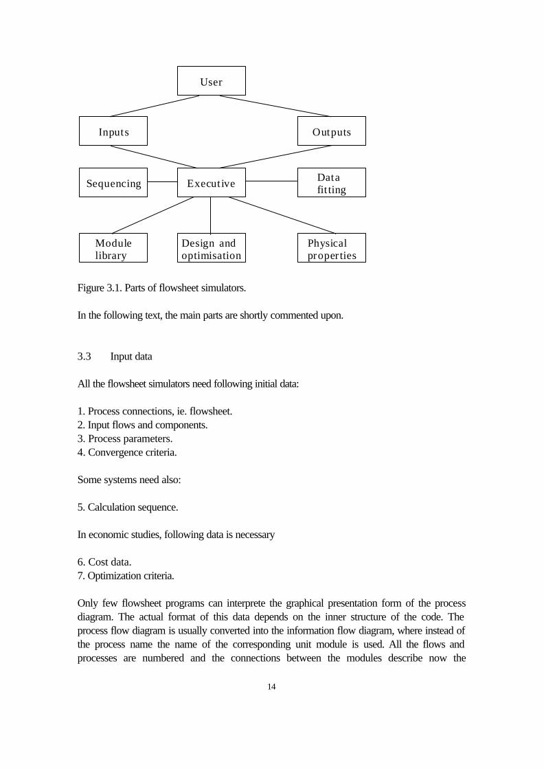
The requirements for the computer memory are small in this approach, because only limited amount of information is needed for the calculation of each module in the flowsheet. A big number of iterations and long computing times can, however, cause problems, especially when large processes are considered. Modular simultaneous approach offers another alternative for solving flowsheeting problems. In this approach the information contained by the flowsheet and modules is converted into a set of linear equations that are solved simultaneously. In this method, the number of iterations is minimized and the fast solution is obtained. The requirements for the computer memory are large. In this approach, the constraints for process design can be included in the system that is not possible in the modular sequential approach. 3.2 Structure of flowsheet simulators Regardless of the solution method, all flowsheet simulators have the following main parts (Figure 3.1). It should, however, be noted that the extent of each part can considerably vary from system to system. 1. Data input using interactive methods or different file and data base structures. 2. Sequencing, ie. the determination of the order of calculation. 3. Executive program. 4. Print-out routines. 5. Module library. 6. Routines for design and optimization. 7. Routines for calculation of physical and thermodynamical properties. 8. Data reconciliation.

14

User

Inputs Outputs

Executive

Modulelibrary

Design andoptimisation

Physicalproper ties

Sequencing Datafit ting

Figure 3.1. Parts of flowsheet simulators. In the following text, the main parts are shortly commented upon. 3.3 Input data All the flowsheet simulators need following initial data: 1. Process connections, ie. flowsheet. 2. Input flows and components. 3. Process parameters. 4. Convergence criteria. Some systems need also: 5. Calculation sequence. In economic studies, following data is necessary 6. Cost data. 7. Optimization criteria. Only few flowsheet programs can interprete the graphical presentation form of the process diagram. The actual format of this data depends on the inner structure of the code. The process flow diagram is usually converted into the information flow diagram, where instead of the process name the name of the corresponding unit module is used. All the flows and processes are numbered and the connections between the modules describe now the

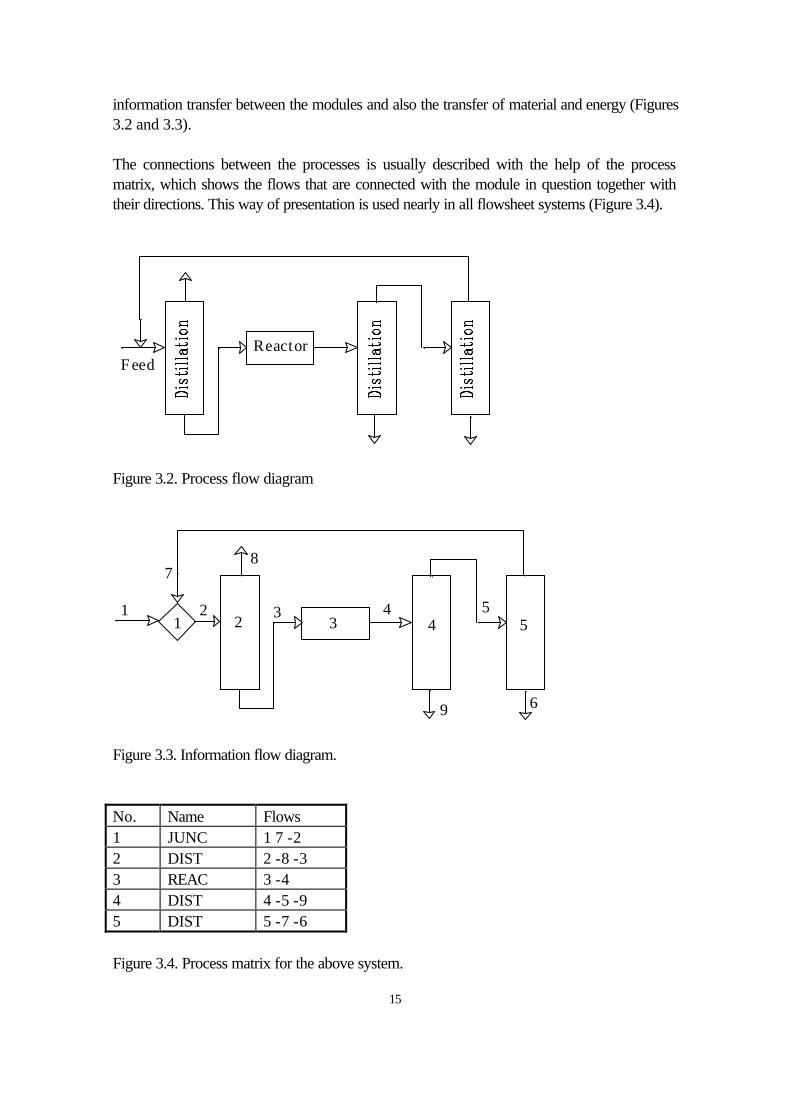
15

information transfer between the modules and also the transfer of material and energy (Figures 3.2 and 3.3). The connections between the processes is usually described with the help of the process matrix, which shows the flows that are connected with the module in question together with their directions. This way of presentation is used nearly in all flowsheet systems (Figure 3.4).

F eedReactor

Figure 3.2. Process flow diagram

1 2 3 4 51 2 3 4 5

6

78

9 Figure 3.3. Information flow diagram. No. Name Flows 1 JUNC 1 7 -2 2 DIST 2 -8 -3 3 REAC 3 -4 4 DIST 4 -5 -9 5 DIST 5 -7 -6 Figure 3.4. Process matrix for the above system.

16

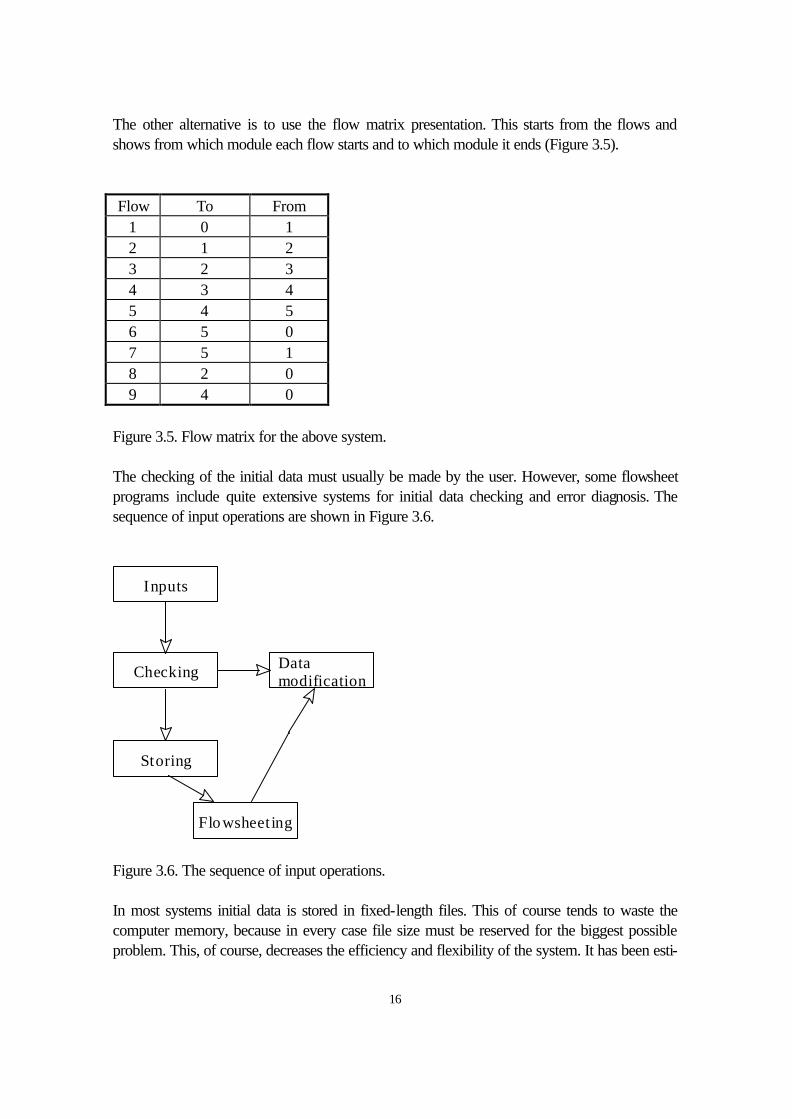
The other alternative is to use the flow matrix presentation. This starts from the flows and shows from which module each flow starts and to which module it ends (Figure 3.5). Flow To From

1 0 1 2 1 2 3 2 3 4 3 4 5 4 5 6 5 0 7 5 1 8 2 0 9 4 0

Figure 3.5. Flow matrix for the above system. The checking of the initial data must usually be made by the user. However, some flowsheet programs include quite extensive systems for initial data checking and error diagnosis. The sequence of input operations are shown in Figure 3.6.

Inputs

Checking

Storing

Flowsheeting

Datamodification

Figure 3.6. The sequence of input operations. In most systems initial data is stored in fixed-length files. This of course tends to waste the computer memory, because in every case file size must be reserved for the biggest possible problem. This, of course, decreases the efficiency and flexibility of the system. It has been esti-

17

mated that big flowsheet simulators use only 20 % of the memory they reserve. In some newest simulators, flexible data base structures are used. 3.4 Sequencing Sequencing means the determination of the calculation order for process modules and it is done with the help of the information flow diagram. It can be done manually, if the number of flows does not exceed 20-30 flows. Automatic procedures are needed if the user has no time or experience to do it manually or if the process to be simulated includes a big number of modules and flows and also there are many recycle flows in the system. Several methods exist for solving this task. Regardless of the method, sequencing consists of the following stages: 1. Partitioning: Identification of recycles and separation of these from the information flow

diagram. 2. Tearing: Identification of the iterative flows, i.e. the flows, the values of which must first

be guessed and later on iteratively improved. 3. Sequencing: Definition of the final order of calculations. Note that the information flow

diagram can include also serial parts, where the order of calculation is easily defined, but they must be included in the final sequence in a logical place.

Iterations are usually done using the standard method of successive substitutions, but in order to shorten the computing time in modular sequential simulators also convergence accelerators have been used. 3.5 Simulation executives Simulation executive programs take care of the actual operation of the flowsheet program. They handle the input data, stores it, call the modules in the preset order of calculation and take care of the print-outs. Several subprograms carry out these tasks. As an example, let us look at PMS/CR process simulator developed at the University of Oulu, Control Engineering Laboratory [Uronen et al., 1985, Jutila et al., 1981, 1982, Leiviskä et al.,1981]. PMS/CR simulator was originally developed for calculation of material and energy balances in the kraft mill chemical recovery but later extended to be capable of entire mill simulations. The

18

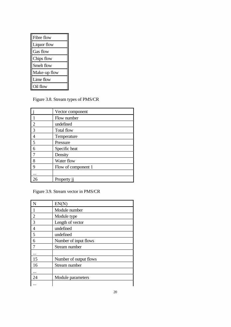
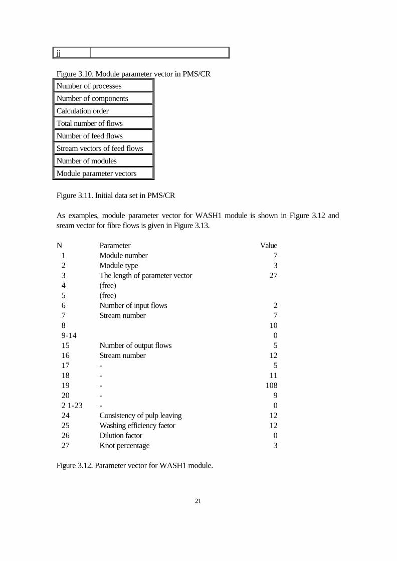
PMS/CR simulation system is a computerized tool for pulp mill balance calculations because of the amount of information to be handled. In practice, material and energy balances must be calculated for all process units separately and also for the whole system, because changes in one unit affect the whole mill. The solution is iterative in nature because of the recycle flows involved. The PMS/CR simulation system has been applied both to 2-line and 1-line kraft pulp mills. Also simple flow dynamics are included. With these experiences in mind the PMS/CR simulation system has proven to be suitable for these kinds of pulp mill simulations. The executive programs, i.e. the programs which read the input data, transfer the data between programs, execute the calculations in the correct sequence, display the results and change the input data if needed (see Figure 3.7), are based on a well-known unproprietary simulation system GEMCS, originally developed at McMaster University. The actual process models were developed in Computer Engineering Laboratory, University of Oulu. In many other modular simulation systems, the models are based on unit operations. In the PMS/CR simulation system the overall material and energy balance models of different process units are used. These models take ongoing reactions and losses into account. An exception is the bleach plant model that utilizes specific dosage models. The simulation system can deal with eight different types of process streams (Figure 3.8). The components of the streams differ from each other. The stream vector formulation is shown in Figure 3.9. The model parameters are given as input data and stored in parameter tables. These parameters correspond to the targets used in the operation of the processes (for example Kappa number, alkali charge, cooking temperature, dilution factor, strong black liquor solids content, white liquor causticity, Figure 3.10). At the beginning of the calculation any parameter can be changed. Moreover, input flow rates, temperatures and concentrations of different components can be respecified (Figure 3.11). The PMS/CR simulation system iteratively calculates the steady state material and energy balances.

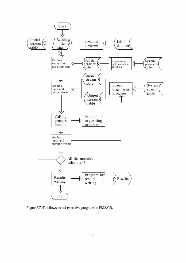
19

Star t

Initialstreamtable

Readinginitialdata

Loadingprogram

Initialdata set

R e a d i n gco n n e ct i o n san d p a r am e t er s

Moduleparametertable

Connectionsand parameterschecking

Systemparametertable

Readinginput andoutput streams

Inputstreamtable

Outputstreamtable

Streamorganisingprogram

Systemstreamtable

Callingprocessmodule

Moduleorganisingprogram

Stor inginput andoutput streams

Resultswriting

Program forresultswriting

Results

End

All the modulescalculated?

Figure 3.7. The flowsheet of executive programs in PMS/CR.

20

Fibre flow Liquor flow Gas flow Chips flow Smelt flow Make-up flow Lime flow Oil flow Figure 3.8. Stream types of PMS/CR j Vector component 1 Flow number 2 undefined 3 Total flow 4 Temperature 5 Pressure 6 Specific heat 7 Density 8 Water flow 9 Flow of component 1 ... 26 Property jj Figure 3.9. Stream vector in PMS/CR N EN(N) 1 Module number 2 Module type 3 Length of vector 4 undefined 5 undefined 6 Number of input flows 7 Stream number ... 15 Number of output flows 16 Stream number ... 24 Module parameters ...

21

jj Figure 3.10. Module parameter vector in PMS/CR Number of processes

Number of components

Calculation order

Total number of flows

Number of feed flows

Stream vectors of feed flows

Number of modules

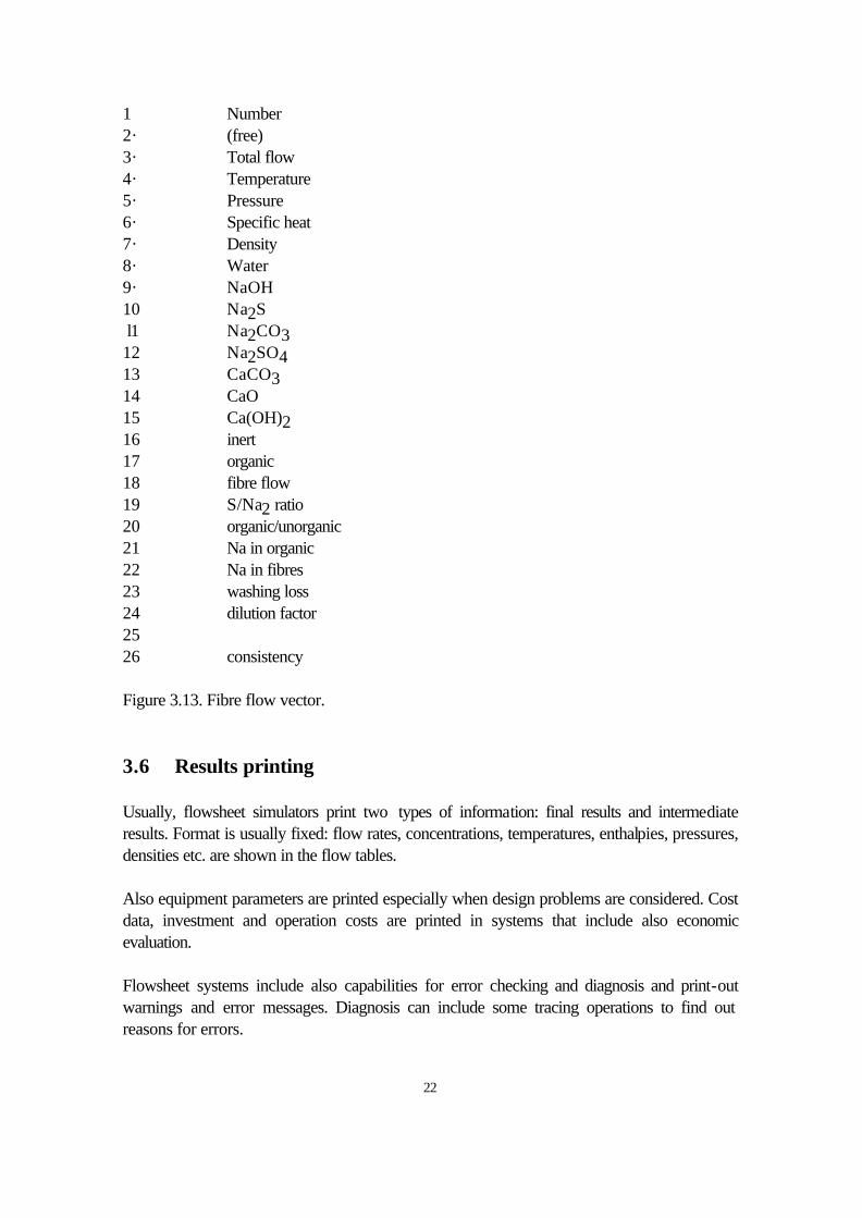
Module parameter vectors Figure 3.11. Initial data set in PMS/CR As examples, module parameter vector for WASH1 module is shown in Figure 3.12 and sream vector for fibre flows is given in Figure 3.13. N Parameter Value 1 Module number 7 2 Module type 3 3 The length of parameter vector 27 4 (free) 5 (free) 6 Number of input flows 2 7 Stream number 7 8 10 9-14 0 15 Number of output flows 5 16 Stream number 12 17 - 5 18 - 11 19 - 108 20 - 9 2 1-23 - 0 24 Consistency of pulp leaving 12 25 Washing efficiency faetor 12 26 Dilution factor 0 27 Knot percentage 3 Figure 3.12. Parameter vector for WASH1 module.

22

1 Number 2· (free) 3· Total flow 4· Temperature 5· Pressure 6· Specific heat 7· Density 8· Water 9· NaOH 10 Na2S l1 Na2CO3 12 Na2SO4 13 CaCO3 14 CaO 15 Ca(OH)2 16 inert 17 organic 18 fibre flow 19 S/Na2 ratio 20 organic/unorganic 21 Na in organic 22 Na in fibres 23 washing loss 24 dilution factor 25 26 consistency Figure 3.13. Fibre flow vector. 3.6 Results printing Usually, flowsheet simulators print two types of information: final results and intermediate results. Format is usually fixed: flow rates, concentrations, temperatures, enthalpies, pressures, densities etc. are shown in the flow tables. Also equipment parameters are printed especially when design problems are considered. Cost data, investment and operation costs are printed in systems that include also economic evaluation. Flowsheet systems include also capabilities for error checking and diagnosis and print-out warnings and error messages. Diagnosis can include some tracing operations to find out reasons for errors.

23

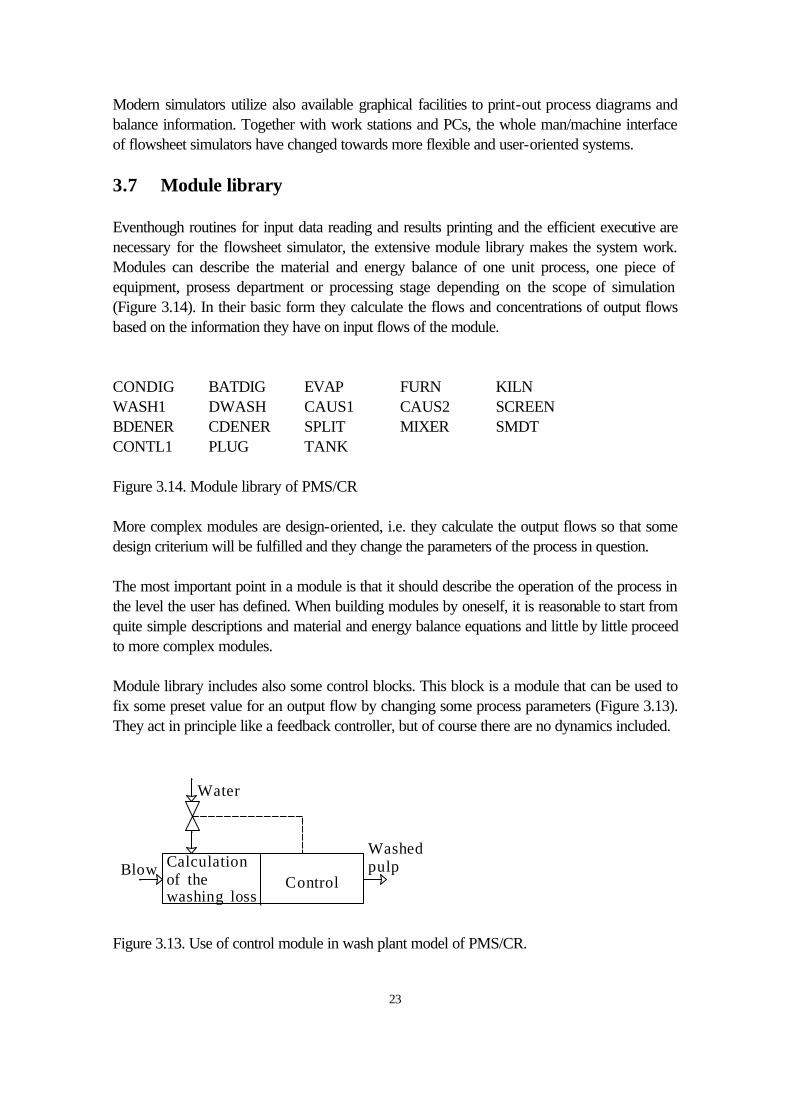
Modern simulators utilize also available graphical facilities to print-out process diagrams and balance information. Together with work stations and PCs, the whole man/machine interface of flowsheet simulators have changed towards more flexible and user-oriented systems. 3.7 Module library Eventhough routines for input data reading and results printing and the efficient executive are necessary for the flowsheet simulator, the extensive module library makes the system work. Modules can describe the material and energy balance of one unit process, one piece of equipment, prosess department or processing stage depending on the scope of simulation (Figure 3.14). In their basic form they calculate the flows and concentrations of output flows based on the information they have on input flows of the module. CONDIG BATDIG EVAP FURN KILN WASH1 DWASH CAUS1 CAUS2 SCREEN BDENER CDENER SPLIT MIXER SMDT CONTL1 PLUG TANK Figure 3.14. Module library of PMS/CR More complex modules are design-oriented, i.e. they calculate the output flows so that some design criterium will be fulfilled and they change the parameters of the process in question. The most important point in a module is that it should describe the operation of the process in the level the user has defined. When building modules by oneself, it is reasonable to start from quite simple descriptions and material and energy balance equations and little by little proceed to more complex modules. Module library includes also some control blocks. This block is a module that can be used to fix some preset value for an output flow by changing some process parameters (Figure 3.13). They act in principle like a feedback controller, but of course there are no dynamics included.

Calculationof thewashing loss

Control

Water

BlowWashedpulp

Figure 3.13. Use of control module in wash plant model of PMS/CR.

24

3.8 Physical and thermodynamic data In order to simulate process, one must know the physical and thermodynamic data connected with the material flows in the system. There are some data banks available that can be used and that are usually used in flowsheet simulators (CIMPP, PPDS). In the flowsheet simulator it must be possible to calculate physical properties continuously as the simulation proceeds and store the calculated values for later usage. Also there must be a possibility for the user to input new data to the system during simulation and to produce new data for the user on such kind of compounds which lack of initial data. Physical and thermodynamical data system must have: 1. Wide range of pure component properties. Both single constant properties and corre-

lations in these cases where the property changes according to the temperature or pressure must be given. Typically properties like molecular weight, critical properties, boiling point, heat capacity, density, enthalpy, free energy, viscosity, thermal conductivity, solubility parameter, etc. are presented. These values must be easily accessible from the simulator.

2. Models, correlations and estimation methods are used in predicting various properties

like critical constants, heat capacities, vapor pressures, heat of vaporization, etc. 3. Methods to calculate thermodynamic properties for mixtures. Factors like enthalpy,

entropy, free energy, fugacity, activity, heat of solution, etc. must be calculated. 3.9 Design and optimization functions In modular sequential simulators, the inclusion of design and optimization functions is difficult. The convergence can be slow with big process diagrams and the use of design- oriented models is difficult. One way is to repeat simulation several time and change process parameters and/or input flows until the design objective has been met. This is however, very time consuming way to work. Also some optimizing routines, LP-models etc., can be used to decide, which parameter to change and how much, but here the computing time becomes easily a limiting factor. Modular simultaneous approach gives better possibilities to make design and optimization with a flowsheet simulator. The design constraints can be added directly into the model and the solution routine does not have to be changed. 3.10 Dynamic flowsheet simulators Introduction of the time factor into the flowsheet simulator framework means a considerable increase in the complexity of the system. There are several factors that contribute to this:

25

1. The dynamics of each module (unit process) must be modelled mathematically and

identified. 2. The resulting set of differential equations must be solved. This may bring about compu-

tational difficulties especially when both slow and fast dynamics are included at the same time. There are special procedures that have been developed to overcome this problem, but anyhow most of computer time is consumed in solving differential equa-tions.

3. The steady-state values for all the flows must be given at simulation start-up time. This

means that this steady-state must be calculated first. This also means that in dynamic part convergence problems do not exist. Dynamic simulation produces of course more results than steady-state simulation.

26

4. SIMULATION IN THE PULP AND PAPER INDUSTRY 4.1 Application viewpoints Process simulation is used for two main tasks in the pulp and paper industry: first to explain the internal behaviour of the process, (i.e. to describe the progress of the process state variables), secondly to explain the external behaviour of the process, (i.e. to compute the values of process output variables based on the input variables). These two views are often mixed together even though the arrangements needed for each case differ considerably from each other. In the calculation of the input-output relationships rather simple models are adequate, while in the simulation of the internal behaviour of the process, thorough and detailed process models and also numerous preliminary studies are required. Thus, in the planning of the simulation studies the purpose of the simulation and the requirements for the results must be considered beforehand. The following text is based on [Jutila and Leiviskä, 1981 and Leiviskä, 1986]. Process flowsheeting In an integrated pulp and paper mill the major material streams from process to process can be described by approx. 90-200 flow vectors. This might lead one to regard material balance calculations as a simple task. However, in the chemical recovery cycle of the pulp mill all the most important active and inactive chemical components must be considered separately, if the propagation and branching of all the materials are to be solved. This, of course, causes an increase in the number of the stream components included in the balance calculations. The same situation is also valid for the pulp mill fibre line and production materials handling in paper and board mills. In spite of the large number of flows and variables, a single material and energy balance calculation for a pulp or a paper mill is not an exceedingly difficult task. However, when the effect of the variations in different stream components on the whole mill material and energy balance is to be studied, a simple case by case calculation manually is no more profitable. The use of computer simulation systems gives extensive advantages in comparison with straightforward calculations: After more extensive work in system design and data collection all kinds of variational effects in stream components can be studied by an incremental additional contribution only. The degree of the model sophistication depends on application. However, in order to minimize the effort for the simulation simple input-output models should be used due to the fact that a lot of unnecessary work can be avoided. It is very difficult to test the validity of very detailed models because of the lack of detailed and accurate process information. This, of course, increases the simulation costs.

27

In steady-state flowsheeting two solution principles are used:modular sequential approach and the modular simultaneous approach. Convergence of sequential solutions is weaker and they often require convergence accelerators [Shewchuk, 1982]. Sequential solutions are also sensitive to the order in which the modules are calculated, so it is possible to affect solution by the selection of the tear streams. The great advantage of the simultaneous approach is that it allows any type of constraint to control the simulation. This makes the expansion to optimization and dynamic simulation easier than in the sequential approach. The computer memory requirements of sequential simulators are smaller than simultaneous ones because of the smaller amount of information needed for the calculation. On the other hand, the memory requirements of simultaneous systems are large, but if the degree of nonlinearity in the system is limited, it provides a very fast solution [Roche and Bouchard, 1983]. In the chemical and petro-chemical industry, most of simulators are, based on historical reasons, mostly of modular sequential type. In the pulp and paper industry both approaches are equally utilized. Adding dynamics to steady-state simulators means the solution of differential equations and therefore the increasing complexity of the system. This is emphasized if the fast control dynamics and slow process dynamics cannot be separated. Inclusion of dynamics means also increasing problems in model fitting and verification. The amount of computations increases and so does also the volume of results. Dynamic simulators are, however, necessary in addition to control design also for the analysis of process dynamics in sizing of storage tanks, rates of reactions, start-ups and shut-downs and grade and rate changes. Comparison of process and mill operational alternatives The comparison of different operational alternatives may require a lot of work, especially when a detailed explanation is desired. When a computer simulation system is available, comparison itself can be carried out easily, but the predetermination of process models and parameters makes the whole project larger than expected. However, the total gain is much higher because of more versatile results than in direct calculation or in experimental evaluation. In other words with the help of a simulation system it is possible to estimate the effect of a change in operational rules on the composition of process streams, on the propagation of flow and concentration disturbances, on the process and storage delays, and on the operational costs resulting in the optimal control strategy of the mill and processes. Process design

28

The role of simulation for pulp and paper mill process design is mainly restricted with respects to the determination of the required capacities of different subprocesses. This capacity for planning is strongly tied with the planned operational strategy and the product mix of the mill because of material recycles and the dependence of same on mill operation. With the help of a simulation system, designing alternatives can be studied and compared. Most process designers use steady-state simulators and some of them are linked with CADD-systems. Besides the determination of required process capacities the dimensioning of sufficient or optimal intermediate storage tanks is often accomplished with the help of simulation studies in the pulp and paper industry. Simulation in process control Modelling and simulation have traditionally been used in defining and testing the control strategies for pulp and paper mill processes. Because of strong interactions between process variables simulation has been a valuable tool for this purpose. This operation has been typically off-line type. This kind of simulation requires a thorough knowledge of process behaviour and relatively detailed models. Simulation has also been used in tuning the control loops as a testing environment. Several computer system vendors have nowadays program packages for automatic tuning of digital control loops and for simulation of proposed controllers. These programs are usually run on-line and they use actual process measurements. For pulp and paper mill processes many strong interactions exist, in which case simulation can make the control design easier. However, problems arise with the identification of suitable models because the interactions typically vary from case to case. Nowadays, it is possible to use steady-state and dynamis simulators to design and testing of DCS systems. This calls for integration of models for controls and actuators together with logic functions into the simulation system [Shewchuk et al., 1991]. Applications of AI and Expert Systems in process control will increase in the future. Process simulators have certain roles to play in this development [Shewchuk et al., 1991]. One is a test-bed role; AI applications are first tested using advanced dynamical mill and process models. It should also be noted that AI applications exist on all control levels, including production scheduling and decision support systems for mill management. This requires new simulation tools. Simulation in production planning and control Simulation can be used in pulp mill production scheduling for testing the production schedules proposed by the operators or calculated by the scheduling system. Including heuristic rules that are used in correcting the initial schedules given by the operators leads to a very effective scheduling approach. Some examples are given in [Leiviskä et al., 1982 and Oldberg, 1983].

29

Simulation is also used in connection with the power plant optimization.Some of the first examples is given by [Sutinen et al., 1984 and Nettamo et al.,1986]. They describe an energy management system which includes also an off-line simulation facility. Simulation starts from the actual state of the process and the operator can enter new values and simulate the new energy demand situation. Training Simulation has been widely used in training in e.g. space flight, pilot training, marine systems and nuclear power plant operator training. In the pulp and paper industry, training applications are few but the trend has been growing during the last ten years. This is undoubtedly due to decreasing prices of simulators and micro-computer-based systems. Mault (1984) has introduced a software simulator for use in teaching control tuning theory and practice for paper machines. A dynamic simulator for operator training is also reported by [Barber et al., 1983]. SACDA is representing the TRAINER system [Shewchuk and Leaver, 1986]. 4.2 Pulp and paper mill simulation problems As already stated, there are some specific but also rather common problems in pulp and paper mill simulation studies. These problems can be roughly classified into two main groups, namely the fitting of models to the process behaviour and the lack of suitable models for certain specific purposes. Because pulp and paper mills consist of many types of subprocesses, especially when the manufacture of byproducts is included, all kinds of problems may arise in addition to the two stated above. Adjustment of models A typical problem for pulp or paper mill simulation is the adjustment of theoretically derived models to process data. Even though the models are in principle based on material balances and therefore the theoretical form of the model should be correct, the adjustment may be correct only at one operating point but incorrect elsewhere for many reasons which will be outlined here. The most frequent problem in the testing of material balance models is the absence or lack of suitable measurements needed for complete balance checking. The flow rates of the main process streams are normally measured in the pulp and paper mill but there are also several material flows which are not measured at all. Typical examples are the flows of knots and rejects as well as sealing waters which are not normally measured thereby rendering inaccurate balance determination.

30

Process streams concentration is not normally measured directly, instead the most important chemicals are sampled and analyzed but this is not the case for all streams. Thus both flow rates and concentrations of several process streams remain undetermined. Also the representativeness of chemical samples is not always good either. The measurement of pulp consistency is still a big problem, especially for high consistency streams and storage tanks. This means that the fibre production rate is not accurately known until final product output. Therefore simulation can give accurate results only on the theoretical level but cannot be compared with measured production data for short periods. As can be concluded from the problems outlined above, the acquisition of process data can be complicated by many practical problems which result in an increase of work required before simulation studies. The process stream variables to be processed in a detailed simulation study of an integrated pulp and paper mill exceeds several thousands. Only a part of these can be determined from the process, the rest must be estimated in some other way. The adjustment of simulation model parameters to uncertain process data requires a lot of fitting experiments before the real simulation studies can be started and also the amount of the data to be processed is high. Therefore the total amount of work for a simulation study becomes so high that a project evaluation must be done before starting. The lack of suitable balance reconciliation methods can be considered one reason for the high manpower requirement needed for pulp and paper mill simulation. The balance reconciliation can be facilitated by computerised methods [Shewchuk, 1983]. However, the development of effective methods decreases some of the above problems but does not solve all of them. Lack of suitable models A vast number of published simulation models of different pulp and paper processes are available. However, this fact does not guarantee the suitability of these models for one's own purposes. This is especially true for the difference between above mentioned internal and external simulation studies. This means, that the models designed for internal process unit simulation should not be utilized in the simulation of the entire production line, because too many useless equations, variables and parameters are involved in the solution of a comparatively simple task. This also increases the margin of error for the results. Thus the simulation models used should be as complicated as necessary but as simple as possible so as to minimize the manpower required and the reliability and to optimize theunderstandability of results. Another problem in the utilization of the available models is the fact that two identical pulp and paper mills do not exist, which forces the designer to change the available models to a certain degree for the particular case in question. After all, complete models are very seldom available and the lack of suitable models is obvious. At a minimum the fitting of model parameters is always required from process to process and from mill to mill. Documentation

31

Only a good documentation assures the continuous usage of the simulation system. It must be possible to use simulation programs after the key-person in system development has left the house or is busy with other projects. All the blocks and routines inside the system must be documented together with the careful explanation of the input parameters. The level of documentation must correspond the normal one in the mill practice and must make it possible for a no-ADP-expert to start using the simulation system. The ideal system for documentation is to include self-documenting and helping features in the system. Results presentation Simulation systems produce far more data than necessary for any purpose. This fact is still emphasized with dynamic simulation. So the presentation of results becomes a very important point in system justification. A recommended way is to use process flowsheets as a report background and print the balance information on these. Also it is possible to make summaries of the balance information. 4.3 Flowsheet simulators in the pulp and paper industry GEMS GEMS is a general purpose mass and heat balance simulator developed originally in the University of Idaho [Edwards and Baldus, 1978]. It utilises a modular sequential solution structure. It is written specially for the pulp and paper industry and includes a wide variety of process models and a physical property package. In addition to the steady-state modules, GEMS also has two dynamic modules; an ideal continuous stirred tank and a plug flow delay block. GEMS has been used extensively for material and energy balance calulations already during 70s [Corson and Edwards, 1976, Gunseor and Rushton, 1979, Venkatesh et al., 1975, 1977,1978, Xuan et al., 1978]. Several different versions have been reported in the literature. GEMSOP is a set of programs working with PC GEMS simulation package making interactive operations and process optimization possible [ Boyle, 1987]. The package has four parts: WINDOW is a program for running GEMS simulation with screen interaction. It is taking care of inputs and outputs in tabular form. CREATE is a program for generating a linear programming model based on the GEMS simulation. This is not done interactively, but the input data is generated automatically. For complex situations, this is a time consuming stage. OPTIMUM is a program for optimization using the linear programming algorithm. Finally, ESTIMATE is a program for model parameter estimation using full simulation models. Real-time dynamic PC GEMS has also been used for training purposes by interfacing it with Moore Products' DCS [Haynes et al., 1990]. A dynamic paper machine saveall simulation running in real time (or faster-than-real-time) has been developed. It utilises standard GEMS

32

models. GEMS has also been used in dynamic simulation of RDH process, where the problem is the changing of the process topology (flows stop and change directions) [Scheldorf and Edwards, 1993, Scheldorf et al., 1991]. GEMS has also been integrated with a millwide information system, an expert system shell and SPC into a prototype advisory system for recovery boiler operation [Smith et al., 1991] and for expert system for multiple-effect evaporators [Brooks and Edwards, 1992]. Recovery boiler model has also been referred by [Uloth et al., 1992]. Strand et al. [1991] also report the application of PCGEMS in on-line control and optimization of the refining process. For this purpose, PCGEMS executive was rewritten resulting in 3-4 times faster execution times than before. MASSBAL MASSBAL MKII was originally developed by SACDA Inc. in cooperation with Energy Mines and Resources Canada as a generalised simultaneous modular process simulation package for calculating the steady-state heat and mass balances for industrial processes [Shewchuk, 1987]. The system has been designed for the modelling of water-based processes such as those found in pulp and paper and mineral industries. It is a successor to the number of earlier systems developed already during the 1970s. It runs on a several hardware possibilities from personal computers to mainframes and includes earlier program packages in an integrated environment. Model generation is carried out by using the user-friendly multi-level keyword-based input language. Language has been designed to be self-documenting. In microcomputer environment an interactive front-end program called the MODEL BUILDER is available. It makes it possible even for user with little or no experience with process simulation to use the system. Another possibility is to use CADSIM graphics front-end and configure the simulated system by simply drawing the process flowsheet. CADSIM generates the simulation model, executes the simulation and returns the results on the flowsheet. Still another possibility is to connect MASSBAL to real-time process distributed control system. In this way process optimization, data reconciliation or predictive calculations can be done. MASSBAL MKII can deal with standard or user specified stream variables and it includes also power streams. Equipment variables are built-in in the modules. Also economic cal-culations can be included. Physical property package include properties for steam, con-densates, calcium and sodium compounds, black liquor, combustion gases, etc. All properties can be changed by user supplied correlations or experimental data. MASSBAL MKII uses a simultaneous approach for solving mass and energy balances. This results in a flexible system that can handle both performance, design and rating calculations. All these problems can be solved using same model, but different configuration. MASSBAL

33

MKII supports also the data reconciliation features available from SACDA. For optimization, successive quadratic programming (SQP) is used. In addition to conventional reporting system, MASSBAL MKII has a generalised report generator for preparing customised reports or linking simulation results to downstream calculation for engineering drawing, spreadsheet programs or word processing. MASSBAL MKII has been used for example in kraft liquor cycle simulation in a Champion International Corporation mill [Misra and Sowul, 1990]. Effects of several key variables such as causticising efficiency, pulp production rate, green liquor strength, etc. were considered. SACDA is also marketing an operator training system called TRAINER, that uses dynamical process models and models for controls and logic. Several cases have been reported. [Terrell and McLaughlin, 1991] report on full paper machine application where TRAINER is connected to Bailey Network 90 DCS. Other flowsheet simulators GEMCS (General Engineering and Management Computation System, pronounced gee-max) was originally developed at McMaster University [Johnson and Peters, 1979]. GEMCS has been used for different Chemical Engineering applications. Boyle et al. [1975] used it to simulate a kraft pulping process. An extensive simulator for kraft mill studies based on GEMCS has also been developed at the University of Oulu [Jutila et al., 1982, Uronen et al., 1985]. FEM (Facility Energy Model) has been developed by the Weyerhauser Company [Thomas, 1979]. Later it was integrated with GEMS resulting in CHAMPS (Chemical Heat and Material Process Simulation). MAPPS is a Fortran-based program utilizing sequential modular approach for simulation of steady-state behaviour of pulp and paper mills. It has been developed by the Institute of Paper Chemistry [Sell and Clay, 1991]. It has been originally designed for calculating mass and energy flows, but it can also be used for equipment design. It can handle up to 12 different stream types including different properties. In the before mentioned reference, it has been used in modelling and design of fluidized bed dryer. PAPDYN is a dynamic modular simulation package developed at Paprican and based on a steady-state modular package, PAPMOD. An example for washing simulation is given in [Turner et al., 1993] Sezgi et al. (1994) have reported on the application SLAM II simulation language for RDH tank farm simulation. Also SIMNON has been applied in dynamic modelling and simulation of the recausticizing plant [Wang et al.,1994]. Some reports have recommended using spreadsheets instead of flowsheet simulators [Frazier, 1991]. It has been found that operating superintendents or mill process engineers more likely

34

use iterative spreadsheets as a starting point for further investigations than flowsheet simulators that seem to be a tool for R&D laboratory or consultants. 5. DYNAMIC PULP MILL MODEL FOR PRODUCTION

SCHEDULING 5.1 Modelling principles Pulp mills are very complex systems from the overall control point of view consisting of processes with storage tanks between them. Shut-downs and disturbances in one process tend to propagate and influence the operation of other processes. This may lead to production losses and to unnecessary changes in production rates which further cause quality disturbances and in some cases also increase the environmental load of the mill. The production rate changes may also cause undesired wear on process equipment. The propagation of disturbances can lead to enforced shut-downs of processes because of either full or empty storage tanks. The start-up of the process after this kind of disturbance can also be problematic. It is clear that all these factors can cause considerable economic losses. These losses are reduced by improved production scheduling. First, this means the determination of production rates for the different processes so that the full utilization of the storage tank capacity of the mill is possible. Secondly, the system must be able to continuously help the staff in decision-making. This is especially important when disturbances and unexpected situations are concerned. This point is usually neglected in theoretical studies that concentrate mostly on the first problem, but its importance from the practical point of view cannot be forgotten. In the following, some points of pulp mill production scheduling are shortly discussed [Leiviskä, 1982,1990, Leiviskä and Niemi, 1988, Sutinen et al., 1990]. Model formalism For production scheduling purposes the pulp mill is usually described as a system of processes and storage tanks between them possibly together with the steam balance (Figure 5.1). The model flows are of pulp, liquor and steam. Concentration of chemicals are assumed to be constant. The dynamics of individual processes are usually neglected and only storage dynamics are included in the model. One important definition in the scheduling models is the concept of transfer ratio ie. the ratio between flows around each process (Figure 5.2). This ratio is usually assumed constant during scheduling. In practice, it means that processes use raw materials and prepare products always in the same ratio, when the same quality is produced.

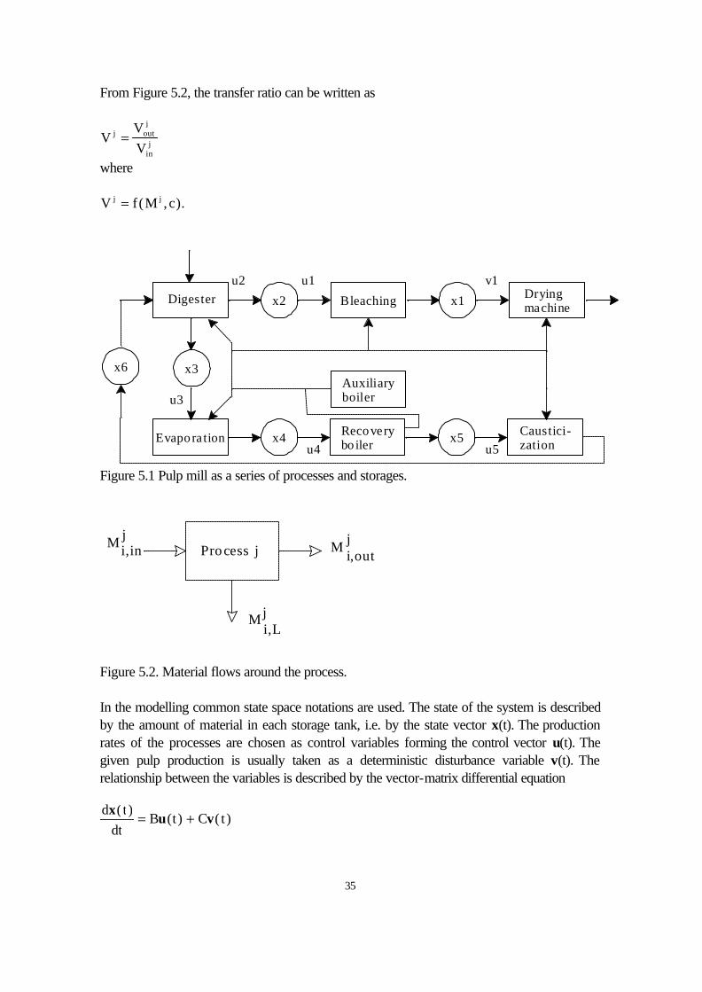
35

From Figure 5.2, the transfer ratio can be written as

VVV

j outj

inj=

where V f M cj j= ( , ).

Digester Bleaching Dryingmachine

Evaporation Recoverybo iler

Auxiliaryboiler

Caustici-zation

v1u1u2

u3

u4 u5

x1x2

x3

x4 x5

x6

Figure 5.1 Pulp mill as a series of processes and storages.

Process j M ji,out

Mji,L

M ji,in

Figure 5.2. Material flows around the process. In the modelling common state space notations are used. The state of the system is described by the amount of material in each storage tank, i.e. by the state vector x(t). The production rates of the processes are chosen as control variables forming the control vector u(t). The given pulp production is usually taken as a deterministic disturbance variable v(t). The relationship between the variables is described by the vector-matrix differential equation d t

dtB t C t

xu v

( )( ) ( )= +

36

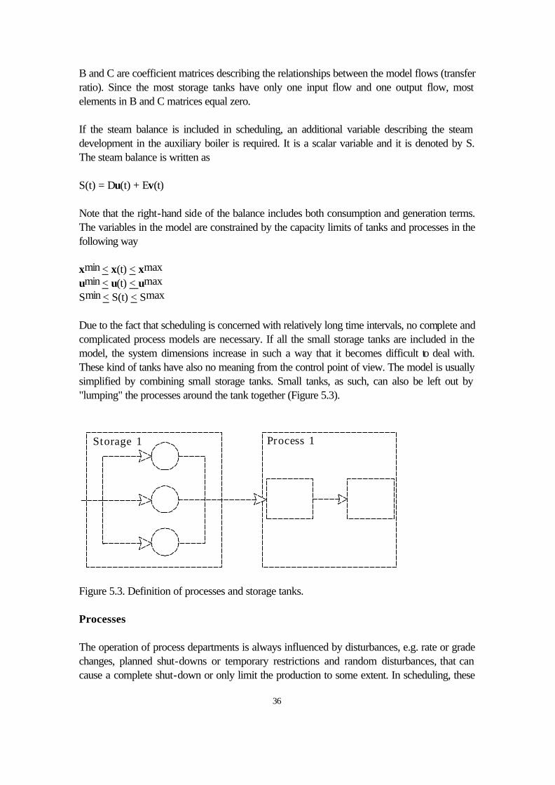
B and C are coefficient matrices describing the relationships between the model flows (transfer ratio). Since the most storage tanks have only one input flow and one output flow, most elements in B and C matrices equal zero. If the steam balance is included in scheduling, an additional variable describing the steam development in the auxiliary boiler is required. It is a scalar variable and it is denoted by S. The steam balance is written as S(t) = Du(t) + Ev(t) Note that the right-hand side of the balance includes both consumption and generation terms. The variables in the model are constrained by the capacity limits of tanks and processes in the following way xmin < x(t) < xmax umin < u(t) < umax Smin < S(t) < Smax Due to the fact that scheduling is concerned with relatively long time intervals, no complete and complicated process models are necessary. If all the small storage tanks are included in the model, the system dimensions increase in such a way that it becomes difficult to deal with. These kind of tanks have also no meaning from the control point of view. The model is usually simplified by combining small storage tanks. Small tanks, as such, can also be left out by "lumping" the processes around the tank together (Figure 5.3).

Storage 1 Process 1

Figure 5.3. Definition of processes and storage tanks. Processes The operation of process departments is always influenced by disturbances, e.g. rate or grade changes, planned shut-downs or temporary restrictions and random disturbances, that can cause a complete shut-down or only limit the production to some extent. In scheduling, these

37

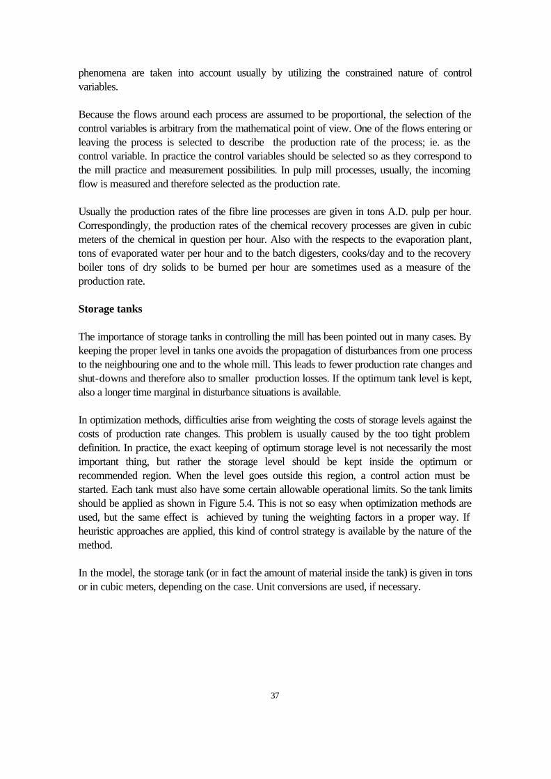
phenomena are taken into account usually by utilizing the constrained nature of control variables. Because the flows around each process are assumed to be proportional, the selection of the control variables is arbitrary from the mathematical point of view. One of the flows entering or leaving the process is selected to describe the production rate of the process; ie. as the control variable. In practice the control variables should be selected so as they correspond to the mill practice and measurement possibilities. In pulp mill processes, usually, the incoming flow is measured and therefore selected as the production rate. Usually the production rates of the fibre line processes are given in tons A.D. pulp per hour. Correspondingly, the production rates of the chemical recovery processes are given in cubic meters of the chemical in question per hour. Also with the respects to the evaporation plant, tons of evaporated water per hour and to the batch digesters, cooks/day and to the recovery boiler tons of dry solids to be burned per hour are sometimes used as a measure of the production rate. Storage tanks The importance of storage tanks in controlling the mill has been pointed out in many cases. By keeping the proper level in tanks one avoids the propagation of disturbances from one process to the neighbouring one and to the whole mill. This leads to fewer production rate changes and shut-downs and therefore also to smaller production losses. If the optimum tank level is kept, also a longer time marginal in disturbance situations is available. In optimization methods, difficulties arise from weighting the costs of storage levels against the costs of production rate changes. This problem is usually caused by the too tight problem definition. In practice, the exact keeping of optimum storage level is not necessarily the most important thing, but rather the storage level should be kept inside the optimum or recommended region. When the level goes outside this region, a control action must be started. Each tank must also have some certain allowable operational limits. So the tank limits should be applied as shown in Figure 5.4. This is not so easy when optimization methods are used, but the same effect is achieved by tuning the weighting factors in a proper way. If heuristic approaches are applied, this kind of control strategy is available by the nature of the method. In the model, the storage tank (or in fact the amount of material inside the tank) is given in tons or in cubic meters, depending on the case. Unit conversions are used, if necessary.

38

Physical limitMaximum limit

Reco mmendedregion

Minimum limit

Physical limit

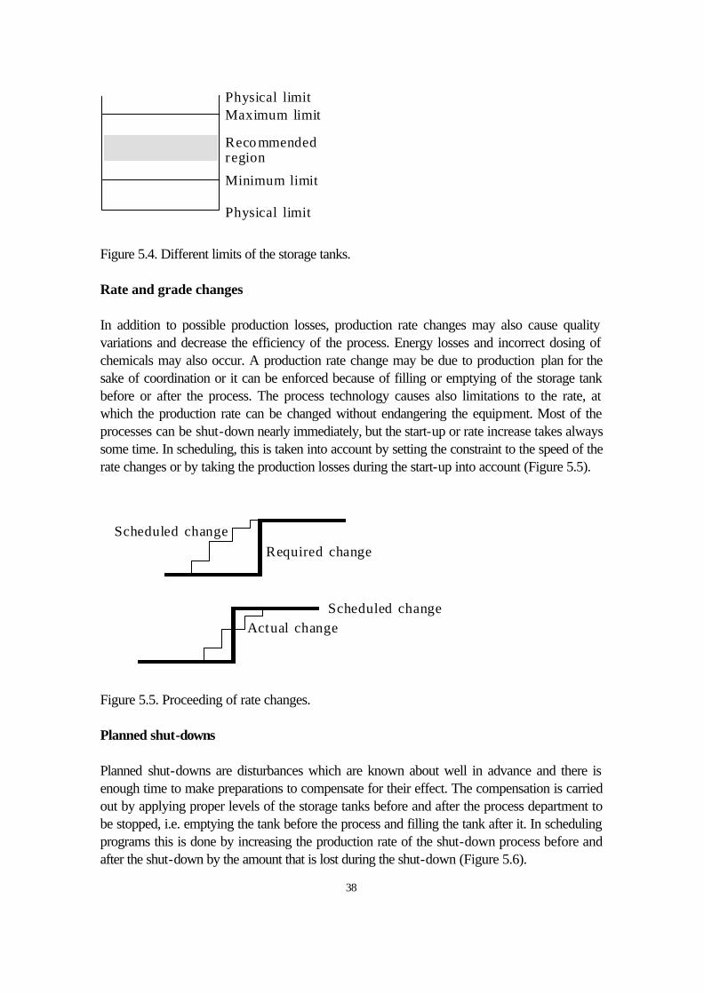
Figure 5.4. Different limits of the storage tanks. Rate and grade changes In addition to possible production losses, production rate changes may also cause quality variations and decrease the efficiency of the process. Energy losses and incorrect dosing of chemicals may also occur. A production rate change may be due to production plan for the sake of coordination or it can be enforced because of filling or emptying of the storage tank before or after the process. The process technology causes also limitations to the rate, at which the production rate can be changed without endangering the equipment. Most of the processes can be shut-down nearly immediately, but the start-up or rate increase takes always some time. In scheduling, this is taken into account by setting the constraint to the speed of the rate changes or by taking the production losses during the start-up into account (Figure 5.5).

Required changeScheduled change

Actual changeScheduled change

Figure 5.5. Proceeding of rate changes. Planned shut-downs Planned shut-downs are disturbances which are known about well in advance and there is enough time to make preparations to compensate for their effect. The compensation is carried out by applying proper levels of the storage tanks before and after the process department to be stopped, i.e. emptying the tank before the process and filling the tank after it. In scheduling programs this is done by increasing the production rate of the shut-down process before and after the shut-down by the amount that is lost during the shut-down (Figure 5.6).

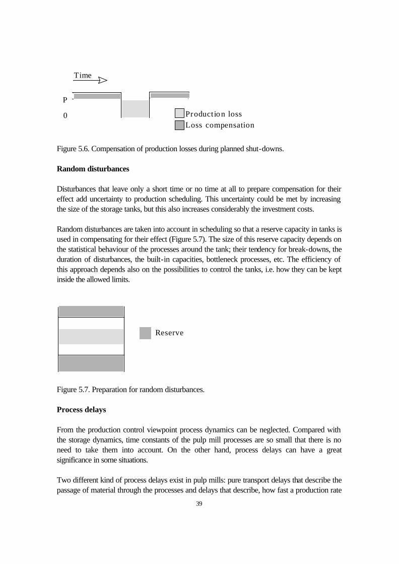
39

Time

P

0 Product io n lossLoss compensation

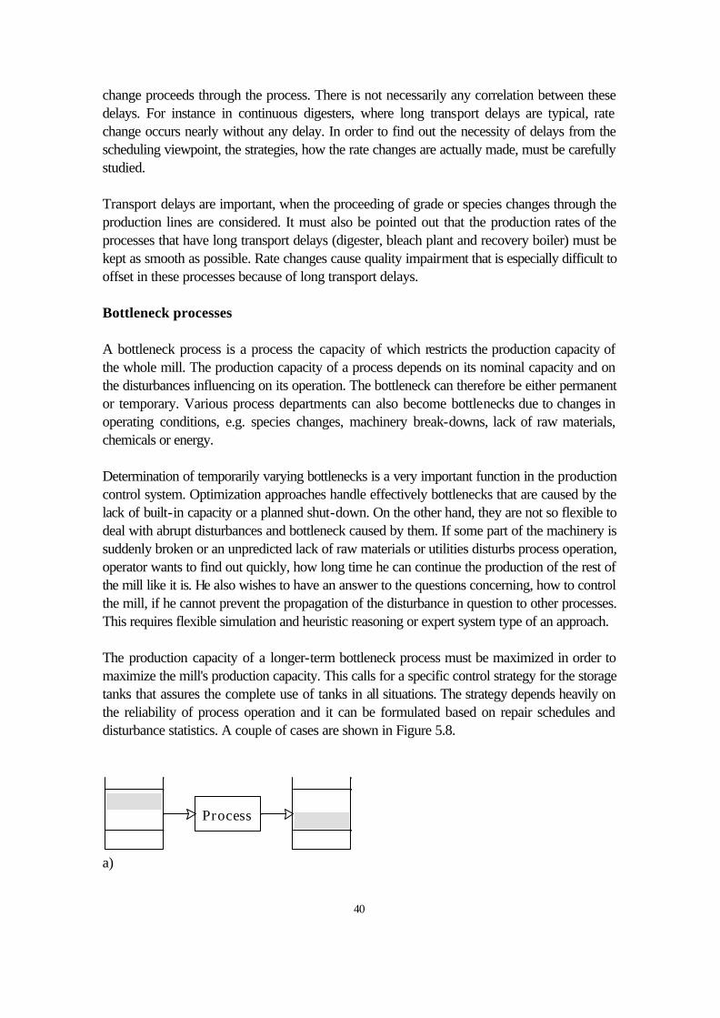
Figure 5.6. Compensation of production losses during planned shut-downs. Random disturbances Disturbances that leave only a short time or no time at all to prepare compensation for their effect add uncertainty to production scheduling. This uncertainty could be met by increasing the size of the storage tanks, but this also increases considerably the investment costs. Random disturbances are taken into account in scheduling so that a reserve capacity in tanks is used in compensating for their effect (Figure 5.7). The size of this reserve capacity depends on the statistical behaviour of the processes around the tank; their tendency for break-downs, the duration of disturbances, the built-in capacities, bottleneck processes, etc. The efficiency of this approach depends also on the possibilities to control the tanks, i.e. how they can be kept inside the allowed limits.

Reserve

Figure 5.7. Preparation for random disturbances. Process delays From the production control viewpoint process dynamics can be neglected. Compared with the storage dynamics, time constants of the pulp mill processes are so small that there is no need to take them into account. On the other hand, process delays can have a great significance in some situations. Two different kind of process delays exist in pulp mills: pure transport delays that describe the passage of material through the processes and delays that describe, how fast a production rate

40

change proceeds through the process. There is not necessarily any correlation between these delays. For instance in continuous digesters, where long transport delays are typical, rate change occurs nearly without any delay. In order to find out the necessity of delays from the scheduling viewpoint, the strategies, how the rate changes are actually made, must be carefully studied. Transport delays are important, when the proceeding of grade or species changes through the production lines are considered. It must also be pointed out that the production rates of the processes that have long transport delays (digester, bleach plant and recovery boiler) must be kept as smooth as possible. Rate changes cause quality impairment that is especially difficult to offset in these processes because of long transport delays. Bottleneck processes A bottleneck process is a process the capacity of which restricts the production capacity of the whole mill. The production capacity of a process depends on its nominal capacity and on the disturbances influencing on its operation. The bottleneck can therefore be either permanent or temporary. Various process departments can also become bottlenecks due to changes in operating conditions, e.g. species changes, machinery break-downs, lack of raw materials, chemicals or energy. Determination of temporarily varying bottlenecks is a very important function in the production control system. Optimization approaches handle effectively bottlenecks that are caused by the lack of built-in capacity or a planned shut-down. On the other hand, they are not so flexible to deal with abrupt disturbances and bottleneck caused by them. If some part of the machinery is suddenly broken or an unpredicted lack of raw materials or utilities disturbs process operation, operator wants to find out quickly, how long time he can continue the production of the rest of the mill like it is. He also wishes to have an answer to the questions concerning, how to control the mill, if he cannot prevent the propagation of the disturbance in question to other processes. This requires flexible simulation and heuristic reasoning or expert system type of an approach. The production capacity of a longer-term bottleneck process must be maximized in order to maximize the mill's production capacity. This calls for a specific control strategy for the storage tanks that assures the complete use of tanks in all situations. The strategy depends heavily on the reliability of process operation and it can be formulated based on repair schedules and disturbance statistics. A couple of cases are shown in Figure 5.8.

Process

a)

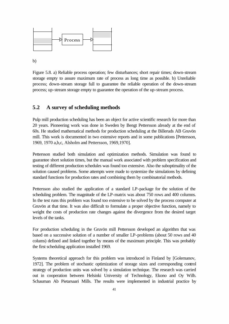
41

Process

b) Figure 5.8. a) Reliable process operation; few disturbances; short repair times; down-stream storage empty to assure maximum rate of process as long time as possible. b) Unreliable process; down-stream storage full to guarantee the reliable operation of the down-stream process; up-stream storage empty to guarantee the operation of the up-stream process. 5.2 A survey of scheduling methods Pulp mill production scheduling has been an object for active scientific research for more than 20 years. Pioneering work was done in Sweden by Bengt Pettersson already at the end of 60s. He studied mathematical methods for production scheduling at the Billeruds AB Gruvön mill. This work is documented in two extensive reports and in some publications [Pettersson, 1969, 1970 a,b,c, Alsholm and Pettersson, 1969,1970]. Pettersson studied both simulation and optimization methods. Simulation was found to guarantee short solution times, but the manual work associated with problem specification and testing of different production schedules was found too extensive. Also the suboptimality of the solution caused problems. Some attempts were made to systemize the simulations by defining standard functions for production rates and combining them by combinatorial methods. Pettersson also studied the application of a standard LP-package for the solution of the scheduling problem. The magnitude of the LP-matrix was about 750 rows and 400 columns. In the test runs this problem was found too extensive to be solved by the process computer at Gruvön at that time. It was also difficult to formulate a proper objective function, namely to weight the costs of production rate changes against the divergence from the desired target levels of the tanks. For production scheduling in the Gruvön mill Pettersson developed an algorithm that was based on a successive solution of a number of smaller LP-problems (about 50 rows and 40 colums) defined and linked together by means of the maximum principle. This was probably the first scheduling application installed 1969. Systems theoretical approach for this problem was introduced in Finland by [Golemanov, 1972]. The problem of stochastic optimization of storage sizes and corresponding control strategy of production units was solved by a simulation technique. The research was carried out in cooperation between Helsinki University of Technology, Ekono and Oy Wilh. Schauman Ab Pietarsaari Mills. The results were implemented in industrial practice by

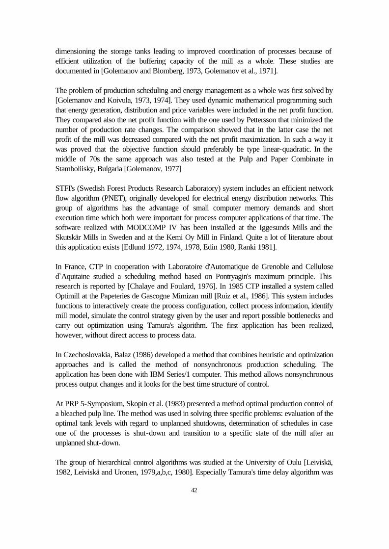
42

dimensioning the storage tanks leading to improved coordination of processes because of efficient utilization of the buffering capacity of the mill as a whole. These studies are documented in [Golemanov and Blomberg, 1973, Golemanov et al., 1971]. The problem of production scheduling and energy management as a whole was first solved by [Golemanov and Koivula, 1973, 1974]. They used dynamic mathematical programming such that energy generation, distribution and price variables were included in the net profit function. They compared also the net profit function with the one used by Pettersson that minimized the number of production rate changes. The comparison showed that in the latter case the net profit of the mill was decreased compared with the net profit maximization. In such a way it was proved that the objective function should preferably be type linear-quadratic. In the middle of 70s the same approach was also tested at the Pulp and Paper Combinate in Stamboliisky, Bulgaria [Golemanov, 1977] STFI's (Swedish Forest Products Research Laboratory) system includes an efficient network flow algorithm (PNET), originally developed for electrical energy distribution networks. This group of algorithms has the advantage of small computer memory demands and short execution time which both were important for process computer applications of that time. The software realized with MODCOMP IV has been installed at the Iggesunds Mills and the Skutskär Mills in Sweden and at the Kemi Oy Mill in Finland. Quite a lot of literature about this application exists [Edlund 1972, 1974, 1978, Edin 1980, Ranki 1981]. In France, CTP in cooperation with Laboratoire d'Automatique de Grenoble and Cellulose d`Aquitaine studied a scheduling method based on Pontryagin's maximum principle. This research is reported by [Chalaye and Foulard, 1976]. In 1985 CTP installed a system called Optimill at the Papeteries de Gascogne Mimizan mill [Ruiz et al., 1986]. This system includes functions to interactively create the process configuration, collect process information, identify mill model, simulate the control strategy given by the user and report possible bottlenecks and carry out optimization using Tamura's algorithm. The first application has been realized, however, without direct access to process data. In Czechoslovakia, Balaz (1986) developed a method that combines heuristic and optimization approaches and is called the method of nonsynchronous production scheduling. The application has been done with IBM Series/1 computer. This method allows nonsynchronous process output changes and it looks for the best time structure of control. At PRP 5-Symposium, Skopin et al. (1983) presented a method optimal production control of a bleached pulp line. The method was used in solving three specific problems: evaluation of the optimal tank levels with regard to unplanned shutdowns, determination of schedules in case one of the processes is shut-down and transition to a specific state of the mill after an unplanned shut-down. The group of hierarchical control algorithms was studied at the University of Oulu [Leiviskä, 1982, Leiviskä and Uronen, 1979,a,b,c, 1980]. Especially Tamura's time delay algorithm was

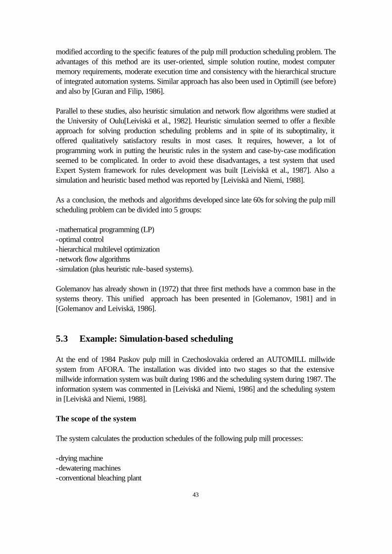
43

modified according to the specific features of the pulp mill production scheduling problem. The advantages of this method are its user-oriented, simple solution routine, modest computer memory requirements, moderate execution time and consistency with the hierarchical structure of integrated automation systems. Similar approach has also been used in Optimill (see before) and also by [Guran and Filip, 1986]. Parallel to these studies, also heuristic simulation and network flow algorithms were studied at the University of Oulu[Leiviskä et al., 1982]. Heuristic simulation seemed to offer a flexible approach for solving production scheduling problems and in spite of its suboptimality, it offered qualitatively satisfactory results in most cases. It requires, however, a lot of programming work in putting the heuristic rules in the system and case-by-case modification seemed to be complicated. In order to avoid these disadvantages, a test system that used Expert System framework for rules development was built [Leiviskä et al., 1987]. Also a simulation and heuristic based method was reported by [Leiviskä and Niemi, 1988]. As a conclusion, the methods and algorithms developed since late 60s for solving the pulp mill scheduling problem can be divided into 5 groups: -mathematical programming (LP) -optimal control -hierarchical multilevel optimization -network flow algorithms -simulation (plus heuristic rule-based systems). Golemanov has already shown in (1972) that three first methods have a common base in the systems theory. This unified approach has been presented in [Golemanov, 1981] and in [Golemanov and Leiviskä, 1986]. 5.3 Example: Simulation-based scheduling At the end of 1984 Paskov pulp mill in Czechoslovakia ordered an AUTOMILL millwide system from AFORA. The installation was divided into two stages so that the extensive millwide information system was built during 1986 and the scheduling system during 1987. The information system was commented in [Leiviskä and Niemi, 1986] and the scheduling system in [Leiviskä and Niemi, 1988]. The scope of the system The system calculates the production schedules of the following pulp mill processes: -drying machine -dewatering machines -conventional bleaching plant

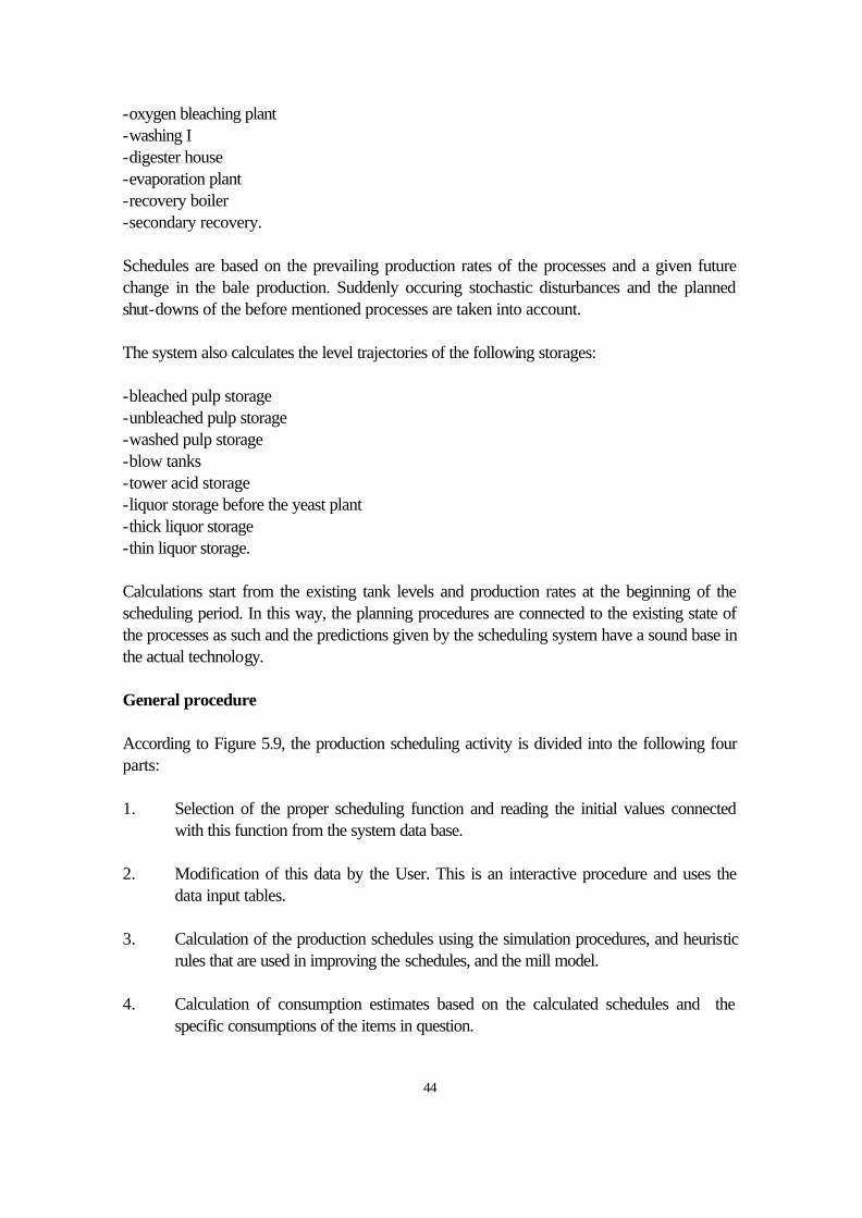
44

-oxygen bleaching plant -washing I -digester house -evaporation plant -recovery boiler -secondary recovery. Schedules are based on the prevailing production rates of the processes and a given future change in the bale production. Suddenly occuring stochastic disturbances and the planned shut-downs of the before mentioned processes are taken into account. The system also calculates the level trajectories of the following storages: -bleached pulp storage -unbleached pulp storage -washed pulp storage -blow tanks -tower acid storage -liquor storage before the yeast plant -thick liquor storage -thin liquor storage. Calculations start from the existing tank levels and production rates at the beginning of the scheduling period. In this way, the planning procedures are connected to the existing state of the processes as such and the predictions given by the scheduling system have a sound base in the actual technology. General procedure According to Figure 5.9, the production scheduling activity is divided into the following four parts: 1. Selection of the proper scheduling function and reading the initial values connected

with this function from the system data base. 2. Modification of this data by the User. This is an interactive procedure and uses the

data input tables. 3. Calculation of the production schedules using the simulation procedures, and heuristic

rules that are used in improving the schedules, and the mill model. 4. Calculation of consumption estimates based on the calculated schedules and the

specific consumptions of the items in question.

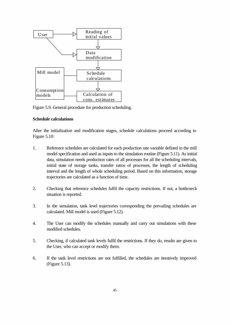
45

Reading ofinit ial values

Datamodification

Schedulecalculations

Calculat ion ofcons. est imates

User

Mill model

Consumptionmodels

Figure 5.9. General procedure for production scheduling. Schedule calculations After the initialization and modification stages, schedule calculations proceed according to Figure 5.10: 1. Reference schedules are calculated for each production rate variable defined in the mill

model specification and used as inputs to the simulation routine (Figure 5.11). As initial data, simulation needs production rates of all processes for all the scheduling intervals, initial state of storage tanks, transfer ratios of processes, the length of scheduling interval and the length of whole scheduling period. Based on this information, storage trajectories are calculated as a function of time.

2. Checking that reference schedules fulfil the capacity restrictions. If not, a bottleneck

situation is reported. 3. In the simulation, tank level trajectories corresponding the prevailing schedules are

calculated. Mill model is used (Figure 5.12). 4. The User can modify the schedules manually and carry out simulations with these

modified schedules. 5. Checking, if calculated tank levels fulfil the restrictions. If they do, results are given to

the User, who can accept or modify them. 6. If the tank level restrictions are not fulfilled, the schedules are iteratively improved

(Figure 5.13).

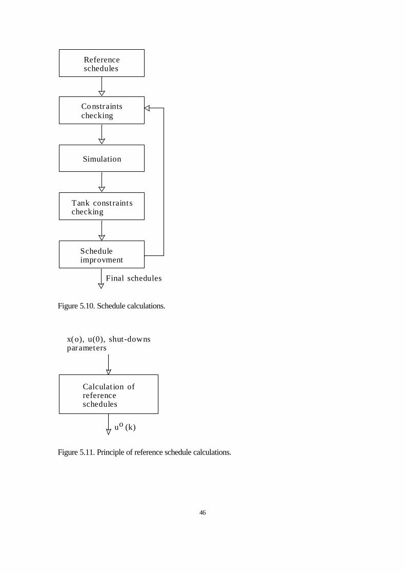
46

Referenceschedules

Constraintschecking

Simulation

Tank constraintschecking

Scheduleimprovment

Final schedules

Figure 5.10. Schedule calculations.

Calculat ion ofreferenceschedules

x(o), u(0), shut-downsparameters

u (k)o

Figure 5.11. Principle of reference schedule calculations.

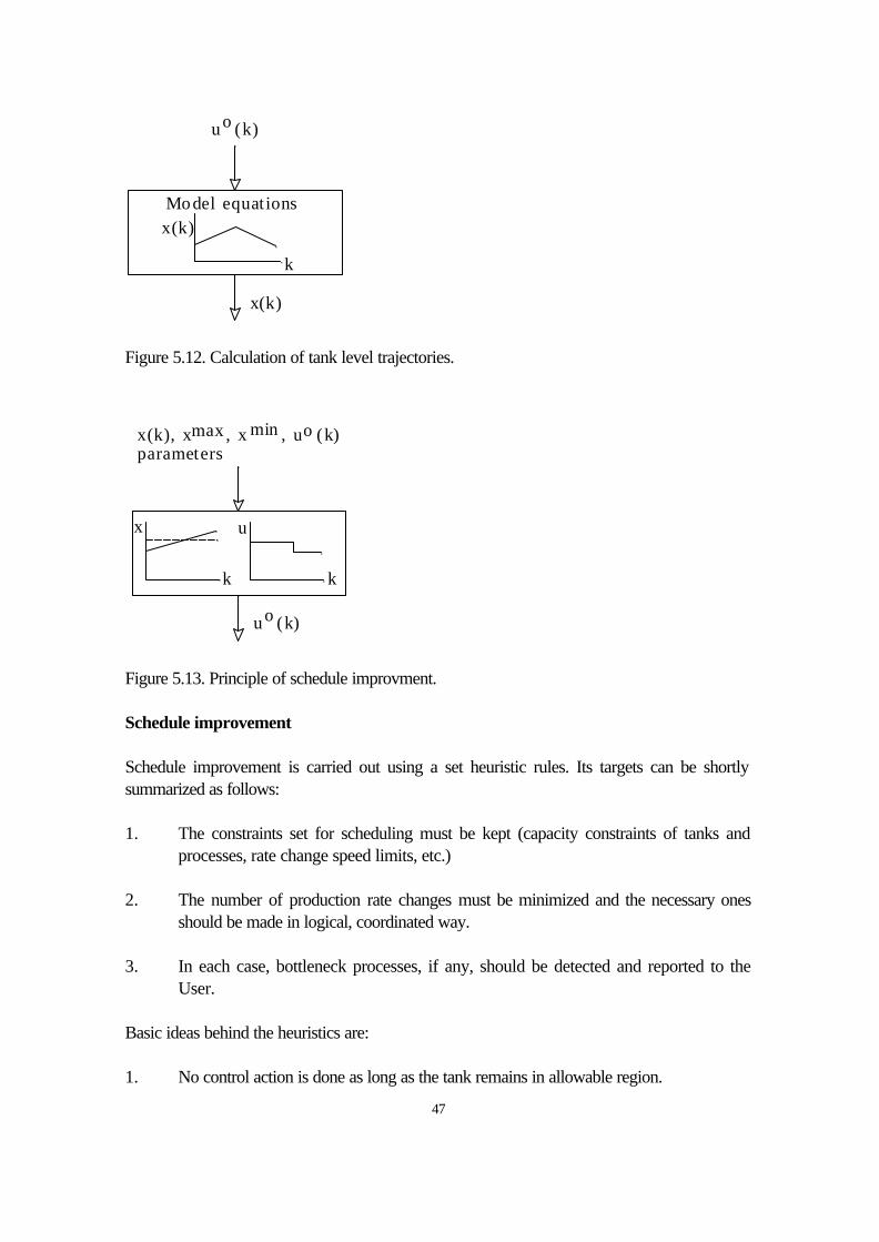
47

u (k)o

x(k)

Model equations

k

x(k)

Figure 5.12. Calculation of tank level trajectories.

u (k)o

u

k

x

k

x(k), x , x , u (k)parameters

max min o

Figure 5.13. Principle of schedule improvment. Schedule improvement Schedule improvement is carried out using a set heuristic rules. Its targets can be shortly summarized as follows: 1. The constraints set for scheduling must be kept (capacity constraints of tanks and

processes, rate change speed limits, etc.) 2. The number of production rate changes must be minimized and the necessary ones

should be made in logical, coordinated way. 3. In each case, bottleneck processes, if any, should be detected and reported to the

User. Basic ideas behind the heuristics are: 1. No control action is done as long as the tank remains in allowable region.

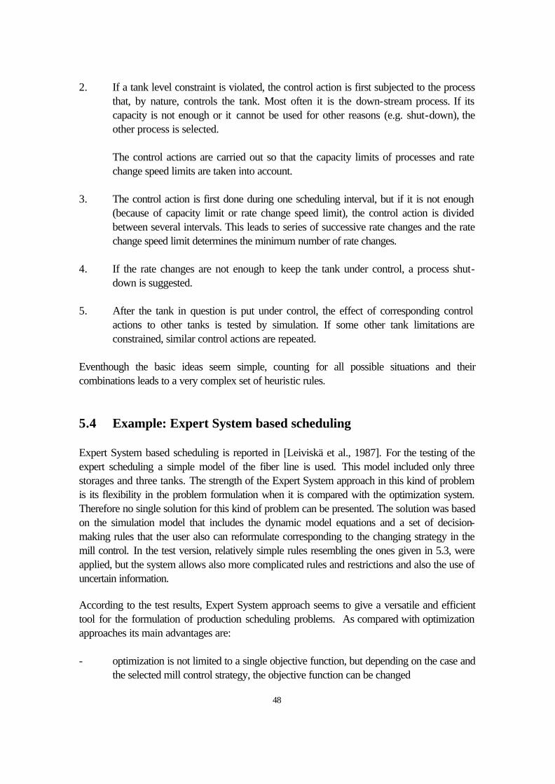
48

2. If a tank level constraint is violated, the control action is first subjected to the process

that, by nature, controls the tank. Most often it is the down-stream process. If its capacity is not enough or it cannot be used for other reasons (e.g. shut-down), the other process is selected.

The control actions are carried out so that the capacity limits of processes and rate

change speed limits are taken into account. 3. The control action is first done during one scheduling interval, but if it is not enough

(because of capacity limit or rate change speed limit), the control action is divided between several intervals. This leads to series of successive rate changes and the rate change speed limit determines the minimum number of rate changes.

4. If the rate changes are not enough to keep the tank under control, a process shut-

down is suggested. 5. After the tank in question is put under control, the effect of corresponding control

actions to other tanks is tested by simulation. If some other tank limitations are constrained, similar control actions are repeated.

Eventhough the basic ideas seem simple, counting for all possible situations and their combinations leads to a very complex set of heuristic rules. 5.4 Example: Expert System based scheduling Expert System based scheduling is reported in [Leiviskä et al., 1987]. For the testing of the expert scheduling a simple model of the fiber line is used. This model included only three storages and three tanks. The strength of the Expert System approach in this kind of problem is its flexibility in the problem formulation when it is compared with the optimization system. Therefore no single solution for this kind of problem can be presented. The solution was based on the simulation model that includes the dynamic model equations and a set of decision-making rules that the user also can reformulate corresponding to the changing strategy in the mill control. In the test version, relatively simple rules resembling the ones given in 5.3, were applied, but the system allows also more complicated rules and restrictions and also the use of uncertain information. According to the test results, Expert System approach seems to give a versatile and efficient tool for the formulation of production scheduling problems. As compared with optimization approaches its main advantages are: - optimization is not limited to a single objective function, but depending on the case and

the selected mill control strategy, the objective function can be changed

49

- the qualitative factors in scheduling are easy to implement and in this way the opinions and adapted operation strategies of the mill staff can be taken into account and it can be compared with the optimum strategy. This has also a training viewpoint connected.

- it is easy to change the mill control strategy and the mill model used in scheduling - stochastic and uncertain features are easier to take into account. It must, however, be commented that experiences from the approach are based on off-line simulation, only. Actual mill applications will bring new questions with them. LITERATURE Chapter 1 Jutila E., Leiviskä K., The use of computer simulation in the pulp and paper industry. -Mathematics and Computers in Simulation XXIII(1981):1 s. 1-11. Wahlström B., Leiviskä K., On the use of simulation in the engineering sciencies. -IMACS Transactions on Scientific Computation -85. Volume III. Elsevier Science Publishers B.V., Amsterdam 1986. s. 3-10. Chapter 2 Wahlström B., Leiviskä K., On the use of simulation in the engineering sciencies. -IMACS Transactions on Scientific Computation -85. Volume III. Elsevier Science Publishers B.V., Amsterdam 1986. s. 3-10. Chapter 3 Jutila E., Leiviskä K., Visuri M., Auer A., Sulfaattisellutehtaan kemikaalikierron ener-giataloudellinen optimointi. Loppuraportti. -Report 64. University of Oulu, Department of Process Engineering. Oulu 1981. 44 s. Jutila E., Leiviskä K., Visuri M., Uronen P., Optimizing energy in chemical recovery, PMS/CR. -Tappi 65(1982):1 s. 43-46. Leiviskä K., Visuri M., Jutila E., Sulfaattisellutehtaan kemikaalikierron osaprosessien ajo-olosuhteiden vaikutukset koko kierron toimintaa. Osa 1. Kemikaalikierron malli. -Report 56. University of Oulu, Department of Process Engineering. Oulu 1981. 82 s. Uronen P., Leiviskä K., Kesti E., Benefits and results of computer control in pulp and paper industry. Ministry of Trade and Industry. Series D:76. Helsinki 1985. 63 s.

50

Chapter 4 Barber A.L., et al., A dynamic process simulator implemented on a microprocessor for operator training. TAPPI 1983 Annual Meeting, 235-237. Boyle T.J., Tuning simulation models into decision support tools. Tappi Journal, June 1987, 75-78. Boyle T.J., Treiber S., Vadnais P., Modular simulation of kraft pulping process. Tappi Engineering Conference Preprint, 1975, 185-190. Brooks T.R., Edwards L.L., A real-time, model-based expert system for multiple effect evaporators. Tappi Journal 75(1992)11, 131-135. Corson S.R., Edwards L., Refiner pulp mill simulation. Appita 29(1976)5, 371-375. Edwards L., Baldus R., GEMS User's Manual. Chemical Engineering Department, The University of Idaho, 1977. Frazier W.C., A comparison of spreadsheet simulations: iterative vs. direct solutions. Pulp & Paper Canada 92(1991)10, 29-33. Gunseor F.D., Rushton J.D., Computer simulation of a bleached kraft pulp and paperboard mill. Tappi 62(1979)3, 63-69. Haynes J.B., Scheldorf J.J., Edwards L.L., Toward better and more economical process trainers. Pulp & Paper Canada 91(1990)5, 45-48. Johnson A.I., Peters N.P., GEMCS User's Manual. SACDA, The University of Western Ontario, 1978. Jutila E., Leiviskä K., The use of computer simulation in the pulp and paper industry. -Mathematics and Computers in Simulation XXIII(1981):1 s. 1-11. Jutila E., Leiviskä K., Visuri M., Uronen P., Optimizing energy in chemical recovery, PMS/CR. -Tappi 65(1982):1 s. 43-46. Leiviskä K., Komokallio H., Aurasmaa H., Uronen P., Heuristic algorithm for production control of an integrated pulp and paper mill. Large Scale Systems 3(1982)13-25. Leiviskä K., Simulation applications in the pulp and paper industry. -IMACS Transactions on Scientific Computation -85. Volume III. Elsevier Science Publishers B.V., Amsterdam 1986, pp. 169-173.

51

Mault K., Process simulation as a tool for training. TAPPI 67(1984)8, 50-53. McCubbin N., Process simulation: a key tool for the design and modernization of mill in the eighties. Pulp & Paper Canada 83(1982)8, 11-15. Misra M.N., Sowul L., Kraft liquor cycle simulation. Pulp & Paper Canada 91(1990)8, 99-104. Nettamo K., Lehtonen K., Muukari P., A corporate-wide approach to energy management systems. PIMA, January 1986. 56-60. Oldberg B., Total mill simulation gives fast pulp mill start-up and tuning. TAPPI 1983 Annual Meeting, 17-21. Parker P.E., DYSCO - A modular, dynamic simulator for the pulp and paper industry. Tappi 64(1981)3, 97-101. Peters N., A user's perception of computer process simulation in the pulp and paper industry. CPPA 68th Annual Meeting, Montreal, January 1982, B17-B21. Potts H.T., et al., Mill involvement in simulation. TAPPI 1982 Engineering Conferenee, 111-116. Roche A.A., Bouchard D.C., Process simulation in the pulp and paper industry. CPPA International Pulp and Paper Control Symp. Vancouver, May 2-4, 1983, 33-41. Roche A.A., Bouchard D.C., An economic model for process management, TAPPI 66(1983)11, 61-64. Scheldorf J.J., Edwards L.L., Challenges in modeling the RDH process: a discontinuous dynamic system. Tappi Journal 76(1993)11, 97-104. Scheldorf J.J., Edwards L.L., Lidskog P., Johnson R.R., Using on-line computer simulation for rapid displacement heating control system check-out. Tappi Journal 74(1991),3, 109-112. Sell N.J., Clay D.T., Computer modelling and design of fluidized bed dryer for kraft black liquor. Tappi Journal 74(1991)6, 177-184. Sezgi U.S., Kirkman A.G., Jameel H., Chang H., Morrison J.J., Bianchini C.A., Wilson J.R., A combined discrete-continuous simulation model of an RDH tank farm. Tappi Journal 77(1994)7, 213-220. Shewchuk C.F., Waite S.J., Lopez J., PAPSYS System, Mass Balance Simulator, User's Manual. SACDA, The University of Western Ontario, 1979.

52

Shewchuk C.F., Process simulation technology for the pulp and paper industry. CPPA 68th Annual Meeting, Montreal January 1982, B5-B12. Shewchuk C.F., The reconciliation of process simulation and actual operation. TAPPI 1983. Annual Meeting, 9-16. Shewchuk C.F., MASSBAL MKII: New process simulation system. Pulp & Paper Canada 88(1987)5, 76-82 Shewchuk C., Leaver E.W., New operator training system called ideal for many uses. PIMA, January 1986, 40-43. Shewchuk C.F., Leaver E.W., Schindler H.E., The roles for process system simulation in the design, testing and operation of processes, process control and advanced control systems. Pulp & Paper Canada 92(1991)9, 53-59. Smith D.B., Edwards L.L., Damon R.A., Development and application of a real-time recovery boiler expert system. Tappi Journal 74(1991)11, 93-96 Strand W.C., Ferritsius O., Mokvist A.V., Use of simulation models in the on-line control and optimization of the refining process. Tappi Journal 74(1991)11, 103-108. Sutinen R., Muukari P., Siro M., Global energy management system online at Schauman mill in Finland. Pulp & Paper, July 1984, 93-97. Terrell J., McLaughlin G., Operator training at Great Northern Paper. Pulp & Paper Canada 92(1991)4, 59-63. Thomas K.V., Process simulation program. Tappi 62(1979)2, 51-57. Turner P.A., Roche A.A., McDonald J.D., van Heiningen A.R.P., Dynamic behaviour of a brownstock washing system. Pulp & Paper Canada 94(1993)9, 37-42. Uloth V., Richardson B., Hogikyan R., Haynes J., Using a recovery boiler computer simulation to evaluate process alternatives for obtaining incremental recovery capacity. Tappi Journal 75(1992)11, 137-147. Uronen P., Leiviskä K., Kesti E., Benefits and results of computer control in pulp and paper industry. Ministry of Trade and Industry. Series D:76, 1985, 63 p. Wang L., Tessier P., Englezos P., Dynamic modeling and simulation of the recausticization plant in a kraft pulp mill. Tappi Journal 77(1994)12, 95-103.

53

Venkatesh V., Corson S.R., Edwards L.L., System analysis of refiner operation. Tappi/CPPA 1975 International Mechanical Pulping Conference, San Francisco, 1975, 173-183. Venkatesh V., Edwards L.L., Systems engineering approach to process design in mechanical pulp mills. Tappi 60(1977)12, 68-76. Venkatesh V., Kirkman A., Mera F., Computer-aided process analysis and economics for pulp and paper mills. Tappi 61(1978)3, 87-91. Xuan N.N., Venkatesh V., Gratzl J.S., McKean W.T., The washing of soda-oxygen pulps. Tappi 61(1978)8, 53-56. Chapter 5 Alsholm O., Pettersson B., Integration of pulp mill control with the production planning of the paper mill. Trans. of the BP&BMA Symposium, 1969,209-231. Alsholm O., Pettersson B., Production control - a link between process control and production planning. Svensk Papperstidning 73(1970)10, 338-343 (In Swedish). Balaz J., Selected problems of pulp production control. Parts I & II. Pulp and Paper Research Institute, Bratislava, 1985, 1986. Chalaye G., Foulard C., Hierarchical control of a pulp mill. Proc. 3rd IFAC PRP Conference, Brussels, 1976, 109-119. Edin C. et al., Supervisory control of the Skutskär pulp mill: an on-line production control system. Preprints of the 4th International IFAC PRP Conference, Ghent, 1980, 115-120. Edlund S.G., Johansson R., Experiences with a multiple unit production control system for the optimization of mill operations. Preprints International Symposium on Process Control, CPPA, Vancouver, 1977, 36-39. Edlund S.G., Kallmen C., Dynamics of coupled process systems. Svensk Papperstidning 75(1972)3, 518-521 (In Swedish). Edlund S.G., Kallmen C., Production control in pulp and paper mills. Preprints of British Paper and Board Industry Federation International Symposium, Kent, 1974, 11 p. Golemanov L.A., Systems theoretical approach in the projecting and control of industrial production systems. Doctoral Thesis, EKONO-publication no 113, 1972. Golemanov L.A. et al., A unified approach in the analysis and design of integrated production management systems. 8th IFAC World Congress, Kyoto, 1981.

54

Golemanov L.A., Blomberg H., Dimensioning storage facilities and optimization of control strategy. Tappi 56(1973)1, 109-112. Golemanov et al., Dimensioning of buffer storages and optimization of control strategy. EKONO-publication no 131, 1971 (In Finnish). Golemanov L.A., Koivula E., Optimal production control and mathematical programming. Paperi ja Puu 55(1973)2, 53-67. Golemanov L.A., Koivula E., An optimal production control system. IFAC Symposium on optimization methods (applied aspects), Varna, 1974. Golemanov L.A., Leiviskä K., Models for mill-wide control in paper industry. Preprints 6th PRP Conference, Akron, Ohio, 1986, 184-191. Guran M., Filip F.G., Hierarchical Real Time Systems. Ed. Technics, Bucharest, 1986, 296 p. (In Romanian). Leiviskä K., Models for production planning and control. Proceedings from a Nordic Workshop on Models for the Forest Sector. Research Report 1982:1, University of Umeå, Sweden, 293-326. Leiviskä K., Short term production scheduling of the pulp mill. Acta Polytechnica Scan-dinavica. Ma 36, Helsinki 1982. Leiviskä K., Optimizing of the pulp mill operations. Pre-prints Control Systems 90, International Conference on Instrumentation and Automation in Pulp and Paper Industry, Sept. 18-20, 1990, Helsinki, pp. 304-319. Leiviskä K., Huttunen R., Uronen P., Pulp mill production scheduling with an Expert System. Presented at the Universidade de Coimbra, Portugal, April 1987. 12p. Leiviskä K., Komokallio H., Aurasmaa H., Uronen P., Heuristic algorithm for production control of an integrated pulp and paper mill. Large Scale Systems 3(1982), 13-25 (Also in 7th CHISA Conference, Prag, 1981). Leiviskä K., Niemi T.: Production control in Paskov mill. -Pulp and Paper Symposium 'Paskov 86, April 22-24 1986, Ostrava, Czechoslovakia. 14 s. Leiviskä K., Niemi T., Production scheduling in pulp mills. -Pulp and Paper Symposium 'Paskov 88, Mars 29-31 1988, Ostrava, Czechoslovakia. 23 s.

55

Leiviskä K., Uronen P., Dynamic optimization of a sulphate mill pulp line. Preprints IFAC/IFORS Symposium, Toulouse, France, 1979a, 25-32. Leiviskä K., Uronen P., Hierarchical control of an integrated pulp and paper mill. Report No 113. PLAIC, Purdue University, West Lafayette, Indiana, 1979b, 109 p. Leiviskä K., Uronen P., Dynamic optimization of a sulphate pulp mill. Preprints 2nd IFAC/IFORS Symposium on Optimization Methods - Applied Aspects. Varna, Bulgaria, 1979c, 291-300. Pettersson B., Production control of a complex integrated pulp and paper mill. Tappi 52(1969)11,2155-2159. Pettersson B., Mathematical methods of a pulp and paper mill scheduling problem. Report 7001, Division of Automatic Control, Lund Institute of Technology, 1970a. Pettersson B., Production control of a pulp and paper mill. Report 7007. Lund Institute of Technology, Division of Automatic Control, Lund, 1970b. Pettersson B., Optimal production schemes coordinating subprocesses in a complex pulp and paper mill. Pulp and Paper Magazine of Canada 71(1970c)5, 59-63. Ranki J., Experiences with computerized production control and supervision in a pulp and board mill. Tappi 66(1981)6,115-118. Ruiz J. et al., Optimill: Optimal management of pulp mill production departments and storage tanks. Proc. 6th IFAC PRP Conference, Akron, Ohio, 1986, 205-211. Skopin I.I. et al., Bleached kraft pulp production optimal control system. Proc. 5th IFAC PRP Conference, Antverp, 1983, 99-106. Sutinen R. & Niemi T. & Leiviskä K.: Overall control of a pulp mill. Pre-prints Control Systems 90, International Conference on Instrumentation and Automation in Pulp and Paper Industry, Sept. 18-20, 1990, Helsinki, pp. 330-342.