2 labour market and monetary policy reforms in the uk: a...

2 Labour market and monetary policy reformsin the UK: a structural interpretation of theimplications

Francesco ZanettiUniversity of Oxford

2.1 Introduction

Two key changes can arguably be said to have characterised the economiclandscape in recent UK history: first, labour market reforms enforcedby the Thatcher government in the late 1980s and, second, the intro-duction of an explicit inflation target in 1992, which entrusted themonetary authority with the mandate of stabilising inflation around anumerical target. Subsequently, the UK economy experienced a stepchange in macroeconomic performance. Figure 2.1 shows the growthrate of real Gross Domestic Product (GDP) and the growth rate ofthe GDP deflator, an inflation indicator, in the UK from 1970 to thepresent: it suggests that both real output growth and inflation have beenmore stable than they were in the 1970s and the 1980s. Moreover, thelevel of inflation has decreased remarkably since the early 1990s. Wouldthe introduction of these policy changes have produced a different eco-nomic outlook if they had been accomplished in the earlier decades?And, if so, to what extent, if at all, might each of these two changeshave played a role?To answer these questions, this chapter uses a model that details the

functioning of the UK economy during the 1970s and 1980s which isable to incorporate the policy reforms described. It then uses the modelto draw inferences about how these policy changes might have alteredthe economic outlook had they been introduced in the early 1970s.

I am very grateful for insightful discussions with John Fender and the extremely usefulcomments and suggestions of Richard Barwell, Arnab Bhattacharjee, Jagjit Chadha,Gulcin Ozkan, Joe Pearlman, Peter Sinclair, Martin Weale and seminar participants at theconference on ‘The Causes and Consequences of the Long UK Expansion: 1992 to 2007’at the University of Cambridge. Correspondence: Francesco Zanetti, University ofOxford, Department of Economics, Manor Road, Oxford, OX1 3UQ, United Kingdom.Email: [email protected].

81

349-CUP_Chadha-3490022_c02 19 January 2016; 20:23:35

The analysis is conducted using a microfounded New Keynesianmodel where firms face a cost to adjusting nominal prices and the labourmarket is characterised by search frictions. The theoretical frameworkalso incorporates a monetary authority that conducts monetary policyby setting the nominal interest rate in reaction to deviations of inflationfrom its target and output from its long-run equilibrium. Unlike theexplicit inflation-targeting framework introduced in 1992, where thetarget of inflation is constant, during the 1970s and 1980s, the mone-tary authority could be perceived as having an implicit time-varying

Inflation

–4

–2

0

2

4

6

8

1971

1974

1977

1980

1983

1986

1989

1992

1995

1998

2001

2004

2007

Output growth

–3–2–10123456

1971

1974

1977

1980

1983

1986

1989

1992

1995

1998

2001

2004

2007

Figure 2.1. Real output growth and inflation in the UKNotes: Output growth is measured by the growth rate of the real GDP(upper figure) and inflation is measured by the growth rate of GDPdeflator (lower figure).

82 Francesco Zanetti


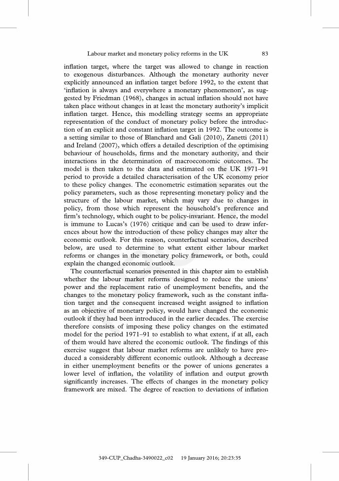
inflation target, where the target was allowed to change in reactionto exogenous disturbances. Although the monetary authority neverexplicitly announced an inflation target before 1992, to the extent that‘inflation is always and everywhere a monetary phenomenon’, as sug-gested by Friedman (1968), changes in actual inflation should not havetaken place without changes in at least the monetary authority’s implicitinflation target. Hence, this modelling strategy seems an appropriaterepresentation of the conduct of monetary policy before the introduc-tion of an explicit and constant inflation target in 1992. The outcome isa setting similar to those of Blanchard and Galì (2010), Zanetti (2011)and Ireland (2007), which offers a detailed description of the optimisingbehaviour of households, firms and the monetary authority, and theirinteractions in the determination of macroeconomic outcomes. Themodel is then taken to the data and estimated on the UK 1971–91period to provide a detailed characterisation of the UK economy priorto these policy changes. The econometric estimation separates out thepolicy parameters, such as those representing monetary policy and thestructure of the labour market, which may vary due to changes inpolicy, from those which represent the household’s preference andfirm’s technology, which ought to be policy-invariant. Hence, the modelis immune to Lucas’s (1976) critique and can be used to draw infer-ences about how the introduction of these policy changes may alter theeconomic outlook. For this reason, counterfactual scenarios, describedbelow, are used to determine to what extent either labour marketreforms or changes in the monetary policy framework, or both, couldexplain the changed economic outlook.The counterfactual scenarios presented in this chapter aim to establish

whether the labour market reforms designed to reduce the unions’power and the replacement ratio of unemployment benefits, and thechanges to the monetary policy framework, such as the constant infla-tion target and the consequent increased weight assigned to inflationas an objective of monetary policy, would have changed the economicoutlook if they had been introduced in the earlier decades. The exercisetherefore consists of imposing these policy changes on the estimatedmodel for the period 1971–91 to establish to what extent, if at all, eachof them would have altered the economic outlook. The findings of thisexercise suggest that labour market reforms are unlikely to have pro-duced a considerably different economic outlook. Although a decreasein either unemployment benefits or the power of unions generates alower level of inflation, the volatility of inflation and output growthsignificantly increases. The effects of changes in the monetary policyframework are mixed. The degree of reaction to deviations of inflation

83Labour market and monetary policy reforms in the UK


from the target is important for explaining the lower variance of infla-tion, output growth and the reduced inflation level. On the other hand,the introduction of a constant inflation target, or a monetary policy thatresponds more forcefully to output fluctuations, actually increases thevolatility of inflation and output growth.

The remainder of the chapter is organised as follows: Section 2.2relates this chapter to the literature, Section 2.3 provides an overview ofthe economic context, Section 2.4 sets up the model, Section 2.5derives the equilibrium and the model’s solution, Section 2.6 presentsthe results and Section 2.7 concludes.

2.2 Related literature

This chapter relates closely to two branches of the literature. First, anumber of works have investigated the causes of the reduced macroeco-nomic volatility in the UK from the early 1990s onward, the periodoften referred to as an era of ‘Great Moderation’. Benati (2008) useseconometric techniques to find that smaller shocks might have causedthe muted economic outlook. Canova et al. (2007) use a time-varyingVAR to show that changes in the transmission of demand shocks andthe reduced volatility of supply and monetary policy shocks account forthe improved macroeconomic stability. On the other hand, Batini andNelson (2009) document that the change in view of policymakers aboutthe importance of monetary policy that culminated with the introduc-tion of inflation targeting, is likely responsible for the post-1990 UKmacroeconomic stability. Bianchi et al. (2009) use a FAVAR model toshow that the slope of the yield curve is related to a lower and stableinflation in the UK. Unlike these works, this chapter is the first to inves-tigate the importance of labour market reforms and the introduction ofa constant inflation target using an estimated, dynamic, stochastic, gen-eral equilibrium model. It therefore provides an empirically groundedassessment of the effect of these reforms and enables the model toquantify the structural shocks, which are used to derive the counterfac-tual scenarios. A closely related study is Blanchard and Galì (2007),which investigates the effect of oil shocks on the US economy. Like thischapter, they find that changes in the labour market, by decreasing realwage rigidities, and a more credible monetary policy, which reactedmore aggressively to inflation, played a role in the more muted effect ofoil shocks and therefore the different economic outlook in the post-1980 period compared to the 1970s. However, both their approach andfocus are different. In Blanchard and Galì (2007) the labour marketrigidities are not microfounded, since they assume that wages are



exogenously prevented from adjusting, whereas here they are derivedfrom first principles. While they interpret the degree of wage rigiditiesas a measure of changes in the labour market, this chapter investigatesthe effect of two well-defined labour market reforms. Moreover, theycalibrate the model’s parameters, while here the estimation uses thedata to determine the parameters’ values. Furthermore, the analysishere also focuses on the introduction of a constant inflation target,which is uncovered in Blanchard and Galì (2007).Second, this chapter also contributes to the estimation of structural

models for the UK economy, which is an understudied area of research,as emphasised by DiCecio and Nelson (2007). Unlike DiCecio andNelson (2007), who estimate the model using a vector autoregressionto match the responses of variables to a monetary policy shock, thischapter uses maximum likelihood estimation to fully exploit the abilityof the structural model to match the data. In addition, this chapter alsoincorporates labour market frictions, which, as advocated by Nickell(1997), are an important feature of the UK labour market, and there-fore provide a more accurate description of the economy. This chapteralso relates to recent works by Kamber and Millard (2008) andHarrison and Oomen (2010), who estimate an array of New Keynesianmodels to investigate the monetary transmission mechanism in the UK.Finally, the chapter is also related to Faccini et al. (2013), who estimatea general equilibrium model with labour market frictions on UK data.While these works focus on the period from the 1980s onward, thischapter is the first study to provide a detailed description of the econ-omy during the 1970s and 1980s. Moreover, the focus here is broader,as it uses the model to perform normative analysis to determine therelevance of labour market reforms and the introduction of inflationtargeting.

2.3 The economic context

To place the analysis in context, before proceeding with the analysis itis worth describing the economic situation and the actual policychanges that took place. In the late 1970s UK economic performancehad been subdued: Bean and Crafts (1996, Table 6.1) document thatthe UK had the lowest growth rate of GDP per capita among a sampleof 12 OECD countries and that output dropped more sharply duringthe 1980s recession than in other developed counties. The top panel ofFigure 2.1 shows that output growth was low during the 1970s, andthat the second half of the 1980s was characterised by a high level ofgrowth. Interestingly, the strong economic performance of the UK



economy coincided with far-reaching labour market and monetarypolicy reforms.

In the late 1980s the Thatcher government introduced a series oflabour market reforms aimed at reducing the distortions in the labourmarket considered responsible for the poor performance of the UKeconomy. In particular, as pointed out by Minford (1983), the unem-ployment benefit system and the power of the unions were regarded asparticularly damaging. Consequently, legislation such as the TradeUnion Act of 1984 and the Employment Act of 1988 led, as documen-ted by Blanchflower and Freeman (1993), to a steady decline in uniondensity and to a reduction of the replacement ratio of unemploymentbenefits. In particular, Gregory (1998) documents that union member-ship declined from 11.7 million in 1979 to 7.2 million in 1996 andunion density of employment also declined from 50 per cent in 1979 to31.3 per cent in 1996. Moreover, Millward, Stevens et al. (1992)reports that the decline of the unions’ role was concentrated in thelate 1980s.

In the late 1980s the UK government started to reconsider the mone-tary policy framework. Following Britain’s departure from theExchange Rate Mechanism in September 1992, the Chancellor of theExchequer, Norman Lamont, established an explicit numerical targetfor the rate of inflation and gave the legal mandate to the monetaryauthority to maintain inflation around the target in the medium term.The 1998 Bank of England Act made the Bank independent to setinterest rates. The Bank of England became accountable to parliamentand started to implement the annual explicit target for the rate of infla-tion set by the Government. The bottom panel of Figure 2.1 shows thatinflation became remarkably low and stable from the early 1990s.

2.4 The economic environment

The theoretical model resembles those used by Blanchard and Galì(2010) and Zanetti (2009, 2011), which combine a standard NewKeynesian model with labour market search. In addition, monetary pol-icy accounts for a time-varying inflation target as in Ireland (2007). Themodel economy consists of a representative household, a representativefinished-goods-producing firm, a continuum of intermediate-goods-producing firms, indexed by i ∈ ½0; 1�, and a monetary authority.

The labour market is similar to that in Blanchard and Galì (2010),which is based on the Diamond–Mortensen–Pissarides model of searchand matching. This framework relies on the assumption that the pro-cesses of job search and recruitment are costly for both the firm and the



worker. Job creation takes place when a firm and a searching workermeet and agree to form a match at a negotiated wage, which depends onthe parties’ bargaining power. The match continues until the parties exo-genously terminate the relationship. When this occurs, job destructiontakes place and the worker moves from employment to unemployment,and the firm can either withdraw from the market or hire a new worker.The goods market is comprised of a representative finished-goods-

producing firm, and a continuum of intermediate-goods-producingfirms indexed by i ∈ ½0; 1�.1 During each period t = 0; 1; 2;…, eachintermediate-goods-producing firm hires workers and produces adistinct, perishable good. During each period t = 0; 1; 2;…, the finished-goods-producing firm purchases intermediate goods from theintermediate-goods-producing firms and sells them at an establishedprice on the market. Each intermediate-goods-producing firm sets theprice as a markup over its marginal cost, and it faces a cost to adjustingits nominal price, as in Rotemberg (1982). This cost to price adjust-ment allows the monetary authority to influence the behavior of realvariables in the short-run.The monetary authority is modelled with a modified Taylor (1993)

rule as in Clarida et al. (1998): it adjusts the nominal interest rate inresponse to deviations of output from its steady state and inflation fromits target. Similarly to Ireland (2007), monetary policy also allows theinflation target to adjust in response to exogenous shocks.The next section describes the agents’ tastes, technologies, the policy

rule and the structure of the goods and labour market in detail.

2.4.1 The representative household

During each period t = 0; 1; 2;…, the representative household maxi-mises the expected utility function

E0

X∞t=0

βtatðln CtÞ; (2.1)

where the variable Ct is consumption, β is the discount factor 0< β< 1,and at is the aggregate preference shock that follows the autoregressiveprocess

lnðatÞ= ρa lnðat−1Þ+ εat; (2.2)

1 Note that the model abstracts from issues of heterogeneity and distribution among eco-nomic agents, since it is based on the representative agent framework.



where ρa < 1. The zero-mean, serially uncorrelated innovation εat isnormally distributed with standard deviation σa: The representativehousehold enters period t with bonds Bt−1. At the beginning of theperiod, the household receives a lump-sum nominal transfer Tt fromthe central bank and nominal profits Dt from the intermediate-goods-producing firms. The household supplies Nt units of labour at the wagerate Wt to each intermediate-goods-producing firm i ∈ ½0; 1� andreceives unemployment benefits bt during period t. Then, the house-hold’s bonds mature, providing Bt−1 additional units of currency. Thehousehold uses part of this additional currency to purchase Bt newbonds at nominal cost Bt=Rt; where Rt represents the gross nominalinterest rate between t and t + 1. The household uses its income forconsumption, Ct, and carries Bt bonds into period t + 1, subject to thebudget constraint

Ct +Bt=PtRt = ½Bt−1 +WtNt +Dt +Tt + ð1−NtÞbt�=Pt; (2.3)

where Nt lies between 0 and 1 for all t = 0; 1; 2;…. Thus the householdchooses fCt;Btg∞t=0 to maximise its utility (Eq. (2.1)) subject to the bud-get constraint (Eq. (2.3)) for all t = 0; 1; 2;…. Letting πt =Pt=Pt−1denote the gross inflation rate, and Λt the non-negative Lagrange multi-plier on the budget constraint (Eq. (2.3)), the first-order conditions forthis problem are

Λt = at=Ct; (2.4)

and

Λt = βRtEtðΛt+1=πt+1Þ: (2.5)

According to Eq. (2.4), the Lagrange multiplier must equal thehousehold’s marginal utility of consumption. Equation (2.5), onceEq. (2.4) is substituted in, is the representative household’s Eulerequation that describes the consumption decision.

2.4.2 The labour market

During each period t = 0; 1; 2;…, the flow into employment results fromthe number of workers who survive from the exogenous separationand the number of new hires, Ht. Hence, total employment evolvesaccording to

NtðiÞ= ð1− δÞNt−1ðiÞ+HtðiÞ; (2.6)

where NtðiÞ and HtðiÞ represent the number of workers employedand hired by firm i in period t, and δ is the exogenous separation rate



and 0< δ< 1: For all t =0; 1; 2;…, the fraction of aggregate employmentand hires supplied by the representative household must satisfyNt =

Ð 10 NtðiÞdi; and Ht =

Ð 10 HtðiÞdi respectively. It is convenient to

introduce the variable xt, labour market tightness:

xt =Ht=Ut; (2.7)

and assume, as in Blanchard and Galì (2010), full participation in thelabour market such that

Ut = 1− ð1− δÞNt−1 (2.8)

is the beginning of the period unemployment. Finally, it is useful todefine

ut = 1−Nt (2.9)

the fraction of the population left without a job after recruitment. Sinceall new hires are from the part of unemployed workers, 0< xt < 1:Hence, xt also represents the probability that an unemployed workerfinds a job.Let WN

t , and WUt , denote the marginal value of the expected income

of an employed, and unemployed worker respectively. The employedworker earns a wage, suffers disutility from work and might lose her jobwith probability δ. Hence, the marginal value of a new match is:

WNt =

Wt

Pt+ βEt

Λt+1

Λt1− δð1− xt+1Þ½ �WN

t+1 + δð1− xt+1ÞWUt+1g:

�(2.10)

This equation states that the marginal value of a job for a worker isgiven by the real wage and the expected-discounted net gain from beingeither employed or unemployed.The unemployed worker expects to move into employment with

probability xt. Hence, the marginal value of unemployment is:

WUt =

btPt

+ βEtΛt+1

Λtxt+1WN

t+1 + ð1− xt+1ÞWUt+1

� �: (2.11)

This equation states that the marginal value of unemployment ismade up of unemployment benefits together with the expected-discounted capital gain from being either employed or unemployed.Similarly to Zanetti (2011), unemployment benefits are set as a propor-tion, ρb, of the established wage, such that bt = ρbwt, where ρb representsthe replacement ratio.The structure of the model guarantees that a realised job match yields

some pure economic surplus. The share of this surplus between theworker and the firm is determined by the wage level, in addition to



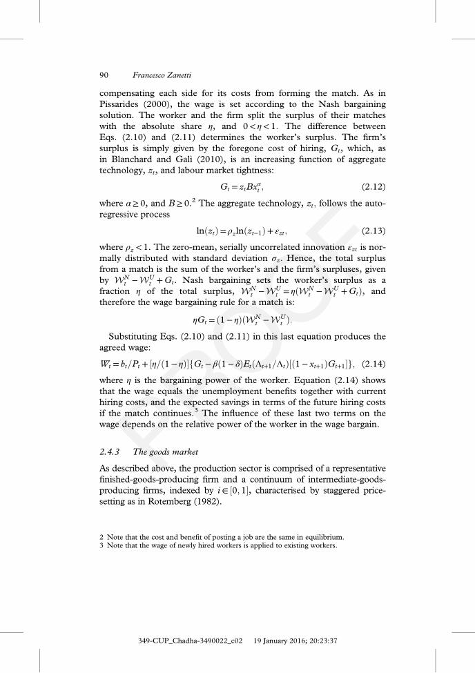
compensating each side for its costs from forming the match. As inPissarides (2000), the wage is set according to the Nash bargainingsolution. The worker and the firm split the surplus of their matcheswith the absolute share η, and 0< η< 1: The difference betweenEqs. (2.10) and (2.11) determines the worker’s surplus. The firm’ssurplus is simply given by the foregone cost of hiring, Gt, which, asin Blanchard and Galì (2010), is an increasing function of aggregatetechnology, zt, and labour market tightness:

Gt = ztBxαt ; (2.12)

where α≥ 0, and B≥ 0.2 The aggregate technology, zt; follows the auto-regressive process

lnðztÞ= ρzlnðzt−1Þ+ εzt; (2.13)

where ρz < 1. The zero-mean, serially uncorrelated innovation εzt is nor-mally distributed with standard deviation σz: Hence, the total surplusfrom a match is the sum of the worker’s and the firm’s surpluses, givenby WN

t −WUt +Gt. Nash bargaining sets the worker’s surplus as a

fraction η of the total surplus, WNt −WU

t = ηðWNt −WU

t +GtÞ, andtherefore the wage bargaining rule for a match is:

ηGt = ð1− ηÞðWNt −WU

t Þ:Substituting Eqs. (2.10) and (2.11) in this last equation produces the

agreed wage:

Wt = bt=Pt + ½η=ð1− ηÞ�fGt − βð1− δÞEtðΛt+1=ΛtÞ½ð1− xt+1ÞGt+1�g; (2.14)

where η is the bargaining power of the worker. Equation (2.14) showsthat the wage equals the unemployment benefits together with currenthiring costs, and the expected savings in terms of the future hiring costsif the match continues.3 The influence of these last two terms on thewage depends on the relative power of the worker in the wage bargain.

2.4.3 The goods market

As described above, the production sector is comprised of a representativefinished-goods-producing firm and a continuum of intermediate-goods-producing firms, indexed by i ∈ ½0; 1�, characterised by staggered price-setting as in Rotemberg (1982).

2 Note that the cost and benefit of posting a job are the same in equilibrium.3 Note that the wage of newly hired workers is applied to existing workers.



2.4.3.1 The representative finished-goods-producing firm During eachperiod t = 0; 1; 2;…, the representative finished-goods-producing firmuses YtðiÞ units of each intermediate good i ∈ ½0; 1�, purchased at nom-inal price PtðiÞ, to produce Yt units of the finished product at constantreturns to scale technology

ð10YtðiÞ

θt−1θt di

� � θtθt−1

≥Yt;

where θt is the time-varying elasticity of substitution among intermedi-ate goods, as first introduced by Smets and Wouters (2007), Steinsson(2003) and Ireland (2004, 2007). This parameter follows the autore-gressive process

lnðθtÞ= ð1− ρθÞ lnðθÞ+ ρθ lnðθt−1Þ+ εθt ; (2.15)

where ρθ < 1. The zero-mean, serially uncorrelated innovation εθt isnormally distributed with standard deviation σθ.Hence, the finished-goods-producing firm chooses YtðiÞ for all

i ∈ ½0; 1� to maximise its profits

Pt

ð10YtðiÞ

θt−1θt di

� � θtθt−1

−ð10PtðiÞYtðiÞdi;

for all t = 0; 1; 2;… The first-order conditions for this problem are

YtðiÞ= PtðiÞ=Pt½ �−θtYt (2.16)

for all i ∈ ½0; 1� and t = 0; 1; 2;… The aggregate shocks θt can be inter-preted as intermediate-goods-producing firm markup over marginalcost.Competition drives the finished-goods-producing firm’s profit to zero

at equilibrium. This zero profit condition implies that

Pt =ð10PtðiÞ1−θt di

� � 11−θt

for all t = 0; 1; 2;…

2.4.3.2 The representative intermediate-goods-producing firm During eachperiod t = 0; 1; 2;…, the representative intermediate-goods-producingfirm hires NtðiÞ units of labour from the representative household in



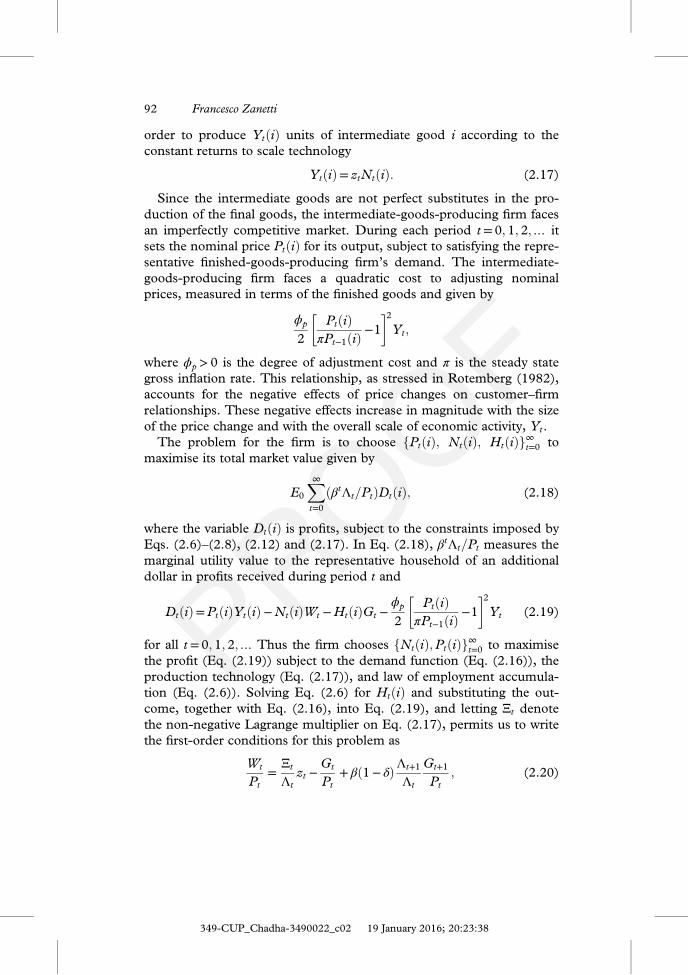
order to produce YtðiÞ units of intermediate good i according to theconstant returns to scale technology

YtðiÞ= ztNtðiÞ: (2.17)

Since the intermediate goods are not perfect substitutes in the pro-duction of the final goods, the intermediate-goods-producing firm facesan imperfectly competitive market. During each period t = 0; 1; 2;… itsets the nominal price PtðiÞ for its output, subject to satisfying the repre-sentative finished-goods-producing firm’s demand. The intermediate-goods-producing firm faces a quadratic cost to adjusting nominalprices, measured in terms of the finished goods and given by

ϕp

2PtðiÞ

πPt−1ðiÞ −1� �2

Yt;

where ϕp > 0 is the degree of adjustment cost and π is the steady stategross inflation rate. This relationship, as stressed in Rotemberg (1982),accounts for the negative effects of price changes on customer–firmrelationships. These negative effects increase in magnitude with the sizeof the price change and with the overall scale of economic activity, Yt.

The problem for the firm is to choose fPtðiÞ; NtðiÞ; HtðiÞg∞t=0 tomaximise its total market value given by

E0

X∞t=0

ðβtΛt=PtÞDtðiÞ; (2.18)

where the variable DtðiÞ is profits, subject to the constraints imposed byEqs. (2.6)–(2.8), (2.12) and (2.17). In Eq. (2.18), βtΛt=Pt measures themarginal utility value to the representative household of an additionaldollar in profits received during period t and

DtðiÞ=PtðiÞYtðiÞ−NtðiÞWt −HtðiÞGt −ϕp

2PtðiÞ

πPt−1ðiÞ −1� �2

Yt (2.19)

for all t = 0; 1; 2;… Thus the firm chooses fNtðiÞ;PtðiÞg∞t=0 to maximisethe profit (Eq. (2.19)) subject to the demand function (Eq. (2.16)), theproduction technology (Eq. (2.17)), and law of employment accumula-tion (Eq. (2.6)). Solving Eq. (2.6) for HtðiÞ and substituting the out-come, together with Eq. (2.16), into Eq. (2.19), and letting Ξt denotethe non-negative Lagrange multiplier on Eq. (2.17), permits us to writethe first-order conditions for this problem as

Wt

Pt=

Ξt

Λtzt −

Gt

Pt+ βð1− δÞΛt+1

Λt

Gt+1

Pt; (2.20)



and

ϕpPtðiÞ

πPt−1ðiÞ − 1

24

35 Pt

πPt−1ðiÞ= ð1− θtÞ PtðiÞPt

24

35−θt

+ θtΞt

Λt

PtðiÞPt

24

35−ð1+θÞ

+ βϕpEtΛt+1

Λt

Pt+1ðiÞπPtðiÞ − 1

24

35Pt+1ðiÞPt

πP2t ðiÞ

Yt+1

Yt

8<:

9=;:

(2.21)

Equation (2.20) is the firm’s labour supply condition, which equates thereal wage with the marginal product of labour minus the hiring costs topay in period t, plus the expected saving on the hiring costs forgone in per-iod t + 1, if the job is not dismissed. Equation (2.21) is the New KeynesianPhillips curve in its non-linearised form and it states that the firm setsprices as a markup over marginal cost, accounting for price adjustmentcosts. As Ravenna and Walsh (2008) and Chadha and Sun (2008) pointout, the presence of labour market search frictions enables the NewKeynesian Phillips curve to track inflation fluctuations more precisely.

2.4.4 The monetary authority

During each period t = 0; 1; 2;…, the monetary authority conductsmonetary policy using a modified Taylor (1993) rule,

lnðRt=RÞ= ρy lnðYt=YÞ+ ρπ lnðπt=π*t Þ+ lnðvtÞ; (2.22)

where R and Y are the steady state values of the nominal interest rateand output, and π*t is the monetary authority time-varying inflationtarget for the period t. According to Eq. (2.22), the monetary authorityadjusts the nominal interest rate in response to movements in outputfrom its steady state and inflation from the target. As pointed out inClarida et al. (1998) and Nelson (2003), this modelling strategy for thecentral bank consistently describes the conduct of monetary policy inthe UK since the early 1970s. The monetary policy shock vt follows theautoregressive process

lnðvtÞ= ρv lnðvt−1Þ+ εvt; (2.23)

where ρv < 1. The zero-mean, serially uncorrelated policy shock εvt isnormally distributed, with a standard deviation σv. Similarly to Ireland(2007), the time-varying inflation target π*t evolves according to

lnðπ*t Þ= lnðπ*Þ+ δaεat − δθεθt − δzεzt + σπεπt; (2.24)



such that it may vary exogenously, when σπ > 0, and may adjust to pre-ference, cost-push and technology shocks, when ½δa; δθ; δz�> 0: Notethat, as in Ireland (2007), since negative realisation of εθt and εzt andpositive realisation of εat increase prices, positive values for δθ; δz and δagenerate more persistent movements in the inflation target. The pre-sumption here, as detailed at the outset, is that changes in inflationshould not have happened without changes in at least the implicit infla-tion target, and that the implicit inflation target reacts to shockssimilarly to the underlying inflation.

2.5 Equilibrium and solution

In a symmetric, dynamic, equilibrium, all intermediate-goods-producingfirms make identical decisions, so that YtðiÞ=Yt, NtðiÞ=Nt, HtðiÞ=Ht,DtðiÞ=Dt and PtðiÞ=Pt, for all i ∈ 0; 1½ � and t = 0; 1; 2;. In addition, themarket clearing conditions Tt =Mt −Mt−1 and Bt =Bt−1 =0 must holdfor all t = 0; 1; 2;… These conditions, together with the firm’s profitconditions (Eq. (2.19)) and the household’s budget constraint(Eq. (2.3)), produce the aggregate resource constraint

Yt =Ct + ðϕp=2Þðπt=π−1Þ2Yt +GtHt; (2.25)

where the term GtHt expresses the resources spent in hiring.Substituting the Lagrange multiplier, Λt, from Eq. (2.4) into Eqs. (2.5),(2.14) and (2.20)–(2.21), and deriving the labour market equilibriumcondition by combining the agreed wage (Eq. (2.14)) with the labourdemand (Eq. (2.20)), the model describes the behavior of 14 endogen-ous variables fbt;Ct;Gt;Ht;Λt;Ξt;Nt; πt; π*t ;Rt;Ut;Wt; xt;Ytg and fourexogenous shocks fat; θt; vt; ztg. The equilibrium is then described bythe representative household’s first-order conditions (Eqs. (2.4) and(2.5)), the law of employment (Eq. (2.6)), the definition of labour mar-ket tightness (Eq. (2.7)), the definition of unemployment accumulation(Eq. (2.8)), the definition of cost per hire (Eq. (2.12)), the agreed wage(Eq. (2.14)), the production function (Eq. (2.17)), the labour marketequilibrium condition (Eq. (2.20)), the New Keynesian Phillips curve(Eq. (2.21)), the monetary authority policy rule (Eq. (2.22)), thetime-varying inflation target (Eq. (2.24)), the aggregate resourceconstraint (Eq. (2.25)), the definition of unemployment benefits andthe specification of the exogenous shocks as in Eqs. (2.2), (2.13), (2.15)and (2.23).



The equilibrium conditions do not have an analytical solution.Instead, the model’s dynamics are characterised by log-linearising themaround the steady state. The log-linearised equilibrium conditions are

Λt = at − Ct;

Λt = Rt +EtΛt+1 − πt;

Nt = ð1− δÞNt−1 + δHt;

xt = Ht − U t;

U t = − ð1− δÞ ðN=UÞNt−1;

Gt =ψ zt + αxt;

W t = ðb=W Þbt + ½η=ð1− ηÞ�ðG=bÞGt + ð1− δÞβðx=bÞ½η=ð1− ηÞ�Ext+1− ðβ=bÞð1− δÞð1− xÞ½η=ð1− ηÞ�ðGt+1 + Λt+1 − ΛtÞ;

Y t = zt + Nt;

bt = ðΞz=ΛbÞðΞt − Λt + ztÞ− f1+ ½η=ð1− ηÞ�gðG=bÞGt

+ βð1− δÞf1+ ð1− xÞ½η=ð1− ηÞ�gðG=bÞðΛt+1 + Gt − ΛtÞ− βð1− δÞðxG=bÞ½η=ð1− ηÞ�Ext+1;

πt = βEt πt+1 + ðθ Ξ=ϕΛÞðΞt − Λt + θtÞ− ðθ=ϕÞθt;Rt = ρyyt + ρπðπt − π*t Þ+ vt;

π*t = δaεat − δθεθt − δzεzt + σπεπt;

Y t = ðC=YÞCt + ðGH=YÞðGt + HtÞ;at = ρaat−1 + εat;

θt = ρθθt−1 + εθt;

vt = ρavt−1 + εvt;

and

zt = ρzzt−1 + εzt;

where a hat on a variable denotes the logarithmic deviation from its steadystate and a variable without the time index represents its value at thesteady state. The solution to this system is derived using Klein (2000),which is a modification of Blanchard and Kahn (1980), and takes the formof a state space representation. This latter can be conveniently used tocompute the likelihood function in the estimation procedure.



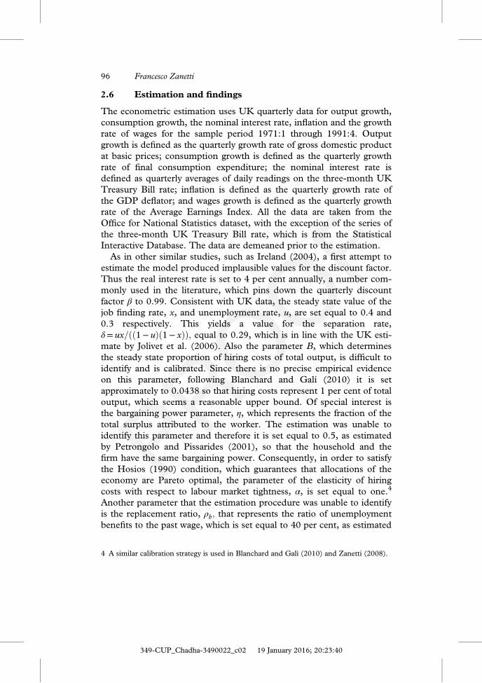
2.6 Estimation and findings

The econometric estimation uses UK quarterly data for output growth,consumption growth, the nominal interest rate, inflation and the growthrate of wages for the sample period 1971:1 through 1991:4. Outputgrowth is defined as the quarterly growth rate of gross domestic productat basic prices; consumption growth is defined as the quarterly growthrate of final consumption expenditure; the nominal interest rate isdefined as quarterly averages of daily readings on the three-month UKTreasury Bill rate; inflation is defined as the quarterly growth rate ofthe GDP deflator; and wages growth is defined as the quarterly growthrate of the Average Earnings Index. All the data are taken from theOffice for National Statistics dataset, with the exception of the series ofthe three-month UK Treasury Bill rate, which is from the StatisticalInteractive Database. The data are demeaned prior to the estimation.

As in other similar studies, such as Ireland (2004), a first attempt toestimate the model produced implausible values for the discount factor.Thus the real interest rate is set to 4 per cent annually, a number com-monly used in the literature, which pins down the quarterly discountfactor β to 0.99. Consistent with UK data, the steady state value of thejob finding rate, x, and unemployment rate, u, are set equal to 0.4 and0.3 respectively. This yields a value for the separation rate,δ= ux=ðð1− uÞð1− xÞÞ; equal to 0.29, which is in line with the UK esti-mate by Jolivet et al. (2006). Also the parameter B, which determinesthe steady state proportion of hiring costs of total output, is difficult toidentify and is calibrated. Since there is no precise empirical evidenceon this parameter, following Blanchard and Galí (2010) it is setapproximately to 0.0438 so that hiring costs represent 1 per cent of totaloutput, which seems a reasonable upper bound. Of special interest isthe bargaining power parameter, η, which represents the fraction of thetotal surplus attributed to the worker. The estimation was unable toidentify this parameter and therefore it is set equal to 0.5, as estimatedby Petrongolo and Pissarides (2001), so that the household and thefirm have the same bargaining power. Consequently, in order to satisfythe Hosios (1990) condition, which guarantees that allocations of theeconomy are Pareto optimal, the parameter of the elasticity of hiringcosts with respect to labour market tightness, α, is set equal to one.4

Another parameter that the estimation procedure was unable to identifyis the replacement ratio, ρb; that represents the ratio of unemploymentbenefits to the past wage, which is set equal to 40 per cent, as estimated

4 A similar calibration strategy is used in Blanchard and Galì (2010) and Zanetti (2008).



by Bean (1994) and Nickell (1997). The steady state value of the elasti-city of substitution between intermediate goods, θ, is set equal to six sothat the equilibrium markup is equal to 20 per cent, as suggested inBritton et al. (2000). The gross steady state value of inflation, π, is setequal to 1.02, matching the average inflation rate in the data. Finally,Eqs. (2.14) and (2.20) pin down the parameter χ which is set equal to0.9985.Table 2.1 displays the maximum likelihood estimates of the model’s

parameters together with their standard errors. The estimate of thedegree of nominal price rigidities, ϕp, is equal to 24.3425. As shown inIreland (2000), given that θ is equal to six, it implies that approximately20 per cent of the firms adjust their price each period, a value in linewith Britton et al. (2000). It is worth noticing that, given the sizablestandard error of this parameter, considerable uncertainty remainsabout the degree of nominal price rigidities in the economy.The parameter estimates of Eqs. (2.22) and (2.24) characterise the

conduct of monetary policy. The estimate of the reaction coefficient tothe fluctuations of output from its steady state, ρy, is 0.1229, and theestimate of the reaction coefficient to the fluctuations of inflation fromthe inflation target, ρπ, is 1.1019. These estimates suggest that themonetary authority responded weakly to inflation and output. This is inline with the estimates in Nelson (2003) and the documentation inBatini and Nelson (2009). The estimates of Eq. (2.24), which describesthe inflation target, point out that preference, cost-push and technology

Table 2.1. Maximum likelihood estimation and standard errors

Parameters Estimates Standard errors

ϕp 24.3425 29.3824ρπ 1.1019 0.0557ρy 0.1229 0.0922δa 0.2375 0.2779δθ 0.1428 0.1824δz 0.2612 0.8819ρa 0.9938 0.0003ρθ 0.8557 0.0148ρv 0.4280 0.1954ρz 0.6506 0.0307σa 0.2920 0.5819σθ 1.1144 0.6935σπ 0.1420 0.5678σv 0.0008 0.0047σz 0.6763 0.0723



shocks are all important components to determine the implicit inflationtarget. In fact, the estimates of δa, δθ and δz are equal to 0.2375, 0.1428and 0.2612 respectively. Interestingly, the monetary authority leaves thetarget to react more aggressively to technology shocks while giving lessweight to preference and cost-push shocks.

The estimates of the exogenous disturbances show that preferenceshocks are highly persistent, with ρa equal to 0.9938, while cost-pushand technology shocks are less so, with ρθ and ρz equal to 0.8557 and0.6506 respectively. The estimates of the volatility of the exogenousdisturbances show that cost-push and technology shocks are highlyvolatile, with σθ and σz equal to 1.1144 and 0.6763 respectively, whileshocks to the monetary policy rule, inflation target and households’ pre-ferences are of lower magnitude, with σv, σπ and σa equal to 0.0008,0.1420 and 0.2920 respectively. Clearly, these values suggest that cost-push and technology shocks are important components of economicfluctuations.

To investigate how the variables of the model react to each shock,Figures 2.2 and 2.3 plot the impulse responses of selected variables toone standard deviation of each of the exogenous shocks. The first col-umn in Figure 2.2 shows that after a one standard deviation technologyshock, output and unemployment both rise, while inflation falls. Thefall in inflation allows for an easing in monetary policy such that thenominal interest rate falls. Finally, the one-period immediate increasein unemployment leads to a fall in labour market tightness, which thenincreases due to the subsequent fall in unemployment. The second col-umn in Figure 2.2 shows that a one standard deviation cost-push shockcauses a fall in inflation and the nominal interest rate, and a rise in out-put. The increase in output triggers a fall in unemployment that gener-ates a rise in labour market tightness. Given the opposite reaction ofoutput and inflation in the case of technology and cost-push shocks,these disturbances behave as supply-side shocks, as mentioned in theoutset. The third column in Figure 2.2 shows that a one standard devia-tion monetary policy shock translates into an increase in the nominalinterest rate and into a fall in output. The fall in output generates anincrease in unemployment and a consequent fall in the number of hires.Opposite shifts in the number of hires and unemployment generate afall in labour market tightness. Since the monetary policy disturbance isserially uncorrelated, the reaction of each variable dies off over a periodof one year. The first column in Figure 2.3 shows that after a one stan-dard deviation preference shock both output and inflation rise, leadingthe nominal interest rate, due to the modified Taylor rule, to increase.Unemployment falls, and therefore labour market tightness rises due to



the lower response of vacancies. Finally, the second column inFigure 2.3 shows that a one standard deviation inflation targetshock decreases the nominal interest rate and raises inflation, whosecombined movements generate a decrease in the real interest rate andtherefore a rise in output. Unemployment falls and so labour markettightness increases.Looking across all these impulse responses also provides some

insights into how the presence of labour market search and the intro-duction of a time-varying inflation target affect the transmission

Output to technology

00.1

0.20.3

0 5 10 15 20 25 30

Output to cost-push

00.050.1

0.150.2

0.25

0 5 10 15 20 25 30

Output to monetary policy

–0.0015

–0.001

–0.0005

0

0 5 10 15 20 25 30

Interest rate to technology

–0.3

–0.2–0.1

0

0 5 10 15 20 25 30

Interest rate to cost-push

–0.25–0.2

–0.15–0.1

–0.050

0 5 10 15 20 25 30

Interest rate to monetary policy

00.00020.00040.00060.0008

0 5 10 15 20 25 30

Inflation to technology

–0.5–0.4–0.3–0.2–0.1

0

0 5 10 15 20 25 30

Inflation to cost-push

–0.3

–0.2

–0.1

0

0 5 10 15 20 25 30

Inflation to monetary policy

–0.00005–0.00004–0.00003–0.00002–0.00001

0

0 5 10 15 20 25 30

Labor market tightness to technology

–2–1.5

–1–0.5

0

0 5 10 15 20 25 30

Labor market tightness tocost-push

00.20.40.60.8

0 5 10 15 20 25 30

Unemployment to technology

00.20.40.60.8

1

0 5 10 15 20 25 30

Unemployment to cost-push

–0.4–0.3–0.2–0.1

0

0 5 10 15 20 25 30

Unemployment to monetarypolicy

00.00050.001

0.00150.002

0 5 10 15 20 25 30

Labor market tightness tomonetary policy

–0.004–0.003–0.002–0.001

0

0 5 10 15 20 25 30

Figure 2.2. Impulse responses to technology, cost-push and monetarypolicy shocksNotes: Each panel shows the percentage-point response of selectedmodels' variables to a one standard deviation shock. The horizontalaxis measures the time, expressed in quarters.



Output to preference

00.02

0.040.06

0.08

0 5 10 15 20 25 30

Output to inflation target

–0.05

00.05

0.1

0.15

0 5 10 15 20 25 30

Interest rate to preference

–0.06

–0.04–0.02

0

0.02

0 5 10 15 20 25 30

Interest rate to inflation target

–0.15

–0.1

–0.05

0

0.05

0 5 10 15 20 25 30

Inflation to preference

0

0.005

0.01

0.015

0 5 10 15 20 25 30

Inflation to inflation target

–0.002

0

0.002

0.004

0.006

0 5 10 15 20 25 30

Labor market tightness to preference

–0.1

0

0.1

0.2

0.3

0 5 10 15 20 25 30

Labor market tightness to inflation target

–0.1

0

0.1

0.2

0.3

0 5 10 15 20 25 30

Unemployment to preference

–0.15

–0.1

–0.05

0

0 5 10 15 20 25 30

Unemployment to inflation target

–0.3

–0.2

–0.1

0

0.1

0 5 10 15 20 25 30

Figure 2.3. Impulse responses to preference and inflation target shocksNotes: Each panel shows the percentage-point response of selectedmodels' variables to a one standard deviation shock. The horizontalaxis measures the time, expressed in quarters.



mechanism of a standard New Keynesian framework. For all shocks,the coexistence of these two features leaves the baseline transmissionmechanism of a New Keynesian setting qualitatively unaffected: all thevariables respond to shocks similarly to a standard New Keynesianmodel without labour market search and a time-varying inflation target,as in Woodford (2003). This corroborates the findings in Christoffelet al. (2006) and Ireland (2007), who show that each of these two fea-tures on its own leaves the qualitative response of the underlying NewKeynesian model unchanged. Nonetheless, as detailed below, the jointpresence of labour market search and the time-varying inflation targetaffects the model’s quantitative response to disturbances.To understand the extent to which the movements of each variable

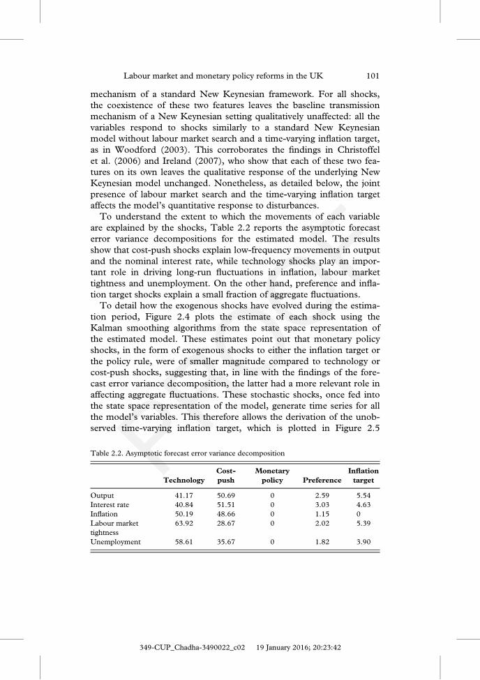
are explained by the shocks, Table 2.2 reports the asymptotic forecasterror variance decompositions for the estimated model. The resultsshow that cost-push shocks explain low-frequency movements in outputand the nominal interest rate, while technology shocks play an impor-tant role in driving long-run fluctuations in inflation, labour markettightness and unemployment. On the other hand, preference and infla-tion target shocks explain a small fraction of aggregate fluctuations.To detail how the exogenous shocks have evolved during the estima-

tion period, Figure 2.4 plots the estimate of each shock using theKalman smoothing algorithms from the state space representation ofthe estimated model. These estimates point out that monetary policyshocks, in the form of exogenous shocks to either the inflation target orthe policy rule, were of smaller magnitude compared to technology orcost-push shocks, suggesting that, in line with the findings of the fore-cast error variance decomposition, the latter had a more relevant role inaffecting aggregate fluctuations. These stochastic shocks, once fed intothe state space representation of the model, generate time series for allthe model’s variables. This therefore allows the derivation of the unob-served time-varying inflation target, which is plotted in Figure 2.5

Table 2.2. Asymptotic forecast error variance decomposition

TechnologyCost-push

Monetarypolicy Preference

Inflationtarget

Output 41.17 50.69 0 2.59 5.54Interest rate 40.84 51.51 0 3.03 4.63Inflation 50.19 48.66 0 1.15 0Labour markettightness

63.92 28.67 0 2.02 5.39

Unemployment 58.61 35.67 0 1.82 3.90



against the observed inflation. The figure shows that during the 1970sthe monetary authority translated adverse technology shocks into higherinflation, by allowing the implicit inflation target to grow. In the early1980s, it had taken advantage of the positive supply shocks to reduceinflation and it subsequently allowed the implicit inflation target togrow throughout the 1990s. This is in line with the narrative evidencein Batini and Nelson (2009).

As detailed at the outset, since this model is immune to Lucas’(1976) critique, counterfactual scenarios can disclose whether the intro-duction of labour market reforms or a monetary policy frameworkbased on a constant inflation target might have altered the economicoutlook if they had been introduced in the earlier decades. The exerciseconsists in superimposing these policy changes on the model, assuming

Preference shocks

–1–0.5

00.5

11.5

1971

1973

1975

1977

1979

1981

1983

1985

1987

1989

1991

Inflation target shocks

−0.2−0.1

00.10.20.3

1971

1973

1975

1977

1979

1981

1983

1985

1987

1989

1991

Cost-push shocks

−2−1

0123

1971

1973

1975

1977

1979

1981

1983

1985

1987

1989

1991

Monetary policy shocks

−0.0001−0.00005

00.000050.0001

1971

1974

1977

1980

1983

1986

1989

Technology shocks

−2−1

012

1971

1973

1975

1977

1979

1981

1983

1985

1987

1989

1991

Figure 2.4. Smoothed estimates of preference, technology, cost-push,monetary policy and inflation target shocksNotes: Each panel shows estimates of the exogenous shocks using theKalman smoothing algorithm from the state space representation ofthe estimated model.



that all the other parameters and stochastic shocks remainedunchanged, to generate time series for the alternative scenarios. To thisend, Figures 2.6 and 2.7 compare the historical series of inflation andoutput growth against the series that would have been generated undercounterfactual scenarios. Figure 2.6(a) shows the counterfactual case ofa reduction of 10 per cent in the replacement ratio of unemploymentbenefits, ρb, such that it equals 0.36 instead of its estimated value. Thispolicy change would have had a sizable effect on the level of inflation,which would have been on average lower compared to its realised coun-terpart: 2.1 per cent instead of 2.3 per cent. However, inflation volatilitywould have increased somewhat (0.0292 instead of 0.0273).Interestingly, output growth would have displayed a substantiallyunchanged level, but a slightly higher variance (0.0140 instead of0.0138). Figure 2.6(b) shows the observed series against those gener-ated under the counterfactual scenarios of a 10 per cent reduction inthe household’s bargaining power, η, such that it equals 0.45 instead of0.5. The level of inflation would have been materially lower, 1.6 percent instead of 2.3 per cent, while the variance of inflation would havedoubled, 0.0560 instead of 0.0273. Similarly, both the level and var-iance of output growth would have remained substantially unchangedcompared to their realised counterparts. This suggests that the imple-mentation of these labour market reforms would have contributed tothe reduction of the level of inflation, but would have been unable to

–0.04

–0.02

0

0.02

0.04

0.06

0.08

0.1

1971

1973

1975

1977

1979

1981

1983

1985

1987

1989

1991

Figure 2.5. Estimate of the time-varying inflation target and inflationNotes: Unobserved time-varying inflation target (black line) andobserved inflation (grey line).



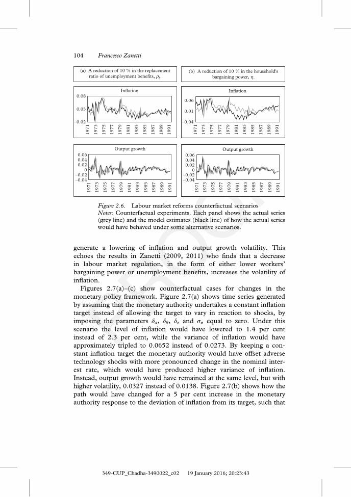
generate a lowering of inflation and output growth volatility. Thisechoes the results in Zanetti (2009, 2011) who finds that a decreasein labour market regulation, in the form of either lower workers’bargaining power or unemployment benefits, increases the volatility ofinflation.

Figures 2.7(a)–(c) show counterfactual cases for changes in themonetary policy framework. Figure 2.7(a) shows time series generatedby assuming that the monetary authority undertakes a constant inflationtarget instead of allowing the target to vary in reaction to shocks, byimposing the parameters δa, δθ, δz and σπ equal to zero. Under thisscenario the level of inflation would have lowered to 1.4 per centinstead of 2.3 per cent, while the variance of inflation would haveapproximately tripled to 0.0652 instead of 0.0273. By keeping a con-stant inflation target the monetary authority would have offset adversetechnology shocks with more pronounced change in the nominal inter-est rate, which would have produced higher variance of inflation.Instead, output growth would have remained at the same level, but withhigher volatility, 0.0327 instead of 0.0138. Figure 2.7(b) shows how thepath would have changed for a 5 per cent increase in the monetaryauthority response to the deviation of inflation from its target, such that

Inflation

–0.02

0.03

0.08

1971

1973

1975

1977

1979

1981

1983

1985

1987

1989

1991

Output growth

–0.04–0.02

00.020.040.06

1971

1973

1975

1977

1979

1981

1983

1985

1987

1989

1991

Inflation

–0.04

0.01

0.06

1971

1973

1975

1977

1979

1981

1983

1985

1987

1989

1991

Output growth

–0.04–0.02

00.020.040.06

1971

1973

1975

1977

1979

1981

1983

1985

1987

1989

1991

(a) A reduction of 10 % in the replacementratio of unemployment benefits, rb.

(b) A reduction of 10 % in the household'sbargaining power, h.

Figure 2.6. Labour market reforms counterfactual scenariosNotes: Counterfactual experiments. Each panel shows the actual series(grey line) and the model estimates (black line) of how the actual serieswould have behaved under some alternative scenarios.



ρπ equals 1.1571. Differently from the case that superimposes a con-stant inflation target, if the monetary authority had increased the degreeof reaction to the deviation of inflation from its time-varying target boththe level and variance of inflation would have been lower, at 2.2 percent instead of 2.3 per cent and 0.0260 instead of 0.0273 respectively,

Inflation

–0.06

–0.01

0.04

0.09

1971

1973

1975

1977

1979

1981

1983

1985

1987

1989

1991

Output growth

–0.15–0.1

–0.050

0.050.1

1971

1973

1975

1977

1979

1981

1983

1985

1987

1989

1991

Inflation

–0.03

0.02

0.07

1971

1973

1975

1977

1979

1981

1983

1985

1987

1989

1991

Output growth

–0.04–0.02

00.020.040.06

1971

1973

1975

1977

1979

1981

1983

1985

1987

1989

1991

Inflation

–0.05

0

0.05

0.1

1971

1973

1975

1977

1979

1981

1983

1985

1987

1989

1991

Output growth

–0.1–0.05

00.050.1

1971

1973

1975

1977

1979

1981

1983

1985

1987

1989

1991

(c) An increase of 5 % in the monetaryauthority response to output, ry.

(a) A constant inflation target, da, dq, dz, andsp equal to zero.

(b) An increase of 5 % in the monetaryauthority response to inflation, rp.

Figure 2.7. Monetary policy reforms counterfactual scenariosNotes: Counterfactual experiments. Each panel shows the actual series(grey line) and the model estimates (black line) of how the actual serieswould have behaved under some alternative scenarios.



while output growth would have remained substantially unchanged.Finally, Figure 2.7(c) displays the counterfactual case where themonetary authority would have increased by 5 per cent its reaction todeviations of output from its steady state, such that ρy equals 0.1291.Under this scenario, inflation would have been substantially unchangedfrom its historical counterpart, while output growth would have dis-played higher volatility, with its variance equal to 0.0418 instead of0.0138. This analysis suggests that the degree to which the monetaryauthority reacted to inflation deviations from the inflation target wouldhave contributed to a decrease in the variance of inflation and outputgrowth and also to a lower level of inflation. On the other hand, theintroduction of a constant inflation target or a monetary policy thatwould have reacted strongly to output would have been unlikely toproduce a different economic outlook. These findings are in line withnumerous related studies on other economies. For instance, Claridaet al. (2000), Boivin and Giannoni (2006), Lubik and Schorfheide(2004) and Castelnuovo (2007) find that by responding more stronglyto inflation, monetary policy has stabilised the US economy moreeffectively in the post-1980 period. Gambetti and Pappa (2008), usingsign restrictions on a VAR, find that the introduction of inflation target-ing is unable to explain the reduced volatility of inflation in severaleconomies.

2.7 Conclusion

This chapter has developed a general equilibrium model that details thefunctioning of the UK economy during the 1970s and 1980s to investi-gate to what extent labour market reforms enforced by the Thatchergovernment in the later 1980s, in the form of reduction of unemploy-ment benefits and union power, and the introduction of a constantinflation target in 1992, might have changed the economic outlook ifthey had been introduced in the early 1970s. The econometric estima-tion of the model has permitted us to separate out the policy para-meters, such as those representing monetary policy and the structure ofthe labour market, which may vary due to changes in policy, from thosewhich represent the household’s preference and firm’s technology thatought to be policy-invariant. Hence, the model positively answersLucas’ (1976) critique and can be used to draw inferences abouthow these policy changes might have altered the economic outlook.The exercise shows that the decreases in unemployment benefits andunion power are unlikely to have produced a different macroeconomicperformance. The results on monetary policy reform are mixed. A



stronger reaction to inflation deviations from target would have loweredthe volatility of inflation and output growth. By contrast, the introduc-tion of a constant inflation target or a monetary policy that had reactedstrongly to output fluctuations are unlikely to have changed the eco-nomic outlook.But while the results do support the importance of the way in which

the monetary authority reacts to inflation, it should also be noted thatthe model abstracts from some relevant attributes of the economy. Forinstance, it ignores the oil sector, which, as Blanchard and Galì (2007)and Nakov and Pescatori (2010) point out, may alter the propagation ofexogenous disturbances and therefore interact with the policy changesto reduce macroeconomic volatility. Similarly, the model also sets asideimportant developments of the period, such as improved inventorymanagement, as emphasised in McConnell and Perez-Quiros (2000),or the development of financial innovations, as pointed out by Dynanet al. (2006), whose presence may also have a non-trivial effect on theway in which the economy reacts to policy changes and how these inter-act with aggregate disturbances. Furthermore, although the modeldeveloped here allows aggregate productivity, cost-push shocks andnominal disturbances to have effects on the economy, in practice a vari-ety of other aggregate shocks may play a role. To establish to whatextent the results hold for refinements of the theoretical frameworkremains an outstanding task for future research.

References

Batini, N. and Nelson, E. (2009). ‘The U.K.’s rocky road to stability’, GlobalEconomic Studies. Nova Science Publishers.

Benati, L. (2008). ‘The Great Moderation: in the United Kingdom’, Journal ofMoney Credit and Banking, 40, 121–148.

Bean, C. R. (1994). ‘European unemployment: a survey’, Journal of EconomicLiterature, 32, 573–619.

Bean, C. R. and Crafts, N. (1996). ‘British economic growth since 1945: rela-tive economic decline ... and renaissance?,’ CEPR Discussion Papers 1092,C.E.P.R. Discussion Papers.

Bianchi, F., Mumtaz, H. and Surico, P. (2009). ‘The UK great stability: a viewfrom the term structure of interest rates’, Journal of Monetary Economics,56, 856–871.

Blanchflower, D.G. and Freeman, R.B. (1993). ‘Did the Thatcher reformschange British labor market performance?’ Conference paper. CEP/NIESR.

Blanchard, O. J. and Kahn, C. (1980). ‘The solution of linear difference modelsunder rational expectations’, Econometrica, 48, 1305–1311.



Blanchard, O. J. and Galì, J. (2010). ‘Labor markets and monetary policy: anew Keynesian model with unemployment’, American Economic Journal:Macroeconomics, 2, 1–30.

(2007). The macroeconomic effects of oil price shocks: why are the 2000s sodifferent from the 1970s? NBER Chapters. In: International Dimensionsof Monetary Policy. National Bureau of Economic Research, Inc.,pp. 373–421.

Boivin, J. and Giannoni, M. (2006). ‘Has monetary policy become more effec-tive?’, The Review of Economics and Statistics, 88, 445–462.

Britton, E., Larsen, J. D. and Small, I. (2000). ‘Imperfect competition and thedynamics of mark-ups’, Bank of England Working Paper No. 110.

Canova, F., Gambetti, L. and Pappa, E. (2007). ‘The structural dynamics ofoutput growth and inflation: some international evidence’, The EconomicJournal, 117, C167–C191.

Castelnuovo, E. (2007). ‘Assessing different drivers of the Great Moderation inthe U.S’, University of Padua Working Paper Series.

Chadha J. and Sun Q. (2008). Labour market search and monetary policy—atheoretical consideration. In: P. Arestis and J. McCombie (Eds).Unemployment: Past and Present. Palgrave Macmillan.

Christoffel, K., Kuester, K. and Linzert, T. (2006). ‘Identifying the role of labormarkets for monetary policy in an estimated DSGE model’, EuropeanCentral Bank Working Paper No. 635.

Clarida, R., Galì, J. and Gertler, M. (1998). ‘Monetary policy rules in practice:some international evidence’, European Economic Review, 42, 1033–1067.

(2000). ‘Monetary policy rules and macroeconomic stability: evidence andsome theory’, Quarterly Journal of Economics, CXV, 147–180.

DiCecio R. and Nelson, E. (2007). ‘An estimated DSGE model for the UnitedKingdom’, Federal Reserve Bank of St. Louis Review, 89, 215–231.

Dynan K., Elmendorf D. W. and Sichel, D. E. (2006). ‘Can financial innova-tion help to explain the reduced volatility of economic activity?’, Journal ofMonetary Economics, 53, 123–150.

Faccini, R., Millard, S. and Zanetti, F. (2013). ‘Wage rigidities in an estimateddynamic, stochastic, general equilibrium model of the UK labour market,’Manchester School, University of Manchester, 1, 66–99, 09.

Friedman, M. (1968). Inflation: causes and consequences. In: Dollars andDeficits: Living with America’s Economic Problems. Englewood Cliffs:Prentice-Hall.

Gambetti, L. and Pappa, E. (2008). ‘To target inflation or not to target: a con-ditional answer’, Universitat Autònoma de Barcelona Working Paper.

Gregory, M. (1998). ‘Reforming the labour market: an assessment of theUK policies of the Thatcher era’, Australian Economic Review, 31,329–344.

Harrison, R. and Oomen, O. (2010). ‘Evaluating and estimating a DSGEmodel for United Kingdom’, Bank of England Working Paper 380.

Hosios, A. (1990). ‘On the efficiency of matching and related models of searchand unemployment’, Review of Economic Studies, 57, 279–298.



Ireland, P. N. (2000). ‘Interest rates, inflation, and Federal Reserve policy since1980’, Journal of Money, Credit, and Banking, 32, 417–434.

(2004). ‘Technology shocks in the New Keynesian model’, Review ofEconomics and Statistics, 86, 923–936.

(2007). ‘Changes in the Federal Reserve’s inflation target: causes and conse-quences’, Journal of Money, Credit, and Banking, 39, 1851–1882.

Jolivet, G., Postel-Vinay, F. and Robin, J. M. (2006). ‘The empirical content ofthe job search model: labor mobility and wage distributions in Europe andthe US’, European Economic Review, 50, 877–907.

Kamber, G. and Millard, S. (2008). Understanding the Monetary TransmissionMechanism in the United Kingdom: The Role of Nominal and Real Rigidities.Bank of England: Mimeo.

Klein, P. (2000). ‘Using the generalized Schur form to solve a multivariate lin-ear rational expectations model’, Journal of Economic Dynamics and Control,24, 1405–1423.

Lubik, T. and Schorfheide, F. (2004). ‘Testing for indeterminacy: an applica-tion to US monetary policy’, American Economic Review, 94, 190–217.

Lucas, R. E., Jr. (1976). ‘Econometric policy evaluation: a critique’, Carnegie-Rochester Conference Series on Public Policy, 1, 19–46.

McConnell, M. and Perez-Quiros G. (2000). ‘Output fluctuations in theUnited States: What has changed since the early 1980’s?’, AmericanEconomic Review, 90, 1464–1476.

Millward, N., Stevens, M., Smart, D. and Hawes, W.R. (1992). WorkplaceIndustrial Relations in Transition: The ED/ESRC/PSI/ACAS Surveys.Aldershot: Dartmouth Publishing.

Minford, P. (1983). Unemployment—Cause and Cure. Oxford: MartinRobertson.

Nakov A. and Pescatori A. (2010). ‘Oil and the Great Moderation’, EconomicJournal, 120, 131–156.

Nelson, E. (2003). UK monetary policy 1972–97: a guide using Taylor rules.In: Mizen, P. (Ed.). Central Banking, Monetary Theory and Practice: Essaysin Honour of Charles Goodhart, Volume One. Cheltenham, UK: EdwardElgar, pp. 195–216.

Nickell, S. (1997). ‘Unemployment and labor market rigidities: Europe versusNorth America’, The Journal of Economic Perspectives, 11, 55–74.

Petrongolo, B. and Pissarides, C. (2001). ‘Looking into the black box: a surveyof the matching function’, Journal of Economic Literature, 38, 390–431.

Pissarides, C. (2000). Equilibrium Unemployment Theory. MIT Press.Ravenna, F. and Walsh, C. (2008). ‘Vacancies, unemployment and the Phillips

curve’, European Economic Review, 52, 1494–1521.Rotemberg, J. (1982). ‘Monopolistic price adjustment and aggregate output’,

The Review of Economic Studies, 49, 517–531.Smets, F. and Wouters, R. (2007). ‘Shocks and frictions in US business cycles:

a Bayesian DSGE approach’, American Economic Review, 97, 586–606.Steinsson, J. (2003). ‘Optimal monetary policy in an economy with inflation

persistence’, Journal of Monetary Economics, 50, 1425–1456.



Taylor, J. (1993). ‘Discretion versus policy rules in practice’, Carnegie-RochesterConference Series on Public Policy, 39, 195–214.

Woodford, M. (2003). Interest and Prices: Foundations of a Theory of MonetaryPolicy. Princeton University Press.

Zanetti, F. (October 2008). ‘Labor and investment frictions in a real businesscycle model’, Journal of Economic Dynamics and Control, Elsevier, 32(10),3294–3314.

Zanetti, F. (2009). ‘Effects of product and labor market regulation on macro-economic outcomes’, Journal of Macroeconomics, 31, 320–332.

(2011). ‘Labor market institutions and aggregate fluctuations in a search andmatching model’, European Economic Review, 55, 644–658.



2 labour market and monetary policy reforms in the uk: a...

Documents