2-0

TABLE OF CONTENTS

Section Page

2.0 HYDROLOGY 2-1

2.1 GENERAL 2-1

2.2 RAINFALL – RUNOFF COMPUTATIONS USING HEC-HMS 2-3

2.2.1 Design Storm Rainfall 2-3

2.2.2 Design Storm Losses 2-4

2.2.3 Design Storm Runoff 2-6

2.2.3.1 General 2-6

2.2.3.2 Adjustment for Ponding 2-7

2.2.4 Procedure for Developing a Design Runoff Hydrograph 2-8

2.2.5 Flood Routing 2-12

2.3 DRAINAGE AREA-DISCHARGE CURVES 2-12

2.4 RATIONAL METHOD 2-13

2.4.1 Runoff Coefficient (C) 2-14

2.4.2 Rainfall Intensity (i) 2-15

2.4.3 Drainage Area (A) 2-17

2.5 HYDROGRAPH DEVELOPMENT FOR SMALL WATERSHEDS 2-17

2-1

2.0 HYDROLOGY

2.1 GENERAL

The planning, design, and construction of drainage facilities are based on the determination of

one or more aspects of storm runoff. If the estimate of storm runoff is incorrect, the constructed facilities

may be undersized, oversized, or otherwise inadequate. An improperly designed drainage system can be

uneconomical, cause flooding, interfere with traffic, disrupt commercial and other activities, and be a

general nuisance in the affected area. However, the peak rate, volume and time-sequence of storm runoff

related to a certain recurrence interval (frequency) can only be approximated due to the many physical

and climatic factors involved.

Continuous long-term records of rainfall and resulting storm runoff in an area provide the best

data source from which to base the design of storm drainage and flood control systems in that area.

However, it is not possible to obtain such records in sufficient quantities for all locations requiring storm

runoff computations. Therefore, the accepted practice is to relate storm runoff to rainfall, thereby

providing a means of estimating the rates, timing and volume of runoff expected within local watersheds

at various recurrence intervals. Although numerous methods to relate rainfall and runoff have been

considered, three methods are recommended for use in Fort Bend County. These methods, discussed

below, provide reasonable and consistent procedures for approximating the characteristics of the rainfall-

runoff process.

It is generally accepted that urban development has a pronounced effect on the rate and volume of

runoff from a given rainfall. Urbanization generally alters the hydrology of a watershed by improving its

hydraulic efficiency, reducing its surface infiltration and reducing its storage capacity. This alteration can

be intensified in flat areas like Fort Bend County. Figure 2-1 illustrates the effect of improving a

watershed’s hydraulic efficiency by presenting runoff rate versus time for the same storm with two

different stages of watershed development. The reduction of a watershed’s storage capacity and surface

infiltration results from the elimination of porous surfaces and ponding areas by grading and paving

building sites, streets, drives, parking lots, and sidewalks and by constructing buildings and other

facilities characteristic of urban development. Zoning maps, future land use maps, and watershed master

plans should be used as aids in establishing the anticipated surface character following development. The

selection of design runoff coefficients and/or percent impervious cover factors, which are explained in the

following discussions of runoff calculation, must be based upon the appropriate degree of urbanization.

2-2

Because of its versatility and accuracy, the widely used computer program HEC-HMS version

3.0.1 (or newer) is recommended as the primary tool for modeling storm runoff hydrographs in Fort Bend

County for new developed models. Versions of HEC-HMS must be consistent throughout each project.

Accordingly, the hydrologic design techniques described in this manual incorporate many of the routines

contained in HEC-HMS. The principal routines used for describing runoff in the county as presented in

this section are based on the Clark unit hydrograph technique, design storms and rainfall loss rates. A

methodology for deriving the parameters used to compute the Clark unit hydrograph was developed from

optimization studies utilizing U.S. Geological Survey (USGS) regional rainfall-runoff data and standard

unit hydrograph techniques is appropriate for a wide range of drainage area sizes and is the preferred

method in all but certain small areas requiring only peak discharge determinations. Appendix A presents

an in-depth discussion of the technical development of this methodology. The HEC models from the Fort

Bend County Drainage District must be obtained for updating the individual watershed in order to submit

any drainage study.

HEC-HMS modeling is required of new development to ensure the development causes no

adverse impact to a watershed for events including the 100-year, 25-year and 10-year rainfall events.

Section 6 and Section 8 of this Manual define certain conditions under which a development may provide

detention without a HEC-HMS analysis.

For areas less than 2000 acres and greater than 200 acres, drainage area-discharge curves have

been developed as a means to determine peak discharge.

For certain small drainage areas (generally less than 200 acres in size), the widely used Rational

Method provides a useful means of determining peak discharges. In situations requiring determination of

a complete flood hydrograph, and not just a peak discharge, the Malcom Small Watershed Method should

be utilized. If the engineer wishes to use an alternative design technique, it is recommended that the Fort

Bend County Drainage District Engineer be consulted prior to design. For large drainage areas,

hydrologic modeling using HEC-HMS is recommended to obtain runoff hydrographs.

The drainage discharge curves, Rational Method and Malcom Small Watershed Method are to be

used as tools to assist in the design of internal drainage components of a development, and to assist in

HEC-HMS modeling. The results provided by these curves/methods alone do not justify the amount of

detention a development must provide to mitigate its impact to the watershed. See Section 6 and/or

Section 8 of this Manual for minimum detention requirements.

2-3

2.2 RAINFALL-RUNOFF COMPUTATIONS USING HEC-HMS

A stream network model which simulates the runoff response of a river basin to rainfall over that

basin can be developed utilizing the HEC-HMS computer program by the appropriate combination of

hydrograph and routing computations. The following sections describe the elements required to develop

a HEC-HMS computer model.

2.2.1 Design Storm Rainfall

Design storm rainfall can be described in terms of frequency, duration, areal extent and

distribution of intensity with time. A design storm’s rainfall distribution in time should be handled in the

HEC-HMS by offsetting the intensity position of hyetograph by 67% in HEC-HMS if either the

watershed is shared with Harris County or there is no existing model for the watershed. If there is an

existing model for the watershed with the intensity position at 50%, then for consistency, the updated

model for the watershed should have the intensity position at 50%. The engineer’s choice for frequency

and duration is dependent upon the physical characteristics, location and study objectives. In most cases,

design will be based on a 24-hour duration storm event. The HEC-HMS program has the capability to

modify runoff hydrographs to account for progressively smaller design storm volumes as areal coverage

increases. The HEC-HMS user manual suggests how to model storm rainfall depth versus drainage area

relationships, based on Figure 15 in the National Weather Service’s Technical Paper No. 40 which

presents a means of reducing point rainfall totals as drainage area size increases.

It is often necessary to increment design rainfall hyetographs in five-minute intervals to meet the

design needs of small drainage areas having short times of concentration. The TP-40 rainfall isopluvial

maps are limited to storm durations no less than 30 minutes. Table 3 of TP-40 then provides a method to

calculate the rainfall amounts for shorter duration storms based on national average values. To more

accurately define these rainfall quantities on a local basis the National Weather Service issued Technical

Memorandum NWS Hydro-35 entitled “Five- to 60-Minute Precipitation Frequency for the Eastern and

Central United States”. Thus, both TP-40 and Hydro-35 were used to develop Table 2-1 in which depth

vs. duration data is presented for a variety of storm frequencies. Table 2-1 is also useful in utilizing the

Rational Method.

2-4

2.2.2 Design Storm Losses

Only a portion of the rainfall volume which falls on a watershed during a storm event actually

ends up as stream runoff. The remainder is intercepted by infiltration, depression storage, evaporation

and other mechanisms. The volume of rainfall which becomes runoff is termed the “excess” rainfall. The

difference between the observed total rainfall hyetograph and the excess rainfall hyetograph is termed

abstractions or losses.

The exponential loss method is one of several loss methods included in HEC-HMS. The

exponential loss method is recommended for calculation of abstractions in Fort Bend County.

Exponential loss method is an empirical method in which the loss rate is determined to be a function of

both the rainfall intensity and accumulated losses. In general, this method should not be used without

calibration. It is highly recommended to obtain exponential loss parameters by calibration whenever

possible.

Following are the description of the parameters of the exponential loss method:

1) Initial range: the amount of initial accumulated infiltration during which the loss rate is

increased. This parameter is considered to be a function primarily of antecedent soil moisture deficiency

and is usually storm-dependent.

2) Initial coefficient: specifies the starting loss rate coefficient on the exponential infiltration

curve. It is assumed to be a function of infiltration characteristics and consequently may be correlated

with soil type, land use, vegetation cover, and other properties of a sub-basin.

3) Coefficient ratio: indicates the rate at which the exponential decrease in infiltration capability

proceeds. It may be considered a function of the ability of the surface of a sub-basin to absorb

precipitation and should be reasonable constant for large, homogeneous areas.

4) Precipitation exponent: reflects the influence of precipitation rate on sub-basin-average loss

characteristics. It reflects the manner in which storms occur within an area and may be considered a

characteristic of a particular region. It varies from 0.0 up to 1.0.

2-5

5) Impervious %: percentage of the sub-basin which is directly connected impervious area can

be specified. No loss calculations are carried out on the impervious area; all precipitation on that portion

of the sub-basin becomes excess precipitation and subject to direct runoff.

Based on the analyses conducted in the original development of the hydrologic methodology (See

Appendix A) and a consideration of soil characteristics in Fort Bend County, the following are

recommended values for the variables to be used with this methodology:

1) Initial Range (in HEC-HMS) or DLKTR (in HEC-1) = amount in inches of initial

accumulated rain loss during which the loss coefficient is increased = 0.0

2) Initial coefficient (in HEC-HMS) or STRKR (in HEC-1) = starting value of the loss

coefficient on the exponential recession curve for rain losses = 0.5

3) Coefficient Ratio (HEC-HMS) or RTIOL (in HEC-1) = parameter computed as the ratio of

STRKR to a value of STRKR after ten inches of accumulated loss. = 3.0

4) Exponent (in HEC-HMS) or ERAIN (in HEC-1) = exponent of precipitation for rain loss

function that reflects the influence of the precipitation rate on the basin-average loss

characteristics = 0.6

5) Impervious % (in HEC-HMS) or RTIMP (in HEC-1) = percentage of drainage basin that is

impervious= (% Urban Development) x (average % impervious cover of the developed area)/100

Typical values for the percentage of impervious cover corresponding to various types of

development in Fort Bend County are given in Table 2-2. These values should be used when only the

general type of planned development is known; once the actual level of development has been determined

for a specific area, a refined value should be used to reflect the actual percent of impervious cover.

2-6

2.2.3 Design Storm Runoff

2.2.3.1 General

Given the design storm excess rainfall, it is necessary to determine the storm runoff hydrograph at

the point of interest utilizing the HEC-HMS program. The Clark unit hydrograph for a drainage area is

described by three parameters: TC, R and a time-area curve. TC represents the time of concentration and

R is a storage coefficient for the area. The time-area curve defines the cumulative area of the watershed

contributing runoff to the design point as a function of time.

A statistical analysis of historical rainfall and runoff data taken from selected watersheds in the

Fort Bend County vicinity was performed to correlate TC and R to drainage area physiographic

characteristics. These characteristics include the length, slope and roughness of the basin’s longest

watercourse, the average basin slope and the effective imperviousness of the basin. From this analysis,

the following equations were derived:

(L/ �¯ S)0.57 (N)0.8 TC + R = 128 (So)0.11 (10)I (2-1)

And TC = (TC+R) x 0.38 (log So) (2-2) R = (TC+R) – TC (2-3) Where TC = Clark’s time of concentration (hrs)

R = Clark’s storage coefficient (hrs)

L = length of the longest watercourse within the drainage area (miles)

S = average slope along the area’s longest watercourse (ft/mile)

N = Manning’s weighted roughness coefficient along the longest watercourse

(see Step 4 of Section 2.2.4)

So = average basin slope of land draining overland into the longest

watercourse (ft/mile)

I = effective impervious ratio

A plot of Equation 2-1, along with the basic data used in it development, is contained in

Appendix A.

2-7

The effective impervious ratio (I) used in equation (2-1) is determined by:

I = CD x 10-4 (2-4)

Where: C = the average percent of impervious cover of the developed area (in

percent)

D = % of the subarea that is developed

Determination of TC and R is carried out by the solution of Equations 2-1, 2-2 and 2-3.

These parameters may then be input into the HEC-HMS program to model the runoff process.

Input of the time-area curve is handled internally by HEC-HMS unless the engineer specifies a particular

time-area relationship. An example of the step-by-step procedure for the development of a design runoff

hydrograph is presented in Section 2.2.4.

For a detailed discussion of unit hydrograph theory and application, the engineer is referred to the

Handbook of Applied Hydrology, by Ven Te Chow, 1964.

2.2.3.2 Adjustment for Ponding

The presence of significant areas of ponding in a drainage subarea will have a pronounced effect

on the nature of the runoff hydrograph from that subarea. Storage in ponding areas tends to cause peak

flow rates to be decreased and the time at which the peak flow occurs to be delayed. To account for this

effect, an adjustment can be made in the R parameter, which reflects the storage-routing characteristics of

the subarea. Figure 2-2 provides sets of equations and curves that relate the percent of the subarea

affected by ponding to an adjustment coefficient for R. Determination of the adjustment coefficient is a

two-step process. First, an adjustment is determined based on the areal extent of the ponding in the

subarea. Second, the fact that only a portion of the entire subarea will drain through the ponded area, and

thus be affected by it, is accounted for.

For example, if a subarea of ten square miles has two square miles of ponded area, the percent

ponding would be 20%. From Figure 2-2, it is seen that the appropriate adjustment factor to R (for the

100-year event) is 1.80.

2-8

This adjustment factor (RM) must then be modified if not all of the ten square mile subarea is

affected by ponding. If, for instance, an additional one square mile of the subarea drains through the two

square mile ponding area, only 30% of the entire drainage subarea is affected by ponding. The

adjustment factor would thus be reduced by 70% (i.e. [(1.8-1.0) x .30] + 1.0 = 1.24).

If a ponding area (such as a gravel pit) does not allow runoff to pass through it for a particular

design storm event, then that portion of the area drainage into the pond plus the pond surface area itself

should be eliminated from the drainage area as being non-contributing. The remaining portions of the

drainage area would not require any adjustment to its R value for this particular ponding area.

2.2.4 Procedure for Developing a Design Runoff Hydrograph

The following general procedure (and example) should be followed in developing design runoff

hydrographs in Fort Bend County.

1. Determine the required frequency and duration of the design storm from the

applicable County criteria. (This usually will be the 100-year, 24-hour storm event.)

Example: For this example assume that a peak discharge is needed to hydraulically

design a major channel for the 100-year, 24-hour storm event.

2. Develop the design storm hyetograph. This process can be carried out internally by

HEC-HMS as discussed in Section 2.2.1. It is required that depth-duration data, as

presented in Table 2-1, be input into HEC-HMS. If necessary, the engineer may

input a different rainfall pattern. If the drainage area upstream of the design point is

greater than approximately 10-15 square miles, depth-area relationships should be

considered.

Example: Table 2-1 was used to assign the appropriate depth of rainfall for each of

the various durations as follows:

2-9

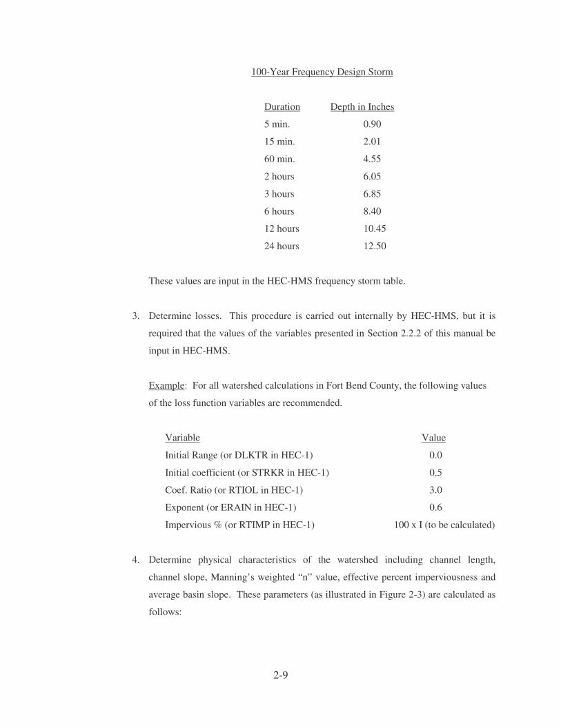
100-Year Frequency Design Storm

Duration Depth in Inches

5 min. 0.90

15 min. 2.01

60 min. 4.55

2 hours 6.05

3 hours 6.85

6 hours 8.40

12 hours 10.45

24 hours 12.50

These values are input in the HEC-HMS frequency storm table.

3. Determine losses. This procedure is carried out internally by HEC-HMS, but it is

required that the values of the variables presented in Section 2.2.2 of this manual be

input in HEC-HMS.

Example: For all watershed calculations in Fort Bend County, the following values

of the loss function variables are recommended.

Variable Value

Initial Range (or DLKTR in HEC-1) 0.0

Initial coefficient (or STRKR in HEC-1) 0.5

Coef. Ratio (or RTIOL in HEC-1) 3.0

Exponent (or ERAIN in HEC-1) 0.6

Impervious % (or RTIMP in HEC-1) 100 x I (to be calculated)

4. Determine physical characteristics of the watershed including channel length,

channel slope, Manning’s weighted “n” value, effective percent imperviousness and

average basin slope. These parameters (as illustrated in Figure 2-3) are calculated as

follows:

2-10

Length (L) The length of the longest watercourse within the subarea

to the watershed divide in miles.

Channel Slope (S) The average slope of the middle 75% of the longest

watercourse in the subarea, in feet per mile.

Manning’s Weighted The Manning’s roughness coefficient as a weighted

“n” (N) average value representative of flow roughness in the

subarea’s main watercourse. It should account for

portions of the design flow contained in the overbanks as

well as the main channel. A recommended simplified

procedure is to divide the basin into upstream and

downstream halves, determine the representative

composite “n” value for a typical section in each half,

then weight the upstream value 25% and the downstream

value 75%.

Average Basin The average slope of the land draining overland into the

Slope (So) longest watercourse, in feet per mile.

Effective Impervious The average percent of the impervious cover of the

Ratio (I) developed area, in percent, times the percent of the total

subarea considered to be developed for design purposes

times 10-4.

Example: (from Figure 2-3)

L = 2.84 miles

S = 55-foot drop over 75% of 2.84 miles = 25.8 feet/mile

N = Upstream composite “n” value = .061

Downstream composite “n” value = .049

N = (.25).061 + (.75)(.049) = .052

So = 36 feet/mile

I = C x D x 10-4 = (35 x 57) x 10-4 = 0.1995

2-11

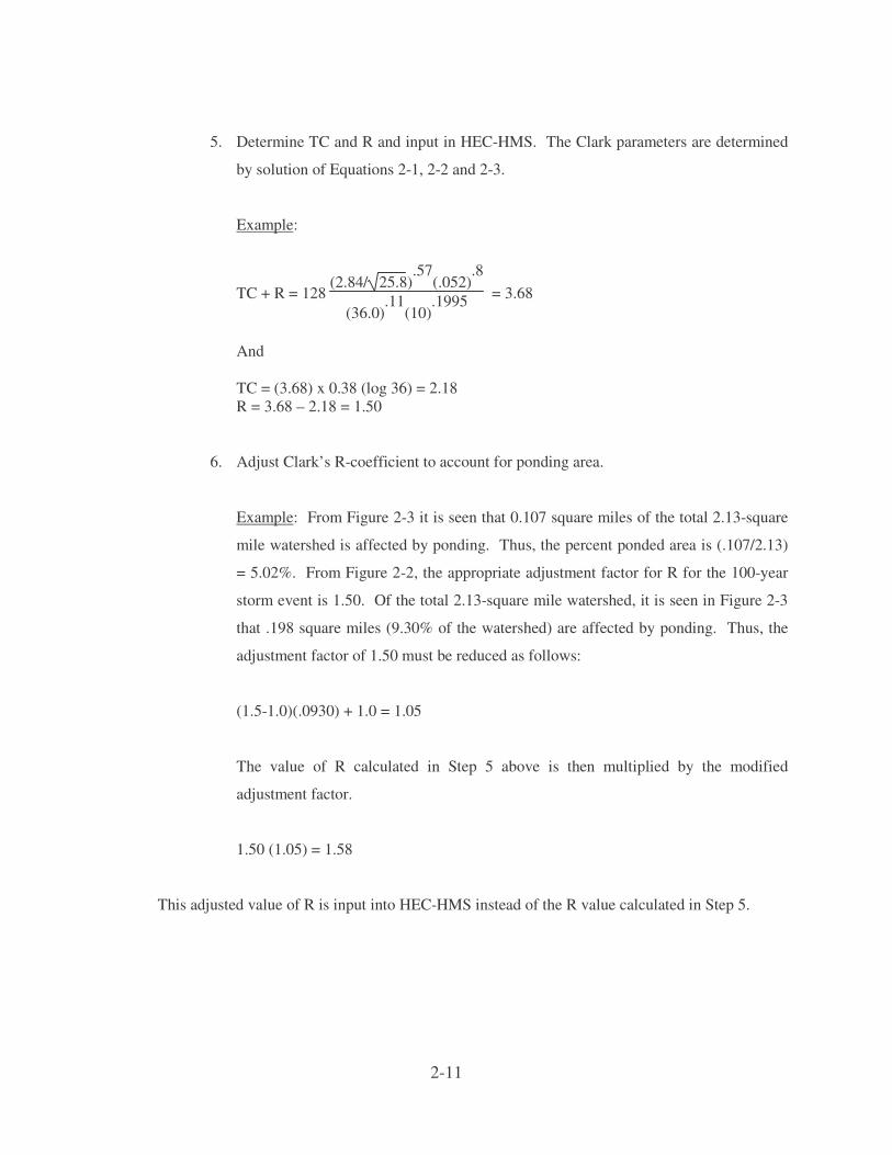
5. Determine TC and R and input in HEC-HMS. The Clark parameters are determined

by solution of Equations 2-1, 2-2 and 2-3.

Example:

TC + R = 128 (2.84/ 25.8)

.57(.052)

.8

(36.0).11

(10).1995 = 3.68

And TC = (3.68) x 0.38 (log 36) = 2.18 R = 3.68 – 2.18 = 1.50

6. Adjust Clark’s R-coefficient to account for ponding area.

Example: From Figure 2-3 it is seen that 0.107 square miles of the total 2.13-square

mile watershed is affected by ponding. Thus, the percent ponded area is (.107/2.13)

= 5.02%. From Figure 2-2, the appropriate adjustment factor for R for the 100-year

storm event is 1.50. Of the total 2.13-square mile watershed, it is seen in Figure 2-3

that .198 square miles (9.30% of the watershed) are affected by ponding. Thus, the

adjustment factor of 1.50 must be reduced as follows:

(1.5-1.0)(.0930) + 1.0 = 1.05

The value of R calculated in Step 5 above is then multiplied by the modified

adjustment factor.

1.50 (1.05) = 1.58

This adjusted value of R is input into HEC-HMS instead of the R value calculated in Step 5.

2-12

2.2.5 Flood Routing

As a flood wave passes downstream through a channel or detention facility, its shape is altered

due to the effects of storage. The procedure for determining how the shape of the flood hydrograph

changes is termed flood routing. Flood routing can be used to determine the effects of this storage on a

flood’s runoff pattern (i.e. its hydrograph).

Flood routing can be classified into two broad but related categories: open channel routing and

reservoir routing. Reservoir routing is generally used to determine the effectiveness of storm water

detention generally used in reducing downstream peak flood flow rates. Open channel routing is a

refinement of the description of an area’s rainfall-runoff process. It modifies the time rate of runoff due

to storage within the channel and its overbanks. Analysis of areas with very flat overbanks and wide

flood plains should consider channel routing to determine possible peak discharge attenuation.

The recommended technique for both channel and reservoir routing is the Modified Puls method.

The Modified Puls method is based on the assumption of an invariable discharge-storage relationship and

a constantly level pool in the storage reach of interest. The HEC-HMS program provides a routine for

this flood routing technique. The required storage-discharge relationships for this routing technique can

be obtained by use of the HEC-RAS backwater program for a variety of flow conditions. Care must be

taken in developing these storage-discharge relationships with HEC-RAS. Cross-sections need to be

provided that adequately define all of the flood plain storage available at various water levels. However,

only the effective area of the cross-section should be used to establish the proper discharge-water level

relationship. For a discussion of the Modified Puls routing technique and other methodologies, the

engineer is referred to the Handbook of Applied Hydrology, by Ven Te Chow, 1964.

2.3 DRAINAGE AREA – DISCHARGE CURVES

Drainage area-discharge curves represent a simplified method for the determination of the peak

discharge in a relatively small watershed. Usage of this type analysis requires that the watershed and its

physical characteristics be relatively uniform and not contain complex hydrologic features such as

ponding areas, storage basins or watershed overflows. The curves developed for this manual for the 25

and 100-year rainfall events, respectively, are shown in Figures 2-4 and 2-5, and are applicable to

drainage areas between 200 and 2,000 acres. Since there is such a great variation in the physical

characteristics of partially developed watersheds along with a wide range of conveyance capacity (i.e.

2-13

flood plain storage), these curves were developed for a typical watershed assuming adequate conveyance

capacity and uniformly-spaced development. Applicable flow rates for existing conditions in the design

of detention facilities should be determined on a case-by-case basis working closely with the Drainage

District Engineer (See Section 6.0).

Whenever the situation requires the determination of a complete flood hydrograph, and not just a

peak discharge, Malcom’s small watershed method, as described in Section 2-5, should be used.

2.4 RATIONAL METHOD

The Rational Method represents an accepted method for determining peak storm runoff rates for

small watersheds that have a drainage system unaffected by complex hydrologic situations such as

ponding areas, storage basins and watershed transfers (overflows) of storm runoff. This widely used

method provides satisfactory results if understood and applied correctly. It is generally recommended

that in Fort Bend County the Rational Method be used only for areas less than 200 acres.

The Rational Method is based on a direct relationship between rainfall and runoff, and is

expressed by the following equation:

Q = CiA (2-5)

Where:

Q is defined as the peak rate of runoff in cubic feet per second. Actually, Q is in

units of inches per hour per acre. Since this rate of in/hr/ac differs from cubic

feet/second by less than one percent, the more common cfs is used.

C is the dimensionless coefficient of runoff representing the ratio of peak discharge

per acre to rainfall intensity (i).

i is the average intensity of rainfall in inches per hour for a period of time equal to

the critical time of concentration for the drainage area to the point of interest.

A is the area in acres contributing runoff to the point of interest during the critical

time of concentration.

Basic assumptions associated with the Rational Method are:

2-14

1. The computed peak rate of runoff at the design point is a function of the average

rainfall rate during the time of concentration to that point.

2. The frequency or recurrence interval of the peak discharge is equal to the frequency of

the average (uniform) rainfall intensity associated with the critical time of

concentration (duration).

3. The time of concentration is the critical time of concentration and is discussed under

paragraph 2.4.2 of this manual.

4. The ratio of runoff to rainfall, C, is uniform during the storm duration.

5. Rainfall intensity is uniform during the storm duration.

6. The contributing area is that area that drains to the point of interest within the critical

time of concentration.

2.4.1 Runoff Coefficient (C)

In relating peak rainfall rates to peak discharges, the runoff coefficient “C” in the Rational

Formula is dependent on the character of the drainage area’s surface. The rate and volume of a storm’s

rainfall that reaches an area’s storm sewer system depends on the relative porosity (imperviousness),

ponding character, slope and conveyance properties of the surface. Soil types, vegetation condition and

impervious surfaces, such as asphalt pavements and roofs of buildings, are the major determining factors

in selecting an area’s “C” factor. The type and condition of the surface determines its ability to absorb

precipitation and transport runoff. The rate at which a soil absorbs precipitation generally decreases as

and if the rainfall continues for an extended period of time. The soil absorption or infiltration rate is also

influenced by the presence of soil moisture before a rain (antecedent precipitation), the rainfall intensity,

the proximity of the ground water table, the degree of soil compaction, the porosity of the subsoil,

vegetation, ground slopes, depressions, and storage. On-site inspections and aerial photographs may

prove valuable in estimating the nature of the surface within the drainage area.

2-15

It should be noted that the runoff coefficient “C” is the variable of the Rational Method which is

least susceptible to precise determination. Proper use requires judgment and experience on the part of the

engineer, and its use in the formula implies a fixed ratio for any given drainage area, which in reality is

not the case. A reasonable coefficient must be chosen to represent the integrated effects of infiltration,

detention storage, evaporation, retention, flow routing, and interception, all of which affect the time

distribution and peak rate of runoff.

Coefficients for specific surface types can be used to develop a composite runoff coefficient

based in part on the percentage of different types of surfaces in the drainage area. This procedure is often

applied to typical “sample” blocks as a guide to selection of reasonable values of the coefficient for an

entire area.

Table 2-3 presents recommended values for the runoff coefficient “C” for various residential

districts and specific surface types for 5-10 year frequency storms. These values were derived from

numerous sources (see References 9, 20, 31, and 32). Adjustment of the “C” value for use with larger

(less frequent) storms can be made by multiplying the right side of the Rational Formula by a frequency

factor Cf, which is used to account for antecedent precipitation conditions. The Rational Formula now

becomes:

Q = CiACf (2-6)

Table 2-4 presents recommended values of Cf. The product of C times Cf should not exceed 1.0.

2.4.2 Rainfall Intensity (i)

Rainfall intensity (i) is the average rainfall rate in inches per hour which is considered for a

particular basin or sub-basin and is selected on the basis of design rainfall duration and design frequency

of occurrence. The design duration is equal to the critical time of concentration for all portions of the

drainage area under consideration that contribute flow to the point of interest. The frequency of

occurrence is a statistical variable, which is established by design standards or chosen by the engineer as a

design parameter.

The time of concentration used in the rational equation is the critical time of concentration for the

point of interest. The critical time of concentration is the time associated with the peak runoff from all or

part of the upstream drainage area to the point of interest. Runoff from a watershed usually reaches a

2-16

peak at the time when the entire drainage area is contributing; in which case, the time of concentration is

the time for water to flow from the most remote point in the watershed to the point of interest. However,

the runoff rate may reach a peak prior to the time the entire upstream drainage area is contributing. In this

instance, only the portions of the drainage area able to contribute flow to the point of interest during the

critical time of concentration should be used in determining the peak discharge. A trial and error

procedure can be used to determine the critical time of concentration.

The time of concentration to any point in a storm drainage system is a combination of the “inlet

time” and the “time of flow in the conduit”.

The inlet time is the time for water to flow over the surface to the storm sewer inlet. Inlet time

decreases as the slope and the imperviousness of the surface increases, and it increases as the distance

over which the water has to travel increases and as retention by the contact surfaces increases. Average

velocities for estimating travel time for overland flow can be calculated using Figure 2-6.

The inlet time shall be determined by direct computation using the following formula:

T = D

F60V (2-7)

where

T = overland flow time (minutes).

DF = flow distance (feet).

V = average velocity of runoff flow (ft/sec).

If the overland flow time is calculated to be in excess of 20 minutes, the designer should verify

that the time is reasonable considering the projected ultimate development of the area.

The time of flow in the conduit is the quotient of the length of the conduit and the velocity of

flow as computed using the hydraulic characteristics of the conduit. The time of concentration within a

conduit is usually less than the actual time for the flood crest to reach a given point by an amount equal to

the time required to fill the conduit. The time required to fill the conduit is defined as the time of storage.

The time of storage shall be neglected in the design of storm runoff conduits even though it may represent

an appreciable percentage to the total time of concentration in some instances. This procedure will not

substantially affect the precision of the calculations and will contribute to a conservative design.

2-17

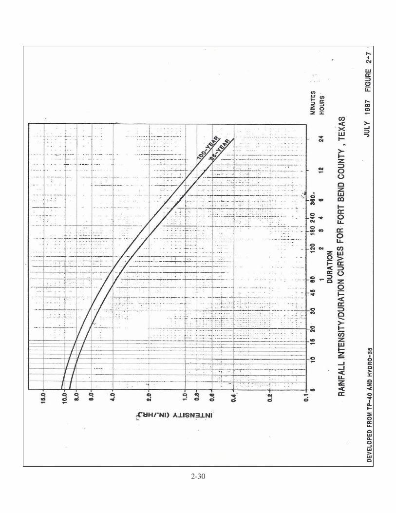
The statistical relationship between the rainfall intensity and duration for the 25-year and 100-

year frequency storms are shown in Figure 2-7. These two curves are presented for the 25-year and 100-

year design frequencies for durations from 5 minutes to 24 hours since the two frequencies are used in

channel design. Table 2-1 presents rainfall amounts for a variety of durations and frequencies.

2.4.3 Drainage Area (A)

The size and shape of the drainage area must be determined. The area may be determined

through the use of topographic maps, supplemented by field surveys where topographic data has changed

or where the contour interval is too great to distinguish the direction of flow. A drainage area map shall

be provided for each project. The drainage area contributing to the system being designed and drainage

subarea contributing to each inlet point shall be identified. The outlines of the drainage divides must

follow actual lines rather than the artificial land divisions as used in the design of sanitary sewers. The

drainage divide lines are determined by the pavement slopes, locations of downspouts, paved and

unpaved yards, grading of lawns and many other features that are introduced by the urbanization process.

As mentioned previously, the drainage area used in determining peak discharges if the portion of

the area that contributes flow to the point of interest within the critical time of concentration.

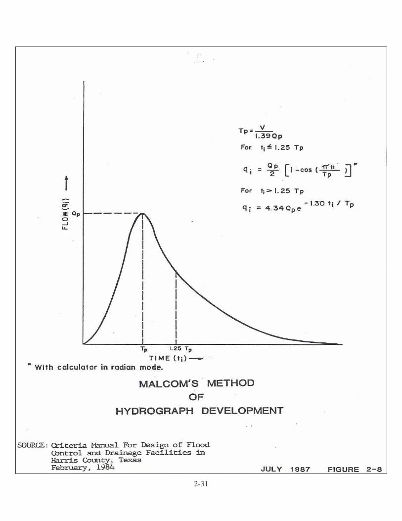
2.5 HYDROGRAPH DEVELOPMENT FOR SMALL WATERSHEDS

A technique for hydrograph development which is useful in the design of detention facilities

serving relatively small watersheds has been presented by H.R. Malcom. This method can be used for

watersheds up to approximately 2 square miles (1280 acres), but is recommended to be used for

watersheds of 1 sq. mile (640 acres) or less.

This procedure can be used in conjunction with the drainage area-discharge curves or the

Rational Method. The methodology utilizes a pattern hydrograph to obtain a curvilinear design

hydrograph which peaks at the design flow rate and which contains a runoff volume consistent with the

design rainfall. The pattern hydrograph is a step function approximation to the dimensionless hydrograph

proposed by the Bureau of Reclamation and the Natural Resources Conservation Service.

2-18

. Malcom’s Method consists of the following equations:

(1) Tp = V

1.39Qp

(2) ���

�

���

�

��

�

�

�−=

p

i

Tt

cos12

πpi

Qq for ti � 1.25 Tp

(3) ��

�

�

�−

= p

i

Tt

pi eQq30.1

34.4 for ti > 1.25 Tp

*Calculator must be in radian mode.

Where: Qp = peak design flow rate in cfs

Tp = time to Qp in seconds

V = total volume of runoff for the design storm in cubic feet

ti and qi = the respective time and flow rates which determine the shape of the

hydrograph.

A plot of a hydrograph illustrating these parameters is included as Figure 2-8.

The peak design flow rate can be calculated directly either from the drainage area – discharge

curves or the Rational Method depending upon the size of the area considered. The total volume of

runoff is dependent on the level of development of the area (i.e. percent of impervious cover). Typical

loss rate totals for the 25- and 100-year, 24-hour rainfall events are included in Table 2-5.

2-19

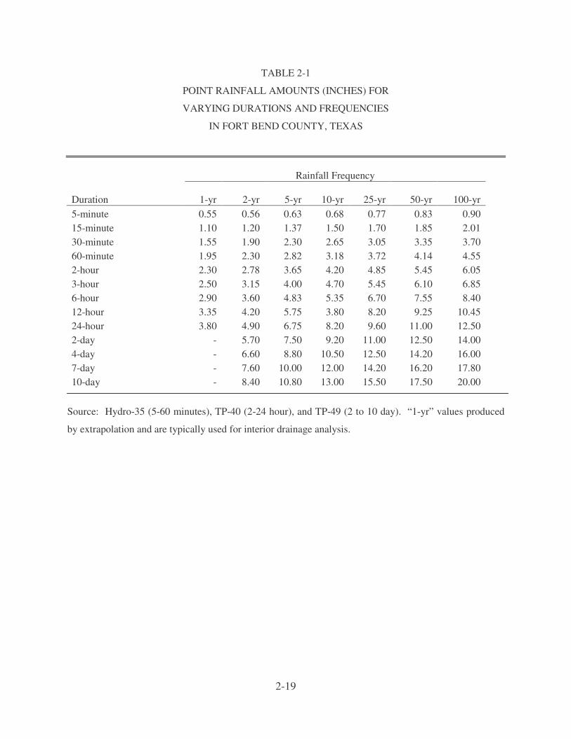
TABLE 2-1

POINT RAINFALL AMOUNTS (INCHES) FOR

VARYING DURATIONS AND FREQUENCIES

IN FORT BEND COUNTY, TEXAS

�

Rainfall Frequency

Duration 1-yr 2-yr 5-yr 10-yr 25-yr 50-yr 100-yr 5-minute 0.55 0.56 0.63 0.68 0.77 0.83 0.90 15-minute 1.10 1.20 1.37 1.50 1.70 1.85 2.01 30-minute 1.55 1.90 2.30 2.65 3.05 3.35 3.70 60-minute 1.95 2.30 2.82 3.18 3.72 4.14 4.55 2-hour 2.30 2.78 3.65 4.20 4.85 5.45 6.05 3-hour 2.50 3.15 4.00 4.70 5.45 6.10 6.85 6-hour 2.90 3.60 4.83 5.35 6.70 7.55 8.40 12-hour 3.35 4.20 5.75 3.80 8.20 9.25 10.45 24-hour 3.80 4.90 6.75 8.20 9.60 11.00 12.50 2-day - 5.70 7.50 9.20 11.00 12.50 14.00 4-day - 6.60 8.80 10.50 12.50 14.20 16.00 7-day - 7.60 10.00 12.00 14.20 16.20 17.80 10-day - 8.40 10.80 13.00 15.50 17.50 20.00

Source: Hydro-35 (5-60 minutes), TP-40 (2-24 hour), and TP-49 (2 to 10 day). “1-yr” values produced

by extrapolation and are typically used for interior drainage analysis.

2-20

TABLE 2-2

TYPICAL AVERAGE VALUES

FOR

IMPERVIOUS COVER

Type of Development Percentage of Impervious Cover

Commercial and Business Areas 85

Industrial 72

Residential

Average lot size

1/8 Acre or less 65

1/4 Acre 38

1/3 Acre 30

1/2 Acre 25

1 Acre 20

Source: NRCS TR55, Urban Hydrology for Small Watersheds (Table 2.2).

2-21

TABLE 2-3 RATIONAL METHOD RUNOFF COEFFICIENTS

FOR 5-10 YEAR FREQUENCY STORMS

Runoff Coefficients For Basin Slopes Description of Area Less than 1% 1% - 3.5% 3.5%-5.5% Residential Districts

Single Family Areas (Lots greater than ½ acre) 0.30 0.35 0.40

Single Family Areas (Lots ¼ - ½ acre) 0.40 0.45 0.50 Single Family Areas (Lots less than ¼ acre) 0.50 0.55 0.60 Multi-Family Areas 0.60 0.65 0.70 Apartment Dwelling Areas 0.75 0.80 0.85

Business Districts Downtown Areas 0.85 0.87 0.90 Neighborhood Areas 0.75 0.80 0.85 Industrial Districts Light Areas 0.50 0.65 0.80 Heavy Areas 0.60 0.75 0.90 Railroad Yard Areas 0.20 0.30 0.40 Parks, Cemeteries 0.10 0.18 0.25 Playgrounds 0.20 0.28 0.35 Streets Asphalt 0.80 0.80 0.80 Concrete 0.85 0.85 0.85 Drives and Walks (Concrete) 0.85 0.85 0.85 Roofs 0.85 0.85 0.85 Lawn Areas Sandy Soil 0.05 0.08 0.12 Clay Soil 0.15 0.18 0.22 Undeveloped Areas Sandy Soil Woodlands 0.15 0.18 0.25 Pasture 0.25 0.35 0.40 Cultivated 0.30 0.55 0.70 Clay Soil Woodlands 0.18 0.20 0.30 Pasture 0.30 0.40 0.50 Cultivated 0.35 0.60 0.80

2-22

TABLE 2-4

FREQUENCY FACTOR ADJUSTMENT

Frequency Frequency Of Storm Factor (years) (Cf) 5 1.00

25 1.10

50 1.20

100 1.25

Note: The product of C times Cf should not be greater than 1.0

Source: Urban Storm Drainage Criteria Manual, 1969 (Reference #31)

2-23

TABLE 2-5

EXCESS RAINFALL FOR COMPUTING RUNOFF VOLUMES

Percent 10-Yr, 24-Hr Losses Excess 25-Yr, 24-Hr Losses Excess 100 -Yr, 24-Hr Losses Excess Impervious Rainfall (in) (in) Rainfall (in) Rainfall (in) (in) Rainfall (in) Rainfall (in) (in) Rainfall (in)

0 8.2 4.13 4.07 9.6 4.43 5.17 12.5 5.14 7.36

20 8.2 3.31 4.89 9.6 3.55 6.05 12.5 4.12 8.38

40 8.2 2.48 5.72 9.6 2.66 6.94 12.5 3.09 9.41

60 8.2 1.65 6.55 9.6 1.77 7.83 12.5 2.06 10.44

80 8.2 0.83 7.37 9.6 0.89 8.71 12.5 1.03 11.47

2-24

2-25

2-26

2-27

25-Year Drainage Area-Discharge Curves

for Fort Bend County Texas

FIGURE 2-4

2-28

100-Year Drainage Area-Discharge Curves

for Fort Bend County Texas

FIGURE 2-5

2-29

FIGURE 2-6

2-30

2-31