8

2 Field study methods and data reductionERARM is an open cut mine in the Alligator Rivers Region (ARR) of the Northern TerritoryAustralia. At the conclusion of mining ore will have been removed from two pits (no 1 andno 3) (fig 2.1). Options for rehabilitation of tailings are (1) stored above-ground in thetailings dam and in pit 1 or (2) stored in pit 1 and tailings from the dam to be stored in pit 3.Whichever option is chosen, rehabilitation design must provide for the long-termcontainment of radioactive tailings (ie over a period of thousands of years) and ensure thatweathering and erosion of the containment structure, in an area which experiences highrainfall intensities, do not result in the release of contaminants that would degrade theenvironment or aesthetics of the surrounding Kakadu National Park.

The ERARM is adjacent to the World Heritage Listed Area of Kakadu National Park andexploits a stratabound uranium deposit hosted by the lower member of the Early ProterozoicCahill Formation. The WRD at ERARM consists of rocks from the lower member thatcomprises carbonates, carbonaceous schists and mica and quartz feldspar schist (Needham1988). The waste rock is highly weatherable (Milnes 1988) and large competent chloriticschist fragments break down into medium and fine gravel and clay-rich detritus within a twoto three year period (Riley & Gardiner 1991). The section of the WRD where this study wasconducted rises to approximately 12 m above the surrounding land surface. The area receiveshigh-intensity storms and rain depressions between October and April (Wet season) withlittle rain falling during the remainder of the year (Dry season). The average annual rainfall is1480 mm.

2.1 Study sitesFour areas of the WRD (fig 2.1) were studied. The first, the cap site has an average slope of0.028 m/m, in the area studied. The surface is covered with fine material overlying a hardpan-like surface which develops cracks during the prolonged Dry season.

Excavations of approximately 1 m on the cap site indicate an impervious layer of finematerial which Riley (1992) suggests can be over 1 m deep and results from verticallydownward transportation of the fine material. As a result there is limited infiltration andincreased runoff. The second area is on a batter slope and has an average slope of 0.207 m/min the area studied. The batter site is covered with coarser material than the cap site.

The surface condition of the cap and batter sites at the time of the study was notrepresentative of the proposed final rehabilitated condition which may include surfacetreatment such as rock mulching or ripping and revegetation. There was negligible vegetationon the cap and batter sites.

The third study area was on an area of the cap referred to as the soil site. This site was a top-soiled, surface ripped and revegetated area of the upper surface of the northern part of theWRD. The soil site had an average slope of 0.012 m/m and was vegetated with low shrubsand grasses providing approximately 90% coverage.

The fourth study area was on the fire trial site on a lower level, above and to the south ofretention pond 4 (RP4). The fire site had an average slope of 0.023 m/m and was originallytop-soiled and surface ripped and is now vegetated with well established trees (eucalyptusand wattle species) that are approximately 10 years old.

The spear grass on the sites grows vigorously during the Wet season to ≈3 m tall and thendies off during the Dry season leaving a cover of dry straw mulch.

9

Vegetatedsoil site

N

Jabiru

Vegetatedfire site

Figure 2.1 Location of the study sites on the ERA Ranger Mine

10

2.2 Runoff and erosion plots

Large scale runoff and erosion plots were constructed on each of the four sites. The cap site plotwas 29.4 m long by 20.1 m wide (591 m2), the batter site 37.7 m long by 15.9 m wide (600 m2),the soil site 30 m long by 20 m wide (600 m2) and the fire site 30 m long by 20 m wide (600 m2)(fig 2.2). An initial topographic survey of the heavily vegetated study sites was conducted todetermine slope gradient and direction to assist with plot location and orientation.

Figure 2.2 Layout of runoff and erosion plots. Details of damp course placement are shown in section A-A.The soil site and fire site had layouts similar to the cap site and with the dimensions given in the text.Because of drainage difficulties, the reservoir and flume on the fire site was placed at the left end of thetrough and not in the centre as shown here.

11

2.2.1 Plot layoutPlot borders were constructed using 100 mm wide damp course. The damp course was bentacross its width in the shape of an ‘L’, with one leg approximately 20 mm long and theother leg approximately 80 mm long. Damp course was laid continuously along the up-slope end and the two sides of the plots which had been previously measured and markedout using star posts and string. The damp course was held in place by pushing a 100 mmnail through the 20 mm long leg in to the WRD surface. This gave an upright wall ofapproximately 80 mm height. Concrete, of a mixture of 3:1, sand to cement, was then laidalong the outer edge of the damp course covering the 20 mm long leg and the nails. Thisheld the damp course in place and prevented runoff from escaping under the damp course(fig 2.2).

Half section 250 mm diameter PVC stormwater pipe troughs were placed at the down slopeends of the plots to catch runoff and channel it through rectangular broad-crested (RBC)flumes (Bos et al 1984) where discharge could be measured. Trenches were carefully dug(to avoid disturbance of the plot surface) along the down-slope edge of the plot across thefull width. The trench was sloped (>0.02 m/m) toward the centre of the plot so that runoffcould be directed through a centrally located RBC flume on the cap, batter and soil sites.On the fire site the flume was placed at one end of the trough. These trenches, the fullwidth of plots, were up to 500 mm deep and in many places required jack-hammeringthrough large competent rock fragments that had to be left in situ because their removalwould cause damage to the plot surface. The half pipes were placed in the troughs andconcrete placed between the pipe and the plot surface and smoothed to form an apron. Thepipe joins were then sealed using a silicon sealant.

A reservoir was constructed at the centre of the plots (at one end on the fire site) where thetroughs met so that bedload sediment in the runoff would drop out. The reservoirs wereapproximately 500 mm deep, 500 mm wide and 1000 mm long with the long axis normal tothe down-slope end of the plot. A 150 mm RBC flume with a trapezoidal broad-crestedcontrol section was placed at the downstream end of the reservoir so that discharge couldbe measured. The surface of the reservoir was concreted and smoothed and blended intothe trough outlets and flume inlet and rocks were placed along the top of the reservoirbetween the troughs and the flume and covered with concrete to prevent runoff enteringthe reservoir from the sides. The flumes, with a single stilling well, were concreted inplace.

The low slopes of the cap, soil and fire sites and the depth to which the troughs had beenplaced on those plots, required a drainage channel so that runoff could be cleared awayfrom the flume and not back-up in to the flume during an event.

2.2.2 SurveyThe plot surfaces were surveyed using a TOPCON Geodetic Total Station (GTS-3C) on a1 m2 grid. Topographic contour maps (figs 2.3 to 2.6) were produced using SURFERsoftware. Three-dimensional views of the sites are shown in figure 2.7. One lineperpendicular to flow of elevations at 100 mm spacings across all plots was also surveyed.

12

Outlet trough

Plot border

-5 0 5 10(metres)

25

30

35

40

45

50

(met

res)

Figure 2.3 Contour map of the cap site

13

-20 -15 -10 -5 0 5(metres)

10

15

20

25

30

35

40

45

(met

res)

Plot border

Outlet trough

Figure 2.4 Contour map of the batter site

14

-10 -5 0 5 10 15 20(metres)

10

15

20

25

30

35

40

45(m

etre

s)

collection trough

Plot border

Figure 2.5 Contour map of the soil site

15

-5 0 5 10(metres)

5

10

15

20

25

30

35(m

etre

s)collection trough

flume outlet

Figure 2.6 Contour map of the fire site

Cap

site

Soil

site

Batte

r site

Fire

site

Axes

dim

ensi

ons

are

in m

etre

s.

Figu

re 2

.7 T

hree

-dim

ensi

onal

vie

w o

f the

plo

t sur

face

s. D

imen

sion

s ar

e in

met

res.

16

17

2.3 Monitoring of natural rainfall eventsDuring the latter half of the 1992/93 Wet season (Evans & Riley 1993a,b) and the 1993/94Wet season, plots on the cap and batter sites were monitored during natural rainfall events tocollect hydrology and sediment loss data. During the 1994/95 Wet season, plots on the firesite and soil site were monitored during natural rainfall events to collect hydrology andsediment loss data (Saynor et al 1995).

2.3.1 Hydrology dataRainfall was measured using a tipping bucket rain gauge placed near the reservoir at the capand batter sites and in the centre of the soil site and fire site.

Stage in the RBC flume was measured automatically (logged) and manually (observed).Automatic measurements were taken using a capacitance rod (water level sensor) placed inthe stilling well and manual measurements were taken off the stilling well by an observer.The capacitance rod output is frequency (Hz).

The rain gauge and capacitance rod were connected to a computer controlled DATATAKERdatalogger. The data from the datalogger were downloaded to a portable computer after eachevent. The water height in the stilling well and time were noted at the start of flow over theweir in the flume and when flow ceased over the weir in the flume. This measurement wasconsidered to be zero head and therefore zero discharge.

Down loaded event data were stored in text files and reduced to the final data files throughthe following steps.

1. Data files were imported into a QUATTRO PRO spreadsheet and parsed. Parsingrequired creating a format and then editing the format. It was necessary to convert timedata to 24 hour time and then decimal days.

2. A frequency for zero head was selected. The time for the manually recorded zero flowwas compared with automatically logged times. The frequency at the time of zero flowwas assumed to be the frequency for zero head. Head (h) in millimetres was determinedby subtracting the selected frequency for zero head from the logged frequency values anddividing the result by two for the cap and batter site. The division by two was necessarysince each unit of frequency (Hz) was equal to 0.5 mm of head for the cap and batter sitewater level sensors. For the soil site and fire site the water level sensors where calibratedin the laboratory by measuring frequency for various water levels. The followingconversion equations were derived where v = frequency and h = head (mm).

Fire site:

h = a + b/v + cv 3 (2.1)

where

a = -755.377

b = 859037.71

c = 2.7395 x 10-8

Soil site:

where capacitance v ≥714 Hz

h = a + bv + cv2 + dv3 + ev4 (2.2)

18

where

a = 43193.675

b = -195.248

c = 0.336

d = -2.595 x 10-4

e = 7.525 x 10-8

where capacitance v <714 Hz

h = a + bv +cv3 (2.3)

where

a = 3509.08

b = -5.775

c = 2.692 x 10-6

3. Head was then converted to discharge (Q) (L s-1) using the following formula (Evans &Riley 1993c):

Q = 18.4h x 940h2 (2.4)

Note: Head value must be converted to metres when using this equation.

4. Line graphs showing the hydrographs were plotted to assess the validity of the zero headvalue.

2.3.2 SedimentRunoff water samples were collected during monitored events and analysed for suspendedsediment concentrations. Bedload samples were collected at the conclusion of each event.

Suspended sediment samples were collected in 600 ml Bunzl flasks at the downstream end ofthe weir in the flume. Records were kept of sediment sample times. Sediment concentration(g L-1) was determined using gravimetric methods. Total suspended sediment loss wasdetermined through integration of the sedigraph produced by comparison of sedimentconcentration with the hydrograph similar to the method of Simanton et al (1991).

Collected bedload was placed in pre-weighed aluminium containers, dried at 105°C andreweighed to obtain the mass of sediment and containers. The container mass was thensubtracted from the oven dried mass to give a total bedload mass.

3 SIBERIA model parameter derivation

The SIBERIA landform evolution model has been described in numerous articles egWillgoose et al (1989, 1991abc, 1992) and Willgoose and Riley (1993). Its use is documentedin Willgoose (1992). At a late stage in this work version 8 of SIBERIA which includes thecapability to model soil development and improved sediment transport modelling wasreleased. All results in this project are done with version 7.05 of SIBERIA. The descriptionbelow is based on these papers.

Willgoose et al (1991a) considered that catchment form determines flood and erosionresponse of a catchment and flood and erosion response over geologic time influences

19

catchment form. Difficulties in understanding interactions between processes, form andtemporal change result from long timescales of catchment evolution, observing changes andattributing differences between catchments to differences in age or process because of spatialand temporal heterogeneity. Computer models, such as SIBERIA, can examine temporaltrends and sensitivity to physical inputs (erodibility, tectonic uplift and runoff).

SIBERIA is a process-response model of erosion development of catchments and their channelnetworks. Long-term changes in elevation with time resulting from large-scale mass transportprocesses (tectonic uplift, fluvial erosion, creep, rainsplash and landsliding) are modelled asaverage affects of processes ie individual landslides are not modelled but the cumulative effectof many landslide events is modelled. The model describes how a catchment will look, onaverage, at a given time and differentiates channel and hillslope. Different transport processesare modelled in each regime. Channels are dominated by fluvial erosion and hillslope by amixture of fluvial and diffusive processes. A channel forms when a channel initiation function(CIF) exceeds a threshold (channel initiation threshold (CIT)). The CIF is nonlinearlydependant on hillslope and discharge and a channel is considered to have formed when the CIFexceeds a CIT; for instance, when shear stress exceeds a shear stress threshold. Channeldimension (depth and width) are determined by regime equations (Leopold et al 1964).

The changes in elevation are described by the following mass transport continuity equation(Willgoose et al 1991ab, 1992):

( ) ( )

∂∂+

∂∂+

∂

∂+

∂∂

−ρ+=

∂∂

2

2

2

2

11

yz

xzD

yq

xq

ntx,c

tz sysx

s0 (3.1)

where

z = elevation (m)

t = time (s)

co(x,y) = rate of tectonic uplift (m s-1)

x,y = the horizontal directions (m)

qsx, qsy = rate of fluvial sediment transport per unit width in the x, y directions (g s-1 m-1)

D = elevation diffusivity (m2 s-1)

ρs = density of sediment (g m-3)

n = porosity of sediment

The differential equation for the channel initiation function is (Willgoose et al 1991a,b, 1992):

=

∂∂

tt a

aY,,dftY

(3.2)

where

Y = 1 (the point in the catchment is a channel), or

Y = 0 (the point in the catchment is a hillslope)

dt = rate of channel growth at a point

a = channel initiation function

at = channel initiation function threshold

20

Willgoose et al (1991b) noted that the exact form of equation 3.2 was not as critical as thefunctional form of the CIF.

SIBERIA predicts the long-term average change in elevation of a point by predicting thevolume of sediment lost from a node. Fluvial sediment transport rate through a point (qs) isdetermined in SIBERIA by the following equation:

111

nms Sqq β= (3.3)

where:

S = slope (m/m)

q = discharge (m3 y-1)

β1= sediment transport rate coefficient

SIBERIA does not directly model runoff (Willgoose 1992) but uses sub-grid effectiveparameterisation which conceptually relates discharge to area (A) draining through a point asfollows (Leopold et al 1964):

333

nm SAq β= (3.4)

To run the SIBERIA model for a field site it is necessary to derive parameter values for β1,m1, n1, and m3. For ease of derivation of β1, it is normally assumed that β3 = 1.

To obtain the parameter values for equations 3.3 and 3.4 it is necessary to:

1. Fit parameters to a soil transport equation using data collected from field sites;

2. To calibrate a hydrology model using rainfall-runoff data from field sites; and

3. Derive long-term average SIBERIA model parameters for the landform being modelled.

The following sections describe this three-step parameter derivation process. Figure 3.1shows a flow chart of this process.

3.1 Sediment transport equationThe total sediment loss model used in this study is derived from the equation described inWillgoose and Riley (1993) of the form:

112

nmwsw Sqq β= (3.5)

where:

qsw = sediment discharge/unit width (g s-1 m-1)

qw = discharge/unit width (L s-1 m-1)

S = local slope (m/m)

β2, m1 and n1 are parameters fixed by flow geometry and erosion physics. Equation 3.5incorporates a shear stress component as described by Willgoose and Riley (1993). Willgooseand Riley (1993) used this equation form to fit parameter values for a relationship betweeninstantaneous discharge and sediment discharge. Smith and Bretherton (1972) considered thatthe equation applies to all elements of a surface ie, channel or nonchannel elements and appliesto bedload transport. However, they also considered that an equation of this form may apply tototal sediment transport.

21

Figure 3.1 Flow chart showing the SIBERIA parameter value derivation process

Sediment loss &Runoff data

Section 3.1Sediment transportEquation – Eq (3.9)

Rainfall & Runoffdata

Section 3.2DISTFW hydrologymodel

Section 3.3.2Long term runoff

Section 3.3.1Discharge-areaRelationship –Eq (3.4)

Section 3.3.2Long term sedimentLoss – Eq (3.9)

SIBERIA inputParameterisationEq (3.3)

Landform evolutionsimulation

22

From equation 3.5, total sediment discharge (Qs) (g s-1) can be determined by

112

nmws SwqQ β= (3.6)

where

w = width (m)

total instantaneous discharge (Q) is

Q = w qw (L s-1) (3.7)

Therefore Qs can be expressed as( ) 1111

2nmm

s SQwQ −β= (3.8)

Total sediment loss (T) (g) during a rainfall event can be determined from the followingequation

( ) dtQ-wS=T mmn 111 12 ∫β (3.9)

where

dtQm1∫ = cumulative function of runoff over the duration of the event

3.1.1 Sediment transport equation: Parameter fittingThe parameters n1, m1 and β2 in equation 3.9 were fitted using log-log linear regression.

Equation 3.9 above can be expressed as

log T = log β2 + n1 log S + x log Y (3.10)

where

dtQwY m)m( 111 ∫= − (3.11)

To fit m1, an arbitrary value of m1 was selected and used to determine a value for dtQm1∫(cumulative mQ 1 ) for each event. This value was then used for Y in equation 3.10 forregression analysis. This process was continued until the value of the coefficient, x, wasequal to 1. The m1 value for the condition, x = 1, was selected as the fitted value. Log β2 wasfitted as a constant.

3.2 Calibration of DISTFW rainfall-runoff model parametersThe DISTFW model is a digital terrain rainfall-runoff model based on the sub-catchmentbased Field-Williams Generalised Kinematic Wave Model (Field & Williams 1983, 1987).The model and its application to mine spoils and waste rock have been described in detail byWillgoose and Riley (1993), Finnegan (1993), Arkinstal et al (1994) and Willgoose andKuczera (1995). DISTFW divides a catchment into a number of sub-catchments connectedtogether with a channel network draining to a single catchment outlet.

The model includes (Finnegan 1993):

1. Nonlinear storage of water on the hillslope surface

2. Philip infiltration (Philip 1969) from the surface storage to the channel

23

3. Discharge from the surface storage to the channel

4. Discharge from ground water storage to the channel

5. Routing of the runoff in channels by use of the kinematic wave (Field 1982)

Hortonian runoff is modelled.

The DISTFW uses digital terrain map (DTM) data on a square grid and each grid isconsidered to be a sub-catchment. Drainage from node to node and through nodes occurs by akinematic wave on the overland flow. The kinematic assumption that friction slope equals thebed slope is used and discharge is determined from the Mannings equation. For this study, itwas assumed that infiltration drained to a very deep aquifer and did not discharge to thesurface within a study site so the groundwater component of the model was disabled.

Antecedent soil moisture (initial wetness) is difficult to measure prior to a rainfall event.Therefore it was assumed that antecedent soil moisture was low so initial wetness was setlow in the model. Initial wetness can be adjusted for individual events to improve fittedhydrograph volume.

The parameters fitted in this study were:

• sorptivity (initial infiltration) Sphi

• long-term infiltration phi

• kinematic wave speed cr and exponent em

• timing, the amount the predicted hydrograph leads the data, when necessary to allow forerrors in timing in data collection

Parameters were fitted using a non-linear regression package, NLFIT version 1.10g (Kuczera1989, 1994) as provided by the University of Newcastle. Basically, an observed rainfall eventand the resulting discharge hydrograph are used to derive the best fit model parameter valuesthat produce a predicted hydrograph similar to the observed hydrograph.

3.2.1 NLFIT Regression program suiteNLFIT is a suite of FORTRAN programs that can be used for regression using complex non-linear models of the form (Kuczera 1994):

qt = f(xt, β) + εt t = 1,.........,n (3.12)

where

qt = an observed response

xt = an input vector

f(xt, β) = a predicted response vector

εt = a random error

The programs of the suite are, NLFIT, RESPONSE, EDPMF, PREDICT and COMPAT. Theprograms NLFIT, PREDICT and COMPAT were available and used in this study.

The following summary of the three programs used is taken from Kuczera (1994):

• NLFIT uses observed data and prior information on model parameters to fit parametervalues to a predictive model, in this case the DISTFW model.

24

• PREDICT computes predicted responses with approximate prediction or confidence limitsfor a future input time series. If a rainfall-runoff event is measured the fitted parametervalues using NLFIT can be tested. The measured data are used in PREDICT withcalibrated parameter values and a predicted hydrograph and prediction limits areproduced. The observed points are also plotted and the graphics show whether or not anacceptable number of observations fall within the limits and if the observed hydrographfollows the predicted hydrograph with the required degree of certainty.

• COMPAT can be used to assess the statistical compatibility of parameters calibrated tothe model. This is necessary when for the same site different parameter values are derivedfor different rainfall and runoff data sets. The program uses .PMF files of different datasets and produces graphic ellipses which indicate the approximate region that the fittedparameters have a 95% chance of falling within. That is they have a 5% chance of fallingoutside these areas. When the ellipses intersect the parameter values can be considered notto be statistically different.

3.2.2 DISTFW-NLFIT input filesThe version of the DISTFW model used has been interfaced with NLFIT (Willgoose et al1995). This interface allows the user to fit (1) parameters to a single rainfall event or rainfallsimulation event for a single site, (2) a number of events at a single site or (3) to fitparameters across a number of sites (this mode has not been used in this study).

To fit parameters to the DISTFW model using NLFIT an input data file (.FW) is required(Willgoose et al 1995). For DISTFW-NLFIT the input file can have one of three formats:(1) a constant width plot, (2) a standard sub-catchment or (3) a DTM grid based catchment.In this study a constant width plot (type 1) .FW file was used for the batter site and standardsub-catchment (type 2) .FW files were used for the cap, soil and fire site. Examples of thesefiles are shown in appendix A.1 (batter site). Details of the requirements of these input filesare given in Willgoose et al (1995).

Site topographic survey information is used to determine input for three parts of the file:INCIDENCES, PARAMETERS and CONVEYANCES.

Using the contour maps produced from site surveys, sub-catchments are mapped for studysites. Flow paths through the sub-catchments are used to determine what sub-catchmentsdrain into other sub-catchments which are identified by a unique number. The flow paths arethen used to set up a matrix describing the sub-catchment INCIDENCES. For constant widthplots (appendix A.1) there is only one row describing the INCIDENCES as each sub-catchment only receives flow from the sub-catchment immediately upstream. For thestandard sub-catchment type plot there may be several rows each one reflecting the numberof different sub-catchments draining into a catchment.

The physical properties for each sub-catchment for the study plots are given in tables 3.1, 3.2,3.3 and 3.4. These properties, area, length and upstream and downstream elevation (slope)and model parameters with default values of 1.0 are tabulated in the PARAMETER part ofthe .FW file. The sub-catchment or plot area is measured from the contour plan using aplanimeter, the length is measured along the flow path and width is the average width normalto the flow path. Therefore, because of the tortuosity of the flow paths, multiplying the lengthby the width does not necessarily give the area shown in the tables 3.1 to 3.4. Elevations aretaken from the contour plan.

25

Table 3.1 Physical properties of the sub-catchments on the cap site

Sub-catchmentNo.

Area(m2)

Length(m)

Width(m)

Slope(m/m)

1/width2/3

1 73.7 18.0 5.0 0.021 0.341

2 105.1 17.1 7.2 0.021 0.268

3 31.6 12.5 3.0 0.034 0.484

4 37.3 12.0 3.8 0.034 0.412

5 5.2 5.3 0.5 0.025 1.587

6 39.3 16.1 2.7 0.036 0.513

7 62.0 17.4 4.1 0.033 0.388

8 30.3 7.5 4.2 0.036 0.386

9 55.8 3.8 1.7 0.009 0.716

10 44.5 14.0 3.6 0.028 0.428

11 61.3 9.8 6.9 0.020 0.276

12 42.6 10.1 4.7 0.046 0.357

13 2.5 1.5 3.5 0.047 0.481

Table 3.2 Physical properties of the constant width plot batter site

Sub-catchmentNo.

Area(m2)

Length(m)

Width(m)

Slope(m/m)

1/width2/3

1 to 10 60.0 3.77 15.9 0.207 0.158

Table 3.3 Physical properties of the sub-catchments on the soil site

Sub-catchmentNo.

Area(m2)

Length(m)

Width(m)

Slope(m/m)

1/width2/3

1 85.7 16.42 4.05 0.022 0.394

2 75.0 20.10 3.88 0.021 0.405

3 71.2 18.76 4.24 0.014 0.382

4 28.8 10.05 2.99 0.021 0.482

5 7.1 4.86 1.76 0.033 0.686

6 23.8 7.37 4.43 0.033 0.371

7 17.7 6.7 2.32 0.042 0.571

8 18.8 8.71 2.23 0.032 0.586

9 13.7 6.03 2.36 0.003 0.564

10 41.4 15.24 2.79 0.012 0.505

11 30.1 10.72 2.88 0.014 0.494

12 4.1 1.59 2.53 0.019 0.539

13 37.3 10.05 3.5 0.006 0.434

14 15.3 6.00 2.55 0.020 0.536

15 11.3 3.02 4.3 0.079 0.378

16 34.4 10.39 3.78 0.020 0.412

17 11.6 3.85 3.13 0.039 0.467

18 8.8 4.19 2.16 0.017 0.598

19 1.9 1.09 0.8 0.028 1.160

20 30.9 13.07 2.26 0.011 0.581

21 30.7 12.06 2.59 0.014 0.530

22 0.01 0.20 0.0028 1.250 50.3

26

Table 3.4 Physical properties of the sub-catchments on the fire site

Sub-catchmentNo.

Area(m2)

Length(m)

Width(m)

Slope(m/m)

1/width2/3

1 47.6 12.0 3.6 0.028 0.425

2 31.5 15.7 2.1 0.022 0.602

3 10.1 2.7 3.3 0.019 0.449

4 5.6 1.7 2.8 0.035 0.503

5 34.9 8.5 3.8 0.023 0.409

6 25.9 6.3 4.6 0.010 0.363

7 42.6 16.5 2.2 0.021 0.597

8 24.8 8.0 3.0 0.026 0.483

9 21.5 8.8 2.7 0.017 0.521

10 22.8 11.3 1.9 0.013 0.659

11 15.8 4.7 2.9 0.041 0.489

12 22.9 9.1 2.5 0.033 0.546

13 28.6 9.7 2.3 0.046 0.576

14 24.2 10.9 2.5 0.029 0.544

15 34.2 8.5 4.4 0.039 0.374

16 7.4 3.7 1.7 0.059 0.713

17 17.7 6.8 2.5 0.078 0.543

18 13.0 6.5 2.7 0.031 0.512

19 22.7 10.9 2.6 0.046 0.529

20 14.9 4.7 2.4 0.028 0.561

21 2.2 1.2 1.1 0.042 0.922

22 2.3 1.9 1.6 0.016 0.725

23 31.9 9.3 3.3 0.050 0.456

24 25.9 9.6 2.5 0.050 0.539

25 60.2 18.4 3.2 0.035 0.464

26 14.7 4.0 3.6 0.080 0.424

27 0.01 0.2 0.0028 1.600 50.3

CONVEYANCES are then input for each catchment. For the constant width plot there is onlyone set of parameters because they are the same for each sub-catchment. For catchment andDTM mode there is a set of parameters for each sub-catchment. The first line gives thecatchment number and the number of conveyance parameters. The parameters are kinematicwave parameters, cr and em, and the maximum discharge for these values. All values except crare set to default values. A nominal value for cr is determined using the following equation:

cr = 1/w2/3 (3.13)

where w is the width of the catchment.

For the soil and fire sites the collection trough at the down-slope end of the plot is consideredto be the ultimate downstream catchment collecting all runoff from the plot. This is becausemore than one catchment drains to the trough. The trough catchment was given a small area,length and width and a very steep slope and this resulted in a high nominal value for cr whichmodels fast runoff through the trough.

RAINFALL is input using a two column text file (.RF file) (appendix A.2). The first columngives time and the second gives cumulative rainfall (mm) (described as CUMPLUVIO in the

27

.FW file). This file must have the same event starting time as the .FW file and if multiplerainfall event files are input each must have the same starting and finishing time. The model hasthe capability to apply a rainfall weighting to each sub-catchment. However, it is very difficultto obtain rainfall amounts for each sub-catchment when monitoring natural events thereforeeach sub-catchment is given a rainfall weighting of 1.0 when monitoring data are used.

RUNOFF is input using a two column text file (.RO file) (appendix A.3). The first columngives time and the second gives instantaneous discharge (m3 s-1). This file must have thesame event starting time as the .FW and .RF files and if multiple events are input each musthave the same starting and finishing time.

3.2.3 Calibration procedureThe parameter calibration procedure using DISTFW-NLFIT is that described in Arkinstal etal (1994) and Willgoose et al (1995). It is a multi-stage process that ensures that a globaloptimum for the parameters is achieved. The stages are aimed at gradually refining parameterestimates as the observed hydrograph is better fit by the model simulations, and with onlythose parameters explicitly mentioned being calibrated at any given stage.

1. Start: Nominal parameters were chosen. The initial wetness (V) and timing error wereset as very small (0.0001 mm and 0.0001 s respectively). The groundwater store supplywas set as large (Cg = 1000 mm hr-1) to ensure that no water came from the groundwater,and the surface water supply co-efficient and dimensionless exponent were set low(Cs = 0.003 m(1-2γ) sγ) and γ = 0.375 respectively) so that water flowed out of the surfacestorage into the kinematic wave without significant routing.

2. Initialisation: The long-term infiltration rate (phi − mm h-1) and kinematic rate(cr - m(3-2m) s-1) were calibrated to the complete hydrograph to obtain an approximatelycorrect mass balance and timing of the hydrograph rise.

3. Infiltration: The sorptivity (Sphi − mm h-0.5) and phi were calibrated to the completehydrograph to accurately distribute losses between initial and continuing losses.

4. Kinematic wave: cr was calibrated to the falling limb of the hydrograph and at the sametime em, to accurately fit the timing of the hydrographic rise and fall.

5. Timing: If there were obvious problems in fitting the timing of the hydrograph, timingwas then fitted. Timing is normally only fitted when multiple events are simultaneouslyused for calibration.

6. Initial wetness: Where problems with hydrograph volume were obvious, initial wetnesswas fitted to individual events.

7. Polishing: All parameters calibrated in stages 2 to 6 were simultaneously fitted on thewhole hydrograph.

Parameters were fitted, using the above procedure, to the hydrographs for observed storms.

At the conclusion of parameter fitting, NLFIT output files (.PRT, .PMF) (see example,appendixes A.4 and A.5) were generated. The .PRT files are used to produce graphic outputand .PMF files are used in COMPAT and PREDICT.

3.3 SIBERIA parameter derivationOnce parameters have been fitted to the sediment transport equation 3.9 and the DISTFWrainfall-runoff model for a site, the results are used to derive SIBERIA input parameters forthe landform to be modelled. In this study the landform used was the ‘above-grade’ option for

28

ERARM initially proposed in 1987 (Unger & Milnes 1992). Determination of parameters forSIBERIA has previously been described by Willgoose and Riley (1993).

The parameters of SIBERIA represent temporal average properties of landscapes and theprocess over the long term. The parameter values derived for the soil loss and the DISTFWmodel represent instantaneous values (Willgoose & Riley 1993).

The SIBERIA parameter derivation process involves several steps as described below and isbased on the description given by Willgoose and Riley (1993).

3.3.1 Scale analysis: Discharge area relationshipThe parameters fitted here define how discharge used in the calculation of sediment transportrate varies with catchment area.

The area discharge relationship is described by the following equation (Willgoose & Riley1993):

33 nmpp SAq β= (3.14)

where, qp = peak discharge, βP = runoff rate constant, A = area and m3 and n3 are fittedparameters.

The equation was fitted using the peak discharges and areas for the largest single catchmenton the 30 m digital terrain map of the ERARM ‘above-grade’ option (fig 3.2).

This catchment was defined by Willgoose and Riley (1993) who considered that hydrologicalresponses of the catchment would be typical of other catchments on the proposed landform.This catchment was approximately 1.6 km2 and contained 1773 nodes each 900 m2. TheDTM based version of the DISTFW model was used to predict peak discharges of areas inthe catchment for mean annual rainfall events. Willgoose and Riley (1993) chose storms ofvarious duration for a 1 in 2 year average return interval (ARI). The mean ARI is 2.33 yearswhich Willgoose et al (1989) showed is the storm that relates the instantaneous erosionphysics with long term physics. Since the ARI is used solely to determine the exponents onarea and slope in equation 3.14 use of the 1 in 2 year rather than 2.33 year is consideredsatisfactory, and consistent with the index flood approach to flood frequency analysis(Pilgrim 1987). Accordingly, in the SIBERIA calibration procedure β3 is normally set to 1,with runoff rate being implicitly calculated and allowed for in the long-term sedimenttransport analysis of section 3.3.2.

The steps were:

1. Parameters for the DISTFW hydrology model were derived for the study sites using themethod described above in section 3.2 – Calibration of DISTFW rainfall-runoff modelparameters.

2. From temporal patterns from the Australian Rainfall and Runoff (Pilgrim 1987) rainfallrates for 2 year ARI storms of various duration were determined. The storm durationswere 10 min, 15 min, 20 min, 25 min, 30 min, 45 min and 60 min.

3. This step used .FW input files for the stand-alone version of the DISTFW model. Eachfile used rainfall input files for 2 years ARI storms developed in step 2 above and DTMdata for the selected 1.6 km2 catchment. The parameter multipliers in the .FW files werechanged to those derived for step 1 above. That is cr, em, Sphi and phi were changed, theremaining parameters stayed at default values.

29

4. The DISTFW stand-alone version was run using the .FW input file for each stormduration with the amended multipliers and a peak discharge file for each event wasoutput (.PKDS). The .PKDS file has two columns: (1) the node number and (2) the peakdischarge from that node (a node may also drain upstream nodes).

5. The .PKDS files were parsed into a spreadsheet and the maximum peak discharge for eachnode determined. The peak discharge values were then fitted (log-log linear regression)against the corresponding area discharging through the corresponding node giving valuesfor βp and m3 in equation 3.14. This gives the value for m3 in equation 3.4.

6. Since there were no major changes in the slope (S) in the selected catchment, Willgooseand Riley (1993) ignored the dependence of slope giving n3 = 0.

Tailings Dam Area

RetentionPond 1

Pit 3

N

Figure 3.2 The ERARM above-grade option showing the 1.6 km2 catchment(from Willgoose & Riley 1993)

3.3.2 Runoff series and long-term sediment loss rate

The runoff series for the Jabiru historical rainfall record was then created. This series wasused to determine long-term erosion rate (qs) in equation 3.3.

The 1.6 km2 catchment was again used in an input .FW file (abovehyd.FW) containing DTMdata for the catchment.

30

The steps were:

1. The parameters fitted to the DISTFW in step 1 section 3.3.1 were put in to the .FW file.The input .RO file was runoff from a measured rainfall event. Using this .FW file in theDTM version of the DISTFW model, a discharge file (.PRD1) was produced for thecatchment.

2. The .PRD1 file was then converted to a .RO file (runoff).

3. The cr parameter was then fitted to the catchment using the DISTFW model sub-catchment mode using the input file calib-1.33.FW which describes the 1773 DTM nodesof the catchment in terms of 10 sub-catchments. The .RO file produced in step 2 aboveand the measured rainfall event were input to calib-1.33.FW and the .FW file was used inNLFIT. All parameters were held constant and cr was refitted.

4. These parameters were then used to generate long-term runoff for several years of theJabiru rainfall record. The sub-catchment model of the stand-alone version of theDISTFW model was used because of the large amount of computer processing timerequired to generate a runoff series using DTM data. The new parameters with theexception of Sphi, fixed at 0.0001 mm hr-05 which indicates a saturated catchment and isconservative, were used in an .FW file with an annual rainfall pattern taken frompluviograph records for Jabiru. This produced an annual runoff file (.PRD1) for the1.6 km2 catchment.

5. The annual runoff determined in step 4 above was then used in the soil loss equation(3.9) (w = 1 for nodes) to determine an annual sediment loss (Mg y-1) which wasconverted to a volume (m3 y-1) by dividing by the bulk density of the waste rock material.Using the annual sediment losses a long term average sediment loss rate was thendetermined (qs) for equation 3.3.

6. The value for qs was then used to determine β1 (equation 3.3). The value of m1 and n1were those fitted for equation 3.9.

3.3.3 Slope correction

The qs value (equation 3.3) is derived for a value S = 1 m/m therefore β1 (equation 3.3) needsto be corrected for use in SIBERIA. In SIBERIA, A is considered to be in nodes ie each nodeis considered to be 1 unit area, and S reflects the number of metres drop between nodeswhich are 30 m apart for the DTM. But S for the soil loss equation is in m/m. To correct thisin SIBERIA β1 must be reduced to reflect the slope calculated by SIBERIA and thecorrection factor is as follows

( )1 1

301 1DTM spacing n n = (3.15)

The value β1 parameter used in SIBERIA must be multiplied by the correction factor derivedin equation 3.15.

31

4 Derivation of sediment transport and DISTFW rainfall-runoffmodel parameters using monitoring dataSIBERIA modelling requires input from the sediment transport model and the DISTFWrainfall-runoff model. Data from rainfall-runoff events are required to parameterise thesemodels which are then used with natural rainfall data to derive annual runoff series and soilloss. Meyer (1994) considered that ‘To obtain realistic estimates of annual erosion rates,results from long-term studies under natural rainfall are required…’. A natural rainfallmonitoring program was undertaken to collect the necessary data.

In the study area the seasonal rainfall of the wet/dry tropics provided a good opportunity toobtain natural rainfall data. However, collection of these data was difficult and labourintensive. To parameterise the models complete data sets of sediment loss, rainfall and runoffare required. This requires an observer to be present on site during rainfall events. Not allsites could be monitored simultaneously. This chapter reports the results of natural rainfallmonitoring and the derivation of model parameters for use in SIBERIA.

4.1 Results of monitoring of natural rainfall eventsThe four study sites were monitored during natural rainfall events as described in section 2.3– Monitoring of natural rainfall events. Because of plot size and location, labour costs andthe difficulty of monitoring the sites (essentially impossible to automate field sampling), itwas not possible to replicate the treatments. 48 events were monitored on the cap site, 32events were monitored on the batter site, 43 events were monitored on the soil site and 35events were monitored on the fire site. Of these events, 5 complete data sets were obtained onthe cap site, 4 complete data sets were obtained on the batter site, 10 complete data sets wereobtained on the soil site and 9 complete data sets were obtained on the fire site. With respectto sediment loss, only the events where complete data sets were obtained are reported.

4.1.1 Rainfall and hydrologyTotal rainfall, maximum 10 minute rainfall intensity (I10), total discharge and runoffcoefficient for the monitored rainfalls are given in table 4.1. Cumulative rainfall and runoffhydrographs are given in appendix B.

4.1.2 Sediment lossEvent sediment losses are given in table 4.1 and suspended sediment discharges are given inappendix B.

4.1.3 DiscussionTotal rainfall ranged from 6 mm to 50 mm and I10 range from 24 mm h-1 to 132 mm h-1. Themean runoff coefficients (and standard deviations) for the sites were; batter − 0.41 (0.13), cap− 0.77 (0.18), soil − 0.10 (0.03) and fire − 0.04 (0.02). The batter site event on 16 November1993 had a low runoff coefficient (0.19) compared with the other events on that site and thecap site event on 21 February 1994 had a high runoff coefficient (1.06) compared with theother events on that site. The runoff coefficient >1 on the cap site on 21 February 1994 couldbe due to observer error. A coefficient >1 may be possible if runoff was still occurring from aprevious event when the monitored event started.

Generally, bedload sediment was the greatest portion of total sediment loss (table 4.1). For allsites there is variation between events in the amount of sediment loss per unit runoff.Discharge and sediment loss per unit runoff were much greater on the cap and batter site thanon the soil and fire site for events with similar total rainfall and I10. This indicates the effectvegetation and surface ripping has on discharge and soil loss.

Table 4.1 Monitored rainfall data

Site Date Total rainfall(mm)

I10a

(mm h-1)Total discharge

(L)Runoff coefficient Suspended sediment loss (g)

[Loss per unit runoff (g L-1)]Bedload loss (g)

[Loss per unit runoff(g L-1)]

Total sediment loss (g)[Loss per unit runoff

(g L-1)]

Batter 22 Feb 93b 7 24 2194 0.52 97 [0.04] 388 [0.18] 485 [0.22]

18 Mar 93b 16 84 4375 0.46 3041 [0.70] 12000 [2.74] 15041 [3.44]

16 Nov 93b 20 44 2021 0.19 263 [0.13] 1079 [0.53] 1341 [0.66]

09 Dec 93b 50 119 14328 0.48 8881 [0.62] 36017 [2.51] 44898 [3.13]

Cap 16 Nov 93b 18 54 6509 0.61 4440 [0.68] 6074 [0.93] 10514 [1.62]

09 Dec 93b 49 132 21638 0.75 18930 [0.87] 25007 [1.16] 43937 [2.03]

10 Dec 93b 11 30 4450 0.68 721 [0.16] 814 [0.18] 1535 [0.34]

20 Dec 93b 9 48 3013 0.57 611 [0.20] 2767 [0.92] 3377 [1.12]

21 Feb 94 16 54 9988 1.06 1683 [0.17] 2914 [0.29] 4597 [0.46]

a Maximum 10 minute rainfall intensity.b These event data were used in model parameter derivation (section 4.2)

32

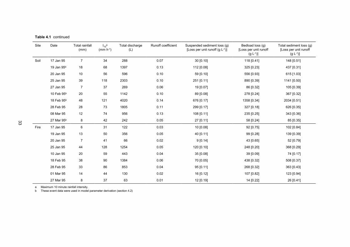
Table 4.1 continued

Site Date Total rainfall(mm)

I10a

(mm h-1)Total discharge

(L)Runoff coefficient Suspended sediment loss (g)

[Loss per unit runoff (g L-1)]Bedload loss (g)

[Loss per unit runoff(g L-1)]

Total sediment loss (g)[Loss per unit runoff

(g L-1)]

Soil 17 Jan 95 7 34 288 0.07 30 [0.10] 118 [0.41] 148 [0.51]

19 Jan 95b 18 68 1397 0.13 112 [0.08] 325 [0.23] 437 [0.31]

20 Jan 95 10 56 596 0.10 59 [0.10] 556 [0.93] 615 [1.03]

25 Jan 95 39 118 2303 0.10 251 [0.11] 890 [0.39] 1141 [0.50]

27 Jan 95 7 37 269 0.06 19 [0.07] 86 [0.32] 105 [0.39]

10 Feb 95b 20 55 1142 0.10 89 [0.08] 278 [0.24] 367 [0.32]

18 Feb 95b 48 121 4020 0.14 676 [0.17] 1358 [0.34] 2034 [0.51]

28 Feb 95 28 73 1805 0.11 299 [0.17] 327 [0.18] 626 [0.35]

08 Mar 95 12 74 956 0.13 108 [0.11] 235 [0.25] 343 [0.36]

27 Mar 95b 8 42 242 0.05 27 [0.11] 58 [0.24] 85 [0.35]

Fire 17 Jan 95 6 31 122 0.03 10 [0.08] 92 [0.75] 102 [0.84]

19 Jan 95 13 50 356 0.05 40 [0.11] 99 [0.28] 139 [0.39]

20 Jan 95 7 41 66 0.02 9 [0.14] 43 [0.65] 52 [0.79]

25 Jan 95 44 128 1254 0.05 120 [0.10] 248 [0.20] 368 [0.29]

10 Jan 95 20 59 443 0.04 35 [0.08] 39 [0.09] 74 [0.17]

18 Feb 95 38 90 1384 0.06 70 [0.05] 438 [0.32] 508 [0.37]

28 Feb 95 33 86 853 0.04 95 [0.11] 268 [0.32] 363 [0.43]

01 Mar 95 14 44 130 0.02 16 [0.12] 107 [0.82] 123 [0.94]

27 Mar 95 8 37 63 0.01 12 [0.19] 14 [0.22] 26 [0.41]

a Maximum 10 minute rainfall intensity.b These event data were used in model parameter derivation (section 4.2)

33

34

Monitoring provided data on storms with a range of total rainfall and rainfall intensity. Forthe high intensity storms the results (table 4.1) did not agree with the analysis by Evans andLoch (1996) which discussed the unexpected observed higher sediment losses under rainfallsimulation (Evans et al 1996) for the lower-sloped cap site than the steeper-sloped batter siteand the effect of surface material properties of the sites. For the events on 09 December1993, similar sediment losses occurred from the cap and batter site even though there wasmuch less runoff from the batter site. For similar medium intensity storms (16 November1993) there was much greater total discharge and sediment loss from the cap site than thebatter site, which agrees with the RUSLE predictions for the cap and batter sites (Evans &Loch 1996). For similar low intensity events (cap 10 December 1993; batter 22 February1993) there was greater sediment loss and discharge from the cap site. The RUSLEpredictions appear to have been valid for small and medium sized events only.

The data from the fire site were not used in model parameter derivation. The vegetationunderstorey on the fire site was extremely dense and was burnt before the plot was surveyedbut after the data were collected. After burning and surveying it was realised that catchments21 and 22 on the plot formed a deep depression with a crack at the lowest point. Much of therunoff from the plot ran into this depression and did not discharge from the plot into theoutlet trough, resulting in very small runoff coefficients (table 4.1). It was considered thatthis depression was not representative of the vegetated area where the plot was constructed.

4.2 Model parameterisationThe monitoring data were used to parameterise (1) the sediment transport model (section 3.1)and (2) the DISTFW rainfall-runoff model (section 3.2). The results of this parameterisationare used to derive long-term average parameters for the SIBERIA model (section 3.3)reported in chapter 5.

4.2.1 Sediment transport modelUsing all data (table 4.1) (except fire site), parameters were fitted to the sediment transportmodel with a ‘lumped’ coefficient. The effect of width term (w) has been shown to beinsignificant for these sites (Evans 1997) and was excluded. This resulted in the followingtotal sediment loss–discharge relationship for the study sites:

T = 0.55 ∫Q 1.38 dt (r2 = 0.89; p < 0.001) (4.1)

A test was conducted for outliers in the data using standardised residuals (Hair et al 1995).This analysis (fig 4.1) indicated that observation 14 (batter 09 December 1993) was outsidethe upper threshold (2 standard deviations) and observation 19 (cap 21 February 1994) wasoutside the lower threshold (-2 standard deviations). These data points were removed andregression analysis was conducted using the remaining data points resulting in the followingrelationship:

T = 0.57 ∫Q 1.38 dt (r2 = 0.90; p <0.001) (4.2)

The removal of the outliers had little effect on the significance of the relationship.

Using the data with outliers omitted, the sediment loss model (equation 3.9) was fitted givingthe following:

T = 0.66 S0.04 ∫Q 1.37 dt (r2 = 0.90; p <0.001) (4.3)

35

The slope (S) exponent (n1 in equation 3.9) of 0.04 is small and effectively results in a slopeterm of unity for most slopes. This indicates that the data may not be sufficiently sensitive tofit a realistic n1 parameter value.

Willgoose and Riley (1993) derived an n1 value of 0.69 for the ERARM waste rock dumpusing combined rainfall simulation and monitoring data from cap and batter site plots. Evanset al (1997), using a laboratory rainfall simulator and mine spoil samples from CentralQueensland, found that for one mine site the CREAMS erodibility parameter (K) was

inversely proportional to S0.624 (ie KS

∝ 10 624. ). Other researchers (Foster 1982, Watson &

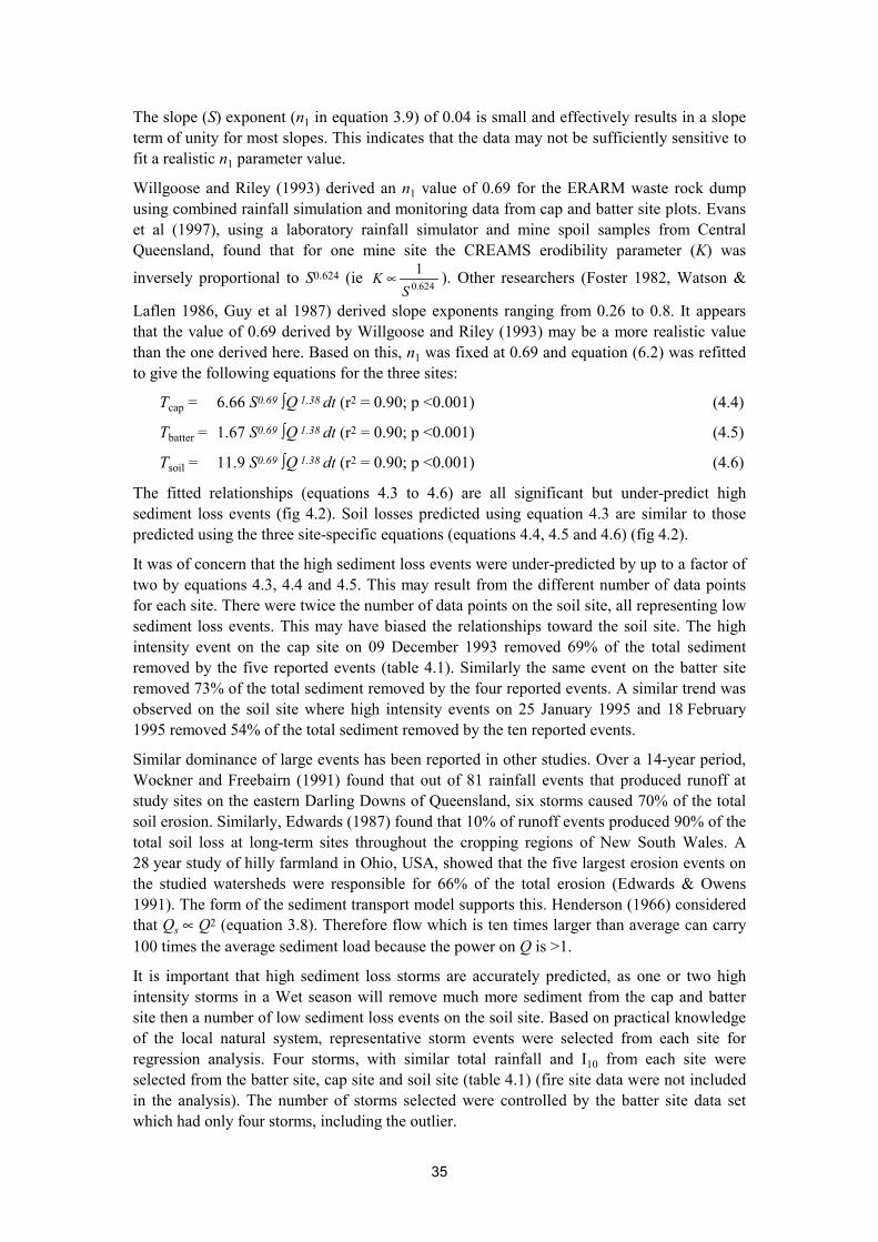
Laflen 1986, Guy et al 1987) derived slope exponents ranging from 0.26 to 0.8. It appearsthat the value of 0.69 derived by Willgoose and Riley (1993) may be a more realistic valuethan the one derived here. Based on this, n1 was fixed at 0.69 and equation (6.2) was refittedto give the following equations for the three sites:

Tcap = 6.66 S0.69 ∫Q 1.38 dt (r2 = 0.90; p <0.001) (4.4)

Tbatter = 1.67 S0.69 ∫Q 1.38 dt (r2 = 0.90; p <0.001) (4.5)

Tsoil = 11.9 S0.69 ∫Q 1.38 dt (r2 = 0.90; p <0.001) (4.6)

The fitted relationships (equations 4.3 to 4.6) are all significant but under-predict highsediment loss events (fig 4.2). Soil losses predicted using equation 4.3 are similar to thosepredicted using the three site-specific equations (equations 4.4, 4.5 and 4.6) (fig 4.2).

It was of concern that the high sediment loss events were under-predicted by up to a factor oftwo by equations 4.3, 4.4 and 4.5. This may result from the different number of data pointsfor each site. There were twice the number of data points on the soil site, all representing lowsediment loss events. This may have biased the relationships toward the soil site. The highintensity event on the cap site on 09 December 1993 removed 69% of the total sedimentremoved by the five reported events (table 4.1). Similarly the same event on the batter siteremoved 73% of the total sediment removed by the four reported events. A similar trend wasobserved on the soil site where high intensity events on 25 January 1995 and 18 February1995 removed 54% of the total sediment removed by the ten reported events.

Similar dominance of large events has been reported in other studies. Over a 14-year period,Wockner and Freebairn (1991) found that out of 81 rainfall events that produced runoff atstudy sites on the eastern Darling Downs of Queensland, six storms caused 70% of the totalsoil erosion. Similarly, Edwards (1987) found that 10% of runoff events produced 90% of thetotal soil loss at long-term sites throughout the cropping regions of New South Wales. A28 year study of hilly farmland in Ohio, USA, showed that the five largest erosion events onthe studied watersheds were responsible for 66% of the total erosion (Edwards & Owens1991). The form of the sediment transport model supports this. Henderson (1966) consideredthat Qs ∝ Q2 (equation 3.8). Therefore flow which is ten times larger than average can carry100 times the average sediment load because the power on Q is >1.

It is important that high sediment loss storms are accurately predicted, as one or two highintensity storms in a Wet season will remove much more sediment from the cap and battersite then a number of low sediment loss events on the soil site. Based on practical knowledgeof the local natural system, representative storm events were selected from each site forregression analysis. Four storms, with similar total rainfall and I10 from each site wereselected from the batter site, cap site and soil site (table 4.1) (fire site data were not includedin the analysis). The number of storms selected were controlled by the batter site data setwhich had only four storms, including the outlier.

36

-4

-2

0

2

4

Stan

dard

ised

resi

dual

1 2 3 4 5 6 7 8 9 10 11 12 13 14 15 16 17 18 19Observation

Upper threshold (2 standard deviations)

Lower threshold (-2 standard deviations)

Figure 4.1 Plot of standardised residuals for equation (4.1).Observations 14 and 19 appear to be outliers.

10

100

1000

10000

100000

Pred

icte

d So

il Lo

ss (g

)

10 100 1000 10000 100000 Observed Soil Loss (g)

Slope exponent = 0.04

Slope exponent = 0.69

1:1 line

Outliers

Figure 4.2 Relationship between predicted and observed sediment loss usingequations 4.3 (n1 = 0.04), 6.4, 6.5 and 6.6 (n1 = 0.69)

37

The fitted sediment transport model using the selected representative storms was:

T = 0.61 S0.06 ∫Q 1.57 dt (r2 = 0.92; p <0.001) (4.7)

Again the slope (S) exponent (n1 in equation 3.9) of 0.06 is small and effectively results in aslope term of unity for most slopes. Therefore, n1 was fixed at 0.69 and the model refittedgiving:

Tcap = 5.79 S0.69 ∫Q 1.59 dt (r2 = 0.92; p <0.001) (4.8)

Tbatter = 1.46 S0.69 ∫Q 1.59 dt (r2 = 0.92; p <0.001) (4.9)

Tsoil = 10.4 S0.69 ∫Q 1.59 dt (r2 = 0.92; p <0.001) (4.10)

Equations 4.7 to 4.10 are significant and are good predictors of observed sediment loss aspredictions are well distributed around the 1:1 line (fig 4.3). Soil losses predicted usingequation 4.7 are similar to those predicted using the three site specific equations (equations4.8, 4.9 and 4.10) (fig 4.3). The sediment transport model constant (β2) reflects differencesbetween sites such as surface cover, surface treatment and erodibility. For these site specificequations the hydrograph volume ( dtQm1∫ ) explains 92% of the variation in sediment loss.

The discharge (Q) exponent (m1) (equations 4.8, 4.9 and 4.10) of 1.59 derived here comparesreasonably with the m1 value of 1.68 derived for small cap and batter site plots by Willgooseand Riley (1993). These equations will be used to predict input into SIBERIA. It appears thatfor these data, n1 has little effect on the soil loss model.

10

100

1000

10000

100000

Pred

icte

d So

il Lo

ss (g

)

10 100 1000 10000 100000 Observed Soil Loss (g)

Slope exponent = 0.06

Slope exponent = 0.69

1:1 line

Figure 4.3 Relationship between predicted and observed sediment lossusing equations 4.7 (n1 = 0.06), 6.8, 6.9 and 6.10 (n1 = 0.69)

38

It is an interesting observation that for the high sediment loss event on 09 December 1993,equation 4.8 closely predicted the observed sediment loss from the cap site (43 937 gobserved; 46 094 g predicted) but equation 4.9 under-predicted sediment loss from the battersite by a factor of ≈0.5 (44 898 g observed; 23 414 g predicted). These equations predictedsediment loss from the cap site to be ≈2.0 times larger than that from the batter site. RUSLEpredictions (Evans & Loch 1996) showed that sediment loss from the cap site would be1.9 times greater than that from the batter site. There is excellent agreement between modelpredictions. It appears that parameters for this model and the RUSLE similarly reflect thedifferences in surface treatment between the two sites. However, the observed sediment lossfrom the batter site during the high intensity event on 9 December 1993 was similar to thatobserved on the cap site, a factor of ≈2.0 times greater than that predicted by the models.Slopes develop such that for average conditions most of the erodible material is removedleaving material which is below an entrainment threshold (Henderson 1966). After a slopehas been exposed for a while most of the transportable material will have been removed. Theremaining material will not be removed by small storms but only transported during largestorms. This results in dramatically increased transport rates for larger erosion events.

It appears that for higher intensity storms on the cap and batter site the total sediment loss perunit runoff increases by an order of magnitude compared to losses for lower intensity storms(table 4.1), and that bedload is the major contributor to this increase, particularly on thebatter site. This is observable for both high intensity events monitored on the batter sites(09 December 1993, I10 = 119 mm h-1 and 18 March 93, I10 = 84 mm h-1). Although based onlimited data points and further research is required for confirmation, it appears that for the0.207 m/m batter slope a threshold discharge may have been reached above which the effectof slope outweighed the effect of surface treatment, and had a greater influence on sedimentloss, resulting in a reduced sediment loss ratio between the two sites in contrast to thatderived by Evans and Loch (1996).

4.2.2 Derivation of DISTFW Rainfall-Runoff Model ParametersParameters were fitted to observed rainfall and runoff for the monitored rainfall events usingDISTFW-NLFIT (method described in section 3.2).

Parameter values were fitted to observed hydrographs for observed rainfalls for individualmonitored events and to four hydrographs for each site simultaneously. The fittedhydrographs for the individual events are given in appendix B and the fitted and observedhydrographs for the multiple events are given in appendix C. Fitted parameter values aregiven in table 4.2. Parameters could not be fitted for the batter site event on22 February 1993, therefore data for an event on 21 February 1993 were used.

Not all catchments on the soil site contribute flow to the hydrographs. The NLFIT .FW inputfiles were configured accordingly.

For five events on the soil site, em was fixed at 1.21. This is a reasonable minimum to usewhen cross-sectional data are unavailable. The value of 1.16 for em, derived using limitedcross-sectional data for the soil site (Evans pers com), seems to support the selection of 1.21.Also, for five events on the soil site, Sphi tried to be fitted to a zero value and was fixed at0.001 when fitting parameters. Except for kinematic wave parameters for the event on22 December 1994, the fitted parameter values for the soil site were fairly consistent. Thebatter site parameter values were also reasonably consistent. The cap site events had thegreatest variation between parameter values.

39

Table 4.2 Fitted mean DISTFW hydrology model parameters. Standard deviations are givenin brackets.

Cap siteDate

cr(m(3–2em) s-1)

em Sphi(mm h-0.5)

phi(mm h-1)

16 Nov 93 2.94 (0.46) 1.32 (0.05) 10.6 (1.92) 1.02 (6.46)

09 Dec 93 68.0 (35.3) 2.11 (0.15) 0.18 (14.2) 29.0 (27.9)

10 Dec 93 4563 (5087) 3.58 (0.39) 2.84 (1.49) 0.57 (5.53)

21 Feb 94 10.5 (4.91) 1.65 (0.11) 0.62 (4.30) 4.81 (16.8)

Simultaneous fit 16 Nov 93, 09 Dec 93,10 Dec 93 and 21 Dec 94b

7.11 (1.28) 1.58 (0.57) 5.31 (0.58) 8.80 (3.01)

Willgoose & Riley (1993) 4.47 1.66 3.85 6.5

Soil siteDate

30 Nov 94 1.50 (1.08) 1.21a (0.15) 0.001 (48.7) 47.5 (126)

22 Nov 94 37.9 (53.9) 2.00 (0.39) 0.66 (1.20) 70.3 (3.74)

17 Jan 95 1.38 (1.85) 1.21a (0.28) 0.001 (203) 61.2 (30.5)

19 Jan 95 3.57 (1.39) 1.21a (0.09) 0.001 (11.8) 59.3 (4.63)

25 Jan 95 4.50 (1.89) 1.36 (0.11) 8.48 (0.84) 61.2 (3.09)

10 Feb 95 3.28 (0.09) 1.29 (0.09) 0.001 (0.17) 48.0 (0.63)

18 Feb 95 1.04 (0.37) 1.21a (0.12) 0.001 (290) 81.7 (76.2)

Simultaneous fit 30 Nov 94, 22 Dec 9419 Jan 95 and 10 Feb 95b

1.25 (0.08) 1.21a (0.02) 7.54 (0.33) 47.2 (0.21)

Batter siteDate

21 Feb 93 19.9 (3.98) 1.97 (0.08) 1.56 (0.80) 19.5 (5.02)

18 Mar 93 15.7 (3.95) 1.83 (0.09) 1.54 (0.87) 52.7 (5.54)

16 Nov 93 5.63 (0.85) 1.47 (0.05) 7.09 (0.57) 12.2 (1.52)

09 Dec 93 5.01 (1.27) 1.50 (0.08) 0.0001 15.7 (0.91)

Simultaneous fit 21 Feb 93, 18 Mar 93,16 Nov93 and 09 Dec 93b

6.71 (0.65) 1.54 (0.03) 5.48 (0.36) 16.3 (0.93)

a em for these events were fixed at 1.21 (Willgoose pers com 1997).b Adopted site parameter values.

For the simultaneously fitted multiple events the kinematic wave parameters are comparablefor the cap and batter site and Sphi is similar for all sites. The cap and batter parameters aresimilar to those adopted by Willgoose and Riley (1993) (table 4.2).

Parameter compatibility analysis of the simultaneously fitted parameters using COMPAT(section 3.2.1) indicated that the kinematic wave parameters, cr and em, were not independentof each other (fig 4.4). The ellipses for the cap and batter site overlapped and therefore theparameter values are considered not to be statistically different. However, the soil site ellipsedid not overlap the cap and batter site ellipses, therefore the parameters values wereconsidered to be statistically different from the cap and batter site parameter values. Thedifference is likely to be due to the different surface roughness conditions on the soil site dueto ripping and vegetation. The infiltration parameters were considered to be statisticallydifferent for all sites as none of the ellipses overlapped (fig 4.5). However, the Sphi value forthe cap (5.31 ± 0.58) and batter (5.48 ± 0.36) site can be considered to be similar even thoughthe long-term infiltration rate, phi, is different.

40

Two sets of parameters were selected for SIBERIA landform evolution modelling (chapter5). The first set are representative of a landform with no surface treatment ie unvegetated andunripped. This first set of parameters were the simultaneously fitted parameters for multiplestorms on the cap site (tables 4.2 and 4.3) since these were in good agreement to thoseadopted by Willgoose and Riley (1993) (table 4.2). The second set of parameters arerepresentative of a landform that has surface treatment such as vegetation and surfaceripping. The second set of parameters were the parameters simultaneously fitted for multiplestorms on the soil site (tables 4.2 and 4.3) which resulted in good agreement betweenpredicted and observed hydrographs (appendix C).

Table 4.3 DISTFW parameters selected for SIBERIA landform evolution modelling. The cap siteparameters are representative of a landform with no surface treatment such as ripping or vegetation.The soil site parameters are representative of a landform with surface treatment (ripping and vegetation).

cr em Sphi phi

Cap site 7.11 ± 1.28 1.58 ± 0.57 5.31 ± 0.58 8.80 ± 3.01

Soil site 1.25 ± 0.08 1.21 ± 0.02 7.54 ± 0.33 47.2 ± 0.21

1.101.00

2.80

4.60

6.40

8.20

10.0

1.24 1.38 1.52 1.66 1.80

cr

em

Batter site

Cap site

Vegetated soil site

Figure 4.4 95% compatibility regions for simultaneously fitted kinematic wave parameter values for thestudy sites derived using monitoring data – (1) batter site, (2) cap site and (3) vegetated soil site

41

2.204.00

4.86

5.72

6.58

7.44

8.30

11.4 20.5 29.7 38.8 48.0

Sphi

phi

Batter site

Cap site

Vegetated soil site

Figure 4.5 95% compatibility regions for simultaneously fitted infiltration parameter values for the studysites derived using monitoring data – (1) batter site, (2) cap site and (3) vegetated soil site

PREDICT (section 3.2.1) was used to test how well the adopted parameters predicted runoffhydrographs (figs 4.6 and 4.7). The adopted parameters for the cap site were used to predictrunoff from the cap site for an event which occurred on 03 January 1995. Although theobserved hydrograph volume was under-predicted, event runoff was well predicted with allobservations falling within 90% prediction limits (fig 4.6).

The second set of adopted parameters (soil site), representing a vegetated and rippedlandform, was used to predict runoff from the soil site for an event which occurred on10 January 1996 (George 1996). This event was not used in the parameter fitting process. Forthis event the hydrograph volume was largely over-predicted and discharge was poorlypredicted (fig 4.7). This may have resulted from the difficulty in predicting infiltrationparameters. This does not mean that the second set of adopted parameters are inadequate formodelling or design purposes. Over-predicting hydrograph volume indicates that theinfiltration parameter values are under-predicted. This may have resulted from thecomplexities of the soil site surface (vegetation and ripping on the low slope 0.012 m/m). Itmay be that no event data were collected where long-term infiltration was achieved. Usingunder-predicted infiltration parameter values in the modelling process may over-predict theamount of discharge, which will result in an over-prediction of sediment loss. Therefore,using the adopted parameters will over-predict erosion, for some rainfall events, resulting inconservative design of erosion control structures on rehabilitated landforms.

42

Figure 4.6 Rainfall for the cap site event on 03 January 1995 and hydrograph predicted using adoptedparameter values for an unvegetated and unripped landform (cap site). Parameter values

are cr = 7.11, em = 1.58, Sphi = 5.31 and phi 8.8. 90% predition limits are shown.

4.3 OverviewThis study highlights the difficulty of deriving sediment transport and hydrology modelparameter values for a site. It was fortunate that the study area was in the wet/dry tropics andit was predictable when rain would occur so a monitoring program could be established.However, over a three year monitoring period only 28 full data sets from four sites werecollected. The nature of the models require that discrete event data of rainfall, discharge andtotal sediment loss data are collected. Water level sensors can be used to monitor dischargewhen an observer is not present but the sensors need to be carefully calibrated and must notbe heat-sensitive as this will result in errors. Suspended sediment data are the most difficultto collect as an observer needs to be present at the start of an event to collect runoff samples.Bedload can be collected at the completion of an event. For many of the storms where datasets were incomplete it was the suspended sediment data that were missing. For this type ofdiscrete sampling, the automatic sediment sampler available for this study was inadequateand therefore not used. If the sampling process is commenced at the first runoff the samplerwill start and continue to sample the event even if rainfall ceases and discharge stops after ashort time. The sampler will continue its cycle resulting in empty sample bottles and will notrestart if a larger event with substantial runoff follows soon after. The variable nature ofevents, ie time of event, is also a problem as for a long event the settings on the sampler mayresult in only the rising stage of the hydrograph being sampled.

0.0 0.4 0.8 1.2Time (h)

0.000

0.003

0.006

0.009

0.012

Dis

char

ge (c

umec

s)

0.0 0.4 0.8 1.2

0

5

10

15

Cum

ulat

ive

Rai

nfal

l (m

m)

Observed

Predicted

90% prediction limits

43

0.0 0.4 0.8 1.2 1.6Time (h)

0.00

0.01

0.02

Dis

char

ge (c

umec

s)

0.0 0.4 0.8 1.2 1.6

0

50

100

Cum

ulat

ive

Rai

nfal

l (m

m)

Observed

Predicted

90% prediction limits

Figure 4.7 Rainfall for the soil site event on 10 January 1996 and hydrograph predicted using adoptedparameter values for a vegetated and ripped landform (soil site). Parameter valuesare cr = 1.25, em = 1.21, Sphi = 7.54 and phi 47.2. 90% predition limits are shown.

For this study it was important when fitting the sediment transport model that a broad rangeof events were used and that high sediment loss events were well predicted. Observationsindicate that one high sediment loss event may remove more than ten times the amount ofsediment that is removed during a low intensity event. Therefore, based on site experience,representative events were selected for parameter derivation. There was difficulty in fittingthe model using batter site data as there may be a threshold discharge above which the effectsof slope outweigh surface properties resulting in observed sediment losses twice thatpredicted. The following significant sediment transport equations (4.8 and 4.10) wereadopted for landform evolution modelling:

Tcap = 5.79 S0.69 ∫Q 1.59 dt (r2 = 0.92; df = 10; p <0.001) (for an unvegetated site withoutsurface amelioration)

Tsoil = 10.4 S0.69 ∫Q 1.59 dt (r2 = 0.92; df = 10; p <0.001) (for a vegetated site withsurface amelioration, ie ripping)

The adopted DISTFW parameter values are summarised in table 4.3.

The cap site parameters values are good predictors of events. The soil site parameters mayover-predict discharge for some rainfall events which will result in conservative design oferosion control structures.