1

1

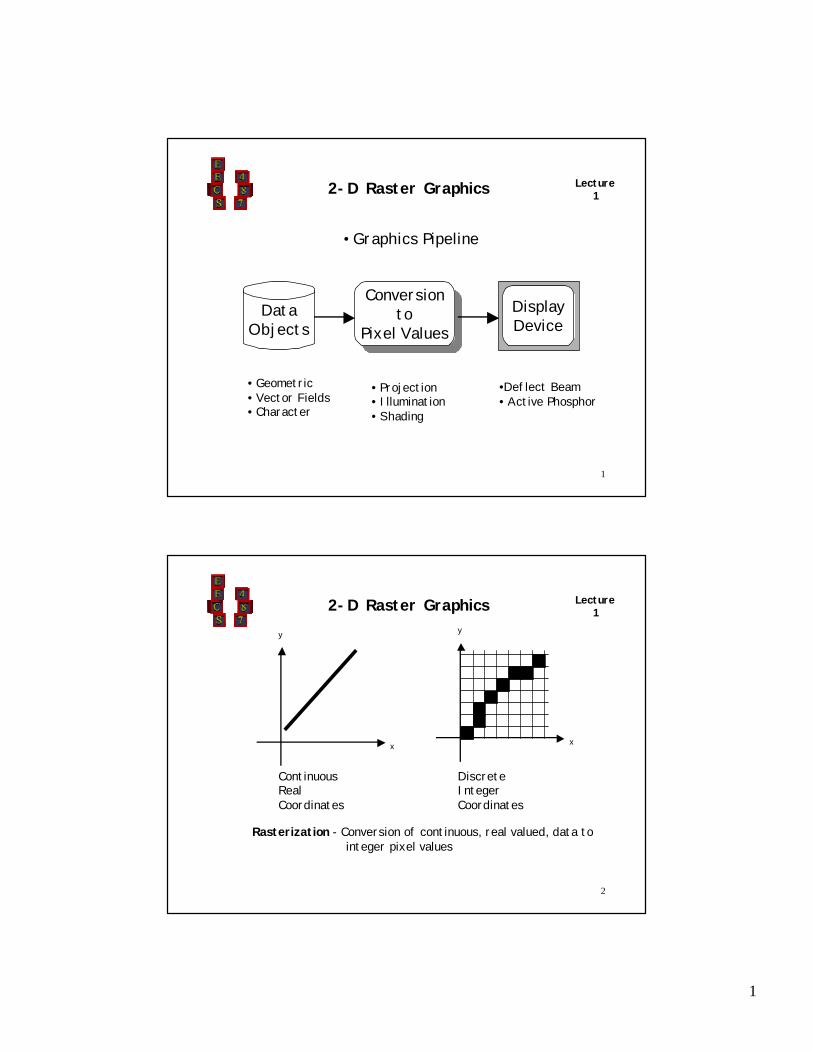
Lecture12-D Raster Graphics

• Graphics Pipeline

Conversionto

Pixel Values

Conversionto

Pixel ValuesData

ObjectsDisplayDevice

• Geometric• Vector Fields• Character

• Projection• Illumination• Shading

•Deflect Beam• Active Phosphor

2

Lecture12-D Raster Graphics

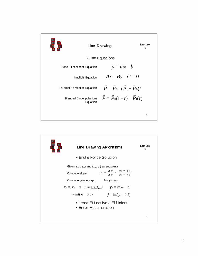
ContinuousRealCoordinates

x

y

DiscreteIntegerCoordinates

x

y

Rasterization - Conversion of continuous, real valued, data tointeger pixel values

2

3

Lecture1Line Drawing

• Line Equations

Slope - Intercept Equation

Implicit Equation

Parametric Vector Equation

Blended (Interpolation) Equation

bmxy +=

0=++ CByAx

tPPPP )( 010

rrrr−= +

)()1( 10 tPtPPrrr

+−=

4

Lecture1Line Drawing Algorithms

• Brute Force Solution

Given: (x0, y0) and (x1, y1) as endpoints

Compute slope:

Compute y-intercept:

• Least Effective / Efficient• Error Accumulation

01

01

xxyy

xy

m−−=

∆∆=

00 mxyb −=

nxxn += 0 { },...3,2,1=n bmxy nn +=

)5.0int( += nxi )5.0int( += nyj

3

5

Lecture1Line Drawing Algorithms

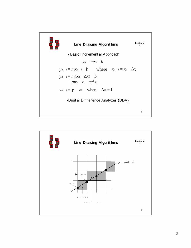
• Basic Incremental Approach

•Digital Difference Analyzer (DDA)

bmxy nn +=

bmxy nn += ++ 11 xxx nn ∆+=+ 1where

bxxmy nn +∆+=+ )(1

xmbmxn ∆++=

1when1 =∆+=+ xmyy nn

6

Lecture1Line Drawing Algorithms

( ))5.0int(, +nn yx

( )nn yx ,

( )myx nn ++ ,1

( ))5.0int(,1 +++ myxn

bmxy +=

4

7

Lecture1Line Drawing Algorithms

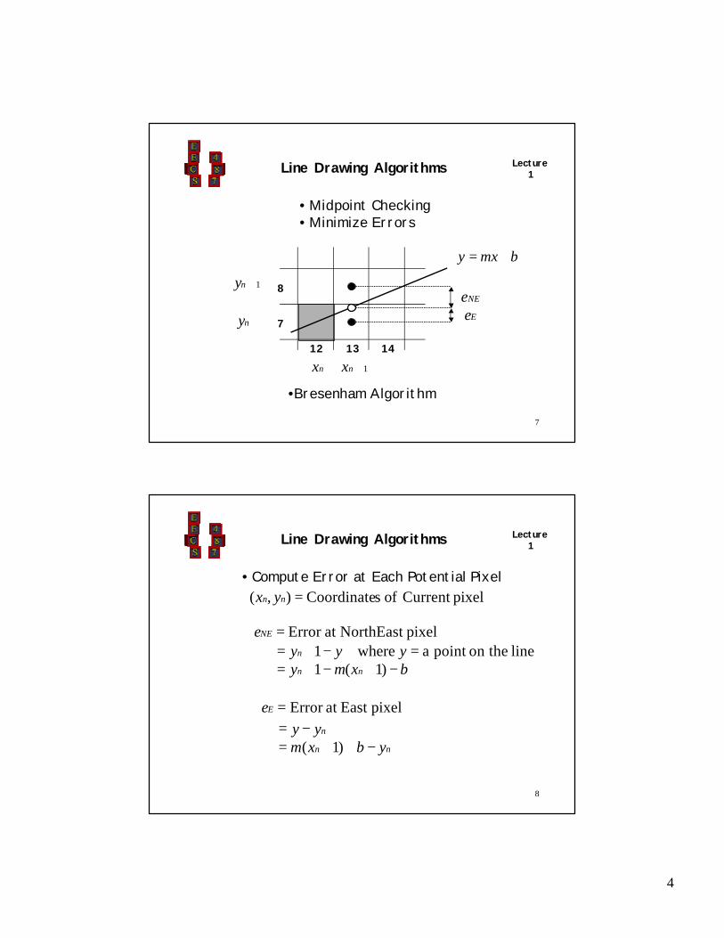
• Midpoint Checking• Minimize Errors

•Bresenham Algorithm

ny

1+ny

1+nxnx

NEeEe

bmxy +=

12 13 14

7

8

8

Lecture1Line Drawing Algorithms

• Compute Error at Each Potential PixelpixelCurrentofsCoordinate),( =nn yx

pixelEastatError=Ee

nn

n

ybxmyy

−++=−=

)1(

bxmyyyy

nn

n

−+−+==−+=

)1(1linetheonpointawhere1

pixelNorthEastatError=NEe

5

9

Lecture1Line Drawing Algorithms

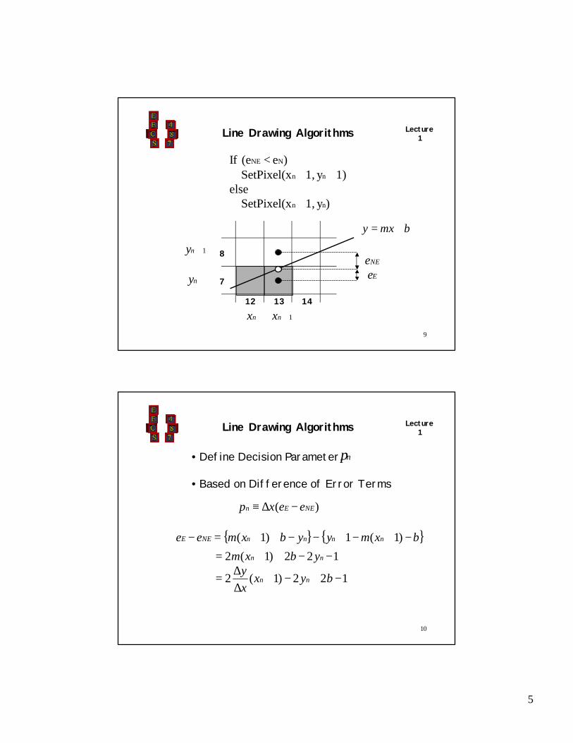
)y1,SetPixel(xelse

1)y1,SetPixel(x)e(eIf

nn

nn

NNE

+

++<

ny

1+ny

1+nxnx

NEeEe

bmxy +=

12 13 14

7

8

10

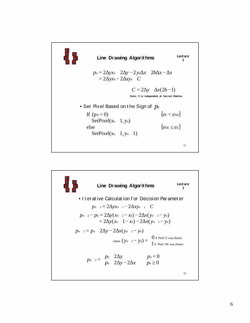
Lecture1Line Drawing Algorithms

• Define Decision Parameter,

• Based on Difference of Error Terms

np

)( NEEn eexp −∆≡

{ } { }bxmyybxmee nnnnNEE −+−+−−++=− )1(1)1(

122)1(2

122)1(2

−+−+∆∆

=

−−++=

byxx

yybxm

nn

nn

6

11

Lecture1Line Drawing Algorithms

• Set Pixel Based on the Sign of np{ }

{ }1)y1,SetPixel(x

else)y1,SetPixel(x

0)(pIf

nn

nn

N

++≤

+<<

ENE

NEE

ee

ee

Cxyyxxxbxyyyxp

nn

nnn

+∆−∆=∆−∆+∆−∆+∆=

222222

)12(2 −∆+∆= bxyCNote: C is Independent of Current Position

12

Lecture1Line Drawing Algorithms

Cxyyxp nnn +∆−∆= +++ 111 22

• Iterative Calculation for Decision Parameter

)(2)1(2)(2)(2

1

111

nnnn

nnnnnn

yyxxxyyyxxxypp

−∆−−+∆=−∆−−∆=−

+

+++

=−

−∆−∆+=

+

++

chosenwasNEPixelif

chosenwasEPixelif1where

11

10

)(

)(22

nn

nnnn

yy

yyxypp

≥∆−∆+<∆+=+

02202

1nn

nnn

pxyppyp

p

7

13

Lecture1Line Drawing Algorithms

• Bresenham Line Drawing Algorithm

xyppyx

yppyx

pxn

)y,(xxypxyyyyyxxx

)y,(x),y,(x

nn

nn

nn

nn

n

startstopstartstop

stopstopstartstart

∆−∆+=++

∆+=+

<−∆=

∆−∆=∆−∆∆−=∆−=∆

+

+

22)1,1(Plot

Else2

),1(Plot )0( If

)1(0For 4.Plot 3.

2,22,2,, :ConstantsCompute2.

:EndpointsEnter1.

1

1

00

0

L

1<m

14

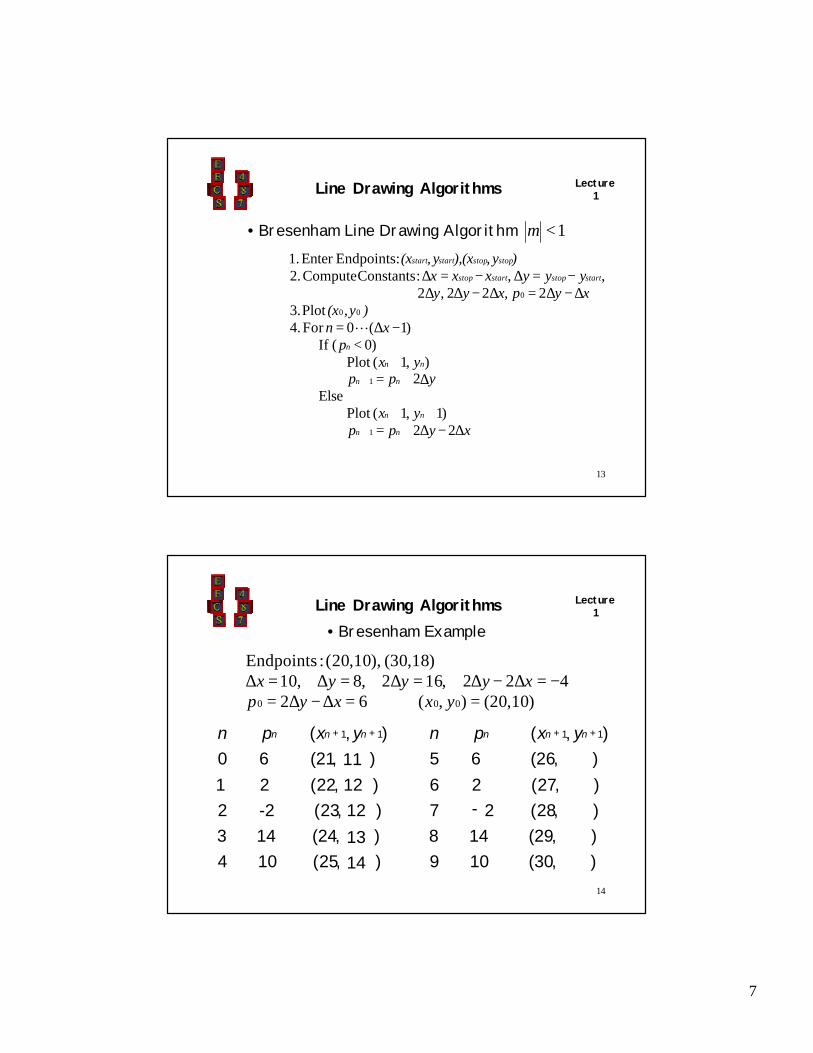
Lecture1Line Drawing Algorithms

• Bresenham Example

)10,20(),(62422,162,8,10

)18,30(),10,20( :Endpoints

000 ==∆−∆=−=∆−∆=∆=∆=∆

yxxypxyyyx

),25(104

),24(143

),23(-22

),22(21

),21(60

),( 11 ++ nnn yxpn

),30(9

),29(8

),28(7

),27(6

),26(5

),( 11

10

14

2

2

6

-

++ nnn yxpn

11

12

12

13

14

8

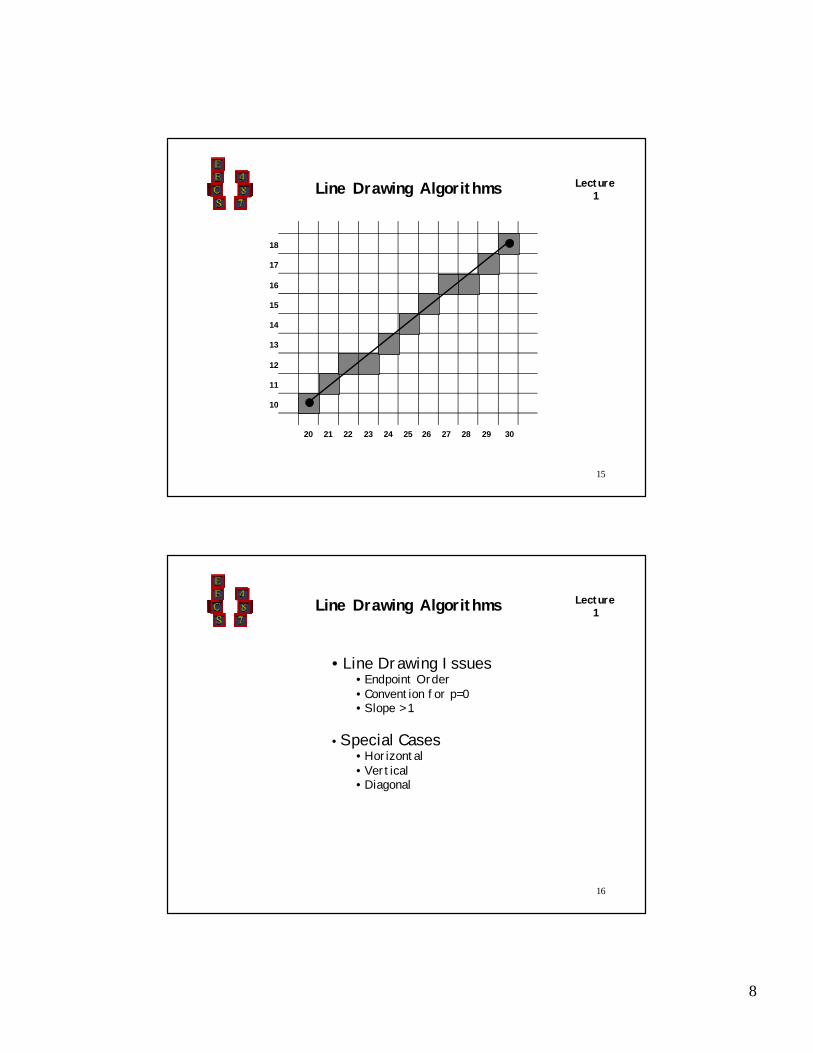
15

Lecture1Line Drawing Algorithms

20 2522 23 2421 2926 27 28 30

10

11

12

13

14

15

16

17

18

16

Lecture1Line Drawing Algorithms

• Line Drawing Issues• Endpoint Order• Convention for p=0• Slope > 1

• Special Cases• Horizontal• Vertical• Diagonal

9

17

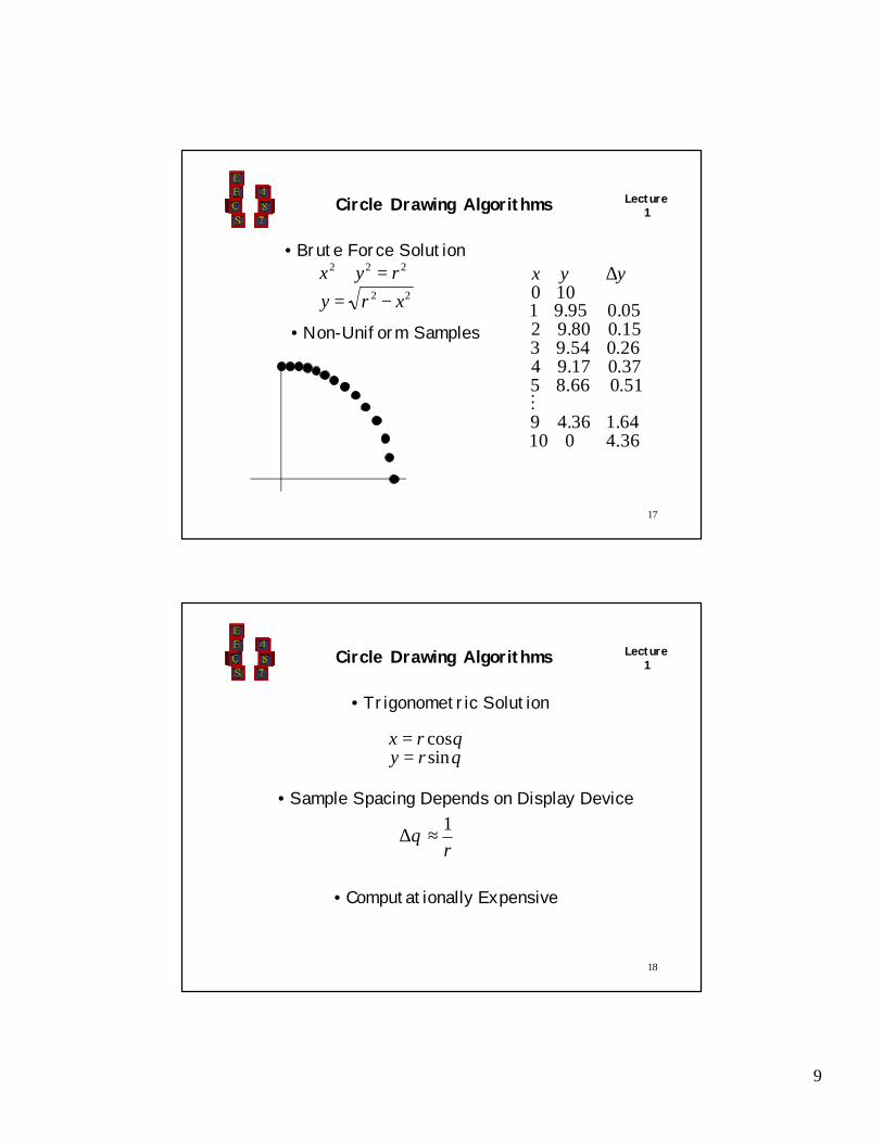
Lecture1Circle Drawing Algorithms

• Brute Force Solution

22

222

xry

ryx

−==+

• Non-Uniform Samples

36.401064.136.49

51.066.8537.017.9426.054.9315.080.9205.095.91

100

M

yyx ∆

18

Lecture1Circle Drawing Algorithms

• Trigonometric Solution

θθ

sincos

ryrx

==

• Sample Spacing Depends on Display Device

r

1≈∆θ

• Computationally Expensive

10

19

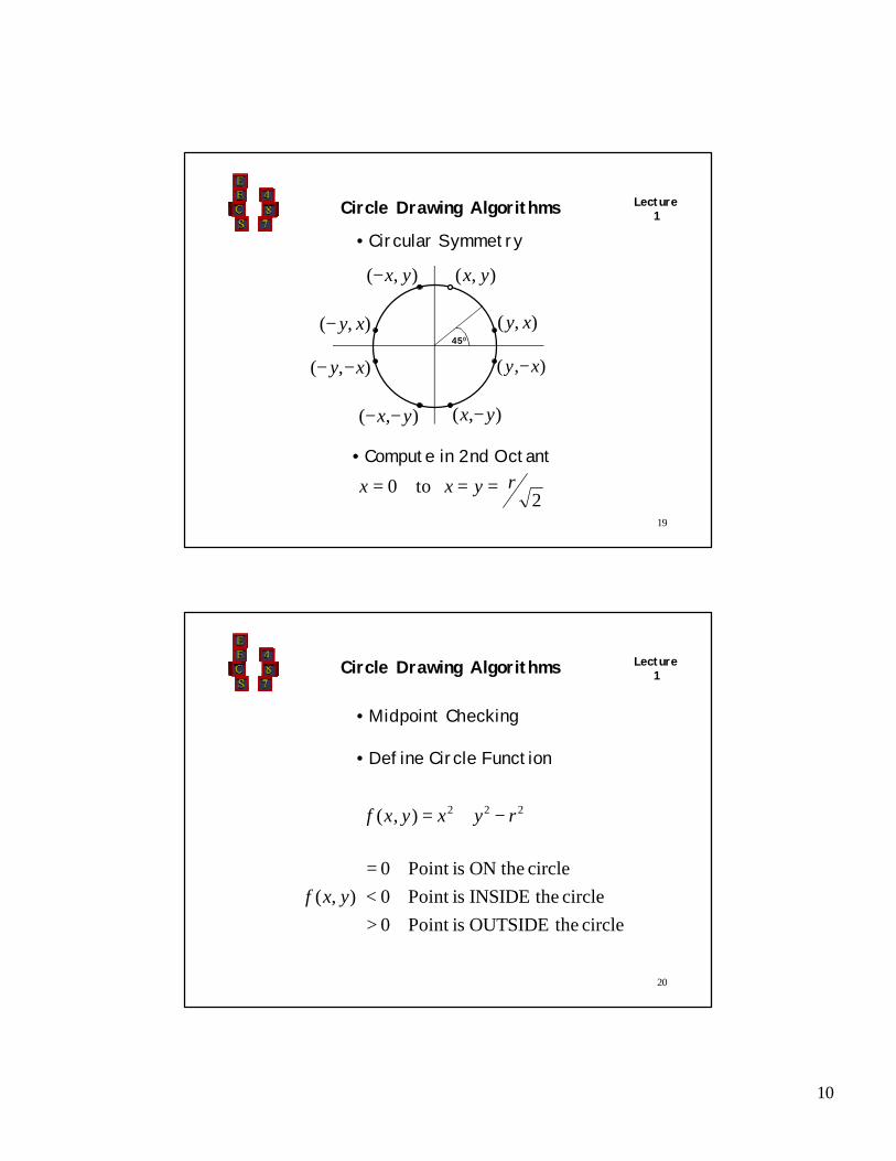
Lecture1Circle Drawing Algorithms

• Circular Symmetry

• Compute in 2nd Octant

2 to0 ryxx ===

),( yx),( yx−

),( xy− ),( xy

),( xy −− ),( xy −

),( yx −− ),( yx −

450

20

Lecture1Circle Drawing Algorithms

• Midpoint Checking

• Define Circle Function

222),( ryxyxf −+=

><=

circle theOUTSIDE isPoint 0

circle theINSIDE isPoint 0

circle theON isPoint 0

),( yxf

11

21

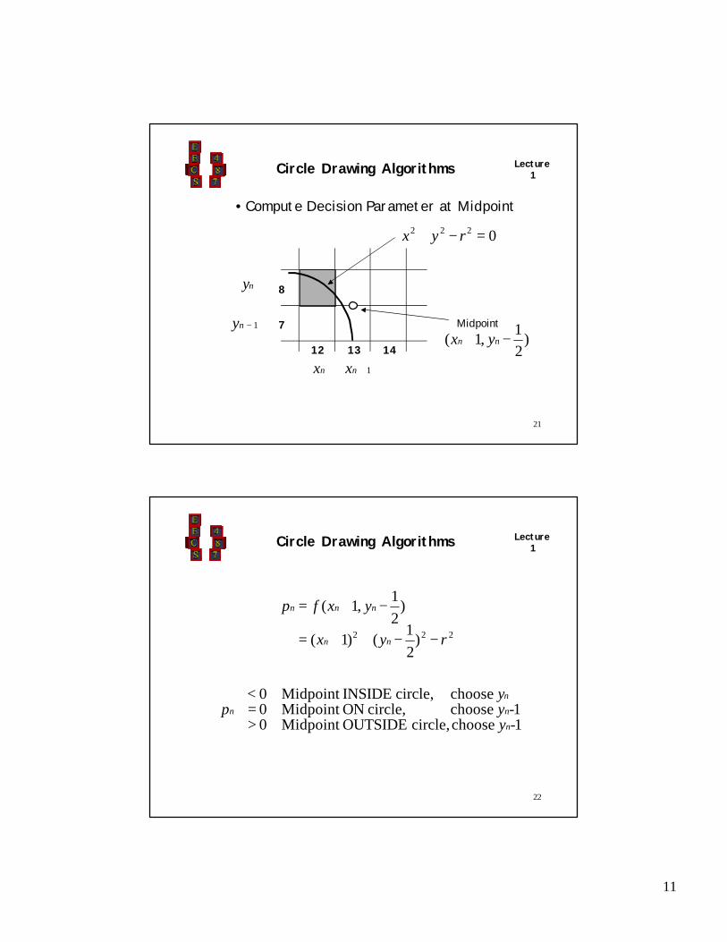
Lecture1Circle Drawing Algorithms

• Compute Decision Parameter at Midpoint

1−ny

ny

1+nxnx

0222 =−+ ryx

12 13 14

7

8

Midpoint)

2

1,1( −+ nn yx

22

Lecture1Circle Drawing Algorithms

222 )2

1()1(

)2

1,1(

ryx

yxfp

nn

nnn

−−++=

−+=

>=<

1 choose circle, OUTSIDEMidpoint 01 choose circle, ONMidpoint 0

choose circle, INSIDEMidpoint 0

-y-y

yp

n

n

n

n

12

23

Lecture1

[ ]

≥−<=

+−−−+++=

−

−+++=

−+=

+

++

+

+++

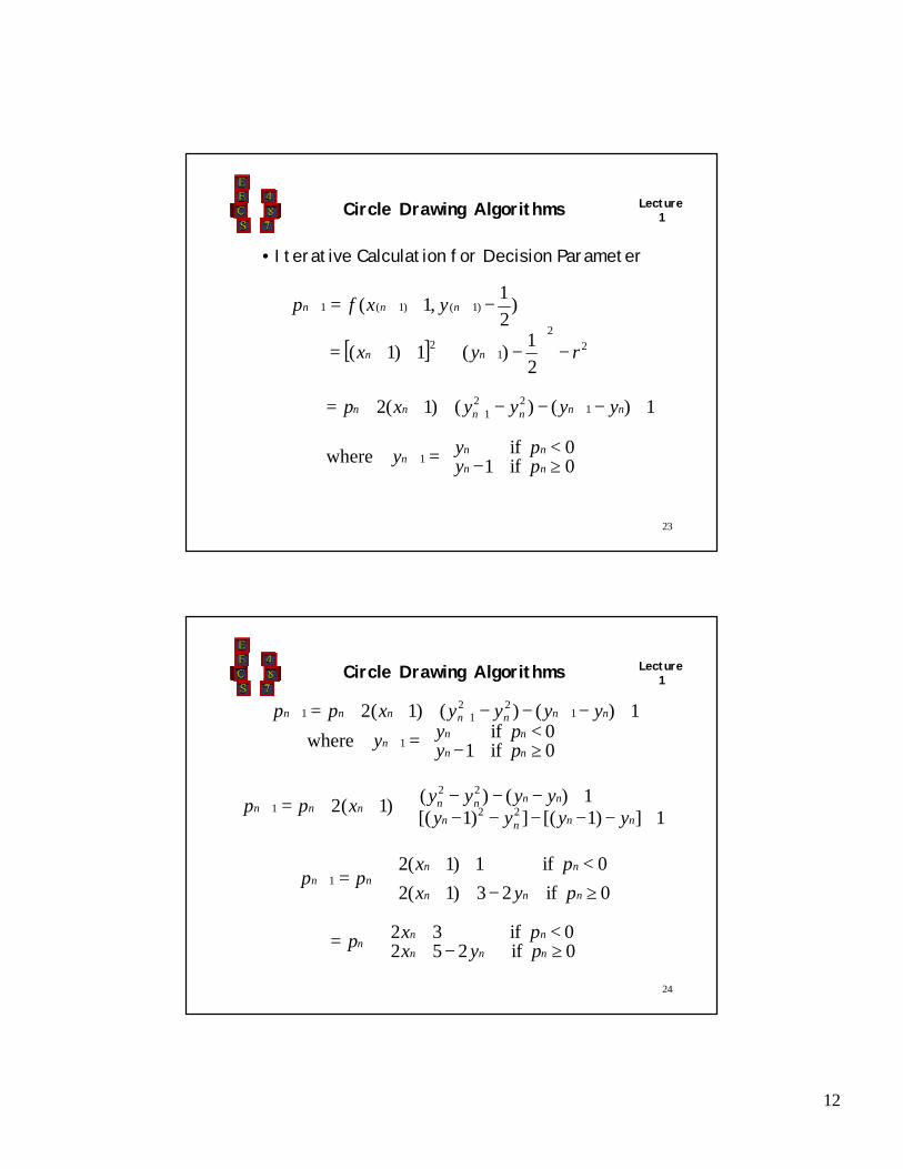
0 if 10 if where

1)()()1(2

2

1)(1)1(

)2

1,1(

1

122

1

22

12

)1()1(1

nn

nnn

nnnnnn

nn

nnn

pypyy

yyyyxp

ryx

yxfp

• Iterative Calculation for Decision Parameter

Circle Drawing Algorithms

24

Lecture1Circle Drawing Algorithms

≥−++<++

+=+0 if23)1(2

0 if1)1(21

nnn

nnnn

pyx

pxpp

+−−−−−+−−−+++=+

1])1[(])1[(1)()()1(2 22

22

1nnnn

nnnnnnnyyyy

yyyyxpp

≥−+<++= 0 if252

0 if32nnn

nnn pyx

pxp

≥−<=

+−−−+++=

+

+++

0 if 10 if where

1)()()1(2

1

122

11

nn

nnn

nnnnnnn

pypyy

yyyyxpp

13

25

Lecture1Circle Drawing Algorithms

• Initializing the Decision Parameter222 )

2

1()1()

2

1,1( ryxyxfp nnnnn −−++=−+=

),0(),( 00 ryx =

r

rrr

rr

rfyxfp

−=

−+−+=

−−+=

−=−+=

4

54

11

)2

1()1(

)2

1,1()

2

1,1(

22

222

000

26

Lecture1Circle Drawing Algorithms

• Simplify Calculations With Integer Arithmetic• Change of Variables in Iterative Equations

4

1−≡ pq

rqrp −=⇒−= 14

500

Decision Parameter Becomes

02

10 <⇒<⇒< nnn qqp

Since q starts as an int and is incremented by int’s

14

27

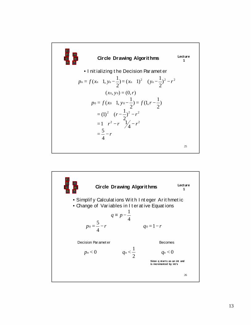
Lecture1Circle Drawing Algorithms

• Midpoint Circle Algorithm

EndwhilePlot and )(Center Circle toPoints Translate

PointsSymmetry Determine11

5)(2Else

132

)0( If)( While5.

Plot and )(Center Circle toPoints Translate 4.)0( ),0( ),0( PointsSymmetry Determine 3.

1),,0(),( :Parameters Initialize2.)(:Radius andCenter Enter1.

cc

cc

cc

y,x

yyxx

yxqq

yyxx

xqqq

yxy,x

-r,r,-r,rqryx

r,y,x

−=+=

+−+=

=+=

++=<

≤

−==

28

Lecture1

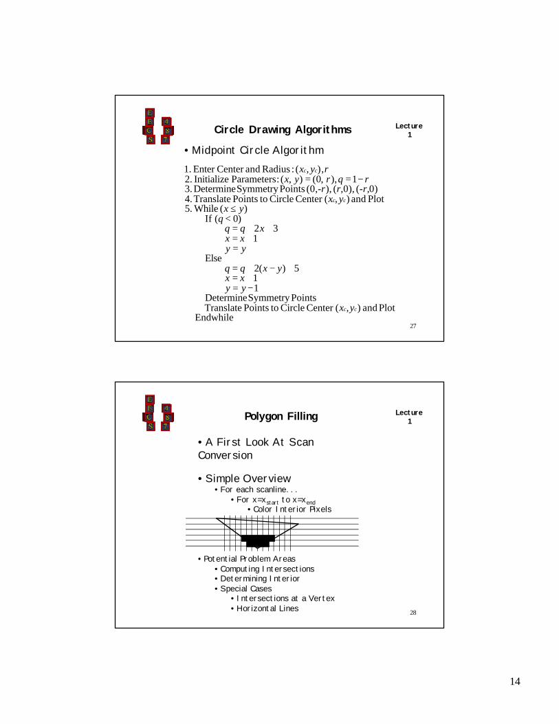
• A First Look At Scan Conversion

• Simple Overview• For each scanline. . .

• For x=xstart to x=xend• Color Interior Pixels

• Potential Problem Areas• Computing Intersections• Determining Interior• Special Cases

• Intersections at a Vertex• Horizontal Lines

Polygon Filling

15

29

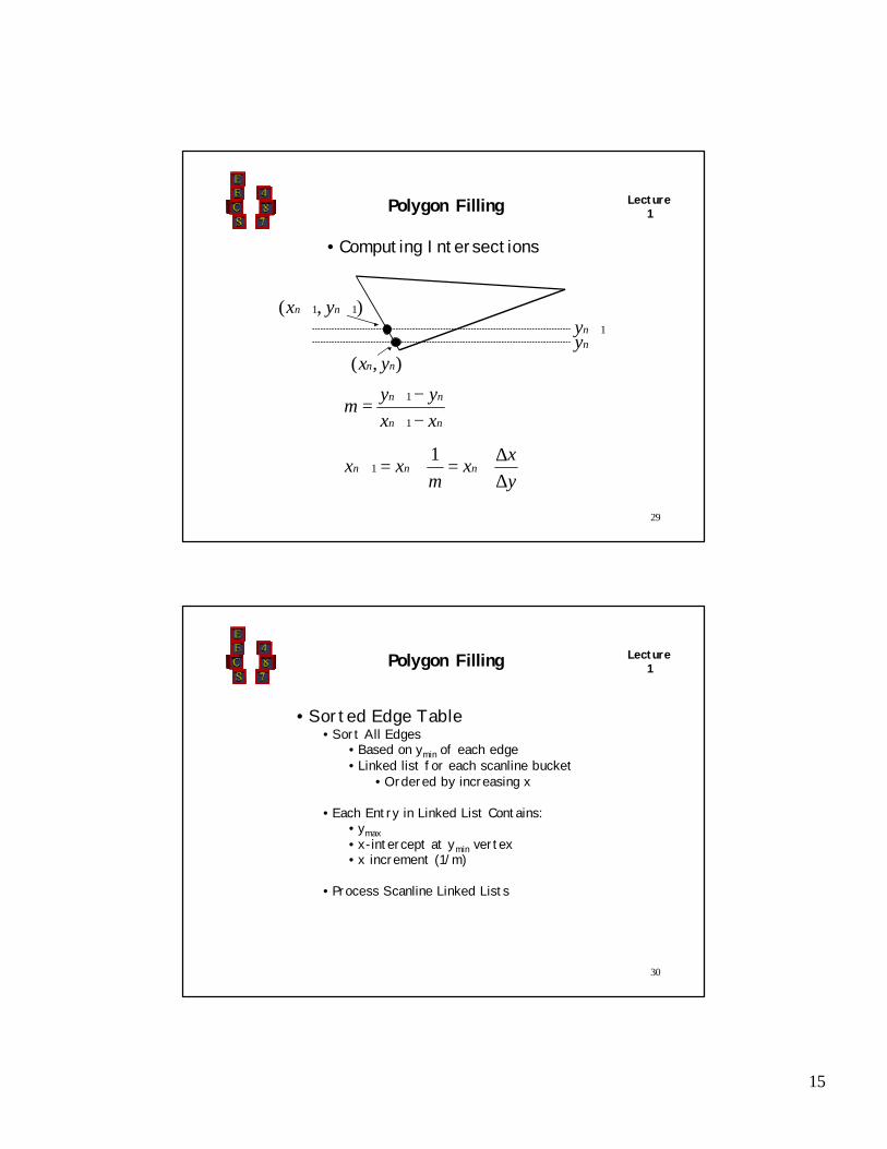
Lecture1Polygon Filling

• Computing Intersections

y

xx

mxx

xx

yym

nnn

nn

nn

∆∆

+=+=

−−

=

+

+

+

11

1

1

1+ny

),( nn yx

),( 11 ++ nn yx

ny

30

Lecture1Polygon Filling

• Sorted Edge Table• Sort All Edges

• Based on ymin of each edge• Linked list for each scanline bucket

• Ordered by increasing x

• Each Entry in Linked List Contains:• ymax• x-intercept at ymin vertex• x increment (1/m)

• Process Scanline Linked Lists

16

31

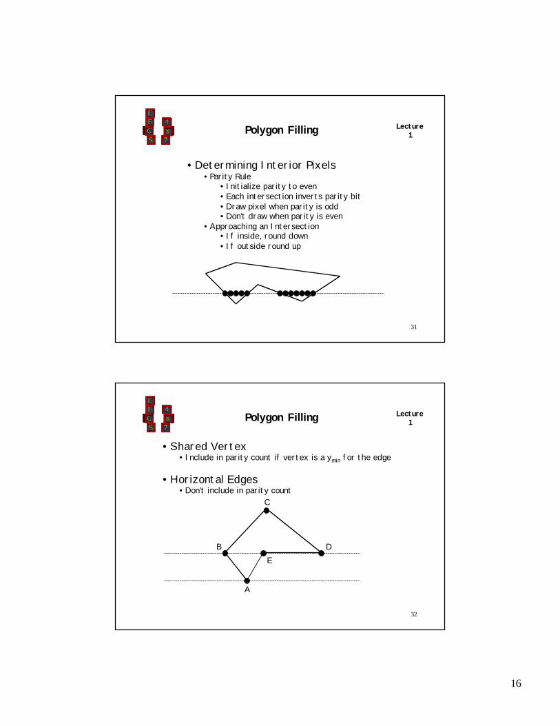
Lecture1Polygon Filling

• Determining Interior Pixels• Parity Rule

• Initialize parity to even• Each intersection inverts parity bit• Draw pixel when parity is odd• Don’t draw when parity is even

• Approaching an Intersection• If inside, round down• If outside round up

32

Lecture1Polygon Filling

• Shared Vertex• Include in parity count if vertex is a ymin for the edge

• Horizontal Edges• Don’t include in parity count

A

D

C

BE