2 9 2003 libraries - massachusetts institute of technology
TRANSCRIPT
Real Estate Opportunity Funds:Past Fund Performance as an Indicator of Subsequent Fund Performance
by
Cathy C. Hahn
B.A., Architecture, 1989B. Arch., 1992
Rice University
Submitted to the Department of Architecture in Partial Fulfillment of the Requirements for theDegree of Master of Science in Real Estate Development
at the
Massachusetts Institute of Technology
September, 2003
MASSACHUSETTS INSTITUTEOF TECHNOLOGY
AUG 2 9 2003
LIBRARIES©2003 Cathy C. Hahn
All rights reserved
The author hereby grants to MIT permission to reproduce and to distribute publicly paper andelectronic copies of this thesis document in whole or in part.
Signature of Author ,;- , o A0artment of Architecture
_Ayugust 4, 2003
Certified by a Finance
Professor of R al Estate FinanceTbzsiis Spervisor
Accepted by(.Dav1Zeltner
Chairman, Interdepartmental Degree Program inReal Estate Development
ROTCHI
Real Estate Opportunity Funds:Past Fund Performance As An Indicator Of Subsequent Fund Performance
by
Cathy C. Hahn
Submitted to the Department of Architectureon August 4, 2003, in partial fulfillment of the requirements
for the Degree of Master of Science inReal Estate Development
ABSTRACT
The returns of opportunistic real estate private equity investment funds were
tested for evidence of performance persistence between subsequent funds by the same
manager. Tests include regression analysis, construction of contingency tables, and
calculation of rank correlation coefficients. Tests were based on return data from the
period 1991 to 2001 and were similar to those used to analyze performance persistence in
other investment vehicles such as mutual funds and hedge funds.
Results indicate that manager performance in a given fund is a significant
indicator of performance in subsequent funds, but that this persistence accounts for only a
limited portion of fund return Gross fund returns exhibit a higher degree of serial
correlation than net returns. Other fund characteristics, analyzed in conjunction with
previous fund performance, are not shown to be significant indicators of performance.
Thesis Supervisor: David GeltnerTitle: Professor of Real Estate Finance

Acknowledgements
I am indebted to Pension Consulting Alliance, Inc. for providing the data used in this
thesis. Thank you to Nori Gerardo Lietz and Denise Mouchakkaa for the time spent
answering my questions, explaining data, and generally helping me to understand the
industry. I would like to thank David Geltner for providing guidance, advice, and an
alternate viewpoint when necessary. Thank you to Jonathan and Aidan for your patience
and support. The author alone is responsible for any errors.

Table of Contents
I. Introduction 5
II. A Brief Overview of Opportunity Funds 6
III. Literature Review 11
Methodologies and Survivorship Bias 11
Mutual Funds 12
Hedge Funds 13
Other Investments 14
IV. Data 15
V. Methodology 20
VI. Results and Analysis 26
Contingency Tables 26
Rank Correlation Statistics 32
Regression Analyses 35
VII. Topics for Further Inquiry 42
VIII. Conclusion 43
IX. Appendix 46
X. Bibliography 64
Real Estate Opportunity Funds: Past Fund Performance as anIndicator of Subsequent Fund Performance
I. Introduction
This thesis investigates correlation in the performance of real estate opportunity
funds. Where alpha is defined as the abnormal return of an investment, either excess or
deficient return, the capital asset pricing model states that the expected value of alpha is
zero and sample alphas should be unpredictable.' If a real estate private equity fund
manager consistently outperforms or underperforms the market, then the hypothesis of
market efficiency is challenged and the use of managers' track records as a selling point
is validated. Because the market for real estate assets is a private market, with
heterogeneous assets and asymmetrical information, it is plausible that managers could
capitalize on market inefficiencies to attain a consistent alpha, which would be evidenced
by correlated performance over time.
While performance persistence in other investment vehicles has been thoroughly
investigated, it has not previously been studied in real estate opportunity funds.
Correlation between returns of opportunity funds is investigated by the means of
statistical tests. Data was provided by an investment consultancy, and covers the period
1991 to 2001, virtually the entire period that opportunistic real estate fund have existed.
While this paper begins to explore the significance of some other factors in
conjunction with past performance, it focuses primarily on return history as an indicator.
Factors that have been tested as possible indicators of future performance in addition to
past performance include: strategy, alliance with a larger financial institution, fund size,
inception year, and amount of capital raised in all funds in the fund's inception year.
1 Zvi Bodie, Alex Kane, and Alan Marcus, Investments, (New York: McGraw-Hill, 2002), p. 303.
II. A Brief Overview of Opportunity Funds
Real estate has traditionally been a small part of the investment portfolio. On
average, for pension funds, 4%2 of the investment portfolio is allocated to real estate, of
which 30% or less is targeted to opportunistic strategies. 3 Other options for real estate
investors include public securities in the form of REIT shares or CMBS, commingled
funds, or separate accounts. Since opportunistic funds are perceived as high risk, similar
to private equity investments such as venture capital or hedge funds, some investors
consider such investment as part of a private equity portfolio rather than as a segment of
their real estate holdings.4 Estimates of value of assets controlled by real estate
opportunity funds range from $100 billion5 to $250 billion.6
Opportunistic real estate private equity funds are a relatively recent option for
institutional and high net worth investors. They first appeared in the late 1980s and early
1990s and are only now starting to build a significant track record. Both the number of
funds and the amount of capital invested are increasing. The current number of fund
general partners is over 100,7 and capital commitments to individual funds have risen
from an average fund size of $293 million in vintage year 1994 to $577 million in vintage
year 2000.8 With close to $100 billion in fund equity raised through the end of 2002,9
opportunistic real estate funds are a growing presence in real estate investments.
2 David Geltner and Norman Miller, Commercial Real Estate Analysis and Investments, (United States:Thomson Learning, South-Western Publishing, 2001) p. 541.3 Pension Consulting Alliance, "Real Estate Opportunity Funds: The Numbers Behind the Story," April2001, p. 50.4 Carol Broad, Russell Real Estate Advisors, quoted by Mike Fickes, 'Feasting on Market InefficiencyWorldwide,' National Real Estate Investor, Atlanta, October, 2001.5 Peter Linneman and Stanley Ross, "Real Estate Private Equity Funds," white paper, Zell/Lurie RealEstate Center, 2002, p. 12.6 Pension Consulting Alliance, "Real Estate Opportunity Funds: DejA vu All Over Again," May 2003, p. 5.7 Ernst & Young, "Opportunistic Investing: Real Estate Private Equity Funds," 2002.8 Based on data provided by Pension Consulting Alliance, Inc.9 Pension Consulting Alliance, "Real Estate Opportunity Funds: Deji vu All Over Again," May 2003, p. 5.
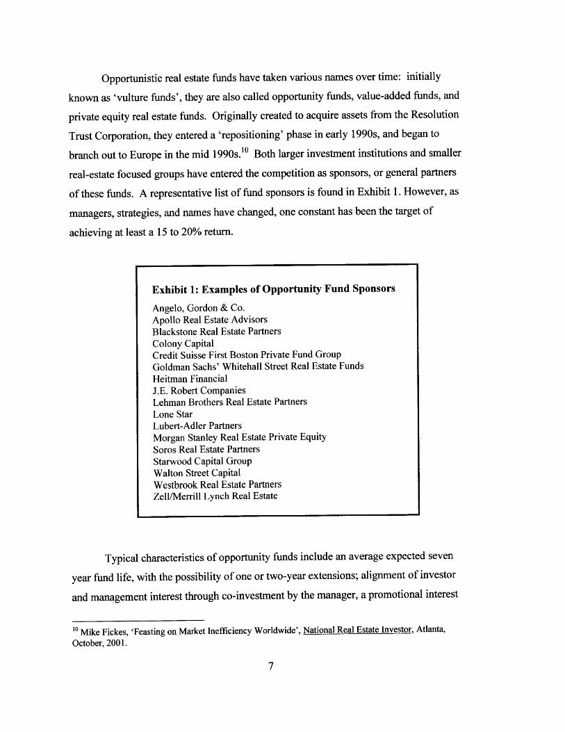
Opportunistic real estate funds have taken various names over time: initially
known as 'vulture funds', they are also called opportunity funds, value-added funds, and
private equity real estate funds. Originally created to acquire assets from the Resolution
Trust Corporation, they entered a 'repositioning' phase in early 1990s, and began to
branch out to Europe in the mid 1990s.10 Both larger investment institutions and smaller
real-estate focused groups have entered the competition as sponsors, or general partners
of these funds. A representative list of fund sponsors is found in Exhibit 1. However, as
managers, strategies, and names have changed, one constant has been the target of
achieving at least a 15 to 20% return.
Typical characteristics of opportunity funds include an average expected seven
year fund life, with the possibility of one or two-year extensions; alignment of investor
and management interest through co-investment by the manager, a promotional interest
10 Mike Fickes, 'Feasting on Market Inefficiency Worldwide', National Real Estate Investor, Atlanta,October, 2001.
Exhibit 1: Examples of Opportunity Fund Sponsors
Angelo, Gordon & Co.Apollo Real Estate AdvisorsBlackstone Real Estate PartnersColony CapitalCredit Suisse First Boston Private Fund GroupGoldman Sachs' Whitehall Street Real Estate FundsHeitman FinancialJ.E. Robert CompaniesLehman Brothers Real Estate PartnersLone StarLubert-Adler PartnersMorgan Stanley Real Estate Private EquitySoros Real Estate PartnersStarwood Capital GroupWalton Street CapitalWestbrook Real Estate PartnersZell/Merrill Lynch Real Estate
paid as an incentive to the manager after a return hurdle has been met, and a 1-2% annual
management fee. In general, opportunity funds offer managers more flexibility than
separate account investment: investors commit capital to the fund and managers have
discretion over which investments are made. On the other hand, opportunity funds are
also less liquid investments: capital is committed for the life of the fund and an investor
has no control over when monies will be returned. One result of the long life cycle of
opportunistic funds is that managers have very limited track records to leverage in
marketing their current funds."1
Funds are usually structured as limited partnerships, with the fund sponsor serving
as the general partner and investors participating as limited partners. Manager and
investor interests are aligned by co-investment in the fund by the general partner and
incentive fees that accrue to the general partner after a hurdle rate of return is achieved.
With high return expectations, investments tend to be assets where the manager
can actively increase value in a short time and then resell the asset: holding periods for
typical assets tend to be two to four years. The majority of return in opportunity funds
comes from appreciation over a short period of time, in contrast to 'core' real estate
investment, where current income is a significant factor in return. Investments are wide-
ranging and include non-performing loan pools, land development, hotel companies,
property conversion or redevelopment.' 3 Because of the focus on high returns, managers
tend to be "'traders' and 'value-enhancers' as opposed to 'operators', frequently pursuing
event-driven assets."' 4 In addition, to increase return, funds tend to be highly leveraged,
with an average of 61% leverage.15
" Peter Linneman and Stanley Ross, "Real Estate Private Equity Funds," white paper, Zell/Lurie Real
Estate Center, 2002, p. 10-11.12 McGurk, John. "Opportunity Funds - Impact of Loads, Leverage and Incentive Interest," Institute for
Fiduciary Education, 2002, p. 2 .13 Ernst & Young, "Opportunistic Investing: Real Estate Private Equity Funds", 2002, p. 5.14 Peter Linneman and Stanley Ross, "Real Estate Private Equity Funds," white paper, Zell/Lurie Real
Estate Center, 2002,, p. 8.15 Pension Consulting Alliance, "Real Estate Opportunity Funds: DejA vu All Over Again," May 2003, p. 5.
The high risk/high return strategy of funds means that benchmarking performance
is problematic. The NAREIT and NCREIF indexes, focusing on 'core' investment
properties, have a much lower risk profile, and thus are not appropriate for comparison.
In addition, they are calculated using a time-weighted return instead of the internal rate of
return measure typically used to evaluate opportunity fund investment performance.
Exacerbating the difficulty of measuring and comparing fund performance is the wide
range of investments: land development, loan work-outs, and assisted-living projects are
all examples of potential opportunity fund investments, but have very few common
characteristics.16 Finally, the absence of valuation standards 7 means that terminal
values, used by fund managers to calculate interim or expected returns, may be historical
cost, tax basis, or appraisal value. This results in questionable reporting consistency:
interim or projected performance measures calculated by different managers may or may
not be appropriate for comparison among funds.
The performance metric most generally accepted and used to measure
performance of opportunity funds is the internal rate of return, or IRR. The internal rate
of return of an investment is the discount rate that, applied to all cash flows associated
with an investment, results in a zero net present value. IRR is also recognized by the
Association of Investment Management Research as being the most appropriate measure
for investments such as venture capital or private equity investments.19 Reasons that the
IRR is the best measure of opportunity fund returns include the fact that the general
partner controls the timing of cash flows in and out, that the calculation of a time-
weighted return is distorted by the low or negative returns generated during the initial
16 Ernst & Young, "Opportunistic Investing: Real Estate Private Equity Funds", 2002, p. 5.17 Peter Linneman and Stanley Ross, "Real Estate Private Equity Funds," white paper, Zell/Lurie RealEstate Center, 2002, p. 15.18 98% of partners use the IRR metric according to the survey conducted by Pension Consulting Alliance,Inc., "Real Estate Opportunity Funds: The Numbers Behind the Story," April 2001, p. 43.19 Venture Economics website, http://www.ventureeconomics.com/vec/methodology.html#13.
asset acquisition period, and the fact that no valuation occurs at interim periods.20 Other
metrics observed include the time-weighted return and the cash multiple.
Topics currently of concern to opportunity fund managers and investors include
the development of a secondary market21 for limited partnership interests, which will
increase liquidity for investors; tax issues of concern to foreign and tax-exempt
investors; and the necessity of establishing reporting standards. This last issue has
arisen in response to criticism from investors surrounding the lack of transparency in
investments, particularly joint venture deals.23
20 Pension Consulting Alliance, Inc., "Real Estate Opportunity Funds: The Numbers Behind the Story",
April, 2001, p. 51.21 Seminar, "Liquidity Through Secondary Market Transactions," Fourth Annual U.S. Real Estate
Opportunity & Private Fund Investing Forum, Information Management Network, May 29, 2003.
22 Ernst & Young, "Opportunistic Investing: Real Estate Private Equity Funds", 2002, p. 2.23 Sally Haskins and Joanne Douvas, presentations constituting part of "Current Issues for Investors" and
presentation by Nori Gerardo Lietz at the Real Estate Opportunity and Private Fund Investing Forum, New
York City, May 29, 2003.

I1. Literature Review
Literature on performance persistence has focused mainly on persistence in
mutual funds. As real estate opportunity funds are a relatively recent investment vehicle,
it is not surprising that there have been no studies of performance persistence in these
funds. Also pertinent is additional literature on correlation and persistence in investments
such as hedge funds and private equity funds that have similarities to opportunity funds.
Methodologies and Survivorship Bias
Carpenter and Lynch (1999) evaluate various tests of persistence in addition to
considering the effects of survivorship bias on performance persistence in mutual funds.
They conclude that the t-test is best for comparing decile performance; the chi-squared
test is the most robust where attrition bias exists; and the Spearman rank correlation
coefficient is the most powerful test in the absence of survivorship bias. The chi-squared
test and Spearman rank correlation coefficient were used in this study in addition to
regression analysis, and are described below in Section V., "Methodology." Construction
of portfolios based on decile performance was not possible due to the nature of the data,
as also described in Section V.
Survivorship bias arises when underperforming funds are eliminated from a data
set, leaving only funds that continue to exist for comparison, as opposed to a true
benchmark of all funds. This bias can affect not only the apparent correlation in returns,
but the returns themselves: Koh, Lee, and Fai (2001) found that with hedge funds,
survivorship bias results in overall returns being overstated by 1.5-3% per year.
Brown, Goetzmann, Ibbotson, and Ross (1992), showed that the survivorship bias
created by eliminating funds with the lowest total returns or lowest alpha creates apparent
performance persistence, although this bias can be addressed by various measures. They

also concluded that the cross-product ratio test is not appropriate when funds drop out of
the sample due to poor performance and that survivorship bias is exacerbated by
volatility.
Various authors have addressed survivorship bias. Grinblatt and Titman (1992),
using a benchmark constructed to avoid bias, still find evidence of persistence in mutual
fund performance. Elton, Gruber, and Blake, (1996) also investigating mutual fund
performance, found that even eliminating the funds most frequently ranked in the top
decile of performance, risk-adjusted returns are still predictive of both short & long-run
future performance.
Mutual Funds
Studies of mutual fund performance generally find evidence of serial performance
correlation. Persistence is strongest in the short term and with poor performance.
Goetzmann and Ibbotson (1994) studied patterns in mutual fund return behavior
over two-year, one-year, and monthly periods and found the strongest evidence of
persistence in the monthly results. In addition, funds with higher volatility exhibited
stronger evidence of correlated returns. Two-way contingency tables were constructed
based on funds' performance as measured by returns and alphas, alpha being defined as
the excess return achieved over that which would be predicted by the amount of
systematic risk. The indication of correlation was verified the by regressing funds'
alphas on the previous period's alpha.
Hedricks, Patel, and Zeckhauser (1993) and Malkiel (1995) also found mutual
fund returns predictable and demonstrated the performance potential of an investment
strategy exploiting the short-term persistence they found. Elton, Gruber, and Blake
(1996) found that risk-adjusted returns are predictive of both short & long-run future
performance, and used Modern Portfolio Theory to select outperforming portfolios of
funds. However, Brown and Goetzmann (1995) showed that investing in deciles of
ranked fund portfolios resulted in high volatility due to a loss of diversification.
Brown and Goetzmann (1995), using contingency tables and the crossproduct
ratio test, compared performance to absolute and relative benchmarks and found that
persistence was due mostly to funds lagging the S&P 500. In addition, performance was
correlated across managers, and was most persistent in underperforming funds.
Carhart (1997) charted factors such as expenses that explain persistence in mutual
funds, concluding that only poor performance is persistent, perhaps due to illiquid stocks.
Using the Spearman nonparametric test of rank ordering, he was unable to reject the null
hypothesis that performance measures are randomly ordered.
Hedge Funds
The literature on hedge funds is more divided than that on mutual funds as to the
existence of performance persistence: different authors have found that performance may
or not be persistent, and that consistently superior strategies may or may not exist.
According to Koh, Lee, and Fai (2001), hedge funds are small, leveraged, and organized
around experienced investment professionals motivated with incentive fees, who often
invest their own capital in partnership. Thus, they have many characteristics in common
with opportunity funds.
Testing for performance by regressing current returns on past returns, Brown,
Goetzmann, and Ibbotson (1998) found no evidence of performance persistence in hedge
funds, also concluding that fund size was unrelated to performance. Kat and Menexe,
(2002) using contingency tables and regression analysis, found persistence in standard
deviation and correlation with the market but little persistence in hedge fund returns.
They suggest that performance measurements may gauge persistence of style rather than

superior returns, recommending that returns are more useful to compare relative risk
among funds with similar strategies than as a predictor of the fund's risk profile.
In contrast, Agarwal and Naik (2001) found performance persistence at a
quarterly level that was unrelated to strategy. Bares, Gibson and Gyger, (2002) testing
for performance persistence using portfolios constructed on return and risk-adjusted
return, also found evidence of performance persistence among hedge funds over short-
term holding periods. They also concluded that some strategies consistently outperform
others.
In a working paper on hedge funds, Getmansky, Lo, and Makarov (2003) found
that serial correlation in returns was most likely due to illiquidity of assets and non-
synchronous trading, and may also be the result of varying expected returns, varying
leverage, and fund compensation structure.
Other Investments
Private equity funds are described by Ljungqvist and Richardson (2003) as having
a long illiquid initial period of several years of negative returns, as being affected by the
drawdown timing, and as being limited by self-reporting and the unknown risk to
investors in the underlying assets. These are all characteristics that make such vehicles
similar to real estate opportunity funds. Their study does not include an analysis of fund
performance persistence, but does find that fund size and the amount of capital
committed in all funds in the inception year of a fund are correlated to fund performance.
IV. Data
Data used in this study was provided by Pension Consulting Alliance, Inc, a
consultancy organization which in addition to providing advisory services for pension
funds, conducts research and reporting on investment topics.2 4 Data was gathered from
fund general partners by questionnaires and interviews for reports in 2001 and 2003. 55
firms representing over 187 partnerships during the period 1988 to 2000 participated in
the initial survey. This was approximately 90% of current firms, based on the number of
firms rather than the amount of capital.2 s The second survey collected information from
51 firms and over 255 funds.26 Manager and fund identity were masked to preserve
confidentiality.
The data set consists of 43 managers with 110 funds started between 1991 and
2001. Eight of the 51 firms were eliminated from the data set, primarily because
confidentiality agreements prevented them from providing information. The eliminated
firms did not share common characteristics such as size, location, or clientele. Of these
43 remaining managers, 24 had more than one fund. Information on the underlying
investments in some of the funds was provided by some managers. One limitation of the
data is that very few of the funds have fully liquidated. Returns for the remaining funds
are based on interim returns and expected return and terminal values calculated by the
managers.
Internal rates of return in the database are based on the managers' valuation of the
residual assets remaining in the funds as of the end of the data history in 2001. Although
investors have noted inconsistency in reporting and measurements among opportunity
2 Pension Consulting Alliance website: http://www.pensionconsulting.com.25 Pension Consulting Alliance, "Real Estate Opportunity Funds: The Numbers Behind the Story," April
2001, p. 2.26 Pension Consulting Alliance, "Real Estate Opportunity Funds: DejA vu All Over Again," May 2003, p. 3.27 Email correspondence with Denise Mouchakkaa, Pension Consulting Alliance, July, 2003.
fund managers,28 Pension Consulting Alliance investigated and confirmed return
calculations where possible, using cash flow information provided by both general
partners and investors.29 Thus, although terminal valuations remain dependent upon
managers' valuation methodology, the data reflects the highest level of consistency
possible.
Opportunistic real estate private equity funds are less liquid than mutual funds:
with no continuous exchange mechanism such as a stock market, it is impossible to
calculate a daily, weekly, or annual return based on daily trading or NAV. With no
market valuation for the fund during its life, a single IRR is calculated for the life of fund
based on contributions and distributions. Thus, although some of the tests employed are
similar to those used in the literature surveyed, only one return data point exists for each
fund, rather than the many data points that can be used to calculate a series of time-
weighted returns for a single mutual fund based on its trading history.
The extent to which attrition bias exists in the sample is unclear. While some
firms included in the earlier survey were not included in the later survey, not all of this
attrition was due to poor performance of their funds. However, if the reduction from 55
managers in 2000 survey to 51 managers in the 2002 survey were indicative of fund
attrition, it suggests that about 4% of managers are eliminated each year. For mutual
funds, Brown Goetzmann, Ibbotson, and Ross find this degree of attrition corresponds to
an return effect of about .4% annually. 30
Another potential issue that could be raised with the data lies with the wide
variation in the definition of opportunity fund: some managers included in the survey
define their funds as value-added or core-plus rather than as opportunity. Pension
28 Pension Consulting Alliance, "Real Estate Opportunity Funds: The Numbers Behind the Story," page
59, and Sally Haskins, Russell Real Estate Advisors, 'Perspectives on Reporting', presented May 29, 2003at the Real Estate Opportunity and Private Fund Investing Forum, New York City.29Email correspondence with Denise Mouchakkaa, Pension Consulting Alliance, July, 2003.30 Brown, Goetzmann, Ibbotson, Ross, "Survivorship Bias in Performance Studies." The Review of
Financial Studies Volume 5, no. 4, 1992, p. 568.
Consulting Alliance considered target returns, leverage, and investment returns in
including a fund in the survey:3 1 funds targeting 18% or higher gross returns and using at
least 50% leverage were defined as opportunity funds. The difficulty in defining the
realm of opportunity funds is illustrated by the difference in estimates of funds and
capital raised: Ernst & Young estimated that by 2000, $55.27 billion had been raised by
122 funds3 2 , compared while Pension Consulting Alliance calculated $71.37 billion
(revised in 2003 to $77.05 billion) raised by 187 funds.33
A manager is considered to be the sponsoring firm rather than the individual
corporate officers. Although individuals may have different management styles, abilities,
and connections to deal sources, this was not tracked in the data set. Considering the
short time period, it may be reasonable to expect that the primary participants stayed the
same over the ten year period for most firms, but future studies may want to consider
individual manager involvement as well as corporate management.
The data characteristics have been well described in Pension Consulting
Alliance's two reports: a summary of fund returns and size follows.
It is interesting to note that of all the funds included in the database, only 48, or
44% of the 110 funds, achieved net returns exceeding 15%. Only 28, or 25% of the
funds, achieved net returns exceeding 20%. Funds from the 1991 - 1997 cohorts were
more successful in reaching their targeted return: 28, or 61% of the 46 funds from the
period, achieved a net IRR in excess of 15%. 15 funds, or 33%, returned in excess of
20% net.
31 Email correspondence with Denise Mouchakkaa, Pension Consulting Alliance, July, 200332 Ernst & Young, "Opportunistic Investing: Real Estate Private Equity Funds", 2002, p. 1.3 Pension Consulting Alliance, "Real Estate Opportunity Funds: The Numbers Behind the Story", April2001, p.6, revised in "Real Estate Opportunity Funds: DejA vu All Over Again", May 2003, p. 5.
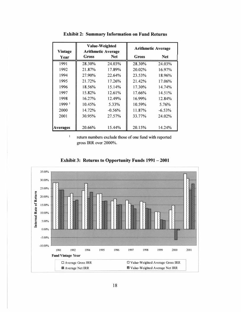
Exhibit 2: Summary Information on Fund Returns
Value-Weighted Arithmetic AverageVintage Arithmetic Average
Year Gross Net Gross Net1991 28.30% 24.03% 28.30% 24.03%1992 21.87% 17.89% 20.02% 16.97%1994 27.90% 22.64% 23.53% 18.96%1995 21.72% 17.26% 21.42% 17.06%1996 18.56% 15.14% 17.30% 14.74%1997 15.82% 12.61% 17.66% 14.51%1998 16.27% 12.49% 16.99% 12.84%1999 1 10.45% 5.33% 10.59% 5.76%2000 14.72% -0.56% 11.87% -6.53%2001 30.95% 27.57% 33.77% 24.02%
Averages 20.66% 15.44% 20.15% 14.24%
1 return numbers exclude thosegross IRR over 2000%.
of one fund with reported
Exhibit 3: Returns to Opportunity Funds 1991 - 2001
35.00%
30.00%
25.00%
20.000/
e15.00%
10.0%/
5.00%
-5.000/
-10.00%1991 1992 1994 1995 1996 1997 1998 1999 2000 2001
Fund Vintage Year
o Average Gross IRR [] Value-Weighted Average Gross IRR
* Average Net IRR H Value-Weighted Average Net IRR
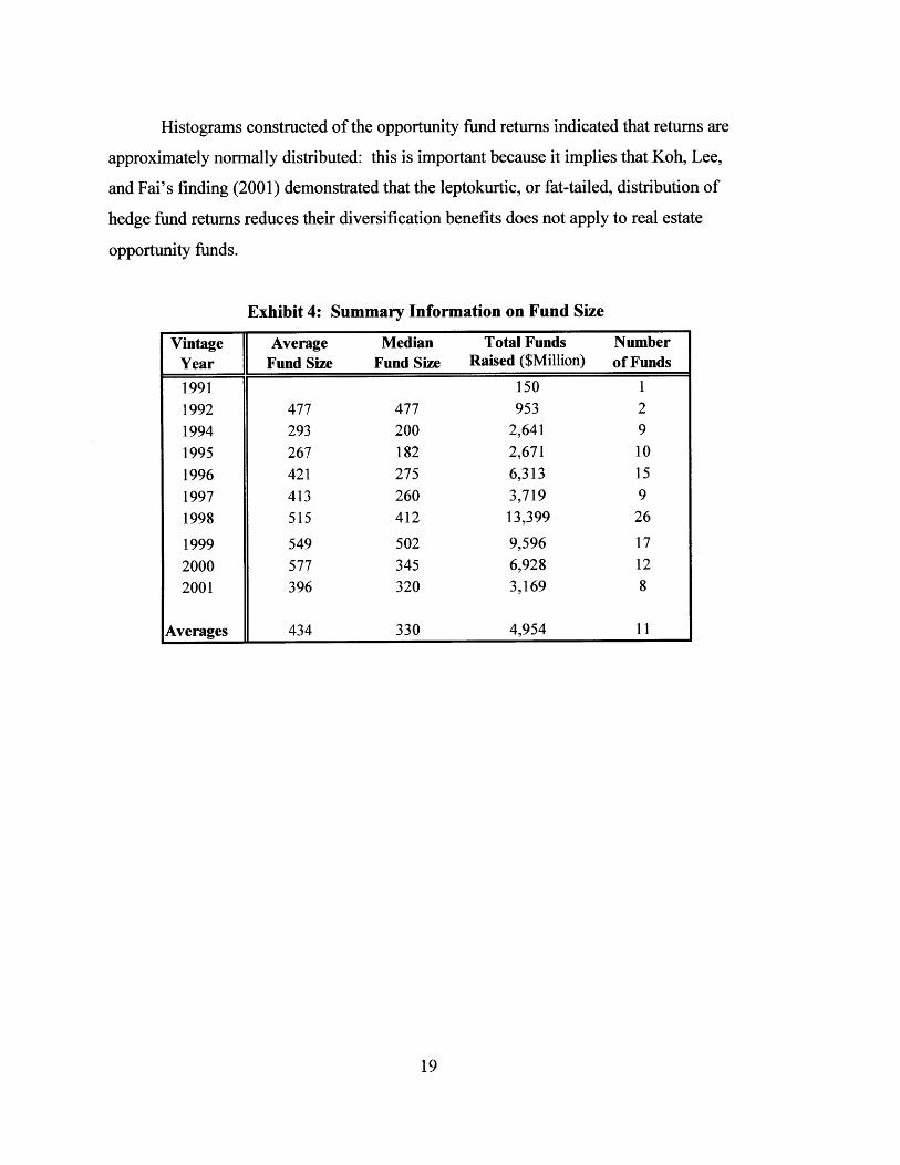
Histograms constructed of the opportunity fund returns indicated that returns are
approximately normally distributed: this is important because it implies that Koh, Lee,
and Fai's finding (2001) demonstrated that the leptokurtic, or fat-tailed, distribution of
hedge fund returns reduces their diversification benefits does not apply to real estate
opportunity funds.
Exhibit 4: Summary Information on Fund Size
Vintage Average Median Total Funds NumberYear Fund Size Fund Size Raised ($Million) of Funds
1991 150 11992 477 477 953 2
1994 293 200 2,641 91995 267 182 2,671 10
1996 421 275 6,313 15
1997 413 260 3,719 91998 515 412 13,399 26
1999 549 502 9,596 172000 577 345 6,928 12
2001 396 320 3,169 8
Averages 434 330 4,954 11
V. Methodology
Various tests, have been used to analyze persistence in mutual funds, hedge funds,
and venture capital funds. Parametric tests are those used with data which has a known
distribution, defined by parameters such as mean and variance. Nonparametric methods
are those that can be used with data that is ordinal, or whose distribution is unknown.3 4 In
both cases the tests attempt to disprove a null hypothesis about relationships that may or
may not exist in the studied data. In this case, both parametric and nonparametric tests
were used to test the null hypothesis that no relationship exists between the performance
of a manager's past funds and a manager's later funds. Parametric tests consisted of
regressing fund performance on past fund performance and other independent variables.
Nonparametric tests included constructing and analyzing contingency tables, and
calculating and analyzing the Spearman rank correlation coefficient and the Kendall
coefficient. All tests were performed using the data analysis software in Microsoft Excel
2002.
An additional test frequently seen in the literature is the creation of an investment
strategy based on historical evidence of persistence and the analysis of the strategy's
simulated performance had it been employed over historical periods of time. Due to the
lack of multiple return measurements and the short period of time captured by the data,
creating an investment strategy and testing its performance over historical periods of time
was not possible.
Tests were performed using the entire database and then repeated using only
funds originated in the years 1991 to 1997. Since funds established prior to 1997 might
be expected to have completed or be reaching the end of their life cycle, and thus have
more definite return numbers, it might be argued that conclusions drawn from this
14 P. Sprent and N.C. Smeeton, Applied Nonparametric Statistical Methods, 3rd edition (New York:
Chapman & Hall/CRC, 2001), p.3.
reiteration could be more reliable. However, it should be noted that further restricting the
already limited size of the data set results in a very small sample size.
To permit comparison of fund performance across different vintage years, fund
performance was ranked and subsequently normalized. Fund performance was evaluated
based on normalized ranking rather than absolute performance or performance relative to
a benchmark. For each group of funds with a common year of inception, each individual
fund was ranked from 1 for highest to n for the lowest-performing fund based on the
calculated IRR. Then, a normalized ranking (NR) with a value from 1 to 0 inclusive was
calculated using:
NR = (n - r)/(n- 1)
where n = number of funds in the vintage year and r absolute rank of the fund. Both
rank and normalized rank were calculated based on both net and gross IRR for each fund,
and tests were performed with both net and gross rankings. In vintage year 1991, only
one fund exists in the data set: it was assigned a normalized rank of 0.5.
The first nonparametric test is the construction of contingency tables, following
the methodology of Brown and Goetzmann (1995). This test has been used in many past
studies of performance persistence, and was selected in part because the chi-squared test
which is based on it was found by Carpenter and Lynch (1999) to be a strong test of
performance persistence even in the presence of any attribution bias. Pairs of funds are
identified from sequential funds: for example, with one manager's funds A, B, and C in
three subsequent years, two pairs are established (A-B and B-C). Then, the pairs of funds
are sorted into a matrix depending on their rankings: win/win, win/lose, lose/win,
lose/lose. 'Win' is defined as a ranking in the top half (NR > 0.5), third (NR > 0.66), or
quartile (NR > 0.75)." The matrix generated is then compared to the frequency that
would be expected if fund performance were independent of previous fund performance.
* In the few cases where a manager had more than one fund in a vintage year, the first variable for the next
pair is defined as a win or lose by an average of the rankings for the preceding year funds.
The chi-squared test is then used to determine if the deviation from the expected
distribution is statistically significant.
Another indicator of statistical significance generated using the contingency table
is the cross-product ratio test. Used by Brown and Goetzmann (1995), the cross-product
ratio is obtained by dividing the product of the win/win and lose/lose cells by the product
of the win/lose and lose/win cells. [ (WWxLL)/(WLxLW) ] In the case of no
performance correlation, the expected ratio is one. The ratio can be tested statistically by
calculating a z-statistic = ln(CPR)/ S1n(CPR) ,36 where the standard error of the natural log
of the cross product ratio, S1n(CPR) = 4(1/WW + 1/WL + 1/LW + 1/LL).
Additional tests for correlation or dependence between two variables are the
Spearman rank correlation coefficient, or rho, and the Kendall correlation coefficient, or
tau. Pairs of funds are identified, as with the contingency tables, and the ranks of each
pair are compared. These measures test whether there is a correlation in trend:37 if
ranking of a subsequent fund increases (decreases) as the ranking of the earlier fund
increases (decreases). The null hypothesis being tested is that the first and second
rankings of each pair are unrelated. Both coefficients will have values between -1 and 1:
a value near zero indicates a lack of association.
The Spearman rank correlation coefficient was identified by Carpenter and Lynch
(1999) as being a strong test for persistence in the absence of attrition bias. The formula
for Spearman's rho is:
rs = 1 -6T/n(n2-1)
36 Harry Kat and Faye Menexe, "Persistence in Hedge Fund Performance: The True Value of a Track
Record," Alternative Investment Research Centre Working Paper Series, Working Paper #0007, 2002.37 P. Sprent and N.C. Smeeton, Applied Nonparametric Statistical Methods, 3 rd edition, p. 243.

where T = i(ri - si) 2, with (ri, si) indicating the ranks of each pair38 . The null hypothesis
of no association between the paired variables is then tested based on a t-statistic
calculated using t = rs4(n-2)/(1-rs2) with d.f. = n - 2.39
Kendall's tau is similar to Spearman's rho, but has been described as having a
more intuitive and simple interpretation. 40 In addition, there is a simple variation to allow
for adjustment due to ties in ranks. Again, pairs of variables are identified - in this study,
fund ranking and subsequent fund ranking. The first member of each set is called the x-
rank, and the second the y-rank. The pairs are arranged with the x-ranks in ascending
order and then the differences between consecutive y-ranks are scored as a concordance
if the difference is positive and a discordance if negative. The number of concordances
(ne) and discordances (nd) are then used to calculate Kendall's tau,
tk = (ne - nd)/{(l/2)n(n-l)}
The basis of Kendall's tau is that if the ranks of x and y are associated, then if the
x-ranks are arranged in ascending order the y-ranks should be increasing if there is
positive association and decreasing if there is negative association. 4 1 Taub, a variation,
reflects an adjustment in the formula to account for ties in rank and is calculated,
tb - 2(ne - n)/(n 2 - n - 2t') 4 (n2 -n-2u')
with t' = (Zt2 - Et)/2 where t is equal to the number of tied observations at any given
value in the x-ranks and u' is the same calculation for the y-ranks.42 The resulting
coefficient is then converted into a t-statistic using the equation 43
38 P. Sprent and N.C. Smeeton, Applied Nonparametric Statistical Methods, 3rd edition, p. 243.39 http://www.stats.ox.ac.uk/~marchini/teaching/booklets/fb.pdf, online resource from Oxford University,p. 8-10.40 Jean Dickinson Gibbons, Nonparametric Measures of Association,, Sage University Papers, Quantitative
Applications in the Social Sciences, vol. 91. (Newbury Park, California: Sage Publications, Inc., 1993), p.20.41 P. Sprent and N.C. Smeeton, Applied Nonparametric Statistical Methods, 3 rd edition, p. 247.
42 Jean Dickinson Gibbons, Nonparametric Measures of Association,, Sage University Papers, Quantitative
Applications in the Social Sciences, vol. 91. (Newbury Park, California: Sage Publications, Inc., 1993), p.
15.
t-statistic = 3tk{' [n(n-1)] / 1 [2 (2n + 5)]}
where n = number of paired ranks. This t-statistic is then used to evaluate the probability
of obtaining the given coefficient in the case that the null hypothesis were true.
In addition to the nonparametric tests conducted, regression analyses were also
performed. Because, as noted earlier, there is only one performance measure for each
fund, the analysis tests for a relationship between the performance of a fund and that of
subsequent fund with the same manager. This is in contrast to the literature surrounding
mutual funds, which tests for a relationship with subsequent performance of the same
fund.
The initial test is to regress the ranking of a fund onto the existence of a previous
fund. A dummy variable is set equal to one if the manager has had a previous fund, zero
if the manager has no previous fund. The formula being estimated in this case takes the
form:
NR=a + pEF
with NR signifying the fund's normalized rank and EF representing a dummy variable for
the existence of an earlier fund. There are two plausible expectations for the results: the
first, that managers benefit from previous experience and therefore that performance will
improve in subsequent funds. The second possible expectation is that managers of funds
who outperform peers get another chance, but then are unlikely to outperform again. In
the first case, a positive coefficient on the independent variable would be expected; in the
second case, a negative coefficient.
Later analyses regress the performance of a fund onto the performance of one or
more earlier funds by the same manager, the performance of a manager's fund exactly or
4 Peter Chen and Paula Popovich, Correlation: Parametric and Nonparametric Measures, Sage UniversityPapers, Quantitative Applications in the Social Sciences, vol. 139. (Thousand Oaks, California: SagePublications, Inc., 2002), p. 84.
more than five years earlier, or the average performance of all the manager's previous
funds. The formula being estimated takes the form:
NR = a + PLR (+ SLLR)
where NR again signifies the fund's normalized rank, LR represents the lagged rank from
the appropriate prior fund, and LLR represents the rank of an additional previous fund.
In all cases, if past performance is positively correlated with future performance, a
positive-signed coefficient on the independent variable or variables would be expected.
Additional regressions test past performance in combination with geographical
focus, product focus, leverage ratio, size of fund, amount of funds raised in a vintage
year, and parent company focus. Information on fund assets and strategies was not
available for all the managers, so the sample size for these regressions was small. The
formula being estimated takes the form:
NR = a + PLR + 6DF
where NR again signifies the fund's normalized rank, LR represents the lagged rank from
the appropriate prior fund, and DF represents the descriptive feature such as focus or size
of the fund. Again, if any of these factors has a positive relationship with fund
performance, a positively-signed coefficient on the independent variable would be
expected.
VI. Results and Analysis
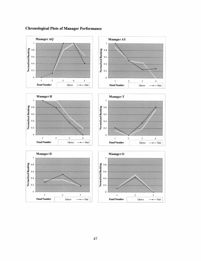
Before commencing statistical analysis of the fund performance data, fund return
and rankings were analyzed graphically. Charting chronological performance of
managers' funds with ranking on the x-axis and fund number on the y-axis gave no clear
indication of any consistent patterns. The series was approximately equally divided
between rising, falling, u-shaped, and bell-shaped graphs, with only one graph taking a
'flat' shape that would most correspond to performance persistence. Interestingly, only
four managers show identical rankings based on both gross and net IRRs. Chronological
charts of all 24 managers with multiple funds are included in the Appendix, as are full
regression analysis outputs.
Contingency Tables
Contingency tables were constructed using pairs of funds from managers with
more than one fund. Using all funds resulted in 68 pairs, while restricting the funds to
those started between 1991 and 1997 resulted in 23 pairs. The first matrices divided
funds into win/win, win/lose, lose/win, and lose/lose quadrants based on above- or
below-median performance. The null hypothesis is that the first ranking and second
ranking are unrelated, giving an expected frequency in each cell of the matrix of one-
quarter of the total number of pairs. The expected and actual frequencies are shown
below.
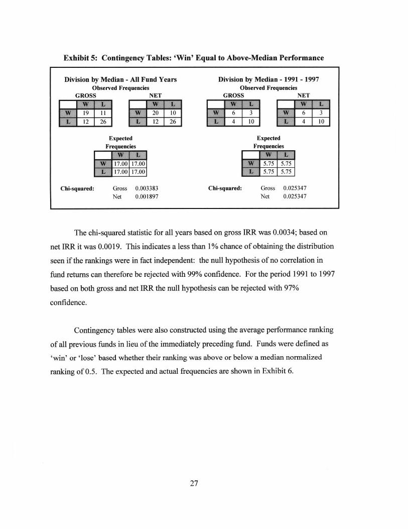
Exhibit 5: Contingency Tables: 'Win' Equal to Above-Median Performance
Division by Median - All Fund Years Division by Median - 1991 - 1997Observed Frequencies Observed Frequencies
GROSS NET GROSS NET
r19 111 20 10 6 3 6 3
12 126 12 26 4 10 4 10
Expected ExpectedFrequencies Frequencies
17.0017.005.75 5.7517.0017.005.75 5.75
Chi-squared: Gross 0.003383 Chi-squared: Gross 0.025347Net 0.001897 Net 0.025347
The chi-squared statistic for all years based on gross IRR was 0.0034; based on
net IRR it was 0.0019. This indicates a less than 1% chance of obtaining the distribution
seen if the rankings were in fact independent: the null hypothesis of no correlation in
fund returns can therefore be rejected with 99% confidence. For the period 1991 to 1997
based on both gross and net IRR the null hypothesis can be rejected with 97%
confidence.
Contingency tables were also constructed using the average performance ranking
of all previous funds in lieu of the immediately preceding fund. Funds were defined as
'win' or 'lose' based whether their ranking was above or below a median normalized
ranking of 0.5. The expected and actual frequencies are shown in Exhibit 6.
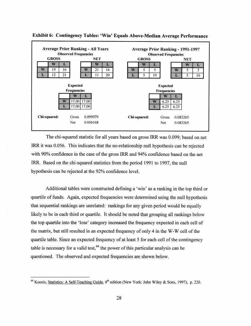
Exhibit 6: Contingency Tables: 'Win' Equals Above-Median Average Performance
Average Prior Ranking - All YearsObserved Frequencies
GROSS NET
19 16 21 16
12 21 11 20
ExpectedFrequencies
I /L1.UU I/u
Gross 0.099979Net 0.056168
Average Prior Ranking - 1991-1997Observed Frequencies
GROSS NET
Expected
Chi-squared: Gross 0.083265Net 0.083265
The chi-squared statistic for all years based on gross IRR was 0.099; based on net
IRR it was 0.056. This indicates that the no-relationship null hypothesis can be rejected
with 90% confidence in the case of the gross IRR and 94% confidence based on the net
IRR. Based on the chi-squared statistics from the period 1991 to 1997, the null
hypothesis can be rejected at the 92% confidence level.
Additional tables were constructed defining a 'win' as a ranking in the top third or
quartile of funds. Again, expected frequencies were determined using the null hypothesis
that sequential rankings are unrelated: rankings for any given period would be equally
likely to be in each third or quartile. It should be noted that grouping all rankings below
the top quartile into the 'lose' category increased the frequency expected in each cell of
the matrix, but still resulted in an expected frequency of only 4 in the W-W cell of the
quartile table. Since an expected frequency of at least 5 for each cell of the contingency
table is necessary for a valid test, 4the power of this particular analysis can be
questioned. The observed and expected frequencies are shown below.
4 Koosis, Statistics: A Self-Teaching Guide, 4O edition (New York: John Wiley & Sons, 1997), p. 220.
Chi-squared:
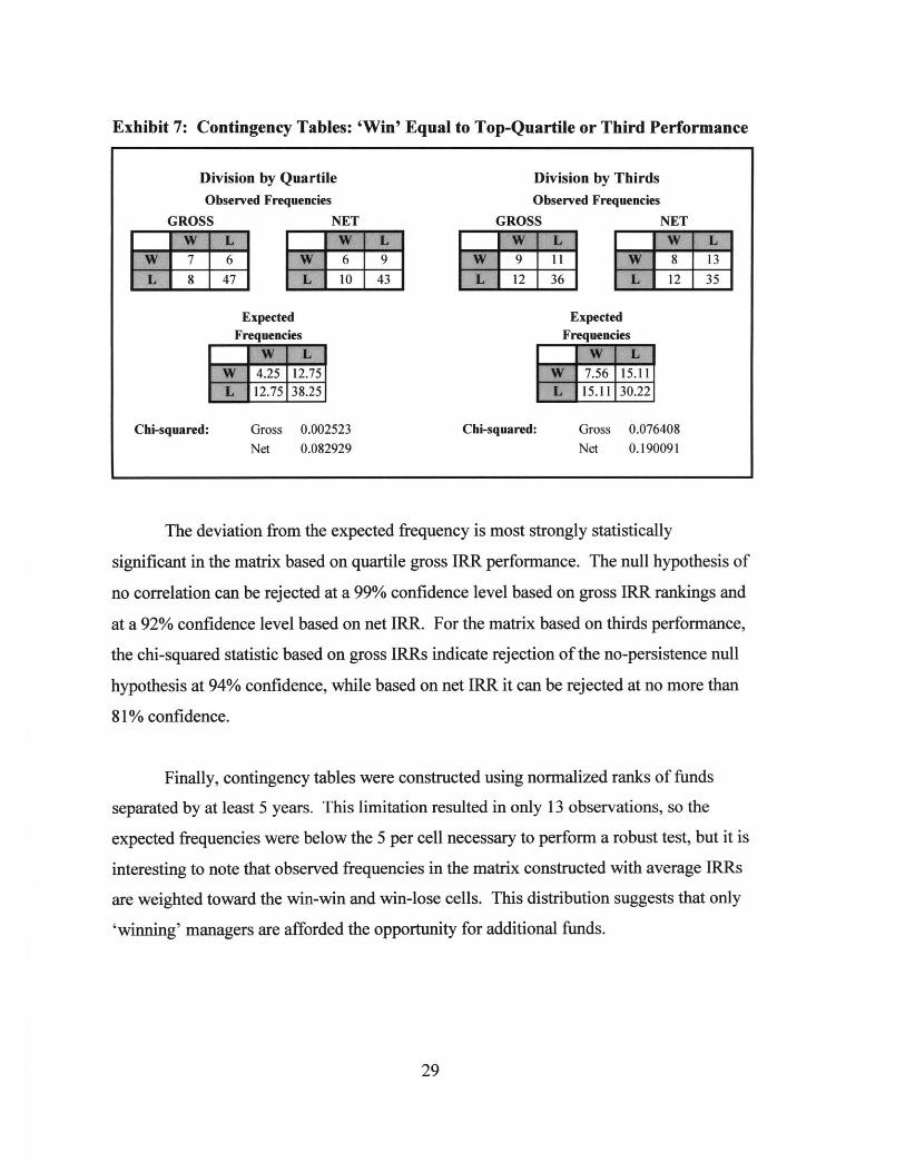
Exhibit 7: Contingency Tables: 'Win' Equal to Top-Quartile or Third Performance
Division by Quartile
Observed FrequenciesGROSS NET
7 6 6
8 47 K 10
ExpectedFrequencies
Gross 0.002523
Net 0.082929
Division by Thirds
Observed FrequenciesGROSS NET
Expected
Chi-squared: Gross 0.076408
Net 0.190091
The deviation from the expected frequency is most strongly statistically
significant in the matrix based on quartile gross IRR performance. The null hypothesis of
no correlation can be rejected at a 99% confidence level based on gross IRR rankings and
at a 92% confidence level based on net IRR. For the matrix based on thirds performance,
the chi-squared statistic based on gross IRRs indicate rejection of the no-persistence null
hypothesis at 94% confidence, while based on net IRR it can be rejected at no more than
81% confidence.
Finally, contingency tables were constructed using normalized ranks of funds
separated by at least 5 years. This limitation resulted in only 13 observations, so the
expected frequencies were below the 5 per cell necessary to perform a robust test, but it is
interesting to note that observed frequencies in the matrix constructed with average IRRs
are weighted toward the win-win and win-lose cells. This distribution suggests that only
'winning' managers are afforded the opportunity for additional funds.
Chi-squared:
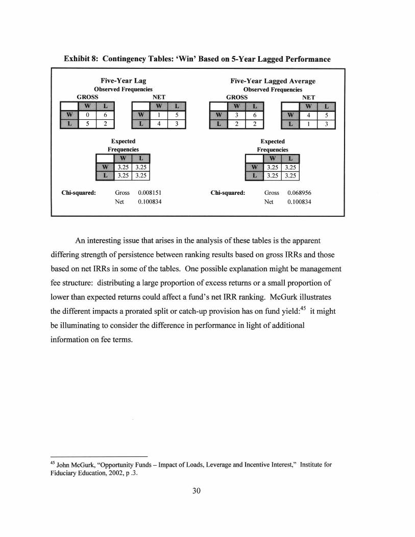
Exhibit 8: Contingency Tables: 'Win' Based on 5-Year Lagged Performance
Five-Year LagObserved Frequencies
GROSS NET
ExpectedFrequencies
3.25 13.25
Chi-squared: Gross 0.008151Net 0.100834
Five-Year Lagged AverageObserved Frequencies
GROSS NET
ExpectedFrequencies
Chi-squared:
L.zf 3.zI3.25 3.25
Gross 0.068956Net 0.100834
An interesting issue that arises in the analysis of these tables is the apparent
differing strength of persistence between ranking results based on gross IRRs and those
based on net IRRs in some of the tables. One possible explanation might be management
fee structure: distributing a large proportion of excess returns or a small proportion of
lower than expected returns could affect a fund's net IRR ranking. McGurk illustrates
the different impacts a prorated split or catch-up provision has on fund yield:45 it might
be illuminating to consider the difference in performance in light of additional
information on fee terms.
4 John McGurk, "Opportunity Funds - Impact of Loads, Leverage and Incentive Interest," Institute forFiduciary Education, 2002, p .3.
- NENMIEVWN __
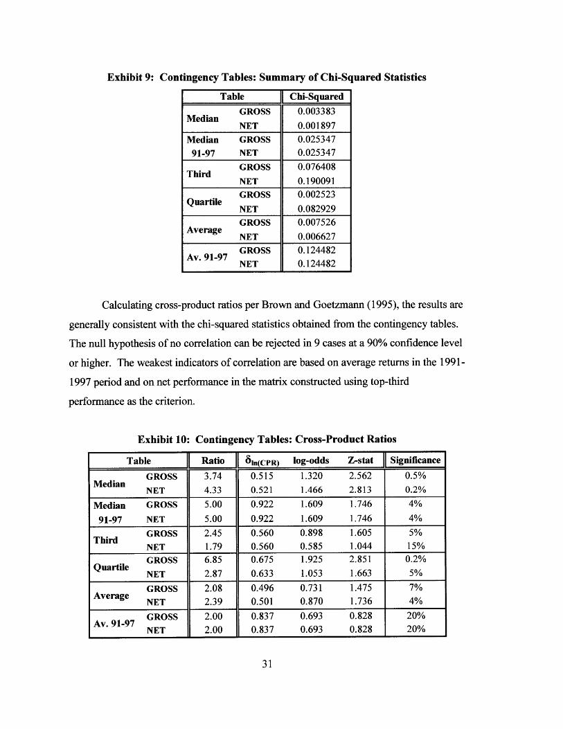
Exhibit 9: Contingency Tables: Summary of Chi-Squared Statistics
Table Chi-SquaredGROSS 0.003383
MedianNET 0.001897
Median GROSS 0.02534791-97 NET 0.025347
GROSS 0.076408Third
NET 0.190091GROSS 0.002523
Quartile NET 0.082929GROSS 0.007526
Average NET 0.006627GROSS 0.124482
Av. 91-97 NET 0.124482
Calculating cross-product ratios per Brown and Goetzmann (1995), the results are
generally consistent with the chi-squared statistics obtained from the contingency tables.
The null hypothesis of no correlation can be rejected in 9 cases at a 90% confidence level
or higher. The weakest indicators of correlation are based on average returns in the 1991-
1997 period and on net performance in the matrix constructed using top-third
performance as the criterion.
Exhibit 10: Contingency Tables: Cross-Product Ratios
Table Ratio Jin(CPR) log-odds Z-stat Significance
GROSS 3.74 0.515 1.320 2.562 0.5%Median NET 4.33 0.521 1.466 2.813 0.2%
Median GROSS 5.00 0.922 1.609 1.746 4%
91-97 NET 5.00 0.922 1.609 1.746 4%
Third GROSS 2.45 0.560 0.898 1.605 5%NET 1.79 0.560 0.585 1.044 15%GROSS 6.85 0.675 1.925 2.851 0.2%
Quartile NET 2.87 0.633 1.053 1.663 5%
GROSS 2.08 0.496 0.731 1.475 7%Average NET 2.39 0.501 0.870 1.736 4%
Av. 91-97 GROSS 2.00 0.837 0.693 0.828 20%NET 2.00 0.837 0.693 0.828 20%
In summary, the contingency tables indicate strong performance persistence based
upon division by above or below-median performance. Above-average performance
based on average past ranking, top quartile, or top third ranking is also persistent,
although weakly in the case of average past rankings over the period 1991 - 1997.
Rank Correlation Statistics
The next series of tests look at correlation in rank from one fund to the next. For
both the Spearman statistic and Kendall's tau, a value of 1 indicates that the first variable
and second variable are perfectly correlated, a value of - indicates the variables are
perfectly negatively correlated, and a value of 0 indicates no correlation between the
variables. The null hypothesis in all cases is that there is no association between the two
variables, with the alternative hypothesis being that there is association between them.
The first Spearman rank statistic was calculated using the normalized rank of a
managers' fund as the first variable and the normalized rank of the manager's next fund
as the second variable. With 68 pairs of variables, the calculated coefficients of 0.465
(based on gross IRR rankings) and 0.413 (based on net IRR rankings) indicate a strong
correlation between rankings: the null hypothesis of no persistence can be rejected at a
99% confidence level. The positively-signed coefficients suggest an alternate hypothesis
of positive correlation between performance of a manager's funds. Additional
coefficients were calculated limiting the data set to funds in the 1991 - 1997 period.
Again, the results were highly significant and the null hypothesis can be rejected at the
99% confidence level.
The Spearman rank statistic was then calculated using the average normalized
rank of all of a manager's previous funds as the first variable and the normalized rank of
the manager's next fund as the second variable. The calculated coefficients of 0.310
(based on gross IRR rankings) and 0.256 (based on net IRR rankings) again indicate a
strong correlation between rankings: the null hypothesis of no persistence can be rejected
at a 99% confidence level. Limiting the data set to funds in the 1991 - 1997 period, the
null hypothesis can be rejected at a 99% confidence level based on gross IRR and at a
95% confidence level based on net IRR.
Additional coefficients were calculated using funds that had another fund by the
same manager with at least a five year lag, resulting in 13 pairs of variables. The first
variable was the rank of the fund most immediately preceding the later fund with the
four-year intervening period, or the average of the ranks of funds by the same manager
that were at least four years previous to the fund ranked in the second variable. In both
cases the second variable was the rank of the later fund. Coefficients generated were in
the range of -0.651 to -0.330. These statistics are not significant at a 10% level of
confidence: the null hypothesis of no correlation cannot be disproved in this case.
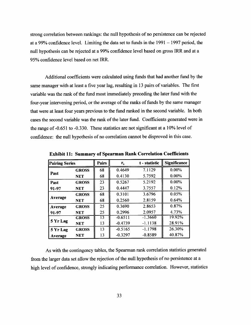
Exhibit 11: Summary of Spearman Rank Correlation Coefficients
Pairing Series Pairs r, t - statistic HSignificanceGROSS 68 0.4649 7.1129 0.00%
NET 68 0.4130 5.7592 0.00%
Past GROSS 23 0.5267 5.2192 0.00%
91-97 NET 23 0.4447 3.7557 0.12%
GROSS 68 0.3101 3.6796 0.05%
Average NET 68 0.2560 2.8159 0.64%
Average GROSS 25 0.3690 2.8653 0.87%
91-97 NET 25 0.2996 2.0957 4.73%GROSS 13 -0.6511 -1.3660 19.92%
5 Yr Lag NET 13 -0.4739 -1.1138 28.91%5 Yr Lag GROSS 13 -0.5165 -1.1798 26.30%
Average NET 13 -0.3297 -0.8589 40.87%
As with the contingency tables, the Spearman rank correlation statistics generated
from the larger data set allow the rejection of the null hypothesis of no persistence at a
high level of confidence, strongly indicating performance correlation. However, statistics
generated using five-year lagged rankings do not allow rejection of the null hypothesis of
no relationship between rankings.
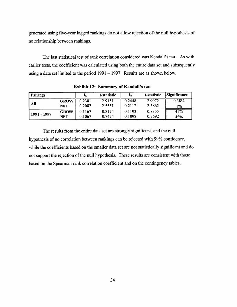
The last statistical test of rank correlation considered was Kendall's tau. As with
earlier tests, the coefficient was calculated using both the entire data set and subsequently
using a data set limited to the period 1991 - 1997. Results are as shown below.
Exhibit 12: Summary of Kendall's tau
Pairings tk t-statistic tb t-statistic SignificanceGROSS 0.2381 2.9151 0.2448 2.9972 0.38%
All NET 0.2087 2.5551 0.2112 2.5862 1%
1991-1997 GROSS 0.1167 0.8174 0.1193 0.8355 41%NET 0.1067 0.7474 0.1098 0.7692 45%
The results from the entire data set are strongly significant, and the null
hypothesis of no correlation between rankings can be rejected with 99% confidence,
while the coefficients based on the smaller data set are not statistically significant and do
not support the rejection of the null hypothesis. These results are consistent with those
based on the Spearman rank correlation coefficient and on the contingency tables.
Regression Analyses
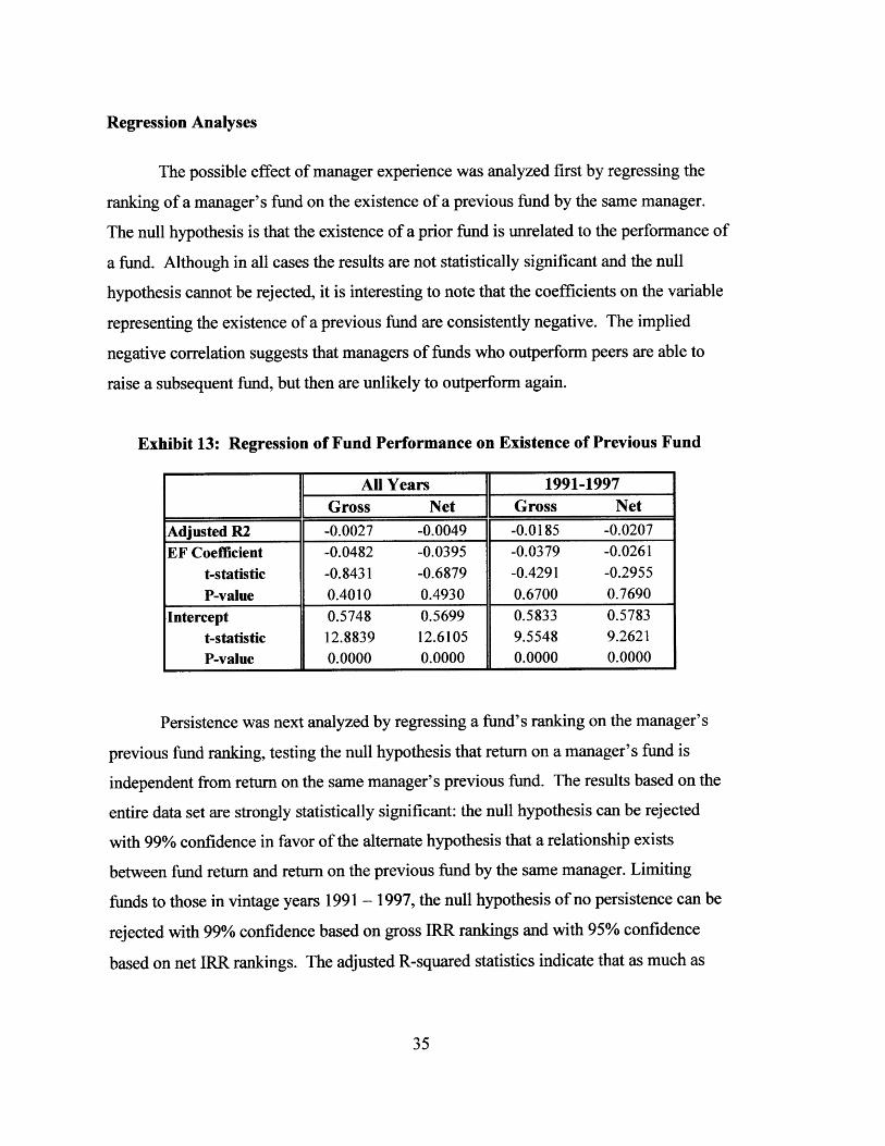
The possible effect of manager experience was analyzed first by regressing the
ranking of a manager's fund on the existence of a previous fund by the same manager.
The null hypothesis is that the existence of a prior fund is unrelated to the performance of
a fund. Although in all cases the results are not statistically significant and the null
hypothesis cannot be rejected, it is interesting to note that the coefficients on the variable
representing the existence of a previous fund are consistently negative. The implied
negative correlation suggests that managers of funds who outperform peers are able to
raise a subsequent fund, but then are unlikely to outperform again.
Exhibit 13: Regression of Fund Performance on Existence of Previous Fund
All Years 1991-1997Gross Net Gross NetAdjusted R2 -0.0027 -0.0049 -0.0185 -0.0207EF Coefficient -0.0482 -0.0395 -0.0379 -0.0261
t-statistic -0.8431 -0.6879 -0.4291 -0.2955
P-value 0.4010 0.4930 0.6700 0.7690
Intercept 0.5748 0.5699 0.5833 0.5783
t-statistic 12.8839 12.6105 9.5548 9.2621P-value 0.0000 0.0000 0.0000 0.0000
Persistence was next analyzed by regressing a fund's ranking on the manager's
previous fund ranking, testing the null hypothesis that return on a manager's fund is
independent from return on the same manager's previous fund. The results based on the
entire data set are strongly statistically significant: the null hypothesis can be rejected
with 99% confidence in favor of the alternate hypothesis that a relationship exists
between fund return and return on the previous fund by the same manager. Limiting
funds to those in vintage years 1991 - 1997, the null hypothesis of no persistence can be
rejected with 99% confidence based on gross IRR rankings and with 95% confidence
based on net IRR rankings. The adjusted R-squared statistics indicate that as much as
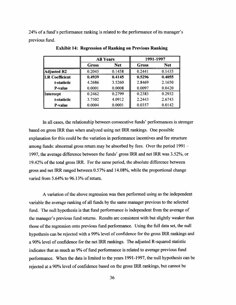
24% of a fund's performance ranking is related to the performance of its manager's
previous fund.
Exhibit 14: Regression of Ranking on Previous Ranking
All Years 1991-1997Gross Net Gross NetAdjusted R2 0.2045 0.1458 0.2441 0.1435LR Coefficient 0.4939 0.4145 0.5296 0.4055
t-statistic 4.2686 3.5260 2.8469 2.1650P-value 0.0001 0.0008 0.0097 0.0420
Intercept 0.2462 0.2799 0.2383 0.2932t-statistic 3.7502 4.0912 2.2443 2.6743P-value 0.0004 0.0001 0.0357 0.0142
In all cases, the relationship between consecutive funds' performances is stronger
based on gross IRR than when analyzed using net IRR rankings. One possible
explanation for this could be the variation in performance incentives and fee structure
among funds: abnormal gross return may be absorbed by fees. Over the period 1991 -
1997, the average difference between the funds' gross IRR and net IRR was 3.52%, or
19.42% of the total gross IRR. For the same period, the absolute difference between
gross and net IRR ranged between 0.57% and 14.08%, while the proportional change
varied from 5.64% to 96.13% of return.
A variation of the above regression was then performed using as the independent
variable the average ranking of all funds by the same manager previous to the selected
fund. The null hypothesis is that fund performance is independent from the average of
the manager's previous fund returns. Results are consistent with but slightly weaker than
those of the regression onto previous fund performance. Using the full data set, the null
hypothesis can be rejected with a 99% level of confidence for the gross IRR rankings and
a 90% level of confidence for the net IRR rankings. The adjusted R-squared statistic
indicates that as much as 9% of fund performance is related to average previous fund
performance. When the data is limited to the years 1991-1997, the null hypothesis can be
rejected at a 90% level of confidence based on the gross IRR rankings, but cannot be
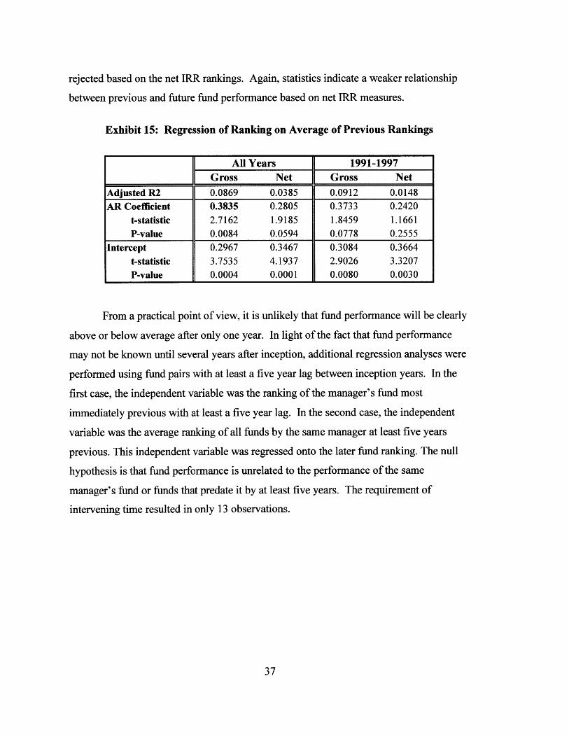
rejected based on the net IRR rankings. Again, statistics indicate a weaker relationship
between previous and future fund performance based on net IRR measures.
Exhibit 15: Regression of Ranking on Average of Previous Rankings
All Years 1991-1997
Gross Net Gross NetAdjusted R2 0.0869 0.0385 0.0912 0.0148AR Coefficient 0.3835 0.2805 0.3733 0.2420
t-statistic 2.7162 1.9185 1.8459 1.1661P-value 0.0084 0.0594 0.0778 0.2555
Intercept 0.2967 0.3467 0.3084 0.3664t-statistic 3.7535 4.1937 2.9026 3.3207P-value 0.0004 0.0001 0.0080 0.0030
From a practical point of view, it is unlikely that fund performance will be clearly
above or below average after only one year. In light of the fact that fund performance
may not be known until several years after inception, additional regression analyses were
performed using fund pairs with at least a five year lag between inception years. In the
first case, the independent variable was the ranking of the manager's fund most
immediately previous with at least a five year lag. In the second case, the independent
variable was the average ranking of all funds by the same manager at least five years
previous. This independent variable was regressed onto the later fund ranking. The null
hypothesis is that fund performance is unrelated to the performance of the same
manager's fund or funds that predate it by at least five years. The requirement of
intervening time resulted in only 13 observations.
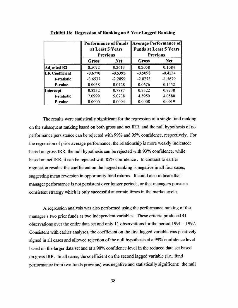
Exhibit 16: Regression of Ranking on 5-Year Lagged Ranking
Performance of Funds Average Performance ofat Least 5 Years Funds at Least 5 Years
Previous PreviousGross Net Gross Net
Adjusted R2 0.5072 0.2613 0.2058 0.1084LR Coefficient -0.6770 -0.5395 -0.5098 -0.4234
t-statistic -3.6537 -2.2899 -2.0273 -1.5679P-value 0.0038 0.0428 0.0676 0.1452
Intercept 0.8232 0.7887 0.7522 0.7238t-statistic 7.0999 5.0738 4.5959 4.0580P-value 0.0000 0.0004 0.0008 0.0019
The results were statistically significant for the regression of a single fund ranking
on the subsequent ranking based on both gross and net IRR, and the null hypothesis of no
performance persistence can be rejected with 99% and 95% confidence, respectively. For
the regression of prior average performance, the relationship is more weakly indicated:
based on gross IRR, the null hypothesis can be rejected with 93% confidence, while
based on net IRR, it can be rejected with 85% confidence. In contrast to earlier
regression results, the coefficient on the lagged ranking is negative in all four cases,
suggesting mean reversion in opportunity fund returns. It could also indicate that
manager performance is not persistent over longer periods, or that managers pursue a
consistent strategy which is only successful at certain times in the market cycle.
A regression analysis was also performed using the performance ranking of the
manager's two prior funds as two independent variables. These criteria produced 41
observations over the entire data set and only 11 observations for the period 1991 - 1997.
Consistent with earlier analyses, the coefficient on the first lagged variable was positively
signed in all cases and allowed rejection of the null hypothesis at a 99% confidence level
based on the larger data set and at a 90% confidence level in the reduced data set based
on gross IRR. In all cases, the coefficient on the second lagged variable (i.e., fund
performance from two funds previous) was negative and statistically significant: the null
hypothesis of no relationship between fund performance and performance of the
manager's fund two funds previous can be rejected at a 90% confidence level for all
cases except based on gross IRR for all years. The sign of this coefficient suggests that
fund performance may be mean reverting. The adjusted R-squared statistics obtained
indicate a large part of fund performance is accounted for by the two lagged rankings: up
to 16% based on the entire data set, or as much as 29% based on the 1991 - 1997 data.
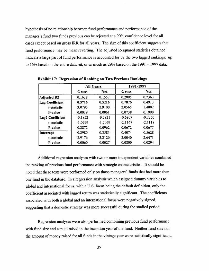
Exhibit 17: Regression of Ranking on Two Previous Rankings
All Years 1991-1997Gross Net Gross Net
Adjusted R2 0.1628 0.1557 0.2895 0.2363Lag Coefficient 0.5716 0.5216 0.7876 0.4913
t-statistic 3.0795 2.9100 2.0565 1.4002P-value 0.0039 0.0061 0.0738 0.1990
Lag2 Coefficient -0.1852 -0.2821 -0.6807 -0.7260t-statistic -1.0799 -1.7069 -2.1167 -2.1118P-value 0.2872 0.0962 0.0672 0.0677
Intercept 0.2980 0.3583 0.4074 0.5628t-statistic 2.9176 3.2120 2.0040 2.6471P-value 0.0060 0.0027 0.0800 0.0294
Additional regression analyses with two or more independent variables combined
the ranking of previous fund performance with strategic characteristics. It should be
noted that these tests were performed only on those managers' funds that had more than
one fund in the database. In a regression analysis which assigned dummy variables to
global and international focus, with a U.S. focus being the default definition, only the
coefficient associated with lagged return was statistically significant. The coefficients
associated with both a global and an international focus were negatively signed,
suggesting that a domestic strategy was more successful during the studied period.
Regression analyses were also performed combining previous fund performance
with fund size and capital raised in the inception year of the fund. Neither fund size nor
the amount of money raised for all funds in the vintage year were statistically significant,
while lagged performance continued to be strongly significant. The coefficient on the
fund size was positive, while the coefficient on the total capital raised in the vintage year
was negative.
An additional analysis of the relationship between fund characteristics and fund
performance assigns a dummy variable with a value of '1' if the manager's parent
company has a real estate focus, and a value of '0' if it is not primarily real estate
focused. This analysis found a real estate focus to have a positive association with fund
performance that is statistically significant at the 10% level. This relationship may
indicate that the desired level of alignment of interests and incentive may not be being
achieved by larger, less specialized managers, even though that investment banks may
have a higher level of co-investment than smaller general partners. 46 However, when
analyzed in combination with a variable for previous fund return, the coefficient on the
real estate-focused variable is not significant, although it is still positively signed.
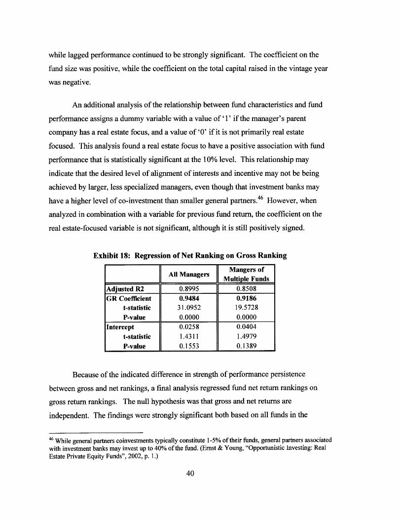
Exhibit 18: Regression of Net Ranking on Gross Ranking
SMangers ofAll Managers MnesoAll Managers M ultiple Funds
Adjusted R2 0.8995 0.8508GR Coefficient 0.9484 0.9186
t-statistic 31.0952 19.5728P-value 0.0000 0.0000
Intercept 0.0258 0.0404
t-statistic 1.4311 1.4979P-value 0.1553 0.1389
Because of the indicated difference in strength of performance persistence
between gross and net rankings, a final analysis regressed fund net return rankings on
gross return rankings. The null hypothesis was that gross and net returns are
independent. The findings were strongly significant both based on all funds in the
4 While general partners coinvestments typically constitute 1-5% of their funds, general partners associatedwith investment banks may invest up to 40% of the fund. (Ernst & Young, "Opportunistic Investing: RealEstate Private Equity Funds", 2002, p. 1.)

database and on just funds by managers with two or more funds, and the null hypothesis
can be rejected with 99% confidence. The adjusted R-squared statistic based on all funds
was 90%, while for funds that were one of multiple by the same manager, the adjusted R-
squared was 85%. The difference in the statistic indicates that the connection between
gross and net rankings is not as strong when managers have had more than one fund.
VII. Topics for Further Inquiry
Many topics remain for further study. Fund characteristics should be studied
independently from previous performance. With additional information on fund assets,
as well as the passage of time, it would be possible to research if opportunity funds, like
hedge funds, have particular strategies that consistently outperform other strategies, or if
successful strategies are cyclical, varying over time. The amount of time between the
inception of a fund and the time at which it has been fully or significantly invested is
another characteristic that remains to be investigated.
As a secondary market develops, 47 more frequent interim return data may be
available, creating many opportunities for future inquiry. Volatility of funds could be
checked, manager valuation could be compared with market valuation, and the impact of
increased liquidity could be examined.
The compensation structure of funds and its impact on returns stand out as a good
subject for further research. The weaker relationship indicated between fund
performances when measured by net IRRs suggests that fees may be diluting some of the
high fund returns. Possible relationships between the underlying compensation structure,
including fee performance incentives, co-investment percentage, and proportion ofjoint
venture deals, and the difference in gross versus net performance could be explored.
Further research on the importance of individual personnel on performance, in addition to
the role of the corporate entity as general partner, may also provide insight.
47 Seminar, "Liquidity Through Secondary Market Transactions," Fourth Annual U.S. Real EstateOpportunity & Private Fund Investing Forum, Information Management Network, May 29, 2003.
VI1. Conclusion
For real estate opportunity funds, the performance of a manager's fund is an
indicator of that manager's future fund performance. The performance of a manager's
earlier fund can accounts for as much as 20-24% of a subsequent fund's ranking relative
to its vintage year peers. This represents a significant relationship, especially since a
brief analysis of other possible indicators of returns failed to identify other significant
associations. Individual fund returns are more indicative of future fund performance than
is the average performance of all a managers' previous funds.
For investors, the finding of return correlation will be tempered by the fact that
performance is apparently less persistent when measured by a net IRR than when based
on a gross IRR. This finding suggests that fund managers may benefit most from
persistent above-average returns, and suffer most from persistent below-average returns.
The analyses based on the limited data set of funds which might be at or near liquidation
found weaker evidence for persistence: it is impossible to conclude if this is due to the
small size of the sample or because there is truly less or no serial performance correlation
among these funds.
One caveat to the finding of performance persistence among managers'
opportunity fund returns is that this result is likely biased by the attrition of under-
performing funds from the database. The likelihood of attrition is reinforced by the
results of the analysis regressing the existence of a prior fund on fund performance,
which weakly suggest that only top-performing fund managers get a chance to raise a
second fund. However, even though the results may be biased towards an indication of
performance persistence due to attrition, they are consistent in their indication of
persistence. Both the chi-squared test, strongest in the presence of attrition bias, and the
Spearman rank correlation coefficient, powerful in the absence of attrition bias, support
the finding of performance correlation. While adjustments to compensate for attrition
have been identified, they require annual performance measures and standard
deviations, 48 statistics which are unavailable for opportunity funds.
An additional qualification pertains to the calculations underlying the data set. As
opportunity funds are still a relatively recent development, most of the funds have not yet
completed their anticipated life cycle, and fewer still have fully liquidated. Thus, return
statistics are only as good as the managers' valuations. An investigation of performance
and performance persistence's sensitivity to terminal values assigned by managers is an
area where further work is possible. The passage of time will increase the quantity and
reliability of return information: a revisiting of this study in five or ten years' time will be
illuminating.
No matter how strong the statistical indication of performance persistence, one
difficulty with using the performance of one fund to predict the performance of a
subsequent fund is the life cycle of real estate opportunity funds. In order to capitalize on
the knowledge that fund performance is most strongly linked to the performance of the
fund immediately preceding it, an investor would need the ability to compare returns
among several recent funds: until current transparency and reporting issues are resolved,
this will be difficult at best. With an expected investment commitment of five years or
more, performance cannot be accurately measured until well into the fund life, possibly
after the next investment decision must be made.
The results indicate that even a good track record accounts for a small part of
future fund performance. Even if a manager achieves above-average performance, it
does not mean that the targeted 15-20% return has been met or exceeded, or that the risk
undertaken was proportional to the return achieved. Management and investors alike
may have a more ambitious definition of successful performance than merely
outperforming the median: if a more stringent definition of success is established, for
48 Brown, Goetzmann, Ibbotson, Ross, "Survivorship Bias in Performance Studies." The Review ofFinancial Studies Volume 5, no. 4, 1992, p. 572 - 575.

example a rating in the top third or quartile of funds of a vintage year, there is still
evidence of persistence.
Even tests strongly disproving the null hypothesis of no relationship between past
and subsequent fund performance give no indication of what aspect of the managers'
involvement results in return correlation. It is important to keep in mind that fund
performance itself does not cause correlated subsequent fund performance, but must
represent some other unidentified element. Consistent returns may be due to a wide
variety of factors: consistent strategy or flexible responses to circumstances,
performance incentives or integrated management structure. Until the manager
characteristics that enable the achievement of consistently high or low results can be
identified, past fund performance will serve as a surrogate indicator of future
performance.
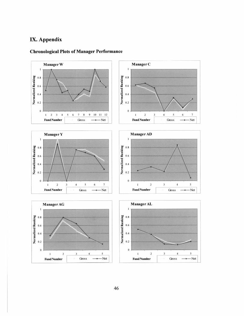
IX. Appendix
Chronological Plots of Manager Performance
Manager C
0.8
0.6
N
0.4
0.2
01 2 3 4 5 6 7
FundNumber Gross i-Net
Manager Y
S0.8
0.6
0.42aI
0.2
1 2
FundNumber
3 4 5 6 7
Gross - Net
Manager AG
a0.8
0.6
0.4
0.2
01 2 3 4 5
Fund Number Gross -.--- Net
Manager AL
be 0.8
0.6
N
0.4
Z 0.2
01 2 3 4 5
FundNumber Gross Net
Chronological Plots of Manager Performance
Manager AY
0.8
0.6
0.4
0.2
1 2 3 4
Fund Number Gross -- Net
Manager D
0.6
0.4
i 0.2
01 2 3
FundNumber Gross Net
Manager T
w 0.8
0.6
0.4
0.2
FundNumber
Manager O
0.8
0.6
N0.4
0.2
2 3 4
Gross - Net
1 2 3
Fund Number Gross -- Net
ManagerH
0.8
0.6
0.4
0.2
1 2 3 4
Fund Number Gross Net

Chronological Plots of Manager Performance
Manager AH
N
0.8
0.6
0.4
0.2
1 2 3
Fund Number Gross Net
Manager AT
0.4
0.2
01 2 3
Fund Number Gross Net]
Manager AO
* 0.8
0.6
N0.4
0.2
1 2 3
Fund Number Gross -- Net
Manager AX
g0.8
0.6
0.4
0.2
01 2 3
FundNumber Gross Net
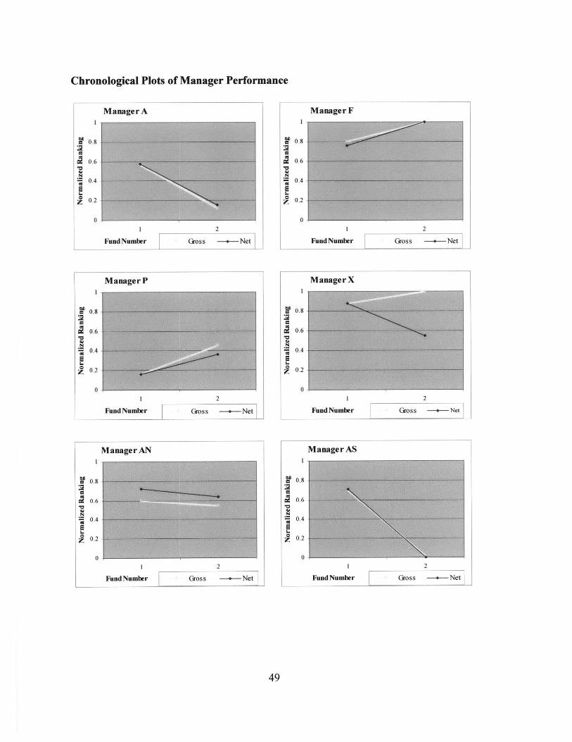
Chronological Plots of Manager Performance
Manager A
U
0.8
0.6
0.4
0.2
0
FundNumber
ManagerP
0.8
00.6N
0.4
0.2
FundNumber
Manager AN
0.8
0.6
04
0.2
FundNumber
2
Gross - Net
Gross - Net
2
Gross - Net
Manager F
n 0.8
0.6
= 0.4
0.2
Fund Number Gross - Net
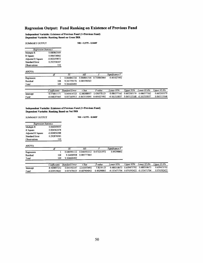
Regression Output: Fund Ranking on Existence of Previous Fund
Independent Variable: Existence of Previous Fund (1=Previous Fund)Dependent Variable: Ranking Based on Gross IRR
SUMMARY OUTPUT NR = 0.575 - 0.048F
Regression Statistics
Multiple R 0.080863109R Square 0.006538842Adjusted R Square -0.002659872Standard Error 0.292558307Observations 110
ANOVAdf SS MS F Significance F
Regression 1 0.060841316 0.060841316 0.710843064 0.401027492
Residual 108 9.243759176 0.085590363Total 109 9.304600492
Coefficients Standard Error t Stat P-value Lower 95% Upper 95% Lower 95.0% Upper 95.0%
Intercept 0.574811171 0.044614723 12.88388957 1.43657E-23 0.486377162 0.663245179 0.486377162 0.663245179
Fund -0.048197445 0.057165913 -0.843115095 0.401027492 -0.161510057 0.065115168 -0.161510057 0.065115168
Independent Variable: Existence of Previous Fund (1=Previous Fund)Dependent Variable: Ranking Based on Net IRR
SUMMARY OUTPUT NR = 0.570 - 0.040F
Regression Statistics
Multiple R 0.066049055R Square 0.004362478Adjusted R Square -0.004856388Standard Error 0.292878583Observations 110
ANOVAdf SS MS F Significance F
Regression 1 0.040591112 0.040591112 0.473211972 0.49298802
Residual 108 9.26400938 0.085777865
Total 109 9.304600492
Coefficients Standard Error t Stat P-value Lower 95% Upper 95% Lower 95.0% Upper 95.0%
Intercept 0.569897232 0.045192147 12.61053692 5.823E-23 0.480318673 0.659475792 0.480318673 0.659475792
Fund -0.039539641 0.057478425 -0.687904042 0.49298802 -0.153471704 0.074392422 -0.153471704 0.074392422
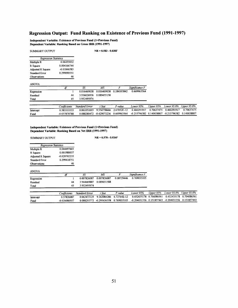
Regression Output: Fund Ranking on Existence of Previous Fund (1991-1997)
Independent Variable: Existence of Previous Fund (1=Previous Fund)Dependent Variable: Ranking Based on Gross IRR (1991-1997)
SUMMARY OUTPUT NR = 0.583 - 0.038F
Regression StatisticsMultiple R 0.06455032R Square 0.004166744Adjusted R Square -0.01846583Standard Error 0.299090551Observations 46
ANOVAdf SS MS F Significance F
Regression 1 0.016469038 0.016469038 0.184103842 0.669963564
Residual 44 3.936026936 0.089455158Total 45 3.952495974
Coefficients Standard Error t Stat P-value Lower 95% Upper 95% Lower 95.0% Upper 95.0%
Intercept 0.583333333 0.061051603 9.554758666 2.67052E-12 0.460291917 0.70637475 0.460291917 0.70637475
Fund -0.037878788 0.088280472 -0.429073236 0.669963564 -0.215796382 0.140038807 -0.215796382 0.140038807
Independent Variable: Existence of Previous Fund (1=Previous Fund)Dependent Variable: Ranking Based on Net IRR (1991-1997)
SUMMARY OUTPUT NR = 0.578 - 0.026F
Regression Statistics
Multiple R 0.044497603
R Square 0.001980037Adjusted R Square -0.020702235Standard Error 0.299418751Observations 46
ANOVAdf SS MS F Significance F
Regression 1 0,007826087 0.007826087 0.08729446 0.769035105
Residual 44 3.944669887 0.089651588
Total 45 3,952495974
Coefficients Standard Error t Stat P-value Lower 95% Upper 95% Lower 95.0% Upper 95.0%
Intercept 0.57826087 0.062433125 9.262084286 6.72764E-12 0.452435178 0.704086561 0.452435178 0.704086561
Fund -0.026086957 0.088293773 -0.295456358 0.769035105 -0.204031356 0.151857443 -0.204031356 0.151857443
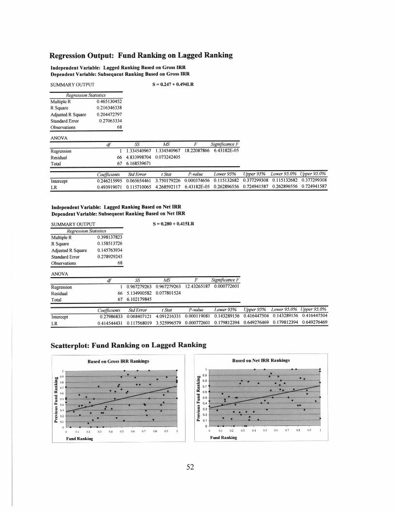
Regression Output: Fund Ranking on Lagged Ranking
Independent Variable: Lagged Ranking Based on Gross IRRDependent Variable: Subsequent Ranking Based on Gross IRR
SUMMARY OUTPUT S = 0.247 + 0.494LR
Regression StatisticsMultiple R 0.465130452R Square 0.216346338Adjusted R Square 0.204472797Standard Error 0.27063334Observations 68
ANOVAdf SS MS F Significance F
Regression 1 1.334540967 1.334540967 18.22087866 6.43182E-05Residual 66 4.833998704 0.073242405Total 67 6.168539671
Coefficients Std Error t Stat P-value Lower 95% Upper 95% Lower 95.0% Upper 95.0%
Intercept 0.246215995 0.065654461 3.750179226 0.000374656 0.115132682 0.377299308 0.115132682 0.377299308LR 0.493919071 0.115710065 4.268592117 6.43182E-05 0.262896556 0.724941587 0.262896556 0.724941587
Independent Variable: Lagged Ranking Based on Net IRRDependent Variable: Subsequent Ranking Based on Net IRR
SUMMARY OUTPUT S = 0.280 + 0.415LR
Regression StatisticsMultiple R 0.398137823R Square 0.158513726Adjusted R Square 0.145763934Standard Error 0.278929245Observations 68
ANOVAdf SS MS F Significance F
Regression 1 0.967279263 0.967279263 12.43265187 0.000772601Residual 66 5.134900582 0.077801524Total 67 6.102179845
Coefficients Std Error t Stat P-value Lower 95% Upper 95% Lower 95.0% Upper 95.0%
Intercept 0.27986833 0.068407121 4.091216331 0.000119081 0.143289156 0.416447504 0.143289156 0.416447504
LR 0.414544431 0.117568019 3.525996579 0.000772601 0.179812394 0.649276469 0.179812394 0.649276469
Scatterplot: Fund Ranking on Lagged Ranking
Based on Gmss IRR Rankings
0 0.1 0.2 0.3 0.4 0.5 0.6 0.7 0.8 0.9 1
Fund Ranking
Based on Net IRR Rankings
0 0.1 0.2 03 0.4 0.5 0. 0,7 0.8 0.9 1
Fund Ranking
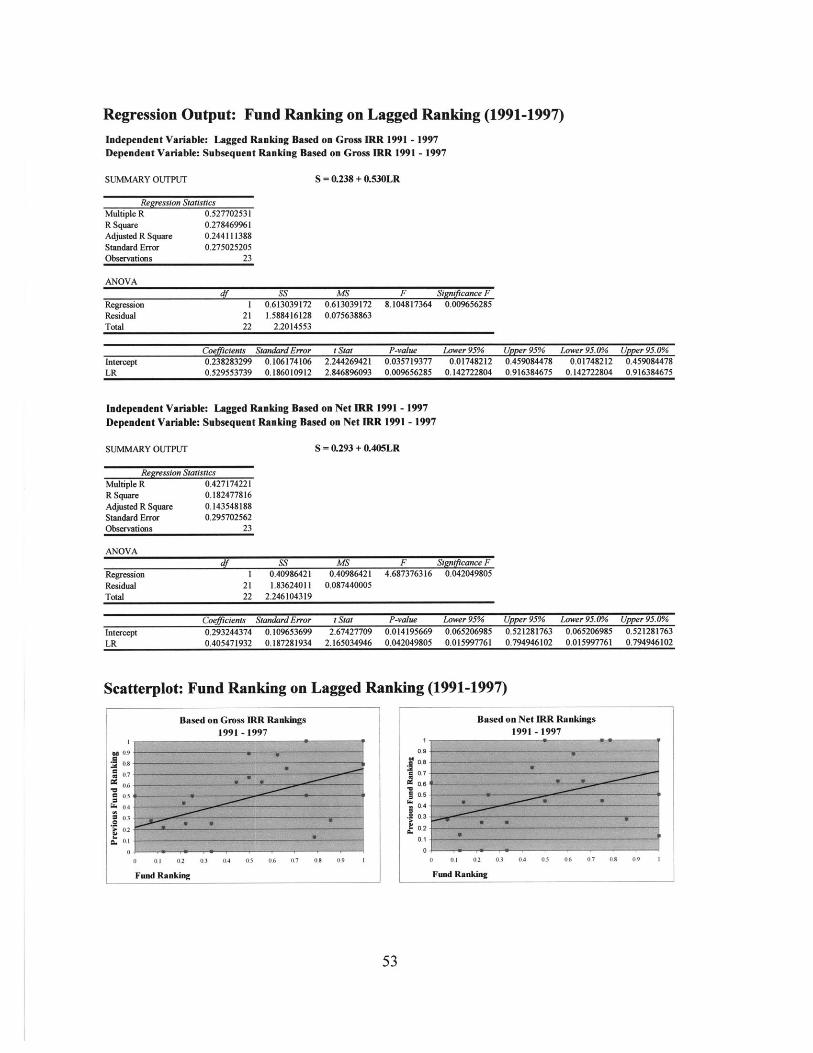
Regression Output: Fund Ranking on Lagged Ranking (1991-1997)
Independent Variable: Lagged Ranking Based on Gross IRR 1991 - 1997Dependent Variable: Subsequent Ranking Based on Gross IRR 1991 - 1997
SUMMARY OUTPUT S = 0.238 + 0.530LR
Regression StatisticsMultiple R 0.527702531R Square 0.278469%1Adjusted R Square 0.244111388Standard Error 0.275025205Observations 23
ANOVAdf SS MS F Significance F
Regression 1 0.613039172 0.613039172 8.104817364 0.009656285Residual 21 1.588416128 0.075638863Total 22 2.2014553
Coefficients Standard Error I Stat P-value Lower 95% Upper 95% Lower 95.0% Upper 95.0%Intercept 0.238283299 0.106174106 2.244269421 0.035719377 0.01748212 0.459084478 0.01748212 0.459084478LR 0.529553739 0.186010912 2.846896093 0.009656285 0.142722804 0.916384675 0.142722804 0.916384675
Independent Variable: Lagged Ranking Based on Net IRR 1991 - 1997Dependent Variable: Subsequent Ranking Based on Net IRR 1991 - 1997
SUMMARY OUTPUT S = 0.293 + 0.405LR
Regression StatisticsMultiple R 0.427174221R Square 0.182477816Adjusted R Square 0.143548188Standard Error 0.295702562Observations 23
ANOVAdf SS MS F Signifcance F
Regression 1 0.40986421 0.40986421 4.687376316 0.042049805Residual 21 1.83624011 0.087440005Total 22 2.246104319
Coefficients Standard Error t Stat P-value Lower 95% Upper 95% Lower 95.0% Upper 95.0%
Intercept 0.293244374 0.109653699 2.67427709 0.014195669 0.065206985 0.521281763 0.065206985 0.521281763LR 0.405471932 0.187281934 2.165034946 0.042049805 0.015997761 0.794946102 0.015997761 0.794946102
Scatterplot: Fund Ranking on Lagged Ranking (1991-1997)
Based on Gmss IRR Rankings1991-1997
W 09
0.8
0.7
0.6
0.504
0301
02
01
0 0.1 0.2 0.3 0.4 0.5 0.6 0.7 0.8 0.9 1Fund Ranking
Based on Net IRR Rankings1991-1997
0-.0.8
0-70.6
0.5
0.4
- 0.3
L0.2
0.1-
0 0.1 0.2 0.3 0.4 0.5 0.6 0.7 0.8 0.9 1Fund Ranking

Regression Output: Fund Ranking on Average Previous Ranking
Independent Variable: Average Previous Ranking Based on Net IRRDependent Variable: Subsequent Ranking Based on Net IRR
SUMMARY OUTPUT S = 0.347 + 0.281AR
Regression Statistics
Multiple R 0.22983353
R Square 0.052823452Adjusted R Square 0.038472292Standard Error 0.295927961
Observations 68
ANOVAdf SS MS F Significance F
Regression 1 0.322338202 0.322338202 3.680779274 0.059370007
Residual 66 5.779841643 0.087573358
Total 67 6.102179845
Coefficients Standard Error t Stat P-value Lower 95% Upper 95% Lower 95.0% Upper 95.0%
Intercept 0.346656119 0.082661852 4.193665028 8.35632E-05 0.181616466 0.511695773 0.181616466 0.511695773
AR 0.280505031 0.146207876 1.918535711 0.059370007 -0.011408306 0.572418369 -0.01140831 0.572418369
Independent Variable: Average Previous Ranking Based on Gross IRR
Dependent Variable: Subsequent Ranking Based on Gross IRR
SUMMARY OUTPUT S = 0.297 + 0.384AR
Regression Statistics
Multiple R 0.317082754
R Square 0.100541473
Adjusted R Square 0.086913313
Standard Error 0.289941102
Observations 68
ANOVAdf SS MS F Significance F
Regression 1 0.620194063 0.620194063 7.377479894 0.008423246
Residual 66 5.548345608 0.084065843Total 67 6.168539671
Coefficients Standard Error t Stat P-value Lower 95% Upper 95% Lower 95.0% Upper 95.0%
Intercept 0.296673247 0.079038347 3.753535577 0.00037055 0.138868153 0.454478341 0.138868153 0.454478341
AR 0.38350682 0.141194921 2.71615167 0.008423246 0.101602167 0.665411472 0.101602167 0.665411472
Scatterplot: Fund Ranking on Average Previous Ranking
Based on Average Gross IRR Rankings
0 0.1 0.2 0.3 04 0.5 06 0.7 0.8 0.9 1
Fund Ranking
Based on Average Net IRR Rankings
0 0.1 0.2 0.3 0.4 0.5 0.6 0.7 0.8 0.9
Fund Ranking
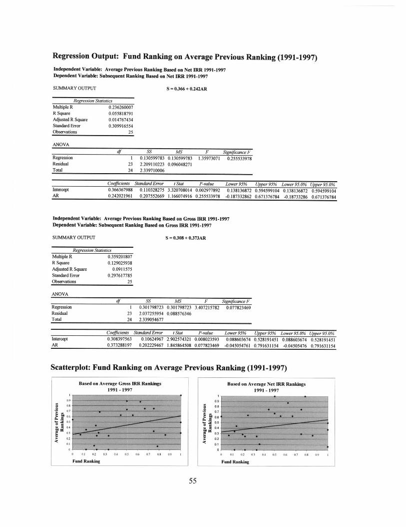
Regression Output: Fund Ranking on Average Previous Ranking (1991-1997)Independent Variable: Average Previous Ranking Based on Net IRR 1991-1997Dependent Variable: Subsequent Ranking Based on Net IRR 1991-1997
SUMMARY OUTPUT S = 0.366 + 0.242AR
Regression StatisticsMultiple R 0.236260007R Square 0.055818791Adjusted R Square 0.014767434Standard Error 0.309916554Observations 25
ANOVA
df SS MS F Significance FRegression 1 0.130599783 0.130599783 1.35973071 0.255533978Residual 23 2.209110223 0.096048271Total 24 2.339710006
Coefficients Standard Error t Stat P-value Lower 95% Upper 95% Lower 95.0% Upper 95.0%Intercept 0.366367988 0.110328275 3.320708014 0.002977892 0.138136872 0.594599104 0.138136872 0.594599104AR 0.242021961 0.207552669 1.166074916 0.255533978 -0.187332862 0.671376784 -0.18733286 0.671376784
Independent Variable: Average Previous Ranking Based on Gross IRR 1991-1997Dependent Variable: Subsequent Ranking Based on Gross IRR 1991-1997
SUMMARY OUTPUT S = 0.308 + 0.373AR
Regression StatisticsMultiple R 0.359201807R Square 0.129025938Adjusted R Square 0.0911575Standard Error 0.297617785Observations 25
ANOVA
df SS MS F Significance FRegression 1 0.301798723 0.301798723 3.407215782 0.077823469Residual 23 2.037255954 0.088576346Total 24 2.339054677
Coefficients Standard Error t Stat P-value Lower 95% Upper 95% Lower 95.0% Upper 95.0%Intercept 0.308397563 0.10624967 2.902574321 0.008023593 0.088603674 0.528191451 0.088603674 0.528191451AR 0.373288197 0.202229467 1.845864508 0.077823469 -0.045054761 0.791631154 -0.04505476 0.791631154
Scatterplot: Fund Ranking on Average Prei
Based on Average Gross IRR Rankings1991-1997
Q
0 0.1 0.2 0.3 0.4 0.5 0.6 0.7 0.8 0.9 1
Fund Ranking
vious Ranking (1991-1997)
Based on Average Net IRR Rankings1991-1997
0.8
0.7
0.4
0.3
0.1-
0 0.1 0.2 0.3 0.4 0.5 0.6 0.7 0.8 0.9 1
Fund Ranking
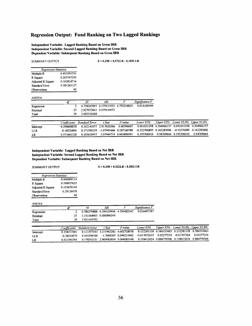
Regression Output: Fund Ranking on Two Lagged Rankings
Independent Variable: Lagged Ranking Based on Gross IRRIndependent Variable: Second Lagged Ranking Based on Gross IRRDependent Variable: Subsequent Ranking Based on Gross IRR
SUMMARY OUTPUT S = 0.298 + 0.572LR - 0.185LLR
Regression Statistics
Multiple R 0.453593753
R Square 0.205747293Adjusted R Square 0.162814714
Standard Error 0.281265127
Observations 40
ANOVAdf SS MS F Significance F
Regression 2 0.758243907 0.379121953 4.792334835 0.014100549
Residual 37 2.927072661 0.079110072
Total 39 3.685316568
Coefficients Standard Error t Stat P-value Lower 95% Upper 95% Lower 95.0% Upper 95.0%
Intercept 0.298008878 0.102141077 2.917620266 0.00596607 0.091051598 0.504966157 0.091051598 0.504966157
LLR -0.18520894 0.171500139 -1.07993466 0.287160789 -0.532700895 0.162283006 -0.53270089 0.162283006
LR 0.571601328 0.185616957 3.07946719 0.003896991 0.195506016 0.94769664 0.195506016 0.94769664
Independent Variable: Lagged Ranking Based on Net IRRIndependent Variable: Second Lagged Ranking Based on Net IRR
Dependent Variable: Subsequent Ranking Based on Net IRR
SUMMARY OUTPUT S = 0.358 + 0.522LR - 0.282LLR
Regression Statistics
Multiple R 0.446069114
R Square 0.198977655
Adjusted R Square 0.155679149
Standard Error 0.29136978Observations 40
ANOVAdf SS MS F Significance F
Regression 2 0.780279888 0.390139944 4.595485547 0.016497787
Residual 37 3.141164905 0.084896349
Total 39 3.921444793
Coefficients Standard Error t Stat P-value Lower 95% Upper 95% Lower 95.0% Upper 95.0%
Intercept 0.358317401 0.111557163 3.211962282 0.002728958 0.132281338 0.584353463 0.132281338 0.584353463
LLR -0.28214975 0.165296546 -1.7069307 0.096215462 -0.617072037 0.05277254 -0.61707204 0.05277254
LR 0.521591765 0.179242151 2.909983854 0.006085548 0.158413024 0.884770506 0.158413024 0.884770506
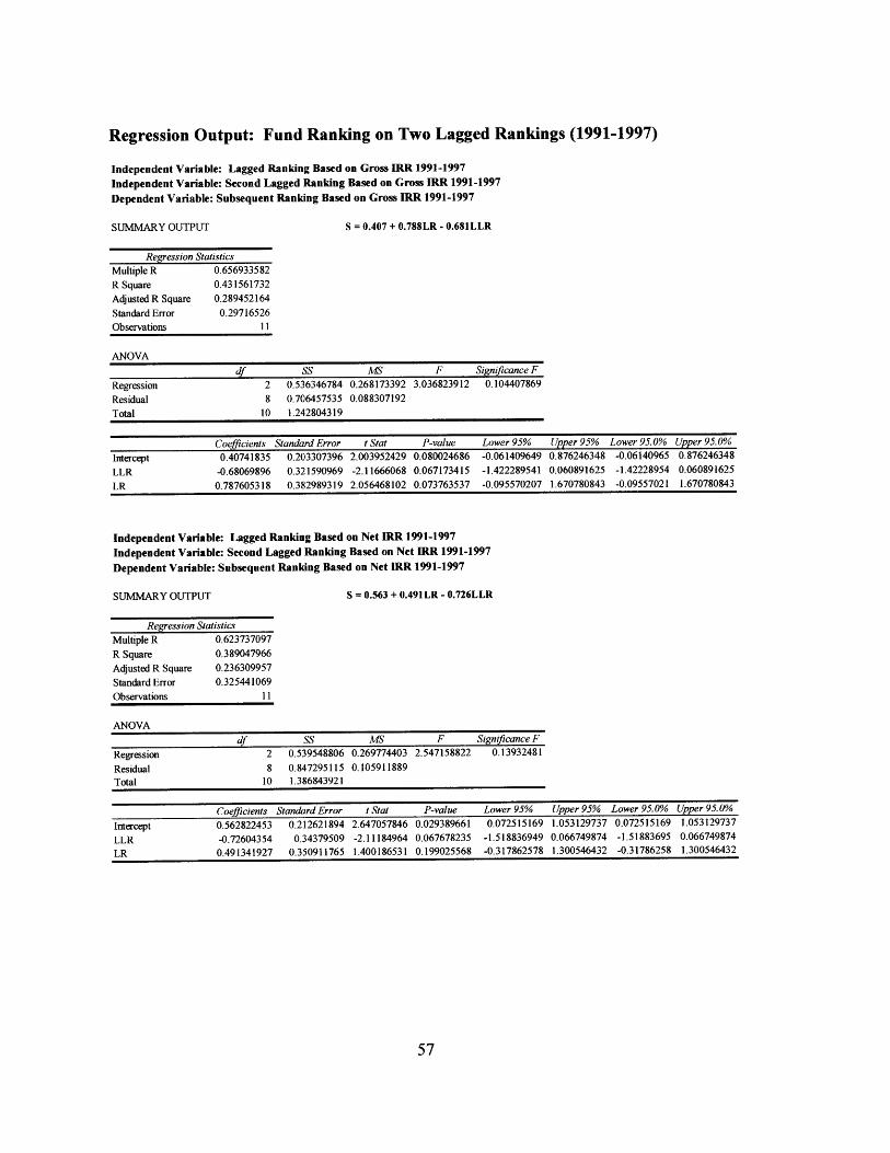
Regression Output: Fund Ranking on Two Lagged Rankings (1991-1997)
Independent Variable: Lagged Ranking Based on Gross IRR 1991-1997Independent Variable: Second Lagged Ranking Based on Gross IRR 1991-1997Dependent Variable: Subsequent Ranking Based on Gross IRR 1991-1997
SUMMARY OUTPUT S = 0.407 + 0.788LR - 0.681LLR
Regression StatisticsMultiple R 0.656933582
R Square 0.431561732Adjusted R Square 0.289452164
Standard Error 0.29716526Observations 11
ANOVA
df SS MS F Significance F
Regression 2 0.536346784 0.268173392 3.036823912 0.104407869
Residual 8 0.706457535 0.088307192
Total 10 1.242804319
Coefficients Standard Error t Stat P-value Lower 95% Upper 95% Lower 95.0% Upper 95.0%
Intercept 0.40741835 0.203307396 2.003952429 0.080024686 -0.061409649 0.876246348 -0.06140965 0.876246348
LLR -0.68069896 0.321590969 -2.11666068 0.067173415 -1.422289541 0.060891625 -1.42228954 0.060891625
LR 0.787605318 0.382989319 2.056468102 0.073763537 -0.095570207 1.670780843 -0.09557021 1.670780843
Independent Variable: Lagged Ranking Based on Net IRR 1991-1997Independent Variable: Second Lagged Ranking Based on Net IRR 1991-1997
Dependent Variable: Subsequent Ranking Based on Net IRR 1991-1997
SUMMARY OUTPUT S = 0.563 + 0.491 LR - 0.726LLR
Regression Statistics
Multiple R 0.623737097
R Square 0.389047966Adjusted R Square 0.236309957
Standard Error 0.325441069
Observations 11
ANOVA
df SS MS F Significance F
Regression 2 0.539548806 0.269774403 2.547158822 0.13932481
Residual 8 0.847295115 0.105911889
Total 10 1.386843921
Coefficients Standard Error t Stat P-value Lower 95% Upper 95% Lower 95.0% Upper 95.0%
Intercept 0.562822453 0.212621894 2.647057846 0.029389661 0.072515169 1.053129737 0.072515169 1.053129737
LLR -0.72604354 0.34379509 -2.11184964 0.067678235 -1.518836949 0.066749874 -1.51883695 0.066749874
LR 0.491341927 0.350911765 1.400186531 0.199025568 -0.317862578 1.300546432 -0.31786258 1.300546432
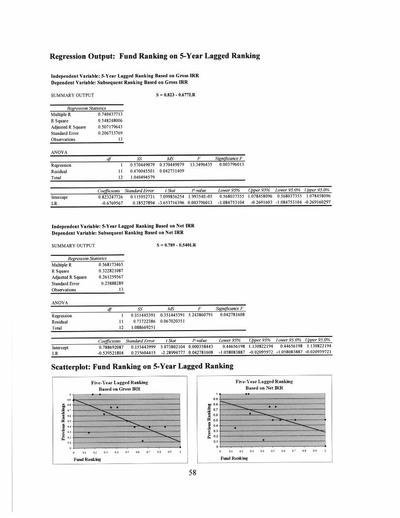
Regression Output: Fund Ranking on 5-Year Lagged Ranking
Independent Variable: 5-Year Lagged Ranking Based on Gross IRRDependent Variable: Subsequent Ranking Based on Gross IRR
SUMMARY OUTPUT S = 0.823 - 0.677LR
Regression StatisticsMultiple R 0.740437713
R Square 0.548248006
Adjusted R Square 0.507179643Standard Error 0.206715769Observations 13
ANOVA
df SS MS F Significance F
Regression 1 0.570449079 0.570449079 13.3496435 0.003796013
Residual 11 0.470045501 0.042731409
Total 12 1.040494579
Coefficients Standard Error I Stat P-value Lower 95% Upper 95% Lower 95.0% Upper 95.0%
Intercept 0.823247726 0.115952731 7.099856254 1.99354E-05 0.568037355 1.078458096 0.568037355 1.078458096
LR -0.6769567 0.18527894 -3.653716396 0.003796013 -1.084753104 -0.2691603 -1.084753104 -0.269160297
Independent Variable: 5-Year Lagged Ranking Based on Net IRR
Dependent Variable: Subsequent Ranking Based on Net IRR
SUMMARY OUTPUT S = 0.789 - 0.540LR
Regression StatisticsMultiple R 0.568173465R Square 0.322821087Adjusted R Square 0.261259367
Standard Error 0.25888289
Observations 13
ANOVAdf SS MS F Significance F
Regression 1 0.351445391 0.351445391 5.243860791 0.042781608
Residual 11 0.73722386 0.067020351
Total 12 1.088669251
Coefficients Standard Error t Stat P-value Lower 95% Upper 95% Lower 95.0% Upper 95.0%
Intercept 0.788692087 0.155443999 5.073802104 0.000358443 0.44656198 1.130822194 0.44656198 1.130822194
LR -0.539521804 0.235604415 -2.28994777 0.042781608 -1.058083887 -0.02095972 -1.058083887 -0.020959721
Scatterplot: Fund Ranking on 5-Year Lagged Ranking
Five-Year Lagged Ranking Five-Year Lagged RankingBased on Gross IRR Based on Net IRR
0 0.1 0.2 03 0A 0- 06 0.' 0.8 0,9 1
Fund Ranking
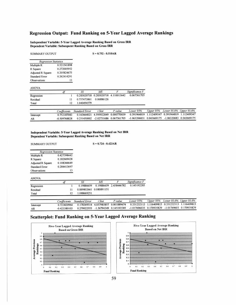
Regression Output: Fund Ranking on 5-Year Lagged Average Rankings
Independent Variable: 5-Year Lagged Average Ranking Based on Gross IRRDependent Variable: Subsequent Ranking Based on Gross IRR
SUMMARY OUTPUT S = 0.752 - 0.510AR
Regression StatisticsMultiple R 0.521541898R Square 0.272005952Adjusted R Square 0.205824675Standard Error 0.262414291Observations 13
ANOVAdf SS MS F Significance F
Regression 1 0.283020718 0.283020718 4.110013642 0.067561705Residual 11 0.757473861 0.06886126Total 12 1.040494579
Coefficients Standard Error t Stat P-value Lower 95% Upper 95% Lower 95.0% Upper 95.0%
Intercept 0.752187083 0.163664021 4.595922049 0.000770039 0.391964819 1.112409347 0.391964819 1.112409347
AR -0.509768828 0.251450002 -2.02731686 0.067561705 -1.063206831 0.043669175 -1.06320683 0.043669175
Independent Variable: 5-Year Lagged Average Ranking Based on Net IRRDependent Variable: Subsequent Ranking Based on Net IRR
SUMMARY OUTPUT S = 0.724 - 0.423AR
Regression StatisticsMultiple R 0.427398442R Square 0.182669428Adjusted R Square 0.108366649Standard Error 0.284413697Observations 13
ANOVAdf SS MS F Significance F
Regression 1 0.19886659 0.19886659 2.458446782 0.145192285
Residual 11 0.889802661 0.080891151Total 12 1.088669251
Coefficients Standard Error t Stat P-value Lower 95% Upper 95% Lower 95.0% Upper 95.0%
Intercept 0.723820964 0.178369514 4.057985857 0.001889674 0.331232113 1.116409815 0.331232113 1.116409815
AR -0.423380103 0.270022553 -1.56794349 0.145192285 -1.017696035 0.170935829 -1.01769603 0.170935829
Scatterplot: Fund Ranking on 5-Year Lagged Average Ranking
Five-Year Lagged Average RankingBased on Gross IRR
09
0.4
0.3
0.1
0 0.1 0.2 03 0.4 05 0.6 0. 0.8 09 1
Fund Ranking
Five-Year Lagged Average RankingBased on Net IRR
08
027
0
0 01 02 03 04 0.5 06 0. 0.8 09 1
Fund Ranking
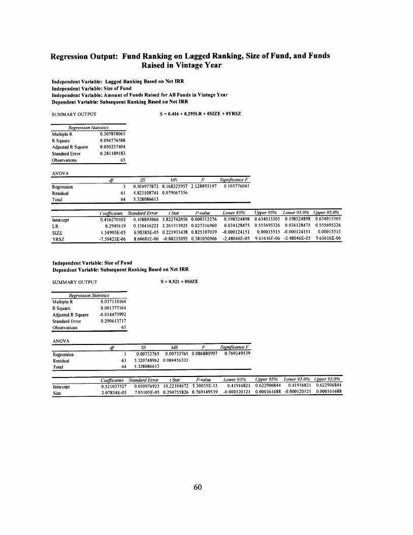
Regression Output: Fund Ranking on Lagged Ranking, Size of Fund, and FundsRaised in Vintage Year
Independent Variable: Lagged Ranking Based on Net IRRIndependent Variable: Size of FundIndependent Variable: Amount of Funds Raised for All Funds in Vintage YearDependent Variable: Subsequent Ranking Based on Net IRR
SUMMARY OUTPUT S = 0.416 + 0.295LR + OSIZE + OYRSZ
Regression StatisticsMultiple R 0.307858065
R Square 0.094776588Adjusted R Square 0.050257404
Standard Error 0.281189183
Observations 65
ANOVA
df SS MS F Significance F
Regression 3 0.504977872 0.168325957 2.128893197 0.105776041
Residual 61 4.823108741 0.079067356
Total 64 5.328086613
Coefficients Standard Error t Stat P-value Lower 95% Upper 95% Lower 95.0% Upper 95.0%
Intercept 0.416270102 0.108893066 3.822742056 0.000312276 0.198524898 0.634015305 0.198524898 0.634015305
LR 0.2949119 0.130416221 2.261313025 0.027316969 0.034128475 0.555695326 0.034128475 0.555695326
SIZE 1.54995E-05 6.98385E-05 0.221933438 0.825107039 -0.000124151 0.00015515 -0.000124151 0.00015515
YRSZ -7.59423E-06 8.60681E-06 -0.88235093 0.381050966 -2.48046E-05 9.61616E-06 -2.48046E-05 9.61616E-06
Independent Variable: Size of FundDependent Variable: Subsequent Ranking Based on Net IRR
SUMMARY OUTPUT S = 0.521 + OSIZE
Regression StatisticsMultiple R 0.037110164
R Square 0.001377164Adjusted R Square -0.014473992
Standard Error 0.290613717Observations 65
ANOVA
df SS MS F Significance F
Regression 1 0.00733765 0.00733765 0.086880997 0.769149539
Residual 63 5.320748962 0.084456333Total 64 5.328086613
Coefficients Standard Error t Stat P-value Lower 95% Upper 95% Lower 95.0% Upper 95.0%
Intercept 0.521037527 0.050976925 10.22104672 5.30035E-15 0.41916821 0.622906844 0.41916821 0.622906844
Size 2.07834E-05 7.05105E-05 0.294755826 0.769149539 -0.000120121 0.000161688 -0.000120121 0.000161688
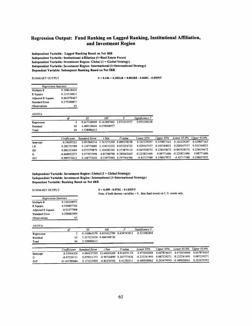
Regression Output: Fund Ranking on Lagged Ranking, Institutional Affiliation,and Investment Region
Independent Variable: Lagged Ranking Based on Net IRRIndependent Variable: Institutional Affiliation (1=Real Estate Focus)Independent Variable: Investment Region: Global (1 = Global Strategy)Independent Variable: Investment Region: International (1=International Strategy)
Dependent Variable: Subsequent Ranking Based on Net IRR
SUMMARY OUTPUT S = 0.346 + 0.282LR + 0.081RE - 0.068G - 0.09INT
Regression StatisticsMultiple R 0.348618434
R Square 0.121534813Adjusted R Square 0.062970467Standard Error 0.279300871Observations 65
ANOVAdf SS MS F Significance F
Regression 4 0.647548009 0.161887002 2.075235557 0.095240138
Residual 60 4.680538604 0.078008977
Total 64 5.328086613
Coefficients Standard Error t Stat P-value Lower 95% Upper 95% Lower 95.0% Upper 95.0%
Intercept 0.34609323 0.091868316 3.767275209 0.000378558 0.162329297 0.529857163 0.162329297 0.529857163
LR 0.281755789 0.130774685 2.154513232 0.035224722 0.020167557 0.543344021 0.020167557 0.543344021
RE 0.081253049 0.073579879 1.104283545 0.273879114 -0.065928574 0.228434672 -0.065928574 0.228434672
G -0.068052273 0.077872996 -0.87388796 0.385663665 -0.223821406 0.08771686 -0.223821406 0.08771686
INT -0.089574412 0.168775656 -0.53073064 0.597564506 -0.42717588 0.248027055 -0.42717588 0.248027055
Independent Variable: Investment Region: Global (1 = Global Strategy)
Independent Variable: Investment Region: International (1=International Strategy)
Dependent Variable: Ranking Based on Net IRR
SUMMARY OUTPUT S = 0.559 - 0.073G - 0.1431NT
Note: if both dummy variables = 0, then fund invests in U.S. assets only.
Regression Statistics
Multiple R 0.144248972
R Square 0.020807766Adjusted R Square -0.01077908
Standard Error 0.290083999Observations 65
ANOVAdf SS MS F Significance F
Regression 2 0.110865579 0.055432789 0.658747812 0.521082844
Residual 62 5.217221034 0.084148726
Total 64 5.328086613
Coefficients Standard Error t Stat P-value Lower 95% Upper 95% Lower 95.0% Upper 95.0%
Intercept 0.55944524 0.044237395 12.64643269 8.01403E-19 0.471016044 0.647874435 0.471016044 0.647874435
G -0.07250111 0.079911373 -0.90726899 0.367777436 -0.232241491 0.087239271 -0.232241491 0.087239271
INT -0.142789684 0.173223909 -0.82430702 0.41292511 -0.489058961 0.203479593 -0.489058961 0.203479593
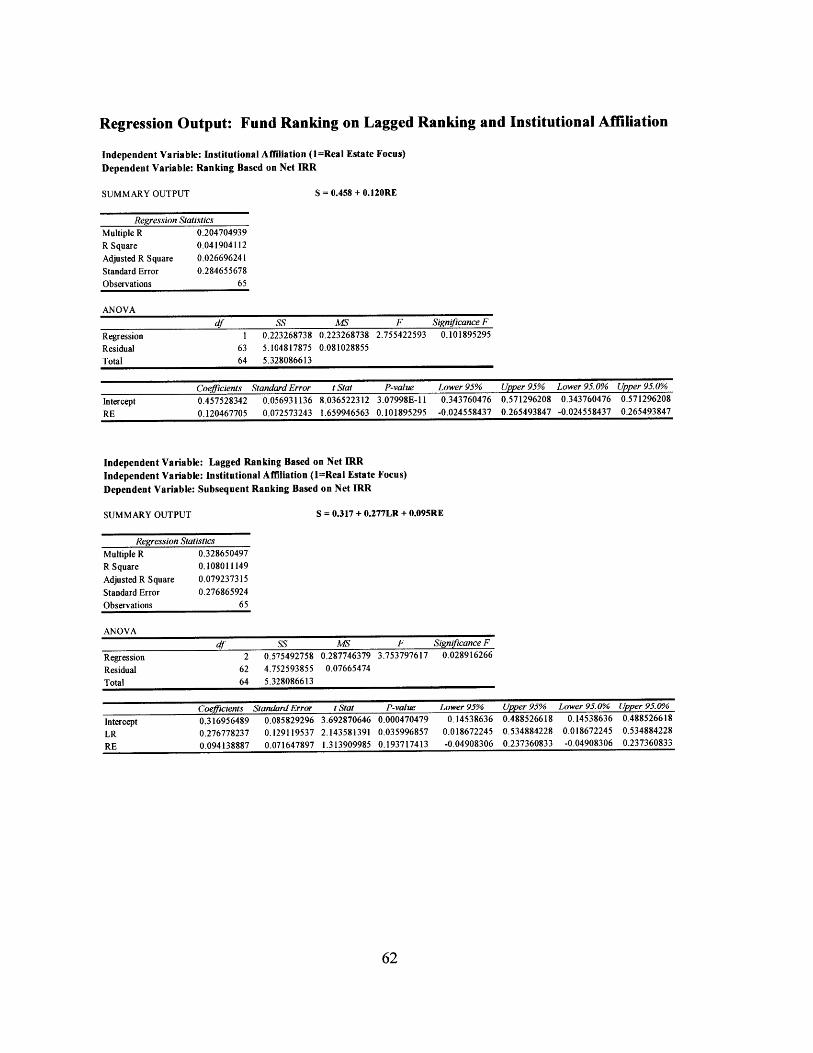
Regression Output: Fund Ranking on Lagged Ranking and Institutional Affiliation
Independent Variable: Institutional Affiliation (1=Real Estate Focus)Dependent Variable: Ranking Based on Net IRR
SUMMARY OUTPUT S = 0.458 + 0.120RE
Regression Statistics
Multiple R 0.204704939
R Square 0.041904112
Adjusted R Square 0.026696241
Standard Error 0.284655678Observations 65
ANOVA
df SS MS F Significance F
Regression 1 0.223268738 0.223268738 2.755422593 0.101895295
Residual 63 5.104817875 0.081028855
Total 64 5.328086613
Coefficients Standard Error t Stat P-value Lower 95% Upper 95% Lower 95.0% Upper 95.0%
Intercept 0.457528342 0.056931136 8.036522312 3.07998E-11 0.343760476 0.571296208 0.343760476 0.571296208
RE 0.120467705 0.072573243 1.659946563 0.101895295 -0.024558437 0.265493847 -0.024558437 0.265493847
Independent Variable: Lagged Ranking Based on Net IRRIndependent Variable: Institutional Affiliation (1=Real Estate Focus)
Dependent Variable: Subsequent Ranking Based on Net IRR
SUMMARY OUTPUT S = 0.317 + 0.277LR + 0.095RE
Regression Statistics
Multiple R 0.328650497R Square 0.108011149
Adjusted R Square 0.079237315
Standard Error 0.276865924Observations 65
ANOVAdf SS MS F Significance F
Regression 2 0.575492758 0.287746379 3.753797617 0.028916266
Residual 62 4.752593855 0.07665474
Total 64 5.328086613
Coefficients Standard Error t Stat P-value Lower 95% Upper 95% Lower 95.0% Upper 95.0%
Intercept 0.316956489 0.085829296 3.692870646 0.000470479 0.14538636 0.488526618 0.14538636 0.488526618
LR 0.276778237 0.129119537 2.143581391 0.035996857 0.018672245 0.534884228 0.018672245 0.534884228
RE 0.094138887 0.071647897 1.313909985 0.193717413 -0.04908306 0.237360833 -0.04908306 0.237360833
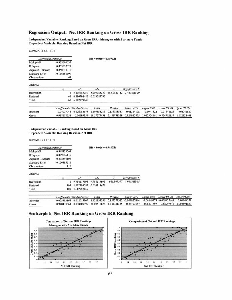
Regression Output: Net IRR Ranking on Gross IRR RankingIndependent Variable: Ranking Based on Gross IRR - Managers with 2 or more FundsDependent Variable: Ranking Based on Net IRR
SUMMARY OUTPUT
Regression StatisticsMultiple R 0.923600037R Square 0.853037028Adjusted R Square 0.850810316Standard Error 0.116566699Observations 68
NR = 0.040 + 0.919GR
ANOVAdf SS MS F Significance F
Regression 1 5.205385359 5.205385359 383.0927142 3.48183E-29Residual 66 0.896794486 0.013587795Total 67 6.102179845
Coefficients Standard Error t Stat P-value Lower 95% Upper 95% Lower 95.0% Upper 95.0%Intercept 0.04037046 0.026952178 1.497855213 0.138938567 -0.01344128 0.0941822 -0.01344128 0.0941822Gross 0.918618658 0.04693354 19.57275438 3.48183E-29 0.824912855 1.012324461 0.824912855 1.012324461
Independent Variable: Ranking Based on Gross IRRDependent Variable: Ranking Based on Net IRR
SUMMARY OUTPUT
Regression Statistics NR = 0.026 + 0.948GR
Multiple R 0.948433664R Square 0.899526416Adjusted R Square 0.898596105Standard Error 0.100595614Observations 110
ANOVAdf SS MS F Significance F
Regression 1 9.784617993 9.784617993 966.909397 1.04131E-55Residual 108 1.092903582 0.010119478Total 109 10.87752157
Coefficients Standard Error t Stat P-value Lower 95% Upper 95% Lower 95.0% Upper 95.0%
Intercept 0.025783168 0.018015909 1.431133296 0.155279322 -0.009927444 0.06149378 -0.009927444 0.06149378Gross 0.948433664 0.030500999 31.09516678 1.04131E-55 0.88797547 1.008891859 0.88797547 1.008891859
Scatterplot: Net IRR Ranking on Gross IRR Ranking
Comparison of Net and IRR RankingsManagers with 2 or More Funds
0.9
0.4
0.1
0 0.1 0.2 03 04 0 0.6 0 08 0.9 1
Net IRR Ranking
Comparison of Net and IRR Rankings
0.4
43 0-3
0 .2
0.1
0 01 0.2 03 0.4 0.5 0.6 0 03 09 1
Net IRR Ranking

X. Bibliography
Books
Bodie, Zvi, Kane, Alex, and Marcus, Alan. Investments, New York: McGraw-Hill, 2002.
Chen, Peter and Popovich, Paula. Correlation: Parametric and Nonparametric Measures,Sage University Papers, Quantitative Applications in the Social Sciences, vol. 139.Thousand Oaks, California: Sage Publications, Inc., 2002.
Dickinson Gibbons, Jean. Nonparametric Measures of Association Sage UniversityPapers, Quantitative Applications in the Social Sciences, vol. 91. Newbury Park,California: Sage Publications, Inc., 1993.
Geltner, David and Miller, Norman. Commercial Real Estate Analysis and Investments.United States: Thomson Learning, South-Western Publishing, 2001.
Koosis, Donald J. Statistics: a Self-teaching Guide, 4h edition. New York: John Wiley &Sons, 1997.
Sprent, P. and Smeeton, N.C. Applied Nonparametric Statistical Methods, 3rd edition.New York: Chapman & Hall/CRC, 2001.
Articles
Agarwal, Vikas and Naik, Narayan. "Multi-Period Performance Persistence Analysis ofHedge Funds." white paper, February 2001.
Bares, P.-A., Gibson, R., and Gyger, S. "Performance in the Hedge Funds Industry: AnAnalysis of Short and Long-Term Persistence." white paper, March 2002.
Brown, Stephen J. and Goetzmann, William N. "Performance Persistence." The Journalof Finance Vol 50 no. 2 (June 1995), pp. 679-698.
Brown, Stephen J., Goetzmann, William N., and Ibbotson, Roger G. "Offshore HedgeFunds: Survival and Performance 1989-1995." Journal of Business 72 (1998), pp. 91-117.
Brown, Stephen J., Goetzmann, William N., Ibbotson, Roger G., and Ross, Stephen A."Survivorship Bias in Performance Studies." The Review of Financial Studies Volume 5,no. 4 (1992), pp. 553-580.

Carhart, Mark M. "On Persistence in Mutual Fund Performance" The Journal of FinanceVol. 52 no. 1 (March 1997), pp. 57-82.
Carpenter, Jennifer and Lynch, Anthony. "Survivorship bias and attrition effects inMeasures of Performance Persistence." Journal of Financial Economics v. 54 (1999), pp.337-374.
Elton, Edwin J., Gruber, Martin J., and Blake, Christopher R. "The Persistence of Risk-Adjusted Mutual Fund Performance." Journal of Business vol. 69, no. 2 (1996), pp. 133-157.
Ernst & Young LLP, "Opportunistic Investing: Real Estate Private Equity Funds." whitePaper, SCORE Retrieval File No. W00269, 2002.
Fickes, Mike. 'Feasting on Market Inefficiency Worldwide.' National Real EstateInvestor, Atlanta, October 2001.
Gerardo Lietz, Nori, with Dewey, David, Mattox, Eliza, and Mouchakkaa, Denise. "RealEstate Opportunity Funds: Dejit vu All Over Again." Pension Consulting Alliance, Inc.,white paper, May 2003.
Gerardo Lietz, Nori, with Chan, Denise, and Dewey, David. "Real Estate OpportunityFunds: The Numbers Behind the Story." Pension Consulting Alliance, Inc., white paper,April 2001.
Getmansky, Mila, Lo, Andrew, and Makarov, Igor. "An Econometric Model of SerialCorrelation and Illiquidity in Hedge Fund Returns." Working Paper 9571, NationalBureau of Economic Research, March 2003.
Goetzmann, William and Ibbotson, Roger. "Do Winners Repeat?" The Journal ofPortfolio Management Winter 1994 pp. 9-18.
Grinblatt, Mark and Titman, Sheridan. "The Persistence of Mutual Fund Performance."The Journal of Finance v. 47 no.5 (December 1992), pp 1997-1984.
Hedricks, Darryl, Patel, Jayendu and Zeckhauser, Richard. "Hot Hands in Mutual Funds:Short-Run Persistence of Performance in Relative Performance, 1974-1988." TheJournal of Finance (March 1993), pp. 93-130.
Kat, Harry M. and Menexe, Faye. "Persistence in Hedge Fund Performance: The True
Value of A Track Record." Alternative Investment Research Centre Working PaperSeries, Working Paper #0007, 2002.

Koh, Francis, Lee, David, and Fai, Phoon Kok. "Investing in Hedge Funds: Risk, Return,and Pitfalls." white paper, 2001.
Linneman, Peter and Ross, Stanley. "Real Estate Private Equity Funds." Zell/Lurie RealEstate Center, white paper, 2002.
Ljungqvist, Alexander and Richardson, Matthew. "The Cash Flow, Return and RiskCharacteristics of Private Equity." white paper, January 2003.
Malkiel, Burton. "Returns from Investing in Equity Mutual Funds 1971-1991." TheJournal of Finance (June 1995), pp. 549-72.
McGurk, John. "Opportunity Funds - Impact of Loads, Leverage and Incentive Interest,"Institute for Fiduciary Education, 2002.
Additional Sources
Oxford University statistics resource website,http://www.stats.ox.ac.ukc/-marchini/teaching/booklets/fb.pdf.
Pension Consulting Alliance, Inc. website, http://www.pensionconsulting.com.
Seminars at the Fourth Annual U.S. Real Estate Opportunity & Private Fund InvestingForum, Information Management Network, May 28-29, 2003.
Venture Economics website, http://www.ventureeconomics.com.