2-14-24

14 Asian Journal of Control, Vol. 1, No. 1, pp. 14-24, March 1999

I. INTRODUCTION

The optimal control of nonlinear systems is one of themost challenging and difficult subjects in control theory. Itis well known that the nonlinear optimal control problemcan be reduced to the Hamilton-Jacobi-Bellman partialdifferential equation [3], but due to difficulties in its solution,this is not a practical approach. Instead, the search for non-linear control schemes has generally been approached onless ambitious grounds than requiring the exact solution tothe Hamilton-Jacobi-Bellman partial differential equation.

In fact, even the problem of stabilizing a nonlinearsystem remains a challenging task. Lyapunov theory, themost successful and widely used tool, is a century old.Despite this, there still do not exist systematic methods forobtaining Lyapunov functions for general nonlinear systems.Nevertheless, the ideas put forth by Lyapunov nearly acentury ago continue to be used and exploited extensivelyin the modern theory of control for nonlinear systems. Onenotably successful use of the Lyapunov methodology is its

generalization to control systems, known as a controlLyapunov function (CLF) [29,30,7,10,16,9,8]. Theknowledge of such a function is sufficient to design stabi-lizing control schemes. Once again, there do not existsystematic techniques for finding CLFs for general non-linear systems, but this approach has been appliedsuccessfully to many classes of systems for which CLFscan be found (feedback linearizable, strict feedback andfeed-forward systems, etc. [16,9,7]).

In contrast to the emphasis on guaranteed stabilitythat is the primary goal of CLFs, another class of nonlinearcontrol schemes that go by the names receding horizon,moving horizon, or model predictive control place impor-tance on optimal performance [18,17,20,12,15]. Thesetechniques apply a so-called receding horizon implementa-tion in an attempt to approximately solve the optimalcontrol problem through on-line computation. For systemsunder which on-line computation is feasible, recedinghorizon control (RHC) has proven quite successful [28,27].But both stability concerns and practical implementationissues remain a major research focus [20,21].

In this paper we consider both techniques, CLFsand receding horizon control, in the context of the non-linear optimal control problem. Important connectionsbetween these techniques and approaches to the nonlinearoptimal control problem are extracted and highlighted.

Manuscript received March 29, 1999; accepted April 9, 1999.James A. Primbs and John C. Doyle are with Dept. of

Control and Dynamical Systems, California Instiute ofTechnology. Vesna Nevistic is with Mckinsey and Co. Inc.,Zürich, Switzerland.

´

NONLINEAR OPTIMAL CONTROL: A CONTROL LYAPUNOV

FUNCTION AND RECEDING HORIZON PERSPECTIVE

James A. Primbs, Vesna Nevistic, and John C. Doyle

ABSTRACT

Two well known approaches to nonlinear control involve the use ofcontrol Lyapunov functions (CLFs) and receding horizon control (RHC), alsoknown as model predictive control (MPC). The on-line Euler-Lagrangecomputation of receding horizon control is naturally viewed in terms of optimalcontrol, whereas researchers in CLF methods have emphasized such notions asinverse optimality. We focus on a CLF variation of Sontag’s formula, whichalso results from a special choice of parameters in the so-called pointwise min-norm formulation. Viewed this way, CLF methods have direct connectionswith the Hamilton-Jacobi-Bellman formulation of optimal control. A singleexample is used to illustrate the various limitations of each approach. Finally,we contrast the CLF and receding horizon points of view, arguing that theirstrengths are complementary and suggestive of new ideas and opportunities forcontrol design. The presentation is tutorial, emphasizing concepts and connec-tions over details and technicalities.

KeyWords: Nonlinear optimal control, control Lyapunov function, recedinghorizon control, predictive control.

´

J.A. Primbs et al.: Nonlinear Optimal Control: A Control Lyapunov Function and Receding Horizon Perspective 15

Thus we hope that this paper will both introduce newinsights into the methods and provide a tutorial on theirstrengths and limitations. In addition, the strengths ofthese approaches are found to be complementary, and offernew perspectives and opportunities for control design.

The organization is as follows. Section 2 presents abrief review of the standard approaches to the nonlinearoptimal control problem, emphasizing the difference be-tween the global aspects of the Hamilton-Jacobi-Bellmansolution and the local properties of Euler-Lagrangetechniques. Control Lyapunov functions are introduced inSection 3, where connections between a variation onSontag’s formula, Hamilton-Jacobi-Bellman equations,and pointwise min-norm formulations are explored. Sec-tion 4 introduces receding horizon control (RHC), con-trasting the philosophy behind this approach with thatwhich underlies the control Lyapunov function approach.Section 5 explores the opportunities created by viewingCLFs and receding horizon control in this framework,while Section 6 summarizes.

II. NONLINEAR OPTIMAL CONTROL

The reals will be denoted by IR, with IR+ indicatingthe set of nonnegative real numbers. For notationalconvenience, the gradient of a function V with respect to x

will be denoted by Vx (i.e. Vx = ∂V∂x = ∂V

∂x1, …, ∂V

∂xn).

We consider the nonlinear dynamics,

x = f (x) + g(x)u , f (0) = 0 (1)

with x ∈ IRn denoting the state, u ∈ IRm the control andf(x): IRn → IRn and g(x): IRn → IRn×m continuously differen-tiable in all arguments. Our emphasis will be on the infinitehorizon nonlinear optimal control problem stated below:(Optimal Control Problem)

infu(⋅)

(q(x) + uTu)dt0

∞

(2) s.t. x = f (x) + g(x)u

for q(x) continuously differentiable, positive semi-definiteand [f,q] zero-state detectable, with the desired solutionbeing a state-feedback control law.

2.1 Hamilton-Jacobi-Bellman equations

A standard dynamic programming argumentreduces the above optimal control problem to theHamilton-Jacobi-Bellman partial differential equation(HJB) [3],

Vx* f – 1

4(Vx*ggTVx

* T) + q(x) = 0 (3)

where V* is commonly referred to as the value function andcan be though of as the minimum cost to go from the currentstate x(t), i.e.,

V * (x(t)) = infu(⋅)

(q(x(τ ))t

∞

+ uT(τ )u(τ ))dτ . (4)

If there exists a continuously differentiable, positive defi-nite solution to the HJB equation (3), then the optimalcontrol action is given by,

u* = – 12gTVx

* T. (5)

At this point, we note the following properties of the HJBapproach to the solution of the optimal control problem.The HJB partial differential equation solves the optimalcontrol problem for every initial condition all at once. Inthis sense it is a global approach, and provides a closed-loop (state-feedback) formula for the optimal control ac-tion (eqn. 5).

Unfortunately, the HJB partial differential equation(3) is extremely difficult to solve and in general precludesany hope of an exact global solution to the nonlinearoptimal control problem.

2.2 Euler-Lagrange equations

An alternate approach to optimal control takes alocal, open-loop viewpoint and is more suited to trajectoryoptimization. Consider the following problem:

infu(⋅)

(q(x)0

T

+ uTu)dt + ϕ(x(T))

s.t. x = f (x) + g(x)u (6)

x(0) = x0 .

In contrast to the optimal control problem (2), in thisformulation an initial condition is explicitly specified andit does not require that the solution be in the form of a state-feedback control law. Moreover, the use of a finite horizonmeans that the solution to this problem will coincide withthe solution to the infinite horizon problem only when theterminal weight ϕ(⋅) is chosen as the value function V*.

A calculus of variations approach results in thefollowing necessary conditions, known as the Euler-Lagrange equations [3]:

x = Hλ(x, u*, λ)

λ = – Hx(x, u*, λ)

u* = arg minu

H(x, u, λ)

where H(x, u, λ) = q(x) + uT u + λT(f(x) + g(x)u) is referredto as the Hamiltonian. These equations are solved subjectto the initial and final condition:

16 Asian Journal of Control, Vol. 1, No. 1, March 1999

x(0) = x0 , λ(T) = ϕ xT(x(T)) .

This is referred to as a two-point boundary valueproblem, which, although is a difficult problem in thecontext of ordinary differential equations, is magnitudes oforder easier than solving the HJB equation. Furthermore,while the classical solution is through these Euler-Lagrangeequations, many modern numerical techniques attack theproblem (6) directly.

We emphasize once again that this approach solvesthe optimal control problem from a single initial conditionand generates an open-loop control assignment. It is oftenused for trajectory optimization and in this sense is a localapproach requiring a new solution at every new initialcondition. By itself, the Euler-Lagrange approach solves amuch more restricted problem than we are interested in,since we ultimately desire a state-feedback controller whichis valid for the entire state space. Yet, as will be clarifiedlater, the receding horizon methodology exploits the sim-plicity of this formulation to provide a state-feedbackcontroller. For an extensive explanation of the connectionsand differences between the HJB and Euler-Lagrangeapproaches see ([22], Chpt 1).

While an exact solution to the nonlinear optimalcontrol problem is currently beyond the means of moderncontrol theory, the problem has motivated a number ofalternate approaches to the control of nonlinear systems.

III. CONTROL LYAPUNOVFUNCTIONS (CLFs)

A control Lyapunov function (CLF) is a continu-ously differentiable, proper, positive definite functionV: IRn → IR+ such that:

infu

[Vx(x) f (x) + Vx(x)g(x)u] < 0 (7)

for all x ≠ 0 [1,29,30]. This definition is motivated by thefollowing consideration. Assume we are supplied with apositive definite function V and asked whether this functioncan be used as a Lyapunov function for a system we wouldlike to stabilize. To determine if this is possible we wouldcalculate the time derivative of this function along trajec-tories of the system, i.e.,

V(x) = Vx( f (x) + g(x)u) .

If it is possible to make the derivative negative at everypoint by an appropriate choice of u, then we have achievedour goal and can stabilize the system with V a Lyapunovfunction under those control actions. This is exactly thecondition given in (7).

Given a general system of the form (1), it may bedifficult to find a CLF or even to determine whether oneexists. Fortunately, there are significant classes of systemsfor which the systematic construction of a CLF is possible

(feedback linearizable, strict feedback and feed-forwardsystems, etc.). This has been explored extensively in theliterature ([16,9,7] and references therein). We will notconcern ourselves with this question. Instead, we will payparticular attention to techniques for designing a stabiliz-ing controller once a CLF has been found, and theirrelationship to the nonlinear optimal control problem.

3.1 Sontag’s formula

It can be shown that the existence of a CLF for thesystem (1) is equivalent to the existence of a globallyasymptotically stabilizing control law u = k(x) which iscontinuous everywhere except possibly at x = 0, [1].Moreover, one can calculate such a control law k explicitlyfrom f, g and V. Perhaps the most important formula forproducing a stabilizing controller based on the existence ofa CLF was introduced in [30] and has come to be known asSontag’s formula. We will consider a slight variation ofSontag’s formula (which we will continue to refer to asSontag’s formula with slight abuse), originally introducedin [10]:

uσs =

–Vx f + (Vx f )2 + q(x)(VxggTVx

T)VxggTVx

T gTVxT Vxg ≠ 0

0 Vxg = 0

(8)

(The use of the notation uσs will become clear later.) Whilethis formula enjoys similar continuity properties to thosefor which Sontag’s formula is known, (i.e. for q(x) positivedefinite it is continuous everywhere except possibly atx = 0, [30]), for us its importance lies in its connection withoptimal control. At first glance, one might note that thecost parameter associated with the state, q(x) (refer toeqn (2)), appears explicitly in (8). In fact, the connectionruns much deeper and our version of Sontag’s formulahas a strong interpretation in the context of Hamilton-Jacobi-Bellman equations.

Sontag’s formula, in essence, uses the directionalinformation supplied by a CLF, V, and scales it properly tosolve the HJB equation. In particular, if V has level curvesthat agree in shape with those of the value function, thenSontag’s formula produces the optimal controller [10]. Tosee this, assume that V is a CLF for the system (1) and, forthe sake of motivation, that V possesses the same shapelevel curves as those of the value function V*. Even thoughin general V would not be the same as V*, this does implya relationship between their gradients. We may assert thatthere exists a scalar function λ(x) such that Vx

* = λ(x)Vx for


every x (i.e. the gradients are co-linear at every point). Inthis case, the optimal controller (5) can also be written interms of the CLF V,

u* = – 12gTVx

* T= – λ(x)

2 gTVxT . (9)

Additionally, λ(x) can be determined by substituting Vx

* = λ(x)Vx into the HJB partial differential equation, (3):

λ(x)Vx f – λ(x)2

4 (VxggTVxT) + q(x) = 0 . (10)

Solving this pointwise as a quadratic equation in λ(x), andtaking only the positive square root gives,

λ(x) = 2

Vx f + [Vx f ]2 + q(x)[VxggTVxT]

VxggTVxT . (11)

Substituting this value into the controller u* given in (9)yields,

u* =

–Vx f + (Vx f )2 + q(x)(VxggTVx

T)VxggTVx

T gTVxT Vxg ≠ 0

0 Vxg = 0

which is exactly Sontag’s formula, uσs (8). In this case,Sontag’s formula will result in the optimal controller.

For an arbitrary CLF V, we may still follow the aboveprocedure which results in Sontag’s formula. HenceSontag’s formula may be though of as using the directiongiven by the CLF (i.e. Vx), which, by the fact that it is a CLFwill result in stability, but pointwise scaling it by λ(x) sothat it will satisfy the HJB equation as in (3). Then λ(x)Vx

is used in place of Vx* in the formula for the optimal con-

troller u*, (5). Hence, we see that there is a strong connec-tion between Sontag’s formula and the HJB equation. Infact, Sontag’s formula just uses the CLF V as a substitutefor the value function in the HJB approach to optimalcontrol.

In the next section, we introduce the notion ofpointwise min-norm controllers ([8,7,9]), and demonstratethat Sontag’s formula is the solution to a specific pointwisemin-norm problem. It is from this framework that connec-tions with optimal control have generally been emphasized.

3.2 Pointwise min-norm controllers

Given a CLF, V > 0, by definition there will exist a

control action u such that V = Vx(f + gu) < 0 for everyx ≠ 0. In general there are many such u that will satisfyVx(f + gu) < 0. One method of determining a specific uis to pose the following optimization problem [8,7,9]:(Pointwise Min-Norm)

minu

uTu (12)

s.t. Vx( f + gu) ≤ – σ(x) (13)

where σ(x) is some positive definite function (satisfyingVxf ≤ –σ(x) whenever Vxg = 0) and the optimization issolved pointwise (i.e. for each x). This formula pointwiseminimizes the control energy used while requiring that Vbe a Lyapunov function for the closed-loop system anddecrease at a rate of σ(x) at every point. The resultingcontroller can be solved for off-line and in closed form (see[7] for details).

In [8] it was shown that every CLF, V, is the valuefunction for some meaningful cost function. In otherwords, it solves the HJB equation associated with a mean-ingful cost. This property is commonly referred to as being“inverse optimal’. Note that a CLF, V, does not uniquelydetermine a control law because it may be the valuefunction for many different cost functions, each of whichmay have a different optimal control. What is important isthat under proper technical conditions the pointwise min-norm formulation always produces one of these inverseoptimal control laws [8].

It turns out that Sontag’s formula results from apointwise min-norm problem by using a special choice ofσ(x). To derive this σ(x), assume that Sontag’s formula isthe result of the pointwise min-norm optimization. Itshould be clear that for Vxg ≠ 0, the constraint will be active,since the norm of u will be reduced as much as possible.Hence, from (13) we can write that:

– σ s = Vx( f + guσ s)

= Vx f + Vxg –

Vx f + (Vx f )2 + q(x)(VxggTVxT)

VxggTVxT gTVx

T

= – (Vx f )2 + q(x)(VxggTVxT) .

Hence, choosing σ to be

σ s = (Vx f )2 + q(x)(VxggTVxT) (14)

in the pointwise min-norm scheme (12) results in Sontag’sformula. This connection, first derived in [10], provides uswith an important alternative method for viewing Sontag’sformula. It is the solution to the above pointwise min-normproblem with parameter σs.

We have seen that these CLF based techniques sharemuch in common with the HJB approach to nonlinear


optimal control. Nevertheless, the strong reliance on aCLF, while providing stability, can lead to suboptimalperformance when applied naively, as demonstrated in thefollowing example.

3.3 Example

Consider the following 2d nonlinear oscillator:

x1 = x2

x2 = – x1(π2 + arctan (5x1)) –

5x12

2(1 + 25x12)

+ 4x2 + 3u

with performance index:

(x22 + u2)dt .

0

∞

This example was created using the so-called converseHJB method [6] so that the optimal solution is known. Forthis problem, the value function is given by:

V * = x12(π2 + arctan (5x1)) + x2

2

which results in the optimal control action:

u* = –3x2.

A simple technique for obtaining a CLF for this system isto exploit the fact that it is feedback linearizable. In thefeedback linearized coordinates, a quadratic may be chosenas a CLF. In order to ensure that this CLF will at leastproduce a locally optimal controller, we have chosen aquadratic CLF that agrees with the quadratic portion of thetrue value function (this can be done without knowledge ofthe true value function by performing Jacobian lineariza-tion and designing an LQR optimal controller for thelinearized system). This results in the following1:

V = π2 x1

2 + x22 .

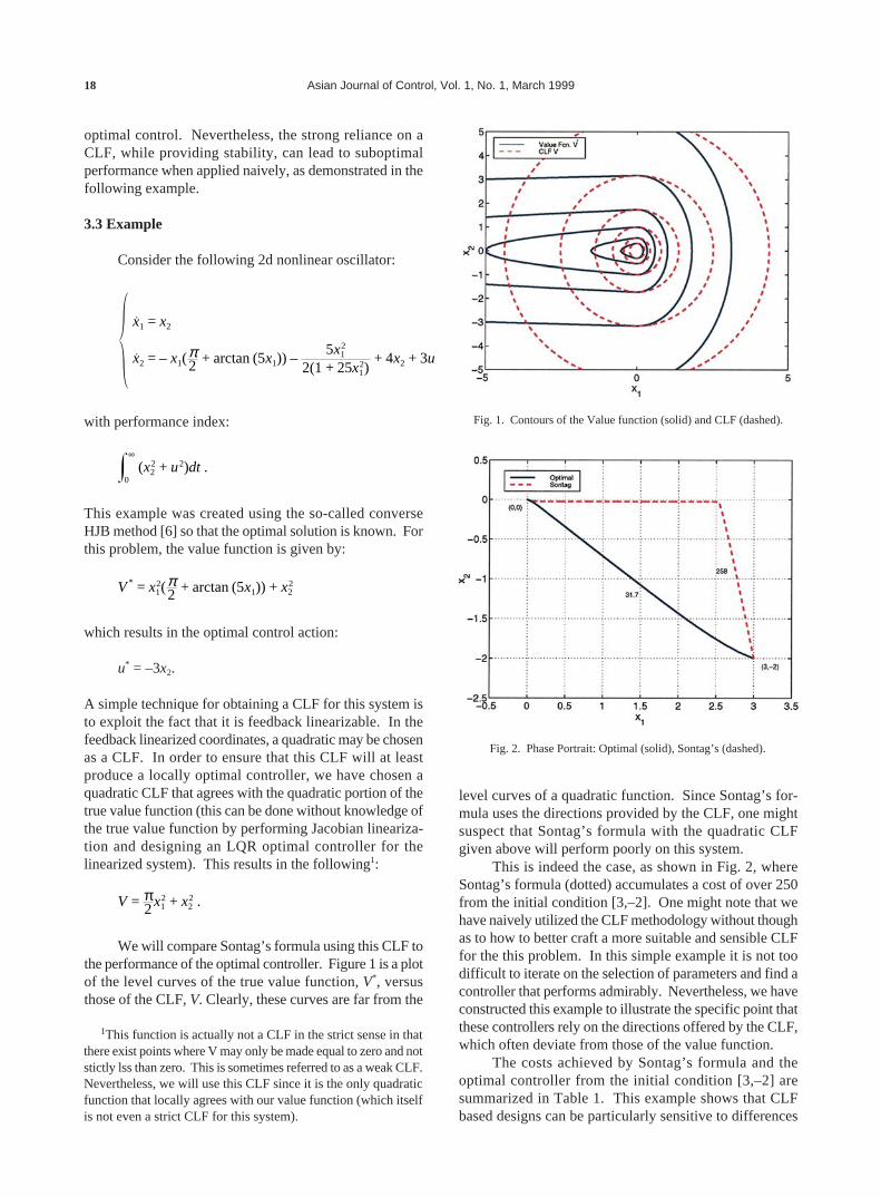
We will compare Sontag’s formula using this CLF tothe performance of the optimal controller. Figure 1 is a plotof the level curves of the true value function, V*, versusthose of the CLF, V. Clearly, these curves are far from the

level curves of a quadratic function. Since Sontag’s for-mula uses the directions provided by the CLF, one mightsuspect that Sontag’s formula with the quadratic CLFgiven above will perform poorly on this system.

This is indeed the case, as shown in Fig. 2, whereSontag’s formula (dotted) accumulates a cost of over 250from the initial condition [3,–2]. One might note that wehave naively utilized the CLF methodology without thoughas to how to better craft a more suitable and sensible CLFfor the this problem. In this simple example it is not toodifficult to iterate on the selection of parameters and find acontroller that performs admirably. Nevertheless, we haveconstructed this example to illustrate the specific point thatthese controllers rely on the directions offered by the CLF,which often deviate from those of the value function.

The costs achieved by Sontag’s formula and theoptimal controller from the initial condition [3,–2] aresummarized in Table 1. This example shows that CLFbased designs can be particularly sensitive to differences

1This function is actually not a CLF in the strict sense in thatthere exist points where V may only be made equal to zero and notstictly lss than zero. This is sometimes referred to as a weak CLF.Nevertheless, we will use this CLF since it is the only quadraticfunction that locally agrees with our value function (which itselfis not even a strict CLF for this system).

Fig. 1. Contours of the Value function (solid) and CLF (dashed).

Fig. 2. Phase Portrait: Optimal (solid), Sontag’s (dashed).


between the CLF and the value function, even for a tech-nique such as Sontag’s formula that directly incorporatesinformation from the optimal control problem into thecontroller design process.

IV. RECEDING HORIZON CONTROL (RHC)

We now switch from the HJB approach embodied inCLF methods to an Euler-Lagrange philosophy introducedin methods known as receding horizon, moving horizon, ormodel predictive control (cf. [18,17,12,20,15,12]). thesetechniques are based upon using on-line computation torepeatedly solve optimal control problems emanatingfrom the current measured state. To be more specific, thecurrent control at state x and time t is obtained by determin-ing on-line the optimal control solution u over the interval[t, t + T] respecting the following objective:(Receding Horizon Control)

infu(⋅)

(q(x(τ ))t

t + T

+ uT(τ )u(τ ))dτ + ϕ(x(t + T))

s.t. x = f (x) + g(x)u

with the current measured state as the initial condition,and applying the optimizing solution û(⋅) until a newstate update is received. Repeating this calculation foreach new state measurement yields a state-feedbackcontrol law. This type of implementation is commonlyreferred to as a receding or moving horizon and is thefoundation of model predictive control [12]. As isevident from this sort of control scheme, obtaining areduced value of the performance index is of utmostimportance.

The philosophy behind receding horizon controlcan be summarized as follows. It exploits the simplicityof the Euler-Lagrange approach by repeatedly solvingtrajectory optimizations emanating from the currentstate. The solution to each optimization provides anapproximation to the value function at the current state, aswell as an accompanying open-loop control trajectory.The receding horizon approach converts these open-looptrajectories into the desired state-feedback. The key tothis methodology is that it only requires that the optimalcontrol problem be solved for the states encounteredalong the current trajectory, in this way avoiding the globalnature of the HJB approach and its associated computa-tional intractability.

4.1 Computational issues

Despite the computational advantages of an Euler-Lagrange approach over those of the HJB viewpoint, theon-line implementation of receding horizon control is stillcomputationally demanding. In fact, the practical imple-mentation of receding horizon control is often hindered bythe computational burden of the on-line optimization whichtheoretically must be solved continuously. In reality, theoptimization is solved at discrete sampling times and thecorresponding control moves are applied until they can beupdated at the next sampling instance. The choice of boththe sampling time and horizon are largely influenced by theability to solve the required optimization within the al-lowed time interval. These considerations often limit theapplication of receding horizon control to systems withsufficiently slow dynamics to be able to accommodate suchon-line inter-sample computation.

For linear systems under quadratic objective functions,the on-line optimization is reduced to a tractable quadraticprogram, even in the presence of linear input and outputconstraints. This ability to incorporate constraints was theinitial attraction of receding horizon implementations. Fornonlinear systems the optimization is in general non-convex and hence has no efficient solution. Methods forfast solutions or approximations to solutions of theseEuler-Lagrange type optimizations have occupied an en-tire research area by themselves and will not be expoundedon here. (See [23,22,11]).

While these numerical and practically oriented issuesare compelling, there are fundamental issues related to thetheoretical foundations of receding horizon control thatdeserve equal scrutiny. The mot critical of these are wellillustrated by considering the stability and performanceproperties of idealized receding horizon control.

4.2 Stability

While using a numerical optimization as an integralpart of the control scheme allows great flexibility, espe-cially concerning the incorporation of constraints, it com-plicates the analysis of stability and performance proper-ties of receding horizon control immensely. The reason forthe difficulty is quite transparent. Since the control actionis determined through a numerical on-line optimization atevery sampling point, there is often no convenient closedform expression for the controller nor for the closed-loopsystem.

The lack of a complete theory for a rigorous analysisof receding horizon stability properties in nonlinear sys-tems often leads to the use of intuition in the design process.Unfortunately, this intuition can be misleading. Consider,for example, the statement that horizon length provides atradeoff between the issues of computation and of stabilityand performance. A longer horizon, while beingcomputationally more intensive for the on-line optimization,

Table. 1. Cost of Sontag’s formula vs. the optimalcontroller from initial condition [3, –2].

Controller Cost

Sontag 258Optimal 31.7


will provide a better approximation to the infinite horizonproblem and hence the controller will inherit the stabilityguarantees and performance properties enjoyed by theinfinite horizon solution. While this intuition is correct inthe limit as the horizon tends to infinity [24], for horizonlengths applied in practice the relationship between hori-zon and stability is much more subtle and often contradictssuch seemingly reasonable statements. This is best illus-trated by the example used previously in Section 3.3.Recall that the system dynamics were given by:

x1 = x2

x2 = – x1(π2 + arctan (5x1)) –

5x12

2(1 + 25x12)

+ 4x2 + 3u

with performance index:

(x22 + u2)

0

∞

dt .

For simplicity we will consider receding horizoncontrollers with no terminal weight (i.e. ϕ(x) = 0) and usea sampling interval of 0.1. By investigating the rela-tionship between horizon length and stability throughsimulations from the initial condition [3,–2], a puzzlingphenomena is uncovered. Beginning from the shortesthorizon simulated, T = 0.2, the closed-loop system is foundto be unstable (see Fig. 3). As the horizon is increased toT = 0.3, the results change dramatically and near optimalperformance is achieved by the receding horizon con-troller. At this point, one might be tempted to assume thata sufficient horizon for stability has been reached andlonger horizons would only improve the performance. Inactuality the opposite happens and as the horizon is in-

creased further the performance deteriorates and has re-turned to instability by a horizon of T = 0.5. This instabilityremains present even past a horizon of T = 1.0. Thesimulation results are summarized in Table 2 and Fig. 3.

It is important to recognize that the odd behavior wehave encountered is not a nonlinear effect, nor the result ofa cleverly chosen initial condition or sampling interval, butrather inherent to the receding horizon approach. In fact,the same phenomena takes place even for the linearizedsystem:

x =

0 1

– π2 4

x + 03 u . (15)

In this case, a more detailed analysis of the closed-loop system is possible due to the fact that the controller andclosed-loop dynamics are linear and can be computed inclosed form. Figure 4 shows the magnitude of the maxi-mum eigenvalue of the discretized closed-loop system2

Fig. 3. RHC for various horizon lengths,.

2 The receding horizon controller was computed by discretizingthe continuous time system using a first order hold and time stepof 0.001, and solving the Riccati difference equation of appropri-ate length, hence the eigenvalues correspond to a discrete-timesystem with stability occurring when the maximum eigenvaluehas modulus less than 1.

Table. 2. Comparison of controller performance frominitial condition [3, –2].

Controller Performance

T = 0.2: (dotted) unstableT = 0.3: (dash-dot) 33.5T = 0.5: (dashed) unstableT = 1.0: (solid) unstable

Fig. 4. Maximum eigenvalue versus horizon length for discretized linearsystem.


versus the horizon length of the receding horizon con-troller. This plot shows that stability is only achieved fora small range of horizons that include T = 0.3 and longerhorizons lead to instability. It is not until a horizon ofT = 3.79 that the controller becomes stabilizing once again.

These issues are not new in the receding horizoncontrol community and related phenomena have beennoted before by in the context of Riccati difference equa-tions [2]. This delicate relationship between horizonlength and stability has been addressed by various means.In fact, the majority of literature focuses on producingstabilizing formulations of receding horizon control. Thefirst stabilizing approach was to employ an end constraintthat required the final predicted state corresponding to theon-line optimization be identically zero. This guaranteedstability in both linear and nonlinear formulations at theexpense of a restrictive and computationally burdensomeequality constraint [18,19]. Other formulations, includingcontraction constraints [5], infinite horizon [26,4] and dualmode [21] have eased the dominating effect of an endconstraint. Numerous other approaches have beendeveloped, each deviating slightly from the formulation ofreceding horizon control that we have presented in order toprovided stability guarantees.

Our focus is on the connection between recedinghorizon control and the classical Euler-Lagrange approachto optimal control. In essence, receding horizon techniquesproduce local approximations to the value function throughEuler-Lagrange type on-line optimizations, and use thesetop produce a control law. It is also this lack of globalinformation that can lead receding horizon control astray interms of stability, and must be dealt with when stabilizingformulations are desired. On the other hand, the locality ofthe optimizations allow receding horizon control to over-come the computational intractability associated with theHJB approach.

V. COMBINING OFF-LINE ANALYSISWITH ON-LINE COMPUTATION:

CLFs AND RHC

The previous sections illustrated the underlying con-cepts and limitations in the control Lyapunov function andreceding horizon methodologies. Table 5 summarizessome of the key properties of each approach.

When viewed together, these properties are seen tobe complementary, suggesting that the control Lyapunov

function and receding horizon methodologies are naturalpartners. Off-line analysis produces a control Lyapunovfunction, representing the best approximation to the valuefunction, while receding horizon style computation canthen be used on-line, optimizing over trajectories emanat-ing from the current state, improving the solution byutilizing as must computation as is available. A propercombination of the properties of CLFs and receding hori-zon control should have the potential to overcome thelimitations imposed by each technique individually.

In this final section we outline two approaches thatblend the information from a CLF with on-line recedinghorizon style computation. The first extends the CLFbased optimization in pointwise min-norm controllers to areceding horizon, while the second enhances the standardreceding horizon scheme by using a CLF as a terminalweight. While this section only offers an initial glimpse atthe opportunities available by viewing CLFs and recedinghorizon control as partners, we hope that it is sufficient tospur others to investigate these connections as well.

5.1 Receding horizon extensions of pointwise min-normcontrollers

Pointwise min-norm controllers are formulated asan on-line optimization (see (12)), but in practice thisoptimization is solved off-line and in closed form. Hence,while benefiting from the stability properties of the under-lying CLF, pointwise min-norm controllers fail to takeadvantage of on-line computing capabilities. Yet, byviewing the pointwise min-norm optimizations (12) as a“zero horizon” receding horizon optimization, it is actuallypossible to extend them to a receding horizon scheme. Oneimplementation of this idea is as follows.

Let V be a CLF and let uσ and xσ denote the controland state trajectories obtained by solving the pointwisemin-norm problem with parameter σ(x) (cf. (12)-(13)).Consider the following receding horizon objective:

infu(⋅)

(q(x))t

t + T

+ uTu)dτ

s.t. x = f (x) + g(x)u (16)

∂V∂x [ f + gu(t)] ≤ – nσ(x(t)) (17)

V(x(t + T)) ≤ V(xσ(t + T)) (18)

with 0 < n ≤ 1. This is a standard receding horizon schemewith two CLF based constraints. The first, (17), applies toall implemented control actions at the beginning of thehorizon, and is a direct stability constraint similar to (13) inthe pointwise min-norm problem, although relaxed by n.On the other hand, the constraint (18) applies at the end ofthe horizon, and uses the pointwise min-norm solution torequire that all allowable trajectories reach a final state

Table. 5

CLF RHC

Relies on global information Relies on local information

Stability oriented Performance oriented

Requires off-line analysis Requires on-line computation

Connections to HJB formulation Connections to E-L formulation


x(t + T) that lies within the level curve of the CLF thatpasses through xσ(t + T).

We refer to this receding horizon scheme as anextension of pointwise min-norm controllers since in thelimit as the horizon T tends to zero, this on-line optimiza-tion reduces to the pointwise min-norm optimization.Additionally, when the parameter σs (14) corresponding toSontag’s formula is used, the property that the controllerwill be optimal when the shape of the level curves from theCLF correspond to those of the value function is preserved.Hence, it even provides a corresponding extension ofSontag’s formula [25].

The CLF constraints, while adding computationaldifficulty to the on-line optimizations, actually ease anumber of implementation problems. Due to (17), whichrequires that all closed-loop trajectories are consistent withthe CLF V, stability properties of this scheme are indepen-dent of the horizon, T. This allows horizon lengths to bevaried on-line, extending when more on-line computationis available, and shrinking to zero (i.e. the pointwise min-norm controller) when no on-line computation is possible.Furthermore, stability does not depend on global or evenlocal solutions to the on-line optimizations. Finally, oneshould note that the trajectory from the pointwise min-norm solution provides an initial feasible trajectory foreach receding horizon optimization. Hence, this schemetruly builds upon the pointwise min-norm controller, ex-ploiting all available on-line computation to improve uponthis solution. More details about this scheme, includingderivations of these properties, can be found in [25].

When this scheme is applied to our 2d nonlinearoscillator example using a small value for n and the param-eter σs corresponding to Sontag’s formula, near optimalperformance is recovered [25]. This is true even forrelatively short horizons, demonstrating the beneficial mixof on-line computation coupled with the knowledge of aCLF. A more representative example can be found in [32]where a number of control techniques are compared on aducted fan model.

5.2 CLF enhanced receding horizon schemes

The preceding scheme began from the CLF point ofview, extending pointwise min-norm controllers to incor-porate on-line optimization. The other point of view is alsopossible. Standard receding horizon formulations can bealtered to benefit from the knowledge of a CLF. Below, webriefly present a scheme that begins from this premise.

A CLF is an obvious choice for a terminal weight ina receding horizon scheme. In this case, each recedinghorizon optimization takes the form:

infu(⋅)

(q(x(τ ))t

t + T

+ uT(τ )u(τ ))dτ + V(x(t + T))

s.t. x = f (x) + g(x)u .

If the CLF were actually the value function, V*, thenthis optimization would be equivalent to the infinite hori-zon objective (2) and produce the optimal controller. Ingeneral, we can only assume the CLF is a rough approxima-tion to the value function, in which case the recedinghorizon scheme based upon the above optimization cannoteven be shown to be stabilizing. Fortunately, if the CLFpossesses a slightly stronger property, specifically that

infu(⋅)

[Vx( f (x) + g(x)u)] ≤ – q(x) ,

then stability does result. CLFs that satisfy this conditionarise from some standard control methodologies, includingthe so-called quasi-LPV approach [31], providing a start-ing point for the derivation of a CLF to be used in conjunc-tion with this scheme.

Here, as before, the idea is to utilize the stabilityproperties of CLFs, without sacrificing the performanceadvantages of receding horizon computation. Combiningboth into a single scheme allows access to their comple-mentary properties, hopefully overcoming the limitationsof each individually. Details of this approach are availablein [14] and applications to a ducted fan model are given in[13].

The two CLF based receding horizon schemes pre-sented in this section are by no means the only possibleapproaches. Our extension of pointwise min-norm con-trollers to a receding horizon scheme is not unique, andCLFs have the potential to couple with on-line computa-tions in numerous ways. Nevertheless, we do hope to haveillustrated some of the opportunities available from thecombination of ideas from control Lyapunov functions andreceding horizon style optimization, and encouraged oth-ers to pursue these connections and opportunities as well.

VI. SUMMARY

In this paper we explored two approaches to thenonlinear optimal control problem. Both have roots instandard optimal control techniques. Control Lyapunovfunctions are best interpreted in the context of Hamilton-Jacobi-Bellman equations, especially a variation of Sontag’sformula that naturally arises from HJB equations andfurthermore is a special case of a more general class of CLFbased controllers known as pointwise min-norm controllers.Even with strong ties to the optimal control problem, CLFbased approaches err on the side of stability and can resultin poor performance when the CLF does not closely re-semble the value function.

The second technique is that of receding horizoncontrol which is based on the repeated on-line solution ofopen-loop optimal control problems which more closelyrelate to an Euler-Lagrange framework. The intractabilityof the HJB equations are overcome by solving for theoptimal control only along the current trajectory throughon-line computation. This approach chooses to err on the


side of performance and in its purest form lacks guaranteedstability properties. Stability and performance concernsbecome even more critical when short horizons must beused to accommodate the extensive on-line computationrequired.

While seemingly unrelated, when viewed in the con-text of the optimal control problem these two techniquesare seen to possess very complementary properties derivedfrom their approaches to the same underlying problem.This suggests the potential to combine approaches intohybrid schemes that blend the most useful aspects of eachpoint of view. Finally, we outlined two such schemes,utilizing the ideas and techniques presented in this paper.In the end, it is our hope that this perspective encouragesresearchers to look beyond their own fields of expertise,and consider the advantages to be gained by coupling theirtechniques with the contibutions of others.

REFERENCES

1. Artstein, Z. “Stabilization with Relaxed Controls,”Nonlinear Anal., Vol. 15, No. 11, pp. 1163-117 (1983).

2. Bitmead, R.R., M. Gevers, I.R. Petersen, and R.J.Kaye, “Monotonicity and Stabilizability Properties ofSolutions of the Riccati Difference Equation:Propositions, Lemmas, Theorems, Fallacious Conjec-tures and Counterexamples,” Syst. Contr. Lett.,pp. 309-315 (1985).

3. Bryson, A.E. and Y. Ho, Applied Optimal Control,Hemisphere Publ. Corp., Washington D.C., (1975).

4. Chen, H. and F. Allgöwer, “A Quasi-infinite HorizonNonlinear Model Predictive Control Scheme forConstrained Nonlinear Systems,” In Proc. the 16thChinese Contr. Conf., Qindao, China, pp. 309-31(1996).

5. Oliveira De S. and M. Morari, “Robust Model Predic-tive Control for Nonlinear Systems with Constraints,”IFAC Symp. Robust Contr., Rio de Janeiro, Brazil, pp.221-226 (1994).

6. Doyle, J.C. J. Primbs, B. Shapiro, and V. Nevistic,“Nonlinear Games: Examples and Counterexamples,”In Proc. the 35th IEEE Conf. Decis. Contr., Kobe,Japan, pp. 3915-3920 (1996).

7. Freeman, R. and P. Kokotovic, “Optimal NonlinearControllers for Feedback Linearizable Systems,” InProc. the Amer. Contr. Conf., Seattle, Washington,pp. 2722-2726 (1995).

8. Freeman, R. and P. Kokotovic, “Inverse Optimality inRobust Stabiliztion,” SIAM J. Contr. Optimiz., Vol.34, pp. 1365-1391 (1996).

9. Freeman, R. and P. Kokotovic, “Robust NonlinearControl Design,” Birkhäuser, Boston (1996).

10. Freeman, R. and J. Primbs, “Control Lyapunov Func-tions : New Ideas from and Old Source,” In Proc. the35th IEEE Conf. Decis. Cont., Kobe, Japan, pp. 3926-3931 (1996).

11. García, C.E. , “Quadratic Dynamic Matrix Control ofNonlinear Processes. An Application to a Batch Reac-tor Process,” In Proc. AIChE Annu. Meet., SanFrancisco, California (1984).

12. García, C.E., D.M. Prett, and M. Morari, “ModelPredicitive Control: Theory and Practice – ASurvey,” Automatica, Vol. 25, No. 3, pp. 335-348(1989).

13. Jadbabaie, A., J. Yu, and J. Hauser, “Receding HorizonControl of the Caltech Ducted Fan: a Control LyapunovFunction Approach,” In Proc. Conf. Contr. Appl.,Hawaii (1999).

14.Jadbabaie, A., J. Yu, and J. Hauser, “Stabilizing Reced-ing Horizon Control of Nonlinear Systems: a ControlLyapunov Function Approach,” In Proc. the Amer.Contr. Conf., San Diego, CA (1999).

15. Keerthi, S. and E. Gilbert, “Optimal Infinite-horizonFeedback Laws for a General Class of ConstrainedDiscrete-time Systems: Stability and Moving-horizonApproximations,” J. Optimiz. Theory Appl., pp. 265-293 (1988).

16. Krstic, M., I. Kanellakopoulos, and P. Kokotovic,“Nonlinear and Adaptive Control Design,” John Wiley& Sons, New York (1995).

17. Kwon, W.H., A.N. Bruckstein, and T. Kailath, “Stabi-lizing State Feedback Design Via the Moving HorizonMethod,” Int. J. Contr., Vol. 37, No. 3, pp. 631-643(1983).

18. Kwon, W.H. and A.E. Pearson, “A modified QuadraticCost Problem and Feedback Stabilization of a LinearSystem.” IEEE Trans. Automat. Contr., Vol. 22, No. 5,pp. 838-842 (1977).

19. Kwon, W.H. and A.E. Pearson, “On Feedback Stabili-zation of Time-varying Discrete Linear Systems,”IEEE Trans. Automat. Contr., Vol. 23, pp. 479-481(1978).

20. Mayne, D.Q. and H. Michalska, “Receding HorizonControl of Nonlinear Systmes,” IEEE Trans. Automat.Contr., Vol. 35, No. 7, pp. 814-824 (1990).

21. Michalska, H. and D.Q. Mayne, “Robust RecedingHorizon Control of Constrained Nonlinear Systems,”IEEE Trans. Automat. Contr., Vol. 38, No. 11, pp.1623-1633 (1993).

22. Nevistic, V., “Constrained Control of NonlinearSystems,” Ph.D. Thesis, ETH Zürich (1997).

23. Ohtsuka, T. and H. Fujii, “Stabilized ContinuationMethod for Solving Optimal Control Problems,” J.Guid., Contr. Dyn., Vol. 17, No. 5, pp. 950-957 (1994).

24. Primbs, J.A. and V. Nevistic, “Constrained FiniteReceding Horizon Linear Quadratic Control,” In Proc.the 36th IEEE Conf. Decis. Contr., San Diego,California, pp. 3196-3201 (1997).

25. Primbs, J.A., V. Nevistic, and J.C. Doyle, “On Reced-ing Horizon Extensions and Control LyapunovFunctions,” In Proc. the Amer. Contr. Conf.,Philadelphia, Pennsylvania (1998).

´

´

´

´ ´

´

´

´

´


26. Rawlings, J.B. and K.R. Muske, “The Stability ofConstrained Receding Horizon Control,” IEEE Trans.Automat. Contr., Vol. 38, No. 10, pp. 1512-1516,(1993).

27. Richalet, J., “Industrial Applications of Model BasedPredictive Control,” Automatica, Vol. 29, pp. 1251-1274 (1993).

28. Richalet, J., A. Rault, J.L. Testud, and J. Papon, “ModelPredictive Heuristic Control: Applications to Indus-trial Processes,” Automatica, Vol. 14, No. 5, pp. 413-428 (1978).

29. Sontag, E.D., “A Lyapunov-like Characterization ofAsymptotic Controllability.,” SIAM J. Contr. Optimiz.,Vol. 21, No. 3, pp. 462-471 (1983).

30. Sontag, E.D., “A ‘Universal’ Construction of Artstein’sTheorem on Nonlinear Stabilization,” Syst. Contr.Lett., Vol. 13, No. 2, pp. 117-123 (1989).

31. Fen Wu, Hua Xin Yang, Andy Packard, and GregBecker, “Induced L2-Norm Control for lpv Systemwith Bounded Parameter Variation,” Int. J. NonlinearRobust Contr., Vol. 6, pp. 983-998 (1996).

32. Yu, J., A. Jadbabaie, J. Primbs, and Y. Huang, “Com-parison of Nonlinear Control Designs for a Ducted FanModel,” In Proc. IFAC 14th World Cong., Beijing,China (1999).

James A. Primbs received B.S. de-grees in electrical engineering andmathematics at the University ofCalifornia, Davis in 1994, the M.S.degree in electrical engineering at

Stanford University in 1995 and the Ph.D in control anddynamical systems from the California Institute of Tech-nology in 1999. He is currently a post-doctoral researcherin the control and dynamical systems department at Caltech.His research interests include nonlinear control, complexsystems, and finance.

Vesna Nevistic received her diplomafrom the department of electronics atthe Military Technical Academy inZagreb in 1998, the M.S. degree fromthe electrical engineering departmentat Zagreb University in 1991 and thePh.D. in electrical engineering fromthe Swiss Federal Institute of Tech-

nology (ETH) in 1997. She currently works as a manage-ment consultant for McKinsey and Co. in their Zurichoffice.

John Doyle received a BS and MS inEE at MIT and a Ph.D. in Mathemat-ics from UC Berkeley. He is nowProfessor in Control and DynamicalSystems at Caltech. His main re-search interest is in robustness ofcomples systems. He has receivedseveral prize paper awards, including

2 Axelby and a Baker prize from the IEEE.

´

2-14-24

Documents