1rm prediction: a data mining case study - archivo...
TRANSCRIPT

1RM prediction:a data mining case study
Adrian Santos Parrilla
Supervised by Aurora Perez Perez
Master of Science Thesis
Facultad Informatica
Universidad Politecnica de Madrid
June 30, 2014


Abstract
In the last few years there has been a heightened interest in data treatment and analysis withthe aim of discovering hidden knowledge and eliciting relationships and patterns within thisdata. Data mining techniques (also known as Knowledge Discovery in Databases) have beenapplied over a wide range of fields such as marketing, investment, fraud detection, manu-facturing, telecommunications and health. In this study, well-known data mining techniquessuch as artificial neural networks (ANN), genetic programming (GP), forward selection linearregression (LR) and k-means clustering techniques, are proposed to the health and sportscommunity in order to aid with resistance training prescription. Appropriate resistance train-ing prescription is effective for developing fitness, health and for enhancing general quality oflife. Resistance exercise intensity is commonly prescribed as a percent of the one repetitionmaximum. 1RM, dynamic muscular strength, one repetition maximum or one execution max-imum, is operationally defined as the heaviest load that can be moved over a specific range ofmotion, one time and with correct performance. The safety of the 1RM assessment has beenquestioned as such an enormous effort may lead to muscular injury. Prediction equations couldhelp to tackle the problem of predicting the 1RM from submaximal loads, in order to avoidor at least, reduce the associated risks. We built different models from data on 30 men whoperformed up to 5 sets to exhaustion at different percentages of the 1RM in the bench pressaction, until reaching their actual 1RM. Also, a comparison of different existing predictionequations is carried out. The LR model seems to outperform the ANN and GP models for the1RM prediction in the range between 1 and 10 repetitions. At 75% of the 1RM some subjects(n = 5) could perform 13 repetitions with proper technique in the bench press action, whilstother subjects (n = 20) performed statistically significant (p < 0.05) more repetitions at 70%than at 75% of their actual 1RM in the bench press action. Rate of perceived exertion (RPE)seems not to be a good predictor for 1RM when all the sets are performed until exhaustion, asno significant differences (p < 0.05) were found in the RPE at 75%, 80% and 90% of the 1RM.Also, years of experience and weekly hours of strength training are better correlated to 1RM(p < 0.05) than body weight. O’Connor et al. 1RM prediction equation seems to arise fromthe data gathered and seems to be the most accurate 1RM prediction equation from thoseproposed in literature and used in this study. Epley’s 1RM prediction equation is reproducedby means of data simulation from 1RM literature equations. Finally, future lines of researchare proposed related to the problem of the 1RM prediction by means of genetic algorithms,neural networks and clustering techniques.Key words: genetic programming, artificial neural network, periodization, one repetition max-imum, performance, RPE, data mining, clustering.
3

En los ultimos anos ha habido un creciente interes en el tratamiento y analisis de datoscon el proposito de descubrir relaciones, patrones y conocimiento oculto en los mismos. Lastecnicas de data mining (tambien llamadas de “Descubrimiento de conocimiento en basesde datos“) se han aplicado consistentemente a lo gran de un gran espectro de areas comoel marketing, inversiones, deteccion de fraude, produccion industrial, telecomunicaciones ysalud. En este estudio, tecnicas bien conocidas de data mining como las redes neuronalesartificiales (ANN), programacion gentica (GP), regresion lineal con seleccion hacia adelante(LR) y la tecnica de clustering k-means, se proponen a la comunidad del deporte y la saludcon el objetivo de ayudar con la prescripcion del entrenamiento de fuerza. Una apropiadaprescripcion de entrenamiento de fuerza es efectiva no solo para mejorar el estado de formageneral, sino para mejorar la salud e incrementar la calidad de vida. La intensidad en unejercicio de fuerza se prescribe generalmente como un porcentaje de la repeticion maxima.1RM, fuerza muscular dinamica, una repeticion maxima o una ejecucion maxima, se defineoperacionalmente como la carga maxima que puede ser movida en un rango de movimientoespecıfico, una vez y con una tecnica correcta. La seguridad de las pruebas de 1RM ha sidocuestionada debido a que el gran esfuerzo requerido para llevarlas a cabo puede derivar enserias lesiones musculares. Las ecuaciones predictivas pueden ayudar a atajar el problema dela prediccion de la 1RM con cargas sub-maximas y son empleadas con el proposito de eliminaro al menos, reducir los riesgos asociados. En este estudio, se construyeron distintos modelos apartir de los datos recogidos de 30 hombres que realizaron hasta 5 series al fallo en el ejerciciopress de banca a distintos porcentajes de la 1RM, hasta llegar a su 1RM real. Tambien semuestra una comparacion de algunas de las distintas ecuaciones de prediccion propuestas conanterioridad. El modelo LR parece superar a los modelos ANN y GP para la prediccionde la 1RM entre 1 y 10 repeticiones. Al 75% de la 1RM algunos sujetos (n = 5) pudieronrealizar 13 repeticiones con una tecnica apropiada en el ejercicio press de banca, mientrasque otros (n = 20) realizaron significativamente (p < 0.05) mas repeticiones al 70% que al75% de su 1RM en el press de banca. El ındice de esfuerzo percibido (RPE) parece no serun buen predictor del 1RM cuando todas las series se realizan al fallo, puesto que no existendiferencias significativas (p < 0.05) en el RPE al 75%, 80% y el 90% de la 1RM. Ademas,los anos de experiencia y las horas semanales dedicadas al entrenamiento de fuerza estanmas correlacionadas con la 1RM (p < 0.05) que el peso corporal. La ecuacion de O’Connoret al. parece surgir de los datos recogidos y parece ser la ecuacion de prediccion de 1RMms precisa de aquellas propuestas en la literatura y empleadas en este estudio. La ecuacionde prediccion de la 1RM de Epley es reproducida mediante simulacion de datos a partir dealgunas ecuaciones de prediccion de la 1RM propuestas con anterioridad. Finalmente, seproponen futuras lıneas de investigacion relacionadas con el problema de la prediccion de la1RM mediante algoritmos geneticos, redes neuronales y tecnicas de clustering.Palabras clave: programacion genetica, red neuronal artificial, periodizacion, una repeticionmaxima, performance, RPE, minerıa de datos, clustering.

Solo envidio a los que no nacieron todavıa,para ellos sera lo que tu y yo creamos un dıa.
Rafael Lechowski


Contents
1 Introduction 1
2 State of the art 32.1 The 1RM prediction problem . . . . . . . . . . . . . . . . . . . . . . . . . . . 3
2.1.1 Prediction formulas from submaximal loads . . . . . . . . . . . . . . . 32.1.2 Percentage of the 1RM . . . . . . . . . . . . . . . . . . . . . . . . . . . 52.1.3 Variables influencing the 1RM . . . . . . . . . . . . . . . . . . . . . . . 6
2.2 Data mining modeling . . . . . . . . . . . . . . . . . . . . . . . . . . . . . . . 82.2.1 Multilayer perceptron with backpropagation . . . . . . . . . . . . . . . 82.2.2 General linear regression with forward selection . . . . . . . . . . . . . 122.2.3 Genetic programming . . . . . . . . . . . . . . . . . . . . . . . . . . . . 142.2.4 K-means algorithm . . . . . . . . . . . . . . . . . . . . . . . . . . . . . 18
2.3 Comparison criteria . . . . . . . . . . . . . . . . . . . . . . . . . . . . . . . . . 192.4 Evaluating the accuracy of a predictor . . . . . . . . . . . . . . . . . . . . . . 20
3 Problem definition 233.1 Design of the experiment . . . . . . . . . . . . . . . . . . . . . . . . . . . . . . 243.2 Data collection procedure . . . . . . . . . . . . . . . . . . . . . . . . . . . . . 303.3 Threats to validity . . . . . . . . . . . . . . . . . . . . . . . . . . . . . . . . . 32
4 KDD process 354.1 Tools used . . . . . . . . . . . . . . . . . . . . . . . . . . . . . . . . . . . . . . 354.2 Data preprocessing . . . . . . . . . . . . . . . . . . . . . . . . . . . . . . . . . 36
4.2.1 Grouping the participants by means of clustering techniques. . . . . . . 414.3 Linear regression models . . . . . . . . . . . . . . . . . . . . . . . . . . . . . . 44
4.3.1 Interaction between weight and repetitions . . . . . . . . . . . . . . . . 464.4 Multilayer perceptron neural network . . . . . . . . . . . . . . . . . . . . . . . 474.5 Genetic programming model . . . . . . . . . . . . . . . . . . . . . . . . . . . . 544.6 Comparison between the different models . . . . . . . . . . . . . . . . . . . . . 58
4.6.1 Comparison between the different models generated . . . . . . . . . . 594.7 Comparison between the different literature equations . . . . . . . . . . . . . . 644.8 Post-hoc analysis . . . . . . . . . . . . . . . . . . . . . . . . . . . . . . . . . . 65
4.8.1 Number of repetitions at a certain percentage of 1RM . . . . . . . . . . 65
i

4.8.2 Comparing repetitions until exhaustion at 70%-75% of 1RM . . . . . . 674.8.3 RPE and repetitions until exhaustion . . . . . . . . . . . . . . . . . . . 68
4.9 Data simulation . . . . . . . . . . . . . . . . . . . . . . . . . . . . . . . . . . . 71
5 Conclusions 75
6 Future research 776.1 Genetic algorithm . . . . . . . . . . . . . . . . . . . . . . . . . . . . . . . . . . 776.2 Multilayer perceptron networks . . . . . . . . . . . . . . . . . . . . . . . . . . 79
6.2.1 Bootstrap and bagging techniques . . . . . . . . . . . . . . . . . . . . . 806.3 Neural network: SOM . . . . . . . . . . . . . . . . . . . . . . . . . . . . . . . 816.4 Clustering with k-means . . . . . . . . . . . . . . . . . . . . . . . . . . . . . . 816.5 Appendix A . . . . . . . . . . . . . . . . . . . . . . . . . . . . . . . . . . . . . 83
ii

List of Figures
2.1 Different anthropometric variables include circumferences and lengths [1]. . . . 72.2 Computations of a neuron. . . . . . . . . . . . . . . . . . . . . . . . . . . . . . 92.3 General multilayer perceptron architecture. . . . . . . . . . . . . . . . . . . . . 102.4 An individual tree structure. A possible individual in the population [2]. . . . 142.5 Tree crossover [2]. . . . . . . . . . . . . . . . . . . . . . . . . . . . . . . . . . . 172.6 K-means execution [3]. . . . . . . . . . . . . . . . . . . . . . . . . . . . . . . . 182.7 Random sub-sampling. . . . . . . . . . . . . . . . . . . . . . . . . . . . . . . 212.8 k-cross fold technique. . . . . . . . . . . . . . . . . . . . . . . . . . . . . . . . 22
4.1 Distribution of the population attributes. . . . . . . . . . . . . . . . . . . . . . 394.2 Distribution of weight and repetitions. . . . . . . . . . . . . . . . . . . . . . . 404.3 Comparison between the generated models. . . . . . . . . . . . . . . . . . . . . 624.4 Repetitions performed until exhaustion vs. %1RM. . . . . . . . . . . . . . . . 654.5 Box plot: RPE at the end of the set. . . . . . . . . . . . . . . . . . . . . . . . 704.6 Repetitions performed until exhaustion vs. %1RM. . . . . . . . . . . . . . . . 714.7 Repetitions performed until exhaustion vs. %1RM. . . . . . . . . . . . . . . . 72
iii

iv

List of Tables
2.1 1RM Prediction equations. . . . . . . . . . . . . . . . . . . . . . . . . . . . . . 42.2 Applicability of the different percentages of the 1RM for different purposes [4]. 5
3.1 Borg’s normalized scale [5]. . . . . . . . . . . . . . . . . . . . . . . . . . . . . 283.2 Attributes collected in the study. . . . . . . . . . . . . . . . . . . . . . . . . . 293.3 Tentative 1RM assessment protocol. . . . . . . . . . . . . . . . . . . . . . . . . 323.4 Attributes collected for each set. . . . . . . . . . . . . . . . . . . . . . . . . . . 32
4.1 Population attributes. . . . . . . . . . . . . . . . . . . . . . . . . . . . . . . . 374.2 Population attributes normality test. . . . . . . . . . . . . . . . . . . . . . . . 384.3 Weight normality test. . . . . . . . . . . . . . . . . . . . . . . . . . . . . . . . 404.4 Correlations with 1RM. . . . . . . . . . . . . . . . . . . . . . . . . . . . . . . . 414.5 Attributes used in the k-means algorithm. . . . . . . . . . . . . . . . . . . . . 424.6 K-means clustering. Cluster centroids. . . . . . . . . . . . . . . . . . . . . . . 434.7 Clustered individuals (n = 30, k = 4). . . . . . . . . . . . . . . . . . . . . . . . 434.8 Linear regression models built. . . . . . . . . . . . . . . . . . . . . . . . . . . 454.9 Linear models with interaction between repetitions and weight. . . . . . . . . 474.10 Coefficients in interaction between weight and repetitions. . . . . . . . . . . . 474.11 Attributes used in the multilayer perceptron models built. . . . . . . . . . . . 514.12 RMSE and MAE with the random sub-sampling method (MLP). . . . . . . . . 524.13 RMSE and MAE with the 6-cross fold validation method (MLP). . . . . . . . 524.14 RMSE and MAE with the the leave-one-out validation method (MLP). . . . . 534.15 Error descriptives for the MLP with two variables, and the MLP with 5 variables
(n = 97). . . . . . . . . . . . . . . . . . . . . . . . . . . . . . . . . . . . . . . . 544.16 U Mann Whitney test. . . . . . . . . . . . . . . . . . . . . . . . . . . . . . . . 544.17 1RM prediction by means of genetic programming. . . . . . . . . . . . . . . . 574.18 RMSE and MAE with the random sub-sampling method. . . . . . . . . . . . . 604.19 RMSE and MAE with the 6-cross-fold-validation method. . . . . . . . . . . . . 604.20 RMSE and MAE with the leave one out validation method. . . . . . . . . . . . 614.21 Error descriptives for the MLP and Linear regression models (n = 76). . . . . 624.22 U Mann Whitney test. . . . . . . . . . . . . . . . . . . . . . . . . . . . . . . . 634.23 Error descriptives for the MLP and Linear regression (interaction) models (n =
76). . . . . . . . . . . . . . . . . . . . . . . . . . . . . . . . . . . . . . . . . . . 634.24 U Mann Whitney test. . . . . . . . . . . . . . . . . . . . . . . . . . . . . . . . 63
v

4.25 1RM Prediction equations from literature. . . . . . . . . . . . . . . . . . . . . 644.26 Descriptives of percentage and repetitions (n = 5). . . . . . . . . . . . . . . . . 664.27 Test of normality: repetitions and percentage. . . . . . . . . . . . . . . . . . . 674.28 Repetitions in the different groups (70-75%1RM). . . . . . . . . . . . . . . . . 684.29 %1RM in the different groups. . . . . . . . . . . . . . . . . . . . . . . . . . . . 684.30 Descriptives of the %1RM in the three groups created. . . . . . . . . . . . . . 694.31 Descriptives of the RPE at the end of the set in the three groups created. . . . 694.32 Coefficients of the 1RM prediction equation by means of data simulation. . . 73
vi

Acknowledgments
Me gustarıa agradecer al Ayuntamiento de San Sebastian de los Reyes, Madrid, y muy enespecial al gimnasio municipal “Claudio Rodrıguez“, y al “Club Balonmano San Sebastian delos Reyes“, por abrirme sus puertas y hacerme sentir como en casa. A Aurora Perez, por suenorme esfuerzo y dedicacion revisandome el trabajo, y sus buenos consejos a la hora de corre-gir la memoria. Querıa dar las gracias a todos los participantes que de forma completamentedesinteresada formaron parte del experimento.
Especialmente a Daniel Campillo Bravo y Sandra Fernandez Rodrıguez por ayudarme atomar las mediciones y estar ahı siempre que les he necesitado; sin vuestra ayuda todo estono hubiera sido posible. A mi madre, por ensenarme el valor del trabajo duro y el sacrificio.A la memoria de mi abuela, siempre me acuerdo de las tardes tan felices que pasamos a tulado. Os quiero.
vii

viii

Terms and definitions
• Exercise: physical activity that is planned, structured, repetitive and has as a final oran intermediate objective the improvement or maintenance of physical fitness. Exerciseis used to improve health, maintain fitness and is important as a means of physicalrehabilitation.1
• Repetition: long for rep, a repetition is a single cycle of lifting and lowering a weight ina controlled manner, moving through the form of an exercise.
• Set: consists of several repetitions performed one after another with no break betweenthem. Several repetitions form a set. It is also referred as an exercise set.
• Dynamic muscular strength: maximal force that can be generated by a muscle or mus-cle group. It is usually referred as 1RM, one repetition maximum or one executionmaximum.
• RPE: or rating of perceived exertion, is one of the most popular methods in the fieldof heavy physical work and the perception of effort and exertion. Ratings of perceivedexertion (or “effort and exertion“) are important complements to physiological measure-ments. Of all single indicators of the degree of physicall strain, perceived exertion is oneof the most informative. It integrates a great amount of information, with cues from theperipheral muscles and joints, cardiovascular and respiratory functions, and the centralnervous system [6]. A category ratio scale, commonly referred to as the CR-10 scaleis commonly used. In this category ratio scale, numbers from 0 to 10 are used. Thenumber 10 implies an extremely strong perceptual intensity as in the perceived intensityin extremely heavy physical exercise like lifting and carrying extremely heavy weights.
1From http://medical-dictionary.thefreedictionary.com/Exercise
ix

x

Chapter 1
Introduction
1RM, one repetition maximum or one execution maximum, is operationally defined as theheaviest load that can be moved over a specific range of motion, one time and with correctperformance [7].
Despite its universal application, the safety of a 1RM protocol has been questioned asindividuals new to maximal load-bearing activity may incur high muscular, bone and ligamentstress with the risk of serious muscular injury. The direct assessment of a 1RM has also beenreferred to as time consuming and impractical for large groups [8, 9]. Such limitations haveled to the development of prediction models which employ sub-maximal loads in order tominimize the limitations and risks of maximal strength assessment [10].
Even though 1RM is a key measurement in order to generate a well-founded trainingprotocol for athletes, training prescription is typically based in a predetermined number ofrepetitions as further research is needed in this area [7]. This way, two different exercises atthe same percentage of the 1RM could lead to a different number of repetitions [11], or evendifferent individuals could achieve different number of repetitions at the same % of the 1RMfor the same exercise (i.e. the bench press action at 90% 1RM [12]).
1RM is one of the keys for generating periodized training protocols, as it helps when itcomes to defining intensity per set in a certain exercise. This way, the 1RM is fundamental fordeveloping a training program based on prescribing exercise intensity as a percentage of the1RM [13, 14, 4]. Periodization, or periodized strength training refers to varying the trainingprogram at regular time intervals in an attempt to bring about optimal gains in strength,power, motor performance, and/or muscle hypertrophy [15]. Its main goal is to optimizetraining during time (longer or shorter periods)[15].
The training variables that can be manipulated in an attempt to optimize the trainingprogram include number of sets performed of each exercise, number of repetitions per set,exercises performed, number of exercises performed per training session, rest periods betweensets and exercises, resistance used for a set, type of muscle action performed (e.g., eccentric,concentric, isometric), and number of training sessions per day and per week [15]. Whenprescribing a certain number of repetitions in a specific training program, a common way ofdoing it is just by selecting a percentage of the athlete’s one repetition maximum. Weight
1

CHAPTER 1. INTRODUCTION
assignment to an exercise set, is often characterized as the most critical aspect of resistancetraining. It can also be thought of in terms of “mechanical work“.
Several approaches have been taken so far to tackle the inherent problem of predictingthe 1RM, and in this study we will focus particularly in one of them (see Section 2.1.1):the prediction of the 1RM from submaximal loads. These tests, to predict the 1RM fromsubmaximal loads, are called muscular endurance tests [7].
In Chapter 2, it is presented the problem of predicting the 1RM from submaximal loads,several predicting equations and the different variables that influence the 1RM. It is alsopresented the different algorithms, methods and well-known data mining techniques that willbe used along this study. Next, in Chapter 3, we take a look at the design of the experiment,the data collection procedure and the threats to validity of the present study. Then, inChapter 4, it is presented the different tools used in this study, how the different proposedmodels for predicting the 1RM were built, and a comparison is conducted between these newproposed models for predicting the 1RM. Widely used 1RM equations are compared as wellattending to different performance criteria used in the study (see Section 2.3). A post-hocanalysis with the available data is shown, and by means of data simulation it is demonstratedhow we can generate predicting equations from submaximal loads, just using data generatedfrom literature equations. Afterwards, in Chapter 5 we can take a look at the conclusions ofthe present study, and finally, future lines of research are proposed in Chapter 6.
2

Chapter 2
State of the art
In this chapter, it is shown the state of the art of the 1RM prediction equations in Section2.1. Then, a brief discussion of the different data mining modeling techniques used in thisstudy is presented in Section 2.2. Then, some performance criteria used in this study forcomparing the different models of the 1RM prediction proposed is presented in Section 2.3.Finally, in Section 2.4 we discuss different ways of evaluating the accuracy of the proposed1RM prediction models.
2.1 The 1RM prediction problem
In this Section, we will take a look at the state of the art in the 1RM prediction. In Section2.1.1, it is presented some of the different proposed prediction equations for the 1RM. Secondly,the implications of performing a certain exercise in a certain percentage of the actual onerepetition maximum (exercise intensity) are exposed in Section 2.1.2. Finally, it is presentedin Section 2.1.3 how different variables influence the subject’s one repetition maximum andhow anthropometric variables could influence its prediction
2.1.1 Prediction formulas from submaximal loads
The use of 1RM has been applied to prescribe training programs by strength coaches,health and fitness professionals [16]. However, investigators have identified the difficulty incompleting 1RM testing on certain populations, and several 1RM strength prediction equa-tions have been developed [8, 17, 18, 19, 20, 21, 22]. Some of these equations are reliable forcertain populations [21] whilst other prediction equations come from an unknown population[8, 17, 18, 19]. Most of them are only suitable for certain exercises like chest press or legpress [8, 17, 18, 19, 20, 21], even though others like O’Connor’s have been tested as well inother single joint exercises such as arm curl [23]. Most of them are only applicable for aspecific range of repetitions: between 2 and 10 repetitions [8, 17]; or fewer than 15 repetitions[21]. These formulas present variability according to their linearity: linear[8, 17, 18, 19] and
3

CHAPTER 2. STATE OF THE ART
non-linear formulas [20, 21, 22]. Reliability of the 1RM test seems to be from moderate tohigh, with correlation coefficients ranging between 0.79 and 0.99, depending on the gender ofthe subjects and the exercise being tested [7].
Validation of the different equations [8, 17, 18, 19, 20, 21, 22] and specifically the O’Connoret al. equation [19], indicates that a certain formula could be used to develop individualizedresistance programs for students, clients etc. [8]. This is of paramount importance to coachesand strength enthusiasts: a reliable one repetition maximum prediction equation could meangreater achievements in performance, as the intensity level would no longer be dependenton the number of repetitions performed until exhaustion, but in an objective intensity setexplicitly by the trainer. This may lead to the creation of best suited formulas for differentexercises, or even best suited formulas for the different population segments. The use of pre-diction equations should be safer for older populations and with those recovering from injury.For some purposes a measured 1RM may be warranted, but the prediction method allows foran accurate estimate without the need to elicit maximal muscle tension [23]. O’Connor etal. equation for predicting the 1RM from submaximal loads [19] seems to be one of the mostreliable equations for bench press prediction [16, 8, 23].
Several approaches for predicting the 1RM were shown in literature [16]. Some of them(those predicting the one maximum repetition from submaximal loads [8, 17, 18, 19, 20, 21, 22])will be compared (see Section 4.7) according to the different performance criteria (see Section2.3) used in this study (RMSE, MAE and R). Some of these equations are shown in Table2.1.
Table 2.1 1RM Prediction equations.
Author 1RM prediction equationBryzcki (1993) 1RM= 100w
102.78−2.78r
Epley (1985) 1RM=(1 + 0.333r)wLander (1985) 1RM= 100w
101.3−2.67123r
Lombardi (1989) 1RM=wr0.1
Mayhew et al. (1992) 1RM= 100w52.2+41.9 exp(−0.055r)
O’Connor (1989) 1RM=w(1 + 0.025r)Wathen (1994) 1RM= 100w
48.8+53.8 exp(−0.075r)
There is a remarkable difference between the equations presented in Table 2.1: the linearityof some equations (Bryzcki [8], Epley [17], Lander [18] and O’Connor [19]), and those with anon-linear behavior (Lombardi [20], Wathen [22] and Mayhew et al.[21]). Non linear equationssuch as the ones proposed by Wathen [22] and Mayhew et al.[21], are more suitable when itcomes to predicting the 1RM from submaximal loads that allow the individual to performmore than 10 repetitions with a correct technique. However, linear equations are suitable fora variable range of repetitions between 2 − 10RM , and in general, the lower the repetitionsperformed by the subject until exhaustion the more accurate tends to be the prediction.
4

2.1.2 Percentage of the 1RM
Resistance exercise intensity is commonly prescribed as a percent of 1RM. However, therelationship between the percentage of the 1RM and the number of repetitions performed atsuch percentage remains poorly studied, especially using free weight exercises [24].
Training prescription based on different percentages of the 1RM, has been used for years(at least since the late 1950s [15]) for different purposes such as increasing the athlete’sperformance. It has been proposed [4], how at different percentages of the 1RM, differenteffects in the athlete’s performance occur (see Table 2.2).
Table 2.2 Applicability of the different percentages of the 1RM for different purposes [4].
Load(%1RM) Movement cadence Rest intervals(minutes)
Applicability
> 105 (eccentric) Slow 4− 5/7 Maximumstrength andmuscle tone
80− 100 Slow to medium 3− 5/7 Maximumstrength andmuscle tone
60− 80 Slow to medium 2 Muscular hyper-trophy
50− 80 Fast 4− 5 Power30− 50 Slow to medium 1− 2 Medium resis-
tance
Alternating training load according to the specific objectives of the athlete, or varying anyof the other variables (such as number of sets, number of exercises, movemement cadences, etc.)is reported to give enormous beneficial advantages to athletes (greater changes in strength,motor performance, total body weight, lean body mass, and percent body fat) with respectto nonperiodized training [15].
Based on the “RM continuum“ (i.e. the range of repetitions and their relationship withdifferent training goals like strength, hypertrophy, endurance or power) proposed by Fleck andKraemer [25], strength gains are more pronounced when exercises are performed at intensitiesof 1-6RM (i.e. 6RM means that no more than 6 repetitions could be performed by theindividual with correct technique for a certain action), hypertrophy is optimized at 6-12RM,and local muscular endurance is greatest at >12RM [24]. Loads of at least 90% 1RM may beoptimal for strength gains in men, training performed at approximately 80%1RM is optimalfor hypertrophy, whilst muscular endurance training intensity should be lower than 80% 1RM[24].
Even though the 1RM is very dependent on the athlete’s characteristics and trainingstatus, no differences in number of repetitions performed at a given exercise intensity were
5

CHAPTER 2. STATE OF THE ART
noted between trained and untrained males in three typical free-weight exercises (bench press,back-squat and arm curl) except during bench press at 90% of the 1RM[24]. The number ofrepetitions performed at a given percent of 1RM is influenced by the amount of muscle massused during the exercise, as more repetitions can be performed during the back squat thaneither the bench press or arm curl [24]. Training status of the individual has a minimal impacton the number of repetitions performed at relative exercise intensity [24].
2.1.3 Variables influencing the 1RM
As stated in [1], muscular strength can be determined by two components: muscle acti-vation and muscle size. The first of these two components, muscle activation, is the resultof efferent output from the central nervous system (CNS). This includes the control of motorunit recruitment (the number of active motor units) and motor unit firing rate (the rate atwhich they fire). Motor unit recruitment and firing rate are reflected in the amplitude of theinterference pattern of the summated action potentials recorded by surface electromyography(sEMG). The second component of strength is based on the amount of contractile proteinswithin skeletal muscle. The amount of contractile tissue can be measured by cross-sectionalarea (CSA) and anthropometric measures used to infer muscle size [1].
Variables relationship influencing the one repetition maximum seems not to be fully under-stood [7]. In addition to repetitions number, other factors may affect the maximum amountof weight an individual can lift. Age, gender, ethnicity, limb lengths and circumferences,body mass, muscle mass, training routine, the rate of contractions and the time distributionbetween concentric, eccentric and recovery phases of a contraction cycle could all possibleinfluence the load able to be lifted for a specific number of repetitions [16].
Kroll et al. [26] extended the research in this field by developing strength predictionequations using non-invasive simple measures of body weight (BW), body volume, segmentallimb lengths and volumes of the upper limb for both males and females. Multiple regressionanalysis revealed that the best predictor of elbow flexion strength was BW for males (R = 0.691) and total upper limb volume for females (R = 0.72)[26]. Even though these anthropometricvariables were applied in an elbow flexion, they could be significant as well for the flat benchpress exercise.
Other variables such as range of motion or movement cadence have an influence in the1RM. As stated by Marta Inez et al. [7], the number of repetitions at 75% of 1RM, at thespeeds of 25 and 100s−1, was also different between squat and bench press exercises, andbetween velocities for the same exercise. As well as velocity has a great influence in the 1RMprediction [7, 27], measurements of cross sectional area, circumferences of the limb involvedin the movement and body mass seem to be the most important anthropometric variablesrelated to strength [7].
Nevertheless, in a study with adolescent elite athletes [28], the variable years of trainingexperience was better correlated to 1RM than any anthropometric variable [7]. Probably,
1R: Pearson product-moment correlation coefficient
6

technique and experience have a greater impact in the assessment of the 1RM rather thanmorphology [7].
As established in [29], hierarchical regression revealed an R = 0.87 when predicting 1RMfrom the NFL-225 test alone, which improved to R = 0.90 with the addition of two differentanthropometric variables: arm circumference and arm length. Equation 2.1 (fixed load of 225lb) was proposed as a sensible model for predicting the 1RM in the bench press action, withthe addition of two different anthropometric measurements [29]:
(2.1) 1RM(lb) = 299.08 + 2.47armcircumference(cm)− 4.60armlength(cm) + 5.84reps.
Body circumferences or limb lengths are examples of anthropometric variables. In Figure2.1 we can see as lengths examples: (a) L1, acromion process to deltoid tubercle; (b) L2,deltoid tubercle to olecranon process; (c) L3, olecranon process to ulnar styloid; (d) L4, ulnarstyloid to tip of the third finger; and different circumferences examples: (a) AC, circumfer-ence at acromion process; (b) DEL, circumference at deltoid tubercle; ELB, circumference atolecranon process; (c) WJS, circumference at distal space to styloid process of the ulna; (d)HND, thickness of the base of the hand, cross-sectional height of a thenar and hypothenareminence.
Figure 2.1: Different anthropometric variables include circumferences and lengths [1].
Other anthropometric variables include estimated fat-free mass, estimated percentage ofbody fat (determined by means of skin fold measurements in different sites such as anterior
7

CHAPTER 2. STATE OF THE ART
thigh, axillaries fold and abdomen), etc. [30]
2.2 Data mining modeling
Three different data mining techniques will be used in this study to model the 1RM prediction:(a) multilayer perceptron with backpropagation algorithm; (b) general linear regression withforward selection; (c) genetic programming. One more data mining technique is used inthis study to group the different subjects participating in the 1RM assessment: the k-meansalgorithm.
In this Section, we take a look at a general explanation of these algorithms, their advantagesand disadvantages and how they work. In Section 2.2.1 the multilayer perceptron architectureis presented, its advantages and disadvantages and the backpropagation learning algorithm.Then in Section 2.2.2, we take a look at the linear regression with forward selection model,its pros and limitations. We continue showing a general genetic programming approach inSection 2.2.3 and finally, in Section 2.2.4 the k-means algorithm is presented.
2.2.1 Multilayer perceptron with backpropagation
Artificial neural networks (ANNs aforementioned), are massively parallel systems inspired bythe architecture of biological neural networks, comprising simple interconnected units (ar-tificial neurons). Neural networks have emerged as an important decision-making tool indifferent tasks such as predicting financial series, diagnosing medical conditions, identifyingfraudulent credit card transaction or even predicting the failure rates of engines [31]. Thevalue of neural network modeling techniques in performing complicated pattern recognitionand non linear estimation has been demonstrated across an impressive spectrum of applica-tions [32]. A few of these applications include particle accelerator beam control, credit cardfraud detection, machine and hand-printed character recognition, mass spectra classification,quality control in manufacturing, petroleum exploration, war on drugs, medical applications,financial forecasting and portfolio management, and loan approvals [32].
Especially in the areas where non-linear relationships exist between dependent and inde-pendent variables, neural networks perform satisfactorily [31]. When designing the neuralnetwork architecture, maybe the most important point is to identify the main attributes thatcan affect the dependent variables. However, there is not a definite way of determining theseattributes, and they are usually refined by trial and error approach such that different setof attributes are tested until the evaluation criteria (RMSE or MAE) is lower than a certainthreshold [31].
A multilayer perceptron (MLP) is a kind of artificial neural network that consists of mul-tiple layers of nodes in a directed graph, with each layer fully connected to the next one.MLP utilizes a supervised learning technique called backpropagation for training the net-work. Backpropagation networks are the most generalized neural networks currently in use[33]. This network requires data from which to learn. In order to learn, the network calcu-lates the error, which is the difference between the desired response and the response, and a
8

portion of it (depending on the learning factor and the momentum) is propagated backwardsthrough the network. At each neuron in the network the error is used to adjust weights, sothat at the next epoch the error in the network response will be lower for the same inputs.This corrective procedure is called backpropagation and is applied continuously for each setof inputs or training data [32].
Classical backpropagation is a gradient method of optimization executed iteratively, withimplicit bounds on the distance moved in the search direction in the weight space. This isachieved by incorporating a learning rate (the gain) and the momentum term (the dampingfactor) in the model [34].
Figure 2.2 (taken from [35]) shows and artificial neuron that computes the weighted sumof its n inputs and generates an output of y. The neural network results from the arrangementof such units in layers, which are interconnected one to another. The resulting architecturessolve problems by learning the characteristics of the available data related to the problem [35].The activation function used is the sigmoid. Different activation functions have been usedin different studies [34][32] such as the Gaussian, linear and a step-wise activation function,resulting generally in lower performance rates than the sigmoid.
Figure 2.2: Computations of a neuron.
In Figure 2.32, we can take a look at a general MLP architecture.
The classical backpropagation algorithm is specified in Algorithm 1 [3].
2Taken from http://www.odec.ca/projects/2006/stag6m2/background.html
9

CHAPTER 2. STATE OF THE ART
Figure 2.3: General multilayer perceptron architecture.
Algorithm 1 Backpropagation learning algorithm.
1: Initialize all weights in network;2: while epochs<maximum number of epochs do3: for each training tuple X in D do4: Propagate the inputs forward:5: for each input layer unit j do6: j outputs its actual input value7: end for8: for each hidden or output layer unit j do9: compute the net input of unit j with respect to the previous layer, i
10: compute the output of each unit j11: end for12: Backpropagate the errors:13: for each unit j in the output layer do14: compute the error15: end for16: for each unit j in the hidden layers from the last to the first hidden layer do17: compute the error with respect to the next higher layer k18: end for19: for each weight wi,j in network do20: compute the weight variance21: weight update22: end for23: end for24: end while10

We can observe a series of particularities in both the architecture (see Figure 2.3) and thelearning algorithm phases (see Algorithm 1):
• Input layer: contains the input neurons. In each training step, each neuron in this layerwill receive as an input the value of a specific tuples’ attribute.
• Weights input-hidden layer: weights connecting the input layer and the hidden layer.The initial value of these weights is usually random.
• Hidden layers: number of different hidden layers used in the model. It is reported thatno more than one or two hidden layers are needed [36] for most of the problems, as theyare are considered universal approximators.
• Hidden neurons: basically all the different nodes that will interact with the input nodesand the output nodes in a single hidden layer network. The number of neurons neededis best determined empirically.
• Weights hidden-output layer: weights connecting the hidden layer with the output layer.The initial value of these weights is usually random.
• Output layer: comprised of several output neurons used to predict the desired dependentvariables.
• Learning rate: percentage of the error between the prediction and the actual value ofthe dependent variable that will be back propagated changing the connection weightsbetween the different layers in the multilayer perceptron network.
• Momentum: simply adds a fraction m of the previous weight update (epoch n − 1) tothe current one. It is commonly used to prevent the system from converging to a localminimum or saddle point.
• Epochs of training: during iterative training of a neural network, an epoch is a singlepass through the entire training set, followed by the prediction of the test set. Whenthe number of epochs is equal to a certain number, the learning algorithm stops.
• Total connectivity: all the neurons of the layer n − 1 are connected to all the neuronsof the layer n. The initial weights of the connections between nodes (neurons) were setrandomly.
In general, MLP networks with backpropagation provide a series of advantages comparedto other methods:
• Adaptive learning: they have the ability to learn how to predict values, based on the datagiven for training. This way, just by selecting some representative cases of each of thepopulation segments, it should be able to predict their actual one repetition maximum.
11

CHAPTER 2. STATE OF THE ART
• Fault tolerance: they are robust models, and are suitable when there is partial destruc-tion of the data, noisy data or outliers [3]. They perform better than other approachessuch as linear regression when it comes to outliers, what makes them less sensitive tothe variability of data values.
• Real-time operation: easy to integrate in hardware and software solutions.
• Once trained, the multilayer perceptron is capable of predicting in an accurate way datatuples never showed before to the network.
MLP networks with backpropagation present several disadvantages as well:
• Risk of overfitting: when learning is performed too long (too many epochs) or becauseof an excessive number of hidden neurons or layers, the neural network tends to “learnby heart“ the tuples forming the training set instead of building a model with a propergeneralization power. In overfitting, the performance on the training examples stillincreases while the performance on unseen data becomes worse.
• Adjustment of parameters and architecture: momentum, learning rate, and architecturedistribution (number of hidden layers and neurons), are best obtained empirically.
• Attribute selection: it can be determined by means of sensitivity analysis how importanta certain variable is, but just after generating the model (i.e. varying/altering the valuesof the attribute in the test set, and looking at the response). This way, if a certainvariable does not modify the output as expected or within a certain threshold, it can beeliminated following the Occam’s razor principle.
2.2.2 General linear regression with forward selection
By far, the most widely used approach for numeric prediction (hereafter referred to as predic-tion) is regression. Regression analysis can be used to model the relationship between one ormore independent or predictor variables and the dependent or response variable (continuous-valued). Many problems can be solved by linear regression, and even more can be tackled byapplying transformations to the variables so that a nonlinear problem can be converted to alinear one [3].
Multiple linear regression is an extension of straight-line regression so as to involve morethan one predictor variable. It allows response variable y to be modeled as a linear functionof, say, n predictor variables or attributes. Our training data set, D, contains data of theform Xi = (Xi1, Xi2, ..., yi1), where the Xi represents a tuple, the different attribute values arerepresented as (Xi1, Xi2, ..., Xin) and yi1 represents the actual value of the dependent variable.An example of a multiple linear regression model based on n predictor attributes or variablesX1, X2, ..., Xn is [3]:
(2.2) Y = w0 + w1X1 + w2X2 + ...+ wnXn
where X1, X2, ..., Xn are the values of the independent variables.
12

The estimates for the wi coefficients are computed so as to minimize the sum of squaresof differences between the predicted values and the observed values. The sum of squareddifferences is given by the “Sum of Squares of Error“=
∑(y − y∗)2
(2.3) SSE(w0, w1, w2, ..., wn) =∑
(y − (w0 + w1X1 + w2X2 + ...+ wnXn))2
at minima
(2.4) δ(SSE
wi
) = 0
and wi=unique solution
Finding the best subset of predictors (independent variables) for predicting the dependentvariable, involves two opposing objectives. On one hand, we want every independent variablethat is even remotely related to the dependent variable to be included. On the other hand, wecan optimize the inclusion of all these variables into the equation, including as few variablesas possible, in order to decrease the complexity of data collection and model maintenance.There are many different strategies for selecting variables for a regression model.
One of the most common approaches for selecting the variables when fitting a regressionmodel is the forward selection method (confidence factor equal to 95%), which involves startingwith no variables in the model, testing the addition of each variable using a chosen modelcomparison criterion (t-test probability), adding the variable (if any) that most improved themodel (attending to R2), and repeating this process until no variable improves the model ornone of the remaining variables are significant. Recall that the R2 of the regression is thefraction of the variation in your dependent variable that is accounted for (or predicted by)your independent variables. Note that once a variable enters the model, it cannot be deleted.
The inclusion of the different independent variables in the linear regression model is basedon the p-value. The p-value for each term tests the null hypothesis that the coefficient is equalto zero (no effect). A low p-value (p < 0.05) indicates that you can reject the null hypothesis.In other words, a predictor that has a low p-value is likely to be a meaningful addition toyour model because changes in the predictor’s value are related to changes in the dependentvariable. Conversely, a larger (insignificant) p-value suggests that changes in the predictorare not associated with changes in the response.3
Linear regression has several advantages:
• Easy to understand and interpret: its output is just a linear formula.
• Parameters do not need to be adjusted (just the confidence factor) or is not very sensitiveto changes in the parameters: this way is really easy to generate the model.
• Following the “forward selection“ method, all the variables in the model will be signif-icant variables at a confidence factor given, this way, you can be sure that your data’smost statistically significant variables are all included in the model.
3From http://blog.minitab.com/blog/adventures-in-statistics/how-to-interpret-regression-analysis-results-p-values-and-coefficients
13

CHAPTER 2. STATE OF THE ART
Linear regression presents several disadvantages as well:
• May not be as good as neural networks when it comes to noisy instances or outliers.
• Assumes that the variance of the dependent variable is the same for every value of theindependent variable (homogeneity of variances or homoscedasticity).
2.2.3 Genetic programming
Genetic Programming (GP aforementioned), is a method to evolve computer programs. GPalgorithms follow Darwins theory of evolution, often paraphrased as “survival of the fittest“.In GP there is a population of individuals that reproduce with each other. Over time, thebest individuals will survive and eventually evolve to do well in the given environment [2].
The fundamental elements of an individual are its genes, which come together to form agenetic code. An individual is a tree-like structure and such there are two types of genes:functions and terminals. Terminals are leaves (nodes without children) while functions arenodes with children. The function’s children provide the arguments for the function [2]. Asan example, it is shown in Figure 2.4 a possible individual.
Figure 2.4: An individual tree structure. A possible individual in the population [2].
In the example (see Figure 2.4) there are two functions (+ and x) and three terminals (3,x and 6). These genes available to the GP system must be selected or created by the user.This selection is crucial, as a wrong selection could lead to a system incapable of evolving asolution.
All these genes, could somehow be combined, in order to increase their performance andsuitability for solving a certain problem. Individuals performance is measured by means ofwhat is usually called a fitness test. Those individuals ranking high in the fitness test will bethose that are better solutions to the problem.
Thus, biasing the system evolution so that highly ranked individuals reproduce more fre-quently, these individuals could reproduce with one another to produce a new population,which almost certainly, could be better than the average of the previous population. Afterthe reproduction process takes place, this population of off-spring (i.e., the new generation)replaces the old population (i.e., the old generation) [37]. It could also be expected that thebest individual in the new population would be better than the best individual of the previouspopulation [2]. Typically, the best individual that appeared in any generation of a run (i.e.,the best-so-far individual) is designated as the result produced by genetic programming [37].
14

It is possible to evaluate now every individual in the new population and rank each oneas done previously. This process could be repeated until a termination criterion is met. Someof the most typical termination criterion are the generation number and the fitness thresholdcriterion. In the generation number criterion the evolution stops when the user-specifiedmax number of evolutions have been run. In the fitness threshold termination criterion,the evolution stops when the best fitness in the current population becomes less than theuser-specified fitness threshold and the objective is set to minimize the fitness. The fitnessthreshold criterion also stops the evolution when the best fitness in the current populationbecomes greater than the user-specified fitness threshold when the objective is to maximize thefitness. Eventually the best individual in the last population could be an excellent solution tothe problem (or not, depending on how the system evolved). Other termination criterion suchas fitness convergence, evolution time or gene convergence can be used as well as terminationcriterion.
On one hand, GP has several advantages such as (a) the dynamic variability of the indi-viduals (or possible solutions) that are developed along the way [37]; (b) absence or relativelyminor role of pre processing of inputs and post processing of outputs: the inputs, intermedi-ate results, and outputs are typically expressed directly in terms of the natural terminologyof the problem domain; (c) simultaneously involves a parallel search involving exactly thenumber of possible individuals in the solution search space [37]. In other words, multiplepotential solutions are tested in each generation, as many as different individuals exist in thatgeneration.
On the other hand, GP presents several disadvantages such as (a) the phenomenal comput-ing resources required before any real-world problem can be tackled [2] (b) the selection of themultiple different parameters needed before starting a genetic programming algorithm suchas the initialization algorithm, the number of individuals in each generation, the probabilitiesof crossover, mutation, etc.;(c) the necessity of implementing an efficient fitness function; (d)the selection of the different genes that could be part of the space of solutions; (e) even theevolution of an acceptable solution cannot be taken for granted, due to the random nature ofGP [2].
A brief description of a basic genetic programming algorithm is shown in Algorithm 2.
We can take a look at Algorithm 2 and notice that the algorithm starts selecting a randompopulation of n individuals or possible solutions to the problem. With the purpose of gen-erating this initial random population three techniques are specified, namely grow, full andramped-half-and-half [37]. With the grow technique, an individual may be a tree of any depthup to a specified maximum, m. The full method is very similar to the grow method except theterminals are guaranteed to be a certain depth, d. To increase the variation om structure bothgrow and full methods can be used in creating the initial population - this technique is calledramped-half-and-half. Only a maximum depth md, is specified but the method generates apopulation with a good range of randomly sized and randomly structured individuals: thepopulation is divided into md−1 parts and half of each part of the population is produced bythe grow method, whilst the other half is produced using the full method. The argument forthe full method is always md, whilst for the grow method starts in 2 and finishes with md− 1[2].
15

CHAPTER 2. STATE OF THE ART
Algorithm 2 Genetic programming algorithm.
1: d=Generate random population of n individuals.2: while termination criterion not met do3: Evaluate the fitness of the population4: for each individual in d do5: evaluate the fitness of the individual fitness(individual)6: end for7: Generate a new population8: new population=empty9: while (size(new population)<maximum individuals) do
10: Select a genetic operation probabilistically (Pe=probability of crossover,Pr=probability of mutation)
11: With a Pe crossover probability select two individuals based on fitness and createtwo new off-springs (children).
12: With a Pr mutation probability select an individual based on fitness and mutatethe individual into a new off-spring (changing a random sub-tree).
13: Insert the new generated individual or individuals into the new population14: end while15: d=new population16: generation = generation+ 117: end while
Once the initial random population has been created, it needs to be tested against thefitness test function (see Algorithm 2). This function answers the question of how good (orbad) is a certain individual to solve the problem. Then, a new group of individuals (newpopulation) will be created from the individuals in the previous generation (see Algorithm 2).This new population, will be created after performing a series of genetic operations such as:
• Crossover: organisms’ sexual reproduction is the analogy for crossover. Crossover re-quires two parent individuals and produces two different individuals for the new popu-lation. An example is shown in Figure 2.5.
• Mutation: a complete branch or sub-tree of a possible individual mutates, what usuallyleads to greater solution diversification, when the population converges to a certain setof solutions due to crossover.
Other common operations such as reproduction (i.e., copying the existing individual intothe next population) may be considered as well as common genetic operations in geneticprogramming [37] and may be part of the genetic operations performed with the individuals.Other genetic operations such as editing, permutation, encapsulation and decimation [37] wereignored in this study.
Typically, all these genetic operations are performed with a certain probability defined bythe user [37]. These genetic operations will be performed with the individuals of generationn until all the individuals of the subsequent generation (n + 1) have been generated. This
16

Figure 2.5: Tree crossover [2].
population of off-spring (i.e., the new generation) replaces the old population (i.e., the oldgeneration), and this process continues until the termination criterion is met.
The creation of the new generation would result in only a random search if it were notfor the selection function [37] (see Algorithm 2). Each of the individuals will be mutated orcombined (with a crossover operation) depending on its ability to solve the problem (fitnessevaluation). Usually it is used the “Fitness-proportionate Selection“ algorithm. With thisalgorithm, individuals are selected depending on their ability compared to the entire popu-lation, thus the best individual of a population is likely to be selected more frequently thanthe worst [2]. A common fitness-proportionate selection technique is called Roulette WheelSelection. Conceptually, each member of the population is allocated a section of an imaginaryroulette wheel. Unlike a real roulette wheel the sections are different sizes, proportional tothe individual’s fitness, such that the fittest individual has the biggest slice of the wheel andthe weakest individual has the smallest. The wheel is then spun and the individual associatedwith the winning section is selected. The wheel is spun as many times as is necessary to selectthe full set of parents for the next generation.
There are as well, some user decisions to take into account before starting the geneticprogramming algorithm as (a) population size: total number of individuals per generationthat will be part of the space of possible solutions to the problem; (b) maximum numberof generations: the number of generations needed by the genetic programming algorithmto converge could vary depending on the problem’s complexity or even could not convergeto an acceptable solution; (c) maximum depth of the individuals tree: or the maximum ofconcatenated operations that will undergo in the actual solutions to the problem; (d) numberof attributes in the different solutions: this is the actual terminals (the different attributesthat will be taken into account when generating possible solutions to the problem); (e) theoperations (i.e., functions) in the individual: the arithmetic operations that will be performed,
17

CHAPTER 2. STATE OF THE ART
etc. (f) the probability of each genetic operation.
2.2.4 K-means algorithm
The k-means algorithm takes the input parameter k, and partitions a set of n objects intok clusters so that the resulting intracluster similarity is high but the intercluster similarity islow. Cluster similarity is measured in regard to the mean value of the objects in a cluster,which can be viewed as the clusters centroid or center of gravity [3]. Typically, the Euclideandistance is used to measure this cluster similarity. The Euclidean distance formula is shownbelow (see Equation 2.5):
(2.5) d(p, q) = d(q, p) = 2√
(q1 − p1)2 + (q2 − p2)2 + . . .+ (qn − pn)2 = 2
√√√√ n∑i=1
(qi − pi)2
A tentative k-means algorithm is shown in Algorithm 3 [3].
Algorithm 3 k-means algorithm.
1: arbitrarily choose k objects from D as the initial cluster centers;2: repeat3: (re)assign each object to the cluster to which the object is the most similar using the
euclidean distance;4: update the cluster means, i.e., calculate the mean value of the objects within each
cluster and assign it as the new cluster center;5: until no change in the clusters
In Figure 2.6 it is shown an example of k-means execution. The algorithm execution startswith a random selection of k objects as cluster centers (cluster centroids), and continues insuccessive iterations updating the cluster centroids with the averaged values of the attributesfrom the objects closest to the centroid (or the objects within the cluster), until no change isobtained in the cluster centroids.
Figure 2.6: K-means execution [3].
18

2.3 Comparison criteria
In this study, different performance criteria was used for comparing the 1RM predictionmodels:
• RMSE: “Root Mean Square Error“ is one of the most used measures of success fornumeric prediction [32]. It is computed basically, by taking the average of the squareddifferences between each computed value and its corresponding correct value, and thentaking the square root:
(2.6) RMSE = 2
√√√√ 1
N
n∑i=1
(yi − y∗i)2
• MAE: “Mean absolute error“ is basically, the absolute difference between each of thepredictions and the actual value, divided by the total number of tuples predicted.
(2.7) MAE =
∑ni=1 |yi − y ∗i |
d
• R: or “correlation coefficient“ is often referred to as Pearson’s product-moment r or rcoefficient. The value requires both a magnitude and a direction of either positive ornegative. It may take on a range of values from -1 to 0 to +1, where the values areabsolute and non dimensional with no units involved. A correlation coefficient of zeroindicates that no association exists between the measured variables (in this case, thepredicted and the actual value). The closer the r coefficient approaches +-1, regardless ofthe direction, the stronger is the existing association indicating a more linear relationshipbetween the two variables.
• R2: or “coefficient of determination“, pronounced R squared, indicates how well datapoints fit a statistical model. Provides a measure of how well observed outcomes arereplicated by the model, as the proportion of total variation of outcomes explained bythe model [38]. The value ranges from 0 to 1, where 1 indicates that the model predictionperfectly fits the data.
A Wilcoxon rank-sum test checks for the null hypothesis that two independent distributionshave the same mean. An advantage when compared to a t-test is that it does not assume thatthe distributions are normal, so it is more robust whenever the distributions are not Gaussian[39]. In a prediction equation, we can estimate the error of the prediction as the differencebetween the predicted and the actual value. Each of these errors can be aggregated in orderto form a distribution (error population) for a certain prediction equation. Intuitively, if wecompare two of these distributions (one per prediction equation or model), we could expectthat the best model should have lower error values than the worst.
A Wilcoxon rank-sum test seems to be an appropriate test to demonstrate the differentperformances of two different models/alternatives as:
19

CHAPTER 2. STATE OF THE ART
• All the observations from both groups (the different error populations) are independentof each other (this is, the two different model’s errors are independent).
• The responses are ordinal as the greater the number, the greater the error when it comesto predicting the dependent variable.
• Under the null hypothesis, it is expected to find symmetry between populations withrespect to probability of random drawing of a larger observation. This is, if both equa-tions predicted equally well, it is expected that randomly, the probability of having ahigher error rate in one of the equations is exactly the same as finding it in the other.
• Under the alternative hypothesis, the probability of an observation from one population(error of the first model) exceeding an observation from the second population (error ofthe second model) is not equal to 0.5.
2.4 Evaluating the accuracy of a predictor
As we only have access to a finite set of tuples, one approach for predicting a certain modelaccuracy could be training the model with the overall data, and then, use the same data to testhow good or bad the model fits the data. However, the problem is pretty straightforward: (a)the final model probably will overfit the training data and (b) the error rate estimation may betoo optimistic. A better approach could be splitting the data into two disjoint subsets: a testand a training set (i.e., the hold-out method). However, this presents several disadvantagesas well: (a) if there are few tuples, we may lack of tuples in the training set; (b) if weget an “unfortunate“ split, the error rate could be misleading as it is a single train-and-testexperiment.
In practice one does not usually have the luxury of a perfect training data set. With limiteddata one has to consider the trade-off between having as large a training set as possible andstill leaving sufficient data points to test and validate the model. However, these limitationscan be overcome with a family of resampling methods at the expense of more computation:the cross validation techniques [32]. The use of such techniques to estimate accuracy increasesthe overall computation time, yet is useful for model selection [3].
In particular, the random sub-sampling technique performs k data splits of the data set,where each split randomly selects a fixed number of examples (i.e., tuples) (size of the subsetsdetermined by the user) without replacement. For each data split we retrain the models withthe training examples (i.e., tuples), and estimate the test examples (i.e., tuples). Randomsub-sampling is a variation of the holdout method in which the holdout method is repeated ktimes.
An example of random sub-sampling selection is presented in Figure 2.7.4
4From http://research.cs.tamu.edu/prism/lectures/iss/iss l13.pdf
20

Figure 2.7: Random sub-sampling.
Thus, the random sub-sampling method randomly splits the data set into training andtest data k times. For each such split, the model is fit to the training data, and predictiveaccuracy is assessed using the validation (i.e., test) data. The results are then averaged overthe splits. In other words, for each data split we retrain the classifier from scratch with thetraining examples and then estimate the errors (Ei) with the test tuples. Hence, the trueerror estimate is obtained as the average of the separate estimates Ei (see Equation 2.8).
(2.8) Error =1
k
k∑i=1
Ei
where Ei can be calculated applying the RMSE or MAE equations (see Section 2.3) withthe test tuples.
With the k-fold cross-validation technique, the original data set is randomly partitionedinto k equal size data splits. Of the k data splits, a single data split is retained as the testset for testing the model, and the remaining k − 1 data splits are used as training data. Thecross-validation process is then repeated k times (the folds), with each of the k data splits usedexactly once as the test data. The k results from the folds can then be averaged (or otherwisecombined) to produce a single estimation. The advantage of this method over random sub-sampling is that all observations are used for both training and test, and each observation isused for validation exactly once. In general k remains an unfixed parameter, and needs to beset by the user.
An example of k-fold cross-validation is presented in Figure 2.8.5
5From http://research.cs.tamu.edu/prism/lectures/iss/iss l13.pdf
21

CHAPTER 2. STATE OF THE ART
Figure 2.8: k-cross fold technique.
As in the example shown in Figure 2.8, the original data set (i.e., total number of examples)could be split in 4 different folds (each fold containing the test examples). Each fold is usedin successive steps (experiments) as the test set. The validation process continues until allthe splits have been used once as the test set. As with the random sub-sampling method, thetrue error is estimated as the average error rate (see Equation 2.9).
(2.9) Error =1
k
k∑i=1
Ei
where Ei can be calculated applying the RMSE or MAE equations (see Section 2.3) withthe test tuples.
When k = n (the number of observations), the k-fold cross-validation is exactly the leave-one-out cross-validation.
22

Chapter 3
Problem definition
In this study, the words “variables“ and “attributes“ will be used indistinctly as if theywere synonyms. However, different connotations can arise when referring them in the differentsections. Thereby, the word “variable“ will be used when referring to the actual value of asubject’s characteristics, whilst the word “attribute“ will be used in the context of the KDDprocess and data analysis.
As discussed in Chapter 2, many different variables influence an individual’s one maximumrepetition. The purpose of this study was basically the inclusion into the health and sport’scommunity of well-known data mining techniques, which could aid in different aspects forpredicting the 1RM and its inherent complexity. The following tasks have been carried outand their results are presented and analyzed throughout the present dissertation:
• Finding the most influential attributes in a linear regression model when it comes topredicting the 1RM from the data collected (see Section 4.3).
• Grouping individuals, based on their attributes, in order to explicitly distinguish amongthem and their possible best matching 1RM prediction equations (see Section 4.2.1).
• A cross validation study of current prediction equations based on submaximal loads (seeTable 4.25 in Section 4.7).
• Building a tentative model, for predicting the 1RM from a wide range of repetitionsnumber by means of an artificial neural network (see Section 4.4).
• Building a possible solution for predicting the 1RM from the data collected, based ongenetic programming (see Section 4.5).
• Presenting the relationship between the selected percentage of the 1RM and the numberof repetitions (differences between 65% and 75% of the 1RM) (see Section 4.8.2).
• Validating the number of repetitions performed at a certain percentage (75%) of the1RM (see Section 4.8.1).
23

CHAPTER 3. PROBLEM DEFINITION
• A validation of O’Connor prediction equation [19] (see Section 4.3).
• By means of data simulation, provide insights into the expected results of one repetitionmaximum prediction from submaximal loads (see Section 4.9).
In different cross validation studies, only Mayhew’s et al. equation was validated (by thesame author [40, 41]), as well as Epley’s [17] formula in Cummings and Finn’s study [7, 42].Several other studies [16, 8] have validated as well the linear model designed by O’Connoret al., and concluded that it was reliable not only for predicting the 1RM in the bench pressexercise, but as well for predicting the 1RM in other exercises such as arm curl.
In Section 3.1 we will take a look at the experiment design. The data gathering process isexposed in Section 3.2, whilst threats to validity of the design are presented in Section 3.3.
3.1 Design of the experiment
With the purpose of reducing measurement errors, Hopkins [43] recommends involving theindividuals taking part in the 1RM assessment in some kind of adaptation sessions beforethe actual one repetition maximum tests are carried out, or repeating the assessment forthe novices and use the results of the second assessment. However it was not possible dueto lack of possibilities of counting with the facilities and availability of people in the study.Nevertheless, people participating in the tests were used to work out with free weights andwere in most of the cases occasional gym users, making the reliability of the test higher thanwith no practitioners.
Even though in this study it was tried to set a fix movement cadence, it was not possibledue to the variability of the individuals participating in the experiment, and their differenttraining backgrounds (handball players or casual gym users). What is more, a previous sessionshould have been needed to assess that the movement cadence was the expected. Nevertheless,the time span between the subject’s first repetition to the last one was measured with achronometer. This could help to set a medium speed per repetition. However, this movementcadence was not always the same, as typically the first ones were performed faster than thelatest ones (even with the encouragement of the experimenters to continue until exhaustionwith the same movement cadence).
Subjects were all gym members in San Sebastian de los Reyes’s local gym, or membersof the Handball Club San Sebastian de los Reyes. A total of 50 subjects took part in theexperiment (men and women). The population was formed by 20 women (ages between18 − 27) and 30 men (ages between 18 − 46). As it was very difficult for the experimenterto have the participation of a specific population, not many restrictions were imposed to thesubjects. It was enough to practice some kind of sport habitually, having a healthy and activelifestyle, and being used to train with free weights in their resistance training routines.
The most important thing was not only good performing of the lifting technique, but theindividual’s safety. This way, and as there was no possibility of having a familiarization weekbefore the experiment took part, people with not a proper lifting technique were encouraged
24

to leave the test as it was detected any deficiency in the technique, or if they had any previousepisode of pain or injure related to weight lifting.
All subjects had some kind of weight training protocol in their training programs, andpractice flat bench press at least once a week in the last six months. Even though whendesigning the experiment, it was taken into account the possibility of including curl of bicepswith EZ bar (single joint exercise) and bench press (multi-joint exercise), the first was omitteddue to the enormous variability existing into the individuals technique, and because it wasnot possible to have a familiarization session prior to the 1RM assessment.
The form template used for the gathering the data of all the subjects participating in theexperiment is presented in Section 6.5. The attributes collected in the experiment are:
• ID: numerical attribute. As data gathering was completely anonymous, a number wasgiven to each of the individuals; therefore, it represents a participant in the data sheetused in this study.
• Date/Hour: when the experimental session took part. All of the 1RM tests took partbetween 16:00-20:00 pm (UGT+1).
• Place: where the experiment session took part. It is important to emphasize that thematerial used was different from place to place. This way, the date were collected intwo different places:
– Claudio Rodriguez Gym: where a mens Olympic bar that is 2.2 meters long andweighs 20 kg was used. The outer ends are 50 millimetres in diameter, while thegrip section is 28 millimetres in diameter, and 1.31 meters in length 1
– Valvanera sports center: where a single bar 2 meters long and weighting 10 kgs wasused. This bar was the most suitable, as not only men but women participatedin the 1RM assessment (even though afterwards, women were discarded from theoverall data used in this study, as discussed in Section 4.2).
• Gender: declared gender of the subject. Even though in the gathering process somewomen participated in the 1RM assessment, data were not used finally, as selectedwomen did not have a proper technique in the bench press action.
• Age: declared age of the participant.
• Body Weight (BW): weight in kilograms of the subject. This measurement was alwaystaken with the same scale for all the subjects. BW is the most common anthropometricmeasure used in strength prediction [44, 1].
• Height: height in centimeters of the subject. Height was taken always with the sametape measure, and was collected as well as in other studies [1] to show the populationcharacteristics participating in the 1RM assessment.
1Taken from http://en.wikipedia.org/wiki/Barbell#Men.27s bar
25

CHAPTER 3. PROBLEM DEFINITION
• Training protocol: split routine or full body routine. Split routine is a type of trainingwhere specific muscle groups are trained in a single session. This way, the athleteseparates their muscle groups or movement patterns on different days. In a full bodyroutine, all muscular groups are trained together in the same workout.
• Weekly hours dedicated to resistance training: weekly hours dedicated to weightlifting (training) in a week (as a mean in the last month).
• Weekly hours dedicated to other sports: weekly hours dedicated to other sportsin a week (as a mean in the last month).
• Years of experience with weight training: experience in resistance training. Themaximum value of this attribute was set to 6 for simplicity’s sake.
• Hours from last session: it is recommended that at least 48 hours have elapsed, sincethe last training, in order to avoid the interference of muscle soreness or fatigue in the1RM assessment [45, 46].
• Volume: the number of exercises, number of sets and number of repetitions per setcould be used to determine an individuals training methodology. This attribute has agreat influence in an individual’s training routine, and could somehow be related to the1RM. This way, people who trained for developing maximum strength, could be moreused to heavy weights and explosive lifting than someone whose training is based on amuscular endurance training protocol. This attribute was not finally selected, as not allthe subjects had a clear idea of the meaning of the attribute, had not a fixed volume oftraining, or were not able to fill it in correctly.
• 14 weeks of exercise: it was assumed that after 14-week of training, the traininghad reduced the neural inhibition thought to limit the full expression of strength duringlifting [21, 47]. This attribute could only take two different values: true or false.
• Resting: subjective scale on how good they rested int the previous night to the 1RMassessment. (0 no sleep at all, 10 completely rested).
• Mood: subjective scale on how good or bad temperament they had the day of theexperiment (0 lowest, 10 greatest).
• Creatine: during intense exercise of short duration, the adenosine triphosphate (ATP)-phosphocreatine (PCr) system is the predominant energy supplier for muscular work[48]. When PCr becomes depleted, performance deteriorates because ATP cannot beresynthesized at the rate required [48]. It has been shown that oral Cr supplementation,in amounts substantially in excess of the normal dietary intake, can elevate the whole-muscle total Cr stores by approximately 20%, one third of which is in the form of PCr[49]. Several studies have shown that short-term Cr supplementation may enhance theathletes capacity to perform repeated muscular actions or bouts of high-intensity exerciseand maintain power output as well as delay onset of muscular fatigue, in addition to
26

promoting faster recovery between bouts of intense exercise [50]. However, in this studyit could not be analyzed the interaction of the attribute, as all the subjects declared notto intake creatine supplementation.
For each of the sets performed by all subjects in the 1RM assessment, several other attributeswere collected:
• Accumulated repetitions: number of repetitions accumulated at the beginning ofthe set. As all the different sets were performed until exhaustion, a new attribute wastaken into account: the total number of repetitions until exhaustion performed prior tothe beginning of the next set. This record, could somehow have a negative influence, asfatigue could be correlated to the actual 1RM performed by an individual. The morerepetitions performed until exhaustion by an individual, the more muscular acidosis theindividual may be experiencing, what could interact with his final power output in the1RM set.
• Weight lifted: weight lifted by the subject in the set. It was first adjusted to aweight that the individual could lift up around 15 times (15RM, roughly at 60% of theirsupposed 1RM). Weight was increased set by set until reaching their actual 1RM in upto 5 sets. Thereby, different weights will be recorded for a single individual (i.e. onedifferent weight in each of the sets performed until reaching his actual 1RM set). Thus,a list of different values (weight lifted) is collected for each of the subjects (one per set)participating in the 1RM assessment. The number of sets performed until reaching theactual 1RM in the bench press action for this study is always lower or equal than 5.
• Repetitions: number of repetitions performed until exhaustion in each of the sets.Thereby, different number of repetitions will be recorded for a single individual (i.e.number of repetitions performed until exhaustion for each of the sets until reaching hisactual 1RM set). Thus, a list of different values (number of repetitions) is collected foreach of the subjects (one per set) participating in the 1RM assessment. The number ofsets performed until reaching the actual 1RM in the bench press action for this study isalways lower or equal than 5.
• Time to exhaustion: time elapsed between the very first moment the individual liftsthe bar from the hooks, and the end of the set, when the individual leaves the bar in thehooks (with our without assistance). Thus, a list of different values (time to exhaustion)is collected for each of the subjects (one per set) participating in the 1RM assessment.The number of sets performed until reaching the actual 1RM in the bench press actionfor this study is always lower or equal than 5.
• RPE at first repetition of each set: there is a great demand for perceptual effortratings in order to better understand man at work. Such ratings are important comple-ments to behavioral and physiological measurements of physical performance and workcapacity. This is true for both theoretical analysis and application in medicine, humanfactors, and sport [5]. Most scientists and practitioners in the health sciences agree that
27

CHAPTER 3. PROBLEM DEFINITION
it is important to understand subjective symptoms and how they relate to objectivefindings [5]. The individual’s perception of exertion during physical work is interest-ing in exercise prescriptions. The overall perceived exertion rating (RPE) integratesvarious information, including the many signals elicited from the peripheral workingmuscles and joints, from the central cardiovascular and respiratory functions, and fromthe central nervous system [5, 51]. All these signals, perceptions, and experiences areintegrated into a configuration [5]: the normalized (0-10) rating of perceived exertion.In this study, it was collected the individual’s perception of exhaustion (RPE) for thefirst repetition in each of the different sets performed in the bench press action, usingthe Borg 10-category scale (see Table 3.1). Thus, a list of different values (RPE at firstrepetition) is collected for each of the subjects (one per set) participating in the 1RMassessment. The number of sets performed until reaching the actual 1RM in the benchpress action for this study is always lower or equal than 5.
Table 3.1 Borg’s normalized scale [5].
0 Nothing at all0.5 Very, very weak (just noticeable)1 Very weak2 Weak (light)3 Moderate4 Somewhat strong5 Strong (heavy)67 Very strong8910 Very, very strong (almost max)* Maximal
• RPE at the end of set: the rating of perceived exertion (RPE) was recorded aftereach set in the assessment [12, 52, 5, 51] using the Borg 10-category scale. Thus, a list ofdifferent values (RPE at the end of the set) is collected for each of the subjects (one perset) participating in the 1RM assessment. The number of sets performed until reachingthe actual 1RM in the bench press action for this study is always lower or equal than 5.
Data tuples were organized attending to sets performed until exhaustion. Thus, an in-dividual in the experiment would have as many tuples, as sets performed until reaching hisactual 1RM. The number of sets was always lower than 5.
Different attribute types are commonly used for describing the different variables that willbe used in the KDD process:
28

• Nominal type: the values of a nominal attribute are just different names, i.e., nominalattributes provide only enough information to distinguish one object from another.
• Ordinal type: the values of an ordinal attribute provide enough information to orderobjects.
• Interval type: for interval attributes, the differences between values are meaningful, i.e.,a unit of measurement exists.
• Ratio type: for ratio variables, both differences and ratios are meaningful.
The names, types and range of possible values for each of the different attributes collectedin the 1RM assessment are specified in Table 3.2. The attributes weight, repetitions, RPE atthe beginning and at the end of the set, time to exhaustion and accumulated repetitions werecollected for all the sets performed by each of the subjects until reaching their actual 1RM.
Table 3.2 Attributes collected in the study.
Attribute Type Possible valuesID Nominal (numeric) [0 . . . 50]
Date/hour Interval Date valuePlace Nominal (binary) [0, 1]
Gender Nominal (binary) [M,W ]Age Interval (numeric) [0. . . 100]
Body Weight (kgs) Interval (numeric) [0. . . 200]Height (cms) Interval (numeric) [0. . . 250]
Training protocol Nominal (binary) [Full Body, Splitroutine]
Weekly hours weight lifting Interval (numeric) [0 . . . 30]Weekly hours other sports Interval (numeric) [0 . . . 30]
Years of experience weight training Interval (numeric) [0 . . . 6]Hours from last session Interval (numeric) [0 . . . 400]
Volume Interval (numeric) [0 . . . 10000]14 weeks of exercise Nominal (binary) [Yes, No]
Resting Ordinal (numeric) [0 . . . 10]Mood Ordinal (numeric) [0 . . . 10]
Creatine Nominal (numeric) [0 . . . 3]Acc. repetitions Interval (numeric) [0 . . . 100]
Weight lifted Interval (numeric) [0 . . . 200]Repetitions Interval (numeric) [0 . . . 20]
Time to exhaustion Interval (numeric) [0 . . . 60]RPE (first set repetition) Ordinal (numeric) [0 . . . 10]RPE (last set repetition) Ordinal (numeric) [0 . . . 10]
29

CHAPTER 3. PROBLEM DEFINITION
3.2 Data collection procedure
Data collection was completely anonymous. All the subjects were assigned a number (ID)which was their identifier during the experiment. They all performed the flat bench pressexercise, in groups of up to five subjects.
There was a established protocol of proceeding before the actual 1RM assessment wascarried out:
1. Each subject signed a written informed consent (see Section 6.5) prior to the instructiveof the technique.
2. Each subject was informed about the procedure of the test, the demands and risksassociated with the study, and the freedom to ask whatever doubt they had with respectto the assessment. The normalized Borg [5] perception scale was explained, and thesubjects were encouraged to use it in the 1RM assessment.
3. As in the study of Reynolds et al. [16], subjects were excluded based upon known diseaseor signs or symptoms of health-related problems that would interfere with their abilityto complete the protocol or compromise their health. They were encouraged to abandonthe test session at any time if they wanted to.
4. Firstly, a general warm up was performed (in the treadmill or static bike) for 10 minutes,in order to increase blood circulation and temperature of the involved muscle groups.
5. Secondly, a specific warm up was performed in the bench press (the barbell without anyextra weight).
Several considerations were taken into account while conducting the experiment:
• The rest interval between sets was between 3 and 5 minutes. Rest periods of less than 3minutes are likely to be too short [16, 53]. Muscle creatine phosphate recovery revealsa dual exponential curve having a fast and slow component. The fast component ofcreatine phosphate recovery is complete within less than 2 minutes and represents 80-90% of complete creatine phosphate recovery. Additionally the slow component mayrequire up to 45-90 seconds after the fast component. Both components of creatinephosphate recovery are slowed with increasing acidosis [16, 53].
• National Strength and Conditioning Association (NSCA) recommendations were fol-lowed while performing the flat bench press action with free barbell weight [54].
• All the sets were performed until exhaustion.
• As in other studies [12], if a repetition was performed by a subject for more than halfof the range of motion, it was taken into account as 0.5 repetitions. This observationwas always done by the same instructor, and could lead to more accurate predictionswhen generating the 1RM estimation models. For example, if a subject performed 2
30

repetitions with correct technique and then, he was able to reach more than half of therange of motion in another one, 2.5 repetitions will be recorded for that set.
• Weight was increased until reaching the 1RM for all subjects in up to 5 sets. Initialweight was set around 60% of the individual’s estimated 1RM, and was increased up to10-20% per set.
• Two spotters were standing always at both sides of the barbell to help in case theparticipant needed helping in the last repetition.
• All the subjects were encouraged to lower the bar until it touched their chests, and keepall the five-point body contact, otherwise, the repetition was not considered as a validrepetition.
• Subjects were encouraged to lift additional resistance to be sure the maximal muscleforce was achieved. Only when it was clear from their effort that no further resistancecould be added was a non-failure set accepted. The 1RM was determined to be the mostresistance the subject could concentrically lift once and using proper technique throughthe full range of motion.
• Even though subjects performed repetitions at a volitional speed, the maximum pauseallowed between each repetition was 3 seconds. All the subjects were encouraged toperform each repetition immediately after the preceding repetition [24].
• After each set, subjects provided the RPE using the Borg CR10 scale [5], for the firstand the last repetition in the set.
• Verbal encouragement was provided during the testing session to ensure adequate mo-tivation and effort[55, 56].
• If a certain subject did not lift his actual 1RM, all his data would be discarded. In otherwords, if the actual 1RM of the subject was not recorded, then his data could not beused to build a predictive model of the 1RM (i.e., it is needed the actual subject 1RMto train the different models).
Time intervals were measured and rounded up to the closest second available.
Different number of sets were performed by each of the subjects until reaching their actual1RM, due to their different abilities and experience in weight lifting, the initial weight liftedin their first set, or the different weight increments between sets. Nevertheless, the load wasset since the very first moment about a 60% for each of the subjects’ 1RM (roughly based ontheir opinions on how much weight they could lift in a maximum repetition), and increasedin a 10-20% per set, until reaching their actual 1RM. If a subject couldn’t lift the weightproposed at the beginning of the set for the 1RM, then successive attempts were performeduntil reaching it. To date there is no standard for minimal rest interval between successive1RM attempts [23]. Several studies have used a 2 to 3 minute rest period [57, 58]. If any of
31

CHAPTER 3. PROBLEM DEFINITION
the subjects performed more than 20 repetitions in a certain set, that set will not be counted,as it could be considered as a warm-up set, and weight will be increased immediately for thenext set in a 10-20%. All sets where the number of repetitions performed by a subject isgreater than 20, was considered a warm-up set. In this study a 3 to 5 minute rest period wasused between sets for each of the subjects, based on their readiness to perform the next setwithout any symptoms of fatigue or soreness.
The tentative 1RM assessment protocol used in this study is presented in Table 3.3.
Table 3.3 Tentative 1RM assessment protocol.
Exercise Barbell flat bench press.Number of sets Up to 5 sets.
Number of repetitions Repetitions until exhaustion.Movement cadence Volitional. Maximum pause allowed 3 seconds.
Rest intervals 3 to 5 minutes.
For each of the sets performed by the different subjects participating in the 1RM assess-ment, several attributes were collected (see Table 3.4).
Table 3.4 Attributes collected for each set.
Attribute Description ValuesAccumulated repetitions The number of repetitions
performed in previous setsuntil exhaustion.
[0 . . . 100]
Repetitions Repetitions until exhaus-tion in the set.
[0 . . . 20]
Weight Weight lifted in the set. [0 . . . 200]Time to exhaustion Time until the subject per-
forms the last repetition inthe set.
[0 . . . 60]
RPE (first set repetition) RPE [0 . . . 10]RPE (last set repetition) RPE [0 . . . 10]
3.3 Threats to validity
• Data were collected in two different locations. Both of the locations had their own benchpress and bar and it was not possible to have always the same equipment. Neverthe-
32

less, cautions were taken for providing all the subjects in the same location the sameconditions.
• Temperature, humidity and clarity conditions may vary between the different subjects’locations.
• The population participating in the experiment was heterogeneous (different sport back-grounds such as handball, or casual gym users) and the size of the data set relativelysmall: after data cleaning and pre-processing (see Section 4.2), just 30 different malesubjects entered in the target data set used for generating the models. Data collectedfrom females was finally removed as stated in Section 4.2.
• All sets were performed until exhaustion. However, a rest interval of 3 to 5 minutesbetween sets was followed in order to allow muscular recuperation [57, 58].
• The size of the population (30) was determined to be appropriate using a priori powerestimates based on the recommendation of at least 10 subjects per independent variablewhen conducting biomedical or physiological research involving human subjects [16].However, some models built in this study (see Section 4.4 and Section 4.3) used morethan 2 attributes, what could lead to not as reliable prediction models as expected.They were built containing in the training set fewer than 30 subjects because it wasnecessary to split the data into both the training and test set. These models should beconsidered with caution.
• Age was diverse (26.69+−6.74 years old) among all the experimental subjects. Physicalcondition may vary throughout an individual’s life. Age may somehow have an influenceon leisure and free time for doing sport, and may affect the individual’s 1RM. In thisstudy, several models were built for predicting the 1RM for a wide range of population.
• Repetitions number was unbalanced in the data set: all the subjects lifted their actual1RM, whilst few of them performed more than 14 repetitions in a set. This resulted inan unbalanced data set, where fewer data sets were found in the upper repetitions rangethan in the lower. Thereby, reliability in the upper range of repetitions may not be ascertain as in the lower range of repetitions.
• Training routines of the subjects were very dissimilar. While most of them used to trainat least 3 times a week in a gym, others just had a one day resistance training in theirroutines.
33

CHAPTER 3. PROBLEM DEFINITION
34

Chapter 4
KDD process
First, the different tools used in this study are presented in Section 4.1. Then we take alook at the data preparation in Section 4.2. Thirdly, in Section 4.2.1 the k-means algorithmis used to differentiate the population participating in the 1RM assessment attending to theirtraining background experience and body weight. Afterwards, separate models for predictingthe 1RM are created applying the different data mining analysis techniques presented (seeSections 4.3, 4.4, and 4.5; where the linear regression, multilayer perceptron neural networksand genetic programming algorithms were applied respectively). Next, in Section 4.6 weevaluate and compare these different models proposed, and compare some of the differentprediction equations presented previously in literature (see Section 4.7) . In Section 4.8, apost-hoc analysis is elicited from the data available in the present study, and by means ofdata simulation in Section 4.9, a model that seems to confirm Epley’s equation [17] is built.
4.1 Tools used
The following tools were used in this study:
• Weka: Weka is a collection of machine learning algorithms for data mining tasks. Thealgorithms can either be applied directly to a dataset or called from your own Javacode. Weka contains tools for data pre-processing, classification, regression, clustering,association rules, and visualization. It is also well-suited for developing new machinelearning schemes.1
• IBM SPSS: IBM SPSS Statistics Base is statistical analysis software that delivers thecore capabilities you need to take the analytical process from start to finish. It is easyto use and includes a broad range of procedures and techniques to help you increaserevenue, outperform competitors, conduct research and make better decisions.2
1More info at: http://www.cs.waikato.ac.nz/ml/weka/2More info at: http://www-03.ibm.com/software/products/en/spss-stats-base
35

CHAPTER 4. KDD PROCESS
• Microsoft Excel: Microsoft Excel is a spreadsheet application developed by Microsoftfor Microsoft Windows and Mac OS. It features calculation, graphing tools, pivot tables,and a macro programming language called Visual Basic for Applications. It has been avery widely applied spreadsheet for these platforms, especially since version 5 in 1993,and it has replaced Lotus 1-2-3 as the industry standard for spreadsheets. Excel formspart of Microsoft Office.3
• Eclipse: Eclipse is an integrated development environment (IDE). It contains a baseworkspace and an extensible plug-in system for customizing the environment. Writ-ten mostly in Java, Eclipse can be used to develop applications. By means of variousplug-ins, Eclipse may also be used to develop applications in other programming lan-guages: Ada, ABAP, C, C++, COBOL, Fortran, Haskell, JavaScript, Lasso, Perl, PHP,Python, R, Ruby (including Ruby on Rails framework), Scala, Clojure, Groovy, Scheme,and Erlang. It can also be used to develop packages for the software Mathematica. De-velopment environments include the Eclipse Java development tools (JDT) for Java andScala, Eclipse CDT for C/C++ and Eclipse PDT for PHP, among others.4
• Java: Java is a computer programming language that is concurrent, class-based, object-oriented, and specifically designed to have as few implementation dependencies as pos-sible. It is intended to let application developers ”write once, run anywhere” (WORA),meaning that code that runs on one platform does not need to be recompiled to runon another. Java applications are typically compiled to bytecode (class file) that canrun on any Java virtual machine (JVM) regardless of computer architecture. Java is,as of 2014, one of the most popular programming languages in use, particularly forclient-server web applications, with a reported 9 million developers. Java was originallydeveloped by James Gosling at Sun Microsystems (which has since merged into Ora-cle Corporation) and released in 1995 as a core component of Sun Microsystems’ Javaplatform. The language derives much of its syntax from C and C++, but it has fewerlow-level facilities than either of them.5
4.2 Data preprocessing
50 subjects participated in the 1RM assessment (men and women). This proportion wasunbalanced (30 men and 20 women), and several differences were found among the two groups:(a) many women participating in the study had not a proper lifting technique, mainly becausethey were most of them handball players, and were not used to resistance training; (b) severalwomen abandoned the assessment due to soreness or muscular fatigue, or just abandonedthe assessment because they wanted to. Hence only men were included in the target data;otherwise the data would have been very unbalanced referring to gender (10 total valid women
3More info at: http://office.microsoft.com/en-us/excel/4More info at: https://www.eclipse.org/5More info at: https://www.java.com/es/
36

Table 4.1 Population attributes.∗1 missing value.
Variable Mean Standard deviationHeight (cm.) 177.97 7.806
Body Weight (kg.) 80.84 11.72Resistance training per week (hours) 4.05 2.29
Other activities per week (hours) 3.92 3.791RM (kg.) 81.35 17.647
Age∗ 26.69 6.74
vs. 30 total valid men), what could lead to inconsistent results or models. In some studies[24], there were no differences between trained and untrained in the number of repetitionsperformed in free weight back squat using various percentages of 1RM. However, differenceswere found between trained and untrained women, and it was attributed to the fact thatwomen habitually performed muscular endurance-type training [59]. As data was unbalancedreferring to gender and that could arise into possible implications to the different models built,these tuples were removed from the final data set.
Thereby in this study the target data set will be comprised of 97 tuples (representing eachof them a set until exhaustion of a certain subject). A total of 30 men subjects were into thetarget data set. These subjects reached to their actual 1RM in a different number of sets (allthe sets were performed until exhaustion). Each of these sets represents a tuple in the targetdata set, and each of the subjects reached to their actual 1RM in fewer than 5 sets. Thereby,the maximum number of tuples per subject in the target data used in this study was 5.
Data was unbalanced attending to repetitions performed in the different sets (there were30 tuples for the actual 1RM and the number of tuples decreased as the number of repetitionsincreased). This happened because of the experiment design: three to five sets to exhaustionhad to be performed by each of the subjects until reaching their actual 1RM. This way, someindividuals performed in the first set more repetitions than others, whilst some of them reachedto their actual 1RM in fewer sets than others. This lead to an unbalanced data set, whereall the subjects had a measurement of their actual 1RM and several other measurements atdifferent repetitions to fatigue.
From the actual data collected, the following variables were removed: (a) creatine: noparticipant declared to have creatine supplementation; (b) volume: some subjects had not acertain idea of the different variables asked in the attribute (the number of repetitions, or thenumber of sets varied depending on the day, or they had not a specific training routine), whatlead to different values, missing values or inconsistent values; (c) gender: as all the subjectswere men, this attribute was discarded; (d) date/hour: it was not considered the date orhour as a valid attribute when trying to predict an individual’s one repetition maximum, ascertainly no correlation was identified between the hour when the assessment took part andthe actual 1RM of the subjects.
37

CHAPTER 4. KDD PROCESS
Table 4.2 Population attributes normality test.∗1 missing value.
Tests of normalityKolmogorov-Smirnov Shapiro-WilkStatistic df Sig. Statistic df Sig.
Height 0.136 30 0.164 0.951 30 0.175Body weight 0.094 30 0.200 0.990 30 0.990
Resistance training per week 0.143 30 0.118. 0.965 30 0.405Other activities per week 0.195 30 0.05 0.878 30 0.03
1RM 0.115 30 0.200 0.972 30 0.608Age∗ 0.230 29 0.000 0.855 29 0.001
The subject’s (n = 30) characteristics with their mean and standard deviations are pre-sented in Table 4.1.
A normality test was conducted, in order to assess if the different variables followed anormal distribution. As shown in Table 4.2, all attributes but “weekly hours dedicated toother sports“ (Other activities per week) and age followed a normal distribution. This could bedue to the population participating in the experiment: handball players used to practice morehours a week their sport than resistance training; whilst population age was very heterogeneousdue to the different individuals participating in the experiment.
Figure 4.1 shows the different attributes histograms of the population participating in the1RM assessment. Body weight, height, weekly hours dedicated to weight lifting (“resistancetraining per week“ in Figure 4.1), weekly hours dedicated to other sports (“other activitiesper week“ in Figure 4.1), age and the actual 1RM of the population, are presented with theirrespective normal distribution line (if the attribute follows the normal distribution) in Figure4.1.
Weekly hours of resistance training was normally distributed around a mean of 4 hours aweek (what seems to indicate that the actual population was formed by casual gym users),whilst weekly hours of other sports, seems not to be normally distributed (as expected, due tothe existing variability among the participant’s training routines). As the population was veryheterogeneous, it did not seem to follow a normal distribution (most hand-ball players used totrain with weights fewer hours a week than people who were used to go to the gym, and theopposite for gym members). 1RM for the bench press action follows a normal distribution,centered in 81.35 kilograms, for the different subjects in the assessment (see Figure 4.1), whilstage did not follow the normal distribution (26.69 + −6.74 years old) as population was veryheterogeneous (1 missing value in the data gathered, see Figure 4.1).
A plot of the different data variables collected and used in the study to generate thedifferent 1RM prediction models from submaximal loads (weight and repetitions) is shown inFigure 4.2. The whole dataset was used to plot the histograms shown in Figure 4.2, as eachof the different tuples represent a subject’s set of the bench press action until exhaustion. It
38

Figure 4.1: Distribution of the population attributes.
39

CHAPTER 4. KDD PROCESS
is important, to emphasize, that weight and repetitions are those variables used in predictionequations based on submaximal loads for the 1RM, and are those of paramount importancefor the models built in this Chapter.
Figure 4.2: Distribution of weight and repetitions.
In Figure 4.2a, we can take a look at weight distribution in the different sets performedby the subjects participating in the 1RM assessment, plotted with the normal distributionline. It is noteworthy that this distribution was formed by the different weights used by allthe participants in the different sets performed until exhaustion. Thereby, around 18 of theparticipants lifted 60kgs (barbell with two discs of 20 kilograms) whilst 16 of them lifted 80kilograms in different sets to exhaustion.
In Figure 4.2b, we can observe how a different number of repetitions was performed inthe different sets for each of the subjects participating in the 1RM assessment. As discussedin Section 3.3, all subjects performed their actual 1RM, whilst none of them performed 12repetitions (see Figure 4.2b). Most of the data gathered in the assessment was in the range of1 to 11 repetitions (see Figure 4.2b). Thus, in those sets where the number of repetitions untilexhaustion is greater than 10, the reliability of the proposed 1RM prediction models could belower than desired.
A test of normality was conducted, in order to determine weight’s adequacy to fit a normaldistribution as expected (like 1RM). Shapiro-Wilk’s test [60] seems to indicate that weight isfollowing a normal distribution (see Table 4.3).
Table 4.3 Weight normality test.
Test of normalityKolmogorov-Smirnov Shapiro-WilkStatistic df Sig. Statistic df Sig.
Weight 0.124 97 0.001 0.982 97 0.215
40

When it comes to the repetitions to exhaustion performed by all the subjects in the differentsets (referred as Repetitions in Figure 4.2), we can see that all the participants performed theiractual 1RM. A maximum of 5 sets until reaching their actual 1RM were performed by each ofthe subjects, and a different number of repetitions was achieved in each of them. Two differentsubjects that reached to their actual 1RM in the fifth set, might had performed a differentnumber of repetitions for each set. This number of repetitions was the highest possible whilelifting the different weights plotted in Figure 4.2.
When trying to predict the 1RM, the attribute “repetitions“ to exhaustion was very un-balanced. This way, the models generated in the present study could be more reliable in therange from 1 to 10 repetitions, as long as there were not many tuples in the upper range ofrepetitions (10-20 repetitions).
A complete list of linear correlations between the 1RM and some of the variables specifiedin the section so far (weekly hours of resistance training, weekly hours dedicated to otheractivities, height and body weight), split routine or full routine, and years of training, isshown in Table 4.4.
Table 4.4 Correlations with 1RM.∗Correlation significant at the 0.01 level (2-tailed).∗∗ Correlation significant at the 0.05 level (2-tailed).The different variables shown are (in order): Resistance training (week); Other activities (week); Height; Body Weight; Split routine; Full bodyroutine; Years of experience with resistance training.
Resistance t.(week) Other a.(week) Height Body Weight Split r. Full r. Years exp.0.681∗∗ -0.018 -0.220 -0.239 0.252 -0.171 0.419∗
The results shown in Table 4.4, seem to indicate that years of training, is better correlatedthan body weight to the actual 1RM in an heterogeneous population. This seems to agreewith the results found for predicting the one repetition maximum in high-school power lifters[28]. Maybe when there is a great difference in the physical conditioning between subjects,body weight is not as important as body composition (free fat mass or body circumferences)for predicting the 1RM.
The data collected seems to follow a normal distribution attending to the one repetitionmaximum, body weight, height and weight lifted by the participants. This seems to validatethe data collected as the distribution is the expected; with the exception of repetition number,age and weekly hours dedicated to other sports by the participants. These irregularities, couldhave an impact in the validity of the models generated in the study, and are treated as threatsto validity in Section 3.3.
4.2.1 Grouping the participants by means of clustering techniques.
As a result of the heterogeneous population participating in the 1RM assessment car-ried out in this study, a way of grouping them could aid when the objective is not justdescribing them, but showing the core characteristics of the different groups. This way, amulti-dimensional map of subjects attributes, could be simplified into a two dimensional map,
41
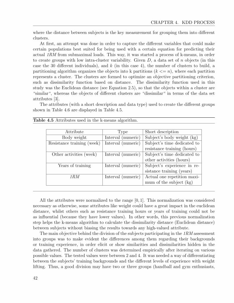
CHAPTER 4. KDD PROCESS
where the distance between subjects is the key measurement for grouping them into differentclusters.
At first, an attempt was done in order to capture the different variables that could makecertain populations best suited for being used with a certain equation for predicting theiractual 1RM from submaximal loads. This way, it was started a process of k-means, in orderto create groups with low intra-cluster variability. Given D, a data set of n objects (in thiscase the 30 different individuals), and k (in this case 4), the number of clusters to build, apartitioning algorithm organizes the objects into k partitions (k <= n), where each partitionrepresents a cluster. The clusters are formed to optimize an objective partitioning criterion,such as dissimilarity function based on distance. The dissimilarity function used in thisstudy was the Euclidean distance (see Equation 2.5), so that the objects within a cluster are“similar“, whereas the objects of different clusters are “dissimilar“ in terms of the data setattributes [3].
The attributes (with a short description and data type) used to create the different groupsshown in Table 4.6 are displayed in Table 4.5.
Table 4.5 Attributes used in the k-means algorithm.
Attribute Type Short descriptionBody weight Interval (numeric) Subject’s body weight (kg)
Resistance training (week) Interval (numeric) Subject’s time dedicated toresistance training (hours)
Other activities (week) Interval (numeric) Subject’s time dedicated toother activities (hours)
Years of training Interval (numeric) Subject’s experience in re-sistance training (years)
1RM Interval (numeric) Actual one repetition maxi-mum of the subject (kg)
All the attributes were normalized to the range [0, 1]. This normalization was considerednecessary as otherwise, some attributes like weight could have a great impact in the euclideandistance, whilst others such as resistance training hours or years of training could not beas influential (because they have lower values). In other words, this previous normalizationstep helps the k-means algorithm to calculate the dissimilarity distance (Euclidean distance)between subjects without biasing the results towards any high-valued attribute.
The main objective behind the division of the subjects participating in the 1RM assessmentinto groups was to make evident the differences among them regarding their backgroundsor training experience, in order elicit or show similarities and dissimilarities hidden in thedata gathered. The number of clusters was determined empirically after iterating on variouspossible values. The tested values were between 2 and 4. It was needed a way of differentiatingbetween the subjects’ training backgrounds and the different levels of experience with weightlifting. Thus, a good division may have two or three groups (handball and gym enthusiasts,
42

and average subjects that practice both sports in a recreational way) and a fourth group, werebeginners and people with limited time for practicing sports would be included. A balancebetween the number of clusters and the number of subjects in each cluster is needed. Clusterswith fewer than 5 subjects were considered inappropriate, as some kind of generalization orrepresentativeness purpose was desired when creating these groups. Finally the value of 4 wasselected as representative for the number of clusters, what resulted in four clearly differentiatedgroups (see Tables 4.6 and 4.7).
Table 4.6 K-means clustering. Cluster centroids.
Cluster centroidsCluster number
Attribute Full data (30) 0(12) 1(8) 2(5) 3(5)Body weight 0.5256 0.5388 0.4099 0.434 0.7706
Resistance training (week) 0.405 0.375 0.3875 0.77 0.14Other activities (week) 0.2798 0.1696 0.5982 0.1 0.2143
Years of training 0.5357 0.7738 0.3214 0.7143 0.12861RM 81.3333 84.9167 79.3125 99.3 58
Table 4.7 Clustered individuals (n = 30, k = 4).
Clustered individualsCluster number Number of individuals Percentage
0 12 (40%)1 8 (27%)2 5 (17%)3 5 (17%)
In Tables 4.6 and 4.7, we can observe:
• Cluster 0: consisted of 12 subjects who spend the average time practicing resistancetraining, and did practice any kind of sports as well, in a recreational way.
• Cluster 1: comprised basically by handball players in the study. As it is shown in the k-means result, they dedicate most of their time to other sports (like handball or jogging)and less time to resistance training (just one or two hours a week).
• Cluster 2: consists basically of people who practiced resistance training more often thanthe mean, and rarely practiced other sports. They were the ones who got higher valuesat the 1RM assessment, possibly due to their experience in weight lifting and betteranaerobic conditioning.
43

CHAPTER 4. KDD PROCESS
• Cluster 3: formed by people with the highest body weight and that were able to dedicatefewer hours to practicing sports or weight lifting in the gym. They were as well beginners(their experience with resistance training was limited) and had lower values of the 1RM.This seems to indicate, that body weight, probably is not related with the 1RM whenthe population is very heterogeneous.
Even though 4 groups were created (the number of groups was determined in a “trialand error“ fashion), it was shown no relationship between the clusters found by the k-meansalgorithm, and the predicting equations that best suited each of the subjects in the cluster(different formulas may suit different repetitions number when predicting the 1RM for acertain subject; maybe when predicting in a certain range of repetitions from submaximalloads, it is not just the subject’s characteristics, but also the number of repetitions performeduntil exhaustion what determines the suitability of a certain prediction equation). This willbe proposed as a future line of research 6.4, as not enough data was collected to undertakesuch an ambitious project.
As presented in Table 4.6, k-means could be a great method for dividing population intoclusters that were best suited for the different predicting formulas. This way, the membersincluded in the cluster number 2, could use certain formulas more suited to people whosetraining routine is principally based of weight lifting, whilst the subjects in cluster 3 coulduse a formula set specifically designed for untrained people or beginners. This generalizationor way of grouping subjects could be done as well taking into account prediction formulasfor different exercises (not only for the bench press action). Not only a clustering algorithmcould help, but as well a SOM (self adapting maps) could shed light on the different predictionequations applicability (the closest two different population or exercise characteristics are, themore reliable a certain or group of prediction formulas could be for both groups).
Clustering techniques and self organizing maps, are a sensible approach to make a 2 dimen-sional projection of the different population characteristics (or even exercise characteristics),in order to tackle the inherent complexity of the relationships among them. This way, it couldease the path in finding the most proper prediction formulas for each of the maps/projectiongroups. These groups can be created, not only for the sake of simplicity, but for mappingdifferent prediction equations with populations’ characteristics. Using some kind of clusteringtechnique, as the one presented in this Section, could lead to a better description of the dif-ferent subjects participating in the study, and can elicit unknown patterns and relationshipsbetween the subjects’ characteristics, unknown at first glance or hidden in the data. Maybe,and having in mind the benefits of these techniques, sports and health professionals couldbe encouraged to include clustering methods in their experiments, in order to describe in astraightforward way the main characteristics of the different populations used in their studies.
4.3 Linear regression models
The main objective behind the creation of the linear regression model was the searching ofthe different attributes that could have somehow any kind of statistically significant influence
44

(p < 0.05) in the 1RM prediction. Following, the creation of several linear models with theforward selection method (see Table 4.8), with all the attributes but the ones removed fromthe initial data set (see Section 4.2) was performed.
Table 4.8 Linear regression models built.
Model SummaryModel R R2 Std. Error of the Estimate
1 0.838 0.703 a 9.2022 0.982 0.965 b 3.1623 0.985 0.970 c 2.9784 0.986 0.971 d 2.9115 0.986 0.973 e 2.843
aPredictors: (Constant), WeightbPredictors: (Constant), Weight, RepetitionscPredictors: (Constant), Weight, Repetitions, Resistance t.dPredictors: (Constant), Weight,Repetitions, Resistance t., O.
activitiesePredictors: (Constant), Weight,Repetitions, Resistance t., O.
activities, Time exhaustion
The confidence factor was set to 0.05 and 5 different models appeared until the executionended. It is noticeable, how weight, and repetitions, were the two first attributes that had astatistical significance in the model, and that with a confidence factor of 0.05, all the attributeschosen in a linear step forward selection model at the end of the execution were weight,repetitions, hours of weighting in a week, other physical activities and time to exhaustion.
Even though resistance training hours, other activities and time to exhaustion seem to havea statistically significant influence in the prediction of the 1RM, no practical implications seemto arise (as only with repetitions and weight, the model is able to explain 96% of the variabilityof the dependent variable [8, 17, 18, 19, 20, 21, 22]). However, R2 was set to 0.973 when thepredictors were all the significant variables. It is important to notice as well, that time toexhaustion had some kind of influence in the response variable: this is, movement cadencehas an effect on the actual 1RM.
Two models from Table 4.8 deserve mentioning (see Equations 4.1 and 4.2):
(4.1) 1RM = −7.089 + 1.077w + 1.859r
(4.2) 1RM = −7.864 + 1.033w + 1.499r + 0.566rt+ 0.210oa+ 0.155te
where w,r,rt,oa and te mean weight, repetitions, weekly mean hours of resistance training,weekly mean hours of other activities, and time to exhaustion respectively.
45

CHAPTER 4. KDD PROCESS
With respect to formula 4.1, with only 2 attributes, we can see a clear tendency in theresult: the 1RM is roughly dependent on twice the number of repetitions performed, and onetime the weight lifted. This finding seems to correlate with the results obtained with thegenetic programming algorithm later presented in Section 4.5, as this individual solution, wasone of the most suited individuals in many executions of the algorithm.
Related to equation 4.2 it is clear that somehow, the more training hours a week were ded-icated to resistance training, the more weight could be lifted in a 1RM assessment. This maybe related to better lifting technique [7], anaerobic conditioning or better neural adaptationto weight stress [4]. Somehow, time to exhaustion had some influence in the prediction of the1RM: having constant the other variables (repetitions, weight, resistance training hours andother activities hours), the more time to exhaustion, the higher the 1RM was. It is remark-able as well, how the Borg scales (in the first repetition, and at the end of the set), had nosignificance in the final model.
Years of experience in weight training, and an approximate mean of weekly hours dedicatedto resistance training (based on their opinions on how much they trained as a weekly meanduring the last month), were collected from each of the individuals participating in the 1RMassessment. Due to the enormous variability in the individuals’ characteristics (age, trainingroutines, or even experience in resistance training), it was not possible to get a solid conclusionabout the influence of all the different variables in the prediction models.
Even though not only weight and repetitions were used in Equation 4.2, the first model(Equation 4.1) seemed to outperform Equation 4.2, when the random sub-sampling validationtechnique was applied to the data set. This could be due to possible outliers in the data, orthe enormous variability between the different subjects participating in the study.
4.3.1 Interaction between weight and repetitions
Considering only the attributes weight and repetitions for predicting the 1RM, and inorder to reproduce O’Connor et al. equation, a third attribute was created: the interactionbetween weight and repetitions “weight*repetitions“. By means of a linear regression modelwith forward selection, and after selecting the data tuples where number of repetitions isgreater or equal than two, three tentative models (confidence factor set to 0.05) were created.The different models with different performance criteria, are presented in Table 4.9.
46

Table 4.9 Linear models with interaction between repetitions and weight.
Model SummaryModel R R2 Std. Error of the Estimate
1 0.859 0.738 a 8.8622 0.985 0.971 b 2.9693 0.985 0.971 c 2.951
aPredictors: (Constant), WeightbPredictors: (Constant), Weight, RWcPredictors: (Constant), Weight, RW, Repetitions
In the second model generated, where the predictors were weight and the interactionbetween weight and repetitions (RW), the model obtained seems to confirm O’Connor et al.equation [19] (see Table 4.10). This finding, somehow might confirm that the data collectionprocedure and the experiment design proposed in this study was valid.
Table 4.10 Coefficients in interaction between weight and repetitions.
Coefficientsa
Variable Unstandardized coefficients t Sig. 95.0% Confidence interval for BB Std.Error Lower Bound Upper Bound
(Constant) 4.635 0.773 5.998 0.000 3.115 6.156Weight 0.933 0.010 96.735 0.000 0.914 0.952
RW 0.026 0.001 50.946 0.000 0.025 0.027
aDependent variable:RM
Within a 95% the lower bound of the mean of RW is 0.025, whilst the multiplier of weightseems close to the value of one, what seems to agree with O’Connor et al. equation [19].In other studies [23], the O’Connor et al. equation was assessed as a reliable equation forpredicting the 1RM for bench press and arm curl actions. This may validate the resultspresented in [23].
4.4 Multilayer perceptron neural network
One repetition maximum prediction is a complex task, with many interrelated factorsaffecting the performance of the practitioner, and many of these interrelationships are notfully understood. Hence, a multilayer perceptron with the backpropagation learning algorithmseems to be a valid approach for predicting the 1RM because:
47

CHAPTER 4. KDD PROCESS
• It seems the “natural“ model for predicting the one repetition maximum (muscularneuronal activation, neural coordination and elasticity seem to be the really importantvariables in weight lifting). Examinations of the human’s central nervous system in-spired the concept of neural networks.6 “Neural Networks“ derives from the fact thatthey were first developed as models for the human brain and could somehow mimic thebehavior of the neural connections existing in humans [61]. Strength is the productof both the ability of the nervous system to activate high threshold motor units, andthe amount of muscle mass available to contract [62]. To date, most of the availableevidence regarding neural modification consequent to strength training has been de-rived from surface electrode electromyography. This technique enables investigators toquantify changes in the electrical (i.e., neural) activation of skeletal muscle as a result ofstrength training. Elevations in maximal force production are accompanied by increasedelectromyographic activity of the muscle while maximally contracting. It has been pos-tulated that the augmented electromyographic activity is the result of greater centraldrive form higher neural centers [62]. Other neural adaptations elicited by resistancetraining include decreased co-contraction of antagonists and expansion in the dimensionsof the neuromuscular junction, indicating greater content of presynaptic neurotransmit-ter and postsynaptic receptors. Greater synchronicity in the discharge of motor unitsafter strength training has also been detected [63, 64].
• Variables relationship influencing the one repetition maximum seems not to be fullyunderstood [7]. In addition to repetitions number, other factors may affect the maxi-mum amount of weight an individual can lift. Age, gender, ethnicity, limb lengths andcircumferences, body mass, muscle mass, training routine, the rate of contractions andthe time distribution between concentric, eccentric and recovery phases of a contractioncycle could all possible influence the load able to be lifted for a specific number of rep-etitions [16]. In this study age, gender, training routine and body mass were added tothe neural networks built in a trial-and-error fashion. None of these variables seemed tobe a good predictor of the actual 1RM, and the models obtained performed statisticallyequal (p < 0.05) than those using just repetitions until exhaustion and weight lifted inthe set.
• When the number of repetitions is lower than 10, linear models correlation seems quitehigh for predicting the 1RM from submaximal loads. However, when the number ofrepetitions is greater than 10, most of these models seem to over/under estimate. A non-linear approach when repetitions are between 10-15 repetitions seems to perform betterthan the linear [21, 22]. Bryzcki [8] as well argues that there is a distinct relationshipbetween anaerobic endurance and strength. Goes on to state that this relationship isnot quite linear beyond ten repetitions. [23]. Furthermore, regression analysis of meandata revealed a nonlinear decrease in load with increasing repetition number (chestpress action; linear Syx = 2.6kgs, nonlinear Syx = 0.2kgs) [16]. Data reveals that nomore than 10 repetitions should be used in linear equations to estimate 1RM for the CP
6From http://en.wikipedia.org/wiki/Artificial neural network
48

action [16]. The accuracy of prediction in linear equations decreases at higher repetitions[21, 22]. Given the limited research of 1RM strength prediction for a variety of weightlifting exercises, and the absence of guidelines for using linear vs. nonlinear equations for1RM strength prediction, additional research of 1RM prediction is needed. Furthermore,because of the limited number of independent variables used in classical 1RM regressionequations, it is possible that additional variables could improve the accuracy of 1RMstrength prediction [16].
The MLP models that will be presented in this study present a series of particularities inboth the architecture and the learning algorithm phases:
• Input layers: before entering the actual data into the MLP, a normalization processwas computed, in order to minimize the effect of “predominant“ attributes with highervalues like weight (73.582 +−17.95kgs) among others like repetitions (5.572 +−5.296),when updating the weights of the net. The formula used in this study for computingthe normalization is presented in Equation 4.3
(4.3) y =x− (max+min)/2
(max−min)/2
where max, min and x are the maximum value of the attribute, the minimum value ofthe attribute, and the actual value of the attribute to be normalized respectively. UsingEquation 4.3, the new range of the attributes normalized will be between 1 and -1.This normalization was used because it comes implemented by default with the WEKAsoftware7 and showed good results in this study.
• Weights input-hidden layer: the initial value of these weights was completely random.
• Hidden layers: One and two layers architectures were used for predicting the 1RM. Onelayer architecture seemed to outperform the two layer architectures for predicting the1RM from submaximal loads.
• The activation function used in this study was the sigmoid activation function: sigmoidy(v) = 1/(1 + e−v). This was used because it is one of the most common activationfunctions used in neural networks [61], showed good results in this study and comes im-plemented by default with the MultiLayerPerceptron algorithm in the WEKA datamin-ing software package. Thereby, the hidden nodes in this network were all sigmoid. Theoutput nodes become unthresholded linear units where the output value is the averagedsum of all the input nodes.
• Weights hidden-output layer: the initial value of these weights was set to random.
• Output layer: comprised by just a single neuron that outputs the predicted one repetitionmaximum for the individual.
7From http://www.cs.waikato.ac.nz/ml/weka/
49

CHAPTER 4. KDD PROCESS
The performance of neural networks depends on the architecture of the network and theirparameter settings. Determining the architecture of a network (size, structure or connectiv-ity) affects the performance criteria, such as the learning speed, accuracy of learning, noiseresistance and generalization ability. There is no clearly defined theory which allows for thecalculation of the ideal parameter settings and as a rule even slight parameter changes cancause major variations in the behavior of almost all networks [34].
All the different architectures used were obtained in a trial-and-error fashion, varying thenumber of hidden neurons in a single layer between two and four, the number of epochsbetween five hundred and two thousand, and learning (0.2, 0.1, 0.05) and momentum rates(0.1, 0.05, 0.01) with different values.
Firstly, an attempt was done in order to create a neural network with some of the 1RMrelated variables gathered in this study. These variables were age, body mass or body weightand training routine. They were included with different other predictors such as repetitionsand weight, and those significant predictors in the linear regression model presented in Section4.3 (“resistance training hours“, “other activities hours“ and time to exhaustion). However,the variables age, body mass and training routine were finally discarded following the Occam’srazor principle, as they did not increase the neural network performance and only complicatedthe model.
Then, different neural network architectures were tested, varying from one hidden layer totwo hidden layers, and from two predictors (repetitions and weight), to five predictors (repe-titions, weight, “resistance training hours“, “other activities hours“ and time to exhaustion).All these different predictors were included, as they were those significant in the linear regres-sion model, and could improve somehow the 1RM prediction from submaximal loads. Recallthat all these variables were normalized between -1 and 1 before entering into the input layerin order to avoid biasing the weights update towards any variable.
Finally, two different multilayer perceptron models were built. Specifically, the differentattributes used for generating both models are detailed in Table 4.11. Different decisions weretaken into account when building these two different neural networks (compared in Section4.6): (a) total connectivity; (b) learning rate equal to 0.1; (c) training epochs set to 500; (d)one hidden layer with three hidden neurons; (e) momentum rate set to 0.01.
The settings of the learning rate and momentum control the way in which the error is usedto correct the weights in the neural network for each training case [32]. When the learningrate was set to values close to 1, an unstable behavior was shown and the average error variedwidely. The higher the momentum, the larger the percentage of previous errors that is appliedto the weight adjustment in each training case [32].
This way, two alternative models were designed: one containing just repetitions and weightas variables, and a second model, with the five different significant predictors found in the stepforward regression model: repetitions, weight, “resistance training hours“, “other activitieshours“ and time to exhaustion.
Applying the hold-out method to the data set, we can see that were slight performancedifferences among the different neural networks built (see Table 4.11). When predicting the33% of the data set the different performance criteria (R = 0.981, MAE= 2.56, RMSE= 3.732with the five attributes presented in Table 4.11, and R = 0.978, MAE= 2.72, RMSE= 4.006
50

Table 4.11 Attributes used in the multilayer perceptron models built.∗ Used in model 1.∗∗Used in model 2.
Attribute Type Short descriptionWeight∗ ∗∗ Interval (numeric) Weight lifted in a repetition
by the subject (kg)Repetitions∗ ∗∗ Interval (numeric) Number of repetitions until
exhaustion performed in aset (reps)
Other activities (week)∗ Interval (numeric) Subject’s time dedicated toother activities (hours)
Resistance training (week) ∗ Interval (numeric) Subject’s time dedicated toresistance training (hours)
Time to exhaustion∗ Interval (numeric) Time to exhaustion in thedifferent sets (seconds)
with weight and repetitions) showed similar results.
It was needed a way of comparing their performance for predicting the 1RM. As data sizewas relatively small (97 tuples), and gathering more data was really difficult due to the lackof participants, it was needed a way of testing these models created, without affecting thequality of these models. Maybe, when predicting the 33% of the data set, an unfortunate splitcould bias the error rates of the models.
Thus, the random sub-sampling, the k-cross-fold and the leave-one-out validation tech-niques (see Section 2.4) were applied in order to determine the models’ accuracy.
Remember that in the target data set we have 97 tuples. Each of these tuples represents aset until exhaustion for a certain subject in the bench press action. For creating the differenttest and training sets, we had to consider not the tuples, but the subjects as the unit ofdivision. Otherwise, the training set could contain tuples of each of the subjects in the study(n = 30) and could bias the models prediction, as the relationship between the differentvariables influencing the subject 1RM performance would be included in the training set.Thus, when splitting the data into training and test set, we will use the subject as the unit ofdivision. When a certain subject is selected as part of the training or test set, all his tupleswill be included in this set.
In other studies [35] and with the objective of increasing the models accuracy, only thosetest sets that had the dependent variable value between the minimum and maximum range inthe training set were predicted. Even though it is a sensible approach and may lead to betterprediction results, this restriction could affect the reliability of the models built. In otherwords, if a new tuple with a higher or lower 1RM value appears and needs to be estimated,then the prediction power of our model could not be as good as expected. Thus, this approachwas discarded in this study, and all the data tuples in the test set were predicted from thebuilt models.
51

CHAPTER 4. KDD PROCESS
A total of 5 different subjects were chosen randomly as the test set using the the randomsub-sampling validation method. This number was determined empirically, and was considereda sensible number of subjects as choosing a higher value could lead to not reliable models forpredicting the 1RM (very few subjects in the training set), and a lower value to over-fittingthe test set (poor generalization power of the models). Remember that when a subject waschosen as part of the test set, all its tuples were included in the test set.
A clear disadvantage of the random sub-sampling method is that that some tuples maynever be selected in the test set, whereas others may be selected more than once. Consequently,random sub-sampling was used 40 times, and 5 different random subjects (with their respectiveset tuples) would enter into the test set in each of these forty combinations. The number 40 wasdetermined empirically, as a different number of combinations was attempted until reachinga point were almost in all executions of the program, all the data tuples were at least once ina test set.
In order to reduce the variability of the performance criteria (i.e., MAE and RMSE) due tothe natural randomness of the random sub-sampling selection criterion, a total of 20 executionswere conducted. This number of executions was determined empirically, as a higher numberresulted in more CPU time consumption and the availability of computing resources waslimited.
In Table 4.12 we can see the MAE and RMSE of the two MLP networks built.
Table 4.12 RMSE and MAE with the random sub-sampling method (MLP).
MAE RMSEMLP 2 variables 2.117 2.858MLP 5 variables 2.231 2.837
The k-cross-fold validation was used in order to assess the 1RM MLP models accuracy aswell. The number k was set to 6. This number allowed the division of the 30 subjects in thetarget data into 6 different folders, containing each folder exactly 5 subjects. This was donewith the purpose of including exactly the same number of subjects in the test set as withthe random sub-sampling partitioning method. Previously to the creation of these folds, adata set randomization (i.e., randomization based on the subject ID) was performed in orderto increase the possible combinations of subjects in the different folders. This 6-cross-foldvalidation process was used 20 times, and the results obtained are presented in Table 4.13.
Table 4.13 RMSE and MAE with the 6-cross fold validation method (MLP).
MAE RMSEMLP 2 variables 2.142 2.892MLP 5 variables 2.238 2.851
52

The results of the MLP models seem pretty similar attending to the MAE and RMSEwith both the 6-cross-fold and the random-subsampling validation methods (see Table 4.13and Table 4.12 respectively).
Using the the leave-one-out validation method, we can show not only the MAE and RMSEfor both MLP models (see Table 4.14), but generate two different error populations with theirpredictions. These two error populations could help us to know if there is any significantdifference in the prediction accuracy between the two MLP models built. Thus, we can trainboth models using the leave-one-out validation approach (29 subjects in the training set and 1subject in the test set), and compute the error of both MLP models for predicting each tuplein the test set. In other words, all the tuples of a certain subject were used as the test set,and both MLP models were built with the tuples of the other 29 subjects. The error for eachtuple was computed as the absolute difference between the actual and the estimated 1RM.This process was repeated until all the tuples 1RM were predicted, and two different errorpopulations appeared (one per MLP model).
Table 4.14 RMSE and MAE with the the leave-one-out validation method (MLP).
MAE RMSEMLP 2 variables 2.417 2.748MLP 5 variables 2.369 2.668
Then a Wilcoxon rank-sum test could be performed between the error populations resultingwith both MLP models.
Thereby, the null and the alternative hypothesis for the comparison between the two MLPnetworks built were (n = 97):
H0: There is no difference in the error population between the first and the second multi-layer perceptron network model as both predict with the same error rate the one repetitionmaximum from 1 repetition up to 19 repetitions with the available data.H1: There are differences in the error population between the first and the second multilayerperceptron network model as both predict with different error rates the one repetition maximumbetween from 1 repetition up to 19 repetitions with the available data.
The error descriptives are presented in Table 4.15, while in Table 4.16 is shown theWilcoxon rank-sum test (also called the U Mann-Whitney test) for both error populations(recall that the error is computed as the difference between the expected 1RM value and theactual 1RM value).
53

CHAPTER 4. KDD PROCESS
Table 4.15 Error descriptives for the MLP with two variables, and the MLP with 5 variables(n = 97).
Mean Std.Deviation Median 95% conf.LowerBound(mean)
95% conf.Upperbound(mean)
MLP 2variables
2.895 2.122 2.656 2.373 3.417
MLP 5variables
2.694 2.106 2.418 2.350 3.212
Table 4.16 U Mann Whitney test.
Test StatisticsZ -0.283
Asymp. Sig.(2-tailed) 0.777
Looking at Table 4.16, we can not reject the null hypothesis, what seems to indicate, thatwe can not state that there is a statistical difference between both models (Z = −0.283, p =0.777). Even though the second MLP has better results than the first one (as shown in Table4.15), these differences do not seem significant (p > 0.05).
Even though correlations are quite high (R > 0.98) and MAE and RMSE are both low,the generated predictions by means of the different neural networks seem pretty similar, andno significant differences were found between the models (p > 0.05). This seems to indicate,that all the different variables influencing the 1RM are somehow intrinsically included in thenumber of repetitions and weight lifted until exhaustion. This seems to agree with the resultsobtained in other 1RM assessments [16]: “these findings indicate that each of these variablesis either unrelated to 1RM strength (e.g., training volume) or is so interrelated to strength(gender and all anthropometric variables) that the 5RM data sufficiently accounts for itscontribution to the explanation of between-subject variance in 1RM strength“.
Thereby, only weight and repetitions will be used in the multilayer perceptron network,when comparing its performance to the other proposed solutions in Section 4.6.
4.5 Genetic programming model
A sensible way of obtaining a 1RM prediction equation by means of genetic programming,is starting with a random set of individuals or prediction equations that may solve the problem
54

and reproduce them generation upon generation until a suitable individual appears.Good individuals, that are good predictors of the 1RM would rank high in the fitness test,
whilst individuals that are worse predictors would rank lower. Recall that all these differentindividuals (formed by genes contained in a tree-like structure) are potential 1RM predictionequations. Intuitively, if two individuals are somewhat effective in solving the 1RM prediction,then some of their parts probably have some merit. By recombining randomly chosen parts ofsomewhat effective individuals, we may produce new individuals that are even fitter in solvingthe 1RM prediction [37]. Generation upon generation, these individuals will reproduce andeventually a suitable solution will emerge in the last generation of the algorithm.
In this study, each of the individuals is tested against the RMSE (i.e., the fitness functionis the RMSE), to check how appropriate it is as a possible solution to the 1RM prediction.Thus an individual could be better suited than other for predicting the 1RM (the lower RMSEvalue, the better the solution), resulting in a higher probability of selection for the geneticoperations performed in each generation.
For building all the different genetic models proposed in this Section, the implementationof Yan Levasseur of the GP algorithm was used 8. It is an open source project and uses theGNU General Public License. It is developed in JAVA and can be integrated into WEKA.The GP algorithm is based on Koza and Banzhaf et al. contributions to genetic programming[37, 65, 66].
The following parameters in the genetic programming algorithm were used to obtain allthe models presented in this Section:
• Termination criterion: the maximum generation number was set to 20 (chosen em-pirically). A lower number lead to no-convergence of the individuals and no suitablesolutions appeared with the execution of the genetic programming algorithm. A greaternumber of generations resulted in more CPU time consumption and was discarded dueto the limited processing power available. Furthermore, time consumption of this algo-rithm was clearly superior to the linear regression or the MLP with the backpropagationlearning algorithms.
• Population size: 1000 individuals will make the initial population, and will evolve overthe following generations. There will always be a fixed number of 1000 individuals ineach of the generations. After the reproduction process takes place, this population ofoff-spring (i.e., the new generation) replaces the old population (i.e., the old generation).This number was chosen empirically and was not increased due to the limited processingpower available for computing the results.
• No normalization or standardization was done to the data: as it was only includedrepetitions and weight, no special preprocessing was necessary to fit the data into aprediction formula.
• Maximum depth of the individual’s tree: 5 (chosen empirically). This number wasselected based on the complexity of the formula desired. More than five operations in
8Available online on 19th of April 2014, at http://www.leyan.org/tiki-index.php?page=Genetic%20Programming
55

CHAPTER 4. KDD PROCESS
depth, led to no convergence, or too complex structures to be suited for an “easy tounderstand“ formula.
• Different attributes used as terminals in the possible individuals: 2 (in our case, rep-etitions and weight will be enough for predicting the 1RM from submaximal loads).Different attributes were tested as possible terminals based on the results from the lin-ear regression model significance tests (see Section 4.3). However no convergence of thepopulation was observed, or the results were not as accurate as those obtained usingjust repetitions and weight.
• Functions used:
– +,−, ∗, /: the four basic arithmetic operators. They perform an arithmetic oper-ation between two operands. These operators were included as possible functionsas they were used at least once in some of the equations proposed in literature sofar for predicting the 1RM (see Table 2.1).
– Pow: a number powered to another. This operator was chosen, in order to allowthe different individuals to mimic Lombardi’s formula [20] (i.e pow(2, 6) = 26).
– Exp: Euler’s number to the power of a certain number. It is the base of the naturallogarithm. It was chosen due to the necessity of modeling non-linear behaviors insets of more than 10 repetitions, like in Mayhew [21] or Wathen [22] predictionequations (i.e. Exp(3)= e3).
– Log: natural logarithm of a number. It is the inverse operation of euler’s number(i.e. Log(e)=1, where e is the Eulers number).
• Cross-over operation: 90% (900 individuals) of the new population will be due to acrossover operation between the ancestors. This number was selected empirically, andwas the number by default in the tool. The probability of the operation (proportion),number of parents and number of children created were:
– Proportion: 0.9
– Number of parents:2
– Number of children:2
• Mutation operation: mutates a whole randomly selected sub-tree from an individual.The probability of performing this operation was set to 7%. This way, 70 individualswill mutate in each generation. This operation must be aware of binary operation nodesor single operation nodes. The probability of the operation (proportion), number ofparents and number of children created were:
– Proportion: 0.07
– Number of parents: 1
– Number of children: 1
56

• New individual operation: creates new random individuals in a generation. It is com-monly used to increase genes variability (i.e. genes diversity) when the generations haveevolved mainly from ancestors. In each generation, 30 new random individuals werecreated. The probability of the operation (proportion) was:
– Proportion: 0.03
First, the five significant variables in the linear regression model (see Table 4.8) wereincluded as possible terminals in the genetic programming algorithm. However, this lead to lowprecision solutions, or even non-convergence after 20 generations of the genetic programmingalgorithm execution. After executing the algorithm more than 20 times with the hold-outmethod (66% training set, %33 test test), and observing misleading results, time to exhaustion,resistance training hours and other activities hours were discarded from the subsequent models.
The following models were built having into the training set a 66% of the tuples of the over-all dataset (validated with the 33% of the data set in the test set), and using just repetitionsand weight as predictors (attributes):
(4.4) 1RM = 2r + w
(4.5) 1RM = w + r + log((r ∗ w)− 192.605)
(4.6) 1RM = w + r + log (w) log (r)0.83
Equation 4.4 was one of the most usual individuals in the final generations (the individualwith the lowest RMSE). This seems to agree with the results obtained by means of the linearregression model (see Section 4.3). Even though it was a suitable solution, it had the form ofa linear equation, what could lead to discouraging predictions of the one repetition maximumfrom submaximal loads, when the number of repetitions is greater than 10.
In Equations 4.5 and 4.6, an individual with the interaction between repetitions and weightseems the best suited solution to the problem. Equation 4.5 seems to outperform equations4.4 and 4.6, and appears to confirm as a good predictor the attribute created showing theinteraction between weight and repetitions in O’Connor et al. [22] and Epley’s [17] equations.
Table 4.17 1RM prediction by means of genetic programming.∗All the models refer to the equations presented previously.
Model R MAE RMSEEquation 4.4 0.970 3.7727 5.543Equation 4.5 0.985 2.608 3.421Equation 4.6 0.970 3.7727 5.543
57

CHAPTER 4. KDD PROCESS
Genetic programming seems a sensible approach when the solution to a certain problem iscomplex. However, convergence is not guaranteed and many parameters need to be adjustedin order to generate a proper solution. Thereby, adding more attributes to the space ofpossible solutions, could lead to misleading results and serious caution should be consideredwhen adjusting the parameters mentioned in Section 2.2.3.
Increasing the number of individuals tested against the 1RM prediction in each of thegenerations, adding different attributes as terminals, varying proportions of the different re-production functions or testing new fitness functions, could give better solutions to the 1RMprediction than those presented in this Section. However, it is proposed as future work, asgreater computing power is needed in order to achieve suitable solutions in such a huge solutionspace.
4.6 Comparison between the different models
As discussed previously, three different approaches were taken into account in this studyto model the 1RM prediction from submaximal loads:
• Multilayer Perceptron Network (MLP): up to the author’s knowledge, multilayer percep-tron networks were never used before for predicting the 1RM from submaximal loads.They are capable of modeling non-linear relationships between the different variablesaffecting the prediction of the 1RM and have been used extensively in a wide range ofapplications with impressive results. In the mathematical theory of neural networks,the universal approximation theorem states that a feed-forward network with a singlehidden layer containing a finite number of neurons, can approximate continuous func-tions on compact subsets of Rn [50, 36]. The theorem thus states that simple neuralnetworks can represent a wide variety of interesting functions when given appropriateparameters.
• Linear Regression (LR): one of the most used models when it comes to predict anindividual’s one repetition maximum. These models are only applicable when the rangeof repetitions performed until exhaustion in a certain set is between 1 and 10. Otherwise,they may present over or under estimation problems.
• Genetic Programming: up to the author’s knowledge, genetic programming was neverused for predicting the 1RM from submaximal loads. It is an evolutionary algorithminspired by biological evolution, which evolves to predict the 1RM from the attributesgathered.
Recall that in the target data set the total number of subjects was 30, and the total numberof tuples was 97. Each of these tuples represent a set until exhaustion of the bench press actionfor the different subjects. Each of the subjects had a total number of up to 5 tuples (the samenumber of tuples as sets until exhaustion performed until reaching their actual 1RM). The
58

number of tuples for each of the subjects is not fixed, as some of them reached their actual1RM in fewer sets than others.
In this Section, we only considered the predictor variables weight and repetitions for build-ing the different models. This was due to the limited size of the target data set and becausethere was a high risk of non-convergence of the genetic programming algorithm if more than 2attributes were added to the space of solutions. Otherwise the genetic programming algorithmperformance could be highly affected by the decision of including more than 2 predictors andmay lead to misleading results. Furthermore, a minimum of ten subjects is recommended foreach predictor used when conducting biomedical or physiological research involving humansubjects (see Section 3.3).
In Section 4.6.1, we can observe how the previously built models (in Sections 4.3, 4.4and 4.5) performed when predicting the one repetition maximum, attending to both theperformance criteria (MAE and RMSE) and the non-parametric tests used to compare theirerror population.
4.6.1 Comparison between the different models generated
We will take into account several constraints when comparing the different models pro-posed in this Section: (a) linear equations seem to be suitable when the range of repetitionsperformed until exhaustion is lower than ten; this way, when comparing the different modelsbuilt with the linear solutions, we are restricted by this range of applicability ;(b) solutionconvergence in the genetic programming algorithm was generally reached including just rep-etitions and weight in the input variables; otherwise the genetic algorithm solution could nothave converged; (c) all the models for predicting the one repetition maximum from submaxi-mal loads in this Section use as predictors only weight and repetitions.
Four different models were built and compared in this Section:
• MLP: the multilayer perceptron network was trained with the two variables used inliterature when predicting the 1RM from submaximal loads: repetitions and weight.The MLP used the same learning and architecture parameters presented in Section 4.4.
• Linear regression: with only repetitions and weight as separate variables in the equation.The formula will have the form:
(4.7) 1RM = aw + br + c
where a,b,c are constants, w and r, weight and repetitions respectively.
• Linear regression (interaction): repetitions, weight and the multiplication of weight andrepetitions. The formula, will emulate that proposed by Epley [17] or O’Connor et al.[19], and will have the form:
(4.8) 1RM = aw + br + cwr + d
where a,b,c and d are constants, w and r, weight and repetitions respectively.
59

CHAPTER 4. KDD PROCESS
• Genetic programming: using, as in the previous models, weight and repetitions as theinput attributes. The Genetic programming model used the same parameters than thosepresented in Section 4.5.
With the restriction of having such a small data set, it was needed a way of comparingall these models without affecting the quality of the models built. Thus, the random sub-sampling, the k-cross-fold and the leave-one-out validation methods were used to compare theperformance of the different models.
First, the MAE and RMSE applying the random sub-sampling validation method for thedifferent models proposed in this study was conducted. As presented previously in Section4.4, 40 combinations of training sets were obtained (attending to the subject ID). This processwas repeated 20 times and the results are presented in Table 4.18. These results are computedtaking into account only those tuples where the repetitions number was a value between 1 and10. In other words, tuples with a number of repetitions greater than ten were not taken intoaccount when comparing the performance of the different models proposed in this Section.
Table 4.18 RMSE and MAE with the random sub-sampling method.
Model RMSE MAEMLP 2.327 1.743
Linear regression 2.569 1.990Linear regression (interaction) 2.117 1.499
Genetic programming 2.723 2.094
Then, a total of 20 rounds of 6-cross-fold validation were executed for the models proposed,and the results are shown in Table 4.19. In each of the 6-cross-fold validation rounds, a priorrandomization of the tuples (attending to subject ID) was carried out. These results arecomputed taking into account only those tuples where the repetitions number was a valuebetween 1 and 10.
Table 4.19 RMSE and MAE with the 6-cross-fold-validation method.
Model RMSE MAEMLP 2.315 1.735
Linear regression 2.510 1.955Linear regression (interaction) 2.073 1.470
Genetic programming 2.643 2.054
MAE and RMSE with both validation techniques (random sub-sampling and 6-cross-fold respectively) seem pretty similar for the same model. However, using the 6-cross-fold-validation (see Table 4.19) seems to give better results than using the random sub-samplingapproach (see Table 4.18) for all the models proposed.
60

Table 4.20 RMSE and MAE with the leave one out validation method.
Model RMSE MAEMLP 2.364 2.114
Linear regression 2.148 1.902Linear regression (interaction) 1.744 1.467
Genetic programming 2.546 2.218
All the equations predict with some error. Nevertheless, as shown in Table 4.19 andTable 4.18 the Linear regression (interaction) model seems to outperform the MLP, Linearregression and Genetic programming model in the range between 1 and 10 repetitions usingonly weight and repetitions as 1RM predictors. The MLP seems to outperform both theLinear regression and the Genetic programming models with both random-subsampling and6-cross-fold validation techniques. It seems that the MLP has greater accuracy with unseendata than both the Linear regression and the Genetic programming model.
Using the leave-one-out validation approach used in Section 4.4, the results of the MAEand RMSE are presented in Table 4.20. These results are computed taking into account onlythose tuples where the repetitions number was a value between 1 and 10.
With the leave-one-out validation approach (see Table 4.20), the Linear regression modelseems to outperform the MLP and the Genetic Programming. These results should be takenwith caution
A plot with the different models for predicted 1RM created in the last execution is shownin Figure 4.3 (weight in the vertical axis, tuple id in the horizontal axis). Figure 4.3 showsthe actual 1RM, and the prediction of the 1RM using the leave-one-out validation method forthe multilayer perceptron network, the Linear Regression model with the interaction betweenweight and repetitions, the Linear regression and the Genetic programming model(1RM, MLP,Linear regression (interaction), Linear regression and Genetic programming respectively).
Even though the MLP (multilayer perceptron network) seems to outperform the geneticprogramming algorithm (Genetic programming), using the leave-one-out method, the linearregression of two variables (Linear regression) seems to outperform the MLP. The most ac-curate model for predicting the 1RM in the range between 1 and 10 repetitions seems tobe the Linear regression (interaction) model. Further study was needed to checkout for thecoefficients that make this model so accurate for predicting the 1RM from submaximal loads(see Section 4.3).
It is surprising how, in the range of repetitions between one and ten, these models seemto be so precise. Nevertheless, the further we move from ten repetitions until exhaustion, theapparent linearity of the prediction disappears (as shown in Figure 4.4 in Section 4.8.1), whatcould make the linear regression models to lose prediction precision.
In order to compare the accuracy of both the Linear regression and MLP models, aWilcoxon rank-sum test was conducted (see 4.22). The steps for generating the error popula-tion were the same as the ones presented in Section 4.4.
61

CHAPTER 4. KDD PROCESS
Figure 4.3: Comparison between the generated models.
This way, the null and the alternative hypothesis were (n = 76):
H0: There is no difference in the error population between the linear and the multilayer per-ceptron network model as both predict with the same error rate the one repetition maximumbetween 1 and 10 repetitions using repetitions and weight as independent variables.H1: There are differences in the error population between the multilayer perceptron networkand the linear model when it comes to predicting the one repetition maximum between 1 and10 repetitions using repetitions and weight as independent variables.
Error descriptives are shown in Table 4.21.
Table 4.21 Error descriptives for the MLP and Linear regression models (n = 76).
Mean Std.Deviation Median 95% conf.LowerBound(mean)
95% conf.Upperbound(mean)
MLP 2.063 1.611 1.696 1.695 2.431Linear re-gression
1.969 1.819 1.430 1.554 2.385
62

Table 4.22 U Mann Whitney test.
Test StatisticsZ -0.687
Asymp. Sig.(2-tailed) 0.492
A Wilcoxon sum-rank test showed (see Table 4.22) that there was not a statistically sig-nificant difference in the error when trying to predict the one repetition maximum fromsubmaximal loads (using as variables weight and repetitions) for the models MLP and Linearregression model between 1 and 10 repetitions (Z = −0.687, p = 0.492). This way, both al-ternatives seem pretty similar for predicting the one repetition maximum (chest press action,from 1 to 10 repetitions until exhaustion) in an heterogeneous population.
A comparison between the Linear regression (interaction) model (with the interactionbetween repetition number and weight, reproducing O’Connor et al. formula [19]) and theMLP is presented in Table 4.23.
Table 4.23 Error descriptives for the MLP and Linear regression (interaction) models (n =76).
Mean Std.Deviation Median 95% LowerBound(mean)
95% Upperbound(mean)
MLP 2.063 1.611 1.696 1.695 2.432Linearregression(interac-tion)
1.481 1.651 0.847 1.104 1.858
Proceeding in an identical way, it will be carried out the same comparison between thesedifferent models (multilayer perceptron and linear model with interaction between weight andrepetitions). The results are presented in Table 4.24 (n = 76):
Table 4.24 U Mann Whitney test.
Test StatisticsZ -3.228
Asymp. Sig.(2-tailed) 0.001
A Wilcoxon rank-sum test showed (see Table 4.22) that there was a statistically significantdifference in the error when trying to predict the one repetition maximum from submaximal
63

CHAPTER 4. KDD PROCESS
loads (using as variables weight and repetitions) for the models MLP and the Linear regression(interaction) model in the range between 1 and 10 repetitions (Z = −3.228, p = 0.001). Thisindicates, that between one and ten repetitions, the Linear regression model with interactionbetween weight and repetitions, predicts better the 1RM (chest press action, from 1 to 10repetitions until exhaustion) in an heterogeneous population than the neural network approach(MLP). This model seems pretty similar to the one proposed by O’Connor et al. [19] and mayvalidate his results.
The results presented in this Section should be taken with caution as the data set wasvery unbalanced attending to repetitions number. Only 76 tuples were considered valid forthe comparisons presented in this Section (those tuples containing repetitions between 1 and10), and 30 of them contained 1 repetition as the number of repetitions performed untilexhaustion in a set for the bench press action (the actual subject’s 1RM). In a balanced dataset, where all repetitions numbers have exactly the same number of tuples, the results mayvary and the models proposed could perform differently. This is proposed as future work.
Furthermore, these results should not be considered valid for other exercises than the benchpress action with free-weight barbell. Different prediction equations may apply to differentexercises, and this is proposed as a possible future line of research.
4.7 Comparison between the different literature equa-
tions
For all the data tuples contained in the target data (n = 97), a predicted 1RM value wascomputed for each of the proposed literature 1RM prediction equations [8, 17, 18, 19, 20, 21, 22]used in this study. In Table 4.25, it is shown some performance criteria values (R, RMSE andMAE) for these equations.
Table 4.25 1RM Prediction equations from literature.
Model RMSE MAE RBryzcki 7.613 3.846 0.936Epley 4.411 3.354 0.987
Lander 7.493 4.161 0.945O’Connor 2.957 2.360 0.986Lombardi 4.073 2.699 0.973Mayhew 5.988 5.269 0.981Wathen 4.427 2.928 0.982
Their applicability for predicting the one repetition maximum is reasonable. However, themodels for predicting the one repetition maximum from submaximal loads that showed to have
64

higher error rates were Bryzcki [8] and Lander’s [18] equations. O’Connor et al. equation [19],clearly outperformed the rest of the equations with the highest coefficient of correlation, andlowest RMSE and MAE. Between those with a non-linear behavior, Lombardi [20] showed thelowest MAE, whilst Mayhew [21] and Wathen [22] presented higher coefficients of correlation.However, these results should be taken with caution, as the applicability of each of these1RM prediction equations is restricted to a certain number of repetitions, and the comparisonamong them is not straightforward. Nevertheless, for recreational use, it is noteworthy thedifferences found between the predicted value of the equation, and the actual value of the1RM (reported errors of up to 25kgs in over-estimation). Prediction equations should be usedwith caution and, when in doubt, prescription of exercise intensity should be expressed as anumber of repetitions.
4.8 Post-hoc analysis
In this section it is discussed the differences found among repetitions number at a cer-tain % of the 1RM (Section 4.8.1) and at different percentages (Section 4.8.2). Finally, therelationship between RPE and the number of repetitions is discussed in Section 4.8.3.
4.8.1 Number of repetitions at a certain percentage of 1RM
A scatter-plot (showing repetitions vs. %1RM), with the whole data set collected in the1RM assessment carried out in this study is shown in Figure 4.4.
Figure 4.4: Repetitions performed until exhaustion vs. %1RM.
In Figure 4.4 is remarkable the non-linearity of the number of repetitions compared to
65

CHAPTER 4. KDD PROCESS
the percentage of the one repetition maximum. This seems to indicate that when trying toestimate one repetition maximum from submaximal loads, and the number of repetitions isgreater than 10, it is needed another approach, different from those linear equations proposedin literature [8, 17, 18, 19].
Training status of the individual has a minimal impact on the number of repetitionsperformed at relative exercise intensity. No differences in number of repetitions performedat a given exercise intensity were noted between trained and untrained individuals (exceptduring bench press at 90% 1RM). Training status of the individual has a minimal impacton the number of repetitions performed at relative exercise intensity [62]. No significantdifferences (p > 0.05) were found for any percent 1RM for the bench press and the leg pressbetween trained and untrained subjects [24]. It seems to agree with Arazi and Asadi [12], whonoted that there were no significant differences (p > 0.05) between the trained and untrainedgroups (except at 85 and 95% of 1RM in the arm curl).
Everything seems to indicate, that no matter how the individual training background was,at the same selected percentage of the 1RM, it will perform the same number of repetitions.
By means of a hypothesis contrast, we will try to assess if as stated by Arazi and Asadi[12], the mean number of repetitions performed by the population in flat bench press is 14 atthe 75% of their actual1RM.
This way, the two hypotheses formulated (null hypothesis and alternative hypothesis) wereas follows:
H0: The mean of repetitions for flat bench press at 75% of 1RM is 14 repetitions.H1: The mean of repetitions for flat bench press at 75% of 1RM is different than 14 repetitions.
All data tuples selected for applying the hypothesis contrast were those where the intensityapplied was around the 75% of the 1RM of the subject. All the subjects with accumulatedrepetitions were removed from the data used (this is, this was their first set until exhaustionin the 1RM assessment). This way, from a total of nine subjects who performed a set at the75% of their actual 1RM, only five performed this set as their first set until exhaustion. Aone-sample t-test (n = 5) was run to determine whether the number of repetitions at 75%of the 1RM was equal to fourteen or not. Repetition number, as well as percentage, werenormally distributed (p > 0.05), as assessed by Shapiro-Wilk’s test [60] (see Table 4.27 andTable 4.26).
Table 4.26 Descriptives of percentage and repetitions (n = 5).
Mean 95% LowerBound(mean)
95% Upperbound(mean)
Std.Deviation Median
Repetitions 13 11.48 14.52 1.225 13% 1RM 0.757 0.728 0.786 0.023 0.757
66

Table 4.27 Test of normality: repetitions and percentage.
Tests of normalityKolmogorov-Smirnov Shapiro-WilkStatistic df Sig. Statistic df Sig.
Repetitions 0.300 5 0.161 0.833 5 0.146%1RM 0.214 5 0.200* 0.896 5 0.386
There is not enough evidence to reject the null hypothesis (p > 0.05) (mean of repetitionsat 75% 1RM is equal to fourteen), by means of a one sample t-student test (t(4) = −1, 826, p =0.142). Thus, we cannot state that the number of repetitions in the chest press action at 75%of the 1RM is different than fourteen. This seems to agree with the results presented by Araziand Asadi [24].
Then, a one sample t-test was carried out with the tuples discarded in the prior hypothesiscontrast (those where the subjects had performed at least one set until exhaustion previously).These subjects performed a mean of 10.6 repetitions until exhaustion (mean+−standard de-viation; 10.6+−2.19). A one sample t-test showed statistically significant differences betweenthe mean of repetitions performed until exhaustion (t(4) = −3.4, p = 0.026) and the supposedmean of repetitions at the 75% of the 1RM: 14. This may suggest that performance decreaseswith increasing acidosis [16, 53].
4.8.2 Comparing repetitions until exhaustion at 70%-75% of 1RM
Two groups were considered in order to analyze the different number of repetitions thatcould be achieved at different exercise intensities. Duplicated subject IDs were removed fromthe target data used to apply hypothesis contrast (independent samples), and all the subjectsthat entered in the target data were those whose accumulated repetitions (this is, previous setsperformed until exhaustion) were zero. This could help when validating the results obtained,as it was the first attempt of the subjects to perform a set until exhaustion.
Two groups were created. The group’s repetitions statistics (i.e., number of repetitionsperformed until exhaustion) and percentage of the 1RM applied in the set are presented inTable 4.28 and 4.29, respectively.
67

CHAPTER 4. KDD PROCESS
Table 4.28 Repetitions in the different groups (70-75%1RM).
N Mean 95% Lowerbound(mean)
95% Upperbound(mean)
Std.Deviation Median
Group 1(70%RM)
6 15.25 13.38 17.12 1.782 15
Group 2(75%RM)
5 13 11.479 14.521 1.224 13
Table 4.29 %1RM in the different groups.
N Mean 95% Lowerbound(mean)
95% Upperbound(mean)
Std.Deviation Median
Group 1(70%RM)
6 0.705 0.694 0.717 0.011 0.706
Group 2(75%RM)
5 0.757 0.728 0.786 0.023 0.756
A hypothesis contrast was applied, in order to determine if there were significant differ-ences in the number of repetitions performed between 70% and 75% of the 1RM. This way, anindependent t-student test (normality of populations checked by a Shapiro-Wilk’s test [60],p > 0.05) was performed, with the following hypothesis:
H0: There is no difference in the number of repetitions performed by individuals between70% and 75% of their actual 1RM.H1: There is any difference in the number of repetitions performed by individuals between 70%and 75% of their actual 1RM.
This study found that number of repetitions until exhaustion, performed at lower inten-sities, is statistically significant greater than at higher intensities (t(9) = 2.383, p = 0.041).Thus, we can reject the null hypothesis, and conclude that there is a statistically significantdifference between the repetitions that could be performed at 70% and 75% of the 1RM.However, this finding is certainly not surprising since a fundamental principle of resistanceexercise is that there is an inverse relationship between intensity and volume [24].
4.8.3 RPE and repetitions until exhaustion
As stated in other studies [24], “few correlations were observed that were meaningfulto the understanding of the interrelationship between RPE and the number of repetitions
68

performed. This was most likely due to the performance of a single set per exercise and theuse of exercise to failure as the end point. However, since many competitive and recreationalstrength-training programs utilize exercise to failure, such data do raise serious equations asto the utility of RPE to monitor differences in effort between sets performed to failure atdifferent percentages of 1RM. If exercise goes to failure, the exertion of subjects is similarwithin any intensity level, and that RPE may not be an effective tool to reflect the intensityof the loading in such an exercise prescription.“
In this study, we collected two measurements of RPE in each of the sets: the RPE in thefirst (at the beginning of the set) and the last repetition (at the end of the set). A Kruskall-Wallis one-way analysis of variance by ranks, was used for testing whether RPE at the endof the set were originated from the same distribution in the different 1RM intensity groupscreated. The Kruskall-Wallis test, is used for comparing more than two samples that areindependent, or not related. Since it is a non-parametric method, the Kruskall-Wallis testdoes not assume a normal distribution of the residuals. When the Kruskal-Wallis test leads tosignificant results, then at least one of the samples (here the RPE distributions of the groupsapplying different intensity levels) is different from the other samples.
Three different groups were created based on their % of the 1RM. This way, the threegroups 1RM percentage and RPE are presented in Table 4.30 and Table 4.31 respectively.
Table 4.30 Descriptives of the %1RM in the three groups created.
N Mean 95% Lowerbound(mean)
95% Upperbound(mean)
Std.Deviation Median
Group 1(75%RM)
7 0.756 0.739 0.7728 0.018 0.756
Group 2(80%RM)
9 0.807 0.797 0.8180 0.0134 0.806
Group 3(90%RM)
4 0.907 0.8792 0.93511 0.017 0.911
Table 4.31 Descriptives of the RPE at the end of the set in the three groups created.
N Mean 95% Lowerbound(mean)
95% Upperbound(mean)
Std.Deviation Median
Group 1(75%RM)
7 9.29 8.83 9.74 0.488 9
Group 2(80%RM)
9 8.44 7.67 9.22 1.014 8
Group 3(90%RM)
4 9.5 7.91 11.09 1 10
69

CHAPTER 4. KDD PROCESS
In Figure 4.5, we can observe a box-plot of the RPE at the end of the set (grouped byvariable “Group“, as defined in Tables 4.30 and 4.31).
Figure 4.5: Box plot: RPE at the end of the set.
The null and alternative hypotheses used in this section, were the following:
H0: There is no difference between the RPE at the end of the set among the different in-tensity levels.H1: There is any difference between the RPE at the end of the set among the different inten-sity levels.
There is not a statistically significant difference between the RPE at the end of the set be-tween the different intensities (%1RM) (H(2) = 4.663, p = 0.097) when all sets are performeduntil exhaustion. This seems to agree with the results presented in other studies [24].
Even though RPE at the end of the set was not statistically different between the differentgroups, RPE in the first repetition seems to correlate quite well with the number of repetitionsperformed until exhaustion (R = −0.812, n = 97, p < 0.01). This seems to indicate thatsomehow, RPE at one repetition could be a good predictor for repetitions until exhaustion.In Figure 4.6, it is plotted the relationship between RPE at one repetition, and the the selectedpercentage of the one repetition maximum.
70

Figure 4.6: Repetitions performed until exhaustion vs. %1RM.
Figure 4.6 suggests that RPE in the first repetition of the set, when used correctly, can bea suitable predictor of exercise intensity (the percentage of the one repetition maximum), andmay help when it comes to predicting the 1RM in a heterogeneous population. The inclusionof the RPE in the first repetition as a predictor in 1RM prediction equations is proposed asfurther work.
4.9 Data simulation
Due to the enormous variability between the different 1RM prediction equations proposedand analyzed so far in the study [8, 17, 18, 19, 20, 21, 22], data simulation was used in orderto emulate subjects performing a set until exhaustion in the chest press action. This way,and iterating though different weights and repetitions, all the equations were used in theirreported valid range of repetitions to generate an estimated value of the 1RM. Thus, all theproposed equations [8, 17, 18, 19, 20, 21, 22] were used in the range from 2 to 10 repetitions;Lombardi [20], Mayhew [21] and Wathan [22] for 11 repetitions; and finally Mayhew [21] andWathan [22] equations were used in the range of 11 up to 15 repetitions [16].
Weight was increased in 5 kilograms for all the different repetitions for each of the formulas(varying from 50 to 100). The repetitions range varied from 2 up to 15 repetitions. Proceeding
71

CHAPTER 4. KDD PROCESS
in such a way, we obtained all the different 1RM values that will be used to create a linearregression model by means of data simulation.
In Figure 4.7 we can see a plot of the repetitions (x axis) and percentage of the 1RM (yaxis) of the data generated applying data simulation.
Figure 4.7: Repetitions performed until exhaustion vs. %1RM.
Certainly, the data plotted in Figure 4.7, seems to agree with that obtained in the presentstudy (see Figure 4.4), where a non-linear behavior seems to appear when the number ofrepetitions is greater than a certain repetition threshold.
Emulating O’Connor’s et al. [19] and Epley’s [17] equation, a third variable representingthe interaction between weight and repetitions (RW in Table 4.32) was considered in themodel. A linear regression model was obtained applying the forward selection method usedpreviously in Section 4.3.
72

Table 4.32 Coefficients of the 1RM prediction equation by means of data simulation.
Coefficientsa
Variable Unstandardized coefficients t Sig. 95.0% Confidence interval for BB Std.Error Lower Bound Upper Bound
(Constant) 0 0.408 1.000 -0.802 0.802Weight 0.998 0.006 168.026 0.000 0.987 1.010
RW 0.031 0.000 99.981 0.000 0.031 0.032
aDependent variable:RM
Thus, the linear regression prediction equation of the 1RM from simulated data obtainedin Table 4.32 has the form:
(4.9) 1RM = 0.998W + 0.031RW
where W is the weight lifted and RW is the interaction between repetitions and weight liftedin the set. Surprisingly, the resulting prediction equation 4.9 seems to confirm Epley’s [17]prediction equation.
73

CHAPTER 4. KDD PROCESS
74

Chapter 5
Conclusions
Based on the athletes’ objectives, different percentages of the 1RM are applied in orderto achieve maximal performance. Many 1RM prediction formulas have been proposed inliterature, whilst few of them have been cross-validated in other studies. In many cases,population is unknown, or its applicability to different exercises is more than questionable(multi joint vs. single joint exercises). Many other investigations have focused on generatinga very specific prediction formula for a restricted population or exercise. More effort is needed,as there is a demanding necessity from beginners and casual resistance training practitionersof a one repetition maximum prediction formula based on their characteristics.
Multilayer perceptron networks, genetic algorithms and clustering techniques, could helpin defining a framework, where all the different prediction equations and subject, exercise orexternal characteristics could be mapped. There is a huge demand, not only by clients, butas well by coaches and sports enthusiasts, to ease the path between the academic and thereal world, when it comes to generating periodized and/or specific training routines from thesubject’s objectives.
O’Connor et al. prediction equation seems to agree with that obtained in the presentstudy, as it seems to be the best prediction equation for a heterogeneous population in thechest press action. By means of genetic programming, a new variable, resulting from theinteraction of weight and repetitions emerged as a sensible predictor in the different equations.The multilayer perceptron network, seems a suitable approach when it comes to the onerepetition maximum prediction. However, its real potential is still unknown in the area, andis proposed as a sensible approach for estimating the one repetition maximum, when thenumber of repetitions is greater than ten.
Years of experience and weekly hours of resistance training, seems more correlated to theactual 1RM in the bench press action for an heterogeneous population, than body weight. Itseems, that different variables are better predictors than others, depending on the populationcharacteristics. More research is needed in this area, and more predictors could be addedto the prediction formulas, in order to increase their performance, based on the subjectscharacteristics. RPE at the end of the set, seems not to be a good predictor of the percentageof the one repetition maximum, as there were not found any statistical significance (p < 0.05)
75

CHAPTER 5. CONCLUSIONS
between the different RPE from the subjects at 75%,80% and 90% of their actual 1RM.Subjects performed statistically (p < 0.05) more repetitions at 70% than at 75% of their
1RM. This is not surprising: the more repetitions can be performed until exhaustion thelower the intensity level is. The number of repetitions performed at 75% of the 1RM (n =5) in the chest press action is fourteen. When the subjects have performed previous setsuntil exhaustion, the number of repetitions at the same 1RM percentage seems to lower, andfourteen repetitions seems not to be the number of repetitions that can be performed untilexhaustion (p < 0.05).
A non-linear relationship seems to appear between the number of repetitions and thepercentage of the 1RM. This seems to indicate that, as the number of repetitions increases,a non-linear approximation for predicting the 1RM is needed. For modeling these non-linearbehaviors, a multilayer perceptron network is proposed as a rational approach.
1RM prediction formulas from submaximal loads should be used with caution, as theymay over-estimate in a great percentage the proposed load for a certain exercise intensityprescription. The linear regression equation proposed in this study seems to agree with thatproposed by O’Connor et al., whilst by means of data simulation, the data revealed a behavior,that was reasonably well estimated by Epley’s formula.
76

Chapter 6
Future research
In this section, it is presented a set of possible approximations when trying to tackle theinherent complexity of 1RM prediction by means of well known data mining analysis tech-niques. A genetic algorithm will be proposed (see Section 6.1) for mapping the differentequations proposed in literature to different best matching subject and/or exercise character-istics (years of experience, body weight, movement cadence, multi joint or single joint actionetc.). A multilayer perceptron neural network seems a “natural“ approach for modeling thenon-linear behavior of the 1RM prediction when the number of repetitions is high (see Sec-tion 6.2), whilst SOM (see Section 6.3) and k-means clustering (see Section 6.4) are valuablemodeling techniques for grouping the different subjects/exercises characteristics, and creatinga framework of similarities/dissimilarities not only between subjects, but as well between thedifferent exercises, in order to match them with reliable one repetition maximum predictionequations.
6.1 Genetic algorithm
A genetic algorithm (GA) is a search heuristic that mimics the process of natural selection.This heuristic is used to generate useful solutions to optimization and search problems.
Genetic algorithms are a family of computational models inspired by evolution. Thesealgorithms encode a potential solution to a specific problem on a simple chromosome-likedata structure, and apply recombination operators to these structures in such a way as topreserve critical information. Genetic algorithms are often viewed as function optimizers,although the range of problems to which genetic algorithms have been applied is quite broad[67].
As there are a lot of different variables influencing the 1RM prediction for the differentpopulation segments, and the relationships among them is not yet known, it is needed a wayof “ordering“ all this information and directing the space of possible solutions towards a bestsuited equation or neural network prediction of the one repetition maximum based on theindividual’s and/or exercise’s characteristics.
77

CHAPTER 6. FUTURE RESEARCH
In this section, it will be proposed a genetic algorithm as a sensible approach to solve theissue of connecting the exercise characteristics, the subject’s attributes, and the predictionequation for the 1RM. The main aim is the evolution of different individuals (i.e., chromo-somes) that will best fit the prediction formulas proposed by the different authors in literature.Furthermore, this approach could help in discovering the characteristics of the subjects whoparticipated in the different 1RM prediction equations and the population remains still un-known [16].
A previous study of the different variables influencing the one repetition maximum pre-diction is needed. When all these different variables are considered, a phase of data gatheringshould be followed. In this section it will be shown a sensible way of proceeding when it comesto evolving a population of different individuals, to achieve a common set of variables thatinfluence a certain 1RM prediction formula.
Example: Let’s imagine five different variables are used in the experiment: repetitionsto fatigue, body weight, length of the arm, circumference of the chest, and one repetitionmaximum. All these variables (in this case, all of them scale variables), can be transformedinto ordinal or nominal variables (i.e. body weight could be transformed to low (BW < 70kgs),medium (70kgs < BW < 90kgs), or high (BW < 90kgs). These differences can be codedwith two consecutive bits in an array (01, 10, 11, respectively). The absence of body weightas a key variable in the sequence generated before, could be coded with two consecutive zeros(00). It can be repeated the same scheme for all the different variables contained in the groupof variables chosen. Let’s have in mind, that more than three subdivisions can be selected forthe different variables, and the genome sequence could be as long as desired.
Logical operations between each of the different variables (AND, OR) can be coded, aswell as the boolean expressions (YES, NO) with a certain sequence (i.e. 0 and 1 respectively).At the end of the sequence (genome), the class is coded (the best suited formula for a certainsubject, based on the difference between the predicted value and the actual 1RM). This isthen, the tuple’s class in the dataset. This way a possible chromosome could be coded andthe representation could look like the following:
Example: Chromosome: 10010101000110001 8 Possible chromosome meaning: ((BW=high)OR ((repetitions to fatigue=low) AND (circumference of the chest=Medium)) => class=8
Thereby, a set of variables and logical operations are key in the previous chromosome forthe individual: body weight high, repetitions to fatigue low and circumference of the chestmedium, with AND/OR operations between these variables.
(6.1) sensitivity =TP
TP + FN
(6.2) specificity =TN
TN + FP
where
78

TP=“select * from <table> where [chromosomei] and class=p“,TN=“select * from <table> where [not(chromosomei)] and not class=p“,FP=“select * from <table> where [chromosomei] and not class=p“,FN=“select * from <table> where [not(chromosomei)] and class=p“
It is needed a way of measuring how “good or bad“ is each of these chromosomes. Hence,a fitness function is needed to measure their performance as possible problem solutions. Sen-sitivity (see Equation 6.1) measures the proportion of actual positives which are correctlyidentified as such, whilst specificity (see Equation 6.2) measures the proportion of negativeswhich are correctly identified as such. Intuitively, a perfect predictor would be describe as100% sensitive and 100% specific. Thereby, a plausible fitness function could be defined asthat which maximizes the product of both equations. The maximum value for this product isequal to one.
True positives, true negatives, false positives and false negatives (TP, TN, FP, and FNrespectively) are obtained from the database containing all the different individuals character-istics with their best matching 1RM prediction equation. Recall that this database containsall the different individual’s characteristics, with the prediction equation that has a the lowesterror rate (attending to RMSE or MAE) when predicting the 1RM for that subject.
Thus, with a coded chromosome like the following:
Example: ((BW=high) OR ((repetitions to fatigue=low) AND (circumference of the chest=Medium))=> class=8;we will select all the subjects in the database with those characteristics that match the class(TP and FN), those that do not match the class (TN and FP) and evaluate the chromosomesperformance by means of the fitness function based on 6.1 and 6.2.
These chromosomes will reproduce in further generations, and hopefully the best individ-uals in the last generation will be selected as the best-suited for the different formulas. Thesechromosomes will have encoded the set of key variables that best describes a type of sub-ject participating in the 1RM assessment for a certain prediction equation. Hence, applyinggenetic algorithms we might be able to find the hidden characteristics of the different popula-tion participating in the 1RM prediction studies and elicit a common framework of influentialvariables that best represents them.
6.2 Multilayer perceptron networks
Not all the variables are meaningful for all the subjects when it comes to predicting the1RM. There are not only different anthropometric variables that have influence in a subjectperformance for a certain exercise, but other variables like movement cadence, type of ex-ercise (multi-joint vs single-joint exercies) or even emotional state that somehow influencean individual’s performance and the 1RM prediction. Different neural networks, with differ-ent architectures and input nodes, could help in predicting the 1RM for different populationsegments.
79

CHAPTER 6. FUTURE RESEARCH
As relationships between variables present even today unknown interactions, several othervariables could be added to the existing prediction formulas based on submaximal loads, fixedload or anthropometrics, such as time to failure, resting intervals between sets, range of motion(distance) or even medium speed (considering an uniform cadence of movement). The effect ofthe usage of supplements such as creatine, the subject’s emotional state, or even with externalinterfaces such as by means of an accelerometer in the bar, could lead to a better predictionof the 1RM with a neural network approach.
Not only for regression, but as well for classification, a neural network could be usedin order to distribute the population based on the individual’s characteristic into a bestsuited neural network/one repetition maximum prediction formula. As neural networks areuniversal approximators and work in an impressive way when it comes to modeling non-linearrelationships between variables and when the interaction between the different variables is notwell-known, they could be helpful to shed light on the 1RM prediction when the number ofrepetitions is high, and the different energetic systems take part into the exercise action.
As neural networks train from samples, an individualized neural network could be trainedfor each individual trying to predict its actual 1RM. Maybe, after all the efforts in trying togeneralize a model for 1RM prediction, it is not possible to create a single model best suitedfor an individual, and its adequacy is based on a combination of factors (experience in weightlifting, motivation, psychological or physical conditions, resting intervals or even externalfactors such as the presence of observers in the assessment [68]) what determines the bestsuited formula for a certain individual at a certain time. Neural networks have been appliedthough a enormous spectrum of fields, and application of multilayer perceptron networks tosports science could bring incredible new discoveries in the area.
6.2.1 Bootstrap and bagging techniques
Bagging is a general strategy for improving classifier and predictor accuracy. Is an exampleof an ensemble method, or a method that uses a combination of models. It combines a seriesof k learned models (classifiers of predictors), M1,M2, . . .Mk, with the aim of creating animproved composite model, M∗ [3].
Given a data set, D, of d tuples, bagging works as follows: for iteration i(i = 1, 2,. . . , k)a training set, Di, of d tuples is sampled with replacement from the original set of tuples,D. Each training set is a bootstrap sample. Note that the term bagging stands for boot-strap aggregation and recall that bootstrap samples the given training tuples uniformly withreplacement (i.e., each time a tuple is selected, it is equally likely to be selected again andincluded in the training set) [3]. Because sampling with replacement is used, some of theoriginal tuples of D may not be included in Di, whereas other may occur more than once.A classifier model, Mi, is learned for each training set, Di. To classify an unknown tuple,X, each classifier Mi, returns its class prediction which counts as one vote. To the baggedclassifier, M∗, counts the votes and assigns the class with the most votes to X. Bagging can beapplied to the prediction of continuous values by taking the average value of each predictionfor a given test tuple [3], and use it for predicting effectively the 1RM.
80

The bagged classifier often has significantly greater accuracy than a single classifier derivedfrom D, the original training data. It will not be considerably worse and is more robust to theeffects of noisy data. The increased accuracy occurs because M∗ reduces the variance of thedifferent classifiers. For prediction, it was theoretically proven that a bagged predictor willalways have improved accuracy over a single predictor derived from D [3].
In the present study, bagging could not be used as a different number of tuples wereobtained for each of the subjects (data set has to be always of a fixed size d). However, thisproblem could be tackled if for each individual exactly the same number of tuples is obtained(different sets at a certain percentage of the subject’s 1RM). This is proposed as a future lineof research.
6.3 Neural network: SOM
The Self-Organizing Map (SOM) defines an ordered mapping, a kind of projection from aset of given data items onto a regular, usually two-dimensional grid. A model mi is associatedwith each grid node. These models are computed by the SOM algorithm. A data item will bemapped into the node which is most similar to the data item, e.g., has the smallest distancefrom the data item in some metric [69] such as the Euclidean distance.
When the data items are computed by the SOM algorithm, they are more similar at thenearby nodes than between nodes located farther away from each other on the grid. In thisway the set of the models can be regarded to constitute a similarity graph, and structured’skeleton’ of the distribution of the given data items [69]. It is an unsupervised artificial neuralnetwork algorithm, a compromise between biological modeling and statistical data processing.All input patterns are shown to all the neurons simultaneously, and the neuron with the largestresponse is chosen to be the representative of that pattern (competitive learning). This way,different populations (attending to their anthropometric variables, experience in training ordifferent sport backgrounds) could be grouped in nearby groups, which potentially could applythe same prediction formulas for the prediction of their actual 1RM, whilst other groupsdiffering in those characteristics, could be best suited to applying different 1RM predictionformulas.
This algorithm gives a big advantage over the k-means algorithm, as you do not have toprovide the algorithm the exact number of clusters or groups that you want to create, andmay elicit a whole set of new groups that were not predictable at all at first sight.
Usage of a classification algorithm (or even SOM), to detect the best matching formulafor predicting the 1RM based on anthropometric characteristics, action characteristics orindividual’s background, is proposed as a future line of research.
6.4 Clustering with k-means
81

CHAPTER 6. FUTURE RESEARCH
As the data gathered in a 1RM assessment could be very heterogeneous, clustering couldbe a good technique in order to separate the different subjects participating into groups,and maybe, this could ease the path to applying different prediction formulas of the 1RM todifferent population based on their characteristics. These characteristics could be the onesused when applying the k-means algorithm in this study (those that seemed to correlatequite well with the 1RM such as years of experience in weight training), or several others(i.e., anthropometric variables such as body weight in trained individuals, action movementcadence or the percentage of the range of motion applied in the exercise). The main objectiveof this could be the acquisition of certain “easy to measure“ variables that best suited for thedifferent subjects when it comes to predicting their actual 1RM in the bench press action.
Due to the lack of data in each of the groups (in the group with more subjects, therewere just twelve of them), in this study it could not be elicited if there was any kind ofsignificant connection between the subjects in each of the groups, and the predicting formulasthat most suited all the subjects in a certain cluster. Nevertheless, it is proposed as a futureline of research, in order to tackle the inherent problem of the usage of a certain predictingformulas for certain population members as stated in [21] (knowing exactly the cluster wherethe subjects belong to, maybe a certain set of formulas will be best suited for them).
Furthermore, the application of the k-means algorithm could help researchers in the cre-ation of not just a single prediction equation for the overall population, but for a specificprediction equation in certain interesting clusters.
82

Appendix
6.5 Appendix A
83

PLACE ID
DATE/HOUR AGE GENDER: M W
HEIGHT cms
WEIGHT kgs
WEIGHT TRAINING/WEEK hours
OTHER SPORTS/WEEK hours
HOURS FROM LAST SESSION hours
14 WEEKS OF EXERCISE: YES NO
TRAINING PROTOCOL
(series*repetitions*exercises)
TRAINING EXPERIENCE YEARS years
0 1 2 3 4 5 6 7 8 9 10
TRAINING METHOD. (**) (**)(0 divided routine; 1 full body)
RESTING
MOOD
CREATINE(*) (*)0: never had
1: load phase
2: estabilization phase
Rest Interval
Acumulated reps.
Reps. Weight Time to exhaustion
BORG/1rep BORG end of serie

1. Finalidad y explicación de la prueba
Realizarás dos ejercicios: press de banca y curl de bíceps con barra EZ, con el objetivo de realizar una medición
de tu 1RM o repetición máxima. La intensidad de los ejercicios comenzará en un nivel bajo, y se irá
incrementando dependiendo de tu estado físico. Se puede parar el test en cualquier momento, debido a
posibles signos de fatiga o cambios en tu ritmo cardiaco, presión arterial o distintos síntomas que puedas
experimentar. Es importante señalar que se puede parar el test en cualquier momento que desees, debido a
sensaciones de fatiga, o cualquier otra molestia que te suceda durante la ejecución de la prueba. La
recolección de datos, se hará de forma completamente anónima.
2. Riesgos del participante y posibilidad de molestias
Existe la posibilidad de que ciertos cambios ocurran durante la prueba. Estos, incluyen los de presión sanguínea
anormal, mareos, ritmo cardiaco irregular, rápido o lento; y en raras ocasiones, ataques al corazón, derrames
cerebrales o incluso muerte. Todo esfuerzo se hará para minimizar estos riesgos, mediante la evaluación previa
de la información recogida, y por la observación atenta y meticulosa durante la prueba. El equipamiento de
emergencia estará disponible para actuar en caso de que algunas de estas situaciones inusuales puedan
suceder.
3. Responsabilidades del participante
La información que posees acerca de tu estado de salud o experiencias previas de síntomas relacionados con la
salud cardiaca (por ejemplo, dificultad de respiración con actividades de bajo nivel; dolor; presión; tirantez;
pesadez en el pecho, cuello, mandíbula, espalda y/o brazos) con esfuerzo físico puede afectar la seguridad de
tu prueba. Debes reportar tan tempranamente como sea posible estas circunstancias, y algún otro sentimiento
inusual relacionado con el esfuerzo realizado durante la prueba. Eres consciente de ello, y de tu historial
médico, así como de los síntomas que pueden ocurrir durante la prueba.
4. Beneficios esperados
Los resultados obtenidos de esta prueba, ayudarán a generalizar un modelo extrapolable a distintas
poblaciones, y ayudarán a realizar una prescripción deportiva sistemática por los organismos que empleen
dicha herramienta.
5. Ruegos o consultas
Cualquier pregunta acerca del procedimiento usado en la prueba o los resultados de tus pruebas es más que
bienvenido. Si tienes alguna preocupación, duda, o ruego, no dudes en hacérmelo notar, para obtener mayores
explicaciones.
6. Libertad de consentimiento
Doy mi consentimiento voluntario para participar en la prueba de la estimación de 1RM. Mi permiso es
completamente voluntario. Entiendo que soy completamente libre de parar en cualquier momento que desee
la prueba, bajo mi criterio personal.
He leído este formulario, entiendo el procedimiento de prueba que realizaré y los riesgos que ello conlleva.
Sabiendo estos riesgos, y habiendo tenido la oportunidad de realizar preguntas, que han sido contestadas para mi
satisfacción plena, consiento participar en la prueba.
Fecha: Firma del participante:
Fecha: Firma del testigo:
Fecha: Firma del organizador:

CHAPTER 6. FUTURE RESEARCH
86

Bibliography
[1] L. A. Green and D. A. Gabriel, “Anthropometrics and electromyography as predictors formaximal voluntary isometric arm strength,” Journal of Sport and Health Science, vol. 1,no. 2, pp. 107–113, 2012.
[2] M. Walker, “Introduction to genetic programming,” Tech. Np: University of Montana,2001.
[3] J. Han, M. Kamber, and J. Pei, Data mining: concepts and techniques. Morgan kauf-mann, 2006.
[4] T. O. Bompa and M. Carrera, Periodization training for sports. Human Kinetics Cham-paign, IL, 1999.
[5] G. A. v. Borg, “Psychophysical bases of perceived exertion,” Med sci sports exerc, vol. 14,no. 5, pp. 377–381, 1982.
[6] G. Borg, “Psychophysical scaling with applications in physical work and the perceptionof exertion,” Scand J Work Environ Health, vol. 16, no. Suppl 1, pp. 55–58, 1990.
[7] S. C. P. Inez Rodrigues Marta, “Muscular strength and endurance tests: reliability andprediction of one repetition maximum review and new evidences,” Rev Bras Med Esporte,vol. 9, pp. 336–346, 2003.
[8] M. Brzycki, “Strength testingpredicting a one-rep max from reps-to-fatigue,” Journal ofPhysical Education, Recreation & Dance, vol. 64, no. 1, pp. 88–90, 1993.
[9] M. A. d. Nascimento, E. S. Cyrino, F. Y. Nakamura, M. Romanzini, H. J. C. Pianca,and M. R. Queiroga, “Validation of the brzycki equation for the estimation of 1-rm inthe bench press,” Revista Brasileira de Medicina do Esporte, vol. 13, no. 1, pp. 47–50,2007.
[10] R. Eston and H. J. L. Evans, “The validity of submaximal ratings of perceived exertionto predict one repetition maximum,” Journal of sports science & medicine, vol. 8, no. 4,p. 567, 2009.
[11] R. A. Tibana, J. Prestes, D. da Cunha Nascimento, and S. Balsamo, “Comparison of thenumber of repetitions and perceived exertion between multi-joint and single-joint exercise
87

BIBLIOGRAPHY
at different intensities in untrained women.” Brazilian Journal of Biomotricity, vol. 5,no. 2, 2011.
[12] H. Arazi and A. Asadi, “The relationship between the selected percentages of one repe-tition maximum and the number of repetitions in trained and untrained males,” Factauniversitatis-series: Physical Education and Sport, vol. 9, no. 1, pp. 25–33, 2011.
[13] T. Bompa, Periodization: Theory And Methodology Of Training. Human Kinetics, 2009.
[14] T. O. Bompa, M. G. Di Pasquale, and L. Cornacchia, Serious strength training. HumanKinetics, 2012.
[15] S. J. Fleck, “Periodized strength training: a critical review,” The Journal of Strength &Conditioning Research, vol. 13, no. 1, pp. 82–89, 1999.
[16] J. M. Reynolds, T. J. Gordon, and R. A. Robergs, “Prediction of one repetition maximumstrength from multiple repetition maximum testing and anthropometry,” The Journal ofStrength & Conditioning Research, vol. 20, no. 3, pp. 584–592, 2006.
[17] B. Epley, “Poundage chart,” Lincoln, NE: Boyd Epley Workout, 1985.
[18] J. Lander, “Maximum based on reps,” Nsca Journal, vol. 6, pp. 60–1, 1985.
[19] R. O’Connor, J. Simmons, and P. O’Shea, Weight training today. West, 1989.
[20] V. P. Lombardi, Beginning weight training: the safe and effective way. WC Brown,1989.
[21] J. L. Mayhew, T. E. Ball, M. D. Arnold, and J. C. Bowen, “Relative muscular enduranceperformance as a predictor of bench press strength in college men and women,” TheJournal of Strength & Conditioning Research, vol. 6, no. 4, pp. 200–206, 1992.
[22] T. R. Baechle and R. W. Earle, Essentials of strength training and conditioning. Humankinetics, 2008.
[23] M. Hutchins and R. Gearhart JR, “Accuracy of 1-rm prediction equations for the benchpress and biceps curl.” Journal of Exercise Physiology Online, vol. 13, no. 3, 2010.
[24] T. Shimano, W. J. Kraemer, B. A. Spiering, J. S. Volek, D. L. Hatfield, R. Silvestre,J. L. Vingren, M. S. Fragala, C. M. Maresh, S. J. Fleck et al., “Relationship betweenthe number of repetitions and selected percentages of one repetition maximum in freeweight exercises in trained and untrained men,” The Journal of Strength & ConditioningResearch, vol. 20, no. 4, pp. 819–823, 2006.
[25] S. J. Fleck, Designing resistance training programs. Human Kinetics, 2004.
[26] W. Kroll, L. Bultman, W. Kilmer, and J. Boucher, “Anthropometric predictors of iso-metric arm strength in males and females,” Clin Kinesiol, vol. 44, p. 5e10, 1990.
88

[27] M. I. Pereira and P. S. Gomes, “Relationship between 1rm and 8-10rm at two speedsfor squat and bench press exercises,” Medicine & Science in Sports & Exercise, vol. 33,no. 5, p. S332, 2001.
[28] L. Kravitz, C. Akalan, K. Nowicki, and S. J. Kinzey, “Prediction of 1 repetition maximumin high-school power lifters,” The Journal of Strength & Conditioning Research, vol. 17,no. 1, pp. 167–172, 2003.
[29] R. K. Hetzler, B. L. Schroeder, J. J. Wages, C. D. Stickley, and I. F. Kimura, “Anthro-pometry increases 1 repetition maximum predictive ability of nfl-225 test for division iacollege football players,” The Journal of Strength & Conditioning Research, vol. 24, no. 6,pp. 1429–1439, 2010.
[30] G. E. Campos, T. J. Luecke, H. K. Wendeln, K. Toma, F. C. Hagerman, T. F. Murray,K. E. Ragg, N. A. Ratamess, W. J. Kraemer, and R. S. Staron, “Muscular adaptations inresponse to three different resistance-training regimens: specificity of repetition maximumtraining zones,” European journal of applied physiology, vol. 88, no. 1-2, pp. 50–60, 2002.
[31] H. Park and S. Baek, “An empirical validation of a neural network model for softwareeffort estimation,” Expert Systems with Applications, vol. 35, no. 3, pp. 929–937, 2008.
[32] G. E. Wittig and G. Finnic, “Using artificial neural networks and function points toestimate 4gl software development effort,” Australasian Journal of Information Systems,vol. 1, no. 2, 2007.
[33] M. McCord-Nelson and W. T. Illingworth, A practical guide to neural nets. Addison-Wesley Longman Publishing Co., Inc., 1991.
[34] G. R. Finnie, G. E. Wittig, and J.-M. Desharnais, “A comparison of software effortestimation techniques: using function points with neural networks, case-based reasoningand regression models,” Journal of Systems and Software, vol. 39, no. 3, pp. 281–289,1997.
[35] J. Kaur, S. Singh, K. S. Kahlon, and P. Bassi, “Neural network-a novel technique forsoftware effort estimation,” International Journal of Computer Theory and Engineering,vol. 2, no. 1, pp. 1793–8201, 2010.
[36] B. C. Csaji, “Approximation with artificial neural networks,” Faculty of Sciences, EtvsLornd University, Hungary, p. 24, 2001.
[37] J. R. Koza, Genetic programming: on the programming of computers by means of naturalselection. MIT press, 1992, vol. 1.
[38] R. G. D. Steel and J. H. Torrie, “Principles and procedures of statistics with specialreference to the biological sciences,” McGraw Hill, New York, vol. 187, p. 287, 1960.
89

BIBLIOGRAPHY
[39] J. Lopez, A. Barbero, and J. R. Dorronsoro, “On the equivalence of the smo and mdm al-gorithms for svm training,” in Machine Learning and Knowledge Discovery in Databases.Springer, 2008, pp. 288–300.
[40] J. L. Mayhew, J. S. Ware, M. G. Bemben, B. Wilt, T. E. Ward, B. Farris, J. Juraszek,and J. P. Slovak, “The nfl-225 test as a measure of bench press strength in college footballplayers,” The Journal of Strength & Conditioning Research, vol. 13, no. 2, pp. 130–134,1999.
[41] J. L. Mayhew, J. Prinster, J. Ware, D. Zimmer, J. Arabas, and M. Bemben, “Muscularendurance repetitions to predict bench press strength in men of different training levels.”The Journal of sports medicine and physical fitness, vol. 35, no. 2, pp. 108–113, 1995.
[42] B. Cummings and K. J. Finn, “Estimation of a one repetition maximum bench press foruntrained women,” The Journal of Strength & Conditioning Research, vol. 12, no. 4, pp.262–265, 1998.
[43] W. G. Hopkins, “Measures of reliability in sports medicine and science,” Sports medicine,vol. 30, no. 1, pp. 1–15, 2000.
[44] W. Kroll, “Motor learning/control,” in Proceedings: NAPEHE, National Associationfor Physical Education in Higher Education: Theory into Practice: Annual Conference,Indianapolis, Indiana, 1983.
[45] P. Dohoney, J. A. Chromiak, D. Lemire, B. Abadie, and C. Kovacs, “Prediction of onerepetition maximum (1-rm) strength from a 4-6 rm and a 7-10 rm submaximal strengthtest in healthy young adult males,” J Exerc Physiol, vol. 5, pp. 54–59, 2002.
[46] T. S. Lyons, J. R. McLester, S. W. Arnett, and M. J. Thoma, “Specificity of trainingmodalities on upper-body one repetition maximum performance: free weights vs. hammerstrength equipment,” The Journal of Strength & Conditioning Research, vol. 24, no. 11,pp. 2984–2988, 2010.
[47] T. Moritani et al., “Neural factors versus hypertrophy in the time course of musclestrength gain,” American Journal of Physical Medicine & Rehabilitation, vol. 58, no. 3,pp. 115–130, 1979.
[48] J. Hirvonen, S. Rehunen, H. Rusko, and M. Harkonen, “Breakdown of high-energy phos-phate compounds and lactate accumulation during short supramaximal exercise,” Euro-pean journal of applied physiology and occupational physiology, vol. 56, no. 3, pp. 253–259,1987.
[49] P. L. Greenhaff, K. Bodin, K. Soderlund, and E. Hultman, “Effect of oral creatinesupplementation on skeletal muscle phosphocreatine resynthesis,” American Journal ofPhysiology - Endocrinology and Metabolism, vol. 266, no. 5, pp. E725–E730, 1994.[Online]. Available: http://ajpendo.physiology.org/content/266/5/E725
90

[50] P. L. Greenhaff, A. Casey, A. H. Short, R. Harris, K. Soderlund, and E. Hultman,“Influence of oral creatine supplementation of muscle torque during repeated bouts ofmaximal voluntary exercise in man.” Clin. Sci., vol. 84, no. 5, pp. 565–571, 1993.[Online]. Available: http://www.clinsci.org/cs/084/cs0840565.htm
[51] B. J. Noble, G. Borg, I. Jacobs, R. Ceci, and P. Kaiser, “A category-ratio perceivedexertion scale: relationship to blood and muscle lactates and heart rate.” Medicine andscience in sports and exercise, vol. 15, no. 6, pp. 523–528, 1982.
[52] J. P. Buckley and G. A. Borg, “Borgs scales in strength training; from theory to practicein young and older adults,” Applied physiology, nutrition, and metabolism, vol. 36, no. 5,pp. 682–692, 2011.
[53] D. Arnold, P. Matthews, and G. Radda, “Metabolic recovery after exercise and theassessment of mitochondrial function in vivo in human skeletal muscle by means of 31pnmr,” Magnetic resonance in medicine, vol. 1, no. 3, pp. 307–315, 1984.
[54] J. K. William A. Sands, Jacob J., Basics of strength and conditioning manual. NSCA,2012.
[55] J. B. Wise, A. E. Posner, and G. L. Walker, “Verbal messages strengthen bench pressefficacy,” The Journal of Strength & Conditioning Research, vol. 18, no. 1, pp. 26–29,2004.
[56] S. A. Mazzetti, W. J. Kraemer, J. S. Volek, N. D. Duncan, N. A. Ratamess, A. Gomez,R. U. Newton, K. Hakkinen, and S. J. Fleck, “The influence of direct supervision of resis-tance training on strength performance.” Medicine and Science in Sports and Exercise,vol. 32, no. 6, pp. 1175–1184, 2000.
[57] H. C. Hitchcock, “Recovery of short-term power after dynamic exercise,” Journal ofapplied physiology, vol. 67, no. 2, pp. 677–681, 1989.
[58] J. P. Weir, L. L. Wagner, and T. J. Housh, “The effect of rest interval length on repeatedmaximal bench presses,” The Journal of Strength & Conditioning Research, vol. 8, no. 1,pp. 58–60, 1994.
[59] W. W. Hoeger, D. R. Hopkins, S. L. Barette, and D. F. Hale, “Relationship betweenrepetitions and selected percentages of one repetition maximum: a comparison betweenuntrained and trained males and females,” The Journal of Strength & Conditioning Re-search, vol. 4, no. 2, pp. 47–54, 1990.
[60] S. S. Shapiro and M. B. Wilk, “An analysis of variance test for normality(completesamples).” Ph.D. dissertation, JSTOR, 1964.
[61] T. Hastie, R. Tibshirani, J. Friedman, T. Hastie, J. Friedman, and R. Tibshirani, Theelements of statistical learning. Springer, 2009, vol. 2, no. 1.
91

BIBLIOGRAPHY
[62] M. R. Deschenes and W. J. Kraemer, “Performance and physiologic adaptations to resis-tance training,” American Journal of Physical Medicine & Rehabilitation, vol. 81, no. 11,pp. S3–S16, 2002.
[63] G. A. Dudley, P. Tesch, B. Miller, and P. Buchanan, “Importance of eccentric actionsin performance adaptations to resistance training.” Aviation, space, and environmentalmedicine, vol. 62, no. 6, pp. 543–550, 1991.
[64] G. Yue and K. J. Cole, “Strength increases from the motor program: comparison oftraining with maximal voluntary and imagined muscle contractions,” Journal of Neuro-physiology, vol. 67, no. 5, pp. 1114–1123, 1992.
[65] W. Banzhaf, P. Nordin, R. E. Keller, and F. D. Francone, Genetic programming: anintroduction. Morgan Kaufmann San Francisco, 1998, vol. 1.
[66] Y. Freund, R. E. Schapire et al., “Experiments with a new boosting algorithm,” in ICML,vol. 96, 1996, pp. 148–156.
[67] D. Whitley, “A genetic algorithm tutorial,” Statistics and computing, vol. 4, no. 2, pp.65–85, 1994.
[68] S. C. Baker, A. P. Jung, and J. K. Petrella, “Presence of observers increases one repetitionmaximum in college-age males and females.” International Journal of Exercise Science,vol. 4, no. 3, 2011.
[69] G. Cybenko, “Approximation by superpositions of a sigmoidal function,” Mathematicsof control, signals and systems, vol. 2, no. 4, pp. 303–314, 1989.
92