1999_budiman_a rudimentary mechanistic model for soil production and landscape development

8/12/2019 1999_Budiman_A Rudimentary Mechanistic Model for Soil Production and Landscape Development

http://slidepdf.com/reader/full/1999budimana-rudimentary-mechanistic-model-for-soil-production-and-landscape 1/19

Ž .Geoderma 90 1999 3–21

A rudimentary mechanistic model for soilproduction and landscape development

Budiman Minasny ) , Alex. B. McBratney Department of Agricultural Chemistry and Soil Science, The Uni Õ ersity of Sydney, NSW 2006,

Australia

Received 27 January 1998; accepted 8 October 1998

Abstract

A rudimentary mechanistic model for soil production and landscape development is proposed.The continuity equation of the model assumes that the change in soil thickness over time dependson the production of soil from the weathering of bedrock and the transport of soil through naturalsurface erosion. The parameters for the model include the weathering rate, and erosive diffusivity.Weathering rate is expressed as an exponential decay function of soil thickness, which representsmechanical weathering. Erosive diffusivity can be estimated from soil erosion models. The modelis solved numerically using the finite-difference approach and is applied to a numerical example.Simulation is performed for a hypothetical landscape with a series of hills and valleys. Resultsshow the development rate of soil initially is very large, and slows down until it reaches asteady-state, defined by a constant change in soil thickness. The model also exhibits thecharacteristics of a nonlinear dynamic system: nonlinearity of soil thickness and curvature, and

Ž .initial randomness appears to cause chaos instability in the system. The results show promisingprogress in quantitative modelling of pedogenesis. The limitations and suggested improvements of the model are also presented. q 1999 Elsevier Science B.V. All rights reserved.

Keywords: quantifying pedogenesis; mechanistic model; soil production; weathering rate; soilerosion; diffusional transport; nonlinear dynamic system

)

Corresponding author. Telefax: q 61-2-935-13706; E-mail: [email protected]

0016-7061 r 99r $ - see front matter q 1999 Elsevier Science B.V. All rights reserved.Ž .PII: S0016-7061 98 00115-3



( ) B. Minasny, A.B. McBratney r Geoderma 90 1999 3–214

1. Introduction

There is an increasing necessity to quantify the processes of pedogenesis.Ž .Hoosbeek and Bryant 1992 pointed out that quantification is a life-line to other

environmental disciplines and also stressed the need for mechanistic models.Ž .Phillips 1998 has discussed the application of the nonlinear dynamic system

Ž .NDS approach to pedogenesis and suggested that this concept has beenŽ .embedded in the classical pedological theory through the work of Jenny 1941 .In the earliest stage, quantitative models were mostly focused on an empirical

approach, relating soil information to soil processes, such as erosion, soilorganic matter production, mineral dissolution etc. The need for better under-standing of the processes, has lead to the development of mechanistic models.The models developed, which are usually at the pedon or horizon scale, are theintegration of sub-models, for example, water and solute movement, heattransport, soil organic matter decomposition, mineral dissolution, ion exchange,adsorption, speciation, complexation and precipitation. These sub-models arisedirectly from models developed in soil physics, chemistry and biology. Hoos-

Ž .beek and Bryant 1994 termed this ‘pedodynamics’, which is defined as thequantitative integrated simulation of physical, chemical, and biological soilprocesses acting over short time increments in response to environmentalfactors. They analysed glacial outwash deposits and calculated the biogeochemi-cal reactions and fluxes of major elements. The pedodynamics model success-fully simulated the chemistry and movement of major elements in the podzoliza-tion process.

Most of the models developed considered the chemical reactions and fluxes inthe soil at the horizon scale. As an alternative, the model presented in this paperprecedes the other models, and considers the soil production spatially at thecatena scale and for time periods greater than 10 years. The following terms areused in describing the model in this paper:

–soil production: the formation of soil resulting from the weathering of Ž 3 y 2 .bedrock in units of volume of soil per unit area mm mm s mm ;

–soil production rate: the rate of soil formation or increase in soil thicknessŽ 3over time, in units of volume of soil per unit area per unit time mm

y 2 y 1 y 1 .mm year s mm year ;–weathering rate: the rate of bedrock weathering or lowering of bedrock surface over time, in units of volume of rock per unit area per unit timeŽ 3 y 2 y 1 y 1 .mm mm year s mm year .

Little work has been done in soil science in order to formulate a generalmechanistic model for the soil production and equilibrium in the landscape. Inthe fields of geology and geomorphology, integrated soil production and slope

Ž .development formulations have been developed e.g., Anderson, 1988 , how-Ž .ever. Heimsath et al. 1997 proposed a model for soil production in a landscape

and have verified it with field data from Tennessee Valley. They also illustrate



( ) B. Minasny, A.B. McBratney r Geoderma 90 1999 3–21 5

how this model can be used to determine whether a landscape is in equilibriumor not.

The purposes of this paper are to introduce a simple mechanistic model forsoil production at the catena scale and to illustrate the application of the modelin quantifying pedogenesis which also show the application of the nonlinear

Ž .dynamical system as proposed by Phillips 1998 . This paper also discusses the

parameters of the model and attempts to bridge the hiatus of soil geneticmodelling between geomorphology and soil science.

2. Theory

Consider a landscape with surface elevation z, soil with thickness h andŽ .soil–bedrock interface e along a horizontal x-axis Fig. 1 . The change in soil

thickness over time depends on two major processes: the production of soil from

weathering of bedrock and the transport of soil by erosion process, or in simplemathematical form:

Change in Soil Thickness s Weathering q Inflow y Outflow 1Ž .

Soil production depends on the rate of breakdown or weathering of theunderlying parent materials under physical, chemical and biological processes,which will result in the lowering of soil–bedrock interface. Considering thesimple nature of the model, these factors are not analyzed individually.

ŽFig. 1. Simplified model for soil production on a landscape Based on Carson and Kirkby, 1972;.Heimsath et al., 1997 .




Ž .The rate of weathering or lowering of bedrock surface y Eer Et is usuallyŽrepresented as an exponential decline with thickening of soil Armstrong, 1980;

.Cox, 1980; Ahnert, 1988 :Ee

sy P exp y bh 2Ž . Ž .0Et

w y 1 xwhere P L T is the potential weathering rate of bedrock at h s 0 and b0

w y 1 x Ž .L is an empirical constant. Ahnert 1977 described that the reduction inmechanical weathering with thickening of soil corresponds to the exponentialdecrease of temperature range with increasing depth below soil surface. This canalso be confirmed by looking at the equation for heat transport in soil. Theanalytical solution for heat transport for a uniform soil under annual periodic

Ž .temperature changes is Jury et al., 1991 :T s T q A exp y zr d sin v t q zr d 3Ž . Ž . Ž .Ž z , t . A 0

where T is the temperature at depth z and time t , A is the amplitude of Ž z, t . 0temperature variation at soil surface, v is the angular frequency of temperature

variation and d is called the damping depth, defined as:2 Dh

d s 4Ž .( v

w 2 y 1 xwhere D is the thermal diffusivity L T . The temperature at any depth of h

Ž .soil decreases at an amplitude of A exp y zr d . By comparing this relation-0

Ž .ship to Eq. 2 , we are able to derive the relationship as follows: P should be0

proportional to A , and b inversely proportional to d . Parameter P is mostly0 0

controlled by the climate, while b is mostly controlled by thermal properties of the rock r soil. Thermal properties of various rocks can be found in SmithŽ . Ž . Ž . Ž .1977 , McGreevy 1985 and Warke and Smith 1998 . Kirkby 1985 arguedthat the exponential decrease in weathering is the result of very slow drainage of water. Temperature is the most important factor in mechanical breakdown of rock. It affects the breakdown indirectly through its control on moisture andprocesses such as freezing–thawing, salt weathering and also controls chemical

Ž .weathering Warke and Smith, 1998 .Despite the wide use of this relationship, the values for the parameters are

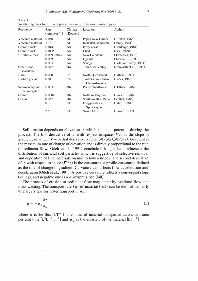
rarely published. Table 1 shows weathering rates for different rock types underdifferent climate conditions which can be used as a guide for the value of P .0

Note that the weathering rates represent both chemical and physical processes.Ž .Heimsath et al. 1997 obtained the production rate from calculated value of in

situ produced cosmogenic nuclide concentration in bedrock samples. They foundthe value of P s 0.77 " 0.09 mm year y 1 and b s 0.0023 " 0.0003 mm y 1 in0

Ž .the Tennessee Valley. Wakatsuki and Rasyidin 1992 predict the rate of rock weathering and soil formation from a simplified geochemical mass-balancecalculation. Other methods for determining rock weathering can be found in

Ž .Colman and Dethier 1986 .




Table 1Weathering rates for different parent materials in various climate regions

Rock type Rate Climate Location Authory 1Ž . Ž .mm year Koppen

Ž .Volcanic material 0.058 Af Papua New Guinea Ruxton, 1968Ž .Volcanic material 7.78 Af Krakatau, Indonesia Jenny, 1941Ž .Granitic rock 0.014 Aw Ivory coast Boulange, 1984´Ž .Granitic rock 0.0135 Aw Chad Gac, 1979Ž .Ultrabasic rock 0.029–0.047 Aw New Caledonia Trescases, 1973Ž .0.009 Aw Uganda Trendall, 1962Ž .0.003 Aw Senegal Fritz and Tardy, 1974Ž .Greenstone, 0.077 Bw Tennessee Valley Heimsath et al., 1997

sandstoneŽ .Basalt 0.0003 Ca North Queensland Pillans, 1997Ž .Biotitic gneiss 0.011 Cb Trnavka river basin, Paces, 1986´ ˇ

ChekoslovakiaŽ .Sedimentary and 0.003 Db Pacific Northwest Dethier, 1986

metamorphicŽ .Granite 0.0004 Db Nothern Virginia Pavich, 1986Ž .Gneiss 0.037 Db Southern Blue Ridge Velbel, 1986Ž .0.3 ET Longyeardalen, Jahn, 1976

SpitsbergenŽ .2.5 ET Swiss Alps Barsch, 1977

Soil erosion depends on elevation z which acts as a potential driving theŽ .process. The first derivative of z with respect to space = z is the slope or

Ž . Ž . Ž . Ž .gradient, in which = s partial derivative vector E r E x , E r E y . Gradient isthe maximum rate of change of elevation and is directly proportional to the rate

Ž .of sediment flow. Odeh et al. 1991 concluded that gradient influences thedistribution of surficial soil particles which is suggestive of selective removaland deposition of fine materials on mid to lower-slopes. The second derivative

Ž 2 . Ž .of z with respect to space = z is the curvature or profile curvature , definedas the rate of change in gradient. Curvature can affects flow acceleration and

Ž .deceleration Odeh et al., 1991 . A positive curvature reflects a convergent slopeŽ . Ž .valley , and negative one is a divergent slope hill .

The process of erosion or sediment flow may occur by overland flow andŽ . Ž .mass wasting. The transport rate q of material soil can be defined similarly

to Darcy’s law for water transport in soil:

E zq sy K 5Ž .e

E x

w y 1 xwhere q is the flux LT or volume of material transported across unit areaw 3 y 2 y 1 x w y 1 xper unit time L L T and K is the erosivity of the material LT .e




The movement of materials in the landscape is usually expressed as diffusiveŽ .transport Scheidegger, 1991 , where the flux is defined as:

E zq sy D 6Ž .s

E xw 2 y 1 xin which q is the sediment flux L T or volume of material that flows acrosss

w 3 y 1 y 1 xa slope profile width per unit time L L T , and D is the erosive diffusivityw 2 y 1 xof the material L T .

Ž .Carson and Kirkby 1972 recognize two limiting processes for materialtransport and weathering: weathering limited , where transport process is morerapid than weathering rate and, transport limited , where weathering rate is morerapid than transport processes.

The erosive diffusivity depends on the erosion factors of the soil, e.g.,vegetation cover, soil physical properties, and weather. For numerical mod-

Ž . Uelling, Koons 1989 suggested that D should be replaced with D , the effectiveerosional diffusivity, which is the diffusivity for the averaged time and spaceconsidered in the numerical modelling. He also found that D is largely a

function of climatic parameters and can be spatially and temporally variable.Ž .Martin and Church 1997 suggested that D should be rewritten with two

Žseparate diffusion terms: diffusivity for slow, continuous mass movements e.g.,. Ž .creep and diffusivity for rapid, episodic mass movement e.g., landslide .

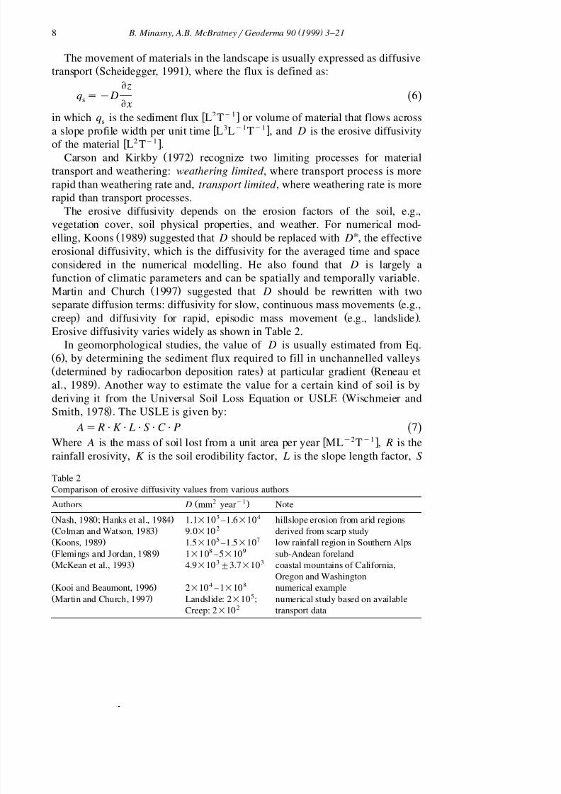
Erosive diffusivity varies widely as shown in Table 2.In geomorphological studies, the value of D is usually estimated from Eq.

Ž .6 , by determining the sediment flux required to fill in unchannelled valleysŽ . Ždetermined by radiocarbon deposition rates at particular gradient Reneau et

.al., 1989 . Another way to estimate the value for a certain kind of soil is byŽderiving it from the Universal Soil Loss Equation or USLE Wischmeier and

.Smith, 1978 . The USLE is given by: As RPK P LPS PC P P 7Ž .

w y 2 y 1 xWhere A is the mass of soil lost from a unit area per year ML T , R is therainfall erosivity, K is the soil erodibility factor, L is the slope length factor, S

Table 2Comparison of erosive diffusivity values from various authors

2 y 1Ž .Authors D mm year Note3 4Ž .Nash, 1980; Hanks et al., 1984 1.1 = 10 –1.6= 10 hillslope erosion from arid regions2Ž .Colman and Watson, 1983 9.0 = 10 derived from scarp study5 7Ž .Koons, 1989 1.5 = 10 –1.5= 10 low rainfall region in Southern Alps

8 9

Ž .Flemings and Jordan, 1989 1 = 10 –5= 10 sub-Andean foreland3 3Ž .McKean et al., 1993 4.9 = 10 " 3.7= 10 coastal mountains of California,Oregon and Washington

4 8Ž .Kooi and Beaumont, 1996 2 = 10 –1= 10 numerical example5Ž .Martin and Church, 1997 Landslide: 2 = 10 ; numerical study based on available

2Creep: 2 = 10 transport data




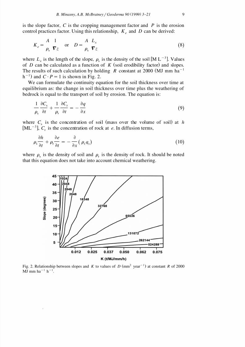
is the slope factor, C is the cropping management factor and P is the erosioncontrol practices factor. Using this relationship, K and D can be derived:e

A 1 A L x

K s or D s 8Ž .er = z r = zs s

w y 3

xwhere L is the length of the slope, r is the density of the soil M L . Values x sŽ .of D can be calculated as a function of K soil erodibility factor and slopes.

Ž y 1The results of such calculation by holding R constant at 2000 MJ mm hay 1 .h and C PP s 1 is shown in Fig. 2.

We can formulate the continuity equation for the soil thickness over time atequilibrium as: the change in soil thickness over time plus the weathering of bedrock is equal to the transport of soil by erosion. The equation is:

1 EC 1 EC Eqs r

q sy 9Ž .r Et r Et E xs r

Ž .where C is the concentration of soil mass over the volume of soil at hs

w y 3 xML , C is the concentration of rock at e. In diffusion terms,r

Eh Ee Er q r sy r q 10Ž . Ž .s r s s

Et Et E x

where r is the density of soil and r is the density of rock. It should be noteds r

that this equation does not take into account chemical weathering.

Ž 2 y 1 .Fig. 2. Relationship between slopes and K to values of D mm year at constant R of 2000MJ mm hay 1 hy 1.




Ž . Ž .If we combine Eqs. 5 and 9 , we obtain the general equation for one-di-mensional soil production:

1 EC 1 EC E E zs r

q sy K 11Ž .ež /r Et r Et E x E xs r

Ž . Ž .Likewise, by combining Eqs. 6 and 10 and assuming D and r constant overs

space, then the soil production function is:

Eh r Ee E2 zr

sy q D 12Ž .2Et r Et E xs

Ž .The above equation destates that the production of soil thickening of h overŽ .time depends on the weathering rate of rock lowering of e and the transport of

Ž .soil through erosion, which is dependent on the diffusivity D and curvature of Ž 2 2 .the landscape E zr E x . The above equations are analogous to heat transport in

Ž .soil. The soil surface z is the analogue of temperature and D the analogue of

Ž . Ž . Ž .soil thermal diffusivity D . Eq. 5 is analogous to Fourier’s law, and Eq. 12h

Ž .to the heat flow equation soil Jury et al., 1991 .Given appropriate initial and boundary conditions, the above partial differen-

Ž Ž ..tial equation Eq. 12 can be solved numerically using the finite-differenceapproach. The formulation using explicit approximation on a rectangular grid

Ž . Ž .over space x and time t is:t q 1 t t q 1 t t t t h y h r e y e z y 2 z q z x x r x x xq 1 x xy 1

sy q D 13Ž .2D t r D t D xŽ .s

under the following initial and boundary conditions:

h s h , zs z at t s 0, xG 0i i

Eesy P exp y bh at t ) 0, 0 - x- `Ž .0

Et

Ehs 0 at t ) 0, xs 0 and xs `

E x

The initial condition describes the soil thickness and elevation at h and z . Thei i

second condition states that the soil production rate is assumed to be an

exponential decay function of the soil thickness. And the third condition definesthe lower and upper boundary for the finite difference space grid. The numericalŽ .solution of Eq. 13 is stable under the condition where the stability ratio

Ž .2 Ž . Ž .2 D D t r D x should be F 1.0 Press et al., 1992 . Eq. 13 could be readilyapplied in a two-dimensional model landscape, using Digital Elevation Modeldata.




3. Methods

3.1. Application of the model

Ž .A numerical example is given to illustrate the application of Eq. 13 . Ahypothetical landscape with initial elevation representing a series of hills and

valleys are simulated with initial soil thickness h . The density of rock and soil,i

and diffusivity D is assumed to be spatially and temporally constant. Theweathering rate decreases exponentially with increasing soil thickness. Theparameters used for the simulation are summarised in Table 3. The time-stepused is 500 years. The calculation is implemented with a commercial spread-

Ž .sheet program MS Excel using rows and columns as time and space grids inthe explicit finite-difference approach.

3.2. The effect of initial randomness on soil de Õ elopment

To illustrate the effect of irregularity and randomness on the stability of thesolution and the soil development, uniformly distributed independent randomnumbers correlated with a moving average across the x-axis were added to theinitial soil elevation which has the average height of 1000 mm. The parametersused are the same as in Table 3, and two time-steps are chosen D t s 250 and500 years in order to satisfy the stability criterion of the numerical solution. ForD t s 500 years the random number has mean of 5.2 mm and variance of 2.6mm 2 and for D t s 250 years the mean is 25.8 mm and variance is 81.6 mm 2 .

3.3. The effect of different rate of soil weathering on soil de Õ elopment

To illustrate the effect of different rates of soil weathering on the soildevelopment in a landscape, two rock types are considered. On the hill tomid-slope the rock type is resistant with P s 0.10 mm yeary 1, while on0

mid-slope to valley, the rock is more easily weatherable with P s 0.19 mm0

Table 3Parameters used in the simulation

Parameters Value2 y 1Ž . D mm year 4000

Ž .D

x mm 500y 3 y 3Ž .r g mm 2.6= 10ry 3 y 3Ž .r g mm 1.4= 10s

Ž .h mm 20iy 1Ž .P mm year 0.190

y 1Ž .b mm 0.005




Table 4Comparison of the square root and logarithmic function on describing the relationship betweensoil thickness and time

aData Eq. S S h RMSR1 2 i

Ž . Ž .Valley this paper Eq. 14 5.84 y 0.0062 106.00 12.40Ž .Eq. 16 256.13 18.40 y 2422.81 44.99

Ž . Ž .Hill this paper Eq. 14 5.23 0.01 122.91 15.35Ž .Eq. 16 117.45 5.09 y 717.60 16.15Ž .Taranaki, New Zealand Eq. 14 1.98 0.02 0.00 1.70

Ž . Ž .Trustum and De Rose, 1988 Eq. 16 7.23 0.08 5.30 1.38y 5Ž .Ventura, California Eq. 14 0.66 2.6 = 10 93.33 58.77

Ž . Ž .Harden and Taylor, 1983 Eq. 16 40.07 0.18 y 105.25 60.34

aRMSR s Root mean squared of the residuals.

yeary 1. The other parameters used are the same as in Table 4, and the time-stepis 250 years.

4. Results and discussion

4.1. Application of the model

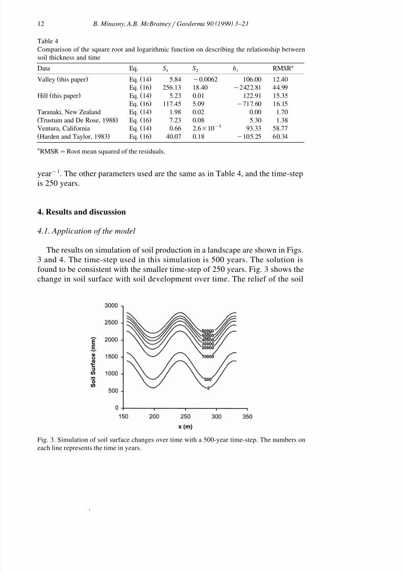
The results on simulation of soil production in a landscape are shown in Figs.3 and 4. The time-step used in this simulation is 500 years. The solution isfound to be consistent with the smaller time-step of 250 years. Fig. 3 shows thechange in soil surface with soil development over time. The relief of the soil

Fig. 3. Simulation of soil surface changes over time with a 500-year time-step. The numbers oneach line represents the time in years.




Fig. 4. Simulation of soil thickness development over time with a 500-year time-step.

surface tends to decrease with time. This is also shown for soil thicknessdevelopment in Figs. 4 and 5, in which soil accumulation is greater for thevalley than for the hill. With the same weathering rate, soil from the hill will betransported downslope by the erosion process and accumulated in the valley.Fig. 5 shows that with an initially thin soil, the rate of production is very high

Ž .which corresponds to the exponential decline function in Eq. 2 . Soil thicknessŽthen increases gradually until it reaches a steady state production rate Ehr Et s

.constant , in our example the production reached steady-state at around fortythousand years.

The soil thickness increase with time can be fitted by a power series on thesquare root of time which is known to be the semi-analytical solution of the

Fig. 5. Soil thickness development over time in the valley, and on the mid-slope and hill.




Fig. 6. Change in curvature with increasing soil thickness over time, each line in the verticaldirection represents a 500-year time-step.

Ž .transport equation Jury et al., 1991 . In this example, the first three terms of theseries were found to be adequate in representing the data:

'h s h q S t q S t 14Ž .i 1 2

w y 1r 2 x w y 1 xwhere S LT and S LT are empirical constants. The rate of soil1 2

Ž .production can be obtained by differentiating Eq. 14 with respect to time:

Eh S 1s q S 15Ž .2'Et 2 t

This function is also found to give a better fit and more realistic values thanthe logarithmic function, which is usually used in describing soil chronofunc-

Ž .tions Mellor, 1985; Trustum and De Rose, 1988 :

h s h q S ln S t 16Ž . Ž .1 1 2

Table 4 shows the comparison between the square root and the logarithmicfunction for our model and also from published empirical data.

Ž .At steady state, the rate of soil production on the divergent slope hillŽ .reaches zero or Ehr Et f 0, and Eq. 12 reduces to:

Ee r E2 zr

s D 17Ž .2Et r E xs




Table 5Ž . Ž y 1 .Summary of the response surface parameters of soil thickness mm to curvature mm and time

Ž .year< <Term Estimate Std. Error t Ratio Prob ) t

Intercept 92.8583 1.2163 76.35 0.0000Curvature y 44099205 450595.9 y 97.87 0.0000

' time 5.5053 0.0144 382.39 0.00002 13 11Curvature 1.1163 = 10 1.86= 10 59.99 0.0000'Curvature P time 702842.42 2401.04 292.72 0.0000

Time y 0.0082 0.000042 y 196.60 0.0000

With soil thickening, the weathering rate is expected to attenuate as suggestedŽ .by the exponential decline function of h or Eer Et f 0, and Eq. 12 reduces to:

Eh E2 zs D 18Ž .2Et E x

So under steady-state conditions soil production is only dependent on the erosivediffusivity and the slope curvature.

Curvature initially changes linearly with increasing soil thickness until itreached around 500 mm then it starts to bend over, as shown in Fig. 6. Soilthickness beyond that point is mostly controlled by the profile curvature. Sincethe soil thickness is a function of the square root of time, a response surface of curvature and square root of time can be fitted to predict the soil thickness. Theparameters of the fitted function are summarised in Table 5. The contour plot of soil thickness as function of time and curvature is given in Fig. 7, which showsthat for a given soil thickness, it will take longer for a site at negative curvatureto develop compared to one with a positive curvature.

Ž .Fig. 7. Contour plot of soil thickness mm as a function of curvature and time.




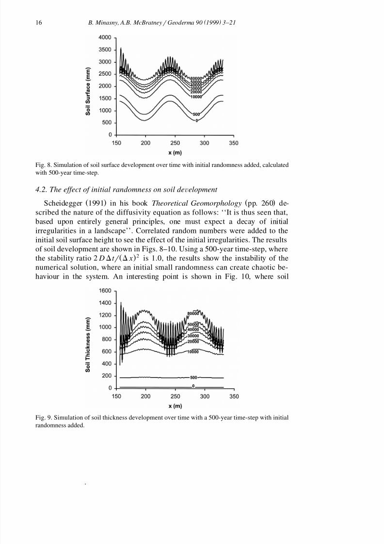
Fig. 8. Simulation of soil surface development over time with initial randomness added, calculatedwith 500-year time-step.

4.2. The effect of initial randomness on soil de Õ elopment Ž . Ž .Scheidegger 1991 in his book Theoretical Geomorphology pp. 260 de-

scribed the nature of the diffusivity equation as follows: ‘‘It is thus seen that,based upon entirely general principles, one must expect a decay of initialirregularities in a landscape’’. Correlated random numbers were added to theinitial soil surface height to see the effect of the initial irregularities. The resultsof soil development are shown in Figs. 8–10. Using a 500-year time-step, where

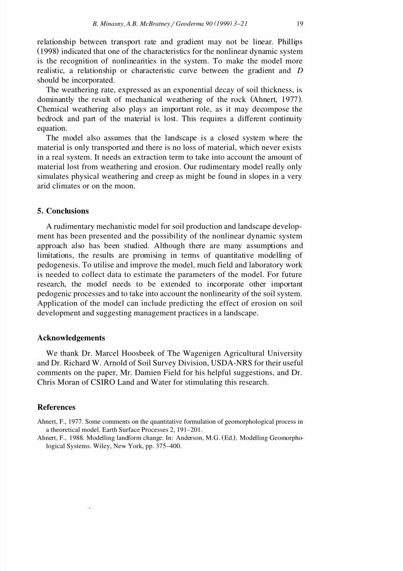
Ž .2the stability ratio 2 D D t r D x is 1.0, the results show the instability of thenumerical solution, where an initial small randomness can create chaotic be-haviour in the system. An interesting point is shown in Fig. 10, where soil

Fig. 9. Simulation of soil thickness development over time with a 500-year time-step with initialrandomness added.




Fig. 10. Soil thickness development over time in the valley, and on the mid-slope and hill with a500-year time-step with initial randomness added.

Žthickness exhibits periodic fluctuation, which is known as bifurcation Gleick,.1987 . Depending on the position on the slope, the fluctuation can become

smaller and larger.Using a 250-year time-step with stability ratio 0.5, the system becomes more

stable, initial randomness does not affect the soil surface but greatly affects soilŽ .thickness Fig. 11 . Initial irregularities do not diminish as foreseen by Schei-

Ž .degger 1991 but tends to intensify. As the solution is based on the finite-dif-ference of h and e, both show amplification of the initial irregularity. This result

Fig. 11. Simulation of soil thickness development over time with a 250-year time-step with initialrandomness added.




also exhibits one of the features of a nonlinear dynamic system characteristic:the recognition of the possibility for inherent stability, deterministic chaosŽ .Phillips, 1998 .

4.3. The effect of different rate of soil weathering on soil de Õ elopment

Numerical solutions have the advantage of flexibility for varying parameters

at different positions on the space and time grid. Fig. 12 illustrate a condition ina landscape where the rock in the valley which has a faster weathering rateŽ y 1 .P s 0.19 mm year is enclosed by the hill which has a lower weathering0

Ž y 1 .rate P s 0.10 mm year . With initial elevation lower than previous simula-0

tions, results showed that after 40,000 years, the surface of the valley has almostreach the same level as the hill, and creates small ridges as the result of the

Ž .sharp boundary or difference between the two rock types. Ollier 1984 notedthat differential weathering of rocks give rise to numerous features such astrenches, walls and ridges on the landscape.

4.4. General discussion

We have illustrated the application and results of the model and here we wishto indicate some limitations of, and suggest improvements to the model. Theerosive diffusivity coefficient D is always assumed to be spatially and tempo-rally constant in a landform or system and to be independent of slope orcurvature. But looking at the results above, it can be seen that there is anonlinear relationship between curvature and soil depth and a dependency of Don the gradient that is clearly affected by curvature. As the soil develops, the

Žgradient and curvature will also change and consequently D which is assumed. Ž .to be constant can change. Martin and Church 1997 pointed out that the

Fig. 12. Soil surface development in a landscape with two different rock types with a 250-yeartime-step.




Ž .Anderson, M.G. Ed. , 1988. Modelling Geomorphological Systems. Wiley, New York.Armstrong, A.C., 1980. Soils and slopes in a humid temperate environment: a simulation study.

Catena 7, 327–338.Barsch, D., 1977. Eine Abschatzung von schuttproduktion und schuttransport im bereich activer¨

blockgletscher der schweizer Alpen. Zeitschrift fur Geomorphologie Suppl. NS28, 148–160.¨Boulange, B., 1984. Les formations bauxitiques lateritiques de Cote d’Ivoire. Les facies, leur´ ´ ˆ ´

transformation, leur distribution et l’evolution du modele. Trav. Docum. ORSTOM, Paris.´ ´

Carson, M.A., Kirkby, M.J., 1972. Hillslope Form and Process. Cambridge Univ. Press, Cam-bridge.Ž .Colman, S.M., Dethier, D.P. Eds. , 1986. Rates of Chemical Weathering of Rocks and Minerals.

Academic Press, Orlando.Colman, S.M., Watson, K., 1983. Ages estimated from a diffusion equation model for scarp

degradation. Science 221, 263–265.Cox, N.J., 1980. On the relationship between bedrock lowering and regolith thickness. Earth

Surface Processes 5, 271–274.Dethier, D.P., 1986. Weathering rates and the chemical flux from catchments in the Pacific

Ž .Northwest, U.S.A. In: Colman, S.M., Dethier, D.P. Eds. , Rates of Chemical Weathering andRocks and Minerals. Academic Press, Orlando, pp. 503–530.

Flemings, P.B., Jordan, T.E., 1989. A synthetic stratigraphic model of foreland basin develop-ment. Journal of Geophysical Research 94, 3851–3866.

´Fritz, B., Tardy, Y., 1974. Etude thermodynamique du systeme gibbsite, quartz, kaolinite, gaz`carbonique. Application a la genese des podzols et des bauxites. Sciences Geologiques Bulletin` ` `26, 339–367.

Gac, J.Y., 1979. Geochimie du bassin du lac Tchad. Thesis, Univ. of Strasbourg.´Gleick, J., 1987. Chaos. Making A New Science. Sphere Books, London.Hanks, T.C., Buckman, R.C., Lajoie, K.R., Wallace, R.E., 1984. Modification of wave-cut and

faulting-controlled landforms. Journal of Geophysical Research 89, 5771–5790.Harden, J.W., Taylor, E.M., 1983. A quantitative comparison of soil development in four climatic

regimes. Quaternary Research 20, 342–359.Heimsath, A.M., Dietrich, W.E., Nishiizumi, K., Finkel, R.C., 1997. The soil production function

and landscape equilibrium. Nature 388, 358–388.Hoosbeek, M.R., Bryant, R.B., 1992. Towards the quantitative modelling of pedogenesis—a

review. Geoderma 55, 183–210.Hoosbeek, M.R., Bryant, R.B., 1994. Developing and adapting soil process submodels for use in

Ž .the pedodynamic Orthod model. In: Bryant, R.B., Arnold, R.W. Eds. , Quantitative Modellingof Soil Forming Processes. SSSA Special Publication 39, Madison, WI, pp. 111–128.

Jahn, A., 1976. Geomorphological modelling and nature protection in Arctic and subarcticenvironments. Geoforum 7, 121–137.

Jenny, H., 1941. Factors of Soil Formation. A System of Quantitative Pedology. McGraw-Hill,New York.

Jury, W.A., Gardner, W.R., Gardner, W.H., 1991. Soil Physics, 5th edn. Wiley, New York.Kirkby, M.J., 1985. A model for the evolution of regolith-mantled slopes. In: Woldenberg, M.J.

Ž .Ed. , Models in Geomorphology, Allen and Unwin, Boston, pp. 213–237.Kooi, H., Beaumont, C., 1996. Large scale geomorphology: classical concepts reconciled and

integrated with contemporary ideas via a surface processes model. Journal of GeophysicalResearch 101, 3361–3386.Koons, P.O., 1989. The topographic evolution of collisional mountain belts: a numerical look at

the Southern Alps, New Zealand. American Journal of Science 289, 1041–1069.Martin, Y., Church, M., 1997. Diffusion in landscape development models: on the nature of basic

transport relations. Earth Surface and Processes and Landforms 22, 273–279.




McGreevy, J.P., 1985. Thermal properties as controls on rock surface temperature maxima, andpossible implications for rock weathering. Earth Surface Processes and Landforms 10, 125–136.

McKean, J.A., Dietrich, W.E., Finkel, R.C., Southon, J.R., Caffee, M.W., 1993. Quantification of soil production and downslope creep rates from cosmogenic

10Be accumulations on a hillslope

profile. Geology 21, 343–346.Mellor, A., 1985. Soil chronosequences on Neoglacial moraine ridges, Jostedalsbreen and

Jotunheimen, southern Norway: a quantitative pedogenic approach. In: Richards, K.S., Arnett,

Ž .R.R., Ellis, S. Eds. , Geomorphology and Soils. Allen and Unwin, Boston.Nash, D.B., 1980. Forms of bluffs degraded for different lengths of time in Emmet County,Michigan, U.S.A. Earth Surface Processes and Landforms 5, 331–345.

Odeh, I.O.A., Chittleborough, D.J., McBratney, A.B., 1991. Evaluation of soil–landform interrela-tionship by canonical ordination analysis. Geoderma 49, 1–32.

Ollier, C., 1984. Weathering, 2nd edn. Longman, London.Paces, T., 1986. Rates of weathering and erosion derived from mass balance in small drainageˇ

Ž .basins. In: Colman, S.M., Dethier, D.P. Eds. , Rates of Chemical Weathering and Rocks andMinerals. Academic Press, Orlando, pp. 531–550.

Pavich, M.J., 1986. Processes and rates of saprolite production and erosion on a foliated graniticŽ .rock of the Virginia Piedmont. In: Colman, S.M., Dethier, D.P. Eds. , Rates of Chemical

Weathering and Rocks and Minerals. Academic Press, Orlando, pp. 552–590.Phillips, J.D., 1998. On the relation between complex systems and the factorial model of soil

Ž .formation with Discussion . Geoderma 86, 1–42.Pillans, B., 1997. Soil development at snail’s pace: evidence from a 6 Ma soil chronosequence on

basalt in North Queensland, Australia. Geoderma 80, 117–128.Press, W.H., Flannery, B.P., Teukolsky, S.A., Vetterling, W.A., 1992. Numerical Recipes: The

Art of Scientific Computing. Cambridge Univ. Press, Cambridge.Reneau, S.L., Dietrich, W.E., Rubin, M., Donahue, D.J., Jull, A.J.T., 1989. Analysis of hillslope

erosion rates using dated colluvial deposits. Journal of Geology 97, 45–63.Ruxton, B.P., 1968. Measures of the degree of chemical weathering of rocks. Journal of Geology

76, 518–527.Scheidegger, A.E., 1991. Theoretical Geomorphology, 3rd edn. Springer-Verlag, Berlin.Smith, B.J., 1977. Rock temperature from the northwest Sahara and their implications for rock

weathering. Catena 4, 41–63.Trendall, A.F., 1962. The formation of ‘apparent peneplains’ by a process of combined laterisation

and surface wash. Zeitschrift fur Geomorphologie NF6, 183–197.¨Trescases, J.J., 1973. Weathering and geochemical behaviour of the elements of ultramafic rocks

in New Caledonia. Bureau of Mineral Resources, Geology and Geophysics, Canberra 141,149–161.

Trustum, N.A., De Rose, R.C., 1988. Soil depth–age relationship of landslides on deforestedhillslopes, Taranaki, New Zealand. Geomorphology 1, 143–160.

Velbel, M.A., 1986. The mathematical basis for determining rates of geochemical and geomorphicprocesses in small forested watersheds by mass balance: examples and implications. In:

Ž .Colman, S.M., Dethier, D.P. Eds. , Rates of Chemical Weathering and Rocks and Minerals.Academic Press, Orlando.

Wakatsuki, T., Rasyidin, A., 1992. Rates of weathering and soil formation. Geoderma 52,

251–263.Warke, P.A., Smith, B.J., 1998. Effects of direct and indirect heating on the validity of rock weathering simulation studies and durability tests. Geomorphology 22, 347–357.

Wischmeier, W.H., Smith, D.D., 1978. Predicting Rainfall Erosion Losses—A Guide to Conser-vation Planning. Agric. Handbook No. 537, USDA, Washington, DC.

1999_budiman_a rudimentary mechanistic model for soil production and landscape development

Documents