1999 forssell
TRANSCRIPT

Linkoping Studies in Science and Technology. Dissertations
No. 566
Closed-loop IdentificationMethods, Theory, and Applications
Urban Forssell
Department of Electrical EngineeringLinkoping University, SE–581 83 Linkoping, Sweden
Linkoping 1999

Closed-loop Identification: Methods, Theory, and Applications
c© 1999 Urban Forssell
http://www.control.isy.liu.se
Department of Electrical EngineeringLinkoping UniversitySE–581 83 Linkoping
Sweden
ISBN 91-7219-432-4 ISSN 0345-7524
Printed in Sweden by Linus & Linnea AB

To Susanne, Tea, and Hugo


Abstract
System identification deals with constructing mathematical models of dynamicalsystems from measured data. Such models have important applications in manytechnical and nontechnical areas, such as diagnosis, simulation, prediction, andcontrol. The theme in this thesis is to study how the use of closed-loop data foridentification of open-loop processes affects different identification methods. Thefocus is on prediction error methods for closed-loop identification and a main resultis that we show that most common methods correspond to different parameteriza-tions of the general prediction error method. This provides a unifying frameworkfor analyzing the statistical properties of the different methods. Here we concen-trate on asymptotic variance expressions for the resulting estimates and on explicitcharacterizations of the bias distribution for the different methods. Furthermore,we present and analyze a new method for closed-loop identification, called the pro-jection method, which allows approximation of the open-loop dynamics in a fixed,user-specified frequency domain norm, even in the case of an unknown, nonlinearregulator.
In prediction error identification it is common to use some gradient-type searchalgorithm for the parameter estimation. A requirement is then that the predictorfilters along with their derivatives are stable for all admissible values of the pa-rameters. The standard output error and Box-Jenkins model structures cannot beused if the underlying system is unstable, since the predictor filters will genericallybe unstable under these circumstances. In the thesis, modified versions of thesemodel structures are derived that are applicable also to unstable systems. Anotherway to handle the problems associated with output error identification of unstablesystems is to implement the search algorithm using noncausal filtering. Severalsuch approaches are also studied and compared.
Another topic covered in the thesis is the use of periodic excitation signals for time-domain identification of errors-in-variables systems. A number of compensationstrategies for the least-squares and total least-squares methods are suggested. Themain idea is to use a nonparametric noise model, estimated directly from data, towhiten the noise and to remove the bias in the estimates.
“Identification for Control” deals specifically with the problem of constructing mod-els from data that are good for control. A main idea has been to try to match theidentification and control criteria to obtain a control-relevant model fit. The use ofclosed-loop experiments has been an important tool for achieving this. We studya number of iterative methods for dealing with this problem and show how theycan be implemented using the indirect method. Several problems with the itera-tive schemes are observed and it is argued that performing iterated identificationexperiments with the current controller in the loop is suboptimal. Related to thisis the problem of designing the identification experiment so that the quality of theresulting model is maximized. Here we concentrate on minimizing the variance er-ror and a main result is that we give explicit expressions for the optimal regulatorand reference signal spectrum to use in the identification experiment in case boththe input and the output variances are constrained.
i


Preface
System identification is a fascinating field for study and research with many chal-lenging problems, both theoretical and practical ones. This thesis deals with variousaspects of system identification using closed-loop data. The main focus is on analy-sis of the statistical properties of different prediction error methods for closed-loopidentification. Other topics covered in the thesis include optimal experiment design,model structure selection, implementation of parameter estimation algorithms, andidentification for control.
Some words on the organization of the thesis: This thesis is divided into two sepa-rate parts plus an introductory chapter, Chapter 1. The first part, entitled Topicsin Identification and Control, is a unified survey of the results in the thesis whilethe second one is a collection of papers. This part is simply called Publications.
Part I can either be read separately or as an extended introduction to the wholethesis. This part contains some background material, an overview of the mostimportant analysis results in the thesis, plus some material on identification forcontrol that is not covered elsewhere in the thesis. The idea has been to keep thestyle rather casual in this first, introductory part, with most technical details leftout. This choice has been made in order to make the results more easily accessiblethan, perhaps, in the papers in Part II which contain the detailed statements. Anoutline of Part I can be found in Chapter 1.
Part II contains edited versions of the following articles and conference papers.
U. Forssell and L. Ljung. Closed-loop identification revisited. Auto-matica, to appear. Preliminary version available as Technical ReportLiTH-ISY-R-2021, Linkoping University, Linkoping, Sweden
U. Forssell and L. Ljung. A projection method for closed-loop identifica-tion. IEEE Transactions on Automatic Control, to appear. Preliminaryversion available as Technical Report LiTH-ISY-R-1984, Linkoping Uni-versity, Linkoping, Sweden
U. Forssell and C. T. Chou. Efficiency of prediction error and instru-mental variable methods for closed-loop identification. In Proceedings ofthe 37th IEEE Conference on Decision and Control, pages 1287–1288,Tampa, FL, 1998
U. Forssell and L. Ljung. Identification of unstable systems using outputerror and Box-Jenkins model structures. In Proceedings of the 37thIEEE Conference on Decision and Control, pages 3932–3937, Tampa,FL, 1998. To appear in IEEE Transactions on Automatic Control
iii

U. Forssell and H. Hjalmarsson. Maximum likelihood estimation ofmodels with unstable dynamics and nonminimum phase noise zeros. InProceedings of the 14th IFAC World Congress, Beijing, China, 1999
U. Forssell, F. Gustafsson, and T. McKelvey. Time-domain identifica-tion of dynamic errors-in-variables systems using periodic excitation sig-nals. In Proceedings of the 14th IFAC World Congress, Beijing, China,1999
U. Forssell and L. Ljung. Identification for control: Some results on opti-mal experiment design. In Proceedings of the 37th IEEE Conference onDecision and Control, pages 3384–3389, Tampa, FL, 1998. Submittedto Automatica
U. Forssell. Asymptotic variance expressions for identified black-boxmodels. Technical Report LiTH-ISY-R-2089, Department of ElectricalEngineering, Linkoping University, Linkoping, Sweden, 1998. Submit-ted to Systems & Control Letters
These papers have all been written independently and hence there is some overlapbetween them. This is especially true for the basic prediction error theory which iscovered in several of the papers. On the other hand, since the same notation hasbeen used in all papers, most readers should be able to skim these introductoryparts of the papers very quickly or skip them completely. Summaries of the paperscan be found in Chapter 1.
Of related interest but not included in the thesis are the following papers:
U. Forssell and P. Lindskog. Combining semi-physical and neural net-work modeling: An example of its usfulness. In Proceedings of the 11thIFAC Symposium on System Identification, volume 4, pages 795–798,Fukuoka, Japan, 1997
L. Ljung and U. Forssell. Variance results for closed-loop identificationmethods. In Proceedings of the 36th IEEE Conference on Decision andControl, volume 3, pages 2435–2440, San Diego, C.A., 1997
L. Ljung and U. Forssell. Bias, variance and optimal experiment design:Some comments on closed loop identification. In Proceedings of theColloqium on Control Problems in Honor of Prof. I.D. Landau, Paris,June 1998. Springer Verlag
iv

L. Ljung and U. Forssell. An alternative motivation for the indirect ap-proach to closed-loop identification. IEEE Transactions on AutomaticControl, to appear. Preliminary version available as Technical ReportLiTH-ISY-R-1989, Linkoping University, Linkoping, Sweden
Several persons have contributed to this thesis. First and foremost I would like tomention my supervisor, Professor Lennart Ljung, who introduced me to the subjectand who has been a constant source of inspiration throughout this work. I wouldalso like to thank my other co-authors: Drs. Tung Chou, Fredrik Gustafsson, HakanHjalmarsson, Peter Lindskog, and Tomas McKelvey for interesting discussions andgood cooperation when preparing the manuscripts.
I have also benefitted a lot from working with the other people in the control grouphere in Linkoping, both the faculty and my fellow graduate students. Special thanksgoes to Fredrik Gunnarsson, Fredrik Tjarnstrom, and Jakob Roll who, togetherwith Peter Lindskog, proofread parts of the manuscript before the printing.
I am also grateful to Professor Johan Schoukens who invited me to visit his researchgroup last year and with whom I have had several enlightening discussions on var-ious topics in system identification. Several other researchers in the identificationfield have also let me borrow some of their time to discuss identification and to askstupid questions, which I am very grateful for. I especially would like to mentionProfessors Michel Gevers and Paul Van den Hof and Dr. Pierre Carrette.
Finally, I would like to express my warm gratitude to my wife Susanne who alwaysis supportive and caring and to our children Tea and Hugo who really light up mydays (and nights!).
Urban Forssell
Linkoping, February 1999
v


Contents
Notation 1
1 Background and Scope 51.1 Introduction . . . . . . . . . . . . . . . . . . . . . . . . . . . . . . . . 51.2 System Identification . . . . . . . . . . . . . . . . . . . . . . . . . . . 61.3 Model Based Control . . . . . . . . . . . . . . . . . . . . . . . . . . . 81.4 The Interplay between Identification and Control . . . . . . . . . . . 91.5 Outline of Part I . . . . . . . . . . . . . . . . . . . . . . . . . . . . . 111.6 Outline of Part II . . . . . . . . . . . . . . . . . . . . . . . . . . . . . 121.7 Main Contributions . . . . . . . . . . . . . . . . . . . . . . . . . . . . 14
I Topics in Identification and Control 15
2 Problems with Closed-loop Experiments 172.1 Technical Assumptions and Notation . . . . . . . . . . . . . . . . . . 172.2 Examples of Methods that May Fail in Closed Loop . . . . . . . . . 19
2.2.1 Instrumental Variable Methods . . . . . . . . . . . . . . . . . 192.2.2 Subspace Methods . . . . . . . . . . . . . . . . . . . . . . . . 202.2.3 Correlation and Spectral Analysis Methods . . . . . . . . . . 22
2.3 Approaches to Closed-loop Identification . . . . . . . . . . . . . . . . 242.4 Generating Informative Data in Closed Loop . . . . . . . . . . . . . 252.5 Summary . . . . . . . . . . . . . . . . . . . . . . . . . . . . . . . . . 26
3 Closed-loop Identification in the Prediction Error Framework 273.1 Further Notation . . . . . . . . . . . . . . . . . . . . . . . . . . . . . 273.2 The Method . . . . . . . . . . . . . . . . . . . . . . . . . . . . . . . . 283.3 Some Common Model Structures . . . . . . . . . . . . . . . . . . . . 293.4 Computing the Estimate . . . . . . . . . . . . . . . . . . . . . . . . . 303.5 Analysis Results for the Prediction Error Method . . . . . . . . . . . 32
3.5.1 Consistency and Identifiability . . . . . . . . . . . . . . . . . 323.5.2 Bias Distribution . . . . . . . . . . . . . . . . . . . . . . . . . 343.5.3 Asymptotic Variance of Parameter Estimates . . . . . . . . . 34
vii

3.5.4 Asymptotic Variance for Identified High-order Black-box Mod-els . . . . . . . . . . . . . . . . . . . . . . . . . . . . . . . . . 35
3.5.5 Discussion . . . . . . . . . . . . . . . . . . . . . . . . . . . . . 363.6 The Indirect Method . . . . . . . . . . . . . . . . . . . . . . . . . . . 363.7 The Projection Method . . . . . . . . . . . . . . . . . . . . . . . . . 39
4 Utilizing Periodic Excitation in System Identification 414.1 Introduction . . . . . . . . . . . . . . . . . . . . . . . . . . . . . . . . 414.2 Notation and Technical Assumptions . . . . . . . . . . . . . . . . . . 424.3 Estimating the Noise Statistics . . . . . . . . . . . . . . . . . . . . . 424.4 Least-squares Estimation Using Periodic Excitation . . . . . . . . . . 434.5 Compensation Methods for Total Least-squares Estimation . . . . . 45
5 Identification for Control 495.1 Models and Robust Control . . . . . . . . . . . . . . . . . . . . . . . 495.2 Uncertainty Bounding and Model Validation . . . . . . . . . . . . . 525.3 Iterative Approaches to Identification for Control . . . . . . . . . . . 535.4 Examples . . . . . . . . . . . . . . . . . . . . . . . . . . . . . . . . . 555.5 Evaluation of the Iterative Schemes . . . . . . . . . . . . . . . . . . . 585.6 Other Approaches and Extensions . . . . . . . . . . . . . . . . . . . 62
6 Optimal Experiment Design 636.1 Minimizing the Performance Degradation Due to Variance Errors . . 636.2 A Novel Approach to Identification for Control . . . . . . . . . . . . 646.3 Summarizing Discussion on Identification for Control . . . . . . . . . 68
Bibliography 69
II Publications 79
A Closed-loop Identification Revisited 811 Introduction . . . . . . . . . . . . . . . . . . . . . . . . . . . . . . . . 84
1.1 Background and Scope . . . . . . . . . . . . . . . . . . . . . . 841.2 Approaches to Closed-loop Identification . . . . . . . . . . . . 851.3 Outline . . . . . . . . . . . . . . . . . . . . . . . . . . . . . . 87
2 Technical Assumptions and Notation . . . . . . . . . . . . . . . . . . 873 Prediction Error Identification . . . . . . . . . . . . . . . . . . . . . 90
3.1 The Method . . . . . . . . . . . . . . . . . . . . . . . . . . . 903.2 Convergence . . . . . . . . . . . . . . . . . . . . . . . . . . . 913.3 Asymptotic Variance of Black Box Transfer Function Estimates 933.4 Asymptotic Distribution of Parameter Vector Estimates . . . 94
4 The Direct and Indirect Approaches . . . . . . . . . . . . . . . . . . 944.1 The Direct Approach . . . . . . . . . . . . . . . . . . . . . . . 944.2 The Idea Behind the Indirect Approach . . . . . . . . . . . . 944.3 Indirect Identification Using the Prediction Error Method . . 95
viii
4.4 A Formal Connection Between Direct and Indirect Methods . 975 The Joint Input-output Approach . . . . . . . . . . . . . . . . . . . . 98
5.1 The Idea . . . . . . . . . . . . . . . . . . . . . . . . . . . . . 995.2 Joint Input-output Identification Using the Prediction Error
Method . . . . . . . . . . . . . . . . . . . . . . . . . . . . . . 995.3 The Two-stage and Projection Methods . . . . . . . . . . . . 1015.4 Unifying Framework for All Joint Input-Output Methods . . 105
6 Convergence Results for the Closed-loop Identification Methods . . . 1076.1 The Direct Approach . . . . . . . . . . . . . . . . . . . . . . . 1086.2 The Indirect Approach . . . . . . . . . . . . . . . . . . . . . . 1096.3 The Joint Input-output Approach . . . . . . . . . . . . . . . 111
7 Asymptotic Variance of Black Box Transfer Function Estimates . . . 1128 Asymptotic Distribution of Parameter Vector Estimates in the Case
of Closed-loop Data . . . . . . . . . . . . . . . . . . . . . . . . . . . 1148.1 The Direct and Indirect Approaches . . . . . . . . . . . . . . 1148.2 Further Results for the Indirect Approach . . . . . . . . . . . 1168.3 Variance Results for the Projection Method . . . . . . . . . . 119
9 Summarizing Discussion . . . . . . . . . . . . . . . . . . . . . . . . . 120References . . . . . . . . . . . . . . . . . . . . . . . . . . . . . . . . . . . . 122A Theoretical Results for the Prediction Error Method . . . . . . . . . 125
A.1 Complement to Section 3.2 . . . . . . . . . . . . . . . . . . . 125A.2 Complement to Section 3.3 . . . . . . . . . . . . . . . . . . . 126A.3 Complement to Section 3.4 . . . . . . . . . . . . . . . . . . . 128
B Additional Proofs . . . . . . . . . . . . . . . . . . . . . . . . . . . . . 129B.1 Proof of Corollary 5 . . . . . . . . . . . . . . . . . . . . . . . 129B.2 Proof of Corollary 6 . . . . . . . . . . . . . . . . . . . . . . . 129B.3 Proof of Corollary 7 . . . . . . . . . . . . . . . . . . . . . . . 130B.4 Proof of Corollary 9 . . . . . . . . . . . . . . . . . . . . . . . 130B.5 Proof of Corollary 10 . . . . . . . . . . . . . . . . . . . . . . . 133B.6 Proof of Corollary 12 . . . . . . . . . . . . . . . . . . . . . . . 135B.7 Proof of Corollary 13 . . . . . . . . . . . . . . . . . . . . . . . 137
B A Projection Method for Closed-loop Identification 1391 Introduction . . . . . . . . . . . . . . . . . . . . . . . . . . . . . . . . 1412 Preliminaries . . . . . . . . . . . . . . . . . . . . . . . . . . . . . . . 1423 The Projection Method . . . . . . . . . . . . . . . . . . . . . . . . . 1444 Convergence Analysis . . . . . . . . . . . . . . . . . . . . . . . . . . 1445 Asymptotic Variance Properties . . . . . . . . . . . . . . . . . . . . . 1476 Simulation Study . . . . . . . . . . . . . . . . . . . . . . . . . . . . . 1487 Conclusions . . . . . . . . . . . . . . . . . . . . . . . . . . . . . . . . 152References . . . . . . . . . . . . . . . . . . . . . . . . . . . . . . . . . . . . 153
C Efficiency of Prediction Error and Instrumental Variable Methodsfor Closed-loop Identification 1551 Introduction . . . . . . . . . . . . . . . . . . . . . . . . . . . . . . . . 157
ix

2 Preliminaries . . . . . . . . . . . . . . . . . . . . . . . . . . . . . . . 1583 Prediction Error Methods . . . . . . . . . . . . . . . . . . . . . . . . 1584 Instrumental Variable Methods . . . . . . . . . . . . . . . . . . . . . 1595 Discussion . . . . . . . . . . . . . . . . . . . . . . . . . . . . . . . . . 160References . . . . . . . . . . . . . . . . . . . . . . . . . . . . . . . . . . . . 161
D Identification of Unstable Systems Using Output Error and Box-Jenkins Model Structures 1631 Introduction . . . . . . . . . . . . . . . . . . . . . . . . . . . . . . . . 1652 Some Basics in Prediction Error Identification . . . . . . . . . . . . . 1673 Commonly Used Model Structures . . . . . . . . . . . . . . . . . . . 1694 An Alternative Output Error Model Structure . . . . . . . . . . . . . 171
4.1 Some Additional Notation . . . . . . . . . . . . . . . . . . . . 1714.2 The Proposed Model Structure . . . . . . . . . . . . . . . . . 1714.3 Connections to the Kalman Filter . . . . . . . . . . . . . . . 1734.4 Computation of the Gradient . . . . . . . . . . . . . . . . . . 1734.5 Simulation Example . . . . . . . . . . . . . . . . . . . . . . . 175
5 An Alternative Box-Jenkins Model Structure . . . . . . . . . . . . . 1766 Conclusions . . . . . . . . . . . . . . . . . . . . . . . . . . . . . . . . 176References . . . . . . . . . . . . . . . . . . . . . . . . . . . . . . . . . . . . 176
E Maximum Likelihood Estimation of Models with Unstable Dy-namics and Nonminimum Phase Noise Zeros 1791 Introduction . . . . . . . . . . . . . . . . . . . . . . . . . . . . . . . . 1822 Prediction Error Identification . . . . . . . . . . . . . . . . . . . . . 1833 The Problem of Unstable Predictors . . . . . . . . . . . . . . . . . . 1844 Maximum Likelihood Estimation . . . . . . . . . . . . . . . . . . . . 1875 Simulation Example . . . . . . . . . . . . . . . . . . . . . . . . . . . 1896 Conclusions . . . . . . . . . . . . . . . . . . . . . . . . . . . . . . . . 192References . . . . . . . . . . . . . . . . . . . . . . . . . . . . . . . . . . . . 192
F Time-domain Identification of Dynamic Errors-in-variables Sys-tems Using Periodic Excitation Signals 1931 Introduction . . . . . . . . . . . . . . . . . . . . . . . . . . . . . . . . 1952 Problem Formulation . . . . . . . . . . . . . . . . . . . . . . . . . . . 1973 Averaging . . . . . . . . . . . . . . . . . . . . . . . . . . . . . . . . . 1984 Estimating the Noise Statistics . . . . . . . . . . . . . . . . . . . . . 1985 Least-squares Estimation Using Periodic Data . . . . . . . . . . . . . 1996 Improving the Accuracy . . . . . . . . . . . . . . . . . . . . . . . . . 2007 Consistent Least-squares Estimation of Errors-in-variables Systems . 2018 The Total Least-squares Solution . . . . . . . . . . . . . . . . . . . . 2029 A Compensation Method for Total Least-squares Estimation . . . . 20310 Prewhitening of the Noise . . . . . . . . . . . . . . . . . . . . . . . . 20411 Example . . . . . . . . . . . . . . . . . . . . . . . . . . . . . . . . . . 20512 Conclusions . . . . . . . . . . . . . . . . . . . . . . . . . . . . . . . . 207
x

References . . . . . . . . . . . . . . . . . . . . . . . . . . . . . . . . . . . . 207
G Identification for Control: Some Results on Optimal ExperimentDesign 2091 Introduction . . . . . . . . . . . . . . . . . . . . . . . . . . . . . . . . 2112 Preliminaries . . . . . . . . . . . . . . . . . . . . . . . . . . . . . . . 2123 Measuring the Performance Degradation . . . . . . . . . . . . . . . . 2144 Main Results . . . . . . . . . . . . . . . . . . . . . . . . . . . . . . . 2165 Examples . . . . . . . . . . . . . . . . . . . . . . . . . . . . . . . . . 221
5.1 Internal Model Control . . . . . . . . . . . . . . . . . . . . . 2215.2 Generalized Minimum Variance Control . . . . . . . . . . . . 2235.3 Model Reference Control . . . . . . . . . . . . . . . . . . . . 223
6 Conclusions . . . . . . . . . . . . . . . . . . . . . . . . . . . . . . . . 225References . . . . . . . . . . . . . . . . . . . . . . . . . . . . . . . . . . . . 225
H Asymptotic Variance Expressions for Identified Black-box Models2271 Introduction . . . . . . . . . . . . . . . . . . . . . . . . . . . . . . . . 2292 Preliminaries . . . . . . . . . . . . . . . . . . . . . . . . . . . . . . . 2303 Main Result . . . . . . . . . . . . . . . . . . . . . . . . . . . . . . . . 2334 Example . . . . . . . . . . . . . . . . . . . . . . . . . . . . . . . . . . 2395 Summary . . . . . . . . . . . . . . . . . . . . . . . . . . . . . . . . . 242A Proof of Theorem 2 . . . . . . . . . . . . . . . . . . . . . . . . . . . . 243References . . . . . . . . . . . . . . . . . . . . . . . . . . . . . . . . . . . . 246
xi

xii

Notation
Operators
arg minxf(x) Minimizing argument of f(x)
Prob(x ≤ C) Probability that the random variable x is less than CCov x Covariance matrix of the random vector xVarx Variance matrix of the random variable xEx Mathematical expectation of the random vector x
Ex(t) limN→∞
1N
∑Nt=1E x(t)
Re z, Im z Real and imaginary parts of the complex number zdetA Determinant of matrix AdimA Dimension of matrix AtrA Trace of matrix AvecA Vector consisting of the columns of AAT Transpose of matrix AA∗ Complex conjugate transpose of matrix AA−1 Inverse of matrix AΠ⊥A Projection matrix onto the orthogonal complement of A:
AΠ⊥A = 0, Π⊥AΠ⊥A = Π⊥Aσ(A) Smallest singular value of matrix Aσ(A) Largest singular value of matrix Aµ Structural singular valueq−1 The delay operator: q−1x(t) = x(t− 1)
Symbols
This list contains symbols used in the text. Occasionally some symbols will haveanother meaning; this will then be stated in the text.
1

2 Notation
xN ∈ AsN(m,P ) Sequence of random variables xN that converges in distributionto the normal distribution with mean m and covariance matrixP
A ⊂ B A is a subset of BC The set of complex numbersDM Set of values over which θ ranges in a model structureDc Set into which the θ-estimate convergese(t) Disturbance at time t; usually {e(t)} is white noise with zero
mean values and variances λ0
ε(t, θ) Prediction error y(t)− y(t|θ)G(q) Transfer function (matrix) from u to yG(q, θ) Transfer function in a model structure, corresponding to the
parameter value θGN (q) Transfer function estimate: GN (q) = G(q, θN )G0(q) “True” transfer function from u to y for a given systemG Set of transfer functions obtained in a given structureH(q) Transfer function from e to yH(q, θ), HN (q) Analogous to GH0(q) Analogous to GK(q) Linear feedback regulatorM Model structureM(θ) Particular model corresponding to the parameter value θO(x) Ordo x: function tending to zero at the same rate as xo(x) Small ordo x: function tending to zero faster than xPθ Asymptotic covariance matrix of θR The set of real numbersRd Euclidian d-dimensional spaceRs(k) Es(t)sT (t− k)Rsw(k) Es(t)wT (t− k)S(q) Sensitivity function: S(q) = (1 +G(q)K(q))−1
S0(q) Analogous to GS The “true” systemT (q) Transfer matrix vec
[G(q) H(q)
]T (q, θ), TN(q) Analogous to GT0(q) Analogous to Gu(t) Input variable at time tU s×N dimensional Hankel matrix with first row [u(1), . . . , u(N)]VN (θ), VN (θ, ZN ) Criterion function to be minimizedV Analogous to U

Notation 3
y(t) Output variable at time tY Analogous to Uy(t|θ) Predicted output at time t using a model M(θ) and based on
Zt−1
Z The set of integer numbersZN Data set {y(1), u(1), . . . , y(N), u(N)}θ Parameter vector, dim θ = d (= d× 1)θN Estimate of θ obtained using N data pointsθ0 “True” parameter valueϕ(t), ϕ(t, θ) Regression vector at time tζ(t), ζ(t, θ) Correlation vector (“instruments”) at time tψ(t, θ) Gradient of y(t|θ) with respect to θΦs(ω) Spectrum of {s(t)} = Fourier transform of Rs(k)Φsw(ω) Cross-spectrum between {s(t)} and {w(t)} = Fourier transform
of Rsw(k)χ0(t) Signal
[uT (t) eT (t)
]T
Abbreviations and Acronyms
ARX AutoRegressive with eXogenous inputARMAX AutoRegressive Moving Average with eXogenous inputBJ Box-JenkinsCLS Compensated Least-SquaresEIV Errors-In-VariablesFFT Fast Fourier TransformGMVC Generalized Minimum Variance ControlIFT Iterative Feedback TuningIMC Internal Model ControlIV Instrumental VariablesLQG Linear Quadratic GaussianLTI Linear Time-invariantMIMO Multiple Input Multiple OutputMRC Model Reference ControlOE Output ErrorPEM Prediction Error MethodSISO Single Input Single OutputTLS Total Least-Squaresw.p. With probability

4 Notation

Chapter 1
Background and Scope
1.1 Introduction
Mathematical models of dynamical systems are of rapidly increasing importancein engineering and today all designs are more or less based on mathematical mod-els. Models are also extensively used in other, nontechnical areas such as biology,ecology, and economy. If the physical laws governing the behavior of the systemare known we can use these to construct so called white-box models of the system.In a white-box model, all parameters and variables can be interpreted in termsof physical entities and all constants are known a priori. At the other end of themodeling scale we have so called black-box modeling or identification. Black-boxmodels are constructed from data using no physical insight whatsoever and themodel parameters are simply knobs that can be turned to optimize the model fit.Despite the quite simplistic nature of many black-box models, they are frequentlyvery efficient for modeling dynamical systems and require less engineering time toconstruct than white-box models.
In this thesis we will study methods for black-box identification of linear, time-invariant dynamical systems given discrete-time data. Such methods have a longhistory going back to Gauss [31] who invented the least-squares method to be ableto predict the motions of the planets based on astronomical observations. By now,several methods exist for identifying discrete-time, linear models, for example, theprediction error methods (e.g., [71]), the subspace approaches (e.g., [114]), and thenonparametric correlation and spectral analysis methods (e.g., [13]). We will focuson the prediction error approach and especially on prediction error methods foridentifying systems operating under output feedback, that is, in closed loop.
5
6 Chapter 1 Background and Scope
Closed-loop identification has often been suggested as a tool for identification ofmodels that are suitable for control, so called identification for control. The mainmotivation has then been that by performing the identification experiments inclosed loop it is possible to match the identification and control criteria so that themodel is fit to the data in a control-relevant way. The second theme in the thesisis to study this area and to analyze methods for identification for control.
In the following section we will provide more background material on system iden-tification, model based control, and the interaction between these two disciplines.
1.2 System Identification
System identification deals with the construction of models from data. This is animportant subproblem in statistics and, indeed, many identification methods, aswell as the tools for analyzing their properties, have their roots in statistics. As aseparate field, system identification started to develop in the 1960’s, see, for exam-ple, the much cited paper [6] by Astrom and Bohlin. An important driving forcefor this development was the increased interest in model based control spurred byKalman’s work on optimal control (e.g., [54, 55]). Since then, the system identifi-cation field has experienced a rapid growth and is today a well established researcharea.
The system identification problem can be divided into a number of subproblems:
• Experiment design.
• Data collection.
• Model structure selection.
• Model estimation.
• Model validation.
Experiment design involves issues like choice of what signals to measure, choiceof sampling time, and choice of excitation signals. Once these issues have beensettled, the actual identification experiment can be performed and process data becollected. The next problem is to decide on a suitable model structure. This is acrucial step in the identification process and to obtain a good and useful model,this step must be done with care. Given a suitable model structure and measureddata, we can turn to the actual estimation of the model parameters. For this,there exist special-purpose software tools that are very efficient and easy to use

1.2 System Identification 7
-Extra input
++
g -Input
Plant - g++?
Noise
-Output
?g- +�Set point
�Controller
6
Figure 1.1 A closed-loop system.
and consequently this step is perhaps the most straightforward one. Before themodel can be delivered to the user it has to pass some validation test. Modelvalidation can loosely be said to deal with the question whether the best modelis also “good enough” for its intended use. Common validation tools are residualanalysis and, so called, cross-validation, where the model is simulated using “fresh”data and the output compared to the measured output. If the first model fails topass the validation tests, some, or all, of the above steps have to be iterated untila model that passes the validations tests is found.
This is a brief outline of the different steps in the identification procedure. Morematerial can be found in the text books [71, 76, 107]. Let us now discuss closed-loopidentification.
Closed-loop identification results when the identification experiment is performedin closed loop, that is, with the output being fed back to the input by meansof some feedback mechanism. A typical situation is when the system is beingcontrolled by some feedback controller, as in Figure 1.1. Automatic controllers arefrequently used for changing the behavior of dynamical systems. The objectivemay, for instance, be to increase the speed of response of the system or to make itless sensitive to disturbances, noise. In such cases it is possible to choose to performthe identification experiment in open loop, with the controller disconnected, or inclosed loop. However, if the system is unstable or has to be controlled for economicor safety reasons, closed-loop experiments are unavoidable. This is also true if thefeedback is inherent in the system and thus cannot be affected by us. Closed-loopexperiments are also optimal in certain situations:
• With variance constraints on the output.
• For identification for control.

8 Chapter 1 Background and Scope
A problem with closed-loop data is that many of the common identification meth-ods, that work well in open loop, fail when applied directly to measured input-output data. This is true for instrumental variables, spectral analysis, and manysubspace methods, for instance. The reason why these methods fail is the nonzerocorrelation between the input and the unmeasurable output noise (cf. Figure 1.1)that is inevitable in a closed-loop situation. Unlike the other methods, the predic-tion error method can be applied directly to closed-loop data and is probably thebest choice among the methods that work in closed loop.
Another problem with closed-loop data is that identifiability may be lost. Thismeans that it becomes impossible to uniquely determine the system parametersfrom measured input-output data. This problem has attracted a lot of interest inthe literature, see, for example, the survey papers [3, 40].
These issues will be further discussed below. Let us now give some backgroundmaterial on model based control.
1.3 Model Based Control
Most modern methods for synthesis of linear controllers require some kind of modelof the system to be controlled. The models may be used explicity in the designschemes or as tools for assessing the performance of the controller before applyingit to the real plant, so called controller validation. To understand some of thequestions that we will deal with in connection to identification for control, it isnecessary to have some basic knowledge of the history of the control field. Thereforewe here give a brief overview of the evolution of the (linear) control field.
The period 1930-1960 is often called the classical control period. Researchers likeBode and Nyquist developed tools to analyze and design control systems in termsof stability, robustness, and performance for single input single output systems.The chief paradigm during this period was the frequency domain and many ofthe design methods of this period are graphical, based on, for instance, Bode andNyquist plots, Nichols charts, and root locus plots. The controllers that were builtwere PI and PID controllers. Gain and phase margins were used as tools to analyzethe robustness of the designs.
With Kalman’s seminal work on state space models in the late 1950’s and early1960’s a new era in control theory begun. This is frequently referred to as theoptimal control period. Now the focus shifted from frequency domain to timedomain methods. Important concepts like optimal state feedback, optimal stateestimation, controllability and observability were introduced. The control synthesismethods were mainly LQG and model reference control. The graphical techniques

1.4 The Interplay between Identification and Control 9
were thus replaced by certainty equivalence control design.
The problem with the optimal control methods is that model uncertainties are noteasily incorporated in the designs. This was one of the motivations for the intro-duction of H∞ methods in the beginning of the 1980’s. The paper by Zames [120]marks the starting point of the modern control or robust control era. In robust con-trol, model uncertainties specified in the frequency domain are again brought backinto center-stage, just like in classical control. Concepts like robust stability androbust performance are central in modern robust control methods like the H∞-loopshaping technique of Glover and McFarlane [79, 80] and µ-synthesis [124].
Parallel to these methods, the adaptive control methods have been developed.Adaptive control is another example of a model based control paradigm and, aswe shall see, there is a close connection between adaptive control and the iterativeapproaches to identification for control that have been suggested in the literature.However, we will not deal directly with adaptive control in this thesis. The inter-ested reader may consult the text book [8] for an introduction to and an overviewof the adaptive control field.
1.4 The Interplay between Identification and Con-
trol
Since most control methods are model based and system identification deals withthe construction of models from measured data, one may think that there shouldexist close connections between the fields. Initially, during the 1960’s, this wasindeed the case, but since then the two fields have developed quite independently.
In identification the emphasis has long been on methods that are consistent andstatistically efficient given that the underlying system is linear, time-invariant, andof finite order and that the disturbances can be modeled as realizations of stochas-tic processes. This ties in nicely with the model demands in many optimal controlmethods, such as LQG and minimum variance control. However, in robust con-trol it is assumed that both a nominal model and “hard”, deterministic boundson the model uncertainty are given a priori. The classical identification methodscan deliver good nominal models but in the stochastic framework we cannot givehard bounds on the model uncertainty – we can only form confidence intervalsfor the models, so called “soft”, probabilistic uncertainty bounds. “Hard” and“soft” uncertainty bounding are two completely different paradigms and, perhapsnot surprisingly, there has been a fierce debate on the relative merits of theseapproaches. Critical and interesting discussions on this can be found in, for exam-ple, [47, 85, 119]. See also the survey paper [86]. In this thesis we will assume astochastic framework and focus on methods for probabilistic uncertainty bounding.

10 Chapter 1 Background and Scope
Probabilistic uncertainty bounds, or confidence intervals, can be constructed fromthe covariance information delivered by the identification routine. A problem withthis information is that it is only reliable when the bias due to undermodeling isnegligible. With undermodeling, special measures have to be taken to obtain reli-able covariance estimates [47, 51]. This is mainly a problem if we have bounds onthe model order. If we can tolerate high-order models it should always be possibleto get an unbiased estimate so that the covariance information is reliable. Theproblem is then that the variance will increase with the number of estimated pa-rameters. This is known as the bias/variance trade-off (e.g., [71]). The limitingfactor is the number of data points. With very long data records the importanceof the bias/variance trade-off is diminished and we can quite safely use high-ordermodels. With short data records, however, this is an important issue [86] and atool for quantifying the size of the undermodeling would be very useful. Stochasticembedding [36, 37] is an approach for estimating the uncertainty in restricted com-plexity models that has been suggested for this purpose. Another example can befound in [44], see also [42], where a method for probabilistic uncertainty boundingis presented in which the bias and variance errors are explicitly evaluated. Withthis method we can therefore manually resolve the bias/variance trade-off problem,which can be advantageous. However, the method described in [44] is much morecomplicated than the straightforward approach of estimating a high-order ARXmodel, say, with small bias and computing the confidence regions for this modelusing the available covariance estimates. This will be further discussed later in thethesis.
“Model error modeling” [69, 70] can be seen as a way to present the informationcontained in the standard residual tests for model validation in a control-orientedfashion. The model validation/unfalsification approach but in a purely determin-istic setting has also been adopted in for example [60, 91, 103, 104]. The idea isto trade-off the possibilities that the model uncertainties are due to unmodeleddynamics or due to disturbances. The problem formulation is closely related torobust control theory. Other deterministic approaches to model error boundinginclude the so called worst-case identification methods (e.g., [78, 83, 119]) and theset membership identification methods (e.g., [81, 82, 88]). A problem with deter-ministic error bounding techniques is that the bounds can be conservative. This isillustrated in [42] where both deterministic and probabilistic uncertainty boundingmethods are studied.
The worst-case and set membership identification methods generally give somenominal model as part of the model set description. These methods could thereforein principle be used for the whole process of constructing a suitable model andcomputing uncertainty bounds. The main benefit would then be that the modelcan be fit to the data in a control-relevant norm, like the H∞-norm. A problemwith the worst-case and set membership identification methods, though, is thatthe nominal models tend to be unsuitable for high-performance control design. Areason for this is that they are chosen to give the smallest upper bounds on the

1.5 Outline of Part I 11
uncertainty rather than to be the best possible approximations of the true system.
A continued discussion on identification for robust control will be given later in thethesis. Let us return to the question of how to identify good nominal models.
What is a good model? In the linear case, the answer is that the model fit hasto be good in certain frequency ranges, typically around the cross-over frequency.This of course a quite vague statement but it is hard to give a more quantitativeanswer that is universally applicable. In general one can say that desired controlperformance dictates the required quality of the model fit: The higher the demandson control performance are, the better model fit is required.
If the important frequency ranges are known, or can be identified, we can useprefiltering and other techniques to obtain a good fit in these ranges. However, insome cases the important frequency ranges are not known and then the situation isless clear. A similar situation occurs when the achievable bandwidth is not knowna priori but part of the information we learn from the identification experiments.A possible solution would then be to use repeated experiments, probing higherand higher frequencies, to gain more and more information about the system thatis to be controlled; the “windsurfer” approach [4, 65]. Variants of this are usedin many of the identification-for-control-schemes that have been suggested in theliterature. A main feature of these schemes is that closed-loop data, generated withthe current controller in the loop, is used for updating the model which in turn isused to update the controller, and so on. This is the same paradigm as adaptivecontrol (e.g., [8]). The only difference is that the model is updated using a batchof data instead of at each iteration. The survey papers [32, 33, 112] give niceoverviews of such methods. Unfortunately, this approach may lead to increasinglypoor control performance which is unacceptable. Later in the thesis we will discussthis in some detail and also point at alternative directions for identification forcontrol.
1.5 Outline of Part I
Part I consists of Chapters 2-6. In Chapter 2 we explain the basics of some al-ternative identification methods, including the instrumental variable method, thesubspace approaches, and spectral analysis, and explain why these fail when ap-plied directly to closed-loop data. This chapter also discusses different approachesfor avoiding the problems associated with closed-loop identification.
Chapter 3 deals with the prediction error method. We describe the algorithmformat and discuss different model structures and how to compute the estimates.In addition, we briefly state some of the most important analysis results for the

12 Chapter 1 Background and Scope
statistical properties of this method. Two alternative prediction error methods forclosed-loop identification are also presented and analyzed: the indirect method andthe projection method.
Chapter 4 discusses the advantages of using periodic excitation signals in time-domain identification. A number of simple and efficient methods that can handlethe general errors-in-variables situation are presented.
In Chapter 5 we return to the question of how to identify models that are suitablefor control. A number of iterative approaches to identification for control will bestudied. Identification for control is also the topic in Chapter 6. Here we presentsome results on optimal experiment design and suggest a novel approach to control-relevant identification.
1.6 Outline of Part II
As mentioned, the second part of the thesis consists of eight different papers whichwill be summarized in this section. The paper outlines below clearly indicate thescope of the thesis and also gives an idea of the contributions. A summary of themain contributions will be given in the next section.
Paper A: Closed-loop Identification Revisited. In this paper a compre-hensive study of closed-loop identification in the prediction error framework is pre-sented. Most of the existing methods are placed in a common framework by treatingthem as different parameterizations of the prediction error method. This facilitatesa simultaneous analysis of the different methods using the basic statements on theasymptotic statistical properties of the general prediction error method: conver-gence and bias distribution of the limit transfer function estimates; asymptoticvariance of the transfer function estimates (as the model orders tend to infinity);asymptotic variance and distribution of the parameter estimates.
Paper B: A Projection Method for Closed-loop Identification. This paperpresents a novel method for closed-loop identification that allows fitting the modelto the data with arbitrary frequency weighting. The method is called the projectionmethod. The projection method is in form similar to the two-stage method [111],but the underlying ideas and the properties are different. The projection methodis applicable to systems with arbitrary feedback mechanisms, just as the directmethod. A drawback with the projection method is the suboptimal accuracy.
Paper C: Efficiency of Prediction Error and Instrumental Variable Meth-ods for Closed-loop Identification The asymptotic variance properties of dif-ferent prediction error and instrumental variable methods for closed-loop identifi-

1.6 Outline of Part II 13
cation are compared. To a certain extent, the results can also be extrapolated tothe subspace methods. One of the key observations is that the suboptimal accuracyof the indirect and a number of other methods is due to the fact that the wholeinput spectrum is not utilized in reducing the variance, as with the direct method.
Paper D: Identification of Unstable Systems Using Output Error andBox-Jenkins Model Structures. The prediction error method requires the pre-dictors to be stable. If the underlying system is unstable and an output error ora Box-Jenkins model structure is used, this condition will not be satisfied. In thispaper it is shown how to modify these model structures to make them applicablealso to unstable systems.
Paper E: Maximum Likelihood Estimation of Models with UnstableDynamics and Nonminimum Phase Noise Zeros. This paper can be seenas a continuation of Paper D and discusses how to implement maximum likelihoodestimation of unstable systems or systems with nonminimum phase noise zeros. Itis shown that, by using noncausal filtering, maximum likelihood estimation of suchsystems is possible.
Paper F: Time-domain Identification of Dynamic Errors-in-variablesSystems Using Periodic Excitation Signals. The use of periodic excitationsignals in time-domain identification is advocated. It is shown that it is possibleto construct simple and noniterative methods for errors-in-variables estimation ifperiodic excitation signals are used. The idea is to include a bias correction step inthe standard least-squares and total least-squares methods. Several such methodsare suggested and compared.
Paper G: Identification for Control: Some Results on Optimal Exper-iment Design. In this paper it is shown that the optimal design for identifica-tion experiments with constrained output variance is to perform the experimentin closed loop with a certain LQ regulator controlling the plant. Explicit formu-las for the optimal controller and the optimal reference signal spectrum are given.This result has important applications in identification for control, for instance. Inthe paper various other optimal experiment design problem formulations are alsostudied.
Paper H: Asymptotic Variance Expressions for Identified Black-boxModels. From classical results on prediction error identification we know thatit is possible to derive expressions for the asymptotic variance of identified trans-fer function models that are asymptotic both in the number of data and in themodel order. These expressions tend to be simpler than the corresponding onesthat hold for fixed model orders and yet they approximate the true covariance wellin many cases. In Paper H the corresponding (doubly) asymptotic variance ex-pressions for the real and imaginary parts of the identified transfer function modelare computed. As illustrated in the paper, these results can be used to compute

14 Chapter 1 Background and Scope
uncertainty regions for the frequency response of the identified model.
1.7 Main Contributions
The main contributions of this thesis are:
• The analysis of the statistical properties of the closed-loop identificationmethods presented in Paper A.
• The projection method introduced in Paper B.
• The modified versions of the common output error and Box-Jenkins modelstructures that are applicable also if the underlying system is unstable, whichwere presented in Paper D.
• The results on optimal experiment design in Paper G dealing with the situ-ation that the output variance is constrained.

Part I
Topics in Identification andControl
15


Chapter 2
Problems with Closed-loopExperiments
As mentioned in Chapter 1, it is sometimes advantageous or even necessary toperform the identification experiment with the system operating in closed loop.Here we will begin our study of the problems associated with this and, amongother things, we will explain why some well known identification methods cannotbe used for closed-loop identification. The chapter starts with an introductorysection that contains some technical assumptions on the data set and introducesthe notation that will be used in the thesis.
2.1 Technical Assumptions and Notation
We will consider the following set-up. The system is given by
y(t) = G0(q)u(t) + v(t), v(t) = H0(q)e(t) (2.1)
Here y(t) is the output, u(t) the input, and e(t) a white noise signal with zero meanand variance λ0. The symbol q denotes the discrete-time shift operator:
q−1u(t) = u(t− 1) (2.2)
Without loss of generality, we assume that G0(q) contains a delay. The noise modelH0(q) is assumed monic and inversely stable. We further assume that the input isgenerated as
u(t) = k(t, yt, ut−1, r(t)) (2.3)
17

18 Chapter 2 Problems with Closed-loop Experiments
-r(t)
+–
g -u(t)
G0(q) - g++?
v(t)
-y(t)
�K(q)
6
Figure 2.1 System controlled by a linear regulator.
where yt = [y(1), . . . , y(t)], etc., and where the reference signal r(t) is a givenquasi-stationary signal, independent of v(t) and k is a given deterministic functionsuch that the closed-loop system is well posed and exponentially stable in the sensedefined in [67]. See also Paper A.
For some of the analytic treatment we will assume that the feedback is linear andgiven by
u(t) = r(t) −K(q)y(t) (2.4)
This set-up is depicted in Figure 2.1. With linear feedback the condition on expo-nential stability is equivalent to internal stability of the closed-loop system (2.1),(2.4).
By combining the equations (2.1) and (2.4) we get the closed-loop relations
y(t) = S0(q)G0(q)r(t) + S0(q)v(t) (2.5)u(t) = S0(q)r(t) −K(q)S0(q)v(t) (2.6)
where S0(q) is the sensitivity function
S0(q) =1
1 +G0(q)K(q)(2.7)
For future use we also introduce
Gc0(q) = S0(q)G0(q) (2.8)
and
Hc0(q) = S0(q)H0(q) (2.9)

2.2 Examples of Methods that May Fail in Closed Loop 19
so that we can rewrite the closed-loop system (2.5) as
y(t) = Gc0(q)r(t) + vc(t), vc(t) = Hc0(q)e(t) (2.10)
We will frequently use the “total expectation” operator E (cf. [71]):
Ef(t) = limN→∞
1N
N∑t=1
Ef(t) (2.11)
The (power) spectrum of a signal s(t) will be denoted by Φs(ω) and the cross-spectrum between two signals s(t) and w(t) will be denoted by Φsw(ω).
2.2 Examples of Methods that May Fail in ClosedLoop
2.2.1 Instrumental Variable Methods
Consider the linear regression model
y(t|θ) = ϕT (t)θ (2.12)
where ϕ(t) is a regression vector and θ a parameter vector. With the standardinstrumental variable method (e.g., [106]) the parameter estimate is found as
θN =
[1N
N∑t=1
ζ(t)ϕT (t)
]−1
1N
N∑t=1
ζ(t)y(t) (2.13)
Here ζ(t) is an instrumental variable vector whose elements are the instruments.(We can note that the celebrated least-squares method is obtained if ζ(t) = ϕ(t).)
Suppose that the true system is
y(t) = ϕT (t)θ0 + e(t) (2.14)
where e(t) is a zero mean, white noise signal. Under mild conditions on the dataset we then have that
θN → θ0 +[Eζ(t)ϕT (t)
]−1Eζ(t)e(t) w.p. 1 as N →∞ (2.15)

20 Chapter 2 Problems with Closed-loop Experiments
See, for example, [106]. (The abbreviation w.p. stands for “with probability”.)It follows that the instrumental variable method is consistent if the following twoconditions hold:
Eζ(t)e(t) = 0 (2.16)
Eζ(t)ϕT (t) has full rank (2.17)
In loose terms, the instruments should thus be well correlated with lagged inputsand outputs but uncorrelated with the noise sequence. In open loop it is commonto let the instruments be filtered and delayed versions of the input. However, thisstraightforward approach will fail in closed loop since the input is correlated withthe noise in this case. There are basically two ways to circumvent this problem:Either we construct the instruments from the reference signal which is uncorrelatedwith the noise (see, e.g., [108]) or we let them be delayed versions of the regressors,where the delay is chosen large enough so that (2.16) holds (at least approximately).With both these solutions we have to be careful to satisfy the rank condition (2.17)which imposes further constraints on the instruments. Furthermore, the choiceof instruments will also determine the statistical efficiency of the method as theaccuracy depends on the inverse of the matrix Eζ(t)ϕT (t), which hence must bewell conditioned. See Paper C.
Thus it is not completely straightforward to apply the instrumental variable methodwith closed-loop data. The reason is basically that it is hard to find instrumentsthat simultaneously satisfy (2.16) and (2.17) in closed loop. A similar situationoccurs with the subspace methods, as will be shown next.
2.2.2 Subspace Methods
A discrete-time, linear, and time-invariant system can always be written as
x(t+ 1) = Ax(t) +Bu(t)y(t) = Cx(t) +Du(t) + v(t)
(2.18)
where v(t) is a lumped noise term. For simplicity we will here only discuss scalarsystems but the discussion below also holds for the multivariable case with someminor notational changes.
Subspace methods can be used to estimate the order n of the system, that is, thedimension of the state vector x(t), and the system matrices (A,B,C,D) up to asimilarity transformation.
2.2 Examples of Methods that May Fail in Closed Loop 21
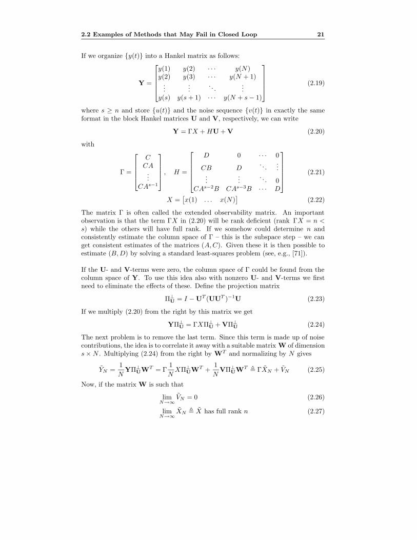
If we organize {y(t)} into a Hankel matrix as follows:
Y =
y(1) y(2) · · · y(N)y(2) y(3) · · · y(N + 1)
......
. . ....
y(s) y(s+ 1) · · · y(N + s− 1)
(2.19)
where s ≥ n and store {u(t)} and the noise sequence {v(t)} in exactly the sameformat in the block Hankel matrices U and V, respectively, we can write
Y = ΓX +HU + V (2.20)
with
Γ =
CCA
...CAs−1
, H =
D 0 · · · 0
CB D. . .
......
.... . . 0
CAs−2B CAs−3B · · · D
(2.21)
X =[x(1) . . . x(N)
](2.22)
The matrix Γ is often called the extended observability matrix. An importantobservation is that the term ΓX in (2.20) will be rank deficient (rank ΓX = n <s) while the others will have full rank. If we somehow could determine n andconsistently estimate the column space of Γ – this is the subspace step – we canget consistent estimates of the matrices (A,C). Given these it is then possible toestimate (B,D) by solving a standard least-squares problem (see, e.g., [71]).
If the U- and V-terms were zero, the column space of Γ could be found from thecolumn space of Y. To use this idea also with nonzero U- and V-terms we firstneed to eliminate the effects of these. Define the projection matrix
Π⊥U = I −UT (UUT )−1U (2.23)
If we multiply (2.20) from the right by this matrix we get
YΠ⊥U = ΓXΠ⊥U + VΠ⊥U (2.24)
The next problem is to remove the last term. Since this term is made up of noisecontributions, the idea is to correlate it away with a suitable matrix W of dimensions×N . Multiplying (2.24) from the right by WT and normalizing by N gives
YN =1N
YΠ⊥UWT = Γ1NXΠ⊥UWT +
1N
VΠ⊥UWT , ΓXN + VN (2.25)
Now, if the matrix W is such that
limN→∞
VN = 0 (2.26)
limN→∞
XN , X has full rank n (2.27)

22 Chapter 2 Problems with Closed-loop Experiments
we will have that
YN = ΓX + EN (2.28)
EN = Γ(XN − X) + VN → 0 as N →∞ (2.29)
From this it follows that we can get a consistent estimate of the column space of Γby computing a singular value decomposition of YN and extracting the left singularvectors corresponding to the n largest singular values of YN .
This is a short description of the subspace approach to system identification. Moredetails can be found in, for example, the text book [114] and the papers [61, 117,118].
The key to good results is to choose the matrix W in such a way that it is un-correlated with the noise (condition (2.26)) and results in a full rank matrix X(condition (2.27)). (Notice the similarity with the conditions (2.16) and (2.17) forthe instrumental variable method!) In open loop we can, for instance, build upW using delayed inputs but, just as with the instrumental variable method, thisapproach will fail in closed loop due to the correlation between the input and thenoise. A feasible approach would be to build up W using delayed versions of thereference signal which would automatically ensure (2.26). In practice, it is alsoimportant that the rank condition (2.27) is satisfied with some margin. Otherwisethe accuracy can be very poor, as is discussed in Paper C.
Other approaches that have been suggested in the literature include the methodsby [115, 116]. The idea proposed in [116] is to identify an augmented system withthe input and the output as outputs and the reference signal as input. The systemand controller parameters are then retrieved in a second, algebraic step. In [115]it is assumed that a number of Markov parameters for the controller are knowna priori. As shown in the paper, it is then possible to consistently estimate theopen-loop system from closed-loop data using subspace techniques.
Here we should also mention that there are alternative forms of the subspace meth-ods that are directly applicable to closed-loop data, see, for example, [14, 15, 90].Some of these methods are yet not fully developed, but the ideas show promise.
2.2.3 Correlation and Spectral Analysis Methods
Correlation and spectral analysis (e.g., [13, 71]) are examples of nonparametricidentification methods. Correlation analysis uses time-domain measurements whilespectral analysis is a frequency-domain method (or can at least be interpreted assuch).

2.2 Examples of Methods that May Fail in Closed Loop 23
Consider the system description
y(t) =∞∑k=1
g(k)u(t− k) + v(t) (2.30)
where u(t) is quasi-stationary [71] and u(t) and v(t) are uncorrelated. Given finitesample estimates RNu (k) and RNyu(k) of the correlation functions
Ru(k) = Eu(t)u(t− k) (2.31)Ryu(k) = Ey(t)u(t− k) (2.32)
respectively, we can estimate the impulse response coefficients g(k), k = 1, . . . ,Mby solving
RNyu(τ) =M∑k=1
g(k)RNu (k − τ) (2.33)
This is the idea behind the correlation approach. This clearly has close connec-tions to the least-squares method, but less emphasis is put on the model structure(regressors) used. Often some kind of prefiltering operation is used to simplify thesolution of (2.33), for example prewhitening of the input signal.
In spectral analysis a similar idea is used: Given spectral estimates ΦNu (ω) andΦNyu(ω) of Φu(ω) and Φyu(ω), respectively, we may estimate the true transfer func-tion (cf. (2.30))
G0(eiω) =∞∑
k=−∞g(k)e−iωk (2.34)
by
GN (eiω) =ΦNyu(ω)
ΦNu (ω)(2.35)
This assumes that the cross-spectrum Φuv(ω) is zero, that is, that u(t) and v(t) areuncorrelated. Spectral analysis can thus be seen as a Fourier domain counterpartof correlation analysis.
A classical result for spectral analysis is that under (2.1) and (2.4) the standardspectral analysis estimate (2.35) will converge to
G∗(eiω) =G0(eiω)Φr(ω)−K(e−iω)Φv(ω)
Φr(ω) + |K(eiω)2|Φv(ω)(2.36)
as the number of data tends to infinity. This was shown in [1]. Obviously thelimit estimate G∗(eiω) 6= G0(eiω), unless the data is noise free (Φv(ω) = 0). Hence

24 Chapter 2 Problems with Closed-loop Experiments
spectral analysis in its standard form also fails in closed loop, just as the standardinstrumental variable and subspace methods discussed above. Also note that withno external reference signal present (i.e., Φr(ω) = 0), the limit estimate will equalthe negative inverse of the controller.
A closed-loop solution for spectral analysis was given in [1]. The idea is as follows:Compute the spectral estimates
GyxN (eiω) =ΦNyx(ω)
ΦNx (ω)and GuxN (eiω) =
ΦNux(ω)ΦNx (ω)
(2.37)
where the signal x(t) is correlated with y(t) and u(t), but uncorrelated with thenoise e(t) (a standard choice is x(t) = r(t)). The open-loop system may then beconsistently estimated as
GyuN (eiω) =GyxN (eiω)
GuxN (eiω)=
ΦNyx(ω)
ΦNux(ω)(2.38)
2.3 Approaches to Closed-loop Identification
In the preceding section we gave some examples of methods that cannot be ap-plied directly to closed-loop data. The prediction error method, on the other hand,works fine as long as the parameterization is flexible enough. This method will bethoroughly studied in the next chapter. In the above section we also mentionedsome alternative ways to implement the methods to make them applicable also inthe closed-loop situation. In fact it turns out that a large number of such “meth-ods”/parameterizations exist, in particular a number of prediction error “methods”for closed-loop identification. It is convenient to consider the following classifica-tion of the different types of methods, which basically is due to [40] (see also [107]and Paper A): Depending on what assumptions are made on the nature of thefeedback, all closed-loop identification methods can be classified as direct, indirect,or joint input-output methods.
In the direct approach, the method is applied directly to measured input-outputdata and no assumptions whatsoever are made on how the data was generated.The indirect methods assume perfect knowledge of the feedback controller used inthe identification experiment and the idea is to identify the closed-loop system andto compute the open-loop parameters from this estimate, using the knowledge ofthe controller. The third approach, the joint input-output approach, amounts tomodeling the input and the output jointly as outputs from an augmented systemdriven by the reference signal and the unmeasurable noise. Given an estimate ofthis augmented system, the open-loop model (and the controller) can be solved for.

2.4 Generating Informative Data in Closed Loop 25
In the joint input-output approach it is thus not required to know the controller,but the controller must be known to have a certain structure.
The indirect and joint input-output approaches are typically only used when thefeedback law is linear, as in (2.4), but can also be applied with nonlinear feed-back. The price is of course that the estimation problems then become much moreinvolved.
It should be noted that the direct approach is only applicable with the predictionerror method and some of the subspace methods. The reason for this is the un-avoidable correlation between the input and the noise, which, as we have seen, rulesout most other methods. With the indirect and joint input-output approaches theclosed-loop problem is converted into an open-loop one since the reference signal(which plays the role of an input) is uncorrelated with the noise. Hence these ap-proaches can be used together with all open-loop methods, for example spectralanalysis and the instrumental variable method.
In the next chapter we will study different prediction error methods that fall intothese categories. Of the methods discussed in the previous section, the methoddescribed in [115] falls into the indirect category while the methods in [1, 108, 116]should be regarded as joint input-output methods.
2.4 Generating Informative Data in Closed Loop
Above we saw examples of how to identify systems operating in closed loop. An un-derlying assumption is that the data is sufficiently rich so that it is indeed possibleto uniquely determine the system parameters. This is a much studied subject in the(closed-loop) identification literature. See, among many references, [3, 40, 71, 105].
In open loop the situation is rather transparent and it can be shown that the dataset is informative enough with respect to the chosen model structure if, and only if,the input is persistently exciting of sufficiently high order. See [71] for more details.In closed loop the situation is more complicated. The following standard exampleshows what can happen.
Example 1 Consider the system
y(t) + ay(t− 1) = bu(t− 1) + e(t) (2.39)
where e(t) is a white noise signal. Suppose that a proportional regulator
u(t) = −ky(t) (2.40)

26 Chapter 2 Problems with Closed-loop Experiments
is used during the identification experiment. Inserting the feedback law into thesystem equation gives
y(t) + (a+ bk)y(t− 1) = e(t) (2.41)
This shows that all models (a, b) of the form
a = a− γk, b = b+ γ (2.42)
give the same input-output description of the system (2.39) under the feedback(2.40) and thus there is no way to distinguish between all these models based onthe measured input-output data.
As this example shows, it is not sufficient in closed loop that the input is persistentlyexciting to be able to guarantee informative data. The reason is basically that thefeedback law used in the example is too simple. With a time-varying, nonlinear,or noisy regulator, or if we switch between several different linear, time-invariantregulators, the data will, in general, be informative (enough). In the next chapterwe will return to this question and derive an explicit condition which must besatisfied for the data to be informative.
2.5 Summary
In this chapter we have studied the closed-loop identification problem and we havegiven examples of methods that fail when applied directly to closed-loop data. Wehave also studied different ways to avoid the problems associated with closed-loopidentification which lead to a characterization of the possible approaches into threedifferent categories: the direct, the indirect, and the joint input-output approaches.With the direct approach one should apply the identification method directly toinput-output data, ignoring possible feedback. This is the simplest approach, butcannot be used with all methods. An exception is the prediction error methodwhich will be studied in the next chapter. The other two approaches aim at iden-tifying some closed-loop transfer function from which the open-loop estimate canbe determined. These approaches can be applied with all open-loop identificationmethods.

Chapter 3
Closed-loop Identification inthe Prediction ErrorFramework
3.1 Further Notation
Consider the model structure M (cf. (2.1)):
y(t) = G(q, θ)u(t) +H(q, θ)e(t) (3.1)
G(q, θ) will be called the dynamics model and H(q, θ) the noise model. H(q, θ) isassumed monic. The parameter vector θ ranges over a set DM ⊂ Rd (d = dim θ)which is assumed compact and connected.
The model structure (3.1), where θ ∈ DM, describes a model set. We say that thetrue system (2.1) is contained in the model set if, for some θ0 ∈ DM,
G(q, θ0) = G0(q), H(q, θ0) = H0(q) (3.2)
This will also be written S ∈ M. The case when the true noise properties cannotbe correctly described within the model set, but where there exists a θ0 ∈ DMsuch that
G(q, θ0) = G0(q) (3.3)
will be denoted G0 ∈ G.
27

28 Chapter 3 Closed-loop Identification in the Prediction Error Framework
We will use the notation
T (q, θ) =[G(q, θ)H(q, θ)
](3.4)
and, in the same vein, we also define
T0(q) =[G0(q)H0(q)
](3.5)
For future use we further introduce the signal
χ0(t) =[u(t) e(t)
]T (3.6)
The spectrum for χ0(t) is
Φχ0(ω) =[
Φu(ω) Φue(ω)Φeu(ω) λ0
](3.7)
We will also frequently use
Φru(ω) = Φu(ω)− |Φue(ω)|2/λ0 (3.8)
which we recognize as the Schur complement of λ0 in the matrix Φχ0(ω) (see,e.g., [53]). The matrix Φr
u(ω) defined in (3.8) can be seen as that part of the inputspectrum that originates from the reference signal r(t). Using (2.6) we can easilyderive the following expression for Φr
u(ω) under (2.4):
Φru(ω) = |S0(eiω)|2Φr(ω) (3.9)
Here Φr(ω) is the spectrum of the reference signal. If u(t) is generated as in (2.4)the cross-spectrum between u(t) and e(t) is
Φue(ω) = −K(eiω)S0(eiω)H0(eiω)λ0 (3.10)
The spectrum of v(t) is
Φv(ω) = |H0(eiω)|2λ0 (3.11)
Let us finally introduce the quantity
Φre(ω) = λ0 − |Φue(ω)|2/Φu(ω) (3.12)
which is the Schur complement of Φu(ω) in the matrix Φχ0(ω).
3.2 The Method
The one-step-ahead predictor for the model structure (3.1) is
y(t|θ) = H−1(q, θ)G(q, θ)u(t) + (1−H−1(q, θ))y(t) (3.13)
3.3 Some Common Model Structures 29
The prediction error is
ε(t, θ) = y(t)− y(t|θ) = H−1(q, θ)(y(t)−G(q, θ)u(t)) (3.14)
Given the model (3.13) and measured data
ZN = {y(1), u(1), . . . , y(N), u(N)} (3.15)
we determine the prediction error estimate through
θN = arg minθ∈DM
VN (θ, ZN ) (3.16)
VN (θ, ZN ) =1N
N∑t=1
`(ε(t, θ)) (3.17)
Here `(·) is a suitably chosen positive (norm) function. The standard choice is
`(ε(t, θ)) =12ε2(t, θ) (3.18)
possibly combined with some linear, monic, and possibly parameterized prefilterL(q, θ):
`(ε(t, θ)) =12ε2F (t, θ) (3.19)
εF (t, θ) = L(q, θ)ε(t, θ) (3.20)
However, since
εF (t, θ) = L(q, θ)H−1(q, θ)(y(t) −G(q, θ)u(t)) (3.21)
the effect of the prefilter can be included in the noise model and L(q, θ) = 1 canbe assumed without loss of generality. This will be done in the sequel.
The above choice of `(·) gives the least-squares method. If we let the criterionfunction `(·) be equal to the negative logarithm of fe(·), the probability densityfunction of e(t), we obtain the maximum likelihood method. These and otherchoices of norms are further discussed in [71]. In this thesis we will for simplicityassume that a quadratic criterion is used.
The following notation will be used for the estimates G(q, θN ), H(q, θN ), etc.:
GN (q) = G(q, θN ) and HN (q) = H(q, θN ) (3.22)
3.3 Some Common Model Structures
With the prediction error approach, the models may have arbitrary parameteri-zations. However, in most cases it is convenient and also sufficient to use some

30 Chapter 3 Closed-loop Identification in the Prediction Error Framework
standard model structure. Consider the following generalized model structure [71]:
A(q)y(t) =B(q)F (q)
u(t) +C(q)D(q)
e(t) (3.23)
where
A(q) = 1 + a1q−1 + · · ·+ anaq
−na (3.24)
and similarly for the C-, D-, and F -polynomials, while
B(q) = b1q−1 + b2q
−2 + · · ·+ bnbq−nb (3.25)
It is also possible to redefine the B-polynomial to include extra delays. For sim-plicity, this is not done here.
The model structure (3.23) contains several common special cases, some of whichare listed in Table 3.1.
Table 3.1 Some Common Model Structures as Special Cases of (3.23).Polynomials Used in (3.23) Name of Model StructureB FIRA,B ARXA,B,C ARMAXB,F OEB,C,D,F BJ
In Table 3.1 the acronyms FIR, ARX, ARMAX, OE and BJ denote Finite ImpulseResponse, AutoRegressive with eXogenous (or eXternal) input, AutoRegressiveMoving Average with eXogenous input, Output Error and Box-Jenkins, respec-tively.
3.4 Computing the Estimate
If an FIR or an ARX model is used together with a quadratic criterion function,we obtain the standard least-squares method. To find the estimate θN we thenonly have to solve a standard least-squares problem, which can be done withoutiterations. For other parameterizations and criteria we typically have to rely onsome numerical search scheme to find the estimate. The standard choice is to usea search routine of the form
θ(i+1)N = θ
(i)N − µ
(i)N [R(i)
N ]−1V ′N (θ(i)N , ZN ) (3.26)

3.4 Computing the Estimate 31
where V ′N (θ(i)N , ZN ) denotes the gradient of the criterion function VN (θ(i)
N , ZN) withrespect to θ, R(i)
N is a matrix that modifies the search direction, and µ(i)N is a scaling
factor that determines the step length.
With the criterion
VN (θ, ZN ) =1N
N∑t=1
12ε2(t, θ) (3.27)
we have
V ′N (θ(i)N , ZN ) = − 1
N
N∑t=1
ψ(t, θ)ε(t, θ) (3.28)
where ψ(t, θ), of dimension d × 1, denotes the negative gradient of the predictionerror:
ψ(t, θ) = − d
dθε(t, θ) (=
d
dθy(t|θ)) (3.29)
A common choice for the matrix R(i)N is
R(i)N =
1N
N∑t=1
ψ(t, θ)ψT (t, θ) (3.30)
which gives the Gauss-Newton method (e.g., [20]).
Here we can note that to be able to implement the algorithm (3.26), the filtersH−1(q, θ)G(q, θ) and H−1(q, θ) along with their derivatives, need to be uniformlystable for θ ∈ DM [71]. This is automatically satisfied with FIR and ARX modelsand can also be ensured with ARMAX models by restricting the noise model to beminimum phase which typically is no restriction (cf. Paper E). However, when theunderlying system is unstable and an output error or a Box-Jenkins model is usedthe situation is more problematic. Consider the standard output error predictor
y(t|θ) =B(q)F (q)
u(t) (3.31)
If the underlying system is unstable, this is bound to become unstable at somepoint in the iterations. The standard way to resolve this problem is simply toproject θ into the region of stability. In some cases this is acceptable, but if thetrue system indeed is unstable we will of course get an erroneous estimate with thisapproach. A more satisfying solution is provided in Paper D. The idea is to usethe following modified output error model structure:
y(t) =B(q)F (q)
u(t) +F ∗a (q)Fa(q)
e(t) (3.32)

32 Chapter 3 Closed-loop Identification in the Prediction Error Framework
where 1/Fa(q) is the anti-stable part of 1/F (q) and where 1/F ∗a (q) is the anti-stable part with the poles reflected into the unit disc. Since the “noise model”F ∗a (q)/Fa(q) is an all-pass filter whose poles are exactly the unstable poles of thedynamics model, the predictor for the modified structure (3.32) is guaranteed tobe stable. Furthermore, since F ∗a (q)/Fa(q) is all-pass the resulting prediction errorestimate will asymptotically be the same as with the standard output error modelstructure. The details are given in Paper D.
Another way to handle the problem with unstable predictor filters is to considernoncausal filtering. The idea is then to divide the filters into their stable and anti-stable parts and to filter the data backwards through the anti-stable part. Thisleads to conceptually very simple solutions with comparable performances as theapproach above. See Paper E.
3.5 Analysis Results for the Prediction Error Method
3.5.1 Consistency and Identifiability
Consider the prediction error method applied with a quadratic criterion
VN (θ, ZN ) =1N
N∑t=1
12ε2(t, θ) (3.33)
Under mild conditions we have that
VN (θ, ZN )→ V (θ) = E12ε2(t, θ) w.p. 1 as N →∞ (3.34)
and
θN → Dc = arg minθ∈DM
V (θ) w.p. 1 as N →∞ (3.35)
See [67].
Using Parseval’s relationship, we can write
V (θ) =1
2π
∫ π
−π
12
Φε(ω)dω (3.36)
where Φε(ω) is the spectrum of the prediction error. If the data was generated by
y(t) = G0(q)u(t) +H0(q)e(t) (3.37)
3.5 Analysis Results for the Prediction Error Method 33
we see that
ε(t, θ) = H−1(q, θ)(y(t) −G(q, θ)u(t))
= H−1(q, θ)[(G0(q)−G(q, θ))u(t) + (H0(q) −H(q, θ))e(t)
]+ e(t)
= H−1(q, θ)T T (q, θ)χ0(t) + e(t) (3.38)
In the last step we introduced T (q, θ) = T0(q)− T (q, θ).
Suppose now that G(q, θ)u(t) (as well as G0(q)u(t)) depends only on e(s) for s < tand that H(q, θ) (and H0(q)) is monic, then the last term is independent of therest and
Φε(ω) =1
|H(eiω, θ)|2 TT (eiω, θ)Φχ0(ω)T (e−iω, θ) + λ0 (3.39)
Together with (3.35) and (3.36) this shows that
θN → Dc = arg minθ∈DM
12π
∫ π
−πT T (eiω, θ)Φχ0(ω)T (e−iω, θ)
1|H(eiω, θ)|2 dω
w.p. 1 as N →∞ (3.40)
Here we have dispensed with the scaling 1/2 in (3.36) which is immaterial for theresult.
The result (3.40) shows that the prediction error estimate T (q, θN) will convergeto the “true” transfer function T0(q) if the parameterization is flexible enough sothat S ∈ M and if the structure T T (eiω, θ) does not lie in the (left) null space ofΦχ0(ω). In [71] the latter is called that the data is informative enough with respectto the chosen model structure. An informative data set is one for which the matrixΦχ0(ω) is positive definite for almost all frequencies. In this case, it follows thatthe limit estimate will always be such that T T (eiω, θ) = 0, that is, TN(eiω) willtend to T0(q) as the number of data tends to infinity.
In fact, we can be more specific about when the data will be informative. Considerthe factorization
Φχ0(ω) =[1 Φue(ω)/λ0
0 1
] [Φru(ω) 0
0 λ0
] [1 0
Φeu(ω)/λ0 1
](3.41)
From this it follows that Φχ0(ω) is positive definite (for almost all frequencies) if,and only if, Φr
u(ω) is positive (for almost all frequencies). The general condition forthis to be true is that there should not be a linear, noise-free relation between theinput and the output, see [71] and Section 2.4 above. With a linear feedback law(2.4) we have that Φr
u(ω) = |S0(eiω)|2Φr(ω) and since the analytic function S0(eiω)only can have finitely many zeros, the condition in this case becomes Φr(ω) > 0 (foralmost all frequencies), that is, that the reference signal r(t) should be persistentlyexciting [71].

34 Chapter 3 Closed-loop Identification in the Prediction Error Framework
3.5.2 Bias Distribution
Inserting the factorization
Φχ0(ω) =[
1 0Φeu(ω)/Φu(ω) 1
] [Φu(ω) 0
0 Φre(ω)
] [1 Φue(ω)/Φu(ω)0 1
](3.42)
into (3.40) immediately gives the following characterization of the limit estimateas the number of data tends to infinity:
θN → Dc = arg minθ∈DM
12π
∫ π
−π
{|G0(eiω) +B(eiω, θ)−G(eiω, θ)|2Φu(ω)
+ |H0(eiω)−H(eiω, θ)|2Φre(ω)} 1|H(eiω, θ)|2 dω w.p. 1 as N →∞ (3.43)
where
B(eiω, θ) = (H0(eiω)−H(eiω, θ))Φeu(ω)/Φu(ω) (3.44)
A variant of this result is given in Paper A. It follows that the bias inclination in theG-estimate will be small in frequency ranges where either the noise model is good(|H0(eiω)−H(eiω, θ)| is small) or the input spectrum Φu(ω) dominates the cross-spectrum Φeu(ω). Also notice that the bias term B(eiω, θ) is always identically zeroin open loop since then Φeu(ω) = 0. For more details on these issues, see Paper A.
3.5.3 Asymptotic Variance of Parameter Estimates
If S ∈ M and the data is sufficiently rich we have that (see, e.g., [72])√N(θN − θ0) ∈ AsN(0, Pθ) (3.45)
Pθ = λ0R−1 (3.46)
R = Eψ(t, θ0)ψT (t, θ0) (3.47)
If the noise e(t) has a normal distribution, the matrix R equals the, so called,Fischer information matrix which shows that the prediction error method is efficientand meets the Cramer-Rao lower bound. By noting that
ψ(t, θ) = − d
dθε(t, θ) =
1H(q, θ)
(T ′(q, θ))T[u(t)ε(t, θ)
](3.48)
where T ′(q, θ) of dimension 2× d denotes the derivative of T (q, θ) with respect toθ, we see that the matrix R can alternatively be written as
R =1
2π
∫ π
−π(T ′(eiω, θ0))TΦχ0(ω)T ′(e−iω, θ0)
1|H0(eiω)|2 dω (3.49)

3.5 Analysis Results for the Prediction Error Method 35
If we specialize to the linear feedback case (2.4) and assume that the model isparameterized as
y(t) = G(q, ρ)u(t) +H(q, β)e(t), θ =[ρβ
](3.50)
we get (cf. Paper A):√N(ρN − ρ0) ∈ AsN(0, PD
ρ ) (3.51a)
where
PDρ = λ0(Rrρ + ∆)−1 (3.51b)
Rrρ =1
2π
∫ π
−πG′ρ(e
iω, ρ0)(G′ρ(e−iω, ρ0))TΦru(ω)|H0(eiω)|2 dω (3.51c)
∆ = Reρ −Reρβ(Reβ)−1Reβρ (3.51d)
Reρ =1
2π
∫ π
−πλ0|K(eiω)|2|S0(eiω)|2G′ρ(eiω, ρ0)(G′ρ(e
−iω, ρ0))T dω (3.51e)
Reρβ = − 12π
∫ π
−πG′ρ(e
iω, ρ0)(H ′β(e−iω, β0))Tλ0
|H0(eiω)|2K(eiω)S0(eiω)H0(eiω)dω
(3.51f)
Reβ =1
2π
∫ π
−πH ′β(eiω, β0)(H ′β(e−iω, β0))T
λ0
|H0(eiω)|2 dω (3.51g)
Here G′ρ(eiω, ρ0) denotes the (dim ρ) × 1 dimensional derivative of G(eiω, ρ) with
respect to ρ, evaluated for ρ = ρ0, etc.
Furthermore,
0 ≤ ∆ ≤ Reρ (3.52)
and ∆ approaches zero as the order of the noise model tends to infinity, while∆ = Reρ if the noise model is fixed and equal to the true one, that is, if H(q, β) =H∗(q) = H0(q).
These results will be further commented upon below.
3.5.4 Asymptotic Variance for Identified High-order Black-box Models
Suppose that the vector θ can be decomposed so that
θ =[θT1 , θ
T2 , . . . , θ
Tn
]T dim θk = s dim θ = n · s (3.53)

36 Chapter 3 Closed-loop Identification in the Prediction Error Framework
and that T (q, θ) has the following shift structure:
∂
∂θkT (q, θ) = q−k+1 ∂
∂θ1T (q, θ) (3.54)
(This condition is satisfied by most polynomial-type model structures, including(3.23). Hence this is a rather mild assumption.) Then it can be shown that thetransfer function estimate T (eiω, θN ) asymptotically, as N as well as the modelorder n (i.e., the dimensionality of θ) tends to infinity, has a normal distributionwith covariance matrix
Cov T (eiω, θN ) ≈ n
NΦv(ω)Φ−1
χ0(−ω) as N, n→∞ (3.55)
This holds regardless of the nature of the feedback as long as certain technicalconditions hold. (For brevity these conditions are not listed here; instead these canbe found in Paper A. See also Paper H and [68, 87, 125].) If we concentrate on theasymptotic variance for the estimate GN (eiω) we have that
Var GN (eiω) ≈ n
N
Φv(ω)Φru(ω)
as N, n→∞ (3.56)
This result follows immediately from (3.55) by noting that
Φ−1χ0
(−ω) =
[1
Φru(ω) − Φeu(ω)λ0Φru(ω)
− Φue(ω)λ0Φru(ω)
1Φre(ω)
](3.57)
3.5.5 Discussion
The direct method, that is, the standard prediction error method applied directlyto input-output data, gives consistency and optimal accuracy provided that theparameterization contains the true system. Furthermore, since no assumptions aremade on how the data was generated, this method is applicable to systems witharbitrary feedback mechanisms. The direct method should therefore be seen asthe first choice of methods for closed-loop identification. However, in the literatureseveral other “methods”/parameterizations have also been suggested. In the fol-lowing sections we will study two of these, first the indirect and then the projectionmethod.
3.6 The Indirect Method
If the control law is known we can use the indirect method. For simplicity, wewill here restrict to the linear feedback case (2.4). The idea can then be explained

3.6 The Indirect Method 37
as follows: Identify the closed-loop system Gc0(q) defined in (2.8) (or some otherclosed-loop transfer function) and compute an open-loop model from the resultingestimate GcN (q) using the knowledge of the regulator K(q). With the prediction er-ror method (that allows arbitrary parameterizations), it is natural to parameterizethe model of the closed-loop system in terms of the open-loop model and use
y(t) =G(q, θ)
1 +G(q, θ)K(q)r(t) +H∗(q)e(t) (3.58)
Here we have included a fixed noise model H∗(q) which is common in this approach.With this parameterization the somewhat problematic second step, of computingthe open-loop estimate, is avoided and the open-loop model is delivered directly.
It can be noted that the indirect method is equivalent to the direct method withthe noise model H(q, θ) parameterized as H(q, θ) = (1 +G(q, θ)K(q))H∗(q). Thisis further discussed in [75] and is also covered in Paper A. Let us also mentionthat another, very interesting, parameterization idea is to use the, so called, dualYoula-Kucera parameterization which parameterizes the set of all models that arestabilized by a certain linear controller. A large number of papers have been writtenon how to use this idea for identification (see, e.g., [2, 17, 45, 46, 95, 110]), but asshown in Paper A this is equivalent to using the standard indirect method, at leastas far as the statistical properties of the resulting estimates are concerned.
Let us now turn to the statistical properties of the indirect method. If the modelstructure is (3.58) we have that
θN → Dc = arg minθ∈DM
12π
∫ π
−π
∣∣∣∣G0(eiω)−G(eiω, θ)1 +G(eiω, θ)K(eiω)
∣∣∣∣2 |S0(eiω)|2Φr(ω)|H∗(eiω)|2 dω
w.p. 1 as N →∞ (3.59)
This means that the indirect method can give consistent estimates of G0(eiω) ifthe parameterization of G(eiω, θ) is flexible enough, that is, if G0 ∈ G, even with afixed noise model. This is the main advantage of the indirect method. In case ofundermodeling the resulting G-estimate will try to minimize the mismatch betweenG0(eiω) and G(eiω, θ) and at the same time try to minimize the model sensitivityfunction S(eiω, θ) = (1 + G(eiω, θ)K(eiω))−1. There will thus be a “bias-pull”towards transfer functions that give a small sensitivity for the given regulator, whichcan be advantageous, for instance, if the model is to be used for control [32, 33, 112].Unlike (3.43) it is not easy to quantify this bias error in the open-loop model,though.
Now suppose that the model structure is changed to
y(t) =G(q, ρ)
1 +G(q, ρ)K(q)r(t) +Hc(q, β)e(t), θ =
[ρβ
](3.60)

38 Chapter 3 Closed-loop Identification in the Prediction Error Framework
and that S ∈ M holds for this model. Under mild conditions, we then have that√N(ρN − ρ0) ∈ AsN(0, P I
ρ) (3.61a)
where
P Iρ = λ0(Rrρ)
−1 (3.61b)
with Rrρ given by (3.51c). Furthermore, if the noise model in (3.60) is fixedHc(q, β) = H∗(q) (or, equivalently, if (3.58) is used) and the model structurenow satisfies G0 ∈ G we have that
√N(ρN − ρ0) ∈ AsN(0, P I
ρ) (3.62a)
where
P Iρ = R−1QR−1 (3.62b)
R =1
2π
∫ π
−πG′ρ(e
iω, ρ0)(G′ρ(e−iω, ρ0))T
|S0(eiω)|2Φru(ω)|H∗(eiω)|2 dω (3.62c)
Q =1
2π
∫ π
−πG′ρ(e
iω, ρ0)(G′ρ(e−iω, ρ0))T
|S0(eiω)|4Φv(ω)Φru(ω)|H∗(eiω)|4 dω (3.62d)
It is interesting to compare these results with the corresponding ones that hold forthe direct method, see (3.51). First of all, we have the following ranking betweenthe asymptotical covariance matrices for the methods:
PDρ ≤ P I
ρ ≤ P Iρ (3.63)
This shows that the indirect method typically gives worse accuracy than the optimaldirect method. The first inequality is due to the term ∆ in (3.51) that is missing in(3.61). An important observation regarding the term ∆ is that it is entirely due tothe noise part of the input spectrum. Since ∆ ≥ 0, this contribution has a positiveeffect on the accuracy, contrarily to what one might have guessed. We concludethat in the direct method the noise in the loop is utilized in reducing the variance.For the indirect methods this contribution is zero as can be seen from (3.61). Thereason for this is that in the indirect method only that part of the input thatoriginates from the reference signal is used in the identification. Another commentregarding the term ∆ is that it vanishes as more and more parameters are usedto estimate the noise color. It is as large as it can be if the noise model is fixedand correct, see Paper A. We can also note that the second inequality becomes anequality if H∗(q) = Hc
0(q) = S0(q)H0(q), that is, if a fixed and correct noise modelis used.
A final comment on the statistical properties of the indirect methods is that, if thefeedback is linear and of the form (2.4), the result (3.56) holds also for this method.Here we should remember that Φr
u(ω) = |S0(eiω)|2Φr(ω) in case of linear feedback.

3.7 The Projection Method 39
3.7 The Projection Method
Paper B describes the projection method. This method can be seen as a jointinput-output method, as is argued in Paper A, and can be explained using thefollowing steps:
1. Estimate the parameters sk in the noncausal FIR model
u(t) = S(q)r(t) + e(t) =M2∑
k=−M1
skr(t− k) + e(t) (3.64)
where M1 and M2 are chosen so large that any correlation between u(t)and r(s) for t − s 6∈ [−M1, . . . ,M2] can be ignored, and simulate the signalu(t) = S(q)r(t).
2. Identify the open-loop system using a model of the kind
y(t) = G(q, θ)u(t) +H∗(q)e(t) (3.65)
Since u(t) is constructed from r(t), which is uncorrelated with the noise, we haveconverted the original closed-loop identification problem into an open-loop one. Ifthe feedback is linear, the signal u(t) will, ideally, be exactly equal to the noise-free part of the input, S0(q)r(t). This idea is thus similar to the idea used inthe instrumental variable approach: Make the instruments approximations of thenoise-free parts of the regressors.
The projection method is in form very similar to the, so called, two-stage methodof Van den Hof and Schrama [111]. The difference is the noncausal FIR modelused in the projection method; the two-stage method only considers causal modelsin the first step. As shown in Paper B, it is exactly this difference that makesthe projection method applicable to systems with arbitrary, nonlinear feedbackmechanisms, whereas the two-stage method can only be used with linear feedback.
For the projection method,
y(t) = G(q, θ)u(t) +H∗(q)e(t), u(t) = SN (q)r(t), u(t) = u(t)− u(t) (3.66)
we have that
θN → Dc = arg minθ∈DM
12π
∫ π
−π|G0(eiω) + B(eiω)−G(eiω, θ)|2 Φu(ω)
|H∗(eiω)|2 dω
w.p. 1 as N →∞ (3.67)

40 Chapter 3 Closed-loop Identification in the Prediction Error Framework
where
B(eiω) = G0(eiω)Φuu(ω)Φ−1u (ω) (3.68)
The result (3.67) holds for both the two-stage and the projection method andfor arbitrary feedback mechanisms. It is clear that any correlation between uand u will deteriorate the G-estimate in these methods. The error is quantifiedby the term B(eiω) defined in (3.68). With the projection method, Φuu(ω) =0 is (asymptotically) achieved by construction, which implies that B(eiω) = 0.Hence, the model can be fit to the data with a fixed, user-specified frequencyweighting with this method by changing the noise model H∗(q). (Observe thatΦu(ω) is known when the second step of the algorithm is applied.) This is a clearadvantage compared to the direct method, which requires a flexible, parameterizednoise model to give unbiased results and thus does not allow a customized fit (cf.(3.43)). Also note that this holds regardless of the feedback. The projection methodis therefore applicable to systems with arbitrary feedback mechanisms, just as thedirect method.
A drawback with the projection method is that it gives suboptimal accuracy. Thereason for this is basically that only the “noise-free part” Φ u(ω) of the total inputspectrum Φu(ω) is utilized for reducing the variance, not Φu(ω) itself as with thedirect method. This is the price we have to pay for obtaining a method that givesan explicitly tunable criterion for the model fit. For more details on the projectionmethod, see Paper B.

Chapter 4
Utilizing Periodic Excitationin System Identification
4.1 Introduction
The use of periodic excitation signals in identification is an often overlooked possi-bility in time-domain identification. With periodic excitation a number of thingsare gained, the most obvious being the data reduction due to the averaging of themeasured signals over the periods. Another advantage is that with periodic exci-tation it is possible to separate the “signal” from the “noise” and hence the noiseproperties can be estimated separately. This information can be used to improvethe quality of the estimates (cf. minimum variance estimation) or to constructidentification methods that can handle special situations, like when both the inputand the output are corrupted by noise. This is called an errors-in-variables prob-lem and in this chapter we will study methods that explicitly use the periodicity ofthe excitation signals to handle such problems. The main reference to the resultspresented here is Paper F.
41

42 Chapter 4 Utilizing Periodic Excitation in System Identification
4.2 Notation and Technical Assumptions
Consider the linear regression model
y(t) = −a1y(t− 1)− · · · − anay(t− na)+ b0u(t− nk) + · · ·+ bnbu(t− nk − nb) (4.1)
The problem we will study is how to identify the model parameters {ai} and {bi}using noisy measurements of y(t) and u(t).
Our measured data can be described by
ZNm = {zm(1), . . . , zm(N)} (4.2)zm(t) = z(t) + w(t) (4.3)
z(t) =[y(t) u(t)
]T, w(t) =
[wy(t) wu(t)
]T (4.4)
We will also use the notation ym(t) = y(t) + wy(t) and um(t) = u(t) + wu(t). Theunknown signals wy(t) and wu(t) act as noise sources on the measured output andinput, respectively. It is assumed that u(t) is periodic with period P and that aninteger number of periods are measured: N = M ·P . We further assume that w(t)is a zero mean, quasi-stationary signal and that w(t) is uncorrelated with z(t).
4.3 Estimating the Noise Statistics
The first operation we should do once we have obtained the measured data is toaverage it over the periods:
z(t) =1M
M−1∑k=0
zm(t+ kP ), t ∈ [1, P ] (4.5)
By periodically continuing z(t) outside t = [1, P ] we can estimate the noise w(t) as
w(t) = zm(t)− z(t), t ∈ [1, N ] (4.6)
A consistent estimate of the covariance function
Rww(k) = Ew(t)wT (t+ k) (4.7)
can now be computed as
Rww(k) =1
(M − 1)P
MP∑t=1
w(t)wT (t+ k) (4.8)

4.4 Least-squares Estimation Using Periodic Excitation 43
where the convention is that all signals outside the interval t = [1,MP ] are replacedby 0. In practice, for large data sets, the covariance function should be computedusing FFT, see [94]. It is important to note that we have used P degrees of freedomfor estimating the mean, so the proper normalization to get an unbiased estimateis MP − P = (M − 1)P . How many periods do we need then? The rather preciseanswer provided in [93] is M ≥ 4. The asymptotic properties (N = MP → ∞) ofthe estimate are then independent of how the excitation is divided into M and P .
An unbiased estimate of the spectrum of w(t) is obtained by the periodogram
Φw(ω) =MP−1∑
k=−MP+1
Rww(k)e−iωk (4.9)
This can be used for prewhitening of w(t) prior to the estimation. It turns out thatthe poor variance properties of (4.9) does not diminish its usefulness for prewhiten-ing, see Paper F and [39]. We also mention that Φw(ω) can be estimated veryefficiently directly from the original data using FFT.
4.4 Least-squares Estimation Using Periodic Ex-citation
Introduce the notation
θ =[a1, . . . , ana , b0, . . . , bnb
]T (4.10)
ϕm(t) =[−ym(t− 1), . . . ,−ym(t− na), um(t− nk), . . . , um(t− nk − nb)
]T(4.11)
ϕz(t) =[−y(t− 1), . . . ,−y(t− na), u(t− nk), . . . , u(t− nk − nb)
]T (4.12)
ϕw(t) =[−wy(t− 1), . . . ,−wy(t− na), wu(t− nk), . . . , wu(t− nk − nb)
]T (4.13)
The least-squares estimate of θ using N data samples can be written
θN = R−1m (N)fm(N) (4.14)
Rm(N) =1N
N∑t=1
ϕm(t)ϕTm(t) (4.15)
fm(N) =1N
N∑t=1
ϕm(t)ym(t) (4.16)
44 Chapter 4 Utilizing Periodic Excitation in System Identification
An important observation is now that both Rm(N) and fm(N) originate from twoseparate and uncorrelated sources: z(t) and w(t). Thus
limN→∞
R(N) = Rm = Rz +Rw (4.17)
limN→∞
f(N) = fm = fz + fw (4.18)
Rz = Eϕz(t)ϕTz (t), Rw = Eϕw(t)ϕTw(t) (4.19)fz = Eϕz(t)y(t), fw = Eϕw(t)wy(t) (4.20)
In the ideal situation where the prediction error
ε(t, θ) = ym(t)− ϕTm(t)θ (4.21)
is a white noise sequence for the “true” parameter value θ = θ0, the least-squaresestimate (4.14) is consistent with asymptotic covariance matrix (cf. (3.45))
N Cov θN ≈ λ0R−1m (4.22)
where λ0 is the variance of ε(t, θ0).
Let R(P ) and f(P ) be defined similar to Rm(P ) and fm(P ), respectively, exceptthat averaged data is used. We then have that
limP→∞
R(P ) = R = Rz +1MRw (4.23)
limP→∞
f(P ) = f = fz +1Mfw (4.24)
The M normalization is due to the averaging which decreases the noise variancewith a factor of M . The least-squares estimate based on averaged data will stillbe unbiased if the prediction error (4.21) is white, but the asymptotic covariancematrix changes to
N Cov θP ≈ λ0R−1 (4.25)
The scaling factor is thus the same, but Rm is replaced by R, and since Rm ≥ Rit follows that the asymptotic covariance increases with averaged data. However,as shown in [39] and also in Paper F, it is possible to compensate for this loss inaccuracy using the nonparametric noise model (4.8).
Here we will go directly to the main result in Paper F, namely that it is possibleto compensate for the bias in the least-squares estimate incurred if the data is notgenerated as (cf. (4.21))
ym(t) = ϕTm(t)θ0 + e(t) (4.26)

4.5 Compensation Methods for Total Least-squares Estimation 45
where e(t) is a white noise signal and where θ0 denotes the true parameter vector,as usual.
The main idea is to construct nonparametric estimates Rnpw and fnpw of Rw and fw,respectively, from Rww(k), k = 0, 1, . . . and to use these to correct for the bias inthe least-squares estimate due to the (colored) noise w(t). We will here describean approach where the aim is to remove all effects of the noise w(t). Form theestimates
Rz(P ) = R(P )− 1M − 1
Rnpw , fz(P ) = f(P )− 1M − 1
fnpw (4.27)
of Rz and fz, respectively. By equating the number of degrees of freedom, it canbe shown that these estimates are consistent, see Paper F, and the result of thecompensation (4.27) is thus that we have removed all effects of the noise w(t) inR(P ) and f(P ). Hence the resulting least-squares estimate
θP = R−1z fz (4.28)
will be consistent regardless of (the color of) w(t).
In Paper F the method (4.27)-(4.28) is referred to as the compensated least-squares(CLS) method. Due to its simplicity and general applicability, this method is avery interesting alternative to other methods that are applicable in the errors-in-variables situation. Note that with the compensated least-squares method noiterations are required to find the estimate – a clear advantage compared to mostother errors-in-variables methods, which frequently use singular value decompo-sitions, and to most other time-domain identification schemes, which often useGauss-Newton type of search algorithms for finding the estimates.
The above idea for bias correction can be combined with prefiltering of the datathrough a prewhitening filter constructed directly from data. See Paper F.
4.5 Compensation Methods for Total Least-squares
Estimation
We will now describe some similar techniques for removing the bias in the totalleast-squares method when applied to data corrupted by colored input and outputnoises.

46 Chapter 4 Utilizing Periodic Excitation in System Identification
Take na = nb = n and nk = 0, for simplicity, and define
TN =[−Y N UN
](4.29)
Y N =
y(n+ 1) . . . y(1)...
. . ....
y(N) . . . y(N − n)
(4.30)
UN =
u(n+ 1) . . . u(1)...
. . ....
u(N) . . . u(N − n)
(4.31)
θ′ =[1, a1, . . . , an, b0, . . . , bn
]T (4.32)
Denote the noisy variant of TN by TNm . The total least-squares solution θ′TLS canthen be stated as
TNTLS = arg minT‖TNm − T ‖2F (4.33)
subject to
TNTLS θ′TLS = 0 (4.34)
The solution can easily be calculated using a singular value decomposition ofTNm [35].
Introduce the notation
R′m(N) =1N
(TNm )TTNm (4.35)
R′z = Eϕ′z(t)(ϕ′z(t))
T (4.36)
ϕ′z(t) =[−y(t), . . . ,−y(t− n), u(t), . . . , u(t− n)
]T (4.37)
R′w = Eϕ′w(t)(ϕ′w(t))T (4.38)
ϕ′w(t) =[−wy(t), . . . ,−wy(t− n), wu(t), . . . , wu(t− n)
]T (4.39)
The solution to the total least-squares problem is given by the right null space of TNmor, alternatively, by the null space of R′m(N). Since z(t) and w(t) are uncorrelatedwe have that
R′m(N)→ R′z +R′w, as N →∞ (4.40)
If R′w is the identity matrix it will not affect the directions of the singular vectorsof R′z and the total least-squares estimate will be consistent.
If we use periodic data we can estimate R′w and compensate for any color in w(t).Let R′w be the nonparametric estimate of R′w computed from (4.8). One possibility

4.5 Compensation Methods for Total Least-squares Estimation 47
is then to subtract R′w from R′m(N), similarly to what we did in the previoussection. Another idea is to scale R′m(N) by the inverse of R′w:
(R′w)−T/2R′m(N)(R′w)−1/2 (4.41)
In this way the term R′w in (4.40) will be replaced by the identity matrix and con-sistency can be restored. This can be seen as a way to whiten the noise w(t) whichalso can be done more directly in the frequency domain using the nonparametricnoise model (4.9). Obviously we can also combine the other approaches above withprefiltering. The benefits of doing so are discussed in Paper F.

48 Chapter 4 Utilizing Periodic Excitation in System Identification

Chapter 5
Identification for Control
What is a good model for control? A general answer is that the model should besuch that the controller design based on this model gives robust/high performancewhen applied to the real system. Different design methods impose different con-straints on the model. The challenge in identification for control is to understandwhat constraints are imposed by different design methods and to device identifi-cation methods that deliver models meeting these constraints. This is the topic ofthis and the next chapter. This chapter is focused on the model demands imposedby the design method and on iterative schemes for identification for control. Herewe will also discuss how to assess the quality of a given model. The next chapterdeals with optimal experiment design aimed at minimizing the performance degra-dation due to model errors. A new approach to identification for control is alsoproposed.
5.1 Models and Robust Control
Introduction
As is well known from the control literature, a wealth of linear control designmethods exist, ranging from very simple PID tuning rules (e.g., [126]) to µ-synthesis(e.g., [124]). Consequently the model demands can be very different depending onwhat type of design method is considered. Take the Ziegler-Nichols rule for PItuning, for example. Here the controller parameters are tuned using an estimateof one single point on the Nyquist curve: at the phase cross-over frequency. Atthe other extreme we have µ-synthesis with structured (parametric) uncertainties.
49
50 Chapter 5 Identification for Control
Here it is assumed that a nominal model and a detailed uncertainty description,including both structural information and hard (norm) bounds on the uncertainties,are given a priori.
Although the uncertainty description may not be used explicitly in the design,as in µ-synthesis, we always need some knowledge of the quality of the model inorder to evaluate the control performance before applying the new controller to thereal plant, so called controller validation. Sometimes this is handled by using priorinformation/assumption, for instance expressed as: “The amplitude of the system’sfrequency response is monotonically decreasing so we can achieve good control usinga PI regulator”, but in most cases we need some mathematical description of theuncertainty to do the controller validation. We therefore need a suitable formatfor representing the model plus its uncertainties. Here we will mostly deal withunstructured uncertainty descriptions, like the following additive one
G∆ = G∆(G,W ) = G+W ·∆, ‖∆‖∞ < 1 (5.1)
where G denotes the nominal model and W represents the uncertainty bound, seebelow. (Here we have omitted the arguments eiω and ω which also frequently willbe done in the sequel for notational simplicity.) Other variants, like multiplicativeuncertainty descriptions, are also possible, but in the scalar case these are essen-tially equivalent to (5.1). Therefore we will only consider this format in the sequel.An important observation is that (5.1) really is a model set description representinga whole family of models centered around the nominal model G.
What are the demands on the nominal model?
As already mentioned, the requirements on the model will strongly depend onthe chosen design method. To limit the scope somewhat we will here focus onmodel based approaches, like certainty equivalence control (e.g., LQG, model ref-erence, and pole placement) and robust control (e.g., H∞ and µ). In both theseapproaches the model is used as a tool for designing high-performance controllersand any plant/model mismatch will limit the achievable performance. Other lim-iting factors include nonminimum phase zeros and poles and nonlinear effects inthe plant (cf. [100]). However, we have little/no control over these so what wecan do is to minimize the performance degradation due to a poor model fit. Thisdoes not imply that the model has to be equally good in all frequency ranges,though. The model fit needs only to be good in frequency ranges where this isimportant. (Notice the difference!) The problem is of course to know what fre-quency ranges are important. Consider, for example, a case where the controllerfor some reason is required to have a built-in integral action. In such a case themodel fit at low frequencies is less important. It is also easy to construct exampleswhere two models with seemingly identical Nyquist curves give rise to controllerswith vastly different control performance (see, e.g., [96, 97, 102]). What typically

5.1 Models and Robust Control 51
has been (purposely) ignored in these examples is the importance of a good modelfit around the cross-over frequency which roughly coincides with the closed-loopbandwidth. This can be said to be part of the folk wisdom in control and a topicthat has been much studied in the literature. To mention just one reference, see[109]. That the model has to be good around the cross-over frequency is a quitestraightforward message that applies to a wide range of design methods, althoughnot all. An exception is pole placement where it is not obvious that a poor modelfit in this frequency region automatically leads to poor control designs. It mightalso be that the achievable bandwidth of the system is unknown a priori. In suchcases the situation is less clear.
What are the demands on the uncertainty description?
If we consider robust control, a general answer is that the uncertainty descriptionshould be reliable, nonconservative, and lend itself easily to robust control de-sign. If we concentrate on scalar, unstructured uncertainty descriptions, the stan-dard format (5.1) clearly satisfies these requirements provided that the frequencyweighting W is chosen properly. Note that in (5.1) the uncertainty is boundedusing the H∞-norm (in the scalar case ‖ · ‖∞ = supω | · |). This means that thestatement/assumption G0 ∈ G∆ with G∆ given by (5.1) is equivalent to sayingthat
|G0 −G| < |W |, ∀ ω (5.2)
This shows that the key issue is that |W | constitutes a reliable error bound for themodel and that, by using the H∞-norm, any phase information provided about Wis obsolete. For robust control (H∞ or µ), however, W still needs to be representedas a (stable) transfer function. It is then important that W is expressed using alow order filter since the order of the resulting controller typically will be equal tothe sum of the orders of G and W (at least).
Summary
To summarize the discussion so far, we can draw the following general conclusions:
1. The model format needs to be well suited for control design. Robust controlrequires both a nominal model and an uncertainty description.
2. The model fit must be good in certain frequency ranges – typically aroundthe cross-over frequency.
52 Chapter 5 Identification for Control
3. It is often sufficient if the uncertainty description is given in terms of an upperbound on the size of the model uncertainty. The bound should be tight andbe given in a suitable norm.
In the next section we will further discuss methods for uncertainty bounding andthe role of model validation. After that, we will turn to the question of how toobtain a customized model fit.
5.2 Uncertainty Bounding and Model Validation
In the stochastic framework we have adopted in this thesis the disturbances areassumed to be realizations of stochastic processes with certain (known) proper-ties. As mentioned in Chapter 1, this implies that it is impossible to constructuncertainty regions for the identified model that hold with certainty; we can onlyguarantee that they will hold with some level of probability. This is a problemsince most robust control methods assume that hard uncertainty bounds are givena priori. However, as is vividly described in [119], given only measured data wecan never be 100% positive about the uncertainty bounds. We can merely say thatthere is no evidence in the data that the true system does not lie within the bounds.Under these premises, any control engineer should therefore, in our opinion, be ableto accept an uncertainty bound that hold with 99.9% certainty, say, although thedesign method requires hard bounds.
There exist several, more or less involved, algorithms for constructing probabilisticuncertainty bounds from data, see for example [44, 86]. A crucial issue is the socalled bias/variance trade-off, that is, finding a good compromise between mini-mizing the bias error and the variance error. Recall, from Chapter 1, that we canonly use estimated covariance information to compute reliable confidence regionsfor the identified model if the bias error is negligible. If we are allowed to increasethe model order until the validation tests do not indicate any systematic error dueto undermodeling this is no problem, as is illustrated in Paper H. However, withbounds on the model order we have to be more careful. Both [44] and [86] discussmethods in which the bias error due to undermodeling is explicitly estimated andaccounted for when constructing the uncertainty regions. In the iterative identifi-cation for control schemes that will be discussed in the next section this questionis avoided completely by simply postulating that all model errors are due to un-dermodeling. However, this is unrealistic since in practice all identified model willbe corrupted by both bias errors due to undermodeling and variance errors due tonoise. The key to good results is to find the model which gives the smallest totalerror.
The above discussion illustrates the importance of the model validation procedure

5.3 Iterative Approaches to Identification for Control 53
for successful uncertainty bounding. In fact, the construction of the uncertaintybounds serves itself as a model validation tool, since a model whose uncertaintybounds are excessively large can hardly be said to be useful in any application.(This of course calls for a nonconservative method for constructing the bounds.)The problem with most traditional validation tools, like residual analysis, is thatthey deliver the results in a format that is hard to incorporate in the control design;recall that for robust control design it is important to have frequency domaindescriptions of the model uncertainty. In order to meet these requirements we canconsider using the concept “model error modeling” [69, 70] where the idea is to fita model to input-residual data and to compute reliable confidence regions for this“model error model” in the frequency domain. If these confidence regions containzero for all frequencies there is no evidence in the current data that the data wasnot generated by the original model. Any systematic error due to undermodelingwill also be detected by this method. It should be noted that model error modelingis suitable if a fixed model structure is used to identify the system. Without thisconstraint it may be better to re-identify the system using a higher-order model,with small bias, and to compute the confidence regions for this models. In fact,this is what we recommend for most practical problems. An exception is whena low-order, linear model is sought that should approximate a given process withcomplex dynamics, as well as possible. In this case one could use a more flexiblestructure for the model error model than the original model. In [26] this idea isused for the modeling of a highly nonlinear plant using a combination of a low-orderlinear regression model and neural network model.
5.3 Iterative Approaches to Identification for Con-trol
A number of iterative approaches to identification for control have been suggestedin the literature. A major part of them assume a fixed, and typically low order,model structure. Since low order models are used, the focus has been on how toshape the bias error to do the least harm in the subsequent design stage. The mainidea has been to try to match the identification and control criteria to obtain acontrol-relevant model fit and the key tool for achieving this has been the use ofclosed-loop experiments.
Suppose we have a prechosen control objective function F (G0,K) in some Banach(normed) space. The design objective is to minimize the control performance costmeasured by ‖F (G0,K)‖ with respect to K, that is
minK‖F (G0,K)‖ (5.3)
The objective function F (G0,K) can be, for example, a weighted sensitivity func-tion and the norm is typically the H2-norm or the H∞-norm. In practice a con-

54 Chapter 5 Identification for Control
troller is found through minimization of ‖F (G,K)‖ where G is a model. For a givenmodel G and a given controller K we can bound ‖F (G0,K)‖ using the followinginequalities (cf. [96, 97])∣∣∣‖F (G,K)‖ − ‖F (G0,K)− F (G,K)‖
∣∣∣ ≤≤ ‖F (G0,K)‖ ≤
≤ ‖F (G,K)‖+ ‖F (G0,K)− F (G,K)‖
(5.4)
From (5.4) it is clear that ‖F (G0,K)‖ is small if
(i) The designed performance cost ‖F (G,K)‖ is small, and
(ii) ‖F (G0,K)− F (G,K)‖ � ‖F (G,K)‖.
These conditions can be interpreted as demands for high nominal performanceand robust performance, respectively. The nominal performance cost ‖F (G,K)‖is minimized in the control design. For robust performance we should minimize‖F (G0,K)− F (G,K)‖ which, for a fixed K, is an identification problem.
To minimize ‖F (G0,K)‖ it has thus been suggested to iterate on
Gi+1 = arg minG‖F (G0,Ki)− F (G,Ki)‖ (5.5a)
Ki+1 = arg minK‖F (Gi+1,K)‖ (5.5b)
A number of observations can be made:
1. The criterion used in the identification step (5.5a) is dictated by the controlcriterion, that is, by F and the chosen norm. The plant/model mismatch isthus minimized in a control-relevant way (for the current controller Ki).
2. The control problem (5.5b) is handled using standard design tools. To solve(5.5a) we may have to construct a customized identification method which canbe highly nontrivial depending on the chosen norm and the control objectivefunction F .
3. With the H2-norm it is possible to tune the prediction error method (3.16),(3.17) to approximate (5.5a) for a wide range of control objective func-tions F (G0,K) using experimental data from the current closed-loop system(G0,Ki). The approximation will become exact as the number of data pointstends to infinity.
4. If we succeed in satisfying ‖F (G0,Ki)− F (Gi,Ki)‖ � ‖F (Gi,Ki)‖ we havetight upper and lower bounds on the achieved performance ‖F (G0,Ki)‖. Ifwe fail we have to reconsider either the identification step or the design stepor both.

5.4 Examples 55
5. As we have formulated the problem here the control objective function Fis fixed a priori. In practice it may be desirable to adjust this as we learnmore and more about the achievable performance. This is also standard incontrol synthesis problems. Some of the proposed iterative schemes includethis feature.
5.4 Examples
As mentioned, most iterative schemes focus on shaping the bias distribution in acontrol-relevant way. A key feature has been the use of closed-loop experiments andthe methods used have often been different variants of the indirect method. Herewe will go through a number of examples and show that with the indirect methodit is actually possible to match the identification and control criteria perfectly fora wide range of control design paradigms.
Consider the indirect method applied with the closed-loop model structure
y(t) =G(q, θ)
1 +G(q, θ)K(q)r(t) +H∗(q)e(t) (5.6)
where G(q, θ) is the open-loop model and H∗(q) a fixed noise model (prefilter). Anexpression for the limit model, as the number of measurements tends to infinitywas given in (3.59). A convenient, but not formally correct, interpretation of thisresult is that the estimate GN (eiω) converges to
G∗(eiω) = arg minG(eiω,θ)∈G
12π
∫ π
−π
∣∣∣∣G0(eiω)−G(eiω, θ)1 +G(eiω, θ)K(eiω)
∣∣∣∣2 |S0(eiω)|2Φr(ω)|H∗(eiω)|2 dω (5.7)
as N tends to infinity. By choosing the design variables Φr and H∗ properly, thisexpression is exactly equal to the criterion (5.5a) for almost all interesting controlcriteria (5.5b) expressed in the H2-norm. In the following we will illustrate thison a number of examples taken from the literature. As a result we will obtain aunifying framework for most existing iterative schemes.
Model Reference Control/Pole Placement/Internal Model Con-trol
One possible approach is to use model reference control (MRC) or the relatedpole placement design method, see [5] for instance. In model reference controlthe desired closed-loop system is specified as y = Gdr and a 1-degree-of-freedom

56 Chapter 5 Identification for Control
controller K (u = K(r − y)) is computed from
Gd =GK
1 +GK(5.8)
where G is the model. (Here we have neglected the arguments which will alsobe done in the sequel for notational simplicity.) The control objective functionF (G0,K) is
F (G0,K) =G0K
1 +G0K−Gd (5.9)
If we measure the deviation with the H2-norm the identification problem (5.5a) atiteration i becomes
Gi = arg minG‖F (G0,Ki)− F (G,Ki)‖22
= arg minG
∥∥∥∥ G0Ki
1 +G0Ki− GKi
1 +GKi
∥∥∥∥2
2
= arg minG
∥∥∥∥ (G0 −G)Ki
(1 +G0Ki)(1 +GKi)
∥∥∥∥2
2
= arg minG
12π
∫ π
−π
∣∣∣∣ G0 −G1 + GKi
∣∣∣∣2 |S0|2|Ki|2dω (5.10)
Comparing this with expression (5.7) we see that the proper design choices are afilter H∗ and a reference spectrum Φr such that Φr/|H∗|2 = |Ki|2.
A variant of this approach is used in the iterative scheme known as the windsurferapproach to adaptive robust control [4, 62, 63, 64, 65, 66]. Here the control designis based on the so called internal model control (IMC) design paradigm which isclosely related to model reference control. In IMC the desired closed-loop system isparameterized using a low-pass filter whose bandwidth is increased gradually as themodel is refined experimentally. In each iteration a similar identification problemas in (5.10) is solved.
Basically the same idea has also been utilized in a number of papers by Keviczkyand Banyasz [9, 56, 57, 58, 59]. They use a modified internal model principle whichis claimed to simplify the calculations and simplify a good tuning of the controllerparameters. However, the necessary re-parameterizations of the different controllerblocks are not trivial.
Optimization Based Methods
The second main approach has been to consider some optimization based controlparadigm, for instance LQG as in [41, 43]. LQG has also been used in the so called

5.4 Examples 57
Zangscheme [121, 122, 123], see also [12, 89]. The design problem is
minK‖F (G0,K)‖22 = min
KlimN→∞
N∑t=1
[(y(t)− r(t))2 + λ2u2(t)] (5.11)
We are thus lead to the following identification problem for a given controller Ki
minG‖F (G0,Ki)− F (G,Ki)‖22 = min
GlimN→∞
N∑t=1
[(y(t)− GKi
1 +GKir(t))2
+ λ2(u(t)− Ki
1 +GKir(t))2] (5.12)
Now, it can be shown (cf. [121]) that
‖F (G0,Ki)− F (G,Ki)‖22 =1
2π
∫ π
−π
∣∣∣∣ G0 −G1 +GKi
∣∣∣∣2 |S0|2(1 + λ2|Ki|2)|Ki|2Φrdω
+1
2π
∫ π
−π|S0|2(1 + λ2|Ki|2)Φvdω (5.13)
A comparison with expression (5.7) tells us that in this case the noise model H∗should be chosen such that 1/|H∗|2 = (1 + λ2|Ki|2)|Ki|2.
The coprime factor identification scheme (e.g., [113]) has been motivated by con-sidering the following control problem (H∞-loop shaping, e.g., [80]):
minK‖F (G0,K)‖∞ (5.14)
where now
F (G0,K) =[G0
1
](1 +G0K)−1
[1 K
](5.15)
If we consider the iterative identification and control scheme (5.5) we should forrobust performance try to minimize
‖F (G0,Ki)− F (G,Ki)‖∞ (5.16)
It is shown in [113] how F (G0,Ki) − F (G,Ki) can be expressed using coprimefactors which, when replacing the H∞-norm by the H2-norm, leads to the coprimefactor identification scheme. See also [96, 97, 98, 99]. Here we will choose a differentand more straight-forward route: We have
‖F (G0,Ki)− F (G,Ki)‖22 =∥∥∥∥{[G0
1
]1
1 +G0Ki−[G1
]1
1 +GKi
}[1 Ki
]∥∥∥∥2
2
=∥∥∥∥[ 1−Ki
]G0 −G
(1 +G0Ki)(1 +GKi)[1 Ki
]∥∥∥∥2
2
=1
2π
∫ π
−π
∣∣∣∣ G0 −G1 +GKi
∣∣∣∣2 |S0|2(1 + |Ki|2)2dω (5.17)
58 Chapter 5 Identification for Control
With the indirect method, the proper design choices becomes to tune H∗ and Φrso that Φr/|H∗|2 = (1 + |Ki|2)2.
The iterative scheme just presented involving H∞-loop shaping has recently beenfurther developed to include robustness considerations, see [16, 18, 19]. Here theproblem formulation is slightly more involved and the control design is done usingµ-synthesis, but the same identification problem is considered.
5.5 Evaluation of the Iterative Schemes
As we just have seen, several of the existing iterative schemes can be seen as variantsof a single, “generic” scheme using the indirect method for the identification step.Therefore the comments given below apply to all of the methods mentioned above.
A number of problems with iterative designs have been noted and we will try tohigh-light some of them here. The discussion will be focused on the following threequestions:
1. Is it relevant to consider a fixed, low-order model class and to concentrate onthe bias error, neglecting the variance error?
2. Is it optimal to perform identification experiments with the current controlleroperating in the loop to obtain more relevant information about the system?
3. Will this type of iterative schemes converge and, in that case, what will theconvergence points be?
Fixed Model Structures
A typical identification session involves collecting the data, estimating a model,and finally checking the quality of the model (model validation). By now, veryefficient software for performing the last two steps exists, so the estimation andvalidation step can be performed at virtually no cost given the experimental data.To find a suitable model one often estimates a number of models of different types(ARX, ARMAX, etc.) and of different orders. The final choice is then made usingmodel validation techniques, such as residual analysis and comparison of measuredand simulated outputs using “fresh” data (cross-validation). For control purposesit is important to ensure that the model fit is good enough around the cross-overfrequency, as we have seen. The validation step must hence also include someverification of this before the model can be accepted. Typically, one starts bychecking if the model of lowest order is sufficiently good. The model order is then

5.5 Evaluation of the Iterative Schemes 59
increased until a model that passes the validation tests is found. As a general ruleof thumb we then know that the variance error will dominate the bias error forthis model [71]. If the resulting model order is too high we can consider modelreduction or repeating the estimation phase using some suitable prefilter (cf. [11]).
With this as a background we think that it is questionable to handle the identifica-tion step as is typically done in the identification-for-control-literature, namely tofix the model structure a priori and to validate the model by evaluating the controlperformance achieved with the new controller designed using the identified model.It is true that if we use a fixed, low model order the bias error will probably be thedominating source of error. Therefore it is also reasonable to tune the identificationcriterion to match the control ditto, as described above. However, if the model isbiased, the existing validation tools will give information about the modeling errorthat is hard to incorporate in the control design, or they will fail completely. Thusit can be hard/impossible to ensure that the best model is also good enough whichreally is the key question.
In the iterative schemes the model is validated through the new controller it givesrise to. The main problem with this is that, instead of learning more about thetrue system, we basically only get information of what model suits the currentcontroller best. This model can be very different from the true system and fromthe model that results in the best controller in the subsequent design step! Thebottom line is that fixing the model order a priori limits the chances of a successfulidentification since we are then not utilizing the full potential of system identifica-tion as a modeling tool and the model validation becomes difficult to perform in areasonable way.
Maximally Informative Experiments
The core of the identification-for-control-problem is to device an identification pro-cedure that gives a model which results in the best possible controller for the givenplant. This includes designing the identification experiments. A key feature ofthe existing schemes has been the use of closed-loop experiments and the mainargument has been that one then gets a control-relevant frequency weighting withthe sensitivity function “for free”, see expression (5.7). Again, this applies if weneglect the variance error or, alternatively, assume infinite data records, so thatthe model error is only due to undermodeling. However, any frequency weightingthat is possible with closed-loop experiments is also possible with open-loop ex-periments provided the prefilter is chosen properly. (To achieve a perfect matchwe may have to know the true system. However, in practice we can never achievea perfect match with the indirect method either, so this drawback of the directmethod is not unique.)

60 Chapter 5 Identification for Control
Closed-loop experiments are only optimal when the experiment design has to bedone with constraints on the output variance, confer Section 6.1, or when the misfitin both the dynamics model and the noise model is penalized, see, e.g., [34, 71] andPaper G. Another comment on the iterative schemes is that they use the currentclosed-loop to generate new data for the identification step in the next iteration.We question this for two reasons. First, updating the model based on data fromonly the current loop implies that we discard information gathered during thepreceding experiments on the system. If the system is time-invariant this is clearlysuboptimal. Secondly, we have already mentioned that collecting data with thecurrent controller operating in the loop may not give the proper information aboutthe system necessary to improve the model quality. In fact, this can be completelyopposite to the optimal experiment design especially if the current controller isreasonably good, achieving good disturbance rejection in the closed-loop. In thiscase, the power that we put in the reference signal to probe the system may befiltered out by the controller so that the actual input seen by the system is verysmooth and brings us very little useful information about the true system. Thisshows that good identification experiments and good control action are conflictingrequirements that counteracts each other. This problem has been studied in detailin dual control (see, e.g., [8, 21]), but so far no practically feasible solution hasbeen found. In the identification for control literature this issue has largely beenneglected but, as the above discussion shows, this is definitely one of the key issuesthat needs to be addressed in the future.
Convergence Analysis
In this section we will present some small steps towards a complete analysis of theconvergence properties of the iterative schemes. As mentioned, it has been commonto use a fixed (low-order) model structure in the identification step (5.5a). This isalso standard in adaptive control which is the same paradigm as iterative design.If we introduce the notation
J(G,K) = ‖F (G0,K)− F (G,K)‖, J ′G(G,K) =∂
∂GJ(G,K), K ′G =
∂
∂GK(G)
(5.18)
the basic adaptive algorithm will be (with a somewhat symbolic notation)
Gi+1 = Gi + µJ ′G(Gi,K(Gi)) (5.19)
The actual convergence analyses for the adaptive and the iterative methods (5.19)and (5.5) are not easy in general and here we shall just comment on possibleconvergence points, the fix points of the schemes. The analysis below has itsroots in Section 7.3.2 of [77]. Similar results have been proven in [50, 70] for theidentification-for-control-application.

5.5 Evaluation of the Iterative Schemes 61
A fix point for (5.19) is a model G∗ such that
0 = J ′G(G∗,K(G∗)) (5.20)
However, note that K in J(G,K) depends on G: K = K(G). The best models forcontrol are therefore those that minimize J(G,K(G)) with respect to G, that is, amodel G∗ such that
0 = J ′G(G∗,K(G∗)) + J ′K(G∗,K(G∗))K ′G(G∗) (5.21)
But (5.21) is not the same as (5.20). They are equal if, and only if, J ′K(G∗,K(G∗)) =0. This means that the criterion J(G,K) must not depend on the controllerK = K(G) at G∗, which in turn implies that the model G∗ must be essentiallycorrect, that is G∗ ≈ G0.
Summary
The three issues discussed above illustrate some of the problems associated withthe iterative schemes. We will here collect some of the main issues in this section.
1. In the literature it has been common to concentrate on the bias error withthe motivation that only low-order models are used. However, in practice wecan never neglect the variance error, especially without a priori bounds onthe model order.
2. If we concentrate on low-order modeling and use the new controller as avalidation tool we are not utilizing the full power of system identification.Before performing a new experiment we should exhaust all possibilities ofobtaining a good model through repeated estimation and prefiltering, etc.
3. In connection to the last remark we should also notice the requirement‖F (G0,Ki)−F (Gi,Ki)‖ � ‖F (Gi,Ki)‖, which is a kind of robustness crite-rion (cf. (5.4)). With a fixed and too low model order we might not be ableto satisfy this at any iteration.
4. In the last section we saw that, for the possible convergence points to be equalto the desired ones, it was necessary that the model was essentially correct.On the other hand, a standing assumption in many of the iterative schemesis that the chosen model order is too low to admit a perfect match. Underthese circumstances it is thus unlikely that a convergence proof can be givenfor the iterative schemes.
5. Collecting experimental data from the current closed-loop may be sub-optimalfor obtaining informative data. Only using the current loop can actually bedetrimental for the identification results since the closed-loop signals mayhave little information contents, especially if the current controller is good.

62 Chapter 5 Identification for Control
5.6 Other Approaches and Extensions
The above evaluation applies to iterative schemes of the same form as (5.5). How-ever, many alternative iterative approaches have also been suggested.
An approach aiming at improved robust performance through iterative modelingand control design can be found in [10]. Here a joint criterion for identification andcontrol is formulated. This leads to a difficult optimization problem and to obtaina feasible algorithm basically the same steps as in (5.5) is used. A restriction isthat noise-free data is assumed.
In [38] an iterative scheme is proposed in which robust performance is monitoredat each iteration. The scheme uses stochastic embedding for uncertainty quantifi-cation and an IMC design method. Robust performance monitoring is also a keyissue in [16, 18, 19] although from the identification point of view this is the sameparadigm as (5.5).
Several authors have also studied the possibility to construct control-relevant pre-filters to apply to the process data, see, for instance, [5, 52, 92, 101]. Note that byiteratively updating the prefilter no new experiments are necessary if the first dataset is informative enough (and the signal-to-noise-ratio is high).
The IFT method for direct controller tuning derived by Hjalmarsson and co-workers(e.g., [49]) avoids the modeling step completely. Instead the controller parametersare tuned directly using iterated closed-loop experiments.
Another, rather obvious, approach is to first identify the system using a high-order model and then to reduce this model to lower order using some suitablefrequency weighting. A nice example, comparing this approach and direct, low-order identification is given in [11]. The dual of the model reduction approach is toapply the reduction techniques to the controller which may be constructed usingthe high-order model. Several such methods are described in [124].
In a sense all iterative schemes can be viewed as (batch) adaptive control algo-rithms where the controller is updated using a batch of data instead of at eachsampling instant. This also means that all adaptive control algorithms can be seenas iterative schemes, but we will not elaborate on that any further here.

Chapter 6
Optimal Experiment Design
In this chapter we will continue the discussion on how to identify models that aregood for control. We will briefly quote some results on optimal experiment designand propose a new method for identification for control.
6.1 Minimizing the Performance Degradation Due
to Variance Errors
If the experimental conditions can be chosen freely it is wise to choose them tooptimize the quality of the identified model. In this section we will consider ex-periment design problems where the goal is to minimize a weighted integral of thevariance of the estimate GN (eiω):
J =∫ π
−πVar GN (eiω)C(ω)dω (6.1)
Here C(ω) is a weighting function that should reflect the relative importance of agood model fit for different frequencies.
The minimization shall be carried out with respect to the design variables K(eiω)(the regulator) and Φr(ω) (the reference spectrum). To obtain a more explicitproblem formulation we replace Var GN (eiω) by the asymptotic expression (3.56):
Var GN (eiω) ≈ n
N
Φv(ω)Φru(ω)
(6.2)
63

64 Chapter 6 Optimal Experiment Design
The above problem formulation is studied in Paper G and here we will briefly statethe main results. Other references dealing with similar problems include [34, 48].
The problem that is considered is to minimize J given by (6.1), (6.2) with respectto K(eiω) and Φr(ω). The minimization is to be carried out under the constraint∫ π
−παΦu(ω) + βΦy(ω)dω ≤ 1 (6.3)
which represents a bound on a linear combination of the variances of the input andthe output.
The solution is to select the regulator u(t) = −K(q)y(t) that solves the LQGproblem
minK
αEu2(t) + βEy2(t), y(t) = G0(q)u(t) +H0(q)e(t) (6.4)
The reference signal spectrum shall be chosen as
Φoptr (ω) = µ√
Φv(ω)C(ω)|1 +G0(eiω)K(eiω)|2√
α+ β|G0(eiω)|2(6.5)
where µ is a constant, adjusted so that∫ π
−παΦu(ω) + βΦy(ω)dω = 1 (6.6)
This is shown in Paper G where also some alternative problem formulations areconsidered.
6.2 A Novel Approach to Identification for Con-trol
Introduction
With the discussion in this and the previous chapter as a background, we willin this section try to point out a new direction for research on identification forcontrol. Both system identification of linear models and linear control design arewell established fields with many efficient software tools available. Therefore, wewill put emphasis on other aspects of this problem, like experiment design andmodel validation which we think have been little treated in the identification-for-control-literature in the past.

6.2 A Novel Approach to Identification for Control 65
We would like to avoid unnecessary simplifying assumptions and instead try toapproach the problem in an unprejudiced way. Thus, for the identification of anominal model we would like to do as well as possible with the existing tools,without a priori constraints on the model order and without neglecting either biasor variance errors. The uncertainty bounding should be treated similarly usingcontrol-relevant model validation tests. The results will to a large part depend onthe experiment design, which consequently has to be done with care. A problemwith the experiment design problem formulation is that the resulting controller willstrongly depend on the choices made in the experiment design but that the linkis typically neither explicit nor simple. To get realistic experiment designs we willhave to impose some constraints, for instance, an upper bound on the number ofdata N or bounds on the input and/or output power, as in the preceding section.
This is an outline of the main features of an ultimate identification for controlscheme where we have emphasized the importance of a good experiment designand put less weight on the estimation of the models.
The inseparability of the control and modeling problems has been noted previouslyin the literature, see, among many references, [7, 96, 102]. Often the conclusionhas been that an iterative solution is required. The alternative would be to treatthese problems jointly, as was suggested in [10]. A problem with such an approachis the rather complicated nature of the optimization problem one then has to dealwith. With an iterative scheme one can use simpler techniques for solving the jointproblem, but one has to be careful in order to obtain a convergent scheme. In thissection we will try to formulate a realistic goal for an identification-for-control-scheme based on a joint approach.
Problem Formulation
We will assume that we from the identification (and uncertainty bounding) cancompute a model set description of the form (cf. (5.1) and (5.2))
G∆ = G+W ·∆, ‖∆‖∞ < 1 (6.7)
such that G0 ∈ G∆ with certainty. X will denote the set of all admissible experi-ment designs and a particular design will be denoted X ; if it is admissible we willwrite X ∈ X . Clearly, since the nominal model G and the uncertainty bound Ware estimated/computed from data, they will both depend on X , that is, G = G(X )and W = W (X ).
The robust control criterion will be to assure robust stability and that∥∥∥∥ WS
1 +G∆K
∥∥∥∥∞≤ 1 (6.8)

66 Chapter 6 Optimal Experiment Design
where WS specifies the performance requirements. This is a robust performanceproblem that can be solved using µ-synthesis [124]. In the scalar case a necessaryand sufficient condition for robust performance is (cf. [84])∣∣∣∣ WK
1 +GK
∣∣∣∣+∣∣∣∣ WS
1 +GK
∣∣∣∣ < 1, ∀ω (6.9)
From this condition it is clear that the robust performance condition is satisfied ifboth the robust stability and the nominal performance requirements are satisfiedwith some margin.
In this framework, the identification and control problems can be formulated jointlyas
Problem 1
minX∈XK
supω
(∣∣∣∣ W (X )K1 +G(X )K
∣∣∣∣+∣∣∣∣ WS
1 +G(X )K
∣∣∣∣) (6.10)
Here it is assumed that the performance weight WS is fixed and given a priori. Inpractice we also would like to optimize over this variable. A simple way to includethis feature in the criterion is to reformulate the joint problem as follows.
Problem 2
maxX∈XK
ρ subject to supω
(∣∣∣∣ W (X )K1 +G(X )K
∣∣∣∣+ ρ
∣∣∣∣ WS
1 +G(X )K
∣∣∣∣) ≤ 1 (6.11)
Clearly, a high value of the constant ρ corresponds to high demands on controlperformance, and vice versa. (A similar problem formulation has previously beensuggested in [10].)
This can be seen as an attempt to formulate the ultimate identification-for-control-problem. Unfortunately it is not clear how to solve such problems in practice. Apossible approach would be to use some iterative procedure.
A Relaxation Algorithm for Problem 1
A relaxation algorithm for solving Problem 1 can look as follows. At iteration iwe have obtained the model Gi, the uncertainty bound Wi, and the controller Ki.For this triple we can compute the current performance index γi:
γ−1i = sup
ω
(∣∣∣∣ WiKi
1 +GiKi
∣∣∣∣+∣∣∣∣ WS
1 +GiKi
∣∣∣∣) (6.12)

6.2 A Novel Approach to Identification for Control 67
Iteration i+ 1 starts with an experiment design update:
minX∈X
supω
(∣∣∣∣ W (X )Ki
1 +G(X )Ki
∣∣∣∣+∣∣∣∣ WS
1 +G(X )Ki
∣∣∣∣) , γ−1i+1 (6.13)
which results in a new experiment design Xi+1, and subsequently in a new modelGi+1 and a new uncertainty bound Wi+1. The updated performance index γi+1
satisfies γi+1 ≥ γi. (If this was not satisfied we would not accept the new designXi+1 but retain the previous one Xi.)
The iteration is completed with a controller update:
minK
supω
(∣∣∣∣ Wi+1K
1 +Gi+1K
∣∣∣∣+∣∣∣∣ WS
1 +Gi+1K
∣∣∣∣) , γ−1i+1 (6.14)
resulting in a new controller Ki+1 and an updated performance index γi+1 ≥ γi+1 ≥γi. (The first inequality holds since the new controller must perform at least asgood as the old one, otherwise we would have to reject it.)
Clearly this algorithm yields a monotonically increasing performance index γ. Thecontroller update can be handled using existing design methods but it is not clearhow to solve the experiment design problem. A possible remedy for this problemis discussed next.
A Pseudo-relaxation Algorithm for Problem 1
If we make the simplifying assumption that∣∣∣∣ WS
1 +GiKi
∣∣∣∣ ≈ ∣∣∣∣ WS
1 +Gi+1Ki
∣∣∣∣ (6.15)
the experiment design step in the above relaxation algorithm can be reduced to
minX∈X
supω
∣∣∣∣W (X )Ki
1 +GiKi
∣∣∣∣ = γ−1i+1 (6.16)
This is still not easy to solve in the framework we consider but, if we replace thesupremum norm by a least mean squares measure and assume that W is entirelydue to the variance error in the estimated model G, we arrive at the followingdesign problem (cf. Section 6.1)
minΦr, K
∫ π
−πVarG ·
∣∣∣∣ Ki
1 +GiKi
∣∣∣∣2 dω (6.17)
The design parameters are the reference spectrum and the controller to be used inthe identification experiment. We can also include a constraint of the form (6.3),say, to make the design more realistic.

68 Chapter 6 Optimal Experiment Design
This would result in a feasible procedure but a problem is that since the supremumnorm is replaced by a least mean squares measure we can never assure γi+1 ≥ γiafter the model update step. This must be verified in each iteration and measureshave to be taken if this is not satisfied. As an example we may have to consider usingmore input power or longer experiments. This is basically the same problem aswith the iterative scheme (5.5), where we had to ensure ‖F (G0,Ki)−F (Gi,Ki)‖ �‖F (Gi,Ki)‖ in each iteration, but the possible failure of the new method willdepend on the experimental conditions rather than on constraints on the modelorder.
6.3 Summarizing Discussion on Identification forControl
For successful robust control design we need good nominal models plus tight un-certainty bounds. Models obtained using standard identification methods need notbe suitable due to a poor model fit in important frequency ranges or due to theuncertainty descriptions that comes with the models. The prediction error methodis a well developed method that can be tuned to give customized model fits. Un-fortunately it is hard to compute reliable uncertainty bounds for such models,especially if a low-order model is sought that should approximate the true systemin some given frequency weighted norm. High-order ARX modeling could then bean alternative and there are several alternative ways to construct such uncertaintybounding/model validation methods. Note, though, that the bounds will be “soft”since the prediction error method assumes stochastic disturbances.
We have advocated that the experiment design and controller synthesis problemsshould be treated jointly; otherwise it is not clear how to guarantee performanceimprovements through model and subsequent controller updates. A problem withsuch an approach is the complexity of the involved optimization problem. Ear-lier attempts to marry identification and (robust) control include the iterativeidentification-for-control-schemes. These are, however, questionable for a num-ber of reasons. A key issue is that in these schemes the experiment design is notdone properly which implies that the new information that can be gained by doinga new closed-loop experiment, with the current controller operating in the loop,may be obsolete and result in degraded control performance.

Bibliography
[1] H. Akaike. Some problems in the application of the cross-spectral method.In B. Harris, editor, Spectral Analysis of Time Series, pages 81–107. JohnWiley & Sons, 1967.
[2] B. D. O. Anderson. From Youla-Kucera to identification, adaptive and non-linear control. Automatica, 34:1485–1506, 1998.
[3] B. D. O. Anderson and M. Gevers. Identifiability of linear stochastic systemsoperating under linear feedback. Automatica, 18:195–213, 1982.
[4] B. D. O. Anderson and R. L. Kosut. Adaptive robust control: on-line learn-ing. In Proceedings of the 30th IEEE Conference on Decision and Control,pages 297–298, Brighton, U.K., 1991.
[5] K. J. Astrom. Matching criteria for control and identification. In Proceedingsof the 2nd European Control Conference, pages 248–251, Groningen, TheNetherlands, 1993.
[6] K. J. Astrom and T. Bohlin. Numerical identification of linear dynamicsystems from normal operating records. In IFAC Symposium on Self-AdaptiveSystems, Teddington, England, 1965. Also in P.H Hammond, ed., Theory ofSelf-Adaptive Control Systems.
[7] K. J. Astrom and B. Wittenmark. Problems of identification and control.Journal of Mathematical Analysis and Applications, 34:90–113, 1971.
[8] K. J. Astrom and B. Wittenmark. Adaptive Control. Addison-Wesley, 2ndedition, 1995.
[9] C. Banyasz and L. Keviczky. Convergence and robustness properties of ageneric regulator refinement scheme. In IFAC Robust Control Design (RO-COND’97), pages 455–460, Budapest, Hungary, 1997.
[10] D. S. Bayard, Y. Yam, and E. Mettler. A criterion for joint optimization ofidentification and robust control. IEEE Transactions on Automatic Control,37:986–991, 1992.
69

70 Bibliography
[11] P. Bendotti, B. Codrons, C.-M. Falinower, and M. Gevers. Control orientedlow order modelling of a complex PWR plant: a comparision between openloop and closed loop methods. In Proceedings of the 37th IEEE Conferenceon Decision and Control, pages 3390–3395, Tampa, FL, 1998.
[12] R. R. Bitmead, M. Gevers, and V. Wertz. Adaptive Optimal Control, TheThinking Man’s GPC. Prentice-Hall, 1990.
[13] D. R. Brillinger. Time Series: Data Analysis and Theory. Holden-Day, 1981.
[14] C. T. Chou and M. Verhaegen. Subspace algorithms for the identification ofmultivariable errors-in-variables models. Automatica, 33:1857–1869, 1997.
[15] C. T. Chou and M. Verhaegen. Closed-loop identification using canonicalvariate analysis. Technical report TUD/ET/SCE98.006, Electrical Engineer-ing Dept., Delft University of Technology, 1998.
[16] R. A. de Callafon. Feedback Oriented Identification for Enhanced and RobustControl. PhD thesis, Delft University of Technology, Delft, The Netherlands,1998.
[17] R. A. de Callafon and P. M. J. Van den Hof. Multivariable closed-loopidentification: From indirect identification to Dual-Youla parametrization.In Proceedings of the 35th Conference on Decision and Control, pages 1397–1402, Kobe, Japan, 1996.
[18] R. A. de Callafon and P. M. J. Van den Hof. Multivariable feedback relevantsystem identification of a wafer stepper system. In Proceedings of DETC’97,Sacramento, CA, 1997. American Society of Mechanical Engineers.
[19] R. A. de Callafon and P. M. J. Van den Hof. Suboptimal feedback control by ascheme of iterative identification and control design. Mathematical Modellingof Systems, 3:77–101, 1997.
[20] J. E. Dennis and R. B. Schnabel. Numerical Methods for UnconstrainedOptimization and Nonlinear Equations. Prentice-Hall, 1983.
[21] A. A. Feldbaum. Optimal Control Theory. Academic Press, 1965.
[22] U. Forssell. Asymptotic variance expressions for identified black-box models.Technical Report LiTH-ISY-R-2089, Department of Electrical Engineering,Linkoping University, Linkoping, Sweden, 1998. Submitted to Systems &Control Letters.
[23] U. Forssell and C. T. Chou. Efficiency of prediction error and instrumentalvariable methods for closed-loop identification. In Proceedings of the 37thIEEE Conference on Decision and Control, pages 1287–1288, Tampa, FL,1998.

Bibliography 71
[24] U. Forssell, F. Gustafsson, and T. McKelvey. Time-domain identificationof dynamic errors-in-variables systems using periodic excitation signals. InProceedings of the 14th IFAC World Congress, Beijing, China, 1999.
[25] U. Forssell and H. Hjalmarsson. Maximum likelihood estimation of modelswith unstable dynamics and nonminimum phase noise zeros. In Proceedingsof the 14th IFAC World Congress, Beijing, China, 1999.
[26] U. Forssell and P. Lindskog. Combining semi-physical and neural networkmodeling: An example of its usfulness. In Proceedings of the 11th IFAC Sym-posium on System Identification, volume 4, pages 795–798, Fukuoka, Japan,1997.
[27] U. Forssell and L. Ljung. Identification for control: Some results on optimalexperiment design. In Proceedings of the 37th IEEE Conference on Decisionand Control, pages 3384–3389, Tampa, FL, 1998. Submitted to Automatica.
[28] U. Forssell and L. Ljung. Identification of unstable systems using outputerror and Box-Jenkins model structures. In Proceedings of the 37th IEEEConference on Decision and Control, pages 3932–3937, Tampa, FL, 1998. Toappear in IEEE Transactions on Automatic Control.
[29] U. Forssell and L. Ljung. Closed-loop identification revisited. Automatica, toappear. Preliminary version available as Technical Report LiTH-ISY-R-2021,Linkoping University, Linkoping, Sweden.
[30] U. Forssell and L. Ljung. A projection method for closed-loop identifica-tion. IEEE Transactions on Automatic Control, to appear. Preliminary ver-sion available as Technical Report LiTH-ISY-R-1984, Linkoping University,Linkoping, Sweden.
[31] K. F. Gauss. Theoria Motus Corporum Celestium. Dover, 1963. Englishtranslation: Theory of the Motion of the Heavenly Bodies.
[32] M. Gevers. Towards a joint design of identification and control. In H. L.Trentelman and J. C. Willems, editors, Essays on Control: Perspectives inthe Theory and its Applications, pages 111–151. Birkhauser, 1993.
[33] M. Gevers. Identification for control. In Proceedings of the 5th IFAC Sym-posium on Adaptive Control and Signal Processing, pages 1–12, Budapest,Hungary, 1995.
[34] M. Gevers and L. Ljung. Optimal experiment design with respect to theintended model application. Automatica, 22:543–554, 1986.
[35] G. H. Golub and C. F. Van Loan. Matrix Computations. Johns HopkinsUniversity Press, 2nd edition, 1989.

72 Bibliography
[36] G. C. Goodwin, M. Gevers, and B. Ninness. Quantifying the error in esti-mated transfer functions with applications to model order selection. IEEETransactions on Automatic Control, AC-37:913–928, 1992.
[37] G. C. Goodwin and M. E. Salgado. A stochastic embedding approach forqualifying uncertainty in the estimation of restricted complexity models. In-ternational Journal of Adaptive Control and Signal Processing, 3:333–356,1990.
[38] S. F. Graebe, M. R. West, and G. C. Goodwin. A laboratory scale applicationof incremental estimation and stochastic embedding. In Proceedings of theAmerican Control Conference, pages 3028–3032, San Francisco, CA, 1993.
[39] F. Gustafsson and J. Schoukens. Utilizing periodic excitation in predictionerror based system identification. In Proceedings of the 37th IEEE Conferenceon Decision and Control, pages 3926–3931, Tampa, FL, 1998.
[40] I. Gustavsson, L. Ljung, and T. Soderstrom. Identification of processes inclosed loop — Identifiability and accuracy aspects. Automatica, 13:59–75,1977.
[41] R. G. Hakvoort. Optimal experiment design for prediction error identificationin view of feedback design. Selected Topics in Identification, Modelling andControl, 2:71–78, 1990. Delft University Press.
[42] R. G. Hakvoort. System Identification for Robust Process Control. PhDthesis, Delft University of Technology, Delft, The Netherlands, 1994.
[43] R. G. Hakvoort, R. J. P. Schrama, and P. M. J. Van den Hof. Approximateidentification with closed-loop criterion and application to LQG feedbackdesign. Automatica, 30:679–690, 1994.
[44] R. G. Hakvoort and P. M. J. Van den Hof. Identification of probabilisticuncertainty regions by explicit evaluation of bias and variance errors. IEEETransactions on Automatic Control, 42:1516–1528, 1997.
[45] F. R. Hansen. A Fractional Representation to Closed-loop System Identifica-tion and Experiment Design. PhD thesis, Stanford University, Stanford, CA,USA, 1989.
[46] F. R. Hansen, G. F. Franklin, and R. Kosut. Closed-loop identification via thefractional representation: experiment design. In Proceedings of the AmericanControl Conference, pages 1422–1427, Pittsburg, PA, 1989.
[47] H. Hjalmarsson. Aspects on Incomplete Modeling in System Identification.PhD thesis, Department of Electrical Engineering, Linkoping University,Linkoping, Sweden, April 1993.

Bibliography 73
[48] H. Hjalmarsson, M. Gevers, and F. De Bruyne. For model-based controldesign, closed loop identification gives better performance. Automatica,32:1659–1673, 1996.
[49] H. Hjalmarsson, M. Gevers, S. Gunnarsson, and O. Lequin. Iterative feedbacktuning: Theory and applications. IEEE Control Systems, 18:26–41, 1998.
[50] H. Hjalmarsson, S. Gunnarsson, and M. Gevers. Optimality and sub-optimality of iterative identification and control schemes. In Proceedingsof the American Control Conference, pages 2559–2563, Seattle, 1995.
[51] H. Hjalmarsson and L. Ljung. Estimating model variance in the case ofundermodeling. IEEE Transactions on Automatic Control, 37:1004–1008,1992.
[52] K. S. Jun, D. E. Rivera, E. Elisante, and V. E. Sater. A computer-aided de-sign tool for robustness analysis and control-relevant identification of horizonpredicitve control with application to a binary distillation column. Journalof Process Control, 6:177–186, 1996.
[53] T. Kailath. Linear Systems. Prentice-Hall, 1980.
[54] R. E. Kalman. Contributions to the theory of optimal control. Bol. Soc. Mat.Mex., 5:102–119, 1960.
[55] R. E. Kalman. When is a control system optimal? American Society ofMechanical Engineers Transactions Series D: Journal of Basic Engineering,86:1–10, 1964.
[56] L. Keviczky. Combined identification and control: Another way. In Proceed-ings of the 5th IFAC Symposium on Adaptive Systems in Control and SignalProcessing, pages 13–30, Budapest, Hungary, 1995.
[57] L. Keviczky and C. Banyasz. A new structure to design optimal controlsystems. In IFAC Workshop on New Trends in Design of Control Systems,pages 102–105, Smolenice, Slovak Republik, 1994.
[58] L. Keviczky and C. Banyasz. A new pole-placement regulator design method.In Proceedings of the 34th IEEE Conference on Decision and Control, pages3408–3413, New Orleans, LA, 1995.
[59] L. Keviczky and C. Banyasz. Interplay between robustness versus control andidentification performances. In IFAC Robust Control Design (ROCOND’97),pages 333–339, Budapest, Hungary, 1997.
[60] R. L. Kosut and B. D. O. Anderson. Uncertainty model unfalsification. InProceedings of the 36th IEEE Conference on Decision and Control, volume 1,pages 163–168, San Diego, CA, 1997.

74 Bibliography
[61] W. E. Larimore. Canonical variate analysis in identification, filtering andadaptive control. In Proceedings of the 29th IEEE Conference on Decisionand Control, pages 596–604, Honolulu, Hawaii, 1990.
[62] W. S. Lee, B. D. O. Anderson, R. L. Kosut, and I. M. Y. Mareels. On adaptiverobust control and control relevant system identification. In Proceedings ofthe American Control Conference, pages 2834–2841, Chicago, IL, 1992.
[63] W. S. Lee, B. D. O. Anderson, R. L. Kosut, and I. M. Y. Mareels. On robustperformace improvement through the windsurfer approach to adaptive robustcontrol. In Proceedings of the 32nd Conference on Decision and Control,pages 2821–2827, San Antonio, TX, 1993.
[64] W. S. Lee, B. D. O. Anderson, I. M. Y. Mareels, and R. L. Kosut. A new ap-proach to adaptive robust control. International Journal of Adaptive Controland Signal Processing, 7:183–211, 1993.
[65] W. S. Lee, B. D. O. Anderson, I. M. Y. Mareels, and R. L. Kosut. On somekey issues in the windsurfer approach to adaptive robust control. Automatica,31:1619–1636, 1995.
[66] W. S. Lee, B. D. O. Anderson, I. M. Y. Mareels, and R. L. Kosut. Onsome practical issues in system identification for the windsurfer approach toadaptive robust control. In M. Blanke and T. Soderstrom, editors, PostprintVolume from the 10th IFAC Symposium on System Identification, volume 1,pages 467–472, Copenhagen, 1995.
[67] L. Ljung. Convergence analysis of parametric identification methods. IEEETransactions on Automatic Control, 23:770–783, 1978.
[68] L. Ljung. Asymptotic variance expressions for identified black-box trans-fer function models. IEEE Transactions on Automatic Control, 30:834–844,1985.
[69] L. Ljung. Identification, model validation, and control. Plenary address atthe 36th IEEE Conference on Decision and Control, San Diego, USA, 1997.
[70] L. Ljung. Identification for control – What is there to learn? In Proceedingsof Workshop on Learning, Control and Hybrid Systems, Bangalore, India,January 1998.
[71] L. Ljung. System Identification: Theory for the User. Prentice-Hall, 2ndedition, 1999.
[72] L. Ljung and P. E. Caines. Asymptotic normality of prediction error estima-tion for approximate system models. Stochastics, 3:29–46, 1979.
[73] L. Ljung and U. Forssell. Variance results for closed-loop identification meth-ods. In Proceedings of the 36th IEEE Conference on Decision and Control,volume 3, pages 2435–2440, San Diego, C.A., 1997.

Bibliography 75
[74] L. Ljung and U. Forssell. Bias, variance and optimal experiment design: Somecomments on closed loop identification. In Proceedings of the Colloqium onControl Problems in Honor of Prof. I.D. Landau, Paris, June 1998. SpringerVerlag.
[75] L. Ljung and U. Forssell. An alternative motivation for the indirect approachto closed-loop identification. IEEE Transactions on Automatic Control, toappear. Preliminary version available as Technical Report LiTH-ISY-R-1989,Linkoping University, Linkoping, Sweden.
[76] L. Ljung and T. Glad. Modeling of Dynamic Systems. Information andSystem Sciences Series. Prentice-Hall, 1994.
[77] L. Ljung and T. Soderstrom. Theory and Practice of Recursive Identification.MIT Press, 1983.
[78] P. M. Makila, J. R. Partington, and T. K. Gustafsson. Worst-case control-relevant identification. Automatica, 31:1799–1819, 1995.
[79] D. McFarlane and K. Glover. Robust Controller Design Using NormalizedCoprime Factor Plant Descriptions, volume 138 of Lecture Notes in Controland Information Sciences. Springer Verlag, 1990.
[80] D. McFarlane and K. Glover. A loop shaping design procedure using H∞synthesis. IEEE Transactions on Automatic Control, pages 759–769, 1992.
[81] M. Milanese. Properties of least squares estimates in set membership identi-fication. Automatica, 31:327–332, 1995.
[82] M. Milanese and A. Vicino. Optimal estimation theory for dynamic systemswith set meembership uncertainty: An overview. Automatica, 27:997–1009,1991.
[83] M. Milanese and A. Vicino. Information based complexity and nonparametricworst-case system identification. Journal of Complexity, 9:427–446, 1993.
[84] M. Morari and E. Zafiriou. Robust Process Control. Prentice-Hall, 1989.
[85] B. Ninness. Stochastic and Deterministic Modelling. PhD thesis, The Uni-versity of Newcastle, Newcastle, NSW, Australia, 1993.
[86] B. Ninness and G. Goodwin. Estimation of model quality. Automatica,31:1771–1797, 1995.
[87] B. Ninness, H. Hjalmarsson, and F. Gustafsson. The fundamental role ofgeneral orthonormal bases in system identification. IEEE Transactions onAutomatic Control, to appear.
[88] J. P. Norton. Identification and application of bounded-parameter models.Automatica, 23:497–507, 1987.
76 Bibliography
[89] A. G. Partanen and R. R. Bitmead. Two stage iterative identifica-tion/controller design and direct experimental controller refinement. In Pro-ceedings of 32nd IEEE Conference on Decision and Control, pages 2833–2838,San Antonio, Texas, December 1993.
[90] K. Peternell, W. Scherrer, and M. Deistler. Statistical analysis of novel sub-space identification methods. Signal Processing, 52:161–177, 1996.
[91] K. Poolla, P. Khargonekar, A. Tikku, J. Krause, and K. Nagpal. A time-domain approach to model validation. IEEE Transactions on AutomaticControl, 39:951–959, 1994.
[92] D. E. Rivera, J. F. Pollard, and C. E. Garcia. Control-relevant prefiltering: Asystematic design approach and case study. IEEE Transactions on AutomaticControl, 37:964–974, 1992.
[93] J. Schoukens, R. Pintelon, G. Vandersteen, and P. Guillaume. Frequency-domain system identification using non-parametric noise models estimatedfrom a small number of data sets. Automatica, 33:1073–1086, 1997.
[94] J. Schoukens, Y. Rolain, F. Gustafsson, and R. Pintelon. Fast calculationsof linear and non-linear least-squares estimates for system identification. InProceedings of the 37th IEEE Conference on Decision and Control, pages3408–3410, Tampa, Florida, 1998.
[95] R. J. P. Schrama. An open-loop solution to the approximate closed-loop iden-tification problem. In Proceedings of the 9th IFAC/IFORS Symposium Iden-tification and System Parameter Estimation, pages 1602–1607, Budapest,Hungary, 1991.
[96] R. J. P. Schrama. Accurate models for control design: the necessity of an it-erative scheme. IEEE Transactions on Automatic Control, 37:991–994, 1992.
[97] R. J. P. Schrama. Approximate Identification and Control Design. PhDthesis, Delft University of Technology, Delft, The Netherlands, 1992.
[98] R. J. P. Schrama and O. H. Bosgra. Adaptive performance enhancement byiterative identification and control design. International Journal of AdaptiveControl & Signal Processing, 7:475–487, 1993.
[99] R. J. P. Schrama and P. M. J. Van den Hof. An iterative scheme for identifi-cation and control desing based on coprime factorizations. In Proceedings ofthe American Control Conference, pages 2842–2846, Chicago, IL, 1992.
[100] M. M. Seron, J. H. Braslavsky, and G. C. Goodwin. Fundamental Limitationsin Filtering and Control. Springer-Verlag, 1997.
[101] D. S. Shook, C. Mohtadi, and S. L. Shah. A control-relevant identificationstrategy for GPC. IEEE Transactions on Automatic Control, 37:975–980,1992.
Bibliography 77
[102] R. E. Skelton. Model error concepts in control design. International Journalof Control, 49:1725–1753, 1989.
[103] R. Smith, G. Dullerud, S. Rangan, and K. Poolla. Model validation fordynamically uncertain systems. Mathematical Modelling of Systems, 3(1):43–58, 1997.
[104] R. S. Smith and J. C. Doyle. Model validation: A connection between robustcontrol and identification. IEEE Transactions on Automatic Control, 37:942–952, 1992.
[105] T. Soderstrom, I. Gustavsson, and L. Ljung. Identifiability conditions forlinear systems operating in closed loop. International Journal of Control,21:234–255, 1975.
[106] T. Soderstrom and P. Stoica. Instrumental Variable Methods for SystemIdentification. Springer-Verlag, 1983.
[107] T. Soderstrom and P. Stoica. System Identification. Prentice-Hall Interna-tional, 1989.
[108] T. Soderstrom, P. Stoica, and E. Trulsson. Instrumental variable methods forclosed loop systems. In Preprints IFAC 10th World Congress on AutomaticControl, pages 364–369, Munich, Germany, July 1987.
[109] G. Stein and J. C. Doyle. Beyond singular values and loop shapes. Journalof Guidance, Control & Dynamics, 14:5–16, 1991.
[110] T. T. Tay, J. B. Moore, and R. Horowitz. Indirect adaptive techniques forfixed controller performance enhancement. International Journal of Control,50:1941–1959, 1989.
[111] P. M. J. Van den Hof and R. J. P. Schrama. An indirect method for transferfunction estimation from closed loop data. Automatica, 29:1523–1527, 1993.
[112] P. M. J. Van den Hof and R. J. P. Schrama. Identification and control —Closed-loop issues. Automatica, 31:1751–1770, 1995.
[113] P. M. J. Van den Hof, R. J. P. Schrama, R. A. de Callafon, and O. H. Bosgra.Identification of normalized coprime factors from closed-loop experimentaldata. European Journal of Control, 1:62–74, 1995.
[114] P. Van Overschee and B. De Moor. Subspace identification for linear systems.Kluwer, 1996.
[115] P. Van Overschee and B. De Moor. Closed-loop subspace system identifica-tion. Submitted to Automatica, 1997.
[116] M. Verhaegen. Application of a subspace model identification technique toidentify LTI systems operating in closed-loop. Automatica, 29:1027–1040,1993.

78 Bibliography
[117] M. Verhaegen. Identification of the deterministic part of MIMO state spacemodels given in innovations form from input-output data. Automatica, 30:61–74, 1994.
[118] M. Viberg. Subspace-based methods for identification of linear time-invariantsystems. Automatica, 31:1835–1851, 1995.
[119] B. Wahlberg and L. Ljung. Hard frequency-domain model error bounds fromleast-squares like identification techniques. IEEE Transactions on AutomaticControl, 37:900–912, 1992.
[120] G. Zames. Feddback and optimal sensitivity: model reference transforma-tions, multiplicative seminorms and approximate inverses. IEEE Transac-tions on Automatic Control, 26:301–320, 1981.
[121] Z. Zang, R. R. Bitmead, and M. Gevers. H2 iterative model refinement andcontrol robustness enhancement. In Proceedings of the 30th IEEE Conferenceon Decision and Control, pages 279–284, Brighton, U.K., 1991.
[122] Z. Zang, R. R. Bitmead, and M. Gevers. Disturbance rejection: on-linerefinement of controllers by closed-loop modelling. In Proceedings of theAmerican Control Conference, pages 2829–2833, Chicago, IL, 1992.
[123] Z. Zang, R. R. Bitmead, and M. Gevers. Iterative weighted least-squaresidentification and weighted LQG control design. Automatica, 31:1577–1594,1995.
[124] K. Zhou, J. C. Doyle, and K. Glover. Robust and Optimal Control. Prentice-Hall, 1996.
[125] Y.-C. Zhu. Black-box identification of MIMO transfer functions: Asymptoticproperties of prediction error models. International Journal of Adaptive Con-trol and Signal Processing, 3:357–373, 1989.
[126] J. G. Ziegler and N. B. Nichols. Optimum settings for automatic controllers.Transactions of the American Society of Mechanical Engineers, 64:759–768,1942.

Part II
Publications
79


Paper A
Closed-loop IdentificationRevisited
Authors: Urban Forssell and Lennart Ljung
Edited version of paper to appear in Automatica.
Preliminary version published as Technical Report LiTH-ISY-R-2021,Department of Electrical Engineering, Linkoping University, Linkoping,Sweden.
81


Closed-loop Identification Revisited
Urban Forssell and Lennart Ljung
Division of Automatic Control,Department of Electrical Engineering,
Linkoping University,S-581 83 Linkoping, Sweden.
URL: http://www.control.isy.liu.se/.
Abstract
Identification of systems operating in closed loop has long been of primeinterest in industrial applications. The problem offers many possibilities,and also some fallacies, and a wide variety of approaches have been sug-gested, many quite recently. The purpose of the current contribution is toplace most of these approaches in a coherent framework, thereby showingtheir connections and display similarities and differences in the asymp-totic properties of the resulting estimates. The common framework iscreated by the basic prediction error method, and it is shown that mostof the common methods correspond to different parameterizations of thedynamics and noise models. The so called indirect methods, e.g., areindeed ”direct” methods employing noise models that contain the regu-lator. The asymptotic properties of the estimates then follow from thegeneral theory and take different forms as they are translated to the par-ticular parameterizations. We also study a new projection approach toclosed-loop identification with the advantage of allowing approximationof the open loop dynamics in a given, and user-chosen frequency domainnorm, even in the case of an unknown, nonlinear regulator.
Keywords: System identification; Closed-loop identification; Predictionerror methods; Modelling; Statistical analysis.
83

84 Paper A Closed-loop Identification Revisited
-Extra input
++
f -InputPlant - f+
+ ?
Noise
-Output
?f- +� Set point�Controller
6
Figure 1 A closed-loop system
1 Introduction
1.1 Background and Scope
System identification is a well established field with a number of approaches, thatcan broadly be classified into the prediction error family, e.g,, [24], the subspaceapproaches, e.g., [35], and the nonparametric correlation and spectral analysis meth-ods, e.g., [5]. Of special interest is the situation when the data to be used has beencollected under closed-loop operation, as in Fig. 1.
The fundamental problem with closed-loop data is the correlation between the un-measurable noise and the input. It is clear that whenever the feedback controller isnot identically zero, the input and the noise will be correlated. This is the reasonwhy several methods that work in open loop fail when applied to closed-loop data.This is for example true for the subspace approach and the nonparametric methods,unless special measures are taken. Despite these problems, performing identifica-tion experiments under output feedback (i.e., in closed loop) may be necessary dueto safety or economic reasons, or if the system contains inherent feedback mecha-nisms. Closed-loop experiments may also be advantageous in certain situations:
• In [13] the problem of optimal experiment design is studied. It is shown thatif the model is to be used for minimum variance control design the identifica-tion experiment should be performed in closed-loop with the optimal minimumvariance controller in the loop. In general it can be seen that optimal exper-iment design with criteria penalizing both the error in the dynamics modeland in the noise model leads to closed-loop solutions [24, 18]. The same istrue with variance constraints on the output [9].
• In “identification for control” (see, e.g., [37, 21, 7]) the objective is to achievea model that is suited for robust control design. Thus one has to tailor theexperiment and preprocessing of data so that the model is reliable in regions

1 Introduction 85
where the design process does not tolerate significant uncertainties. The useof closed-loop experiments has been a prominent feature in these approaches.
Historically, there has been a substantial interest in both special identificationtechniques for closed-loop data, and for analysis of existing methods when appliedto such data. One of the earliest results was given by Akaike [1] who analyzedthe effect of feedback loops in the system on correlation and spectral analysis. Inthe seventies there was a very active interest in questions concerning closed-loopidentification, as summarized in the survey paper [15]. See also [2]. Up to thispoint much of the attention had been directed towards identifiability and accuracyproblems. With the increasing interest ”identification for control”, the focus hasshifted to the ability to shape the bias distribution so that control-relevant modelapproximations of the system are obtained. The surveys [12] and [32] cover mostof the results along this line of research.
It is the purpose of the present paper to “revisit” the area of closed-loop identifi-cation, to put some of the new results and methods into perspective, and to give astatus report of what can be done and what cannot. In the course of this expos e,new results will also be generated.
We will exclusively deal with methods derived in the prediction error frameworkand most of the results will be given for the multi-input multi-output (MIMO)case. The leading idea in the paper will be to provide a unified framework formany closed-loop methods by treating them as different parameterizations of theprediction error method. This will be a useful starting point for a comparativestudy of the different methods and it allows a simultaneous analysis of the methodsusing the basic statements on the asymptotic statistical properties of the generalprediction error method:
• Convergence and bias distribution of the limit transfer function estimates.• Asymptotic variance of the transfer function estimates (as the model orders
tend to infinity).• Asymptotic variance and distribution of the parameter estimates.
(For completeness and ease of reference we have included precise formulations ofthese theoretical results in Appendix A.)
1.2 Approaches to Closed-loop Identification
In the literature several different types of closed-loop identification methods havebeen suggested. We will use the set-up depicted in Fig. 1 to explain the ideas. Onemay distinguish between methods that

86 Paper A Closed-loop Identification Revisited
(a) Assume no knowledge about the nature of the feedback mechanism and useonly measurements of the plant input, ignoring extra inputs or set-point sig-nals even if known.
(b) Assume the feedback to be known and use possible extra inputs or set-pointsignals.
(c) Assume the regulator to be unknown, but of a certain structure (like in Fig.1).
In (b) and (c) it is common to assume that the controller is linear, but the sameideas can also be applied if nonlinear and/or time-varying controllers are used.The price is, of course, that the estimation problems then become much moreinvolved. For simplicity, we will in general assume linear, time-invariant feedbackwhen discussing methods that fall under (b) and (c) in this paper. If the plantinput is measured it can be noted that knowing the controller and extra inputsor set-point signals brings no additional information about the open-loop system.Conversely, with a known linear, time-invariant, and noise-free controller we caneasily reconstruct the plant input using measurements of the output and extrainputs or set-point signals and then these carry no further information about theopen-loop system. Thus there is no major difference between (a), (b), and (c) whenthe controller is linear, time-invariant, and noise-free. The problem in industrialpractice is rather that no controller has this simple form: Various delimiters, anti-windup functions and other nonlinearities will have the controller deviate from thelinear, time-invariant form, even if the regulator parameters (e.g. PID-coefficients)are known. This strongly disfavors the second approach.
In this paper we will use a classification of the different methods that is similar tothe one in [15]. See also [28]. The basis for the classification is the different kinds ofpossible assumptions on the feedback listed above. The closed-loop identificationmethods correspondingly fall into the following main groups (cf. Fig. 1):
1. The Direct Approach: Ignore the feedback and identify the open-loop systemusing measurements of the input and the output.
2. The Indirect Approach: Identify some closed-loop transfer function and deter-mine the open-loop parameters using the knowledge of the (linear) controller.
3. The Joint Input-Output Approach: Regard the input and output jointly as theoutput from a system driven by some extra input or set-point signal and noise.Use some method to determine the open-loop parameters from an estimate ofthis augmented system.
These categories are basically the same as those in [15], the only difference isthat in the joint input-output approach we allow the augmented system to havea measurable input in addition to the unmeasurable noise. The indirect and joint

2 Technical Assumptions and Notation 87
input-output approaches typically assume linear feedback but can also be appliedwith nonlinear feedback, although these schemes then tend to be very involved.
In the closed-loop identification literature it has been common to classify the meth-ods primarily based on how the final estimates are computed (e.g. directly or indi-rectly using multi-step estimation schemes), and then the main groupings have beeninto “direct” and “indirect” methods. This should not, however, be confused withthe classification (1)-(3) which is based on the assumptions made on the feedback.
1.3 Outline
The rest of the paper is organized as follows. Next, in Section 2 the assumptionswe make on the data generating mechanism are formalized. This section alsointroduces some of the notation that will be used in the paper. Section 3 presentsthe prediction error method and contains a summary of the asymptotic statisticalproperties of this method. The three basic approaches to closed-loop identificationare discussed in Sections 4 and 5. The direct and indirect approaches are coveredin Section 4, while Section 5 deals with the joint input-output approach. Theasymptotic properties of the different methods are studied in Sections 6-8. InSection 6 convergence results for the limit estimates are given. Section 7 deals withthe asymptotic variance of the transfer function estimates as the model orders tendto infinity. The asymptotic distribution of the parameter estimates is studied inSection 8. The last section, Section 9, contains a summarizing discussion on themain results. Two appendices have also been included in the paper. AppendixA contains the basic results for the statistical properties of the prediction errormethod, here given in full detail. Appendix B contains the deferred proofs fromSections 6-8.
2 Technical Assumptions and Notation
The basis of all identification is the data set
ZN = {u(1), y(1), . . . , u(N), y(N)} (1)
consisting of measured input and output signals u(t) and y(t), t = 1, . . . , N . Wewill make the following assumptions regarding how this data set was generated.
Assumption 1 The true system S is causal, linear, and time-invariant with poutputs and m inputs and given by
y(t) = G0(q)u(t) + v(t), v(t) = H0(q)e(t) (2)

88 Paper A Closed-loop Identification Revisited
where {e(t)} (p× 1) is a zero-mean white noise process with covariance matrix Λ0,and bounded moments of order 4 + δ, some δ > 0, and H0(q) is an inversely stable,monic filter.
Assumption 2 The input {u(t)} is given by
u(t) = k(t, yt, ut−1, r(t)) (3)
where yt = [y(1), . . . , y(t)], etc., and where the reference signal {r(t)} is a givenquasi-stationary signal, independent of {v(t)} and k is a given deterministic func-tion such that the closed-loop system (2) and (3) is exponentially stable, whichwe define as follows: For each t, s; t ≥ s there exist random variables ys(t), us(t),independent of rs and vs but not independent of rt and vt, such that
E‖y(t)− ys(t)‖4 < Cλt−s (4)
E‖u(t)− us(t)‖4 < Cλt−s (5)
for some C < ∞, λ < 1. In addition, k is such that G0(q)u(t) is independent ofe(s) for s ≥ t.
In the paper q will denote the time-shift operator (i.e., q−1u(t) = u(t − 1)). Thesymbol E is defined as
Ef(t) = limN→∞
1N
N∑t=1
Ef(t) (6)
Unless otherwise stated, we will assume that all signals are quasi-stationary [24].This means that we can define spectra and cross-spectra of signals, which will bedenoted Φu(ω), Φue(ω), etc. We will assume that we can factorize the Φu(ω) (andall other signal spectra) as
Φu(ω) = Mu(eiω)MTu (e−iω) (7)
where Mu(eiω) is causal, stable, and inversely stable.
Introduce the signal χ0(t) =[uT (t) eT (t)
]T . The spectrum is
Φχ0 =[
Φu ΦueΦeu Λ0
](8)
Here we have suppressed the argument ω which also will be done in the sequelwhenever there is no risk of confusion. Similarly, we will also frequently suppressthe arguments t, q, and eiω for notational convenience. The following factorizationsof Φχ0 will be useful (it is assumed that Φu > 0 and Λ0 > 0):
Φχ0 =[I ΦueΛ−1
0
0 I
][Φru 00 Λ0
] [I 0
Λ−10 Φeu I
](9)
=[
I 0ΦeuΦ−1
u I
] [Φu 00 Φre
][I Φ−1
u Φue0 I
](10)

2 Technical Assumptions and Notation 89
Here
Φru = Φu − ΦueΛ−10 Φeu (11)
Φre = Λ0 − ΦeuΦ−1u Φue (12)
We will also use
Φχ0 = Φrχ0+ Φeχ0
, Φrχ0=[Φru 00 0
], Φrχ0
=[
Φeu ΦueΦeu Λ0
](13)
Φeu = Φu − Φru = ΦueΛ−10 Φeu (14)
The matrix Φru defined in (11) can be seen as that part of the input spectrum that
originates from the reference signal r. Similarly, Φeu defined in (14) can be seen as
that part of the input spectrum that originates from the noise e.
For some of the analytic treatment we shall assume that the input u is generatedas
u(t) = r(t) −K(q)y(t) (15)
where K is a linear, time-invariant regulator of appropriate dimensions and where ris the reference signal (e.g., an extra input or a set-point signal), which is assumedindependent of the noise v. If (15) holds then Assumption 2 simply means thatthe closed-loop system is asymptotically stable.
Let us now introduce some further notation for the linear feedback case. By com-bining the equations (2) and (15) we get the closed-loop relations
y(t) = S0(q)G0(q)r(t) + S0(q)v(t) (16)
u(t) = Si0(q)r(t) − Si0(q)K(q)v(t) (17)
where S0 and Si0 are the output and input sensitivity functions, respectively,
S0(q) = (I +G0(q)K(q))−1 (18)
Si0(q) = (I +K(q)G0(q))−1 (19)
For future use we also introduce
Gc0(q) = S0(q)G0(q) and Hc0(q) = S0(q)H0(q) (20)
so that we can rewrite the closed-loop system (16) as
y(t) = Gc0(q)r(t) + vc(t), vc(t) = Hc0(q)e(t) (21)
Using (17) we can easily derive the following expressions for Φru and Φeu under (15):
Φru = Si0Φr(Si0)∗ (22)
Φeu = Si0KΦvK∗(Si0)∗ = KS0ΦvS∗0K∗ (23)

90 Paper A Closed-loop Identification Revisited
Here Φr is the spectrum of the reference signal and Φv = H0Λ0H∗0 the noise
spectrum. Superscript ∗ denotes complex conjugate transpose. If u is generated asin (15) the cross-spectrum between u and e is
Φue = −KS0H0Λ0 = −Si0KH0Λ0 (24)
Occasionally we shall also consider the case where the regulator is linear as in (15)but contains an unknown additive disturbance d:
u(t) = r(t)−K(q)y(t) + d(t) (25)
We will assume that the nature of d is such that the closed-loop system (2), (25)is exponentially stable in the sense defined in Assumption 2. The origin of thedisturbance d can, e.g., be an imperfect knowledge of the true regulator parameters:Suppose that the true regulator is given by K + ∆K where K is known and ∆K
is unknown. We could then use the model (25) to describe how the input wasgenerated. (In this case d = −∆Ky.) It is also worth noting that if K is knownand both u and y are measured we can regard d as part of the external excitationsince then we can always construct
r′(t) = u(t) +K(q)y(t) (= r(t) + d(t)) (26)
and replace r by this signal in our model. This would lead us back to the situation(15). See, e.g., [30].
3 Prediction Error Identification
In this section we shall review some basic results on prediction error methods, thatwill be used in the sequel. See Appendix A and [24] for more details.
3.1 The Method
We will work with a model structure M of the form
y(t) = G(q, θ)u(t) +H(q, θ)e(t) (27)
G will be called the dynamics model and H the noise model. Unless otherwiseexplicitly stated, we will assume that G is causal and such that G(q, θ)u(t) isindependent of e(s) for s ≥ t and that H is monic and causal. The parametervector θ ranges over a set DM which is assumed compact and connected. Theone-step-ahead predictor for the model structure (27) is, [24]
y(t|θ) = H−1(q, θ)G(q, θ)u(t) + (I −H−1(q, θ))y(t) (28)
3 Prediction Error Identification 91
The prediction error is
ε(t, θ) = y(t)− y(t|θ) = H−1(q, θ)(y(t)−G(q, θ)u(t)) (29)
Given the model (28) and measured data ZN we determine the prediction errorestimate through
θN = arg minθ∈DM
VN (θ, ZN ) (30)
VN (θ, ZN ) =1N
N∑t=1
εTF (t, θ)Λ−1εF (t, θ) (31)
εF (t, θ) = L(q, θ)ε(t, θ) (32)
Here Λ is a symmetric, positive definite weighting matrix and L a (possibly parameter-dependent) monic prefilter that can be used to enhance certain frequency regions.It is easy to see that
εF (t, θ) = L(q, θ)H−1(q, θ)(y(t) −G(q, θ)u(t)) (33)
Thus the effect of the prefilter L can be included in the noise model and L(q, θ) = Ican be assumed without loss of generality. This will be done in the sequel. Theresulting transfer function (matrix) estimates will be denoted GN (q), GN (q) =G(q, θN ), etc.
We say that the true system is contained in the model set if, for some θ0 ∈ DM,
G(q, θ0) = G0(q), H(q, θ0) = H0(q) (34)
This will also be written S ∈ M. The case when the true noise properties cannotbe correctly described within the model set but where there exists a θ0 ∈ DM suchthat
G(q, θ0) = G0(q) (35)
will be denoted G0 ∈ G.
3.2 Convergence
Define the average criterion V (θ) as
V (θ) = EεT (t, θ)Λ−1ε(t, θ) (36)
Then we have the following result (see, e.g., [22, 24]):
θN → Dc = arg minθ∈DM
V (θ) with probability (w. p.) 1 as N →∞ (37)

92 Paper A Closed-loop Identification Revisited
Note that we can write V (θ) as
V (θ) = E tr[Λ−1ε(t, θ)εT (t, θ)
]=
12π
∫ π
−πtr[Λ−1Φε
]dω (38)
Here Φε is the spectrum of the prediction error ε(t, θ). It can thus be seen that Dc
defined in (37) depends only on the second order properties of (the spectrum) ofthe prediction error.
In case the input-output data can be described by (2) we have the following char-acterization of Dc (Gθ is short for G(q, θ), etc.):
Dc =
arg minθ∈DM
∫ π
−πtr[[
(G0 −Gθ) (H0 −Hθ)]Φχ0
[(G0 −Gθ)∗(H0 −Hθ)∗
](HθΛH∗θ )−1
]dω (39)
where Φχ0 is given by (8). This is shown in Appendix A.1. Note that the resultholds regardless of the nature of the regulator, as long as Assumptions 1 and 2 holdand the signals involved are quasistationary (which is a standing assumption).
From (39) several conclusions regarding the consistency of the method can bedrawn. First of all, suppose that the parameterization of G and H is sufficientlyflexible so that S ∈ M. If this holds, the method will give consistent estimatesof G0 and H0 if the experiment is informative [24], which means that the matrixΦχ0 is positive definite for all frequencies. (Note that it will always be positivesemi-definite since it is a spectral matrix.) From the factorization (9) we see thatthis holds if, and only if, Φr
u defined in (11) is positive definite. The generalcondition for this to be true is that there should not be a linear, time-invariant,and noise-free relationship between u and y. With an external reference signalthis is automatically satisfied, but it should be clear that informative closed-loopexperiments can also be guaranteed if we switch between different linear regulatorsor use a nonlinear regulator. (See, e.g., [15, 24].) With a linear controller we needa persistently exciting reference signal to ensure that Φr
u is positive definite. Tosee this note that, in the linear case, Φr
u = Si0Φr(Si0)∗ so Φru is positive definite for
all frequencies if, and only if, Φr is (which is the same as to say that the referencesignal is persistently exciting [24]), since the analytical function Si0 (cf. (22)) canbe zero at at most finitely many points.
It can also be noted that the prediction error method can give consistent estimateseven if the experiment is not informative, depending on the parameterization of Gand H : If S ∈ M the method still gives consistent estimates of G0 and H0 eventhough Φχ0 is not positive definite provided that
[(G0 − Gθ) (H0 − Hθ)
]does
not lie in the (left) null space of Φχ0 . In [24] this is called that the experiment isinformative enough with respect to the chosen model structure.

3 Prediction Error Identification 93
3.3 Asymptotic Variance of Black Box Transfer Function Es-timates
Consider the model structure (27). Introduce
T (q, θ) = vec[G(q, θ) H(q, θ)
](40)
(The vec-operator stacks the columns of its argument on top of each other in avector. A more formal definition is given in Appendix A.2.) Suppose that thevector θ can be decomposed so that
θ =[θT1 , θ
T2 , . . . , θ
Tn
]T dim θk = s dim θ = n · s (41)
We shall call n the order of the model structure (27) and for some results we willallow n to tend to infinity as N tends to infinity. Suppose also that T in (40) hasthe following shift structure:
∂
∂θkT (q, θ) = q−k+1 ∂
∂θ1T (q, θ) (42)
It should be noted that most polynomial-type model structures, including the onesstudied in this paper, satisfy this shift structure. Thus (42) is a rather weakassumption.
More background material including further technical assumptions and additionalnotation can be found in Appendix A.2. For brevity reasons we here go directly tothe main result (⊗ denotes the Kronecker product):
Cov vec[TN(eiω)
]∼ n
N(Φχ0(ω))−T ⊗ Φv(ω) (43)
The covariance matrix is thus proportional to the model order n divided by thenumber of data N . This holds asymptotically as both n and N tend to infinity. Inopen loop we have Φue = 0 and
Cov vec[GN (eiω)
]∼ n
N(Φu(ω))−T ⊗ Φv(ω) (44)
Cov vec[HN (eiω)
]∼ n
NΛ−1
0 ⊗ Φv(ω) (45)
Notice that the result (44) for the dynamics model holds also in case the noisemodel is fixed (e.g., H(q, θ) = I).

94 Paper A Closed-loop Identification Revisited
3.4 Asymptotic Distribution of Parameter Vector Estimates
If S ∈ M then θN → θ0 as N → ∞ under reasonable conditions on the dataset [24]. Then, if Λ = Λ0,
√N(θN − θ0) ∈ AsN(0, Pθ) (46a)
Pθ =[Eψ(t, θ0)Λ−1
0 ψT (t, θ0)]−1
(46b)
where ψ is the negative gradient of the prediction error ε with respect to θ.
In this paper we will restrict to the SISO case when discussing the asymptoticdistribution of the parameter vector estimates for notational convenience. For easeof reference we have in Appendix A.3 stated a variant of (46) as a theorem.
4 The Direct and Indirect Approaches
4.1 The Direct Approach
The direct approach amounts to applying a prediction error method directly toinput-output data, ignoring possible feedback. This implies that this method canbe applied to system with arbitrary (unknown) feedback mechanisms. In generalone works with model structures of the form (27), that is
y(t) = G(q, θ)u(t) +H(q, θ))e(t) (47)
The direct method can thus be formulated as in (30)-(32) and coincides with thestandard (open-loop) prediction error method (e.g., [24, 28]).
It is sometimes claimed that the direct approach cannot be used if the underlyingsystem is unstable. This is not correct: The prediction error method can be applieddirectly also to unstable systems as long as the predictor is stable. This is automat-ically satisfied with ARX and ARMAX models and can also be guaranteed for theoutput error and Box-Jenkins model structures if special measures are taken [10].Let us now turn to the indirect approach.
4.2 The Idea Behind the Indirect Approach
If the controller and some extra input or set-point signal (cf. Fig. 1) is knownwe may use indirect identification. This method can be applied to systems with

4 The Direct and Indirect Approaches 95
nonlinear feedback, but to explain the idea it is easier to restrict to linear feedback.This has also been a standard assumption in the literature. Suppose therefore thatthe input is generated as in (15). The closed-loop system is (cf. (21)):
y(t) = Gc0(q)r(t) + vc(t) (48)
where Gc0 = (I +G0K)−1G0. If the regulator K is known and r is measurable, wecan identify the closed-loop system, e.g., using the prediction error method with amodel
y(t) = Gc(q, θ)r(t) +H∗(q)e(t) (49)
and compute an estimate GN of the open-loop system by solving the equation
GcN (q) = (I + GN (q)K(q))−1GN (q) (50)
This is the basic idea behind the indirect method and illustrates the some of thefeatures of this method. For instance, note that by identifying the closed-loopsystem we have transformed the closed-loop identification problem into an “openloop” one, since r and v are uncorrelated. This means that we may use any methodthat works in open loop to find a model of the closed-loop system, for instance asubspace method or instrumental variables. Here we will focus on prediction errormethods.
We have outlined a procedure consisting of two steps: First the closed-loop systemis identified, then an open-loop model is computed. It should be realized, however,that there are alternative ways of implementing this method. For instance, insteadof identifying the closed-loop system we may also identify the sensitivity functionusing measurements of u and r, see [6]. Here we will limit the discussion to methodsthat aim at identifying the closed-loop system. The prediction error approachallows arbitrary parameterizations of the models, so if this method is used it isalso possible to construct different indirect “methods” that suit our purposes byconsidering different parameterizations. Such ideas will be studied next.
4.3 Indirect Identification Using the Prediction Error Method
With the indirect method we can use output error models with fixed noise mod-els/prefilters to shape the bias distribution (cf. Corollary 6 below). The modelstructure would then be given by (49) where Gc(q, θ) is a parameterized model ofthe closed-loop system. This gives us an estimate GcN of the closed-loop systemand the open-loop estimate can then be found using (50). The exact solution is
GN (q) = GcN (q)(I − GcN (q)K(q))−1 (51)
This is of course a perfectly valid solution, although an estimate GN computedthis way will generally be of high order. (The order will typically be equal to the
96 Paper A Closed-loop Identification Revisited
sum of the orders of GcN and K.) If we attempt to solve (50) with the additionalconstraint that GN should be of a certain (low) order we end up with an over-determined system of equations which can be solved in many ways, for instance ina weighted least squares sense. Examples of such indirect “methods” will be givenin Section 8.2 below. A particularly simple and attractive approach is to let theparameters θ relate to properties of the open-loop system G, so that in the firststep we should parameterize Gc(q, θ) as
Gc(q, θ) = (I +G(q, θ)K(q))−1G(q, θ) (52)
(This was apparently first suggested as an exercise in [24]. See also [34].) Theadvantage with this parameterization is that the (problematic) second step (50) isavoided and an open loop model GN is delivered directly.
The parameterization of Gc(q, θ) may thus be important for numeric and algebraicreasons, but we emphasize that it does not affect the asymptotic statistical prop-erties of the estimate GcN (q), as long as it covers the same set of transfer functions.
Another nice and interesting parameterization idea is to use the, so called, dualYoula parameterization that parameterizes all systems that are stabilized by acertain regulator K (see, e.g., [36]). This will be studied next.
The Dual Youla Parameterization
To present the idea, the concept of coprime factorizations of transfer functions isrequired: A pair of stable transfer functions N, D is a right coprime factorization(rcf) of G if G = ND−1 and there exist stable transfer functions X, Y such thatXN +Y D = I. The dual Youla parameterization now works as follows. Let Gnomwith rcf(N,D) be any system that is stabilized by K with rcf(X,Y ). Then, as Rranges over all stable transfer functions, the set{
G : G(q, θ) = (N(q) + Y (q)R(q, θ))(D(q) −X(q)R(q, θ))−1}
(53)
describes all systems that are stabilized by K. The unique value of R that corre-sponds to the true plant G0 is given by
R0(q) = Y −1(q)(I +G0(q)K(q))−1(G0(q)−Gnom(q))D(q) (54)
This idea can now be used for identification (see, e.g., [16], [17], and [6]): Given anestimate RN of R0 we can compute an estimate of G0 as
GN (q) = (N(q) + Y (q)RN (q))(D(q) −X(q)RN (q))−1 (55)

4 The Direct and Indirect Approaches 97
Using the dual Youla parameterization we can write
Gc(q, θ) = (N(q) + Y (q)R(q, θ))(D(q) +X(q)Y −1(q)N(q))−1 (56)
, (N(q) + Y (q)R(q, θ))M(q) (57)
With this parameterization the identification problem (49) becomes
z(t) = R(q, θ)x(t) + vc(t) (58)
where
z(t) = Y −1(q)(y(t) −N(q)M(q)r(t)) (59)x(t) = M(q)r(t) (60)
vc(t) = Y −1(q)vc(t) (61)
Thus it can be seen that the dual Youla method is a special parameterization of thegeneral indirect method. This means, as mentioned, that the statistical propertiesof the resulting estimates for the indirect method remain unaffected for the dualYoula method. The main advantage of this method is of course that the obtainedestimate GN is guaranteed to be stabilized by K, which clearly is a nice feature.A drawback is that this method typically will give high-order estimates – typicallythe order will be equal to the sum of the orders of Gnom and RN .
Before turning to the joint input-output approach, let us pause and study an inter-esting variant of the parameterization idea used in (52) which will provide usefulinsights into the connection between the direct and indirect methods.
4.4 A Formal Connection Between Direct and Indirect Meth-ods
The noise model H in a linear dynamics model structure has often turned outto be a key to interpretation of different “methods”. The distinction betweenthe models/“methods” ARX, ARMAX, output error, Box-Jenkins, etc., is entirelyexplained by the choice of the noise model. Also the practically important featureof prefiltering is equivalent to changing the noise model. Even the choice betweenminimizing one- or k-step prediction errors can be seen as a noise model issue. See,e.g., [24] for all this.
Therefore it should not come as a surprise that also the distinction between thefundamental approaches of direct and indirect identification can be seen as a choiceof noise model.
The idea is to use a model parameterized as
y(t) = G(q, θ)u(t) + (I +G(q, θ)K(q))H1(q, θ)e(t) (62)

98 Paper A Closed-loop Identification Revisited
We thus link the noise model to the dynamics model. There is nothing strange withthat: So do ARX and ARMAX models. The parameterization (62) is thus perfectlyvalid, but it should still be pointed out that this is a highly specialized parameter-ization using the knowledge of K. Also note that this particular parameterizationscales H1 with the inverse model sensitivity function. Similar parameterizationideas have been studied in, e.g., [4, 20, 8, 34].
The predictor for (62) is
y(t|θ) = H−1(q, θ)G(q, θ)u(t) + (I −H−1(q, θ))y(t) (63)
Using u = r −Ky and inserting (62) we get
y(t|θ) = H−11 (q, θ)(I +G(q, θ)K(q))−1G(q, θ)r(t) + (I −H−1
1 (q, θ))y(t) (64)
But this is exactly the predictor also for the closed-loop model structure
y(t) = (I +G(q, θ)K(q))−1G(q, θ)r(t) +H1(q, θ)e(t) (65)
and hence the two approaches are equivalent. We formulate this result as a lemma:
Lemma 3 Suppose that the input is generated as in (15) and that both u andr are measurable and that the linear regulator K is known. Then, applying aprediction error method to (62) or to (65) gives identical estimates θN . This holdsregardless of the parameterization of G and H1.
Among other things, this shows that we can use any theory developed for the directapproach (allowing for feedback) to evaluate properties of the indirect approach,and vice versa. It can also be noted that the particular noise model used in (62) isthe answer to the question how H should be parameterized in the direct methodin order to avoid the bias in the G-estimate in the case of closed-loop data, evenif the true noise characteristics is not correctly modeled. This is further studied in[25].
After having discussed so many variants of the indirect method it is perhaps in placeto remark that we will refer to the model structure (49) with Gc is parameterized asin (52) when discussing the indirect method in the sequel. The only exception willbe Section 8.2 where we discuss a different implementation of the indirect method.
5 The Joint Input-output Approach
The third main approach to closed-loop identification is the so called joint input-output approach. The basic assumption in this approach is that the input is gener-ated using a regulator of a certain form, e.g., (15). Exact knowledge of the regulator

5 The Joint Input-output Approach 99
parameters is not required – an advantage over the indirect method where this isa necessity.
5.1 The Idea
Suppose that the feedback is linear and given by (15). Closed-loop expressions forthe output and the input were given in (16) and (17), respectively:
y(t) = Gc0(q)r(t) + S0(q)v(t) (66)
u(t) = Si0(q)r(t) − Si0(q)K(q)v(t) (67)
The basic idea in the joint input-output approach is to compute estimates of theopen-loop system using estimates of the different transfer functions in (66) and (67).A straightforward approach would be to identify the closed-loop system and theinput sensitivity function and form the estimate GN = GcN (SiN )−1. (The rationalebehind this is the relation Gc0(Si0)−1 = G0.) This idea really goes back to Akaike[1] who showed that spectral analysis of closed-loop data should be performed asfollows: Compute the spectral estimates (SISO)
GyxN =ΦNyxΦNx
and GuxN =ΦNuxΦNx
(68)
where the signal x is correlated with y and u, but uncorrelated with the noise e (astandard choice is x = r) and estimate the open-loop system as
GyuN =GyxNGuxN
=ΦNyxΦNux
(69)
For a discussion on “classical” joint input-output methods, see [15]. Recently, sev-eral new prediction error methods that fall in this framework have been suggested,e.g., the two-stage method [31] and the related projection method [11], and thecoprime factor identification scheme [33]. In the following we will discuss how toimplement the joint input-output approach utilizing the fact that the predictionerror method allows arbitrary parameterizations of the models. This will allow usto do a unified analysis of all joint input-output methods using the general theoryand to compare the results with the corresponding ones obtained for the direct andindirect approaches.
5.2 Joint Input-output Identification Using the PredictionError Method
Suppose that the regulator is linear and of the form (25) and suppose e and d areindependent noise sources (d does not necessarily have to be white). The output y

100 Paper A Closed-loop Identification Revisited
and input u then obey [y(t)u(t)
]= G0(q)r(t) + H0(q)
[e(t)d(t)
](70)
G0(q) =[Gc0(q)Si0(q)
], H0(q) =
[S0(q)H0(q) G0(q)Si0(q)
−K(q)S0(q)H0(q) Si0(q)
](71)
The idea is to identify the augmented system (70) using a model of the form[y(t)u(t)
]= G(q, θ)r(t) + H(q, θ)
[e(t)d(t)
](72)
where the parameterizations of the transfer functions G(q, θ) and H(q, θ), for thetime being, are not further specified, and to compute an open loop estimate GNusing GN and HN . Different parameterization will lead to different methods, aswe shall see. Here we have assumed a nonzero reference signal r. There are alsomethods that assume r = 0 and model y and u jointly as time series and retrievesthe open-loop system from an estimate of H0. See, e.g., [15, 28].
If we parameterize G(q, θ) in (72) as
G(q, θ) =[Gyr(q, θ)Gur(q, θ)
](73)
and estimate the parameters θ using, e.g., a fixed noise model H(q, θ) = H∗(q) wecan use the straightforward approach of simply dividing the estimates GyrN and GurN(cf. (68)-(69)):
GN (q) = GyrN (q)(GurN (q))−1 (74)
We can also include a prefilter for r and use the filtered signal x = Frr (again, cf.(68)-(69)) in the model:[
y(t)u(t)
]=[Gyx(q, θ)Gux(q, θ)
]x(t) + H∗(q)
[e(t)d(t)
](75)
and use
GN (q) = GyxN (q)(GuxN (q))−1 (76)
It can be shown that the prefilter Fr can be used to shape the bias distribution ofthe resulting models (in case of undermodeling). See Corollary 7 below.
A drawback with proceeding bluntly as in (76) is that the estimate GN inevitablywill be of high order. This problem is similar to the one we are faced with in theindirect method, where we noted that solving for the open-loop estimate in (50)

5 The Joint Input-output Approach 101
typically gives high-order estimates. A solution is to parameterize Gyx(q, θ) andGux(q, θ) as
Gyx(q, θ) = Gyu(q, ρ)Gux(q, β), Gux(q, θ) = Gux(q, β), θ =[ρβ
](77)
This would give us control over the order of GN through the factor Gyu(q, ρ), andcircumvent the step (76). If we disregard the correlation between the noise sourcesaffecting y and u, we may also first estimate the β-parameters separately using uand r and then estimate the ρ-parameters using y and r, keeping the β-parametersfixed to their estimated values. We will study such methods further in Section 5.3below.
Another interesting idea is to use the prefilter Fr to tune the method to givemodels GyxN and GuxN that are normalized coprime (GyxN , G
yxN stable, (GyxN )∗GyxN +
(GuxN )∗GuxN = I). If we succeed in estimating normalized coprime factors, theopen-loop model GN will be of minimal order (the McMillan degree of GN willbe equal to that of GyxN and GuxN ) and we will achieve a complete elimination ofredundant dynamics. This is the idea behind the so called coprime factor identi-fication scheme [33]. (Note, though, that in practice GyxN and GuxN will never beexactly normalized coprime due to noise and the fact that the proper filter Fr toachieve normalized coprimeness cannot be calculated unless the system is perfectlyknown. In [33] it is therefore suggested to use an iterative procedure to achieveapproximate normalized coprimeness.) In this method it is also suggested that themodels GyxN and GuxN are parameterized on a common denominator form, similarto (77), to simplify the computation of GN .
5.3 The Two-stage and Projection Methods
The two-stage method [31] and the projection method [11] can both be explainedusing the following two steps:
1. Estimate the β-parameters in the model
u(t) = S(q, β)r(t) +H1(q)e(t) (78)
and construct the signal u = SNr.
2. Identify the open-loop system using the model
y(t) = G(q, ρ)u(t) +H2(q)e(t) (79)
This is the same parameterization idea as in (77) and these methods can thus beseen as joint input-output methods where the correlation between the noise sources

102 Paper A Closed-loop Identification Revisited
in (78) and (79) is ignored. This classification will be further motivated in the nextsection.
The two-stage method was originally suggested as a method for consistently esti-mating the open-loop system, regardless of the noise model used, in case of linearfeedback. Indeed, if the feedback is linear, given by (15), and the first step of thealgorithm was successful so that SN = Si0, then the simulated signal u will beexactly equal to the noise-free part of the input and the open-loop system can beconsistently estimated using (79). See Corollary 7 below. (Note that in the firststep a high-order model of S0 can be used, since we in the second step can controlthe open-loop model order independently. This implies that in most cases we canfind a practically unbiased estimate of Si0 in the first step.)
The two-stage method is quite robust and rather simple to use, therefore it is anattractive alternative to many of the existing closed-loop identification methods, in-cluding the direct method. However, the two-stage method will fail if the controlleris nonlinear and/or contains some unknown disturbance signal d like in (25) thatis not accounted for in the model. And, as we mentioned in the introduction, thiswill typically be the case in industrial applications even when the basic controllerstructure is linear. With the projection method these problems can be circum-vented and, consequently, this method can be applied to systems with arbitraryfeedback mechanisms, just as the direct method, and gives consistent estimates ofG0 regardless of the noise model used in the second step (79). The idea is to usea noncausal FIR model
u(t) = S(q, β)r(t) + e(t) =M2∑
k=−M1
skr(t − k) + e(t) (80)
with M1 and M2 chosen so large that any correlation between u(t) and r(s) fort− s 6∈ [−M1, . . . ,M2] can be ignored, in the first step of the algorithm. This willimply that u and u = u − u (asymptotically) will be uncorrelated or, in a leastsquares estimation language, orthogonal (hence the name projection method). Aswe shall see, this is the key to obtaining a consistent open-loop estimate.
It can thus be seen that the noncausal taps in the FIR model (80) is what distin-guishes the projection method from the two-stage method, which considers onlycausal models. In [11] (see also below) it is shown that the noncausal taps can-not be excluded in general if the controller is nonlinear, even though the feedbacksystem is causal (which we assume).
The model (80) can be seen as an approximation of the Wiener smoother (e.g., [19])solving the linear least mean square problem (assuming infinite data records):
minSE(u(t)− S(q)r(t))T (u(t)− S(q)r(t)), S(q) =
∞∑k=−∞
skq−k (81)

5 The Joint Input-output Approach 103
The Wiener smoother has the property that u (= Sr) and u (= u − u) are uncor-related. In the frequency domain the solution can be expressed as S = Φur(Φr)−1
(cf. (68)). In the linear case this equals Si0 which of course is causal operator.In the nonlinear case, however, the asymptotically optimal Wiener smoother neednot be causal even though the feedback system is causal. This is the reason why anoncausal model can be strictly better than a causal one (or, equivalently, why theprojection method outperforms the two-stage method) asymptotically. In practice,with finite data records, the noncausal taps in (80) can be used to decrease the defacto correlation between u and u, which will have a positive effect on the qualityof the final estimate. This is illustrated in the following example.
Example 4 Consider the closed-loop system in Fig. 2. The system G0 is given by
-r+
-
e -u G0(q) - e++?
v
-y
�κ(·)
6
Figure 2 Closed-loop system with nonlinear feedback.
G0(q) = q−1 − 0.8q−2 (82)
and the feedback controller is
κ(x) =
{0.25x+ 4, if x ≥ 00.25x− 4, if x < 0
(83)
Thus, apart from just a proportional term, the controller consists of a columbicfriction element.
In order to identify G0 we performed a noise-free (v = 0) simulation of this systemusing a Gaussian white noise reference signal. 5000 data samples were collected.Thus the only errors in the models should be bias errors.
To identify the system we used the two-stage and the projection methods. Thefollowing models were employed in the first step of the two-stage method:
1. An FIR model:
u(t) = b0r(t) + b1r(t− 1) + · · ·+ b10r(t− 10) + e(t) (84)

104 Paper A Closed-loop Identification Revisited
2. An ARX model:
u(t) = −a1u(t− 1)− · · · − a5u(t− 5) + b0r(t) + · · ·+ b5r(t − 5) + e(t) (85)
In the first step of the projection method the model was
u(t) = s−5r(t+ 5) + · · ·+ s0r(t) + · · ·+ s5r(t− 5) + e(t) (86)
That is, a noncausal FIR model. Notice that the same number of parameters areused in all three cases. In the second step of the methods the model was chosen as
y(t) = b1u(t− 1) + b2u(t− 2) + e(t) (87)
where u was obtained using the first step models.
The identification results are summarized in Table 1:
Table 1. Summary of identification results.
b1 b2
True system 1.0000 −0.8000Two-stage (FIR) 0.9595 −0.8258Two-stage (ARX) 0.8857 −0.6906
Projection 0.9985 −0.7965
Here we can note that the two variants of the two-stage method give biased re-sults while the projection method gives a very accurate estimate. Bode plots ofthe resulting model errors are shown in Fig. 3 together with a plot of G0. Theonly practical difference between the two-stage method and the projection methodis that the latter uses a noncausal model in the first step of the method. As wesaw above, the noncausal taps in the FIR model used in the projection methodare important for obtaining asymptotically unbiased results. This example showsthat the noncausal taps can also make a difference in case of finite data records.Note especially that we in this example have used a Gaussian white noise referencesignal and that the nonlinearity is static, so there should be no noncausal corre-lation between r and u (asymptotically). Despite this, the projection method stilloutperforms the two-stage method in this example. The reason is that there is infact a significant noncausal correlation between r and u, in this finite sample case,that is picked up by the noncausal FIR model.
Finally it can be noted that the direct method, applied with a correct/parameterizednoise model, will retrieve the true system perfectly regardless of the controller, sincethe simulation is noise free. The indirect method is not easy to apply in this kindof situation, even if the controller is perfectly known. The reason is that the non-linearity will make the estimation problem nontrivial. If we ignore the nonlinearity

5 The Joint Input-output Approach 105
10−3
10−2
10−1
100
101
10−3
10−2
10−1
100
101
True system G0
|G0−G| two−stage (FIR)
|G0−G| two−stage (ARX)
|G0−G| projection
Figure 3 Bode plot of the true system and the errors in the estimated models.
when applying the indirect method the resulting estimate will (quite naturally) bevery poor.
5.4 Unifying Framework for All Joint Input-Output Meth-ods
It will now be shown that the joint input-output approach can be seen as a “direct”approach where both the system and the controller is identified and that the two-stage and projection methods are indeed joint input-output methods with speciallychosen noise models. To achieve this we will exploit the links between the predictionerror method (30)-(32) and maximum likelihood estimation.
Consider the joint system (70) and assume that d is white noise with covariancematrix Λd, independent of e. The maximum likelihood estimates of G0 and H0 arecomputed as
minθ∈DM
1N
N∑t=1
[y(t)− y(t|θ)u(t)− u(t|θ)
]T [Λ0 00 Λd
]−1 [y(t)− y(t|θ)u(t)− u(t|θ)
](88)

106 Paper A Closed-loop Identification Revisited
where [y(t|θ)u(t|θ)
]= H−1(q, θ)G(q, θ)r(t) + (I − H−1(q, θ))
[y(t)u(t)
](89)
The parameterizations of G and H can be arbitrary. The relation (70) was obtainedusing the assumption that the noise e affect the open-loop system only and thedisturbance d affect the regulator only. The natural way to parameterize H inorder to reflect these assumptions in the model is
H(q, θ) =[
(I +G(q, θ)K(q, θ))−1H(q, θ) G(q, θ)(I +K(q, θ)G(q, θ))−1
−K(q, θ)(I +G(q, θ)K(q, θ))−1H(q, θ) (I +K(q, θ)G(q, θ))−1
](90)
With G parameterized as
G(q, θ) =[G(q, θ)(I +K(q, θ)G(q, θ))−1
(I +K(q, θ)G(q, θ))−1
](91)
we get [y(t|θ)u(t|θ)
]=[0I
]r(t) +
[I −H−1(q, θ) H−1(q, θ)G(q, θ)−K(q, θ) 0
][y(t)u(t)
](92)
or
y(t|θ) = (I −H−1(q, θ))y(t) +H−1(q, θ)G(q, θ)u(t) (93)u(t|θ) = r(t)−K(q, θ)y(t) (94)
The predictor (93) is the same as for the direct method (cf. (28)), while (94) isthe natural predictor for estimating the regulator K. The maximum likelihoodestimate becomes
minθ∈DM
1N
{ N∑t=1
(y(t)− y(t|θ))TΛ−10 (y(t)− y(t|θ))
+N∑t=1
(u(t)− u(t|θ))TΛ−1d (u(t)− u(t|θ))
}(95)
This shows that we may view the joint input-output method as a combinationof direct identification of the open-loop system and a direct identification of theregulator. Note that this holds even in the case where r(t) = 0.
If the parameterization of the regulator K is independent of the one of the systemthe two terms in (95) can be minimized separately which decouples the two iden-tification problems. This idea is used in the two-stage and projection methods tobe studied next.

6 Convergence Results for the Closed-loop Identification Methods 107
Let us return to (70). Suppose that the model (cf. (77) and (78)-(79))[y(t|θ)u(t|θ)
]=[G(q, ρ)I
]Si(q, β)r(t), θ =
[ρβ
](96)
is used. The maximum likelihood estimate becomes
minθ∈DM
1N
{ N∑t=1
(y(t)−G(q, ρ)Si(q, β)r(t))TΛ−10 (y(t)−G(q, ρ)Si(q, β)r(t))
+N∑t=1
(u(t)− Si(q, β)r(t))TΛ−1d (u(t)− Si(q, β)r(t))
}(97)
It will be assumed that Λ0 = λ0 · I and Λd = λd · I. (If Λ0 and Λd are knownthis can always be achieved by suitable prefiltering or, equivalently, by changingthe noise models.) As λd tends to zero the maximum likelihood estimate (97) willapproach the one obtained with the two-stage/projection methods. This is truebecause for small λd the β-parameters will minimize
1N
N∑t=1
(u(t)− Si(q, β)r(t))T (u(t)− Si(q, β)r(t)) (98)
regardless of the ρ-parameters, which then will minimize
1N
N∑t=1
(y(t)−G(q, ρ)Si(q, β)r(t))T (y(t)−G(q, ρ)Si(q, β)r(t)) (99)
Thus the two-stage and projection methods may be viewed as special cases ofthe general joint input-output approach corresponding to special choices of thenoise models. This means especially that any results that hold for the joint input-output approach without constraints on the noise models, hold for the two-stageand projection methods as well. We will use this fact in Corollary 9 below.
6 Convergence Results for the Closed-loop Iden-tification Methods
Let us now apply the result of Theorem A.1 to the special case of closed-loopidentification. We will first study the direct approach. (In the following we willwrite G0 as short for G0(eiω) and Gθ as short for G(eiω, θ), etc. The subscript θ isincluded to emphasize the parameter dependence.)

108 Paper A Closed-loop Identification Revisited
6.1 The Direct Approach
Corollary 5 Consider the situation in Theorem A.1 and suppose that u is persis-tently exciting. With a model structure
y(t) = G(q, θ)u(t) +H(q, θ)e(t) (100)
we then have that, w. p. 1 as N →∞,
θN → Dc = arg minθ∈DM
∫ π
−πtr[{
(G0 +Bθ −Gθ)Φu(G0 +Bθ −Gθ)∗
+ (H0 −Hθ)Φre(H0 −Hθ)∗}
(HθΛH∗θ )−1]dω (101)
where
Bθ = (H0 −Hθ)ΦeuΦ−1u (102)
The proof is given in Appendix B.1.
Remark: The “bias-pull” term Bθ defined in (102) can be noncausal depending,e.g., on the nature of the feedback. However, since both G0 and Gθ are causal wecan replace Bθ by a causal counterpart in (101). The exact statement is as follows.If we let [A]+ denote the causal part and [A]− the anti-causal part of A we canreformulate (101) as
θN → Dc = arg minθ∈DM
∫ π
−πtr[{
(G0 +B+θ −Gθ)Φu(G0 +B+
θ −Gθ)∗
+ (H0 −Hθ)Φre(H0 −Hθ)∗ +B−θ Φu(B−θ )∗}
(HθΛH∗θ )−1]dω (103)
where
B+θ = Hθ
[H−1θ (H0 −Hθ)ΦeuM−∗u
]+M−1u (104)
B−θ = Hθ
[H−1θ (H0 −Hθ)ΦeuM−∗u
]−M
−1u (105)
A proof is included in Appendix B.1. �
If the parameterization of the model G and the noise model H is flexible enoughso that S ∈ M then V (θ0) = Λ0, and provided this is a unique minimum we thushave Dc = {θ0}. See, e. g., the discussion following Eq. (39) and Theorem 8.3in [24].
We can also note that if the system operates in open loop, so that Φue = 0, thenthe bias term Bθ = 0 regardless of the noise model Hθ and the limit model willbe a compromise between making Gθ an as good approximation of G0 as possible

6 Convergence Results for the Closed-loop Identification Methods 109
and making Hθ an as good approximation of H0 as possible (with the indicatedfrequency weightings). A consequence of this is that in open loop we can use fixednoise models and still get consistent estimates of G0 provided that G0 ∈ G andcertain identifiability conditions hold. See, e.g., Theorem 8.4 in [24].
In case of undermodeling we get a characterization of the bias error through theterm Bθ in (102). A straightforward upper bound on σ(Bθ) (the maximal singularvalue of Bθ) is
σ(Bθ) ≤ σ(H0 −Hθ) · σ(Φeu) · 1σ(Φu)
(106)
(σ(Φu) denotes the minimal singular values of Φu.) If the feedback is linear andgiven by (15) we get the following alternative upper bound:
σ(Bθ) ≤ σ(H0 −Hθ) ·
√σ(Λ0)σ(Φu)
·
√σ(Φeu)σ(Φu)
(107)
It follows that the bias inclination in the G-estimate will be small in frequencyranges where either (or all) of the following holds:
• The noise model is good (σ(H0 −Hθ) is small).• The feedback noise contribution to the input spectrum (σ(Φeu)/σ(Φu)) is small.• The signal-to-noise ratio is high (σ(Λ0)/σ(Φu) is small).
In particular, if a reasonable flexible, independently parameterized noise model isused the bias-inclination of the G-estimate can be small.
6.2 The Indirect Approach
We will now give the corresponding convergence result for the indirect method.Here we assume that this method is implemented using a model structure of theform (49) where Gc is parameterized as in (52).
Corollary 6 Consider the situation in Theorem A.1 and suppose that r is persis-tently exciting and that the input u is given by (25). Then, if the model structureis
y(t) = Gc(q, θ)r(t) +H∗(q)e(t) (108)
we have that, w. p. 1 as N →∞,
θN → Dc = arg minθ∈DM
∫ π
−πtr[(Gc0 + B −Gcθ)Φr(Gc0 + B −Gcθ)∗(H∗ΛH∗∗ )−1
]dω
(109)
110 Paper A Closed-loop Identification Revisited
where
B = Gc0ΦdrΦ−1r (110)
The proof is given in Appendix B.2.
Remark: Since we consider causal systems and models we can alternatively write(109) as
θN → Dc = arg minθ∈DM
∫ π
−πtr[(Gc0+B+−Gcθ)Φr(Gc0+B+−Gcθ)∗(H∗ΛH∗∗ )−1
]dω
(111)
where
B+ = H∗[H−1∗ Gc0ΦdrM−∗r
]+M−1r (112)
This is shown in Appendix B.2. �
From (109) we can draw a number of conclusions regarding the limit estimates forthe indirect method. We remember that the closed-loop model Gc is parameterizedas Gc(q, θ) = (I +G(q, θ)K(q))−1G(q, θ).
If d is uncorrelated with r then Φdr = 0 and B = 0 (cf. (110)), and the G-estimatewill try to minimize the norm of
Gc0 −Gcθ = Gc0 − SθGθ = S0(G0 −Gθ)Siθ (113)
with the indicated frequency weighting. This shows that the indirect method cangive consistent estimates of G0 if the parameterization of G is flexible enough,that is, if G0 ∈ G, even with a fixed noise model. This is the main advantageof the indirect method. In case of under-modeling the resulting G-estimate willtry to minimize the mismatch between G0 and G and at the same time try tominimize the model sensitivity function Si. There will thus be a “bias-pull” towardstransfer functions that give a small sensitivity for the given regulator, which canbe advantageous, e.g., if the model is to be used for control [12, 32]. Unlike (101)it is not easy to quantify this bias error in the open-loop model, though.
If d and r are correlated then B 6= 0 and the G-estimate will try to minimize the(frequency weighted) norm of
Gc0 + B − (I +GθK)−1Gθ (114)
which can lead to an arbitrarily bad open-loop estimate depending on B. Thissituation will, e.g., occur if the assumed controller parameters deviate from thetrue ones or if the true controller is nonlinear. See the discussion in Section 2. (Incase we know u in addition to y and r there is a simple remedy for this problem,since then we can construct r′ = u+Ky (= r + d) and use this signal instead of rwhich would eliminate the bias.)

6 Convergence Results for the Closed-loop Identification Methods 111
6.3 The Joint Input-output Approach
Finally, we will treat the joint input-output approach. Here we will study twocases, first a “classical” joint input-output method, where the final G estimate isfound as in (72)-(74), and, second, the two-stage/projection method.
Corollary 7 Consider the situation in Theorem A.1 and suppose that r is persis-tently exciting and that the input u is given by (25). Then
1. if the model structure is[y(t)u(t)
]=[Gc(q, θ)Si(q, θ)
]r(t) + H∗(q)
[e(t)d(t)
](115)
we have that, w. p. 1 as N →∞,
θN → Dc = arg minθ∈DM∫ π
−πtr[[Gc0 ·D −Gc(q, θ)Si0 ·D − Si(q, θ)
]Φr
[Gc0 ·D −Gc(q, θ)Si0 ·D − Si(q, θ)
]∗(H∗ΛH∗∗)
−1]dω (116)
where
D = I + ΦdrΦ−1r (117)
2. if the model structure is
y(t) = G(q, θ)u(t) +H∗(q)e(t), u(t) = SN (q)r(t), u(t) = u(t)− u(t) (118)
we have that, w. p. 1 as N →∞,
θN → Dc = arg minθ∈DM
∫ π
−πtr[(G0+B−Gθ)Φu(G0+B−Gθ)∗(H∗ΛH∗∗ )−1
]dω
(119)
where
B = G0ΦuuΦ−1u (120)
The proof is given in Appendix B.3.
Remark: We could also rewrite (116) and (119) in similar forms as (111), but forbrevity we do not give the details here. �
Let us first comment on the result (116). We assume that the open-loop estimateis computed as GN = GcN (SiN )−1. If D = I and the parameterizations of Gc

112 Paper A Closed-loop Identification Revisited
and Si are flexible enough, then this method will give consistent estimates of G0,since GN = GcN (SiN )−1 → Gc0(Si0)−1 = G0 as N tends to infinity, regardless of thenoise models used, just as for the indirect method. An advantage compared to theindirect method is that the controller need not be known. We can also note that ifthe parameterizations of Gc and Si are such that GcN → Gc0D and SiN → Si0D as Ntends to infinity, then this joint input-output method gives consistent G-estimatesregardless of the disturbance d. This follows since Gc0D(Si0D)−1 = G0 regardlessof D.
The result (119) holds for both the two-stage and the projection method. It isclear that any correlation between u and u will deteriorate the G-estimate in thesemethods. The error is quantified by the term B defined in (120). With the projec-tion method Φuu = 0 is (asymptotically) achieved, by construction, which impliesthat B = 0. Hence, with this method it is possible to obtain consistent estimatesof G0 with fixed noise models (prefilters), regardless of the feedback just as withthe direct method. An important advantage compared to the direct method isthat with the projection method we can guarantee consistency even if a fixed noisemodel is used. This also means that in case of undermodeling the model can be fitto the data with arbitrary frequency weighting with this method.
7 Asymptotic Variance of Black Box Transfer Func-
tion Estimates
Consider first the direct approach. The following result follows directly from The-orem A.2 after noting that
Φ−1χ0
=[
(Φru)−1 −(Φru)−1ΦueΛ−10
−Λ−10 Φeu(Φru)−1 (Φre)
−1
](121)
Corollary 8 Suppose that the conditions in Theorem A.2 hold. Then√N vec
[GN (eiω, n, δ)−G∗n(eiω)
]∈ AsN(0, P (ω, n, δ))
as N →∞ for fixed n, δ (122)
where
limδ→0
limn→∞
1nP (ω, n, δ) = (Φru(ω))−T ⊗ Φv(ω) (123)
(The notation is explained in Appendix A.2.)
An intuitive, but not formally correct, interpretation of (122), (123) is
Cov vec[GN (eiω)
]∼ n
N(Φru(ω))−T ⊗ Φv(ω) (124)
7 Asymptotic Variance of Black Box Transfer Function Estimates 113
as the model order n as well as the number of data N tends to infinity.
The difference between (124) (in the sequel we will use (124) when referring tothe result in Corollary 8) and the corresponding open-loop expression (44) is thusthat Φru replaces Φu, or, in other words, that the part of the input spectrum thatoriginates from the reference signal r replaces the total input spectrum.
The expression (124) – which also is the asymptotic Cramer-Rao lower limit – tellsus precisely “the value of information” of closed-loop experiments. It is the noise-to-signal ratio (where “signal” is what derives from the injected reference) thatdetermines how well the open-loop transfer function can be estimated. From thisperspective, that part of the input that originates from the feedback noise has noinformation value when estimating G.
If we in the direct method use a fixed noise model equal to the true one, H(q, θ) =H∗(q) = H0(q), we have that
Cov vec[GN (eiω, n)
]∼ n
N(Φu(ω))−T ⊗ Φv(ω) (125)
as the model order tends to infinity, just as in the open-loop case. This is truesince the covariance matrix is determined entirely by the second order properties(the spectrum) of the input, and it is immaterial whether this spectrum is a resultof open-loop or closed-loop operation. We emphasize that this alternative resultholds only if we use a fixed and correct noise model. The importance of this forthe improved accuracy will be further discussed below.
It should be noted that (124) holds for the direct method if S ∈ M. If we restrictto linear feedback as in (15) we have Φr
u = Si0Φr(Si0)∗. In this case (124) alsoholds for the indirect and joint input-output approaches if G0 ∈ G, regardless ofthe parameterizations and the noise models used. This follows from
Corollary 9 Suppose that the input is generated as in (15). If the estimate GNis found using either the indirect or the joint input-output approach and the con-ditions in Corollary A.3 hold. Then (122), (123) holds also for these methods.
The proof is given in Appendix B.4.
We stress that in Corollary 9 we restricted to linear feedback. Hence, Φru in (123)
should really be replaced by Φru = Si0Φr(Si0)∗ in this case.
It can also be noted that the results in, for example, (43), (44), and (124) are in-dependent of the parameterization and an important assumption is that the modelorder tends to infinity. It is then quite natural that the differences between theclosed-loop identification methods disappear, since, as we have seen, they may beviewed as different parameterizations of the same general prediction error method.

114 Paper A Closed-loop Identification Revisited
8 Asymptotic Distribution of Parameter VectorEstimates in the Case of Closed-loop Data
8.1 The Direct and Indirect Approaches
We will first consider the case when the dynamics and noise models are indepen-dently parameterized. The two following corollaries to Theorem A.4 in AppendixA.3 states what the asymptotic distribution of the parameter estimates will be forthe direct and indirect approaches, respectively, in their standard formulations.The results will be given for the SISO case only and in the following G′ρ will beused as short for (d/dρ)G(eiω , ρ)|ρ=ρ0 , etc. λ0 denotes the variance of e in the SISOcase.
Corollary 10 Assume that the conditions in Theorem A.4 hold and that themodel structure M is
y(t) = G(q, ρ)u(t) +H(q, β)e(t), θ =[ρβ
](126)
Suppose that S ∈ M and that M is globally identifiable at θ0. Suppose also thatthe regulator is given by (15) and that the data set Z∞ is informative enough withrespect to M. Then
√N(ρN − ρ0) ∈ AsN(0, PD
ρ ) (127a)
where
PDρ = λ0(Rrρ + ∆)−1 (127b)
Rrρ =1
2π
∫ π
−π
Φru|H0|2
G′ρG′∗ρ dω (127c)
∆ = Reρ −Reρβ(Reβ)−1Reβρ (127d)
Reρ =1
2π
∫ π
−πλ0|K|2|S0|2G′ρG′∗ρ dω (127e)
Reρβ = − 12π
∫ π
−π
λ0
|H0|2KS0H0G
′ρH′∗β dω (127f)
Reβ =1
2π
∫ π
−π
λ0
|H0|2H ′βH
′∗β dω (127g)
Furthermore,
0 ≤ ∆ ≤ Reρ (128)
and ∆ approaches zero as the order of the noise model tends to infinity, while∆ = Reρ if the noise model is fixed and equal to the true one, that is, if H(q, β) =H∗(q) = H0(q).

8 Asymptotic Distribution of Parameter Vector Estimates . . . 115
The proof is given in Appendix B.5.
Corollary 11 Consider the same situation as in Corollary 10 but assume that themodel structure is
y(t) =G(q, ρ)
1 +G(q, ρ)K(q)r(t) +Hc(q, β)e(t), θ =
[ρβ
](129)
Then
√N(ρN − ρ0) ∈ AsN(0, P I
ρ) (130a)
where
P Iρ = λ0(Rrρ)
−1 (130b)
with Rrρ given by (127c)
If the noise model in (129) is fixed Hc(q, β) = H∗(q) and the model structure nowsatisfies G0 ∈ G and is globally identifiable at ρ0, we have that
√N(ρN − ρ0) ∈ AsN(0, P I
ρ) (131a)
where
P Iρ = R−1QR−1 (131b)
R =1
2π
∫ π
−π
|S0|2Φru|H∗|2
G′ρG′∗ρ dω (131c)
Q =1
2π
∫ π
−π
|S0|4ΦvΦru|H∗|4
G′ρG′∗ρ dω (131d)
Proof The main result is a consequence of Theorem A.4. The expressions for thecovariance matrices follow from the corresponding open-loop expressions (see, e.g.,Equation (9.55) in [24]) after noting that (Gcρ)
′ = S20G′ρ and Hc
0 = S0H0. � �
An important observation regarding the result (127) is that the term ∆ is entirelydue to the noise part of the input spectrum and since ∆ ≥ 0 this contribution hasa positive effect on the accuracy, contrarily to what one might have guessed. Weconclude that in the direct method the noise in the loop is utilized in reducing thevariance. For the indirect methods this contribution is zero as can be seen from(130). The reason for this is that in the indirect method only that part of the inputthat originates from the reference signal is used in the identification.

116 Paper A Closed-loop Identification Revisited
From (127) it is also clear that – from the accuracy point of view – the worst-caseexperimental conditions with respect to the reference signal is when there is noexternal reference signal present, that is, when Φr = 0. In this case
Cov ρN ∼λ0
N∆−1 (132)
Thus ∆ characterizes the lower limit of achievable accuracy for the direct method.Now, if ∆ is nonsingular, (127) says that we can consistently estimate the systemparameters using the direct method even though no reference signal is present. Theexact conditions for this to happen are given in [26] for some common special cases.However, even if ∆ is singular it will have a beneficial effect on the variance of theestimates, according to (127). Only when ∆ = 0 there is no positive effect fromthe noise source on the accuracy of the estimates. According to Corollary 10 thiswould be the case when the order of the noise model tends to infinity. At the otherextreme we have that a fixed (and correct) noise model will make ∆ as “large” asit can be.
This puts the finger on the value of information in the noise source e for estimatingthe dynamics:
It is the knowledge/assumption of a constrained noise model thatimproves the estimate of G0.
This also explains the difference between (124) (which assumes the noise modelorder to tend to infinity) and (125) (which assumes a fixed and correct noise model).
For the indirect approach, we can further note that for all fixed H∗,
P Iρ ≤ P I
ρ (133)
with equality for H∗ = Hc0 = S0H0. By comparing (130) with (127) we also see
that the covariance matrix for the indirect method will always be larger than theone for the direct. The difference is the term ∆ that is missing in (130). We thushave the following ranking:
PDρ ≤ P I
ρ ≤ P Iρ (134)
8.2 Further Results for the Indirect Approach
In Corollary 11 we considered two particular variants of the indirect approach. It isimportant to realize that the conclusions drawn in the previous section do not hold

8 Asymptotic Distribution of Parameter Vector Estimates . . . 117
for all possible variants and parameterizations of the indirect approach. In this sec-tion we will study two other variants where first the closed-loop system is identifiedand then the open-loop system is estimated by solving an over-determined systemof equations, relating the open-loop parameters to the closed-loop parameters, ina least squares sense using the knowledge of the controller (cf. the discussion inSection 4.2). We will then see that it is possible to get the same level of accuracywith the indirect method as with the direct, even with finite model orders. Thiswas first shown in [27] and in this section we will review and extend the resultsthere. See also [15] and [29].
Indirect Identification Using ARMAX Models
Let us now outline the idea. Suppose that the regulator is linear and of the form(15), that is
u(t) = r(t) −K(q)y(t) (135)
Factorize K as
K(q) =X(q)Y (q)
(136)
where the polynomials X and Y are coprime. Let the closed-loop and open-loopmodel structures be
Ac(q)y(t) = Bc(q)r(t) + Cc(q)e(t) (137)
and
A(q)y(t) = B(q)u(t) + C(q)e(t) (138)
respectively. From
Gc(q) =G(q)
1 +G(q)K(q)and Hc(q) =
H(q)1 +G(q)K(q)
(139)
(cf. (21)) it follows that we may solve for A, B and C inAc(q) = A(q)Y (q) +B(q)X(q)Bc(q) = B(q)Y (q)Cc(q) = C(q)Y (q)
(140)
Let η and θ denote the closed-loop and open-loop parameter vectors, respectively.Then, for given η, (140) is a system of linear equations in θ from which θ can beestimated. If the Markov estimate is used, that is, if (140) is solved in a least squaressense, using the estimated covariances of ηN as weights, Corollary 12 below statesthat this indirect method is consistent under reasonable assumptions and gives thesame accuracy as the direct method with an ARMAX model structure.

118 Paper A Closed-loop Identification Revisited
Corollary 12 Consider the situation in Theorem A.4 and let the model structureM be given by (137). Assume that M is identifiable at η0 and that the dataset Z∞ = {y(1), r(1), . . . , y(∞), r(∞)} is informative enough with respect to M.Assume also that S ∈ M holds for the model structure (138). Then, if the open-loop parameters θ are estimated from (140) using the Markov estimate, we havethat
√N(θN − θ0) ∈ AsN(0, PAX
θ ) (141a)
where
PAXθ = λ0
[Eψ(t, θ0)ψT (t, θ0)
]−1(141b)
ψ(t, θ) = − d
dθ
A(q)C(q)
(y(t)− B(q)
A(q)u(t)
)(141c)
The proof is given in Appendix B.6.
We emphasize that (141) is exactly what we would get with the direct methodapplied using an ARMAX model. Through this corollary we have therefore estab-lished yet another link between the direct and indirect approaches. As will becomemore apparent below, the fact that the dynamics model and the noise model sharethe same poles is crucial for obtaining the same accuracy as with the direct ap-proach.
Indirect Identification Using Box-Jenkins Models
Suppose now that we in the first step in the indirect method use the followingmodel structure with an independently parameterized noise model:
y(t) = Gc(q, ρη)r(t) +Hc(q, βη)e(t)
=Bc(q)F c(q)
r(t) +Cc(q)Dc(q)
e(t)(142)
This is also known as a Box-Jenkins model structure. Let the open-loop model be
y(t) = G(q, ρ)u(t) +H(q, β)e(t)
=B(q)F (q)
r(t) +C(q)D(q)
e(t)(143)
To find the indirect estimate of G0 we may solve for B and F in (cf. (140)){Bc(q) = B(q)Y (q)F c(q) = F (q)Y (q) +B(q)X(q)
(144)
The final estimate will also this time be consistent (under mild conditions) but notof optimal accuracy. Instead we get

8 Asymptotic Distribution of Parameter Vector Estimates . . . 119
Corollary 13 Consider the situation in Theorem A.4 and let the model structureM be given by (142). Assume that M is identifiable at η0 and that the dataset Z∞ = {y(1), r(1), . . . , y(∞), r(∞)} is informative enough with respect to M.Assume also that G0 ∈ G holds for the model structure (143). Then, if the open-loop parameters θ are estimated from (144) using the Markov estimate, we havethat
√N(ρN − ρ0) ∈ AsN(0, PBJ
ρ ) (145a)
where
PBJρ = λ0
[1
2π
∫ π
−π
Φru|H0|2
G′ρG′∗ρ dω
]−1
(145b)
The proof is given in Appendix B.7.
Thus
PBJρ = P I
ρ (≥ PDρ ) (146)
and once again we conclude that with an independently parameterized noise modelthe indirect method gives worse accuracy than the direct method. The differenceis quantified by the term ∆ (cf. (127)) which is missing in (145).
8.3 Variance Results for the Projection Method
In this section some results for the efficiency of the projection method will bepresented. Exact analysis of the asymptotic variance of the parameter estimatesis not easy in the general case and we will not go into any further details on thishere. However, if we consider the model (cf. (79))
y(t) = G(q, ρ)u(t) +H∗(q)e(t) (147)
and rewrite the true system (2) as
y(t) = G0(q)u(t) + w(t) (148)
where
w(t) = v(t) +G0(q)(u(t) − u(t)) (149)
we can nevertheless gain some insight into the variance properties of the projectionmethod.
With the projection method, u and w in (148) are uncorrelated. We may thusregard the second step of the projection method as an open-loop identification of

120 Paper A Closed-loop Identification Revisited
G0 using measurements of y and u. The difference the second step of the projectionmethod and direct identification of G0 using measurements of y and u is that ureplaces u and w replaces v. Typically we will have
Φu < Φu and Φw > Φv (150)
implying that
ΦuΦw
<ΦuΦv
(151)
This shows that the signal-to-noise ratio will be worse than for direct identificationusing y and u, and we can thus expect that the accuracy of the projection methodwill be suboptimal. See also [11].
If u is generated as in (15) and u = S0r (SISO) we have that w = S0v and we areback in an open-loop situation and all standard open-loop results hold (since r andv are independent). As an example we have the following consequence of TheoremA.4 (G′ρ is short for d/dρG(eiω, ρ)|ρ=ρ0):
Corollary 14 Consider the estimate ρN defined by (30)-(32) where ε is deter-mined from the model structure (147) which we assume is uniformly stable andsatisfies G0 ∈ G. Suppose that Assumptions 1 and 2 hold and that the input isgenerated as in (15) and that u = S0r. Suppose also that for a unique value ρ0
interior to DM we have
ρN → ρ0, w.p. 1 as N →∞ (152)
R =1
2π
∫ π
−π
Φu|H∗|2
G′ρG′∗ρ dω > 0 (153)
√NE
[1N
N∑t=1
[ψ(t, ρ0)ε(t, ρ0)− Eψ(t, ρ0)ε(t, ρ0)]
]→ 0, as N →∞ (154)
where ψ denotes the negative gradient of ε. Then√N(ρN − ρ0) ∈ AsN(0, Pρ) (155a)
Pρ = R−1QR−1 (155b)
Q =1
2π
∫ π
−π
ΦwΦu|H∗|4
G′ρG′∗ρ dω (155c)
9 Summarizing Discussion
We have attempted to give a status report on identification of closed-loop systems.Several methods have been studied and we have shown that most of the common

9 Summarizing Discussion 121
methods can be viewed as special parameterizations of the general prediction errormethod. This allows simultaneous analysis of the statistical properties of the meth-ods using the general prediction error theory. The main results can be summarizedas follows.The direct approach
• gives consistency and optimal accuracy, regardless of the feedback, if the noiseand dynamic models contain a true description of the system.
• requires a correct noise model (possibly estimated) to avoid bias in the dy-namics transfer function for closed-loop data (Corollary 5). For this reason,user chosen weightings for custom-made bias distribution cannot be used.
The indirect approach
• requires perfect knowledge of the regulator but can be applied with fixed noisemodels and still guarantee consistency (Corollary 6).
• is equivalent to the direct approach applied with a noise model containing theregulator (Lemma 3).
The joint input-output approach
• gives consistent estimates of the open-loop system regardless of the noise mod-els used, as long as the feedback has a certain (linear) structure.
• can be seen as a combination of direct identification of the open-loop systemand of the regulator.
The projection method
• allows the true system to be approximated in an arbitrary, user chosen fre-quency domain norm regardless of the feedback (Corollary 7).
Further comments:
1. As the model orders tend to infinity, the asymptotic variance expressions arethe same for all methods in case of linear feedback (Corollaries 8 and 9).
2. For the finite model order case, the direct method meets the Cramer-Raobound and is thus optimal. The indirect method generally gives worse accu-racy. The improved accuracy for the direct method can be traced to the factthat a constrained noise model (that includes the true noise description) al-lows some leverage from the noise part of the input to estimate the dynamics(Corollaries 10 and 11, and Corollaries 12 and 13).
122 References
The optimal statistical properties, the simplicity, and the general applicability ofthe direct method implies that this should be seen as the first choice of methods forclosed-loop identification. When this method fails no other method will succeed. Inthe literature several other methods, e.g., the indirect method, have been advocatedmainly due to their ability to shape the bias distribution by use of fixed noisemodels (prefilters). However, a drawback with most of these methods is that theycannot be applied to systems with arbitrary/unknown feedback mechanisms (theindirect method, e.g., requires a perfectly known feedback law to be applicable).An exception is the projection method that works regardless of the nature of thefeedback. Another drawback with the indirect and joint input-output methods isthat they generally give suboptimal accuracy.
If a low order model is sought that should approximate the system dynamics in apre-specified frequency norm there are two ways to proceed:
1. First estimate a high order model, with small bias, using the direct approachand then reduce this model to lower order using the proper frequency weight-ing.
2. Use the projection method.
Compared to the former approach, the projection method has the advantage that alow order model can be fitted directly to the data with arbitrary frequency weight-ing. However, if the high order model used in the first approach is (essentially)bias free this will also give us explicit information about the error in the low ordermodel, which favors this approach.
Acknowledgment
The authors wish to thank the anonymous reviewers for their many helpful com-ments and suggestions for improvements of the manuscript.
References
[1] H. Akaike. Some problems in the application of the cross-spectral method. InB. Harris, editor, Spectral Analysis of Time Series, pages 81–107. John Wiley& Sons, 1967.
[2] B. D. O. Anderson and M. Gevers. Identifiability of linear stochastic systemsoperating under linear feedback. Automatica, 18:195–213, 1982.

References 123
[3] B. D. O. Anderson and J. B. Moore. Optimal Filtering. Information andSystem Sciences Series. Prentice-Hall, 1979.
[4] K. J. Astrom. Matching criteria for control and identification. In Proceed-ings of the 2nd European Control Conference, pages 248–251, Groningen, TheNetherlands, 1993.
[5] D. R. Brillinger. Time Series: Data Analysis and Theory. Holden-Day, 1981.
[6] R. de Callafon and P. Van den Hof. Multivariable closed-loop identification:From indirect identification to Dual-Youla parametrization. In Proceedings ofthe 35th Conference on Decision and Control, pages 1397–1402, Kobe, Japan,1996.
[7] R. de Callafon, P. Van den Hof, and M. Steinbuch. Control relevant iden-tification of a compact disc pick-up mechanism. In Proceedings of the 32ndConference on Decision and Control, volume 3, pages 2050–2055, San Anto-nio,TX, 1993.
[8] B. Egardt. On the role of noise models for approximate closed loop iden-tification. In Proceedings of the 4th European Control Conference, Brussels,Belgium, 1997.
[9] U. Forssell and L. Ljung. Identification for control: Some results on optimalexperiment design. In Proceedings of the 37th IEEE Conference on Decisionand Control, pages 3384–3389, Tampa, FL, 1998. Submitted to Automatica.
[10] U. Forssell and L. Ljung. Identification of unstable systems using output errorand Box-Jenkins model structures. In Proceedings of the 37th IEEE Conferenceon Decision and Control, pages 3932–3937, Tampa, FL, 1998. To appear inIEEE Transactions on Automatic Control.
[11] U. Forssell and L. Ljung. A projection method for closed-loop identifica-tion. IEEE Transactions on Automatic Control, to appear. Preliminary ver-sion available as Technical Report LiTH-ISY-R-1984, Linkoping University,Linkoping, Sweden.
[12] M. Gevers. Towards a joint design of identification and control. In H. L.Trentelman and J. C. Willems, editors, Essays on Control: Perspectives in theTheory and its Applications, pages 111–151. Birkhauser, 1993.
[13] M. Gevers and L. Ljung. Optimal experiment design with respect to theintended model application. Automatica, 22:543–554, 1986.
[14] A. Graham. Kronecker Products and Matrix Calculus: with Applications. EllisHorwood Limited, 1981.
[15] I. Gustavsson, L. Ljung, and T. Soderstrom. Identification of processes inclosed loop — Identifiability and accuracy aspects. Automatica, 13:59–75,1977.
[16] F. R. Hansen. A Fractional Representation to Closed-loop System Identifica-tion and Experiment Design. PhD thesis, Stanford University, Stanford, CA,USA, 1989.

124 References
[17] F. R. Hansen, G. F. Franklin, and R. Kosut. Closed-loop identification via thefractional representation: experiment design. In Proceedings of the AmericanControl Conference, pages 1422–1427, Pittsburg, PA, 1989.
[18] H. Hjalmarsson, M. Gevers, and F. De Bruyne. For model-based control de-sign, closed loop identification gives better performance. Automatica, 32:1659–1673, 1996.
[19] T. Kailath. Lectures on Wiener and Kalman Filtering. Springer-Verlag, 1981.
[20] I. D. Landau and K. Boumaiza. An output error recursive algorithm foridentification in closed loop. In Proceedings of the 13th IFAC World Congress,volume I, pages 215–220, San Francisco, CA, 1996.
[21] W. S. Lee, B. D. O. Anderson, I. M. Y. Mareels, and R. L. Kosut. On somekey issues in the windsurfer approach to adaptive robust control. Automatica,31:1619–1636, 1995.
[22] L. Ljung. Convergence analysis of parametric identification methods. IEEETransactions on Automatic Control, 23:770–783, 1978.
[23] L. Ljung. Asymptotic variance expressions for identified black-box transferfunction models. IEEE Transactions on Automatic Control, 30:834–844, 1985.
[24] L. Ljung. System Identification: Theory for the User. Prentice-Hall, 1987.
[25] L. Ljung and U. Forssell. An alternative motivation for the indirect approachto closed-loop identification. IEEE Transactions on Automatic Control, toappear. Preliminary version available as Technical Report LiTH-ISY-R-1989,Linkoping University, Linkoping, Sweden.
[26] T. Soderstrom, I. Gustavsson, and L. Ljung. Identifiability conditions forlinear systems operating in closed loop. International Journal of Control,21:234–255, 1975.
[27] T. Soderstrom, L. Ljung, and I. Gustavsson. On the accuracy of identificationand the design of identification experiments. Technical Report 7428, Depart-ment of Automatic Control, Lund Institute of Technology, Lund, Sweden,1974.
[28] T. Soderstrom and P. Stoica. System Identification. Prentice-Hall Interna-tional, 1989.
[29] T. Soderstrom, P. Stoica, and B. Friedlander. An indirect prediction errormethod for system identification. Automatica, 27:183–188, 1991.
[30] P. Van den Hof. Closed-loop issues in system identification. In Procedings ofthe 11th IFAC Symposium on System Identification, volume 4, pages 1651–1664, Fukuoka, Japan, 1997.
[31] P. M. J. Van den Hof and R. J. P. Schrama. An indirect method for transferfunction estimation from closed loop data. Automatica, 29:1523–1527, 1993.
[32] P. M. J. Van den Hof and R. J. P. Schrama. Identification and control —Closed-loop issues. Automatica, 31:1751–1770, 1995.

A Theoretical Results for the Prediction Error Method 125
[33] P. M. J. Van den Hof, R. J. P. Schrama, R. A. de Callafon, and O. H. Bosgra.Identification of normalized coprime factors from closed-loop experimentaldata. European Journal of Control, 1:62–74, 1995.
[34] E. T. van Donkelaar and P. M. J. Van den Hof. Analysis of closed-loop identifi-cation with a taylor-made parametrization. In Proceedings of the 4th EuropeanControl Conference, Brussels, Belgium, 1997.
[35] P. Van Overschee and B. De Moor. Subspace identification for linear systems.Kluwer, 1996.
[36] M. Vidyasagar. Control System Synthesis: A Factorization Approach. MITPress, 1985.
[37] Z. Zang, R. R. Bitmead, and M. Gevers. Iterative weighted least-squaresidentification and weighted LQG control design. Automatica, 31:1577–1594,1995.
[38] Y.-C. Zhu. Black-box identification of MIMO transfer functions: Asymptoticproperties of prediction error models. International Journal of Adaptive Con-trol and Signal Processing, 3:357–373, 1989.
A Theoretical Results for the Prediction Error
Method
A.1 Complement to Section 3.2
Here we will prove (39). Let us formalize the result in a theorem:
Theorem A.1 Let θN be defined by (30)-(32) where L(q, θ) = I. Suppose thatthe model structure (27) is uniformly stable and that Assumptions 1 and 2 hold.Then, w. p. 1 as N →∞,
θN → Dc =
arg minθ∈DM
∫ π
−πtr[[
(G0 −Gθ) (H0 −Hθ)]Φχ0
[(G0 −Gθ)∗(H0 −Hθ)∗
](HθΛH∗θ )−1
]dω
(A.1)
Proof From [22] we have that θN will tend to the minimizing argument of V (θ),w. p. 1 as N →∞. This is (37). To derive the expression (A.1) we need to derivean expression for the spectrum of the prediction error ε, cf. (38). Write Hθ asshort for H(eiω, θ), etc. Then, using (2) we get
ε = H−1θ (y −Gθu) = H−1
θ
[(G0 −Gθ)u + (H0 −Hθ)e
]+ e (A.2)
126 Appendix
The last term is independent of the rest since (G0(q) − G(q, θ))u(t) depends onlyon e(s) for s < t (by assumption) and H0(q)−H(q, θ) contains a delay (since bothH0 and H are monic). Using (8) the spectrum of ε thus becomes
Φε = H−1θ
[(G0 −Gθ) (H0 −Hθ)
]Φχ0
[(G0 −Gθ)∗(H0 −Hθ)∗
]H−∗θ + Λ0 (A.3)
The result now follows since the last term is independent of θ and tr[AB] = tr[BA]for any matrices A and B of appropriate dimensions. �
A.2 Complement to Section 3.3
In this appendix we will give the exact statements of the results (43)-(45), includingthe necessary technical assumptions. The main results are given in Theorem A.2and Corollary A.3 below.
First of all the vec-operator introduced in (40) is defined as (Ai,j is the (i, j) elementof the (n×m) matrix A)
vec[A]
=[A1,1, A2,1, . . . , An,1, A1,2, A2,2, . . . , An,m
]T (A.4)
The model structure considered is
ε(t, θ) = y(t)− y(t|θ) = H−1(q, θ)(y(t)−G(q, θ)u(t)) (A.5)
Let
θ∗(n) = arg minθ∈DM
EεT (t, θ)ε(t, θ) (A.6)
(If the minimum is not unique, let θ∗(n) denote any minimizing element.) Nowdefine the estimate θN(n, δ) by
θN (n, δ) = arg minθ∈DM
VN (θ, n, δ, ZN) (A.7)
VN (θ, n, δ, ZN) =1N
N∑t=1
εT (t, θ)ε(t, θ) + δ‖θ − θ∗(n)‖2 (A.8)
Here δ is a regularization parameter helping us to select a unique minimizing ele-ment in (A.7) in case δ = 0 leads to nonunique minima. Let
T ∗n(eiω) = T (eiω, θ∗(n)) (A.9)
TN(eiω, n, δ) = T (eiω, θN (n, δ)) (A.10)
T0(eiω) = vec[G0(eiω) H0(eiω)
](A.11)

A Theoretical Results for the Prediction Error Method 127
It will be assumed that
limn→∞
n2E‖ε(t, θ∗(n))− e(t)‖2 = 0 (A.12)
which implies that T ∗n(eiω) tends to T0(eiω) as n tends to infinity. Define Z(q, θ)through (cf. (42))
∂
∂θkT (q, θ) = q−k+1 ∂
∂θ1T (q, θ) , q−k+1Z(q, θ) (A.13)
Let the matrix function Z(eiω, θ) be denoted by Z0(eiω) when evaluated for T0(eiω).It will also be assumed that
Z0(eiω)ZT0 (eiω) (A.14)
is invertible and that
limN→∞
1√N
N∑t=1
E[ ddθ‖ε(t, θ∗(n))‖2
]= 0 (n fixed) (A.15)
Finally it will be assumed that all signal spectra involved exist and are well definedand that
σ(Φu(ω)) ≤ C, σ(Φu(ω)) ≥ λ > 0 ∀ω (A.16)
The main variance result is now
Theorem A.2 Consider the estimate TN(eiω, n, δ) under the assumptions (42)and (A.5)-(A.16). Suppose also that Assumptions 1 and 2 hold. Then
√N vec
[TN(eiω, n, δ)− T ∗n(eiω)
]∈ AsN(0, P (ω, n, δ))
as N →∞ for fixed n, δ (A.17)
where
limδ→0
limn→∞
1nP (ω, n, δ) = (Φχ0(ω))−T ⊗ Φv(ω) (A.18)
(Here ⊗ denotes the Kronecker product.)
This was proven for the SISO case in [23]. The extention to the MIMO case wasestablished in [38].
The expression (43) can be seen as an intuitive, but not formally correct, interpre-tation of (A.17), (A.18).
In open loop we have [23, 38]

128 Appendix
Corollary A.3 Consider the same situation as in Theorem A.2 but assume thatH(q, θ) is independent of θ. Assume that Φue = 0 and that (A.12) is relaxed to
n2‖G∗n(eiω)−G0(eiω)‖ → 0 as n→∞ (A.19)
Then
√N vec
[GN (eiω, n, δ)−G∗n(eiω)
]∈ AsN(0, P (ω, n, δ))
as N →∞ for fixed n, δ (A.20)
where
limδ→0
limn→∞
1nP (ω, n, δ) = (Φu(ω))−T ⊗ Φv(ω) (A.21)
A.3 Complement to Section 3.4
We will now turn to the question of asymptotic distribution of the parameter vectorestimates. For notational convenience the discussion will be limited to the SISOcase. Let λ0 denote the variance of the noise e in (2) in the SISO case. Thefollowing result is a variant of Theorem 9.1 in [24]:
Theorem A.4 Consider the estimate θN determined by (30)-(32) with L(q, θ) =1. Assume that the model structure is linear and uniformly stable and that As-sumptions 1 and 2 hold. Suppose that for a unique value θ∗ interior to DM wehave
θN → θ∗, w. p. 1 as N →∞ (A.22)R = V ′′(θ∗) > 0 (A.23)
√NE
[ 1N
N∑t=1
[ψ(t, θ∗)ε(t, θ∗)− Eψ(t, θ∗)ε(t, θ∗)]]→ 0, as N →∞ (A.24)
Then
√N(θN − θ∗) ∈ AsN(0, Pθ) (A.25a)
Pθ = R−1QR−1 (A.25b)
Q = limN→∞
N ·E{
[V ′N (θ∗, ZN)][V ′N (θ∗, ZN)]T}
(A.25c)
Remark: Frequency domain expressions for R and Q can easily be derived usingParseval’s relationship (cf. [24], Section 9.4). �

B Additional Proofs 129
B Additional Proofs
B.1 Proof of Corollary 5
The result is direct consequence of Theorem A.1. To derive the expression (101)we simply have to insert the factorization (10) of Φχ0 into (A.1). �
We now turn to the proof of (103). Consider the first term in (101). If we defineGθ = G0 − Gθ we have (neglecting the trace operator and the scaling Λ−1 whichare irrelevant here)∫ π
−πH−1θ (Gθ +Bθ)Φu(Gθ +Bθ)∗H−∗θ dω
=∫ π
−π(H−1
θ GθMu +H−1θ BθMu)(H−1
θ GθMu +H−1θ BθMu)∗dω
=∫ π
−π
(H−1θ GθMu +
[H−1θ BθMu
]+
)(H−1θ GθMu +
[H−1θ BθMu
]+
)∗+[H−1θ BθMu
]−[H−1θ BθMu
]∗− dω
=∫ π
−πH−1θ
{(Gθ +B+
θ )Φu(Gθ +B+θ )∗ +B−θ Φu(B−θ )∗
}H−∗θ dω (B.26)
where we in the second step used that H−1θ GθMu is causal. (103) follows. �
B.2 Proof of Corollary 6
The main convergence result was given in Theorem A.1. To derive the expression(109) we need to compute Φε. The prediction error is (using (25))
ε = H−1∗ (y −Gcθr) = H−1
∗[(Gc0 −Gcθ)r + S0v +Gc0d
](B.27)
Thus
Φε = H−1∗[(Gc0−Gcθ)Φr(Gc0−Gcθ)∗+(Gc0−Gcθ)Φrd(Gc0)∗+Gc0Φdr(Gc0−Gcθ)∗
]H−∗∗
+ θ-indep. terms (B.28)
With B given by (110) this can be rewritten as
Φε = H−1∗[(Gc0 + B − Gcθ)Φr(G
c0 + B − Gcθ)
∗]H−∗∗ + θ-indep. terms (B.29)
(109) follows if we consider only the θ-dependent terms. �

130 Appendix
The alternative expression (111) will now be derived. Define Gcθ = Gc0 −Gcθ. Then∫ π
−πH−1∗ (Gcθ + B)Φr(Gcθ + B)∗H−∗∗ dω
=∫ π
−π(H−1∗ GcθMr +H−1
∗ BMr)(H−1∗ GcθMr +H−1
∗ BMr)∗dω
=∫ π
−π
(H−1∗ GcθMr +
[H−1∗ BMr
]+
)(H−1∗ GθMr +
[H−1∗ BMr
]+
)∗+[H−1∗ BMr
]−[H−1∗ BMr
]∗− dω
=∫ π
−πH−1∗ (Gcθ + B+)Φr(Gcθ + B+)∗H−∗∗ dω + C (B.30)
where B+ is given by (112) and C is a constant matrix, independent of θ. In thesecond step used that H−1
∗ GcθMr is causal. It follows that (111) is equivalent to(109), as claimed. �
B.3 Proof of Corollary 7
The proof of (116) is analogous to the corresponding proof for the indirect approachand hence omitted. For the proof of (119) we first note that the main convergenceresult follows from Theorem A.1. We need to compute Φε. The prediction error is
ε = H−1∗ (y −Gθu) = H−1
∗[(G0 −Gθ)u+ w(t)
](B.31)
where w = G0u+ v. Hence
Φε = H−1∗[(G0 −Gθ)Φu(G0 −Gθ)∗ + (G0 −Gθ)Φwu + Φuw(G0 −Gθ)∗
]H−∗∗
+ (H∗)−1ΦwH−∗∗ (B.32)
where we can note that Φwu = G0Φuu. If we use B defined in (120) we can thusalternatively write Φε as
Φε = H−1∗[(G0 + B −Gθ)Φu(G0 + B −Gθ)∗
]H−∗∗ + θ-indep. terms (B.33)
from which (119) follows. �
B.4 Proof of Corollary 9
For the proof of the result for the indirect approach we will assume that the modelis given by (49). (The parameterization as well as the noise model can be arbitrary.

B Additional Proofs 131
Thus the result applies to all variants of the indirect method studied in this paper.)According to Corollary A.3 the random variable
√N vec
[GcN (eiω, n, δ)−Gc,∗n (eiω)
](B.34)
will have an asymptotic normal distribution with covariance matrix P (ω, n, δ) sat-isfying
limδ→0
limn→∞
1nP (ω, n, δ) = (Φr(ω))−T ⊗ Φvc(ω) (B.35)
where Φvc = S0ΦvS∗0 . From the Taylor expansion
vec[GN (eiω, n, δ)−G∗n(eiω)
]=
=(d vec[G]d vec[Gc]
(eiω, θ∗(n)))T {
vec[GcN (eiω, n, δ)−Gc,∗n (eiω)
]}+ O(‖vec
[GcN (eiω, n, δ)−Gc,∗n (eiω)
]‖) (B.36)
we see that the covariance matrix of√N vec
[GN (eiω, n, δ)−G∗n(eiω)
](B.37)
will be
P (ω, n, δ) =(d vec[G]d vec[Gc]
(eiω, θ∗(n)))−T
P (ω, n, δ)(d vec[G]d vec[Gc]
(e−iω, θ∗(n)))−1
(B.38)
Note that
Gc = SG = (I +GK)−1G = G−GKG+GKGKG− . . . (B.39)
Repeated use of the formula [14]
d vec[AXB]d vec[X ]
= (B ⊗AT ) (B.40)
and the chain rule now gives
d vec[Gc]d vec[G]
= I − (KG⊗ I)− (I ⊗KTGT ) + (KG⊗KTGT ) +
+ (KGKG⊗ I) + (I ⊗KTGTKTGT )− . . . (B.41)
As can be readily verified, with Si = (I + KG)−1 and S = (I + GK)−1, we thushave that
d vec[Gc]d vec[G]
=(Si ⊗ ST
)=((Si)T ⊗ S
)T(B.42)

132 Appendix
Consequently
limn→∞
1nP (ω, n, δ) =
((Si0)T ⊗ S0
)−1 ((Φr)−T ⊗ Φvc
) ((Si0)T ⊗ S0
)−∗=((Si0)−T ⊗ S−1
0
) ((Φr)−T ⊗ Φvc
) (((Si0)T )−∗ ⊗ S−∗0
)=((Si0)−T (Φr)−T ((Si0)∗)−T
)⊗(S−1
0 ΦvcS−∗0
)= (Φru)−T ⊗ Φv (B.43)
which concludes the proof for the indirect approach.
For the joint input-output approach we will in this proof assume that the model is[y(t, θ)u(t, θ)
]=[Gc(q, θ)Si(q, θ)
]r(t) (B.44)
and that the open-loop estimate is computed as GN = GcN (SiN )−1. (The resultholds regardless of the parameterization and regardless of the noise model used,hence it holds for all joint input-output method studied in this paper, including thetwo-stage/projection method.) Write Q as short for
[(Gc)T (Si)T
]T . According toCorollary A.3 the random variable
√N vec
[QN (eiω, n, δ)−Q∗n(eiω)
](B.45)
will have an asymptotic normal distribution with covariance matrix P (ω, n, δ) sat-isfying
limδ→0
limn→∞
1nP (ω, n, δ) = (Φr(ω))−T ⊗
[I
−K(eiω)
]Φvc(ω)
[I
−K(eiω)
]∗(B.46)
where Φvc = S0ΦvS∗0 . From the Taylor expansion
vec[GN (eiω, n, δ)−G∗n(eiω)
]=
=
(d vec[G]d vec
[Q](eiω, θ∗(n))
)T {vec[QN (eiω, n, δ)−Q∗n(eiω)
]}+O(‖vec
[QN (eiω, n, δ)−Q∗n(eiω)
]‖) (B.47)
we see that the covariance matrix of√N vec
[GN (eiω, n, δ)−G∗n(eiω)
](B.48)
will be
P (ω, n, δ) =(d vec[G]d vec[Q]
(eiω, θ∗(n)))−T
P (ω, n, δ)(d vec[G]d vec[Q]
(e−iω, θ∗(n)))−1
(B.49)

B Additional Proofs 133
By use of the formula (B.40) and the chain rule it can be shown that
d vec[G]d vec[Q]
=(
(Si)−1 ⊗[I 0]T)+
((Si)−1 ⊗
[0 −Gc(Si)−1
]T)= (Si)−1 ⊗
[I −Gc(Si)−1
]T (B.50)
Note that Gc(Si)−1 → G0 as n→∞. Thus
limn→∞
1nP (ω, n, δ) =
((Si0)−T ⊗
[I −G0
])·
·(
(Φr)−T ⊗[I−K
]Φvc
[I−K
]∗)((Si0)−T ⊗
[I −G0
])∗=((Si0)−T (Φr)−T ((Si0)∗)−T
)⊗(S−1
0 ΦvcS−∗0
)= (Φru)−T ⊗ Φv (B.51)
which concludes the proof for the joint input-output approach and the also theproof of Corollary 9. �
B.5 Proof of Corollary 10
Under the conditions in the corollary we have that θN → θ0 w. p. 1 as N → ∞.See, e.g., Theorem 8.3 in [24]. It follows from Theorem A.4 that
√N(θN − θ0) ∈ AsN(0, Pθ) (B.52)
where
Pθ = λ0Rθ (B.53)
Rθ =[Eψ(t, θ0)ψT (t, θ0)
](B.54)
Using Parseval’s relationship Rθ can be written as (see, e.g., [24])
Rθ =1
2π
∫ π
−π
1|H0|2
T ′θΦχ0 T′∗θ dω (B.55)
where T = [G H] and where T ′θ = ddθ T |θ=θ0. From (13) it follows that
T ′θΦχ0 T′∗θ = T ′θΦ
rχ0T ′∗θ + T ′θΦ
eχ0T ′∗θ (B.56)
We may thus write
Rθ = Rrθ +Reθ (B.57)

134 Appendix
where, due to the chosen parameterization,
Rrθ =1
2π
∫ π
−π
1|H0|2
T ′θΦeχ0T ′∗θ dω =
[Rrρ 00 0
](B.58)
and
Reθ =1
2π
∫ π
−π
1|H0|2
T ′θΦrχ0T ′∗θ dω =
[Reρ ReρβReβρ Reβ
](B.59)
Straight-forward calculations will also show that
Rrρ =1
2π
∫ π
−π
Φru|H0|2
G′ρG′∗ρ dω (B.60)
and
Reθ =1
2π
∫ π
−π
1|H0|2
T ′θΦeχ0T ′∗θ dω =
12π
∫ π
−π
λ0
|H0|2
[KS0H0G
′ρ
−H ′β
] [KS0H0G
′ρ
−H ′β
]∗dω
(B.61)
Pρ, the covariance matrix for ρN can be found as the top left block of Pθ. Combining(B.53), (B.54), (B.58), and (B.59) we thus have that
Pρ = λ0(Rrρ + ∆)−1 (B.62)
∆ = Reρ −Reρβ(Reβ)−1Reβρ (B.63)
where Rrρ is given by (B.60) and expressions for Reρ, Reρβ , and Reβ can be extracted
from (B.61).
To prove the lower bound in (128) note that ∆ is the Schur complement of Reβ inthe matrix Reθ given by (B.59). Since Reθ ≥ 0 we thus have ∆ ≥ 0. Next, define
ψe(t, θ0) = T ′θ(q, θ0)[K(q)S0(q)H0(q)
−1
]e(t) (B.64)
Then we can alternatively write Reθ as
Reθ = Eψe(t, θ0)ψTe (t, θ0) (B.65)
Now introduce the notation
w(t) = H−10 (q)e(t) (B.66)
G′ρ(q) = K(q)S0(q)H0(q)G′ρ(q) (B.67)
so that
ψe(t, θ0) =[G′ρ(q)w(t)−H ′β(q)w(t)
](B.68)

B Additional Proofs 135
Here the number of rows in G′ρ and H ′β are consistent with the partitioning (B.58),(B.59). From well known least squares projections (see, e.g., [3]), we recognize ∆as the error covariance matrix when estimating G′ρw from H ′βw. Suppose now thatthe order of the noise model tends to infinity. Without loss of generality we canassume that
H(q, β) = 1 + limM→∞
M∑k=1
hkq−k (B.69)
Then knowing H ′βw is equivalent to knowing all past w. Then G′ρw can be deter-mined exactly from H ′βw, and ∆ = 0. At the other extreme, a fixed (and correct)noise model will make ∆ = Reρ = EG′ρw(G′ρw)T , which is the largest value ∆ mayhave. This proves the upper bound in (128) and the remaining statements in thecorollary. �
B.6 Proof of Corollary 12
Let
A(q) = 1 + a1q−1 + · · ·+ anaq
−na
B(q) = b1q−1 + · · ·+ bnbq
−nb
C(q) = 1 + c1q−1 + · · ·+ cncq
−nc
(B.70)
and similarly for the closed-loop polynomials. Define θ as
θ =[a1, . . . , ana , b1, . . . , bnb , c1, . . . , cnc
]T (B.71)
and η equivalently. Furthermore let the regulator polynomials be
X(q) = x0 + x1q−1 + · · ·+ xnxq
−nx
Y (q) = 1 + y1q−1 + · · ·+ ynyq
−ny(B.72)
With these definitions the system of equations (140) can be written as
Γθ = η (B.73)
where
Γ =
ΓY ΓX 00 ΓY 00 0 ΓY
, ΓY =
1
y1. . .
.... . . 1
y1
...
, ΓX =
x0
x1. . .
.... . . x0
x1
...
(B.74)

136 Appendix
while
η =[ac,1 − y1, ac,2 − y2, . . . , bc,1, bc,2, . . . , cc,1 − y1, cc,2 − y2, . . .
]T (B.75)
Now, if the closed-loop parameters η are estimated from a set of N data we havefrom Theorem A.4 that
√N(ηN − η0) ∈ AsN(0, Pη) (B.76)
Pη = λ0
[Eψc(t, η0)ψTc (t, η0)
]−1 (B.77)
ψc(t, η) = − d
dη
Ac(q)Cc(q)
(y(t)− Bc(q)
Ac(q)r(t)
)(B.78)
Consider equation (B.73). The Markov estimate of θ is
θN =[ΓT (Cov ˆηN )−1Γ
]−1ΓT (Cov ˆηN )−1 ˆηN (B.79)
from which it follows that√N(θN − θ0) ∈ AsN(0, Pθ) (B.80)
Pθ = N[ΓT (Cov ˆηN )−1Γ
]−1 (B.81)
We also have that
Cov ˆηN =1NPη =
λ0
N
[Eψc(t, η0)ψTc (t, η0)
]−1 (B.82)
Hence
Pθ = λ0
[EΓTψc(t, η0)ψTc (t, η0)Γ
]−1 (B.83)
The gradient vector ψc(t, η0) is
ψc(t, η0) =1
Cc0(q)[−y(t− 1), . . . , −y(t− nac),
r(t− 1), . . . , r(t− nbc), e(t− 1), . . . , e(t− ncc)]T (B.84)
and since
Y (q)Cc0(q)
=1
C0(q)and
X(q)y(t)Cc0(q)
− Y (q)r(t)Cc0(q)
= − 1C0(q)
u(t) (B.85)
we have
ΓTψc(t, η0) =1
C0(q)[−y(t− 1), . . . , −y(t− na),
u(t− 1), . . . , u(t− nb), e(t− 1), . . . , e(t− nc)]T (B.86)

B Additional Proofs 137
It follows that
ΓTψc(t, η0) = − d
dθ
A(q)C(q)
(y(t)− B(q)
A(q)u(t)
)(B.87)
where the right-hand side should be evaluated at θ = θ0. But the expression onthe right is equal to the negative gradient of the open-loop prediction error, thatis ψ(t, θ), evaluated at θ = θ0. Thus ΓTψc(t, η0) = ψ(t, θ0) and
Pθ = λ0
[Eψ(t, θ0)ψT (t, θ0)
]−1 (B.88)
which together with (B.80) proves the corollary. �
B.7 Proof of Corollary 13
Let
B(q) = b1q−1 + · · ·+ bnbq
−nb
F (q) = 1 + f1q−1 + · · ·+ fnf q
−nf
C(q) = 1 + c1q−1 + · · ·+ cncq
−nc
D(q) = 1 + d1q−1 + · · ·+ dndq
−nd
(B.89)
and similarly for the closed-loop polynomials and let X , Y , ΓX , and ΓY be as inthe proof of Corollary 12. Then (144) can be written
Γρ = ρη (B.90)
where
Γ =[
ΓY 0ΓX ΓY
], ρη =
[bc,1, bc,2, . . . , fc,1 − y1, fc,2 − y2, . . .
]T (B.91)
Using the same arguments as in the proof of Corollary 12 we get√N(ρN − ρ0) ∈ AsN(0, Pρ) (B.92)
Pρ = N[ΓT (Cov ˆρη,N )−1Γ
]−1 (B.93)
We also have that
Cov ˆρη,N = Cov ρη,N =λ0
N
[Eψc,ρη(t, η0)ψTc,ρη (t, η0)
]−1 (B.94)
where ψc,ρη is the negative gradient of the closed-loop predictions error,
εc(t, η) =1
Hc(q, βη)
(y(t)−Gc(q, ρη)r(t)
)(B.95)
=1
Hc(q, βη)
(y(t)− Bc(q)
F c(q)r(t)
)(B.96)

138 Appendix
taken w.r.t. ρη, giving
ψc,ρη (t, η0) =1
Hc0(q)F c0 (q)
[r(t − 1), . . . , r(t− nbc),
−Bc0(q)
F c0 (q)(r(t − 1), . . . , r(t− nfc))
](B.97)
Returning to Pρ we thus have that
Pρ = λ0
[EΓTψc(t, η0)ψTc (t, η0)Γ
]−1 (B.98)
However, since
Hc0 = S0H0,
F c0Y −Bc0X(F c0 )2
=S2
0
F0,
Bc0Y
(F c0 )2=S2
0
F0· B0
F0(B.99)
we get (after some calculations)
ΓTψc,ρη (t, η0) =S0(q)
H0(q)F0(q)[r(t − 1), . . . , r(t − nb),
−B0(q)F0(q)
(r(t − 1), . . . , r(t− nf ))]T (B.100)
so
ΓTψc,ρη(t, η0) = − S0(q)H0(q)
· d
dρθ
(y(t)− B(q)
F (q)r(t)
)(B.101)
=S0(q)H0(q)
· d
dρθG(q, ρθ)r(t) (B.102)
where the derivatives on the right should be evaluated at ρθ = ρθ,0. Using Parseval’sformula we thus have that
Pρ = λ0
[1
2π
∫ π
−π
Φru|H0|2
G′ρG′∗ρ dω
]−1
(B.103)
and the corollary follows. �

Paper B
A Projection Method forClosed-loop Identification
Authors: Urban Forssell and Lennart Ljung
Edited version of paper to appear in IEEE Transactions on Automatic Control.
Preliminary version published as Technical Report LiTH-ISY-R-2080,Department of Electrical Engineering, Linkoping University, Linkoping,Sweden.
139


A Projection Method for Closed-loopIdentification
Urban Forssell and Lennart Ljung
Division of Automatic Control,Department of Electrical Engineering,
Linkoping University,S-581 83 Linkoping, Sweden.
E-mail: [email protected], [email protected].
Abstract
A new method for closed-loop identification that allows fitting the modelto the data with arbitrary frequency weighting is described and analyzed.Just as the direct method this new method is applicable to systems witharbitrary feedback mechanisms. This is in contrast to other methods,such as the indirect method and the two-stage method, that assume linearfeedback. The finite sample behavior of the proposed method is illustratedin a simulation study.
Keywords: Closed-loop identification, Prediction error methods.
1 Introduction
In “Identification for Control” the goal is to construct models that are suitablefor control design. It is widely appreciated that small model uncertainty aroundthe cross-over frequency is essential for successful control design. Consequentlythere has been a substantial interest in identification methods that provide a tun-able optimality criterion so that the model can be fit to the data with a suitablefrequency weighting. With open-loop experiments this is no problem: It is wellknown that arbitrary frequency weighting can be obtained by applying a predic-tion error method to an output error model structure with a suitable fixed noisemodel/prefilter (recall (cf. [4]) that the effect of any prefilter may be included in the
141

142 Paper B A Projection Method for Closed-loop Identification
noise model). However, open-loop experiments are not always possible since thesystem might be unstable or has to be controlled for safety or production reasons.In such cases closed-loop experiments have to be used. The problem is now that thesimple approach of using an output error model with a fixed noise model/prefilterwill give biased results when applied directly to closed-loop data, unless the fixednoise model correctly models the true noise color (see, e.g., Theorem 8.3 in [4]). Away around this would be to use a flexible, parameterized noise model. This wouldeliminate the bias but the frequency weighting would then not be fixed.
In this contribution we describe and analyze a closed-loop identification methodthat is consistent and, in the case of under-modeling, allows fitting the model tothe data with arbitrary frequency weighting. This method will be referred to asthe projection method. The projection method is in form similar to the two-stagemethod [5] but the ideas underlying the projection method are also related to thecross-spectral method described in [1] and to Wiener filtering, e.g., [2].
2 Preliminaries
In this section we will specify the assumptions we make on the system and thefeedback and present the identification method considered. Some notation willalso be introduced.
Assumption 1 The true system is scalar, linear, time-invariant, and causal andgiven by
y(t) = G0(q)u(t) + v(t), v(t) = H0(q)e(t) (1)
where {e(t)} is a zero-mean white noise process with variance λ0, and boundedmoments of order 4 + δ, some δ > 0, and H0(q) is an inversely stable, monic filter.(The symbol q denotes the shift operator, i.e., q−1u(t) = u(t− 1).)
Assumption 2 The input is generated as
u(t) = k(t, yt, ut−1, r(t)) (2)
where yt = [y(1), . . . , y(t)], etc., and where the reference signal {r(t)} is a givenquasi-stationary signal, independent of {v(t)} and k is a given deterministic func-tion such that the closed-loop system (1) and (2) is exponentially stable, whichwe define as follows: For each t, s; t ≥ s there exist random variables ys(t), us(t),independent of rs and vs but not independent of rt and vt, such that
E|y(t)− ys(t)|4 < Cλt−s (3)
E|u(t)− us(t)|4 < Cλt−s (4)
for some C <∞, λ < 1.

2 Preliminaries 143
Here we have used the notation
Ef(t) = limN→∞
1N
N∑t=1
Ef(t) (5)
The concept of quasi-stationarity is defined in, e.g., [4]. For a quasi-stationarysignal {s(t)} we define the covariance function and the spectrum as
Rs(τ) = Es(t)s(t− τ) and Φs(ω) =∞∑
τ=−∞Rs(τ)e−iωτ (6)
respectively. Similarly, for two jointly quasi-stationary signals {s(t)} and {w(t)}we define the cross-covariance function and cross-spectrum as
Rsw(τ) = Es(t)w(t − τ) and Φsw(ω) =∞∑
τ=−∞Rsw(τ)e−iωτ (7)
respectively. We will assume that we can factorize the spectrum Φs(ω) as Φs(ω) =Ms(eiω)Ms(e−iω) where Ms(eiω) is causal, stable, and inversely stable. (To reducethe notational burden we will in the sequel suppress the arguments t, q, ω, and eiω
whenever there is no risk of confusion.)
In this paper we will consider the standard prediction error method. This can beunderstood as follows. Given measured data ZN = {y(1), u(1), . . . , y(N), u(N)}and a parameterized predictor model y(t|θ), where the parameters θ range over aset DM which is assumed compact and connected, the prediction error estimate isfound as [4]:
θN = arg minθ∈DM
VN (θ), VN (θ) =1N
N∑t=1
ε2(t, θ), ε(t, θ) = y(t)− y(t|θ) (8)
Here ε(t, θ) is called the prediction error. Define the average criterion V (θ) =Eε2(t, θ). We then have the following convergence result [3]:
Theorem 3 Let θN be defined as in (8), where ε(t, θ) is determined from a uni-formly stable linear model structure, and suppose that Assumptions 1 and 2 hold.Then
θN → θopt = arg minθ∈DM
V (θ) w.p. 1 as N →∞ (9)
Remark: Using Parseval’s relationship we may rewrite V (θ) as
V (θ) =1
2π
∫ π
−πΦεdω (10)
where Φε denotes the spectrum of the prediction error. It can thus be seen thatV (θ) (and consequently θopt) depends only on the second order properties (thespectrum) of the prediction error. �

144 Paper B A Projection Method for Closed-loop Identification
3 The Projection Method
The projection method consists of the following two steps:
1. Estimate the parameters sk in the noncausal FIR model
u(t) = S(q)r(t) + e(t) =M2∑
k=−M1
skr(t− k) + e(t) (11)
where M1 and M2 are chosen so large that any correlation between u(t) andr(s) for t− s 6∈ [−M1, . . . ,M2] can be ignored, and simulate the signal u(t) =S(q)r(t).
2. Identify the open-loop system using a model of the kind
y(t) = G(q, θ)u(t) +H∗(q)e(t) (12)
The two-stage method [5] can be explained using essentially the same steps. Whatdistinguishes the projection method from the two-stage method is that a noncausalmodel is used in the first step instead of a causal one. (In the two-stage method itis common to use (causal) high-order FIR or ARX models in the first step.) Thisdifference might seem subtle, but as we shall see this has important consequencesfor the applicability of the method and the quality of the estimates.
The first step in the projection method can be viewed as a least squares projectionof u onto r – hence the name projection method – and this method (asymptotically)achieves that the least squares estimate u and the residual u = u−u are orthogonal,or uncorrelated (Φuu = 0). This will be further discussed in the next section.
4 Convergence Analysis
In this section we will characterize the limit models as N tends to infinity usingthe result in Theorem 3. The analysis will apply to both the two-stage methodand the projection method. The main result is
Corollary 4 Consider the situation in Theorem 3 and assume that the predictionerror is obtained from the model (12) where u = Sr. Suppose that the model (12)is uniformly stable and that r is persistently exciting. Then
θN → θopt = arg minθ∈DM
∫ π
−π
∣∣∣G0 + B −Gθ∣∣∣2 Φu|H∗|2
dω w.p. 1 as N →∞, B =G0Φuu
Φu(13)

4 Convergence Analysis 145
If G(q, θ) and H∗(q) in (12) are causal the term B in (13) can be replaced by
B+ =[G0ΦuuH∗M∗u
]+
H∗Mu
(14)
where superscript ∗ denotes complex conjugate and [·]+ denotes the causal part.
Proof The main convergence result
θN → θopt = arg minθ∈DM
V (θ) w. p. 1 as N →∞ (15)
follows from Theorem 3. To derive the expression (13) we need to compute Φε.The model is given by (12). The prediction error can thus be written
ε(t, θ) = H−1∗ (q)[y(t)−G(q, θ)u(t)] = H−1
∗ (q)[(G0(q)−G(q, θ))u(t) + w(t)] (16)
where
w(t) = G0(q)(u(t)− u(t)) + v(t) (17)
We have
Φε =1|H∗|2
[|G0 −Gθ|2Φu + 2<{(G0 −Gθ)Φuw}+ Φw] (18)
Since Φu > 0 (this follows since r is persistently exciting [4]) this can also bewritten
Φε =1|H∗|2
[∣∣∣G0 −Gθ +ΦwuΦu
∣∣∣2Φu −|Φwu|2
Φu+ Φw
](19)
The result (13) now follows from Theorem 3 after noting that Φwu = G0Φuu. IfG(q, θ) and H∗(q) are causal we have that∫ π
−π
∣∣∣G0 + B −Gθ∣∣∣2 Φu|H∗|2
dω =∫ π
−π
∣∣∣G0 + B+ −Gθ∣∣∣2 Φu|H∗|2
dω + C (20)
where C is a constant. This ends the proof. �
The expression (13) shows that Φuu = 0 (i.e., that u and u are uncorrelated) is anecessary condition for consistency. This applies both to the projection method andto the two-stage method. By construction the projection method (asymptotically)achieves this regardless of the nature of the feedback. If u is generated as
u(t) = r(t) −K(q)y(t) (21)

146 Paper B A Projection Method for Closed-loop Identification
where K is a linear regulator we have that
u(t) = S0(q)r(t) −K(q)S0(q)v(t) (22)
where S0 is the sensitivity function S0 = (1 + G0K)−1. In this case the conditionΦuu = 0 is equivalent to S = S0. This can be achieved (asymptotically) also withthe two-stage method and hence this method can give consistent estimates of G0
if the feedback is linear. The more general applicability of the projection methodis due to the noncausal model used in the first step of the algorithm. This will befurther discussed below.
From (13) it is also clear that, in case of undermodeling, the model can be fit tothe data with arbitrary frequency weighting – if we have succeeded in achievingΦuu = 0.
Let us return to the question of how to obtain an estimate u = Sr of u such thatΦuu = 0 or, equivalently, such that Φru = 0. Consider the linear least mean squares(l.l.m.s.) estimation problem (cf. (11))
minsk
E(u(t)−M2∑
k=−M1
skr(t − k))2 (23)
The optimal solution can be found by solving the normal equations
Rur(τ) =M2∑
k=−M1
skRr(k − τ), τ = −M1, . . . ,M2 (24)
Note that this implies that, for the optimal solution, u(t) will be uncorrelated withr(t − τ) for τ = −M1, . . . ,M2. To achieve that u(t) is uncorrelated with r(t − τ)for all τ (Φur = 0) we should let both M1 and M2 tend to infinity in (24), whichthen becomes an infinite set of linear equations. However, the optimal solution canstill readily be found using Fourier techniques and it is given by
Sopt(eiω) =Φur(ω)Φr(ω)
(25)
This l.l.m.s. estimator is often called the Wiener smoother [2]. In the linear feed-back case the optimal solution is Sopt(eiω) = S0(eiω) which of course is a causaloperator. With linear feedback it is therefore no restriction to consider only causalmodels as in the two-stage method. However, in the nonlinear case the Wienersmoother can be noncausal even though the mapping from r to u is causal. In suchcases it would thus be suboptimal to restrict to causal models.
Example 5 One might be tempted to think that the Wiener smoother cannotbe noncausal if the mapping from r to u is causal (be it linear or nonlinear).

5 Asymptotic Variance Properties 147
However, in general no such guarantees can be given. A simple counterexamplecan be constructed as follows. Let r(t) = ε(t) + ε2(t − 1) − λ, where ε(t) is asequence of independent Gaussian random variables with zero mean and varianceλ, and let u(t) = r2(t)−Er2(t). Then Er(t)r(t− τ) = (λ+ 2λ2)δτ and Eu(t)r(t−τ) = 8λ3δτ + 2λ2δτ+1 (δ(·) denotes the Kronecker delta operator). It follows that
the Wiener smoother is Sopt(q) = 2λ1+2λq + 8λ2
1+2λ which is noncausal although themapping from r to u is causal. �
To find the optimal solution when Φur and Φr are unknown we can, for instance, usespectral analysis as in [1]. In the projection method a parametric approach is usedand the optimal, doubly infinite (M1 → ∞, M2 → ∞) FIR filter is replaced by afinite approximation. If M1 and M2 are chosen large enough we will achieve Φru ≈0, which implies that the resulting model will be essentially bias free, regardless ofthe nature of the feedback.
So far we have mainly discussed the asymptotic properties of the projection method.In the simulation study below we will illustrate the finite sample behavior of thismethod and it will then be clear that the noncausal FIR model used in the first stepof the projection method can be used to decrease the de facto correlation between rand u and which will lead to improved results, compared to the two-stage method,even though the asymptotically optimal Wiener smoother is causal.
5 Asymptotic Variance Properties
This section will contain a brief discussion on the asymptotic variance propertiesof the projection (two-stage) method. Exact analysis of the asymptotic varianceof the parameter estimates is not easy in the general case and we will not go intoany further details on this here. However, to get some insight into the varianceproperties we rewrite the true system (1) as
y(t) = G0(q)u(t) + w(t), w(t) = G0(q)(u(t)− u(t)) + v(t) (26)
As can be seen, the difference compared to (1) is that we have replaced u by u andv by w. It follows that we may regard the second step of the projection methodas a direct identification of the open-loop system using measurements of y and u.Typically we will have
Φu < Φu and Φw > Φv (27)
implying that
ΦuΦw
<ΦuΦv
(28)

148 Paper B A Projection Method for Closed-loop Identification
This shows that the signal to noise ratio will be worse than for direct identificationusing y and u, and we can thus expect that the accuracy of the projection methodwill be suboptimal. The Monte Carlo simulation presented in the next sectionillustrates this quite clearly.
If u is generated as in (21) and u = S0r we have that w = S0v and we are back inan open-loop situation (since r and v are independent) and all standard open-loopresults hold. As an example we have [4] (G′θ is short for d/dθG(eiω, θ)|θ=θ0):
Theorem 6 Consider the estimate θN defined by (8) where y(t|θ) is determinedfrom the model structure (12) which we assume is uniformly stable. Supposethat Assumptions 1 and 2 hold and that the input is generated as in (21) andthat u = S0r. Suppose also that for a unique value θ0 interior to DM such thatG(q, θ0) = G0(q) we have
θN → θ0, w.p. 1 as N →∞ (29)
R =1
2π
∫ π
−π
Φu|H∗|2
G′θG′∗θ dω > 0 (30)
√NE
[1N
N∑t=1
[ψ(t, θ0)ε(t, θ0)− Eψ(t, θ0)ε(t, θ0)]
]→ 0, as N →∞ (31)
where ψ denotes the negative gradient of ε. Then√N(θN − θ0) ∈ AsN(0, Pθ) (32a)
Pθ = R−1QR−1 (32b)
Q =1
2π
∫ π
−π
ΦwΦu|H∗|4
G′θG′∗θ dω (32c)
Remark: In the situation considered in Theorem 6 we can also write the matricesR and Q as
R =1
2π
∫ π
−π
|S0|2Φr|H∗|2
G′θG′∗θ dω (33)
Q =1
2π
∫ π
−π
|S0|4ΦvΦr|H∗|4
G′θG′∗θ dω (34)
�
6 Simulation Study
In this section we illustrate the performance of the closed-loop methods presentedearlier when applied to a system with a nonlinearity in the loop. The set-up is

6 Simulation Study 149
-r+
-
e -u G0(q) - e++?
v
-y
�K(q)�κ(·)
6
Figure 1 Closed-loop system with nonlinear feedback.
illustrated in Figure 1. The system G0 and the noise model H0 (cf. (1)) are givenby
G0(q) =b01q−1
1 + a01q−1 + a0
2q−2, H0(q) = 1 (35)
where b01 = 1, a01 = −1.2, and a0
2 = 0.61. The feedback controller is a proportionalcontroller K(q) = 0.25 and at the output of the controller there is a static nonlinearelement κ given by
κ(x) =
{x+ 2.5, if x ≥ 0x− 2.5, if x < 0
(36)
The goal is to identify the open-loop system G0 using the simulated closed-loopdata. Four different methods will be considered: The direct, the indirect, thetwo-stage, and the projection methods. In the direct method the model was
y(t) = G(q, θ)u(t) + e(t) =b1q−1
1 + a1q−1 + a2q−2u(t) + e(t) (37)
In the indirect method we used
y(t) =G(q, θ)
1 +G(q, θ)K(q)r(t) + e(t) (38)
where G(q, θ) as in (37). (This model would give a consistent estimate of G0 if thenonlinearity was not present.) In the first step of the two-stage method we useda 20th order ARX model and for the projection method the noncausal FIR filterhad 41 taps (M1 = M2 = 20 in Eq. (11)). In the second step of these method weused a model of the form (37) except that u was replaced by u.
In order to high-light the bias errors in the resulting estimates we first performed anoise-free simulation of the system. The data was generated using a unit variance,Gaussian, white noise reference signal. N = 512 data points were collected. Theresults of the identification are illustrated in Figure 2. With the direct method

150 Paper B A Projection Method for Closed-loop Identification
the true system is retrieved exactly, hence this estimate is not plotted separately.The indirect method performs very badly, which could be expected since there is aconsiderable error in the assumed feedback law. It is also clear that the projectionmethod is able to model the true system quite accurately while the two-stagemethod performs less well. The identification results are summarized in Table B.1.
0 0.5 1 1.5 2 2.5 3−10
−5
0
5
10
15
20dB
True systemIndirectTwo−stageProjection
Figure 2 Bode plot of true and estimated transfer functions.
Table B.1 True and estimated parameter values. (D = Direct method; I= Indirectmethod; T = Two-stage method; P = Projection method)
True D I T Pvalue
a1 −1.2000 −1.2000 −0.2456 −1.2906 −1.1887a2 0.6100 0.6100 0.7777 0.7163 0.5899b1 1.0000 1.0000 0.8050 0.9003 0.9797
Note that in this example r is a white noise signal and asymptotically there is nononcausal correlation between r and u so the Wiener smoother is causal. The reasonwhy the projection method outperforms the two-stage method in this situation isthat for a finite data set, like this one, the noncausal model used in the projection
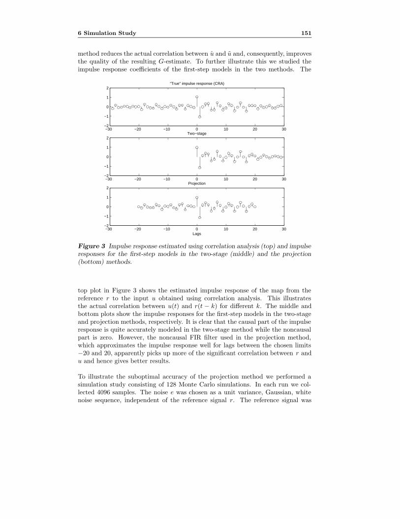
6 Simulation Study 151
method reduces the actual correlation between u and u and, consequently, improvesthe quality of the resulting G-estimate. To further illustrate this we studied theimpulse response coefficients of the first-step models in the two methods. The
−30 −20 −10 0 10 20 30−2
−1
0
1
2"True" impulse response (CRA)
−30 −20 −10 0 10 20 30−2
−1
0
1
2Two−stage
−30 −20 −10 0 10 20 30−2
−1
0
1
2Projection
Lags
Figure 3 Impulse response estimated using correlation analysis (top) and impulseresponses for the first-step models in the two-stage (middle) and the projection(bottom) methods.
top plot in Figure 3 shows the estimated impulse response of the map from thereference r to the input u obtained using correlation analysis. This illustratesthe actual correlation between u(t) and r(t − k) for different k. The middle andbottom plots show the impulse responses for the first-step models in the two-stageand projection methods, respectively. It is clear that the causal part of the impulseresponse is quite accurately modeled in the two-stage method while the noncausalpart is zero. However, the noncausal FIR filter used in the projection method,which approximates the impulse response well for lags between the chosen limits−20 and 20, apparently picks up more of the significant correlation between r andu and hence gives better results.
To illustrate the suboptimal accuracy of the projection method we performed asimulation study consisting of 128 Monte Carlo simulations. In each run we col-lected 4096 samples. The noise e was chosen as a unit variance, Gaussian, whitenoise sequence, independent of the reference signal r. The reference signal was

152 Paper B A Projection Method for Closed-loop Identification
also chosen as a unit variance, Gaussian, white noise sequence, just as before. Inthis simulation only the optimal direct method and the projection method werecompared. In the projection method we used a noncausal FIR filter with 41 taps,also as before. The results of the Monte Carlo simulation are presented in TableB.2. The values shown are the mean values of the parameter estimates togetherwith their estimated standard deviations. Clearly the accuracy of the projection
Table B.2 Summary of results of Monte Carlo simulation.True D Pvalue
a1 −1.2000 −1.2002 −1.1659±0.0042 ±0.0196
a2 0.6100 0.6100 0.5894±0.0046 ±0.0146
b1 1.0000 1.0009 0.9929±0.0055 ±0.0181
method is worse than that of the direct method, as expected. There is also a slightbias in the parameter estimates obtained with the projection method which is dueto a nonvanishing correlation between u and u. One reason for this is that we usedrather small M1 and M2, another is that the estimated coefficients in the noncausalFIR filter are not perfect due to the noise in u. The latter effect tends to be worseas model order increases, while the former decreases with increasing model order.In a practical situation it is therefore recommended to try different values of M1
and M2 to optimize the results.
7 Conclusions
The projection method consists of two steps: First the mapping from the referencesignal r to the input u is modeled using a noncausal FIR filter. This gives anestimate u of u that is asymptotically uncorrelated with u− u. In the second stepthe open-loop system is identified using measurements of y and u. The methodgives consistent estimates regardless of the nature of the feedback but the accuracyis suboptimal. In case of undermodeling, the model can be fit to the data witharbitrary frequency weighting which is a clear advantage compared to the directmethod.

References 153
References
[1] H. Akaike. Some problems in the application of the cross-spectral method. InB. Harris, editor, Spectral Analysis of Time Series, pages 81–107. John Wiley& Sons, 1967.
[2] T. Kailath. Lectures on Wiener and Kalman Filtering. Springer-Verlag, 1981.[3] L. Ljung. Convergence analysis of parametric identification methods. IEEE
Transactions on Automatic Control, 23:770–783, 1978.[4] L. Ljung. System Identification: Theory for the User. Prentice-Hall, 1987.[5] P. M. J. Van den Hof and R. J. P. Schrama. An indirect method for transfer
function estimation from closed loop data. Automatica, 29:1523–1527, 1993.

154 References

Paper C
Efficiency of PredictionError and InstrumentalVariable Methods forClosed-loop Identification
Authors: Urban Forssell and Chun Tung Chou
Edited version of paper originally published in Proceedings of the 37th IEEE Con-ference on Decision and Control, pages 1287-1288, Tampa, FL, 1998.
155


Efficiency of Prediction Error and
Instrumental Variable Methods forClosed-loop Identification
Urban Forssell1
Division of Automatic Control,Department of Electrical Engineering,
Linkoping University,S-581 83 Linkoping, Sweden.
E-mail: [email protected].
Chun Tung Chou2
Department of Electrical Engineering,Delft University of Technology,P.O. Box 5031, 2600 GA Delft,
The Netherlands.E-mail: [email protected].
Abstract
We study the efficiency of a number of closed-loop identification methods.Results will be given for methods based on the prediction error approach aswell as those based on the instrumental variable approach. Moreover, in-teresting insights in the properties of a recently suggested subspace methodfor closed-loop identification are obtained by exploring the links betweenthis method and the instrumental variable method.
1 Introduction
The accuracy of different prediction error (PE) methods for closed-loop identifica-tion has been studied in, e.g., [3]. Here we will review these results and link themto corresponding results for instrumental variable (IV) methods for closed-loopidentification, e.g., [5]. By studying the special case of single-input single-output
1U. Forssell is supported by the Swedish Research Council for Engineering Sciences.2C.T. Chou is supported by the Dutch Technology Foundation (STW) under project number
DEL55.3891.
157

158 Paper C Efficiency of Prediction Error and Instrumental Variable . . .
ARMAX models it is possible to compare these methods with a modified, butyet representative, form of a recently proposed errors-in-variables (EIV) subspacemethod [1], that can be applied to closed-loop data.
2 Preliminaries
We assume that the true system is given by the ARMAX model
A0(q)y(t) = B0(q)u(t) + C0(q)e(t), Ee(s)e(t) = λ0δs−t (1)
and that there is a stabilizing LTI feedback between u(t) and y(t) given by
R(q)u(t) = R(q)r(t) − S(q)y(t) (2)
where the reference signal r(t) is independent of e(t).
To identify this system we will work with models of the form
y(t|θ) = ϕT (t)θ (3)
where ϕ(t) is contains the regressors and θ the parameters of the A- and B-polynomials. We will frequently use the notation
ϕ(t) = ϕr(t) + ϕe(t) (4)
where ϕr(t) and ϕe(t) are the parts of ϕ(t) that are due to r(t) and e(t), respectively.In some cases the model (3) will be applied together with a (possibly parameter-dependent) monic prefilter L that can be used to emphasize certain frequencyregions. The resulting parameter vector estimate will be denoted θ.
The main focus in the paper will be to characterize the asymptotic covariancematrix Pθ,
N Cov θ → Pθ, as N →∞ (5)
for a number of identification methods that guarantee that the parameter estimatesconverge to the true values also when applied to closed-loop data.
3 Prediction Error Methods
The PE estimate is found as the straightforward fit:
θ = arg minθ,η
1N
N∑t=1
[L(q, η)(y(t)− y(t|θ))]2 (6)
4 Instrumental Variable Methods 159
This approach can also be applied to closed-loop identification. Depending on howL(q, η) is parameterized, different methods are obtained.
If we think of L(q, η) as an inverse noise model and parameterize in a straightfor-ward way the direct method is obtained. If the chosen parameterization is suffi-ciently flexible, the direct method is consistent and gives optimal accuracy [4, 3].It can be shown that (see [2]) for the direct method we have (’D’ stands for direct)
PDθ = λ0
[E
1C0(q)
ϕr(t)1
C0(q)ϕTr (t) + Re
]−1
(7)
where Re ≥ 0 depends on e(t) and not on r(t). (The symbol E is defined in,e.g., [4].) This means that the noise actually helps reducing the variance in thedirect method. In case the optimal, fixed prefilter L(q, η) = L(q) = 1/C0(q) is usedwe can write (7) as
PDθ = λ0
[E
1C0(q)
ϕ(t)1
C0(q)ϕT (t)
]−1
, PODθ (8)
If we parameterize the prefilter as
L(q, η) = L(q, θ) =L1(q)R(q)
A(q)R(q) +B(q)S(q)(9)
we obtain the indirect method (see, e.g., [2]). For this method the asymptoticcovariance matrix satisfies
P IDθ ≥ λ0
[E
1C0(q)
ϕr(t)1
C0(q)ϕTr (t)
]−1
, POIDθ (10)
for all choices of the filter L1(q). Equality holds ifL1(q) = (A0(q)R(q) +B0(q)S(q))/(C0(q)R(q)). Note that POID
θ ≥ PDθ , due to the
term Re ≥ 0 in (7).
4 Instrumental Variable Methods
Consider the linear regression (3). Let ζ(t) denote an IV vector (of the same sizeas ϕ(t)) and L(q) be a prefilter, then with the standard IV method the parameterestimate is computed as
θ =[ 1N
N∑t=1
ζ(t)L(q)ϕT (t)]−1 1
N
N∑t=1
ζ(t)L(q)y(t) (11)

160 Paper C Efficiency of Prediction Error and Instrumental Variable . . .
given that the indicated inverse exists. Consistency requires the instruments bechosen such that
E[ζ(t)L(q)C0(q)e(t)] = 0 (12)
Depending on the choices of instruments ζ(t) and prefilter L(q) different instru-mental variable “methods” result. For all choices of ζ(t) and L(q),
P IVθ ≥ POD
θ (13)
Equality holds if ζ(t) = 1/C0(q)ϕ(t) and L(q) = 1/C0(q) (given that these choicessatisfy (12)).
If the instruments are chosen as filtered versions of r(t) then (12) will be automat-ically satisfied since r(t) and e(t) are independent. The resulting method will herebe denoted RIV (’R’ for reference signal). For this method it can be shown that(see [5]) for any prefilter L(q) and any ζ(t) constructed from r(t) through filteringwe have that
PRIVθ ≥ POID
θ (14)
Equality holds if ζ(t) = 1C0(q)ϕr(t) and L(q) = 1
C0(q) .
Another possibility is to use delayed versions of the regression vector, ζ(t) =ϕ(t − k). To satisfy (12), the delay k has to be larger than the maximal delayin L(q)C0(q). This method will be referred to as PIV (’P’ for past regressors). Thecovariance matrix becomes
PPIVθ = λ0[E ϕ(t−k)L(q)ϕT (t)]−1[E ϕ(t−k)ϕT (t−k)][E ϕ(t−k)L(q)ϕT (t)]−T
(15)
where
ϕ(τ) = L(q−1)C0(q−1)ϕ(τ) (16)
This can be better or worse than the RIV method depending, e.g., on how L(q)and the delay k are chosen. When the feedback loop is noisy it is likely that PIVgives better accuracy than RIV [2]. Under all circumstances PPIV
θ ≥ PODθ .
5 Discussion
The direct method gives optimal accuracy, while the other PE and IV methodsstudied in this paper all give worse accuracy. A key point in understanding thisdifference is that in the direct method the whole input spectrum is used to reduce

References 161
the variance, whereas in the indirect and RIV methods only the noise-free partis used. In the PIV method the whole input spectrum is used, but, like all IVmethods, this method suffers from the fact that cross-correlation, rather than theauto-correlation, is used to reduce the variance. The special case is when the noisemodel is known exactly, then one can use the auto-correlation to achieve minimumvariance on par with the direct method. The use of a periodic reference signalcan also increase the correlation between the instruments and the regressors, andhence improve the accuracy. To balance the picture somewhat we also point outthat with an increasing SNR the differences between the methods will disappearand all will perform similarly.
The EIV method [1] can to a certain extent be interpreted as PIV with the prefilterchosen to be unity [2]. This gives new insights into the statistical properties of EIV.We conjecture that with a low SNR this method is likely to be better than RIVand the indirect method, although the efficiency may still be sub-optimal. Thiserratic type of statistical behavior of EIV is also shared by some other subspacealgorithms, as pointed out in [6], and can be corrected by using say subspace fitting[6].
References
[1] C. T. Chou and M. Verhaegen. Subspace algorithms for the identification ofmultivariable errors-in-variables models. Automatica, 33:1857–1869, 1997.
[2] U. Forssell and C.T. Chou. Efficiency of prediction error and instrumentalvariable methods for closed-loop identification. Technical Report LiTH-ISY-R-2015, Department of Electrical Engineering, Linkoping University, Linkoping,Sweden, 1998.
[3] U. Forssell and L. Ljung. Closed-loop identification revisited – Updated ver-sion. Technical Report LiTH-ISY-R-2021, Department of Electrical Engineer-ing, Linkoping University, Linkoping, Sweden, 1998.
[4] L. Ljung. System Identification: Theory for the User. Prentice-Hall, 1987.
[5] T. Soderstrom, P. Stoica, and E. Trulsson. Instrumental variable methods forclosed loop systems. In Preprints IFAC 10th World Congress on AutomaticControl, pages 364–369, Munich, Germany, July 1987.
[6] M. Viberg, B. Wahlberg, and B. Ottersten. Analysis of state space systemidentification methods based on instrumental variables and subspace fitting.Automatica, 33:1603–1616, 1997.

162 References

Paper D
Identification of UnstableSystems Using Output Errorand Box-Jenkins ModelStructures
Authors: Urban Forssell and Lennart Ljung
Edited version of paper originally published in Proceedings of the 37th IEEE Con-ference on Decision and Control, pages 3932-3937, Tampa, FL, 1998.
To appear in IEEE Transactions on Automatic Control.
163


Identification of Unstable Systems Using
Output Error and Box-Jenkins Model
Structures
Urban Forssell and Lennart Ljung
Division of Automatic Control,Department of Electrical Engineering,
Linkoping University,S-581 83 Linkoping, Sweden.
E-mail: [email protected], [email protected].
Abstract
It is well known that the output error and Box-Jenkins model structures can-not be used for prediction error identification of unstable systems. The reasonfor this is that the predictors in this case generically will be unstable. Typ-ically this problem is handled by projecting the parameter vector into theregion of stability which gives erroneous results when the underlying systemis unstable. The main contribution of this work is that we derive modified,but asymptotically equivalent, versions of these model structures that can beapplied also in the case of unstable systems.
1 Introduction
In this note we will discuss prediction error identification of unstable systems usingoutput error and Box-Jenkins model structures. As is well known from text bookson system identification in the prediction error framework (e.g., [5, 9]), it is requiredthat the predictors are stable. In case the parameters are estimated using somenumerical search algorithm that requires gradients of the predictor to be computed,these must also be stable. With the ARX and ARMAX model structures this is
165

166 Paper D Identification of Unstable Systems . . .
no problem since the dynamics model and the noise model share denominatorpolynomials, which cancel when the predictors are formed. For the output errorand Box-Jenkins model structures this is not the case and if the underlying systemis unstable the predictors will generically be unstable, which seemingly makes themodel structures inapplicable in these cases. Also, when identifying stable systemsthat are “close” to being unstable it might be that the predictors become unstablein one or more of the steps in the search algorithm due to numerical problems, sothat the search has to be terminated before the global optimum is reached.
Traditionally the problem of unstable predictors has been handled by projecting theparameter vector into the region of stability. This will, of course, lead to completelyuseless results if the underlying system is unstable. If the system is stable but thepredictors become unstable in some intermediate step in the numerical search,projecting the parameter vector into the region of stability can lead to convergenceproblems. However, as we shall see it is possible to re-parameterize the outputerror and Box-Jenkins model structures to guarantee stability of the predictors,and this without increasing the total number of parameters to be estimated. Withthe new versions of the output error and Box-Jenkins model structures we thusgain two things: these model structures can be applied to unstable systems andthe numerical properties of the search algorithm are improved. The price we payis an increase in complexity of the search algorithm in case the predictors areunstable. (If they are stable we can use the standard algorithms.)
If the system is unstable, we will assume that the experimental data are generatedunder stabilizing feedback. It is clear that such feedback will involve some knowl-edge of the system. However this knowledge may by quite rudimentary, and theremay still be an obvious need for an improved system model. One example – amongmany – is flight testing unstable aircraft to build accurate dynamic models.
With a stabilizing controller in the loop we are faced with a closed-loop identifi-cation problem. Closed-loop identification is often used in connection to so calledcontrol-relevant identification where the goal is to estimate models that are suit-able for (robust) control design, see, e.g., the surveys [3, 11, 2]. It is then oftenonly interesting to model the dynamics of the plant, the noise properties are lessinteresting, so that it would be natural to use an output error model structure.However, since unstable plants cannot be handled using output error models theconclusion has been that this approach cannot be used when the plant is unstable.Alternative solutions have been suggested in, e.g., [4, 10, 12]. Unfortunately thesemethods are considerably more involved than a direct application of an outputerror or a Box-Jenkins model to the closed-loop data.
A problem when identifying systems in closed-loop directly is that the results willbe biased unless the noise model accurately describes the true noise characteris-tics [5, 6, 7]. This has traditionally been a main issue in the closed-loop identifi-cation literature that has further motivated the search for alternative closed-loop

2 Some Basics in Prediction Error Identification 167
identification methods. The bias problems will of course also be present when us-ing the new model structures suggested in this paper. However, in many cases thebias errors due to poor modeling of the true noise characteristics will be small,especially if the signal-to-noise ratio is high [7, 2]. It must also be realized thatin practice the model errors will be due to both bias and variance errors [5] and ifa reasonably flexible noise model is used, the bias error due to the feedback willtypically be small compared to the variance error. The variance error also increaseswith the number of parameters which favors model structures with few parameters.We would also like to point out that most other closed-loop identification methods,that are designed to give unbiased estimates, give higher variance errors than thedirect method [1, 8]. This is an issue that in our opinion has received too littleattention in the closed-loop identification literature.
The organization of the paper is as follows. Next, in Section 2, we study somebasic facts on prediction error methods and in Section 3 we discuss some standardchoices of model structures. This section also contains an illustration of the prob-lems faced when trying to identify unstable systems using output error models.Section 4 contains the main result of the paper: How the standard output errormodel structure should be modified to cope also with unstable systems. After in-troducing some additional notation we present the basic idea and go through thederivation of the required gradient filters in some detail. This is then followed by asimulation study that illustrates the feasibility of the idea. Before concluding we,in Section 5, briefly mention the corresponding changes of the Box-Jenkins modelstructure that are necessary to make it applicable to unstable systems.
2 Some Basics in Prediction Error Identification
In prediction error identification one typically considers linear model structuresparameterized in terms of a parameter vector θ:
y(t) = G(q, θ)u(t) +H(q, θ)e(t) (1)
Here G(q, θ) and H(q, θ) are rational functions of q−1, the unit delay operator(q−1u(t) = u(t − 1), etc.) parameterized in terms of θ; y(t) is the output; u(t) isthe input; e(t) is white noise. In this paper we will limit the study to single inputsingle output models for ease of exposition.
Typically θ ranges over some open subset DM of Rd (d = dim θ):
θ ∈ DM ⊂ Rd (2)
Note the distinction between a model and a model structure: When viewed asa function of θ, (1) is a model structure, while for a fixed θ = θ∗, (1) is a model.

168 Paper D Identification of Unstable Systems . . .
Furthermore, we also have that (1) together with (2) defines a model set and it is ourtask to find the best model in the set, typically by performing a numerical searchover all possible models. Refer to [5] for a comprehensive treatment, includingexact definitions, of the concepts model, model structure and model set.
The one-step-ahead predictor for (1) is
y(t|θ) = H−1(q, θ)G(q, θ)u(t) + (1−H−1(q, θ))y(t) (3)
Here it is required that the filters H−1(q, θ)G(q, θ) and (1 −H−1(q, θ)) are stablefor the predictor to be well defined. It is easy to see that this calls for an inverselystable noise model H(q, θ) and that the unstable poles of G(q, θ) are also poles ofH(q, θ). These issues will play important roles in this paper.
The prediction errors ε(t, θ) = y(t)− y(t|θ) corresponding to the predictor (3) are
ε(t, θ) = H−1(q, θ)(y(t) −G(q, θ)u(t)) (4)
We will also use the following notation for the gradient of y(t|θ):
ψ(t, θ) =d
dθy(t|θ) (= − d
dθε(t, θ)) (5)
In the standard case of least-squares prediction error identification one calculatesthe parameter estimate as the minimizing argument of the criterion function
VN (θ) =1N
N∑t=1
12ε2(t, θ) (6)
Typically one finds the estimate through some numerical search routine of the form
θ(i+1)N = θ
(i)N − µ
(i)N [R(i)
N ]−1V ′N (θ(i)N ) (7)
where V ′N denotes the gradient of the criterion function, RN is a matrix thatmodifies the search direction and µN a scaling factor that determines the steplength. From (5) we see that
V ′N (θ) = − 1N
N∑t=1
ψ(t, θ)ε(t, θ) (8)
and typically RN is chosen approximately equal to the Hessian V ′′N (which wouldmake (7) a Newton algorithm); a standard choice is
RN =1N
N∑t=1
ψ(t, θ)ψT (t, θ) + δI (9)

3 Commonly Used Model Structures 169
where δ ≥ 0 is chosen so that RN becomes positive definite. This is also called theLevenberg-Marquardt regularization procedure.
Clearly it is required that both the predictor (3) and the gradient (5), which haveto be computed and used in the search algorithm (7), are stable. When dealingwith unstable systems this introduces constraints on the possible model structures.
3 Commonly Used Model Structures
With these stability requirements in mind, let us now discuss some standard choicesof model structures.
A quite general model structure is the following [5]:
A(q)y(t) =B(q)F (q)
u(t) +C(q)D(q)
e(t) (10)
where
A(q) = 1 + a1q−1 + · · ·+ anaq
−na (11)
and similarly for the C, D, and F polynomials, while
B(q) = q−nk(b0 + b1q−1 + · · ·+ bnbq
−nb) (12)
This model structure includes some common special cases:
1. C(q) = 1, D(q) = 1, F (q) = 1, an ARX model structure.
2. D(q) = 1, F (q) = 1, an ARMAX model structure.
3. A(q) = 1, C(q) = 1, D(q) = 1, an output error model structure.
4. A(q) = 1, a Box-Jenkins model structure.
In the sequel we will assume nk = 0 (which always can be achieved by replacingu(t) by u(t− nk)).
A sufficient condition for the predictor and gradient filters to be stable is thatC(q) ·F (q) is stable for all θ ∈ DM (cf. Lemma 4.1 in [5]). Note that this conditionis automatically satisfied for ARX models, and for ARMAX models it is sufficientthat the C-polynomial is stable, which does not impose any stability constraints onthe dynamics model. For identification of unstable system these model structuresthus are natural choices.
170 Paper D Identification of Unstable Systems . . .
The output error model structure has a fixed noise model (H(q, θ) = 1) and is anatural choice if only a model of the system dynamics is required. In case onewants to model also the noise characteristics (e.g., to improve the efficiency) butdo not want the noise and dynamics models to be dependent as in the ARX andARMAX cases, then the Box-Jenkins model structure would the one to choose.However, if the underlying system is unstable these model structures can not beused without modifications, e.g., the ones we propose in this paper. To see wherethe problem lies, let us study the output error case.
Suppose that we want to identify an unstable system, stabilized by some controller,and that we are only interested in modeling the dynamics with no modeling effortspent on the noise characteristics. Then the natural choice would be to use anoutput error model structure:
y(t) =B(q)F (q)
u(t) + e(t) (13)
Now, since the system is unstable the predictor
y(t|θ) =B(q)F (q)
u(t) (14)
as well as the gradient filters
∂
∂bky(t|θ) =
1F (q)
u(t− k) (15a)
∂
∂fky(t|θ) = − B(q)
F 2(q)u(t− k) (15b)
will generically be unstable. When implementing a parameter estimation algorithmfor the output error case one typically secures stability in every iteration of thealgorithm (7) by projecting the parameter vector into the region of stability. Forunstable systems this of course leads to erroneous results.
These problems are also present when using the Box-Jenkins model structure:
y(t) =B(q)F (q)
u(t) +C(q)D(q)
e(t) (16)
Also in this case one has to resort to projections into the region of stability to ensurestability of the predictors and gradient filters, which makes this model structure inits standard form useless for identification of unstable systems.
In the following sections we will describe how to modify these model structures toavoid these problems.

4 An Alternative Output Error Model Structure 171
4 An Alternative Output Error Model Structure
4.1 Some Additional Notation
Let Fs(q) (Fa(q)) be the stable (anti-stable), monic part of F (q):
F (q) = Fs(q)Fa(q) (17)
and let the polynomials Fs(q) and Fa(q) be parameterized as
Fs(q) = 1 + fs,1q−1 + · · ·+ fs,nfs q
−nfs (18)
Fa(q) = 1 + fa,1q−1 + · · ·+ fa,nfa q
−nfa (19)
With the notation
fa,k =
1 k = 0fa,k 1 ≤ k ≤ nfa0 else
(20)
and
fs,k =
1 k = 0fs,k 1 ≤ k ≤ nfs0 else
(21)
we have
fk =nf∑j=0
fs,j fa,k−j , k = 1, 2, . . . , nf (22)
Furthermore, let F ∗a (q) denote the monic, stabilized Fa-polynomial, i.e., F ∗a (q) isthe monic polynomial whose zeros are equal to the zeros of Fa(q) reflected into theunit disc. In terms of fa,i, the coefficients of Fa(q), we can write F ∗a (q) as
F ∗a (q) = 1 +fa,nfa−1
fa,nfaq−1 + · · ·+ 1
fa,nfaq−nfa (23)
(Here we have used the implicit assumption that fa,nfa 6= 0.)
4.2 The Proposed Model Structure
Now consider the following modified output error model structure:
y(t) =B(q)F (q)
u(t) +F ∗a (q)Fa(q)
e(t) (24)

172 Paper D Identification of Unstable Systems . . .
with the predictor
y(t|θ) =Fa(q)B(q)F ∗a (q)F (q)
u(t) + (1− Fa(q)F ∗a (q)
)y(t)
=B(q)
F ∗a (q)Fs(q)u(t) + (1− Fa(q)
F ∗a (q))y(t) (25)
The difference between this model structure and the basic output error model struc-ture (13) is thus that we have included a noise model F ∗a (q)/Fa(q) and obtained adifferent “dummy” noise term
e(t) =F ∗a (q)Fa(q)
e(t) (26)
instead of just e(t). At first glance it may thus seem as the model structures (13)and (24) will give different results, but in fact they are (asymptotically) equivalentas can be seen from the following result:
Proposition 1 When applying a prediction error method to the model structures(13) and (24) the resulting estimates will asymptotically, as N →∞, be the same.
Proof From classical prediction error theory we know that under mild conditionsthe limiting models will minimize the integral of the spectrum of the predictionerrors (see, e.g., Theorem 8.2 in [5]). Now, if we let εF (t, θ) denote the predictionerrors obtained with the model (25) and let ε(t, θ) denote the prediction errorscorresponding to the model (14), we have that the spectrum of εF (t, θ) is given by
ΦεF (ω) =∣∣∣∣Fa(eiω)F ∗a (eiω)
∣∣∣∣2 Φε(ω) (27)
= |fa,nfa |2Φε(ω) (28)
where Φε(ω) denotes the spectrum of ε(t, θ). Thus the spectra differ by only aconstant scaling and hence the corresponding limiting models will be the same. �
As we have seen, the results will asymptotically be the same with both modelstructures; the difference is of course that the predictor (25) will always be stablealong with all its derivatives even if F (q) is unstable (as opposed to standard outputerror case which require a stable F (q) for the predictor to be stable). Note thatin (24) the noise model is monic and inversely stable and the unstable poles of thedynamics model are also poles of the noise model (cf. the discussion in Section 2).
The basic idea behind the equivalence result in Proposition 1 is really that a con-stant spectrum may be factorized in infinitely many ways using all-pass functions.Here we chose convienient pole locations for these all-pass functions to have stablepredictors. This is actually very closely related to classical Kalman filter theory,as will be illustrated next.

4 An Alternative Output Error Model Structure 173
4.3 Connections to the Kalman Filter
There is a very straightforward interpretation of the second order equivalent (25)of (14). Suppose we realize (13) in state-space form:
x(t+ 1) = Ax(t) + Bu(t)y(t) = Cx(t) + e(t)
(29)
The steady state Kalman filter predictor is
x(t+ 1) = (A−KC)x(t) + Bu(t) +Ky(t)y(t|θ) = Cx(t)
(30)
where K is determined from an algebraic Riccati equation in the usual way: K =AΠCT /(R+ CΠCT ), Π = AΠAT −K(R+ CΠCT )KT . Here R is the variance of theinnovations e(t): R = Ee2(t) > 0. (E denotes mathematical expectation.)
Now, if A is stable the solution is K = 0 and (30) corresponds to (14). Howeverif A is not stable, the solution to the Kalman predictor problem is a nonzero Kwhich makes (30) exactly equal to (25). Note that this holds regardless of R.
We thus have two alternative ways of computing the gradient y(t|θ) in the outputerror case: (25) and (30). As we have seen these two variants give identical solu-tions y(t|θ) although (25) is computationally less demanding. In contrast with theKalman filter solution (30), it is also straightforward to generalize (25) to othermodel structures, like the Box-Jenkins model structure. This is briefly discussedin Section 5 below. Another important issue is how to compute the gradient (5).Using the explicit predictor formula (25) this is relatively straightforward, albeittedious, as shown in the next section.
4.4 Computation of the Gradient
As mentioned above, the gradient ψ(t, θ) is needed for the implementation of thesearch scheme (7). With the predictor (25) the expression for the gradient willbe much more involved than (15) but for completeness we will go through thesecalculations in some detail (after all, the gradient is needed for the implementationof the estimation algorithm).
Given the predictor model (25) we have that
∂
∂bky(t|θ) =
1Fs(q)F ∗a (q)
u(t− k) (31)

174 Paper D Identification of Unstable Systems . . .
while
∂
∂fky(t|θ) =
∂
∂fk
B(q)Fs(q)F ∗a (q)
u(t)− ∂
∂fk
Fa(q)F ∗a (q)
y(t) (32)
Introducing
W k1 (q) =
∂
∂fkFs(q) (33)
W k2 (q) =
∂
∂fkFa(q) (34)
W k3 (q) =
∂
∂fkF ∗a (q) (35)
and
x1(t) = − B(q)F 2s (q)F ∗a (q)
u(t) (36)
x2(t) = − 1F ∗a (q)
y(t) (37)
x3(t) = − B(q)Fs(q)(F ∗a (q))2
u(t) +Fa(q)
(F ∗a (q))2y(t) (38)
we may write
∂
∂fky(t|θ) = W k
1 (q)x1(t) +W k2 (q)x2(t) +W k
3 (q)x3(t) (39)
What we then finally need in order to be able to compute the gradient ∂∂fk
y(t|θ)are explicit expressions for the filters W k
i , i = 1, 2, 3. Using (22) we have that
W k1 (q) =
nfs∑i=1
wk1,iq−i, wk1,i =
{f−1a,k−i k − nfa ≤ i ≤ k
0 else(40)
W k2 (q) =
nfa∑i=1
wk2,iq−i, wk2,i =
{f−1s,k−i k − nfs ≤ i ≤ k
0 else(41)
while
W k3 (q) =
1fa,nfa
·
nfa−1∑i=1
wk3,iq−i + wk3,0(1− F ∗a (q))
,wk3,i =
{f−1s,k−nfa+i nfa − k ≤ i ≤ nfs + nfa − k
0 else(42)
The equations (31)-(42) together constitute a complete and explicit description ofthe gradient ψ(t, θ) = d
dθ y(t|θ) which may be used in an implementation of thesearch algorithm (7).

4 An Alternative Output Error Model Structure 175
4.5 Simulation Example
To illustrate the applicability of the proposed model structure (24) to identifica-tion problems involving unstable systems we will in this section present a smallsimulation study.
The “true” system – to be identified – is given by
y(t) =b0
1 + f1q−1 + f2q−2u(t) + e(t) (43)
with b0 = 1, f1 = −1.5, and f2 = 1.5. This system is unstable with poles in0.75± 0.9682i.
To generate identification data we simulated this system using the feedback law
u(t) = r(t) − (−0.95q−2)y(t) = r(t) + 0.95y(t− 2) (44)
which places the closed-loop poles in 0.8618 and 0.6382. In the simulation we usedindependent, zero mean, Gaussian white noise reference and noise signals {r(t)}and {e(t)} with variances 1 and 0.01, respectively. N = 200 data samples wereused.
In Table D.1 we have summarized the results of the identification, the numbersshown are the estimated parameter values together with their standard deviations.For comparison we have, apart from the model structure (24), used a standardoutput error model model structure and a second-order ARMAX model structure.As can be seen the standard output error model structure gives completely uselessestimates while the modified output error and the ARMAX model structures givevery similar and accurate results.
Table D.1 Summary of identification results.Parameter b0 f1 f2
True value 1 -1.5 1.5OE 0.6218 −1.0336 0.7389
±0.0382 ±0.0481 ±0.0391Modified OE 0.9898 −1.5008 1.5035
±0.0084 ±0.0052 ±0.0079ARMAX 1.0028 −1.5026 1.5052
±0.0077 ±0.0049 ±0.0074

176 References
5 An Alternative Box-Jenkins Model Structure
The trick to include a modified noise model in the output error model structure isof course also applicable to the Box-Jenkins model structure. The alternative formwill in this case be
y(t) =B(q)F (q)
u(t) +F ∗a (q)C(q)Fa(q)D(q)
e(t) (45)
with the corresponding predictor
y(t|θ) =Fa(q)D(q)B(q)F ∗a (q)C(q)F (q)
u(t) + (1− Fa(q)D(q)F ∗a (q)C(q)
)y(t)
=D(q)B(q)
C(q)F ∗a (q)Fs(q)u(t) + (1− D(q)Fa(q)
C(q)F ∗a (q))y(t) (46)
An explicit expression for the gradient filters for this predictor can be derived quitesimilarly as in the output error case, albeit that the formulas will be even messier.For the sake of readability we skip the details.
6 Conclusions
In this paper we have proposed new versions of the well known output error andBox-Jenkins model structures that can be used also for identification of unstablesystems. The new model structures are equivalent to the standard ones, as faras number of parameters and asymptotical results are concerned, but guaranteestability of the predictors.
References
[1] U. Forssell. Properties and Usage of Closed-loop Identification Methods. Li-centiate thesis LIU-TEK-LIC-1997:42, Department of Electrical Engineering,Linkoping University, Linkoping, Sweden, September 1997.
[2] U. Forssell and L. Ljung. Closed-loop identification revisited – Updated ver-sion. Technical Report LiTH-ISY-R-2021, Department of Electrical Engineer-ing, Linkoping University, Linkoping, Sweden, 1998.
[3] M. Gevers. Towards a joint design of identification and control. In H. L.Trentelman and J. C. Willems, editors, Essays on Control: Perspectives in theTheory and its Applications, pages 111–151. Birkhauser, 1993.

References 177
[4] F. R. Hansen, G. F. Franklin, and R. Kosut. Closed-loop identification via thefractional representation: experiment design. In Proceedings of the AmericanControl Conference, pages 1422–1427, Pittsburg, PA, 1989.
[5] L. Ljung. System Identification: Theory for the User. Prentice-Hall, 1987.
[6] L. Ljung. Information contents in identification data from closed loop opera-tion. In Proceedings of the 32nd IEEE Conference on Decision and Control,pages 2242–2247, San Antonio, TX, December 1993.
[7] L. Ljung. Identification in closed loop: some aspects on direct and indirect ap-proaches. In Preprints of the 11th IFAC Symposium on System Identification,volume 1, pages 141–146, Fukuoka, Japan, July 1997.
[8] L. Ljung and U. Forssell. Variance results for closed-loop identification meth-ods. In Proceedings of the 36th IEEE Conference on Decision and Control,volume 3, pages 2435–2440, San Diego, C.A., 1997.
[9] T. Soderstrom and P. Stoica. System Identification. Prentice-Hall Interna-tional, 1989.
[10] P. M. J. Van den Hof and R. J. P. Schrama. An indirect method for transferfunction estimation from closed loop data. Automatica, 29:1523–1527, 1993.
[11] P. M. J. Van den Hof and R. J. P. Schrama. Identification and control —Closed-loop issues. Automatica, 31:1751–1770, 1995.
[12] P. M. J. Van den Hof, R. J. P. Schrama, R. A. de Callafon, and O. H. Bosgra.Identification of normalized coprime factors from closed-loop experimentaldata. European Journal of Control, 1:62–74, 1995.

178 References

Paper E
Maximum LikelihoodEstimation of Models withUnstable Dynamics andNonminimum Phase NoiseZeros
Authors: Urban Forssell and Hakan Hjalmarsson
Edited version of paper to appear in Proceedings of the 14th IFAC World Congress,Beijing, China, 1999.
Preliminary version published as Technical Report LiTH-ISY-R-2043, Departmentof Electrical Engineering, Linkoping University, Linkoping, Sweden.
179


Maximum Likelihood Estimation of
Models with Unstable Dynamics
and Nonminimum Phase Noise Zeros
Urban Forssell
Division of Automatic Control,Department of Electrical Engineering,
Linkoping University,S-581 83 Linkoping, Sweden.
E-mail: [email protected].
Hakan Hjalmarsson
Signal Processing Group,Department of Signals, Sensors and
Systems,Royal Institute of Technology,S-100 44 Stockholm, Sweden.
E-mail: [email protected].
Abstract
Maximum likelihood estimation of single-input/single-output linear time-invariantdynamic models requires that the model innovation (the nonmeasurable whitenoise source that is assumed to be the source of the randomness of the sys-tem) can be computed from the observed data. For many model structures,the prediction error and the model innovation coincide and the prediction er-ror can be used in maximum likelihood estimation. However, when the modeldynamics and the noise model have unstable poles which are not shared orwhen the noise dynamics have unstable zeros this is not the case. One suchexample is an unstable output error model. In this contribution we show thatin this situation the model innovation can be computed by noncausal filtering.Different implementations of the model innovation filter are also studied.
Keywords: Identification, Output error identification, Prediction error meth-ods, Maximum likelihood estimators, Innovation, Spectral factorization
181

182 Paper E Maximum Likelihood Estimation of Models . . .
1 Introduction
In the prediction error approach (e.g., [5]) to system identification, the model pa-rameters are determined by minimizing the prediction error, that is, the errorbetween the true output and the optimal (w.r.t. the model), linear predictor basedon past inputs and outputs. In this paper we consider causal, linear, and time-invariant models of the form
y(t) = G(q, θ)u(t) +H(q, θ)e(t) (1)
where {u(t)} is the input, {y(t)} is the output, and {e(t)} is assumed to be a zeromean white noise sequence which will be called the model innovation. Furthermore,θ is a parameter vector and q is the time shift operator in discrete time. Throughoutthis paper we will assume that the data really has been generated by a model inthe model structure we are considering, that is, for the structure (1) there is aparameter θ0 such that the data are described exactly by (1):
y(t) = G(q, θ0)u(t) +H(q, θ0)e(t) (2)
We will denote the corresponding model, the true model and the correspondingsequence {e(t)} the true model innovation.
If H−1(q, θ)G(q, θ) and H−1(q, θ) are stable, the optimal one-step-ahead predictorfor (1) is, [5]
y(t|θ) = H−1(q, θ)G(q, θ)u(t) + (1−H−1(q, θ))y(t) (3)
The prediction error ε(t, θ) = y(t)− y(t|θ) is
ε(t, θ) = H−1(q, θ)(y(t) −G(q, θ)u(t)) (4)
For the true model it then holds that the prediction error is equal to the true modelinnovation
ε(t, θ0) = e(t) (5)
This property underlies the nice consistency properties of the prediction errormethod. It also implies that there is a close connection between maximum likeli-hood estimation and the prediction error method. If the probability distributionfunction (PDF) of e(t) is known and the log-likelihood function of this PDF is usedas criterion in the prediction error method, the maximum likelihood estimate ofthe parameters is obtained. (Further details will be given below.)
When either H−1(q, θ)G(q, θ) or H−1(q, θ) is unstable, (3) is not the optimal pre-dictor and, consequently, the property (5) does not hold. This was shown in [1]and in this paper we will further study this situation, when it occurs, and what

2 Prediction Error Identification 183
it implies in terms of the properties of the estimates and the applicability of theprediction error/maximum likelihood method.
To illustrate the ideas we will for simplicity concentrate on the problem of iden-tification of unstable output error models. Apart from discussing the theoreticalissues alluded to above we will also study different implementations of the modelinnovation filter and present a simulation study. Here we compare three differentmethods that are applicable to output error identification of unstable systems. Thefirst one was originally derived in [1] and relies on causal filtering operations only.This method circumvents the problem of unstable predictors by modifying the out-put error model structure. The other two method are novel and utilize noncausalfiltering. Since the “predictors” in these methods are computed using noncausalfiltering and are based on future signals, the prediction error ε(t, θ) should be in-terpreted not as the “prediction error” but rather as the model innovation. Thesemethods therefore should be seen as maximum likelihood methods rather thanprediction error methods.
We also mention that with minor changes the methods for parameter estimationpresented in this paper can also be used in other applications, such as methods fortuning of controller parameters based on direct criterion minimization (e.g., [3])when the controller is nonminimum phase and/or unstable.
2 Prediction Error Identification
Given a parameterized predictor model y(t|θ), where θ is assumed to range oversome subset DM of Rd (d = dim θ), and measured data
ZN = {y(1), u(1), . . . , y(N), u(N)} (6)
the prediction error estimate is found as, [5]
θN = arg minθ∈DM
VN (θ, ZN ) (7)
VN (θ, ZN ) =1N
N∑t=1
` (εF (t, θ)) (8)
εF (t, θ) = L(q, θ)ε(t, θ) (9)
Here `(·) is a suitably chosen function. A standard choice is `(x) = 12x
2 which givesthe least-squares method. For maximum likelihood estimation `(x) = − log(fe(x)),where fe(·) is the PDF of the true model innovation. εF (t, θ) is the filtered predic-tion error corresponding to the predictor (3). L(q, θ) is a stable (possibly parameterdependent) prefilter that, e.g., can be used to affect the frequency domain fit ofthe resulting estimate.

184 Paper E Maximum Likelihood Estimation of Models . . .
Typically one finds the estimate θN using a gradient search algorithm. This isa crucial step in the identification but a detailed discussion of these issues goesbeyond the scope of this paper. Instead we refer to [5] for further details.
Note that the model structure (cf. (1))
y(t) = G(q, θ)u(t) + L−1(q, θ)H(q, θ)e(t) (10)
has the optimal predictor
y(t|θ) = L(q, θ)H−1(q, θ)G(q, θ)u(t) + (1− L(q, θ)H−1(q, θ))y(t) (11)
so the prediction error is
ε(t, θ) = L(q, θ)H−1(q, θ)(y(t) −G(q, θ)u(t)) (12)
This is equivalent to εF (t, θ) defined in (9) when the prediction error ε(t, θ) isdetermined from (1). This shows that we may view L(q, θ) either as a prefilter oras a noise model depending on what is most natural in the application at hand.
In this paper we will mainly consider all-pass filters L(q, θ). If a quadratic criterionis used this implies that the resulting estimate asymptotically (as N →∞) will bethe same as the one obtained with L(q, θ) = 1. This follows since from standardprediction error theory we have that
θN → arg minθ∈DM
12π
∫ π
−π
12
ΦεF (ω)dω (13)
with probability 1 as N → ∞. Here ΦεF (ω) is the spectrum of the filtered pre-diction error εF (t, θ) = L(q, θ)ε(t, θ) and, if L(q, θ) is all-pass, ΦεF (ω) = c · Φε(ω)for some positive constant c, which does not affect the frequency domain fit of thelimit estimate.
3 The Problem of Unstable Predictors
We will now discuss how the prefilter L(q, θ) should be parameterized so that (11)is the optimal predictor for the model (1) in case (3) is unstable. The material inthis section can be seen as a generalization of the results in [1].
A rather general parameterization of the model (1) is, [5]
A(q)y(t) =B(q)F (q)
u(t) +C(q)D(q)
e(t) (14)
3 The Problem of Unstable Predictors 185
where A(q), B(q), C(q), D(q), and F (q) are polynomials in q−1. Without lossof generality A(q), C(q), D(q), and F (q) can be taken monic. Using the genericformula (3) we may write the “predictor” for this model as
y(t|θ) =D(q)C(q)
B(q)F (q)
u(t) + (1− A(q)D(q)C(q)
)y(t) (15)
The corresponding “prediction error” is
ε(t, θ) =D(q)C(q)
(A(q)y(t) − B(q)F (q)
u(t)) (16)
For stability we have to require that the zeros of the C(q)- and F (q)-polynomialslie strictly inside the unit circle. In this case (15) is the optimal one-step-aheadpredictor for (14) and (16) the corresponding prediction error.
In practical implementations of the prediction error method the zeros of the noisemodel (i.e., the zeros of C(q)) are usually constrained to be inside the unit circle.(C(q) is then said to be minimum phase.) If the true model innovation is filteredthrough some filter with zeros outside the unit circle, the minimum phase equiva-lent of this filter will be identified and a consistent estimate of the noise spectrumobtained. It follows from the spectral factorization theorem that this is no lim-itation for identification based on second order statistics, that is, with quadraticcriteria. This situation changes if other criteria than a quadratic are used, astypically is the case in maximum likelihood estimation. Restricting to minimumphase noise models in such cases would imply that consistency would be lost. Forthe moment, however, we will assume a quadratic criterion and a minimum phaseC(q)-polynomial. It then remains to study the case when F (q) has zeros outsidethe unit circle.
The solution, derived in [1], is to modify the predictor as follows. Let Fn(q) denotethe nonminimum phase part and Fm(q) the minimum phase part of F (q), F (q) =Fn(q)Fm(q). Also let F ∗n(q) denote the monic polynomial whose zeros are equal tothe zeros of Fn(q) reflected into the unit disc. Then the optimal predictor for (14)is (given that C(q) is minimum phase)
y(t|θ) =D(q)C(q)
B(q)F ∗n(q)Fm(q)
u(t) + (1− Fn(q)A(q)D(q)F ∗n (q)C(q)
)y(t) (17)
Clearly all filters in (17) are stable. To see that (17) is indeed optimal, notice thatthe prediction error can be written
ε(t, θ) =Fn(q)F ∗n(q)
D(q)C(q)
(A(q)y(t)− B(q)F (q)
u(t)) (18)
When evaluated for θ0 we get
ε(t, θ0) =Fn(q)F ∗n(q)
e(t) (19)

186 Paper E Maximum Likelihood Estimation of Models . . .
and since Fa(q)/F ∗a (q) is an all-pass filter this means that the prediction error iswhite (for θ = θ0) and hence uncorrelated with past inputs and outputs. Theorthogonality principle now proves that (17) is optimal.
As can be seen, the key feature of this solution is that the prediction error is asecond order equivalent to the true model innovation (filtered through an all-passfilter). This is also evident if we compare (18), (16), and (12) since this will showthat (18) results if the model (14) is applied with the all-pass prefilter
L(q, θ) =Fn(q)F ∗n (q)
(20)
At this point we should also remark that a similar solution is possible when modelswith nonminimum phase zeros are encountered. The predictor would then use afactorization of C(q) into one minimum phase and one nonminimum phase part.(Note, though, that this is not necessary or even desirable if a quadratic criterionis used.)
In the sequel we will for simplicity mainly discuss identification of unstable outputerror models. This corresponds to the case when A(q) = C(q) = D(q) = 1. In thissituation there is a nice and simple interpretation of (17) in terms of the Kalmanfilter (cf. [1]): Realize the output error model
y(t) =B(q)F (q)
u(t) + e(t) (21)
in state-space form:
x(t+ 1) = Ax(t) + Bu(t)y(t) = Cx(t) + e(t)
(22)
The steady state Kalman filter predictor is
x(t+ 1) = (A−KC)x(t) + Bu(t) +Ky(t)y(t|θ) = Cx(t)
(23)
where K is determined from an algebraic Riccati equation in the usual way:
K =AΠCT
(R + CΠCT )(24)
Π = AΠAT −K(R + CΠCT )KT (25)
Here R is the variance of the model innovation e(t). Now, if A is stable the solutionis K = 0 and (23) corresponds to the standard output error predictor (cf. (15))
y(t|θ) =B(q)F (q)
u(t) (26)
4 Maximum Likelihood Estimation 187
However if A is not stable, the solution to the Kalman predictor problem is anonzero K which makes (23) exactly equal to (cf. (17))
y(t|θ) =B(q)
F ∗n(q)Fm(q)u(t) + (1 − Fn(q)
F ∗n(q))y(t) (27)
It can thus be seen that the optimal steady state Kalman filter performs a canonicalfactorization of the prediction error spectrum into one stable and one anti-stablepart. This also follows from the general Kalman/Wiener filtering theory (e.g., [4])and applies as long as the (spectrum of) the prediction error does not have zeroson the unit circle. When there are zeros on the unit circle, there exists no asymp-totically stable stationary optimal predictor and a time-varying Kalman filter hasto be used. We will now study methods employing noncausal filtering to handlethe unstable predictors. These methods can be interpreted as methods that givesdifferent factorizations of the prediction error spectrum than the canonical one.
4 Maximum Likelihood Estimation
Suppose that the PDF fe(·) of e(t) in the model (1) is known and that we would liketo use maximum likelihood estimation. We then need a way to compute the modelinnovation. In some cases the prediction error coincides with the model innovation,as we saw in the previous section. However, if the noise model has nonminimumphase zeros or if the model dynamics has unstable poles that are not shared withthe noise model the prediction error is an all-pass filtered version of the modelinnovation. Hence, the prediction error cannot be used for maximum likelihoodestimation (unless the PDF is Gaussian since then the maximum likelihood criterionis quadratic).
In this section we will show that by instead using noncausal filters, the modelinnovation e(t) can indeed be obtained. Since noncausal filtering is required thismethod is limited to off-line identification. For simplicity we will only discuss thecase of maximum likelihood estimation of unstable output error models.
Consider the model (21) and assume that F (q) has some zero(s) outside the unitcircle. Furthermore, suppose that through some feedback mechanism (not neces-sarily linear) {y(t)} and {u(t)} are stationary and bounded even though the openloop system (21) is unstable. From (21) it follows that the signals y(t), u(t), ande(t) in the system satisfy
F (q)y(t)−B(q)u(t) = F (q)e(t) (28)
If F (q) is nonminimum phase it is not possible to obtain e(t) from F (q)y(t) −B(q)u(t) by stable, causal filtering. However, no constraint is imposed, unless
188 Paper E Maximum Likelihood Estimation of Models . . .
F (q) has some zero(s) on the unit circle, if noncausal filtering is applied! Henceby applying the noncausal filter 1/F (q) to F (q)y(t) − B(q)u(t), e(t) is obtainedmodulo transient effects. This gives
e(t) =1
F (q)(F (q)y(t) −B(q)u(t)) (29)
= y(t)− B(q)F (q)
u(t) (30)
where 1/F (q) is a noncausal filter. This suggests a way to implement maximumlikelihood estimation of unstable output error models using the method (7)-(9)(with L(q, θ) = 1): Use noncausal filtering!
Consider the predictor (26):
y(t|θ) =B(q)F (q)
u(t)
This can also be written
y(t|θ) =1
Fn(q)B(q)Fm(q)
u(t) =B(q)Fm(q)
1Fn(q)
u(t) (31)
using the factorization F (q) = Fn(q)Fm(q). Thus we can generate the signal y(t|θ)by first computing
ycausal(t|θ) =B(q)Fm(q)
u(t) (32)
followed by backwards filtering of the reversed sequence {yRcausal(t|θ)}Nt=1 throughthe filter 1
Fn(q) giving
yR(t|θ) =1
Fn(q)yRcausal(t|θ) (33)
The desired signal y(t|θ) is then finally obtained by reversing the sequence{yR(t|θ)}Nt=1. It is also clear from (31) that the filtering operations can changeplaces so that the noncausal filter is applied before the causal. Algorithmicallythese two versions are equivalent; in practice the results will differ due to unknowninitial conditions in both the causal and noncausal filtering. This will be furtherdiscussed below. Here we will assume that the causal filtering is performed firstfollowed by the noncausal filtering.
An alternative to using (31) is to rewrite the predictor as
y(t|θ) = (P (q)Fn(q)
+Q(q)Fm(q)
)u(t) (34)

5 Simulation Example 189
that is, to rewrite the predictor filter using a partial fraction expansion in one stablepart and one anti-stable part. The anti-stable filter should of course be appliedusing backwards filtering, just as in the previous method. The polynomials P (q)and Q(q) in (34) are found by solving the Diophantine equation
P (q)Fm(q) +Q(q)Fn(q) = B(q) (35)
This variant requires more computations compared to factoring the denominatorinto stable and anti-stable factors, but on the other hand both filters should beapplied directly to the input signal and not to some intermediate signal like in theprevious case. Also in this case will transients due to unknown initial conditionsin both the causal and the anti-causal filter deteriorate the results, unless somemeasures are taken to circumvent this.
We remind that since (31) and (34) utilize noncausal filtering the error signal y(t)−y(t|θ) (neglecting transient effects) should be regarded as the model innovation,not the prediction error. The two methods (31) or (34) (together with (7)-(9)) aretherefore maximum likelihood methods rather than prediction error methods.
Forward/backward filtering is common in off-line signal processing applications,like zero-phase filtering using IIR filters (cf. the function filtfilt in Matlab’sSignal Processing Toolbox, [7]) and implementation of noncausal Wiener filters(e.g., [4]), but has not been widely used in identification applications even thoughthese typically are also off-line applications.
As we have mentioned, the effects of unknown initial states in the different fil-ters will deteriorate the results of the identification and it is desirable to havesome means for circumventing this. In [2] methods for eliminating the transientsin forward/backward filtering are derived. The idea is to match the output of aforward/backward implementation with that of a backward/forward implementa-tion of the same filter. This leads to good compromise solutions in many signalprocessing problems. Unfortunately these methods are not well suited for the iden-tification problem. The reason is mainly that in prediction error identification itis more important that the criterion function is kept small than that all predictedoutputs are kept small. However, with some changes the ideas in [2] could perhapsbe useful in this case too. This is a topic for future research.
5 Simulation Example
To illustrate the applicability of the proposed methods for output error identifica-tion of unstable systems we will in this section present a small simulation study.We will refer to the prediction error method using (27) as Method 1 and the twomaximum likelihood methods which employ noncausal filtering as in (31) and (34)

190 Paper E Maximum Likelihood Estimation of Models . . .
will be called Method 2 and 3, respectively. The estimates are found using (7)-(9)where `(x) = 1
2x2 and L(q, θ) = 1.
In the Matlab implementations of the methods we have tried to reduce the negativeeffects of transients by matching the initial conditions in the predictor filters tothe measured outputs, as far as possible. For Method 1 this is done by ensuringthat the first few samples of the predicted output is equal the the correspondingsamples of the measured output. Methods 2 and 3 involve both forwards andbackwards filtering and transient effects will be present both at the beginningand at the end of the resulting sequence of predicted outputs. It is relativelystraightforward to remove the transients at one end, the beginning say, but it isnot clear how to achieve transient free results both at the beginning and the end.The implementation we have used removes the transients at the end for Method 2and at the beginning for Method 3.
The true model – to be identified – is given by
y(t) =b0
1 + a1q−1 + a2q−2u(t) + e(t) (36)
with b0 = 1, a1 = −2.5, and a2 = 1. This system is unstable with poles in 2 and0.5. To generate identification data we simulated this system using the feedbacklaw
u(t) = r(t) − 1.5y(t− 1) + 0.75y(t− 2) (37)
which places both closed-loop poles in 0.5. In the Monte Carlo simulation we usedindependent, zero mean, Gaussian white noise reference and noise signals {r(t)}and {e(t)} with variances 1 and 0.01, respectively. The Monte Carlo simulationcomprised 100 different runs, in each run N = 200 data samples were used. Thesearch was initialized at the point θ(0) =
[−2.48 0.98 1.02
]T in Methods 1,2, and3, for fair comparisons between the methods. Apart from the methods presentedabove, we also tried the standard prediction error method with an output errormodel structure and a second-order ARMAX model structure. Here we used thestandard routines for output error and ARMAX identification available in Mat-lab’s System Identification Toolbox, [6]. It should be noted that all these methods,except the standard output error method, should under ideal conditions give con-sistent estimates of the true system, despite the feedback.
In Table E.1 we have summarized the results of the identification, the numbersshown are the estimated parameter values together with their standard deviations.
From Table E.1 we see that the standard output error method gives completelyuseless results, as could be expected since the system is unstable. Methods 1, 2,and 3 all give estimates of roughly the same quality. The ARMAX method givesthe best results in this simulation although the differences are not that big. A
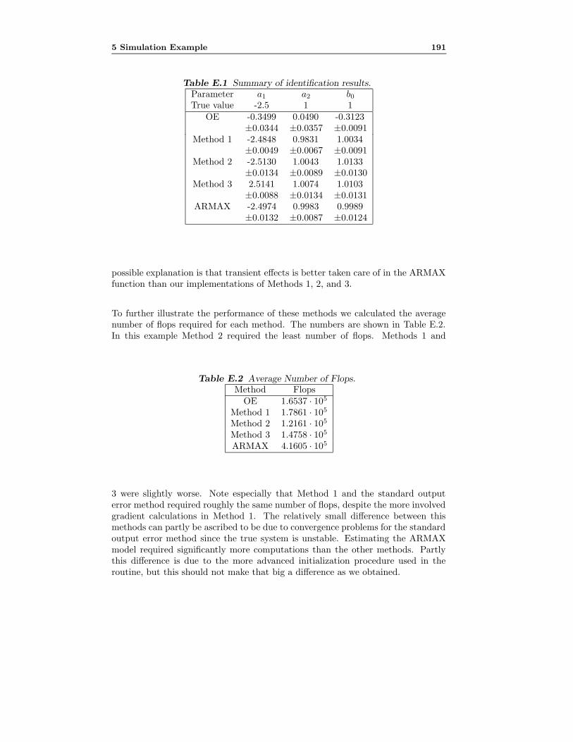
5 Simulation Example 191
Table E.1 Summary of identification results.Parameter a1 a2 b0True value -2.5 1 1
OE -0.3499 0.0490 -0.3123±0.0344 ±0.0357 ±0.0091
Method 1 -2.4848 0.9831 1.0034±0.0049 ±0.0067 ±0.0091
Method 2 -2.5130 1.0043 1.0133±0.0134 ±0.0089 ±0.0130
Method 3 2.5141 1.0074 1.0103±0.0088 ±0.0134 ±0.0131
ARMAX -2.4974 0.9983 0.9989±0.0132 ±0.0087 ±0.0124
possible explanation is that transient effects is better taken care of in the ARMAXfunction than our implementations of Methods 1, 2, and 3.
To further illustrate the performance of these methods we calculated the averagenumber of flops required for each method. The numbers are shown in Table E.2.In this example Method 2 required the least number of flops. Methods 1 and
Table E.2 Average Number of Flops.Method Flops
OE 1.6537 · 105
Method 1 1.7861 · 105
Method 2 1.2161 · 105
Method 3 1.4758 · 105
ARMAX 4.1605 · 105
3 were slightly worse. Note especially that Method 1 and the standard outputerror method required roughly the same number of flops, despite the more involvedgradient calculations in Method 1. The relatively small difference between thismethods can partly be ascribed to be due to convergence problems for the standardoutput error method since the true system is unstable. Estimating the ARMAXmodel required significantly more computations than the other methods. Partlythis difference is due to the more advanced initialization procedure used in theroutine, but this should not make that big a difference as we obtained.

192 References
6 Conclusions
We have discussed estimation of models where the dynamic model is unstableand/or the noise model has nonminimum phase zeros. In such situations the pre-dictor has to be modified and the prediction error does no longer coincide withthe model innovation. The main contribution was to show that by instead usingnoncausal stationary filters, the model innovation can be computed if the trans-fer functions from the observed data to the model innovation does not have anypoles on the unit circle. The advantage of using these noncausal filters is thatsince the model innovation is obtained, maximum likelihood identification can beperformed. Hence, maximum likelihood identification of systems with unstabledynamics or nonminimum phase noise zeros is possible.
References
[1] U. Forssell and L. Ljung. Identification of unstable systems using output errorand Box-Jenkins model structures. In Proceedings of the 37th IEEE Conferenceon Decision and Control, pages 3932–3937, Tampa, FL, 1998. To appear inIEEE Transactions on Automatic Control.
[2] F. Gustafsson. Determining the initial states in forward-backward filtering.IEEE Transactions on Signal Processing, 46:988–992, 1996.
[3] H. Hjalmarsson, M. Gevers, S. Gunnarsson, and O. Lequin. Iterative feedbacktuning: Theory and applications. IEEE Control Systems, 18:26–41, 1998.
[4] T. Kailath. Lectures on Wiener and Kalman Filtering. Springer-Verlag, 1981.
[5] L. Ljung. System Identification: Theory for the User. Prentice-Hall, 1987.
[6] L. Ljung. System Identification Toolbox – User’s Guide. The MathWorks, Inc.,Cochituate Place, Natick, MA. USA, 1995.
[7] The MathWorks, Inc., Cochituate Place, Natick, MA. USA. Signal ProcessingToolbox – User’s Guide, 1993.

Paper F
Time-domain Identificationof DynamicErrors-in-variables SystemsUsing Periodic ExcitationSignals
Authors: Urban Forssell, Fredrik Gustafsson, and Tomas McKelvey
Edited version of paper to appear in Proceedings of the 14th IFAC World Congress,Beijing, China, 1999.
Preliminary version published as Technical Report LiTH-ISY-R-2044, Departmentof Electrical Engineering, Linkoping University, Linkoping, Sweden.
193


Time-domain Identification of Dynamic
Errors-in-variables Systems
Using Periodic Excitation Signals
Urban Forssell, Fredrik Gustafsson, and Tomas McKelvey
Division of Automatic Control,Department of Electrical Engineering,
Linkoping University,S-581 83 Linkoping, Sweden.
E-mail: {ufo,fredrik,tomas}@isy.liu.se.
Abstract
The use of periodic excitation signals in identification experiments is advo-cated. With periodic excitation it is possible to separate the driving signalsand the disturbances, which for instance implies that the noise properties canbe independently estimated. In the paper a nonparametric noise model, esti-mated directly from the measured data, is used in a compensation strategy ap-plicable to both least-squares and total least-squares estimation. The resultingleast-squares and total least-squares methods are applicable in the errors-in-variables situation and give consistent estimates regardless of the noise. Thefeasibility of the idea is illustrated in a simulation study.
Keywords: Identification, Identification algorithms, Least-squares estima-tion, Excitation, Dynamic systems
1 Introduction
One of the most important steps in the identification process is the experimentdesign. This involves, for example, deciding what signals to measure, choosing
195

196 Paper F Time-domain Identification of Dynamic . . .
the sampling interval, and designing the excitation signals. In this paper we willadvocate the use of periodic excitation.
Periodic excitation has up to this point mostly been used in frequency domain iden-tification (e.g, [6, 5]), but offer several interesting and useful advantages comparedto nonperiodic (random) excitation also in time domain identification. The mainadvantages with periodic excitation in time domain identification are:
• Data reduction. By averaging over M periods the amount of data is reduced Mtimes.
• Improved signal-to-noise ratio. By averaging over M periods the noise varianceis lowered by a factor M . This will have important consequences for both thenumerical properties of the estimation algorithms and the statistical propertiesof the estimates.
• Separation of driving signals and noise. With periodic excitation all nonperiodicsignal variations over the periods will be due to random disturbances, noise. Thismeans, for instance, that we can estimate the noise level and thus compute apriori bounds for the least-squares cost function used in the identification.
• Independent estimation of nonparametric noise models. Since we can separatethe signals from the noise it is possible to independently estimate the noiseproperties. Such a noise model can be used as a prewhitening filter appliedbefore the estimation or as a tool for model validation.
In this paper we will study how to identify dynamic errors-in-variables systemsusing time-domain data. This is a problem that has received considerable interestin the literature, see, e.g., [9, 1, 12] and the more recent [13, 2]. With periodic exci-tation a number of possibilities opens up for constructing simple, efficient methodsthat solves this problem. We will study some of them in this contribution. In par-ticular, compensation methods for least-squares and total least-squares estimationthat can handle also the errors-in-variables problem will be presented. The ideaused is similar to the bias-correction technique studied in for instance [10, 12, 13].Compared to the methods studied in these references, the proposed methods havethe advantage of giving consistent estimates regardless of the properties of thenoise.

2 Problem Formulation 197
2 Problem Formulation
Consider a linear, time-invariant, discrete-time system
y(t) = G(q)u(t) =∞∑k=0
gkq−ku(t) (1)
where u(t) ∈ R is the input, y(t) ∈ R is the output, and q−1 is the delay operator(q−ku(t) = u(t− k)). We will assume that the order of the system is finite, so thatthe system can be represented as
y(t) = −a1y(t− 1)− · · · − anay(t− na) + b0u(t− nk) + bnbu(t− nk − nb) (2)
Here we have explicitly included the possibility of a delay nk. The transfer operatorG(q) in this case becomes
G(q) =q−nkB(q)A(q)
(3)
B(q) = b0 + b1q−1 + · · ·+ bnbq
−nb (4)
A(q) = 1 + a1q−1 + · · ·+ anaq
−na (5)
The problem we consider is how to identify G(q) using noisy measurements of y(t)and u(t). Our measured data can thus be described by
ZNm = {zm(1), . . . , zm(N)} (6)zm(t) = z(t) + w(t) (7)
z(t) =[y(t) u(t)
]T, w(t) =
[wy(t) wu(t)
]T (8)
We will also use the notation ym(t) = y(t) + wy(t) and um(t) = u(t) + wu(t). Theunknown signals wy(t) and wu(t) act as noise sources on the measured output andinput, respectively. We will make the following assumptions about the signals z(t)and w(t):
A1 u(t) is periodic with period P , P ≥ 2n + 1 where n is an a priori given upperbound on the system order.
A2 u(t) is persistently exciting of order n.
A3 z(t) and w(t) are jointly quasi-stationary.
A4 w(t) has the property
limM→∞
1M
M−1∑k=0
w(t+ kP ) = 0 ∀t (9)
198 Paper F Time-domain Identification of Dynamic . . .
A5 z(t) and w(t) are uncorrelated.
Assumption A2 is required in order to uniquely identify the system. AssumptionsA1 and A4 enable us to use simple averaging to remove the noise. In a stochasticsetting we assume A4 to hold with probability 1. Assumption A5 implies thatsample means of products of z(t) and w(t−k) tend to zero as the number of samplestends to infinity. In addition to the assumptions listed above, it is also assumedthat an integer number of periods has been measured, that is N = M · P, M ≥ 1.
3 Averaging
An important step in the identification is to average the measured data. Definethe averaged input and output as
u(t) =1M
M−1∑k=0
um(t+ kP ), t ∈ [1, P ] (10)
y(t) =1M
M−1∑k=0
ym(t+ kP ), t ∈ [1, P ] (11)
From assumption A4 it follows that u(t) → u(t), t ∈ [1, P ] and y(t) → y(t), t ∈[1, P ] as M tends to infinity. u(t) and y(t) are thus consistent estimates of noisefree signals u(t) and y(t), respectively. In [4] this is used to derive simple, consis-tent methods for the identification of errors-in-variables systems. The idea in [4]was that as M tends to infinity, the noise will average out and we are effectivelyidentifying a noise-free system. In this paper we will not generally assume that thenumber of periods tends to infinity, which makes the problem significantly harder.
4 Estimating the Noise Statistics
Let z(t) =[y(t) u(t)
]. By periodically continuing z(t) outside t = [1, P ] we can
estimate the noise w(t) as
w(t) = zm(t)− z(t), t ∈ [1, N ] (12)
A consistent estimate of the covariance function
Rww(k) = Ew(t)wT (t+ k) (13)

5 Least-squares Estimation Using Periodic Data 199
can now be computed as
Rww(k) =1
(M − 1)P
MP∑t=1
w(t)wT (t+ k) (14)
where the convention is that all signals outside the interval t = [1,MP ] are replacedby 0. In practice for large data sets, the covariance function should be computedusing FFT, see [8]. It is important to note that we have used P degrees of freedomfor estimating the mean, so the proper normalization to get an unbiased estimateis MP − P = (M − 1)P . How many periods do we need then? The rather preciseanswer provided in [7] is M ≥ 4. The asymptotic properties N = MP →∞ of theestimate are then independent of how the excitation is divided into M and P .
An unbiased estimate of the spectrum of w(t) is obtained by the periodogram
Φw(ω) =MP−1∑
k=−MP+1
Rww(k)e−iωk (15)
This can be used for prewhitening of w(t) prior to the estimation. It turns out thatthe poor variance properties of (15) does not diminish its usefulness for prewhiten-ing. An example of this will be shown in Section 11. We also mention that Φw(ω)can be estimated very efficiently using FFT directly from the original data.
5 Least-squares Estimation Using Periodic Data
Consider the linear regression model
ym(t, θ) = ϕT (t)θ (16)
ϕ(t) =[−ym(t− 1), . . . ,−ym(t− na), um(t− nk), . . . , um(t− nk − nb)
]T(17)
θ =[a1, . . . , ana , b0, . . . , bnb
]T (18)
The least-squares (LS) estimate of θ using N data samples can be written
θN = R−1N fN (19)
RN =1N
N∑t=1
ϕ(t)ϕT (t), fN =1N
N∑t=1
ϕ(t)y(t) (20)
Introduce the notation
ϕz(t) =[−y(t− 1), . . . ,−y(t− na), u(t− nk), . . . , u(t− nk − nb)
]T (21)
ϕw(t) =[−wy(t− 1), . . . ,−wy(t− na), wu(t− nk), . . . , wu(t− nk − nb)
]T (22)

200 Paper F Time-domain Identification of Dynamic . . .
Since z(t) and w(t) are uncorrelated we have that
limN→∞
RN = R = Rz +Rw (23)
limN→∞
fN = f = fz + fw (24)
Rz = Eϕz(t)ϕTz (t), Rw = Eϕw(t)ϕTw(t) (25)
fz = Eϕz(t)y(t), fw = Eϕw(t)wy(t) (26)
If, indeed
ym(t) = ϕT (t)θ + e(t) (27)
where e(t) is white noise with variance λ0, then the least-squares estimate is con-sistent with asymptotic covariance matrix
N Cov θ ≈ λ0R−1 (28)
However, with colored noise and/or noisy measurements of the input this is nolonger true and the least-squares estimate will be biased.
Let RP and fP be defined similar to RP and fP , respectively, except that averageddata is used. We then have that
limP→∞
RP = R = Rz +1MRw (29)
limP→∞
fP = f = fz +1Mfw (30)
The M normalization is due to the averaging which decreases the noise variancewith a factor of M . The least-squares estimate using averaged data will still beunbiased if the true system is given by (27), but the asymptotic covariance matrixchanges to
MP Cov θP ≈Mλ0
MR−1 = λ0R
−1 (31)
The scaling factor is thus the same, but R is replaced by R, and since R ≥ R thismeans that the asymptotic covariance increases with averaged data.
6 Improving the Accuracy
If we have periodic excitation and if (27) holds then we can recover the originalinformation in Rw and fw using the nonparametric noise model (14). The idea

7 Consistent Least-squares Estimation of Errors-in-variables Systems 201
is to construct nonparametric estimates Rnpw and fnpw of Rw and fw, respectively,from Rww(k), k = 0, 1, . . . and compensate for the missing terms in R and f . Aspointed out before, these estimates use (M − 1)P degrees of freedom. Note alsothat RP and fP already contain estimates of Rw and fw, respectively. These haveP degrees of freedom (averages over P samples), and are functions of the samplemean w(t). This is important since the nonparametric estimates are based on thesecond-order properties of w(t), and thus these two estimates of Rw and fw areuncorrelated, and even independent if Gaussian noise is assumed. This implies thatwe can compensate the least-squares quantities obtained from averaged data
RcP = RP + Rnpw , f cP = fP + fnpw (32)
and recover all MP = (M − 1)P +P degrees of freedom. This is further discussedin [3].
7 Consistent Least-squares Estimation of Errors-
in-variables Systems
A similar idea can be used to remove the bias in the least-squares estimate dueto (colored) noise w(t) acting on the input and the output: we simply have tosubtract away the terms in RP and fP that are due to the noise w(t) using thenonparametric estimates Rnpw and fnpw . By equating the degrees of freedom it canbe shown that
Rz = RP −1
M − 1Rnpw , fz = fP −
1M − 1
fnpw (33)
are consistent estimates of Rz and fz, respectively. We have thus removed all effectof the noise w(t) in RP and fP by a simple subtraction operation and the resultingleast squares estimate
θP = R−1z fz (34)
will be consistent regardless of w(t). The method (33)-(34) will be referred to asthe compensated least-squares (CLS) method. Due to its simplicity and generalapplicability, this method is a very interesting alternative to other methods that areapplicable in the errors-in-variables situation. Note that with the CLS method noiterations are required to find the estimate – a clear advantage compared to mostother errors-in-variables methods which frequently use singular value decomposi-tions (SVDs) and to most other time-domain identification schemes which oftenuse Gauss-Newton type search algorithms for finding the estimates.

202 Paper F Time-domain Identification of Dynamic . . .
8 The Total Least-squares Solution
For simplicity, assume that na = nb = n and nk = 0. The relation (2), t ∈ [1, N ],can in this case be restated as
TNθ′ = 0 (35)
where
TN =[−Y N UN
](36)
Y N =
y(n+ 1) . . . y(1)...
. . ....
y(N) . . . y(N − n)
(37)
UN =
u(n+ 1) . . . u(1)...
. . ....
u(N) . . . u(N − n)
(38)
θ′ =[1, a1, . . . , an, b0, . . . , bn
]T (39)
The nontrivial right null space of the data matrix TN describes the system.
With noisy measurements zm(t) of z(t), a total least-squares (TLS) solution isnatural to apply. Denote the noisy variant of TN by TNm . The total least-squaressolution θ′TLS can be stated as
TNTLS = arg minT‖TNm − T ‖2F (40)
subject to
TNTLS θ′TLS = 0 (41)
The solution is easily calculated by a singular value decomposition of the datamatrix TNm . Introduce the error
WN = TNm − TN (42)
With periodic data, averaged over M periods (N = MP ), we have that
‖WP ‖2F → 0, as M →∞ (43)
using Assumption A4. Under these conditions the TLS estimate is a consistentestimate of the system.
Let R′w be the covariance matrix of
ϕ′w(t) =[−wy(t), . . . ,−wy(t− n), wu(t), . . . , wu(t− n)
]T (44)
9 A Compensation Method for Total Least-squares Estimation 203
(cf. (22)). To improve the efficiency of the total least squares estimator one canuse R′w which lead to the generalized total least-squares (GTLS) solution [11]. TheGTLS solution θ′GTLS is
TNGTLS = arg minT‖(TNm − T )(R′w)−1/2‖2F (45)
subject to
TNGTLS θ′GTLS = 0 (46)
To understand the effect of the scaling (R′w)−1/2 it is instructive to study theproduct of TNm and its transpose. Introduce the notation
R′N =1N
(TNm )TTNm (47)
R′z = Eϕ′z(t)(ϕ′z(t))T (48)
ϕ′z(t) =[−y(t), . . . ,−y(t− n), u(t), . . . , u(t− n)
]T (49)
The solution to the TLS (GTLS) problem is given by the right null space of TNm oralternatively by the null space of R′N . Using Assumption A5 we see that
R′N → R′z +R′w, as N →∞ (50)
If we include the scaling (R′w)−1/2 the covariance matrix R′w is replaced by theidentity matrix, which does not affect the directions of the singular vectors of R′z.This means that the GTLS solution can be computed by finding the singular vectorcorresponding to the smallest singular value of the matrix (R′w)−T/2R′N (R′w)−1/2.If the true R′w is known, or if a consistent estimate of it can be computed, theGTLS estimator is consistent even if the variance of the noise w(t) does not tendto zero.
The point is now that with periodic excitation we can obtain a consistent estimateof R′w very easily using the nonparametric noise model (14). In the rest of the paperwe shall refer to this variant of the general algorithm as the GTLS algorithm.
9 A Compensation Method for Total Least-squares
Estimation
Let R′P be defined as R′P except that periodic data is used. With periodic data,averaged over M periods, we have that
R′P → R′z +1MR′w, as N →∞ (51)

204 Paper F Time-domain Identification of Dynamic . . .
Let R′npw be a nonparametric estimate of R′w obtained using (14). Similar argumentsas in Section 7 will show that
R′P −1
M − 1R′npw (52)
is a consistent estimate of R′z. This holds regardless of the noise, which impliesthat the total least-squares estimator with the compensation (52) gives consistentestimates regardless of the noise even though the number of periods, M , does nottend to infinity. This method will be referred to as the compensated total least-squares (CTLS) estimator.
10 Prewhitening of the Noise
As mentioned in Section 4 the spectrum of the noise signal w(t) can be estimatedvery efficiently using FFT when periodic data is used. Similarly we can prefilterthe data very easily in the frequency domain simply by multiplying the Fouriertransformed data sequences and the inverse of a square-root factor of the estimatednoise spectrum. The corresponding time-domain signals are then obtained throughIFFT. To preserve the relation between u(t) and y(t) it is important that um(t)and ym(t) are prefiltered using the same filter. We thus have the two choices:either we compute the prefilter that will whiten the noise in ym(t) (wy(t)), orcompute the prefilter that will whiten the noise in um(t) (wu(t)). In many casesit is most natural to whiten the noise on the output, but in other cases the choiceis more arbitrary. The former would for instance be the case if we know that themeasurement noise on y(t) and u(t) is negligible, so that w(t) basically is due toprocess noise acting on the output, or if the system operates in closed-loop and themeasurement noise is negligible, which typically leads to similar spectra of wu(t)and wy(t). If the choice is less obvious, one can benefit from whitening the noisewhich has the highest variance. This will of course distort the spectrum of theother noise signal, but since the variance is smaller the net effect will be positive.
Prewhitening of the noise can also be used to derive simplified estimation algo-rithms. Consider for instance the least-squares estimator (19)-(20). If wy(t) iswhite noise and if wy(t) is uncorrelated with wu(t−nk−k), k ≥ 0, then fw definedin (26) will be zero. This means that the CLS algorithm (33)-(34) can be simplifiedsince the second compensation in (33) may be skipped.

11 Example 205
11 Example
Consider the system
y(t) = 1.5y(t− 1)− 0.7y(t− 2)+ u(t− 1) + 0.5u(t− 2) + v(t) (53)
v(t) = −0.9v(t− 1) + e(t) (54)
where e(t) is white Gaussian noise with variance σ2e . Apart from the noise v(t),
(53) is of the form (2) with a1 = −1.5, a2 = 0.7, b0 = 1, b1 = 0.5, na = 2, nb = 2,and nk = 1. This system was simulated using the control law
u(t) = r(t) − 0.25y(t) (55)
where r(t) is a periodic reference signal with period P . In the simulations r(t)was taken as a unit binary random signal. We also added colored measurementnoise on both y(t) and u(t). These noise sources were independent but with equalspectra. The measurement noises were realized as Gaussian, white noise sequencesfiltered through a second-order, high-pass Butterworth filter with cut-off frequency0.3. The variance of the white noise was σ2
n.
A number of identification approaches were considered:
1. LS, LS-A, LS-AF least-squares estimation using raw data, averaged data, andaveraged and prefiltered data, respectively.
2. CLS, CLS-F least-squares estimation with compensation, cf. Eqs. (33)-(34),using averaged data and averaged and prefiltered data, respectively.
3. TLS, TLS-A, TLS-AF Total least-squares estimation using raw data, averageddata, and averaged and prefiltered data, respectively.
4. GTLS, GTLS-F Generalized total least-squares estimation with estimated noisestatistics using averaged data and averaged and prefiltered data, respectively.
5. CTLS, CTLS-F Total least-squares estimation with compensation, cf. Eq.(52), using averaged data and averaged and prefiltered data, respectively.
With colored noise on both the input and the output the LS and TLS method willbe biased. LS-A, LS-AF, TLS-A, and TLS-AF will be consistent as the number ofperiods tends to infinity, otherwise these methods will also give biased results. Theother methods give consistent estimates regardless of the noise and the number ofperiods used (as long as M ≥ 4).
In the simulation we used P = 64, M = 32, σ2e = 0.09, σ2
n = 0.01. In the prefilteringof the data using a nonparametric noise model we chose to whiten the data on the

206 Paper F Time-domain Identification of Dynamic . . .
output. The results of a Monte Carlo simulation consisting of 16 different runsare summarized in Table F.1. The numbers shown are the means and standarddeviations of the estimated parameter values for each method.
Table F.1 Summary of identification results.Parameter a1 a2 b0 b1True value -1.5000 0.7000 1.0000 0.5000
LS -1.0799 0.2033 0.9969 0.9158±0.1340 ±0.1079 ±0.1037 ± 0.0634
TLS -0.9891 -0.5340 1.7171 3.2591±1.6012 ±1.5505 ±3.0464 ±4.6528
LS-A -1.4798 0.6766 0.9963 0.5240±0.0251 ±0.0247 ±0.0565 ±0.0637
CLS -1.4991 0.6992 0.9970 0.5058±0.0246 ±0.0238 ±0.0586 ±0.0647
TLS-A -1.5026 0.6874 1.0412 0.5245±0.0259 ±0.0244 ±0.0656 ±0.0670
GTLS -1.5095 0.7087 1.0209 0.4788±0.0266 ±0.0252 ±0.0602 ±0.0666
CTLS -1.5102 0.7131 1.0170 0.4698±0.0255 ±0.0235 ±0.0636 ±0.0634
LS-AF -1.4992 0.6991 0.9991 0.4994±0.0030 ±0.0028 ±0.0116 ±0.0126
CLS-F -1.5006 0.7006 0.9988 0.4984±0.0032 ±0.0029 ±0.0118 ±0.0127
TLS-AF -1.5002 0.7001 1.0013 0.4981±0.0032 ±0.0029 ±0.0118 ±0.0127
GTLS-F -1.5009 0.7008 1.0013 0.4957±0.0033 ±0.0030 ±0.0118 ±0.0128
CTLS-F -1.5013 0.7012 1.0013 0.4944±0.0032 ±0.0029 ±0.0118 ±0.0126
Studying Table F.1, we can first note that the LS and TLS methods perform verybadly, while the results are quite good when averaged data is used. Focusing onthe proposed methods, CLS and CTLS, we see that these compare well with theother methods, both with averaged data and with averaged and prefiltered data. Inthis example, the improvement in the accuracy with prefiltered data is substantialdespite the poor variance properties of the periodogram (15). This holds for allmethods, as can be seen from Table F.1.
12 Conclusions 207
12 Conclusions
We have studied the problem of identifying dynamic errors-in-variables systemsusing periodic excitation signals. Two new algorithms, the CLS and the CTLSalgorithms, have been presented that gives consistent estimates regardless of thenoise on the input and output. With the CLS algorithm the estimate is foundwithout iterations by solving a standard least-squares problem, which can be donevery efficiently using FFT. This method can therefore be an interesting alternativeto existing time- and frequency-domain methods for this problem. The CTLSalgorithm is an alternative to the GTLS algorithm where the noise statistics areestimated from data. The performance of the CTLS method and the GTLS methodis similar.
References
[1] B. D. O. Anderson. Identification of scalar errors-in-variables models withdynamics. Automatica, 21:709–716, 1985.
[2] C. T. Chou and M. Verhaegen. Subspace algorithms for the identification ofmultivariable errors-in-variables models. Automatica, 33:1857–1869, 1997.
[3] F. Gustafsson and J. Schoukens. Utilizing periodic excitation in predictionerror based system identification. In Proceedings of the 37th IEEE Conferenceon Decision and Control, pages 3926–3931, Tampa, FL, 1998.
[4] T. McKelvey. Periodic excitation for identification of dynamic errors-in-variables systems operating in closed loop. In Proceedings of the 13th IFACWorld Congress, volume J, pages 155–160, San Francisco, CA, 1996.
[5] J. Schoukens, P. Guillaume, and R. Pintelon. Design of broadband excitationsignals. In K. Godfrey, editor, Perturbation Signals for System Identification,pages 126–159. Prentice-Hall, 1993.
[6] J. Schoukens and R. Pintelon. Identification of Linear Systems. A PracticalGuideline to Accurate Modeling. Pergamon Press, 1991.
[7] J. Schoukens, R. Pintelon, G. Vandersteen, and P. Guillaume. Frequency-domain system identification using non-parametric noise models estimatedfrom a small number of data sets. Automatica, 33:1073–1086, 1997.
[8] J. Schoukens, Y. Rolain, F. Gustafsson, and R. Pintelon. Fast calculationsof linear and non-linear least-squares estimates for system identification. InProceedings of the 37th IEEE Conference on Decision and Control, pages 3408–3410, Tampa, Florida, 1998.

208 References
[9] T. Soderstrom. Identification of stochastic linear systems in presence of inputnoise. Automatica, 17:713–725, 1981.
[10] P. Stoica and T. Soderstrom. Bias correction in least-squares identification.International Journal of Control, 35:449–457, 1982.
[11] S. Van Huffel and J. Vandewalle. Analysis and properties of the generalizedtotal least squares problem AX ≈ B when some or all columns in A aresubject to error. SIAM Journal on Matrix Analysis and Applications, 10:294–315, 1989.
[12] W.-X. Zheng and C.-B. Feng. Unbiased parameter estimation of linear systemsin the presence of input and output noise. International Journal of AdaptiveControl and Signal Processing, 3:231–251, 1989.
[13] W.-X. Zheng and C.-B. Feng. Identification of a class of dynamic errors-in-variables models. International Journal of Adaptive Control and SignalProcessing, 6:431–440, 1992.
Paper G
Identification for Control:Some Results on OptimalExperiment Design
Authors: Urban Forssell and Lennart Ljung
Edited version of paper originally published in Proceedings of the 37th IEEE Con-ference on Decision and Control, pages 3384-3389, Tampa, FL, 1998.
Submitted to Automatica.
209


Identification for Control: Some Resultson Optimal Experiment Design
Urban Forssell and Lennart Ljung
Division of Automatic Control,Department of Electrical Engineering,
Linkoping University,S-581 83 Linkoping, Sweden.
E-mail: [email protected], [email protected].
Abstract
The problem of designing the identification experiments to make them maxi-mally informative with respect to the intended use of the model is studied. Afocus will be on model based control and we show how to choose the feedbackregulator and the spectrum of the reference signal in case of closed-loop ex-periments. A main result is that when only the misfit in the dynamics modelis penalized and when both the input and the output power are constrainedthen the optimal controller is given by the solution to a standard LQ problem.When only the input power is constrained, it is shown that open-loop experi-ments are optimal. Some examples are also given to exemplify the theoreticalresults.
1 Introduction
The validation step in the identification procedure should be devoted to evaluatingthe model with respect to its intended use; simulation, prediction, control, etc.To make fair judgments it is important to know what factors affect the model’sperformance and how these factors can be manipulated. In this paper we focuson experiment design issues and especially how one should choose the feedbackregulator in closed-loop experiments. The aim will be to design the experiments
211

212 Paper G Identification for Control: Some Results on Optimal . . .
so as to minimize the variance errors in the identified models. This route was alsotaken in [2] and [4], and the presentation here will be inspired by these papers. Seealso [7].
The main drawback with the optimal solutions that will be derived is that theytypically will depend on unknown quantities, like the unknown system that weare trying to identify. Clearly this will lead to infeasible designs. This problemis inevitable and shared with any optimal design problem. A way around this isto use iterations and to replace the true system in the optimal solutions with thecurrent estimate of the system.
Despite this problem the optimal solutions derived here give important and usefulinsights into questions like “Should open-loop or closed-loop experiments be used?”and “To which frequency ranges should the input signal power be concentrated?”.
The rest of the presentation will unveil as follows. Section 2 contains some back-ground material on the identification method used and the assumptions made onthe underlying system. The notation will also be introduced in this section. InSection 3 we provide a motivation for the type of criterion we will consider. Akey issue is that the criterion will reflect the variance error introduced when usingidentified models in the control design. Section 4 contains the main results andin Section 5 these results are applied to some well known control design schemeslike internal model control and model reference control. Conclusions are given inSection 6.
2 Preliminaries
To evaluate a model’s performance one needs some notion of the “best” or “true”model. We will assume that the true system is single-input, single-output (SISO)and given by
y(t) = G0(q)u(t) + v(t), v(t) = H0(q)e(t) (1)
Here {e(t)} is white noise with variance λ0. To simplify the notation we introducethe transfer matrix
T0(q) =[G0(q) H0(q)
]T (2)
Given measured data {y(1), u(1), . . . , y(N), u(N)} and a parameterized model struc-ture
y(t|θ) = H−1(q, θ)G(q, θ)u(t) + (1−H−1(q, θ))y(t) (3)

2 Preliminaries 213
we can estimate the model by the straightforward fit:
θN = arg minθVN (θ) (4)
VN (θ) =N∑t=1
ε2(t, θ) (5)
ε(t, θ) = y(t)− y(t|θ) = H−1(q, θ)(y(t)−G(q, θ)u(t)) (6)
For more details on this identification method see, e.g., [7]. The model structure(3) may also be represented as
y(t) = G(q, θ)u(t) +H(q, θ)e(t) (7)
In the sequel G(q, θ) and H(q, θ) will be called the dynamics model and the noisemodel, respectively. Let GN (q) = G(q, θN ) and HN (q) = H(q, θN ) and also intro-duce
TN (q) =[GN (q) HN (q)
]T(8)
The error between the true transfer matrix T0(q) and the estimated one TN(q) willbe denoted TN(q),
TN(q) = T0(q)− TN (q) =[GN (q) HN (q)
]Twith an obvious notation for GN (q) and HN (q). As the number of data tends toinfinity and the model order n increases we have that (cf. [5], [9])
Cov TN(eiω) ≈ n
NP (ω) (9)
=n
NΦv(ω)
[Φu(ω) Φue(ω)
Φue(−ω) λ0
]−T(10)
In this paper we will assume that the input is generated as
u(t) = r(t) −K(q)y(t) (11)
where K(q) is a linear regulator. The reference signal r(t) is assumed uncorrelatedwith the disturbance e(t), i.e., the cross spectrum Φre(ω) = 0. This means that wecan split the input spectrum into two parts, one that is due to r(t) and one that isdue to e(t):
Φu(ω) = Φru(ω) + Φeu(ω) (12)
By combining (1) and (11) we see that the input can be written
u(t) = S0(q)r(t) −K(q)S0(q)H0(q)e(t) (13)

214 Paper G Identification for Control: Some Results on Optimal . . .
Consequently
Φru(ω) = |S0(eiω)|2Φr(ω) (14)
Φeu(ω) = |K(eiω)|2|S0(eiω)|2|H0(eiω)|2λ0 (15)
Φue(ω) = −K(eiω)S0(eiω)H0(eiω)λ0 (16)
With these definitions we may rewrite P (ω) as
P (ω) = Φv(ω)[
Φu(ω) Φue(ω)Φue(−ω) λ0
]−T=
Φv(ω)λ0Φu(ω)− |Φue(ω)|2
[λ0 −Φue(ω)
−Φue(−ω) Φu(ω)
]T=|H0(eiω)|2
Φru(ω)
[λ0 −Φue(ω)
−Φue(−ω) Φru(ω) + Φeu(ω)
]T(17)
Here we have used the fact that
Φv(ω) = λ0|H0(eiω)|2 (18)
A remark regarding (17) is that this result holds not only for the direct method, con-sidered here, but also for the so called indirect and joint input-output approachesto closed-loop identification. See, e.g., [1] and [3]. Therefore all the results belowwill also apply to these approaches as well.
For future use we also note that the output spectrum can be written
Φy(ω) = |G0(eiω)|2Φru(ω) + |S0(eiω)|2Φv(ω) (19)
3 Measuring the Performance Degradation
Our focus here will be on model-based control. It is then natural to evaluate themodel’s performance by comparing the outputs of the closed-loop system resultingfrom control design using the “true” models and the estimated ones, respectively.In general this output will be a function of both G(q) and H(q) and some drivingsignal w(t):
y(t) = f(T (q))w(t) (20)
The “true” or “best” signal is
y0(t) = f(T0(q))w(t) (21)

3 Measuring the Performance Degradation 215
while the one resulting from the estimated models is
yN(t) = f(TN(q))w(t) (22)
A measure of the performance degradation can be obtained by computing the meansquare error
Ey2N (t) = E(y0(t)− yN (t))2 (23)
Using first-order approximations we may write
yN (t) = T TN (q)F (q)w(t) (24)
where
F (q) =∂
∂Tf(T )
∣∣∣T=T0(q)
(25)
From the definition of the spectrum it follows that
Ey2N(t) =
12π
∫ π
−πΦyN (ω)dω =
12π
∫ π
−πtr [Π(ω)C(ω)] dω (26)
where
Π(ω) = ETN(e−iω)T TN (eiω) (27)
C(ω) = F (eiω)Φw(ω)FT (e−iω) (28)
Thus, if we want to minimize the performance degradation due to the use of iden-tified models, a natural criterion to minimize would be
J =∫ π
−πtr [Π(ω)C(ω)] dω (29)
Let us comment on the matrix functions Π(ω) and C(ω). First, if the bias errorsare negligible then Π(ω) will be the (transpose of the) covariance matrix of theestimate TN(eiω),
Π(ω) =[Cov TN (eiω)
]T(30)
The error made in this approximation should be small if the model structure isreasonably flexible. Using the standard result (9) we thus have
Π(ω) ≈ n
NPT (ω) =
n
NΦv(ω)
[Φu(ω) Φue(ω)
Φue(−ω) λ0
]−1
(31)
Second, the weighting function C(ω) should reflect the relative importance of agood fit in G(eiω) and H(eiω), respectively, for different frequencies. We shall

216 Paper G Identification for Control: Some Results on Optimal . . .
assume that C(ω) is Hermitian and positive semi-definite as in (28). In general wemay write
C(ω) =[C11(ω) C12(ω)C12(−ω) C22(ω)
](32)
If we neglect the scaling n/N (which will have the affect that the prejudice againsthigh order models is reduced [7]), the criterion (29) simplifies to
J =∫ π
−πtr [P (ω)C(ω)] dω (33)
This criterion will be used here.
4 Main Results
In this section we will consider experiment design problems where the goal is tominimize J with respect to the design variables, which we take as K(eiω) and Φr(ω).Other equivalent choices are also possible, e.g., Φu(ω) and Φue(ω) or K(eiω) andΦru(ω). To make the designs realistic we will also impose constraints on the inputpower or the output power, or both. We will also discuss the case where the powerof the reference signal is bounded. Without loss of generality we will take theupper bounds to be unity. This is done to simplify the notation and can always beachieved by suitable scaling. In the sequel we also will omit the arguments ω andeiω whenever there is no risk of confusion.
First consider the case where penalty only is put on the misfit in G. This corre-sponds to C12 = C22 = 0. We then have the following result which to our knowledgeis new.
Theorem 1 The solution to the problem
minK,Φr
{∫ π
−πtr [PC] dω : C12 = 0, C22 = 0;∫ π
−π{αΦu + (1− α)Φy}dω ≤ 1, α ∈ [0, 1]
}(34)
is
Kopt = arg minK
∫ π
−π
α|K|2 + (1− α)|1 +G0K|2
Φvdω (35)
Φoptr = µ√
ΦvC11|1 +G0K
opt|2√α+ (1− α)|G0|2
(36)
4 Main Results 217
where µ is a constant, adjusted so that∫ π
−π{αΦu + (1− α)Φy}dω = 1 (37)
Remark: It should be noted that equation (35), defining the optimal controllerKopt, is a standard LQ problem. If G0 and Φv were known this could be easilysolved to give an explicit expression for Kopt.
Proof Replace the design variables K and Φr by the equivalent pair K and Φru.Then, by using (12), (17), and (19), problem (34) can be rewritten as
minK,Φru
{∫ π
−π
ΦvΦru
C11dω :∫ π
−π{(α+ (1 − α)|G0|2)Φru +
α|K|2 + (1− α)|1 +G0K|2
Φv}dω ≤ 1,
α ∈ [0, 1]}
(38)
The criterion function is independent of K hence the optimal controller Kopt canbe found by solving the LQ problem
minK
∫ π
−π
α|K|2 + (1− α)|1 +G0K|2
Φvdω (39)
(Here it is implicitly assumed that y(t) = G0(q)u(t) + v(t), u(t) = −K(q)y(t), andα ∈ [0, 1].) This proves (35). Define the constant γ as
γ = 1−∫ π
−π
α|Kopt|2 + (1− α)|1 +G0Kopt|2 Φvdω (40)
Problem (38) now reads
minΦru{∫ π
−π
ΦvΦru
C11dω :∫ π
−π(α+ (1− α)|G0|2)Φrudω ≤ γ} (41)
This problem has the solution (cf. [7], p. 376)
Φru = µ
√ΦvC11
(α+ (1− α)|G0|2)(42)
where µ is a constant, adjusted so that∫ π
−π((α+ (1− α)|G0|2)Φrudω = γ (43)

218 Paper G Identification for Control: Some Results on Optimal . . .
or in other words so that ∫ π
−π{αΦu + (1− α)Φy}dω = 1 (44)
Consequently the optimal Φr is
Φoptr = µ√
ΦvC11|1 +G0K
opt|2√α+ (1 − α)|G0|2
(45)
which ends the proof. �
We stress that the optimal controller Kopt in (35) can easily be found by solvingthe indicated discrete-time LQ problem (if G0 and Φv were known). Among otherthings this implies that the optimal controller Kopt is guaranteed to stabilize theclosed-loop system and be linear, of the same order as G0. This is a clear advantageover the results reported in, e.g., [4] and also over the results in Theorem 3 below.Furthermore, the optimal controller is independent of C11 which also is quite inter-esting and perhaps somewhat surprising. This means that whatever weighting C11
is used in the design criterion, it is always optimal to use the LQ regulator (35) inthe identification experiment.
From Theorem 1 we also see that closed-loop experiments are optimal as long asthe is a constraint on the output power, i.e., as long as α 6= 1. If α = 1 thenKopt = 0 and the optimal input spectrum Φopt
u (= Φoptr ) becomes
Φoptu = µ√
ΦvC11 (46)
This side result can in fact be strengthened [7]:
Theorem 2 The problem
minK,Φr
{∫ π
−πtr [PC] dω :
∫ π
−πΦudω ≤ 1, C12 = 0
}(47)
has the solution
Kopt = 0 (open-loop operation) (48)
Φoptr = Φoptu = µ√
ΦvC11 (49)
where µ is a constant, adjusted so that∫ π
−πΦudω = 1 (50)

4 Main Results 219
Consider now the case where the power of the reference signal is constrained. Thefollowing theorem, which we believe is new, then states what the optimal controllerand reference spectrum are. The expression for the optimal controller also holdsfor the case where the reference signal is fixed and pre-specified (which would bethe case if data were collected under normal (controlled) operation of the plant).
Theorem 3 The problem
minK,Φr
{∫ π
−πtr [PC] dω :
∫ π
−πΦrdω ≤ 1
}(51)
has the solution
Kopt = − C11G∗0 + C12H
∗0
C11|G0|2 + 2 Re(C12G0H∗0 ) + C22|H0|2(52)
Φoptr = µ
√Φv · detC · |H0|2
C11|G0|2 + 2 Re(C12G0H∗0 ) + C22|H0|2(53)
where µ is a constant, adjusted so that∫ π
−πΦrdω = 1 (54)
Remark: Note that Kopt in (52) only is a feasible design if Kopt is proper andstabilizes the closed-loop system. Unfortunately no such guarantees can be given,which is a clear disadvantage compared to the result in Theorem 1. The optimalsolutions derived in [4] suffer from the same type of problems, as mentioned earlier.To circumvent this problem it was suggested in [4] that the so called Youla param-eterization (e.g., [8]) should be used. This idea could lead to interesting extensionsof the results in Theorem 3 also, although we will not study it any further here.
Proof Introduce the following square-root factorization of C:
C =[C1 C2
0 C3
][C1 C2
0 C3
]∗(55)
Clearly we have the relations
C11 = |C1|2 + |C2|2 (56)C12 = C2C
∗3 (57)
C22 = |C3|2 (58)
With P given by (17) we have that
tr [PC] = C22|H0|2 + Ψ (59)

220 Paper G Identification for Control: Some Results on Optimal . . .
where
Ψ =ΦvΦru
[C11 + 2 Re(C∗12KS0H0) + C22|K|2|S0|2|H0|2
](60)
=ΦvΦru
[|C1|2 + |C2 + C3KS0H0|2
](61)
=ΦvΦr
[|C1(1 +KG0)|2 + |C2(1 +KG0) + C3KH0|2
](62)
=ΦvΦr‖[C1 C2
]+K
[C1G0 C2G0 + C3H0
]‖2 (63)
There is no constraint on K so to minimize the criterion function we should, ateach frequency, choose K as the least-squares estimate
Kopt = −[C1 C2
] [C1G0 C2G0 + C3H0
]∗‖[C1G0 C2G0 + C3H0
]‖2
(64)
= − (|C1|2 + |C2|2)G∗0 + C2C∗3H∗0
(|C1|2 + |C2|2)|G0|2 + 2 Re(C2C∗3G0H∗0 ) + |C3|2|H0|2(65)
= − C11G∗0 + C12H
∗0
C11|G0|2 + 2 Re(C12G0H∗0 ) + C22|H0|2(66)
With this choice of K it can be shown (by straightforward but tedious calculations)that
tr [PC]∣∣∣K=Kopt
= C22|H0|2 +
+ΦvΦr
detC · |H0|2C11|G0|2 + 2 Re(C12G0H∗0 ) + C22|H0|2
(67)
The first term is independent of Φr, hence we get (cf. [7], p. 376)
Φoptr = µ
√Φv · detC · |H0|2
C11|G0|2 + 2 Re(C12G0H∗0 ) + C22|H0|2(68)
where µ is a constant, adjusted so that∫ π
−πΦoptr dω = 1
This proves the theorem. �
Note that if C is singular the optimal Φr in (53) can be chosen at will, as long as∫ π
−πΦoptr dω = 1 (69)

5 Examples 221
This is due to the factor detC in (53) which vanishes when C is singular. Further-more, when C is singular the optimal K in (52) simplifies to (cf. [6, 2])
Kopt = − C12
C12G0 + C22H0(70)
Theorem 4 If C is singular then the problem
minK,Φr
{∫ π
−πtr [PC] dω : any constraint
}(71)
has the solution
Kopt = − C12
C12G0 + C22H0(72)
Φoptr arbitrary (73)
as long as u given by
u(t) = r(t) +C12(q)
C12(q)G0(q) + C22(q)H0(q)y(t) (74)
is an admissible input.
5 Examples
5.1 Internal Model Control
In Internal Model Control (IMC) the control law is chosen as
u(t) = K(q)(rc(t)− y(t)) =Q(q)
1−G(q)Q(q)(rc(t)− y(t)) (75)
where Q is some stable transfer function and G a model of the true plant G0. Hererc denotes the reference signal to be used in the control application, not to bemixed up with the reference signal r used in the identification experiment. Notethat the control design will not depend on the noise model. Also note that thedesigned closed-loop system is
Gdesc (q) =G(q)K(q)
1 +G(q)K(q)= G(q)Q(q) (76)
For this 1-dof regulator Gc coincides with the complementary sensitivity function.From (76) we see that Q = Gc/G should be large where a raise in the system’sgain is desired.

222 Paper G Identification for Control: Some Results on Optimal . . .
Ideally, that is when G = G0, the “best” or “true” IMC controller results:
K0(q) =Q(q)
1−G0(q)Q(q)(77)
In general the model G is obtained through identification using N data samples.In that case G = GN and the corresponding controller is
KN(q) =Q(q)
1− GN (q)Q(q)(78)
Neglecting the response from the noise source e we obtain the “true” output y0 as
y0(t) =G0(q)K0(q)
1 +G0(q)K0(q)rc(t) = G0(q)Q(q)rc(t) (79)
The actual output resulting from use of the suboptimal controller (78) is
yN(t) =G0(q)KN (q)
1 +G0(q)KN (q)rc(t) =
G0(q)Q(q)1 + GN (q)Q(q)
rc(t) (80)
Using these expressions it can now be shown that the weighting matrix C (cf.Section 3) in this case is given by
CIMC =[|G0|2|Q|4Φrc 0
0 0
](81)
Suppose now that we want to solve the problem
minK,Φr
{∫ π
−πtr [PCIMC ] dω :
∫ π
−π{Φu + Φy}dω <∞
}(82)
where K and r refers to the set-up (11) used in the identification. Theorem 1 thenstates that the optimal strategy is to use closed-loop experiments with K and Φrchosen as
Kopt = arg minK
∫ π
−π
|K|2 + 1|1 +G0K|2
Φvdω (83)
Φoptr ∝√
ΦvΦrc · |G0| · |Q|2 ·|1 +G0K
opt|2√1 + |G0|2
(84)
A remark on this choice of reference spectrum is that (for fixed G0 and Φv) Φoptr
will be large where either of Φrc or |Q| ≈ |Gdesc /G0|, is large.
5 Examples 223
5.2 Generalized Minimum Variance Control
In Generalized Minimum Variance Control (GMVC) the goal is to make the closed-loop system behave like
y0(t) = R(q)e(t) (85)
This can be accomplished by using a regulator of the form
u(t) = −H0(q)−R(q)G0(q)R(q)
y(t) (86)
The corresponding C-matrix is given by [2]:
CGMV C = λ0
∣∣∣∣ RH0
∣∣∣∣2[ |H0−R|2|G0|2 −H0−R
G0
−H∗0−R∗G∗0
1
](87)
Note that CGMV C is singular. Hence the choice
Kopty = − −(H0 −R)/G0
−(H0 −R) +H0=H0 −RG0R
(88)
minimizes
Ey2N (t) (89)
subject to any constraint according to Theorem 4. In other words, the optimalcontroller is the true GMVC controller. This was first shown in [2].
5.3 Model Reference Control
In Model Reference Control (MRC) the closed-loop system should ideally behavelike
y0(t) = Q(q)rc(t) +R(q)e(t) (90)
for some desired Q and R1. This can be achieved by letting
u(t) = Kr,0(q)rc(t)−Ky,0(q)y(t) (91)
where
Kr,0(q) =Q(q)H0(q)R(q)G0(q)
, Ky,0(q) =H0(q)−R(q)G0(q)R(q)
(92)
1The case where Q = 0 is also termed generalized minimum variance control.
224 Paper G Identification for Control: Some Results on Optimal . . .
When using identified models GN and HN in the control design we will obtain
Kr,N (q) =Q(q)HN (q)R(q)GN (q)
, Ky,N (q) =HN (q)−R(q)GN (q)R(q)
(93)
giving the sub-optimal output yN . By studying the degradation signal yN = y0−yNit can be shown that the C-matrix in this case is given by
CMRC =∣∣∣∣ RH0
∣∣∣∣2[ |Q|2|G0|2 Φrc + |H0−R|2
|G0|2 λ0 −H0−RG0
λ0
−H∗0−R∗G∗0
λ0 λ0
](94)
Note that
CMRC =∣∣∣∣ RH0
∣∣∣∣2[|Q|2|G0|2 Φrc 0
0 0
]+ CGMV C (95)
Consider now the design problem
minK,Φr
{∫ π
−πtr [PCMRC ] dω : r(t) = rc(t)
}(96)
where K and r refers to (11). The constraint that r = rc means that the iden-tification experiment should be performed using the same reference signal as inthe control application, or in other words that the data should be collected undernormal operation of the controlled plant.
Using the results of Theorem 3 it can be shown that the optimal controller is
Kopt = − 1G0
|Q|2Φrc + (|R|2 −H0R∗)λ0
|Q|2Φrc + |R|2λ0(97)
= − 1G0
(1− H0R
∗
|Q|2Φrc/λ0 + |R|2
)(98)
It is interesting to study how the optimal solution changes as a function of thecontrol design variables Q, R, Φrc and λ0. Here we consider the following specialcases:
• When Φrc/λ0 →∞,
Kopt → − 1G0
(99)
We recognize the right-hand side expression as the optimal controller when C12 =0, C22 = 0, cf. (52).

6 Conclusions 225
• When Φrc/λ0 → 0,
Kopt → −|R|2 −H0R
∗
G0|R|2=H0 −RG0R
= Ky,0 (100)
The true MRC feedback controller Ky,0 is thus optimal in the identification onlywhen Φrc/λ0 = 0 or when Q = 0 (compare with the results in [4, 2]).
6 Conclusions
We have studied the problem of optimal experiment design. A main result wasthat we, possibly for the first time, have been able to give explicit solution to aexperiment design problem with constraints on both the input and output power.The optimal controller is in this case given by the solution to a standard LQproblem. Another main conclusion is that closed-loop experiments are optimalwhenever the output variance is constrained, otherwise open-loop experiments arepreferable.
References
[1] U. Forssell and L. Ljung. Closed-loop identification revisited – Updated ver-sion. Technical Report LiTH-ISY-R-2021, Department of Electrical Engineer-ing, Linkoping University, Linkoping, Sweden, 1998.
[2] M. Gevers and L. Ljung. Optimal experiment design with respect to the in-tended model application. Automatica, 22:543–554, 1986.
[3] M. Gevers, L. Ljung, and P. Van den Hof. Asymptotic variance expression forclosed-loop identification and their relevance in identification for control. InProceedings of the 11th IFAC Symposium on System Identification, volume 3,pages 1449–1454, Fukuoka, Japan, 1997.
[4] H. Hjalmarsson, M. Gevers, and F. De Bruyne. For model-based control design,closed loop identification gives better performance. Automatica, 32:1659–1673,1996.
[5] L. Ljung. Asymptotic variance expressions for identified black-box transferfunction models. IEEE Transactions on Automatic Control, 30:834–844, 1985.
[6] L. Ljung. Parametric methods for identification of transfer functions of linearsystems. In C. L. Leondes, editor, Advances in Control, volume 24. AcademicPress, 1986.

226 References
[7] L. Ljung. System Identification: Theory for the User. Prentice-Hall, 1987.
[8] M. Vidyasagar. Control System Synthesis: A Factorization Approach. MITPress, 1985.
[9] Y.-C. Zhu. Black-box identification of MIMO transfer functions: Asymptoticproperties of prediction error models. International Journal of Adaptive Controland Signal Processing, 3:357–373, 1989.

Paper H
Asymptotic VarianceExpressions for IdentifiedBlack-box Models
Author: Urban Forssell
Preliminary version published as Technical Report LiTH-ISY-R-2089,Department of Electrical Engineering, Linkoping University, Linkoping,Sweden.
Submitted to Systems & Control Letters.
227


Asymptotic Variance Expressions forIdentified Black-box Models
Urban Forssell
Department of Electrical Engineering,Linkoping University,
S-581 83 Linkoping, Sweden.E-mail: [email protected].
Abstract
The asymptotic probability distribution of identified black-box transfer func-tion models is studied. The main contribution is that we derive varianceexpressions for the real and imaginary parts of the identified models that areasymptotic in both the number of measurements and the model order. Theseexpressions are considerably simpler than the corresponding ones that hold forfixed model orders, and yet they frequently approximate the true covariancewell already with quite modest model orders. We illustrate the relevance ofthe asymptotic expressions by using them to compute uncertainty regions forthe frequency response of an identified model.
Keywords: Identification; Prediction error methods; Covariance; Uncertainty
1 Introduction
A general linear, discrete-time model of a time-invariant system can be written
y(t) =∞∑k=1
g(k)u(t− k) + v(t) (1)
229

230 Paper H Asymptotic Variance Expressions for Identified . . .
Here {y(t)} is the output, {u(t)} the input, and {v(t)} an additive disturbance,whose character we will discuss later. With (1) we associate the transfer function
G(eiω) =∞∑k=1
g(k)e−ikω, −π ≤ ω ≤ π (2)
In this paper we will discuss the statistical properties of transfer function modelsof the form (2) when the impulse response coefficients g(k) are determined or esti-mated using measured data ZN = {y(1), u(1), . . . , y(N), u(N)}. The identificationmethod we will consider is the classical prediction error method, e.g., [4].
The main goal of the paper is to derive explicit expressions for the covariancematrix
P (ω) = E
[Re[GN (eiω)− EGN (eiω)]Im[GN (eiω)− EGN (eiω)]
][Re[GN (eiω)− EGN (eiω)]Im[GN (eiω)− EGN (eiω)]
]T(3)
where GN (eiω) denotes the identified model obtained using N measurements, thatare asymptotic both in the number of observed data and in the model order. Sim-ilar results have previously been given in [3]. There, however, the focus was onexpressions for
P∗(ω) = E|GN (eiω)− EGN (eiω)|2 (= trP (ω)) (4)
which is real-valued and hence does not bring any information about the phase ofGN (eiω)−EGN (eiω). With an explicit expression for the covariance matrix P (ω)defined in (3) we can construct confidence ellipsoids for GN (eiω) in the complexplane which is useful, e.g., for robust control design and analysis.
2 Preliminaries
Notation and Definitions
The delay operator is denoted by q−1,
q−1u(t) = u(t− 1) (5)
and the set of integers by Z. The Kronecker delta function δ(·) is defined as
δk =
{1, k = 00, k 6= 0
(6)

2 Preliminaries 231
As we shall work with signals that may contain deterministic components, we willconsider generalized covariances and spectra of the form
Ryu(k) = Ey(t)u(t− k) (7)
Φyu(ω) =∞∑
k=−∞Ryu(k)e−ikω (8)
In (7) the symbol E is defined as
Ef(t) = limN→∞
1N
N∑t=1
Ef(t) (9)
A filter F (q),
F (q) =∞∑k=0
f(k)q−k (10)
is said to be stable if∞∑k=0
|f(k)| <∞ (11)
A set of filters F (q, θ); θ ∈ DM,
F (q, θ) =∞∑k=0
f(k, θ)q−k (12)
is said to be uniformly stable if∞∑k=0
supθ∈DM
|f(k, θ)| <∞ (13)
Basic Prediction Error Theory
Consider the set of models
y(t) = G(q, θ)u(t) +H(q, θ)e(t); θ ∈ DM ⊂ Rd (14)
where DM is a compact and connected subset of Rd (d = dim θ), and where
G(q, θ) =∞∑k=1
g(k, θ)q−k (15)
H(q, θ) = 1 +∞∑k=1
h(k, θ)q−k (16)

232 Paper H Asymptotic Variance Expressions for Identified . . .
(In (14) {e(t)} is supposed to be a sequence of independent, identically distributedrandom variables of zero means, variances λ0, and bounded fourth order moments.)The corresponding one-step-ahead predictor is
y(t|θ) = H−1(q, θ)G(q, θ)u(t) + (1−H−1(q, θ))y(t) (17)
The prediction error is
ε(t, θ) = y(t)− y(t|θ) = H−1(q, θ)(y(t)−G(q, θ)u(t)) (18)
The standard least-squares prediction error estimate is found as
θN = arg minθ∈DM
VN (θ) (19)
VN (θ) =1N
N∑t=1
12ε2(t, θ) (20)
We will denote the corresponding transfer function estimates, GN (q) and HN (q),respectively; GN (q) = G(q, θN ) and HN (q) = H(q, θN).
Under weak regularity conditions we have (see, e.g., [4])
θN → θ∗ with probability 1 as N →∞ (21)θ∗ = arg min
θ∈DMV (θ) (22)
V (θ) = E12ε2(t, θ) (23)
Further,√N(θN − θ∗) ∈ AsN(0, Pθ) (24)
Pθ = R−1QR−1 (25)R = V ′′(θ∗) (26)
Q = limN→∞
E N · V ′N (θ∗)(V ′N (θ∗))T (27)
Here prime and double prime denotes differentiation once and twice, respectively,with respect to θ.
Asymptotic Variances for Identified Models
The result (24)-(27) states that asymptotically, as N tends to infinity, the estimate√N · θN will have a normal distribution with mean
√N · θ∗ and covariance matrix

3 Main Result 233
Pθ. Using the Taylor expansion[Re[GN (eiω)−G(eiω, θ∗)]Im[GN (eiω)−G(eiω, θ∗)]
]=[Re[G′θ(e
iω, θ∗)]Im[G′θ(e
iω, θ∗)]
](θN − θ∗) + o(|θN − θ∗|) (28)
where G′θ(eiω, θ∗) is a 1 × d dimensional matrix being the derivative of G(eiω, θ)
with respect to θ evaluated at θ = θ∗, we thus have
√N
[Re[GN (eiω)−G(eiω, θ∗)]Im[GN (eiω)−G(eiω, θ∗)]
]∈ AsN(0, P (ω)) (29)
with
P (ω) =[Re[G′θ(e
iω, θ∗)]Im[G′θ(e
iω, θ∗)]
]Pθ
[Re[G′θ(e
iω, θ∗)]Im[G′θ(e
iω, θ∗)]
]T(30)
The matrix P (ω) in (30) gives an expression for the sought covariance matrix (3).However, evaluation of (30) is complicated and leads to intractable expressions,which limits the usefulness of the result. From, e.g., [3] we know that it is possibleto compute variance expressions that are asymptotic in the model order, i.e., in thedimensionality of θ. This type of expressions tend to be simpler and, hence, easierto work with and to interpret than those obtainable using the above technique.Furthermore, despite the fact that these results are asymptotic in both the numberof measurements and the model order, they frequently give reasonable approxima-tions of the variance even for fixed model orders. In the next section we will derivethe corresponding expressions for (3).
3 Main Result
Introduce
T (q, θ) =[G(q, θ)H(q, θ)
](31)
and define
χ0(t) =[u(t)e(t)
](32)
The spectrum of {χ0(t)} is
Φχ0(ω) =[
Φu(ω) Φue(ω)Φue(−ω) λ0
](33)
Using (31) and (32) we can rewrite the model (14) as
y(t) = T T (q, θ)χ0(t) (34)
234 Paper H Asymptotic Variance Expressions for Identified . . .
Suppose that the parameter vector θ can be decomposed so that
θ =[θT1 , θ
T2 , . . . , θ
Tn
]T dim θk = s dim θ = n · s (35)
We shall call n the order of the model (34). Suppose also that
∂
∂θkT (q, θ) = q−k+1 ∂
∂θ1T (q, θ) , q−k+1Z(q, θ) (36)
where the matrix Z(q, θ) in (36) is of size 2 × s.
It should be noted that most polynomial-type model structures, like ARMAX, Box-Jenkins, etc., satisfy this shift structure. Thus (36) is a rather weak assumption.Consider, e.g., an ARX model
y(t) =B(q)A(q)
u(t) +1
A(q)e(t) (37)
where
A(q) = 1 + a1q−1 + · · ·+ anq
−n (38)
B(q) = 1 + b1q−1 + · · ·+ bnq
−n (39)
In this case we have θk =[ak bk
]Tand
Z(q, θ) = q−1
[− B(q)A2(q)
1A(q)
− 1A2(q) 0
](40)
From (36) it follows that the 2× d dimensional matrix T ′θ(eiω, θ), being the deriva-
tive of T (eiω, θ) with respect to θ, can be written
T ′θ(eiω, θ) = eiωZ(eiω, θ)Wn(eiω) (41)
where
Wn(eiω) =[e−iωI e−i2ωI · · · e−inωI
](42)
with I being an s × s identity matrix. The following lemma, which also is ofindependent interest, will be used in the proof of the main result, Theorem 2,below.
Lemma 1 Let Wn(eiω) be defined by (42) and let {w(t)} be an s-dimensionalprocess with invertible spectrum Φw(ω). Then
limn→∞
1nWn(eiω1)
[1
2π
∫ π
−πWTn (e−iξ)Φw(−ξ)Wn(eiξ)dξ
]−1
WTn (e−iω2)
=[Φw(−ω1)
]−1δ(ω1−ω2) mod 2π (43)

3 Main Result 235
Proof From Lemma 4.3 in [7] (see also [5], Lemma 4.2) we have that
limn→∞
1nWn(eiω1)
[1
2π
∫ π
−πWTn (eiξ)Φw(ξ)Wn(e−iξ)dξ
]−TWTn (e−iω2)
=[Φw(ω1)
]−Tδ(ω1−ω2) (44)
(Note especially the transposes, which are due to different definitions of correlationfunctions and spectra than the ones used here.) The result (43) follows sinceΦTw(ω) = Φw(−ω) and Wn(ei(ω+2πk)) = Wn(eiω) ∀ k ∈ Z. � �
For the proof of Theorem 2 below we additionally need a number of technicalassumptions which we now list. Let
θ∗(n) = arg minθ∈DM
V (θ) (45)
(If the minimum is not unique, let θ∗(n) denote any, arbitrarily chosen minimizingelement.) The argument n is added to emphasize that the minimization is carriedout over nth order models. Define
θN (n, δ) = arg minθ∈DM
VN (θ, δ, n) (46)
VN (θ, δ, n) =12
[1N
N∑t=1
ε2(t, θ) + δ|θ − θ∗(n)|2]
(47)
where δ is a regularization parameter, helping us to select a unique minimizingelement in (46) in case δ = 0 leads to nonunique minima.
Assume that the true system can be described by
y(t) = G0(q)u(t) + v(t), v(t) = H0(q)e(t) (48)
where {e(t)} is a sequence of independent, identically distributed random variableswith zero means, variances λ0, and bounded fourth order moments, and whereG0(q) is stable and strictly causal and H0(q) is monic and inversely stable. From(48) it follows that the spectrum of the additive disturbance {v(t)} is
Φv(ω) = λ0|H0(eiω)|2 (49)
It will be assumed that there exists a θ0 ∈ DM such that
G(q, θ0) = G0(q) and H(q, θ0) = H0(q) (50)
Further, suppose that the predictor filters
H−1(q, θ)G(q, θ) and H−1(q, θ) (51)
236 Paper H Asymptotic Variance Expressions for Identified . . .
are uniformly stable for θ ∈ DM along with their first, second, and third orderderivatives.
Let
T ∗n(eiω) = T (eiω, θ∗(n)) (52)
TN (eiω, n, δ) = T (eiω, θN (n, δ)) (53)
T0(eiω) = T (eiω, θ0) (54)
Assume that
limn→∞
n2E[ε(t, θ∗(n))− e(t)]2 = 0 (55)
which implies that T ∗n(eiω) tends to T0(eiω) as n tends to infinity. Let Z(eiω, θ)defined in (36) be denoted by Z0(eiω) when evaluated for θ = θ0. Assume that
Z0(eiω)ZT0 (e−iω) (56)
is invertible. Further assume that Ru(k) and Rue(k) exist and that Rue(k) = 0,k < 0. Finally, assume that
limN→∞
1√N
N∑t=1
E
[d
dθε2(t, θ∗(n))
]= 0 (n fixed) (57)
We can now state the main result of the paper.
Theorem 2 Consider the estimate TN (eiω, n, δ) under the assumptions (36) and(45)-(57). Then
√N
[Re[TN(eiω, n, δ)− T ∗n(eiω)]Im[TN (eiω, n, δ)− T ∗n(eiω)]
]∈ AsN(0, P (ω, n, δ)) (58)
[as N →∞ for fixed n, δ]
where
limδ→0
limn→∞
1nP (ω, n, δ) =
12Φv(ω)
[Re[Φ−1
χ0(ω)] Im[Φ−1
χ0(ω)]
− Im[Φ−1χ0
(ω)] Re[Φ−1χ0
(ω)]
], if ωmod π 6= 0
Φv(ω)
[Re[Φ−1
χ0(ω)] 0
0 0
], if ωmod π = 0
(59)
The proof is given in Appendix A.
3 Main Result 237
From (58)-(59) we conclude that, for ωmod π 6= 0, the random variable
√N(TN (eiω, n, δ)− T ∗n(eiω)) (60)
asymptotically has a complex normal distribution (e.g., [1]) with covariance matrixP∗(ω, n, δ) satisfying
limδ→0
limn→∞
1nP∗(ω, n, δ) = Φv(ω)Φ−1
χ0(−ω) (61)
Compare also with the results in [3]. (In connection to this the author would liketo point out that the matrix on the right hand side of equation (3.22) in [3] shouldbe transposed.) For ωmod π = 0 this is no longer true, since then the diagonalblocks of
limδ→0
limn→∞
1nP (ω, n, δ) (62)
are not equal. That the covariance for the imaginary part is zero in this case isvery natural, since the transfer function is real-valued for ωmod π = 0.
Further, with basically only notational differences the result in Theorem 2 alsoholds for multivariable models. The extension of the results in [3] to the multi-variable case was given in [8]. We can also prove the result for polynomial modelswhere the different polynomials are of unequal orders, or if other criteria than thequadratic one is used. In open loop the situation simplifies and, e.g., to provethe corresponding results for the model GN (eiω, n, δ) in this case the conditions inTheorem 2 can be relaxed so that a fixed, arbitrary noise model H(q, θ) = H∗(q)can be used. See [3] for all this.
Let us return to the result in Theorem 2. A more explicit expression for (59) canbe obtained if we note that
Φ−1χ0
(ω) =[
1/Φru(ω) −Φue(ω)/(λ0Φru(ω))−Φeu(ω)/(λ0Φru(ω)) 1/Φre(ω)
](63)
Φru(ω) = Φu(ω)− |Φue(ω)|2/λ0 (64)
Φre(ω) = λ0 − |Φue(ω)|2/Φu(ω) (65)
Φru(ω) can be interpreted as the “noise-free” part of the input spectrum, i.e., thatpart of the total input spectrum Φu(ω) that does not originate from {e(t)} butfrom some external reference or set-point signal. In open loop we have Φue(ω) = 0,which, e.g., implies that Φr
u(ω) = Φu(ω), and the expression for Φ−1χ0
(ω) simplifiesto
Φ−1χ0
(ω) =[1/Φu(ω) 0
0 1/λ0
](66)

238 Paper H Asymptotic Variance Expressions for Identified . . .
If we return to the general, closed loop situation we see from (63) that
Re[Φ−1χ0
(ω)] =[
1/Φru(ω) −Re[Φue(ω)/(λ0Φru(ω))]−Re[Φeu(ω)/(λ0Φru(ω))] 1/Φre(ω)
](67)
Im[Φ−1χ0
(ω)] =[
0 − Im[Φue(ω)/(λ0Φru(ω))]− Im[Φeu(ω)/(λ0Φru(ω))] 0
](68)
Using (67) and (68) we can thus easily prove the following consequence of Theorem2, dealing with the asymptotic distribution of the estimate GN (eiω, n, δ).
Corollary 3 Consider the situation in Theorem 2. Then
√N
[Re[GN (eiω, n, δ)−G∗n(eiω)]Im[GN (eiω, n, δ)−G∗n(eiω)]
]∈ AsN(0, P (ω, n, δ)) (69)
[as N →∞ for fixed n, δ]
where
limδ→0
limn→∞
1nP (ω, n, δ) =
12Φv(ω)
[1/Φru(ω) 0
0 1/Φru(ω)
], if ωmod π 6= 0
Φv(ω)
[1/Φru(ω) 0
0 0
], if ωmod π = 0
(70)
From (69)-(70) we see that, for ωmod π 6= 0, the random variable√N(GN (eiω, n, δ)−G∗n(eiω)) (71)
asymptotically has a complex normal distribution with covariance matrix P∗(ω, n, δ)satisfying
limδ→0
limn→∞
1nP∗(ω, n, δ) =
Φv(ω)Φru(ω)
(72)
This does not hold for ωmod π = 0, but for all ω we nevertheless have that
tr(
limδ→0
limn→∞
1nP (ω, n, δ)
)=
Φv(ω)Φru(ω)
(73)
which ties in nicely with the results in [3], cf. (3) and (4).
An intuitive, but not formally correct, interpretation of the result (69)-(70) is thatit gives the following convenient expression for the covariance matrix (3) (for thecase ωmod π 6= 0):
P (ω) ≈ n
N
12
Φv(ω)[1/Φru(ω) 0
0 1/Φru(ω)
]as N, n→∞ (74)
From (74) we see that asymptotically, as both n and N tend to infinity, the real andimaginary parts of the G-estimate are uncorrelated with equal variance proportionalto the number-of-parameters-to-number-of-measurements ratio (n/N ) and to thenoise-to-signal ratio (Φv(ω)/Φru(ω)).
4 Example 239
4 Example
If we assume that the random variable[Re[GN (eiω)]Im[GN (eiω)]
](75)
has a normal distribution with covariance matrix P (ω), we may compute an α%confidence ellipsoid for GN (eiω) at a particular frequency ωk, ωk mod π 6= 0, as theset of all G(eiωk) such that[
Re[G(eiωk)− GN (eiωk)]Im[G(eiωk)− GN (eiωk)]
]P−1(ωk)
[Re[G(eiωk )− GN (eiωk)]Im[G(eiωk)− GN (eiωk)]
]T≤ Cα (76)
where Cα is defined through Prob(X ≤ Cα) = α%, X ∈ χ2(2). In this example wewill construct such confidence ellipsoids for the frequency response of an identified15th order ARX model of the system
y(t) =0.1589q−1 + 0.3042q−2 + 0.0323q−3
1− 1.3219q−1 + 0.4618q−2 − 0.0408q−3u(t) + e(t) (77)
for 40 distinct frequencies ωk: 0 and 39 logarithmically spaced frequencies between0.01 and π. (For ωk mod π = 0 the confidence region becomes an interval on thereal axis. The details are omitted.) For the identification, a data set consisting ofN = 1000 samples of y(t) and u(t) is generated by simulating the system using aunit binary random signal {u(t)} and a uniformly [−1, 1] distributed random signal{e(t)}, independent of {u(t)}.
We remark that a high-order ARX model can approximate any linear system arbi-trarily well if the model order is sufficiently large, see, e.g., [4]. Hence we can quitesafely neglect the bias error in this example and use the covariance matrix P (ω) todescribe the model uncertainty. However, since we do not know P (ω) we have toreplace it by some estimate P (ω). Here we will first consider (29)-(30) and replaceP (ω) by
P (ω) =[Re[G′θ(e
iω, θN )]Im[G′θ(e
iω, θN)]
]1NPθ
[Re[G′θ(e
iω, θN)]Im[G′θ(e
iω, θN )]
]T(78)
where Pθ denotes the estimated parameter covariance delivered by the identificationroutine. The resulting 95% confidence ellipsoids for GN (eiωk), k ∈ [1, . . . , 40], areshown in Figure 1. The solid line represents the true system.
The results in Figure 1 should be compared with the confidence ellipsoids shown inFigure 2 obtained using the following estimate of P (ω) (for ωmodπ 6= 0) derivedfrom (74):
P (ω) =n
N
12λN |HN (eiω)|2
[1/Φu(ω) 0
0 1/Φu(ω)
](79)
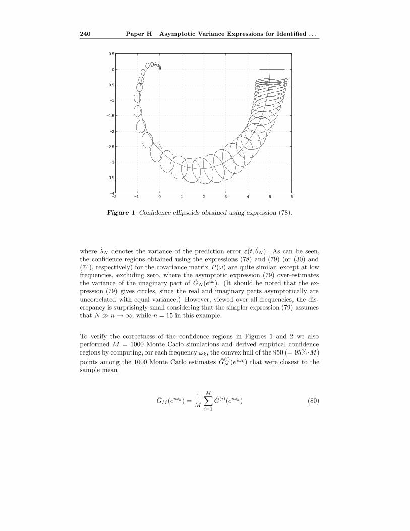
240 Paper H Asymptotic Variance Expressions for Identified . . .
−2 −1 0 1 2 3 4 5 6−4
−3.5
−3
−2.5
−2
−1.5
−1
−0.5
0
0.5
Figure 1 Confidence ellipsoids obtained using expression (78).
where λN denotes the variance of the prediction error ε(t, θN ). As can be seen,the confidence regions obtained using the expressions (78) and (79) (or (30) and(74), respectively) for the covariance matrix P (ω) are quite similar, except at lowfrequencies, excluding zero, where the asymptotic expression (79) over-estimatesthe variance of the imaginary part of GN (eiω). (It should be noted that the ex-pression (79) gives circles, since the real and imaginary parts asymptotically areuncorrelated with equal variance.) However, viewed over all frequencies, the dis-crepancy is surprisingly small considering that the simpler expression (79) assumesthat N � n→∞, while n = 15 in this example.
To verify the correctness of the confidence regions in Figures 1 and 2 we alsoperformed M = 1000 Monte Carlo simulations and derived empirical confidenceregions by computing, for each frequency ωk, the convex hull of the 950 (= 95% ·M)points among the 1000 Monte Carlo estimates G(i)
N (eiωk) that were closest to thesample mean
GM (eiωk) =1M
M∑i=1
G(i)(eiωk) (80)
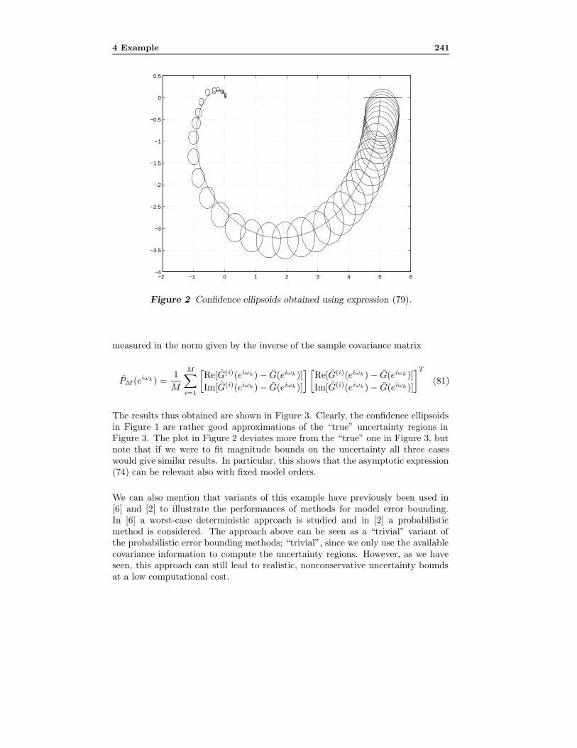
4 Example 241
−2 −1 0 1 2 3 4 5 6−4
−3.5
−3
−2.5
−2
−1.5
−1
−0.5
0
0.5
Figure 2 Confidence ellipsoids obtained using expression (79).
measured in the norm given by the inverse of the sample covariance matrix
PM (eiωk) =1M
M∑i=1
[Re[G(i)(eiωk)− G(eiωk)]Im[G(i)(eiωk)− G(eiωk)]
][Re[G(i)(eiωk)− G(eiωk)]Im[G(i)(eiωk)− G(eiωk)]
]T(81)
The results thus obtained are shown in Figure 3. Clearly, the confidence ellipsoidsin Figure 1 are rather good approximations of the “true” uncertainty regions inFigure 3. The plot in Figure 2 deviates more from the “true” one in Figure 3, butnote that if we were to fit magnitude bounds on the uncertainty all three caseswould give similar results. In particular, this shows that the asymptotic expression(74) can be relevant also with fixed model orders.
We can also mention that variants of this example have previously been used in[6] and [2] to illustrate the performances of methods for model error bounding.In [6] a worst-case deterministic approach is studied and in [2] a probabilisticmethod is considered. The approach above can be seen as a “trivial” variant ofthe probabilistic error bounding methods; “trivial”, since we only use the availablecovariance information to compute the uncertainty regions. However, as we haveseen, this approach can still lead to realistic, nonconservative uncertainty boundsat a low computational cost.

242 Paper H Asymptotic Variance Expressions for Identified . . .
−2 −1 0 1 2 3 4 5 6−4
−3.5
−3
−2.5
−2
−1.5
−1
−0.5
0
0.5
Figure 3 Confidence regions obtained using Monte Carlo simulations.
5 Summary
We have derived asymptotic expressions for the covariance of the real and imaginaryparts of identified transfer function models that are asymptotic both in the numberof measurements and in the model orders. The relevance of these expressionsalso with fixed model orders has been shown in a Monte Carlo simulation whereconfidence regions for an identified model are computed.
Acknowledgment
The author gratefully acknowledges F. Tjarnstrom who provided the Matlab codewith which the figures were generated.

A Proof of Theorem 2 243
A Proof of Theorem 2
Let ψ(t, θ) of dimension d× 1 be the gradient of the predictor y(t|θ) and define
Mn(θ) = Eψ(t, θ)ψT (t, θ) (A.1)
If we introduce
χ(t, θ) =[u(t)ε(t, θ)
](A.2)
and
ζ(t, θ) = H−1(q, θ)ZT (q, θ)χ(t, θ) (A.3)
we can also write ψ(t, θ) as
ψ(t, θ) = WTn (q)ζ(t, θ) (A.4)
(Wn(q) is the time-domain counterpart of (42).) From Lemma A.4 in [3] we have√N(θN (n, δ)− θ∗(n)) ∈ AsN(0, R(n, δ)) (A.5)
R(n, δ) = λ0
[Mn(θ∗(n)) + δI
]−1 − λ0δ[Mn(θ∗(n)) + δI
]−2 + Cδ · ρn (A.6)
where Cδ is a constant and ‖ρn‖ → 0 as n→∞. Considering the Taylor expansion[Re[TN (eiω, n, δ)− T ∗n(eiω)]Im[TN (eiω, n, δ)− T ∗n(eiω)]
]=[Re[T ′θ(e
iω, θ∗(n))]Im[T ′θ(e
iω, θ∗(n))]
](θN (n, δ)− θ∗(n))
+ o(|θN (n, δ)− θ∗(n)|) (A.7)
we thus see that the random variable
√N
[Re[TN(eiω, n, δ)− T ∗n(eiω)]Im[TN (eiω, n, δ)− T ∗n(eiω)]
](A.8)
will have asymptotic normal distribution with covariance matrix
P (ω, n, δ) =[Re[T ′θ(e
iω, θ∗(n))]Im[T ′θ(e
iω, θ∗(n))]
]R(n, δ)
[Re[T ′θ(e
iω, θ∗(n))]Im[T ′θ(e
iω, θ∗(n))]
]T(A.9)
Denote the upper left block of P (ω, n, δ) by P1,1(ω, n, δ):
P1,1(ω, n, δ) = Re[T ′θ(eiω, θ∗(n))]R(n, δ)(Re[T ′θ(e
iω, θ∗(n))])T
=12[T ′θ(e
iω, θ∗(n)) + T ′θ(e−iω, θ∗(n))
]R(n, δ)×
× 12[T ′θ(e
iω, θ∗(n)) + T ′θ(e−iω, θ∗(n))
]T (A.10)

244 Appendix
In view of (41) we have
1nP1,1(ω, n, δ)
=1n
14
(eiωZ(eiω, θ∗(n))Wn(eiω) + e−iωZ(e−iω, θ∗(n))Wn(e−iω))R(n, δ)×
× (WTn (eiω)ZT (eiω, θ∗(n))eiω +WT
n (e−iω)ZT (e−iω, θ∗(n))e−iω)
=1n
14[eiωZ(eiω, θ∗(n))Wn(eiω)R(n, δ)WT
n (eiω)ZT (eiω, θ∗(n))eiω
+ eiωZ(eiω, θ∗(n))Wn(eiω)R(n, δ)WTn (e−iω)ZT (e−iω, θ∗(n))e−iω
+ e−iωZ(e−iω, θ∗(n))Wn(e−iω)R(n, δ)WTn (eiω)ZT (eiω, θ∗(n))eiω
+ e−iωZ(e−iω, θ∗(n))Wn(e−iω)R(n, δ)WTn (e−iω)ZT (e−iω, θ∗(n))e−iω
](A.11)
Together with (A.6) this shows that we need to consider limits like
limn→∞
1nWn(eiω1)λ0
[Mn(θ∗(n)) + δI
]−1WTn (e−iω2) (A.12)
and
limn→∞
1nWn(eiω1)λ0δ
[Mn(θ∗(n)) + δI
]−2WTn (e−iω2) (A.13)
Using Lemma 1 together with (A.1)-(A.4), where we note that ε(t, θ∗(n)) → e(t)as n→∞, we have
limn→∞
1nWn(eiω1)λ0
[Mn(θ∗(n)) + δI
]−1Wn(e−iω2)
= λ0
[ZT0 (e−iω1)S(−ω1)Z0(eiω1) + δI
]−1δ(ω1−ω2) mod 2π (A.14)
where
S(ω) =Φχ0(ω)|H0(eiω)|2 (A.15)
Similarly,
limn→∞
1nWn(eiω1)λ0δ
[Mn(θ∗(n)) + δI
]−2Wn(e−iω2)
= λ0δ[ZT0 (e−iω1)S(−ω1)Z0(eiω1) + δI
]−2δ(ω1−ω2) mod 2π (A.16)
Now, consider the terms in (A.11) that originate from the first term in R(n, δ) (cf.(A.6)). Using the result (A.14) repeated times will show that as n tends to infinity
A Proof of Theorem 2 245
these terms tend to
14
[eiωZ0(eiω)λ0
[ZT0 (e−iω)S(−ω)Z0(eiω) + δI
]−1ZT0 (eiω)eiωδωmod π
+ eiωZ0(eiω)λ0
[ZT0 (e−iω)S(−ω)Z0(eiω) + δI
]−1ZT0 (e−iω)e−iω
+ e−iωZ0(e−iω)λ0
[ZT0 (eiω)S(ω)Z0(e−iω) + δI
]−1ZT0 (eiω)eiω
+ e−iωZ0(e−iω)λ0
[ZT0 (eiω)S(ω)Z0(e−iω) + δI
]−1ZT0 (e−iω)e−iωδωmod π
]=
12
[12{Z0(e−iω)λ0
[ZT0 (eiω)S(ω)Z0(e−iω) + δI
]−1ZT0 (eiω)
+ Z0(eiω)λ0
[ZT0 (e−iω)S(−ω)Z0(eiω) + δI
]−1ZT0 (e−iω)
}+
12{Z0(eiω)λ0
[ZT0 (e−iω)S(−ω)Z0(eiω) + δI
]−1ZT0 (eiω)
+ Z0(e−iω)λ0
[ZT0 (eiω)S(ω)Z0(e−iω) + δI
]−1ZT0 (e−iω)
}δωmodπ
](A.17)
If we apply the matrix inversion lemma
[A+BCD]−1 = A−1 −A−1B[C−1 +DA−1B]−1DA−1 (A.18)
to, e.g., [ZT0 (e−iω)S(−ω)Z0(eiω) + δI
]−1ZT0 (e−iω) (A.19)
we see that[ZT0 (e−iω)S(−ω)Z0(eiω) + δI
]−1ZT0 (e−iω)
=[δ−1I − δ−1ZT0 (e−iω)[δS−1(−ω) + Z0(eiω)ZT0 (e−iω)]−1Z0(eiω)
]ZT0 (e−iω)
= δ−1ZT0 (e−iω)− δ−1ZT0 (e−iω)[δ(Z0(eiω)ZT0 (e−iω))−1S−1(−ω) + I
]−1
≈ δ−1ZT0 (e−iω)− δ−1ZT0 (e−iω)[I − δ(Z0(eiω)ZT0 (e−iω))−1S−1(−ω)
]= ZT0 (e−iω)(Z0(eiω)ZT0 (e−iω))−1S−1(−ω) (A.20)
where the approximate inequality in the third step holds for small δ. We thus seethat, e.g.,
Z0(eiω)λ0
[ZT0 (e−iω)S(−ω)Z0(eiω) + δI
]−1ZT0 (e−iω)
→ λ0S−1(−ω) = Φv(ω)Φ−1
χ0(−ω) as δ →∞ (A.21)
It follows that the limit of (A.17) as δ tends zero is
12
Φv(ω)[
12{
Φ−1χ0
(ω) + Φ−1χ0
(−ω)}
+12{
Φ−1χ0
(ω) + Φ−1χ0
(−ω)}δωmodπ
]=
12
Φv(ω)[Re[Φ−1
χ0(ω)] + Re[Φ−1
χ0(ω)]δωmod π
](A.22)
246 References
Next, we may use similar arguments as in [3] to prove that the terms in (A.11)of the form (A.16), originating from the second term in R(n, δ), and the terms in(A.11) originating from the third terms in R(n, δ) all tend to zero as δ tends tozero. In summary we thus have that
limδ→0
limn→∞
1n
Re[T ′θ(eiω, θ∗(n))]R(n, δ)(Re[T ′θ(e
iω, θ∗(n))])T
=12
Φv(ω)[Re[Φ−1
χ0(ω)] + Re[Φ−1
χ0(ω)]δωmod π
](A.23)
Analogous calculations will also show that
limδ→0
limn→∞
1n
Re[T ′θ(eiω, θ∗(n))]R(n, δ)(Im[T ′θ(e
iω, θ∗(n))])T
=12
Φv(ω)[Im[Φ−1
χ0(ω)]− Im[Φ−1
χ0(ω)]δωmodπ
](A.24)
and
limδ→0
limn→∞
1n
Im[T ′θ(eiω, θ∗(n))]R(n, δ)(Im[T ′θ(e
iω, θ∗(n))])T
=12
Φv(ω)[Re[Φ−1
χ0(ω)]− Re[Φ−1
χ0(ω)]δωmod π
](A.25)
which ends the proof. �
References
[1] D. R. Brillinger. Time Series: Data Analysis and Theory. Holden-Day, 1981.
[2] R. G. Hakvoort and P. M. J. Van den Hof. Identification of probabilistic uncer-tainty regions by explicit evaluation of bias and variance errors. IEEE Trans-actions on Automatic Control, 42:1516–1528, 1997.
[3] L. Ljung. Asymptotic variance expressions for identified black-box transferfunction models. IEEE Transactions on Automatic Control, 30:834–844, 1985.
[4] L. Ljung. System Identification: Theory for the User. Prentice-Hall, 1987.
[5] L. Ljung and Z.-D. Yuan. Asymptotic properties of black-box identification oftransfer function. IEEE Transactions on Automatic Control, 30:514–530, 1985.
[6] B. Wahlberg and L. Ljung. Hard frequency-domain model error bounds fromleast-squares like identification techniques. IEEE Transactions on AutomaticControl, 37:900–912, 1992.

References 247
[7] Z.-D. Yuan and L. Ljung. Black-box identification of multivariable transferfunctions – Asymptotic properties and optimal input design. InternationalJournal of Control, 40:233–256, 1984.
[8] Y.-C. Zhu. Black-box identification of MIMO transfer functions: Asymptoticproperties of prediction error models. International Journal of Adaptive Controland Signal Processing, 3:357–373, 1989.