(1998). "evolution of langmuir circulation during a storm."

JOURNAL OF GEOPHYSICAL RESEARCH, VOL. 103, NO. C6, PAGES 12,649-12,668, JUNE 15, 1998

Evolution of Langmuir circulation during a storm Jerome A. Smith

Scripps Institution of Oceanography, La Jolla, California

Abstract. Wind stress, waves, stratification, velocity profiles, and surface fields of radial velocity and acoustic backscatter intensity were measured along a drift track 50 to 150 km off Point Arguello, California. On March 8, 1995, the wind increased from calm to 12 rn/s from the SE, opposing swell from the NW. It increased to 15 rn/s at noon UTC on March 9, remained steady over the next 12 hours, briefly dropped and veered by 60 ø, then returned. A mixed layer deepened quickly to 25 m, then held roughly steady through the next 2 days, in spite of gusty winds continuing at 15-25 rn/s. A phased-array Doppler sonar system took measurements covering 250 m by 150 m of the surface, with 5 m by 10 m spatial resolution. Averages over 6 min removed surface waves, permitting continuous assessment of strength, orientation, spacing, and degree of organization of features associated with surface motion (e.g., Langmuir circulation), even when conditions were too rough for visual assessment. Several results stand out: (1) As found previously, most wind mixing arises from inertial shear across the thermocline. (2) Consistent with wind/wave forcing of Langmuir circulation, Plueddemann et al. [ 1996] suggest that surface velocity variance <V2> scales like (u'US), where u* is friction velocity and US is the surface Stokes' drift; however, the measurements here scale with (Us)2 alone, once Langmuir circulation is established. (3) The velocity variance is weaker here than expected, given the magnitudes of wind and waves, leading to a smaller estimated mixing effect. (4) Large vacillations in LC strength are seen just before the brief veering of the wind; it is suggested that bubble buoyancy could play a dynamic role. (5) Mean orientation and spacing can differ for intensity versus radial velocity features.

1. Introduction

The mixed layer at the surface of oceans acts as the skin through which the water masses interact with the atmosphere. The mass and heat capacity of the top few meters are comparable to those of the entire atmosphere above. This mismatch in capacities has allowed considerable progress in modeling the air and sea independent of each other: as a first approximation, atmospheric dynamics regulate rates of heat and momentum exchange, while the ocean surface provides a roughly unmoving, fixed temperature boundary condition. However, key variables such as moisture flux in the atmosphere and freshwater flux in the ocean are sensitive to details of this exchange, and gas or particle fluxes are even more so. These influence the general circulation of both air and sea, affecting cloud cover and latent heat transfer in the air, and the thermohaline circulation in the

oceans. Refinement of our understanding of climate (for example), and hence our ability to anticipate future weather and climate changes, depends in some measure on our understanding of the processes governing these exchanges between air and sea, in other words, on our understanding of the mechanisms and dynamics of the mixed layer.

Considerable success in modeling the oceanic mixed layer has been enjoyed with simple one-dimensional "slab- models." In these models, only vertical profiles are considered, and both horizontal variations and internal wave

straining are ignored. Under active mixing, the density

Copyright 1998 by the American Geophysical Union.

Paper number 97JC03611. 0148-0227/98/97JC-03611 $09.00

profile erodes from the surface downward, producing a uniform layer over the remaining deeper profile. This mixed layer is approximately uniform in both velocity and density, with "jumps" occurring in both at the relatively sharp thermocline at the layer's base (like a "slab"). To complete the simplest model, the erosion rate is prescribed to maintain a threshold value of the bulk Richardson number, depending only on the depth of the layer and the jumps in velocity and density at the base [Pollard et al., 1973]. Additional deepening occurs when water at the surface is made more dense by surface buoyancy fluxes; conversely, restratification occurs when heating exceeds mixing [e.g., Price et al., 1986]. The velocity jump is primarily the result of inertial currents generated by the wind stress. Thus, while this bulk-shear mechanism is responsible for dramatically rapid initial deepening, it drops off near a quarter of an inertial day after the onset of wind. For longer duration storms, surface stirring due to wind stress can cause continued slower erosion [e.g., Niiler and Krauss, 1977], and inhibits restratification. In its simplest form, the surface stirring is parameterized by a power of the friction velocity u*; however, it has become apparent that the "constant" multiplier best fitting the data varies from site to site. It is of interest to note two instances where these simple models deviate perceptibly from the data: (1) O'Brien et al. [ 1991 ] note the failure of the real mixed laver to restratify as quickly as the model immediately after a rapid drop in wind; (2) Li et al. [ 1995] note a tendency for the mixed layer depth to continue increasing slightly faster than the model with sustained winds. Li et al. [1995; Li and Garrett, 1997] suggest that Langmuir circulation is responsible for the continued erosion and that therefore the deepening should depend on the combination of wave Stokes' drift and wind

12,649

12,650 SMITH: LANGMUIR CIRCULATION DURING A STORM

stress, as derived for the forcing of Langmuir circulation. Where waves are nearly fully developed, the waves and wind are tightly coupled. In this case, scaling by the combined wind-wave term can be hard to separate statistically from just wind stress scaling (provided the magnitude of this stirring term is adjusted for the "typical' waves there). Notably, however, there are both places and times when the relation between wind and waves is not so

direct. In particular, case (1) mentioned above occurs during a time of large waves and small stress, supporting the claim that waves play an important role. It is suggested that it is "wave climate" variations which cause the surface stirring parameter to vary from place to place. Finally, it is also worth noting tha.t wave breaking represents direct injection of momentum, gas, and turbulent energy into the mixed layer of the sea. Thus it appears essential to include waves in the parameterization of fluxes through the oceanic mixed layer, as well as through the air/sea interface.

Observations of boundary layers often reveal coherent structures. Their presence invites modeling with simplified dynamics, with hope of understanding their existence, behavior, and mixing efficiency. One such structure consists of alternating roll vortices, with axes roughly aligned with the stress. These typically have scales comparable to the depth of the mixing layer in the cross-stress direction, and much larger scales parallel to the stress. In oceans and lakes this structure is called "Langmuir circulation," in honor of the first published account of its existence [Langmuir, 1938]. Langmuir circulation is believed to dominate the dynamics of wind mixing within the surface layer of lakes [Langmuir, 1938] and to be important in the oceans [Leibovich, 1983; Weller et al., 1985]. A mechanism for the generation of Langmuir circulation was identified in the late 1970s [Craik and Leibovich, 1976; Garrett, 1970; Craik, 1977; Leibovich, 1977, 1980], based on an interaction between waves and wind-driven currents. The combination

of an identifiable structure and a straightforward generation mechanism has inspired a modeling renaissance in mixed layer dynamics. The catalytic effect is twofold: the mechanism provides a focus around which to build and refine models, and the structure provides a focus for comparison with observations.

Modeling has progressed from initial stability analyses [e.g., Craik, 1977; Leibovich, 1977; Leibovich and Paolucci, 1980] through simplified dynamics of the rolls themselves [e.g., Leibovich and Paolucci, 1980; Cox, et al., 1992; Thorpe, 1992; Cox and Leibovich. 1993; Cox and Leibovich, 1994; Tandon and Leibovich, 1995] and, recently, to "large eddy simulations" (LES) of the fully turbulent surface layer. The initial work established that, for reasonable lake and

ocean conditions, the surface layer should indeed be unstable to the formation of such alternating rolls. Then the nonlinear dynamics were found to be complex, including quasi-chaotic behavior. The analyses explored vortex pairing and 3-D instabilities [Thorpe, 1992; Leibovich and Tandon, 1993; Tandon and Leibovich, 1995], relating to the formation of "Y junctions" in the bubble streaks observed in some sonar images [Thorpe, 1992; Farmer and Li, 1995; Plueddemann, et al., 1996]. They also predicted behaviors previously unobserved; in particular, oscillations in the strength of the vortex array in time or in space are seen

under certain conditions with "strong" forcing [Cox et al., 1992; Tandon and Leibovich, 1995]. On reflection, it is apparent that the observational tools needed to see such behavior were absent until recently. Finally, recent LES simulations have shown that the system remains turbulent, modified slightly by the "vortex force" due to waves [Skyllingstad and Denbo, 1995' McWilliams et al., 1997]. This is consistent with observations, especially from the open ocean, where it appears that the rolls are rather irregular. To date, none of these simulations of Langmuir circulation has included the effects of inertial shears across the thermocline.

With the recognition that the mixed layer contains coherent structures infused with a rich variety of possible behavior, appreciation of the importance of 2-D maps of surface features has grown. In past experiments such as the Mixed Layer Dynamics Experiment (MILDEX) and the Surface Wave Processes Program (SWAPP), surface scattering Doppler sonar systems proved effective at measuring surface velocity and strain rates in a few isolated directions [Smith et al., 1987; Smith, 1992; Plueddemann et al., 1996]. One of the interesting findings is that streaks associated with Langmuir cells occasionally appear to split into pairs or, conversely, to coalesce with neighboring streaks [e.g., Thorpe, 1992; Farmer and Li, 1995; Plueddemann et al., 1996]. This has been interpreted as indicating vortex splitting or pairing, which is an exciting potential feature of the nonlinear dynamics of these structures. The one-dimensional views provided by single- beam sonars is ambiguous: the apparent time evolution of the pairing process could result either from time evolution of parallel features or from the lateral advection of essentially frozen Y-shaped features in a direction normal to the sonar beam. To resolve this, some form of area imaging is needed. For example, Farmer and Li [1995] examined some time series of acoustic intensity gathered with a mechanically scanning system, covering a full 360 ø circle every half minute or so, and verified that the Y junctions are, in general, spatial. Here too backscatter intensity and radial velocity are imaged over a continuous sector. In contrast to the system described by Farmer and Li [ 1995], this "phased- array Doppler sonar" (PADS) system simultaneously images the whole area, so that surface waves are sampled at 0.75 s intervals everywhere and can be reliably averaged out. Also, the data here were gathered continuously over several weeks, so there are no gaps and no phase of evolution is missed. The space-time evolution of surface velocity and strain rate can be examined unambiguously using the image sequences produced by this system, over the entire course of any storms encountered.

A195 kHz PADS was deployed and operated through both legs of the Marine Boundary Layer Experiment (MBLEX, February-March and April-May 1995). In MBLEX leg 1, it was operated with the beam-formed sector lying horizontally across the surface, mapping the surface over a pie-shaped area roughly 25 ø wide and 190-450 m in range. This provided a continuous sequence of 2-D images of the low-frequency radial velocity field at the ocean surface over a couple weeks, in particular, over a period of strong forcing associated with a gale-force storm. These PADS measurements are the central focus of this paper.

SMITH: LANGMUIR CIRCULATION DURING A STORM 12,651

35øN

34ON

122ow 121øW 120øW

Figure 1. Flip's track over year days 67 to 70, during MBLEX leg 1. The primary driving force is the average current over the top 90 m of water. Depths are in meters.

2. Field Experiment Setting

Leg 1 of the MBLEX took place along a drift track 50 to 100 km offshore of Point Arguello, just north of Point. Conception, California (Figure 1). For the 2 weeks beginning on February 19, 1995, the Floating Instrument Platform (Flip) was moored at 121øW, 34.5øN on a single-point mooring. The mooring line eventually threatened to destroy equipment on the starboard boom, so at 2316 UTC March 6

FLIP Profile Met.

(year day 65.96) the line was cut, and Flip drifted NW for the next week, until the end of operations on March 12.

The location of the various instruments deployed from Flip during MBLEX leg 1 are shown in Figure 2. In addition to the instruments mentioned below, a four-beam surface-

scanning Doppler sonar [cf. Smith, 1992] was operated from 15 m depth; a vane anemometer, air thermometer, and dew- point hygrometer were operated on a mast 22 m above the mean ocean surface; and a surface float measured the water temperature at a nominal depth of 5 cm below the moving surface. In the absence of radiometer and rainfall

measurements, buoyancy flux estimates must be made partly on the basis of visual observations. Over the latter part of March 10 (year day 69), rainfall accumulated up to 30 cm on the nearby land. Visual estimates on Flip suggest accumulations were comparable at sea. This would contribute significantly to the buoyancy flux Oust after the focus period discussed here); hence mixed layer budget estimates become less reliable after this. Before this, during the 2-day focus period itself, skies were gray (100% cloud cover, mostly stratus), there was occasional drizzle and mist, and the air and sea temperatures were within a degree, favoring slightly unstable conditions. Thus heat fluxes and buoyancy fluxes in general were very likely small over this particular 2-day time period.

The wind and Stokes' drift are among the primary input parameters for models of Langmuir circulation. The wind stress is estimated from sonic anemometer data, using both bulk and eddy-correlation methods. The sonic anemometer was mounted directly above a four-wire wave array, facilitating wind-wave correlation studies [e.g., Rieder and Smith, 1998]. Both sonic and wave wire data were corrected for motion of Flip [cf. Smith and Rieder, 1997]. The Stokes' drift is derived using data from the four-wire wave array, from surface elevations and tilts as functions of frequencies up to 0.5 Hz [cf. Longuet-Higgins et al., 1963]. The results are converted to Stokes' drift via linear theory and integrated

Secscan

-15m

_ MLD_ -- _._

Plan View Met. tower

SST _ Float •• / ,•', Secscan ••.• •i• k• Wave '•>•>•>' S n r••••• • X / Wires

• :.• Anemometer CTD / *

Figure 2. Plan and profile views of Flip, MBLEX leg 1, showing various instrument locations. The phaased array and SW sonars were mounted on an active heading compensation system, maintaining bearing to within 0.1 ø rms.

ao/ ': i Mag nitudesl i ^ I

. l0

o 300• ,,- , , , , • '•,•' ' ,, Directions : :

.... •,- -, ........... , ........... i ........... ! .......... F25ø•'"1 ,.: : : : 200 ...... ........

100 _ 67 67.5 68 68.5 69 69.5

Year Day 1995 (UTC)

Figure 3. Wind (solid curve) and Stokes' drift (dashed curve) over the focus time segment of MBLEX leg 1. Note the delay between the onset of wind and development of Stokes' drift. Just prior to this segment, the wind was from the NW, and swell continued to come from that direction, explaining the slow reversal in Stokes' drift direction.


lO

Temperature

14

13.5

20

30

50

60

12.5

11.5

70

10

30

50

60

Rescaled Temperature (45m Heatc)

10.5

10

14 t 13.5

13

...... 12.5

...... • 12

11.5

10.5

_ _ 10 67 67.5 68 68.5 69 69.5 70

Yearday 1995 (UTC)

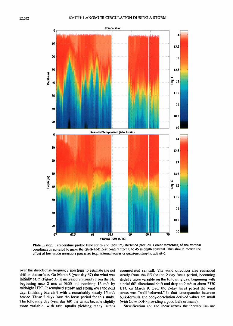
Plate 1. (top) Temperature profile time series and (bottom) stretched profiles. Linear stretching of the vertical coordinate is adjusted to make the (stretched) heat content from 0 to 45 m depth constant. This should reduce the effect of low-mode reversible processes (e.g., internal waves or quasi-geostrophic activity).

over the directional-frequency spectrum to estimate the net drift at the surface. On March 8 (year day 67) the wind was initially calm (Figure 3). It increased uniformly from the SE, beginning near 2 m/s at 0600 and reaching 12 m/s by midnight UTC. It remained steady and strong over the next day, finishing March 9 with a remarkably steady 15 m/s breeze. These 2 days form the focus period for this study. The following day (year day 69) the winds became slightly more variable, with rain squalls yielding many inches

accumulated rainfall. The wind direction also remained

steady from the SE for the 2-day focus period, becoming slightly more variable on the following day, beginning with a brief 60 ø directional shift and drop to 9 m/s at about 2330 UTC on March 9. Over the 2-day locus period the wind stress was "well behaved," in that discrepancies between bulk-formula and eddy-correlation derived values are small (with Cd = .0010 providing a good bulk estimate).

Stratification and the shear across the thermocline are


primary input parameters to the simple "slab-type" mixed layer models. The stratification was monitored with a rapid- profiling conductivity-temperature-depth (CTD) system, providing temperature and salinity profiles to over 400 m depth every couple minutes. The vertical profile of horizontal velocity was monitored with an uplooking and downlooking Doppler sonar system in the standard janus configuration, with one set of beams looking from about 90 m depth up to the surface and another from there downward several hundred meters. Due to sidelobe interference from

the surface, velocity estimates within about 20 m of the surface are unavailable from this instrument. Thus, to

complete the shear estimate, the surface velocities estimated from the PADS system (described in some detail below) are used together with velocity estimates averaged over an intermediate range interval (35-45 m) of the uplooking data.

The rapid-profiling CTD provided profiles of conductivity and temperature versus depth every 1 to 4 min. Near the surface the conductivity is unreliable due to contamination by air bubbles. To extend the profiles as near the surface as possible, temperature profiles are employed here (Plate 1). From data where the conductivities are valid, it was verified that the temperature-density relation is tight over the focus period: for data in the interval 11.4 ø to 14øC (i.e., from 50 m depth to the surface), the fit err= 29.517-(0.325)T captures over 99.7% of the variance in tYT. Thus the temperature signal is a good proxy for density, as well as for heat content. Internal waves can induce large isotherm displacements, especially near tidal periods. To assess this, advantage is taken of the small heat fluxes: assuming the vertical excursions due to internal waves are primarily low mode, the vertical coordinate is scaled uniformly such that the net heat content from 45 m to the surface is conserved (Plate 1, bottom; note that here "small heat flux" is in comparison to that needed to significantly change the heat content over the entire 45 m). For the purpose of this rescaling, the shallowest temperature is extended to the surface. This undoubtedly introduces some error near the beginning of the mixing, between year days 67.2 and 67.4. In this stretched view of the upper ocean, it appears that a mixed layer forms over the middle third of March 8 (year day 67) and then remains nearly constant with a depth of about 25 m over the next 2 days. The deepening occurs primarily during the increasing wind segment, over the first quarter to half inertial day. With the subsequent steady 15 m/s winds, the (scaled) mixed layer depth remains approximately constant.

3. PADS Data Processing

3.1. Acoustic Doppler Basics

In a Doppler sonar system, pulses of sound are transmitted and reflect off scatterers in the medium (in this case, bubbles in the water). The recorded backscatter is processed to determine both the intensity of backscatter and the frequency (Doppler) shift. The pulses travel outward at the speed of sound, and knowledge of this speed is used to convert the information into functions of range. In a typical system the signal is complex demodulated such that a zero Doppler shift would yield a zero-frequency (complex dc) signal. The temporal rate of change of phase of this demodulated signal yields the mean Doppler shift. This phase rate of change is estimated from the phase of a complex covariance, formed between the demodulated

signal at 2 times a small time apart. The magnitude of this same time-lagged complex covariance provides the intensity estimate. The duration of the pulses, together with the time lag used for the covariance estimates, determine the range resolution of the results [e.g., Rummler, 1968].

The intensity (magnitude) is a good measure of bubble density, and the Doppler shift (phase) yields an estimate of the radial velocity of the cloud of scatterers. Additional accuracy for the phase estimates (velocity) can be obtained with coded pulses [Brumley et al., 1991; Smith and Pinkel, 1991; Pinkel and Smith, 1992; Trevorrow and Farmer, 1992]. Here this approach is extended to an array of receivers, permitting simultaneous digital beam forming of these complex acoustic covariances, providing both intensity and Doppler shift over a continuous sector from each transmission. Details are described in the appendix.

For MBLEX leg 1, the PADS system was oriented so the beam forming is horizontal, covering an area of the surface 25 ø wide and from 190 to 450 m in range from Flip. The intensity images shown are corrected for both attenuation and beam pattern. Values of rms velocity, etc., were found to be insensitive to small changes in the analyzed area. To examine the characteristics and evolution of surface features

over the first 40 hours of the storm, the analysis employed every other (even) hour's data from 0800 March 8 to 2300 March 9, 1995, UTC. Over this period, the PADS axis (center-beam) heading was held near 12øT with an active compensation system or "rotator"; this held the heading variations to about 0.1 ø rms. To provide a more detailed look at the last stages of evolution, all 10 hours from 1800 March 9 to 0400 March 10 were analyzed. This final segment includes some especially interesting behavior (vacillations) and also includes a few hours after the wind shifts in direction, drops to 9 m/s, and then rebuilds and shifts slowly back. It incidentally includes a PADS axis rotation to the across wind direction (after the wind shift); this last detail provided no surprises and so is not discussed further.

3.2. Scatterer Dynamics

The acoustic backscatter intensity fields approximately correspond to horizontal maps of the vertically integrated content of bubbles near 15 gm radius. The Doppler shift fields represent bubble-weighted vertically averaged radial velocities. It is therefore worthwhile to consider briefly the general behavior of the bubbles.

Conceptually, the bubbles are injected at the surface by breaking waves and are mixed vertically by turbulence: turbulence competes against rise velocity to distribute the bubbles initially. As bubbles are mixed deeper, they are compressed to smaller size and can dissolve (depending on effects such as gas saturation levels, surfactants, etc.). The competing effects are thought to lead to a distribution which is roughly exponential in depth, with a 1 to 1.5 m scale [Crawford and Farmer, 1987]. Significant horizontal variability is also expected, due to both the isolated nature of wave breaking and also to the advection into downwelling zones by larger scale motion such as Langmuir circulation [Thorpe, 1982, 1986; Vagle et al., 1990; Zedel and Farmer, 1991; Farmer and Li, 1995].

Breaking waves inject bubble clouds that dissipate slowly over several minutes. This should result in a sudden increase

in backscattered acoustic intensity at the injection point, with a more gradual decay back to the background level.


Because of strong horizontal advection by inertial currents at high-frequency internal wave packet. Once the wind rose sea, this signature has proven elusive in previous narrow- above 2-3 m/s, there were no more problems, and the beam data sets from the open ocean. Only a few isolated tracking was robust. events have been unambiguously identified and painstakingly hand analyzed, and these were from places 4. Results where inertial currents are small [e.g., Thorpe and Hall, 1983]. Intensity information from a 2-D area of the ocean 4.1. Feature Versus Doppler Velocities: Stokes' Drift surface should resolve the true temporal evolution of the The mean velocity derived from the feature-tracking bubble plumes resulting from breaking waves, avoiding algorithm can be compared to an analogous estimate derived contamination by advection across a narrow beam. In strong from the Doppler (radial) velocities. The insonified area winds the breaking events become more common and less spans about 12.5 ø on either side of the center direction (the isolated and the bubbles might begin to act as tracers of the "axis," aimed toward 12øT over the focus period; e.g., see underlying field of Langmuir circulation. Details of the Plate 2 below). For approximately uniform flow, the along- time-space distribution of bubble clouds in stormy axis component is given by a cosine-weighted mean, which conditions are not yet well known, so there is some interest in examining these distributions per se, and in tracing the evolution from the former isolated injection events to the latter quasi-continuous streaks.

3.3. Time Averaging and Feature Tracking

for this geometry is essentially the area mean. The cross-axis component is given by a sine-weighted mean; this roughly amounts to taking the difference between the means over two much smaller areas and multiplying by 8. The along- axis component is therefore better determined. The overall agreement between the Doppler and feature-tracking

The acoustic covariance estimates were averaged over 30 velocity is remarkable, with both velocity time series s segments (40 pings) in real time. With advection speeds describing an inertial motion having up to 30 cm/s amplitude relative to Flip of up to 30 cm/s, this is barely short enough over the focus time period (Figure 4a). Also shown is the to avoid significant smearing of features by the inertial velocity jump across the thermocline, estimated by advection past Flip (up to 10 m smearing). However, it is subtracting an average over 35-45 m depth (from the not long enough to reduce the surface wave orbital velocities uplooking sonar data) from the surface Doppler-based (of the order of 1 m/s) below the size of the mixed layer motions (of the order of 3 cm/s). To attain longer averaging times without smearing the features, a "feature-tracking average" was devised, using 2-D spatial correlations of each 30-s frame with the next. First, each 30-s average field of acoustic covariances is projected by bilinear interpolation onto a 2 m by 2 m resolution, geometrically corrected, north-aligned grid, using the mean bearing of the sonar system over each 30 s interval. The magnitudes (intensities) are used to compute 30-s-lagged spatial correlations (using 2-D fast Fourier transforms reduces the computation time by a factor of about 100 relative to direct computation, a significant savings for this data volume). The location of the maximum magnitude of each 30-s-lagged spatial correlation yields a two-component Lagrangian velocity estimate, discretized to 0.067 m/s. This is refined by fitting a biquadratic surface to the 5-by-5 square surrounding the maximum. The result corresponds to an area-mean horizontal advection velocity of the bubble clouds across the field of view, or the "feature-tracking velocity." The accumulated average is shifted by the appropriate offset to align it with the new frame (with bilinear interpolation), and the new acoustic covariance fields are averaged in. The time averaging is roughly exponential, of the form

An = (l-l/T) An-I + (l/T) On, (1)

with a time constant T = 3 min (or six frames), where the A are averages and D the new data field. These geometrically corrected, spatially overresolved, time-averaged fields of acoustic covariance estimates are then converted to radial

velocity (in cm/s, from the phase) and 10*1og10(intensity) (dB, from the magnitude) and stored for analysis and/or construction of movie sequences. During times of low signal (e.g., early on March 8), this feature tracking process can be unstable. In one instance, the feature tracking locked onto a wave-like disturbance moving at about 60 cm/s; probably a

30 (a3 Surface Felture and Dol•pler Velocities 20 .......... : •'• ' ',•',• .................................. •, ,

.......... ' ........ i ........... ' ........ "', ...........

-20 - • i '

(b) A{J = UD-U35.45m 40 ............... •1•' .... ! ...................... 30 -

• 10 -- v:/--

-10 .................................... ,

-20 ....... X(j ........................................... '3(•7 67•.5 6• 68.5 69 69.5

Year Day 1995 (UTC)

Figure 4. (a) Mean surface feature velocities (thick lines) versus mean Doppler velocities (thin lines) estimated from the PADS sonar data. The along-axis components (solid lines) are better estimated than the cross-axis (dashed lines); the axis aims toward 12øT. Note the ever-increasing difference between the two along-axis estimates. (b) Net velocity jump across the thermocline, estimated as the difference between the surface Doppler velocities and the mean from the uplooker over 35 rn to 45 rn depth. The predominant feature in both is an inertial oscillation. Decay of the inertial shear is evident. The magnitude (thick line) of this shear dominates the mixing dynamics.


18 (F'eature-Doppier) and Stok'es' Velocitie• 16 ....................................................

, , ,

. ,

14

...... i ........... ; ....... • ........ •.... ..........

o ,

,

i

-267 67.5 68 6•.5 69 69.5 Year Day 1995 (UTC)

12,

•8

6

4

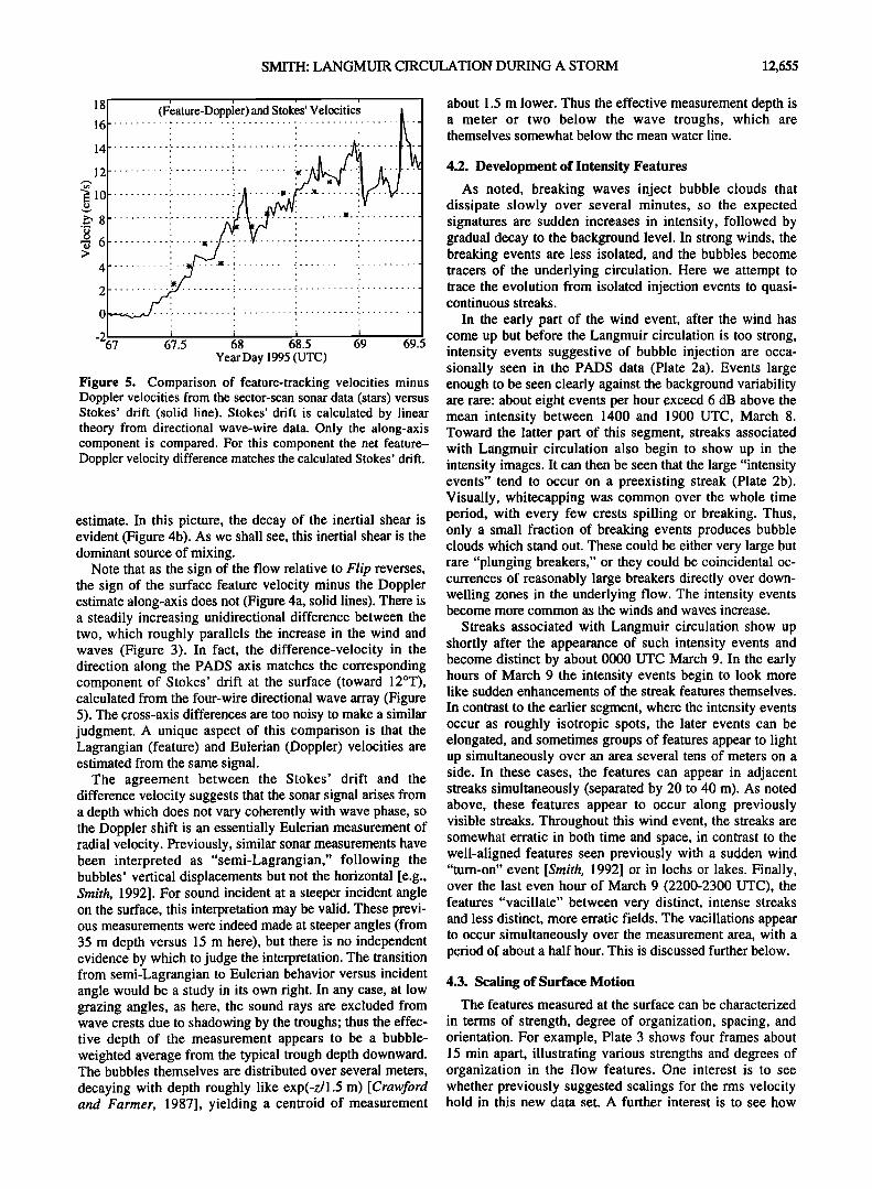
Figure 5. Comparison of feature-tracking velocities minus Doppler velocities from the sector-scan sonar data (stars) versus Stokes' drift (solid line). Stokes' drift is calculated by linear theory from directional wave-wire data. Only the along-axis component is compared. For this component the net feature- Doppler velocity difference matches the calculated Stokes' drift.

estimate. In this picture, the decay of the inertial shear is evident (Figure 4b). As we shall see, this inertial shear is the dominant source of mixing.

Note that as the sign of the flow relative to Flip reverses, the sign of the surface feature velocity minus the Doppler estimate along-axis does not (Figure 46, solid lines). There is a steadily increasing unidirectional difference between the two, which roughly parallels the increase in the wind and waves (Figure 3). In fact, the difference-velocity in the direction along the PADS axis matches the corresponding component of Stokes' drift at the surface (toward 12øT), calculated from the four-wire directional wave array (Figure 5). The cross-axis differences are too noisy to make a similar judgment. A unique aspect of this comparison is that the Lagrangian (feature) and Eulerian (Doppler) velocities are estimated from the same signal.

The agreement between the Stokes' drift and the difference velocity suggests that the sonar signal arises from a depth which does not vary coherently with wave phase, so the Doppler shift is an essentially Eulerian measurement of radial velocity. Previously, similar sonar measurements have been interpreted as "semi-Lagrangian," following the bubbles' vertical displacements but not the horizontal [e.g., Smith, 1992]. For sound incident at a steeper incident angle on the surface, this interpretation may be valid. These previous measurements were indeed made at steeper angles (from 35 m depth versus 15 m here), but there is no independent evidence by which to judge the interpretation. The transition from semi-Lagrangian to Eulerian behavior versus incident angle would be a study in its own right. In any case, at low grazing angles, as here, the sound rays are excluded from wave crests due to shadowing by the troughs; thus the effective depth of the measurement appears to be a bubble- weighted average from the typical trough depth downward. The bubbles themselves are distributed over several meters,

decaying with depth roughly like exp(-z/1.5 m) [Crawford and Farmer, 1987], yielding a centroid of measurement

about 1.5 m lower. Thus the effective measurement depth is a meter or two below the wave troughs, which are themselves somewhat below the mean water line.

4.2. Development of Intensity Features

As noted, breaking waves inject bubble clouds that dissipate slowly over several minutes, so the expected signatures are sudden increases in intensity, followed by gradual decay to the background level. In strong winds, the breaking events are less isolated, and the bubbles become tracers of the underlying circulation. Here we attempt to trace the evolution from isolated injection events to quasi- continuous streaks.

In the early part of the wind event, after the wind has come up but before the Langmuir circulation is too strong, intensity events suggestive of bubble injection are occasionally seen in the PADS data (Plate 26). Events large enough to be seen clearly against the background variability are rare: about eight events per hour exceed 6 dB above the mean intensity between 1400 and 1900 UTC, March 8. Toward the latter part of this segment, streaks associated with Langmuir circulation also begin to show up in the intensity images. It can then be seen that the large "intensity events" tend to occur on a preexisting streak (Plate 2b). Visually, whitecapping was common over the whole time period, with every few crests spilling or breaking. Thus, only a small fraction of breaking events produces bubble clouds which stand out. These could be either very large but rare "plunging breakers," or they could be coincidental oc- currences of reasonably large breakers directly over downwelling zones in the underlying flow. The intensity events become more common as the winds and waves increase.

Streaks associated with Langmuir circulation show up shortly after the appearance of such intensity events and become distinct by about 0000 UTC March 9. In the early hours of March 9 the intensity events begin to look more like sudden enhancements of the streak features themselves.

In contrast to the earlier segment, where the intensity events occur as roughly isotropic spots, the later events can be elongated, and sometimes groups of features appear to light up simultaneously over an area several tens of meters on a side. In these cases, the features can appear in adjacent streaks simultaneously (separated by 20 to 40 m). As noted above, these features appear to occur along previously visible streaks. Throughout this wind event, the streaks are somewhat erratic in both time and space, in contrast to the well-aligned features seen previously with a sudden wind "turn-on" event [Smith, 1992] or in lochs or lakes. Finally, over the last even hour of March 9 (2200-2300 UTC), the features "vacillate" between very distinct, intense streaks and less distinct, more erratic fields. The vacillations appear to occur simultaneously over the measurement area, with a period of about a half hour. This is discussed further below.

4.3. Scaling of Surface Motion

The features measured at the surface can be characterized

in terms of strength, degree of organization, spacing, and orientation. For example, Plate 3 shows four frames about 15 min apart, illustrating various strengths and degrees of organization in the flow features. One interest is to see whether previously suggested scalings for the rms velocity hold in this new data set. A further interest is to see how

12,656 SMITH' LANGMUIR CIRCULATION DURING A STORM

1.5

1

0.5

i i

i 5 Dark Symbols=Velocity

Light Symbols=Intensity 4.5 Solid = 0.25 Stokes' Drift

Dashed = 0.2%W= 1.5u*

4 Dotted = 0.3(USu *) 1/2

3.5

3

l\ '"• f'"""•' - ., ;..1ø:5.,- '

..."?o_ ox _/_ **070 o oOo /x .... ß •. •; •o- ø o

x-- -' '/ ;-' '•,'•:•X • rboo

0 67.5 68 68. 69 Year Day 1995 (UTC)

Figure 6. RMS radial velocity (dark symbols) and intensity (light symbols) associated with the features, versus time. Each symbol represents a half-hour average; crosses represent dubious estimates, circles more reliable ones. For scaling and comparison, 0.25Us (solid line), 0.002W (dashed line), and 0.023(UsW) 1/2 (dotted line) are also shown.

well the scaling of intensity compares to that of the dynamically more important velocity: can intensity images be used as a proxy for velocity in characterizing some aspects of the flow?

To estimate time series of these four characteristics for

both intensity and radial velocity, data from stored sequences of time frames 3 min apart were processed as follows: (1) spatial Fourier transforms were performed in two dimensions, zero-padded to 256 by 256 points (512 by 512 m); (2) the squared magnitudes were formed; (3) these were corrected for the simulated response of the array and processing and normalized into power densities; (4) a noise estimate was formed from the area between 0.1 and 0.25

fractional power response; (5) the high wavenumbers were masked off where the response drops below 0.25 (13 to 18 m wavelength, depending on orientation); and (6) the noise estimate was subtracted. Results for the four example frames are shown in Plate 4. From these corrected power densities, S(t, kx, ky), the four characteristics of interest (strength, spacing, orientation, and organization) were estimated as follows:

4.3.1. Strength. Strength is gauged here by the square root of the integral over wavenumber of the trimmed, corrected spectra (Figure 6); i.e., rms values. For radial velocity the results are expressed in cm/s and denoted V; for intensity I they are expressed in decibels (dB). Log-intensity relative to the mean, corrected for beam pattern and attenuation, is used for two pragmatic reasons: (1) it makes the result independent of source loudness, and (2) the log- intensity is more nearly normally distributed. Note that the ratio of rms radial velocity (cm/s) to rms intensity (dB) remains close to 1.5 over the whole 44-hour period, indicating that similar information is obtained from either with respect to gross strength.

In the absence of wave forcing, the only relevant velocity scale would be the wind W (or friction velocity u*; for this particular data segment, these are roughly proportional). For the Craik-Leibovich mechanism of wind/wave forcing of

Langmuir circulation, it has been suggested that the cross- wind velocity fluctuations should scale roughly with either the geometric mean of the wind and Stokes' drift, (W US) i/2 [Plueddernann, et al., 1996] or with (W2 US)i/3 [Smith, 1996]. Both wind speed W and Stokes' drift US are shown in Figure 6, scaled by a constant chosen to yield a reasonable fit over the middle section of the time period. As noted above, streaks are first seen sometime between the two "wave breaking frames" shown in Plate 2. More precisely, they first appear between 1600 and 1700 March 8, i.e., after year day 67.66, as the wind exceeds 8 m/s. It is therefore reasonable to restrict the scaling analysis to the time segment after this. The strength scales of surface radial velocity features (or intensity) follow the Stokes' drift quite closely from year day 67.66 to the end of the segment, i.e., for winds over 8 m/s.

The suggested scalings for the surface velocity associated with Langmuir circulation can be cast in the general form V- u* (U.Vu*)n. The value of n is then sought as the slope of the best fit line to logto(V/u*) versus loglo(Us/u*) (Figure 7). Surprisingly, the value n=l is found, with very little uncertainty (note that Us/u* varies over almost an order of magnitude and r2=0.89; error bounds on the slope are a standard deviation derived by the bootstrap method with 5000 trials [cf. Diaconis and Efron, 1983]. In other words, once the Langmuir circulation is well developed, V-Us, and wind stress no longer enters directly in scaling the motion. This surprising result appears to imply a strongly nonlinear influence of the waves on the flow (nonlinear, since a threshold value of wind > 8 m/s must be applied, or, more precisely, a threshold for the existence of well-developed Langmuir circulation). This result is not really at odds with

5 10 20 U'/u*

Figure 7. Scaling of the rms measured radial surface velocity takes the general form V-.u*(Us/u*) n. The value of n is sought as the slope of (V/u*) versus (Us/u *) on a log-log plot. This Figure indicates a well-determined value for n very near 1.0; i.e., V-- U s, with no dependence on u* once Langmuir circulation is well formed. Values before year day 67.66, when there were no signs of Langmuir circulation, were excluded from this plot.


(a) Event 1

: i i 518:45 .... i ............. ; .......... i ............. :1520:15 i i i -• 521:45'. : ' ' • i ! ß i i ' : ' : i - : ' i : i . . i - i : i i : :

400 ß ' ' ....i ............. -: ............ _• ............ .• ..................... i ............. : ............. -• ............ :•. ...............

ß . • ß . : ß . - .

. . : : . : . i ! : ...: ............. :. ............ .: ................................ : .......................... .: .............. '2 .................... -• ............. : ............. • ............ Z ................

:

: : 2 ! ' ! ' i : :: ß •

ß

ß ' ' ' ' : ' . ' i ß

300...• ............. i ............. :: .................................... i ............. i ............ i. ............ :: ...................... t ............. i. ' ß • ß

' i : i ' .' • : . ß ' ß : . ! ß 2 . ' .

ß ; - : .'. ß .

..... i ............. i ........... .! ....................... ..X.. i ......... ............. i .......... ! .............. ! ......... ..X.. .......................... i .............. i. ....... ..5.., ß , o

ß . •

ß

.

0 100 200 0 100 200 0 160 200

-10 +10

Intensity dB

(b) Event 2

400 .... ß . .

o .

i '

300

200

............... : ..... • ............. 839:45' ß •

ß .. " o •

ß . •'- ............. '- ............ z ............. z... ' ..........

ß . : . ! :' : ß •

ß • .

ß ' ' : i • .

.... ; ............. ; ............ .:.. ................................. ; .......................... .• ............. : ...............

- ....X .... ....X ........................ . .............. ß .... . ...... ..

ß . • • : : : ß o

0 100 200 0 100 200

Meters E-W

Plate 2. Intensity "injection" events. (a) Near 1520 UTC March 8 1995, before linear features are seen. There is uniform advection up to the right. Note the sudden appearance of two red spots between the first two frames, and two more by the next. Frames are 1.5 min apartß (b) Near 1840 March 8. Now some stripes are evident; note that the two spots appearing in the last frame occur over preexisting stripes. The arrows in the lower right corners indicate the wind speed and direction. An arrow 50 m long (on the image's scale) corresponds to a 10 m/s wind.

the earlier reports [Plueddemann et al., 1996; Smith, 1996], as no attempt was made in these to find an optimal combination. Rather, these works focused only on the fact that including the waves improves the fit over using the wind alone.

A comparison of the magnitude of this velocity scale is also revealing. For SWAPP the maximum rms scale was 7 cm/s with 12 m/s winds; here the rms surface velocity scale V approaches 3.5 cm/s with 15 m/s wind, about 2.5 times smaller as a fraction of wind speed. Alternatively, the wind- only regression from SWAPP is V= 4.4u*. For present purposes, u* (the friction velocity in the water) is roughly W/750 in the SWAPP data, so this translates to V = 0.006W. In contrast, Figure 6 implies a fit toward the end of the

segment of about V = 0.0023W, or 2.6 times smaller as a fraction of wind speed. The overall fit shown in Figure 6 (1.5u*) is smaller than SWAPP's by a factor of 3. In SWAPP the rms cross-wind velocity scaled better with 2(u'US) ll2 than with 4.4u* (or 0.006W) alone. Could some of the discrepancy arise from differences in the Stokes' drift? From Figure 6, the rms radial velocity toward the end scales as 0.25US and 0.0023W (or 1.7u*). Combining these yields 0.65(u'US) 1/2. This is different by a factor of 3.1, an even larger discrepancy, since the ratio US/u* is larger here (up to 6.9) than it was in SWAPP (about 4.8). Finally, it was noted above that the optimal fit here is between V and Us alone. While no search for the optimal combination of Us and u* was attempted for the SWAPP data set, this relation


. . . 03/09/95 2200:02 UTC . . . 400

350 • 300

i 250 .............................................................. [ • 200

ß ' ' 03/09/95 2215:02 UTC ' ' ß .

400 ........ ' '

• 350 ' '

• 300 . i - ": .... : ............... .', - . ? - .............. ß

• 200 ..... . . . . ..

: : i 03./09/95 2230:0.2 UTC : . ß , ,

350 . ' ............ ß

,• 300 ' ' ' . ..................... m, .

• : • :

i• 200 ..... - . : :

: : : 03/09/95 22 .... Intensity 400 ß - ...' ' (ñ•0d•)

300 ....... :. . ........ -'- ? .:.

200 , .: .......... ß .... . : .... : ...... .: ...... 0 50 100 150 200 0 50 100 150 200

Distance E-W (rn) Distance E-W (rn)

Velocity (+20 cm/s)

Plate 3. Four frames 15 min apart during strong forcing conditions. Note how the stripes alternate between well- defined and irregular. The arrows indicate the wind- a 50 m vector (on the image's scale) represents a 10 m/s wind. North is up.

would imply an even larger discrepancy in the magnitudes of V between here and SWAPP. This reduction in V could

help explain the reduced mixing: a reduction of V by 3.1 implies an order of magnitude less kinetic energy at the surface than for corresponding SWAPP-like conditions. This is addressed further below.

What could be responsible for this apparent reduction in the observed velocity scale V? One possibility is the relative directions of low-period swell relative to the wind: these

were initially opposed here and aligned in SWAPP. This could directly affect the wind/wave interaction thought to drive Langmuir circulation. Another possibility is that the bubble-injection rates are unusually high for this event (perhaps also due to the existence of the opposing swell), providing some "buoyant damping" of the motion. Further investigations are needed to select between such alternatives and to determine why and when such suppression of the motion occurs.


100

50-

-50 -

ñ1•"

50-

•o-

ñ100'

50-

-50-

ñ1•'

50-

-100 -100

Intensity Velocity i 03/09/95 '220•':0'2 UTC :

ß H ' ...... •. .... .• ,; ...... 7, ....... H ....... -' ............... ......... • ..... : ........................... • ........ : ..........

" I , ,"['[ ..... , ','.','. ..... ,:':',"'; I . : 03/09/95 2215:02 UTC i : ,• . ,,

................ ! ................ • ...... :•..•.•.-:- •. ...... :_: .....

...... :r:.: .... • ................ • .... .. • .... •:.:..•.•: ..... : •!! ' .-- '-

,

: 03/•/9• 224•:02 •C :

...... ? ..... ......................... ..... ................... , ....................

0 •100 0

Spectral Density (dB relative to peak)

-20 -10 0

Plate 4. Wavenumber spectra for the four frames of (left) intensity and (right) radial velocity shown in Plate 3. All values are relative to the maximum. The vector again represents the wind speed and direction at each time.

4.3.2. Spacing and orientation. To estimate both spacing and orientation, a useful guide is the mean wavenumber. Here the wavenumber spectrum has a 180 ø ambiguity, and the signal is somewhat noisy. To enhance the signal, the power densities are first squared. Then, noting that the wind remains from the SE over this time, and that the orientation of the features remains fairly steady as well, the mean wavenumber is simply estimated from the upper right half of the plane (over the area where kx+ky>O; see

Plate 4)'

l(kx+k..•,>0)S 2 (t,•)d• ' (2) where S(t,k) is the spectral power density of the selected signal. The spacing is found from the magnitude of the mean wavenumber (Figure 8); the orientation from its angle on the wavenumber plane (Figure 9).


i i i

. Dark Symbols = Velocity 5 ..•....' ........... Light=Intensity

...... i•. ' Line =Mixed Laye.r Depth 10 .....

15 : : o o o •3:• . 20 - . . ' ......... o o - øo d - 4-%-

•. o 08 o •o• i +, OoW v++ o o ooOT/[ -o- 4-4- - 0 30 - . . o . .. + o o c•' + oo•-,.•-o• } Q

35 + + .......... 0-O ............ ....... + .... 4: ....... ++ .... :'6 ............. 4- 4'•

* o ............. i3 ....... •'¾ ...... 40 ......... +.4- .......... + ...............

45 .... ++ ..... +. .............................................. + .....

50 • • • 67.5 68 68.5 69

Year Day 1995 (UTC)

Figure 8. Half the feature spacing versus time (symbols), and mixed layer depth (solid line). Crosses represent dubious data. Note the velocity feature spacing (darker circles) generally lies below that of intensity (light circles). This relation indicates that the rolls are approximately as deep as they are wide.

The maximum (and usually dominant) spacing has been seen to track 2 to 3 times the mixed layer depth [Smith et al., 1987; Smith, 1992]. Here the spacing eventually settles on 2 to 2.5 times the mixed layer depth (Figure 8). In the early portion of the time period, the spacing is not well estimated, based on the criterion that the wavenumber uncertainty should be smaller than the magnitude of the mean

•' . ' (a) Orientatzon ' 220 '• Dark Symbols = Velocity \ Light Symbols = Intensity

200 ' ' t .... Solid Line= Stokes'Drift

180 . . ,

160 140 ' ,.,'•

120 . ...... ?'.

+

40 - - ,

30

20

!0 + + 0 + 0 0 o00

-!0 ..... • ......... • .; ......... • . m •

......... + Dark Sym•ls = Vel•ity -30 ... • .................. Light S•ls = Intensity

+ Solid Line = Stokes' Drift

67. 68. Year Day 1995 (UTC)

Figure 9. Orientation of (a) the features relative to north, and (b) relative to the wind direction. Note that the intensity features (light symbols) consistently lie closer to the wind direction than the velocity features.

wavenumber estimate itself (see section 4.3.3). Unreliable estimates are marked by crosses, while the more reliable estimates are marked with open circles. The more reliable estimates occur only after the mixed layer has mixed to 20 m, after which no further deepening is systematically observed. Looking at only the reliable estimates, the intensity features track roughly 2 times the mixed layer depth (MLD), while the radial velocity features tend to be slightly farther apart, at about 2.5 times the MLD. Note that the radial velocity features are consistently larger scale than the intensity.

The mean orientations of the features appear to be more robustly estimated than the spacing. Even when the mean wavenumbers are not well determined, the orientations of the streaks tend to lie nearly parallel to the wind direction (i.e., the mean wavenumber lies about 90 ø off the wind; Figure 9a). To examine this more closely, the orientations relative to the wind are shown in Figure 9b. The mean orientations relative to the wind are formed over just points where both radial velocity and intensity based estimates are judged good. Surprisingly, the mean orientations of intensity versus radial velocity features are not the same: the radial velocity features tend to lie about 10 ø to the right of the wind, while the intensity features average only 2 ø to the right of the wind.

The difference in both spacing and orientation of radial velocity versus intensity features is a new and unexpected observation. This tendency is exemplified in Plate 3b: the radial velocity features have a slightly larger spacing, and an orientation slightly clockwise, relative to the features in the intensity field. This is verified by examination of the spectra (Plate 4b), which show single intense peaks at different wavenumbers for the two fields. This shows that the

differences in scale are not due to noise bias. Sometimes, as in Plate 4b, the peaks in intensity versus velocity spectra are distinct and unrelated to each other; at other times there are

two or more peaks appearing in both spectra, with one favored by the intensity field and the other, clockwise and

3 , , ' l•eakines's , .

Dark Symbols =Velocity ' 2.5 Light Symbols = Intensity ................ ' .......... •>"

o

: : oo o , , ,

: : : : o 9 : : o ',o

.... i ............ : ...... : ...... :--_- - - -; ..... O.:o- 's: ....... 1 ' ' ' o ' ' o' o ' o : : : o • :øo 0 o •oo,., :u o: : : ,:o '" :,, o : ocp: • 0 0 : O , , • "0, 0 ,• 0 O, 0 , v , --'0

.... •--- :..-.,. -d•- ...... -';.-0-0--,o ...... 0'o ...... •"' •'d"- I +-- • ! 0 I J; • • IO: • • • I : -- I: • I ,+ _ •.++Xl',.,.+. i. , , +"'-, , ,

4- , + • 44]• 4- ,-r .....

67.4 67.6 67.8 68 68.2 68.4 68.6 68.8 69

Year Day 1995 (UTC)

Figure 10. Peakiness index for intensity (light symbols) and radial velocity (dark symbols). The peakiness is also used as an indicator of quality: here, and in the related Figures, crosses represent cases where the peakiness falls below 7/8 (dashed line).


closer to the origin, favored by radial velocity (e.g., Plate 4d). The tendency for the radial velocity features to be larger scale and further to the right of the wind than intensity is consistent throughout the "good data" section of the time period (i.e., from year day 67.66 to the end).

4.3.3. Degree of organization. One measure of the degree of organization is the ratio of the magnitude of the mean wavenumber to its uncertainty. The corresponding "peakiness" parameter (analogous to the "Q" of a damped oscillator) is defined as

_ 1/2

ltk+k,.>0)S 2(t,)ar: . (3) kx+kv>O)

Again, the squared power density is used to increase the robustness of the estimated parameters (this differentiates P from the standard Q). Time series of half-hour-mean peakiness are shown in Figure 10. The intensity I features generally have higher peakiness values than velocity V. The ratio of peakiness values Pi/Pv remains near 1.5 over the whole time segment. For this parameter, I again appears to provide a suitable proxy for V, at least for the longer-term averages (but see the vacillation section, below).

Overall, peakiness increases in time, as both the wind and waves increase in strength. However, there are a couple dips in both peakiness series that do not correspond to variations in the wind/wave series: one near year day 68.4 and another near 68.8. In particular, note that over the last 12 hours (year day 68.5 to 69) the wind was exceptionally steady in both magnitude and direction, at 15 rn/s from the SE, while the waves increased only slightly in magnitude.

In addition to providing a measure of the degree of organization or simplicity of the flow, this parameter also indicates when the mean vector wavenumber is reliable and

is used for quality control of the spacing and orientation estimates. A simple threshold is used to distinguish between

3.5

2.5

0.5

I i i i

ß Peakiness, 10-hour close-up

Dark Symbols = Velocity

Light Symbols =tintensity 20 22

0 i I

18 24 02 04

Hour UTC, Year Day 68 & 69

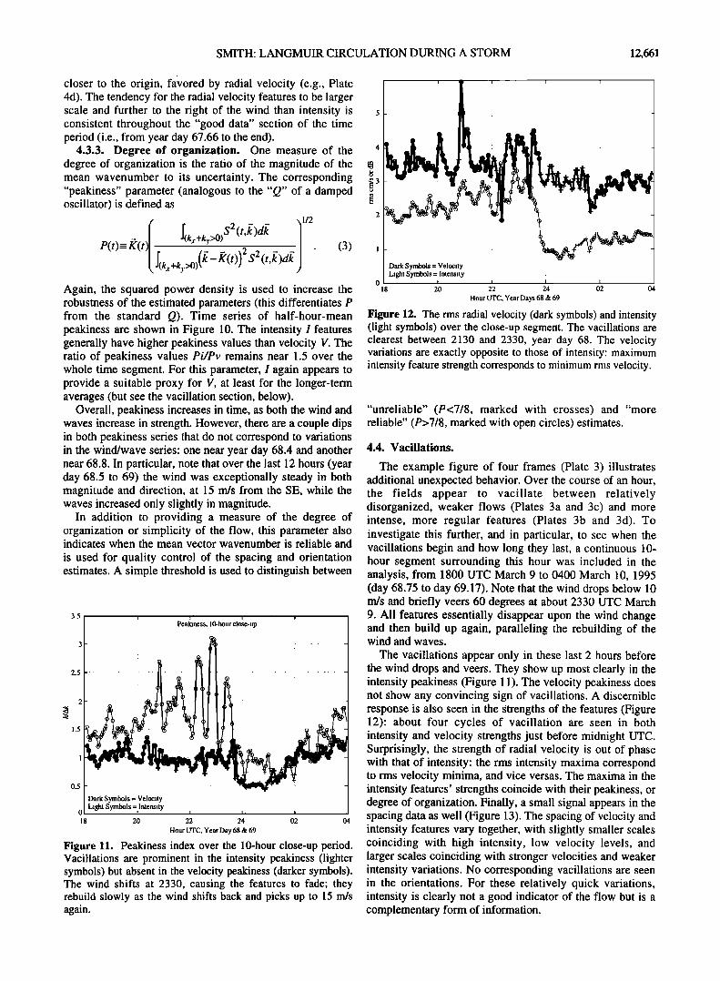
Figure 11. Peakiness index over the 10-hour close-up period. Vacillations are prominent in the intensity peakiness (lighter symbols) but absent in the velocity peakiness (darker symbols). The wind shifts at 2330, causing the features to fade; they rebuild slowly as the wind shifts back and picks up to 15 m/s again.

Dark Symbols = Velocity Light Symbols = Intensity

0 i 2 • • • 18 20 2 24 02 04

Hour UTC, Year Days 68 & 69

Figure 12. The rms radial velocity (dark symbols) and intensity (light symbols) over the close-up segment. The vacillations are clearest between 2130 and 2330, year day 68. The velocity variations are exactly opposite to those of intensity: maximum intensity feature strength corresponds to minimum rms velocity.

"unreliable" (?<7/8, marked with crosses) and "more reliable" (P>7/8, marked with open circles) estimates.

4.4. Vacillations.

The example figure of four frames (Plate 3) illustrates additional unexpected behavior. Over the course of an hour, the fields appear to vacillate between relatively disorganized, weaker flows (Plates 3a and 3c) and more intense, more regular features (Plates 3b and 3d). To investigate this further, and in particular, to see when the vacillations begin and how long they last, a continuous 10- hour segment surrounding this hour was included in the analysis, from 1800 UTC March 9 to 0400 March 10, 1995 (day 68.75 to day 69.17). Note that the wind drops below 10 rn/s and briefly veers 60 degrees at about 2330 UTC March 9. All features essentially disappear upon the wind change and then build up again, paralleling the rebuilding of the wind and waves.

The vacillations appear only in these last 2 hours before the wind drops and veers. They show up most clearly in the intensity peakiness (Figure 11). The velocity peakiness does not show any convincing sign of vacillations. A discernible response is also seen in the strengths of the features (Figure 12): about four cycles of vacillation are seen in both intensity and velocity strengths just before midnight UTC. Surprisingly, the strength of radial velocity is out of phase with that of intensity: the rms intensity maxima correspond to rms velocity minima, and vice versas. The maxima in the intensity features' strengths coincide with their peakiness, or degree of organization. Finally, a small signal appears in the spacing data as well (Figure 13). The spacing of velocity and intensity features vary together, with slightly smaller scales coinciding with high intensity, low velocity levels, and larger scales coinciding with stronger velocities and weaker intensity variations. No corresponding vacillations are seen in the orientations. For these relatively quick variations, intensity is clearly not a good indicator of the flow but is a complementary form of information.


o

• 30

,or: ..... ............. rk •l•ols: •;loc'ity ' I Dashed Line -- M•ixed Layer Depth

18 20 22 24 02 04


Figure 13. Half the spacing (connected symbols) and mixed layer depth (dashed line). During the vacillations (2130 to 2330), the spacing of features in both intensity and radial velocity oscillates together, with minimum spacing coinciding with maximum intensities, minimum velocities (compare with Figure 12). After the wind drops, just before 0000 day 69, the mixed layer shoals. Plate 1 indicates this is partly accounted for by low- mode "vertical stretching."

The vacillations do not appear to be caused by variations in the forcing. Wind and wave speeds and directions are shown in Figure 14 (scaled as before, to facilitate comparisons with Figures 10 and 12). Corresponding variations in the wind speed and direction are absent. The estimated Stokes' drift from time segments shorter than 15 rain are somewhat noisy; however, it is seen that the variations are not coherent with the vacillations. Another

possibility is that the vacillations are forced by internal waves. As indicated above, the mixed layer depth (MLD) over this time is a good indicator of internal wave displacement. As seen in Figure 13, the overall spacing roughly tracks twice the MLD, even after the wind drops and begins to rebuild. However, over the 2 or 3 hours of vacillations, the mixed layer oscillates with a period between 1.5 and 2 hours. The vacillations in strength, spacing, and peakiness are uncorrelated with either the MLD displacement or the magnitude of vertical straining.

5. Discussion

At the outset, three goals of this work were to see (1) how well the mixed layer development is described by current simple modeling ideas; (2) how well previously suggested scalings for the surface velocity variance work; and (3) to what extent sonar intensity signals can serve as an indicator of the flow field, and hence (with another leap of faith) of the underlying vorticity. As it turns out, the observations contain, in addition, two surprises worthy of discussion. (4) There are significant vacillations, never before observed, in the strength, spacing, and peakiness of surface features associated with Langmuir circulation; and (5) the spacing and orientation of intensity (bubbles) and surface radial velocity features do not match.

5.1. Mixing Versus Advection.

Before proceeding to the comparison with simple mixed layer models (which are, for simplicity, one dimensional), it is worth considering the extent to which the measurements may be influenced by advection, both horizontal and vertical.

First, consider uniform uplift of the deeper isotherms, with horizontal spreading or advection of the surface layer (this could be accomplished by upwelling or quasi- geostrophic activity, for example). This would result in net cooling over a fixed depth interval near the surface, say from 0 to 45 m depth. To examine this possibility, the depth axis was rescaled by a constant for each time step such that the heat content in the top 45 m remains constant (Plate lb). The raw and rescaled MLD are both shown in Figure 15. As a fringe benefit, this rescaling appears somewhat successful in removing distortions due to higher frequency internal waves; however, the halt in mixed layer deepening is made even more clear. Indeed, low-mode straining appears to be increasing the mixed layer depth in time, consistent with the fact that the platform is drifting with the flow into deeper water. Low-mode vertical straining or uplift can be ruled out as an explanation for halted deepening.

Next, consider horizontal advection. Flip was freely drifting over this period, moving with the mean over the upper 90 m of the flow plus a small contribution due to windage. The surface layer exhibits inertial motion relative to Flip (see Figure 4): the surface motion reverses in time, with about 1.5 inertial periods represented in the 1.5-day

l! .... sSCo•c•t•e=•o'.25*Stokes ' Dri '' / Dashed Line = 0.2% Wind .

(b) Direction: . •: ' 200 ...... Solid Line = Stokes' Drift. 'PI• ' Dashed Line = Wind I , , ,

18 20 22 24 02 04


Figure 14. (a) Scaled wind speed W (dashed line) and Stokes' drift Us (solid line) and (b) their directions. No "vacillations" in wind speed or direction are seen. Careful comparison of the noisier Stokes' drift estimate shows that the variability is not correlated with the vacillations in the intensity and radial velocity features.


1o

35

40

67 67.5 68 68.5 69 69.5

Year Day 1995

E 20

• 25 ...........

70

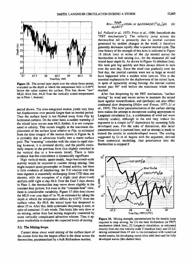
Figure 15. The mixed layer depth over the whole focus period, evaluated as the depth at which the temperature falls to 0.05øC below the value nearest the surface. Thin line shows "raw"

MLD; thick line, MLD from the vertically scaled temperatures (as in Plate 1, bottom).

period shown. The time-integrated motion yields very little net displacement over periods longer than an inertial period. Thus the surface layer is not flushed away from Flip by horizontal currents. On the other hand, a sudden warming of the mixed layer occurs near 68.0; further, it is not compensated in salinity. This occurs roughly at the maximum displacement of the surface layer relative to Flip, as estimated from the time-integral of the motion shown in Figure 4a. It is probably due to advection briefly into a warm surface pool. The "warming" coincides with the cease in rapid mixing; however, it is reversed shortly, and the profile essentially returns to the previous form (but slightly stretched in the vertical due to a low-mode trend). There is little evidence that this coincidence is dynamically significant.

High vertical-mode, quasi-steady, large-horizontal-scale activity would be required to counter strong mixing. One might suspect quasi-geostrophic or frontal activity, but there is little evidence of interleaving: the T-S relation over this time segment is essentially unchanging (from CTD data; not shown), with the exception of a slight (and short-lived) uniform shift right at day 68.0. Over the final 2 days shown in Plate 1, the thermocline may move down slightly in the constant-heat picture; but even in this "constant-heat" view, there is considerable variability. Figure 15 (thin line) shows the MLD over year days 67 to 70, as estimated by taking the depth at which the temperature differs by 0.05øC from the surface value. By 68.0, the mixed layer has deepened to about 25 m. After this, little systematic deepening is seen, in spite of sustained 15 rn/s winds. This looks like very slow or no mixing, rather than fast mixing magically countered by some vertically complicated advection scheme. Thus it appears worthwhile to examine the expected levels of mixing.

5.2. The Mixing Stops.

Current ideas about wind mixing of the surface layer of the oceans hold that the largest effect is the shear across the thermocline, parameterized by a bulk Richardson number,

Ri-- Apgh p0(AU) 2 •>0.64, or Ap>O.64(AU)2(po/gh) (4)

[cf. Pollard et al., 1973; Price et al., 1986; henceforth the "PRT mechanism"]. The velocity jump across the thermocline AU is primarily due to inertial currents generated by sudden changes in the wind; it therefore generally decreases rapidly after a quarter inertial cycle. The time history of the strength of this term is indicated in Figure 16 (thick line) in terms of the Ap needed across the thermocline to halt mixing (i.e., for the measured AU and mixed layer depth h). As shown in Figure 16 (thickest line), this term gets big quickly and then decays almost to zero over the next day. Since the wind rose gradually over the first day, the inertial currents were not as large as would have happened with a sudden wind turn-on. This is the essential explanation for the shallowness of the mixed layer, in spite of apparently strong forcing: the inertial current turned past 90 ø well before the maximum winds were reached.

After fast deepening by the PRT mechanism, "surface stirring" by wind and waves serves to maintain the mixed layer against restratification, and (perhaps) can also effect continued slow deepening [Niiler and Krauss, 1977; Li et al., 1995]. The latter parameterization of the surface stirring term makes the attempt to incorporate scaling appropriate to Langmuir circulation (i.e., a combination of wind and wave velocity scales), although in the end they reduce the argument to a simple (u*)2 dependence by assuming fully developed seas. For the sake of discussion, this latter parameterization is pursued here, and an attempt is made to extend the results to underdeveloped waves. The scaling suggested by Li et al. begins with the argument, derived from numerical modeling, that penetration into the thermocline is stopped if

o

' i.:: i i. i :•: i'! ' '• .> 9.8(USu,2)2/3o/g h" :x.' ! : ! i : ! .: : .at.':-.-'-i .-:i,' " 5:'-.-: ..\..',.i ....................... ;./...

-I 10

10

I

67.5 6•8 68.5 69 Year Day 1995 (UTC)

Figure 16. Mixing strength, parameterized by the density jump required to stop mixing, for (1) the bulk Richardson (or PRT) mechanism (thick line); (2) Langmuir circulation, as estimated directly from the rms velocity scale V (medium line); and (3) LC mixing estimated from Us and vt via comparison with numerical model results, for developing waves (thin solid line) and for fully developed waves (thin dashed line).


Ap > 1.23 w•n (Po/gh), (5) where Wdn is the maximum downwelling velocity associated with the Langmuir circulation. Using model results for Wdn, they rewrite this in the form

AP >Cu*2 (Po /gh) (6) where

C=0.36US/kvt , (7) in which vt is the turbulent kinematic eddy viscosity and k is the wavenumber of the dominant surface waves. For fully developed seas, they argue C is about 50 (Figure 16, thin dashed line). This criterion is evaluated two ways here: (1) using the rms horizontal scale to estimate Wdn directly for use in (5), or (2) extending the evaluation of C to underdeveloped waves, using estimates of Us, k, and vt in (7).

Since the spacing is about twice the mixed layer depth, the rolls appear to be roughly isotropic in the cross-wind plane. It is therefore reasonable to assume the vertical and cross-wind velocity scales are comparable. Assume also that the rms radial velocity scale V derived from the PADS measurements is a good estimate of the cross-wind component size. Finally, to estimate the maximum downwelling velocity from an rms, an argument analogous to that for significant wave height from rms displacement is needed. In brief, the circulation is not simply sinusoidal (in which case Wmax '• 2 •/2V) but varies somewhat randomly. As in the case of wave height, we need to set a threshold, say, one exceeded by l/3 of all downwelling local maxima. This leads to a value roughly 2 times the rms. Hence we substitute 4V2 from the PADS measurements (section 4.3.1) for Wdn in (5). This provides a fairly direct estimate of the strength of mixing due to the observed Langmuir cells (Figure 16, medium width line).

For the indirect approach, a significant requirement is estimation of vt. Recent dissipation measurements near the surface indicate that the turbulent velocity scale q is reasonable well described by the energy dissipation rate of the waves [e.g., Terrav et al., 1996]. This, in turn, is well estimated by the energy input to the waves (within 7% or so). The growth rate •1 of a wave of radian frequency t• and phase speed c is approximately •1 = 33cr(u*/c) 2 [Plant, 1982], so the net energy flux can be written in the form

q3 o,: p-l•lE = 33ga2o.(u */c) 2 = 33(USu*2). (8)

Conveniently, the final form in (8) remains approximately unchanged with integration over the wave spectrum (with perhaps a factor representing the typical directional spread). The length scale appropriate to wave breaking is proportional to the wave amplitude a, so we obtain an ß I oc • ,2 '• estimate of vt of the formv t a(U u ) -. Substituting this into (7), and noting that ak in general does not vary significantly from about 0.1, we obtain

(9)

The values employed by Liet al. for fully developed waves imply U.,7u* • 11.5. To obtain 50 with this value in (9), the constant of proportionality is set to 9.8. Then (6) becomes

Ap >_ 9.8(U S u. 2 ) 2/3 (po /gh ) . (10)

This criterion is also shown in Figure 16 (thin solid line). It is seen that the mixing effect estimated from the

measured velocities falls far below the parametric estimate (10). The discrepancy is very similar in magnitude to that between the velocity scale observed here versus SWAPP: the velocity variance V2 measured here (and hence the corresponding mixing effect) is smaller by a factor between 6 and 10 (thus the SWAPP variance estimates would presumably agree closely with (10)). Over a period of several days, such a reduction could lead to a significant difference in the mixed layer depth. It is therefore important to understand why this variance is reduced. Again, it is conjectured that the existence of opposing swell is important, either directly via the wave/current generation mechanism of Langmuir circulation or indirectly via enhanced wave breaking and bubble injection.

5.3. Vacillations

Vacillations have been described in some simulations of

Langmuir circulation [e.g., Tandon and Leibovich 1995, henceforth TL95]. For strong forcing conditions (defined below), TL95 lind instabilities with two timescales: one "slow" oscillation in strength and organization and a "fast" variation associated with propagation of sinuous perturbations downwind. The slow oscillation has maximum distortions at the times of strongest rms cross-wind velocities and minimum distortion in between. This

compares favorably with the maximum intensity peakiness being observed to coincide with the minimum rms velocities. However, the timescale of the simulated

oscillations corresponds here to tens of hours. At periods of tens of minutes, the fast oscillations might appear attractive for comparison; however, these are self-similar forms propagating downwind and would show up as such in the 2- D views presented here.

The equations used in TL95 depend on two parameters. One is a Reynolds number, Re=u*d/vt, where d is the mixed layer depth and vt is the eddy viscosity, assumed constant. The other is a Rayleigh number, which can be written in the form R=Re3(US/u*). For initial (2-D) instabilities, only R enters, and the critical number for the onset of Langmuir circulation is about Rc=669 (presumably depending on details of the geometry and boundary conditions).

The eddy viscosity, and hence Re, is hard to estimate (notwithstanding the arguments of section 5.2). On the other hand, it is straightforward to compute US/u* (Figure 17). One approach is to assume that the "turbulence" (all motion excluding the Langmuir circulation (LC)) adjusts so that Re remains constant. Then let R=Rc at the moment LCs are first detected, i.e., no sooner than year day 67.66 (as noted above). At that time, US/u * is about 2 and increasing rapidly (Figure 17); thus Re=(669/2)•/3=6.9. For Re=5.9, TL95 find no oscillatory instabilities no matter how much R is increased. The oscillatory behavior is observed for R>900 and Re=22.36 (or Re.•=l 1,180), but this large a value for Re is hard to reconcile with the observed onset of LC activity. To get R below the critical value would require US/u*<O.06. The lower bound on Re for such oscillatory instabilities has not been established. Given both this and the mismatch in

timescales, comparison with the simulations is not convincing. Furthermore, if we use the viscosity estimate of section 5.2, Re actually decreases between the onset of LC

SMITH' LANGMUIR CIRCULATION DURING A STORM 12,665

7

6

5

c> 4 .,..•

a• 3 2

3.5

3

2.5

1.5

1

0.5

0

(b) (U." u*2) •/-•

67'.5 6• 68'.5 6• Year Day 1995 (UTC)

Figure 17. (a) Ratio of Stokes' drift to friction velocity, US/u *. The ratio is formed with a vector dot-product, so that opposing wind and waves produce a negative ratio as seen early on year day 67. The ratio increases over the course of the storm, finally skyrocketing when the wind relaxes, and staying high until the wind resumes. (b) Scaling arguments lead to the idea that bubble density, viscosity, and Langmuir circulation strength each may

each half cycle; in the latter the locations from one realization to the next would be random. In either case, rms velocity maxima would occur halfway between the intensity maxima in time, as observed. To pursue the first possibility a bit, in this case the intensity maxima occur every half cycle, so the period of oscillation is an hour. A sinusoidal oscillation having an hour period with velocity maxima of 6 cm/s would produce displacements of +35 m. Over this time segment, the rolls have about 25 m spacing, so this is enough displacement to move bubbles back and forth into the downwelling zones (and some distance downward). Accelerations associated with such oscillating rolls would reach 0.0001 m/s2, about equal to the estimated reduced gravity value. Thus buoyancy forcing by bubbles produces a self-consistent scenario, demonstrating that it is feasible for bubble buoyancy to be important to the overall forcing. Similar arguments apply for the regeneration case: the estimated displacements are sufficient to sweep the surface bubble clouds into the downwelling lines and "shut off" the circulation; these must then regenerate in 15 min or so (consistent with typical LC growth rates) before the bubbles are again sufficiently well organized to stop the flow.

In either scenario, the occurrence of vacillations is linked to a high level of bubble generation; thus it would be appropriate to parameterize it in terms of some measure of wave breaking. A reasonable conjecture is that bubble density is related to the rate of wave breaking. A reasonable approach is to combine the arguments of section 5.2 with the arguments of Bagnold [1962] for self-suspending turbidity currents (that the turbulent velocity scale q must exceed the settling velocity, but here with the buoyancy and vertical

scale with q = (Usu*2) 1/3. In particular, note the brief but distinct axes reversed). Then the maximum bubble size, and hence peak in this parameter near the end of year day 68. Vacillations are seen only over the time of this peak (for q>3.6 cm/s).

and the vacillations. Indeed, it would appear possible that the parameters are moved back to marginal stability rather than to "overforced" conditions.

An interesting possibility is that the bubbles influence the dynamics. For 15 m/s winds the volume fraction of bubbles a meter below the surface is expected to be about 10-6 [e.g., Crawford and Farmer, 1987]. During the intense phase of the vacillations, the intensity varies by +10 dB, yielding estimated volume fractions of 10-5 at the convergences. This corresponds to a density anomaly of 0.01 kg/m3, yielding a reduced gravity acceleration of 10 -4 m/s2. This acceleration would stop a downwelling velocity of 6 cm/s in 10 min. The bubbles do not disappear instantly, so the flow could actually reverse due to continued buoyancy forcing, or the structures could simply break up and dissipate. If the flow reverses, the reversed flow could be reinforced by the same LC instability mechanism (e.g., the freshly upwelled water is now moving downwind more slowly, inducing a wave force reinforcing the upwelling). This would produce new intensity maxima falling somewhere between the maxima of the previous cycle (over the half-hour between maxima, advection moves the features beyond the sample area, so this possibility can not be directly tested). Alternatively, the structures could simply regenerate from scratch. In the former scenario the rolls would oscillate back and forth, with upwelling and downwelling zones exchanging places at

total bubble density (assuming a self-similar spectrum of bubbles), is parameterized by q- (Usu*2) 1/3 (Figure 17b). The vacillations only occur only over the 2 hours where this parameter exceeds 3.6 cm/s. Such a wind-wave parameter indicative of wave breaking has proven elusive to verify; however, visual observations during this segment confirm that wave breaking was vigorous. Interestingly, this particular combination (Usu*2) •/3 also can parameterize the theoret- ical strength of forcing of the Langmuir circulation: in other words, from a scaling point of view, turbulence, bubble density, and Langmuir cell forcing may be indistinguishable.

5.4. Relations Between I and V

In terms of overall strength and organization (e.g., hourly means), the statistics of I (intensity) correlate well with those of V (radial velocity). However, in terms of the orientation and spacing, there is a surprising but consistent difference: the intensity features tend to be slightly smaller in scale (2.0 versus 2.5 times the mixed layer depth) and more nearly aligned with the wind (2 ø versus 10ø). Further, this is not simply a matter of different weightings of broad distributions. For example, in Plate 4b, unimodal peaks appear in the spatial spectra of I and V but in different locations. In detailed comparisons (e.g., section 4.4, during the vacillations), even the strength and organization values can differ, with half-hour period variations occurring out of phase between I and V. These puzzling differences between the distribution and behavior of I versus V do not appear to have a simple explanation.

The link between spatial distributions of the bubbles (intensity) and the velocity field has not been rigorously


investigated. Given that the velocity fields vary in time and that bubble dynamics involve wave breaking, surfactants, gas saturation levels, and pressure effects (to name a few), it is plausible that bubble distributions are not always reliable indicators of the instantaneous flow. The bubble field is a

complex time integral of both the velocity field and some nonnegligible (and marginally understood) chemistry. Thus, given the observed mismatches, caution is advised in using intensity maps as indicators of surface convergence zones, much less as indicators of the underlying vorticity. Simulations of the behavior of bubble clouds may help to understand these differences. In situ correlations between

(for example) vertical velocity and bubble density may also help. This is suggested as a reasonable avenue of research.

6. Conclusions

1. The mixed layer deepened rapidly initially, to about 20 m. After the inertial current veered more than 90 ø off the

wind, the mixing slowed. This is consistent with current thinking, where the "bulk dynamics" of shear across the thermocline due to inertial motion is the primary agent for deepening. Surface stirring by the combined action of wind and waves may have helped maintain the mixed layer after this and may even have induced some additional slow deepening. In any case, it is emphasized that the inertial current "bulk Richardson number" mechanism is the lowest

order term in wind-induced mixing (and no model is complete without it).

2. The magnitude of surface velocity variance associated with the mixed layer motion, as observed here, is considerably smaller than in previously reported cases. It is suggested that this is related to swell opposing the wind.

3. For the data considered here, rms velocities associated

with the low-frequency features scale quite tightly with the Stokes' drift alone, rather than with the wind or a combination of wind and waves. This relation is nonlinear in

the sense that a threshold must be set for the existence of

Langmuir circulation before it holds. 4. Langmuir circulation can vary significantly in strength,

spacing, and peakiness over timescales of the order of 15 min. Neither the wind, waves, nor mixed layer depths vary significantly on this timescale. In these "vacillations," the strengths of velocity versus intensity features were 180 ø out of phase: strongest intensity features coincided with weakest rms velocities. It is suggested that the buoyancy of bubbles may be nonnegligible in the dynamics of these phenomena.

5. Overall strength and peakiness values correlate well between intensity and velocity features (over timescales comparable to a day). However, in details such as spacing, orientation, or short-time behavior, significant differences can occur. Also, the typical spacing and orientation of intensity versus velocity features near the surface differ. For the data studied here, intensity features aligned within a couple degrees of the wind (favoring the right), while the velocity features were typically 10 ø to the right of the wind. The intensity spacing tracks 2 times the mixed layer depth, while the velocity feature spacing is closer to 2.5 times MLD. While this mismatch is puzzling, it would appear likely that the time/space-dependent behavior of bubbles in a time-varying flow should be investigated. Simulations with realistic bubble dynamics may help to understand these differences.

6. The difference between mean feature-tracking and Doppler velocity estimates provides a reasonable and direct estimate of the Stokes' drift near the surface. A unique aspect is that both estimates come from the same data stream, without explicitly resolving the waves.

Appendix

The PADS system operates by transmitting repeat- sequence codes [Pinkel and Smith, 1992] over a 25 ø (horizontal) by 2 ø (vertical) swath, and receiving on a horizontal array of 16 receivers. The receivers are arranged in a semisparse array of the form "1111-1111-0000-0000- 1111-0000-1111," where the 1 's represent receivers and the O's represent gaps of a size equal to a receiver (the dashes are to make this easier to read; they represent no space). The spacing is as uniform as practical, at 0.976 cm per unit on average. This configuration provides four or more pairs at each spatial lag up to 24, tapering to one pair at the maximum separation of 27 units (center to center). This "semisparseness" trades some phase uncertainty (velocity error) for added angular resolution, relative to a simple 16- in-a-row array. For sound at 194.3 kHz, 12øC, salinity 33, and 16 m depth (typical of conditions here), the Nyquist wavenumber of the receiver array corresponds to 23.2 ø off- axis. The 194.3 kHz center-frequency signal from each receiver is electronically mixed to a nonzero frequency and digitized with 16 bit accuracy. The mix frequency is selected to produce four samples/cycle at the center frequency with no Doppler shift. To avoid aliasing of the signal across zero frequency with this one-sided mixing scheme, we initially oversample by a factor of 2; thus the repeat-sequence code "bits" are four samples long, and the signal is constrained to the center half of the sampling bandwidth. The amplifiers, mixing, and filtering electronics maintain nearly the full 96 dB dynamic range achievable with 16 bit digitization. This obviates the complexity and uncertainties associated with a time-variable gain, as the signal varies about 70 dB from near to far range. The digitized signal is computationally remixed and filtered to a complex signal having zero frequency for zero Doppler shift and resampled to 0.25 times as many complex points (C samples).

Matrices of time-lagged covariances are then formed as a function of range: the signal at one C sample on a given receiver is multiplied by the conjugate of each signal at the previous C sample, resulting in a set of 16 by 16 matrices of covariances versus range. Because of the finite time lag, these matrices are not symmetric except in the case of exactly zero Doppler shift. The matrices of covariances are averaged over a specified range interval (2.7 m) and further averaged over consecutive pings (keeping range bins aligned) for a specified time interval (40 pings or 30 s). Retaining the full set of matrices for each range permits postcalibration of the receivers and refinement of beam- forming strategies. The penalty is 256/55, or about 5 times larger, storage requirements relative to storing only nonredundant lags.

The following postcalibration scheme was adopted as effective and robust: for each hour, the full hour time- averaged covariance matrix is formed for each range. The matrix's column averages represent the covariances of each indexed receiver with the mean signal. These provide an empirical amplitude and phase relative to the mean of all


receivers. This can be range dependent, as the angle of incidence varies with range, and the receivers do not have identical beam patterns in the vertical. To facilitate display, a log-linear profile (corresponding to constant attenuation) is fit to the hour-mean intensities over a central range interval and compensated for. The hour averages do not vary much from hour to hour but can change over the course of a day, especially as wind and wave conditions change. The calibrated, attenuation-corrected covariances are finally averaged into a nonredundant array, windowed with a Kaiser-Bessel fifth order window, zero-padded to 128 points, and fast Fourier transformed. The FFT output corresponds to beams at an array of 128 angles from-23.2 to +23.2 ø off axis. This array wraps around at +23.2ø; to avoid confusion, the transmitted beam pattern was designed to insonify only the central +12.5 ø, and the outer 10.7 ø on each side is discarded. The combined transmit-receive beam

pattern is computed from the hour-average covariances, and the retained 25 ø wedge is corrected for this in the intensity plots shown.

Acknowledgments. Thanks are due to the many people involved in MBLEX for making it a success. Regarding the gathering of this pm'ticulm' data, thanks go especially to Eric Slater, Lloyd Green, Mike Golden, Chris Neely, R. Pinkel, K. Rieder, M. Alford, and to the crew of the research platform Flip, captained by Tom Golfinas. Thanks also for useful comments from R. Pinkel, C. Garrett, A. Tandon, and W. Drennan concerning this work and interpretation. This work was supported by the Office of Naval Research, grants N00014-93-1-0359 and N00014-96-1-0030.

References

Bagnold, R. A., Autosuspension of transported sediment: Turbidity currents, Proc. R. Soc. London, Ser. A, 265, 315, 1962.

Brumley, B. H., R. G. Cabrera, K. L. Deines, and E. A. Terray, Performance of a broad-band acoustic Doppler current profiler, IEEE J. Oceanic Eng., ! 6, 402-407, 1991.

Cox, S. M., and S. Leibovich, Langmuir circulations in a surface layer bounded by a strong thermocline, J. Phys. Oceanogr., 23, 1330- 1345, 1993.

Cox, S. M., and S. Leibovich, Large-scale Langmuir circulation and double-diffusive convection - evolution equations and flow transitions, J. Fluid Mech., 276, 189-210, 1994.

Cox, S. M., S. Leibovich, I. M. Moroz, and A. Tandon, Nonlinear dynamics in Langmuir circulations with 0(2) symmetry, J. Fluid Mech., 241,669-704, 1992.

Craik, A.D. D., The generation of Langmuir circulation by an instability mechanism, J. Fluid Mech., 81,209-223, 1977.

Craik, A.D. D., and S. Leibovich, A rational model for Langmuir circulations, J. Fluid Mech., 73, 401-426, 1976.

Crawford, C. B., and D. M. Farmer, On the spatial distribution of ocean bubbles, J. Geophys. Res., 92, 8231-8243, 1987.

Diaconis, and B. Eft'on, Computer-intensive methods in statistics, Sci. Am., 248, 116-130, 1983.

Farmer, D., and M. Li, Patterns of bubble clouds organized by Langmuir circulation, J. Phys. Oceanogr., 25, 1426-1440, 1995.

Gan'ett, C., Generation of Langmuir circulations by surface waves- A feedback mechanism, J. Mar. Res., 34, 117-130, 1976.

Langmuir, I., Surface motion of water induced by wind, Science, 87, 119-123, 1938.

Leibovich, S., Convective instability of stably stratified water in the ocean, J. Fluid Mech., 82, 561-581, 1977.

Leibovich, S., On wave-current interaction theories of Langmuir circulations, J. Fluid Mech., 99, 715-724, 1980.

Leibovich, S., The form and dynamics of Langmuir circulations, Annu. Rev. Fluid Mech., 15, 391-427, 1983.

Leibovich, S., and S. Paolucci, The Langmuir circulation as a mixing mechanism in the upper ocean, J. Phys. Oceanogr., 10, 186-207, 1980.

Leibovich, S., and A. Tandon, Three-dimensional Langmuir

circulation instability in a stratified layer, d. Geophys. Res., 98, 16,501 - 16,507, 1993.

Li, M., and C. Garrett, Mixed layer deepening due to Langmuir circulation, J. Phys. Oceanogr., 27, 121-132, 1997.

Li, M., K. Zahariev, and C. Garrett, Role of Langmuir circulation in the deepening of the ocean surface mixed layer, Science, 270, 1955-1957, 1995.

Longuet-Higgins, M. S., D. E. Cartwright, and N. D. Smith, Observations of the directional spectrum of sea waves using the motions of a floating buoy, in Ocean Wave Spectra: Proceedings of a Conference, edited by National Academy of Sciences, pp. 11 1-132, Prentice-Hall, Englewood Cliffs, N.J., 1963.

McWilliams, J. C., P. P. Sullivan, and C. H. Moeng, Langmuir turbulence in the ocean, J. Fluid Mech., 334, 1-30, 1997.

Niiler, P. P., and E. B. Krauss, One-dimensional models of the upper ocean, in Modeling and Prediction of the Upper Layers of the Ocean, edited by E. B. Krauss, pp. 143-172, Pergammon, Tarrytown, N.Y., 1977.

O'Brien, M. M., A. Plueddemann, and R. A. Weller, The response of oceanic mixed layer depth to physical forcing - modelled vs observed, Biol. Bull., 181,360-361, 1991.

Pinkel, R., and J. A. Smith, Repeat-sequence coding for improved precision of Doppler sonar and sodar, J. Atmos. Oceanic Technol., 9, 149-163, 1992.

Plant, W. J., A relationship between wind stress and wave slope, J. Geophys. Res., 87, 1961 - 1967, 1982.

Plueddemann, A. J., J. A. Smith, D. M. Farmer, R. A. Weller, W. R. Crawford, R. Pinkel, S. Vagle, and A. Gnanadesikan, Structure and variability of Langmuir circulation during the surface waves processes program, J. Geophys. Res., 101, 3525-3543, 1996.

Pollard, R. T., P. B. Rhines, and R. Thompson, The deepening of the wind-mixed layer, Geophys. Fluid Dyn., 4, 381-404, 1973.

Price, J. F., R. A. Weller, and R. Pinkel, Diurnal cycling: Observations and models of the upper ocean response to diurnal heating, cooling, and wind mixing, J. Geophys. Res., 91, 8411- 8427, 1986.

Rieder, K. F., and J. A. Smith, Removing wave effects from the wind stress vector, J. Geophys. Res., 103, 1363-1374, 1998.

Rummler, W. D., Introduction of a new estimator for velocity spectral parameters. Rep. MM-68-4141-5, AT&T Bell Labs., Murray Hill, N.J., 1968.

Skyllingstad, E. D., and D. W. Denbo, An ocean large-eddy simulation of Langmuir circulations and convection in the surface mixed layer, J. Geophys. Res., 100, 8501-8522, 1995.

Smith, J. A., Observed growth of Langmuir circulation, J. Geophys. Res., 97, 5651-5664, 1992.

Smith, J. A., Observations of Langmuir circulation, waves, and the mixed layer, in The Air Sea Interface: Radio and Acoustic Sensing, Turbulence, and Wave Dynamics, edited by M. A. Donelan, W. H. Hui, and W. J. Plant, pp. 613-622, Univ. of Toronto Press, Toronto, Ont., 1996.

Smith, J. A., and R. Pinkel, Improvement of Doppler estimation through repeat sequence coding, in Oceans '91?Proceedings, October 1-3, 1991, Honolulu, Hawaii, USA/Ocean Technologies and Opportunities in the ?acifi'c for the 90's, pp. 977-984, IEEE, Piscataway, N.J., 1991.

Smith, J. A., and K. F. Rieder, Wave induced motion of FLIP, Ocean Eng., 24, 95-110, 1997.

Smith, J. A., R. Pinkel, and R. Weller, Velocity structure in the mixed layer during MILDEX, J. Phys. Oceanogr., 17, 425-439, 1987.

Tandon, A., and S. Leibovich, Simulations of three-dimensional Langmuir circulation in water of constant density, J. Geophys. Res., 100, 22613-22623, 1995.

Terray, E. A., M. A. Donelan, Y. C. Agrawal, W. M. Drennan, K. K. Kahma, A. J. Williams, P. A. Hwang, and S. A. Kitaigorodskii, Estimates Of Kinetic Energy Dissipation Under Breaking Waves, Journal Of Physical Oceanography, 26, 792-807, 1996.

Thorpe, S. A., On the clouds of bubbles formed by breaking wind waves in deep water, and their role in air-sea gas transfer., Philos. Trans. R. Soc. London, Ser. A, 304, 155-210, 1982.

Thorpe, S., Bubble clouds: A review of their detection by sonar, of related models, and of how K v may be determined., in Oceanic Whitecaps and Their Role in Air-Sea Exchange Processes, edited by E. C. Monahan and G. Mac Noicall, pp. 57-68, D. Reidel, Norwell, Mass., 1986.

Thorpe, S. A., The breakup of Langmuir circulation and the instability of an an'ay of vortices, J. Phys. Oceanogr., 22,350-360, 1992.


Thorpe, S., and A. J. Hall, The characteristics of breaking waves, bubble clouds, and near-surface currents observed using side-scan sonar, Cont. Shelf Res., 1,353-384, 1983.

Trevorrow, M. V., and D. M. Farmer, The use of Barker codes in Doppler sonar measurements, J. Atmos. Oceanic Technol., 9, 699- 704, 1992.

Vagle, S., W. G. Large, and D. M. Farmer, An evaluation of the WOTAN technique of inferring oceanic winds from underwater ambient sound, J. Atmos. Oceanic Technol., 7, 576-595, 1990.

Weller, R., J.P. Dean, J. Matra, J. Price, E. A. Francis, and D.C. Boardman, Three-dimensional flow in the upper ocean, Science, 227, 1552-1556, 1985.

Zedel, L., and D. Farmer, Organized structures in subsurface bubble clouds - Langmuir circulation in the open ocean, J. Geophys. Res., 96, 8889-8900, 1991.

J. A. Smith, Scripps Institution of Oceanography, code 0213, La Jolla, CA 92093-0213. (e-mail: [email protected])

(Received May 7, 1997; revised November 12, 1997; accepted December 1, 1997.)

(1998). "evolution of langmuir circulation during a storm."

Documents