18.440: lecture 25 .1in covariance and some conditional...
TRANSCRIPT

18.440: Lecture 25
Covariance and some conditionalexpectation exercises
Scott Sheffield
MIT
18.440 Lecture 25

Outline
Covariance and correlation
Paradoxes: getting ready to think about conditional expectation
18.440 Lecture 25
Outline
Covariance and correlation
Paradoxes: getting ready to think about conditional expectation
18.440 Lecture 25

A property of independence
I If X and Y are independent thenE [g(X )h(Y )] = E [g(X )]E [h(Y )].
I Just write E [g(X )h(Y )] =∫∞−∞
∫∞−∞ g(x)h(y)f (x , y)dxdy .
I Since f (x , y) = fX (x)fY (y) this factors as∫∞−∞ h(y)fY (y)dy
∫∞−∞ g(x)fX (x)dx = E [h(Y )]E [g(X )].
18.440 Lecture 25

A property of independence
I If X and Y are independent thenE [g(X )h(Y )] = E [g(X )]E [h(Y )].
I Just write E [g(X )h(Y )] =∫∞−∞
∫∞−∞ g(x)h(y)f (x , y)dxdy .
I Since f (x , y) = fX (x)fY (y) this factors as∫∞−∞ h(y)fY (y)dy
∫∞−∞ g(x)fX (x)dx = E [h(Y )]E [g(X )].
18.440 Lecture 25

A property of independence
I If X and Y are independent thenE [g(X )h(Y )] = E [g(X )]E [h(Y )].
I Just write E [g(X )h(Y )] =∫∞−∞
∫∞−∞ g(x)h(y)f (x , y)dxdy .
I Since f (x , y) = fX (x)fY (y) this factors as∫∞−∞ h(y)fY (y)dy
∫∞−∞ g(x)fX (x)dx = E [h(Y )]E [g(X )].
18.440 Lecture 25
Defining covariance and correlation
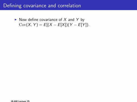
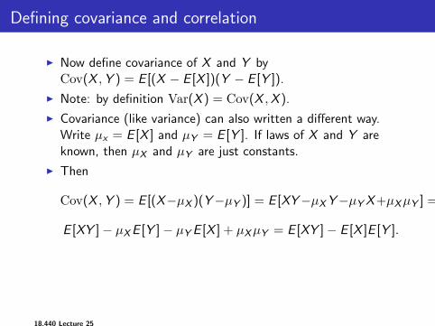
I Now define covariance of X and Y byCov(X ,Y ) = E [(X − E [X ])(Y − E [Y ]).
I Note: by definition Var(X ) = Cov(X ,X ).
I Covariance (like variance) can also written a different way.Write µx = E [X ] and µY = E [Y ]. If laws of X and Y areknown, then µX and µY are just constants.
I Then
Cov(X ,Y ) = E [(X−µX )(Y−µY )] = E [XY−µXY−µYX+µXµY ] =
E [XY ]− µXE [Y ]− µYE [X ] + µXµY = E [XY ]− E [X ]E [Y ].
I Covariance formula E [XY ]− E [X ]E [Y ], or “expectation ofproduct minus product of expectations” is frequently useful.
I Note: if X and Y are independent then Cov(X ,Y ) = 0.
18.440 Lecture 25

Defining covariance and correlation
I Now define covariance of X and Y byCov(X ,Y ) = E [(X − E [X ])(Y − E [Y ]).
I Note: by definition Var(X ) = Cov(X ,X ).
I Covariance (like variance) can also written a different way.Write µx = E [X ] and µY = E [Y ]. If laws of X and Y areknown, then µX and µY are just constants.
I Then
Cov(X ,Y ) = E [(X−µX )(Y−µY )] = E [XY−µXY−µYX+µXµY ] =
E [XY ]− µXE [Y ]− µYE [X ] + µXµY = E [XY ]− E [X ]E [Y ].
I Covariance formula E [XY ]− E [X ]E [Y ], or “expectation ofproduct minus product of expectations” is frequently useful.
I Note: if X and Y are independent then Cov(X ,Y ) = 0.
18.440 Lecture 25

Basic covariance facts
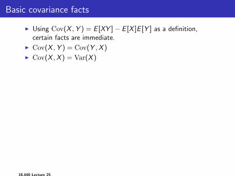
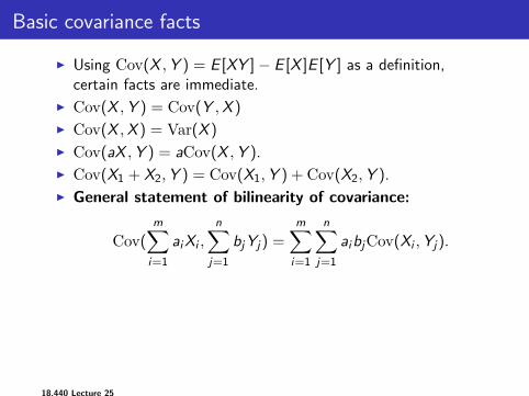
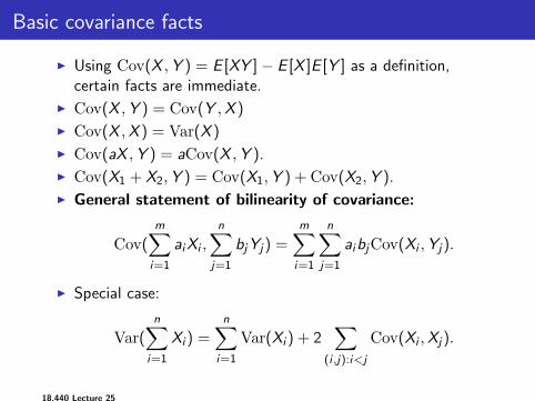
I Using Cov(X ,Y ) = E [XY ]− E [X ]E [Y ] as a definition,certain facts are immediate.
I Cov(X ,Y ) = Cov(Y ,X )
I Cov(X ,X ) = Var(X )
I Cov(aX ,Y ) = aCov(X ,Y ).
I Cov(X1 + X2,Y ) = Cov(X1,Y ) + Cov(X2,Y ).
I General statement of bilinearity of covariance:
Cov(m∑i=1
aiXi ,
n∑j=1
bjYj) =m∑i=1
n∑j=1
aibjCov(Xi ,Yj).
I Special case:
Var(n∑
i=1
Xi ) =n∑
i=1
Var(Xi ) + 2∑
(i ,j):i<j
Cov(Xi ,Xj).
18.440 Lecture 25

Basic covariance facts
I Using Cov(X ,Y ) = E [XY ]− E [X ]E [Y ] as a definition,certain facts are immediate.
I Cov(X ,Y ) = Cov(Y ,X )
I Cov(X ,X ) = Var(X )
I Cov(aX ,Y ) = aCov(X ,Y ).
I Cov(X1 + X2,Y ) = Cov(X1,Y ) + Cov(X2,Y ).
I General statement of bilinearity of covariance:
Cov(m∑i=1
aiXi ,
n∑j=1
bjYj) =m∑i=1
n∑j=1
aibjCov(Xi ,Yj).
I Special case:
Var(n∑
i=1
Xi ) =n∑
i=1
Var(Xi ) + 2∑
(i ,j):i<j
Cov(Xi ,Xj).
18.440 Lecture 25

Defining correlation
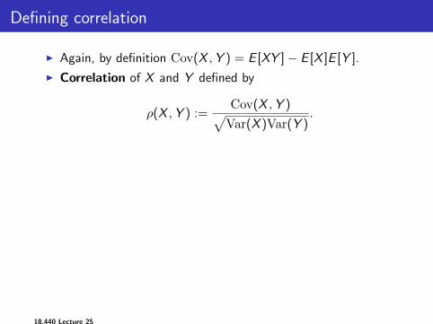
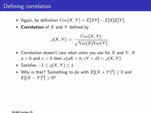
I Again, by definition Cov(X ,Y ) = E [XY ]− E [X ]E [Y ].
I Correlation of X and Y defined by
ρ(X ,Y ) :=Cov(X ,Y )√Var(X )Var(Y )
.
I Correlation doesn’t care what units you use for X and Y . Ifa > 0 and c > 0 then ρ(aX + b, cY + d) = ρ(X ,Y ).
I Satisfies −1 ≤ ρ(X ,Y ) ≤ 1.
I Why is that? Something to do with E [(X + Y )2] ≥ 0 andE [(X − Y )2] ≥ 0?
I If a and b are positive constants and a > 0 thenρ(aX + b,X ) = 1.
I If a and b are positive constants and a < 0 thenρ(aX + b,X ) = −1.
18.440 Lecture 25
Defining correlation
I Again, by definition Cov(X ,Y ) = E [XY ]− E [X ]E [Y ].
I Correlation of X and Y defined by
ρ(X ,Y ) :=Cov(X ,Y )√Var(X )Var(Y )
.
I Correlation doesn’t care what units you use for X and Y . Ifa > 0 and c > 0 then ρ(aX + b, cY + d) = ρ(X ,Y ).
I Satisfies −1 ≤ ρ(X ,Y ) ≤ 1.
I Why is that? Something to do with E [(X + Y )2] ≥ 0 andE [(X − Y )2] ≥ 0?
I If a and b are positive constants and a > 0 thenρ(aX + b,X ) = 1.
I If a and b are positive constants and a < 0 thenρ(aX + b,X ) = −1.
18.440 Lecture 25

Important point
I Say X and Y are uncorrelated when ρ(X ,Y ) = 0.
I Are independent random variables X and Y alwaysuncorrelated?
I Yes, assuming variances are finite (so that correlation isdefined).
I Are uncorrelated random variables always independent?
I No. Uncorrelated just means E [(X − E [X ])(Y − E [Y ])] = 0,i.e., the outcomes where (X − E [X ])(Y − E [Y ]) is positive(the upper right and lower left quadrants, if axes are drawncentered at (E [X ],E [Y ])) balance out the outcomes wherethis quantity is negative (upper left and lower rightquadrants). This is a much weaker statement thanindependence.
18.440 Lecture 25

Examples
I Suppose that X1, . . . ,Xn are i.i.d. random variables withvariance 1. For example, maybe each Xj takes values ±1according to a fair coin toss.
I Compute Cov(X1 + X2 + X3,X2 + X3 + X4).
I Compute the correlation coefficientρ(X1 + X2 + X3,X2 + X3 + X4).
I Can we generalize this example?
I What is variance of number of people who get their own hatin the hat problem?
I Define Xi to be 1 if ith person gets own hat, zero otherwise.
I Recall formulaVar(
∑ni=1 Xi ) =
∑ni=1Var(Xi ) + 2
∑(i ,j):i<j Cov(Xi ,Xj).
I Reduces problem to computing Cov(Xi ,Xj) (for i 6= j) andVar(Xi ).
18.440 Lecture 25
Outline
Covariance and correlation
Paradoxes: getting ready to think about conditional expectation
18.440 Lecture 25

Outline
Covariance and correlation
Paradoxes: getting ready to think about conditional expectation
18.440 Lecture 25
Famous paradox
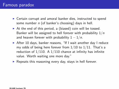
I Certain corrupt and amoral banker dies, instructed to spendsome number n (of banker’s choosing) days in hell.
I At the end of this period, a (biased) coin will be tossed.Banker will be assigned to hell forever with probability 1/nand heaven forever with probability 1− 1/n.
I After 10 days, banker reasons, “If I wait another day I reducemy odds of being here forever from 1/10 to 1/11. That’s areduction of 1/110. A 1/110 chance at infinity has infinitevalue. Worth waiting one more day.”
I Repeats this reasoning every day, stays in hell forever.
I Standard punch line: this is actually what banker deserved.
I Fairly dark as math humor goes (and no offense intended toanyone...) but dilemma is interesting.
18.440 Lecture 25

Famous paradox
I Certain corrupt and amoral banker dies, instructed to spendsome number n (of banker’s choosing) days in hell.
I At the end of this period, a (biased) coin will be tossed.Banker will be assigned to hell forever with probability 1/nand heaven forever with probability 1− 1/n.
I After 10 days, banker reasons, “If I wait another day I reducemy odds of being here forever from 1/10 to 1/11. That’s areduction of 1/110. A 1/110 chance at infinity has infinitevalue. Worth waiting one more day.”
I Repeats this reasoning every day, stays in hell forever.
I Standard punch line: this is actually what banker deserved.
I Fairly dark as math humor goes (and no offense intended toanyone...) but dilemma is interesting.
18.440 Lecture 25

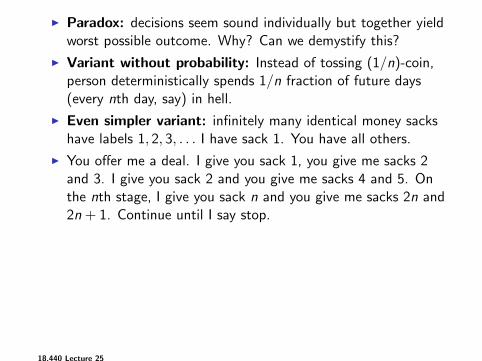
I Paradox: decisions seem sound individually but together yieldworst possible outcome. Why? Can we demystify this?
I Variant without probability: Instead of tossing (1/n)-coin,person deterministically spends 1/n fraction of future days(every nth day, say) in hell.
I Even simpler variant: infinitely many identical money sackshave labels 1, 2, 3, . . . I have sack 1. You have all others.
I You offer me a deal. I give you sack 1, you give me sacks 2and 3. I give you sack 2 and you give me sacks 4 and 5. Onthe nth stage, I give you sack n and you give me sacks 2n and2n + 1. Continue until I say stop.
I Lets me get arbitrarily rich. But if I go on forever, I returnevery sack given to me. If nth sack confers right to spend nthday in heaven, leads to hell-forever paradox.
I I make infinitely many good trades and end up with less than Istarted with. “Paradox” is really just existence of 2-to-1 mapfrom (smaller set) {2, 3, . . .} to (bigger set) {1, 2, . . .}.
18.440 Lecture 25
Money pile paradox
I You have an infinite collection of money piles with labeled0, 1, 2, . . . from left to right.
I Precise details not important, but let’s say you have 1/4 inthe 0th pile and 3
85j in the jth pile for each j > 0. Importantthing is that pile size is increasing exponentially in j .
I Banker proposes to transfer a fraction (say 2/3) of each pileto the pile on its left and remainder to the pile on its right.Do this simultaneously for all piles.
I Every pile is bigger after transfer (and this can be true even ifbanker takes a portion of each pile as a fee).
I Banker seemed to make you richer (every pile got bigger) butreally just reshuffled your infinite wealth.
18.440 Lecture 25

Two envelope paradox
I X is geometric with parameter 1/2. One envelope has 10X
dollars, one has 10X−1 dollars. Envelopes shuffled.
I You choose an envelope and, after seeing contents, areallowed to choose whether to keep it or switch. (Maybe youhave to pay a dollar to switch.)
I Maximizing conditional expectation, it seems it’s alwaysbetter to switch. But if you always switch, why not justchoose second-choice envelope first and avoid switching fee?
I Kind of a disguised version of money pile paradox. But moresubtle. One has to replace “jth pile of money” with“restriction of expectation sum to scenario that first chosenenvelop has 10j”. Switching indeed makes each pile bigger.
I However, “Higher expectation given amount in first envelope”may not be right notion of “better.” If S is payout withswitching, T is payout without switching, then S has samelaw as T − 1. In that sense S is worse.
18.440 Lecture 25

Moral
I Beware infinite expectations.
I Beware unbounded utility functions.
I They can lead to strange conclusions, sometimes related to“reshuffling infinite (actual or expected) wealth to createmore” paradoxes.
I Paradoxes can arise even when total transaction is finite withprobability one (as in envelope problem).
18.440 Lecture 25