18.218 lecture notes - evan chenweb.evanchen.cc/notes/mit-18-218.pdf · 18.218 lecture notes taught...
TRANSCRIPT
18.218 Lecture NotesTaught by Alex Postnikov
Evan Chen
Spring 2017
This is MIT’s graduate 18.218, instructed by Alex Postnikov. The for-mal name for this class is “Topics in Combinatorics”. All errors are myresponsibility.
The permanent URL for this document is http://web.evanchen.cc/
coursework.html, along with all my other course notes.
Contents
1 February 8, 2017 61.1 Bert Kostant’s game . . . . . . . . . . . . . . . . . . . . . . . . . . . . . . 61.2 Sponsor game . . . . . . . . . . . . . . . . . . . . . . . . . . . . . . . . . . 71.3 Excited sponsor game . . . . . . . . . . . . . . . . . . . . . . . . . . . . . 71.4 Chip-firing game . . . . . . . . . . . . . . . . . . . . . . . . . . . . . . . . 8
2 February 10, 2017 92.1 Chip-firing with games . . . . . . . . . . . . . . . . . . . . . . . . . . . . . 92.2 Cartan firing . . . . . . . . . . . . . . . . . . . . . . . . . . . . . . . . . . 92.3 Matrix firing . . . . . . . . . . . . . . . . . . . . . . . . . . . . . . . . . . 102.4 Diamond lemma . . . . . . . . . . . . . . . . . . . . . . . . . . . . . . . . 11
3 February 15, 2017 133.1 Diamond/Hex Lemma . . . . . . . . . . . . . . . . . . . . . . . . . . . . . 133.2 Roman lemma . . . . . . . . . . . . . . . . . . . . . . . . . . . . . . . . . 13
4 February 17, 2017 154.1 Review . . . . . . . . . . . . . . . . . . . . . . . . . . . . . . . . . . . . . 154.2 Vinberg’s additive function . . . . . . . . . . . . . . . . . . . . . . . . . . 154.3 Infinitude of Kostant games . . . . . . . . . . . . . . . . . . . . . . . . . . 164.4 Simply-laced Dynkin diagrams . . . . . . . . . . . . . . . . . . . . . . . . 174.5 Recap . . . . . . . . . . . . . . . . . . . . . . . . . . . . . . . . . . . . . . 18
5 February 21, 2017 195.1 Reflection game (generalize Kostant game) . . . . . . . . . . . . . . . . . 195.2 Weyl group . . . . . . . . . . . . . . . . . . . . . . . . . . . . . . . . . . . 195.3 Classification of finite Weyl groups . . . . . . . . . . . . . . . . . . . . . . 205.4 Proof of uniqueness . . . . . . . . . . . . . . . . . . . . . . . . . . . . . . 225.5 Proof of finiteness . . . . . . . . . . . . . . . . . . . . . . . . . . . . . . . 23
1
Evan Chen (Spring 2017) 18.218 Lecture Notes
6 February 22, 2017 246.1 Linear algebra results . . . . . . . . . . . . . . . . . . . . . . . . . . . . . 246.2 Axioms for square matrices . . . . . . . . . . . . . . . . . . . . . . . . . . 246.3 Finite, affine, indefinite type . . . . . . . . . . . . . . . . . . . . . . . . . 256.4 Generalized Cartan matrices . . . . . . . . . . . . . . . . . . . . . . . . . 26
7 February 24, 2017 277.1 Outline of proof of Vinberg theorem . . . . . . . . . . . . . . . . . . . . . 277.2 Matrix firing for A via Vinberg theorem . . . . . . . . . . . . . . . . . . . 287.3 Cartan matrices via Vinberg theorem . . . . . . . . . . . . . . . . . . . . 297.4 Finite list . . . . . . . . . . . . . . . . . . . . . . . . . . . . . . . . . . . . 297.5 Affine list . . . . . . . . . . . . . . . . . . . . . . . . . . . . . . . . . . . . 30
8 February 27, 2017 318.1 Constructing affine diagrams . . . . . . . . . . . . . . . . . . . . . . . . . 318.2 Draw all affine diagrams . . . . . . . . . . . . . . . . . . . . . . . . . . . . 318.3 Observations . . . . . . . . . . . . . . . . . . . . . . . . . . . . . . . . . . 328.4 Root system . . . . . . . . . . . . . . . . . . . . . . . . . . . . . . . . . . 34
9 March 1 2017 369.1 Notations . . . . . . . . . . . . . . . . . . . . . . . . . . . . . . . . . . . . 369.2 Definition of root systems . . . . . . . . . . . . . . . . . . . . . . . . . . . 369.3 Examples of root systems . . . . . . . . . . . . . . . . . . . . . . . . . . . 36
9.3.1 Crystallographic examples of rank two . . . . . . . . . . . . . . . . 369.3.2 Non-crystallographic examples of rank two . . . . . . . . . . . . . . 37
9.4 Structure of root systems . . . . . . . . . . . . . . . . . . . . . . . . . . . 37
10 March 3, 2017 4110.1 Simple reflections . . . . . . . . . . . . . . . . . . . . . . . . . . . . . . . . 4110.2 Cartan matrices . . . . . . . . . . . . . . . . . . . . . . . . . . . . . . . . 41
11 March 6, 2017 4311.1 Presentation of the Weyl group . . . . . . . . . . . . . . . . . . . . . . . . 4311.2 Proof of Coxeter relations . . . . . . . . . . . . . . . . . . . . . . . . . . . 4311.3 Dual description . . . . . . . . . . . . . . . . . . . . . . . . . . . . . . . . 4511.4 Weak Bruhat . . . . . . . . . . . . . . . . . . . . . . . . . . . . . . . . . . 45
12 March 8, 2017 4712.1 Inversions . . . . . . . . . . . . . . . . . . . . . . . . . . . . . . . . . . . . 4712.2 Construction of root system of type An−1 . . . . . . . . . . . . . . . . . . 4712.3 Wiring diagrams . . . . . . . . . . . . . . . . . . . . . . . . . . . . . . . . 4812.4 Generalizing permutation statistics to Weyl groups . . . . . . . . . . . . . 48
13 March 10, 2017 5013.1 The root poset . . . . . . . . . . . . . . . . . . . . . . . . . . . . . . . . . 5013.2 Coxeter number . . . . . . . . . . . . . . . . . . . . . . . . . . . . . . . . 51
14 March 13, 2017 5414.1 Root lattice and weight lattice . . . . . . . . . . . . . . . . . . . . . . . . 5414.2 A picture . . . . . . . . . . . . . . . . . . . . . . . . . . . . . . . . . . . . 5514.3 Affine Weyl group . . . . . . . . . . . . . . . . . . . . . . . . . . . . . . . 56
2
Evan Chen (Spring 2017) 18.218 Lecture Notes
15 March 15, 2017 5815.1 Recap . . . . . . . . . . . . . . . . . . . . . . . . . . . . . . . . . . . . . . 5815.2 Proof of Weyl’s formula . . . . . . . . . . . . . . . . . . . . . . . . . . . . 5915.3 Example: An−1 . . . . . . . . . . . . . . . . . . . . . . . . . . . . . . . . . 60
16 March 17, 2017 6116.1 The example An−1 . . . . . . . . . . . . . . . . . . . . . . . . . . . . . . . 6116.2 Affine permutations, and cylindrical wiring diagrams . . . . . . . . . . . . 6116.3 Alcoves in the example . . . . . . . . . . . . . . . . . . . . . . . . . . . . 6316.4 Bruhat orders . . . . . . . . . . . . . . . . . . . . . . . . . . . . . . . . . . 64
17 March 20, 2017 6517.1 Reduced decomposition . . . . . . . . . . . . . . . . . . . . . . . . . . . . 6517.2 Commutation classes . . . . . . . . . . . . . . . . . . . . . . . . . . . . . . 6517.3 Inversion sets . . . . . . . . . . . . . . . . . . . . . . . . . . . . . . . . . . 6617.4 Order ideals . . . . . . . . . . . . . . . . . . . . . . . . . . . . . . . . . . . 6717.5 Recap . . . . . . . . . . . . . . . . . . . . . . . . . . . . . . . . . . . . . . 6717.6 A bijection . . . . . . . . . . . . . . . . . . . . . . . . . . . . . . . . . . . 67
18 March 22, 2017 6918.1 Tableaus . . . . . . . . . . . . . . . . . . . . . . . . . . . . . . . . . . . . 6918.2 The easy direction . . . . . . . . . . . . . . . . . . . . . . . . . . . . . . . 7018.3 The hard direction . . . . . . . . . . . . . . . . . . . . . . . . . . . . . . . 7118.4 Edelman-Greene Correspondence . . . . . . . . . . . . . . . . . . . . . . . 71
19 March 24, 2017 72
20 April 3, 2017 7320.1 Examples . . . . . . . . . . . . . . . . . . . . . . . . . . . . . . . . . . . . 7320.2 Definition . . . . . . . . . . . . . . . . . . . . . . . . . . . . . . . . . . . . 73
21 April 5, 2017 7521.1 Saturated chains . . . . . . . . . . . . . . . . . . . . . . . . . . . . . . . . 7521.2 Cyclic polytopes . . . . . . . . . . . . . . . . . . . . . . . . . . . . . . . . 7521.3 Proof of Gale evenness condition . . . . . . . . . . . . . . . . . . . . . . . 7621.4 Cyclic zonotopes . . . . . . . . . . . . . . . . . . . . . . . . . . . . . . . . 7721.5 Zonotopal tilings . . . . . . . . . . . . . . . . . . . . . . . . . . . . . . . . 78
22 April 7, 2017 7922.1 Vinberg with integer entries . . . . . . . . . . . . . . . . . . . . . . . . . . 7922.2 Pseudoline arrangements have n− 2 arguments . . . . . . . . . . . . . . . 79
23 April 10, 2017 8023.1 A remark on moment . . . . . . . . . . . . . . . . . . . . . . . . . . . . . 8023.2 Positive Grassmannian . . . . . . . . . . . . . . . . . . . . . . . . . . . . . 8023.3 Cyclic zonotopes . . . . . . . . . . . . . . . . . . . . . . . . . . . . . . . . 8023.4 B(n, n− 3) . . . . . . . . . . . . . . . . . . . . . . . . . . . . . . . . . . . 8123.5 Generalization of B(n, n− 3) . . . . . . . . . . . . . . . . . . . . . . . . . 81
24 April 12, 2017 8324.1 Invariant algebra . . . . . . . . . . . . . . . . . . . . . . . . . . . . . . . . 8324.2 Coinvariant algebra . . . . . . . . . . . . . . . . . . . . . . . . . . . . . . 83
3
Evan Chen (Spring 2017) 18.218 Lecture Notes
24.3 Geometrical background . . . . . . . . . . . . . . . . . . . . . . . . . . . . 8524.4 Schubert classes . . . . . . . . . . . . . . . . . . . . . . . . . . . . . . . . 85
25 April 14, 2017 8625.1 Divided differences . . . . . . . . . . . . . . . . . . . . . . . . . . . . . . . 8625.2 Divided difference via Weyl group . . . . . . . . . . . . . . . . . . . . . . 8725.3 BGG . . . . . . . . . . . . . . . . . . . . . . . . . . . . . . . . . . . . . . . 8725.4 Choices of basis polynomials . . . . . . . . . . . . . . . . . . . . . . . . . 88
26 April 19, 2017 8926.1 Double Schubert polynomials . . . . . . . . . . . . . . . . . . . . . . . . . 8926.2 Nil-Hecke Algebra . . . . . . . . . . . . . . . . . . . . . . . . . . . . . . . 89
27 April 21, 2017 9027.1 Main Theorem . . . . . . . . . . . . . . . . . . . . . . . . . . . . . . . . . 9027.2 A Word on RC graphs . . . . . . . . . . . . . . . . . . . . . . . . . . . . . 92
28 April 24, 2017 9328.1 RC graphs . . . . . . . . . . . . . . . . . . . . . . . . . . . . . . . . . . . 9328.2 Cauchy formula . . . . . . . . . . . . . . . . . . . . . . . . . . . . . . . . . 9428.3 Linear space of Schubert polynomial . . . . . . . . . . . . . . . . . . . . . 95
29 April 26, 2017 9729.1 The n = 3 example . . . . . . . . . . . . . . . . . . . . . . . . . . . . . . . 9729.2 Infinite permutations . . . . . . . . . . . . . . . . . . . . . . . . . . . . . . 9729.3 Geometrical background . . . . . . . . . . . . . . . . . . . . . . . . . . . . 9829.4 Wiring diagrams of Grassmanian permutations . . . . . . . . . . . . . . . 99
30 April 28, 2017 10230.1 The correspondence . . . . . . . . . . . . . . . . . . . . . . . . . . . . . . 10230.2 Schur symmetric polynomial . . . . . . . . . . . . . . . . . . . . . . . . . 10330.3 Symmetry of H•(Fln) = C[x1, . . . , xn]/In . . . . . . . . . . . . . . . . . . 10330.4 Monk’s formula . . . . . . . . . . . . . . . . . . . . . . . . . . . . . . . . . 104
31 May 1, 2017 105
32 May 3, 2017 106
33 May 4, 2017 107
34 May 8, 2017 10834.1 Generalizing Schubert calculus . . . . . . . . . . . . . . . . . . . . . . . . 10834.2 K-theory of G/B . . . . . . . . . . . . . . . . . . . . . . . . . . . . . . . . 10834.3 Linear basis of K(G/B) . . . . . . . . . . . . . . . . . . . . . . . . . . . . 10934.4 Specializing to An−1 . . . . . . . . . . . . . . . . . . . . . . . . . . . . . . 10934.5 Construction of Grothendiek polynomial . . . . . . . . . . . . . . . . . . . 110
35 May 10, 2017 11135.1 Definition of Grothendiek polynomials . . . . . . . . . . . . . . . . . . . . 11135.2 Grothendiek pipe dreams . . . . . . . . . . . . . . . . . . . . . . . . . . . 11135.3 Extended Example for n = 3 . . . . . . . . . . . . . . . . . . . . . . . . . 11235.4 Monk’s Formula for Grothendiek polynomials . . . . . . . . . . . . . . . . 114
4

Evan Chen (Spring 2017) 18.218 Lecture Notes
35.5 Alcove path model . . . . . . . . . . . . . . . . . . . . . . . . . . . . . . . 115
36 May 12, 2017 11736.1 Another perspective on pipe dreams . . . . . . . . . . . . . . . . . . . . . 11736.2 Alcove path model, continued . . . . . . . . . . . . . . . . . . . . . . . . . 118
37 May 15, 2017 120
38 May 17, 2017 12138.1 Weyl Characters . . . . . . . . . . . . . . . . . . . . . . . . . . . . . . . . 12138.2 Kostant partition function . . . . . . . . . . . . . . . . . . . . . . . . . . . 121
5
Evan Chen (Spring 2017) 18.218 Lecture Notes
§1 February 8, 2017
Examples of chip-firing games.
§1.1 Bert Kostant’s game
Actually “find the highest root”.Let G = (V,E) be a simple graph, and set V = [n]. For i ∈ V let N(i) denote the
neighbors of i.For i ∈ V we have ci ≥ 0 chips; the vector (ci)1≤i≤n is called a configuration. We say a
vertex i is:
• Happy if ci = 12
∑j∈N(i) cj .
• Unhappy if ci <12
∑j∈N(i) cj .
• Excited if ci >12
∑j∈N(i) cj .
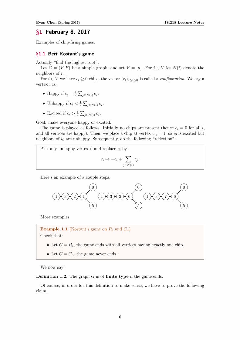
Goal: make everyone happy or excited.The game is played as follows. Initially no chips are present (hence ci = 0 for all i,
and all vertices are happy). Then, we place a chip at vertex vi0 = 1, so i0 is excited butneighbors of i0 are unhappy. Subsequently, do the following “reflection”:
Pick any unhappy vertex i, and replace ci by
ci 7→ −ci +∑j∈N(i)
cj .
Here’s an example of a couple steps.
1 3 2 1
0
5
1 3 2 6
0
5
1 3 7 6
0
5
More examples.
Example 1.1 (Kostant’s game on Pn and Cn)
Check that:
• Let G = Pn, the game ends with all vertices having exactly one chip.
• Let G = Cn, the game never ends.
We now say:
Definition 1.2. The graph G is of finite type if the game ends.
Of course, in order for this definition to make sense, we have to prove the followingclaim.
6
Evan Chen (Spring 2017) 18.218 Lecture Notes
Proposition 1.3
If there is a way to play so that the game ends, then any sequence of moves eventuallyleads to a terminating state. Moreover, the final configuration vector does not dependon the choice of moves, nor on the initial vertex we added a chip on.
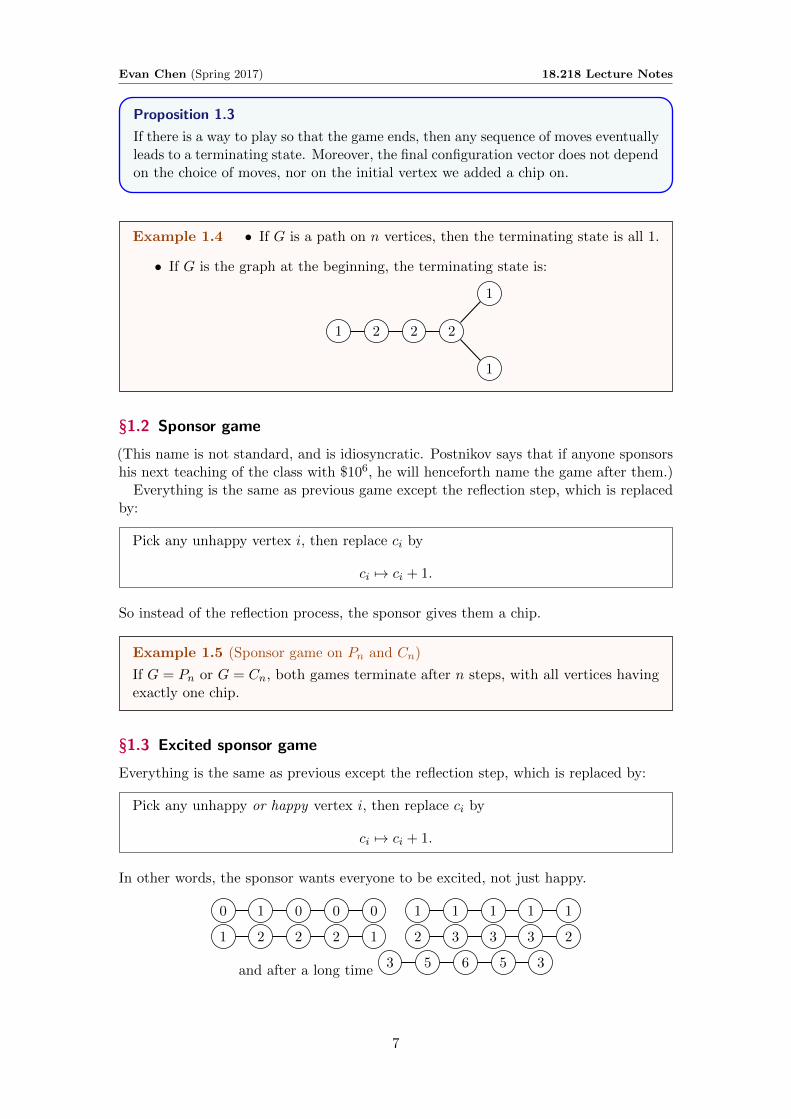
Example 1.4 • If G is a path on n vertices, then the terminating state is all 1.
• If G is the graph at the beginning, the terminating state is:
1 2 2 2
1
1
§1.2 Sponsor game
(This name is not standard, and is idiosyncratic. Postnikov says that if anyone sponsorshis next teaching of the class with $106, he will henceforth name the game after them.)
Everything is the same as previous game except the reflection step, which is replacedby:
Pick any unhappy vertex i, then replace ci by
ci 7→ ci + 1.
So instead of the reflection process, the sponsor gives them a chip.
Example 1.5 (Sponsor game on Pn and Cn)
If G = Pn or G = Cn, both games terminate after n steps, with all vertices havingexactly one chip.
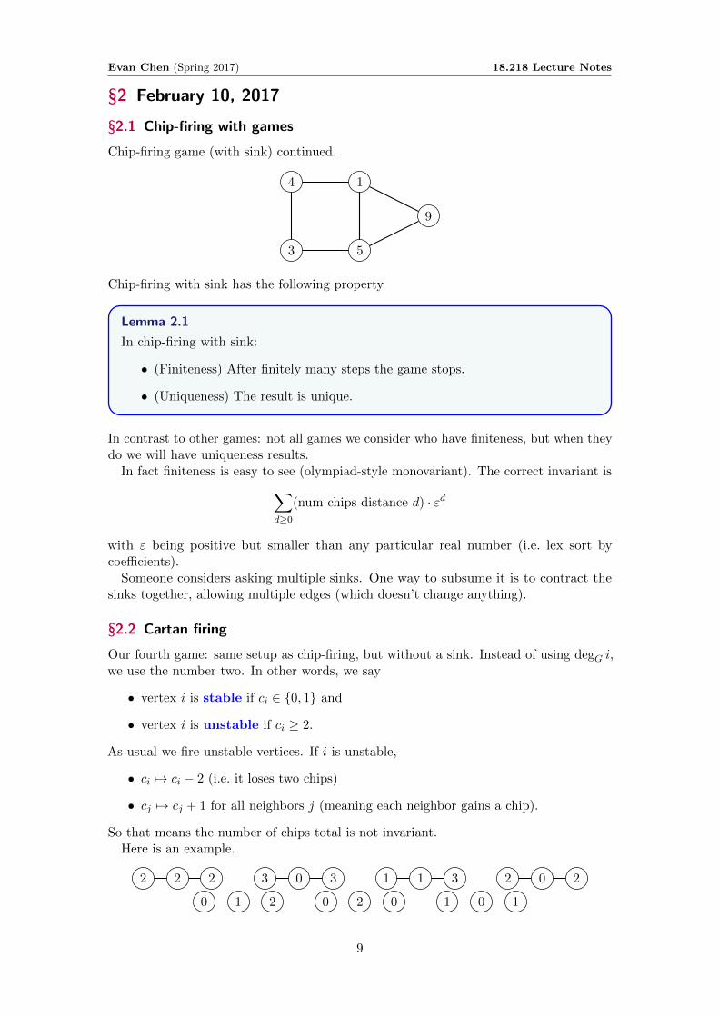
§1.3 Excited sponsor game
Everything is the same as previous except the reflection step, which is replaced by:
Pick any unhappy or happy vertex i, then replace ci by
ci 7→ ci + 1.
In other words, the sponsor wants everyone to be excited, not just happy.
0 1 0 0 0 1 1 1 1 1
1 2 2 2 1 2 3 3 3 2
and after a long time3 5 6 5 3
7

Evan Chen (Spring 2017) 18.218 Lecture Notes
On the other hand the excited sponsor game never terminates on a cycle, because itis impossible for the inequality ci >
12(ci−1 + ci+1) to hold for all i (by noting that the
minimal vertex is always un-excited).So the excited sponsor game feels more like Kostant’s game, but the terminal state is
different in the path case (35653 rather than 11111).
§1.4 Chip-firing game
Also called “abelian sandpile model”.Retain the notation G = (V,E), V = [n], and ci.
Definition 1.6. A vertex i is stable if ci < degG(i), and unstable if ci ≥ degG(i).
In a firing move, we pick an unstable i, we move a chip from i to each neighbor of i.Obviously the game goes on forever if the number of chips is sufficiently large (since
the number of chips is invariant). To fix this, we add a sink : a vertex which eats allchips fired at it.
It turns out:
Proposition 1.7
With a sink, chip-firing games always terminate.
8
Evan Chen (Spring 2017) 18.218 Lecture Notes
§2 February 10, 2017
§2.1 Chip-firing with games
Chip-firing game (with sink) continued.
4
3
1
5
9
Chip-firing with sink has the following property
Lemma 2.1
In chip-firing with sink:
• (Finiteness) After finitely many steps the game stops.
• (Uniqueness) The result is unique.
In contrast to other games: not all games we consider who have finiteness, but when theydo we will have uniqueness results.
In fact finiteness is easy to see (olympiad-style monovariant). The correct invariant is∑d≥0
(num chips distance d) · εd
with ε being positive but smaller than any particular real number (i.e. lex sort bycoefficients).
Someone considers asking multiple sinks. One way to subsume it is to contract thesinks together, allowing multiple edges (which doesn’t change anything).
§2.2 Cartan firing
Our fourth game: same setup as chip-firing, but without a sink. Instead of using degG i,we use the number two. In other words, we say
• vertex i is stable if ci ∈ {0, 1} and
• vertex i is unstable if ci ≥ 2.
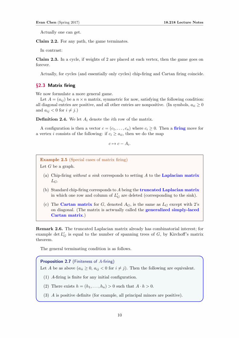
As usual we fire unstable vertices. If i is unstable,
• ci 7→ ci − 2 (i.e. it loses two chips)
• cj 7→ cj + 1 for all neighbors j (meaning each neighbor gains a chip).
So that means the number of chips total is not invariant.Here is an example.
2 2 2 3 0 3 1 1 3 2 0 2
0 1 2 0 2 0 1 0 1
9
Evan Chen (Spring 2017) 18.218 Lecture Notes
Actually one can get.
Claim 2.2. For any path, the game terminates.
In contrast:
Claim 2.3. In a cycle, if weights of 2 are placed at each vertex, then the game goes onforever.
Actually, for cycles (and essentially only cycles) chip-firing and Cartan firing coincide.
§2.3 Matrix firing
We now formulate a more general game.Let A = (aij) be a n× n matrix, symmetric for now, satisfying the following condition:
all diagonal entries are positive, and all other entries are nonpositive. (In symbols, aii ≥ 0and aij < 0 for i 6= j.)
Definition 2.4. We let Ai denote the ith row of the matrix.
A configuration is then a vector c = (c1, . . . , cn) where ci ≥ 0. Then a firing move fora vertex i consists of the following: if ci ≥ aii, then we do the map
c 7→ c−Ai.
Example 2.5 (Special cases of matrix firing)
Let G be a graph.
(a) Chip-firing without a sink corresponds to setting A to the Laplacian matrixLG.
(b) Standard chip-firing corresponds to A being the truncated Laplacian matrixin which one row and column of L′G are deleted (corresponding to the sink).
(c) The Cartan matrix for G, denoted AG, is the same as LG except with 2’son diagonal. (The matrix is actwually called the generalized simply-lacedCartan matrix.)
Remark 2.6. The truncated Laplacian matrix already has combinatorial interest; forexample detL′G is equal to the number of spanning trees of G, by Kirchoff’s matrixtheorem.
The general terminating condition is as follows.
Proposition 2.7 (Finiteness of A-firing)
Let A be as above (aii ≥ 0, aij < 0 for i 6= j). Then the following are equivalent.
(1) A-firing is finite for any initial configuration.
(2) There exists h = (h1, . . . , hn) > 0 such that A · h > 0.
(3) A is positive definite (for example, all principal minors are positive).
10

Evan Chen (Spring 2017) 18.218 Lecture Notes
The notation h > 0 means hi > 0 for all i. Since the proof (2) ⇐⇒ (3) is linear algebra,we will prove (2) =⇒ (1).
Proof that (2) =⇒ (1). A · h > 0 implies the dot product 〈h,Ai〉 is positive for each i.Thus over configurations c, the dot product 〈h, c〉 is decreasing over time, as it decreasesby 〈h,Ai〉 when i is fired. On the other hand h > 0 and c ≥ 0 so done.
So it remains to show uniqueness in the strongest sense possible: for fixed A, gameseither terminate always in exactly the same way, else they never terminate. The proof ofthis recalls on so-called diamond lemma.
§2.4 Diamond lemma
We state the diamond lemma in the context of A-firing.
Lemma 2.8 (Diamond lemma)
If there are two ways to fire, say ci−→ c1 and c
j−→ c2, where i 6= j, then we cancomplete the diagram to get
c
c1 c2
c3
i j
j i
Proof. Just c3 = c−Ai −Aj .
Remark 2.9. This “commutativity property” expressed by the diamond lemma is whywe physicists call this game “abelian sand piles”.
Proof of uniqueness from diamond lemma. Consider the following diagram:
c c′1 c′2 . . .
c1
c2
...
c`
11

Evan Chen (Spring 2017) 18.218 Lecture Notes
Assume for contradiction c` is final. Then, assume ` is minimal. Then diamond lemmarepeatedly gives a downward path from c′1, until we find an index k such that ck+1 = c′′k,for example
c c′1 c′2 . . .
c1 c′′1
c2 c′′2
c3
...
c`
This contradicts minimality of ` then.
In fact, this diamond lemma applies for every game (sponsor game, A-firing, etc.)except the second game.
Definition 2.10. G is Cartan finite if Cartan firing is finite for any initial configuration.
Lemma 2.11
If a graph is Cartan finite, then any subgraph is Cartan finite.
12
Evan Chen (Spring 2017) 18.218 Lecture Notes
§3 February 15, 2017
§3.1 Diamond/Hex Lemma
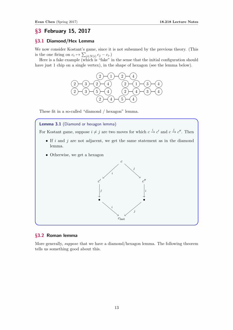
We now consider Kostant’s game, since it is not subsumed by the previous theory. (Thisis the one firing on ci 7→
∑j∈N(i) cj − ci.)
Here is a fake example (which is “fake” in the sense that the initial configuration shouldhave just 1 chip on a single vertex), in the shape of hexagon (see the lemma below).
2 1 2 4
2 3 2 4 2 1 3 4
2 3 5 4 2 4 3 4
2 4 5 4
These fit in a so-called “diamond / hexagon” lemma.
Lemma 3.1 (Diamond or hexagon lemma)
For Kostant game, suppose i 6= j are two moves for which ci−→ c′ and c
j−→ c′′. Then
• If i and j are not adjacent, we get the same statement as in the diamondlemma.
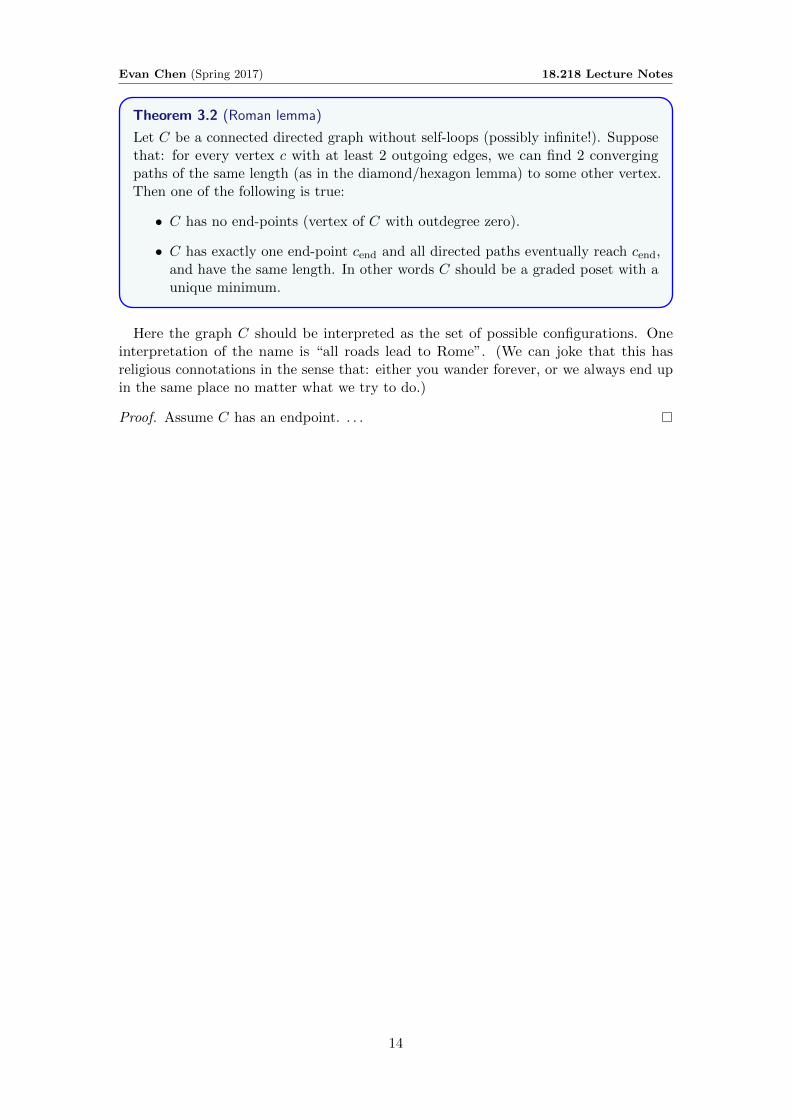
• Otherwise, we get a hexagon
c
c′ c′′
• •
clast
i
j
j i
i
j
§3.2 Roman lemma
More generally, suppose that we have a diamond/hexagon lemma. The following theoremtells us something good about this.
13
Evan Chen (Spring 2017) 18.218 Lecture Notes
Theorem 3.2 (Roman lemma)
Let C be a connected directed graph without self-loops (possibly infinite!). Supposethat: for every vertex c with at least 2 outgoing edges, we can find 2 convergingpaths of the same length (as in the diamond/hexagon lemma) to some other vertex.Then one of the following is true:
• C has no end-points (vertex of C with outdegree zero).
• C has exactly one end-point cend and all directed paths eventually reach cend,and have the same length. In other words C should be a graded poset with aunique minimum.
Here the graph C should be interpreted as the set of possible configurations. Oneinterpretation of the name is “all roads lead to Rome”. (We can joke that this hasreligious connotations in the sense that: either you wander forever, or we always end upin the same place no matter what we try to do.)
Proof. Assume C has an endpoint. . . .
14
Evan Chen (Spring 2017) 18.218 Lecture Notes
§4 February 17, 2017
§4.1 Review
• Cartan’s firing game: Let G be a simple graph, and define the Cartan matrix
A = AG = 2I − adj matrix of A.
Then a configuration c = (c1, . . . , cn) ∈ Zn≥0. Now let e1, . . . , en be the standardbasis of Rn.
Then firing fi as usual corresponds to
fi : c 7→ c−Aei.
• Kostant’s game (a reflection game):
si : c 7→ c− (Ac, ei) ei
if (Ac, ei) < 0. (We are using (•, •) for the dot product.)
We have written this in terms of an arbitrary matrix A, since we will use this generalitylater. In what follows, all graphs G are connected.
§4.2 Vinberg’s additive function
We replace the notion with “happy” now.
Definition 4.1. A configuration h ∈ Zn≥0 is called a(n)
• (Vinberg) additive function if Ah = 0.
• subadditive function if Ah ≥ 0 (happy or excited)
• strictly subadditive function if Ah > 0 (excited).
We think of h as a function from vertices to Z≥0, hence the name.
We now give a complete classification of all additive functions.
15
Evan Chen (Spring 2017) 18.218 Lecture Notes
Theorem 4.2 (Vinberg’s theorem)
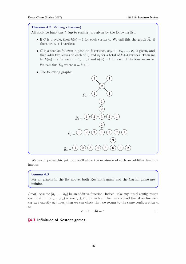
All additive functions h (up to scaling) are given by the following list.
• If G is a cycle, then h(v) = 1 for each vertex v. We call this the graph An ifthere are n+ 1 vertices.
• G is a tree as follows: a path on k vertices, say v1, v2, . . . , vk is given, andthen adds two leaves on each of v1 and vk for a total of k+ 4 vertices. Then welet h(vi) = 2 for each i = 1, . . . , k and h(w) = 1 for each of the four leaves w.
We call this Dn where n = k + 3.
• The following graphs:
D4 =
2
11
11
E6 =1 2 3 2 1
2
1
E7 =1 2 3 4 3 2 1
2
E8 =1 2 3 4 5 6 4 2
3
We won’t prove this yet, but we’ll show the existence of such an additive functionimplies:
Lemma 4.3
For all graphs in the list above, both Kostant’s game and the Cartan game areinfinite.
Proof. Assume (h1, . . . , hn) be an additive function. Indeed, take any initial configurationsuch that c = (c1, . . . , cn) where ci ≥ 2hi for each i. Then we contend that if we fire eachvertex i exactly hi times, then we can check that we return to the same configuration c,as
c 7→ c−Ah = c.
§4.3 Infinitude of Kostant games
16
Evan Chen (Spring 2017) 18.218 Lecture Notes
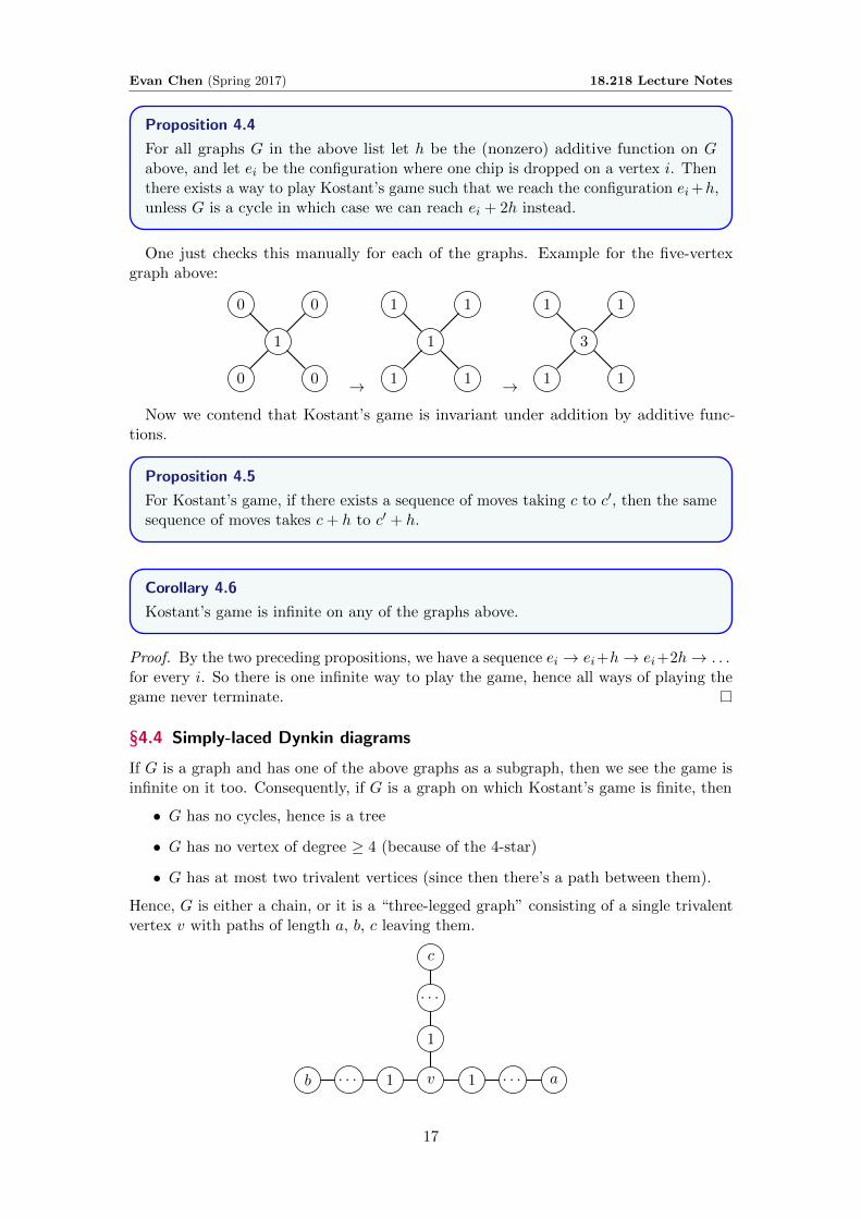
Proposition 4.4
For all graphs G in the above list let h be the (nonzero) additive function on Gabove, and let ei be the configuration where one chip is dropped on a vertex i. Thenthere exists a way to play Kostant’s game such that we reach the configuration ei+h,unless G is a cycle in which case we can reach ei + 2h instead.
One just checks this manually for each of the graphs. Example for the five-vertexgraph above:
1
00
00 →
1
11
11 →
3
11
11
Now we contend that Kostant’s game is invariant under addition by additive func-tions.
Proposition 4.5
For Kostant’s game, if there exists a sequence of moves taking c to c′, then the samesequence of moves takes c+ h to c′ + h.
Corollary 4.6
Kostant’s game is infinite on any of the graphs above.
Proof. By the two preceding propositions, we have a sequence ei → ei+h→ ei+2h→ . . .for every i. So there is one infinite way to play the game, hence all ways of playing thegame never terminate.
§4.4 Simply-laced Dynkin diagrams
If G is a graph and has one of the above graphs as a subgraph, then we see the game isinfinite on it too. Consequently, if G is a graph on which Kostant’s game is finite, then
• G has no cycles, hence is a tree
• G has no vertex of degree ≥ 4 (because of the 4-star)
• G has at most two trivalent vertices (since then there’s a path between them).
Hence, G is either a chain, or it is a “three-legged graph” consisting of a single trivalentvertex v with paths of length a, b, c leaving them.
v 1 . . . a1. . .b
1
. . .
c
17
Evan Chen (Spring 2017) 18.218 Lecture Notes
On the other hand, the three exceptional graphs in Vinberg’s theorem imply thatmin(a, b, c) < 2, hence WLOG a = 1. Then we must have min(b, c) < 3, hence b ≤ 2, andalso when b = 2 it follows that c ≤ 4.
Thus we conclude that
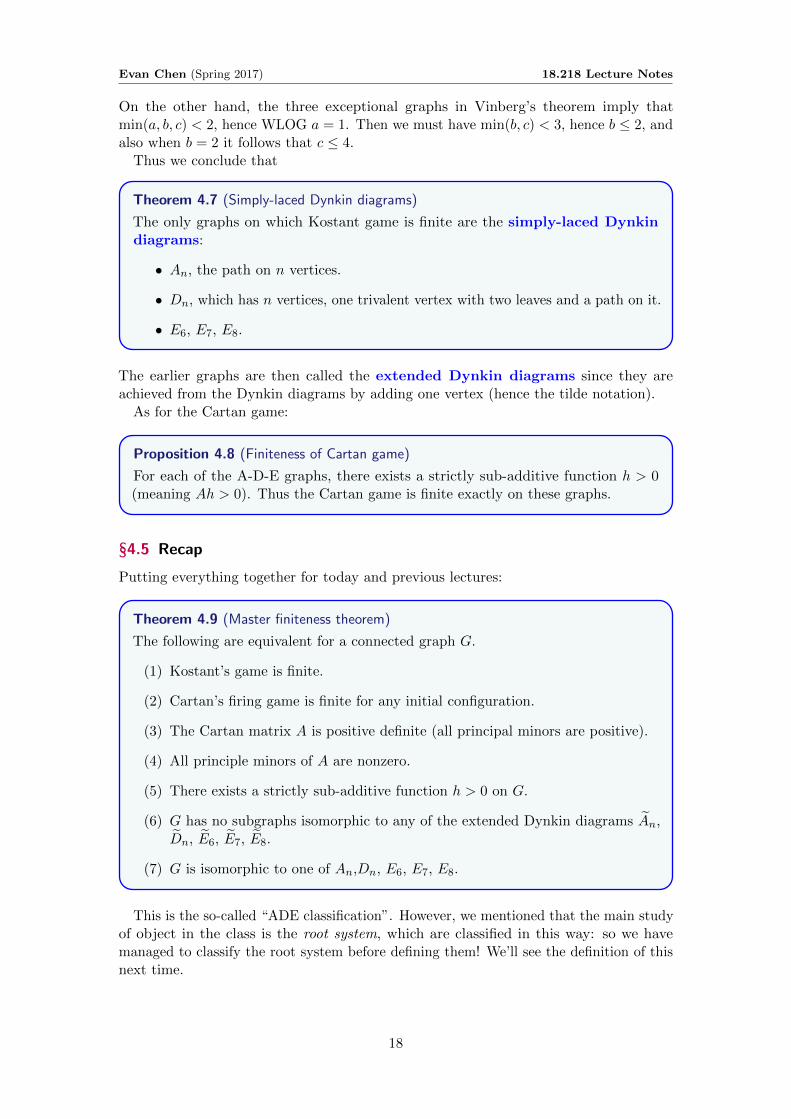
Theorem 4.7 (Simply-laced Dynkin diagrams)
The only graphs on which Kostant game is finite are the simply-laced Dynkindiagrams:
• An, the path on n vertices.
• Dn, which has n vertices, one trivalent vertex with two leaves and a path on it.
• E6, E7, E8.
The earlier graphs are then called the extended Dynkin diagrams since they areachieved from the Dynkin diagrams by adding one vertex (hence the tilde notation).
As for the Cartan game:
Proposition 4.8 (Finiteness of Cartan game)
For each of the A-D-E graphs, there exists a strictly sub-additive function h > 0(meaning Ah > 0). Thus the Cartan game is finite exactly on these graphs.
§4.5 Recap
Putting everything together for today and previous lectures:
Theorem 4.9 (Master finiteness theorem)
The following are equivalent for a connected graph G.
(1) Kostant’s game is finite.
(2) Cartan’s firing game is finite for any initial configuration.
(3) The Cartan matrix A is positive definite (all principal minors are positive).
(4) All principle minors of A are nonzero.
(5) There exists a strictly sub-additive function h > 0 on G.
(6) G has no subgraphs isomorphic to any of the extended Dynkin diagrams An,Dn, E6, E7, E8.
(7) G is isomorphic to one of An,Dn, E6, E7, E8.
This is the so-called “ADE classification”. However, we mentioned that the main studyof object in the class is the root system, which are classified in this way: so we havemanaged to classify the root system before defining them! We’ll see the definition of thisnext time.
18
Evan Chen (Spring 2017) 18.218 Lecture Notes
§5 February 21, 2017
We will now consider so-called cluster algebra games, in which we not only changeconfigurations but also alter the graph.
§5.1 Reflection game (generalize Kostant game)
Definition 5.1. A generalized Cartan matrix is a matrix A = (aij) with integerentries such that:
(1) aii = 2 for all i
(2) aij ≤ 0 for i 6= j.
(3) if aij < 0 then aji < 0.
As usual we can obtain a graph G on vertices {1, . . . , n} by letting (i, j) be an edgeexactly when ai,j < 0. As usual we may assume G is connected (since otherwise we maysub-divide the matrix).
We then have the reflection game (generalizing Kostant’s game) as follows.
Definition 5.2. Let e1, . . . , en be a standard basis of Rn. Then the reflection gameconsists of moves
si : Rn → Rn
by
c 7→ c−(A>c, ei
)ei.
To be explicit, the map is
(c1, . . . , cn) 7→ (c1, . . . , c′i, . . . , cn)
wherec′i = −ci −
∑j 6=i
ajicj .
As usual s2i = id.
So this is somewhat symmetric, but not quite as symmetric as before. This time we(for now) place no constraints on the ci in order to “reflect” by si.
§5.2 Weyl group
We now give an unorthodox definition of root systems. This is not the “usual” definition,but it is equivalent to them.
Definition 5.3. A Weyl group W and real root system Φ is defined as follows.
• W ⊆ GL(n) is the subgroup generated by si.
• Φ = W {e1, . . . , en} ⊆ Zn is the image of basis elements under the reflections in W .The elements of Φ can be called roots. (Remark for experts: they are currentlywritten in some particular choice of coordinates.)
We are interested in when W and Φ are finite.
19

Evan Chen (Spring 2017) 18.218 Lecture Notes
Example 5.4 (n = 2 case)
Let n = 2. Then we can write
A =
[2 −a−b 2
].
In that case, the following are equivalent:
(1) W is finite
(2) Φ is finite
(3) ab < 4. That is, A must be one of the matrices
A2 =
[2 −1−1 2
]B2 =
[2 −2−1 2
]G2 =
[2 −1−3 2
]or one of the transposes.
So we can imagine the graphs as follows:
• A2 corresponds to two vertices joined by a single edge.
• B2 corresponds to two arrows right and an arrow left:
• G2 corresponds to three arrows left and one arrow right:
By convention a picture
with k lines means that we have k arrows in the direction of the arrow head, and just 1arrow in the reverse direction.
§5.3 Classification of finite Weyl groups
Theorem 5.5
The following are equivalent.
(1) Φ is finite.
(2) W is finite.
(3) A is corresponds to one of the following Dynkin diagrams: An, Bn, Cn, Dn,E6, E7, E8, F4, G2.
Here are pictures of each of them:
• An:
• Bn:
• Cn:
20
Evan Chen (Spring 2017) 18.218 Lecture Notes
• Dn:
• E6, E7, E8 as before.
• F4:
• G2:
The types An, Bn, Dn are thus called simply-laced because they don’t have doubleedges.
(1) ⇐⇒ (2). Obviously if W is finite then Φ is finite (|Φ| ≤ n |W |). To see the otherdirection, assume Φ is finite; there is then a canonical map
W → SΦ
onto permutations of Φ. As Φ contains the basis elements e1 . . . , en the map is injective;hence |W | ≤ |SΦ| <∞.
Now let’s give an example.
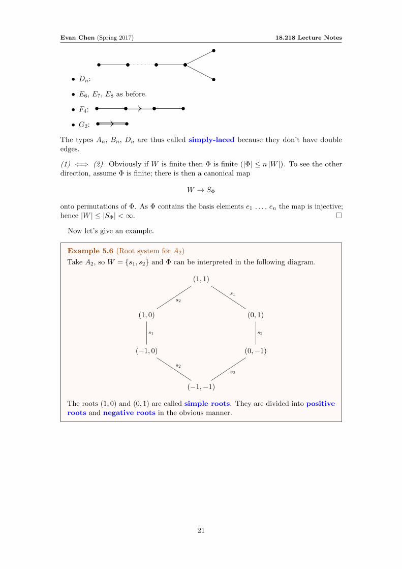
Example 5.6 (Root system for A2)
Take A2, so W = {s1, s2} and Φ can be interpreted in the following diagram.
(1, 1)
(1, 0) (0, 1)
(−1, 0) (0,−1)
(−1,−1)
s2
s1
s1 s2
s2s2
The roots (1, 0) and (0, 1) are called simple roots. They are divided into positiveroots and negative roots in the obvious manner.
21
Evan Chen (Spring 2017) 18.218 Lecture Notes
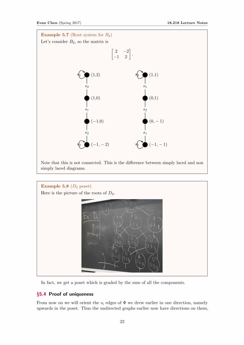
Example 5.7 (Root system for B2)
Let’s consider B2, so the matrix is [2 −2−1 2
].
(1,2)
(1,0)
(−1,0)
(−1,− 2)
(1,1)
(0,1)
(0,− 1)
(−1,− 1)
s2
s2
s1
s1
s1
s2
s1
s2
s2
s1
Note that this is not connected. This is the difference between simply laced and nonsimply laced diagrams.
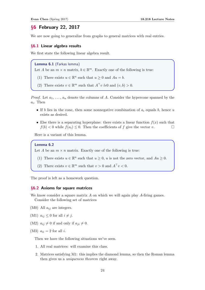
Example 5.8 (D4 poset)
Here is the picture of the roots of D4.
In fact, we get a poset which is graded by the sum of all the components.
§5.4 Proof of uniqueness
From now on we will orient the si edges of Φ we drew earlier in one direction, namelyupwards in the poset. Thus the undirected graphs earlier now have directions on them,
22

Evan Chen (Spring 2017) 18.218 Lecture Notes
similar to our situation before, and we would like for the game to terminate.We now prove the lemma from before. The main idea remains intact from before.The analog of “diamond/hexagon lemma” from before is:
Lemma 5.9 (Diamond / hexagon / octagon / dodecagon lemma)
Suppose si : c 7→ c′ and sj : c 7→ c′′. Then there are four cases:
• If aij = aji = 0, then we have a diamond lemma as before.
• If aij = aji = −1, we have a hexagon lemma as before.
• If aijaji = 2, then there are two paths of length 4 converging to a given endconfiguration (octagon).
• If aijaji = 3, then there are two paths of length 6 converging to a given endconfiguration (dodecagon).
Consequently, the Roman Lemma implies the uniqueness result: if we climb a (finite)root system following the edges si, we will always end at a unique place.
(Note that this is per connected component; for example the root system of B2 hastwo connected components.)
§5.5 Proof of finiteness
All that remains to do is show finiteness. Again:
• A function h ∈ Rn is called an additive function if h > 0 and A>h = ~0.
As before we just need to exhibit a bunch of additive functions in order to get a list offorbidden subgraphs. We now give a list of all additive functions.
• An, Dn, E6,7,8 are as before.
• If A =
[2 −2−2 2
], we have the additive function
1 1
• If A =
[4 −2−1 2
], the additive function is
1 2
• 1 2 3
• 1 2 1
• . . . to be finished next lecture.
23
Evan Chen (Spring 2017) 18.218 Lecture Notes
§6 February 22, 2017
We are now going to generalize from graphs to general matrices with real entries.
§6.1 Linear algebra results
We first state the following linear algebra result.
Lemma 6.1 (Farkas lemma)
Let A be an m× n matrix, b ∈ Rm. Exactly one of the following is true:
(1) There exists u ∈ Rn such that u ≥ 0 and Au = b.
(2) There exists v ∈ Rm such that A>v le0 and (v, b) > 0.
Proof. Let a1, . . . , an denote the columns of A. Consider the hypercone spanned by theai. Then
• If b lies in the cone, then some nonnegative combination of ai equals b, hence uexists as desired.
• Else there is a separating hyperplane: there exists a linear function f(x) such thatf(b) < 0 while f(ai) ≤ 0. Then the coefficients of f give the vector v.
Here is a variant of this lemma.
Lemma 6.2
Let A be an m× n matrix. Exactly one of the following is true:
(1) There exists u ∈ Rn such that u ≥ 0, u is not the zero vector, and Au ≥ 0.
(2) There exists v ∈ Rm such that v > 0 and A>v < 0.
The proof is left as a homework question.
§6.2 Axioms for square matrices
We know consider a square matrix A on which we will again play A-firing games.Consider the following set of matrices
(M0) All aij are integers.
(M1) aij ≤ 0 for all i 6= j.
(M2) aij 6= 0 if and only if aji 6= 0.
(M3) aii = 2 for all i.
Then we have the following situations we’ve seen.
1. All real matrices: will examine this class.
2. Matrices satisfying M1: this implies the diamond lemma, so then the Roman lemmathen gives us a uniqueness theorem right away.
24

Evan Chen (Spring 2017) 18.218 Lecture Notes
3. Matrices satisfying M1 and M2. This already implies a lot about the matrix.
4. Matrices satisfying all four: these are the generalized Cartan matrices we discussedlast class. Kostant’s game makes sense in this context.
5. Simply-laced generalized Cartan matrices: those matrices coming from simplegraphs (meaning aij ∈ {0,−1} for i 6= j). For these we have the ADE classification,and the very strong uniqueness result that the result of the Kostant game doesn’tdepend on the starting position of the initial chip.
§6.3 Finite, affine, indefinite type
Here is the theorem:
Theorem 6.3 (Vinberg, see [Kat, Theorem 4.3])
Let A be an indecomposable n × n matrix which satisfies conditions (M1), (M2).Then exactly one of the following is true:
• (Finite type) There exists a vector u > 0 such that Au > 0.
• (Affine type) There exists a vector u > 0 such that Au = ~0.
• (Indefinite type) There exists a vector u > 0 such that Au < 0.
Moreover, A and A> are of the same type.
Note (M0) and (M3) are explicitly not required.
Remark 6.4 (Contiuining the religious connotations). In our old terminology:
• Finite type is “heaven” because we can make everyone excited.
• Indefinite type is “hell” because we can make everyone unhappy.
• Affine type is “purgatory” because we can make everyone happy but not excited.
In fact, affine type and finite type turn out to be much more closely related to each other(while indefinite type is much “worse” than both), in the same way that people go toheaven after purgatory.
Remark 6.5. Note that if any diagonal is negative (note that there’s no axioms ondiagonal entries) then A is automatically of indefinite type.
In fact, there’s more.
Theorem 6.6 (Vinberg, continued)
Retain the setting of the previous theorem. Then
• Suppose A is of finite type. Whenever Av ≥ 0, either v > 0 or v = ~0.Moreover detA 6= 0.
• Suppose A i s of affine type. If Av ≥ 0, then Av = ~0. Moreover, the columnrank of A is exactly 1.
• Suppose A is of indefinite type. If Av ≥ 0 and v ≥ 0, then v = ~0.
25
Evan Chen (Spring 2017) 18.218 Lecture Notes
In other words:
• Whenever A is of finite type, there are no additive functions but there exists asub-additive function.
• Whenever A is of affine type, then every sub-additive function is additive.
• Whenever A is of indefinite type, then we cannot find any sub-additive functionsat all.
We now give a characterization in terms of the firing game.
Corollary 6.7 (via Firing Game)
For A satisfying (M1) and (M2):
(1) A is of finite type if and only if the A-firing game is finite for every initialconfiguration.
(2) Assume also A has integer entries. Then A is of affine type if and only if thereexists a cycle in the A-firing game.
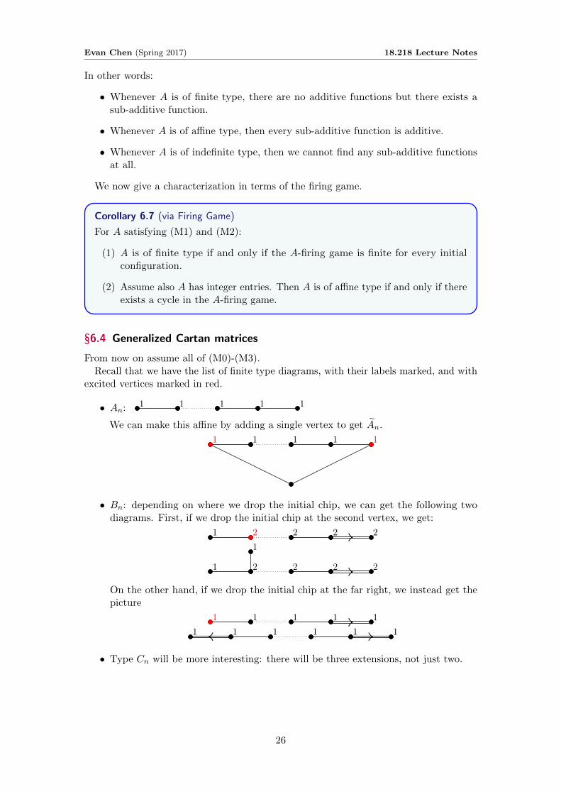
§6.4 Generalized Cartan matrices
From now on assume all of (M0)-(M3).Recall that we have the list of finite type diagrams, with their labels marked, and with
excited vertices marked in red.
• An: 1 1 1 1 1
We can make this affine by adding a single vertex to get An.
1 1 1 1 1
• Bn: depending on where we drop the initial chip, we can get the following twodiagrams. First, if we drop the initial chip at the second vertex, we get:
1 2 2 2 2
1 2 2 2 2
1
On the other hand, if we drop the initial chip at the far right, we instead get thepicture
1 1 1 1 1
1 1 1 1 11
• Type Cn will be more interesting: there will be three extensions, not just two.
26

Evan Chen (Spring 2017) 18.218 Lecture Notes
§7 February 24, 2017
§7.1 Outline of proof of Vinberg theorem
Definition 7.1. Let A be an indecomposable real n×n matrix (so the resulting directedmulti-graph is connected). We say c ∈ Rn≥0 is
• additive if A>c = ~0,
• coadditive if Ac = ~0,
• subadditive if A>c ≥ 0, and
• co-subadditive if Ac ≥ 0.
Here is the key observation for the Vinberg trichotomy theorem we mentioned lasttime, which seems almost trivial at first.
Lemma 7.2
For any (co)subadditive c, either c = ~0 or c > 0.
Proof. Assume c 6= ~0. Consider neighboring vertices i and j, where cj 6= 0. (meaningaij < 0). Since A>c ≥ 0, we require
aiici ≥∑j 6=i−aijcj .
The right-hand side is strictly positive now, so ci > 0.Hence connected-ness now implies ck > 0 for every k.
Now, consider the coneKA = {u ∈ Rn | Au ≥ 0}
and the positive orthantO = {u ∈ Rn | u ≥ 0}
and observe that KA ∩O consists exactly of the co-subadditive functions. The previouslemma then implies KA intersects the boundary of O only at the origin. This geometricsurprise then implies that one of three situations happens:
• KA is completely contained inside O — the finite case.
• KA is a line through the origin — the affine case.
• KA is completely disjoint from O — the indefinite case.
(Image below, with KA drawn in red.)
~0 ~0 ~0
27
Evan Chen (Spring 2017) 18.218 Lecture Notes
§7.2 Matrix firing for A via Vinberg theorem
We consider firing as before, with real entries. Explicitly, if the ith position has morethan aii counters, then we may fire by subtracting off the ith column.
We can imagine the configuration space as points in Rn. Then the three cases wementioned are as follows:
• Finite: any firing process is finite.
• Affine: any firing process is bounded (stays inside some simplex).
• Indefinite: any firing process is unbounded given sufficiently large starting configu-rations.
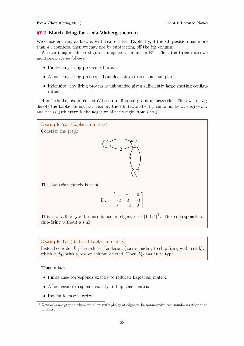
Here’s the key example: let G be an undirected graph or network1. Then we let LGdenote the Laplacian matrix, meaning the ith diagonal entry contains the outdegree of iand the (i, j)th entry is the negative of the weight from i to j.
Example 7.3 (Laplacian matrix)
Consider the graph
1 2
3
2
2
The Laplacian matrix is then
LG =
1 −1 0−2 3 −10 −2 2
This is of affine type because it has an eigenvector [1, 1, 1]>. This corresponds tochip-firing without a sink.
Example 7.4 (Reduced Laplacian matrix)
Instead consider L′G the reduced Laplacian (corresponding to chip-firing with a sink),which is LG with a row or column deleted. Then L′G has finite type.
Thus in fact
• Finite case corresponds exactly to reduced Laplacian matrix.
• Affine case corresponds exactly to Laplacian matrix.
• Indefinite case is weird.
1 Networks are graphs where we allow multiplicity of edges to be nonnegative real numbers rather thanintegers
28

Evan Chen (Spring 2017) 18.218 Lecture Notes
§7.3 Cartan matrices via Vinberg theorem
Let A be a generalized Cartan matrix now, meaning aij ∈ Z, aii = 2 in addition toprevious assumptions. These two conditions “make everything very rigid”, meaning thatthere are only a few finite and affine cases.
Remark 7.5 (Classification philosophy). The hardest part is to write down this list.Once it’s done, one can “by examination” verify that it’s correct.
§7.4 Finite list
• For n > 1, on An there are two excited vertices, shown in red.
1 1 1 1 1
When n = 1, there’s only a single vertex which is somehow “doubly excited”.
1
• Bn: there are two ways to play the Kostant game, depending on whether we placethe initial chip on the left and right, respectively.
1 2 2 2 2
1 1 1 1 1
Like with An there is an exceptional case B2:
1 2
• Cn: there are two ways to play the Kostant game, depending on whether we placethe initial chip on the left and right, respectively. Again we have “doubly excitedpoints”.
2 2 2 2 1
1 2 2 2 1
Note C2 = B2.
• Dn:
1 2 2 2
1
1
• E6:
1 2 3 2 1
2
• E7:
2 3 4 3 2 1
2
29
Evan Chen (Spring 2017) 18.218 Lecture Notes
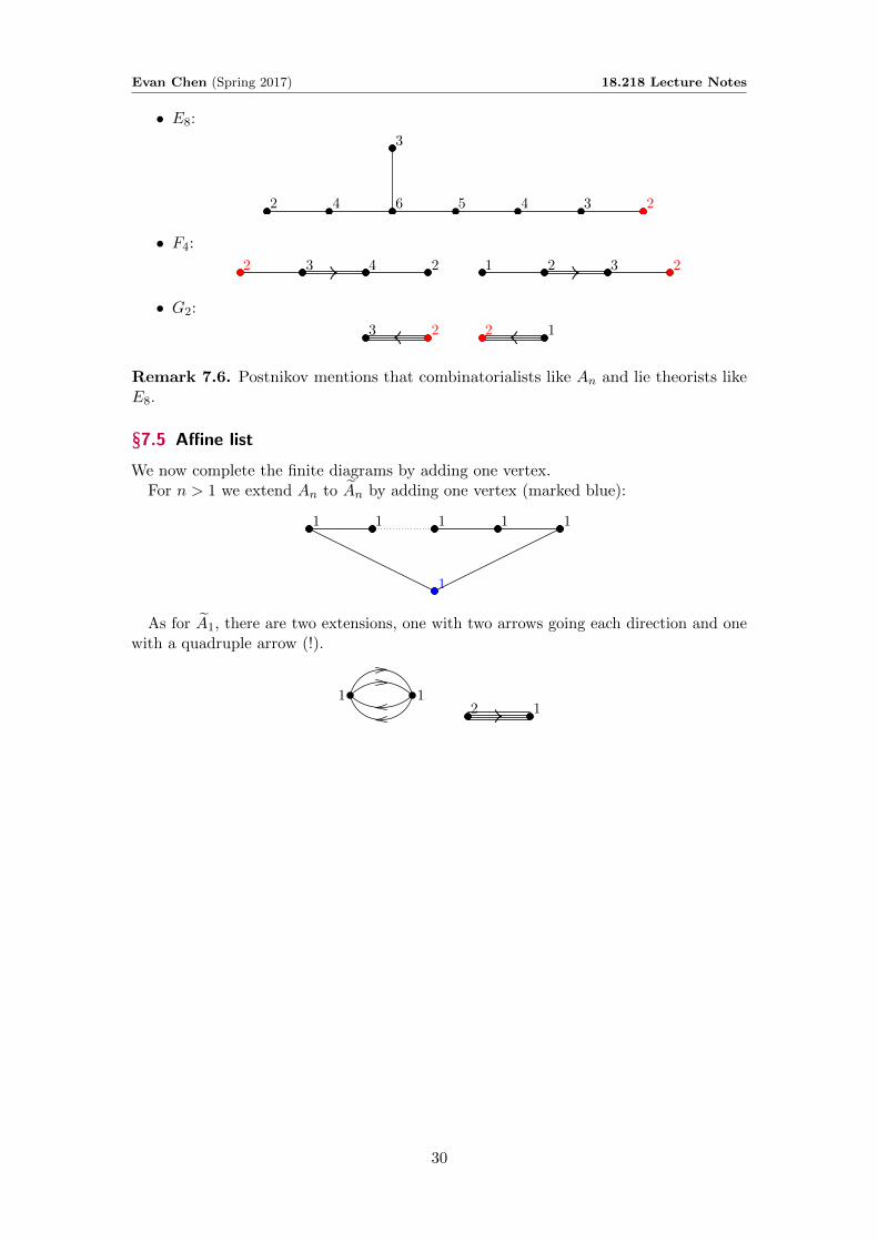
• E8:
2 4 6 5 4 3 2
3
• F4:
2 3 4 2 1 2 3 2
• G2:
3 2 2 1
Remark 7.6. Postnikov mentions that combinatorialists like An and lie theorists likeE8.
§7.5 Affine list
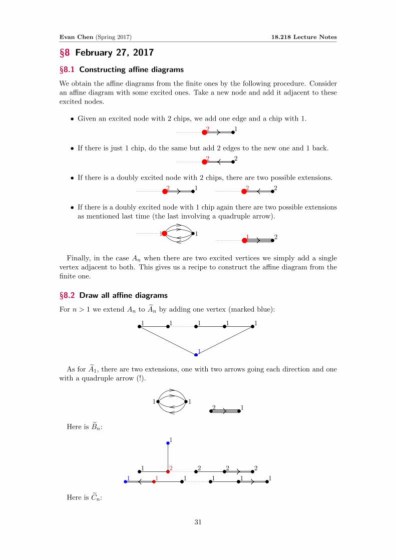
We now complete the finite diagrams by adding one vertex.For n > 1 we extend An to An by adding one vertex (marked blue):
1 1 1 1 1
1
As for A1, there are two extensions, one with two arrows going each direction and onewith a quadruple arrow (!).
1 12 1
30
Evan Chen (Spring 2017) 18.218 Lecture Notes
§8 February 27, 2017
§8.1 Constructing affine diagrams
We obtain the affine diagrams from the finite ones by the following procedure. Consideran affine diagram with some excited ones. Take a new node and add it adjacent to theseexcited nodes.
• Given an excited node with 2 chips, we add one edge and a chip with 1.
2 1
• If there is just 1 chip, do the same but add 2 edges to the new one and 1 back.
2 2
• If there is a doubly excited node with 2 chips, there are two possible extensions.
2 1 2 2
• If there is a doubly excited node with 1 chip again there are two possible extensionsas mentioned last time (the last involving a quadruple arrow).
1 1 1 2
Finally, in the case An when there are two excited vertices we simply add a singlevertex adjacent to both. This gives us a recipe to construct the affine diagram from thefinite one.
§8.2 Draw all affine diagrams
For n > 1 we extend An to An by adding one vertex (marked blue):
1 1 1 1 1
1
As for A1, there are two extensions, one with two arrows going each direction and onewith a quadruple arrow (!).
1 12 1
Here is Bn:
1 2 2 2 2
1
1 1 1 1 11
Here is Cn:
31

Evan Chen (Spring 2017) 18.218 Lecture Notes
2 2 2 2 11
1 2 2 2 12
1 2 2 2 1
1
Here is Dn:
1
2 2 2
1
1
1
Here are E6, E7, E8:
• E6:
1 2 3 2 1
22
• E7:
2 3 4 3 2 1
2
1
• E8:
2 4 6 5 4 3 2
3
1
Here are the two versions F4:
2 3 4 21 1 2 3 2 1
Here are the extensions of G2:
3 2 1 2 11
§8.3 Observations
Recall that:
• Finite type iff there exists a nonzero subadditive function which is not additive.
• Affine type iff there exists a nonzero additive function.
32
Evan Chen (Spring 2017) 18.218 Lecture Notes
Lemma 8.1
Any proper induced subgraph of a graph of finite or affine type is of affine type.
Proof. Simply restrict the additive function to the subgraph.
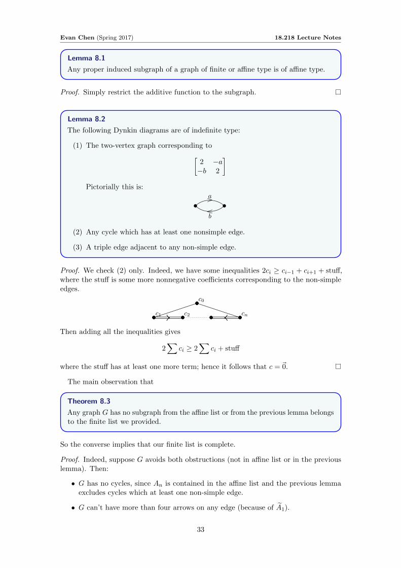
Lemma 8.2
The following Dynkin diagrams are of indefinite type:
(1) The two-vertex graph corresponding to[2 −a−b 2
]Pictorially this is:
a
b
(2) Any cycle which has at least one nonsimple edge.
(3) A triple edge adjacent to any non-simple edge.
Proof. We check (2) only. Indeed, we have some inequalities 2ci ≥ ci−1 + ci+1 + stuff,where the stuff is some more nonnegative coefficients corresponding to the non-simpleedges.
c1 c2 cn
c0
Then adding all the inequalities gives
2∑
ci ≥ 2∑
ci + stuff
where the stuff has at least one more term; hence it follows that c = ~0.
The main observation that
Theorem 8.3
Any graph G has no subgraph from the affine list or from the previous lemma belongsto the finite list we provided.
So the converse implies that our finite list is complete.
Proof. Indeed, suppose G avoids both obstructions (not in affine list or in the previouslemma). Then:
• G has no cycles, since An is contained in the affine list and the previous lemmaexcludes cycles which at least one non-simple edge.
• G can’t have more than four arrows on any edge (because of A1).
33
Evan Chen (Spring 2017) 18.218 Lecture Notes
• If G contains a triple edge, then G = G2 (because of the extensions G2 and thecycle condition).
• There is at most one double edge, because of Bn, Cn.
• There exists at most one trivalent vertex (because of Dn) and moreover in such agraph we have no double edges (because of the last Cn).
• . . .
Thus we have shown the lemma together with the forbidden subgraphs An, Bn, Cn, Dn,E6, E7, E8, F4, G2 give us the conclusion.
This proof is weird because it seems almost circular. The algorithm is:
• Write down the finite list, and claim it’s complete.
• Generate the affine list by augmenting the finite list appropriately.
• Use the lemma along with the affine list as forbidden subgraphs, and check thatthese forbidden conditions restrict us back to the finite list we started with.
Thus we have
Theorem 8.4
This is a complete classification of finite and affine generalized Cartan matrices.
Corollary 8.5
Kostant’s game is finite if and only if the generalized Cartan matrix is finite.
Proof. If the game stops, then the ending point is a subadditive function which is notadditive, since in a final configuration has at least one excited vertex.
Exercise 8.6. Prove that if A is of finite type, then Kostant’s group is finite, withoutusing classification.
§8.4 Root system
We now define a root system (at last!).
Definition 8.7. Suppose V is a Euclidean space (Rn with a dot product) and let αbe a nonzero vector. By Hα we denote the hyperplane orthogonal to α and by sα thereflection about Hα.
Definition 8.8. A root system is a finite subset
Φ ⊂ V \ {0}
such that
(1) If α ∈ Φ, then sαΦ = Φ. In other words reflecting one root with another root givesanother root.
(2) Φ spans V .
34

Evan Chen (Spring 2017) 18.218 Lecture Notes
(3) If α and β are linearly dependent, then either α = β or α = −β.
(We alluded to a “crystallographic” condition that can be added. But we give the fulldefinition next lecture.)
Condition (1) is the main condition. For (2), we can restrict any non-spanning Φ toits span anyways. Condition (3) is cosmetic, and some authors omit it.
In the next lecture we will see that this root system picture corresponds exactly toCartan matrices of finite type.
35
Evan Chen (Spring 2017) 18.218 Lecture Notes
§9 March 1 2017
Today we’ll be going through standard notations and definitions of root systems, andthen in the near future talk about some “numerology” of these root systems (some specialnumbers associated to them). Afterwards the direction of the course may vary dependingon interest and demand.
§9.1 Notations
From now on V is a Euclidean space of dimension r with inner product (−,−) (we haveswitched to the letter r, which is standard in this area of mathematics). As in last lecture,we let Hα be the hyperplane perpendicular to a nonzero vector 0 6= α ∈ V and we let sαbe the reflection across Hα by
sα : λ 7→ λ− 2(λ, α)
(α, α)α.
(We can check this works since sα(α) = −α and that it fixes the hyperplane.) Weintroduce the following notation:
Definition 9.1. For each 0 6= α ∈ V denote
α∨def=
2
(α, α)α.
This lets us simplify the formula sα to
sα(λ) = λ− (λ, α∨)α.
§9.2 Definition of root systems
We recall the definition of the root system from the previous lecture. We add in thefollowing terminology:
• The rank of a root system Φ is the dimension of the ambient vector space.
• The elements of Φ are called roots.
Finally, we add a new condition:
Definition 9.2. A root system Φ is crystallographic if for any α, β ∈ Φ, we have(α∨, β) ∈ Z. Thus sα(β) will be an integer linear combination of α and β.
§9.3 Examples of root systems
§9.3.1 Crystallographic examples of rank two
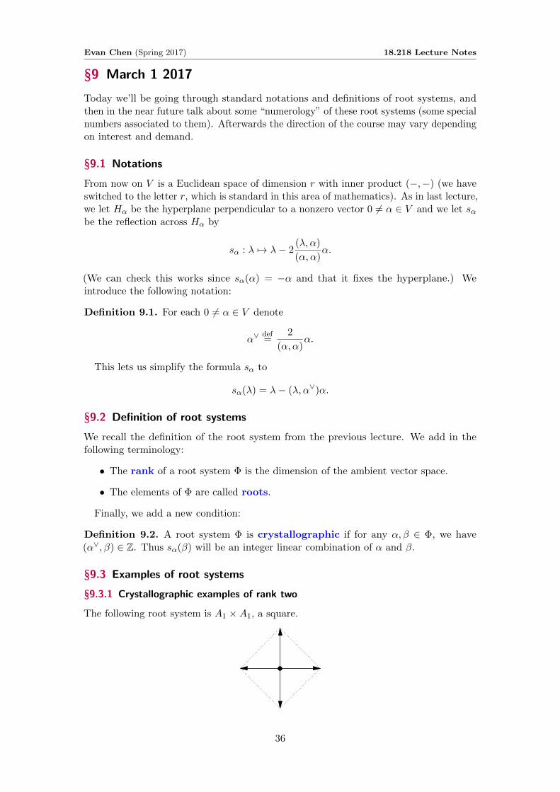
The following root system is A1 ×A1, a square.
36
Evan Chen (Spring 2017) 18.218 Lecture Notes
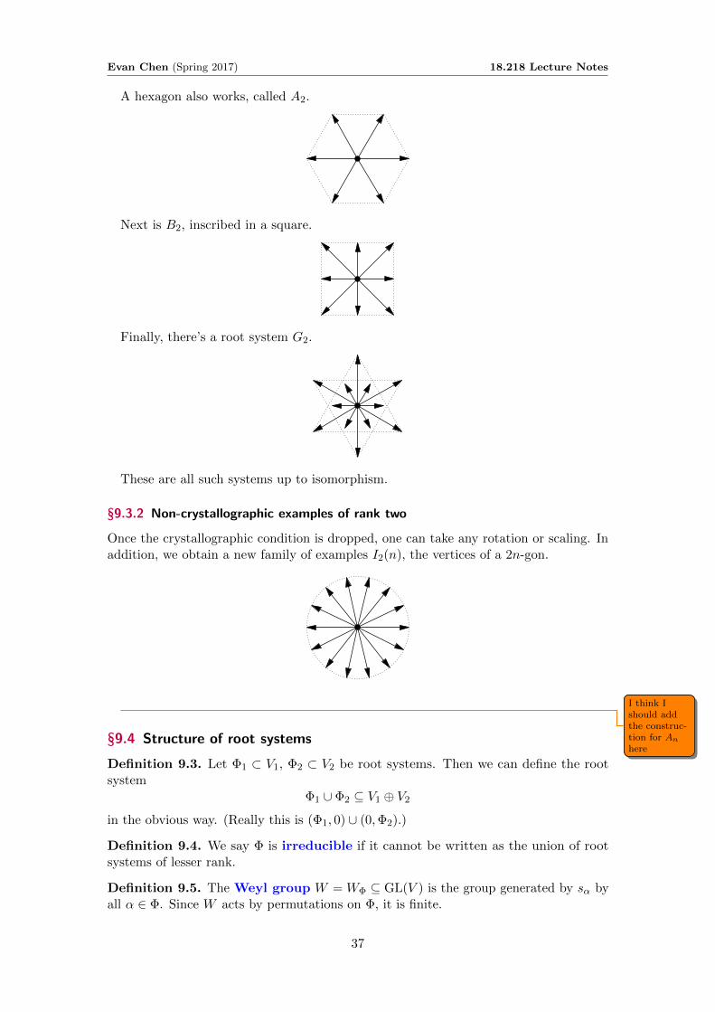
A hexagon also works, called A2.
Next is B2, inscribed in a square.
Finally, there’s a root system G2.
These are all such systems up to isomorphism.
§9.3.2 Non-crystallographic examples of rank two
Once the crystallographic condition is dropped, one can take any rotation or scaling. Inaddition, we obtain a new family of examples I2(n), the vertices of a 2n-gon.
I think Ishould addthe construc-tion for Anhere
I think Ishould addthe construc-tion for Anhere
§9.4 Structure of root systems
Definition 9.3. Let Φ1 ⊂ V1, Φ2 ⊂ V2 be root systems. Then we can define the rootsystem
Φ1 ∪ Φ2 ⊆ V1 ⊕ V2
in the obvious way. (Really this is (Φ1, 0) ∪ (0,Φ2).)
Definition 9.4. We say Φ is irreducible if it cannot be written as the union of rootsystems of lesser rank.
Definition 9.5. The Weyl group W = WΦ ⊆ GL(V ) is the group generated by sα byall α ∈ Φ. Since W acts by permutations on Φ, it is finite.
37
Evan Chen (Spring 2017) 18.218 Lecture Notes
Definition 9.6. Pick a generic linear form f(x) = (λ, x) on V , not vanishing on anyelement of Φ. We define
• The positive roots α ∈ Φ+λ such that f(α) > 0.
• The negative roots β ∈ Φ−λ such that f(β) < 0.
Thus vectors of Φ are split into Φ+ and Φ−.
There are multiple choices of λ but in fact they are all equivalent.
Lemma 9.7 (Positive roots are unique)
Let Φ+λ and Φ+
λ′ be two choices of positive roots. Then there exists w ∈W such that
w(Φ+λ ) = Φ+
λ′ .
In fact we will later see that the choice of this w is unique. For now, to prove this lemmawe use the notion of a Weyl chamber.
Definition 9.8. The Coxeter arrangement is the collection of hyperplanes orthogonalto any some root of Φ. The resulting regions are called Weyl chambers.
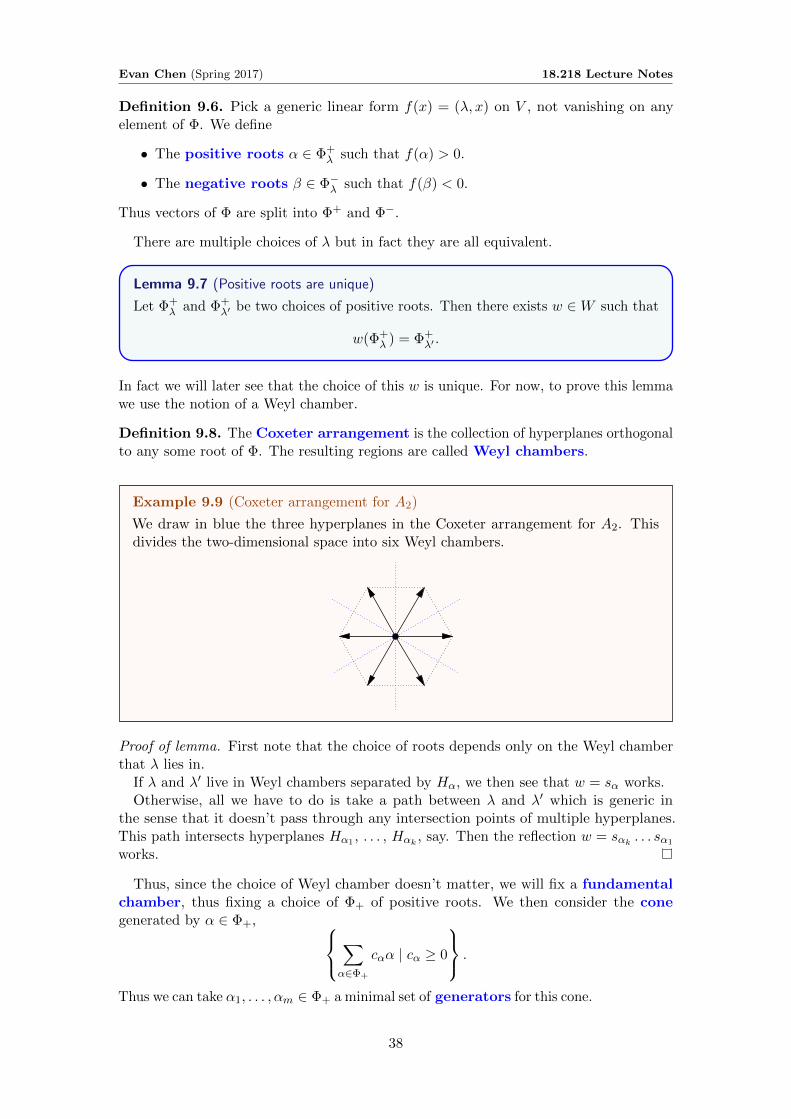
Example 9.9 (Coxeter arrangement for A2)
We draw in blue the three hyperplanes in the Coxeter arrangement for A2. Thisdivides the two-dimensional space into six Weyl chambers.
Proof of lemma. First note that the choice of roots depends only on the Weyl chamberthat λ lies in.
If λ and λ′ live in Weyl chambers separated by Hα, we then see that w = sα works.Otherwise, all we have to do is take a path between λ and λ′ which is generic in
the sense that it doesn’t pass through any intersection points of multiple hyperplanes.This path intersects hyperplanes Hα1 , . . . , Hαk , say. Then the reflection w = sαk . . . sα1
works.
Thus, since the choice of Weyl chamber doesn’t matter, we will fix a fundamentalchamber, thus fixing a choice of Φ+ of positive roots. We then consider the conegenerated by α ∈ Φ+, ∑
α∈Φ+
cαα | cα ≥ 0
.
Thus we can take α1, . . . , αm ∈ Φ+ a minimal set of generators for this cone.
38
Evan Chen (Spring 2017) 18.218 Lecture Notes
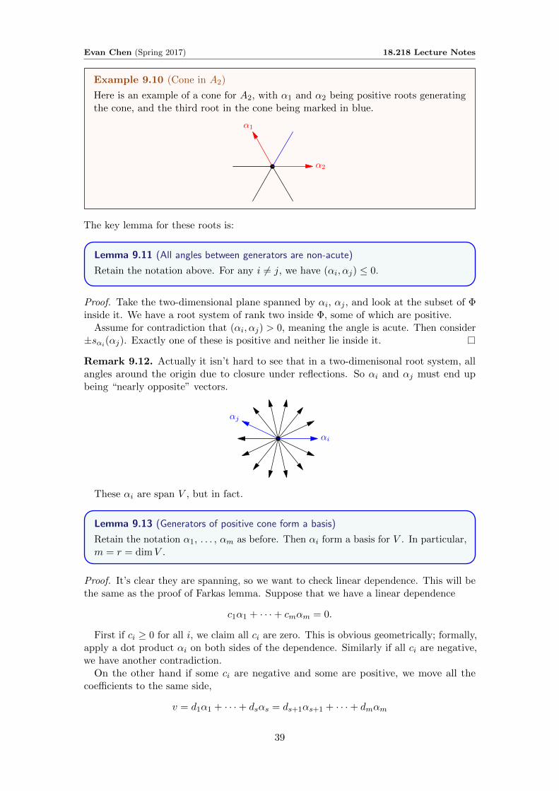
Example 9.10 (Cone in A2)
Here is an example of a cone for A2, with α1 and α2 being positive roots generatingthe cone, and the third root in the cone being marked in blue.
α1
α2
The key lemma for these roots is:
Lemma 9.11 (All angles between generators are non-acute)
Retain the notation above. For any i 6= j, we have (αi, αj) ≤ 0.
Proof. Take the two-dimensional plane spanned by αi, αj , and look at the subset of Φinside it. We have a root system of rank two inside Φ, some of which are positive.
Assume for contradiction that (αi, αj) > 0, meaning the angle is acute. Then consider±sαi(αj). Exactly one of these is positive and neither lie inside it.
Remark 9.12. Actually it isn’t hard to see that in a two-dimenisonal root system, allangles around the origin due to closure under reflections. So αi and αj must end upbeing “nearly opposite” vectors.
αi
αj
These αi are span V , but in fact.
Lemma 9.13 (Generators of positive cone form a basis)
Retain the notation α1, . . . , αm as before. Then αi form a basis for V . In particular,m = r = dimV .
Proof. It’s clear they are spanning, so we want to check linear dependence. This will bethe same as the proof of Farkas lemma. Suppose that we have a linear dependence
c1α1 + · · ·+ cmαm = 0.
First if ci ≥ 0 for all i, we claim all ci are zero. This is obvious geometrically; formally,apply a dot product αi on both sides of the dependence. Similarly if all ci are negative,we have another contradiction.
On the other hand if some ci are negative and some are positive, we move all thecoefficients to the same side,
v = d1α1 + · · ·+ dsαs = ds+1αs+1 + · · ·+ dmαm
39

Evan Chen (Spring 2017) 18.218 Lecture Notes
where each di is nonnegative. We have v 6= 0 by the preceding paragraph. But now
0 < (v, v) = (d1α1 + · · ·+ dsαs, ds+1αs+1 + · · ·+ dmαm) .
The right hand side is non-positive by expanding the dot product. Contradiction.
Thus in summary, we have that:
• A choice of Weyl chamber gives a set of positive roots.
• This gives us a choice of basis, which we call simple roots.
40
Evan Chen (Spring 2017) 18.218 Lecture Notes
§10 March 3, 2017
I was not feeling well this fine Friday afternoon, and thus did not attend lecture. Thanksto Tom Roby for sending me his handwritten notes.
§10.1 Simple reflections
Let Φ be a root system for the Weyl group W , and let Φ+ ⊂ Φ be the positive roots. Wedenote by α1, . . . , αr the simple roots. We have the following properties:
• α1, . . . , αr form a basis of V .
• (αi, αj) ≤ 0 for i 6= j.
• Any α ∈ Φ+ is a N-linear combination of αi’s.
• For any other choice of simple roots α′1, . . . , α′r, there exists w ∈ W such that
w {α1, . . . , αr} = {α′1, . . . , α′r}.
• For all α ∈ Φ, there exists αi and w ∈W such that w(αi) = α.
Definition 10.1. A simple reflection is one of the form
sidef= sαi
for some 1 ≤ i ≤ r (as noted αi is a simple root).
Lemma 10.2 (Simple reflections generate W )
W is generated by simple reflections s1, . . . , sr.
Proof. Here is a geometric proof. Note that si correspond to reflections around walls ofthe fundamental chamber C0. So if C ′ is an adjacent chamber, then C ′ = si(C0).
Then reflections with respect to walls of C ′ are of teh form
s′j = ssi(αj) = sisjsi
for some j, with i fixed (C ′ = si(C0)). And so on. Later we’ll see more details of thisconstruction.
§10.2 Cartan matrices
Recall that α∨ = 2α(α,α) . Now given a root system Φ with simple roots {α1, . . . , αr}, we
can construct the matrix
A = AΦ = (aij) where aij =(α∨i , αj
).
We now have:
41
Evan Chen (Spring 2017) 18.218 Lecture Notes
Proposition 10.3 (It’s a generalized Cartan matrix)
Let A = AΦ = (aij) as above.
(i) aii = 2.
(ii) aij ≤ 0 for i 6= j.
(iii) aij 6= 0 ⇐⇒ aji 6= 0.
(iv) aij ∈ Z if Φ is crystallographic.
Hence A is a generalized Cartan matrix.
This lets us relate configurations to the Kostant game in the following way: a configu-ration maps to a vector via
~c = (c1, . . . , cr) 7→ λ = c1α1 + · · ·+ crαr.
We now compute
si(λ) = λ−(α∨i , λ
)αi
= λ−∑j
aijcjαi
= c1α1 + · · ·+ c′iαi + · · ·+ crαr.
with c′i corresponding to Kostant game.Then we observe that
Theorem 10.4 (Root system ↔ Kostant game)
Thus vectors lying in the cone of the root system Φ correspond exactly to con-figurations in Kostant’s game with the matrix A = AΦ, with simple reflectionscorresponding to firings.
Accordingly,
Theorem 10.5 (Irreducible Φ ← finite type Cartan)
Crystallographic irreducible root systems correspond to generalized indecomposableCartan matrices of finite type, up to re-ordering the rows and columns of the matrix(equivalently, relabelling the nodes of the Dynkin diagram).
42
Evan Chen (Spring 2017) 18.218 Lecture Notes
§11 March 6, 2017
Let W be a Weyl group with simple reflections s1, . . . , sr as usual.
§11.1 Presentation of the Weyl group
Theorem 11.1 (Presentation of the Weyl group)
The group W is generated by s1, . . . , sr with the following Coxeter relations:
(1) s2i = 1 for all i, and
(2)sisjsi . . .︸ ︷︷ ︸ = sjsisj . . .︸ ︷︷ ︸ for all i 6= j
where 2mij = # {±αi,±αj ,±si(αj),±sj(αi),±sisj(αi), . . . }.
Remark 11.2. In the crystallographic case, we have only four cases for mij .
mij Graph Picture Matrix
mij = 2 i jaij = aji = 0
mij = 3 aij = aji = −1mij = 4 aij = −2, aji = −1mij = 6 aij = −3, aji = −1.
§11.2 Proof of Coxeter relations
It’s not hard to see the Coxeter relations are true; we want to show they are necessary.
Proposition 11.3
Let C0 be the fundamental Weyl chamber and let C any other Weyl chamber. If
si1 . . . sik(C0) = sj1 . . . sjk′ (C0) = C
then si1 . . . sik and sj1 . . . sjk′ are related by Coxeter moves.
Proof. Suppose w = si1 . . . sik ∈W . We are going to write
w = . . . (si1si2si3s−1i2s−1i1
)(si1si2s
−1i1
)si1 = sβk . . . sβ1
where sβ1 = α−1i1
, β2 = si1αi2 , β3 = si1si2(αi3), and so on. The trick is that:
The sβ will tell us which hyperplanes we cross when we go from C0
to C.
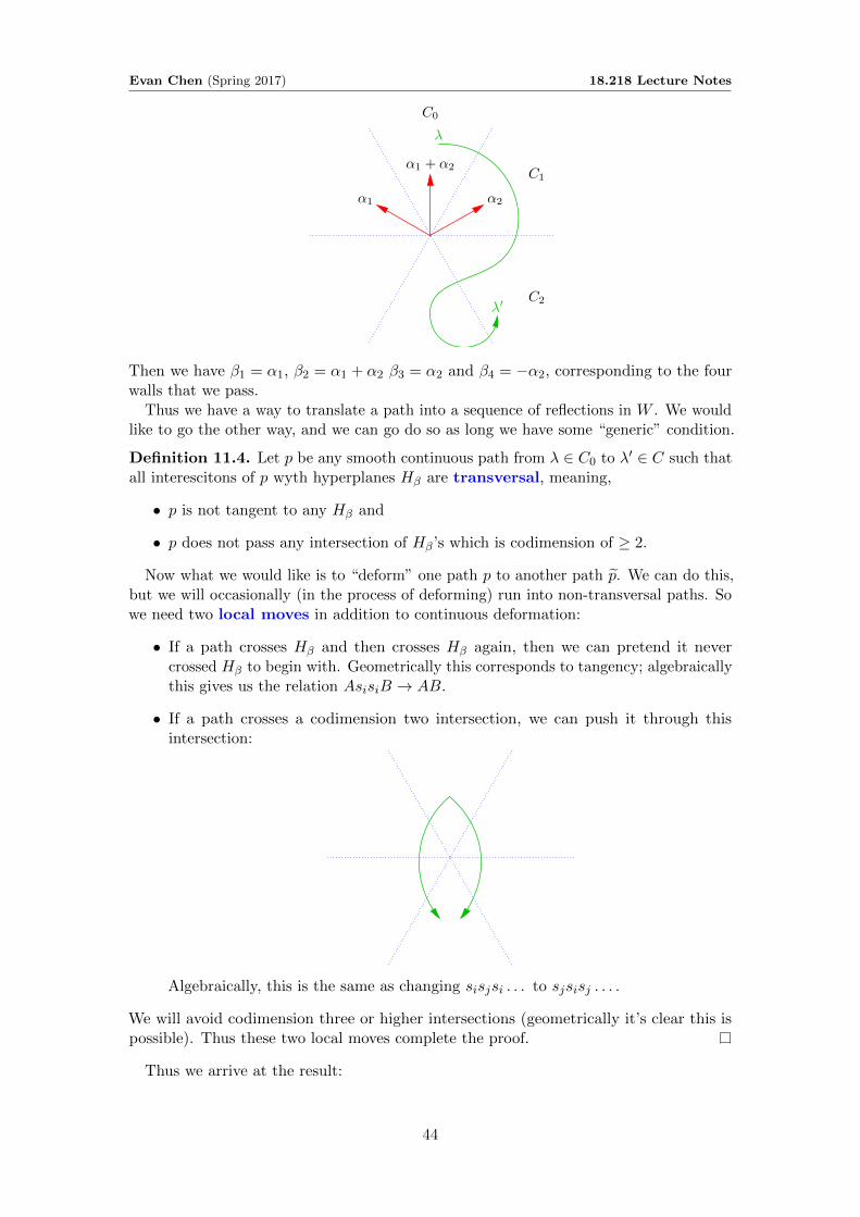
For example, consider the following figure:
43
Evan Chen (Spring 2017) 18.218 Lecture Notes
C0
C1
C2
α1
α1 + α2
α2
λ
λ′
Then we have β1 = α1, β2 = α1 + α2 β3 = α2 and β4 = −α2, corresponding to the fourwalls that we pass.
Thus we have a way to translate a path into a sequence of reflections in W . We wouldlike to go the other way, and we can go do so as long we have some “generic” condition.
Definition 11.4. Let p be any smooth continuous path from λ ∈ C0 to λ′ ∈ C such thatall interescitons of p wyth hyperplanes Hβ are transversal, meaning,
• p is not tangent to any Hβ and
• p does not pass any intersection of Hβ’s which is codimension of ≥ 2.
Now what we would like is to “deform” one path p to another path p. We can do this,but we will occasionally (in the process of deforming) run into non-transversal paths. Sowe need two local moves in addition to continuous deformation:
• If a path crosses Hβ and then crosses Hβ again, then we can pretend it nevercrossed Hβ to begin with. Geometrically this corresponds to tangency; algebraicallythis gives us the relation AsisiB → AB.
• If a path crosses a codimension two intersection, we can push it through thisintersection:
Algebraically, this is the same as changing sisjsi . . . to sjsisj . . . .
We will avoid codimension three or higher intersections (geometrically it’s clear this ispossible). Thus these two local moves complete the proof.
Thus we arrive at the result:
44
Evan Chen (Spring 2017) 18.218 Lecture Notes
Corollary 11.5 (W bijects to Weyl chambers)
There are exactly |W | Weyl chambers, corresponding to w(C0) for w ∈W .
§11.3 Dual description
Here is a dual description of the result we just proved. Let W be a Weyl group withfundamental chamber C0.
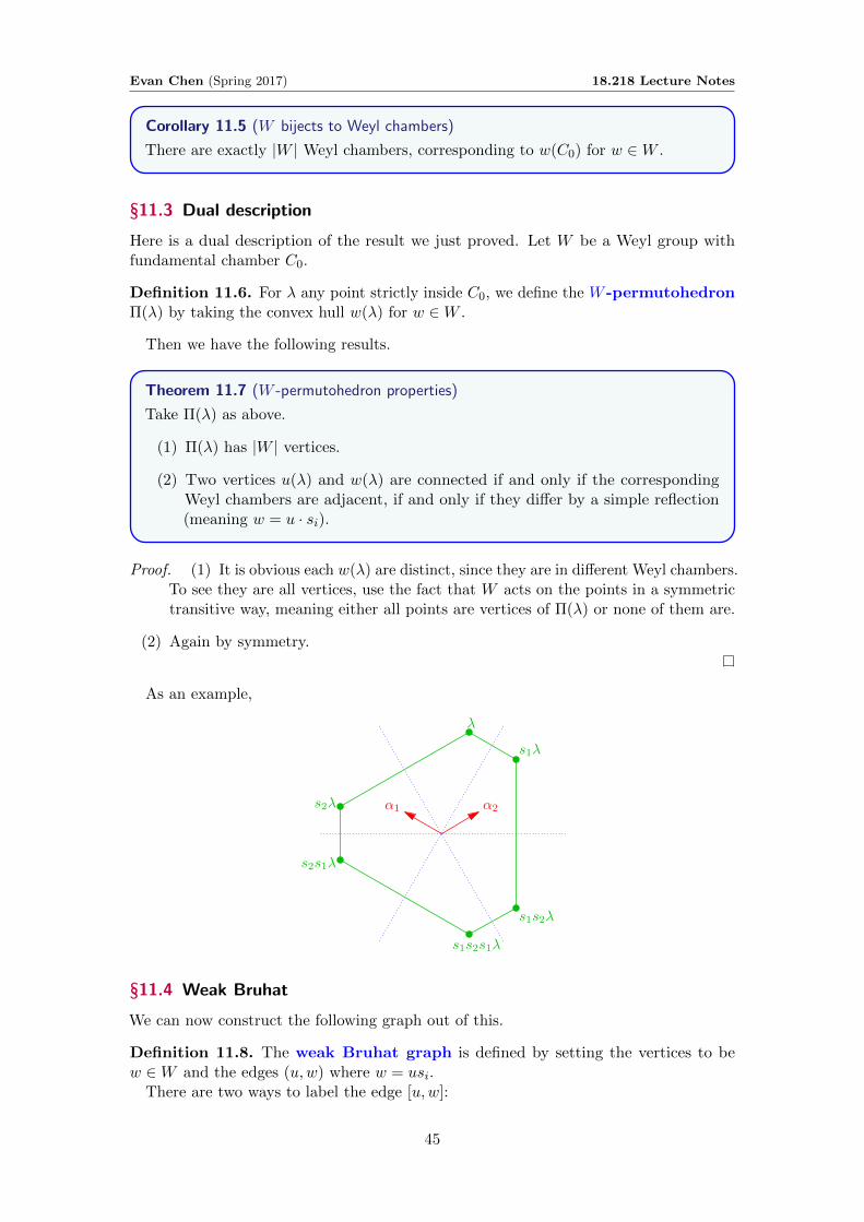
Definition 11.6. For λ any point strictly inside C0, we define the W -permutohedronΠ(λ) by taking the convex hull w(λ) for w ∈W .
Then we have the following results.
Theorem 11.7 (W -permutohedron properties)
Take Π(λ) as above.
(1) Π(λ) has |W | vertices.
(2) Two vertices u(λ) and w(λ) are connected if and only if the correspondingWeyl chambers are adjacent, if and only if they differ by a simple reflection(meaning w = u · si).
Proof. (1) It is obvious each w(λ) are distinct, since they are in different Weyl chambers.To see they are all vertices, use the fact that W acts on the points in a symmetrictransitive way, meaning either all points are vertices of Π(λ) or none of them are.
(2) Again by symmetry.
As an example,
α1 α2
λ
s1λ
s1s2λ
s1s2s1λ
s2s1λ
s2λ
§11.4 Weak Bruhat
We can now construct the following graph out of this.
Definition 11.8. The weak Bruhat graph is defined by setting the vertices to bew ∈W and the edges (u,w) where w = usi.
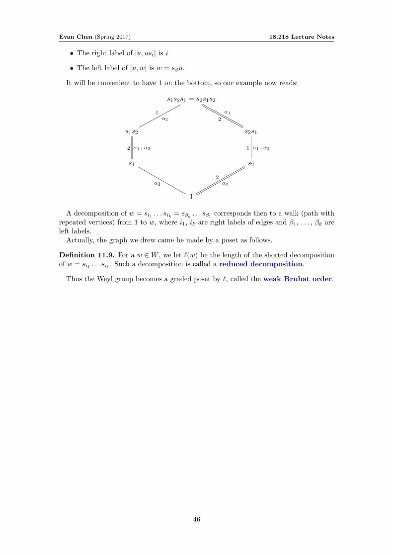
There are two ways to label the edge [u,w]:
45
Evan Chen (Spring 2017) 18.218 Lecture Notes
• The right label of [u, usi] is i
• The left label of [u,w] is w = sβu.
It will be convenient to have 1 on the bottom, so our example now reads:
s1s2s1 = s2s1s2
s1s2 s2s1
s1 s2
1
1α2 2
α1
2 α1+α2 1 α1+α2
1α1
2α2
A decomposition of w = si1 . . . sik = sβk . . . sβ1 corresponds then to a walk (path withrepeated vertices) from 1 to w, where i1, ik are right labels of edges and β1, . . . , βk areleft labels.
Actually, the graph we drew came be made by a poset as follows.
Definition 11.9. For a w ∈W , we let `(w) be the length of the shorted decompositionof w = si1 . . . si` . Such a decomposition is called a reduced decomposition.
Thus the Weyl group becomes a graded poset by `, called the weak Bruhat order.
46
Evan Chen (Spring 2017) 18.218 Lecture Notes
§12 March 8, 2017
As usual W is a Weyl group with simple reflections s1, . . . , sr satisfying the Coxeterrelations.
We retain the notation `(w) from last lecture. Notice that `(w) = `(w−1) just becauseif w = si1 . . . si` hen w−1 = si` . . . si1 .
§12.1 Inversions
Definition 12.1. An inversion of w is a root α ∈ Φ+ such that w(α) ∈ Φ−. We letInv(w) denote the set of such inversions.
Lemma 12.2 (Length is number of inversions)
For any w we have `(w) = `(w−1) = # Inv(w).
Proof. Let λ be strictly dominant, meaning λ is in the interior of the fundamentalchamber C0. Then we’ve seen already that `(w) is the minimal number of hyperplanesHα we need to cross to get from λ to w(λ).
Now take α ∈ Φ+, so (α, λ) > 0. Then we have that Hα separates λ and w(λ) if andonly if
(w(λ), α) < 0 ⇐⇒ (λ,w−1(α)) < 0 ⇐⇒ w−1(α) ∈ Φ−1.
So the number of separating planes is exactly Inv(w−1).
Corollary 12.3 (βi are inversion set)
Let w = si1 . . . si` be a reduced decomposition and assume w = sβ` . . . sβ1 as lastlecture. Then Inv(w−1) = {β1, . . . , β`}.
Corollary 12.4 (Weak Bruhat order via inversions)
We have u ≤ w in the weak Bruhat order exactly if Inv(u−1) ⊆ Inv(w−1).
Remark. u ≤ w 6 ⇐⇒ u−1 ≤ w−1.
§12.2 Construction of root system of type An−1
We’ll adopt the convention r = n− 1. Let V be the vector space
V ={
(x1, . . . , xn) ∈ Rn |∑
xi = 0}⊆ Rn
be a hyperplane of codimension one. If we equip Rn with the usual basis e1, . . . , en. Then,we let
Φ ={αij
def= ei − ej | i 6= j
}and let Hαij = {x ∈ V | xi = xj}. This forms the so-called braid arrangement. Finally,the reflection sαij turns out to be
sαij : (x1, . . . , xi, . . . , xj , . . . , xn) 7→ (x1, . . . , xj , . . . , xi, . . . , xn) .
47
Evan Chen (Spring 2017) 18.218 Lecture Notes
We pick simple roots αi = αi,i+1 whence si are adjacent transpositions. Then, W ∼= Snis the symmetry group.
Why is this related to An−1? To see this, we simply construct the Cartan matrix, andfind that it coincides with that of a chain on n vertices.
§12.3 Wiring diagrams
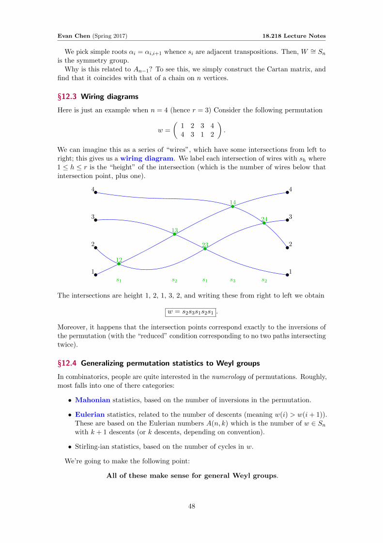
Here is just an example when n = 4 (hence r = 3) Consider the following permutation
w =
(1 2 3 44 3 1 2
).
We can imagine this as a series of “wires”, which have some intersections from left toright; this gives us a wiring diagram. We label each intersection of wires with sh where1 ≤ h ≤ r is the “height” of the intersection (which is the number of wires below thatintersection point, plus one).
1
2
3
4
1
2
3
4
12
13
23
14
24
s1 s2 s1 s3 s2
The intersections are height 1, 2, 1, 3, 2, and writing these from right to left we obtain
w = s2s3s1s2s1 .
Moreover, it happens that the intersection points correspond exactly to the inversions ofthe permutation (with the “reduced” condition corresponding to no two paths intersectingtwice).
§12.4 Generalizing permutation statistics to Weyl groups
In combinatorics, people are quite interested in the numerology of permutations. Roughly,most falls into one of there categories:
• Mahonian statistics, based on the number of inversions in the permutation.
• Eulerian statistics, related to the number of descents (meaning w(i) > w(i+ 1)).These are based on the Eulerian numbers A(n, k) which is the number of w ∈ Snwith k + 1 descents (or k descents, depending on convention).
• Stirling-ian statistics, based on the number of cycles in w.
We’re going to make the following point:
All of these make sense for general Weyl groups.
48
Evan Chen (Spring 2017) 18.218 Lecture Notes
Specifically, we’ve said i ∈ {1, . . . , r} is an inversion if w ∈W when i ∈ Inv(w). Now weadd:
Definition 12.5. We say i ∈ {1, . . . , r} is a descent of w ∈ W if `(wsi) < `(w).This corresponds to going “downwards” in the Bruhat picture. Thus we can defineCoxter-Eulerian numbers by
AΦ(k) = {w ∈W with k descents} .
(Here we’re identifying numbers i with simple roots si. In Lie theory, apparently peopledon’t do this.)
Remark 12.6. The Coxter-Eulerian numbers give the so-called h-numbers (definedbelow) of the permutahedron Π(λ) we saw earlier.
To define the h-numbers for a polyhedron P, we first define
fi = #i-dimensional faces of P
and we let the f -polynomial be f(x) =∑
i ge0 fixi. Then we define the h-polynomial to
satisfy
f(x− 1) = h(x) =∑i≥0
hixi.
It turns out hi are symmetric and nonnegative as long as P is simple.For the permutahedron Π(λ) we get AΦ(k).
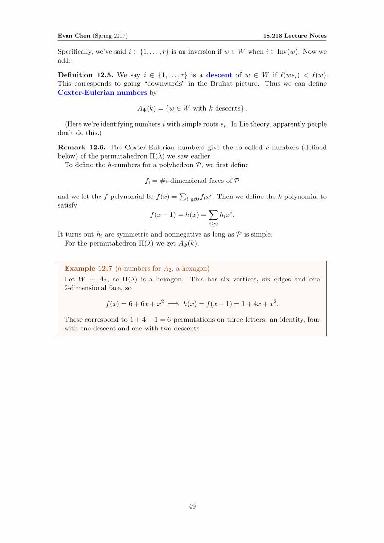
Example 12.7 (h-numbers for A2, a hexagon)
Let W = A2, so Π(λ) is a hexagon. This has six vertices, six edges and one2-dimensional face, so
f(x) = 6 + 6x+ x2 =⇒ h(x) = f(x− 1) = 1 + 4x+ x2.
These correspond to 1 + 4 + 1 = 6 permutations on three letters: an identity, fourwith one descent and one with two descents.
49

Evan Chen (Spring 2017) 18.218 Lecture Notes
§13 March 10, 2017
Let Φ be a crystallographic root system. This lecture we’ll generalize the formula |Sn| = n!to a formula for |W | for any Weyl group W .
§13.1 The root poset
Definition 13.1. We define the root poset to be the partial ordering on the positiveroots Φ+ with the relation ≥ where α ≥ β if α − β is a nonnegative combination ofpositive (equivalently, simple) roots.
Thus the simple roots are the bottom of the poset.
Proposition 13.2 (The Highest Root)
For irreducible root systems the root poset has a unique maximal element θ calledthe highest root.
Example 13.3 (Root poset for An−1)
Take W = An−1. ThenΦ+ = {αij = ei − ej}
with simple roots αi = αi, i+ 1. Then αij ≥ αi′j′ ⇐⇒ i ≤ i′ < j′ ≤ j.Here is a picture of the poset for n = 5:
α1 α2 αn−1
θ = α1n
Remark 13.4. In fact, we get the height function for the poset by: when α = c1α1 · · ·+crαr we get
ht(α) = c1 + · · ·+ cr.
This implies the poset is graded.
50

Evan Chen (Spring 2017) 18.218 Lecture Notes
Example 13.5 (Root poset for Bn)
In this example we have
Φ+ = {ei ± ej | 1 ≤ i < j ≤ n} ∪ {ei | 1 ≤ i ≤ n}
The simple roots are αi = ei − ei+1 and αn = en. Here is the picture of the poset forn = 3; it is “half” the An picture.
θ
α1 α2 αn−1 αn
In the context of Kostant game, θ corresponds to the following endpoint.
1 2 2 2 2
§13.2 Coxeter number
We now define some “magic numbers” of Weyl groups.
Definition 13.6. A Coxeter element of W is an element of the form c = s1 . . . sr ∈W .
Lemma 13.7 (Coxeter elemens are conjugate)
Fixing W , all Coxeter elements are conjugate to each other (as we vary the order inwhich the si are multiplied).
Thus we can define
Definition 13.8. The Coxeter number h is the order of the Coxeter element (well-defined since they’re all conjugate).
Definition 13.9. The exponents of W are positive integers 0 < m1 ≤ · · · ≤ mr < hsuch that the eigenvalues of a Coxeter element c ∈ GL(V ) (actually c ∈ O(V )) are
exp(
2πi · mj
h
)j = 1, . . . , r.
Finally,
Definition 13.10. The index of connection f is the determinant of the Cartan matrix.
51

Evan Chen (Spring 2017) 18.218 Lecture Notes
Now, let θ = a1α1 + · · ·+arαr and set a0 = 1. Then (a0, . . . , ar) is an additive functionon the nodes of the extended Dnykin diagram.
Example 13.11 (Dn)
Suppose we have the Dynkin diagram Dn.
1
2 2 2
1
1
1
Then we choose(a0, . . . , ar) =
(1, 1, 2, . . . , 2︸ ︷︷ ︸
r−3
, 1, 1).
Theorem 13.12 (h and f determined by θ)
We have
h = a0 + a1 + · · ·+ ar = ht(θ) + 1
f = # {i | ai = 1} .
Theorem 13.13 (Exponents determined by root poset; Kostant)
Let λ = (mr,mr−1, . . . ,m1) be a partition and λ∗ = (k1, . . . , kmr) its conjugatepartition. Then ki is the number of positive roots of height i.
In particular, mr = h− 1 and k1 ≥ k2 ≥ · · · ≥ kh−1.
Example 13.14 (Exponents for An)
For W = An, we have k1 = r, k2 = r − 1, . . . , kr−1 = 1. Thus λ∗ = (r, r − 1, r −2, . . . , 1). This is self-dual, so we obtain
λ = (r, r − 1, . . . , 1)
hence the exponents are 1, 2, . . . , r.
Example 13.15 (Exponents for Bn)
For W = Bn, we have
λ∗ = (r, r − 1, r − 1, r − 2, r − 2, . . . , 1, 1).
Taking the dual givesλ = (1, 3, 5, . . . , 2r − 1)
hence the exponents are 1, 3, 5, . . . , 2r − 1.
52
Evan Chen (Spring 2017) 18.218 Lecture Notes
Actually, the exponents satisfy the following properties.
• m1 = 1 and mr = h− 1.
• mi = mr−i+1 = h for all i.
Now the number of elements in the root poset is equal to∣∣Φ+∣∣ = m1 + · · ·+mr =
rh
2
so we obtain
Theorem 13.16 (Number of roots)
We have|Φ| = rh.
In fact the following theorem is true too.
Theorem 13.17 (Order of the Weyl group)
For any W , we have the following two formulas:
|W | =r∏i=1
(1 +mi)
= f · r! · a1 . . . ar.
53
Evan Chen (Spring 2017) 18.218 Lecture Notes
§14 March 13, 2017
Last time we saw Weyl’s formula
|W | = f · r! · a1 . . . ar
where θ is the highest root a1α1 + · · ·+ arαr and f = detAΦ = #{1 ≤ i ≤ r | ai = 1} isthe index of connection. This lecture we’ll prove this formula, using the so-called affineWeyl group (which is infinite!).
§14.1 Root lattice and weight lattice
In fact we well define four lattices in this section: the (co-)root lattice, the (co-)weightlattice.
Definition 14.1. We say λ ∈ V is an integral weight if (λ, α∨) ∈ Z for each α ∈ Φ.
The fundamental weights, denoted ω1, . . . , ωr, are the dual basis to the basis ofsimple co-roots α∨i (i = 1, . . . , r), in the sense that
(ωi, α∨j ) =
{1 i = j
0 else.
Definition 14.2. The weight lattice P is the Z-lattice of all the integral weights,generated by ωi.
Definition 14.3. The root lattice Q is the Z-lattice of all roots α ∈ Φ (or equivalently,just the simple roots α1, . . . , αr).
Proposition 14.4 (Q ⊂ P )
The root lattice in contained inside the weight lattice.
Proof. It suffices to show each simple root αi is an integral weight. Assume αi =c1ω1 + · · · + crωr, so (αi, α
∨j ) = cj for each j, which is an entry of the Cartan matrix,
hence an integer.
Remark 14.5 (Cartan matrix corresponds to αi in wj). In fact, this shows that whenwe express αi as linear combinations of ωi, we end up with the Cartan matrix. For
example in A2 with A =
[2 −1−1 2
]we will find α1 = 2ω1 − ω2 and α2 = −ω1 + 2ω2.
Definition 14.6. The co-root lattice and co-weight lattice are defined by
• The co-root lattice Q∨ is defined by α∨1 , . . . , α∨r .
• The co-weight lattice P∨ is defined by ω∨1 , . . . , ω∨r .
Remark 14.7. This is a bit confusing since two types of duality are going on:
• The duality going from Q to P corresponds to taking the transpose of the Cartanmatrix.
• The between Q and P∨ is the (Euclidean) dual basis (with respect to inner product).Ditto for Q∨ and P∨.
54

Evan Chen (Spring 2017) 18.218 Lecture Notes
Proposition 14.8 (Index of connection)
f = [P : Q] = [P∨ : Q∨].
Proof. Since f = detA, follows by Remark 14.5.
§14.2 A picture
Example 14.9 (Lattice in A2)
Let V = {(x1, x2, x3) | x1 + x2 + x3 = 0} be the usual ambient subspace of R3. Thenwe have
α1 = α∨1 = (1,−1, 0)
α2 = α∨2 = (0, 1,−1).
In that case, one can check
ω1 = ω∨1 = (1, 0, 0)− 1
3(1, 1, 1)
ω2 = ω∨2 = (1, 1, 0)− 2
3(1, 1, 1).
Here is the picture:
α1α2ω1ω2
We see visibly, f = 3 which follows as
α1 = 2ω1 − ω2
α2 = −ω1 + 2ω2
and hence
A =
[2 −1−1 2
]hence f = detA = 3.
55

Evan Chen (Spring 2017) 18.218 Lecture Notes
§14.3 Affine Weyl group
Definition 14.10. Let α ∈ Φ, and k ∈ Z. We define2 the affine hyperplanes by
Hα,k = {λ ∈ V | (λ, α) = k}
and thus the affine reflection sα,k the reflection with respect to Hα,k.Thus we have
s(α, k)(λ)def= sα(λ) + kα∨
= λ− (λ, α)α∨ + kα∨
= λ− ((λ, α)− k)α∨.
Definition 14.11. The affine Coxeter arrengement is the hyperplane arrangementconsisting of the (infinitely many!) hyperplane arrangements Hα,k. The affine Weylgroup Waff is the group generated by all sα,k.
Lemma 14.12 (Affine Weyl group is semidirect product)
We have Waff = W nQ∨.
Proof. For β ∈ Q∨, we let shβ be the shift λ 7→ λ+β. We claim Waff = {shβ ◦w}. ClearlyWaff ⊆ {shβ ◦w}; on the other hand shα∨ = sα,1 ◦ sα.
Definition 14.13. The regions in the affine Weyl arrangement are called alcoves.
Here is a picture of an affine Weyl arrangement, with the hyperplanes drawn in dottedlines.:
α∨1α∨
2ω∨1ω∨
2
2 Some people prefer to use α∨ instead of α in the definition of Hα,k.
56
Evan Chen (Spring 2017) 18.218 Lecture Notes
Lemma 14.14 (Invariance under Waff)
The affine Coxeter arrangement Waff is invariant under the action of Waff .
Lemma 14.15 (Waff simply transitive)
Waff acts simply transitively on the alcoves.
Proof. Same proof as we did for W acting on chambers, with the word “chamber” replacedby “alcove” everywhere.
Thus as before we like to pick a fundamental alcove A0. Like before all of them areequivalent, but typically we like to select the alcove A0 inside the fundamental chamberC0 which touches the origin. It turns out that
A0 = {x ∈ V | (αi, x) ≥ 0 and (θ, x) ≤ 1} .
and in particular A0 is a simplex.
57
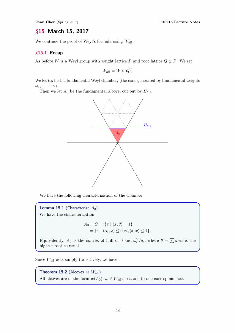
Evan Chen (Spring 2017) 18.218 Lecture Notes
§15 March 15, 2017
We continue the proof of Weyl’s formula using Waff .
§15.1 Recap
As before W is a Weyl group with weight lattice P and root lattice Q ⊂ P . We set
Waff = W nQ∨.
We let C0 be the fundamental Weyl chamber, (the cone generated by fundamental weightsω1, . . . , ωr).
Then we let A0 be the fundamental alcove, cut out by Hθ,1.
A0
Hθ,1
We have the following characterization of the chamber.
Lemma 15.1 (Characterize A0)
We have the characterization
A0 = C0 ∩ {x | (x, θ) = 1}= {x | (αi, x) ≤ 0 ∀i, (θ, x) ≤ 1} .
Equivalently, A0 is the convex of hull of 0 and ω∨i /ai, where θ =∑aiαi is the
highest root as usual.
Since Waff acts simply transitively, we have
Theorem 15.2 (Alcoves ↔ Waff)
All alcoves are of the form w(A0), w ∈Waff , in a one-to-one correspondence.
58
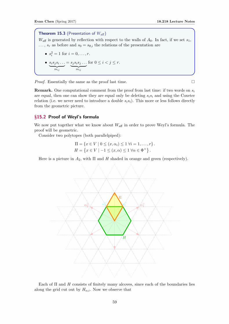
Evan Chen (Spring 2017) 18.218 Lecture Notes
Theorem 15.3 (Presentation of Waff)
Waff is generated by reflection with respect to the walls of A0. In fact, if we set s1,. . . , sr as before and s0 = sθ,i the relations of the presentation are
• s2i = 1 for i = 0, . . . , r.
• sisjsi . . .︸ ︷︷ ︸mij
= sjsisj . . .︸ ︷︷ ︸mij
for 0 ≤ i < j ≤ r.
Proof. Essentially the same as the proof last time.
Remark. One computational comment from the proof from last time: if two words on siare equal, then one can show they are equal only be deleting sisi and using the Coxeterrelation (i.e. we never need to introduce a double sisi). This more or less follows directlyfrom the geometric picture.
§15.2 Proof of Weyl’s formula
We now put together what we know about Waff in order to prove Weyl’s formula. Theproof will be geometric.
Consider two polytopes (both parallelpiped):
Π = {x ∈ V | 0 ≤ (x, αi) ≤ 1 ∀i = 1, . . . , r} .H =
{x ∈ V | −1 ≤ (x, α) ≤ 1 ∀α ∈ Φ+
}.
Here is a picture in A2, with Π and H shaded in orange and green (respectively).
α∨1α∨
2ω∨1ω∨
2
Π
H
Each of Π and H consists of finitely many alcoves, since each of the boundaries liesalong the grid cut out by Hα,i. Now we observe that
59
Evan Chen (Spring 2017) 18.218 Lecture Notes
• Π is really the parallelpiped generated by ω∨1 , . . . , ω∨r . Meanwhile A0 is theparallelpiped generated by ω∨1 /a1, . . . , ω∨r /ar. Consequently, we obtain
Vol Π
VolA0= r!a1 . . . ar.
• Since H consists of all alcoves adjacent to the origin, it has |W | alcoves, meaning
VolH
VolA0= |W |.
So it remains to compare H and A0. For this we use the following lemma.
Lemma 15.4 (Π, H are fundamental domains of P∨, Q∨)
We have that:
• Π is the fundamental domain of the coweight lattice P∨.
• H is the fundamental domain of the coroot lattice Q∨.
Proof. Equivalently, if we take Π and translate by P∨ we tile the whole space, while ifwe take H and translate by Q∨ we also tile the whole space.
The first one is more or less obvious. For the second one, follows from Waff =W nQ∨.
Thus, we have that
|W |r!a1 . . . ar
=VolH
VolP= [P∨ : Q∨] = f.
This implies Weyl’s formula.
§15.3 Example: An−1
Claim that in the case W = An−1, Waff corresponds to affine permutations, i.e. permu-tations w : Z → Z for which w(i + n) = w(i) + n subject to the additional constraintw(1) + · · ·+ w(n) = 1 + · · ·+ n. More about this example coming next lecture.
60
Evan Chen (Spring 2017) 18.218 Lecture Notes
§16 March 17, 2017
§16.1 The example An−1
Let r = n− 1, so we have An−1. We consider the roots as living in the vector space
V ={
(x1, . . . , xn) ∈ Rn |∑
xi = 0}
and for which we have the dual space
V ∗ = Rn/(1, . . . , 1)R ' V.
The simple roots αi = (0, . . . , 0, 1,−1, 0, . . . 0) and the fundamental weights ωi aregiven modulo (1, . . . , 1) by
ωi =
1, . . . , 1︸ ︷︷ ︸i
, 0, . . . , 0
≡1, . . . , 1︸ ︷︷ ︸
i
, 0, . . . , 0
− i
n(1, . . . , 1) ∈ V ∗.
Then the root lattice is given by
Q ={
(x1, . . . , xn) ∈ Zn |∑
xi = 0}.
and the weight lattice isP = p(ZN )
where p is the projection onto the∑xi = 0 plane used earlier,
p : Rn −→ V
(x1, . . . , xn) 7−→ (x1, . . . , xn)−∑xin
(1, . . . , 1).
§16.2 Affine permutations, and cylindrical wiring diagrams
In the case W = An−1 we are describing, Waff becomes the so-called affine permutations.
Definition 16.1. Fix n ≥ 1. A map w : Z→ Z is an affine permutation if
(i) w is a bijection.
(ii) w(i+ n) = w(i) + n for all i.
(iii) w(1) + · · ·+ w(n) = 1 + 2 + · · ·+ n.
These permutations from a group under function composition, which we call the Georgegroup after George Lusztig.
We introduce the following notation. Given w an affine permutation, we identify wwith
w = [w(1), . . . , w(n)]
and thenw = (w(1) mod n, . . . , w(n) mod n) .
Obviously w is a bijection on Z/n.
61
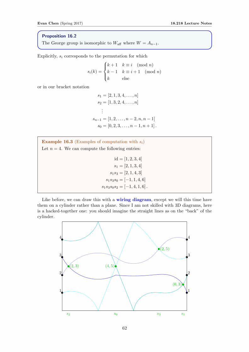
Evan Chen (Spring 2017) 18.218 Lecture Notes
Proposition 16.2
The George group is isomorphic to Waff where W = An−1.
Explicitly, si corresponds to the permutation for which
si(k) =
k + 1 k ≡ i (mod n)
k − 1 k ≡ i+ 1 (mod n)
k else
or in our bracket notation
s1 = [2, 1, 3, 4, . . . , n]
s2 = [1, 3, 2, 4, . . . , n]
...
sn−1 = [1, 2, . . . , n− 2, n, n− 1]
s0 = [0, 2, 3, . . . , n− 1, n+ 1] .
Example 16.3 (Examples of computation with si)
Let n = 4. We can compute the following entries:
id = [1, 2, 3, 4]
s1 = [2, 1, 3, 4]
s1s3 = [2, 1, 4, 3]
s1s3s0 = [−1, 1, 4, 6]
s1s3s0s2 = [−1, 4, 1, 6] .
Like before, we can draw this with a wiring diagram, except we will this time havethem on a cylinder rather than a plane. Since I am not skilled with 3D diagrams, hereis a hacked-together one: you should imagine the straight lines as on the “back” of thecylinder.
1
2
3
4
1
2
3
4
(0, 3)
(2, 5)
(4, 5)(2, 3)
s1s3s0s2
62
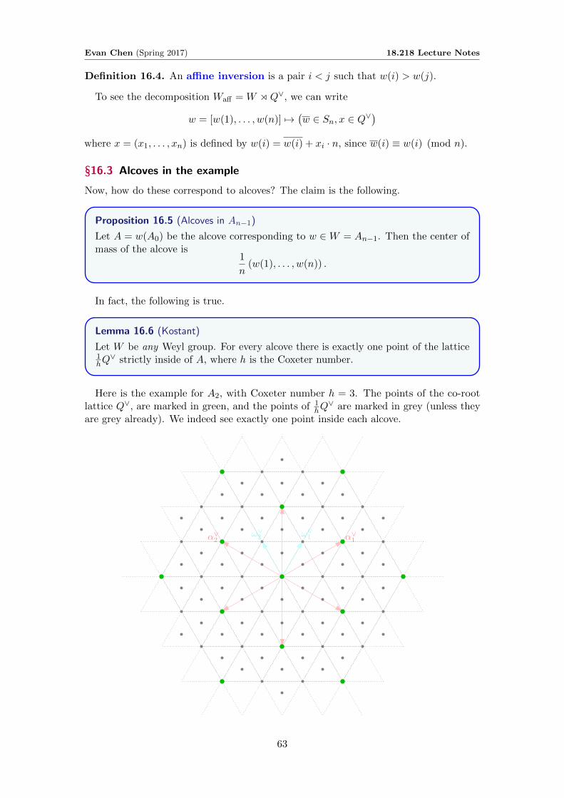
Evan Chen (Spring 2017) 18.218 Lecture Notes
Definition 16.4. An affine inversion is a pair i < j such that w(i) > w(j).
To see the decomposition Waff = W oQ∨, we can write
w = [w(1), . . . , w(n)] 7→(w ∈ Sn, x ∈ Q∨
)where x = (x1, . . . , xn) is defined by w(i) = w(i) + xi · n, since w(i) ≡ w(i) (mod n).
§16.3 Alcoves in the example
Now, how do these correspond to alcoves? The claim is the following.
Proposition 16.5 (Alcoves in An−1)
Let A = w(A0) be the alcove corresponding to w ∈W = An−1. Then the center ofmass of the alcove is
1
n(w(1), . . . , w(n)) .
In fact, the following is true.
Lemma 16.6 (Kostant)
Let W be any Weyl group. For every alcove there is exactly one point of the lattice1hQ∨ strictly inside of A, where h is the Coxeter number.
Here is the example for A2, with Coxeter number h = 3. The points of the co-rootlattice Q∨, are marked in green, and the points of 1
hQ∨ are marked in grey (unless they
are grey already). We indeed see exactly one point inside each alcove.
α∨1α∨
2ω∨1ω∨
2
63
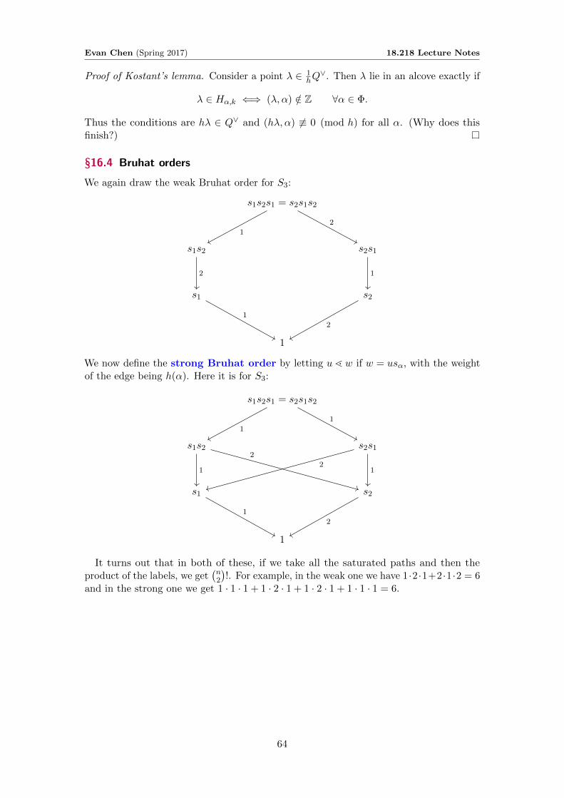
Evan Chen (Spring 2017) 18.218 Lecture Notes
Proof of Kostant’s lemma. Consider a point λ ∈ 1hQ∨. Then λ lie in an alcove exactly if
λ ∈ Hα,k ⇐⇒ (λ, α) /∈ Z ∀α ∈ Φ.
Thus the conditions are hλ ∈ Q∨ and (hλ, α) 6≡ 0 (mod h) for all α. (Why does thisfinish?)
§16.4 Bruhat orders
We again draw the weak Bruhat order for S3:
s1s2s1 = s2s1s2
s1s2 s2s1
s1 s2
1
1
2
2 1
1
2
We now define the strong Bruhat order by letting ul w if w = usα, with the weightof the edge being h(α). Here it is for S3:
s1s2s1 = s2s1s2
s1s2 s2s1
s1 s2
1
1
1
1
2
12
1
2
It turns out that in both of these, if we take all the saturated paths and then theproduct of the labels, we get
(n2
)!. For example, in the weak one we have 1 ·2 ·1+2 ·1 ·2 = 6
and in the strong one we get 1 · 1 · 1 + 1 · 2 · 1 + 1 · 2 · 1 + 1 · 1 · 1 = 6.
64
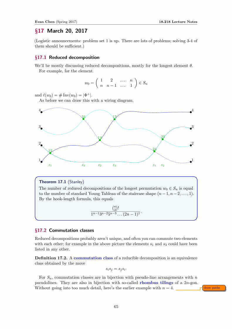
Evan Chen (Spring 2017) 18.218 Lecture Notes
§17 March 20, 2017
(Logistic announcements: problem set 1 is up. There are lots of problems; solving 3-4 ofthem should be sufficient.)
§17.1 Reduced decomposition
We’ll be mostly discussing reduced decompositions, mostly for the longest element θ.For example, for the element
w0 =
(1 2 . . . nn n− 1 . . . 1
)∈ Sn
and `(w0) = # Inv(w0) = |Φ+|.As before we can draw this with a wiring diagram.
1
2
3
4
1
2
3
4
12
13
14 23
24
34
s1 s3 s2 s3 s1 s2
Theorem 17.1 (Stanley)
The number of reduced decompositions of the longest permutation w0 ∈ Sn is equalto the number of standard Young Tableau of the staircase shape (n− 1, n− 2, . . . , 1).By the hook-length formula, this equals(
n2
)!
1n−13n−25n−3 . . . (2n− 1)1.
§17.2 Commutation classes
Reduced decompositions probably aren’t unique, and often you can commute two elementswith each other; for example in the above picture the elements s1 and s3 could have beenlisted in any other.
Definition 17.2. A commutation class of a reducible decomposition is an equivalenceclass obtained by the move
sisj = sjsi.
For Sn, commutation classes are in bijection with pseudo-line arrangements with npseudolines. They are also in bijection with so-called rhombus tilings of a 2n-gon.Without going into too much detail, here’s the earlier example with n = 4. draw pathsdraw paths
65
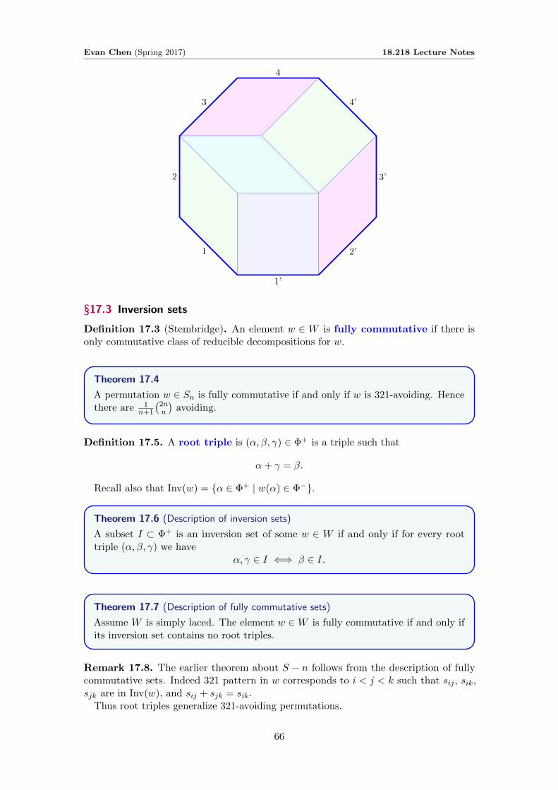
Evan Chen (Spring 2017) 18.218 Lecture Notes
1
2
3
4
4’
3’
2’
1’
§17.3 Inversion sets
Definition 17.3 (Stembridge). An element w ∈ W is fully commutative if there isonly commutative class of reducible decompositions for w.
Theorem 17.4
A permutation w ∈ Sn is fully commutative if and only if w is 321-avoiding. Hencethere are 1
n+1
(2nn
)avoiding.
Definition 17.5. A root triple is (α, β, γ) ∈ Φ+ is a triple such that
α+ γ = β.
Recall also that Inv(w) = {α ∈ Φ+ | w(α) ∈ Φ−}.
Theorem 17.6 (Description of inversion sets)
A subset I ⊂ Φ+ is an inversion set of some w ∈ W if and only if for every roottriple (α, β, γ) we have
α, γ ∈ I ⇐⇒ β ∈ I.
Theorem 17.7 (Description of fully commutative sets)
Assume W is simply laced. The element w ∈W is fully commutative if and only ifits inversion set contains no root triples.
Remark 17.8. The earlier theorem about S − n follows from the description of fullycommutative sets. Indeed 321 pattern in w corresponds to i < j < k such that sij , sik,sjk are in Inv(w), and sij + sjk = sik.
Thus root triples generalize 321-avoiding permutations.
66
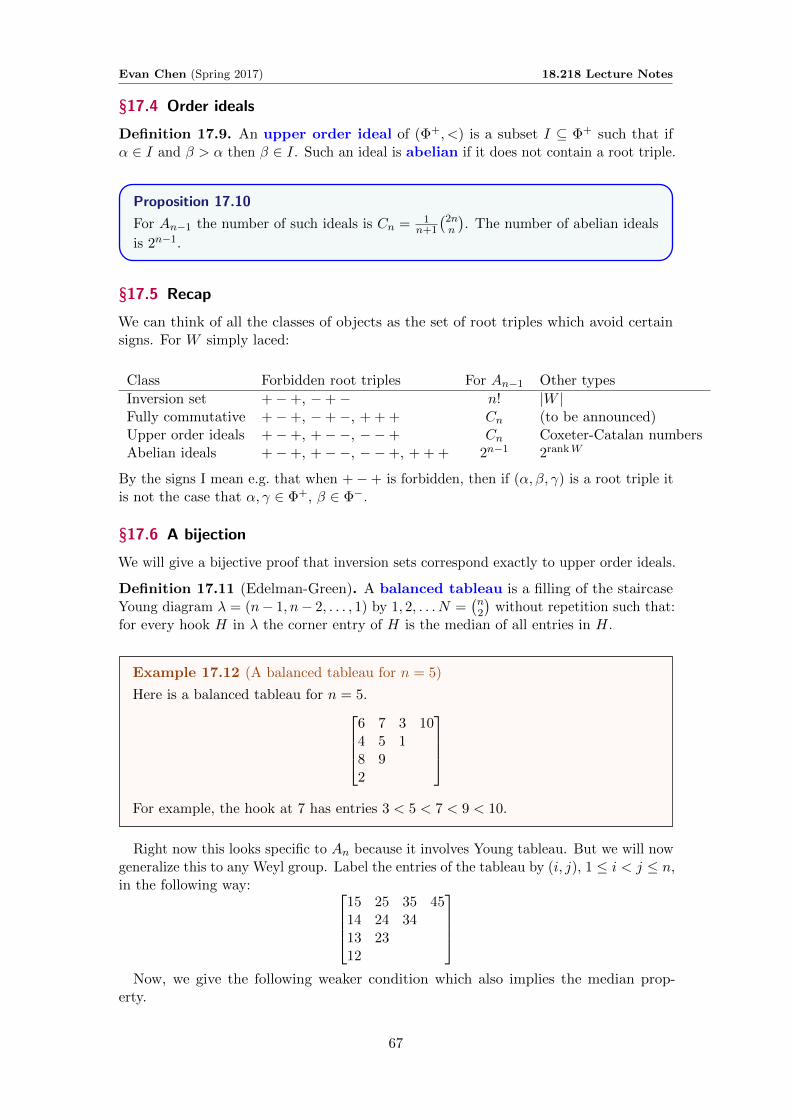
Evan Chen (Spring 2017) 18.218 Lecture Notes
§17.4 Order ideals
Definition 17.9. An upper order ideal of (Φ+, <) is a subset I ⊆ Φ+ such that ifα ∈ I and β > α then β ∈ I. Such an ideal is abelian if it does not contain a root triple.
Proposition 17.10
For An−1 the number of such ideals is Cn = 1n+1
(2nn
). The number of abelian ideals
is 2n−1.
§17.5 Recap
We can think of all the classes of objects as the set of root triples which avoid certainsigns. For W simply laced:
Class Forbidden root triples For An−1 Other types
Inversion set +−+, −+− n! |W |Fully commutative +−+, −+−, + + + Cn (to be announced)Upper order ideals +−+, +−−, −−+ Cn Coxeter-Catalan numbersAbelian ideals +−+, +−−, −−+, + + + 2n−1 2rankW
By the signs I mean e.g. that when +−+ is forbidden, then if (α, β, γ) is a root triple itis not the case that α, γ ∈ Φ+, β ∈ Φ−.
§17.6 A bijection
We will give a bijective proof that inversion sets correspond exactly to upper order ideals.
Definition 17.11 (Edelman-Green). A balanced tableau is a filling of the staircaseYoung diagram λ = (n− 1, n− 2, . . . , 1) by 1, 2, . . . N =
(n2
)without repetition such that:
for every hook H in λ the corner entry of H is the median of all entries in H.
Example 17.12 (A balanced tableau for n = 5)
Here is a balanced tableau for n = 5.6 7 3 104 5 18 92
For example, the hook at 7 has entries 3 < 5 < 7 < 9 < 10.
Right now this looks specific to An because it involves Young tableau. But we will nowgeneralize this to any Weyl group. Label the entries of the tableau by (i, j), 1 ≤ i < j ≤ n,in the following way:
15 25 35 4514 24 3413 2312
Now, we give the following weaker condition which also implies the median prop-
erty.
67

Evan Chen (Spring 2017) 18.218 Lecture Notes
Lemma 17.13 (Balanced tableaus)
A filling T of λ = (n − 1, n − 2, . . . , 1) is balanced if and only if for any indicesi < j < k the entries a, b, c in boxes (i, j), (i, k), and (j, k) satisfy either a < b < cor a > b > c.
Thus we can generalize the notion of balanced tableau to any root system.
Definition 17.14. A balanced Φ-tableau is a bijection
T : Φ+ → {1, . . . , N}
such that given any root triple (α, β, γ) the number T (β) is the median of {T (α), T (β), T (γ)}
This will give us a bijection to reduced decomposition. We claim it as follows: if
w = si1 . . . siN = sβN . . . sβ1 .
Then set T (βi) = i.
68

Evan Chen (Spring 2017) 18.218 Lecture Notes
§18 March 22, 2017
§18.1 Tableaus
As before we identify the boxes of the Staircase Young diagram with the pairs([n]
2
)= {(i, j) | 1 ≤ i < j ≤ n}.
Then recall that a balanced tableau is a bijective map
T :
([n]
2
)→ {1, . . . ,
(n
2
)}
such that T (i, k) is between T (i, j) and T (j, k) (equivalent to the hook property).This generalizes to give us the following definition for a general root system.
Definition 18.1. Let Φ be a crystallographic root system. A balanced Φ-tableau is abijection
Φ+ →{
1, . . . , |Φ+|}
such that for any root triple α, β, γ ∈ Φ+ such that β = α+γ we have T (α) < T (β) < T (γ)or T (α) > T (β) > T (γ).
Theorem 18.2 (Dyer)
Balanced Φ-tableaux are in canonical bijection with reduced decomposition of thelongest element w0 ∈W .
The bijection is explicitly given as follows: given a reduced decomposition w0 =si1 . . . siN = sβN . . . sβ1 in the usual way (β1 = α− i1, β2 = si1(αi2), and so on), thenthe corresponding tableau is given by T (βi) = i.
One can also think of this as a reflection ordering, corresponding to an ordering
β1 < β2 < · · · < βn
of the set of positive roots (by T ), satisfying the “balanced” condition.
Remark 18.3. The balanced condition can be rewritten as follows. Consider any rank 2root subsystem Ψ in Φ; for crystallographic Φ we have three possibilities (four possibilitiesif we count A2 ×A2, but we’ll ignore it).
• In A2, we have three positive roots, say γ1, γ2, γ3 in that order; we will require that
T (γ1) < T (γ2) < T (γ3) or T (γ1) > T (γ2) > T (γ3).
• In B2 we have four positive roots γ1, γ2, γ3, γ4 in that order, and we will require
T (γ1) < T (γ2) < T (γ3) < T (γ4) or T (γ1) > T (γ2) > T (γ3) > T (γ4).
69
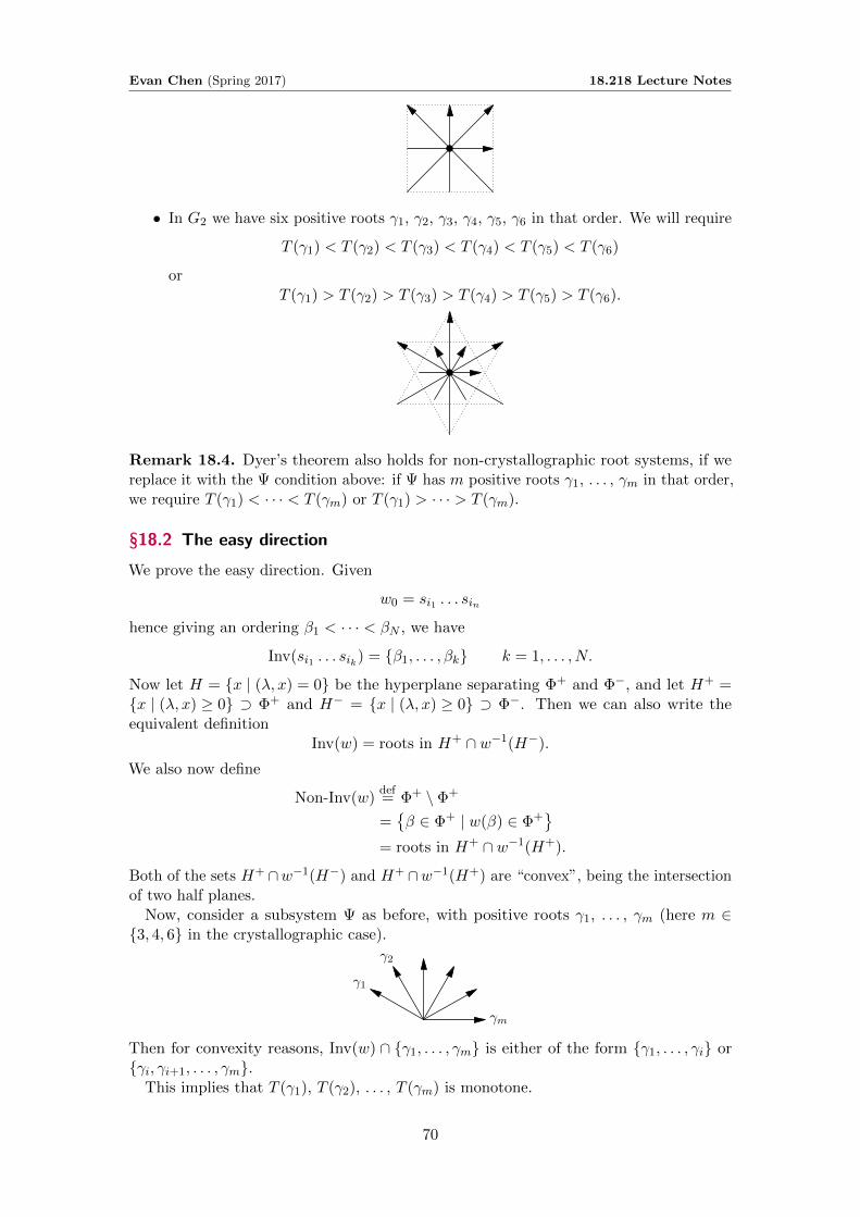
Evan Chen (Spring 2017) 18.218 Lecture Notes
• In G2 we have six positive roots γ1, γ2, γ3, γ4, γ5, γ6 in that order. We will require
T (γ1) < T (γ2) < T (γ3) < T (γ4) < T (γ5) < T (γ6)
orT (γ1) > T (γ2) > T (γ3) > T (γ4) > T (γ5) > T (γ6).
Remark 18.4. Dyer’s theorem also holds for non-crystallographic root systems, if wereplace it with the Ψ condition above: if Ψ has m positive roots γ1, . . . , γm in that order,we require T (γ1) < · · · < T (γm) or T (γ1) > · · · > T (γm).
§18.2 The easy direction
We prove the easy direction. Given
w0 = si1 . . . sin
hence giving an ordering β1 < · · · < βN , we have
Inv(si1 . . . sik) = {β1, . . . , βk} k = 1, . . . , N.
Now let H = {x | (λ, x) = 0} be the hyperplane separating Φ+ and Φ−, and let H+ ={x | (λ, x) ≥ 0} ⊃ Φ+ and H− = {x | (λ, x) ≥ 0} ⊃ Φ−. Then we can also write theequivalent definition
Inv(w) = roots in H+ ∩ w−1(H−).
We also now define
Non-Inv(w)def= Φ+ \ Φ+
={β ∈ Φ+ | w(β) ∈ Φ+
}= roots in H+ ∩ w−1(H+).
Both of the sets H+ ∩w−1(H−) and H+ ∩w−1(H+) are “convex”, being the intersectionof two half planes.
Now, consider a subsystem Ψ as before, with positive roots γ1, . . . , γm (here m ∈{3, 4, 6} in the crystallographic case).
γ1
γ2
γm
Then for convexity reasons, Inv(w) ∩ {γ1, . . . , γm} is either of the form {γ1, . . . , γi} or{γi, γi+1, . . . , γm}.
This implies that T (γ1), T (γ2), . . . , T (γm) is monotone.
70

Evan Chen (Spring 2017) 18.218 Lecture Notes
§18.3 The hard direction
The hard direction is to show that the monotonicity condition is sufficient, since theremarks above show it’s necessary. For now we will give some comments showing this isindeed hard.
For this we will use A3. To draw a picture of A3 in the plane (despite the fact thatA− 3 lives in R3), we take the affine hyperplane
H = {x | (λ, x) = 1}
and then take the intersection of the ray for each positive root with the plane H. Thesegives the six positive roots of A3, drawn in the following picture:
e1 − e2 e3 − e4
e2 − e3
e1 − e3 e2 − e4
e1 − e4
As before the Inversions of a w are then given by drawing the plane w−1(H), and thentaking the inversions to be those on one side of the line. Thus the condition is that
For any collinear points, the inversions are separated from the non-inversions.
But the situation is more complicated in general. Consider n lines in general position,giving
(n2
)intersections. Then we would hope:
Claim 18.5. Given an assignment of + and − such that on each line the + and −’s areseparated, is it always possible to separate them by a line?
For example:
− +
+
− +
+
Here’s the caveat. For general line arrangements, while we can draw a curve separatingthe + and − signs, but it is not true pure geometrically; there exists line arrangements inR2 for which it’s impossible to straighten the line. The miracle is that for root systems,it turns out it’s in fact always possible to straighten the line, not only in the rank threecase but generally for any root system in higher dimensions.
§18.4 Edelman-Greene Correspondence
71
Evan Chen (Spring 2017) 18.218 Lecture Notes
§19 March 24, 2017
Missed class for spring break. Covered Edelman-Greene algorithm.
72
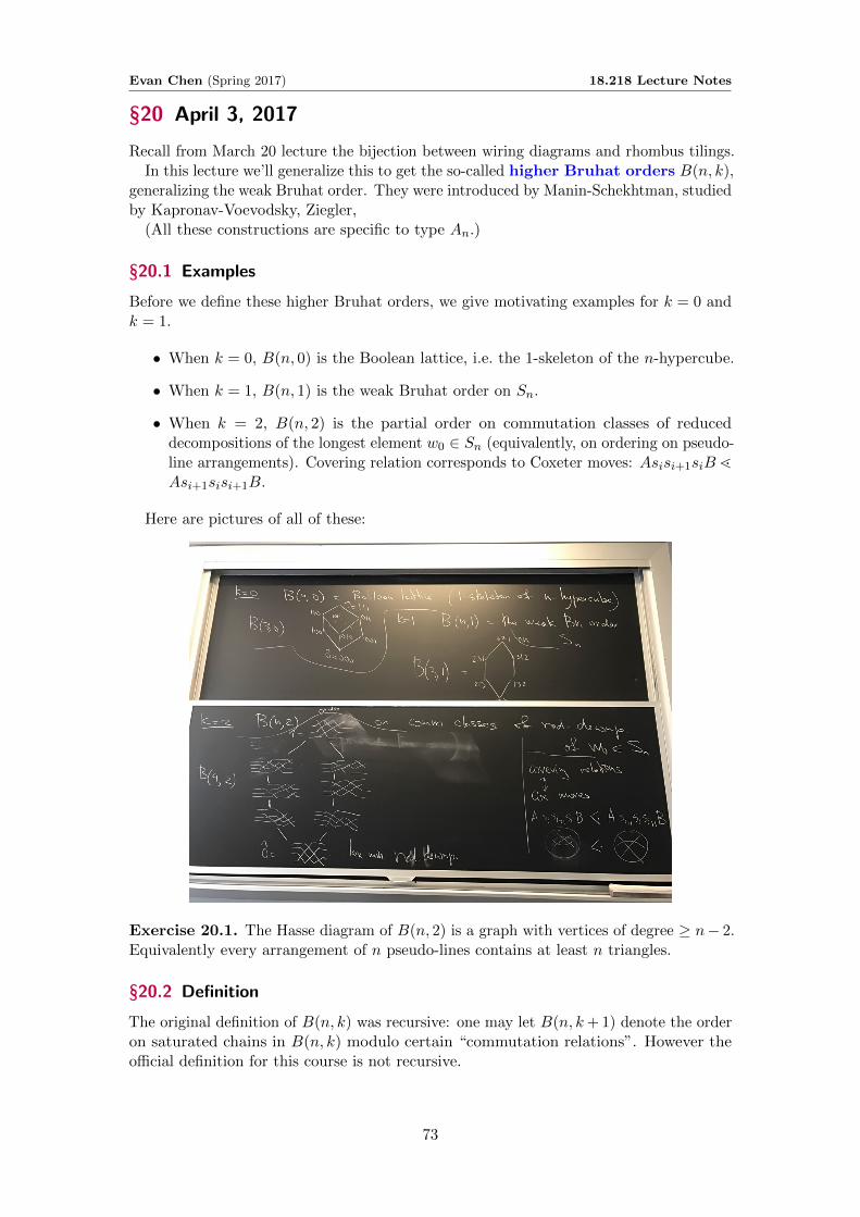
Evan Chen (Spring 2017) 18.218 Lecture Notes
§20 April 3, 2017
Recall from March 20 lecture the bijection between wiring diagrams and rhombus tilings.In this lecture we’ll generalize this to get the so-called higher Bruhat orders B(n, k),
generalizing the weak Bruhat order. They were introduced by Manin-Schekhtman, studiedby Kapronav-Voevodsky, Ziegler,
(All these constructions are specific to type An.)
§20.1 Examples
Before we define these higher Bruhat orders, we give motivating examples for k = 0 andk = 1.
• When k = 0, B(n, 0) is the Boolean lattice, i.e. the 1-skeleton of the n-hypercube.
• When k = 1, B(n, 1) is the weak Bruhat order on Sn.
• When k = 2, B(n, 2) is the partial order on commutation classes of reduceddecompositions of the longest element w0 ∈ Sn (equivalently, on ordering on pseudo-line arrangements). Covering relation corresponds to Coxeter moves: Asisi+1siBlAsi+1sisi+1B.
Here are pictures of all of these:
Exercise 20.1. The Hasse diagram of B(n, 2) is a graph with vertices of degree ≥ n− 2.Equivalently every arrangement of n pseudo-lines contains at least n triangles.
§20.2 Definition
The original definition of B(n, k) was recursive: one may let B(n, k+ 1) denote the orderon saturated chains in B(n, k) modulo certain “commutation relations”. However theofficial definition for this course is not recursive.
73
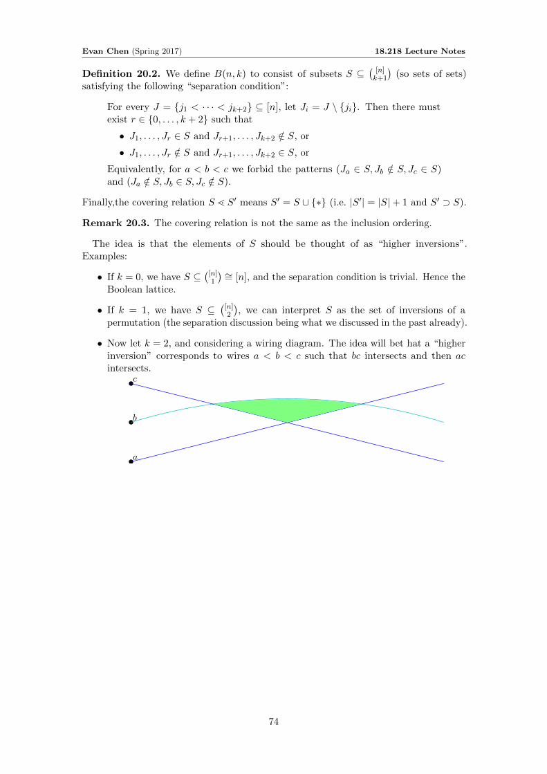
Evan Chen (Spring 2017) 18.218 Lecture Notes
Definition 20.2. We define B(n, k) to consist of subsets S ⊆( [n]k+1
)(so sets of sets)
satisfying the following “separation condition”:
For every J = {j1 < · · · < jk+2} ⊆ [n], let Ji = J \ {ji}. Then there mustexist r ∈ {0, . . . , k + 2} such that
• J1, . . . , Jr ∈ S and Jr+1, . . . , Jk+2 /∈ S, or
• J1, . . . , Jr /∈ S and Jr+1, . . . , Jk+2 ∈ S, or
Equivalently, for a < b < c we forbid the patterns (Ja ∈ S, Jb /∈ S, Jc ∈ S)and (Ja /∈ S, Jb ∈ S, Jc /∈ S).
Finally,the covering relation S l S′ means S′ = S ∪ {∗} (i.e. |S′| = |S|+ 1 and S′ ⊃ S).
Remark 20.3. The covering relation is not the same as the inclusion ordering.
The idea is that the elements of S should be thought of as “higher inversions”.Examples:
• If k = 0, we have S ⊆(
[n]1
) ∼= [n], and the separation condition is trivial. Hence theBoolean lattice.
• If k = 1, we have S ⊆(
[n]2
), we can interpret S as the set of inversions of a
permutation (the separation discussion being what we discussed in the past already).
• Now let k = 2, and considering a wiring diagram. The idea will bet hat a “higherinversion” corresponds to wires a < b < c such that bc intersects and then acintersects.
a
b
c
74
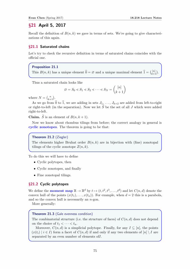
Evan Chen (Spring 2017) 18.218 Lecture Notes
§21 April 5, 2017
Recall the definition of B(n, k) we gave in terms of sets. We’re going to give characteri-zations of this again.
§21.1 Saturated chains
Let’s try to check the recursive definition in terms of saturated chains coincides with theofficial one.
Proposition 21.1
This B(n, k) has a unique element 0 = ∅ and a unique maximal element 1 =( [n]k+1
).
Thus a saturated chain looks like
∅ = S0 l S1 l S2 l · · ·l SN =
([n]
k + 1
)where N =
(nk+1
).
As we go from 0 to 1, we are adding in sets J1, . . . , Jk+2 are added from left-to-rightor right-to-left (in the separation). Now we let S be the set of all J which were addedright-to-left.
Claim. S is an element of B(n, k + 1).
Now we know about rhombus tilings from before; the correct analogy in general iscyclic zonotopes. The theorem is going to be that:
Theorem 21.2 (Ziegler)
The elements higher Bruhat order B(n, k) are in bijection with (fine) zonotopaltilings of the cyclic zonotope Z(n, k).
To do this we will have to define
• Cyclic polytopes, then
• Cyclic zonotopes, and finally
• Fine zonotopal tilings.
§21.2 Cyclic polytopes
We define the moment map R→ Rd by t 7→ (t, t2, t3, . . . , td) and let C(n, d) denote theconvex hull of the points (x(t1), . . . , x(tn)). For example, when d = 2 this is a parabola,and so the convex hull is necessarily an n-gon.
More generally:
Theorem 21.3 (Gale evenness condition)
The combinatorial structure (i.e. the structure of faces) of C(n, d) does not dependon the choice of t1 < · · · < tn.
Moreover, C(n, d) is a simplicial polytope. Finally, for any I ⊆ [n], the points(x(ti) | i ∈ I) form a facet of C(n, d) if and only if any two elements of [n] \ I areseparated by an even number of elements ofI.
75
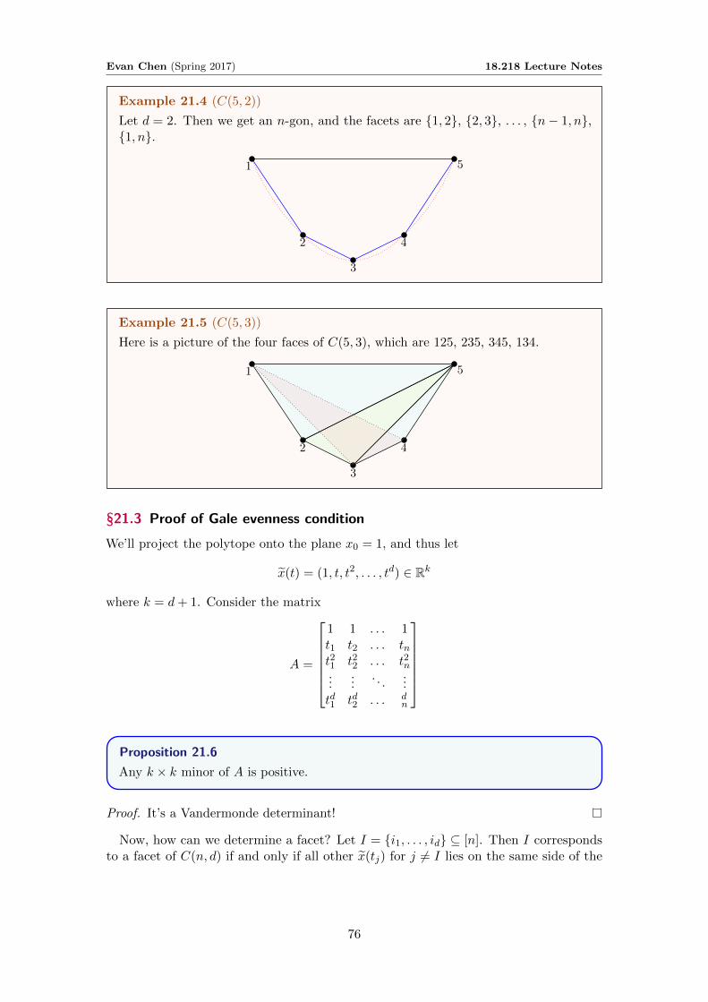
Evan Chen (Spring 2017) 18.218 Lecture Notes
Example 21.4 (C(5, 2))
Let d = 2. Then we get an n-gon, and the facets are {1, 2}, {2, 3}, . . . , {n− 1, n},{1, n}.
1
2
3
4
5
Example 21.5 (C(5, 3))
Here is a picture of the four faces of C(5, 3), which are 125, 235, 345, 134.
1
2
3
4
5
§21.3 Proof of Gale evenness condition
We’ll project the polytope onto the plane x0 = 1, and thus let
x(t) = (1, t, t2, . . . , td) ∈ Rk
where k = d+ 1. Consider the matrix
A =
1 1 . . . 1t1 t2 . . . tnt21 t22 . . . t2n...
.... . .
...td1 td2 . . . d
n
Proposition 21.6
Any k × k minor of A is positive.
Proof. It’s a Vandermonde determinant!
Now, how can we determine a facet? Let I = {i1, . . . , id} ⊆ [n]. Then I correspondsto a facet of C(n, d) if and only if all other x(tj) for j 6= I lies on the same side of the
76
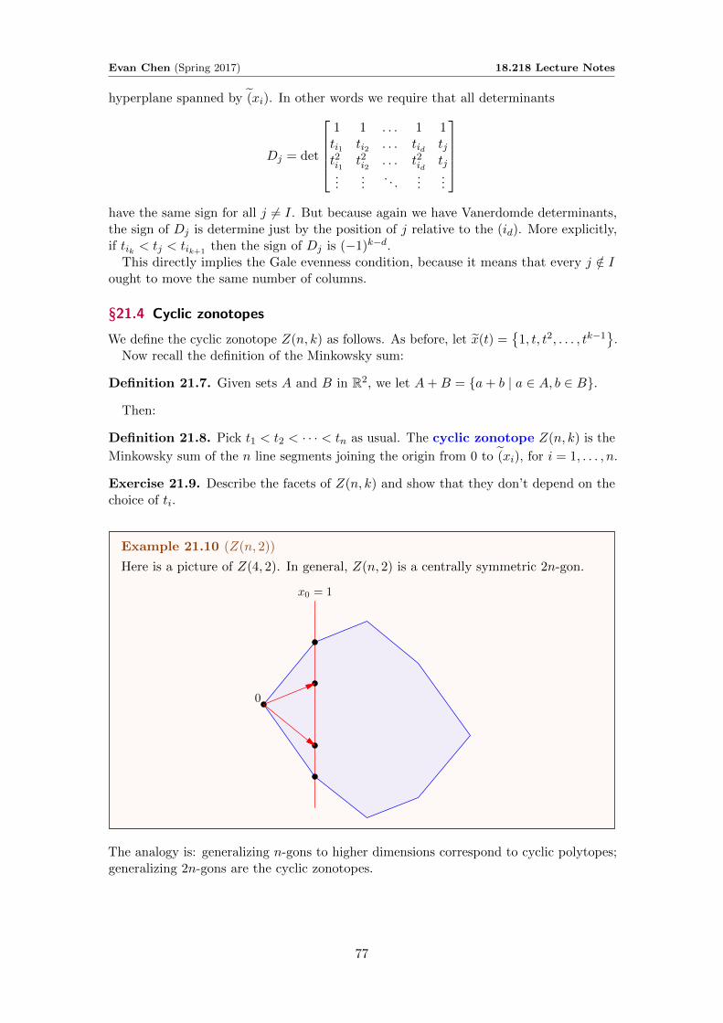
Evan Chen (Spring 2017) 18.218 Lecture Notes
hyperplane spanned by (xi). In other words we require that all determinants
Dj = det
1 1 . . . 1 1ti1 ti2 . . . tid tjt2i1 t2i2 . . . t2id tj...
.... . .
......
have the same sign for all j 6= I. But because again we have Vanerdomde determinants,the sign of Dj is determine just by the position of j relative to the (id). More explicitly,if tik < tj < tik+1
then the sign of Dj is (−1)k−d.This directly implies the Gale evenness condition, because it means that every j /∈ I
ought to move the same number of columns.
§21.4 Cyclic zonotopes
We define the cyclic zonotope Z(n, k) as follows. As before, let x(t) ={
1, t, t2, . . . , tk−1}
.Now recall the definition of the Minkowsky sum:
Definition 21.7. Given sets A and B in R2, we let A+B = {a+ b | a ∈ A, b ∈ B}.
Then:
Definition 21.8. Pick t1 < t2 < · · · < tn as usual. The cyclic zonotope Z(n, k) is the
Minkowsky sum of the n line segments joining the origin from 0 to (xi), for i = 1, . . . , n.
Exercise 21.9. Describe the facets of Z(n, k) and show that they don’t depend on thechoice of ti.
Example 21.10 (Z(n, 2))
Here is a picture of Z(4, 2). In general, Z(n, 2) is a centrally symmetric 2n-gon.
0
x0 = 1
The analogy is: generalizing n-gons to higher dimensions correspond to cyclic polytopes;generalizing 2n-gons are the cyclic zonotopes.
77
Evan Chen (Spring 2017) 18.218 Lecture Notes
§21.5 Zonotopal tilings
We now have the correct generalization of rhombus tilings.
Definition 21.11. A (fine) zonotopal tiling of Z = Z(n, k) is a subdivision of Z intoparallelepipeds called tiles such that
• The edges of each parallelepiped tile are parallel translations of some edges of thezonotope Z.
• Z is the union of the tiles.
• Every pair of tiles T and T ′ intersects at the common face of these tiles (possiblyempty).
Thus for k = 2 we get rhombus tilings.
78
Evan Chen (Spring 2017) 18.218 Lecture Notes
§22 April 7, 2017
§22.1 Vinberg with integer entries
Theorem 22.1
If A is an n × n matrix with integer entries, then there exists v > 0 with integerentries such that:
• If A is finite type, then v > 0 and Av > 0.
• If A is affine type, then v > 0 and Av = 0.
• If A is indefinite type, then v > 0 and Av < 0.
(The previous result was shown with A a real matrix, with v ∈ Rn instead.)
Proof. In the finite case, we can easily pick v in Qn with this property; then scale vupwards.
In the affine case, we need Dirichlet approximation theorem in the following way.
Theorem 22.2 (Dirichlet)
Let α1, . . . , αd be real numbers and pick some integer M ≥ 1. Then there existsintegers p, q1, . . . , qd ∈ Z such that 1 ≤ p ≤M and∣∣∣∣αi − qi
p
∣∣∣∣ ≤ 1
pM1/d∀i.
Then let αi be the entries of v, C = maxj∑
i |Aij| and then pick M = (2C)d. ThenA~q = 0 with q as in Dirichlet, so A(p~q) = 0 and p~v ∈ Zn.
§22.2 Pseudoline arrangements have n− 2 arguments
Proposition 22.3
In a pseudoline arrangement with n pseudolines, it has at least n − 2 triangularregions.
Consider the obvious planar graph on(n2
)vertices, which has E = n2 − 2n and
F = n2−3n+22 .
We use a so-called “discharging” argument: we put one unit of charge on each edge e.Then for each edge e = vw, we let x be the intersection of the pseudolines through v andw, and discharge the edge into the face on the same side of e as x.
Claim 22.4. A face has at most 3 units of charge, with equality if and only if it’s atriangle.
79
Evan Chen (Spring 2017) 18.218 Lecture Notes
§23 April 10, 2017
§23.1 A remark on moment
Earlier we used the moment curve
x(t) =(t, t2, . . . , td
)and define the cyclic polytope
C(n, d) = Hull (x(t1), . . . , x(tn))
for any choice t1 < t2 < · · · < tn.However, we claim that we don’t really need the moment curve itself to study the
combinatorial structure of C(n, d). We can replace it as follows:
Theorem 23.1
Let A = [v1, . . . , vn] be a k × n matrix, where k = d+ 1. Assume that:
• All maximal k × k minors are positive
• All endpoints of vi lie in some affine hyperplane (this condition is cosmetic,since one can scale).
Then the convex hull of v1, . . . , vn is combinatorially equivalent to C(n, d).
Proof. Our proof of Gale’s evennes condition used only positivity of matrix minors.
In fact, the following converse holds.
Theorem 23.2
If P is combinatorially equivalent to C(n, d) with a given order of the vertices v1,. . . , vn, then all maximal minors of A = [v1, . . . , vn] are positive.
§23.2 Positive Grassmannian
In what follows the base field always R.We define the positive Grassmannian Gr>0(k, n) as the set of k×n (real) matrices
with positive matrix minors, modulo the action of GL(k). This is a very rich structurethat one can teach a whole course on. For now we’ll just talk about:
This is essentially the same thing as “moduli spaces of cyclic polytopes”.
Remark 23.3. There exists an even more complicated object, the amplituhedron,developed my physicists. We may talk about this more later, but the point is the positiveGrassmannian is just the tip of the iceberg.
§23.3 Cyclic zonotopes
Recall the cyclic zonotope Z(n, k) is produced from the cyclic polytoppe C(n, k − 1) bytaking Minkowski sums.
80
Evan Chen (Spring 2017) 18.218 Lecture Notes
Z(4, 3)
Missing
figure
(Vertices correspond to subsets of {1, 2, . . . , n}.)
Exercise 23.4. Show that vertices of Z(n, 3) correspond to cyclic intervals. What aboutZ(n, k)?
Exercise 23.5. Any tiling of Z(n, k) has exactly(nk
)tiles.
§23.4 B(n, n− 3)
Recall:
• B(n, n− 1) has just two elements.
• B(n, n− 2) has a Hasse diagram which gives a 2n-gon.
So let’s start with the interesting case B(n, n − 3). These correspond to subsets of([n]n−2
)satisfying the separation condition. We can think of it in terms of cyclic line
arrangements which we separate using a pseudoline.
Cyclic line arrangement
Missing
figure
§23.5 Generalization of B(n, n− 3)
Let A be any pseudoline arrangement (corresponding to commutation classes of reduceddecompositions of the longest word w0 ∈ Sn). Let B(A) denote all admissible subsets Sof vertices of A (all pseudoline elements in S are separated from elements not in S), withthe poset structure S l S′ if S′ = S ∪ {∗}.
Proposition 23.6
The poset B(A) has a unique minimal element 0 = ∅ and a unique maximal element1. In particular, the Hasse diagram of this poset is connected.
The proof is based on the following lemma.
81

Evan Chen (Spring 2017) 18.218 Lecture Notes
Lemma 23.7
Given any pseudoline arrangement and a directed pseudoline, consider the verticesto the left of this pseudoline. Then as long as there is at least one vertex on the left,then there is a triangle using a vertex on the left and an edge along the directedpseudoline.
This is not true in higher dimensions (possibly not even in three dimensions).
82
Evan Chen (Spring 2017) 18.218 Lecture Notes
§24 April 12, 2017
Today: Schubert calculus! We’ll be working over C today for convenience.
§24.1 Invariant algebra
Let Φ ⊆ V be a root system of rank r and W a Weyl group. The symmetric algebra is
Sym(V ) = C[V ∨] = C[y1, . . . , yr]
is the polynomial ring on the dual space V ∨.Then W acts on this set of polynomials C[V ∨]. We’ll consider C[V ∨]W the subalgebra
of W -invariant polynomials.
Theorem 24.1 (Chevalley)
We have C[V ∨]W = C[f1, . . . , fr] where fiare homogeneous, algebraically independentpolynomials with degrees deg fi = mi + 1. (Here mi are the exponents of Φ.)
Example 24.2 (Fundamental theorem of symmetric polynomials)
Let Φ = An−1 hence W = Sn as usual (V = {x ∈ Rn | x1 + · · ·+ xn}). Then
C[V ∨]W = C[x1, . . . , xn]Sn/(x1 + · · ·+ xn)
is the algebra of symmetric polynomials.The fundamental theorem of symmetric polynomials then gives us C[x1, . . . , xn]Sn
is generated by homogeneous independent polynomials.Of course there are many choices of bases. Two common examples:
• the elementary symmetric ones ek =∑
i1<···<ik xi1 . . . xik , or
• the complete homogeneous polynomials hk =∑
i1≤i2≤···≤ik xi1 . . . xik .
Note that we’ve modded out by e1 = h1 already in the context of the theorem. Theexponents of An−1 are {1, 2, . . . , n− 1} and hence the fi have degrees {2, 3, . . . , n}.
So we see that while the choice of {fi} is not unique at all, the degrees are determinedcompletely.
§24.2 Coinvariant algebra
Definition 24.3. Let IW denote the ideal in C[V ∨] generated byW -invariant polynomialswith no constant term. Then we define the coinvariant algebra by
CW = C[V ∨]/IW .
Equivalently, IW is the ideal generated by f1, . . . , fr in the context of Chevalley’stheorem.
83
Evan Chen (Spring 2017) 18.218 Lecture Notes
Corollary 24.4 (Corollary of Chevalley theorem)
CW is a finite dimensional algebra graded by degree:
CW =⊕k≥0
CW,k.
Its Hilbert series satisfies the relation
Hilb(CW ) =∑i≥0
qi · dimCW,i =r∏i=1
[mi + 1]q
where as usual [n]qdef= 1 + q + · · ·+ qn−1 = 1−qn
1−q .
Proof. We have
Hilb(CW ) =Hilb(C[V ∗])
Hilb(IW )
=(1− q)−r∏
i(1− qmi+1)−1
as desired.
Now compare this to the earlier formula
∑w∈W
q`(w) =r∑i=1
[mi + 1]q.
Hence we deduce dimCW = |W |.
Example 24.5 (An−1)
In this case we haveHilb(CW ) = [2]q[3]q . . . [n]q
which is sometimes denoted [n]q! for obvious reasons.
Example 24.6 (A2)
Let W = S3. In this case,
CW = C[x, y, z]/ 〈x+ y + z, xy + yz + zx, xyz〉= C[x, y]/
⟨xy − (x+ y)2, xy(x+ y)
⟩.
One choice of linear basis: {1, x, y, x2, xy, x2y}. This matches
HilbCW = [2]q[3]q = (1 + q)(1 + q + q2) = 1 + 2q + 2q2 + q3.
Exercise 24.7. For An−1, one choice of basis for C[x1, . . . , xn−1]/ 〈e1, . . . , en〉 is thoseelements of the form xa11 x
a22 . . . x
an−1
n−1 where a1 ≤ n− 1, a2 ≤ n− 2, . . . , an−1 ≤ 1.(Possible hint: Grobner basis.)
84
Evan Chen (Spring 2017) 18.218 Lecture Notes
§24.3 Geometrical background
Here is some geometrical context for the invariant and coinvariant algebra. In whatfollows it’s important that our ground field is C.
Definition 24.8. The flag manifold over C is the manifold whose points are completeflags over C:
Fln = {{0} = V0 ( V1 ( V2 ( · · · ( Vn = Cn} .(Here dimVi = i for each i.) It is isomorphic to SL(n)/B where B is the group of uppertriangular matrices.
We can generalize this to any root system in a way that we won’t define now: there isa so-called generalized flag manifold G/B where G is a semisimple Lie group and Bis Borel group. The previous flag manifold corresponds to type An−1.
The connection is:
Theorem 24.9 (Borel’s Theorem)
We have an isomorphism of the cohomology ring of G/B to the coinvariant algebra:
H•(G/B) ∼= C[V ∨]/IW .
This isn’t really a theorem since we haven’t defined G/B. But you can think of it as ajustification for studying C[V ∨]/IW .
Now H•(G/B) turns out to have a “natural” linear basis of Schubert classes, so thisisomorphism should imply that there’s one distinguished nice linear basis C[V ∨]/IW .
So, all this motivates the construction of Schubert classes.
§24.4 Schubert classes
There are two algebraic/combinatorial ways to construct the Schubert classes σw ∈C[V ∨]/IW .
• The “bottom-to-top” approach (using so-called Monk-Chevalley formula) is arecursive construction starting from the identity element and going upwards alongthe strong Bruhat order.
• The “top-to-bottom” approach (Bernstein-Gelfand-Gelfand, see also Demazure)starts from the longest element and goes down the edges of the weak Bruhat order.
Some historical remarks: the Monk-Chevalley formula came first and was geometric.Then Bernstein-Gelfand-Gelfand deduced from Monk-Chevalley that their algebraicmethod should exist. Then Lascoux-Schutzenberger used this in order to obtain theso-called Schubert polynomials using the work of Bernstein-Gelfand-Gelfand.
This gives us one nice choice of (fi). They are not the only ones; for example, theKostant polynomials also behave well.
The key of the BGG approach is the divided difference operators. Given α ∈W ,we define
∂α : C[V ∨]→ C[V ∨]
by
f(x) 7→ f(x)− sαf(x)
α.
This is well-defined since α divides f(x)− sα(f(x)), since it’s symmetric with respect tothe reflection about α, so the numerator is actually divisible by α as claimed.
85
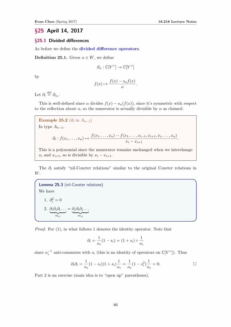
Evan Chen (Spring 2017) 18.218 Lecture Notes
§25 April 14, 2017
§25.1 Divided differences
As before we define the divided difference operators.
Definition 25.1. Given α ∈W , we define
∂α : C[V ∨]→ C[V ∨]
by
f(x) 7→ f(x)− sαf(x)
α.
Let ∂idef= ∂αi .
This is well-defined since α divides f(x)− sα(f(x)), since it’s symmetric with respectto the reflection about α, so the numerator is actually divisible by α as claimed.
Example 25.2 (∂i in An−1)
In type An−1,
∂i : f(x1, . . . , xn) 7→ f(x1, . . . , xn)− f(x1, . . . , xi−1, xi+1, xi, . . . , xn)
xi − xi+1.
This is a polynomial since the numerator remains unchanged when we interchangexi and xi+1, so is divisible by xi − xi+1.
The ∂i satisfy “nil-Coxeter relations” similar to the original Coxeter relations inW .
Lemma 25.3 (nil-Coxeter relations)
We have
1. ∂2i = 0
2. ∂i∂j∂i . . .︸ ︷︷ ︸mij
= ∂j∂i∂j . . .︸ ︷︷ ︸mij
Proof. For (1), in what follows 1 denotes the identity operator. Note that
∂i =1
αi(1− si) = (1 + si) ◦
1
αi
since α−1i anti-commutes with si (this is an identity of operators on C[V ∨]). Thus
∂i∂i =1
αi(1− si)(1 + si)
1
αi=
1
αi(1− s2
i )1
αi= 0.
Part 2 is an exercise (main idea is to “open up” parentheses).
86
Evan Chen (Spring 2017) 18.218 Lecture Notes
§25.2 Divided difference via Weyl group
Definition 25.4. Henceforth, if w = si1 . . . si` is a reduced decomposition then we let
∂wdef= ∂i1 . . . ∂i` .
Lemma 25.5
∂w is well-defined in the sense that it depends only on w and not on the choice ofreduced decomposition.
Proof. This follows from the fact that the nil-Coxeter relations above give a presentation.Our approach earlier was via alcove walks; another proof is by the so-called exchangelemma.
Lemma 25.6
Let w = si1 . . . si` = sj1 . . . sj` be a reduced decomposition of w. Then there existsr ∈ {1, . . . , `} such that
w = si1 . . . sir−1sir+1 . . . si`sj` .
Consequently, for all w ∈W we have a well-defined action ∂w : C[V ∨]→ C[V ∨]. These∂i function much like derivative operators: they drop the degree of the polynomial by 1.Actually, we in fact have the following “product formula”.
Lemma 25.7 (Product rule aka Leibniz formula)
We have∂i(fg) = ∂i(f)g + si(f)∂i(g).
Proof. Easy exercise (plug and chug).
Corollary 25.8
If f is W -invariant, then ∂i(fg) = f∂i(g).Thus, ∂i (and hence ∂w) preserve the ideal IW , so they induced well-defined
operators on the coinvariant algebra C[V ∨]/IW .
§25.3 BGG
Theorem 25.9 (Bernstein-Gelfand-Gelfand)
The Schubert classes σw ∈ C[V ∨]/IW are given by
σw = ∂w−1w0(σw0).
These form a linear basis of C[V ∨]/IW .
(You can take this as the definition of Schubert classes, if you like.)
87
Evan Chen (Spring 2017) 18.218 Lecture Notes
Remark 25.10. One may obtain polynomial representations of these Schubert classesin the following way:
1. Take any fw0 ∈ C[V ∨] of degree `(w0).
2. Set fw = ∂w−1w0(fw0).
3. Rescale them so that f1 = 1.
The basis of C[V ∨]/IW does not depend on the initial choice, but the actual representativepolynomials do.
§25.4 Choices of basis polynomials
A good choice of fw0 is the Kostant polynomial
Pw0 =1
|W |∏α∈Φ+
α.
For example, in type An−1 this gives 1n! =
∏i<j(xi − xj). These then obey the relation
Pwsi = ∂iPw if `(wsi) = `(w)− 1.
Exercise 25.11. Prove that P1 = 1 in this case, so the “scaling” step is not needed.
Remark 25.12. The above polynomials don’t have N coefficients.
In type An−1 a particularly nice starting choice is
Definition 25.13 (Schubert polynomials). We let
Sw0 = xn−11 xn−2
2 . . . xn−1.
Then Swsi = ∂iσw if `(wsi) = `(w)− 1. These are very nice combinatorially and haveN-coefficients.
88

Evan Chen (Spring 2017) 18.218 Lecture Notes
§26 April 19, 2017
Last time we defined the single-variable Schubert polynomials Sw(x) by stipulatingSw0 = xn−1
1 . . . x1n−1 and Swsi = ∂iSw for `(wsi) = `(w)− 1.
§26.1 Double Schubert polynomials
We define the double Schubert polynomials as follows.
Definition 26.1. We let Sw(x, y) = Sw(x1, . . . , xn, y1, . . . , yn) according to the relations
Sw0(x, y) =∏
i+j≤ni,j∈[n]
(xi − yj)
and Sws0(x, y) = ∂iSw(x, y) if `(wsi) = `(w)− 1.
These satisfy the following properties.
Proposition 26.2 (Properties of Sw(x, y))
We have:
• Sw(x) = Sw(x, 0) is a linear basis for the co-invariant algebra.
• Sw(x,−y) has nonnegative integer coefficients.
• Sw(x,−y) = Sw−1(y, x) (symmetry).
• Let w ∈ Sn and w ∈ Sn+1 by fixing n+ 1. Then Sw(x, y) = Sw(x, y).
These will be proven later; see the next lecture.
§26.2 Nil-Hecke Algebra
Definition 26.3. We define the nil-Hecke algebra NHn over C (say) to be the algebragenerated by u1, . . . , un−1 with the following relations:
• u2i = 0,
• uiuj = ujui for |i− j| ≥ 2,
• uiui+1ui = ui+1uiui+1.
Definition 26.4. We let hi(x) = 1 + xui ∈ NHn[x].
The hi satisfy the following relations:
Lemma 26.5 (Yang-Baxter relations)
The following relations hold in NHn[x, y].
hi(x)hi(y) = hi(x+ y)
hi(x)hj(y) = hj(y)hi(x) |i− j| ≥ 2
hi(x)hi+1(x+ y)hi(y) = hi+1(y)hi(x+ y)hi+1(x).
Thus x and y “commute with everything”.
89
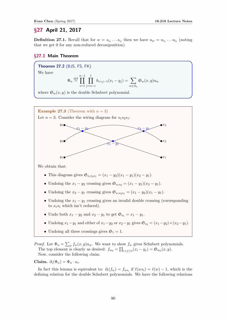
Evan Chen (Spring 2017) 18.218 Lecture Notes
§27 April 21, 2017
Definition 27.1. Recall that for w = si1 . . . si` then we have uw = ui1 . . . ui` (notingthat we get 0 for any non-reduced decomposition).
§27.1 Main Theorem
Theorem 27.2 (BJS, FS, FK)
We have
Φndef=
n−1∏i=1
1∏j=n−i
hi+j−1(xi − yj) =∑w∈Sn
Sw(x, y)uw
where Sw(x, y) is the double Schubert polynomial.
Example 27.3 (Theorem with n = 3)
Let n = 3. Consider the wiring diagram for s1s2s1:
y1
y2
y3
x1
x2
x3x1 − y2 x2 − y1
x1 − y1
We obtain that:
• This diagram gives Ss1s2s1 = (x1 − y2)(x1 − y1)(x2 − y1).
• Undoing the x1 − y2 crossing gives Ss1s2 = (x1 − y1)(x2 − y1).
• Undoing the x2 − y1 crossing gives Ss1s2s1 = (x1 − y2)(x1 − y1).
• Undoing the x1 − y1 crossing gives an invalid double crossing (correspondingto s1s1 which isn’t reduced).
• Undo both x1 − y2 and x2 − y1 to get Ss1 = x1 − y1.
• Undoing x1−y1 and either of x1−y2 or x2−y1 gives Ss2 = (x1−y2)+(x2−y1).
• Undoing all three crossings gives S1 = 1.
Proof. Let Φn =∑
w fw(x, y)uw. We want to show fw gives Schubert polynomials.The top element is clearly as desired: fw0 =
∏i+j≤n(xi − yj) = Sw0(x, y).
Now, consider the following claim.
Claim. ∂i(Φn) = Φn · ui.In fact this lemma is equivalent to: ∂i(fw) = fwsi if `(wsi) = `(w)− 1, which is the
defining relation for the double Schubert polynomials. We have the following relations
90
Evan Chen (Spring 2017) 18.218 Lecture Notes
from nil-Coxeter algebra:
uvui =
{uvsi `(vsi) = `(v) + 1
0 otherwise.
Also, consider the following calculation:
∂i(Φn) = Φnui
⇐⇒ 1
xi − xi+1(1− si)(Φn) = Φnui
⇐⇒ (1− si)Φn = Φn · ui(xi − xi+1)
⇐⇒ si(Φn) = Φn (1 + (xi+1 − xi)ui)= Φnhi(xi+1 − xi).
since xi commutes with ui. So it suffices to prove si(Φn) = Φnhi(xi+1 − xi). We invokethe Yang-Baxter relations below.
Lemma 27.4
si(Φn) = Φnhi(xi+1 − xi).
Example 27.5 (n = 3, i = 2)
We have
Φnhi(xi+1 − xi) = h2(x1 − y2)h1(x1 − y1)h2(x2 − y1)︸ ︷︷ ︸=Φ3
h2(x3 − x2)
= h2(x1 − y2)h1(x1 − y2)h2(x3 − y1) = s2(Φ3).
Example 27.6 (n = 3, i = 2)
We have
Φnhi(xi+1 − xi) = h2(x1 − y2)h1(x1 − y1)h2(x2 − y1)︸ ︷︷ ︸=Φ3
h1(x2 − x1)
= h2(x1 − y2)h2(x2 − x1)h1(x2 − y1)h2(x1 − x1)
= h2(x2 − y2)h1(x2 − y1)h2(x1 − x1) = s1(Φ3).
An outline of the general proof. We have
Φn = hn−1(x1 − yn−1)hn−2(x1 − yn−2)hn−1(x2 − yn−2) . . .
h1(x1 − y1)h2(x2 − y1) . . . hn−1(xn−1 − y1) · hi(xi+1 − xi).
Then commute the hi until it bumps into something, and keep throwing Yang-Baxterrelations at it.
91
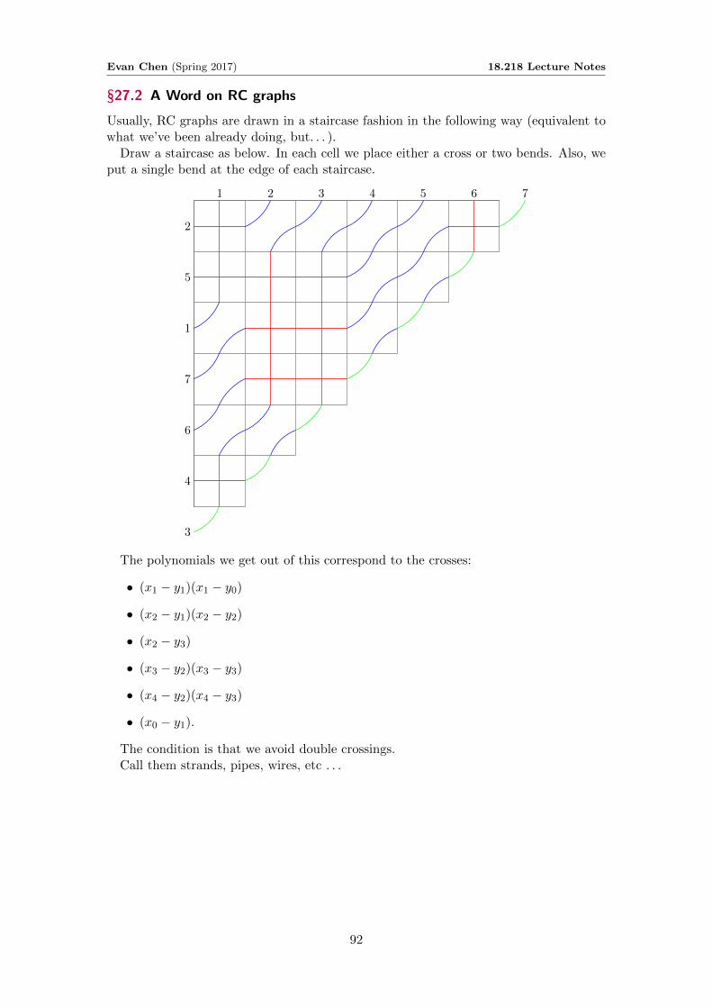
Evan Chen (Spring 2017) 18.218 Lecture Notes
§27.2 A Word on RC graphs
Usually, RC graphs are drawn in a staircase fashion in the following way (equivalent towhat we’ve been already doing, but. . . ).
Draw a staircase as below. In each cell we place either a cross or two bends. Also, weput a single bend at the edge of each staircase.
1 2 3 4 5 6 7
2
5
1
7
6
4
3
The polynomials we get out of this correspond to the crosses:
• (x1 − y1)(x1 − y0)
• (x2 − y1)(x2 − y2)
• (x2 − y3)
• (x3 − y2)(x3 − y3)
• (x4 − y2)(x4 − y3)
• (x0 − y1).
The condition is that we avoid double crossings.Call them strands, pipes, wires, etc . . .
92
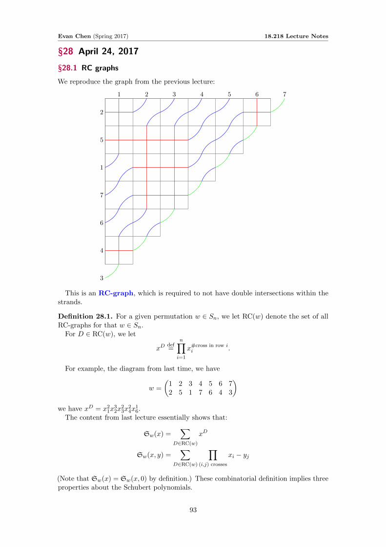
Evan Chen (Spring 2017) 18.218 Lecture Notes
§28 April 24, 2017
§28.1 RC graphs
We reproduce the graph from the previous lecture:
1 2 3 4 5 6 7
2
5
1
7
6
4
3
This is an RC-graph, which is required to not have double intersections within thestrands.
Definition 28.1. For a given permutation w ∈ Sn, we let RC(w) denote the set of allRC-graphs for that w ∈ Sn.
For D ∈ RC(w), we let
xDdef=
n∏i=1
x#cross in row ii .
For example, the diagram from last time, we have
w =
(1 2 3 4 5 6 72 5 1 7 6 4 3
)we have xD = x2
1x32x
23x
24x
16.
The content from last lecture essentially shows that:
Sw(x) =∑
D∈RC(w)
xD
Sw(x, y) =∑
D∈RC(w)
∏(i,j) crosses
xi − yj
(Note that Sw(x) = Sw(x, 0) by definition.) These combinatorial definition implies threeproperties about the Schubert polynomials.
93

Evan Chen (Spring 2017) 18.218 Lecture Notes
Corollary 28.2 (Properties of Schubert polynomials)
The Schubert polynomials satisfy the following properties.
• (Positivity) Sw(x,−y) is a polynomial in x1, . . . , xn−1 and y1, . . . , yn−1 withnonnegative integer coefficients.
• (Symmetry) Sw(x,−y) = Sw−1(y, x−1).
• (Stability) Consider the map Sn ↪→ Sn+1 by w 7→ w with w fixing n+ 1. ThenSw(x, y) = Sw(x, y).
Proof. First two are obvious. Stability follows by noting that to avoid a double crossing,the only way that a strand from n + 1 to reach n + 1 is for it to never encounter acrossing.
§28.2 Cauchy formula
Theorem 28.3 (Cauchy formula for Schubert polynomials, Lascoux 1982)
Sw(x, y) =∑u,v
w=v−1u`(w)=`(u)+`(v)
Su(x)Sv(−y).
Hence this expresses double Schubert polynomials in terms of the ordinary Schubertvalues.
In particular, if w is the longest permutation, we deduce that∑i+j≤ni,j≥1
(xi − yj) = Sw(x, y) =∑w∈Sn
Sw(x)Sw0w(−y).
Remark 28.4 (Digression on Schur polynomials). This is reminiscent of Schur polyno-mials sλ(x) (which turn out to be a special case of Schubert polynomials, which we’lldefine later). To be concrete, the dual Cauchy formula for Schur polynomials states∑
λ
sλ(x)sλ′(y) =∏i,j
(1 + xiyj)
where λ and λ′ are the dual. (The usual Cauchy formula for Schur polynomials states∑λ
sλ(x)sλ(y) =∏i,j
(1− xiyj)−1
instead.)
We now prove Cauchy’s formula. Define Φn(x, y) = Φn(x1, . . . , xn−1, y1, . . . , yn−1) asin previous lectures.
Lemma 28.5
Cauchy’s formula is equivalent to
Φn(x, y) = Φn(0, y)Φn(x, 0).
94
Evan Chen (Spring 2017) 18.218 Lecture Notes
Proof. Recall the notation uw = ui1 . . . ui` if w = si1 . . . si` in the nil-Coxeter algebra.Then
uvuw =
{uv·w `(v · w) = `(v) + `(w)
0 else.
So one sees this just by writing out definition of Φn(x, y).
Thus we prove Φn(x, y) = Φn(0, y)Φn(x, 0). This will be repeated application ofYang-Baxter relations.
Example 28.6 (n = 2)
Let’s check the above formula for n = 2. Recall that Φ2(x, y) = h1(x1 − y1) and soit’s equivalent to show
h1(x1 − y1) = h1(−y1)h1(x1)
which is more or less obvious.
Example 28.7 (n = 3)
Let’s check the above formula for n = 3. Recall that We wish to show
Φ3(x, y)def= h2(x1 − y2)h1(x1 − y1)h2(x2 − y1)
= h2(−y2)h1(−y1)h2(−y1)h2(x1)h1(x1)h2(x2).
Again keep using Yang-Baxter relations.
§28.3 Linear space of Schubert polynomial
We letStairn =
{xa11 x
a22 . . . x
an−1
n−1 | ai ≤ n− i}
be the n! monomials which divide xn−11 xn−2
2 . . . x1, and let 〈Stairn〉 denote their span(which is an n!-dimensional space). Obviously, if D ∈ RC(w) we have D ∈ 〈Stairn〉. Wenow make the following claim about the linear bases of 〈Stairn〉.
Theorem 28.8 (Basis of 〈Stairn〉)The space 〈Stairn〉 has the following three linear bases.
• xa11 . . . xan−1
n−1 , i.e. the elements of 〈Stairn〉 (by definition).
• Sw(x) for w ∈ Sn.
• Products
ei1(x1)ei2(x1, x2)ei3(x1, x2, x3) . . . ein−1(x1, x2, . . . , xn−1)
of elementary symmetric polynomials. Here ik ∈ {0, 1, . . . , k} for each k.
Moreover the images of these polynomials in the coinvariant algebra also form abasis.
95
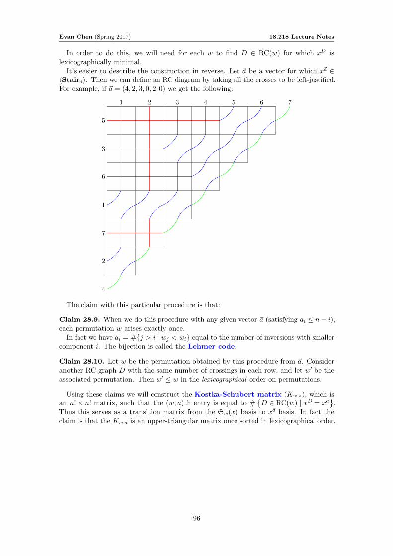
Evan Chen (Spring 2017) 18.218 Lecture Notes
In order to do this, we will need for each w to find D ∈ RC(w) for which xD islexicographically minimal.
It’s easier to describe the construction in reverse. Let ~a be a vector for which x~a ∈〈Stairn〉. Then we can define an RC diagram by taking all the crosses to be left-justified.For example, if ~a = (4, 2, 3, 0, 2, 0) we get the following:
1 2 3 4 5 6 7
5
3
6
1
7
2
4
The claim with this particular procedure is that:
Claim 28.9. When we do this procedure with any given vector ~a (satisfying ai ≤ n− i),each permutation w arises exactly once.
In fact we have ai = #{j > i | wj < wi} equal to the number of inversions with smallercomponent i. The bijection is called the Lehmer code.
Claim 28.10. Let w be the permutation obtained by this procedure from ~a. Consideranother RC-graph D with the same number of crossings in each row, and let w′ be theassociated permutation. Then w′ ≤ w in the lexicographical order on permutations.
Using these claims we will construct the Kostka-Schubert matrix (Kw,a), which isan n! × n! matrix, such that the (w, a)th entry is equal to #
{D ∈ RC(w) | xD = xa
}.
Thus this serves as a transition matrix from the Sw(x) basis to x~a basis. In fact theclaim is that the Kw,a is an upper-triangular matrix once sorted in lexicographical order.
96
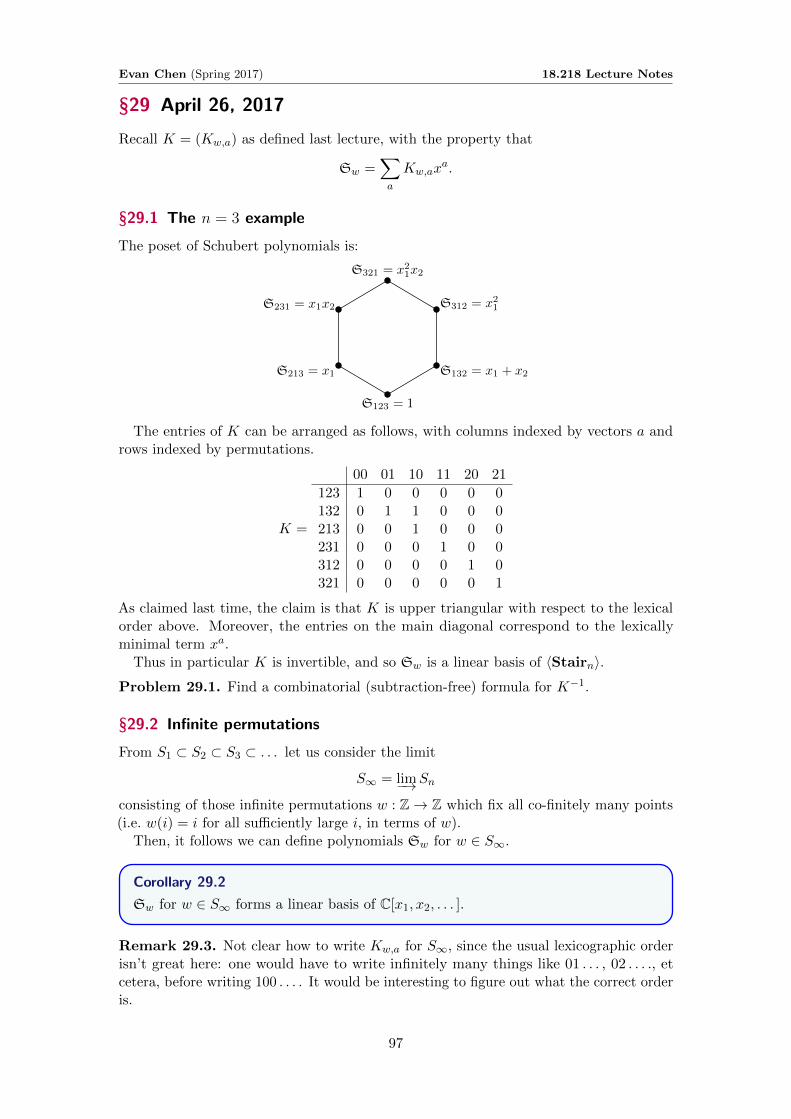
Evan Chen (Spring 2017) 18.218 Lecture Notes
§29 April 26, 2017
Recall K = (Kw,a) as defined last lecture, with the property that
Sw =∑a
Kw,axa.
§29.1 The n = 3 example
The poset of Schubert polynomials is:
S321 = x21x2
S312 = x21
S132 = x1 + x2
S123 = 1
S231 = x1x2
S213 = x1
The entries of K can be arranged as follows, with columns indexed by vectors a androws indexed by permutations.
K =
00 01 10 11 20 21
123 1 0 0 0 0 0132 0 1 1 0 0 0213 0 0 1 0 0 0231 0 0 0 1 0 0312 0 0 0 0 1 0321 0 0 0 0 0 1
As claimed last time, the claim is that K is upper triangular with respect to the lexicalorder above. Moreover, the entries on the main diagonal correspond to the lexicallyminimal term xa.
Thus in particular K is invertible, and so Sw is a linear basis of 〈Stairn〉.Problem 29.1. Find a combinatorial (subtraction-free) formula for K−1.
§29.2 Infinite permutations
From S1 ⊂ S2 ⊂ S3 ⊂ . . . let us consider the limit
S∞ = lim−→Sn
consisting of those infinite permutations w : Z→ Z which fix all co-finitely many points(i.e. w(i) = i for all sufficiently large i, in terms of w).
Then, it follows we can define polynomials Sw for w ∈ S∞.
Corollary 29.2
Sw for w ∈ S∞ forms a linear basis of C[x1, x2, . . . ].
Remark 29.3. Not clear how to write Kw,a for S∞, since the usual lexicographic orderisn’t great here: one would have to write infinitely many things like 01 . . . , 02 . . . ., etcetera, before writing 100 . . . . It would be interesting to figure out what the correct orderis.
97

Evan Chen (Spring 2017) 18.218 Lecture Notes
§29.3 Geometrical background
Consider the two manifolds we define earlier:
• Fln, the complete flags of Cn.
• Grk,n, the manifold of k-dimensional linear subspaces in Cn, for k ≤ n.
There is a natural map
p : Fln � Grk,n
(V0 ⊆ V1 ⊆ · · · ⊆ Vn) 7→ Vk.
This gives a map of cohomology rings
p• : H•(Grk,n) ↪→ H•(Fln).
We now give a description of the two bases of these maps. First, notation for the ideal:
Definition 29.4. Let In denote the ideal generated by homogeneous symmetric polyno-mials of positive degree. (This notation will be retained in next lectures.)
• H•(Grk,n) has a linear basis of Schubert polynomials σλ, where λ is partition whoseYoung diagram fits inside a k × (n − k) rectangle. (That is, λ = (λ1, λ2, . . . , λk)where n− k ≥ λ1 ≥ λ2 ≥ · · · ≥ λk.) This space has dimension
(nk
).
• H•(Fln) ∼= C[x1, . . . , xn]/In has a linear basis of Schur polynomials σw, wherew ∈ Sn. This space has dimension n!.
Both of these cohomology rings can be thought of as quotients for the cohomology ring.So the bottom line is the we have a map
λ 7→ w(λ) ∈ Sn
for which Sw(λ) is sλ(x1, . . . , xk).Let’s now describe this map taking partitions to permutations. First, we describe the
permutations achievable as the image of Grk,n.
Definition 29.5. A permutation w ∈ Sn is (n, k)-Grassmanian if w1 < w2 < · · · < wkand wk+1 < wk+2 < · · · < wn.
Lemma 29.6
Grassmanian permutations are in bijection with Young diagrams λ which fit insidek × (n− k) rectangles.
Given a partition λ, the permutation w = w(λ) is such that:
The Lemer code of w(λ) coincides with (λk, λk−1, . . . , λ1, 0, . . . , 0).
98
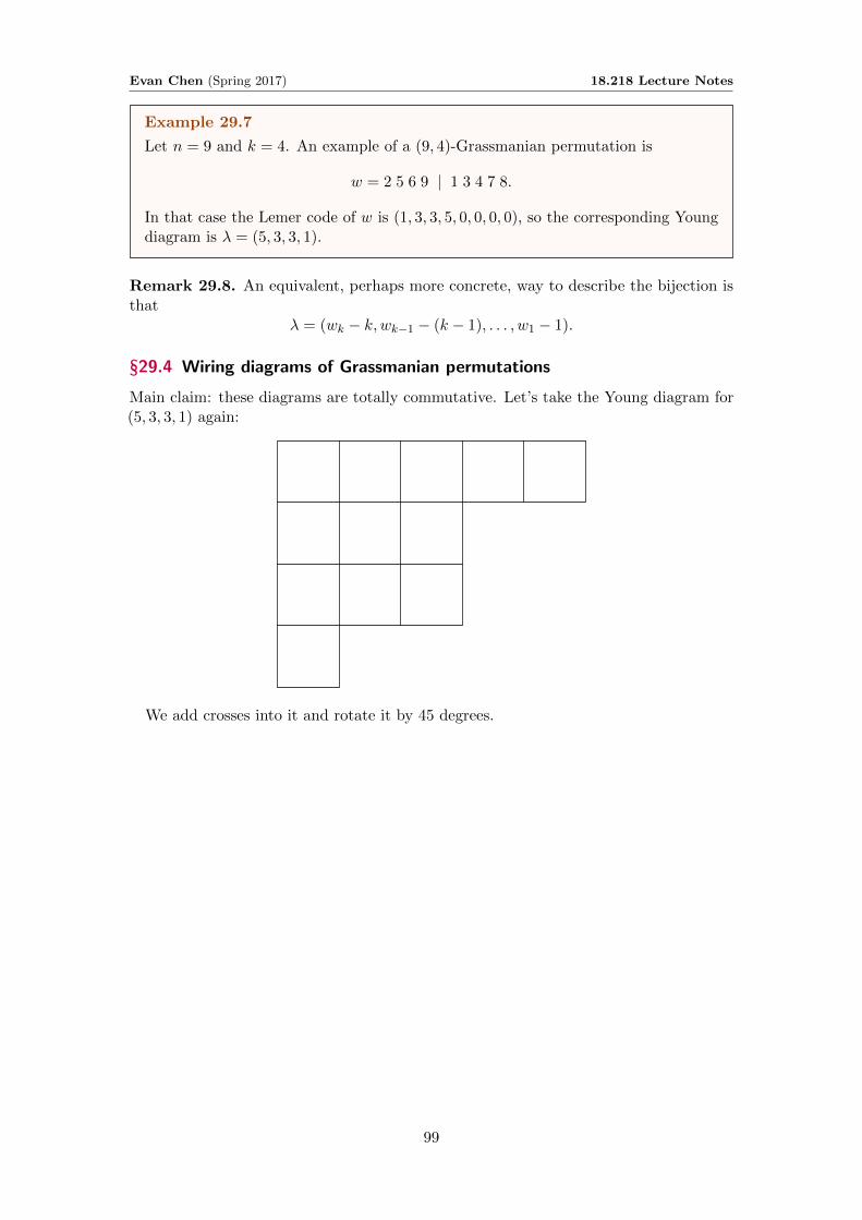
Evan Chen (Spring 2017) 18.218 Lecture Notes
Example 29.7
Let n = 9 and k = 4. An example of a (9, 4)-Grassmanian permutation is
w = 2 5 6 9 | 1 3 4 7 8.
In that case the Lemer code of w is (1, 3, 3, 5, 0, 0, 0, 0), so the corresponding Youngdiagram is λ = (5, 3, 3, 1).
Remark 29.8. An equivalent, perhaps more concrete, way to describe the bijection isthat
λ = (wk − k,wk−1 − (k − 1), . . . , w1 − 1).
§29.4 Wiring diagrams of Grassmanian permutations
Main claim: these diagrams are totally commutative. Let’s take the Young diagram for(5, 3, 3, 1) again:
We add crosses into it and rotate it by 45 degrees.
99
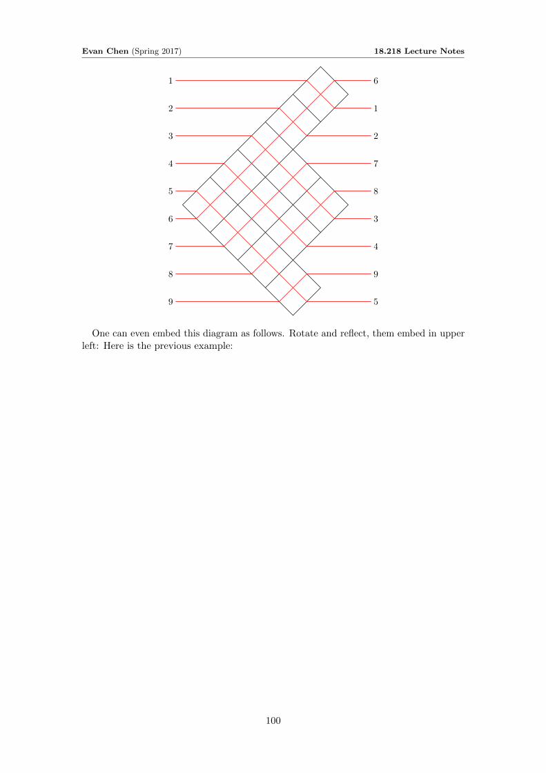
Evan Chen (Spring 2017) 18.218 Lecture Notes
1
2
3
4
5
6
7
8
9
6
1
2
7
8
3
4
9
5
One can even embed this diagram as follows. Rotate and reflect, them embed in upperleft: Here is the previous example:
100
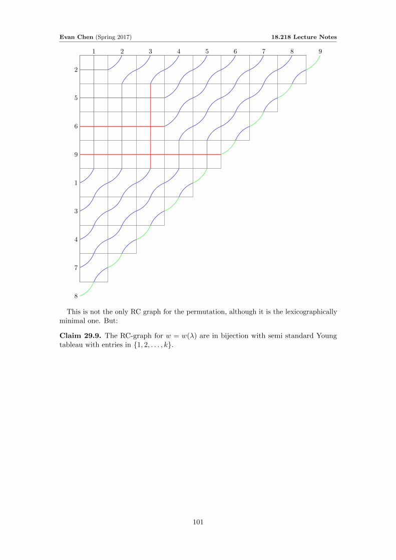
Evan Chen (Spring 2017) 18.218 Lecture Notes
1 2 3 4 5 6 7 8 9
2
5
6
9
1
3
4
7
8
This is not the only RC graph for the permutation, although it is the lexicographicallyminimal one. But:
Claim 29.9. The RC-graph for w = w(λ) are in bijection with semi standard Youngtableau with entries in {1, 2, . . . , k}.
101
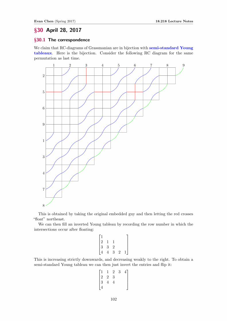
Evan Chen (Spring 2017) 18.218 Lecture Notes
§30 April 28, 2017
§30.1 The correspondence
We claim that RC-diagrams of Grassmanian are in bijection with semi-standard Youngtableaux. Here is the bijection. Consider the following RC diagram for the samepermutation as last time.
1 2 3 4 5 6 7 8 9
2
5
6
9
1
3
4
7
8
This is obtained by taking the original embedded guy and then letting the red crosses“float” northeast.
We can then fill an inverted Young tableau by recording the row number in which theintersections occur after floating:
12 1 13 3 24 4 3 2 1
This is increasing strictly downwards, and decreasing weakly to the right. To obtain asemi-standard Young tableau we can then just invert the entries and flip it:
1 1 2 3 42 2 33 4 44
102

Evan Chen (Spring 2017) 18.218 Lecture Notes
Now this is weakly increasing to right, and strictly increasing down. The associatedpolynomial is x2
1x32x
33x
44, with xi having #i as an exponent.
§30.2 Schur symmetric polynomial
Definition 30.1. We define
sλ(x) = sλ(x1, . . . , xk)def=∑
x#11 x#2
2 . . . x#kk
where the sum is taken over all semi-standard Young tableau of shape λ with entries in{1, . . . , k}.
The bijection earlier gives:
Corollary 30.2
If w = w(λ), then Sw(λ) = sλ(x1, . . . , xk).
Examples:
• Ssk = x1 + x+2 + · · ·+ xk = e1(x1, . . . , xk).
• Ssk−i+1sk−i+2...sk = ei(x1, . . . , xk).
• Ssk+i−1sk+i−2...sk = hi(x1, . . . , xk) (complete homogeneous polynomial).
§30.3 Symmetry of H•(Fln) = C[x1, . . . , xn]/In
Those familiar with this area may know of the so-called involution ω defined by
xi 7→ −xn−i+1
si 7→ sn−i
Thus if w = si1si2 . . . si` , and ω(w) = sn−i1 . . . sn−i` = w0ww0. In terms of Youngdiagram, this corresponds to conjugation of λ.
Proposition 30.3 (ω on Schubert polynomials)
ω sends σw to σw0ww0 .
Corollary 30.4
Sw(x1, . . . , xn) ≡ Sw0ww0(−xn,−xn−1, . . . ,−x1) (mod In).
Corollary 30.5
sλ(x1, . . . , xk) ≡ sλ′(xn,−xn−1, . . . ,−xk+1) (mod In).
Corollary 30.6
ei(x1, . . . , xk) = hi(−xn,−xn−1, . . . ,−xk+1) (mod In).
103
Evan Chen (Spring 2017) 18.218 Lecture Notes
Example 30.7
When i = 1 in the last corollary, we have e1(x1, . . . , xk) = x1 + · · · + xk, andh1(−xn,−xn−1, . . . ,−xk+1) = −xn−xn−1−· · ·−xk+1. But In contains x1+· · ·+xn ≡0.
Exercise 30.8. Check the last corollary algebraically from definitions, for all i.
§30.4 Monk’s formula
There are many variations; here is one.Recall that Sw forms a basis of C[x1, . . . ] for w ∈ S∞.
Theorem 30.9 (Monk’s formula)
Ssk︸︷︷︸=x1+···+xk
·Sw =∑i,j
i≤k<j`(wtij)=`(w)+1
Swtij
where tij is the transposition (i j).
The sum is exactly the covering relations in the strong Bruhat order on S∞. (We reallywant S∞, not just Sn! So e.g. when computing Ss3S315462 it’s possible that some newterms will have 7 in them.)
104

Evan Chen (Spring 2017) 18.218 Lecture Notes
§31 May 1, 2017
Was ill today. To be written.
105

Evan Chen (Spring 2017) 18.218 Lecture Notes
§32 May 3, 2017
Was ill today. To be written.
106
Evan Chen (Spring 2017) 18.218 Lecture Notes
§33 May 4, 2017
Was ill today. To be written.
107
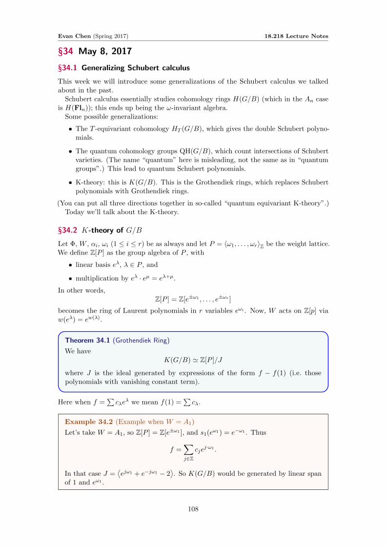
Evan Chen (Spring 2017) 18.218 Lecture Notes
§34 May 8, 2017
§34.1 Generalizing Schubert calculus
This week we will introduce some generalizations of the Schubert calculus we talkedabout in the past.
Schubert calculus essentially studies cohomology rings H(G/B) (which in the An caseis H(Fln)); this ends up being the ω-invariant algebra.
Some possible generalizations:
• The T -equivariant cohomology HT (G/B), which gives the double Schubert polyno-mials.
• The quantum cohomology groups QH(G/B), which count intersections of Schubertvarieties. (The name “quantum” here is misleading, not the same as in “quantumgroups”.) This lead to quantum Schubert polynomials.
• K-theory: this is K(G/B). This is the Grothendiek rings, which replaces Schubertpolynomials with Grothendiek rings.
(You can put all three directions together in so-called “quantum equivariant K-theory”.)Today we’ll talk about the K-theory.
§34.2 K-theory of G/B
Let Φ, W , αi, ωi (1 ≤ i ≤ r) be as always and let P = 〈ω1, . . . , ωr〉Z be the weight lattice.We define Z[P ] as the group algebra of P , with
• linear basis eλ, λ ∈ P , and
• multiplication by eλ · eµ = eλ+µ.
In other words,Z[P ] = Z[e±ω1 , . . . , e±ωr ]
becomes the ring of Laurent polynomials in r variables eωi . Now, W acts on Z[p] viaw(eλ) = ew(λ).
Theorem 34.1 (Grothendiek Ring)
We haveK(G/B) ' Z[P ]/J
where J is the ideal generated by expressions of the form f − f(1) (i.e. thosepolynomials with vanishing constant term).
Here when f =∑cλe
λ we mean f(1) =∑cλ.
Example 34.2 (Example when W = A1)
Let’s take W = A1, so Z[P ] = Z[e±ω1 ], and s1(eω1) = e−ω1 . Thus
f =∑j∈Z
cjej·ω1 .
In that case J =⟨ejω1 + e−jω1 − 2
⟩. So K(G/B) would be generated by linear span
of 1 and eω1 .
108

Evan Chen (Spring 2017) 18.218 Lecture Notes
§34.3 Linear basis of K(G/B)
In general, dimK(G/B) = |W |.In fact the ring is isomorphic to the coinvariant algebra. Despite the fact that K(G/B)
is isomorphic to the coinvariant algebra, there is something new here. It turns outK(G/B) has a linear basis of the form [Ow], w ∈W . We won’t discuss the geometry ofthis basis, but these are actually structure sheafs. The main question is to understand[Ou][Ov].
In order to define Ow, we need to define the Demazure operators (analogous to thedivided difference operator before).
Definition 34.3. The ith Demazure operator is defined by
Di : Z[P ]→ Z[P ]
f 7→ f − e−αisi(f)
1− e−αi .
Proposition 34.4
The Demazure operators satisfy the 0-Hecke relations:
(1) D2i = Di.
(2) DiDjDi · · · = DjDiDj . . . (each mij times, as usual).
Exercise 34.5. Check the relations.
Thus again given w = si1 . . . si` reduced, we may define
Dwdef= Di1 . . . Di`
which depends only on w and not the choice of reduced decomposition.
Theorem 34.6 (Kostant-Kumar)
We have the relation[Ow] = Dw−1([O1])
with 1 ∈W being the identity of W .
Thus [Ow] is a K-theoretic analogue of σw0w. Anyways, since we haven’t given thegeometric definition of Ow yet, we can just take this as a definition.
§34.4 Specializing to An−1
We now specialize to type An−1.We introduce variables z1, . . . , zn such that z1z2 . . . zn = 1 and
eωi = z1z2 . . . zi
eαi =zi+1
zi.
We then haveK(Fln) = Z[z±1
1 , . . . , z±1n ]/J.
Here Jn is generated by f − f(1) for symmetric Laurent polynomials f . The claim isthat:
109

Evan Chen (Spring 2017) 18.218 Lecture Notes
Theorem 34.7
We have an isomorphism of the n!-dimensional rings
Z[z±11 , . . . , z±1
n ]/Jn → Z[x1, . . . , xn]/In
zi 7→ 1− xi.
So the Schubert classes σw correspond to Schubert polynomials, while [Ow] correspondto so-called Grothendiek polynomials under this isomorphism.
Under this isomorphism the Demazure operators gain the following shape:
f 7→f − zi
zi+1si(f)
1− zizi+1
=zi+1f − zisi(f)
zi+1 − zi.
These are called isoberic divided differences.So the interesting thing happening is that the expression 1 − zi
zi+1that we get in
K-theory becomes zi+1 − zi in cohomology.
§34.5 Construction of Grothendiek polynomial
In the language of the xi, one first notices that Di preserves the ideal Jn, then writes
πi(f)def= ∂i ((1− xi+1)f)
where ∂i is the usual divided difference. These satisfy the relations
(1) π2i = πi.
(2) πiπj = πjπi
(3) πiπi+1πi = πi+1πiπi+1.
When then constructs the Grothendiek polynomial Gw (Gothic G) by replacing ∂i withπi, verbatim. The interesting bit is that πi is not homogeneous in degree n.
For example, with n = 3 we get
G321 = x21x2
G312 = x21
G132 = x1 + x2 − x1x2
G123 = 1
G231 = x1x2
G213 = x1
so the only difference in G132 = x1 +x2−x1x2. There is also an RC-graph interpretation,but the big change is that Monks’ rule becomes very interesting. We’ll see this in futurelectures.
110
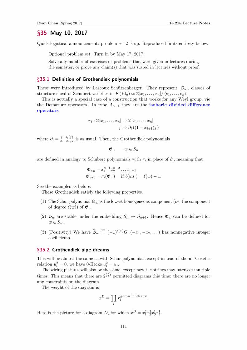
Evan Chen (Spring 2017) 18.218 Lecture Notes
§35 May 10, 2017
Quick logistical announcement: problem set 2 is up. Reproduced in its entirety below.
Optional problem set. Turn in by May 17, 2017.
Solve any number of exercises or problems that were given in lectures duringthe semester, or prove any claim(s) that was stated in lectures without proof.
§35.1 Definition of Grothendiek polynomials
These were introduced by Lascoux Schutzenberger. They represent [Ou], classes ofstructure sheaf of Schubert varieties in K(Fln) ' Z[x1, . . . , xn]/ 〈e1, . . . , en〉.
This is actually a special case of a construction that works for any Weyl group, viethe Demazure operators. In type An−1 they are the isobaric divided differenceoperators
πi : Z[x1, . . . , xn]→ Z[x1, . . . , xn]
f 7→ ∂i ((1− xi+1)f)
where ∂i = f−si(f)xi−xi+1
is as usual. Then, the Grothendiek polynomials
Gw w ∈ Sn
are defined in analogy to Schubert polynomials with πi in place of ∂i, meaning that
Gw0 = xn−11 xn−2
2 . . . xn−1
Gwsi = πi(Gw) if `(wsi) = `(w)− 1.
See the examples as before.These Grothendiek satisfy the following properties.
(1) The Schur polynomial Sw is the lowest homogeneous component (i.e. the componentof degree `(w)) of Gw.
(2) Gw are stable under the embedding Sn ↪→ Sn+1. Hence Gw can be defined forw ∈ S∞.
(3) (Positivity) We have Gwdef= (−1)`(w)Gw(−x1,−x2, . . . ) has nonnegative integer
coefficients.
§35.2 Grothendiek pipe dreams
This will be almost the same as with Schur polynomials except instead of the nil-Coxeterrelation u2
i = 0, we have 0-Hecke u2i = ui.
The wiring pictures will also be the same, except now the strings may intersect multiple
times. This means that there are 2(n2) permitted diagrams this time: there are no longerany constraints on the diagram.
The weight of the diagram is
xD =∏i
x#cross in ith rowi .
Here is the picture for a diagram D, for which xD = x21x
22x
13x
14.
111

Evan Chen (Spring 2017) 18.218 Lecture Notes
1 2 3 4 5
2
4
1
5
3
There is one more difference in reading the permutation from the wiring diagram —the relation u2
i = ui means that if two strands intersect twice, then we have to ignore thesecond cross (and thus turn at a sharp right angle at the cross). So for example, in theabove example,
w(D) =
(1 2 3 4 52 4 1 5 3
)
Theorem 35.1 (Fomin-Kirillov)
We haveGw =
∑D:w(D)=w
xD.
Proof. Basically exactly the same. Exercise: do so.
§35.3 Extended Example for n = 3
We draw all the 23 = 8 diagrams for n = 3:
• The permutation 321 and monomial x21x2.
1 2 3
3
2
1
• The permutation 231 and monomial x1x2.
112

Evan Chen (Spring 2017) 18.218 Lecture Notes
1 2 3
2
3
1
• The permutation 312 and monomial x21.
1 2 3
3
1
2
• The permutation 132 and monomial x1x2. (This is the new term that wasn’t therebefore; note the double crossing, and how 3 and 2 don’t switch at the southwestintersection.)
1 2 3
1
3
2
• The permutation 213 and monomial x1.
1 2 3
2
1
3
• The permutation 132 and monomial x1.
113
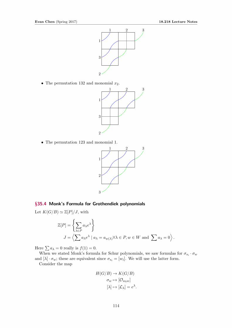
Evan Chen (Spring 2017) 18.218 Lecture Notes
1 2 3
1
3
2
• The permutation 132 and monomial x2.
1 2 3
1
3
2
• The permutation 123 and monomial 1.
1 2 3
1
2
3
§35.4 Monk’s Formula for Grothendiek polynomials
Let K(G/B) ' Z[P ]/J , with
Z[P ] =
{∑λ∈P
aλeλ
}J =
⟨∑aλe
λ | aλ = aw(λ)∀λ ∈ P,w ∈W and∑
aλ = 0⟩.
Here∑aλ = 0 really is f(1) = 0.
When we stated Monk’s formula for Schur polynomials, we saw formulas for σsi · σwand [λ] · σw; these are equivalent since σsi = [wi]. We will use the latter form.
Consider the map
H(G/B)→ K(G/B)
σw 7→ [Ow0w]
[λ] 7→ [Lλ] = eλ.
114
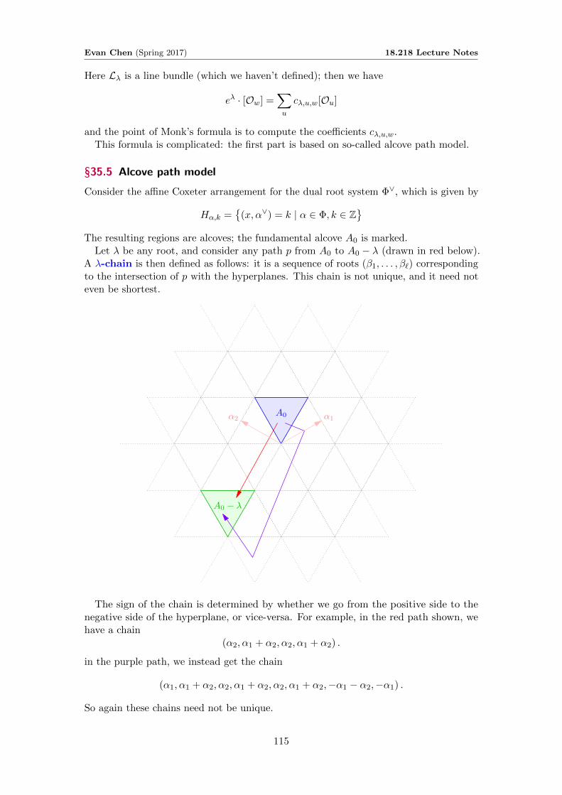
Evan Chen (Spring 2017) 18.218 Lecture Notes
Here Lλ is a line bundle (which we haven’t defined); then we have
eλ · [Ow] =∑u
cλ,u,w[Ou]
and the point of Monk’s formula is to compute the coefficients cλ,u,w.This formula is complicated: the first part is based on so-called alcove path model.
§35.5 Alcove path model
Consider the affine Coxeter arrangement for the dual root system Φ∨, which is given by
Hα,k ={
(x, α∨) = k | α ∈ Φ, k ∈ Z}
The resulting regions are alcoves; the fundamental alcove A0 is marked.Let λ be any root, and consider any path p from A0 to A0 − λ (drawn in red below).
A λ-chain is then defined as follows: it is a sequence of roots (β1, . . . , β`) correspondingto the intersection of p with the hyperplanes. This chain is not unique, and it need noteven be shortest.
A0
A0 − λ
α1α2
The sign of the chain is determined by whether we go from the positive side to thenegative side of the hyperplane, or vice-versa. For example, in the red path shown, wehave a chain
(α2, α1 + α2, α2, α1 + α2) .
in the purple path, we instead get the chain
(α1, α1 + α2, α2, α1 + α2, α2, α1 + α2,−α1 − α2,−α1) .
So again these chains need not be unique.
115

Evan Chen (Spring 2017) 18.218 Lecture Notes
Next, for α ∈ Φ+ we define the operator
Bα : [Ow] 7→{
[Owsα ] if `(wsα) = `(w)− 1
0 otherwise.
Then define B−α = −Bα. Now, the result, due to Leneert and Postnikov, is:
Pick any λ-chain (β1, . . . , β`). We have
eλ · [Ow] = (1 +Bβ`)(1 +Bβ`−1
). . . (1 +Bβ1) ([Ow]) .
116

Evan Chen (Spring 2017) 18.218 Lecture Notes
§36 May 12, 2017
§36.1 Another perspective on pipe dreams
Given w ∈ Sn, we can consider the so-called Rothe diagram.Definition by example: let
w =
(1 2 3 4 5 63 5 2 1 6 4
)We place an X in all the cells, then shade in all the squares which are not either belowor to the right of any X. This gives the Rothe diagram; the dominant part is theconnected component in the upper-left (which may be empty if w(1) = 1); this will be aYoung diagram.
X
X
X
X
X
X
1
2
3
4
5
6
1 2 3 4 5 6
Exercise 36.1. The Rothe diagram coincides with the dominant part (i.e. no othersquares) if and only if the permutation is 132-avoiding.
Pick any outer corner (i.e. x adjacent to dominant part), denote it (i, j), so thatw(i) = w(j).
Claim 36.2. We have
(xi − yj)Sw(x, y) =∑w′mww′(i)6=j
Sw′(x, y).
Here the covering m is in the strong Bruhat order; so it’s equivalent to w′(i) > j.
Claim 36.3. Given the Rothe diagram for w, all pipe dreams for w have;
• a cross inside the dominant part, and
• a non-crossing in each dominant corner.
117
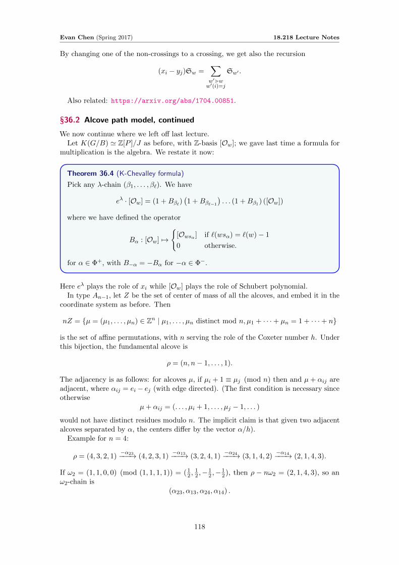
Evan Chen (Spring 2017) 18.218 Lecture Notes
By changing one of the non-crossings to a crossing, we get also the recursion
(xi − yj)Sw =∑w′mww′(i)=j
Sw′ .
Also related: https://arxiv.org/abs/1704.00851.
§36.2 Alcove path model, continued
We now continue where we left off last lecture.Let K(G/B) ' Z[P ]/J as before, with Z-basis [Ow]; we gave last time a formula for
multiplication is the algebra. We restate it now:
Theorem 36.4 (K-Chevalley formula)
Pick any λ-chain (β1, . . . , β`). We have
eλ · [Ow] = (1 +Bβ`)(1 +Bβ`−1
). . . (1 +Bβ1) ([Ow])
where we have defined the operator
Bα : [Ow] 7→{
[Owsα ] if `(wsα) = `(w)− 1
0 otherwise.
for α ∈ Φ+, with B−α = −Bα for −α ∈ Φ−.
Here eλ plays the role of xi while [Ow] plays the role of Schubert polynomial.In type An−1, let Z be the set of center of mass of all the alcoves, and embed it in the
coordinate system as before. Then
nZ = {µ = (µ1, . . . , µn) ∈ Zn | µ1, . . . , µn distinct mod n, µ1 + · · ·+ µn = 1 + · · ·+ n}
is the set of affine permutations, with n serving the role of the Coxeter number h. Underthis bijection, the fundamental alcove is
ρ = (n, n− 1, . . . , 1).
The adjacency is as follows: for alcoves µ, if µi + 1 ≡ µj (mod n) then and µ+ αij areadjacent, where αij = ei − ej (with edge directed). (The first condition is necessary sinceotherwise
µ+ αij = (. . . , µi + 1, . . . , µj − 1, . . . )
would not have distinct residues modulo n. The implicit claim is that given two adjacentalcoves separated by α, the centers differ by the vector α/h).
Example for n = 4:
ρ = (4, 3, 2, 1)−α23−−−→ (4, 2, 3, 1)
−α13−−−→ (3, 2, 4, 1)−α24−−−→ (3, 1, 4, 2)
−α14−−−→ (2, 1, 4, 3).
If ω2 = (1, 1, 0, 0) (mod (1, 1, 1, 1)) = (12 ,
12 ,−1
2 ,−12), then ρ − nω2 = (2, 1, 4, 3), so an
ω2-chain is(α23, α13, α24, α14) .
118
Evan Chen (Spring 2017) 18.218 Lecture Notes
This gives us an ω2-chain example. So, we can now apply the formula to
eω2 [O4321] =∑u∈W
nu[Ou]
where nu is the number of decreasing chains from 4321 to u whose label path forms asubsequence of (α23, α13, α24, α14). One can compute the corresponding terms:
• [O4321] from the empty sequence.
• [O4231] from α23
• [O3241] + [O4132] from α23α13 and α23α24
• [O3142] from α23α13α24.
• [O2143] from α23α13α24α14.
Monk’s formula corresponds to the “linear part of this” i.e. the length-one chain [O4231]in the above.
119
Evan Chen (Spring 2017) 18.218 Lecture Notes
§37 May 15, 2017
To be added.
120
Evan Chen (Spring 2017) 18.218 Lecture Notes
§38 May 17, 2017
In this lecture we’ll briefly mention a lot of the topics that we didn’t get to.
§38.1 Weyl Characters
In last lecture we discussed the characters
ch(Vλ) =∑µ
mλ(µ)eλ.
(In type An−1 these are Kostant numbers.) Related topics:
• Weyl’s character formula
• Demazure character formula
• Littlemenn path model
• Berenstein-Zelevinsky polytopes
• Alcove path model (Gaussat-Littlemann galleries)
The ultimate goal is to understand the irreducible representations Vλ of Uq(g). Themodels we have do a very good job of giving the characters ch(Vλ), but this doesn’t tellus the whole Vλ. Related keywords: Lustzsig’s canonical basis, Koshiwara’s crystal basis.
§38.2 Kostant partition function
For λ ∈ Q, we let K(λ) denote the number of ways to express λ as a positive linearcombination of positive roots. We thus have∏
α∈Φ+
1
1− eα =∑λ∈Q+
K(λ)eλ.
For example, in type An−1, we end up with
∏1≤i<j≤n
(1− xi
xj
)−1
=∑
(a1,...,an)∈Zna1+···+ak≥0 ∀ka1+···+an=0
K(a1, . . . , an)xa11 . . . xann .
Example 38.1
We compute K(2,−1,−1) in the case A2. The ways to write (2, 1,−1) as the sumare:
(2,−1,−1) = (1,−1, 0) + (1, 0,−1)
= 2(1,−1, 0) + (0, 1,−1)
So K(2,−1,−1) = 2.
121

Evan Chen (Spring 2017) 18.218 Lecture Notes
Example 38.2
We compute K(1, 2,−3) in the case A2.
(1, 2,−3) = (1,−1, 0) + 3(0, 1,−1)
= (1, 0,−1) + 2(0, 1,−1).
So K(1, 2,−3) = 2.
Theorem 38.3 (Conjectured by Chan-Robbins-Yuen, proved in 1998 by D. Ziellberger)
In type An−1, we have
K
(1, 2, 3, . . . , n,−
(n+ 1
2
))= C1C2 . . . Cn
where Ck = 1k+1
(2kk
)is the Catalan number.
Example 38.4
This implies K(1, 2, 3,−6) = 1 · 2 · 5 = 10. One can visualize this as follows: we canplace the coefficeints of the root in the triangular latticea b c
d ef
Then we require that
a+ b+ c = 1
d+ e− a = 2
f − (d+ b) = 3.
Remark 38.5. It turns out one can express mλ(µ) as an alternating sum of K(µ).
It turns out this result is a special case of Morris identity, proved analytically: theone-page proof is https://arxiv.org/abs/math/9811108v2. However, apparently nocombinatorial proof is known.
122