18.156 Differential Analysis II

Lectures 31-34

Instructor: Larry GuthTrans.: Kevin Sackel

Lecture 31: 27 April 2015

Today we start to study the Non-Linear Schrodinger Equation (NLS). Let’s consider two PDEs on R3 × R.

FNLS (focusing NLS): ∂tu = i∆u+ i|u|2u

DNLS (defocusing NLS): ∂tu = i∆u− i|u|2u

What we will be working towards is the following:

Theorem 1 ((Vague version)). If u0 (at t = 0) is smooth and decaying, then there is a solution u to DNLSon R3 × [0,∞). For FNLS, we will show that there is a solution on R3 × [0, T0) for some T0 > 0, but notnecessarily for all time.

Remark 2. Part of our goal will be to understand why these behave so differently from each other.

Lemma 1. If u obeys either NLS, then∫

d |u(x, t)R |2 dx is preserved.

Proof. We have

d

dt

∫|u|2 =

∫(∂tu) · u+ u · (∂tu)

= 2Re

∫u · ∂tu

= 2Re

∫u · (i∆u± i|u|2u)

= 2Re

∫(iu∆u+ i|u|4)

The second term i|u|4 in the integrand is pure imaginary, and so contributes nothing to the real part, andusing integration by parts on the first term yields that the above is equal to

−2Re

∫(i∇u · ∇u),

and this is also zero since the integrand is pure imaginary.

Lemma 2. If u obeys either NLS and Ω is some domain, then

d

dt

∫Ω

|u|2 =

∫N

∂Ω

· p~

where N is the inward pointing normal vector to the boundary and p~ = 2Re(−ui∇u).

Proof. This is the same as the last proof except for the last step when we integrate by parts, in which wepick up the extra term required.

It is worthwhile to spend some time trying to understand how this equation behaves on an intuitive level.We consider two cases.

1

• Let’s first consider what happens when u0 = εf for some f ∈ Cc∞ as ε→ 0. In this case, we have that|∆u0| ∼ ε while |i|u|2u| ∼ ε3, and so the first term dominates the evolution of u. We expect that thesolution is pretty well approximated by the Schrodinger solution eit∆u0.

• Now let’s consider large smooth data, say u0 = Af where A→∞. Then |∆u| ∼ A and |i|u|2u| ∼ A3,so the second term dominates, and we expect that the solution is initially well approximated by thesolution of the ODE ∂tu = ±i|u|2 2 2

u, which is just u(x, t) = Ae±iA |f(x)| tf(x). For this u, we have|∆ut| ∼ A5t2+A3t+A and |u3| ∼ A3, so we expect that for t up to about order A−1, this approximationshould be decent, while for t & A−1 the |∆u| term will kick in.

Let’s consider this small scale u(x, t) = Ae±iA2|f(x)|2tf(x) and consider p~ as defined in the preced-

ing proposition. We have ∇u = ±iA2t∇x(|f(x)|2) + O(A), and so we find that p~ is approximately±A2t|w|2∇x(|f(x)|2), where the + sign is for the FNLS and the − sign is for the DNLS. Qualitatively,if we draw f(x) as a Gaussian or something similar, then we see that the flux is inward pointing in thefocusing case and outward pointing in the defocusing case, which gives justification for these names‘focusing’ and ‘defocusing’.

Lemma 3. The quantities1 1

ED[u](t) :=

∫Rd

(2|∇u|2 +

4|u|4)

1 1E t 2F [u]( ) :=

∫Rd

(2|∇u| +

4|u|4)

are preserved for solutions to the DNLS and FNLS respectively.

Proof. We have that

∂t|∇u|2 = ∂t (∂iu)2 = 2 (∂i∂tu) · (∂iu),

and so integrating by parts, we find

(∑ ) ∑

∂

∫|∇u|2t = −2

∫(∂tu) · (∆u).

Rd Rd

In fact, the left hand side is real, so we further have that this is equal to∫Re( 2

Rd− ∂tu ·∆u).

In addition, one finds∂t|u|4 = ∂t(u

2u2) = 2 (∂tu)|u|2u+ (∂tu)|u|2u .

If one writes this out in real and imaginary componen

[ts for u, it is easy to c

]heck that this is in fact

∂t|u|4 = Re(−2i|u|2u · ∂tu).

The corresponding conservation laws now follow immediately.

Remark 3. ED[u] will sometimes just be denoted E[u], and will be called the ‘energy’.

Corollary 4. If u obeys DNLS, then for all t,∫1

Rd 2|∇ut|2 ≤ E[u](0).

Proof. The LHS is at most E[u](t) by definition, and this is just E[u](0) by the lemma.

Remark 5. This corollary doesn’t control ‖u(t)‖L∞x

, unfortunately, but it does in fact control3

2

‖u(t)‖L6 , sincex

this is bounded by ‖∇u(t)‖L by the Sobolev inequality onx

R , and we showed this was bounded by about

E1/2.

2

Remark 6. The energy we have above is Hamiltonian! First, let’s recall what this means in finicte dimensions.Suppose we have CN with complex coordinates un = Un + iVn with Un, Vn real coordinates. Considera function H : CN → R, called a Hamiltonian. Then there is an associated Hamiltonian flow given byd U H

n = ∂H and d Vn = − ∂ In particular, if there is some path tracing out the Hamiltonian flow, thendt ∂Vn dt ∂Unwe have that H is conserved along this path, because

dH =

dt

∑n

(∂H dUn ∂H dVn

+∂Un dt ∂Vn dt

)= 0.

Now instead, the ‘coordinates’ themselves are indexed by Rd, so that we have ‘coordinates’ u(x) = U(x) +iV (x) for u : Rd → C. Then one cansider the Hamiltonian function given by

H(u) =

∫ (1

(|∇U |2 + |∇V |2) + h(U, V )2

)dx.

For example, we can take h(U, V ) = 1 |u|4. Hamilton’s equations adopted to this case then become4

d ∂H ∂h d ∂H ∂hU = = ∆V + V = = ∆U .

dt ∂V ∂V dt−∂U

− −∂U

So we have that this Hamiltonian is conserved for

∂tu = −i∆u+ h(u)

where h comes from h. If we take h(u) = ± 14 |u|

4, we recover the NLS we are considering.

Lecture 32: 29 April 2015

Recall the set-up: we’re trying to solve ∂tu = i∆u + N(u), in particular for N(u) = ±i|u|2u. One thingto try is Picard iteration via the Duhamel formula for solving the inhomogeneous Schrodinger Equation,whereby we set u0(t) = 0 and inductively define

t

u (t) = eit∆j+1 u(0) +

∫ei(t−τ)∆(N(uj(τ)))dτ.

0

Our hope might then be that uj converges to some actual solution u, at least on some time interval [0, T ].This is precisely what we will show to be the case.

Definition 7. We define the Hs norm of a function by

‖f‖2 2 2sHs(Rd) :=

∫f(w) (1 + w ) dw.

Rd| | | |

Note that this is easily seen to be a norm if we just write

it as ‖f(w)(1 + |w|)s‖2.

sLemma 4. For s an integer, ‖f‖Hs ∼ ‖f‖2 + ‖∂sf‖2 ∼

∑j=0 ‖∂jf‖2.

Proof. This is just a sketch - the details are left for the reader. Write out (1 + |wk

|)2s using binomial

coefficients. Then note that |∂ f | ∼ |wkf | up to a constant. It is then easy to get bounds to prove thelemma.

Lemma 5. ‖eit∆f‖Hs = ‖f‖Hs2

Proof. Immediate from the fact that eit∆f = eiC|w| tf where C = (2πi)2 is real.

Proposition 8. If u(0) ∈ Hs for s ≥ 4 an integer, then on [0, T ], we have uj(t)→ u(t) in Hs uniformly in tfor some u(t) which solves the NLS (so u

∈ C2, for example), and where T = T (‖u(0)‖Hs) is a monotonically

decreasing function of the Hs norm of the starting condition.

3

This proof comes pretty easily from the following lemma:

Lemma 6. ‖uj(t)‖Hs ≤ 2‖u(0)‖Hs for all j and all 0 ≤ t ≤ T (this T > 0 will be defined in the proof).

In order to prove this, we will need a certain ‘product lemma,’ which occurs further as a result of thefollowing:

Lemma 7 (Sobolev Inequality). If s > d/2 (not necessarily an integer), then

‖f‖L∞(Rd) ≤ C(s)‖f‖Hs(Rd).

Proof. We have that this is a simple application of Cauchy-Schwarz:

‖f‖∞ ≤ ‖f‖1= ‖f(1 + |w|)s(1 + |w|)−s‖1≤ ‖f= ‖f

(1 + |w|)s‖2‖(1 + |w|)−s‖2‖Hs‖(1 + |w|)−s‖2

and if s > d/2, then ‖(1 + |w|)−s‖2 <∞.

Lemma 8 (Product Lemma). If s > d is an integer, then

‖fg‖Hs . ‖f‖Hs‖g‖Hs .

Proof. We have

‖fg‖2Hs ∼∑‖∂α(fg)‖22

|α|≤s

=∑ ∫

|∂If |2|∂Jg|2Rd|I|+|J|≤s

Now either |I| ≤ s/2 or |J | ≤ s/2 for each term in the sum. If |I| ≤ s/2, then we have that for any0 < ε < 1/2,

‖∂If‖∞ . ‖∂If‖Hd/2+ε . ‖∂If‖Hs/2 . ‖f‖Hs

where the first inequality is by Sobolev, the second is since s > d, and the last is since |I| ≤ s/2. Hence, forsuch I, we have that the terms have bound∫

|∂If |2|∂Jg|2 ≤ ‖∂If‖2∫|∂Jg|2 . ‖f‖2Hs‖g∞ ‖2Hs .

We have similar bounds for the |J | ≤ s/2 terms. Finally, the number of terms depends only on s and d, sowe are done.

Proof of Lemma 6. We proceed by induction. We clearly have the result for u0 = 0.

t

‖uj+1(t)‖ it∆ i(t τ)∆ 2Hs ≤ ‖e u(0)‖Hs + ‖

∫e − (±i|uj | uj(τ)) dτ

0

‖Hs

t

≤ ‖u(0)‖Hs +

∫‖|u 2

j | uj‖Hs dτ0

≤ ‖u(0)‖Hs + C

∫ t

‖u 3j‖Hsdτ

0

≤ ‖u(0)‖Hs + 8Ct‖u(0)‖3Hs

where the first inequality is just the triangle inequality, the second inequality is the Minkowski inequality,the third inequality is from the product lemma where C depends only on s, d, and the last inequality is bythe inductive hypothesis. It is now clear that the induction holds if we choose T = (8C)−1‖u(0)‖−2

Hs .

4

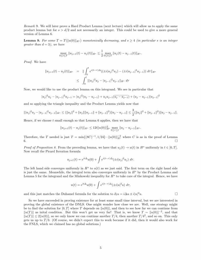
Remark 9. We will later prove a Hard Product Lemma (next lecture) which will allow us to apply the sameproduct lemma but for s > d/2 and not necessarily an integer. This could be used to give a more generalversion of Lemma 6.

Lemma 9. For some T = T (‖u(0)‖Hs) monotonically decreasing, and s ≥ 4 (in particular s is an integergreater than d = 3), we have

1max ‖uj+1(t)− uj(t)‖Hs max≤t≤T

≤ j2 0≤t≤T

‖u (t)0

− uj−1(t)‖Hs .

Proof. We have

‖uj+1(t)− uj(t)‖ (H = ‖

∫ t

ei ts−τ)∆(( i u 2 2

j uj) ( i uj 1 uj 1)) dτ Hs∫ 0

± | | − ± | − | − ‖

t

≤0

‖|uj |2uj − |uj−1|2uj−1‖Hs dτ

Now, we would like to use the product lemma on this integrand. We see in particular that

|uj |2uj − |uj 1|2uj 1 = |uj |2(uj − uj 1) + ujuj 1(u− − − − j − uj−1) + (uj − uj−1)|uj−1|2

and so applying the triangle inequality and the Product Lemma yields now that

2 2 3‖|uj | uj − |uj 1| u− j−1‖ 2Hs ≤ (‖u 2

j‖ + ‖uj‖‖uj 1‖+ ‖uj 1‖ )‖uj −u (− − j−1‖ ≤2‖uj‖2 + ‖uj−1‖2)‖uj −uj−1‖.

Hence, if we choose t small enough so that Lemma 6 applies, then we have that

‖uj+1(t)− u 2j(t)‖Hs ≤ 12t‖u(0)‖Hs max uj uj 1 Hs .

0≤τ≤t‖ − − ‖

Therefore, the T needed is just T = min(8C)−1, 1/24 · ‖u(0)‖−H2s where C is as in the proof of Lemma

6.

Proof of Proposition 8. From the preceding lemma, we have that uj(t)→ u(t) in Hs uniformly in t ∈ [0, T ].Now recall the Picard Iteration formula

uj+1(t) = eit∆u(0) +

∫ei(t−τ)∆(±i|uj |2uj) dτ.

The left hand side converges uniformly in Hs to u(t) as we just said. The first term on the right hand sideis just the same. Meanwhile, the integral term also converges uniformly in Hs by the Product Lemma andLemma 5 for the integrand and the Minkowski inequality for Hs to take care of the integral. Hence, we have

u(t) = eit∆u(0) +

∫ei(t−τ)∆(±i|u|2u) dτ,

and this just matches the Duhamel formula for the solution to ∂tu = i∆u± i|u|2u.

So we have succeeded in proving existence for at least some small time interval, but we are interested inproving the global existence of the DNLS. One might wonder how close we are. Well, one strategy mightbe to find the solution for [0, T ] where T depends on ‖u(0)‖, and then to see how far we can continue from‖u(T )‖ as inital condition. But this won’t get us very far! That is, we know T ∼ ‖u(0)‖−2, and that‖u(T )‖ ≤ 2‖u(0)‖, so we only know we can continue another T/4, then another T/42, and so on. This onlygets us up to T/3. (Of course, we didn’t expect this to work because if it did, then it would also work forthe FNLS, which we claimed has no global solutions.)

5

Lecture 33: 1 May 2015

Consider the PDE ∂tu = i(∆u±u3), which looks similar to our NLS situation, but is slightly changed. Notethat if ∆u± u3 = 0, then we get a steady state solution. However, with the minus sign, which is almost thedefocusing case, there is a maximum principle, so any u(0) that decays to zero at ∞ and has ∆u − u3 = 0must be just 0, and so this ‘D’NLS has no steady state solutions. Meanwhile, the ‘F’NLS considered herewill have solutions to ∆u+ u3 = 0 decaying to zero at ∞, and so will have steady state solutions.

We remark that without this non-linear part, Strichartz implies automatically that every solution to theSchrodinger equation will eventually decay, so the example above does fundamentally show how an NLS canbe qualitatively quite different from the linear Schrodinger Equation.

33.1 The Hard Product Lemma and Persistence of Regularity

Changing focus back to the problem at hand, we had shown last time how to use the easy product lemmato obtain a solution to the FNLS and DNLS for a time interval which was about the size of T ∼ ‖u(0)‖−2

Hs .We would like to do a bit better for the DNLS. Recall in particular that we had ‖u(T )‖Hs ≤ 2‖u(0)‖Hs ,but this was not good enough to extend for all time. Our first main task is to find a better version of theproduct lemma, which will be used to obtain better bounds on ‖u(T )‖Hs and will in turn show the existenceof a global solution for the DNLS (though the whole story will only be completed next lecture). Let us firststate this Hard Product Lemma.

Lemma 10 (Hard Product Lemma). For all s ≥ 0,

‖fg‖Hs . ‖f‖ g∞‖ ‖Hs + ‖f‖Hs‖g‖ .∞

We will prove it later, but for now, let us look at why this might be hard. For s an integer, we have thatthe Hs norm squared is equivalent to a sum of L2 norms squared for up to s derivatives, so we can look ats = 0, 1, 2 to start.

• For s = 0, the inequality is trivial because ‖fg‖2 ≤ ‖f‖∞‖g‖2

• For s = 1, the inequality is still relatively easy. Namely,

‖fg‖sH1 = ‖fg‖22 + ‖(∇f)g‖22 + ‖f(∇g)‖22

and each term is boundable in the same way as the s = 0 case.

• For s = 2, we could try the same computation, but now there is a ‖(∇f)(∇g)‖22 term which is tricky.So we need another tool.

Corollary 10. For s > d/2, ‖fg‖Hs . ‖f‖Hs‖g‖Hs .

Proof. This is just the Hard Product Lemma combined with the Sobolev Inequality from last lecture tobound the L∞ terms.

Remark 11. For s < d/2, the statement of the corollary is false. One can take f = g with compact supportand scale so that the support lies inside a small enough ball.

We continue to delay the proof of the Hard Product Lemma for now, and turn to why it is useful. Wecan actually generalize our DNLS and FNLS examples to consider instead ∂tu = i∆u± i|u|p−1u for p an oddinteger. We will denote this by NLSp. Then we have the following corollary of the Hard Product Lemma,which finally gives a bound on ‖u(T )‖Hs which will be more tractable to show global existence of a solutionto DNLS (by which I mean DNLS3). In particular, the estimate now interplays with ‖u(t)‖L∞

xfor times

0 ≤ t ≤ T . We will see next lecture how to use this.

Corollary 12 (Persistence of regularity). If u obeys NLSp on [0, T ], then

T

‖u(T )‖ p 1Hs ≤ ‖u(0)‖Hsexp

(C(s)

∫0

‖u(t)‖L− dt∞x

)

6

Proof. By the Duhamel formula, we have

T

u(T ) = eiT∆u(0) +

∫ei(T−t)∆(±i|u|p−1u(t))dt.

0

Hence, taking the Hs norm, we have

‖u(T )‖ = ‖e−iT∆Hs u(T )‖Hs

= ‖u(0) +

∫ T

e−it∆(±i|u|p−1u)dt0

‖Hs

We therefore find that

d ‖u(T )‖Hs ≤ ‖e−iT∆(±i|u(T ) s

dT|p−1u(T ))‖H

≤ C(s)‖ p 1u(T )‖L−∞x‖u(T )‖Hs

where the last inequality is by the Hard Product Lemma. In particular, dividing out the ‖u(T )‖Hs termyields

d plog ‖ 1u(T )‖Hs ≤ Cs‖u(T )dT

‖L−∞x

and integrating this yields the desired result.

33.2 Proof of the Hard Product Lemma

We turn our attention back to the Hard Product Lemma. We note that the Hs norm is all about integratingthe Fourier transform of the function against a (1 + |w|)−2s term. It might therefore make sense to want tosplit our function into its frequency components, and this goes back to Littlewood-Paley which we covereda number of lectures ago. We modify some of the notation slightly just for our convenience.

• For k ≥ 1, set Ak := w : 2k−1 ≤ |w| ≤ 2k+1

• Fix a partition of unity ψkk 0 subordinate to the open cover of the frequency domain by B(2) and≥the Ak, i.e. such that suppψ0 ⊆ B(2) and suppψk ⊆ Ak for k ≥ 1.

• Define Pkf := (ψkf)∨.

Lemma 11. ‖Pkf‖Hs ∼ 2ks‖Pkf‖L2

Proof. First suppose k ≥ 1. We have

‖Pkf‖2Hs =

∫|Pkf |2(1 + |w|)2sdw

=

∫Ak

|Pkf |2(1 + |w|)2sdw

where the second equality is because P ψ

kf = kf is supported on Ak. Then 2k−1 ≤ |w| ≤ 2k+1 on this region,

and since k ≥ 1, we therefore have 2k−1 ≤ 1 + |w| ≤ 2k+2, so we immediately find that up to constants(which depend on s),

‖Pkf‖2Hs ∼ 22ks‖P 2kf‖ s

2 = 22k ‖P 2kf‖2,

where we have used Plancherel’s theorem to obtain the last inequality.In the case where k = 0, the same trick works.

Lemma 12. If k ≤ `, then‖Pkf · P`g‖Hs . ‖Pkf‖L∞ · ‖P`g‖Hs

7

Proof. The square of the left hand side is simply Phas support on A + A ⊆ B(10 · 2`1 e

∫|

k ` ) (where A0 =+ |w| ≤ C2` and w get that

| skf ∗ P`g 2(1 + |w|)2 dw, and we see that the integrandB(2) to include the k = 0 case). Hence, we see that

‖Pkf · P`g‖2Hs . 22`s‖Pkf · P`g‖22.

Applying Plancherel and Holder, we thus obtain

‖Pkf · P`g‖2 2`s 2Hs . 2 ‖Pkf · P`g‖2

≤ 22`s‖Pkf‖2 P g 2∞‖ ` ‖2

but the previous lemma thus allows us to replace 22`s‖P`g‖22 with ‖P`g‖2Hs , and we obtain the desiredresult.

This last result tells us that the Littlewood-Paley parts themselves satisfy the correct inequality, andthis is good indication that we’re on our way. Let us first build up our arsenal of weapons (or array oftools, if you’re a pacifist) a little more before we finally proof the Hard Product Lemma. Really, we want toeventually understand bounds on f and not on the pieces Pkf , so let’s do that.

Lemma 13. ‖f‖Hs ∼∑k ‖Pkf‖Hs

Proof.

‖f‖2Hs =

∫|f |2(1 + |w|)2s dw

=

∫ ∣∣∣∑ ∣∣ ψ f

∣2∣∣ (1 + |w|)2s∣ k

k∣ dw

∼∫ ∑

k

|ψkf |2(1 + |w|)2s dw

=∑k

‖Pkf‖2Hs

where the asymptotic comes from the fact that each ψk is positive and the supports of the ψk form a locallyfinite cover of Rd with constant O(1) (i.e. a point is in at most N of the Ak for some fixed constant N).

Lemma 14. ‖Pkf‖Lq . ‖f‖Lq for all 1 ≤ q ≤ ∞, where the constant is independent of q and k.

Proof. We have Pkf = f ∗ ψk∨, and so we have ‖Pkf‖Lq ≤ ‖f‖Lq‖ψk∨‖L1 , so it suffices to bound ‖ψk∨‖L1 .We sketch the details. We can set up so that |ψk| ≤ 1, |∂ψk| . 2−k, |∂2ψk| . 2−2k, and so on. Then|ψ kk∨(x)| . 2 d on B(2−k) and rapidly decays for |x| > 2−k, and so ‖ψk∨‖L1 . 1.

For convenience in notation, we will define P kf :=∑` k Pkf and similarly let ψ k =

∑` k ψ` so that≤ ≤ ≤ ≤

P kf = (ψ kf)∨. We have that the previous lemma applies also to P≤ ≤ ≤k. Finally, with this notation, wecome to the proof we’ve been delaying:

Proof of the Har

d Product Lemma. We write

‖fg‖2Hs =

∫ ∣∣ 2∣∣∑∣∣ P 2skf

Rd ,`

∗ P`g

∣∣∣(1 +

k

|w|) dw.

Now we can break this up into three sums to bound.

The

first

∣∣is when k ≤ `− 4, the second when ` ≤ k− 4,

and the last when

∣|k − `| ≤ 3. Let us try to bound these parts of the sum.

8

• First consider the indices with k ≤ `− 4. We have

∫ ∣∣∣∣∣∣∑ 2 2

P f ∗ P g

∣∣∣∣ (1 + |w|)2s .∑∫ ∣∣ ∗∣∣ | |2 s∣ k ` dw P 4 ` + w ) dw≤` f P g (1−

k≤`−4 ∣ `

.

∣ ∣∑

22`s

`

‖P ` g≤ 4fP− ` ‖22

.∑‖P f‖2 · 22`s‖P g‖2≤`−4 L∞ ` 2

`

. ‖f‖2∞∑

P`g2Hs

`

‖ ‖

∼ ‖f‖2∞‖g‖2Hs

where the 22`s comin the second inequality came from noting that the support of that integral wascontained in a ball of radius |w| ∼ 2`.

• The ` ≤ k − 4 case is symmetric.

• Now consider just the case of |k − `| ≤ 3. In this case, we have that the sets Bk,` = Ak + A` form alocally finite cover in this restricted range, so we can just exchange our sums and absolute values at

will since Pkf ∗ P`g will be supported on Bk,`. In particular, we find:

∫ ∣∣∣∣|k

∣−

∑ ∣2 2∣∣ Pkf ∗ P`g∣∣∣∣ (1 + |w|)2s dw ∼

∑ ∫ ∣∣∣Pkf ∗ P`g (13

∣|

`|≤3 |k−`

∣+ w|)2s dw

|≤

.∑ ∫ ∣∣∣P 2

2`skf ∗ P`g

∣|k |≤3

∣2

∣2 dw

−`

.∑

2`s‖(P 2kf

)(P`

∣g)‖2

|k−`|≤3

.∑ ` `+3

22`s

[P P f 2kf

2 P g 2 + P g 2∞ ` 2 k 2 ` ∞

` [ k=

∑`

‖ ‖ ‖ ‖ ‖−3

∑k=`

‖ ‖ ‖

]

.∑ `+3

‖f‖2 2∞‖P 2 2

`g|Hs +∑k=`

‖Pkf`

‖Hs‖g‖∞

]. ‖f‖2∞‖g‖2Hs + ‖f‖2Hs‖g‖2∞

Combining these three pieces yields the result. (We’ve used a lot of the preceding tools and lemmas in thisproof implicitly, and the active reader should attempt to understand each inequality in this proof.)

Lecture 34: 4 May 2015 (Last Lecture)

Let us list what we already know. Recall that NLS is just the equation ∂ u = i∆u ± i|u|p 1p t

− u, where p isan odd integer, and we are thinking of the equation on R3 ×R. We have the following facts (some of whichwe only proved for p = 3, but which are essentially the same otherwise).

• If u(0) ∈ Hs for s > 3/2, then there is a solution for time T = c‖u(0)‖−2s .

• We had conservation of energy E =

case, this implies that ‖u(t)‖H1 . (M

∫ H

1 2 1 u p+1 and mass M =2 |∇u +11/

| p2

± | |∫|u|2. For the defocusing

+ E) .

• T p 1There was a persistence of regularity, so that ‖u(T )‖Hs ≤ ‖u(0)‖Hs exp(C(s) ·

∫u

0‖ (t)‖L

− dt∞x

).

9

34.1 Finishing the Proof - the Key Estimate and Bootstrapping

We turn now to the last piece of the puzzle. With the persistence of regularity in place, all we need is thefollowing:

Proposition 13 (Key Estimate). If u obeys NLS3 (either version) on [0, T ] where T ≤ T0(‖u(0)‖H1) then∫ T

‖u‖2L 1.∞x

0

≤

Corollary 14. If u solves DNLS3 on [0, T ] for any T , then

‖u(T )‖Hs ≤ ‖u(0)‖Hs exp(CT/T0).

Proof. Combine the Key Estimate with the fact that there is abound for ‖u(t)‖H1 for this defocusing case.

Corollary 15. We have global solutions to DNLS3.

So it remains to prove the Key Estimate! This is not actually very obvious and will rely on a new idea.But let us first do a warm-up lemma.

TLemma 15 (Warm-Up ‘Linear Version’). There is some α > 0 such that 2

0‖eit∆u(0)‖2 α

L dt∞x

. T ‖u(0)‖H1 .

Proof. Recall that Strichartz tells us that for σ = 2 · d+2 = 10 , we haved 3

∫the estimate

‖eit∆u(0)‖Lσx,t ≤ K‖u(0)‖L2

for some constant K. In particular, this is bounded by K‖u(0)‖H1 . Then note that ∇x commutes with both∆ and ∂t, so eit∆(∇xu(0)) = ∇xeit∆u(0). Hence, we find therefore that

‖∇xeit∆u(0)‖Lσx,t ≤ K‖∇xu(0)‖L2 ≤ K‖u(0)‖H1 .

Now we can use a variant of the Sobolev inequality we proved two lectures ago, we obtain:

‖eit∆u(0)‖ it∆ it∆L∞x

. ‖e u(0)‖Lσx + ‖∇e u(0)‖Lσx .

Finally, putting it all together,∫ T T

‖ 2eit∆u(0)‖2L dt∞ .

∫ (‖eit∆u(0)‖Lσx + ‖∇xeit∆u(0)‖L

x∞x

0 0

)(∫ ( ) )2/σ

T

. T 1− 2 itσ ‖eit∆u(0)‖ σ∆Lσx + e u(0)

0

‖∇x ‖L∞x

. T 1− 2σ ‖u(0)‖2H1

In that warm-up, what was really important? At the end, all we needed was that ‖eit∆u(0)‖Lσx,t[0,T ] and

that ‖∇xeit∆u(0)‖Lσx were bounded by some constant times ‖u(0)‖H1 . We really need to do this up to sometime T0. The trick for doing this is called bootstrapping. The lemma is provided below, and following thelemma, we will show how this actually proves the Key Estimate.

Lemma 16 (Bootstrap Lemma). Suppose u obeys NLS3 on [0, T ] with T ≤ T0 = T0(‖u(0)‖H1) (which willbe discovered in the proof) and

‖u(t)‖H1 ≤ 4‖u(0)‖H1

‖u‖Lσ ([0,T ]) ≤ 4Kx,t

‖u(0)‖H1

‖∇xu‖Lσx ≤ 4K‖u(0)‖H1 .

The constant K is the same one as in the proof of the previous lemma. Let us call these conditions A,B,C,respectively. Under these hypotheses, we have that the same estimates hold on [0, T ] but where the constantsin the inequalities are changed from 4 to 2. We will call these changed hypotheses A’,B’,C’.

10

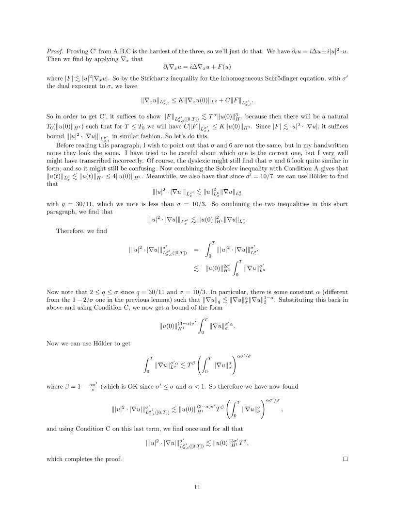
Proof. Proving C’ from A,B,C is the hardest of the three, so we’ll just do that. We have ∂ 2tu = i∆u± i|u| ·u.

Then we find by applying ∇x that∂t∇xu = i∆∇xu+ F (u)

where |F | . |u|2|∇xu|. So by the Strichartz inequality for the inhomogeneous Schrodinger equation, with σ′

the dual exponent to σ, we have

‖∇xu‖Lσx,t ≤ K‖∇xu(0)‖L2 + C‖F‖Lσ′ .x,t

So in order to get C’, it suffices to show ‖F‖ α 3Lσ

′x,t([0,T ]) . T ‖u(0)‖H1 because then there will be a natural

T0(‖u(0)‖ we 2H1) such that for T ≤ T0 will have C‖F‖Lσ′ u

x,t≤ K‖u(0)‖H1 . Since |F | . |u| · |∇ |, it suffices

bound ‖|u|2 · |∇u|‖Lσ′ in similar fashion. So let’s do this.x,t

Before reading this paragraph, I wish to point out that σ and 6 are not the same, but in my handwrittennotes they look the same. I have tried to be careful about which one is the correct one, but I very wellmight have transcribed incorrectly. Of course, the dyslexic might still find that σ and 6 look quite similar inform, and so it might still be confusing. Now combining the Sobolev inequality with Condition A gives that‖u(t)‖L6 . ‖u(t)‖H1 ≤ 4‖u(0)‖H1 . Meanwhile, we also have that since σ

x

′ = 10/7, we can use Holder to findthat

‖|u|2 · |∇u|‖Lσx′ . ‖u‖2L6x‖∇u‖ qLx

with q = 30/11, which we note is less than σ = 10/3. So combining the two inequalities in this shortparagraph, we find that

‖|u|2 · |∇u|‖Lσ′ . ‖u(0)‖2H1‖∇u‖ qLx .x

Therefore, we find

T

‖|u|2 · |∇u|‖σ′ ′

σ′ = u 2 u σLx,t([0,T ])

∫0

‖| | · |∇ |‖Lσx

′

. ‖u(0)‖2σ′

H1

∫ T

0

‖∇′

u‖σLq

Now note that 2 ≤ q ≤ σ since q = 30/11 and σ = 10/3. In particular, there is some constant α (differentfrom the 1− 2/σ one in the previous lemma) such that ‖∇u‖q . ‖∇u‖ασ‖∇u‖1−α2 . Substituting this back inabove and using Condition C, we now get a bound of the form

T

‖ ‖(3−α)σ′u(0) H1

∫0

‖∇u‖σ′ασ .

Now we can use Holder to get

∫ ασT

‖∇u‖σ′αLσ . T β

(∫ ′/σT

‖∇u σ

0 0

‖σ

)

where β = 1− ασ′(which is OK since σ′ ≤ σ and α < 1. So therefore we have now foundσ

ασ′/σT

‖|u|2 · |∇u|‖σ′ (3 α)σ′

σ′ . ‖u(0)−

])‖ T β

Lx,t([0 H1

(∫0

‖∇u‖σ,T σ

),

and using Condition C on this last term, we find once and for all that

‖|u|2 · |∇u|‖σ′ 3σ′ βLσ

′ u]). ‖ (0)

x,t([0‖H1T ,

,T

which completes the proof.

11

So how do we now finally prove the Key Estimate? Well, A’,B’,C’ imply the Key Estimate on the interval[0, T ] in which they are satisfied. So suppose now that u satisfies NLSp on [0, T ] with T ≤ T0(‖u(0)‖H1).Then let S ⊆ [0, T ] be the set on which A,B,C are satisfied, and S0 the component of this in which 0 iscontained (u(0) trivially satisfies these with 4 replaced with 1). Note that if u(0) is nonzero, then in fact theratios ‖u(t)‖H1/‖u(0)‖H1 and similar ratios corresponding to B and C will be continuous, so S0 is a closedinterval of the form [0, T ′] for some T ′ ≤ T . Suppose by way of contradiction that T ′ = T . Then on S0, theBootstrapping Lemma tells us that not only A,B,C are satisfied, but also A’,B’,C’, and by the continuity ofthe ratios in question, S0 extends past T ′, which contradicts the fact that S0 = [0, T ′].

Remark 16. In fact, the Key Estimate then gives existence of the solution to the DNLS for all time, and sothe above reasoning actually proves that the solution to the DNLS satisfies A,B,C, and hence A’,B’,C’, forall t ∈ [0, T0].

Remark 17. It might be worth reiterating what goes wrong for the FNLS case, since it might not be clear.The point is that T0 depends on ‖u(0)‖H1 , and so for DNLS, the important thing was that ‖u(t)‖H1 isalways bounded above by (M +E)1/2. This allowed us to combine what we knew about how long we couldextend our solution based on ‖u(0)‖H2 to keep extending by enough that we will eventually cover all time.For FNLS, we have no such bound, and so we might not be able to keep extending by the entirety of thatamount! It is worth writing out a proof of Corollary 14 to see how this works!

34.2 Final RemarksT p 1Question 1. If u obeys NLSp on [0, T ] with T ≤ T0(‖u(0)‖H1) for some function T0 then does∫

0‖u‖L

− dt∞x

≤1?

There’s also a linear version:

Question 2. Is it true that ∫ T

‖eit∆u(0)‖p−1L dt∞ . Tα‖u(0)‖H1x

0

for some α ≥ 0?

This is a bit more approachable to start. Note that we can use scaling, i.e. by forming u(x/λ, t/λ2), andso if it is true for this linear version, then α = 1− 1 (p− 1), and so we see that for p ≥ 7 (remember p is an4odd integer) we would have α < 0, which is nonsense. For p < 5, we have α > 0, and this is in fact true.The tricky case of p = 5 with α = 0 also turns out to be true. In fact, bootstrapping will always work here.

How about what is known about global solutions for DNLSp? In the ‘70s and ‘80s, this was solved forp < 5. The p = 5 case is in fact very delicate, and in particular, for the first question, the answer is NO ingeneral. However, global solutions DO exist! This was solved throughout the ‘90s and ‘00s by Bowgain andColliander-Keel-Staffilani-Takaoka-Tao.

For p > 5, this is still an open question, and so is the mathematics of the future (and extrapolating fromprevious data points, should be solved in the ‘10s and ‘20s).

12

6

MIT OpenCourseWarehttp://ocw.mit.edu

18.156 Differential Analysis II: Partial Differential Equations and Fourier AnalysisSpring 2016

For information about citing these materials or our Terms of Use, visit: http://ocw.mit.edu/terms.