18.04 complex analysis with applications · 18.04 complex analysis with applications spring 2020...
TRANSCRIPT
18.04 Complex analysis with applications
Spring 2020 lecture notes
Instructor: R. R. Rosales
These notes are an adaption and extension of the original notes for 18.04 by Andre Nachbinand Jeremy Orloff — and later on by Jorn Dunkel. Credit for course design and contentshould go to them; responsibility for typos and errors lies with me.I will be updating and modifying the notes.Check the date to make sure that you have the most current version. February 3, 2020
Contents
1 Brief course description 61.1 Topics needed from prerequisite math classes . . . . . . . . . . . . . . . . . 61.2 Level of mathematical rigor . . . . . . . . . . . . . . . . . . . . . . . . . . . 61.3 Speed of the class . . . . . . . . . . . . . . . . . . . . . . . . . . . . . . . . . 6
2 Complex algebra and the complex plane 72.1 Motivation . . . . . . . . . . . . . . . . . . . . . . . . . . . . . . . . . . . . 72.2 Fundamental theorem of algebra . . . . . . . . . . . . . . . . . . . . . . . . 72.3 Terminology and basic arithmetic . . . . . . . . . . . . . . . . . . . . . . . . 82.4 The complex plane . . . . . . . . . . . . . . . . . . . . . . . . . . . . . . . . 9
2.4.1 The geometry of complex numbers . . . . . . . . . . . . . . . . . . . 92.4.2 The triangle inequality . . . . . . . . . . . . . . . . . . . . . . . . . . 9
2.5 Polar coordinates . . . . . . . . . . . . . . . . . . . . . . . . . . . . . . . . . 102.6 Euler’s Formula . . . . . . . . . . . . . . . . . . . . . . . . . . . . . . . . . . 11
2.6.1 Imaginary exponential behaves like a true exponential . . . . . . . . 112.6.2 Complex exponentials and polar form . . . . . . . . . . . . . . . . . 122.6.3 Complexification or complex replacement . . . . . . . . . . . . . . . 14
1

2.6.4 Nth roots . . . . . . . . . . . . . . . . . . . . . . . . . . . . . . . . . 152.6.5 The geometry of Nth roots . . . . . . . . . . . . . . . . . . . . . . . 16
2.7 Inverse Euler formula . . . . . . . . . . . . . . . . . . . . . . . . . . . . . . . 172.8 de Moivre’s formula . . . . . . . . . . . . . . . . . . . . . . . . . . . . . . . 172.9 Representing complex multiplication as matrix multiplication . . . . . . . . 17
3 Complex functions 183.1 The exponential function . . . . . . . . . . . . . . . . . . . . . . . . . . . . 183.2 Complex functions as mappings . . . . . . . . . . . . . . . . . . . . . . . . . 193.3 The function arg(z) . . . . . . . . . . . . . . . . . . . . . . . . . . . . . . . 24
3.3.1 Many-to-one functions . . . . . . . . . . . . . . . . . . . . . . . . . . 243.3.2 Branches of arg(z) . . . . . . . . . . . . . . . . . . . . . . . . . . . . 253.3.3 The principal branch of arg(z) . . . . . . . . . . . . . . . . . . . . . 27
3.4 Concise summary of branches and branch cuts . . . . . . . . . . . . . . . . 283.5 The function log(z) . . . . . . . . . . . . . . . . . . . . . . . . . . . . . . . . 28
3.5.1 Figures showing w = log(z) as a mapping . . . . . . . . . . . . . . . 293.5.2 Complex powers . . . . . . . . . . . . . . . . . . . . . . . . . . . . . 31
4 Analytic functions 324.1 The derivative: preliminaries . . . . . . . . . . . . . . . . . . . . . . . . . . 324.2 Open disks, open deleted disks, open regions . . . . . . . . . . . . . . . . . 334.3 Limits and continuous functions . . . . . . . . . . . . . . . . . . . . . . . . . 34
4.3.1 Properties of limits . . . . . . . . . . . . . . . . . . . . . . . . . . . . 354.3.2 Continuous functions . . . . . . . . . . . . . . . . . . . . . . . . . . . 354.3.3 Properties of continuous functions . . . . . . . . . . . . . . . . . . . 36
4.4 The point at infinity . . . . . . . . . . . . . . . . . . . . . . . . . . . . . . . 374.4.1 Limits involving infinity . . . . . . . . . . . . . . . . . . . . . . . . . 374.4.2 Stereographic projection from the Riemann sphere . . . . . . . . . . 38
4.5 Derivatives . . . . . . . . . . . . . . . . . . . . . . . . . . . . . . . . . . . . 394.5.1 Derivative rules . . . . . . . . . . . . . . . . . . . . . . . . . . . . . . 39
4.6 Cauchy-Riemann equations . . . . . . . . . . . . . . . . . . . . . . . . . . . 404.6.1 Partial derivatives as limits . . . . . . . . . . . . . . . . . . . . . . . 404.6.2 The Cauchy-Riemann equations . . . . . . . . . . . . . . . . . . . . 414.6.3 Using the Cauchy-Riemann equations . . . . . . . . . . . . . . . . . 424.6.4 f ′(z) as a 2× 2 matrix . . . . . . . . . . . . . . . . . . . . . . . . . . 43
4.7 Geometric interpretation & linear elasticity theory . . . . . . . . . . . . . . 444.8 Cauchy-Riemann all the way down . . . . . . . . . . . . . . . . . . . . . . . 454.9 Gallery of functions . . . . . . . . . . . . . . . . . . . . . . . . . . . . . . . 46
4.9.1 Gallery of functions, derivatives and properties . . . . . . . . . . . . 464.9.2 A few proofs . . . . . . . . . . . . . . . . . . . . . . . . . . . . . . . 50
4.10 Branch cuts and function composition . . . . . . . . . . . . . . . . . . . . . 514.11 Appendix: Limits . . . . . . . . . . . . . . . . . . . . . . . . . . . . . . . . . 53
4.11.1 Limits of sequences . . . . . . . . . . . . . . . . . . . . . . . . . . . . 534.11.2 lim
z→z0f(z) . . . . . . . . . . . . . . . . . . . . . . . . . . . . . . . . . 55
4.11.3 Connection between limits of sequences and limits of functions . . . 55
2

5 Line integrals and Cauchy’s theorem 555.1 Complex line integrals . . . . . . . . . . . . . . . . . . . . . . . . . . . . . . 565.2 Fundamental theorem for complex line integrals . . . . . . . . . . . . . . . . 575.3 Path independence . . . . . . . . . . . . . . . . . . . . . . . . . . . . . . . . 585.4 Examples . . . . . . . . . . . . . . . . . . . . . . . . . . . . . . . . . . . . . 595.5 Cauchy’s theorem . . . . . . . . . . . . . . . . . . . . . . . . . . . . . . . . . 605.6 Extensions of Cauchy’s theorem . . . . . . . . . . . . . . . . . . . . . . . . . 63
6 Cauchy’s integral formula 666.1 Cauchy’s integral for functions . . . . . . . . . . . . . . . . . . . . . . . . . 666.2 Cauchy’s integral formula for derivatives . . . . . . . . . . . . . . . . . . . . 68
6.2.1 Another approach to some basic examples . . . . . . . . . . . . . . . 696.2.2 More examples . . . . . . . . . . . . . . . . . . . . . . . . . . . . . . 696.2.3 The triangle inequality for integrals . . . . . . . . . . . . . . . . . . 72
6.3 Proof of Cauchy’s integral formula . . . . . . . . . . . . . . . . . . . . . . . 746.3.1 A useful theorem . . . . . . . . . . . . . . . . . . . . . . . . . . . . . 746.3.2 Proof of Cauchy’s integral formula . . . . . . . . . . . . . . . . . . . 75
6.4 Proof of Cauchy’s integral formula for derivatives . . . . . . . . . . . . . . . 766.5 Consequences of Cauchy’s integral formula . . . . . . . . . . . . . . . . . . . 77
6.5.1 Existence of derivatives . . . . . . . . . . . . . . . . . . . . . . . . . 776.5.2 Cauchy’s inequality . . . . . . . . . . . . . . . . . . . . . . . . . . . 776.5.3 Liouville’s theorem . . . . . . . . . . . . . . . . . . . . . . . . . . . . 786.5.4 Maximum modulus principle . . . . . . . . . . . . . . . . . . . . . . 79
7 Introduction to harmonic functions 817.1 Harmonic functions . . . . . . . . . . . . . . . . . . . . . . . . . . . . . . . . 827.2 Del notation . . . . . . . . . . . . . . . . . . . . . . . . . . . . . . . . . . . . 82
7.2.1 Analytic functions have harmonic pieces . . . . . . . . . . . . . . . . 827.2.2 Harmonic conjugates . . . . . . . . . . . . . . . . . . . . . . . . . . . 84
7.3 A second proof that u and v are harmonic . . . . . . . . . . . . . . . . . . . 847.4 Maximum principle and mean value property . . . . . . . . . . . . . . . . . 857.5 Orthogonality of curves . . . . . . . . . . . . . . . . . . . . . . . . . . . . . 85
8 Two dimensional hydrodynamics and complex potentials 898.1 Velocity fields . . . . . . . . . . . . . . . . . . . . . . . . . . . . . . . . . . . 908.2 Stationary flows . . . . . . . . . . . . . . . . . . . . . . . . . . . . . . . . . . 908.3 Physical assumptions, mathematical consequences . . . . . . . . . . . . . . 91
8.3.1 Physical assumptions . . . . . . . . . . . . . . . . . . . . . . . . . . . 918.3.2 Examples . . . . . . . . . . . . . . . . . . . . . . . . . . . . . . . . . 928.3.3 Summary . . . . . . . . . . . . . . . . . . . . . . . . . . . . . . . . . 93
8.4 Complex potentials . . . . . . . . . . . . . . . . . . . . . . . . . . . . . . . . 938.4.1 Analytic functions give us incompressible, irrotational flows . . . . . 938.4.2 Incompressible, irrotational flows always have complex potential func-
tions . . . . . . . . . . . . . . . . . . . . . . . . . . . . . . . . . . . . 948.5 Stream functions . . . . . . . . . . . . . . . . . . . . . . . . . . . . . . . . . 95
3

8.5.1 Examples . . . . . . . . . . . . . . . . . . . . . . . . . . . . . . . . . 968.5.2 Stagnation points . . . . . . . . . . . . . . . . . . . . . . . . . . . . . 98
8.6 More examples . . . . . . . . . . . . . . . . . . . . . . . . . . . . . . . . . . 98
9 Taylor and Laurent series 1019.1 Geometric series . . . . . . . . . . . . . . . . . . . . . . . . . . . . . . . . . 102
9.1.1 Connection to Cauchy’s integral formula . . . . . . . . . . . . . . . . 1039.2 Convergence of power series . . . . . . . . . . . . . . . . . . . . . . . . . . . 103
9.2.1 Ratio test and root test . . . . . . . . . . . . . . . . . . . . . . . . . 1049.3 Taylor series . . . . . . . . . . . . . . . . . . . . . . . . . . . . . . . . . . . . 105
9.3.1 Order of a zero . . . . . . . . . . . . . . . . . . . . . . . . . . . . . . 1059.3.2 Taylor series examples . . . . . . . . . . . . . . . . . . . . . . . . . . 1069.3.3 Proof of Taylor’s theorem . . . . . . . . . . . . . . . . . . . . . . . . 110
9.4 Singularities . . . . . . . . . . . . . . . . . . . . . . . . . . . . . . . . . . . . 1119.5 Laurent series . . . . . . . . . . . . . . . . . . . . . . . . . . . . . . . . . . . 111
9.5.1 Examples of Laurent series . . . . . . . . . . . . . . . . . . . . . . . 1149.6 Digression to differential equations . . . . . . . . . . . . . . . . . . . . . . . 1169.7 Poles . . . . . . . . . . . . . . . . . . . . . . . . . . . . . . . . . . . . . . . . 117
9.7.1 Examples of poles . . . . . . . . . . . . . . . . . . . . . . . . . . . . 1189.7.2 Residues . . . . . . . . . . . . . . . . . . . . . . . . . . . . . . . . . . 119
10 Residue Theorem 12010.1 Poles and zeros . . . . . . . . . . . . . . . . . . . . . . . . . . . . . . . . . . 12010.2 Words: Holomorphic and meromorphic . . . . . . . . . . . . . . . . . . . . . 12110.3 Behavior of functions near zeros and poles . . . . . . . . . . . . . . . . . . . 121
10.3.1 Picard’s theorem and essential singularities . . . . . . . . . . . . . . 12210.3.2 Quotients of functions . . . . . . . . . . . . . . . . . . . . . . . . . . 122
10.4 Residues . . . . . . . . . . . . . . . . . . . . . . . . . . . . . . . . . . . . . . 12310.4.1 Residues at simple poles . . . . . . . . . . . . . . . . . . . . . . . . . 12510.4.2 Residues at finite poles . . . . . . . . . . . . . . . . . . . . . . . . . 12810.4.3 cot(z) . . . . . . . . . . . . . . . . . . . . . . . . . . . . . . . . . . . 129
10.5 Cauchy Residue Theorem . . . . . . . . . . . . . . . . . . . . . . . . . . . . 13110.6 Residue at ∞ . . . . . . . . . . . . . . . . . . . . . . . . . . . . . . . . . . . 136
11 Definite integrals using the residue theorem 13811.1 Integrals of functions that decay . . . . . . . . . . . . . . . . . . . . . . . . 138
11.2 Integrals
∫ ∞−∞
and
∫ ∞0
. . . . . . . . . . . . . . . . . . . . . . . . . . . . . 141
11.3 Trigonometric integrals . . . . . . . . . . . . . . . . . . . . . . . . . . . . . . 14411.4 Integrands with branch cuts . . . . . . . . . . . . . . . . . . . . . . . . . . . 14611.5 Cauchy principal value . . . . . . . . . . . . . . . . . . . . . . . . . . . . . . 15111.6 Integrals over portions of circles . . . . . . . . . . . . . . . . . . . . . . . . . 15311.7 Fourier transform . . . . . . . . . . . . . . . . . . . . . . . . . . . . . . . . . 15511.8 Solving ODEs using the Fourier transform . . . . . . . . . . . . . . . . . . . 158
4

12 Conformal transformations 16212.1 Geometric definition of conformal mappings . . . . . . . . . . . . . . . . . . 16212.2 Tangent vectors as complex numbers . . . . . . . . . . . . . . . . . . . . . . 16412.3 Analytic functions are conformal . . . . . . . . . . . . . . . . . . . . . . . . 16512.4 Digression to harmonic functions . . . . . . . . . . . . . . . . . . . . . . . . 16512.5 Riemann mapping theorem . . . . . . . . . . . . . . . . . . . . . . . . . . . 16612.6 Fractional linear transformations . . . . . . . . . . . . . . . . . . . . . . . . 166
12.6.1 Examples . . . . . . . . . . . . . . . . . . . . . . . . . . . . . . . . . 16712.6.2 Lines and circles . . . . . . . . . . . . . . . . . . . . . . . . . . . . . 16912.6.3 Mapping zj to wj . . . . . . . . . . . . . . . . . . . . . . . . . . . . . 17012.6.4 Correspondence with matrices . . . . . . . . . . . . . . . . . . . . . . 171
12.7 Reflection and symmetry . . . . . . . . . . . . . . . . . . . . . . . . . . . . . 17212.7.1 Reflection and symmetry in a line . . . . . . . . . . . . . . . . . . . 17212.7.2 Reflection and symmetry in a circle . . . . . . . . . . . . . . . . . . 17312.7.3 Reflection in the unit circle . . . . . . . . . . . . . . . . . . . . . . . 174
12.8 Solving the Dirichlet problem for harmonic functions . . . . . . . . . . . . . 17712.8.1 Harmonic functions on the upper half-plane . . . . . . . . . . . . . . 17812.8.2 Harmonic functions on the unit disk . . . . . . . . . . . . . . . . . . 179
12.9 Flows around cylinders . . . . . . . . . . . . . . . . . . . . . . . . . . . . . . 18112.9.1 Milne-Thomson circle theorem . . . . . . . . . . . . . . . . . . . . . 18112.9.2 Examples . . . . . . . . . . . . . . . . . . . . . . . . . . . . . . . . . 181
12.10Examples of conformal maps and excercises . . . . . . . . . . . . . . . . . . 183
5

1 Brief course description
Complex analysis is a beautiful, tightly integrated subject. It revolves around complexanalytic functions. These are functions that have a complex derivative. Unlike calculususing real variables, the mere existence of a complex derivative has strong implications forthe properties of the function.
Complex analysis is a basic tool in many mathematical theories. By itself and throughsome of these theories it also has a great many practical applications.
There are a small number of far-reaching theorems that we’ll explore in the first part ofthe class. Along the way, we’ll touch on some mathematical and engineering applications ofthese theorems. The last third of the class will be devoted to a deeper look at applications.
The main theorems are Cauchy’s Theorem, Cauchy’s integral formula, and the existenceof Taylor and Laurent series. Among the applications will be harmonic functions, twodimensional fluid flow, easy methods for computing (seemingly) hard integrals, Laplacetransforms, and Fourier transforms with applications to engineering and physics.
1.1 Topics needed from prerequisite math classes
We will review these topics as we need them:
• Limits
• Power series
• Vector fields
• Line integrals
• Green’s theorem
1.2 Level of mathematical rigor
We will make careful arguments to justify our results. Though, in many places we will allowourselves to skip some technical details if they get in the way of understanding the mainpoint, but we will note what was left out.
1.3 Speed of the class
(Borrowed from R. Rosales 18.04 OCW 1999)Do not be fooled by the fact things start slow. This is the kind of course where things
keep on building up continuously, with new things appearing rather often. Nothing is reallyvery hard, but the total integration can be staggering - and it will sneak up on you if youdo not watch it. Or, to express it in mathematically sounding lingo, this course is ‘locallyeasy’ but ‘globally hard’. That means that if you keep up-to-date with the homework andlectures, and read the class notes regularly, you should not have any problems.
6

2 Complex algebra and the complex plane
We will start with a review of the basic algebra and geometry of complex numbers. Mostlikely you have encountered this previously in 18.03 or elsewhere.
2.1 Motivation
The equation x2 = −1 has no real solutions, yet we know that this equation arises naturallyand we want to use its roots. So we make up a new symbol for the roots and call it acomplex number.
Definition. The symbols ±i will stand for the solutions to the equation x2 = −1. We willcall these new numbers complex numbers. We will also write
√−1 = ±i
where i is also called an imaginary number.1 This is a historical term. These are perfectlyvalid numbers that don’t happen to lie on the real number line.2 We’re going to look at thealgebra, geometry and, most important for us, the exponentiation of complex numbers.
Before starting a systematic exposition of complex numbers, we’ll work a simple example.
Example. Solve the equation z2 + z + 1 = 0.
Solution: We can apply the quadratic formula to get
z =−1±
√1− 4
2=−1±
√−3
2=−1±
√3√−1
2=−1±
√3 i
2.
Q: Do you know how to solve quadratic equations by completing the square? This is howthe quadratic formula is derived and is well worth knowing!
2.2 Fundamental theorem of algebra
One of the reasons for using complex numbers is because allowing complex roots meansevery polynomial has exactly the expected number of roots. This is the fundamentaltheorem of algebra:
A polynomial of degree n has exactly n complex roots (repeated roots are counted withmultiplicity).
In a few weeks, we will be able to prove this theorem as a remarkably simple consequenceof one of our main theorems.
1Engineers typically use j instead of i. We’ll follow mathematical custom in 18.04.2Our motivation for using complex numbers is not the same as the historical motivation. Historically,
mathematicians were willing to say x2 = −1 had no solutions. The issue that pushed them to accept complexnumbers had to do with the formula for the roots of cubics. Cubics always have at least one real root, andwhen square roots of negative numbers appeared in this formula, even for the real roots, mathematicianswere forced to take a closer look at these (seemingly) exotic objects.
7
2.3 Terminology and basic arithmetic
Definitions
• Complex numbers are defined as the set of all numbers
z = x+ yi,
where x and y are real numbers.
• We denote the set of all complex numbers by C. (On the blackboard we will usuallywrite C –this font is called blackboard bold.)
• We call x the real part of z. This is denoted by x = Re(z).
• We call y the imaginary part of z. This is denoted by y = Im(z).
Important: The imaginary part of z is a real number. It does not include the i.
The basic arithmetic operations follow the standard rules. All you have to remember isthat i2 = −1. We will go through these quickly using some simple examples. It almost goeswithout saying that in 18.04 it is essential that you become fluent with these manipulations.
• Addition: (3 + 4i) + (7 + 11i) = 10 + 15i
• Subtraction: (3 + 4i)− (7 + 11i) = −4− 7i
• Multiplication:
(3 + 4i)(7 + 11i) = 21 + 28i+ 33i+ 44i2 = −23 + 61i
Here we have used the fact that 44i2 = −44.
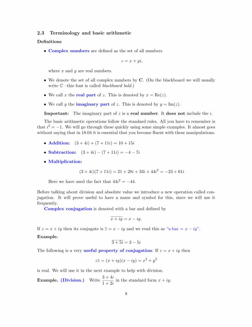
Before talking about division and absolute value we introduce a new operation called con-jugation. It will prove useful to have a name and symbol for this, since we will use itfrequently.
Complex conjugation is denoted with a bar and defined by
x+ iy = x− iy.
If z = x+ iy then its conjugate is z = x− iy and we read this as “z-bar = x− iy”.
Example.3 + 5i = 3− 5i
The following is a very useful property of conjugation: If z = x+ iy then
zz = (x+ iy)(x− iy) = x2 + y2
is real. We will use it in the next example to help with division.
Example. (Division.) Write3 + 4i
1 + 2iin the standard form x+ iy.
8

Solution: We use the useful property of conjugation to clear the denominator:
3 + 4i
1 + 2i=
3 + 4i
1 + 2i· 1− 2i
1− 2i=
11− 2i
5=
11
5− 2
5i.
In the next section we will discuss the geometry of complex numbers, which give someinsight into the meaning of the magnitude of a complex number. For now we just give thedefinition.
Definition. The magnitude of the complex number x+ iy is defined as
|z| =√x2 + y2.
The magnitude is also called the absolute value, norm or modulus.
Example. The norm of 3 + 5i =√
9 + 25 =√
34.Important. The norm is the sum of x2 and y2. It does not include the i and istherefore always positive.
2.4 The complex plane
2.4.1 The geometry of complex numbers
Because it takes two numbers x and y to describe the complex number z = x + iy wecan visualize complex numbers as points in the xy-plane. When we do this we call it thecomplex plane. Since x is the real part of z we call the x-axis the real axis. Likewise, they-axis is the imaginary axis.
Real axis
Imaginary axis
r
z = x+ iy = (x, y)
x
y
θ Real axis
Imaginary axis
r
z = x+ iy = (x, y)
r
z = x− iy = (x,−y)
θ−θ
2.4.2 The triangle inequality
The triangle inequality says that for a triangle the sum of the lengths of any two legs isgreater than the length of the third leg.
A
B
C
Triangle inequality: |AB|+ |BC| > |AC|
9

For complex numbers the triangle inequality translates to a statement about complexmagnitudes. Precisely: for complex numbers z1, z2
|z1|+ |z2| ≥ |z1 + z2|with equality only if one of them is 0 or arg(z1) = arg(z2). This is illustrated in the followingfigure.
x
y
z1
z2
z1 + z2
Triangle inequality: |z1|+ |z2| ≥ |z1 + z2|
We get equality only if z1 and z2 are on the same ray from the origin.
2.5 Polar coordinates
In the figures above we have marked the length r and polar angle θ of the vector from theorigin to the point z = x+ iy. These are the same polar coordinates you saw in 18.02 and18.03. There are a number of synonyms for both r and θ
r = |z| = magnitude = length = norm = absolute value = modulus
θ = arg(z) = argument of z = polar angle of z
As in 18.02 you should be able to visualize polar coordinates by thinking about the distancer from the origin and the angle θ with the x-axis.
Example. Let’s make a table of z, r and θ for some complex numbers. Notice that θ isnot uniquely defined since we can always add a multiple of 2π to θ and still be at the samepoint in the plane.z = a+ bi r θ
1 1 0, 2π, 4π, . . . Argument = 0, means z is along the x-axisi 1 π/2, π/2 + 2π . . . Argument = π
2 , means z is along the y-axis
1 + i√
2 π/4, π/4 + 2π . . . Argument = π4 , means z is along the ray at 45◦ to the x-axis
Real axis
Imaginary axisi
1
1 + i
10

When we want to be clear which value of θ is meant, we will specify a branch of arg.For example, 0 ≤ θ < 2π or −π < θ ≤ π. This will be discussed in much more detail in thecoming weeks. Keeping careful track of the branches of arg will turn out to be one of thekey requirements of complex analysis.
2.6 Euler’s Formula
Euler’s (pronounced ‘oilers’) formula connects complex exponentials, polar coordinates, andsines and cosines. It turns messy trig identities into tidy rules for exponentials. We will useit a lot. The formula is the following:
eiθ = cos(θ) + i sin(θ). (1)
There are many ways to approach Euler’s formula. Our approach is to simply take Equation1 as the definition of complex exponentials. This is legal, but does not show that it’s a gooddefinition. To do that we need to show the eiθ obeys all the rules we expect of an exponential.To do that we go systematically through the properties of exponentials and check that theyhold for complex exponentials.
2.6.1 eiθ behaves like a true exponential
P1. eit differentiates as expected:deit
dt= ieit
Proof. This follows directly from the definition:
deit
dt=
d
dt(cos(t) + i sin(t)) = − sin(t) + i cos(t) = i(cos(t) + i sin(t)) = ieit
P2. ei·0 = 1.Proof.
ei·0 = cos(0) + i sin(0) = 1
P3. The usual rules of exponents hold:
eiaeib = ei(a+b)
Proof. This relies on the cosine and sine addition formulas.
eia · eib = (cos(a) + i sin(a)) · (cos(b) + i sin(b))
= cos(a) cos(b)− sin(a) sin(b) + i (cos(a) sin(b) + sin(a) cos(b))
= cos(a+ b) + i sin(a+ b) = ei(a+b).
P4. The definition of eiθ is consistent with the power series for ex.
11

Proof. To see this we have to recall the power series for ex, cos(x) and sin(x). They are
ex = 1 + x+x2
2!+x3
3!+x4
4!+ . . . (2a)
cosx = 1− x2
2!+x4
4!− x6
6!+ . . . (2b)
sinx = x− x3
3!+x5
5!+ . . . (2c)
Now we can write the power series for eiθ and then split it into the power series for sineand cosine:
eiθ =∞∑0
(iθ)n
n!
=
∞∑0
(−1)kθ2k
(2k)!+ i
∞∑0
(−1)kθ2k+1
(2k + 1)!
= cos(θ) + i sin(θ).
So the Euler formula definition is consistent with the usual power series for ex.Properties P1-P4 should convince you that eiθ behaves like an exponential.
2.6.2 Complex exponentials and polar form
Now let’s turn to the relation between polar coordinates and complex exponentials.Suppose z = x + iy has polar coordinates r and θ. That is, we have x = r cos(θ) and
y = r sin(θ). Thus, we get the important relationship
z = x+ iy = r cos(θ) + ir sin(θ) = r(cos(θ) + i sin(θ)) = reiθ.
This is so important you shouldn’t proceed without understanding. We also record itwithout the intermediate equation.
z = x+ iy = reiθ. (3)
Because r and θ are the polar coordinates of (x, y) we call z = reiθ the polar form of z. Wenext show that
Magnitude, argument, conjugate, multiplication and division are easy in polarform.
Magnitude. |eiθ| = 1.Proof.
|eiθ| = | cos(θ) + i sin(θ)| =√
cos2(θ) + sin2(θ) = 1
In words, this says that eiθ is always on the unit circle – this is useful to remember! Likewise,if z = reiθ then |z| = r. You can calculate this, but it should be clear from the definitions:|z| is the distance from z to the origin, which is exactly the same definition as for r.
12

Argument. If z = reiθ then arg(z) = θ.Proof. This is again the definition: the argument is the polar angle θ.
Conjugate. (reiθ) = re−iθ.Proof.
(reiθ) = r(cos(θ) + i sin(θ)) = r(cos(θ)− i sin(θ)) = r(cos(−θ) + i sin(−θ)) = re−iθ.
Thus, complex conjugation changes the sign of the argument.Multiplication. If z1 = r1eiθ1 and z2 = r2eiθ2 then
z1z2 = r1r2ei(θ1+θ2)
This is what mathematicians call trivial to see, just write the multiplication down. In words,the formula says the for z1z2 the magnitudes multiply and the arguments add.Division. Again it’s trivial that
r1eiθ1
r2eiθ2=r1
r2ei(θ1−θ2)
Example. (Multiplication by 2i) Here’s a simple but important example. By looking atthe graph we see that the number 2i has magnitude 2 and argument π/2. So in polarcoordinates it equals 2eiπ/2. This means that multiplication by 2i multiplies lengths by 2and adds π/2 to arguments, i.e. rotates by 90◦. The effect is shown in the figures below
Re
Im
2i = 2eiπ/2
π/2
|2i| = 2, arg(2i) = π/2
Re
Im
Re
Im× 2i
Multiplication by 2i rotates by π/2 and scales by 2
Example. (Raising to a power) Let’s compute (1 + i)6 and(
1+i√
32
)3.
Solution: 1 + i has magnitude =√
2 and arg = π/4, so 1 + i =√
2eiπ/4. Raising to a poweris now easy:
(1 + i)6 =(√
2eiπ/4)6
= 8e6iπ/4 = 8e3iπ/2 = −8i
Similarly,1 + i
√3
2= eiπ/3, so
(1 + i
√3
2
)3
= (1 · eiπ/3)3 = eiπ = −1
13

2.6.3 Complexification or complex replacement
In the next example we will illustrate the technique of complexification or complex replace-ment. This can be used to simplify a trigonometric integral. It will come in handy whenwe need to compute certain integrals.
Example. Use complex replacement to compute
I =
∫dx ex cos(2x)
Solution: We have Euler’s formula
e2ix = cos(2x) + i sin(2x)
so cos(2x) = Re(e2ix). The complex replacement trick is to replace cos(2x) by e2ix. We get(justification below)
Ic =
∫dx (ex cos 2x+ iex sin 2x) , I = Re(Ic).
Computing Ic is straightforward:
Ic =
∫dx exei2x =
∫dx ex(1+2i) =
ex(1+2i)
1 + 2i.
Here we will do the computation first in rectangular coordinates3
Ic =ex(1+2i)
1 + 2i· 1− 2i
1− 2i
=ex(cos(2x) + i sin(2x))(1− 2i)
5
=1
5ex(cos(2x) + 2 sin(2x) + i(−2 cos(2x) + sin(2x)))
So,
I = Re(Ic) =1
5ex(cos(2x) + 2 sin(2x)).
Justification of complex replacement. The trick comes by cleverly adding a new
integral to I as follows. Let J =
∫ex sin(2x) dx. Then we let
Ic = I + iJ =
∫dx ex(cos(2x) + i sin(2x)) =
∫dx exe2ix
Clearly, by construction, Re(Ic) = I as claimed above.
3In applications, for example throughout 18.03, polar form is often preferred because it is easier and givesthe answer in a more useable form.
14

We can use polar coordinates to simplify the expression for Ic: In polar form, we have1 + 2i = reiφ, where r =
√5 and φ = arg(1 + 2i) = tan−1(2) in the first quadrant. Then:
Ic =ex(1+2i)
√5eiφ
=ex√
5ei(2x−φ) =
ex√5
(cos(2x− φ) + i sin(2x− φ)).
Thus,
I = Re(Ic) =ex√
5cos(2x− φ)
2.6.4 Nth roots
We are going to need to be able to find the nth roots of complex numbers, i.e., solveequations of the form
zN = c
where c is a given complex number. This can be done most conveniently by expressing cand z in polar form, c = Reiφ and z = reiθ. Then, upon substituting, we have to solve
rNeiNθ = Reiφ
For the complex numbers on the left and right to be equal, their absolute values must besame and the arguments can only differ by an integer-multiple of 2π, which gives
r = R1/N , Nθ = φ+ 2πn , n = 0,±1,±2, . . . (4)
Solving for θ, we have
θ =φ
N+ 2π
n
N. (5)
Example. Find all 5 fifth roots of 2.
Solution: For c = 2, we have R = 2 and φ = 0, so the fifth roots of 2 are
zn = 21/5e2nπi/5, where n = 0,±1,±2, . . .
Looking at the right hand side we see that for n = 5 we have 21/5e2πi which is exactly thesame as the root when n = 0, i.e. 21/5e0i. Likewise n = 6 gives exactly the same root asn = 1, and so on. This means, we have 5 different roots corresponding to n = 0, 1, 2, 3, 4.
zn = 21/5, 21/5e2πi/5, 21/5e4πi/5, 21/5e6πi/5, 21/5e8πi/5
Similarly we can say that in general c = Reiφ has N distinct Nth roots:
zn = r1/Neiφ/N+i 2π(n/N) for n = 0, 1, 2, . . . N − 1.
15

Example. Find the 4 fourth roots of 1.
Solution: Need to solve z4 = 1, so φ = 0. So the 4 distinct fourth roots are in polar form
zn = 1, eiπ/2, eiπ, ei3π/2
and in Cartesian representationzn = 1, i, −1, −i
Example. Find the 3 cube roots of -1.
Solution: z2 = −1 = ei π+i 2πn. So, zn = ei π/3+i 2π(n/3) and the 3 cube roots are eiπ/3, eiπ, ei5π/3.Since π/3 radians is 60◦ we can simpify:
eiπ/3 = cos(π/3) + i sin(π/3) =1
2+ i
√3
2⇒ zn = −1,
1
2± i√
3
2
Example. Find the 5 fifth roots of 1 + i.
Solution: z5 = 1 + i =√
2ei(π/4+2nπ), for n = 0, 1, 2, . . .. So, the 5 fifth roots are
21/10eiπ/20, 21/10ei9π/20, 21/10ei17π/20, 21/10ei25π/20, 21/10ei33π/20.
Using a calculator we could write these numerically as a+ bi, but there is no easy simplifi-cation.
Example. We should check that our technique works as expected for a simple problem.Find the 2 square roots of 4.
Solution: z2 = 4ei 2πn. So, zn = 2ei πn with n = 0, 1. So the two roots are 2e0 = +2 and2eiπ = −2 as expected.
2.6.5 The geometry of Nth roots
Looking at the examples above we see that roots are always spaced evenly around a circlecentered at the origin. For example, the fifth roots of 1+ i are spaced at increments of 2π/5radians around the circle of radius 21/5.
Note also that the roots of real numbers always come in conjugate pairs.
x
y
12 + i
√3
2
12 − i
√3
2
−1
Cube roots of -1
x
y
1 + i
Fifth roots of 1 + i
16

2.7 Inverse Euler formula
Euler’s formula gives a complex exponential in terms of sines and cosines. We can turn thisaround to get the inverse Euler formulas. Euler’s formula says:
eit = cos(t) + i sin(t) and e−it = cos(t)− i sin(t).
By adding and subtracting we get:
cos(t) =eit + e−it
2and sin(t) =
eit − e−it
2i.
Please take note of these formulas we will use them frequently!
2.8 de Moivre’s formula
For positive integers n we have de Moivre’s formula:
(cos(θ) + i sin(θ))n = cos(nθ) + i sin(nθ)
Proof. This is a simple consequence of Euler’s formula:
(cos(θ) + i sin(θ))n = (eiθ)n = einθ = cos(nθ) + i sin(nθ)
The reason this simple fact has a name is that historically de Moivre stated it before Euler’sformula was known. Without Euler’s formula there is not such a simple proof.
2.9 Representing complex multiplication as matrix multiplication
Consider two complex numbers z1 = a+ bi and z2 = x+ yi and their product
z1z2 = (a+ bi)(x+ iy) = (ax− by) + i(bx+ ay) =: w (6)
Now let’s define two matrices
Z1 =
[a −bb a
], Z2 =
[x −yy x
](7)
Note that these matrices store the same information as z1 and z2, respectively. Let’scompute their matrix product
Z1Z2 =
[a −bb a
] [x −yy x
]=
[ax− by −(bx+ ay)bx+ ay ax− by
]= W (8)
Comparing with Eq. (6), we see that W is indeed the matrix corresponding to the complexnumber w = z1z2. Thus, we can represent any complex number z equivalently by the matrix
Z =
[Re z − Im zIm z Re z
](9)
17

and complex multiplication then simply becomes matrix multiplication. Further note thatwe can write
Z = Re z
[1 00 1
]+ Im z
[0 −11 0
], (10)
i.e., the imaginary unit i corresponds to the matrix
[0 −11 0
]and i2 = −1 becomes
[0 −11 0
] [0 −11 0
]= −
[1 00 1
]. (11)
Polar form (decomposition). Writing z = reiθ = r(cos θ + i sin θ), we find
Z = r
[cos θ − sin θsin θ cos θ
]=
[cos θ − sin θsin θ cos θ
] [r 00 r
](12)
corresponding to a 2D rotation matrix multiplied by the stretch factor r. In particular,multiplication by i corresponds to the rotation with angle θ = π/2 and r = 1.
3 Complex functions
3.1 The exponential function
We have Euler’s formula: eiθ = cos(θ) + i sin(θ). We can extend this to the complexexponential function ez.
Definition. For z = x+ iy the complex exponential function is defined as
ez = ex+iy = exeiy = ex(cos(y) + i sin(y)).
In this definition ex is the usual exponential function for a real variable x. It is easy to seethat all the usual rules of exponents hold:
1. e0 = 1
2. ez1+z2 = ez1ez2
3. (ez)n = enz for positive integers n.
4. (ez)−1 = e−z
5. ez 6= 0
It will turn out that the propertydez
dz= ez also holds, but we can’t prove this yet
because we haven’t defined what we mean by the complex derivatived
dz.
Here are some more simple, but extremely important properties of ez. You shouldbecome fluent in their use and know how to prove them.
18
6. |eiθ| = 1
Proof.
|eiθ| = | cos(θ) + i sin(θ)| =√
cos2(θ) + sin2(θ) = 1.
7. |ex+iy| = ex (as usual z = x+ iy and x, y are real).
Proof. You should be able to supply this. If not: ask a teacher or TA.
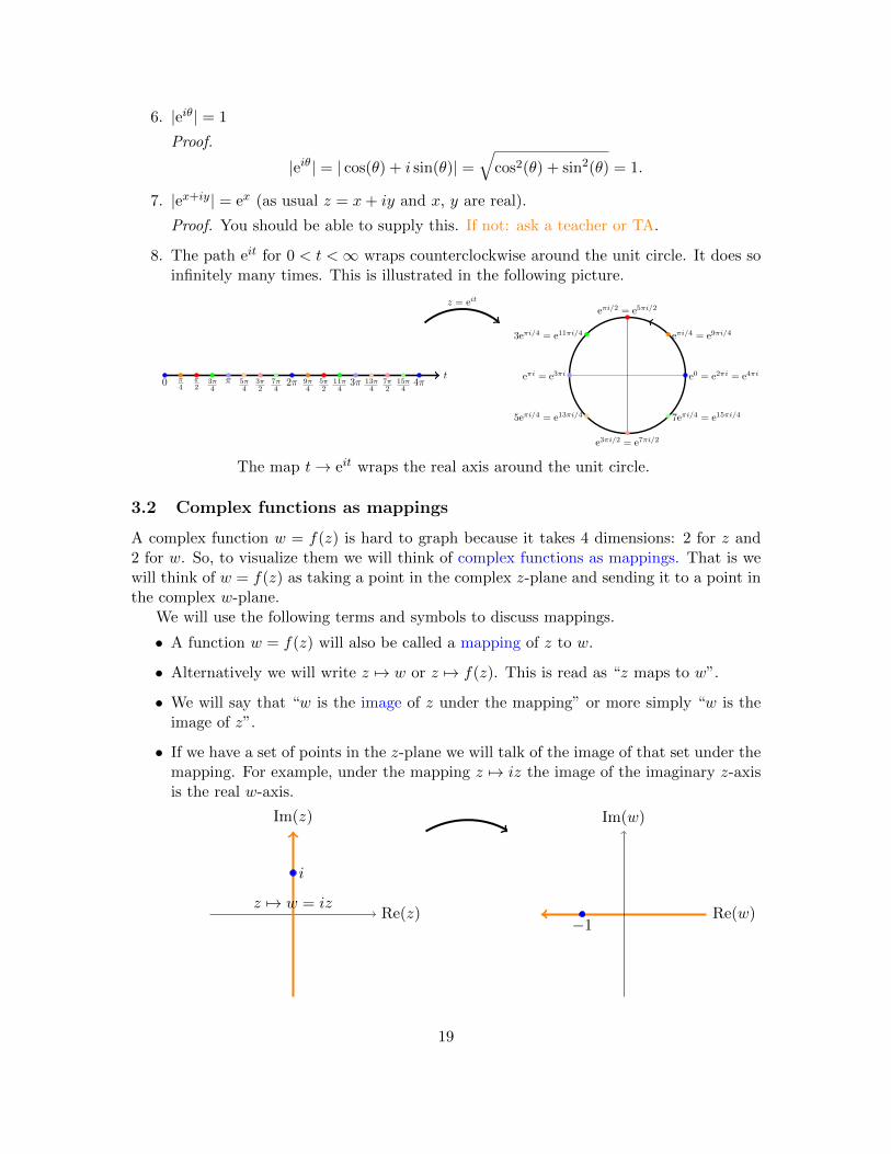
8. The path eit for 0 < t <∞ wraps counterclockwise around the unit circle. It does soinfinitely many times. This is illustrated in the following picture.
t0 π
4π2
3π4
π 5π4
3π2
7π4
2π 9π4
5π2
11π4
3π 13π4
7π2
15π4
4πe0 = e2πi = e4πi
eπi/4 = e9πi/4
eπi/2 = e5πi/2
3eπi/4 = e11πi/4
eπi = e3πi
5eπi/4 = e13πi/4
e3πi/2 = e7πi/2
7eπi/4 = e15πi/4
z = eit
The map t→ eit wraps the real axis around the unit circle.
3.2 Complex functions as mappings
A complex function w = f(z) is hard to graph because it takes 4 dimensions: 2 for z and2 for w. So, to visualize them we will think of complex functions as mappings. That is wewill think of w = f(z) as taking a point in the complex z-plane and sending it to a point inthe complex w-plane.
We will use the following terms and symbols to discuss mappings.
• A function w = f(z) will also be called a mapping of z to w.
• Alternatively we will write z 7→ w or z 7→ f(z). This is read as “z maps to w”.
• We will say that “w is the image of z under the mapping” or more simply “w is theimage of z”.
• If we have a set of points in the z-plane we will talk of the image of that set under themapping. For example, under the mapping z 7→ iz the image of the imaginary z-axisis the real w-axis.
Re(z)
Im(z)
i
Re(w)
Im(w)
−1
z 7→ w = iz
19

The image of the imaginary axis under z 7→ iz.
Next, we’ll illustrate visualizing mappings with some examples:
Example. The mapping w = z2. We visualize this by putting the z-plane on the left andthe w-plane on the right. We then draw various curves and regions in the z-plane and thecorresponding image under z2 in the w-plane.
In the first figure we show that rays from the origin are mapped by z2 to rays from theorigin. We see that
1. The ray L2 at π/4 radians is mapped to the ray f(L2) at π/2 radians.2. The rays L2 and L6 are both mapped to the same ray. This is true for each pair of
diametrically opposed rays.3. A ray at angle θ is mapped to the ray at angle 2θ.
Re(z)
Im(z)
L1
L2
L3L4
L5
L6
L7
L8
f(L1)& f(L5)
f(L2)& f(L6)
f(L3)& f(L7)
f(L4)& f(L8)
z 7→ w = z2
f(z) = z2 maps rays from the origin to rays from the origin.
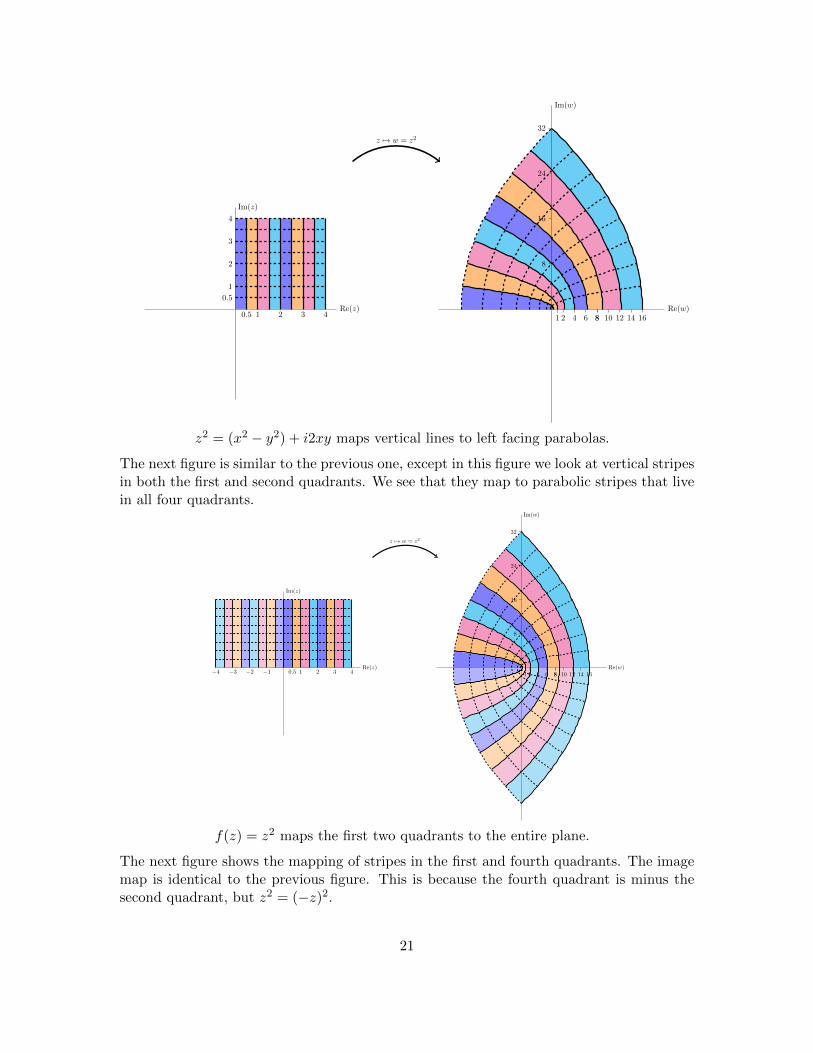
The next figure gives another view of the mapping. Here we see vertical stripes in the firstquadrant are mapped to parabolic stripes that live in the first and second quadrants.
20
Re(z)
Im(z)
0.5 1 2 3 4
0.5
1
2
3
4
Re(w)
Im(w)
1 2 4 6 88 10 12 14 16
8
16
24
32
z 7→ w = z2
z2 = (x2 − y2) + i2xy maps vertical lines to left facing parabolas.
The next figure is similar to the previous one, except in this figure we look at vertical stripesin both the first and second quadrants. We see that they map to parabolic stripes that livein all four quadrants.
Re(z)
Im(z)
0.5 1 2 3 4−1−2−3−4 Re(w)
Im(w)
1 2 4 6 88 10 12 14 16
8
16
24
32
z 7→ w = z2
f(z) = z2 maps the first two quadrants to the entire plane.
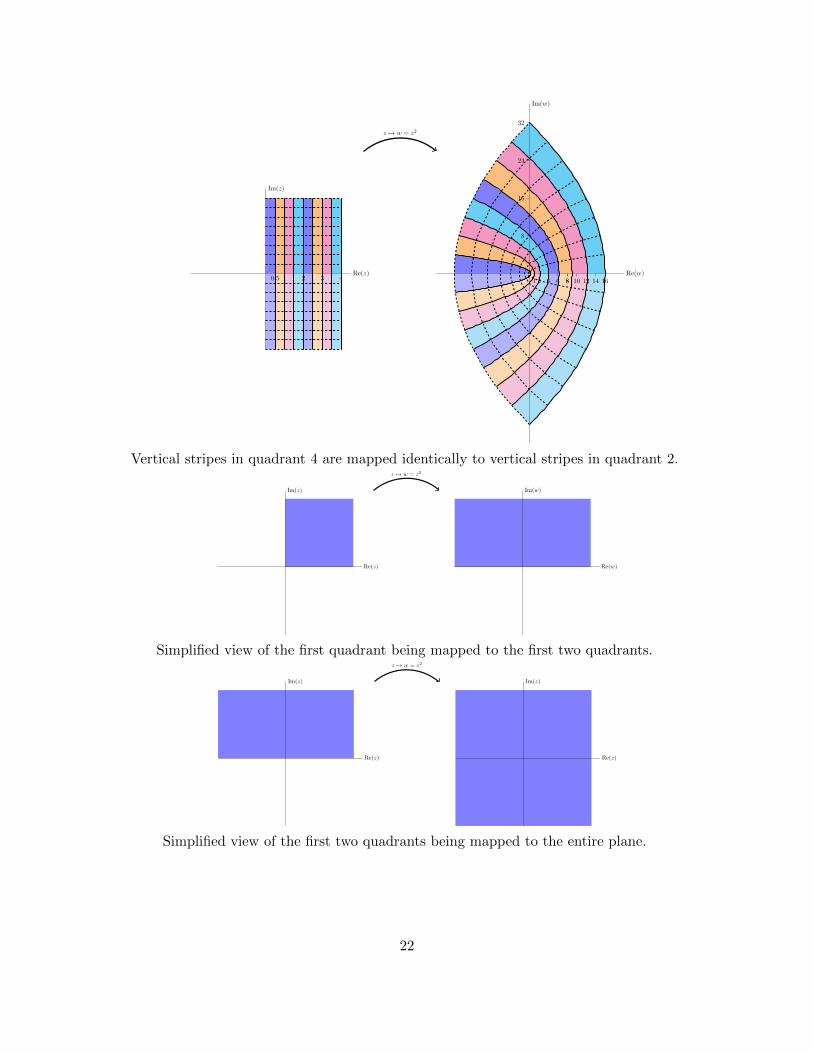
The next figure shows the mapping of stripes in the first and fourth quadrants. The imagemap is identical to the previous figure. This is because the fourth quadrant is minus thesecond quadrant, but z2 = (−z)2.
21
Re(z)
Im(z)
0.5 1 2 3 4Re(w)
Im(w)
1 2 4 6 88 10 12 14 16
8
16
24
32
z 7→ w = z2
Vertical stripes in quadrant 4 are mapped identically to vertical stripes in quadrant 2.
Re(z)
Im(z)
Re(w)
Im(w)
z 7→ w = z2
Simplified view of the first quadrant being mapped to the first two quadrants.
Re(z)
Im(z)
Re(z)
Im(z)
z 7→ w = z2
Simplified view of the first two quadrants being mapped to the entire plane.
22
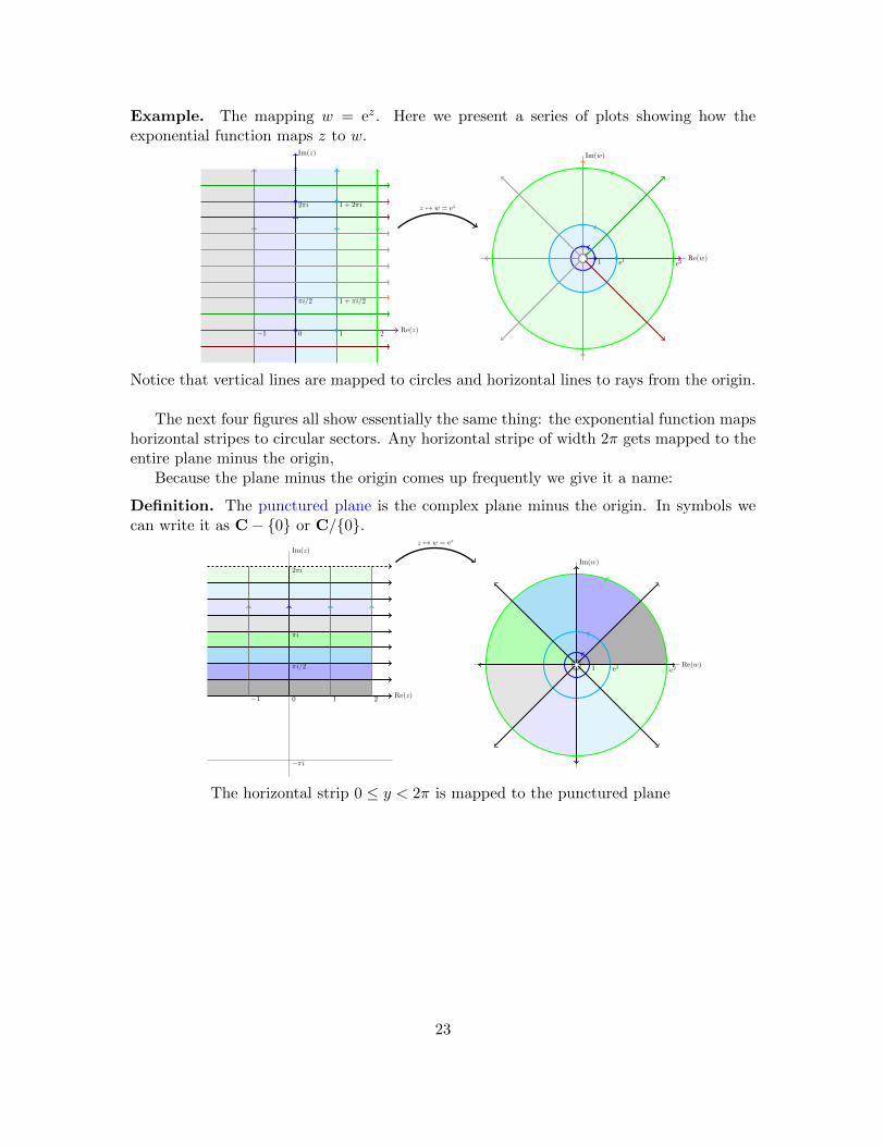
Example. The mapping w = ez. Here we present a series of plots showing how theexponential function maps z to w.
Re(z)
Im(z)
×
×
×
×
0 1 2−1
πi/2
2πi 1 + 2πi
1 + πi/2
Re(w)
Im(w)
1
×
e1 e2
×
z 7→ w = ez
Notice that vertical lines are mapped to circles and horizontal lines to rays from the origin.
The next four figures all show essentially the same thing: the exponential function mapshorizontal stripes to circular sectors. Any horizontal stripe of width 2π gets mapped to theentire plane minus the origin,
Because the plane minus the origin comes up frequently we give it a name:
Definition. The punctured plane is the complex plane minus the origin. In symbols wecan write it as C− {0} or C/{0}.
Re(z)
Im(z)
0 1 2−1
πi/2
2πi
πi
−πi
Re(w)
Im(w)
1 e1 e2
z 7→ w = ez
The horizontal strip 0 ≤ y < 2π is mapped to the punctured plane
23

Re(z)
Im(z)
0 1 2−1
πi/2
2πi
πi
−πi
Re(w)
Im(w)
1 e1 e2
z 7→ w = ez
The horizontal strip −π < y ≤ π is mapped to the punctured plane
Re(z)
Im(z)
0
πi
2πi
Re(w)
Im(w)
z 7→ w = ez
Simplified view showing ez maps the horizontal stripe 0 ≤ y < 2π to the punctured plane.
Re(z)
Im(z)
0
πi
−πi
Re(w)
Im(w)z 7→ w = ez
Simplified view showing ez maps the horizontal stripe −π < y ≤ π to the punctured plane.
3.3 The function arg(z)
3.3.1 Many-to-one functions
The function f(z) = z2 maps ±z to the same value, e.g. f(2) = f(−2) = 4. We say thatf(z) is a 2-to-1 function. That is, it maps 2 different points to each value. (Technically,
24
it only maps one point to 0, but we will gloss over that for now.) Here are some otherexamples of many-to-one functions.Example 1. w = z3 is a 3-to-1 function. For example, 3 different z values get mapped tow = 1:
13 =
(−1 +
√3 i
2
)3
=
(−1−
√3 i
2
)3
= 1
Example 2. The function w = ez maps infinitely many points to each value. For example
e0 = e2πi = e4πi = . . . = en2πi = . . . = 1
eiπ/2 = eiπ/2+2πi = eiπ/2+4πi = . . . = eiπ/2+n2πi = . . . = i
In general, ez+n 2πi has the same value for every integer n.
3.3.2 Branches of arg(z)
Important note. You should master this section. Branches of arg(z) are the key thatreally underlies all our other examples. Fortunately it is reasonably straightforward.
The key point is that the argument is only defined up to multiples of 2πi so every zproduces infinitely many values for arg(z). Because of this we will say that arg(z) is amultiple-valued function.
Note. In general a function should take just one value. What that means in practice isthat whenever we use such a function will have to be careful to specify which of the possiblevalues we mean. This is known as specifying a branch of the function.
Definition. By a branch of the argument function we mean a choice of range so that itbecomes single-valued. By specifying a branch we are saying that we will take the singlevalue of arg(z) that lies in the branch. Let’s look at several different branches to understandhow they work:
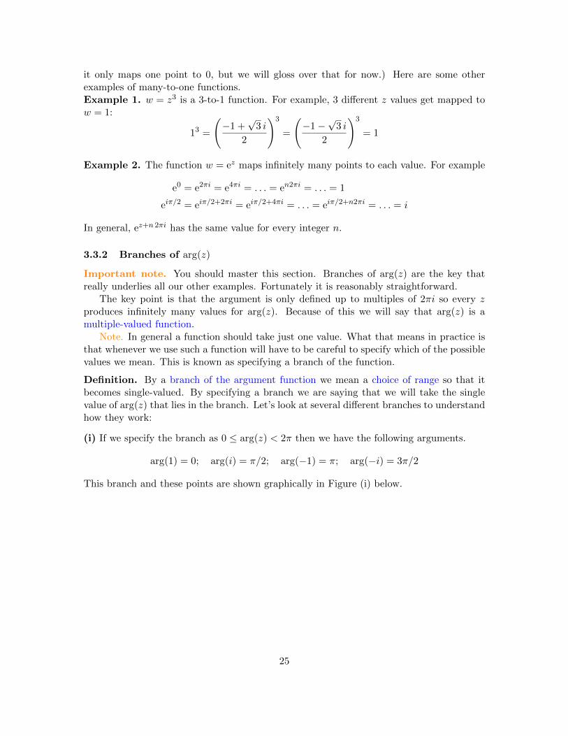
(i) If we specify the branch as 0 ≤ arg(z) < 2π then we have the following arguments.
arg(1) = 0; arg(i) = π/2; arg(−1) = π; arg(−i) = 3π/2
This branch and these points are shown graphically in Figure (i) below.
25

x
y
arg = 0
arg = π/4
arg = π/2
arg = 3π/4
arg = π
arg = 5π/4
arg = 3π/2
arg = 7π/4
arg ≈ 2πarg ≈ π
Figure (i): The branch 0 ≤ arg(z) < 2π of arg(z).
Notice that if we start at z = 1 on the positive real axis we have arg(z) = 0. Then arg(z)increases as we move counterclockwise around the circle. The argument is continuous untilwe get back to the positive real axis. There it jumps from almost 2π back to 0.
There is no getting around (no pun intended) this discontinuity. If we need arg(z) tobe continuous we will need to remove (cut) the points of discontinuity out of the domain.The branch cut for this branch of arg(z) is shown as a thick orange line in the figure. Ifwe make the branch cut then the domain for arg(z) is the plane minus the cut, i.e. we willonly consider arg(z) for z not on the cut.
For future reference you should note that, on this branch, arg(z) is continuous near thenegative real axis, i.e. the arguments of nearby points are close to each other.
(ii) If we specify the branch as −π < arg(z) ≤ π then we have the following arguments:
arg(1) = 0; arg(i) = π/2; arg(−1) = π; arg(−i) = −π/2This branch and these points are shown graphically in Figure (ii) below.
x
y
arg = 0
arg = π/4
arg = π/2
arg = 3π/4
arg = π
arg = −3π/4
arg = −π/2
arg = −π/4
arg ≈ 0arg ≈ −π
Figure (ii): The branch −π < arg(z) ≤ π of arg(z).
26

Compare Figure (ii) with Figure (i). The values of arg(z) are the same in the upper halfplane, but in the lower half plane they differ by 2π.
For this branch the branch cut is along the negative real axis. As we cross the branchcut the value of arg(z) jumps from π to something close to −π.
(iii) Figure (iii) shows the branch of arg(z) with π/4 ≤ arg(z) < 9π/4.
x
y
arg = 2π
arg = π/4
arg = π/2
arg = 3π/4
arg = π
arg = 5π/4
arg = 3π/2
arg = 7π/4
arg ≈ 2πarg ≈ π
arg ≈ 9π/4
Figure (iii): The branch π/4 ≤ arg(z) < 9π/4 of arg(z).
Notice that on this branch arg(z) is continuous at both the positive and negative real axes.The jump of 2π occurs along the ray at angle π/4.
(iv) Obviously, there are many many possible branches. For example,
42 < arg(z) ≤ 42 + 2π.
(v) We won’t make use of this in 18.04, but, in fact, the branch cut doesn’t have to be astraight line. Any curve that goes from the origin to infinity will do. The argument will becontinuous except for a jump by 2π when z crosses the branch cut.
3.3.3 The principal branch of arg(z)
Branch (ii) in the previous section is singled out and given a name:
Definition. The branch −π < arg(z) ≤ π is called the principal branch of arg(z). We willuse the notation Arg(z) (capital A) to indicate that we are using the principal branch. (Ofcourse, in cases where we don’t want there to be any doubt we will say explicitly that weare using the principal branch.)Note. The examples above show that there is no getting around the jump of 2π as wecross the branch cut. This means that when we need arg(z) to be continuous we will haveto restrict its domain to the plane minus a branch cut.
27

3.4 Concise summary of branches and branch cuts
We discussed branches and branch cuts for arg(z). Before talking about log(z) and itsbranches and branch cuts we will give a short review of what these terms mean. You shouldprobably scan this section now and then come back to it after reading about log(z).
Consider the function w = f(z). Suppose that z = x+ iy and w = u+ iv.
Domain. The domain of f is the set of z where we are allowed to compute f(z).
Range. The range (image) of f is the set of all f(z) for z in the domain, i.e. the set of allw reached by f .
Branch. For a multiple-valued function, a branch is a choice of range for the function. Wechoose the range to exclude all but one possible value for each element of the domain.
Branch cut. A branch cut removes (cuts) points out of the domain. This is done to removepoints where the function is discontinuous.
3.5 The function log(z)
Our goal in this section is to define the log function. We want log(z) to be the inverse ofez. That is, we want elog(z) = z. We will see that log(z) is multiple-valued, so when we useit we will have to specify a branch.
We start by looking at the simplest example which illustrates that log(z) is multiple-valued.
Example. Find log(1).
Solution: We know that e0 = 1, so log(1) = 0 is one answer. We also know that e2πi = 1,so log(1) = 2πi is another possible answer. In fact, we can choose any multiple of 2πi:
log(1) = n 2πi, where n is any integer
This example leads us to consider the polar form for z as we try to define log(z). If z = reiθ
then one possible value for log(z) is
log(z) = log(reiθ) = log(r) + iθ,
here log(r) is the usual logarithm of a real positive number. For completeness we showexplicitly that with this definition elog(z) = z:
elog(z) = elog(r)+iθ = elog(r)eiθ = reiθ = z.
Since r = |z| and θ = arg(z) we have arrived at our definition.
Definition. The function log(z) is defined as
log(z) = log(|z|) + i arg(z),
where log(|z|) is the usual natural logarithm of a positive real number.
28

Remarks.
1. Since arg(z) has infinitely many possible values, so does log(z).
2. log(0) is not defined. (Both because arg(0) is not defined and log(|0|) is not defined.)
3. Choosing a branch for arg(z) makes log(z) single valued. The usual terminology is tosay we have chosen a branch of the log function.
4. The principal branch of log comes from the principal branch of arg. That is,
log(z) = log(|z|) + i arg(z), where − π < arg(z) ≤ π (principal branch).
Example. Compute all the values of log(i). Specify which one comes from the principalbranch.
Solution: We have that |i| = 1 and arg(i) =π
2+ 2πn, so
log(i) = log(1) + iπ
2+ i2πn = i
π
2+ i2πn, where n is any integer.
The principal branch of arg(z) is between −π and π, so Arg(i) = π/2. The value of log(i)from the principal branch is therefore iπ/2.
Example. Compute all the values of log(−1 −√
3 i). Specify which one comes from theprincipal branch.
Solution: Let z = −1 −√
3 i. Then |z| = 2 and in the principal branch Arg(z) = −2π/3.So all the values of log(z) are
log(z) = log(2)− i2π3
+ i2πn.
The value from the principal branch is log(z) = log(2)− i2π/3.
3.5.1 Figures showing w = log(z) as a mapping
The figures below show different aspects of the mapping given by log(z).In the first figure we see that a point z is mapped to (infinitely) many values of w. In
this case we show log(1) (blue dots), log(4) (red dots), log(i) (blue cross), and log(4i) (redcross). The values in the principal branch are inside the shaded region in the w-plane. Notethat the values of log(z) for a given z are placed at intervals of 2πi in the w-plane.
29

Re(z)
Im(z)
×
×
1 2 4
2
4
Re(w)
Im(w)
× ×
× ×
× ×
× ×
−4π
−4
−2π
−2
2π
2
4π
4
π
−π
z 7→ w = log(z)
z = ew ←w
Mapping log(z): log(1), log(4), log(i), log(4i)
The next figure illustrates that the principal branch of log maps the punctured plane to thehorizontal strip −π < Im(w) ≤ π. We again show the values of log(1), log(4), log(i) andlog(4i). Since we’ve chosen a branch, there is only one value shown for each log.
Re(z)
Im(z)
×
×
1 2 4
2
4
Re(w)
Im(w)
× ×
−4π
−4
−2π
−2
2π
2
4π
4
π
−π
z 7→ w = log(z)
z = ew ←w
Mapping log(z): the principal branch and the punctured plane
30

The third figure shows how circles centered on 0 are mapped to vertical lines, and raysfrom the origin are mapped to horizontal lines. If we restrict ourselves to the principalbranch the circles are mapped to vertical line segments and rays to a single horizontal linein the principal (shaded) region of the w-plane.
Re(z)
Im(z)
2 4
2
4
Re(w)
Im(w)
−4π
−4
−2π
−2
2π
2
4π
4
π
−π
z 7→ w = log(z)
z = ew ←w
Mapping log(z): mapping circles and rays
3.5.2 Complex powers
We can use the log function to define complex powers.
Definition. Let z and a be complex numbers then the power za is defined as
za = ea log(z).
This is generally multiple-valued, so to specify a single value requires choosing a branch oflog(z).
Example. Compute all the values of√
2i. Give the value associated to the principal branchof log(z).
Solution: We havelog(2i) = log(2e
iπ2 ) = log(2) + i
π
2+ i2nπ
So, √2i = (2i)1/2 = e
log(2i)2 = e
log(2)2
+ iπ4
+inπ =√
2eiπ4
+inπ.
(As usual n is an integer.) As we saw earlier, this only gives two distinct values. Theprincipal branch has Arg(2i) = π/2, so
√2i =
√2e( iπ4 ) =
√2
(1 + i)√2
= 1 + i.
The other distinct value is when n = 1 and gives minus the value just above.
31

Example. Cube roots: Compute all the cube roots of i. Give the value which comes fromthe principal branch of log(z).
Solution: We have log(i) = iπ
2+ i2πn, where n is any integer. So,
i1/3 = elog(i)
3 = eiπ6
+i 2nπ3
This gives only three distinct values
eiπ/6, ei5π/6, ei9π/6
On the principal branch log(i) = iπ
2, so the value of i1/3 which comes from this is
eiπ/6 =
√3
2+i
2.
Example. Compute all the values of 1i. What is the value from the principal branch?
Solution: This is similar to the problems above. log(1) = 2nπi, so
1i = ei log(1) = ei2nπi = e−2nπ, where n is an integer.
The principal branch has log(1) = 0 so 1i = 1.
4 Analytic functions
The main goal of this section is to define and give some of the important properties ofcomplex analytic functions. A function f(z) is analytic if it has a complex derivative f ′(z).In general, the rules for computing derivatives will be familiar to you from single variablecalculus. However, a much richer set of conclusions can be drawn about a complex analyticfunction than is generally true about real differentiable functions.
4.1 The derivative: preliminaries
In calculus we defined the derivative as a limit. In complex analysis we will do the same.
f ′(z) = lim∆z→0
∆f
∆z= lim
∆z→0
f(z + ∆z)− f(z)
∆z.
Before giving the derivative our full attention we are going to have to spend some timeexploring and understanding limits. To motivate this we’ll first look at two simple examples– one positive and one negative.
Example 4.1. Find the derivative of f(z) = z2.
Solution: We compute using the definition of the derivative as a limit.
lim∆z→0
(z + ∆z)2 − z2
∆z= lim
∆z→0
z2 + 2z∆z + (∆z)2 − z2
∆z= lim
∆z→02z + ∆z = 2z.
32

That was a positive example. Here’s a negative one which shows that we need a carefulunderstanding of limits.
Example 4.2. Let f(z) = z. Show that the limit for f ′(0) does not converge.
Solution: Let’s try to compute f ′(0) using a limit:
f ′(0) = lim∆z→0
f(∆z)− f(0)
∆z= lim
∆z→0
∆z
∆z=
∆x− i∆y∆x+ i∆y
.
Here we used ∆z = ∆x+ i∆y.Now, ∆z → 0 means both ∆x and ∆y have to go to 0. There are lots of ways to do
this. For example, if we let ∆z go to 0 along the x-axis then, ∆y = 0 while ∆x goes to 0.In this case, we would have
f ′(0) = lim∆x→0
∆x
∆x= 1.
On the other hand, if we let ∆z go to 0 along the positive y-axis then
f ′(0) = lim∆y→0
−i∆yi∆y
= −1.
The limits don’t agree! The problem is that the limit depends on how ∆z approaches 0.If we came from other directions we’d get other values. This means that the limit does notexist.
We next explore limits in more detail.
4.2 Open disks, open deleted disks, open regions
Definition. The open disk of radius r around z0 is the set of points z with |z − z0| < r,i.e. all points within distance r of z0.
The open deleted disk of radius r around z0 is the set of points z with 0 < |z − z0| < r.That is, we remove the center z0 from the open disk. A deleted disk is also called a punctureddisk.
z0
r
z0
r
Left: an open disk around z0; right: a deleted open disk around z0
Definition. An open region in the complex plane is a set A with the property that everypoint in A can be be surrounded by an open disk that lies entirely in A. We will often dropthe word open and simply call A a region.
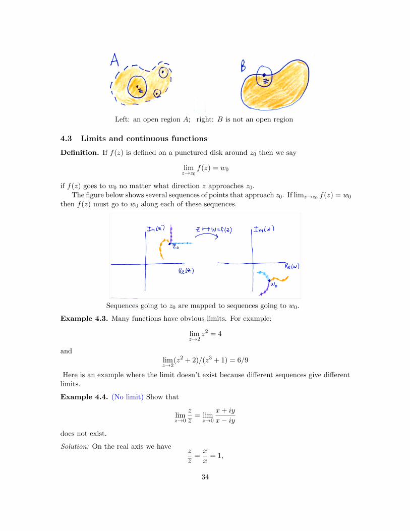
In the figure below, the set A on the left is an open region because for every point in Awe can draw a little circle around the point that is completely in A. (The dashed boundaryline indicates that the boundary of A is not part of A.) In contrast, the set B is not anopen region. Notice the point z shown is on the boundary, so every disk around z containspoints outside B.
33
Left: an open region A; right: B is not an open region
4.3 Limits and continuous functions
Definition. If f(z) is defined on a punctured disk around z0 then we say
limz→z0
f(z) = w0
if f(z) goes to w0 no matter what direction z approaches z0.The figure below shows several sequences of points that approach z0. If limz→z0 f(z) = w0
then f(z) must go to w0 along each of these sequences.
Sequences going to z0 are mapped to sequences going to w0.
Example 4.3. Many functions have obvious limits. For example:
limz→2
z2 = 4
andlimz→2
(z2 + 2)/(z3 + 1) = 6/9
Here is an example where the limit doesn’t exist because different sequences give differentlimits.
Example 4.4. (No limit) Show that
limz→0
z
z= lim
z→0
x+ iy
x− iydoes not exist.
Solution: On the real axis we havez
z=x
x= 1,
34

so the limit as z → 0 along the real axis is 1. By contrast, on the imaginary axis we have
z
z=
iy
−iy = −1,
so the limit as z → 0 along the imaginary axis is -1. Since the two limits do not agree thelimit as z → 0 does not exist!
4.3.1 Properties of limits
We have the usual properties of limits. Suppose
limz→z0
f(z) = w1 and limz→z0
g(z) = w2
then
• limz→z0
f(z) + g(z) = w1 + w2.
• limz→z0
f(z)g(z) = w1 · w2.
• If w2 6= 0 then limz→z0
f(z)/g(z) = w1/w2
• If h(z) is continuous and defined on a neighborhood of w1 then limz→z0
h(f(z)) = h(w1)
(Note: we will give the official definition of continuity in the next section.)
We won’t give a proof of these properties. As a challenge, you can try to supply it usingthe formal definition of limits given in the appendix.
We can restate the definition of limit in terms of functions of (x, y). To this end, let’s write
f(z) = f(x+ iy) = u(x, y) + iv(x, y)
and abbreviateP = (x, y) , P0 = (x0, y0) , w0 = u0 + iv0
Then
limz→z0
f(z) = w0 iff
{limP→P0 u(x, y) = u0
limP→P0 v(x, y) = v0.
Note. The term ‘iff’ stands for ‘if and only if’ which is another way of saying ‘is equivalentto’.
4.3.2 Continuous functions
A function is continuous if it doesn’t have any sudden jumps. This is the gist of the followingdefinition.
Definition. If the function f(z) is defined on an open disk around z0 and limz→z0
f(z) = f(z0)
then we say f is continuous at z0. If f is defined on an open region A then the phrase ‘f iscontinuous on A’ means that f is continuous at every point in A.
35

As usual, we can rephrase this in terms of functions of (x, y):
Fact. f(z) = u(x, y) + iv(x, y) is continuous iff u(x, y) and v(x, y) are continuous asfunctions of two variables.
Example 4.5. (Some continuous functions)(i) A polynomial
P (z) = a0 + a1z + a2z2 + . . .+ anz
n
is continuous on the entire plane. Reason: it is clear that each power (x+ iy)k is continuousas a function of (x, y).(ii) The exponential function is continuous on the entire plane. Reason:
ez = ex+iy = ex cos(y) + iex sin(y),
so the both the real and imaginary parts are clearly continuous as a function of (x, y).(iii) The principal branch Arg(z) is continuous on the plane minus the non-positive realaxis. Reason: this is clear and is the reason we defined branch cuts for arg. We have toremove the negative real axis because Arg(z) jumps by 2π when you cross it. We also haveto remove z = 0 because Arg(z) is not even defined at 0.(iv) The principal branch of the function log(z) is continuous on the plane minus the non-positive real axis. Reason: the principal branch of log has
log(z) = log(r) + iArg(z),
so the continuity of log(z) follows from the continuity of Arg(z).
4.3.3 Properties of continuous functions
Since continuity is defined in terms of limits, we have the following properties of continuousfunctions.
Suppose f(z) and g(z) are continuous on a region A. Then
• f(z) + g(z) is continuous on A.
• f(z)g(z) is continuous on A.
• f(z)/g(z) is continuous on A except (possibly) at points where g(z) = 0.
• If h is continuous on f(A) then h(f(z)) is continuous on A.
Using these properties we can claim continuity for each of the following functions:
• ez2
• cos(z) = (eiz + e−iz)/2
• If P (z) and Q(z) are polynomials then P (z)/Q(z) is continuous except at roots ofQ(z).
36

4.4 The point at infinity
By definition the extended complex plane = C∪{∞}. That is, we have one point at infinityto be thought of in a limiting sense described as follows.
A sequence of points {zn} goes to infinity if |zn| goes to infinity. This “point at infinity”is approached in any direction we go. All of the sequences shown in the figure below aregrowing, so they all go to the (same) “point at infinity”.
Various sequences all going to infinity.
If we draw a large circle around 0 in the plane, then we call the region outside this circlea neighborhood of infinity.
R
Re(z)
Im(z)
The shaded region outside the circle of radius R is a neighborhood of infinity.
4.4.1 Limits involving infinity
The key idea is 1/∞ = 0. By this we mean
limz→∞
1
z= 0
We then have the following facts:
• limz→z0
f(z) =∞ ⇔ limz→z0
1/f(z) = 0
• limz→∞
f(z) = w0 ⇔ limz→0
f(1/z) = w0
• limz→∞
f(z) =∞ ⇔ limz→0
1
f(1/z)= 0
37
Example 4.6. limz→∞
ez is not defined because it has different values if we go to infinity in
different directions, e.g. we have ez = exeiy and
limx→−∞
exeiy = 0
limx→+∞
exeiy =∞
limy→+∞
exeiy is not defined, since x is constant, so exeiy loops in a circle indefinitely.
Example 4.7. Show limz→∞
zn =∞ (for n a positive integer).
Solution: We need to show that |zn| gets large as |z| gets large. Write z = Reiθ, then
|zn| = |Rneinθ| = Rn = |z|n
Clearly, as |z| = R→∞ also |z|n = Rn →∞.
4.4.2 Stereographic projection from the Riemann sphere
This is a lovely section and we suggest you read it. However it will be a while before weuse it in 18.04.
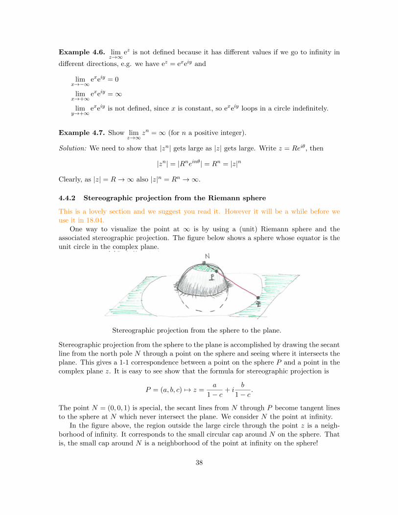
One way to visualize the point at ∞ is by using a (unit) Riemann sphere and theassociated stereographic projection. The figure below shows a sphere whose equator is theunit circle in the complex plane.
Stereographic projection from the sphere to the plane.
Stereographic projection from the sphere to the plane is accomplished by drawing the secantline from the north pole N through a point on the sphere and seeing where it intersects theplane. This gives a 1-1 correspondence between a point on the sphere P and a point in thecomplex plane z. It is easy to see show that the formula for stereographic projection is
P = (a, b, c) 7→ z =a
1− c + ib
1− c .
The point N = (0, 0, 1) is special, the secant lines from N through P become tangent linesto the sphere at N which never intersect the plane. We consider N the point at infinity.
In the figure above, the region outside the large circle through the point z is a neigh-borhood of infinity. It corresponds to the small circular cap around N on the sphere. Thatis, the small cap around N is a neighborhood of the point at infinity on the sphere!
38

The figure below shows another common version of stereographic projection. In thisfigure the sphere sits with its south pole at the origin. We still project using secant linesfrom the north pole.
4.5 Derivatives
The definition of the complex derivative of a complex function is similar to that of a realderivative of a real function: For a function f(z) the derivative f at z0 is defined as
f ′(z0) = limz→z0
f(z)− f(z0)
z − z0
Provided, of course, that the limit exists. If the limit exists we say f is analytic at z0 or fis differentiable at z0.
Remember: The limit has to exist and be the same no matter how you approach z0!
If f is analytic at all the points in an open region A then we say f is analytic on A. Asusual with derivatives there are several alternative notations. For example, if w = f(z) wecan write
f ′(z0) =dw
dz
∣∣∣∣z0
= limz→z0
f(z)− f(z0)
z − z0= lim
∆z→0
∆w
∆z
Example 4.8. Find the derivative of f(z) = z2.
Solution: We did this above in Example 4.1. Take a look at that now. Of course, f ′(z) = 2z.
Example 4.9. Show f(z) = z is not differentiable at any point z.
Solution: We did this above in Example 4.2. Take a look at that now.
Challenge. Use polar coordinates to show the limit in the previous example can be anyvalue with modulus 1 depending on the angle at which z approaches z0.
4.5.1 Derivative rules
It wouldn’t be much fun to compute every derivative using limits. Fortunately, we have thesame differentiation formulas as for real-valued functions. That is, assuming f and g aredifferentiable we have:
• Sum rule:d
dz(f(z) + g(z)) = f ′ + g′
39

• Product rule:d
dz(f(z)g(z)) = f ′g + fg′
• Quotient rule:d
dz(f(z)/g(z)) =
f ′g − fg′g2
• Chain rule:d
dzg(f(z)) = g′(f(z))f ′(z)
• Inverse rule:df−1(z)
dz=
1
f ′(f−1(z))
To give you the flavor of these arguments we’ll prove the product rule.
d
dz(f(z)g(z)) = lim
z→z0
f(z)g(z)− f(z0)g(z0)
z − z0
= limz→z0
(f(z)− f(z0))g(z) + f(z0)(g(z)− g(z0))
z − z0
= limz→z0
f(z)− f(z0)
z − z0g(z) + f(z0)
(g(z)− g(z0))
z − z0
= f ′(z0)g(z0) + f(z0)g′(z0)
Here is an important fact that you would have guessed. We will prove it in the next section.
Theorem. If f(z) is defined and differentiable on an open disk and f ′(z) = 0 on the diskthen f(z) is constant.
4.6 Cauchy-Riemann equations
The Cauchy-Riemann equations are our first consequence of the fact that the limit definingf(z) must be the same no matter which direction you approach z from. The Cauchy-Riemann equations will be one of the most important tools in our toolbox.
4.6.1 Partial derivatives as limits
Before getting to the Cauchy-Riemann equations we remind you about partial derivatives.If u(x, y) is a function of two variables then the partial derivatives of u are defined as
∂u
∂x(x, y) = lim
∆x→0
u(x+ ∆x, y)− u(x, y)
∆x
i.e. the derivative of u holding y constant.
∂u
∂y(x, y) = lim
∆y→0
u(x, y + ∆y)− u(x, y)
∆y
i.e. the derivative of u holding x constant.
40
4.6.2 The Cauchy-Riemann equations
The Cauchy-Riemann equations use the partial derivatives of u and v to do two things:first, to check if f has a complex derivative and second, how to compute that derivative.We start by stating the equations as a theorem.
Theorem. (Cauchy-Riemann equations) If f(z) = u(x, y) + iv(x, y) is analytic (complexdifferentiable) then
f ′(z) =∂u
∂x+ i
∂v
∂x=∂v
∂y− i∂u
∂y
In particular,∂u
∂x=∂v
∂yand
∂u
∂y= −∂v
∂x.
This last set of partial differential equations is what is usually meant by the Cauchy-Riemannequations. Here is the short form of the Cauchy-Riemann equations:
ux = vy
uy = −vx
Proof. Let’s suppose that f(z) is differentiable in some region A and
f(z) = f(x+ iy) = u(x, y) + iv(x, y).
We’ll compute f ′(z) by approaching z first from the horizontal direction and then from thevertical direction. We’ll use the formula
f ′(z) = lim∆z→0
f(z + ∆z)− f(z)
∆z,
where ∆z = ∆x+ i∆y.Horizontal direction: ∆y = 0, ∆z = ∆x
f ′(z) = lim∆z→0
f(z + ∆z)− f(z)
∆z
= lim∆x→0
f(x+ ∆x+ iy)− f(x+ iy)
∆x
= lim∆x→0
(u(x+ ∆x, y) + iv(x+ ∆x, y))− (u(x, y) + iv(x, y))
∆x
= lim∆x→0
u(x+ ∆x, y)− u(x, y)
∆x+ i
v(x+ ∆x, y)− v(x, y)
∆x
=∂u
∂x(x, y) + i
∂v
∂x(x, y)
41

Vertical direction: ∆x = 0, ∆z = i∆y (We’ll do this one a little faster.)
f ′(z) = lim∆z→0
f(z + ∆z)− f(z)
∆z
= lim∆y→0
(u(x, y + ∆y) + iv(x, y + ∆y))− (u(x, y) + iv(x, y))
i∆y
= lim∆y→0
u(x, y + ∆y)− u(x, y)
i∆y+ i
v(x, y + ∆y)− v(x, y)
i∆y
=1
i
∂u
∂y(x, y) +
∂v
∂y(x, y)
=∂v
∂y(x, y)− i∂u
∂y(x, y)
We have found two different representations of f ′(z) in terms of the partials of u and v. Ifput them together we have the Cauchy-Riemann equations:
f ′(z) =∂u
∂x+ i
∂v
∂x=∂v
∂y− i∂u
∂y⇒ ∂u
∂x=∂v
∂y, and − ∂u
∂y=∂v
∂x.
It turns out that the converse is true and will be very useful to us.
Theorem. Consider the function f(z) = u(x, y) + iv(x, y) defined on a region A. If uand v satisfy the Cauchy-Riemann equations and have continuous partials then f(z) isdifferentiable on A.
The proof of this is a tricky exercise in analysis. It is somewhat beyond the scope of thisclass, so we will skip it.
4.6.3 Using the Cauchy-Riemann equations
The Cauchy-Riemann equations provide us with a direct way of checking that a function isdifferentiable and computing its derivative.
Example 4.10. Use the Cauchy-Riemann equations to show that ez is differentiable andits derivative is ez.
Solution: We write ez = ex+iy = ex cos(y) + iex sin(y). So
u(x, y) = ex cos(y) and v(x, y) = ex sin(y).
Computing partial derivatives we have
ux = ex cos(y) , uy = −ex sin(y)
vx = ex sin(y) , vy = ex cos(y)
We see that ux = vy and uy = −vx, so the Cauchy-Riemann equations are satisfied. Thus,ez is differentiable and
d
dzez = ux + ivx = ex cos(y) + iex sin(y) = ez.
42
Example 4.11. Use the Cauchy-Riemann equations to show that f(z) = z is not differen-tiable.
Solution: f(x+ iy) = x− iy, so u(x, y) = x, v(x, y) = −y. Taking partial derivatives
ux = 1, uy = 0, vx = 0, vy = −1
Since ux 6= vy the Cauchy-Riemann equations are not satisfied and therefore f is notdifferentiable.
Theorem. If f(z) is differentiable on a disk and f ′(z) = 0 on the disk then f(z) is constant.Proof. Since f is differentiable and f ′(z) ≡ 0, the Cauchy-Riemann equations show that
ux(x, y) = uy(x, y) = vx(x, y) = vy(x, y) = 0
We know from multivariable calculus that a function of (x, y) with both partials identicallyzero is constant. Thus u and v are constant, and therefore so is f .
4.6.4 f ′(z) as a 2× 2 matrix
Recall that we could represent a complex number a+ ib as a 2× 2 matrix
a+ ib ↔[a −bb a
]. (13)
Now if we write f(z) in terms of (x, y) we have
f(z) = f(x+ iy) = u(x, y) + iv(x, y) ↔ f(x, y) = (u(x, y), v(x, y))
We havef ′(z) = ux + ivx
so we can represent f ′(z) as [ux −vxvx ux
]Using the Cauchy-Riemann equations we can replace −vx by uy and ux by vy which givesus the representation
f ′(z) ↔[ux uyvx vy
]i.e. f ′(z) is just the Jacobian of f(x, y).
For me, it is easier to remember the Jacobian than the Cauchy-Riemann equations.Since f ′(z) is a complex number I can use the matrix representation in Equation (13) toremember the Cauchy-Riemann equations!
43
4.7 Geometric interpretation & linear elasticity theory
Consider a mapping R2 → R2
z = (x, y) → w = f(z) = (u(x, y), v(x, y)) (14)
We can interpret w = f(z) as the (in general nonlinear) deformation map of a two-dimensional planar continuum body – that is, an infinite flat elastic sheet. Let’s considersmall deformations, corresponding to the assumption that the displacement field
d(z) := f(z)− z (15)
is small,
|d(z)| = |f(z)− z| � 1 (16)
In terms of the components d1 and d2 of d, this means that
d1(x, y) = u(x, y)− x and d2(x, y) = v(x, y)− y (17)
are small everywhere. Picking some point z, we can Taylor-expand d(z) at z + ε, where
ε = (δx, δy)
is a small shift vector. Defining
x1 = x , x2 = y , di,j =∂
∂xjdi(x1, x2)
and adopting Einstein’s summation convention, aibi =∑2
i=1 aibi, the Taylor expansionreads
di(z + ε) = di(z) + di,j(z)εj + O(ε2). (18)
The coefficients di,j(z) of the linear term are the elements of the Jacobian matrix of thedisplacement map d(z),
(di,j) =
(ux − 1 uyvx vy − 1
)=
(ux uyvx vy
)− I (19)
where the first matrix on the right-hand side is the Jacobian of the deformation f(z) andI = (δij) the 2 × 2 identity matrix. By splitting into symmetric and antisymmetric parts,we can decompose this matrix into the form
di,j =1
2(di,j + dj,i) +
1
2(di,j − dj,i)− δij
=1
2di,iδij +
1
2[(di,j + dj,i)− di,iδij ] +
1
2(di,j − dj,i)− δij (20)
In the second line, we have still split off the trace from the symmetric part. Substitutingback u(x, y) and v(x, y), we have
(di,j) =1
2(ux + vy)I +
1
2
(ux − vy uy + vxvx + uy vy − ux
)−{I +
1
2(uy − vx)
(0 −11 0
)}(21)
44

Now recall that an infinitesimal rotation is represented by the matrix
R(φ) =
(cosφ − sinφsinφ cosφ
)≈ I + φ
(0 −11 0
)(22)
we can interpret the contributions in terms of intuitive fundamental deformations:
• The first term
1
2(ux + vy)I =
1
2(∇ · d)I (23a)
represents stretching or compression.
• The last term term {I +
1
2(uy − vx)
(0 −11 0
)}(23b)
represents an infinitesimal rotation by an angle φ = 12(uy − vx) = 1
2∇∧ d.
• The middle term
1
2
(ux − vy vx + uyvx + uy −(ux − vy)
)=
1
2(ux − vy)
(1 00 −1
)+
1
2(vx + uy)
(0 11 0
)(23c)
is the sum of a scaled reflection (via the diagonal components) and shear strain (viathe off-diagonal components).
Thus, deformations that preserve orientation and angles locally must satisfy
ux = vy , uy = −vx (24)
But these are just the Cauchy-Riemann conditions !
4.8 Cauchy-Riemann all the way down
We’ve defined an analytic function as one having a complex derivative. The following theo-rem shows that if f is analytic then so is f ′. Thus, there are derivatives all the way down!
Theorem 4.12.Assume the second order partials of u and v exist. If f(z) = u + iv isanalytic, then so is f ′(z).
Proof. To show this we have to prove that f ′(z) satisfies the Cauchy-Riemann equations.If f = u+ iv we know
ux = vy , uy = −vx , f ′ = ux + ivx
Let’s writef ′ = U + iV
45
soU = ux = vy , V = vx = −uy
We want to show that Ux = Vy and Uy = −Vx. We do them one at a time.To prove Ux = Vy, we note that
Ux = vyx , Vy = vxy
Since vxy = vyx, we have Ux = Vy.Similarly, to show Uy = −Vx, we compute
Uy = uxy , Vx = −uyx.
Thus, Uy = −Vx.
Technical point. We’ve assumed as many partials as we need. So far we can’t guaranteethat all the partials exist. Soon we will have a theorem which says that an analytic functionhas derivatives of all order. We’ll just assume that for now. In any case, in most examplesthis will be obvious.
4.9 Gallery of functions
In this section we’ll look at many of the functions you know and love as functions of z. Foreach one we’ll have to do three things.
1. Define how to compute it.
2. Specify a branch (if necessary) giving its range.
3. Specify a domain (with branch cut if necessary) where it is analytic.
4. Compute its derivative.
Most often, we can compute the derivatives of a function using the algebraic rules like thequotient rule. If necessary we can use the Cauchy-Riemann equations or, as a last resort,even the definition of the derivative as a limit.
Before we start on the gallery we define the term “entire function”.Definition. A function that is analytic at every point in the complex plane is called anentire function. We will see that ez, zn, sin(z) are all entire functions.
4.9.1 Gallery of functions, derivatives and properties
The following is a concise list of a number of functions and their complex derivatives. Noneof the derivatives will surprise you. We also give important properties for some of thefunctions. The proofs for each follow below.
1. f(z) = ez = ex cos(y) + iex sin(y).
Domain = all of C (f is entire).
f ′(z) = ez.
46

2. f(z) ≡ c (constant)
Domain = all of C (f is entire).
f ′(z) = 0.
3. f(z) = zn (n an integer ≥ 0)
Domain = all of C (f is entire).
f ′(z) = nzn−1.
4. P (z) (polynomial)
A polynomial has the form P (z) = anzn + an−1z
n−1 + . . .+ a0.
Domain = all of C (P (z) is entire).
P ′(z) = nanzn−1 + (n− 1)an−1z
n−1 + . . .+ 2a2z + a1.
5. f(z) = 1/z
Domain = C− {0} (the punctured plane).
f ′(z) = −1/z2.
6. f(z) = P (z)/Q(z) (rational function).
When P and Q are polynomials P (z)/Q(z) is called a rational function.
If we assume that P and Q have no common roots, then:
Domain = C− {roots of Q}
f ′(z) =P ′Q− PQ′
Q2.
7. sin(z), cos(z)
Definition. cos(z) =eiz + e−iz
2, sin(z) =
eiz − e−iz
2i
(By Euler’s formula we know this is consistent with cos(x) and sin(x) when z = x isreal.)
Domain: these functions are entire.
d cos(z)
dz= − sin(z),
d sin(z)
dz= cos(z).
Other key properties of sin and cos:
- cos2(z) + sin2(z) = 1
- ez = cos(z) + i sin(z)
- Periodic in x with period 2π, e.g. sin(x+ 2π + iy) = sin(x+ iy).
- They are not bounded!
47

- In the form f(z) = u(x, y) + iv(x, y) we have
cos(z) = cos(x) cosh(y)− i sin(x) sinh(y)
sin(z) = sin(x) cosh(y) + i cos(x) sinh(y)
(cosh and sinh are defined below.)
- The zeros of sin(z) are z = nπ for n any integer.The zeros of cos(z) are z = π/2 + nπ for n any integer.(That is, they have only real zeros that you learned about in your trig. class.)
8. Other trig functions cot(z), s(z) etc.
Definition. The same as for the real versions of these function, e.g. cot(z) =cos(z)/ sin(z), s(z) = 1/ cos(z).
Domain: The entire plane minus the zeros of the denominator.
Derivative: Compute using the quotient rule, e.g.
d tan(z)
dz=
d
dz
(sin(z)
cos(z)
)=
cos(z) cos(z)− sin(z)(− sin(z))
cos2(z)=
1
cos2(z)= s2z
(No surprises there!)
9. sinh(z), cosh(z) (hyperbolic sine and cosine)
Definition.
cosh(z) =ez + e−z
2, sinh(z) =
ez − e−z
2
Domain: these functions are entire.
d cosh(z)
dz= sinh(z),
d sinh(z)
dz= cosh(z)
Other key properties of cosh and sinh:
- cosh2(z)− sinh2(z) = 1
- For real x, cosh(x) is real and positive, sinh(x) is real.
- cosh(iz) = cos(z), sinh(z) = −i sin(iz).
10. log(z) (See Topic 1.)
Definition. log(z) = log(|z|) + i arg(z).
Branch: Any branch of arg(z).
Domain: C minus a branch cut where the chosen branch of arg(z) is discontinuous.
d
dzlog(z) =
1
z
48

11. za (any complex a) (See Topic 1.)
Definition. za = ea log(z).
Branch: Any branch of log(z).
Domain: Generally the domain is C minus a branch cut of log. If a is an integer ≥ 0then za is entire. If a is a negative integer then za is defined and analytic on C−{0}.
dza
dz= aza−1.
12. sin−1(z)
Definition. sin−1(z) = −i log(iz +√
1− z2).
The definition is chosen so that sin(sin−1(z)) = z. The derivation of the formula is asfollows. Let w = sin−1(z), so z = sin(w). Then,
z =eiw − e−iw
2i⇒ e2iw − 2izeiw − 1 = 0
Solving the quadratic in eiw gives
eiw =2iz +
√−4z2 + 4
2= iz +
√1− z2.
Taking the log gives
iw = log(iz +√
1− z2) ⇔ w = −i log(iz +√
1− z2).
From the definition we can compute the derivative:
d
dzsin−1(z) =
1√1− z2
.
Choosing a branch is tricky because both the square root and the log require choices.We will look at this more carefully in the future.
For now, the following discussion and figure are for your amusement.
Sine (likewise cosine) is not a 1-1 function, so if we want sin−1(z) to be single-valuedthen we have to choose a region where sin(z) is 1-1. (This will be a branch of sin−1(z),i.e. a range for the image,) The figure below shows a domain where sin(z) is 1-1. Thedomain consists of the vertical strip z = x + iy with −π/2 < x < π/2 together withthe two rays on boundary where y ≥ 0 (show as red lines). The figure indicates howthe regions making up the domain in the z-plane are mapped to the quadrants in thew-plane.
49

A domain where z 7→ w = sin(z) is one-to-one
4.9.2 A few proofs
Here we prove at least some of the facts stated in the list just above.
1. f(z) = ez. This was done in Example 4.10 using the Cauchy-Riemann equations.
2. f(z) ≡ c (constant). This case is trivial.
3. f(z) = zn (n an integer ≥ 0): show f ′(z) = nzn−1
It’s probably easiest to use the definition of derivative directly. Before doing that wenote the factorization
zn − zn0 = (z − z0)(zn−1 + zn−2z0 + zn−3z20 + . . .+ z2zn−3
0 + zzn−20 + zn−1
0 )
Now
f ′(z0) = limz→z0
f(z)− f(z0)
z − z0= lim
z→z0
zn − zn0z − z0
= limz→z0
(zn−1 + zn−2z0 + zn−3z20 + . . .+ z2zn−3
0 + zzn−20 + zn−1
0 )
= nzn−10 .
Since we showed directly that the derivative exists for all z, the function must beentire4.
4. P (z) (polynomial). Since a polynomial is a sum of monomials, the formula for thederivative follows from the derivative rule for sums and the case f(z) = zn. Likewisethe fact the P (z) is entire.
5. f(z) = 1/z. This follows from the quotient rule.
6. f(z) = P (z)/Q(z). This also follows from the quotient rule.
7. sin(z), cos(z). All the facts about sin(z) and cos(z) follow from their definition interms of exponentials.
4An entire function is a complex-valued function that is complex differentiable at all finite points overthe whole complex plane.
50

8. Other trig functions cot(z), s(z) etc. Since these are all defined in terms of cos andsin, all the facts about these functions follow from the derivative rules.
9. sinh(z), cosh(z). All the facts about sinh(z) and cosh(z) follow from their definitionin terms of exponentials.
10. log(z). The derivative of log(z) can be found by differentiating the relation elog(z) = zusing the chain rule. Let w = log(z), so ew = z and
d
dzew =
dz
dz= 1 ⇒ dew
dw
dw
dz= 1 ⇒ ew
dw
dz= 1 ⇒ dw
dz=
1
ew
Using w = log(z) we getd log(z)
dz=
1
z
11. za (any complex a). The derivative for this follows from the formula
za = ea log(z) ⇒ dza
dz= ea log(z) · a
z=aza
z= aza−1
4.10 Branch cuts and function composition
We often compose functions, i.e. f(g(z)). In general in this case we have the chain rule tocompute the derivative. However we need to specify the domain for z where the function isanalytic. And when branches and branch cuts are involved we need to take care.
Example 4.13. Let f(z) = ez2. Since ez and z2 are both entire functions, so is f(z) = ez
2.
The chain rule gives usf ′(z) = ez
2(2z).
Example 4.14. Let f(z) = ez and g(z) = 1/z. f(z) is entire and g(z) is analytic everywherebut 0. So f(g(z)) is analytic except at 0 and
df(g(z))
dz= f ′(g(z))g′(z) = e1/z · −1
z2.
Example 4.15. Let h(z) = 1/(ez − 1). Clearly h is entire except where the denominatoris 0. The denominator is 0 when ez − 1 = 0. That is, when z = 2πni for any integer n.Thus, h(z) is analytic on the set
C− {2πni, where n is any integer}
The quotient rule gives h′(z) = −ez/(ez − 1)2. A little more formally: h(z) = f(g(z)).where f(w) = 1/w and w = g(z) = ez−1. We know that g(z) is entire and f(w) is analyticeverywhere except w = 0. Therefore, f(g(z)) is analytic everywhere except where g(z) = 0.
Example 4.16. It can happen that the derivative has a larger domain where it is analytic
51

than the original function. The main example is f(z) = log(z). This is analytic on C minusa branch cut. However
d
dzlog(z) =
1
z
is analytic on C− {0}. The converse can’t happen.
Example 4.17. Define a region where√
1− z is analytic.
Solution: Choosing the principal branch of argument, we have√w is analytic on
C− {x ≤ 0, y = 0}, (see figure below.).
So√
1− z is analytic except where w = 1− z is on the branch cut, i.e. where w = 1− z isreal and ≤ 0. It’s easy to see that
w = 1− z is real and ≤ 0 ⇔ z is real and ≥ 1.
So√
1− z is analytic on the region (see figure below)
C− {x ≥ 1, y = 0}
Note. A different branch choice for√w would lead to a different region where
√1− z is
analytic.The figure below shows the domains with branch cuts for this example.
Re(w)
Im(w)
Re(z)
Im(z)
1
domain for√w domain for
√1− z
Example 4.18. Define a region where f(z) =√
1 + ez is analytic.
Solution: Again, let’s take√w to be analytic on the region
C− {x ≤ 0, y = 0}
So, f(z) is analytic except where 1 + ez is real and ≤ 0. That is, except where ez is realand ≤ −1. Now, ez = exeiy is real only when y is a multiple of π. It is negative only wheny is an odd mutltiple of π. It has magnitude greater than 1 only when x > 0. Thereforef(z) is analytic on the region
C− {x ≥ 0, y = odd multiple of π}
52

The figure below shows the domains with branch cuts for this example.
Re(w)
Im(w)
Re(z)
Im(z)
−3πi
−πi
πi
3πi
domain for√w domain for
√ez + 1
4.11 Appendix: Limits
The intuitive idea behind limits is relatively simple. Still, in the 19th century mathemati-cians were troubled by the lack of rigor, so they set about putting limits and analysis ona firm footing with careful definitions and proofs. In this appendix we give you the for-mal definition and connect it to the intuitive idea. In 18.04 we will not need this level offormality. Still, it’s nice to know the foundations are solid, and some of you may find thisinteresting.
4.11.1 Limits of sequences
Intuitively, we say a sequence of complex numbers z1, z2, . . . converges to a if for large n, znis really close to a. To be a little more precise, if we put a small circle of radius ε around athen eventually the sequence should stay inside the circle. Let’s refer to this as the sequencebeing captured by the circle. This has to be true for any circle no matter how small, thoughit may take longer for the sequence to be ‘captured’ by a smaller circle.
This is illustrated in the figure below. The sequence is strung along the curve shownheading towards a. The bigger circle of radius ε2 captures the sequence by the time n = 47,the smaller circle doesn’t capture it till n = 59. Note that z25 is inside the larger circle, butsince later points are outside the circle we don’t say the sequence is captured at n = 25
53
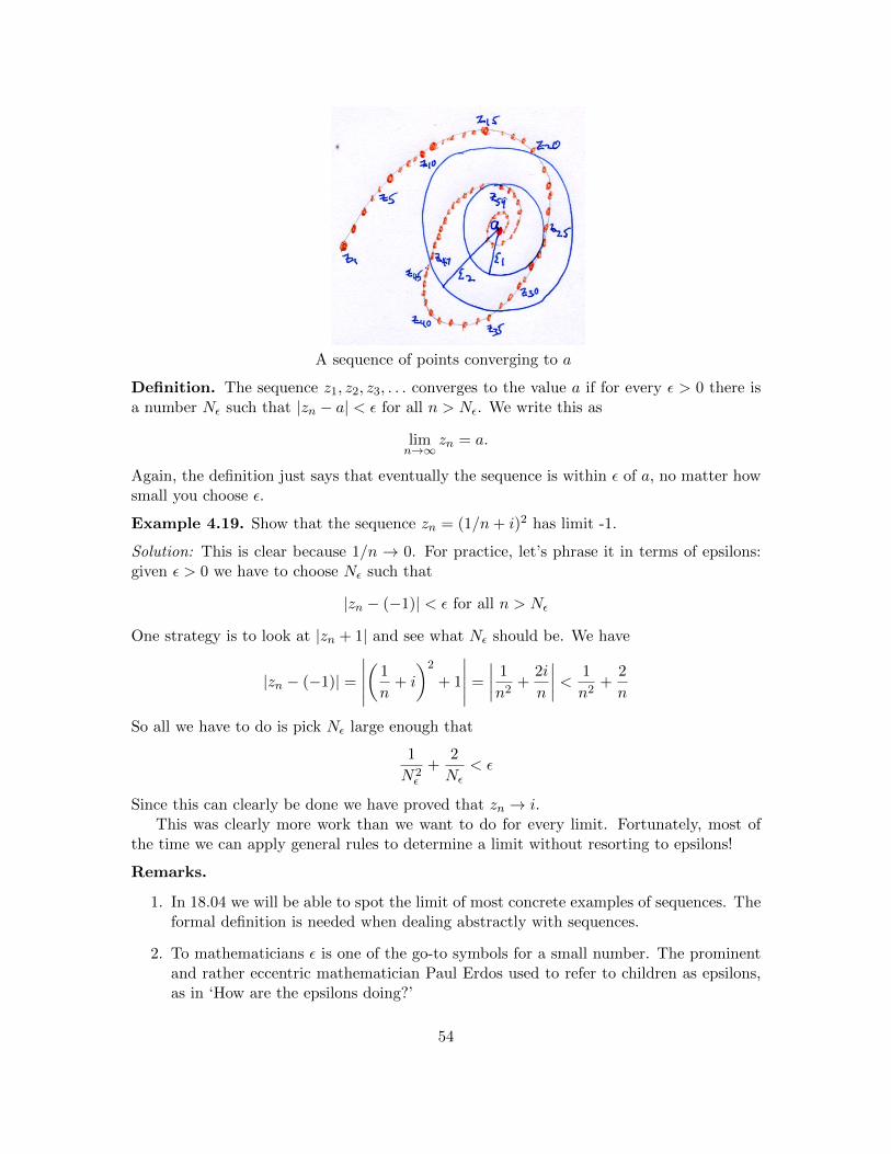
A sequence of points converging to a
Definition. The sequence z1, z2, z3, . . . converges to the value a if for every ε > 0 there isa number Nε such that |zn − a| < ε for all n > Nε. We write this as
limn→∞
zn = a.
Again, the definition just says that eventually the sequence is within ε of a, no matter howsmall you choose ε.
Example 4.19. Show that the sequence zn = (1/n+ i)2 has limit -1.
Solution: This is clear because 1/n → 0. For practice, let’s phrase it in terms of epsilons:given ε > 0 we have to choose Nε such that
|zn − (−1)| < ε for all n > Nε
One strategy is to look at |zn + 1| and see what Nε should be. We have
|zn − (−1)| =∣∣∣∣∣(
1
n+ i
)2
+ 1
∣∣∣∣∣ =
∣∣∣∣ 1
n2+
2i
n
∣∣∣∣ < 1
n2+
2
n
So all we have to do is pick Nε large enough that
1
N2ε
+2
Nε< ε
Since this can clearly be done we have proved that zn → i.This was clearly more work than we want to do for every limit. Fortunately, most of
the time we can apply general rules to determine a limit without resorting to epsilons!
Remarks.
1. In 18.04 we will be able to spot the limit of most concrete examples of sequences. Theformal definition is needed when dealing abstractly with sequences.
2. To mathematicians ε is one of the go-to symbols for a small number. The prominentand rather eccentric mathematician Paul Erdos used to refer to children as epsilons,as in ‘How are the epsilons doing?’
54

3. The term ‘captured by the circle’ is not in common usage, but it does capture whatis happening.
4.11.2 limz→z0
f(z)
Sometimes we need limits of the form limz→z0
f(z) = a. Again, the intuitive meaning is clear:
as z gets close to z0 we should see f(z) get close to a. Here is the technical definition
Definition. Suppose f(z) is defined on a punctured disk 0 < |z − z0| < r around z0. Wesay lim
z→z0f(z) = a if for every ε > 0 there is a δ such that
|f(z)− a| < ε whenever 0 < |z − z0| < δ
This says exactly that as z gets closer (within δ) to z0 we have f(z) is close (within ε) to a.Since ε can be made as small as we want, f(z) must go to a.
Remarks.
1. Using the punctured disk (also called a deleted neighborhood) means that f(z) doesnot have to be defined at z0 and, if it is then f(z0) does not necessarily equal a. Iff(z0) = a then we say the f is continuous at z0.
2. Ask any mathematician to complete the phrase “For every ε” and the odds are thatthey will respond “there is a δ . . . ”
4.11.3 Connection between limits of sequences and limits of functions
Here’s an equivalent way to define limits of functions: the limit limz→z0
f(z) = a if, for every
sequence of points {zn} with limit z0 the sequence {f(zn)} has limit a.
5 Line integrals and Cauchy’s theorem
The basic theme here is that complex line integrals will mirror much of what we’ve seen formultivariable calculus line integrals. But, just like working with eiθ is easier than workingwith sine and cosine, complex line integrals are easier to work with than their multivariableanalogs. At the same time they will give deep insight into the workings of these integrals.
To define complex line integrals, we will need the following ingredients
• The complex plane: z = x+ iy
• The complex differential dz = dx+ idy
• A curve in the complex plane: γ(t) = x(t) + iy(t), defined for a ≤ t ≤ b.
• A complex function: f(z) = u(x, y) + iv(x, y)
55

5.1 Complex line integrals
Line integrals are also called path or contour integrals. Given the above ingredients, wedefine the complex line integral by∫
γf(z) dz :=
∫ b
af(γ(t))γ′(t) dt. (25a)
You should note that this notation looks just like integrals of a real variable. We don’t needthe vectors and dot products of line integrals in R2. Also, make sure you understand thatthe product f(γ(t))γ′(t) is just a product of complex numbers.
An alternative notation uses dz = dx+ idy to write∫γf(z) dz =
∫γ(u+ iv)(dx+ idy) (25b)
Let’s check that Equations (25a) and (25b) are the same. Equation (25b) is really a multi-variable calculus expression, so thinking of γ(t) as (x(t), y(t)) it becomes∫
γf(z) dz =
∫ b
a[u(x(t), y(t)) + iv(x(t), y(t)]
(x′(t) + iy′(t)
)dt
But,u(x(t), y(t)) + iv(x(t), y(t)) = f(γ(t))
andx′(t) + iy′(t) = γ′(t)
so the right hand side of this equation is∫ b
af(γ(t))γ′(t) dt.
That is, it is exactly the same as the expression in Equation (25a).
Example 5.1. Compute∫γ z
2dz along the straight line from 0 to 1 + i.
Solution: We parametrize the curve as γ(t) = t(1 + i) with 0 ≤ t ≤ 1. So γ′(t) = 1 + i. Theline integral is ∫
z2dz =
∫ 1
0t2(1 + i)2(1 + i) dt =
2i(1 + i)
3.
Example 5.2. Compute∫γ z dz along the straight line from 0 to 1 + i.
Solution: We can use the same parametrization as in the previous example. So,∫γz dz =
∫ 1
0t(1− i)(1 + i) dt = 1
56
Example 5.3. Compute∫γ z
2 dz along the unit circle.
Solution: We parametrize the unit circle by γ(θ) = eiθ, where 0 ≤ θ ≤ 2π. We haveγ′(θ) = ieiθ. So, the integral becomes∫
γz2 dz =
∫ 2π
0e2iθieiθ dθ =
∫ 2π
0ie3iθ dθ =
ei3θ
3
∣∣∣∣2π0
= 0.
Example 5.4. Compute
∫z dz along the unit circle.
Solution: Parametrize C: γ(t) = eit, with 0 ≤ t ≤ 2π. So, γ′(t) = ieit. Putting this intothe integral gives ∫
Cz dz =
∫ 2π
0eit i eit dt =
∫ 2π
0i dt = 2πi.
5.2 Fundamental theorem for complex line integrals
This is exactly analogous to the fundamental theorem of calculus.
Theorem 5.5. (Fundamental theorem of complex line integrals) If f(z) is a complexanalytic function and γ is a curve from z0 to z1 then∫
γf ′(z) dz = f(z1)− f(z0).
Proof. This is an application of the chain rule. We have
df(γ(t))
dt= f ′(γ(t)) γ′(t).
So ∫γf ′(z) dz =
∫ z1
z0
f ′(γ(t)) γ′(t) dt =
∫ z1
z0
df(γ(t))
dtdt = f(γ(t))
∣∣∣∣z1z0
= f(z1)− f(z0).
Another equivalent way to state the fundamental theorem is: if f has an antiderivative F ,i.e. F ′ = f then ∫
γf(z) dz = F (z1)− F (z0).
Example 5.6. Redo∫γ z
2 dz, with γ the straight line from 0 to 1 + i.
Solution: We can check by inspection that z2 has an antiderivative F (z) = z3/3. Thereforethe fundamental theorem implies∫
γz2 dz =
z3
3
∣∣∣∣1+i
0
=(1 + i)3
3=
2i(1 + i)
3.
57

Example 5.7. Redo∫γ z
2 dz, with γ the unit circle.
Solution: Again, since z2 had antiderivative z3/3 we can evaluate the integral by pluggingthe endpoints of γ into the z3/3. Since the endpoints are the same the resulting differencewill be 0!
5.3 Path independence
We say the integral∫γ f(z) dz is path independent if it has the same value for any two paths
with the same endpoints. More precisely, if f(z) is defined on a region A then∫γ f(z) dz
is path independent in A, if it has the same value for any two paths in A with the sameendpoints. This statement follows directly from the fundamental theorem.
Theorem 5.8. (Path independence) If f(z) has an antiderivative in a simply connectedopen region A, then the path integral
∫γ f(z) dz is path independent for all paths in A.
Proof. Since f(z) has an antiderivative of f(z), the fundamental theorem tells us that theintegral only depends on the endpoint of γ, i.e.∫
γf(z) dz = F (z1)− F (z0)
where z0 and z1 are the beginning and end point of γ.
An alternative way to express path independence uses closed paths.
Theorem 5.9. The following two things are equivalent.
1. The integral
∫γf(z) dz is path independent.
2. The integral
∫γf(z) dz around any closed path is 0.
Proof. This is essentially identical to the corresponding multivariable proof. We have toshow two things:
(i) Path independence implies the line integral around any closed path is 0.
(ii) If the line integral around all closed paths is 0 then we have path independence.
To see (i), assume path independence and consider the closed path C shown in figure (i)below. Since the starting point z0 is the same as the endpoint z1 the line integral
∫C f(z) dz
must have the same value as the line integral over the curve consisting of the single pointz0. Since that is clearly 0 we must have the integral over C is 0.
To see (ii), assume∫C f(z) dz = 0 for any closed curve. Consider the two curves C1 and
C2 shown in figure (ii). Both start at z0 and end at z1. By the assumption that integrals
58

over closed paths are 0 we have
∫C1−C2
f(z) dz = 0. So,
∫C1
f(z) dz =
∫C2
f(z) dz.
That is, any two paths from z0 to z1 have the same line integral. This shows that the lineintegrals are path independent.
x
y
Cc
P = Q
Figure (i)
x
y
C2
C1
P
Q
Figure (ii)
5.4 Examples
Example 5.10. Why can’t we compute
∫γz dz using the fundamental theorem.
Solution: Because z doesn’t have an antiderivative. We can also see this by noting that if
z had an antiderivative, then its integral around the unit circle would have to be 0. But,we saw in Example 5.4 that this is not the case.
Example 5.11. Compute
∫γz−1 dz over several contours
(i) The line from 1 to 1 + i.(ii) The circle of radius 1 around z = 3.(iii) The unit circle.
Solution: For parts (i) and (ii) there is no problem using the antiderivative log(z) becausethese curves are contained in a simply connected region that doesn’t contain the origin.
(i) ∫γ
1
zdz = log(1 + i)− log(1) = log(
√2) + i
π
4
(ii) Since the beginning and end points are the same∫γ
1
zdz = 0
59

(iii) We parametrize the unit circle by γ(θ) = eiθ with 0 ≤ θ ≤ 2π. We compute γ′(θ) = ieiθ.So the integral becomes ∫
γ
1
zdz =
∫ 2π
0
1
eiθieiθ dt =
∫ 2π
0i dt = 2πi
Notice that we could use log(z) if we were careful to let the argument increase by 2π as itwent around the origin once.
Example 5.12. Compute∫γ z−2 dz, where γ is the unit circle in two ways.
(i) Using the fundamental theorem.
(ii) Directly from the definition.
Solution: (i) Let f(z) = −1/z. Since f ′(z) = 1/z2, the fundamental theorem says∫γ
1
z2dz =
∫γf ′(z) dz = f(endpoint)− f(start point) = 0.
It equals 0 because the start and endpoints are the same.(ii) As usual, we parametrize the unit circle as γ(θ) = eiθ with 0 ≤ θ ≤ 2π. So,
γ′(θ) = ieiθ and the integral becomes∫γ
1
z2dz =
∫ 2π
0
1
e2iθieiθ dθ =
∫ 2π
0ie−iθ dθ = −e−iθ
∣∣∣2π0
= 0.
5.5 Cauchy’s theorem
Cauchy’s theorem is analogous to Green’s theorem for curl free vector fields.
Theorem 5.13. (Cauchy’s theorem) Suppose A is a simply connected region, f(z) isanalytic on A and C is a simple closed curve in A. Then the following three things hold:
(i) ∫Cf(z) dz = 0
(i′) We can drop the requirement that C is simple in part (i).
(ii) Integrals of f on paths within A are path independent. That is, two paths with sameendpoints integrate to the same value.
(iii) f has an antiderivative in A.
Proof. We will prove (i) using Green’s theorem – we could give a proof that didn’t rely onGreen’s, but it would be quite similar in flavor to the proof of Green’s theorem.
Let R be the region inside the curve. And write f = u + iv. Now we write out theintegral as follows∫
Cf(z) dz =
∫C
(u+ iv) (dx+ idy) =
∫C
(u dx− v dy) + i(v dx+ u dy).
60

Let’s apply Green’s theorem to the real and imaginary pieces separately. First the realpiece: ∫
Cu dx− v dy =
∫R
(−vx − uy) dx dy = 0.
We get 0 because the Cauchy-Riemann equations say uy = −vx, so −vx − uy = 0.Likewise for the imaginary piece:∫
Cv dx+ u dy =
∫R
(ux − vy) dx dy = 0.
We get 0 because the Cauchy-Riemann equations say ux = vy, so ux − vy = 0.To see part (i′) you should draw a few curves that intersect themselves and convince
yourself that they can be broken into a sum of simple closed curves. Thus, (i′) followsfrom (i).5
Part (ii) follows from (i) and Theorem 5.9.To see (iii), pick a base point z0 ∈ A and let
F (z) =
∫ z
z0
f(w) dw.
Here the integral is over any path in A connecting z0 to z. By part (ii), F (z) is well defined.If we can show that F ′(z) = f(z) then we’ll be done. Doing this amounts to managing thenotation to apply the fundamental theorem of calculus and the Cauchy-Riemann equations.Let’s write
f(z) = u(x, y) + iv(x, y) , F (z) = U(x, y) + iV (x, y)
Then we can write∂f
∂x= ux + ivx, etc.
We can formulate the Cauchy-Riemann equations for F (z) as
F ′(z) =∂F
∂x=
1
i
∂F
∂y(26a)
i.e.
F ′(z) = Ux + iVx =1
i(Uy + iVy) = Vy − iUy. (26b)
For reference, we note that using the path γ(t) = x(t) + iy(t), with γ(0) = z0 and γ(b) = zwe have
F (z) =
∫ z
z0
f(w) dw =
∫ z
z0
(u(x, y) + iv(x, y))(dx+ idy)
=
∫ b
0(u(x(t), y(t)) + iv(x(t), y(t))(x′(t) + iy′(t)) dt. (27)
5In order to truly prove part (i′) we would need a more technically precise definition of simply connectedso we could say that all closed curves within A can be continuously deformed to each other.
61

Our goal now is to prove that the Cauchy-Riemann equations given in Equation (27) holdfor F (z). The figure below shows an arbitrary path from z0 to z, which can be used tocompute F (z). To compute the partials of F we’ll need the straight lines that continue Cto z + h or z + ih.
A
z0
z z + h
z + ih
C
Cx
Cy
Paths for proof of Cauchy’s theorem
To prepare the rest of the argument we remind you that the fundamental theorem of calculusimplies
limh→0
∫ h0 g(t) dt
h= g(0). (28)
(That is, the derivative of the integral is the original function.)
First we’ll look at∂F
∂x. So, fix z = x+ iy. Looking at the paths in the figure above we
have
F (z + h)− F (z) =
∫C+Cx
f(w) dw −∫Cf(w) dw =
∫Cx
f(w) dw.
The curve Cx is parametrized by γ(t) = x+ t+ iy, with 0 ≤ t ≤ h. So,
∂F
∂x= lim
h→0
F (z + h)− F (z)
h= lim
h→0
∫Cxf(w) dw
h
= limh→0
∫ h0 u(x+ t, y) + iv(x+ t, y) dt
h
= u(x, y) + iv(x, y)
= f(z) (29)
The second to last equality follows from Equation (28).Similarly, we get (remember: w = z + it, so dw = i dt)
1
i
∂F
∂y= lim
h→0
F (z + ih)− F (z)
ih= lim
h→0
∫Cyf(w) dw
ih
= limh→0
∫ h0 u(x, y + t) + iv(x, y + t) i dt
ih
= u(x, y) + iv(x, y)
= f(z). (30)
62

Together Equations (29) and (30) show
f(z) =∂F
∂x=
1
i
∂F
∂y
By Equation (26) we have shown that F is analytic and F ′ = f . �
5.6 Extensions of Cauchy’s theorem
Cauchy’s theorem requires that the function f(z) be analytic on a simply connected region.In cases where it is not, we can extend it in a useful way.
Suppose R is the region between the two simple closed curves C1 and C2. Note, bothC1 and C2 are oriented in a counterclockwise direction.
Theorem 5.14. (Extended Cauchy’s theorem) If f(z) is analytic on R then∫C1−C2
f(z) dz = 0.
Proof. The proof is based on the following figure. We ‘cut’ both C1 and C2 and connectthem by two copies of C3, one in each direction. (In the figure we have drawn the twocopies of C3 as separate curves, in reality they are the same curve traversed in oppositedirections.)
With C3 acting as a cut, the region enclosed by C1 +C3−C2−C3 is simply connected,so Cauchy’s Theorem 5.13 applies. We get∫
C1+C3−C2−C3
f(z) dz = 0
The contributions of C3 and −C3 cancel, which leaves
∫C1−C2
f(z) dz = 0. �
Note. This clearly implies
∫C1
f(z) dz =
∫C2
f(z) dz.
63

Example 5.15. Let f(z) = 1/z. f(z) is defined and analytic on the punctured plane.
x
y
Punctured plane: C− {0}
What values can
∫Cf(z) dz take for C a simple closed curve (positively oriented) in the
plane?
Solution: We have two cases (i) C1 not around 0, and (ii), C2 around 0
x
y
C1RC2
Case (i): Cauchy’s theorem applies directly because the interior does not contain the prob-lem point at the origin. Thus, ∫
C1
f(z) dz = 0
Case (ii): we will show that ∫C2
f(z) dz = 2πi
Let C3 be a small circle of radius a centered at 0 and entirely inside C2.
x
y
C2C3R
Figure for part (ii)
By the extended Cauchy theorem we have∫C2
f(z) dz =
∫C3
f(z) dz.
64

Using the usual parametrization of a circle we can easily compute that the line integral is∫C2
f(z) dz =
∫C3
f(z) dz =
∫ 2π
0i dt = 2πi
We can extend this answer in the following way:
If C is not simple, then the possible values of∫Cf(z) dz
are 2πni, where n is the number of times C goes (counterclockwise) around the origin 0.
Definition. n is called the winding number of C around 0. n also equals the number oftimes C crosses the positive x-axis, counting +1 for crossing from below and −1 for crossingfrom above.
x
y
C
A curve with winding number 2 around the origin.
Example 5.16. A further extension: using the same trick of cutting the region by curvesto make it simply connected we can show that if f is analytic in the region R shown belowthen ∫
C1−C2−C3−C4
f(z) dz = 0.
C1
C2 C3 C4
R
That is, C1 − C2 − C3 − C4 is the boundary of the region R.
Orientation. It is important to get the orientation of the curves correct. One way to dothis is to make sure that the region R is always to the left as you traverse the curve. Inthe above example. The region is to the right as you traverse C2, C3 or C4 in the directionindicated. This is why we put a minus sign on each when describing the boundary.
65

6 Cauchy’s integral formula
Cauchy’s theorem is a big theorem which we will use almost daily from here on out. Rightaway it will reveal a number of interesting and useful properties of analytic functions. Morewill follow as the course progresses. If you learn just one theorem this week it should beCauchy’s integral formula! We start with a statement of the theorem for functions. Aftersome examples, we’ll give a generalization to all derivatives of a function. After some moreexamples we will prove the theorems. After that we will see some remarkable consequencesthat follow fairly directly from the Cauchy’s formula.
6.1 Cauchy’s integral for functions
Theorem 6.1. (Cauchy’s integral formula) Suppose C is a simple closed curve and thefunction f(z) is analytic on a region containing C and its interior. We assume C is orientedcounterclockwise. Then for any z0 inside C:
f(z0) =1
2πi
∫C
f(z)
z − z0dz (31)
Re(z)
Im(z)
z0
C
A
Cauchy’s integral formula: simple closed curve C, f(z) analytic on and inside C.
This is remarkable: it says that knowing the values of f on the boundary curve C means weknow everything about f inside C!! This is probably unlike anything you’ve encounteredwith functions of real variables.
Aside 1. With a slight change of notation (z becomes w and z0 becomes z) we often writethe formula as
f(z) =1
2πi
∫C
f(w)
w − z dw (32)
Aside 2. We’re not being entirely fair to functions of real variables. We will see that forf = u+ iv the real and imaginary parts u and v have many similar remarkable properties.u and v are called conjugate harmonic functions.
Example 6.2. Compute
∫c
ez2
z − 2dz, where C is the curve shown.
66
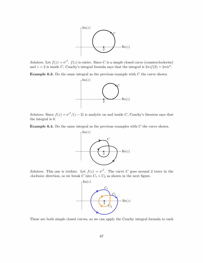
Re(z)
Im(z)
C
2
Solution: Let f(z) = ez2. f(z) is entire. Since C is a simple closed curve (counterclockwise)
and z = 2 is inside C, Cauchy’s integral formula says that the integral is 2πif(2) = 2πie4.
Example 6.3. Do the same integral as the previous example with C the curve shown.
Re(z)
Im(z)
C
2
Solution: Since f(z) = ez2/(z − 2) is analytic on and inside C, Cauchy’s theorem says that
the integral is 0.
Example 6.4. Do the same integral as the previous examples with C the curve shown.
Re(z)
Im(z)
C
2
Solution: This one is trickier. Let f(z) = ez2. The curve C goes around 2 twice in the
clockwise direction, so we break C into C1 + C2 as shown in the next figure.
Re(z)
Im(z)
C1
C1
C2
2
These are both simple closed curves, so we can apply the Cauchy integral formula to each
67

separately. (The negative signs are because they go clockwise around z = 2.)∫C
f(z)
z − 2dz =
∫C1
f(z)
z − 2dz +
∫C2
f(z)
z − 2dz = −2πif(2)− 2πif(2) = −4πif(2)
6.2 Cauchy’s integral formula for derivatives
Cauchy’s integral formula is worth repeating several times. So, now we give it for allderivatives f (n)(z) of f . This will include the formula for functions as a special case.
Theorem 6.5. Cauchy’s integral formula for derivatives. If f(z) and C satisfy the samehypotheses as for Cauchy’s integral formula then, for all z inside C we have
f (n)(z) =n!
2πi
∫C
f(w)
(w − z)n+1dw, n = 0, 1, 2, . . . (33)
where, C is a simple closed curve, oriented counterclockwise, z is inside C and f(w) isanalytic on and inside C.
Example 6.6. Evaluate I =
∫C
e2z
z4dz where C : |z| = 1.
Solution: With Cauchy’s formula for derivatives this is easy. Let f(z) = e2z. Then,
I =
∫C
f(z)
z4dz =
2πi
3!f ′′′(0) =
8
3πi.
Example 6.7. Now Let C be the contour shown below and evaluate the same integral asin the previous example.
Re
Im
C
Solution: Again this is easy: the integral is the same as the previous example, i.e. I =8
3πi.
68

6.2.1 Another approach to some basic examples
Suppose C is a simple closed curve around 0. We have seen that∫C
1
zdz = 2πi
The Cauchy integral formula gives the same result. That is, let f(z) = 1, then the formulasays
1
2πi
∫C
f(z)
z − 0dz = f(0) = 1.
Likewise Cauchy’s formula for derivatives shows∫C
1
(z)ndz =
∫C
f(z)
zn+1dz = f (n)(0) = 0, (34)
for integers n > 1
6.2.2 More examples
Example 6.8. Compute
∫C
cos(z)
z(z2 + 8)dz over the contour shown.
Im(z)
Im(z)2i
−2i
C
Solution: Let f(z) = cos(z)/(z2 + 8). f(z) is analytic on and inside the curve C. That is,
the roots of z2 + 8 are outside the curve. So, we rewrite the integral as∫C
cos(z)/(z2 + 8)
zdz =
∫C
f(z)
zdz = 2πif(0) = 2πi
1
8=πi
4
69

Example 6.9. Compute
∫C
1
(z2 + 4)2dz over the contour shown.
Re(z)
Im(z)
C
i
2i
−i
−2i
Solution: We factor the denominator as
1
(z2 + 4)2=
1
(z − 2i)2(z + 2i)2
Let
f(z) =1
(z + 2i)2
Clearly f(z) is analytic inside C. So, by Cauchy’s formula for derivatives:∫C
1
(z2 + 4)2dz =
∫C
f(z)
(z − 2i)2= 2πif ′(2i) = 2πi
[ −2
(z + 2i)3
]z=2i
=4πi
64i=
π
16
Example 6.10. Compute
∫C
z
z2 + 4dz over the curve C shown below.
Re(z)
Im(z)
Ci
2i
−i
−2i
70
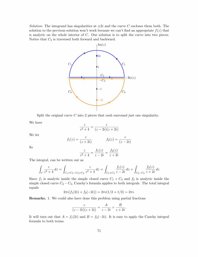
Solution: The integrand has singularities at ±2i and the curve C encloses them both. Thesolution to the previous solution won’t work because we can’t find an appropriate f(z) thatis analytic on the whole interior of C. Our solution is to split the curve into two pieces.Notice that C3 is traversed both forward and backward.
Re(z)
Im(z)
C1C1
C3
C2C2
−C3
i
2i
−i
−2i
Split the original curve C into 2 pieces that each surround just one singularity.
We havez
z2 + 4=
z
(z − 2i)(z + 2i)
We letf1(z) =
z
(z + 2i)f2(z) =
z
(z − 2i)
Soz
z2 + 4=
f1(z)
z − 2i=
f2(z)
z + 2i
The integral, can be written out as∫C
z
z2 + 4dz =
∫C1+C3−C3+C2
z
z2 + 4dz =
∫C1+C3
f1(z)
z − 2idz +
∫C2−C3
f2(z)
z + 2idz
Since f1 is analytic inside the simple closed curve C1 + C3 and f2 is analytic inside thesimple closed curve C2−C3, Cauchy’s formula applies to both integrals. The total integralequals
2πi(f1(2i) + f2(−2i)) = 2πi(1/2 + 1/2) = 2πi.
Remarks. 1. We could also have done this problem using partial fractions
z
(z − 2i)(z + 2i)=
A
z − 2i+
B
z + 2i.
It will turn out that A = f1(2i) and B = f2(−2i). It is easy to apply the Cauchy integralformula to both terms.
71
2. Important note. In an upcoming topic we will formulate the Cauchy residuetheorem. This will allow us to compute the integrals in Examples 6.8-6.10 in an easier andless ad hoc manner.
6.2.3 The triangle inequality for integrals
We discussed the triangle inequality in the Topic 1 notes. It says that
|z1 + z2| ≤ |z1|+ |z2|,
with equality if and only if z1 and z2 lie on the same ray from the origin.Since an integral is basically a sum, this translates to the triangle inequality for integrals.
We’ll state it in two ways that will be useful to us.
Theorem 6.11. (Triangle inequality for integrals I) Suppose g(t) is a complex valuedfunction of a real variable, defined on a ≤ t ≤ b. Then∣∣∣∣∫ b
ag(t) dt
∣∣∣∣ ≤ ∫ b
a|g(t))| dt,
with equality if and only if the values of g(t) all lie on the same ray from the origin.
Proof. This follows by approximating the integral as a Riemann sum.∣∣∣∣∫ b
ag(t) dt
∣∣∣∣ ≈ ∣∣∣∑ g(tk)∆t∣∣∣ ≤∑ |g(tk)|∆t ≈
∫ b
a|g(t)| dt.
The middle inequality is just the standard triangle inequality for sums of complex num-bers. �
Theorem 6.12. (Triangle inequality for integrals II) For any function f(z) and any curveγ, we have ∣∣∣∣∫
γf(z) dz
∣∣∣∣ ≤ ∫γ|f(z)| |dz|.
Here dz = γ′(t) dt and |dz| = |γ′(t)| dt.
Proof. This follows immediately from the previous theorem:∣∣∣∣∫γf(z) dz
∣∣∣∣ =
∣∣∣∣∫ b
af(γ(t))γ′(t) dt
∣∣∣∣ ≤ ∫ b
a|f(γ(t))||γ′(t)| dt =
∫γ|f(z)| |dz|.
Corollary. If |f(z)| < M on C then∣∣∣∣∫Cf(z) dz
∣∣∣∣ ≤M · (length of C)
72
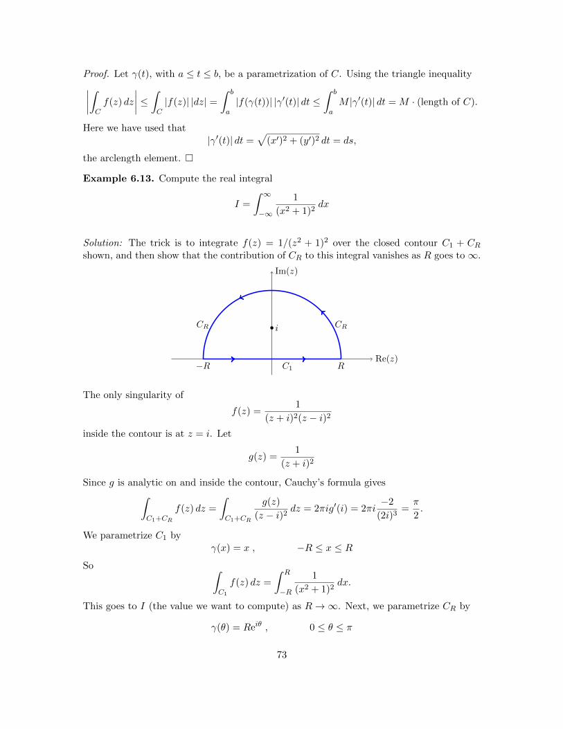
Proof. Let γ(t), with a ≤ t ≤ b, be a parametrization of C. Using the triangle inequality∣∣∣∣∫Cf(z) dz
∣∣∣∣ ≤ ∫C|f(z)| |dz| =
∫ b
a|f(γ(t))| |γ′(t)| dt ≤
∫ b
aM |γ′(t)| dt = M · (length of C).
Here we have used that|γ′(t)| dt =
√(x′)2 + (y′)2 dt = ds,
the arclength element. �
Example 6.13. Compute the real integral
I =
∫ ∞−∞
1
(x2 + 1)2dx
Solution: The trick is to integrate f(z) = 1/(z2 + 1)2 over the closed contour C1 + CRshown, and then show that the contribution of CR to this integral vanishes as R goes to∞.
Re(z)
Im(z)
CRCR
C1 R−R
i
The only singularity of
f(z) =1
(z + i)2(z − i)2
inside the contour is at z = i. Let
g(z) =1
(z + i)2
Since g is analytic on and inside the contour, Cauchy’s formula gives∫C1+CR
f(z) dz =
∫C1+CR
g(z)
(z − i)2dz = 2πig′(i) = 2πi
−2
(2i)3=π
2.
We parametrize C1 byγ(x) = x , −R ≤ x ≤ R
So ∫C1
f(z) dz =
∫ R
−R
1
(x2 + 1)2dx.
This goes to I (the value we want to compute) as R→∞. Next, we parametrize CR by
γ(θ) = Reiθ , 0 ≤ θ ≤ π
73

So ∫CR
f(z) dz =
∫ π
0
1
(R2e2iθ + 1)2iReiθ dθ
By the triangle inequality for integrals, if R > 1∣∣∣∣∫CR
f(z) dz
∣∣∣∣ ≤ ∫ π
0
∣∣∣∣ 1
(R2e2iθ + 1)2iReiθ
∣∣∣∣ dθ. (35)
From the triangle equality for complex numbers
R2 = |R2e2iθ| = |R2e2iθ + 1 + (−1)| ≤ |R2e2iθ + 1|+ | − 1| = |R2e2iθ + 1|+ 1
we get|R2e2iθ + 1| ≥ R2 − 1
Thus1
|R2e2iθ + 1|2 ≤1
(R2 − 1)2
Using Equation (35), we then have∣∣∣∣∫CR
f(z) dz
∣∣∣∣ ≤ ∫ π
0
∣∣∣∣ 1
(R2e2iθ + 1)2iReiθ
∣∣∣∣ dθ ≤ ∫ π
0
R
(R2 − 1)2dθ =
πR
(R2 − 1)2
Clearly this goes to 0 as R→∞. Thus, the integral over the contour C1 +CR goes to I asR gets large. But ∫
C1+CR
f(z) dz = π/2
for all R > 1. We can therefore conclude that I = π/2.As a sanity check, we note that our answer is real and positive as it needs to be.
6.3 Proof of Cauchy’s integral formula
6.3.1 A useful theorem
Before proving the theorem we’ll need a theorem that will be useful in its own right.
Theorem 6.14. (A second extension of Cauchy’s theorem) Suppose that A is a simplyconnected region containing the point z0. Suppose g is a function which is
1. Analytic on A− {z0}
2. Continuous on A. (In particular, g does not blow up at z0.)
Then, ∫Cg(z) dz = 0
for all closed curves C in A.
74
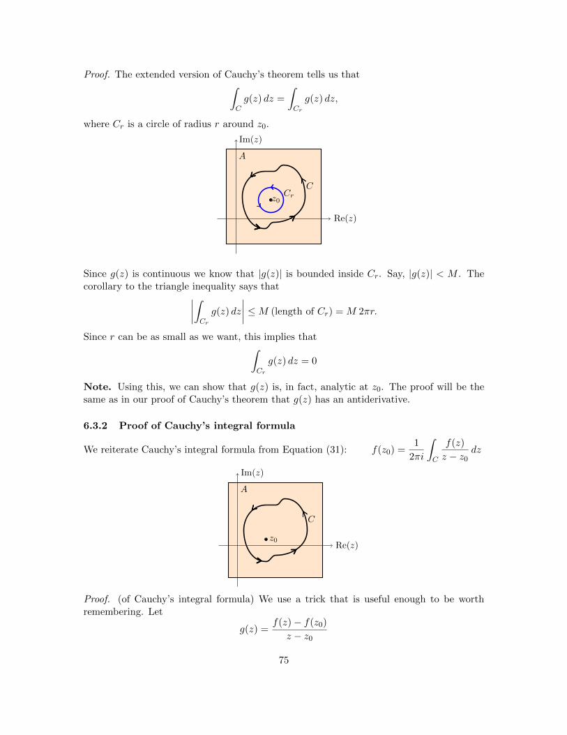
Proof. The extended version of Cauchy’s theorem tells us that∫Cg(z) dz =
∫Cr
g(z) dz,
where Cr is a circle of radius r around z0.
Re(z)
Im(z)
z0
C
A
Cr
Since g(z) is continuous we know that |g(z)| is bounded inside Cr. Say, |g(z)| < M . Thecorollary to the triangle inequality says that∣∣∣∣∫
Cr
g(z) dz
∣∣∣∣ ≤M (length of Cr) = M 2πr.
Since r can be as small as we want, this implies that∫Cr
g(z) dz = 0
Note. Using this, we can show that g(z) is, in fact, analytic at z0. The proof will be thesame as in our proof of Cauchy’s theorem that g(z) has an antiderivative.
6.3.2 Proof of Cauchy’s integral formula
We reiterate Cauchy’s integral formula from Equation (31): f(z0) =1
2πi
∫C
f(z)
z − z0dz
Re(z)
Im(z)
z0
C
A
Proof. (of Cauchy’s integral formula) We use a trick that is useful enough to be worthremembering. Let
g(z) =f(z)− f(z0)
z − z0
75

Since f(z) is analytic on A, we know that g(z) is analytic on A−{z0}. Since the derivativeof f exists at z0, we know that
limz→z0
g(z) = f ′(z0)
That is, if we define g(z0) = f ′(z0) then g is continuous at z0. From the extension ofCauchy’s theorem just above, we have∫
Cg(z) dz = 0, i.e.
∫C
f(z)− f(z0)
z − z0dz = 0
Thus ∫C
f(z)
z − z0dz =
∫C
f(z0)
z − z0dz = f(z0)
∫C
1
z − z0dz = 2πif(z0).
The last equality follows from our, by now, well known integral of 1/(z − z0) on a looparound z0.
6.4 Proof of Cauchy’s integral formula for derivatives
Recall that Cauchy’s integral formula in Equation (33) says
f (n)(z) =n!
2πi
∫C
f(w)
(w − z)n+1dw, n = 0, 1, 2, . . .
First we’ll offer a quick proof which captures the reason behind the formula, and then aformal proof.
Quick proof: We have an integral representation for f(z), z ∈ A, we use that to find anintegral representation for f ′(z), z ∈ A.
f ′(z) =d
dz
[1
2πi
∫C
f(w)
w − z dw]
=1
2πi
∫C
d
dz
(f(w)
w − z
)dw =
1
2πi
∫C
f(w)
(w − z)2dw
(Note, since z ∈ A and w ∈ C, we know that w − z 6= 0) Thus,
f ′(z) =1
2πi
∫C
f(w)
(w − z)2dw
Now, by iterating this process, i.e. by mathematical induction, we can show the formulafor higher order derivatives.
Formal proof: We do this by taking the limit of
lim∆z→0
f(z + ∆z)− f(z)
∆z
using the integral representation of both terms:
f(z + ∆z) =1
2πi
∫C
f(w)
w − z −∆zdw , f(z) =
1
2πi
∫C
f(w)
w − z dw
76

Now, using a little algebraic manipulation we get
f(z + ∆z)− f(z)
∆z=
1
2πi∆z
∫C
f(w)
w − z −∆z− f(w)
w − z dw
=1
2πi∆z
∫C
f(w)∆z
(w − z −∆z)(w − z) dw
=1
2πi
∫C
f(w)
(w − z)2 −∆z(w − z) dw
Letting ∆z go to 0, we get Cauchy’s formula for f ′(z)
f ′(z) =1
2πi
∫C
f(w)
(w − z)2dw
There is no problem taking the limit under the integral sign because everything is continuousand the denominator is never 0. �
6.5 Consequences of Cauchy’s integral formula
6.5.1 Existence of derivatives
Theorem. Suppose f(z) is analytic on a region A. Then, f has derivatives of all order.
Proof. This follows from Cauchy’s integral formula for derivatives. That is, we have aformula for all the derivatives, so in particular the derivatives all exist. A little moreprecisely: for any point z in A we can put a small disk around z0 that is entirely containedin A. Let C be the boundary of the disk, then Cauchy’s formula gives a formula for all thederivatives f (n)(z0) in terms of integrals over C. In particular, those derivatives exist. �
Remark. If you look at the proof of Cauchy’s formula for derivatives you’ll see that fhaving derivatives of all orders boils down to 1/(w − z) having derivatives of all orders forw on a curve not containing z.
Important remark. We have at times assumed that for f = u+ iv analytic, u and v havecontinuous higher order partial derivatives. This theorem confirms that fact. In particular,uxy = uyx, etc.
6.5.2 Cauchy’s inequality
Theorem 6.15. (Cauchy’s inequality) Let CR be the circle |z−z0| = R. Assume that f(z)is analytic on CR and its interior, i.e. on the disk |z− z0| ≤ R. Finally let MR = max |f(z)|over z on CR. Then
|f (n)(z0)| ≤ n!MR
Rn, n = 1, 2, 3, . . . (36)
Proof. Using Cauchy’s integral formula for derivatives (Equation 33) we have
|f (n)(z0)| ≤ n!
2π
∫CR
|f(w)||w − z0|n+1
|dw| ≤ n!
2π
MR
Rn+1
∫CR
|dw| = n!
2π
MR
Rn+1· 2πR
77

6.5.3 Liouville’s theorem
Theorem 6.16. (Liouville’s theorem) Assume f(z) is entire and suppose it is bounded inthe complex plane, namely |f(z)| < M for all z ∈ C then f(z) is constant.
Proof. For any circle of radius R around z0 the Cauchy inequality says |f ′(z0)| ≤ M
R. But,
R can be as large as we like so we conclude that |f ′(z0)| = 0 for every z0 ∈ C. Since thederivative is 0, the function itself is constant.
In short:
If f is entire and bounded then f is constant.
Note. P (z) = anzn + . . .+ a0, sin(z), ez are all entire but not bounded.
Now, practically for free, we get the fundamental theorem of algebra.
Corollary. (Fundamental theorem of algebra) Any polynomial P of degree n ≥ 1, i.e.
P (z) = a0 + a1z + . . .+ anzn, an 6= 0,
has exactly n roots.
Proof. There are two parts to the proof.Hard part: Show that P has at least one root.This is done by contradiction, together with Liouville’s theorem. Suppose P (z) does
not have a zero. Then1. f(z) = 1/P (z) is entire. This is obvious because (by assumption) P (z) has no zeros.2. f(z) is bounded. This follows because 1/P (z) goes to 0 as |z| goes to ∞.
Im(z)
Im(z)
R
CR
M = max of |1/P (z)| in here.
|1/P (z)| small out here.
(It is clear that |1/P (z)| goes to 0 as z goes to infinity, i.e. |1/P (z)| is small outside a largecircle. So |1/P (z)| is bounded by M .)
So, by Liouville’s theorem f(z) is constant, and therefore P (z) must be constant as well.But this a contradiction, so P must have a zero.
78

Easy part: P has exactly n zeros. Let z0 be one zero. We can factor P (z) = (z−z0)Q(z).Q(z) has degree n− 1. If n− 1 > 0, then we can apply the result to Q(z). We can continuethis process until the degree of Q is 0.
6.5.4 Maximum modulus principle
Briefly, the maximum modulus principle states that if f is analytic and not constant ina domain A then |f(z)| has no relative maximum in A and the absolute maximum of |f |occurs on the boundary of A.
In order to prove the maximum modulus principle we will first prove the mean valueproperty. This will give you a good feel for the maximum modulus principle. It is alsoimportant and interesting in its own right.
Theorem 6.17. (Mean value property) Suppose f(z) is analytic on the closed disk ofradius r centered at z0, i.e. the set |z − z0| ≤ r. Then,
f(z0) =1
2π
∫ 2π
0f(z0 + reiθ) dθ (37)
Proof. This is an application of Cauchy’s integral formula on the disk Dr = |z − z0| ≤ r.
Re(z)
Im(z)
z0
r Cr
We can parametrize Cr, the boundary of Dr, as
γ(t) = z0 + reiθ, with 0 ≤ θ ≤ 2π, so γ′(θ) = ireiθ.
By Cauchy’s formula we have
f(z0) =1
2πi
∫Cr
f(z)
z − z0dz =
1
2πi
∫ 2π
0
f(z0 + reiθ)
reiθireiθ dθ =
1
2π
∫ 2π
0f(z0 + reiθ) dθ
This proves the property. �In words, the mean value property says f(z0) is the arithmetic mean of the values on
the circle.We can now prove maximum modulus principle.
Theorem 6.18. (Maximum modulus principle) Suppose f(z) is analytic in a connectedregion A and z0 is a point in A.
1. If |f | has a relative maximum at z0 then f(z) is constant in a neighborhood of z0.
2. If A is bounded and connected, and f is continuous on A and its boundary, then eitherf is constant or the absolute maximum of |f | occurs only on the boundary of A.
79

Proof. Part (1): The argument for is a little fussy. We will use the mean value propertyand the triangle inequality from Theorem 6.11.
Since z0 is a relative maximum of |f |, for every small enough circle C : |z − z0| = raround z0 we have |f(z)| ≤ |f(z0)| for z on C. Therefore, by the mean value property andthe triangle inequality
|f(z0)| =∣∣∣∣ 1
2π
∫ 2π
0f(z0 + reiθ) dθ
∣∣∣∣ (mean value property)
≤ 1
2π
∫ 2π
0|f(z0 + reiθ)| dθ (triangle inequality)
≤ 1
2π
∫ 2π
0|f(z0)| dθ (|f(z0 + reiθ)| ≤ |f(z0)|)
= |f(z0)|
Since the beginning and end of the above are both |f(z0)| all the inequalities in the chainmust be equalities.
The first inequality can only be an equality if for all θ, f(z0 + reiθ) lie on the same rayfrom the origin, i.e. have the same argument or are 0.
The second inequality can only be an equality if all |f(z0 + reiθ)| = |f(z0)|. So we haveall f(z0 + reiθ) have the same magnitude and the same argumeny. This implies they are allthe same.
Finally, if f(z) is constant along the circle and f(z0) is the average of f(z) over thecircle then f(z) = f(z0), i.e. f is constant on a small disk around z0.
Part (2): The assumptions that A is bounded and f is continuous on A and its boundaryserve to guarantee that |f | has an absolute maximum (on A combined with its boundary).Part (1) guarantees that the absolute maximum can not lie in the interior of the region Aunless f is constant. (This requires a bit more argument. Do you see why?) If the absolutemaximum is not in the interior it must be on the boundary.�
Example 6.19. Find the maximum modulus of ez on the unit square with 0 ≤ x, y ≤ 1.Solution:
|ex+iy| = ex
so the maximum is when x = 1, 0 ≤ y ≤ 1 is arbitrary. This is indeed on the boundary ofthe unit square
Example 6.20. Find the maximum modulus for sin(z) on the square [0, 2π] × [0, 2π].Solution: We use the formula
sin(z) = sinx cosh y + i cosx sinh y
So
| sin(z)|2 = sin2 x cosh2 y + cos2 x sinh2 y
= sin2 x cosh2 y + (1− sin2 x) sinh2 y
= sin2 x+ sinh2 y
80

We know the maximum over x of sin2(x) is at x = π/2 and x = 3π/2. The maximumof sinh2 y is at y = 2π. So maximum modulus is√
1 + sinh2(2π) =
√cosh2(2π) = cosh(2π)
This occurs at the points
z = x+ iy =π
2+ 2πi , z =
3π
2+ 2πi
Both these points are on the boundary of the region.
Example 6.21. Suppose f(z) is entire. Show that if limz→∞
f(z) = 0 then f(z) ≡ 0.
Solution: This is a standard use of the maximum modulus principle. The strategy is to showthat the maximum of |f(z)| is not on the boundary (of the appropriately chosen region), sof(z) must be constant.
Fix z0. For R > |z0| let MR be the maximum of |f(z)| on the circle |z| = R. Themaximum modulus theorem says that |f(z0)| < MR. Since f(z) goes to 0, as R goes toinfinity, we must have MR also goes to 0. This means |f(z0)| = 0. Since this is true for anyz0, we have f(z) ≡ 0.
Example 6.22. Here is an example of why you need A to be bounded in the maximummodulus theorem. Let A be the upper half-plane
Im(z) > 0
So the boundary of A is the real axis.Let f(z) = e−iz. We have
|f(x)| = |e−ix| = 1
for x along the real axis. Since |f(2i)| = |e2| > 1, we see |f | cannot take its maximum alongthe boundary of A.
Of course, it can’t take its maximum in the interior of A either. What happens hereis that f(z) doesn’t have a maximum modulus. Indeed |f(z)| goes to infinity along thepositive imaginary axis.
7 Introduction to harmonic functions
Harmonic functions appear regularly and play a fundamental role in math, physics andengineering. In this topic we’ll learn the definition, some key properties and their tightconnection to complex analysis. The key connection to 18.04 is that both the real andimaginary parts of analytic functions are harmonic. We will see that this is a simpleconsequence of the Cauchy-Riemann equations. In the next topic we will look at someapplications to hydrodynamics.
81

7.1 Harmonic functions
We start by defining harmonic functions and looking at some of their properties.
Definition 7.1. A function u(x, y) is called harmonic if it is twice continuously differen-tiable and satisfies the following partial differential equation:
∇2u = uxx + uyy = 0. (38)
Equation (38) is called Laplace’s equation. So a function is harmonic if it satisfies Laplace’sequation. The operator ∇2 is called the Laplacian and ∇2u is called the Laplacian of u.
7.2 Del notation
Here’s a quick reminder on the use of the notation ∇. For a function u(x, y) and a vectorfield F(x, y) = (u, v), we have
(i) ∇ =(∂∂x ,
∂∂y
)in Cartesian coordinates
(ii) gradu = ∇u = (ux, uy)
(iii) curl F = ∇× F = (vx − uy)
(iv) div F = ∇ · F = ux + vy
(v) div gradu = ∇ ·∇u = ∇2u = uxx + uyy
(vi) curl gradu = ∇×∇u = 0
7.2.1 Analytic functions have harmonic pieces
The connection between analytic and harmonic functions is very strong. In many respectsit mirrors the connection between ez and sine and cosine.
Let z = x+ iy and write f(z) = u(x, y) + iv(x, y).
Theorem 7.2. If f(z) = u(x, y) + iv(x, y) is analytic on a region A then both u and v areharmonic functions on A.
Proof. This is a simple consequence of the Cauchy-Riemann equations. Since ux = vy wehave
uxx = vyx
Likewise, uy = −vx impliesuyy = −vxy
Since vxy = vyx we haveuxx + uyy = vyx − vxy = 0
Therefore u is harmonic. We can handle v similarly. �
Note. Since we know an analytic function is infinitely differentiable we know u and v have
82

the required two continuous partial derivatives. This also ensures that the mixed partialsagree, i.e. vxy = vyx.
To complete the tight connection between analytic and harmonic functions we show thatany harmonic function is the real part of an analytic function.
Theorem 7.3. If u(x, y) is harmonic on a simply connected region A, then u is the realpart of an analytic function f(z) = u(x, y) + iv(x, y).
Proof. This is similar to our proof that an analytic function has an antiderivative. First wecome up with a candidate for f(z) and then show it has the properties we need. Here arethe details broken down into steps 1-4.
1. Find a candidate, call it g(z), for f ′(z):
If we had an analytic f with f = u+iv, then Cauchy-Riemann says that f ′ = ux−iuy.So, let’s define
g = ux − iuyThis is our candidate for f ′.
2. Show that g(z) is analytic:
Write g = φ + iψ, where φ = ux and ψ = −uy. Checking the Cauchy-Riemannequations we have [
φx φyψx ψy
]=
[uxx uxy−uyx −uyy
]Since u is harmonic we know uxx = −uyy, so φx = ψy. It is clear that φy = −ψx.Thus g satisfies the Cauchy-Riemann equations, so it is analytic.
3. Let f be an antiderivative of g:
Since A is simply connected our statement of Cauchy’s theorem guarantees that g(z)has an antiderivative in A. We’ll need to fuss a little to get the constant of integrationexactly right. So, pick a base point z0 in A. Define the antiderivative of g(z) by
f(z) =
∫ z
z0
g(z) dz + u(x0, y0).
(Again, by Cauchy’s theorem this integral can be along any path in A from z0 to z.)
4. Show that the real part of f is u.
Let’s write f = U + iV . So, f ′(z) = Ux − iUy. By construction
f ′(z) = g(z) = ux − iuyThis means the first partials of U and u are the same, so U and u differ by at most aconstant. However, also by construction,
f(z0) = u(x0, y0) = U(x0, y0) + iV (x0, y0)
So, U(x0, y0) = u(x0, y0) (and V (x0, y0) = 0). Since they agree at one point we musthave U = u, i.e. the real part of f is u as we wanted to prove.
83

Important corollary. u is infinitely differentiable.
Proof. By definition we only require a harmonic function u to have continuous secondpartials. Since the analytic f is infinitely differentiable, we have shown that so is u!
7.2.2 Harmonic conjugates
Definition. If u and v are the real and imaginary parts of an analytic function, then wesay u and v are harmonic conjugates.
Note. If f(z) = u + iv is analytic then so is if(z) = −v + iu. So, u and v are harmonicconjugates and so are u and −v.
7.3 A second proof that u and v are harmonic
This fact is important enough that we will give a second proof using Cauchy’s integralformula. One benefit of this proof is that it reminds us that Cauchy’s integral formula cantransfer a general question on analytic functions to a question about the function 1/z. Westart with an easy to derive fact.
Fact. The real and imaginary parts of f(z) = 1/z are harmonic away from the origin.Likewise for
g(z) = f(z − a) =1
z − aaway from the point z = a.
Proof. We have1
z=
x
x2 + y2− i y
x2 + y2
It is a simple matter to apply the Laplacian and see that you get 0. We’ll leave the algebrato you! The statement about g(z) follows in either exactly the same way, or by noting thatthe Laplacian is translation invariant.
Second proof that f analytic implies u and v are harmonic. We are proving that iff = u+ iv is analytic then u and v are harmonic. So, suppose f is analytic at the point z0.This means there is a disk of some radius, say r, around z0 where f is analytic. Cauchy’sformula says
f(z) =1
2πi
∫Cr
f(w)
w − z dw,
where Cr is the circle |w − z0| = r and z is in the disk |z − z0| < r.Now, since the real and imaginary parts of 1/(w − z) are harmonic, the same must be
true of the integral, which is limit of linear combinations of such functions. Since the circleis finite and f is continuous, interchanging the order of integration and differentiation isnot a problem.
84

7.4 Maximum principle and mean value property
These are similar to the corresponding properties of analytic functions. Indeed, we deducethem from those corresponding properties.
Theorem. (Mean value property) If u is a harmonic function then u satisfies the meanvalue property. That is, suppose u is harmonic on and inside a circle of radius r centeredat z0 = x0 + iy0 then
u(x0, y0) =1
2π
∫ 2π
0u(z0 + reiθ) dθ
Proof. Let f = u + iv be an analytic function with u as its real part. The mean valueproperty for f says
u(x0, y0) + iv(x0, y0) = f(z0) =1
2π
∫ 2π
0f(z0 + reiθ) dθ
=1
2π
∫ 2π
0u(z0 + reiθ) + iv(z0 + reiθ) dθ
Looking at the real parts of this equation proves the theorem.
Theorem. (Maximum principle) Suppose u(x, y) is harmonic on a open region A.
(i) Suppose z0 is in A. If u has a relative maximum or minimum at z0 then u is constanton a disk centered at z0.
(ii) If A is bounded and connected and u is continuous on the boundary of A then theabsolute maximum and absolute minimum of u occur on the boundary.
Proof. The proof for maxima is identical to the one for the maximum modulus principle.The proof for minima comes by looking at the maxima of −u.
Note. For analytic functions we only talked about maxima because we had to use themodulus in order to have real values. Since | − f | = |f | we couldn’t use the trick of turningminima into maxima by using a minus sign.
7.5 Orthogonality of curves
An important property of harmonic conjugates u and v is that their level curves are orthog-onal. We start by showing their gradients are orthogonal.
Lemma 7.4. Let z = x + iy and suppose that f(z) = u(x, y) + iv(x, y) is analytic. Thenthe dot product of their gradients is 0, i.e.
∇u ·∇v = 0.
Proof. The proof is an easy application of the Cauchy-Riemann equations.
∇u ·∇v = (ux, uy) · (vx, vy) = uxvx + uyvy = vyvx − vxvy = 0
85
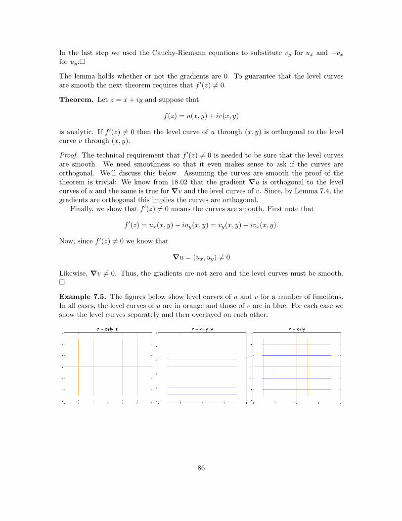
In the last step we used the Cauchy-Riemann equations to substitute vy for ux and −vxfor uy.�
The lemma holds whether or not the gradients are 0. To guarantee that the level curvesare smooth the next theorem requires that f ′(z) 6= 0.
Theorem. Let z = x+ iy and suppose that
f(z) = u(x, y) + iv(x, y)
is analytic. If f ′(z) 6= 0 then the level curve of u through (x, y) is orthogonal to the levelcurve v through (x, y).
Proof. The technical requirement that f ′(z) 6= 0 is needed to be sure that the level curvesare smooth. We need smoothness so that it even makes sense to ask if the curves areorthogonal. We’ll discuss this below. Assuming the curves are smooth the proof of thetheorem is trivial: We know from 18.02 that the gradient ∇u is orthogonal to the levelcurves of u and the same is true for ∇v and the level curves of v. Since, by Lemma 7.4, thegradients are orthogonal this implies the curves are orthogonal.
Finally, we show that f ′(z) 6= 0 means the curves are smooth. First note that
f ′(z) = ux(x, y)− iuy(x, y) = vy(x, y) + ivx(x, y).
Now, since f ′(z) 6= 0 we know that
∇u = (ux, uy) 6= 0
Likewise, ∇v 6= 0. Thus, the gradients are not zero and the level curves must be smooth.�
Example 7.5. The figures below show level curves of u and v for a number of functions.In all cases, the level curves of u are in orange and those of v are in blue. For each case weshow the level curves separately and then overlayed on each other.
86
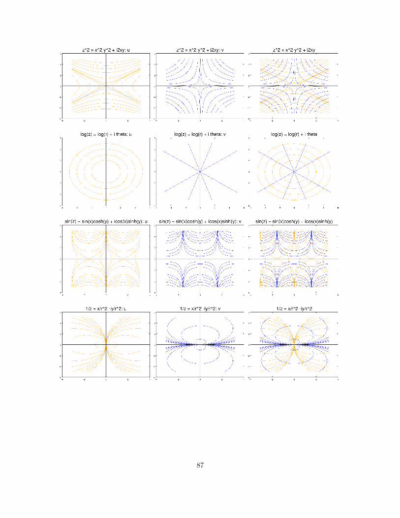
87

88

Example 7.6. Let’s work out the gradients in a few simple examples.
(i) Letf(z) = z2 = (x2 − y2) + i2xy
So∇u = (2x,−2y) and ∇v = (2y, 2x).
It’s trivial to check that ∇u ·∇v = 0, so they are orthogonal.
(ii) Let
f(z) =1
z=
x
r2− i y
r2
So, it’s easy to compute
∇u =
(y2 − x2
r4,−2xy
r4
)and ∇v =
(2xy
r4,y2 − x2
r4
).
Again it’s trivial to check that ∇u ·∇v = 0, so they are orthogonal.
Example 7.7. (Degenerate points: f ′(z) = 0.) Consider
f(z) = z2
From the previous example we have
u(x, y) = x2 − y2, v(x, y) = 2xy, ∇u = (2x,−2y), ∇v = (2y, 2x).
At z = 0, the gradients are both 0 so the theorem on orthogonality doesn’t apply.Let’s look at the level curves through the origin. The level curve (really the ‘level set’)
foru = x2 − y2 = 0
is the pair of lines y = ±x. At the origin this is not a smooth curve.Look at the figures for z2 above. It does appear that away from the origin the level
curves of u intersect the lines where v = 0 at right angles. The same is true for the levelcurves of v and the lines where u = 0. You can see the degeneracy forming at the origin:as the level curves head towards 0 they get pointier and more right angled. So the levelcurve u = 0 is more properly thought of as four right angles. The level curve of u = 0, notknowing which leg of v = 0 to intersect orthogonally takes the average and comes into theorigin at 45◦.
8 Two dimensional hydrodynamics and complex potentials
Laplace’s equation and harmonic functions show up in many physical models. As we havejust seen, harmonic functions in two dimensions are closely linked with complex analyticfunctions. In this section we will exploit this connection to look at two dimensional hydro-dynamics, i.e. fluid flow.
Since static electric fields and steady state temperature distributions are also harmonic,the ideas and pictures we use can be repurposed to cover these topics as well.
89

8.1 Velocity fields
Suppose we have water flowing in a region A of the plane. Then at every point (x, y) in Athe water has a velocity. In general, this velocity will change with time. We’ll let F standfor the velocity vector field and we can write
F(x, y, t) = (u(x, y, t), v(x, y, t)).
The arguments (x, y, t) indicate that the velocity depends on these three variables. Ingeneral, we will shorten the name to velocity field.
A beautiful and mesmerizing example of a velocity field is at http://hint.fm/wind/
index.html. This shows the current velocity of the wind at all points in the continentalU.S.
8.2 Stationary flows
If the velocity field is unchanging in time we call the flow a stationary flow. In this case,we can drop t as an argument and write:
F(x, y) = (u(x, y), v(x, y))
Here are a few examples. These pictures show the streamlines from similar figures intopic 5. We’ve added arrows to indicate the direction of flow.
Example 8.1. Uniform flow. F = (1, 0).
Example 8.2. Eddy (vortex) F = (−y/r2, x/r2)
90
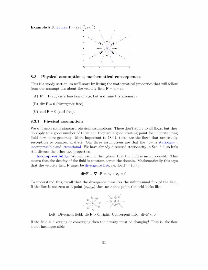
Example 8.3. Source F = (x/r2, y/r2)
8.3 Physical assumptions, mathematical consequences
This is a wordy section, so we’ll start by listing the mathematical properties that will followfrom our assumptions about the velocity field F = u+ iv.
(A) F = F(x, y) is a function of x,y, but not time t (stationary).
(B) div F = 0 (divergence free).
(C) curl F = 0 (curl free).
8.3.1 Physical assumptions
We will make some standard physical assumptions. These don’t apply to all flows, but theydo apply to a good number of them and they are a good starting point for understandingfluid flow more generally. More important to 18.04, these are the flows that are readilysusceptible to complex analysis. Our three assumptions are that the flow is stationary ,incompressible and irrotational. We have already discussed stationarity in Sec. 8.2, so let’sstill discuss the other two properties.
Incompressibility. We will assume throughout that the fluid is incompressible. Thismeans that the density of the fluid is constant across the domain. Mathematically this saysthat the velocity field F must be divergence free, i.e. for F = (u, v):
divF ≡∇ · F = ux + vy = 0.
To understand this, recall that the divergence measures the infinitesimal flux of the field.If the flux is not zero at a point (x0, y0) then near that point the field looks like
Left: Divergent field: divF > 0, right: Convergent field: divF < 0
If the field is diverging or converging then the density must be changing! That is, the flowis not incompressible.
91

As a fluid flow the left hand picture represents a source and the right represents a sink.In electrostatics where F expresses the electric field, the left hand picture is the field of apositive charge density and the right is that of a negative charge density.
If you prefer a non-infinitesimal explanation, we can recall Green’s theorem in flux form.It says that for a simple closed curve C and a field F = (u, v), differentiable on and insideC, the flux of F through C satisfies
Flux of F across C =
∫C
F · n ds =
∫ ∫R
divF dx dy,
where R is the region inside C. Now, suppose that divF(x0, y0) > 0, then divF(x, y) > 0for all (x, y) close to (x0, y0). So, choose a small curve C around (x0, y0) such that divF > 0on and inside C. By Green’s theorem
Flux of F through C =
∫ ∫R
divF dx dy > 0.
Clearly, if there is a net flux out of the region the density is decreasing and the flow isnot incompressible. The same argument would hold if divF(x0, y0) < 0. We conclude thatincompressible is equivalent to divergence free.
Irrotational flow. We will assume that the fluid is irrotational. This means that thethere are no infinitesimal vortices in A. Mathematically this says that the velocity field Fmust be curl free, i.e. for F = (u, v):
curlF ≡∇× F = vx − uy = 0.
To understand this, recall that the curl measures the infinitesimal rotation of the field.Physically this means that a small paddle placed in the flow will not spin as it moves withthe flow.
8.3.2 Examples
Example 8.4. The eddy is irrotational! The eddy from Example 8.2 is irrotational. Thevortex at the origin is not in A = C−{0} and you can easily check that curlF = 0 everywherein A. This is not physically impossible: if you placed a small paddle wheel in the flow itwould travel around the origin without spinning!
Example 8.5. Shearing flows are rotational. Here’s an example of a vector field that hasrotation, though not necessarily swirling.
Re(z)
Im(z)
Shearing flow: box turns because current is faster at the top.
The field F = (ay, 0) is horizontal, but curlF = −a 6= 0. Because the top moves faster than
92

the bottom it will rotate a square parcel of fluid. The minus sign tells you the parcel willrotate clockwise! This is called a shearing flow. The water at one level will be sheared awayfrom the level above it.
8.3.3 Summary
(A) Stationary: F depends on x, y, but not t, i.e.,
F(x, y) = (u(x, y), v(x, y))
(B) Incompressible: divergence free
divF = ux + vy = 0
(C) Irrotational: curl freecurlF = vx − uy = 0
For future reference we put the last two equalities in a numbered equation:
ux = −vy and uy = vx (39)
These look almost like the Cauchy-Riemann equations (with sign differences)!
8.4 Complex potentials
There are different ways to do this. We’ll start by seeing that every complex analyticfunction leads to an irrotational, incompressible flow. Then we’ll go backwards and see thatall such flows lead to an analytic function. We will learn to call the analytic function thecomplex potential of the flow.
Annoyingly, we are going to have to switch notation. Because u and v are already takenby the vector field F, we will call our complex potential
Φ = φ+ iψ
8.4.1 Analytic functions give us incompressible, irrotational flows
Let Φ(z) be an analytic function on a region A. For z = x+ iy we write
Φ(z) = φ(x, y) + iψ(x, y).
From this we can define a vector field
F = ∇φ = (φx, φy) =: (u, v),
here we mean that u and v are defined by φx and φy.
93

From our work on analytic and harmonic functions we can make a list of properties ofthese functions.
1. φ and ψ are both harmonic.
2. The level curves of φ and ψ are orthogonal.
3. Φ′ = φx − iφy.
4. F is divergence and curl free (proof just below). That is, the analytic function Φ hasgiven us an incompressible, irrotational vector field F.
It is standard terminology to call φ a potential function for the vector field F. We will alsocall Φ a complex potential function for F. The function ψ will be called the stream functionof F (the name will be explained soon). The function Φ′ will be called the complex velocity.
Proof. (F is curl and divergence free.) This is an easy consequence of the definition. Wefind
curlF = vx − uy = φyx − φxy = 0
divF = ux + vy = φxx + φyy = 0 (since φ is harmonic).
We’ll postpone examples until after deriving the complex potential from the flow.
8.4.2 Incompressible, irrotational flows always have complex potential func-tions
For technical reasons we need to add the assumption that A is simply connected. This isnot usually a problem because we often work locally in a disk around a point (x0, y0).
Theorem. Assume F = (u, v) is an incompressible, irrotational field on a simply connectedregion A. Then there is an analytic function Φ which is a complex potential function for F.
Proof. We have done all the heavy lifting for this in previous topics. The key is to use theproperty Φ′ = u− iv to guess Φ′. Working carefully we define
g(z) = u− iv
Step 1: Show that g is analytic. Keeping the signs straight, the Cauchy Riemann equationsare
ux = (−v)y and uy = −(−v)x = vx.
But, these are exactly the equations in Equation (39). Thus g(z) is analytic.
Step 2: Since A is simply connected, Cauchy’s theorem says that g(z) has an antiderivativeon A. We call the antiderivative Φ(z).
94

Step 3: Show that Φ(z) is a complex potential function for F. This means we have to showthat if we write Φ = φ+ iψ, then F = ∇φ. To do this we just unwind the definitions.
Φ′ = φx − iφy (standard formula for Φ′)
Φ′ = g = u− iv (definition of Φ and g)
Comparing these equations we get
φx = u, φy = v.
But this says precisely that ∇φ = F. �
Example 8.6. Source fields. The vector field
F = a( xr2,y
r2
)models a source pushing out water or the 2D electric field of a positive charge at the origin.If you prefer a 3D model, it is the field of an infinite wire with uniform charge density alongthe z-axis. Show that F is curl-free and divergence-free and find its complex potential.
We could compute directly that this is curl-free and divergence-free away from 0. Analternative method is to look for a complex potential Φ. If we can find one then this willshow F is curl and divergence free and find φ and ψ all at once. If there is no such Φ thenwe’ll know that F is not both curl and divergence free.
One standard method is to use the formula for Φ′:
Φ′ = u− iv = a(x− iy)
r2= a
z
(zz)=a
z.
This is analytic and we haveΦ(z) = a log(z)
8.5 Stream functions
In everything we did above poor old ψ just tagged along as the harmonic conjugate ofthe potential function φ. Let’s turn our attention to it and see why it’s called the stream
95

function.
Theorem. Suppose thatΦ = φ+ iψ
is the complex potential for a velocity field F. Then the fluid flows along the level curvesof ψ. That is, the F is everywhere tangent to the level curves of ψ. The level curves of ψare called streamlines and ψ is called the stream function.
Proof. Again we have already done most of the heavy lifting to prove this. Since F isthe velocity of the flow at each point, the flow is always tangent to F. You also need toremember that ∇φ is perpendicular to the level curves of φ. So we have:
1. The flow is parallel to F.
2. F = ∇φ, so the flow is orthogonal to the level curves of φ.
3. Since φ and ψ are harmonic conjugates, the level curves of ψ are orthogonal to thelevel curves of φ.
Combining 2 and 3 we see that the flow must be along the level curves of ψ.
8.5.1 Examples
We’ll illustrate the streamlines in a series of examples that start by defining the complexpotential for a vector field.
Example 8.7. Uniform flow. LetΦ(z) = z.
Find F and draw a plot of the streamlines. Indicate the direction of the flow.
Solution: WriteΦ = x+ iy.
Soφ = x , F = ∇φ = (1, 0)
which says the flow has uniform velocity and points to the right. We also have
ψ = y,
so the streamlines are the horizontal lines y = constant.
96

Uniform flow to the right.
Note that another way to see that the flow is to the right is to check the direction that thepotential φ increases. The previous section showed pictures of this complex potential whichshow both the streamlines and the equipotential lines.
Example 8.8. Linear source. Let
Φ(z) = log(z).
Find F and draw a plot of the streamlines. Indicate the direction of the flow.
Solution: WriteΦ = log(r) + iθ
Soφ = log(r) , F = ∇φ = (x/r2, y/r2)
which says the flow is radial and decreases in speed as it gets farther from the origin. Thefield is not defined at z = 0. We also have
ψ = θ
so the streamlines are rays from the origin.
Linear source: radial flow from the origin.
97

8.5.2 Stagnation points
A stagnation point is one where the velocity field is 0.
Stagnation points. If Φ is the complex potential for a field F then the stagnation pointsF = 0 are exactly the points z where Φ′(z) = 0.
Proof. This is clear since F = (φx, φy) and Φ′ = φx − iφy.
Example 8.9. Stagnation points. Draw the streamlines and identify the stagnation pointsfor the potential Φ(z) = z2.
Solution: (We drew the level curves for this in the previous section.) We have
Φ = (x2 − y2) + i2xy
So the streamlines are the hyperbolas: 2xy = constant. Since φ = x2 − y2 increases as |x|increases and decreases as |y| increases, the arrows, which point in the direction of increasingφ, are as shown on the figure below.
Stagnation flow: stagnation point at z = 0.
The stagnation points are the zeros of
Φ′(z) = 2z
i.e. the only stagnation point is at the z = 0.
Note. The stagnation points are what we called the critical points of a vector field in 18.03.
8.6 More examples
Example 8.10. Linear vortex. Analyze the flow with complex potential function
Φ(z) = i log(z).
Solution: Multiplying by i switches the real and imaginary parts of log(z) (with a signchange). We have
Φ = −θ + i log(r)
The stream lines are the curves log(r) = constant, i.e. circles with center at z = 0. Theflow is clockwise because the potential φ = −θ increases in the clockwise direction.
98

Linear vortex.
This flow is called a linear vortex. We can find F using Φ′.
Φ′ =i
z=
y
r2+ i
x
r2= φx − iφy.
SoF = (φx, φy) = (y/r2,−x/r2)
By now this should be a familiar vector field. There are no stagnation points, but there isa singularity at the origin.
Example 8.11. Double source. Analyze the flow with complex potential function
Φ(z) = log(z − 1) + log(z + 1)
Solution: This is a flow with linear sources at ±1. We used Octave to plot the level curvesof ψ = Im(Φ).
Two sources.
We can analyze this flow further as follows.
• Near each source the flow looks like a linear source.
• On the y-axis the flow is along the axis. That is, the y-axis is a streamline. It’s worthseeing three different ways of arriving at this conclusion.
Reason 1: By symmetry of vector fields associated with each linear source, the x componentscancel and the combined field points along the y-axis.
99

Reason 2: We can write
Φ(z) = log(z − 1) + log(z + 1) = log((z − 1)(z + 1)) = log(z2 − 1).
So
Φ′(z) =2z
z2 − 1
On the imaginary axis
Φ′(iy) =2iy
−y2 − 1
Thus,
F =
(0,
2y
y2 + 1
)which is along the axis.Reason 3: On the imaginary axis Φ(iy) = log(−y2 − 1). Since this has constant imaginarypart, the axis is a streamline.
Because of the branch cut for log(z) we should probably be a little more careful here.First note that the vector field F comes from Φ′ = 2z/(z2−1), which doesn’t have a branchcut. So we shouldn’t really have a problem. Now, as z approaches the y-axis from oneside or the other, the argument of log(z2 − 1) approaches either π or −π. That is, as suchlimits, the imaginary part is constant. So the streamline on the y-axis is the limit case ofstreamlines near the axis.
Since Φ′(z) = 0 when z = 0, the origin is a stagnation point. This is where the fieldsfrom the two sources exactly cancel each other.
Example 8.12. A source in uniform flow. Consider the flow with complex potential
Φ(z) = z +Q
2πlog(z).
This is a combination of uniform flow to the right and a source at the origin. The figurebelow was drawn using Octave. It shows that the flow looks like a source near the origin.Farther away from the origin the flow stops being radial and is pushed to the right by theuniform flow.
A source in uniform flow.
Since the components of Φ′ and F are the same except for signs, we can understand theflow by considering
Φ′(z) = 1 +Q
2πz.
100

Near z = 0 the singularity of 1/z is most important and
Φ′ ≈ Q/(2πz)So, the vector field looks a linear source. Far away from the origin the 1/z term is smalland Φ′(z) ≈ 1, so the field looks like uniform flow.
Setting Φ′(z) = 0 we find one stagnation point
z = −Q/(2π)
It is the point on the x-axis where the flow from the source exactly balances that fromthe uniform flow. For bigger values of Q the source pushes fluid farther out before beingoverwhelmed by the uniform flow. That is why Q is called the source strength.
Example 8.13. Source + sink. Consider the flow with complex potential
Φ(z) = log(z − 2)− log(z + 2).
This is a combination of source (log(z − 2)) at z = 2 and a sink (− log(z + 2)) at z = −2.
A source plus a sink.
9 Taylor and Laurent series
We originally defined an analytic function as one where the derivative, defined as a limitof ratios, existed. We went on to prove Cauchy’s theorem and Cauchy’s integral formula.These revealed some deep properties of analytic functions, e.g. the existence of derivativesof all orders.
Our goal in this topic is to express analytic functions as infinite power series. This willlead us to Taylor series. When a complex function has an isolated singularity at a pointwe will replace Taylor series by Laurent series. Not surprisingly we will derive these seriesfrom Cauchy’s integral formula.
Although we come to power series representations after exploring other properties ofanalytic functions, they will be one of our main tools in understanding and computing withanalytic functions.
101

9.1 Geometric series
Having a detailed understanding of geometric series will enable us to use Cauchy’s integralformula to understand power series representations of analytic functions. We start with thedefinition:
Definition. A finite geometric series has one of the following (all equivalent) forms.
Sn = a(1 + r + r2 + r3 + . . .+ rn)
= a+ ar + ar2 + ar3 + . . .+ arn
=n∑j=0
arj
= a
n∑j=0
rj
The number r is called the ratio of the geometric series because it is the ratio of consecutiveterms of the series.
Theorem. The sum of a finite geometric series is given by
Sn = a(1 + r + r2 + r3 + . . .+ rn) =a(1− rn+1)
1− r . (40)
Proof. This is a standard trick that you’ve probably seen before.
Sn = a+ ar + ar2 + . . .+ arn
rSn = ar + ar2 + . . .+ arn +arn+1
When we subtract these two equations most terms cancel and we get
Sn − rSn = a− arn+1
Some simple algebra now gives us the formula in Equation (40).
Definition. An infinite geometric series has the same form as the finite geometric series
except there is no last term:
S = a+ ar + ar2 + . . . = a
∞∑j=0
rj .
Note. We will usually simply say ‘geometric series’ instead of ‘infinite geometric series’.
Theorem. If |r| < 1 then the infinite geometric series converges to
S = a
∞∑j=0
rj =a
1− r (41)
If |r| ≥ 1 then the series does not converge.
Proof. This is an easy consequence of the formula for the sum of a finite geometric series.Simply let n→∞ in Equation (40).
102

9.1.1 Connection to Cauchy’s integral formula
Cauchy’s integral formula says
f(z) =1
2πi
∫C
f(w)
w − z dw
Inside the integral we have the expression
1
w − zwhich looks a lot like the sum of a geometric series. We will make frequent use of thefollowing manipulations of this expression.
1
w − z =1
w· 1
1− z/w =1
w
(1 + (z/w) + (z/w)2 + . . .
)(42)
The geometric series in this equation has ratio z/w. Therefore, the series converges, i.e. theformula is valid, whenever |z/w| < 1, or equivalently when
|z| < |w|
Similarly
1
w − z = −1
z· 1
1− w/z = −1
z
(1 + (w/z) + (w/z)2 + . . .
)(43)
The series converges, i.e. the formula is valid, whenever |w/z| < 1, or equivalently when
|z| > |w|
9.2 Convergence of power series
When we include powers of the variable z in the series we will call it a power series. In thissection we’ll state the main theorem we need about the convergence of power series.
Theorem 9.1. Consider the power series
f(z) =
∞∑n=0
an(z − z0)n
There is a number R ≥ 0 such that:
1. If R > 0 then the series converges absolutely to an analytic function for |z − z0| < R.
2. The series diverges for |z − z0| > R. R is called the radius of convergence. The disk|z − z0| < R is called the disk of convergence.
3. The derivative is given by term-by-term differentiation
f ′(z) =
∞∑n=0
nan(z − z0)n−1
The series for f ′ also has radius of convergence R.
103

4. If γ is a bounded curve inside the disk of convergence then the integral is given byterm-by-term integration ∫
γf(z) dz =
∞∑n=0
∫γan(z − z0)n
Notes.
• The theorem doesn’t say what happens when |z − z0| = R.
• If R =∞ the function f(z) is entire.
• If R = 0 the series only converges at the point z = z0. In this case, the series doesnot represent an analytic function on any disk around z0.
• Often (not always) we can find R using the ratio test.
9.2.1 Ratio test and root test
Here are two standard tests from calculus on the convergence of infinite series.
Ratio test. Consider the series∑∞
0 cn. If L = limn→∞ |cn+1/cn| exists, then:
1. If L < 1 then the series converges absolutely.
2. If L > 1 then the series diverges.
3. If L = 1 then the test gives no information.
Note. In words, L is the limit of the absolute ratios of consecutive terms.
Example 9.2. Consider the geometric series 1+z+z2 +z3 + . . .. The limit of the absoluteratios of consecutive terms is
L = limn→∞
|zn+1||zn| = |z|
Thus, the ratio test agrees that the geometric series converges when |z| < 1. We know thisconverges to 1/(1− z). Note, the disk of convergence ends exactly at the singularity z = 1.
Example 9.3. Consider the series f(z) =∞∑n=0
zn
n!. The limit from the ratio test is
L = limn→∞
|zn+1|/(n+ 1)!
|zn|/n!= lim
|z|n+ 1
= 0.
Since L < 1 this series converges for every z. Thus, by Theorem 9.1, the radius of conver-gence for this series is ∞. That is, f(z) is entire. Of course we know that f(z) = ez.
Root test. Consider the series∑∞
0 cn. If L = limn→∞ |cn|1/n exists, then:
1. If L < 1 then the series converges absolutely.
104

2. If L > 1 then the series diverges.
3. If L = 1 then the test gives no information .
Note. In words, L is the limit of the nth roots of the (absolute value) of the terms.
The geometric series is so fundamental that we should check the root test on it.
Example 9.4. Consider the geometric series 1 + z + z2 + z3 + . . .. The limit of the nthroots of the terms is
L = limn→∞
|zn|1/n = lim |z| = |z|
Happily, the root test agrees that the geometric series converges when |z| < 1.
9.3 Taylor series
The previous section showed that a power series converges to an analytic function inside itsdisk of convergence. Taylor’s theorem completes the story by giving the converse: aroundeach point of analyticity an analytic function equals a convergent power series.
Theorem 9.5. (Taylor’s theorem) Suppose f(z) is an analytic function in a region A. Letz0 ∈ A. Then,
f(z) =∞∑n=0
an(z − z0)n,
where the series converges on any disk |z − z0| < r contained in A. Furthermore, we haveformulas for the coefficients
an =f (n)(z0)
n!=
1
2πi
∫γ
f(z)
(z − z0)n+1dz. (44)
(Where γ is any simple closed curve in A around z0, with its interior entirely in A.)
We call the series the power series representing f around z0.
The proof will be given below. First we look at some consequences of Taylor’s theorem.
Corollary. The power series representing an analytic function around a point z0 is unique.That is, the coefficients are uniquely determined by the function f(z).
Proof. Taylor’s theorem gives a formula for the coefficients.
9.3.1 Order of a zero
Theorem. Suppose f(z) is analytic on the disk |z − z0| < r and f is not identically 0.Then there is an integer k ≥ 0 such that ak 6= 0 and f has Taylor series around z0 given by
f(z) = (z − z0)k(ak + ak+1(z − z0) + . . .) = (z − z0)k∞∑n=k
an(z − z0)n−k. (45)
105

Proof. Since f(z) is not identically 0, not all the Taylor coefficients are zero. So, we take kto be the index of the first nonzero coefficient.
Theorem 9.6. Zeros are isolated. If f(z) is analytic and not identically zero then the zerosof f are isolated (by isolated we mean that we can draw a small disk around any zeros thatdoesn’t contain any other zeros).
Isolated zero at z0: f(z0) = 0, f(z) 6= 0 elsewhere in the disk.
Proof. Suppose f(z0) = 0. Write f as in Equation (45). There are two factors:
(z − z0)k
andg(z) = ak + ak+1(z − z0) + . . .
Clearly (z − z0)k 6= 0 if z 6= z0. We have g(z0) = ak 6= 0, so g(z) is not 0 on some smallneighborhood of z0. We conclude that on this neighborhood the product is only zero whenz = z0, i.e. z0 is an isolated 0.
Definition. The integer k in Theorem 9.6 is called the order of the zero of f at z0.
Note, if f(z0) 6= 0 then z0 is a zero of order 0.
9.3.2 Taylor series examples
The uniqueness of Taylor series along with the fact that they converge on any disk aroundz0 where the function is analytic allows us to use lots of computational tricks to find theseries and be sure that it converges.
Example 9.7. Use the formula for the coefficients in terms of derivatives to give the Taylorseries of f(z) = ez around z = 0.
Solution: Since f ′(z) = ez, we have f (n)(0) = e0 = 1. So,
ez = 1 + z +z2
2!+z3
3!+ . . . =
∞∑n=0
zn
n!
106

Example 9.8. Expand f(z) = z8e3z in a Taylor series around z = 0.
Solution: Let w = 3z. So,
e3z = ew =∞∑n=0
wn
n!=∞∑k=0
3n
n!zn
Thus,
f(z) =
∞∑n=0
3n
n!zn+8.
Example 9.9. Find the Taylor series of sin(z) around z = 0 (Sometimes the Taylor seriesaround 0 is called the Maclaurin series.)
Solution: We give two methods for doing this.Method 1.
f (n)(0) =dn sin(z)
dzn=
{(−1)m for n = 2m+ 1 = odd, m = 0, 1, 2, . . .
0 for n even
Method 2. Using
sin(z) =eiz − e−iz
2i
we have
sin(z) =1
2i
[ ∞∑n=0
(iz)n
n!−∞∑n=0
(−iz)nn!
]=
1
2i
∞∑n=0
[(1− (−1)n)]inzn
n!
(We need absolute convergence to add series like this.)Conclusion:
sin(z) =∞∑n=0
(−1)nz2n+1
(2n+ 1)!,
which converges for |z| <∞.Example 9.10. Expand the rational function
f(z) =1 + 2z2
z3 + z5
around z = 0.
Solution: Note that f has a singularity at 0, so we can’t expect a convergent Taylor seriesexpansion. We’ll aim for the next best thing using the following shortcut.
f(z) =1
z3
2(1 + z2)− 1
1 + z2=
1
z3
[2− 1
1 + z2
].
Using the geometric series we have
1
1 + z2=
1
1− (−z2)=
∞∑n=0
(−z2)n = 1− z2 + z4 − z6 + . . .
107

Putting it all together
f(z) =1
z3
(2− 1 + z2 − z4 + . . .
)=
(1
z3+
1
z
)−∞∑n=0
(−1)nz2n+1
Note. The first terms are called the singular part, i.e. those with negative powers of z. Thesummation is called the regular or analytic part. Since the geometric series for 1/(1 + z2)converges for |z| < 1, the entire series is valid in 0 < |z| < 1
Example 9.11. Find the Taylor series for
f(z) =ez
1− zaround z = 0. Give the radius of convergence.
Solution: We start by writing the Taylor series for each of the factors and then multiplythem out.
f(z) =
(1 + z +
z2
2!+z3
3!+ . . .
)(1 + z + z2 + z3 + . . .
)= 1 + (1 + 1)z +
(1 + 1 +
1
2!
)z2 +
(1 + 1 +
1
2!+
1
3!
)z3 + . . .
The biggest disk around z = 0 where f is analytic is |z| < 1. Therefore, by Taylor’s theorem,the radius of convergence is R = 1.
f(z) is analytic on |z| < 1 and has a singularity at z = 1.
Example 9.12. Find the Taylor series for
f(z) =1
1− zaround z = 5. Give the radius of convergence.
Solution: We have to manipulate this into standard geometric series form.
f(z) =1
−4(1 + (z − 5)/4)= −1
4
(1−
(z − 5
4
)+
(z − 5
4
)2
−(z − 5
4
)3
+ . . .
)Since f(z) has a singularity at z = 1 the radius of convergence is R = 4. We can also seethis by considering the geometric series. The geometric series ratio is (z − 5)/4. So theseries converges when |z − 5|/4 < 1, i.e. when |z − 5| < 4, i.e. R = 4.
108

Disk of convergence stops at the singularity at z = 1.
Example 9.13. Find the Taylor series for
f(z) = log(1 + z)
around z = 0. Give the radius of convergence.
Solution: We know that f is analytic for |z| < 1 and not analytic at z = −1. So, the radiusof convergence is R = 1. To find the series representation we take the derivative and usethe geometric series.
f ′(z) =1
1 + z= 1− z + z2 − z3 + z4 − . . .
Integrating term by term (allowed by Theorem 9.1) we have
f(z) = a0 + z − z2
2+z3
3− z4
4+ . . . = a0 +
∞∑n=1
(−1)n−1 zn
n
Here a0 is the constant of integration. We find it by evalating at z = 0.
f(0) = a0 = log(1) = 0.
Disk of convergence for log(1 + z) around z = 0.
Example 9.14. Can the series ∑an(z − 2)n
converge at z = 0 and diverge at z = 3.
Solution: No! We have z0 = 2. We know the series diverges everywhere outside its radiusof convergence. So, if the series converges at z = 0, then the radius of convergence is atleast 2. Since |3− z0| < 2 we would also have that z = 3 is inside the disk of convergence.
109

9.3.3 Proof of Taylor’s theorem
For convenience we restate Taylor’s Theorem 9.5.
Taylor’s theorem. (Taylor series) Suppose f(z) is an analytic function in a region A. Letz0 ∈ A. Then,
f(z) =∞∑n=0
an(z − z0)n,
where the series converges on any disk |z − z0| < r contained in A. Furthermore, we haveformulas for the coefficients
an =f (n)(z0)
n!=
1
2πi
∫γ
f(z)
(z − z0)n+1dz (46)
Proof. In order to handle convergence issues we fix 0 < r1 < r2 < r. We let γ be the circle|w − z0| = r2 (traversed counterclockise).
Disk of convergence extends to the boundary of Ar1 < r2 < r, but r1 and r2 can be arbitrarily close to r.
Take z inside the disk |z − z0| < r1. We want to express f(z) as a power series around z0.To do this we start with the Cauchy integral formula and then use the geometric series.
As preparation we note that for w on γ and |z − z0| < r1 we have
|z − z0| < r1 < r2 = |w − z0|
so|z − z0||w − z0|
< 1.
Therefore,
1
w − z =1
w − z0· 1
1− z−z0w−z0
=1
w − z0
∞∑n=0
(z − z0
w − z0
)n=
∞∑n=0
(z − z0)n
(w − z0)n+1
110

Using this and the Cauchy formula gives
f(z) =1
2πi
∫γ
f(w)
w − z dw
=1
2πi
∫γ
∞∑n=0
f(w)
(w − z0)n+1(z − z0)n dw
=∞∑n=0
(1
2πi
∫γ
f(w)
(w − z0)n+1dw
)(z − z0)n
=
∞∑n=0
f (n)(z0)
n!(z − z0)n
The last equality follows from Cauchy’s formula for derivatives. Taken together the lasttwo equalities give Taylor’s formula. �
9.4 Singularities
Definition. A function f(z) is singular at a point z0 if it is not analytic at z0
Definition. For a function f(z), the singularity z0 is an isolated singularity if f is analytic
on the deleted disk 0 < |z − z0| < r for some r > 0.
Example 9.15. f(z) =z + 1
z3(z2 + 1)has isolated singularities at z = 0,±i.
Example 9.16. f(z) = e1/z has an isolated singularity at z = 0.
Example 9.17. f(z) = log(z) has a singularity at z = 0, but it is not isolated because abranch cut, starting at z = 0, is needed to have a region where f is analytic.
Example 9.18. f(z) =1
sin(π/z)has singularities at z = 0 and z = 1/n for n = ±1,±2, . . .
The singularities at ±1/n are isolated, but the one at z = 0 is not isolated.
Every neighborhood of 0 contains zeros at 1/n for large n.
9.5 Laurent series
Theorem 9.19. (Laurent series). Suppose that f(z) is analytic on the annulus
A : r1 < |z − z0| < r2
111

Then f(z) can be expressed as a series
f(z) =∞∑n=1
bn(z − z0)n
+∞∑n=0
an(z − z0)n.
The coefficients have the formulus
an =1
2πi
∫γ
f(w)
(w − z0)n+1dw
bn =1
2πi
∫γf(w)(w − z0)n−1 dw,
where γ is any circle |w − z0| = r inside the annulus, i.e. r1 < r < r2.Furthermore
• The series
∞∑n=0
an(z − z0)n converges to an analytic function for |z − z0| < r2.
• The series
∞∑n=1
bn(z − z0)n
converges to an analytic function for |z − z0| > r1.
• Together, the series both converge on the annulus A where f is analytic.
The proof is given below. First we define a few terms.
Definition. The entire series is called the Laurent series for f around z0. The series
∞∑n=0
an(z − z0)n
is called the analytic or regular part of the Laurent series. The series
∞∑n=1
bn(z − z0)n
is called the singular or principal part of the Laurent series.
Note. Since f(z) may not be analytic (or even defined) at z0 we don’t have any formulasfor the coefficients using derivatives.
Proof. (Laurent series). Choose a point z in A. Now set circles C1 and C3 close enough tothe boundary that z is inside C1 +C2−C3−C2 as shown. Since this curve and its interiorare contained in A, Cauchy’s integral formula says
f(z) =1
2πi
∫C1+C2−C3−C2
f(w)
w − z dw
112

The contour used for proving the formulas for Laurent series.
The integrals over C2 cancel, so we have
f(z) =1
2πi
∫C1−C3
f(w)
w − z dw.
Next, we divide this into two pieces and use our trick of converting to a geometric series.The calculuations are just like the proof of Taylor’s theorem. On C1 we have
|z − z0||w − z0|
< 1
so
1
2πi
∫C1
f(w)
w − z dw =1
2πi
∫C1
f(w)
w − z0· 1(
1− z−z0w−z0
) dw=
1
2πi
∫C1
∞∑n=0
f(w)
(w − z0)n+1(z − z0)n dw
=∞∑n=0
(1
2πi
∫C1
f(w)
(w − z0)n+1dw
)(z − z0)n
=∞∑n=0
an(z − z0)n
Here an is defined by the integral formula given in the statement of the theorem. Examiningthe above argument we see that the only requirement on z is that |z − z0| < r2. So, thisseries converges for all such z.
Similarly on C3 we have|w − z0||z − z0|
< 1
113

so
1
2πi
∫C3
f(w)
w − z dw =1
2πi
∫C3
− f(w)
z − z0· 1(
1− w−z0z−z0
) dw= − 1
2πi
∫C3
∞∑n=0
f(w)(w − z0)n
(z − z0)n+1dw
= − 1
2πi
∞∑n=0
(∫C1
f(w)(w − z0)n dw
)(z − z0)−n−1
= −∞∑n=1
bn(z − z0)n
In the last equality we changed the indexing to match the indexing in the statement of thetheorem. Here bn is defined by the integral formula given in the statement of the theorem.Examining the above argument we see that the only requirement on z is that |z − z0| > r1.So, this series converges for all such z.
Combining these two formulas we have
f(z) =1
2πi
∫C1−C3
f(w)
w − z dw =∞∑n=1
bn(z − z0)n
+∞∑n=0
an(z − z0)n
The last thing to note is that the integrals defining an and bn do not depend on the exactradius of the circle of integration. Any circle inside A will produce the same values. Wehave proved all the statements in the theorem on Laurent series. �
9.5.1 Examples of Laurent series
In general, the integral formulas are not a practical way of computing the Laurent coef-ficients. Instead we use various algebraic tricks. Even better, as we shall see, is the factthat often we don’t really need all the coefficients and we will develop more techniques tocompute those that we do need.
Example 9.20. Find the Laurent series for
f(z) =z + 1
z
around z0 = 0. Give the region where it is valid.
Solution: The answer is simply
f(z) = 1 +1
z
This is a Laurent series, valid on the infinite region 0 < |z| <∞.
Example 9.21. Find the Laurent series for
f(z) =z
z2 + 1
114

around z0 = i. Give the region where your answer is valid. Identify the singular (principal)part.
Solution: Using partial fractions we have
f(z) =1
2· 1
z − i +1
2· 1
z + i
Since1
z + iis analytic at z = i it has a Taylor series expansion. We find it using geometric
series:1
z + i=
1
2i· 1
1 + (z − i)/(2i) =1
2i
∞∑n=0
(−z − i
2i
)nSo the Laurent series is
f(z) =1
2· 1
z − i +1
4i
∞∑n=0
(−z − i
2i
)nThe singular (principal) part is given by the first term. The region of convergence is0 < |z − i| < 2.
Note. We could have looked at f(z) on the region 2 < |z − i| < ∞. This would haveproduced a different Laurent series. We discuss this further in an upcoming example.
Example 9.22. Compute the Laurent series for
f(z) =z + 1
z3(z2 + 1)
on the region A : 0 < |z| < 1 centered at z = 0.
Solution: This function has isolated singularities at z = 0,±i. Therefore it is analytic on
the region A.
f(z) has singularities at z = 0,±i.
At z = 0 we have
f(z) =1
z3(1 + z)(1− z2 + z4 − z6 + . . .)
Multiplying this out we get
f(z) =1
z3+
1
z2− 1
z− 1 + z + z2 − z3 − . . . .
115

The following example shows that the Laurent series depends on the region under consid-eration.
Example 9.23. Find the Laurent series around z = 0 for f(z) =1
z(z − 1)in each of the
following regions:
• (i) the region A1 : 0 < |z| < 1
• (ii) the region A2 : 1 < |z| <∞.
Solution: For (i)
f(z) = −1
z· 1
1− z = −1
z(1 + z + z2 + . . .) = −1
z− 1− z − z2 − . . .
For (ii): Since the usual geometric series for 1/(1 − z) does not converge on A2 we need adifferent form,
f(z) =1
z· 1
z(1− 1/z)=
1
z2
(1 +
1
z+
1
z2+ . . .
)Since |1/z| < 1 on A2 our use of the geometric series is justified.
One lesson from this example is that the Laurent series depends on the region as wellas the formula for the function.
9.6 Digression to differential equations
Here is a standard use of series for solving differential equations.
Example 9.24. Find a power series solution to the equation
f ′(x) = f(x) + 2 , f(0) = 0
Solution: We look for a solution of the form
f(x) =∞∑n=0
anxn.
Using the initial condition we find f(0) = 0 = a0. Substituting the series into the differentialequation we get
f ′(x) = a1 + 2a2x+ 3a3x3 + . . . = f(x) + 2 = a0 + 2 + a1x+ a2x
2 + . . .
Equating coefficients and using a0 = 0 we have
a1 = a0 + 2 ⇒ a1 = 2
2a2 = a1 ⇒ a2 = a1/2 = 1
3a3 = a2 ⇒ a3 = 1/3
4a4 = a3 ⇒ a4 = 1/(3 · 4)
116
In general
(n+ 1)an+1 = an ⇒ an+1 =an
(n+ 1)=
1
3 · 4 · 5 · · · (n+ 1).
You can check using the ratio test that this function is entire.
9.7 Poles
Poles refer to isolated singularities. So, we suppose f(z) is analytic on 0 < |z − z0| < r andhas Laurent series
f(z) =∞∑n=1
bn(z − z0)n
+∞∑n=0
an(z − z0)n.
117

Definition of poles. If only a finite number of the coefficients bn are nonzero we sayz0 is a finite pole of f . In this case, if bk 6= 0 and bn = 0 for all n > k then we say z0 is apole of order k.
• If z0 is a pole of order 1 we say it is a simple pole of f .
• If an infinite number of the bn are nonzero we say that z0 is an essential singularityor a pole of infinite order of f .
• If all the bn are 0, then z0 is called a removable singularity. That is, if we definef(z0) = a0 then f is analytic on the disk |z − z0| < r.
The terminology can be a bit confusing. So, imagine that I tell you that f is defined andanalytic on the punctured disk 0 < |z−z0| < r. Then, a priori we assume f has a singularityat z0. But, if after computing the Laurent series we see there is no singular part we canextend the definition of f to the full disk, thereby ‘removing the singularity’.
We can explain the term essential singularity as follows. If f(z) has a pole of order kat z0 then (z − z0)kf(z) is analytic (has a removable singularity) at z0. So, f(z) itself isnot much harder to work with than an analytic function. On the other hand, if z0 is anessential singularity then no algebraic trick will change f(z) into an analytic function at z0.
9.7.1 Examples of poles
We’ll go back through many of the examples from the previous sections.
Example 9.25. The rational function
f(z) =1 + 2z2
z3 + z5
expanded to
f(z) =
(1
z3+
1
z
)−∞∑n=0
(−1)nz2n+1.
Thus, z = 0 is a pole of order 3.
Example 9.26. Consider
f(z) =z + 1
z= 1 +
1
z
Thus, z = 0 is a pole of order 1, i.e. a simple pole.
Example 9.27. Consider
f(z) =z
z2 + 1=
1
2· 1
z − i + g(z),
where g(z) is analytic at z = i. So, z = i is a simple pole.
118

Example 9.28. The function
f(z) =1
z(z − 1)
has isolated singularities at z = 0 and z = 1. Show that both are simple poles.
Solution: In a neighborhood of z = 0 we can write
f(z) =g(z)
z, g(z) =
1
z − 1
Since g(z) is analytic at 0, z = 0 is a finite pole. Since g(0) 6= 0, the pole has order 1, i.e.it is simple.
Likewise, in a neighborhood of z = 1,
f(z) =h(z)
z − 1, h(z) =
1
z
Since h is analytic at z = 1, f has a finite pole there. Since h(1) 6= 0 it is simple.
Example 9.29. Consider
e1/z = 1 +1
z+
1
2!z2+
1
3!z3+ . . .
So, z = 0 is an essential singularity.
Example 9.30. log(z) has a singularity at z = 0. Since the singularity is not isolated, itcan’t be classified as either a pole or an essential singularity.
9.7.2 Residues
In preparation for discussing the residue theorem in the next topic we give the definitionand an example here.
Note well, residues have to do with isolated singularites.
Definition 9.31. Consider the function f(z) with an isolated singularity at z0, i.e. definedon 0 < |z − z0| < r and with Laurent series
f(z) =∞∑n=1
bn(z − z0)n
+∞∑n=0
an(z − z0)n.
The residue of f at z0 is b1. This is denoted
Res(f, z0) or Resz=z0
f = b1.
What is the importance of the residue? If γ is a small, simple closed curve that goescounterclockwise around z0 then ∫
γf(z) = 2πib1.
119

γ is small enough to be inside |z − z0| < r, and surround z0.
This is easy to see by integrating the Laurent series term by term. The only nonzero integralcomes from the term b1/z.
Example 9.32. The function
f(z) = e1/(2z) = 1 +1
2z+
1
2(2z)2+ . . .
has an isolated singularity at 0. From the Laurent series we see that
Res(f, 0) =1
2
10 Residue Theorem
10.1 Poles and zeros
We remind you of the following terminology: Suppose f(z) is analytic at z0 and
f(z) = an(z − z0)n + an+1(z − z0)n+1 + . . .
with an 6= 0. Then we say f has a zero of order n at z0. If n = 1 we say z0 is a simple zero.Suppose f has an isolated singularity at z0 and Laurent series
f(z) =bn
(z − z0)n+
bn−1
(z − z0)n−1+ . . .+
b1z − z0
+ a0 + a1(z − z0) + . . .
which converges on 0 < |z − z0| < R and with bn 6= 0. Then we say f has a pole of ordern at z0. If n = 1 we say z0 is a simple pole. There were several examples in the previoussection. Here is one more
Example 10.1.
f(z) =z + 1
z3(z2 + 1)
has isolated singularities at z = 0,±i and a zero at z = −1. We will show that z = 0 is apole of order 3, z = ±i are poles of order 1 and z = −1 is a zero of order 1. The style ofargument is the same in each case.
120

At z = 0:
f(z) =1
z3· z + 1
z2 + 1
Call the second factor g(z). Since g(z) is analytic at z = 0 and g(0) = 1, it has a Taylorseries
g(z) =z + 1
z2 + 1= 1 + a1z + a2z
2 + . . .
Therefore
f(z) =1
z3+a1
z2+a2
z+ . . .
This shows z = 0 is a pole of order 3.At z = i:
f(z) =1
z − i ·z + 1
z3(z + i)
Call the second factor g(z). Since g(z) is analytic at z = i, it has a Taylor series
g(z) =z + 1
z3(z + i)= a0 + a1(z − i) + a2(z − i)2 + . . .
where a0 = g(i) 6= 0. Therefore
f(z) =a0
z − i + a1 + a2(z − i) + . . .
This shows z = i is a pole of order 1.The arguments for z = −i and z = −1 are similar.
10.2 Words: Holomorphic and meromorphic
Definition. A function that is analytic on a region A is called holomorphic on A.A function that is analytic on A except for a set of poles of finite order is called meromorphicon A.
Example 10.2. Let
f(z) =z + z2 + z3
(z − 2)(z − 3)(z − 4)(z − 5).
This is meromorphic on C with (simple) poles at z = 2, 3, 4, 5.
10.3 Behavior of functions near zeros and poles
The basic idea is that near a zero of order n, a function behaves like (z − z0)n and near apole of order n, a function behaves like 1/(z − z0)n. The following make this a little moreprecise.
Behavior near a zero. If f has a zero of order n at z0 then near z0,
f(z) ≈ an(z − z0)n
for some constant an.
121

Proof. By definition f has a Taylor series around z0 of the form
f(z) = an(z − z0)n + an+1(z − z0)n+1 + . . .
= an(z − z0)n(
1 +an+1
an(z − z0) +
an+2
an(z − z0)2 + . . .
)Since the second factor equals 1 at z0, the claim follows.
Behavior near a finite pole. If f has a pole of order n at z0 then near z0,
f(z) ≈ bn(z − z0)n
,
for some constant bn.
Proof. This is nearly identical to the previous argument. By definition f has a Laurentseries around z0 of the form
f(z) =bn
(z − z0)n+
bn−1
(z − z0)n−1+ . . .+
b1z − z0
+ a0 + . . .
=bn
(z − z0)n
(1 +
bn−1
bn(z − z0) +
bn−2
bn(z − z0)2 + . . .
)Since the second factor equals 1 at z0, the claim follows.
10.3.1 Picard’s theorem and essential singularities
Near an essential singularity we have Picard’s theorem. We won’t prove or make use of thistheorem in 18.04. Still, we feel it is pretty enough to warrant showing to you.
Picard’s theorem. If f(z) has an essential singularity at z0 then in every neighborhoodof z0, f(z) takes on all possible values infinitely many times, with the possible exception ofone value.
Example 10.3. It is easy to see that in any neighborhood of z = 0 the function w = e1/z
takes every value except w = 0.
10.3.2 Quotients of functions
We have the following statement about quotients of functions. We could make similarstatements if one or both functions has a pole instead of a zero.
Theorem. Suppose f has a zero of order m at z0 and g has a zero of order n at z0. Let
h(z) =f(z)
g(z).
122

Then
• If n > m then h(z) has a pole of order n−m at z0.
• If n < m then h(z) has a zero of order m− n at z0.
• If n = m then h(z) is analytic and nonzero at z0.
We can paraphrase this as h(z) has ‘pole’ of order n −m at z0. If n −m is negative thenthe ‘pole’ is actually a zero.
Proof. You should be able to supply the proof. It is nearly identical to the proofs above:express f and g as Taylor series and take the quotient.
Example 10.4. Let
h(z) =sin(z)
z2
We know sin(z) has a zero of order 1 at z = 0 and z2 has a zero of order 2. So, h(z) has apole of order 1 at z = 0. Of course, we can see this easily using Taylor series
h(z) =1
z2
(z − z3
3!+ . . .
)
10.4 Residues
In this section we’ll explore calculating residues. We’ve seen enough already to know thatthis will be useful. We will see that even more clearly when we look at the residue theoremin the next section.
We introduced residues in the previous topic. We repeat the definition here for com-pleteness.
Definition. Consider the function f(z) with an isolated singularity at z0, i.e. defined onthe region 0 < |z − z0| < r and with Laurent series (on that region)
f(z) =∞∑n=1
bn(z − z0)n
+∞∑n=0
an(z − z0)n.
The residue of f at z0 is b1. This is denoted
Res(f, z0) = b1 or Resz=z0
f = b1.
What is the importance of the residue? If γ is a small, simple closed curve that goescounterclockwise around b1 then ∫
γf(z) = 2πib1.
123
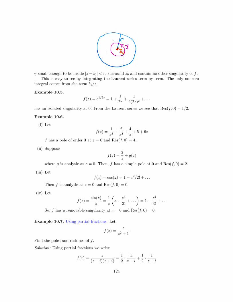
γ small enough to be inside |z− z0| < r, surround z0 and contain no other singularity of f .This is easy to see by integrating the Laurent series term by term. The only nonzero
integral comes from the term b1/z.
Example 10.5.
f(z) = e1/2z = 1 +1
2z+
1
2(2z)2+ . . .
has an isolated singularity at 0. From the Laurent series we see that Res(f, 0) = 1/2.
Example 10.6.
(i) Let
f(z) =1
z3+
2
z2+
4
z+ 5 + 6z
f has a pole of order 3 at z = 0 and Res(f, 0) = 4.
(ii) Suppose
f(z) =2
z+ g(z)
where g is analytic at z = 0. Then, f has a simple pole at 0 and Res(f, 0) = 2.
(iii) Letf(z) = cos(z) = 1− z2/2! + . . .
Then f is analytic at z = 0 and Res(f, 0) = 0.
(iv) Let
f(z) =sin(z)
z=
1
z
(z − z3
3!+ . . .
)= 1− z2
3!+ . . .
So, f has a removable singularity at z = 0 and Res(f, 0) = 0.
Example 10.7. Using partial fractions. Let
f(z) =z
z2 + 1
Find the poles and residues of f .
Solution: Using partial fractions we write
f(z) =z
(z − i)(z + i)=
1
2· 1
z − i +1
2· 1
z + i
124
The poles are at z = ±i. We compute the residues at each pole:At z = i:
f(z) =1
2· 1
z − i + something analytic at i
Therefore the pole is simple and Res(f, i) = 1/2.At z = −i:
f(z) =1
2· 1
z + i+ something analytic at − i
Therefore the pole is simple and Res(f,−i) = 1/2.
Example 10.8. Mild warning! Let
f(z) = − 1
z(1− z)
then we have the following Laurent expansions for f around z = 0.On 0 < |z| < 1:
f(z) = −1
z· 1
1− z = −1
z(1 + z + z2 + . . .)
Therefore the pole at z = 0 is simple and Res(f, 0) = −1.On 1 < |z| <∞:
f(z) =1
z2· 1
1− 1/z=
1
z2
(1 +
1
z+
1
z2+ . . .
)Even though this is a valid Laurent expansion you must not use it to compute the residueat 0. This is because the definition of residue requires that we use the Laurent series on theregion 0 < |z − z0| < r.
Example 10.9. Letf(z) = log(1 + z)
This has a singularity at z = −1, but it is not isolated, so not a pole and therefore there isno residue at z = −1.
10.4.1 Residues at simple poles
Simple poles occur frequently enough that we’ll study computing their residues in somedetail. Here are a number of ways to spot a simple pole and compute its residue. Thejustification for all of them goes back to Laurent series.
Suppose f(z) has an isolated singularity at z = z0. Then we have the following properties.
Property 1. If the Laurent series for f(z) has the form
b1z − z0
+ a0 + a1(z − z0) + . . .
then f has a simple pole at z0 and Res(f, z0) = b1.
125

Property 2 Ifg(z) = (z − z0)f(z)
is analytic at z0 then z0 is either a simple pole or a removable singularity. In either caseRes(f, z0) = g(z0). (In the removable singularity case the residue is 0.)
Proof. Directly from the Laurent series for f around z0.
Property 3. If f has a simple pole at z0 then
limz→z0
(z − z0)f(z) = Res(f, z0)
This says that the limit exists and equals the residue. Conversely, if the limit exists theneither the pole is simple, or f is analytic at z0. In both cases the limit equals the residue.
Proof. Directly from the Laurent series for f around z0.
Property 4. If f has a simple pole at z0 and g(z) is analytic at z0 then
Res(fg, z0) = g(z0) Res(f, z0)
If g(z0) 6= 0 then
Res(f/g, z0) =1
g(z0)Res(f, z0)
Proof. Since z0 is a simple pole,
f(z) =b1
z − z0+ a0 + a1(z − z0)
Since g is analytic,g(z) = c0 + c1(z − z0) + . . . ,
where c0 = g(z0). Multiplying these series together it is clear that
Res(fg, z0) = c0b1 = g(z0) Res(f, z0). �
The statement about quotients f/g follows from the proof for products because 1/g isanalytic at z0.
Property 5. If g(z) has a simple zero at z0 then 1/g(z) has a simple pole at z0 and
Res(1/g, z0) =1
g′(z0)
Proof. The algebra for this is similar to what we’ve done several times above. The Taylorexpansion for g is
g(z) = a1(z − z0) + a2(z − z0)2 + . . . ,
126
where a1 = g′(z0). So
1
g(z)=
1
a1(z − z0)
(1
1 + a2a1
(z − z0) + . . .
)
The second factor on the right is analytic at z0 and equals 1 at z0. Therefore we know theLaurent expansion of 1/g is
1
g(z)=
1
a1(z − z0)(1 + c1(z − z0) + . . .)
Clearly the residue is 1/a1 = 1/g′(z0). �
Example 10.10. Let
f(z) =2 + z + z2
(z − 2)(z − 3)(z − 4)(z − 5).
Show all the poles are simple and compute their residues.
Solution: The poles are at z = 2, 3, 4, 5. They are all isolated. We’ll look at z = 2 theothers are similar. Multiplying by z − 2 we get
g(z) = (z − 2)f(z) =2 + z + z2
(z − 3)(z − 4)(z − 5).
This is analytic at z = 2 and g(2) =8
−6= −4
3. So the pole is simple and Res(f, 2) = −4/3.
Example 10.11. Let
f(z) =1
sin(z)
Find all the poles and their residues.
Solution: The poles of f(z) are the zeros of sin(z), i.e. nπ for n an integer. Since thederivative
sin′(nπ) = cos(nπ) 6= 0
the zeros are simple and by Property 5 above
Res(f, nπ) =1
cos(nπ)= (−1)n
Example 10.12. Let
f(z) =1
z(z2 + 1)(z − 2)2
Identify all the poles and say which ones are simple.
Solution: Clearly the poles are at z = 0,±i, 2.At z = 0:
g(z) = zf(z)
127
is analytic at 0 and g(0) = 1/4. So the pole is simple and the residue is g(0) = 1/4.At z = i:
g(z) = (z − i)f(z) =1
z(z + i)(z − 2)2
is analytic at i, the pole is simple and the residue is g(i).At z = −i: This is similar to the case z = i. The pole is simple.At z = 2:
g(z) = (z − 2)f(z) =1
z(z2 + 1)(z − 2)
is not analytic at 2, so the pole is not simple. (It should be obvious that it’s a pole of order2.)
Example 10.13. Let p(z), q(z) be analytic at z = z0. Assume p(z0) 6= 0, q(z0) = 0,q′(z0) 6= 0. Find
Resz=z0
p(z)
q(z)
Solution: Since q′(z0) 6= 0, q has a simple zero at z0. So 1/q has a simple pole at z0 and
Res(1/q, z0) =1
q′(z0)
Since p(z0) 6= 0 we know
Res(p/q, z0) = p(z0) Res(1/q, z0) =p(z0)
q′(z0)
10.4.2 Residues at finite poles
For higher-order poles we can make statements similar to those for simple poles, but theformulas and computations are more involved. The general principle is the following
Higher order poles. If f(z) has a pole of order k at z0 then
g(z) = (z − z0)kf(z)
is analytic at z0 and ifg(z) = a0 + a1(z − z0) + . . .
then
Res(f, z0) = ak−1 =g(k−1)(z0)
(k − 1)!
Proof. This is clear using Taylor and Laurent series for g and f .
Example 10.14. Let
f(z) =sinh(z)
z5
128

find the residue at z = 0.
Solution: We know the Taylor series for
sinh(z) = z + z3/3! + z5/5! + . . .
(You can find this using sinh(z) = (ez − e−z)/2 and the Taylor series for ez.) Therefore,
f(z) =1
z4+
1
3!z2+
1
5!+ . . .
We see Res(f, 0) = 0.Note, we could have seen this by realizing that f(z) is an even function.
Example 10.15. Let
f(z) =sinh(z)ez
z5
Find the residue at z = 0.
Solution: It is clear that Res(f, 0) equals the coefficient of z4 in the Taylor expansion ofsinh(z)ez. We compute this directly as
sinh(z)ez =
(z +
z3
3!+ . . .
)(1 + z +
z2
2+z3
3!+ . . .
)= . . .+
(1
4!+
1
3!
)z4 + . . .
So
Res(f, 0) =1
4!+
1
3!=
5
24
Example 10.16. Find the residue of
f(z) =1
z(z2 + 1)(z − 2)2
at z = 2.
Solution:
g(z) = (z − 2)2f(z) =1
z(z2 + 1)
is analytic at z = 2. So, the residue we want is the a1 term in its Taylor series, i.e. g′(2).This is easy, if dull, to compute
Res(f, 2) = g′(2) = − 13
100
10.4.3 cot(z)
The function cot(z) turns out to be very useful in applications. This stems largely from thefact that it has simple poles at all multiples of π and the residue is 1 at each pole. We showthat first.
129

Fact. f(z) = cot(z) has simple poles at nπ for n an integer and Res(f, nπ) = 1.
Proof.
f(z) =cos(z)
sin(z)
This has poles at the zeros of sin, i.e. at z = nπ. At poles f is of the form p/q where q hasa simple zero at z0 and p(z0) 6= 0. Thus we can use the formula
Res(f, z0) =p(z0)
q′(z0).
In our case, we have
Res(f, nπ) =cos(nπ)
cos(nπ)= 1
as claimed.Sometimes we need more terms in the Laurent expansion of cot(z). There is no known
easy formula for the terms, but we can easily compute as many as we need using thefollowing technique.
Example 10.17. Compute the first several terms of the Laurent expansion of cot(z) aroundz = 0.
Solution: Since cot(z) has a simple pole at 0 we know
cot(z) =b1z
+ a0 + a1z + a2z2 + . . .
We also know
cot(z) =cos(z)
sin(z)=
1− z2/2 + z4/4!− . . .z − z3/3! + z5/5!− . . .
Cross multiplying the two expressions we get(b1z
+ a0 + a1z + a2z2 + . . .
)(z − z3
3!+z5
5!− . . .
)= 1− z2
2+z4
4!− . . .
We can do the multiplication and equate the coefficients of like powers of z.
b1 + a0z +
(−b1
3!+ a1
)z2 +
(−a0
3!+ a2
)z3 +
(b15!− a1
3!+ a3
)z4 = 1− z2
2!+z4
4!
So,
b1 = 1 , a0 = 0
−b1/3! + a1 = −1/2! ⇒ a1 = −1/3
−a0/3! + a2 = 0 ⇒ a2 = 0
b1/5!− a1/3! + a3 = 1/4! ⇒ a3 = −1/45
As noted above, all the even terms are 0 as they should be. We have
cot(z) =1
z− z
3− z3
45+ . . .
130

10.5 Cauchy Residue Theorem
This is one of the major theorems in 18.04. It will allow us to make systematic our previoussomewhat ad hoc approach to computing integrals on contours that surround singularities.
Theorem. (Cauchy’s residue theorem) Suppose f(z) is analytic in the region A exceptfor a set of isolated singularities. Also suppose C is a simple closed curve in A that doesn’tgo through any of the singularities of f and is oriented counterclockwise. Then∫
Cf(z) dz = 2πi
∑residues of f inside C
Proof. The proof is based of the following figures. They only show a curve with two singu-larities inside it, but the generalization to any number of signularities is straightforward. Inwhat follows we are going to abuse language and say pole when we mean isolated singularity,i.e. a finite order pole or an essential singularity (‘infinite order pole’).
The left figure shows the curve C surrounding two poles z1 and z2 of f . The right figureshows the same curve with some cuts and small circles added. It is chosen so that there areno poles of f inside it and so that the little circles around each of the poles are so smallthat there are no other poles inside them. The right hand curve is
C = C1 + C2 − C3 − C2 + C4 + C5 − C6 − C5
The left hand curve is C = C1 +C4. Since there are no poles inside C we have, by Cauchy’stheorem, ∫
Cf(z) dz =
∫C1+C2−C3−C2+C4+C5−C6−C5
f(z) dz = 0
Dropping C2 and C5, which are both added and subtracted, this becomes∫C1+C4
f(z) dz =
∫C3+C6
f(z) dz (47)
If
f(z) = . . .+b2
(z − z1)2+
b1z − z1
+ a0 + a1(z − z1) + . . .
131

is the Laurent expansion of f around z1 then∫C3
f(z) dz =
∫C3
. . .+b2
(z − z1)2+
b1z − z1
+ a0 + a1(z − z1) + . . . dz = 2πib1
= 2πiRes(f, z1)
Likewise ∫C6
f(z) dz = 2πiRes(f, z2)
Using these residues and the fact that C = C1 + C4, Equation (47) becomes∫Cf(z) dz = 2πi [Res(f, z1) + Res(f, z2)]
That proves the residue theorem for the case of two poles. As we said, generalizing to anynumber of poles is straightforward.
Example 10.18. Let
f(z) =1
z(z2 + 1)
Compute
∫f(z) dz over each of the contours C1, C2, C3, C4 shown.
Solution: The poles of f(z) are at z = 0,±i. Using the residue theorem we just need tocompute the residues of each of these poles.At z = 0:
g(z) = zf(z) =1
z2 + 1
is analytic at 0 so the pole is simple and
Res(f, 0) = g(0) = 1
At z = i:
g(z) = (z − i)f(z) =1
z(z + i)
132

is analytic at i so the pole is simple and
Res(f, i) = g(i) = −1/2
At z = −i:g(z) = (z + i)f(z) =
1
z(z − i)is analytic at −i so the pole is simple and
Res(f,−i) = g(−i) = −1/2
Using the residue theorem we have∫C1
f(z) dz = 0 (since f is analytic inside C1)∫C2
f(z) dz = 2πiRes(f, i) = −πi∫C3
f(z) dz = 2πi [Res(f, i) + Res(f, 0)] = πi∫C4
f(z) dz = 2πi [Res(f, i) + Res(f, 0) + Res(f,−i)] = 0
Example 10.19. Compute ∫|z|=2
5z − 2
z(z − 1)dz
Solution: Let
f(z) =5z − 2
z(z − 1)
The poles of f are at z = 0, 1 and the contour encloses them both.
At z = 0:
g(z) = zf(z) =5z − 2
(z − 1)
is analytic at 0 so the pole is simple and
Res(f, 0) = g(0) = 2
133
At z = 1:
g(z) = (z − 1)f(z) =5z − 2
z
is analytic at 1 so the pole is simple and
Res(f, 1) = g(1) = 3
Finally ∫C
5z − 2
z(z − 1)dz = 2πi [Res(f, 0) + Res(f, 1)] = 10πi
.
Example 10.20. Compute ∫|z|=1
z2 sin(1/z) dz
Solution: Letf(z) = z2 sin(1/z)
f has an isolated singularity at z = 0. Using the Taylor series for sin(w) we get
z2 sin(1/z) = z2
(1
z− 1
3!z3+
1
5!z5− . . .
)= z − 1/6
z+ . . .
So, Res(f, 0) = b1 = −1/6. Thus the residue theorem gives∫|z|=1
z2 sin(1/z) dz = 2πiRes(f, 0) = − iπ3.
Example 10.21. Compute ∫C
dz
z(z − 2)4dz
where C : |z − 2| = 1.
Solution: Let
f(z) =1
z(z − 2)4
The singularity at z = 0 is outside the contour of integration so it doesn’t contribute to theintegral.
134

To use the residue theorem we need to find the residue of f at z = 2. There are anumber of ways to do this. Here’s one:
1
z=
1
2 + (z − 2)
=1
2· 1
1 + (z − 2)/2
=1
2
(1− z − 2
2+
(z − 2)2
4− (z − 2)3
8+ . . .
)This is valid on 0 < |z − 2| < 2. So,
f(z) =1
(z − 2)4· 1
z=
1
2(z − 2)4− 1
4(z − 2)3+
1
8(z − 2)2− 1
16(z − 2)+ . . .
Thus, Res(f, 2) = −1/16 and∫Cf(z) dz = 2πiRes(f, 2) = −πi
8
Example 10.22. Compute ∫C
1
sin(z)dz
over the contour C shown.
Solution: Letf(z) = 1/ sin(z)
There are 3 poles of f inside C at 0, π and 2π. We can find the residues by taking the limitof (z− z0)f(z). Each of the limits is computed using L’Hospital’s rule. (This is valid, sincethe rule is just a statement about power series. We could also have used Property 5 fromthe section on residues of simple poles above.)At z = 0:
limz→0
z
sin(z)= lim
z→0
1
cos(z)= 1
Since the limit exists, z = 0 is a simple pole and
Res(f, 0) = 1
135
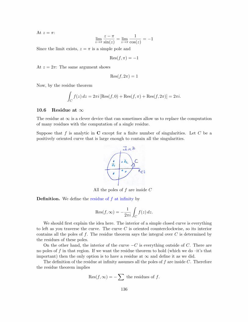
At z = π:
limz→π
z − πsin(z)
= limz→π
1
cos(z)= −1
Since the limit exists, z = π is a simple pole and
Res(f, π) = −1
At z = 2π: The same argument shows
Res(f, 2π) = 1
Now, by the residue theorem∫Cf(z) dz = 2πi [Res(f, 0) + Res(f, π) + Res(f, 2π)] = 2πi.
10.6 Residue at ∞The residue at∞ is a clever device that can sometimes allow us to replace the computationof many residues with the computation of a single residue.
Suppose that f is analytic in C except for a finite number of singularities. Let C be apositively oriented curve that is large enough to contain all the singularities.
All the poles of f are inside C
Definition. We define the residue of f at infinity by
Res(f,∞) = − 1
2πi
∫Cf(z) dz.
We should first explain the idea here. The interior of a simple closed curve is everythingto left as you traverse the curve. The curve C is oriented counterclockwise, so its interiorcontains all the poles of f . The residue theorem says the integral over C is determined bythe residues of these poles.
On the other hand, the interior of the curve −C is everything outside of C. There areno poles of f in that region. If we want the residue theorem to hold (which we do –it’s thatimportant) then the only option is to have a residue at ∞ and define it as we did.
The definition of the residue at infinity assumes all the poles of f are inside C. Thereforethe residue theorem implies
Res(f,∞) = −∑
the residues of f .
136

To make this useful we need a way to compute the residue directly. This is given by thefollowing theorem.
Theorem. If f is analytic in C except for a finite number of singularities then
Res(f,∞) = −Res
(1
w2f(1/w), 0
).
Proof. The proof is just a change of variables: w = 1/z.
Change of variable: w = 1/z
First note that z = 1/w anddz = −(1/w2) dw
Next, note that the map w = 1/z carries the positively oriented z-circle of radius R to thenegatively oriented w-circle of radius 1/R. (To see the orientiation, follow the circled points1, 2, 3, 4 on C in the z-plane as they are mapped to points on C in the w-plane.) Thus,
Res(f,∞) = − 1
2πi
∫Cf(z) dz =
1
2πi
∫Cf(1/w)
1
w2dw
Finally, note that z = 1/w maps all the poles inside the circle C to points outside thecircle C. So the only possible pole of (1/w2)f(1/w) that is inside C is at w = 0. Now, sinceC is oriented clockwise, the residue theorem says
1
2πi
∫Cf(1/w)
1
w2dw = −Res
(1
w2f(1/w), 0
)Comparing this with the equation just above finishes the proof.
Example 10.23. Let
f(z) =5z − 2
z(z − 1)
Earlier we computed ∫|z|=2
f(z) dz = 10πi
by computing residues at z = 0 and z = 1. Recompute this integral by computing a singleresidue at infinity.
137

Solution:1
w2f(1/w) =
1
w2
5/w − 2
(1/w)(1/w − 1)=
5− 2w
w(1− w)
We easily compute that
Res(f,∞) = −Res
(1
w2f(1/w), 0
)= −5.
Since |z| = 2 contains all the singularities of f we have∫|z|=2
f(z) dz = −2πiRes(f,∞) = 10πi.
This is the same answer we got before!
11 Definite integrals using the residue theorem
In this topic we’ll use the residue theorem to compute some real definite integrals.∫ b
af(x) dx
The general approach is always the same
1. Find a complex analytic function g(z) which either equals f on the real axis or whichis closely connected to f , e.g. f(x) = cos(x), g(z) = eiz.
2. Pick a closed contour C that includes the part of the real axis in the integral.
3. The contour will be made up of pieces. It should be such that we can compute∫g(z) dz over each of the pieces except the part on the real axis.
4. Use the residue theorem to compute
∫Cg(z) dz.
5. Combine the previous steps to deduce the value of the integral we want.
11.1 Integrals of functions that decay
The theorems in this section will guide us in choosing the closed contour C described in theintroduction.
The first theorem is for functions that decay faster than 1/z.
Theorem 11.1. (a) Suppose f(z) is defined in the upper half-plane. If there is an a > 1and M > 0 such that
|f(z)| < M
|z|afor |z| large then
limR→∞
∫CR
f(z) dz = 0,
138

where CR is the semicircle shown below on the left.
Re(z)
Im(z)
R−R
CR
Re(z)
Im(z)R−R
CR
Semicircles: left: Reiθ, 0 < θ < π right: Reiθ, π < θ < 2π.
(b) If f(z) is defined in the lower half-plane and
|f(z)| < M
|z|a ,
where a > 1 then
limR→∞
∫CR
f(z) dz = 0,
where CR is the semicircle shown above on the right.
Proof. We prove (a), (b) is essentially the same. We use the triangle inequality for integralsand the estimate given in the hypothesis. For R large∣∣∣∣∫
CR
f(z) dz
∣∣∣∣ ≤ ∫CR
|f(z)| |dz| ≤∫CR
M
|z|a |dz| =∫ π
0
M
RaRdθ =
Mπ
Ra−1.
Since a > 1 this clearly goes to 0 as R→∞. �
The next theorem is for functions that decay like 1/z. It requires some more care to stateand prove.
Theorem 11.2. (a) Suppose f(z) is defined in the upper half-plane. If there is an M > 0such that
|f(z)| < M
|z|for |z| large then for a > 0
limx1→∞, x2→∞
∫C1+C2+C3
f(z)eiaz dz = 0,
where C1 + C2 + C3 is the rectangular path shown below on the left.
Re(z)
Im(z)
x1−x2
i(x1 + x2)C1
C2
C3
Re(z)
Im(z)x1−x2
−i(x1 + x2)
C1
C2
C3
139
Rectangular paths of height and width x1 + x2.
(b) Similarly, if a < 0 then
limx1→∞, x2→∞
∫C1+C2+C3
f(z)eiaz dz = 0,
where C1 + C2 + C3 is the rectangular path shown above on the right.
Note. In contrast to Theorem 11.1 this theorem needs to include the factor eiaz.
Proof. (a) We start by parametrizing C1, C2, C3.
C1: γ1(t) = x1 + it, t from 0 to x1 + x2
C2: γ2(t) = t+ i(x1 + x2), t from x1 to −x2
C3: γ3(t) = −x2 + it, t from x1 + x2 to 0.
Next we look at each integral in turn. We assume x1 and x2 are large enough that
|f(z)| < M
|z|on each of the curves Cj .∣∣∣∣∫
C1
f(z)eiaz dz
∣∣∣∣ ≤ ∫C1
|f(z)eiaz| |dz| ≤∫C1
M
|z| |eiaz| |dz|
=
∫ x1+x2
0
M√x2
1 + t2|eiax1−at| dt
≤ M
x1
∫ x1+x2
0e−at dt
=M
x1(1− e−a(x1+x2))/a.
Since a > 0, it is clear that this last expression goes to 0 as x1 and x2 go to ∞.
∣∣∣∣∫C2
f(z)eiaz dz
∣∣∣∣ ≤ ∫C2
|f(z)eiaz| |dz| ≤∫C2
M
|z| |eiaz| |dz|
=
∫ x1
−x2
M√t2 + (x1 + x2)2
|eiat−a(x1+x2)| dt
≤ Me−a(x1+x2)
x1 + x2
∫ x1+x2
0dt
≤Me−a(x1+x2)
Again, clearly this last expression goes to 0 as x1 and x2 go to ∞.The argument for C3 is essentially the same as for C1, so we leave it to the reader.The proof for part (b) is the same. You need to keep track of the sign in the exponentials
and make sure it is negative.
Example. See Example 11.16 below for an example using Theorem 11.2.
140

11.2 Integrals
∫ ∞−∞
and
∫ ∞0
Example 11.3. Compute
I =
∫ ∞−∞
1
(1 + x2)2dx
Solution: Letf(z) = 1/(1 + z2)2
It is clear that for z largef(z) ≈ 1/z4
In particular, the hypothesis of Theorem 11.1 is satisfied. Using the contour shown belowwe have, by the residue theorem,∫
C1+CR
f(z) dz = 2πi∑
residues of f inside the contour. (48)
Re(z)
Im(z)
R−R
CR
C1
i
We examine each of the pieces in the above equation.∫CR
f(z) dz: By Theorem 11.1(a),
limR→∞
∫CR
f(z) dz = 0.
∫C1
f(z) dz: Directly, we see that
limR→∞
∫C1
f(z) dz = limR→∞
∫ R
−Rf(x) dx =
∫ ∞−∞
f(x) dx = I.
So letting R→∞, Eq. (48) becomes
I =
∫ ∞−∞
f(x) dx = 2πi∑
residues of f inside the contour.
Finally, we compute the needed residues: f(z) has poles of order 2 at ±i. Only z = i isinside the contour, so we compute the residue there. Let
g(z) = (z − i)2f(z) =1
(z + i)2
141

Then
Res(f, i) = g′(i) = − 2
(2i)3=
1
4i
So,
I = 2πiRes(f, i) =π
2
Example 11.4. Compute
I =
∫ ∞−∞
1
x4 + 1dx
Solution: Let f(z) = 1/(1 + z4). We use the same contour as in the previous example
Re(z)
Im(z)
R−R
CR
C1
eiπ/4ei3π/4
As in the previous example,
limR→∞
∫CR
f(z) dz = 0
and
limR→∞
∫C1
f(z) dz =
∫ ∞−∞
f(x) dx = I
So, by the residue theorem
I = limR→∞
∫C1+CR
f(z) dz = 2πi∑
residues of f inside the contour.
The poles of f are all simple and at
eiπ/4, ei3π/4, ei5π/4 ei7π/4
Only eiπ/4 and ei3π/4 are inside the contour. We compute their residues as limits usingL’Hospital’s rule. For z1 = eiπ/4 :
Res(f, z1) = limz→z1
(z − z1)f(z) = limz→z1
z − z1
1 + z4= lim
z→z1
1
4z3=
1
4ei3π/4=
e−i3π/4
4
and for z2 = ei3π/4 :
Res(f, z2) = limz→z2
(z − z2)f(z) = limz→z2
z − z2
1 + z4= lim
z→z2
1
4z3=
1
4ei9π/4=
e−iπ/4
4
142

So,
I = 2πi(Res(f, z1) + Res(f, z2)) = 2πi
(−1− i4√
2+
1− i4√
2
)= 2πi
(− 2i
4√
2
)= π
√2
2
Example 11.5. Suppose b > 0. Show∫ ∞0
cos(x)
x2 + b2dx =
πe−b
2b
Solution: The first thing to note is that the integrand is even, so
I =1
2
∫ ∞−∞
cos(x)
x2 + b2.
Also note that the square in the denominator tells us the integral is absolutely convergent.We have to be careful because cos(z) goes to infinity in either half-plane, so the hy-
potheses of Theorem 11.1 are not satisfied. The trick is to replace cos(x) by eix, so
I =
∫ ∞−∞
eix
x2 + b2dx with I =
1
2Re(I)
Now let
f(z) =eiz
z2 + b2
For z = x+ iy with y > 0 we have
|f(z)| = |ei(x+iy)||z2 + b2| =
e−y
|z2 + b2| .
Since e−y < 1, f(z) satisfies the hypotheses of Theorem 11.1 in the upper half-plane. Nowwe can use the same contour as in the previous examples
Re(z)
Im(z)
R−R
CR
C1
ib
We have
limR→∞
∫CR
f(z) dz = 0
and
limR→∞
∫C1
f(z) dz =
∫ ∞−∞
f(x) dx = I
143

So, by the residue theorem
I = limR→∞
∫C1+CR
f(z) dz = 2πi∑
residues of f inside the contour.
The poles of f are at ±bi and both are simple. Only bi is inside the contour. We computethe residue as a limit using L’Hospital’s rule
Res(f, bi) = limz→bi
(z − bi) eiz
z2 + b2=
e−b
2bi.
So,
I = 2πiRes(f, bi) =πe−b
b
Finally,
I =1
2Re(I) =
πe−b
2b,
as claimed.Warning: Be careful when replacing cos(z) by eiz that it is appropriate. A key point
in the above example was that I = 12 Re(I). This is needed to make the replacement useful.
11.3 Trigonometric integrals
The trick here is to put together some elementary properties of z = eiθ on the unit circle.
1. e−iθ = 1/z.
2. cos(θ) =eiθ + e−iθ
2=z + 1/z
2.
3. sin(θ) =eiθ − e−iθ
2i=z − 1/z
2i.
We start with an example. After that we’ll state a more general theorem.
Example 11.6. Compute ∫ 2π
0
dθ
1 + a2 − 2a cos(θ)
Assume that |a| 6= 1.
Solution: Notice that [0, 2π] is the interval used to parametrize the unit circle as z = eiθ.
We need to make two substitutions:
cos(θ) =z + 1/z
2
dz = ieiθ dθ ⇔ dθ =dz
iz
144

Making these substitutions we get
I =
∫ 2π
0
dθ
1 + a2 − 2a cos(θ)
=
∫|z|=1
1
1 + a2 − 2a(z + 1/z)/2· dziz
=
∫|z|=1
1
i((1 + a2)z − a(z2 + 1))dz
So, let
f(z) =1
i((1 + a2)z − a(z2 + 1))
The residue theorem implies
I = 2πi∑
residues of f inside the unit circle.
We can factor the denominator:
f(z) =−1
ia(z − a)(z − 1/a)
The poles are at a, 1/a. One is inside the unit circle and one is outside.
If |a| > 1 then 1/a is inside the unit circle and Res(f, 1/a) =1
i(a2 − 1)
If |a| < 1 then a is inside the unit circle and Res(f, a) =1
i(1− a2)
We have
I =
{2πa2−1
if |a| > 12π
1−a2 if |a| < 1
The example illustrates a general technique which we state now.
Theorem 11.7. Suppose R(x, y) is a rational function with no poles on the circle
x2 + y2 = 1
then for
f(z) =1
izR
(z + 1/z
2,z − 1/z
2i
)we have ∫ 2π
0R(cos(θ), sin(θ)) dθ = 2πi
∑residues of f inside |z| = 1.
Proof. We make the same substitutions as in Example 11.6. So,∫ 2π
0R(cos(θ), sin(θ)) dθ =
∫|z|=1
R
(z + 1/z
2,z − 1/z
2i
)dz
iz
The assumption about poles means that f has no poles on the contour |z| = 1. The residuetheorem now implies the theorem.
145

11.4 Integrands with branch cuts
Example 11.8. Compute
I =
∫ ∞0
x1/3
1 + x2dx
Solution: Let
f(x) =x1/3
1 + x2
Since this is asymptotically comparable to x−5/3, the integral is absolutely convergent. Asa complex function
f(z) =z1/3
1 + z2
needs a branch cut to be analytic (or even continuous), so we will need to take that intoaccount with our choice of contour.
First, choose the following branch cut along the positive real axis. That is, for z = reiθ
not on the axis, we have 0 < θ < 2π.Next, we use the contour C1 + CR − C2 − Cr shown below.
Re(z)
Im(z)
CR
C1
−C2
−Cr
i
−i
Contour around branch cut: inner circle of radius r, outer of radius R.
We put convenient signs on the pieces so that the integrals are parametrized in a naturalway. You should read this contour as having r so small that C1 and C2 are essentially onthe x-axis. Note well, that, since C1 and C2 are on opposite sides of the branch cut, theintegral ∫
C1−C2
f(z) dz 6= 0
First we analyze the integral over each piece of the curve.On CR: Theorem 11.1 says that
limR→∞
∫CR
f(z) dz = 0
146

On Cr: For concreteness, assume r < 1/2. We have |z| = r, so
|f(z)| = |z1/3||1 + z2| ≤
r1/3
1− r2≤ (1/2)1/3
3/4.
Call the last number in the above equation M . We have shown that, for small r, |f(z)| < M .So, ∣∣∣∣∫
Cr
f(z) dz
∣∣∣∣ ≤ ∫ 2π
0|f(reiθ)||ireiθ| dθ ≤
∫ 2π
0Mr dθ = 2πMr.
Clearly this goes to zero as r → 0.On C1:
limr→0, R→∞
∫C1
f(z) dz =
∫ ∞0
f(x) dx = I
On C2: We have (essentially) θ = 2π, so z1/3 = ei2π/3|z|1/3. Thus,
limr→0, R→∞
∫C2
f(z) dz = ei2π/3∫ ∞
0f(x) dx = ei2π/3I.
The poles of f(z) are at ±i. Since f is meromorphic inside our contour the residuetheorem says ∫
C1+CR−C2−Crf(z) dz = 2πi(Res(f, i) + Res(f,−i)).
Letting r → 0 and R→∞ the analysis above shows
(1− ei2π/3)I = 2πi(Res(f, i) + Res(f,−i))
All that’s left is to compute the residues using the chosen branch of z1/3
Res(f,−i) =(−i)1/3
−2i=
(ei3π/2)1/3
2ei3π/2=
e−iπ
2= −1
2
Res(f, i) =i1/3
2i=
eiπ/6
2eiπ/2=
e−iπ/3
2
A little more algebra gives
(1− ei2π/3)I = 2πi · −1 + e−iπ/3
2= πi(−1 + 1/2− i
√3/2) = −πieiπ/3.
Continuing
I =−πieiπ/31− ei2π/3
=πi
eiπ/3 − e−πi/3=
π/2
(eiπ/3 − e−iπ/3)/2i=
π/2
sin(π/3)=
π√3
Whew! (Note: a sanity check is that the result is real, which it had to be.)
147
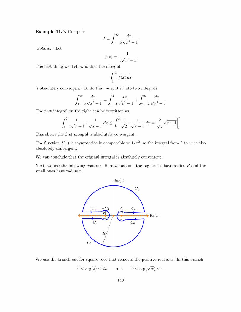
Example 11.9. Compute
I =
∫ ∞1
dx
x√x2 − 1
Solution: Let
f(z) =1
z√z2 − 1
The first thing we’ll show is that the integral∫ ∞1
f(x) dx
is absolutely convergent. To do this we split it into two integrals∫ ∞1
dx
x√x2 − 1
=
∫ 2
1
dx
x√x2 − 1
+
∫ ∞2
dx
x√x2 − 1
The first integral on the right can be rewritten as∫ 2
1
1
x√x+ 1
· 1√x− 1
dx ≤∫ 2
1
1√2· 1√
x− 1dx =
2√2
√x− 1
∣∣∣∣21
This shows the first integral is absolutely convergent.
The function f(x) is asymptotically comparable to 1/x2, so the integral from 2 to∞ is alsoabsolutely convergent.
We can conclude that the original integral is absolutely convergent.
Next, we use the following contour. Here we assume the big circles have radius R and thesmall ones have radius r.
Re(z)
Im(z)
R
rr
C1
C2 −C3
−C4
C5
−C6
−C7
1−1
C8
We use the branch cut for square root that removes the positive real axis. In this branch
0 < arg(z) < 2π and 0 < arg(√w) < π
148

For f(z), this necessitates the branch cut that removes the rays [1,∞) and (−∞,−1] fromthe complex plane.
The pole at z = 0 is the only singularity of f(z) inside the contour. It is easy to computethat
Res(f, 0) =1√−1
=1
i= −i.
So, the residue theorem gives us∫C1+C2−C3−C4+C5−C6−C7+C8
f(z) dz = 2πiRes(f, 0) = 2π. (49)
In a moment we will show the following limits
limR→∞
∫C1
f(z) dz = limR→∞
∫C5
f(z) dz = 0
limr→0
∫C3
f(z) dz = limr→0
∫C7
f(z) dz = 0.
We will also show
limR→∞, r→0
∫C2
f(z) dz = limR→∞, r→0
∫−C4
f(z) dz
= limR→∞, r→0
∫−C6
f(z) dz = limR→∞, r→0
∫C8
f(z) dz = I.
Using these limits, Equation (49) implies 4I = 2π, i.e.
I = π/2
All that’s left is to prove the limits asserted above.
The limits for C1 and C5 follow from Theorem 11.1 because
|f(z)| ≈ 1/|z|3/2
for large z.
We get the limit for C3 as follows. Suppose r is small, say much less than 1. If
z = −1 + reiθ
is on C3 then,
|f(z)| = 1
|z√z − 1
√z + 1| =
1
| − 1 + reiθ|√| − 2 + reiθ|√r
≤ M√r.
where M is chosen to be bigger than
1
| − 1 + reiθ|√| − 2 + reiθ|
149
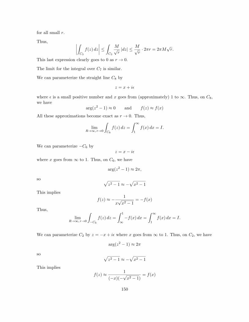
for all small r.
Thus, ∣∣∣∣∫C3
f(z) dz
∣∣∣∣ ≤ ∫C3
M√r|dz| ≤ M√
r· 2πr = 2πM
√r.
This last expression clearly goes to 0 as r → 0.
The limit for the integral over C7 is similar.
We can parameterize the straight line C8 by
z = x+ iε
where ε is a small positive number and x goes from (approximately) 1 to ∞. Thus, on C8,we have
arg(z2 − 1) ≈ 0 and f(z) ≈ f(x)
All these approximations become exact as r → 0. Thus,
limR→∞, r→0
∫C8
f(z) dz =
∫ ∞1
f(x) dx = I.
We can parameterize −C6 byz = x− iε
where x goes from ∞ to 1. Thus, on C6, we have
arg(z2 − 1) ≈ 2π,
so √z2 − 1 ≈ −
√x2 − 1
This implies
f(z) ≈ − 1
x√x2 − 1
= −f(x)
Thus,
limR→∞, r→0
∫−C6
f(z) dz =
∫ 1
∞−f(x) dx =
∫ ∞1
f(x) dx = I.
We can parameterize C2 by z = −x+ iε where x goes from ∞ to 1. Thus, on C2, we have
arg(z2 − 1) ≈ 2π
so √z2 − 1 ≈ −
√x2 − 1
This implies
f(z) ≈ 1
(−x)(−√x2 − 1)
= f(x)
150

Thus,
limR→∞, r→0
∫C2
f(z) dz =
∫ 1
∞f(x) (−dx) =
∫ ∞1
f(x) dx = I.
The last curve −C4 is handled similarly.
11.5 Cauchy principal value
First an example to motivate defining the principal value of an integral. We’ll actuallycompute the integral in the next section.
Example 11.10. Let
I =
∫ ∞0
sin(x)
xdx
This integral is not absolutely convergent, but it is conditionally convergent. Formally, ofcourse, we mean
I = limR→∞
∫ R
0
sin(x)
xdx
We can proceed as in Example 11.5. First note that sin(x)/x is even, so
I =1
2
∫ ∞−∞
sin(x)
xdx.
Next, to avoid the problem that sin(z) goes to infinity in both the upper and lower half-
planes we replace the integrand by eix
x .
We’ve changed the problem to computing
I =
∫ ∞−∞
eix
xdx.
The problems with this integral are caused by the pole at 0. The biggest problem is that theintegral doesn’t converge! The other problem is that when we try to use our usual strategyof choosing a closed contour we can’t use one that includes z = 0 on the real axis. This isour motivation for defining principal value. We will come back to this example below.
Definition. Suppose we have a function f(x) that is continuous on the real line except at
the point x1, then we define the Cauchy principal value as
p.v.
∫ ∞−∞
f(x) dx = limR→∞, r1→0
∫ x1−r1
−Rf(x) dx+
∫ R
x1+r1
f(x) dx.
Provided the limit converges. You should notice that the intervals around x1 and around∞ are symmetric. Of course, if the integral∫ ∞
−∞f(x) dx
converges, then so does the principal value and they give the same value. We can make thedefinition more flexible by including the following cases.
151

1. If f(x) is continuous on the entire real line then we define the principal value as
p.v.
∫ ∞−∞
f(x) dx = limR→∞
∫ R
−Rf(x) dx
2. If we have multiple points of discontinuity, x1 < x2 < x3 < . . . < xn, then
p.v.
∫ ∞−∞
f(x) dx = lim
∫ x1−r1
−Rf(x) dx+
∫ x2−r2
x1+r1
+
∫ x3−r3
x2+r2
+ . . .
∫ R
xn+rn
f(x) dx.
Here the limit is taken as R→∞ and each of the rk → 0.
xx1 x2
[ ] [ ] [ ]
−R x1 − r1 x1 + r1 x2 − r2 x2 + r2 R
Intervals of integration for principal value are symmetric around xk and ∞
The next example shows that sometimes the principal value converges when the integralitself does not. The opposite is never true. That is, we have the following theorem.
Theorem 11.11. If f(x) has discontinuities at x1 < x2 < . . . < xn and
∫ ∞−∞
f(x) dx
converges then so does p.v.
∫ ∞−∞
f(x) dx.
Proof. The proof amounts to understanding the definition of convergence of integrals aslimits. The integral converges means that each of the limits
limR1→∞, a1→0
∫ x1−a1
−R1
f(x) dx (50)
limb1→0, a2→0
∫ x2−a2
x1+b1
f(x) dx
. . .
limR2→∞, bn→0
∫ R2
xn+bn
f(x) dx
converges. There is no symmetry requirement, i.e. R1 and R2 are completely independent,as are a1 and b1 etc.
The principal value converges means
lim
∫ x1−r1
−R+
∫ x2−r2
x1+r1
+
∫ x3−r3
x2+r2
+ . . .
∫ R
xn+rn
f(x) dx (51)
converges. Here the limit is taken over all the parameter R → ∞, rk → 0. This limit hassymmetry, e.g. we replaced both a1 and b1 in Equation (50) by r1 etc. Certainly if thelimits in Equation (50) converge then so do the limits in Equation (51). �
152

Example 11.12. Consider both∫ ∞−∞
1
xdx and p.v.
∫ ∞−∞
1
xdx
The first integral diverges since∫ −r1−R1
1
xdx+
∫ R2
r2
1
xdx = ln(r1)− ln(R1) + ln(R2)− ln(r2).
This clearly diverges as R1, R2 →∞ and r1, r2 → 0.On the other hand the symmetric integral∫ −r
−R
1
xdx+
∫ R
r
1
xdx = ln(r)− ln(R) + ln(R)− ln(r) = 0.
This clearly converges to 0.We will see that the principal value occurs naturally when we integrate on semicircles
around points. We prepare for this in the next section.
11.6 Integrals over portions of circles
We will need the following theorem in order to combine principal value and the residuetheorem.
Theorem 11.13. Suppose f(z) has a simple pole at z0. Let Cr be the semicircle γ(θ) =z0 + reiθ, with 0 ≤ θ ≤ π. Then
limr→0
∫Cr
f(z) dz = πiRes(f, z0) (52)
Re(z)
Im(z)
z0
r
Cr
Small semicircle of radius r around z0
Proof. Since we take the limit as r goes to 0, we can assume r is small enough that f(z)has a Laurent expansion of the punctured disk of radius r centered at z0. That is, since thepole is simple,
f(z) =b1
z − z0+ a0 + a1(z − z0) + . . . for 0 < |z − z0| ≤ r.
Thus,∫Cr
f(z) dz =
∫ π
0f(z0 + reiθ) rieiθ dθ =
∫ π
0
(b1i+ a0ire
iθ + a1ir2ei2θ + . . .
)dθ
153

The b1 term gives πib1. Clearly all the other terms go to 0 as r → 0. �
If the pole is not simple the theorem doesn’t hold and, in fact, the limit does not exist.
The same proof gives a slightly more general theorem.
Theorem 11.14. Suppose f(z) has a simple pole at z0. Let Cr be the circular arcγ(θ) = z0 + reiθ, with θ0 ≤ θ ≤ θ0 + α. Then
limr→0
∫Cr
f(z) dz = αiRes(f, z0)
Re(z)
Im(z)
z0r
Cr
α
Small circular arc of radius r around z0
Example 11.15. (Return to Example 11.10.) A long time ago we left off Example 11.10to define principal value. Let’s now use the principal value to compute
I = p.v.
∫ ∞−∞
eix
xdx
Solution: We use the indented contour shown below. The indentation is the little semicirclethe goes around z = 0. There are no poles inside the contour so the residue theorem implies∫
C1−Cr+C2+CR
eiz
zdz = 0.
Re(z)
Im(z)
0
C1 C2
CR
−Cr
−R −r r R
2Ri
Next we break the contour into pieces.
limR→∞, r→0
∫C1+C2
eiz
zdz = I .
154

Theorem 11.2(a) implies
limR→∞
∫CR
eiz
zdz = 0
Equation (52) in Theorem 11.13 tells us that
limr→0
∫Cr
eiz
zdz = πiRes
(eiz
z, 0
)= πi
Combining all this together we have
limR→∞, r→0
∫C1−Cr+C2+CR
eiz
zdz = I − πi = 0,
so I = πi. Thus, looking back at Example 52, where I =
∫ ∞0
sin(x)
xdx, we have
I =1
2Im(I) =
π
2.
There is a subtlety about convergence we alluded to above. That is, I is a genuine (con-ditionally) convergent integral, but I only exists as a principal value. However since I is aconvergent integral we know that computing the principle value as we just did is sufficientto give the value of the convergent integral.
11.7 Fourier transform
Definition. The Fourier transform of a function f(x) is defined by
f(ω) =
∫ ∞−∞
f(x)e−ixω dx
This is often read as ‘f -hat’.
Theorem. (Fourier inversion formula.) We can recover the original function f(x) with theFourier inversion formula
f(x) =1
2π
∫ ∞−∞
f(ω)eixω dω.
So, the Fourier transform converts a function of x to a function of ω and the Fourier inversionconverts it back. Of course, everything above is dependent on the convergence of the variousintegrals.
Proof. We will not give the proof here.
Example 11.16. Let
f(t) =
{e−at for t > 0
0 for t < 0
155

where a > 0. Compute f(ω) and verify the Fourier inversion formula in this case.
Solution: Computing f is easy: For a > 0
f(ω) =
∫ ∞−∞
f(t)e−iωt dt =
∫ ∞0
e−ate−iωt dt =1
a+ iω
We should first note that the inversion integral converges. To avoid distraction we showthis at the end of this example.
Now, let
g(z) =1
a+ iz
Note that f(ω) = g(ω) and |g(z)| < M
|z| for large |z|.
To verify the inversion formula we consider the cases t > 0 and t < 0 separately. For t > 0we use the standard contour.
Re(z)
Im(z)
x1−x2
i(x1 + x2) C1
C2
C3
C4
Theorem 11.2(a) implies that
limx1→∞, x2→∞
∫C1+C2+C3
g(z)eizt dz = 0 (53)
Clearly
limx1→∞, x2→∞
∫C4
g(z)eizt dz =
∫ ∞−∞
f(ω) dω (54)
The only pole of g(z)eizt is at z = ia, which is in the upper half-plane. So, applying theresidue theorem to the entire closed contour, we get for large x1, x2:∫
C1+C2+C3+C4
g(z)eizt dz = 2πiRes
(eizt
a+ iz, ia
)=
e−at
i. (55)
Combining the three equations 53, 54 and 55, we have∫ ∞−∞
f(ω) dω = 2πe−at for t > 0
This shows the inversion formula holds for t > 0.
156

For t < 0 we use the contour
Re(z)
Im(z)
x1−x2
−i(x1 + x2) C1
C2
C3
C4
Theorem 11.2(b) implies that
limx1→∞, x2→∞
∫C1+C2+C3
g(z)eizt dz = 0
Clearly
limx1→∞, x2→∞
1
2π
∫C4
g(z)eizt dz =1
2π
∫ ∞−∞
f(ω) dω
Since, there are no poles of g(z)eizt in the lower half-plane, applying the residue theoremto the entire closed contour, we get for large x1, x2:∫
C1+C2+C3+C4
g(z)eizt dz = −2πiRes
(eizt
a+ iz, ia
)= 0.
Thus,1
2π
∫ ∞−∞
f(ω) dω = 0 for t < 0
This shows the inversion formula holds for t < 0.Finally, we give the promised argument that the inversion integral converges. By defi-
nition ∫ ∞−∞
f(ω)eiωt dω =
∫ ∞−∞
eiωt
a+ iωdω
=
∫ ∞−∞
a cos(ωt) + ω sin(ωt)− iω cos(ωt) + ia sin(ωt)
a2 + ω2dω
The terms without a factor of ω in the numerator converge absolutely because of the ω2 inthe denominator. The terms with a factor of ω in the numerator do not converge absolutely.For example, since
ω sin(ωt)
a2 + ω2
decays like 1/ω, its integral is not absolutely convergent. However, we claim that the integraldoes converge conditionally. That is, both limits
limR2→∞
∫ R2
0
ω sin(ωt)
a2 + ω2dω and lim
R1→∞
∫ 0
−R1
ω sin(ωt)
a2 + ω2dω
157

exist and are finite. The key is that, as sin(ωt) alternates between positive and negative
arches, the functionω
a2 + ω2is decaying monotonically. So, in the integral, the area under
each arch adds or subtracts less than the arch before. This means that as R1 (or R2) growsthe total area under the curve oscillates with a decaying amplitude around some limitingvalue.
ω
Total area oscillates with a decaying amplitude.
11.8 Solving ODEs using the Fourier transform
Let
D =d
dt
Our goal is to see how to use the Fourier transform to solve differential equations like
P (D)y = f(t)
Here P (D) is a polynomial operator, e.g.
D2 + 8D + 7I
We first note the following formula:
Df(ω) = iωf . (56)
Proof. This is just integration by parts:
Df(ω) =
∫ ∞−∞
f ′(t)e−iωt dt
= f(t)e−iωt∣∣∞−∞ −
∫ ∞−∞
f(t)(−iωe−iωt dt
= iω
∫ ∞−∞
f(t)e−iωt dt
= iωf(ω)
In the third line we assumed that f decays so that f(∞) = f(−∞) = 0.
158

It is a simple extension of Equation (56) to see
(P (D)f)(ω) = P (iω)f .
We can now use this to solve some differential equations.
Example 11.17. Solve the equation
y′′(t) + 8y′(t) + 7y(t) = f(t) =
{e−at if t > 0
0 if t < 0
Solution: In this case, we have
P (D) = D2 + 8D + 7I
soP (s) = s2 + 8s+ 7 = (s+ 7)(s+ 1)
The ODEP (D)y = f(t)
transforms toP (iw)y = f
Using the Fourier transform of f found in Example 11.16 we have
y(ω) =f
P (iω)=
1
(a+ iω)(7 + iω)(1 + iω).
Fourier inversion says that
y(t) =1
2π
∫ ∞−∞
y(ω)eiωt dω
As always, we want to extend y to be function of a complex variable z. Let’s call it g(z):
g(z) =1
(a+ iz)(7 + iz)(1 + iz).
Now we can proceed exactly as in Example 11.16. We know |g(z)| < M/|z|3 for someconstant M . Thus, the conditions of Theorem 11.2 are easily met. So, just as in Example11.16, we have:
For t > 0, eizt is bounded in the upper half-plane, so we use the contour below on theleft.
y(t) =1
2π
∫ ∞−∞
y(ω)eiωt dω =1
2πlim
x1→∞, x2→∞
∫C4
g(z)eizt dz
=1
2πlim
x1→∞, x2→∞
∫C1+C2+C3+C4
g(z)eizt dz
= i∑
residues of eiztg(z) in the upper half-plane
159

The poles of eiztg(z) are atia, 7i, i
These are all in the upper half-plane. The residues are respectively,
e−at
i(7− a)(1− a),
e−7t
i(a− 7)(−6),
e−t
i(a− 1)(6)
Thus, for t > 0 we have
y(t) =e−at
(7− a)(1− a)− e−7t
(a− 7)(6)+
e−t
(a− 1)(6).
Re(z)
Im(z)
x1−x2
i(x1 + x2) C1
C2
C3
C4
Contour for t > 0
Re(z)
Im(z)
x1−x2
−i(x1 + x2) C1
C2
C3
C4
Contour for t < 0
More briefly, when t < 0 we use the contour above on the right. We get the exact samestring of equalities except the sum is over the residues of eiztg(z) in the lower half-plane.Since there are no poles in the lower half-plane, we find that
y(t) = 0
when t < 0.Conclusion (reorganizing the signs and order of the terms):
y(t) =
{0 for t < 0
e−at
(7−a)(1−a) + e−7t
(7−a)(6) − e−t
(1−a)(6) for t > 0.
Note. Because |g(z)| < M/|z|3, we could replace the rectangular contours by semicirclesto compute the Fourier inversion integral.
Example 11.18. Consider
y′′ + y = f(t) =
{e−at if t > 0
0 if t < 0.
Find a solution for t > 0.
Solution: We work a little more quickly than in the previous example.Taking the Fourier transform we get
y(ω) =f(ω)
P (iω)=
f(ω)
1− ω2=
1
(a+ iω)(1− ω2).
160
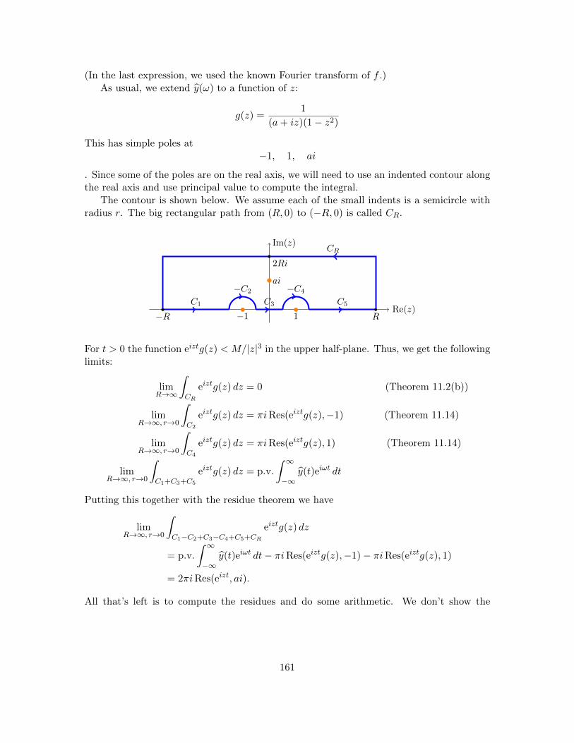
(In the last expression, we used the known Fourier transform of f .)As usual, we extend y(ω) to a function of z:
g(z) =1
(a+ iz)(1− z2)
This has simple poles at−1, 1, ai
. Since some of the poles are on the real axis, we will need to use an indented contour alongthe real axis and use principal value to compute the integral.
The contour is shown below. We assume each of the small indents is a semicircle withradius r. The big rectangular path from (R, 0) to (−R, 0) is called CR.
Re(z)
Im(z)
1−1
ai
C1 C3 C5
CR
−C2 −C4
−R R
2Ri
For t > 0 the function eiztg(z) < M/|z|3 in the upper half-plane. Thus, we get the followinglimits:
limR→∞
∫CR
eiztg(z) dz = 0 (Theorem 11.2(b))
limR→∞, r→0
∫C2
eiztg(z) dz = πiRes(eiztg(z),−1) (Theorem 11.14)
limR→∞, r→0
∫C4
eiztg(z) dz = πiRes(eiztg(z), 1) (Theorem 11.14)
limR→∞, r→0
∫C1+C3+C5
eiztg(z) dz = p.v.
∫ ∞−∞
y(t)eiωt dt
Putting this together with the residue theorem we have
limR→∞, r→0
∫C1−C2+C3−C4+C5+CR
eiztg(z) dz
= p.v.
∫ ∞−∞
y(t)eiωt dt− πiRes(eiztg(z),−1)− πiRes(eiztg(z), 1)
= 2πiRes(eizt, ai).
All that’s left is to compute the residues and do some arithmetic. We don’t show the
161

calculations, but give the results
Res(eiztg(z),−1) =e−it
2(a− i)
Res(eiztg(z), 1) = − eit
2(a+ i)
Res(eiztg(z), ai) = − e−at
i(1 + a2)
We get, for t > 0,
y(t) =1
2πp.v.
∫ ∞−∞
y(t)eiωt dt
=i
2Res(eiztg(z),−1) +
i
2Res(eiztg(z), 1) + iRes(eiztg(z), ai)
=e−at
1 + a2+
a
1 + a2sin(t)− 1
1 + a2cos(t)
12 Conformal transformations
In this topic we will look at the geometric notion of conformal maps. It will turn outthat analytic functions are automatically conformal. Once we have understood the generalnotion, we will look at a specific family of conformal maps called fractional linear trans-formations and, in particular at their geometric properties. As an application we will usefractional linear transformations to solve the Dirichlet problem for harmonic functions onthe unit disk with specified values on the unit circle. At the end we will return to somequestions of fluid flow.
12.1 Geometric definition of conformal mappings
We start with a somewhat hand-wavy definition:
Informal definition. Conformal maps are functions on C that preserve the angles betweencurves.
More precisely: Suppose f(z) is differentiable at z0 and γ(t) is a smooth curve through z0.To be concrete, let’s suppose γ(t0) = z0. The function maps the point z0 to w0 = f(z0) andthe curve γ to
γ(t) = f(γ(t)).
Under this map, the tangent vector γ′(t0) at z0 is mapped to the tangent vector
γ′(t0) = (f ◦ γ)′(t0)
at w0. With these notations we have the following definition.
162

Definition. The function f(z) is conformal at z0 if there is an angle φ and a scale a > 0such that for any smooth curve γ(t) through z0 the map f rotates the tangent vector atz0 by φ and scales it by a. That is, for any γ, the tangent vector (f ◦ γ)′(t0) is found byrotating γ′(t0) by φ and scaling it by a.
If f(z) is defined on a region A, we say it is a conformal map on A if it is conformal at eachpoint z in A.
Note. The scale factor a and rotation angle φ depends on the point z, but not on any ofthe curves through z.
Example 12.1. The figure below shows a conformal map f(z) mapping two curves throughz0 to two curves through w0 = f(z0). The tangent vectors to each of the original curves areboth rotated and scaled by the same amount.
x
y
γ′1(t0)
γ1(t)
γ′2(t0)
γ2(t)
z0
u
v
(f ◦ γ1)′(t0)
f(γ1(t))
(f ◦ γ2)′(t0)f(γ2(t))
w0
z 7→ w = f(z)
w0 = f(z0)
A conformal map rotates and scales all tangent vectors at z0 by the same ammount.
Remark 1. Conformality is a local phenomenon. At a different point z1 the rotation angleand scale factor might be different.
Remark 2. Since rotations preserve the angles between vectors, a key property of conformalmaps is that they preserve the angles between curves.
Example 12.2. Recall that way back we saw that f(z) = z2 maps horizontal and verticalgrid lines to mutually orthogonal parabolas. We will see that f(z) is conformal. So, theorthogonality of the parabolas is no accident. The conformal map preserves the right anglesbetween the grid lines.
163
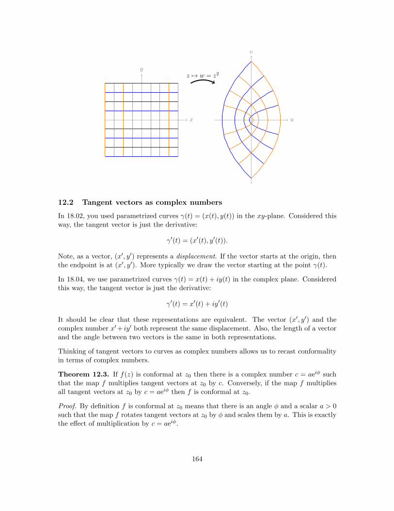
x
y
u
v
z 7→ w = z2
12.2 Tangent vectors as complex numbers
In 18.02, you used parametrized curves γ(t) = (x(t), y(t)) in the xy-plane. Considered thisway, the tangent vector is just the derivative:
γ′(t) = (x′(t), y′(t)).
Note, as a vector, (x′, y′) represents a displacement. If the vector starts at the origin, thenthe endpoint is at (x′, y′). More typically we draw the vector starting at the point γ(t).
In 18.04, we use parametrized curves γ(t) = x(t) + iy(t) in the complex plane. Consideredthis way, the tangent vector is just the derivative:
γ′(t) = x′(t) + iy′(t)
It should be clear that these representations are equivalent. The vector (x′, y′) and thecomplex number x′+ iy′ both represent the same displacement. Also, the length of a vectorand the angle between two vectors is the same in both representations.
Thinking of tangent vectors to curves as complex numbers allows us to recast conformalityin terms of complex numbers.
Theorem 12.3. If f(z) is conformal at z0 then there is a complex number c = aeiφ suchthat the map f multiplies tangent vectors at z0 by c. Conversely, if the map f multipliesall tangent vectors at z0 by c = aeiφ then f is conformal at z0.
Proof. By definition f is conformal at z0 means that there is an angle φ and a scalar a > 0such that the map f rotates tangent vectors at z0 by φ and scales them by a. This is exactlythe effect of multiplication by c = aeiφ.
164

12.3 Analytic functions are conformal
Theorem 12.4. (Operational definition of conformal) If f is analytic on the region A andf ′(z0) 6= 0, then f is conformal at z0. Furthermore, the map f multiplies tangent vectorsat z0 by f ′(z0).
Proof. The proof is a quick computation. Suppose z = γ(t) is curve through z0 withγ(t0) = z0. The curve γ(t) is transformed by f to the curve w = f(γ(t)). By the chain rulewe have
df(γ(t))
dt
∣∣∣∣t0
= f ′(γ(t0))γ′(t0) = f ′(z0)γ′(t0).
The theorem now follows from Theorem 12.3.
Example 12.5. (Basic example) Suppose c = aeiφ and consider the map f(z) = cz.Geometrically, this map rotates every point by φ and scales it by a. Therefore, it musthave the same effect on all tangent vectors to curves. Indeed, f is analytic and f ′(z) = c isconstant.
Example 12.6. Let f(z) = z2. So f ′(z) = 2z. Thus the map f has a different affect ontangent vectors at different points z1 and z2.
Example 12.7. (Linear approximation) Suppose f(z) is analytic at z = 0. The linearapproximation (first two terms of the Taylor series) is
f(z) ≈ f(0) + f ′(0)z.
If γ(t) is a curve with γ(t0) = 0 then, near t0,
f(γ(t)) ≈ f(0) + f ′(0)γ(t).
That is, near 0, f looks like our basic example plus a shift by f(0).
Example 12.8. The map f(z) = z has lots of nice geometric properties, but it is notconformal. It preserves the length of tangent vectors and the angle between tangent vectors.The reason it isn’t conformal is that is does not rotate tangent vectors. Instead, it reflectsthem across the x-axis.
In other words, it reverses the orientation of a pair of vectors. Our definition of conformalmaps requires that it preserves orientation.
12.4 Digression to harmonic functions
Theorem 12.9. If u and v are harmonic conjugates and g = u + iv has g′(z0) 6= 0, thenthe level curves of u and v through z0 are orthogonal.
Note. We proved this in an earlier topic using the Cauchy-Riemann equations. Here willmake an argument involving conformal maps.
Proof. First we’ll examine how g maps the level curve u(x, y) = a. Since g = u + iv, theimage of the level curve is w = a+ iv, i.e it’s (contained in) a vertical line in the w-plane.
165

Likewise, the level curve v(x, y) = b is mapped to the horizontal line w = u+ ib.
Thus, the images of the two level curves are orthogonal. Since g is conformal it preservesthe angle between the level curves, so they must be orthogonal.
x
y
u = av = b
z0
u
vu = a
v = bw0
z 7→ w = g(z) = u(x, y) + iv(x, y)
w0 = g(z0)
g = u+ iv maps level curves of u and v to grid lines.
12.5 Riemann mapping theorem
The Riemann mapping theorem is a major theorem on conformal maps. The proof is fairlytechnical and we will skip it. In practice, we will write down explicit conformal mapsbetween regions.
Theorem 12.10. (Riemann mapping theorem) If A is simply connected and not the wholeplane, then there is a bijective conformal map from A to the unit disk.
Corollary. For any two such regions there is a bijective conformal map from one to theother. We say they are conformally equivalent.
12.6 Fractional linear transformations
Definition. A fractional linear transformation is a function of the form
T (z) =az + b
cz + d, where a, b, c, d are complex constants and ad− bc 6= 0
These are also called Mobius transforms or bilinear transforms. We will abbreviate fractionallinear transformation as FLT.
Simple point. If ad− bc = 0 then T (z) is a constant function.
Proof. The full proof requires that we deal with all the cases where some of the coefficientsare 0. We’ll give the proof assuming c 6= 0 and leave the case c = 0 to you. Assuming c 6= 0,the condition ad− bc = 0 implies
a
c(c, d) = (a, b)
So,
T (z) =(a/c)(cz + d)
cz + d=a
c.
That is, T (z) is constant.
166
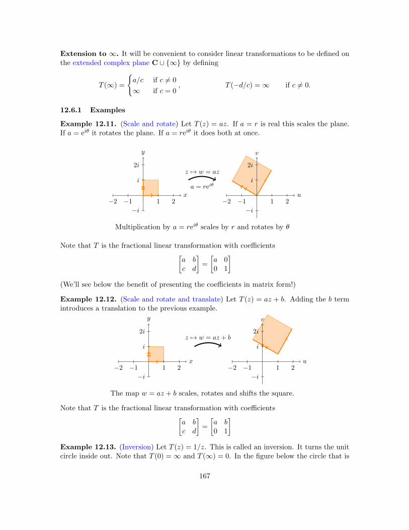
Extension to ∞. It will be convenient to consider linear transformations to be defined onthe extended complex plane C ∪ {∞} by defining
T (∞) =
{a/c if c 6= 0
∞ if c = 0, T (−d/c) =∞ if c 6= 0.
12.6.1 Examples
Example 12.11. (Scale and rotate) Let T (z) = az. If a = r is real this scales the plane.If a = eiθ it rotates the plane. If a = reiθ it does both at once.
x
y
−1−2 1 2
−i
i
2i
u
v
−2 −1 1 2
−i
i
2iz 7→ w = az
a = reiθ
Multiplication by a = reiθ scales by r and rotates by θ
Note that T is the fractional linear transformation with coefficients[a bc d
]=
[a 00 1
](We’ll see below the benefit of presenting the coefficients in matrix form!)
Example 12.12. (Scale and rotate and translate) Let T (z) = az + b. Adding the b termintroduces a translation to the previous example.
x
y
−1−2 1 2
−i
i
2i
u
v
−2 −1 1 2
−i
i
2iz 7→ w = az + b
The map w = az + b scales, rotates and shifts the square.
Note that T is the fractional linear transformation with coefficients[a bc d
]=
[a b0 1
]Example 12.13. (Inversion) Let T (z) = 1/z. This is called an inversion. It turns the unitcircle inside out. Note that T (0) =∞ and T (∞) = 0. In the figure below the circle that is
167

outside the unit circle in the z plane is inside the unit circle in the w plane and vice-versa.Note that the arrows on the curves are reversed.
x
y
1
i
u
v
1
i
z 7→ w = 1/z
The map w = 1/z inverts the plane.
Note that T is the fractional linear transformation with coefficients[a bc d
]=
[0 11 0
].
Example 12.14. Let
T (z) =z − iz + i
We claim that this maps the x-axis to the unit circle and the upper half-plane to the unitdisk.
Proof. First take x real, then
|T (x)| = |x− i||x+ i| =
√x2 + 1√x2 + 1
= 1
So, T maps the x-axis to the unit circle.Next take z = x+ iy with y > 0, i.e. z in the upper half-plane. Clearly
|y + 1| > |y − 1|,
so|z + i| = |x+ i(y + 1)| > |x+ i(y − 1)| = |z − i|,
implying that
|T (z)| = |z − i||z + i| < 1.
So, T maps the upper half-plane to the unit disk.We will use this map frequently, so for the record we note that
T (i) = 0, T (∞) = 1, T (−1) = i, T (0) = −1, T (1) = −i.
These computations show that the real axis is mapped counterclockwise around the unitcircle starting at 1 and coming back to 1.
168

x
y
-1 0 1
i
u
v
1
i
−i
z 7→ w =z − iz + i
The map w =z − iz + i
maps the upper-half plane to the unit disk.
12.6.2 Lines and circles
Theorem. A linear fractional transformation maps lines and circles to lines and circles.
Before proving this, note that it does not say lines are mapped to lines and circles to circles.For example, in Example 12.14 the real axis is mapped the unit circle. You can also checkthat inversion w = 1/z maps the line z = 1 + iy to the circle |z − 1/2| = 1/2.
Proof. We start by showing that inversion maps lines and circles to lines and circles. Givenz and w = 1/z we define x, y, u and v by
z = x+ iy and w =1
z=
x− iyx2 + y2
= u+ iv
So,
u =x
x2 + y2and v = − y
x2 + y2
Now, every circle or line can be described by the equation
Ax+By + C(x2 + y2) = D
(If C = 0 it descibes a line, otherwise a circle.) We convert this to an equation in u, v asfollows.
Ax+By + C(x2 + y2) = D
⇔ Ax
x2 + y2+
By
x2 + y2+ C =
D
x2 + y2
⇔ Au−Bv + C = D(u2 + v2).
In the last step we used the fact the
u2 + v2 = |w|2 = 1/|z|2 = 1/(x2 + y2).
We have shown that a line or circle in x, y is transformed to a line or circle in u, v. Thisshows that inversion maps lines and circles to lines and circles.
We note that for the inversion w = 1/z.
169

1. Any line not through the origin is mapped to a circle through the origin.
2. Any line through the origin is mapped to a line through the origin.
3. Any circle not through the origin is mapped to a circle not through the origin.
4. Any circle through the origin is mapped to a line not through the origin.
Now, to prove that an arbitrary fractional linear transformation maps lines and circlesto lines and circles, we factor it into a sequence of simpler transformations.
First suppose that c = 0. So,
T (z) = (az + b)/d
Since this is just translation, scaling and rotating, it is clear it maps circles to circles andlines to lines.
Now suppose that c 6= 0. Then,
T (z) =az + b
cz + d=
ac (cz + d) + b− ad
c
cz + d=a
c+b− ad/ccz + d
So, w = T (z) can be computed as a composition of transforms
z 7→ w1 = cz + d 7→ w2 = 1/w1 7→ w =a
c+ (b− ad/c)w2
We know that each of the transforms in this sequence maps lines and circles to lines andcircles. Therefore the entire sequence does also. �
12.6.3 Mapping zj to wj
It turns out that for two sets of three points z1, z2, z3 and w1, w2, w3 there is a fractionallinear transformation that takes zj to wj . We can construct this map as follows.
Let
T1(z) =(z − z1)(z2 − z3)
(z − z3)(z2 − z1)
Notice thatT1(z1) = 0, T1(z2) = 1, T1(z3) =∞
Likewise let
T2(w) =(w − w1)(w2 − w3)
(w − w3)(w2 − w1)
Notice thatT2(w1) = 0, T2(w2) = 1, T2(w3) =∞
Now T (z) = T−12 ◦ T1(z) is the required map.
170

12.6.4 Correspondence with matrices
We can identify the transformation
T (z) =az + b
cz + d
with the matrix [a bc d
]This identification is useful because of the following algebraic facts.
1. If r 6= 0 then
[a bc d
]and r
[a bc d
]correspond to the same FLT.
Proof. This follows from the obvious equality
az + b
cz + d=raz + rb
rcz + rd.
2. If T (z) corresponds to A =
[a bc d
]and S(z) corresponds to B =
[e fg h
]then composi-
tion T ◦ S(z) corresponds to matrix multiplication AB.
Proof. The proof is just a bit of algebra.
T ◦ S(z) = T
(ez + f
gz + h
)=a ((ez + f)/(gz + h)) + b
c ((ez + f)/(gz + h)) + d=
(ae+ bg)z + af + bh
(ce+ dg)z + cf + dh
AB =
[a bc d
] [e fg h
]=
[ae+ bg af + bhce+ dg cf + dh
]The claimed correspondence is clear from the last entries in the two lines above.
3. If T (z) corresponds to A =
[a bc d
]then T has an inverse and T−1(w) corresponds to
A−1 and also to
[d −b−c a
], i.e. to A−1 without the factor of 1/det(A).
Proof. Since AA−1 = I it is clear from the previous fact that T−1 corresponds to A−1.Since
A−1 =1
ad− bc
[d −b−c a
]Fact 1 implies A−1 and
[d −b−c a
]both correspond to the same FLT, i.e. to T−1.
Example 12.15.
1. The matrix
[a b0 1
]corresponds to T (z) = az + b.
171

2. The matrix
[eiα 00 e−iα
]corresponds to rotation by 2α.
3. The matrix
[0 11 0
]corresponds to the inversion w = 1/z.
12.7 Reflection and symmetry
12.7.1 Reflection and symmetry in a line
Example 12.16. Suppose we have a line S and a point z1 not on S. The reflection of z1
in S is the point z2 so that S is the perpendicular bisector to the line segment z1z2. Sincethere is exactly one such point z2, the reflection of a point in a line is unique.
Definition. If z2 is the reflection of z1 in S, we say that z1 and z2 are symmetric with
respect to the line S.
In the figure below the points z1 and z2 are symmetric in the x-axis. The points z3 and z4
are symmetric in the line S.
x
y
z1
z2
a
a
Sz3
z4
b
b
In order to define the reflection of a point in a circle we need to work a little harder. Lookingback at the previous example we can show the following.
Fact. If z1 and z2 are symmetric in the line S, then any circle through z1 and z2 intersectsS orthogonally.
Proof. Call the circle C. Since S is the perpendicular bisector of a chord of C, the centerof C lies on S. Therefore S is a radial line, i.e. it intersects C orthogonally.
172

x
y
z1
z2
a
a
Sz3
z4
b
b
Circles through symmetric points intersect the line at right angles.
12.7.2 Reflection and symmetry in a circle
We will adapt this for our definition of reflection in a circle. So that the logic flows correctlywe need to start with the definition of symmetric pairs of points.
Definition. Suppose S is a line or circle. A pair of points z1, z2 is called symmetric withrespect to S if every line or circle through the two points intersects S orthogonally.
First we state an almost trivial fact.
Fact. Fractional linear transformations preserve symmetry. That is, if z1 and z2 are sym-metric in a line or circle S, then, for an FLT T , T (z1) and T (z2) are symmetric in T (S).
Proof. The definition of symmetry is in terms of lines and circles, and angles. Fractionallinear transformations map lines and circles to lines and circles and, being conformal, pre-serve angles. �
Theorem. Suppose S is a line or circle and z1 a point not on S. There is a unique pointz2 such that the pair z1, z2 is symmetric in S.
Proof. Let T be a fractional linear transformation that maps S to a line. We know thatw1 = T (z1) has a unique reflection w2 in this line. Since T−1 preserves symmetry, z1 andz2 = T−1(w2) are symmetric in S. Since w2 is the unique point symmetric to w1 the sameis true for z2 vis-a-vis z1. This is all shown in the figure below.
x
y
z1 z2 = T−1(w2)
S
x
y
w1 = T (z1) w2
T (S)
w = T (z)
We can now define reflection in a circle.
173
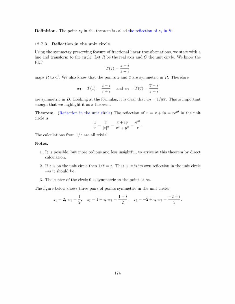
Definition. The point z2 in the theorem is called the reflection of z1 in S.
12.7.3 Reflection in the unit circle
Using the symmetry preserving feature of fractional linear transformations, we start with aline and transform to the circle. Let R be the real axis and C the unit circle. We know theFLT
T (z) =z − iz + i
maps R to C. We also know that the points z and z are symmetric in R. Therefore
w1 = T (z) =z − iz + i
and w2 = T (z) =z − iz + i
are symmetric in D. Looking at the formulas, it is clear that w2 = 1/w1. This is importantenough that we highlight it as a theorem.
Theorem. (Reflection in the unit circle) The reflection of z = x + iy = reiθ in the unitcircle is
1
z=
z
|z|2 =x+ iy
x2 + y2=
eiθ
r.
The calculations from 1/z are all trivial.
Notes.
1. It is possible, but more tedious and less insightful, to arrive at this theorem by directcalculation.
2. If z is on the unit circle then 1/z = z. That is, z is its own reflection in the unit circle–as it should be.
3. The center of the circle 0 is symmetric to the point at ∞.
The figure below shows three pairs of points symmetric in the unit circle:
z1 = 2; w1 =1
2, z2 = 1 + i; w2 =
1 + i
2, z3 = −2 + i; w3 =
−2 + i
5.
174
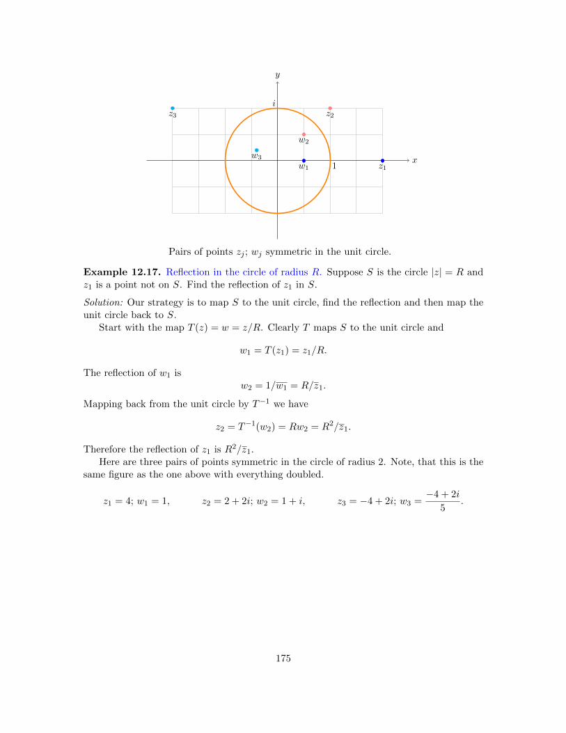
x
y
1
i
z1w1
z2
w2
z3
w3
Pairs of points zj ; wj symmetric in the unit circle.
Example 12.17. Reflection in the circle of radius R. Suppose S is the circle |z| = R andz1 is a point not on S. Find the reflection of z1 in S.
Solution: Our strategy is to map S to the unit circle, find the reflection and then map theunit circle back to S.
Start with the map T (z) = w = z/R. Clearly T maps S to the unit circle and
w1 = T (z1) = z1/R.
The reflection of w1 isw2 = 1/w1 = R/z1.
Mapping back from the unit circle by T−1 we have
z2 = T−1(w2) = Rw2 = R2/z1.
Therefore the reflection of z1 is R2/z1.Here are three pairs of points symmetric in the circle of radius 2. Note, that this is the
same figure as the one above with everything doubled.
z1 = 4; w1 = 1, z2 = 2 + 2i; w2 = 1 + i, z3 = −4 + 2i; w3 =−4 + 2i
5.
175

x
y
1
i
z1w1
z2
w2
z3
w3
Pairs of points zj ; wj symmetric in the circle of radius 2.
Example 12.18. Find the reflection of z1 in the circle of radius R centered at c.
Solution: Let T (z) = (z − c)/R. T maps the circle centered at c to the unit circle. The
inverse map isT−1(w) = Rw + c.
So, the reflection of z1 is given by mapping z to T (z), reflecting this in the unit circle, andmapping back to the original geometry with T−1. That is, the reflection z2 is
z1 →z1 − cR
→ R
z1 − c→ z2 =
R2
z1 − c+ c.
We can now record the following important fact.
Fact. (Reflection of the center) For a circle S with center c the pair c, ∞ is symmetricwith respect to the circle.
Proof. This is an immediate consequence of the formula for the reflection of a point in acircle. For example, the reflection of z in the unit circle is 1/z. So, the reflection of 0 isinfinity.
Example 12.19. Show that if a circle and a line don’t intersect then there is a pair ofpoints z1, z2 that is symmetric with respect to both the line and circle.
Solution: By shifting, scaling and rotating we can find a fractional linear transformation T
that maps the circle and line to the following configuration: The circle is mapped to theunit circle and the line to the vertical line x = a > 1.
176

x
y
a1/r r1
For any real r, w1 = r and w2 = 1/r are symmetric in the unit circle. We can choose aspecific r so that r and 1/r are equidistant from a, i.e. also symmetric in the line x = a. Itis clear geometrically that this can be done. Algebraically we solve the equation
r + 1/r
2= a ⇒ r2 − 2ar + 1 = 0 ⇒ r = a+
√a2 − 1 ⇒ 1
r= a−
√a2 − 1.
Thus z1 = T−1(a+√a2 − 1) and z2 = T−1(a−
√a2 − 1) are the required points.
Example 12.20. Show that if two circles don’t intersect then there is a pair of points z1,z2 that is symmetric with respect to both circles.
Solution: Using a fractional linear transformation that maps one of the circles to a line (andthe other to a circle) we can reduce the problem to that in the previous example.
Example 12.21. Show that any two circles that don’t intersect can be mapped conformallyto concentric circles.
Solution: Call the circles S1 and S2. Using the previous example start with a pair of pointsz1, z2 which are symmetric in both circles. Next, pick a fractional linear transformation Tthat maps z1 to 0 and z2 to infinity. For example,
T (z) =z − z1
z − z2.
Since T preserves symmetry 0 and ∞ are symmetric in the circle T (S1). This implies that0 is the center of T (S1). Likewise 0 is the center of T (S2). Thus, T (S1) and T (S2) areconcentric.
12.8 Solving the Dirichlet problem for harmonic functions
In general, a Dirichlet problem in a region A asks you to solve a partial differential equationin A where the values of the solution on the boundary of A are specificed.
Example 12.22. Find a function u harmonic on the unit disk such that
u(eiθ) =
{1 for 0 < θ < π
0 for −π < θ < 0
This is a Dirichlet problem because the values of u on the boundary are specified. Thepartial differential equation is implied by requiring that u be harmonic, i.e. we require∇2u = 0. We will solve this problem in due course.
177

12.8.1 Harmonic functions on the upper half-plane
Our strategy will be to solve the Dirichlet problem for harmonic functions on the upperhalf-plane and then transfer these solutions to other domains.
Example 12.23. Find a harmonic function u(x, y) on the upper half-plane that satisfiesthe boundary condition
u(x, 0) =
{1 for x < 0
0 for x > 0
Solution: We can write down a solution explicitly as
u(x, y) =1
πθ,
where θ is the argument of z = x + iy. Since we are only working on the upper half-plane we can take any convenient branch with branch cut in the lower half-plane, say−π/2 < θ < 3π/2.
x
y
u = 1 u = 0
z = x+ iy
r2r1
θ
To show u is truly a solution, we have to verify two things:
1. u satisfies the boundary conditions
2. u is harmonic.
Both of these are straightforward. First, look at the point r2 on the positive x-axis. Thishas argument θ = 0, so u(r2, 0) = 0. Likewise arg(r1) = π, so u(r1, 0) = 1. Thus, we haveshown point (1).
To see point (2) remember that
log(z) = log(r) + iθ.
So,
u = Re
(1
πilog(z)
).
Since it is the real part of an analytic function, u is harmonic.
178

Example 12.24. Suppose x1 < x2 < x3. Find a harmonic function u on the upperhalf-plane that satisfies the boundary condition
u(x, 0) =
c0 for x < x1
c1 for x1 < x < x2
c2 for x2 < x < x3
c3 for x3 < x
Solution: We mimic the previous example and write down the solution
u(x, y) = c3 + (c2 − c3)θ3
π+ (c1 − c2)
θ2
π+ (c0 − c1)
θ1
π.
Here, the θj are the angles shown in the figure. One again, we chose a branch of θ that has0 < θ < π for points in the upper half-plane. (For example the branch −π/2 < θ < 3π/2.)
x
y
x1 x2 x3
u = c0 u = c1 u = c2 u = c3
z = x+ iy
θ1 θ2 θ3
r0 r1 r2 r3
To convince yourself that u satisfies the boundary condition test a few points:
• At r3: all the θj = 0. So, u(r3, 0) = c3 as required.
• At r2: θ1 = θ2 = 0, θ3 = π. So, u(r2, 0) = c3 + c2 − c3 = c2 as required.
• Likewise, at r1 and r0, u have the correct values.
As before, u is harmonic because it is the real part of the analytic function
Φ(z) = c3 +(c2 − c3)
πilog(z − x3) +
(c1 − c2)
πilog(z − x2) +
(c1 − c0)
πilog(z − x1).
12.8.2 Harmonic functions on the unit disk
Let’s try to solve a problem similar to the one in Example 12.22.
Example 12.25. Find a function u harmonic on the unit disk such that
u(eiθ) =
{1 for −π/2 < θ < π/2
0 for π/2 < θ < 3π/2
179
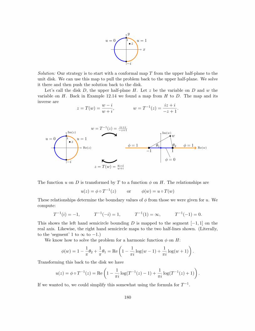
x
y
i
−i
u = 1u = 0z
Solution: Our strategy is to start with a conformal map T from the upper half-plane to theunit disk. We can use this map to pull the problem back to the upper half-plane. We solveit there and then push the solution back to the disk.
Let’s call the disk D, the upper half-plane H. Let z be the variable on D and w thevariable on H. Back in Example 12.14 we found a map from H to D. The map and itsinverse are
z = T (w) =w − iw + i
, w = T−1(z) =iz + i
−z + 1.
Re(z)
Im(z)
i
−i
u = 1u = 0z
Re(w)
Im(w)
−1 1
φ = 1 φ = 1
φ = 0
w
θ1 θ2
w = T−1(z) = iz+i−z+1
z = T (w) = w−iw+i
The function u on D is transformed by T to a function φ on H. The relationships are
u(z) = φ ◦ T−1(z) or φ(w) = u ◦ T (w)
These relationships determine the boundary values of φ from those we were given for u. Wecompute:
T−1(i) = −1, T−1(−i) = 1, T−1(1) =∞, T−1(−1) = 0.
This shows the left hand semicircle bounding D is mapped to the segment [−1, 1] on thereal axis. Likewise, the right hand semicircle maps to the two half-lines shown. (Literally,to the ‘segment’ 1 to ∞ to −1.)
We know how to solve the problem for a harmonic function φ on H:
φ(w) = 1− 1
πθ2 +
1
πθ1 = Re
(1− 1
πilog(w − 1) +
1
πilog(w + 1)
).
Transforming this back to the disk we have
u(z) = φ ◦ T−1(z) = Re
(1− 1
πilog(T−1(z)− 1) +
1
πilog(T−1(z) + 1)
).
If we wanted to, we could simplify this somewhat using the formula for T−1.
180

12.9 Flows around cylinders
12.9.1 Milne-Thomson circle theorem
The Milne-Thomson theorem allows us to insert a circle into a two-dimensional flow andsee how the flow adjusts. First we’ll state and prove the theorem.
Theorem. (Milne-Thomson circle theorem) If f(z) is a complex potential with all itssingularities outside |z| = R then
Φ(z) = f(z) + f
(R2
z
)is a complex potential with streamline on |z| = R and the same singularities as f in theregion |z| > R.
Proof. First note that R2/z is the reflection of z in the circle |z| = R.Next we need to see that f(R2/z) is analytic for |z| > R. By assumption f(z) is analytic
for |z| ≤ R, so it can be expressed as a Taylor series
f(z) = a0 + a1z + a2z2 + . . . (57)
Therefore,
f
(R2
z
)= a0 + a1
R2
z+ a2
(R2
z
)2
+ . . . (58)
All the singularities of f are outside |z| = R, so the Taylor series in Equation 57 convergesfor |z| ≤ R. This means the Laurent series in Equation 58 converges for |z| ≥ R. That is,f(R2/z) is analytic for |z| ≥ R, i.e. it introduces no singularies to Φ(z) outside |z| = R.
The last thing to show is that |z| = R is a streamline for Φ(z). This follows because forz = Reiθ
Φ(Reiθ) = f(Reiθ) + f(Reiθ)
is real. Thereforeψ(Reiθ) = Im(Φ(Reiθ) = 0.
12.9.2 Examples
Think of f(z) as representing flow, possibly with sources or vortices outside |z| = R.Then Φ(z) represents the new flow when a circular obstacle is placed in the flow. Here area few examples.
Example 12.26. (Uniform flow around a circle) We know from earlier that f(z) = z is thecomplex potential for uniform flow to the right. So,
Φ(z) = z +R2/z
is the potential for uniform flow around a circle of radius R centered at the origin.
181

Uniform flow around a circle
Just because they look nice, the figure includes streamlines inside the circle. These don’tinteract with the flow outside the circle.
Note, that as z gets large flow looks uniform. We can see this analytically because
Φ′(z) = 1−R2/z2
goes to 1 as z gets large. (Recall that the velocity field is (φx, φy), where Φ = φ+ iψ . . . )
Example 12.27. (Source flow around a circle) Here the source is at z = −2 (outside theunit circle) with complex potential
f(z) = log(z + 2).
With the appropriate branch cut the singularities of f are also outside |z| = 1. So we canapply Milne-Thomson and obtain
Φ(z) = log(z + 2) + log
(1
z+ 2
)
Source flow around a circle
We know that far from the origin the flow should look the same as a flow with just asource at z = −2. Let’s see this analytically. First we state a useful fact:
Useful fact. If g(z) is analytic then so is h(z) = g(z) and h′(z) = g′(z).
182

Proof. Use the Taylor series for g to get the Taylor series for h and then compare h′(z)and g′(z). �
Using this we have
Φ′(z) =1
z + 2− 1
z(1 + 2z)
For large z the second term decays much faster than the first, so
Φ′(z) ≈ 1
(z + 2)
That is, far from z = 0, the velocity field looks just like the velocity field for f(z), i.e. thevelocity field of a source at z = −2.
Example 12.28. (Transforming flows) If we use
g(z) = z2
we can transform a flow from the upper half-plane to the first quadrant
Source flow around a quarter circular corner
12.10 Examples of conformal maps and excercises
As we’ve seen, once we have flows or harmonic functions on one region, we can use conformalmaps to map them to other regions. In this section we will offer a number of conformalmaps between various regions. By chaining these together along with scaling, rotating andshifting we can build a large library of conformal maps. Of course there are many manyothers that we will not touch on.
For convenience, in this section we will let
T0(z) =z − iz + i
.
183

This is our standard map of taking the upper half-plane to the unit disk.
Example 12.29. Let Hα be the half-plane above the line
y = tan(α)x
i.e., {(x, y) : y > tan(α)x}. Find an FLT from Hα to the unit disk.
Solution: We do this in two steps. First use the rotation
T−α(z) = e−iαz
to map Hα to the upper half-plane. Follow this with the map T0. So our map is T0 ◦T−α(z).
You supply the picture
Example 12.30. Let A be the channel 0 ≤ y ≤ π in the xy-plane. Find a conformal mapfrom A to the upper half-plane.
Solution: The map f(z) = ez does the trick.
You supply the picture: horizontal lines get mapped to rays from the origin and verticalsegments in the channel get mapped to semicircles.
Example 12.31. Let B be the upper half of the unit disk. Show that T−10 maps B to the
second quadrant.
Solution: You supply the argument and figure.
Example 12.32. Let B be the upper half of the unit disk. Find a conformal map from Bto the upper half-plane.
Solution: The map T−10 (z) maps B to the second quadrant. Then multiplying by −i maps
this to the first quadrant. Then squaring maps this to the upper half-plane. In the end wehave
f(z) =
(−i(iz + i
−z + 1
))2
.
You supply the sequence of pictures.
Example 12.33. Let A be the infinite well {(x, y) : x ≤ 0, 0 ≤ y ≤ π}. Find a conformalmap from A to the upper half-plane.
184
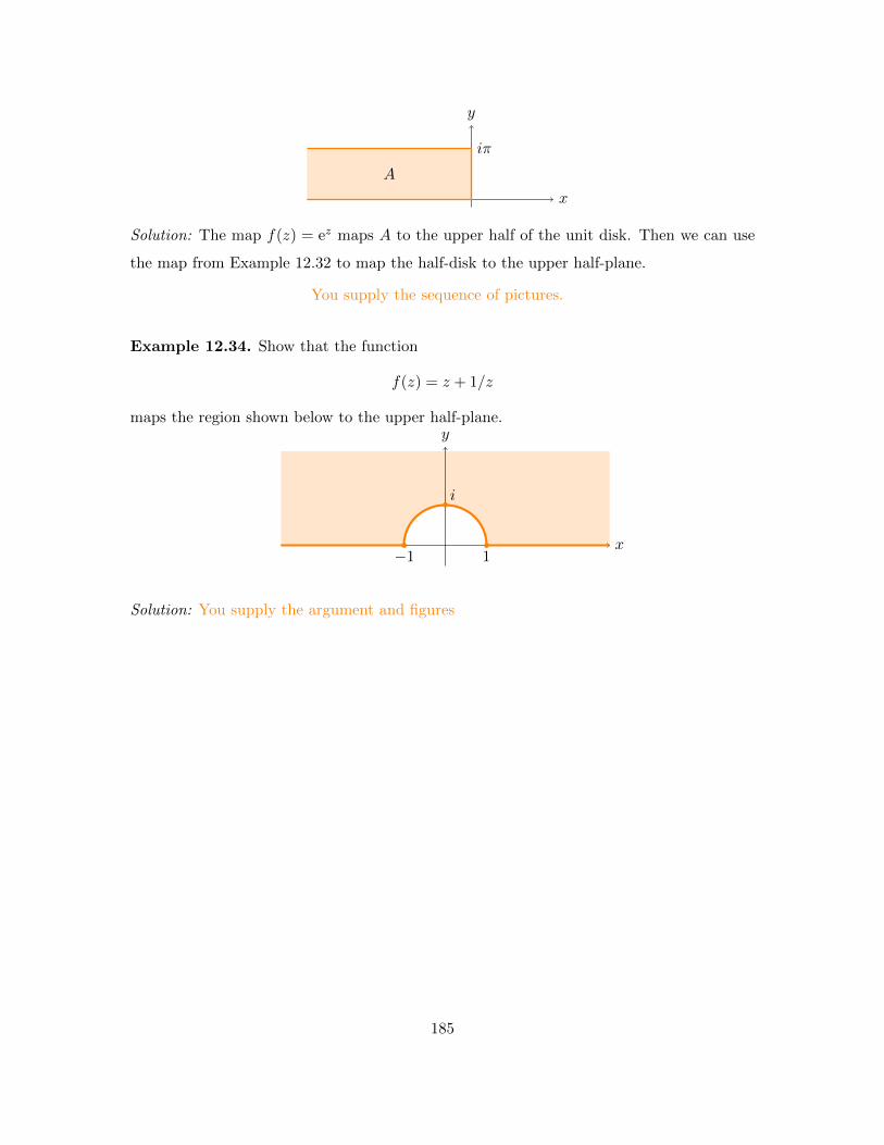
x
y
iπ
A
Solution: The map f(z) = ez maps A to the upper half of the unit disk. Then we can use
the map from Example 12.32 to map the half-disk to the upper half-plane.
You supply the sequence of pictures.
Example 12.34. Show that the function
f(z) = z + 1/z
maps the region shown below to the upper half-plane.
x
y
−1 1
i
Solution: You supply the argument and figures
185