178 ieee transactions on visualization and computer...

View-Dependent Multiscale Fluid SimulationYue Gao, Chen-Feng Li, Bo Ren, and Shi-Min Hu, Member, IEEE

Abstract—Fluid flows are highly nonlinear and nonstationary, with turbulence occurring and developing at different length and time

scales. In real-life observations, the multiscale flow generates different visual impacts depending on the distance to the viewer. We

propose a new fluid simulation framework that adaptively allocates computational resources according to the viewer’s position. First, a

3D empirical mode decomposition scheme is developed to obtain the velocity spectrum of the turbulent flow. Then, depending on the

distance to the viewer, the fluid domain is divided into a sequence of nested simulation partitions. Finally, the multiscale fluid motions

revealed in the velocity spectrum are distributed nonuniformly to these view-dependent partitions, and the mixed velocity fields defined

on different partitions are solved separately using different grid sizes and time steps. The fluid flow is solved at different spatial-

temporal resolutions, such that higher frequency motions closer to the viewer are solved at higher resolutions and vice versa. The new

simulator better utilizes the computing power, producing visually plausible results with realistic fine-scale details in a more efficient way.

It is particularly suitable for large scenes with the viewer inside the fluid domain. Also, as high-frequency fluid motions are distinguished

from low-frequency motions in the simulation, the numerical dissipation is effectively reduced.

Index Terms—Fluid simulation, Hilbert-Huang transform, fluid velocity spectrum, flow field decomposition, view-dependent partition

Ç

1 INTRODUCTION

FLUID simulations based on the Navier-Stokes equationshave achieved great success in computer graphics. Many

compelling methods with impressive animations have beenreported in the past decade. However, fluid simulationremains a challenging task where improving the visualeffect of fine-scale fluid motions and reducing the demandof computational resources are the main concerns. Unlikecomputational physics, the focus of graphics applications ison the visual effect of the final rendered images andanimations. This implies a high-potential value for exploit-ing the unique viewing information to improve existingfluid simulators. In this work, we propose a novel approachwhich incorporates the viewing information into the fluidsolver and adaptively simulates the fluid at multiple scales,such that the computational resources are allocated to thekey regions and to the key scales that have importantimpacts on the visual impression of turbulent flows. Thisapproach is particularly suitable for large scenes with theviewer immersed in the fluid domain. Such kind of scenesare rare to be seen in previous publications, but are oftenmost desired by movie directors and game designers.

Generally, the techniques considering the viewer arereferred as the levels of details, which has become a standardtool widely used in 3D geometry representation and texturerendering. The basic idea is that when the object is far fromthe viewer, a reduced geometry representation or a reducedtexture is applied. This simplification is supported by the fact

that, for human visual perception, the higher frequencysignals play a more important role when the viewer is nearby,while the lower frequency signals are more important whenthe viewer is at distance [1].

Inspired by view-dependent rendering techniques, wefirst decompose the fluid velocity field into a series offrequency components using a modified empirical modedecomposition (EMD) method. Higher frequency compo-nents represent smaller scale fluid motions (typically localturbulent flows), while lower frequency components repre-sent motions at larger scales (typically large eddies andglobal laminar flows). Also, the fluid domain is divided intoa series of nested partitions centered with respect to theviewing frustum. Different grid sizes and time steps areassigned to different partitions depending on their distancesto the viewer. The control of levels of details is then appliedto each frequency component by distributing it nonuni-formly to the simulation partitions. Higher frequencycomponents closer to the viewer are allocated to partitionswith finer grids and smaller time steps, while lowerfrequency components more away from the viewer areallocated to partitions with coarser grids and larger timesteps. As a result, the effective velocity field defined on eachsimulation partition is a mixture of frequency components,and the visible evolution of the mixed velocity can besufficiently captured by the space-time resolution associatedwith the specific partition. To obtain the final solution, theeffective velocity fields are solved semi-independently ondifferent partitions, which provides richer visual details tothe viewer in a more efficient way. Although the nestedsimulation partitions differ in size and resolution, they are allmeshed with uniform rectangular grids, which makes thesolver robust and efficient.

This novel view-dependent multiscale simulation frame-work distributes the computational resources according tothe viewing settings of the target fluid motion, and is adaptivein both space and time dimensions. The main technicalinnovations include:

178 IEEE TRANSACTIONS ON VISUALIZATION AND COMPUTER GRAPHICS, VOL. 19, NO. 2, FEBRUARY 2013

. Y. Gao, B. Ren, and S.-M. Hu are with the Department of ComputerScience, Tsinghua University, Beijing 100084, China.E-mail: {gaoyuear, renboeverywhere}@gmail.com,[email protected].

. C.-F. Li is with the College of Engineering, Swansea University, SwanseaSA2 8PP, United Kingdom. E-mail: [email protected].

Manuscript received 29 Aug. 2011; revised 23 Feb. 2012; accepted 15 Apr.2012; published online 2 May 2012.Recommended for acceptance by H.-S. Ko.For information on obtaining reprints of this article, please send e-mail to:[email protected], and reference IEEECS Log Number TVCG-2011-08-0203.Digital Object Identifier no. 10.1109/TVCG.2012.117.

1077-2626/13/$31.00 � 2013 IEEE Published by the IEEE Computer Society

. Using a novel approach of space-filling curves, theEMD is efficiently extended to 3D and applied todecompose the velocity field into a small number offrequency components, which represent the fluidmotion at different length scales.

. A spectrum-based simulation pipeline is proposed, inwhich different frequency components evolve atdifferent space-time resolutions. By doing so, itsignificantly reduces the numerical diffusion thatcauses damping of high-frequency turbulence inprevious methods, and preserves more fine-scaleturbulence details in the result.

. The fluid domain is adaptively partitioned accord-ing to the camera position, and the fluid is simulatedat different space-time resolution depending on itsdistance to the viewer. This approach considers bothrendering and simulation together, and efficientlyutilizes the computational resources in the placesthat most affect the final rendered result.

2 PREVIOUS WORK

Stam’s unconditionally stable solver [2] made the grid-basedfluid simulation popular in the graphics community. Sincethen, many different techniques have been developed to adddetails to the fluid. The basic approach is to reduce thenumerical dissipation. Fedkiw et al. used the vorticityconfinement technique to prevent the rapid dissipation ofvortices. Artificial divergence sources are introduced in [3] tosimulate gas explosion. Vortex particles are used in [4] to addthe vorticity more accurately. Zhu and Bridson [5] intro-duced FLIP to overcome advection dissipation. Othermethods including BFECC [6], QUICK [7], MacCormack [8]suggested using higher order space discretization schemesand higher order time integration schemes (e.g., Runge-Kutta methods). These methods discretize the whole fluiddomain using uniform grids, thus they are all limited by theNyquist frequency.

For 3D fluid simulation, a small increase of the gridresolution by a factor of k will cause a dramatic increase tothe computational cost by a factor of k4 [9]. Therefore,various techniques have been investigated in order toincrease the simulation resolution while controlling thecomputational expense. Different methods [10], [11], [12],[13] have been proposed to generate divergence free fieldsfrom random noise, and then used these artificial velocityfields to represent the turbulent flow. Other methods [14],[15], [16], [17], [18] simulated the fluid on a low-resolution

grid to obtain the macroscale flow, which was thencombined with the artificial divergence-free velocity fieldsto mimic the turbulent flow at the micro scale. Instead ofadding noise, Yoon et al. [19] used the vortex particle method[4] to directly generate a high-resolution turbulent flow, andRasmussen et al. [12] synthesized the 3D velocity field from2D slices. These synthesis methods do not perform high-resolution computation on the Navier-Stokes equations, andinstead attempt to produce plausible results using artificialmeans. Thus, their results are nonphysical, but can becombined with any grid-based method.

Although grid-based fluid solvers are often preferred inthe graphics community, other numerical schemes includ-ing finite volume [20], [21] and finite element methods [22]have also been used in many specific graphics applications.Some researchers have also exploited the viewing informa-tion in fluid simulations. Until recently, there have beenmainly two types of approaches: 1) octree [23], adaptivemesh refinement (AMR) [24] and mesh coupling [25]methods, which use nonuniform meshes to distinguishdifferent levels of details for the fluids; and 2) multigridmethods [7], [9], [26], which use multiple layers of meshesto represent fluid motions at different length scales. Theidea of multigrid simulations has also been adopted in theframework of smoothed-particle hydrodynamics to accel-erate fluid simulation [27]. In a wider context, it is alsonoted that Horvath and Geiger [28] presented a view-dependent multiscale simulation framework for fire simu-lations, and for accelerating sea-wave simulations [29], theviewing information is used to adaptively determined thesurface mesh and to filter out invisible wave lengths.

3 ALGORITHM OVERVIEW

Fluid phenomena are interesting and visually attractivebecause of turbulent fluid motions. It is well known influid dynamics that turbulence occurs and develops atdifferent length and time scales, with the extent of scaledifference indicated by the Reynolds number. In order tocapture fine-scale features of turbulent flows, it is normallynecessary to use fine simulation grids and small time steps,or to use higher order space discretization and timeintegration schemes. This creates a huge computationalburden to the fluid simulator, in particular when simulat-ing a large fluid domain. On the other hand, objects in alarge scene are observed at different resolutions by humaneyes depending on their distances to the viewer. Fine localfluid motions have a significant visual impact when the

GAO ET AL.: VIEW-DEPENDENT MULTISCALE FLUID SIMULATION 179

Fig. 1. Four snapshots of a view-dependent multiscale fluid simulation with moving camera positions. (six partitions, grid sizes: 1=400-1=100, timesteps: 1=120 s-1=30 s).

viewer is nearby, and as the distance to the viewerincreases, these fine-scale features become less and lessvisible, while global fluid motions at larger scales becom-ing more and more dominant. Thus, for the purpose ofachieving visually appealing results, there is a clearpotential of benefit of utilizing the viewing informationto improve the performance of fluid simulators.

We propose a view-dependent multiscale simulationframework as shown in Fig. 2. First, the fluid velocity fieldis decomposed into a series of frequency components u1;u2; . . . ;um, representing the fluid motion at different lengthscales ranging from small to large. Next, according to theposition of the viewer, m nested simulation partitions �i areconstructed, with �1 indicating the vicinity of the viewerand �m representing the whole fluid domain. Thesesimulation partitions are all meshed into uniform rectan-gular grids, and each partition �i is set with a different gridsize depending on the length scale of the correspondingfrequency component ui. Then, each frequency componentui is sequentially allocated to partitions �i, �iþ1; . . . ;�m,such that for each partition, it only carries the componentquantity that has not been supported by the previous ones.Thus, the effective velocity field u�i defined on partition �i

is a mixture of velocity components u1; . . . ;ui that share asimilar visual significance determined by their intrinsiclength scales and distances to the viewer. To solve thiscombined velocity field u�i with uniform visual significance,a separate fluid simulation is performed on partition �i

with individually assigned grid size and time step. Finally,the total fluid motion in the whole fluid domain isconstructed by adding up the results obtained on allsimulation partitions. Depending on the fluid evolution,the velocity spectrum is repeatedly computed to ensure thatthe new fluid motion is efficiently represented by thefrequency components u1; . . . ;um.

The proposed view-dependent multiscale fluid simula-tion framework can be viewed as a multigrid methodcombined with spectral decomposition. The idea of usingspectral analysis in CFD applications is not entirely new,and a remarkable example is the large eddy simulation [30]that introduces spatial-temporal filters to reduce the range

of length scales of the solution, hence reducing thecomputational cost. The feasibility of this new simulationframework relies on two assumptions: 1) the fluid velocityfield can be decomposed into a small number of mean-ingful frequency components at different length scales; and2) the Navier-Stokes equations can be linearized to allowseparately solving each frequency component with varyinggrids and varying time steps. The consideration andsolution of these two issues are addressed in Sections 4and 5, respectively.

4 3D VELOCITY FIELD DECOMPOSITION

The fluid velocity field can be viewed as a time-varyingsignal defined in a 3D domain. From the viewpoint ofphysics, it is clear that the 3D velocity signal consists ofintrinsic structures at different length scales. However, asturbulence is highly nonlinear and nonstationary, standarddata analysis tools such as singular value decomposition[31], Fourier and wavelet analysis, etc., typically producemany spurious frequency components causing energyspreading, which makes the resulting spectrum have littlephysical meaning. An exception is the EMD [32], alsoknown as Hilber-Huang transform, which was originallydeveloped for processing nonlinear and nonstationary timeseries. Over the past decade, the EMD method has beenextremely successful in engineering and successfullyapplied in various complicated data sets, including seawaves and earthquake signals, etc.

For the sake of completeness, the standard EMDprocedure is briefly reviewed in Section 4.1, after which itis extended into 3D cases in Section 4.2 for processing thefluid velocity field.

4.1 EMD Basics

The standard EMD method is designed for the analysis ofone-dimensional signals, in particular time series. The mainidea of EMD is to decompose the signal into a small numberof intrinsic mode functions (IMF), which are based on andderived from the data. An IMF is any function with thesame number of extrema and zero crossings, and with zero


Fig. 2. The algorithm framework of view-dependent multiscale fluid simulation.

mean of the upper and lower envelops defined, respec-tively, by the local maxima and minima. From thisdefinition, the IMF is a general oscillatory function, withpossibly varying amplitude and frequency along the timeaxis. Thus, for representing signals, an IMF is much morepowerful than the simple harmonic function, which hasconstant amplitude and frequency. Given a 1D signal f , itsEMD representation is

f ¼XKk¼1

ck þ rK; ð1Þ

where ci; i ¼ 1; 2; ::;K are the IMFs with the frequencyranging from high to low and rK is the residual. The EMDalgorithm sequentially extracts its IMFs via a “sifting”procedure as follows:

1. Initialization r0 ¼ f , set index k ¼ 12. Compute the kth IMF, ck

a. Initialization h0 ¼ rk�1, set index j ¼ 1b. Find all local maxima and local minima of hj�1

c. Build the upper envelope Emax;j�1 by connectingall local maxima with a cubic spline, and buildthe lower envelope Emin;j�1 by connecting alllocal minima with a cubic spline

d. Compute the mean of the upper and lowerenvelopes, Emean;j�1 ¼ 1

2 ðEmin;j�1 þ Emax;j�1Þe. hj ¼ hj�1 � Emean;j�1

f. If the IMF stopping criterion is satisfied, thenck ¼ hj, else j ¼ jþ 1 and go to step 2b

3. rk ¼ rk�1 � ck4. If rk is monotonic, the decomposition stops, else k ¼

kþ 1 and go to step 2.

For the IMF stopping criterion in step 2f, different criteriahave been suggested in the literature based on the definitionof IMFs. In our applications, it is found that there is novisible difference in the final result if we simply fix theiteration number as 8 to 10. There is no rigorous conver-gence proof for the above algorithm, but practically italways converges very quickly [32]. The physical justifica-tion of the above EMD procedure is very solid and has beenverified and validated in numerous experiments by variousreal data sets (see, e.g., [33]).

4.2 3D EMD of Velocity Fields

The main challenge of extending the EMD into higherdimensional signals arises in the construction of the upperand lower envelopes (step 2c in the EMD algorithm). Unlikethe simple closed-form solution of the 1D cubic splineinterpolation, higher dimensional surface interpolation iscomplex and often involves time-consuming computation.For the 2D case, 2D radial basis functions are introduced[34], [35] to transform the interpolation problem into a globaloptimization problem. It requires to solve a m�m linearsystem, where m is the total number of extrema. Theassociated computation is affordable for 2D image applica-tions with hundreds of pixels along each axis, but is too slowfor our 3D fluid simulations that require the EMD to berepeatedly performed in a large 3D space as turbulencedevelops. A fast bidimensional EMD algorithm is proposedin [36], which is based on the Delaunay triangulation and

cubic interpolation on triangles. In order to ensure theDelaunay triangulation to cover the whole domain, thismethod has to introduce a bunch of artificial extrema, andas a result it is not suitable for our 3D fluid simulations thatrequire the highest level of automation and robustness.Liu and Peng [37] tested a tensor-product-based 2D EMDapproach that applies separately 1D EMD on each row andcolumn of an image, after which averaging the envelopesfrom different directions. Although it is much faster to do so,our experiments led to a similar conclusion as [37]: the resultis generally worse in that each slice of data only contain asmall portion of samples and the connection informationcontained in the original data has been seriously lost. As theEMD will be repeatedly performed in our fluid simulationframework, a more efficient and more robust 3D algorithmis needed.

We propose to use space-filling curves to flatten 3D datainto 1D. First, a space filling curve is constructed to fill thefluid domain, and moving along the curve an index isassigned to each grid cell and saved in a template. Then, the3D velocity field is rearranged into a 1D signal arrayaccording to the index template. Finally, the reshaped 1Dsignal is decomposed by using the 1D EMD algorithm, andthe decomposition result is mapped back to the 3D space byusing the same index template. In this simple 3D EMDapproach, the EMD operation is essentially performed onthe flattened 1D data set, and therefore it converges in thesame way as the standard 1D EMD method [32]. As theindex template of space-filling curve can be precomputed,the CPU expense of the 3D EMD is essentially the same as1D EMD, which is linearly proportional to the samplingdensity. Owing to the analytic cubic spline interpolation,our space-filling curve EMD technique is extremely fast. For2D cases, we have compared with the RBF method. It isfound that our approach is at least 20 times faster in all testexamples, and the new method also provides betteraccuracy because it avoids the numerical error caused bythe least squares approximation required in the RBFapproach. In the context of fluid simulation, the CPU costof an individual 3D EMD is about half of a single pressuresolver executed on the same sampling grid.

Different space-filling curves have been tested, includingthe Hilbert curve, the Z-order curve, the Koch curve and theGosper curve. In 2D cases, the Hilbert curve and the Z-ordercurve are found to have boundary artifacts caused bytheir regular quad fractal structures. By using Koch orGosper curves, the boundary artifacts can be effectivelyremoved. In 3D cases, all four curves give good decomposi-tion results without visible discontinuities. The reason is thatboth the 3D velocity filed and the 3D space filling curves aresufficiently complex to avoid the development of boundaryartifacts. For the sake of simplicity, we use the Koch curve for2D examples and the Hilbert curve for 3D examples in thispaper. It is noted that the Z-order curve has recently beenused in SPH simulations to compute SPH neighborhoodsrapidly [38], which also demonstrates the benefit of usingspace-filling curves to accelerate 3D data processing.

The 3D Hilbert curve is defined on a cube, and whenusing the nth approximation to the limiting curve, thelength of the curve is 2n. However, the fluid domain is notnecessarily a cube. Therefore, we build the Hilbert curvewith the smallest n such that 2n=3 is greater than the


maximum velocity resolution in x-, y-, and z- directions.When moving along the Hilbert curve, the cell index isincreased and saved if and only if the current position islocated in the fluid domain. A similar method is applied tothe Koch curve in 2D cases. In Fig. 4, the gray line is thewhole Koch curve and the bold black line is the space fillingcurve we used. This strategy preserves as much as possiblethe locality of the space filling curve.

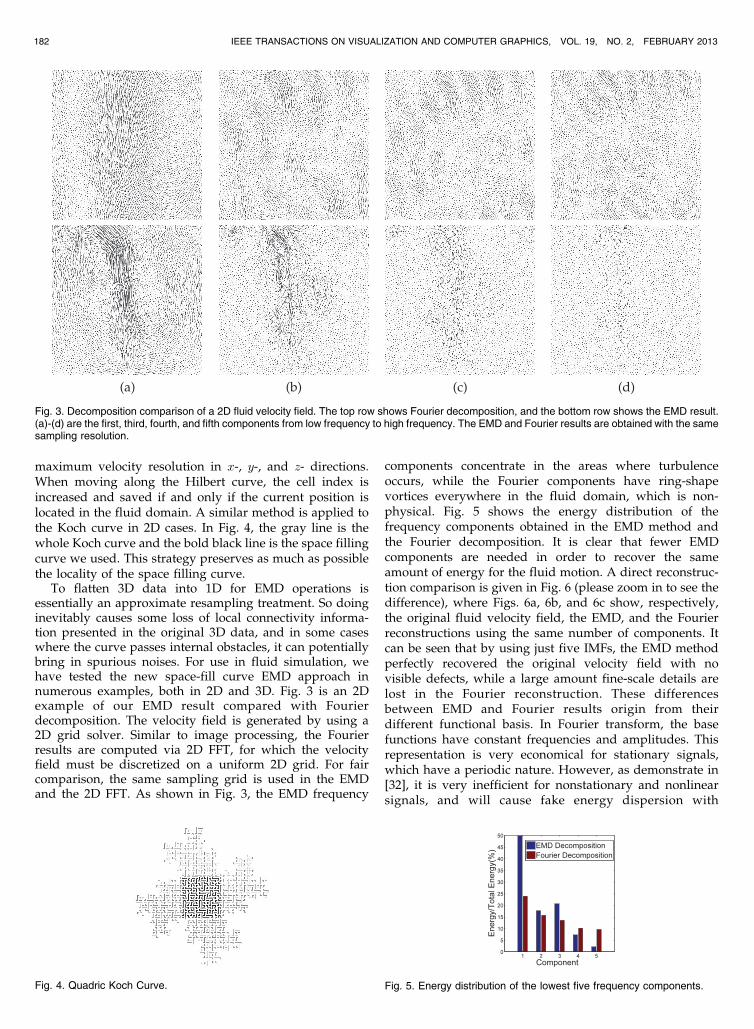
To flatten 3D data into 1D for EMD operations isessentially an approximate resampling treatment. So doinginevitably causes some loss of local connectivity informa-tion presented in the original 3D data, and in some caseswhere the curve passes internal obstacles, it can potentiallybring in spurious noises. For use in fluid simulation, wehave tested the new space-fill curve EMD approach innumerous examples, both in 2D and 3D. Fig. 3 is an 2Dexample of our EMD result compared with Fourierdecomposition. The velocity field is generated by using a2D grid solver. Similar to image processing, the Fourierresults are computed via 2D FFT, for which the velocityfield must be discretized on a uniform 2D grid. For faircomparison, the same sampling grid is used in the EMDand the 2D FFT. As shown in Fig. 3, the EMD frequency

components concentrate in the areas where turbulenceoccurs, while the Fourier components have ring-shapevortices everywhere in the fluid domain, which is non-physical. Fig. 5 shows the energy distribution of thefrequency components obtained in the EMD method andthe Fourier decomposition. It is clear that fewer EMDcomponents are needed in order to recover the sameamount of energy for the fluid motion. A direct reconstruc-tion comparison is given in Fig. 6 (please zoom in to see thedifference), where Figs. 6a, 6b, and 6c show, respectively,the original fluid velocity field, the EMD, and the Fourierreconstructions using the same number of components. Itcan be seen that by using just five IMFs, the EMD methodperfectly recovered the original velocity field with novisible defects, while a large amount fine-scale details arelost in the Fourier reconstruction. These differencesbetween EMD and Fourier results origin from theirdifferent functional basis. In Fourier transform, the basefunctions have constant frequencies and amplitudes. Thisrepresentation is very economical for stationary signals,which have a periodic nature. However, as demonstrate in[32], it is very inefficient for nonstationary and nonlinearsignals, and will cause fake energy dispersion with


Fig. 3. Decomposition comparison of a 2D fluid velocity field. The top row shows Fourier decomposition, and the bottom row shows the EMD result.(a)-(d) are the first, third, fourth, and fifth components from low frequency to high frequency. The EMD and Fourier results are obtained with the samesampling resolution.

Fig. 4. Quadric Koch Curve. Fig. 5. Energy distribution of the lowest five frequency components.

numerous spurious high-frequency components. The em-pirical mode decomposition uses adaptive base functionswith varying frequencies and amplitudes, and it isparticularly suitable for nonstationary and nonlinearsignals. This is why we chose the EMD for the decomposi-tion of turbulent flows.

For decomposing the fluid velocity field, an added benefitof the EMD method is on dealing with objects presentedinside the fluid domain, where the fluid velocity field can bediscontinuous on the object boundary. Most standard dataanalysis tools use functional basis with fixed amplitudes andfrequencies, and consequently the signal discontinuity willcause many spurious frequency components due to energyspreading. However, the functional basis of the EMDmethod is adaptively determined by the local features ofthe signal. The IMFs have varying amplitudes and frequen-cies, so that the energy spreading caused by signaldiscontinuity is minimized. Indeed, this is one of the majoradvantages of the EMD technique [32].

Using the EMD method, the velocity field u in thesimulation domain is represented as:

u ¼Xmi¼1

ui; ð2Þ

where ui, i ¼ 1; 2; . . . ;m, are frequency components repre-senting fluid motions at different length scales, ranging fromsmall to large. In our implementation, m is a user specifiedconstant controlling how many IMFs to be extracted from thevelocity field. Thus, ui, i ¼ 1; . . . ;m� 1, are IMF compo-nents, and um is a non-IMF component. As um consists of alllower frequency tail IMFs and the residual term, it carries themajority of the kinetic energy of the fluid flow. Benefitedfrom the adaptive and data dependent nature of IMFs, thenonlinear and nonstationary fluid velocity field can beeffectively represented with a small number of frequencycomponents. In our limited experiments, four to sixfrequency components are sufficient to represent the velocityfields. Note that the EMD is performed separately for x-, y-,and z- components, and then adding them together to obtainthe vector-valued decomposition (2).

5 VIEW DEPENDENT MULTISCALE SIMULATION

For incompressible ideal fluids, the Euler equations are

�@u

@tþ �ðu � rÞu ¼ �rpþ f ; ð3Þ

r � u ¼ 0; ð4Þ

where u is the velocity, p the pressure, � the fluid density,and f the effective body force including gravity, buoyancyand vorticity confinement, etc.

Determined by human visual perception [1], real-lifeobservation of a large dynamic fluid scene has two mainfeatures:

. Fluid motions are observed at different resolutionsby human eyes, depending on the distance from theviewer to the location where the motion is develop-ing. The smaller the distance is, the higher resolutionwill be received; and vice versa.

. The fluid motion consists of intrinsic structures, i.e.,frequency components, evolving at different lengthand time scales. These multiscale frequency compo-nents generate unequal visual impacts. When theviewer is nearby, the fast-developing small scalecomponents are more significant in our observation;and when the viewer is at distance, the slow-movinglarge scale components become more dominant.

In order to achieve the best visual effects with the minimumcomputational cost, the fluid solver needs to take intoaccount both of the above aspects. This is done by integratingspectral analysis and domain partition into a view drivensimulation framework, whose details are explained in thefollowing sections.

5.1 Dynamics of Multiscale Flow

In the space dimension, the multiscale motion componentsof a turbulent flow are revealed in (2) by using the EMDmethod. Substituting (2) into equations (3)-(4) and settingthe fluid density to unit yields

Xmi¼1

@ui@tþXmi¼1

ðu � rÞui ¼ �rpþ f ; ð5Þ

Xmi¼1

r � ui ¼ 0: ð6Þ

When an explicit solver is adopted, the total fluid velocity uis computed using the results from the previous time steps,thus u can be considered as semidecoupled from ui in (5).

Equations (5)-(6) show that multiscale fluid motions arecoupled together to satisfy momentum and mass conserva-tion. However, from the viewpoint of physics [39], fluidmotions ui differ not only in their length scales, but they alsodevelop at different pace in the time dimension, withmicroscale motions developing fast and macroscale motionsdeveloping relatively slow. Thus, if the observation is fixedto a small window T in the time axis and if the inter-frequency exchange of momentum and mass can be ignored,this leads to

@ui@tþ ðu � rÞui ¼ �rpi i ¼ 1; 2; . . . ;m� 1; ð7Þ

@um@tþ ðu � rÞum ¼ �rpm þ f ; ð8Þ

r � ui ¼ 0 i ¼ 1; 2; . . . ;m; ð9Þ

where pi, i ¼ 1; 2; . . . ;m are the unknown fluid pressurecorresponding to the motion components ui. Typical body


Fig. 6. Reconstruction comparison. (a) is the original velocity field, (b) isthe sum of the first five EMD components, and (c) is the sum of the firstfive Fourier components.

forces, such as gravity and buoyancy, change much slowercomparing to the rapid development of microscale turbulentmotions. This is particularly true for ideal fluids [39], whoseviscous force is zero and Reynolds number is infinity.Therefore, in the momentum (7), the influence from the slowchanging body forces to the fast developing microscale fluidmotions is also ignored, and the body force is only includedin (8) for the mixed low-frequency component um. Byallowing all body forces to directly work on the um motion,the dominant energy carrier obtained in the EMD (2), theenergy transfer process occurring at the macro-scale level isemphasized. However, if fast changing body forces areinvolved, they should be likewise decomposed and appliedto the corresponding velocity component.

5.2 View-Dependent Simulation of Multiscale Flow

Equations (7)-(9) describe the dynamics of multiscale flow.Our aim is to solve these equations according to the camerasettings such that all visible fluid motions at both micro-and macroscales are accurately captured with the minimumcomputational cost.

First, the fluid domain is divided into m nested partitions�i, i ¼ 1; 2; . . . ;m such that �1 � �2 � � � � � �m, where �m

represents the whole fluid domain. These nested partitionsare all centered with respected to the view frustum, so thatpartitions �i, i ¼ 1; 2; . . . ;m provide a natural indication forthe distance between the viewer and the fluid point,ranging from small to large. It is noted that by buildingthe partitions �i with respect to the view frustum, the viewdirection and view angle are also taken into account. As theviewer-to-fluid distance increases, the visibility of the fluidmotion drops, which sequentially reduces the accuracyrequirement of the simulation. Therefore, these simulationpartitions are discretized using different grid sizes and timesteps, and with the increase of index i, the space-timeresolution of �i decreases. In particular, the grid size andtime step of each partition �i are set to allow an economicaland yet sufficiently accurate description of the motion ui.

Next, depending on the viewer-to-fluid distance, eachmotion component ui is adaptively represented at differentspace-time resolutions. This is achieved by distributing thevelocity quantities of ui to partitions �j, j ¼ i; iþ 1; . . . ;msuch that the motion ui is discretized on a composite grid�i [ f�iþ1 � �ig [ � � � [ f�m � �m�1g. As shown in Fig. 2,after all frequency components ui have been distributed tothe simulation partitions, the velocity field on each partition�i becomes a composite field u�i as follows:

u�i ¼ui for �i�1Xij¼1

uj for �i � �i�1:

8><>:

ð10Þ

The effective velocity u�i collects all visible fluid motionsmeasured at the space-time resolution of �i.

Then, reorganizing (7)-(9) according to (10) yields

@u�i@tþ ðu � rÞu�i ¼ �rp�i i ¼ 1; 2; . . . ;m� 1; ð11Þ

@u�m@tþ ðu � rÞu�m ¼ �rp�m þ f ; ð12Þ

r � u�i ¼ 0 i ¼ 1; 2; . . . ;m; ð13Þ

where p�i , i ¼ 1; 2; . . . ;m are the unknown fluid pressurecorresponding to the composite velocity components u�i .Although similar in formulation, it should be noted that (11)-(13) and (7)-(9) describe totally different physical phenomena.Equations (11)-(13) are defined on partitions �i,i ¼ 1; 2; . . . ;m, respectively, and for each partition �i, theydescribe the evolution of all fluid motions that are visible atthe space-time resolution associated with �i. Equations (7)-(9) are defined in the whole fluid domain, and they describethe dynamics of the fluid motion at each individual lengthscale, regardless of its visibility to the viewer.

Finally, the fluid simulation is performed by solving the(11)-(13) on nested partitions �i, i ¼ 1; 2; . . . ;m, respec-tively. The initial values of u�i are computed with (10), inwhich the frequency components ui are obtained from theEMD (2). Starting from i ¼ 1 and going through eachsimulation partition �i, the solution u�i is obtained by usingthe standard advection-projection scheme [2]. Specifically,the advection step solves equation

@u�i@tþ ðu � rÞu�i ¼ 0: ð14Þ

Note that the background velocity field for advection is thetotal velocity u instead of the velocity component u�i .Similarly, the projection step solves equations

@u�i@t¼ �rp�i ; ð15Þ

r � u�i ¼ 0: ð16Þ

Note that for the last partition �m, the external body force fis added into (15). For the pressure solver, we use thestandard preconditioned conjugate gradient method withthe preconditioner obtained through the incomplete Cho-lesky decomposition. The final solution of the fluid is

u ¼ u�1 � u�2 � � � � � u�m; ð17Þ

where � denotes the superposition of velocity fields u�idefined in different partitions. As (11)-(13) hold only whenthe observation is fixed in a relatively small time window T ,the EMD operation (2) needs to be repeatedly performedafter certain time steps to reinitialize the solution process(14)-(17). This EMD reinitialization step is necessary toensure an adequate and timely capture of the cross-scalemotion transfer of the fluid.

Boundary conditions. For internal partitions �i; i ¼1; . . . ;m� 1, the boundary conditions are set as u�i ¼ 0 on@�i. For the partition �m, the real boundary condition of thewhole fluid domain is used on @�m. These simplificationspractically over restrict the energy exchange betweenpartitions. By doing so, we sacrifice the accuracy in orderto minimize the coupling between partitions and improvethe efficiency of obtaining visually plausible results. Ourmethod also supports internal boundaries. For static ob-stacles in the fluid domain, each velocity component dealswith the obstacle in the same way as the traditional methods,e.g., using simple obstacle discretization or some moreprecise models. As the obstacle is static, the final velocityfield automatically satisfies the nonslip boundary condition.


For dynamic obstacles, a practical approach is to add thedynamic boundary condition to the lowest frequencycomponent, while adding static boundary conditions to allthe other components.

5.3 Computational Issues

Our multiscale fluid simulation is driven by the viewer. Instandard rendering systems, such as the PBRT [40] used inthis work, the fluid domain is defined in the object space,then transformed into the view space by model and viewmatrices, and finally projected into the image space accord-ing to camera parameters (projection matrix and viewport).We integrate the inverse of this pipeline into our simulator tocontrol the levels of details in the simulation.

The fluid domain is divided into simulation partitionsaccording to the distance to the viewer and the viewdirection, and each partition is individually assigned witha grid size and a time step. Thus, the partitions move whenthe viewer moves, which then requires the fluid velocity tobe transferred between grids of different sizes. For simpli-city, we use linear interpolation for the velocity transferbetween coarse grids and fine grids.

In the current implementation, the grid sizes and timesteps are manually set by the user based on the size ofsimulation domain, the camera setting, and the character-istics of IMFs. Separate velocity components communicatewith each other through the advection term (14) and theEMD reinitialization. It is possible to automatically deter-mine the spatial-temporal resolution. Specifically, the gridsize can be associated with the dimension of the simulationdomain and the spatial frequencies of IMFs, which can beobtained via Hilbert transforms. Once the grid size is fixed,the corresponding time step can then be determined inconjunction with the camera motion. This importantadaptivity aspect will be pursued in our future work asdetailed in Section 7.

Given a target fluid and the camera settings, the view-dependent multiscale fluid simulation is performed asfollows:

1. Generate a Hilbert curve to cover the whole fluiddomain and build the 3D-to-1D index template

2. Compose an ordered work list consisting of fourtypes of jobs: partition, EMD, simulation, and output

3. Follow the work list to do

a. For partition request: according to the currentcamera settings, the whole fluid domain isdivided into simulation partitions �i with fixedgrid sizes and time steps

b. For EMD request: compute the velocity spec-trum (2) with 3D EMD

c. For simulation request: solve (14)-(16) on thespecific simulation partition �i

d. For output request: output the current velocityfield u.

In step (2), time entries of the partition request aredetermined according to the camera motion; time entries ofthe EMD request are set with a fixed time interval specifiedby the user; time entries of the simulation request arecalculated according to the fixed time step of each simulationpartition; and time entries of the output request are setaccording to the animation requirement. In the current

implementation, the oldest time step is always executed firstin order to get the most up-to-date information from theother fluid simulations. Also, in the advection step, wesimply use the latest total velocity field as the backgroundvelocity. By doing so, we ignore the numerical error causedby the simulations being out of synchronization. The maincomputational cost of our simulation framework is in theadvection-projection solutions, which are performed sepa-rately on different partitions with different space-timeresolutions. As high-resolution solutions are only performedfor the closest partitions to the viewer, usually very smalldomains, our simulation runs much faster comparing to thestandard N-S solver using a uniform high-resolution grid.

Comparing with octree and adaptive mesh refinement(AMR) methods, the proposed method differs mainly intwo aspects: 1) We distinguish the fluid flow not only by itsdistance to the viewer (resolved by setting multiplesimulation partitions), but also by its intrinsic motions atdifferent length scales (resolved by EMD). Both spatial andtemporal resolutions are adaptive in our method, while theoctree and AMR approaches are often adaptive only in thespace dimension. 2) Octree and AMR methods use nonuni-form grids, and we use multiple partitions meshed intouniform grids. The use of uniform grids and simple datastructures significantly simplifies the implementation andcomputational complexity. In a wider sense, the newmethod can be viewed as a multigrid approach combinedwith spectral analysis. Unlike other multigrid methodsusing prefixed simulation resolutions independent to theevolution of fluid flows, the space-time resolutions fordifferent simulation partitions are determined according tothe spectral decomposition result of the fluid velocity field.Therefore, the new method is more adaptive, and cansupport moving camera positions and developing fluidflows in a uniform framework.

6 RESULT

Several examples are presented in this section to demon-strate the performance of the new fluid simulation frame-work. All numerical simulations are performed on a PCplatform with an Intel Core2 2.4 GHz CPU and 8 GB memory.

Assumption verification 1. Our new method assumesthat the low-frequency components of a velocity field can besimulated on coarse grids to save computational cost. This isverified in Fig. 7, where a plume is developed in a velocityfield that only contains low-frequency components. Figs. 7a,7b, and 7c are the results obtained using a fine grid(128� 256� 128), and Figs. 7d, 7e, and 7f are solved on acoarse grid (64� 128� 64). The two groups of results arevery similar up to frame 8 and they become more different asthe simulation continues. This observation confirms that thelow-frequency components of a velocity field do generatehigh-frequency motions as time goes, but these newlygenerated high-frequency components are neglectable inthe beginning period, during which the fluid motion can bewell captured by using a coarse grid. Therefore, we choosedifferent grid resolutions to economically simulate differentfrequency components, and periodically recompute thevelocity spectrum to adjust the frequency-componentallocation and ensure that every frequency component isalways simulated using the right grid resolution.


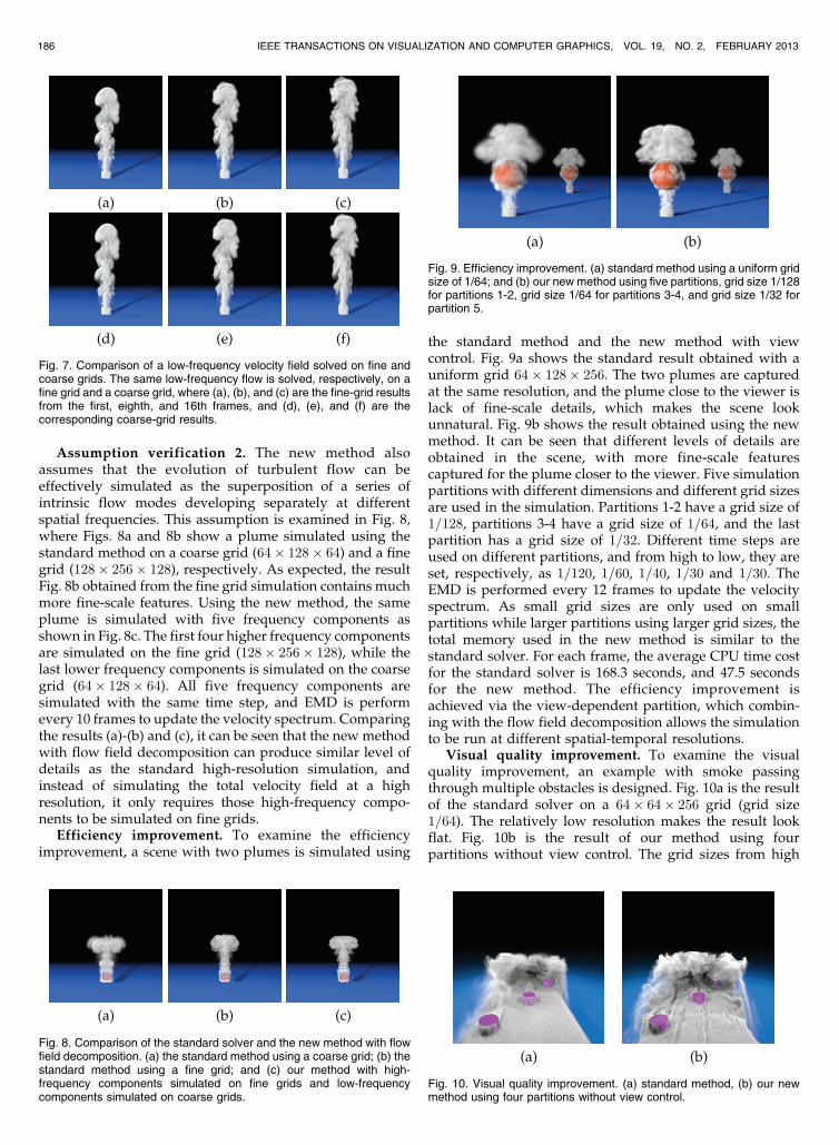
Assumption verification 2. The new method alsoassumes that the evolution of turbulent flow can beeffectively simulated as the superposition of a series ofintrinsic flow modes developing separately at differentspatial frequencies. This assumption is examined in Fig. 8,where Figs. 8a and 8b show a plume simulated using thestandard method on a coarse grid (64� 128� 64) and a finegrid (128� 256� 128), respectively. As expected, the resultFig. 8b obtained from the fine grid simulation contains muchmore fine-scale features. Using the new method, the sameplume is simulated with five frequency components asshown in Fig. 8c. The first four higher frequency componentsare simulated on the fine grid (128� 256� 128), while thelast lower frequency components is simulated on the coarsegrid (64� 128� 64). All five frequency components aresimulated with the same time step, and EMD is performevery 10 frames to update the velocity spectrum. Comparingthe results (a)-(b) and (c), it can be seen that the new methodwith flow field decomposition can produce similar level ofdetails as the standard high-resolution simulation, andinstead of simulating the total velocity field at a highresolution, it only requires those high-frequency compo-nents to be simulated on fine grids.

Efficiency improvement. To examine the efficiencyimprovement, a scene with two plumes is simulated using

the standard method and the new method with viewcontrol. Fig. 9a shows the standard result obtained with auniform grid 64� 128� 256. The two plumes are capturedat the same resolution, and the plume close to the viewer islack of fine-scale details, which makes the scene lookunnatural. Fig. 9b shows the result obtained using the newmethod. It can be seen that different levels of details areobtained in the scene, with more fine-scale featurescaptured for the plume closer to the viewer. Five simulationpartitions with different dimensions and different grid sizesare used in the simulation. Partitions 1-2 have a grid size of1=128, partitions 3-4 have a grid size of 1=64, and the lastpartition has a grid size of 1=32. Different time steps areused on different partitions, and from high to low, they areset, respectively, as 1=120, 1=60, 1=40, 1=30 and 1=30. TheEMD is performed every 12 frames to update the velocityspectrum. As small grid sizes are only used on smallpartitions while larger partitions using larger grid sizes, thetotal memory used in the new method is similar to thestandard solver. For each frame, the average CPU time costfor the standard solver is 168.3 seconds, and 47.5 secondsfor the new method. The efficiency improvement isachieved via the view-dependent partition, which combin-ing with the flow field decomposition allows the simulationto be run at different spatial-temporal resolutions.

Visual quality improvement. To examine the visualquality improvement, an example with smoke passingthrough multiple obstacles is designed. Fig. 10a is the resultof the standard solver on a 64� 64� 256 grid (grid size1=64). The relatively low resolution makes the result lookflat. Fig. 10b is the result of our method using fourpartitions without view control. The grid sizes from high


Fig. 7. Comparison of a low-frequency velocity field solved on fine andcoarse grids. The same low-frequency flow is solved, respectively, on afine grid and a coarse grid, where (a), (b), and (c) are the fine-grid resultsfrom the first, eighth, and 16th frames, and (d), (e), and (f) are thecorresponding coarse-grid results.

Fig. 8. Comparison of the standard solver and the new method with flowfield decomposition. (a) the standard method using a coarse grid; (b) thestandard method using a fine grid; and (c) our method with high-frequency components simulated on fine grids and low-frequencycomponents simulated on coarse grids.

Fig. 9. Efficiency improvement. (a) standard method using a uniform gridsize of 1/64; and (b) our new method using five partitions, grid size 1/128for partitions 1-2, grid size 1/64 for partitions 3-4, and grid size 1/32 forpartition 5.

Fig. 10. Visual quality improvement. (a) standard method, (b) our newmethod using four partitions without view control.

frequency to low frequency are 1=128, 1=128, 1=64, and1=32. In Fig. 10b, the nonpotential flow structures observedat the upwind of the cylinders are caused by the interactionof the closely placed cylinders and the nonslip boundaryeffect. These high-frequency structures are not resolved bythe standard solver (Fig. 10a) due to numerical dissipationon the coarser mesh (grid size 1/64), while they areemphasized in the proposed solver (Fig. 10b) because thehigh-frequency motion is solved separately on a finer mesh(grid size 1/128). The average CPU time costs of thestandard method and our new method are 56.7 and69.2 seconds, respectively. With a similar computationalcost, the new method doubled the simulation resolutionproducing much more fine-scale details consistent withreal-life observations. The speedup gained in the newmethod is because 1) the last partition is solved on thecoarse grid; and 2) the first four partitions do not have anybody force and as a result, their simulations converge veryfast, typically within five iterations. However, at each timestep, the standard N-S solver typically takes 50-80 iterationsto converge to the error threshold 10�5.

Simulation with moving camera positions. The lastexample demonstrates the new method in a simulation witha moving viewpoint. Fig. 1 shows the simulation result,which is computed on six moving partitions. The maximumgrid size is 1=100, and the minimum is 1=400. Themaximum time step is 1=30, which is used on the largestpartition, and the minimum time step is 1=120, which isused on the smallest partition. The space-time resolution ofeach partition is fixed, but its position and dimensionchange automatically as the viewpoint moves. It can be seenthat the new method is robust and efficient, and it providesnatural-looking results with multiple levels of details thatare consistent with real-life observations.

7 CONCLUSION AND LIMITATION

We propose a view-dependent multiscale fluid simulationframework that exploits both the viewing information inhuman visual perception and the multiscale velocityspectrum of a turbulent flow. In the new simulationframework, the fluid is solved at different space-timeresolutions according to its visual impact. Specifically,high-resolution simulations are performed for the fluidregions closer to the viewer and for the frequencycomponents more visible to human eyes, and vice versa.The new simulator better utilizes the computing power suchthat 1) for the same simulation task, it is faster than thetraditional grid-based N-S solver; and 2) with the samecomputational resources (CPU time and memory storage), itcan simulate a larger fluid scene or produce richer fine-scaledetails. Also, as the multiscale fluid motions are distin-guished in our simulation, the numerical dissipation iseffectively reduced. By modulating the simulation in thefrequency space of the fluid motion, the new simulator canpotentially provide the animator a simple way to modulateand enhance the visual effects of fluid flows, which will bepursued in our future work.

The current implementation does not allow movinginternal obstacles. However, the extension to cope withmoving internal objects is relatively straightforward, andcare must be taken when the object moves across the

boundary of simulation partitions. The main limitation ofthe proposed new framework is in threefolds:

. For a fluid scene observed at multiple viewpoints,the simulation partitions become irregularly shaped,depending on the relative positions of differentviewpoints. The complicated geometry of simulationpartitions make the grid-based solver more complexin implementation, and a finite-volume solver mightthen become a better option.

. The proposed view-dependent simulation frameworkrequires the camera to move continuously withoutjump. Discontinuous camera positions will cause thealgorithm lose its advantage of capturing fine-scaledetails. This is because fine-scale motions are onlysimulated in the neighborhood of the previous camerafocus instead of the whole fluid domain. Similarly, theperformance can potentially drop with rapidly mov-ing cameras because a larger buffer area will beneeded for high-resolution partitions.

. Our current implementation is purely sequential. Asthe simulations running on different partitions arerelatively independent, the algorithm can be readilyparallelized. Furthermore, as each partition ismeshed into uniform grids, its simulation can alsobe accelerated with GPU implementation.

These three important aspects will be pursued in our futurework.

ACKNOWLEDGMENTS

The authors would like to thank the anonymous reviewersfor their constructive comments. This work was supportedby the National Basic Research Project of China (ProjectNumber 2011CB302205) and the Natural Science Foundationof China (Project Number 61120106007). The authors wouldalso like to thank the Royal Society and Natural ScienceFoundation of China for support through an InternationalJoint Project (No. JP100987/61111130210).

REFERENCES

[1] A. Oliva, A. Torralba, and P.G. Schyns, “Hybrid Images,” ACMTrans. Graphics, vol. 25, pp. 527-532, July 2006.

[2] J. Stam, “Stable Fluids,” Proc. ACM SIGGRAPH ’99, pp. 121-128,1999.

[3] B.E. Feldman, J.F. O0Brien, and O. Arikan, “Animating SuspendedParticle Explosions,” ACM Trans. Graphics, vol. 22, pp. 708-715,July 2003.

[4] A. Selle, N. Rasmussen, and R. Fedkiw, “A Vortex Particle Methodfor Smoke, Water and Explosions,” ACM Trans. Graphics, vol. 24,pp. 910-914, July 2005.

[5] Y. Zhu and R. Bridson, “Animating Sand as a Fluid,” ACM Trans.Graphics, vol. 24, pp. 965-972, July 2005.

[6] T.F. Dupont and Y. Liu, “Back and Forth Error Compensation andCorrection Methods for Removing Errors Induced by UnevenGradients of the Level Set Function,” J. Computational Physics,vol. 190, pp. 311-324, 2003.

[7] J. Molemaker, J.M. Cohen, S. Patel, and J. Noh, “Low ViscosityFlow Simulations for Animation,” Proc. ACM SIGGRAPH/Euro-graphics Symp. Computer Animation (SCA ’08), pp. 9-18, 2008.

[8] A. Selle, R. Fedkiw, B. Kim, Y. Liu, and J. Rossignac, “AnUnconditionally Stable Maccormack Method,” J. Scientific Comput-ing, vol. 35, nos. 2/3, pp. 350-371, 2008.

[9] M. Lentine, W. Zheng, and R. Fedkiw, “A Novel Algorithm forIncompressible Flow Using Only a Coarse Grid Projection,” ACMTrans. Graphics, vol. 29, pp. 114:1-114:9, July 2010.


[10] J. Stam and E. Fiume, “Turbulent Wind Fields for GaseousPhenomena,” Proc. 20th Ann. Conf. Computer Graphics and Inter-active Techniques (SIGGRAPH ’93), pp. 369-376, 1993.

[11] A. Lamorlette and N. Foster, “Structural Modeling of Flames for aProduction Environment,” ACM Trans. Graphics, vol. 21, pp. 729-735, July 2002.

[12] N. Rasmussen, D.Q. Nguyen, W. Geiger, and R. Fedkiw, “SmokeSimulation for Large Scale Phenomena,” ACM Trans. Graphics, vol.22, pp. 703-707, July 2003.

[13] R. Bridson, J. Houriham, and M. Nordenstam, “Curl-Noise forProcedural Fluid Flow,” ACM Trans. Graphics, vol. 26, article 46,July 2007.

[14] T. Kim, N. Thurey, D. James, and M. Gross, “Wavelet Turbulencefor Fluid Simulation,” ACM Trans. Graphics, vol. 27, pp. 50:1-50:6,Aug. 2008.

[15] R. Narain, J. Sewall, M. Carlson, and M.C. Lin, “Fast Animation ofTurbulence Using Energy Transport and Procedural Synthesis,”ACM Trans. Graphics, vol. 27, pp. 166:1-166:8, Dec. 2008.

[16] H. Schechter and R. Bridson, “Evolving Sub-Grid Turbulence forSmoke Animation,” Proc. ACM SIGGRAPH/Eurographics Symp.Computer Animation (SCA ’08), pp. 1-7, 2008.

[17] T. Pfaff, N. Thuerey, A. Selle, and M. Gross, “Synthetic TurbulenceUsing Artificial Boundary Layers,” ACM Trans. Graphics, vol. 28,pp. 121:1-121:10, Dec. 2009.

[18] T. Pfaff, N. Thuerey, J. Cohen, S. Tariq, and M. Gross, “ScalableFluid Simulation Using Anisotropic Turbulence Particles,” ACMTrans. Graphics, vol. 29, pp. 174:1-174:8, Dec. 2010.

[19] J.-C. Yoon, H.R. Kam, J.-M. Hong, S.-J. Kang, and C.-H. Kim,“Procedural Synthesis Using Vortex Particle Method for FluidSimulation,” Computer Graphics Forum, vol. 28, no. 7, pp. 1853-1859, 2009.

[20] P. Mullen, K. Crane, D. Pavlov, Y. Tong, and M. Desbrun,“Energy-Preserving Integrators for Fluid Animation,” ACM Trans.Graphics, vol. 28, pp. 38:1-38:8, July 2009.

[21] S. Elcott, Y. Tong, E. Kanso, P. Schroder, and M. Desbrun, “Stable,Circulation-Preserving, Simplicial Fluids,” ACM Trans. Graphics,vol. 26, article 4, Jan. 2007.

[22] B.E. Feldman, J.F. O’Brien, and B.M. Klingner, “Animating Gaseswith Hybrid Meshes,” ACM Trans. Graphics, vol. 24, pp. 904-909,July 2005.

[23] F. Losasso, F. Gibou, and R. Fedkiw, “Simulating Water andSmoke with An Octree Data Structure,” ACM Trans. Graphics,vol. 23, pp. 457-462, Aug. 2004.

[24] J. Kim, I. Ihm, and D. Cha, “View-Dependent Adaptive Animationof Liquids,” ETRI J., vol. 28, pp. 697-708, Dec. 2006.

[25] G. Irving, E. Guendelman, F. Losasso, and R. Fedkiw, “EfficientSimulation of Large Bodies of Water by Coupling Two and ThreeDimensional Techniques,” ACM Trans. Graphics, vol. 25, pp. 805-811, July 2006.

[26] M.B. Nielsen, B.B. Christensen, N.B. Zafar, D. Roble, and K.Museth, “Guiding of Smoke Animations through VariationalCoupling of Simulations at Different Resolutions,” Proc. ACMSIGGRAPH/Eurographics Symp. Computer Animation (SCA ’09),pp. 217-226, 2009.

[27] S. Barbara and M. Gross, “Two-Scale Particle Simulation,” ACMTrans. Graphics, vol. 30, no. 4, pp. 72:1-72:8, 2011.

[28] C. Horvath and W. Geiger, “Directable, High-Resolution Simula-tion of Fire on the GPU,” ACM Trans. Graphics, vol. 28, pp. 41:1-41:8, July 2009.

[29] D. Hinsinger, F. Neyret, and M.-P. Cani, “Interactive Animation ofOcean Waves,” Proc. ACM SIGGRAPH/Eurographics Symp. Com-puter Animation, July 2002.

[30] M. Lesieur, O. Mtais, and P. Comte, Large-Eddy Simulations ofTurbulence. Cambridge Univ. Press, 2005.

[31] M. Wicke, M. Stanton, and A. Treuille, “Modular Bases for FluidDynamics,” ACM Trans. Graphics, vol. 28, pp. 39:1-39:8, July 2009.

[32] N. Huang, Z. Shen, S. Long, M. Wu, H. Shih, Q. Zheng, N. Yen, C.Tung, and H. Liu, “The Empirical Mode Decomposition and theHilbert Spectrum for Nonlinear and Non-Stationary Time SeriesAnalysis,” Proc. Royal Soc. of London Series A-Math. Physical andEng. Sciences, vol. 454, no. 1971, pp. 903-995, Mar. 1998.

[33] N. Huang and S. Shen, The Hilbert-Huang Transform and ItsApplications. World Scientific Publishing Company, 2005.

[34] J. Nunes, Y. Bouaoune, E. Delechelle, O. Niang, and P. Bunel,“Image Analysis by Bidimensional Empirical Mode Decomposi-tion,” Image and Vision Computing, vol. 21, no. 12, pp. 1019-1026,Nov. 2003.

[35] K. Subr, C. Soler, and F. Durand, “Edge-Preserving MultiscaleImage Decomposition Based on Local Extrema,” ACM Trans.Graphics, vol. 28, pp. 147:1-147:9, Dec. 2009.

[36] C. Damerval, S. Meignen, and V. Perrier, “A Fast Algorithm forBidimensional EMD,” IEEE Signal Processing Letters, vol. 12, no. 10,pp. 701-704, Oct. 2005.

[37] Z. Liu and S. Peng, “Boundary Processing of Bidimensional EMDUsing Texture Synthesis,” IEEE Signal Processing Letters, vol. 12,no. 1, pp. 33-6, Jan. 2005.

[38] P. Goswami, P. Schlegel, B. Solenthaler, and R. Pajarola,“Interactive Sph Simulation and Rendering on the Gpu,” Proc.ACM SIGGRAPH/Eurographics Symp. Computer Animation (SCA’10), pp. 55-64, 2010.

[39] L.D. Landau and E. Lifshitz, Fluid Mechanics, (Course of TheoreticalPhysics), vol. 6, second ed. Butterworth-Heinemann, 1987.

[40] M. Pharr and G. Humphreys, Physically Based Rendering: FromTheory to Implementation. Morgan Kaufmann, Aug. 2004.

Yue Gao received the PhD degree at theDepartment of Computer Science and Technol-ogy of Tsinghua University in 2011. His researchinterest is in physical simulation and rendering.

Chen-Feng Li received the BEng and MScdegrees from Tsinghua University, China in1999 and 2002, respectively, and the PhDdegree from Swansea University in 2006. He iscurrently a lecturer at the College of Engineeringof Swansea University, United Kingdom. Hisresearch interests include computer graphicsand numerical analysis.

Bo Ren is working toward the PhD degree at theDepartment of Computer Science and Technol-ogy of Tsinghua University. His research interestis in physical simulation and rendering.

Shi-Min Hu received the PhD degree fromZhejiang University in 1996. He is currently aprofessor in the Department of ComputerScience and Technology at Tsinghua Univer-sity, Beijing. His research interests includedigital geometry processing, video processing,rendering, computer animation, and computer-aided geometric design. He is an associateeditor-in-chief of The Visual Computer (Spring-er), and on the editorial boards of Computer-

Aided Design and Computer & Graphics (Elsevier). He is a member ofthe IEEE and the ACM.

. For more information on this or any other computing topic,please visit our Digital Library at www.computer.org/publications/dlib.


178 ieee transactions on visualization and computer...

Documents